Desiyn and Analysis
Sharon l. Lotir
Duxbury Press
An Imprint of Brooks/Cole Publishing Company
An International Thomson Publishing Company
Patifit Grove • Alliaiif • Belmnf • Bmn • Boston
MexitoBy • Newyork • Paris • Si

Contents
CHAPTER I Introduction 1
1.1 A Sample Controversy 1
1.2 Requirements of a Good Sample 2
1.3 Selection Bias 4
1.4 Measurement Bias 8
1.5 Questionnaire Design 10
1.6 Sampling and Nonsampling Errors 15
1.7 Exercises 17
CHAPTER L Simple Probability Samples 23
2.1 Types of Probability Samples 23
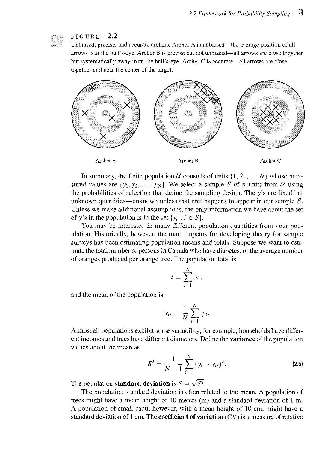
2.2 Framework for Probability Sampling 25
2.3 Simple Random Sampling 30
2.4 Confidence Intervals 35
2.5 Sample Size Estimation 39
2.6 Systematic Sampling 42
2.7 Randomization Theory Results for Simple Random Sampling* 43
2.8 A Model for Simple Random Sampling* 46
2.9 When Should a Simple Random Sample Be Used? 49
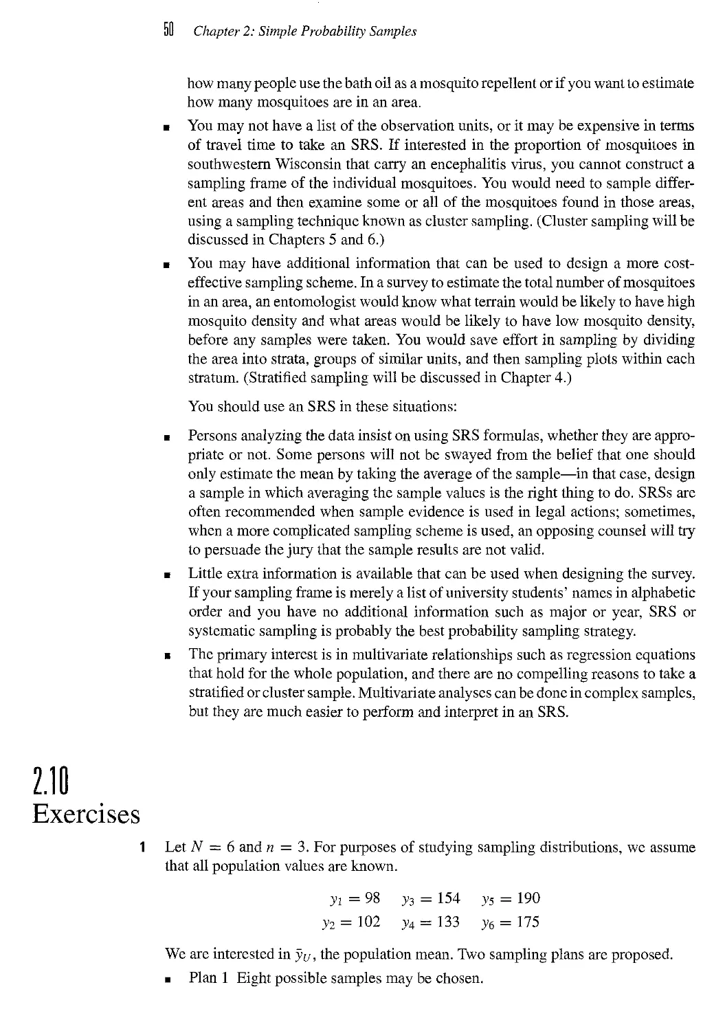
2.10 Exercises 50

Kill Contents
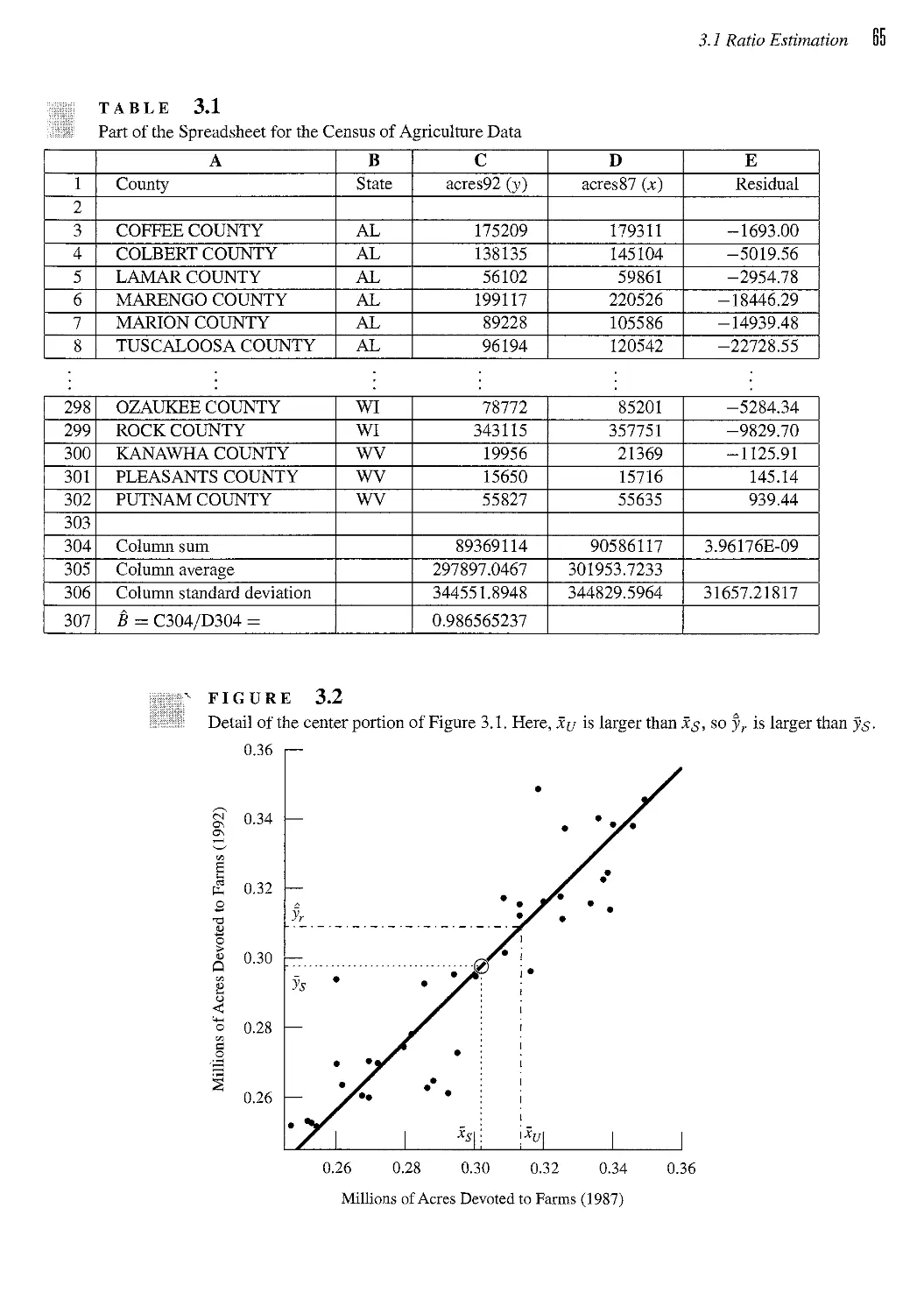
CHAPTER J Ratio and Regression Estimation 59
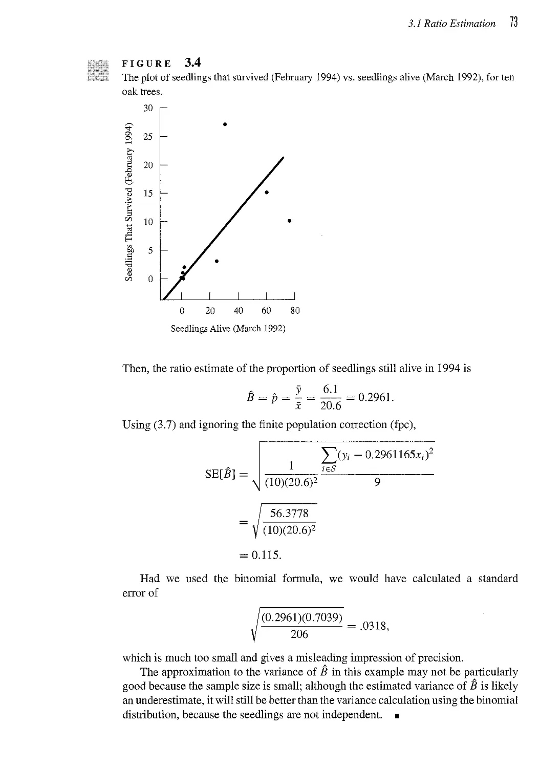
3.1 Ratio Estimation 60
3.2 Regression Estimation 74
3.3 Estimation in Domains 77
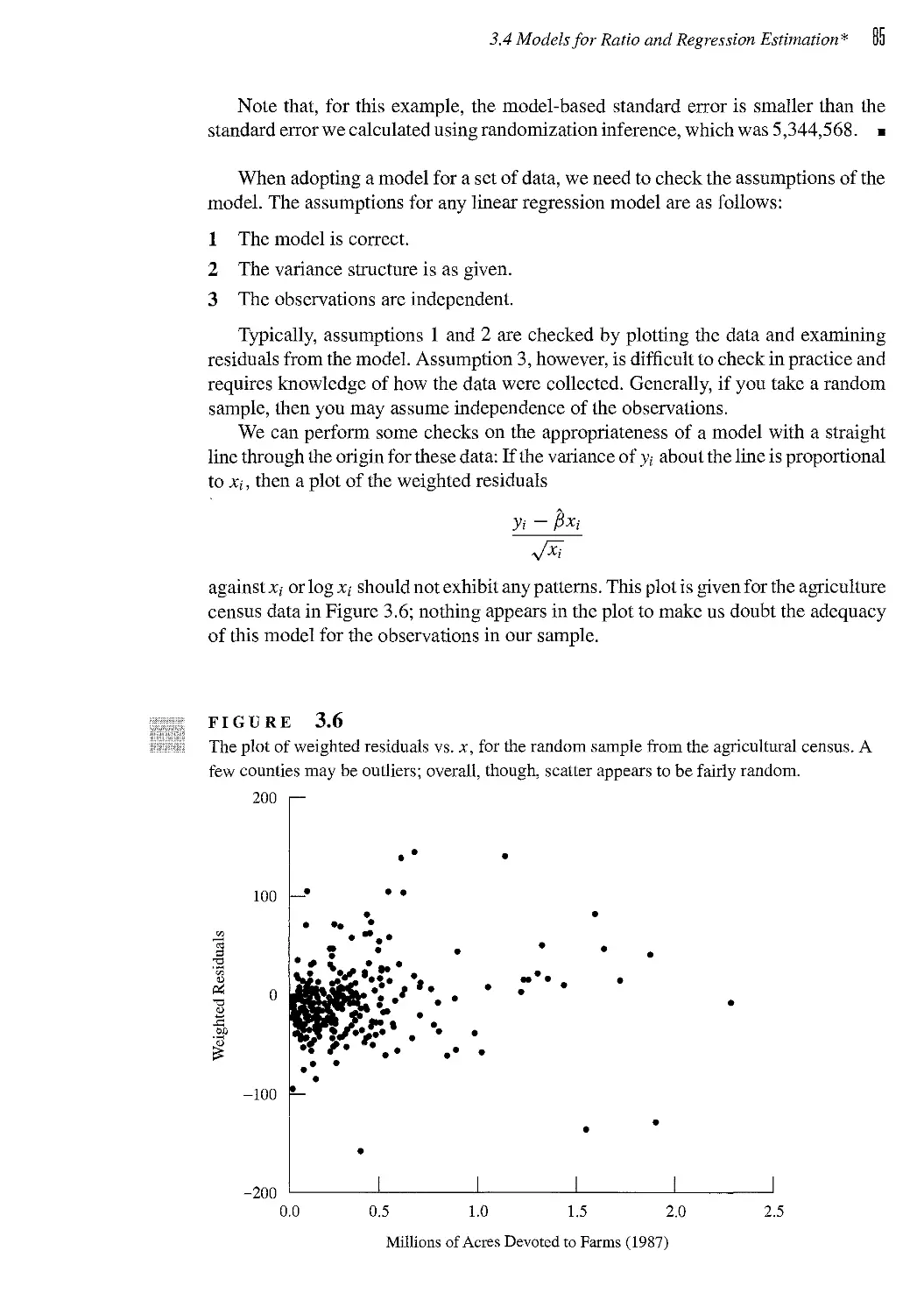
3.4 Models for Ratio and Regression Estimation* 81
3.5 Comparison 88
3.6 Exercises 89
CHAPTER 4 Stratified Sampling 95
4.1 What Is Stratified Sampling? 95
4.2 Theory of Stratified Sampling 99
4.3 Sampling Weights 103
4.4 Allocating Observations to Strata 104
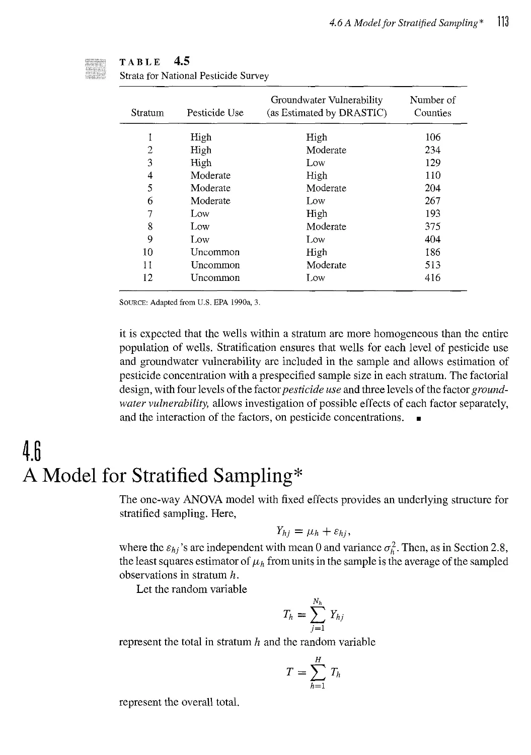
4.5 Defining Strata 109
4.6 A Model for Stratified Sampling* 113
4.7 Poststratification 114
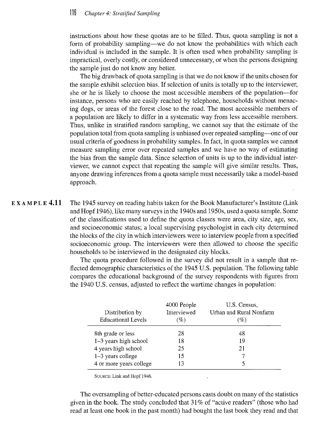
4.8 Quota Sampling 115
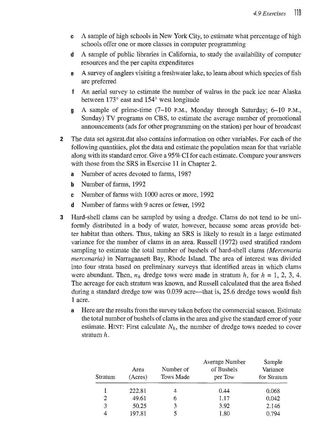
4.9 Exercises 118
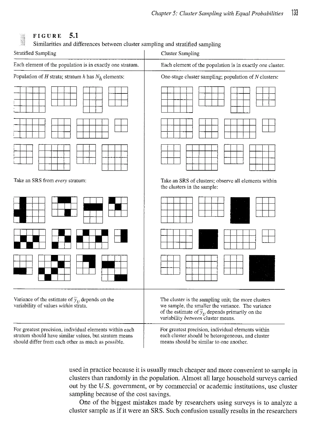
CHAPTER U Cluster Sampling with Equal Probabilities 131
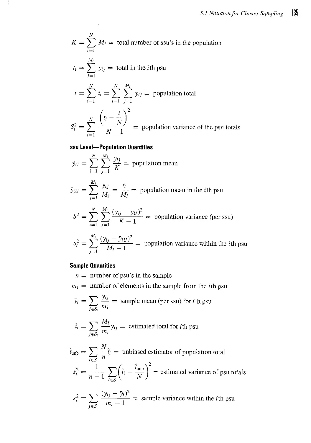
5.1 Notation for Cluster Sampling 134
5.2 One-Stage Cluster Sampling 136
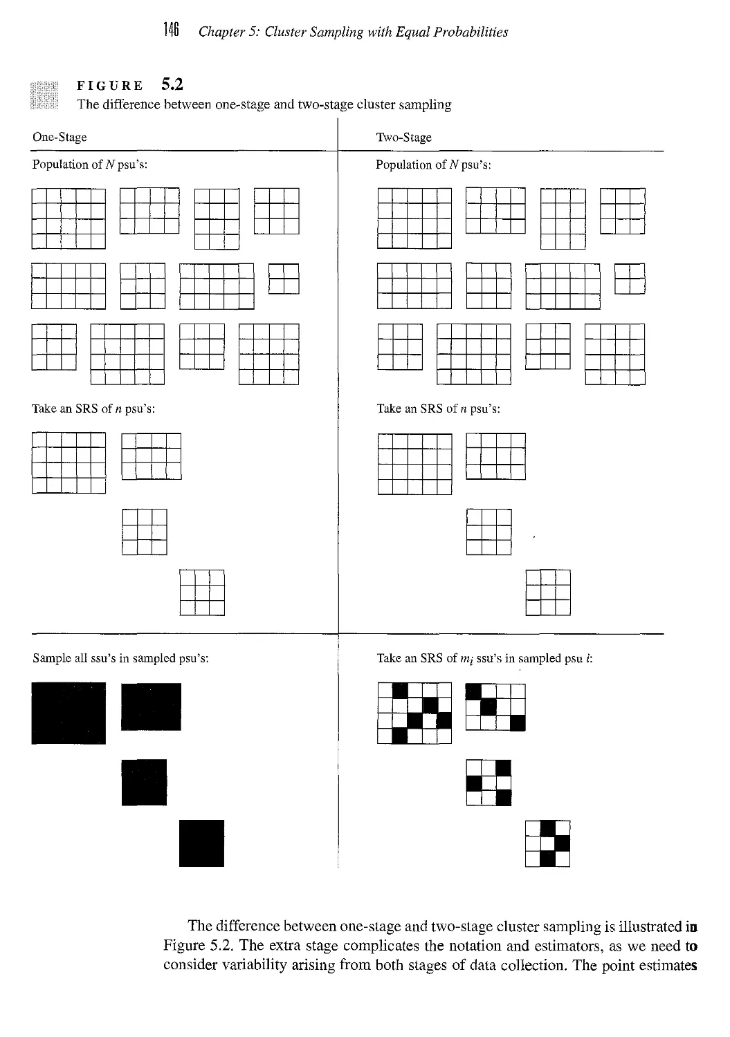
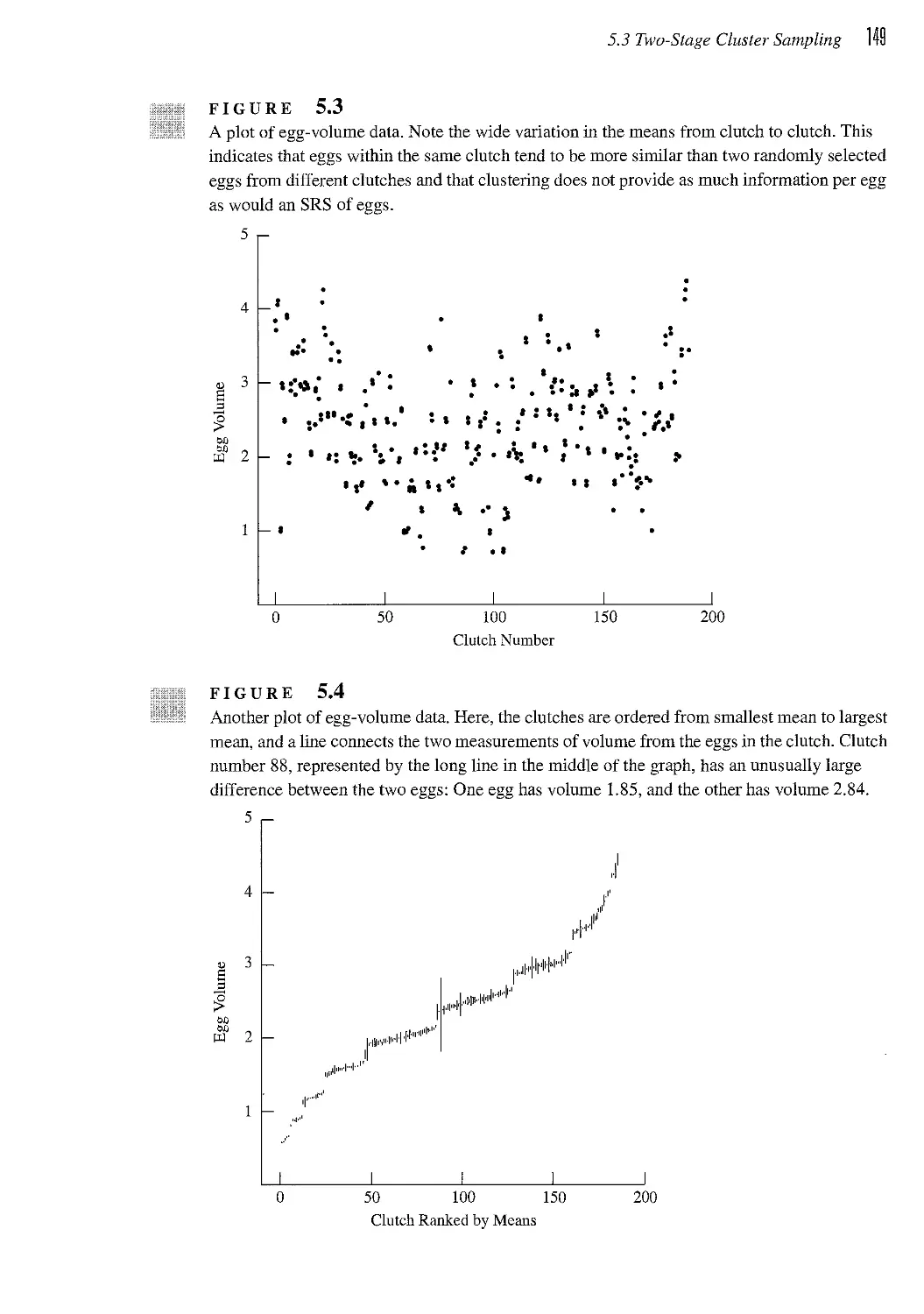
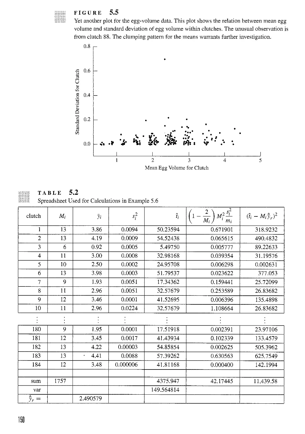
5.3 Two-Stage Cluster Sampling 145
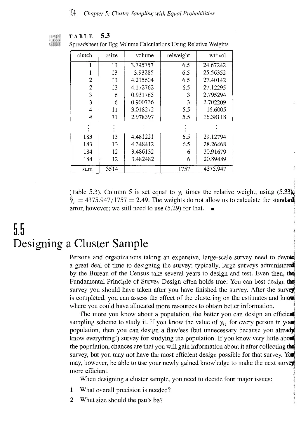
5.4 Using Weights in Cluster Samples 153
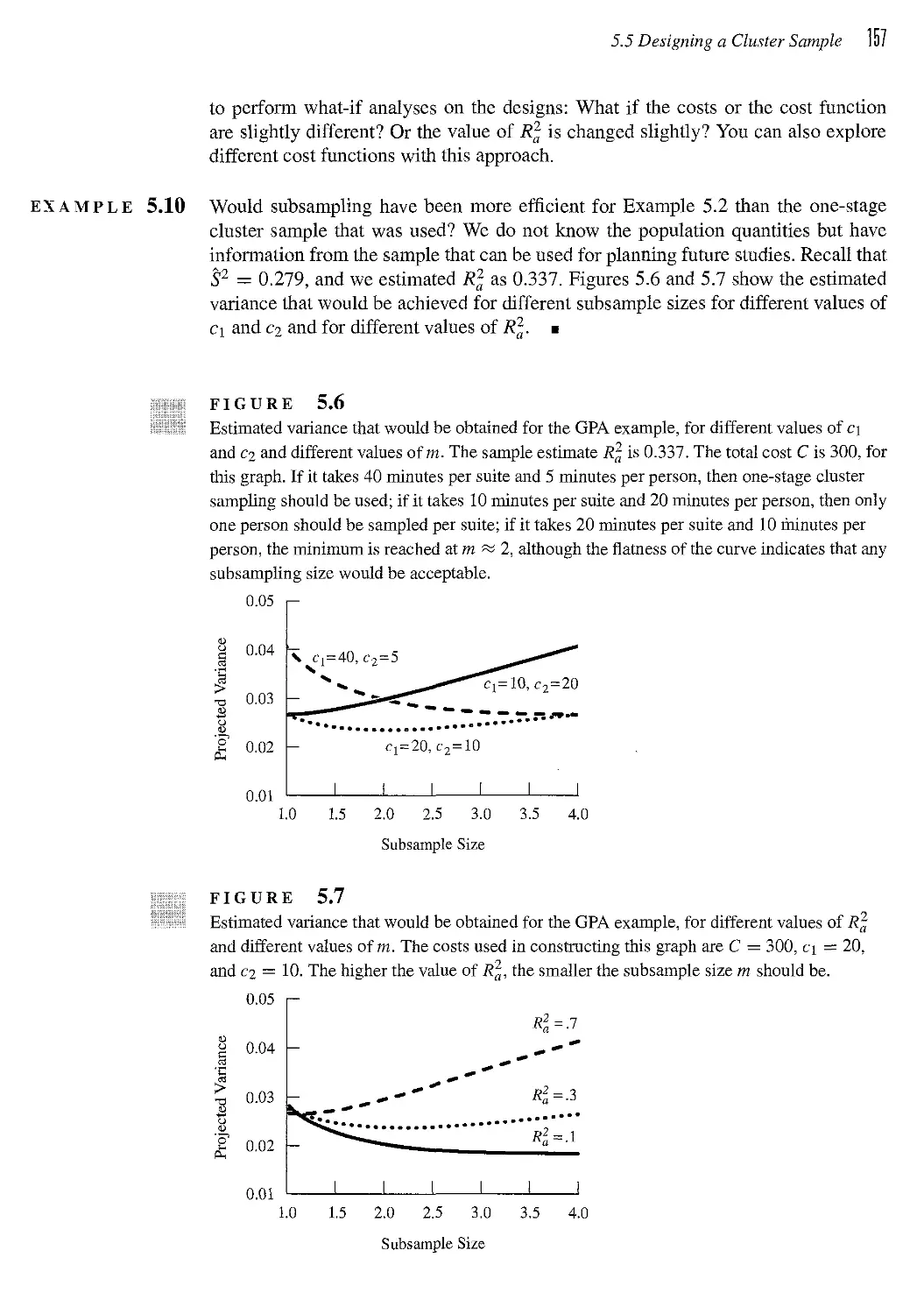
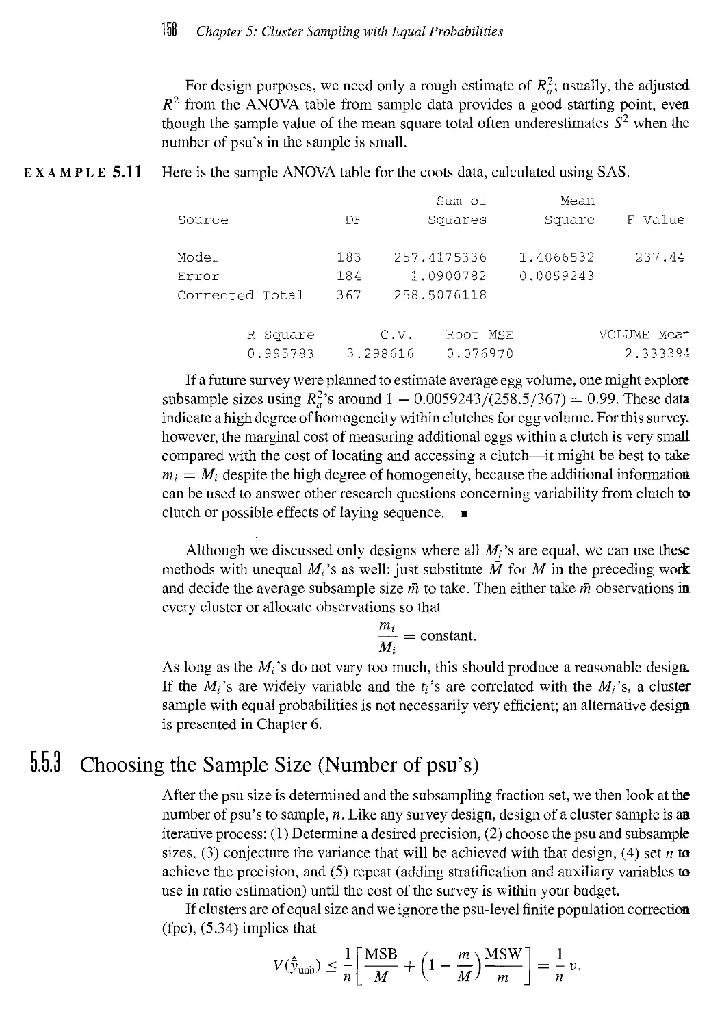
5.5 Designing a Cluster Sample 154
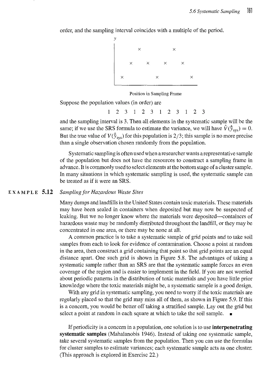
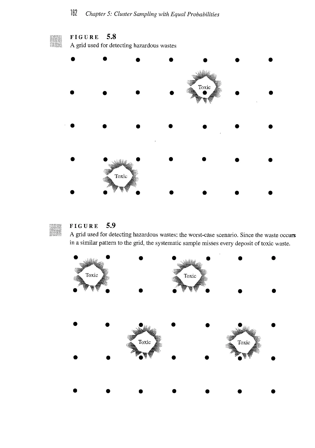
5.6 Systematic Sampling 159
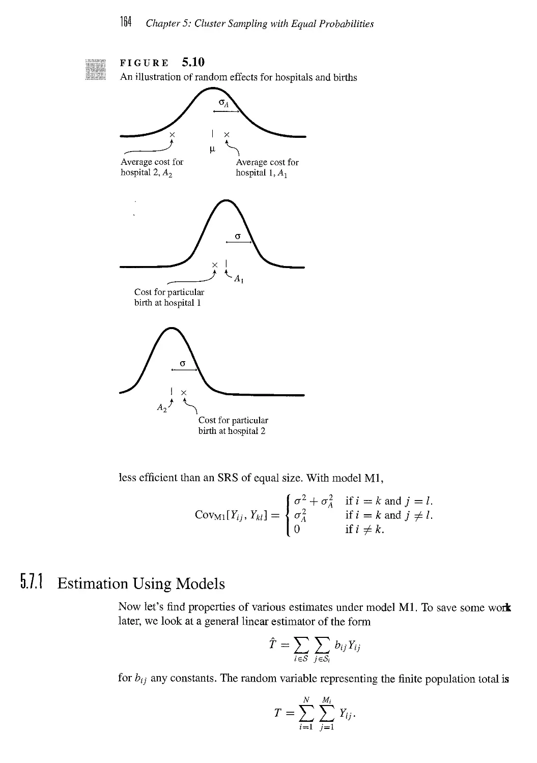
5.7 Models for Cluster Sampling* 163
5.8 Summary 168
5.9 Exercises 169

Contents
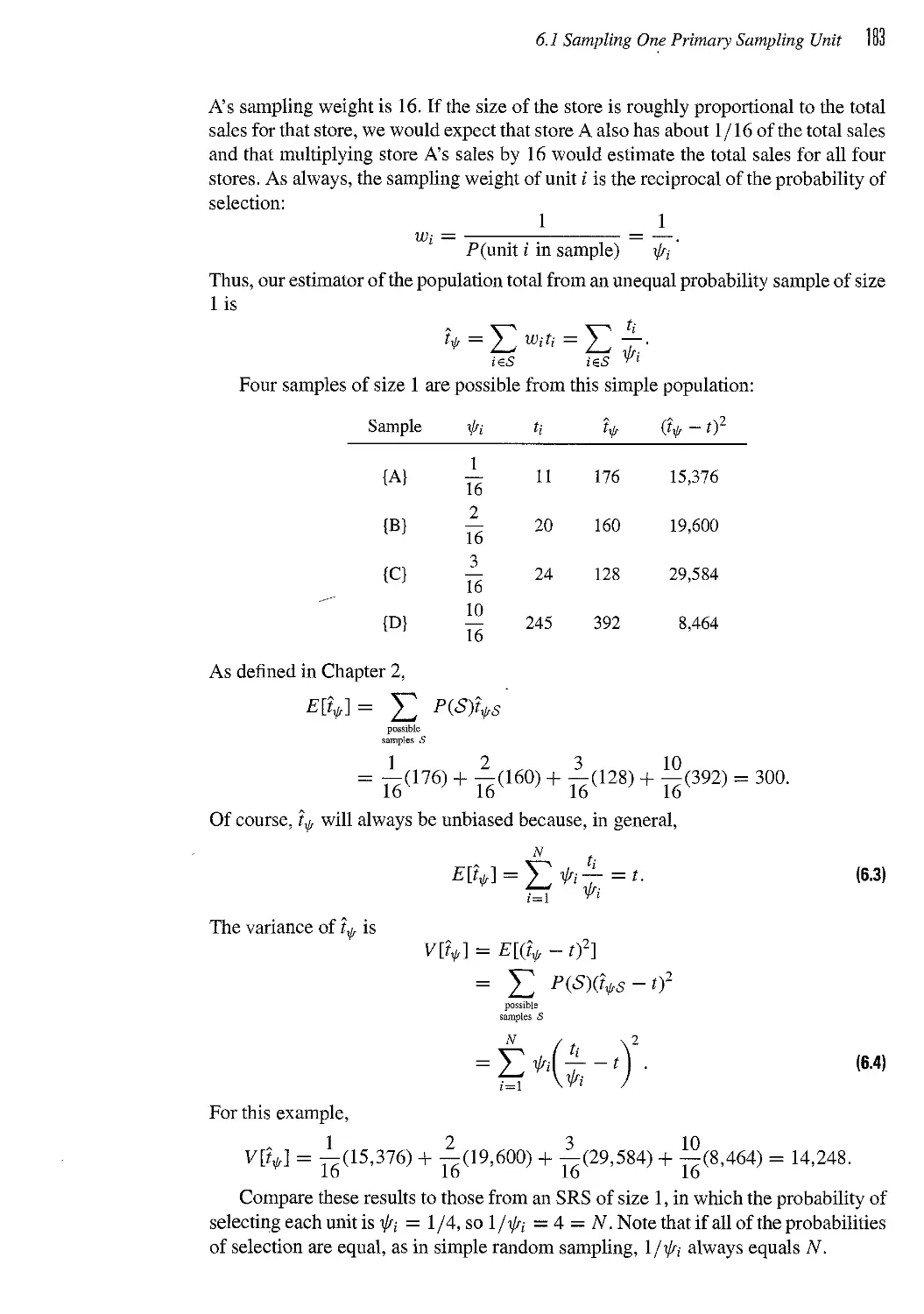
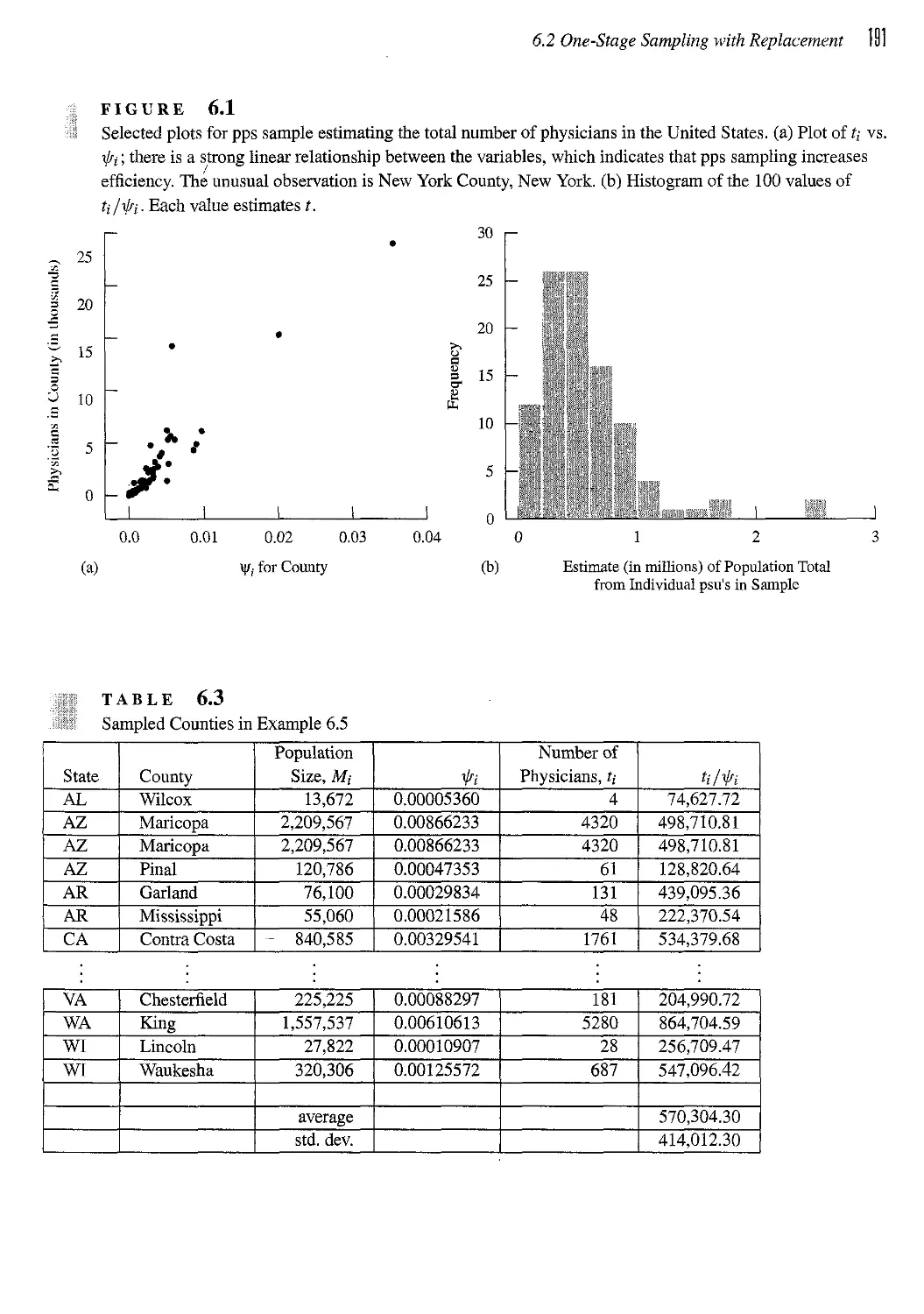
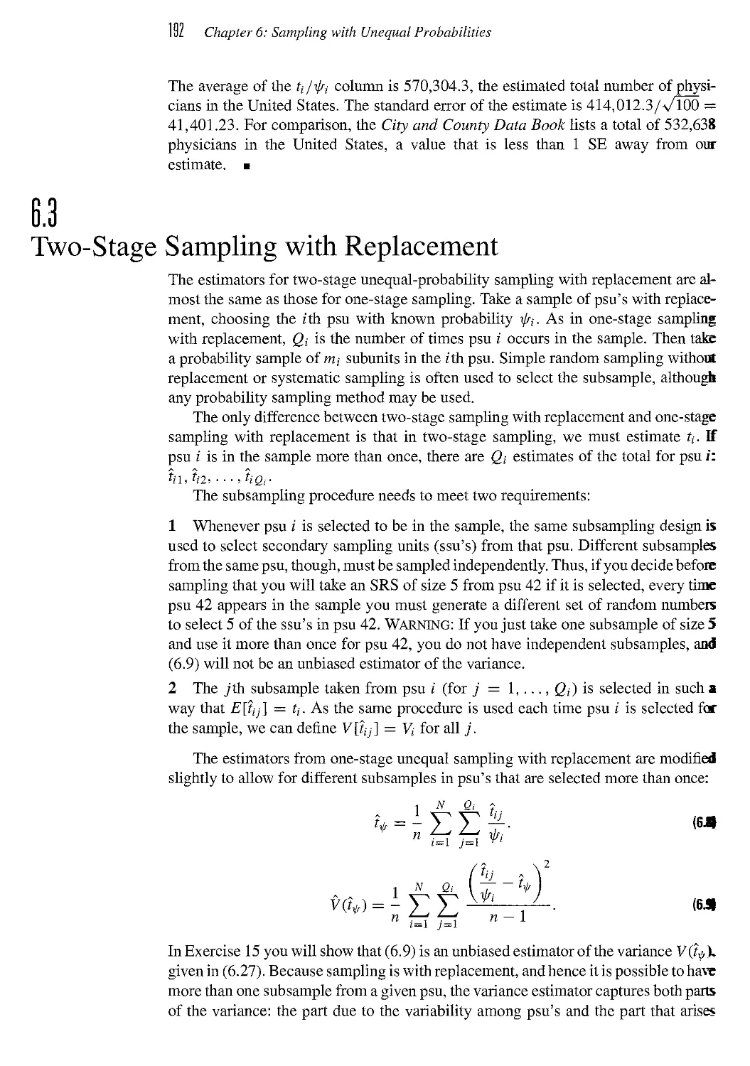
CHAPTER D Sampling with Unequal Probabilities 179
6.1 Sampling One Primary Sampling Unit 181
6.2 One-Stage Sampling with Replacement 184
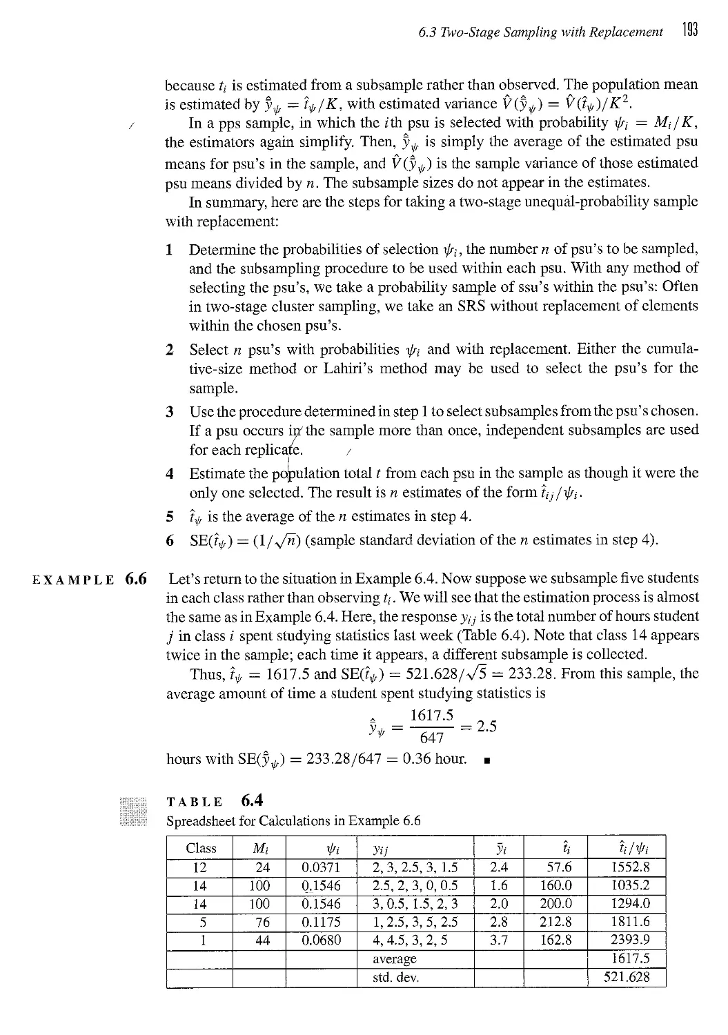
6.3 Two-Stage Sampling with Replacement 192
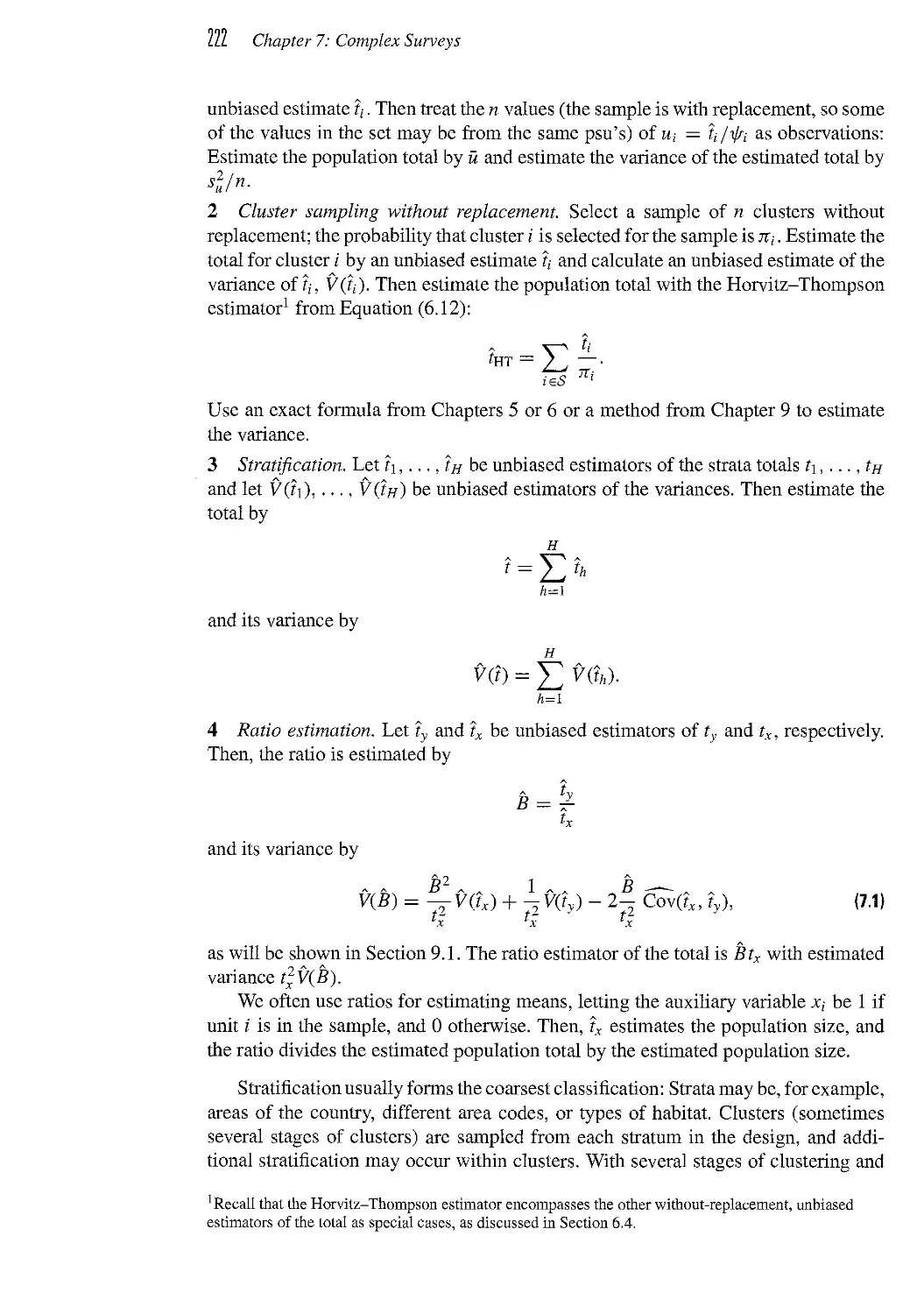
6.4 Unequal-Probability Sampling Without Replacement 194
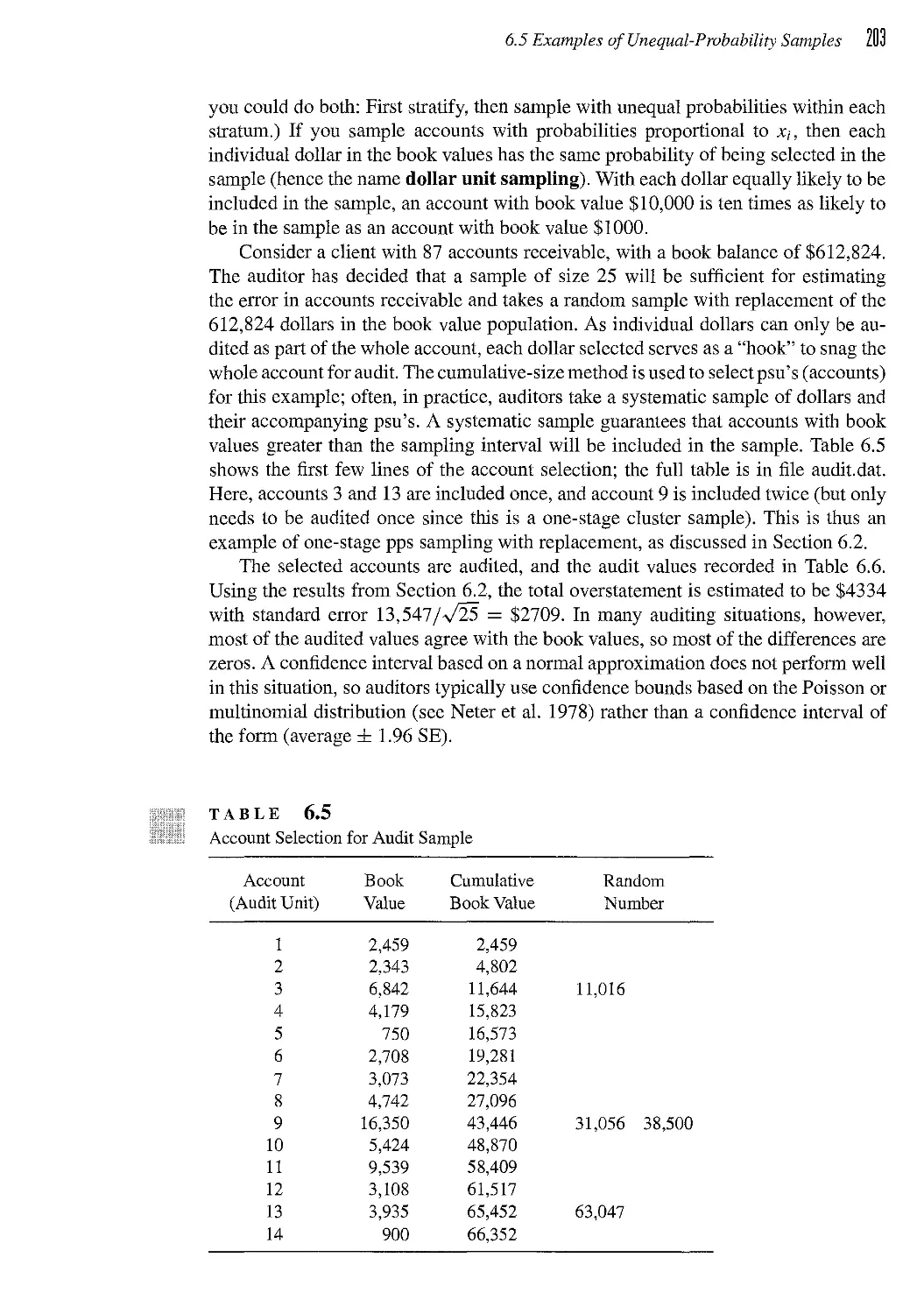
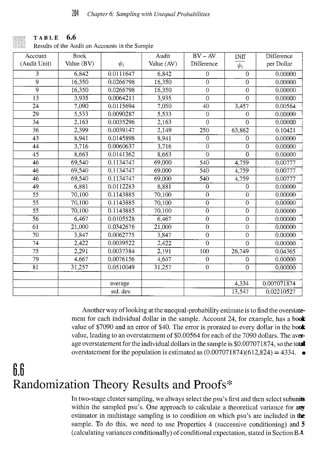
6.5 Examples of Unequal-Probability Samples 199
6.6 Randomization Theory Results and Proofs* 204
6.7 Models and Unequal-Probability Sampling* 211
6.8 Exercises 213
CHAPTER / Complex Surveys 221
7.1 Assembling Design Components 221
7.2 Sampling Weights 225
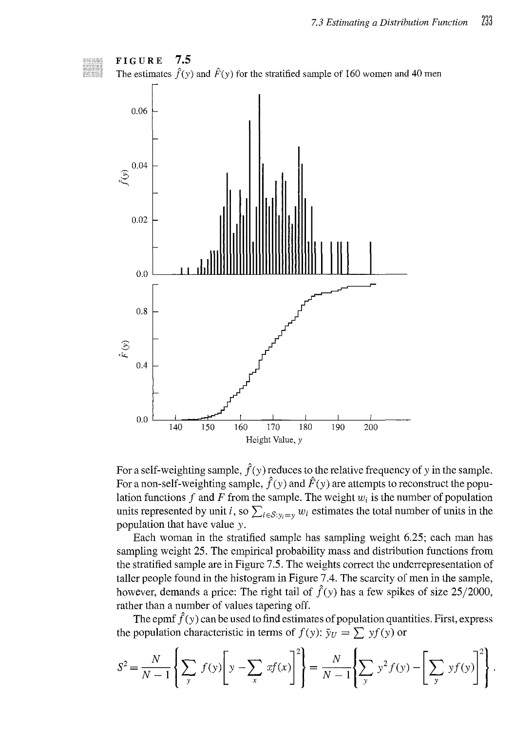
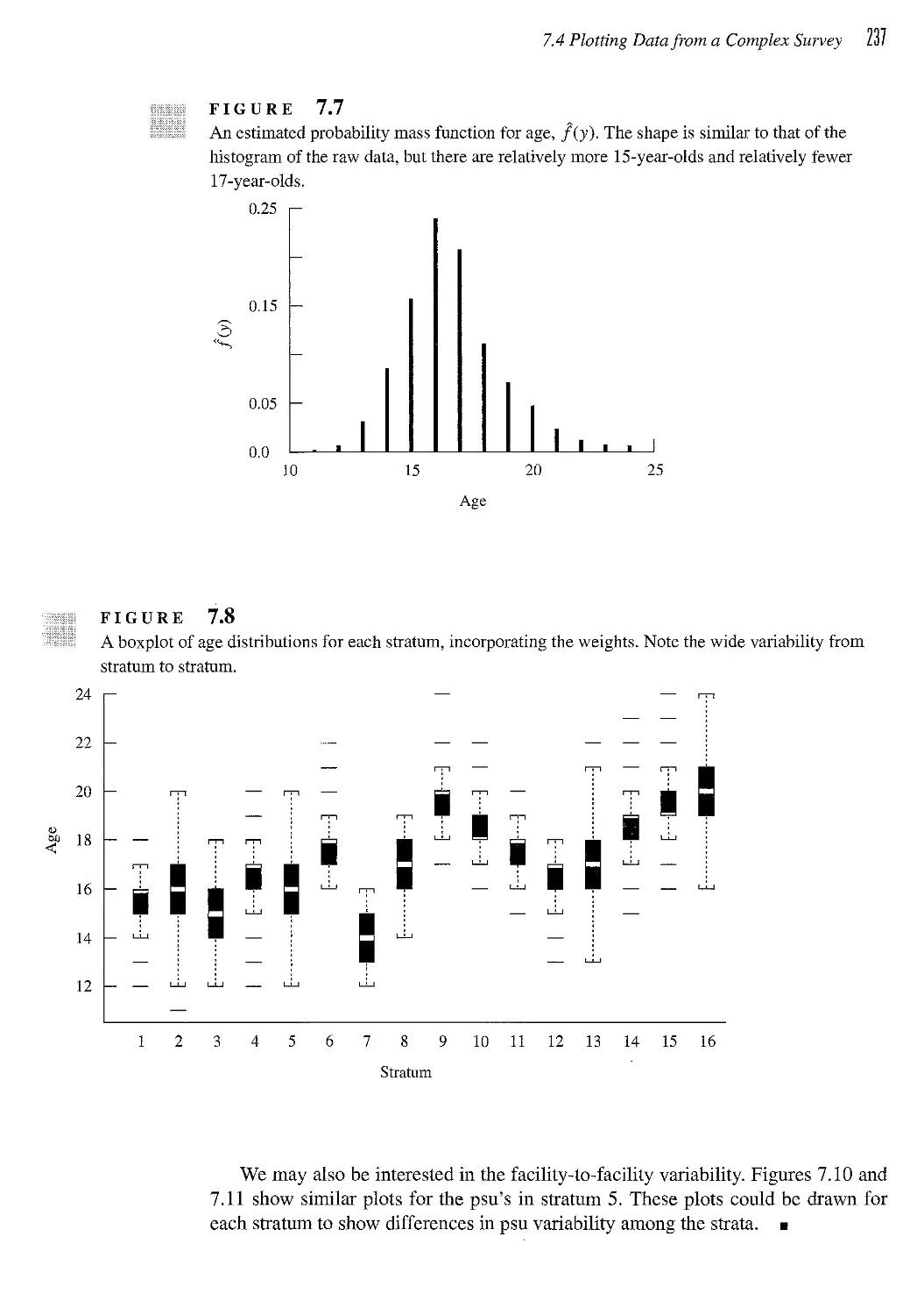
7.3 Estimating a Distribution Function 229
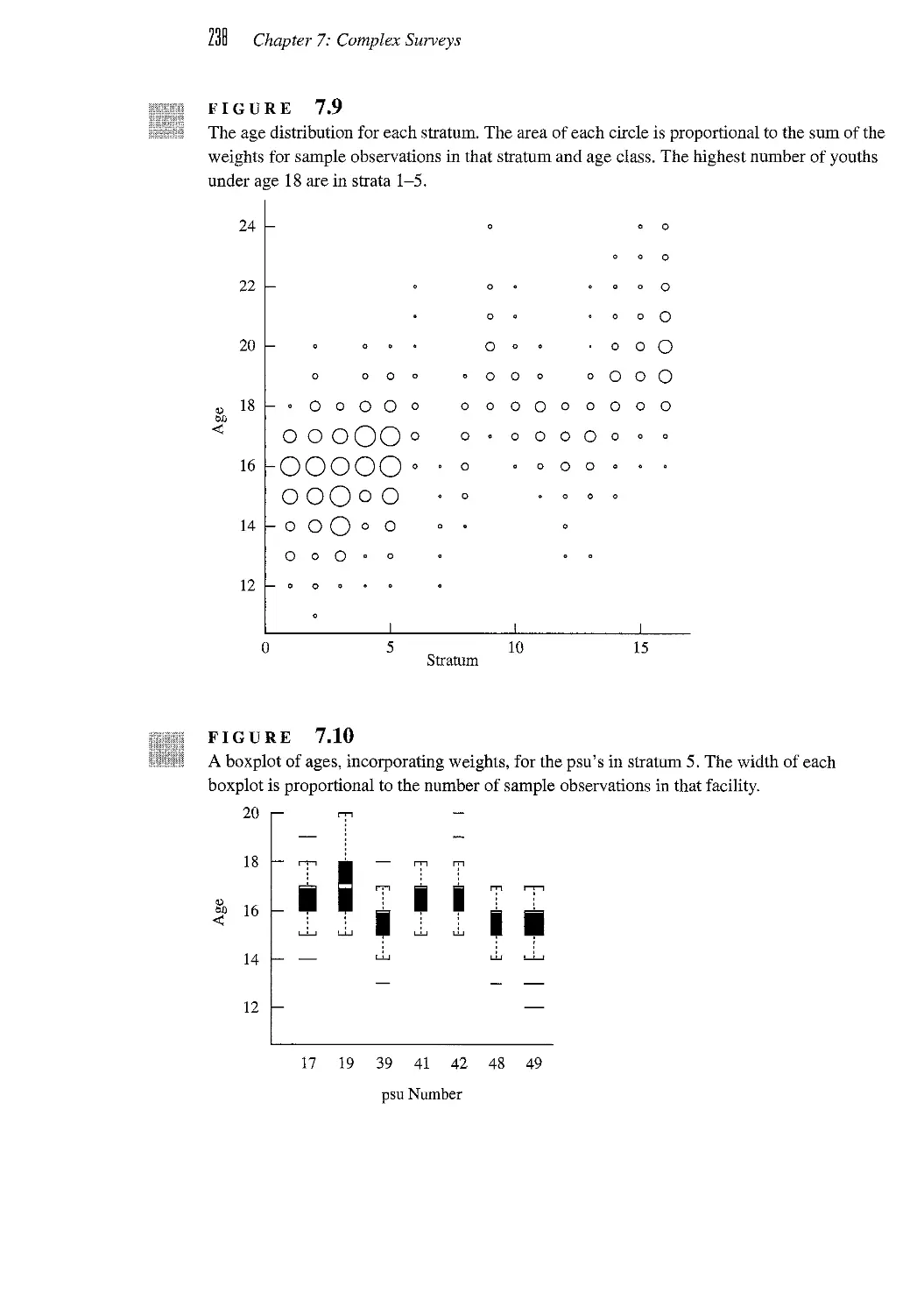
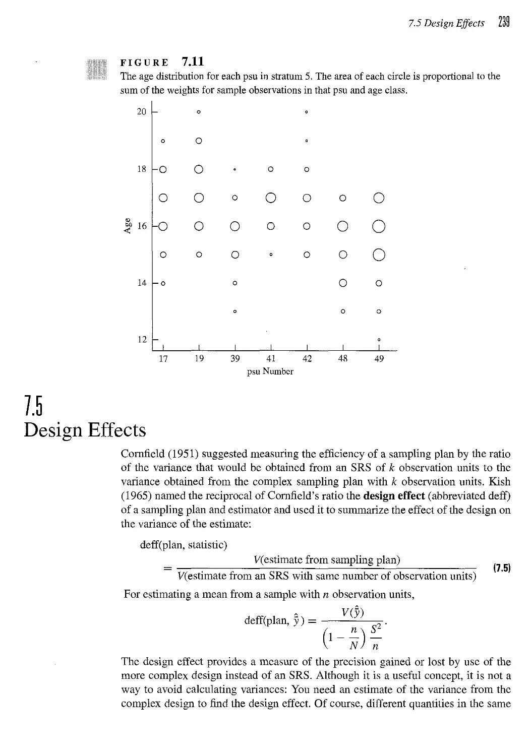
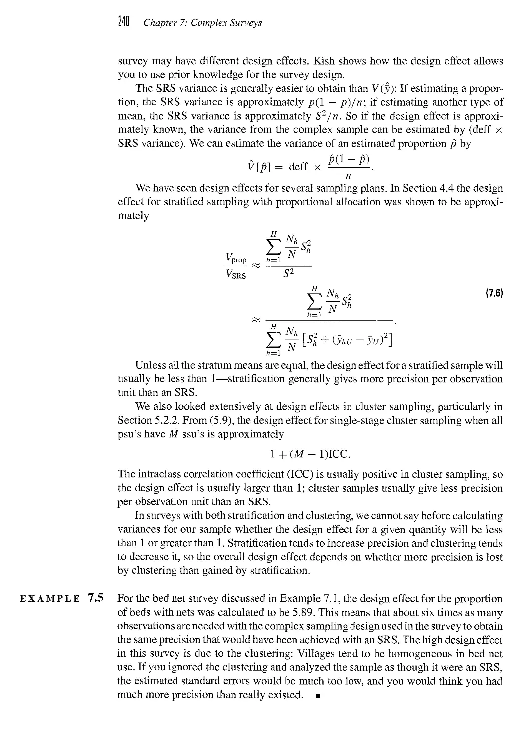
7.4 Plotting Data from a Complex Survey 235
7.5 Design Effects 239
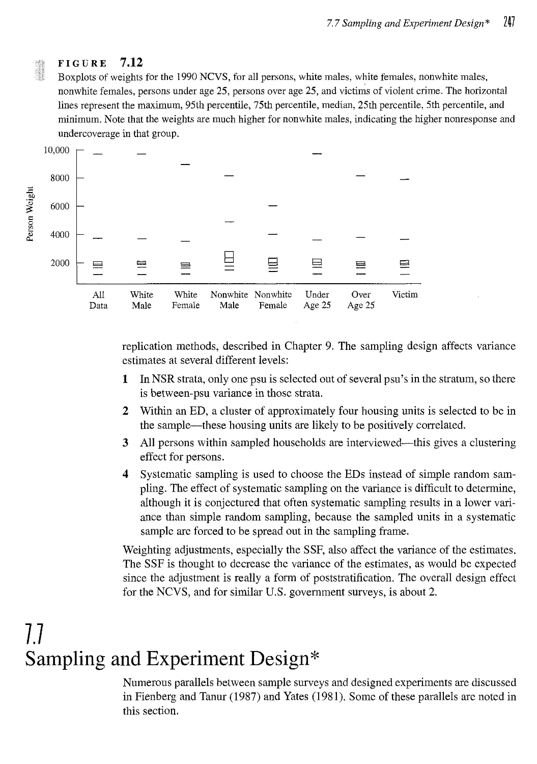
7.6 The National Crime Victimization Survey 242
7.7 Sampling and Experiment Design* 247
7.8 Exercises 249
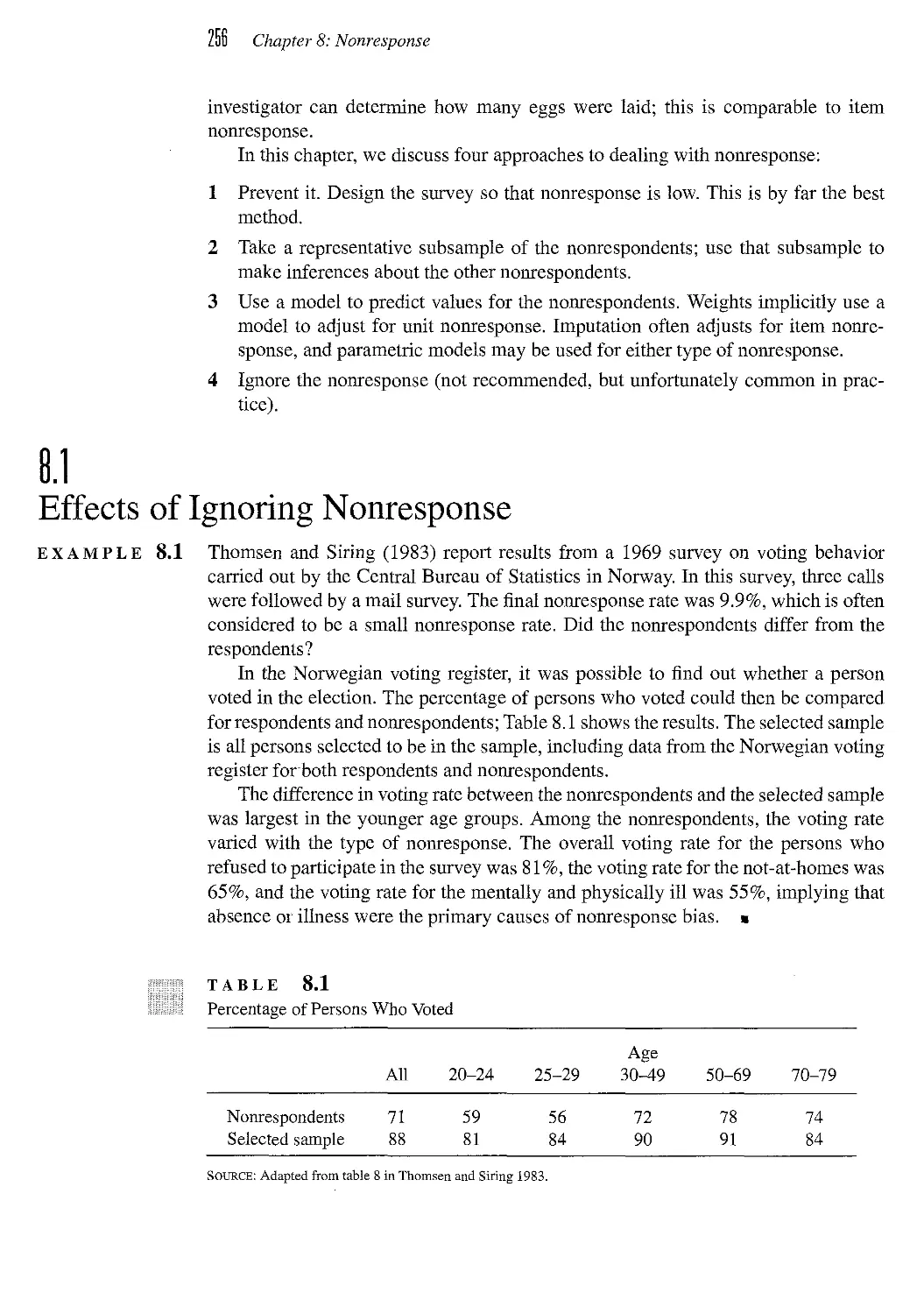
CHAPTER 0 Nonresponse 255
8.1 Effects of Ignoring Nonresponse 256
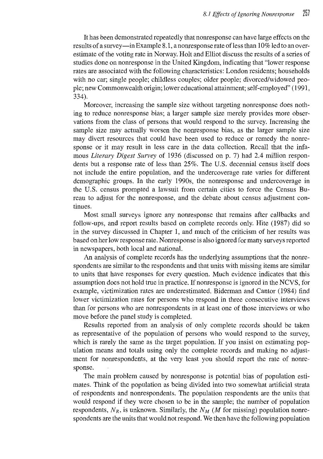
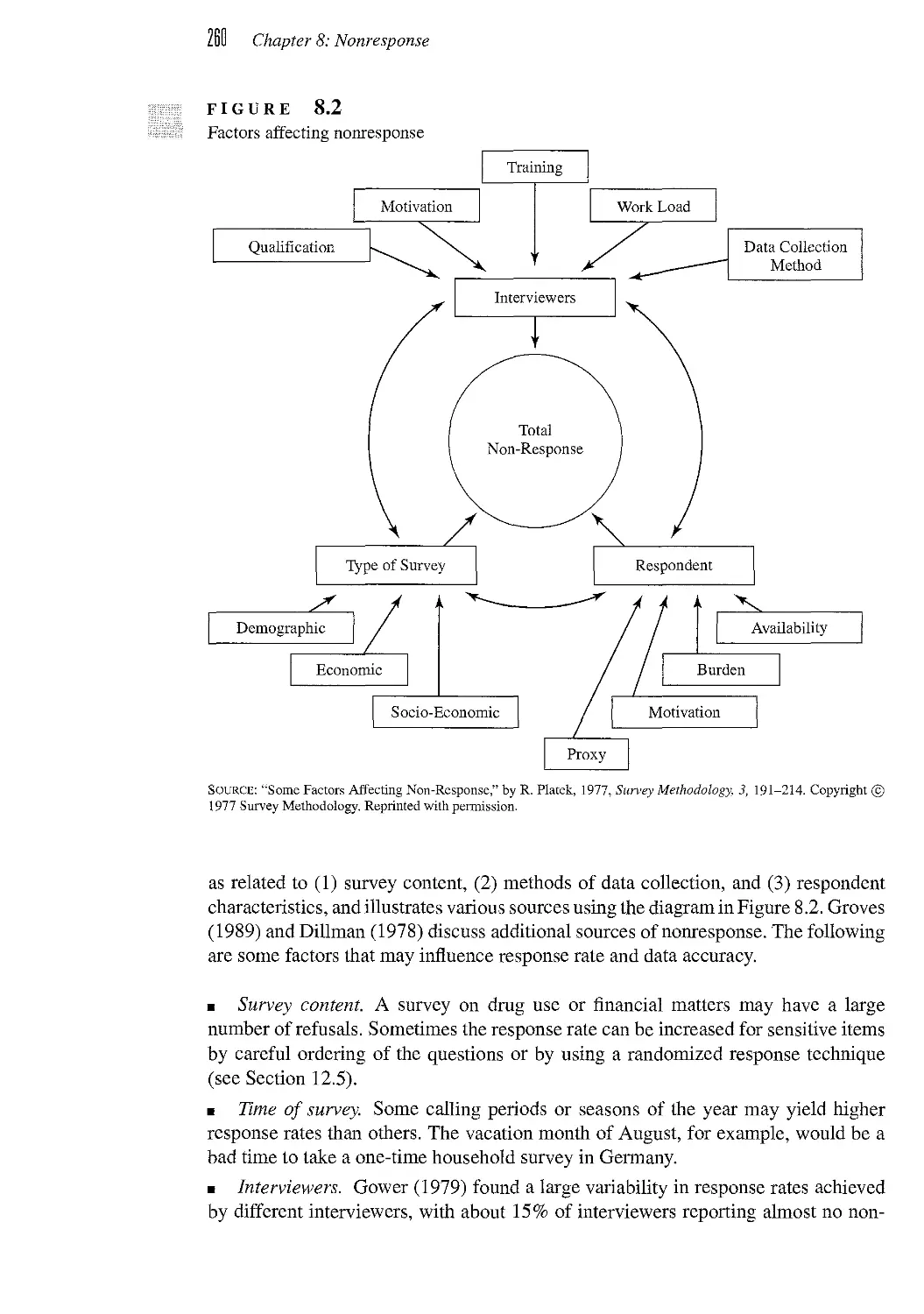
8.2 Designing Surveys to Reduce Nonsampling Errors 258
8.3 Callbacks and Two-Phase Sampling 262
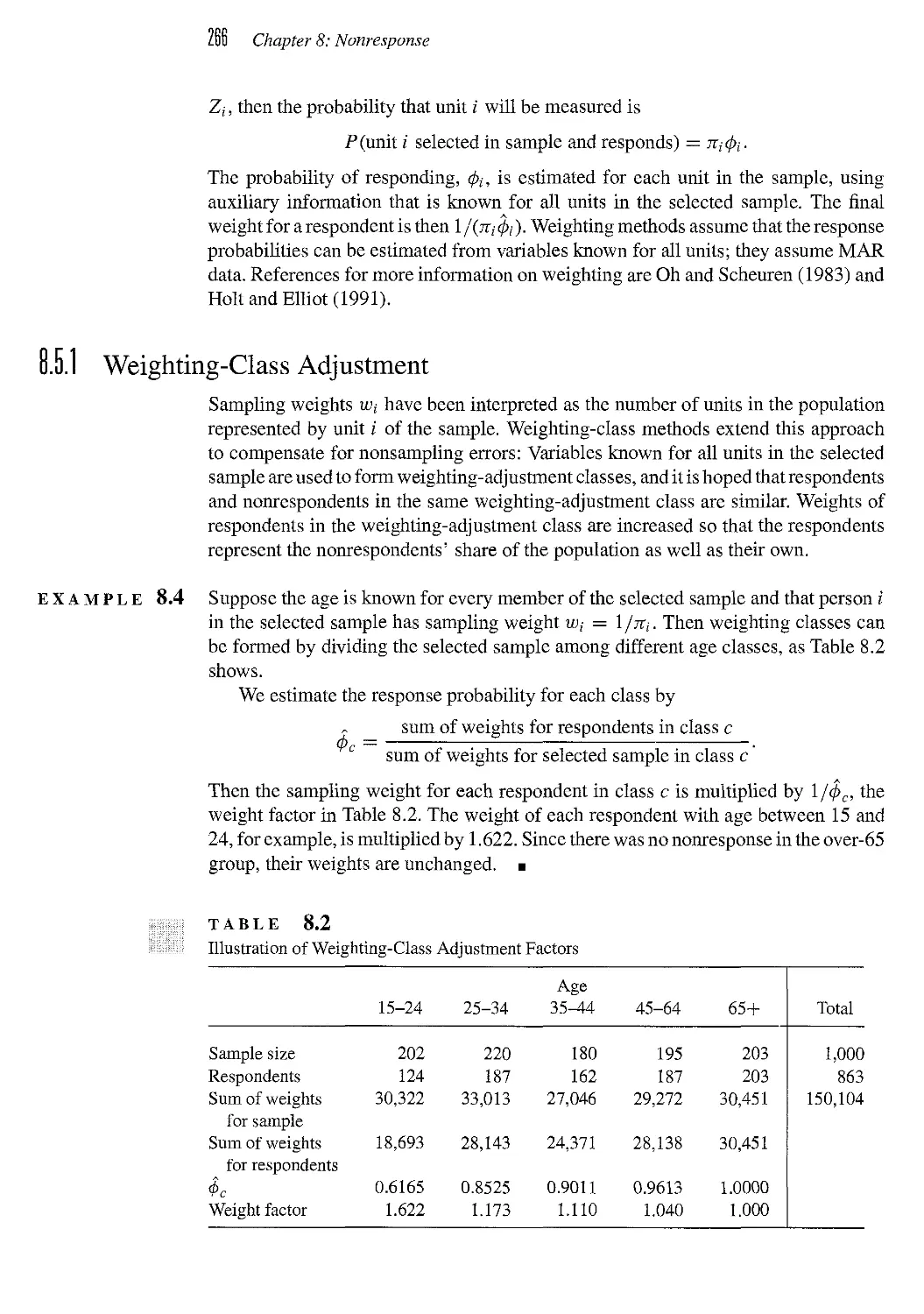
8.4 Mechanisms for Nonresponse 264
8.5 Weighting Methods for Nonresponse 265
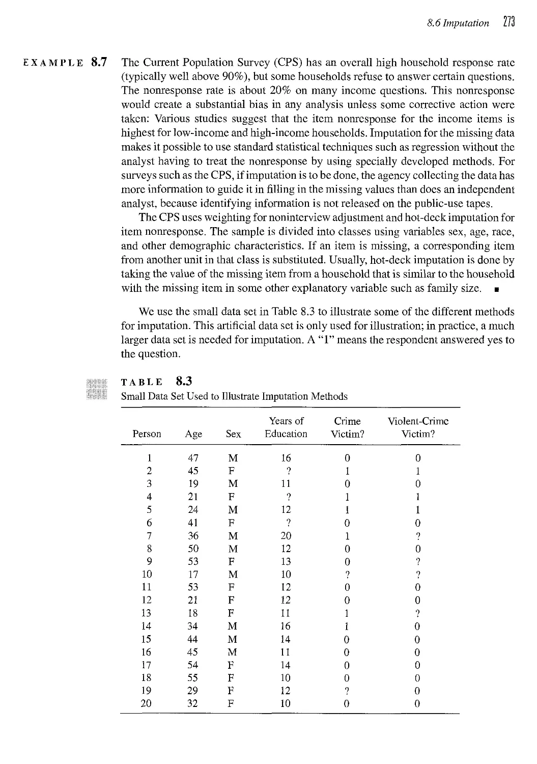
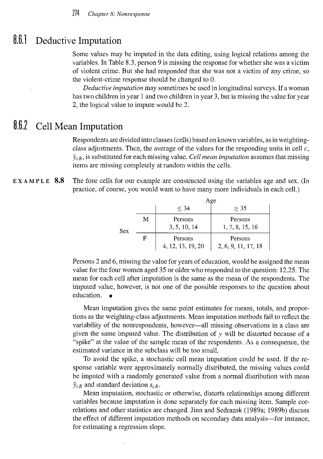
8.6 Imputation 272
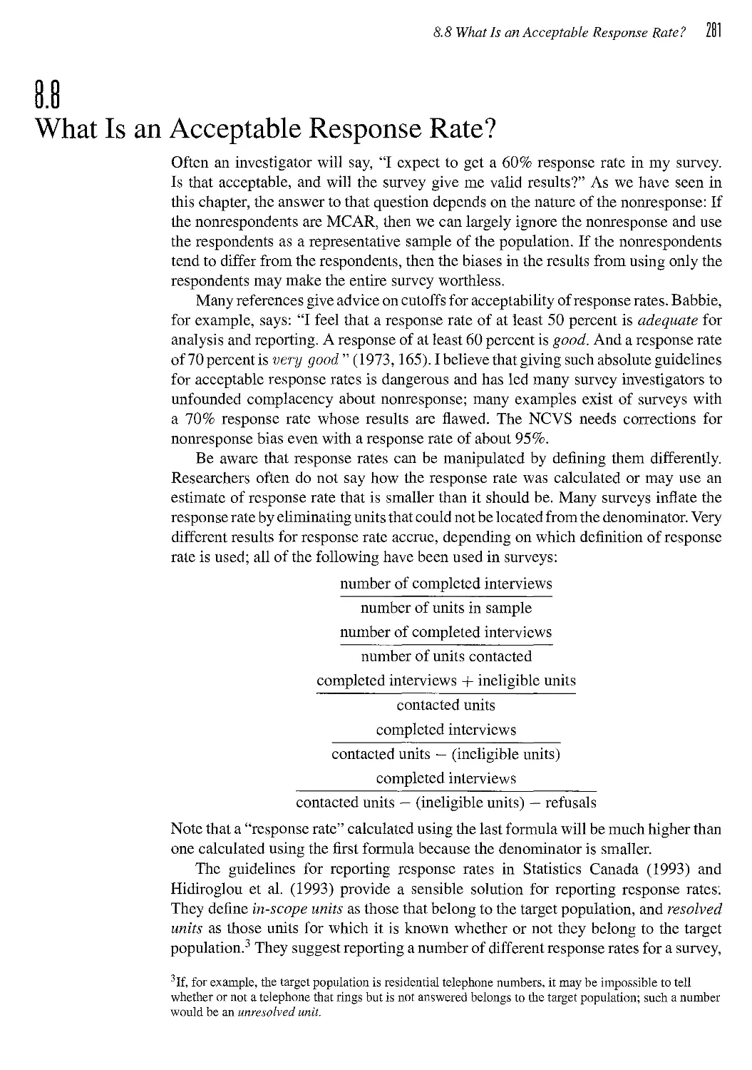
8.7 Parametric Models for Nonresponse* 278
8.8 What Is an Acceptable Response Rate? 281
8.9 Exercises 282

X Contents
CHAPTER u Variance Estimation in Complex Surveys* 289
9.1 Linearization (Taylor Series) Methods 290
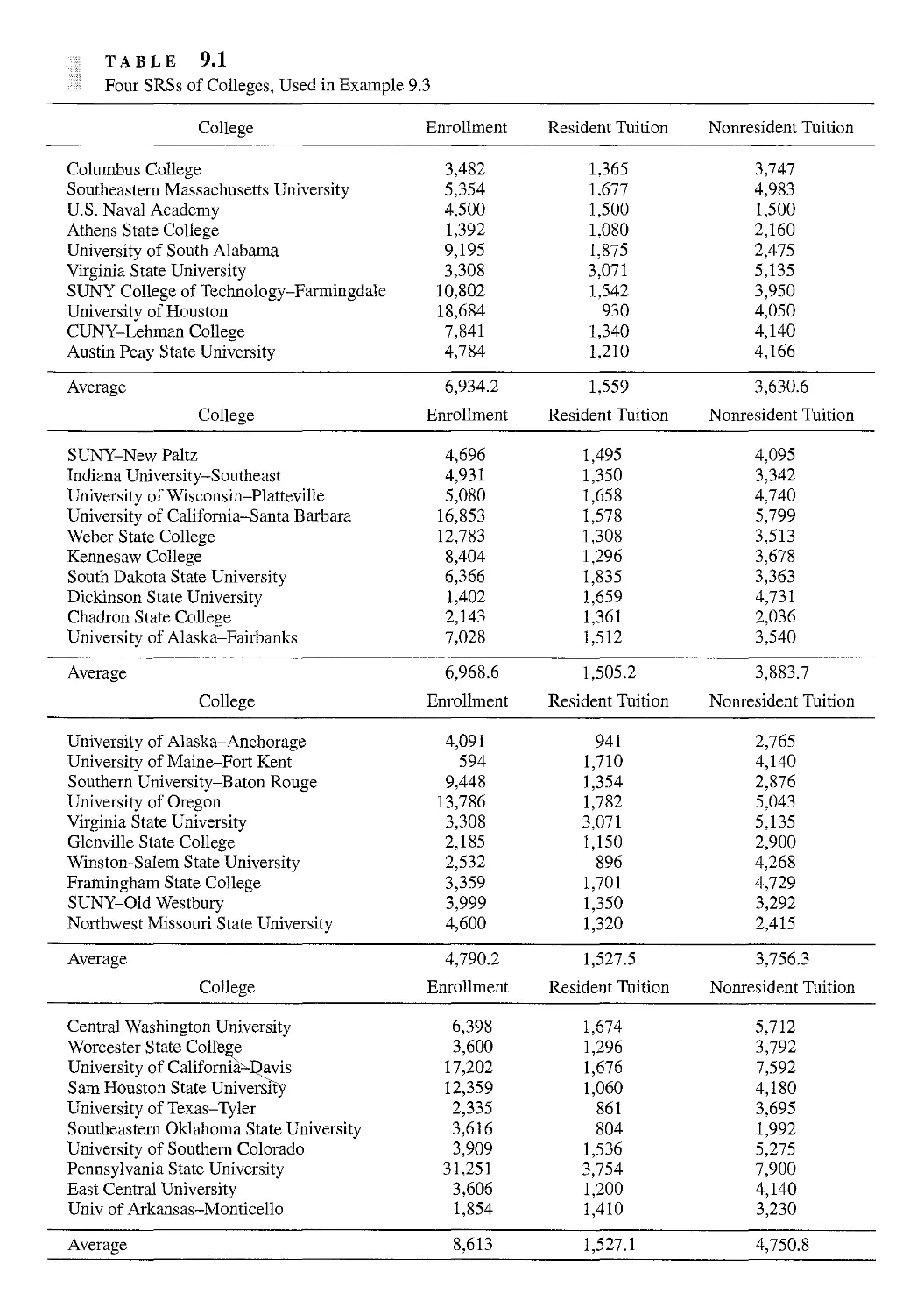
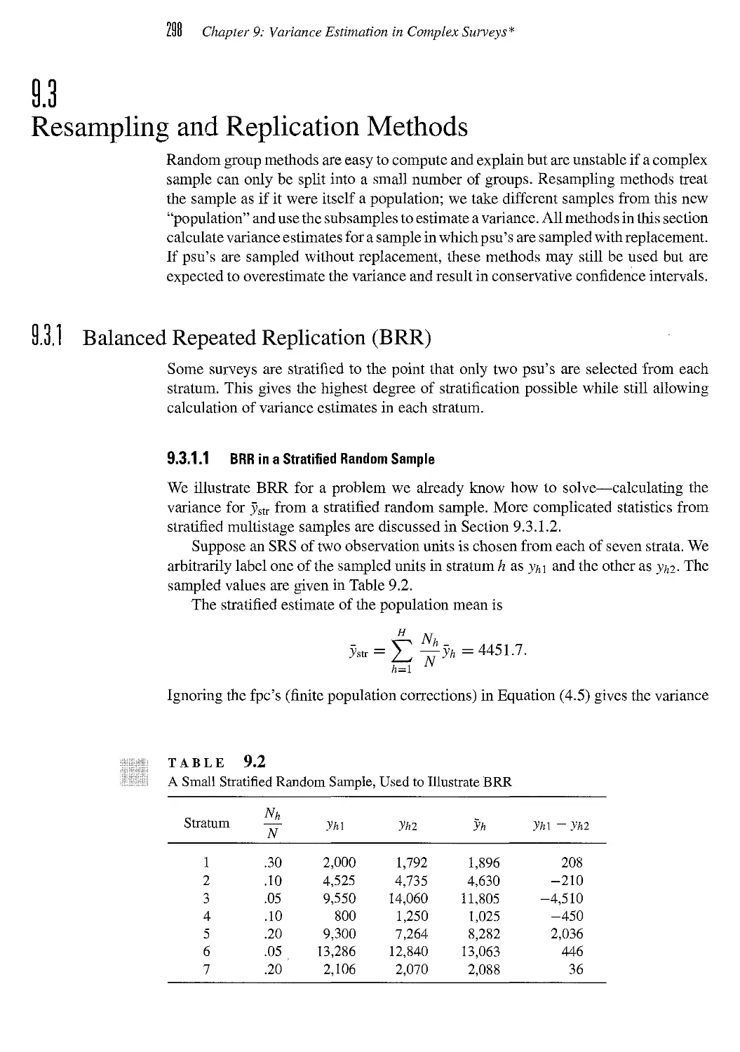
9.2 Random Group Methods 293
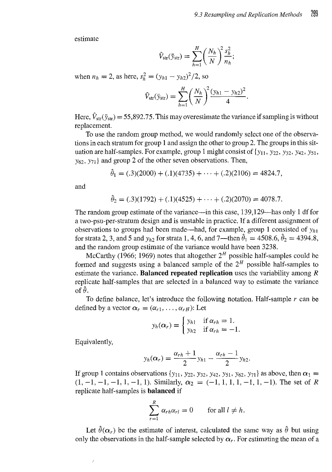
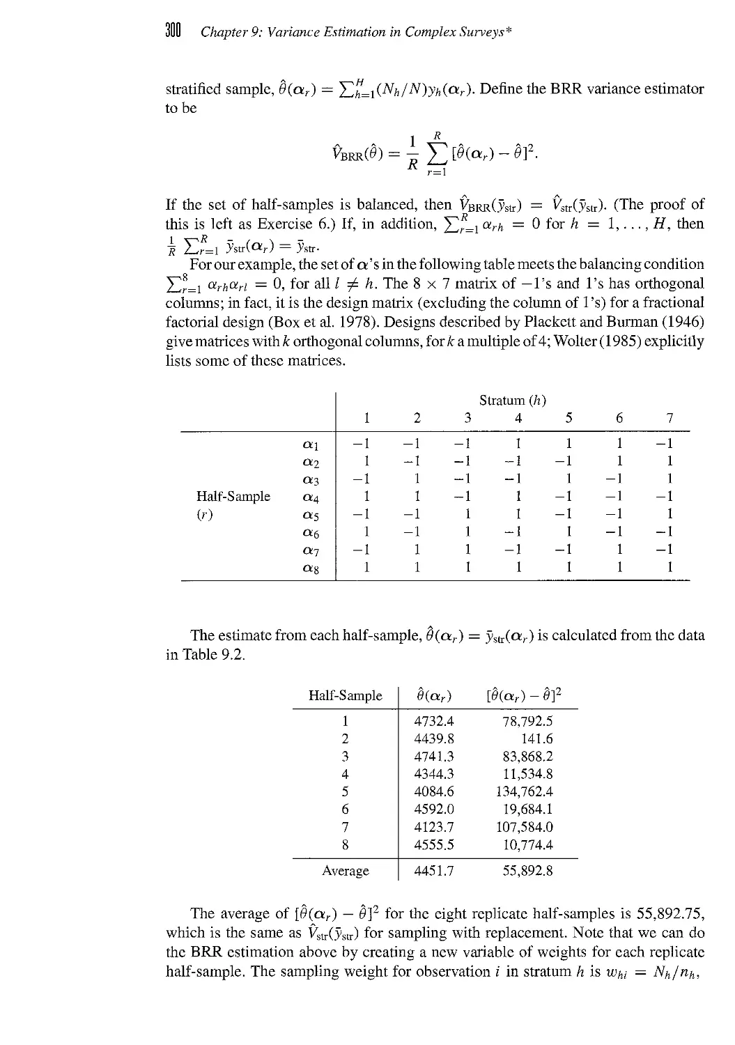
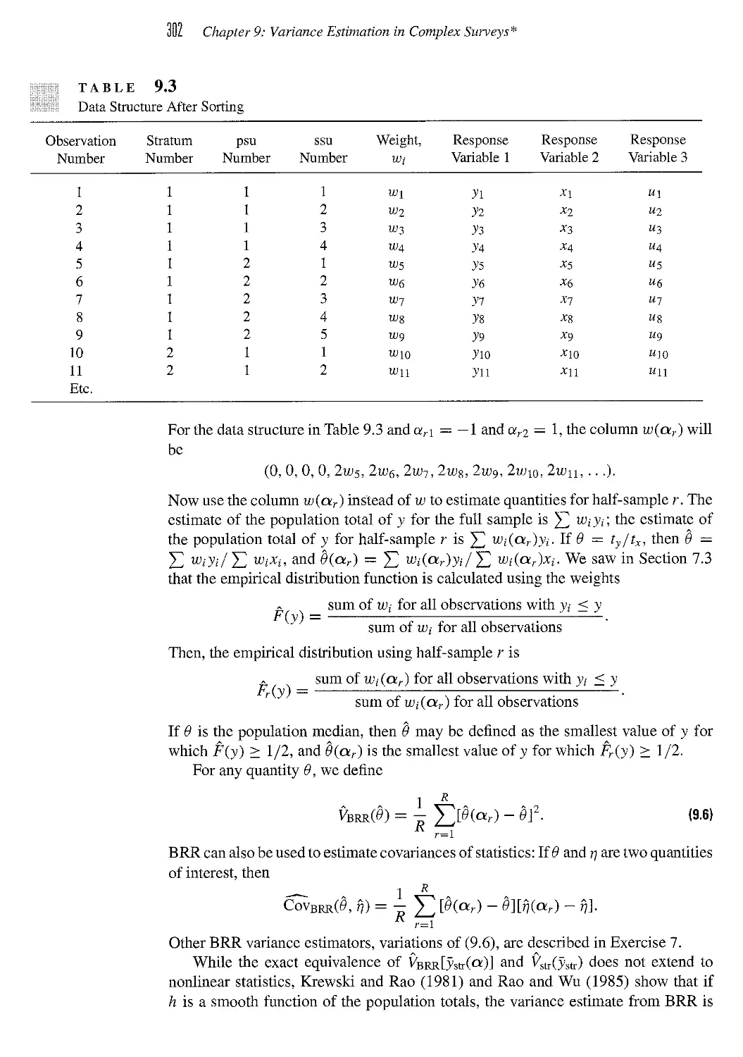
9.3 Resampling and Replication Methods 298
9.4 Generalized Variance Functions 308
9.5 Confidence Intervals 310
9.6 Summary and Software 313
9.7 Exercises 315
CHAPTER lU Categorical Data Analysis in Complex Surveys * 319
10.1 Chi-Square Tests with Multinomial Sampling 319
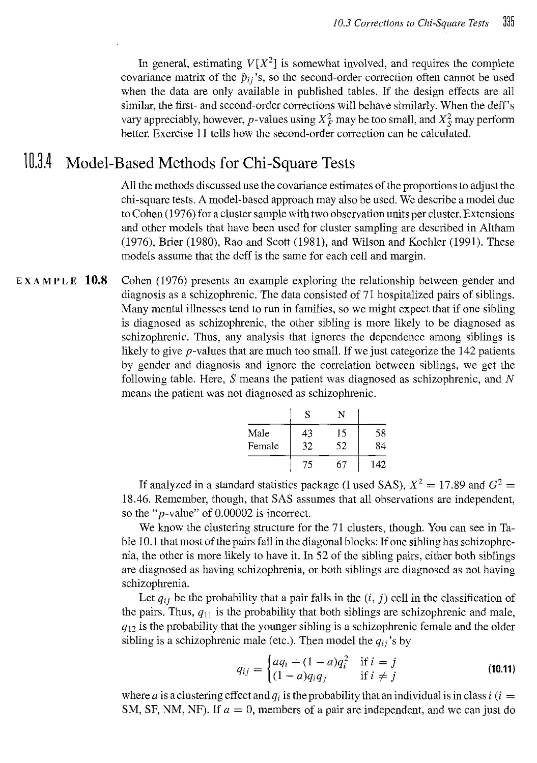
10.2 Effects of Survey Design on Chi-Square Tests 324
10.3 Corrections to Chi-Square Tests 329
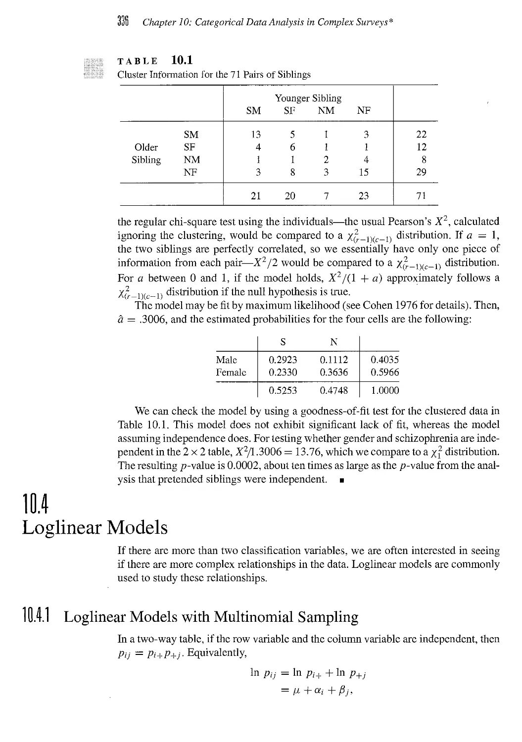
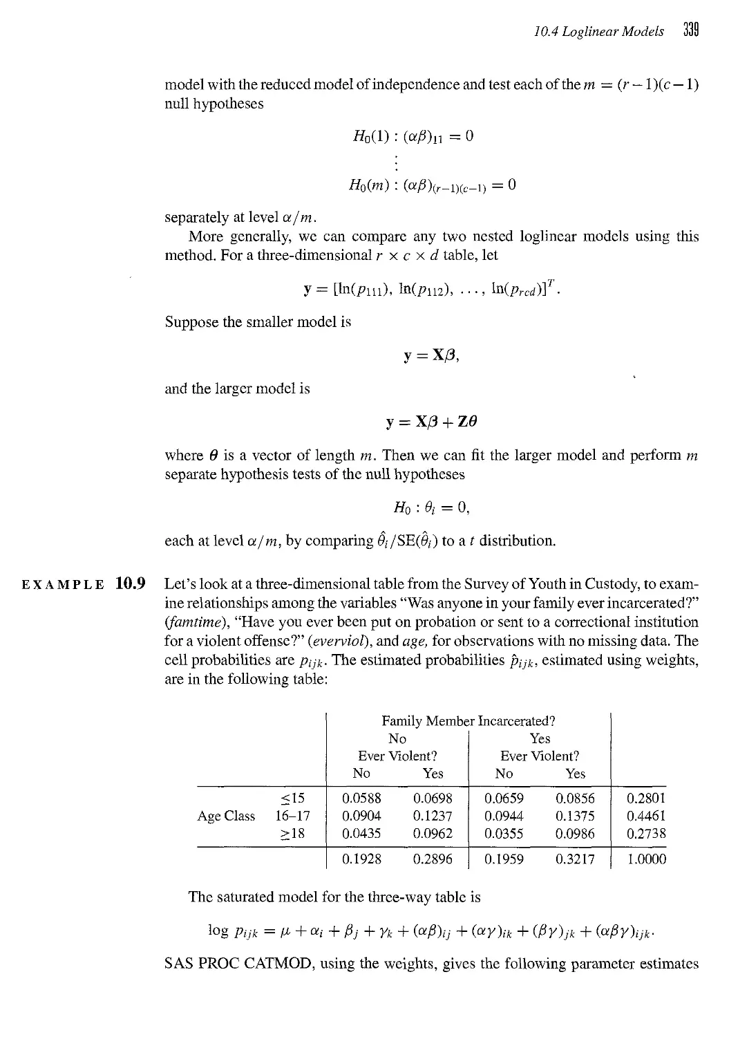
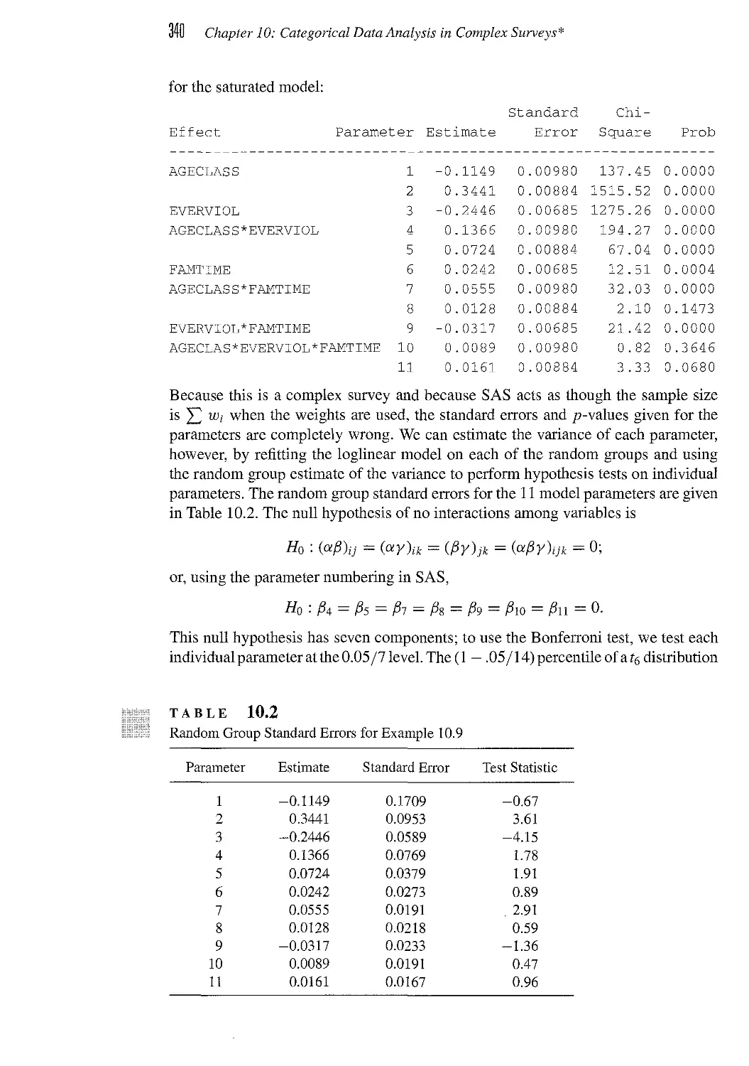
10.4 Loglinear Models 336
10.5 Exercises 341
CHAPTER 11 Regression with Complex Survey Data* 347
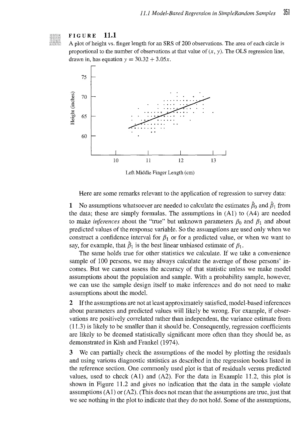
11.1 Model-Based Regression in Simple Random Samples 348
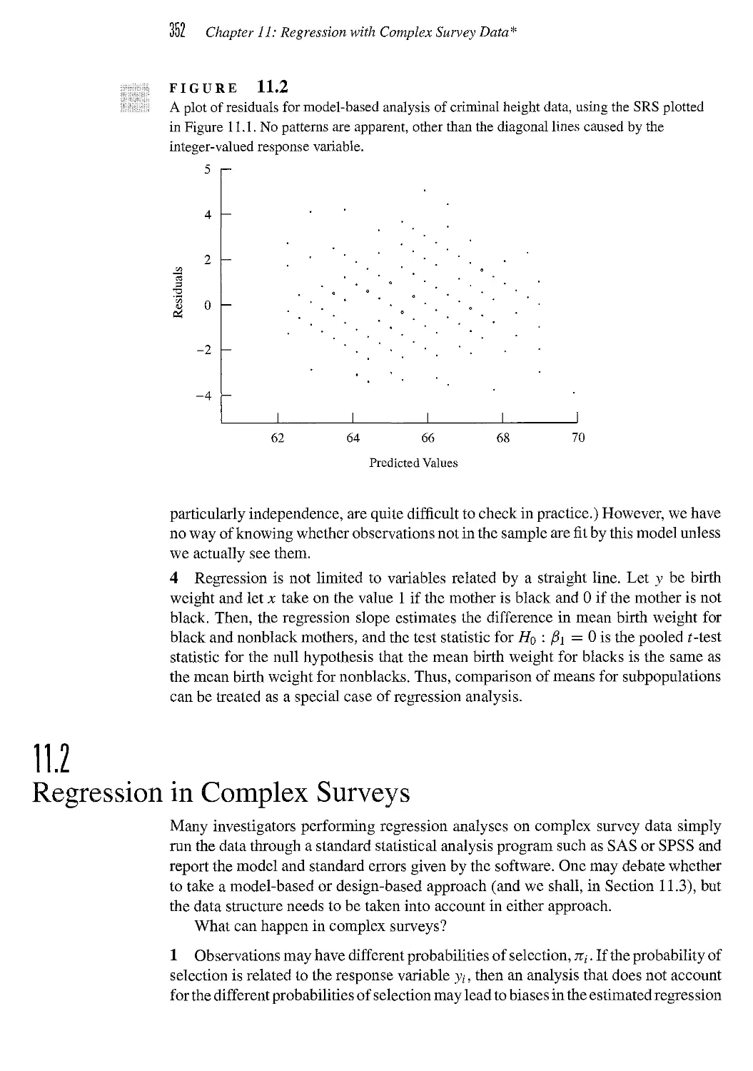
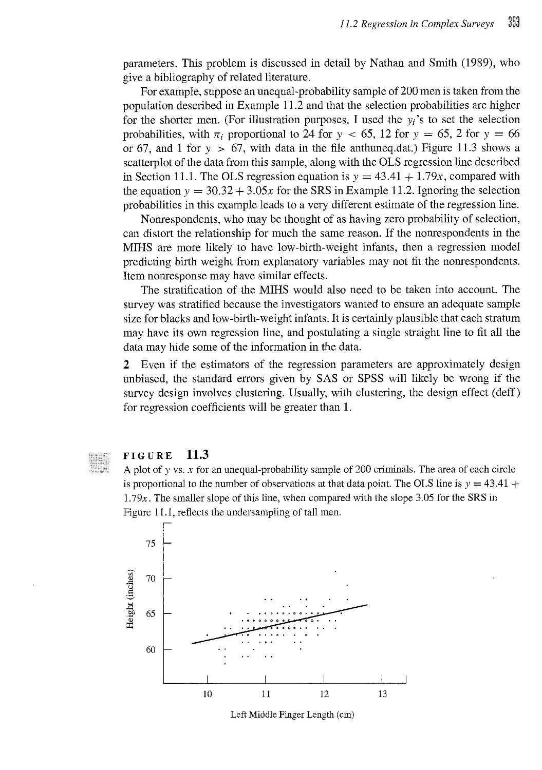
11.2 Regression in Complex Surveys 352
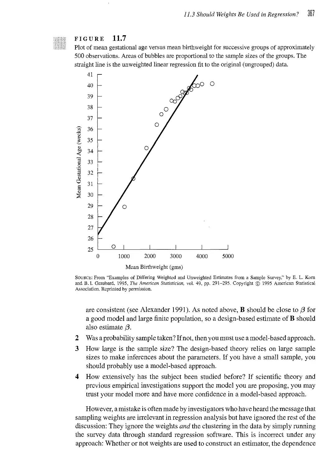
11.3 Should Weights Be Used in Regression? 362
11.4 Mixed Models for Cluster Samples 368
11.5 Logistic Regression 370
11.6 Generalized Regression Estimation for Population Totals 372
11.7 Exercises 374
CHAPTER 1/ Other Topics in Sampling* 379
12.1 Two-Phase Sampling 379
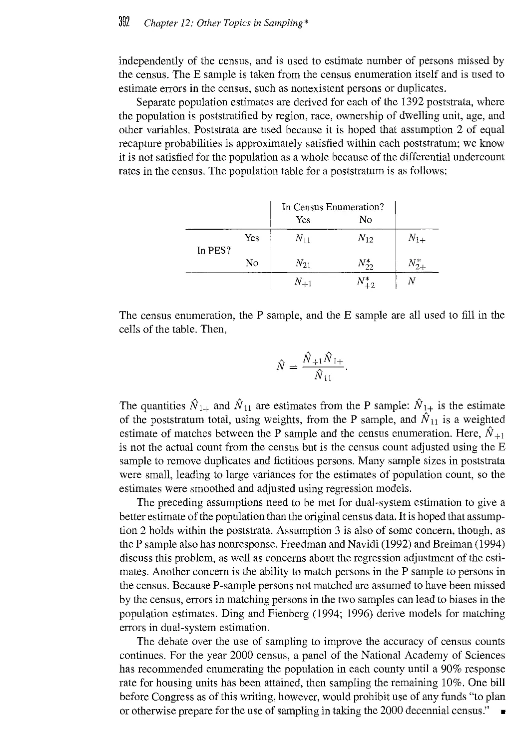
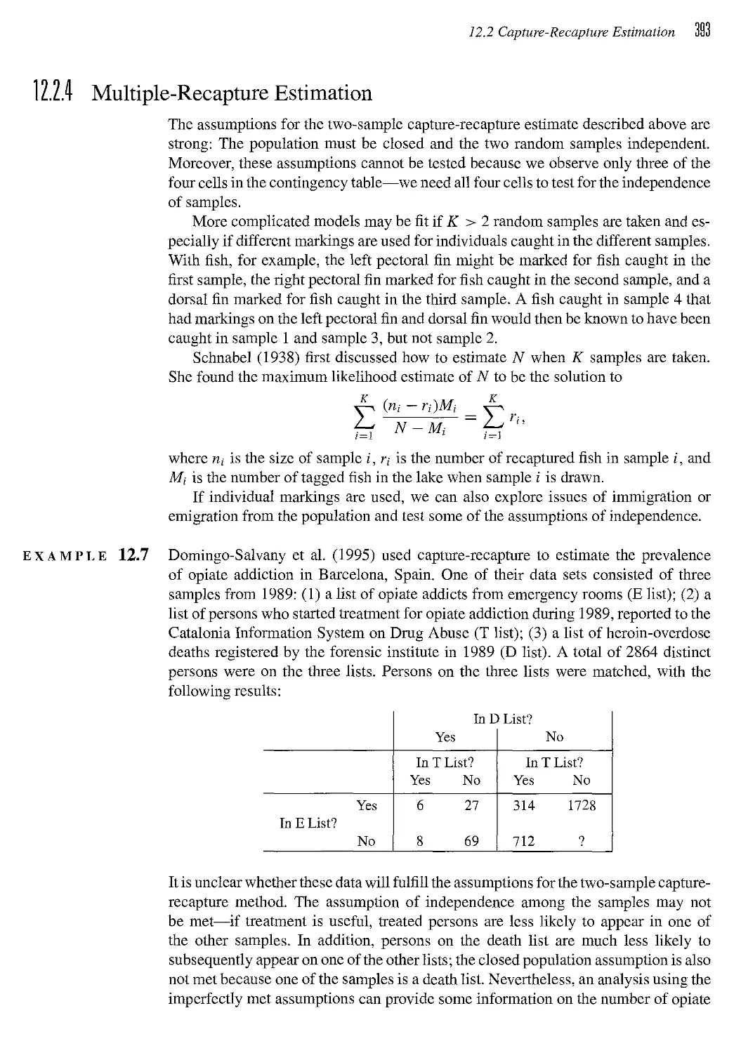
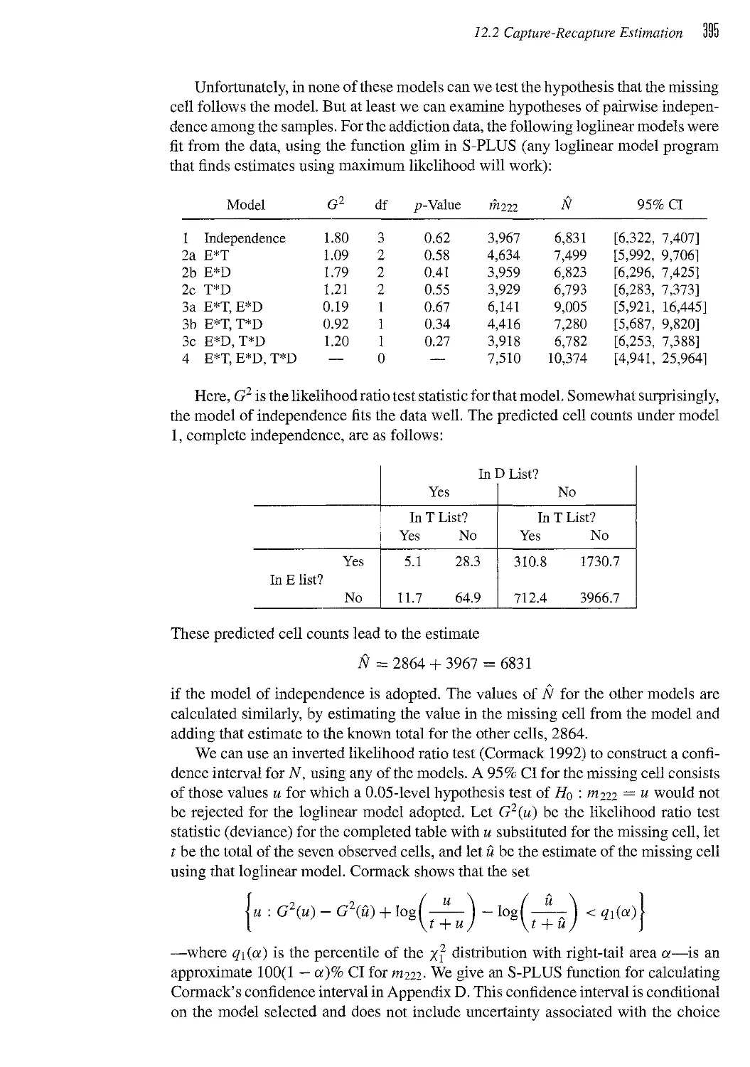
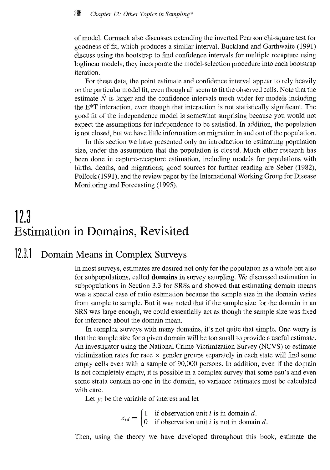
12.2 Capture-Recapture Estimation 387
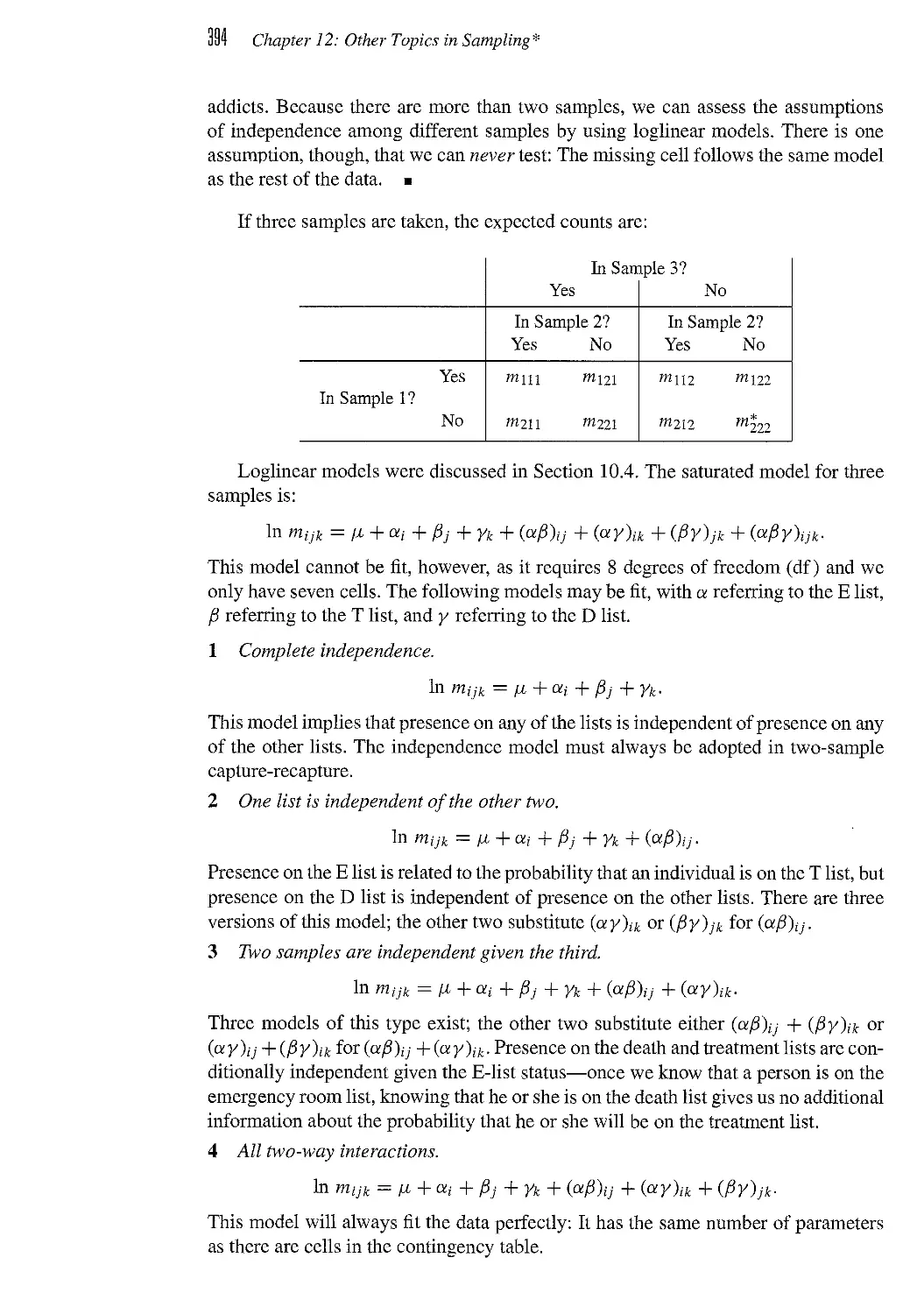
12.3 Estimation in Domains, Revisited 396

Contents XI
12.4 Sampling for Rare Events 400
12.5 Randomized Response 404
12.6 Exercises 407
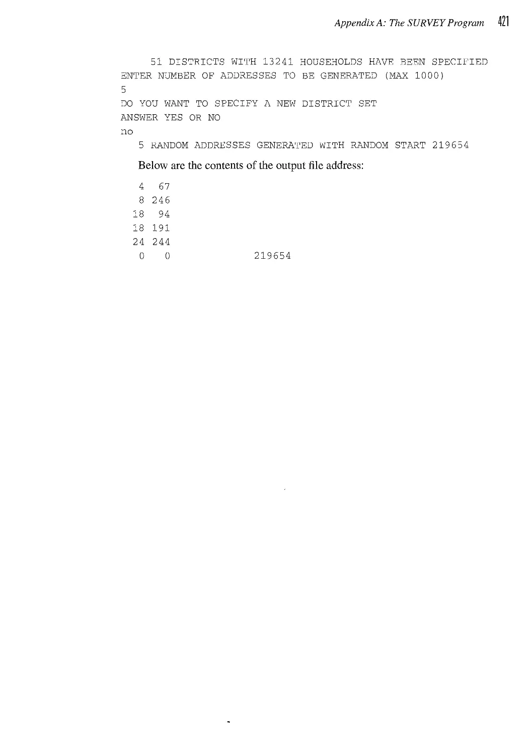
APPENDIX A The SURVEY Program 413
APPENDIX D Probability Concepts Used in Sampling 423
B.l Probability 423
B.2 Random Variables and Expected Value 426
B.3 Conditional Probability 430
B.4 Conditional Expectation 432
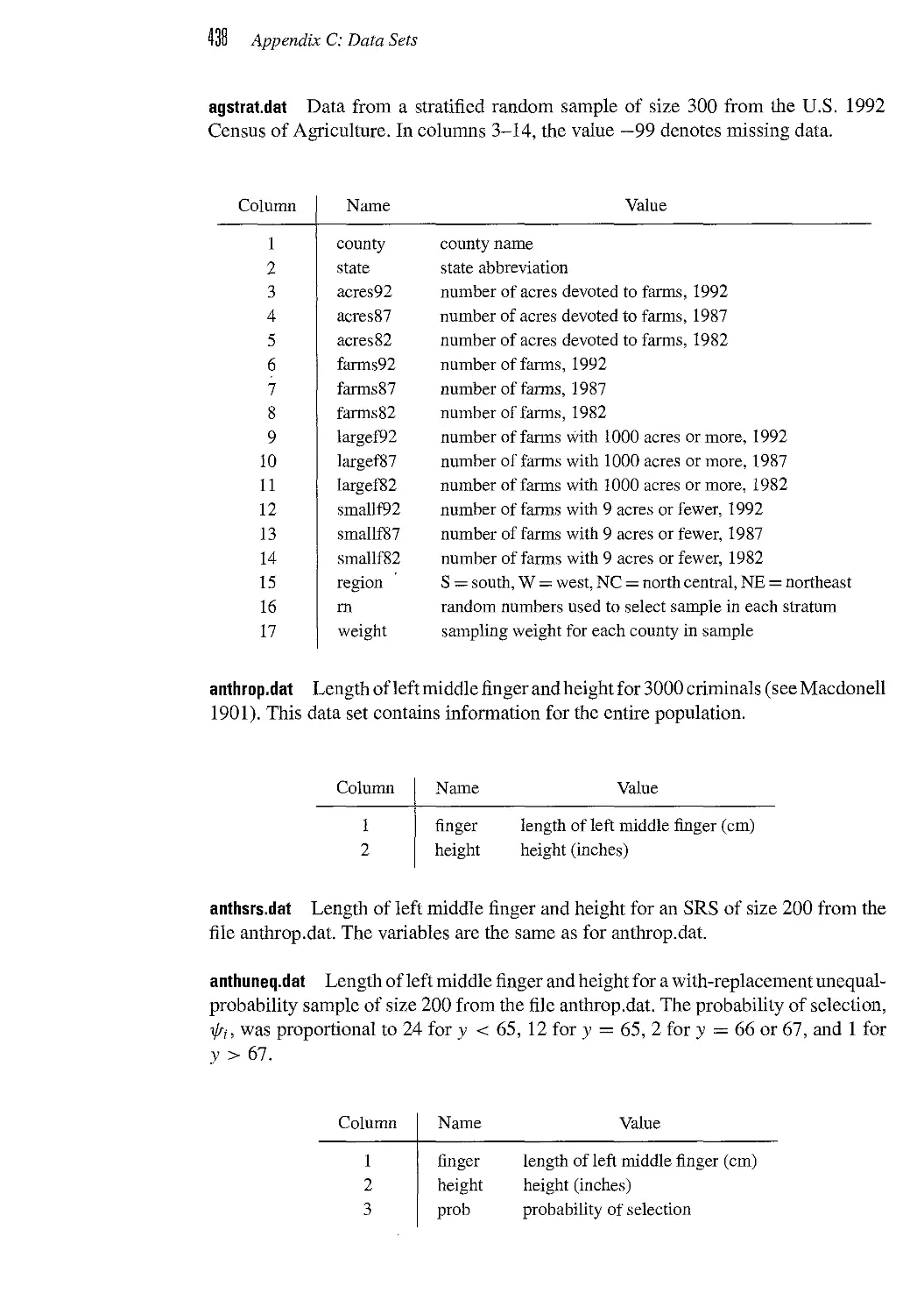
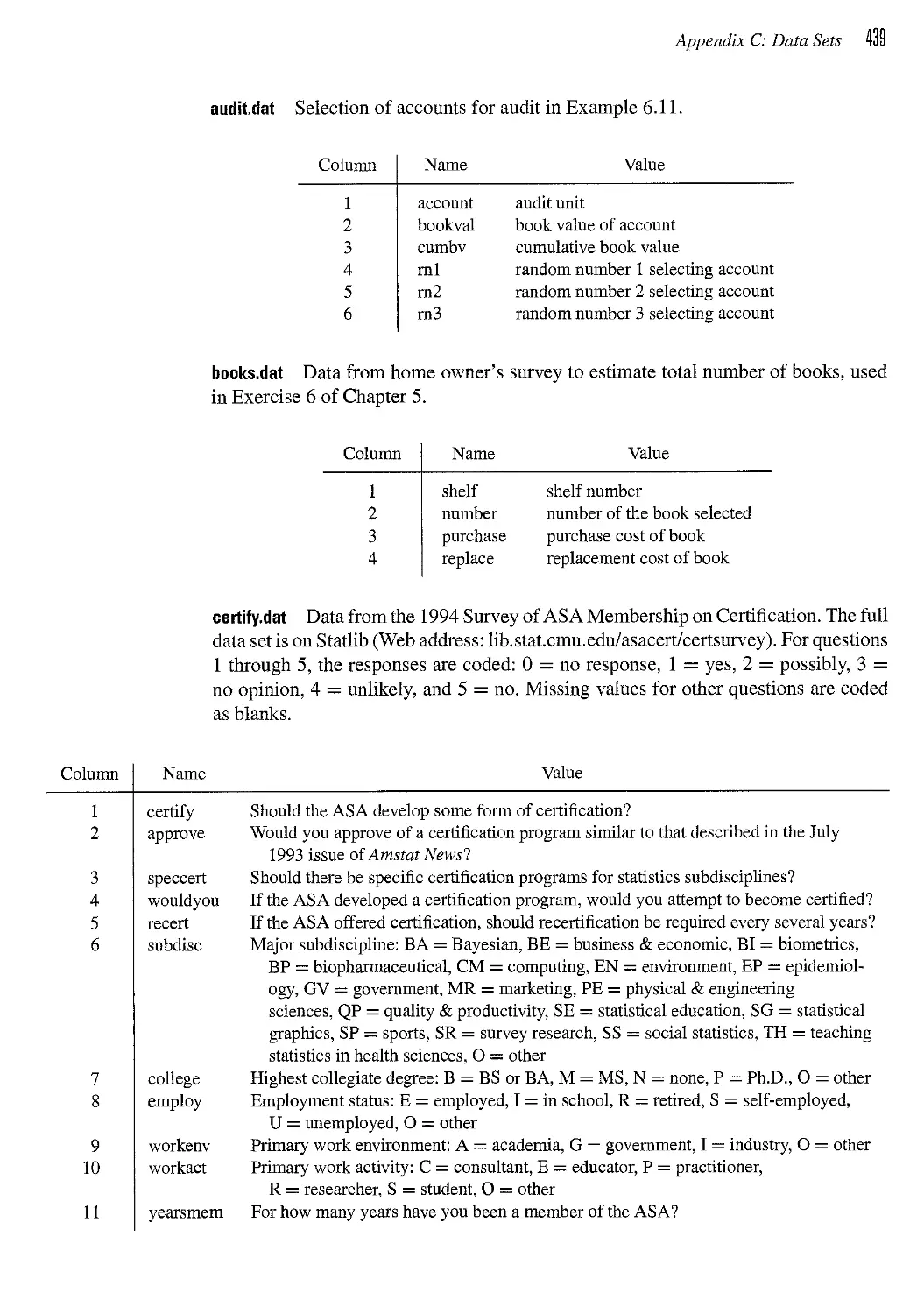
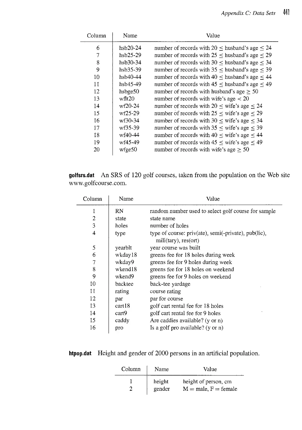
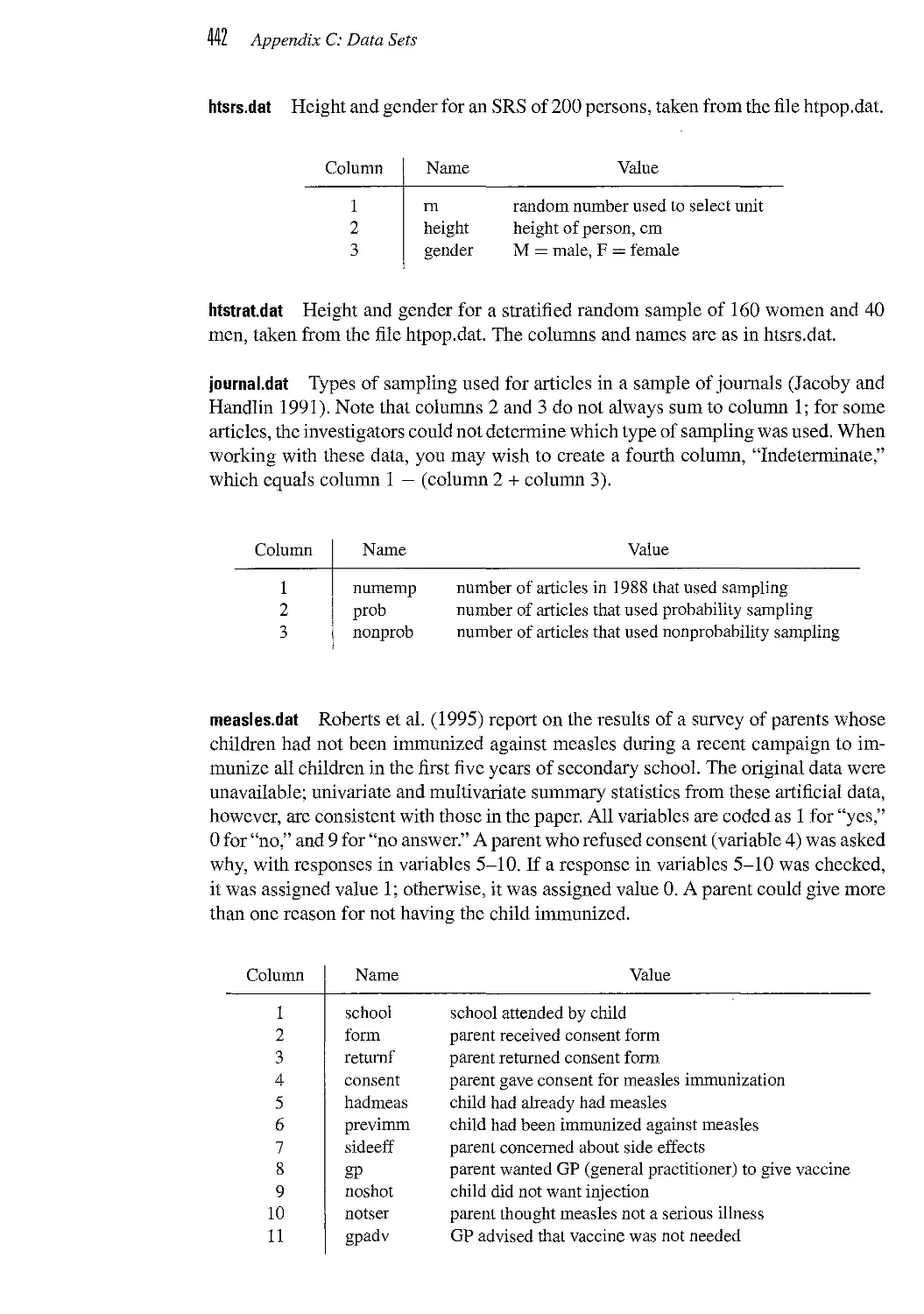
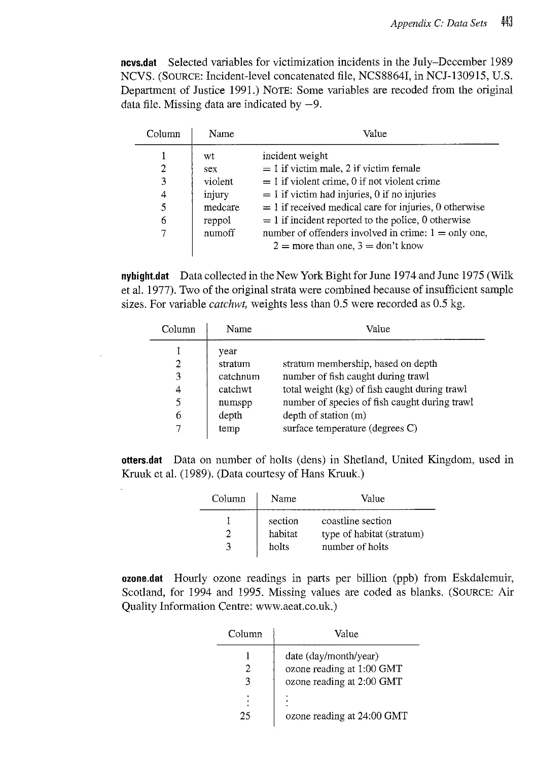
APPENDIX L Data Sets 437
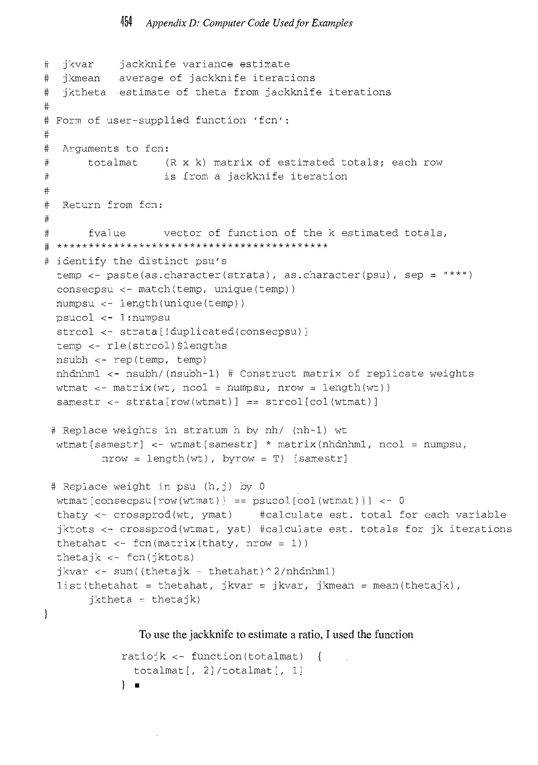
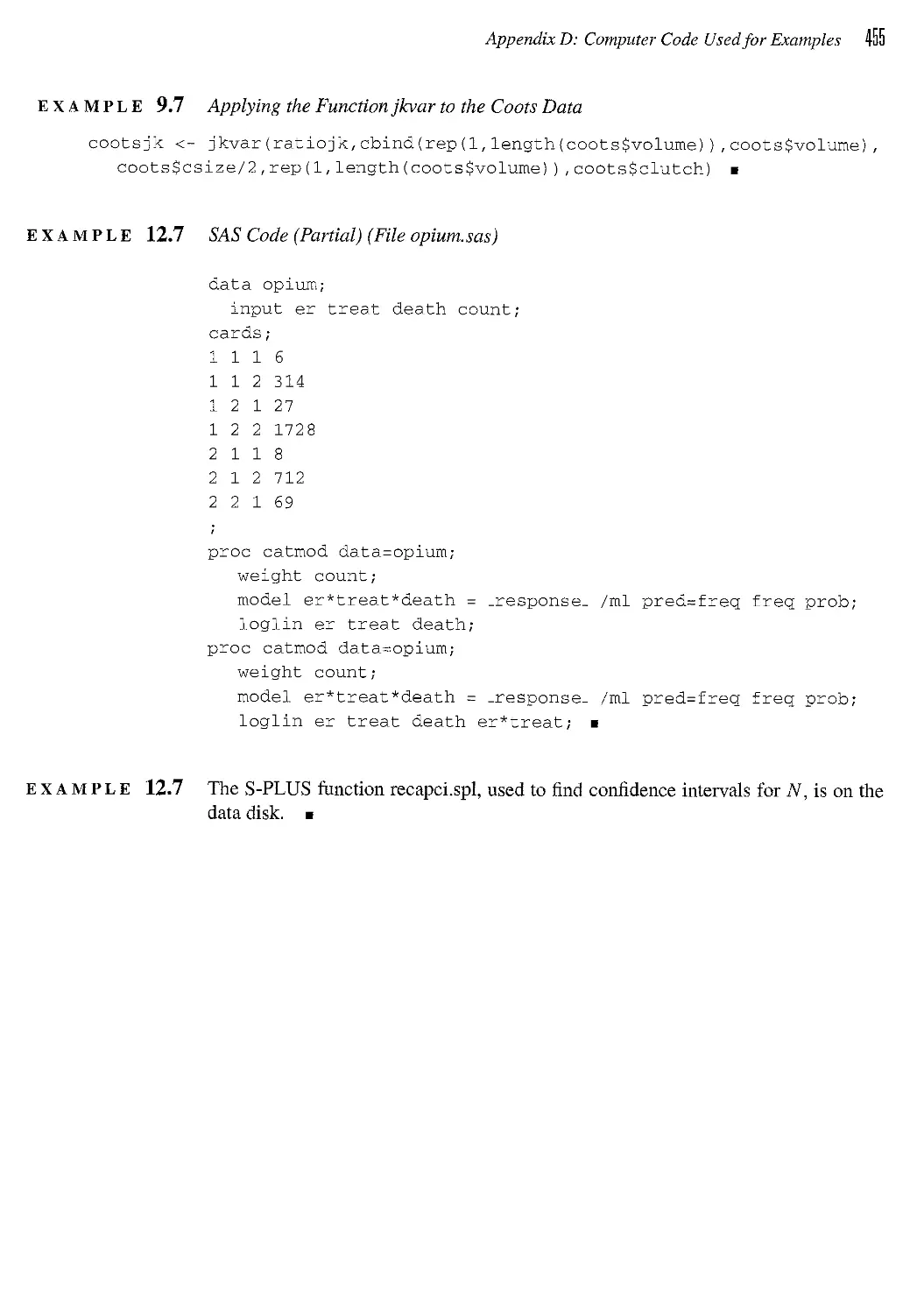
APPENDIX U Computer Codes Used for Examples 449
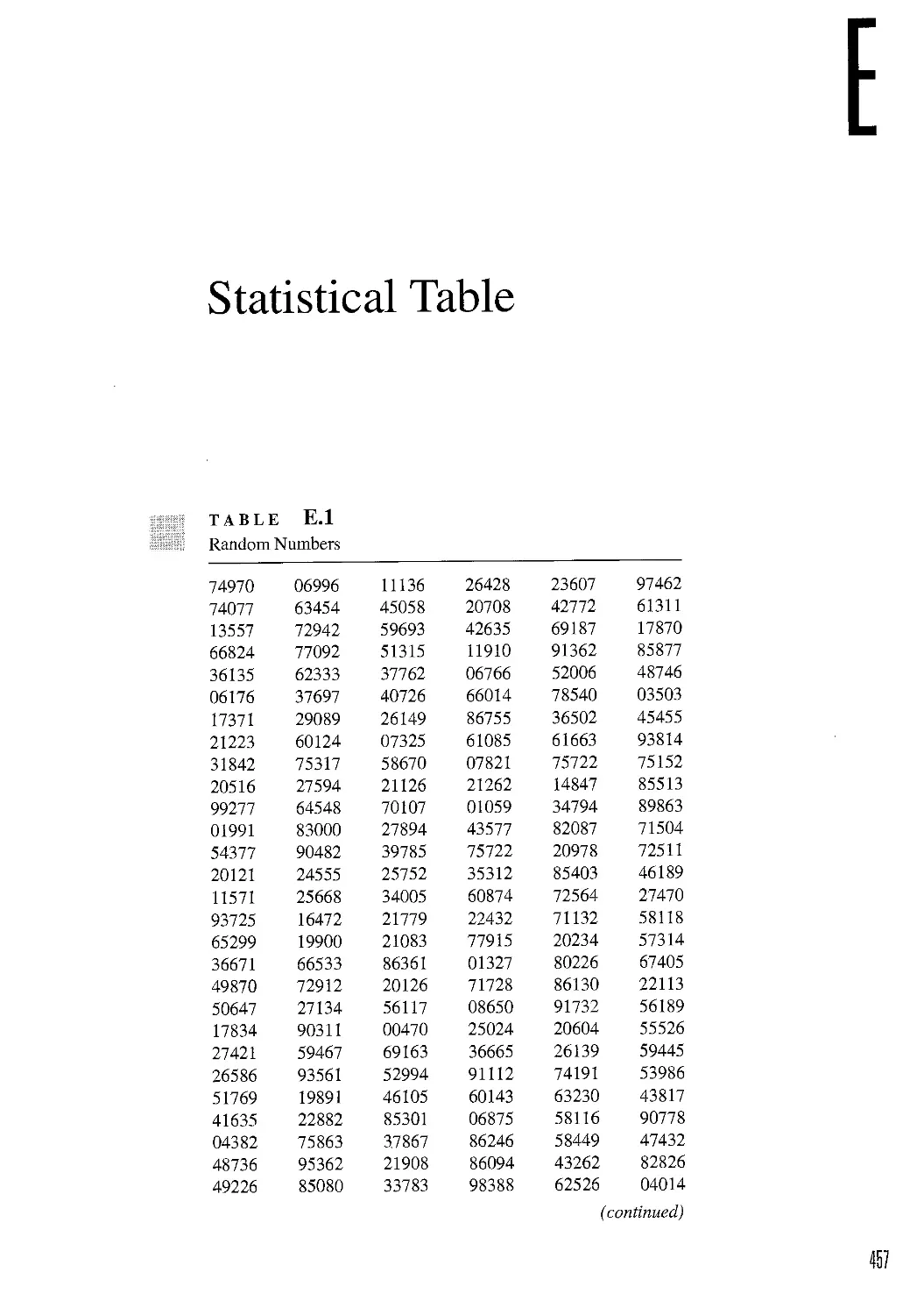
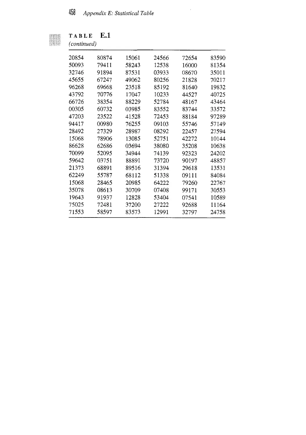
APPENDIX L Statistical Table 457
References 459
Author Index 485
Subject Index 489

Preface
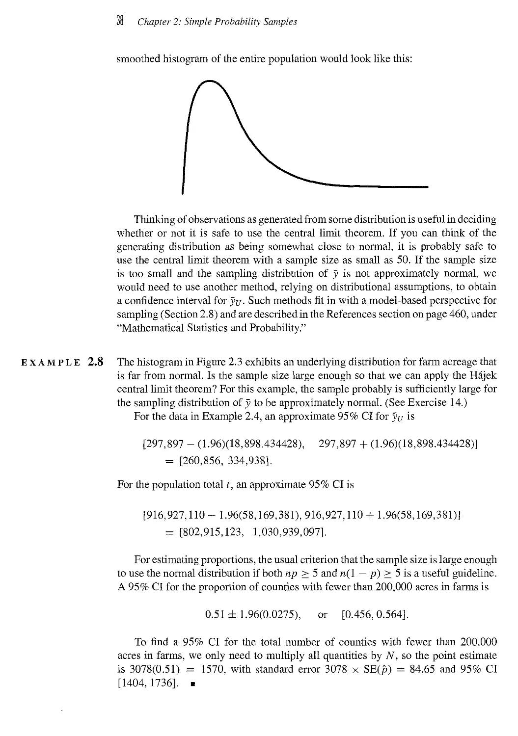
s
urveys and samples sometimes seem to surround you. Many give valuable
information; some, unfortunately, are so poorly conceived and implemented that it would
be better for science and society if they were simply not done. This book gives you
guidance on how to tell when a sample is valid or not, and how to design and analyze
many different forms of sample surveys.
The book concentrates on the statistical aspects of taking and analyzing a sample.
How to design and pretest a questionnaire, construct a sampling frame, and train field
investigators are all important issues, but are not treated comprehensively in this book.
I have written the book to be accessible to a wide audience, and to allow flexibility
in choosing topics to be read. To read most of Chapters 1 through 6, you need to be
familiar with basic ideas of expectation, sampling distributions, confidence intervals,
and linear regression—material covered in most introductory statistics classes. These
chapters cover the basic sampling designs of simple random sampling, stratification,
and cluster sampling with equal and unequal probabilities of selection. The optional
sections on the statistical theory for these designs are marked with asterisks—these
sections require you to be familiar with calculus or mathematical statistics. Appendix
B gives a review of probability concepts used in the theory of probability sampling.
Chapters 7 through 12 discuss issues not found in many other sampling textbooks:
how to analyze complex surveys such as those administered by the United States
Bureau of the Census or by Statistics Canada, different approaches to analyzing
sample surveys, what to do if there is nonresponse, and how to perform chi-squared
tests and regression analyses using data from complex surveys. The National Crime
Victimization Survey is discussed in detail as an example of a complex survey. Since
many of the formulas used to find standard errors in simpler sampling designs are
difficult to implement in complex samples, computer-intensive methods are discussed
for estimating the variances.
The book is suitable for a first course in survey sampling. It can be used for a class
of statistics majors, or for a class of students from business, sociology, psychology, or
biology who want to learn about designing and analyzing data from sample surveys.
Chapters 1 through 6 treat the building blocks of sampling, and the sections without
asterisks in Chapters 1 through 6 would provide material for a one-quarter course on

Preface
sampling. In my one-semester course, I cover sections without asterisks in Chapters
1 through 8, and selected topics from the other chapters. The material in Chapters 9
through 12 can be covered in almost any order, and topics chosen from those chapters
to fit the needs of the students.
Exercises in the book are of three types: exercises involving critiquing and
analyzing data from real surveys, or designing your own surveys, expose you to a variety
of applications of sampling; mathematical exercises (indicated by asterisks) develop
your theoretical knowledge of the subject; and exercises using SURVEY allow you
to experiment with different sample designs without having to collect all the data in
the field. The computer program SURVEY, developed by Professor Ted Chang of the
University of Virginia (Chang, Lohr, and MacLaren, 1992), allows you to generate
samples on the computer from a hypothetical population. The SURVEY exercises
allow you to go through all the steps involved in sampling, rather than just plug
numbers into a formula found earlier in the chapter. A disk that includes the data sets and
the SURVEY program is provided with the book .
You must know how to use a statistical computer package or spreadsheet to be
able to do the problems in this book. I encourage you to use a statistical package
such as Splus, SAS, or Minitab, or to use a spreadsheet such as Excel, Quattro Pro, or
Lotus 1-2-3 for the exercises. The package or spreadsheet you choose will depend on
the length and level of the class. In a one-quarter class introducing the basic concepts
of sampling, a spreadsheet will suffice for the computing. Some exercises in the later
chapters require some computer progranmiing; I have found that Splus is ideal for
these exercises as it combines programming capability with existing functions for
statistical analysis. Sampling packages such as SUDAAN (Shah et al., 1995) and
WesVarPC (Brick et al., 1996), while valuable for the sampling practitioner, hide the
structure behind the calculations from someone trying to learn the material. I have
therefore not relied on any of the computer packages that exist for analyzing survey
data in this book, although various packages are discussed in Section 9.6. Once you
understand why the different designs and estimators used in survey sampUng work
the way they do, it is a small step to read the user's manual for the survey package
and to use the software; however, if you have only relied on computer packages as a
black box, it is difficult to know when you are performing an appropriate analysis.
Six main features distinguish this book from other texts intended for students
from statistics and other disciplines who need to know about sampling methods.
¦ The book is flexible for content and level. Many sampling courses have students
with a wide range of statistical knowledge. By appropriate choice of sections, this
book can be used for an audience of undergraduates who have had one introductory
statistics course or for a first-year graduate course for statistics students. The book
is also useful for a person doing survey research wanting to learn more about the
statistical aspects of surveys and to learn about recent developments. The exercises
are flexible as well. Some of the exercises emphasize mastering the mechanics. Many,
however, encourage the student to think about the sampling issues involved, and to
understand the structure of the sample design at a deeper level. Other exercises are
open-ended, and encourage the student to explore the ideas further.
¦ I have tried to use real data as much as possible—the Acme Widget Company
never appears in this book. The examples and exercises come from social sciences.

Preface XII
engineering, agriculture, ecology, medicine, and a variety of other disciplines, and
are selected to illustrate the wide applicability of sampling methods. A number of the
data sets have extra variables not specifically referred to in text; an instructor can use
these for additional exercises or variations.
¦ I have incorporated model-based as well as randomization-based theory into the
text, with the goal of placing sampling methods within the framework used in other
areas of statistics. Many of the important results in the last twenty years of sampling
research have involved models, and an understanding of both approaches is essential
for the survey practitioner. The model-based approach is introduced in Section 2.8 and
further developed in successive chapters; however, those sections could be discussed
at any time later in the course.
¦ Many topics in this book, such as variance estimation and regression analysis of
noindent complex surveys, are not found in other textbooks at this level. The
comprehensive sampling reference Model Assisted Survey Sampling, by Samdal, Swensson,
and Wretman is at a much higher mathematical level.
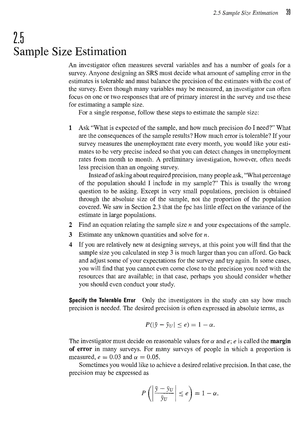
¦ This book emphasizes the importance of graphing the data. Graphical analysis
of survey data is often neglected because of the large sizes of data sets and the emphasis
on randomization theory, and this neglect can lead to flawed data analyses.
¦ Design of surveys is emphasized throughout, and is related to methods for
analyzing the data from a survey. The philosophy presented in this book is that the design
is by far the most important aspect of any survey: no amount of statistical analysis
can compensate for a badly-designed survey. Models are used to motivate designs,
and graphs presented to check the sensitivity of the design to model assumptions. For
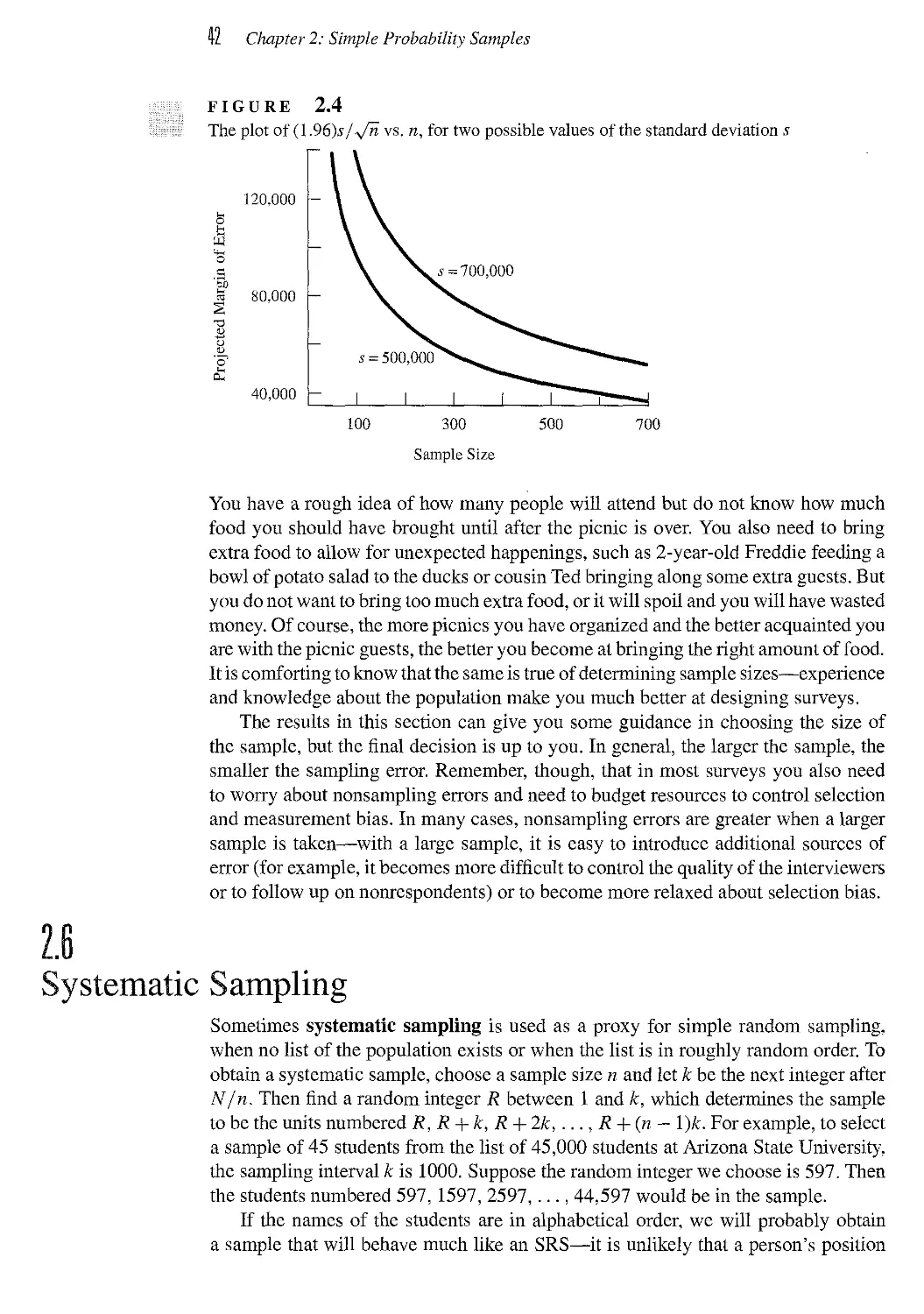
example, in Chapter 2, the usual formula for calculating sample size is presented. But
a graph is also given so that the investigator can see the sensitivity of the sample size
to the assumed population variance.
Many people have been generous with their encouragement and suggestions for
this book. I am deeply in their debt, although I reserve any credit for the book's
shortcomings for myself. The following persons reviewed or used various versions of the
manuscript, and provided invaluable suggestions for improvement: Jon Rao,
Elizabeth Stasny, Fritz Scheuren, Nancy Heckman, Ted Chang, Steve MacEachem, Mark
Conaway, Ron Christensen, Michael Hamada, Partha Lahiri, and several anonymous
reviewers: Dale Everson, University of Idaho; James Gentle, George Mason
University; Ruth Mickey, University of Vermont; Sarah Nusser, Iowa State University; N. G.
Narasimha Prasad, University of Alberta, Edmonton; and Deborah Rumsey, Kansas
State University. I had many helpful discussions with, and encouragement from, Jon
Rao, Fritz Scheuren, and Elizabeth Stasny. David Hubble and Marshall DeBerry
provided much helpful advice on the National Crime Victimization Survey. Ted Chang
first encouraged me to turn my class notes into a book, and generously allowed use
of the SURVEY program in this book. Many thanks go to Alexander Kugushev,
Carolyn Crockett, and the production staff at Brooks/Cole for their help, advice, and
encouragement. Finally, I would like to thank Alastair Scott, whose inspiring class
on sampling at the University of Wisconsin introduced me to the joys of the subject.
Sharon L. Lohr

1
Introduction
When statistics are not based on strictly accurate calculations, they mislead instead of guide. The mind
easily lets itself be taken in by the false appearance of exactitude which statistics retain in their
mistakes, and confidently adopts errors clothed in the form of mathematical truth.
—Alexis de Tocqueville, Democracy in America
1.1
A Sample Controversy
Shere Hite's book Women and Love: A Cultural Revolution in Progress A987) had a
number of widely quoted results:
¦ 84% of women are "not satisfied emotionally with their relationships" (p. 804).
¦ 70% of all women "married five or more years are having sex outside of their
marriages" (p. 856).
¦ 95% of women "report forms of emotional and psychological harassment from
men with whom they are in love relationships" (p. 810).
¦ 84% of women report forms of condescension from the men in their love
relationships (p. 809).
The book was widely criticized in newspaper and magazine articles throughout the
United States. The Time magazine cover story "Back Off, Buddy" (October 12,1987),
for example, called the conclusions of Hite's study "dubious" and "of limited value."
Why was Hite's study so roundly criticized? Was it wrong for Hite to report the
quotes from women who feel that the men in their lives refuse to treat them as equals,
who perhaps have never been given the chance to speak out before? Was it wrong to
report the percentages of these women who are unhappy in their relationships with men?
Of course not. Hite's research allowed women to discuss how they viewed their
experiences, and reflected the richness of these women's experiences in a way that a
multiple-choice questionnaire could not. Hite's error was in generalizing these results
to all women, whether they participated in the survey or not, and in claiming that the
percentages applied to all women. The following characteristics of the survey make

1 Chapter 1: Introduction
it unsuitable for generalizing tlie results to all women.
¦ The sample was self-selected—that is, recipients of questionnaires decided
whether they would be in the sample or not. Hite mailed 100,000 questionnaires;
of these, 4.5% were returned.
¦ The questionnaires were mailed to such organizations as professional women's
groups, counseling centers, church societies, and senior citizens' centers. The
members may differ in political views, but many have joined an "all-women"
group, and their viewpoints may differ from other women in the United States.
¦ The survey has 127 essay questions, and most of the questions have several parts.
Who will tend to return such a survey?
¦ Many of the questions are vague, using words such as love. The concept of love
probably has as many interpretations as there are people, making it impossible to
attach a single interpretation to any statistic purporting to state how many women
are "in love." Such question wording works well for eliciting the rich individual
vignettes that comprise most of the book but makes interpreting percentages
difficult.
¦ Many of the questions are leading—they suggest to the respondent which response
she should make. For instance: "Does your husband/lover see you as an equal?
Or are there times when he seems to treat you as an inferior? Leave you out of
the decisions? Act superior?" (p. 795).
Hite writes, "Does research that is not based on a probability or random sample
give one the right to generalize from the results of the study to the population at
large? If a study is large enough and the sample broad enough, and if one
generalizes carefully, yes" (p. 778). Most survey statisticians would answer Kite's question
with a resounding no. In Hite's survey, because the women sent questionnaires were
purposefully chosen and an extremely small percentage of the women returned the
questionnaires, statistics calculated from these data cannot be used to indicate
attitudes of all women in the United States. The final sample is not representative of
women in the United States, and the statistics can only be used to describe women
who would have responded to the survey.
Hite claims that results from the sample could be generalized because
characteristics such as the age, educational, and occupational profiles of women in the sample
matched those for the population of women in the United States. But the women in
the sample differed on one important aspect—they were willing to take the time to
fill out a long questionnaire dealing with harassment by men and to provide intensely
personal information to a researcher. We would expect that in every age group and
socioeconomic class, women who choose to report such information would in general
have had different experiences than women who choose not to participate in the survey.
1.2
Requirements of a Good Sample
In the movie Magic Town, the public opinion researcher played by James Stewart
discovered a town that had exactly the same characteristics as the whole United States:
Grandview had exactly the same proportion of people who voted Republican, the same

1.2 Requirements of a Good Sample 3
proportion of people under the poverty line, the same proportion of auto mechanics,
and so on, as the United States taken as a whole. All that Stewart's character had to do
was to interview the people of Grandview, and he would know what public opinion
was in the United States.
A perfect sample would be like Grandview: a scaled-down version of the
population, mirtoring every characteristic of the whole population. Of course, no such
perfect sample can exist for complicated populations (even if it did exist, we would
not know it was a perfect sample without measuring the whole population). But a
good sample will reproduce the characteristics of interest in the population, as closely
as possible. It will be representative in the sense that each sampled unit will represent
the characteristics of a known number of units in the population.
Some definitions are needed to make the notion of a good sample more precise.
Observation unit An object on which a measurement is taken. This is the basic
unit of observation, sometimes called an element. In studying human populations,
observation units are often individuals.
Target population The complete collection of observations we want to study.
Defining the target population is an important and often difficult part of the study. For
example, in a political poll, should the target population be all adults eligible to vote?
All registered voters? All persons who voted in the last election? The choice of target
population will profoundly affect the statistics that result.
Sample A subset of a population.
Sampled population The collection of all possible observation units that might have
been chosen in a sample; the population from which the sample was taken.
Sampling unit The unit we actually sample. We may want to study individuals but
do not have a list of all individuals in the target population. Instead, households
serve as the sampling units, and the observation units are the individuals living in the
households.
Sampling frame The list of sampling units. For telephone surveys, the samphng
frame might be a list of all residential telephone numbers in the city; for personal
interviews, a list of all street addresses; for an agricultural survey, a list of all farms
or a map of areas containing farms.
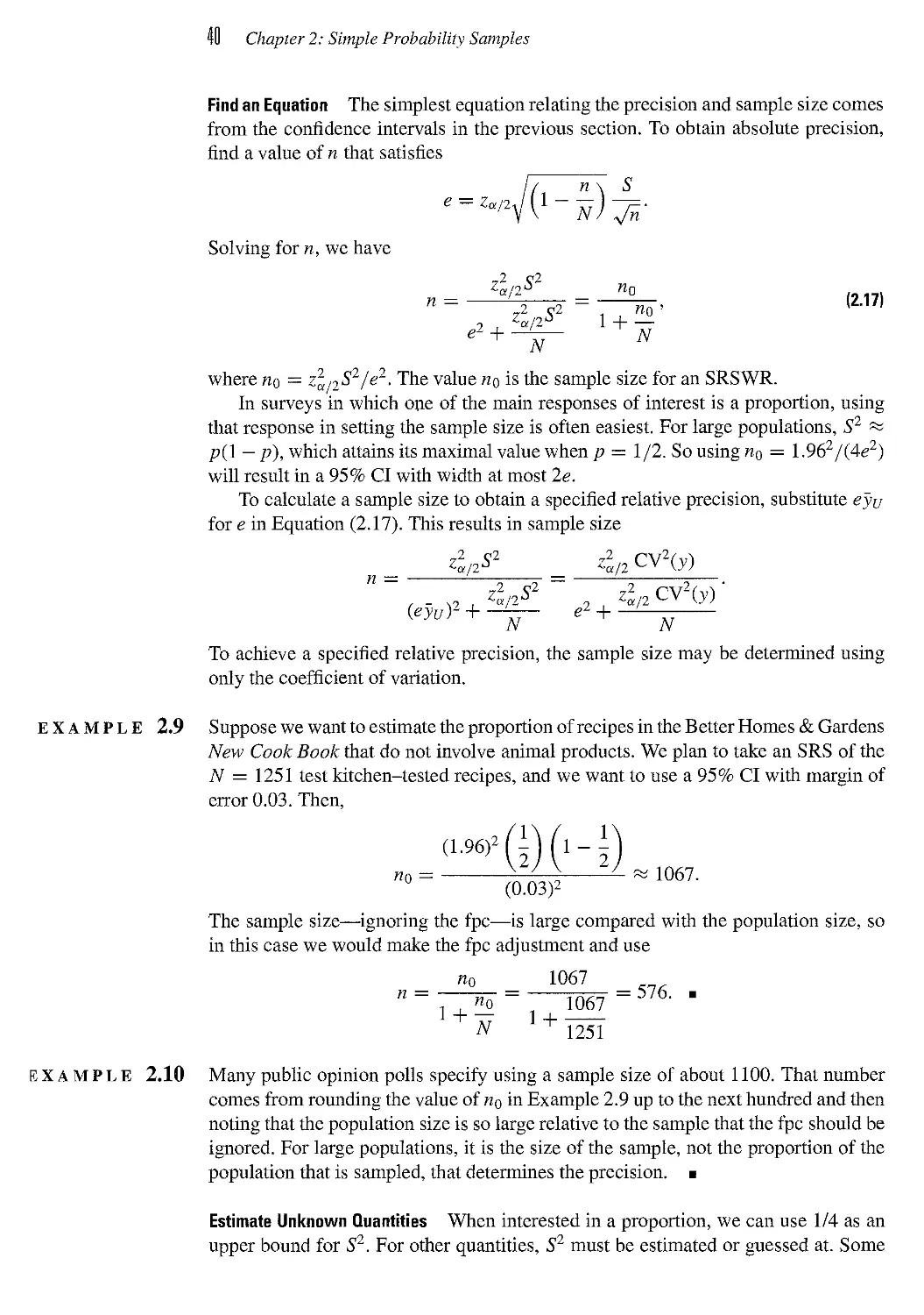
In an ideal survey, the sampled population will be identical to the target population,
but this ideal is rarely met exactly. In surveys of people, the sampled population is
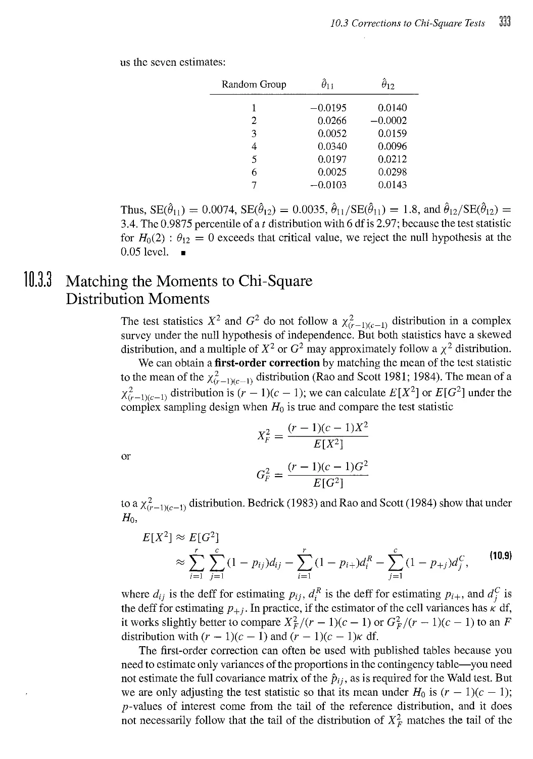
usually smaller than the target population. As Figure 1.1 illustrates, not all persons
in the target population are included in the sampling frame, and a number of persons
will not respond to the survey.
In the Hite study, one characteristic of interest was the percentage of women who
are harassed in their relationship. An individual woman was an element. The target
population was all adult women in the United States. Kite's sampled population was
women belonging to women's organizations who would return the questionnaire.
Consequently, inferences can only be made to the sampled population, not to the
population of all adult women in the United States.
The National Crime Victimization Survey is an ongoing survey to study
victimization rates, administered by the U.S. Bureau of the Census and the Bureau of Justice

1 Chapter 1: Introduction
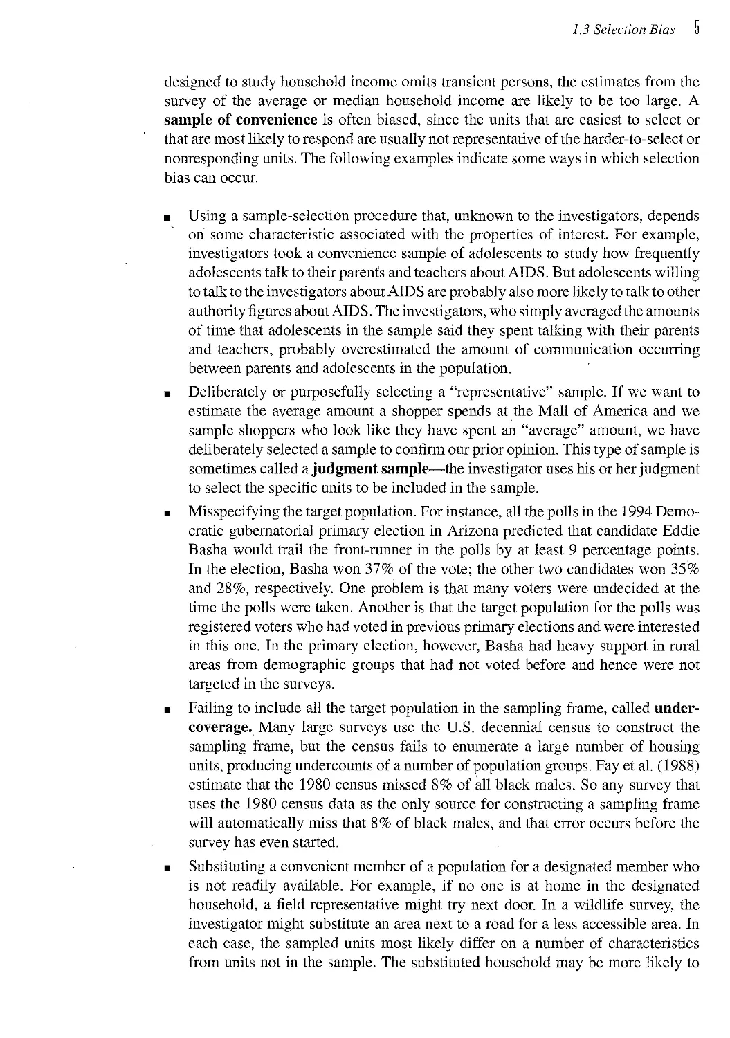
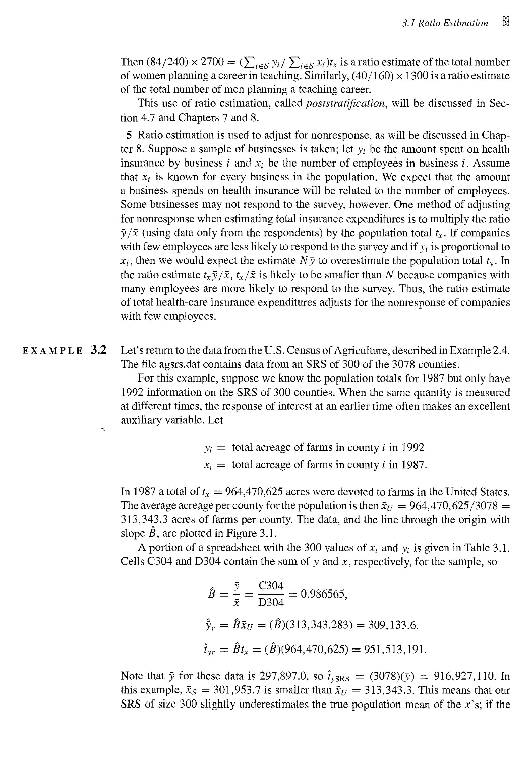
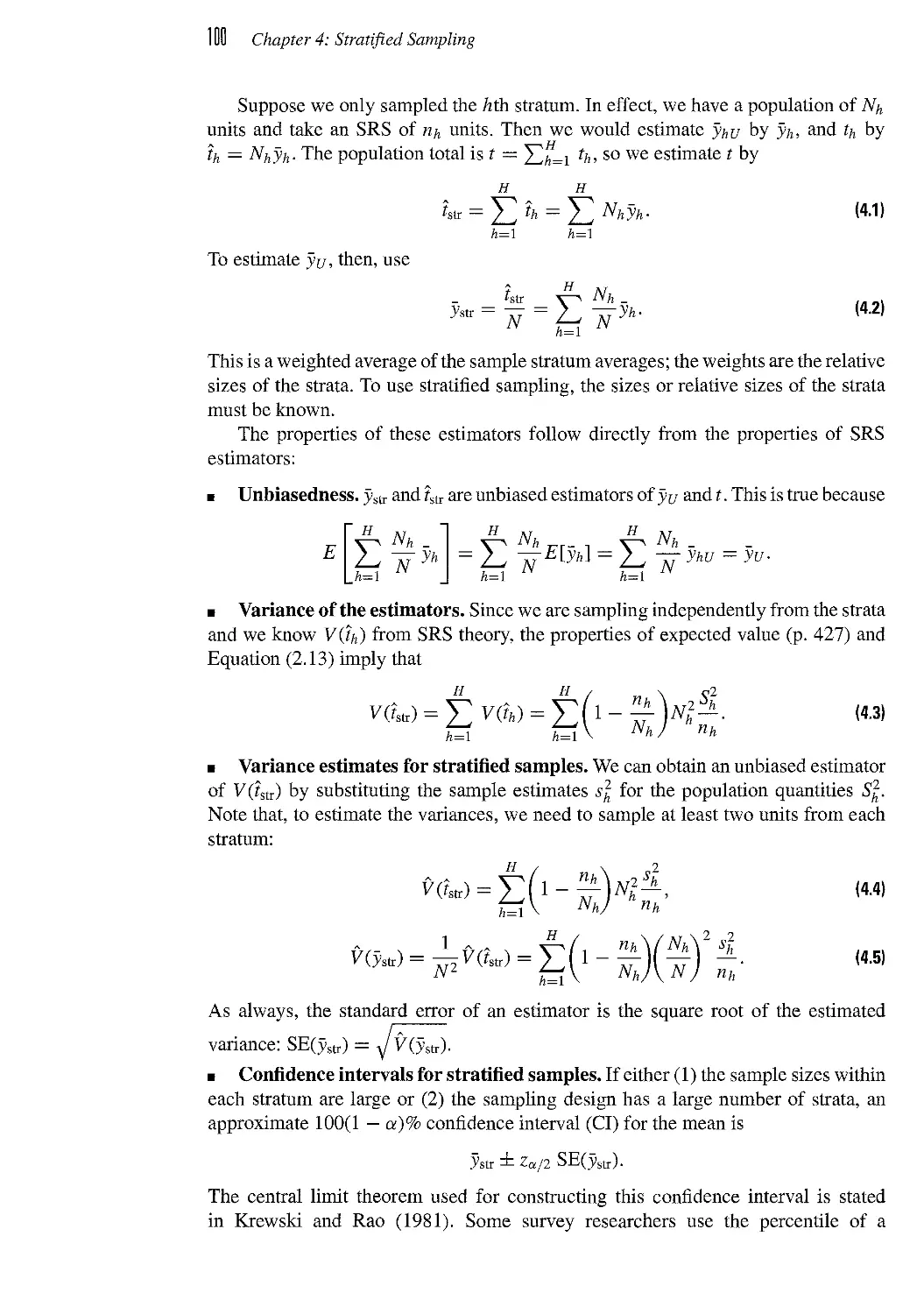
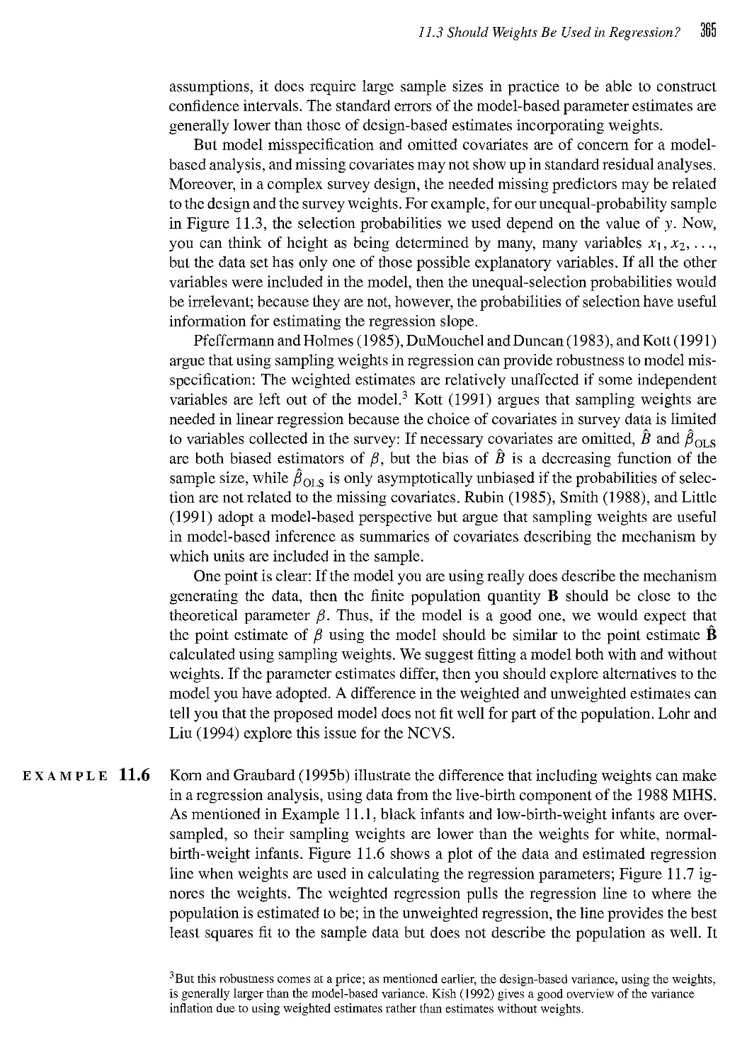
FIGURE 1.1
The target population and sampled population in a telephone.survey of likely voters. Not all
households will have telephones, so a number of persons in the target population of likely
voters will not be associated with a telephone number in the sampling frame. In some
households with telephones, the residents are not registered to vote and hence are ineligible
for the survey. Some eligible persons in the samphng frame population do not respond
because they cannot be contacted, some refuse to respond to the survey, and some may be ill
and incapable of responding.
TARGET POPULATION
Not included in
sampling frame
Not
reachable
Refuse to
respond
Not capable
of responding
SAMPLED
POPULATION
SAMPLING
FRAME
POPULATION
^
Not eligible
for survey
J
Statistics. If the characteristic of interest is the total number of households in the
United States that were victimized by crime last year, the elements are households,
the target population consists of all households in the United States, and the sampled
population consists of households in the sampling frame, constructed from census
information and building permits, that are "at home" and agree to answer questions.
The goal of the National Pesticide Survey, conducted by the Environmental
Protection Agency, was to study pesticides and nitrate in drinking water wells nationwide.
The target population was all community water systems and rural domestic wells in
the United States. The sampled population was all community water systems (all
are listed in the Federal Reporting Data System) and all identifiable domestic wells
outside of government reservations that belonged to households willing to cooperate
with the survey.
Public opinion polls are often taken to predict which candidate will win the next
election. The target population is persons who will vote in the next election; the
sampled population is often persons who can be reached by telephone and say they
are likely to vote in the next election. Few national polls in the United States include
Alaska or Hawaii or persons in hospitals, dormitories, or jails; they are not part of the
sampling frame or of the sampled population.
1.3
Selection Bias
A good sample will be as free from selection bias as possible. Selection bias occurs
when some part of the target population is not in the sampled population. If a survey

1.3 Selection Bias U
designed to study household income omits transient persons, the estimates from the
survey of the average or median household income are likely to be too large. A
sample of convenience is often biased, since the units that are easiest to select or
that are most likely to respond are usually not representative of the harder-to-select or
nonresponding units. The following examples indicate some ways in which selection
bias can occur.
¦ Using a sample-selection procedure that, unknown to the investigators, depends
on some characteristic associated with the properties of interest. For example,
investigators took a convenience sample of adolescents to study how frequently
adolescents talk to their parent's and teachers about AIDS. But adolescents willing
to talk to the investigators about AIDS are probably also more likely to talk to other
authority figures about AIDS. The investigators, who simply averaged the amounts
of time that adolescents in the sample said they spent talking with their parents
and teachers, probably overestimated the amount of communication occurring
between parents and adolescents in the population.
¦ Deliberately or purposefully selecting a "representative" sample. If we want to
estimate the average amount a shopper spends at the Mall of America and we
sample shoppers who look like they have spent an "average" amount, we have
deliberately selected a sample to confirm our prior opinion. This type of sample is
sometimes called a judgment sample—the investigator uses his or her judgment
to select the specific units to be included in the sample.
¦ Misspecifying the target population. For instance, all the polls in the 1994
Democratic gubernatorial primary election in Arizona predicted that candidate Eddie
Basha would trail the front-runner in the polls by at least 9 percentage points.
In the election, Basha won 37% of the vote; the other two candidates won 35%
and 28%, respectively. One problem is that many voters were undecided at the
time the polls were taken. Another is that the target population for the polls was
registered voters who had voted in previous primary elections and were interested
in this one. In the primary election, however, Basha had heavy support in rural
areas from demographic groups that had not voted before and hence were not
targeted in the surveys.
¦ Failing to include all the target population in the sampling frame, called under-
coverage. Many large surveys use the U.S. decennial census to construct the
sampling frame, but the census fails to enumerate a large number of housing
units, producing undercounts of a number of population groups. Fay et al. A988)
estimate that the 1980 census missed 8% of all black males. So any survey that
uses the 1980 census data as the only source for constructing a sampling frame
will automatically miss that 8% of black males, and that error occurs before the
survey has even started.
¦ Substituting a convenient member of a population for a designated member who
is not readily available. For example, if no one is at home in the designated
household, a field representative might try next door. In a wildlife survey, the
investigator might substitute an area next to a road for a less accessible area. In
each case, the sampled units most likely differ on a number of characteristics
from units not in the sample. The substituted household may be more likely to

Chapter 1: Introduction
have a member who does not work outside the home than the originally selected
household. The area by the road may have fewer frogs than the area that is harder
to reach.
Failing to obtain responses from all the chosen sample. Nonresponse distorts the
results of many surveys, even surveys that are carefully designed to minimize
other sources of selection bias. Often, nonrespondents differ critically from the
respondents, but the extent of that difference is unknown unless you can later
obtain information about the nonrespondents. Many surveys reported in newspapers
or research journals have dismal response rates—in some, the response rate is as
low as 10%. It is difficult to see how results can be generalized to the population
when 90% of the targeted sample cannot be reached or refuses to participate.
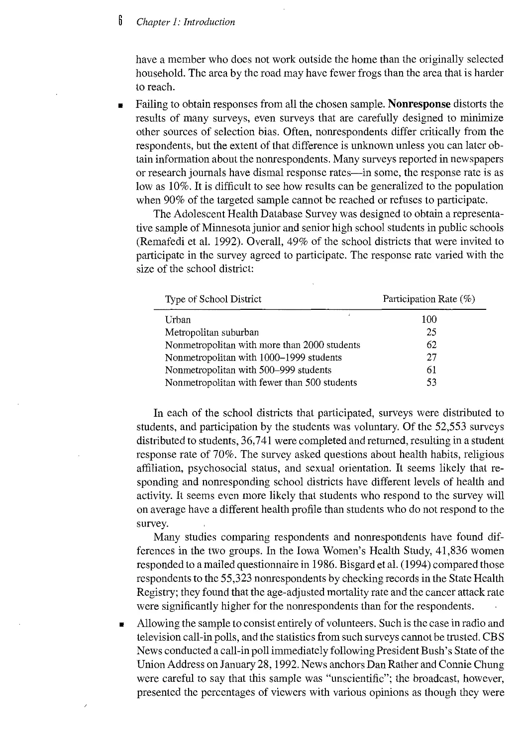
The Adolescent Health Database Survey was designed to obtain a
representative sample of Minnesota junior and senior high school students in public schools
(Remafedi et al. 1992). Overall, 49% of the school districts that were invited to
participate in the survey agreed to participate. The response rate varied with the
size of the school district:
Type of School District Participation Rate (%)
Urban ' 100
Metropolitan suburban 25
Nonmetropolitan with more than 2000 students 62
Nonmetropolitan with 1000-1999 students 27
Nonmetropolitan with 500-999 students 61
Nonmetropolitan with fewer than 500 students 53
In each of the school districts that participated, surveys were distributed to
students, and participation by the students was voluntary. Of the 52,553 surveys
distributed to students, 36,741 were completed and returned, resulting in a student
response rate of 70%. The survey asked questions about health habits, religious
affiliation, psychosocial status, and sexual orientation. It seems likely that
responding and nonresponding school districts have different levels of health and
activity. It seems even more likely that students who respond to the survey will
on average have a different health profile than students who do not respond to the
survey.
Many studies comparing respondents and nomrespondents have found
differences in the two groups. In the Iowa Women's Health Study, 41,836 women
responded to a mailed questionnaire in 1986. Bisgard et al. A994) compared those
respondents to the 55,323 nonrespondents by checking records in the State Health
Registry; they found that the age-adjusted mortality rate and the cancer attack rate
were significantly higher for the nonrespondents than for the respondents.
Allowing the sample to consist entirely of volunteers. Such is the case in radio and
television call-in polls, and the statistics from such surveys cannot be trusted. CBS
News conducted a call-in poll immediately following President Bush's State of the
Union Address on January 28,1992. News anchors Dan Rather and Connie Chung
were careful to say that this sample was "unscientific"; the broadcast, however,
presented the percentages of viewers with various opinions as though they were

1.3 Selection Bias 1
from a statistically sound survey. Almost 315,000 callers responded to what the
New York Times called "the largest biased sample in the history of instant polling,"
and many more tried to respond—AT&T computers recorded almost 25 million
attempts to reach the toll-free telephone number. The Nielsen ratings estimated
that about 9 million households had a television tuned to the CBS program,
indicating that many individuals or organizations tried to call multiple times. The
possibility always exists in a call-in survey that a determined organization will
skew the results by monopolizing the toll-free number.
EXAMPLE 1.1 Many surveys have more than one of these problems. The Literary Digest A932,
1936a, b, c) began taking polls to forecast the outcome of the U.S. presidential election
in 1912, and their polls attained a reputation for accuracy because they forecast the
correct winner in every election between 1912 and 1932. In 1932, for example, the
poll predicted that Roosevelt would receive 56% of the popular vote and 474 votes
in the electoral college; in the actual election, Roosevelt received 58% of the popular
vote and 472 votes in the electoral college.
With such a strong record of accuracy, it is not surprising that the editors of the
Literary Digest had a great deal of confidence in their polling methods by 1936.
Launching the 1936 poll, they said:
The Poll represents thirty years' constant evolution and perfection. Based on the
"commercial sampling" methods used for more than a century by publishing houses to push
book sales, the present mailing list is drawn from every telephone book in the United
States, from the rosters of clubs and associations, from city directories, lists of
registered voters, classified mail-order and occupational data. A936a, 3)
On October 31, the poll predicted that Republican Alf Landon would receive
55% of the popular vote, compared with 41% for President Roosevelt. The article
"Landon, 1,293,669; Roosevelt, 972,897: Final Returns in The Digest's Poll of Ten
Million Voters" contained this statement: "We make no claim to infallibility. We did
not Coin the phrase 'uncanny accuracy' which has been so freely applied to our Polls"
A936b). It is a good thing they made no claim to infallibility; in the election, Roosevelt
received 61% of the vote; Landon, 37%.
What went wrong? One problem may have been undercoverage in the sampling
frame, which relied heavily on telephone directories and automobile registration
lists—the frame was used for advertising purposes, as well as for the poll.
Households with a telephone or automobile in 1936 were generally more affluent than other
households, and opinion of Roosevelt's economic policies was generally related to
the economic class of the respondent. But sampling frame bias does not explain all the
discrepancy. Postmortem analyses of the poll by Squire A988) and Calahan A989)
indicate that even persons with both a car and a telephone tended to favor Roosevelt,
¦ though not to the degree that persons with neither car nor telephone supported him.
The low response rate to the survey was likely the source of much of the error. Ten
million questionnaires were mailed out, and 2.3 million were returned—an enormous
sample but a response rate of less than 25%. In Allentown, Pennsylvania, for example,
the survey was mailed to every registered voter, but the survey results for Allentown
were still incorrect because only one-third of the ballots were returned. Squire A988)
reports that persons supporting Landon were much more likely to have returned the

0 Chapter 1: Introduction
survey; in fact, many Roosevelt supporters did not even remember receiving a survey,
even though they were on the mailing list.
One lesson to be learned from the Literary Digest poll is that the sheer size of
a sample is no guarantee of its accuracy. The Digest editors became complacent
because they sent out questionnaires to more than one quarter of all registered voters
and obtained a huge sample of 2.3 million people. But large unrepresentative samples
can perform as badly as small unrepresentative samples. A large unrepresentative
sample may do more damage than a small one because many people think that large
samples are always better than small ones. The design of the survey is far more
important than the absolute size of the sample. ¦
What Good Are Samples with Selection Bias? We prefer to have samples with no
selection bias, that serve as a microcosm of the population. When the primary interest is in
estimating the total number of victims of violent crime in the United States or the
percentage of likely voters in the United Kingdom who intend to vote for the Labour Party
in the next election, serious selection bias can cause the sample estimates to be invalid.
Purposive or judgment samples can provide valuable information, though,
particularly in the early stages of an investigation. Teichman et al. A993) took soil samples
along Interstate 880 in Alameda County, California, to determine the amount of lead
in yards of homes and in parks close to the freeway. In taking the samples, they
concentrated on areas where they thought children were likely to play and areas where
soil might easily be tracked into homes. The purposive sampling scheme worked well
for justifying the conclusion of the study, that "lead contamination of urban soil in the
east bay area of the San Francisco metropolitan area is high and exceeds hazardous
waste levels at many sites." A sampling scheme that avoided selection bias would
only be needed for this study if the investigators wanted to generalize the estimated
percentage of contaminated sites to the entire area.
Measurement Bias
A good sample has accurate responses to the items of interest. Measurement bias
occurs when the measuring instrument has a tendency to differ from the true value
in one direction. As with selection bias, measurement bias must be considered and
minimized in the design stage of the survey; no amount of statistical analysis will
disclose, for instance, that the scale erroneously added 5 kilograms to the weight of
every person in a health survey.
Measurement bias is a concern in all surveys and can be insidious. In many
surveys of vegetation, for example, areas to be sampled are divided into smaller plots.
A sample of plots is selected, and the number of plants in each plot is recorded. When
a plant is near the boundary of the region, the field researcher needs to decide whether
to include the plant in the tally. A person who includes all plants near or on the
boundary in the count is likely to produce an estimate of the total number of plants in
the area that is too high because some plants may be counted twice. Duce et al. A972)
report concentrations of trace metals, lipids, and chlorinated hydrocarbons in the top
100 micrometers of Narragansett Bay that are 1.5 to 50 times as great as those in the

1.4 Measurement Bias o
water 20 centimeters below the surface. If studying the transport of pollutants from
coaistal waters to the deeper waters of the ocean, a sampling scheme that ignores this
boundary effect may underestimate the amount transported.
Sometimes measurement bias is unavoidable. In the North American Breeding
Bird Survey, observers stop every one-half mile on designated routes and count all
birds heard singing or calling or sighted within a quarter-mile radius (Droege 1990).
The count of birds for that point is almost always an underestimate of the number of
birds in the area; statistical models may possibly be used to adjust for the measurement
bias. If data are collected with the same procedure and with similarly skilled observers
from year to year, the survey can be used to estimate trends in the population of
different species—the biases from different years are expected to be similar and may
cancel when year-to-year differences are calculated.
Obtaining accurate responses is challenging in all types of surveys, but particularly
so in surveys of people:
¦ People sometimes do not tell the truth. In an agricultural survey, farmers in an
area with food-aid programs may underreport crop yields, hoping for more food
aid. Obtaining truthful responses is a particular challenge in surveys involving
sensitive subject matter, such as surveys about drug use.
¦ People do not always understand the questions. Many persons in the United States
were shocked by the results of a 1993 Roper poll reporting that 25 % of Americans
did not believe the Holocaust really happened. When the double-negative structure
of the question was eliminated and the question reworded, only 1 % thought it was
"possible ... the Nazi extermination of the Jews never happened."
¦ People forget. One problem faced in the design of the National Crime
Victimization Survey is that of telescoping: Persons are asked about experiences as a crime
victim that took place in the last six months, but some include victimizations that
occurred more than six months ago.
¦ People give different answers to different interviewers. Schuman and Converse
A971) employed both white and black interviewers to interview black residents
of Detroit. To the question "IJo you personally feel that you can trust most white
people, some white people, or none at all?" the response of 35% of those
interviewed by a white person was that they could trust most white people. The
percentage was 7% for those interviewed by a black person.
¦ People may say what they think an interviewer wants to hear or what they think
will impress the interviewed. In experiments done with questions beginning with
"Do you agree or disagree with the fohowing statement?" it has been found that a
subset of the population tends to agree with any statement regardless of its content.
Lenski and Leggett A960) found that about one-tenth of their sample agreed with
both of the following statements:
It is hardly fair to bring children into the world, the way things look for the future.
Children born today have a wonderful future to look forward to.
Some commentators speculate that the "shame factor" may have played a part
in the polls before the British general election of 1992, in which the Conservative
Party government won the election but almost all polls predicted that Labour

ID Chapter 1: Introduction
would win: "People may say they would prefer better public services, but in the
end they will vote for tax cuts. At least some of them had the decency to feel too
ashamed to admit it" (Harris 1992).
¦ A particular interviewer may affect the accuracy of the response by misreading
questions, recording responses inaccurately, or antagonizing the respondent. In a
survey about abortion, a poorly trained interviewer with strong feelings against
abortion may encourage the respondent to provide one answer rather than another.
¦ Certain words mean different things to different people. A simple question such
as "Do you own a car?" may be answered yes or no depending on the respondent's
interpretation of you (does it refer to just the individual or to the household?), own
(does it count as ownership if you are making payments to a finance company?),
or car (are pickup trucks included?).
¦ Question wording and order have a large effect on the responses obtained. Two
surveys were taken in late 1993 and early 1994 about Elvis Presley. One survey
asked, "In the past few years, there have been a lot of rumors and stories about
whether Elvis Presley is really dead. How do you feel about this? Do you think
there is any possibility that these rumors are true and that Elvis Presley is still
alive, or don't you think so?" The other survey asked, "A recent television show
examined various theories about Elvis Presley's death. Do you think it is possible
that Elvis is alive or not?" To the first survey, 8% of the respondents said it is
possible that Elvis is still alive; to the second survey, 16% of the respondents said
it is possible that Elvis is still alive.
Excellent discussions of these problems can be found in Groves A989) and Asher
A992). In some cases, accuracy can be increased by careful questionnaire design.
1.5
Questionnaire Design
This section, a very brief introduction to writing and testing questions, provides
some general guidelines and examples. If you are writing a questionnaire, however,
consult one of the more comprehensive references on questionnaire design listed
in the References. Much recent research has been done in the area of using results
from cognitive psychology when writing questionnaires; Tanur A993) and Blair and
Presser A993) are useful references on the topic.
¦ Decide what you want to find out; this is the most important step in writing
a questionnaire. Write down the goals of your survey and be precise. "I want
to learn something about the homeless" won't do. Instead, write down specific
questions such as "What percentage of persons using homeless shelters in Chicago
between January and March 1996 are under 16 years old?" Then, write or select
questions that will elicit accurate answers to the research questions and that will
encourage persons in the sample to respond to the questions.
¦ Always test your questions before taking the survey. Ideally, the questions would
be tested on a small sample of members of the target population. Try different
versions for the questions and ask respondents in your pretest how they interpret
the questions.

1.5 Questionnaire Design
The National Crime Victimization Survey (NCVS) was tested for several
years before it was conducted on a national scale (Lehnen and Skogan 1981).
The pretests were used to help decide on a recall period (it was decided to ask
respondents about victimizations that had occurred in the previous six months), to
test the effects of different interviewing procedures and questions, and to compare
information from selected interviews with information found in the police report
about the victimization. As a result of the pretests, some of the long and repetitious
questions were shortened and more specific wording introduced.
The questionnaire was revised in 1985 and again in 1991 to make use of
recent research in cognitive psychology and to include topics, such as victim and
bystander behavior, that were not found in the earlier versions. All revisions are
tested extensively in the field before being used (Taylor 1989). In the past, for
example, the NCVS has been criticized for underreporting the crime of rape; when
the questionnaire was designed in the early 1970s, there was worry that asking
about rape directly would be perceived as insensitive and embarrassing and would
provoke congressional outrage. The original NCVS questionnaire asked a series of
specific questions intended to prompt the memory of respondents. These included
questions such as "Did anyone take something directly from you by using force,
such as by a stickup, mugging or threat?" The last question in the violent-crime
screening section of the questionnaire was "Did anyone try to attack you in some
other way?" If the respondent mentioned in response that he or she was raped,
then a rape was reported. Not surprisingly, the victimization rate for rape reported
for the 1990 and earlier NCVS is very low: It is reported that about 1 per 1000
females aged 12 and older were raped in 1990. The latest version of the NCVS
questionnaire asks about rape directly; as a result, estimates of the prevalence of
rape have doubled.
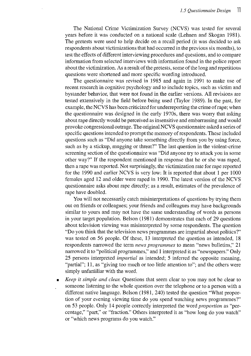
You will not necessarily catch misinterpretations of questions by trying them
out on friends or colleagues; your friends and colleagues may have backgrounds
similar to yours and may not have the same understanding of words as persons
in your target population. Belson A981) demonstrates that each of 29 questions
about television viewing was misinterpreted by some respondents. The question
"Do you think that the television news programmes are impartial about politics?"
was tested on 56 people. Of these, 13 interpreted the question as intended, 18
respondents narrowed the term news programmes to mean "news bulletins," 21
narrowed it to "political programmes," and 1 interpreted it as "newspapers." Only
25 persons interpreted impartial as intended; 5 inferred the opposite meaning,
"partial"; 11, as "giving too much or too little attention to"; and the others were
simply unfanliliar with the word.
Keep it simple and clear. Questions that seem clear to you may not be clear to
someone listening to the whole question over the telephone or to a person with a
different native language. Belson A981, 240) tested the question "What
proportion of your evening viewing time do you spend watching news programmes?"
on 53 people. Only 14 people correctly interpreted the word proportion as
"percentage," "part," or "fraction." Others interpreted it as "how long do you watch"
or "which news programs do you watch."

12 Chapter 1: Introduction
Use specific questions instead of general ones, if possible. Strunk and White
advise writers to "prefer the specific to the general, the definite to the vague, the
concrete to the abstract" A959, 15). Good questions result from good writing.
Instead of asking "Did anyone attack you in the last six months?" the NCVS
asks a series of specific questions detailing how one might be attacked. The NCVS
question is "Has anyone attacked or threatened you in any of these ways: (a) With
any weapon, for instance, a gun or knife, (b) With anything like a baseball bat,
frying pan, scissors, or stick "
Relate your questions to the concept of interest. This seems obvious but is forgotten
or ignored in many surveys. In some disciplines, a standard set of questions has
been developed and tested, and these are then used by subsequent researchers.
Often, use of a common survey instrument allows results from different studies
to be compared. In some cases, however, the standard questions are inappropriate
for addressing the research hypotheses.
Pincus A993) criticizes early research that concluded that persons with
arthritis were more likely to have psychological problems than persons without
arthritis. In those studies, persons with arthritis were given the Minnesota Multiphasic
Personality Inventory, a test of 566 true/false questions commonly used in
psychological research. Patients with rheumatoid arthritis tended to have high scores
on the scales of hypochondriasis, depression, and hysteria. Part of the reason they
scored high on those scales is clear when the actual questions are examined. A
person with arthritis can truthfully answer false to questions such as "I am about
as able to work as I ever was," "I am in just as good physical health as most of
my friends," and "I have few or no pains" without being either hysterical or a
hypochondriac.
Decide whether to use open or closed questions. An open question (the respondent
is not prompted with categories for responses) allows respondents to form their
own response categories; in a closed question (multiple choice), the respondent
chooses from a set of categories read or displayed on a card. Each has
advantages. A closed question may prompt the respondent to remember responses that
might otherwise be forgotten and is in accordance with the principle that specific
questions are better than general ones. If the subject matter has been thoroughly
pretested and responses of interest are known, a well-written closed question will
usually elicit more accurate responses, as in the NCVS question "Has anyone
attacked or threatened you with anything like a baseball bat, frying pan, scissors,
or stick?" If the survey is exploratory or questions are sensitive, though, it is often
better to use an open question. Bradbum and Sudman A979) note that respondents
reported higher frequency of drinking alcoholic beverages when asked an open
question than a closed question with categories "never" through "daily."
The survey by Skelly et al. A968) on women's attitudes toward fabrics used
in clothing gave about half the sample an open version of the questionnaire and
the other half a closed version of the questionnaire, to study the difference in
responses. The first question in the open questionnaire was "What difficulties and
problems do you run into most often when buying clothes, any kind of clothes,
for yourself?"

1.5 Questionnaire Design IJ
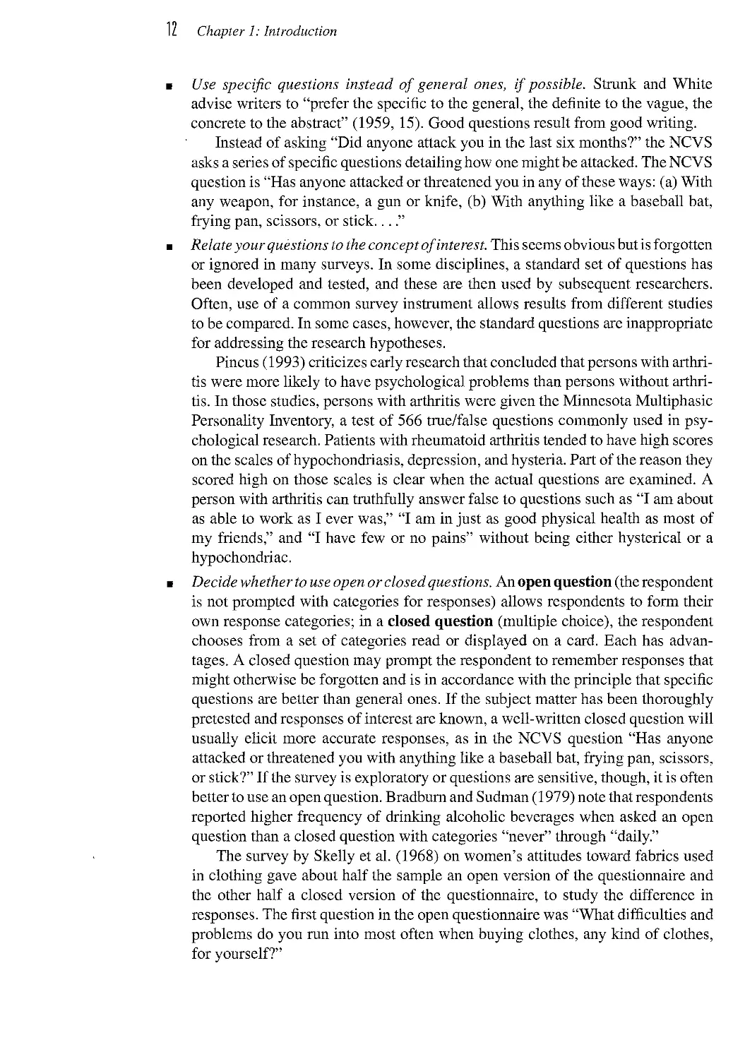
The corresponding question in the closed version of the questionnaire was
"Which of these reasons best describes the difficulties and problems you run into
most often when buying clothes, any kind of clothes, for yourself? Any others?"
The respondent was asked to indicate the statements on Card A that apply to her.
Card A
1. I am short waisted. 8. I have wide hips.
2. I am long waisted. 9. Limited styles, selections.
3. I need a short length. 10. I have problems with necklines.
4. I need a long length. 11. Can't find correct sizes.
5. I have a small waist. 12. Sizes don't run true.
6. I have a large waist. 13. Poor workmanship.
7. Doesn't fit around the shoulders.
Of the women given the closed questionnaire, 25% mentioned that they were
short waisted, whereas only 9% of the women given the open questionnaire
mentioned that they were short waisted. A higher percentage of women mentioned
each of the difficulties on the card in the closed group than in the open group.
However, 10% of the women in the open group mentioned the difficulty that the
price is too high; in the closed group, only 1% of the respondents mentioned high
price, perhaps because the card emphasized fitting problems and focused on the
woman's figure rather than other difficulties.
If using a closed question, always have an "other" category. In one study of
sexual activity among adolescents, adolescents were asked from whom they felt
the most pressure to have sex. Categories for the closed question were "friends of
same sex," "boyfriend/girlfriend," "friends of opposite sex," "TV or radio," "don't
feel pressure," and "other." The response "parents" or "father" was written in by
a number of the adolescent respondents, a response that had not been anticipated
by the researchers.
Report the actual question asked. Public opinion is complex, and you inevitably
leave a distorted impression of it when you compress the results of your careful
research into a summary statement "x% of Americans favor affirmative action."
The results of three surveys in spring 1995, all purportedly about affirmative
action, emphasize the importance of reporting the question. A Newsweek poll
asked, "Should there be special consideration for each of the following groups
to increase their opportunities for getting into college and getting jobs or
promotions?" and asked about these groups: blacks, women, Hispanics, Asians, and
Native Americans. The poll found that 62% of blacks but only 25% of whites
answered yes to the question about blacks. A USA Today-CNN-Gallup poll asked
the question "What is your opinion on affirmative action programs for women
and minorities: do you favor them or oppose them?" and reported that 55% of
respondents favored such programs. A Harris poll asking "Would you favor or
oppose a law limiting affirmative action programs in your state?" reported 51%
of respondents favoring such a law. These questions are clearly addressing
different concepts because the differences in percentages obtained are too great to be
ascribed to the different samples of people taken by the three organizations. Yet

14 Chapter 1: Introduction
all three polls' results were described in newspapers in terms of percentages of
persons who support affirmative action.
Avoid questions that prompt or motivate the respondent to say what you would
like to hear. These are often called leading, or loaded, questions. The May 17,
1994, issue of the Wall Street Journal reported the following question asked by the
Gallup Organization in a survey commissioned by the American Paper Institute:
"It is estimated that disposable diapers account for less than 2 percent of the trash
in today's landfills. In contrast, beverage containers, third-class mail and yard
waste are estimated to account for about 21 percent of trash in landfills. Given
this, in your opinion, would it be fair to tax or ban disposable diapers?"
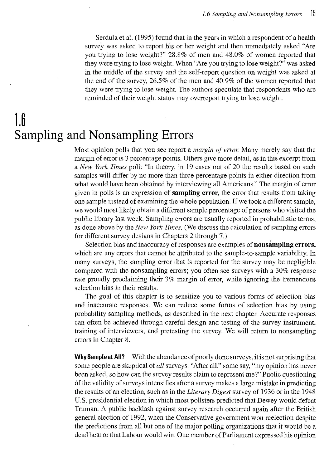
Use forced-choice, rather than agree/disagree, questions. As noted earlier, some
persons will agree with almost any statement. Schuman and Presser A981, 223)
report the following differences from an experiment comparing agree/disagree
with forced-choice versions:
Ql: Do you agree or disagree with this statement: Most men are better suited
emotionally for politics than are most women.
Q2: Would you say that most men are better suited emotionally for politics than
are most women, that men and women are equally suited, or that women are better
suited than men in this area?
Years of Schooling
0-11 12 13+
Ql: percent "agree" 57 44 39
Q2: percent "men better suited" 33 38 28
Ask only one concept in each question. In particular, avoid what are sometimes
called double-barreled questions—so named because if one barrel of the shotgun
does not get you, the other one will.
The question "Do you agree with Bill Clinton's $50 billion bailout of
Mexico?" appeared on a survey distributed by a member of the U.S. House of
Representatives to his constituents. The question is really confusing two opinions of
the respondent: the opinion of Bill Clinton and the opinion of the Mexico policy.
Disapproval of either one will lead to a "disagree" answer to the question. Note
also the loaded content of the word bailout, which will almost certainly elicit
more negative responses than the term aid package would.
Pay attention to question-order effects. If you ask more than one question on a
topic, it is usually (but not always) better to ask the more general question first and
follow it by the specific questions. McFarland A981) conducted an experiment
in which half of the respondents were given general questions first (for example,
"How interested would you say you are in religion: very interested, somewhat
interested, or not very interested?"), followed by specific questions on the subject
("Did you, yourself, happen to attend church in the last seven days?"); the other
half were asked the specific questions first and then asked the general questions.
When the general question was asked first, 56% reported that they were "very
interested in religion"; the percentage rose to 64% when the specific question was
asked first.

1.6 Sampling and Nonsampling Errors 1 j
Serdula et al. A995) found that in the years in which a respondent of a health
survey was asked to report his or her weight and then immediately asked "Are
you trying to lose weight?" 28.8% of men and 48.0% of women reported that
they were trying to lose weight. When "Are you trying to lose weight?" was asked
in the middle of the survey and the self-report question on weight was asked at
the end of the survey, 26.5% of the men and 40.9% of the women reported that
they were trying to lose weight. The authors speculate that respondents who are
reminded of their weight status may overreport trying to lose weight.
1.B
Sampling and Nonsampling Errors
Most opinion polls that you see report a margin of error. Many merely say that the
margin of error is 3 percentage points. Others give more detail, as in this excerpt from
a New York Times poll: "In theory, in 19 cases out of 20 the results based on such
samples will differ by no more than three percentage points in either direction from
what would have been obtained by interviewing all Americans." The margin of error
given in polls is an expression of sampling error, the error that results from taking
one sample instead of examining the whole population. If we took a different sample,
we would most likely obtain a different sample percentage of persons who visited the
public library last week. Sampling errors are usually reported in probabilistic terms,
as done above by the New York Times. (We discuss the calculation of sampling errors
for different survey designs in Chapters 2 through 7.)
Selection bias and inaccuracy of responses are examples of nonsampling errors,
which are any errors that cannot be attributed to the sample-to-sample variability. In
many surveys, the sampling error that is reported for the survey may be negligible
compared with the nonsampling errors; you often see surveys with a 30% response
rate proudly proclaiming their 3% margin of error, while ignoring the tremendous
selection bias in their results.
The goal of this chapter is to sensitize you to various forms of selection bias
and inaccurate responses. We can reduce some forms of selection bias by using
probability sampling methods, as described in the next chapter. Accurate responses
can often be achieved through careful design and testing of the survey instrument,
training of interviewers, and pretesting the survey. We will return to nonsampling
errors in Chapter 8.
Why Sample at All? With the abundance of poorly done surveys, it is not surprising that
some people are skeptical of all surveys. "After all," some say, "my opinion has never
been asked, so how can the survey results claim to represent me?" Public questioning
of the validity of surveys intensifies after a survey makes a large mistake in predicting
the results of an election, such as in the Literary Digest survey of 1936 or in the 1948
U.S. presidential election in which most pollsters predicted that Dewey would defeat
Truman. A public backlash against survey research occurred again after the British
general election of 1992, when the Conservative government won reelection despite
the predictions from all but one of the major polling organizations that it would be a
dead heat or that Labour would win. One member of Parliament expressed his opinion

ID Chapter 1: Introduction
that "extrapolating what tens of millions are thinking from a tiny sample of opinions
affronts human intelligence and negates true freedom of thought."
Some people insist that only a complete census, in which every element of the
population is measured, will be satisfactory; this objection to sampling has a long
history. When Anders Kiaer A897), director of Norwegian statistics, proposed using
sampling for collecting official government statistics, his proposal was by no means
universally well received. Opponents of sampling argued that it was dangerous and that
samples could never replace a census. Within a few years, however, the international
statistical community was largely persuaded that representative samples are a good
thing, although probability samples were not widely used until the 1930s and 1940s.
For small populations, a census may of course be practical. For example, if you
want to know about the employment history of 1990 Arizona State University
graduates who majored in mathematics, it would be sensible to try to contact all of them. If
all graduates respond, then estimates from the survey will have no samphng error. The
estimates will have nonsampling errors, however, if the questions are poorly written
or if respondents give inaccurate information. If some of the graduates do not return
the questionnaire, then the estimates will likely be biased because of nonresponse.
In general, taking a complete census of a population uses a great deal of time
and money and does not eliminate error. The biggest causes of error in a survey are
often undercoverage, nonresponse, and sloppiness in data collection. Most of us have
kept a checkbook register at some time, which is essentially a census of all check
and deposit amounts. How many of us can say that we have never made an error in
our checkbooks? It is usually much better to take a high-quality sample and allocate
resources elsewhere, for instance, by being more careful in collecting or recording
data, doing follow-up studies, or measuring more variables.
After all, the Literary Digest poll (see Example 1.1) predicted the vote wrong even
in some counties in which it attempted to take a census. The decennial census, which
attempts to enumerate every U.S. resident, misses segments of the population. For the
year 2000 census, a panel from the National Academy of Sciences has recommended
that enumeration be combined with sampling to improve the accuracy of the census.
Congress is currently debating this proposal.
There are three main justifications for using sampling:
¦ Sampling can provide reliable information at far less cost than a census. With
probability samples (described in the next chapter), you can quantify the sampling
error from a survey. In some instances, an observation unit must be destroyed to
be measured, as when a cookie must be pulverized to determine the fat content. In
such a case, a sample provides reliable information about the population; a census
destroys the population and, with it, the need for information about it.
¦ Data can be collected more quickly, so estimates can be published in a timely
fashion. An estimate of the unemployment rate for 1994 is not very helpful if it
takes until 2004 to interview every household.
¦ Finally, and less well known, estimates based on sample surveys are often more
accurate than those based on a census because investigators can be more careful
when collecting data. A complete census often requires a large administrative
organization and involves many persons in the data collection. With the
administrative complexity and the pressure to produce timely estimates, many types of

1.]
Exercises
1.7 Exercises 1/
errors can be easily injected into the census. In a sample, more attention can be
devoted to data quality through training personnel and following up on nonre-
spondents. It is far better to have good measurements on a representative sample
than unreliable or biased measurements on the whole population.
Deming says, "Sampling is not njere substitution of a partial coverage for a total
coverage. Sampling is the science and art of controlling and measuring the reliability
of useful statistical information through the theory of probability" A950, 2). In the
remaining chapters of this book, we will explore this science and art in detail.
For each of the following surveys, describe the target population, sampling frame,
sampling unit, and observation unit. Discuss any possible sources of selection bias or
inaccuracy of responses.
1 The article "What Readers Say About Marijuana" reports that "more than 75% of the
readers who took part in an informal PARADE telephone poll say marijuana should
be as legal as alcoholic beverages" {Parade, 31 July 1994, 16). The telephone poll
was announced on page 5 of the June 12 issue; readers were instructed to "call 1-900-
773-1200, at 75 cents a call, if you would like to answer the following questions. Use
touch-tone phones only. To participate, call between 8 a.m. EDT [Eastern Daylight
Time] on Saturday, June 11, and midnight EDT on Wednesday, June 15."
2 A student wants to estimate the percentage of mutual funds whose shares went up in
price last week. She selects every tenth fund listing in the mutual fund pages of the
newspaper and calculates the percentage of those in which the share price increased.
3 Potential jurors in some jurisdictions are chosen from a list of county residents who
are registered voters or licensed drivers over age 18. In the fourth quarter of 1994,
there were 100,300 jury summons mailed to Maricopa County, Arizona, residents.
Approximately 23,000 of those were returned from the post office as undeliverable.
Approximately 7000 persons were unqualified for service because they were not
citizens, were under age 18, were convicted felons, or had other reasons that disqualified
them from serving on a jury. An additional 22,000 were excused from jury service
because of illness, financial hardship, military service, or other acceptable reason. The
final sample consists of persons who appear for jury duty; some unexcused jurors faU
to appear.
4 A sample of 8 architects was chosen in a city with 14 architects and architectural
¦ firms. To select a survey sample, each architect was contacted by telephone in order
of appearance in the telephone directory. The first 8 agreeing to be interviewed formed
the sample.
5 To estimate how many books in the library need rebinding, a librarian uses a random
number table to randomly select 100 locations on library shelves. He then walks to
each location, looks at the book that resides at that spot, and records whether the book
needs rebinding or not.

Chapter 1: Introduction
6 Many scholars and policymakers are interested in the proportion of homeless people
who are mentally ill. Wright A988) estimates that 33 percent of all homeless people
are mentally ill, by sampling homeless persons who received medical attention from
one of the clinics in the Health Care for the Homeless (HCH) project. He argues that
selection bias is not a serious problem because the clinics were easily accessible to the
' homeless and because the demographic profiles of HCH clients were close to those
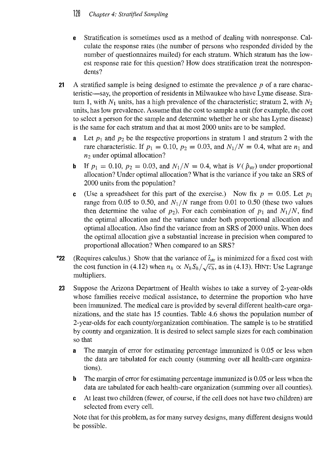
of the general homeless population in each city in the sample. Do you agree?
7 Approximately 16,500 women returned the Healthy Women Survey that appeared
in the September 1992 issue of Prevention. The May 1993 issue, reporting on the
survey, stated that "ninety-two percent of our readers rated their health as excellent,
very good or good."
8 A survey is conducted to find the average weight of cows in a region. A list of all
farms is available for the region, and 50 farms are selected at random. Then the weight
of each cow at the 50 selected farms is recorded.
9 The Arizona Intrastate Travel Committee commissioned a study to identify in-state
travel patterns of Phoenix and Tucson residents and to evaluate different sources of
vacation planning information. They conducted 400 interviews with Phoenix
residents and 400 interviews with Tucson residents. Telephone numbers with Phoenix
and Tucson exchanges were generated randomly so that listed and unlisted telephone
numbers could be reached. "Respondents were limited to heads of household and
quotas were established in order to have an equal representation of male and female
respondents. Additionally, income and age brackets were monitored in order to
maintain the same proportions as the general population bases of metropolitan Phoenix
and Tucson" (Arizona Office of Tourism 1991).
10 The following letter to the editor appeared in the December 10, 1995, issue of the
Appleton Post-Crescent: "Paul Harvey, God bless him, has started a nationwide
survey being conducted by independent radio stations through their talk show hosts to
determine the real sentiments of the American people relative to the sending of troops
to Bosnia. So far, the results from one end of the nation to the other average out to
over 90% against."
11 To study nutrient content of menus in boarding homes for the elderly in Washington
State, Goren et al. A993) mailed surveys to all 184 licensed homes in the state,
directed to the administrator and food service manager. Of those, 43 were returned
by the deadline and included menus.
12 The June 1994 issue of PC World (on newsstands. May 1994) included a report on
reliability and service support for personal computers (PCs). One of the conclusions,
5% of new PC's have problems," formed the top headline of the May 23, 1994,
issue of USA Today. Every issue of PC World since October 1993 had included a
survey form asking questions about users' hardware troubles. Survey respondents for
each month were entered in a drawing to win a new PC, and over 45,000 responses
were received.
13 In lawsuits about trademarks, a plaintiff claiming that another company is infringing
on its trademarks must often show that the marks have a secondary meaning in the
marketplace—that is, potential users of the product associate the trademarks with

1.7 Exercises 1!)
the plaintiff even when the company's name is missing. In the court case Harlequin
Enterprises Ltdv. Gulf& Western Corporation E03 F. Supp. 647,1980), the publisher
of Harlequin Romances persuaded the court that the cover design for "Harlequin
Presents" novels had acquired secondary meaning. Part of the evidence presented
was a survey of 500 women from three cities who identified themselves as readers of
romance fiction. They were shown copies of unpublished "Harlequin Presents" novels
with the Harlequin name hidden; over 50% identified the novel as a Harlequin product.
14 Ann Landers A976) asked readers of her column to respond to this question: "If you
had it to do over again, would you have children?" About 70% of the readers who
responded said no. She received over 10,000 responses, 80% of those from women.
15 The August 1996 issue of Consumer Reports contained satisfaction ratings for
various health maintenance organizations (HMOs) used by readers of the magazine.
Describing the survey, the editors say that "the Ratings are based on more than
20,000 responses to our 1995 Annual Questionnaire about experiences in HMOs
between May 1994 and April 1995, Those results reflect experiences of Consumer
Reports subscribers, who are a more affluent and educated cross-section of the U.S.
population" (p. 40). Answer the general questions about target population, sampling
frame, and units for this survey. Also, do you think this survey provides valuable
information for comparing health plans? If you were selecting an HMO for yourself,
which information would you rather have: results from this survey or results from
customer-satisfaction surveys conducted by the individual HMOs?
16 Mutations of the BRCAl gene on chromosome 17 have been shown to be associated
with higher risk of breast and ovarian cancer. Ford et al. A994) studied cancer risks in
BRCAl-mutation carriers, using a sample of 33 families in North America and
Western Europe. The families were selected by researchers who study breast cancer. Each
family in the sample had at least four persons who had been diagnosed with breast
or ovarian cancer before age 60. The researchers estimated breast and ovarian cancer
risk from the occurrence of second cancers in individuals with breast cancers and
estimated a "cumulative risk of breast cancer in gene carriers of 87% by age 70." They
concluded: "This study confirms that Si?CAi-gene carriers have a lifetime risk of
, either breast or ovarian cancer of close to 100%, and that carriers previously with one
cancer have a high risk of developing a second breast or ovarian cancer and need to be
managed accordingly" (p. 694). Based on the high calculated risks from this analysis
and samples with similar designs, many physicians have recommended that women
with a family history of breast cancer have genetic testing; some women have
undergone prophylactic mastectomies after discovering they are likely to have the gene.
a Answer the general questions about target population, sampling frame, and units
for this sample.
b Does this study provide an estimate of the probability that a woman having the
gene will develop breast or ovarian cancer? Explain.
17 The following questions, quoted in Kinsley A981), are from a survey conducted by
Cambridge Reports and financed by Union Carbide. Critique these questions.
Some people say that granting companies tax credits for the taxes they actually pay to
foreign nations could increase these companies' international competitiveness. If you
knew for a fact that the tax credits for taxes paid to foreign countries would increase the

Chapter 1: Introduction
money available to U.S. companies to expand and modernize their plants and create
more jobs, would you favor or oppose such a tax policy?
Do you favor or oppose changing environmental regulations so that while they still
protect the public, they cost American businesses less and lower product costs?
18 The following article, "Abortion-Rights Groups Surveying Voters' Views," by Jack
Coffman, appeared in the December 26, 1989, issue of the St. Paul Pioneer Press
Dispatch^. Critique the survey described in this article.
What has been called the biggest survey of abortion-rights sentiment in the nation has
become even bigger than its organizers expected, leaders of the survey effort say.
Since Nov. 20, more than 7,000 volunteers have operated six telephone centers
in the Twin Cities metropolitan area and Duluth with an additional 1,000 volunteers
waiting to begin work in January after a two-week holiday break that started Dec.
15. Another 2,000 volunteers next month will begin telephone operations in their own
homes in rural Minnesota.
Since it started, the effort has contacted nearly 160,000 Minnesota families about
their views on abortion and lined up county chairmen or chairwomen in 74 of the
state's 87 counties. The announced goal of the survey is to contact the families of
every registered voter to determine how the voters feel about abortion.
"It's bigger than any political campaign by far," said Marlene Kayser, president of
the board of Planned Parenthood of Minnesota, the leading abortion-rights group in
the state and key group connected with the survey.
The survey is expected to play an important role in the 1990 legislative session
when lawmakers, who traditionally have had anti-abortion leanings, will have to
grapple with the volatile abortion issue. The issue has been made even more sensitive
because of the decision last summer by the U.S. Supreme Court upholding a Missouri
law that increases abortion restrictions and appears to open the way for action by state
legislatures.
Anti-abortion forces are gearing up for new abortion restrictions. Backers of the
abortion-rights survey plan to use the results in part to try to head off any further
anti-abortion legislation.
So far the results of the survey are "overwhelmingly pro-choice," said Kayser.
Results from the calls made since November are being tabulated and will be made
available during the next legislative session, which begins Feb. 12. The survey of
1 million Minnesotans is expected to end March 10.
The survey, sponsored by several abortion-rights groups, is being conducted under
a contract with Nancy Brataas Associates Inc., a consulting firm owned by state Sen.
Nancy Brataas, IR-Rochester. It is expected to cost $250,000.
"It's the most wonderful outpouring of volunteers I have ever seen, and that
includes campaigns for president and governor," said Brataas. (The Minnesota
presidential campaign of Massachusetts Gov. Michael Dukakis involved about 8,000
volunteers, according to a campaign official.)
Brataas said she believes the strong volunteer response results from "people who
are pro-choice and have depended on the Supreme Court and are suddenly very worried
and concerned about a woman's right to choose."
'Reproduced with permission of the St. Paul Pioneer Press.

1.7 Exercises lA
Recruiting volunteers "wasn't hard," said Mary Stringer, co-chairwoman of the
St. Paul survey center in the Griggs-Midway building, where 865 volunteers have
operated 15 telephones trying to meet a goal of 1,625 calls a day.
Stringer, who described the outpouring of volunteers as "incredible," pointed to
tw6 boxes of forms filled out by volunteers who haven't been called yet. Calls also
are being made from phone banks in Bloomington, St. Louis Park, White Bear Lake,
Minneapolis and Duluth.
Jackie Schwietz, co-director of Minnesota Citizens Concerned for Life, said the
survey is "biased" and "dishonest" because the questions don't mention abortion.
She said the MCCL has a "definite plan" for "more restrictive" abortion legislation
to be pushed in the 1990 Legislature. However, she declined to describe the group's
proposals, which she said will be the subject of a public announcement before the
session begins.
When volunteers telephone registered voters, they ask this question: "Do you agree
or disagree with the following statement; The decision to terminate a pregnancy is a
private matter between a woman, her family and doctor ... and not a decision to be
made by government and politicians."
If the person questioned answers yes, the person is then asked: "In light of current
government threats to safe, legal abortion ... will this issue influence your opinion of
politicians in the future?"
If the answer to the original question was no, the person is then asked: "Are you
opposed to abortion in cases of rape ... incest ... serious fetal deformity ... or to
save the life of a woman?"
19 On March 21, 1993, NBC televised "The First National Referendum—Government
Reform Presented by Ross Perot." During the show, 1992 U.S. presidential candidate
Perot asked viewers to express their opinions by mailing in the National Referendum
on Government Reform, printed in the March 20 issue of TV Guide. Some of the
questions on the survey were the following:
Do you believe that for every dollar of tax increase there should be $2.00 in
spending cuts with the savings earmarked for deficit and debt reduction?
¦ Should the President present an overall plan including spending cuts, spending
increases, and tax increases and present the net result of the overall plan, so that
the people can know the net result before paying more taxes?
Should the electoral college be replaced with a popular vote for the Presidetitial
election?
Was this TV forum worthwhile? Do you wish to continue participating as a voting
member of United We Stand America?
20 Read the following article that describes a proposal for using sampling in the year
2000 U.S. census: W. Roush, 1996. "A census in which all Americans count," Science
274:1\3-1\A. What are the main arguments for using sampling in 2000? Against?
What do you think?
21 (For students of U.S. history.) Eighty-five letters appeared in New York City
newspapers in 1787 and 1788, with the purpose of drawing support in the state for the
newly drafted Constitution. Collectively, these letters are known as The Federalist.
Read number 54 of The Federalist, in which the author (widely thought to be James

// Chapter 1: Introduction
Madison) discusses using a population census to apportion elected representatives
and taxes among the states. This article explains part of Article I, Section II, of the
U.S. Constitution.
Write a short paper discussing Madison's view of a population census. What is the
target population and samphng frame? What sources of bias does Madison mention,
and how does he propose to reduce bias? What is your reaction to Madison's plan,
from a statistical point of view? Where do you think Madison would stand today on the
issue of using sampling versus complete enumeration to obtain population estimates?-
22 Find a recent survey reported in a newspaper or popular magazine. Describe the
survey. What are the target population and sampled population? What conclusions are
drawn about the survey in the article? Do you think those conclusions are justified?
What are possible sources of bias for the survey?
23 Find a survey on the Internet. For example, SurveyNet (www.survey.net) allows you to
participate in surveys on a variety of subjects; you can find other surveys by searching
online for survey or take survey. Participate in one of the surveys yourself and write a
paragraph or two describing the survey and its results (most online surveys allow you to
see the statistics from all persons who have taken the survey). What are the target
population and sampled population? What biases do you think might occur in the results?

2
Simple Probability Samples
[Kennedy] read every fiftieth letter of the thirty thousand coming weel<ly to the White House, as well
as a statistical summary of the entire batch, but he knew that these were often as organized and
unrepresentative as the pickets on Pennsylvania Avenue.
—Theodore Sorensen, Kennedy
The examples of bad surveys in Chapter 1—for example, the Literary Digest survey,
Example 1.1—had major flaws that resulted in unrepresentative samples. In this
chapter, we discuss how to use probability sampling to conduct surveys. In a probability
sample, each unit in the population has a known probability of selection, and a chance
method such as using numbers from a random number table is used to choose the
specific units to be included in the sample. If a probability sampling design is
implemented well, an investigator can use a relatively small sample to make inferences
about an arbitrarily large population.
In Chapters 2 through 6, we explore survey design and properties of estimates
for the three major design components used in a probability sample: simple random
sampling, stratified sampling, and cluster sampling. We will integrate all these ideas
in Chapter 7 and show how they are combined in complex surveys such as the U.S.
National Crime Victimization Survey. To simplify presentation of the concepts, we
assume for now that the sampled population is the target population, that the
sampling frame is complete, that there is no nonresponse or missing data, and that all
measurements are accurate. We return to nonsampling errors in Chapter 8.
As you might suppose, you need to know some probability to be able to understand
probability sampling. You may want to review the material in Sections B.l and B.2
of Appendix B while reading this chapter.
2.1
Types of Probability Samples
The terms simple random sample, stratified sample, and cluster sample are basic to
any discussion of sample surveys, so let's define them now.
23

24 Chapter 2: Simple Probability Samples
¦ A simple random sample (SRS) is the simplest form of probability sample. An
SRS of size n is taken when every possible subset of n units in the population
has the same chance of being the sample. SRSs are the focus of this chapter and
the foundation for more complex sampling designs. In taking a random sample,
the investigator is in effect mixing up the population before grabbing n units.
The investigator does not need to examine every member of the population for
the same reason that a medical technician does not need to drain you of blood
to measure your red blood cell count: Your blood is sufficiently well mixed that
any sample should be representative. SRSs are discussed in Section 2.3, after we
present the basic framework for probability samples in Section 2.2.
¦ In a stratified random sample, the population is divided into subgroups called
strata. Then an SRS is selected from each stratum, and the SRSs in the strata
are selected independently. The strata are often subgroups of interest to the
investigator—for example, the strata might be different ethnic or age groups in a
survey of people, different types of terrain in an ecological survey, or sizes of firms
in a business survey. Elements in the same stratum often tend to be more similar
than randomly selected elements from the whole population, so stratification often
increases precision, as we will see in Chapter 4.
¦ In a cluster sample, observation units in the population are aggregated into larger
sampling units, called clusters. Suppose you want to survey Lutheran church
members in Minneapolis but do not have a list of all church members in the city,
so you cannot take an SRS of church members. However, you do have a list of
all the Lutheran churches. You can then take an SRS of the churches and then
subsample all or some church members in the selected churches. In this case, the
churches form the clusters, and the church members are the observation units.
It is more convenient to sample at the church level; however, members of the
same church may have more similarities than Lutherans selected at random in
Minneapolis, so a cluster sample of 500 Lutherans may not provide as much
information as an SRS of 500 Lutherans. We will explore this idea further in
Chapter 5.
Suppose you want to estimate the average amount of time that professors at your
university spent grading homework in a specific week. To take an SRS, construct
a list of all professors and randomly select n of them to be your sample. Now ask
each professor in your sample how much time he or she spent grading homework that
week—you would of course have to define the words homework and grading carefully
in your questionnaire. In a stratified sample, you might classify faculty by college:
engineering, liberal arts and sciences, business, nursing, and fine arts. You would then
take an SRS of faculty in the engineering college, a separate SRS of faculty in liberal
arts and sciences, and so on. For a cluster sample, you might randomly select 10 of
the 60 academic departments in the university and ask each faculty member in those
departments how much time he or she spent grading homework.
All these methods—SRS, stratified random sampling, and cluster sampling—
involve random selection of units to be in the sample. In an SRS, the observation
units themselves are selected at random from the population of observation units;
in a stratified random sample, observation units within each stratum are randomly
selected; in a cluster sample, the clusters are randomly selected from the population

2.2 Framework for Probability Sampling Zu
of all clusters. Each method is a form of probability sampling, which we will discuss
in the next section.
2.2
Framework for Probability Sampling
To show how probability sampling works, we need to be able to list the N units in
the finite population. The finite population, or universe, of T<S units is denoted by the
index set
W=={1,2, ...,Af}. B.1)
Out of this population we can choose various samples, which are subsets of W. The
particular sample chosen is denoted by S, a subset consisting of n of the units in U.
Suppose the population has four units: W = {1, 2, 3,4}. Six different samples of
size 2 could be chosen from this population:
5i = {l,2} 54 = {2, 3}
<S2 = {1,3} 55 = {2, 4}
53 = {1,4} 56 = {3, 4}
In probability sampling, each possible sample 5 from the population has a known
probability PE) of being chosen, and the probabilities of the possible samples sum
to 1. One possible sample design for a probability sample of size 2 would have
PEi) = 1/3, P{Si) = 1/6, and PE6) = 1/2, and PiS^) = P{Sa) = PiSs) = 0.
The probabilities PEi), -f'E2), and PiS^) of the possible samples are known before
the sample is drawn. One way to select the sample is to place six labeled balls in a
box; two of the balls are labeled 1, one is labeled 2, and three are labeled 6. Now
choose one at random; if a ball labeled 6 is chosen, then 56 is the sample.
In a probability sample, since each possible sample has a known probability of
being the chosen sample, each unit in the population has a known probability of
appearing in our selected sample. We calculate
P{umt i in sample) = tt,-
by summing the probabilities of all possible samples that contain unit i. In probability
sampling, the iti are known before the survey commences, and we assume that tt,- >
0 for every unit in the population. For the sample design described above, jt\ —
P{Si) + P{S2) + P{S3) = 1/2, Jt2 = P(Si) + PE4) + PE5) = 1/3, 7T3 =
P(S2) + P(S4) + PiSs) = 2/3, and 714 = PiSs) + PiSs) + PiSe) = 1/2.
Of course, we never write all possible samples down and calculate the probability
with which we would choose every possible sample—^this would take far too long.
But such enumeration underlies all of probability sampling. Investigators using a
probability sample have much less discretion about which units are included in the
sample, so using probability samples helps us avoid some of the selection biases
described in Chapter 1. In a probability sample, the interviewer cannot choose to
substitute a friendly looking person for the grumpy person selected to be in the
sample by the random selection method. A forester taking a probability sample of trees
cannot simply measure the trees near the road but must measure the trees designated

/u Chapter 2: Simple Probability Samples
for inclusion in the sample. Taking a probability sample is much harder than taking a
convenience sample, but a probability sampling procedure guarantees that each unit
in the population could appear in the sample and provides information that can be
used to assess the precision of statistics calculated from the sample.
Within the framework of probability sampling, we can quantify how likely it is
that our sample is a "good" one. A single probability sample is not guaranteed to
be representative of the population with regard to the characteristics of interest, but
we can quantify how often samples will meet some criterion of representativeness.
The notion is the same as that of confidence intervals: We do not know whether the
particular 95% confidence interval we construct for the mean contains the true value
of the mean. We do know, however, that if the assumptions for the confidence interval
procedure are valid and if we repeat the procedure over and over again, we can expect
95% of the resulting confidence intervals to contain the true value of the mean.
Let yt be a characteristic associated with the (th unit in the population. We consider
y,- to be a fixed quantity; if farm 723 is included in the sample, then the amount of
com produced on farm 723, 3^723, is known exactly.
EXAMPLE 2.1 To illustrate these concepts, let's look at an artificial situation in which we know the
value of yi for each of theN = 8 units in the whole population. The index set for the
population is
W = {1,2, 3,4, 5,6, 7, 8}.
The values of y,- are
12 3 4 5 6 7 8
yt 12 4 4 7 7 7 8
There are 70 possible samples of size 4 that can be drawn without replacement
from this population; the samples are listed in file samples.dat on the data disk. If
the sample consisting of units {1, 2, 3, 4} were chosen, the corresponding values of
yt would be 1, 2, 4, and 4. The values of y, for the sample {2, 3, 6, 7} are 2, 4, 7, and
7. Define P(S) = 1/70 for each distinct subset of size 4 from U. As you will see
after you read Section 2.3, this design is an SRS without replacement. Each unit is in
exactly 35 of the possible samples, so tt, = 1/2 for j = 1, 2,..., 8.
A random mechanism is used to select one of the 70 possible samples. One
possible mechanism for this example, because we have listed all possible samples, is
to generate a random number between 1 and 70 and select the corresponding sample.
With large populations, the number of samples is so great that in practice the units
themselves are randomly selected according to prespecified probabilities. ¦
Most results in sampling rely on the sampling distribution of a statistic, the
distribution of different values of the statistic obtained by the process of taking all
possible samples from the population. A sampling distribution is an example of a
discrete probability distribution.
Suppose we want to use a sample to estimate a population quantity—say, the
population total t = '^,^1 yt- One estimate we might use for f is f^ = Nys, where
ys is the average of the y,- 's in <S, the chosen sample. In our example, t = 40. If the
sample S consists of units 1, 3, 5, and 6, then ts = 8x A+4 + 7 + 7)/4 = 38. Since

2.2 Framework for Probability Sampling II
we know the whole population here, we can find is for each of the 70 possible samples.
The probabilities of selection for the samples give the sampling distribution of i :
P{t = k}
E
S:is=k
P(S).
The summation is over all samples S for which ts = k. We know the probability
PiS) with which we select a sample S because we take a probability sample.
EXAMPLE 2.2 The sampling distribution of i for the population and sampling design in Example 2.1
derives entirely from the probabilities of selection for the various samples. Four
samples ({3, 4, 5, 6}, {3, 4, 5, 7}, {3, 4, 6, 7}, and {1, 5, 6, 7}) result in the estimate
i = 44, so P{i = 44} = 4/70. For this example, we can write out the sampling
distribution of t because we know the values for the entire population.
k
P{i = k}
22 28
1 6
70 70
30
2
70
32
3
70
34 36
7 4
70 70
38
6
70
40 42 44
12 6 4
70 70 70
46 48 50 52 58
7 3 2 6 1
70 70 70 70 70
Figure 2.1 displays the sampling distribution. ¦
The expected value of ?, E[i], is the mean of the sampling distribution of i :
£[n = ^/'(<5)?5 B.2)
Y^ kP{i = k).
The expected value of the statistic is the weighted average of the possible sample
values of the statistic, with weights the probability that that particular value of the
statistic would occur.
The estimation bias of the estimator i is
Bias[?] = £[?]-?.
B.3)
! [ G U R E 2.1
Siimpling distribution of the sample total in Example 2.2.
.15
.10
.05
.00
Jj
20 30 40 50
Estimate of t from Sample
60

Chapter 2: Simple Probability Samples
If Bias [?] = 0, we say that the estimator i is unbiased for t. For the data in Example 2.1,
the expected value of t is
1 6 1
E[i] = —B2) + —B8) +¦•• + —E8) = 40.
70 70 70
Thus, the estimator is unbiased.
Note that the mathematical definition of bias in Equation B.3) is not the same thing
as the selection or measurement bias described in Chapter 1. All indicate a systematic
deviation from the population value, but from different sources. Selection bias is due
to the method of selecting the sample—often, the investigator acts as though every
possible sample S has the same probability of being selected, but some subsets of
the population actually have a different probability of selection. With undercoverage,
for example, the probability of including a unit not in the sampling frame is zero.
Measurement bias means that the yt's are not really the quantities of interest, so
although t may be unbiased in the sense of B.3) for t — J2h=i Vt > t itself would not
be the true total of interest. Estimation bias means that the estimator chosen results
in bias—for example, if we used is = Ylis^s yi ^^'^ '^^'^ ^°'^ ^^^ ^ census, i would
be biased. To illustrate these distinctions, suppose you want to estimate the average
height of male actors belonging to the Screen Actor's Guild. Selection bias would
occur if you took a convenience sample of actors on the set—perhaps taller actors are
more or less likely to be working. Measurement bias would occur if your tape measure
inaccurately added 3 centimeters (cm) to each actor's height. Estimation bias would
occur if you took an SRS from the list of all actors in the Guild but estimated mean
height by the average height of the six shortest men in the sample—the sampling
procedure is good, but the estimator is bad.
The variance of the sampling distribution of i is
V[i] = E[(i-E[i]?] B.4)
PiS)iis-E[i]?.
= E
all possible
samples S
For the data in Example 2.1,
1,1, 3840
V[t] = -B2 - 40J + • ¦ • + -E8 - 40J ^—-= 54.86.
Because we sometimes use biased estimators, we often use the mean squared error
(MSE) father than variance to measure the accuracy of an estimator:
MSE[f] = E[ii-t)^]
= El(i-E[i] + E[i]-tf]
= E[{i-E[i]J] + {E[i]-tf + 2E[{i-E[t]){E[i] - f)]
= y[f] + (Bias[f])^
Thus,anestimator?oftisMMZ5Jase<iif£'[f ] = t, precise if V[i] — E[{t — E[i])^]
is small, and accurate if MSE[?] = £[(? — f)^] is small. A badly biased estimate
may be precise, but it will not be accurate; accuracy (MSE) is how close the estimate
is to the true value, whereas precision (variance) measures how close estimates from
different samples are to each other. Figure 2.2 illustrates these concepts.

2.2 Framework for Probability Sampling
FIGURE 2.2
Unbiased, precise, and accurate archers. Archer A is unbiased—the average position of all
arrows is at the bull's-eye. Archer B is precise but not unbiased—all arrows are close together
but systematically away from the bull's-eye. Archer C is accurate—all arrows are close
together and near the center of the target.
Archer A
Archer B
Archer C
In summary, the finite population U consists of units {1, 2,..., A''} whose
measured values are {yi, y2,. ¦ ¦, yN}- We select a sample 5 of n units from U using
the probabilities of selection that define the sampling design. The y's are fixed but
unknown quantities—unknown unless that unit happens to appear in our sample S.
Unless we make additional assumptions, the only information we have about the set
of y's in the population is in the set {j,- : i e S}.
You may be interested in many different population quantities from your
population. Historically, however, the main impetus for developing theory for sample
surveys has been estimating population means and totals. Suppose we want to
estimate the total number of persons in Canada who have diabetes, or the average number
of oranges produced per orange tree. The population total is
i = I
yi
and the mean of the population is
yu
1 "
1=1
Almost all populations exhibit some variability; for example, households have
different incomes and trees have different diameters. Define the variance of the population
values about the mean as
52 =
N
1 '^
i=l
yuf
B.5)
The population standard deviation is 5' = V 5*^.
The population standard deviation is often related to the mean. A population of
trees might have a mean height of 10 meters (m) and a standard deviation of 1 m.
A population of small cacti, however, with a mean height of 10 cm, might have a
standard deviation of 1 cm. The coefficient of variation (CV) is a measure of relative

JO Chapter 2: Simple Probability Samples
variability, which can be defined when y;/ 7^ 0 as
S
yu
If tree height is measured in meters, then yu and S are also in meters. The coefficient
of variation does not depend on the unit of measurement. In this example, the trees
and the cacti have the same coefficient of variation.
It is sometimes helpful to have a special notation for proportions. The proportion
of units having a characteristic is simply a special case of the mean, obtained by
letting y, = 1 if the ith unit has the characteristic of interest, and j,- = 0 if the ith
unit does not have the characteristic. Let
number of units with the characteristic in the population
P = N •
EXAMPLE 2.3 For the population in Example 2.1, let
1 if the (th unit has the value 7
0 if the ith unit does not have the value 7
Let ps = YlieS Vi/^' ^^^ proportion of 7s in the sample. The list of all possible
samples in the data file samples.dat has 5 samples with no 7s, 30 samples with
exactly one 7, 30 samples with exactly two 7s, and 5 samples with three 7s. Since one
of the possible samples is selected with probability 1/70, the sampling distribution of
p is^:
k
P{p = k)
° 11
5 30 30
70 70 70
3
4
5
70
2.3
Simple Random Sampling
Simple random sampling is the most basic form of probability sampling and provides
the theoretical basis for the more complicated forms. There are two ways of taking
a simple random sample: with replacement, in which the same unit may be included
more than once in the sample, and without replacement, in which all units in the
sample are distinct.
A simple random sample with replacement (SRSWR) of size n from a
population of N units can be thought of as drawing n independent samples of size 1.
One unit is randomly selected from the population to be the first sampled unit, with
probability 1/A^. Then the sampled unit is replaced in the population, and a second
unit is randomly selected with probability l/N. This procedure is repeated until the
sample has n units, which may include duplicates from the population.
In finite population sampling, however, sampling the same person twice provides
no additional information. We usually prefer to sample without replacement so that
'An alternative derivation of the sampling distribution is in Exercise B.2 (p. 427).

2.3 Simple Random Sampling i\
the sample contains no duplicates. A simple random sample without replacement
(SRS) of size n is selected so that every possible subset of n distinct units in the
population has the same probability of being selected as the sample. There are ( ^ 1
possible samples (see Appendix B), and each is equally likely, so the probability of
selecting any individual sample Sofn units is
1 nKN-ny.
PiS) =
i~)
Nl
As a consequence of this definition, the probability that any given unit appears in the
sample is n/N, as shown later in Equation B.18).
To take an SRS, you need a list of all observation units in the population; this list
is the sampling frame. In an SRS, the sampling unit and observation unit coincide.
Each unit is assigned a number, and a sample is selected so that A) each unit has the
same chance of occurring in the sample and B) the selection of a unit is not influenced
by which other units have already been selected. This can be thought of as drawing
numbers out of a hat; in practice, computer-generated pseudorandom numbers are
usually used to select a sample.
EXAMPLE 2.4 The U.S. government conducts a Census of Agriculture every five years, collecting
data on all farms (defined as any place from which $1000 or more of agricultural
products were produced and sold) in the 50 states.^ The Census of Agriculture provides
data on number of farms, the total acreage devoted to farms, farm size, yield of different
crops, and a wide variety of other agricultural measures for each of the A^ = 3078
counties and county-equivalents in the United States. The file agpop.dat on the data
disk contains the 1982,1987, and 1992 information on the number of farms, acreage
devoted to farms, number of farms with fewer than 9 acres, and number of farms with
more than 1000 acres for the population.
To take an SRS of size 300 from this population, I generated 300 random numbers
between 0 and 1 on the computer, multiplied each by 3078, and rounded the result
up to the next highest integer. This procedure generates an SRSWR. If the population
is large relative to the sample, it is likely that each unit in the sample occurs only
once in the list. In this case, however, 13 of the 300 numbers were duplicates. The
duplicates were discarded and replaced with new randomly generated numbers
between 1 and 3078, until all 300 numbers were distinct; the set of random numbers
generated is in the file selectrs.dat, and the data set for the SRS is in agsrs.dat. Other
methods that might be used to select an SRS are described in the exercises and in
Appendix D.
The counties selected to be in the sample may not "feel" very random at first glance.
For example, counties 2840,2841, and 2842 are all in the sample, whereas none of the
counties between 2740 to 2787 appear. The sample contains 18% of Virginia counties,
but no counties in Alaska, Arizona, Connecticut, Delaware, Hawaii, Rhode Island,
Utah, or Wyoming. There is a quite natural temptation to want to "adjust" the random
^The Census of Agriculture was formerly conducted by the U.S. Bureau of the Census; currently, it is
conducted by the U.S. National Agricultural Statistics Service (NASS). More information about the
census and selected data are available on the Internet through the NASS material on www.fedstats.gov.

it Chapter 2: Simple Probability Samples
FIGURE 2.3
Histogram: number of acres devoted to farms in 1992, for an SRS of 300 counties. Note the skewness of the
data. Most of the counties have fewer than 500,000 acres in farms; some counties, however, have more than
1.5 million acres in farms.
50
40
30
20
10
0
0.0
J_
0.5
1 1.5
Millions of Acres Devoted to Farms
2.5
number list, to spread it out a bit more. If you want a random sample, you must resist
this temptation. Research, beginning with Neyman A934), repeatedly demonstrates
that purposive samples often do not represent the population on key variables. If you
deliberately substitute other counties for those in the randomly generated sample, you
may be able match the population on one particular characteristic such as geographic
distribution; however, you will likely fail to match the population on characteristics
of interest such as number of farms or average farm size. If you want to ensure that
all states are represented, do not adjust your randomly selected sample purposively
but take a stratified sample (to be discussed in Chapter 4).
Let's look at the variable acres92, the number of acres devoted to farms in 1992.
A small number of counties in the population are missing that value—in some cases,
the data are withheld to prevent disclosing data on individual farms. Thus, we first
check to see the extent of the missing data in our sample. Fortunately, our sample has
no missing data (see Exercise 7 to see how likely such an occurrence is). Figure 2.3
displays a histogram of the acreage devoted to farms in each of the 300 counties. ¦
For estimating the population mean yu in an SRS, we use the sample mean
1
ys =
n '—i
B.6)
In the following, we use y to refer to the sample mean and drop the subscript <S unless
it is needed for clarity. As will be shown in Section 2.7, y is an unbiased estimator of
the population mean yu, and the variance of y is
for S^ defined in Equation B.5). The variance V(y) measures the variability among
estimates of yu from different samples. ^

2.3 Simple Random Sampling U
The factor A — n/N) is called the finite population correction (fpc). Intuitively,
we make this correction because with small populations the greater our sampling
fraction n/N, the more information we have about the population and thus the smaller
the variance. If N — 10 and we sample all 10 observations, we would expect the
variance of y to be 0 (which it is). If N = 10, there is only one possible sample S of
size 10 without replacement, with ys = yu, so there is no variability due to taking a
sample. For a census, the fpc, and hence V(y), is 0. When the sampling fraction n/N
is large in an SRS without replacement, the sample is closer to a census, which has
no sampling variability.
For most samples that are taken from extremely large populations, the fpc is
approximately 1. For large populations it is the size of the sample taken, not the
percentage of the population sampled, that determines the precision of the estimator:
If your soup is well stirred, you need to taste only one or two spoonfuls to check the
seasoning, whether you have made 1 liter or 20 liters of soup. A sample of size 100
from a population of 100,000 units has almost the same precision as a sample of size
100 from a population of 100 million units:
S^ 99,900 52
V[y] = = -—@.999) for N = 100,000
¦^ 100 100,000 100
S^ 99,999,900 S^
V[y] = ' ^' ^„^ = @.999999) for N = 100,000,000
100 100,000,000 100
The population variance 5*^, which depends on the values for the entire population,
is still unknown. We estimate it by the sample variance:
s^ = ^T(yi-yf- B.8)
An unbiased estimator of the variance of y is (see Section 2.7)
Vm^(l-^)-. B.9)
We usually report not the estimated variance of y but its square root, the standard
error (SE):
SE[v] = J(l--j-. B.10)
The estimated coefficient of variation of an estimate gives a measure of the relative
variability of an estimate. It is the standard error divided by the mean (defined only
when the mean is nonzero):
— SE[v]
CY{y) = ——. B.11)
y
All these results apply to the estimation of a population total, t, since
N
t = Y,y' = ^yu-
i-l

31 Chapter 2: Simple Probability Samples
To estimate t, we use the unbiased estimator
t^Ny. B.12)
Then, from Equation B.7),
V[t} = N^V{y^ = N^{\-—\— B.13)
N J n
and
V{n = N^(\--\^. B.14)
V N J n
EXAMPLE 2.5 For the data in Example 2.4, N = 3078 and n = 300, so the samphng fraction is
300/3078 = 0.097. The sample statistics are y = 297,897, s = 344,551.9, and t =
Ny = 916,927,110. Standard errors are
300 \
= 18,898.434428
3078/
and
SE[f ] = C078X18,898.434428) = 58,169,381
and the estimated coefficient of variation is
CV[i] = CV[y]
^ SE[y]
y
_ 18,898.434428
297,897
= 0.06344.
Since these data are so highly skewed, we should also report the median number
of farm acres in a county, which is 196,717. ¦
We might also want to estimate the proportion of counties in Example 2.4 with
fewer than 200,000 acres in farms. Since estimating a proportion is a special case of
estimating a mean, the results in Equations B.6)-B.11) hold for proportions as well,
and they take a simple form. Suppose we want to estimate the proportion of units in
the population that have some characteristic—call this proportion p. Define yi to be 1
if the unit has the characteristic and to be 0 if the unit does not have that characteristic.
Then p = J2i^i yt/N = yu, and p is estimated hy p = y. Consequently, ^ is an
unbiased estimator of p. For the response y,-, taking on values 0 or 1,
n2
EL (yi - pf Ef=i yl - 2p Ef=i yt + np' n
s' = "-'=' ¦''—^ = ^'=^ ^' " ^'=^"' —— = p{\ - p).
Thus, B.7) implies that
'N -n\ »A - »)

2.4 Confidence Intervals Ju
Also,
„2
1 v-> T n
n-l{^ n-l
So from B.9),
ym = (i-^Y-^. B.16)
V N J n-l
EXAMPLE 2.6 For the sample described in Example 2.4, the estimated proportion of counties with
fewer than 200,000 acres in farms is
153
p = = 0.51
^ 300
with standard error
300 \ @.51)@.49)
SE(^) == J 1 ^^ = 0.0275.
^ Vv 3078/ 299
U
Confidence Intervals
When you take a sample survey, it is not sufficient to simply report the average height
of trees or the sample proportion of voters who intend to vote for candidate B in the
next election. You also need to give an indication of how accurate your estimates
are. In statistics, confidence intervals (CIs) are used to indicate the accuracy of an
estimate.
A 95% CI is often explained heuristically: If we take samples from our population
over and over again and construct a confidence interval using our procedure for each
possible sample, we expect 95% of the resulting intervals to include the true value of
the population parameter.
In probability sampling from a finite population, only a finite number of possible
samples exist, and we know the probability with which each will be chosen; if we
could generate all possible samples from the population, we could calculate the exact
confidence level for a confidence interval procedure.
EXAMPLE 2.7 Return to Example 2.1, in which the entire population is known. Let's choose an
arbitrary procedure for calculating a confidence interval, constructing interval estimates
for t as
CIiS) = [is-4ssJs+4ss].
There is no theoretical reason to choose this procedure, but it will illustrate the concept
of a confidence interval. Define u(S) to be 1 if CI{S) contains the true population
value 40, and 0 if CI(<S) does not contain 40. Since we know the population, we can
calculate the confidence interval CIE) and the value of u{S) for each possible sample
S. Some of the 70 confidence intervals are shown in Table 2.1 (all entries are rounded
to two decimals).

Chapter 2: Simple Probability Samples
TABLE 2.1
Confidence intervals for possible samples from small population
Sample S
jiJ e S
ts
ss
CIE)
u(S)
1,2,3,4
1,2,3,5
1,2,3,6
1,2,3,7
1,2,3,8
1,2,4,5
1,2,4,6
1,2,4,7
1,2,4,8
1,2,5,6
2,3,4,8
2,3,5,6
2,3,5,7
2,3,5,8
2,3,6,7
2,3,6,8
4,5,6,7
,5,6,8
,5,7,8
4,6,7,8
5,6,7,8
1, 2, 4, 4
1, 2, 4, 7
1, 2, 4, 7
1,2,4,7
1,2,4,8
1, 2, 4, 7
1, 2, 4, 7
1,2,4,7
1, 2, 4, 8
1,2,7,7
2, 4, 4, 8
2, 4, 7, 7
2, 4, 7, 7
2, 4, 7, 8
2, 4, 7, 7
2, 4, 7, 8
4, 7, 7, 7
4, 7, 7, 8
4, 7, 7, 8
4, 7, 7, 8
7, 7, 7, 8
22
28
28
28
30
28
28
28
30
34
36
40
40
42
40
42
50
52
52
52
58
1.50
2.65
2.65
2.65
3.10
2.65
2.65
2.65
3.10
3.20
2.52
2.45
2.45
2.75
2.45
2.75
1.50
1.73
1.73
1.73
0.50
[16.00, 28.00]
[17.42, 38.58]
[17.42, 38.58]
[17.42, 38.58]
[17.62, 42.38]
[17.42, 38.58]
[17.42, 38.58]
[17.42, 38.58]
[17.62, 42.38]
[21.19, 46.81]
[25.93, 46.07]
[30.20, 49.80]
[30.20, 49.80]
[30.98, 53.02]
[30.20, 49.80]
[30.98, 53.02]
[44.00, 56.00]
[45.07, 58.93]
[45.07, 58.93]
[45.07, 58.93]
[56.00, 60.00]
0
0
0
0
1
0
0
0
1
1
1
1
1
1
1
1
0
0
0
0
0
Each individual confidence interval either does or does not contain the population
total 40. The probability statement in the confidence interval is made about the
collection of all possible samples; for this confidence interval procedure and population,
the confidence level is
Y^ P(SMS) = 0.77.
This means that if we take an SRS of four elements without replacement from this
population of eight elements, there is a 77% chance that our sample is one of the
'"good" ones whose confidence interval contains the true value 40. This procedure
thus creates a 77% confidence interval.
Of course, in real life, we take only one sample and do not know the value of the
population total t. Without further investigation, we have no way of knowing whether
the sample we obtained is one of the "good" ones, such as <S = {2, 3, 5, 6}, or one
of the "bad" ones, such as 5 = {4, 6, 7, 8}. The confidence interval gives us only a
probabilistic statement of how often we expect to be right. ¦

2.4 Confidence Intervals J;
In practice, we do not know the values of statistics from all possible samples,
so we cannot calculate the exact confidence coefficient for a procedure as done in
Example 2.7. In your introductory statistics class, you relied largely on asymptotic
(as the sample size goes to infinity) results to construct confidence intervals for an
unknown mean /x. The central limit theorem says that if we have a random sample with
replacement, then the probability distribution of sfnij — ix) converges to a normal
distribution as the sample size n approaches infinity.
In most sample surveys, though, we only have a finite population. To use
asymptotic results in finite population sampling, we pretend that our population is itself part
of a larger superpopulation; the superpopulation is itself a subset of a larger super-
population, and so on, until the superpopulations are as large as we could wish. Our
population is embedded in a series of increasing finite populations. This embedding
can give us properties such as consistency and asymptotic normality. One can
imagine the superpopulations as "alternative universes" in a science fiction sense—what
might have happened if circumstances were slightly different.
Hajek A960) proves a central limit theorem for simple random sampling without
replacement. In practical terms, Hajek's theorem says that if certain technical
conditions hold and if «, N, and A^ — « are all "sufficiently large," then the sampling
distribution of
y -yv
W^)
in
is approximately normal (Gaussian) with mean 0 and variance 1. A large-sample
100A — a)% CI for the population mean is
L n S I n S
where Za/2 is the A — Q;/2)th percentile of the standard normal distribution. Usually,
S is unknown, so in large samples s is substituted for S with little change in the
approximation; the large-sample confidence interval is
\y - Za/2SE{y), y + z„/2SE(y)].
In simple random sampling without replacement, 95% of the possible samples that
could be chosen will give a 95% CI for yy that contains the true value of yy. When
n/N ^ 0, this confidence interval is the same as the one taught in introductory
statistics classes for sampling with replacement.
The imprecise term sufficiently large in the theorem occurs because the adequacy
of the normal approximation depends on n and on how closely the population {yi, i =
1,..., N} resembles a population generated from the normal distribution. The "magic
number" of « = 30, often cited in introductory statistics books as a sample size that is
"sufficiently large" for the central limit theorem to apply, often does not suffice in finite
population sampling problems. Many populations we sample are highly skewed—we
may be measuring income, number of acres on a farm that are devoted to corn, or the
concentration of mercury in Minnesota lakes. For these examples, we expect most
of the observations to be relatively small but a few to be very, very large, so that a

dO Chapter 2: Simple Probability Samples
smoothed histogram of the entire population would look like this:
Thinking of observations as generated from some distribution is useful in deciding
whether or not it is safe to use the central limit theorem. If you can think of the
generating distribution as being somewhat close to normal, it is probably safe to
use the central limit theorem with a sample size as small as 50. If the sample size
is too small and the sampling distribution of y is not approximately normal, we
would need to use another method, relying on distributional assumptions, to obtain
a confidence interval for yu- Such methods fit in with a model-based perspective for
sampling (Section 2.8) and are described in the References section on page 460, under
"Mathematical Statistics and Probability."
EXAMPLE 2.8 The histogram in Figure 2.3 exhibits an underlying distribution for farm acreage that
is far from normal. Is the sample size large enough so that we can apply the Hajek
central limit theorem? For this example, the sample probably is sufficiently large for
the sampling distribution of y to be approximately normal. (See Exercise 14.)
For the data in Example 2.4, an approximate 95% CI for yu is
[297,897 - A.96)A8,898.434428), 297,897 + A.96)A8,898.434428)]
= [260,856, 334,938].
For the population total /, an approximate 95% CI is
[916,927,110 - 1.96E8,169,381), 916,927,110 + 1.96E8,169,381)]
= [802,915,123, 1,030,939,097].
For estimating proportions, the usual criterion that the sample size is large enough
to use the normal distribution if both np >5 and n(l — />) > 5 is a useful guideline.
A 95% CI for the proportion of counties with fewer than 200,000 acres in farms is
0.51 ± 1.96@.0275), or [0.456,0.564].
To find a 95% CI for the total number of counties with fewer than 200,000
acres in farms, we only need to multiply all quantities by A^, so the point estimate
is 3078@.51) = 1570, with standard error 3078 x SE(|>) = 84.65 and 95% CI
[1404, 1736]. ¦

2.5 Sample Size Estimation
2.5
Sample Size Estimation
An investigator often measures several variables and has a number of goals for a
survey. Anyone designing an SRS must decide what amount of sampling error in the
estimates is tolerable and must balance the precision of the estimates with the cost of
the survey. Even though many variables may be measured, an investigator can often
focus on one or two responses that are of primary interest in the survey and use these
for estimating a sample size.
For a single response, follow these steps to estimate the sample size:
1 Ask "What is expected of the sample, and how much precision do I need?" What
are the consequences of the sample results? How much error is tolerable? If your
survey measures the unemployment rate every month, you would like your
estimates to be very precise indeed so that you can detect changes in unemployment
rates from month to month. A preliminary investigation, however, often needs
less precision than an ongoing survey.
Instead of asking about required precision, many people ask, "What percentage
of the population should I include in my sample?" This is usually the wrong
question to be asking. Except in very small populations, precision is obtained
through the absolute size of the sample, not the proportion of the population
covered. We saw in Section 2.3 that the fpc has little effect on the variance of the
estimate in large populations.
2 Find an equation relating the sample size n and your expectations of the sample.
3 Estimate any unknown quantities and solve for n.
4 If you are relatively new at designing surveys, at this point you will find that the
sample size you calculated in step 3 is much larger than you can afford. Go back
and adjust some of your expectations for the survey and try again. In some cases,
you will find that you cannot even come close to the precision you need with the
resources that are available; in that case, perhaps you should consider whether
you should even conduct your study.
Specify the Tolerable Error Only the investigators in the study can say how much
precision is needed. The desired precision is often expressed in absolute terms, as
P{\y-yu\<e) = l-a.
The investigator must decide on reasonable values for a and e; e is called the margin
of error in many surveys. For many surveys of people in which a proportion is
measured, e = 0.03 and a = 0.05.
Sometimes you would like to achieve a desired relative precision. In that case, the
precision may be expressed as
y-yv
yu
<e\ = 1

Chapter 2: Simple Probability Samples
Find an Equation The simplest equation relating the precision and sample size comes
from the confidence intervals in the previous section. To obtain absolute precision,
find a value of n that satisfies
Za/2
(-^)
5^
NJ JE'
Solving for n, we have
a/2- "i_ ,2.17)
2 , VZ'^ 1 -\
e H N
N ^^
where no = zlnS^/e^- The value no is the sample size for an SRSWR.
In surveys in which one of the main responses of interest is a proportion, using
that response in setting the sample size is often easiest. For large populations, S^ w
p(l — p), which attains its maximal value when p = 1/2. So using no = 1.96^/De^)
will result in a 95% CI with width at most 2e.
To calculate a sample size to obtain a specified relative precision, substitute eyu
for e in Equation B.17). This results in sample size
4/2^' zlf2cy\y)
^a/2^ ^a/2
n = — —
,..2^4/2^' , , 4/2Cv^(y)'
To achieve a specified relative precision, the sample size may be determined using
only the coefficient of variation.
EXAMPLE 2.9 Suppose we want to estimate the proportion of recipes in the B etter Homes & Gardens
New Cook Book that do not involve animal products. We plan to take an SRS of the
N = 1251 test kitchen-tested recipes, and we want to use a 95% CI with margin of
error 0.03. Then,
n, = VfZ-A 1^ « 1067.
@.03J
The sample size—ignoring the fpc—is large compared with the population size, so
in this case we would make the fpc adjustment and use
no 1067
1 , no 1067
576.
EXAMPLE 2.10 Many pubUc opinion polls specify using a sample size of about 1100. That number
comes from rounding the value of no in Example 2.9 up to the next hundred and then
noting that the population size is so large relative to the sample that the fpc should be
ignored. For large populations, it is the size of the sample, not the proportion of the
population that is sampled, that determines the precision. ¦
Estimate Unknown Quantities When interested in a proportion, we can use 1/4 as an
upper bound for S^. For other quantities, S^ must be estimated or guessed at. Some

2.5 Sample Size Estimation 11
methods for estimating S include:
1 Use sample quantities obtained when pretesting your survey. This is probably the
best method, because your pretest should be similar to the survey you take. A pilot
sample, a small sample taken to provide information and guidance for the design of
the main survey, can be used to estimate quantities needed for setting the sample size.
2 Use previous studies or data available in the literature. You are rarely the first
person in the world to study anything related to your investigation. You may be able
to find estimates of variances that have been published in related studies; use these as
a starting point for estimating your sample size. You have no control over the quality
or design of those studies, however, and their estimates may be unreliable or may not
apply to your study. In addition, estimates may change over time and vary in different
geographic locations.
Sometimes you can use the coefficient of variation (CV), the ratio of the standard
deviation to the mean, in obtaining estimates of variability. The CV of a quantity is a
measure of relative error and tends to be more stable over time and location than the
variance. If we take a random sample of houses for sale in the United States today, we
will find that the variability will be much greater than if we had taken a similar survey
in 1930. But the average price of a house has also increased from 1930 to today. We
would probably find that the CV today is close to the CV in 1930.
3 If nothing else is available, guess the variance. Sometimes a hypothesized
distribution of the data will give us information about the variance. For example, if you
believe the population to be normally distributed, you may not know what the variance
is, but you may have an idea of the range of the data. You could then estimate S by
range/4 or range/6, because approximately 95% of values from a normal population
are within 2 standard deviations of the mean, and 99.7% of the values are within
3 standard deviations of the mean.
EXAMPLE 2.11 Before taking the sample of size 300 in Example 2.4, a pilot sample of size 30 was
taken from the population. One county in the pilot sample of size 30 was missing the
value of acres92; the sample standard deviation of the remaining 29 observations was
519,085. Using this value and a desired margin of error of 60,000,
,519,0852
no = A.96J —- = 288.
^ 60,0002
We took a sample of size 300 in case the estimated standard deviation from the pilot
sample is too low. Also, we ignored the fpc in the sample size calculations; in most
populations, the fpc will have little effect on the sample size.
You may also view possible consequences of different sample sizes graphically.
Figure 2.4 shows the value of A.96)s/^, for a range of sample sizes between 50
and 700, and for two possible values of the standard deviation s. The plot shows that
if we ignore the fpc and if the standard deviation is about 500,000, a sample of size
300 will give a margin of error of about 60,000. ¦
Determining the sample size is one of the early steps that must be taken in an
investigation, and no magic formula will tell you the perfect sample size for your
investigation (you only know that in hindsight, after you have completed the study!).
Choosing a sample size is somewhat like deciding how much food to take on a picnic.

U Chapter 2: Simple Probability Samples
FIGURE 2.4
The plot of A.96L'/Vn vs. n, for two possible values of the standard deviation s
120,000
S 80,000 -
40,000 -
100 300
Sample Size
500
700
You have a rough idea of how many people will attend but do not know how much
food you should have brought until after the picnic is over. You also need to bring
extra food to allow for unexpected happenings, such as 2-year-old Freddie feeding a
bowl of potato salad to the ducks or cousin Ted bringing along some extra guests. But
you do not want to bring too much extra food, or it will spoil and you will have wasted
money. Of course, the more picnics you have organized and the better acquainted you
are with the picnic guests, the better you become at bringing the right amount of food.
It is comforting to know that the same is true of determining sample sizes—experience
and knowledge about the population make you much better at designing surveys.
The results in this section can give you some guidance in choosing the size of
the sample, but the final decision is up to you. In general, the larger the sample, the
smaller the sampling error. Remember, though, that in most surveys you also need
to worry about nonsampling errors and need to budget resources to control selection
and measurement bias. In many cases, nonsampling errors are greater when a larger
sample is taken—with a large sample, it is easy to introduce additional sources of
error (for example, it becomes more difficult to control the quality of the interviewers
or to follow up on nonrespondents) or to become more relaxed about selection bias.
2.6
Systematic Sampling
Sometimes systematic sampling is used as a proxy for simple random sampling,
when no list of the population exists or when the list is in roughly random order. To
obtain a systematic sample, choose a sample size n and let k be the next integer after
NIn. Then find a random integer R between 1 and k, which determines the sample
to be the units numbered R,R + k, R + 2k,..., R + {n — l)k. For example, to select
a sample of 45 students from the list of 45,000 students at Arizona State Universit)',
the sampling interval k is 1000. Suppose the random integer we choose is 597. Then
the students numbered 597, 1597, 2597,..., 44,597 would be in the sample.
If the names of the students are in alphabetical order, we will probably obtain
a sample that will behave much like an SRS—it is unlikely that a person's position

2.7 Randomization Theory Results for Simple Random Sampling*
in the alphabet is associated with the characteristic of interest. However, systematic
sampUng is not the same as simple random sampling; it does not have the property
that every possible group of n units has the same probability of being the sample. In
the preceding example, it is impossible to have students 345 and 346 both appear in
the sample. Systematic sampling is technically a form of cluster sampling, as will be
discussed in Chapter 5.
Most of the time, a systematic sample gives results comparable to those of an
SRS, and SRS methods can be used in the analysis. If the population is in random
order, the systematic sample will be much like an SRS. The population itself can be
thought of as being mixed. In the quote at the beginning of the chapter, Sorensen
reports that President Kennedy used to read a systematic sample of letters written to
him at the White House. This systematic sample most likely behaved much like a
random sample. Note that Kennedy was well aware that the letters he read, although
representative of letters written to the White House, were not at all representative of
public opinion.
Systematic sampling does not necessarily give a representative sample, though,
if the listing of population units is in some periodic or cyclical order. If male and
female names alternate in the list, for example, and k is even, the systematic sample
will contain either all men or all women—this cannot be considered a representative
sample. In ecological surveys done on agricultural land, a ridge-and-furrow
topography may be present that would lead to a periodic pattern of vegetation. If a systematic
sampling scheme follows the same cycle, the sample will not behave like an SRS.
On the other hand, some populations are in increasing or decreasing order. A list
of accounts receivable may be ordered from largest amount to smallest amount. In
this case, estimates from the systematic sample may have smaller (but unestimable)
variance than comparable estimates from the SRS. A systematic sample from an
ordered list of accounts receivable is forced to contain some large amounts and some
small amounts. It is possible for an SRS to contain all small amounts or all large
amounts, so there may be more variability among the sample means of all possible
SRSs than there is among the sample means of all possible systematic samples.
In systematic sampling, we must still have a sampling frame and be careful when
defining the target population. Sampling every 20th student to enter the library will
not give a representative sample of the student body. Sampling every 10th person
exiting an airplane, though, will probably give a representative sample of the persons
on that flight. The sampling frame for the airplane passengers is not written down,
but it exists all the same.
11
Randomization Theory Results for Simple
Random S ampling ^ ^
, In this section we show that y is an unbiased estimator of yu: yu is the average of all
possible values of ys if we could examine all possible SRSs S that could be chosen.
We also calculate the variance of y given in Equation B.7) and show that the estimator
in Equation B.9) is unbiased over repeated sampling.
'An asterisk (*) indicates a section, ctiapter, or exercise that requires more mathematical background.

44 Chapter 2: Simple Probability Samples
No distributional assumptions are made about the yt 's in order to ascertain that y is
unbiased for estimating yu. We do not, for instance, assume that the yt's are normally
distributed with mean /x. In the randomization theory (also called design-based)
approach to sampling, the y, 's are considered to be fixed but unknown numbers—
any probabilities used arise from the probabilities of selecting units to be in the
sample. The randomization theory approach provides a nonparametric approach
to inference—we need not make any assumptions about the distribution of random
variables.
Let's see how the randomization theory works for deriving properties of the sample
mean in simple random sampling. As done in Cornfield A944), define
_ 11 if unit i is in the sample
' "" I 0 otherwise
Then
N
The Z,'s are the only random variables in the above equation because, according to
randomization theory, the y^s are fixed quantities. When we choose an SRS of n
units out of the N units in the population, {Zi,..., Z/v} are identically distributed
Bernoulli random variables with
n
m = P{Zi = 1) = P(select unit; in sample) = —. B.18)
The probability in B.18) follows from the definition of an SRS. To see this, note that
if unit (' is in the sample, then the other « — 1 units in the sample must be chosen from
the other A'^ — 1 units in the population. A total of ( ^~j^ j possible samples of size
n — 1 may be drawn from a population of size A^ — 1, so
number of samples mcluding unit / \ n — 1 / n
number of possible samples (^\ ^'
n
P(Zi = 1) =
As a consequence of Equation B.18),
N
E[Zi] = E[Zf] = ^
and
E[y] = E
L / y.
i=l
N
1=1 1=1
The variance of y is also calculated using properties of the random variables
Zi,..., Z^r. Note that
VB,) = £[Z-]-OTZ,l,'- = --(-)=-(l--).

2.7 Randomization Theory Results for Simple Random Sampling* 4u
Fori ^ J,
E[ZiZj] = P(Zi = 1 and Zj = 1)
= P{Zj = \\Zi = l)P(Z, = 1)
\N-lJ \nJ
Because the population is finite, the Z, 's are not quite independent—if we know that
unit i is in the sample, we do have a small amount of information about whether
unit j is in the sample, reflected in the conditional probability PiZj — \ \ Zi — 1).
Consequently, for / ^ j,
Cov(Z,-, Z^) = EVZiZ^] - E[Zi]E[Zj]
n — \ n / ^ \^
\'n)
N -IN
1
-IV nJ\n/
We use the covariance (Cov) of Z; and Zj to calculate the variance of y; see
Appendix B for properties of covariances. The negative covariance of Z; and Zj is the
source of the fpc.
' N N N
J2 yfviZi) + J2J2 y^yj ^ovcz^ z,)
."¦=1 '¦=! Ji^i
/ \ N N N 1
^['-^jHy'-Jli:, y^yjw^, {'-^)(^)
_ ' = 1 1 = 1 J^!
/ nXf'^ 1 'vw
\ -" / \_i=i '- i=i j^i
(^-1)E3'?-(E3'0
N / ^ \
^Zyf-iZy)
1=1 V ;=i /
1 n
1
n
1
NjNiN- 1)
1
E^.^
«
To show that the estimator in B.9) is an unbiased estimator of the variance, we
need to show that E[s^ = S'^. The argument proceeds much like the previous one.
Since S^ = J2i=i(yi - yuf/iN - 1), it makes sense when trying to find an unbiased
estimator to find the expected value of '^i^giyi — y)^ and then find the multiplicative

46 Chapter 2: Simple Probability Samples
constant that will give the unbiasedness;
E(^'-
_ie5
-yf
-
= E
= E
= E
J2 {(>'' - yu'> ~ ^y" y"'^^^
-ieS
XI C'! - yuf ~ My - yuf
_i€S
N
Y, Zfyi - yuf
-'¦=1
-nV{y)
(n - l)^^
Thus,
-^T.^yi-yf
n - \ ^
= E[s^] = 5l
2.8
A Model for Simple Random Sampling
*
Unless you have studied randomization theory in the design,of experiments, the
proofs in the preceding section probably seemed strange to you. The random variables
in randomization theory are not concerned with the responses >>,•; They are simply
random variables that tell us whether the ith unit is'^in the sample or not. In a design-
based, or randomization theory, approach to sampling inference, the only relationship
between units sampled and units not sampled is that the nonsampled units could
have been sampled had we used a different starting value for the random number
generator.
In Section 2.7 we found properties of the sample mean y using randomization
theory: yi, yi, ¦¦¦ ,yN were considered to be fixed values, and y is unbiased because
the average of ys for all possible samples S equals yu. The only probabilities used
in finding the expected value and variance of y are the probabilities that units are
included in the sample.
In your basic statistics class, you learned a different approach to inference. There,
you had random variables {F,} that followed some probability distribution, and the
actual sample values were realizations of those random variables. Thus you assumed,
for example, that Yi,Y2,... ,Y„ were independent and identically distributed from
a normal distribution with mean /x and variance a-^ and used properties of
independent random variables and the normal distribution to find expected values of various
statistics.
We can extend this approach to sampling by thinking of random variables Yi,
Y2, ..., Y[f generated from some model. The actual values for the finite population,

2.8 A Model for Simple Random Sampling * 1/
yi, y2, ¦. ¦, y^, are one realization of the random variables. The joint probability
distribution of Fi, Y2, ..., Y^ supplies the link between units in the sample and
units not in the sample in this model-based approach—a link that is missing in the
randomization approach. Here, we sample {y,- ,ieS} and use these data to predict the
unobserved values {y;, i ^S). Thus, problems in finite population sampling may be
thought of as prediction problems.
In an SRS, a simple model to adopt is
Yi,Y2,...,Ym independent with EmIYj] = /x and Vm[Yj] = a^. B,19)
The subscript M indicates that the expectation uses the model, not the randomization
distribution used in Section 2.7. Here, yu. and a^ represent unknown infinite population
parameters, not the finite population quantities in Section 2.7. We take a sample S and
observe the values yt for i e S; that is, we see realizations of the random variables 7,-
for i € S. The other observations in the population {y,- ,i ^ S} are also realizations of
random variables, but we do not see those. The finite population total t can be written
i=l ieS i^S
and is one possible value that can be taken on by the random variable
!=1 ie5 lys
We know the values {y,, / e 5}. To estimate t from the sample, we need to
find estimates of the y values not in the sample. This is where our model of the
common mean /x comes in. The least squares estimator of \i from the sample is
Ys = Y^i^s^il^' ^^^ ^^^ i^ ^^ ^^^'- linear unbiased predictor (under the model) of
the unobserved values, so that
N
The estimator T is model-unbiased: If the model is true, then the average oiT — T
over repeated realizations of the population is
Em[T -T] = -T EmVYi] - V EmUi} = 0.
n ^ ^
leS 1=1
(Notice the difference between finding expectations under the model-based approach
and under the design-based approach. In the model-based approach, the Y, 's are the
random variables, and the sample has no information for calculating expected values.
In the design-based approach, the random variables are contained in the sample S.)
The mean squared error is also calculated as the average squared deviation between
the estimate and the finite population total. For any given realization of the random
variables, the squared error is
' N ^ ''^
-T,y'-Jl yi
" i€S i = l

Chapter 2: Simple Probability Samples
Averaging this quantity over all possible realizations of the random variables gives
the mean squared error under the model assumptions:
EM[(T~Tr] =
= E
E
/ ieS i<^S
^-iy(gr,-».).(E .,-(«-»..)¦
+ {N -n)<y^
n \ n)
In practice, if the model in Equation B.19) were adopted, you would estimate
a^ by the sample variance s'^. Thus, the design-based approach and the model-based
approach—with the model in B.19)—lead to the same estimate of the population
total and the same variance estimate. If a different model were adopted, however, the
estimates might differ. We will see in Chapters 3 and 11 how a design-based approach
and a model-based approach can lead to different inferences.
The design-based approach and the model-based approach with the model in
B.19) also lead to the same confidence interval for the mean. These confidence
intervals have different interpretations, however. The design-based confidence interval
for yu may be interpreted as follows: If we take all possible SRSs of size n from the
finite population of size N and construct a 95% confidence interval for each sample,
95% of all confidence intervals constructed will include the true population value
yy. Thus, the design-based confidence interval has a repeated sampling
interpretation.
The model-based confidence interval for the parameter /x is interpreted in terms
of the model in B.19). The confidence interval procedure results in two random
variables; LL=Ys-\ .965/V" and UL-Ys + \ .96S/^. Then, using the model to
infer that Ys is approximately normally distributed with mean /x and variance S^/ii,
P(LL <ii<UL) = 0.95.
This model-based confidence interval is also commonly interpreted using repeated
samples in introductory statistics courses: If we generate values for the population
over and over again using the model in B.19) and construct a confidence interval for
each resulting sample, we expect that 95% of the confidence intervals will contain
the trae value of /x. Although both the design-based and model-based confidence
intervals may be interpreted using repeated samples, there is a difference between
them. The design-based confidence level gives the expected proportion of confidence
intervals that will include yu, from the set of all confidence intervals that could be
constructed by taking an SRS of size n from the finite population of fixed values

2.9 When Should a Simple Random Sample Be Used?
{yi.yi^ ¦ ¦ ¦ ,yN]- The model-based confidence level gives the expected proportion of
confidence intervals that will include /u-, from the set of all samples that could be
generated from the model in B.19).
A Note on Notation Some books (for example, Cochran 1977) and journal articles use
Y to represent the population total (f in this book) and Y to represent the population
mean (our yy). In this book, we reserve Y and T to represent random variables in
a model-based approach. Our usage is consistent with other areas of statistics, in
which capital letters near the end of the alphabet usually represent random variables.
However, you should be aware that notation in the survey sampling literature is not
uniform.
2.9
When Should a Simple Random Sample
Be Used?
Simple random sampling without replacement is the simplest of all probability
sampling methods, and estimates are all computed very much as you learned in your
introductory statistics class. The estimates are:
Population Quantity
Population mean, yjj
Population proportion, p
Population total, t
Estimate
p
t = Ny
Standard Error of Estimate
\
\
(¦
y N1 n
n\p{l- p)
N j n-\
N SE{y)
The only feature found in the estimates for wifhout-replacement random samples
that does not occur in with-replacement random samples is the finite population
correction, A — n/N), which decreases the standard error when the sample size is
large relative to the population size. In most surveys done in practice, the fpc is so
close to 1 that it can be ignored.
For "sufficiently large" sample sizes, an approximate 95% CI is given by
estimate ± 1.96 SE(estimate).
The margin of error of an estimate is the half-width of the confidence interval—that
is, 1.96 X SE(estimate).
SRSs are usually easy to design and analyze. But they are not the best design to
use in the following situations:
¦ Before taking an SRS, consider whether a survey sample is the best method for
studying your research question. If you want to study whether a certain brand
of bath oil is an effective mosquito repellent, you should perform a controlled
experiment, not take a survey. You should take a survey if you want to estimate

2.10
Exercises
Chapter 2: Simple Probability Samples
how many people use the bath oil as a mosquito repellent or if you want to estimate
how many mosquitoes are in an area.
You may not have a list of the observation units, or it may be expensive in terms
of travel time to take an SRS. If interested in the proportion of mosquitoes in
southwestern Wisconsin that carry an encephalitis virus, you cannot construct a
sampling frame of the individual mosquitoes. You would need to sample
different areas and then examine some or all of the mosquitoes found in those areas,
using a sampling technique known as cluster sampling. (Cluster sampling will be
discussed in Chapters 5 and 6.)
You may have additional information that can be used to design a more cost-
effective sampling scheme. In a survey to estimate the total number of mosquitoes
in an area, an entomologist would know what terrain would be likely to have high
mosquito density and what areas would be likely to have low mosquito densit)',
before any samples were taken. You would save effort in sampling by dividing
the area into strata, groups of similar units, and then sampling plots within each
stratum. (Stratified sampUng will be discussed in Chapter 4.)
You should use an SRS in these situations:
Persons analyzing the data insist on using SRS formulas, whether they are
appropriate or not. Some persons will not be swayed from the belief that one should
only estimate the mean by taking the average of the sample—in that case, design
a sample in which averaging the sample values is the right thing to do. SRSs are
often recommended when sample evidence is used in legal actions; sometimes,
when a more complicated sampling scheme is used, an opposing counsel will tr}^
to persuade the jury that the sample results are not valid.
Litde extra information is available that can be used when designing the survey.
If your sampling frame is merely a list of university students' names in alphabetic
order and you have no additional information such as major or year, SRS or
systematic sampling is probably the best probability sampling strategy.
The primary interest is in multivariate relationships such as regression equations
that hold for the whole population, and there are no compelling reasons to take a
stratified or cluster sample. Multivariate analyses can be done in complex samples,
but they are much easier to perform and interpret in an SRS.
1 Let N = 6 and n = 3. For purposes of studying sampling distributions, we assume
that all population values are known.
yi =98 y3 = 154 ys = 190
y2 = 102 j4 = 133 j6 = 175
We are interested in yc/, the population mean. Two sampling plans are proposed.
¦ Plan 1 Eight possible samples may be chosen.

2.10 Exercises ul
Sample Number Sample, S PE)
1
2
3
4
5
6
7
8
Plan 2 Three possible samples
may
Sample Number
{1,3,5}
{1,3,6}
{1,4,5}
{1,4,6}
{2, 3, 5}
{2, 3, 6}
{2, 4, 5}
{2,4,6}
be chosen.
Sample, S
1
8
1
8
1
8
1
8
1
8
1
8
1
8
1
8
PE)
1 {1,4,6} 1
2 {2,3,6} i
3 {1,3,5} ^
a What is the value of yu ?
b Let y be the mean of the sample values. For each sampling plan, find:
E[y]
vm
Bias()')
iv MSE(j)
c Which sampling plan do you think is better? Why?
2 For the population in Example 2.1, consider the following sampling scheme:
S PE)
{1,3,5,6}
{2, 3, 7, 8}
{1,4,6,8}
{2,4, 6, 8}
{4, 5, 7, 8}

uZ Chapter 2: Simple Probability Samples
a Find the probability of selection itt for each unit i.
b What is the sampling distribution of ? = Sy?
3 For the population in Example 2.1, find the sampling distribution of y for:
a an SRS of size 3 without replacement.
b an SRS of size 3 with replacement.
For each, draw the histogram of the sampling distribution of y. Which sampUng
distribution has the smaller variance, and why?
4 One way of selecting an SRS is to assign a number to every unit in the population,
then use a random number table to select units from the list. A page from a random
number table is given in Appendix E. Explain why each of the following methods
will or will not result in an SRS.
a The population has 742 units and we want to take an SRS of size 30. Divide the
random list into segments of size 3 and throw out any sequences of three digits
not between 001 and 742. If a number occurs that has already been included ia
the sample, ignore it. If we used this method with the first line of random numbers
in Appendix E, the sequence of three-digit numbers would be
749 700 699 611 136
We would include units 700, 699, 611, and 136 in the sample.
b For the situation in part (a), when a random three-digit number is larger than 742,
eliminate only the first digit and start the sequence with the next digit. With this
procedure, the first five numbers would be 497, 006, 611, 136, and 264.
c The population has 170 items. Using the procedures described in part (a) or (b),
we would throw away many of the numbers from the list. To avoid this waste,
divide every random three-digit number by 170 and use the rounded remainder as
the unit in the sample. If the remainder is 0, use unit 170. As in parts (a) and (b),
eliminate the duplicates. For the sequence in the first row of the random number
table, the numbers generated would be
69 20 19 101 136
d The population has 200 items. Take two-digit sequences of random numbers and
put a decimal point in front of each to obtain the sequence
.74 .97 .00 .69 .96
Then multiply each decimal by 200 to get the units for the sample (convert .00 to
200):
148 194 200 138 192
e A school has 20 homeroom classes; each homeroom class contains between 20
and 40 students. To select a student for the sample, draw a random number between
1 and 20, then select a student at random from the chosen class. Do not include
duplicates in your sample.
f For the situation described in part (e), select a random number between 1 and
20 to choose a class. Then select a second random number between 1 and 40.
If the number corresponds to a student in the class, then select that student; if
the second random number is larger than the class size, then ignore this pair of
random numbers and start again. As usual, ehminate duplicates from your Ust.

2.10 Exercises
5 Mayr et al. A994) took an SRS of 240 children aged 2 to 6 years who visited their
pediatric outpatient clinic. They found the following frequency distribution for free
(unassisted) walking among the children:
Age (months)
Number of children
9
13
10 11 12
35 44 69
13
36
14
24
15
7
16
3
17
2
18
5
19
1
20
1
a Construct a histogram of the distribution of age at walking. Is the shape normally
distributed? Do you think the sampling distribution of the sample average will be
normally distributed? Why, or why not?
b Find the mean, standard error, and a 95% CI for the average age for onset of free
walking.
c Suppose the researchers want to do another study in a different region and want
a 95% CI for the mean age of onset of walking to have margin of error 0.5. Using
the estimated standard deviation for these data, what sample size would they need
to take?
6 One quantity that is often of interest for a medical clinic is the percentage of patients
that are overdue for a vaccination. Some clinics examine every record to determine
that percentage; in a large practice, though, taking a census of the records can be time-
consuming. Cullen A994) took a sample of the 580 children served by an Auckland
family practice to estimate the proportion of interest.
a What sample size in an SRS (without replacement) would be necessary to estimate
the proportion with 95% confidence and margin of error 0.10?
b Cullen actually took an SRSWR of size 120, of whom 27 were not overdue
for vaccination. Give a 95% CI for the proportion of children not overdue for
vaccination.
*7 (Requires probability.) In the population used in Example 2.4,19 of the 3078 counties
in the population are missing the value of acres92. What is the probabihty that an
SRS of size 300 would have no missing data for that variable?
8 At one university there were 807 faculty members and research specialists in the
College of Liberal Arts and Science in 1993; the list of faculty and their reported
publications for 1992-1993 were available on the computer system. For each faculty
member, the number of refereed publications was recorded. This number is not directly
available on the database, so the investigator is required to examine each record
separately. A frequency table for number of refereed publications is given for an SRS
of 50 faculty members.
Refereed publications
Faculty members
0 123456789 10
28 434421021 1
a Plot the data using a histogram. Describe the shape of the data.
b Estimate the mean number of publications per faculty member and give a standard
error for your estimate.

dI Chapter 2: Simple Probability Samples
c Do you think that y from part (b) will be approximately normally distributed?
Why, or why not?
d Estimate the proportion of faculty members with no publications and give a 95%
CI for your estimate.
9 Define a confidence interval procedure by
CIE) = [ts - 1.96 SE(?5), ts + 1.96 SE(%)].
Using the method illustrated in Example 2.7, find the exact confidence level for a
confidence interval based on an SRS without replacement of size 4 from the population
in Example 2.1. Does your confidence level equal 95%?
10 A letter in the December 1995 issue of Dell Champion Variety Puzzles stated: "I've
noticed over the last several issues there have been no winners from the South in your
contests. You always say that winners are picked at random, so does this mean you're
getting fewer entries from the South?" In response, the editors took a random sample
of 1000 entries from the last few contests and found that 175 of those came from the
South.
a Find a 95% CI for the percentage of entries that come from the South.
b Accordingto Statistical Abstract of the United States, 30.9% of the U.S. population
live in states that the editors considered to be in the South. Is there evidence from
your confidence interval that the percentage of entries from the South differs from
the percentage of persons living in the South?
11 The data set agsrs.dat also contains information on other variables. For each of the
following quantities, plot the data and estimate the population mean for that variable,
along with its standard error. Give a 95% CI for your estimate.
a Number of acres devoted to farms in 1987
b Numberof farms, 1992
c Number of farms with 1000 acres or more, 1992
d Number of farms with 9 acres or fewer, 1992
12 The Special Census of Maricopa County, Arizona, gave 1995 populations for the
following cities:
City Population
Buckeye
Gilbert
Gila Bend
Phoenix
Tempe
4,857
59,338
1,724
1,149,417
153,821
Suppose you want to estimate the percentage of persons who have been immunized
against polio in each city and can take an SRS of persons. What should be your sample
size in each of the five cities if you want the estimate from each city to have margin
of error of 4 percentage points? For which cities does the finite population correction
make a difference?

2.10 Exercises 55
I IG U R E 2.5
I listogram of the means of 1000 samples of size 300, taken with replacement from the data in
Example 2.4
200
150
100
50
0
J
240,000 280,000 320,000 360,000
Estimated Sampling Distribution of jj
*13 Decision theoretic approach for sample-size estimation. (Requires calculus.) In a
decision theory approach, two functions are specified:
L{n) = loss or "cost" of a bad estimate
C(n) — cost of taking the sample
Suppose for some constants cq, cj, and k,
Lin) = kViys) = ^ (l - ^) -
\ N/ n
C(n) = Co + Cin.
What sample size n minimizes the total cost L(n) + C(n)l
14 (Requires computing.) If you have a large SRS, you can estimate the sampling
distribution of ys by repeatedly taking samples of size n with replacement from the list
of sample values. A histogram of the means from 1000 samples of size 300 with
replacement from the data in Example 2.4 is displayed in Figure 2.5; the shape may
be slightly skewed but still appears approximately normal. Would a sample of size
100 from this population be sufficiently large to use the central limit theorem? Take
500 samples with replacement of size 100 from the variable acres92 in agsrs.dat and
draw a histogram of the 500 means. The approach described in this exercise is known
as the bootstrap (see Efron and Tibshirani 1993); we discuss the bootstrap further in
Section 9.3.
15 The Internet site www.golfcourse.com lists 14,938 golf courses by state. It gives a
variety of information about each course, including greens fees, course rating, par for
the course, and facilities. Data from an SRS of 120 of the golf courses are in the file
golfsrs.dat on the data disk.
a Display the data in a histogram for the weekday greens fees for nine holes of golf.
How would you describe the shape of the data?
b Find the average weekday greens fee to play nine holes of golf and give the
standard error for your estimate.

DO Chapter 2: Simple Probability Samples
16 Repeat Exercise 15 for the back-tee yardage.
17 For the data in golfsrs.dat, estimate the proportion of golf courses that have 18 holes
and give a 95% CI for your estimate.
18 In an SRS, each possible subset of n units has probabihty 1/ (^) of being chosen
as the sample; in this chapter, we showed that this definition implies that each unit
has probability njN of appearing in the sample. The converse is not true, however.
Exhibit a sampling design for which the selection probability for each unit is n/N,
but the design is not an SRS.
*19 (Requires probability.) A typical opinion poll surveys about 1000 adults. Suppose the
sampling frame contains 100 million adults, including yourself, and that an SRS of
1000 adults is chosen from the frame without replacement.
a What is the probability that you are selected to be in the sample?
b Now suppose that 2000 such samples are selected, each sample selected
independently of the others. What is the probability that you will not be in any of the
samples?
c How many samples must be selected for you to have a .5 probability of being in
at least one sample?
*20 (Requires probability.) In an SRSWR, a population unit can appear in the sample
anywhere between 0 and n times. Let
Qi = number of times unit i appears in the sample
and
N ""
J2 Q'y'-
a Argue that the joint distribution of Qi, Q2,..., Qn is multinomial with n trials
and pi = p2 = ¦¦¦ ^ Pn ^ ^/N.
h Using part (a), show that E[i] = t.
c Using part (a), find V[i].
*21 (Requires probability.) Suppose you would like to take an SRS of size n from a list
of A'^ units but do not know the population size N in advance. Consider the following
procedure;
a Set iSo = {1, 2,...,«} so that the initial sample for consideration consists of the
first n units on the list.
b For k = 1,2,..., generate a random number Uk between 0 and 1. If H;^; >
n/{n + k), then set Sk equal to S^-i. If uj^ < n/(n + k), then select one of the
units in Sk-i at random and replace it by unit (n + k) to form S^.
Show that Si^-n from this procedure is an SRS of size n from the population.
22 Take a small SRS of something you're interested in. Explain what it is you decide to
study and carefully describe how you chose your random sample (give the random
numbers generated and explain how you translated them into observations), report

2.10 Exercises 0/
your data, and give a a point estimate and the standard error for the quantity or
quantities of interest.
The data collection for this exercise should not take a great deal of effort, as you
are surrounded by things waiting to be sampled. Some examples: mutual fund data in
the financial section of today's newspaper, actual weights of 1-pound bags of carrots
at the supermarket, cost of an item at various stores, and time it takes to wait until
your modem connects you to the computer system.
23 How trustworthy is information found on the Internet? Choose a topic you are
knowledgeable about for which there is some controversy. Use a search engine to generate a
sampling frame of contributions on the subject. If you are familiar with medical
treatments for asthma, for example, you might do a search on "asthma treatment." Now
select an SRS of those contributions, using the numbers assigned by the search engine
to the contributions to select your sample. Estimate the proportion of contributions
in the list that give incorrect information and give a 95% CI for your proportion.
SURVEY Exercises
The following exercises use the SURVEY program described in Appendix A.
24 Why is the following procedure not suitable for drawing an SRS of addresses in
Lockhart City?
3 Randomly select a district between 51 and 75.
b Randomly select a house from those in the chosen district.
c Reject both district and house selection if the house is already in the sample.
d Repeat parts (a)-(c) until the desired sample size is achieved.
25 No district in Lockhart City has more than 1313 houses. Prove that the following
procedure produces an SRS of houses in Lockhart City:
a Randomly select a district between 51 and 75.
b Randomly select a random number (the potential house selection) between 1 and
1313.
c Reject the two random numbers from parts (a) and (b) if the number in part (b)
exceeds the number of houses in the district or if the house is already in the sample.
Otherwise, add that house to your sample.
d Repeat parts (a)-(c) until the desired sample size is achieved.
26 Use the random number table in Appendix E to select an SRS of size 10 from Lockhart
City. Report the list of the random numbers you selected and the addresses to which
they correspond. Describe exactly how you converted a random number to an address.
27 Use the SURVEY program to obtain the answers to the questionnaire for your ten
randomly selected addresses. Hand in a printout of the output file. Estimate the following
from your sample often households. Give standard errors for your estimates.
a The average number of TVs per household in Lockhart City
b The average price a household in Lockhart City is willing to pay for cable TV
service

Chapter 2: Simple Probability Samples
Actually, we only know for each sampled household the price it is willing to pay fca:
service, rounded down to the nearest $5. Recognizing this limitation to question 4
of the survey questionnaire, use the answers to that question as the prices that the
sampled houses are willing to pay.
28 Use the program ADDGEN to generate 200 random addresses in Lockhart City and
then the program SURVEY to obtain the responses of these houses. Estimate the
following:
a The average price a household is willing to pay for cable TV
b The average number of TVs in a household in Lockhart City
c The proportion of houses willing to pay at least $10 for cable service.
B e sure to give standard errors for all estimates. (Use the fpc, even though it may not be
strictly necessary.) Make sure you save the sample you obtained for this exercise—yoa
will use it again in the next chapter.
29 Using your sample of size 200, estimate the average assessed valuation in Lockhart
City. Does a 95 % CI include the known value of $71,117 ? Estimating a known quantity
is often used to check the representativeness of a sample.
30 Draw a histogram or stem-and-leaf diagram of the responses to question 8 of the
survey (number of hours watching children's TV) using the sample you drew in
Exercise 28. Does the distribution of number of hours spent watching children's TV
for households in Lockhart City appear normal? Find an approximate 95% CI for
the mean number of hours spent watching children's TV. Based on your histogram,
is constructing a confidence interval an appropriate thing to do? Why, or why not?
Hint: Do you think that the sampling distribution of the mean viewing time for
children's TV could be normal?

Ratio and Regression
Estimation
The registers of births, which are l<ept with care in order to assure the condition of the citizens, can
serve to determine the population of a great empire without resorting to a census of its inhabitants, an
operation which is laborious and difficult to do with exactness. But for this it is necessary to know the
ratio of the population to the annual births. The most precise means for this consists of, first, choosing
subdivisions in the empire that are distributed in a nearly equal manner on its whole surface so as to
render the general result independent of local circumstances; second, carefully enumerating the
inhabitants of several communes in each of the subdivisions, for a specified time period; third,
determining the corresponding mean number of annual births, by using the accounts of births during
several years preceding and following this time period. This number, divided by that of the inhabitants,
will give the ratio of the annual births to the population, in a manner that will be more reliable as the
enumeration becomes larger.
—Pierre-Simon Laplace, Essai Philosophique surles Probabilites[trans. S. Lohr)
France had no population census in 1802, and Laplace wanted to estimate the number
of persons living there (Cochran 1978; Laplace 1814). He obtained a sample of 30
communes spread throughout the country. These communes had a total of 2,037,615
inhabitants on September 23, 1802. In the 3 years preceding September 23, 1802, a
total of 215,599 births were registered in the 30 communes. Laplace determined the
annual number of registered births in the 30 communes to be 215,599/3 = 71,866.33.
Dividing 2,037,615 by 71,866.33, Laplace estimated that each year there was one
registered birth for every 28.352845 persons. Reasoning that communes with large
populations are also likely to have large numbers of registered births and judging
that the ratio of population to annual births in his sample would likely be similar to
that throughout France, he concluded that one could estimate the total population of
France by multiplying the total number of annual births in all of France by 28.352845.
(For some reason, Laplace decided not to use the actual number of registered births
in France in the year prior to September 22, 1802, in his calculation but instead
multiplied the ratio by 1 million.)
Laplace was not interested in the total number of registered births for its own sake
but used it as auxiliary information for estimating the total population of France. We
often have auxiliary information in surveys; few investigators go to the expense of

Chapter 3: Ratio and Regression Estimation
taking a good sample and then measure only one quantity. Often the sampling frame
gives us extra information about each unit that can be used to improve the precision of
our estimates. Ratio and regression estimation use variables that are correlated with'
the variable of interest to improve the precision of estimates of the mean and total of
a population.
3.1
Ratio Estimation
For ratio estimation to apply, two quantities y,- and Xi must be measured on each
sample unit; x, is often called an auxiliary variable or subsidiary variable. In the
population of size A^
N N
1=1 i=l
and their ratio ^ is
B = ^ = ^.
In the simplest use of ratio estimation, a simple random sample (SRS) of size n is
taken, and the information in both x and y is used to estimate B,ty,oi yu-
Ratio and regression estimation both take advantage of the correlation of x and y in
the population; the higher the correlation, the better they work. Define the population
correlation coefficient of x and y to be
^ (x; - X[/)(y,- - yu)
R = ~ . C.1)
(N - l)SxSy
Here, Sx is the population standard deviation of the the population standard
deviation of the y^'s, and R is simply the Pearson correlation coefficient of x and y
for the A*" units in the population.
EXAMPLE 3.1 Suppose the population consists of agricultural fields of different sizes. Let
yi = bushels of grain harvested in field /
Xi =¦ acreage of field /.
Then
B — average yield in bushels per acre
yy = average yield in bushels per field
ty = total yield in bushels. ¦
'Why use the letter B to represent the ratio? As we will see in Section 3.4, ratio estimation is motivated
by a regression model: 7; = fixi + si, with £[£,] = 0 and V[£;] = cr^x,. Thus, the ratio of ty and t^ is
actually a regression coefficient.

3.1 Ratio Estimation
If an
where t^
SRSis
andxj/
taken, natural estimators for B,ty,
B
tyy
are assumed known.
= 1 = ^2-
X Ix
= Bt,
= Bxu,
and
yu
are
C.2)
3.1.1 Why Use Ratio Estimation?
1 Sometimes we simply want to estimate a ratio. In Example 3.1, B—the average
yield per acre—is of interest and is estimated by the ratio of the sample means
B = y/x.lf the fields differ in size, both numerator and denominator are random
quantities; if a different sample is selected, both y and x are likely to change. In other
survey situations, ratios of interest might be the ratio of liabilities to assets, the ratio
of the number of fish caught to the number of hours spent fishing, or the per capita
income of household members in Australia.
Some ratio estimates appear disguised because the denominator looks like it is
just a regular sample size. To determine whether you need to use ratio estimation
for a quantity, ask yourself, "If I took a different sample, would the denominator be
a different number?" If yes, then you are using ratio estimation. Suppose you are
interested in the percentage of pages in Good Housekeeping magazine that contain
at least one advertisement. You might take an SRS of ten issues of the magazine and
for each issue measure the following:
Xi = total number of pages in issue i
ji = total number of pages in issue i
that contain at least one advertisement.
The proportion of interest can be estimate4 as
B
E
A^ ^'
The denominator is the total number of pages in the ten issues and will likely be
different if a different sample of issues is taken.
Technically, we are using ratio estimation every time we take an SRS and estimate
a mean or proportion for a subpopulation, as will be discussed in Section 3.3.
2 Sometimes we want to estimate a population total, but the population size A^ is
unknown. Then we cannot use the estimator ty = Ny from Chapter 2. But we know
that N = tx/xu and can estimate N by t^/x. We thus use another measure of size, t^,
instead of the population count A^.
To estimate the total number of fish in a haul that are longer than 12 cm, you could
take a random sample offish, estimate the proportion that are longer than 12 cm, and
multiply that proportion by the total number of fish, A^. Such a procedure cannot be
used if N is unknown. You can, however, weigh the total haul of fish and use the fact

62 Chapter 3: Ratio and Regression Estimation
that having a length of more than 12 cm {y) is related to weight (x), so
_ h
tyr =y--
X
The total weight of the haul, f;^, is easily measured, and tx /x estimates the total number
of fish in the haul.
3 Ratio estimation is often used to increase the precision of estimated means and
totals. Laplace used ratio estimation for this purpose in the example at the
beginning of the chapter, and increasing precision will be the main use discussed in the
chapter.
In Laplace's use of ratio estimation,
ji = number of persons in commune ;
Xi = number of registered births in commune ;.
Laplace could have estimated the total population of France by multiplying the average
number of persons in the 30 communes (y) by the total number of communes in France
(A'^). He reasoned that the ratio estimate would attain more precision: on average, the
larger the population of a commune, the higher the number of registered births. Thus,
the population correlation coefficient R, defined in Equation C.1), is likely to be
positive. Since y and x are then also positively correlated (see Equation (B.ll) in
Appendix B), the sampling distribution of y/x will have less variability than the
sampling distribution of y/xj. So if
tx = total number of registered births
is known, the mean squared error (MSE) of tyr = Btx is likely to be smaller than the
MSE of Ny, an estimator that does not use the auxiliary information of registered
births.
4 Ratio estimation is used to adjust estimates from the sample so that they reflect
demographic totals. An SRS of 400 students taken at a university with 4000 students
may contain 240 women and 160 men, with 84 of the sampled women and 40 of the
sampled men planninjj'^to follow careers in teaching. Using only the information from
the SRS, you would estimate that
4000
X 124 = 1240
400
students plan to be teachers. Knowing that the college has 2700 women and 1300
men, a better estimate of the number of students planning teaching careers might be
84 40
-— X 2700 + X 1300 = 1270.
240 160
Ratio estimation is used within each gender: In the sample, 60% are women, but
67.5% of the population are women, so we adjust the estimate of the total number of
students planning a career in teaching accordingly. To estimate the total number of
women who plan to follow a career in teaching, let
1 if woman and plans career in teaching
' 0 otherwise
-{
1 if woman
0 otherwise.

3.1 Ratio Estimation uJ
Then (84/240) x 2700 = (X^jg^ yi/ YlteS ^i^^x is a ratio estimate of the total number
of women planning a career in teaching. Similarly, D0/160) x 1300 is a ratio estimate
of the total number of men planning a teaching career.
This use of ratio estimation, called poststratification, will be discussed in
Section 4.7 and Chapters 7 and 8.
5 Ratio estimation is used to adjust for nonresponse, as will be discussed in
Chapter 8. Suppose a sample of businesses is taken; let yt be the amount spent on health
insurance by business / and Xi be the number of employees in business ;. Assume
that Xi is known for every business in the population. We expect that the amount
a business spends on health insurance will be related to the number of employees.
Some businesses may not respond to the survey, however. One method of adjusting
for nonresponse when estimating total insurance expenditures is to multiply the ratio
y/x (using data only from the respondents) by the population total tx. If companies
with few employees are less likely to respond to the survey and if y,- is proportional to
Xi, then we would expect the estimate Ny to overestimate the population total ty. In
the ratio estimate txy/x, t^jx is likely to be smaller than A^ because companies with
many employees are more likely to respond to the survey. Thus, the ratio estimate
of total health-care insurance expenditures adjusts for the nonresponse of companies
with few employees.
EXAMPLE 3.2 Let's return to the data from the U.S. Censusof Agriculture, described in Example 2.4.
The file agsrs.dat contains data from an SRS of 300 of the 3078 counties.
For this example, suppose we know the population totals for 1987 but only have
1992 information on the SRS of 300 counties. When the same quantity is measured
at different times, the response of interest at an earlier time often makes an excellent
auxiliary variable. Let
yi = total acreage of farms in county i in 1992
Xi = total acreage of farms in county i in 1987.
In 1987 a total of tx = 964,470,625 acres were devoted to farms in the United States.
The average acreage per county for the population is then XJ/ = 964,470,625/3078 =
313,343.3 acres of farms per county. The data, and the line through the origin with
slope B, are plotted in Figure 3.1.
A portion of a spreadsheet with the 300 values of x,- and yt is given in Table 3.1.
Cells C304 and D304 contain the sum of y and x, respectively, for the sample, so
^ = Z.^= 0.986565,
X D304
% = Bxu = (B)C13,343.283) = 309,133.6,
ty, = Btx = (B)(964,470,625) = 951,513,191.
Note that y for these data is 297,897.0, so tySRs = C078)E)) = 916,927,110. In
this example, xs — 301,953.7 is smaller than xu = 313,343.3. This means that our
SRS of size 300 slightly underestimates the true population mean of the x's; if the

Chapter 3: Ratio and Regression Estimation
FIGURE 3.1
The plot of acreage, 1992 vs. 1987, for an SRS of 300 counties. The line in the plot goes
through the origin and has slope B = 0.9866. Note that the variability about the line increases
Vi'ith:*:.
2.5 1—
'a
0.5 1.0 1.5 2.0
Millions of Acres Devoted to Farms A987)
2.5
sampling distribution of x is normally distributed, our particular sample value of xg
may be approximately in the position given below:
Since the x's and y's are positively correlated, we have reason to believe that ys may
also underestimate the population value yu- Ratio estimation gives a more precise
estimate of yu by expanding ys by the factor xu/xs- Figure 3.2 shows the ratio and
SRS estimates of yu on a graph of the center part of the data. ¦

3.1 Ratio Estimation
TABLE 3.1
Part of the Spreadsheet for the Census of Agriculture Data
1
2
3
4
5
6
7
8
A
County
COFFEE COUNTY
COLBERT COUNTY
LAMAR COUNTY
MARENGO COUNTY
MARION COUNTY
TUSCALOOSA COUNTY
B
State
AL
AL
AL
AL
AL
AL
C
acres92 {y)
175209
138135
56102
199117
89228
96194
D
acres87 {x)
179311
145104
59861
220526
105586
120542
E
Residual
-1693.00
-5019.56
-2954.78
-18446.29
-14939.48
-22728.55
298
299
300
301
302
303
304
305
306
307
OZAUKEE COUNTY
ROCK COUNTY
KANAWHA COUNTY
PLEASANTS COUNTY
PUTNAM COUNTY
Column sum
Column average
Column standard deviation
B = C304/D304 =
WI
WI
WV
WV
WV
78772
343115
19956
15650
55827
89369114
297897.0467
344551.8948
0.986565237
85201
357751
21369
15716
55635
90586117
301953.7233
344829.5964
-5284.34
-9829.70
-1125.91
145.14
939.44
3.96176E-09
31657.21817
I IGURE 3.2
i)etail of the center portion of Figure 3.1. Here, .xy is larger than %, so % is larger than ys-
0.36
0.34
o
0.32 —
0.30
0.28
0.26 —
0.26 0,28 0.30 0.32 0.34
Millions of Acres Devoted to Farms A987)
0.36

Chapter 3: Ratio and Regression Estimation
3.1.2 Bias and Mean Squared Error of Ratio Estimators
Unlike the estimators y and Ny in an SRS, ratio estimators are usually biased for
estimating yu and ty. We start with the unbiased estimate y—if we calculate ys for
each possible SRS S, then the average of all sample means from the possible samples
is the population mean yu- The estimation bias in ratio estimation arises because y
is multiplied by xu/x; if we calculate y^ for all possible SRSs <S, then the average of
all the values of y^ from the different samples will be close to yu but will usually not
equal yu exactly.
The reduced variance of the ratio estimator usually compensates for the presence
ofbias—although£[f^] =^ y^, the value of j^ for any individual sample is likely to be
closer to yu than is the sample mean ys. After all, we take only one sample in practice;
most people would prefer to say that their particular estimate from the sample is likely
to be close to the true value—rather than that their particular value of ys may be quite
far from yu, but that the average deviation ys — yu^ averaged over all possible samples
S that could be obtained, is zero. For large samples, the sampling distributions of both
y and % will be approximately normal; if x and y are highly positively correlated,
the following illustrates the relative bias and variance of the two estimators:
Sampling Distribution of y
Sampling Distribution of y^
yu yu
The calculation of both bias and variance for ratio estimation uses the identity
tx ^T.
tyr ty ^ t^ ly ty \ i
tx
ty.
Since E[ty] = ty.
E[iyr - ty] = E[iy] -ty- E
ki.-t.)
-E [B{% - fj]
-CovE,fJ,
C4
and E[B — B] — E\tyr — ty]/t^ — —Cov(B,x)/xu- Consequently, as shown by
Hartley and Ross A954),
|BiasE)|
[V(B)]i/2
Corr(B,x)
Xu
\ ViB) } Xu
In an SRS, then, the absolute value of the bias of the ratio estimator is small relative
to the standard deviation of the estimator if CV(x) is small.

3.1 Ratio Estimation u/
We can use an argument similar to that used in Section 2.7 (see Exercise 16 on
page 91) to show that
E[B -B]^(l-^) -\(BSl - RS^Sy)
V N / nxfj
¦^[BVix)-CoYix,y)]:
C.4)
with R the correlation between x and y. The last equality uses the derivation of the
covariance of Jc and y in Equation (B.IO) in Appendix B. The bias of B is thus small
if
¦ The sample size n is large.
¦ The sampling fraction «/A^ is large.
¦ xu is large.
¦ Sx is small.
¦ The correlation R is close to 1,
For estimating the MSB of 5, the same identity used in the calculation of the bias
gives
EliB - By] = E
y-Bx
X
y - Bx
Xu
X — Xu
= E
y-BxY /y-fijc^^
Xu
Xu
X — Xu \ ^X — Xu
The denominator of the first term is a constant, not a random variable. It can be shown
that the second term is generally small compared with the first term, so the variance
and MSE are approximated by
E[{B - Bf] » E
y - Bx
Xu
= —E[iy- Bxf].
Let
di =yi - Bxi.
Then, y — Bx = d, so
n\ 1
E[iy-B-xf] = Vid)=(l-!iy-Y^
d}
N -1
C.5)
and
EKB - Bf]
¦V{d).
Note the method used here: We approximate B — B by {y — Bx)/xu, which
contains no sampled quantity in the denominator. Then we rewrite the numerator as

Do Chapter 3: Ratio and Regression Estimation
the sample mean of a new variable. An alternative expression, algebraically equivalent
to C.5), is
^E{{y- Bxf] = (l - ^) 4y E' - 2BRS,Sy + B^S]). C.6)
(See Exercise 12.)
From C.5) and C.6), the approximated MSB will be small when
¦ The sample size n is large.
¦ The sampling fraction n/N is large.
¦ The deviations about the line y = Bx are small.
¦ The correlation between x and y is close to +1.
¦ xu is large.
In practice, B is unknown, so we cannot calculate dt for the sampled values.
Instead, use
et = yi - Bxi,
which is the iih residual from fitting the line y = Bx. Estimate the variance of B by
If Xu is unknown, we can substitute xg for it in C.7).
It follows from C.2) and C.7) that
V[tyr] = V[t.B]=N\l-^yl
C.8)
and
2
Vlyr] = V[xuB] = (l-^)'-^. C.9)
If the sample sizes are sufficiently large, 95% confidence intervals (CIs) can be
constructed as
5±1.96SE[B], y^±1.96SE[y,], or f^,, ± 1.96SE[?3„].
In large samples, the bias of the estimator is typically small relative to the
standard error (SE), so we can ignore the effect of bias in the confidence intervals (see
Exercise 14).
Note that if all x's are the same value (S^ = 0), then the simple random sampling
estimator is the same as the ratio estimator: % = y and SE[y^] = SE[3)].
EXAMPLE 3.3 Let's return to the sample taken from the Census of Agriculture. In the spreadsheet in
Table 3.1, we created column E, containing the residuals e, = yt — Bxi. The sample
standard deviation of column E, calculated in cell E306, is s^. Thus, using C.8),
/ 300 Se
SE(?y,) = 3078 J1 4= = 5,344,568.
^ V 3078 V300

3.1 Ratio Estimation m
An approximate 95% CI for the total farm acreage, using the ratio estimator, is
951,513,191 ± 1.96E,344,568) = [941,037,838, 961,988,544].
In contrast, the standard error of Nys is more than ten times as large:
300 \ Sy
SECAT,.) = 3078 J|l-—)-^= 58,169,381.
The estimated coefficient of variation (CV) for the ratio estimator is 5,344,568/
951,513,191 = 0.0056, as compared with the CV of 0.0634 for the SRS estimator Ny
that does not use the auxiliary information. Including the 1987 information through
the ratio estimator has greatly increased the precision. If all quantities to be estimated
were highly correlated with the 1987 acreage, we could dramatically reduce the sample
size and still obtain high precision by using ratio estimators rather than Ny. ¦
EXAMPLE 3.4 Let's take another look at the hypothetical population used in Example 2.1 to exhibit
the sampling distribution of iyr. Now suppose we also have an auxiliary measurement
X for each unit in the population; the population values are the following:
Unit Number x y
1 4 1
2 5 2
3 5 4
4 6 4
5 8 7
6 7 7
7 7 7
8 5 8
Note that x and y are positively correlated. We can calculate population quantities
since we know the entire population and sampling distribution:
tx
Sx
R
= 47
= 1.3562027
= 0.6838403
ty =40
Sy = 2.618615
B =0.8510638
Part of the sampling distribution for tyr is given in Table 3.2. Figure 3.3 gives
histograms for the sampling distributions of two estimates of ty-. ?srs = Ny, the
estimate used in Chapter 2; and iyr- The sampling distribution for the ratio estimate
is not spread out as much as the sampling distribution for Ny; it is also skewed rather
than symmetric. The skewness leads to the slight estimation bias of the ratio estimate.
The population total is ty = 40; the mean value of the sampling distribution of iyr is
39.85063.
The mean value of the sampling distribution of B is 0.8478857, resulting in a
bias of —0.003178. Using the population quantities above, the approximate bias from
C.4) is
1
N'' nxi
(¦-s)
-z^iBS^^ - RS^Sy) = -0.003126.

/D Chapter 3: Ratio and Regression Estimation
TABLE 3.2
Sampling Distribution for tyr.
Sample Number
1
2
3
4
5
6
67
68
69
70
Sample, S
{1,2,3,4}
{1,2,3,5}
{1,2,3,6}
{1,2,3,7}
{1,2,3,8}
{1,2,4,5}
{4, 5, 6, 8}
{4, 5, 7, 8}
{4, 6, 7, 8}
{5, 6, 7, 8}
^5
5.00
5.50
5.25
5.25
4.75
5.75
6.50
6.50
6.25
6.75
ys
2.75
3.50
3.50
3.50
3.75
3.50
6.50
6.50
6.50
7.25
B
0.55
0.64
0.67
0.67
0.79
0.61
1.00
1.00
1.04
1.07
tSRS
22.00
28.00
28.00
28.00
30.00
28.00
52.00
52.00
52.00
58.00
tyr
25.85
29.91
31.33
31.33
37.11
28.61
47.00
47.00
48.88
50.48
I'IGURE 3.3
.Sampling distributions for (a) ?SRS and (b) tyr.
0.20 I- 0.20
0.15
fi 0.10
Ki
0.05
0.0
Jj
0.15
0.10
0.05
0.0
20 30 40 50
SRS Estimate of t
60
_L1
llL
20 30 40 50
Ratio Estimate of t
60
The variance of the sampUng distribution of B, calculated using the definition of
variance in B.4), is 0.015186446; the approximation in C.6) is
(l - —) —^(Sl - IBRS^Sy + B^Sl) = 0.01468762. .
V N/ nxfr ^
3.1.2.1 Accuracy of the MSE Approximation
Example 3.4 demonstrates that the approximation to the MSE in C.6) is in fact only
an approximation; it happens to be a good approximation in that example even though
the population and sample are both small.
For C.6) to be a good approximation to the MSE, the bias should be small, and the
terms discarded in the approximation of the variance should be small. If the coefficient

3.1 Ratio Estimation l\
of variation of x is small—that is, ifxu is estimated with high relative precision—the
bias is small relative to the square root of the variance. If we form a confidence interval
using iyr ± 1.96 SE[iyr], using C.8) to find the estimated variance and standard error,
then the bias will not have any great effect on the coverage probability of the confidence
interval. A small CV(x) also means that x is stable from sample to sample and that
X is likely to be nonzero—a desirable result since we divide by x when forming the
ratio estimate. In some of the complex sampling designs to be discussed in subsequent
chapters, though, the bias may be a matter of concern—we will return to this issue in
Chapters 9 and 12.
For C.6) to be a good approximation of MSB, we want a large sample size (n
larger than 30 or so) and CV(.x) < .1, CV(y) < .1. If these conditions are not met,
then C.6) may severely underestimate the true MSB.
3.1.2.2 Advantages of Ratio Estimation
What do we gain from using ratio estimation? If the deviations of y,- from Bxt are
smaller than the deviations of yt from y, then Vly^] < V[y]. Recall from Chapter 2
that
MSEm = y[3;] = (l-^)^.
V N / n
Using the approximation in C.6),
MSB[5,] ^ (l - ^)\iSl - 2BRS,Sy + B^S^J.
Thus,
MSB[^,] - MSB[3;] « (l - ^)^(^' - 2BRS,Sy + B'^SI - S^y)
=^ (l - ^)~S,B{-2RSy + BS,).
So to the accuracy of the approximation,
BSr CV(X)
MSE[5;,] < MSB[5i] if and only if R> —- = --.
^¦u-y Z,K^ V yy )
If the coefficients of variation are approximately equal, then it pays to use ratio
estimation when the correlation between x and y is larger than 1/2.
Ratio estimation is most appropriate if a straight line through the origin
summarizes the relationship between Xi and yi and if the variance of y; about the line is
proportional to xi. Under these conditions, B is the weighted least squares regression
slope for the line through the origin with weights proportional to l/x,-—the slope B
minimizes the sum of squares
HvSy^-Bx^f.
i€S ^'

// Chapter 3: Ratio and Regression Estimation
3.1.3 Ratio Estimation with Proportions
Ratio estimation works the same way when the quantity of interest is a proportion.
EXAMPLE 3.5 Peart A994) collected the data shown in Table 3.3 as part of a study evaluating the
effects of feral pig activity and drought on the native vegetation on Santa Cruz Island,
California. She counted the number of woody seedlings in pig-protected areas under
each of ten sampled oak trees in March 1992, following the drought-ending rains of
1991. She put a flag by each seedling, then determined how many were still alive in
February 1994. The data (courtesy of Diann Peart) are plotted in Figure 3.4.
When most people who have had one introductory statistics course see data like
these, they want to find the sample proportion of the 1992 seedlings that are still alive
in 1994 and then use the formula for the variance of a binomial random variable to
calculate the standard error of their estimate. Using the binomial standard error is
incorrect for these data since the binomial distribution requires that trials be indepen-
' dent; in this example, that assumption is inappropriate. Seedling survival depends on
many factors, such as local rainfall, amount of light, and predation. Such factors are
likely to affect seedlings in the same plot to a similar degree, leading different plots
to have, in general, different survival rates. The sample size in this example is 10, not
206.
The design is actually a cluster sample; the clusters are the plots associated with
each tree, and the observation units are individual seedlings in those plots. To look at
this example from the framework of ratio estimation, let
yi = number of seedlings near tree / that are alive in 1994
Xi = number of seedlings near tree i that are alive in 1992.
I'ABLE 3.3
Santa Cruz Island Seedling Data
Tree
1
2
3
4
5
6
7
8
9
10
Total
Average
Standard deviation
X =
Number of Seedlings,
1
0
8
2
76
60
25
2
1
31
206
20.6
27.4720
3/92
y =
Seedlings Alive, 2/94
0
0
1
2
10
15
3
2
1
27
61
6.1
8.8248

3.1 Ratio Estimation /3
FIGURE 3.4
The plot of seedlings that survived (February 1994) vs. seedlings alive (March 1992), for ten
oak trees.
30 1-
0 20 40 60
Seedlings Alive (March 1992)
Then, the ratio estimate of the proportion of seedlings still alive in 1994 is
B
Using C.7) and ignoring the finite population correction (fpc).
y 6.1
p=- = = 0.2961.
^ X 20.6
SE[B] =
1
Yjiyt - 0.2961165x,)^
ie5
^ A0)B0.6J
/ 56.3778
~ Y A0)B0.6J
= 0.115.
Had we used the binomial formula, we would have calculated a standard
error of
/@.2961)@.7039)
206
.0318,
which is much too small and gives a misleading impression of precision.
The approximation to the variance of B in this example may not be particularly
good because the sample size is small; although the estimated variance of B is likely
an underestimate, it will still be better than the variance calculation using the binomial
distribution, because the seedlings are not independent. ¦

n Chapter 3: Ratio and Regression Estimation
3.2
Regression Estimation
3.2.1 Using a Straight-Line Model
Ratio estimation works best if the data are well fit by a straight line through the origin.
Sometimes, data appear to be evenly scattered about a straight line that does not go
through the origin—that is, the data look as though the usual straight-line regression
model
y = Bo + Bix
would provide a good fit.
Suppose we know xu, the population mean for the x's. Then the regression
estimator of yu is the predicted value of y from the fitted regression model when x =xii:
Jreg = Bq + BiXu = y + Bi(xu - x), C.10)
where Bq and 5i are the ordinary least squares regression coefficients of the intercept
and slope, respectively. For this model,
ieS
Bo = y - Bix,
and r is the sample correlation coefficient of x and y.
Like the ratio estimator, the regression estimator is biased. Let Bi be the least
squares regression slope calculated from all the data in the population:
N
^(xi -xuXyi -yu)
22, (Xi - Xu?
(=1
Then, using C.10), the bias of y^^^ is given by
E[%,g - yu] = E[y - yu] + E[Bi{xu - x)] = ~Cov(Bux). C.11)
If the regression line goes through all points (x,-, y,) in the population, then the bias
is zero: In that situation, Si = Bi for every sample, so Cov{Bi,x) = 0.
As with ratio estimation, for large SRSs the MSB for regression estimation is
approximately equal to the variance (see Exercise 18); the bias can often be disregarded
in large samples.
The method used in approximating the MSB in ratio estimation can also be applied
to regression estimation. Let dt = y,- — [yu + Bi(xi — xj/)]. Then,
MSE(f ,,g) = E[{y + Biixu - x) - yu]^]
^ V[d] C.12)
= ('-^)
?2

3.2 Regression Estimation /u
Using the relation Bi = RSy/Sx,il may be shown that
V n) n V NJ n^
N -\
C.13)
= ('-^)>-''^''
(See Exercise 17.) Thus, the approximate MSE is small when
¦ n is large.
¦ n/N is large.
¦ Sy is small.
¦ The correlation R is close to — 1 or +1.
The standard error can be calculated by finding the sample variance of the
residuals. Let Ci = yt — (So + Bixt); then,
SE(f ,eg) ^
V nJ n
C.14)
EXAMPLE 3.6 To estimate the number of dead trees in an area, we divide the area into 100 square
plots and count the number of dead trees on a photograph of each plot. Photo counts
can be made quickly, but sometimes a tree is misclassified or not detected. So we
select an SRS of 25 of the plots for field counts of dead trees. We know that the
population mean number of dead trees per plot from the photo count is 11.3. The
data—^plotted in Figure 3.5—and selected SAS output are as follows:
Photo
Field
Photo
10 12 7 13
15 14 9 14
5 12 10 10
13 6 17
8 5 18
9 6 11
16
15
7
15
13
9
10
15
11
14
11
10
12 10
15 12
10
Field
13 9 11 12 9 12 13 11 10 9
Simple Statistics
Variable
PHOTO
FIELD
N
25-
25
10
11
Mean
6000
.5600
Std Dev
3.0687
3.0150
265
289
Sum
0000
0000
Minimum
5.0000
5.0000
Maximum
17.0000
18.0000
Dependent Variable: FIELD
Analysis of Variance
Source
DF
Sum of Mean
Squares Square F Value Prob>F
Model 1
Error 23
C Total 24
84.99982
133.16018
218.16000
84.99982 14.682 0.0009
5.78957
(Output continued on page 76)

/D Chapter 3: Ratio and Regression Estimation
FIGURE 3.5
The plot of photo and field tree-count data, along with the regression line. Note that y^gg is
the predicted value from the regression equation when x = xu-
18
o
U
t3
10 12 14 16 18
Photo Count of Dead Trees
Root MSE
Dep Mean
C.V.
2.40615
11.56000
20.81447
R-square 0.3896
Adj R-sq 0.3631
Parameter Estimates
Variable DF
Parameter
Estimate
Standard
Error
T for HO:
Parameter=0
Prob > |T|
INTERCEP
PHOTO
5.059292
0.613274
1.76351187
0.16005493
2.869
3.832
0.0087
0.0009
Using C.10), the regression estimate of the mean is
^,gg = 5.06 + 0.613A1.3) = 11.99.
From the SAS output, si can be calculated from the residual sum of squares; s^ —
133.16018/24 = 5.54834 (alternatively, you could use the MSE of the residuals,
which divides by n — 2 rather than n — 1). Thus, the standard error is, from C.14),
SEaj = J( 1-^)^:^^=0.408.
Again, the standard error is less than that for y:
SE[y] = j(l-
25
V
: 0.522.
100/25
We expect regression estimation to increase the precision in this example because the

3.3 Estimation in Domains 11
variables photo and field are positively correlated (r = 0.62). To estimate the total
number of dead trees, use
fyreg = A00X11.99) = 1199;
SE[ryreg] = A00)@.408) = 40.8.
An approximate 95% confidence interval for the total number of dead trees is given
by
1199 ± B.07)D0.8) = [1114, 1283].
Because of the relatively small sample size, we used the ^-distribution percentile (with
n — 2 = 23 degrees of freedom) of 2.07 rather than the normal distribution percentile
of 1.96. ¦
J.2.Z Difference Estimation
Difference estimation is a special case of regression estimation, used when the
investigator "knows" that the slope Bi is 1. Difference estimation is often recommended
in accounting when an SRS is taken. A list of accounts receivable consists of the
book value for each account—the company's listing of how much is owed on each
account. In the simplest sampling scheme, the auditor scrutinizes a random sample
of the accounts to determine the audited value—the actual amount owed—in order
to estimate the error in the total accounts receivable. The quantities considered are
yi = audited value for company i
Xi = book value for company /.
Then, y — x is the mean difference for the audited accounts.
The estimated total difference is ty — tx = N{y — x); the estimated audited value
for accounts receivable is „ ^ ^
tydie = tx + (ty - t^)-
Again, define the residuals from this model: Here, e,- = yt — x,-. The variance of iynfc
is
V(?3,diff) = V[tx + (iy - ?,)] = V{te\
where te = (N/n) X!ie5 ^i- If the variability in the residuals e,- is smaller than the
variability among the 3'j's, then difference estimation will increase precision.
Difference estimation works best if the population and sample have a large fraction
of nonzero differences that are roughly equally divided between overstatements and
understatements, and if the sample is large enough so that the sampling distribution
of (y — x) is approximately normal.
In auditing, it is possible that all audited values in the sample are the same as
the corresponding book values. Then, y = x, and the standard error of ty would be
calculated as zero. In such a situation, where most of the differences are zero, more
sophisticated modeling is needed.
3.3
Estimation in Domains
Often we want separate estimates for subpopulations; the subpopulations are called
domains or subdomains. We may want to take an SRS of visitors who fly to New
York City on September 18 and to estimate the proportion of out-of-state visitors who

/o Chapter 3: Ratio and Regression Estimation
intend to stay longer than 1 week. For that survey, there are two domains of study:
visitors from in-state and visitors from out-of-state. We do not know which persons
in the population belong to which domain until they are sampled, though. Thus, the
number of persons in an SRS who fall into each domain is a random variable, with
value unknown at the time the survey is designed.
Suppose there are D domains. Let Ud be the index set of the units in the population
that are in domain d and let Sd be the index set of the units in the sample that are in
domain d,foxd — \,2,..., D. Let Nd be the number of population units in Ud, and
rid be the number of sample units in Sd- Suppose we want to estimate
yv, = Y^
A natural estimator of yu^ is
ieUd
Nd'
—
i^Sd
nd
C.15)
which looks at first just like the sample means studied in Chapter 2.
The quantity Ud is a random variable, however: If a different SRS is taken, we
will very likely have a different value for w^. Different samples from New York City
would have different numbers of out-of-state visitors. Technically, C.15) is a ratio
estimate. To see this, let
Ui =
Ji if i € Ud
0 if J ^ Ud
1 if / e Ud
0 if i ^Ud-
Then, xu = Nd/N, yuj = Eili "i/ T,f=i ^i' and
_ Jl «'¦
yd = B = -^ -=^—.
i€S
Because we are estimating a ratio, we use C.7) to calculate the standard error:
SE(yd)
N
J2(Ui-Bxif
V Ny nxr, n-l
N
0-^)
1 >e<S,
Y.^yi-Bf
nx
u
n- 1
n\l f N^itid- l)sl
N
yd
n-l
N/ rid
The approximation in the last line depends on a large sample size in domain d; if the
sample is large enough, then we will expect that «rf/w ^ A^^/A'^ and (w^ —!)/(«-1) ^

3.3 Estimation in Domains /o
tid/n. In a large sample, the standard error of y^ is approximately the same as if we
used formula B.10). Thus, in a sufficiently large sample, the technicality that we are
using a ratio estimator makes Uttle difference in practice for estimating a domain mean.
The situation is a little more complicated when estimating a domain total. If A^^
is known, estimation is simple: Use NdJd- If Nd is unknown, though, we need to
estimate it by Nnd/n. Then,
E
Ui
tyd = N = Nu.
n Ud
The standard error is
SE(f,rf) = ^SE(S) = N^(\-~Y-^.
EXAMPLE 3.7 In the SRS of size 300 from the Census of Agriculture (see Example 2.4), 39 counties
are in western states.^ What is the estimated total number of acres devoted to farming
in the West?
The sample mean of the 39 counties is y^ = 598,680.6, with sample standard
deviation Syd = 516,157.7. Thus,
300 \ 516,157.7
3078,
SEE'.) = J ( 1 - ;;7^J —^ = 78,520.
Thus, CYlyd] = 0.1312, and an approximate 95% confidence interval for the mean
farm acreage for counties in the western United States is [444,781, 752,580].
For estimating the total number of acres devoted to farming in the West, suppose
we do not know how many counties in the population are in the western United States.
Define
Ui =
yt if county i is in the western United States
0 otherwise
Then,
tyd = Nu^ 3078G7,828.48) = 239,556,051.
The standard error is
SE(v) = 3078/('l-i§)?2!;Si=«,090.460^
The estimated coefficient of variation for tyd is CY[tyd] = 46,090,460/239,556,051
= 0.1924; had we known the number of counties in the western United States and
been able to use that value in the estimate, the coefficient of variation for the estimated
total would have been 0.1312, the coefficient of variation for the estimated mean. ¦
EXAMPLE 3.8 An SRS of 1500 licensed boat owners in a state was sampled from a list of 400,000
names with currently licensed boats; 472 of the respondents said they owned an open
motorboat longer than 16 feet. The 472 respondents with large motorboats reported
^Alaska (AK), Arizona (AZ), California (CA), Colorado (CO), Hawaii (HI), Idaho (ID), Montana (MT),
Nevada (NV), New Mexico (NM), Oregon (OR), Utah (UT), Washington (WA), and Wyoming (WY).

Chapter 3: Ratio and Regression Estimation
having the following numbers of children:
Number of
Children
0
1
2
3
4
5
6
8
Total
Number of
Respondents
76
139
166
63
19
5
3
1
472
To estimate the percentage of large-motorboat owners who have children, we can
use p = 396/472 = 0.839. This is a ratio estimator, but in this case, as explained
above, the standard error is approximately what you would think it would be. Ignoring
the fpc,
/.839A -.839)
SE(^) = V 471 =°-°^'-
To look at the average number of children per household among registered boat owners
who register a motorboat more than 16 feet long, note that the average number of
children for the 472 respondents in the domain is 1.667373, with variance 1.398678.
Thus, an approximate 95% confidence interval for the average number of children in
large-motorboat households is
1.667 ±1.96
1.398678
472
[1.56, 1.77].
To estimate the total number of children in the state whose parents register a large
motorboat, we create a new variable u for the respondents that takes on the value
number of children if respondent has a motorboat, and zero otherwise. The frequency
distribution for the variable u is then
Number of
Children
0
1
2
3
4
5
6
8
Total
Number of
Respondents
1104
139
166
63
19
5
3
1
1500
Now, u = 0.52466 and s^ = 1.0394178, so ?w = 400,000(.524666) = 209,867
and
SEityd) = J D00,000)'
1.0394178
1500
= 10,529.5.

3.4 Models for Ratio and Regression Estimation* ol
In this example, the variable m,- simply counts the number of children in household /
who belong to a household with a large open motorboat. ¦
In this section, we have shown that estimating domain means is a special case of
ratio estimation because the sample size in the domain varies from sample to sample.
If the sample size for the domain in an SRS is sufficiently large, we can use SRS
formulas for inference about the domain mean.
Inference about totals depends on whether the population size of the domain, Nd,
is known. If Nd is known, then the estimated total is Ndjd- If Nd is unknown, then
define a new variable m,- that equals y,- for observations in the domain and zero for
observations not in the domain; then use ?„ to estimate the domain total.
The results of this section are only for SRSs. In Section 12.3, we will discuss
estimating domain means if the data are collected using other sampling designs.
3.4
Models for Ratio and Regression Estimation
Many statisticians have proposed that A) if a regression model provides a good fit
to survey data, the model should be used to estimate the total for y and its standard
error and that B) how one obtains the data is not as important as the model that is
fit. In this section we discuss models that give the point estimates in Equations C.2)
and C.10) for ratio and regression estimation. The variances under a model-based
approach, however, are slightly different, as we will see.
3.1.1 A Model for Ratio Estimation
We stated earlier that ratio estimation is most appropriate in an SRS when a straight
line through the origin fits well and when the variance of the observations about
the line is proportional to x. We can state these conditions as a linear regression
model: Assume that xi, X2,..., x^v are known (and all are greater than zero) and that
Yi,Y2, ¦ ¦. ,Yn aie, independent and follow the model
Yi=Pxi+Si, C.16)
where EmIsi} = 0 and VmLsi] = cr^Xi. The independence of observations in the
model is an explicit statement that the sampling design gives no information that can
be used in estimating quantities of interest; the sampling procedure has no effect on
the validity of the model. Under the model, Ty = X!i=i Yi is a random variable, and
the population total of interest, ty, is one realization of the random variable Ty (this
is in contrast to the randomization approach, in which ty is considered to be a fixed
but unknown quantity and the only random variables are the sample indicators Z,)-
If <S represents the set of units in our sample, then
ieS i^S
We observe the values of jt for units in the sample and predict those for units not in
the sample as ^xt, where /§ =yjx\s the weighted least squares estimate of p under

Chapter 3: Ratio and Regression Estimation
the model in C.16). Then, a natural estimate of ty is
yv- 3^ '
= ^)''+^ IZ ^-- = «>^ + i X] ^'- = ^ I] ^'
:t^.
ieS
i^S
i^S
This is simply the ratio estimate of ty.
In many common sampling schemes, we find that if we adopt a model consistent
with the reasons we would adopt a certain sampling scheme or method of estimation,
the point estimators obtained using the model are very close to the design-based
estimators. The model-based variance, though, may differ from the variance from
the randomization theory. In randomization theory, or design-based sampling, the
sampling design determines how sampling variability is estimated. In model-based
sampling, the model determines how variability is estimated, and the sampling design
is irrelevant—as long as the model holds, you could choose any n units you want to
from the population.
The model-based estimator
i€5 1^5
is model-unbiased since
EuVTy — T] = Em
= 0.
The model-based variance is
Vuify -T] = Vm
= Vm
+ Vm
because fi and Xiivs ^i ^^ independent under the model assumptions. The model
C.16) does not depend on which population units are selected to be the sample S, so
S can be treated as though it is fixed. Consequently, using C.16),
V.
M E ^'
and. similarly,
= Vi
M
Vv
'Y5
E ^i I ^*f
= Vm
i&S
E^'
ie5
E^'
=l§"Jr^
(e5
Combining the two terms gives
^' E ^^ / V
vuVTy - n = ^^ E ^' + E^'
ieS

3.4 Models for Ratio and Regression Estimation*
a2 ^ Xi
ieS
C.17)
1-
i(=S
\
aHl
Note that if the sample size is small relative to the population size, then
fT2f2
VuVTy - T]
E^'
i€5
The quantity A — Xljgs xi/tx) serves as an fpc in the model-based approach to ratio
estimation.
EXAMPLE 3.9 Let's perform a model-based analysis of the data from the Census of Agriculture, used
ill Examples 3.2 and 3.3. We already plotted the data in Figure 3.1, and it looked as
though a straight line through the origin would fit well and that the variability about
the line was greater for observations with larger values of x. For the data points with
X positive, we can run a regression analysis in SAS or S-PLUS with no intercept and
with weight variable 1/x. In SAS, we add two lines to the bottom of the data file to
obtain predicted values, as shown in Appendix E.
Model: MODELl
NOTE: No intercept in model. R-square is redefined.
Dependent Variable: ACRES92
Analysis of Variance
Source
Model
Error
U Total
Root
Dep
MSE
Mean
DF
1
298
299
46
38097
Sum of
Squares
88168461.147
633306.99655
88801768.143
09980 R-s
06433 Adj
Mean
Square
88168461.147
2125.19126
quare
R-sq
0
0
F Value
41487.306
9929
9928
Prob>F
0.0001
Parameter Estimates
Variable DF
Parameter
Estimate
Standard
Error
T for HO:
Parameter=0
Prob > ITI
ACRES87
0.986565
0.00484360
203.684 0.0001
{Output continued on page 84)

Chapter 3: Ratio and Regression Estimation
Obs
1
2
3
4
5
6
7
8
9
10
299
300
301
302
5
6
0
4
9
8
0
4
0
4
0
0
Weight
577E-6
892E-6
000017
535E-6
471E-6
296E-6
000015
472E-6
000012
252E-6
000064
000018
0
0
Dep Var
ACRES92
175209
138135
56102.0
199117
89228.0
96194.0
57253.0
210692
78498.0
219444
15650.0
55827.0
Predict
Value
176902
143155
59056.8
217563
104167
118923
65414.2
220590
79188.6
231453
15504.9
54887.6
309134
9.5151E8
Std Err
Predict
868.511
702 .826
289.943
1068.140
511.416
583.857
321.155
1083.000
388.781
1136.333
76.122
269.474
1517.709
4671509
Lower95%
Mean
175193
141771
58486.2
215461
103161
117774
54782.2
218459
78423.5
229217
15355.1
54357.2
306147
9.4232E8
Upper9 5%
Mean
178611
144538
59627.4
219665
105174
120072
66046.2
222721
79953 .7
233689
15654.7
55417.9
312120
9.6071E8
Residual
-1693
-5019
-2954
-18446
-14939
-22728
-8161
-9898
-690
-12009
145
939
0
6
8
3
5
5
2
1
6
1
1
4
The slope, 0.986565, and the model-based estimate of the total, 9.5151 x 10^ are
the same as the design-based estimates obtained in Example 3.2. The model-based
standard error of the estimated total, using C.17), is
N
-^X;
i€S
-fx-
We can use the weighted residuals (for nonzero x,)
ri =
to estimate a^: If the model assumptions hold, a^ = J2 rf/in — 1) (given as the MSB
in the SAS ANOVA table) estimates a^. Thus,
I /964,470,625 - 90,586,117\
SEuiTy] = /B125.19126) ^^ ^^^ ^^l )(964,470,625)
90,586,117
4,446,719.
A model-based analysis is easier if we ignore the fpc. Then the standard error for
the estimated total is the standard error for the mean response when x is set equal to
t^f. If we ignore the fpc, the model-based standard error is exactly that given as the
"Std Err Predict" in the SAS output (in SAS, this is the standard error of the mean
predicted value), which is
N
MSB
ieS
= 4,671,509.

3.4 Models for Ratio and Regression Estimation*
Note that, for this example, the model-based standard error is smaller than the
standard error we calculated using randomization inference, which was 5,344,568. ¦
When adopting a model for a set of data, we need to check the assumptions of the
model. The assumptions for any linear regression model are as follows:
1 The model is correct.
2 The variance structure is as given.
3 The observations are independent.
Typically, assumptions 1 and 2 are checked by plotting the data and examining
residuals from the model. Assumption 3, however, is difficult to check in practice and
requires knowledge of how the data were collected. Generally, if you take a random
sample, then you may assume independence of the observations.
We can perform some checks on the appropriateness of a model with a straight
line through the origin for these data: If the variance of y,- about the line is proportional
to Xi, then a plot of the weighted residuals
Ji - hi
against x,- or log x,- should not exhibit any patterns. This plot is given for the agriculture
census data in Figure 3.6; nothing appears in the plot to make us doubt the adequacy
of this model for the observations in our sample.
FIGURE 3.6
The plot of weighted residuals vs. x, for the random sample from the agricultural census. A
few counties may be outliers; overall, though, scatter appears to be fairly random.
200 1—
100
«
•'V
-100 —
-200
±
0.0 0.5 1.0 1.5 2.0
Millions of Acres Devoted to Farms A987)
2.5

Chapter 3: Ratio and Regression Estimation
3.4.2 A Model for Regression Estimation
A similar result occurs for regression estimation; for that, the model is
where the e,'s are independent and identically distributed with mean 0 and constant
variance ct^. The least squares estimators of Pq and ^i in this model are
Y^{xi-xs){Yi-Ys)
i€S
51
^ {Xi - Xsf
ieS
Po = Ys - Pixs-
Then, using the predicted values in place of the units not sampled,
ieS i^S
= n0o + Pixs) + ^ (y§o + h^i)
N
i=i
= NCh + hxu).
The regression estimator of Ty is thus A'^ times the predicted value under the model
aixu-
In practice, if the sample size is small relative to the population size and we have
an SRS, we can simply ignore the fpc and use the standard error for estimating the
mean value of a response. From regression theory (see one of the regression books
Usted in the references for Chapter 11), the variance of {% + P\Xu) is
^ {Xy - xf
-xf
ieS
Thus, if n/N is small.
2_2
VMlTy -T]^ N'a
{Xu - Xsf
Y^ (Xi - Xsf
C.18)
EXAMPLE 3.10 In Example 3.6, the predicted value when x = 11.3 is the regression estimator for
yu. The predicted value is easily obtained from SAS as 11.9893:
Dep Var Predict Std Err Lower95% Upper95%
Obs FIELD Value Predict Mean Mean Residual
1 15.0000 11.1920 0.491 10.1769 12.2072 3.8080

3.4 Models for Ratio and Regression Estimation * o /
2
3
24
25
26
14
9
9
8
0000
0000
0000
GOOD
12
9
11
11
11
4186
3522
1920
1920
9893
0
0
0
0
0
531
751
491
491
494
11.3205 13.5167 1.5814
7.7992 10.9052 -0.3522
10.1769 12.2072
10.1769 12.2072
10.9672 13.0114
-2.1920
-3 .1920
Substituting estimates into C.18),
S>EM\Jrez\
N L
1
- +
(X[/ - Xsf_
^ \2
n Y,i^i-^s)
i€S
1 A1.3-10.6J
25 "^ 226.006
5.79
: 0.494.
The value 0.494 is easy to compute using standard software but does not incorporate
the fpc. Exercise 21 examines the fpc in model-based regression. ¦
3.4.3 Differences Between Model-Based and
Design-Based Estimates
Why aren't standard errors the same as in randomization theory? That is, how can
we have two different variances for the same estimator? The discrepancy is due to
the different definitions of variance: In design-based sampling, the variance is the
average squared deviation of the estimate from its expected value, averaged over
all samples that could be obtained using a given design. If we are using a model,
the variance is again the average squared deviation of the estimate from its expected
value, but here the average is over all possible samples that could be generated from the
population model. Thompson A997) discusses inference using regression estimators
and provides references for further reading.
If you were absolutely certain that your model was correct, you could minimize
the model-based variance of the regression estimator by including only the members
of the population with the largest and smallest values of x to be in the sample and
excluding units with values of x between those extremes. No one would reconamend
such a design in practice, of course, because one never has that much assurance in
a model. However, nothing in the model says that you should take an SRS (or any
other type of probability sample) or that the sample needs to be representative of the
population—as long as the model is correct.
What if the model is wrong? The model-based estimates are only model-unbiased—
that is, they are unbiased only within the structure of that particular model. If the model
is wrong, the model-based estimators will be biased, but, from within the model, we
will not necessarily be able to tell how big the bias is. Thus, if the model is wrong,
the model-based estimate of the variance will underestimate the MSE. When using
model-based inference in sampling, you need to be very careful to check the
assumptions of the model by examining residuals and using other diagnostic tools. Be very
careful with the assumption of independence, for that typically is the most difficult to

Chapter 3: Ratio and Regression Estimation
check. You can (and should!) perform diagnostics to check some assumptions of the
model for the sampled data; however, you are making a strong, untestable assumption
that the model applies to population units you did not observe.
The randomization-based estimate of the MSE may be used whether or not any
given model fits the data because randomization inference depends only on how the
sample was selected. But even the most die-hard randomization theorist relies on
models for nonresponse and for designing the survey. Hansen et al. A983) point out
that generally randomization theory samplers have a model in mind when designing
the survey and take that model into account to improve efficiency.
We will return to this issue in Chapter 11.
3.5
Comparison
Both ratio and regression estimation provide a way of using an auxiliary variable that
is highly correlated with the variable of interest. We "know" that y is correlated with
X, and we know how far x is from xu, so we use this information to adjust y and (we
hope) increase the precision of our estimate. The estimators in ratio and regression
estimation come from models that we hope describe the data, but the randomization
theory properties of the estimators do not depend on these models.
As will be seen in Chapter 11, the ratio and regression estimators discussed in this
chapter are special cases of a generalized regression estimator. All three estimators of
the population total discussed so far—ty, tyr, and f^reg—can be expressed in terms of
regression coefficients. For an SRS of size n, the estimators are given in the following
table:
Estimator e,
SRS ty ji — y
Ratio ^^ \ ~ ) •^' ^ ¦^'^'
Regression Nly + B\{xu - x)\ yi - Bq- Bixi
For each, the estimated variance is
2
') n
for the particular e,- in the table; s^ is the sample variance of the e; 's.
Ratio or regression estimators give greater precision than iy when ^ ef for the
\\~' glWCll-V^X pj. \_'\_'J.01\_'J,1 Llia.ll ty VVllVll /_, ^j
method is smaller than '^(yi — y)^. Ratio estimation is especially useful in cluster
sampling, as we will see in Chapters 5 and 6.
In this chapter, we discussed ratio and regression estimation using just one
auxiliary variable x. In practice, you may have several auxiliary variables you want to
use to improve the precision of your estimates. The principles for using multiple
regression models will be the same; we will present the theory for general surveys in
Section 11.6.

3.6 Exercises
3.6
Exercises
For each of the following situations, indicate how you might use ratio or regression
estimation.
a Estimate the proportion of time devoted to sports in television news broadcasts in
your city.
b Estimate the average number of fish caught per hour by anglers visiting a lake in
August.
c Estimate the average amount that undergraduate students spent on textbooks at
your university in the fall semester.
d Estimate the total weight of usable meat (discarding bones, fat, and skin) in a
shipment of chickens.
The data set agsrs.dat also contains information on the number of farms in 1987 for
the sample of 300 counties. In 1987 the United States had a total of 2,087,759 farms.
a Plot the data.
b Use ratio estimation to estimate the total number of acres devoted to farming in
1992, using the number of farms in 1987 as the auxiliary variable.
c Repeat part (b), using regression estimation.
d Which method gives the most precision: ratio estimation with auxiliary variable
acres87, ratio estimation with auxiliary variable/arm^SZ, or regression estimation
with auxiliary vaiiahle farms877 Why?
Using the data set agsrs.dat, estimate the total number of acres devoted to farming in
1992 for each of two domains: (a) counties with fewer than 600 farms and (b) counties
with 600 or more farms. Give standard errors for your estimates.
Foresters want to estimate the average age of trees in a stand. Determining age is
cumbersome because one needs to count the tree rings on a core taken from the
tree. In general, though, the older the tree, the larger the diameter, and diameter
is easy to measure. The foresters measure the diameter of all 1132 trees and find
that the population mean equals 10.3. They then randomly select 20 trees for age
measurement.
Tree No.
1
2
3
4
5
6
7
8
9
10
Diameter, x
12.0
11.4
7.9
9.0
10.5
7.9
7.3
10.2
11.7
11.3
Age, 3)
125
119
83
85
99
117
69
133
154
168
Tree No.
11
12
13
14
15
16
17
18
19
20
Diameter, x
5.7
8.0
10.3
12.0
9.2
8.5
7.0
10.7
9.3
8.2
Age, y
61
80
114
147
122
106
82
88
97
99

90 Chapter 3: Ratio and Regression Estimation
a Plot the data.
b Estimate the population mean age of trees in the stand and give an approximate
standard error for your estimate. Label your estimate on your graph. Why did you
use the method of estimation that you chose?
5 The data set counties.dat contains information on land area, population, number of
physicians, unemployment, and a number of other quantities for an SRS of 100 of
the 3141 counties in the United States (U.S. Bureau of the Census 1994). The total
land area for the United States is 3,536,278 square miles; the 1993 population was
estimated to be 255,077,536.
a Draw a histogram of the number of physicians for the 100 counties.
b Estimate the total number of physicians in the United States, along with its
standard error, using Ny.
c Plot the number of physicians versus population for each county. Which method
do you think is more appropriate for these data: ratio estimation or regression
estimation? Why?
d Using the method you chose in part (c), use the auxiliary variable population
to estimate the total number of physicians in the United States, along with the
standard error.
e The "true" value for total number of physicians in the population is 532,638.
Which method of estimation came closer?
6 Repeat Exercise 5, with y = farm population and x - land area.
7 Repeat Exercise 5, with y = number of veterans and x = population.
8 Use the data in golfsrs.dat for this problem. Using the 18-hole courses only, estimate
the average greens fee to play 18 holes on a weekend. Give a standard error for your
estimate.
9 For the 18-hole courses in golfsrs.dat, plot the weekend 18-hole greens fee versus the
back-tee yardage. Estimate the regression parameters for predicting weekend greens
fees from back-tee yardage. Is there a strong relationship between the two variables?
10 Use the data in golfsrs.dat for this problem.
a Estimate the mean weekday greens fee to play 9 holes, for courses with a golf
professional available.
b Estimate the mean weekday greens fee to play 9 holes, for courses without a golf
professional.
c Perform a hypothesis test to compare the mean weekday greens fee for golf courses
with a professional to golf courses without a professional.
*11 Refer to the situation in Exercise 5. Use a model-based analysis to estimate the total
number of physicians in the United States. Which model did you choose, and why?
What are the assumptions for the model? Do you think they are met? Be sure to
examine the residual plots for evidence of the inadequacy of the model. How do your
results differ from those you obtained in Exercise 5?

3.6 Exercises HI
*12 (Requires probability.) Use covariances derived in Appendix B to show formula C.6).
13 Some books use the formula
Vm = A - ^) 4tD - 2Brs,Sy + B^sl),
where r is the sample correlation coefficient of x and y for the values in the sample,
to estimate the variance of a ratio.
a Show that this formula is algebraically equivalent to C.7).
b It often does not work as well as C.7) in practice, however: If s^ and Sy are large,
many computer packages will truncate some of the significant digits so that the
subtraction will be inaccurate. For the data in Example 3.2, calculate the values
of s-^,s^,r, and B. Use the preceding formula to calculate the estimated variance
->'
7
of tyr- Is it exactly the same as the value from C.7)
*14 Recall from Section 2.2 that MSE = variance + (Bias)^. Using C.4) and other
approximations in Section 3.1, show that {E[B — B])^ is small compared to MSE[B],
when n is large.
*15 Show that if we consider approximations to the MSE in C.6) and C.12) to be accurate,
then the variance of y^ from ratio estimation is at least as large as the variance of
jjgg from regression estimation. Hint: Look at Viy^.) — V(y^^^) using the formulas
in C.6) and C.12) and show that the difference is nonnegative.
*16 Prove Equations C.4) and C.11).
*17 Prove C.13).
*18 Let di = yt — [yu + Si(x,- - xu)]. Show that for regression estimation,
n
I- -77 N ... _ - .2
nSl ^ N -I
As in Exercise 14, show that {EYy^,.^ — yu})^ is small compared to MSE[yj-gg], when
n is large.
*19 (Requires knowledge of linear models.) Suppose we have a stochastic model
Yi =pxi+Si,
where the e,'s are independent with mean 0 and variance ct^x,-, and all x,- > 0. Show
that the weighted least squares estimator of ,6 is Y/x and thus that ,6 can be calculated
by using weighted least squares. Is the standard error for /§ that comes from weighted
least squares the same as that in C.7)?
*20 (Requires knowledge of linear models.) Suppose the model in C.16) misspecifies
the variance structure and that a better model has V[e,] = a^.
a What is the weighted least squares estimator of j6 if y[e,] = cr^? What is the
corresponding estimator of the population total for yl
b Derive V[fy - Ty].

c
Chapter 3: Ratio and Regression Estimation
Apply your estimators to the data in agsrs.dat. How do these estimates compare
with those in Examples 3.2 and 3.9?
*21 Equation C.18) gives the model-based variance for a population total when it is
assumed that the sample size is small relative to the population size. Derive the
variance incorporating the finite population correction.
22 The quantity B used in ratio estimation is sometimes called the ratio-of-means
estimator. In some situations, one might prefer to use a mean-of-ratios estimator: Let
bi = yt /xi for unit /; then the mean-of-ratios estimator is
ieS
with standard error
-'^i = »/('-^)t
from SRS theory.
a Do you think the mean-of-ratios estimator is appropriate for the data in
Example 3.5? Why, or why not?
*b (Requires knowledge of linear models.) Show that fo is the weighted least squares
estimate of /S under the model
Yi = pxi + Si
when e,- has mean 0 and variance a^xf.
*23 (Requires computing.)
a Generate 500 data sets, each with 30 pairs of observations {xi, yt). Use a bivariate
normal distribution with mean 0, standard deviation 1, and correlation 0.5 to
generate each pair (x,-, yt). For each data set, calculate y and y^^g, using xu = 0.
Graph a histogram of the 500 values of y and another histogram of the 500 values
of jjgg. What do you see?
b Repeat part (a) for 500 data sets, each with 60 pairs of observations.
24 Find a dictionary of a language you have studied. Choose 30 pages at random from
the dictionary. For each, record
X — number of words on the page
y = number of words that you know on the page (be honest!).
How many words do you estimate are in the dictionary? How many do you estimate
that you know? What percentage of the words do you know? Give standard errors for
all your estimates.
SURVEY Exercises
25 Using the same sample of size 200, repeat Exercise 28 in Chapter 2, using a ratio
estimate with assessed value of the house as the auxiliary variable. Which estimate

3.6 Exercises ou
of the mean gives greater precision? How are your results related to the SURVEY
program assumptions? Be sure to include an appropriate plot of the data.
26 Using your sample of size 200, estimate the average number of adults per household
in Lockhart City households willing to pay at least $10 for cable service. Give the
standard error and the estimated coefficient of variation of your estimate.
27 Using your sample of size 200, estimate the total number of adults in Lockhart City
who live in households willing to pay at least $10 for cable service. Give the standard
error and the estimated coefficient of variation of your estimate.

4
Stratified Sampling
One of the things she [Mama] taught me should be obvious to everyone, but I still find a lot of cooks
w/ho haven't figured it out yet. Put the food on first that takes the longest to cook.
— Pearl Bailey, Pearl's Kitchen
4.1
What Is Stratified Sampling'?
?
Often, we have supplementary information that can help us design our sample. For
example, we would know before undertaking an income survey that men generally
earn more than women, that New York City residents pay more for housing than
residents of Des Moines, or that rural residents shop for groceries less frequently than
urban residents.
If the variable we are interested in takes on different mean values in different sub-
populations, we may be able to obtain more precise estimates of population quantities
by taking a stratified random sample. The word stratify comes from Latin words
meaning "to make layers"; we divide the population into H subpopulations, called
strata. The strata do not overlap, and they constitute the whole population so that
each sampling unit belongs to exactly one stratum. We draw an independent
probability sample from each stratum, then pool the information to obtain overall population
estimates.
We use stratified sampling for one or more of the following reasons:
1 We want to be protected from the possibility of obtaining a really bad
sample. When taking a simple random sample (SRS) of size 100 from a population of
1000 male and 1000 female students, obtaining a sample with no or very few males
is theoretically possible, although such a sample is not likely to occur. Most people
would not consider such a sample to be representative of the population and would
worry that men and women might respond differently on the item of interest. In a
stratified sample, one could take an SRS of 50 males and an independent SRS of 50
females, guaranteeing that the proportion of males in the sample is the same as that in
the population. With this design, a sample with no or few males cannot be selected.

ao Chapter 4: Stratified Sampling
2 We may want data of known precision for subgroups. These subgroups should
be the strata, which then coincide with the domains of study. Mcllwee and Robinson
A992) sampled graduates from electrical and mechanical engineering programs at
public universities in southern California. They were interested in comparing the
educational and workforce experiences of male and female graduates, so they stratified
their sampling frame by gender and took separate random samples of male graduates
and female graduates. Because there were many more male than female graduates,
they sampled a higher fraction of female graduates than male graduates in order to
obtain comparable precisions for the two groups.
3 A stratified sample may be more convenient to administer and may result in a
lower cost for the survey. For example, diiferent sampling approaches may be used
for different strata. In a survey of businesses, a mail survey might be used for large
firms, whereas a personal or telephone interview is used for small firms. In other
surveys, different sampling methods may be needed in urban and rural strata.
4 Stratified sampling, if done correctly, will give more precise (having lower
variance) estimates for the whole population. Persons of different ages tend to have
different blood pressures, so in a blood pressure study it would be helpful to stratify
by age groups. If studying the concentration of plants in an area, one would stratify
by type of terrain; marshes would have different plants than woodlands. Stratification
works for lowering the variance because the variance within each stratum is often
lower than the variance in the whole population. Prior knowledge can be used to save
money in the sampling procedure.
EXAMPLE 4.1 Refer to Example 2.4, in which we took an SRS to estimate the average number of
farm acres per county. In Example 2.4, we noted that, even though we scrupulously
generated a random sample, some areas were overrepresented and others not
represented at all. Taking a stratified sample can provide some balance in the sample on
the stratifying variable.
The SRS in Example 2.4 exhibited a wide range of values for yt, the number of
acres devoted to farms in county i in 1992. You might conjecture that part of the large
variability arises because counties in the western United States are larger, and thus
tend to have larger values of y, than counties in the eastern United States.
For this example, we use the four census regions of the United States—Northeast,
North Central, South, and West—as strata. The SRS in Example 2.4 sampled about
10% of the population; to compare the results of the stratified sample with the SRS,
we also sample about 10% of the counties in each stratum. (We discuss other stratified
sampling designs later in the chapter.)
Stratum
Northeast
North Central
South
West
Total
Number of
Counties
in Stratum
220
1054
1382
422
3078
Number of
Counties
in Sample
21
103
135
41
300

4.1 What Is Stratified Sampling ? o /
FIGURE 4.1
The boxplot of data from Example 4.1. The thick line for each region is the median of the
sample data from that region; the other horizontal lines in the boxes are the 25th and 75th
percentiles. The Northeast region has a relatively low median and small variance; the West
region, however, has a much higher median and variance. The distribution of farm acreage
appears to be positively skewed in each of the regions.
2.5 -
2.0
1.5
a 1.0
s
0.5
0.0
_
1 1
1 1
1 1
Northeast
B
South
a
North Central
1
West
Region
We select four separate SRSs, one from each of the four strata. To select the SRS
from the Northeast stratum, we number the counties in that stratum from 1 to 220 and
select 21 numbers randomly from {1, ..., 220}. We follow a similar procedure for
the other three strata, selecting 103 counties at random from the 1054 in the North
Central region, 135 counties from the 1382 in the South, and 41 counties from the
422 in the West. The four SRSs are independent: Knowing which counties are in the
sample from the Northeast tells us nothing about which counties are in the sample
from the South.
The data sampled from all four strata are in data file agstrat.dat. A boxplot, showing
the data for each stratum, is in Figure 4.1. Summary statistics for each stratum are
given below:
Region
Northeast
North Central
South
West
Sample Size
21
103
135
41
Average
97,629.8
300,504.2
211,315.0
662,295.5
Variance
7,647,472,708
29,618,183,543
53,587,487,856
396,185,950,266
Since we took an SRS in each stratum, we can use Equations B.12) and B.14) to
estimate the population quantities for each stratum. We use
B20)(97,629.8i) = 21,478,558.2

iJo Chapter 4: Stratified Sampling
to estimate the total number of acres devoted to farms in the Northeast, with estimated
variance
,/ 21 \ 7,647,472,708 ,,
B20f 1 = 1.594316 x 10^1
V 220y 21
The following table gives estimates of the total number of farm acres and estimated
variance of the total for each of the four strata:
Stratum
Northeast
North Central
South
West
Total
Estimated Total
of Farm Acres
21,478,558
316,731,379
292,037,391
279,488,706
909,736,034
Estimated Variance
of Total
1.59432 X IQl^
2.88232 X 10i4
6.84076 X 1014
1.55365 X 10i5
2.5419 X 10'^
We can estimate the total number of acres devoted to farming in the United States
by adding the totals for each stratum; as sampling was done independently in each
stratum, the variance of the U.S. total is the sum of the variances of the population
stratum totals. Thus, we estimate the total number of acres devoted to farming as
909,736,034, with standard error V2.5419 x W^ = 50,417,248. We would estimate
the average number of acres devoted to farming per county as 909,736,034/3078 =
295,560.7649, with standard error 50,417,248/3078 = 16,379.87.
For comparison, the estimate of the total in Example 2.4, using an SRS of size
300, was 916,927,110, with standard error 58,169,381. For this example, stratified
sampling ensures that each region of the United States is represented in the sample
and produces an estimate with a slightly smaller standard error than an SRS with
the same number of observations. The sample variance in Example 2.4 was s'^ =
1.1872 X 10' \ Only the West had sample variance larger than i'^; the sample variance
in the Northeast was only 7.647 x 10^.
Observations within many strata tend to be more homogeneous than observations
in the population as a whole, and the reduction in variance in the individual strata
often leads to a reduced variance for the population estimate. In this example, the
relative gain from stratification can be estimated by the ratio
estimated variance from stratification, with n = 300 2.5419 x 10^^
estimated variance from SRS, with n = 300
3.3837 X 101
0.75.
If these figures were the population variances, we would expect that we would need
only C00)@.75) = 225 observations with a stratified sample to obtain the same
precision as from an SRS of 300 observations.
Of course, no law says that you must sample the same fraction of observations in
every stratum. In this example, there is far more variability from county to county in
the western region; if acres devoted to farming were the primary variable of interest,
you would reduce the variance of the estimated total even further by taking a higher

4.2 Theory of Stratified Sampling oo
sampling fraction in the western region than in the other regions. You will explore an
alternative sampling design in Exercise 12. b
4.2
Theory of Stratified Sampling
We divide the population of N sampling units into H "layers," or strata, with Nh
sampling units in the /zth stratum. For stratified sampling to work, we must Imow the
values of Ni, N2, ¦ ¦ ¦, Nh and must have
A^i + A^2 H \-Nh = N,
where A'^ is the total number of units in the entire population.
In stratified random sampling, the simplest form of stratified sampling, we
independently take an SRS from each stratum so that Uh observations are randomly
selected from the population units in stratum h. Define Sh to be the set of «;, units in
the SRS for stratum h.
Notation for Stratification The population quantities are:
yi^j = value of jth unit in stratum h
th = 2_, y^J ~ population total in stratum h
H
t = 2_] h = population total
jhu = = population mean in stratum h
Nh
H Nh
yu = — = = overall population mean
^ N N ^ ^
Sf; = > — — = population variance m stratum h
Corresponding quantities for the sample, using SRS estimates within each stratum,
are:
E y^j
J€Sh
yh =
nh
th ^ — 2^ yhj = Nhyh
"'^ J^Sh
= E
{yhj - yh)
2

Chapter 4: Stratified Sampling
Suppose we only sampled the hth stratum. In effect, we have a population of A';,
units and take an SRS of rih units. Then we would estimate ytu by yt, and tf, by
if, — Nkjh- The population total is f — Xlfe=i h^ so we estimate t by
H H
htr^^h^^ NhJh- D.1)
h=\ h=l
To estimate yu, then, use
h=l
This is a weighted average of the sample stratum averages; the weights are the relative
sizes of the strata. To use stratified sampling, the sizes or relative sizes of the strata
must be known.
The properties of these estimators follow directly from the properties of SRS
estimators:
Unbiasedness. ystr and ?str are unbiased estimators of yj/ and ^ This is true because
ft=i
¦ Variance of the estimators. Since we are sampling independently from the strata
and we know VD) from SRS theory, the properties of expected value (p. 427) and
Equation B.13) imply that
¦ Variance estimates for stratified samples. We can obtain an unbiased estimator
of y(tstr) by substituting the sample estimates s^ for the population quantities Sf.
Note that, to estimate the variances, we need to sample at least two units from each
stratum:
As always, the standard error of an estimator is the square root of the estimated
variance: SE(ystr) = y V(ystr).
¦ Confidence intervals for stratified samples. If either (I) the sample sizes within
each stratum are large or B) the sampling design has a large number of strata, an
approximate 100A — a)% confidence interval (CI) for the mean is
%ti ± Za/2 SEE)str).
The central Umit theorem used for constructing this confidence interval is stated
in Krewski and Rao A981). Some survey researchers use the percentile of a

4.2 Theory of Stratified Sampling
t distribution with n
normal distribution.
H degrees of freedom (df) rather than the percentile of the
EXAMPLE 4.2
Siniff and Skoog A964) used stratified random sampling to estimate the size of the
Nelchina herd of Alaskan caribou in February 1962. In January and early February,
several sampling techniques were field-tested. The field tests told the investigators
that several of the proposed sampling units, such as equal-flying-time sampling units,
were difficult to implement in practice and that an equal-area sampling unit of 4
square miles (mi^) would work well for the survey. The biologists used preliminary
estimates of caribou densities to divide the area of interest into six strata; each
stratum was then divided into a grid of 4-mi^ sampling units. Stratum A, for example,
contained A'l = 400 sampling units; ni = 98 of these were randomly selected to be
in the survey. The following data were reported:
Stratum
Nh
nh
yh
A
B
C
D
E
F
400
30
61
18
70
120
98
10
37
6
39
21
24.1
25.6
267.6
179.0
293.7
33.2
5,575
4,064
347,556
22,798
123,578
9,795
With the data in this form, using a spreadsheet to do the calculations necessary
for stratified sampling is easy. The spreadsheet shown in Table 4.1 simplifies the
calculations that the estimated total number of caribou is 54,497 with standard error
5840. An approximate 95% CI for the total number of caribou is
54,497 ± 1.96E840) = [43,051, 65,943].
TABLE 4.1
Spreadsheet for Calculations in Example 4.2
1
2
3
4
5
6
7
8
9
A
Stratum
A
B
C
D
E
F
total
sqrt(total)
B
Nh
400
30
61
18
70
120
C
m
98
10
37
6
39
21
211
D
h
24.1
25.6
267.6
179.0
293.7
33.2
E
^h
5,575
4,064
347,556
22,798
123,578
9,795
F
th = Nhyh
9,640
768
16,324
3,222
20,559
3,984
54,497
G
V Nh) "nh
6,872,040.82
243,840.00
13,751,945.51
820,728.00
6,876,006.67
5,541,171.43
34,105,732.43
5,840.01

Chapter 4: Stratified Sampling
Of course, this confidence interval only reflects the uncertainty due to sampling error;
if the field procedure for counting caribou tends to miss animals, then the entire
confidence interval will be too low. ¦
Stratified Sampling for Proportions As we observed in Section 2.3, a proportion is a
mean of a variable that takes on values 0 and 1. To make inferences about proportions,
we just use Equations D.1)-D.5), with yh = ph and s^ = [nh/(nh — l)]ph(i — Ph)-
Then,
Psti = 2^-f-rPh D.6)
h=l
and
N
Estimating the total number of population units having a specified characteristic is
similar:
tslT- 'Y^NhPh-
h=\
Thus, the estimated total number of population units with the characteristic is the sum
of the estimated totals in each stratum. Similarly, Vi^stc) = N^V(psti)-
EXAMPLE 4.3 The American Council of Learned Societies (ACLS) used a stratified random sample
of selected ACLS societies in seven disciplines to study publication patterns and
computer and library use among scholars who belong to one of the member organizations
of the ACLS (Morton and Price 1989). The data are shown in Table 4.2.
Ignoring the nonresponse for now (we'll return to the nonresponse in Exercise 9 in
Chapter 8) and supposing there are no duplicate memberships, let's use the stratified
sample to estimate the percentage and number of respondents of the major societies
in those seven disciplines who are women. Here, let A^^ be the membership figures
1 VBLE 4.2
i lata from ACLS Survey
Discipline
Literature
Classics
Philosophy
History
Linguistics
Political science
Sociology
Totals
Membership
9,100
1,950
5,500
10,850
2,100
5,500
9,000
44,000
Number
Mailed
915
633
658
855
667
833
824
5,385
Valid
Returns
636
451
481
611
493
575
588
3,835
Female
Members (%)
38
27
18
19
36
13
26

4.3 Sampling Weights
and let nu be the number of valid surveys. Thus
Nh ^ 9100 „ ^„ 9000
—Ph = 0.38 + ¦ ¦ ¦ + 0.26 = 0.2465
TV-^" 44,000 44,000
and
M h=\
y(i_MfM'M^:Z^^ 0.0071.
NhJ\Nj rih-l
Sampling Weights
The estimated total number of female members in the societies is ?str =
44,000 X @.2465) = 10,847, with SE(?str) = 44,000(.0071) = 312. ¦
The stratified sampling estimator fstr can be expressed as a weighted sum of the
individual sampling units. Using D.1),
The sampling weight Whj ={Nh/nh) can be thought of as the number of units in
the population represented by the sample member {h, j).li the population has 1600
men and 400 women and the stratified sample design specifies sampling 200 men and
200 women, then each man in the sample has weight 8 and each woman has weight 2.
Each woman in the sample represents herself and 1 other woman not selected to be in
the sample, and each man represents himself and 7 other men not in the sample. Note
that the probability of selecting the jth unit in the /zth stratum to be in the sample is
jThj = rih/Nh, the sampling fraction in the /zth stratum. Thus, the samphng weight is
simply the reciprocal of the probability of selection:
Whj = —. D.8)
TThj
The sum of the sampling weights equals the population size A^; each sampled
unit "represents" a certain number of units in the population, so the whole sample
"represents" the whole population. This identity provides a check on whether you
have constructed your weight variable correctly: If the sum of the weights for your
sample is something other than A^, then you have made a mistake somewhere.
The stratified estimate of the population total may thus be written as
H
fstr = ^ X! ^hjyhj, D.9)
h=l jeSn
and the estimate of the population mean as
H
Jstr = —^ • D.10)
£ J2 ""^i

Chapter 4: Stratified Sampling
EXAMPLE 4.4 For the caribou survey in Example 4.2, the weights are
Stratum Nh nu Whj
A
B
C
D
E
F
400
30
61
18
70
120
98
10
37
6
39
21
4.08
3.00
1.65
3.00
1.79
5.71
In stratum A, each sampling unit of 4 mi^ represents 4.08 sampling units in the
stratum (including itself); in stratum B, a sampling unit in the sample represents itself
and 2 other sampling units that are not in the sample. To estimate the population total,
then, a new variable of weights could be constructed. This variable would contain the
value 4.08 for every observation in stratum A, 3.00 for every observation in stratum
B, and so on. ¦
EXAMPLE 4.5 The sample in Example 4.1 was designed so that each county in the United States
would have approximately the same probability of appearing in the sample. To
estimate the total number of acres devoted to agriculture in the United States, we can create
a column in the data set (column 17 in the file agstrat.dat) consisting of the sampling
weights. The weight column contains the value 220/21 for counties in the Northeast
stratum, 1054/103 for the North Central counties, 1382/135 for the South counties,
and 422/41 for the West counties. We can use D.9) to estimate the population total by
forming a new column containing the product of the variables weight and acres92, then
calculating the sum of the new column. In doing so, we calculate ?str — 909,736,035,
the same estimate (except for roundoff error) as obtained in Example 4.1.
The variable weight in column 17 can be used to estimate the population total for
every variable measured in the sample. Note, however, that you cannot calculate the
standard error of ?str unless you know the stratification. Equation D.4) requires that
you calculate the variance separately within each stratum; the weights do not tell you
the stratum membership of the observations. ¦
Allocating Observations to Strata
So far we have simply analyzed data from a survey that someone else has designed.
Designing the survey is the most important part of using a survey in research: If the
survey is badly designed, then no amount of analysis will yield the needed information.
In this section, different methods of allocating observations to strata are discussed.
\.\\ Proportional Allocation
If you are taking a stratified sample to ensure that the sample reflects the population
with respect to the stratification variable and you would like your sample to be a
miniature version of the population, you should use proportional allocation when
designing the sample.

4.4 Allocating Observations to Strata 105
In proportional allocation, so called because the number of sampled units in
each stratum is proportional to the size of the stratum, the probability of selection
jT/jj = Hh/Nk is the same (= n/N) for all strata; in apopulation of 2400 men and 1600
women, proportional allocation with a 10% sample would mean sampling 240 men
and 160 women. Thus, the probability that an individual will be selected to be in the
sample, n/N, is the same as in an SRS, but many of the "bad" samples that could
occur in an SRS (for example, a sample in which all 400 persons are men) cannot be
selected in a stratified sample with proportional allocation.
If proportional allocation is used, each unit in the sample represents the same
number of units in the population: In our example, each man in the sample represents
10 men in the population, and each woman represents 10 women in the population.
The sampling weight for every unit in the sample thus equals 10, and the stratified
sampling estimate of the population mean is simply the average of all observations.
When every unit in the sample has the same weight and represents the same number of
units in the population, the sample is called self-weighting. The sample in Example 4.1
was designed to be self-weighting. In a self-weighting sample, jstr is the average of
all observations in the sample.
When the strata are large enough, the population variance of ystr under proportional
allocation is usually at most as large as the population variance of y, using the same
number of observations but collected in a random sample. This is true no matter how
silly the stratification scheme may be. To see why this might be so, let's display the
between-strata and within-strata variances, for proportional allocation, in an ANOVA
table for the population (Table 4.3).
In a stratified sample of size n with proportional allocation, since n^/Nk = n/N,
Equation D.3) imphes that
/ n\N J^ n
h=l
T ABLE 4.3
Population ANOVA Table
Source
Between strata
Within strata
Total, about yu
df
H -I
N-H
N-1
Sum of Squares
H Nh H
SSB = ^ £] {yhu - yuf = Y. ^hiyhu - yuf-
h=l ;=1 h=l
H Nh H
SSW = ^ ^ {yhj - nvf = YI^Nh - \)Sl
h=\ J = l A=l
H Nh
ssTo = X] E ^y^j - yu^^ = (^ -1)^'
h=ij=i

Chapter 4: Stratified Sampling
The sums of squares add up, with SSTO = SSB + SSW, so
VsRs@=(l-T7)A''-
= V,
Af/ n Af- 1
/ n \ N^
A ) (SSW + SSB)
N
prop(?str)+(l--)-
(A^-l)
N{SS^)-Y.^N - Nh)Sl
h=\
This result shows us that proportional allocation with stratification always gives
an equal or smaller variance than SRS unless
SSB<E(i-^M^ D.11)
This rarely happens when the A^^j's are large; generally, the large population sizes of
the strata will force Nhiyhu — yu)"^ > Sf. In general, the variance of the estimator of
t from proportional allocation will be smaller than the variance of the estimator of t
from simple random sampling. The more unequal the stratum means yhu, the more
precision you will gain by using proportional allocation. Of course, this result only
holds for population variances; it is possible for a variance estimate from proportional
allocation to be larger than that from an SRS merely because the sample selected
resulted in a large sample variance.
4.4.2 Optimal Allocation
If the variances S^ are more or less equal across all the strata, proportional allocation
is probably the best allocation for increasing precision. In cases where the ^^'s vary
greatly, optimal allocation can result in smaller costs. In practice, when we are
sampling units of different sizes, the larger units are likely to be more variable than
the smaller units, and we would sample them at a higher rate. For example, if we were
to take a sample of American corporations and our goal was to estimate the amount of
trade with Europe, the variation among the larger corporations would be greater than
the variation among smaller ones. As a result, we would sample a higher percentage
of the larger corporations. Optimal allocation works well for sampling units such as
corporations, cities, and hospitals, which vary greatly in size. It is also effective when
some strata are much more expensive to sample than others.
Neter A978) tells of a study done by the Chesapeake and Ohio (C&O) Railroad
Company to determine how much revenue they should get from interline freight
shipments, since the total freight from a shipment that traveled along several railroads
was divided among the different railroads. The C&O took a stratified sample of
waybills, the documents that detailed the goods, route, and charges for the shipments.
The waybills were stratified by tlie total freight charges, and all waybills with charges
of over $40 were sampled, whereas only 1% of the waybills with charges less than
$5 were sampled. The justification was that there was little variability among the
amounts due the C&O in the stratum of the smallest total freight charges, whereas
the variabihty in the stratum with charges of over $40 was much higher.

4.4 Allocating Observations to Strata
EXAMPLE 4.6 How are musicians paid when their compositions are performed? In the United States,
many composers are affiliated with the American Society of Composers, Authors, and
Publishers (ASCAP). Television networks, local television and radio stations, services
such as Muzak, symphony orchestras, restaurants, nightclubs, and other operations
pay ASCAP an annual license fee, based largely on the size of the audience, that
allows them to play compositions in the ASCAP catalog. ASCAP then distributes
royalties to composers whose works are played.
Theoretically, an ASCAP member should get royalties every time one of his or her
compositions is played. Taking a census of every piece of music played in the United
States, however, would be impractical; to estimate the amount of royalties due to
members, ASCAP uses sampling. According to Dobishinski A991) and "The ASCAP
Advantage" A992), ASCAP relies on television producers' cue sheets, which provide
details on the music used in a program, to identify and tabulate musical pieces played
on network television and major cable channels. About 60,000 hours of tapes are
made from radio broadcasts each year, and experts identify the musical compositions
aired in these broadcasts.
Stratified sampling is used to sample radio stations for the survey. Radio stations
are grouped into strata based on the license fee paid to ASCAP, the type of community
the station is in, and the geographic region. As stations paying higher license fees
contribute more money for royalties, they are more likely to be sampled; once in the
sample, high-fee stations are taped more often than low-fee stations. ASCAP thus
uses a form of optimal allocation in taping: Strata with the highest radio fees, and
thus with the highest variability in royalty amounts, have larger sampling fractions
than strata containing radio stations that pay small fees. ¦
The objective in sampling is to gain the most information for the least cost. A
simple cost function is given below: Let C represent total cost, cq represent overhead
costs such as maintaining an office, and c^ represent the cost of taking an observation
in stratum h so that
C = co + '^Chnh. D.12)
h=l
We want to allocate observations to strata in order to minimize V(}'str) for a given
total cost C or, equivalently, to minimize C for a fixed V(}^str)- Suppose the costs
ci,C2, ¦ ¦ ¦ ,ch are fixed. To minimize the variance for a fixed cost, we can prove,
using calculus, that the optimal allocation has n^ proportional to
NhSh
D.13)
/Ch
for each h (see Exercise 22). Thus, the optimal sample size in stratum h is
nh
Y NiSi
n.

lUo Chapter 4: Stratified Sampling
We then sample heavily within a stratum if
¦ The stratum accounts for a large part of the population.
¦ The variance within the stratum is large; we sample more heavily to compensate
for the heterogeneity.
¦ Sampling in the stratum is inexpensive.
EXAMPLE 4.7 Dollar stratification is often used in accounting. The recorded book amounts are
used to stratify the population. If you are auditing the loan amounts for a financial
institution, stratum 1 might consist of all loans of more than $1 million, stratum
2 might consist of loans between $500,000 and $999,999, and so on, down to the
smallest stratum of loans less than $10,000. Optimal allocation is often an efficient
strategy for such a stratification: Sf will be much larger in the strata with the large
loan amounts, so optimal allocation will prescribe a higher sampling fraction for those
strata. If the goal of the audit is to estimate the dollar discrepancy between the audited
amounts and the amounts in the institution's books, an error in the recorded amount
of one of the $3 million loans is likely to contribute more to the audited difference
than an error in the recorded amount of one of the $3000 loans. In a survey such as
this, you may even want to use sample size A^^i in stratum 1 so that each population
unit in stratum 1 has probability 1 of appearing in the sample. ¦
If all variances and costs are equal, proportional allocation is the same as optimal
allocation. If we know the variances within each stratum and they differ, optimal
allocation gives a smaller variance for the estimate of yy than proportional allocation.
But optimal allocation is a more complicated scheme; often the simplicity and self-
weighting property of proportional allocation are worth the extra variance. In addition,
the optimal allocation will differ for each variable being measured, whereas the
proportional allocation depends only on the number of population units in each stratum.
Neyman allocation is a special case of optimal allocation, used when the costs
in the strata (but not the variances) are approximately equal. Under Neyman
allocation, nti is proportional to NhSu- If the variances Sf are specified correctly, Neyman
allocation will give an estimator with smaller variance than proportional allocation.
EXAMPLE 4.8 The caribou survey in Example 4.2 used a form of optimal allocation to determine the
nil. Before taking the survey, the investigators obtained approximations of the caribou
densities and distribution and then constructed strata to be relatively homogeneous
in terms of population density. They set the total sample size as « = 225. They then
used the estimated count in each stratum as a rough estimate of the standard deviation,
with the result shown in Table 4.4. The first row contains the names of the spreadsheet
columns, and the second row contains the formulas used to calculate the table. The
investigators wanted the sampling fraction to be at least 1/3 in smaller strata, so they
used the optimal allocation sample sizes in column E as a guideline for determining
the sample sizes they actually used, in column F. ¦
4.4.3 Allocation for Specified Precision Within Strata
Sometimes you are less interested in the precision of the estimate of the population
total or mean for the whole population than in comparing means or totals among
different strata. In that case, you would determine the sample size needed for the
individual strata, using the guidelines in Section 2.5.

4.5 Defining Strata 103
TABLE 4.4
Quantities Used for Designing ttie Caribou Survey in Example 4.8
1
2
3
4
5
6
7
8
9
A
Stratum
A
B
C
D
E
F
total
B
Nh
400
30
61
18
70
120
699
C
Sh
3,000
2,000
9,000
2,000
12,000
1,000
D
NhSh
B*C
1,200,000
60,000
549,000
36,000
840,000
120,000
2,805,000
E
nh
D*225/$DS9
96.26
4.81
44.04
2.89
67.38
9.63
225
F
Sample size
98
10
37
6
39
21
211
EXAMPLE 4.9
The U.S. Postal Service often conducts surveys asking postal customers about their
perceptions of the quality of mail service. The population of residential postal
service customers is stratified by geographic area, and it is desired that the precision be
±3 percentage points, at a 95% confidence level, within each area. If there were no
nonresponse, such a requirement would lead to sampling at least 1067 households
in each stratum, as calculated in Example 2.9. Such an allocation is neither
proportional, because the number of residential households varies a great deal from stratum
to stratum, nor optimal in the sense of providing the greatest efficiency for estimating
percentages for the whole population. It does, however, provide the desired precision
within each stratum. ¦
Determining Sample Sizes
-Nisi
The different methods of allocating observations to strata give the relative sample
sizes Uh/n. After strata are constructed (see Section 4.5) and observations allocated
to strata, Equation D.3) can be used to determine the sample size necessary to achieve
a prespecified variance. Because
1 ^ n
v{t,^) < - V -
nfr{nu
an approximate 95% CI if the fpc's can be ignored and if the normal approximation
is valid will be fjtr ± Zai2\/v/n. Set n = z^^n^/e^ to achieve a desired confidence
interval half-width e.
This approach requires knowledge of the values of S\. An alternative approach,
which works for any survey design, will be discussed in Section 7.5.
1.5
Defining Strata
One might wonder, since stratified sampling almost always gives higher precision
than simple random sampling, why anyone would ever take SRSs. The answer is that
stratification adds complexity to the survey, and the added complexity may not be
worth a small gain in precision. In addition, to carry out a stratified sample, we need

Chapter 4: Stratified Sampling
more information: For each stratum, we need to know how many and which members
of the population belong to that stratum. In general, we want stratification to be very
efficient, or the strata to be subgroups we are interested in, before we will be willing to
incur the additional administrative costs and complexity associated with stratifying.
Remember, stratification is most efficient when the stratum means differ widely;
then the between sum of squares is large, and the variability within strata will be
smaller. Consequently, when constructing strata we want the strata means to be as
different as possible. Ideally, we would stratify by the values of y; if our survey is to
estimate total business expenditures on advertising, we would like to put businesses
that spent the most on advertising in stratum 1, businesses with the next highest level
of advertising expenditures in stratum 2, and so on, until the last stratum contained
businesses that spent nothing on advertising. The problem with this scheme is that
we do not know the advertising expenditures for all the businesses while designing
the survey—if we did, we would not need to do a survey at all! Instead, we try to
find some variable closely related to y. For estimating total business expenditures on
advertising, we might stratify by number of employees or size of the business and
by the type of product or service. For farm income, we might use the size of the
farm as a stratifying variable, since we expect that larger farms would have higher
incomes.
Most surveys measure more than one variable, so any stratification variable should
be related to many characteristics of interest. The U.S. Census Bureau's Current
Population Survey, which measures characteristics relating to employment, stratifies the
primary sampling units by geographic region, population density, racial composition,
principal industry, and similar variables. In the Canadian Survey of Employment,
Payrolls, and Hours, business establishments are stratified by industry, province, and
estimated number of employees. The Nielsen television ratings stratify by geographic
region, county size, and cable penetration, among other variables. If several
stratification variables are available, use the variables associated with the most important
responses.
The number of strata you choose depends on many factors—for example, the
difficulty in constructing a sampling frame with stratifying information and the cost
of stratifying. A general rule to keep in mind is: The less information, the fewer strata
you should use. Thus, you should use an SRS when little prior information about the
target population is available.
You can often collect preliminary data that can be used to stratify your design.
If you are taking a survey to estimate the number of fish in a region, you can use
physical features of the area that are related to fish density, such as depth, salinity, and
water temperature. Or you can use survey information from previous years or data
from a preliminary cruise to aid in constructing strata. In this situation, according to
Saville, "Usually there will be no point in designing a sampling scheme with more
than 2 or 3 strata, because our knowledge of the distribution of fish will be rather
imprecise. Strata may be of different size, and each stratum may be composed of
several distinct areas in different parts of the total survey area" A977,10). In a survey
with more precise prior information, we will want to use more strata—many surveys
are stratified to the point that only two sampling units are observed in each stratum.
For many surveys, stratification can increase precision dramatically and often well
repays the effort used in constructing the strata. Example 4.10 describes how strata
were constructed in one large-scale survey, the National Pesticide Survey.

4.5 Defining Strata
EXAMPLE 4.10 Between 1988 and 1990, the U.S. Environmental Protection Agency A990a, b)
sampled drinking water wells to estimate the prevalence of pesticides and nitrate. When
designing the National Pesticide Survey (NPS), the EPA scientists wanted a sample
that was representative of drinking water wells in the United States. In particular, they
wanted to guarantee that wells in the sample would have a wide range of levels of
pesticide use and susceptibility to groundwater pollution. They also wanted to study two
categories of wells: community water systems (CWSs), defined as "systems of piped
drinking water with at least 15 connections and/or 25 or more permanent residents of
the service area that have at least one working well used to obtain drinking water";
and rural domestic wells, "drinking water wells supplying occupied housing units
located in rural areas of the United States, except for wells located on government
reservations."
The following selections from the EPA describe how it chose the strata for the
survey:
In order to determine how many wells to visit for data collection, EPA first needed
to identify approximately how many drinking water wells exist in the United States.
This process was easier for community water systems than for rural domestic wells
because a list of all public water systems, with their addresses, is contained in the
Federal Reporting Data System (FRDS), which is maintained by ER\. From FRDS,
EPA estimated that there were approximately 51,000 CWSs with wells in the United
States. EPA did not have a comprehensive list of mral domestic wells to serve as the
foundation for well selection, as it did for CWSs. Using data from the Census Bureau
for 1980, EPA estimated that there were approximately 13 million rural domestic wells
in the country, but the specific owners and addresses of these rural domestic wells were
not known.
EPA chose a survey design technique called "stratification" to ensure that survey
data would meet its objectives. This technique was used to improve the precision of the
estimates by selecting extra wells from areas with substantial agricultural activity and
high susceptibility to ground-water pollution (vulnerability). EPA developed criteria
for separating the population of CWS wells and rural domestic wells into four
categories of pesticide use and three relative ground-water vulnerability measures. This
design ensures that the range of variability that exists nationally with respect to the
agricultural use of pesticides and ground-water vulnerability is reflected in the sample
of wells.
EPA identified five subgroups of wells for which it was interested in obtaining
information. These subgroups were community water system wells in counties with
relatively high average ground-water vulnerability; rural domestic wells in counties
with relatively high average ground-water vulnerability; mral domestic wells in
counties with high pesticide use; mral domestic wells in counties with both high pesticide
use and relatively high average ground-water vulnerability; and mral domestic wells
in "cropped and vulnerable" parts of counties (high pesticide use and relatively high
ground-water vulnerability).
Two of the most difficult design questions were determining how many wells to
include in the Survey and determining the level of precision that would be sought
for the NPS national estimates. These two questions were connected, because greater
precision is usually obtained by collecting more data. Resolving these questions would
have been simpler if the Survey designers had known in advance what proportion of

112 Chapter 4: Stratified Sampling
wells in the nation contained pesticides, but answering that question was one of the
purposes of the Survey. Although many State studies have been conducted for specific
pesticides, no reliable national estimates of well water contamination existed. EPA
evaluated alternative precision requirements and costs for collecting data from different
numbers of wells to determine the Survey size that would meet EPA's requirements
and budget.
The Survey designers ultimately selected wells for data collection so that the
Survey provided a 90 percent probability of detecting the presence of pesticides in the
CWS wells sampled, assuming 0.5 percent of all community water system wells in the
country contained pesticides. The rural domestic well Survey design was structured
with different probabilities of detection for the several subgroups of interest, with
the greatest emphasis placed on the cropped and vulnerable subcounty areas, where
EPA was interested in obtaining very precise estimates of pesticide occurrence. EPA
assumed that 1 percent of rural domestic wells in these areas would contain pesticides
and designed the Survey to have about a 97 percent probabiUty of detection in "cropped
and vulnerable" areas if the assumption proved accurate. EPA concluded that sampling
approximately 1,300 wells E64 public wells and 734 private wells) would meet the
Survey's accuracy specifications and provide a representative national assessment of
the number of wells containing pesticides.
Selecting Wells for the Survey. Because the exact number and location of
rural domestic wells was unknown, EPA chose a survey design composed of several
steps (stages) for those wells. The design began with a sampling of counties, and then
characterized pesticide use and ground-water vulnerability for subcounty areas. This
eventually allowed small enough geographic areas to be delineated to enable the
sampling of individual rural domestic wells. This procedure was not needed for community
water system wells, because their number and location were known.
The first step in well selection was common to both CWS wells and rural domestic
wells. Each of the 3,137 counties or county equivalents in the U.S. was characterized
according to pesticide use and ground-water vulnerability to ensure that the variability
in agricultural pesticide use and ground-water vulnerability was reflected in the
Survey. EPA used data on agricultural pesticide use obtained from a marketing research
source and information on the proportion of the county area that was in agricultural
production to rank agricultural pesticide use for each county as high, medium, low, or
uncommon. Ground-water vulnerability of each county was estimated using a
numerical classification system called Agricultural DRASTIC, which assesses seven factors:
(depth of water, recharge, aquifer media, soil media, topography, impact of unsaturated
zone, conductivity of the aquifer). The model was modified for the Survey to evaluate
the vulnerability of aquifers to pesticide and nitrate contamination, and one of the
subsidiary purposes of the Survey was to assess the effectiveness of the DRASTIC
classification. Each area was evaluated and received a score of high, moderate, or low,
based on information obtained from U.S. Geological Survey maps, U.S. Department
of Agriculture soil survey maps and other resources from State agencies, associations,
and universities. A990a)
The procedure resulted in 12 strata for counties, as given in Table 4.5.
Stratification provides several advantages in this survey. It allows for more precise
estimates of pesticide and nitrate concentrations in the United States as a whole, as

'¦.6 A Model for Stratified Sampling * 110
TABLE 4.5
Strata for National Pesticide Survey
Stratum
1
2
3
4
5
6
7
8
9
10
11
12
Pesticide Use
High
High
High
Moderate
Moderate
Moderate
Low
Low
Low
Uncommon
Uncommon
Uncommon
Groundwater Vulnerability
(as Estimated by DRASTIC)
High
Moderate
Low
High
Moderate
Low
High
Moderate
Low
High
Moderate
Low
Number of
Counties
106
234
129
110
204
267
193
375
404
186
513
416
Source: Adapted from U.S. EPA 1990a, 3.
it is expected that the wells within a stratum are more homogeneous than the entire
population of wells. Stratification ensures that wells for each level of pesticide use
and groundwater vulnerability are included in the sample and allows estimation of
pesticide concentration with a prespecified sample size in each stratum. The factorial
design, with four levels of the factor pesticide use and three levels of the factor
groundwater vulnerability, allows investigation of possible effects of each factor separately,
and the interaction of the factors, on pesticide concentrations. ¦
IB
A Model for Stratified Sampling*
The one-way ANOVA model with fixed effects provides an underlying structure for
stratified sampling. Here,
Yhj = Hh + Shj,
where the Shj 's are independent with mean 0 and variance a^. Then, as in Section 2.8,
the least squares estimator of /U,ft from units in the sample is the average of the sampled
observations in stratum h.
Let the random variable
represent the total in stratum h and the random variable
H
h=l
represent the overall total.

Chapter 4: Stratified Sampling
From Section 2.8, the best linear unbiased estimator for Th is
Hi. ¦'—'
rih
JsSh
Then, from the results shown for simple random sampling in Section 2.8,
EMith -Th]=0
and
EMliTk - Thf] = N,
2^
nh_
Since we sample independently in the strata.
Em[{T - Tf\ = E,
M
IM
\Y.^f,-n)\
= E
M
' H H
Y, (fh - Thf + Y^Y.^fu- Wit, - Tt)
h=l h=\ ki=h
¦ H
Y^^th-Th)-
h=l
The theoretical variance cr^ can be estimated by s^. Adopting this model results in
the same estimates for t and its standard error as found under randomization theory
in Equations D.1) and D.4). If a different model is used, however, then different
estimates are obtained.
4.7
Poststratification
Suppose a sampling frame lists all households in an area, and you would like to
estimate the average amount spent on food in a month. One desirable stratification
variable might be household size because large households might be expected to have
higher food bills than smaller households. From U.S. census data, the distribution of
household size in the region is known:
Number of Persons
in Household
1
2
3
4
5+
Percentage
of Households
25.75
31.17
17.50
15.58
10.00

4.8 Quota Sampling 11 u
The sampling frame, however, does not include information on household size—it
only lists the households.
Without additional information, you cannot design an intelligent stratified
sampling plan. You can, however, take an SRS and record the amount spent on food as
well as the household size for each household in your sample. If n, the size of the
SRS, is large enough, then the sample is likely to resemble a stratified sample with
proportional allocation: We would expect about 26% of the sample to be one-person
households, about 31% to be two-person households, and so on.
Considering the different household-size groups to be different domains, we can
use the methods from Section 3.3 to estimate the average amount spent on groceries
for each domain: Take an SRS of size n. Let ni,n2, ¦ ¦ ¦ ,nH^& the numbers of units
sampled in the various household-size groups (domains) and y i,..., y/^ be the sample
means for the groups.
After the observations are taken, form a "stratified" estimate of j^:
If A) Nh/N is known, B) rih is reasonably large (>30 or so), and C) n is large, then
we can use the variance for proportional allocation as a good approximation to the
variance:
h=l
Warning: Poststratification can be dangerous if you indulge in data snooping:
You can obtain arbitrarily small variances if you choose the strata after seeing the
data, just as you can always obtain statistical significance if you decide on your
null and alternative hypotheses after looking at the data. Poststratification is most
often used to correct for the effects of differential nonresponse in the poststrata (see
Chapter 8).
Quota Sampling
Many samples that masquerade as stratified random samples are actually quota
samples. In quota sampling, the population is divided into different subpopulations
just as in stratified random sampling, but with one important difference:
Probability sampling is not used to choose individuals in the subpopulation for the sample.
In extreme versions of quota sampling, choice of units in the sample is entirely at
the discretion of the interviewer, so a sample of convenience is chosen within each
subpopulation.
In quota sampling, specified numbers (quotas) of particular types of population
units are required in the final sample. For example, to obtain a quota sample with
n = 3000, you might specify that the sample contain 1000 white males, 1000 white
females, 500 men of color, and 500 women of color, but you might give no further

11U Chapter 4: Stratified Sampling
instructions about how tliese quotas are to be filled. Thus, quota sampling is not a
form of probability sampling—we do not know the probabilities with which each
individual is included in the sample. It is often used when probability sampling is
impractical, overly costly, or considered unnecessary, or when the persons designing
the sample just do not know any better.
The big drawback of quota sampling is that we do not know if the units chosen for
the sample exhibit selection bias. If selection of units is totally up to the interviewer,
she or he is likely to choose the most accessible members of the population—for
instance, persons who are easily reached by telephone, households without
menacing dogs, or areas of the forest close to the road. The most accessible members of
a population are likely to differ in a systematic way from less accessible members.
Thus, unlike in stratified random sampling, we cannot say that the estimate of the
population total from quota sampling is unbiased over repeated sampling—one of our
usual criteria of goodness in probability samples. In fact, in quota samples we cannot
measure sampling error over repeated samples and we have no way of estimating
the bias from the sample data. Since selection of units is up to the individual
interviewer, we cannot expect that repeating the sample will give similar results. Thus,
anyone drawing inferences from a quota sample must necessarily take a model-based
approach.
EXAMPLE 4.11 The 1945 survey on reading habits taken for the Book Manufacturer's Institute (Link
and Hopf 1946), like many surveys in the 1940s and 1950s, used a quota sample. Some
of the classifications used to define the quota classes were area, city size, age, sex,
and socioeconomic status; a local supervising psychologist in each city determined
the blocks of the city in which interviewers were to interview people from a specified
socioeconomic group. The interviewers were then allowed to choose the specific
households to be interviewed in the designated city blocks.
The quota procedure followed in the survey did not result in a sample that
reflected demographic characteristics of the 1945 U.S. population. The following table
compares the educational background of the survey respondents with figures from
the 1940 U.S. census, adjusted to reflect the wartime changes in population:
Distribution by
Educational Levels
8th grade or less
1-3 years high school
4 years high school
1-3 years college
4 or more years college
4000 People
Interviewed
(%)
28
18
25
15
13
U.S
. Census,
Urban and Rural Nonfarm
(%)
48
19
21
7
5
Source: Link and Hopf 1946.
The oversampling of better-educated persons casts doubt on many of the statistics
given in the book. The study concluded that 31% of "active readers" (those who had
read at least one book in the past month) had bought the last book they read and that

4.8 Quota Sampling 117
25% of all last books read by active readers cost $1 or less. Who knows whether a
stratified random sample would have given the same results? ¦
In the 1948 U.S. presidential election, all major polls printed just a few days
before the election predicted that Dewey would handily defeat Truman. In fact, of
course, Truman won the election. According to Mosteller et al. A949), one problem
of those polls was that they all used quota sampling, not a probability-based method.
This 1948 polling debacle spurred many American survey organizations to turn away
from quota sampling, at least for a few years.
Many electoral polls in Britain used probability samples in the 1960s and 1970s.
Probability samples, however, were much more expensive than quota samples, and
quota samples used in the 1970s gave accurate predictions of the election results,
so several large polling organizations went back to quota sampling (Taylor 1995).
The polls that erred in predicting the winner in the 1992 British general election all
used quota methods in selecting persons to interview in their homes or in the street;
the primary quota classes used were sex, age, socioeconomic class, and employment
status. Although we may never know exactly what went wrong in those polls (see
Crewe 1992 for some other explanations), the use of quota samples may have played
a part—if interviewing persons "in the street," it is certainly plausible that persons
from a quota class who are accessible differ from persons who are less accessible.
Although quota sampling is not as good as probability sampUng under ideal
conditions, it will usually give much better results than the convenience samples that are
often taken because it at least forces the inclusion of members of the different quota
groups. Quota samples have the advantage of being less expensive than probability
samples. The quality of the data from quota samples can be improved by allowing the
interviewer less discretion in the choice of persons or households to be included in
the sample. Many survey organizations use probability sampling along with quotas;
they use probability sampling to select small blocks of potential respondents and then
take a quota sample within each block, using variables such as age, sex, and race to
define the quota classes.
A quota sample performs unfavorably compared with a stratified random
sample when there is no nonresponse in the stratified random sample. When there is
nonresponse, the comparison is unclear. Quota sampling can be considered as a
substitution method for dealing with nonresponse, as is considered in Chapter 8: A
nonrespondent is replaced by another person in the same quota class.
Because we do not know the probabilities with which units were sampled, we
must take a model-based approach when analyzing data from a quota sample. The
model generally adopted is that of Section 4.6—within each subclass the random
variables generating the subpopulation are independent and identically distributed. Such
a model implies that any selection of units from the subclass will give a representative
sample; if the model holds, then quota sampling will likely give good estimates of
the population quantity. If the model does not hold, then the estimates from quota
sampling may be badly biased.
Deville A991, 177) argues that quota samples may be useful for market research,
when the organization requesting the survey is aware of the model being used. Persons
collecting official statistics about crime, unemployment, or other matters that may be
debated should use probability samples, however.

lie Chapter 4: Stratified Sampling
EXAMPLE 4.12 Sanzo et al. A993) used a combination of stratified random sampling and quota
sampling for estimating the prevalence of Coxiella burnetii infection within the Basque
country in northern Spain. Coxiella burnetii can cause Q fever, which can lead to
complications such as heart and nerve damage. Reviews of Q fever patient records
from Basque hospitals showed that about three-fourths of the victims were male, about
one-half were between 16 and 30 years old, and victims were disproportionately likely
to be from areas with low population density.
The authors stratified the target population by population density and then
randomly selected health-care centers from the three strata. In selecting persons for blood
testing, however, "a probabilistic approach was rejected as we considered that the
refusal rate of blood testing would be high" (p. 1185). Instead, they used quota sampling
to balance the sample by age and gender; physicians asked patients who needed
laboratory tests whether they would participate in the study and recruited subjects for
the study until the desired sample sizes in the six quota groups were reached for each
stratum.
Because a quota sample was taken instead of a probability sample, persons
analyzing the data must make strong assumptions about the representativeness of the
sample in order to apply the results to the general population of the Basque country.
First, the assumption must be made that persons attending a health clinic for
laboratory tests (the sampled population of the study) are neither more nor less likely to be
infected than persons who would not be visiting the clinic. Second, one must assume
that persons who are requested and agree to do the study are similar in terms of the
infection to persons in the same quota class having laboratory tests that do not
participate in the study. These are strong assumptions. The authors of the article argue that
the assumptions are justified, but of course they cannot prove that the assumptions
hold unless follow-up investigations are done.
If they had taken a probability sample of persons instead of the quota sample,
they would not have had to make these strong assumptions. A probability sample of
persons, however, would have been exhorbitantly expensive when compared with the
quota design used, and a probability sample would also have taken longer to design
and implement. With the quota sample, the authors could collect information about
the pubUc health problem; it is unclear whether the results can be generalized to the
entire population, but the data do provide a great deal of quick information on the
prevalence of infection that can be used in future investigation of who is likely to be
infected, and why. ¦
Exercises
1 What stratification variable(s) would you use for each of the following situations?
a A political poll to estimate the percentage of registered voters in Arizona who
approve of the job the governor is doing
b A telephone survey of students at your university, to estimate the total amount of
money students spend on textbooks

4.9 Exercises 119
c A sample of high schools in New York City, to estimate what percentage of high
schools offer one or more classes in computer programming
d A sample of public libraries in California, to study the availability of computer
resources and the per capita expenditures
e A survey of anglers visiting a freshwater lake, to learn about which species of fish
are preferred
f An aerial survey to estimate the number of walrus in the pack ice near Alaska
between 173° east and 154° west longitude
g A sample of prime-time G-10 P.M., Monday through Saturday; 6-10 P.M.,
Sunday) TV programs on CBS, to estimate the average number of promotional
announcements (ads for other programming on the station) per hour of broadcast
The data set agstrat.dat also contains information on other variables. For each of the
following quantities, plot the data and estimate the population mean for that variable
along with its standard error. Give a 95% CI for each estimate. Compare your answers
with those from the SRS in Exercise 11 in Chapter 2.
a Number of acres devoted to farms, 1987
b Numberof farms, 1992
c Number of farms with 1000 acres or more, 1992
d Number of farms with 9 acres or fewer, 1992
Hard-shell clams can be sampled by using a dredge. Clams do not tend to be
uniformly distributed in a body of water, however, because some areas provide
better habitat than others. Thus, taking an SRS is likely to result in a large estimated
variance for the number of clams in an area. Russell A972) used stratified random
sampling to estimate the total number of bushels of hard-shell clams (Mercenaria
mercenaria) in Narragansett Bay, Rhode Island. The area of interest was divided
into four strata based on preliminary surveys that identified areas in which clams
were abundant. Then, w^ dredge tows were made in stratum h, ioi h = 1,2, 3, 4.
The acreage for each stratum was known, and Russell calculated that the area fished
during a standard dredge tow was 0.039 acre—that is, 25.6 dredge tows would fish
1 acre.
a Here are the results from the survey taken before the commercial season. Estimate
the total number of bushels of clams in the area and give the standard error of your
estimate. Hint: First calculate Nh, the number of dredge tows needed to cover
stratum h.
Stratum
Area
(Acres)
Number of
Tows Made
Average Number
of Bushels
per Tow
Sample
Variance
for Stratum
222.81
49,61
50.25
197.81
0.44
1.17
3.92
1.80
0.068
0.042
2.146
0.794

Chapter 4: Stratified Sampling
Another survey was performed at the end of the commercial season. In this survey,
strata 1, 2, and 3 were collapsed into a single stratum, called stratum 1 below.
Estimate the total number of bushels of clams (with standard error) at the end of
the season.
Stratum
Area
(Acres)
Number of
Tows Made
Average Number
of Bushels
per Tow
Sample
Variance
for Stratum
322.67
197.81
0.63
0.40
0.083
0.046
Return to the hypothetical population in Example 3.4. Now, instead of using x as an
auxiliary variable in ratio estimation, use it as a stratification variable: A population
unit is in stratum 1 if x < 5 and in stratum 2 if x > 5. With this stratification,
Ni = N2 = 4. The population is as follows:
Unit Number
1
2
3
8
4
5
6
7
Stratum
1
1
1
1
2
2
2
2
y
I
2
4
8
4
7
7
7
Consider the stratified sampling design in which «i = «2 = 2.
a Write out all possible SRSs of size 2 from stratum 1 and find the probability of
each sample. Do the same for stratum 2.
b Using your work in part (a), find the sampling distribution of ?str.
c Find the mean and variance of the sampling distribution of ?str- How do these
compare with the mean and variance in Examples 2.1 and 3.4?
Suppose a city has 90,000 dwelling units, of which 35,000 are houses, 45,000 are
apartments, and 10,000 are condominiums. You believe that the mean electricity
usage is about twice as much for houses as for apartments or condominiums and that
the standard deviation is proportional to the mean.
a How would you allocate a sample of 900 observations if you want to estimate the
mean electricity consumption for all households in the city?
b Now suppose that you want to estimate the overall proportion of households in
which energy conservation is practiced. You have strong reason to believe that
about 45% of house dwellers use some sort of energy conservation and that the
corresponding percentages are 25% for apartment dwellers and 3% for condo-

4.9 Exercises 121
minium residents. What gain would proportional allocation offer over simple
random sampling?
Someone else has taken a small survey, using an SRS, of energy usage in houses.
On the basis of the survey, each house is categorized as having electric heating or
some other kind of heating. The January electricity consumption in kilowatt-hours
for each house is recorded (yi) and the results are given below:
Type of Number of Sample Sample
Heating Houses Mean Variance
Electric 24 972 202,396
Nonelectric 36 463 96,721
Total 60
From other records, it is known that 16,450 of the 35,000 houses have electric
heating, and 18,550 have nonelectric heating.
i Using the sample, give an estimate and its standard error of the proportion
of houses with electric heating. Does your 95% CI include the true
proportion?
ii Give an estimate and its standard error of the average number of kilowatt-
hours used by houses in the city. What type of estimator did you use, and why
did you choose that estimator?
A public opinion researcher has a budget of $20,000 for taking a survey. She knows
that 90% of all households have telephones. Telephone interviews cost $ 10 per
household; in-person interviews cost $30 each if all interviews are conducted in person and
$40 each if only nonphone households are interviewed in person (because there will
be extra travel costs). Assume that the variances in the phone and nonphone strata
are similar and that the fixed costs are cq = $5000. How many households should be
interviewed in each stratum if
a All households are interviewed in person.
b Households with a phone are contacted by telephone and households without a
phone are contacted in person.
For Example 4.3, construct a data set with 3835 observations. Include three columns:
column 1 is the stratum number (from 1 to 7), column 2 contains the response variable
of gender @ for males and 1 for females), and column 3 contains the sampling weight
Nh/rih for each observation. Using columns 2 and 3 along with D.10), calculate ^str-
Is it possible to calculate SE( psit) by using only columns 2 and 3, with no additional
information?
The survey in Example 4.3 collected much other data on the subjects. Another of the
survey's questions asked whether the respondent agreed with the following statement:
"When I look at a new issue of my discipline's major journal, I rarely find an article

I Tl Chapter 4: Stratified Sampling
that interests me." The results are as follows:
Discipline
Agree (%)
Literature
Classics
Philosophy
History
Linguistics
Political science
Sociology
37
23
23
29
19
43
41
a What is the sampled population in this survey?
b Find an estimate of the proportion of persons in the sampled population that agree
with the statement and give the standard error of your estimate.
9 Construct a small population and stratification for which VCfstr) using proportional
allocation is larger than the variance that would be obtained by taking an SRS with
the same number of observations. Hint: Use D.11).
10 In Exercise 8 of Chapter 2, data on numbers of publications were given for an SRS
of 50 faculty members. Not all departments, however, were represented in the SRS.
The SRS contained several faculty members from psychology and from chemistry
but none from foreign languages. The following data are from a stratified sample of
faculty, using the areas biological sciences, physical sciences, social sciences, and
humanities as the strata. Proportional allocation was used in this sample.
Total
Stratum
Biological sciences
Physical sciences
Social sciences
Humanities
Number of
Faculty Members
in Stratum
102
310
217
178
Number of
Faculty Members
in Sample
7
19
13
11
807
50
The frequency table for number of publications in the strata is given below.
Number of
Refereed Publications
0
1
2
3
4
5
6
7
8
Biological
1
2
0
1
0
2
0
1
0
Number of Faculty Members
Physical
10
2
0
1
2
1
1
0
2
Social
9
0
1
0
2
0
1
0
0
Humanities
8
2
0
1
0
0
0
0
0

4.9 Exercises 123
a Estimate the total number of refereed publications by faculty members in the
college and give the standard error.
b How does your result from part (a) compare with the result from the SRS in
Exercise 8 of Chapter 2?
c Estimate the proportion of faculty with no refereed publications and give the
standard error.
d Did stratification increase precision in this example? Explain why you think it did
or did not.
11 Lydersen and Ryg A991) used stratification techniques to estimate ringed seal
populations in Svalbard fjords. The 200-km^ study area was divided into three zones:
Zone 1, outer Sassenfjorden, was covered with relatively new ice during the study
period in March 1990 and had little snow cover; zone 3, Tempelfjorden, had a stable
ice cover throughout the year; zone 2, inner Sassenfjorden, was intermediate between
the stable zone 3 and the unstable zone 1. Ringed seals need good ice to establish
territories with breeding holes, and snow cover enables females to dig out birth lairs.
Thus, it was thought that the three zones would have different seal densities.
' To select the sample, investigators divided the entire region into 200 1-km^ areas;
"a sampling grid covering 20% of the total area was made ... by picking 40 numbers
between one and 200 with the random number generator." In each sampled area, Im-
jak the Siberian husky tracked seal structures by scent; the number of breathing holes
in each sampled square was recorded. A total of 199 breathing holes were located in
zones 1-3. The data (reconstructed from information given in the paper) are in the file
seals.dat.
The following table gives the number of plots, and the number of plots sampled,
in each zone:
Zone
1
2
3
Number
of Plots
68
84
48
Plots
Sampled
17
12
11
Total 200 40
a Is this a stratified random sample, or a poststratified SRS? Explain.
b Estimate the total number of breathing holes in the study region, along with its
standard error.
c If you were designing this survey, how would you allocate observations to strata
if the goal was to estimate the total number of breathing holes? If the goal was to
compare the density of breathing holes in the three zones?
12 Proportional allocation was used in the stratified sample in Example 4.1. It was noted,
however, that variability was much higher in the West than in the other regions. Using
the estimated variances in Example 4.1 and assuming that the sampling costs are the
same in each stratum, find an optimal allocation for a stratified sample of size 300.
13 Select a stratified random sample of size 300 from the data in the file agpop.dat,
using your allocation in Exercise 12. Estimate the total number of acres devoted to

]1^ Chapter 4: Stratified Sampling
farming in the United States and give the standard error of your estimate. How does
this standard error compare with that found in Example 4.1?
14 Bumard A992) sent a questionnaire to a stratified sample of nursing tutors and students
in Wales, to study what the tutors and students understood by the term experiential
learning. The population size and sample size obtained for each of the four strata are
given below:
Stratum
General nursing tutors (GT)
Psychiatric nursing tutors (PT)
General nursing students (GS)
Psychiatric nursing students (PS)
Total 3434 397
Respondents were asked which of the following techniques could be identified as
experiential learning methods; the number of students and tutors in each group who
identified the method as an experiential learning method are given below;
Population Size
150
34
2680
570
Sample Size
109
26
222
40
Method
Role play
Problem-solving activities
Simulations
Empathy-building exercises
Gestalt exercises
GS
213
182
95
89
24
PS
38
33
20
25
4
PT
26
22
22
20
5
GT
104
95
64
54
12
Estimate the overall percentage of nursing students and tutors who identify each of
these techniques as experiential learning. Be sure to give standard errors for your
estimates.
15 Kruuk et al. A989) used a stratified sample to estimate the number of otter (Lutra lutra)
dens along the 1400-km coastline of Shetland, UK. The coastline was divided into
242 B37 that were not predominantly buildings) 5-km sections, and each section was
assigned to the stratum whose terrain type predominated. Sections were then chosen
randomly from the sections in each stratum. In each section chosen, investigators
counted the total number of dens in a 110-m-wide strip along the coast.
The data are in the file otters.dat. The population sizes for the strata are as follows:
Stratum
1 Cliffs over 10 m
2 Agriculture
3 Not 1 or 2, peat
4 Not 1 or 2, nonpeat
Total
Sections
89
61
40
47
Sections
Counted
19
20
22
21

4.9 Exercises 125
a Estimate the total number of otter dens along the coast in Shetland, along with a
standard error for your estimate.
b Discuss possible sources of bias in this study. Do you think it is possible to avoid
all selection and measurement bias?
16 Marriage and divorce statistics are compiled by the National Center for Health
Statistics and published in volumes of Vital Statistics of the United States. State
and local officials provide NCHS with annual counts of marriages and divorces in
each county. In addition, some states send computer tapes of additional data or
microfilm copies of marriage or divorce certificates. These additional data are used
to calculate statistics about age at marriage or divorce, previous marital status of
marrying couples, and children involved in divorce. In 1987, if a state sent a
computer tape, all records were included in the divorce statistics; if a state sent
microfilm copies, a specified fraction of the divorce certificates was randomly sampled
and data recorded. The sampling rates (probabilities of selection) and number of
records sampled in each state in the divorce registration area for 1987 are in the file
divorce.dat.
a How many divorces were there in the divorce registration area in 1987? Hint:
Use the sampling weights.
b Why did NCHS use different sampling rates in different states?
c Estimate the total number of divorces granted to men aged 24 or less; to women
aged 24 or less. Give 95% CIs for your estimates.
d In what proportion of all divorces is the husband between 40 and 49 years old?
In what proportion is the wife between 40 and 49 years old? Give confidence
intervals for your estimates.
17 Jackson et al. A987) compared the precision of systematic and stratified sampling for
estimating the average concentration of lead and copper in the soil. The 1-km^ area
was divided into 100-m squares, and a soil sample was collected at each of the
resulting 121 grid intersections. Summary statistics from this systematic sample are given
below:
Average Range Standard Deviation
Element n (mgkg~') (mgkg^^) (mgkg~')
Lead 121 127 22-942 146
Copper 121 35 15-90 16
The investigators also poststratified the same region. Stratum A consisted of farmland
away from roads, villages, and woodlands. Stratum B contained areas within 50 m of
roads and was expected to have larger concentrations of lead. Stratum C contained the
woodlands, which were also expected to have larger concentrations of lead because
the foliage would capture airborne particles. The data on concentration of lead and
copper were not used in determining the strata. The data from the grid points falling

Chapter 4: Stratified Sampling
in each stratum are in the following table:
Element
Lead
Lead
Lead
Copper
Copper
Copper
Stratum
A
B
C
A
B
C
Hh
82
31
8
82
31
8
Average
(mgkg~i)
71
259
189
28
50
45
Range
(mg kg-i)
22-201
36-942
88-308
15-68
22-90
31-69
Standard Deviation
(mgkg~i)
28
232
79
9
18
15
a Calculate a 95 % CI for the average concentration of lead in the area, using the
systematic sample. (You may assume that this sample behaves like an SRS.) Repeat
for the average concentration of copper.
b Now use the poststratified sample and find 95% CIs for the average
concentration of lead and copper. How do these compare with the confidence intervals in
part (a)? Do you think that using stratification in future surveys would increase
precision?
18 In Exercise 17 the sample size in each stratum was proportional to the area of the
stratum. Using the sample standard deviations, what would an optimal allocation be
for taking a stratified random sample with 121 observations? Is the optimal allocation
the same for copper and lead?
19 Wilk et al. A977) report data on the number and types of fish and environmental data
for the area of the Atlantic continental shelf between eastern Long Island, New York,
and Cape May, New Jersey. The ocean survey area was divided into strata based on
depth. Sampling was done at a higher rate close to shore than farther away from shore:
"In-shore strata @-28 m) were sampled at a rate of approximately one station per
515 km^ and off-shore strata B9-366 m) were sampled at a rate of approximately
one station per 1,030 km^" (p. 1). Thus, each record in strata 3-6 represents twice
as much area as each record in strata 1 and 2. In calculating average numbers of fish
caught and numbers of species, we can use a relative sampling weight of 1 for strata
1 and 2, and weight 2 for strata 3-6.
Stratum
1
2
3
4
5
6
Depth (m)
0-19
20-28
29-55
56-100
111-183
184-366
Relative
Sampling Weight
1
1
2
2
2
2
The file nybight.dat contains data on the total catch for sampling stations visited in
June 1974 and June 1975.
a Construct side-by-side boxplots of the number of fish caught in the trawls in June
1974. Does there appear to be a large variation among the strata?

4.9 Exercises w
b Calculate estimates of the average number and average weight of fish caught per
haul in June 1974, along with the standard error.
c Calculate estimates of the average number and average weight of fish caught per
haul in June 1975, along with the standard error.
d Is there evidence that the average weight of fish caught per haul differs between
June 1974 and June 1975? Answer using an appropriate hypothesis test.
20 In January 1995 the Office of University Evaluation at Arizona State University
surveyed faculty and staff members to find out their reaction to the closure of the
university during the winter break in 1994. Faculty and staff in academic units
that were closed during the winter break were divided into four strata and sub-
sampled:
Stratum
Number
1
2
3
4
Employee Type
Faculty
Classified staff
Administrative staff
Academic professional
Population
Size (JV;,)
1374
1960
252
95
Sample
Size
500
653
98
95
Questionnaires were sent through campus mail to persons in strata 1-4; the sample
size in the above table is the number of questionnaires mailed in each stratum. We'll
come back to the issue of nonresponse in this survey in Chapter 8; for now, just
analyze the respondents in the stratified sample of employees in closed units; the data
for the 985 survey respondents are found in the file winter.dat. For this exercise, look
at the answers to the question "Would you want to have Winter Break closure again?"
(variable breakaga).
a Not all persons in the survey responded to the question. Find the number of persons
who responded to the question in each of the four strata. For this exercise, use
fiiese values as the n^.
b Use D.6) and D.7) to estimate the proportion of faculty and staff that would answer
yes to the question "Would you want to have Winter Break closure again?" and
give the standard error.
c Create a new variable, in which persons who respond yes to the question take
on the value 1, persons who respond no to the question take on the value 0, and
persons who do not respond are either left blank (if you are using a spreadsheet) or
assigned the missing value code (if you are using statistical software). Construct
a column of sampling weights Nh/nu for the observations in the sample. (The
sampling weight will be zero or missing for nonrespondents.) Now use D.10) to
estimate the proportion of faculty and staff that would answer yes to the question
"Would you want to have Winter Break closure again?"
d Using the column of Os and Is you constructed in the previous question, find si
for each stratum by calculating the sample variance of the observations in that
stratum. Now use D.5) to calculate the standard error of your estimate of the
proportion. Why is your answer the same as you calculated in part (b)?

126 Chapter 4: Stratified Sampling
e Stratification is sometimes used as a method of dealing with nonresponse.
Calculate the response rates (the number of persons who responded divided by the
number of questionnaires mailed) for each stratum. Which stratum has the
lowest response rate for this question? How does stratification treat the nonrespon-
dents?
21 A stratified sample is being designed to estimate the prevalence j? of a rare
characteristic—say, the proportion of residents in Milwaukee who have Lyme disease.
Stratum 1, with A'^i units, has a high prevalence of the characteristic; stratum 2, with N2
units, has low prevalence. Assume that the cost to sample a unit (for example, the cost
to select a person for the sample and determine whether he or she has Lyme disease)
is the same for each stratum and that at most 2000 units are to be sampled.
a Let pi and p2 be the respective proportions in stratum 1 and stratum 2 with the
rare characteristic. If pi = 0.10, p2 = 0.03, and Ni/N = 0.4, what are ni and
^2 under optimal allocation?
b If pi = 0.10, p2 = 0.03, and Ni/N = 0.4, what is V(psti) under proportional
allocation? Under optimal allocation? What is the variance if you take an SRS of
2000 units from the population?
c (Use a spreadsheet for this part of the exercise.) Now fix p — 0.05. Let pi
range from 0.05 to 0.50, and Ni/N range from 0.01 to 0.50 (these two values
then determine the value of p2)- For each combination of pi and Ni/N, find
the optimal allocation and the variance under both proportional allocation and
optimal allocation. Also find the variance from an SRS of 2000 units. When does
the optimal allocation give a substantial increase in precision when compared to
proportional allocation? When compared to an SRS?
*22 (Requires calculus.) Show that the variance of ?str is minimized for a fixed cost with
the cost function in D.12) when n^ oc NuSh/sfch, as in D.13). HINT: Use Lagrange
multipliers.
23 Suppose the Arizona Department of Health wishes to take a survey of 2-year-olds
whose families receive medical assistance, to determine the proportion who have
been immunized. The medical care is provided by several different health-care
organizations, and the state has 15 counties. Table 4.6 shows the population number of
2-year-olds for each county/organization combination. The sample is to be stratified
by county and organization. It is desired to select sample sizes for each combination
so that
a The margin of error for estimating percentage inununized is 0.05 or less when
the data are tabulated for each county (summing over all health-care
organizations).
b The margin of error for estimating percentage immunized is 0.05 or less when the
data are tabulated for each health-care organization (summing over all counties).
c At least two children (fewer, of course, if the cell does not have two children) are
selected from every cell.
Note that for this problem, as for many survey designs, many different designs would
be possible.

4.9 Exercises 129
TABLE 4.6
Table for Exercise 23
Apache
Cochise
Coconino
Gila
Graham
Greenlee
Maricopa
Mohave
Navajo
Pima
Pinal
Santa Cruz
Yavapai
Yuma
LaPaz
Total
A
1
2
1
0
0
0
118
4
2
62
5
0
7
5
0
217
B
13
5
6
2
2
0
169
6
5
26
10
5
8
5
1
263
C
19
0
0
51
0
0
0
0
132
0
13
0
0
0
0
215
D
0
637
125
151
63
58
3,732
44
124
1,097
22
118
173
837
89
7,270
E
0
40
0
0
0
0
2,675
0
0
727
360
150
0
0
0
3,952
Other
94
0
289
0
143
0
5,105
476
0
1,786
478
0
198
0
0
8,569
Total
127
694
421
204
208
58
11,799
530
263
3,698
888
273
386
847
90
20,486
SURVEY Exercises
24 In the quest to estimate the average price a household in Stephens County is willing
to pay for cable TV service, we are fortunate to know a great deal about some
demographic aspects of the county, as given in the district map and tables in Appendix A.
According to the SURVEY assumptions, what information might be used to stratify
Stephens County in order to improve the precision of estimates? Are any other reasons
for stratification relevant to Stephens County?
25 Use any considerations you like to divide Stephens County into strata. Your
stratification should divide Lockhart City into approximately five strata. Why did you choose
your stratification variable? Count the total number of households in each of your
strata. (You may use the ADDGEN program to do this.)
The remainder of these exercises concern Lockhart City only.
26 Using ADDGEN, generate a stratified random sample of size 200 from Lockhart City
with your stratification in Exercise 25 and proportional allocation. Find the responses
using the SURVEY program. Estimate the average price a household in Lockhart
City is wilhng to pay for cable service and the average number of TVs per household
in Lockhart City. How do these estimates compare with those obtained with simple
random sampling and sample mean and ratio estimates? Which estimates are the most
precise?
27 Pilot studies are often used to estimate Su- In this case we are fortunate to have a
very large pilot study from the sample of size 200 used in Exercise 28 in Chapter 2.

Chapter 4: Stratified Sampling
Divide your sample from Chapter 2 into the strata you chose above and thus obtain
estimates of the variances S^ in each of the strata for the average price a household is
willing to pay for cable TV service.
28 The sampling costs for Stephens County are given in Appendix A. Using your
estimates of Sh, optimally allocate a sample of size 200 to estimate the average price a
household in Lockhart City is willing to pay for cable TV service. Using that
allocation, take a stratified random sample of Lockhart City and estimate the average price
a household is willing to pay for cable TV service and the average number of TVs
per household.
29 Under what conditions can optimal allocation be expected to perform much better
than proportional allocation? Do these conditions occur in Lockhart City? Comment
on the relative performance that you observed between these two allocations.
30 Using the variances estimated in Exercise 28 of Chapter 2, what sample size would
be needed with simple random sampling to achieve the same precision in estimating
the average price a household is willing to pay as a stratified sample of size 200 using
the strata you have designed and optimal allocation? Proportional allocation?
31 Are there any deficiencies in your design? How would you correct them if you were
to do this exercise a second time?

6
Cluster Sampling with
Equal Probabilities
"But averages aren't real," objected Milo; "they're just imaginary."
"That may be so," he agreed, "but they're also very useful at times. For instance, if you didn't have
any money at all, but you happened to be with four other people who had ten dollars apiece, then you'd
each have an average of eight dollars. Isn't that right?"
"I guess so," said IVIilo weakly.
"Well, think how much better off you'd be, just because of averages," he explained convincingly.
"And think of the poor farmer when it doesn't rain all year: if there wasn't an average yearly rainfall of
37 inches in this part of the country, all his crops would wither and die."
It all sounded terribly confusing to Milo, for he had always had trouble in school with just this
subject.
"There are still other advantages," continued the child. "For instance, if one rat were cornered by
nine cats, then, on the average, each cat would be 10 per cent rat and the rat would be 90 per cent cat.
If you happened to be a rat, you can see how much nicer it would make things."
—Norton Juster, The Phantom Tollbooth
In all the sampling procedures discussed so far, we have assumed that the population
is given and all we must do is reach in and take a suitable sample of units. But units
are not necessarily nicely defined, even when the population is. There may be several
ways of listing the units, and the unit size we choose may very well contain smaller
subunits.
Suppose we want to find out how many bicycles are owned by residents in a
community of 10,000 households. We could take a simple random sample (SRS) of
400 households, or we could divide the community into blocks of about 20 households
each and sample every household (or subsample some of the households) in each of
20 blocks selected at random from the 500 blocks in the community. The latter plan is
an example of cluster sampling. The blocks are the primary sampling units (psu's),
or clusters. The households are the secondary sampling units (ssu's); often the ssu's
are the elements in the population.
The cluster sample of 400 households is likely to give less precision than an SRS
of 400 households; some blocks of the community are composed mainly of families
(with more bicycles), whereas the residents of other blocks are mainly retirees (with
131

132 Chapter 5: Cluster Sampling with Equal Probabilities
fewer bicycles). Twenty households in the same block are not as likely to mirror the
diversity of the community as well as 20 households chosen at random. Thus, cluster
sampling in this situation will probably result in less information per observation
than an SRS of the same size. However, if you conduct the survey in person, it is
much cheaper and easier to interview all 20 households in a block than 20 households
selected at random from the community, so cluster sampling may well result in more
information per dollar spent.
In cluster sampling, individual elements of the population are allowed in the
sample only if they belong to a cluster (primary sampling unit) that is included in the
sample. The sampling unit (psu) is not the same as the observation unit (ssu), and the
two sizes of experimental units must be considered when calculating standard errors
from cluster samples.
Why use cluster samples?
1 Constructing a sampling frame list of observation units may be difficult, expensive,
or impossible. We cannot list all honeybees in a region or all customers of a store;
we may be able to construct a list of all trees in a stand of northern hardwood forest
or a list of individuals in a city for which we only have a list of housing units, but
constructing the list will be time-consuming and expensive.
2 The population may be widely distributed geographically or may occur in natural
clusters such as households or schools. If the target population is residents of nursing
homes in the United States, it is much cheaper to sample nursing homes and interview
every resident in the selected homes than to interview an SRS of nursing home
residents: With an SRS of residents, you might have to travel to a nursing home just
to interview one resident. If taking an archaeological survey, you would examine aU
artifacts found in a region—you would not just choose points at random and examine
only artifacts found at those isolated points.
Clusters bear a superficial resemblance to strata: A cluster, like a stratum, is a
grouping of the members of the population. The selection process, though, is quite
different in the two methods. Similarities and differences between cluster samples
and stratified samples are illustrated in Figure 5.1.
Whereas stratification generally increases precision when compared with simple
random sampling, cluster sampling generally decreases it. Members of the same
cluster tend to be more similar than elements selected at random from the whole
population—members of the same household tend to have similar political views; fish
in the same lake tend to have similar concentrations of mercury; residents of the same
nursing home tend to have similar opinions of the quality of care. These similarities
usually arise because of some underlying factors that may or may not be measurable—
residents of the same nursing home may have similar opinions because the care is
poor, and the concentration of mercury in the fish will reflect the concentration of
mercury in the lake. Thus, we do not obtain as much information about all nursing
home residents in the United States by sampling two residents in the same home as
by sampling two residents in different homes, because the two residents in the same
home are likely to have more similar opinions. By sampling everyone in the cluster,
we partially repeat the same information instead of obtaining new information, and
that gives us less precision for estimates of population quantities. Cluster sampling is

Chapter 5: Cluster Sampling with Equal Probabilities iJu
FIGURE 5.1
Similarities and differences between cluster sampling and stratified sampling
Stratified S
im
pling
Each element of the population is in exactly one stratum.
i'opulation of i? strata; stratum h has N^
Take
¦
J
1
anSR
Sf
itW-
EJi
rom every s
tratun
^
^
a:
elements:
T
1
I
•t
¦J L ¦ 1 ¦ 1 ¦
-fa ¦
¦ ¦
W- I"
T
^
¦ mm
r
m
Variance of the estimate of y>^ depends on the
variability of values within strata.
Fo
str
sh(
rg
atu
3Ul
rea
m
dd
tes
5hc
iff
tp
ul(
;rf
rec
Ih
Tor
sic
ive
n e
in,
si
ac
inc
ni;
10
iv]
ar
the
du
val
r a
ale
ues
i m
;lei
,b
uc
ne
ut
ha
IltS
3tri
sp
wi
itm
OSS
thi
nr
ibl
tt e
ne£
e.
ach
ins
Cluster Samp]
mg
Each element of the population is in exactly one cluster.
One-stage cluster
sampling;
copulation of TV clusters:
Take an SRS of clusters; observe all elements within
the clusters in the sample;
1
¦
¦ ^
Hl^^l
^HHH
I^^HH
^^^Hl
The cluster is the sampling unit; the more clusters
we sample, the smaller the variance. The variance
of the estimate of^^ depends primarily on the
variability between cluster means.
^01
;ac
me
gi
he
anf
ea
lus
si
est
tei
ou
pr
sh
Id
eci
ou
be
sio
Idl
sin
n,
3e
lila
mc
bet
r t
ivi
ero
30
dui
ge
ne
de
nee
am
ler
us
3th
nents within
and cluster
sr.
used in practice because it is usually much cheaper and more convenient to sample in
clusters than randomly in the population. Almost all large household surveys carried
out by the U.S. government, or by commercial or academic institutions, use cluster
sampling because of the cost savings.
One of the biggest mistakes made by researchers using surveys is to analyze a
cluster sample as if it were an SRS. Such confusion usually results in the researchers

131 Chapter 5: Cluster Sampling with Equal Probabilities
reporting standard errors that are much smaller than they should be; this gives the
impression that the survey results are much more precise than they really are.
EXAMPLE 5.1 BasowandSilbergA987)reportresultsoftheirresearchonwhetherstudentsevaluate
female college professors differently than they evaluate male college professors. The
authors matched 16 female professors with 16 male professors by subject taught, years
of teaching experience, and tenure status, and then gave evaluation questionnaires to
students in those professors' classes. The sample size for analyzing this study is
n = 32, the number of faculty studied; it is not 1029, the number of students who
returned questionnaires. Students' evaluations of faculty reflect the different styles of
faculty teaching; students within the same class are likely to have some agreement
in their rating of the professor and should not be treated as independent observations
because their ratings will probably be positively correlated. If this positive correlation
is ignored and the student ratings treated as independent observations, differences will
be declared statistically significant far more often than they should be. ¦
After a brief journey into "notation land" in Section 5.1, we begin by discussing
one-stage cluster sampling, in which every element within a sampled cluster is
included in the sample. We then generalize the results to two-stage cluster sampling, in
which we subsample only some of the elements of selected clusters, in Section 5.3. hi
Section 5.4, we show how to use sampling weights, introduced in Section 4.3, to
estimate population means and totals. In Section 5.5, we discuss design issues for cluster
sampling, including selection of subsample and sample sizes. In Section 5.6, we
return to systematic sampling and show that it is a special case of cluster sampling. The
chapter concludes with theory of cluster sampling from the model-based perspective:
we derive the design-based theory in the more general setting of Section 6.6.
5.1
Notation for Cluster Sampling
In simple random sampling, the units sampled are also the elements observed. In
cluster sampling, the sampling units are the clusters, and the elements observed are
the ssu's within the clusters. The universe U is the population of A'' psu's; S designates
the sample of psu's chosen from the population of psu's, and St is the sample of ssu's
chosen from the ith psu. The notation given below is used throughout this chapter
and Chapter 6. The measured quantities are
yij = measurement for jth element in ;th psu.
In cluster sampling, however, it is easiest to think at the psu level in terms of cluster
totals. No matter how you define it, the notation for cluster sampling is messy because
you need notation for both the psu and the ssu levels. The notation used in this chapter
and Chapter 6 is presented in this section for easy reference. Note that in Chapters 5
and 6, A^ is the number of psu's, not the number of observation units.
psu Level—Population Quantities
N = number of psu's in the population
Mi — number of ssu's in ilh psu

5.1 Notation for Cluster Sampling 135
N
K = ^ Mi = total number of ssu's in the population
!=1
M,
ti = y^ jij — total in the ith psu
N N Ml
t = y^ ti = y^ 22i y'J ~ population total
!=1 1=1 ;=1
5j^ = 2^ = population variance of the psu totals
ssu Level—Population Quantities
TV Mi
yu = Yj 2__, ~^ — population mean
Mi
Mi Mi
yiu = y^ ~^ ~ 1^ ~ population mean in the ith psu
5^ = \] \] —t; 1— — population variance (per ssu)
1=1 ;=1
Sf = > —^^^ \— = population variance within the ith psu
Sample Quantities
n = number of psu's in the sample
Mi — number of elements in the sample from the ith psu
yi = 7 — = sample mean (per ssu) for (th psu
j^i '"'•
x-^ Mi
ti — > —yij — estimated total for ith psu
i^Si '"'¦
?unb = y^ —% — unbiased estimator of population total
'—i n
9 t ^—\ / ^ ^unb \
sf = > [ti = estimated variance of psu totals
sf = > — '-— = sample variance within the ;th psu
jeSi '

Chapter 5: Cluster Sampling with Equal Probabilities
One-Stage Cluster Sampling
In one-stage cluster sampling, either all or none of the elements that compose a
cluster (= psu) are in the sample. One-stage cluster sampling is used in many surveys
in which the cost of sampling ssu's is negligible compared with the cost of sampling
psu's. For education surveys, a natural psu is the classroom; all students in a selected
classroom are often included as the ssu's since little extra cost is added by handing
out a questionnaire to all students in the classroom rather than some.
In the population of A^ psu's, the ith psu contains Mi ssu's (elements). From the
population, we take an SRS of n psu's and measure our variable of interest on every
element in the chosen psu's. Thus, for one-stage cluster sampling, Mi = mi.
5.2.1 Clusters of Equal Sizes: Estimation
Let's consider the simplest case in which each cluster has the same number of
elements, with Mi = Mi = M. Most naturally occurring clusters of people do not fit
into this framework, but it can occur in agricultural and industrial sampling.
Estimating population means or totals is simple: We treat the cluster means or totals as the
observations and simply ignore the individual elements.
Thus, we have an SRS of n observations {ti, i e S}; ti is the total for all the
elements in psu ;. Then, Is estimates the average of the cluster totals. In a household
survey to estimate income in two-person households, the individual observations ytj
are the incomes of individual persons within the household, ti is the total income
for household i {ti is known for sampled households because both persons are
interviewed), tu is the average income per household, and yu is the average income per
person. To estimate the total income f, we can use the estimator
t = -Tti. E.1)
n 'r-i
The results in Sections 2.3 and 2.7 apply to t because we have an SRS of « units from
a population of A'^ units. As a result, f is an unbiased estimator of t, with variance
given by
Wit) = ^H\-'^\^^ E.2)
V NI n
and with
SE(?) = A^y'(l-^)|, E.3)
where S^ and s^ are the population and sample variance, respectively, of the psu totals:

EXAMPLE 5.2
5.2 One-Stage Cluster Sampling
and
^§("-0
To estimate yu, divide the estimated total by the number of persons, obtaining
t
y^
with
and
V{y)
NM'
V N/nM
nJuM^
1 / / n\ s.
E.4)
E.5)
E.6)
No new ideas are introduced to carry out one-stage cluster sampling; we simply
use the results for simple random sampling with the cluster totals as the observations.
A student wants to estimate the average grade point average (GPA) in his dormitory.
Instead of obtaining a listing of all students in the dorm and conducting an SRS, he
notices that the dorm consists of 100 suites, each with four students; he chooses 5 of
those suites at random and asks every person in the 5 suites what her or his GPA is.
The results are as follows:
Person
Number
1
2
3
4
Total
1
3.08
2.60
3.44
3.04
12.16
2
2.36
3.04
3.28
2.68
11.36
iuite (Cluster)
3
2.00
2.56
2.52
1.88
8.96
4
3.00
2.88
3.44
3.64
12.96
5
2.68
1.92
3.28
3.20
11.08
The psu's are the suites, so N = 100, « = 5, and M = 4. The estimate of the
population total (the estimated sum of all the GPAs for everyone in the dorm—a
meaningless quantity for this example but useful for demonstrating the procedure) is
i = ^ A2.16 + 11.36 + 8.96 + 12.96 + 11.08) = 1130.4,
and
5- 1
[A2.16-11.304J
A1.08-11.304J] ^2.256.
In this example, 5^ is simply the usual sample variance of the 5 suite totals. Thus,
using E.4) and E.6), y = 1130.4/400 = 2.826, and
SE(^)
5 \ 2.256 „_^
1 =0.164.
, lOO; E)DJ
Note that in these calculations only the "total" row of the data table is used—the
individual GPAs are only used for their contribution to the suite total. ¦

Chapter 5: Cluster Sampling with Equal Probabilities
One-stage cluster sampling with an SRS of psu's produces a self-weighting
sample. The weight for each observation unit is
1 A^
P{ssu j of psu ;¦ is in sample}
For the data in Example 5.2, then,
ieS jgSi
= —C.08 + 2.60 -I-
n
+ 3.28 + 3.20)
100
= —E6.52) = 1130.4.
Thus, as in stratified sampling, we can estimate a population total by summing the
product of the observed values and the sampling weights.
If we had taken an SRS of nM elements, each element in the sample would have
been assigned weight {NM)/{nM) = N/n—the same weights we obtain for cluster
sampling. The precision obtained for the two types of sampling, however, can differ
greatly; the difference in precision is explored in the next section.
5.2.2 Clusters of Equal Sizes: Theory
In this section we compare cluster sampling with simple random sampling: Cluster
sampling almost always provides less precision for the estimators than one would
obtain by taking an SRS with the same number of elements.
As in stratified sampling, let's look at the ANOVA table (Table 5.1) for the whole
population. In stratified sampling, the variance of the estimator of t depends on the
variability within the strata; Equation D.3) and Table 4.3 imply that the variance in
stratified sampling is small if SSW is small relative to SSTO, or equivalently, if the
within mean square (MSW) is small relative to S'^. In stratified sampling, you have
some information about every stratum, so you need not worry about variability due
to unsampled strata. If MSB/MSW is large—that is, the variability among the
stratum means is large when compared with the variability within strata—then stratified
sampling increases precision.
T\BLE 5.1
Population ANOVA Table—Cluster Sampling
Source
Between psu's
Within psu's
Total, about yu
df
N-l
N(M - 1)
NM-l
Sum of Squares
N M
ssB =J212^y'u-yuf
1 = 1 ;=1
N M
SSW =^^(yy-y;j;)'
i=l j=\
N M
ssT0 = J2J2^yij-yuf
j=i ;=i
Mean Square
MSB
MSW
S2

5.2 One-Stage Cluster Sampling
The opposite situation occurs in cluster sampling. In one-stage cluster sampling,
the variability of the unbiased estimator of t depends entirely on the between-c\\xs,Xex
part of the variability, because
Thus, for cluster sampling.
2/, n\M(MSB)
V(tduster) ^N'[\--\ -^ . E.7)
If MSB/MSW is large in cluster sampling, then cluster sampling decreases
precision. In that situation, MSB is relatively large because it measures the cluster-to-cluster
variability: Elements in different clusters often vary more than elements in the same
cluster because different clusters have different means. If we took a cluster sample
of classes and sampled all students within the selected classes, we would likely find
that average reading scores varied from class to class. An excellent reading teacher
might raise the reading scores for the entire class; a class of students from an area
with much poverty might tend to be undernourished and not score as high at reading.
Unmeasured factors, such as teaching skill or poverty, can affect the overall mean for
a cluster and thus cause MSB to be large.
Within a class, too, students' reading scores vary. The MSW is the pooled value
of the within-cluster variances: the variance from element to element, present for
all elements of the population. If the clusters are relatively homogeneous—if, for
example, students in the same class have similar scores—the MSW will be small.
Now let's compare cluster sampling to simple random samphng. If, instead of
taking a cluster sample of M elements in each of n clusters, we had taken an SRS
with nM observations, the variance of the estimated total would have been
2 / nM\S^ 2/
N/ n
Comparing this with E.7), we see that if MSB > S^, then cluster sampling is less
efficient than simple random sampling.
The intraclass (sometimes called intracluster) correlation coefficient (ICC)
tells us how similar elements in the same cluster are. It provides a measure of
homogeneity within the clusters. ICC is defined to be the Pearson correlation coefficient
for the NM{M — 1) pairs {yij, yik) for i between 1 and A'' and j y^ k (see Exercise 9)
and can be written in terms of the population ANOVA table quantities as
_^ , M SSW , ,
ICC=1 . 5.8
M - 1 SSTO
Because 0 < SSW/SSTO < 1, it follows from E.8) that
^ <ICC<1.
M-1
If the clusters are perfectly homogeneous and hence SSW = 0, then ICC = 1.
Equation E.8) also implies that
NM -1 2

140 Chapter 5: Cluster Sampling with Equal Probabilities
How much precision do we lose by taking a cluster sample? From the above
equation and E.7),
^(fcluster) MSB NM - I
^ T = —^ = [1 +{M- 1)ICC]. 5.9
If N, the number of psu's in the population, is large so that NM - 1 ?» M{N — 1), thea
the ratio of the variances in E.9) is approximately 1 + (M - 1)ICC. So 1 + (M - 1)ICC
ssu's, taken in a one-stage cluster sample, give us approximately the same amount of
information as one ssu from an SRS. If ICC = 1/2 and M = 5, then 1 + (M - 1)ICC =
3, and we would need to measure 300 elements using a cluster sample to obtain the
same precision as an SRS of 100 elements. We hope, though—because it is often
much cheaper and easier to collect data in a cluster sample—that we will have more
precision per dollar spent in cluster sampling.
The ICC provides a measure of homogeneity for the clusters. The ICC is positive
if elements within a psu tend to be similar; then, SSW will be small relative to SSTO,
and the ICC relatively large. When the ICC is positive, cluster sampling is less efficient
than simple random sampling of elements.
If the clusters occur naturally in the population, the ICC is usually positive.
Elements within the same cluster tend to be more similar than elements selected at
random from the population. This may occur because the elements in a cluster share a
similar environment—we would expect wells in the same geographic cluster to have
similar levels of pesticides, or we would expect one area of a city to have a
different incidence of measles than another area of a city. In human populations, personal
choice as well as interactions among household members or neighbors may cause the
ICC to be positive—wealthy households tend to live in similar neighborhoods, and
persons in the same neighborhood may share similar opinions.
The ICC is negative if elements within a cluster are dispersed more than a
randomly chosen group would be. This forces the cluster means to be very nearly
equal—because SSTO = SSW + SSB, if SSTO is held fixed and SSW is large,
then SSB must be small. If ICC < 0, cjuster sampling isjnore^ficientjl]^^
random sampling of elements. The ICC is rarely negative in naturally occurring
clusters; negative values can occur in some systematic samples or artificial clusters, as
discussed in Section 5.6.
The ICC is only defined for clusters of equal sizes. An alternative quantity that
can be used as a measure of homogeneity in general populations is the adjusted B},
called R^ and defined as
, MSW
^' = 1 - ^^T- <5.10)
If all clusters are of the same size, then the increase in variance due to cluster
sampling is
MSB Af(M-l) 2
by comparing with E.9), you can see that for many populations R^ is close to the
ICC. R^ is a reasonable measure of homogeneity because of its interpretation in
linear regression: It is the relative amount of variability in the population explained
by the cluster means, adjusted for the number of degrees of freedom. If the clusters
are homogeneous, then the cluster means are highly variable relative to the variation
within clusters, and R^ will be high.

5.2 One-Stage Cluster Sampling 111
EXAMPLE 5.3 Consider two artificial populations, each having three clusters with three elements
per cluster.
Cluster 1
Cluster 2
Cluster 3
Population A
10 20 30
11 20 32
9 17 31
Population B
9 10 11
17 20 20
31 32 30
The elements are the same in the two populations, so the populations share the
values yxj = 20 and S^ = 84.5. In population A, most of the variability occurs within
clusters; in population B, most of the variability occurs between clusters.
Cluster 1
Cluster 2
Cluster 3
Population A
ytu sf
20
21
19
100
111
124
Population B
ytu sf
10 1
19 3
31 1
ANOVA Table for Population A:
Source df SS MS
Between clusters
Within clusters
2 6 3 0.03
6 670 111.67
Total, about mean
676 84.5
ANOVA Table for Population B:
Source df SS MS
Between clusters
Within clusters
2 666 333 199.1
6 10 1.67
Total, about mean 8 676 84.5
Rt = -0.3215 and ICC = 1 -
3\670
\—2 = -0.4867 for population A.
Ri
0.9803 and ICC = 1 -
2/676
3\ 10
- -- = 0.9778 for population B.
2/676
Population A has much variation among elements within the clusters but little
variation among the cluster means. This is reflected in the large negative values of
the ICC and Rf: Elements in the same cluster are actually less similar than randomly
selected elements from the whole population. For this situation, cluster sampling is
more efficient than simple random sampling.
The opposite situation occurs in population B: Most of the variability occurs
between clusters, and the clusters themselves are relatively homogeneous. The ICC
and R^ are very close to 1, indicating that little new information would be gleaned
by sampling more than one element in a cluster. Here, one-stage cluster sampling is
much less efficient than simple random sampling. ¦
Most real-life populations fall somewhere between these two extremes. The ICC
is usually positive but not overly close to 1. Thus, there is a penalty in efficiency for
using cluster sampling, and that decreased efficiency should be offset by cost savings.
EXAMPLE 5.4 When all clusters are the same size, we can estimate the variance of i and the ICC
from the sample ANOVA table. Here is the sample ANOVA table for the GPA data

Hi Chapter 5: Cluster Sampling with Equal Probabilities
from Example 5.2:
Source
Between suites
Within suites
Total
df
4
15
19
SS
2.2557
2.7756
5,0313
MS
0.56392
0.18504
0.26480
In one-stage cluster sampling with equal cluster sizes, the mean squares for within
suites and between suites are unbiased estimators of the corresponding quantities in
the population ANOVA table (see Exercise 11). Thus,
C2
£[MSB] = MSB = '
M
and, using E.7),
n\MSB
-)
0.56392
lOO; E)D)
0.164,
as calculated in Example 5.2.
The sample mean square total should not be used to estimate S^ when n is small,
however: These data were collected as a cluster sample and thus do not reflect enough
of the cluster-to-cluster variability. Instead, multiply the unbiased estimates of MSB
and MSW by the degrees of freedom from the population ANOVA table to estimate
the population sums of squares in the table below. First, estimate the population
quantities SSB and SSW, then add them to estimate SSTO.
For these data, because the population has 100 suites and hence 99 df for suites,
SSB = 99 X 0.56392 = 55.828. The estimates of the population sums of squares
are given in the following table:
Source
Between suites
Within suites
Total
df
99
300
399
SS (Estimated)
55.828
55.512
111.340
MS
0.56392
0.18504
0.279
Using these estimates, 5*^ = 111.340/399 = 0.279 (note the small difference between
this estimate and the one from the sample ANOVA table, 0.265). In addition.
ICC=.1-A)^^
.3/111.34
0.335
and
/?f = l
0.18504
= 0.337.
0.279
The increase in variance for using cluster sampling is estimated to be
MSB 0.56392
= 2.02.
52 0.279
This says that we need to sample about 2.02n elements in a cluster sample to get the
same precision as an SRS of size n. There are four persons in a cluster, so in terms of
precision one cluster is worth about 4/2.02 = 1.98 SRS persons. ¦

5.2 One-Stage Cluster Sampling
EXAMPLE 5.5 When is a cluster not a cluster? When it's the whole population.
Consider the situation of sampling oak trees on Santa Cruz Island, described in
Example 3.5. There, the sampling unit was one tree, and an observation unit was a
seedling by the tree. The population of interest was seedlings of oak trees on Santa
Cruz Island. Since a random sample was taken of trees, we treated them as independent
in the context of the problem; the independence was reasonable since we were only
interested in generalizing to the population of oak trees on the island.
But suppose the investigator had been interested in seedling survival in all of
California, had divided the regions with oak trees into equal-sized areas, and had
randomly selected five of those areas to be in the study. Then the primary sampling
unit is the area, and trees are subsampled in each area. If Santa Cruz Island had been
selected as one of the five areas, we could no longer treat the ten trees on Santa Cruz
Island as though they were part of a random sample of trees from the population;
instead, those trees are part of the Santa Cruz Island cluster. We would expect all ten
trees on Santa Cruz Island to experience, as a group, different environmental factors
(such as weather conditions and numbers of predators) than the ten trees selected
in the Santa Ynez Valley on the mainland. Thus, the ICC within each cluster (area)
would likely be positive.
However, suppose we were only interested in the seedlings from tree number 10
on Santa Cruz Island. Then the population is all seedlings from tree number 10, and
the primary sampling unit is the seedling. In this situation, then, the tree is not a cluster
but the entire population. ¦
5.2.3 Clusters of Unequal Sizes
Clusters are rarely of equal sizes in social surveys. In one of the early probability
samples (Converse 1987), the Enumerative Check Census of 1937, a 2% sample
of postal routes was chosen, and questionnaires were distributed to all households
on each chosen postal route, with the goal of checking unemployment figures. Since
postal routes had different numbers of households, the cluster sizes could vary greatly.
In a one-stage cluster sample of n of the N psu's, we know how to estimate
population totals and means in two ways: using unbiased estimation and using ratio
estimation.
5.2.3.1 Unbiased Estimation
An unbiased estimator of t is calculated exactly as in E.1):
N ^^
tnnh =^ — l^ti. E.11)
leS
By E.3),
SEikn,) = N^(l-^y-l. E.12)
The difference between unequal- and equal-sized clusters is that the variation among
the individual cluster totals ?, is likely to be large when the clusters have different

Chapter 5: Cluster Sampling with Equal Probabilities
sizes. The investigators conducting tiie Enumerative Check Census of 1937 were
interested in the total number of unemployed persons, and t, would be the number of
unemployed persons in postal route /. One would expect to find more persons, and
hence more unemployed persons, on a postal route with a large number of households
than on a postal route with a small number of households. So we would expect that
ti would be large when the cluster size M, was large, and small when M,- was smalL
Often, then, sf is larger in a cluster sample when the psu's have unequal sizes than
when the psu's all have the same number of ssu's.
The probability that a psu is in the sample is n/N, as an SRS of n of the A^ psu's
is taken. Since one-stage cluster sampling is used, an ssu is included in the sample
whenever its psu is included in the sample. Thus, as on page 138,
1 _N
'' P{ssu j of psu i is in sample} n
One-stage cluster sampling produces a self-weighting sample when the psu's are
selected with equal probabilities. Using the weights, E.11) may be written as
We can use E.11) and E.12) to derive an unbiased estimator for yu and its
variance. Define
TV
i=\
as the total number of ssu's in the population; then
and
c-c/- \ ^^(%nb) /c««
SE(>'u„b) = J. ¦ E-l5i
To use E.14), though, we need to know K, and we often know M, only for the sampled
clusters. In the Enumerative Check Census, for example, the number of households
on a postal route would be ascertained only for the postal routes actually chosen to
be in the sample.
5.2.3.2 Ratio Estimation
We usually expect ti to be correlated with M,; using ratio estimation, the M,- 's are the
auxiliary variables, taking the role of the x, 's in Chapter 3. Define:
E^.-
yr = 4^^, E-i«
^M.'
ir = K%. E.171
The estimator % in E.16) is the quantity B from Chapter 3: The denominator
depends on which particular psu's are included in the sample, so both numerator and

5.3 Two-Stage Cluster Sampling
denominator vary from sample to sample. From C.7)
SE(i) =
N
J2(ti-yrMif
nM,
n-\
E.18)
, _ «_\ 1 i€S
\\^ N^nMl n-l
and, consequently,
SE(fr) = A^
N
t2rr.
r, l2
N/n
eS
n-\
E.19)
If Mjj = K/N, the average cluster size in the population, is unknown, one may
substitute the average of the psu sizes in the sample, Ms, for Ma in E.18). Rao
and Rao A971) found that the variance estimator using Mg has less bias than the
variance estimator using M[/ if the variance of the y's at x,- is proportional to x'- for
0 <t < 3/2, under certain conditions.
Note that y,. from E.16) may also be calculated using the weights wij, as
Jr =
Y. Y. "^'jy'j
ieS jeSi
E.20)
The variance of the ratio estimator depends on the variability of the means per
element in the clusters and can be much smaller than that of the unbiased estimator.
Note, though, that % requires that we know the total number of elements in the
population, K; the unbiased estimator in E.11) makes no such requirement.
5.3
Two-Stage Cluster Sampling
In one-stage cluster sampling, we examine all the ssu's within the selected psu's. In
many situations, though, the elements in a cluster may be so similar that examining all
subunits within a psu wastes resources; alternatively, it may be expensive to measure
ssu's relative to the cost of sampling psu's. In these situations, taking a subsample
within each psu selected may be much cheaper. The stages within a two-stage cluster
sample, when we sample the psu's and subsample the ssu's with equal probabilities,
are as follows:
1 Select an SRS <S of n psu's from the population of A^ psu's.
2 Select an SRS of ssu's from each selected psu. The SRS of m,- elements from the
jth cluster is denoted St.

Chapter 5: Cluster Sampling with Equal Probabilities
FIGURE 5.2
The difference between one-stage and two-stage cluster sampling
One-Stage
Two-Stage
Population of Af psu's:
Take an SRS of « psu's:
Population of A^ psu's:
Take an SRS of n psu's:
Sample all ssu's in sampled psu's:
Take an SRS of W; ssu's in sampled psu i:
The difference between one-stage and two-stage cluster sampling is illustrated in
Figure 5.2. The extra stage complicates the notation and estimators, as we need to
consider variability arising from both stages of data collection. The point estimates

5.3 Two-Stage Cluster Sampling U/
of t and yu are analogous to those in one-stage cluster sampling, but the variance
formulas become much messier.
In one-stage cluster sampling, we could estimate the population total by funb =
{N/n)'^j^g tt; the psu totals t,- were known because we sampled every ssu in the
selected psu's. In two-stage cluster sampling, however, since we do not observe every
ssu in the sampled psu's, we need to estimate the individual psu totals by
Mi
ti
Eivii
and an unbiased estimator of the population total is
funb = — >^ ^i = — >^ ^Oi- E-21)
i€S igS
In two-stage sampling, the ?,¦ 's are random variables. Consequently, the variance
of t has two components: A) the variability between psu's and B) the variability of
ssu's within psu's. We do not have to worry about component B) in one-stage cluster
sampling.
The variance of ?unb equals the variance of ?unb from one-stage cluster sampling
plus an extra term because the f,'s estimate the cluster totals. For two-stage cluster
sampling,
V N/ n n f-^\ Mi J nii
where 5^^ is the population variance of the cluster totals and 5? is the population
variance among the elements within cluster ;. The first term in E.22) is the variance
from one-stage cluster sampling, and the second term is the additional variance due to
subsampling. To prove E.22), we need to condition on the units included in the sample.
This is more easily done in the general setting of unequal probability sampling; to
avoid proving the same result twice, we will prove the general result in Section 6.6.^
To estimate V(?unb)> let
'unb
" - 1
E
and
H^yi
ij - ytf
sf^^ E.24)
nii - I
As will be shown in Section 6.6, an unbiased estimator of the variance in E.22) is
given by
V N/ n n f^\ Mi J nii
^Working with the additional level of abstraction will allow us to see the structure of the variance more
clearly, without floundering in the notation of the special case of equal probabilities discussed in this
chapter. If you prefer to see the proof before you use the variance results, read Section 6.6 now.

Chapter 5: Cluster Sampling with Equal Probabilities
The standard error, SE(?unb)! is of course the square root of E.25). In many situations,
N/n will be small relative to A'^^, so the contribution of the second term in E.25) to
the variance estimator will be negligible compared with that of the first term.
If we know the total number of elements in the population, K, we can estimate
the population mean by
yu„b = ^ E.26)
with standard error
SE(}'unb)=—-—. E.27)
As in one-stage cluster sampling with unequal cluster sizes, the between-psu
component of variance can be very large since it is affected both by variations in the
unit sizes (the Mi) and by variations in the jt. If the cluster sizes are disparate, this
component is large, even if the cluster means are fairly constant.
Ratio Estimation We can also use a ratio estimator for estimating the population mean.
Again, the y's of Chapter 3 are the cluster totals (now estimated) and the x's are the
cluster sizes M,-:
E?'- E^'-
ji
% = ^^ = '^ • E.28)
E ^'- E Mi
ieS > eS
The variance formula is based on the Taylor series approximation in C.7) again:
— + V M,M 1 -)-^ , E.29)
n nN f^ ' \ Mijmij
where the sf's are defined in E.24),
M
Y^iMi
yt - Mij^f
2 <£<?
s: = —
n-l
and M is the average cluster size—either the population average or sample average
can be used in the estimate of the variance.
EXAMPLE 5.6 The data in the file coots.dat come from Arnold's A991) work on egg size and volume
of American coot eggs in Minnedosa, Manitoba. In this data set, we look at volumes
of a subsample of eggs in clutches (nests of eggs) with at least two eggs available for
measurement.
The data are plotted in Figures 5.3-5.5. Data from a cluster sample can be plotted
in many ways, and you often need to construct more than one type of plot to see
features of the data. Because we have only two observations per clutch, we can plot
the individual data points. If we had many observations per clutch, we could instead
construct side-by-side boxplots, with one boxplot for each psu.'^ We will return to the
issue of plotting data from complex surveys in Section 7.4.
^We did a similar plot in Figure 4.1 for a stratified sample, constructing a boxplot for each stratum.

5.3 Two-Stage Cluster Sampling
I [ G U R E 5.3
A plot of egg-volume data. Note the wide variation in the means from clutch to clutch. This
indicates that eggs within the same clutch tend to be more similar than two randomly selected
eggs from different clutches and that clustering does not provide as much information per egg
as would an SRS of eggs.
5
i
t :
t •
» *. •
«»
•« If
50
100
Clutch Number
150
200
I 1G U R E 5.4
Another plot of egg-volume data. Here, the clutches are ordered from smallest mean to largest
mean, and a line connects the two measurements of volume from the eggs in the clutch. Clutch
number 88, represented by the long line in the middle of the graph, has an unusually large
difference between the two eggs: One egg has volume 1.85, and the other has volume 2.84.
5
,1
u 3
a
W 2
,|..|rffl'"l
M'"*
J ^¦^¦¦
_L
_L
50 100 150
Clutch Ranked by Means
200

FIGURE 5.5
Yet another plot for the egg-volume data. This plot shows the relation between mean egg
volume and standard deviation of egg volume within clutches. The unusual observation is
from clutch 88. The clumping pattern for the means warrants further investigation.
O.S
I 0-6
3
0.4 -
I °-2
0.0
•
•
..•• ••••
1 1 1
•
•
•
• . •
1 1
12 3 4
Mean Egg Volume for Clutch
1 A B L E 5.2
.Spreadsheet Used for Calculations in Example 5.6
clutch
1
2
3
4
5
6
7
8
9
10
180
181
182
183
184
sum
var
yr =
Mi
13
13
6
11
10
13
9
11
12
11
9
12
13
13
12
1757
Ji
3.86
4.19
0.92
3.00
2.50
3.98
1.93
2.96
3.46
2.96
1.95
3.45
4.22
• 4.41
3.48
2.490579
^f
0.0094
0.0009
0.0005
0.0008
0.0002
0.0003
0.0051
0.0051
0.0001
0.0224
0.0001
0.0017
0.00003
0.0088
0.000006
ti
50.23594
54.52438
5.49750
32.98168
24.95708
51.79537
17.34362
32.57679
41.52695
32.57679
17.51918
41.43934
54.85854
57.39262
41.81168
4375.947
149.564814
V MiJ ' nii
0.671901
0.065615
0.005777
0.039354
0.006298
0.023622
0.159441
0.253589
0.006396
1.108664
0.002391
0.102339
0.002625
0.630563
0.000400
42.17445
(ti-Mi%)^
318.9232
490.4832
89.22633
31.19576
0.002631
377.053
25.72099
26.83682
135.4898
26.83682
23.97106
133.4579
505.3962
625.7549
142.1994
11,439.58

5.3 Two-Stage Cluster Sampling idI
Next, we use a spreadsheet (Table 5.2) to calculate summary statistics for each
clutch. The summary statistics can then be used to estimate the average egg volume
and its variance. The numbers have been rounded so that they will fit on the page; in
practice, of course, you should carry out all calculations to machine precision.
We use the ratio estimator to find the mean egg volume. In this case we cannot
use the unbiased estimator since K, the total number of eggs in the population, is
unknown. From E.28),
E
From the spreadsheet (Table 5.2),
^^^4375^^
'' Y^ Mi 1757
and Ms =
„2 _ i€S
.5 —
n
= ^^''^^^'^^ =62.511
-1 183
1757/184 = 9.549. Using E.29), then.
V(v )
^^'' 9.5492
Y 184\62.511 /1\42.17'
A N ) 184 ' \n) 184 _
Now A^, the total number of clutches in the population, is unknown but presumed to
be large (and known to be larger than 184). Thus, we take the psu-level fpc to be 1
and note that the second term in the estimated variance will be very small relative to
the first term. We then use
SE(J.)=^J^^ =0.061.
' 9.549V 184
The estimated coefficient of variation for % is
SE(y,) 0.061
—^ = = 0.0245. .
Jr 2.49
¦ In Example 5.6 we could only use the ratio estimator because we know neither
N nor K. The M,'s, however, did not vary widely, so the unbiased estimator would
probably have had similar coefficient of variation. If all M,- 's are equal, the unbiased
estimator is in fact the same as the ratio estimator (see Exercise 11); if the M, 's vary,
the unbiased estimator often performs poorly. The next example illustrates that the
unbiased estimator of t may have large variance when the cluster sizes are highly
variable.
EXAMPLE 5.7 The Case of the Six-Legged Puppy
Suppose we want to estimate the average number of legs on the healthy puppies in
Sample City puppy homes. Sample City has two puppy homes: Puppy Palace with
30 puppies and Dog's Life with 10 puppies. Let's select one puppy home with
probability 1/2. After the home is selected, then select 2 puppies at random from the home
and use y^^i, to estimate the average number of legs per puppy.
Suppose we select Puppy Palace. Not surprisingly, each of the 2 puppies sampled
has four legs, so fpp = 30 x 4 = 120. Then, using E.21) and E.26), an unbiased

152 Chapter 5: Cluster Sampling with Equal Probabilities
estimate for the total number of puppy legs in both homes is
twh = -fpp = 240.
We divide the estimated total by the number of puppies to estimate the mean number
of legs per puppy as 240/40 = 6.
If we select Dog's Life instead, ?dl = 10 x 4 = 40, and
2„
twh — T^DL = 80.
If Dog's Life is selected, the unbiased estimate of the mean number of legs per puppy
is 80/40 = 2.
These are not good estimates of the number of legs per puppy. But the estimator
is mathematically unbiased: F + 2)/2 = 4, so averaging over all possible samples
results in the right number. The poor quality of the estimator is reflected in the ver}'
large variance of the estimate, calculated using E.22):
= -D)C200) = 6400.
The ratio estimator, however, is right on target: If Puppy Palace is selected, y^ =
120/30 = 4; if Dog's Life is selected, y^ — 40/10 = 4. Because the estimate is the
same for all possible samples, Viy^) — 0. ¦
In general, the unbiased estimator of the population total is inefficient if the cluster
sizes are unequal and f,- is roughly proportional to M,-. The variance of funb depends
on the variance of ti, and that variance may be large if the M,- 's are unequal.
The ratio estimator, however, generally performs well when f,- is roughly
proportional to Mi. Recall from C.5) that the approximate mean squared error (MSB)
of the estimator B is proportional to the variance of the residuals from the model:
Using the notation of this chapter, the approximate MSB of y^(=B) is proportional
to Ylf=i(^i ~ yuMi)^. When f,- (the response variable) is highly positively correlated
with Mi (the auxiliary variable), the residuals are small. In Bxample 5.7, the total
number of puppy legs in a puppy home (f,) is exactly four times the total number of
puppies in the home (M,), so the variance of the ratio estimator is zero.
This is an important issue, since many naturally occurring clusters are of unequal
sizes, and we expect that the cluster totals will often be proportional to the number
of ssu's. In a cluster sample of nursing homes, we expect that a larger number of
residents will be satisfied with the level of care in a home with 500 residents than in
a home with 20 residents, even though the proportions of residents who are satisfied
may be the same. The total of the math scores for all students in a class will be much
greater for large classes than for small classes. In general, we expect to see more
honeybees in a large area than in a small area. Bor all these situations, then, while the
estimator y^ works well, the estimator ?unb tends to have large variability. In Chapter 6,
we will discuss an alternative design and estimator for cluster sampling that result
in a much lower variance for the estimated population total when f,- is proportional
toM,:.

5.4 Using Weights in Cluster Samples luo
5.1
Using Weights in Cluster Samples
For estimating overall means and totals in cluster samples, most survey statisticians
use sampling weights. As we will discuss in Sections 7.2 and 7.3, weights can be
used to find a point estimate of almost any quantity of interest from any probability
samphng design. They are thus an extremely valuable tool for analyzing survey data.
Remember from stratified sampling that the weight of an element is the reciprocal
of the probability of its selection. For cluster sampling,
P(jth ssu in j'th psu is selected)
= Piiih psu selected) x P(;th ssu selected | iih psu selected) iggQi
n rtii
Thus,
«., = ^. E.31)
nrrii
If psu's are blocks, for example, and ssu's are households, then household j in block
;¦ represents {NMi)/{nmi) households in the population: itself, and (NMi)/{nmi) — 1
other households. Then,
and
f, = '^ . E.33)
Z^ Z. "''i
Note that ?unb is the same as in E.21) and that y^ is the same as in E.28). The
sampling weights merely provide a convenient way of calculating these estimates;
they do not avoid associated shortcomings such as large variances. Also, the sampling
weights give no information on how to find standard errors; either the formulas in
this chapter or a method from Chapter 9 needs to be used.
In two-stage cluster samphng, a self-weighting design has each ssu representing
the same number of ssu's in the population. For a self-weighting sample of persons in
Illinois, we could take an SRS of counties in Illinois and then take a sample of m; of
the Mi persons from county i. To have every person in the sample represent the same
number of persons in the population, m,- needs to be proportional to M,-, so nii/Mi
is approximately constant. Thus, the large counties have more persons sampled than
the small counties.
EXAMPLE 5.8 In Example 5.6, the weights for the observations are
N Mi _ N Mi
n Mi ~ 184 2 ¦
Because N is unknown, we display the relative weights Mi/2 in a spreadsheet

154 Chapter 5: Cluster Sampling with Equal Probabilities
TABLE 5.3
Spreadsheet for Egg Volume Calculations Using Relative Weights
clutch
1
1
2
2
3
3
4
4
csize
13
13
13
13
6
6
11
11
volume
3.795757
3.93285
4.215604
4.172762
0.931765
0.900736
3.018272
2.978397
relweight
6.5
6.5
6.5
6.5
3
3
5.5
5.5
wt*vol
24.67242
25.56352
27.40142
27.12295
2.795294
2.702209
16.6005
16.38118
183
183
184
184
sum
13
13
12
12
3514
4.481221
4.348412
3.486132
3.482482
6.5
6.5
6
6
1757
29.12794
28.26468
20.91679
20.89489
4375.947
(Table 5.3). Column 5 is set equal to yi times the relative weight; using E.33)^
y^ = 4375.947/1757 = 2.49. The weights do not allow us to calculate the standardj
error, however; we still need to use E.29) for that. ¦
5.5
Designing a Cluster Sample
Persons and organizations taking an expensive, large-scale survey need to devoai
a great deal of time to designing the survey; typically, large surveys administered
by the Bureau of the Census take several years to design and test. Even then, thel
Fundamental Principle of Survey Design often holds true: You can best design th^
survey you should have taken after you have finished the survey. After the surve^
is completed, you can assess the effect of the clustering on the estimates and know"
where you could have allocated more resources to obtain better information. |
The more you know about a population, the better you can design an efficient
sampling scheme to study it. If you know the value of y^ for every person in yoj^
population, then you can design a flawless (but unnecessary because you alreadji
know everything!) survey for studying the population. If you know very little aboo|
the population, chances are that you will gain information about it after collecting thd
survey, but you may not have the most efficient design possible for that survey. Y(
may, however, be able to use your newly gained knowledge to make the next surv(
more efficient.
When designing a cluster sample, you need to decide four major issues:
1 What overall precision is needed?
2 What size should the psu's be?

5.5 Designing a Cluster Sample 1 uU
3 How many ssu's should be sampled in each psu selected for the sample?
4 How many psu's should be sampled?
Question 1 must be faced in any survey design. To answer questions 2 through 4, you
need to know the cost of sampling a psu for possible psu sizes, the cost of sampling
an ssu, and a measure of homogeneity (R^ or ICC) for the possible sizes of psu.
5.5.1 Choosing the psu Size
The psu size is often a natural unit. In Example 5.6, a clutch of eggs was an obvious
cluster unit. A survey to estimate calf mortality might use farms as the psu's; a survey
of sixth-grade students might use classes or schools as the psu's.
In other surveys, however, the investigator may have a wide choice for psu size.
In a survey to estimate the sex and age ratios of mule deer in a region of Colorado (see
Bowden et al. 1984 for more discussion of the problem), psu's might be designated
areas, and ssu's might be individual deer or groups of deer in those areas. But should
the size of the psu's be 1 km^, 2 km^, or 100 m^?
A general principle in area surveys is that the larger the psu size, the more
variability you expect to see within a psu. Hence, you expect R^ and ICC to be smaller
with a large psu than with a small psu. If the psu size is too large, however, you may
lose the cost savings of cluster sampling.
Bellhouse A984) gives a review of optimal design for sampling, and the theory
provides useful guidance for designing your own survey. There are many ways to "try
out" different psu sizes before taking your survey. One way is to postulate a model for
the relationship between R^ or MSW and M and to fit the model using preliminary
data or information from other studies. Then use different combinations of R^ and M
and compare the costs. Another way is to perform an experiment and collect data on
relative costs and variances with different psu sizes.
EXAMPLE 5.9 The Colorado potato beetle has long been considered a major pest by potato farmers.
Zehnder et al. A990) studied different sizes of sampling units that could be used
to estimate potato beetle counts. Ten randomly selected sites were sampled from
each of ten fields. The investigators visually inspected each site for small larvae,
large larvae, and adults on all foliage from a single stem on each of five adjacent
plants.
They then considered different psu sizes, ranging from one stem per site to five
stems per site. To study the efficiency of a one-stem-per-site design, they examined
data from stem 1 of each site. Similarly, the data from stems 1 and 2 of each site
gave a cluster sample with two ssu's per psu, and so on. It takes about 30 minutes
to walk among the sites in each field; sampling one stem requires about 10 seconds
during the early part of the season. Thus, the total cost to sample all ten sites with the
one-stem-per-site design is estimated to be 30 + 100/60 = 31.67 minutes. Data for
estimating the number of small larvae are given in Table 5.4.
The relative net precision is calculated as 1 /[(cost)CVCi)]. For this example, since
the cost to sample additional stems at a site is small compared with the time to traverse
the field, the five-stem-per-site design is most efficient among those studied. ¦

1 ub Chapter 5: Cluster Sampling with Equal Probabilities
TABLE 5.4
Relative Net Precision in tlie Potato Beetle Study
Number of Stems
Sampled
per Site
1
2
3
4
5
y
1.12
1.01
0.96
0.91
0.91
SE(^)
0.15
0.10
0.08
0.07
0.06
Cost to
Sample
One Field
31.67
33.33
35.00
36.67
38.33
Relative
Net
Precision
0.24
0.30
0.34
0.35
0.40
5.5.Z Choosing Subsampling Sizes
The goal in designing a sample is generally to get the most information for the least
cost and inconvenience. In this section, we concentrate on designing a two-stage
cluster survey when all clusters have the same number, M, of ssu's; designing cluster
samples will be treated more generally in Chapters 6 and 7. One approach for equal-
sized clusters, discussed in Cochran A977), is to minimize the variance in E.22) for
a fixed cost. If M,- = M and to,- = m for all psu's, then V(^unb) "i^Y be rewritten as
(see Exercise 10)
V(yunb) = 1
«\MSB
/ m \ MSW
E.34
N ^ nM ' V m' nm
where MSB and MSW are the between and within mean squares, respectively, in
Table 5.1, the population ANOVA table.
If MSW = 0 and hence R^ = I, for R^ defined in E.10), then all elements withia
a cluster have the value of the cluster mean. In that case you may as well take m — \;
examining more than one element per cluster just costs extra time and money without
increasing precision. For other values of R^, the optimal allocation depends on the
relative costs of sampling psu's and ssu's.
Consider the simple cost function
total cost — C — cin + C2nm,
E.351
where cj is the cost per psu (not including the cost of measuring ssu's) and C2 is the
cost of measuring each ssu. One can easily determine, using calculus, that the values
C
Ci + cxm
and
ciM(MSW)
lciM{N ~ 1) / 1
C2(MSB - MSW) y C2(NM ~ 1) \Rl
minimize the variance for fixed total cost C under this cost function (see Exercises 10
and 23); often, though, a number of different values of m will work about equaUf
well, and graphing the projected variance of the estimate will give more informatios
than merely computing one fixed solution. A graphical approach also allows yoe

5.5 Designing a Cluster Sample lu/
to perform what-if analyses on the designs: What if the costs or the cost function
are slightly different? Or the value of R^ is changed slightly? You can also explore
different cost functions with this approach.
EXAMPLE 5.10
Would subsampling have been more efficient for Example 5.2 than the one-stage
cluster sample that was used? We do not know the population quantities but have
information from the sample that can be used for planning future studies. Recall that
S^ — 0.279, and we estimated R^ as 0.337. Figures 5.6 and 5.7 show the estimated
variance that would be achieved for different subsample sizes for different values of
ci and C2 and for different values of R^. ¦
1 IGURE 5.6
I .stimated variance that would be obtained for the GPA example, for different values of ci
and C2 and different values of m. The sample estimate R^ is 0.337. The total cost C is 300, for
this graph. If it takes 40 minutes per suite and 5 minutes per person, then one-stage cluster
sampling should be used; if it takes 10 minutes per suite and 20 minutes per person, then only
one person should be sampled per suite; if it takes 20 minutes per suite and 10 minutes per
person, the minimum is reached at m « 2, although the flatness of the curve indicates that any
subsampling size would be acceptable.
0.05
i 0-04 s c,=40,c,=5
I
:^ 0.03
0.02
0.01
cj = 20, C2=10
_L
J \ \ I
1.0 1.5 2.0 2.5 3.0 3.5 4.0
Subsample Size
I [ G U R E 5.7
I .stimated variance that would be obtained for the GPA example, for different values of R^
and different values of m. The costs used in constructing this graph are C = 300, ci = 20,
and C2 = 10. The higher the value of R^, the smaller the subsample size m should be.
0,05
>
-o
o
0.04
0.03
0.02
0.01
Ri
.7
_L
1.0
1.5
2.0 2.5 3.0
Subsample Size
3.5
4.0

Chapter 5: Cluster Sampling with Equal Probabilities
For design purposes, we need only a rough estimate of R^\ usually, the adjusted
R^ from the ANOVA table from sample data provides a good starting point, even
though the sample value of the mean square total often underestimates S"^ when the
number of psu's in the sample is small.
EXAMPLE 5.11 Here is the sample ANOVA table for the coots data, calculated using SAS.
Source
Model
Error
Corrected
R
0
Total
-Square
995783
DF
183
184
367
3.
257
1
258
C.V.
298616
Sum of
Squares
4175336
0900782
5076118
Root MSE
0.076970
Mean
Square
1.4066532
0.0059243
F Value
237.44
VOLUME Mean
2.333394
If a future survey were planned to estimate average egg volume, one might explore
subsample sizes using RI's around 1 - 0.0059243/B58.5/367) = 0.99. These data
indicate a high degree of homogeneity within clutches for egg volume. For this survey,
however, the marginal cost of measuring additional eggs within a clutch is very small
compared with the cost of locating and accessing a clutch—it might be best to take
Mi = Mi despite the high degree of homogeneity, because the additional informatioa
can be used to answer other research questions concerning variability from clutch to
clutch or possible effects of laying sequence. ¦
Although we discussed only designs where all M,- 's are equal, we can use these
methods with unequal M,'s as well: just substitute M for M in the preceding work
and decide the average subsample size m to take. Then either take m observations in
every cluster or allocate observations so that
—^ = constant.
Mi
As long as the M,- 's do not vary too much, this should produce a reasonable design-
If the Mi's are widely variable and the f,'s are correlated with the Mi's, a clustCT
sample with equal probabilities is not necessarily very efficient; an alternative design
is presented in Chapter 6.
5.5.3 Choosing the Sample Size (Number of psu's)
After the psu size is determined and the subsampling fraction set, we then look at the
number of psu's to sample, n. Like any survey design, design of a cluster sample is an
iterative process: A) Determine a desired precision, B) choose the psu and subsample
sizes, C) conjecture the variance that will be achieved with that design, D) set n to
achieve the precision, and E) repeat (adding stratification and auxiliary variables to
use in ratio estimation) until the cost of the survey is within your budget.
If clusters are of equal size and we ignore the psu-level finite population correction
(fpc), E.34) implies that
n
MSB / m\MSW
+ 1-TT
V M)
M \ Ml m
1
- V.
n

5.6 Systematic Sampling I Da
An approximate 100A — a)% confidence interval (CI) will be
yunb^Za/lJ-V.
V n
Thus, to achieve a desired confidence interval half-width e, set n = z^n^/e^- Of
course, this approach presupposes that you have some knowledge of v, perhaps from
a prior survey. In Section 7.5, we will examine how to determine sample sizes for any
situation in which you know the efficiency of the specified design relative to an SRS
design.
Systematic Sampling
Systematic samphng, discussed briefly in Chapter 2, is really a special case of cluster
sampling. Suppose we want to take a sample of size 3 from a population that has
12 elements:
1 2 3 4 5 6 7 8 9 10 11 12
To take a systematic sample, choose a number randomly between 1 and 4. Draw that
element and every fourth element thereafter. Thus, the population contains four psu's
(they are clusters even though the elements are not contiguous):
{1,5,9} {2,6,10} {3,7,11} {4,8,12}.
Now we take an SRS of one psu.
In a population of NM elements, there are A'^ possible choices for the systematic
sample, each of size M. We observe only the mean of the one cluster that comprises
our systematic sample,
yi = ytu = jsys-
Because one-stage cluster sampling with equal-sized clusters produces unbiased
estimates, E[y^yJ = yu. For a simple systematic sample, we select n = 1 of the A^
clusters, so by E.5) and E.9), the theoretical variance is
E.36)
1)ICC].
With the notation for cluster sampling, M is the size of the systematic sample. Ignoring
the fpc, we see that systematic sampling is more precise than an SRS of size M if the
ICC is negative. Systematic sampling is more precise than simple random sampling
when the variance within the possible systematic samples (clusters) is larger than the
overall population variance—then the cluster means will be more similar. If there is
little variation within the systematic samples relative to that in the population (that is,
ICC > 0), then the elements in the sample all give similar information, and systematic
samphng would be expected to have higher variance than an SRS.
^sys) = ( 1
(,
= ('
.^1
N ) M^
1\MSB
n) m
:i + (M -1:

Chapter 5: Cluster Sampling with Equal Probabilities
Since n = I, however, we cannot obtain an unbiased estimate of V(ysys); we need
to know something about the stracture of the population to estimate the variance.
Let's look at three different population structures.
1 The list is in random order. Systematic sampling is likely to produce a sample that
behaves like an SRS. In many situations, the ordering of the population is unrelated
to the characteristics of interest, as when the list of persons in the sampling frame
is in alphabetic order. There is no reason to believe that the persons in a systematic
sample will be more or less similar than a random sample of persons: We expect that
ICC ^ 0. In this situation, simple random and systematic sampling will give similar
results. We can use SRS results and formulas to estimate VCysys).
Position in Sampling Frame
2 The sampling frame is in increasing or decreasing order. Systematic sampling
is likely to be more precise than simple random sampling. Financial records may be
listed with the largest amounts first and the smallest amounts last. Such a population
is said to have positive autocorrelation: Adjacent elements tend to be more similar
than elements that are farther apart. In this case, V{%y^) is less than the variance of
the sample mean in an SRS of the same size since ICC < 0. A systematic sample
forces the sample values to be spread out; it is possible that an SRS would consist of
all low values or all high values. When the frame is in increasing or decreasing order,
you may use the SRS formula for standard error, but it will likely be an overestimate
and confidence intervals constructed using the SRS standard error will be too wide.
Position in Sampling Frame
Stratified sampling may work better than systematic sampling for positively autocor-
related populations: If the random start is close to either end of the sampling interval,
a systematic sample will tend to give an estimate that is too low or too high.
3 The sampling frame has aperiodic pattern. If we sample at the same interval as the
periodicity, systematic sampling will be less precise than simple random sampling.
Systematic sampling is most dangerous when the population is in a cyclical or periodic

5.6 Systematic Sampling 1 ol
order, and the sampling interval coincides with a multiple of the period.
y
Position in Sampling Frame
Suppose the population values (in order) are
123123123123
and the sampHng interval is 3. Then all elements in the systematic sample will be the
same; if we use the SRS formula to estimate the variance, we will have V(jsys) = 0.
But the true value of V(jsys) for this population is 2/3; this sample is no more precise
than a single observation chosen randomly from the population.
Systematic sampling is often used when a researcher wants a representative sample
of the population but does not have the resources to construct a sampling frame in
advance. It is commonly used to select elements at the bottom stage of a cluster sample.
In many situations in which systematic sampling is used, the systematic sample can
be treated as if it were an SRS.
EXAMPLE 5.12 Sampling for Hazardous Waste Sites
Many dumps and landfills in the United States contain toxic materials. These materials
may have been sealed in containers when deposited but may now be suspected of
leaking. But we no longer know where the materials were deposited—containers of
hazardous waste may be randomly distributed throughout the landfill, or they may be
concentrated in one area, or there may be none at all.
A common practice is to take a systematic sample of grid points and to take soil
samples from each to look for evidence of contamination. Choose a point at random
in the area, then construct a grid containing that point so that grid points are an equal
distance apart. One such grid is shown in Figure 5.8. The advantages of taking a
systematic sample rather than an SRS are that the systematic sample forces an even
coverage of the region and is easier to implement in the field. If you are not worried
about periodic patterns in the distribution of toxic materials and you have little prior
knowledge where the toxic materials might be, a systematic sample is a good design.
With any grid in systematic sampling, you need to worry if the toxic materials are
regularly placed so that the grid may miss all of them, as shown in Figure 5.9. If this
is a concern, you would be better off taking a stratified sample. Lay out the grid but
select a point at random in each square at which to take the soil sample. ¦
If periodicity is a concern in a population, one solution is to use interpenetrating
systematic samples (Mahalanobis 1946). Instead of taking one systematic sample,
take several systematic samples from the population. Then you can use the formulas
for cluster samples to estimate variances; each systematic sample acts as one cluster.
(This approach is explored in Exercise 22.)

lb/ Chapter 5: Cluster Sampling with Equal Probabilities
IIGURE 5.8
A grid used for detecting hazardous wastes
^ Toxic 2
Toxic X
^¦g
IIGURE 5.9
A grid used for detecting iiazardous wastes: the worst-case scenario. Since the waste occurs
in a similar pattern to the grid, the systematic sample misses every deposit of toxic waste.
• • • • • • •
Toxic > Toxic
^W ^ ^ , H^ ,
Toxic
• • --i^^ • , ^?*^ .

5.7 Models for Cluster Sampling *
5.7
Models for Cluster Sampling
*
The one-way ANOVA model with fixed effects provides a theoretical framework for
stratified sampling; one possible analogous model for cluster sampling is the one-way
ANOVA model with random effects (Scott and Smith 1969). Let's look at a simple
version of this model:
Ml: Yij = Ai+Sij, E.37)
with Ai generated by a distribution with mean ix and variance <y^, Sij generated by a
distribution with mean 0 and variance a^, and all At's and £,/s independent.
Model Ml implies that the expected total for a cluster increases linearly with the
number of elements in the cluster, because Eui [Yij] = jjl and
EmiVTi]
-Ml
¦ Mi
= MilJL.
This assumption is often appropriate for cluster samples taken in practice. Suppose we
are taking a two-stage cluster sample to estimate total hospital charges for delivering
babies; hospitals are selected at the first stage, and birth records are selected at the
second stage (twins and triplets count as one record). For illustrative purposes, assume
that /x, the nationwide average cost for a hospital birth, is about $10,000. We expect
total costs billed by a hospital to be larger if the hospital delivers more babies.
The average cost per birth, however, varies from hospital to hospital—some
hospitals may have higher personnel costs, and others may serve a higher-risk population
or have more expensive equipment. That variation is reflected in the model by the
random effects A,-.- A; is the random variable representing the average cost per birth
in the Jth hospital, and a\ is the population variance among the hospital means. In
addition, costs vary from birth to birth within the hospitals; that variation is
incorporated into the model by the term e,; with variance a^. These ideas are illustrated in
Figure 5.10, presuming that the A,'s and Sj/s are normally distributed.
Figure 5.10 illustrates that, according to the model in E.37), costs for births in the
same hospital tend to be more similar than costs for births selected randomly across
the entire population of hospital births, because the cost for a birth in a given
hospital incorporates the hospital characteristics such as personnel costs or nurse/patient
ratios. The intraclass correlation coefficient for model Ml is defined to be
P = , ^ ,. E.38)
Note that p in model Ml is always nonnegative, in contrast to the ICC that can take
on negative values.^ Thus, if model Ml describes the data, cluster sampling must be
^Model Ml, with ,o > 0, would not be appropriate if tliere is competition within clusters so that one
member of a cluster profits at the expense of another. For example, if other environmental factors can be
discounted, competition within the uterus might cause some fraternal twins to be more variable than
nontwin full siblings.

Ib'l Chapter 5: Cluster Sampling with Equal Probabilities
IIGURE 5.10
\ 11 illustration of random effects for hospitals and births
Average cost for
hospital 2, A2
Average cost for
hospital 1, Aj
^^A,
Cost for particular
birth at hospital 1
Cost for particular
birth at hospital 2
less efficient than an SRS of equal size. With model Ml,
CovmiK/,7h] =
a^ + <y\ ifi=k and j = I.
a\ ifi=k and j ^ I.
0 iiii^k.
5.7.1 Estimation Using Models
Now let's find properties of various estimates under model Ml. To save some wode
later, we look at a general linear estimator of the form
ieS ;€<Si
for bij any constants. The random variable representing the finite population total is
N M,

5.7 Models for Cluster Sampling * 103
Then, the bias is
Em\\J — r] = Eu\
N Mi
\jeS j€5,-
K
Thus, r is model-unbiased when YlieS 5Z/es, ^u — ^- The model-based (for model
Ml) variance of T" — T is
,2
VMi[T'-r]=a2
E(E^y-^')+E^<'
,i€S jeSi
E.39)
(See Exercise 26.)
Now let's look at what happens with design-based estimators under model Ml.
The random variable for the design-unbiased estimator is
ieS jeSi
nnij
the coefficients btj are simply the sampling weights {NMi)/(nmi). But
^ ^ ' n ^ ^ Mi n ^
so the bias under model E.37) is
"(^§"'-4
ieS
Note that the bias depends on which sample is taken, and the estimator is model-
unbiased under E.37) only when the average of the M,'s in the sample equals the
average of the M, 's in the population, such as will occur when all M,- 's are the same.
This result helps explain why the design-unbiased estimator performs poorly when
cluster totals are roughly proportional to cluster sizes: It is a poor estimator for a
model that describes the population.
For the ratio estimator, the coefficients are bij = K(Mi/mi)/ J2keS ^k and
T
isS j€Si
Mi
nii
E^^
k^S
For these fcy's.
KM,
EE^y = Y.H X-,^
K,
k€S
so the ratio estimator is model-unbiased under model Ml. If model Ml describes

Chapter 5: Cluster Sampling with Equal Probabilities
the population, then the ratio estimator adjusts for the sizes of the particular psu's
chosen for the sample; it uses Mi, a quantity that is correlated with the rth psu total,
to compensate for the possibility that the sample may have a different proportion of
large psu's than does the population.
The variance expression in E.39) is complicated; if M, = M and m,- = m for all
/, then Tunb — Ty, bij — {NM)/{nm), and the variance in E.39) simplifies to
2 2
Vmi [tunb -T] = KM{N - «)^ + K{MN -mn)—. E.40)
n win
EXAMPLE 5.13 Let's return to the puppy homes discussed in Example 5.7. They certainly follow
model Ml: All puppies have four legs, so F^- = /x = 4 for all i and j. Consequently,
o\— a''- — 0. The model-based variance of the estimate f^^ is therefore zero, no
matter which puppy home and puppies are chosen. If Puppy Palace is selected for the
sample, the bias under model E.37) is 4B x 30 — 40) = 80; if Dog's Life is selected
the bias is 4B x 10 — 40) = —80. The large variance in the design-based approach
thus becomes a bias when a model-based approach is adopted. It is not surprising that
Tunb performs poorly for the puppy homes—it is a poor estimator for a model that
describes the situation well. Both bias and variance for %, though, are zero. ¦
The above results are only for model M1. Suppose a better model for the population
is
M2: Yij = Bi+eij, E.41)
with E\Bi\ = /x/M,-, y[M;5,] = ct|, £[e,y] = 0, M\Sij\ = cr^, and all 5,- and %-
independent. Under model M2, then, the cluster totals all have expected value [i,
regardless of cluster size. Examples that are described by this model are harder to
come by in practice, but let's construct one based on the principle that tasks expand
to fill up the allotted time. All students at Idyllic College have 100 hours available
for writing term papers, but an individual student may have from one to five papers
assigned. It would never occur to an Idyllic student to finish a paper quickly and relax
in the extra time, so a student with one paper spends all 100 hours on the paper, a
student with two papers spends 50 hours on each, and so on. Thus, the expected total
amount of time spent writing term papers, E\Ji\, is 100 for each student, although
the numbers of papers assigned (M;) vary.
The estimator Tunb is unbiased under model M2:
£'M2[Tunb — ^\ — EmZ
^5 nm'j'' ^^^''
leS jsSi ' 1 = 1 ; = 1
^ ^ nrrii Mi ^ ^ Mi
(€5 jeoj ' ' 1=1 ;=1 '
Thus, funb performs poorly if model E.37) is appropriate but often quite well if
model E.41) is appropriate. Of course, these are not the only two possible models:
Royall A976a) derives results for a general class of possible models that includes
both E.37) and E.41) and allows unequal variances for different clusters.
If you decide to use a model-based approach to analyze cluster sample data, be
very careful that the model chosen is appropriate. We saw in the puppy example thai
the model Ml variance for T^nh is zero, but the bias is large; we could only evaluate

5.7 Models for Cluster Sanipling*
EXAMPLE 5.14
the bias, however, because we knew the results for the whole population. A person
who sampled only Puppy Palace and did not know the results for Dog's Life could
not evaluate the bias and might conclude that puppies average six legs each! Thus,
assessing the adequacy of the model is crucial in any model-based analysis. You must
check the assumption that V[Sij] = cr^ by plotting the variances of each cluster, just
as you assess the equal variance assumption in ANOVA. A plot of % versus M, is
often useful in assessing the appropriateness of a model for the data in the sample.
As always in model-based inference, we must assume that the model also holds for
population elements not in the sample.
Let's fit model Ml, a one-way random-effects model, to the coots data. Looking at
Figures 5.4 and 5.5, it seems plausible (except for one clutch) that the within-clutch
variance is the same for each clutch. Figure 5.11 shows the plot of % versus M; for
the coots data.
For these data, Corr(f,, M,) = 0.97. If model Ml is appropriate for the data,
we expect that ?,¦ will increase with M,-; if model M2 is appropriate, we expect that
horizontal line will fit the plotted points. For these data, ?,• and M,- are clearly related,
although the relationship does not appear to be a straight line.
Using SAS Proc Mixed, the estimated variance components are aj = 0.70036
and a^ = 0.00592. Using bij = Mi/{mi Y^j^^s ^t), the estimated mean egg
volume is 2.492196; adapting E.39) to ignore the fpc (see Exercise 26), the estimated
model-based variance is
/
E
\
Mi
\k£S
Mt
J
^i+E-
/
\
Mi
\keS
Mk
a2
a^ = 0.003944 -f 0.000017 = 0.00396.
/
If a different model were adopted, the estimated variance would be different.
1 IGURE 5.11
The plot of ti vs. Mi, for the coots data
60
B 50
40
30
I 20
S 10
a
0 -
8 10
Clutch Size
12
14

Chapter 5: Cluster Sampling with Equal Probabilities
5.I.Z Design Using Models
5.8
Summary
Models are extremely useful for designing a cluster sample. Using a model for design
does not mean you have to use a model for analysis of your survey data when it
is collected; rather, the model provides a useful way of summarizing information
you can use to make the survey more efficient. Much research has been done on
using models for design; see Rao A979b), Bellhouse A984), and Royall A992b) for
literature reviews.
Suppose model Ml seems reasonable for your population and all psu sizes in
the population are equal. Then you would like to design the survey to minimize the
variance in E.40), subject to cost constraints. Then, using the cost function in E.35),
the model-based variance is minimized when
C2gI'
Suppose the Mj's are unequal and model Ml holds. We can use the variance in
E.39) to determine the optimal subsampling size m; for each cluster This approach
was used by Royall A976a) for more general models than considered in this
section. For Tr, bij = KMi/(mi ^^g^ M/^), and the variance is minimized when m,- is
proportional to M; (see Exercise 28).
Cluster sampling is commonly used in large surveys, but estimates obtained from
cluster samples usually have greater variance than if we were able to measure the
same number of observation units using an SRS. If it is much less expensive to
sample clusters than individual elements, though, cluster sampling can provide more
precision per dollar spent.
All the formulas in this chapter for cluster sampling with equal probabilities are
special cases of the general results for two-stage cluster sampling with unequal cluster
sizes. They can be applied to any two-stage cluster sample in which the clusters were
selected with equal probability. These formulas were given in E.21), E.25), E.28),
and E.29) and are repeated here, respectively:
^ J2 ^iyt' E-21'
^unb — / ,i
n f-^
ieS
V(funb)
V nJ n n f^\ Mi J ' mi
J2 ^'yi
Jr =
Y^Mi
ieS
^ ' \m^J V NJn nN f^\ Mt) ' rm
E.25»
E.28
E.2«

5.9 Exercises I Do
5.9
Exercises
with
s} = ^
so-^y
K-l
and
,2 _ 165
s —
n — \
For one-stage cluster sampling, m,- = M,-, so the second term in E.25) and E.29) is
zero. In fact, the formulas for stratified sampling are also a special case of those in
this chapter: For stratified sampling, n — N, and we sample rm observations from
the Mi observations in stratum i.
In practice, point estimates of the population mean and total are usually calculated
using weights. You need to use the preceding formulas or a method such as the
jackknife from Chapter 9 to calculate standard errors.
1 A city council of a small city wants to know the proportion of eligible voters who
oppose having an incinerator built for burning Phoenix garbage, just outside city
limits. They randomly select 100 residential numbers from the city's telephone book
that contains 3000 such numbers. Each selected residence is then called and asked
for (a) the total number of eligible voters and (b) the number of voters opposed to
the incinerator. A total of 157 voters are surveyed; of these, 23 refuse to answer the
question. Of the remaining 134 voters, 112 oppose the incinerator, so the council
estimates the proportion by
112
^ = -= .83582
with
. ^ .83582A - .83582)
V[p] = ^ '- = 0.00102.
134
Are these estimates valid? Why, or why not?
2 Senturia et al. A994) describe a survey taken to study how many children have
access to guns in their households. Questionnaires were distributed to all parents who
attended selected clinics in the Chicago area during a 1-week period for well- or
sick-child visits.
a Suppose the quantity of interest is percentage of the households with guns.
Describe why this is a cluster sample. What is the psu? The ssu? Is it a one-stage or
two-stage cluster sample? How would you estimate the percentage of households
with guns and the standard error of your estimate?
b What is the sampling population for this study? Do you think this sampHng
procedure results in a representative sample of households with children? Why,
or why not?

I/O Chapter 5: Cluster Sampling with Equal Probabilities
3 An accounting firm is interested in estimating the error rate in a compliance audit it
is conducting. The population contains 828 claims, and the firm audits an SRS of 85
of those claims. In each of the 85 sampled claims, 215 fields are checked for errors.
One claim has errors in 4 of the 215 fields, 1 claim has three errors, 4 claims have two
errors, 22 claims have one error, and the remaining 57 claims have no errors. (Data
courtesy of Fritz Scheuren.)
a Treating the claims as psu's and the observations for each field as ssu's, estimate
the error rate for all 828 claims. Give a standard error for your estimate.
b Estimate (with SE) the total number of errors in the 828 claims.
c Supposethat,insteadoftakingaclustersample,theflrmtakesanSRSof85 x 215
= 18,275 fields from the 178,020 fields in the population. If the estimated error
rate from the SRS is the same as in part (a), what will be the estimated variance
^( PsRs)? How does this compare with the estimated variance from part (a)?
4 Survey evidence is often introduced in court cases involving trademark violation and
employment discrimination. There has been controversy, however, about whether
nonprobability samples are acceptable as evidence in htigation. Jacoby and Handlin
A991) selected 26 from a list of 1285 scholarly journals in the social and behavioral
\ sciences. They examined all articles published during 1988 for the selected journals
Vnd recorded A) the number of articles in the j ournal that described empirical research
from a survey (they excluded articles in which the authors analyzed survey data that
had been collected by someone else) and B) the total number of articles for each
journal that used probability sampling, nonprobability sampling, or for which the
sampling method could not be determined. The data are in file joumal.dat.
a Explain why this is a cluster sample.
b Estimate the proportion of articles in the 1285 journals that use nonprobabilitj'
sampling, and give the standard error of your estimate.
c The authors conclude that, because "an overwhelming proportion of ...
recognized scholarly and practitioner experts rely on non-probability sampling
designs," courts "should have no problem admitting otherwise well-conducted non-
probability surveys and according them due weight" (p. 175). Comment on this
statement.
5 Use the data in the file coots.dat to estimate the average egg length, along with its
standard error. Be sure to plot the data appropriately.
6 A home owner with a large library needs to estimate the purchase cost and replacement
value of the book collection for insurance purposes. She has 44 shelves containing
books and selects 12 shelves at random. To prepare for the second stage of sampling,
she counts the books on the selected shelves. She then generates five random numbers
between 1 and Mi for each selected shelf (see Table 5.5) to determine which specific
books, numbered from left to right, to examine more closely. She then looks up the
replacement value for the sampled books in Books in Print. The data are given in the
file books.dat.
a Draw side-by-side boxplots for the replacement costs of books on each shelf.
Does it appear that the means are about the same? The variances?

5.9 Exercises 1/1
TABLE 5.5
Table for Exercise 6
Shelf Number
2
4
11
14
20
22
23
31
37
38
40
43
Number of Books (Mf)
26
52
70
47
5
28
27
29
21
31
14
27
3
2
19
8
1
1
5
10
8
5
5
4
Book Numbers Selected
5
15
45
9
2
3
14
14
16
9
6
6
6
25
48
16
3
7
16
16
17
17
7
12
18
36
56
40
4
14
19
19
18
20
8
16
19
37
65
44
5
27
26
23
21
27
14
24
b Estimate the total replacement cost for the library and find the standard error of
your estimate. What is the estimated coefficient of variation?
c Estimate the average replacement cost per book, along with the standard error.
What is the estimated coefficient of variation?
Repeat Exercise 6 for the purchase cost for each book. Plot the data and estimate the
total and average amount she has spent for books, along with the standard errors.
Construct a sample ANOVA table for the replacement cost data in Exercise 6. What
is your estimate for R^l Do books on the same shelf tend to have more similar
replacement costs? Suppose ci = 10 and C2 = 4. If all shelves had 30 books, how
many books should be sampled per shelf?
The ICC was defined on page 139 as the Pearson correlation coefficient for the
NM{M — 1) pairs (yij, yti) for; between 1 and N and j j^ k:
ICC =
N M M
E E E(^.-.
'¦=1 ;=i kjtj
yu)(yik - yu)
(NM - 1)(M - 1)S2
Show that the above definition is equivalent to E.8). Hint: First show that
E.42)
N M M
i=l ;=1 k^j
N M
r, ^2
yuXytk - yy) + 2^ 2^ (ytj - yu)
M(SSB).
*10 Suppose in a two-stage cluster sample that all population cluster sizes are equal (M,-
M for all 0 and that all sample sizes for the clusters are equal (mt = m for all /).
a Show E.34).
b Show that MSW = 5^A - R^) and that
'N(M-i)Rl
MSB = 5"^
A^-1
+ 1

III Chapter 5: Cluster Sampling with Equal Probabilities
c Using parts (a) and (b), express Viy) as a function of n, m, N, M, S^, and R^.
A Show that if S^ and the sample and population sizes are fixed, and if
(m — l)/m > n/N, then V{y) is an increasing function of R^.
*11 Suppose in a two-stage cluster sample that all population cluster sizes are equal;
{Mi = M for all i) and that all sample sizes for the clusters are equal (m,- = m fof
alii)-
a Show that ?unb = ?r and, hence, that fjjnf, = j^.
b Fill in the formulas for the sums of squares in the following ANOVA table, for
the sample data.
Source
Between clusters
Within clusters
Total
df
n-1
n{m — 1)
nm — 1
Sum of Squares
Mean Square
MSB
MSW
c Show that E[MSW] = MSW and E[MSB] = (m/M)MSB + [1 - (m/M)]MSW,:
where MSB and MSW are the between and within mean squares, respectively,
from the population ANOVA table.
d Show, using E.25) or E.29), that
V{%.0={^-
n \ MSB 1
N
-
N' nm
1
m\MSW
m) m
12 An inspector samples cans from a truckload of canned> creamed com to estimate
the average number of worm fragments per can. The truck has 580 cases; each case
contains 24 cans. The inspector samples 12 cases at random and subsamples 3 cam
randomly from each selected case.
Canl
Can 2
Can 3
1
1
5
7
2
4
2
4
3
0
1
2
4
3
6
6
5
4
9
8
6
0
7
3
Case
7
5
5
1
8
3
0
2
9
7
3
5
10
3
1
4
11
4
7
9
12
0
0
0
13
a Estimate the mean number of worm fragments per can, along with the standard
error of your estimate. (You may use the result of Exercise 11 to calculate the SE.)
b Suppose a new truckload is to be inspected and is thought to be similar to this
one. It takes 10 minutes to locate and open a case, and 8 minutes to locate and
examine each specified can within a case. How many cans should be examined
per case?
The new candy Green Globules is being test-marketed in an area of upstate New York.
The market research firm decides to sample 6 of the 45 cities in the area and then

5.9 Exercises m
to sample supermarkets within those cities, wanting to know the number of cases of
Green Globules sold.
City
1
2
3
4
5
6
Number of
Supermarkets
52
19
37
39
8
14
Number of Cases Sold
146, 180, 251, 152, 72, 181, 171, 361, 73, 186
99, 101, 52, 121
199, 179, 98, 63, 126, 87, 62
226, 129, 57, 46, 86, 43, 85, 165
12,23
87, 43, 59
Use any statistical package to obtain summary statistics for each cluster. Plot the
data, and estimate the total number of cases sold and the average number sold per
supermarket, along with the standard errors of your estimates.
|14 The Arizona Health Care Cost Containment System (AHCCCS) provides medical
I assistance to low-income households in Arizona. Each county determines whether
1 households are eligible for assistance. Sometimes, however, households are certified
to be eligible when they really are not. The Arizona Statutes, Section 36-2905.01,
mandate the collection of a "statistically valid quality control sample of the eligibility
certifications made by each county." The certification error rate for each county is to be
determined "by dividing the number of members in the sample who were erroneously
certified by the total number of members in the sample." Quality control audits are
done by sampling household records, however; once a household record is selected
and audited, it costs the same amount to evaluate one person in the household as it
does to evaluate all persons in the household.
a Explain how to use cluster sampling to estimate the certification error rate for a
county.
b Suppose a county certified 1572 households to be eligible for medical assistance
in 1995. In past years, the certification error rate per household has been about
10%. How many households should be included in your sample so that the half-
width of a 95% CI for estimating the per-person certification error rate is less than
0.03? What assumptions did you need to make to arrive at your sample size?
15 A researcher wants to study the prevalence of smoking and other hight-risk behaviors
among female high school students in a region with 35 high schools.
Number of Students
0-499
500-999
1000-1499
1500-2000
Number of Schools
3
7
18
5
She intends to drive to n of the schools and then interview some or all female students
in the selected schools. She has conducted a similar study with 4 schools out of 29 in
another region. The results were as follows:

Ill Chapter 5: Cluster Sampling with Equal Probabilities
School
1
2
3
4
Number of
Students
1471
890
1021
1587
Number of Female
Students
792
447
511
800
Number of Females
Interviewed
25
15
20
40
Number of Smokers
10
3
6
27
a Estimate the percentage of female students who smoke, from the study of the 4
schools.
b Using information from the previous study, propose a design for the new one.
Suppose it takes about 50 hours per school to make contact with school officials,
obtain permission, obtain a list of female students, and travel back and forth.
Although interviews themselves are only about 10 minutes, it takes about 30 minutes
per interview obtained to allow for additional scheduling of no-shows, obtaining
parental permission, and other administrative tasks. The investigator would like
to spend 300 hours or less on the data collection.
16 Gnap A995) conducted a survey to estimate the teacher workload in Maricopa
County, Arizona, public school districts. Her target population was all first- through
sixth-grade, full-time public school teachers with at least 1 year of experience. In
1994 Maricopa County had 46 school districts with 311 elementary schools and
15,086 teachers. Gnap stratified the schools by size of school district; the large
stratum, consisting of schools in districts with more than 5000 students, is considered in
this exercise. The stratum contained 245 schools; 23 participated in the survey. All
teachers in the selected schools were asked to fill out the questionnaire. Due to nonre-
sponse, however, some questionnaires were not returned. (We will examine possible
effects of nonresponse in Exercise 17 of Chapter 8.) The data are found in the file
teachers.dat, with psu information in teachmi.dat.
a Why would a cluster sample be a better design than an SRS for this study? Consider
issues such as cost, ease of collecting data, and confidentiality for respondents.
What are some disadvantages of using a cluster sample?
b Calculate the mean and standard deviation of the variable hrwork for each school
in the "large" stratum. Construct a graph of the means for each school and a
separate graph of the standard deviations. Does there seem to be more variation
within a school, or does more of the variability occur between different schools?
How did you deal with the missing values (coded as —9)?
c Construct a scatterplot of the standard deviations versus the means for the schools
for the variable hrwork. Is there more variability in schools with higher workloads?
Less? No apparent relation?
d Estimate the average of hrwork in the large stratum in Maricopa County, along
with its standard error. Use popteach in the file teachmi.dat for the M,- 's.
17 The file measles.dat contains data consistent with that obtained in a survey of parents
whose children had not been immunized for measles during a recent campaign to
immunize all children between the ages of 11 and 15. During the campaign, 7633
children from the 46 schools in the area were immunized; 9962 children whose records
showed no previous immunization were not immunized. In a follow-up survey to

19
5.9 Exercises m
explore why the children had not been inununized during the campaign, Roberts et
al. A995) sent questionnaires to the parents of a cluster sample of the 9962 children.
Ten schools were randomly selected, then nonimmunized children from each school
were selected, and the parents of those children were sent a questionnaire. Not all
parents responded to the questionnaire (you will examine the effects of nonresponse
in Exercise 18 of Chapter 8).
Number of Students
School Not Immunized (M,)
1
2
3
4
5
6
7
8
9
10
78
238
261
174
236
188
113
170
296
207
a Using the data from the returned questionnaires, estimate, separately for each
school, the percentage of parents who returned a consent form. For this exercise,
ignore the "no answer" responses.
b Estimate the overall percentage of parents who returned a consent form, and give
a 95% CI for your estimate.
c How do your estimate and interval in part (b) compare with the results you would
have obtained if you had ignored the clustering and analyzed the data as an SRS?
Find the ratio:
estimated variance from part (b)
estimated variance if the data were analyzed as an SRS
What is the effect of clustering?
18 Repeat Exercise 17, for estimating the percentage of children who had previously had
measles.
Refer to Example 5.9. Later in the potato-growing season, it takes more time to
inspect stems. Suppose it takes 2 minutes to inspect each stem. Which psu size is
most efficient?
20 a For the SRS from the Census of Agriculture in the file agsrs.dat (discussed in
Example 2.4), find the sample ANOVA table of acres92, using state as the cluster
variable. What is R^ for this sample? Is there a clustering effect?
b Suppose ci = 15c2, where ci is the cost to sample a state and C2 is the cost to
sample a county within a state. Using M as the cluster size, what should m be, if it
is desired to sample a total of 300 counties? How many states would be sampled
(that is, what is n)l

1 /D Chapter 5: Cluster Sampling with Equal Probabilities
21 Using the value of n determined in Exercise 20, draw a self-weighting cluster samplei:
of 300 counties from the file agpop.dat. Plot the data using side-by-side boxplots.
Estimate the total number of acres devoted to farms in the United States, along with;;
the standard error, using both the unbiased estimate and the ratio estimate. How do
these values compare, and how do they compare with the SRS and stratified samples;
from Examples 2.4 and 4.1?
22 The file ozone.dat contains hourly ozone readings from Eskdalemuir, Scotland, for
1994 and 1995.
a Construct a histogram of the population values. Find the mean, standard deviation,;
and median of the population.
b Take a systematic sample with period 24. To do this, select a random integer t:
between 1 and 24 and select the column containing the observations with GMT kJ.
Construct a histogram of the sample values.
c Now suppose you treat your systematic sample as though it were an SRS. Find
the sample mean, standard deviation, and median. Construct an interval estimate
of the population mean using the procedure in Section 2.4. Does your inters'al
contain the true value of the population mean from part (a)?
d Take four independent systematic samples, each with period 96. Now use formulas
from cluster sampling to estimate the population mean and construct a 95% CI
for the mean.
*23 (Requires calculus.) Show that if M; = M and m,- — m for all ;' and if the cost
function is C = ci« -I- C2nm, then
ciMGV - 1)A - «2)
m = '
C2(NM - l)Rl
minimizes the variance of junb fo^ fixed total cost C. HINT: Use Exercise 10.
*24 (Requires knowledge of trigonometry.) In Example 5.12, a systematic sampling
scheme was proposed for detecting hazardous wastes in landfills. How far apart
should sampling points be placed? Suppose there is a leakage and it spreads to a
circular region with radius R. Let 2D be the distance between adjacent sampling poinS
in the same row or column.
a Calculate the probability with which a contaminant will be detected. Hint:
Consider three cases, with R < D, D < R < -VlD, and R > V2D.
b Propose a sampling design that gives a higher probability that a contaminant wil
be detected than the square grid, but does not increase the number of samplii^
points.
*25 (Requires knowledge of random-effects models.) Under model Ml in E.37), a
oneway random-effects model, p can be estimated by
crl + a^
where ct^ and a^ estimate the variance components crj and a^. The method-of-
moment estimators for one-stage cluster sampling when all clusters are of the same

5.9 Exercises w
MSW and aj = (MSB - MSW)/M.
a What is p in Example 5.4? How does it compare with ICC?
b Calculate p for populations A and B in Example 5.3. Why do these differ from
the ICC?
*26 (Requires knowledge of random-effects models.)
a Suppose we ignore the fpc of a model-based estimator. Find
\ieS jeS, I
b Prove E.39). Hint: Let
G S and j e Si.
^_po-i Hi
'•' I —1 otherwise.
N -t-^Mj
Then, T -T ^ J^.^^ Yljli CijYij-
*27 (Requires linear algebra and calculus.) Although fr is unbiased for model Ml,
constructing an estimator with smaller variance is possible. Let
mi
Ck =
and
mi
1 + p{mk - 1)
^ - p E CkMk
pMi + =:^
keS
Yij-
Show that Topt is unbiased and minimizes the variance in E.39) among all unbiased
estimators for model E.37).
*28 (Requires calculus.) Suppose the M,- 's are unequal and model Ml holds. The budget
allows you to take a total of L measurements on subunits. Show that the variance
in E.39) is minimized for f^ when m; is proportional to M,. Hint: Use Lagrange
multipliers, with the constraint Xli€5 '"' ~ -^•
29 The January 1994 issue of The Nation ranked 22 columnists by how much they used
the words /, me, and myself. Select your favorite newspaper columnist. Randomly
select five of the columnist's columns that appeared in the past year and use one-stage
cluster samphng to estimate the proportion of total words taken up by /, me, and
myself. What is your psu? Your ssu?
SURVEY Exercises
30 We would like to see if a cluster sample from the rural areas of Stephens County can
improve on the precision of an SRS of size 100 while costing the same. To do this, we
need to know the cost of sampling 100 houses randomly in districts 1 through 43. Use
ADDGEN to generate ten different SRSs of size 100 from the rural districts; calculate

I/O Chapter 5: Cluster Sampling with Equal Probabilities
how much each of those different samples would cost, and average the costs to g^
an estimate of the cost of sampling 100 houses randomly in districts 1 through 43. ,
31 Design a two-stage cluster sampling scheme for the rural areas (districts 1-43) of
Stephens County. Your design should (a) choose between 25 and 50% of the districts^
(clusters) with equal probability, (b) subsample within each chosen district with sam-'
pie size proportional to district size (number of houses), and (c) cost about the same
amount as an SRS of size 100. ;
32 Using your sample from Exercise 31, estimate the average price a rural household is
willing to pay for cable TV, using both an unbiased estimate and a ratio estimate. Be
sure to give standard errors and to plot the data appropriately.

Sampling with
Unequal Probabilities
'Personally I never care for fiction or storybooks. What I like to read about are facts and statistics of any
kind. If they are only facts about the raising of radishes, they interest me. Just now, for instance, before
you came in'—he pointed to an encyclopedia on the shelves—'I was reading an article about
"Mathematics." Perfectly pure mathematics.
'My own knowledge of mathematics stops at "twelve times twelve," but I enjoyed that article
immensely I didn't understand a word of it; but facts, or what a man believes to be facts, are always
delightful. That mathematical fellow believed in his facts. So do I. Get your facts first, and'—the voice
dies away to an almost inaudible drone—'then you can distort 'em as much as you please.'
—Mark Twain, quoted in Rudyard Kipling, From Sea to Sea
Up to now, we have only discussed sampling schemes in which the probabilities of
choosing sampling units are equal. Equal probabilities give schemes that are often
easy to design and explain. Such schemes are not, however, always possible or, if
practicable, as efficient as schemes using unequal probabilities. We saw in
Example 5.7 that a cluster sample with equal probabilities may result in a large variance
for the design-unbiased estimator of the population mean and total.
EXAMPLE 6.1 O'Brien et al. A995) took a sample of nursing home residents in the Philadelphia area,
with the objective of determining residents' preferences on life-sustaining treatments.
Do they wish to have cardiopulmonary resuscitation (CPR) if the heart stops beating,
or to be transferred to a hospital if a serious illness develops, or to be fed through
an enteral tube if no longer able to eat? The target population was all residents of
licensed nursing homes in the Philadelphia area. There were 294 such homes, with
a total of 37,652 beds (before sampling, they only knew the number of beds, not the
number of residents).
Because the survey was to be done in person, cluster sampling was essential for
keeping survey costs manageable. Had the researchers chosen to use cluster sampling
with equal probabilities of selection, they would have taken a simple random sample
(SRS) of nursing homes, then another SRS of residents within each selected home.
In a cluster sample with equal probabilities, however, a nursing home with 20
beds is as likely to be chosen for the sample as a nursing home with 1000 beds. The
179

Chapter 6: Sampling with Unequal Probabilities
sample is only self-weighting if the subsample size for each home is proportional to
the number of beds in the home. Each bed sampled represents the same number of
beds in the population if one-stage cluster sampling is used, or if 10% (or any other
percentage) of beds are sampled in each selected home.
Sampling homes with equal probabilities would result in a mathematically valid
estimator, but it has three major shortcomings. First, you would expect that the total
number of patients in a home who desire CPR (f;) would be proportional to the
number of beds in the home (M,), so estimators from Chapter 5 may have large
variance. Second, a self-weighting equal-probability sample may be cumbersome
to administer. It may require driving out to a nursing home just to interview one
or two residents, and equalizing workloads of interviewers may be difficult. Third,
the cost of the sample is unknown in advance—a random sample of 40 homes may
consist primarily of large nursing homes, which would lead to greater expense than
anticipated.
Instead of taking a cluster sample of homes with equal probabilities, the
investigators randomly drew a sample of 57 nursing homes with probabilities proportional
to the number of beds. They then took an SRS of 30 beds (and their occupants) from a
list of all beds within the nursing home. If the number of residents equals the number
of beds and if a home has the same number of beds when visited as are listed in the
sampling frame, then the sampling design results in every resident having the same
probability of being included in the sample. The cost is known before selecting the
sample, the same number of interviews are taken at each home, and the estimator of
a population total will likely have a smaller variance than estimators in Chapter 5.
Since this sample is self-weighting, you can easily obtain point estimates (but not
standard errors) of desired quantities by usual methods. You can estimate the median
age of the nursing home residents by finding the sample median of the residents in
the sample, or the 70th percentile by finding the 70th percentile of the sample. If a
sample is not self-weighting, point estimates are still easily calculated using weights.
A warning, though: Always consider the cluster design when calculating the precision
of your estimates. ¦
In Chapter 4 we noted that sometimes stratified sampling is used to sample
different units with different probabilities. In a survey to estimate total business expenditures
on advertising, we might want to stratify by company sales or income. The largest
companies such as IBM would be in one stratum, medium-sized companies would
be in a number of different strata, and very small companies such as Robin's Tailor
Shop would be in yet another stratum. An optimal allocation scheme would sample
a very high fraction (perhaps 100%) in the stratum with the largest companies and a
small fraction of com.panies in the stratum with the smallest companies; the variance
from company to company will be much higher among IBM, AT&T, and Phillip
Morris than among Robin's Tailor Shop, Pat's Shoe Repair, and Flowers by Leslie. The
variance is larger in the large companies just because the amounts of money involved
are so much larger. Thus, the sampling variance is decreased by assigning unequal
probabilities to sampling units in different strata.
To estimate the total spent on advertising using this stratified sample, we assign
higher weights to companies with lower probabilities of selection. As discussed in
Section 4.3, the probability that a company in stratum h will be included in the
sample is Uh/Nh', the sampling weight for that company is Nu/nu- Each company

6.1 Sampling One Primary Sampling Unit lol
sampled in stratum h represents Nh/rih companies in the population, and ?str =
We can also use unequal probability of selection to decrease variances without
explicitly stratifying. When sampling with unequal probabilities, we deliberately vary
the probabilities that we will select different psu's for the sample and compensate by
providing suitable weights in the estimation. The key is that we know the probabilities'
with which we will select a given unit:
P(unit i selected on first draw) = i/f,-. F.1)
P(unit i in sample) = iti. F.2)
The deliberate selection of psu's with known but unequal probabilities differs
greatly from the selection bias discussed in Chapter 1. Many surveys with selection
bias do sample with unequal probabilities, but the probabilities of selection are
unknown and unestimable, so the survey takers cannot compensate for the unequal
probabilities in the weighting. If you take a survey of students by asking students who walk
by the library to participate, you certainly are sampling with unequal probabilities—
students who use the library frequently are more likely to be asked to participate in
the survey, while other students never go by the library at all. But you have no idea
how many students in the population are represented by a participant in your survey
and no way of correcting for the unequal probabilities of selection in the estimation.
When first presented with the idea of unequal-probability sampling, some
people think of it as "unnatural" or "contrived." On the contrary, for many populations
with clustering, unequal-probabihty samphng at the psu level produces a sample that
mirrors the population better than an equal-probability sample. Examples of unequal-
probability samples are given in Section 6.5. To understand these examples and to
design your own samples, it is essential that you have an understanding of probability.
We will consider with-replacement sampling first, starting with the simple design of
selecting only one primary sampling unit (psu). In Section 6.4, we consider unequal-
probability sampling without replacement. Notation used in this chapter is defined in
Section 5.1.
6.1
Sampling One Primary Sampling Unit
As a special case, suppose we select just one {n = 1) of the A'^ psu's to be in the
sample. The total for psu i is denoted by f,-, and we want to estimate the population
total, t. Sampling one psu will demonstrate the ideas of unequal-probability sampling
without introducing the complications.
Let's start out by looking at what happens for a situation in which we know the
whole population. A town has four supermarkets, ranging in size from 100 square
meters (m^) to 1000 m^. We want to estimate the total amount of sales in the four
stores for last month by sampling just one of the stores. (Of course, this is just
an illustration—if we really had only four supermarkets we would probably take a
census.) You might expect that a larger store would have more sales than a smaller
'We consider two different probabilities in this chapter because, when sampling with unequal
probabilities without replacement (see Section 6.4), selecting a unit on the first draw can affect the
selection probabilities for other units.

m Chapter 6: Sampling with Unequal Probabilities
store and that the variability in total sales among several 1000-m^ stores will be greater
than the variability in total sales among several 100-m^ stores.
Since we sample only one store, we have that the probability that a store is selected
on the first draw (i/f;) is the same as the probability that the store is included in the
sample (jt,). For this example, take
m = ^i = /"(store i selected)
proportional to the size of the store. Since store A accounts for 1/16 of the total floor
area of the four stores, it is sampled with probability 1/16. For illustrative purposes,
we know the values of f,- for the whole population:
Store
A
B
C
D
Size (m^)
100
200
300
1000
i^i
1
16
2
16
3
16
10
16
ti (in Thousands)
11
20
24
245
Total
1600
300
We could select a probability sample of size 1 with the probabilities given above
by shuffling cards numbered 1 through 16 and choosing one card. If the card's numbei
is 1, choose store A; if 2 or 3, choose B; if 4, 5, or 6, choose C; and if 7 through 16,
choose D. Or we could spin once on a spinner like this:
We compensate for the unequal probabilities of selection by also using i/', in
the estimator. We have already seen such compensation for unequal probabilities of
selection in stratified sampling: If we select 10% of the units in stratum 1 and 20%
of the units in stratum 2, the sampling weight is 10 for each unit in stratum 1 and
5 for each unit in stratum 2. Here, we select store A with probability 1/16, so store

6.1 Sampling One Primary Sampling Unit
A's sampling weight is 16. If the size of the store is roughly proportional to the total
sales for that store, we would expect that store A also has about 1/16 of the total sales
and that multiplying store A's sales by 16 would estimate the total sales for all four
stores. As always, the sampling weight of unit i is the reciprocal of the probability of
selection:
1 1
F(unit (' in sample) i/f,'
Thus, our estimator of the population total from an unequal probability sample of size
lis
ieS i€S ^>
Four samples of size 1 are possible from this simple population:
Sample
{A}
{B}
{C}
{D}
fi
1
16
2
16
3
16
10
16
ti
11
20
24
245
?i/f
176
160
128
392
(h - tf
15,376
19,600
29,584
8,464
As defined in Chapter 2,
possible
samples ^S
1 2 3 10
= —A76) + —A60) + —A28) + —C92) = 300.
16 16 16 16
Of course, if will always be unbiased because, in general.
N
ti
E[tf]^J2iii-l-=t. F.3)
The variance of i^ is
,•=1 ^'
\2
V[tf] = E[(tf - tY]
= J2 P(S)(ifs-tf
N / , \2
For this example,
1 2 3 10
V[if] = —A5,376) + —A9,600) + —B9,584) + —(8,464) = 14,248.
16 16 16 16
Compare these results to those from an SRS of size 1, in which the probability of
selecting each unit is i/fj = 1/4, so l/i/f; =4 — N. Notethatif all of the probabilities
of selection are equal, as in simple random sampling, l/i/f,- always equals A'^.

Chapter 6: Sampling with Unequal Probabilities
Sample
{A}
{B}
{C}
{D}
fi
1
4
1
4
1
4
1
4
ti
11
20
24
245
?v
44
80
96
980
Of - tf
65,536
48,400
41,616
462,400
As always, ?srs is unbiased and thus has expectation 300, but for this example the
SRS variance is much larger than the variance from the unequal-probability sampling
scheme:
y[f^] = -F5,536) + -D8,400) + -D1,616) + -D62,400) = 154,488.
The variance from the unequal-probability scheme, 14,248, is much smaller because
it uses auxiliary information: We expect the store size to be related to the sales, and
we use that information in designing the sampling scheme.
We believe that f,- is correlated to the size of the store, which is known. Since
store D accounts for 10/16 of the total floor area of supermarkets, it is reasonable to
believe that store D will account for about 10/16 of the total sales as well. Thus, if
store D is chosen and is believed to account for about 10/16 of the total sales, we
would have a good estimate of total sales by multiplying store D's sales by 16/10.
What if store D accounts for only 4/16 of the total sales? Then the unequal-
probability estimator t^ will still be unbiased over repeated sampling, but it will have
a large variance (see Exercise 5). The method still works mathematically but is not
as efficient as if f, is roughly proportional to i/f,-.
Sampling only one psu is not as unusual as you might think. Many large, complex
surveys are so highly stratified that each stratum contains only a few psu's. A large
number of strata is used to increase the precision of the survey estimates. In such
a survey, it may be perfectly reasonable to want to select only one psu from each
stratum. But, with only one psu per stratum in the sample, we do not have an estimate
of the variability between psu's within a stratum. When large survey organizations
sample only one psu per stratum, they often split the psu selected in some way to
estimate the stratum variance; this method is discussed in Chapter 9.
6.2
One-Stage Sampling with Replacement
Now suppose n > 1, and we sample with replacement. Sampling with replacement
means that the selection probabilities do not change after we have drawn the first unit
Let
ifi = P(select unit i on first draw).
If we sample with replacement, then i/f,- is also the probability that unit;' is selected
on the second draw, or the third draw, or any other given draw. The overall probabihtj-

6.2 One-Stage Sampling with Replacement luu
that unit i is in the sample at least once is
m =-\ — P(unit / is not in sample) = 1 — A — x/',)".
\in — 1, thenTTj — ^i.
The idea behind unequal-probability sampling is simple. Draw n psu's with
replacement. Then estimate the population total, using the estimator from the previous
section, separately for each psu drawn. Some psu's may be drawn more than once—the
estimated population total, calculated using a given psu, is included as many times as
the psu is drawn. Since the psu's are drawn with replacement, we have n independent
estimates of the population total. We then estimate the population total t by averaging
those n independent estimates of t. The estimated variance is the sample variance of
the n independent estimates of t, divided by n.
D.2.1 Selecting Primary Sampling Units
6.2.1.T The Cumulative-Size Method
There are several ways to sample psu's with unequal probabilities. All require that
you have a measure of size for all psu's in the population. The cumulative-size method
extends the method used in the previous section, in which random numbers are
generated, and psu's corresponding to those numbers are included in the sample. For the
supermarkets, we drew cards from a deck with cards numbered 1 through 16. If the
card's number is 1, choose store A; if 2 or 3, choose B; if 4, 5, or 6, choose C; and if 7
through 16, choose D. To sample with replacement, put the card back after selecting
a psu and draw again.
EXAMPLE 6.2 Consider the population of introductory statistics classes at a college shown in Table
6.1. The college has 15 such classes; class i has M, students, for a total of 647 students
in introductory statistics courses. We decide to sample 5 classes with replacement,
with probability proportional to M,-, and then collect a questionnaire from each student
in the sampled classes. For this example then, i/f; = M,7647.
To select the sample, generate five random integers with replacement between 1
and 647. Then the psu's to be chosen for the sample are those whose range in the
cumulative M,- includes the randomly generated numbers. The set of five random
numbers {487, 369, 221, 326, 282} results in the sample of units {13, 9, 6, 8, 7}.
The cumulative-size method allows the same unit to appear more than once: The five
random numbers {553, 082, 245, 594,150} leads to the sample {14, 3, 6,14, 5}—psu
14 is then included twice in the data, a
Of course, we can take an unequal-probability sample when the ^f; 's are not
proportional to the M;'s: Simply form a cumulative i/f,- range instead, and sample
uniform random numbers between 0 and 1. This variation of the method is discussed
in Exercise 4.
Systematic sampling is often used to select psu's in large, complex samples, rather
than generating random numbers with replacement. Systematic sampling really gives
a sample without replacement, but in large populations sampling without replacement
and sampling with replacement are very similar, as the probabihty that a unit will be
selected twice is small. To sample psu's systematically, list the population elements

loo Chapter 6: Sampling with Unequal Probabilities
TABLE 6.1
Population of Introductory Statistics Classes
Class
Number
1
2
3
4
5
6
7
8
9
10
11
12
13
14
15
Total
Mi
44
33
26
22
76
63
20
44
54
34
46
24
46
100
15
647
fi
0.068006
0.051005
0.040185
0.034003
0.117465
0.097372
0.030912
0.068006
0.083462
0.052550
0.071097
0.037094
0.071097
0.154560
0.023184
1
Cumulative
Mi Range
1 44
45 77
78 103
104 125
126 201
202 264
265 284
285 328
329 382
383 416
417 462
463 486
487 532
533 632
633 647
for the first psu in the sample, followed by the elements for the second psu, and so on.
Then take a systematic sample of the elements. The psu's to be included in the sample
are those in which at least one element is in the systematic sample of elements. The
larger the psu, the higher the probability it will be in the sample.
The statistics classes have a total of 647 students. To take a (roughly, because 647
is not a multiple of 5) systematic sample, choose a random number fc between 1 and
129 and select the psu containing student k, the psu containing student 129 + k, the
psu containing student 2A29) + k, and so on. Suppose the random number we select
as a start value is 112. Then the systematic sample of elements results in the foUowii^
psu's being chosen:
Number in
Systematic Sample
112
241
370
499
628
psu
Chosen
4
6
9
13
14
Larger classes (psu's) have a higher chance of being in the sample because it is
more likely that a multiple of the random number chosen will be one of the numbered
elements in a large psu. Systematic sampling does not give us a true random sampte
with replacement, though, because it is impossible for classes with 129 or fewer
students to occur in the sample more than once, and classes with more than 129 studenS
are sampled with probability 1. In many populations, however, it is much easier to im-

6.2 One-Stage Sampling with Replacement Id/
plement than methods that give a random sample. If the psu's are arranged
geographically, taking a systematic sample may force the selected psu's to be spread out over
more of the region and may give better results than a random sample with replacement.
6.2.1.2 Lahiri's Method
Lahiri's A951) method may be more tractable than the cumulative-size method when
the number of psu's is large. It is an example of a rejective method, because you
generate pairs of random numbers to select psu's and then reject some of them if
the psu size is too small. Let N = number of psu's in population and max{Mj} =
maximum psu size. You will show that Lahiri's method produces a with-replacement
sample with the desired probabilities in Exercise 14.
1 Draw a random number between 1 and N. This indicates which psu you are
considering.
2 Draw a random number between 1 and max{M,}; if the random number is less
than or equal to M;, then include psu i in the sample; otherwise, go back to step 1.
3 Repeat until the desired sample size is obtained.
EXAMPLE 6.3 Let's use Lahiri's method for the classes in Example 6.2. For Lahiri's method, we
only need to know M,- for each psu. The largest class has maxfM,-} = 100 students, so
we generate pairs of random integers, the first between 1 and 15, the second between
1 and 100, until the sample has five psu's (Table 6.2). The psu's to be sampled are
{12,14,14,5,1}. .
6.2.2 Theory of Estimation
Because we are sampling with replacement, the sample may contain the same unit
more than once. To allow us to keep track of which psu's occur multiple times in the
sample, define the random variable Qt by
Qi = number of times unit / occurs in the sample.
TABLE
6.2
Lahiri's Method, for Example
First Random
Number (psu i)
12
14
1
7
10
14
15
5
11
1
6.3
Second Random
Number
6
24
65
84
49
47
43
24
87
36
Mi
24
100
44
20
34
100
15
76
46
44
Action
6 < 24; include psu 12 in sample
Include in sample
65 > 44; discard pair of numbers and try again
84 > 20; try again
Try again
Include
Try again
Include
Try again
Include

Chapter 6: Sampling with Unequal Probabilities
Then, i^ is the average of all ti/irt for units chosen to be in the sample:
1 ^ t-
ff = - > Qi-r-
y, ^—1 ^.
F.9
i=\
If a unit appears k times in the sample, it is counted k times in the estimator. Note
that X!;=i Qi = " ^^'^ E[Qi] = ni/^j, so ?,(, is unbiased for estimating t.
To calculate the variance, note that the estimator in F.5) is the average of n
independent observations, each with variance J],=i i^iiti/^fi — 0^ [from F.4)], so
V[if] = -T" iril — -t
n^H^.
1=1
F.6J
To estimate V[t^] from a sample, you might think we could use a formula of
the same form as F.6), but that will not work. Equation F.6) involves a weighted
average of the (f,/iAi — t)^, weighted by the unequal probabilities of selection. Bii
in taking the sample, we have already used the unequal probabilities—they appear
in the random variables Qt in F.5). If we included the i/fj's again as multipliers in
estimating the sample variance, we would be using the unequal probabilities twice.
Instead, to estimate the variance, use
viU)
1 ^
II
tf
(=1
1
F.71
Note that F.7) is just a variation of the formula 5^/n you used in introductory statistics:
The sum is simply the sample variance of the numbers fj/i/f,- for the sampled psu's^
Equation F.7) is an unbiased estimator of the variance in F.6) because
1 "^
ElVii^)] = ^ E
n(n — 1) ^
n{n - 1) fr^
E^
Q^\j^-H
ed^-0 -Qii:H-tf
1
n{n — 1)
We are sampling with replacement, so unit i will occur in the sample with
approximate frequency ni/f;. One caution: If N is small or some of the i//-j's are unusually-
large, it is possible that the sample will consist of one psu sampled n times. In th«
case, the estimated variance is zero; it is better to use sampling without replacement
(see Section 6.4) if this may occur.
EXAMPLE 6.4
For the situation in Example 6.3, suppose we sample the psu's selected by Lahiri's
method, {12,14,14, 5,1}. The response ti is the total number of hours all students ia

6.2 One-Stage Sampling with Replacement
class / spent studying statistics last week, with the following data:
Class Vi H til-fi
12
14
14
5
1
24
647
100
647
100
647
76
647
44
647
75
203
203
191
168
2021.875
1313.410
1313.410
1626.013
2470.364
The numbers in the last column of the table are the estimates of t that would be
obtained if that psu were the only one selected in a sample of size 1. The population
total is estimated by averaging the five values of ?,¦ / V^,-:
2021.875 + 1313.410 + 1313.410 + 1626.013 + 2470.364
t^ = = 1749.014.
The standard error (SE) of t^ is simply s/^, where s is the sample standard
deviation of the five numbers in the rightmost column of the table:
1 /B021.875 - 1749.014J + • • • + B470.364 - 1749.014J
SE[f^] = —y ^
= 222.42.
The average amount of time a student spent studying statistics is
1749.014
647
hours with SE(y^) = 222.42/647 = 0.34 hour.
^. = ^^=2.70
0.2.3 Designing the Selection Probabilities
We would like to choose the i/f,- 's so that the variances of the estimates are as small as
possible. Ideally, we would use i/fj = ?j/f (thenf^ = ? for all samples and y[f^] = 0),
so if ti was the annual income of the iih. household, fi would be the proportion of
total income in the population that came from the Jth household. But of course, the
ti's are unknown until sampled. Even if the income were known before the survey was
taken, we are often interested in more than one quantity; using income for designing
the probabilities of selection may not work well for estimating other quantities.
Because many totals in a psu are related to the number of elements in a psu, we
often take ^,- to be the relative proportion of elements in psu ( or the relative size
of psu i. Then, a large psu has a greater chance of being in the sample than a small
psu. With M, the number of elements in the (th psu and K the number of elements

Chapter 6: Sampling with Unequal Probabilities
in the population, we take i/'i = Mi/K. With this choice of the probabilities i/fj^
we have probability proportional to size (pps) sampling. We used pps sampling m
Example 6.2.
Then, for one-stage pps sampling, fj/i/f,- = Kyi, so
K ^
ft. V—\
V = — 7^ QiVi'
i=l
1 ^
! = 1
2
« -^ M — 1 w -f—;' « — 1
! = 1 ( = 1
n ^ n — \
1=1
The sum in the variance estimates is simply the sample variance of the psu means y,-.
All the work in pps sampling has been done in the sampling design itself. The pps
estimates can be calculated simply by treating the y,- 's as individual observations and
finding their mean and sample variance. In practice, however, there are usually some
deviations from a strict pps scheme, so you should use F.5) and F.7) for estimating
the population total and its estimated variance.
EXAMPLE 6.5 The file statepop.dat contains data from an unequal-probability sample of 100 counties
in the United States. Counties were chosen using the cumulative-size method from
the listings in the City and County Data Book, 1994, with probabilities proportional to
their populations. Sampling was done with replacement, so very large counties occtb
multiple times in the sample: Los Angeles County, with the largest population in the
United States, occurs four times.
One of the quantities recorded for each county was the number of physicians in the
county. You would expect larger counties to have more physicians, so pps sampUng
should work well for estimating the total number of physicians in the United States.
You must be careful in plotting data from an unequal-probability sample, as yoa
need to consider the unequal probabilities when interpreting the plots. A plot of %
versus i/f; (Figure 6.1a) tells the efficiency of the unequal-probability design: The
closer the plot is to a straight line, the better unequal-probability sampling works. A
histogram of fj in a pps sample will not give a representative view of the populatioa
of psu's, as psu's with large V^,'s are overrepresented in the sample. A histogram ol
ti/ij-i, however, may give an idea of the spread involved in the population estimates,
and may help you identify unusual psu's (Figure 6.1b).
The sample was chosen using the cumulative-size method; Table 6.3 shows
the sampled counties arranged alphabetically by state. The i/^,'s were calculated as
Mi/255,077,536.

6.2 One-Stage Sampling with Replacement
FIGURE 6.1
Selected plots for pps sample estimating the total number of physicians in the United States, (a) Plot of f; vs.
fi; there is a strong linear relationship between the variables, which indicates that pps sampUng increases
efficiency. The unusual observation is New York County, New York, (b) Histogram of the 100 values of
ti /fi. Each value estimates t.
30 I-
-^ 25
20
r 15
'-> 10
/•
0.0
0.01
(a)
0.02
\|/; for County
0.03
25
20
15
10
0.04
(b) Estimate (in millions) of Population Total
from Individual psu's in Sample
TABLE 6.3
Sampled Counties in Example 6.5
State
AL
AZ
AZ
AZ
AR
AR
CA
VA
WA
WI
WI
County
Wilcox
Maricopa
Maricopa
Pinal
Garland
Mississippi
Contra Costa
Chesterfield
King
Lincoln
Waukesha
Population
Size, Mi
13,672
2,209,567
2,209,567
120,786
76,100
55,060
' 840,585
225,225
1,557,537
27,822
320,306
average
std. dev.
ifi
0.00005360
0.00866233
0.00866233
0.00047353
0.00029834
0.00021586
0.00329541
0.00088297
0.00610613
0.00010907
0.00125572
Number of
Physicians, f,-
4
4320
4320
61
131
48
1761
181
5280
28
687
ti/fi
74,627.72
498,710.81
498,710.81
128,820.64
439,095.36
222,370.54
534,379.68
204,990.72
864,704.59
256,709.47
547,096.42
570,304.30
414,012.30

Chapter 6: Sampling with Unequal Probabilities
The average of the ti/ip'i column is 570,304.3, the estimated total number of
physicians in the United States. The standard error of the estimate is 414,012.3/\/T00 =
41,401.23. For comparison, the City and County Data Book lists a total of 532,638
physicians in the United States, a value that is less than 1 SE avi'ay from our
estimate. ¦
6.3
Two-Stage Sampling with Replacement
The estimators for two-stage unequal-probability sampling with replacement are
almost the same as those for one-stage sampling. Take a sample of psu's with
replacement, choosing the j'th psu with known probability i/^!- As in one-stage sampling
with replacement, Qi is the number of times psu ; occurs in the sample. Then take
a probability sample of m,- subunits in the ;'th psu. Simple random sampling without
replacement or systematic sampling is often used to select the subsample, although
any probability sampling method may be used.
The only difference between two-stage sampling with replacement and one-stage
sampling with replacement is that in two-stage sampling, we must estimate ti. ff"
psu ( is in the sample more than once, there are Qi estimates of the total for psu /:
til, kl, ¦ ¦ ¦ , kQr
The subsampling procedure needs to meet two requirements:
1 Whenever psu / is selected to be in the sample, the same subsampling design is
used to select secondary sampling units (ssu's) from that psu. Different subsamples
from the same psu, though, must be sampled independently. Thus, if you decide before
sampling that you will take an SRS of size 5 from psu 42 if it is selected, every time
psu 42 appears in the sample you must generate a different set of random numbeis
to select 5 of the ssu's in psu 42. WARNING: If you just take one subsample of size 5
and use it more than once for psu 42, you do not have independent subsamples, and
F.9) will not be an unbiased estimator of the variance.
2 The ;'th subsample taken from psu i (for j = 1,..., Qt) is selected in such a
way that E\tij'\ = ti. As the same procedure is used each time psu i is selected for
the sample, we can define V[?y] = V, for all j.
The estimators from one-stage unequal sampling with replacement are modified
sUghtly to allow for different subsamples in psu's that are selected more than once:
I ^Qi^[j--^^
2
n -f-f ^ n — \
1 = 1 ; = 1
In Exercise 15 you will show that F.9) is an unbiased estimator of the variance Vit^X
given in F.27). Because samphng is with replacement, and hence it is possible to hsse
more than one subsample from a given psu, the variance estimator captures both parts
of the variance: the part due to the variability among psu's and the part that arises

6.3 Two-Stage Sampling with Replacement laJ
because f,- is estimated from a subsample rather than observed. The population mean
is estimated by y^ = tf/K, with estimated variance Vij^) = V{}f)/K^.
In a pps sample, in which the iXh psu is selected with probability i/f,- = Mt/K,
the estimators again simplify. Then, y^ is simply the average of the estimated psu
means for psu's in the sample, and V{y^) is the sample variance of those estimated
psu means divided by n. The subsample sizes do not appear in the estimates.
In summary, here are the steps for taking a two-stage unequal-probability sample
with replacement:
1 Determine the probabilities of selection V^,-, the number n of psu's to be sampled,
and the subsampling procedure to be used within each psu. With any method of
selecting the psu's, we take a probability sample of ssu's within the psu's: Often
in two-stage cluster sampling, we take an SRS without replacement of elements
within the chosen psu's.
2 Select n psu's with probabilities t/^,- and with replacement. Either the
cumulative-size method or Lahiri's method may be used to select the psu's for the
sample.
3 Use the procedure determined in step 1 to select subsamples from the psu' s chosen.
If a psu occurs iff the sample more than once, independent subsamples are used
for each replicate. /
4 Estimate the population total t from each psu in the sample as though it were the
only one selected. The result is n estimates of the form tij/ift-
5 if is the average of the n estimates in step 4.
6 SE(f^) = (If-s/n) (sample standard deviation of the n estimates in step 4).
EXAMPLE 6.6
Let's return to the situation in Example 6.4. Now suppose we subsample five students
in each class rather than observing f,-. We will see that the estimation process is almost
the same as in Example 6.4. Here, the response ytj is the total number of hours student
j in class i spent studying statistics last week (Table 6.4). Note that class 14 appears
twice in the sample; each time it appears, a different subsample is collected.
Thus, if = 1617.5 and SE(f^) = 521.628/VS = 233.28. From this sample, the
average amount of time a student spent studying statistics is
1617.5
yf
hours with SE(y^) = 233.28/647 =
647
0.36 hour.
2.5
I A B L E 6.4
Spreadsheet for Calculations in Example 6.6
Class
12
14
14
5
1
Mi
24
100
100
76
44
fi
0.0371
0,1546
0.1546
0.1175
0.0680
yij
2,3,2.5,3, 1.5
2.5, 2, 3, 0, 0.5
3, 0.5, 1.5, 2, 3
1, 2.5, 3, 5, 2.5
4, 4.5, 3, 2, 5
average
std. dev.
n
2.4
1.6
2.0
2.8
3.7
ii
57.6
160.0
200.0
212.8
162.8
ii/i^i
1552.8
1035.2
1294.0
1811.6
2393.9
1617.5
521.628

I HI Chapter 6: Sampling with Unequal Probabilities
In Example 6.6, classes were selected with probability proportional to number ol
students in the class, so i//-,- = Mi/K. Subsampling the same number of students ii
each class resulted in a self-weighting sample. Under pps sampling with replacemeii
with simple random sampling at the second stage, the sampling weight for an elemeai
sampled from psu / is, from F.8),
_\Mi 1
n nii i/f;
In pps sampling, with ^i = Mi/K, we have that Wi = K/{nmi); the sample is self^
weighting if all m, 's are equal. For Example 6.6, the sampling weight is 647/E x 5) =
25.88 for each observation. The population total is equivalently estimated as
-^B + 3+ 2.5 +••• + 3 + 2 + 5) = 1617.5. 1
i
EXAMPLE 6.7 Let's see what happens if we use unequal-probability sampling on the puppy homes)
considered in Example 5.7. Take ft proportional to the number of puppies in the home;,!
so that Puppy Palace with 30 puppies is sampled with probability 3/4 and Dog's Lifej
with 10 puppies is sampled with probability 1/4. As before, once a puppy home k'
chosen, take an SRS of 2 puppies in the home. Then if Puppy Palace is selected.
L = tpp/C/4) = C0)D)/C/4) = 160. If Dog's Life is chosen, t^ = ?dl/A/4) =
A0)D)/(l/4) = 160. Thus, either possible sample results in an estimated average ofj
y^ — 160/40 = 4 legs per puppy, and the variance of the estimator is zero. ¦
Sampling with replacement has the advantage that it is very easy to select tbe^
sample and to obtain estimates of the population total and its variance. If 7\f is small,;
however, as occurs in many highly stratified complex surveys with few clusters in eacfci
stratum, samphng with replacement is less efficient than many designs for sampUi^^
without replacement. In the next section, we discuss advantages and challenges of;
sampling without replacement.
Unequal-Probability Sampling Without
Replacement
Generally, sampling with replacement is less efficient than sampling without
replacement; with-replacement sampling is used because of the ease in selecting ami:
analyzing samples. Nevertheless, in large surveys with many small strata, the inef-^
ficiencies may wipe out the gains in convenience. Much research has been done o«
unequal-probability sampling without replacement; the theory is more complicated
because the probability that a unit is selected is different for the first unit chosen tha»
for the second, third, and subsequent units. When you understand the probabilistic
arguments involved, however, you can find the properties of any sampling scheme.
EXAMPLE 6.8 The supermarket example from Section 6.1 can be used to illustrate some of the
features of unequal-probability sampling with replacement. Here is the populatioa
again:

6.4 Unequal-Probability Sampling Without Replacement
Store
A
B
C
D
Size (m^)
100
200
300
1000
ti (in
Thousands)
11
20
24
245
Total 1600 300
Let's select two psu's without replacement and with unequal probabilities. As in
Sections 6.1 to 6.3, let
t/f; = F(select unit (' on first draw).
Since we are sampling without replacement, though, the probability that unit j is
selected on the second draw depends on which unit was selected on the first draw.
One way to select the units with unequal probabilities is to use ^f; as the probability
of selecting unit; on the first draw, and then adjust the probabilities of selecting the
other stores on the second draw. If store A was chosen on the first draw, then for
selecting the second store we would spin the wheel while blocking out the section for
store A, or shuffle the deck and redeal without card 1. Thus,
P (store A chosen on first draw) = i/fa = —
16
and
2
16 V^B
F(B chosen on second draw | A chosen on first draw) =
] _ 1 1 - ^A
16
The denominator is the sum of the i/r, for stores B, C, and D. In general,
P(unit / chosen first, unit j chosen second)
= P(unit i chosen first) P(unit j chosen second | unit i chosen first)
1 - ifi
Similarly,
P(unit i chosen first, unit i chosen second) = ^^
1-V^;
Note that P(unit i chosen first, unit j chosen second) is not the same as P(unit j
chosen first, unit i chosen second): The order of selection makes a difference! By
adding the probabilities of the two choices, though, we can find the probability that
a sample of size 2 consists of psu's i and j:
For n = 2, /"(units / and j in sample) = nij = tj/i 1- ^j:
For a sample of size 2, the probability that psu i is in the sample is then the sum over

Chapter 6: Sampling with Unequal Probabilities
j of the probabilities that psu's / and j are both in the sample:
N
For n —2, P(unit; in sample) = tt,- = V" TTy.
The following table gives the jr, and Jtij for the supermarkets. The entries of the table
are Jiy for each pair of stores (rounded to four decimal places); the margins give the
jti for the four stores.
Store j
Store (¦
A
B
C
D
^j
A
.0173
.0269
.1458
.1900
B
.0173
—
.0556
.2976
.3705
C
.0269
.0556
—
.4567
.5393
D
.1458
.2976
.4567
—
.9002
JTi
.1900
.3705
.5393
.9002
2.0000
6.4.1 The Horvitz-Thompson Estimator
In without-replacement sampling, tt,- is the inclusion probability, the probability that
the ith unit is in the sample; Tiy is the probability that units i and j are both in the
sample. The inclusion probability tt,- can be calculated as the sum of the probabilities
of all samples containing the ith unit and has the property that
^ m = n.
F.1«
i = l
For the 7r,/'s, as will be shown in Theorem 6.1 of Section 6.6,
E
(n - lOTi
F.m
For the supermarkets, the resulting :?t,'s are not proportional to the sizes of the
stores—in fact, they cannot be proportional to the store sizes, as store D accounts for
more than half of the total floor area but cannot be sampled with a probability greater
than 1. The tt,- 's that result from this draw-by-draw method due to Yates and Grundy
A953) may or may not be the desired probabilities of inclusion in the sample; yam
may need to adjust the ^^,'8 to obtain a prespecified set of jt,-'s.
In Example 6.8, tta = /'(store A in sample) = 0.19, and the Ttj's sum to 2. Thus,
7ti/n is the average probability that a unit will be selected on one of the draws: It is the
probability we would assign to the ith unit's being selected on draw k(k = 1,... ,n}
if we did not know the true probabilities.
Recall that for sampling with replacement, t^ is the average of iij/i/i for psu's
in the sample. But when samples are drawn without replacement, the probabilities of
selection depend on what was drawn before. Instead of dividing the estimated totd
for psu i by i/'i, we divide by the average probability of selecting that unit in a draw,
7ti/n. We then have the Horvitz-Thompson (HT) estimator of the population totd

6.4 Unequal-Probability Sampling Without Replacement 19?
(Horvitz and Thompson 1952):
;65 """ isS ^' r = l ^'
where Z,- = 1 if psu / is in the sample, and 0 otherwise.
The Horvitz-Thompson estimator is easily shown to be unbiased for t by using
Theorem 6.2, to be proven in Section 6.6. Here, P{Zi = 1) = tt;, so by F.19),
Using F.20) through F.22), the variance of the Horvitz-Thompson estimator is
N -, _ N N _ N
i—1 ' ;—1 k^i '¦ "¦ ;—1 '
F.13)
/ t- t \
=v E^^'^'fc ~ jr,-4)(^—^) + y]
1 = 1 K>! ^ ' " ' 1 = 1
The second expression in F.13) is the Sen-Yates-Grundy form (Sen 1953; Yates and
Grundy 1953).
Theorem 6.3 in Section 6.6 implies that
Viltm] = > A - Jr,)-^ + > > + > F.14)
and the Sen-Yates-Grundy form,
f^ fe ^<-^ \^i ^kj f^ TZi
k>i
axe both unbiased estimators of the variance in F.13). A problem can arise in
estimating the variance of ?ht> however: The unbiased estimators in F.14) or F.15) can
result in a negative estimate of the variance in some unequal-probability designs! The
stability can sometimes be improved by careful choice of the sampling design, but in
general the calculations are cumbersome.
An alternative, which avoids some of the potential instability and computational
complexity, is to use the with-replacement variance estimator in F.9) rather than
F.14) or F.15). This was suggested by Durbin A953). If without-replacement
sampling is more efficient than with-replacement sampling, the with-replacement variance
estimator in F.9) is expected to overestimate the variance and result in conservative
confidence intervals, but in many instances the bias is small. The commonly used
computer-intensive methods described in Chapter 9 calculate the with-replacement
variance.
Note that to use the Horvitz-Thompson estimator when n > 1, we must know the
inclusion probability Jti for each psu. The draw-by-draw procedure used in the
supermarket example—finding the probability of any pair of psu's being in the sample and
then finding the overall probability that the; th psu would be in the sample—becomes
somewhat tedious for large populations and sample sizes larger than 2. Systematic

lyii Chapter 6: Sampling with Unequal Probabilities
sampling can be used to draw a sample without replacement and is relatively simple ta
implement (hence its widespread use), but many of the Try's for the population are zera
Brewer and Hanif A983) present over 50 methods for selecting without-replacemeii
unequal-probability samples. Most of these methods are for n = 2. Some methodi
are easier to compute, some are more suitable for specific applications, and some giw
a more stable estimate of the variance of the Horvitz-Thompson estimator of r.
6.4.2 Weights in Unequal-Probability Samples
All without-replacement sampling schemes discussed so far can be considered ai
special cases of two-stage cluster sampling with (possibly) unequal probabilities.
In the Horvitz-Thompson estimator, the sampling weight for the ith psu is
1
Wi = —.
Thus, the Horvitz-Thompson estimator for the population total is
?HT = ^ Wiii.
isS
For a without-replacement probability sample of ssu's within psu's, we can define,
using the notation of Samdal et al. A992),
jtjii = P( jth ssu in ith psu included in sample | ith psu is in the sample).
Then,
The overall probability that the (i, J)th element is selected is 7ry|,-:7r,-. Thus, we cai
define the sampling weight for the (i, j)th element as
Wij = F.14
and the Horvitz-Thompson estimator of the population total as
ie5 ;s<Si
The population mean is estimated as
J2 2] ^ijyij
Z. 2^ ^ij
u.4.3 The Horvitz-Thompson Estimator for General
Without-Replacement Designs
We noted in Section 5.8 that the formulas for stratified sampling were a special case
of those for two-stage cluster sampling. In fact, all formulas for unbiased estim*
tion of totals in without-replacement sampling in Chapters 2, 4, 5, and 6 are special
cases of F.12) through F.15).

6.5 Examples of Unequal-Probability Samples 119
In simple random sampling, for example, a psu is an individual element and
ti = yi. We show in Appendix B that
m = P{Zt = 1) = ^
and
n(n — 1)
mj = p(Zi = I, Zj = 1) = —^ -.
Thus, for simple random sampling,
N
and
tm = V Zi—yi = Ny,
¦fr' n
1=1
>- -^i 2 . \-^ Sr^ ^ik - ^i^k
vih.) = E^yf+EE
-ytyk
i=\ ^i ITi t^i ^i^k
n n — 1 n
N 1 N N — - —
EN 2,V^V^A^-1 N
i = \ — i=l ki=i —
N N
j2l 1 1
In Exercise 18 you will show that the formulas for stratified sampling are a special
case of Horvitz-Thompson estimation.
6.5
Examples of Unequal-Probability Samples
Many sampUng situations are well suited for unequal-probabihty samples. This
section gives three examples of sampling designs in common use.
EXAMPLE 6.9 Random Digit Dialing
In telephone surveys, it is important to have a well-defined and efficient procedure
by which telephone numbers to appear in the sample are generated. In the early days
of telephone surveys, many organizations simply took numbers from the telephone
directory. That approach leads to selection bias, however, because unlisted telephone
numbers do not appear in the directory and a directory does not contain telephone
numbers added since its publication. Modifications of sampling from the directory
have been suggested to allow inclusion of unUsted numbers, but most have some
difficulties with undercoverage.
Random Digit Dialing Element Sampling Generating telephone numbers at random
from the frame of all possible telephone numbers avoids undercoverage of unlisted
numbers. In the United States, telephone numbers consist of
area code + prefix (or exchange) + suffix.
C digits) C digits) D digits)

Chapter 6: Sampling with Unequal Probabilities
Thus, a random sample of telephone numbers in the United States can be chos«
by randomly selecting an area code and prefix combination known to be in use anJ;
appending a four-digit number chosen randomly from 0000 to 9999. If the random
number chosen does not belong to a household, the number is discarded and a new
ten-digit number tried.
This method is simple to understand and explain and, assuming no nonresponse,
produces an SRS of telephone numbers from the frame of all possible telephone
numbers. The method is self-weighting because we expect to dial residential numbers from'
a prefix at a rate proportional to the relative frequency of residential numbers beginning
with the prefix. In practice, the method can be expensive: Lepkowski A988) reports
that fewer than 25% of all potential telephone numbers generated by this method
belong to a household. Multiple calls to a number may be needed to ascertain whether
or not the number is residential.
The Mitofsky-Waksberg Method Mitofsky A970) and Waksberg A978) developed*
cluster-sampling method for sampling residential telephone numbers. The following
description is of the "sampler's Utopia" procedure in which everyone answers the
phone; Lavrakas A993) and Potthoff A994) give suggestions for how to use the
Mitofsky-Waksberg method when residents are not as cooperative.
1 Construct a frame of all area codes and prefixes in the area of interest.
2 Draw a random sample of ten-digit telephone numbers from the set of telephone
numbers with area code and prefix in the frame and suffix between 0000 and 9999.
After step 2, you have a sample of telephone numbers exactly as in random digit
dialing element sampling.
3 Dial each number selected in step 2. If the selected number is residential,
interview the household and choose its psu to be in the sample; the associated pa
is the block of 100 telephone numbers that have the same first eight digits as.
the selected number. For example, if the randomly selected telephone number
B02L56-1414 is detemiined to be residential, then the psu of all numbers of
the form B02L56-14xx is included in the sample. The telephone numbers kept
are an SRS of residential households in the region. If the selected number is not
residential, discard it and its psu. Continue sampHng at the first stage until the
desired number of psu's, n, is selected.
4 For the second stage of sampling, randomly select additional telephone numbeu
without replacement from each psu in the sample until the desired sample size foe
each psu is attained.
The Mitofsky-Waksberg method dramatically increases the percentage of calls
made that reach residential households. Lepkowski A988) found that 60% of tele-'
phone numbers chosen at stage two reached households, as compared with 25% fat;
random digit element sampling. The method works because the psu's of 100 telephone
numbers are clustered—some psu's are unassigned, some tend to be assigned to
commercial establishments, and some are largely residential. The two-stage procedure;
eliminates sampling unassigned psu's at the second stage and reduces the probabilirf
of selecting psu's with few residential telephone numbers.
Under ideal conditions, the Mitofsky-Waksberg procedure samples psu's wiA
probabilities proportional to the number of residential telephone numbers in the psu"s.

6.5 Examples of Unequal-Probability Samples
If the second stage prescribes selecting an additional (k — I) residential telephone
numbers in each sampled psu and if all psu's in the sample have at least k residential
telephone numbers, then the Mitofsky-Waksberg procedure gives each residential
telephone number the same probability of being selected in the sample—the result is
a self-weighting sample of residential telephone numbers.
Our procedures for pps sampling require that the probabilities of selection be
known for all psu's in the sample. In the Mitofsky-Waksberg procedure, the
probabilities are unknown before sampling, but we can still calculate weights. Let M,- be
the number of residential telephone numbers in the;'th psu, and let k be the number of
residential telephone numbers in each psu that are selected to be in the sample. Then,
/^(number selected) = P(ith psu selected) P(number selected | psu selected)
Mi k _ k
"^ 'YWi ~ 'k'
To estimate a population total, you would need to know K, the total number of
residential telephone numbers in the population, and use sampling weights Wij = K/k.
To estimate an average or proportion, the typical goal of telephone surveys, you
do not need to know K. You only need to know a "relative weight" Wy for each
response jy in the sample, and you can estimate the population mean as
i _ ieS jeSi
J2 J2 "^'j
Here, with a self-weighting sample, you can use relative weights of Wjj = 1.
Note that although under ideal conditions the Mitofsky-Waksberg method leads
to a self-weighting sample of residential telephone numbers, it does not give a self-
weighting sample of households—some households may have more than one
telephone number; others may not have a telephone. In practice, someone using the
Mitofsky-Waksberg method would adjust the weights to compensate for multiple
telephone lines and nonresponse, as will be discussed in Chapter 8. ¦
EXAMPLE 6.10 3-PSampling
Probability Proportional to Prediction C-P) sampling, described by Schreuder et al.
A968), is commonly recommended as a sampling scheme in forestry. Suppose an
investigator wants to estimate the total volume of timber in an area. Several options
are available: A) Estimate the volume for each tree in the area. There may be thousands
of trees, however, and this can be very time-consuming. B) Use a cluster sample in
which plots of equal areas are selected and the volume of every tree in the selected
plots measured. C) Use an unequal-probability sampling scheme in which points in
the area are selected at random, and the trees closest to the points are included in the
sample. In this design, a tree is selected with probability proportional to the area of
the region that is closer to that tree than to any other tree. D) Estimate the volume of
each tree by eye and then select trees with probabiUty proportional to the estimated
volume. When done in one pass, with trees selected as the volume is estimated, this

202 Chapter 6: Sampling with Unequal Probabilities
is 3-P sampling—the prediction P stands for the predicted (estimated) volume used
in determining the jr,- 's.
As a form of unequal-probability sampling in which the probability of selecting
a psu is unknown in advance of taking the sample, 3-P sampling is a special case of
Poisson sampling. The largest trees tend to produce the most timber and contribute
most to the variability of the estimate of total volume. Thus, unequal-probabiUty
sampling can be expected to lead to less sampUng effort. Theoretically, you could
estimate the volume of each of the A^ trees in the forest by eye, obtaining a value Xi for
tree i. Then, you could revisit trees randomly selected with probabilities proportional
to Xi and carefully measure the volume r,-. Such a procedure, however, requires two
trips through the forest and adds much work to the sampling process. In 3-P sampling,
only one trip is made through the forest, and trees are selected for the sample at the
same time the xt 's are measured. The procedure is as follows:
1 Estimate or guess what the maximum value of x,- for the trees is likely to ba
Define a value L that is larger than your estimated maximum value of xt.
2 Proceed to a tree in the forest and determine xi for that tree. Generate a random
number m, in [0, L]. If m; < x,-, then measure the volume y,- on that tree; otherwise,
go on to the next tree.
3 Repeat step 2 on every tree in the forest.
The unequal-probability sampling in this case essentially gives every board-foot
of timber an equal chance of being selected for the sample. Note that the size of the
unequal-probability sample is unknown until sampling is completed. The probability
that tree i is included in the sample is tt, = Xi/L. The Horvitz-Thompson estimator is
ieS ^' ieS ^' (=1 ^'
where Z,- = 1 if tree i is in the sample, and 0 otherwise. Then, the sample size is the
random variable X!!=i ^i ^i^h expected value Xl!=i ^(/¦^•
Because the sample size is variable rather than fixed, Poisson sampling provides*
different method of unequal-probability sampling than those discussed in Sections 6.1
through 6.4. Brewer and Hanif A983) give additional theory and references for
Poisson sampling. ¦
In natural-resource sampling, 3-P sampling is one example of the use of unequal
probabilities. A number of other examples are given in Overton and Stehman A995).
EXAMPLE 6.11 Dollar Unit Sampling
An accountant auditing the accounts receivable for a company often takes a sample
to estimate the true total accounts receivable balance. The book value x, is known for
each account in the population; the audited value f, will be known only for accounts
in the sample. In Section 3.2 we saw how the auxiliary information xi could be used
in difference estimation to improve the precision from an SRS of accounts. Ratio or
regression estimation could be used similarly.
Instead of being used in the analysis, the book values could be used in the design
of the sample. You could stratify the accounts by the value of x,-, or you could take
an unequal-probability sample with selection probabilities proportional to x,-. (Or

6.5 Examples of Unequal-Probability Samples
you could do both: First stratify, then sample with unequal probabilities within each
stratum.) If you sample accounts with probabilities proportional to Xi, then each
individual dollar in the book values has the same probability of being selected in the
sample (hence the name dollar unit sampling). With each dollar equally likely to be
included in the sample, an account with book value $10,000 is ten times as likely to
be in the sample as an account with book value $1000.
Consider a client with 87 accounts receivable, with a book balance of $612,824.
The auditor has decided that a sample of size 25 will be sufficient for estimating
the error in accounts receivable and takes a random sample with replacement of the
612,824 dollars in the book value population. As individual dollars can only be
audited as part of the whole account, each dollar selected serves as a "hook" to snag the
whole account for audit. The cumulative-size method is used to select psu's (accounts)
for this example; often, in practice, auditors take a systematic sample of dollars and
their accompanying psu's. A systematic sample guarantees that accounts with book
values greater than the sampling interval will be included in the sample. Table 6.5
shows the first few lines of the account selection; the full table is in file audit.dat.
Here, accounts 3 and 13 are included once, and account 9 is included twice (but only
needs to be audited once since this is a one-stage cluster sample). This is thus an
example of one-stage pps sampling with replacement, as discussed in Section 6.2.
The selected accounts are audited, and the audit values recorded in Table 6.6.
Using the results from Section 6.2, the total overstatement is estimated to be $4334
with standard error 13,547/^/25 = $2709. In many auditing situations, however,
most of the audited values agree with the book values, so most of the differences are
zeros. A confidence interval based on a normal approximation does not perform well
in this situation, so auditors typically use confidence bounds based on the Poisson or
multinomial distribution (see Neter et al. 1978) rather than a confidence interval of
the form (average ± 1.96 SE).
TABLE 6.5
Account Selection for Audit Sample
Account
(Audit Unit)
1
2
3
4
5
6
7
8
9
10
11
12
13
14
Book
Value
2,459
2,343
6,842
4,179
750
2,708
3,073
4,742
16,350
5,424
9,539
3,108
3,935
900
Cumulative
Book Value
2,459
4,802
11,644
15,823
16,573
19,281
22,354
27,096
43,446
48,870
58,409
61,517
65,452
66,352
Random
Number
11,016
31,056 38,500
63,047

Chapter 6: Sampling with Unequal Probabilities
TABLE 6.6
Results of the Audit on Accounts in the Sample
Account
(Audit Unit)
3
9
9
13
24
29
34
36
43
44
45
46
46
46
49
55
55
55
56
61
70
74
75
79
81
Book
Value (BV)
6,842
16,350
16,350
3,935
7,090
5,533
2,163
2,399
8,941
3,716
8,663
69,540
69,540
, 69,540
6,881
70,100
70,100
70,100
6,467
21,000
3,847
2,422
2,291
4,667
31,257
fi .
0.0111647
0.0266798
0.0266798
0.0064211
0.0115694
0.0090287
0.0035296
0.0039147
0.0145898
0.0060637
0.0141362
0.1134747
0.1134747
0.1134747
0.0112283
0.1143885
0.1143885
0.1143885
0.0105528
0.0342676
0.0062775
0.0039522
0.0037384
0.0076156
0.0510049
average
std. dev.
Audit
Value (AV)
6,842
16,350
16,350
3,935
7,050
5,533
2,163
2,149
8,941
3,716
8,663
69,000
69,000
69,000
6,881
70,100
70,100
70,100
6,467
21,000
3,847
2,422
2,191
4,667
31,257
BV-AV
Difference
0
0
0
0
40
0
0
250
0
0
0
540
540
540
0
0
0
0
0
0
0
0
100
0
0
Diff
1^
0
0
0
0
3,457
0
0
63,862
0
0
0
4,759
4,759
4,759
0
0
0
0
0
0
0
0
26,749
0
0
4,334
13,547
Difference
per Dollar
0.00000
0.00000
0.00000
0.00000
0.00564
0.00000
0.00000
0.10421
0.00000
0.00000 J
0.00000
0.00777
0.00777
0.00777
0.00000
0.00000
0.00000
0.00000
0.00000
0.00000
0.00000
0.00000
0.04365
0.00000
0.00000
0.007071874
0.02210527
Another way of looking at the unequal-probabihty estimate is to find the
overstatement for each individual dollar in the sample. Account 24, for example, has a book
value of $7090 and an error of $40. The error is prorated to every dollar in the book
value, leading to an overstatement of $0.00564 for each of the 7090 dollars. The
average overstatement for the individual dollars in the sample is $0.007071874, so the total
overstatement for the population is estimated as @.007071874)F12,824) = 4334. ¦
6.6
Randomization Theory Results and Proofs
^
In two-stage cluster sampling, we always select the psu's first and then select subunia;
within the sampled psu's. One approach to calculate a theoretical variance for aw
estimator in multistage sampling is to condition on which psu's are included in the
sample. To do this, we need to use Properties 4 (successive conditioning) and 5
(calculating variances conditionally) of conditional expectation, stated in Section BA

6.6 Randomization Theory Results and Proofs * iuD
In this section, we state and prove Theorem 6.2, the Horvitz-Thompson theorem
(Horvitz and Thompson 1952), which gives the properties of the Horvitz-Thompson
estimator in F.12). In Theorem 6.3, we find unbiased estimators of the variance.
We then show that the variance for cluster sampling with equal probabilities in E.22)
follows as a special case of these theorems. First, however, we prove F.10) and F.11).
THEOREM 6.1
For a without-replacement probability sample of n units, let
_ 11 if psu ;' is in the sample
' ~ |0 if psu i is not in the sample
P{Zi = 1) = m
P(Zi = 1 and Z^ = 1) = jtik-
N
and define
and
Then
i = l
and
XI ^ik = (« - 1O^;-
k=l
Proof Since the sample size is n, J2;=i Z, = n. Also,
E[Zi] = E[Zf] = jti
because f (Z, = 1) = jti. Consequently,
E^'-
= J^JTi.
Also,
J2^ik = J2 ^tZiZ,] = E[Zi{n - Zi)] = jr,(n - 1),
k=l
k^i
k=\
kyti
which completes the proof. ¦
THEOREM 6.2 Horvitz-Thompson
Let Zi, TZi, and 7r,t be as in Theorem 6.1. Suppose that sampling is done at the second
stage so that sampling in any psu is done independently of the sampling in any other
psu, and that?, is independent of (Zi,..., Z/v)with£'[?;] — E[ii \ Zi,..., Z^] —ti.
Then
^ Zi^
1=1
Eh
F.19)
(=1

Chapter 6: Sampling with Unequal Probabilities
and
where
V
! = 1
'¦'^psu T vssu
Vpsu = V
'^ t-
E^4
tt
N N
ti h
VCl - Tti) — + V VCTTji - TTiJti,)-
1=1 ¦ (=1 k=\ ' "
and
K»
E
v(?,-)
F^
m
F21
Pwo/ First note that
CoYiZi,Zk) =
7ti{l — Tti) Hi = k.
[jtik — JtiTtk if! ^ k.
We use successive conditioning to show F.19):
N
E\E Y^Zi
ti
N
1=1 '
(=1
ti_
yti
= E
i=
i=l
t.
ti_
'Tti
The first step simply applies successive conditioning; in the second step, we use thi
independence off, and (Zi,..., Zjv).
To find the variance, use the expression for calculating the variance conditional^
in Property 5 of Section B.4, and again use the independence of ?, and (Zi,..., Zjv)
V
i=l
= V
+ E
= V
I ^ t
E^4
N N
Zi,..., Za
Zi, ..., Zi\
t^f-f
(=1
Ttr
h tk
-EE^|Cov(Z.Z.) + ^.,
N ^2 N N
V{ti)
' 2
ti tic
V^TiCl - TTi)-^ + V y^^^ik - TTiTtk) — — + Y]
V{ti)
i = \
"i !=1 k=\
kjti
i=l

6.6 Randomization Theory Results and Proofs * 20 /
Equation F.19) establishes that the Horvitz-Thompson estimator is unbiased,
and Equations F.20) through F.22) show that F.13) is the variance of the Horvitz-
Thompson estimator.
Theorem 6.3 gives an unbiased estimator for the variance in F.13).
THEOREM 6.3
Suppose the conditions of Theorem 6.2 hold and that V(ti) is an unbiased estimator
of V{ti). Then,
, V0i)
V(ii)
F.23)
and
(=1
v(ii)
nr
— ^ssu>
F.24)
p N N_
Ttik — JlilTk ti
1 = 1
T^.
X;ZKl-:r,)-i^+^^Z,Z,
=1 k=\
ki^i
JZiJtk - Ttik ( U ik
i i=l k=l
kyii
= E
N N
,•=1 k=i+l
N
= ^ps"+E^^ ~ ^'^
Ttik Tti Kk
T
T^ik y^i Ttk
v(ii)
TCi
F.25)
Proof We prove F.23) and F.24) by again using successive conditioning:
vih)-
EiZ,
v{ii)
Ttr
Zi,..., Z^
Zi
V{%)'
Viti)
Tti
Result F.24) follows immediately.
To prove F.25), note that because ?,- and {Z\,..., Zjq) are independent,
Thus,
E[tt\Zu...,ZN] = E[tt]^tt + V{ti).
E2<a-^')r2
i=l
= E
= E
E[Y,Zi{i-^iA
i=l
Z\,... ,Zm
" 1 -n-
;=i
Ttt
{tt + y{ti)}
1 ''' /

Chapter 6: Sampling with Unequal Probabilities
Because subsampling is done independently in different clusters, E[iiiic] — tit^
for A: 7^ /, so
N N
HH^i^^
=1 k=l
= E
Itjk — TtjJtk tj tk
(
N N
E E ^'^>
TCjk — TtjJtk tj tk
T^ik ^i ^k
Zi, . . . , Zi\
/J
^E
N N
TH^^^^
i=\ k=l
kjii
71 ik — TtiTZk ti tk
ITik TTi Ttk
N N
/, 7, {Ttik - TtiJTk)
(=1 k=l
tj tk
T^i TTk
Combining the two results, we see that
$2 N N
J2Zj{l-nj)^+J2J2ZiZ,
i^k-
i=\
Ttik — TtiTCk ti tk
Ttik TTi Ttk
k^i
™ 1 -rr
Ei- — Tti
-V{ti),
i=l ^'
which proves the first part of F.25). We show the second part of F.25) similarly:
TtiTZk — Ttik I ti tk \
N N
E E^^^^
1=1 k=i+l
Ttik \Tti JTt
E\E
N N
E E^'2'
,•=1 k=i+i
N N
TtiTtk - Ttik I tj tk^
Ttik \Tti Ttk
Z\, ... ,Z^
y^ Y-ZZ ^'^^ ~ ^'^ I '''^ "*" "^^^"^ 2 ^' ^'^ ^'^ ^ ^^^^^
i=\ J:=!+l
^ i=\ k=\ \ ^i
kjii
Ttik \ Tt- Tti Ttk Ttf^
2 ^„. ^ + ^2
Tti Ttk Ttu
= E ^""'^^ -Tti)-{n- lOr,] I
tf + V{fi)
ti tk
N N
E Z_^(^ik - ^i^k) — -
kj^i
The last step follows from Theorem 6.1, and the last expression is easily seen to
be equivalent
Theorem 6.3.
be equivalent to Vpsu + Yli=i(^ ~ ^iW(ti)/^i- This completes the proof of

6.6 Randomization Theory Results and Proofs*
Theorem 6.3 implies that F.14) and F.15) are unbiased estimators of the variance
of the Horvitz-Thompson estimator.
If psu's are selected with equal probabilities, as in Chapter 5, then
P{Zi = 1) = m =
N
P{Zi = 1 and Zj = 1) = Ttij =
n n — \
'n N - V'
N
'unb — / , f( — / , ^i ^i'
ie<S 1=1
SO we can apply Theorem 6.2 with tt, = n/N. Then,
^ N n
1=1
and, from F.21),
Vr
n\ fN
psu
fv.i = E(i-^)^ .?.EE
N N r
n n — 1 / « \2
1 'k=r L
NN-l \N
mh
tk
= ^f 1 - ^)
n\ N)
N N
1\ 1 I\ iV
1 = 1 i=\ k=l
i=l k=l
k^i
^ (l - ^)
n{N-l)\ N)
n{N-l)\ N)
i=i i=i k=i
.2 ,^2
( = 1
Af2(l
N
)-¦
/ n
i=\
By result B.7) from SRS theory,
V{ti) = MHl
so, using F.22),
mi \ Si-
Mi J Mi
JZ{ n 'V Mijrrii
This completes the proof of E.22),

Chapter 6: Sampling with Unequal Probabilities
After a bit of algebra, it may be shown that when taking a cluster sample witi
equal probabilities,
ff /!vr\2 N N _ __ /\r\2 , „ , „2
Thus, by Theorem 6.3,
N'
n \S} N
consequently.
V N/ n V AT/ n «\ N/^
1 '^
£[.2] = 5,2 + _ ^ V{%)
Note that the expected value of 5^^ is larger than S^: It includes the variation frompsi
total to psu total, plus variation from not knowing the psu total.
Because
\ Mi J mi
is an unbiased estimator of V(ti), Theorem 6.3 implies that
N
n-)m)
i^S
K.
i:z,(^-iv«)
Using F.26), then,
l€S
;=i
i=l
N
N/ n « r-f
Thus, E.25) is an unbiased estimator of E.22).
The methods used in these proofs can be applied to any number of levels d
clustering. You may want to sample schools, then classes within schools, then studa*
within classes. Exercise 28 asks you to find an expression for the variance in threa
stage cluster sampling. Rao A979a) presents an alternative and elegant approadi
relying on properties of nonnegative definite matrices, for deriving mean squaroi
errors and variance estimators for linear estimators of population totals.

6.7 Models and Unequal-Probability Sampling * Z11
Models and Unequal-Probability Sampling
H<
In general, data from a good sampling design should produce reasonable inferences
from either a model-based or randomization approach. Let's see how the pps estimator
performs for model Ml from E.37). The model is
Ml:
Yij — Ai + Sij,
with the Aj's generated by a distribution with mean /x and variance a|, the gy's
generated by a distribution with mean 0 and variance 1, and all A,- 's and e^ 's
independent.
As we did for the estimators in Chapter 5, we can write the pps estimator as a
linear combination of the random variables Yij. For a pps design, i/f,- = Mt/K, so
leS ' i€S i€S jeSi '
Note that X!ie5 SjeS; K/{nmi) = K, so Tp is unbiased under model Ml in E.37).
In addition, from E.39),
\2
VuilTp - T] =^ ai
+ <7'
K
nmi
-2-
K
nni!
EE
. i€S jeSi
;s<S
;=1
+ K
+ cr'
E
I€,S
K^
K
The model-based variance for tp has implications for design. Suppose a sample is
desired that will minimize Vmi [Tp — T]. The psu sizes Mi for the sample units appear
only in the term —2a\{K/n) Xl,s5 M'. so for fixed n the variance is smallest when
the n units with largest M,- 's are included in the sample. If, in addition, a constraint
is placed on the number of subunits that can be examined, X^is^CV'";) is smallest
when all m,'s are equal.
Inference in the model-based approach does not depend on the sampling design.
As long as model Ml holds for the population, fp is model-unbiased with the variance
given above. In a model-based approach, an investigator with complete faith in the
model can simply select the psu's with the largest values of M,- to be the sample. In
practice, however, this would not be done—no one has complete faith in a model,
especially before data collection. Royall and Eberhardt A975) suggest using balanced
sampling, in which the sample is selected in such a way that inferences are robust to
certain forms of model misspecification.
As described in Section 6.2, pps sampling can be thought of as a way of
introducing randomness into the optimal design for model Ml and estimator tp. The
self-weighting design of taking all m,'s to be equal also minimizes the variance in
the model-based approach. Thus, if model Ml is thought to describe the data, pps

Ul Chapter 6: Sampling with Unequal Probabilities
sampling and estimation should perform well in practice. Samdal A978) and
Thompson A997) discuss differences between design- and model-based inference in survey
samples.
We conclude our discussion with a widely quoted example from Basu, often used
to demonstrate that Horvitz-Thompson estimates can be as silly as any other statistical
procedures improperly applied.
The circus owner is planning to ship his 50 adult elephants and so he needs a rough
estimate of the total weight of the elephants. As weighing an elephant is a cumbersome
process, the owner wants to estimate the total weight by weighing just one elephant.
Which elephant should he weigh? So the owner looks back on his records and discovers
a list of the elephants' weights taken 3 years ago. He hnds that 3 years ago Sambo the
middle-sized elephant was the average (in weight) elephant in his herd. He checks with
the elephant trainer who reassures him (the owner) that Sambo may still be considered
to be the average elephant in the herd. Therefore, the owner plans to weigh Sambo
and take 50 y (where y is the present weight of Sambo) as an estimate of the total
weight F = Fi -f 72 + • • ¦ + i'so of the 50 elephants. But the circus statistician is
horrified when he learns of the owner's purposive sampling plan. "How can you get
an unbiased estimate of F this way?" protests the statistician. So, together they work
out a compromise sampling plan. With the help of a table of random numbers they
devise a plan that allots a selection probability of 99/100 to Sambo and equal selection
probabilities of 1/4900 to each of the other 49 elephants. Naturally, Sambo is selected
and the owner is happy. "How are you going to estimate F?", asks the statistician.
"Why? The estimate ought to be 5Qy of course," says the owner "Oh! No! That cannot
possibly be right," says the statistician, "I recently read an article in the Annals of
Mathematical Statistics where it is proved that the Horvitz-Thompson estimator is the
unique hyperadmissible estimator in the class of all generahzed polynomial unbiased
estimators." "What is the Horvitz-Thompson estimate in this case?" asks the owner,
duly impressed. "Since the selection probability for Sambo in our plan was 99/100,"
says the statistician, "the proper estimate of F is 100^/99 and not SOy." "And how
would you have estimated F," inquires the incredulous owner, "if our sampling plan
made us select, say, the big elephant Jumbo?" "According to what I understand of
the Horvitz-Thompson estimation method," says the unhappy statistician, "the proper
estimate of F would then have been 4900y, where y is Jumbo's weight." That is how
the statistician lost his circus job (and perhaps became ateacher of statistics!). A971,
212-213)
Should the circus statistician have been fired? A statistician desiring to use a
model in analyzing survey data would say yes: The circus statistician is using the
model yi oc 99/100 for Sambo and j, oc 1/4900 for all other elephants in the herd—
certainly not a model that fits the data well. A randomization-inference statistician
would also say yes: Even though models are not used explicitly in the Horvitz-
Thompson theory, the estimator is most efficient (has the smallest variance) when
the psu total (here, y,) is proportional to the probability of selection. The silly design
used by the circus statistician leads to a huge variance for the Horvitz-Thompson
estimator. If that were not reason enough, the statistician proposes a sample of size
1—^he can neither check the validity of the model in a model-based approach nor
estimate the variance of the Horvitz-Thompson estimator!

6.8 Exercises 213
61
Exercises
For each of the following situations, which unit might be used as the psu? Do you
believe there would be a strong clustering effect? Would you sample psu's with equal
or unequal probabilities?
a You want to estimate the percentage of patients who wear contact lenses from the
population of all patients of U.S. Air Force optometrists and ophthalmologists.
b Human taeniasis is acquired by ingesting larvae of the pork tapeworm in
inadequately cooked pork. You have been asked to design a survey to estimate the
percentage of inhabitants of a village who have taeniasis. A medical examination
is required to diagnose the condition.
c You wish to estimate the total number of cows and heifers on all Ontario dairy
farms; in addition, you would like to find estimates of the birth rate and stillbirth
rate.
d You want to estimate the percentages of undergraduate students at U.S. universities
who are registered to vote, and who are affiliated with each political party.
e A fisheries agency is interested in the distribution of carapace width of snow crabs.
A trap hauled from a fishing boat has a limit of 30 crabs.
f You wish to conduct a customer satisfaction survey of persons who have taken
guided bus tours of the Grand Canyon rim area. Tour groups range in size from 8
to 44 persons.
Historians wanting to use data from U.S. censuses collected in the precomputer age
faced the daunting task of poring over reels of handwritten records on microfilm,
arranged in geographic order. The Public Use Microdata Samples (PUMS) were
constructed by taking samples of the records and typing those records into the computer.
Ruggles describes the PUMS construction for the 1940 census:
The population schedules of the 1940 census are preserved on 4,576 microfilm reels.
Each census page contains information on forty individuals. Two lines on each page
were designated as "sample lines" by the Census Bureau: the individuals falling on
those lines—5 percent of the population—were asked a set of supplemental questions
that appear at the bottom of the census page.
Two of every five census pages were systematically selected for examination. On
each selected census page, one of the two designated sample lines was then randomly
selected. Data-entry personnel then counted the size of the sample unit containing the
targeted sample line. Units size six or smaller were included in the sample in inverse
proportion to their size. Thus, every one-person unit was included in the sample, every
second two-person unit, every third three-person unit, and so on. Units with seven or
more persons were included with a probability of l-in-7: every seventh household of
size seven or more was selected for the sample. A995, 44)
a Explain why this is a cluster sample. What are the psu's? The ssu's?
b What effect do you think the clustering will have on estimates of race? Age?
Occupation?

m Chapter 6: Sampling with Unequal Probabilities
c Construct a table for the probability of selection for persons in one-person units,
two-person units, and so on.
d What happens if you estimate the mean age of the population by the average age
of all persons in the sample? What estimator should you use?
e Do you think that taking a systematic sample was a good idea for this sample?
Why, or why not?
f Does this method provide a representative sample of households? Why, or why
not?
g What type of sample is taken of the individuals with supplementary information?
Explain.
3 Ruggles also describes the 1950 PUMS:
The 1950 census schedules are contained on 6,278 microfilm reels. Each census page
contains information on thirty individuals. Every fifth line on the census page was
designated as a sample line, and additional questions for the sample-line individuals
appear at the bottom of the form. For the last sample-line individual on each page,
there was a block of additional supplemental questions. Thus, 20 percent of individuals
were asked abasic set of supplemental questions, and 3.33 percent of individuals were
asked a full set of supplemental questions.
One-in-eleven pages within enumeration districts was selected randomly. On each
selected census page, the sixth sample-line individual (the one with the full set of
questions) was selected for inclusion in the sample. Any other members of the sample
unit containing the selected individual were also included. A995, 45)
For the 1950 PUMS, answer the same questions from Exercise 2.
4 An investigator wants to take an unequal-probability sample of 10 of the 25 psu's in
the population listed below and wishes to sample units with replacement.
psu
1
2
3
4
5
6
7
8
9
10
11
12
13
in
0.000110
0.018556
0.062999
0.078216
0.075245
0.073983
0.076580
0.038981
0.040772
0.022876
0.003721
0.024917
0.040654
psu
14
15
16
17
18
19
20
21
22
23
24
25
fi
0.014804
0.005577
0.070784
0.069635
0.034650
0.069492
0.036590
0.033853
0.016959
0.009066
0.021795
0.059185
a Adapt the cumulative-size method to draw a sample of size 10 with replacement
with probabilities \jfi.
b Adapt Lahiri's method to draw a sample of size 10 with replacement with
probabilities i/fj.

6.8 Exercises m
5 For the supermarket example in Section 6.1, suppose the \jfi's are as given but that
each store has f,- = 75. What is E[t^\l V{tf]l
6 For the supermarket example in Section 6.1, suppose the V',- 's are 7/16 for store A and
3/16 for each of stores B, C, and D. Show that t-^ is unbiased and find its variance.
Do you think that the sampling scheme with these i/f,- 's is a good one?
7 Return to the supermarket example of Section 6.1. Now let's select two supermarkets
with replacement. List the 16 possible samples (A, A), (A, B), etc., and find the
probability with which each sample would be selected. Calculate t^ for each sample.
Whatis£[fv,]? V[?,fr]?
8 The file statepps.dat lists the number of counties, land area, and 1992 population for
the 50 states plus the District of Columbia.
a Use the cumulative-size method to draw a sample of size 10 with replacement,
with probabilities proportional to land area. What is ^; for each state in your
sample?
b Use the cumulative-size method to draw a sample of size 10 with replacement,
with probabilities proportional to population. What is i/^,- for each state in your
sample?
c How do the two samples differ? Which states tend to be in each sample?
9 Use your sample of states drawn with probability proportional to population, from
Exercise 8, for this problem.
a Using the sample, estimate the total number of counties of the United States and
find the standard error of your estimate. How does your estimate compare with
the true value of total number of counties (which you can calculate, since the file
statepps.dat contains the data for the whole population)?
b Now suppose that your friend Tom finds the ten values of numbers of counties in
your sample but does not know that you selected these states with probabilities
proportional to population. Tom then estimates the total land area using formulas
for an SRS. What values for the estimated total and its standard error are calculated
by Tom? How do these values differ from yours? Is Tom's estimate unbiased for
the population total?
10 In Example 2.4, we took an SRS to estimate the total acreage devoted to farming in
the United States in 1992. In Example 3.2, we used ratio estimation, with auxiUary
variable the number of acres of farms in 1987, to increase the precision of the estimate.
Now, use the sample of states drawn with probability proportional to land area in
Exercise 8 and then subsample five counties randomly from each state using file
agpop.dat. Estimate the total acreage devoted to farming in 1992, along with its
standard error.
11 The file statepop.dat, used in Example 6.5, also contains information on total number
of farms, number of veterans, and other items.
a Plot the total number of farms versus the probabilities of selection i/^,-. Does your
plot indicate that unequal-probability sampling will be helpful here?
b Estimate the total number of farms in the United States, along with its standard
error.

21 d Chapter 6: Sampling with Unequal Probabilities
12 Use the file statepop.dat for this problem.
a Plot the total number of veterans versus the probabilities of selection i/r,-. Does
your plot indicate that unequal-probability sampling will be helpful here?
b Estimate the total number of veterans in the United States and find the standard
error for your estimate.
c Estimate the total number of Vietnam veterans in the United States and find the
standard error for your estimate.
13 Let's return to the situation in Exercise 8 of Chapter 2, in which we took an SRS to
estimate the average and total numbers of refereed publications of faculty and research
associates. Now, consider a pps sample of faculty: The 27 academic units range in
size from 2 to 92. We used Lahiri's method to choose ten psu's with probabilities
proportional to size and with replacement and took an SRS of four (or fewer, if
Mi < 4) members from each psu. Note that academic unit 14 appears three times in
the sample; each time it appears, a different subsample was collected.
Academic
Unit
14
23
9
14
16
6
14
19
21
11
Mi
65
25
48
65
2
62
65
62
61
41
fi
0.0805452
0.0309789
0.0594796
0.0805452
0.0024783
0.0768278
0.0805452
0.0768278
0.0755886
0.0508055
yij
3, 0, 0, 4
2, 1, 2, 0
0, 0, 1, 0
2,0, 1,0
2,0,
0, 2, 2, 5
1,0,0,3
4, 1, 0, 0
2, 2, 3, 1
2, 5, 12, 3
Find the estimated total number of publications, along with its standard error.
*14 (Requires probability.)
a Prove that Lahiri's method results in a pps sample with replacement.
b Suppose the population has A'^ psu's, with sizes Mi, M2, ¦. ¦, M^. Let X represent
the number of pairs of random numbers that must be generated to obtain a sample
of size n. Find E[X].
*15 (Requires probability.) In Section 6.3, note that the random variables Qi, ..., Qat
have a joint multinomial distribution with probabilities i/^i, 1/^2, • • •, V^tv- Use
properties of the multinomial distribution to show that i^ in F.8) is an unbiased estimator
of t with variance given by
1 'V / ^2 , AT
>'<v)=^E<|-')-i|:
F.27)
Also show that F.9) is an unbiased estimator of the variance in F.27). Hint; Use
properties of conditional expectation in Appendix B and write
V^) ^ vm^ I Gi,..., Qn]) + E{Vm I Gi,..., Qn]).

6.8 Exercises TO
16 Show that the two expressions for the variance in F.13) are equivalent. HINT: Use
F.10) and F.11).
17 Show that F.14) and F.15) are equivalent when psu's and ssu's are selected with
equal probabilities, as in Chapter 5. Are they equal if psu's are selected with unequal
probabilities?
18 Show that the formulas for stratified sampling in D.3) and D.5) follow from the
formulas for the Horvitz-Thompson estimator.
19 Use the population in Example 3.4 for this exercise. Let i/f; be proportional to xi.
a Using the draw-by-draw method illustrated in Example 6.8, calculate Tti for each
unit and TTy- for each pair of units, for a without-replacement sample of size 2.
b What is V(?ht)? How does it compare with the with-replacement variance using
F.27)?
*20 (Requires probability.) Brewer's A963, 1975) procedure for without-replacement
unequal-probability sampling. For a sample of size n = 2, let jt, be the desired
probability of inclusion for psu ;, with the usual constraint that Yli=\ ^t — ^- Let
fi = TTi/land
fiii - in)
ai = — .
1 -Tti
Draw the first psu with probability a,/ 52^.=i ak of selecting psu;'. Supposing psu / is
selected at the first draw, select the second psu from the remaining N — I psu's with
probabilities i^j/il — fi).
a Show that
fifj / 1 , 1
^y=jv Vl-:r.
b Show that P(psu i selected in sample) — ui. Hint: First show that
i=l k=l - ^k
c The Sen-Yates-Grundy (SYG) estimator of the variance in F.15) for one-stage
sampling is
Show that 7tiJCj — itij > 0 for Brewer's method, so that the SYG estimator of the
variance is always nonnegative.

ZId Chapter GiSampling with Unequal Probabilities
21 The following table gives population values for a small population of clusters:
psu, i Ml Values, yij tt
1
2
3
4
5
5
4
8
5
3
3, 5, 4, 6, 2,
7, 4, 7, 7,
7, 2, 9, 4, 5, 3, 2, 6
2, 5, 3, 6, 8,
9,7,5
20
25
38
24
21
You wish to select two psu's without replacement with probabilities of inclusion
proportional to M,-. Using Brewer's method from Exercise 20, construct a table of tt,;
for the possible samples. What is the variance of the Horvitz-Thompson estimator?
*22 (Requires probability.) Rao A963) discusses the following rejective method for
selecting a pps sample without replacement: Select n psu's with probabilities V^, and
with replacement. If any psu appears more than once in the sample, reject the whole
sample and select another n psu's with replacement. Repeat until you obtain a sample
of n psu's with no duplicates.
Find jtij and tt, for this procedure, for n — 2.
*23 (Requires probability.) The Rao-Hartley-Cochran {1962) methodfor selecting psu's
with unequal probabilities. To take a sample of size n, divide the population into
n random groups of psu's, U\, U2,..., t/„. Then select one psu from each group
(independently) with probability proportional to size. If psu i is in group k, it is
selected with probability Xki — Mi/Y,jsUi ^r ^^^ "^^^ ^^ ^^^ lahel of the psu
selected from group k. Then, conditionally on the groups, ici(k)/xk,a(k) estimates the
total in group k. The estimator of the population total is
" t
?RHC — / , —
Show that ?RHc is unbiased for t and find its variance. Hint: Use two sets of indicator
variables. Let hi = 1 if psu i is in group k, and 0 otherwise; let Z; = 1 if psu ;' is
selected to be in the sample. Then, t^MC = Yll^i Jlf=i hiZiti/xki.
*24 (Requires calculus.) Suppose in F.27) that the variance of the estimator of the total
in psu i is Vi — MfSf/mt. If you can only subsample an expected total of C =
^[ Si65 '"i] ssu's, what values of m,- minimize F.27)?
25 In Example 6.9, it was shown that the Mitofsky-Waksberg method produces a self-
weighting sample if any psu in the sample has at least k residential telephone numbers.
Suppose a psu in the sample has x < k residential numbers. What is the relative weight
for a telephone number in that psu?
26 One drawback of the Mitofsky-Waksberg method as described in Example 6.9 is that
the sequential sampling procedure of selecting numbers in the psu until one has a total
of k residential numbers can be cumbersome to implement. Suppose in the second
stage you dial an additional (^ - 1) numbers whether they are residential or not and

6.8 Exercises m
let X be the number of residential lines among the {k — I) numbers. What are the
relative weights for the residential telephone numbers?
27 The Mitofsky-Waksberg method, described in Example 6.9, gives a self-weighting
sample of telephone numbers under ideal circumstances. Does it give a self-weighting
sample of adults? Why, or why not? If not, what relative weights should be used?
*28 (Requires probability.) Suppose a three-stage cluster sample is taken from a
population with A'^ psu's. Mi ssu's in the ;th psu, and Ly tsu's (tertiary sampling units) in
the j'th ssu of the ith psu. To draw the sample, n psu's are randomly selected, then
nii ssu's from the selected psu's, then Zy tsu's from the selected ssu's.
a Show that the sample weights are
N Mi Lij
b Let
n nii lij
ieS jeSi keSij
Show that
N Mi Lij
(=1 j=l k=\
c Using the properties of conditional expectation in Section B.4, find an expression
foxV{t).
*29 (Model based.) Suppose the entire population is observed in the sample so that n = A'^
and Mi = Mi. Examine the three estimators Tunb, Tr (from Section 5.7), and Tp (from
Section 6.7). If the entire population is observed, which of these estimators equal
T = J:l^I:'i^YiJl
SURVEY Exercises
30 Design a self-weighting sampling scheme for districts 1-43, with districts (clusters)
chosen with probability proportional to size and with replacement. Your design should
have the same number of clusters and cost about the same amount as the sample in
Chapter 5. For this sample, estimate the average price a rural household is willing to
pay for cable TV, along with the standard error of your estimate.
31 Comment on the relative performance of the three estimates:
a Cluster sample with equal probabilities, unbiased estimate
b Cluster sample with equal probabilities, ratio estimate
c Cluster sample with probabilities proportional to district size [You calculated the
estimates for parts (a) and (b) in Exercise 32, Chapter 5.]
Which estimate is most precise? Explain.

]
Complex Surveys
There is no more effective medicine to apply to feverish public sentiment than figures. To be sure, they
must be properly prepared, must cover the case, not confine themselves to a quarter of it, and they must
be gathered for their own sake, not for the sake of a theory. Such preparation we get in a national
census.
— IdaTarbell, The Ways of Woman (]91b]
Most large surveys involve several of the ideas we have discussed: A survey may be
stratified with several stages of clustering and rely on ratio and regression estimates
to adjust for other variables. The formulas for estimating standard errors can become
horrendous, especially if there are several stages of clustering without replacement.
Sampling weights and design effects are commonly used in complex surveys to
simplify matters. These, and plots for complex survey data, are discussed in this chapter.
The chapter concludes with a description of the National Crime Victimization Survey
design, and with parallels between survey samples and designed experiments.
7.1
Assembling Design Components
We have seen most of the components of a complex survey: random sampling, ratio
estimation, stratification, and clustering. Now, let's see how to assemble them into
one sampling design. Although in practice weights (Section 7.2) are often used to
find point estimates and computer-intensive methods (Chapter 9) are used to calculate
variances of the estimates, understanding the basic principles of how the components
work together is important. Here are the concepts you already know, in a modular
form ready for assembly.
1.1.1 Building Blocks for Surveys
1 Cluster sampling with replacement. Select a sample of n clusters with
replacement; cluster i is selected with probability ^i. Estimate the total for cluster ;' by an
221

222 Chapter 7: Complex Surveys
unbiased estimate %. Then treat the n values (the sample is with replacement, so some
of the values in the set may be from the same psu's) of m; = ii/i^i as observations:
Estimate the population total by u and estimate the variance of the estimated total by
^«/«-
2 Cluster sampling without replacement. Select a sample of n clusters without
replacement; the probabiHty that cluster (is selected for the sample is tt,- . Estimate the
total for cluster / by an unbiased estimate % and calculate an unbiased estimate of the
variance off,-, V(^i). Then estimate the population total with the Horvitz-Thompson
estimator^ from Equation F.12):
to ^
TTi
Use an exact formula from Chapters 5 or 6 or a method from Chapter 9 to estimate
the variance.
3 Stratification. Let ?i,...,?// be unbiased estimators of the strata totals ti,... Jh
and let V(ii), ¦ • •. V(tH) be unbiased estimators of the variances. Then estimate the
total by
H
and its variance by
y(?) = Y, yD).
ft=i
4 Ratio estimation. Let ty and fj be unbiased estimators of ty and J_j, respectively.
Then, the ratio is estimated by
B =
and its variance by
%B) = ^V{h) + \v{ty) - 2^ Cov(?,, iy), G.1)
/ r t
'x 'x '*
as will be shown in Section 9.1. The ratio estimator of the total is Bt^ with estimated
variance t^V{B).
We often use ratios for estimating means, letting the auxiliary variable x,- be 1 if
unit / is in the sample, and 0 otherwise. Then, t^ estimates the population size, and
the ratio divides the estimated population total by the estimated population size.
Stratification usually forms the coarsest classification: Strata may be, for example,
areas of the country, different area codes, or types of habitat. Clusters (sometimes
several stages of clusters) are sampled from each stratum in the design, and
additional stratification may occur within clusters. With several stages of clustering and
' Recall that the Horvitz-Thompson estimator encompasses the other without-replacement, unbiased
estimators of the total as special cases, as discussed in Section 6.4.

7.1 Assembling Design Components m
stratification, it helps to draw a diagram or construct a table of the survey design, as
illustrated in the following example.
EXAMPLE 7.1 Malaria is a serious health problem in The Gambia. Malaria morbidity can be reduced
by using bed nets that are impregnated with insecticide, but this is only effective if
the bed nets are in widespread use. In 1991 a nationwide survey was designed to
estimate the prevalence of bed net use in rural areas. The survey is described and
results reported in D'Alessandro et al. A994).
The sampling frame consisted of all rural villages of fewer than 3000 people
in The Gambia. The villages were stratified by three geographic regions (eastern,
central, and western) and by whether the village had a public health clinic (PHC)
or not. In each region five districts were chosen with probability proportional to the
district population as estimated in the 1983 national census. In each district four
villages were chosen, again with probability proportional to census population: two
PHC villages and two non-PHC villages. Finally, six compounds were chosen more
or less randomly from each village, and a researcher recorded the number of beds and
nets, along with other information, for each compound.
In summary, the sample design is the following:
Stage Sampling Unit Stratification
1 District Region
2 Village PHC/non-PHC
3 Compound
To calculate estimates or standard errors using formulas from the previous
chapters, you would start at stage 3 and work up. The following are steps you would use
to estimate the total number of bed nets (without using ratio estimation):
1 Record the total number of nets for each compound.
2 Estimate the total number of nets for each village by (number of compounds in the
village) X (average number of nets per compound). Find the estimated variance
of the total number of nets, for each village.
3 Estimate the total number of nets for the PHC villages in each district. Villages
were sampled from the district with probabilities proportional to population, so
formulas from Chapter 6 need to be used to estimate the total and the variance of
the estimated total. Repeat for the non-PHC villages in each district.
4 Add the estimates from the two strata (PHC and non-PHC) to estimate the number
of nets in each district; sum the estimated variances from the two strata to estimate
the variance for the district.
5 At this point you have the estimated total number of nets and the estimated
variance, for each district. Now use two-stage cluster-sampling formulas to estimate
the total number of nets for each region.
6 Finally, add the estimated totals for each region to estimate the total number of bed
nets in The Gambia. Add the region variances as called for in stratified sampling.

Chapter 7: Complex Surveys
Sounds a little complicated, doesn't it? And we have not even included ratio
estimation, which would almost certainly be incorporated here because we know
approximate population numbers for the numbers of beds at each stage. Fortunately,
we do not always have to go to this much trouble in complex surveys. As we will see
later in this chapter and in Chapter 9, we can use sampling weights and computer-
intensive methods to avoid much of this effort. ¦
7.1.2 Ratio Estimation in Complex Surveys
Ratio estimation is part of the analysis, not the design, and does not appear in a
diagram of the design. Ratio estimation may be used at almost any level of the survey,
although it is usually used near the top.
One quantity of interest in the bed net survey was the proportion of beds that have
nets. The ratio used for the proportions could be calculated at almost any level of
the survey; for simplicity, assume we are only interested in the PHC villages. In the
following, X refers to beds and y refers to nets.
1 Compound level. Calculate the proportion of beds in the compound that have nets
and use these proportions as the observations. Then, the estimate at the village
level would be the average of the six compound proportions, the estimate at the
district level would be calculated from the five village estimates, and so on. This
is similar to the mean-of-ratios estimator from Exercise 22 of Chapter 3.
2 Village level For each village, calculate (total number of nets)/(total number
of beds). The estimated variance at the village level will be calculated from
G.1). Then, at the district level, average the ratios obtained for the villages in the
district.
3 District level This is similar to the village level, except ratios are formed for each
district.
4 Region level Use the pps formulas to estimate the total number of beds and total
number of nets for the regions C (central), E (eastern), and W (western). The
result is six estimates of totals—ttc> hs, fxw. ?yc. tyE, iyw—and estimates of the
variances and covariances associated with the estimated totals. Now calculate the
three ratios iyc/txc, tys/txE, and tyw/t^w and use the ratio estimate formula to
estimate the variance of each ratio. Then combine the three ratio estimates by
using stratification:
^ = E
h=\
Nh\tyh
N )hh'
HB,=i:(^)%(g
5 Above the region level. Use the stratification to estimate ty and tx for the whole
population, along with the estimated variances and covariance. Now estimate the
ratio ty/tx and use G.1) to estimate the variance.

7.2 Sampling Weights ZZD
Recall from Chapter 3 that the ratio estimator is biased and the bias can be serious
with small sample sizes. The sample size is small for many of the levels, so you need
to be very careful with the estimator: Only six compounds are sampled per village,
and five villages per district, so bias is a concern at those levels. Cassel et al. A977,
ch. 7) compare several strategies involving ratio estimators.
At the region level, a comparable estimate of the population total is the separate
ratio estimator:
H
^xh^yh
h=\ ^^^^
E
Ratio estimation, done separately in each stratum, can improve efficiency if tyh/hh^
vary from stratum to stratum. It should not be used when strata sample sizes are small
because each ratio is biased and the bias can propagate through the strata.
Above the region level, the combined ratio estimator tjy/tx provides a
comparable estimate of the population total. The combined estimator has less bias when
few psu's are sampled per stratum. When the ratios vary greatly from stratum to
stratum, however, the combined estimator does not take advantage of the extra efficiency
afforded by stratification, as does the separate ratio estimator.
m Simplicity in Survey Design
All these design components have been shown to increase efficiency in survey after
survey. Sometimes, though, an inexperienced survey designer is tempted to use a
complex sampling design simply because it is there or has been used in the past, not
because it has been demonstrated to be more efficient. Make sure you know from
pretests or previous research that a complex design really is more efficient and
practical. A simpler design giving the same amount of information per dollar spent is almost
always to be preferred to a more complicated design: It is often easier to administer and
easier to analyze, and data from the survey are less likely to be analyzed incorrectly
by subsequent analysts. A complex design should be efficient for estimating all
quantities of primary interest—an optimal allocation in stratified sampling for estimating
the total amount U.S. businesses spend on health-care benefits may be very inefficient
for estimating the percentage of businesses that declare bankruptcy in a year.
].2
Sampling Weights
1.2.1 Constructing Sampling Weights
In many large sample surveys, weights are used to deal with the effects of stratification
and clustering on point estimates. We have already seen how sampling weights are
used in stratified sampling and in cluster sampling. The sampling weight for an
observation unit is always the reciprocal of the probability that the observation unit
is selected to be in the sample.

/2d Chapter 7: Complex Surveys
Recall that for stratified sampling,
T.I:
H
^^ Whjyhj,
=1 j^Su
where the sampling weight Whj = (Nk/rih) can be thought of as the number of
observations in the population represented by the sample observation ynj ¦ The probability
of selecting the 7th unit in the hth stratum to be in the sample is tchj = nn/Nh, so the
sampling weight is simply the inverse of the probability of selection: Whj = l/Tthj ¦
The sum of the sampling weights in stratified sampling equals the population size
N; each sampled unit "represents" a certain number of units in the population, so the
whole sample "represents" the whole population. The stratified-sampling estimate of
Y^ Yl ^^jy^i
_ _ h=l jeSk
Jstr — J^ •
Y J2 *^^^
h=l jeSi,
The same forms of the estimators were used in cluster sampling in Section 5.4, and
the general form of weighted estimators was given in Section 6.4. In cluster sampling
with equal probabilities,
_ NMi _ 1
'¦' nnii probability that the jth ssu in the ith psu is in the sample'
Again, ^
i€S jeS,
and the estimate of the population mean is
t
ieS jeSi
For cluster sampling with unequal probabilities, when tt, is the probability that the
ith psu is in the sample and jtjn is the probability that the jth ssu is in the sample
given that the ith psu is in the sample, the sampling weights are Wij — l/ijTiTVjii).
For three-stage cluster sampling, the principle extends: Let Wp be the weight for
the psu, Ws\p be the weight for the ssu, and Wt\s,p be the weight associated with the tsu
(tertiary sampling unit). Then, the overall sampling weight for an observation unit is
W = Wp X Ws\p X Wt\s,p.
All the information needed to construct point estimates is contained in the
sampling weights; when computing point estimates, the sometimes cumbersome
probabilities with which psu's, ssu's, and tsu's are selected appear only through the weights.
But the sampling weights give no information on how to find standard errors of the
estimates, and thus knowing the sampling weights alone will not allow you to do
inferential statistics. Variances of estimates depend on the probabilities that any pair
of units is selected to be in the sample and requires more knowledge of the sampling
design than given by weights alone.

7.2 Sampling Weights 22/
Very large weights are often truncated, so that no single observation has a very
large contribution to the overall estimate. While this biases the estimators, it can
reduce the mean squared error (MSB). Truncation is often used when weights are
used to adjust for nonresponse, as described in Chapter 8.
Since we will be considering stratified multistage designs in the remainder of
this book, from now on we will adopt a unified notation for estimates of population
totals. We will consider y,- to be a measurement on observation unit / and w; to
be the sampling weight of observation unit i. Thus, for a stratified sample, >>,• is an
observation unit within a particular stratum, and w,- — Nh/nu, where unit / is in
stratum h. This allows us to write the general estimator of the population total as
ty = ^ wiyt, G.2)
where all measurements are at the observation unit level. The general estimator of the
population mean is
y=v^; G.3)
i€S
^i^g Wi estimates the number of observation units, N, in the population.
EXAMPLE 7.2 The Gambia bed net survey in Example 7.1 was designed so that within each region
each compound would have almost the same probability of being included in the
survey; probabilities varied only because different districts had different numbers of
persons in PHC villages and because number of compounds might not always be
exactly proportional to village population. For the central region PHC villages, for
example, the probability that a given compound would be included in the survey
was
F (district selected) x P (village selected | district selected)
X P (compound selected | district and village selected)
Dl V 1
DC X X —,
R D2 C
where
C = number of compounds in the village
V = number of people in the village
Dl = number of people in the district
D2 = number of people in the district in PHC villages
R = number of people in PHC villages in all central districts
Since the number of compounds in a village will be roughly proportional to
the number of people in a village, V/C should be approximately the same for all
compounds. R is also the same for all compounds within a region. The weights for
each region, the reciprocals of the inclusion probabilities, differ largely because of
the variability in DI/D2. As R varies from stratum to stratum, though, compounds
in more populous strata have higher weights than those in less populous strata. ¦

Chapter 7: Complex Surveys
111 Self-Weighting and Non-Self-Weighting Samples
Sampling weights for all observation units are equal in self-weighting surveys. Self-
weighting samples can, in the absence of nonsampling errors, be considered
representative of the population because each observed unit represents the same number of
unobserved units in the population. Standard statistical methods may then be applied
to the sample to obtain point estimates. A histogram of the sample values displays
the approximate frequencies of occurrence in the population; the sample mean,
median, and other sample statistics estimate the corresponding population quantities. In
addition, self-weighting samples often yield smaller variances, and sample statistics
are more robust (Kish 1992).
Most large self-weighting samples used in practice are not simple random
samples (SRSs), however. Stratification is used to reduce variances and obtain
separate estimates for domains of interest; clustering, usually with pps, is used to
reduce costs. Standard statistical software—software written to analyze data fulfilling
the usual statistical assumption that observations are independent and identically
distributed—gives correct estimates for the mean, percentiles, and other quantities
in a self-weighting complex survey. Standard errors, hypothesis-test statistics, and
confidence intervals constructed by standard software are wrong, however, as
mentioned above. When you read a paper or book in which the authors analyze data from
a complex survey, see whether they accounted for the data structure in the analysis
or whether they simply ran the raw data through a standard SAS or SPSS procedure
and reported the results. If the latter, their inferential results must be viewed with
suspicion; it is possible that they only find statistical significance because they fail to
account for the survey design in the standard errors.
Many surveys, of course, purposely sample observation units with different
probabilities. The disproportionate sampling probabilities often occur in the stratification:
A higher sampling fraction is used for a stratum of large businesses than for a stratum
of small businesses. The U.S. National Health and Nutrition Examination Survey
(NHANES) purposely oversamples areas containing large black and Mexican
American populations (Ezzati-Rice and Murphy 1995); oversampling these populations
allows comparison of the health of racial and ethnic minorities.
ill Weights and a Model-Based Analysis of Survey Data
You might think that a statistician taking a model-based perspective could ignore the
weights altogether. After all, to a model-based survey statistician, the sample design
is irrelevant and the important part of the analysis is finding a model that summarizes
the population structure; as sampling weights are functions of the probabilities of
selection in the design, perhaps they too are irrelevant.
The model-based and randomization-based approaches, however, are not as far
apart as some of the literature debating the issue would have you believe.
Remember, a statistician designing a survey to be analyzed using weights implicitly
visualizes a model for the data; NHANES is stratified and subpopulations oversam-
pled precisely because researchers believe there will be a difference among the

7.3 Estimating a Distribution Function
subpopulations. Such differences also need to be included in the model. If you
ignore the weights in analyzing data from NHANES, for example, you implicitly
assume that whites, blacks, and Mexican Americans are largely interchangeable in
health status. Ignoring the clustering in the inference assumes that observations in
the same cluster are uncorrelated, which is not generally true. A data analyst who
ignores stratification variables and dependence among observations is not fitting a
good model to the data but is simply being lazy. A good analysis of survey data
using models is difficult and requires extensive validation of the model. The book
by Skinner et al. A989) contains several chapters on modeling data from complex
surveys.
Many researchers have found that sampling weights contain information that can
be used in a model-based analysis. Little A991) develops a class of models that result
in estimators that behave like estimators obtained using survey weights. Pfeffermann
A993) describes a framework for deciding on whether to use sampling weights in
regression models of survey data.
7.3
Estimating a Distribution Function
So far, we have concentrated on estimating population means, totals, and ratios.
Historically, sampling theory was developed primarily to find these basic statistics
and to answer questions such as "What percentage of adult males are unemployed?"
or "What is the total amount of money spent on health care in the United States?" or
"What is the ratio of the numbers of exotic to native birds in an area?"
But statistics other than means or totals may be of interest. You may want to
estimate the median income in Canada, find the 95th percentile of test scores, or
construct a histogram to show the distribution of fish lengths. An insurance company
may set reimbursements for a medical procedure using the 75th percentile of charges
for the procedure. We can estimate any of these quantities (but not their standard
errors, however) with sampling weights. The sampling weights allow us to construct
an empirical distribution for the population.
Suppose the values for the entire population of A^ units are known. Then any
quantity of interest may be calculated from the probability mass function,
number of units whose value is y
m = ^ ,
or the distribution function,
number of units with value < y v-^
x<y
In probability theory, these are the probability mass function and distribution function
for the random variable Y, where Y is the value obtained from a random sample of
size 1 from the population. Then f{y) = P{Y — y] and F(y) — P[Y < y]. Of
course, J^ f{y) = F(oo) = 1.

Chapter 7: Complex Surveys
Any population quantity can be calculated from the probability mass function or
distribution function. The population mean is
yu
E yf^y^-
A population median is any value m that satisfies F{m) > 1/2 and P(Y > m) >
1/2; in general, a: is a lOOrth percentile if F(x) > r and P{Y > x) > l—r. The
population variance, too, can be written using the probability mass function:
1=1
N
N
¦ y X—\
E xf{x)
N
N -1
J2 y'f^y^ - E yf^y^
EXAMPLE 7.3
Consider an artificial population of 1000 men and 1000 women in file htpop.dat.
Each person's height is measured to the nearest centimeter (cm). The frequency table
(Table 7.1) gives the probability mass function and distribution function for the 2000
persons in the population. Figures 7.1 and 7.2 show the graphs of F{y) and fiy). The
population mean is ^ yfiy) = 168.6.
Now let's take an SRS of size 200 from the population (file htsrs.dat). An SRS
is self-weighting; each person in the sample represents 10 persons in the
population. Hence, the histogram of the sample should resemble f(y) from the population;
Figure 7.3 shows that it does.
But suppose a stratified sample of 160 women and 40 men (file htstrat.dat) is
taken instead of a self-weighting sample. A histogram of the raw data will distort the
population distribution, as illustrated in Figure 7.4. The sample mean and median are
too low because men are underrepresented in the sample. ¦
Sampling weights allow us to construct empirical probabiHty mass and distribution
functions for the data. Any statistics can then be calculated. Define the empirical
probability mass function (epmf) to be the sum of the weights for all observations
taking on the value y, divided by the sum of all the weights:
ny) =
J2 ^i
ieS:y!=y
The empirical distribution function F{y) is the sum of all weights for observations
with values < y, divided by the sum of all weights:
F(y) = J2 f^^^-
x<y

TABLE 7.1
Frequency Table for Population in Example 7.3
Value, y
136
140
141
142
143
144
145
146
147
148
149
150
151
152
153
154
155
156
157
158
159
160
161
162
163
164
165
166
167
168
169
170
171
Frequency
1
1
2
1
6
3
4
3
14
11
13
20
15
18
28
38
38
57
53
49
55
77
72
66
62
61
60
75
79
62
79
72
56
/(y)
0.0005
0.0005
0.0010
0.0005
0.0030
0.0015
0.0020
0.0015
0.0070
0.0055
0.0065
0.0100
0.0075
0.0090
0.0140
0.0190
0.0190
0.0285
0.0265
0.0245
0.0275
0.0385
0.0360
0.0330
0.0310
0.0305
0.0300
0.0375
0.0395
0.0310
0.0395
0.0360
0.0280
F{y)
0.0005
0.0010
0.0020
0.0025
0.0055
0.0070
0.0090
0.0105
0.0175
0.0230
0.0295
0.0395
0.0470
0.0560
0.0700
0.0890
0.1080
0.1365
0.1630
0.1875
0.2150
0.2535
0.2895
0.3225
0.3535
0.3840
0.4140
0.4515
0.4910
0.5220
0.5615
0.5975
0.6255
Value, y
172
173
174
175
176
177
178
179
180
181
182
183
184
185
186
187
188
189
190
191
192
193
194
195
196
197
198
199
200
201
204
206
Frequency
57
45
52
57
49
54
57
40
35
43
29
26
29
23
21
19
17
15
10
14
10
9
7
2
7
8
4
2
4
1
1
2
/()')
0.0285
0.0225
0.0260
0.0285
0.0245
0.0270
0.0285
0.0200
0.0175
0.0215
0.0145
0.0130
0.0145
0.0115
0.0105
0.0095
0.0085
0.0075
0.0050
0.0070
0.0050
0.0045
0.0035
0.0010
0.0035
0.0040
0.0020
0.0010
0.0020
0.0005
0.0005
0.0010
F{y)
0.6540
0.6765
0.7025
0.7310
0.7555
0.7825
0.8110
0.8310
0.8485
0.8700
0.8845
0.8975
0.9120
0.9235
0.9340
0.9435
0.9520
0.9595
0.9645
0.9715
0.9765
0.9810
0.9845
0.9855
0.9890
0.9930
0.9950
0.9960
0.9980
0.9985
0.9990
1.0000
FIGURE 7.1
The function F{y') for the population of heights
160 180
Height Value, y
200

FIGURE 7.2
The function f{y) for the population of heights
0.04 I-
0.02
0.0
Lili
140
160 180
Height Value, y
200
FIGURE 7.3
A histogram of raw data from an SRS of size 200. The general shape is similar to that of f{y)
for the population because the sample is self-weighting.
ft!
0.04
0.02
0.0
140
160
200
Height (cm)
FIGURE 7.4
A histogram of raw data from a stratified sample of 160 women and 40 men. Tall persons are
underrepresented in the sample.
0.04
£ 0.02
e<
0.0
140
160
180
200
Height (cm)

7.3 Estimating a Distribution Function
FIGURE 7.5
The estimates /(y) and P{y) for the stratified sample of 160 women and 40 men
0.06
0.04
0.02
0.0
140 150 160 170 180
Height Value, y
190
200
For a self-weighting sample, /(y) reduces to the relative frequency of y in the sample.
For a non-self-weighting sample, /(y) and F(y) are attempts to reconstruct the
population functions / and F from the sample. The weight w; is the number of population
units represented by unit/, so Xlie5:yi=y "^i estimates the total number of units in the
population that have value y.
Each woman in the stratified sample has sampling weight 6.25; each man has
sampling weight 25. The empirical probability mass and distribution functions from
the stratified sample are in Figure 7.5. The weights correct the underrepresentation of
taller people found in the histogram in Figure 7.4. The scarcity of men in the sample,
however, demands a price: The right tail of /(y) has a few spikes of size 25/2000,
rather than a number of values tapering off.
The epmf /(y) can be used to find estimates of population quantities. First, express
the population characteristic in terms of /(y): yv = Y^ yf(y) or
N
N-l
Ef(y^
-J2 ^-^^^^
N
N-l
-\2
E 3'V(y) -
E yfiy)

231 Chapter 7: Complex Surveys
I ABLE 7.2
F.stimates from samples in Example 7.3
Quantity
Mean
Median
25th percentile
90th percentile
Variance
Population
168.6
168
160
184
124.5
SRS
168.9
169
160
184
122.6
Stratified,
No Weights
164.6
163
157
178
93.4
Stratified,
with Weights
169.0
168
161
182
116.8
Then, substitute f{y) for every appearance of f{y) to obtain an estimate of the
population characteristic. Using this method, then.
X! y^^i
y
ieS
ieS
and
E yf^y'^
G.4)
Table 7.2 shows the difference in the estimates when weights for the stratified sample
are incorporated through the function f{y). The statistics calculated using weights
are much closer to the population quantities.
This simple example involved only stratification, but the method is the same for
any survey design. You need to know only the sampling weights to estimate almost
anything through the empirical distribution function. If desired, you can smooth the
empirical distribution function before estimating quantiles; see Silverman A986),
Scott A992), or Venables and Ripley A994, sec. 5.5). Gill et al. A988) show that this
empirical distribution function is uniformly asymptotically consistent; in small
samples, though, the tails of the epmf f(j) are often too short, whether or not the sample is
self-weighting, because extreme values may not be included in the sample.^ Nusser et
al. A996) use a semiparametric approach for estimating daily dietary intakes of various
nutrients from the Continuing Survey of Food Intakes by Individuals, a stratified
multistage survey.
Although the weights may be used to find point estimates through the empirical
distribution function, calculating standard errors is much more complicated and
requires knowledge of the sampling design. Variances of statistics calculated from the
empirical distribution function will be discussed in Chapter 9.
^Additional problems may occur in estimating distribution functions because respondents may round
their answers. For example, some respondents may round their height to 165 or 170 cm, causing spikes at
those values. If you smooth the epmf, you may want to choose a bandwidth to increase the amount of
smoothing, or you may want to adopt a model for the effect of rounding by the respondent.

7.4 Plotting Data from a Complex Survey 235
7.4
Plotting Data from a Complex Survey
Simple plots reveal much information about data from a small SRS or representative
systematic sample. Histograms or smoothed density estimates display the shape of
the data; scatterplots and scatterplot matrices show relationships between variables;
other plots discussed in Chambers et al. A983) and Cleveland A994) emphasize
other features of the data. In a complex sampling design, however, a single plot will
not display the richness of the data. As seen in Figure 7.4, plots commonly used
for SRSs can mislead when applied to raw data from non-self-weighting samples.
Clustering causes numerous difficulties in plotting data from a complex survey, as
noted in Example 5.6, because the clustering structure as well as possible unequal
weighting must be displayed in the graphs; the problems are compounded because
data sets from surveys are often very large and involve several layers of clustering.
Data should be plotted both with and without weights to see the effect of the
weights. In addition, data should be plotted separately for each stratum and for each
psu, if possible, to examine variability in the responses. You already know how to
plot the raw data without weights; in this section we provide some examples of
incorporating the weights into the graphics.
EXAMPLE 7.4 The 1987 Survey of Youth in Custody (Beck et al. 1988; U.S. Department of
Justice 1989) sampled juveniles and young adults in long-term, state-operated juvenile
institutions. Residents of facilities at the end of 1987 were interviewed about family
background, previous criminal history, and drug and alcohol use. Selected variables
from the survey are in the file syc.dat.
The facilities form a natural cluster unit for an in-person survey; the sampling
frame of 206 facilities was constructed from the 1985 Children in Custody (CIC)
Census. The psu's (facilities) were divided into 16 strata by number of residents in
the 1985 CIC. Each of the 11 faciUties with 360 or more youth formed its own stratum
(strata 6-16); each of these facilities was included in the sample, and residents of the
11 facilities were subsampled. In strata 1-5, facilities were sampled with probabihty
proportional to size from the 195 remaining facilities; residents were subsampled with
predetermined sampling fractions. Table 7.3 contains information about the strata.
TABLE 7.3
Survey of Youth in Custody Stratum Information
Stratum
1
2
3
4
5
CIC Size
(Number of
Residents)
1-59
60-119
120-179
180-239
240-359
Number of
psu's in
Frame
99
39
30
13
14
Number of
Residents
in CIC
2881
3525
4355
2594
4129
Number of Eligible
psu's in
Sample
11
7
7
7
7

Chapter 7: Complex Surveys
The stratum boundaries were chosen so that the number of residents in each
stratum would be comparable. It was originally intended that each resident have
probability 1 /8 of inclusion in the sample, which would result in a self-weighting sample with
constant weight 8. The facilities in strata 14 and 16, however, had experienced a great
deal of growth between 1985 and 1987, so the sampling fractions in those strata were
changed to 1/11 and 1/12, respectively. In strata 1-5, weights varied from about 5 to
about 15, depending on the facility's probability of selection and the predetermined
sampling fraction in that facihty. The weights were further adjusted for nonresponse
and to match the sample counts with the 1987 census count of youths in long-term,
state-operated facilities. After all weighting adjustments were made, weights ranged
from 5 (in stratum 4) to 58 (for some youths in states that required parental permission
and hence had lower response rates).
Let's look at some plots of the age of residents. Some youths are over age 18
because California Youth Authority facilities were included in the sample. As the
survey aimed to be approximately self-weighting, the histogram of the unweighted
data in Figure 7.6 and the epmf incorporating weights in Figure 7.7 are overall
similar in shape. Some discrepancies appear on closer examination, though—the
weights indicate that youths aged 15 were somewhat undersampled due to unequal
selection probabilities and nonresponse, while youths aged 17 were somewhat over-
sampled.
If we were only interested in the distribution for the entire population, we could
concentrate on plots such as those in Figures 7.6 and 7.7, and similar plots
informative about univariate distributions such as quantile-quantile plots (see Chambers et
al. 1983). But we would also like to explore stratum-to-stratum differences in age
distribution. Figure 7.8 incorporates weights into boxplots of the data.
As the response variable age is discrete, we can show even more detail for each
stratum. Figure 7.9 display's the sum of the weights for each age within each stratum.
The estimated relative frequency of youths with that age in each stratum is indicated
by a circle whose area is proportional to the sum of the weights.
FIGURE 7.6
N histogram of all data, not incorporating weights. The histogram shows the distribution of
ages in the sample.
0.25 I-
0.15 -
0.05 -
0.00
10
15
20
25
Age

7.4 Plotting Data from a Complex Survey m
1 [CURE 7.7
\ii estimated probability mass function for age, f(y). The shape is similar to that of the
histogram of the raw data, but there are relatively more 15-year-olds and relatively fewer
17-year-olds.
0.25
0.15
0.05
0.0
10
A.
15 20
Age
25
FIGURE 7.8
A boxplot of age distributions for each stratum, incorporating the weights. Note the wide variability from
stratum to stratum.
24
22
20
^ 18
16 h
14
12
[—7—1
- ^ - ^ - i
r-i-l r-r-i ^^
1 T T 1 i i ^
—
It U
1 i T i 1
[—n
M
— ^
1 2 3 4 5 6 7 8 9 10 11 12 13 14 15 16
Stratum
We may also be interested in the facility-to-facility variability. Figures 7.10 and
7.11 show similar plots for the psu's in stratum 5. These plots could be drawn for
each stratum to show differences in psu variability among the strata. ¦

Chapter 7: Complex Surveys
II CURE 7.9
Ike age distribution for each stratum. The area of each circle is proportional to the sum of the
weights for sample observations in that stratum and age class. The highest number of youths
under age 18 are in strata 1-5.
60
<
24
22
20
18
16
14
12
— '
0 , .
0 0 0 o
- • O 0 O O o
o ooOO °
-OOOOO'
OOOo O
- o O O ° o
O o O » o
— 0 O o » 0
1
0 o o
0 0 o
O . . o o O
O o » 0 O O
O = = • o 0 O
= o 0 0 0 o o O
OOOOOOOOO
0»OOOOOoo
. 0 = o O O = • •
0 0 " O 0 O
o .
. ,
1 1
Stratum
10
15
FIGURE 7.10
¦\ boxplot of ages, incorporating weights, for the psu's in stratum 5. The width of each
boxplot is proportional to the number of sample observations in that facility.
20
18 -
M 16
<
14
12
I
a
11
i I
17 19 39 41 42 48 49
psu Number

7.5 Design Effects
FIGURE 7.11
The age distribution for each psu in stratum 5. The area of each circle is proportional to the
sum of the weights for sample observations in that psu and age class.
18
^ 16
14
12
-
0
-o
o
-o
o
-0
1
0
o
O
O
O
o
1
•
o
0
o
0
o
1
0
o
o
o
1
0
0
0
o
o
O
1
o
0
o
o
0
1
O
O
O
o
o
o
1
17 19 39 41 42
psu Number
48
49
7.5
Design Effects
Cornfield A951) suggested measuring the efficiency of a sampling plan by the ratio
of the variance that would be obtained from an SRS of k observation units to the
variance obtained from the complex sampling plan with k observation units. Kish
A965) named the reciprocal of Cornfield's ratio the design effect (abbreviated deff)
of a sampling plan and estimator and used it to summarize the effect of the design on
the variance of the estimate:
deff(plan, statistic)
^(estimate from sampling plan)
^(estimate from an SRS with same number of observation units)
For estimating a mean from a sample with n observation units,
V(f)
G.5)
deff(plan, y) =
V NJ n
The design effect provides a measure of the precision gained or lost by use of the
more complex design instead of an SRS. Although it is a useful concept, it is not a
way to avoid calculating variances: You need an estimate of the variance from the
complex design to find the design effect. Of course, different quantities in the same

Chapter 7: Complex Surveys
survey may have different design effects. Kish shows how the design effect allows
you to use prior knowledge for the survey design.
The SRS variance is generally easier to obtain than V{y): If estimating a
proportion, the SRS variance is approximately p{\ — p)/n; if estimating another type of
mean, the SRS variance is approximately S^/n. So if the design effect is
approximately known, the variance from the complex sample can be estimated by (deff x
SRS variance). We can estimate the variance of an estimated proportion p by
V[p] = deff X .
n
We have seen design effects for several sampling plans. In Section 4.4 the design
effect for stratified sampling with proportional allocation was shown to be
approximately
V {-( N '
^prop h=l
VsRs S'
h=i ^^
Nh „2 ('-6)
" Nh
E
h=l
[Sh + Ohu - yuf]
Unless all the stratum means are equal, the design effect for a stratified sample will
usually be less than 1—stratification generally gives more precision per observation
unit than an SRS.
We also looked extensively at design effects in cluster sampling, particularly in
Section 5.2.2. From E.9), the design effect for single-stage cluster sampling when all
psu's have M ssu's is approximately
1 + (M - 1)ICC.
The intraclass correlation coefficient (ICC) is usually positive in cluster sampling, so
the design effect is usually larger than 1; cluster samples usually give less precision
per observation unit than an SRS.
In surveys with both stratification and clustering, we cannot say before calculating
variances for our sample whether the design effect for a given quantity will be less
than 1 or greater than 1. Stratification tends to increase precision and clustering tends
to decrease it, so the overall design effect depends on whether more precision is lost
by clustering than gained by stratification.
EXAMPLE 7.5 For the bed net survey discussed in Example 7.1, the design effect for the proportion
of beds with nets was calculated to be 5.89. This means that about six times as many
observations are needed with the complex samphng design used in the survey to obtain
the same precision that would have been achieved with an SRS. The high design effect
in this survey is due to the clustering: Villages tend to be homogeneous in bed net
use. If you ignored the clustering and analyzed the sample as though it were an SRS,
the estimated standard errors would be much too low, and you would think you had
much more precision than really existed. ¦

7.5 Design Effects ill
7.5.1 Design Effects and Confidence Intervals
If the design effect for each statistic is known, one can use it in conjunction with
standard software to obtain confidence intervals (CIs) for means and totals. If n
observation units are sampled from a population of A^ possible observation units and
if p is the survey estimate of the proportion of interest, an approximate 95% CI for p
is (assuming the finite population correction is close to 1):
P±1.96Vd^J^^'-^\ G.7)
V n
When estimating a mean rather than a proportion, if the sample is large enough to
apply a central limit theorem, an approximate 95% CI is
where S^ may be calculated using G.4).
Kish A995) and other authors sometimes now use design effect to refer to the
quantity^
deftiy)= f—,
so that deft will be an appropriate multiplier for a standard error or confidence interval
half-width. In practice, as Kish points out, choice of deff or deft makes little difference,
but you need to pay attention to which definition a survey uses.
l.d.l Design Effects and Sample Sizes
Design effects are extremely useful for estimating the sample size needed for a survey.
That is the purpose for which it was introduced by Cornfield A951), who used it
to estimate the sample size that would be needed if the sampling unit in a survey
estimating the prevalence of tuberculosis was a census tract or block rather than
an individual. The maximum allowable error was specified to be 20% of the true
prevalence, or 0.2 x p. If the prevalence of tuberculosis was p = 0.01, the sample
size for an SRS would need to be
1.96Vl-p)^
@.2^J
Cornfield recommended increasing the sample size for an SRS to 20,000, to allow
more precision in separate estimates for subpopulations. He estimated the design
effect for sampling census tracts rather than individuals to be 7.4 and concluded that
if census tracts, which averaged 4600 individuals, were used as a sampling unit, a
sample size of 148,000 adults, rather than 20,000 adults, would be needed.
If you know the design effect for a similar survey, you need to estimate only
the sample size you would take using an SRS. Then multiply that sample size by
^The term deft is due to Tukey A968).

212 Chapter 7: Complex Surveys
deff to obtain the number of observation units you need to observe with the complex
design. For sample-size purposes, you may wish to use separate design effects for
each stratum.
7.6
The National Crime Victimization Survey
Most crime statistics given in U.S. newspapers come from the Uniform Crime Reports,
compiled by the FBI from reports submitted by law enforcement agencies. But the
Uniform Crime Reports underestimate the amount of crime in the United States,
largely because not all crimes are reported to the police.
The National Crime Victimization Survey (NCVS)'* is a large national survey
administered by the Bureau of Justice Statistics, with interviews conducted by the
Bureau of the Census. Like the Current Population Survey (CPS), the NCVS follows
a stratified, multistage cluster design. Information on the design of the CPS is found
in Hanson A978) and in McGuiness A994); additional information on the NCVS
is in documentation released by the Bureau of Justice Statistics. The NCVS surveys
households from across the United States and asks household members 12 years old
and older about their experiences as victims of crime in the past 6 months. The NCVS
is the only national source of information about victims of crime.
The CPS and the NCVS once used similar designs—in fact, the 1970-based NCVS
design used a subset of the CPS's primary sampling units. This was done to save on
administrative and interviewer costs. For the 1980 and 1990 NCVS sample designs,
overlap with the previous NCVS design was maximized as much as possible. We
describe the 1980-based design here as used to produce the 1990 NCVS estimates;
the basic features of the design are the same for the post-1990 NCVS. We return
to the NCVS in Chapter 8, to show how weights are adjusted for nonresponse and
undercoverage in this large complex survey.
A psu in the NCVS is a county, a group of adjacent counties, or a metropolitan
statistical area (MSA). An MSA is a large city together with adjacent
communities that are economically and socially integrated with the city. Examples are the
Montgomery, Alabama MSA (included in both the 1980 and 1990 sample designs),
which includes Autauga, Elmore, and Montgomery counties; the Columbus, Ohio
MSA, including Delaware, Fairfield, Franklin, Madison, Pickaway, and Union
counties; and the Albany-Schenectady-Troy, New York MSA, including Albany, Greene,
Montgomery, Rensselaer, Saratoga, and Schenectady counties.
Any psu with population about 550,000 or more (according to the 1980 census) is
automatically included in the sample. Such a psu is said to be self-representing (SR)
because it does not represent any psu's other than itself. The probability this psu will
be selected is 1.
All other psu's are grouped into strata so that each stratum group has a
population of about 650,000. In the NCVS, psu's are grouped into strata based on
geographic location, demographic information available from the 1980 census, and on
Uniform Crime Report crime rates. One psu is selected from each of these strata, with
"^The survey was previously called the National Crime Survey. We use NCVS to refer to both names.

7.6 The National Crime Victimization Survey IM
probability proportional to population size; this psu is called non-self-representing
(NSR) because it is supposed to represent not just itself but all psu's in that stratum.
Within a stratum, a psu with 100,000 population is twice as likely to be selected for
the sample as a psu with population 50,000. For the 1990 NCVS, there were 84 SR
psu's and 153 NSR psu's. As victimization rates vary regionally, the large number of
strata in the NCVS increases the precision of the estimates.
The second stage of sampling involves selecting enumeration districts (EDs),
geographic areas used in the 1980 decennial census; an ED typically contains about
300 to 400 households, but EDs vary considerably in population and land area.^
The EDs are selected with probability proportional to their 1980 population size; the
number of EDs selected within a psu is determined so that the sample of EDs will be
approximately self-weighting. In the census listing, EDs are arranged by geographic
location; EDs are selected using systematic sampling, as described in Section 6.2, so
that the sampled EDs will be distributed geographically over the selected psu. If the
overall sampling rate is 1/x, in SR psu's the sampling interval is x. If using census
records for the sampling frame, the addresses are numbered from 1 to the number of
households in the psu. A random number k is chosen between 1 and x, and the EDs
chosen to be in the sample are the ones containing addresses fe. A: + x, fe + 2x, and so
on. In NSR psu's, the sampling interval is (probability psu is selected) x {x).
In the third stage of sampling, each selected ED is divided into clusters of
approximately four housing units each. The census lists housing units within an ED in
geographic order, and when possible that listing is used. A sample of those clusters
is taken, and each housing unit in a selected cluster of about four housing units is
included in the sample. All persons aged 12 and over in the housing unit are to be
interviewed for the survey.
In some regions area sampling is used. If the census listing of housing units were
the only one used throughout that decade, there would be substantial undercoverage
of the population, since no newly built housing units would be included in the sample.
To allow new housing units to be included in the sample, the NCVS uses a sample
of building permits for residential units and samples those. In area sampling, a field
representative lists all housing units or other living quarters within a selected area of
an ED, and that listing then serves as the sampling frame for that area.
In summary, the stages for the 1990 NCVS are shown in Table 7.4.
Interviews for the NCVS with persons aged 12 and over are taken every month,
with the housing units selected for the sample covered in a 6-month period—this
allows the interviewing workload to be distributed evenly throughout the year. To
allow for longitudinal analyses of the data and to be relatively certain that crimes
reported for a 6-month period occurred during those 6 months and not during an earlier
time, the residents of each housing unit are interviewed every 6 months over a 3-year
period, for a total of seven interviews. The first interview is not used for estimating
victimization rates but only for bounding—hounding establishes a time frame for
reported victimizations so that a victimization reported in two successive interview
periods is only counted once. Being a victim of a crime is a memorable experience
for most people—so memorable, in fact, that it is easy to remember a victimization
as more recent than it really was and to telescope an earlier victimization into the
'For the 1990 census, EDs were renamed as address register areas, ARAs.

m Chapter 7: Complex Surveys
T ABLE 7.4
Sampling Stages for the 1990 NCVS
Stage Sampling Unit Stratification
1 psu (county, set of adjacent coun- Location, demographic information,
ties, or MSA) and crime-related characteristics
2 Enumeration district
3 Cluster of four housing units
4 Household
5 Person within household
6-month reference period. Using a panel study allows the Bureau of Justice Statistics
to bound each interview by the previous one; a respondent is questioned in further
detail if an incident appears to have been repeated from the last interview.
For 1990 about 62,600 housing units (including group quarters) were in the
sample. Of those, 56,800 housing units received the main questionnaire (occupants of
the remaining housing units were given a new questionnaire being phased in). About
8200 of the 56,800 selected housing units were ineligible for the NCVS because they
were vacant, demolished, or no longer used as residences. No interviews were
completed in about 1600 of the housing units, however, because the residents could not be
reached or refused to participate in the survey. The NCVS for 1990 had a household
nonresponse rate of 1600/48,600, or about 3.3%. Altogether, about 95,000 persons
gave responses to the questionnaire.
Clearly, this is a complex survey design, and weights are used to calculate estimates
of victimization rates and total numbers of crimes. The survey is designed to be
approximately self-weighting, so initially each individual is assigned the same base
weight of A/probability of housing-unit selection). For the NCVS in the late 1980s,
each person represents approximately 1658 other persons in the United States, so the
base weight is 1658.
The NCVS is designed to be self-weighting, but sometimes a selected cluster
within an ED has more housing units than originally thought; for example, an
apartment building might have been erected in place of detached housing units. Then only
housing units in a subsample of the cluster are interviewed. If subsampling is used,
the units subsampled are assigned a weighting-control factor (WCF). If only one-third
are sampled, for instance, the sampled units are assigned a WCF of 3 because they
will represent three times as many units. If a housing unit is in a cluster in which
subsampling is not needed, it is assigned a WCF of 1. At this level, a sampled housing
unit represents
base weight x WCF
housing units in the population. This is the sampling weight for a housing unit sampled
in the NCVS; as the survey attempts to interview all persons aged 12 and older in the
sampled housing units, the sampling weight for a person in the sample is set equal to
the weight for the housing unit.
All other weighting adjustments in the NCVS adjust for nonresponse or are used
in poststratification. Some persons selected to be in the sample are not interviewed

7.6 The National Crime Victimization Survey m
because they are absent or refuse to participate. The interviewer gathers demographic
information on the nonrespondents, and that demographic information is used to
adjust the weights in an attempt to counteract the nonresponse. (This is an example
of weighting-class adjustments for nonresponse, as discussed in Section 8.5.) Two
different weighting adjustments for nonresponse are used: the within-household non-
interview adjustment factor (WHHNAF) and the household noninterview adjustment
factor (HHNAF). In each adjustment factor, the goal is to increase weights of
interviewed units that are most similar to units that cannot be interviewed.
The WHHNAF is used to compensate for individual nonrespondents in households
in which at least one member responded to the survey. It is computed separately for
each of the regions (Northeast, Midwest, South, and West) of the United States. Within
each region, the persons from households in which there was at least one respondent
are classified into 24 cells, using the race of the person designated as reference person;
the age and sex of the nonresponding household member; and the nom-espondent's
relationship to the reference person. Any of the 24 cells that contain fewer than
30 interviewed cases or that produce a WHHNAF of 2 or more are combined with
similar cells; the collapsing of cells prevents some individuals from having weights
that are too large. Then,
sum of weights of all persons in cell
WHHNAF = .
sum of weights of all interviewed persons in cell
The weights used to calculate the WHHNAF are the weights assigned to this point
in the weighting procedure—that is, (base weight) x (WCF). Thus, the weights of
respondents in a cell are increased so that they represent the nom-espondents and the
persons in the population that the nonrespondent would represent, in addition to their
original representation. After applying the WHHNAF, the weight for an individual is
base weight x WCF x WHHNAF.
Some of the nonresponse is due to nonresponding individuals in responding
households ; other nonresponse occurs because the entire household is nonrespondent. About
3 to 4% of households are eligible for the survey but cannot be reached or refuse to
respond; the HHNAF is used to attempt to compensate for nonresponse at the household
level. For the HHNAF, households are grouped into cells by MSA status, urban/rural,
and race of reference person. Then,
A Tj ^^"^ °^ weights of all persons in cell
sum of weights of all interviewed persons in cell'
As with the WHHNAF, the weights used in calculating the HHNAF are the weights
calculated so far: (base weight) x (WCF) x (WHHNAF). Cells are combined until
the HHNAF is less than 2.
At this point in the construction of the weights, the weight assigned to an individual
is
base weight x WCF x WHHNAF x HHNAF.
The sampling weights for responding individuals have been increased so that they
also represent nonrespondents who are demographically similar.
Because the NCVS is a sample, the demographic information in the sample
usually differs from that of the U.S. population as a whole. Two stages of ratio estimation

/4d Chapter 7: Complex Surveys
are used to adjust the sample values so that they agree better with updated census
information. This adjustment is expected to reduce the variance of estimates of
victimization rates.
The first stage of ratio estimation is used in NSR psu's only and is intended to
reduce the variability that results from using one psu to represent the stratum. Ratio
estimation is used to assign different weights to cells stratified by region, MSA status,
and race. The first-stage factor,
independent count of number of persons in cell
sample estimate (sum of weights) of the number of persons in cell'
adjusts for differences between census characteristics of sampled NSR psu's and
characteristics of the full set of NSR psu's. The FSF equals 1 for SR psu's and is
truncated at 1.3 for NSR psu's.
The second-stage factor (SSF) of ratio estimation is applied to everyone in the
sample. The persons in the sample are classified into 72 groups on the basis of their
age, race, and sex. Cells need to have a count of at least 30 interviewed persons, and
the SSF needs to be between 0.5 and 2.0; cells are collapsed until these conditions
are met.
independent count of number of persons in cell
sample estimate (sum of weights) of the number of persons in cell
The SSF is a form of poststratification: It is intended to adjust the sample distribution
of age, race, and sex so that the cross-classification agrees with independently taken
counts that are thought to be more accurate. If the sum of weights of elderly white
women in the sample is larger than the current "best" estimate of the number of elderly
white women in the population from updated census information, then the SSF will
be less than 1 for all elderly white women in the sample.
After all the adjustments, the final weight for person i is
Wi = base weight x WCF x WHHNAF x HHNAF x FSF x SSF.
The weight w; is used as though there were actually w,- persons in the population
exactly like the one to which the weight is attached. In the 1990 NCVS, the person
weights range from 1100 to 9000, with most weights between 1500 and 2500.
Figure 7.12 gives boxplots for the weights for persons interviewed between July and
December 1990. The weights are included on the public-use tapes of the NCVS:
To use them to estimate the total number of aggravated assaults reported by white
females, you would define
{k if person ;' is a white female who reported k aggravated assaults
0 otherwise.
and use X^jg^ wiyi as your estimate.
Even though the noiu'esponse is relatively low in the NCVS, the weights make
a difference in calculating victimization rates. Estimates of victimization rates are
generally higher when weights are used than when they are not used. Young black
male respondents to the survey are disproportionately likely to be victims of crime,
and undercoverage and nonresponse among black males is high.
Since the sampling design and the weighting scheme are so complicated in the
NCVS, finding design effects requires much work. Variances are now calculated by

7.7 Sampling and Experiment Design * m
FIGURE 7.12
Boxplots of weights for the 1990 NCVS, for all persons, white males, white females, nonwhite males,
nonwhite females, persons under age 25, persons over age 25, and victims of violent crime. The horizontal
lines represent the maximum, 95th percentile, 75th percentile, median, 25th percentile, 5th percentile, and
minimum. Note that the weights are much higher for nonwhite males, indicating the higher nonresponse and
undercoverage in that group.
so
I
3
u,uuu
8000
6000
4000
2000
—
" —
— B
—
—
-
—
5
—
B
—
—
B
—
—
B
—
—
B
—
—
B
All White White Nonwhite Nonwhite Under Over Victim
Data Male Female Male Female Age 25 Age 25
replication methods, described in Chapter 9. The sampling design affects variance
estimates at several different levels:
1 In NSR strata, only one psu is selected out of several psu's in the stratum, so there
is between-psu variance in those strata.
2 Within an ED, a cluster of approximately four housing units is selected to be in
the sample—these housing units are likely to be positively correlated.
3 All persons within sampled households are interviewed—this gives a clustering
effect for persons.
4 Systematic sampling is used to choose the EDs instead of simple random
sampling. The effect of systematic sampling on the variance is difficult to determine,
although it is conjectured that often systematic sampling results in a lower
variance than simple random samphng, because the sampled units in a systematic
sample are forced to be spread out in the sampling frame.
Weighting adjustments, especially the SSF, also affect the variance of the estimates.
The SSF is thought to decrease the variance of the estimates, as would be expected
since the adjustment is really a form of poststratification. The overall design effect
for the NCVS, and for similar U.S. government surveys, is about 2.
Sampling and Experiment Design
*
Numerous parallels between sample surveys and designed experiments are discussed
in Fienberg and Tanur A987) and Yates A981). Some of these parallels are noted in
this section.

Chapter 7: Complex Surveys
Simple random sampling, in which the universe U has A'^ units, is similar to
the randomization approach to the comparison of two treatments using a total of A''
experimental units. To test the hypothesis Hq : jii — 1x2, randomly assign n of the
A'' units to treatment 1 and the remaining N — n units to treatment 2. The observed
value of the test statistic is compared with the reference distribution based on all (^)
possible assignments of experimental units to treatments. The p-value comes from the
randomization distribution. Using randomization for inference dates back to Fisher
A925), and the theory is developed in Kempthome A952).
Randomization serves similar purposes in sampling and in experiment design. In
sampling, the goal is to generalize our results to the population, and we hope that
randomization gives us a representative sample. When we design an experiment, we
attempt to "randomize out" all other possible influences, and we hope that we can
separate the differences due to the treatments from random error. In both cases, we
can quantify how often we expect to have a sample or a design that gives us a "bad"
result. This quantification appears in confidence intervals: It is expected that 95% of
possible samples or possible replications of an experiment will yield a 95% CI that
contains the true value.
The purpose of stratification is to increase the precision of our estimates by
grouping similar items together. The same purpose is met in design of experiments with
blocking. Cluster samples also group similar items together, but the purpose is
convenience, not precision. An analog in experiment design is a split-plot design, which
generally gives greater precision in the subplot estimate than in the whole-plot estimate.
The structural similarity between surveys and designed experiments was exploited
by using ANOVA tables to develop the theory of stratification and cluster sampling. We
used a fixed-effects one-way ANOVA for a model-based approach to stratification and
a random-effects one-way ANOVA for a model-based approach to cluster sampling.
Much of the theory in cluster sampling is similar to the theory of random-effects
models; in the models in Chapters 5 and 6, we relied on variance components to
explain the dependence in the data.
Poststratification and ratio and regression estimation in sampling allow us to
increase the precision of our estimates by taking advantage of the relationship between
the variable of interest and other classification variables; the same goal in designed
experiments is met by using covariate adjustment, as in analysis of covariance.
Both experiment design and sampling are involved in similar debates between
using a randomization theory approach or using a model-based approach. We have
touched on the different philosophical approaches for estimating functions of totals
in Sections 2.8, 3.4, 4.6, 5.7, and 6.7, but much more has been said. I encourage the
interested reader to start with the discussion papers by Smith A994) and Hansen et
al. A983) and the book by Thompson A997). Royall A992a) succinctly summarizes
a model-based approach to sampling.
Finally, in both sample surveys and designed experiments, it is crucial that
adequate effort be spent on the design of the study. No amount of statistical analysis,
however sophisticated, can compensate for a poor design. Chapter 1 presented
examples of disastrous results from selection bias resulting from poor survey design
or execution. A call-in poll is not only useless for generalizing to a population but
also harmful, as people may believe its statistics are accurate. Similarly, little can be
concluded about the efficacy of treatments A and B for a medical condition if the

7.8
Exercises
7.8 Exercises
most ill patients are assigned to treatment A; if the mean duration of symptoms is
significantly less for treatment B than for treatment A, is the difference due to the
treatment or to the difference in the patients?
Of course, adjusting for an imperfect design in the analysis is sometimes possible.
If a measure of the severity of the illness at the beginning of the study is available, it
could be used as a covariate in comparing the two treatments, although there will still
be worries about confounding with other, unmeasured quantities. Values for missing
cells in a two-way ANOVA design can be estimated by a model. Similarly, available
information about nonrespondents can be used to improve estimation in the presence
of nonresponse, as discussed in the next chapter.
Obtain one of the papers listed below, or another paper employing a complex survey
design, and write a short critique. Your critique should include:
a A brief summary of the design and analysis.
b A discussion of the effectiveness of the design and the appropriateness of the
analysis.
c Your recommendations for future studies of this type.
Stewart, R. E., and H. A. Kantrud. 1973. Ecological distribution of breeding
waterfowl populations in North Dakota. Journal of Wildlife Management 37 A):
39-50.
Matson, R. G., and W. D. Lipe. 1975. Regional sampling: A case study of Cedar
Mesa, Utah. In Sampling in archaeology, 124-143. Edited by J. W. Mueller.
Tucson: University of Arizona Press.
U.S. Veterans Administration. 1980. Study of former prisoners of war
Washington, D.C.: Goverrmient Printing Office. The sampling design is discussed on pages
16-21.
Carra, J. S. 1984. Lead levels in blood of children around smelter sites in Dallas.
In Environmental sampling for hazardous wastes. Edited by E. G. Schweitzer
and J. A. Santolucito, ACS Symposium Series 267. Washington, D.C: American
Chemical Society.
Gerbert, B., B. T. Maguire, and T. J. Coates. 1990. Are patients talking to their
physicians about AIDS? American Journal of Public Health 80:467-468.
Langley, G. R., D. L. Tritchler, H. A. Llewellyn-Thomas, and J. E. Till. 1991. Use
of written cases to study factors associated with regional variations in referral
rates. Journal of Clinical Epidemiology 44 D/5): 391-402.
OppUger, R. A., G. L. Landry, S. W Foster, and A. C. Lambrecht. 1993. Bulimic
behaviors among interscholastic wrestlers: A statewide survey. Pediatrics 91 D):
826-831.
Tanfer, K. 1993. National Survey of Men: Design and execution. Family Planning
Perspectives 25:83-86.

/uU Chapter 7: Complex Surveys
Wadsworth, J., J. Field, A. M. Johnson, S. Bradshaw, and K. Wellings. 1993.
Methodology of the National Survey of Sexual Attitudes and Lifestyles. Journal
of the Royal Statistical Society, Ser. A, 156:407^21.
Benson, V., and M. A. Marano. 1994. Current estimates from the National Health
Interview Survey. Vital and Health Statistics 10 A89). The survey design is
described in Appendix I, starting on page 132.
Guyon, A. B., A. Barman, J. U. Ahmed, A. U. Ahmed, and M. S. Alam. 1994.
A baseline survey on use of drugs at the primary health care level in Bangladesh.
Bulletin of the World Health Organization 72 B): 265-271.
Heneman, H. G., D. L. Huett, R. J. Lavigna, and D. Ogsten. 1995. Assessing
managers' satisfaction with staffing services. Personnel Psychology 48:
163-172.
Kellermann, A. L., L. Westphal, L. Fischer, and B. Harvard. 1995. Weapon
involvement in home invasion crimes. Journal of the American Medical Association
273 B2): 1759-1762.
Tielsch, J. M., J. Katz, H. A. Quigley, J. C. Javitt, and A. Sommer. 1995. Diabetes,
intraocular pressure, and primary open-angle glaucoma in the Baltimore Eye
Survey. Ophthalmology 102 A): 48-54.
Many government statistical organizations and other collectors of survey data now
have Web sites where they provide information on the survey design. Some Internet
addresses are given in Table 7.5 (these are subject to change, but you should be able
to find the organization through a search). The first site listed, www.fedstats.gov,
provides links to U.S. government agencies that spend at least $500,000 per year
on statistical activities. Many of these agencies conduct surveys. The Web site
www.lib.umich.edu/libhome/Documents.center/stats.html provides links to
information about surveys on a wide variety of topics, from finance to agriculture.
TABLE 7.5
Web Sites with Information on Large Surveys
Organization Address
Federal Interagency Council www.fedstats.gov
on Statistical Policy
U.S. Bureau of the Census www.census.gov
Statistics Canada www.statcan.ca
Statistics Norway www.ssb.no
Statistics Sweden www.scb.se
UK Office for National Statistics www.ons.gov.uk
Australian Bureau of Statistics www.statistics.gov.au
Statistics New Zealand www.stats.govt.nz
Statistics Netherlands www.cbs.nl
Gallup Organization www.gallup.com
Nielsen Media Research www.nielsenmedia.com
National Opinion Research Center www.norc.uchicago.edu
Inter-University Consortium for www.icpsr.umich.edu
Political and Social Research

7.8 Exercises 251
Look up a site on the Internet describing a complex survey. Write a summary of
the purpose, design, and method used for analysis. Do you think that the design used
could be improved upon? If so, how?
3 You are asked to design a survey to estimate the total number of cars without permits
that park in handicapped parking places on your campus. What variables (if any)
would you consider for stratification? For clustering? What information do you need
to aid in the design of the survey? Describe a survey design that you think would
work well for this situation.
4 Repeat Exercise 3 for a survey to estimate the total number of books in a library that
need rebinding.
5 Repeat Exercise 3 for a survey to estimate the percentage of persons in your city who
speak more than one language.
6 Repeat Exercise 3 for a survey to estimate the distribution of number of eggs laid by
Canada geese.
7 Show that in a stratified sample ^ yfiy) produces the estimator in D.2).
8 What is S^ in G.4) for an SRS? How does it compare with the sample variance
9 In a two-stage cluster sample of rural and urban areas in Nepal, Rothenberg et al.
A985) found that the design effect for common contagious diseases was much higher
than for rare contagious diseases. In the urban areas, measles—with an estimated
incidence of 123.9 cases per 1000 children per year—had a design effect of 7.8;
diphtheria—with an estimated incidence of 2.1 cases per 1000 children per year—
had a design effect of 1.9.
Explain why one would expect this disparity in the design effects. Hint: Suppose
a sample of 1000 children is taken, in 50 clusters of 20 children each. Also suppose
that the disease is as aggregated as possible, so if the estimated incidence were 40
per 1000, all children in two clusters would have the disease, and no children in
the remaining 38 clusters would have the disease. Now calculate deff for incidences
varying from 1 per 1000 to 200 per 1000.
10 Using the data in the file nybight.dat (see Exercise 19 of Chapter 4), find the epmf of
number of species caught per trawl in 1974. Be sure to use the sampling weights.
11 Using the data in the file teachers.dat (see Exercise 16 of Chapter 5), use the
sampling weights to find the epmf of the number of hours worked. What is the design
effect?
12 Using the data in the file measles.dat (see Exercise 17 of Chapter 5), what is the design
effect for percentage of parents who returned a consent form? For the percentage of
children who had previously had measles?
13 The Survey of Youth in Custody sampled youth who were residents of long-term
facilities at the end of 1987. Is the sample representative of youth who have been in
long-term facilities in 1987? Why, or why not?

UM. Chapter 7: Complex Surveys
14 The file syc.dat contains other information from the 1987 Survey of Youth in
Custody. Plot data for the age of the youth at first arrest. What is the average age
of first arrest? The median? The 25th percentile? (Use the "final weight" to estimate
these quantities. Do not calculate standard errors for now.) How do your estimates
compare to estimates obtained without using weights?
15 Using the file syc.dat and the final weights, estimate the proportion of youths who
a Are age 14 or younger.
b Are held for a violent offense.
c Lived with both parents when growing up.
d Are male.
e Are Hispanic.
f Grew up primarily in a single-parent family.
g Have used illegal drugs.
16 The file ncvs.dat includes selected variables for victimization incidents reported
between July and December 1989 in the NCVS. The incident weights are the person
weights divided by the number of victims involved in the incident. Using the data,
find estimates of the percentage of
a Victimization incidents that are violent.
b Violent crime victimizations that involve injury.
c Violent crime victimizations that are reported to the police.
Do your calculations both with and without weights. Do the weights appear to make
a difference? (Do not find standard errors, as you are not given enough information
to do so.)
17 The British Crime Survey is also a stratified, multistage survey (Aye Maung 1995). In
contrast to the NCVS, the BCS is not designed to be approximately self-weighting,
as inner-city areas are sampled at about twice the rate of non-inner-city areas. In the
BCS, households are selected using probability sampling, but only one adult (selected
at random) is interviewed in each responding household. Set the relative sampling
weight for an inner-city household to be 1.
a Consider the BCS as a sample of households. What is the relative sampling weight
for a non-inner-city household?
b Consider the BCS as a sample of adults. Construct a table of relative sampling
weights for the sample of adults.
Number of Adults Inner City Non-Inner City
1
2
3
4
5
*18 (Requires probability.) Combined ratio estimators. In a stratified sample, the
combined ratio estimator of the population total is defined to be fjcomb = txty/tx, where

7.8 Exercises m
h = lZh=i hh' tyh is an unbiased estimator of the population total for y in stratum
h,ix = Y^h=i^xh,ixhisan unbiased estimator of the population total for x in stratum
h, and tx is the population total for x.
a Show that
JV{tycomh)
Hint: See page 66.
b In a stratified random sample, find the approximate bias and MSB of fycomb-
*19 (Requires probability.) Separate ratio estimators. In a stratified sample, the separate
ratio estimator of the population total is defined to be
^ txhtyh
%sep
where ty^ is an unbiased estimator of the population total for y in stratum h, t^h is an
unbiased estimator of the population total for x in stratum h, and f^A is the population
total for X in stratum h.
Using results from Section 3.1, find the bias and an approximation to the MSB of
fysep in a stratified random sample. Allow different ratios, B/,, in each stratum. When
will the bias be small?
SURVEY Exercises
20 Design a stratified cluster survey for Stephens County. Stratify on two variables:
urban/rural and assessed valuation. Then, within each stratum, select two districts with
probability proportional to population and sample an equal number of households
within each district selected. Construct the sampling weights for each household in
your sample.
21 Execute the sample and estimate the average price a household is willing to pay for
cable TV. Be sure to give standard errors.
22 Compare your results with those from an SRS with the same number of households.
What is the estimated design effect for your survey? How do the costs compare?

Nonresponse
Miss Schuster-Slatt said she thougfit English husbands were lovely, and that she was preparing a
questionnaire to be circulated to the young men of the United Kingdom, with a view to finding out their
matrimonial preferences.
"But English people won't fill up questionnaires," said Harriet.
"Won't fill up questionnaires?" cried Miss Schuster-Slatt, taken aback.
"No," said Harriet, "they won't. As a nation we are not questionnaire-conscious."
— Dorothy Sayers, Gaudy Night
The best way to deal with nonresponse is to prevent it. After nonresponse has
occurred, it is sometimes possible to model the missing data, but predicting the missing
observations is never as good as observing them in the first place. Nonrespondents
often differ in critical ways from respondents; if the nonresponse rate is not negligible,
inference based upon only the respondents may be seriously flawed.
We discuss two types of nonresponse in this chapter: unit nonresponse, in which
the entire observation unit is missing, and item nonresponse, in which some
measurements are present for the observation unit but at least one item is missing. In a
survey of persons, unit nonresponse means that the person provides no information
for the survey; item nonresponse means that the person does not respond to a
particular item on the questionnaire. In the Current Population Survey and the National
Crime Victimization Survey (NCVS), unit nonresponse can arise for a variety of
reasons: The interviewer may not be able to contact the household; the person may be
ill and cannot respond to the survey; the person may refuse to participate in the
survey. In these surveys, the interviewer tries to get demographic information about the
nonrespondent, such as age, sex, and race, as well as characteristics of the dwelling
unit, such as urban/rural status; this information can be used later to adjust for the
nonresponse. Item nonresponse occurs largely because of refusals: A household may
decline to give information about income, for example.
In agriculture or wildlife surveys, the term missing data is generally used
instead of nonresponse, but the concepts and remedies are similar. In a survey of
breeding ducks, for example, some birds will not be found by the researchers; they
are, in a sense, nonrespondents. The nest may be raided by predators before the
255

/ub Chapter 8: Nonresponse
investigator can determine how many eggs were laid; this is comparable to item
nonresponse.
In this chapter, we discuss four approaches to dealing with nonresponse:
1 Prevent it. Design the survey so that nonresponse is low. This is by far the best
method.
2 Take a representative subsample of the nonrespondents; use that subsample to
make inferences about the other nonrespondents.
3 Use a model to predict values for the nonrespondents. Weights implicitly use a
model to adjust for unit nonresponse. Imputation often adjusts for item
nonresponse, and parametric models may be used for either type of nonresponse.
4 Ignore the nonresponse (not recommended, but unfortunately common in
practice).
B.1
Effects of Ignoring Nonresponse
EXAMPLE 8.1 Thomsen and Siring A983) report results from a 1969 survey on voting behavior
carried out by the Central Bureau of Statistics in Norway. In this survey, three calls
were followed by a mail survey. The final nonresponse rate was 9.9%, which is often
considered to be a small nonresponse rate. Did the nonrespondents differ from the
respondents?
In the Norwegian voting register, it was possible to find out whether a person
voted in the election. The percentage of persons who voted could then be compared
for respondents and nonrespondents; Table 8.1 shows the results. The selected sample
is all persons selected to be in the sample, including data from the Norwegian voting
register for both respondents and nonrespondents.
The difference in voting rate between the nonrespondents and the selected sample
was largest in the younger age groups. Among the nonrespondents, the voting rate
varied with the type of nonresponse. The overall voting rate for the persons who
refused to participate in the survey was 81 %, the voting rate for the not-at-homes was
65%, and the voting rate for the mentally and physically ill was 55%, implying that
absence or illness were the primary causes of nonresponse bias. ¦
r ^BLE 8.1
MtTcentage of Persons Who Voted
All
Nonrespondents 71
Selected sample 88
20-24
59
81
25-29
56
84
Age
30-49
72
90
50-69
78
91
70-79
74
84
Source: Adapted ftom table 8 in Thomsen and Siring 1983.

8.1 Effects of Ignoring Nonresponse
It has been demonstrated repeatedly that nonresponse can have large effects on the
results of a survey—in Example 8.1, a nonresponse rate of less than 10% led to an
overestimate of the voting rate in Norway. Holt and Elliot discuss the results of a series of
studies done on nonresponse in the United Kingdom, indicating that "lower response
rates are associated with the following characteristics: London residents; households
with no car; single people; childless couples; older people; divorced/widowed
people; new Commonwealth origin; lower educational attainment; self-employed" A991,
334).
Moreover, increasing the sample size without targeting nonresponse does
nothing to reduce nonresponse bias; a larger sample size merely provides more
observations from the class of persons that would respond to the survey. Increasing the
sample size may actually worsen the nonresponse bias, as the larger sample size
may divert resources that could have been used to reduce or remedy the
nonresponse or it may result in less care in the data collection. Recall that the
infamous Literary Digest Survey of 1936 (discussed on p. 7) had 2.4 million
respondents but a response rate of less than 25%. The U.S. decennial census itself does
not include the entire population, and the undercoverage rate varies for different
demographic groups. In the early 1990s, the nonresponse and undercoverage in
the U.S. census prompted a lawsuit from certain cities to force the Census
Bureau to adjust for the nonresponse, and the debate about census adjustment
continues.
Most small surveys ignore any nonresponse that remains after callbacks and
follow-ups, and report results based on complete records only. Hite A987) did so
in the survey discussed in Chapter 1, and much of the criticism of her results was
based on her low response rate. Nonresponse is also ignored for many surveys reported
in newspapers, both local and national.
An analysis of complete records has the underlying assumptions that the nonre-
spondents are similar to the respondents and that units with missing items are similar
to units that have responses for every question. Much evidence indicates that this
assumption does not hold true in practice. If nonresponse is ignored in the NCVS, for
example, victimization rates are underestimated. Biderman and Cantor A984) find
lower victimization rates for persons who respond in three consecutive interviews
than for persons who are nonrespondents in at least one of those interviews or who
move before the panel study is completed.
Results reported from an analysis of only complete records should be taken
as representative of the population of persons who would respond to the survey,
which is rarely the same as the target population. If you insist on estimating
population means and totals using only the complete records and making no
adjustment for nonrespondents, at the very least you should report the rate of
nonresponse.
The main problem caused by nonresponse is potential bias of population
estimates. Think of the population as being divided into two somewhat artificial strata
of respondents and nonrespondents. The population respondents are the units that
would respond if they were chosen to be in the sample; the number of population
respondents, Nr, is unknown. Similarly, the Nm (M for missing) population
nonrespondents are the units that would not respond. We then have the following population

iuij Chapter 8: Nonresponse
quantities:
Stratum Size Total Mean Variance
Respondents
Nonrespondents
Entire population
Nr
Nm
N
tR
tM
t
JRU
yuu
yu
^R
92
52
The population as a whole has variance S^ = Jli^iiyt ~ yu)^/{N — 1), mean
yu, and total t. A probability sample from the population will likely contain some
respondents and some nonrespondents. But, of course, on the first call we do not
observe yt for any of the units in the nonrespondent stratum. If the population mean
in the nonrespondent stratum differs from that in the respondent stratum, estimating
the population mean using only the respondents will produce bias.^
Let yR be an approximately unbiased estimator of the mean in the respondent
stratum, using only the respondents. Because
Nr_ ^Nm.
yu = ~T7yRu + -j—yMu,
the bias is approximately
Nm
E[yR] -yu ^ 'JT^y^" " y^v)-
The bias is small if either A) the mean for the nonrespondents is close to the mean for
the respondents or B) N^/N is small—there is little nonresponse. But we can never
be assured of A), as we generally have no data for the nonrespondents. Minimizing
the nonresponse rate is the only sure way to control nonresponse bias.
8.2
Designing Surveys to
Reduce Nonsampling Errors
A common feature of poor surveys is a lack of time spent on the design and
nonresponse follow-up in the survey. Many persons new to surveys (and some,
unfortunately, not new) simply jump in and start collecting data without considering potential
problems in the data-collection process; they mail questionnaires to everyone in the
target population and analyze those that are returned. It is not surprising that such
surveys have poor response rates. Many surveys reported in academic journals on
purchasing, for example, have response rates between 10 and 15%. It is difficult to
see how anything can be concluded about the population in such a survey.
A researcher who knows the target population well will be able to anticipate some
of the reasons for nonresponse and prevent some of it. Most investigators, however,
do not know as much about reasons for nonresponse as they think they do. They
need to discover why the nonresponse occurs and resolve as many of the problems as
possible before commencing the survey.
The variance is often too low as well. In income surveys, for example, the rich and the poor are more
likely to be nonrespondents on the income questions. In that case, S\, for the respondent stratum, is
smaller than 5^. The point estimate of the mean may be biased, and the variance estimate may be biased,
too.

S.2 Designing Surveys to Reduce Nonsampling Errors
These reasons can be discovered through designed experiments and appHcation
of quality-improvement methods to the data collection and processing. You do not
know why previous surveys related to yours have a low response rate? Design an
experiment to find out. You think errors are introduced in the data recording and
processing? Use a nested design to find the sources of errors. Any book on quality
control or designed experiments will tell you how to collect your data.
And, of course, you can rely on previous researchers' experiments to help you
minimize nonsampling errors. The references on experiment design and quality
control at the end of the book are a good place to start; Hidoroglou et al. A993) give a
general framework for nonresponse.
EXAMPLE 8.2
The 1990 U.S. decennial census attempted to survey each of the over 100 million
households in the United States. The response rate for the mail survey was 65%;
households that did not mail in the survey needed to be contacted in person, adding
milHons of dollars to the cost of the census. Increasing the mail response rate for
future censuses would result in tremendous savings.
Dillman et al. A995a) report results of a factorial experiment employed in the
1992 Census Implementation Test, designed to explore the individual effects and
interactions of three experimental factors on response rates. The three factors were
A) a prenotice letter alerting the household to the impending arrival of the census
form, B) a stamped return envelope included with the census form, and C) a reminder
postcard sent a few days after the census form. The results were dramatic, as shown
in Figure 8.1. The experiment established that, although all three factors influenced
the response rate, the letter and postcard led to greater gains in response rate than the
stamped return envelope. ¦
Nonresponse can have many different causes; as a result, no single method can
be recommended for every survey. Platek A977) classifies sources of nonresponse
I r G U R E 8.1
Kcsponse rates achieved for each combination of the factors letter, envelope, and postcard.
llie observed response rate was 64.3% when all three aids were used and only 50% when
none were used.
59.5
64.3
Yes
Envelope
No
^2.6 1
1 58.0
/
y
/
.'50.0
59.8
56.4
62.7
Yes
Postcard
No
Letter
Yes

zbll Chapter 8: Nonresponse
FIGURE 8.2
Factors affecting nonresponse
Source: "Some Factors Affecting Non-Response," by R. Platek, 1977, Survey Methodology, 3, 191-214. Copyright ©
1977 Survey Methodology. Reprinted with permission.
as related to A) survey content, B) methods of data collection, and C) respondent
characteristics, and illustrates various sources using the diagram in Figure 8.2. Groves
A989) and Dillman A978) discuss additional sources of nonresponse. The following
are some factors that may influence response rate and data accuracy.
¦ Survey content. A survey on drug use or financial matters may have a large
number of refusals. Sometimes the response rate can be increased for sensitive items
by careful ordering of the questions or by using a randomized response technique
(see Section 12.5).
¦ Time of survey. Some calling periods or seasons of the year may yield higher
response rates than others. The vacation month of August, for example, would be a
bad time to take a one-time household survey in Germany.
¦ Interviewers. Gower A979) found a large variability in response rates achieved
by different interviewers, with about 15% of interviewers reporting almost no non-

8.2 Designing Surveys to Reduce Nonsampling Errors iul
response. Some field investigators in a bird survey may be better at spotting and
identifying birds than others. Standard quahty-improvement methods can be applied
to increase the response rate and accuracy for interviewers. The same methods can
be applied to the data-coding process.
¦ Data-collection method. Generally, telephone and mail surveys have a lower
response rate than in-person surveys (they also have lower costs, however).
Computer Assisted Telephone Interviewing (CATI) has been demonstrated to improve
accuracy of data collected in telephone surveys; with CATI, all questions are
displayed on a computer, and the interviewer codes the responses in the computer as
questions are asked. CATI is especially helpful in surveys in which a respondent's
answer to one question determines which question is asked next (Catlin and Ingram
1988).
Mail, fax, and Internet surveys often have low response rates. Possible reasons for
nonresponse in a mail survey should be explored before the questionnaire is mailed:
Is the survey sent to the wrong address? Do recipients discard the envelope as junk
mail even before opening it? Will the survey reach the intended recipient? Will the
recipient believe that filling out the survey is worth the time?
¦ Questionnaire design. We have already seen that question wording has a large
effect on the responses received; it can also affect whether a person responds to an
item on the questionnaire. The volume edited by Tanur A993) explores some recent
research on application of cognitive research on question design. In a mail survey, a
well-designed form for the respondent may increase data accuracy.
¦ Respondent burden. Persons who respond to a survey are doing you an immense
favor, and the survey should be as nonintrusive as possible. A shorter questionnaire,
requiring less detail, may reduce the burden to the respondent. Respondent burden is
a special concern in panel surveys such as the NCVS, in which sampled households
are interviewed every six months for 3^ years. DeVries et al. A996) discuss methods
used in reducing respondent burden in the Netherlands. Techniques such as
stratification can reduce respondent burden because a smaller sample suffices to give the
required precision.
¦ Survey introduction. The survey introduction provides the first contact between
the interviewer and potential respondent; a good introduction, giving the recipient
motivation to respond, can increase response rates dramatically. Nielsen Media
Research emphasizes to households in its selected sample that their participation in the
Nielsen ratings affects which television shows are aired. The respondent should be
told for what purpose the data will be used (unscrupulous persons often pretend to
be taking a survey when they are really trying to attract customers or converts) and
assured confidentiality.
¦ Incentives and disincentives. Incentives, financial or otherwise, may increase the
response rate. Disincentives may work as well: Physicians who refused to be assessed
by peers after selection in a stratified sample from the College of Physicians and
Surgeons of Ontario registry had their medical licenses suspended. Not surprisingly,
nonresponse was low (McAuley et al. 1990).
¦ Follow-up. The initial contact of the sample is usually less costly per unit than
follow-ups of the initial nonrespondents. If the initial survey is by mail, a reminder

Chapter 8: Nonresponse
may increase the response rate. Not everyone responds to follow-up calls, though;
some persons will refuse to respond to the survey no matter how often they are
contacted. You need to decide how many follow-up calls to make before the marginal
returns do not justify the money spent.
You should try to obtain at least some information about nonrespondents that can
be used later to adjust for the nonresponse, and include surrogate items that can be
used for item nonresponse. True, there is no complete compensation for not having
the data, but partial information may be better than none. Information about the race,
sex, or age of a nonrespondent may be used later to adjust for nonresponse. Questions
about income may well lead to refusals, but questions about cars, employment, or
education may be answered and can be used to predict income. If the pretests of the
survey indicate a nonresponse problem that you do not know how to prevent, try to
design the survey so that at least some information is collected for each observation
unit.
The quality of survey data is largely determined at the design stage. Fisher's
A938) words about experiments apply equally well to the design of sample surveys:
"To call in the statistician after the experiment is done may be no more than asking
him to perform a postmortem examination: he may be able to say what the experiment
died of." Any survey budget needs to allocate sufficient resources for survey design
and for nonresponse follow-up. Do not scrimp on the survey design; every hour spent
on design may save weeks of remorse later.
8.3
Callbacks and Two-Phase Sampling
Virtually all good surveys rely on callbacks to obtain responses from persons not at
home for the first try. Analysis of callback data can provide some information about
the biases that can be expected from the remaining nonrespondents.
EXAMPLE 8.3 Traugott A987) analyzed callback data from two 1984 Michigan polls on preference
for presidential candidates. The overall response rates for the surveys were about 65%,
typical for large political polls. About 21% of the interviewed sample responded on
the first call; up to 30 attempts were made to reach persons who did not respond on
the first call. Traugott found that later respondents were more likely to be male, older,
and Republican than early respondents; while 48% of the respondents who answered
the first call supported Reagan and 45% supported Mondale, 59% of the entire sample
supported Reagan as opposed to 39% for Mondale. Differing procedures for
nonresponse follow-up and persistence in callback may explain some of the inconsistencies
among political polls.
If nonrespondents resemble late respondents, one might speculate that
nonrespondents were more likely to favor Reagan. But nonrespondents do not necessarily
resemble the hard-to-reach; persons who absolutely refuse to participate may differ
greatly from persons who could not be contacted immediately, and nonrespondents
may be more likely to have illnesses or other circumstances preventing participation.
We also do not know how likely it is that nonrespondents to the surveys will vote in

8.3 Callbacks and Two-Phase Sampling
the election; even if we speculate that they were more likely to favor Reagan, they
are not necessarily more likely to vote for Reagan. ¦
Often, when the survey is designed so that callbacks will be used, the initial
contact is by mail survey; the follow-up calls use a more expensive method such as a
personal interview.
Hansen and Hurwitz A946) proposed subsampling the nonrespondents and using
two-phase sampling (also called double sampling) for stratification to estimate the
population mean or total. The population is divided into two strata, as described in
Section 8.1; the two strata are respondents and initial nonrespondents, persons who
do not respond to the first call. We will develop the theory of two-phase sampling
for general survey designs in Section 12.1; here, we illustrate how it can be used for
nonresponse.
In the simplest form of two-phase sampling, randomly select n units in the
population. Of these, hr respond and hm do not respond. The values iir and ««, though,
are random variables; they will change if a different simple random sample (SRS)
is selected. Then, make a second call on a random subsample of 100v% of the hm
nonrespondents in the sample, where the subsampling fraction v does not depend on
the data collected.
Suppose that through some superhuman effort all the targeted nonrespondents are
reached. Let y^ be the sample average of the original respondents and yM (M stands
for "missing") be the average of the subsampled nonrespondents. The two-phase
sampling estimates of the population mean and total are
y = —yR H ym (S-D
n n
and
f = iV3) = - Vy; + Y, y,., (8.2)
n f-^ n V ^
where Sr represents the sampled units in the respondent stratum and Sm represents
the sampled units in the nonrespondent stratum. Note that f is a weighted sum of
the observed units; the weights are N/n for the respondents and N/(nv) for the sub-
sampled nonrespondents. Because only a subsample was taken in the nonrespondent
stratum, each subsampled unit in that stratum represents more units in the population
than does a unit in the respondent stratum.
The expected value and variance of these estimators are found in Section 12.1.
Because t is an appropriately weighted unequal-probability estimator. Theorem 6.2
implies that E[t] = t. From A2.5), if the finite population corrections can be ignored,
we can estimate the variance by
riR - I si nu - I sj^ I
Viy)=^^-—^ +
In n — I vn n — \
—{jR - y) + —{yu- y)
n n
If everyone responds in the subsample, two-phase sampling not only removes
the nonresponse bias but also accounts for the original nonresponse in the estimated
variance.

Chapter 8: Nonresponse
8.4
Mechanisms for Nonresponse
Most surveys have some residual nonresponse even after careful design and follow-up
of nonresponse. All methods for fixing up nonresponse are necessarily model-based.
If we are to make any inferences about the nonrespondents, we must assume that they
are related to respondents in some way. A good nontechnical reference for methods
of dealing with nonresponse is Groves A989); the three-volume set edited by Madow
et al. A983) contains much information on the statistical research on nonresponse up
to that date.
Dividing population members into two fixed strata of would-be respondents and
would-be nomespondents is fine for thinking about potential nonresponse bias and for
two-phase methods. To adjust for nomesponse that remains after all other measures
have been taken, we need a more elaborate setup, letting the response or nonresponse
of unit i be a random variable. Define the random variable
_ |l if unit;'responds.
' ~ |0 if unit ;¦ does not respond.
After sampling, the realizations of the response indicator variable are known for the
units selected in the sample. A value for yi is recorded if r,-, the realization of i?,-, is
1. The probability that a unit selected for the sample will respond,
4>i = P{Ri = 1),
is of course unknown but assumed positive. Rosenbaum and Rubin A983) call 0,- the
propensity score for the ith unit.
Suppose that y,- is a response of interest and that x,- is a vector of information
known about unit i in the sample. Information used in the survey design is included
in X(. We consider three types of missing data, using the Little and Rubin A987)
terminology of nonresponse classification.
Missing Completely at Random If (pi does not depend on x,-, y,-, or the survey design, the
missing data are missing completely at random (MCAR). Such a situation occurs if,
for example, someone at the laboratory drops a test tube containing the blood sample
of one of the survey participants—there is no reason to think that the dropping of the
test tube had anything to do with the white blood cell count.^ If data are MCAR, the
respondents are representative of the selected sample.
Missing data in the NCVS would be MCAR if the probability of nonresponse
is completely unrelated to region of the United States, race, sex, age, or any other
variable measured for the sample and if the probability of nomesponse is umelated
to any variables about victimization status. Nonrespondents would be essentially
selected at random from the sample.
^Even here, though, the suspicious mind can create a scenario in which the nonresponse might be related
to quantities of interest: Perhaps laboratory workers are less likely to drop test tubes that they beheve
contain HIV.

8.5 Weighting Methods for Nonresponse Im
If the response probabilities (pi are all equal and the events {R, = 1} are
conditionally independent of each other and of the sample-selection process given n^,
then the data are MCAR. If an SRS of size n is taken, then under this mechanism
the respondents will be a simple random subsample of variable size hr. The sample
mean of the respondents, y^, is approximately unbiased for the population mean. The
MCAR mechanism is implicitly adopted when nonresponse is ignored.
Missing at Random Given Covariates, or Ignorable Nonresponse If 0, depends on x, but
not on yi, the data are missing at random (MAR); the nonresponse depends only on
observed variables. We can successfully model the nonresponse, since we know the
values of X; for all sample units. Persons in the NCVS would be missing at random if
the probability of responding to the survey depends on race, sex, and age—all known
quantities—but does not vary with victimization experience within each age/race/sex
class. This is sometimes termed ignorable nonresponse: Ignorable means that a
model can explain the nonresponse mechanism and that the nomesponse can be
ignored after the model accounts for it, not that the nonresponse can be completely
ignored and complete-data methods used.
Nonignorable Nonresponse If the probability of nonresponse depends on the value of
a response variable and cannot be completely explained by values of the x's, then
the nonresponse is nonignorable. This is likely the situation for the NCVS: It is
suspected that a person who has been victimized by crime is less likely to respond to
the survey than a nonvictim, even if they share the values of all known variables such
as race, age, and sex. Crime victims may be more likely to move after a victimization
and thus not be included in subsequent NCVS interviews. Models can help in this
situation, because the nonresponse probability may also depend on known variables
but cannot completely adjust for the nonresponse.
The probabilities of responding, </>,¦, are useful for thinking about the type of non-
response. Unfortunately, they are unknown, so we do not know for sure which type
of nonresponse is present. We can sometimes distinguish between MCAR and MAR
by fitting a model attempting to predict the observed probabilities of response for
subgroups from known covariates; if the coefficients in a logistic regression model
are significantly different from zero, the missing data are likely not MCAR.
Distinguishing between MAR and nonignorable nonresponse is more difficult. In the next
section, we discuss a method for estimating the 0,- 's.
8.5
Weighting Methods for Nonresponse
In previous chapters we have seen how weights can be used in calculating estimates
for various sampling schemes (see Sections 4.3, 5.4, and 7.2). The sampling weights
are the reciprocals of the probabilities of selection, so an estimate of the population
total is 52F5 ^iJi- Por stratification, the weights are w,- = Nh/rih if unit i is in
stratum h; for sampling elements with unequal probabilities, Wi = l/iti.
Weights can also be used to adjust for nonresponse. Let Z; be the indicator variable
for presence in the selected sample, with P(Z,- = 1) = iti. If Ri is independent of

ibb Chapter 8: Nonresponse
Zi, then the probability that unit i will be measured is
P(unit ;¦ selected in sample and responds) = Jticpi.
The probability of responding, 0,-, is estimated for each unit in the sample, using
auxiliary information that is known for all units in the selected sample. The final
weight for a respondent is then l/{ni 0,). Weighting methods assume that the response
probabilities can be estimated from variables known for all units; they assume MAR
data. References for more information on weighting are Oh and Scheuren A983) and
Holt and Elliot A991).
y.l Weighting-Class Adjustment
EXAMPLE 8.4
Sampling weights w, have been interpreted as the number of units in the population
represented by unit / of the sample. Weighting-class methods extend this approach
to compensate for nonsampling errors: Variables known for all units in the selected
sample are used to form weighting-adjustment classes, and it is hoped that respondents
and nonrespondents in the same weighting-adjustment class are similar. Weights of
respondents in the weighting-adjustment class are increased so that the respondents
represent the nonrespondents' share of the population as well as their own.
Suppose the age is known for every member of the selected sample and that person i
in the selected sample has sampling weight w;,- = I/i/Tj. Then weighting classes can
be formed by dividing the selected sample among different age classes, as Table 8.2
shows.
We estimate the response probability for each class by
sum of weights for respondents in class c
(pc
sum of weights for selected sample in class c
Then the sampling weight for each respondent in class c is multiplied by \l$c' the
weight factor in Table 8.2. The weight of each respondent with age between 15 and
24, for example, is multiplied by 1.622. Since there was no nonresponse in the over-65
group, their weights are unchanged. ¦
TABLE 8.2
Illustration ofWeighting-Class Adjustment Factors
Sample size
Respondents
Sum of weights
for sample
Sum of weights
for respondents
4>c
Weight factor
15-24
202
124
30,322
18,693
0.6165
1.622
25-34
220
187
33,013
28,143
0.8525
1.173
Age
35^4
180
162
27,046
24,371
0.9011
1.110
45-64
195
187
29,272
28,138
0.9613
1.040
65+
203
203
30,451
30,451
1.0000
1.000
Total
1,000
863
150,104

1.5 Weighting Methods for Nonresponse m
The probability of response is assumed to be the same within each weighting
class, with the implication that within a weighting class, the probability of response
does not depend on y. As mentioned earlier, weighting-class methods assume MAR
data. The weight for a respondent in weighting class c is l/Gr,-0^).
To estimate the population total using weighting-class adjustments, let x„- = 1 if
unit i is in class c, and 0 otherwise. Then let the new weight for respondent i be
Wi = 2^ —
4>c
where lO; is the sampling weight for unit r, w,- = u)i/4>^ if unit i is in class c. Assign
Wi = 0 if unit / is a nonrespondent. Then,
twc =/^ wiyi
and
ywc
J2^'
In an SRS, for example, if n^ is the number of sample units in class c, Hcr is the
number of respondents in class c, and y^fi is the average for the respondents in class
c, then 0^ = UcrIuc and
leS c ^^ c
EXAMPLE 8.5 The National Crime Victimization Swvey
To adjust for individual nonresponse in the NCVS, the within-household noninter-
view adjustment factor (WHHNAF) of Chapter 7 is used. NCVS interviewers gather
demographic information on the nonrespondents, and this information is used to
classify all persons into 24 weighting-adjustment cells. The cells depend on the age of
the person, the relation of the person to the reference person (head of household), and
the race of the reference person.
For any cell, let Wr be the sum of the weights for the respondents and Wm be
the sum of the weights for the nonrespondents. Then the new weight for a respondent
in a cell will be the previous weight multiplied by the weighting-adjustment factor
(Wm + Wr)/Wr. Thus, the weights that would be assigned to nonrespondents are
reallocated among respondents with similar (we hope) characteristics.
A problem occurs if (Wm + Wr)/ Wr is too large. If {Wm + Wr)/ Wr > 2, the
cell contains more nonrespondents than respondents. In this case, the variance of
the estimate increases; if the number of respondents in the cell is small, the weight
may not be stable. The Census Bureau collapses cells to obtain weighting-adjustment
factors of 2 or less. If there are fewer than 30 interviewed persons in a cell or if
the weighting-adjustment factor is greater than 2, the cell is combined (collapsed)
with neighboring cells until the collapsed cell has more than 30 observations and a
weighting-adjustment factor of 2 or less. ¦

Zuo Chapter 8: Nonresponse
Construction of Weighting Classes Weighting-adjustment classes should be
constructed as though they were strata; as shown in the next section, weighting adjustment is
similar to poststratiflcation. The classes should be formed so that units within each
class are as similar as possible with respect to the major variables of interest and so
that the response rates vary from class to class.
Little A986) suggests estimating the response probabilities 0,- as a function of
the known variables (perhaps using logistic regression) and grouping observations
into classes based on 4>i ¦ This approach is preferable to simply using the estimated
values of (pi in individual case weights, as the estimated response probabihties may
be extremely variable and might cause the final estimates to be unstable.
0.0.2 Poststratiflcation
Poststratiflcation is similar to weighting-class adjustment, except that population
counts are used to adjust the weights. Suppose an SRS is taken. After the sample
is collected, units are grouped into H different poststrata, usually based on
demographic variables such as race or sex. The population has A^;, units in poststratum
h; of these, «;, were selected for the sample and rihR responded. The poststratifled
estimator for yu is
h=\
the weighting-class estimator for yv, if the weighting classes are the poststrata, is
H
>«
— JhR
h=l «
The two estimators are similar in form; the only difference is that in poststratiflcation
the Nh are known, whereas in weighting-class adjustments the A^^ are unknown and
estimated by Nuh/n.
For the poststratifled estimator, often the conditional variance given the nun is
used. For an SRS,
^'-'""•-'•¦¦•«'=S (^10 - If )(£)¦ '"'
The unconditional variance of jpost is slightly larger, with additional terms of order
l/«^jj, as given in Oh and Scheuren A983). A variance estimator for poststratiflcation
will be given in Exercise 5 of Chapter 9.
8.5.2.1 Poststratification Using Weights
In a general survey design, the sum of the weights in subgroup h is supposed to
estimate the population count Nh for that subgroup. Poststratiflcation uses the ratio
estimator within each subgroup to adjust by the true population count.

8.5 Weighting Methods for Nonresponse
Let Xhi = 1 if unit i is a respondent in poststratum h, and 0 otherwise. Then let
H
h=l
"" Nh
¦ ^ WjXhj
Using the modified weights,
^ w*Xhi = Nh,
i€S
and the poststratified estimator of the population total is
post
^J2^iyi-
ieS
Poststratification can adjust for undercoverage as well as nonresponse if the
population count Nh includes individuals not in the sampling frame for the survey.
EXAMPLE 8.6 The second-stage factor in the NCVS (see Section 7.6) uses poststratification to
adjust the weights. After all other weighting adjustments have been done, including
the weighting-class adjustments for nonresponse, poststratification is used to make
the sample counts agree with estimates of the population counts from the Bureau of
the Census. Each person is assigned to one of 72 poststrata based on the person's age,
race, and sex. The number of persons in the population falling in that poststratum,
Nh, is known from other sources. Then, the weight for a person in poststratum h is
multiplied by
Nh
sum of weights for all respondents in poststratum h
With weighting classes, the weighting factor to adjust for unit nonresponse is always
at least 1. With poststratification, because weights are adjusted so that they sum to a
known population total, the weighting factor can be any positive number, although
weighting factors of 2 or less are desirable. ¦
Poststratification assumes that A) within each poststratum each unit selected to
be in the sample has the same probability of being a respondent, B) the response or
nonresponse of a unit is independent of the behavior of all other units, and C) nonre-
spondents in a poststratum are like the respondents. The data are MCAR within each
poststratum. These are big assumptions; to make them seem a little more plausible,
survey researchers often use many poststrata. But a large number of poststrata may
create additional problems, in that few respondents in some poststrata may result in
unstable estimates, and may preclude the application of the central limit theorem. If
faced with poststrata with few observations, most practitioners collapse the poststrata
with others that have similar means in key variables until they have a reasonable
number of observations in each poststratum. For the Current Population Survey, a
"reasonable" number means that each group has at least 20 observations and that the
response rate for each group is at least 50%.
8.5.2.2 Raking Adjustments
Raking is a poststratification method that can be used when poststrata are formed
using more than one variable, but only the marginal population totals are known.

Chapter 8: Nonresponse
Raking was first used in the 1940 census to ensure that the complete census data
and samples taken from it gave consistent results and was introduced in Deming and
Stephan A940); Brackstone and Rao A976) further developed the theory. Oh and
Scheuren A983) describe raking ratio estimates for nonresponse.
Consider the following table of sums of weights from a sample; each entry in
the table is the sum of the sampling weights for persons in the sample falling in that
classification (for example, the sum of the sampling weights for black females is 300).
Female
Male
Sum of
Weights
Black
300
150
450
White
1200
1080
2280
Asian
60
90
150
Native
American
30
30
60
Other
30
30
60
Sum of
Weights
1620
1380
3000
Now suppose we know the true population counts for the marginal totals; We
know that the population has 1510 women and 1490 men, 600 blacks, 2120 whites,
150 Asians, 100 Native Americans, and 30 persons in the "Other" category. The
population counts for each cell in the table, however, are unknown; we do not know
the number of black females in this population and cannot assume independence.
Raking allows us to adjust the weights so that the sums of weights in the margins
equal the population counts.
First, adjust the rows. Multiply each entry by (true row population)/(estimated
row population). Multiplying the cells in the female row by 1510/1620 and the cells
in the male row by 1490/1380 results in the following table:
Female
Male
Total
Black
279.63
161.96
441.59
White
1118.52
1166.09
2284.61
Asian
55.93
97.17
153.10
Native
American
27.96
32.39
60.35
Other
27.96
32.39
60.35
Sum of
Weights
1510
1490
3000
The row totals are fine now, but the column totals do not yet equal the population
totals. Repeat the same procedure with the columns in the new table. The entries in
the first column are each multiplied by 600/441.59. The following table results:
Female
Male
Total
Black
379.94
220.06
600.00
White
1037.93
1082.07
2120.00
Asian
54.79
95.21
150.00
Native
American
46.33
53.67
100.00
Other
13.90
16.10
30.00
Sum of
Weights
1532.90
1467.10
3000.00
But this has thrown the row totals off again. Repeat the procedure until both row
and column totals equal the population counts. The procedure converges as long as
all cell counts are positive. In this example, the final table of adjusted counts is

8.5 Weighting Methods for Nonresponse Z/1
Female
Male
Total
Black
375.59
224.41
600.00
White
1021.47
1098.53
2120.00
Asian
53.72
96.28
150.00
Native
American
45.56
54.44
100.00
Other
13.67
16.33
30.00
Sum of
Weights
1510
1490
3000
The entries in the last table may be better estimates of the cell populations (that
is, with smaller variance) than the original weighted estimates, simply because they
use more information about the population. The weighting-adjustment factor for each
white male in the sample is 1098.53/1080; the weight of each white male is increased
a little to adjust for nonresponse and undercoverage. Likewise, the weights of white
females are decreased because they are overrepresented in the sample.
The assumptions for raking are the same as for poststratification, with the
additional assumption that the response probabilities depend only on the row and column
and not on the particular cell. If the sample sizes in each cell are large enough, the
raking estimator is approximately unbiased.
Raking has some difficulties—the algorithm may not converge if some of the
cell estimates are zero. There is also a danger of "overadjustment"—if there is httle
relation between the extra dimension in raking and the cell means, raking can increase
the variance rather than decrease it.
.5.3 Estimating the Probability of Response:
Other Methods
Some weighting-class methods use weights that are the reciprocal of the estimated
probability of response. A famous example is the Politz-Simmons method for
adjusting for nonavailability of sample members.
Suppose all calls are made during Monday through Friday evenings. Each
respondent is asked whether he or she was at home, at the time of the interview, on each
of the four preceding weeknights. The respondent replies that she was home k of the
four nights. It is then assumed that the probability of response is proportional to the
number of nights at home during interviewing hours, so the probability of response
is estimated by 4>i — ih + l)/5. The sampUng weight wi for each respondent is then
multiplied by 5/(A:,- + 1). The respondents with k = 0 were home on only one of the
five nights and are assigned to represent their share of the population plus the share of
four persons in the sample who were called on one of their "unavailable" nights. The
respondents most likely to be home have A: = 4; it is presumed that all persons in the
sample who were home every night were reached, so their weights are unchanged.
The estimate of the population mean is
Y^ 5u)iyi
y =
fi5^' + l
E
ieS
5wi
ki + l
This method of weighting—described by Hartley A946) and Politz and Simmons
A949)—is based on the premise that the most accessible persons will tend to be

272 Chapter 8: Nonresponse
overrepresented in the survey data. The method is easy to use, theoretically appealing,
and can be used in conjunction with callbacks. But it still misses people who were not
at home on any of the five nights or who refused to participate in the survey. Because
nonresponse is due largely to refusals in some telephone surveys, the Politz-Simmons
method may not be helpful in dealing with all nonresponse. Values of k may also be
in error, because people may err when recalling how many evenings they were home.
Potthoff et al. A993) modified and extended the Politz-Simmons method to
determine weights based on the number of callbacks needed, assuming that the 0;'s
follow a beta distribution.
8.5.4 A Caution About Weights
The models for weighting adjustments for nonresponse are strong: In each weighting
cell, the respondents and nonrespondents are assumed to be similar. Each individual
in a weighting class is assumed equally likely to respond to the survey, regardless
of the value of the response. These models never exactly describe the true state of
affairs, and you should always consider their plausibility and imphcations. It is an
unfortunate tendency of many survey practitioners to treat the weighting adjustment
as a complete remedy and to then act as though there was no nonresponse. Weights
may improve many of the estimates, but they rarely eliminate all nonresponse bias.
If weighting adjustments are made (and remember, making no adjustments is itself
a model about the nature of the nonresponse), practitioners should always state the
assumed response model and give evidence to justify it. Weighting adjustments are
usually used for unit nonresponse, not for item nonresponse (which would require a
different weight for each item).
8.6
Imputation
Missing items may occur in surveys for several reasons: An interviewer may fail to
ask a question; a respondent may refuse to answer the question or cannot provide
the information; a clerk entering the data may skip the value. Sometimes, items with
responses are changed to missing when the data set is edited or cleaned—a data editor
may not be able to resolve the discrepancies for an individual 3-year-old who voted
in the last election and may set both values to missing.
Imputation is commonly used to assign values to the missing items. A
replacement value, often from another person in the survey who is similar to the item non-
respondent on other variables, is imputed for the missing value. When imputation
is used, an additional variable that indicates whether the response was measured or
imputed should be created for the data set.
Imputation procedures are used not only to reduce the nonresponse bias but to
produce a "clean," rectangular data set—one without holes for the missing values. We
may want to look at tables for subgroups of the population, and imputation allows us to
do that without considering the item nonresponse separately each time we construct a
table. Some references for imputation include Sande A983) and Kalton and Kasprzyk
A982; 1986).

8.6 Imputation m
EXAMPLE 8.7
The Current Population Survey (CPS) has an overall high household response rate
(typically well above 90%), but some households refuse to answer certain questions.
The nonresponse rate is about 20% on many income questions. This nonresponse
would create a substantial bias in any analysis unless some corrective action were
taken: Various studies suggest that the item nonresponse for the income items is
highest for low-income and high-income households. Imputation for the missing data
makes it possible to use standard statistical techniques such as regression without the
analyst having to treat the nonresponse by using specially developed methods. For
surveys such as the CPS, if imputation is to be done, the agency collecting the data has
more information to guide it in filling in the missing values than does an independent
analyst, because identifying information is not released on the public-use tapes.
The CPS uses weighting for noninterview adjustment and hot-deck imputation for
item nonresponse. The sample is divided into classes using variables sex, age, race,
and other demographic characteristics. If an item is missing, a corresponding item
from another unit in that class is substituted. Usually, hot-deck imputation is done by
taking the value of the missing item from a household that is similar to the household
with the missing item in some other explanatory variable such as family size. ¦
We use the small data set in Table 8.3 to illustrate some of the different methods
for imputation. This artificial data set is only used for illustration; in practice, a much
larger data set is needed for imputation. A " means the respondent answered yes to
the question.
T .4 B L E 8.3
Small Data Set Used to Illustrate Imputation Methods
Person
1
2
3
4
5
6
7
8
9
10
11
12
13
14
15
16
17
18
19
20
Age
47
45
19
21
24
41
36
50
53
17
53
21
18
34
44
45
54
55
29
32
Sex
M
F
M
F
M
F
M
M
F
M
F
F
F
M
M
M
F
F
F
F
Years of
Education
16
?
11
?
12
7
20
12
13
10
12
12
11
16
14
11
14
10
12
10
Crime
Victim?
0
1
0
1
1
0
1
0
0
7
0
0
1
1
0
0
0
0
?
0
Violent-Crime
Victim?
0
1
0
1
1
0
9
0
?
?
0
0
7
0
0
0
0
0
0
0

2/1 Chapter 8: Nonresponse
8.6.1 Deductive Imputation
Some values may be imputed in the data editing, using logical relations among the
variables. In Table 8.3, person 9 is missing the response for whether she was a victim
of violent crime. But she had responded that she was not a victim of any crime, so
the violent-crime response should be changed to 0.
Deductive imputation may sometimes be used in longitudinal surveys. If a woman
has two children in year 1 and two children in year 3, but is missing the value for year
2, the logical value to impute would be 2.
0.6.2 Cell Mean Imputation
Respondents are divided into classes (cells) based on known variables, as in weighting-
class adjustments. Then, the average of the values for the responding units in cell c,
jcR, is substituted for each missing value. Cell mean imputation assumes that missing
items are missing completely at random within the cells.
EXAMPLE 8.8 The four cells for our example are constructed using the variables age and sex. (In
practice, of course, you would want to have many more individuals in each cell.)
M
F
A
<34
Persons
3,5,10,14
Persons
4, 12, 13, 19, 20
ge
> 35
Persons
1,7,8, 15,16
Persons
2,6,9, 11, 17, 18
Sex
Persons 2 and 6, missing the value for years of education, would be assigned the mean
value for the four women aged 35 or older who responded to the question: 12.25. The
mean for each cell after imputation is the same as the mean of the respondents. The
imputed value, however, is not one of the possible responses to the question about
education. ¦
Mean imputation gives the same point estimates for means, totals, and
proportions as the weighting-class adjustments. Mean imputation methods fail to reflect the
variability of the nomespondents, however—all missing observations in a class are
given the same imputed value. The distribution of y will be distorted because of a
"spike" at the value of the sample mean of the respondents. As a consequence, the
estimated variance in the subclass will be too small.
To avoid the spike, a stochastic cell mean imputation could be used. If the
response variable were approximately normally distributed, the missing values could
be imputed with a randomly generated value from a normal distribution with mean
ycR and standard deviation Scr.
Mean imputation, stochastic or otherwise, distorts relationships among different
variables because imputation is done separately for each missing item. Sample
correlations and o±ier statistics are changed. Jinn and Sedransk A989a; 1989b) discuss
the effect of different imputation methods on secondary data analysis—for instance,
for estimating a regression slope.

1.6 Imputation m
.0.3 Hot-Deck Imputation
In hot-deck imputation, as in cell mean imputation and weighting-adjustment methods,
the sample units are divided into classes. The value of one of the responding units in
the class is substituted for each missing response. Often, the values for a set of related
missing items are taken from the same donor, to preserve some of the multivariate
relationships. The name hot deck is from the days when computer programs and data
sets were punched on cards—the deck of cards containing the data set being analyzed
was warmed by the card reader, so the term hot deck was used to refer to imputations
made using the same data set. Fellegi and Holt A976) discuss methods for data editing
and hot-deck imputation with large surveys.
How is the donor unit to be chosen? Several methods are possible.
Sequential Hot-Deck Imputation Some hot-deck imputation procedures impute the
value in the same subgroup that was last read by the computer. This is partly a
carryover from the card days of computers (imputation could be done in one pass)
and partly a belief that, if the data are arranged in some geographic order, adjacent
units in the same subgroup will tend to be more similar than randomly chosen units in
the subgroup. One problem with using the value on the previous "card" is that often
nonrespondents also tend to occur in clusters, so one person may be a donor multiple
times, in a way that the sampler cannot control. One of the other hot-deck imputation
methods is usually used today for most surveys.
In our example, person 19 is missing the response for crime victimization. Person
13 had the last response recorded in her subclass, so the value 1 is imputed.
Random Hot-Deck Imputation A donor is randomly chosen from the persons in the cell
with information on all missing items. To preserve multivariate relationships, usually
values from the same donor are used for all missing items of a person.
In our small data set, person 10 is missing both variables for victimization. Persons
3, 5, and 14 in his cell have responses for both crime questions, so one of the three
is chosen randomly as the donor. In this case, person 14 is chosen, and his values are
imputed for both missing variables.
Nearest-Neighbor Hot-Deck Imputation Define a distance measure between
observations, and impute the value of a respondent who is "closest" to the person with the
missing item, where closeness is defined using the distance function.
If age and sex are used for the distance function, so that the person of closest age
with the same sex is selected to be the donor, the victimization responses of person 3
will be imputed for person 10.
.0.4 Regression Imputation
Regression imputation predicts the missing value by using a regression of the item
of interest on variables observed for all cases. A variation is stochastic regression
imputation, in which the missing value is replaced by the predicted value from the
regression model, plus a randomly generated error term.

276 Chapter 8: Nonresponse
We only have 18 complete observations for the response crime victimization
(not really enough for fitting a model to our data set), but a logistic regression of
the response with explanatory variable age gives the following model for predicted
probability of victimization, p:
log -^— = 2.5643 - 0.0896 x age.
I- p
The predicted probability of being a crime victim for a 17-year-old is 0.74; because
that is greater than a predetermined cutoff of 0.5, the value 1 is imputed for person
10.
EXAMPLE 8.9 Paulin and Ferraro A994) discuss regression models for imputing income in the U.S.
Consumer Expenditure Survey. Households selected for the interview component of
the survey are interviewed each quarter for five consecutive quarters; in each interview,
they are asked to recall expenditures for the previous 3 months. The data are used to
relate consumer expenditures to characteristics such as family size and income; they
are the source of reports that expenditures exceed income in certain income classes.
The Consumer Expenditure Survey conducts about 5000 interviews each year,
as opposed to about 60,000 for the NCVS. This sample size is too small for hot-
deck imputation methods, as it is less likely that suitable donors will be found for
nonrespondents in a smaller sample. If imputation is to be done at all, a parametric
model needs to be adopted. Paulin and Ferraro used multiple regression models to
predict the log of family income (logarithms are used because the distribution of
income is skewed) from explanatory variables including total expenditures and
demographic variables. These models assume that income items are MAR, given the
covariates. ¦
o.G.G Cold-Deck Imputation
In cold-deck imputation, the imputed values are from a previous survey or other
information, such as from historical data. (Since the data set serving as the source
for the imputation is not the one currently ruiming through the computer, the deck is
"cold.") Little theory exists for the method. As with hot-deck imputation, cold-deck
imputation is not guaranteed to eliminate selection bias.
8.6.6 Substitution
Substitution methods are similar to cold-deck imputation. Sometimes interviewers
are allowed to choose a substitute while in the field; if the household selected for
the sample is not at home, they try next door. Substitution may help reduce some
nonresponse bias, as the household next door may be more similar to the nonrespond-
ing household than would be a household selected at random from the population.
But the household next door is still a respondent; if the nonresponse is related to the
characteristics of interest, there will still be nonresponse bias. An additional problem
is that, since the interviewer is given discretion about which household to choose, the
sample no longer has known probabilities of selection.

16 Imputation 111
The 1975 Michigan Survey of Substance Abuse was taken to estimate the number
of persons that used 16 types of substances in the previous year. The sample design
was a stratified multistage sample with 2100 households. Three calls were made at a
dwelling; then the house to the right was tried, then the house to the left. From the
data, evidence shows that the substance-use rate increases as the required number of
calls increases.
Some surveys select designated substitutes at the same time the sample units
are selected. If a unit does not respond, then one of the designated substitutes is
randomly selected. The National Longitudinal Study (see National Center of Educational
Statistics 1977) used this method. This stratified, multistage sample of the high school
graduating class of 1972 was intended to provide data on the educational experiences,
plans, and attitudes of high school seniors. Four high schools were randomly selected
from each of 600 strata. Two were designated for the sample, and the other two were
saved as backups in case of nonresponse. Of the 1200 schools designated for the
sample, 948 participated, 21 had no graduating seniors, and 231 either refused or
were unable to participate. Investigators chose 122 schools from the backup group
to substitute for the nonresponding schools. Follow-up studies showed a consistent
5% bias in a number of estimated totals, which was attributed to the use of substitute
schools and to nonresponse.
Substitution has the added danger that efforts to contact the designated units may
not be as great as if no "easy way out" was provided. If substitution is used, it should
be reported in the results.
y.] Multiple Imputation
In multiple imputation, each missing value is imputed m(>2) different times.
Typically, the same stochastic model is used for each imputation. These create m different
"data" sets with no missing values. Each of the m data sets is analyzed as if no
imputation had been done; the different results give the analyst a measure of the additional
variance due to the imputation. Multiple imputation with different models for non-
response can give an idea of the sensitivity of the results to particular nonresponse
models. See Rubin A987; 1996) for details on implementing multiple imputation.
8.6.8 Advantages and Disadvantages of Imputation
Imputation creates a "clean," rectangular data set that can be analyzed by standard
software. Analyses of different subsets of the data will produce consistent results.
If the nonresponse is missing at random given the covariates used in the imputation
procedure, imputation substantially reduces the bias due to item nonresponse. If parts
of the data are confidential, the data collector can perform the imputation. The data
collector has more information about the sample and population than is released to
the public (for example, the collector may know the exact address for each sample
member) and can often perform a better imputation using that information.
The foremost danger of using imputation is that future data analysts will not
distinguish between the original and the imputed values. Ideally, the imputer should
record which observations are imputed, how many times each nonimputed record

218 Chapter 8: Nonresponse
is used as a donor, and which donor was used for a specific response imputed to a
recipient. The imputed values may be good guesses, but they are not real data.
Variances computed using the data together with the imputed values are always
too small, partly because of the artificial increase in the sample size and partly because
the imputed values are treated as though they were really obtained in the data
collection. The true variance will be larger than that estimated from a standard software
package. Rao A996) and Fay A996) discuss methods for estimating the variances
after imputation.
8.]
Parametric Models for Nonresponse
Most of the methods for dealing with nonresponse assume that the nonresponse is
ignorable—that is, conditionally on measured covariates, nonresponse is independent
of the variables of interest. In this situation, rather than simply dividing units among
different subclasses and adjusting weights, one can fit a superpopulation model. From
the model, then, one predicts the values of the y's not in the sample. The model fitting
is often iterative.
In a completely model-based approach, we develop a model for the complete data
and add components to the model to account for the proposed nonresponse
mechanism. Such an approach has many advantages over other methods: The modeling
approach is flexible and can be used to include any knowledge about the nonresponse
mechanism, the modeler is forced to state the assumptions about nonresponse
explicitly in the model, and some of these assumptions can be evaluated. In addition,
variance estimates that result from fitting the model account for the nonresponse, if
the model is a good one.
EXAMPLE 8.10 Many people believe that spotted owls in Washington, Oregon, and California are
threatened with extinction because timber harvesting in mature coniferous forests
reduces their available habitat. Good estimates of the size of the spotted owl population
are needed for reasoned debate on the issue.
In the sampling plan described by Azuma et al. A990), a region of interest is
divided into A'^ sampling regions (psu's), and an SRS of n psu's is selected. Let
Yi = 1 if psu i is occupied by a pair of owls, and 0 otherwise. Assume that the F; 's
are independent and that P(F,- = 1) = p, the true proportion of occupied psu's.
If occupancy could be definitively determined for each psu, the proportion of psu's
occupied could be estimated by the sample proportion y. While a fixed number of
visits can establish that a psu is occupied, however, a determination that a psu is
unoccupied may be wrong—some owl pairs are "nonrespondents," and ignoring the
nonresponse will likely result in a too-low estimate of percentage occupancy.
Azuma et al. A990) propose using a geometric distribution for the number of visits
required to discover the owls in an occupied unit, thus modeling the nonresponse.
The assumptions for the model are A) the probability of determining occupancy on
the first visit, ri, is the same for all psu's, B) each visit to a psu is independent, and
C) visits can continue until an owl is sighted. A geometric distribution is commonly
used for number of callbacks needed in surveys of people (see Potthoff et al. 1993).

8.7 Parametric Models for Nonresponse* Z/a
Let Xi be the number of visits required to determine whether psu i is occupied or
not. Under the geometric model,
P{Xi =x\Yi = l)=^ r]{l - T])"-^ for J = 1, 2, 3, ....
The budget of the U.S. Forest Service, however, does not allow for an infinite
number of visits. Suppose a maximum of s visits are to be made to each psu. The
random variable Yi cannot be observed; the observable random variables are
V; =
Ui
k ifYi = l,Xi=k,w.dXi<s.
0 otherwise.
1 if Yi = 1 and Xi < s.
0 otherwise.
Here, J^ieS ^' counts the number of psu's observed to be occupied, and J^teS ^'
counts the total number of visits made to occupied units. Using the geometric model,
the probability that an owl is first observed in psu i on visit k(<s) is
P(Vi =k) = 7,A - rjf-'p,
and the probability that an owl is observed on one of the s visits to psu i is
PiUi - 1) = E[Ui] = [1 - A - rjr]p.
Thus, the expected value of the sample proportion of occupied units, E[U], is
[1 - A — r]y]p and is less than the proportion of interest p if ri < I. The
geometric model agrees with the intuition that owls are missed in the s visits.
We find the maximum likelihood estimates of p and rj under the assumption that
all psu's are independent. The likelihood function
riY] ^'
iVP)^'"
is maximized when
and when f] solves
'A-
- v)^^'-''-'*'^ [i-P + Pi
u
^ ~ 1 - A - ?)y
V 1 s(l — vY
u rj \ — {1 — -qY
numerical methods are needed to calculate I). Maximum likelihood theory also allows
calculation of the asymptotic covariance matrix of the parameter estimates.
An SRS of 240 habitat psu's in California had the following results;
Visit number
Number of
occupied psu's
3 4 5
33 17 12 7 7 5
A total of 81 psu's were observed to be occupied in six visits, so u = 81/240 =
0.3375. The average number of visits made to occupied units was v/ii = 196/81 =
2.42. Thus, the maximum likelihood estimates are ?) = 0.334 and p = 0.370; using
the asymptotic covariance matrix from maximum likehhood theory, we estimate the

Chapter 8: Nonresponse
variance of p by 0.00137. Thus, an approximate 95% confidence interval for the
proportions of units that are occupied is 0.370 ± 0.072.
Incorporating the geometric model for number of visits gave a larger estimate of
the proportion of units occupied. If the model does not describe the data, hovi'ever,
the estimate p will still be biased; if the model is poor, p may be a worse estimate
of the occupancy rate than u. If, for example, field investigators were more likely to
find owls on later visits because they accumulate additional information on where to
look, the geometric model would be inappropriate.
We need to check whether the geometric model adequately describes the number
of visits needed to determine occupancy. Unfortunately, we cannot determine whether
the model would describe the situation for units in which owls are not detected in
six visits, as the data are missing. We can, however, use a x^ goodness-of-fit test to
see whether data from the six visits made are fit by the model. Under the model, we
expect nrj{l — ri)'^~^p of the psu's to have owls observed on visit k, and we plug in
our estimates of;? and rj to calculate expected counts:
Visit
1
2
3
4
5,6
Count
33
17
12
7
12
Count
29.66
19.74
13.14
8.75
9.71
Total 81 80.99
Visits 5 and 6 were combined into one category so that the expected cell count would
be greater than 5. The /^ test statistic is 1.75, with jc-value >0.05. There is no
indication that the model is inadequate for the data we have. We cannot check its
adequacy for the missing data, however. The geometric model assumes observations
are independent and that an occupied psu would eventually be determined to be
occupied if enough visits were made. We cannot check whether that assumption of
the model is reasonable or not: If some wily owls will never be detected in any number
of visits, p will still be too small. ¦
To use models with nonresponse, you need A) a thorough knowledge of
mathematical statistics, B) a powerful computer, and C) knowledge of numerical methods
for optimization. ComLmonly, maximum likelihood methods are used to estimate
parameters, and the likelihood equations rarely have closed-form solutions. Calculation
of estimates required numerical methods even for the simple model adopted for the
owls, and that was an SRS with a simple geometric model for the response mechanism
that allowed us to easily write down the likelihood function. Likelihood functions for
more complex sampling designs or nonresponse mechanisms are much more difficult
to construct (particularly if observations in the same cluster are considered
dependent), and calculating estimates often requires intensive computations. Little and
Rubin A987) discuss likelihood-based methods for missing data in general. Stasny
A991) gives an example of using models to account for noiu^esponse.

' What Is an Acceptable Response Rate?
n
What Is an Acceptable Response Rate?
Often an investigator will say, "I expect to get a 60% response rate in my survey.
Is that acceptable, and will the survey give me valid results?" As we have seen in
this chapter, the answer to that question depends on the nature of the nonresponse: If
the nonrespondents are MCAR, then we can largely ignore the nonresponse and use
the respondents as a representative sample of the population. If the nonrespondents
tend to differ from the respondents, then the biases in the results from using only the
respondents may make the entire survey worthless.
Many references give advice on cutoffs for acceptability of response rates. Babbie,
for example, says: "I feel that a response rate of at least 50 percent is adequate for
analysis and reporting. A response of at least 60 percent is good. And a response rate
of70percentis very good" A973,165). I believe that giving such absolute guidelines
for acceptable response rates is dangerous and has led many survey investigators to
unfounded complacency about nonresponse; many examples exist of surveys with
a 70% response rate whose results are flawed. The NCVS needs corrections for
nonresponse bias even with a response rate of about 95%.
Be aware that response rates can be manipulated by defining them differently.
Researchers often do not say how the response rate was calculated or may use an
estimate of response rate that is smaller than it should be. Many surveys inflate the
response rate by eliminating units that could not be located from the denominator. Very
different results for response rate accrue, depending on which definition of response
rate is used; all of the following have been used in surveys:
number of completed interviews
number of units in sample
number of completed interviews
number of units contacted
completed interviews + ineligible units
contacted units
completed interviews
contacted units — (ineligible units)
completed interviews
contacted units — (ineligible units) — refusals
Note that a "response rate" calculated using the last formula will be much higher than
one calculated using the first formula because the denominator is smaller.
The guidelines for reporting response rates in Statistics Canada A993) and
Hidiroglou et al. A993) provide a sensible solution for reporting response rates;
They define in-scope units as those that belong to the target population, and resolved
units as those units for which it is known whether or not they belong to the target
population.^ They suggest reporting a number of different response rates for a survey,
^If, for example, the target population is residential telephone numbers, it may be impossible to tell
whether or not a telephone that rings but is not answered belongs to the target population; such a number
would be an unresolved unit.

8.9
Exercises
Lu Chapter 8: Nonresponse
including the following;
¦ Out-of-scope rate: the ratio of the number of out-of-scope units to the number of
resolved units
¦ No-contact rate: the ratio of the number of no-contacts and unresolved units to
the number of in-scope and unresolved units
¦ Refusal rate: the ratio of number of refusals to the number of in-scope units
¦ Nonresponse rate: the ratio of number of nonrespondent and unresolved units to
the number of in-scope and unresolved units
Different measures of response rates may be appropriate for different surveys,
and I hesitate to recommend one "fits-all" definition of response rate. The quantities
used in calculating response rate, however, should be defined for every survey. The
following recommendations from the U.S. Office of Management and Budget's
Federal Coimnittee on Statistical Methodology, reported in Gonzalez et al. A994), are
helpful:
Reconunendation 1. Survey staffs should compute response rates in a uniform fashion
over time and document response rate components on each edition of a survey.
Recommendation 2. Survey staffs for repeated surveys should monitor response rate
components (such as refusals, not-at-homes, out-of-scopes, address notlocatable,
postmaster returns, etc.) over time, in conjunction with routine documentation of cost and
design changes.
Recommendation 3. Response rate components should be published in survey reports;
readers should be given definitions of response rates used, including actual counts, and
commentary on the relevance of response rates to the quality of the survey data.
Recommendation 4. Some research on nonresponse can have real payoffs. It should
be encouraged by survey administrators as a way to improve the effectiveness of data
collection operations.
1 Ryan et al. A991) report results from the Ross Laboratories Mothers' Survey, a
national mail survey investigating infant feeding in the United States. Questionnaires
asking mothers about the type of milk fed to their infants during each of the first 6
months and about socioeconomic variables were mailed to a sample of mothers of
6-month-old infants. The authors state that the number of questionnaires mailed
increased from 1984 to 1989: "In 1984, 56,894 questionnaires were mailed and 30,694
were returned. In 1989, 196,000 questionnaires were mailed and 89,640 were
returned." Low-income families were oversampled in the survey design because they
had the lowest response rates. Respondents were divided into subclasses defined by
region, ethnic background, age, and education; weights were computed using
information from the Bureau of the Census.
a Which was used: weighting-class adjustments or poststratification?

8.9 Exercises Lai
b Oversampling the low-income families is a form of substitution. What are the
advantages and drawbacks of using substitution in this survey?
c Weighted counts are "comparable with those published by the U.S. Bureau of
the Census and the National Center for Health Statistics" on ethnicity, maternal
age, income, education, employment, birth weight, region, and participation in the
Women, Infants, and Children supplemental food program. Using the weighted
counts, the investigators estimated that about 53% of mothers had one child,
whereas the government data indicated that about 43% of mothers had one child.
Does the agreement of weighted counts with official statistics indicate that the
weighting corrects the nonresponse bias? Explain.
d Discuss the use of weighting in this survey. Can you think of any improvements?
Investigators selected an SRS of 200 high school seniors from a population of 2000
for a survey of TV-viewing habits, with an overall response rate of 75%. By
checking school records, they were able to find the grade point average (GPA) for the
nonrespondents and classify the sample accordingly:
Sample Number of Hours of TV
GPA Size Respondents y Sy
3.00-4.00
2.00-2.99
Below 2.00
75
72
53
66
58
26
32
41
54
15
19
25
Total 200 150
a What is the estimate for the average number of hours of TV watched per week if
only respondents are analyzed? What is the standard error of the estimate?
b Perform a /^ test for the null hypothesis that the three GPA groups have the same
response rates. What do you conclude? What do your results say about the type
of missing data; Do you think the data are MCAR? MAR? Nonignorable?
c Perform a one-way ANOVA to test the null hypothesis that the three GPA groups
have the same mean level of TV viewing. What do you conclude? Does your
ANOVA indicate that GPA would be a good variable for constructing weighting
cells? Why, or why not?
d Use the GPA classification to adjust the weights of the respondents in the sample.
What is the weighting-class estimate of the average viewing time?
e The population counts are 700 students with a GPA between 3 and 4; 800 students
with a GPA between 2 and 3; and 500 students with a GPA less than 2. Use these
population counts to construct a poststratified estimate of the mean viewing time.
f What other methods might you use to adjust for the nonresponse?
g What other variables might be collected that could be used in nonresponse models?
The following description and assessment of nonresponse is from a study of Hamilton,
Ontario, home owners' attitudes on composting toilets:
The survey was carried out by means of a self-administered mail questionnaire. Twelve
hundred questionnaires were sent to a randomly selected sample of house-dwellers.

m Chapter 8: Nonresponse
Follow-up thank you notes were sent a week later. In total, 329 questionnaires were
returned, representing a response rate of 27%. This was deemed satisfactory since
many mail surveyors consider a 15 to 20% response rate to be a good return. (Wynia
et al. 1993, 362)
Do you agree that the response rate of 27% is satisfactory? Suppose the investigators
came to you for statistical advice on analyzing these data and designing a follow-up
survey. What would you tell them?
Kosmin and Lachman A993) had a question on religious affiliation included in 56
consecutive weekly household surveys; the subject of household surveys varied from
week to week from cable TV use, to preference for consumer items, to political issues.
After four callbacks, the unit nonresponse rate was 50%; an additional 2.3% refused
to answer the religion question. The authors say:
Nationally, the sheer number of interviews and careful research design resulted in a
high level of precision ... Standard error estimates for our overall national sample
show that we can be 95% confident that the figures we have obtained have an error
margin, plus or minus, of less than 0.2%. This means, for example, that we are more
than 95% certain that the figure for Catholics is in the range of 25.0% to 26.4% for the
U.S. population, (p. 286)
a Critique the preceding statement.
b If you anticipated item nonresponse, do you think it would be better to insert the
question of interest in different surveys each week, as was done here, or to use
the same set of additional questions in each survey? Explain your answer. How
would you design an experiment to test your conjecture?
Find an example of a survey in a popular newspaper or magazine. Is the nonresponse
rate given? If so, how was it calculated? How do you think the nonresponse might
have affected the conclusions of the survey? Give suggestions for how the journalist
could deal with nonresponse problems in the article.
Find an example of a survey in a scholarly journal. How did the authors calculate
the nonresponse rate? How did the survey deal with nonresponse? How do you think
the nonresponse might have affected the conclusions of the study? Do you think the
authors adequately account for potential nonresponse biases? What suggestions do
you have for future studies?
The issue of nonresponse in the Winter Break Closure Survey (in the file winter.dat)
was briefly mentioned in Exercise 20 of Chapter 4. What model is adopted for
nonresponse when the formulas from stratified sampling are used to estimate the proportion
of university employees who would answer yes to the question "Would you want to
have Winter Break Closure again?" Do you think this is a reasonable model? How
else might you model the effects of nonresponse in this survey? What additional
information could be collected to adjust for unit nonresponse?
One issue in the U.S. statistical community in recent years is whether the American
Statistical Association (ASA) should offer a certification process for its members so
that statisticians meeting the qualifications could be designated as "Certified
Statisticians." In 1994 the ASA surveyed its membership about this issue (data are in the file
certify.dat). The survey was sent to all 18,609 members, and 5001 responses were

8.9 Exercises /ou
obtained. Results from the survey were reported in the October 1994 issue of Amstat
News.
Assume that in 1994, the ASA membership had the following characteristics:
Fifty-five percent have Ph.D.s and 38% have master's degrees; 29% work in indus-
ti"y, 34% work in academia, and 11% work in government. The cross-classification
between education and workplace was unavailable.
a What are the response rates for the various subclasses of ASA membership? Are
the nonrespondents MCAR? Do you think they are MAR?
b Use raking to adjust the weights for the six cells defined by education (Ph.D.
or non-Ph.D.) and workplace (industry, academia, or other). Start with an initial
weight of 18,609/5001 for each respondent. What assumptions must you make
to use raking?
Estimate the proportion of ASA members who respond to each of categories
0 through 5 (variable certify), both with and without the raking weights. For this
exercise, you may want to classify missing values in the "non-Ph.D." or the "other
workplace" category.
c Do you think that opponents of certification are justified in using results from this
survey to claim that a majority of the ASA membership opposes certification?
Why, or why not?
9 The ACLS survey in Example 4.3 had nonresponse. Calculate the response rate in each
stratum for the survey. What model was adopted for the nonresponse in Example 4.3?
Is there evidence that the nonresponse rate varies among the strata, or that it is related
to the percentage female membership?
10 Weights are used in the Survey of Youth in Custody (discussed in Example 7.4) to
adjust for unit nonresponse. Use a hot-deck procedure to impute values for the variable
measuring with whom the youth lived when growing up. What variables will you use
to group the data into classes?
11 Repeat Exercise 10, using a regression imputation model.
12 Repeat Exercise 10, for the variable have used illegal drugs.
13 Repeat Exercise 11, for the variable have used illegal drugs.
14 The U.S. National Science Foundation Division of Science Resources Studies
published results from the 1995 Survey of Doctorate Recipients in "Characteristics of
Doctoral Scientists and Engineers in the United States: 1995.""* How does this survey
deal with nonresponse? Do you think that nonresponse bias is a problem for this
survey?
15 How did the survey you critiqued in Exercise 1 of Chapter 7 deal with nonresponse? In
your opinion, did the investigators adequately address the problems of nonresponse?
What suggestions do you have for improvement?
16 Answer the questions in Exercise 15 for the survey you examined in Exercise 2 of
Chapter 7.
"^NSF Publication 97-319. Single copies are available free of charge from the Division of Science
Resources Studies, National Science Foundation, Arlington, VA 22230; by e-mail from pubs@nsf.gov;
or through the Internet (www.nsf.gov/sbe/srs).

/ob Chapter 8: Nonresponse
17 Gnap A995) conducted a survey on teacher workload, which was used in Exercise 16
of Chapter 5.
a The original survey was intended as a one-stage cluster sample. What was the
overall response rate?
b Would you expect nonresponse bias in this study? If so, in which direction would
you expect the bias to be? Which teachers do you think would be less likely to
respond to the survey?
c Gnap also collected data on a random subsample of the nonrespondents in the
"large" stratum, in the file teachnr.dat. How do the respondents and
nonrespondents differ?
d Is there evidence of nonresponse bias when you compare the subsample of non-
respondents to the respondents in the original survey?
18 Not all of the parents surveyed in the study discussed in Exercise 17 of Chapter 5
returned the questionnaire. In the original sampling design, 50 questionnaires were
mailed to parents of children in each school, for a total planned sample size of 500.
We know that of the 9962 children who were not immunized during the campaign,
the consent form had not been returned for 6698 of the children, the consent form had
been returned but inamunization refused for 2061 of the children, and 1203 children
whose parents had consented were absent on immunization day.
a Calculate the response rate for each cluster. What is the correlation of the response
rate and the percentage of respondents in the school who returned the consent
form? Of the response rate and the percentage of respondents in each school who
refused consent?
b Overall, about 67% F698/9962) of the parents in the target population did not
return the consent form. Using the data from the respondents, calculate a 95%
confidence interval for the proportion of parents in the sample who did not return
the consent form. Calculate two additional interval estimates for this quantity:
one assuming that the missing values are all Os and one assuming that the missing
values are all Is. What is the relation between your estimates and the population
quantity?
c Repeat part (b), examining the percentage of parents who returned the form but
refused to have their children immunized.
d Do you think nonresponse bias is a problem for this survey?
SURVEY Exercises
When running SURVEY, you may have noticed the prompt
ENTER DESIRED THREE NONRESPONSE RATES:
NOT-AT-HOMES, REFUSALS, RANDOM ANSWERS
If you enter
.3 0 0
in response, about 30% of the households in Stephens County will "not be home." If
you enter
0 .3 0
about 30% of the households in Stephens County will refuse to say how much they

8.9 Exercises m
would be willing to pay to subscribe to cable TV. If you enter
0 0 .3
about 30% of the households in Stephens County will give random answers to certain
questions.
19 Generate 200 random addresses for an SRS of the households in Stephens County.
You will use this same list of addresses for all exercises in this chapter. Draw the full
sample of size 200 specified by those addresses with no nonresponse. This sample
gives the values you would have if all households responded. Estimate the means for
the assessed value of the house and for each of questions 1 through 9 in Figure A.3
on page 417.
20 Using the list of addresses from Exercise 19, draw an SRS of size 200 with 30% unit
nonresponse rate. You will find that about 30% of the households have the information
on district, household number, and assessed value, but the words "NOT AT HOME"
instead of answers to questions 1 through 9. Find the means for the assessed value of the
house and for questions 1 through 9 for just the responding households. How do these
compare with the results from the full SRS? Is there evidence of nonresponse bias?
21 Apply two-phase sampling to the nonrespondents, taking a random subsample of 30%
of the nonrespondents. (Assume that all households respond to the second call.) Now
estimate for the price a household is willing to pay for cable TV and the number of
TVs, along with their standard errors. How do these estimates compare with those in
Exercise 20?
22 Poststratify your sample from Exercise 20, using the strata you constructed in
Chapter 4. Now calculate the poststratified estimates for the price a household is willing
to pay for cable TV and the number of TVs. Are these closer to the values from
Exercise 19? What are you assuming about the nature of the nonresponse when you
use this weighting scheme? Do you think these assumptions are justified?
23 For the respondents, fit the linear regression model y = a + bx, where y = price
household is willing to pay for cable and x — assessed value of the house. Now, for
the nonrespondents, impute the predicted value from this regression model for the
missing y values and use the "completed" data set to estimate the average price a
household is willing to pay for cable. Compare this estimate to the previous one and
to the estimate from the full data set. Is the standard error given by your statistical
package correct here? Why, or why not?
24 Generate another set of data from the same address list, this time with a 30% item
nonresponse rate. (The nonresponse parameters are 0, .3, 0.) What is the average
price the respondents are willing to pay for cable? Using the respondents, develop a
regression model for cable price based on the other variables. Impute the predicted
values from this model for your missing observations and recalculate your estimate.
25 Perform another imputation on the data, this time using a sequential hot-deck
procedure. Impute the value of the household immediately preceding the one with the
missing item (if that one also has missing data, move up through the previous
households until you find one that has the data and then impute that value). How does the
value using this imputation scheme differ from the estimate in Exercise 24?

Variance Estimation in
Complex Surveys*
Rejoice that under cloud and star
The planet's more than Maine or Texas.
Bless the delightful fact there are
Twelve months, nine muses, and two sexes;
And infinite in earth's dominions
Arts, climates, wonders, and opinions.
- Phyllis McGinley, "In Praise of Diversity"
Population means and totals are easily estimated using weights. Estimating variances
is more intricate: In Chapter 7 we noted that in a complex survey with several levels of
stratification and clustering, variances for estimated means and totals are calculated
at each level and then combined as the survey design is ascended. Poststratification
and nonresponse adjustments also affect the variance.
In previous chapters, we have presented and derived variance formulas for a
variety of sampling plans. Some of the variance formulas, such as those for simple
random samples (SRSs), are relatively simple. Other formulas, such as V(t) from a
two-stage cluster sample without replacement, are more complicated. All work for
estimating variances of estimated totals. But we often want to estimate other quantities
from survey data for which we have presented no variance formula. For example, in
Chapter 3 we derived an approximate variance for a ratio of two means when an SRS
is taken. What if you want to estimate a ratio, but the survey is not an SRS? How
would you estimate the variance?
This chapter describes several methods for estimating variances of estimated totals
and other statistics from complex surveys. Section 9.1 describes the commonly used
linearization method for calculating variances of nonlinear statistics. Sections 9.2 and
9.3 present random group and resampling methods for calculating variances of linear
and nonlinear statistics. Section 9.4 describes the calculation of generalized variance
iprom The Love Letters of Phyllis McGinley, by Phyllis McGinley. Copyright 1951, 1952, 1953, 1954 by
Phyllis McGinley. Copyright renewed © 1979, 1980, 1981, 1982 by Phyllis Hayden Blake. Used by
permission of Viking Penguin, a division of Penguin Books USA Inc.

Chapter 9: Variance Estimation in Complex Surveys*
functions, and Section 9.5 describes constructing confidence intervals. These methods
are described in more detail by Wolter A985) and Rao A988); Rao A997) and Rust
and Rao A996) summarize recent work.
9.1
Linearization (Taylor Series) Methods
Most of the variance formulas in Chapters 2 through 6 were for estimates of means
and totals. Those formulas can be used to find variances for any linear combination
of estimated means and totals. If fi,..., 4 are unbiased estimates of k totals in the
population, then
(k \ k k k
! = 1 / 1=1 !=1 j=i + l
The result can be expressed equivalently using unbiased estimates of k means in the
population:
(k \ k k k
E ^Si = J2 «.'^(^.)+2 E E «'«i ^°^^^'i' ^^¦>-
i=l / j=l i=l i=i+l
Thus, if fi is the total number of dollars robbery victims reported stolen, f2 is the
number of days of work robbery victims missed because of the crime, and t^ is the total
medical expenses incurred by robbery victims, one measure of financial consequences
of robbery (assuming $150 per day of work lost) might be fi + 150f2 +f3. By (9.1),
the variance is
V{ti + 150^2 + h) = V{ii) + 150V(?2) + Vih)
+ 300 Cov(?i, ?2) + 2 Cov(ri, h) + 300 Cov(f2, h)-
This expression requires calculation of six variances and covariances; it is easier
computationally to define a new variable at the observation unit level,
qt =yii + I50yi2 + yi3,
and find V(tq) = V{Y,i^s ^ili) directly.
Suppose, though, that we are interested in the proportion of total loss accounted for
by the stolen property, h/tq. This is not a linear statistic, as ti/tq cannot be expressed
in the form aiti + aztq for constants a;. But Taylor's theorem from calculus allows
us to linearize a smooth nonhnear function h(ti,t2,... ,tk) of the population totals;
Taylor's theorem gives the constants ao,ai,... ,ak so that
h{ti, ...,tk) ^ ap+y ^ ajti.
E
(=1
Then V[h{ti,..., %)] may be approximated by V{^Ya=i '^itt)^ which we know how
to calculate using (9.1).
Taylor series approximations have long been used in statistics to calculate
approximate variances. Woodruff A971) illustrates their use in complex surveys. Binder

9.1 Linearization (Taylor Series) Methods
FIGURE 9.1
The function hix) = xil — x), along with the tangent to the function at point p. If p is close to
p, then h{p) will be close to the tangent line. The slope of the tangent line is h\p) = 1 —2p.
h(p)
A983) gives a more rigorous treatment of Taylor series methods for complex
surveys and tells how to use linearization when the parameter of interest 0 solves
h(9, h,... ,tk) = 0, but 6 is not necessarily expressed as an explicit function of
h, ¦ ¦ ¦ ,tk-
EXAMPLE 9.1 The quantity 9 = p(l - p), where pis a population proportion, may be estimated by
6 = pil — p). Assume that p is an unbiased estimator of p and that V{p) is known.
Let h{x) = x{\ — x), so 0 = h(p) and 0 = h(p). Now ft is a nonlinear function of
X, but the function can be approximated at any nearby point a by the tangent line to
the function; the slope of the tangent line is given by the derivative, as illustrated in
Figure 9.1.
The first-order version of Taylor's theorem states that if the second derivative of
h is continuous, then
h{x) = h{a) + h'{a){x - a) + (x - t)h"{t)dt;
Ja
under conditions commonly satisfied in statistics, the last term is small relative to the
first two, and we use the approximation
h{p)^h{p) + h\p){p-p)
= p{^ - rt + A - ^P){P - P)-
Then,
V[h{p)]^il-2pfV{p-p),
and V(p) is known, so the approximate variance of h(p) can be calculated. ¦
The following are the basic steps for constructing a linearization estimator of the
variance of a nonlinear function of means or totals:
1 Express the quantity of interest as a function of means or totals of variables
measured or computed in the sample. In general, 9 = h{ti, t2, ..., f,t) or 61 =
hiyiu, ¦¦¦, yw)- In Example 9.1, 6* = h{yu) = h(p) = pil - p).
2 Find the partial derivatives of h with respect to each argument. The partial
derivatives, evaluated at the population quantities, form the linearizing constants a,.

292 Chapter 9: Variance Estimation in Complex Surveys*
3 Apply Taylor's theorem to linearize the estimate:
hiiu ?2,..., h) « h(ti, t2,...,tk) + J2 ^i^h - O)'
where
dh{ci,C2, ¦.¦,cic)
dcj
;=i
ti,t2,...,tk
4 Define the new variable q by
Now find the estimated variance of iq — Yltas ^'^i¦ ^^^^ ^^'^ generally
approximate the variance of /z(?i, ...,%)¦
EXAMPLE 9.2 We used linearization methods to approximate the variance of the ratio and regression
estimators in Chapter 3. In Chapter 3, we used an SRS, estimator B = y/x = ty/tx,
and the approximation
y — Bx y — Bx -^—^ yi — Bxt
B - B
= E
X Xu .^g
The resulting approximation to the variance was
1
nxu
V[B - B]
rfixy
V
Y,^yi-Bxi)
i€S
Essentially, we used Taylor's theorem to obtain this approximation. The steps
below give the same result.
1 Express 5 as a function of the population totals. Let h{c, d) — d/c, so
B = h{tx,ty)- — and B = hii^Jy) = ^.
Assume that the sample estimates t^ and ty are unbiased.
2 The partial derivatives are
dh{c, d) —d dh(c, d) 1
= —r- and — -;
dc c^ dd c
evaluated ate = tx and d — ty, these are —ty/t^ and l/tj.
3 By Taylor's theorem,
B=h{tx,iy)
h(tx,ty) +
dh(c, d)
dc
(tx - tx) +
dh(c, d)
dd
{ty - ty).
t.,ty
Using the partial derivatives from step 2,
B- B
;(tx - tx) + -{ty - ty).

9.2 Random Group Methods 233
4 The approximate mean squared error of B is
EliB - Bf\
tl 1 .,_ .h
= 7a ^(^-) + 72 ^(^y) - H Covfe, iy) (9.2)
'¦x h h
= -^{B^Vih) + V{ty) - 2B Cov(?^, iy)}.
We can substitute estimated values for 5, for the variances and covariance, and
possibly for t^ from the particular sampUng scheme used into (9.2). Alternatively, we
would define
1
qi = ~[yi - Bxi]
tx
and find V{ig).
If the sampling design is an SRS of size n, then V{ix) = N-^{1 — n/N)S^/n,
V(ty) = N\l - n/N)Slln, and Cov(?;,, ?,) = N\1 - n/N)RS^Sy/n. ¦
Advantages If the partial derivatives are known, linearization almost always gives
a variance estimate for a statistic and can be applied in general sampling designs.
Linearization methods have been used for a long time in statistics, and the theory is
well developed. Software exists for calculating linearization variance estimates for
many nonlinear functions of interest, such as ratios and regression coefficients; some
software will be discussed in Section 9.6.
Disadvantages Calculations can be messy, and the method is difficult to apply for
complex functions involving weights. You must either find analytical expressions for
the partial derivatives of h or calculate the partial derivatives numerically. A separate
variance formula is needed for each nonlinear statistic that is estimated, and that can
require much special programming; a different method is needed for each statistic.
In addition, not all statistics can be expressed as a smooth function of the population
totals—the median and other quantiles, for example, do not fit into this framework.
The acciu"acy of the linearization approximation depends on the sample size—the
estimate of the variance is often biased downward if the sample is not large enough.
3.2
Random Group Methods
0.2.1 Replicating the Survey Design
Suppose the basic survey design is replicated independently R times. Independently
here means that after each sample is drawn, the sampled units are replaced in the
population so that they are available for later samples. Then, the R replicate samples
produce R independent estimates of the quantity of interest; the variability among those
estimates can be used to estimate the variance of 9. Mahalanobis A946) describes

m Chapter 9: Variance Estimation in Complex Surveys'^
early uses of the method, which he calls "replicated networks of sample units" and
"interpenetrating sampling."
Let
d = parameter of interest
dr — estimate of 6 calculated from rth replicate
If 9r is an unbiased estimate of 0, so is (9, and
is an unbiased estimate of V{6). Note that Vi{6) is the sample variance of the R
independent estimates of 6 divided by R—the usual estimate of the variance of a
sample mean.
EXAMPLE 9.3 The 1991 Information Please Almanac listed enrollment, tuition, and room-and-board
costs for every 4-year college in the United States. Suppose we want to estimate the
ratio of nonresident tuition to resident tuition for public colleges and universities in the
United States. In a typical implementation of the random group method, independent
samples would be chosen using the same design and 6 found for each sample. Let's
take four SRSs of size 10 each (Table 9.1). The four SRSs are without replacement,
but the same college can appear in more than one of the four SRSs.
For this example,
2 average of nonresident tuitions for sample r
average of resident tuitions for sample r
Thus, §1 =2.3288,^2 =2.5802,03 =2.4591, and04 = 3.1110. The sample average of the
four independent estimates of 0 is ^ = 2.6198. The sample standard deviation (SD) of
the four estimates is 0.343, so the standard error (SE) of 6 is 0.343/V4 = 0.172. The
estimated variance is based on four independent observations, so a 95% confidence
interval (CI) for the ratio is
2.6198 ±3.18@.172)
where 3.18 is the appropriate t critical value with 3 degrees of freedom (df). Note
that the small number of replicates causes the confidence interval to be wider than it
would be if more replicate samples were taken, because the estimate of the variance
with 3 df is not very stable. ¦
0.2.2 Dividing the Sample into Random Groups
In practice, subsamples are not usually drawn independently, but the complete sample
is selected according to the survey design. The complete sample is then divided into
R groups so that each group forms a miniature version of the survey, mirroring the
sample design. The groups are then treated as though they are independent replicates
of the basic survey design.

TABLE 9.1
Four SRSs of Colleges, Used in Example 9.3
College
Columbus College
Southeastern Massachusetts University
U.S. Naval Academy
Athens State College
University of South Alabama
Virginia State University
SUNY College of Technology-Farmingdale
University of Houston
CUNY-Lehman College
Austin Peay State University
Average
College
SUNY-New Paltz
Indiana University-Southeast
University of Wisconsin-Platteville
University of California-Santa Barbara
Weber State College
Kennesaw College
South Dakota State University
Dickinson State University
Chadron State College
University of Alaska-Fairbanks
Average
College
University of Alaska-Anchorage
University of Maine-Fort Kent
Southern University-Baton Rouge
University of Oregon
Virginia State University
Glenville State College
Winston-Salem State University
Framingham State College
SUNY-Old Westbury
Northwest Missouri State University
Average
College
Central Washington University
Worcester State CoUtege
University of CalifomiaNQavis
Sam Houston State University
University of Texas-Tyler
Southeastern Oklahoma State University
University of Southern Colorado
Pennsylvania State University
East Central University
Univ of Arkansas-Monticello
Average
Enrollment
3,482
5,354
4,500
1,392
9,195
3,308
10,802
18,684
7,841
4,784
6,934.2
Enrollment
4,696
4,931
5,080
16,853
12,783
8,404
6,366
1,402
2,143
7,028
6,968.6
Enrollment
4,091
594
9,448
13,786
3,308
2,185
2,532
3,359
3,999
4,600
4,790.2
Enrollment
6,398
3,600
17,202
12,359
2,335
3,616
3,909
31,251
3,606
1,854
8,613
Resident Tuition
1,365
1.677
1.500
1,080
1,875
3,071
1,542
930
1,340
1,210
1,559
Resident Tuition
1,495
1,350
1,658
1,578
1,308
1,296
1,835
1,659
1,361
1,512
1,505.2
Resident Tuition
941
1,710
1,354
1,782
3,071
1,150
896
1,701
1,350
1,320
1,527.5
Resident Tuition
1,674
1,296
1,676
1,060
861
804
1,536
3,754
1,200
1,410
1,527.1
Nonresident Tuition
3,747
4,983
1,500
2,160
2,475
5,135
3,950
4,050
4,140
4,166
3,630.6
Nonresident Tuition
4,095
3,342
4,740
5,799
3,513
3,678
3,363
4,731
2,036
3,540
3,883.7
Nonresident Tuition
2,765
4,140
2,876
5,043
5,135
2,900
4,268
4,729
3,292
2,415
3,756.3
Nonresident Tuition
5,712
3,792
7,592
4,180
3,695
1,992
5,275
7,900
4,140
3,230
4,750.8

Chapter 9: Variance Estimation in Complex Surveys*
If the sample is an SRS of size n, the groups are formed by randomly apportioning
the n observations into R groups, each of size n/R. These pseudo-random groups are
not quite independent replicates because an observation unit can only appear in one
of the groups; if the population size is large relative to the sample size, however, the
groups can be treated as though they are independent replicates. In a cluster sample,
the psu's are randomly divided among the R groups. The psu takes all its observation
units with it to the random group, so each random group is still a cluster sample. In
a stratified multistage sample, a random group contains a sample of psu's from each
stratum. Note that if k psu's are sampled in the smallest stratum, at most k random
groups can be formed.
If 0 is a nonlinear quantity, 9 will not, in general, be the same as 6, the estimator
calculated directly from the complete sample. For example, in ratio estimation, 9 =
i'^/R)T,f=i yr/Xr, while 0 = y/x. Usually, 9 is a more natural estimator than 9.
Sometimes V'lC^) from (9.3) is used to estimate V(d), although it is an overestimate.
Another estimator of the variance is slightly larger but is often used:
R
y^(o) = ^^^^j-^. (9.4)
EXAMPLE 9.4 The 1987 Survey of Youth in Custody, discussed in Example 7.4, was divided into
seven random groups. The survey design had 16 strata. Strata 6-16 each consisted of
one facility {= psu), and these facilities were sampled with probability 1. In strata 1-5,
facilities were selected with probability proportional to number of residents in the
1985 Children in Custody census.
It was desired that each random group be a miniature of the sampling design. For
each self-representing facility in strata 6-16, random group numbers were assigned as
follows: The first resident selected from the facihty was assigned a number between
1 and 7. Let's say the first resident was assigned number 6. Then the second resident
in that facility would be assigned number 7, the third resident 1, the fourth resident
2, and so on. In strata 1-5, all residents in a facility (psu) were assigned to the same
random group. Thus, for the seven facilities sampled in stratum 2, all residents in
facility 33 were assigned random group number 1, all residents in facility 9 were
assigned random group number 2 (etc.). Seven random groups were formed because
strata 2-5 each have seven psu's.
After all random group assignments were made, each random group had the
same basic design as the original sample. Random group 1, for example, forms a
stratified sample in which a (roughly) random sample of residents is taken from the
self-representing facilities in strata 6-16, and apps (probability proportional to size)
sample of facilities is taken from each of strata 1-5.
To use the random group method to estimate a variance, 9 is calculated for each
random group. The following table shows estimates of mean age of residents for each
random group; each estimate was calculated using
unyt
E
Wi
where W; is the final weight for resident i and the summations are over observations
in random group r.

9.2 Random Group Methods 29/
Random Group Number Estimate of Mean Age, Qy
1 16.55
2 16.66
3 16.83
4 16.06
5 16.32
6 17.03
7 17.27
The seven estimates, Q^, are treated as independent observations, so
§ = - ^ ^, = 16.67
and
7
vm='-^ =.^:iZ21= 0.024,
7 6 7
Using the entire data set, we calculate 9 = 16.64 with
7
/ o /
We can use either ^ or ^ to calculate confidence intervals; using 9, a 95% CI for mean
age is
16.64 ± 2.45 VO.025 = [16.3, 17.0]
B.45 is the t critical value with 6 df). ¦
Advantages No special software is necessary to estimate the variance, and it is very
easy to calculate the variance estimate. The method is well suited to multiparameter
or nonparametric problems. It can be used to estimate variances for percentiles and
nonsmooth functions, as well as variances of smooth functions of the population totals.
Random group methods are easily used after weighting adjustments for nonresponse
and undercoverage.
Disadvantages The number of random groups is often small—this gives imprecise
estimates of the variances. Generally, you would like at least ten random groups to
obtain a more stable estimate of the variance and to avoid inflating the confidence
interval by using the t distribution rather than the normal distribution. Setting up the
random groups can be difficult in complex designs, as each random group must have
the same design structure as the complete survey. The survey design may limit the
number of random groups that can be constructed; if two psu's are selected in each
stratum, then only two random groups can be formed.

/oU Chapter 9: Variance Estimation in Complex Surveys'^
9.3
Resampling and Replication Methods
Random group methods are easy to compute and explain but are unstable if a complex
sample can only be split into a small number of groups. Resampling methods treat
the sample as if it were itself a population; we take different samples from this new
"population" and use the subsamples to estimate a variance. All methods in this section
calculate variance estimates for a sample in which psu's are sampled with replacement.
If psu's are sampled without replacement, these methods may still be used but are
expected to overestimate the variance and result in conservative confidence intervals.
9.3.1 Balanced Repeated Replication (BRR)
Some surveys are stratified to the point that only two psu's are selected from each
stratum. This gives the highest degree of stratification possible while still allowing
calculation of variance estimates in each stratum.
9.3.1.1 BRR in a Stratified Random Sample
We illustrate BRR for a problem we already know how to solve—calculating the
variance for ^str from a stratified random sample. More complicated statistics from
stratified multistage samples are discussed in Section 9.3.1.2.
Suppose an SRS of two observation units is chosen from each of seven strata. We
arbitrarily label one of the sampled units in stratum hasyhi and the other as y/,2. The
sampled values are given in Table 9.2.
The stratified estimate of the population mean is
h=l
Ignoring the fpc's (finite population corrections) in Equation D.5) gives the variance
TABLE 9.2
A Small Stratified Random Sample, Used to Illustrate BRR
Stratum
1
2
3
4
5
6
7
Nh
'JF
.30
.10
.05
.10
.20
.05
.20
yhi
2,000
4,525
9,550
800
9,300
13,286
2,106
yhi
1,792
4,735
14,060
1,250
7,264
12,840
2,070
yh
1,896
4,630
11,805
1,025
8,282
13,063
2,088
yhi - yhi
208
-210
-4,510
-450
2,036
446
36

9.3 Resampling and Replication Methods
estimate
when Uh - 2, as here, sf = (y^i - yhif IX so
^.<5... = E(^)
"" '^h'^iyhi-yhif
h=\
Here, VstrE'str) = 55,892.75. This may overestimate the variance if sampling is without
replacement.
To use the random group method, we would randomly select one of the
observations in each stratum for group 1 and assign the other to group 2. The groups in this
situation are half-samples. For example, group 1 might consist of {yu, Jii, >'32: ^42! Jsi,
y62, yvi} and group 2 of the other seven observations. Then,
§1 = (.3)B000) + (.1)D735) -f- • • • + (.2)B106) = 4824.7,
and
§2 = (.3)A792) + (.1)D525) + ¦¦¦ + (.2)B070) = 4078.7.
The random group estimate of the variance—in this case, 139,129—has only 1 df for
a two-psu-per-stratum design and is unstable in practice. If a different assignment of
observations to groups had been made—^had, for example, group 1 consisted of yhi
for strata 2, 3, and 5 and yui for strata 1,4,6, and 7—then Oi = 4508.6,02 = 4394.8,
and the random group estimate of the variance would have been 3238.
McCarthy A966; 1969) notes that altogether 2^ possible half-samples could be
formed and suggests using a balanced sample of the 2^ possible half-samples to
estimate the variance. Balanced repeated replication uses the variability among R
replicate half-samples that are selected in a balanced way to estimate the variance
of^.
To define balance, let's introduce the following notation. Half-sample r can be
defined by a vector a^ = (ari> • • • > a^H): Let
yhiar) =
Equivalently,
y^i ifarh = 1-
yhi iiarh = -l-
yh(ar) = —-—yhi z—yh2-
If group 1 contains observations {3^11, y22, ^32, y42, ysi^ yei, yvi) as above, then ai =
A, -1, -1, -1, 1, -1, 1). Similarly, 0:2 = (-1, 1, 1, 1, -1, 1, -1). The set of R
replicate half-samples is balanced if
R
2_] ccrhoiri = 0 for all I ^ h.
Let 6{a.r) be the estimate of interest, calculated the same way as 6 but using
only the observations in the half-sample selected by a^. For estimating the mean of a

Chapter 9: Variance Estimation in Complex Surveys'^
stratified sample, d{a.r) = J2h=i^^h/N)yhiar). Define the BRR variance estimator
to be
1 *
t>BRR@) = - V[S(a,)-0]2.
If the set of half-samples is balanced, then yBRRCjstr) = ^str(ystr)- (The proof of
this is left as Exercise 6.) If, in addition, Ylr=i ^rh = 0 for /? = I,..., H, then
For our example, the set of a' s in the following table meets the balancing condition
5Zr=i ^rhCiri = 0, for all I j^ h. The 8x7 matrix of — I's and I's has orthogonal
columns; in fact, it is the design matrix (excluding the column of 1 's) for a fractional
factorial design (Box et al. 1978). Designs described by Plackett and Burman A946)
give matrices with A: orthogonal columns, for A: a multiple of 4; Wolter A985) explicitly
lists some of these matrices.
Stratum (h)
3 4 5
Half-Sample
The estimate from each half-sample, ^(a^) = ysuictr) is calculated from the data
in Table 9.2.
Half-Sample
1
2
3
4
5
6
7
8
Average
kar)
4732.4
4439.8
4741.3
4344.3
4084.6
4592.0
4123.7
4555.5
4451.7
[e(ar) - ef
78,792.5
141.6
83,868.2
11,534.8
134,762.4
19,684.1
107,584.0
10,774.4
55,892.8
The average of [Oia^) — 0]^ for the eight replicate half-samples is 55,892.75,
which is the same as V'str(}'str) for sampling with replacement. Note that we can do
the BRR estimation above by creating a new variable of weights for each replicate
half-sample. The sampling weight for observation / in stratum h is Wht — Nh/rih,

9.3 Resampling and Replication Methods
and
ystr =
X! 12 ^hiyhi
h=\ i = l
H 2
H I] "^M
h=l i = \
In BRR with a stratified random sample, we eliminate one of the two observations in
stratum h to calculate yh{ar). To compensate, we double the weight for the remaining
observation. Define
2whi if observation i of stratum h is in
the half-sample selected by cxr-
0 otherwise.
WhiiOLr)
Then,
12i H Whi{OLr)yhi
h=l i=l
h=l i=l
Similarly, for any statistic 6 calculated using the weights w;^,-, 9(ar) is calculated
exactly the same way, but using the new weights Whtictr)- Using the new weight
variables instead of selecting the subset of observations simplifies calculations for
surveys with many response variables—the same column w{cxr) can be used to find
the rth half-sample estimate for all quantities of interest. The modified weights also
make it easy to extend the method to stratified multistage samples.
9.3.1.2 BRR in a Stratified Multistage Survey
When yu is the only quantity of interest in a stratified random sample, BRR is simply
a fancy method of calculating the variance in Equation D.5) and adds little extra to
the procedure in Chapter 4. BRR's value in a complex survey comes from its ability
to estimate the variance of a general population quantity 6, where 6 may be a ratio of
two variables, a correlation coefficient, a quantile, or another quantity of interest.
Suppose the population has H strata, and two psu's are selected from stratum
h with unequal probabilities and with replacement. (In replication methods, we like
samphng with replacement because the subsampling design does not affect the
variance estimator, as we saw in Section 6.3.) The same method may be used when
sampling is done without replacement in each stratum, but the estimated variance of
6, calculated under the assumption of with-replacement sampling, is expected to be
larger than the without-replacement variance.
The data file for a complex survey with two psu's per stratum often resembles that
shown in Table 9.3, after sorting by stratum and psu.
The vector otr defines the half-sample r: If arh = 1, then all observation units
in psu 1 of stratum h are in half-sample r; if art = — 1, then all observation units
in psu 2 of stratum h are in half-sample r. The vectors cXr are selected in a balanced
way, exactly as in stratified random sampling. Now, for half-sample r, create a new
column of weights m;(q;,.):
, , f 2wi if observation unit i is in half-sample r.
"^'¦^"^^ =0 otherwise. <^-^>

Chapter 9: Variance Estimation in Complex Surveys*
TABLE
9.3
Data Structure After Sorting
Observation
Number
1
2
3
4
5
6
7
8
9
10
11
Etc.
Stratum
Number
2
2
psu
Number
1
1
1
1
2
2
2
2
2
1
1
ssu
Number
1
2
3
4
1
2
3
4
5
1
2
Weight,
lUj
lOl
W2
w^
W4
W5
106
WJ
ws
109
Wio
Wll
Response
Variable 1
yi
yi
yz
J4
ys
ye
yv
ys
^9
yio
yil
Response
Variable 2
XI
X2
X3
X4
•"CS
JC6
X7
^8
X<)
JCIO
Xll
Response
Variable 3
Ml
M2
M3
M4

M6
M7
MS
M9
MlO
Mil
For the data structure in Table 9.3 and a^i = — 1 and Uri — 1, the column w{oLr) will
be
@, 0, 0, 0, 2w5, 2w(,, 2w-i, 2u)8, 2m;9, 2u;io, 2m;ii, ...).
Now use the column w{cxr) instead of w to estimate quantities for half-sample r. The
estimate of the population total of y for the full sample is ^ Wiji; the estimate of
the population total of y for half-sample r is ^Z Wi(.OLr)yi- If ^ = ty/tx, then 9 —
Zl ^tyi/Jl ^i^i, and 0(ar) = X! "^Koir))',/!] wJi(«r)-'fi- We saw in Section 7.3
that the empirical distribution function is calculated using the weights
F(y) =
sum of Wi for all observations with yt < y
sum of Wi for all observations
Then, the empirical distribution using half-sample r is
sum of Wiictr) for all observations with yt
Friy)
sum of Wiictr) for all observations
If 0 is the population median, then 6 may be defined as the smallest value of y for
which F(y) > 1/2, and 9(cXr) is the smallest value of y for which Friy) > 1/2-
For any quantity 6, we define
1
R
Vbrr(9) = - > [e(a,)
^ .=1
¦er
(9.6)
BRR can also be used to estimate covariances of statistics: If 9 and r? are two quantities
of interest, then
1 R
Covbrr(§, 0) =-^ Ylkar)
¦0][fi{ar)-fl].
Other BRR variance estimators, variations of (9.6), are described in Exercise 7.
While the exact equivalence of VBRRLS'strCQ:)] and VstrCjstr) does not extend to
nonlinear statistics, Krewski and Rao A981) and Rao and Wu A985) show that if
h is a smooth function of the population totals, the variance estimate from BRR is

9.3 Resampling and Replication Methods
asymptotically equivalent to that from linearization. BRR also provides a consistent
estimator of the variance for quantiles when a stratified random sample is taken (Shao
and Wu 1992).
EXAMPLE 9.5 Bye and Gallicchio A993) describe BRR estimates of variance in the U.S. Survey of
Income and Program Participation (SIPP). SIPP, like the National Crime Victimization
Survey (NCVS), has a stratified multistage cluster design. Self-representing (SR)
strata consist of one psu that is sampled with probability 1, and one psu is selected
with pps from each non-self-representing (NSR) stratum. Strictly speaking, BRR
does not apply since only one psu is selected in each stratum, and BRR requires two
psu's per stratum. To use BRR, "pseudostrata" and "pseudo-psu's" were formed. A
typical pseudostratum was formed by combining an SR stratum with two similar NSR
strata: The psu selected in each NSR stratum was randomly assigned to one of the two
pseudo-psu's, and the segments in the SR psu were randomly split between the two
pseudo-psu's. This procedure created 72 pseudostrata, each with two pseudo-psu's.
The 72 half-samples, each containing the observations from one pseudo-psu from
each pseudostratum, were formed using a 71-factor Plackett-Burman A946) design.
This design is orthogonal, so the set of replicate half-samples is balanced.
About 8500 of the 54,000 persons in the 1990 sample said they received Social
Security benefits; Bye and Gallicchio wanted to estimate the mean and median monthly
benefit amount for persons receiving benefits, for a variety of subpopulations. The
mean monthly benefit for married males was estimated as
E
i sSm
where y, is the monthly benefit amount for person / in the sample, u); is the weight
assigned to person i, and Sm is the subset of the sample consisting of married males
receiving Social Security benefits. The median benefit payment can be estimated from
the empirical distribution function for the married men in the sample:
sum of weights for married men with 0 < y,- < y
F(y) = .
sum of weights for all mamed men receiving benefits
The estimate of the sample median, 6, satisfies F0) > 1/2, but F{x) < 1/2 for all
X <e.
Calculating Or for a replicate is simple: Merely define a new weight variable
w(ar), as previously described, and use w(ar) instead of w to estimate the mean and
median. ¦
Advantages BRR gives a variance estimate that is asymptotically equivalent to that
from linearization methods for smooth functions of population totals and for quantiles.
It requires relatively few computations when compared with the jackknife and the
bootstrap.
Disadvantages As defined earlier, BRR requires a two-psu-per-stratum design. In
practice, though, it is often extended to other sampling designs by using more com-
phcated balancing schemes. BRR, like the jackknife and bootstrap, estimates the
with-replacement variance and may overestimate the variance if the Nk's, the number
of psu's in stratum h in the population, are small.

Chapter 9: Variance Estimation in Complex Surveys*
fl.3.2 The Jackknife
The jackknife method, Uke BRR, extends the random group method by allowing the
replicate groups to overlap. The jackknife was introduced by Quenouille A949; 1956)
as a method of reducing bias; Tukey A958) used it to estimate variances and calculate
confidence intervals. In this section, we describe the delete-1 jackknife; Shao and Tu
A995) discuss other forms of the jackknife and give theoretical results.
For an SRS, let 9(j) be the estimator of the same form as 6, but not using observation
j. Thus, if 9 = y, then Oq) = y^) = Yli^kj Ji/in — 1). For an SRS, define the delete-1
jackknife estimator (so called because we delete one observation in each replicate) as
VjK(e) =
1
E<
'(J)
~ef
(9.7)
EXAMPLE 9.6
Why the multipher {n - V)/nl Let's look at yjK@) when 6
1
yu)
"^E^''
yj
y-
y. When 6 = y,
:—T^yj - yy
Then,
J2^yu) - yf
1
in - 1)
.E
(yj - yf
Thus, VjK(y) = Sy/n, the with-replacement estimate of the variance of y.
Let's use the jackknife to estimate the ratio of nonresident tuition to resident tuition
for the first group of colleges in Table 9.1. Here, 0 = y/x, 9{j) = B(j) = yy)/X(j),
and
Vjk(S)
1
E'
(By) - Bf.
For each jackknife group, omit one observation. Thus, X{\) is the average of all
x's except for xi: X(\) — A/9) XIL2 ^' (Table 9.4).
Here, B = 2.3288, T,iBu) - Bf = 0.1043, and VjkE) = 0.0938. ¦
TABLE 9.4
Jackknife Calculations for Example 9.6
j
1
2
3
4
5
6
7
8
9
10
X
1365
1677
1500
1080
1875
3071
1542
930
1340
1210
y
3747
4983
1500
2160
2475
5135
3950
4050
4140
4166
XU)
1580.6
1545.9
1565.6
1612.2
1523.9
1391.0
1560.9
1628.9
1583.3
1597.8
xn
3617.7
3480.3
3867.3
3794.0
3759.0
3463.4
3595.1
3584.0
3574.0
3571.1
5(i)
2.2889
2.2513
2.4703
2.3533
2.4667
2.4899
2.3032
2.2003
2.2573
2.2350

9.3 Resampling and Replication Methods
How can we extend this to a cluster sample? One might think that you could just
delete one observation unit at a time, but that will not work—deleting one observation
unit at a time destroys the cluster structure and gives an estimate of the variance that
is only correct if the intraclass correlation is zero. In any resampling method and
in the random group method, keep observation units within a psu together while
constructing the replicates—this preserves the dependence among observation units
within the same psu. For a cluster sample, then, we would apply the jackknife variance
estimator in (9.7) by letting n be the number of psu's and letting 8(j-) be the estimate
of 6 that we would obtain by deleting all the observations in psu j.
In a stratified multistage cluster sample, the jackknife is applied separately in each
stratum at the first stage of sampling, with one psu deleted at a time. Suppose there
are H strata, and Uh psu's are chosen for the sample from stratum h. Assume these
psu's are chosen with replacement.
To apply the jackknife, delete one psu at a time. Let 9(hj) be the estimator of the
same form as 0 when psu j of stratum h is omitted. To calculate %;¦), define a new
weight variable: Let
VJi(hj)
Wi if observation unit i is not in stratum h.
0 if observation unit i is in psu j of stratum h.
nil
Wi if observation unit;' is in stratum h but not in psu j.
, «/j - 1
Then use the weights 10,(^7) to calculate 6(hj), and
^ n^ - 1 ""
vjk@) = Yl -— E ^^w) - ^^'- t^'^'
A=l "'^ j = l
EXAMPLE 9.7 Here we use the jackknife to calculate the variance of the mean egg volume from
Example 5.6. We calculated 0 = y, = 4375.947/1757 = 2.49. In that example,
since we did not know the number of clutches in the population, we calculated the
with-replacement variance.
First, find the weight vector for each of the 184 jackknife iterations. We have only
one stratum, so h — 1 for all observations. For 0(n), delete the first psu. Thus, the
new weights for the observations in the first psu are 0; the weights in all remaining
psu's are the previous weights times fih/irih — 1) = 184/183. Using the weights from
Example 5.8, the new jackknife weight columns are shown in Table 9.5.
Note that the sums of the jackknife weights vary from column to column because
the original sample is not self-weighting. We calculated ^ as (J^ ^iji)/^ wt; to
find 9(hj), follow the same procedure but use w,(fey) in place of k;,-. Thus, §A4) =
4349.348/1753.53 = 2.48034; 0(i,2) = 4345.036/1753.53 = 2.47788; 0(i,i84) =
4357.819/1754.54 = 2.48374. Using (9.8) then, we calculate t>jK(^) = 0.00373.
This results in a standard error of 0.061, the same as calculated in Example 5.6. ¦
Advantages This is an all-purpose method. The same procedure is used to estimate
the variance for every statistic for which the jackknife can be used. The jackknife
works in stratified multistage samples in which BRR does not apply because more
than two psu's are sampled in each stratum. The jackknife provides a consistent

jlJb Chapter 9: Variance Estimation in Complex Surveys*
TABLE 9.5
Jackknife Weights, for Example 9.7
clutch
1
1
2
2
3
3
4
4
183
183
184
184
Sum
csize
13
13
13
13
6
6
11
11
13
13
12
12
3514
relweight
6.5
6.5
6.5
6.5
3
3
5.5
5.5
6.5
6.5
6
6
1757
w(l,l)
0
0
6.535519
6.535519
3.016393
3.016393
5.530055
5.530055
6.535519
6.535519
6.032787
6.032787
1753.53
w(l,2)
6.535519
6.535519
0
0
3.016393
3.016393
5.530055
5.530055
6.535519
6.535519
6.032787
6.032787
1753.53
w(l,184)
6.535519
6.535519
6.535519
6.535519
3.016393
3.016393
5.530055
5.530055
6.535519
6.535519
0
0
1754.54
estimator of the variance when (
and Rao 1981).
is a smooth function of population totals (Krewski
Disadvantages The jackknife performs poorly for estimating the variances of some
statistics. For example, the jackknife produces a poor estimate of the variance of
quantiles in an SRS. Little is known about how the jackknife performs in unequal-
probability, without-replacement sampling designs in general.
0.3.3 The Bootstrap
EXAMPLE 9.8
As with the jackknife, theoretical results for the bootstrap were developed for areas
of statistics other than survey sampling; Shao and Tu A995) summarize theoretical
results for the bootstrap in complex survey samples. We first describe the bootstrap
for an SRS with replacement, as developed by Efron A979, 1982) and described in
Efron and Tibshirani A993). Suppose S is an SRS of size n. We hope, in drawing
the sample, that it reproduces properties of the whole population. We then treat the
sample S as if it were a population and take resamples from S. If the sample really
is similar to the population—if the empirical probability mass function (epmf) of the
sample is similar to the probability mass function of the population—then samples
generated from the epmf should behave like samples taken from the population.
Let's use the bootstrap to estimate the variance of the median height, 6, in the height
population from Example 7.3, using the sample in the file ht.srs. The population
median height \& 9 = 168; the sample median from ht.srs is § = 169. Figure 7.2,
the probability mass function for the population, and Figure 7.3, the histogram of the
sample, are similar in shape (largely because the sample size for the SRS is large), so
we would expect that taking an SRS of size n with replacement from S would be like
taking an SRS with replacement from the population. A resample from S, though,

9.3 Resampling and Replication Methods
Median of
resample
will not be exactly the same as S because the resample is with replacement—some
observations in S may occur twice or more in the resample, while other observations
in S may not occur at all.
We take an SRS of size 200 with replacement from S to form the first resample.
The first resample from S has an epmf similar to but not identical to that of S\ the
resample median is 61 - 170. Repeating the process, the second resample from S has
median 0| = 169. We take a total of R = 2000 resamples from S and calculate the
sample median from each sample, obtaining 61,02,... ,6^. ^® obtain the following
frequency table for the 2000 sample medians:
165.0 166.0 166.5 167.0 167.5 168.0 168.5 169.0 169.5 170.0 170.5 171.0 171.5 172.0
Frequency
1
40
15
268 87 739 111 491 44 188
The sample mean of these 2000 values is 169.3, and the sample variance of these
2000 values is 0.9148; this is the bootstrap estimator of the variance. The bootstrap
distribution may be used to calculate a confidence interval directly: Since it estimates
the sampling distribution of 6, a 95% CI is calculated by finding the 2.5 percentile
and the 97.5 percentile of the bootstrap distribution. For this distribution, a 95% CI
for the median is [167.5, 171]. ¦
If the original SRS is without replacement. Gross A980) proposes creating N/n
copies of the sample to form a "pseudopopulation," then drawing R SRSs without
replacement from the pseudopopulation. If n/N is small, the with-replacement and
without-replacement bootstrap distributions should be similar.
Sitter A992) describes and compares three bootstrap methods for complex
surveys. In all these methods, bootstrapping is applied within each stratum. Here are
steps for using one version of the rescaling bootstrap of Rao and Wu A988) for a
stratified random sample:
1 For each stratum, draw an SRS of size «/, — 1 with replacement from the sample
in stratum h. Do this independently for each stratum.
2 For each resample r{r = 1,2,..., R), create a new weight variable
Wiir) = Wi X
-mi{r)
tih - 1
where m;(r) is the number of times that observation / is selected to be in the
resample. Calculate 6*, using the weights w;,(r).
Repeat steps 1 and 2 R times, for R a large number.
Calculate
1
Vsie)
R
R-1 ^
r=l
F* - ey
Advantages The bootstrap will work for nonsmooth functions (such as quantiles) in
general sampling designs. The bootstrap is well suited for finding confidence intervals
directly: To get a 90% CI, merely take the 5th and 95th percentiles from 6^,62,... ,6*^
or use a bootstrap-? method such as that described in Efron A982).

Chapter 9: Variance Estimation in Complex Surveys*
Disadvantages The bootstrap requires more computations than BRR or jackknife,
since R is typically a very large number. Compared with BRR and jackknife, less
theoretical work has been done on properties of the bootstrap in complex sampling
designs.
9.1
Generalized Variance Functions
In many large government surveys such as the U.S. Current Population Survey (CPS)
or the Canadian Labour Force Survey, hundreds or thousands of estimates are
calculated and published. The agencies analyzing the survey results could calculate standard
errors for each published estimate and publish additional tables of the standard errors
but that would add greatly to the labor involved in publishing timely estimates from
the surveys. In addition, other analysts of the public-use tapes may wish to calculate
additional estimates, and the public-use tapes may not provide enough information
to allow calculation of standard errors.
Generalized variance functions (GVFs) are provided in a number of surveys
to calculate standard errors. They have been used for the CPS since 1947. Here, we
describe some GVFs in the 1990 NCVS.
Criminal Victimization in the United States, 1990 (U.S. Department of Justice
1992, 146) gives GVF formulas for calculating standard errors. If i is an estimated
number of persons or households victimized by a particular type of crime or if t
estimates a total number of victimization incidents,
V{t) = af + bi. (9.9)
If p is an estimated proportion,
V{p) = (x)p(l - P), (9-10)
where x is the estimated base population for the proportion. For the 1990 NCVS, the
values of a and b were a = —.00001833 and b = 3725. For example, it was estimated
that 1.23% of persons aged 20 to 24 were robbed in 1990 and that 18,017,100 persons
were in that age group. Thus, the GVF estimate of SE(^) is
3725
-(.0123)A - .0123) = .0016.
18,017,100
Assuming that asymptotic results apply, this gives an approximate 95% CI of .0123 ±
A.96)(.0016), or [.0091, .0153].
There were an estimated 800,510 completed robberies in 1990. Using (9.9), the
standard error of this estimate is
V(-.00001833)(800,510J + 3725(800,510) = 54,499.
Where do these formulas come from? Suppose f, is the total number of observation
units belonging to a class—say, the total number of persons in the United States who
were victims of violent crime in 1990. Let pi = tt/N, the proportion of persons in

9.4 Generalized Variance Functions
the population belonging to that class. If di is the design effect (deff) in the survey
for estimating pi (see Section 7.5), then
V{pi)^di = —pj{\-pi), (9.11)
n N
where bt = di x (N/n). Similarly,
V(ii) « diN^^'^^~^'^ = aitf + biti,
n
where a, = —di/n. If estimating a proportion in a domain—say, the proportion of
persons in the 20-24 age group who were robbery victims—the denominator in (9.11)
is changed to the estimated population size of the domain (see Section 3.3).
If the deff's are similar for different estimates so that a,- ^ a and bi ^ b, then
constants a and b can be estimated that give (9.9) and (9.10) as approximations to
the variance for a number of quantities. The general procedure for constructing a
generalized variance function is as follows:
1 Using replication or some other method, estimate variances for k population
totals of special interest, ?i, ?2, ¦ • • > 4- Let ii,- be the relative variance for ?,-, Vi =
V(ii)/tf = CY(ii)\ for / = 1, 2,..., ^.
2 Postulate a model relating Vi to ?,•. Many surveys use the model
Vi —a + -.
H
This is a linear regression model with response variable t;,- and explanatory variable
l/?j. Valliant A987) found that this model produces consistent estimates of the
variances for the class of superpopulation models he studied.
3 Use regression techniques to estimate a and ji. Valliant A987) suggests using
weighted least squares to estimate the parameters, giving higher weight to items
with small i;,-. The GVF estimate of variance, then, is the predicted value from the
regression equation, a + b/t.
The tti and bi for individual items are replaced by quantities a and b, which are
calculated from all k items. For the 1990 NCVS, b = 3725. Most weights in the 1990
NCVS are between 1500 and 2500; b approximately equals the (average weight) x
(deff), if the overall design effect is about 2.
Valliant A987) found that if deff's for the k estimated totals are similar, the GVF
variances were often more stable than the direct estimate, as they smooth out some of
the fluctuations from item to item. If a quantity of interest does not follow the model
in step 2, however, the GVF estimate of the variance is likely to be poor, and you can
only know that it is poor by calculating the variance directly.
Advantages The GVF may be used when insufficient information is provided on the
public-use tapes to allow direct calculation of standard errors. The data collector can
calculate the GVF, and the data collector often has more information for estimating
variances than is released to the public. A generalized variance function saves a great
deal of time and speeds production of annual reports. It is also useful for designing
similar surveys in the future.

Chapter 9: Variance Estimation in Complex Surveys^
Disadvantages The model relating vi to U may not be appropriate for the quantity
you are interested in, resulting in an unreliable estimate of the variance. You must be
careful about using GVFs for estimates not included when calculating the regression
parameters. If a subpopulation has an unusually high degree of clustering (and hence
a high deff), the GVF estimate of the variance may be much too small.
9.5
Confidence Intervals
0.5.1 Confidence Intervals for Smooth Functions of
Population Totals
Theoretical results exist for most of the variance estimation methods discussed in
this chapter, stating that under certain assumptions 0 — 9)/^/V{0) asymptotically
follows a standard normal distribution. These results and conditions are given in
Binder A983), for linearization estimates; in Krewski and Rao A981) and Rao and
Wu A985), for jackknife and BRR; in Rao and Wu A988) and Sitter A992), for
bootstrap. Consequently, when the assumptions are met, an approximate 95% confidence
interval for 9 may be constructed as
e±l.96^Vie).
Alternatively, a f^f percentile may be substituted for 1.96, with df = (number of
groups —1) for the random group method. Rust and Rao A996) give guidelines for
appropriate df's for other methods.
Roughly speaking, the assumptions for linearization, jackknife, BRR, and
bootstrap are as follows:
1 The quantity of interest 6 can be expressed as a smooth function of the
population totals; more precisely, 9 = h{t\,t2, ¦ ¦¦ ,h), where the second-order partial
derivatives oih are continuous.
2 The sample sizes are large: Either the number of psu's sampled in each stratum is
large, or the survey contains a large number of strata. (See Rao and Wu 1985 for
the precise technical conditions needed.) Also, to construct a confidence interval
using the normal distribution, the sample sizes must be large enough so that the
sampling distribution of 9 is approximately normal.
Furthermore, a number of simulation studies indicate that these confidence
intervals behave well in practice. Wolter A985) summarizes some of the simulation
studies; others are found in Kovar et al. A988) and Rao et al. A992). These studies
indicate that the jackknife and linearization methods tend to give similar estimates of
the variance, while the bootstrap and BRR procedures give slightly larger estimates.
Sometimes a transformation may be used so that the sampling distribution of a
statistic is closer to a normal distribution: If estimating total income, for example, a log
transformation may be used because the distribution of income is extremely skewed.

9.5 Confidence Intervals Jl I
9.5.2 Confidence Intervals for Population Quantiles
The theoretical results described above for BRR, jackknife, bootstrap, and
linearization do not apply to population quantiles, however, because they are not smooth
functions of population totals. Special methods have been developed to construct
confidence intervals for quantiles; McCarthy A993) compares several confidence
intervals for the median, and his discussion applies to other quantiles as well.
Let q be between 0 and 1. Then define the quantile 6q as 6q — F~^(q), where
F~^{q) is defined to be the smallest value y satisfying F{y) > q. Similarly, define
0q = F (q). Now F~^ and F are not smooth functions, but we assume the
population and sample are large enough so that they can be well approximated by
continuous functions.
Some of the methods already discussed work quite well for constructing
confidence intervals for quantiles. The random group method works well if the number
of random groups, R, is moderate. Let 9q{r) be the estimated quantile from random
group r. Then, a confidence interval for 9q is
9,±t
J2^M'-)
%f
where t is the appropriate percentile from a t distribution with R — I df. Similarly,
empirical studies by McCarthy A993), Kovar et al. A988), Sitter A992), and Rao et
al. A992) indicate that in certain designs confidence intervals can be formed using
•^9
±1.96 J Vie,)
where the variance estimate is calculated using BRR or bootstrap.
An alternative interval can be constructed based on a method introduced by
Woodruff A952). For any y, F(y) is a function of population totals: F(y) =
J2 WiUil ^ Wi, where m; = 1 if yi < y and m,- = 0 if >>; > y. Thus, a method
in this chapter can be used to estimate V[F{y)] for any value y, and an approximate
95% CI for F(y) is given by
F{y)± 1.96^ V[Fiy)].
Now let's use the confidence interval for q = F(Oq) to obtain an approximate
confidence interval for 0^. Since we have a 95% CI,
0.95 « P Fie,) - l.96JV[F{9q)] <q< FiOg) + 1.96Jy[f @,)]
= P\q- 1.96Jy[F@,)] < FiOq) <q + l.96JV[F{0q)-\
P[F '\q- 1.967t>[F@,)] \<eq<F '\q + l.96JV{F{e„)]

dlz Chapter 9: Variance Estimation in Complex Surveys*
FIGURE 9.2
Woodruff's confidence interval for the quantile 9q if the empirical distribution function is continuous. Since
F(y) is a proportion, we can easily calculate a confidence interval (CI) for any value of y, shown on the
vertical axis. We then look at the corresponding points on the horizontal axis to form a confidence interval
for9„.
95% CI
for
q+l.96
q-l.96JV[F{e^)]
So an approximate 95% CI for the quantile 6q is
F '\q-l.96Jv[FiL)]\, F Uq + 1.96JVm0g)]
The derivation of this confidence interval is illustrated in Figure 9.2.
Now we need several technical assumptions to use the Woodruff-method interval.
These assumptions are stated by Rao and Wu A987) and Francisco and Fuller A991),
who studied a similar confidence interval. Basically, the problem is that both F and
F are step functions; they have jumps at the values of y in the population and sample.
The technical conditions basically say that the jumps in F and in F should be small
and that the sampling distribution of F{y) is approximately normal.
EXAMPLE 9.9
Let's use Woodruff's method to construct a 95% CI for the median height in the file
ht.srs, discussed in Examples 7.3 and 9.8. Note that F{6g) is the sample proportion
of observations in the SRS that take on value at most 0^; so, ignoring the fpc.
V[F{eg)]
Thus, for this sample,
1
-F(e,)[l-Fi9,)] = -qil-q).
1.96VV[F(%5)]«^1.96
(¦5)(.5)
200
= 0.0693.
The lower confidence bound for the median is then F (.5 — 0.0693), and the upper
confidence bound for the median is F (.5 + 0.0693). As heights were only measured
to the nearest centimeter, we'll use linear interpolation to smooth the step function

9.6 Summary and Software 313
F. The following values were obtained for the empirical distribution function:
y F(y)
167
168
170
171
172
0.405
0.440
0.515
0.550
0.605
Then, interpolating,
-1
-. . .4307 - .405
F @.4307) = 167 + -— jT^i^^^ - 167) = 167.7,
and
.-1 .5693-.55
F @.5693) = 171 + A72-171)= 171.4.
.605 - .55
Thus, an approximate 95% CI for the median is [167.7, 171.4]. ¦
9.5.3 Conditional Confidence Intervals
The confidence intervals presented so far in this chapter have been developed under the
design-based approach. A 95% CI may be interpreted in the repeated-sampling sense
that, if samples were repeatedly taken from the finite population, we would expect
95% of the resulting confidence intervals to include the true value of the quantity in
the population;
Sometimes, especially in situations when ratio estimation or poststratiflcation
are used, you may want to consider constructing a conditional confidence interval
instead. In poststratiflcation as used for nonresponse (Section 8.5.2), the respondent
sample sizes tihR in the poststrata are unknown when the sample is selected; they
are thus random variables, which may differ if a different sample is taken. In (8.3),
the conditional variance, conditional on the values of ni,R, was presented. A 95%
conditional confidence interval, constructed using the variance in (8.3), would have
the interpretation that we would expect 95% of all samples having those specific
values of UhR to yield confidence intervals containing yu.
The theory of conditional confidence intervals is beyond the scope of this book;
we refer the reader to Samdal et al. A992, sec. 7.10), Casady and Valliant A993),
and Thompson A997, sec. 5.12) for more discussion and bibliography.
9.6
Summary and Software
This chapter has briefly introduced you to some basic types of variance estimation
methods that are used in practice: linearization, random groups, replication, and
generalized variance functions. But this is just an introduction; you are encouraged to
read some of the references mentioned in this chapter before applying these methods

Chapter 9: Variance Estimation in Complex Surveys'''
to your own complex survey. Much of the research done exploring properties and
behavior of these methods has been done since 1980, and variance estimation methods
are still a subject of research by statisticians.
Linearization methods are perhaps the most thoroughly researched in terms of
theoretical properties and have been widely used to find variance estimates in complex
surveys. The main drawback of linearization, though, is that the derivatives need
to be calculated for each statistic of interest, and this complicates the programs for
estimating variances. If the statistic you are interested in is not handled in the software,
you must write your own code.
The random group method is an intuitively appealing method for estimating
variances. Easy to explain and to compute, it can be used for almost any statistic of
interest. Its main drawback is that we generally need enough random groups to have
a stable estimate of the variance, and the number of random groups we can form is
limited by the number of psu's sampled in a stratum.
Resampling methods for stratified multistage surveys avoid partial derivatives
by computing estimates for subsamples of the complete sample. They must be
constructed carefully, however, so that the correlation of observations in the same cluster
is preserved in the resampling. Resampling methods require more computing time
than lineaiization but less programming time: The same method is used on all
statistics. They have been shown to be equivalent to linearization for large samples when
the characteristic of interest is a smooth function of population totals.
The BRR method can be used with almost any statistic, but it is usually used only
for two-psu-per-stratum designs or for designs that can be reformulated into two psu
per strata. The jackknife and bootstrap can also be used for most estimators likely to
be used in surveys (exception: the delete-1 jackknife may not work well for estimating
the variance of quantiles) and may be used in stratified multistage samples in which
more than two psu's are selected in each sample, but they require more computing
than BRR.
Generalized variance functions are cheap and easy to use but have one major
drawback: Unless you can calculate the variance using one of the other methods, you
cannot be sure that your statistic follows the model used to develop the GVF.
All methods except GVFs assume that information on the clustering is available
to the data analyst. In many surveys, such information is not released because it might
lead to identification of the respondents. See Dippo et al. A984) for a discussion of
this problem.
Various software packages have been developed to assist in analyzing data from
complex surveys; Cohen A997), Lepkowski and Bowles A996), and Carlson et al.
A993) evaluate PC-based packages for analysis of complex survey data.^ SUDAAN
(Shah et al. 1995), OSIRIS (Lepkowski 1982), Stata (StataCorp 1996), and PC-CARP
(Fuller et al. 1989) all use linearization methods to estimate variances of nonlinear
statistics. SUDAAN, for example, calculates variances of estimated population
totals for various stratified multistage sampling designs that have H strata, unequal-
probability cluster sampling with or without replacement at the first stage of sampling,
^Lepkowski and Bowles A996) tell how to access the free (or almost-free) software packages CENVAR,
CLUSTERS, Epi Info, VPLX, and WesVarPC through e-mail or from the Internet. Software for analysis
of survey data is changing rapidly; the Survey Research Methods Section of the American Statistical
Association (www.amstat.org) is a good resource for updated information.

97
Exercises
9.7 Exercises 315
and SRS with or without replacement at subsequent stages. The formula in F.9) is
used to estimate the variance for each stratum in with-replacement sampling, and the
Sen-Yates-Grundy form in F.15) is used for without-replacement variance. Then,
the variances for the totals in the strata are added to estimate the variance for the
estimated population total. SUDAAN then uses linearization to find variances for ratios,
regression coefficients, and other nonlinear statistics. Recent versions of SUDAAN
also implement BRR and jackknife.
OSIRIS also implements BRR and jackknife methods. The survey software
packages WesVarPC (Brick et al. 1996; at press time, WesVarPC could be downloaded
free from www.westat.com) and VPLX (Fay 1990) both use resampling methods to
calculate variance estimates. A simple S-PLUS function for jackknife is given in
Appendix D; this is not intended to substitute for well-tested commercial software but to
give you an idea of how these calculations might be done. Then, after you understand
the principles of the methods, you can use commercial software for your complex
surveys.
Which of the variance estimation methods in this chapter would be suitable for
estimating the proportion of beds that have bed nets for the Gambia bed net survey in
Example 7.1? Explain why each method is or is not appropriate.
As in Example 9.1, let h{p) = ip{\ — p).
a Find the remainder term in the Taylor expansion, J^ {x — t)h"(J:) dt, and use it to
find an exact expression for h{p).
b Is the remainder term likely to be smaller than the other terms? Explain.
c Find an exact expression for Vihip)] for an SRS with replacement. How does it
compare with the approximation in Example 9.1?
The straight-line regression slope for the population is
V
^(xj - xuXji - yu)
N
Y^(Xi - Xuf
a Express Bi as a function of population totals fj — J^j^j Xi, ti — X!i=i Ji'
h = Ya=i x}, and U = Y!i=\ ^iJi so that B^ = h{h, tj, h, h).
b Let Bi = h{ti, t2, h, h) and suppose that £[%] = tt, for (' = 1, 2, 3, 4. Use the
linearization method to find an approximation to the variance of Bi. Express your
answer in terms of V{ti) and Cov(?j, tj).
c What is the linearization approximation to the variance for an SRS of size n?
d Find a linearized variate qi so that V(B\) = V(tq).

JiD Chapter 9: Variance Estimation in Complex Surveys*
4 The correlation coefficient for the population is
N
Yy^i - xuXyt - yu)
a Express R as a function of population totals ?j = X!j=i ^i' ^2 = Z],=i yt, h =
E^i xf, h = Elti XiVi^ and ts = ^^^j yf so that R = Hh, ?2, ts, U, ts).
b Let R = /i(fi,..., fs) and suppose that £[%] = ti, for i = 1,..., 5. Use the
linearization method to find an approximation to the variance of R.
c What is the linearization approximation to the variance for an SRS of size nl
5 Variance estimation with poststratification. Suppose we poststratify the sample into L
poststrata, with population counts Ni, N2, ¦ ¦., Nl- Then the poststratified estimator
for the population total is
L j^
fpost = y] T^fi = h(ii, ...,tL,Ni,..., Nl),
1=1 ^i
where
and Si is the set of sample units that are in poststratum I. Show, using linearization,
that
6 Suppose a stratified random sample is taken with two observations per stratum. Show
that if J2f^i ctrhdri = 0, for I / h, then
VBRRCystt) = Vstr(ystr)-
Hint: First note that
H
h=\
Then express VeRRCystr) directly using yui and yui.
7 Other BRR estimators of the variance are
Nh yh\- yh2
1 *
-^[g(a,)-g(-a,)f
4R .
and
R
-^ ^{[0(a,) - ef + m-ocr) - ef
IR ,
r=l

9.7 Exercises i\\
For a stratified random sample with two observations per stratum, show that if
Sf=i f^rh ccri = 0 for / ^ h, then each of these variance estimators is equivalent
to Vstr(ystr)-
Suppose the parameter of interest is 6* = h{t), where h{t) = at^ + bt + c and t
is the population total. Let 0 — h{i). Show, in a stratified random sample with two
observations per stratum, that if X!r=i '^rh Ctrl = 0 for I ^h, then
1 "
e{ar)-e{-cc,)
2
= v^e),
which is the linearization estimate of variance (see: Rao and Wu 1985).
9 Use the random groups in the data file syc .dat to estimate the variances for the estimates
of the proportion of youth who:
a Are age 14 or younger.
b Are held for a violent offense.
c Lived with both parents when growing up.
d Are male.
e Are Hispanic.
f Grew up primarily in a single-parent family.
g Have used illegal drugs.
10 The linearization method in Section 9.1 is the one historically used to find variances.
Binder A996) proposes proceeding directly to the estimate of the variance by
evaluating the partial derivatives at the sample estimates rather than at the population
quantities. What is Binder's estimate for the variance of the ratio estimator? Does it
differ from that in Section 9.1?
11 Find a jackknife estimate of the population mean age of trees in a stand for the data
in Exercise 4 of Chapter 3 and calculate the jackknife estimate of the variance. How
do these estimates compare with those based on Taylor series methods? Be sure to
include details about how you computed the jackknife estimates.
12 Use the jackknife to estimate the variances of your estimates in parts (a) and (b) of
Exercise 17 of Chapter 5.
13 Use the jackknife to estimate the variance of the ratio estimator used in Example 3.2.
How does it compare with the linearization estimator?
14 Use Woodruff's method to construct a confidence interval for the median weekday
greens fee for nine holes, using the SRS in the file golfsrs.dat.
SURVEY Exercises
15 Draw an SRS of size 200 from Lockhart City (use the sample from Chapter 2 if you
wish). We want to estimate B = yu/xu, the ratio of the price a household is willing
to pay for cable TV (y) to the assessed value of the house (x). Use the linearization
method to estimate the variance of B = y/x.

Chapter 9: Variance Estimation in Complex Surveys*
16 Randomly divide your sample into 10 different subsamples, each of size 20. This can
be done in SAS by creating a new variable scramble, which has 200 uniform random
numbers between 0 and 1. Sort the data by the variable scramble; then assign the
first 20 observations to group 1, the second 20 to group 2 (etc). The group means
can be easily calculated by doing a one-way ANOVA on the data. Now find the ratio
Bi = yt/xi for each group and use the random group method to estimate the variance
of 5.
17 Calculate 200 different estimates B(j) of B, each using all but one of the 200 data
points. Calculate the jackknife estimate of the variance of B — y/x.
18 How do your variance estimates from Exercises 15-17 compare?

Categorical Data Analysis in
Complex Surveys*
But Statistics must be made otherwise than to prove a preconceived idea.
— Florence Nightingale, annotation in Physique Sociale, by A. Quetelet
Up to now we have mostly been looking at how to estimate summary quantities such
as means, totals, and percentages in different sampling designs. Totals and
percentages are important for many surveys, for they provide a description of the population:
for instance, the percentage of the population victimized by crime or the total number
of unemployed persons in the United States. Often, though, researchers are interested
in multivariate questions: Is race associated with criminal victimization, or can we
predict unemployment status from demographic variables? Such questions are
typically answered in statistics using techniques in categorical data analysis or regression
(which we will discuss in Chapter 11). The techniques you learned in an introductory
statistics course, though, assumed that observations were all independent and
identically distributed from some population distribution. These assumptions are no longer
met in data from complex surveys; in this and the following chapter we examine the
effects of the complex sampling design on commonly used statistical analyses.
Since much information from sample surveys is collected in the form of
percentages, categorical data methods are extensively used in the analysis. In fact, many of
the data sets used to illustrate the chi-square test in introductory statistics textbooks
originate in complex surveys. Our greatest concern is with the effects of clustering
on commonly used hypothesis tests and models for categorical data, as clustering
usually decreases precision. We begin by reviewing various chi-square tests when a
simple random sample (SRS) is taken from a large population.
1
Chi-Square Tests with Multinomial Sampling
EXAMPLE 10.1 Each couple in an SRS of 500 married couples from a large population is asked
whether A) the household owns at least one personal computer and B) the
household subscribes to cable television. The following contingency table presents the

Chapter 10: Categorical Data Analysis in Complex Surveys'^
outcomes:
Cable?
Yes
No
Computer?
Yes No
119
188
105
207
293
307
193
500
Are households with a computer more likely to subscribe to cable? A chi-square
test for independence is often used for such questions. Under the null hypothesis that
owning a computer and subscribing to cable are independent, the expected counts for
each cell in the contingency table are the following:
Computer?
Yes No
Cable?
Yes
No
127.1
79.9
179.9
113.1
207
Pearson's chi-square test statistic is
293
307
193
500
2 ¦^-^ (observed count — expected count)^
X = ^ : = 2.281.
all
cells
expected count
The likelihood ratio chi-square test statistic is
o -^-^ /observed count \
G^ = 2 > (observed count) In =2.275.
¦^ \expected county
cells
The two test statistics are asymptotically equivalent; for large samples, each
approximately follows a chi-square (x^) distribution with 1 degree of freedom (df) under
the null hypothesis. The p-value for each statistic is 0.13, giving no reason to doubt
the null hypothesis that owning a computer and subscribing to cable television are
independent.
If owning a computer and subscribing to cable are independent events, the odds
that a cable subscriber will own a computer should equal the odds that a non-cable-
subscriber will own a computer. We estimate the odds of owning a computer if the
household subscribes to cable as 119/188 and estimate the odds of owning a computer
if the household does not subscribe to cable as 88/105. The odds ratio is therefore
estimated as
119
^^ = 0.755.
105
If the null hypothesis of independence is true, we expect the odds ratio to be close
to 1. Equivalently, we expect the logarithm of the odds ratio to be close to 0. The log

10.1 Chi-Square Tests with Multinomial Sampling JZl
odds is —0.28 with asymptotic standard error
(- h h = 0.186;
119 88 188 105
an approximate 95% confidence interval (CI) for the log odds is -0.28 ± 1.96@.186)
= [—0.646, 0.084]. This confidence interval includes zero, and confirms the result of
the hypothesis test that there is no evidence against independence. ¦
Chi-square tests are commonly used in three situations; each assumes a form
of random sampling. These tests are discussed in more detail in Lindgren A993,
chap. 10), Agresti A990), and Christensen A990).
.1.1 Testing Independence of Factors
Each of n independent observations is cross-classified by two factors: row factor R
with r levels and column factor C with c levels. Each observation has probability pij
of falling into row category / and column category j, giving the following table of
true probabihties. Here, pi+ = Yl^i Pij is the probability that a randomly selected
unit will fall in row category i, and p+j = X![=i Pij is the probability that a randomly
selected unit will fall in column category j:
R
1
2
r
1
Pn
P21
Pr\
P+l
2
Pl2
P22
Pr2
P+2
c
c
Pic
P2c
Pre
P+c
P\ +
P2+
Pr+
1
The observed count in cell {i, j) from the sample is xtj. If all units in the sample
are independent, the xy 's are from a multinomial distribution with re categories; this
sampling scheme is known as multinomial sampling. In surveys the assumptions
for multinomial sampling are met in an SRS with replacement; they are
approximately met in an SRS without replacement when the sample size is small compared
with the population size. The latter situation occurred in Example 10.1: Independent
multinomial sampling means we have a sample of 500 (approximately) independent
households, and we observe to which of the four categories each household belongs.
The null hypothesis of independence is
Ho ¦ Pij = Pi+P+j for ;• = 1,,
and J = 1,
, .,c.
A0.1)
Let rriij = npij represent the expected counts. If Hq is true, m^ = npi+p+j, and w;
can be estimated by
Mij -npi+p+j =«¦
n n

322 Chapter 10: Categorical Data Analysis in Complex Surveys'^
where pij = xij/n and p;+ = 52/=i Pij- Pearson's chi-square test statistic is
^2 ^ y^ y^ fey - mjj) ^ ^^ y^ y^ iPij - Pi+P+j) ^^^^^
The likehhood ratio test statistic is
G^ = 2±± X, in(l^) =2nj:t p, In(^). A0.3)
,¦=1 j=i \^i] / i=i j=i \Pi+P+j/
If multinomial samphng is used with a sufficiently large sample size, X^ and G^ axe
approximately distributed as a chi-square random variable with (r — l)(c — 1) df
under the null hypothesis. How large is "sufficiently large" depends on the number
of cells and expected probabiUties; Fienberg A979) argues that p-vahxes will be
approximately correct if (a) the expected count in each cell is greater than 1 and
(b) n > 5 X (number of cells).
An equivalent statement to A0.1) is that all odds ratios equal 1:
Ho : ^^^^ = 1 for all i > 2 and j > 2.
PijPn
We may estimate any odds ratio PijPu/puPkj by substituting in estimated
proportions: pijpki/pnpkj-^i^^ sample is sufficiently large, the logarithm of the estimated
odds ratio is approximately normally distributed with standard error
1 1 1 1
'—-F —-h —+ —.
^ij ^kl ^il -^kj
10.1.2 Testing Homogeneity of Proportions
The Pearson and likelihood ratio test statistics in A0.2) and A0.3) may also be used
when independent random samples from r populations are each classified into c
categories. Multinomial sampling is done within each population, so the sampling
scheme is called product-multinomial sampling. Product-multinomial sampling is
equivalent to stratified random sampling when the sampling fraction for each stratum
is small or when sampling is with replacement.
The difference between product-multinomial sampling and multinomial
sampling is that the row totals p,+ and Xi+ are fixed quantities in product-multinomial
sampling—x,_|_ is the predetermined sample size for stratum i. The null hypothesis
that the proportion of observations falling in class j is the same for all strata is
Ho:^ = ^ = --- = ^^p+i forallj = l,...,c. A0.4)
Pl+ P2+ Pr +
If the null hypothesis in A0.4) is true, again niij = npi+p+j and the expected counts
under Hq are ot,j = npt+p+j, exactly as in the test for independence.
EXAMPLE 10.2 The sample sizes used in Exercise 14 of Chapter 4, the stratified sample of nursing
students and tutors, were the sample sizes for the respondents. Let's use a chi-square
test for homogeneity of proportions to test the null hypothesis that the nonresponse

10.1 Chi-Square Tests with Multinomial Sampling 323
rate is the same for each stratum. The four strata form the rows in the following
contingency table:
General student
General tutor
Psychiatric student
Psychiatric tutor
Nonrespondent
46
41
17
8
112
Respondent
222
109
40
26
397
268
150
57
34
509
The two chi-square test statistics are Z^ = 8.218, with p-value 0.042, and G^ =
8.165, with /7-value 0.043. There is thus evidence of different noiuresponse rates
among the four groups. However, the following table shows that the difference is not
attributable to the main effect of either general/psychiatric or student/tutor:
Nonresponse Rate
Student Tutor
General
Psychiatric
17%
30%
27%
24%
Further investigation would be needed to explore the nonresponse pattern.
.1.3 Testing Goodness of Fit
Multinomial sampling is again assumed, with independent observations classified
into k categories. The null hypothesis is
Ho : Pi
JO)
fori = I,... ,k,
JO)
where p\ is prespecified or is a function of parameters 6 to be estimated from the
data.
EXAMPLE 10.3
Webb A955) examined the safety records for 17,952 U.S. Air Force pilots for an
8-year period around World War II and constructed the following frequency table.
Number of Accider
0
1
2
3
4
5
6
7
Its Number of Pilots
12,475
4,117
1,016
269
53
14
6
2
If accidents occur randomly—if no pilots are more or less "accident prone" than
others—a Poisson distribution should fit the data well. We estimate the mean of the
Poisson distribution by the mean number of accidents per pilot in the sample, 0.40597.
The observed and expected probabilities under the null hypothesis that the data follow

JM Chapter 10: Categorical Data Analysis in Complex Surveys*
a Poisson distribution are given in tlie following table. The expected probabilities are
computed using the Poisson probabilities e~^X'^/x! with A = 0.40597.
Number of Observed Expected Probability
Accidents Proportion, p,- Under Hq, p.
0
1
2
3
4
5+
The two chi-square test statistics
v2_ ^
.6949
.2293
.0566
.0150
.0030
.0012
are
—\ (observed count -
.6663
.2705
.0549
.0074
.0008
.0001
- expected count)^
all
cells
expected count
=1 npl
,2
k
E
and
2«E
For the pilots, Z^ = 756 and G^ = 400. If the null hypothesis is true, both statistics
approximately follow a x<? distribution with 4 df B df are spent on n and A). Both
/(-values are less than 0.0001, providing evidence that a Poisson model does not fit
the data. More pilots have no accidents, or more than two accidents, than would be
expected under the Poisson model. Thus, evidence shows that some pilots are more
accident-prone than would occur under the Poisson model. ¦
All the chi-square test statistics in A0.2), A0.3), A0.5), and A0.6) grow with n. If
the null hypothesis is not exactly true in the population—if households with cable are
even infinitesimally more likely to own a personal computer than households without
cable—we can almost guarantee rejection of the null hypothesis by taking a large
enough random sample. This property of the hypothesis test means that it will be
sensitive to artificially inflating the sample size by ignoring clustering.
10.2
Effects of Survey Design on Chi-Square Tests
The survey design can affect both the estimated cell probabilities and the tests of
association or goodness of fit. In complex survey designs, we no longer have the
random sampling that gives both X"^ and G^ an approximate /^ distribution. Thus, if
we just run a standard statistical package to do our chi-square tests, the significance

EXAMPLE 10.4
10.2 Ejfects of Survey Design on Chi-Square Tests 325
levels and /^-values will be wrong. Clustering, especially, can have a strong effect
on the /7-values of chi-square tests. In a cluster sample with a positive intraclass
correlation coefficient (ICC), the true jo-value will often be much larger than the
/?-value reported by the statistical package under the assumption of independent
multinomial sampling. Let's see what can happen to hypothesis tests if the survey
design is ignored in a cluster sample.
Suppose both husband and wife are asked about the household's cable and computer
status for the survey discussed in Example 10.1, and both give the same answer.
While the assumptions of multinomial sampling were met for the SRS of couples,
they are not met for the cluster sample of persons—far from being independent units,
the husband and wife from the same household agree completely in their answers.
The ICC for the cluster sample is 1.
What happens if we ignore the clustering? The contingency table for the observed
frequencies is as follows;
Computer?
Yes No
Cable?
Yes
No
238 376
176 210
414
586
614
386
1000
The estimated proportions and odds ratio are identical to those in Example 10.1:
pn = 238/1000 = 119/500, and the odds ratio is
238
376
176
210
0.755.
But X^ = 4.562 and G^ = 4.550 are twice the values of the test statistics in
Example 10.1. If you ignored the clustering and compared these statistics to a x ^ distribution
with 1 df, you would report a "p-value" of 0.033 and conclude that the data provided
evidence that having a computer and subscribing to cable are not independent. If
playing this game, you could lower the "p-value" even more by interviewing both
children in each household as well, thus multiplying the original test statistics by 4.
Can you attain an arbitrarily low /7-value by observing more ssu's per psu?
Absolutely not. The statistics X^ and G^ have a null X\ distribution when multinomial
sampling is used. When a cluster sample is taken instead and when the ICC is positive,
X^ and G^ do not follow a Xi distribution under the null hypothesis. For the 1000
husbands and wives, X^l and G^/2 follow a xf distribution under Hq—this gives
the same ;5-value found in Example 10.1. ¦
10.2.1 Contingency Tables for Data from Complex Surveys
The observed counts Xij do not necessarily reflect the relative frequencies of the
categories in the population unless the sample is self-weighting. Suppose an SRS

Chapter 10: Categorical Data Analysis in Complex Surveys*
of elementary school classrooms in Denver is taken, and each of ten randomly
selected students in each classroom is evaluated for self-concept (high or low) and
clinical depression (present or not). Students are selected for the sample with
unequal probabilities—students in small classes are more likely to be in the sample than
students from large classes. A table of observed counts from the sample, ignoring
the probabilities of selection, would not give an accurate picture of the association
between self-concept and depression in the population if the degree of association
differs with class size. Even if the association between self-concept and depression
is the same for different class sizes, the estimates of numbers of depressed students
using the margins of the contingency table may be wrong.
Remember, though, that sampling weights can be used to estimate any population
quantity. Here, they can be used to estimate the cell proportions. Estimate pij by
Y. ^'^y^'J
Pij
keS
ksS
A0.7)
where
_ 1 if observation unit k is in cell (/, j)
y^'j - 1 0 otherwise
and wjc is the weight for observation unit k. Thus,
sum of weights for observation units in cell (i, j)
Pij
sum of weights for all observation units in sample'
If the sample is self-weighting, pij will be the proportion of observation units falling
in cell (i, j). Using the estimates pij, construct the table
R
1
2
r
1
Pn
p21
Prl
P+1
2
pn
P22
Pr2
P+2
c
c
Pic
p2c
Pre
P+c
Pl+
P2+
Pr+
1
to examine associations, and estimate odds ratios by pijpki/PuPkj- A confidence
interval for pij may be constructed by using any method of variance estimation
discussed so far, or a design effect (deff) may be used to modify the SRS confidence
interval, as in G.7).
Do not throw the observed counts away, however. If the odds ratios calculated
using the pij differ appreciably from the odds ratios calculated using the observed
counts Xij, you should explore why they differ. Perhaps the odds ratio for depression
and self-concept differs for larger classes or depends on socioeconomic factors related
to class size. If that is the case, you should include these other factors in a model for
the data or perhaps test the association separately for large and small classes.

10.2 Effects of Survey Design on Chi-Square Tests m
10.2.2 Effects on Hypothesis Tests and Confidence Intervals
We can estimate contingency table proportions and odds ratios using weights. The
weights, however, provide no help in constructing hypothesis tests and confidence
intervals—these depend on the clustering and (sometimes) stratification of the survey
design.
Let's look at the effect of stratification first. If the strata are the row categories, the
stratification poses no problem—we essentially have product-multinomial sampling,
as described in Section 10.1.2, and can test for homogeneity of proportions the usual
way.
In highly stratified surveys, though, the association between strata and other factors
may not be of interest. In the National Crime Victimization Survey, for example, we
may be interested in the association between gender and violent-crime victimization
and want to include data from all strata in the examination. In general, stratification
increases precision of the estimates over SRS. For an SRS, A0.2) gives
j^2 _ ^ y^ y^ iPij - Pi+P+j)
tt U Pi+P+J
A stratified sample with n observation units provides the same precision for estimating
Pij as an SRS with n/djj observation units, where dy is the deff for estimating ptj. If
the stratification is worthwhile, the deff's will generally be less than 1. Consequently,
if we use the SRS test statistics in A0.2) or A0.3) with the ptj from the stratified
sample, X^ and G^ will be smaller than they should be to follow a null x^r-i)(c-i)
distribution; "/^-values" calculated ignoring the stratification will be too large, and Hq
will not be rejected as often as it should be. Thus, while SAS PROC FREQ or another
standard statistics package may give you a />-value of 0.04, the actual p-value may be
0.02. Ignoring the stratification results in a conservative test. Similarly, a confidence
interval constructed for a log odds ratio is generally too large if the stratification
is ignored. Your estimates are really more precise than the SRS confidence interval
indicates.
Clustering usually has the opposite effect. Design effects for pij with a cluster
sample are usually greater than 1—a cluster sample with n observation units gives the
same precision as an SRS with fewer than n observations. If the clustering is ignored,
X^ and G^ are expected to be larger than if the equivalently sized SRS were taken,
and "p-values" calculated ignoring the clustering are likely to be too small. SAS may
give you a ;j-value of 0.04, while the actual p-value may be 0.25. If you ignore the
clustering, you may well declare an association to be statistically significant when it
is really just due to random, variation in the data. Confidence intervals for log odds
ratios will be narrower than they should be—the estimates are not as precise as the
confidence intervals from SAS would lead you to believe.
Ignoring clustering in chi-square tests is often more dangerous than ignoring
stratification. An SRS-based chi-square test using stratified data will still indicate strong
associations; it just will not uncover all weaker associations. Ignoring clustering,
however, will lead to declaring associations statistically significant that really are not.
Ignoring the clustering in goodness-of-fit tests may lead to adopting an unnecessarily
complicated model to describe the data.

Chapter 10: Categorical Data Analysis in Complex Surveys'^
An investigator ignorant of sampling theory will often analyze a stratified sample
correctly, using the strata as one of the classification variables. But the investigator may
not even record the clustering, and too often simply runs the observed counts through
SAS PROC FREQ or SPSS CROSSTABS and accepts the printed-out ;?-value as
truth. To see hovy this could happen, consider an investigator wanting to replicate
Basow and Silberg's A987) study on whether male and female professors are
evaluated differently by college students. (The original study was discussed in
Example 5.1.) The investigator selects a stratified sample of male and female professors
at the college and asks each student in those professors' classes to evaluate the
professor's teaching. Over 2000 student responses are obtained, and the investigator
cross-classifies those responses by professor gender and by whether the student gives
the professor a high or low rating. The investigator, comparing Pearson's X^ statistic
on the observed counts to a xf distribution, declares a statistically significant
association between professor gender and student rating. The stratification variahleprofessor
gender is one of the classification variables, so no adjustments need be made for the
stratification. But the reported p-value is almost certainly incorrect, for a number
of reasons: A) The clustering of students within a class is ignored—indeed, the
investigator does not even record which professor is evaluated by a student but only
records the professor's gender, so the investigation cannot account for the clustering.
If student evaluations reflect teaching quality, students of a "good" professor would
be expected to give higher ratings than students of a "bad" professor. The ICC for
students is positive, and the equivalent sample size in an SRS is less than 2000. The
p-value reported by the investigator is then much too small, and the investigator may
be wrong in concluding faculty women receive a different mean level on student
evaluations. B) A number of students may give responses for more than one professor in
the sample. It is unclear what effect these multiple responses would have on the test
of independence. C) Not all students attend class or turn in the evaluation. Some of
the nonresponse may be missing completely at random (a student was ill the day of
the study), but some may be related to perceived teaching quality (the student skips
class because the professor is confusing).
The societal implications of reporting false positive results because clustering
is ignored can be expensive. A university administrator may decide to give female
faculty an unnecessary handicap when determining raises that are based in part on
student evaluations. A medical researcher may conclude that a new medication with
more side effects than the standard treatment is more effective for combating a disease,
even though the statistical significance is due to the cluster inflation of the sample
size. A government official may decide that a new social program is needed to remedy
an "inequity" demonstrated in the hypothesis test. The same problem occurs outside
of sample surveys as well, particularly in biostatistics. Clusters may correspond to
pairs of eyes, to patients in the same hospital, or to repeated measures on the same
person.
Is the clustering problem serious in surveys taken in practice? A number of studies
have found that it can be. Holt et al. A980) found that the actual significance levels for
tests nominally conducted at the a = 0.05 level ranged from 0.05 to 0.50. Fay A985)
references a number of studies demonstrating that the SRS-based test statistics "may
give extremely erroneous results when applied to data arising from a complex sample
design." The simulation study in Thomas et al. A996) calculated actual significance

10.3 Corrections to Chi-Square Tests Jio
levels attained for X^ and G^ when the nominal significance level was set at a =
0.05—they found actual significance levels of about 0.30 to 0.40.
10.3
Corrections to Chi-Square Tests
A number of methods have been proposed to account for the survey design when
testing for goodness of fit, homogeneity of populations, and independence of variables.
Thomas et al. A996) describe more than 25 methods that have been developed for
testing independence in two-way tables and provide a useful bibliography. Some of
these methods and variations are described in more detail in Rao and Thomas A988;
1989). Fay A985) describes an alternative method that involves jackknifing the test
statistic itself.
In this section we outline some of the basic approaches for testing independence
of variables. The theory for goodness-of-fit tests and tests for homogeneity of
proportions is similar. In complex surveys, though, unlike in multinomial and product-
multinomial sampling, the tests for independence and homogeneity of proportions
are not necessarily the same. Holt et al. A980) note that often (but not always)
clustering has less effect on tests for independence than on tests for goodness of fit or
homogeneity of proportions.
Recall from A0.1) that the null hypothesis of independence is
Ho : pij = pi+p+j fori = 1, ...,r and j = l,...,c.
For a 2 X 2 table, pij = pi+p+j is equivalent to pnP22 — PnPii = 0 for all;' and
j, so the null hypothesis reduces to a single equation. In general, the null hypothesis
can be expressed as (r — l)(c — 1) distinct equations, which leads to (r — l)(c — 1)
df for multinomial sampling. Let
eij = Pij-Pi+p+j.
Then, the null hypothesis of independence is
^0 : &u = 0, 6^12 = 0,..., 6r-ir-i = 0.
.3.1 Wald Tests
The Wald A943) test was the first to be used for testing independence in complex
surveys (Koch et al. 1975). For the 2 x 2 table, the null hypothesis involves one
quantity,
e =eu- pn - Pi + p+i = PnP22 - P12P2U
and d is estimated by
^ = ^11^22 -^12^21-
The quantity 0 is a smooth function of population totals, so we can find an estimate
of y @) by using one of the methods in Chapter 9. If the sample sizes are sufficiently

Chapter 10: Categorical Data Analysis in Complex Surveys*
large and Hq: 9 = Qis trae, then
y/W)
approximately follows a standard normal distribution. Equivalently, under H^, the
Wald statistic
Y2 -
A^ —
ym
A0.8)
approximately follows a /^ distribution with 1 df.
EXAMPLE 10.5
Let's look at the association between "Was anyone in your family ever incarcerated?"
(variable/amf/me) and "Have you ever been put on probation or sent to a correctional
institution for a violent offense?" (variable everviol) using data from the Survey of
Youth in Custody. A total of n = 2588 youths in the survey had responses for both
items. The following table gives the sum of the weights for each category. Note that
this table can be calculated using SAS with the weight variable, but the chi-square test
from SAS is completely wrong because it acts as though there are 24,699 observations.
In this case, SAS, with the weights, gives X^ — G^ = 11.6, with incorrect ";?-value"
< 0.001.
Family Member
Incarcerated?
No
Yes
Ever Violent?
No Yes
4,761
4,838
9,599
7,154
7,946
15,100
11,915
12,784
24,699
This results in the following table of estimated proportions:
Family Member
Incarcerated?
No
Yes
Ever Violent?
No Yes
.1928
.1959
.3887
.2896
.3217
.6113
.4824
.5176
1.0000
Thus,
d = PnP22 - Pupil = Pn - Pi+P+i - 0.0053
One way to estimate the variance of 0 is to calculate pnpii — Pnpii for each of
the seven random groups, as discussed in Example 9.4, and find the variance of the
seven nearly independent estimates of 0. The seven estimates, with the average and

JO.3 Corrections to Chi-Square Tests
Standard deviation (SD), are
Random Group 9
1
2
3
4
5
6
7
Average
SD
0.0132
0.0147
0.0252
-0.0224
0.0073
-0.0057
0.0135
0.0065
0.0158
Using the random group method, the standard error (SE) of 0 is 0.0158/V? = 0.0060,
so the test statistic is
ft
= = 0.89.
V{6)
Since our estimate of the variance from the random group method has only 6 df,
we compare the test statistic to a fe distribution rather than to a standard normal
distribution. This test gives no evidence of an association between the two factors,
when we look at the population as a whole. But the hypothesis test does not say
anything about possible associations between the two variables in subpopulations—it
could occur, for example, that violence and incarceration of a family member are
positively associated among older youth and negatively associated among younger
youth—we would need to look at the subpopulations separately or fit a loglinear
model to see if this was the case. ¦
For larger tables, let 6 = [On On ¦ ¦ ¦ &r-i,c-iV (the superscript T means
"transpose") be the (r — l)(c — l)-vector of 0y, so that the null hypothesis is
//o : 6* = 0.
The Wald statistic is then
where VF) is the estimated covariance matrix of 6. In very large samples under Hq,
X"^ approximately follows a X(r-i){c-i) distribution. But "large" in a complex survey
refers to a large number of psu's, not necessarily to a large number of observation
units. In a 4 X 4 contingency table, V{9) is a 9 x 9 matrix and requires calculation
of 45 different variances and covariances. If a cluster sample has only 50 psu's, the
estimated covariance matrix will be very unstable. In practice, the Wald test for large
contingency tables often performs poorly, and we do not recommend its use. Some
modifications of the Wald test perform better; see Thomas et al. A996) for details.
10.3.2 Bonferroni Tests
The null hypothesis of independence.
Ho : 9n = 0, 0i2 = 0, ... , 9r-i,c-i = 0,

Chapter 10: Categorical Data Analysis in Complex Surveys*
EXAMPLE 10.6
has m = (r — l)(c — 1) components:
Hod)
HoB)
Hoim)
On=0
012 = 0
^(r-l)(c-l)
= 0.
Instead of using the estimated covariance of all % 's as in the Wald test, we can use
the Bonferroni inequality to test each component Ho(k) separately with significance
level a/m (Thomas 1989). The Bonferroni procedure gives a conservative test. Hq
will be rejected at level a if any of the Ho(k) is rejected at level a/m—that is, if
\Si.
> t,
'ViOij)
J-
\2m.
for any i and j. Each test statistic is compared to a f^ distribution, where the estimator
of the variance has k df. If the random group method is used to estimate the variance,
then K equals (number of groups) — 1; if another method is used, k equals (number
of psu's) — (number of strata).
Even though this is a conservative test, it appears to work quite well in practice.
In addition, it is easy to implement, particularly if a resampHng method is used to
estimate variances, as each test can be done separately.
In the Survey of Youth in Custody, let's look at the relationship between age and
whether the youth was sent to the institution for a violent offense (using variable
crimtype, currviol was defined to be 1 if crimtype = 1 and 0 otherwise). Using the
weights, we estimate the proportion of the population falling in each cell:
Violent Offense?
No
Yes
<15
.1698
.1107
.2805
Age Class
16 or 17
.2616
.1851
.4467
>18
.1275
.1453
.2728
.5589
.4411
1.0000
The null hypothesis is
Ho : On = Pn - Pi+P+i = 0
On = Pn - Pi+P+2 = 0.
First, let's look at what happens if we ignore the clustering and pretend that the
test statistic in A0.2) follows a x^ distribution with 2 df. With n = 2621 youths in
the table, Pearson's Z^ statistic is
X^ = nTT
i=i j=i
iPij - Pi+P+jf
Pi+P+j
= 34.
Comparing this to a x| distribution yields an incorrect ";7-value" of 4 x 10 ^.
Now let's use the Bonferroni test. For these data, 9n = 0.0130 and On = 0.0119.
Using the random group method to estimate the variances, as in Example 10.5, gives

10.3 Corrections to Chi-Square Tests
us the seven estimates:
Random Group
1
2
3
4
5
6
7
^11
-0.0195
0.0266
0.0052
0.0340
0.0197
0.0025
-0.0103
en
0.0140
-0.0002
0.0159
0.0096
0.0212
0.0298
0.0143
Thus, SE@ii) = 0.0074, SE(§i2) = 0.0035, eii/SEFiii) = 1.8, and en/SEiOn) =
3.4. The 0.9875 percentile of a f distribution with 6 df is 2.97; because the test statistic
for HoB) -.612 = 0 exceeds that critical value, we reject the null hypothesis at the
0.05 level. ¦
10.3.3 Matching the Moments to Chi-Square
Distribution Moments
The test statistics X^ and G^ do not follow a X(r-i)(c-i) distribution in a complex
survey under the null hypothesis of independence. But both statistics have a skewed
distribution, and a multiple of X^ or G^ may approximately follow a /^ distribution.
We can obtain a first-order correction by matching the mean of the test statistic
to the mean of the X(r-i){c-i) distribution (Rao and Scott 1981; 1984). The mean of a
Xfr-i)(c-i) distribution is (r — l)(c — 1); we can calculate E[X^] or E[G^] under the
complex sampling design when T/q is true and compare the test statistic
2 _ (r - l)(c - l)X
2
^ £[Z2]
or
2 (r - l)(c - 1)G2
^ E[G^]
to a X(r-i)(c-i) distribution. Bedrick A983) and Rao and Scott A984) show that under
Ho,
E[X^] ^ E[G^]
i=i j=\ 1=1 i=\
where dtj is the deff for estimating pij, df is the deff for estimating p,+, and d'j is
the deff for estimating p+j. In practice, if the estimator of the cell variances has k df,
it works slightly better to compare X\l{r — l)(c — 1) or G\/{r — l)(c — 1) to an F
distribution with (r — l)(c — 1) and (r — l)(c - \)k df.
The first-order correction can often be used with published tables because you
need to estimate only variances of the proportions in the contingency table—you need
not estimate the full covariance matrix of the pij, as is required for the Wald test. But
we are only adjusting the test statistic so that its mean under Hq is (r — l)(c — 1);
/7-values of interest come from the tail of the reference distribution, and it does
not necessarily follow that the tail of the distribution of X\ matches the tail of the

Chapter 10: Categorical Data Analysis in Complex Surveys*
SX AMPLE 10.7
X(i_i)(c-i) distribution. Rao and Scott A981) show that X\ and G^ have a null x^
distribution if and only if all the deff's for the variances and covariances of the ptj
are equal. Otherwise, the variance of X\ is larger than the variance of a x'{r-i)(c-\)
distribution, and p-values from Z| are often a bit smaller than they should be (but
closer to the actual p-values than if no correction was done at all).
We can also conduct the hypothesis test in Example 10.6 using the first-order
correction. The following design effects were estimated, using the random group method
to estimate the cell variances:
Several of the deff's are very large, as might be expected because some facilities
have mostly violent or mostly nonviolent offenders. All residents of facility 31, for
example, are there for a violent offense. In addition, the facilities with primarily
nonviolent offenders tend to be larger. We would expect the clustering, then, to have
a substantial effect on the hypothesis test.
Using A0.9), we estimate E[X^] by 4.2 and use X], = IX^jM = 16.2.
Comparing 16.2/2 to an 7^2,12 distribution (the random group estimate of the variance has
6 df) gives an approximate p-value of 0.006. This p-value is probably still a bit too
small, though, because of the wide disparity in the deff's. ¦
Rao and Scott A981; 1984) also propose a second-order correction—matching
the mean and variance of the test statistic to the mean and variance of a /^ distribution,
as done for ANOVA model tests by Satterthwaite A946). Satterthwaite compared a
test statistic T with skewed distribution to a x^ reference distribution by choosing a
constant k and degrees of freedom v so that ElkT] = v and y{kT\ = 2v (v and 2v are
the mean and variance of a x ^ distribution with v df). Here, letting m = (r — l)(c -1),
we know that E[kXJp] = km and
V[kXl] = V\
so matching the moments gives
kmX^
EX^
2m2
2^2.
VlX^Wm
ImxW
v = 2
[E(X^)]
V[X^
and k ¦
Then,
Xl =
vXl
(r - l)(c - 1)
A0.10)
is compared to a x^ distribution with v df The statistic G| is formed similarly. Again,
if the estimator of the variances of the ptj has k df, it works slightly better to compare
X'^/v or G|/v to an F distribution with v and vk df.

10.3 Corrections to Chi-Square Tests
In general, estimating V[X^] is somewhat involved, and requires the complete
covariance matrix of the p,/s, so the second-order correction often cannot be used
when the data are only available in pubUshed tables. If the design effects are all
similar, the first- and second-order corrections will behave similarly. When the deff's
vary appreciably, however, j^-values using X\ may be too small, and X\ may perform
better. Exercise 11 tells how the second-order correction can be calculated.
1.3.4 Model-Based Methods for Chi-Square Tests
All the methods discussed use the covariance estimates of the proportions to adjust the
chi-square tests. A model-based approach may also be used. We describe a model due
to Cohen A976) for a cluster sample with two observation units per cluster. Extensions
and other models that have been used for cluster sampling are described in Altham
A976), Brier A980), Rao and Scott A981), and Wilson and Koehler A991). These
models assume that the deff is the same for each cell and margin.
EXAMPLE 10.8 Cohen A976) presents an example exploring the relationship between gender and
diagnosis as a schizophrenic. The data consisted of 71 hospitalized pairs of siblings.
Many mental illnesses tend to run in families, so we might expect that if one sibling
is diagnosed as schizophrenic, the other sibling is more likely to be diagnosed as
schizophrenic. Thus, any analysis that ignores the dependence among siblings is
likely to give jo-values that are much too small. If we just categorize the 142 patients
by gender and diagnosis and ignore the correlation between siblings, we get the
following table. Here, S means the patient was diagnosed as schizophrenic, and A^
means the patient was not diagnosed as schizophrenic.
Male
Female
S
43
32
75
N
15
52
67
58
84
142
If analyzed in a standard statistics package (I used SAS), X^ = 17.89 and G^ =
18.46. Remember, though, that SAS assumes that all observations are independent,
so the "p-value" of 0.00002 is incorrect.
We know the clustering structure for the 71 clusters, though. You can see in
Table 10.1 that most of the pairs fall in the diagonal blocks: If one sibling has
schizophrenia, the other is more likely to have it. In 52 of the sibling pairs, either both siblings
are diagnosed as having schizophrenia, or both siblings are diagnosed as not having
schizophrenia.
Let qij be the probability that a pair falls in the (i, j) cell in the classification of
the pairs. Thus, qn is the probability that both siblings are schizophrenic and male,
qn is the probabihty that the younger sibling is a schizophrenic female and the older
sibling is a schizophrenic male (etc.). Then model the qtj 's by
aq,+{l-a)q} if.=; ^^^^^^
{\-a)qiqj iii¥=J
where a is a clustering effect and qt is the probabihty that an individual is in class; {i =
SM, SF, NM, NF). If a = 0, members of a pair are independent, and we can just do
lij

dju Chapter 10: Categorical Data Analysis in Complex Surveys'^
TABLE 10,1
Cluster Infonnation for the 71 Pairs of Siblings
Older
Sibling
SM
SF
NM
NF
SM
13
4
1
3
21
Younger
SF
5
6
1
8
20
Sibling
NM
1
1
2
3
7
NF
3
1
4
15
23
22
12
8
29
71
the regular chi-square test using the individuals—the usual Pearson's X'^, calculated
ignoring the clustering, would be compared to a X(,
r-l)(c-l)
distribution. If a — 1,
the two siblings are perfectly correlated, so we essentially have only one piece of
information from each pair—X^/2 would be compared to a X(r~i)ic-i) distribution.
For a between 0 and 1, if the model holds, X^/{1 + a) approximately follows a
i)(^c~i) distribution if the null hypothesis is true.
y2
The model may be fit by maximum likelihood (see Cohen 1976 for details). Then,
a = .3006, and the estimated probabilities for the four cells are the following:
Male
Female
S
0.2923
0.2330
0.5253
N
0.1112
0.3636
0.4748
0.4035
0.5966
1.0000
We can check the model by using a goodness-of-fit test for the clustered data in
Table 10.1. This model does not exhibit significant lack of fit, whereas the model
assuming independence does. For testing whether gender and schizophrenia are
independent in the 2 X 2 table, Z^l .3006 = 13.76, which we compare to a Xi distribution.
The resulting p-value is 0.0002, about ten times as large as the p-value from the
analysis that pretended siblings were independent. ¦
10.4
Loglinear Models
If there are more than two classification variables, we are often interested in seeing
if there are more complex relationships in the data. Loglinear models are commonly
used to study these relationships.
10.4.1 Loglinear Models with Multinomial Sampling
In a two-way table, if the row variable and the column variable are independent, then
Pij = Pi+p+j. Equivalently,
In Pij = In pi+ + In p+j
= ix + ai + Pj,

10.4 Loglinear Models 337
where
^ «; = 0 and Y. Pj
0.
This is called a loglinear mode! because the logarithms of the cell probabilities follow
a linear model: The model for independence in a 2 x 2 table may be written as
where
X =
/3 =
y = x/3,
In(pii)
ln(;?i2)
ln(p2i)
ln(j>22)
1 1 1
1 1 -1
1 -1 1
1 -1 -1
/x
Oil
Pi
The parameters f3 are estimated using the estimated probabiUties pij. For the data in
Example 10.1, the estimated probabilities are as follows:
The parameter estimates are A = -1.428, &i = 0.232, and ft = -0.174. The
fitted values of pij for the model of independence are then
Pij = exp(A + at + Pj)
and are given in the following table:

Chapter 10: Categorical Data Analysis in Complex Surveys*
We would also like to see how well this model fits the data. We can do that in two
ways:
1 Test the goodness of fit of the model using either X^ in A0.5) or G^ in A0.6):
For a two-way contingency table, these statistics are equivalent to the statistics for
testing independence. For the computer/cable example, the likelihood ratio statistic
for goodness of fit is 2.27. In multinomial sampling, X^ and G^ approximately follow
a xlr-i^c-i) distribution if the model is correct.
2 A full, or saturated, model for the data can be written as
In pij ^ ii + ai+ Pj + iafi)ij
with Yl'i=i('^P)'j — iyj=i('^P)ij — 0- The last term is analogous to the interaction
term in a two-way ANOVA model. This model will give a perfect fit to the observed
cell probabilities because it has re parameters. The null hypothesis of independence
is equivalent to
Ho ¦¦ {aP)ij =0 for / = 1, ..., r - 1; J = 1, ..., c - 1.
Standard statistical packages such as SAS give estimates of the (a,6)i/s and their
asymptotic standard errors under multinomial sampling. For the saturated model in
the computer/cable example, SAS PROC CATMOD gives the following:
standard Chi-
Effect Parameter Estimate Error Square Prob
CABLE 1 0.2211 0.0465 22.59 0.0000
COMP 2 -0.1585 0.0465 11.61 0.0007
CABLE*COMP 3 -0.0702 0.0465 2.28 0.1313
The values in the column "Chi-Square" are the Wald test statistics for testing whether
that parameter is zero. Thus, the p-value, under multinomial sampling, for testing
whether the interaction term is zero is 0.1313—again, for this example, this is exactly
the same as the p-value from the test for independence.
10.4.2 Loglinear Models in a Complex Survey
What happens in a complex survey? We obtain point estimates of the model parameters
like we always do, by using weights. Thus, we estimate the />,/s by A0.7) and use
the estimates ptj in standard software for estimating the model parameters. But, as
usual, the test statistics for goodness of fit and the asymptotic standard errors for the
parameter estimates given by SAS are wrong. Scheuren A973) discusses some of the
challenges in fitting loglinear models to CPS data.
Many of the same corrections used for chi-square tests of independence can also be
used for hypothesis tests in loglinear models. Rao and Thomas A988; 1989) and Fay
A985) describe various tests of goodness of fit for contingency tables from complex
surveys; these include Wald tests, jackknife, and first- and second-order corrections
to X^ and G^.
The Bonferroni inequality may also be used to compare nested loglinear models.
For testing independence in a two-way table, for example, we compare the saturated

10.4 Loglinear Models JJa
model with the reduced model of independence and test each of the m = (r — l)(c — 1)
null hypotheses
//o(l) : {ccP)n = 0
HQ{m) : (aP\r^i)(c-i) = 0
separately at level a/m.
More generally, we can compare any two nested loglinear models using this
method. For a three-dimensional r x c x d table, let
y = [In(piii), lii(pii2), • • • > In(Prcd)]^-
Suppose the smaller model is
and the larger model is
y = X/3 + Z6I
where 0 is a vector of length m. Then we can fit the larger model and perform m
separate hypothesis tests of the null hypotheses
Ho : 9i = 0,
each at level a/m, by comparing ^,/SE(§,) to a f distribution.
EXAMPLE 10.9 Let's look at a three-dimensional table from the Survey of Youth in Custody, to
examine relationships among the variables "Was anyone in your family ever incarcerated?"
(famtime), "Have you ever been put on probation or sent to a correctional institution
for a violent offense?" (everviol), and age, for observations with no missing data. The
cell probabilities are ptj^. The estimated probabilities pijic, estimated using weights,
are in the following table:
Age Class
<15
16-17
>18
Family Member Incarcerated?
No
Ever Violent?
No Yes
0.0588 0.0698
0.0904 0.1237
0.0435 0.0962
0.1928 0.2896
Yes
Ever Violent?
No Yes
0.0659 0.0856
0.0944 0.1375
0.0355 0.0986
0.1959 0.3217
0.2801
0.4461
0.2738
1.0000
The saturated model for the three-way table is
log pijk = ^l + oci+ Pj + Yk + {oiP)ij + (ay)ik + {PY)jk + (ci^y)ijk-
SAS PROC CATMOD, using the weights, gives the following parameter estimates

Chapter 10: Categorical Data Analysis in Complex Surveys*
for the saturated model:
Effect
AGECLASS
EVERVIOL
AGECLASS*EVERVIOL
FAMTIME
AGECLASS*FAMTIME
EVERVIOL*FAMTIME
AGEC LAS * EVERVIOL *
Paramet
FAMTIME
er
1
2
3
4
5
6
7
8
9
10
11
Estimate
-0.1149
0.3441
-0.2446
0.1366
0.0724
0.0242
0.0555
0.0128
-0.0317
0.0089
0.0161
Standard
Error
0.00980
0
0
0
0
0
0
0
0
0
0
00884
00685
00980
00884
00685
00980
00884
00685
00980
00884
Chi-
Square
137.45
1515.52
1275.26
194.27
67.04
12.51
32 .03
2.10
21.42
0.82
3.33
0
0
0
0
0
0
0
0
0
0
0
Prob
0000
0000
0000
0000
0000
0004
0000
1473
0000
3646
0680
Because this is a complex survey and because SAS acts as though the sample size
is Y. ^i when the weights are used, the standard errors and p-values given for the
parameters are completely wrong. We can estimate the variance of each parameter,
however, by refitting the loglinear model on each of the random groups and using
the random group estimate of the variance to perform hypothesis tests on individual
parameters. The random group standard errors for the 11 model parameters are given
in Table 10.2. The null hypothesis of no interactions among variables is
Ho : {aP)ij = {ay)ik = iPy)jk
or, using the parameter numbering in SAS,
//o:" " " " "
ioiPy)ijk = 0;
34 = P5 = P7 =
/Sio = A
0.
This null hypothesis has seven components; to use the Bonferroni test, we test each
individual parameter at the 0.05/7 level. The A - .05/14) percentile of a t^ distribution
TABLE 10.2
Random Group Standard Errors for Example 10.9
Parameter
1
2
3
4
5
6
7
8
9
10
11
Estimate
-0.1149
0.3441
-0.2446
0.1366
0.0724
0.0242
0.0555
0.0128
-0.0317
0.0089
0.0161
Standard Error
0.1709
0.0953
0.0589
0.0769
0.0379
0.0273
0.0191
0.0218
0.0233
0.0191
0.0167
Test Statistic
-0.67
3.61
-4.15
1.78
1.91
0.89
, 2.91
0.59
-1.36
0.47
0.96

5
Exercises
10.5 Exercises
is 4.0; none of the test statistics j§,/SE(/S;), for i = 4, 5, 7, 8, 9, 10, 11, exceed that
critical value, so we would not reject the null hypothesis that all three variables are
independent. We might want to explore the ageclass*famtime interaction further,
however. ¦
The survey packages SUDAAN, PC CARP, and WesVarPC, among others,
perform hypothesis tests using data from complex surveys. These packages were briefly
discussed in Section 9.6.
1 Find an example or exercise in an introductory statistics textbook that performs a
chi-square test on data from a survey. What design do you think was used for the
survey? Is a chi-square test for multinomial sampling appropriate for the data? Why,
or why not?
2 Read one of the following articles or another research article in which a categorical
data analysis is performed on data from a complex survey. Describe the sampling
design and the method of analysis. Did the authors account for the design in their data
analysis? Should they have?
Gold, M. R., R. Hurley, T. Lake, T. Ensor, and R. Berenson. 1995. A national survey
of the arrangements managed-care plans make with physicians. New England Journal
of Medicine 333: 1689-1683.
Koss, M. P., C. A. Gidycz, and N. Wisniewski. 1987. The scope of rape: Incidence
and prevalence of sexual aggression and victimization in a national sample of higher
education students. Journal of Consulting and Clinical Psychology 55: 162-170.
Lipton, R. B., W. F. Stewart, D. D. Celentano, andM. L. Reed. 1992. Undiagnosed
migraine headaches: A comparison of symptom-based and reported physician diagnosis.
Archives of Internal Medicine 152: 1273-1278.
Sarti, E., P. M. Schantz, A. Plancarte, M. Wilson, I. Gutierrez, A. Lopez, J. Roberts,
and A. Flisser. 1992. Prevalence and risk factors for Taenia Solium taeniasis and
cysticercosis in humans and pigs in a village in Morelos, Mexico. American Journal
of Tropical Medicine and Hygiene 46: 677-685.
3 Schei and Bakketeig A989) took an SRS of 150 women between 20 and 49 years of
age from the city of Trondheim, Norway. Their goal was to investigate the relationship
between sexual and physical abuse by a spouse and certain gynecological symptoms
in the women. Of the 150 women selected to be in the sample, 15 had moved, 1 had
died, 3 were excluded because they were not eligible for the study, and 13 refused to
participate.
Of the 118 women who participated in the study, 20 reported some type of sexual
or physical abuse from their spouse: Eight reported being hit, 2 being kicked or bitten,
7 being beaten up, and 3 being threatened or cut with a knife. Seventeen of the women
in the study reported a gynecological symptom of irregular bleeding or pelvic pain.
The numbers of women falling into the four categories of gynecological symptom

Chapter 10: Categorical Data Analysis in Complex Surveys*
and abuse by spouse are given in the following contingency table:
Gynecological Symptom Present?
No
Yes
Abuse
No Yes
89
9
98
12
8
20
101
17
118
a If abuse and presence of gynecological symptoms are not associated, what are the
expected probabilities in each of the four cells?
b Perform a chi-square test of association for the variables abuse and presence of
gynecological symptoms.
c What is the response rate for this study? Which definition of response rate did
you use? Do you think that the nonresponse might affect the conclusions of the
study? Explain.
Samuels A996) collected data to examine how well students do in follow-up courses
if the prerequisite course is taught by a part-time or full-time instructor. The following
table gives results for students in Math I and Math II.
Instructor
for Math I
Full time
Full time
Part time
Part time
Instructor
for Math II
Full time
Part time
Full time
Part time
A, B, or
797
311
570
909
2587
Grade
C
in
D
Math II
F,
or Withdraw
461
181
480
449
1571
1258
492
1050
1358
4158
a The null hypothesis here is that the proportion of students receiving an A, B, or
C is the same for each of the four combinations of instructor type. Is this a test of
independence, homogeneity, or goodness of fit?
b Perform a hypothesis test for the null hypothesis in part (a), assuming students
are independent.
c Do you think the assumption that students are independent is valid? Explain.
Use the file winter.dat for this exercise. The data were first discussed in Exercise 20
of Chapter 4.
a Test the null hypothesis that class is not associated with breakaga. In the context
of Section 10.1, what type of sampling was done?
b Now construct a 2 x 2 contingency table for the variables breakaga and work.
Use the sampling weights to estimate the probabilities pij for each cell.
c Calculate the odds ratio using the pij from part (b). How does this compare with
an odds ratio calculated using the observed counts (and ignoring the sampling
weights)?
Estimate 6 = pnPii — PiiPii using the pij you calculated in part (b).
Test the null hypothesis Hq : 6 =0.
How did the stratification affect the hypothesis test?

10.5 Exercises j4J
Use the file teachers.dat for this exercise. The data were first discussed in Exercise 16
of Chapter 5.
a Construct a new variable zassist, which takes on the value 1 if a teacher's aide
spends any time assisting the teacher, and 0 otherwise. Construct another new
variable zprep, which takes on values low, medium, and high based on the amount
of time the teacher spends in school on preparation.
b Construct a 2 x 3 contingency table for the variables zassist and zprep. Use the
sampling weights to estimate the probabilities pij for each cell.
c Using the Bonferroni method, test the null hypothesis that zassist is not associated
with zprep.
Some researchers have used the following method to perform tests of association in
two-way tables. Instead of using the original observation weights w^, define
^k = x=^
leS
where n is the number of observation units in the sample. The sum of the new weights
w^, then, is n. The "observed" count for cell {i, j) is
Xij = sum of the w*^ for observations in cell (;', j),
and the "expected" count for cell (/, j) is
Mi J = '-.
n
Then compare the test statistic
Y^ y^ {Xjj - rhjjf
to a /(r_i)(c-i) distribution.
Does this test give correct p-values for data from a complex survey? Why, or why
not? Hint: Try it out on the data in Examples 10.1 and 10.4.
(Requires calculus.) Consider Z^ in A0.8).
a Use the linearization method of Section 9.1 to approximate V{9) in terms of
V {pi j) and Coy {pi j,pki).
b What is the Wald statistic, using the linearization estimate of V{6) in part (a),
when multinomial sampling is used? (Under multinoinial sampling, V{pij) =
Pij{l — Pij)/n and Coy{pij, pid) = —pijPu/n.) Is this the same as Pearson's X^
statistic?
(Requires calculus.) Estimating the log odds ratio in a complex survey. Let
e=U'-^ and g==logfM!iY
\Pi2P2\J \PnPi\J
a Use the linearization method of Section 9.1 to approximate V{9) in terms of
V{pij)aRdiCo-w{pij,pki).
b Using part (a), what is V{9) under multinomial sampling?

JM Chapter 10: Categorical Data Analysis in Complex Surveys'''
*11
10 Show that for muhinomial sampUng, X| — X^. Hint: What is E[X^] in A0.9) for a
multinomial sample?
(Requires mathematical statistics and linear algebra.) Deriving the first- and second-
order corrections to Pearson's X^ (see Rao and Scott 1981).
a Suppose the random vector Y is normally distributed with mean 0 and covariance
matrix S. Then, if C is symmetric, show that Y^CY has the same distribution
as J2 ^i ^i' where the Wt 's are independent xf random variables and the A,- 's are
the eigenvalues of CS.
b Let 0 = (§11,..., 9i,(c~i), • • •, d(r-i).u ¦¦¦, 0{r-i){c-i))^, where % = Pij -
Pi+p+j. Let A be the covariance matrix of § if a multinomial sample of size
n is taken and the null hypothesis is true. Using part (a), argue that asymptotically
e A-i^hasthe same distribution as ^ 1; Wi, where the Wi 's are independent Xi
random variables and the A,- 's are the eigenvalues of A^^V{9).
12
13
c What are E Te^A"
'0
andy
e A
Find £6/ A~^e
answer in Exercise
andy
6 A-
^G\ intermsofthe;.i's?
^G for a 2 X 2 table. You may want to use your
We know the clustering structure for the data in Example 10.8. Use results from
Chapter 5 (assume one-stage cluster sampling) to estimate the proportion for each
cell and margin in the 2 x 2 table and find the variance for each estimated proportion.
Now use estimated deff's to perform a hypothesis test of independence using X|.
How do the results compare with the model-based test?
The following data are from the Canada Health Survey and given in Rao and Thomas
A989, 107). They relate smoking status (current smoker, occasional smoker, never
smoked) to fitness level for 2505 persons. Smokers who had quit were not included
in the analysis. The estimated proportions in the table below were found by applying
the sample weights to the sample. The deff's are in brackets. We would like to test
whether smoking status and fitness level are independent.
Fitness level:
Minimum
Recommended acceptable Unacceptable
Smoking
status:
Current
Occasional
Never
.220 [3.50]
.023 [3.45]
.203 [3.49]
.150 [4.59]
.010 [L07]
.099 [2.07]
.170 [1.50]
.011 [1.09]
.114 [1.51]
[4.69]
.259 [5.96]
.295 [1.71]
.540 [1.44]
.044 [2.32]
.416 [2.44]
1
What is the value of X^ if you assume the 2505 observations were collected
in a multinomial sample? Of G^? What is the jj-value for each statistic under
multinomial sampling, and why are these /)-values incorrect?
Using A0.9), find the approximate expected value of X^ and G^.
Calculate the corrected statistics Z| and G|. for these data and find />-values for
the hypothesis tests. Does the clustering in the Canada Health Survey make a
difference in the p-value you obtain?

10.5 Exercises
14 The following data are from Rao and Thomas A988) and were collected in the
Canadian Class Structure Survey, a stratified multistage sample collected in 1982-
1983 to study employment and social structure. Canada was divided into 35 strata
by region and population size; two psu's were sampled in 34 of the strata, and one
psu sampled in the 35th stratum. Variances were estimated using balanced repeated
replication (BRR) using the 34 strata with two psu's. Estimated deff's are in brackets
behind the estimated proportion for each cell.
Decision-making managers
Advisor-managers
Supervisors
Semi-autonomous workers
Workers
Males
0.103 [1.20]
0.018 [0.74]
0.075 [1.81]
0.105 [0.71]
0.239 [1.42]
0.540 [1.29]
Females
0.038 [1.31]
0.016 [1.95]
0.043 [0.92]
0.085 [1.85]
0.278 [1.15]
0.460 [1.29]
0.141 [1.09]
0.034 [1.95]
0.118 [1.30]
0.190 [1.44]
0.516 [1.86]
What is the value of X^ if you assume the 1463 persons were surveyed in an SRS?
Of G^l What is the p-yahxe. for each statistic under multinomial sampling, and
why are these jc-values incorrect?
Using A0.9), find the approximate expected value of X^ and G^.
How many degrees of freedom are associated with the BRR variance estimates?
Calculate the first-order corrected statistics Z^ and G\ for these data and find
approximate p-values for the hypothesis tests. Does the clustering in the survey
make a difference in the ;j-value you obtain?
The second-order Rao-Scott con'ection gave test statistic Z| = 38.4, with 3.07 df
How does the p-value obtained using the X^ compare with the /i-value from X|?
SURVEY Exercises
15 Take an SRS of 400 households in Stephens County. Cross-classify the sample on
two variables: whether the household has any children under age 12 and the number
of televisions in the household A, 2, or more than 2). Test the null hypothesis that the
two variables are not associated.
16 Use your sample from the SURVEY Exercises in Chapter 5. Test the association
between number of televisions A, 2, 3 or more) and the price a household is willing
to pay for cable TV (less than $10, $10 or more). What method did you use to account
for the survey design?

Regression with Complex
Survey Data*
Now he knew that he knew nothing fundamental and, like a lone monk stricken with a conviction of sin,
he mourned, "If I only knew more! .. .Yes, and if I could only remember statistics!"
—Sinclair Lewis, It Can't Happen Here
EXAMPLE 11.1 How are maternal drug use and smoking related to birth weight and infant mortality?
What variables are the best predictors of neonatal mortality? How is the birth weight
of an infant related to that of older siblings?
In most of this book, we have emphasized estimating population means and
totals—for example, how many low-birth-weight babies are bom in the United States
each year? Questions on the relation between variables, however, are often answered
in statistics by using some form of a regression analysis. A response variable (for
example, birth weight) is related to a number of explanatory variables (for example,
maternal smoking, family income, and maternal age). We would like to use the
resulting regression equation not only to identify the relationship among variables for
our data but also to predict the value of the response for future infants or infants not
included in the sample.
You know how to fit regression models if the "usual assumptions," reviewed in
Section 11.1, are met. These assumptions are often not met for data from complex
surveys, however. To answer the questions above, for example, you might want to
use data from the 1988 Maternal and Infant Health Survey (MIHS) in the United
States. The survey, collected by the Bureau of the Census for the National Center for
Health Statistics, provides data on a number of factors related to pregnancy and infant
health, including weight gain, smoking, and drug use during pregnancy; maternal
exposure to toxic wastes and hazards; and complications during pregnancy and delivery
(Sanderson et al. 1991). But, like most large-scale surveys, the MIHS is not a simple
random sample (SRS). Stratified random samples were drawn from the 1988 vital
records from the "contiguous 48 states and the District of Columbia. The samples
included 10,000 certificates of live birth from the 3,909,510 live births in 1988, 4000
reports of fetal death from the estimated 15,000 fetal deaths of 28 weeks' or more
gestation, and 6000 certificates of death for infants under 1 year of age from the
population of 38,910 such deaths. Because black infants have higher incidence of
34]

Chapter 11: Regression with Complex Survey Data"*
low birth weight and infant mortality than white infants, black infants had a higher
sampling fraction than nonblack infants. Low-birth-weight infants were also over-
sampled. Mothers in the sampled records were mailed a questionnaire asking about
prenatal care; smoking, drinking, and drug use; family income; hospitalization; health
of the baby; and a number of other related variables. After receiving permission from
the mother, investigators also sent questionnaires to the prenatal-care providers and
hospitals, asking about the mother's and baby's health before and after birth. ¦
As we found for analysis of contingency tables in Chapter 10, unequal probabilities
of selection and the clustering and stratification of the sample complicate a statistical
analysis. In the MIHS, the unequal-selection probabilities for infants in different
strata may need to be considered when fitting regression models. If a survey involves
clustering, as does the National Crime Victimization Survey (NCVS), then standard
errors for the regression coefficients calculated under the assumption that observations
are independent will be incorrect.
In this chapter, we explore how to do regression in complex sample surveys. We
review the traditional model-based approach to regression analysis, as taught in
introductory statistics courses, in Section 11.1. In Section 11.2, we discuss a design-based
approach to regression and give methods for calculating standai^d errors of regression
coefficients. Section 11.3 contrasts design-based and model-based approaches,
Section 11.4 presents a model-based approach, and Section 11.5 applies these ideas to
logistic regression.
We already used regression estimation in Chapter 3. In Chapter 3, though, the
emphasis was on using information in an auxiliary variable to increase the precision
of the estimate of the population total, ty = 'Y^f^i >',-. In Sections 11.1 to 11.5,
our primary interest is in exploring the relation among different variables, and thus
in estimating the regression coefficients. In Section 11.6 we return to the use of
regression for improving the precision of estimated totals.
11.1
Model-Based Regression in Simple
Random Samples
As usually exposited in areas of statistics other than sampling, regression inference is
based on a model that is assumed to describe the relationship between the explanatory
variable, x, and the response variable, y. The straight-line model commonly used for
a single explanatory variable is
Yi\xi=PQ+PiXi+ei, A1.1)
where Yi is a random variable for the response, x; is an explanatory variable, and ySo
and fii are unknown parameters. The F,'s are random variables; the data collected
in the sample are one reahzation of those random variables, y,- ,ieS. The e,- 's, the
deviations of the response variable about the line described by the model, are assumed
to satisfy conditions (Al) through (A3):
(Al) E[Si] = 0 for all;. In other words, E[Yi \ Xj] = Pq + Pix,.

11.1 Model-Based Regression in SimpleRandom Samples Jlo
(A2) V [£;¦] = CT^ for all i. The variance about the regression line is the same for all
values of X.
(A3) Cov[e;, Sj] = 0 for / ^ j. Observations are uncorrelated.
Often, (A4) is also assumed: It implies (Al) through (A3) and adds the additional
assumption of normally distributed e, 's.
(A4) Conditionally on the xi's, the £,'s are independent and identically distributed
from a normal distribution with mean 0 and variance cr^.
The ordinary least squares (OLS) estimates of the parameters are the values of
y6o and Pi that minimize the residual sum of squares ^ [y, — (Po+PiXj)]^. Estimators
of the slope fii and intercept /Jq are obtained by solving the normal equations: For
the model in A1.1), these are
Pon + p^^Xi =Y^ yt
Po X] ^i + ^i X] ^'^ = m ^'y'-
Solving the normal equations gives the parameter estimates
J2 ""iy -
(E
0(E..)
E-
i^")'
A1.2)
Both Pi and Po are linear estimates in y, as we can write each in the form Y^ atyt
for known constants a,-. Although not usually taught in this form, it is equivalent to
A1.2) to write
A = E
BZ^i)/"
E^'-(E^i)/«.
and
so = E
.'~ E4-(E-.)/«.
If assumptions (Al) to (A3) are satisfied, then Pq and Pi are the best linear unbiased
estimates—that is, among all linear estimates that are unbiased under model A1.1),
Pq and Pi have the smallest variance. If assumption (A4) is met, we can use the t
distribution to construct confidence intervals and hypothesis tests for the slope and

M Chapter 11: Regression with Complex Survey Data*
intercept of the "trae" regression line. Under assumption (A4),
Vm(/Si)
follows a t distribution with n — 2 degrees of freedom (df). The subscript M refers
to the use of the model to estimate the variance; for model A1.1), a model-unbiased
estimator of the variance is
vuipi) = ^=^- —5 • ni-3)
2_(.Xi ~xY
The coefficient of determination R^ in straight-line regression is
n
Y^iyt -h- hxif
T.^yi - yf
i = \
These are the results obtained from any good statistical software package.
5XAMPLE 11.2 To illustrate regression in the setting just discussed, we use data from Macdonell
A901), giving the length (cm) of the left middle finger and height (inches) for 3000
criminals. At the end of the nineteenth century, it was widely thought that criminal
tendencies might also be expressed in physical characteristics that were distinguishable
from the physical characteristics of noncriminal classes. Macdonell compared means
and correlations of anthropometric measurements of the criminals to those of
Cambridge men (presumed to come from a different class in society). This is an important
data set in the history of statistics—it is the one Student A908) used to demonstrate
the t distribution. The entire data set for the 3000 criminals is in the file anthrop.dat.
An SRS of 200 individuals (file anthsrs.dat) was taken from the 3000 observations.
Fitting a straight-line model with y — height and x = (length of left middle finger)
with S-PLUS results in the following output:
Value SE f-value Pr(>|r|)
Intercept 30.3162 2.5668 11.8109 0.0000
X 3.0453 0.2217 13.7348 0.0000
The sample data are plotted along with the OLS regression line in Figure 11.1. The
model appears to be a good fit to the data {R^ = 0.49), and, using the model-based
analysis, a 95% confidence interval for the slope of the line is
3.0453 ± 1.972@,2217) = [2.61, 3.48].
If we generated samples of size 200 from the model in A1.1) over and over again
and constructed a confidence interval for the slope for each sample, we would expect
95% of the resulting confidence intervals to include the true value of ySi. ¦

11.1 Model-Based Regression in SimpleRandom Samples
riGURE 11.1
\ plot of height vs. finger length for an SRS of 200 observations. The area of each circle is
proportional to the number of observations at that value of (x, y). The OLS regression line,
drawn in, has equation y — 30.32 + 3.05a:.
75
70
.£P 65
60
±
±
_L
J I
10 11 12
Left Middle Finger Length (cm)
13
Here are some remarks relevant to the application of regression to stirvey data:
1 No assumptions whatsoever are needed to calculate the estimates % and pi from
the data; these are simply formulas. The assumptions in (Al) to (A4) are needed
to make inferences about the "true" but unknown parameters ^q and jii and about
predicted values of the response variable. So the assumptions are used only when we
construct a confidence interval for fii or for a predicted value, or when we want to
say, for example, that fix is the best linear unbiased estimate of fi\.
The same holds true for other statistics we calculate. If we take a convenience
sample of 100 persons, we may always calculate the average of those persons'
incomes. But we cannot assess the accuracy of that statistic unless we make model
assumptions about the population and sample. With a probability sample, however,
we can use the sample design itself to make inferences and do not need to make
assumptions about the model.
2 If the assumptions are not at least approximately satisfied, model-based inferences
about parameters and predicted values will likely be wrong. For example, if
observations are positively correlated rather than independent, the variance estimate from
A1.3) is likely to be smaller than it should be. Consequently, regression coefficients
are likely to be deemed statistically significant more often than they should be, as
demonstrated in Kish and Frankel A974).
3 We can partially check the assumptions of the model by plotting the residuals
and using various diagnostic statistics as described in the regression books listed in
the reference section. One commonly used plot is that of residuals versus predicted
values, used to check (Al) and (A2). For the data in Example 11.2, this plot is
shown in Figure 11.2 and gives no indication that the data in the sample violate
assumptions (Al) or (A2). (This does not mean that the assumptions are true, just that
we see nothing in the plot to indicate that they do not hold. Some of the assumptions.

3u2 Chapter 11: Regression with Complex Survey Data*
I IGURE 11.2
\ plot of residuals for model-based analysis of criminal height data, using the SRS plotted
in Figure 11.1. No patterns are apparent, other than the diagonal lines caused by the
integer-valued response variable.
5
«;
62
64 66
Predicted Values
70
particularly independence, are quite difficult to check in practice.) However, we have
no way of knowing whether observations not in the sample are fit by this model unless
we actually see them.
4 Regression is not hmited to variables related by a straight line. Let y be birth
weight and let x take on the value 1 if the mother is black and 0 if the mother is not
black. Then, the regression slope estimates the difference in mean birth weight for
black and nonblack mothers, and the test statistic for Ho : fii = 0 is the pooled t-tost
statistic for the null hypothesis that the mean birth weight for blacks is the same as
the mean birth weight for nonblacks. Thus, comparison of means for subpopulations
can be treated as a special case of regression analysis.
11.2
Regression in Complex Surveys
Many investigators performing regression analyses on complex survey data simply
run the data through a standard statistical analysis program such as SAS or SPSS and
report the model and standard errors given by the software. One may debate whether
to take a model-based or design-based approach (and we shall, in Section 11.3), but
the data structure needs to be taken into account in either approach.
What can happen in complex surveys?
1 Observations may have different probabilities of selection, ttj . If the probability of
selection is related to the response variable y;, then an analysis that does not account
for the different probabilities of selection may lead to biases in the estimated regression

11.2 Regression in Complex Surveys
parameters. This problem is discussed in detail by Nathan and Smith A989), who
give a bibliography of related literature.
For example, suppose an unequal-probability sample of 200 men is taken from the
population described in Example 11.2 and that the selection probabilities are higher
for the shorter men. (For illustration purposes, I used the y,'s to set the selection
probabilities, with Jti proportional to 24 for y < 65, 12 for y = 65,2 for y = 66
or 67, and 1 for y > 67, with data in the file anthuneq.dat.) Figure 11.3 shows a
scatterplot of the data from this sample, along with the OLS regression line described
in Section 11.1. The OLS regression equation is y = 43.41 + 1.79x, compared with
the equation y = 30.32 + 3.05x for the SRS in Example 11.2. Ignoring the selection
probabilities in this example leads to a very different estimate of the regression line.
Nonrespondents, who may be thought of as having zero probability of selection,
can distort the relationship for much the same reason. If the nonrespondents in the
MIHS are more likely to have low-birth-weight infants, then a regression model
predicting birth weight from explanatory variables may not fit the nonrespondents.
Item nonresponse may have similar effects.
The stratification of the MIHS would also need to be taken into account. The
survey was stratified because the investigators wanted to ensure an adequate sample
size for blacks and low-birth-weight infants. It is certainly plausible that each stratum
may have its own regression line, and postulating a single straight line to fit all the
data may hide some of the information in the data.
2 Even if the estimators of the regression parameters are approximately design
unbiased, the standard errors given by SAS or SPSS will likely be wrong if the
survey design involves clustering. Usually, with clustering, the design effect (deff)
for regression coefficients will be greater than 1.
FIGURE 11.3
A plot of y vs. X for an unequal-probability sample of 200 criminals. The area of each circle
is proportional to the number of observations at that data point. The OLS line is j; = 43.41 -I-
1.79;c. The smaller slope of this line, when compared with the slope 3.05 for the SRS in
Figure 11.1, reflects the undersampling of tall men.
75
70
.£? 65
60
_L
10 11 12
Left Middle Finger Length (cm)
13

354 Chapter 11: Regression with Complex Survey Data*
11.2.1 Point Estimation
Traditionally, design-based sampling theory has been concerned with estimating
quantities from a finite population, quantities such as ty = Xlj=i Vt or yu = ty/N. In
that descriptive spirit, then, the finite population quantities of interest for regression
are the least squares coefficients for the population, Bq and Bi, that minimize
N
J2iyi -Bo- BiXif
i=\
over the entire finite population. It would be nice if the equation y = Bq + B\x
summarizes useful information about the population (otherwise, why are you really
interested in Bq and Si?), but no assumptions are necessary to say'that these could
be the quantities of interest. As in Section 11.1, the normal equations are
bqn +Bij2^i =12 y
i=l i=l
N N N
Bo ^ Xi + Bi'^xf = ^ xtyi,
1=1 ! = 1 ! = 1
and Bo and Si can be expressed as functions of the population totals:
N / N \ / N \ /
E^'>''- E^O E^O/^ , ^x.>
B, = ^ ^'=' ' ^'=' ' ' = -—7^ A1-4)
N N
Zy^-B^E'
tj2
N
(=1 \i = l
N
' Xi
i = l 1=1 ty — B\tx
So = - ^ - = ^^^. A1.5)
We know the values for the entire population for the sample drawn in
Example 11.2. These population values are plotted in Figure 11.4, along with the population
least squares line y = 30.179 -|- 3.056;«:.
As both So and Si are functions of population totals, we can use methods derived
in earlier chapters to estimate each total separately and then substitute estimates into
A1.4) and A1.5). We estimate each population total in A1.4) and A1.5) using weights,
to obtain
WiXiJi - ^
E
Si = '^ . A1.6)
E
W,-X,. —
E ^i^i I
E
ieS
Wi

11.2 Regression in Complex Surveys
FIGURE 11.4
A plot of population for 3000 criminals. The area of each circle is proportional to the number
of population observations at those coordinates. The population OLS regression line is
>> = 30.18+ 3.06;c.
75
70
.2? 65
60
• . o o o o o c
.."OOOOOOOOC
> 0 o ooooooo0 o;;
' oooOOOOOd^Too 0 0 <
¦ o O OOOOOpSCyOOOO e
> O 0 0 0^0^0000 0 O o e
3000 o o . o 0
iOOOOOO 0 o o o 0 . .
r'ooooooooooeo»«.
> O O 0 0 0 o . .
±
±
10 11 12
Left Middle Finger Length (cm)
Y. ""^yi -^iJl
WiXi
Bn =
ieS
ieS
X^ W>
13
A1.7)
ieS
Computational Note Although A1.6) and A1.7) are correct expressions for the
estimators, they are subject to roundoff error and are not as good for computation as other
algorithms that have been developed. In practice, use professional software designed
for estimating regression parameters in complex surveys. If you do not have access
to such software, use any statistical regression package that calculates weighted least
squares estimates. If you use weights w, in the weighted least squares estimation, you
will obtain the same point estimates as in A1.6) and A1.7); however, in complex
surveys, the standard errors and hypothesis tests the software provides will be incorrect
and should be ignored.
Plotting the Data In any regression analysis, you must plot the data. Plotting
multivariate data is challenging even for data from an SRS (Cook and Weisberg 1994 discuss
regression graphics in depth). Data from a complex survey design—with stratification,
unequal weights, and clustering—have even more features to incorporate into plots. In
Figure 11.5, we indicate the weighting by circle area. The unequal-probability sample
used on page 353 and in Example 11.3 has no clustering or stratification, though. If
a survey has relatively few clusters or strata, you can plot the data separately for
each, or indicate cluster membership using color. Graphics for survey data is an area
currently being researched. Kom and Graubard A998) independently develop some
of the plots shown here and discuss other possible plots.
EXAMPLE 11.3 Let's estimate the finite population quantities Bq and 5i for the unequal-probability
sample plotted in Figure 11.3. The point estimates, using the weights, are Bq = 30.19
and Bi =3.05. If we ignored the weights and simply ran the observed data through a

356 Chapter 11: Regression with Complex Survey Data"*
FIGURE 11.5
\ plot of data from an unequal-probability sample. The area of each circle is proportional to
the sum of the weights for observations with that value of x and y. Note that the taller men in
the sample also have larger weights, so the slope of the regression line using weights is drawn
upward.
75
70
65
60
10 11 12 13
Left Middle Finger Length (cm)
Standard regression program such as S AS PROC REG, we get very different estimates:
^0 =43.41 andjSi = 1.79.
Figure 11.5 shows why the weights, which were related to y, made a difference
here. Taller men had lower selection probabilities and thus not as many of them
appeared in the unequal-probability sample. However, the taller men that were selected
had higher sampling weights; a 69-inch man in the sample represented 24 times
as many population units as a 60-inch man in the sample. When the weights are
incorporated, estimates of the parameters are computed as though there were actually
Wi data points with values (x,- ,yi). ¦
.2.2 Standard Errors
Let's now examine the effect of the complex sampling design on the standard errors.
As So and Bi are functions of estimated population totals, methods from Chapter 9
may be used to calculate variance estimates.
For any method of estimating the variance, under certain regularity conditions an
approximate 100A — a)% CI for Bj is given by
Bi±t„f2^V{Bi)
where ta/i is the upper a/2 point of a f distribution with degrees of freedom associated
with the variance estimate. For linearization, jackknife, or BRR (balanced repeated
replication) in a stratified multistage sample, we would use (number of sampled
psu's) — (number of strata) as the degrees of freedom. For the random group method
of estimating the variance, the appropriate degrees of freedom would be (number of
groups) — 1.

11.2 Regression in Complex Surveys 35]
11.2.2.1 Standard Errors Using Linearization
The linearization variance estimator for tlie slope may be used because Bi is a function
of four population totals t^y, tx,ty, and f^2. Using linearization, then, as you showed
in Exercise 3 from Chapter 9,
VdBr) ^ V
= V
Define
(txy - txy) + ^^—fe - t^) + -l^ih - ty) + fe2 - h2)
atxy Otjc Oty Ot^2
tr2
N
2\-l
^ Wiiyi - Bo~ BiXi)lxi - ~
ieS
qi = (yi - So - BiXi){xi - x),
where x = ix/N. Then, we may use
Vl(Bi) =
^E"''*)
A1.8)
I] ^i^
^ WiX,
ieS
ieS
Wi
to estimate the variance of Bi.
Note that the design-based variance estimator in A1.8) differs from the model-
based variance estimator in A1.3), even if an SRS is taken. In an SRS of size n,
ignoring the fpc (finite population correction),
vlj^mc
v(l) =
Nhl
\i€S
with
2 i'eS
J^(X; - Xsfiji -Bo- BiXif
n-\
Thus, if we ignore the fpc, A1.8) gives
n Yy^i ~ ^sfiji -Bo- BiXif
Vl{Bi) =
i<=S
{n-D
However, from A1.3),
Y^Xi - Xsf
ieS
Yl,^yi -Po- hxif
Vuifii)
ieS
(n-2)J2(^i-xf'
ieS

Chapter 11: Regression with Complex Survey Data^
Why the difference? The design-based estimator of the variance Vl comes from
the selection probabihties of the design, while Vm comes from the average squared
deviation over all possible realizations of the model. Confidence intervals constructed
from the two variance estimates have different interpretations. With the design-based
confidence interval
the confidence level is ^ u{S)P{S), where the sum is over all possible samples S
that can be selected using the sampling design, P{S) is the probability that sample
<S is selected, and u{S) = 1 if the confidence interval constructed from sample 5
contains the population characteristic Si and u{S) = 0 otherwise. In an SRS, the
design-based confidence level is the proportion of possible samples that result in a
confidence interval that includes Bi, from the set of all SRSs of size n from the finite
population of fixed values {{xi, yi), fe, yi), ¦ ¦ ¦, (x^, yn)}.
For the model-based confidence interval
$1 ±fa/2Y ^m(A).
the confidence level is the expected proportion of confidence intervals that will
include Pi, from the set of all samples that could be generated from the model in (Al)
to (A3). Thus, the model-based estimator assumes that (Al) to (A3) hold for the
infinite population mechanism that generates the data. The SRS design of the
sample makes assumption (A3) (uncorrelated observations) reasonable. If a straight-line
model describes the relation between x and y, then (Al) is also plausible. A violation
of assumption (A2) (equal variances), however, can have a large effect on inferences.
The linearization estimator of the variance is more robust to assumption (A2), as
explored in Exercise 16.
EXAMPLE 11.4
For the SRS in Example 11.2, the model-based and design-based estimates of the
variance are quite similar, as the model assumptions appear to be met for the sample
and population. For these data, B\ — Pi because w,- = 3000/200 for all;'; Vi(Si) —
0.048; and Vuih) - @.2217)^ = 0.049. In other situations, however, the estimates
of the variance can be quite different; usually, if there is a difference, the hnearization
estimate of the variance is larger than the model-based estimate of the variance.
For the unequal-probability sample of 200 criminals, we define the new variable
qi ^ (yi -Bo- BiXi)(xi -x) = (yi - 30.1859 - 3.0541x,)(xi - 11.51359).
(Note that x is the estimate of xu calculated using the unequal probabilities; the
sample average of the 200 x; 's in the sample is 11.2475, which is quite a bit smaller.)
Then, V{Zi^s ^ili) = 238,161, and
E
WiX,
E
\ieS
E
WiXi
Wi
= 688,508,

11.2 Regression in Complex Surveys
s,oVl{Bi) — 0.346. Ifthe weights are ignored, then the OLS analysis gives/Sj = 1.79
and Vm{^\) — 0.05121169. The estimated variance is much smaller using the model,
but jSj is biased as an estimator of 5i. ¦
11.2.2.2 Standard Errors Using Jackknife
Suppose we have a stratified multistage sample, with weights k;, and H strata. A total
of Hh psu's are sampled in stratum h. Recall (see Section 9.3.2) that for jackknife
iteration j in stratum /i, we omit all observation units in psu j and recalculate the
estimate using the remaining units. Define
Wi
Hhj)
Wi if observation unit i is not in stratum h.
0 if observation unit / is in psu j of stratum h.
Wi if observation unit i is in stratum h but not in psu j.
Then, the jackknife estimator of the with-replacement variance of Si is
Vjk(Bi) = Yl E^^iW) - -^i)'' <"-^>
h^l
rih
where fii is defined in A1.6) and Bi(ftj) is of the same form but with w^hj) substituted
for every occurrence of w,- in A1.6).
EXAMPLE 11.5 For our two samples of size 200 from the 3000 criminals,
199 ^
VJK(Bl)=^E(^lO•)-fil)^
7=1
where B\(j) is the estimated slope when observation j is deleted and the other
observations reweighted accordingly. The difference between the SRS and the unequal-
probabihty sample is in the weights. For the SRS, the original weights are w,- =
3000/200; consequently, Wi(j) = 200w,/199 = 3000/199 for / 5^ j. Thus, for the
SRS, Bi(j) is the OLS estimate of the slope when observation j is omitted. For the
SRS, we calculate V]k(Bi) = 0.050.
For the unequal-probabiUty sample, the original weights are w, = l/jr, and
w)j(j) = 200«;j/199 for i ^ j. The new weights wjq) are used to calculate 5i(;) for
each jackknife iteration, giving Vjk(Bi) = 0.461. The jackknife estimated variance
is larger than the linearization variance, as often occurs in practice. ¦
11.2.3 Multiple Regression Using Matrices
Now let's give results for multiple regression in general. We rely heavily on matrix
results found in the linear models and regression books listed in the references at the
end of the book. If you are not well versed in regression theory, you should learn that
material before reading this section.
Suppose we wish to find a relation between y; and a /^-dimensional vector of
explanatory variables x,-, where x, = [Xi\,Xi2, ¦. ¦, XipY. We wish to estimate the

Chapter 11: Regression with Complex Survey Data*
p-dimensional vector of population parameters, B, in the model y = x^ B. Define
yu
and Xf/ =
M
. 3'A' J L ^W .
The normal equations for the entire population are
XyX[/B = Xj^yu,
and the finite population quantities of interest are, assuming that (X^X^)""^ exists,
B = (XyXy) Xyjjy,
which are the least squares estimates for the entire population.
Both X^Xj/ and X^yjy are matrices of population totals. The G, A:)th element of
the ;? X /? matrix X^Xy is X!(=i ^tj^ik, and the A;th element of the p-Ytciox X^yt/ is
Ei=i XiJcyi-
Thus, we can estimate the matrices X^Xy and X^y^ using weights. Let X5 be
the matrix of explanatory values for the sample, yg be the response vector of sample
observations, and W5 be a diagonal matrix of the sample weights wt. Then, the (j, fe)th
element of the p x p matrix X^W^Xs is X!ie5 WiXijXik, which estimates the
population total Xl;=i XijXik; the feth element of the ;7-vector X^W^y^ is Xlies wixayt,
which estimates the population total Yl^=\ ^ityt- Then, analogously to A1.6) and
A1.7), define the estimator of B to be
B = {XlWsXs)~'xlWsys. A1-10)
Let
q,=xf(j,-xfB).
Then, using linearization, as shown in Shah et al. A977),
y( B I = (x^WsXs) v(Y^ Wiq^fxlWsXs
Confidence intervals for individual parameters may be constructed as
A1.11)
Bk±t^V(Bk),
where t is the appropriate percentile from the t distribution. Korn and Graubard A990)
suggest using the Bonferroni method for simultaneous inference about m regression
parameters, constructing a 100A — a/m)% CI for each of the parameters.
.2.4 Regression Using Weights versus Weighted
Least Squares
Many regression textbooks discuss regression estimation using weighted least squares
as a remedy for unequal variances. If the model generating the data is
Yi=xff3 + Si

11.2 Regression in Complex Surveys
with Si independent and normally distributed with mean 0 and variance af, then £; /ct,-
follows a normal distribution with mean 0 and variance 1. The weighted least squares
estimate is
with S = diag(crj^, a|,..., o^). The weighted least squares estimate minimizes
X)(yi — ^fl3)^/o'^ and gives observations with smaller variance more weight in
determining the regression equation. If the model holds, then under weighted least squares
theory,
y(/3) = (X^S-^X)"'.
We are not using weighted least squares in this sense, even though our point
estimator is the same. Our weights come from the sampling design, not from an assumed
covariance structure. Our estimated variance of the coefficients is not (X-^ S X)~',
the estimated variance under weighted least squares theory, but is
{xlyvsXs)-'v
J2wixf{yt-xfB)
ieS
{XlWsXsY
One may, of course, combine the weighted least squares approach as taught in
regression courses with the finite population approach by defining the population
quantities of interest to be
B = (XySy Xu) Xj/Sy yu,
thus generalizing the regression model. This is essentially what is done in ratio
estimation, using S[/ = diag(xi, X2,..., x^), as will be shown in Example 11.9.
11.2.5 Software for Regression in Complex Surveys
Several software packages among those discussed in Section 9.6 will calculate
regression coefficients and their standard errors for complex survey data. SUDAAN and
PC CARP both use linearization to calculate the estimated variances of parameter
estimates. OSIRIS and WesVarPC use replication methods to estimate variances.
Before you use software written by someone else to perform a regression analysis
on sample survey data, investigate how it deals with missing data. For example, if an
observation is missing one of the x-values, SUDAAN, like SAS, excludes the
observation from the analysis. If your survey has a large amount of item nonresponse on
different variables, it is possible that you may end up performing your regression analysis
using only 20 of the observations in your sample. You may want to consider amount of
item nonresponse as well as scientific issues when choosing covariates for your model.
Many surveys conducted by government organizations do not release enough
information on the public-use tapes to allow you to calculate estimated variances for
regression coefficients. The 1990 NCVS pubhc-use data set, for example, contains
weights for each household and person in the sample but does not provide clustering
information. Such surveys, however, often provide information on deff's for
estimating population totals. In this situation, estimate the regression parameters using the
provided weights. Then estimate the variance for the regression coefficients as though

3d2 Chapter 11: Regression with Complex Survey Data*
an SRS were taken and multiply each estimated variance by an overall deff for
population totals. In general, deff's for regression coefficients tend to be (but do not have to
be) smaller than deff's for estimating population means and totals, so multiplying
estimated variances of regression coefficients by the deff often results in a conservative
estimate of the variance (see Skinner 1989). Intuitively, this can be explained because
a good regression model may control for some of the cluster-to-cluster variability in
the response variable. For example, if part of the reason households in the same
cluster tend to have more similar crime-victimization experiences is the average income
level of the neighborhood, then we would expect that adjusting for income in the
regression might account for some of the cluster-to-cluster variability. The residuals
from the model would then show less effect from the clustering.
,3
Should Weights Be Used in Regression?
In most areas of statistics, a regression analysis generally has one of three purposes:
1 It describes the relationship between two or more variables. Of interest may
be the relationship between family income and the infant's birth weight or the
relationship between education level, income, and likelihood of being a victim
of violent crime. The interest is simply in a summary statistic that describes the
association between the explanatory and response variables.
2 It predicts the value of y for a future observation. If we know the values for a
number of demographic and health variables for an expectant mother, can we
predict the birth weight of the infant or the probability of the infant's survival?
3 It allows us to control future values of y by changing the values of the explanatory
variables. For this purpose, we would like the regression equation to give us a
cause-and-effect relationship between x and y.
Survey data can be used for the first and second purposes, but they generally
cannot be used to establish definitive causal relationships among variables.' Sample
surveys generally provide observational, not experimental, data. We observe a subset
of possible explanatory variables, and these do not necessarily include the variables
that are the root causes of changes in j. In a health survey intended to study the
relationship between nutrition, exercise, and cancer incidence, survey participants
may be asked about their diet and exercise habits (or the researcher may observe
them) and be followed up later to see whether they have contracted cancer. Suppose
a regression analysis indicates a significant negative association between vitamin
E intake and cancer incidence, after adjusting for other variables such as age. The
analysis only establishes association, not causation; you cannot conclude that cancer
incidence will decrease if you start feeding people vitamin E. Although vitamin E
could be the cause of the decreased cancer incidence, the cause could also be one of
the unmeasured variables that is associated with both vitamin E intake and cancer
incidence. To conclude that vitamin E affects cancer incidence, you need to perform
'Many statisticians would say that survey data cannot be used to make causal statements in any shape or
form. Experimental units must be randomly assigned to treatments in order to infer causation. Some
surveys, however, such as the study in Example 8.2, include experimentation, and for these we can often
conclude that a change in the treatment caused a change in the response.

11.3 Should Weights Be Used in Regression? 383
an experiment: Randomly assign study participants to vitamin E and no-vitamin-E
groups and observe the cancer incidence at a later time.
The purpose of a regression analysis often differs from that of an analysis to
estimate population means and totals. When estimating the total number of unemployed
persons from a survey, we are interested in the finite population quantity ty; we want to
estimate how many persons in the population in August 1994 were unemployed. But
in a regression analysis, are you interested in Bq and Bi, the summary statistics for the
finite population? Or are you interested in uncovering a "universal truth"—to be able
to say, for example, that not only do you find a positive association between amount
of fat in diet and systohc blood pressure for the population studied, but also that you
would expect a similar association in other populations? Cochran notes this point for
comparison of domain means: "It is seldom of scientific interest to ask whether [the
finite population domain means are equal], because these means would not be exactly
equal in a finite population, except by rare chance. Instead, we test the null hypothesis
that the two domains were drawn from infinite populations having the same mean"
A977, 39). Comparing domain means is a special case of linear regression (see
Exercise 13), and Cochran's comments apply equally well to linear regression in general.
Many survey statisticians have debated whether the sampling weights are
relevant for inference in regression; some of the papers involved in the debate are in
the references for this chapter. Brewer and Mellor A973) present an entertaining
and insightful dialogue between a model-based and a design-based statistician who
eventually reach a compromise; this dialogue is an excellent starting point for further
study. These references provide a much deeper discussion of the issues involved than
we present in this section; we try to summarize the various approaches and present
the contributions of each to a good analysis of survey data.
Two basic approaches have been advocated:
1 Design-based. The design-based position was presented in the previous section.
The quantities of interest are the finite population characteristics B, regardless of how
well the model fits the population. Inferences are based on repeated sampling from
the finite population, and the probability structure used for inference is that defined
by the random variables indicating inclusion in the sample. A model that generates
the data may exist, but we do not necessarily know what it is, so the analysis does not
rely on any theoretical model. Weights are needed for estimating population means
and totals and by analogy should be used in linear regression as well.
2 Model-based. A stochastic model describes the relation between y,- and x,- that
holds for every observation in the population. One possible model is F,- | x,- =xj fi -{-
Si, with the e,'s independent and normally distributed with constant variance. If the
observations in the population really follow the model, then the sample design should
have no effect as long as the probabilities of selection depend on y only through the
x's. The value B is merely the least squares estimate of p if values for the whole
population were known; since only a sample is known, use the OLS estimates
Search for a model that can be thought to generate the population and then estimate
the parameters for that model.
Samdal et al. A992) adopt a model-assisted approach; for that approach, a model
is used to specify the parameters of interest, but all inference is based on the survey

Chapter 11: Regression with Complex Survey Data^
design. Thus, you fit a particular model because you believe it a plausible candidate
for generating the population but use the sampling weights to estimate the parameters
and the sample design to estimate variances of the estimate. As inference is made
using the sample design, we consider the model-assisted approach to be part of the
design-based approach in this section.
The distinction between the approaches is important for the survey analyst
because most software packages use either a design-based or a model-based approach.
Standard statistical software such as S AS, S-PLUS, BMDP, or SPSS assumes a model-
based approach to regression, as exposited in Section 11.1. Survey packages such as
SUDAAN, PC CARP, and "WesVarPC are based on estimating the finite population
parameters using the approach in Section 11.2. Thus, knowing which approach you
wish to take is important. Blindly running your data through software, without
understanding what the software is estimating, can lead to misinterpreted results.
Most statisticians agree that it is a good thing if a regression model describes the
true state of nature. Thus, if it were known that a model would describe every possible
observation involving x and y, then that model should be adopted. In the physical
sciences, many models such as force = mass x acceleration can be theoretically
derived. As long as you stay away from near-light velocity, any observation for which
force, mass, and acceleration are accurately measured should be fit by the model.
The design for how observations are sampled should then make little difference for
finding the point estimates of regression coefficients, as every possible observation is
described by the model.-^
Unfortunately, theoretically derived models known to hold for all observations
do not often exist for survey situations. An economist may conjecture a relationship
between number of children, income, and amount spent on food, but there is no
guarantee that this model will be appropriate for every subgroup in the population.
Other variables may be related to the amount spent on food (such as educational level
or amount of time away from home), but not measured in the survey. In addition, the
true relation among the variables might not be exactly linear. Thus, the main challenge
to model-based inference is specifying the model.
If taking a model-based approach, then, examine the model assumptions carefully
and do everything you can to check the adequacy of the model for your data. This
includes plotting the data and residuals, performing diagnostic tests, and using
sampling designs that allow estimation of alternative models that may provide a better
description of the relationship between variables. (Of course, you should also plot the
data if adopting a design-based approach.) Inference about observations not in the
sample is based solely on the assumption that the model you have adopted applies to
them, and you need to be very careful about generalizing outside the sampled data.
You must assume that the nonsampled population units can also be described by the
model, and this is a very strong assumption.
Much is attractive about the model-based approach for regression: It links with
sociological theories of the investigator, is consistent with other areas of statistics, and
provides a mechanism for accounting for nonresponse. The model-based approach
provides a framework for comparing theories about structural relationships. In
addition, model-based estimates can be used with relatively small samples and with
nonprobability samples. Although design-based inference does not depend on model
^The sampling design, however, can affect the variances of the point estimates.

11.3 Should Weights Be Used in Regression?
assumptions, it does require large sample sizes in practice to be able to construct
confidence intervals. The standard errors of the model-based parameter estimates are
generally lower than those of design-based estimates incorporating weights.
But model misspecification and omitted covariates are of concern for a model-
based analysis, and missing covariates may not show up in standard residual analyses.
Moreover, in a complex survey design, the needed missing predictors may be related
to the design and the survey weights. For example, for our unequal-probability sample
in Figure 11.3, the selection probabilities we used depend on the value of y. Now,
you can think of height as being determined by many, many variables x\,X2, ¦ ¦.,
but the data set has only one of those possible explanatory variables. If all the other
variables were included in the model, then the unequal-selection probabilities would
be irrelevant; because they are not, however, the probabilities of selection have useful
information for estimating the regression slope.
Pfeffermann and Holmes A985), DuMouchel and Duncan A983), and Kott A991)
argue that using sampling weights in regression can provide robustness to model mis-
specification: The weighted estimates are relatively unaffected if some independent
variables are left out of the model.^ Kott A991) argues that sampling weights are
needed in linear regression because the choice of covariates in survey data is limited
to variables collected in the survey: If necessary covariates are omitted, B and ySgLs
are both biased estimators of /i, but the bias of fi is a decreasing function of the
sample size, while ySgLs is only asymptotically unbiased if the probabilities of
selection are not related to the missing covariates. Rubin A985), Smith A988), and Little
A991) adopt a model-based perspective but argue that sampling weights are useful
in model-based inference as summaries of covariates describing the mechanism by
which units are included in the sample.
One point is clear: If the model you are using really does describe the mechanism
generating the data, then the finite population quantity B should be close to the
theoretical parameter p. Thus, if the model is a good one, we would expect that
the point estimate of jS using the model should be similar to the point estimate B
calculated using sampling weights. We suggest fitting a model both with and without
weights. If the parameter estimates differ, then you should explore alternatives to the
model you have adopted. A difference in the weighted and unweighted estimates can
tell you that the proposed model does not fit well for part of the population. Lohr and
Liu A994) explore this issue for the NCVS.
EXAMPLE 11,6 Kom and Graubard A995b) illustrate the difference that including weights can make
in a regression analysis, using data from the live-birth component of the 1988 MIHS.
As mentioned in Example 11.1, black infants and low-birth-weight infants are over-
sampled, so their sampling weights are lower than the weights for white, normal-
birth-weight infants. Figure 11.6 shows a plot of the data and estimated regression
line when weights are used in calculating the regression parameters; Figure 11.7
ignores the weights. The weighted regression pulls the regression line to where the
population is estimated to be; in the unweighted regression, the line provides the best
least squares fit to the sample data but does not describe the population as well. It
^But this robustness comes at a price; as mentioned eariier, the design-based variance, using the weights,
is generally larger than the model-based variance. Kish A992) gives a good overview of the variance
inflation due to using weighted estimates rather than estimates without weights.

abb Chapter 11: Regression with Complex Survey Data*-
FIGURE 11.6
Plot of weighted mean gestational age versus weiglited mean birtliweiglit for successive
groups of approximately 500 observations. Areas of bubbles are proportional to the estimated
population sizes of the groups. The straight Une is the weighted linear regression fit to the
original (ungrouped) data.
41
^ o
s
5000
Weighted Mean Birthweight (gms)
Source: From "Examples of Differing Weighted and Unweighted Estimates from a Sample Survey," by E. L. Kom
and B. I. Graubard, 1995, The American Statistician, vol. 49, pp. 291-295. Copyright © 1995 American Statistical
Association. Reprinted by permission.
is clear from examining the plots that the regression lines differ to such an extent
because a straight-line model is not appropriate for the data; if a quadratic
regression were fit instead, then the models from the weighted and unweighted regressions
would show greater agreement. In this example, then, the differences between the
parameter estimates with weights and without weights arise because the straight-line
model adopted is inappropriate. ¦
Each of the approaches to inference about regression parameters in complex
surveys can be appropriate, depending on the desired use of the regression model.
You may want to consider the following questions when deciding on your approach:
1 Are you performing a regression to generate official statistics that will be used
to determine public policy? If so, you may want to use the weights to estimate
parameters and the design to make inferences about the parameters. If you are
using weights to estimate population and domain means, you may also want to use
them to estimate regression parameters so that the results from different analyses

11.3 Should Weights Be Used in Regression?
FIGURE 11.7
I'lot of mean gestational age versus mean birthweight for successive groups of approximately
500 observations. Areas of bubbles are proportional to the sample sizes of the groups. The
straight hne is the unweighted linear regression fit to the original (ungrouped) data.
41 I-
'-0 O
<
¦a
5000
Mean Birthweight (gms)
Source: From "Examples of Differing Weighted and Unweighted Estimates from a Sample Survey," by E. L. Kom
and B.I. Graubard, 1995, The American Statistician, vol. 49, pp. 291-295. Copyright © 1995 American Statistical
Association. Reprinted by permission.
are consistent (see Alexander 1991). As noted above, B should be close to /3 for
a good model and large finite population, so a design-based estimate of B should
also estimate /3.
2 Was a probability sample taken? If not, then you must use a model-based approach.
3 How large is the sample size? The design-based theory relies on large sample
sizes to make inferences about the parameters. If you have a small sample, you
should probably use a model-based approach.
4 How extensively has the subject been studied before? If scientific theory and
previous empirical investigations support the model you are proposing, you may
trust your model more and have more confidence in a model-based approach.
However, a mistake is often made by investigators who have heard the message that
sampling weights are irrelevant in regression analysis but have ignored the rest of the
discussion: They ignore the weights and the clustering in the data by simply running
the survey data through standard regression software. This is incorrect under any
approach: Whether or not weights are used to construct an estimator, the dependence

ud Chapter 11: Regression with Complex Survey Data*
in the data reflected in the clustering must be considered when calculating standard
errors. A model-based approach that incorporates the positive correlation among
observations in the same cluster is discussed in the next section.
11.4
Mixed Models for Cluster Samples
In Chapters 5 and 6 we discussed using a random-effect model as a superpopulation
model for cluster sampling. We can use this approach for regression analyses as well,
by allowing different clusters to have their own regression equations but relating the
different regression equations for the clusters through a model.
EXAMPLE 11.7 The National Assessment of Educational Progress (NAEP) collects data on student
background and achievement in the United States. It is sometimes referred to as "The
Nation's Report Card" because it provides a scale for measuring student progress and
comparing student achievement among different states and over time. A wealth of
information is collected for each student, teacher, and participating school. Besides
proficiency scores for various subjects, the student-level data include information
on the students' gender, race, ethnicity, courses taken, and variables related to
socioeconomic status. School-level information includes fiscal resources, instructional
methods, student-body characteristics, and expectations of academic achievement.
The NAEP data can be used to identify school- and student-level variables that
are associated with mathematics achievement among eighth-grade students. For
simplicity, let's consider one student-level characteristic, gender; and one school-level
characteristic, average amount of time spent in class on math tests. In practice, of
course, you would probably include more variables in the model, as you would expect
a number of characteristics to be associated with the tested mathematics achievement.
Let Yij be the mathematics proficiency score of student j at school i in the sample
and let xtj = 1 if student j at school i is female and 0 if student j at school i is male.
We expect a clustering effect in these data—measuring all variables that might
be associated with student achievement scores in mathematics is impossible, and the
characteristics of the schools, teachers, and neighborhoods that are not included in the
model induce a positive correlation in the test scores within a school. For example,
the seventh- and eighth-grade mathematics teacher in one school might be superb at
inspiring students to learn mathematics, but that excellence would not be recorded in
the survey. The students from that class might then all perform better than average on
the proficiency test, so their scores are more similar, even after adjusting for known
covariates, than scores of a random sample of students from the population. When
unmeasured characteristics such as these are considered over all schools, the result is
a positive intraclass correlation coefficient.
Thus, a model Yij = Po + xtjPi + Stj, with the e,j 's independent random variables
with mean 0 and variance ct^, is likely to be inappropriate for these data. If this
erroneous model is adopted and the data for all students ran through SAS PROC
REG, then the p-values for parameter estimates will be far too small. In addition, the
model does not allow for different relations between gender and test score in different

11.4 Mixed Models for Cluster Samples
schools—which may certainly occur, as some schools may encourage students of one
gender more than students of the other gender.
A model that incorporates cluster effects and allows schools to have different
slopes for gender is
Yij = j6oi + {xij - xdPii + Sij.
Here, the Sy's are assumed to be independent N{0, a^) random variables; the mean
of Xij for school i, x,-, is subtracted from each xy so that /Jo; can be interpreted as
the average test score in school i. School / has its own straight-line regression model
with intercept ySoi and slope ^u. But the slopes and intercepts from different schools
are also related through a model. A simple model for the slopes and intercepts allows
them to essentially be randomly distributed about a mean:
with5o; andEi,-following abivariatenormal distribution with £'m['5o!] = Em[Su] — 0,
Vm[5o!] = Too, VmL"?!;] = tn, and Covm(%, Su) = tqi. Under this situation, the
model may then be written as
Yij =Po + {xij - Xi)fii + 5o,- + {Xij - Xi)8ii + Sij. A1.12)
The parameter fio represents the mean test score for schools; fix represents the mean
slope for gender for schools. The random effects 5o,- and Su represent the difference
in the intercept and slope between school (' and the average values for intercept and
slope for all schools; they measure the school effect. Finally, e,-^- refers to additional
deviation from the mean due to the individual student, after the effect of gender and
school have been accounted for.
Note that if too = tu = 0, there is no school effect on test score, and the model
then reduces to a regular straight-line regression model. In most applications, however,
the slopes and intercepts will vary from school to school. ¦
In statistics, the model in A1.12) is an example of a mixed linear model; it
has both fixed (jSq and fii) and random (So;, &\i, and Sij) effects. In econometrics,
A1.12) is often referred to as a random-coefficient regression model; in the social
sciences, it is called a multilevel or hierarchical linear model. The summer 1995
issue of the Journal of Educational and Behavioral Statistics was devoted to multilevel
models; these articles contain a useful bibliography and are a good starting point
for further reading. Other references providing a good introduction to the subject
include deLeeuw and Kreft A986), Goldstein A987), Goldstein and Silver A989),
and Bryk and Raudenbush A992). These models may be fit in SAS PROG MIXED or
in specialized packages such as HLM (Bryk et al. 1988) or ML3 (Prosser et al. 1992).
The mixed model in A1.12) is a superpopulation model and is assumed to hold
for all schools and students in the population. One advantage of using such a model
is that it does not require that the schools be randomly selected, as long as the model
describes the population. A mixed model approach is also congenial to testing different
theories about mathematics education.
The model in A1.12) may also be used as a starting point for further investigation.
The random effects So,- and ^i, may be estimated for each school; the investigator

Chapter 11: Regression with Complex Survey Data'*
may want to examine schools with unusually high or low values to try to conjecture
why those schools might be different. The investigator may also want to include other
predictor variables when estimating the intercepts and slopes for the different schools.
For example, it might be conjectured that having more math tests at a school might
lead to better mathematics proficiency scores and might also lead to a smaller gender
difference in the school. This extra predictor can easily be included in the mixed
model. Let Zi be the average amount of time spent on math tests at school;'. Then,
the intercept and slope at school (' can be modeled as
Poi = Po + YoZi + Soi and Pu = fii + yizt + Su,
where yo represents the effect of time spent on math tests on the intercept and 5o,-
represents the remaining school effect after adjusting for zt ¦
.5
Logistic Regression
In linear regression, the response variable is usually considered to be approximately
continuous—for example, birth weight, income, or leaf area. In surveys, however,
many variables of interest are dichotomous, with y,- taking only values of 1 (yes) or 0
(no). Logistic regression (see Hosmer and Lemeshow 1989 for a general reference)
is often used to predict probabilities of having response 1 for dichotomous variables.
Let X be a vector of independent variables and C be the vector of unknown
parameters. Then the standard logistic regression model takes the form
exp fx^/3)
P^^^- ,J IT ay <11-13)
1 + exp (x-' /3)
where jc(x) represents the probability that a unit with covariates x will have a response
of 1. Alternatively, the model may be expressed in logit scale, where logit(;7) =
ln[p/(l - p)\.
logit[p(x)] = x^/3. A1.14)
EXAMPLE 11.8 For the data in Example 10.1, let ji = 1 if household;'has a computer and y; =Oif
household i does not have a computer. Let x, = 1 if household;' subscribes to cable
and Xi — 0 if household i does not subscribe to cable. The fitted logistic regression
model is
logit[/7i] z:. -0.177 - 0.28Ix,-.
Note that the slope, -0.28, is the log odds ratio from Example 10.1. It is easy to
transform back to predicted conditional probabilities: When x = 1, then
ln[^/(l - py\ = -0.4573184 so that
^ ^xp(-a4573184)_ ^ m _
l+exp(-0.4573184) 307
Much of the previous discussion in this chapter on linear regression also applies
to logistic regression—a complex sample design will affect standard errors of the

11.5 Logistic Regression j/l
logistic regression coefficients, just as it aiifects standard errors of the linear
regression coefficients. Logistic regression with one dichotomous independent variable is
essentially equivalent to finding the odds ratio in a 2 x 2 contingency table, so the
discussion in Chapter 10 about how the sampling design affects standard goodness-of-fit
tests also applies to testing the significance of logistic regression coefficients.
Binder A983), Chambless andBoyle A985), and Roberts et al. A987) give design-
based theory for estimating logistic regression parameters. Just as the design-based
theory for linear regression started with defining the population quantities of interest
using the normal equations, here the quantities of interest are defined in terms of
the likelihood function that would be adopted if the entire population were available
for study. If there are A'^ units in the population, this likelihood (assuming
independence) is
c{^) = Y\pf{i-Pif'
A1.15)
where pi — exp(Xj^/3)/[l -|- exp(x?^/3)] represents the probability that a unit with
covariates X; has a response of 1. The finite population parameter B is then defined
to be the maximum likelihood estimate of C using A1.15). The parameter B is the
solution to the system of equations
Ji
exp(xfB)
l+exp(xfB)
:0
for; = 1,..., p
A1.16)
if all elements in the population could be observed.
Now that B is defined, estimate it by substituting estimates for the population
totals. A design-based estimate of B is given by the solution B to
165
yt -
exp(xfB)
l+exp(xfB)J
= 0
for; = 1,..., p,
A1.17)
where S denotes the units included in the sample. The (th observation in the sample
represents Wi observations in the population.
For a model-based estimate of/3, the weights are simply omitted: ^ is the solution
to
E
ie5
yt
exp (xf/3)
l+exp(xf3)J
0
for; = 1,..., p.
A1.18)
Variance estimation for logistic regression is discussed in the references cited
above. Rao et al. A998) present a modified version of score tests for testing the
significance of logistic regression coefficients.
Logistic regression has one important difference from linear regression. In
Section 11.2 we noted the bias that can occur in estimating linear regression parameters
if the probabilities of selection are related to the response variable, but the unequal
probabilities of selection are not accounted for in the analysis. In a health survey, for
example, blood pressure might be used as a stratification variable, and a higher
sampling fraction used in the high-blood-pressure stratum than in the low-blood-pressure
stratum. If we ignore the selection probabilities and fit a linear regression model pre-

OIL Chapter 11: Regression with Complex Survey Data*
dieting the continuous variable blood pressure from covariates such as age, diet, and
smoking history, the regression coefficients may be severely biased for estimating B.
Prentice and Pyke A979), however, show that if a logistic regression model is valid
and contains an intercept term, then the intercept is the only parameter estimate
affected by a sample design that depends on the y 's. Such sample designs are particularly
common in epidemiology and economics, where they are referred to as case-control
studies and choice-based sampling. In an epidemiology application, the population
may be divided into two strata: persons with lung cancer, and persons without lung
cancer. A sample is selected from each stratum; as lung cancer is rare, the stratified
sample has a far greater sampling fraction (and lower sampling weights) in the cancer
stratum than in the noncancer stratum. But if the primary interest is in estimating the
coefficients of age, diet, and smoking history in a logistic regression, the
disproportionate sampling makes no difference in a model-based analysis. We would expect
that if the model is good, the only difference between a weighted and unweighted
analysis would appear in the intercept terms. Of course, if a cluster sample is used, the
dependence of the data induced by clustering will need to be considered in the logistic
regression model for variance estimation, as discussed by Scott and Wild A989).
11.6
Generalized Regression Estimation for
Population Totals
In Chapter 3 we introduced ratio and regression estimation in the setting of SRSs,
with estimators
tx
fjreg ^ ty -\- Biitx — txJ-
Now let's extend these estimates to complex survey samples. We want to improve
on the estimator iy — Xiies ^iyt by including auxiliary information through the
model
Yi\Xi=xJf3 + Si, A1.19)
with xj = {xii, Xj2, ¦ ¦ •, Xip) and VMisi) = af. We assume that the true population
totals i-c are known and thus can be used to adjust the estimate ty. We allow the
variances to differ so that ratio estimation and poststratification also fit into this
general framework. We are using the model-assisted approach further described in
Sarndal et al. A992, chap. 6 and 7).
Define
B = (X^Sy^Xy) XySyVc/,
where Hjj i^ a. diagonal matrix with jth diagonal element af. The finite population
parameter B is the weighted least squares estimate of E for observations in the
population, using the model in A1.19). Thus, the form of B is inspired by A1.19), but
we then treat B as a finite population quantity. The (jA:)th entry of (X^S^'Xj/) is

11.6 Generalized Regression Estimation for Population Totals J/J
Yl'i^i ^ij^ikl^'i- Now estimate B by
B = (X^W5S^iX5)"'x|W5S5iy5. A1-20)
The generalized regression estimator of the population total is
fygreg = ?, + (tx - t,)^B. A1.21)
Using hnearization,
V(?ygreg) = V[f, + (t, - t,)^B] ^ y (fj, - tjB) .
Let e,- = y,- — xf B be the /th residual. The variance may then be estimated by
If the model is a good one, we expect the variability in the residuals to be smaller than
the variability in the original observations, so the generalized regression estimator
will be more efficient than ty. In an SRS, for example,
N
1 , „ s ^~l
€S
iyi - yf
vsKsa,) = -(i--)^
NJ n-\
but
JV72 ^-^
VsRs(Wg)=—(l-]^j^—P'
if the residuals tend to be smaller than the deviations of j; about the mean, then the
estimated variance is smaller for the generalized regression estimator.
EXAMPLE 11.9 Ratio Estimation
Adopt the model
yt = Pxi + Si, VM(£i) - (T^Xi.
Then,
/ \-l E ''^iyi
ft _ /y^ U)ixf\ Y^ WiXiJi _ i^s _ ty
^i I vc.c -*"!
E
i^S -"' / ieS ¦"' ^ VJiXi
ieS
The generalized regression estimator of the population total is
^>'greg ^^ ty ~r {tx — tx)-^ — ~g. ?
^x ^x
which is the standard ratio estimator. ¦

3/4 Chapter 11: Regression with Complex Survey Data"*
EXAMPLE 11.10 Poststratification
1
Exercises
Suppose we know the population counts Nc for C poststrata, c = 1,... ,C. Define the
variables xtc = 1 if observation unit; is in poststratum c and 0 otherwise. Consida^
the model
yi = Pixn + PiXii H h PcXic + Si,
with VMi£i) = o^. Then,
a^X^Sy^Xu = XlXu = diagGVi, ...,Nc),
and
a^XlWs^E^'Xs = X^yVsXs = diag(iVi,..., Nc)-
As a result, Be = iyc/Nc, where tyc = X!ie5 WiXuyi is the estimated population
total in poststratum c and Nc = ^tes ^i^ic is the estimated population count in
poststratum c. The generalized regression estimator is
c=l ¦''c c=l "c
Often, the auxiliary variables are useful for many of the response variables of
interest. You may want to poststratify by age, race, and gender groups when
estimating every population total for your survey. This is easily implemented because the
generalized regression estimator is a linear estimator in y. To see this, define
gi = l + (t, - t,f {X^s'^s^s'^s) '||.
Then,
ygreg
==IZ ^iStyt
ieS
where the gi 's do not depend on values of the response variable. To estimate totals
with the generalized regression estimator, form a new column in the data with values
a, = Wi gi. Then use the vector of a,- as the weight vector for estimating the population
total of any variable.
1 Read one of the following articles or another article in which regression or logistic
regression is used on data from a complex survey.
Stevens, R. G., D. Y. Jones, M. S. Micozzi, and R R. Taylor. 1988. Body iron stores
and the risk of cancer. New England Journal of Medicine 319: 1047-1052.
Martorell, R., F. Mendoza, and R. O. Castillo. 1989. Genetic and environmental
determinants of growth in Mexican-Americans. Pediatrics 84: 864-871.
Patterson, C. J., J. S. Kupersmidt, andN. A. Vaden. 1990. Income level, gender,
ethnicity, and household composition as predictors of children's school-based competence.
Child Development 61: 485^94.

11.7 Exercises
Tymms, P. B., and C. T. Fitz-Gibbon. 1992. The relationship between part-time
employment and A-level results. Educational Research 34: 193-199.
Breen, N., and L. Kessler. 1994. Changes in the use of screening mammography:
Evidence from the 1987 and 1990 National Health Interview Surveys. American
Journal of Public Health 84: 62-67.
Subar, A. R, R. G. Ziegler, B. H. Patterson, G. Ursin, and B. Graubard. 1994. US
dietary patterns associated with fat intake: The 1987 National Health Interview Survey.
American Journal of Public Health 84: 359-366.
Bachman, R., and A. L. Coker. 1995. Police involvement in domestic violence: The
interactive effects of victim injury, offender's history of violence, and race. Violence
and Victims 10: 91-106.
Flegal, K. M., R. P Troiano, E. R. Pamuk, R. J. Kuczmarksi, and S. M. Campbell.
1995. The influence of smoking cessation on the prevalence of overweight in the
United States. New England Journal of Medicine 333: 1165-1170.
Sashi, C. M., and L. W. Stem. 1995. Product differentiation and market performance
in producer goods industries. Journal of Business Research 33: 115-127.
Singhapakdi, A., K. L. Kraft, S. J. Vitell, and K. C. Rallapalh. 1995. The perceived
importance of ethics and social responsibility on organizational effectiveness: A survey
of marketers. Journal of the Academy of Marketing Science 23: 49-56.
Wang, X., B. Zuckerman, G. A. Coffman, and M. J. Corwin. 1995. Familial
aggregation of low birth weight among whites and blacks in the United States. New England
Journal of Medicine 333: 1744-1749.
Write a critique of the article. What is the purpose and design of the survey? What is
the goal of the analysis? How do the authors use information from the survey design
in the analysis? Do you think that the data analysis is done well? If so, why? If not,
how could it have been improved? Are the conclusions drawn in the article
justified?
An investigator wants to study the relationship between a child's age, number of
siblings, and the dollar amount of the child's Christmas list presented to Santa Claus.
She also wants to estimate the total number of children that visit Santa Claus and the
total dollar amount of all children's requests. It would be very difficult to construct
a sampling frame of children who will visit Santa Claus between December 1 and
24, but the investigator has a list of shopping malls and stores in which Santa will
appear in the city, as well as the times that Santa will be at each location. The Santa
sites are divided into four categories: 23 department stores, 19 discount stores, 15 toy
stores, and 5 shopping malls. The investigator wants you to help design the sample
of children.
a What questions would you ask the investigator to clarify the problem?
b Assuming any answers you like to the questions you asked, suggest a design for
the survey.
c How will your survey design affect the regression analysis of the data? How do
you propose to analyze the data? Are there other explanatory variables that you
would suggest to the investigator?

J/b Chapter 11: Regression with Complex Survey Data*
3 Use the data in the file anthrop.dat for this problem.
a Construct a population from the 3000 observations in anthrop.dat in which the
1000 individuals with the highest value of y have been removed. Now take an SRS
of size 200 from the remaining 2000 individuals and plot the data along with the
OLS regression line. How does this line compare to the population regression hne?
b Repeat part (a) but use as the population the 2000 individuals with the lowea
value of X.
c Is there a difference in the regression equations in parts (a) and (b)? Explain and
relate your findings to the model in A1.1).
4 Use the data in the file nybight.dat (see Exercise 19 of Chapter 4) for this problem.
Using the 1974 data, estimate the coefficients in a straight-line regression modd
predicting weight of the catch from the number of fish caught. Give standard erroix
for your estimates. (Be sure to plot the data!)
5 Perform a model-based analysis for the setting in Exercise 4. Examine the residuals
and postulate an appropriate variance structure for the model.
6 Repeat Exercise 4 for predicting the number of species caught from the surface
temperature.
7 Repeat Exercise 5 for predicting the number of species caught from the surface
temperature.
8 Use the data in the file teachers.dat (described in Exercise 16 of Chapter 5) for this
problem.
a Estimate the coefficients in a straight-line regression model predicting preprmin
from size. Give standard errors for your estimates. Is there evidence that the two
variables are related? (Be sure to plot the data!)
b Perform a model-based analysis of the same data. Examine the residuals and
postulate an appropriate variance structure for the model.
9 Use the data in the file books.dat (described in Exercise 6 of Chapter 5) for this
problem.
a Plot replace vs. purchase for the raw data.
b Plot replace vs. purchase using the sampling weights.
c Using a design-based approach, estimate the regression equation for predicting
replace fxovapurchase, along with standard errors. How many degrees of freedom
would you use in constructing a confidence interval for the slope?
10 For the situation in Exercise 9, postulate a model for the variance structure. Using
your model, estimate the slope of the regression line predicting replace hompurchase.
How do your estimate and its standard error compare with your answers in Exercise 9?
11 Use your data set from Exercise 13 of Chapter 4 for this problem. Using the weights,
fit a regression model predicting acres92 from largef92. Give a standard error for
the estimated slope. Now ignore the sampling design and calculate the OLS estimate
of the slope. Do your point estimates differ? Explain why or why not by examining
plots of the data.

11.7 Exercises
12 Lush A945, 95) discusses different estimates of heritability for milk-fat percentage
in dairy cattle herds. Heritability is defined to be the percentage of variability in fat
percentage that is attributable to differences in the heredity of different individuals;
the remainder of the variability is attributed to differences in environment. He notes
that when the herd was treated as an SRS, the estimate of heritability was about 0.8;
when fat percentage for daughters was regressed on fat percentage for dams and where
each dam was represented by only one record, the estimate of heritability decreased
to below 0.3.
From a sampling perspective, why are these estimates so different? Discuss how
you would analyze the full-herd data from both a design-based and a model-based
perspective.
13 Comparison of domain means. Suppose the population may be divided into two
groups, with respective sizes A^i and A^2 and population means yw and yau- The
overall population mean is % = (Niyiu + N2y2u)/N, with N = N\ + Ni- Let
Xi = 1 if observation unit i is in group 1 and xt = 0 if it is in group 2. The weight for
observation unit i is Wt.
Show that Bi =yi,j — yiu and Bq — y2u- Also show that
Y^ WiXiyi Y^Wiil- Xi)yi
Bi = -^ Y" ,^ = yi-y2
2_^WiXi 2_^Wii\-Xi)
ieS ieS
and Bo = J2-
14 Consider the SRS data in the file uneqvar.dat.
a Plot y vs. X.
b Find the fitted regression line under the assumption of equal variances.
c Calculate ViM0\) and Vl($i)- How do they compare?
15 Show that A1.10) is equivalent to A1.6) and A1.7) for straight-line regression.
*16 (Requires theory of linear models.) Suppose the "true" model describing the relation
between x and y is
Yi \xi = Po + PiXi +£,-,
where the s; 's are independently generated from a A''@, a^) distribution. Let S be
a matrix with diagonal entries cr^,cr2,... ,(y^. What is the covariance matrix for
the OLS parameter estimates? How does this relate to the discussion of different
estimators of the variance on pages 357-358?
17 The coefficient of determination R^ is often reported for regression analyses. For a
straight-line regression, the finite population quantity R^ is defined to be
Bi ^ {xi - xu){yi - yu)
R^ = ^
i](y,-yc/)'

3/0 Chapter 11: Regression with Complex Survey Data*
a Show that R^ is the square of the population correlation coefficient R defined in
C.1).
b Write R^ as a function of population totals.
c Give an estimator R^ of R^ for data from a complex sample, using weights.
18 Fienberg A980) says, "We know of no justification whatsoever for applying standard
multivariate methods to weighted data ... the automatic insertion of a matrix of
sample-based weights into a weighted least-squares analysis is more often than not
misleading, and possibly even incorrect." Which approach to regression inference
does Fienberg advocate? What is your reaction?
19 Assuming a model
yi = Po + PiXi +Si,
with F^(e,) = c^, what is the generalized regression estimator of tyl Show that
SURVEY Exercises
20 Use your stratified sample with optimal allocation from Exercise 28 of Chapter 4
and fit a regression model predicting the amount a household is willing to spend for
cable TV from the assessed value of the house. As part of your analysis, plot the data.
Give standard errors for your parameter estimates. Does it make a difference for the
parameter estimates whether you include the weights or not? Should you consider
different regression models for the different strata?
21 Repeat Exercise 20, using the cluster sample from Exercise 30 of Chapter 6. What
effect does the clustering have on the regression coefficients and their standard
errors?

Other Topics in Sampling*
Nearly the whole of the states have now returned their census. I send you the result, which as far as
founded on actual returns is written in black ink, and the numbers not actually returned, yet pretty well
known, are written in red ink. Making a very small allowance for omissions, we are upwards of four
millions; and we know in fact that the omissions have been very great.
—Thomas Jefferson, letter to David Humphreys, August 23,1791
12.1
Two-Phase Sampling
Sometimes, you would like to use stratification, unequal-probability sampling, or
ratio estimation to increase the precision of your estimator, but the sampling frame
has no information on useful auxiliary variables. For example, suppose you want to
sample businesses with probability proportional to income but do not have income
information in the sampling frame. Or you want to estimate the total timber volume
that has been cut in the forest by measuring the total volume in a sample of truckloads
of logs. Timber volume in a truck is related to the weight of the truckload, so you
would expect to gain precision by using ratio estimation with yt = timber volume in
truck i and x; = weight of truck;. But the ratio estimate tyr = t^ iy /i^ requires that the
total weight for all truckloads be known, and weighing every truck in the population
is impractical.
Two-phase sampling, also called double sampling, provides a solution. Two-
phase sampling, as introduced by Neyman A938), is useful when the variable of
interest y is relatively expensive to measure, but a correlated variable x can be
measured fairly easily and used to improve the precision of the estimator of ty.
Suppose the population has A^ observation units. The sample is taken in two
phases:
1 Phase I sample. Take a probability sample of n'^^^ units, called the phase I sample.
Measure the auxiliary variables x for every unit in the phase I sample. In the survey
of businesses, you could take a random sample of tax records and record the reported
income for each business in the sample. For measuring timber volume, you could

Chapter 12: Other Topics in Sampling*
weigh a sample of trucks selected either randomly or with probability proportional to
estimated timber volume. The phase I sample is generally relatively large (and can be
large because the auxiliary information is inexpensive to obtain) and should provide
accurate information about the distribution of the x's.
2 Phase II sample. Now act as though the phase I sample is a population and select a
probability sample from the phase I sample. Measure the variables of interest for each
unit in the subsample, called the phase II sample. Since you are treating the phase I
sample as the population from which the phase II sample is drawn, you may use the
auxiliary information gathered in phase I when designing the phase 11 sample. You
might select the businesses to be contacted with probability proportional to the income
measured in the phase I sample. Alternatively, you might use the income information
to stratify the businesses in the phase I sample and then contact a randomly selected
subset of the businesses in each income stratum to obtain the desired information
on variables such as total expenses. You could select the truckloads on which timber
volume is to be measured with probability proportional to weight, or you could use
the information in the phase I sample to obtain a better estimate of total weight and
use ratio estimation. In each case, the y variables are relatively expensive to measure,
but y is correlated with x.
Two-phase sampling can save time and money if the auxiliary information is
relatively inexpensive to obtain and if having that auxiliary information can increase
the precision of the estimates for quantities of interest.
EXAMPLE 12.1 Stockford and Page A984) used two-phase sampling to estimate the percentage of
Vietnam-era veterans in U.S. Veterans Administration (VA) hospitals who actually
served in Vietnam.
The 1982 VA Annual Patient Census (APC) included a random sample of 20%
of the patients in VA hospitals. The following question was included: "If period of
service is 'Vietnam era,' was service in Vietnam?" with answer categories "yes," "no,"
and "not available." The answers to the question were obtained from patients' medical
records. The response from medical records could be inaccurate, however, for several
reasons: A) The medical record classification was largely self-reported, and the patient
may not have been able to recall the location of service due to medical problems or
may have been confused about the definition of Vietnam service (some pilots whose
duty station was officially recorded as Thailand flew missions over Vietnam); B) a
patient might misstate Vietnam service because he or she thought the answer might
affect VA benefits; or C) errors might be made in recording the response in the
medical record. In addition, a large number of patients had "not available" for the
answer. Thus, the answer to the question on Vietnam service in the APC survey was
unsatisfactory for estimating the percentage of Vietnam-era veterans in VA hospitals
who served in Vietnam.
Stockford and Page checked the military records for a stratified subsample of
the hospitalized veterans to determine the true classification of Vietnam service.
The information in the original survey was used for the stratification, as different
percentages with Vietnam service were expected in the "yes," "no," and "not available"
groups in the AFC survey. Military records for all patients in the "not available"
stratum were checked. It was expected that the within-stratum variances would be

12.1 Two-Phase Sampling
relatively low in the "yes" and "no" strata—even though the APC survey data are
inaccurate, you would expect a higher percentage of "yes" respondents to have served
in Vietnam than "no" respondents—and military records for a 10% subsample were
checked for each of those two strata.
The results for the question "Was service in Vietnam?" were as follows:
APC APC Survey Subsample Vietnam Service
Group Classification Size in Subsample
Yes
No
Not available
755
804
505
67
72
505
49
11
211
Total 2064 644 271
As expected, the percentage of veterans with Vietnam service differed for the
three groups: Of the veterans with a "yes" response to the APC survey question, 73%
actually served in Vietnam, compared with 15% for the "no" group and 42% for the
veterans for whom the information was not available. ¦
EXAMPLE 12.2 Two-phase sampling is often used in forestry surveys. Aerial photographs are
available for the region of interest, and points are systematically distributed across the
photographs. Areas around the points are inspected on the photographs and classified
by land class: forest land, unproductive forest land, nonforest land, and water. A phase
I sample of points is then drawn from the grid, with a higher sampling fraction for
grid points classified as forest land than those classified as nonforest land. Areas in
the phase I sample are examined more closely to classify them by stand size and
density. Then, a subsample is taken of the points in the phase I sample, and ground
measurements such as land use, volume, and mortality taken; the percentage of area
that is forest from the phase II ground sample may differ somewhat from the photo
estimate in phase I, and ratio estimation can be used in the phase II sample to increase
the precision of the estimate. ¦
EXAMPLE 12.3 We have already seen two-phase sampling used in nonresponse adjustment, in
Section 8.3. A probability sample is taken from the population; the sampled units are then
divided into the two strata of respondents and nonrespondents. Then, a subsample is
taken of the nonrespondents. The phase I sample is the original probability sample.
The variable
1 if observation ;' responds
0 if observation / is a nonrespondent
is observed for everyone in the phase I sample. The information about Xi is then used
in the phase II sample. The value of interest yt is observed for all observations with
X; = 1; a subsample is taken for observations with x,- =0. ¦
Xi =
12.1.1 Two-Phase Sampling Theory
We first state the results in general and then for the case when both phase I and phase.
II samples are simple random samples (SRSs). A general framework for two-phase
sampling is given in Sarndal and Swensson A987),

382 Chapter 12: Other Topics in Sampling*
Let sS^^-* denote the phase I sample; the units selected for the sample are determined
by the random variables
_ f 1 if unit i is in the phase I sample.
' "" [0 if unit i is not in the phase I sample.
Let w] be the sampling weight for the phase I sample: w] = 1/[P(Z,- = 1)].
We observe a vector of auxiliary characteristics x; = [xn, Xi2, ¦ ¦ ¦, Xik]^ for each
observation unit in the phase I sample. Using the theory developed in earlier chapters,
we can estimate the population total for auxihary variable j as
i^^=j:u/rx,=±z,w^%.
iesm !=l
Now, indicate membership in the phase II sample S'-^^ by the random variable
1 if unit i is in the phase II sample.
' 10 if unit i is not in the phase II sample.
The probability that a unit is in the phase II sample depends on whether it is in the
phase I sample and also may depend on auxiliary information collected in the phase
I sample; we denote this dependence by writing P(Di = 1 | Z), where Z is the
vector (Zi, Z2,..., Z^)^. Thus, when we find an expectation conditional on Z, we
are treating the information from the phase I sample as known. The subsampling
weights for the final, phase II sample also depend on which units were selected to be
in the phase I sample:
«;P = U)P(Z) =
^ ifZ,= l.
P(Di = 11 Z)
0 ifZ,=0.
An analog of the Horvitz-Thompson estimator for two-phase sampling is
N
tB)
^^f)t.fV,=^Z,A«^Pu;[S. A2.1)
We use the following device to find properties of two-phase estimates. Define
fO)=^,.fV,=f^Z,u;<S.
iesm j=l
Now, we do not know what ? ^^' is, because we only observe the j; 's in the phase n
sample. But tj^^ serves as the "population total" estimated in phase II—if we knew
yi for all units in the phase I sample, we would estimate ty by L*^'. Treating the phase
I sample as known, we have
E [?f I z] =. ^ z,«;«^pv,-£[A m = j2 ^^^y^ = ^y
(=1

12.1 Two-Phase Sampling
Then, using successive conditioning (see p. 434, Section B.4),
£[?f] = i?{£[?f |Z]} = £
E ^^^y^
i=l
Also, from property 5 in Section B.4,
y (?f) = V {E [?f I z]) + £ {V [?f I z]) = y (?;i>) + £ (y [?f | z]).
The first term is the variance that would be obtained if yi had been observed for every
observation in S^^^\ the second term is the additional variance from subsampling in
phase II.
12.1.2 Two-Phase Sampling with Ratio Estimation
Define 15*^^^ 5^^\ Z,-, and /),- as above. The auxiliary variable xi is measured for each
observation in the phase I sample; from that sample, we may estimate the population
total t^ = Y!i=i Xi by
KD
J2 ^l^^Xi = Y,^i^?^^i-
ieS<»
Now select the phase II subsample and measure j,- on units in the subsample. From
the phase II sample S^-^\ we can calculate i^^^ using A2.1) and
K2)
J^u,f'wf>x,=J2^iD^^^'^'^^^-
ie<S<2)
Then,
(=1
mp
?B) _ ^ y
y iB)
Note that this estimator is very similar to the ratio estimator in C.2); we use t^^^ from
the phase I sample instead of the unknown quantity t^.
Using linearization,
Then,
V m?) - V
= v\
^B) + ^ (?(!)_ ^B))
?f + ? (?i^^ - ?f)
+ E{V
?B) + DL (?a) _ ?a))
?B)
!ZJB)
= yp«] + £[y(^;
= y[?«] + £[y(?f |Z)],
where <i, = y,- — {ty/tx)Xi. Thus, the variance of the two-phase ratio estimator is the
variance that would be calculated for ?^'^ if we observed y,- for every unit in the phase

Chapter 12: Other Topics in Sampling*
I sample, plus an extra term involving the variance of the residuals from the ratio
model. Exercise 2 gives the variance and an estimator of the variance if the sample
design for both phases is an SRS. Rao and Sitter A995) and Sitter A997) derived
other variance estimators for ratio and regression estimators in two-phase sampling.
12.1.3 Two-Phase Sampling for Stratification
For simplicity, assume that an SRS is taken in phase I and that simple random sampling
is used for the subsamples in phase II. (Samdal et al. 1992 give a more general
treatment, allowing unequal-probability sampling for either phase.) Define 5'-^^ 5^^\
Zj, and Di as above. If an SRS of size n is taken in phase I,
P(Z. = l)=f
The observation units are divided among H strata, but we do not know which
stratum a unit belongs to until it is selected in phase I. In the population, however,
stratum h has Nu units {Nu is unknown), and A'^ = 'Ylh=i ^h (assume A'^ is known).
Let
^ih —
1 if unit / is in stratum h.
0 if unit i is not in stratum h.
Observe xih, h = I,..., H for each unit in the phase I sample; assume that at
least two units from each stratum are sampled. The number of units in the phase I
sample that belong to stratum A is a random variable:
N
«A = 2^ ZiXih-
! = 1
Now take a simple random subsample of size m^ in stratum h; rrih may depend
on the first phase of the sampling. The subsamples in different strata are selected
independently, given the information in the phase I sample. With random subsampling,
H
P(Di = l\Z) = Zi Vxih~.
Although P(D; = 11Z) is written as a sum, all but one of the x,7, for ft = 1,..., //will
equal zero because each unit belongs to exactly one stratum. The sampling weight for
a phase II unit in stratum h is w] = rih/nih; in general, w] = Zt '}2h=\ ^thnh/mh-
The two-phase-sampHng stratified estimator of the population total is
i^ = j: Z, A«^f
1B) V^ ry ri A) B)
i=\
YYZiDi xthji A2.2)

12.1 Two-Phase Sampling
where yl = ^i^gm Xihyi/nih is the average of the phase II units in stratum h. The
corresponding estimator of the population mean is
3's-
= 1:?
yl
A2.3)
h=l
Recall that a stratified random sampling estimator of the population total from
D.1) is
7 AT^ ^1^-
kit = N 2_^ -rryh'.
h=l
N
the two-phase sampling estimator simply substitutes rih/n for Nu/N. As was shown
B)
?B)n
for the estimator in A2.1), E[t^^' \ Z] = t^^\ so Eit^^'} = t
The variance is again computed conditionally:
V
(e) =
V(E
hii I ^
) + £(y[?i^z])
= V{i'^^^)+N^E\V
h=\
n
EtS-'iz
= NHI-
N / n
^ +N^E
' H o / \ 2A) ¦
The first term is the variance from the phase ISRS; the second term is the additional
variance resulting from the subsamphng in phase II. Here, 5*^ = Ya=\ (^i ~ Ju)^/
{N — 1) is the population variance of the y's;
2A) _ i€Sm
^h —
E Xih{yi -y[
A)\2
Uh
1
would be the sample variance of the yi 's in stratum h in the phase I sample if we
observed all of them. The variance of ?sV is left as an expectation because w/, and nih
are random variables.
Rao A973) gives the estimated variance in two-phase sampling as
h=\ ^
1 \ 2B)
mh-l\nhSf^
N — 1 J n mil
H
A2.4)
E
"^^yf-fS)
2B)
where s^ is the sample variance of the y,- 's in stratum ^. If we can ignore the fpc's
(finite population corrections),
H 2B) H
V>/:=B)\ ^ v^ nh-\nh s^ 1 Y^ ^ /
[y^-m
A2.5)

Chapter 12: Other Topics in Sampling"^
EXAMPLE 12.4 Let's apply these results to the data in Example 12.1. Because y\^^ =ph^&^ proportion,
Sj^- = rrihphi^ — Ph)/{nih — !)• The statistics from the phase II sample are as
follows:
Stratum rih mu ph Sf^
Yes
No
Not available
755
804
505
67
72
505
0.7313
0.1528
0.4178
0.1995
0.1313
0.2437
Total 2064 644
The estimated percentage of Vietnam-era VA hospital patients who served in Vietnam
is, from A2.3),
f<^ = f ^)@.7313) + f i^Vo-1528) + f |^Vo.4178) = 0.4293.
V2064;' V2064y' V2064,
The phase I sample is an SRS with n/N — 0.2, so the fpc should be included in the
variance estimate. Calculating the terms in A2.4),
H / 1 1 \ 2B)
E
h=l
and
— -^^—= 0.000391 + 0.000271 + 0.0000231 = 0.000686,
n — I N — I J n nih
1
n\^ tlh /_B) -B)\2
N J-'VV'^ -^-)
' h=l
n-l\ N,
n=
= A.29 X 10-5) _^ ^11^ X ;^Q-5) _^ ^24 X 10-^) = 0.0000245.
Thus, y(f 15 = 0.000686 + 0.0000245 = 0.00071, and SE{yf^) ^ 0.027.
Was two-phase samphng more efficient here? Had an SRS of size 644 been taken
directly from the records and had p = 0.429 been observed, the .standard error would
have been SE(^) = 0.019, which is actually smaller than the standard error from
the two-phase sampling design. If you look at the individual terms in the variance
estimates, you can see why two-phase sampling did not increase efficiency in this
example. All the phase I units in the "not available" stratum were subsampled, giving
a very low value of s^ /nih for that stratum. But the sample sizes in the other two
strata were too small, leading to relatively large contributions to the overall variance
from those two strata.
Suppose proportional allocation had been used in the phase II sample instead and
that the same sample proportions had been observed. Then, you would subsample 236
records in the "yes" stratum, 251 records in the "no" stratum, and 157 records in the
"not available" stratum. In that case, if the sample proportions remained the same, the
standard error from the two-phase sample would have been 0.017, a modest decrease
from the standard error of an SRS of size 644. More savings could possibly have been
achieved if some sort of optimal allocation had been used (see Exercise 5). ¦

12.2 Capture-Recapture Estimation Jo/
12.2
Capture-Recapture Estimation
EXAMPLE 12.5 Suppose we want to estimate A^, the number offish in a lake. One method is as follows:
Catch and mark 200 fish in the lake, then release them. Allow the marked and released
fish to mix with the other fish in the lake. Then, take a second, independent sample
of 100 fish. Suppose that 20 of the fish in the second sample are marked. Then,
assuming that the population of fish has not changed between the two samples and
that each catch gives an SRS of fish in the lake, estimate that 20% of the fish in the
lake are marked and therefore the 200 fish tagged in the original sample represent
approximately 20% of the population of fish. The population size N is then estimated
to be approximately 1000. ¦
This method for estimating the size of a population is called two-sample capture-
recapture estimation. Other names sometimes used are tag- or mark-recapture, the
Petersen A896) method, or the Lincoln A930) index. The method relies on the
following assumptions:
1 The population is closed—no fish enter or leave the lake between the samples.
This means that Af is the same for each sample.
2 Each sample of fish is an SRS from the population. This means that each fish
is equally likely to be chosen in a sample—it is not the case, for example, that
smaller or less healthy fish are more likely to be caught. Also, there are no "hidden
fish" in the population that are impossible to catch.
3 The two samples are independent. The marked fish from the first sample become
re-mixed in the population so that the marking status of a fish is unrelated to
the probability that the fish is selected in the second sample. Also, fish included
in the first sample do not become "trap-shy" or "trap-happy"—the probability
that a fish will be caught in the second sample does not depend on its capture
history.
4 Fish do not lose their markings, and marked fish can be identified as such. Water-
soluble paint, for example, would not be a good choice for marking material.
In this simple form, capture-recapture is a special case of ratio estimation of a
population total, and results from Chapter 3 may be used when the samples and
population are large. Let wi be the size of the first sample, ni the size of the second sample,
and m the number of marked fish caught in the second sample. In Example 12.5,
n\ = 200, ^2 = 100, m = 20, and we used the estimate N = n\n2/m. To see how
this estimate fits into the framework of Chapter 3, let
ji = 1 for every fish in the lake.
1 if fish i is marked.
' 10 if fish i is not marked.
Then estimate N = ty = X!i=i Jt by ?>r = t^B, where t^ = Xl(=i ^i = n\ and

JoD Chapter 12: Other Topics in Sampling'^
B — y/x — n2/m. This ratio estimate,
N = Ur
ni«2
m
A2.61
is also tlie maximum likelihood estimate (see Exercises 8 and 9). Applying C.7) to
the second SRS and ignoring the fpc,
iin2\^ n2 — m ^ nj«2(«2
m / m(«2 — 1) wi^
V(N) = t^V{B):
m)
For the data in Example 12.5, V(A^) = 40,000.
Being a ratio estimator, though, N is biased, and the bias can be large in wildhfe
applications with small sample sizes. Indeed, it is possible for the second sample to
consist entirely of unmarked animals, making the estimate in A2.6) infinite. Chapman
A951) proposes the less biased estimate
(m + l)(n2 + 1)
N = ^J__^^^^ 1 _ 1.
m + 1
A variance estimate for N (Seber 1970) is
(ni + l)(n2 + l)(ni - 'm)(«2 - m)
ViN)^
A2.7)
A2.8)
(m + \)Hm + 2)
The estimates in A2.7) and A2.8) are often used in wildlife applications. For the fish
data, N = B01)A01)/21 - 1 = 966, and V{N) = 30,131.
Many researchers have constructed confidence intervals for the population size
using either
N ±\.96^V{N) or N ± l.96yJV{N).
These are not entirely satisfactory, however, because both require that ^ or iV be
approximately normally distributed, and the normal distribution may not be a good
approximation to the distribution of TV or TV for small populations and samples. We'U
discuss confidence intervals in Section 12.2.2; first, however, let's look at another
approach for these data that will be useful in developing confidence intervals.
12.2.1 Contingency Tables for Capture-Recapture
Experiments
Fienberg A972) suggests viewing capture-recapture data in an incomplete
contingency table. For the data in Example 12.5, the table is as follows:
In
Sample
1?
Yes
No
In Samp
Yes
20
80
100
e2?
No
180
?
7
200
?
N
In general, if Xy is the observed count in cell (;, j), the contingency table looks as

12.2 Capture-Recapture Estimation
follows. An asterisk indicates that we do not observe that cell.
In Sample 1?
Yes
No
In Sample
Yes
X+\{= M2)
2?
No
xn
T*
¦^+2
xi+i=n\)
r*
¦^2+
X*
The expected counts are the following:
In Sample 1?
Yes
No
In Samp
Yes
mil
OT21
m+i
e2?
No
mi2
>n*22
Kl
mi+
'+
«++
= iV
To estimate the expected counts then, we would use oth = xw, mu = xyi, and
OT21 = X2\ ¦ If presence in sample 1 is independent of presence in sample 2, then
the odds of being in sample 2 are the same for marked fish as for unmarked fish:
mii/OT2i = m\2/ni22- Consequently, under independence, the estimated count in the
cell of fish not included in either sample is
«22
mi2OT21 X12X21
and
OTii
Xn
N = m\
¦mi2 + m2i +m22
Xu
The estimate A^ is calculated based on the assumption that the two samples are
independent; unfortunately, this assumption cannot be tested because only three of
the four cells of the contingency table are observed.
12.2.2 Confidence Intervals for A/^
In many applications of capture-recapture, confidence intervals (CIs) have been
constructed using
N ± l.96y/v(N) or TV ± 1.96yn^.
If we use the first interval for the data in Example 12.5, V{N) = 40,000, and an
asymptotic 95% CI would be 1000 ± 1.96B00) = [608, 1392]. The confidence
interval using the normal distribution and N is [626,1306]. Unfortunately, confidence
intervals based on the assumption that N or N follow a normal distribution often have
poor coverage probability in small samples because the distribution of A^ and N is
actually quite skewed, as you will see in Exercise 13. In general, we do not recommend
using these confidence intervals.
An additional shortcoming of confidence intervals based on the normal
distribution can occur in small samples. For example, suppose «i = 30, «2 = 20, andm = 15.

Chapter 12: Other Topics in Sampling'^
Then A^ = C0)B0)/15 = 40, and V{N) = 26.7. Using a normal approximation to
the distribution of N results in the confidence interval [30, 50]. The lower bound of
30 is silly, however; a total of 35 distinct animals were observed in the two samples,
so we know that N must be at least 35.
Cormack A992) discusses using the Pearson or likelihood ratio chi-square test
for independence to construct a confidence interval. Using this method, we fill in the
missing observation X22 by some value u and perform a chi-square test for
independence on the artificially completed data set. The 95% CI for m22 is then all values of
u for which the null hypothesis of independence for the two samples would not be
rejected at the 0.05 level. For the data in Example 12.5, let's try the value u — 600.
With this value, the "completed" contingency table is
We can easily perform Pearson's chi-square test for independence on this table,
obtaining a p-value of 0.49. As 0.49 > 0.05, the value 600 would be inside the 95%
CI for u, and the value 880 would be inside the 95% CI for A'^. Setting u equal to
1500, though, gives p-value 0.0043, so 1500 is outside the 95% CI for u, and 1780
is thus outside the 95% CI for A^. Continuing in this manner, we find that values of
u between 430 and 1198 are the only ones that result in j»-value > 0.05, so [430,
1198] is a 95% CI for m22- The corresponding confidence interval for A^ is obtained
by adding the number of observed animals in the other cells, 280, to the endpoints of
the confidence interval for m22, resulting in the interval [710, 1478].
The likelihood ratio test may be used in a similar manner, by including in the
confidence interval all values of u for which the p-value from the likelihood ratio test
exceeds 0.05. Using the S-PLUS code given in Appendix D, we find that values of u
between 437 and 1233 give a likelihood ratio p-value exceeding 0.05. The confidence
interval for A'^, using the likelihood ratio test, is then [717, 1513].
Another alternative for confidence intervals is to use the bootstrap (Buckland
1984). To apply bootstrap here, resample from the observed individuals in the second
sample. Take R samples of size 100 with replacement from the 20 tagged and 80
untagged fish we observed. Calculate n" for each of the R resamples and find the 2.5
and 97.5 percentage points of the R values. With R = 999, the 95% CI was the 25th
and 975th values from the ordered list of the A^', [714, 1538].
Note that all three of these confidence intervals resulting from Pearson's chi-
square test, the likelihood ratio chi-square test, and the bootstrap are similar, but all
differ from the confidence intervals based on the asymptotic normality of N or N.
12.2.3 Using Capture-Recapture on Lists
Capture-recapture estimation is not limited to estimating wildlife populations. It
can also be used when the two samples are lists of individuals, provided that the

72.2 Capture-Recapture Estimation
assumptions for the method are met. Suppose you want to estimate the number of
statisticians in the United States, and you obtain membership hsts from the
American Statistical Association (ASA) and the Institute for Mathematical
Statistics (IMS). Every statistician either is or is not a member of the ASA, and either is
or is not a member of the IMS. (There are other worthy statistical organizations, but
for simphcity let's limit the discussion here to these two.) Then, rti is the number of
ASA members, «2 the number of IMS members, and m is the number of persons on
both lists. We can estimate the number of statisticians using A^ = ninx/m, exactly
as if statisticians were fish. The assumptions for this estimate are as above, but with
slightly different implications than in wildhfe settings:
1 The population is closed. In wildlife surveys, this assumption may not be met
because animals often die or migrate between samples. When treating lists as the
samples, though, we can usually act as though the population is closed if the lists are
from the same time period.
2 Each list provides an SRS from the population of statisticians. This assumption is
more of a problem; it implies that the probability of belonging to ASA is the same for
all statisticians and the probability of belonging to IMS is the same for all statisticians.
It does not allow for the possibility that a group of statisticians may refuse to belong
to either organization or for the possibility that subgroups of statisticians may have
different probabilities of belonging to an organization.
3 The two lists are independent. Here, this means that the probability that a
statistician is in ASA does not depend on his or her membership in IMS. This assumption is
also often not met—it may be that statisticians tend to belong to only one
organization and therefore that ASA members are less likely to belong to IMS than non-ASA
members.
4 Individuals can be matched on the lists. This sounds easy but often proves
surprisingly difficult. Is J. Smith on list 1 the same person as Jonquil Smith on
list 2?
EXAMPLE 12.6 The Bureau of the Census tries to enumerate as many persons as possible in the
decennial census. Inevitably, however, persons are missed, leading population estimates
from the census to underestimate the true population count. Moreover, it is thought
that the undercount rate is not uniform; the undercount is thought to be greater for
inner-city areas and minority groups and varies among different regions of the United
States. Because congressional representatives, billions of dollars of federal funding,
and other resources are apportioned based on census results, many state and local
governments are concerned that the population counts be accurate. Capture-recapture
estimation, called dual-system estimation in this context, has been used since 1950
to evaluate the coverage of the decennial census. In recent years there has been
considerable controversy, culminating in lawsuits, over whether these methods should also
be used to adjust the population estimates from the census. Fienberg A992) gives
a bibliography for dual-system estimation; articles in the November 1994 issue of
Statistical Science discuss the controversy.
Hogan A993) describes the 1990 Post-Enumeration Survey (PES) used by the
Census Bureau. A similar procedure, called the Reverse Record Check, is used in
Canada. Two samples are taken. The P sample is taken directly from the population,

Chapter 12: Other Topics in Sampling"^
independently of the census, and is used to estimate number of persons missed by
the census. The E sample is taken from the census enumeration itself and is used to
estimate errors in the census, such as nonexistent persons or duplicates.
Separate population estimates are derived for each of the 1392 poststrata, where
the population is poststratified by region, race, ownership of dwelling unit, age, and
other variables. Poststrata are used because it is hoped that assumption 2 of equal
recapture probabilities is approximately satisfied within each poststratum; we know
it is not satisfied for the population as a whole because of the differential undercount
rates in the census. The population table for a poststratum is as follows:
In Census Enumeration?
Yes No
The census enumeration, the P sample, and the E sample are all used to fill in the
cells of the table. Then,
^^ _ N+iNi+
Nn
The quantities Ni+ and Nn are estimates from the P sample: ^i+ is the estimate
of the poststratum total, using weights, from the P sample, and Nu is a weighted
estimate of matches between the P sample and the census enumeration. Here, ^+i
is not the actual count from the census but is the census count adjusted using the E
sample to remove duplicates and fictitious persons. Many sample sizes in poststrata
were small, leading to large variances for the estimates of population count, so the
estimates were smoothed and adjusted using regression models.
The preceding assumptions need to be met for dual-system estimation to give a
better estimate of the population than the original census data. It is hoped that
assumption 2 holds within the poststrata. Assumption 3 is also of some concern, though, as
the P sample also has nonresponse. Freedman and Navidi A992) and Breiman A994)
discuss this problem, as well as concerns about the regression adjustment of the
estimates. Another concern is the ability to match persons in the P sample to persons in
the census. Because P-sample persons not matched are assumed to have been missed
by the census, errors in matching persons in the two samples can lead to biases in the
population estimates. Ding and Fienberg A994; 1996) derive models for matching
errors in dual-system estimation.
The debate over the use of sampling to improve the accuracy of census counts
continues. For the year 2000 census, a panel of the National Academy of Sciences
has recommended enumerating the population in each county until a 90% response
rate for housing units has been attained, then sampling the remaining 10%. One bill
before Congress as of this writing, however, would prohibit use of any funds "to plan
or otherwise prepare for the use of sampling in taking the 2000 decennial census." ¦

12.2 Capture-Recapture Estimation
12.2.4 Multiple-Recapture Estimation
EXAMPLE 12.7
The assumptions for the two-sample capture-recapture estimate described above are
strong: The population must be closed and the two random samples independent.
Moreover, these assumptions cannot be tested because we observe only three of the
four cells in the contingency table—we need all four cells to test for the independence
of samples.
More complicated models may be fit if i>r > 2 random samples are taken and
especially if different markings are used for individuals caught in the different samples.
With fish, for example, the left pectoral fin might be marked for fish caught in the
first sample, the right pectoral fin marked for fish caught in the second sample, and a
dorsal fin marked for fish caught in the third sample. A fish caught in sample 4 that
had markings on the left pectoral fin and dorsal fin would then be known to have been
caught in sample 1 and sample 3, but not sample 2.
Schnabel A938) first discussed how to estimate A' when K samples are taken.
She found the maximum likelihood estimate of A'^ to be the solution to
K
E
i=l
irij - ri)Mi
N -Mi
-E
j=)
where ni is the size of sample i, r, is the number of recaptured fish in sample ;, and
Mi is the number of tagged fish in the lake when sample ;' is drawn.
If individual markings are used, we can also explore issues of immigration or
emigration from the population and test some of the assumptions of independence.
Domingo-Salvany et al. A995) used capture-recapture to estimate the prevalence
of opiate addiction in Barcelona, Spain. One of their data sets consisted of three
samples from 1989: A) a list of opiate addicts from emergency rooms (E list); B) a
list of persons who started treatment for opiate addiction during 1989, reported to the
Catalonia Information System on Drug Abuse (T list); C) a list of heroin-overdose
deaths registered by the forensic institute in 1989 (D list). A total of 2864 distinct
persons were on the three lists. Persons on the three lists were matched, with the
following results:
In E List?
Yes
No
In D List?
Yes
In T List?
Yes No
6 27
8 69
No
In T List?
Yes No
314 1728
712 ?
It is unclear whether these data will fulfill the assumptions for the two-sample capture-
recapture method. The assumption of independence among the samples may not
be met—if treatment is useful, treated persons are less likely to appear in one of
the other samples. In addition, persons on the death list are much less likely to
subsequently appear on one of the other lists; the closed population assumption is also
not met because one of the samples is a death list. Nevertheless, an analysis using the
imperfectly met assumptions can provide some information on the number of opiate

Chapter 12: Other Topics in Sampling"^
addicts. Because there are more than two samples, we can assess the assumptions
of independence among different samples by using loglinear models. There is one
assumption, though, that we can never test; The missing cell follows the same model
as the rest of the data. ¦
If three samples are taken, the expected counts are:
In Sample 1?
Yes
No
In Sample 3?
Yes No
In Sample 2?
Yes No
Mill mni
"'211 m22l
In Sample 2?
Yes No
mm mi22
m2i2 'M222
Loglinear models were discussed in Section 10.4. The saturated model for three
samples is:
In Mijk = /x + a,- + Pj +Yk + {aP)ij + {ay)ik + (fiy)jk + {aPy)ijk-
This model cannot be fit, however, as it requires 8 degrees of freedom (df) and we
only have seven cells. The following models may be fit, with a referring to the E list,
yS referring to the T list, and y referring to the D list.
1 Complete independence.
In mijk = ii + ai+ Pj + Yk.
This model implies that presence on any of the lists is independent of presence on any
of the other lists. The independence model must always be adopted in two-sample
capture-recapture.
2 One list is independent of the other two.
In niijt = yu. + a,- + fij +yk + (oiP)ij.
Presence on the E list is related to the probability that an individual is on the T list, but
presence on the D list is independent of presence on the other lists. There are three
versions of this model; the other two substitute {ay)ik or {^y)jk for iaP)ij.
3 Two samples are independent given the third.
In mijk = ix + ai+ ^j + Yk + (a/S)y + (ay^k.
Three models of this type exist; the other two substitute either (a/S),; + iPy)ik or
iay)ij + iPY)ik for (q;^),j + {ay)ik. Presence on the death and treatment lists are
conditionally independent given the E-list status—once we know that a person is on the
emergency room list, knowing that he or she is on the death list gives us no additional
information about the probability that he or she will be on the treatment list.
4 All two-way interactions.
In mijk = ii + ai+ Pj + yk + (a^),; -1- iay)ik + iPy)jk-
This model will always fit the data perfectly: It has the same number of parameters
as there are cells in the contingency table.

12.2 Capture-Recapture Estimation Oau
Unfortunately, in none of these models can we test the hypothesis that the missing
cell follows the model. But at least we can examine hypotheses of pairwise
independence among the samples. For the addiction data, the following loglinear models were
fit from the data, using the function glim in S-PLUS (any loglinear model program
that finds estimates using maximum likelihood will work):
Model
df p-Value m222
N
95% CI
1 Independence
2a E*T
2b E*D
2c T*D
3a E*T,E*D
3b E*T, T*D
3c E*D,T*D
4 E*T, E*D, T*D
1.80
1.09
1.79
1.21
0.19
0.92
1.20
—
3
2
2
2
1
1
1
0
0.62
0.58
0.41
0.55
0.67
0.34
0.27
—
3,967
4,634
3,959
3,929
6,141
4,416
3,918
7,510
6,831
7,499
6,823
6,793
9,005
7,280
6,782
10,374
[6,322, 7,407]
[5,992, 9,706]
[6,296, 7,425]
[6,283, 7,373]
[5,921, 16,445]
[5,687, 9,820]
[6,253, 7,388]
[4,941, 25,964]
Here, G^ is the hkelihood ratio test statistic for that model. Somewhat surprisingly,
the model of independence fits the data well. The predicted cell counts under model
1, complete independence, are as follows:
In E list?
Yes
No
In D List?
Yes
In T List?
Yes No
5.1 28.3
11.7 64.9
No
In T List?
Yes No
310.8 1730.7
712.4 3966.7
These predicted cell counts lead to the estimate
TV = 2864+ 3967 = 6831
if the model of independence is adopted. The values of N for the other models are
calculated similarly, by estimating the value in the missing cell from the model and
adding that estimate to the known total for the other cells, 2864.
We can use an inverted likelihood ratio test (Cormack 1992) to construct a
confidence interval for A'^, using any of the models. A 95% CI for the missing cell consists
of those values u for which a 0.05-level hypothesis test of Hq : m222 = « would not
be rejected for the loglinear model adopted. Let G^{u) be the likelihood ratio test
statistic (deviance) for the completed table with u substituted for the missing cell, let
t be the total of the seven observed cells, and let u be the estimate of the missing cell
using that loglinear model. Cormack shows that the set
u : G\u) - G^iu) + log ( —^ ) - log
\t + uj
< qi(oi)
-where ^i(a) is the percentile of the xf distribution with right-tail area a-
-is an
approximate 100A — a)% CI for OT222- We give an S-PLUS function for calculating
Cormack's confidence interval in Appendix D. This confidence interval is conditional
on the model selected and does not include uncertainty associated with the choice

Jab Chapter 12: Other Topics in Sampling'^
of model. Coraiack also discusses extending the inverted Pearson chi-square test for
goodness of fit, which produces a similar interval. Buckland and Garthwaite A991)
discuss using the bootstrap to find confidence intervals for multiple recapture using
loglinear models; they incorporate the model-selection procedure into each bootstrap
iteration.
For these data, the point estimate and confidence interval appear to rely heavily
on the particular model fit, even though all seem to fit the observed cells. Note that the
estimate N is larger and the confidence intervals much wider for models including
the E*T interaction, even though that interaction is not statistically significant. The
good fit of the independence model is somewhat surprising because you would not
expect the assumptions for independence to be satisfied. In addition, the population
is not closed, but we have little information on migration in and out of the population.
In this section we have presented only an introduction to estimating population
size, under the assumption that the population is closed. Much other research has
been done in capture-recapture estimation, including models for populations with
births, deaths, and migrations; good sources for further reading are Seber A982),
Pollock A991), and the review paper by the International Working Group for Disease
Monitoring and Forecasting A995).
12.3
Estimation in Domains, Revisited
12.3.1 Domain Means in Complex Surveys
In most surveys, estimates are desired not only for the population as a whole but also
for subpopulations, called domains in survey sampling. We discussed estimation in
subpopulations in Section 3.3 for SRSs and showed that estimating domain means
was a special case of ratio estimation because the sample size in the domain varies
from sample to sample. But it was noted that if the sample size for the domain in an
SRS was large enough, we could essentially act as though the sample size was fixed
for inference about the domain mean.
In complex surveys with many domains, it's not quite that simple. One worry is
that the sample size for a given domain will be too small to provide a useful estimate.
An investigator using the National Crime Victimization Survey (NCVS) to estimate
victimization rates for race x gender groups separately in each state will find some
empty cells even with a sample of 90,000 persons. In addition, even if the domain
is not completely empty, it is possible in a complex survey that some psu's and even
some strata contain no one in the domain, so variance estimates must be calculated
with care.
Let ji be the variable of interest and let
{1 if observation unit i is in domain d.
0 if observation unit i is not in domain d.
Then, using the theory we have developed throughout this book, estimate the

12.3 Estimation in Domains, Revisited
population total for domain d by
and the population mean for domain d, assuming the sample has some observations
in domain d, by
i td
yd
ieS
Because y^ is a ratio, the variance is estimated using linearization (see Example 9.2) as
' d
A2.9)
Y^ yjiXidiyt - h)
The sample size in domain d must be large if the linearization variance is to be
accurate.
As discussed in Chapter 3, if we ignore the fpc and an SRS is taken, A2.9) gives
V{yd)^f,
rid
where nd is the number of sample observations in domain d and s^ is the sample
variance for the sample observations in domain d.
Warning In an SRS, if you create a new data set that consists solely of sampled
observations in domain d and then apply the standard variance formula, your variance
estimate is approximately unbiased. Do not adopt this approach for estimating the
variance of domain means in complex samples. It is quite common for a sampled psu
to contain no observations in domain d\ if you eliminate such psu's and then apply
the standard variance formula, you will likely underestimate the variance.
Sometimes, when using published tables or public-use data files, you cannot
calculate standard errors for each domain because you are not provided with enough
information about the sample design. One possible solution is to multiply the standard
error under simple random sampling by Vdeff (design effect) for the overall mean. As
noted by Kish and Frankel A974), this approach may often overestimate the standard
error, as the cluster effect may be reduced within the domain. For small domains, and
especially for differences, the deff's tend toward 1.
12.3.2 Small Area Estimation
In the preceding discussion, we used linearization to approximate the variance of the
ratio td/Nd- The validity of this approximation depends on having a sufficiently large
sample size in the domain. In practice, the sample size in domain d may be so small
that the variance of y^ is extremely large. Some domains of interest may have no
observations at all.
Many large government surveys provide very accurate estimates at the national
level. The NCVS, for example, gives reliable information on the incidence of different
types of criminal victimizations in the United States. However, if you are interested

Chapter 12: Other Topics in Sampling'*
in estimates of violent-crime rates at the state level, to be used in allocating federal
funds for additional police officers, the sample sizes for some states are so small
that direct estimates of the violent-crime rate for those states are of very little use.
You might conjecture, though, that crime rates are similar in neighboring states with
similar characteristics and use information from other states to improve the estimate
of violent-crime rate for the state with a small sample size. You could also incorporate
information on crime rate from other sources, such as police statistics, to improve
your estimate.
Similarly, the National Assessment of Educational Progress (NAEP; see
Example 11.7) data collected on students in New York may be sufficient for estimating
eighth-grade mathematics achievement for students in the state, but not for a direct
assessment of mathematics achievement in individual cities such as Rochester. The
survey data from Rochester, though, can be combined with estimates from other cities
and with school administrative data (scores on other standardized tests, for example,
or information about mathematics instruction in the schools) to produce an estimate
of eighth-grade mathematics achievement for Rochester that we hope has smaller
mean squared error (MSB).
Small area estimation techniques, in which estimates are obtained for domains
with small sample sizes, have in recent years been the focus of intense research
in statistics. A number of techniques have been proposed; a detailed description of
the techniques and a bibliography for further reading is given in Ghosh and Rao
A994). Here, we summarize some of the proposed approaches. In the following,
the quantities of interest are the domain totals t^, ford = 1, ...,£); the indicator
variables for membership in domain d are x;^, as defined earlier.
1 Direct estimators. A direct estimator of td depends only on the sampled
observations in domain d; as exposited above,
= E
This direct estimator is unbiased, but the small sample size can lead to an unacceptably
large variance (especially if domain d has no sampled observations!).
2 Synthetic estimators. Assume that we have some quantity associated with td for
each domain d. For estimating violent-crime-victimization rates, we might use Ud -
total amount of violent crime in domain d obtained from police reports. Then, if the
ratios td/ud are similar in different domains and if each ratio is similar to the ratio of
population totals ty/tu, then a simple form of synthetic estimator
?d(dir) = 2_^ WiXidyt.
td(syn)= [fjud
may be more accurate than ?d(dir). Certainly, the variance of frf(syn) will be relatively
small, as (?y/?„) is estimated from the entire sample and is expected to be precise. If the
ratios are not homogeneous, however—if, for example, the proportion of violent-crime
victimizations reported to the police varies greatly from domain to domain—then the
synthetic estimator may have large bias.
You can also use synthetic estimation in subsets of the population and then
combine the synthetic estimators for each subset. For estimating violent-crime victimiza-

12.3 Estimation in Domains, Revisited
tion in small areas, you could divide the population into different age-race-gender
classes. Then find a synthetic estimate of the total violent-crime victimization in
domain d for each age-race-gender class and sum the estimates for the age-race-
gender classes to estimate the total violent-crime victimizations in small area d. It is
hoped that the ratios (violent-crime victimizations in domain d for age-race-gender
class c from NCVS)/(violent-crime victimizations in domain d for age-race-gender
class c from police reports) are more homogeneous than the ratios td/ud-
3 Composite estimators. The direct estimator is unbiased but has large variance;
the synthetic estimator has smaller variance but may have large bias. They may be
combined to form a composite estimator:
?^(comp) = a^fdCdir) + {l- o;j)frf(syn)
for 0 < aj < 1. The relative optimal weights dd are difficult to estimate, but one
possible solution has Ud related to the sample size in domain d. Then, if too few units
are observed in domain d, oid will be close to zero and more reliance will be placed
on the synthetic estimator.
4 Model-based estimators. In a model-based approach, a superpopulation model is
used to predict values in domain d. The model often "borrows strength" from the data
in closely related domains or incorporates auxiliary information from administrative
data or other surveys.
Mixed models, described in Section 11.4, are often used in small area estimation.
In the NAEP, if Yjd is the mathematics achievement of student j in domain d in the
population, you might postulate a model such as
Yjd - Pod + (ujd - Ud)Pi + Sjd,
where Pod = y^o + Zd Ko + &od, the Sjd 's are independent random variables with mean 0
and variance a^, the ^o^'s are independent random variables with mean 0 and variance
(Tg, and Sjd and Sod are independent of each other. The student-level covariate Ujd
(we just used one covariate for simplicity, but several covariates could of course be
included) could come from administrative records—for example, the student's score
on an achievement test given to all students in the state or the student's grades in
mathematics classes. A domain-level covariate Zd could be, for example, an
assessment of the socioeconomic status of the domain or a variable related to methods of
mathematics teaching in the domain. The mixed model approach allows the estimate
for domain d to borrow strength from other domains through the model for Pod', a
common regression equation is assumed for predicting the mean achievement in
domain d, and all domains in the area of interest contribute to estimating the parameters
in that regression equation. Similarly, in this example, all students sampled in the area
of interest contribute to the estimation of fii.
Indirect estimation—whether synthetic, composite, or model-based—is
essentially an exercise in predicting missing data. Indirect estimators are thus highly
dependent on the model used to predict the missing data—the synthetic estimator, for
example, assumes that the ratios are homogeneous across domains. When possible,
the model assumptions should be checked empirically; one method for exploring
validity of the model assumptions is to pretend that some of the data you have are

Chapter 12: Other Topics in Sampling*
actually not available and to compare the indirect estimator with the direct estimator
computed with all the data.
12.4
Sampling for Rare Events
Sometimes you would like to investigate characteristics of a population that is difficult
to find or that is dispersed widely in the target population. For example, relatively
few people are victims of violent crime in a given year, but you may want to obtain
information about the population of violent-crime victims. In an epidemiology survey,
you may want to estimate the incidence of a rare disease and to make sure you have
enough cases of the disease in your sample to analyze how the persons with the disease
differ from persons without the disease.
One possibility, of course, is to take a very large sample. That is done in the NCVS,
which is used to estimate victimization rates. As it was intended to estimate
victimization rates for many different types of victimizations and to investigate households'
victimization experiences over time, the NCVS was designed to be approximately
self-weighting. If you are interested in domestic-violence victims, however, the
sample size is very small. The NCVS would need to be prohibitively expensive to remain
a self-weighting survey and still give sufficient sample sizes for all different types of
crime victims.
A number of methods have been proposed to allow estimation of the prevalence
of the rare characteristic and to estimate quantities of interest for the rare populations.
Many of these ideas are discussed in Kalton and Anderson A986), and several are
based on concepts we have already discussed in this book. We briefly describe some
of these methods, so you have a general idea of what is available and where to look
to learn more.
12.4.1 Stratified Sampling with Disproportional Allocation
Sometimes strata can be constructed so that the rare characteristic is much more
prevalent in one of the strata (say, in stratum 1). Then, a stratified sample in which
the sampling fraction is higher in stratum 1 can give a more accurate estimate of the
prevalence of the rare characteristic in the general population. The higher sampling
fraction in stratum 1 also increases the domain sample size for population members
with the rare characteristic. The National Maternal and Infant Health Survey (MIHS),
discussed in Example 11.1, sampled a higher fraction of records from low-birth-
weight infants to ensure an adequate sample size of such infants.
Disproportional stratified sampling may work well when the allocation is
efficient for all items of interest. For example, in the MIHS, a major concern was
low-birth-weight infants, who have many more health problems. But disproportional
stratification may not be helpful for all items of interest in other surveys. A design in
which New York City and San Francisco are oversampled is sensible for estimating
prevalence of AIDS and obtaining information about persons with AIDS, as New
York City and San Francisco are thought to have the highest AIDS prevalence in the

12.4 Sampling for Rare Events
United States; the design would not be as efficient for estimating the prevalence of
Alzheimer's disease, which is rare but not concentrated in New York City and San
Francisco.
12.4.2 Two-Phase Sampling
Screen the phase I sample units to determine whether they have the rare
characteristic or not. Then subsample all (or a high sampling fraction) of the units with the
rare characteristic for the phase II sample. If the screening technique is completely
accurate, use the phase I sample to estimate prevalence of the rare characteristic and
the phase II sample to estimate other quantities for the rare population.
What if the screening technique is not completely accurate? If sampling Arctic
regions for presence of walruses, it is possible that you will not see walruses in
some of the sectors from the air because the walruses are under the ice. Asking
persons whether they have diabetes will not always produce an accurate response,
because persons do not always know whether they have the disease. As Deming
A977) points out, placing a person with diabetes in the "no-diabetes" stratum is
more serious than placing a person without diabetes in the "diabetes" stratum: If only
the "diabetes" stratum is subsampled, it is likely that the persons without diabetes
who have been erroneously placed in that stratum will be discovered, while the error
for the diabetic misclassified into the "no-diabetes" stratum will not be found. One
possible solution is to broaden the screening criterion so that it encompasses all
units that might have the rare characteristic. Another is to subsample both strata in
phase II but to use a much higher sampling fraction in the "likely to have diabetes"
stratum.
12.4.3 Multiple Frame Surveys
Even though you may not have a list of all members of the rare population, you may
have some incomplete samphng frames that contain a high percentage of units with
the rare characteristic. You can sometimes combine these incomplete frames, omitting
duplicates, to construct a complete sampling frame for the population. Alternatively,
you can select samples independently from the frames, then combine sample
estimates from the incomplete frames (and, possibly, a complete frame) to obtain general
population estimates. This idea was first explored by Hartley A962).
For example, suppose you want to estimate the prevalence of Alzheimer's disease
in the noninstitutionalized population. Because many users of adult day-care centers
have Alzheimer's disease, you would expect that a sample of adult day-care centers
would yield a higher percentage of persons with Alzheimer's disease than a general
population survey. But not all persons with Alzheimer's attend an adult day-care
center. Thus, you might have two sampling frames: frame A, which is the sampling
frame for the general population survey, and frame B, which is the sampling frame
of adult day-care centers. As all persons covered in frame B are presumed to also
be in the frame for the general population survey, there are two domains: ab, which
consists of persons in frame A and in frame B, and a, which consists of persons in

Wl Chapter 12: Other Topics in Sampling^
frame A but not in frame B.
Frame A
Frame B
When taking the survey, determine whether each person sampled from frame A is
also in frame B. Then estimate the population total by ta + tab. where ta is an estimate
of the total in domain a and tab is an estimate of the total in domain ab. A variety
of estimates can be used to estimate the two domain totals; Skinner and Rao A996)
describe some of these.
lachan and Dennis A993) describe the use of multiple frames to sample the
homeless population in Washington, D.C. Four frames were used: A) homeless shelters,
B) soup kitchens, C) encampments such as vacant buildings and locations under
bridges, and D) streets, sampled by census blocks. Theoretically, the four frames
together should capture much of the homeless population; homeless persons are mobile,
however, and some may be actively hiding.
Shelters /^ JXT ^\ Soup Kitchen
(frame A) / / \ \ (frame B)
Encampments and Streets
(taken together to form frame C)
Membership in more than one frame was estimated by asking survey respondents
whether they had been or expected to be in soup kitchens, shelters, or on the street in
the 24-hour period of sampling.
12.4.4 Network Sampling
In a household survey such as the NCVS, each household provides information only
on victimizations that have occurred to members of that household. In a network
sample to study crime victimization (Czaja and Blair 1990; see Sudman et al. 1988
for the general method), each household in the population is linked to other units in
the population; the sampled household can also provide information on units linked
to it (called the network for that household). For example, the network of a household
might be defined to be the sibhngs of adult household members.

12.4 Sampling for Rare Events
Suppose an equal-probability sample of households is taken. Each adult member
of a household selected to be in the sample is asked to provide information about
crime incidents that occurred to him or her and to his or her siblings. Information
about Rob Victim could be obtained, then, because his household is selected for the
sample or because one of his sibling's households is selected. The probability that
Rob is included in the sample depends on the number of separate households in which
he has siblings; if he has many siblings in different households, the weight assigned
to him will be smaller than the weight of a person with no siblings.
12.4.5 Snowball Sampling
Snowball sampling is based on the premise that members of the rare population know
one another. To take a snowball sample of homeless persons, you would find a few
homeless persons. Ask each of those persons to identify other homeless persons for
your sample, then ask the new persons in your sample to identify additional
homeless persons, etc., until a desired sample size is attained. Snowball sampling can
create a fairly large sample of a rare population, but it is not a probability sample;
strong modeling assumptions (that are usually not met!) need to be made to
generalize results from a snowball sample to the population. However, snowball sampling
can be useful in early stages of an investigation, to learn something about the rare
population.
12.4.G Sequential Sampling
In sequential sampling, observations or psu's are sampled one or a few at a time, and
information from previously drawn psu's can be used to modify the sampling design
for subsequently selected psu's. In one method dating back to Stein A945) and Cox
A952), an initial sample is taken, and results from that sample are used to estimate
the additional sample size necessary to achieve a desired precision. If it is desired that
the sample contain a certain number of members from the rare population, the initial
sample could be used to obtain a preliminary estimate of prevalence, and that estimate
of prevalence is used to estimate the necessary size of the second sample. After the
second sample is collected, it is combined with the initial sample to obtain estimates
for the population. A sequential sampling scheme generally needs to be accounted
for in the estimation; in Cox's method, for example, the sample variance obtained
after combining the data from the initial and second samples is biased downward
(Lohr 1990). The book by Wetherill and Glazebrook A986) is a good starting point
for further reading about sequential methods.
Adaptive cluster sampling assumes that the rare population is aggregated—
caribou are in herds, an infectious disease is concentrated in regions of the
country, or artifacts are clustered at specific sites of an archaeological dig. An initial
probability sample of psu's (often quadrats, in wildlife applications) is selected. For
each psu in the initial sample, a response is measured, such as the number of caribou
in the psu. If the number of caribou in psu i exceeds a predetermined figure, then
neighboring units are added to the sample. Again, the adaptive nature of the sampling
scheme needs to be accounted for when estimating population quantities—if you

'Ill'l Chapter 12: Other Topics in Sampling*
estimate caribou density by (number of caribou observed)/(number of psu's
sampled), your estimate of caribou density will be far too high. Thompson and Seber
A996) describe various approaches of adaptive cluster sampling and give a
bibliography for the subject.
12.4.] Nonresponse When Sampling Rare Populations
We never like nonresponse, but it can be an especial hazard for surveys of rare
populations. If population members with the rare characteristic are more likely to be nonre-
spondents than members without the rare characteristic, estimates of prevalence will
be biased. In some health surveys, the characteristic itself can lead to nonresponse—a
survey of cancer patients may have nonresponse because the illness prevents persons
from responding.
12.5
Randomized Response
Sometimes you want to conduct a survey asking very sensitive questions, such as
"Do you use cocaine?" or "Have you ever shoplifted?" or "Did you understate your
income on your tax return?"
These are all questions that "yes" respondents could be expected to lie about.
A question form that encourages truthful answers but makes people comfortable is
desired. Horvitz et al. A967), in a variation of Warner's A965) original idea, suggest
using two questions—the sensitive question and an innocuous question—and using a
randomizing device (such as a coin flip) to determine which question the respondent
should answer. If a coin flip is used as the randomizing device, the respondent might be
instructed to answer the question "Did you use cocaine in the past week?" if the coin
is heads, and "Is the second hand on your watch between 0 and 30?" if the coin is tails.
The interviewer does not know whether the coin was heads or tails and hence does
not know which question is being answered. It is hoped that the randomization and
the knowledge that the interviewer does not know which question is being answered
will encourage respondents to tell the truth if they have used cocaine in the past week.
The randomizing device can be anything, but it must have known probability P
that the person is asked the sensitive question and probability 1 — P that the person
is asked the innocuous question. Other forms of randomized response are described
in Fox and Tracy A986).
The key to randomized response is that the probability that the person responds
yes to the innocuous question, pi, is known. We want to estimate ps, the proportion
responding yes to the sensitive question.
EXAMPLE 12.8 In one implementation of randomized response (Duffy and Waterton 1988), the
respondent was given a deck of 50 cards. Ten cards had the instruction "Say 'Yes,' "
10 had the instruction "Say 'No,' " and the other 30 contained the sensitive question
"Have you ever drunk more than the legal limit immediately before driving a car?"
The respondent was asked to examine the deck (so he or she would know that there

12.5 Randomized Response 4111)
were indeed some cards that did not ask tlie sensitive question), to shuffle the cards,
and then select one. The respondent did not show the card to the interviewer but was
asked to answer the sensitive question truthfully if it was on the card, and otherwise
to say yes or no as the card directed. In this setting,
P = P(asked sensitive question) = 0.6,
and
pi = P(say yes | asked innocuous question) = 0.5. ¦
If everyone answers the questions truthfully, then
(p = J" (respondent replies yes)
= f (yes I asked sensitive question) P (asked sensitive question)
+ P(yes I asked innocuous question) P (asked innocuous question)
= PsP+Pi{l-P).
Let ^ be the estimated proportion of "yesses" from the sample. Because P is known
and pi is known, ps can be estimated by
^ - A - P)pj
PS = p ^ . A2.10)
Then, the estimated variance of ps is
ViPs)
P2
The "penalty" for randomized response appears in the factor l/P^ in the estimated
variance. If P = 1/3, for example, the variance is nine times as great as it would have
been had everyone in the sample been asked the sensitive question and responded
truthfully.
You need to think before choosing P: The larger P is, the smaller the variance
of ps- But if P is too large, respondents may think that the interviewer will know
which question is being answered. Some respondents may think that only a P = 0.5
is "fair" and that no other probabilities exist when choosing between two items.
EXAMPLE 12.9 An SRS of high school seniors is selected. Each senior in the sample is presented
with a card containing the following two questions:
Question 1: Have you ever cheated on an exam?
Question 2: Were you bom in July?
We know from birth records that pj = 0.085. Suppose the randomizing device
is a spinner, with P = 1/5. Of the 800 people surveyed, 175 say yes to whichever
question the spinner indicated they should answer. Then, $ = 175/800. Because this
is an SRS,
^A - &)
V((p) = — — = 0.0002139.
n — 1

Wo Chapter 12: Other Topics in Sampling'^
Thus,
175 /4
, , .085
. 800 \5
Ps = 7 = .75375,
5
and
0.0002139
Vlps] = , ,2 = 0.0053.
Before using randomized response methods in your survey, though, test the method
with persons in your population to see if the extra complication does indeed increase
compliance and appear to reduce bias. Brown and Harding A973), comparing ran-
doinized response with an anonymous questionnaire asking the questions directly,
found that estimates of drug use among army officers were higher for the randomized
response method than for the questionnaire. It is presumed that a higher estimate in
this situation has less bias. Not all field tests, however, show that randomized response
is an improvement.
EXAMPLE 12.10 Duffy and Waterton A988) used a two-stage cluster sample to select respondents in
their survey to estimate incidence of various alcohol-related problems in Edinburgh,
Scotland. The 20 psu's (polling districts) were selected with probability proportional
to the number of registered voters. Then 75 persons were randomly selected from
each selected district, and persons in hospitals and other institutions were eliminated
from the sample. One-fifth of the respondents were randomly assigned to be asked
direct questions; the others participated in randomized response. Because this was
a cluster sample, formulas from Chapter 6 should be used to estimate ^ and V@),
with Vips) = V{4>)/P^. For this study, the response rate was 81.1% for the direct
question group and 76.5% for the randomized response group. The estimates of ps,
the proportion who had drunk more than the legal limit immediately before driving a
car, were 0.469 for the direct question group and 0.382 for the randomized response
group (the difference in these proportions was not statistically significant). In this
study then, the investigators found that randomized response did not increase the
response rate, nor did it increase the estimated incidence of the sensitive
characteristic.
Randomized response did, however, increase the complexity of the interviews.
Interviewers reported that few persons in the randomized response group examined the
cards before choosing one. A number of respondents, particularly older and less well-
educated respondents, had difficulty understanding the method. In addition, many
respondents answered "Say yes" or "Say no" rather than "Yes" or "No" when they
drew one of the innocuous question cards, so the interviewer knew which card had
been selected. Duffy and Waterton suggest that the skills of the interviewer may be
more important than the survey technique in obtaining truthful answers and high
response rates. ¦

12.6 Exercises
m
Exercises
*1 (Requires probability.) Suppose the phase I sample is an SRS of size n'-^^ and the
phase II subsample is an SRS of size m*^^', with n^"^^ < n'^^\ Show that
7B) \ 52
^y ' \ N )n^^)
is the same variance that would result if an SRS of size n^^^ were taken directly.
*2 (Requires probability.) For two-phase sampling with ratio estimation (page 383),
suppose the phase I sample is an SRS of size n^^^ and the phase II sample is an SRS
of fixed size w®.
a Show that P{Zi = 1) = n^^'^/N, and P(A = 1 | Z) = Zi«B)/„(i).
b Show that the variance of the estimator is
y' V N Jnm \ nmjn(^^
where Sj is the population variance of the dt 's and J, = y,- — {ty/tx)xi.
c Let e,- = yt — (ij'^yi^^^)xi and let s^ and sj be the sample variances of the ^j's
and the e,- 's from the phase II sample. Show that
estimates V(t^y^^).
*3 Estimating the variance in two-phase sampling for stratification. Show that A2.4) is
an unbiased estimator of V{tlf/) in Section 12.1.3. Hint: Use the result from Chapter 4
(page 105) that S^ = [EtiiNh - D^f + Ef=i miyuu - yuf]/iN- 1).
*4 (Requires calculus.) Optimal allocation for two-phase sampling with stratification.
Efficiency gains for two-phase sampling arise when more observations are subsampled
in strata with large variance, large values of Nh, or low cost. Rao A973) proposes
letting m/i = Vf,nh for stratum h, with Vh, h = 1,..., H, being constants to be
determined before sampling.
a Let c be the cost to sample a unit in the phase I sample and to determine its stratum
membership. Let Ch be the cost of measuring y for a unit in stratum h in phase 11.
Assume the total cost will be a Hnear function:
H
C = en -\- y^ c^mff.
A=l
The total cost C varies from sample to sample, because the m^ are only determined
after the phase I sample is taken. Show that the expected cost is
H
E[C] = cn + nY^ ChV^Wh, A2.11)
where Wh = Nh/N.

41I) Chapter 12: Other Topics in Sampling'^
b With Vh fixed,
V
m-^il,-^)-lt-^4v.
iB)
Show that y(}'s,j) is minimized, subject to the constraint in A2.11), when
cSl
Vh -
Hint: Use Lagrange multipliers. Alternatively, use A2.11) to express n as a
function of expected cost and the other values, substitute this expression for n in
±B)
y(>'3(j), and then take partial derivatives.
c For a given expected cost C*, determine the value of «.
Other forms of optimal allocation have been proposed; see Treder and Sedransk A993)
for other methods and algorithms.
5 Use the results of Exercise 4 to determine an optimal allocation for a follow-up survey
similar to that in Example 12.1. Assume that the relative costs are c = 1 and Ch = 20,
for /z = 1, 2, 3. Use the data in Example 12.1 to estimate quantities such as Wu and
S^. How does your allocation differ from the one used? From proportional allocation?
6 Note that in A2.6), N = ni/p, where p is the sample proportion of individuals in
the second sample that are tagged. Use linearization to find an estimate of V{N).
7 The distribution of A'^ in A2.6) is often not approximately normal. The distribution
of p = m/n2, however, is often close to normality, and confidence intervals for p
are easily constructed. For the data in Example 12.5, find a 95% CI for p. How can
you use that interval to obtain a confidence interval for A'^? How does the resulting
confidence interval compare with others we calculated? Is the interval symmetric
about Nl
*8 (Requires probability.) In a lake with N fish, ni of them tagged, the probability of
obtaining m recaptured and n^ — m previously uncaught fish in an SRS of size ^2 is
L{J^ i ni,n2)
niVA^-ni
m/\«2 — w

The maximum likelihood estimate ^ oiN \% the value that maximizes LiN')—it is
the value that makes the observed value of m appear most probable if we know n \ and
n^. Find the maximum Ukelihood estimate of A^. Hint: When is L{N) > C{N - 1)?
*9 (Requires mathematical statistics.) Maximum likelihood estimation of N in large
samples. Suppose that ui of the A'' fish in a lake are marked. An SRS of «2 fish is
then taken, and m of those fish are found to be marked. Assume that A^, ni, and m2
are all "large." Then, the probability that m of the fish in the sample are marked is

12.6 Exercises 4US)
approximately
a Show that N — nxn^jm is the maximum likelihood estimate of ¥i.
b Using maximum likelihood theory, show that the asymptotic variance of TV is
approximately A'^^(A^ — mi)/(«iM2)-
*10 (Requires calculus.) Suppose the cost of catching a fish is the same for each fish in
the first and second samples and you have enough resources to catch a total of «i +
«2 = C fish altogether. If A^ and C are known and C < N, what should n\ and «2 be
to minimize the variance in Exercise 9(b)?
*11 (Requires probability.)
a For Chapman's estimate N in A2.7), let X be the random variable denoting
the number of marked individuals in the second sample. What is the probability
distribution of X?
b Show that E[N] = N if n2> N -ni.
12 Investigators in the Wisconsin Department of Natural Resources A993) used capture-
recapture to estimate the number of fishers in the Monico Study Area in Wisconsin.
a In the first study, 7 fishers were captured between August 11, 1981, and January
31, 1982. Twelve fishers were captured between February 1 and February 19,
1982; of those 12, 4 had also been captured in the first sample. Give an estimate
of the total number of fishers in the area, along with a 95% CI for your estimate.
b In the second study, 16 fishers were captured between September 28 and October
31, 1982, and 19 fishers were captured between November 1 and November 17,
1982. Eleven of the 19 fishers in the second sample had also been caught in the
first sample. Give an estimate of the total number of fishers in the area, along with
a 95% CI for your estimate.
c What assumptions are you making to calculate these estimates? What do these
assumptions mean in terms of fisher behavior and "catchabifity" ?
13 Suppose the lake has A^ fish, and ni of them are marked. A sample of size ^2 is
then drawn from the lake. Choose three values of A'', ni, and m2- Approximate the
distribution of N by drawing 1000 different samples of size nz from the population
of A^ units and drawing a histogram of the iV's that result from the different samples.
Repeat this for other values of A", rii, and «2- When does the histogram appear
approximately normally distributed?
[An alternative version of this problem is to calculate the probability distribution of
N for different values of N, ni, and n2 using the hypergeometric distribution given
in Exercise 8. You may want to use Stirling's formula (see Durrett 1994, 156) to
approximate the factorials.]
14 Try out the two-sample capture-recapture method to estimate the total number of
popcorn kernels or dried beans in a package or to estimate the total number of coins
in ajar. Describe fully what you did and give the estimate of the population size along
with a 95% CI for A^. How did you select the sizes of the two samples?

Chapter 12: Other Topics in Sampling*
15 Repeat Exercise 14, using three samples and loglinear models. Would you expect the
model of complete independence to fit well? Does it?
16 Domingo-Salvany et al. A995) also used capture-recapture on the emergency room
survey by dividing the list into four samples according to trimester (TR). The following
data are from table 1 of their paper:
TRl yes
TR2 yes
TRl yes
TR2no
TRl no
TR2 yes
TRl no
TR2no
TR3 yes, TR4 yes
TR3 yes, TR4 no
TR3 no, TR4 yes
TR3 no, TR4 no
29
48
25
97
35
58
77
357
35
80
50
312
96
400
376
7
Fit loglinear models to these data. Which model do you think is best? Use your model
to estimate the number of persons in the missing cell and construct a 95% CI for your
estimate.
17 Cochi et al. A989) recorded data on congenital rubella syndrome from two sources.
The National Congenital Rubella Syndrome Registry (NCRSR) obtained data through
voluntary reports from state and local health departments. The Birth Defects
Monitoring Program (BDMP) obtained data from hospital discharge records from a subset
of hospitals. Below are data from 1970 to 1985, from the two systems:
Year
1970
1971
1972
1973
1974
1975
1976
1977
NCRSR
45
23
20
22
12
22
15
13
BDMP
15
3
6
13
6
9
7
8
Both
2
0
2
3
1
1
2
3
Year
1978
1979
1980
1981
1982
1983
1984
1985
NCRSR
18
39
12
4
11
3
3
1
BDMP
9
11
4
0
2
0
0
0
Both
2
2
1
0
0
0
0
0
The authors state that the NCRSR and the BDMP are independent sources of
information. Do you think that is plausible? What about the other assumptions
for capture-recapture?
Use Chapman's estimate A2.7) to find N for each year.
Now aggregate the data for all the years and estimate the total number of cases
of congenital rubella syndrome between 1970 and 1985. How does your estimate
from the aggregated data compare with the sum of the estimates from part (b)?
Which do you think is more reliable?
Is there evidence of a decline in congenital rubella syndrome? Provide a statistical
analysis to justify your answer.

12.6 Exercises 411
18 Frank A978) reports on the following experiment to estimate the number of minnows
in a tank. The first two samples used a minnow trap to catch fish, while the third used
a net to catch the minnows. Minnows trapped in the first sample were marked by
clipping their caudal fin, and minnows trapped in the second sample were marked by
clipping the left pectoral fin.
Sample 1?
Y
Y
N
N
Y
Y
N
Sample 2?
Y
N
Y
N
Y
N
Y
Sample 3?
Y
Y
Y
Y
N
N
N
Number of Fish
17
28
52
234
80
223
400
Which loghnear model provides the best fit to these data? Using that model, estimate
the total number of fish and provide a 95% CI for your estimate.
19 In the experiment in Exercise 18, what does it mean in terms of fish behavior if there
is an interaction between presence in sample 1 and presence in sample 2? Between
presence in sample 1 and presence in sample 3?
20 Egeland et al. A995) used capture-recapture to estimate the total number of fetal
alcohol syndrome cases among Alaska Natives bom between 1982 and 1989. Two
sources of cases were used: thirteen cases identified by private physicians and 45 cases
identified by the Indian Health Service (IHS). Eight cases were on both fists.
a Estimate the total number of fetal alcohol syndrome cases. Give a 95% CI for
your estimate, using either the inverted chi-square test or the bootstrap method.
i) The capture-recapture estimate relies on the assumption that the two sources of
data are independent—that is, a child on the IHS list has the same probability of
appearing on the private physicians' list as a child not on the IHS list. Do you
think this assumption will hold here? Why, or why not? What advice would you
give the investigators if they were concerned about independence?
c Suppose that children who are seen by private physicians are less likely to be seen
by the IHS. Is N then likely to underestimate or to overestimate the number of
children with fetal alcohol syndrome? Explain.
21 A university wishes to estimate the proportion of its students who have used cocaine.
Students were classified into one of three groups—undergraduate, graduate, or
professional school (that is, medical or law school)—and were sampled randomly within
the groups. Since there was some concern that students might be unwilling to disclose
their use of cocaine to a university official, the following method was used. Thirty red
balls, sixteen blue balls, and four white balls were placed in a box and mixed well.
The student was then asked to draw one ball from the box. If the ball drawn was red,
the person answered question 1. Otherwise question 2 was answered.
Question 1: Have you ever used cocaine?
Question 2: Is the ball you drew white?

Ili Chapter 12: Other Topics in Sampling*
The results are as follows:
Group
Total number of
students in group
Number of smdents
sampled
Number answering yes
Undergraduates
8972
900
123
Graduates
1548
150
27
Professional
860
80
27
Assuming that all responses were truthful, estimate the proportion of students who
have used cocaine and report the standard error of your estimate. Compare this
standard error with the standard error you would expect to have if you asked the sample
students question 1 directly and if all answered truthfully.
Now suppose that all respondents answer truthfully with the randomized response
method, but 25% of those who have used cocaine deny the fact when asked directly.
Which method gives an estimate of the overall proportion of students who have used
cocaine with the smallest MSE?
22 Kuk A990) proposes the following randomized response method. Ask the respondent
to generate two independent binary variables Xi and X2 with P(Zi = I) = 9i and
P{X2 = 1) = 02- The probabilities 61 and O2 are known. Now ask the respondent
to tell you the value of Xi if she is in the sensitive class and X2 if she is not in the
sensitive class. Suppose the true proportion of persons in the sensitive class is ps-
a What is the probability that the respondent reports 1 ?
b Using your answer to part (a), give an estimate ps of ps- What conditions must
Oi and 02 satisfy?
c What is V(ps) if an SRS is taken?
SURVEY Exercises
23 Draw an SRS of size 500 from Lockhart City. Pretend that you do not see the price a
household is willing to pay for cable TV; you only see the assessed value of the house.
Use the assessed value to divide the phase I sample into five strata of approximately
equal size.
24 Draw a stratified phase II sample, with proportional allocation, of 100 observations.
Estimate the average amount that households are willing to spend on cable, along
with the standard error. How does the precision of this estimate compare with that of
an SRS with the same overall cost?
25 Repeat Exercise 24, after determining the optimal allocation using results in Exer
cise 4. Use information from the samples drawn in Chapter 4 to estimate the Sj; or
postulate a model for them.

A
The SURVEY Program
Two thirds of Americans tell researchers they get "most of their information" about the world from
television, and the other statistics are so familiar we hardly notice them—more American homes have
TVs than plumbing and they're on an average of seven hours a day; children spend more time watching
TV than doing anything else save sleeping; on weekday evenings in the winter half the American
population is sitting in front of the television; as many as 12 percent of adults (that is, one in eight) feel
they are physically addicted to the set, watching an average of fifty-six hours a week; and so on.
—Bill iVlcKibben, The Age of Missing Information
The computer program SURVEY,^ developed by Theodore Chang, simulates the
results and costs that might be experienced in actual sample surveys. The exercises
using SURVEY are designed to provide a practical illustration of the theoretical
aspects of survey design and to allow comparisons between the different designs
discussed in the course. FORTRAN code for the program is available on the diskette
in the programs survey.for and addgen.for, and updated versions may be obtained
from the publications server at www.stat.virginia.edu.
Stephens County is a fictitious county in the midwestem part of the United States
with a population of approximately 103,000. It has two main cities: Lockhart City,
population 57,500, and Eavesville, population 11,700. Both cities are commercial
and transportation centers and boast a variety of light industries. Among the county's
industrial products are farm chemicals, pet foods, cable and wire, aircraft radios,
greeting cards, corrugated paper boxes, industrial gases, and pipe organs. The county
has three smaller municipalities: Villegas, Weldon, and Routledge with populations
between 1000 and 2000. These cities are local commercial centers. The surrounding
areas are agricultural, although a sizable number of persons commute to the larger
cities. The county's main agricultural products are beef cattle, wheat, sorghum, and
soybeans.
Stephens County has been organized into 75 districts, with the houses within a
district numbered consecutively starting with 1. For the purposes of these exercises,
^Part of the material in this appendix previously appeared in Chang et al. A992), which introduced the
SURVEY program. The computer programs SURVEY and ADDGEN, and many of the exercises using
the SURVEY program, are included, in either the data disk or in the text or in both, with the permission
of Dr. Theodore C. Chang of the University of Virginia.
413

414 Appendix A: The SURVEY Program
FIGURE A.l
A district map of Stephens County
1
44
7
13
17
21
27
46
33
2
8
14
18
22
28
34
40
3
9
51
56
61
66
71
52
57
62
67
72
4
10
53
58
63
68
73
23
29
35
54
59
64
69
74
55
60
65
70
75
24
30
36
' 47
49
48
50
5
11
15
19
25
31
37
42
6
12
45
16
20
26
32
38
Area
Districts
Number
of houses
Rural areas
Lockhart City
Eavesville
Villegas
Weldon
Routledge
1-43
51-75
47-50
44
45
46
7,932
19,664
3,236
283
562
312

Appendix A: The SURVEY Program 115
you may assume that houses in the same district with close numbers are physically
close. The district map of Stephens County is provided in Figure A. 1, and information
about each district is in Figure A.2.
The Stephens County Cablevision Company (SCCC) has been formed to provide
cable TV service to Stephens County. It has commissioned this survey to help it with
its pricing and programming decisions.
The Interview Questionnaire SCCC has supplied an interview questionnaire for your
use, shown in Figure A.3.
In addition, for each surveyed household, the SCCC has obtained from the county
tax assessor the assessed valuation of that household's living quarters. This
information is meant to provide a measure of family income (without having to ask about it).
Note that Stephens County is somewhat behind the rest of the United States in terms
of cable TV and satellite dishes; this may be because the original SURVEY program
was written in 1982.
Survey Program Assumptions To make as realistic a simulation as possible, certain
assumptions have been programmed into SURVEY (Figure A.4). These assumptions
should be used in efficient design. Assumptions 1 and 2 are obvious; the others seem
reasonable.
Costs of Sampling in Stephens County Of course, one does not obtain information from
survey respondents for free. SURVEY has built-in costs for sampling various units:
SAMPLING COSTS IN STEPHENS COUNTY
$60 per rural district visited A-46)
$20 per urban district visited D7-50)
$6 per rural household visited (whether home or not)
$3 per urban household visited (whether home or not)
$10 processing cost per completed interview
As an example of the preceding costs, if the addresses visited and interviewed were
3-47,3-25,5-16,51-25, and 51-36, the sampling cost printed at the end of the output
from the program SURVEY would be 2*60 + 1*20 + 3*6 -|- 2*3 + 5*10 = $214.
Running the SURVEY Program The FORTRAN source code is provided on the data
disk, and is also available from the publications server at www.stat.virginia.edu. You
need to compile SURVEY, using a FORTRAN compiler available for your system.
After compilation, type survey.exe to run the program on an IBM PC.
SURVEY first asks you to enter the desired nonresponse rates. For now, we're
assuming that everyone in Stephens County is always at home and cooperative, so
type
0 0 0
and press the Enter key. Then, when asked, type the address of each household
(text continues on page 418)

FIGURE A.2
Stephens County district information
Column 1: District number
Column 2: Number of houses
Column 3: Cumulative house count
Column 4: Population
Column 5: Mean assessed
house valuation
A)
1
2
3
4
5
6
7
8
9
10
11
12
13
14
15
16
17
18
19
20
21
22
23
24
25
26
27
28
29
30
31
32
33
34
35
36
37
38
Distri
Rural
B)
142
153
135
128
110
103
105
385
296
287
253
172
198
432
248
251
221
297
235
171
135
254
203
244
202
103
102
115
180
190
152
141
143
135
178
221
174
101
-CtS
C)
142
295
430
558
668
771
876
1261
1557
1844
2097
2269
2467
2899
3147
3398
3619
3916
4151
4322
4457
4711
4914
5158
5360
5463
5565
5680
5860
6050
6202
6343
6486
6621
6799
7020
7194
7295
Villegas, Weldon, ]
Eavesville
Lockhart Ci
-ty
Stephens County
D)
526
624
508
560
455
404
421
1488
1112
994
929
628
768
1595
864
915
864
1099
812
687
525
923
708
825
799
388
398
448
693
766
633
572
610
491
699
811
719
390
Routledge
E)
65248.
58759.
62319.
59416.
57202.
59290.
71122.
79265.
75921.
68254.
60660.
53569.
65182 .
77907.
65739.
53771.
68257 .
78449.
70772.
52711.
66739.
66249.
74757.
75766.
68989.
56994.
58940.
60448.
69111.
69685.
70276.
63819.
58636.
55554.
62361.
60052 .
55699.
53322.
A)
39
40
41
42
43
44
45
46
47
48
49
50
51
52
53
54
55
56
57
58
59
60
61
62
63
64
65
66
67
68
69
70
71
72
73
74
75
Districts of
1-
44-
47-
51-
1-
-43
-46
-50
-75
-75
B)
95
130
152
169
91
283
562
312
897
734
963
642
525
726
674
585
553
583
911
1051
918
799
545
895
1313
968
717
651
886
912
898
759
722
753
793
725
802
Number
Houses
7932
1157
3236
19664
31989
C)
7390
7520
7672
7841
7932
8215
8777
9089
9986
10720
11683
12325
12850
13576
14250
14835
15388
15971
16882
17933
18851
19650
20195
21090
22403
23371
24088
24739
25625
26537
27435
28194
28916
29669
30462
31187
31989
D)
312
446
533
672
371
1029
2079
1149
3263
2623
3490
2318
1825
2497
1948
1219
1090
1977
2691
2663
1824
1636
1853
2588
2642
2457
2203
2197
-2711
2750
2671
2650
2568
2652
2763
2560
2870
Population
29985
4257
11694
57505
103441
E)
57174.
55702.
53285.
55866.
50710.
60057.
57233 .
52719.
62034.
60764.
60010.
54498.
95123.
68406.
53634.
48643.
43493.
95110.
84394.
57657.
36706.
44308.
101906.
74815.
55560.
62813.
69846.
93771.
82902.
76832.
72062.
79887.
87383.
80341.
79833.
83354.
80522.
Mean Assessed
House Valuation
655H
56706
59 649
7111'l
6804S
m

FIGURE A.3
The Interview Questionnaire
I am doing a survey for Stephens County Cablevision. As you may know, Stephens
County will soon have cable service; you can help us make sure that the programming
we offer meets your needs by answering the following questions.
1 How many persons aged 12 or older live at this address? Please include any persons
you consider to be part of your family; do not include persons renting rooms from
you.
2 How many persons aged 11 or younger live at this address?
3 How many television sets are in this household?
4 If cable television service cost $5 per month, would your household subscribe? If
it cost $10 per month? $15? $20? $25? [The interviewer records the highest price
the respondent would be willing to pay for cable.]
5 How many hours did you, personally, spend watching TV last week, in the period
from to ? Your spouse? Each child? Other persons living in the
household? [The interviewer sums these amounts and records the sum. If other
persons are available, they are asked directly.]
For the following types of programming, the total number of hours spent watching the
type of programming is recorded.
1 How many hours did you watch news and "public affairs" programming last week?
What about other members of the household?
2 Sports?
3 Children's programming?
4 Movies?
FIGURE A.4
Assumptions for Survey
1 Each occupied address has at least one adult.
2 Only households with televisions will be willing to subscribe to cable service.
3 All other factors being equal, a household with a higher income will tend to have
a more expensive house.
4 Assessed valuation is a reasonably accurate estimate of house price.
5 All other factors being equal, a household with a higher income will tend to be
willing to pay more for cable service.
6 All other factors being equal, a household with a higher income will tend to own
more television sets. This tendency is much weaker than that of assumption 5
because of the low cost and longevity of most TV sets.
7 Larger families tend to be more willing to subscribe to cable TV.
8 All other factors being equal, a family's willingness to subscribe to cable TV
decreases as the other entertainment options available to it increase. These options
decrease the further one moves from the population concentrations in Stephens
County.
9 Due to zoning and development practices, urban neighborhoods tend to be more
homogeneous than rural neighborhoods.

418 Appendix A: The SURVEY Program
to be questioned in the form
district number, house number
and press Enter. SURVEY responds DONE to each correctly entered address. When
you have finished your Ust of houses, enter 0 for the district number, followed by any
house number, and press Enter. The following shows a sample run.
DEMONSTRATION EDUCATIONAL SAMPLE SURVEY PROGRAM
COPYRIGHT (C) 1992, TED CHANG AND SHARON LOHR
ENTER FILENAME CONTAINING ADDRESSES—8 OR FEWER LETTERS
IF ENTERING FROM TERMINAL, TYPE T
t
ENTER FILENAME FOR OUTPUT—8 OR FEWER LETTERS
myoutput
ENTER DESIRED THREE NONRESPONSE RATES:
NOT-AT-HOMES, REFUSALS, RANDOM ANSWERS
0 0 0
ENTER DISTRICT NUMBER, HOUSE NUMBER
23,45
DONE
ENTER DISTRICT NUMBER, HOUSE NUMBER
22,96
DONE
ENTER DISTRICT NUMBER, HOUSE NUMBER
53,47
DONE
ENTER DISTRICT NUMBER, HOUSE NUMBER
583,22
DISTRICT NUMBERS MUST BE BETWEEN -75 AND 75.
RE-ENTER DISTRICT NUMBER, HOUSE NUMBER
SET DISTRICT NUMBER = 0 TO STOP PROGRAM.
ENTER DISTRICT NUMBER, HOUSE NUMBER
55,9999
IN DISTRICT 55 HOUSE NUMBERS MUST BE BETWEEN 1 AND 553
RE-ENTER DISTRICT NUMBER, HOUSE NUMBER
SET DISTRICT NUMBER = 0 TO STOP PROGRAM.
ENTER DISTRICT NUMBER, HOUSE NUMBER
0,0
THE COST OF THIS SESSION IS 185 DOLLARS.
The file myoutput is displayed below.
ADDRESS
23 45
22 96
53 47
VALUE
59722
101571
50366
1
1
6
1
2
0
0
0
3
0
1
0
4
0
25
0
5
0
125
0
6
0
12
0
7
0
54
0
8
0
0
0
9
0
35
0
THE COST OF THIS SESSION IS 185 DOLLARS.

Appendix A: The SURVEY Program 119
In the file myoutput, VALUE = house value, and the numbers in columns labeled
1 through 9 are the household's responses to questions 1 through 9. SURVEY places
the answers that each house gives in the file you have specified. You may then edit or
print the file using a word processor or spreadsheet.
To analyze the data, use a computer package or program that has subset selection
capabilities and allows you to write your own programs. Most programs that only
have menus but no programming language are not flexible enough to be useful in
survey sampling.
Analyzing SURVEY Data Using a Spreadslieet Spreadsheets are ideal for learning the
basic concepts of sampling and for analyzing the data from small stratified or cluster
samples. Guidelines are given throughout the text for using a basic spreadsheet; all
widely used spreadsheets have a number of features that may simplify your data
analysis, but you don't need the latest version to be able to analyze samples.
To read in the data, use the instructions in your spreadsheet for importing a text
(ASCII) file. In some spreadsheets, all 12 columns of data from SURVEY will be
in column A of the worksheet. For you to analyze the data, the answers to the 12
questions need to be in separate columns. In your spreadsheet, you need to "parse"
the columns. Column G then contains the information about the price of cable TV.
The functions you will be using the most will be average, standard deviation, and sum.
¦ Excel To find the average and standard deviation of cable price for a sample
of size 200, use the functions AVERAGE(G1:G200) and STDEV(G1:G200). When
asked to find the proportion of households willing to spend at least $10, it may be
easiest to create a new column using the command =IF(G1>9,1,0) in the first row
and then to copy the command to the other 199 rows of the data set. You can then
find the mean of that column of Os and Is.
¦ Quattro Pro The functions @SUM(G1..G200), @AVG(G1..G200), and
@STDS(G1..G200) find the sum, mean, and standard deviation for the 200
observations of cable price in column G. The subset selection command is @IF(G1>9,1,0).
Analyzing SURVEY Data in a Statistical Package To use any statistical package, you
must first use a text editor to remove the last fine of the output from SURVEY. For
some packages, you must remove the first line, with the variable names, as well.
¦ S-PLUS In S-PLUS for Windows, you can import the output file into a data
frame using menu commands. To access any variable—say, cable price—use
survout$cable; the average cable price is mean (survout$cable). Subset
selection is simple in S-PLUS: To find the proportion of households willing to spend
at least $10, type and enter
survout$cable[survout$cable >= 10]
¦ SAS If the output is in the file myoutput in the directory from which you started
SAS, you can read in the data and calculate summary statistics for the variables by
typing (and entering)
data tv;
infile 'myoutput';

Appendix A: The SURVEY Program
input dist house value overl2 underl2 numtv cable hourstv
news sports child movies;
proc means data=tv;
One way to select a subset of the data is to define a new variable; for example, to find
the proportion of households willing to spend at least $10, revise the above code as:
data tv;
infile 'myoutput';
input dist house value overl2 underl2 numtv cable hourstv
news sports child movies;
if cable >= 10 then highcab = 1;
else highcab = 0;
proc means data=tv;
Computer Generation of Random Addresses For any sampling scheme to work
effectively, the units must be selected randomly. This is a laborious process, and many
sample surveys are ruined by attempts to shortcut it.
C. G. McLaren wrote the program ADDGEN to randomly select addresses from
any specified set of districts. ADDGEN asks the user for a random start. This is any
integer between 1 and 1,000,000 that the program uses as a start point in a long table
of random numbers. Given the same start, districts, sample size, and type of computer,
ADDGEN always produces the same sample of addresses. It is extremely important
that you record the start in order to repeat a particular sample for further analysis in
future assignments. The random start is written on the last line of the output file from
ADDGEN.
The program then asks for the districts that you wish to sample. Any subset of
the districts 1-75 can be specified. Simply enter the desired district numbers along a
line separated by commas. If you want consecutive districts, type only the first and
last district numbers separated by a - (dash symbol). If you need to continue your list
onto a new line, simply end the previous line with a $ (dollar symbol), press Enter,
and continue on the next line. Finally, the program asks for the number of addresses
to be selected from the specified districts.
The program ADDGEN generates an output file named by you in a format suitable
for input into the SURVEY program. When running SURVEY, merely type in the
name of the file you created using ADDGEN.
Sample Run of ADDGEN The following is a journal of a sample run, which was made
using the above procedure. ADDGEN was used to create a random sample of size
5 from districts 1^9,60,70. The output file address from ADDGEN can be fed to
SURVEY.
ENTER FILENAME FOR ADDRESS SET—8 OR FEWER LETTERS
address
ENTER RANDOM START—ANY INTEGER BETWEEN 1 AND 1000000
219654
ENTER DISTRICTS FROM WHICH YOU WISH TO SAMPLE
1-49,60,70

Appendix A: The SURVEY Program 421
51 DISTRICTS WITH 13241 HOUSEHOLDS HAVE BEEN SPECIFIED
ENTER NUMBER OF ADDRESSES TO BE GENERATED (MAX 1000)
5
DO YOU WANT TO SPECIFY A NEW DISTRICT SET
ANSWER YES OR NO
no
5 RANDOM ADDRESSES GENERATED WITH RANDOM START 219 654
Below are the contents of the output file address:
4 67
8 246
18 94
18 191
24 244
0 0 219654

B
Probability Concepts Used
in Sampling
I recollect nothing that passed that day, except Johnson's quickness, who, when Dr. Seattle observed,
as something remarkable which had happened to him, that he had chanced to see both No. 1, and No.
1000, of the hackney-coaches, the first and the last; "Why, Sir, (said Johnson,) there Is an equal chance
for one's seeing those two numbers as any other two." He was clearly right; yet the seeing of the two
extremes, each of which is In some degree more conspicuous than the rest, could not but strike one In a
stronger manner than the sight of any other two numbers."
—James Boswell, The Life of SamuelJohnson
The essence of probability sampling is that we can calculate the probability with which
any subset of observations in the population will be selected as the sample. Most of
the randomization theory results used in this book depend on probability concepts
for their proof. In this appendix we present a brief review of some of the basic ideas
used. The reader should consult a more comprehensive reference on probability, such
as Ross A998) or Durrett A994), for more detail and for derivations and proofs.
Because all work in randomization theory concerns discrete random variables,
only results for discrete random variables are given in this section. We use the results
in Sections B.1-B.3 in Chapters 2-4, and the results in Section B.4 in Chapters 5
and 6.
B.]
Probability
Consider performing an experiment in which you can write out all outcomes that
could possibly happen, but you do not know exactly which one of those outcomes
will occur. You might flip a coin, draw a card from a deck, or pick three names out of
a hat containing 20 names. Probabilities are assigned to the different outcomes and
to sets composed of outcomes (called events), in accordance with the likelihood that
the events will occur. Let ^ be the sample space, the Ust of all possible outcomes.
For flipping a coin, Q = {heads, tails}. Probabilities in finite sample spaces have three
423

m Appendix B: Probability Concepts Used in Sampling
basic properties:
1 P(fl)=l.
2 For any event A, 0 < P{A) < 1.
3 If the events Aj, ..., A^ are disjoint, then P(uf^i A,) = Y!i=i PiM)-
In sampling, we have a population of A^ units and use a probability sampling
scheme to select n of those units. We can think of those A^ units as balls labeled 1
through A^ in a box, and we draw n balls from the box. For illustration, suppose N = 5
and n = 2. Then we draw two labeled balls out of the box:
If we take a simple random sample (SRS) of one ball, each ball has an equal probability
1/A'^ of being chosen as the sample.
D.I.I Simple Random Sampling with Replacement
In sampling with replacement, we put a ball back after it is chosen, so the same
population is used on successive draws from the population. For the box with N = 5,
there are 25 possible samples (a, b) in Q, where a represents the first ball chosen and
b represents the second ball chosen:
A,1)
A,2)
A,3)
A,4)
A,5)
B,1)
B,2)
B,3)
B,4)
B,5)
C,1)
C,2)
C,3)
C,4)
C,5)
D,1)
D,2)
D,3)
D,4)
D,5)
E,1)
E,2)
E,3)
E,4)
E,5)
Since we are taking a random sample, each of the possible samples has the same
probability, 1 /25, of being the one chosen. When we take a sample, though, we usually
do not care whether we chose unit 4 first and unit 5 second, or the other way around.
Instead, we are interested in the probability that our sample consists of 4 and 5 in
either order, which we write as 5 = {4, 5}. By the third property in the definition of
a probability,
P{{^, 5}) = /'[D, 5) U E,4)] = P[D, 5)] + F[E, 4)] = ^.
Suppose we want to find P(unit 2 is in the sample). We can either count that
nine of the outcomes above contain 2, so the probability is 9/25, or we can use the
addition formula;
P{A U B) = P(A) + P{B) - P{A n B).
(B.I)

B.l Probability 125
Here, let A = {unit 2 is cliosen on the first draw} and let B — {unit 2 is chosen on the
second draw}.
P(unit 2 is in the sample) = P{A) + P{B) - P{A n B)
_ 1 1 1 _ 9
'^5~25~25'
Note that, for this example,
P{A C\B)= P{A) X P{B).
That occurs in this situation because events A and B are independent—that is,
whatever happens on the first draw has no effect on the probabilities of what will
happen on the second draw. Independence of the draws occurs in finite population
sampling only when we sample with replacement.
B.l.2 Simple Random Sampling Without Replacement
Most of the time, we sample without replacement because it is more efficient—if
Heather is already in the sample, why should we use resources by sampling her
again? If we plan to take an SRS without replacement of our population with A'^ balls,
the ten possible samples (ignoring the ordering) are
{1,2}
{2,4}
{1,3}
{2,5}
{1,4}
{3,4}
{1,5}
{3,5}
{2,3}
{4,5}
Since there are ten possible samples and we are sampling with equal probabilities,
the probability that a given sample will be chosen is 1/10.
In general, there are
^ (B.2)
"/ n\{N ~n)\
possible samples of size n that can be drawn without replacement and with equal
probabilities from a population of size A'', where
k\^m-\){k-2)---\ and 0! = 1.
For our example, there are
^5\ 5! 5 •4-3 •2-1
2!E-2)! B-l)C-2-l)
10
possible samples of size 2, as we found when we hsted them.
Note that in samphng without replacement, successive draws are not independent.
For this example,
Pi2 chosen on first draw, 4 chosen on second draw) = —.
20
But PB chosen on first draw) = 1/5, and PD chosen on second draw) = 1/5, so
the product of the probabilities of the two events is not the probability of the
intersection.

Appendix B: Probability Concepts Used in Sampling
EXAMPLE B.l Players of the Arizona State Lottery game "Fantasy 5" choose 5 numbers without
replacement from the numbers 1 through 35. If the 5 numbers you choose match the
5 official winning numbers, you win $50,000. What is the probability you will win
$50,000? You could select a total of
^^^ ^^' 324,632
,5/ 5!30!
possible sets of 5 numbers. But only
of those sets will match the official winning numbers, so your probability of winning
$50,000 is 1/324,632.
Cash prizes are also given if you match 3 or 4 of the numbers. To match 4, you
must select 4 numbers out of the set of 5 winning numbers and the remaining number
out of the set of 30 nonwinning numbers, so the probability is
P (match exactly 4 numbers) ¦•
5\/30\
4il 1 / 150
35\ 324,632
EXERCISE Bl What is the probability you match exactly 3 of the numbers? Match at least 1 of the
numbers? ¦
EXERCISE B2 Calculating the Sampling Distribution in Example 2.3
A box has eight balls; three of the balls contain the number 7. You select an SRS
without replacement of size 4. What is the probability that your sample contains no
7s? Exactly one 7? Exactly two 7s? ¦
B.2
Random Variables and Expected Value
A random variable is a function that assigns a number to each outcome in the sample
space. Which number the random variable will actually assume is determined only
after we conduct the experiment and depends on a random process: Before we conduct
the experiment, we only know probabilities with which the different outcomes can
occur. The set of possible values of a random variable, along with the probability with
which each value occurs, is called the probability distribution of the random variable.
Random variables are denoted by capital letters in this book to distinguish them from
the fixed values y,-. If X is a random variable, then P(X = x) is the probability
that the random variable takes on the value x. The quantity x is sometimes called a
realization of the random variable X; x is one of the values that could occur if we
performed the experiment.

B.2 Random Variables and Expected Value
EXAMPLE B.2 In the lottery game "Fantasy 5," let X be the amount of money you will win from
your selection of numbers. You win $50,000 if you match all 5 winning numbers,
$500 if you match 4, $5 if you match 3, and nothing if you match fewer than 3. Then
the probability distribution of X is given in the following table:
X
P{X = x)
0
320,131
324,632
5
4350
324,632
500
150
324,632
50,000
1
324,632
If you played "Fantasy 5" many, many times, what would you expect your average
winnings per game to be? The answer is the expected value of X, defined by
E(X) = EX = ^ xP(X = x). (B.3)
For "Fantasy 5,"
/ 320,131 \ / 4350 \ / 150
EX=(Qy. —^—x + 5 X + 500 x
324,632/ V 324,632/ V 324,632
+ E0,000 x-^) = 1^^^.0.45.
V 324,632/ 324,632
Think of a box containing 324,632 balls, in which 1 ball has the number 50,000 inside
it, 150 balls have the number 500, 4350 balls have the number 5, and the remaining
balls have the number 0. The expected value is simply the average of the numbers
written inside all the balls in the box. One way to think about expected value is to
imagine repeating the experiment over and over again and calculating the long-run
average of the results. If you play "Fantasy 5" many, many times, you would expect
to win about 450 per game, even though 450 is not one of the possible realizations
ofZ.
Variance, covariance, correlation, and the coefficient of variation are defined
directly in terms of the expected value:
y(Z) = £[(X - EXf\ = Cov(Z, X). fB.4j
Cov(X, F) = El(X - EX){Y - EY)]. (B.5)
Corr(Z,F) = -|^X(HL. SB.6)
CV(X) = ^^^:~^ for EX ^ 0. (B.7)
EX
Expected value and variance have a number of properties that follow directly from
the definitions above.
Properties of Expected Value
1 If ^ is a function, then E[g(X)] = ^^ ^(x)F(Z == x).
2 If a and b are constants, then E{aX + b) = aE{X) + b.
3 If Z and Y are independent, then E{XY) = {EX)(EY).
4 Cov(X, Y) == EiXY) - {EX){EY).

liu Appendix B: Probability Concepts Used in Sampling
5 Gov E UiXi +bi,j: CjYj + dy = E E aiCj Cov(Z,-, Yj).
6 y(Z) = E(X^) - {EXf.
7 y(z + 7) = y(Z) + y(F) + 2 Cov(z, f).
8 -1 < Corr(Z, Y) < 1.
EXERCISE B3 Prove properties 1 through 8 using the definitions in (B.3) through (B.7). ¦
In sampling, we often use estimators that are ratios of two random variables. But
E{Y/X) usually does not equal EY/EX. To illustrate this, consider the following
probability distribution for X and Y:
X y - P{X = x,Y = y)
X
1 2 2
2 8 4
3 6 2
4 8 2
Then, EY/EX = 6/2.5 = 2.4, but E{Y/X) = 2.5. In this example, the values are
close but are not equal.
The random variable we use most frequently in this book is
1 if unit / is in the sample.
Zi =
0 if unit i is not in the sample.
This indicator variable tells us whether the ith unit is in the sample or not. In an SRS
without replacement, n of the random variables Zi, Z2,..., Za? will take on the value
1, and the remaining N — n will be 0. For Z,- to equal 1, one of the units in the sample
must be unit i, and the other n — 1 units must come from the remaining A'^ — I units
in the population, so
P{Zi = 1) = P(ith unit is in the sample) (B.9)
Thus,
'N
. n
n
E(Zi) = 0 X P{Zi = 0) + 1 X P{Zi = 1)
n
= P(Zi = 1) = —.
N

B.2 Random Variables and Expected Value
Similarly, for/ ^ j,
P{ZiZj = l)^P{Zi = \,Zj = \)
= P{ith unit is in the sample, and j'th unit is in the sample)
a)\n-i
Thus, for / ^ J,
(N\
\n)
nin — 1)
Af(A^ - 1)
EiZiZj) = 0 X P{ZiZ^ = 0) + 1 X PiZiZj = 1)
nin — 1)
= P{ZiZi = 1) = ^ -.
^ NiN - 1)
EXERCISE B4 Show that
n(N - n)
V{Zi)= Cov(Z,-,Z,) =
and that, for; ^ j.
Cov(Z;,Z,) =
n{N - n)
NHN - !)¦
The properties of expectation and covariance may be used to prove many results
in finite population sampling. One result, used in Chapters 2 and 3, is given below.
Covariance ofx and y from an SRS Let
I iV 1 '^
1=1 j=i
N 1 TV
X
J
N
1 iV -l iV
1=1 ;=1
Efe - xuXji - yu)
R
{N-l)S,Sy
Then,
Coyix,y)=(l--)^^^^. (B.10)
V N / n
We use properties 5 and 6 of expected value, along with some algebra, to show
(B.IO):
I / N N \
C0V(X, y)= -^ ^°^( IZ ^i^i' E ^jy-i )

Appendix B: Probability Concepts Used in Sampling
1 _^ . \
1 N ¦ ^ N N
1 = 1 1 = 1 ]:^l
IN-n^ 1 N-n " ^
n
El ly — n -r—\ -r-^
^2 ^ „^,2(^_1)^^
A?" - w TV - «
+
nl N^ NHN-1)
N N
" 1 N-n v^v^
1=1 ^ ' 1=1 7=1
\ N-n ^ IN-n
El iV — /"/. _
nNiN - 1) ^ « Af- 1
i=l
1 N-n ^
—jT X! '^^' ~ ^u^^y'" y^^
n N(N - 1) ¦^
n V A?/
n\ N'
EXERCISE B5 Show that
Corr(Jc, y) = R. ¦ (B.11)
B.3
Conditional Probability
In an SRS without replacement, successive draws from the population are dependent:
The unit we choose on the first draw changes the probabilities of selecting the other
units on subsequent draws. For our box of five balls, each ball has probability 1/5
of being chosen on the first draw. If we choose ball 2 on the first draw and sample
without replacement, then
P(ball 3 on second draw | ball 2 on first draw) = -.
(Read as "the conditional probability that ball 3 is selected on the second draw given
that ball 2 is selected on the first draw equals 1/4.") Conditional probability allows
us to adjust the probability of an event if we know that a related event occurred.
The conditional probability of A given B is defined to be
P(A|B)=^^A:1^. (B.12)
' ' P(B)
In sampling we usually use this definition the other way around:
P{A n B) = PiA I B)P(B). (B.13)

B.3 Conditional Probability
If events A and B are independent—that is, knowing whether A occurred gives us
absolutely no information about whether B occurred—then P(A \ B) = P{A) and
P{B\A) = P{B).
Suppose we have a population with eight households (HHs) and 15 persons living
in the households, as follows:
Household
1
2
3
4
5
6
7
8
Persons
1,2,3
4
5
6,7
8
9,10
11,12, 13,14
15
In a one-stage cluster sample, as discussed in Chapter 5, we might take an SRS
of two households, then interview each person in the selected households. Then,
/¦(interview person 10) = P(select HH 6) P(interview person 10 | select HH 6)
'2\n\ 2
In fact, the probability that any individual in the population is interviewed is the same
value, 2/8, because the probabihty a person is selected is the same as the probability
that the household is selected.
If we interview only one randomly selected person in each selected household,
though, we are more likely to interview persons living alone than those living with
others:
P (interview person 4) = P (select HH 2) P (interview person 4 | select HH 2)
'2\/l\ 2
but
P (interview person 12) = P (select HH 7) P (interview person 12 | select HH 7)
'2\/l\ ^2_
,4/ ~ 32'
These calculations extend to multistage cluster sampling because of the general
result
P(Ai n A2 n • • • n A^)
= P(Ai I A2, ..., A,)P(A2 I A3,..., A,) • • • P{Ak). (B.14)
Suppose we take a three-stage cluster sample of grade school students. First, we
take an SRS of schools, then sample classes within schools, then sample students
within classes. Then, the event {Joe will be selected in the sample} is the same as
{Joe's school is selected n Joe's class is selected n Joe is selected}, and we can find

132 Appendix B: Probability Concepts Used in Sampling
Joe's probability of inclusion by
/'(Joe in sample) = P(Joe's school is selected)
X P(Joe's class is selected | Joe's school is selected)
X P(Joe is selected | Joe's school and class are selected).
If we sample 10% of the schools, 20% of classes within selected schools, and 50%
of students within selected classes, then
P(Joein sample) =^ @.10)@.20)@.50) = 0.01.
B.4
Conditional Expectation
Conditional expectation is used extensively in the theory of cluster sampling. Let X
and Y be random variables. Then, using the definition of conditional probability,
P(Y = ynX = x)
P(Y = y\X=x).
(B.15)
PiX = x)
This gives the conditional distribution of Y given that X = x. The conditional
expectation of Y given that X = x simply follows the definition of expectation using
the conditional distribution:
£G I Z = x) = ^ yP(Y = y\X ^x).
(B.16)
The conditional variance of Y given that X = x is defined similarly:
y(F I X = x) = ^ [y - £(F i X = x)fPiY = y\X = x). (B.17)
y
EXAMPLE B.3 Consider a box with two balls:
Choose one of the balls at random, then choose one of the numbers inside that
ball. Let Y = the number that we choose and let
1 if we choose ball A.
H if we choose ball B.
Then,
Z =
/'G = 1 I Z :
-5-

B.4 Conditional Expectation 433
p(y = 31 z = 1)
and
Similarly,
£(F|Z = 1)== 1 X
P{Y = A\Z = \)^-,
3x
4x-l=3.
so
P{Y = 2\Z = {)) = -,
1
1
£(y I Z = 0) = I 2 X - 1 + ( 6 X - I = 4.
In short, if we know that ball A is picked, then the conditional expectation of Y is the
average of the numbers in ball A since an SRS is taken; the conditional expectation
of Y given that ball B is picked is the average of the numbers in ball B. ¦
Note that E{Y \X = x) is a function of x; call it g{x). Define the conditional
expectation of Y given X, E{Y | X), to be g{X), the same function but of the random
variable instead. £'G | X) is a random variable and gives us the conditional expected
value of Y for the general random variable X: For each possible value of x, the value
E{Y \X = x) occurs with probability P{X = x).
EXAMPLE B.4 In Example B.3, we know the probability distribution of Z and can thus use the
conditional expectations calculated to write the probability distribution of E{Y | Z):
z
0
1
£(y 1 z =
4
3
-z)
Probability
1
2
1
2
In sampling, we need this general concept of conditional expectation largely so
we can use the following properties of conditional expectation to find expected values
and variances in cluster samples.
Properties of Conditional Expectation
1 EiX \X) = X.
2 E[fiX)Y I X] = f{X)E(Y I X).
3 If Z and Y are independent, then £G | X) = E{Y).
4 E{Y) = E[EiY I X)].
5 ViY)=V[EiY\X)] + E[ViY\X)].

Appendix B: Probability Concepts Used in Sampling
Conditional expectation can be confusing, so let's talk about what these properties
mean. The interested reader should see Ross A998) or Durrett A994) for proofs of
these properties.
1 E{X\X) = X.lfvit know what X is already, then we expect X to be X. The
probability distribution of E{X \ X) is the same as the probability distribution of X.
2 E{f{X)Y I X] = f{X)E{Y \ X). If we know what X is, then we know X^, or
log X, or any function f{X) of X.
3 If Z and Y are independent, then E{Y \ X) = E(Y). IfX and Y are independent,
then knowing X gives us no information about Y. Thus, the expected value of Y, the
average of all the possible outcomes of Y in the experiment, is the same no matter
what X is.
4 E{Y) = E[E{Y I X)]. This property, called successive conditioning, and
property 5 are the ones we use the most in sampling to show that certain estimates in
cluster sampling are unbiased and to calculate their variances. Successive
conditioning simply says that if we average the conditional averages the result is the average
of the response of interest. You use successive conditioning every time you take a
weighted average of a quantity over subpopulations: If a population has 60 women
and 40 men, and if the average height of the women is 64 inches and the average
height of the men is 69 inches, then the average height for the class is
64 X 0.6 + 69 X 0.4 = 66 inches.
In this example, 64 is the conditional expected value of height given that the person
is a woman, and 66 is the expected value of height for all persons in the population.
5 V{Y) = V[E{Y I Z)] + E[V{Y \ X)]. This property gives an easy way of
calculating variances in two-stage cluster samples. It says that the total variability has two
parts: the variability that arises because (a) E{Y \X = x) varies with different values
of X and (b) not all y's associated with the same value of x have the same value.
EXAMPLE B.5 Here's how conditional expectation properties work in Example B.3. Successive
conditioning implies that
EY = E{Y\Z = \)P{Z = l) + E{Y\Z = 0)P{Z = 0)
= Cxi) + Dxl)=3.5.
We can also find the distribution of ViY \ Z), using property 6 of expected value:
V{Y\Z = 0) = E{Y^ 1 Z = 0) - [E{Y \ Z = Q)f
= Dxl) + C6xl)-D)^.4.
V{Y\Z = l) = E(Y^ I Z = 1) - [EiY I Z = 1)]^

B.4 Conditional Expectation
z
0
1
F(F 1 Z = z)
4
1.5
Thus,
Probability
V[E{Y I Z)] = ( 16 X i") + (^9 X 1 ) - {E{E{Y \ Z)]f
16 X i") + (^9 X i ) - C.5J ^ q 25,
E[V{Y I Z)] = 4 X
1
1.5x - ) =2.75;
V{Y) = 0.25 + 2.75 = 3.00.
If we did not have the properties of conditional expectation, we would need to
find the unconditional probability distribution of Y to calculate its expectation and
variance—a relatively easy task for the small number of options in Example B.3 but
cumbersome to do for general multistage cluster sampling.

Data Sets
In some cases, the data sets used in this book are a subset of the original data; in others,
the information has been modified to protect the confidentiaUty of the respondents.
They are included for instructional purposes only. Anyone wishing to investigate the
subject matter further should obtain the original data from the source. Neither the
data collectors nor the distributors bear any responsibility for analyses presented in
this book.
All data sets use commas as a separator between fields.
agpop.dat Data from the U.S. 1992 Census of Agriculture. In columns 3-14, the
value —99 denotes missing data.
Column
1
2
3
4
5
6
7
8
9
10
11
12
13
14
15
Name
county
state
acres92
acres87
acres82
farms92
farms87
farms 82
largef92
largef87
largef82
smallf92
smallf87
smallf82
region
Value
county name
state abbreviation
number of acres devoted to farms, 1992
number of acres devoted to farms, 1987
number of acres devoted to farms, 1982
number of farms, 1992
number of farms, 1987
number of farms, 1982
number of farms with 1000 acres or more, 1992
number of farms with 1000 acres or more, 1987
number of farms with 1000 acres or more, 1982
number of farms with 9 acres or fewer, 1992
number of farms with 9 acres or fewer, 1987
number of farms with 9 acres or fewer, 1982
S = south, W = west, NC = north central, NE = northeast
agsrs.dat Data from an SRS of size 300 from the U.S. 1992 Census of Agriculture.
The variables are as in columns 1-14 of the file agpop.dat. In columns 3-14, the value
—99 denotes missing data.
43]

438 Appendix C: Data Sets
agstrat.dat Data from a stratified random sample of size 300 from the U.S. 1992
Census of Agriculture. In columns 3-14, the value —99 denotes missing data.
Column
1
2
3
4
5
6
7
8
9
10
11
12
13
14
15
16
17
Name
county
state
acres92
acres87
acres82
farms92
farms87
farms82
largef92
largef87
largef82
smallf92
smallf87
smallf82
region
m
weight
Value
county name
state abbreviation
number of acres devoted to farms, 1992
number of acres devoted to farms, 1987
number of acres devoted to farms, 1982
number of farms, 1992
number of farms, 1987
number of farms, 1982
number of farms with 1000 acres or more, 1992
number of farms with 1000 acres or more, 1987
number of farms with 1000 acres or more, 1982
number of farms with 9 acres or fewer, 1992
number of farms with 9 acres or fewer, 1987
number of farms with 9 acres or fewer, 1982
S = south, W = west, NC = north central, NE = northeast
random numbers used to select sample in each stratum
sampling weight for each county in sample
anthrop.dat Length of left middle finger and height for 3000 criminals (see Macdonell
1901). This data set contains information for the entire population.
Column
Name
Value
finger length of left middle finger (cm)
height height (inches)
anthsrs.dat Length of left middle finger and height for an SRS of size 200 from the
file anthrop.dat. The variables are the same as for anthrop.dat.
anthuneq.dat Length of left middle finger and height for a with-replacement unequal-
probability sample of size 200 from the file anthrop.dat. The probability of selection,
fi, was proportional to 24 for y < 65, 12 for y = 65, 2 for y = 66 or 67, and 1 for
y > 67.
Column
Name
Value
finger length of left middle finger (cm)
height height (inches)
prob probability of selection

Appendix C: Data Sets
audit.dat Selection of accounts for audit in Example 6.11.
Column
1
2
3
4
5
6
Name
account
bookval
cumbv
ml
m2
m3
Value
audit unit
book value of account
cumulative book value
random number 1 selecting account
random number 2 selecting account
random number 3 selecting account
books.dat Data from home owner's survey to estimate total number of books, used
in Exercise 6 of Chapter 5.
Column
Name
Value
shelf shelf number
number number of the book selected
purchase purchase cost of book
replace replacement cost of book
certify.dat Datafromthe 1994 Survey of AS A Membership on Certification. The full
data set is on Statlib (Web address: lib.stat.cmu.edu/asacert/certsurvey). For questions
1 through 5, the responses are coded: 0 = no response, 1 = yes, 2 = possibly, 3 —
no opinion, 4 = unlikely, and 5 — no. Missing values for other questions are coded
as blanks.
Column
Name
Value
certify
approve
speccert
wouldyou
recert
subdisc
7
8
9
10
11
college
employ
workenv
workact
yearsmem
Should the ASA develop some form of certification?
Would you approve of a certification program similar to that described in the July
1993 issue of Amstat News!
Should there be specific certification programs for statistics subdisciplines?
If the ASA developed a certification program, would you attempt to become certified?
If the ASA offered certification, should recertification be required every several years?
Major subdiscipline: BA = Bayesian, BE = business & economic, BI = biometrics,
BP = biopharmaceutical, CM = computing, EN = environment, EP =
epidemiology, GV = government, MR = marketing, PE = physical & engineering
sciences, QP = quality & productivity, SE = statistical education, SG = statistical
graphics, SP = sports, SR = survey research, SS = social statistics, TH = teaching
statistics in health sciences, O = other
Highest collegiate degree: B = BS or BA, M = MS, N = none, P = Ph.D., O = other
Employment status: E = employed, I = in school, R = retired, S = self-employed,
U = unemployed, O = other
Primary work environment: A = academia, G = government, I = industry, O = other
Primary work activity: C = consultant, E = educator, P = practitioner,
R = researcher, S = student, O = other
For how many years have you been a member of the ASA?

44u Appendix C: Data Sets
coots.dat Selected information on egg size, from a larger study by Arnold A991).
(Data provided courtesy of Todd Arnold.) Not all observations are used for this data
set, so results may not agree with those in Arnold A991).
Column
1
2
3
4
5
6
Name
clutch
csize
length
breadth
volume
tmt
Value
clutch number from which eggs were subsampled
number of eggs in clutch (M,-)
length of egg (mm)
maximum breadth of egg (mm)
calculated as 0.000507 x length x breadth^
= 1 if received supplemental feeding, 0 otherwise
counties.dat Data from an SRS of 100 of the 3141 counties in the United States (U.S.
Bureau of the Census 1994). Missing values are coded as —99.
Column
1
2
3
4
5
6
7
8
9
10
11
12
13
14
15
16
17
18
Name
RN
State
County
landarea
totpop
physician
enroll
percpub
civlabor
unemp
farmpop
numfarm
farmacre
fedgrant
fedciv
milit
veterans
percviet
Value
random number used to select the county
land area, 1990 (square miles)
total persons, 1992
active nonfederal physicians on Jan. 1, 1990
school enrollment in elementary or high school, 1990
percent of school enrollment in public schools
civilian labor force, 1991
number unemployed, 1991
farm population, 1990
number of farms, 1987
acreage in farms, 1987
total expenditures in federal funds and grants, 1992 (millions
of dollars)
civilians employed by federal government, 1990
military personnel, 1990
number of veterans, 1990
percent of veterans from Vietnam era, 1990
divorce.dat Data from a sample of divorce records for states in the Divorce
Registration Area (National Center for Health Statistics 1987).
Column
Name
Value
1
2
3
4
5
state
abbrev
samprate
numrecs
hsblt20
state name
state abbreviation
sampling rate for state
number of records sampled in state
number of records in sample with husband's age < 20
(continued)

Appendix C: Data Sets Wl
Column
6
7
8
9
10
11
12
13
14
15
16
17
18
19
20
Name
hsb20-24
hsb25-29
hsb30-34
hsb35-39
hsb40-44
hsb45-49
hsbgeSO
wflt20
wf20-24
wf25-29
wf30-34
WB5-39
wf40-44
wf45-49
wfgeSO
Value
number of records with 20 < husband's age < 24
number of records with 25 < husband's age < 29
number of records with 30 < husband's age < 34
number of records with 35 < husband's age < 39
number of records with 40 < husband's age < 44
number of records with 45 < husband's age < 49
number of records with husband's age > 50
number of records with wife's age < 20
number of records with 20 < wife's age < 24
number of records with 25 < wife's age < 29
number of records with 30 < wife's age < 34
number of records with 35 S wife's age < 39
number of records with 40 < wife's age < 44
number of records with 45 < wife's age < 49
number of records with wife's age > 50
golfsrs.dat An SRS of 120 golf courses, taken from the population on the Web site
www.golfcourse.com.
Column
1
2
3
4
5
6
7
8
9
10
11
12
13
14
15
16
Name
RN
state
holes
type
yearblt
wkdaylS
wkday9
wkendlS
wkend9
backtee
rating
par
cartl8
cart9
caddy
pro
Value
random number used to select golf course for sample
state name
number of holes
type of course: priv(ate), semi(-private), pub(lic),
mili(tary), res(ort)
year course was built
greens fee for 18 holes during week
greens fee for 9 holes during week
greens fee for 18 holes on weekend
greens fee for 9 holes on weekend
back-tee yardage
course rating
par for course
golf cart rental fee for 18 holes
golf cart rental fee for 9 holes
Are caddies available? (y or n)
Is a golf pro available? (y or n)
htpop.dat Height and gender of 2000 persons in an artificial population.
Column
Name
Value
height height of person, cm
gender M = male, F = female

442 Appendix C: Data Sets
htsrs.dat Height and gender for an SRS of 200 persons, taken from the file htpop.dat.
Column
Name
Value
m random number used to select unit
height height of person, cm
gender M = male, F = female
htstrat.dat Height and gender for a stratified random sample of 160 women and 40
men, taken from the file htpop.dat. The columns and names are as in htsrs.dat.
journal.dat Types of sampling used for articles in a sample of journals (Jacoby and
Handlin 1991). Note that columns 2 and 3 do not always sum to column 1; for some
articles, the investigators could not determine which type of sampling was used. When
working with these data, you may wish to create a fourth column, "Indeterminate,"
which equals column 1 — (column 2 + column 3).
Column
Name
Value
numemp number of articles in 1988 that used sampling
prob number of articles that used probability sampling
nonprob number of articles that used nonprobability sampling
measles.dat Roberts et al. A995) report on the results of a survey of parents whose
children had not been immunized against measles during a recent campaign to
immunize all children in the first five years of secondary school. The original data were
unavailable; univariate and multivariate summary statistics from these artificial data,
however, are consistent with those in the paper. All variables are coded as 1 for "yes,"
0 for "no," and 9 for "no answer." A parent who refused consent (variable 4) was asked
why, with responses in variables 5-10. If a response in variables 5-10 was checked,
it was assigned value 1; otherwise, it was assigned value 0. A parent could give more
than one reason for not having the child immunized.
Column
1
2
3
4
5
6
7
8
9
10
11
Name
school
form
retumf
consent
hadmeas
previmm
sideeff
gP
noshot
notser
gpadv
Value
school attended by child
parent received consent form
parent returned consent form
parent gave consent for measles immunization
child had already had measles
child had been immunized against measles
parent concemed about side effects
parent wanted GP (general practitioner) to give vaccine
child did not want injection
parent thought measles not a serious illness
GP advised that vaccine was not needed

Appendix C: Data Sets
ncvs.dat Selected variables for victimization incidents in the July-December 1989
NCVS. (Source: Incident-level concatenated file, NCS8864I, in NCJ-130915, U.S.
Department of Justice 1991.) NOTE: Some variables are recoded from the original
data file. Missing data are indicated by —9.
Column
1
2
3
4
5
6
7
Name
wt
sex
violent
injury
medcare
reppol
numoff
Value
incident weight
= 1 if victim male, 2 if victim female
= 1 if violent crime, 0 if not violent crime
= 1 if victim had injuries, 0 if no injuries
= 1 if received medical care for injuries, 0 otherwise
= 1 if incident reported to the police, 0 otherwise
number of offenders involved in crime: 1 = only one,
2 = more than one, 3 = don't know
nybight.dat Data collected in the New York Bight for June 1974 and June 1975 (Wilk
et al. 1977). Two of the original strata were combined because of insufficient sample
sizes. For variable catchwt, weights less than 0.5 were recorded as 0.5 kg.
Column
1
2
3
4
5
6
7
Name
year
stratum
catchnum
catchwt
numspp
depth
temp
Value
stratum membership, based on depth
number of fish caught during trawl
total weight (kg) of fish caught during trawl
number of species of fish caught during trawl
depth of station (m)
surface temperature (degrees C)
otters.dat Data on number of holts (dens) in Shetland, United Kingdom, used in
Kruuk et al. A989). (Data courtesy of Hans Kruuk.)
Column
Name
Value
section coastline section
habitat type of habitat (stratum)
holts number of holts
ozone.dat Hourly ozone readings in parts per billion (ppb) from Eskdalemuir,
Scotland, for 1994 and 1995. Missing values are coded as blanks. (SOURCE: Air
Quality Information Centre: www.aeat.co.uk.)
Column
1
2
3
25
Value
date (day/month/year)
ozone reading at 1:00 GMT
ozone reading at 2:00 GMT
ozone reading at 24:00 GMT

441 Appendix C: Data Sets
samples.dat All possible SRSs that can be generated from the population in
Example 2.1.
Column
Value
1
2-5
6-9
10
sample number
sampled units in S
{yi,ieS}
is
seals.dat Data on number of breathing holes found in sampled areas of Svalbard
fjords, reconstructed from summary statistics given in Lydersen and Ryg A991).
These data are used in Exercise 11 in Chapter 4.
Column
Name
Value
zone zone number for sampled area
holes number of breathing holes Imjak found in area
selectrs.dat Steps used in selecting the SRS in Example 2.4.
Column
Value
random number generated between 0 and 1
ceilingC078*RN)
distinct values in column 2
new values generated to replace duplicates
set of 300 distinct values to be used in sample
statepop.dat Unequal-probability sample of counties in the United States; counties
selected with probability proportional to 1992 population.
Column
1
2
3
4
5
6
7
8
9
10
Name
state
county
landarea
popn
phys
farmpop
numfarm
farmacre
veterans
percviet
Value
state abbreviation
county
land area of county, 1990 (square miles)
population of county, 1992
number of physicians, 1990
farm population, 1990
number of farms, 1987
number of acres devoted to farming, 1987
number of veterans, 1990
percent of veterans from Vietnam era, 1990

Appendix C: Data Sets
statepps.dat Number of counties, land area, and population for the 50 states plus the
District of Columbia.
Column
1
2
3
4
5
6
7
Name
state
counties
cumcount
landarea
cumland
popn
cumpopn
Value
state name
number of counties in state
cumulative number of counties
land area of state, 1990 (square miles)
cumulative land area
population of state, 1992
cumulative population
syc.dat Selected variables from the Survey of Youth in Custody. (SOURCE: Inter-
University Consortium on Political and Social Research, NCJ-130915, U.S.
Department of Justice 1989.)
Column
1
2
3
4
5
6
7
8
9
10
11
12
13
14
15
16
Name
stratum
psu
psusize
inilwt
final wt
randgrp
age
race
ethnicty
educ
sex
livewith
famtime
crimtype
everviol
numarr
Value
stratum number
psu (facility) number
number of eligible residents in psu
initial weight
final weight
random group number
age of resident (99 = missing)
race of resident: 1 = white; 2 = black; 3 = Asian/Pacific Islander; 4 = American
Indian, Aleut, Eskimo; 5 = other; 9 = missing
1 = Hispanic, 2 = not Hispanic, 9 = missing
highest grade attended before sent to correctional institution: 00 = never attended
school, 01-12 = highest grade attended, 13 = GED, 14 = other, 99 = missing
1 = male, 2 — female, 9 = missing
Who did you live with most of the time you were growing up? 1 = mother only,
2 = father only, 3 = both mother and father, 4 = grandparents, 5 = other
relatives, 6 = friends, 7 = foster home, 8 = agency or institution, 9 = someone
else, 99 = missing
Has anyone in your family, such as your mother, father, brother, sister, ever served
time in jail or prison? 1 = yes, 2 = no, 7 = don't know, 9 = missing
most serious crime in current offense:
1 = violent (e.g., murder, rape, robbery, assault)
2 = property (e.g., burglary, larceny, arson, fraud, motor vehicle theft)
3 = drug (drug possession or trafficking)
4 = public order (weapons violation, perjury, failure to appear in court)
5 = juvenile-status offense (truancy, running away, incorrigible behavior)
9 = missing
Ever put on probation or sent to correctional institution for violent offense?
1 = yes, 0 = no
number of times arrested (99 = missing)
(continued)

Appendix C: Data Sets
(continued)
Column
17
18
19
20
21
22
23
24
25
26
27
28
Name
probtn
corrinst
evertime
prviol
prprop
prdrag
prpub
prjuv
agefirst
usewepn
alcuse
everdrag
Value
number of times on probation (99 = missing)
number of times previously committed to correctional institution (99 = missing)
Prior to being sent here, did you ever serve time in a correctional institution?
1 = yes, 2 = no, 9 = missing
= 1 if previously arrested for violent offense
= 1 if previously arrested for property offense
= 1 if previously arrested for drug offense
= 1 if previously arrested for public-order offense
= 1 if previously arrested for juvenile-status offense
age first arrested (99 = missing)
Did you use a weapon ... for this incident? 1 — yes, 2 = no, 9 = missing
Did you drink alcohol at all during the year before being sent here this time?
1 = yes; 2 = no, didn't drink during year before; 3 = no, don't drink at all;
9 = missing
Ever used illegal drugs? 0 = no, 1 = yes, 9 = missing
teachers.dat Selected variables from a study on elementary school teacher workload
in Maricopa County, Arizona. (Data courtesy of Rita Gnap 1995.) The psu sizes
are given in file teachmi.dat. The large stratum had 245 schools; the small/medium
stratum had 66 schools. Missing values are coded as -9. The study is described in
Exercise 16 of Chapter 5.
Column
1
2
3
4
5
6
Name
dist
school
hrwork
size
preprmin
assist
Value
school district size: large or medium/small
school identifier
number of hours required to work at school per week
class size
minutes spent per week in school on preparation
minutes per week that a teacher's aide works with the
teacher in the classroom
teachmi.dat Cluster sizes for data in the file teachers.dat.
Column
Name
Value
dist school district size; large or medium/small
school school identifier
popteach number of teachers in that school
ssteach number of surveys returned from that school

Appendix C: Data Sets
teachnr.dat Data from a follow-up study of nonrespondents from Gnap A995). See
teachers.dat for a description.
Column
Name
Value
hrwork number of hours required to work at school per week
size class size
preprmin minutes spent per week in school on preparation
assist minutes per week that a teacher's aide works with the
teacher in the classroom
uneqvar.dat Artificial data used in Exercise 14 of Chapter 11.
Column
Name
winter.dat Selected variables from the Arizona State University Winter Closure
Survey, taken in January 1995 (provided courtesy of the ASU Office of University
Evaluation). This survey was taken to investigate the attitudes and opinions of university
employees toward the closing of the university between December 25 and January 1.
Missing values are coded as 9. For the yes/no questions, the responses are coded as
1 = no, 2 = yes. The variables treatsta and treatme were coded as 1 = strongly agree,
2 = agree, 3 = undecided, 4 = disagree, 5 = strongly disagree. The vaxiablQS, process
and satbreak were coded as 1 = very satisfied, 2 = satisfied, 3 = undecided, 4 =
dissatisfied, 5 — very dissatisfied. Variables ownsupp through ojfclose were coded as
1 if the person checked that the statement applied to him/her, and as 2 if the statement
was not checked.
Column
1
2
3
4
5
6
7
8
9
10
Name
class
yearasu
vacation
work
havediff
negaeffe
ownsupp
othersup
utility
environ
Value
stratum number: 1 = faculty, 2 = classified staff, 3 = administrative staff, 4 =
academic professional
number of years worked at ASU: 1 = 1-2 years, 2 = 3^ years, 3 = 5-9 years,
4 = 10-14 years, 5 = 15 or more years
In the past, have you usually taken vacation days the entire period between
December 25 and January 1?
Did you work on campus during Winter Break Closure?
Did the Winter Break Closure cause you any difficulty/concerns?
Did the Winter Break Closure negatively affect your work productivity?
1 was unable to obtain staff support in my department/office.
I was unable to obtain staff support in other departments/offices.
I was unable to access computers, copy machine, etc. in my department/office.
I was unable to endure environmental conditions—e.g., not properly climatized.
(continued)

Appendix C: Data Sets
(continued)
Column
11
12
13
14
15
16
17
18
Name
uniserve
workelse
offclose
treats ta
treatme
process
satbreak
breakaga
Value
I was unable to access university services necessary to my vi'ork.
I was unable to work on my assignments because I work in another
department/office.
I was unable to work on my assignments because my office was closed.
Compared to other departments/offices, I feel staff in my department/office
were treated fairly.
Compared to other people working in my department/office, I feel I was
treated fairly.
How satisfied are you with the process used to inform staff about Winter
Break Closure?
How satisfied are you with the fact that ASU had a Winter Break Closure
this year?
Would you want to have Winter Break Closure again?

D
Computer Code Used
for Examples
EXAMPLE 2.4 S-PLUS provides the easiest way to select a simple random sample (SRS) from a set
of A'^ units. For the SRS from the Census of Agriculture in Example 2.4, the command
sample(l:3078, 300, replace=F)
gives an SRS of size 300 from the integers 1 to 3078.
Minitab also has a command called sample. To select an SRS of size 300 from
N = 3078 units, type
MTB > set cl
DATA > 1:3078
DATA > end
MTB > sample 3 00 cl c2
Column c2 will then contain an SRS of 300 of the numbers between 1 and 3078. ¦
In SAS, in another statistical package, or in a spreadsheet, selecting an SRS can
be more work. If the population is small, one way to select an SRS is to generate a
random number between 0 and 1 for each unit in the population, then select the units
with the n smallest random numbers as the sample.
EXAMPLE 2.5 Analyzing the data from an SRS is easy: Use descriptive statistics from any
spreadsheet or statistical package. Here is the SAS code used to obtain summary statistics
for the SRS from the Census of Agriculture, also in the file agsrs.sas on the data disk
and at http://math.la.asu.edur lohr/
data agsrs;
infile'agsrs . CSV' delimiter= ',' ;
input county $ state $ acres92 acresSV acres82 farnis92
farms87 farms82 largef92 largefS?
Iargef82 smallf92 smallf87 smallf82;
if acres92 = -99 then acres92 = . ; /* check for missing values*/
proc univariate data = agsrs plot;
var acres92; ¦
m

Appendix D: Computer Code Used for Examples
CHAPTER 2
EXERCISE 14
In Exercise 14 a statistical technique known as the bootstrap (see Efron and Tibshirani
1993) was used to repeatedly take samples of size 300 with replacement from the data
and then to display the estimated sampling distribution of y in Figure 2.5. S-PLUS
code used to construct this figure is given below:
nboot.lOOO
sampsize-3 00
boot - matrix(sample(agsrs[,3],size=sampsize*nboot, replace=T),
nrow=nboot)
ybarstar <- apply(boot, 1, mean)
hist(ybarstar, nclass=14, xlab="Estimated sampling
distribution of ybar")
Version 4.5 of S-PLUS has a function bootstrap that will now do the calculations
in the above code. The Web site www.sas.com/techsup/download/stat/jackboot.sas
provides an SAS macro for using the bootstrap with an SRS. ¦
EXAMPLE 3.2
In SAS, add two lines to the bottom of the data set to obtain agsrs 1 .cs v. These lines tell
SAS to calculate the predicted value and standard error for the model-based analysis.
The lines are
.,MEAN,.,.,313343.283,
.,TOTAL, ., . ,964470625,
The SAS code is in the file agratio.sas on the data disk.
data agsrs;
infile 'agsrsl.csv' delimiter= ',';
input randnum county $ state $ acres92 acres87 acres82 farms92
farms87 farms82 largef92 largef87
largef82 smallf92 smallf87 smallf82;
if acres92 =
if acres87 =
if acres82 =
if farms92 =
if farms87 =
if farms82 =
if largef92
-99 then acres92 =
-99 then acres87 =
-99 then acres82 =
-99 then farms92 =
-99 then farms87 =
-99 then farms82 =
-99 then largef92 =
/* check for missing values */
if largef87 = -99 then largef87 =
if largef82 = -99 then largefB2 =
if smallf92 = -99 then smallf92 =
if smallf87 = -99 then smallf87 =
if smallf82 = -99 then smallf82 =
if acres87 > 0 then recacr87 = 1.0/acres87;

Appendix D: Computer Code Used for Examples 451
/* Obtain suramary statistics for x and y */
proc univariate data = agsrs plot;
var acres92 acres87;
proc corr data=agsrs;
var acres92 acres87;
/* ALWAYS plot the data ! */
proc plot data = agsrs;
plot acres92*acres87;
/* Use weighted least squares to estimate parameters */
proc reg data=agsrs;
model acres92=acres87 / noint r p elm;
weight recacr87;
output out = resids residual = residual;
/* Examine residuals (used in model-based analysis) */
data resids;
set resids;
if acres87 <= 0 then delete;
wtresid = residual/sqrt(acres87);
proc plot data = resids;
plot wtresid*acres87; ¦
EXAMPLE 4.1 Here is the SAS code for obtaining summary statistics for each stratum, in the file
agstrat.sas.
infile 'agstrat.csv' delimiter= ',';
input county $ state $ acres92 acres87 acres82 farms92 farms87 farms82
largef92 largef87 largef82 smallf92 smallfB? smallf82
region $ rn;
if acres92 = -99 then acres92 = . ; /* check for missing values */
if acres87 = -99 then acres87 =
if acres82 = -99 then acres82 =
if farms92 = -99 then farms92 =
if farms87 = -99 then farms87 =
if farms82 = -99 then farms82 =
if largef92 = -99 then largef92
if largef87 = -99 then largef87
if largef82 = -99 then largef82
if smallf92 = -99 then smallf92

452 Appendix D: Computer Code Used for Examples
if smallf87 = -99 then smallfS? = . ;
if smallf82 = -99 then smallf82 = . ;
/* Obtain summary statistics for each stratum */
proc sort data=agstrat;
by region;
proc univariate data = agstrat plot;
var acres92;
by region;
/* Construct ANOVA table (optional) */
proc glm data=agstrat;
class region;
model acres92=region;
means region; ¦
EXAMPLE 5.6 The following is SAS code (in the file coots.sas) for obtaining summary statistics for
each cluster and for fitting the model in Example 5.14.
data coots;
infile "coots.csv" delimiter=",";
input clutch csize length breadth volume trt;
wt = csize/2;
proc univariate data=coots; /*use weights to estimate total*/
var volume;
weight wt;
proc glm data=coots;
class clutch;
model volume=clutch;
means clutch;
proc mixed data=coots method=reml;
class clutch;
model volume=;
random clutch; ¦
CHAPTER 6 An S-PLUS Function for Using Lahiri 's Method to Draw Samples
This is found in the file lahiri.spl on the data disk.
lahiri.design <- function(relsize, n, clnames = seq(l:length(relsize)))
# Argument s:
# relsize vector of relative sizes of population .psu's
# n desired sample size
# clnames vector of psu names for population
#
# Return

Appendix D: Computer Code Used for Examples 453
# clusters vector of n psu's selected with replacement and
# with probability proportional to relsize.
^ ******************************************************
{
maxrel <- max(relsize)
sizeratio <- maxrel/mean(relsize)
numpsu <- length(relsize)
size <- 0
clusters <- NULL
while{size < n) {
ss <- ceiling((n - size) * sizeratio)
temp <- sample (seqd :numpsu) , ss, replace = T)
tempi <- clnames[temp[relsize[temp] .> runif(ss, min = 0, max = maxrel)]]
clusters <- append(clusters, tempi[!is.na(tempi)])
size <- length(clusters)
}
clusters[1:n]
}
S-PLUS code for drawing the graphs in Chapter 6 is in the file chap6.spl. Professor
Ted Chang has written S-PLUS programs to calculate the Horvitz-Thompson
estimate; these programs are available from the publications site at www.stat.virginia. edu.
CHAPTER 7 To calculate the empirical probability mass function, we used the following function
in S-PLUS:
emppmf . function(y, weight)
{ tapply(weight, y, sum, na.rm=T)/sum(weight[!is.na(y)],na.rm=T) }
This function, and S-PLUS functions I used to construct the plots in Chapter 7,
are in the file chap7.spl. ¦
CHAPTER 9 A Jackknife Function for Stratified Multistage Samples (File jack, spl)
This program requires that observations be sorted by stratum and psu.
j]<:var <- function (fen, ymat, wt, strata, psu) {
# *******************************************
# Arguments:
# fen function calculated from estimated totals
# ymat matrix of y's
# wt vector of weights
# strata vector indicating stratum membership
# psu vector indicating psu membership
#
# Return:
# list with four components
#
# thetahat estimate of theta from full data

'154 Appendix D: Computer Code Used for Examples
# jkvar jackknife variance estimate
# jkmean average of jackknife iterations
# jktheta estimate of theta from jackknife iterations
#
# Form of user-supplied function 'fen':
#
# Arguments to fen:
# totalmat (R x k) matrix of estimated totals; each row
# is from a jackknife iteration
#
# Return from fen:
#
# fvalue vector of function of the k estimated totals,
# *******************************************
# identify the distinct psu's
temp <- paste(as.character(strata), as.character(psu), sep = "**")
consecpsu <- match(temp, unique(temp))
numpsu <- length(unique(temp))
psucol <- 1:numpsu
strcol <- strata[!duplicated(consecpsu)]
temp <- rle(strcol)$lengths
nsubh <- rep(temp, temp)
nhdnhm.l <- nsubh/(nsubh-1) # Construct matrix of replicate weights
wtmat <- matrix(wt, ncol = numpsu, nrow = length(wt))
samestr <- strata[row(wtmat)] == strcol[col(wtmat)]
# Replace weights in stratum h by nh/ (nh-1) wt
wtmat[samestr] <- wtmat[samestr] * matrix(nhdnhml, ncol = numpsu,
nrow = length(wt), byrow = T) [samestr]
# Replace weight in psu (h, j) by 0
wtmat[consecpsu[row(wtmat)] == psucol[col(wtmat)]] <- 0
thaty <- crossprod(wt, ymat) #calculate est. total for each variable
jktots <- crossprod(wtmat, yat) #calculate est. totals for jk iterations
thetahat <- fen(matrix(thaty, nrow = 1))
thetajk <- fcn(jktots)
jkvar <- sum( (thetajk - thetahat) ^ 2/nhdnliml)
list(thetahat = thetahat, jkvar = jkvar, jkmean = mean(thetajk),
jktheta = thetajk)
}
To use the jackknife to estimate a ratio, I used the function
ratiojk <- function(totalmat) {
totalmat[, 2]/totalmat[, 1]
} ¦

Appendix D: Computer Code Used for Examples 455
EXAMPLE 9,7 Applying the Function jkvar to the Coots Data
cootsjk <- jkvar(ratiojk,cbind(repA,length(coots$volume)),coots$volume),
coots$csize/2,repA,length(coots$volume)),coots$clutch) ¦
EXAMPLE 12.7 SAS Code (Partial) (File opium, sas)
data opium;
input er treat death count;
cards;
1116
1 1 2 314
1 2 1 27
12 2 1728
2 118
2 12 712
2 2 1 69
proc catmod data=opium;
weight count;
model er*treat*death = .response, /ml pred=freq freq prob;
loglin er treat death;
proc catmod data=opium;
weight count;
model er*treat*death = .response, /ml pred=freq freq prob;
loglin er treat death er*treat; ¦
EXAMPLE 12.7 The S-PLUS function recapci.spl, used to find confidence intervals for A^, is on the
data disk. ¦

Statistical Table
TABLE
E.l
Random Numbers
74970
74077
13557
66824
36135
06176
17371
21223
31842
20516
99277
01991
54377
20121
11571
93725
65299
36671
49870
50647
17834
27421
26586
51769
41635
04382
48736
49226
06996
63454
72942
77092
62333
37697
29089
60124
75317
27594
64548
83000
90482
24555
25668
16472
19900
66533
72912
27134
90311
59467
93561
19891
22882
75863
95362
85080
11136
45058
59693
51315
37762
40726
26149
07325
58670
21126
70107
27894
39785
25752
34005
21779
21083
86361
20126
56117
00470
69163
52994
46105
85301
37867
21908
33783
26428
20708
42635
11910
06766
66014
86755
61085
07821
21262
01059
43577
75722
35312
60874
22432
77915
01327
71728
08650
25024
36665
91112
60143
06875
86246
86094
98388
23607
42772
69187
91362
52006
78540
36502
61663
75722
14847
34794
82087
20978
85403
72564
71132
20234
80226
86130
91732
20604
26139
74191
63230
58116
58449
43262
62526
97462
61311
17870
85877
48746
03503
45455
93814
75152
85513
89863
71504
72511
46189
27470
58118
57314
67405
22113
56189
55526
59445
53986
43817
90778
47432
82826
04014
(continued)
157

Appendix E: Statistical Table
TABLE
E.1
(continued)
20854
50093
32746
45655
96268
43792
66726
00305
47203
94417
28492
15068
86628
70099
59642
21373
62249
15068
35078
19643
75025
71553
80874
79411
91894
67247
69668
70776
38354
60732
23522
00980
27329
78906
62686
52095
03751
68891
55787
28465
08613
91937
72481
58597
15061
58243
87531
49062
23518
17047
88229
03985
41528
76255
28987
13085
03694
34944
88891
89516
68112
20985
30709
12828
37200
83573
24566
12538
03933
80256
85192
10233
52784
83552
72453
09103
08292
52751
38080
74139
73720
31394
51338
64222
07408
53404
27222
12991
72654
16000
08670
21828
81640
44527
48167
83744
88184
55746
22457
42272
35208
92323
90197
29618
09111
79260
99171
07541
92688
32797
83590
81354
35011
70217
19832
40725
43464
33572
97289
57149
27594
10144
10638
24202
48857
13531
84084
22767
30553
10589
11164
24758

References
The goal of this book has been to introduce you to the subject of sampling. Now it's
up to you to continue learning about the subject. The references have been organized
into two sections:
¦ Books and articles for further exploration of the chapter topics. These have been
chosen for their importance in the historical development of sampling and for their
clarity in presenting material in more detail. Often, recent papers on a subject are
more difficult to read than the early papers, in which the researchers were struggling
with the initial concepts. Much insight can be gained from reading original papers
in which a concept was introduced or exposited in a new way; many of the original
papers are given as chapter references.
¦ All references cited in the book. Many of these are more mathematically involved
than those hsted as further reading for each chapter. The reference section of the book
does not list all of the important contributions made to sampling, and I apologize to
researchers whose work is not cited. Were I to include every substantial contribution
to survey sampling, however, a better title for the book would be A Bibliography
of Survey Sampling, as all pages would be filled entirely with references. Instead, I
have tried to mention one or two references for each topic that will start you on your
exploration. Bon voyage!
For Further Exploration
Sampling Theory and Techniques
Books
Cochran, W. G. 1977. Sampling techniques. 3d ed. New York: Wiley. Cochran's book has been
an indispensible reference for persons doing sampling since the first edition was published
in 1953. The book belongs in the library of any serious student of the subject.
Deming, W. E. 1950. Some theory of sampling. New York: Dover. One of the classic books on
sampling.

References
Hansen, M. H., W. N. Hurwitz, and W. G. Madow. 1953. Sample survey methods and theory.
New York: Wiley. Vols. I and 11. Two of the earliest books on sampling, full of ideas and
insights.
Jessen, R. J. 1978. Statistical survey techniques. New York: Wiley.
Kish, L. 1965. Survey sampling. New York: Wiley. A useful, classic reference for the survey
practitioner, with many examples in social applications.
Lehtonen, R., and E. J. Pahkinen. 1995. Practical methods for design and analysis of complex
surveys. New York: Wiley. Discusses software and additional applications for methods
discussed in Chapters 9-11 of this book.
Madow, W G., I. Olkin, and D. B. Rubin, eds. 1983. Incomplete data in sample surveys. New
York: Academic Press. Many of the articles in this three-volume set provide descriptions
of various causes of and remedies fornonresponse.
Raj, D. 1968. Sampling theory. New York: McGraw-Hill. A concise and insightful treatment
of the theory of sampling methods, as known in 1968.
. 1971. The design of sample surveys. New York: McGraw-Hill.
Samdal, C. E., B. Swensson, and J. Wretman. 1992. Model assisted survey sampling. New
York: Springer-Verlag. This book has something to say on almost any topic you would
want to know about, from unequal-probability sampling to optimal design to models for
nonresponse. The authors take a "model-assisted" approach; they use models to drive
designs and methods of point estimation but use randomization theory results for estimating
standard errors. Highly recommended.
Skinner, C. J., D. Holt, and T. M. P. Smith, eds. 1989. Analysis of complex surveys. New York:
Wiley. This is the most complete book to date on doing secondary analyses on complex
survey data.
Stuart, A. 1984. The ideas of sampling. New York: Oxford University Press. Stuart's book is a
short, nontechnical introduction to the concepts of sampling.
Sudman, S. 1976. Applied sampling. San Diego: Academic Press. A wonderful guide to how
to use survey samples in practice, with many examples from real surveys.
Sukhatme, P. V., B. V. Sukhatme, S. Sukhatme, and C. Asok. 1984. Sampling theory of surveys
with applications. 3rd ed. Ames: Iowa State University Press.
Thompson, M. E. 1997. Theory of sample surveys. London: Chapman & Hall. Thompson's
book gives a concise treatment of classical and recent theoretical work in sample surveys. If
you are interested in foundational issues or a more theoretical approach to survey sampling,
you should buy this book. Highly recommended.
Thompson, S. K. 1992. Sampling. New York: Wiley.
Yates, F. 1981. Sampling methods for censuses and surveys. 4th ed. New York: Macmillan.
Stuart says of this book: "This is a comprehensive work on the principles and techniques
of survey design and analysis which cannot be too highly recommended to the practitioner,
for whom it is compulsory bedside reading" A984, 90).
Journals
Many statistical journals, such as Journal of the American Statistical Association,
Biometrika, and Journal of the Royal Statistical Society, publish technical papers on
sampling theory and practice. The American Statistician, Statistical Science, and
International Statistical Review often carry review articles and articles that will help the
survey practitioner Two excellent journals are devoted exclusively to issues in survey
research: Journal of Official Statistics and Survey Methodology. The International
Association of Survey Statisticians publishes The Survey Statistician, a newsletter
devoted to activities and issues of interest to survey statisticians.
Mathematical Statistics and Probability
Bain, L., and M. Engelhardt. 1992. Introduction to probability and mathematical statistics.
2d ed. Boston: PWS-Kent.

For Further Exploration
Durrett, R. 1994. The essentials of probability. Belmont, Calif.: Duxbury Press.
Lindgren, B. 1993. Statistical theory. 4th ed. New York: Chapman & Hall.
Ross, S. 1998. A first course in probability. 5th ed. Upper Saddle River, N.J.: Prentice-Hall.
History of Sampling
Converse, J. M. 1987. Survey research in the United States: Roots and emergence 1890-1960.
Berkeley: University of California Press. Focuses on the history of social survey research
in the United States, with emphasis on the history of polling and the persons involved in
developing methods of public opinion research.
Duncan, J. W., and W. C. Shelton. 1978. Revolution in United States government statistics,
1926-1976. Washington, D.C.: Department of Commerce.
Fienberg, S. E., and J. M. Tanur. 1996, Reconsidering the fundamental contributions of Fisher
and Neyman on experimentation and sampling. International Statistical Review 64:
237-253.
Hansen, M. H., and W. G. Madow. 1976. Some important events in the historical development
of sample surveys. In On the history of statistics and probability. Edited by D. B. Owen,
75-102. New York; Marcel Dekker.
Ifruskal, W., and F. Mosteller. 1980. Representative sampling, IV: The history of the concept
in statistics, 1895-1939. International Statistical Review 48: 169-195.
Rao, J. N. K., andD. R. Bellhouse. 1990. History and development of the theoretical foundations
of survey based estimation and analysis. Survey Methodology 16: 3-29.
Seng, Y. P. 1951. Historical survey of the development of sampling theories and practice.
Journal of the Royal Statistical Society, ser. A, 114: 214-231.
Snedecor, G. W. 1939. Design of sampling experiments in the social sciences. Journal of Farm
Economics2\: 846-855.
Yates, F. 1946. A review of recent statistical developments in sampling and sampling surveys.
Journal of the Royal Statistical Society 109: 12-30.
Expanding Chapter-Content Knowledge
Chapter 1
The American Statistical Association series on "What Is a Survey?" provides an
introduction to survey sampling, with examples of many of the concepts discussed
in Chapter 1. In particular, see the pamphlet on "Judging the Quahty of a Survey."
These pamphlets are available by contacting
Section on Survey Research Methods
American Statistical Association
1429 Duke Street
Alexandria, VA 22314-3402 USA
or from the Survey Research Methods Section's home page at www.amstat.org.
Three other good sources for further reading on nonsampling errors are the
following:
Biemer, P. P., R. M. Groves, L. E. Lyberg, N. A. Mathiowetz, and S. Sudman. \99\.
Measurement errors in surveys. New York: Wiley.
Groves, R. M. 1989. Survey errors and survey costs. New York: Wiley.
Lessler, I. T., and W. D. Kalsbeek. 1992. Nonsampling Errors in Surveys. New York: Wiley.

ml References
If you are interested in more information on questionnaire design and or on
procedures for taking social surveys, the following references are a good place to
start. All are clearly written and list other references. In addition, many issues of the
journal Public Opinion Quarterly have articles dealing with questioimaire design.
Asher, H. 1992. Polling and the public: What every citizen should know. Washington, D.C.:
Congressional Quarterly Press.
Belson, W. A. 1981. The design and understanding of survey questions. Aldershot, Hants.,
England: Gower.
Blair, J., and S. Presser. 1993. Survey procedures for conducting cognitive interviews to pretest
questionnaires: A review of theory and practice. Proceedings of the Section on Survey
Research Methods, American Statistical Association, 370-375.
Converse, J. M., and S. Presser. 1986. Survey questions: Handcrafting the standardized
questionnaire. Beverly Hills, Calif.: Sage University Press.
Dillman, D. 1978. Mail and telephone surveys. New York: Wiley.
Fienberg, S. E., and J. M. Tanur. 1992. Cognitive aspects of surveys: Yesterday, today, and
tomorrow. Journal of Official Statistics 8: 5-17.
Fowler, F. J. 1993. Survey research methods. 2d ed. Newbury Park, Calif.: Sage.
Khurshid, A., and H. Sahai. 1995. A bibliography on telephone sampling methodology. Journal
of Official Statistics 11: 325-367.
Lavrakas, P. J. 1993. Telephone survey methods: Sampling, selection, and supervision. 2d ed.
Newbury Park, Calif.: Sage.
Lepkowski, J. M. 1988. Telephone sampling methods in the United States. In Telephone survey
methodology. Edited by R. M. Groves, P. P. Biemer, L. E. Lyberg, J. T. Massey, W. L.
NichoUs II, and J. Waksberg, 73-99. New York; Wiley
Parten, M. 1950. Surveys, polls, and samples: Practical procedures. New York: Harper and
Brothers. Some of the material in this book is outdated, but it has useful insights.
Potthoff, R. F. 1994. Telephone sampling in epidemiologic research: To reap the benetits, avoid
the pitfalls. American Journal of Epidemiology 139: 967-978.
Scheaffer, N. C. 1995. A decade of questions. Journal of Official Statistics 11: 79-92. Contains
a summary and bibhography of recent work in designing survey instruments.
Schuman, H., and S. Presser. 1981. Questions and answers in attitude surveys: Experiments
on question form, wording, and context. New York: Academic Press.
Schwarz, N. 1995. What respondents learn from questionnaires: The survey interview and the
logic of conversation. International Statistical Review 63: 153-177.
Schwarz, N., and S. Sudman, eds. 1990. Context effects in social and psychological research.
New York: Springer-Verlag.
Sudman, S., and N. M. Bradbum. 1982. Asking questions: A practical guide to questionnaire
design. San Francisco: lossey-Bass.
Sudman, S., N. M. Bradbum, andN. Schwarz. 1995. Thinking about answers: The application
of cognitive processes to survey methodology. San Francisco: lossey-Bass.
Tanur, I., ed. 1993. Questions about questions: Inquiries into the cognitive bases of surveys.
New York: Sage.
Chapter 2
If you would like more insight into the structure of probability sampling, you should
read
Stuart, A. 1984. The ideas of sampling. New York: Oxford University Press.
For a more rigorous mathematical treatment, see Raj A968) and Thompson A997).
One of the most important papers in the development of sampling theory is

For Further Exploration
Neyman, J. 1934. On the two different aspects of the representative method: The method of
stratified sampling and the method of purposive selection. Journal of the Royal Statistical
Society 97: 558-606.
Neyman's paper pretty much finished off the idea that results from purposive
samples could be generalized to the population. He presented an example of the
purposive sample taken by Gini and Galvani in the late 1920s. Gini and Galvani
chose 29 districts that gave the averages of all 214 districts in the 1921 Italian census,
on a dozen variables. But Neyman showed that "all statistics other than the average
values of the controls showed a violent contrast between the sample and the whole
population."
Another paper of historical interest is
Bowley, A. L. 1906. Address to the economic science and statistic section of the British
Association for the Advancement of Science. Journal of the Royal Statistical Society 69:
540-558.
Bowley argues that samples could completely replace censuses and that the central
limit theorem could be used to evaluate the precision of the sample.
Chapter 3
Raj A968) and Cochran A977) have good treatments of ratio and regression
estimation in SRSs. For regression models in a general framework, discussed in this book
in Chapter 11, see Sarndal et al. A992). Some papers for further reading include the
following:
Bellhouse, D. R. 1987. Model-based estimation in finite population sampling. American
Statistician 41: 260-262.
Brewer, K. R. W. 1963. Ratio estimation and finite populations: Some results deducible from
the assumption of an underlying stochastic process. Australian Journal of Statistics 5:
93-105. Brewer first proposed a model-dependent approach to survey inference.
Hansen, M. H., W. G. Madow, and B. J. Tepping. 1983. An evaluation of model-dependent
and probability-sampling inferences in sample surveys (with discussion). Journal of the
American Statistical Association 78: 776-807. Discusses the relative merits of design- and
model-based approaches to inference. An excellent place to start further exploration.
Laplace, R S. 1814. Essai philosophique sur les probabilites. Paris: MME VE Courcier,
Imprimeur-Libraire pour les Mathematiques, quai des Augustins, no. 57. (An English
translation was published by Dover in 1951.) This is the first instance of ratio estimation
that I am aware of.
Rao, J. N. K. 1997. Developments in sample survey theory: An appraisal. Canadian Journal
of Statistics 25: 1-21.
Royall, R. M. 1970. On finite population sampling theory under certain linear regression
models. Biometrika 57: ?>ll~3?n. Royall further developed the theory of model-based
inference in this and a series of subsequent papers, which are listed in the technical references.
. 1976. Current advances in sampling theory: Implications for human observational
studies. American Journal of Epidemiology 104: 463-474. Gives a clear exposition of a
model-based approach to survey inference.
The papers by Ericson A969a; 1969b; 1988) present model-based inference in a
Bayesian framework.

References
Chapter 4
Raj A968, chap. 4) gives a rigorous and concise treatment of stratification. Some
papers to start you on your journey include the following:
Bethel, J. 1989. Sample allocation in multivariate surveys. Survey Methodology 15: Al-51.
Considers optimal allocation for stratification when there is more than one variable of
interest.
Cochran, W. G. 1939. The use of analysis of variance in enumeration by sampling. Journal
of the American Statistical Association 34: 492-510. Cochran describes using ANOVA
tables to give relative precision of suitable sampling designs.
Neyman, J. 1934. On the two different aspects of the representative method: The method of
stratified sampling and the method of purposive selection. Journal of the Royal Statistical
Society 97: 558-606. If you did not read this paper for Chapter 2, read it now!
Chapters 5 and 6
Any of the books in the general references offer further discussion on cluster sampling.
Stuart A984) gives a great deal of intuition into cluster sampling.
Brewer, K. R. W., and M. Hanif. 1983. Sampling with unequal probabilities. New York:
Springer-Verlag. Presents over 50 different methods for drawing with- and without-
replacement samples with unequal probabilities.
Overton, W. S., and S. V. Stehman. 1995. The Horvitz-Thompson theorem as a unifying
perspective for probability sampling: With examples from natural resource sampling.
American Statistician 49:261-268. Gives a clearly written overview of unequal-probability
sampling and includes examples.
Some interesting papers for the historical development of cluster sampling are the
following:
Godambe, V. P. 1955. A unified theory of sampling from finite populations. Journal of the Royal
Statistical Society, ser. B, 17: 269-278. Presents a mathematical framework for inference
in finite population sampling. In this paper, Godambe also shows that optimal estimators
do not exist. Must reading for the student interested in the theoretical foundations of survey
sampling.
Hansen, M. H., and W. N. Hurwitz. 1943. On the theory of sampling from a finite
population. Annals of Mathematical Statistics 14: 333-362. In this paper, Hansen and Hurwitz
developed the theory of pps sampling with replacement.
Horvitz, D. G., and D. J. Thompson. 1952. A generalization of sampling without replacement
from a finite universe. Journal of the American Statistical Association 47:663-685. Horvitz
and Thompson extended the work of Hansen and Hurwitz to unequal-probability sampling
without replacement.
Mahalanobis, P. C. 1946. Recent experiments in statistical sampling in the Indian Statistical
Institute. Journal of the Royal Statistical Society 109: 325-70. One of the classics in the
development of survey sampling, this paper gives insight into many different issues. Among
other concepts, Mahalanobis developed the technique of interpenetrating subsampling,
in which the sample is drawn as two smaller, independent subsamples. In Chapter 5,
we mentioned this technique briefly for estimating the variance of systematic samples.
Ultimately, Mahalanobis's idea led to the replication methods (discussed in Sections 9.2
and 9.3) now commonly used for variance estimation in complex surveys.
Royall, R. M. 1976. The linear least-squares prediction approach to two-stage sampling. Journal
of the American Statistical Association 71: 657-664. Applies best linear unbiased
estimation to finite population sampling problems with naturally occurring clusters. Essential
reading for those wishing to pursue a model-based approach.

For Further Exploration
Scott, A. J., and T. M. F. Smith. 1969. Estimation in multi-stage surveys. Journal of the
American Statistical Association 71: 657-664.
Two papers on optimal design for sampling are the following:
Bellhouse, D. R. 1984. A review of optimal designs in survey sampling. Canadian Journal of
Statistics 12: 53-65.
Rao, J. N. K. 1979. Optimization in the design of sample surveys. In Optimizing methods in
statistics: Proceedings of an international conference. Edited by J. S. Rustagi, 419^34.
New York: Academic Press.
Chapter 7
The book edited by Skinner et al. A989) is a good place to start your reading about
complex surveys. Thompson A997) presents general theory for estimation in complex
surveys. Two papers by Kish A992; 1995) further explain the ideas behind weighting
and design effects: The idea of using design effects for sample-size estimation was
introduced by Cornfield A951); the paper gives an interesting example of sampling
in practice.
Chapter 8
The most complete work to date on incomplete data is the following three-volume
set:
Madow, W. G., I. Olkin, and D. B. Rubin, eds. 1983. Incomplete data in sample sur\>eys. New
York: Academic Press.
Groves A989) is another useful reference for methods of dealing with nonre-
sponse. Another general reference for missing data (not necessarily in surveys) is
Little and Rubin A987). Dalenius A981) emphasizes the importance of dealing with
nonsampling as well as sampling errors.
The following references on experiment design and quality improvement for
surveys may be useful when designing a survey;
Alwin, D. F. 1991. Research on survey quality. Sociological Methods and Research 20:
3-29.
Biemer, P., and R. Caspar. 1994. Continuous quality improvement for survey operations: Some
general principles and applications. Journal of Official Statistics 10: 307-326.
Colledge, M., and M. March. 1993. Quality management: Development of a framework for a
statistical agency. Journal of Business and Economic Statistics 11: 157-165.
Deming, W. E. 1986. Out of the crisis. Cambridge: MIT Press.
Fienberg, S. E., and J. M. Tanur. 1988. From the inside out and the outside in: Combining
experimental and sampling structures. Canadian Journal of Statistics 16; 135-151.
Fisher, R. A. 1925. Statistical methods for research workers. London: Oliver and Boyd.
Frankel, L. R. 1983. The report of the CASRO task force on response rates. In Improving data
quality in sample surveys. Edited by F. Wiseman, 1-11. Cambridge, Mass.; Marketing
Science Institute.
Gonzalez, M. E. 1994. Improving data quality awareness in the United States federal statistical
agencies. American Statistician 48; 12-17.
Gower, A. R. 1979. Nonresponse in the Canadian Labour Force Survey. Survey Methodology
5: 29-58.

References
Hidiroglou, M. A., J. D. Drew, and G. B. Gray. 1993. A framework for measuring and
reducing nonresponse in surveys. Survey Methodology 19: 81-94. Gives definitions of various
response rates. The place to start if you are concerned about how to define nonresponse
for your survey.
Joiner, B. L. 1994. Fourth generation management: The new business consciousness. New
York: McGraw-Hill.
Kempthome, O. 1952. The design and analysis of experiments. New York: Wiley.
Morganstein, D., and M. Hansen. 1990. Survey operations processes: The key to quality
improvement. In Data quality control: Theory and pragmatics. Edited by G. E. Lepins
and V. R. R. Uppuluri, 91-104. New York: Marcel Dekker.
Platek, R. 1977. Some factors affecting non-response. Survey Methodology 3: 191-214.
Ryan, T. R 1989. Statistical methods for quality improvement. New York: Wiley.
Salant, P., and D. A. Dillman. 1994. How to conduct your own survey. New York: Wiley.
Spisak, A. W. 1995. Statistical process control of sampling frames. Survey Methodology 21:
185-190.
The journals Survey Methodology, Journal of Official Statistics, and Public
Opinion Quarterly publish many articles on experiments that have been done to reduce
nonresponse in surveys of persons.
Chapter 9
Binder, D. A. 1983. On the variances of asymptotically normal estimators from complex
surveys. International Statistical Review 51: 279-292. Presents a general theory for using
the linearization method of estimating the variance, even when the quantities of interest
are defined implicitly.
McCarthy, P. J. 1969. Pseudo-replication: Half-samples. Review of the International Statistical
Institute 37: 239-264. Describes the BRR method.
Rao, J. N. K., and C. F. J. Wu. 1985. Inference from stratified samples: Second-order analysis of
three methods for nonlinear statistics. Journal of the American Statistical Association 80:
620-630. Gives theory (and references to earlier work) showing the asymptotic equivalence
of different variance estimators.
Shao, J., and D. Tu. 1995. The jackknife and bootstrap. New York: Springer-Verlag. Presents
theory for the jackknife and bootstrap methods used in complex surveys.
Wolter, K. M. 1985. Introduction to variance estimation. New York: Springer-Verlag. Describes
many of the methods used to estimate variances in sample surveys and summarizes research
on these methods up to 1985. The place to start your exploration of variance estimation
methods.
Chapter 10
The first two books are general references on categorical data analysis:
Agresti, A. 1990. Categorical data analysis. New York: Wiley.
Christensen, R. 1990. Log-linear models. New York: Springer-Verlag.
Skinner, C. J., D. Holt, and T. M. F. Smith, eds. 1989. Analysis of complex surveys. New York:
Wiley. Contains chapters on categorical data analysis on complex survey data.
Chapter 11
Regression analysis (not in complex surveys):
Cook, R. D., and S. Weisberg. 1994. An introduction to regression graphics. New York: Wiley.
Draper, N. R., and H. Smith. 1998. Applied regression analysis. 3d ed. New York: Wiley.

For Further Exploration
Graybill, F. A. 1976. Theory and application of the linear model. North Scituate, Mass.:
Duxbury Press.
Graybill, F. A., and H. K. Iyer. 1994. Regression analysis: Concepts and applications. Belmont,
Calif.: Duxbury Press.
Neter, J., M. H. Kutner, C. J. Nachtsheim, and W. Wasserman. 1996. Applied linear statistical
models. 4th ed. Chicago: Irwin.
Schafer, J. L. 1997. Analysis of incomplete multivariate data. London: Chapman & Hall.
Presents methods and models for statistical inference in multivariate data in which some
observations have missing data in all or some items. One example given is from the National
Health and Nutrition Examination Survey.
Searle, S. 1971. Linear models. New York: Wiley.
Weisberg, S. 1985. Applied linear regression. 2d ed. New York: Wiley.
Regression in complex surveys:
Brewer, K. R. W., and R. W. Mellor. 1973. The effect of sample structure on analytical surveys.
Australian Journal of Statistics 15: 145-152. You can't tell from the title, but this paper is
an insightful and entertaining debate between "Harry," a design-based survey statistician,
and "Fred," who is fresh from graduate school and promotes a model-based approach. This
is the paper to start with if you want to learn more about different approaches to inference
in sample surveys.
Cassel, C.-M., C.-E. Samdal, and I. H. Wretman. 1977. Foundations of inference in survey
sampling. New York: Wiley. This book summarizes and presents results on design-based
and model-based inference in finite population surveys. It requires familiarity with theory
of statistical inference. Put on your theory glasses before you pick it up.
Kish, L., and M. R. Frankel. 1974, Inference from complex samples (with discussion). Journal
of the Royal Statistical Society, ser. B, 36: 1-37. One of the first papers to show that the
sample design affects estimates of regression parameters.
Robinson, I. 1987. Conditioning ratio estimates under simple random sampling. Journal of
the American Statistical Association 82: 826-831. Robinson studies another approach to
inference in survey sampling, conditional design-based inference; references to earlier
work are given in the paper.
Smith, T. M. F, 1994. Sample surveys 1975-1990: An age of reconcihation? (with
discussion). International Statistical Review 62: 5-34. An interesting review of philosophies of
inference, by a statistician whose previous work adhered to a model-based approach.
The theory for regression estimation in complex surveys has been developed by
many people. Other references for further reading include Konijn A962), Royall
A970; 1976a, b), Fuller A975; 1984), Holt et al. A980), Siimdal A980), Hansen et
al. A983), KaltonA983), RubinA985), Smith A988), Skinner A989), Rao andBell-
house A990), Kott A991), Little A991), Samdal et al. A992), Pfeffermann A993),
Brewer A995), and Hidoroglou et al. A995).
Chapter 12
See Cochran A977) for more discussion on two-phase sampling with SRSs; Samdal
et al. A992, chap. 9) give a theoretical development for general probability sampling
designs. Other references are as follows:
Armstrong, J., C. Block, and K. P. Srinath. 1993. Two-phase sampling of tax records for
business surveys. Journal of Business and Economic Statistics 11: 407-416. An example
of two-phase sampling in the 1990s.
Ghosh, M., and J. N. K. Rao. 1994. Small area estimation: An appraisal (with discussion).
Statistical Science 9: 55-93.

References
International Working Group for Disease Monitoring and Forecasting. 1995. Capture-recapture
and multiple-record systems estimation. American Journal of Epidemiology 142; 1047-
1068. Gives a good overview and bibliography for capture-recapture estimation.
Kalton, G., and D. W. Anderson. 1986. Sampling rare populations. Journal of the Royal
Statistical Society, ser. A, 149: 65-82.
Neyman, J. 1938. Contribution to the theory of sampling human populations. Journal of
the American Statistical Association 33: 101-116. Develops the theory for two-phase
sampling.
Watson, D. J. 1937. The estimation of leaf area in field crops. Journal of Agricultural Science
27: 474^83. An early example of two-phase sampling for regression.
All References Cited in Book
Agresti, A. 1990. Categorical data analysis. New York: Wiley.
Alexander, C. H. 1991. Discussion of papers on survey weights. In Proceedings of the Section
for Suryey Methods, American Statistical Association, 643-645.
Altham, P. M. E. 1976. Discrete variable analysis for individuals grouped into families. Bio-
metrika 63: 263-269.
Alwin, D. F. 1991. Research on survey quality. Sociological Methods and Research 20: 3-29.
Arizona Office of Tourism. 1991. In-state travel patterns of Arizona residents. Phoenix:
Arizona Office of Tourism.
Armstrong, J., C. Block, and K. P. Srinath. 1993. Two-phase sampling of tax records for business
surveys. Journal of Business and Economic Statistics 11: 407^16.
Arnold, T. W. 1991. Intraclutch variation in egg size of American coots. The Condor 93: 19-27.
"The ASCAP Advantage." 1992. ASCAP in action (spring): 10-11.
Asher, H. 1992. Polling and the public: What every citizen should know. Washington, D.C.:
Congressional Quarterly Press.
Aye Maung, N. 1995. Survey design and interpretation of the British Crime Survey. In
Interpreting crime statistics. Edited by M. Walker, 207-227. Oxford, Eng.: Oxford University
Press.
Azuma, D. L., J. A. Baldwin, and B. R. Noon. 1990. Estimating the occupancy of spotted owl
habitat areas by sampling and adjusting for bias. U.S. Forest Service General Technical
Report PSW-124. Berkeley, Calif.: Pacific Southwest Research Station, Forest Service,
Department of Agriculture.
Babbie, E. R. 1973. Survey research methods. Belmont, Calif.: Wadsworth.
Bain, L., and M. Engelhardt. 1992. Introduction to probability and mathematical statistics,
2d ed. Boston: PWS-Kent.
Basow, S. A., and N. T. Silberg. 1987. Student evaluations of college professors: Are female
and male professors rated differently? Journal of Educational Psychology 79: 308-314.
Basu, D. 1971. An essay on the logical foundations of survey sampling, part 1. In Foundations
of Statistical Inference. Edited by V. P. Godambe and D. A. Sprott, 203-242. Toronto: Holt,
Rinehart & Winston.
Beck, A. J., S. A. Kline, and L. A. Greenfeld. 1988. Survey of youth in custody. Bureau of
Justice Statistics Special Report NCJ-113365. Washington, D.C.: Bureau of Justice
Statistics.
Bedrick, E. J. 1983. Adjusted chi-squared tests for cross-classified tables of survey data.
Biometrikal 0:591-596.
Bellhouse, D. R. 1984. A review of optimal designs in survey sampling. Canadian Journal of
Statistics 12: 53-65.
. 1987. Model-based estimation in finite population sampling. American Statistician
41:260-262.
Belson, W A. 1981. The design and understanding of survey questions. Aldershot, Hants.,
England: Gower.
Bethel, J. 1989. Sample allocation in multivariate surveys. Survey Methodology 15: 47-57.

All References Cited in Book
Biderman, A. D., and D. Cantor. 1984. A longitudinal analysis of bounding, respondent
conditioning and mobility as sources of panel bias in the National Crime Survey. Proceedings
of the Section for Survey Research Methods, American Statistical Association, 708-713.
Biemer, P., and R. Caspar. 1994. Continuous quality improvement for survey operations: Some
general principles and applications. Journal of Official Statistics 10: 307-326.
Biemer, P. P., R. M. Groves, L. E. Lyberg, N. A. Mathiowetz, and S. Sudman. 1991.
Measurement errors in surveys. New York: Wiley.
Binder, D. A. 1983. On the variances of asymptotically normal estimators from complex
surveys. International Statistical Review 51: 279-292.
. 1996. Linearization methods for single phase and two phase samples: A cookbook
approach. Survey Methodology 22: 17-22.
Bisgard, K. M., A. R. Folsom, C. P. Hong, and T. A. Sellers. 1994. Mortality and cancer rates
in nonrespondents to a prospective study of older women: 5-year follow-up. American
Journal of Epidemiology 139: 990-1000.
Blair, J., and S. Presser. 1993. Survey procedures for conducting cognitive interviews to pretest
questionnaires: A review of theory and practice. Proceedings of the Section on Survey
Research. Methods, American Statistical Association, 370-375.
Bowden, D. C, A. E. Anderson, and D. E. Medin. 1984. Sampling plans for mule deer sex and
age ratios. Journal of Wildlife Management 48: 500-509.
Bowley, A. L. 1906. Address to the economic science and statistic section of the British
Association for the Advancement of Science. Journal of the Royal Statistical Society 69:
540-558.
Box, G. E. P., W. G. Hunter, and J. S. Hunter. 1978. Statistics for experimenters: An introduction
to design, data analysis, and model building. New York : Wiley.
Brackstone, G. J., and J. N. K. Rao. 1976. Raking ratio estimators. Survey Methodology 2:
63-69.
Bradbum, N., and S. Sudman. 1979. Improving interview method and questionnaire design.
San Francisco: Jossey-Bass.
Breiman, L. 1994. The 1991 census adjustment: Undercount or bad data? Statistical Science
9: 458-475.
Brewer, K. R. W. 1963. Ratio estimation and finite populations: Some results deducible from
the assumption of an underlying stochastic process. Australian Journal of Statistics 5: 93-
105.
. 1975. A simple procedure for sampling :rrpswor. Australian Journal of Statistics 17:
166-172.
1995. Combining design-based and model-based inference. In Business survey
methods. Edited by B. G. Cox, D. A. Binder, B. N. Chinnappa, A. Christianson, M. J. Colledge,
and P S. Kott, 589-606. New York: Wiley.
Brewer, K. R. W., E. K. Foreman, R. W. Mellor, and D. J. Trewin. 1977. Use of experimental
design and population modelling in survey sampling. Bulletin of the International
Statistical Institute y. 173-190.
Brewer, K. R. W, and M. Hanif. 1983. Sampling with unequal probabilities. New York;
Springer-Verlag.
Brewer, K. R. W., and R. W. Mellor. 1973. The effect of sample structure on analytical surveys.
Australian Journal of Statistics 15: 145-152.
Brewer, K. R. W, and C. Samdal. 1983. Six approaches to enumerative siu'vey sampling (with
discussion). In Incomplete data in sample surveys. Vol. 3. Edited by W. G. Madow, I. Olkin,
and D. B. Rubin, 363-405. New York: Academic Press.
Brick, J. M.,P. Broene, P. James, and J. Severynse. 1996. A user's guide to WesVarPC. Rockville,
Md.: Westat. (The Web site www.westat.com has the software available for downloading
free of charge.)
Brier S. E. 1980. Analysis of contingency tables under cluster sampling. Biometrika 67:
591-596.
Brown, G. H., and F. D. Harding. 1973. A comparison of methods of studying illicit drug
usage. Human Resources Research Organization, Technical Report 73-9. Alexandria, VA:
Human Resources Research Organization.

References
Bryk, A. S., and S. W. Raudenbush. 1992. Hierarchical linear models: Applications and data
analysis methods. Newbury Park, Calif.: Sage.
Bryk, A. S., S. W. Raudenbush, M. Seltzer, and R. T. Congdon. 1988. An introduction to HLM:
Computer program and user's guide. Chicago; University of Chicago Press.
Buckland, S. T. 1984. Monte Carlo confidence intervals. Biometrics 40: 811-817.
Buckland, S. T., and P. H. Garthwaite. 1991. Quantifying precision of mark-recapture estimates
using the bootstrap and related methods. Biometrics 47: 255-268.
Bumard, P. 1992. Learning from experience: Nurse tutors' and student nurses' perceptions of
experiential learning in nurse education: Some initial findings. International Journal of
Nursing Studies 29: 151-161.
Bye, B. V., and S.J. Gallicchio. 1993. Sampling variance estimates for SS A program recipients
from the 1990 Survey of Income and Program Participation. Social Security Bulletin 56:75-
86.
Calahan, D. 1989. The Dj'geif poll rides again. Public Opinion Quarterly 53: 129-133.
Carlson, B. L., A. E. Johnson, and S. B. Cohen. 1993. An evaluation of the use of personal
computers for variance estimation with complex survey data. Journal of Official Statistics
9: 795-814.
Casady, R. J., and R. Valliant. 1993. Conditional propeities of post-stratified estimators under
normal theory. Survey Methodology 19: 183-192.
Cassel, C.-M., C.-E. Samdal, and J. H. Wretman. 1977. Foundations of inference in survey
sampling. New York: Wiley.
Catlin, G., and S. Ingram. 1988. The effects of CATI on cost and quality. In Telephone survey
methodology. Edited by R. M. Groves, P. P. Biemer, L. E. Lyberg, J. T. Massey, W. L.
NichoUs II, and J. Waksberg, 437^50. New York: Wiley.
Chambers, J. M., W. S. Cleveland, B. Kleiner, and P. A. Tukey. 1983. Graphical techniques
for data analysis. Belmont, Calif.: Duxbury Press.
Chambless, L. E., and K. E. Boyle. 1985. Maximum likelihood methods for complex sample
data: Logistic regression and discrete proportional hazards models. Communications in
Statistics—Theory and Methods 14: 1377-1392.
Chang, T., S. Lohr, and C. G. McLaren. 1992. Teaching survey sampling using simulation.
American Statistician 46: 232-237.
Chapman, D. G. 1951. Some properties of the hypergeometric distribution with applications to
zoological sample censuses. University of California Publications in Statistics 1:131-160.
Christensen, R. 1990. Log-linear models. New York: Springer-Verlag.
Cleveland, W. 1994. Visualizing data. Summit, N.J.: Hobart Press.
Cochi, S. L., L. E. Edmonds, K. Dyer, W. L. Greaves, J. S. Marks, E. Z. Rovira, S. R. Preblud,
and W. A. Orenstein. 1989. Congenital rubella syndrome in the United States: 1970-1985.
American Journal of Epidemiology 129: 349-361.
Cochran, W. G. 1939. The use of the analysis of variance in enumeration by sampling. Journal
of the American Statistical Association 34: 492-510.
. 1977. Sampling techniques. 3d ed. New York: Wiley.
. 1978. Laplace's ratio estimator. In Contributions to survey sampling and applied
statistics. Edited by H. A. David, 3-10. New York: Academic Press.
Cohen, J. E. 1976. The distribution of the chi-squared statistic under clustered sampling from
contingency tables. Journal of the American Statistical Association 71: 665-670.
Cohen, S. B. 1997. An evaluation of alternative PC-based software packages developed for the
analysis of complex survey data. American Statistician 51: 285-292.
CoUedge, M., and M. March. 1993. Quality management: Development of a framework for a
statistical agency. Journal of Business and Economic Statistics 11: 157-165.
Converse, J. M. 1987. Survey research in the United States: Roots and emergence 1890-1960.
Berkeley: University of California Press.
Converse, J. M., and S. Presser. 1986. Survey questions: Handcrafting the standardized
questionnaire. Beverly Hills, Calif.: Sage University Press.

All References Cited in Book 4/1
Converse, P. E., and M. W. Traugott. 1986. Assessing the accuracy of polls and surveys. Science
234: 1094-1098.
Cook, R. D., and S. Weisberg. 1994. An introduction to regression graphics. New York: Wiley.
Cormack, R. M. 1992. Interval estimation for mark-recapture studies of closed populations.
Biometrics 48: 567-576.
Cornfield, J. 1944. On samples from finite populations. Journal of the American Statistical
Association. 39: 236-239.
. 1951. Modem methods in the sampling of human populations. American Journal of
Public Health 41: 654-661.
Cox, D. R. 1952. Estimation by double sampling. Biometrika 39: 217-227.
Crewe, I. 1992. A nation of liars? Opinion polls and the 1992 election. Parliamentary Affairs
45: 475-495.
Cullen, R. 1994. Sample survey methods as a quality assurance tool in a general practice
imnmrnssition audit New Zealand Medical Journal 107: 152-153.
Czaja, R., and J. Blair. 1990. Using network samphng in crime victimization surveys. Journal
of Quantitative Criminology 6: 185-206.
Dalenius, T. E. 1981. The survey statistician's responsibility for both sampling and
measurement errors. In Current topics in survey sampling. Edited by D. Krewski, R. Platek, and
J. N. K. Rao, 17-29. New York: Academic Press.
D'Alessandro, U., M. K. Aikins, P. Langerock, S. Bennett, and B. M. Greenwood. 1994.
Nationwide survey of bednet use in rural Gambia. Bulletin of the World Health
Organization 72: 391-394.
deLeeuw, J., and I. Kreft. 1986. Random coefficient models for multilevel analysis. Journal of
Educational Statistics 11: 57-85.
Deming, W. E. 1950. Some theory of sampling. New York: Dover.
. 1956. On simplification of sampling design through replication with equal probabilities
and without stages. Journal of the American Statistical Association 51: 24-53.
1977. An essay on screening, or on two-phase sampling, applied to surveys of a
community. International Statistical Review 45: 29-37.
1986. Out of the crisis. Cambridge: MIT Press.
Deming, W. E., and F. F. Stephan. 1940. On a least squares adjustment of a sample frequency
table when the expected marginal totals are known. Annals of Mathematical Statistics 11:
427-444.
Deville, J.-C. 1991. A theory of quota surveys. Survey Methodology 17: 163-181.
DeVries, W., W. Keller, and A. Willeboordse. 1996. Reducing the response burden: Some
developments in the Netherlands. International Statistical Review 64; 199-213.
Dillman, D. 1978. Mail and telephone surveys. New York: Wiley.
Dillman, D. A., I. R. Clark, and M. D. Sinclair. 1995a. How prenotice letters, stamped return
envelopes and reminder postcards affect mailback response rates for census questionnaires.
Survey Methodology 21:159-165.
Dillman, D. A., D. E. Dolsen, and G. E. MacMis. 1995b. Increasing response to personally-
delivered mail-back questionnaires. Journal of Official Statistics 11: 129-139.
Ding, Y, and S. E. Fienberg. 1994. Dual system estimation of census undercount in the presence
of matching error. Survey Methodology 20: 149-158.
. 1996. Multiple sample estimation of population and census undercount in the presence
of matching errors. Survey Methodology 22: 55-64.
Dippo, C. S., R. E. Fay, and D. H. Morganstein. 1984. Computing variances from complex
samples with replicate weights. Proceedings of the Section on Survey Research Methods,
American Statistical Association, 489^94.
Dobishinski, W. M. 1991. ASCAP/BMI primer. In The musician's business and legal guide.
4th ed. Edited by M. Halloran, 176-221. Englewood Chffs, N.J.: Prentice-Hall.
Domingo-Salvany, A., R. L. HartnoU, A. Maquire, J. M. Suelves, and J. M. Anto. 1995. Use
of capture-recapture to estimate the prevalence of opiate addiction in Barcelona, Spain,
\9?:9. American Journal of Epidemiology 141; 567-574.
Droege, S. 1990. The North American Breeding Bird Survey. Biological Report 90: 1-^.

m References
Duce, R. A., J. G. Quinn, C. E. Olney, S. R. Piotrowicz, B. J. Ray, andT. L. Wade. 1972.
Enrichment of heavy metals and organic compounds in the surface microlayer of Narragansett
Bay, Rhode Island. Science 176: 161-163.
Duffy, J. C, and J. J. Waterton. 1988. Randomized response vs. direct questioning: Estimating
the prevalence of alcohol related problems in a field survey. Australian Journal of Statistics
30: 1-14.
DuMouchel, W. H., and G. J. Duncan. 1983. Using sample survey viJeights in multiple
regression analysis of stratified samples. Journal of the American Statistical Association
78: 535-543.
Duncan, J. W., and W. C. Shelton. 1978. Revolution in United States government statistics,
1926-1976. Washington, D.C.; Department of Coromerce.
Durbin, J. 1953. Some results in sampling theory when the units are sampled with unequal
probabilities. Journal of the Royal Statistical Society, ser. B, 15: 262-269.
Durrett, R. 1994. The essentials of probability. Belmont, Calif.: Duxbury Press.
Efron, B. 1979. Bootstrap methods: Another look at the jackknife. Annals of Statistics 7: 1-26.
. 1982. The jackknife, the bootstrap, and other resampling plans. Philadelphia: SIAM.
Efron, B., and R. J. Tibshirani. 1993. An introduction to the bootstrap. London: Chapman &
Hall.
Egeland, G. M., K. A. Perham-Hester, andE. B. Hook. 1995. Use of capture-recapture analyses
in fetal alcohol syndrome surveillance in Alaska. American Journal of Epidemiology 141:
335-341.
Ericson, W. A. 1969a. Subjective Bayesian models in sampling finite populations. Journal
of the Royal Statistical Society, ser. B, 31: 195-233.
. 1969b. Subjective Bayesian models in sampling finite populations: Stratification. In
New developments in survey sampling. Edited by N. L. Johnson and H. Smith, 326-357.
New York: Wiley.
1988. Bayesian inference in finite populations. In Handbook of statistics. Vol. 6. Edited
by R R. Krishnaiah and C. R. Rao, 213-246. New York: North Holland.
Ezzati-Rice, T. M., and R. S. Murphy. 1995. Issues associated with the design of a national
probability sample for human exposure assessment. Environmental Health Perspectives,
103 (suppl. 3): 55-59.
Fay, R. E. 1985. A jacldmifed chi-squared test for complex samples Journal of the American
Statistical Association 80: 148-157.
. 1990. VPLX: Variance estimates for complex samples. Proceedings of the Section for
Survey Research Methods, American Statistical Association, 266-271. (Updated
documentation is available on the Bureau of the Census Web site at ftp.census.gov/ftp/pub/sdms/
www/v welcome .html.)
1996. Alternative paradigms for the analysis of imputed survey data. Journal of the
American Statistical Association 91: 490^9
Fay, R. E., J. S. Passel, and J. G. Robinson. 1988. The coverage of population in the 1980
census. Evaluation and Research Report PHC80-E4. Washington, D.C.: Department of
Commerce.
Fellegi, I. P., and D, Holt. 1976. A systematic approach to automatic edit and imputation.
Journal of the American Statistical Association 71: 17-35.
Fienberg, S. E. 1972. The multiple recapture census for closed populations and incomplete 2*
contingency tables. Biometrika 59: 591-603. ¦
. 1979. The use of chi-squared statistics for categorical data problems. Journal of the
Royal Statistical Society, ser. B, 41: 54-64.
. 1980. The measurement of crime victimization: Prospects for panel analysis of a panel
survey. Statistician 29: 313-350.
1992. Bibliography on capture-recapture modelling with application to census under-
count adjustment. Survey Methodology 18: 143-154.
Fienberg, S. E., and J. Tanur. 1987. Experimental and sampling structures: Parallels diverging
and meeting. International Statistical Review 55: 75-96.
. 1988. From the inside out and the outside in: Combining experimental and samphng
structures. Canadian Journal of Statistics 16: 135-151.

All References Cited in Book W
. 1992. Cognitive aspects of surveys: Yesterday, today, and tomorrow. Journal of Official
Statistics 8: 5-17.
1996. Reconsidering the fundamental contributions of Fislier and Neyman on
experimentation and sampling. International Statistical Review 64: 237-253.
Fisher, R. A. 1925. Statistical methods for research workers. London: Oliver and Boyd,
. 1938. Presidential address. In Proceedings of the Indian Statistical Conference.
Calcutta: Statistical PubUshing Society.
Ford, D., D. F. Easton, D. T. Bishop, S. A. Narod, D. E. Goldgar, and the Breast Cancer Linkage.
1994. Risks of cancer in 5i?CAi-mutation carriers. Lancet 343: 692-695.
Fowler, F. J. 1993. Survey research methods. 2d ed. Newbury Park, Calif.: Sage.
Fox, J. A., and P. E. Tracy. 1986. Randomized response: A method for sensitive surveys. Beverly
Hills, CaUf: Sage.
Francisco, C. A., and W. A. Fuller. 1991. Quantile estimation with a complex survey design.
Annals of Statistics 19: 454-469.
Frank, A. 1978. The contingency table approach to mark-recapture population estimate.
University of Minnesota Department of Applied Statistics Plan B Paper.
Frankel, L. R. 1983. The report of the CASRO task force on response rates. In Improving data
quality in sample surveys. Edited by F. Wiseman, 1-11. Cambridge, Mass.: Marketing
Science Institute.
Freedman, D. A., and W. C. Navidi. 1992. Should we have adjusted the U.S. Census of 1980?
Survey Methodology 18: 3-74.
Fuller, W. A. 1975. Regression analysis for sample survey. Sankyhd, ser. C, 37: 117-132.
. 1984. Least squares and related analyses for complex survey designs. Survey
Methodology 10:91-11%.
Fuller, W. A., W. Kennedy, D. Schnell, G. Sullivan, and H. J. Park. 1989. PC CARP. Ames:
Iowa State University, Statistical Laboratory.
Ghosh, M., and J. N. K. Rao. 1994. Small area estimation: An appraisal (with discussion).
Statistical Science 9: 55-93.
Gill, R. D., Y. Vardi, and J. A. Wellner. 1988. Large sample theory of empirical distributions
in biased sampling models. Annals of Statistics 106; 1069-1112.
Gnap, R. 1995. Teacher load in Arizona elementary school districts in Maricopa County. Ph.D.
diss., Arizona State University.
Godambe, V. P. 1955. A unified theory of sampling from finite populations. Journal of the
Royal Statistical Society, ser. B, 17: 269-278.
Goldstein, H. 1987. Multilevel models in educational and social research. London: Griffin.
Goldstein, H., and R. Silver. 1989. Multilevel and multivariate models in survey analysis. In
Analysis of complex surveys. Edited by C. J. Skinner, D. Holt, and T. M. F. Smith, 221-235.
New York: Wiley.
Gonzalez, M. E. 1994. Improving data quality awareness in the United States federal statistical
agencies. American Statistician 48: 12-17.
Gonzalez, M. E., D. Kasprzyk, and F. Scheuren. 1994. Nonresponse in federal surveys: An
exploratory study. Amstat News 208: Iff.
Goren, S., L. Silverstein, and N. Gonzales. 1993. A survey of food service managers of
Washington state boarding homes for the elderly. Journal of Nutrition for the Elderly 12:
27-36.
Gower, A. R. 1979. Nonresponse in the Canadian Labour Force Survey. Survey Methodology
5: 29-58.
Graybill, F. A. 1976. Theory and application of the linear model. North Scituate, Mass.:
Duxbury Press.
Graybill, F. A., and H. K. Iyer. 1994. Regression analysis: Concepts and applications. Belmont,
Calif: Duxbury Press.
Gross, S. 1980. Median estimation in sample surveys. Proceedings of the Section on Survey
Research Methods, American Statistical Association, 181-184.
Groves, R. M. 1989. Survey errors and survey costs. New York: Wiley.
Hajek, J. 1960. Limiting distributions in simple random sampling from a finite population.
Publication of the Mathematical Institute of the Hungarian Academy of Sciences 5:

471 Refe,
361-374.
Hansen, M. H., T. Dalenius, and B. J. Tepping. 1985. The development of sample surveys
of finite populations. In A celebration of statistics. Edited by A. C. Atkinson and S. E.
Fienberg, 327-354. New York: Springer-Verlag.
Hansen, M, H., and W. N. Hurwitz. 1943. On the theory of sampling from a finite population.
Annals of Mathematical Statistics 14: 333-362.
. 1946. The problem of non-response in sample surveys. Journal of the American
Statistical Association 41: 517-529.
, 1949. On the determination of the optimum probabilities in sampling. Annals of
Mathematical Statistics 20: 426^32.
Hansen, M. H., W. N. Hurwitz, and W. G. Madow. 1953. Sample survey methods and theory.
Vols. I and II. New York: Wiley.
Hansen, M. H., and W. G. Madow. 1976. Some important events in the historical development
of sample surveys. In On the history of statistics and probability. Edited by D. B. Owen,
75-102. New York: Marcel Dekker.
Hansen, M. H., W. G. Madow, and B. J. Tepping. 1983. An evaluation of model-dependent
and probability-sampling inferences in sample surveys (with discussion). Journal of the
American Statistical Association, 776-807.
Hanson, R. H. 1978. The Current Population Survey: Design and methodology. Technical paper
40. Washington, D.C.: Department of Commerce, Bureau of the Census.
Harris, R. 1992. We are a nation of liars. (London) Sunday Times, April 12.
Hartley, H. O. 1946. Discussion of paper by F. Yates. Journal of the Royal Statistical Society
109: 37-38.
. 1962. Multiple frame surveys. Proceedings of the Social Statistics Section, American
Statistical Association, 203-206.
Hartley, H. O., and A. Ross. 1954. Unbiased ratio estimators. Nature 11 A: 270-271.
Hedayat, A. S., and B. K. Sinha. 1991. Design and inference infinite population sampling.
New York: Wiley.
Hidiroglou, M. A., J. D. Drew, and G. B. Gray. 1993. A framework for measuring and reducing
nonresponse in surveys. Survey Methodology 19: 81-94.
Hidoroglou, M. A., C.-E. Samdal, and D. A. Binder. 1995. Weighting and estimation in business
surveys. In Business survey methods. Edited by B. G. Cox, D. A. Binder, B. N. Chinnappa,
A. Christianson, M. J. CoUedge, and R S. Kott, 477-502. New York: Wiley.
Hite, S. 1987. Women and love: A cultural revolution in progress. New York: Knopf.
Hogan, H. 1993. The 1990 post-enumeration survey: Operations and results. Journal of the
American Statistical Association 88: 1047-1060.
Holt, D., and D. Elliot. 1991. Methods of weighting for unit non-response. Statistician 40:
333-342,
Holt, D., A. I. Scott, and P. O. Ewings. 1980. Chi-squared tests with survey data. Journal of
the Royal Statistical Society, ser. A, 143: 303-320.
Horvitz, D. G., B. V. Shah, and W. R. Simmons. 1967. The unrelated question randomized
response model. Proceedings of the Social Statistics Section, American Statistical
Association, 65-72.
Horvitz, D. G., and D. J. Thompson. 1952. A generalization of sampling without replacement
from a finite universe. Journal of the American Statistical Association 47: 663-685.
Hosmer, D. W., and S. Lemeshow. 1989. Applied logistic regression. New York: Wiley,
lachan, R., and M. L. Dennis. 1993. A multiple frame approach to sampling the homeless and
transient population. Journal of Official Statistics 9: 747-764.
International Working Group for Disease Monitoring and Forecasting. 1995. Capture-recapture
and multiple-record systems estimation. American Journal of Epidemiology 142: 1047-
1068.
Jackson, K. W., I. W Eastwood, and M. S. Wild. 1987. Stratified sampling protocol for
monitoring trace metal concentrations in soil. Soil Science 143: 436-443.
Jacoby, J., and A. H. Handlin. 1991. Non-probability sampling designs for litigation surveys.
Trademark Reporter ?,\: 169-179.
lessen, R. J. 1978. Statistical survey techniques. New York: Wiley.

All References Cited in Book l/u
Jinn, J. H., and J. Sedransk. 1989a. Effect on secondary data analysis of common imputation
methods. Sociological Methodology 19: 213-241.
. 1989b. Effect on secondary data analysis of the use of imputed values: The case where
missing data are not missing at random. Proceedings of the Section for Survey Research
Methods, American Statistical Association, 51-59.
Joiner, B. L. 1994. Fourth generation management: The new business consciousness. New
York: McGraw-Hill.
Kalton, G. 1983. Models in the practice of survey sampling. International Statistical Review
51: 175-188.
Kalton, G., and D. W. Anderson. 1986. Sampling rare populations. Journal of the Royal
Statistical Society, ser. A, 149: 65-82.
Kalton, G., and D. Kasprzyk. 1982. Imputing for missing survey responses. Proceedings of the
Section for Survey Research Methods, American Statistical Association, 22-33.
. 1986. The treatment of missing survey data. Survey Methodology 12: 1-16.
Kempthome, O. 1952. The design and analysis of experiments. New York: Wiley.
Khurshid, A., and H. Sahai. 1995. A bibliography on telephone sampling methodology. Journal
of Official Statistics 11: 325-367.
Kiaer, A. 1897. The representative method of statistical surveys [1976 translation of the original
Norwegian]. Oslo: Central Bureau of Statistics of Norway.
Kinsley, M. 1981. The art of polling. New Republic 184: 16-19.
Kish, L. 1965. Survey sampling. New York: Wiley.
. 1987. Statistical design for research. New York: Wiley.
. 1992. Weighting for unequal Pi. Journal of Official Statistics 8: 183-200.
. 1995. Methods for design effects. Journal of Official Statistics 11: 55-77.
Kish, L., and M. R. Frankel. 1974. Inference from complex samples (with discussion). Journal
of the Royal Statistical Society, ser. B, 36: 1-37.
Koch, G. G., D. H. Freeman, and D. L. Freeman. 1975. Strategies in the multivariate analysis
of data from complex surveys. International Statistical Review 93: 59-78.
Konijn, H. S. 1962. Regression analysis in sample surveys. Journal of the American Statistical
Association 57: 509-606.
Korn, E. L., and B. I. Graubard. 1990. Simultaneous testing of regression coefficients with
complex survey data: Use of Bonferroni f-statistics. American Statistician 44: 270-276.
. 1995a. Analysis of large health surveys: Accounting for the sampling design. Journal
of the Royal Statistical Society, ser. A, 158: 263-295.
1995b. Examples of differing weighted and unweighted estimates from a sample
survey. American Statistician 49: 291-295.
1998. Scatterplots with survey data. American Statistician 52: 58-69.
Kosmin, B. A., and S. R Lachman. 1993. One nation under God: Religion in contemporary
American society. New York: Harmony Books.
Kott, P. S. 1991. A model-based look at linear regression with survey data. American
Statistician A5: 107-112.
Kovar, J. G., J. N. K. Rao, and C. F. J. Wu. 1988. Bootstrap and other methods to measure
errors in survey estimates. Canadian Journal of Statistics 16 (suppL): 25^5.
Krewski, D., and J. N. K. Rao. 1981. Inference from stratified samples: Properties of the
linearization, jackknife, and balanced repeated replication methods. Annals of Statistics 9:
1010-1019.
Kmskal, W, and F. Mosteller. 1980. Representative sampling, IV: The history of the concept
in statistics, 1895-1939. International Statistical Review 48: 169-195.
Rruuk, H., A. Moorhouse, J. W. H. Conroy, L. Durbin, and S. Frears. 1989. An estimate of
numbers and habitat preferences of otters Lutra lutra in Shetland, UK. Biological
Conservation 49: 241-254.
Kuk, A. Y. C. 1990. Asking sensitive questions indirectly. Biometrika 11: 436-438.
Lahiri, D. B. 1951. A method of sample selection providing unbiased ratio estimates. Bulletin
of the International Statistical Institute 33: 133-140.
Landers, A. 1976. If you had it to do over again, would you have children? Good Housekeeping
182 (June): 100-101, 215-216, 223-224.

References
Laplace, P. S. 1814. Essai philosophique sur les probabilites. Paris: MME VE Courcier,
Imprimeur-Libraire pour les Mathematiques, quai des Augustins, no. 57. [An English
translation was published by Dover in 1951.]
Lavrakas, P. J. 1993. Telephone survey methods: Sampling, selection, and supervision. 2d ed.
Newbury Park, CaUf.: Sage.
Lehnen, R. G., andW. G. Skogan. 1981. The National Crime Survey: Working papers.
Washington, D.C.: Department of Justice.
Lehtonen, R., andE. J. Pahkinen. 1995. Practical methods for design and analysis of complex
surveys. New York: Wiley.
Lenski, G., and J. Leggett. 1960. Caste, class, and deference in the research interview. American
Journal of Sociology 65: 463^67.
Lepkowski, J. M. 1982. The use of OSIRIS IV to analyse complex sample survey data.
Proceedings of the Section on Survey Research Methods, American Statistical Association,
38^3.
. 1988. Telephone sampling methods in the United States, In Telephone survey
methodology. Edited by R. M. Groves, P. P. Biemer, L. E. Lyberg, J. T. Massey, W. L. NichoUs H,
and J. Waksberg, 73-99. New York: Wiley.
Lepkowski, J„ and J. Bowles. 1996. Sampling error software for personal computers. Survey
Statistician 35 (December): 10-17.
Lessler, J. T, and W. D. Kalsbeek. 1992. Nonsampling errors in surveys. New York:
Wiley.
Lincoln, F. C. 1930. Calculating waterfowl abundance on the basis of banding returns. Circular
of the U.S. Department of Agriculture 118; 1-4.
Lindgren, B. 1993. Statistical theory. 4th ed. New York: Chapman & Hall.
Link, H. C, and H. A. Hopf. 1946. People and books: A study of reading and book-buying
habits. New York: Book Manufacturer's Institute.
Literary Digest. 1932. Roosevelt bags 41 states out of 48. Literary Digest 114 (November 5):
8-9.
. 1936a. "The Digesf presidential poll is on: Famous forecasting machine is thrown
into gear for 1936. Literary Digest 111 (August 22): 3-4.
. 1936b. Landon, 1,293,669: Roosevelt, 972,897. Literary Digest 111 (October 31):
5-6.
. 1936c. What went wrong with the polls? Literary Digest 111 (November 14):
7-8.
Little, R. J. A. 1986. Survey nonresponse adjustments for estimates of means. International
Statistical Review 5A: 139-157.
. 1991. Inference with survey weights. Journal of Official Statistics 7: 405-424.
Little, R. J. A., and D, B. Rubin. 1987. Statistical analysis with missing data. New York: Wiley.
Lohr, S. 1990. Accurate multivariate estimation using triple sampling. Annals of Statistics 18:
1615-1633.
Lohr, S., and J. Liu. 1994. A comparison of weighted and unweighted analyses in the NCVS.
Journal of Quantitative Criminology 10: 343-360.
Lush, J. L. 1945. Animal breeding plans. Ames: Iowa State College Press.
Lydersen, C, and M. Ryg. 1991. Evaluating breeding habitat and populations of ringed seals
Phoca hispida in Svalbard fjords. Polar Record 11:113-118.
Macdonell, W. R. 1901. On criminal anthropometry and the identification of criminals.
Biometrika 1: 111-111.
Madow, W. G., I. OMn., and D. B. Rubin, eds. 1983. Incomplete data in sample surveys. New
York: Academic Press.
Mahalanobis, P. C. 1946. Recent experiments in statistical sampling in the Indian Statistical
Institute. Journal of the Royal Statistical Society 109: 325-370.
Mayr, J., M. Gaisl, K. Purtscher, H. Noeres, G. Schimpl, and G. Fasching. 1994. Baby walkers-
an underestimated hazard for our children? European Journal of Pediatrics 153: 531-534.
McAuley, R. G., W. M. Paul, G. H. Morrison, R. F. Beckett, and C. H. Goldsmith. 1990. Five-
year results of the peer assessment program of the College of Physicians and Surgeons of
Ontario. Canadian Medical Association Journal 143; 1193-1199.

All References Cited in Book
McCarthy, P. J. 1966. Replication: An approach to the analysis of data from complex surveys.
In Vital and Health Statistics, ser. 2, no. 14. Washington, D.C.; National Center for Health
Statistics.
. 1969. Pseudo-replication: Half-samples. Review of the International Statistical
Institute 37: 239-264.
1993. Standard error and confidence interval estimation for the median. Journal of
Official Statistics 9: 691-703.
McFarland, S. G. 1981. Effects of question order on survey responses. Public Opinion Quarterly
45: 208-215.
McGuiness, R. A. 1994. Redesign of the sample for the Current Population Survey. Employment
and Earnings 41 (May): 7-10.
Mcllwee, J. S., and J. G. Robinson. 1992. Women in engineering: Gender, power, and
workplace culture. Albany: State University of New York Press.
Mitofsky, W. J. 1970. Sampling of telephone households. Unpublished CBS News
memorandum.
Morganstein, D., and M. Hansen. 1990. Survey operations processes: The key to quality
improvement. In Data quality control: Theory and pragmatics. Edited by G. E. Lepins and
V. R. R. Uppuluri, 91-104. New York: Marcel Dekker.
Morton, H. C, and A. I. Price. 1989. The ACES survey of scholars: Final report of views
on publications, computers, and libraries. Washington, D.C.: University Press of
America.
Mosteller, R, H. Hyman, P. I. McCarthy, E. S. Martis, and D. B. Truman. 1949. The pre-election
polls of 1948. New York: Social Sciences Research Council.
Nathan, G., and T. M. F. Smith. 1989. The effect of selection on regression analysis. In Analysis
of complex surveys. Edited by C. J. Skinner, D. HoU, and T. M. F. Smith, 149-163. New
York: Wiley.
National Center of Educational Statistics. 1977. National longitudinal study of the high school
class of 1972: First followup survey design, instrument preparation, data collection, and
file development. NCES 77-262. Washington, D.C.: Government Printing Office.
National Center for Health Statistics. 1987. Vital statistics of the United States. Washington,
D.C.: Government Printing Office.
Neter, J. 1978. How accountants save money by sampling. In Statistics: A guide to the unknown.
Edited by J. M. Tanur, 249-258. San Francisco: Holden-Day.
Neter, J., M. H. Kutner, C. J. Nachtsheim, and W. Wasserman. 1996. Applied linear statistical
models. 4th ed. Chicago: Irwin.
Neter, J., R. A. Leitch, and S. E. Fienberg. 1978. Dollar unit sampling: Multinomial bounds
for total overstatement and understatement errors. Accounting Review 58:11-9?).
Neyman, J. 1934. On the two different aspects of the representative method: The method of
stratified sampling and the method of purposive selection. Journal of the Royal Statistical
Society 97: 558-606.
. 1938. Contribution to the theory of samphng human populations. Journal of the
American Statistical Association 33: 101-116.
Nusser, S. M., A. L. Carriquiry, K. W. Dodd, and W. A. Fuller. 1996. A semiparametric
transformation approach to estimating usual daily intake distributions. Journal of the American
Statistical Association 91: 1440-1449.
O'Brien, L. A., J. A. Grisso, G. Maishn, K. LaPann, K. P. Krotki, P. J. Greco, E. A. Siegert,
and L. K. Evans. 1995. Nursing home residents' preferences for Hfe-sustaining treatments.
Journal of the American Medical Association 21 A: 1775-1779.
Oh, H. L., and F. J. Scheuren. 1983. Weighting adjustment for unit nonresponse. In Incomplete
data in sample surveys. Vol. 2. Edited by W. G. Madow, I. Olkin, and D. B. Rubin, 143-184.
New York: Academic Press.
Overton, W. S., and S. V. Stehman. 1995. The Horvitz-Thompson theorem as a unifying
perspective for probabihty sampling: With examples from natural resource sampling.
American Statistician 49: 261-268.
Parten, M. 1950. Surveys, polls, and samples: Practical procedures. New York; Harper and
Brothers.

478 References
Paulin, G. D., and D. L. Ferraro. 1994. Imputing income in the Consumer Expendimre Survey.
Monthly Labor Review (December): 23-31.
Peart, D. 1994. Impacts of feral pig activity on vegetation patterns associated with Quercus
agrifolia on Santa Cruz Island, CaUfomia. Ph.D. diss., Arizona State University.
Petersen, C. G. J. 1896. The yearly immigration of young plaice into the Limfjord from the
German Sea. Reports of the Danish Biological Station 6; 5-84.
Pfeffermann, D. 1993. The role of sampling weights when modeling survey data. International
Statistical Review 61: 317-337.
Pfeffermann, D., and D. J. Holmes. 1985. Robustness considerations in the choice of method
of inference for the regression analysis of survey data. Journal of the Royal Statistical
Society, ser. A, 148: 268-278.
Pincus, T. 1993. Arthritis and rheumatic diseases: What doctors can learn from their patients.
In Mind/body medicine: How to use your mind for better health. Edited by D. Goleman
and J. Gurin, 177-192. Yonkers, N.Y.: Consumer Reports Books.
Plackett, R. L., and J. P. Burman. 1946. The design of optimum multifactorial experiments.
Biometrika 33: 305-325.
Platek, R. 1977. Some factors affecting non-response. Survey Methodology 3: 191-214.
Politz, A., and W. Simmons. 1949. An attempt to get the "not at homes" into the sample without
callbacks. Journal of the American Statistical Association 44: 9-31.
Pollock, K. H. 1991. Modeling capture, recapture, and removal statistics for estimation of
demographic parameters for fish and wildlife populations: Past, present, and future. Journal
of the American Statistical Association 86: 225-238.
Potthoff, R. F. 1994. Telephone sampling in epidemiologic research: To reap the benefits, avoid
the pitfalls. American Journal of Epidemiology 139: 967-978.
Potthoff, R. F., K. G. Manton, and M. A. Woodbury. 1993. Correcting for nonavailability bias
in surveys by weighting based on number of callbacks. Journal of the American Statistical
Association 88: 1197-1207.
Prentice, R. L., and R. Pyke. 1979. Logistic disease incidence models and case-control studies.
Biometrika 66: 403-411.
Prosser, R., J. Rabash, and H. Goldstein. 1992. ML3 software for three-level analysis: User's
guide for V2. London: University of London, Institute of Education.
Quenouille, M. H. 1949. Problems in plane sampling. Annals of Mathematical Statistics 20:
355-375.
. 1956. Notes on bias in estimation. Biometrika 43: 353-360.
Raj, D. 1968. Sampling theory. New York: McGraw-Hill.
. 1971. The design of sample surveys. New York: McGraw-Hill.
Rao, J. N. K. 1963. On three procedures of unequal probability sampling without replacement.
Journal of the American Statistical Association 58: 202-215.
. 1973. On double sampling for stratification and analytical surveys. Biometrika 60:
125-133, 669.
. 1979a. On deriving mean square errors and their non-negative unbiased estimators in
finite population sampling. Journal of the Indian Statistical Association 17: 125-136.
. 1979b. Optimization in the design of sample surveys. In Optimizing methods in
statistics: Proceedings of an international conference. Edited by J. S. Rustagi, 419-434. New
York: Academic Press.
. 1988. Variance estimation in sample surveys, hi Handbook of statistics. Vol, 6. Edited
by P, R, Krishnaiah and C, R, Rao, 427-447, Amsterdam: Elsevier.
, 1996, On variance estimation with imputed survey data. Journal of the American
Statistical Association 91: 499-506.
. 1997. Developments in sample survey theory: An appraisal. Canadian Journal of
Statistics 25: 1-21.
Rao, J. N. K,, and D, R, Bellhouse, 1990, History and development of the theoretical foundations
of survey based estimation and analysis. Survey Methodology 16: 3-29,
Rao, J, N. K,, H, O, Hartley, and W, G, Cochran, 1962, A simple procedure for unequal
probability sampling without replacement. Journal of the Royal Statistical Society, ser, B, 24:
482^91,

All References Cited in Book 4/!)
Rao, J. N. K., and A. J. Scott. 1981. The analysis of categorical data from complex sample
surveys; Chi-squared tests for goodness of fit and independence in two-way tables. Journal
of the American Statistical Association 76: 221-230.
. 1984. On chi-squared tests for multi-way tables with cell proportions estimated from
survey data. Annals of Statistics 12: 46-60.
1987. On simple adjustments to chi-squared tests with sample survey data. Annals of
Statistics 15: 385-397.
Rao, J. N. K., A. J. Scott, and C. J. Skinner. 1998. Quasi-score tests with survey data. Statistica
Sinica 8: 1059-1070.
Rao, J. N. K., and R. R. Sitter. 1995. Variance estimation under two-phase sampling with
application to imputation for missing data. Biometrika 82: 453-460.
Rao, J. N. K., and D. R. Thomas. 1988. The analysis of cross-classified categorical data from
complex sample surveys. Sociological Methodology 18: 213-269.
. 1989. Chi-squared tests for contingency tables. In Analysis of complex surveys. Edited
by C. J. Skinner, D. Holt, and T. M. R Smith, 89-114. New York: Wiley.
Rao, J. N. K., and C. F. J. Wu. 1985. Inference from stratified samples: Second-order analysis
of three methods for nonlinear statistics. Journal of the American Statistical Association
80: 620-630.
. 1987. Methods for standard errors and confidence intervals from sample survey data:
Some recent work. Bulletin of the International Statistical Institute 52: 5-21.
1988. Resampling inference with complex survey data. Journal of the American
Statistical Association 83: 231-241.
Rao, J. N. K., C. F. J. Wu, and K. Yue. 1992. Some recent work on resampling methods for
complex surveys. Survey Methodology 18: 209-217.
Rao, R S. R. S., and J. N. K. Rao. 1971. Small sample results for ratio estimators. Biometrika
58: 625-630.
Remafedi, G., M. Resnick, R. Blum, and L. Harris. 1992. Demography of sexual orientation
in adolescents. Pediatrics 89: 714—721.
Roberts, G., J. N. K. Rao, and S. Kumar. 1987. Logistic regression analysis of sample survey
data. Biometrika 74: 1-12.
Roberts, R. J., Q. D. Sandifer, M. R. Evans, M. Z. Nolan-Farrell, and R M. Davis. 1995.
Reasons for non-uptake of measles, mumps, and rubella catch up immunisation in a
measles epidemic and side effects of the vaccine. British Medical Journal 310: 1629-
1632.
Robinson, J. 1987. Conditioning ratio estimates under simple random sampling. Journal of the
American Statistical Association 82: 826-831.
Rosenbaum, R R., and D. B. Rubin. 1983. The central role of the propensity score in
observational studies for causal effects. Biometrika 70: 41-55.
Ross, S. 1998. A first course in probability. 5th ed. Upper Saddle River, N.J.: Prentice-
Hall.
Rothenberg, R. B., A. Lobanov, K. B. Singh, and G. Stroh. 1985. Observations on the
application of EPI cluster survey methods for estimating disease incidence. Bulletin of the World
Health Organization 63: 93-99.
Royall, R. M. 1970. On finite population sampling theory under certain linear regression
models. Biometrika 57: 377-387.
. 1976a. The linear least-squares prediction approach to two-stage sampling. Journal
of the American Statistical Association 71: 657-664.
. 1976b. Current advances in sampling theory: Implications for human observational
studies. American Journal of Epidemiology 463-474.
. 1988. The prediction approach to sampling theory. In Handbook of statistics. Vol. 6.
Edited by R R. Krishnaiah and C. R. Rao, 399-413. New York: North Holland.
1992a. The model based (prediction) approach to finite population sampling
theory. In Current issues in statistical inference: Essays in honor of D. Basu. Edited
by M. Ghosh and P. K. Pathak, IIS-IAQ. Hayward, Calif.: Institute of Mathematical
Statistics.

References
-. 1992b. Robustness and optimal design under prediction models in finite population
sampling. Survey Methodology 18; 179-195.
Royall, R. M., and W. G. Cumberland. 1981a. An empirical study of the ratio estimator and
estimators of its variance. Journal of the American Statistical Association 76: 66-77.
. 1981b. The finite-population hnear regression estimator and estimators of its
variance—an empirical study. Journal of the American Statistical Association 76: 924-930.
Royall, R. M., and K. R. Eberhardt. 1975. Variance estimates for the ratio estimator. Sankhya
C 37: 43-52.
Royall, R. M., and J. H. Herson. 1973. Robust estimation in finite populations, I. Journal of
the American Statistical Association 68: 880-889.
Rubin, D. B. 1985. The use of propensity scores in applied Bayesian inference. In Bayesian
statistics 2. Edited by J. M. Bernardo, M. H. DeGroot, D. V. Lindley, and A. F. M. Smith.
Amsterdam: North Holland.
. 1987. Multiple imputation for nonresponse in surveys. New York: Wiley.
. 1996. Multiple imputation after 18+ years. Journal of the American Statistical
Association 91: Al'i^?,9.
Ruggles, S. 1995. Sample designs and sampling errors. Historical Methods 28: 40^6.
Russell, H. J. 1972. Use of a commercial dredge to estimate a hardshell clam population by
stratified random sampling. Journal of the Fisheries Research Board of Canada 29: 1731-1735.
Rust, K. R, and J. N. K. Rao. 1996. Variance estimation for complex surveys using rephcation
techniques. Statistical Methods in Medical Research 5: 283-310.
Ryan, A. S., D. Rush, F. W. Krieger, and G. E. Levs'andowski. 1991. Recent declines in
breastfeeding in the United States, 1984-1989. Pediatrics 88: 719-727.
Ryan, T. R 1989. Statistical methods for quality improvement. New York: Wiley.
Salant, R, and D. A. Dillman. 1994. How to conduct your own survey. New York: Wiley.
Samuels, C. 1996. Full-time vs. part-time instructors. Arizona AAUP Advocate 45: 1-3.
Sande, 1. G. 1983. Hot-deck imputation procedures. In Incomplete data in sample surveys.
Vol. 3. Edited by W. G. Madow, I. Olkin, and D. B. Rubin, 339-349. New York: Academic
Press.
Sanderson, M., R J. Placek, and K. G. Keppel. 1991. The 1988 National Maternal and Infant
Health Survey; Design, content, and data availability. Birth 18: 26-32.
Sanzo, J. M., M. A. Garcia-Calabuig, A. Audicana, and V. Dehesa. 1993. Q fever:
Prevalence of antibodies to Coxiella burnetii in the Basque country. International Journal of
Epidemiology 22: 1183-1188.
Samdal, C.-E. 1978. Design-based and model-based inference in survey sampling.
Scandinavian Journal of Statistics 5: 27-52.
. 1980. On 71 inverse weighting versus best linear unbiased weighting in probability
sampling. Biometrika 67: 639-650.
Samdal, C.-E., and B. Swensson. 1987. A general view of estimation for two phases of
selection with applications to two-phase sampling and nonresponse. International Statistical
Review 55: 279-294.
Samdal, C.-E., B. Swensson, and J. Wretman. 1992. Model assisted survey sampling. New
York: Springer-Verlag.
Satterthwaite, F. E. 1946. An approximate distribution of estimates of variance components.
Biometrics 2: 110-114.
Saville, A. 1977. Survey methods of appraising fishery resources. FAO Fisheries technical
paper no. 171. Rome; Food and Agriculture Organization of the United Nations.
Schafer, J. L. 1997. Analysis of incomplete multivariate data. London: Chapman & Hall.
Scheaffer, N. C. 1995. A decade of questions. Journal of Official Statistics 11; 79-92.
Schei, B., and L. S. Bakketeig. 1989. Gynaecological impact of sexual and physical abuse by
spouse; A study of a random sample of Norwegian women. British Journal of Obstetrics
and Gynaecology 96: 1379-1383.
Scheuren, F. J. 1973. Ransacking CPS tabulations: Applications of the log linear model to
poverty statistics. Annals of Economic and Social Measurement 2: 159-182.
Schnabel, Z. E. 1938. The estimation of the total fish population of a lake. American
Mathematical Monthly 45: 348-352.

All References Cited in Book
Schreuder, H. T, J. Sedransk, and K. D, Ware. 1968. 3-P sampling and some alternatives, I.
Forest Science 14: 429^53.
Schuman, H., and J. M. Converse. 1971. The effects of black and vs'hite intervievv'ers on black
responses in 1968. Public Opinion Quarterly 35: 44-68.
Schuman, H., and S. Presser. 1981. Questions and answers in attitude surveys: Experiments
on question form, wording, and context. New York: Academic Press.
Schvi'arz, N. 1995. What respondents learn from questionnaires: The survey interview and the
logic of conversation. International Statistical Review 63: 153-177.
Schwarz, N., and S. Sudman, eds. 1990. Context effects in social and psychological research.
New York: Springer-Verlag.
Scott, A. J., and T. M. F. Smith. 1969. Estimation in multi-stage surveys. Journal of the
American Statistical Association 71: 657-664.
. 1974. Analysis of repeated surveys using time series methods. Journal of the American
Statistical Association 64; 674-678.
1975. Minimax designs for sample surveys. Biometrika 62: 353-357.
Scott, A. J., and C. J. Wild. 1989. Selection based on the response variable in logistic
regression. In Analysis of complex surveys. Edited by C. J. Skinner, D. Holt, and T. M. F. Smith,
191-208. New York: Wiley.
Scott, D. W. 1992. Multivariate density estimation: Theory, practice, and visualization. New
York: Wiley.
Searle, S. 1971. Linear models. New York: Wiley.
Seber, G. A. F. 1970. The effects of trap response on tag-recapture estimates. Biometrics 26:
13-22.
. 1982. The estimation of animal abundance and related parameters. 2d ed. London:
Griffin.
Sen, A. R. 1953. On the estimate of the vaiiance in sampling with varying probabilities. Journal
of the Indian Society of Agricultural Statistics 5: 119-127.
Seng, Y. P. 1951. Historical survey of the development of sampling theories and practice.
Journal of the Royal Statistical Society, ser. A, 114: 214-231.
Senturia, Y D., K. K. Christoffel, and M. Donovan. 1994. Children's household exposure to
guns: A pediatric practice-based survey. Pediatrics 93: 469^75.
Serdula, M., A. Mokdad, E. Pamuk, D. Williamson, and T. Byers. 1995. Effects of question
order on estimates of the prevalence of attempted weight loss. American Journal of
Epidemiology 142: 64—67.
Shah, B. v., B. G. Barnwell, and G. S. Bieler. 1995. SUDAAN user's manual: Software for
the statistical analysis of correlated data. Research Triangle Park, N.C.: Research
Triangle Institute. [Also see www.rti.org/patents/sudaan/sudaan.html, the SUDAAN Web
page.]
Shah, B. v., M. M. Holt, and R. E. Folsom. 1977. Inference about regression models from
sample survey data. Bulletin of the International Statistical Institute 47: 43-57.
Shao, J., and D. Tu. 1995. The jackknife and bootstrap. New York: Springer-Verlag.
Shao, J., and C. F. J. Wu. 1992. Asymptotic properties of the balanced repeated replication
method for sample quantiles. Annals of Statistics 20: 1371-1393.
Silverman, B. W. 1986. Density estimation for statistics and data analysis. London: Chapman
& Hall.
Siniff, D. B., and R. O. Skoog. 1964. Aerial censusing of caribou using stratified random
sampling. Journal of Wildlife Management 28: 391—401.
Sitter, R. R. 1992. Comparing three bootstrap methods for survey data. Canadian Journal of
Statistics 20: 135-154.
. 1997. Variance estimation for the regression estimator in two-phase sampling. Journal
of the American Statistical Association 92: 780-787.
Skelly, R, R. Goldberg, and D. Yankelovich. 1968. Women's attitudes toward cotton and
other fibers used in wearing apparel. U.S. Department of Agriculture Statistical
Reporting Service, Marketing Research Report no. 820. Washington, D.C.: Government Printing
Office.

References
Skinner, C. J, 1989. Domain means, regression, and multivariate analysis. In Analysis of
complex surveys. Edited by C. J. Skinner, D. Holt, and T. M. F. Smith, 59-88. New York:
Wiley.
Skinner, C. J., D. Holt, and T. M. F. Smith, eds. 1989. Analysis of complex surveys. New York:
Wiley.
Skinner, C. J., and J. N. K. Rao. 1996. Estimation in dual frame surveys with complex designs.
Journal of the American Statistical Association 91: 349-356.
Smith, T. M. F. 1988. To weight or not to weight: That is the question. In Bayesian statistics
3. Edited by J. M. Bernardo, M. H. DeGroot, D. V. Lindley, and A. R M. Smith, 437-451.
Oxford, Eng.: Oxford University Press.
. 1994. Sample surveys 1975-1990: An age of reconciliation? (with discussion).
International Statistical Review 62: 5-34.
Snedecor, G. W. 1939. Design of sampling experiments in the social sciences. Journal of Farm
Economics 21: 846-855.
Spisak, A. W. 1995. Statistical process control of sampling frames. Survey Methodology 21:
185-190.
Squire, P. 1988. Why the 1936 Literary Digest poll failed. Public Opinion Quarterly 52:
125-133,
Stasny, E. A. 1991. Hierarchical models for the probabilities of a survey classification and
nonresponse. Journal of the American Statistical Association 86: 296-303.
StataCorp. 1996. Stata statistical software: Release 5.0. College Station, Tex.: Stata
Corporation.
Statistics Canada. 1993. Standards and guidelines for reporting of nonresponse rates. Ottawa,
Canada.
Stein, C. 1945. A two-sample test for a linear hypothesis whose power is independent of the
variance. Annals of Mathematical Statistics 1I: 36-50.
Stockford, D. D., and W. F. Page. 1984. Double sampling and the misclassification of Vietnam
service. ASA Proceedings of the Social Statistics Section, 261-264.
Strunk, W., and E. B. White. 1959. The elements of style. New York: Macmillan.
Stuart, A. 1984. The ideas of sampling. New York: Oxford University Press.
Student. 1908. The probable error of the mean. Biometrika 6: 1-25.
Sudman, S. 1976. Applied sampling. San Diego: Academic Press.
Sudman, S., and N. M. Bradbum. 1982. Asking questions: A practical guide to questionnaire
design. San Francisco: Jossey-Bass.
Sudman, S., N. M. Bradbum, and N. Schwarz. 1995. Thinking about answers: The application
of cognitive processes to survey methodology. San Francisco: Jossey-Bass.
Sudman, S., M. G. Sirken, and C. D. Cowan. 1988. Sampling rare and elusive populations.
Science 240: 991-996.
Sukhatme, P. V., B. V. Sukhatme, S. Sukhatme, and C. Asok. 1984. Sampling theory of surveys
with applications. 3rd ed. Ames: Iowa State University Press.
Tanur, J., ed. 1993. Questions about questions: Inquiries into the cognitive bases of surveys.
New York: Sage.
Taylor, B. M. 1989. Redesign of the National Crime Survey. Washington, D.C.: Department of
Justice.
Taylor, H. 1995. Horses for courses: How different countries measure public opinion in very
different ways. Public Perspective 6: 3-7.
Teichman, J., D. Coltrin, K. Prouty, and W Bir. 1993. A survey of lead contamination in soil
along Interstate 880, Alameda County, California. American Industrial Hygiene
Association 54: 557-559.
Thomas, D. R. 1989. Simultaneous confidence intervals for proportions under cluster sampling.
Survey Methodology 15: 187-201.
Thomas, D. R., and J. N. K. Rao. 1987. Small-sample comparisons of level and power for
simple goodness-of-fit statistics under cluster sampling. Journal of the American Statistical
Association 82: 630-636.
Thomas, D. R., A. C. Singh, and G. R. Roberts. 1996. Tests of independence on two-way tables
under cluster sampling: An evaluation. International Statistical Review 64: 295-311.

All References Cited in Book
Thompson, M. E. 1997. Theory of sample surveys. London: Chapman & Hall.
Thompson, S. K. 1992. Sampling. New York: Wiley.
Thompson, S. K., and G. A. F. Seber. 1996. Adaptive sampling. New York: Wiley.
Thomsen, L, and E. Siring. 1983. On the causes and effects of nonresponse: Norwegian
experience. In Incomplete data in sample surveys. Vol. 3. Edited by W. G. Madow, I. Olkin,
and D. B. Rubin, 25-59. New York: Academic Press.
Traugott, M. W. 1987. The importance of persistence in respondent selection for preelection
surveys. Public Opinion Quarterly 51: 48-57.
Treder, R. R, and J. Sedransk. 1993. Double sampling for stratification. Survey Methodology
19: 95-101.
Tukey, J. W. 1958. Bias and confidence in not-quite large samples. Annals of Mathematical
Statistics 29: 614.
. 1968. Discussion of "Balanced repeated replications for analj^ica! statistics" by
L. Kish and M. Frankel. Proceedings of the Social Statistics Section, American
Statistical Association, 32.
U.S. Bureau of the Census. 1994. County and city data book. Washington, D.C.: Department
of Commerce.
U.S. Department of Justice. Bureau of Justice Statistics. 1989. Survey of Youths in Custody,
1987. United States computer file. Conducted by Department of Commerce, Bureau of the
Census. 2d ICPSR ed. Ann Arbor, Mich.: Inter-University Consortium for PoUtical and
Social Research.
. 1991. National Crime Surveys: National sample, 1986-1990. Near-term data
computer file. Conducted by Department of Commerce, Bureau of the Census. 3d ICPSR ed.
Ann Arbor, Mich.: Inter-University Consortium for Political and Social Research.
-. 1992. Criminal victimization in the United States, 1990 (NCJ-134126). Washington,
D.C.: Government Printing Office.
U.S. Environmental Protection Agency. 1990a. National Pesticide Survey: Survey design.
Washington, D.C.: Government Printing Office.
. 1990b. National Pesticide Survey: Summary results ofEPA's National Survey of
Pesticides in Drinking Water Wells. Washington, D.C.: Government Printing Office.
Valliant, R. 1987. Generahzed variance functions in stratified two-stage sampling. Journal of
the American Statistical Association 82: 499-508.
Venables, W. N., and B. D. Ripley. 1994. Modern applied statistics with S-PLUS. New York:
Springer-Verlag.
Waksberg, J. 1978. Sampling methods for random digit diahng. Journal of the American
Statistical Association 73: 40^6.
Wald, A. 1943. Tests of statistical hypotheses concerning several parameters when the
number of observations is large. Transactions of the American Mathematical Society 54:
426-482.
Warner, S. L. 1965. Randomized response: A survey technique for eliminating evasive answer
bias. Journal of the American Statistical Association 60: 63-69.
Watson, D. J. 1937. The estimation of leaf area in field crops. Journal of Agricultural Science
27: 474^83.
Webb, W. B. 1955. The illusive phenomena in accident proneness. Public Health Reports 70:
951.
Weisberg, S. 1985. Applied linear regression. 2d ed. New York: Wiley.
Wetherill, G. B., and K. D. Glazebrook. 1986. Sequential methods in statistics. 3d ed. London:
Chapman & Hall.
Wilk, S. J., W. W Morse, D. E. Ralph, and T. R. Azarovitz. 1977. Fishes and associated
environmental data collected in New York bight, June 1974-June 1975. NOAA Technical
Report NMFS SSRF-716. Washington, D.C.: Government Printing Office.
Wilson, J. R., and K. J. Koehler. 1991. Hierarchical models for cross-classified overdispersed
multinomial data. Journal of Business and Economic Statistics 9: 103-110.
Wisconsin Department of Natural Resources. 199?). The fisher in Wisconsin. Technical Bulletin
no. 183. Madison: Department of Natural Resources.
Wolter, K. M. 1985. Introduction to variance estimation. New York: Springer-Verlag.

104 References
Woodruff, R. S. 1952. Confidence intervals for medians and other position measures. Journal
of the American Statistical Association 47: 635-646.
. 1971. A simple method for approximating the variance of a complicated estimate.
Journal of the American Statistical Association 66: 411-414.
Wright, J. 1988. The mentally ill homeless: What is myth and what is fact? Social Problems
35: 182-191.
Wynia, W., A. Sudar, and G. Jones. 1993. Recycling human waste: Composting toilets as a
remedial action plan option for Hamilton Harbour. Water Pollution Research Journal of
Canada 28: 355-368.
Yates, F. 1946. A review of recent statistical developments in sampling and sampling surveys.
Journal of the Royal Statistical Society 109: 12-30.
. 1981. Sampling methods for censuses and surveys. 4th ed. New York: Macmillan.
Yates, R, and R M. Grundy. 1953. Selection without replacement from within strata with
probability proportional to size. Journal of the Royal Statistical Society, ser. B, 15:
253-261.
Zehnder, G. W, D. M. Kolodny-Hirsch, and J. J. Linduska. 1990. Evaluation of various
potato plant sample units for cost-effective sampling of Colorado potato beetle (Coleoptera
chrysomelidae). Journal of Economic Entomology 83: 428^33.

Author Index
Agresti, A., 321,466
Alexander, C, 367
Altham, P., 335
Alwin, D.R, 465
Anderson, D.W., 400, 468
Arizona Office of Tourism, 18
Armstrong, J., 467
Arnold, T, 148, 440
ASCAP, 107
Asher, H., 10, 462
Asok, C, 460
Aye Maung, N., 252
Azuma, D.L., 278
Babbie, E.R., 281
Bailey, P, 95
Bain, L., 460
Bakketeig, L.S., 341
Basow, S.A., 134, 328
Basu, D., 212
Beck, A.J., 235
Bedrick, E.J., 333
Bellhouse, D.R., 155, 168, 461,
463, 465, 467
Belson,W.A., 11,462
Bethel, J., 464
Biderman,A.D., 257
Biemer,P, 461,465
Binder, D., 290, 310, 317, 371, 466
Bisgard, K.M., 6
Blair, J., 10, 402, 462
Block, C, 467
Boswell, J., 423
Bowden, D.C., 155
Bowles,!., 314
Bowley, A., 463
Box, G.E.P, 300
Boyle, K.E., 371,470
Brackstone, G., 270
Bradbum, N., 12, 462
Breiman, L., 392
Brewer, K., 198, 202, 217, 363,
463, 464, 467
Brick, J.M.,xvi, 315
Brier, S.E., 335
Brown, G.H., 406
Bryk, A.S., 369
Buckland, S.T., 390, 396
Burman, J.P, 300, 303
Burnard, P, 124
Bye, B.V., 303
Calahan, D., 7
Cantor, D., 257
Carlson, B.L., 314
Casady, R.J., 313
Caspar, R., 465
Cassel, C.-M., 225, 467
Catlin, G., 261
Chambers, J.M., 235, 236
Chambless, L.E., 371
Chang, T, xvi, 413
Chapman, D.G., 388
Christensen,R., 321,466
Cleveland, W., 235
Cochi, S.L., 410
Cochran, W.G., 49, 59, 156, 218,
363, 459, 463, 464, 467
Coffman, J., 20
Cohen, I.E., 335, 336
Cohen, S.B., 314
CoUedge, M., 465
Converse, J.M., 9, 143, 456, 462
Cook, R.D., 355, 466
Cormack, R.M., 390, 395
Cornfield, J., 44, 239, 241, 465
Cox, D.R., 403
Crewe, I., 117
CuUen, R., 53
Czaja, R., 402
Dalenius, T., 465
D'Alessandro, U., 223
deTocqueville, A., 1
deLeeuw, J., 369
Deming, W., 17, 270, 401, 459,
465
Dennis, M.L., 402
Deville, J.-C, 117
DeVries, W., 261
Dillman, D., 259, 260, 462, 466
Ding, Y, 392
Dippo, C, 314
Dobishinski, W.M., 107
Domingo-Salvany, A., 393, 410
Draper, N.R., 466
Drew, J.D., 466
Droege, S., 9
Duce, R.A., 8
Duffy, J.C, 404, 406
DuMouchel, W., 365
Duncan, G.J., 365
Duncan, J.W., 461
Durbin, J., 197
Durrett, R., 409, 423, 434, 461

Author Index
Eberhardt,K.R.,211
Efron,B., 55, 306,307,450
Egeland, G.M., 411
Elliot, D., 257, 266
Engelhardt, M., 460
Ericson, W.A., 463
Ezzati-Rice, T, 228
Fay, R., 5, 278, 315, 328, 329, 338
Fellegi, I., 275
Fen-aro, D.L., 276
Fienberg, S., 247, 322, 378, 388,
391,392,461,462,465
Fisher, R.A., 248, 262, 465
Ford, D., 19
Fowler, F.J., 462
Fox, J.A., 404
Francisco, C, 312
Frank, A., 411
Franlcel, L.R., 465
Frankel, M.R., 351, 397, 467
Freedman, D.A., 392
Fuller, W., 312,314,467
Gallicchio, S.J., 303
Garthwaite, RH,, 396
Ghosh, M., 398, 467
Gill, R.D., 234
Glazebrook, K.D., 403
Gnap, R., 174, 286, 446
Godambe, V.R, 464
Goldstein, H., 369
Gonzalez, M., 282, 465
Goren, S., 18
Gower, A.R., 260, 465
Graubard, B.I., 355, 360, 365-367
Gray, G.B., 466
Graybill, RA., 467
Gross, S., 307
Groves, R., 10, 260, 264, 461,465
Grundy, RM., 196, 197
Hajek, J., 37
Handlin, A., 170, 442
Hanif, M., 198, 202, 464
Hansen, M.H., 88, 248, 263, 459,
461,463,464,466,467
Hanson, R.H., 242
Harding, ED., 406
Harris, R., 10
Hartley, H.O., 66, 218, 271, 401
Hidiroglou, M.A., 259, 281, 466,
467
Kite, S., 1-3, 257
Hogan, H., 391
Holmes, D.J., 365
Holt, D., 257, 266, 275, 328, 329,
460, 466,467
Hopf,H.A., 116
Horvitz, D.G., 197, 205, 404, 464
Hosmer, D.W., 370
Hurwitz, W.N., 263, 460, 464
lachan, R., 402
Ingram, S., 261
International Working Group for
Disease Monitoring and
Forecasting, 396, 468
Iyer, H.K., 467
Jackson, K.W., 125
Jacoby, J., 170, 442
Jefferson, T, 379
lessen, R., 460
Jinn, J.H., 274
Joiner, B.L., 466
Juster, N., 131
Kalsbeek, W.D., 461
Kalton, G., 272, 400, 467, 468
Kasprzyk, D., 272
Kempthome, O., 248, 466
Khurshid, A., 462
Kiaer, A., 16
Kinsley, M., 19
Kipling, R., 179
Kish, L., 228, 239, 241, 351, 365,
397, 460, 465, 467
Koch, G., 329
Koehler, K., 335
Konijn, H., 467
Kom, E., 355, 360, 365-367
Kosmin, B., 284
Kott, R, 365, 467
Kovar,J.G.,310, 311
Kreft, I., 369
Krewski, D., 100, 302, 306, 310
Kruskal,W.,461
Kruuk, H., 124, 443
Kuk, A.Y.C., 412
Kutner, M., 467
Lachman, S., 284
Lahiri,D.B., 187
Landers, A., 19
Laplace, R-S., 59, 463
Lavrakas, R, 200, 462
Leggett, J., 9
Lehnen,R.G., 11
Lehtonen, R., 460
Lemeshow, S., 370
Lenski, G., 9
Lepkowski, J., 200, 314, 462
Lessler, J.T., 461
Lewis, S., 347
Lincoln, EC., 387
Lindgren, B., 321, 461
Link, H.C., 116
Literary Digest, 7
Little, R.J.A., 229, 264, 268, 280,
365, 465, 467
Liu, J., 365
Lohr, S., 365, 403
Lush, J.L., 377
Lyberg, L.E., 461
Lydersen, C., 123, 444
Macdonell, W.R., 350,438
Madison, J., 22
Madow, W.G., 264, 460, 461, 463,
465
Mahalanobis, RC., 161, 293, 464
March, M., 465
Mathiowetz, N.A., 461
Mayr, J., 53
McAuley, R., 261
McCarthy, R, 299, 311,466
McFarland, S.G., 14
McGinley, R, 289
McGuiness, R.A., 242
Mcllwee, J.S., 96
McKibben, B., 413
Mellor, R.W., 363, 467
Mitofsky,W.J.,200
Morganstein, D., 466
Morton, H.C., 102
Mosteller,F, 117,461
Murphy, R.S., 228
Nachtsheim, C.J., 467
Nathan, G., 353
National Center for Health
Statistics, 440
National Center of Educational
Statistics, 277
Navidi, W.C, 392
Neter,J., 106, 203, 467
Neyman, J., 379, 463, 464, 468
Nightingale, F., 319

Author Index
Nusser, S., 234
O'Brien, L.A., 179
Oh, H.L., 266, 268, 270
Olkin, I., 460, 465
Overton, W., 202, 464
Page, W.F., 380
Pahkinen, E., 460
Parten, M., 462
Paulin, G.D., 276
Peart, D., 72
Petersen, C.G.J., 387
Pfeffermann, D., 229, 365, 467
Pincus, T., 12
Plackett, R.L., 300, 303
Platek, R., 259, 260, 466
Politz,A.,271
Pollock, K., 396
Potthoff, R., 200, 272, 278, 462
Prentice, R., 372
Presser, S., 10, 14, 462
Price, A.J., 102
Prosser, R., 369
Pyke, R., 372
Quenouille, M., 304
Raj, D., 460, 462, 463, 464
Rao, J.N.K., 100, 145, 168, 210,
218,270,278,290,302,306,
307,
310-312, 317, 329, 333-335, 338,
344, 345,
371, 384, 385, 398, 402, 407, 461,
463, 465-467
Rao, PS.R.S., 145
Raudenbush, S.W., 369
Remafedi, G., 6
Ripley, B.D., 234
Roberts, G., 371
Roberts, RJ., 175, 442
Robinson, J., 467
Robinson, J.G., 100
Rosenbaum, P., 264
Ross, A., 66
Ross, S., 423, 434, 461
Rothenberg, R.B., 251
Roush, W., 21
Royall, R., 168, 211, 248, 463, 464,
467
Rubin, D.B., 264, 277, 280, 365,
460, 465, 467
Ruggles, S., 213, 214
Russell, H.J., 119
Rust, K., 290, 310
Ryan, A.S., 282
Ryan, T.R, 466
Ryg, M., 123, 444
Sahai, H., 462
Salant, R, 466
Samuels, C, 342
Sande, I.G., 272
Sanderson, M., 347
Sanzo.J., 118
Samdal xvii, 198, 212, 313, 363,
372,381,384,460,463,467
Satterthwaite, F.E., 334
Saville,A., 110
Sayers, D., 255
Schafer, J.L., 467
Scheaffer, N.C., 462
Schei, B., 341
Scheuren, R, 170, 266, 268, 270,
338
Schnabel, Z., 393
Schreuder, H., 201
Schuman, H., 9, 14, 462
Schwarz, N., 462
Scott, A.J., 163, 333-335, 344, 372,
465
Scott, D., 234
Searle, S., 467
Seber,G.A.F., 388,396,404
Sedransk, J., 274, 408
Sen,A.R., 197
Seng, Y.R, 461
Senturia, YD., 169
Serdula, M., 15
Shah,B.V.,xvi, 314, 360
Shao, J., 303, 304, 306,466
Shelton, W.C, 461
Silberg, N.T., 134, 328
Silver, R., 369
Silverman, B.W., 234
Simmons, W., 271
Siniff, D.B., 101
Siring, E., 256
Sitter, R., 307,310,311,384
Skelly, R, 12
Skinner, C., 229, 362, 402, 460,
465-467
Skogan,W.G., 11
Skoog, R.O., 101
Smith, H., 466
Smith, T.M.R, 163, 248, 353, 365,
460, 465-467
Snedecor, G.W., 461
Sorensen, T., 23
Spisak, A.W., 466
Squire, P., 7
Srinath, K.R, 467
Stasny, E.A., 280
StataCorp, 314
Statistics Canada, 281
Stehman, S., 202,464
Stein, C, 403
Stephan, P., 270
Stockford, D., 380
Strunk, W., 12
Stuart, A., 460, 462, 464
Student, 350
Sudman, S., 12, 401, 460-462
Sukhatme, B.V., 460
Sukhatme, RV., 460
Sukhatme, S., 460
Swensson.B., 381,460
Tanur, J.M., 10, 247, 261, 461, 462,
465
Tarbell, L, 221
Taylor, B., 11
Taylor, H., 117
Teichman, J., 8
Tepping, B.J., 463
Thomas, D.R., 328, 329, 331, 332,
338, 344, 345
Thompson, D.J., 197, 205, 464
Thompson, M.E., 87, 212, 248, 313,
460, 462, 465
Thompson, S., 404, 460
Thomsen, I., 256
Tibshirani, R., 55, 306, 450
Tracy, RE., 404
Traugott, M., 262
Treder, R.R, 408
Tu, D., 304, 306, 466
Tukey, J., 241,304
Twain, M., 179
U.S. Bureau of the Census, 90, 440
U.S. Department of Justice, 235,
308, 443, 445
U.S. Environmental Protection
Agency, 111-113
Valliant,R., 309, 313
Venables, W.N., 234

Author Index
Wa:;sberg, J„ 200
Wald, A., 329
Warner, S.L., 404
Wasserman, W., 467
Waterton, J.J., 404, 406
Watson, DJ., 468
Webb, W.B., 323
Weisberg, S., 355, 466, 467
WetheriU, G.B., 403
White, E.B., 12
Wild, CJ., 372
Wilii, S J., 126, 443
Wilson, J., 335
Wisconsin Department of Natural
Resources, 409
Wolter, K.M., 290, 300, 310, 466
Woodruff, R.S., 290, 311
Wretman, J., 460, 467
Wright, J., 18
Wu, C.F.J., 302, 303, 307, 310, 312,
317, 466
Wynia, W., 284
Yates, R, 196, 197, 247, 460, 461
Zehnder, G.W., 155

Subject Index
Accounting, sampling in, 77, 108,
170, 202-204
Accurate estimator, 28-29
Adaptive cluster sampling, 403^04
Adjusted R-squared, 140-141,
156-158
Advantages of sampling, 15-17
Agriculture, U.S. Census of, 31-32,
34, 38, 41, 63-65, 68-69,
83-85, 96-99, 104, 175
Allocation, in stratified sampling,
104-109
American Statistical Association,
284, 314, 465
Analysis of Variance (ANOVA)
in cluster sampling, 138-142,
156-158, 163
in stratified sampling, 105-106,
113,248,468
Asymptotic results, 37
Autocorrelation, 160
Auxiliary variable, 60
Balanced repeated replication
(BRR), 298-303, 305, 308,
310-311,314-317,356
Balanced sampling, 211
Best linear unbiased estimate, 349,
351,468
Best linear unbiased predictor, 47
Bias
estimation, 27-28
measurement, 8-10, 28
nonresponse and, 257-258
ratio estimator, 66-71
Bias (continued)
regression estimator, 74
selection, 4-8, 15, 25, 28, 181
Binomial distribution, 72-13
Bonferroni test
chi-square test, 331-333
loglinear models, 338-339
regression parameters, 360
Bootsfi-ap, 55, 306-308, 310,
313-314,450
Callbacks, 262-263
Call-in surveys, 6-7, 248
Capture-recapture estimation,
387-395
assumptions, 387, 391
confidence intervals, 388-390,
395-396
contingency tables in, 388-390
loglinear models, 394-396
multiple samples, 393-396
Case-control study, 372
Categorical data analysis, 319-341,
470. See also Chi-square test
Census, compared with sample,
16-17, 33, 467
Census, U.S. decennial, 5, 16, 21-22
undercount in, 5, 257, 391-392
Cenfi-al limit theorem, 37-38, 100,
269, 300
Chi-square test
complex surveys, 329-336
design effects and, 326-327,
333-335
likelihood ratio, 320, 322
Chi-square test (continued)
model-based inference, 335-336
moment matching, 333-335
multinomial sampling, 319-324
Pearson, 320, 322
software, 341
survey design and, 324-329
Choice-based sampling, 372
Cluster, 24, 131
Cluster samphng, 23-25, 43, 50,
131-16H, 229,468. See also
Unequal-probability sampling
adaptive, 403^04
chi-square test and, 325-329
confidence intervals, 159
design, 155-159, 168
design-based inference, 209-210
design effect, 240
estimating means, 136, 144-145,
147-148, 168
estimating totals, 136,143-144,
147-148, 168
model-based inference, 163-168
notation for, 134-135
one-stage, 134, 136-146
precision and, 131-133, 240
reasons for use, 132-133
sample size, 158-159
simple random sampling
compared with, 24, 50, 131-134,
138-141
stratified sampling compared
with, 132-133, 138-139
three-stage, 210, 219, 226
two-stage, 134, 145-152

Subject Index
Cluster sampling (continued)
variance, 136-137,139-140, 147
variance estimation, 137,
144-145, 147-148, 168-169
weights in, 138, 144-145,
153-154, 226
Coefficient of determination (R2),
350, 377
Coefficient of variation
estimator, 33
population values, 29-30, 41
random variable, 427
Cognitive psychology, 10, 261
Cold-deck imputation, 276
Combined ratio estimator, 225,
252-253
Complex surveys, 221-247, 469
building blocks, 221-223
confidence intervals, 241,
310-313
design, 221-224
estimating means, 226
estimating totals, 226
notation for, 227
ratio estimation in, 222, 224-225
reasons for use, 225
sample size, 241-242
variance, 238-240, 290-293
variance estimation in, 221,
289-315
weights in, 221,225-239
Composite estimator, 399
Computer assisted telephone
interviewing (CATI), 261
Computer software. See Software
Conditional expectation, 204,
432-435
Conditional inference, 268, 313
Conditional probability, 430^32
Confidence interval, 26, 35-38,
48-49,100-101,159,310-313
cluster sampling, 159
complex surveys, 241, 310-313
conditional, 313
design effect and, 241
interpretation of, 35-36, 48-49
log odds ratio, 321,327
model-based, 48-49
for population size, 388-390,
395-396
quantiles, 311-313
regression coefficients, 356, 360
sample size and, 40
Confidence interval (continued)
simple random sampling, 35-38,
48,49
stratified sampling, 100-101
Contingency tables, 319-326
in capture-recapture, 388-390
Convenience sample, 5, 26, 117
Correlation, 427
Correlation coefficient
intraclass, 139-143,159,171,
240, 325
Pearson, 60, 139
population, 60, 316
sample, 74
Covariance, 45, 427, 429^30
Cumulative-size method, 185-187
Current Population Survey, U.S.
(CPS), 110,242, 255,269,
273, 308, 328
Degrees of freedom (df), 101, 294,
297,310,332,334,356
Design
cluster sampling, 155-159, 168
complex surveys, 221-224
importance of, 8, 248-249, 258,
262
model-based approach and, 87,
168
nonsampling error reduction,
258-262
optimal, 469
simple random sampling, 39
stratified sampling, 104-110
unequal-probability sampling,
189-192,211
Design-based inference, 43-46,423
cluster sampling, 209-210
regression coefficients, 354-368
simple random sampling, 43-46
unequal-probability sampling,
204-210
Design effect, 239-242
in chi-square tests, 326-327,
333-335
cluster sampling, 240
confidence intervals and, 241
domains, 397
regression coefficients, 353,
361-362
sample size estimation and,
241-242, 469
stratified sampling, 240
Difference estimation, 77
Distribution function, 229
Dollar stratification, 108
Dollar unit sampling, 202-204
Domains, 77-81, 96, 309, 363, 377,
396-400
Double sampling. See Two-phase
samphng
Dual-system estimation, 391-392
Element, 3
Empirical distribution function,
230-234
Empirical probability mass
function, 230-234
Error
nonsampling, 15-17, 23, 42,
258-262, 465, 469
sampling, 15-17
Estimation bias, 27-28
Event, 423
Expected value, 27, 47^8,
427-428
Experiment, designed
contrasted with survey, 49-50,
247-249
nonresponse investigation,
259-262, 469-470
Finite population correction (fpc),
33,45
First-order correction to chi-square
test, 333-335
Fixed-effects ANOVA model, 113,
248
Frame, sampling, 3, 5, 23, 31
Generalized regression (GREG), 88,
372-374
Generahzed variance function
(GVF), 308-310, 313-314
Goodness-of-fit tests, 280, 323-324.
See also Categorical data
analysis
Graphs
cluster samples, 148-150,
190-191, 235
complex samples, 235-239
design of surveys with, 42,
156-157
regression, 351-352, 355, 364
simple random samples, 32
stratified samples, 97

Subject Index
Hierarchical linear model, 369
Homogeneity
measure of, 139-140,155
test of, 322-323
Horvitz-Thompson estimator,
196-199, 205-210, 212, 222,
453
Horvitz-Thompson theorem,
205-207
Hot-deck imputation, 275
Ignorable nonresponse, 265
Imputation, 272-278
Inclusion probability, 196
Incomplete data. See Capture-
recapture estimation;
Nonresponse
Independence
chi-square test for, 321-322
cluster sampling and, 143, 163
events, 425
random variables, 44
Indicator variable, 44, 264-266,428
Internet addresses for survey
resources, 22, 31, 250, 314, 413,
453, 465, 476
Interpenetrating subsampling, 294,
468
Interpenetrating systematic
sampling, 161
Interviewers, effect on survey
accuracy, 9-10, 260-261, 406
Intraclass correlation coefficient
(ICC), 139-143, 159, 171, 240,
325
Item nonresponse, 255. See also
Nonresponse
Jackknife, 169, 304-306, 310,
313-315
regression coefficients, 356, 359
Judgment sample, 5, 8
Lahiri's method, 187, 216
Leading question, 2,14
Likelihood ratio test, 320, 322. See
also Chi-square test
Linearization, 290-293, 303, 310,
313-315
regression coefficients, 356-361
Linear regression. See
Regression analysis; Regression
estimation
Literary Digest Survey, 7-8, 15-16,
23, 257
Logistic regression, 276, 370-372
Loglinear models
capture-recapture, 394-396
complex surveys, 336-341
Margin of error, 15, 39, 49
Mark-recapture estimation. See
Capture-recapture estimation
Maternal and Infant Health Survey
(MIHS), 347-348, 353,
365-367,400
Maximum likelihood estimation,
279, 336
Mean
population, 29
sample, 32
Mean-of-ratios estimator, 92, 224
Mean squared error (MSB)
design-based, 28
model-based, 47
Measurement bias, 8-10
Measure of homogeneity, 139-140,
155
Median, estimating, 230, 302-303,
306-307,311-313
Missing at random (MAR), 265
Missing completely at random
(MCAR), 264
Missing data, 255. See also
Nonresponse
Mitofsky-Waksberg method,
200-201
Mixed models, 368-370
Model-assisted inference, 363,
372
Model-based inference, 46-49,
81-88, 113-114,163-168,
335-336, 348-352, 362-370,
467
chi-square tests, 335-336
cluster sampling, 163-168
confidence intervals, 48^9
design and, 87, 168
quota sampling, 116-117
ratio estimation, 81-85, 87-88
regression analysis, 348-352,
356-360, 362-370
regression estimation, 86-88
simple random sampling, 38,
46^9
stratified sampling, 113-114
Model-based inference (continued)
unequal-probability sampling,
211-212
weights and, 228-229
Model-unbiased estimator, 47
Multilevel linear model, 369
Multinomial distribution, 56, 321
Multinomial sampling
chi-square tests with, 319-325
definition, 321
loglinear models and, 336-338
Multiple frame surveys, 401^02
Multiple imputation, 277
Multiple regression, 359-361. See
also Regression analysis
National Assessment of Educational
Progress, 368-370, 398
National Crime Victimization
Survey, 3-4, 9, 11-12, 23, 221,
242-247, 252
chi-square tests with, 327
design of, 242-244
domains in, 396-398
nonresponse in, 255, 257, 267,
269
questionnaire design, 11-12
regression, 348
variance estimation in, 246-247,
308-309
weights in, 244-247
National Health and Nutrition
Examination Survey, 228-229,
471
National Pesticide Survey, 4,
110-113
Network sampling, 402-403
Neyman allocation, 108
Nonignorable nonresponse, 265
Nonparametric inference, 44
Nonresponse, 6, 63, 249, 255-282
bias, 257-258
effects of ignoring, 256-258
factors affecting, 259-262
guidelines for reporting, 281-282
ignorable, 265
imputation for, 272-278
item, 255
mechanisms, 264-265
missing at random, 265
missing completely at random,
264
models for, 264, 278-280

Subject Index
Nonresponse (continued)
nonignorable, 265
rare events and, 404
rate, 281-282
survey design and, 258-262
unit, 255
vi'eight adjustments for, 244-245,
265-272
Nonsampling error, 15-17, 23, 42,
465, 469. See also -
Nonresponse
Normal distribution, 37-38, 41, 310
Normal equations, 349, 354
Not-at-homes, 4. See also
Nonresponse
Notation
cluster sampling, 134-135
complex surveys, 227
ratio estimation, 60
simple random sampling, 27-30
stratified sampling, 99
Odds ratio, 320, 322, 325-327,
343
One-stage cluster sampling. See
Cluster sampling
Optimal allocation, 106-108
Ordinary least squares, 74, 349
Pearson's chi-square test. See Chi-
square test
Percentiles, 229, 313-313
Pilot sample, 41
Plots. See Graphs
Poisson sampling, 202
Politz-Simmons method, 271-272
Polls, public opinion, 6-8, 13-15,
40,56
Population
estimating the size of, 387-395
finite, 25, 29
sampled, 3^
target, 3-5
Poststratification, 63, 114-115, 313,
316
as generalized regression, 372,
374
for nonresponse, 268-269
Precise estimator, 28-29
Presley, Elvis, 10
Primary sampling unit (psu), 131
Probability distribution, 26, 426
Probability mass function, 229, 304
Probability proportional to size
(pps) sampling, 190, 211-212.
See also Unequal probability
sampling
Probability sampling, 23-30, 423,
466
Probability theory, 17, 23, 423^35
Product-multinomial sampling, 322,
327
Propensity score, 264
Proportion, 30
Proportional allocation, 104-106
Public Use Microdata Samples,
213-214
Purposive sample, 8, 467
Quality improvement, 259-262,
469^70
Quantiles, estimation of, 311-313
Question order, effect of, 10, 14-15
Questionnaire design, 9-15, 261,
466
Quota sampling, 115-118
Raking, 269-271
Random-coefficient regression
model, 369
Random digit dialing, 199-201
Random effects, 369
Random-effects ANOVA model,
163-168,176-177,211,248
Random group methods, 293-297,
313-314,356
Randomization inference, 43-46.
See also Design-based
inference
Randomized response, 404^06
Random numbers
table, 457-458
use in selecting sample, 23, 26,
31,52
Random variable, 44, 46, 423, 426
Rao-Hartley-Cochran estimator,
218
Rare events, sampling for, 400-404
Ratio estimation, 61-71, 81-85,
373, 467
bias, 66-71
capture-recapture and, 387-388
combined, 225, 252-253
complex surveys, 222, 224-225
design-based inference, 82
estimating means, 61
Ratio estimation (continued)
estimating proportions, 72-73,
225, 252-253
estimating ratios, 61
estimating totals, 61, 66
mean squared error, 67-71
model-based inference, 81-85,
87-88
reasons for use, 71
separate, 225, 253
two-phase sampling and,
383-384
variance, 66-68
variance estimation, 68,
292-293
Realization, of random variable, 47,
426
Refusals, 4. See also Nonresponse
Regression analysis, 347-374,
470^71
causal relationships and, 362-363
complex surveys, 352-362
confidence intervals, 356, 360
design-based inference, 354-368
design effects, 353, 361-362
effects of unequal probabilities,
352-353
estimating coefficients, 349, 351,
354-355, 360
graphs, 351-352, 355, 364
model-based inference, 348-352,
362-370
purposes of, 362
software, 361-362, 364
straight-line model, 348-359
variance, 357
variance estimation, 356-360
Regression estimation, 74-77, 348,
467
bias, 74
estimating means, 74
estimating totals, 88
generalized, 88, 372-374
mean squared error, 74-75
model-based inference, 86-88
reasons for use, 74
variance, 74-75
variance estimation, 75, 373
Regression imputation, 275-276
Replication for variance estimation,
298-308,313-315,468
Resampling for variance estimation,
298-308,313-315

Subject Index
Residuals
plotting, 85, 351-352
use in variance estimation, 68
Respondent burden, 261
Response rate, 258, 281-282. See
also Nonresponse
Sample. See also specific sample
design
cluster, 23-25, 131-168
convenience, 5, 26, 117
definition of, 3
judgment, 5, 8
probability, 23-30
purposive, 8, 467
quota, 115-118
representative, 2-3
self-selected, 2
self-weighting, 105
simple random, 24, 26, 30-50
stratified, 23-24, 95-118
systematic, 42-43, 159-162
Sampled population, 3^
Sample size, 39^2, 241-242
accuracy and, 8
cluster sampling, 158-159
complex surveys, 241-242
decision-theoretic approach, 55
design effect and, 241-242, 469
importance of, 41-42
simple random sampling, 39^2,
55
stratified sampling, 109
Sampling, advantages of, 15-17
Sampling distribution, 26-27
Sampling error, 15-17
Sampling fraction, 33
Sampling frame, 3, 5, 23, 31
Sampling unit, 3
Sampling weight. See Weights
Secondary sampling unit, 131
Second-order correction to chi-
square test, 334
Selection bias, 4-8, 15, 25, 28, 181
Self-representing psu, 242
Self-selected sample, 2
Self-weighting sample, 105, 138,
153, 180, 228
advantages of, 228
complex surveys, 228, 230, 232,
233, 236, 244
Sen-Yates-Grundy variance, 197
Separate ratio estimator, 225, 253
Sequential sampfing, 403^04
Simple random sampling, 24, 26,
30-50,466^67
cluster sampling contrasted with,
24, 50, 131-134, 138-141
confidence intervals, 35-38, 48,
49
design, 39
design-based inference, 43^6
design effect and, 240
estimating means, 32, 49
estimating proportions, 34-35
estimating totals, 33-34, 49
model-based inference, 38, 46^9
notation for, 27-30, 33
probability of, 31
reasons for use, 50
sample size, 39-42, 55
selection of, 30, 52, 56, 449
stratified sampling contrasted
with, 24, 50,106
systematic sampling contrasted
with, 43
variance, 32, 34, 44^5
variance estimation, 33-34,45^6
with replacement (SRSWR), 30,
40, 424^25
without replacement (SRS),
30-50, 56, 425-426
Small area estimation, 397-400
Snowball sampling, 403
Software
chi-square tests, 341
regression, 361-362, 364
variance estimation, xvi, 314-315
Standard deviation, 29
Standard error, 33. See also
Variance
Stochastic regression imputation,
275
Strata, 24, 95
Stratification variable, choice of, 110
Stratified random sampling,
95-118, 322
allocating observations to strata,
104-109
cluster sampling constrasted
with, 132-133,138-139
confidence intervals, 100-101
defining strata, 109-113
design, 104-110
design effects, 240
estimating means, 100
Stratified random sampling
(continued)
estimating proportions, 102
estimating totals, 100, 102
model-based inference, 113-114
notation for, 99
precision and, 96, 240
reasons for use, 95-96, 109-110,
112-113
sample size, 109
simple random sampling
contrasted with, 106
variance, 100
variance estimation, 100
weights in, 103, 226
Stratified sampling, 23-24, 32, 50,
95-118,227,322,468
chi-square tests and, 327
complex survey component, 222
rare events, 128, 400-401
two-phase sampling and,
384-386
Subdomains. See Domains
Subsidiary variable, 60
Substitution, for nonrespondents,
5-6, 276-277
Successive conditioning, 204, 434
Superpopulation, 37
Survey of Youth in Custody,
235-239, 251-252, 296-297,
330-334, 339-341
SURVEY program, 57-58, 92-93,
129-130, 177-178, 219, 253,
286-287, 317-318, 345, 378,
413-421
Synthetic estimator, 398-399
Systematic sampling, 42-43,
159-162, 185-186, 197-198
Tag-recapture estimation. See
Capture-recapture estimation
Target population, 3-5
Taylor series, 290-293
Telephone surveys, 3, 199-201,
261
Telescoping of responses, 9
3-P sampling, 201-202
Three-stage cluster sampling, 210,
219, 226
Total, population, 26, 29
Two-phase sampling, 263, 379-386,
401, 471-472
for nomesponse, 263, 381

Subject Index
Two-phase sampling (continued)
for rare events, 401
for ratio estimation, 383-384
for stratification, 384-386
Two-stage cluster sampling. See
Cluster sampling
Unbiased estimator
design-based, 28-29, 43-44
model-based, 47, 87
Undercount, in U.S. census, 5, 257,
391-392
Undercoverage, 5
Unequal-probability sampling,
179-212, 221-222
complex surveys and, 221-222
design, 189-192,211
design-based inference, 204-210
estimating means, 198
estimating totals, 183, 185, 188,
192
examples of, 179-180, 199-204
model-based inference, 211-212
with one psu, 181-184
one-stage, 184-192
reasons for use, 179-181
with replacement, 184-194,
221-222
without replacement, 194-199,
222
selecting psu's, 185-187
simple random sampling
contrasted with, 183-184
stratified sampUng contrasted
with, 180-181, 199
two-stage, 192-194
variance, 183, 188, 197
variance estimation, 188, 192,
197
Unequal-probability sampling
(continued)
weights, 180, 183, 198
Unit
observation, 3
primary sampling (psu), 131
sampling, 3
secondary samphng (ssu), 131
Unit nonresponse, 255. See also
Nonresponse
Universe, 25
Variance
cluster sampling, 136-137,
139-140, 147
complex surveys, 238-240,
290-293
model-based, 87
population, 29, 33
random variable, 427
ratio estimation, 66-68
regression coefficients, 357
regression estimation, 74-75
sample, 33
sampling distribution, 28
simple random samphng, 32, 34,
44-45
stratified sampling, 100
unequal-probability samphng,
183, 188, 197
Variance estimation
cluster sampling, 137, 144—145,
147-148, 168-169
complex surveys, 221, 289-315,
470
insufficiency of weights for, 104,
226, 234, 367
ratio estimation, 68, 292-293
regression coefficients, 356-360
Variance estimation (continued)
regression estimation, 75, 373
replication methods, 298-308,
313-315,468
simple random sampling, 33-34,
45^6
software, xvi, 314—315
stratified sampling, 100
unequal-probability sampling,
188, 192, 197
Wald test, 329-331, 338
Weighted least squares, 81, 355,
360-361
Weighting-class adjustments for
nonresponse, 266-268
Weights, 103-104, 144-145,
153-154, 225-239, 265-272,
360-368
cluster sampling, 138, 144-145,
153-154, 226
complex surveys, 221,
225-229
contingency tables, 326
epmf and, 230-234
graphs and, 235-239
insufficiency for variance
estimation, 104, 226, 234, 367
model-based analysis and,
228-229
nonresponse adjustments,
265-272
regression and, 354-355,
360-368
stratified sampling, 103-104,
226
truncation of, 227
unequal-probability sampling,
180, 183, 198