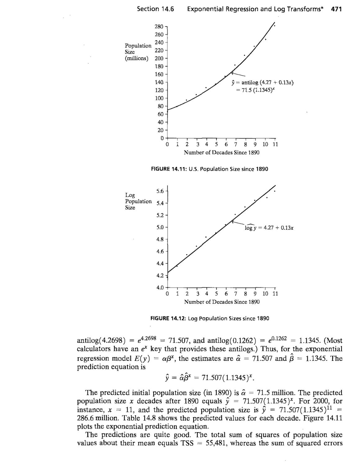
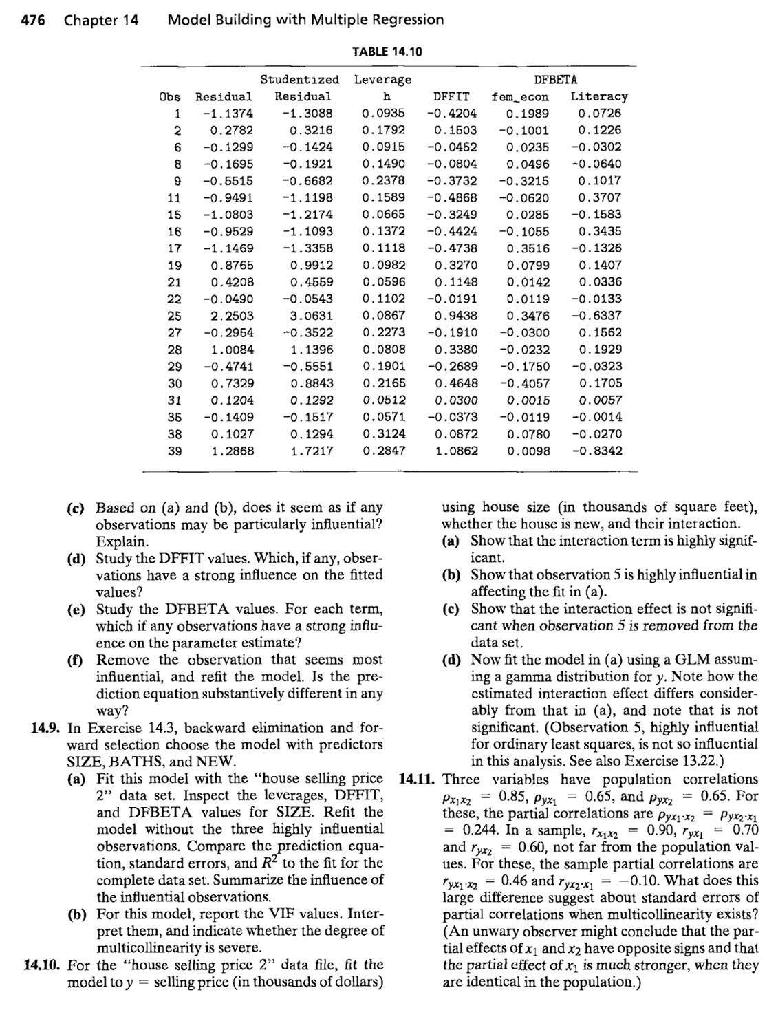
/


Автор: Alan Agresti Barbara Finlay
Теги: physics


Текст
Key Formulas for Statistical Methods
Chapter 3 Descriptive Statistics
Mean y = -^ Standard deviation s = ^ —^ ^-^
n \l n - 1
Chapter 4 ProbabiHty Distributions
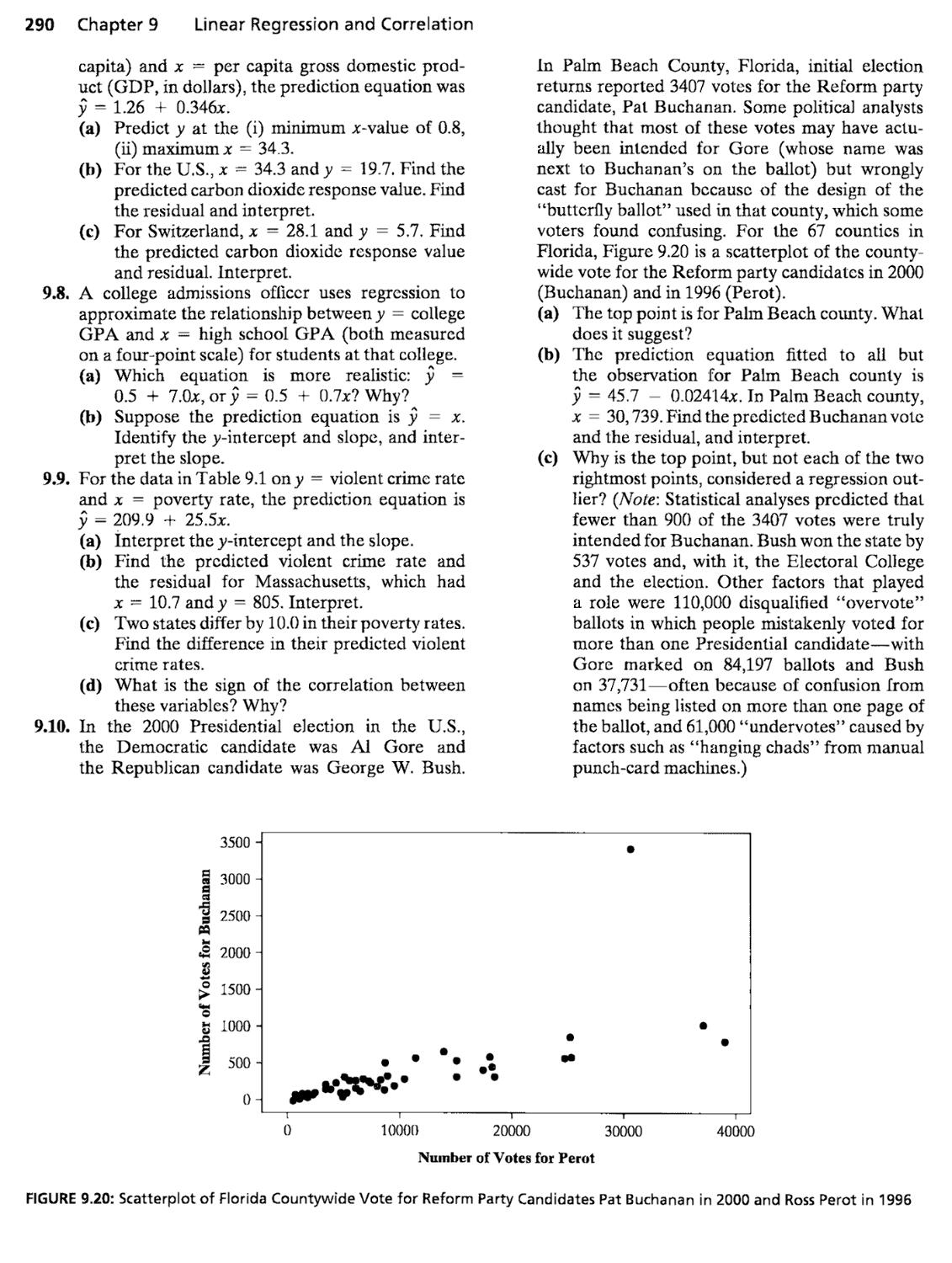
^-score z = -—-^ Standard error ay ^ —-
Chapter 5 Statistical Inference: Estimation
Confidence interval for mean y ± z{se) with se
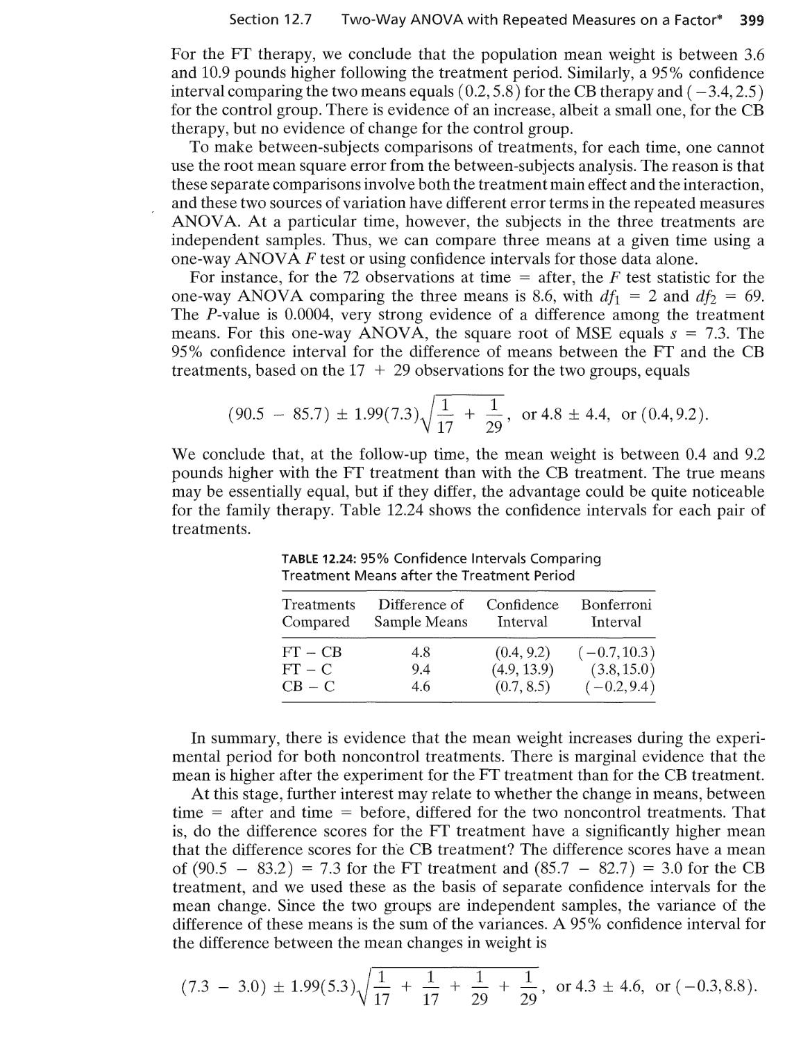
s
_ ln{l-ir)
Confidence interval for proportion tt ± z{se) with se ^ J
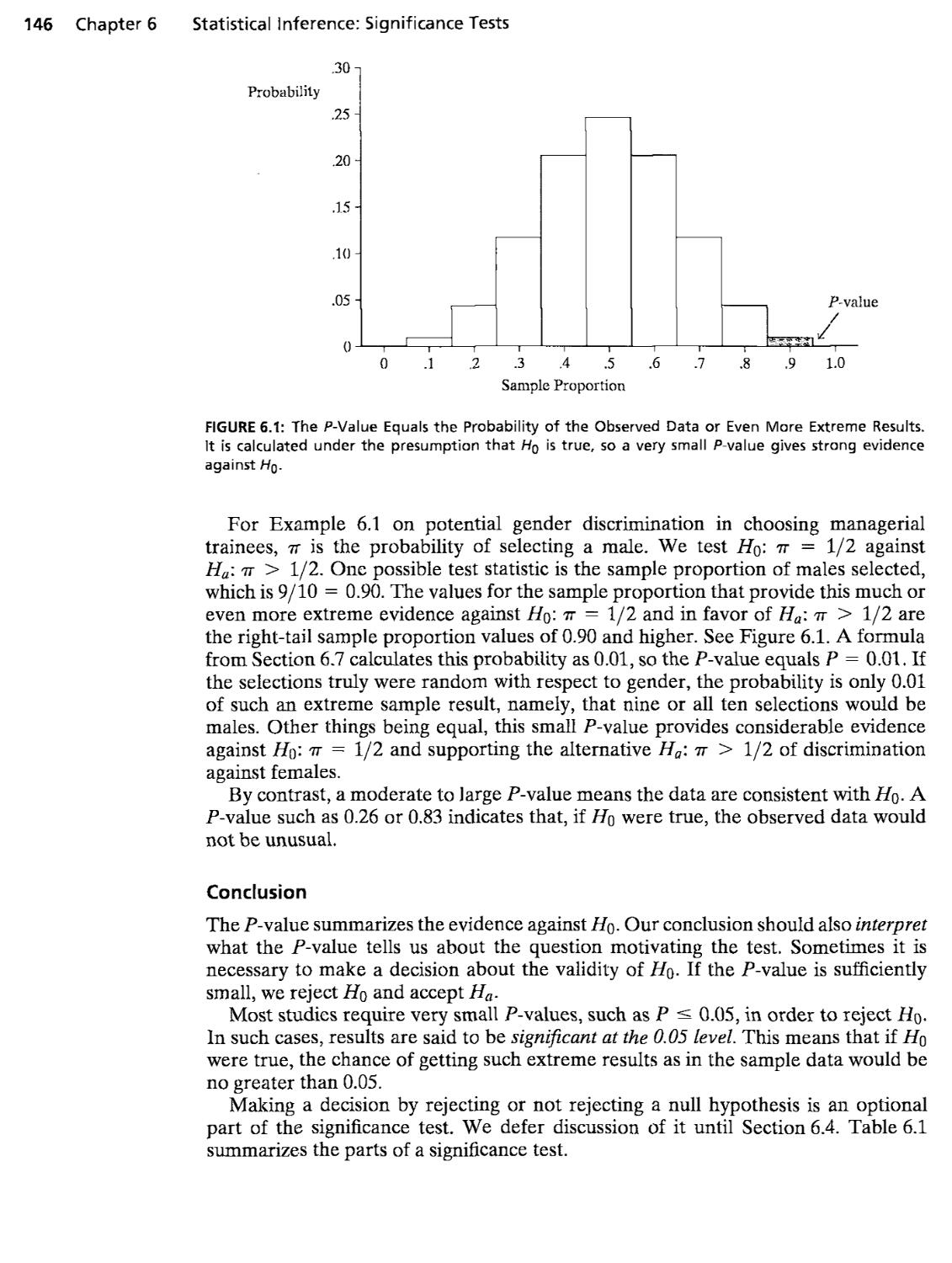
Chapter 6 Statistical Inference: Significance Tests
Hq : fji = jjiri test statistic t ^ — with se ^ -
se
Ho : TT = TTQ test statistic z = —¦ with seo =
seo
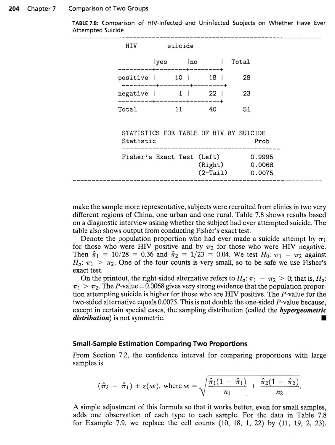
Chapter 7 Comparison of Two Groups
Compare means: (^2 ~ ^i) ± t{se) with se = ^
Test Hq : fLi = /jlj usmg /^ = -^
se
Compare proportions: (ttz - tti) ± ^(^e) with 5e = /^i(^—^i) + '^^(^"'^^^
Chapter 8 Analyzing Association Between Categorical Variables
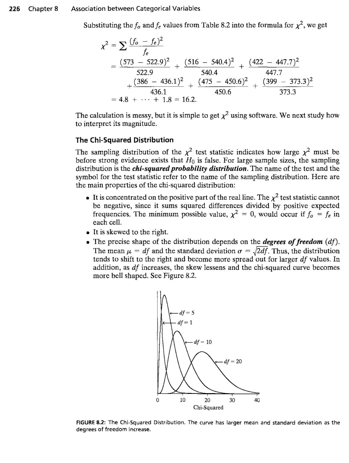
Chi-squaredtestof/fo:Independence, X^ = ^ ~ , df = (r - l)(c - 1)
>'^^ = " -
/7ro(l -
\
^i + ^
- 1
'^o)
fe
C + -lJ cr-
Ordinal measure y ^ ^;p-—^, -1 < y < 1, ^ = ^, -y ± ^o--
7
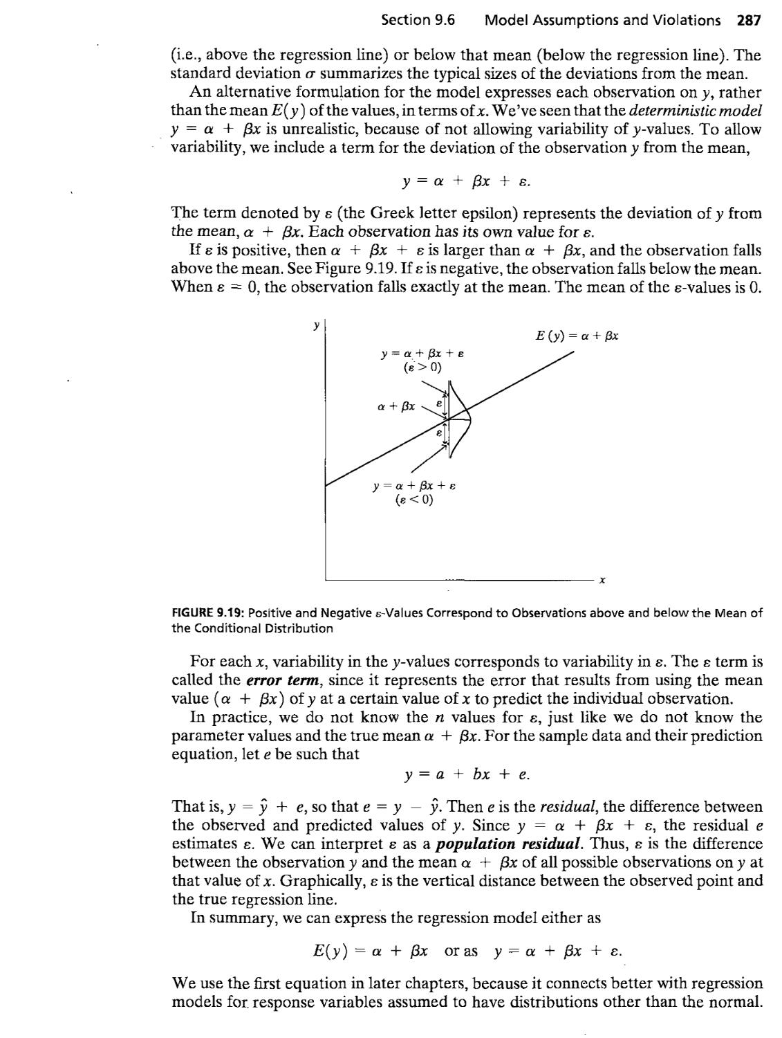
Chapter 9 Linear Regression and Correlation
Linear regression model E{y) ^ a + /Sx, prediction equation y = a + bx
Pearson correlation r=—16, —l<r<l
^ - ^^^^3/^-. TSS ^ ^{y - y)\ SSE = ^{y - y)\ 0 ^ r^ ^ 1
Test of independence Hq : C = 0, t = —, df ^ n - 2
se
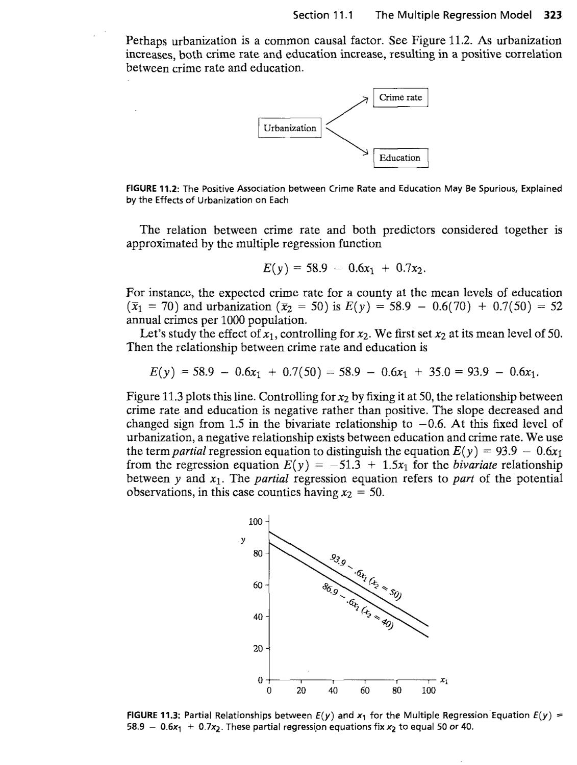
Chapter 11 Multiple Regression and Correlation
Multiple regression model E{y) - a + )8ixi + 182^:2 + ¦ ¦ + ^k^k
Global test Hq : I3i = - ¦ = ^k = 0
Test statistic i^ = Model mean square ^ R^/k
Error mean square A - R?-)/[n — {k + 1)]
dfi = k,df2 = n - (/c + 1)
Partial test Hq : f^t ^ 0, test statistic t = ^, df = n - {k + 1)
se
Chapter 12 Comparing Groups: Analysis of Variance Methods
//o : /xi = ¦ • ¦ = fjLg, One-way ANOVA test statistic
f = Between-groups sum of squares/(g - 1) ^r ^ ^ ^ ^r ^ -^ _
Within-groups sum of squares/(A^ - g) '
Chapter 13 Combining Regression and ANOVA: Analysis of Covariance
E{y) = a + ^x + jSi^i + ¦¦¦ + pg^iZg^i, Zi = 1 or 0 is dummy variable for
group i
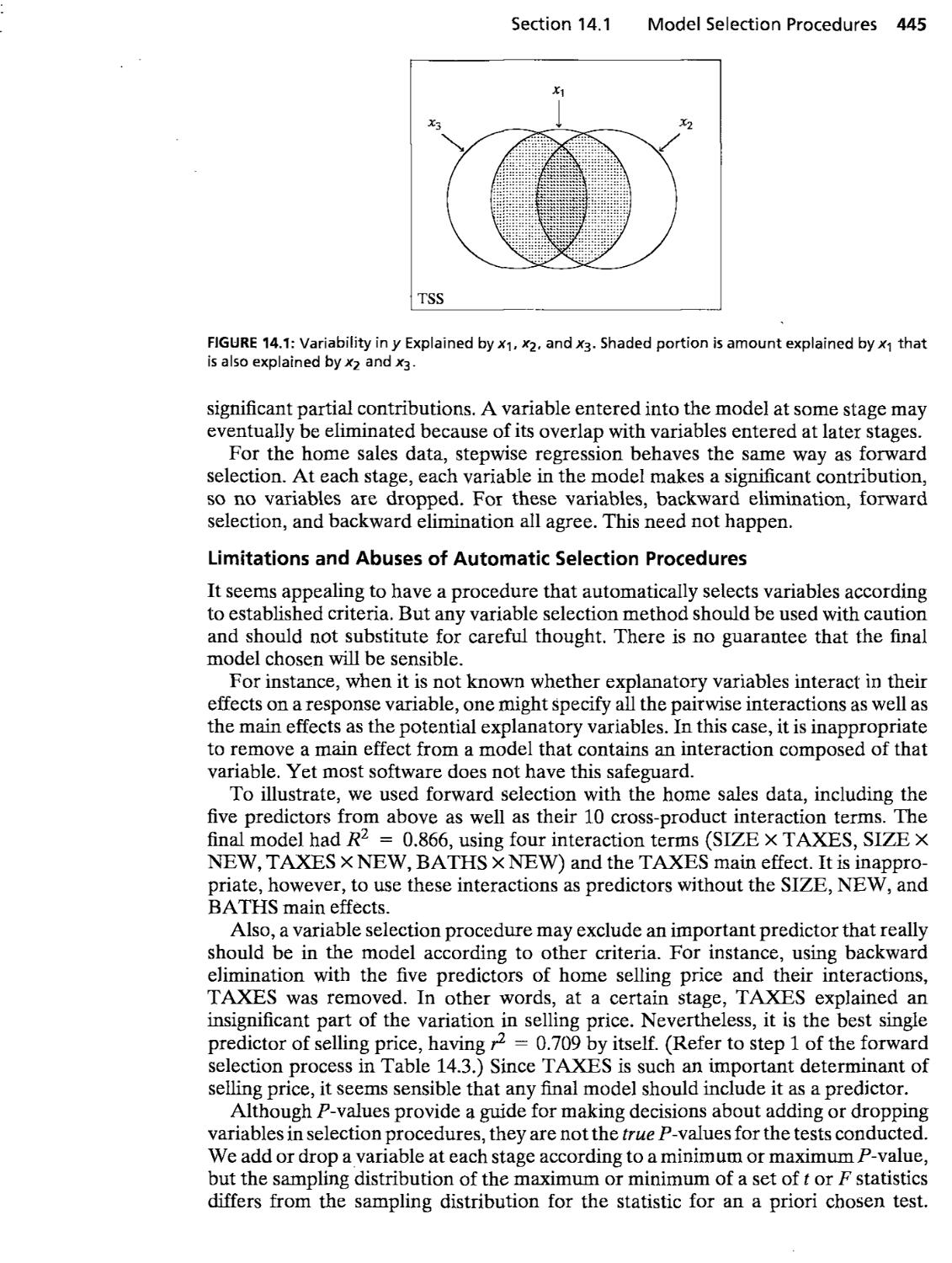
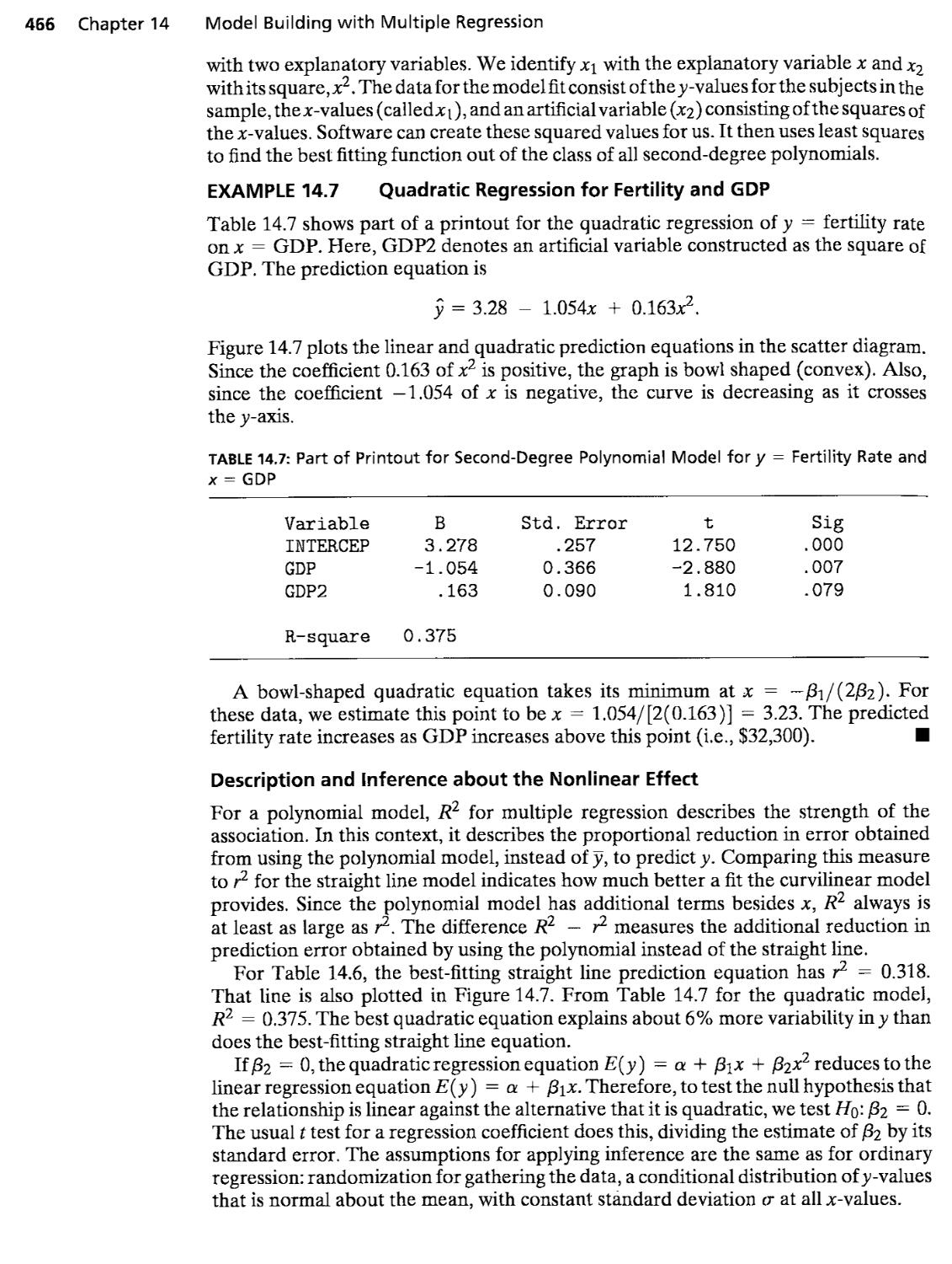
Chapter 14 Model Building with Multiple Regression
Quadratic regression E{y) = a + ^ix + ^2^
Exponential regression E{y) = a^^ (log of mean is linear in x)
Chapter 15 Logistic Regression: Modeling Categorical Responses
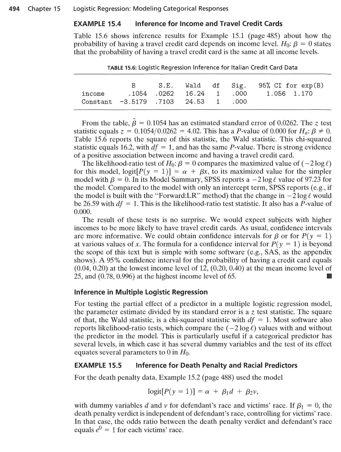
Logistic regression logit = log (odds) = log I -—^7 \ \ — a -\- ^x
P{y = l)- '"""'^ °''^'
l+e«+^ 1 + odds
STATISTICAL METHODS FOR THE
SOCIAL SCIENCES
Fourth Edition
Alan Agresti
University of Florida
Barbara Finlay
Texas A &M University
PEARSON
Prentice
Hall
Upper Saddle River, New Jersey 07458
Library of Congress Cataloging-in-Publicafion Data
Agresti, Alan,
Statistical methods for the social sciences / Alan Agresti, Barbara Finlay.^
4th ed.
p. cm.
Includes bibliographical references and index.
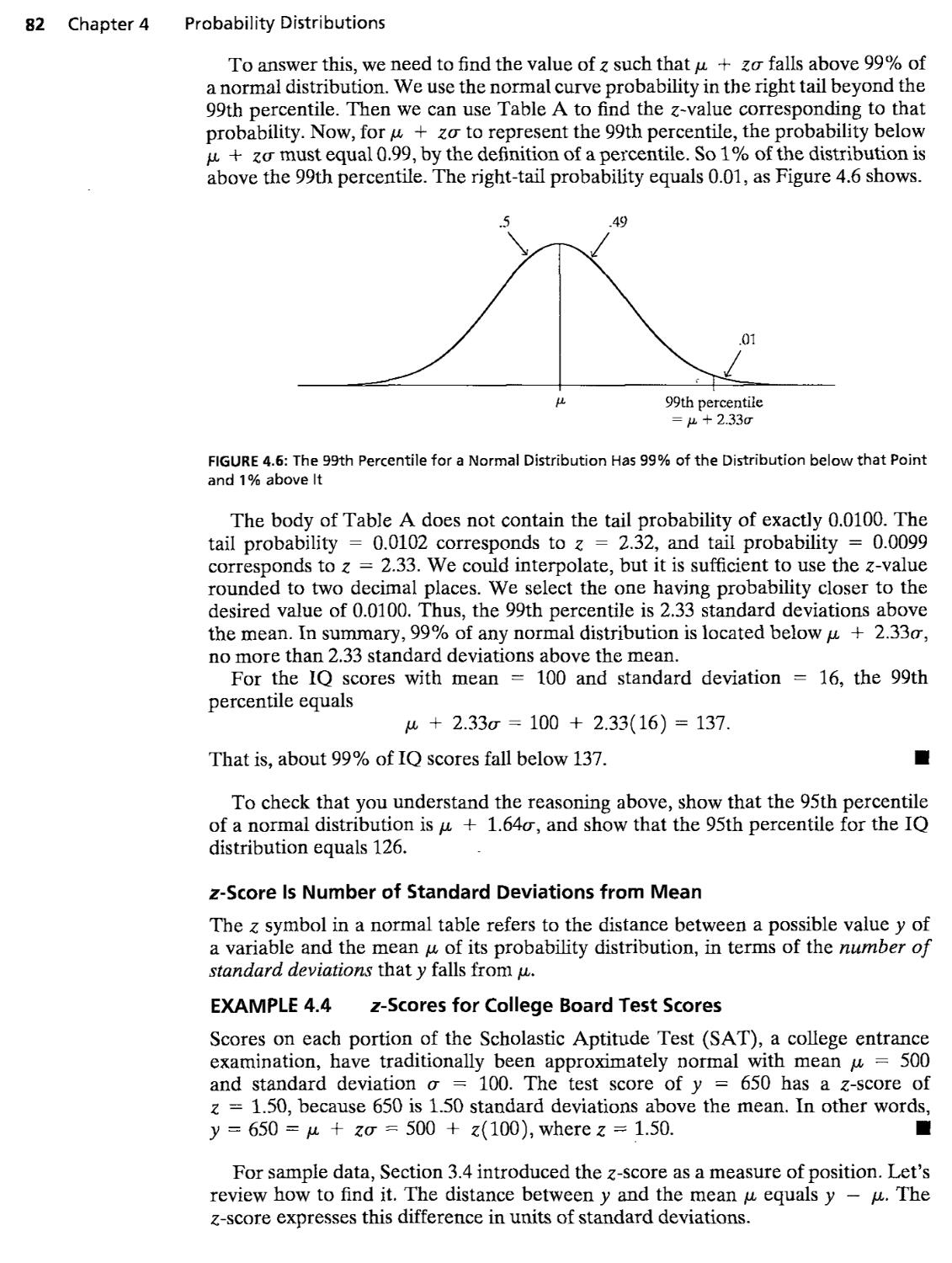
ISBN-13: 978-0-13-027295-9 (alk. paper)
1. Statistics. 2. Social sciences—Statistical methods. I. Finlay, Barbara. 11.
Title.
QA276.12.A34 2009
5J9.5—dc22
2007038723
Editor-in-Chief: Deirdre Lynch
Vice President and Editorial Director, Mathematics: Christine Hoag
Sponsoring Editor: Dawn Murrin
Editorial Assistant/Print Supplements Editor: Joanne Wenddken
Senior Managing Editor: Linda Behrens
Associate Managing Editor: Bayani Mendoza de Leon
Project Manager, Production: Traci Douglas
Senior Operations Supervisor: Diane Peirano
Executive Marketing Manager: Kate Valentine
Marketing Manager: Wayne Parkins
Assistant Manager, Marketing Support: Diana Penha
Marketing Assistant: Kathleen DeChavez
Art Director: Jayne Conte
Cover Designer: Kiwi Design
Cover Painting: "Harvest" by Albina Felski
Composition/Art Studio: Laserwords
gjg ©2009,1997 by Prentice Hall, Inc.
Pearson Prentice Hall
Pearson Education, Inc.
Upper Saddle River, New Jersey 07458
Previous edition copyright © 1986 and 1979 by Dellen Publishing Company, a division of Macmillan, Inc.
All rights reserved. No part of this book may be reproduced in any form or by any means, without
permission in writing from the publisher.
Pearson Prentice Hall™ is a trademark of Pearson Education, Inc.
Printed in the United States of America
10 9 8 7 6 5 4
ISBN-13: T7fi-D-13-a27ETS-T
ISBN-ID: 0-13-0272^5-7
Pearson Education Ltd., London
Pearson Education Australia Pty. Ltd., Sydney
Pearson Education Singapore, Pte. Ltd.
Pearson Education North Asia Ltd., Hong Kong
Pearson Education Canada, Inc., Toronto
Pearson Educacion de Mexico, S.A. de C.V.
Pearson Education—Japan, Tokyo
Pearson Education Malaysia, Pte. Ltd.
To my parents
Louis J. Agresti and Marjorie H, Agresti
Contents
Preface ix
Acknowledgments xiii
1 Introduction 1
1.1 Introduction to Statistical Methodology 1
1.2 Descriptive Statistics and Inferential Statistics 4
1.3 The Role of Computers in Statistics 6
1.4 Chapter Summary . 7
2 Sampling and Measurement 11
2.1 Variables and Their Measurement 11
2.2 Randomization 15
2.3 Sampling Variability and Potential Bias 18
2.4 Other Probability Sampling Methods* 21
2.5 Chapter Summary 24
3 Descriptive Statistics 31
3.1 Describing Data with Tables and Graphs 31
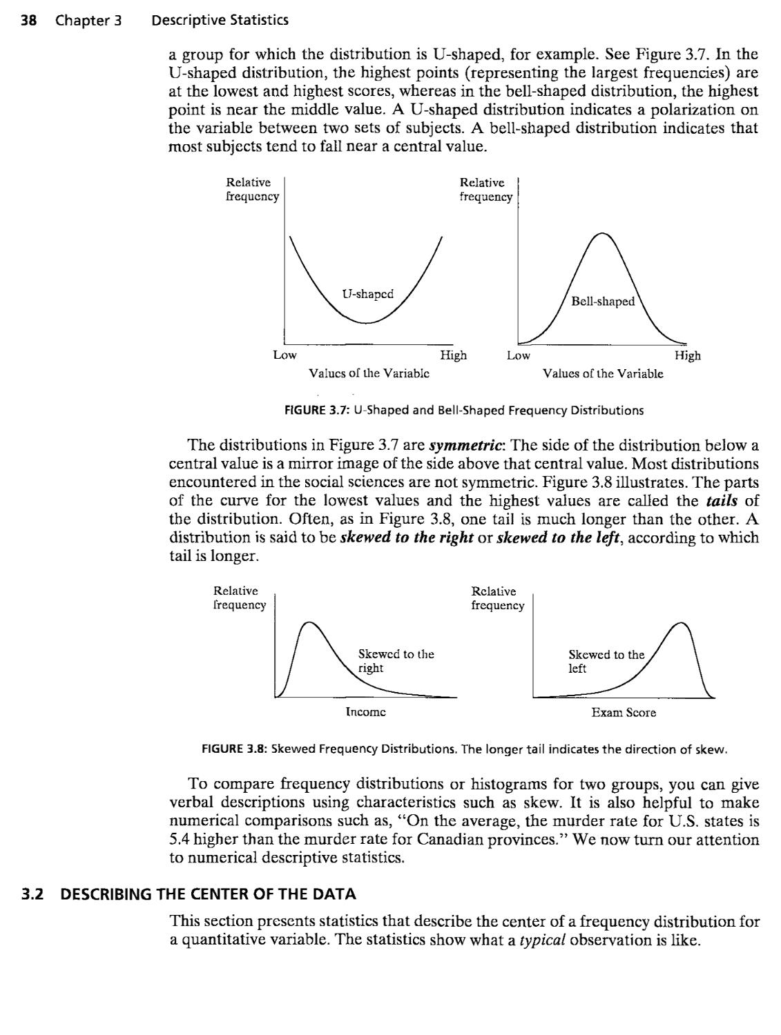
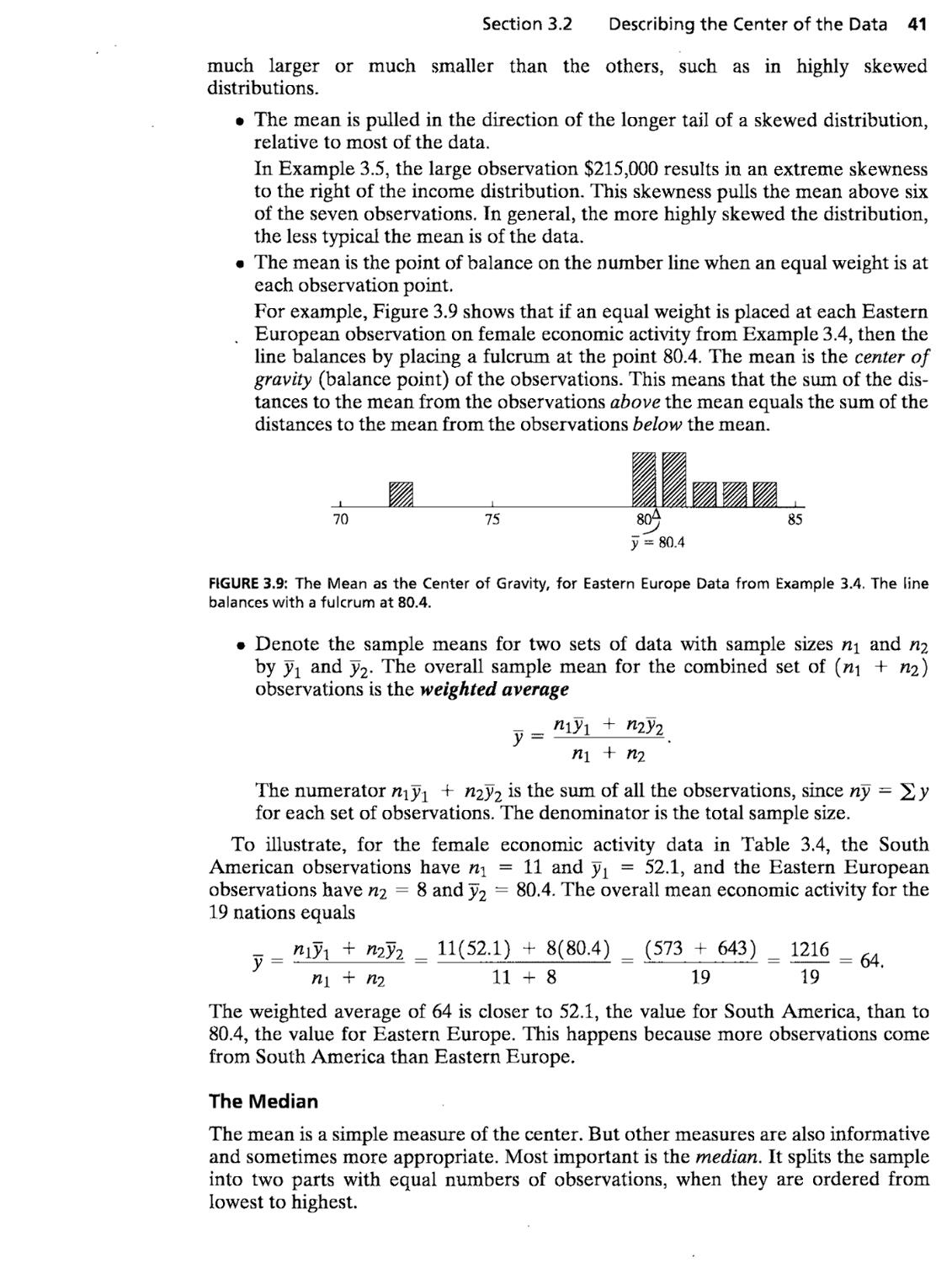
3.2 Describing the Center of the Data 38
3.3 Describing Variability of the Data 46
3.4 Measures of Position 51
3.5 Bivariate Descriptive Statistics 55
3.6 Sample Statistics and Population Parameters 58
3.7 Chapter Suirunary 59
4 Probability Distributions 73
4.1 Introduction to Probability 73
4.2 Probability Distributions for Discrete and Continuous Variables ... 75
4.3 The Normal Probability Distribution 78
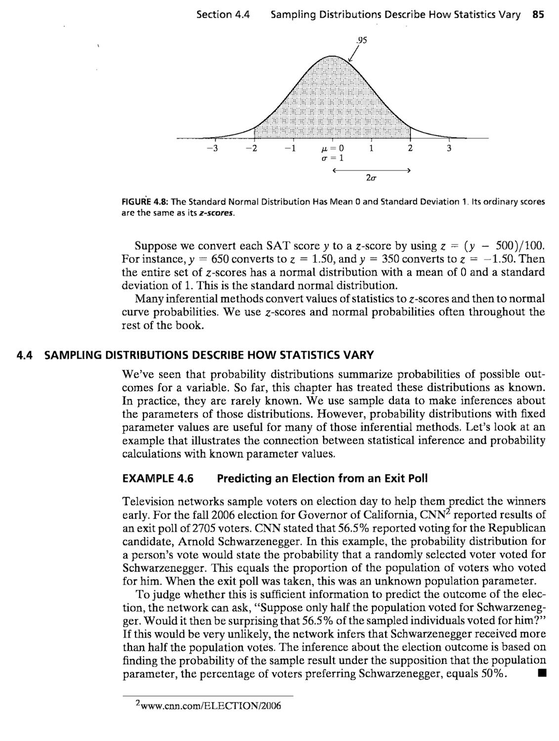
4.4 Sampling Distributions Describe How Statistics Vary 85
4.5 Sampling Distributions of Sample Means 89
4.6 Review: Population, Sample Data, and Sampling Distributions .... 95
4.7 Chapter Summary 99
5 Statistical Inference: Estimation 107
5.1 Point and Interval Estimation 107
5.2 Confidence Interval for a Proportion 110
5.3 Confidence Interval for a Mean 116
5.4 Choice of Sample Size 124
5.5 Confidence Intervals for Median and Other Parameters* 129
5.6 Chapter Summary 132
6 Statistical Inference: Significance Tests 143
6.1 The Five Parts of a Significance Test 144
6.2 Significance Test for a Mean 147
6.3 Significance Test for a Proportion 156
¦"Sections or subsections marked with an asterisk liave less importance for a first introduction to statistics and are optional. V
vi Contents
6.4 Decisions and Types of Errors in Tests 159
6.5 Limitations of Significance Tests 163
6.6 Calculating P (Type II Error)* 166
6.7 Small-Sample Test for a Proportion—the Binomial Distribution* . . . 169
6.8 Chapter Summary 173
7 Comparison of Two Groups 183
7.1 Preliminaries for Comparing Groups 183
7.2 Categorical Data: Comparing Two Proportions 187
7.3 Quantitative Data: Comparing Two Means 191
7.4 Comparing Means with Dependent Samples 193
7.5 Other Methods for Comparing Means* 197
7.6 Other Methods for Comparing Proportions* 201
7.7 Nonparametric Statistics for Comparing Groups* 205
7.8 Chapter Summary 208
8 Analyzing Association between Categorical Variables 221
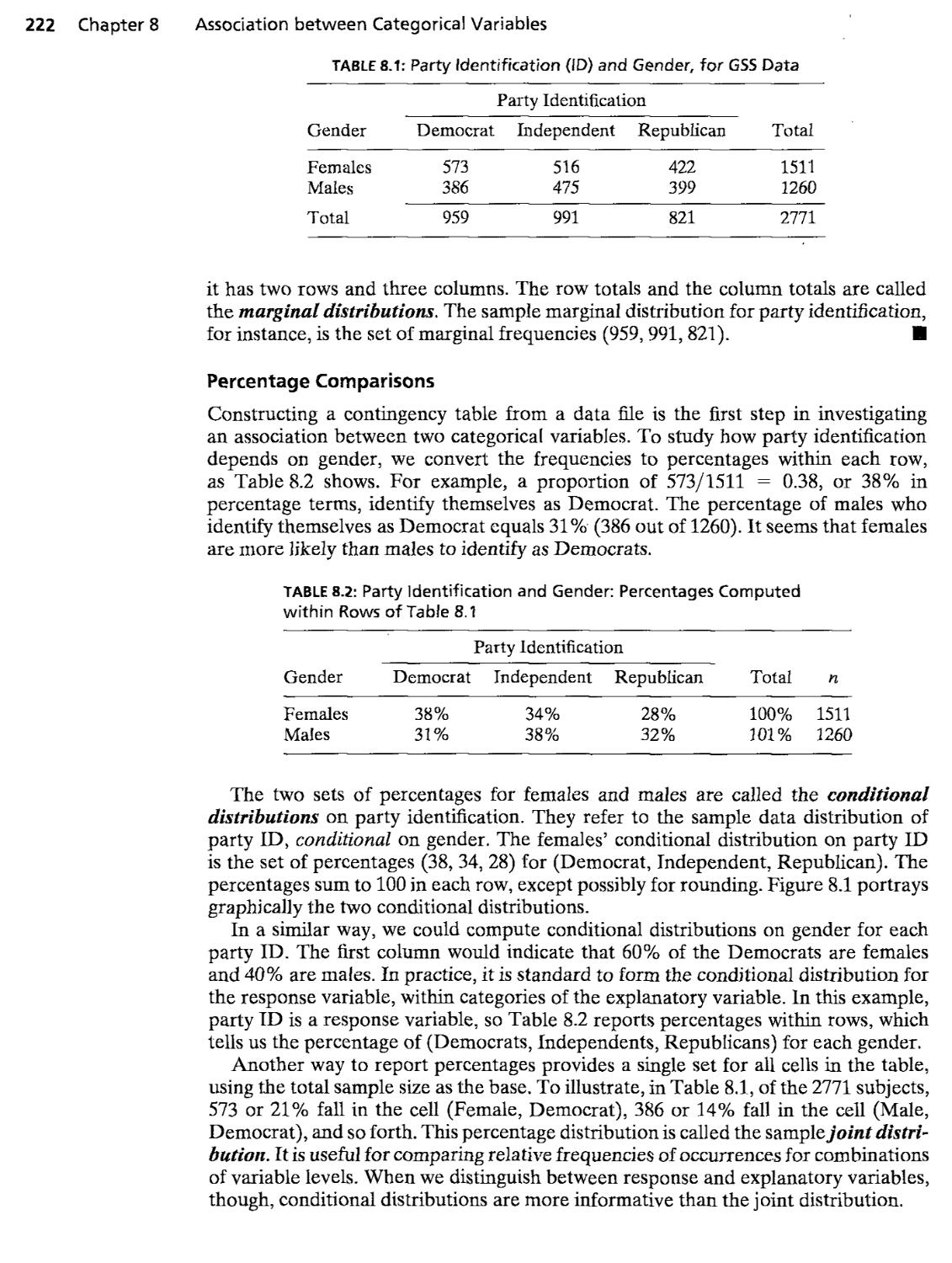
8.1 Contingency Tables 221
8.2 Chi-Squared Test of Independence 224
8.3 Residuals: Detecting the Pattern of Association 229
8.4 Measuring Association in Contingency Tables 233
8.5 Association between Ordinal Variables* 239
8.6 Inference for Ordinal Associations* 243
8.7 Chapter Summary 246
9 Linear Regression and Correlation 255
9.1 Linear Relationships 256
9.2 Least Squares Prediction Equation 259
9.3 The Linear Regression Model 265
9.4 Measuring Linear Association: The Correlation 269
9.5 Inferences for the Slope and Correlation 276
9.6 Model Assumptions and Violations 283
9.7 Chapter Summary 288
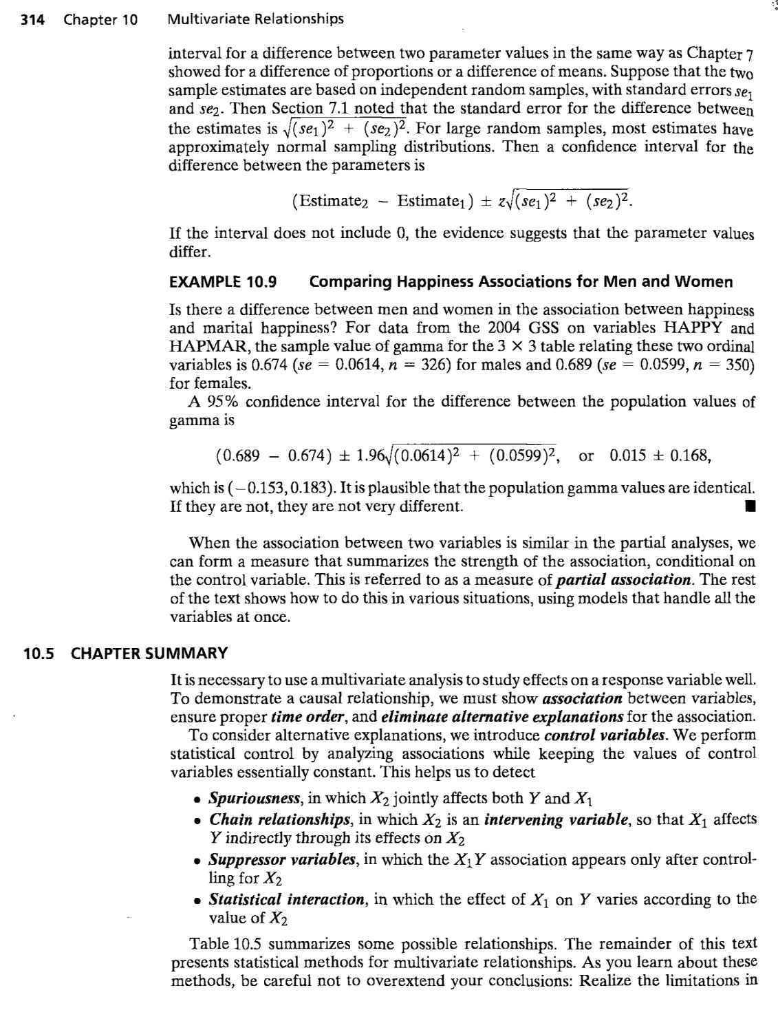
10 Introduction to Multivariate Relationships 301
10.1 Association and Causality 301
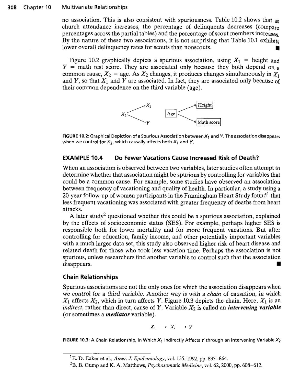
10.2 Controlling for Other Variables 304
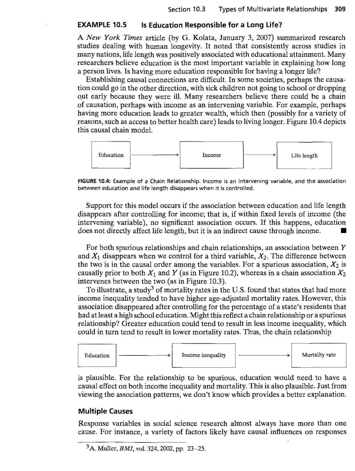
10.3 Types of Multivariate Relationships 307
10.4 Inferential Issues in Statistical Control 313
10.5 Chapter Summary .^ 314
11 Multiple Regression and Correlation 321
11.1 The Multiple Regression Model 321
11.2 Example with Multiple Regression Computer Output 326
11.3 Multiple Correlation and i?^ 331
11.4 Inference for Multiple Regression Coefficients 335
11.5 Interaction between Predictors in Their Effects 340
11.6 Comparing Regression Models 345
11.7 Partial Correlation* 347
11.8 Standardized Regression Coefficients* 351
11.9 Chapter Summary 354
Contents vu
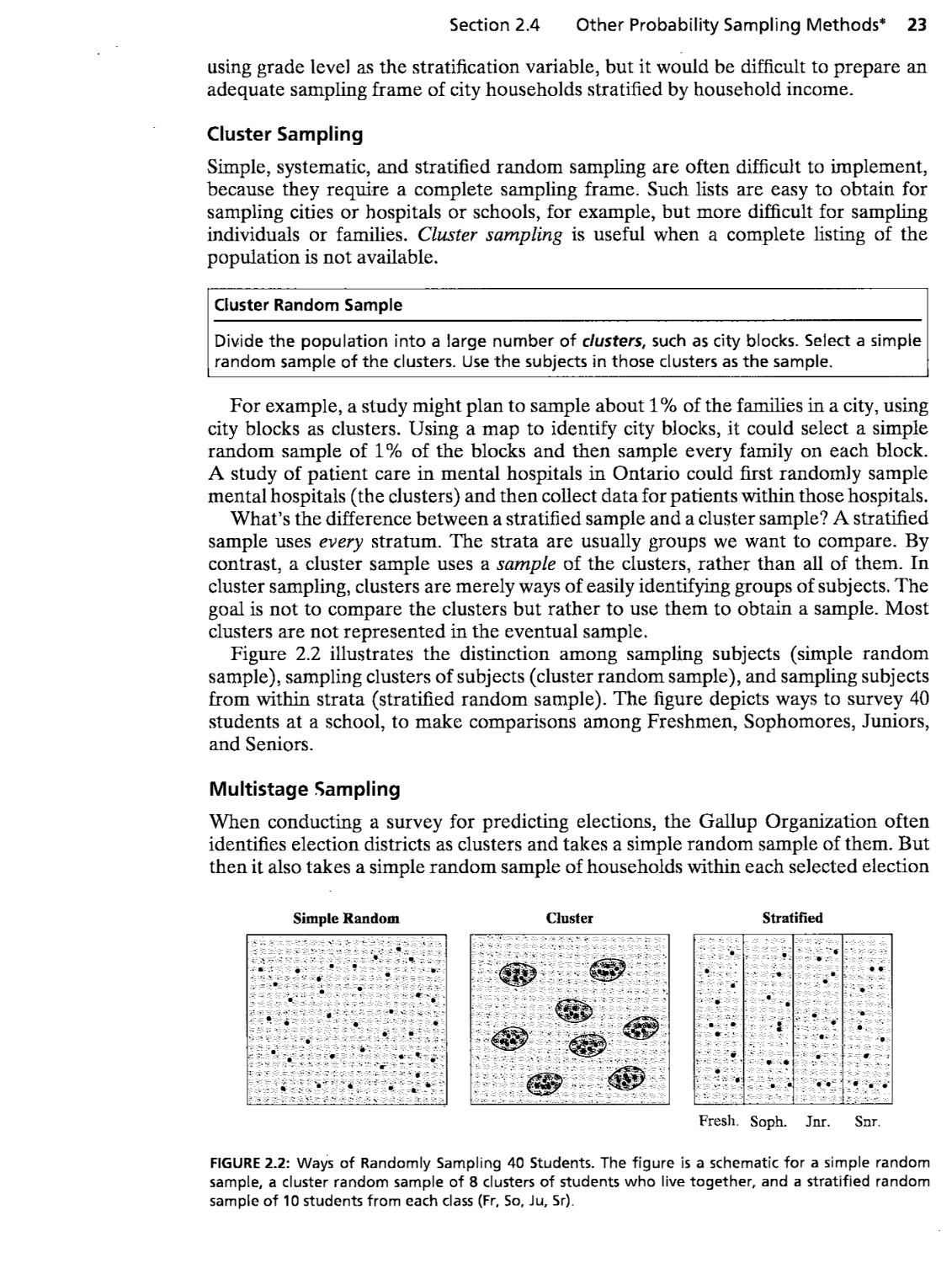
12 Comparing Groups: Analysis of Variance (ANOVA) Methods 369
12.1 Comparing Several Means: The Analysis of Variance F Test 369
12.2 Multiple Comparisons of Means 376
12.3 Performing ANOVA by Regression Modeling 378
12.4 Two-Way Analysis of Variance 382
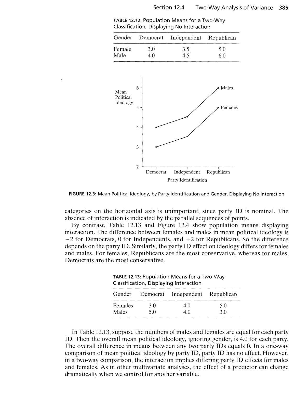
12.5 Two-Way ANOVA and Regression 386
12.6 RepeatedMeasures Analysis of Variance* 391
12.7 Two-Way ANOVA with Repeated Measures on a Factor* 395
12.8 Effects of Violations of ANOVA Assumptions 400
12.9 Chapter Summary 402
13 Combining Regression and ANOVA: Quantitative and
Categorical Predictors 413
13.1 Comparing Means and Comparing Regression Lines 414
13.2 Regression with Quantitative and Categorical Predictors 416
13.3 Permitting Interaction between Quantitative and Categorical
Predictors 419
13.4 Inference for Regression with Quantitative and Categorical
Predictors 422
13.5 Adjusted Means* 426
13.6 Chapter Summary 433
14 Model Building with Multiple Regression 441
14.1 Model Selection Procedures 441
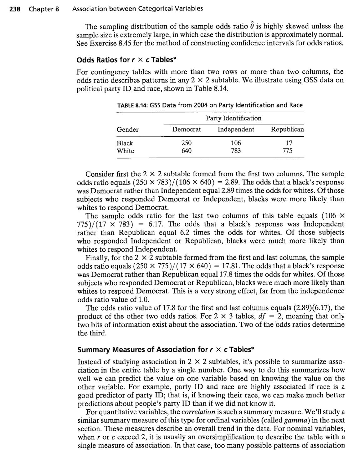
14.2 Regression Diagnostics 448
14.3 Effects of MulticoUinearity 456
14.4 Generalized Linear Models 458
14.5 Nonlinear Relationships: Polynomial Regression 462
14.6 Exponential Regression and Log Transforms* 469
14.7 Chapter Summary 473
15 Logistic Regression: Modeling Categorical Responses 483
15.1 Logistic Regression 483
15.2 Multiple Logistic Regression 488
15.3 Inference for Logistic Regression Models 493
15.4 Logistic Regression Models for Ordinal Variables* 496
15.5 Logistic Models for Nominal Responses* 501
15.6 Loglinear Models for Categorical Variables* 503
15.7 Model Goodness-of-Fit Tests for Contingency Tables* 507
15.8 Chapter Summary 511
16 An Introduction to Advanced Methodology 519
16.1 Longitudinal Data Analysis* 519
16.2 Multilevel (Hierarchical) Models* 523
16.3 Event History Models* 524
16.4 Path Analysis* 527
16.5 Factor Analysis* . . 532
16.6 Structural Equation Models* 537
16.7 Markov Chains* 541
viii Contents
Appendix A: SPSS and SAS for Statistical Analyses 545
Appendix B: Answers to Selected Odd-Numbered Exercises 567
Tables 591
Bibliography 599
Index 601
Preface
When I undertook the first edition of this book nearly three decades ago, my goal was
to introduce statistical methods in a style that emphasized their concepts and their
application to the social sciences rather than the mathematics and computational
details behind them. I did this by focusing on how the methods are used and
interpreted rather than their theoretical derivations.
This fourth edition of the book has an even stronger emphasis on concepts and
appHcations, with greater attention to "real data" both in the examples and exercises.
I continue to downplay mathematics, in particular probability, which is all too often a
stumbling block for students. On the other hand, the text is not a cookbook. Reliance
on an overly simphstic recipe-based approach to statistics is not the route to good
statistical practice.
Changes in the Fourth Edition
Since the first edition, the increase in computer power coupled with the continued
improvement and accessibility of statistical software has had a maj or impact on the way
social scientists analyze data. Because of this, this book does not cover the traditional
shortcut hand-computational formulas and approximations. The presentation of
computationally complex methods, such as regression, emphasizes interpretation
of software output rather than the formulas for performing the analysis. The text
contains numerous sample printouts, mainly in the style of SPSS and occasionally
SAS, both in chapter text and homework problems. This edition also has an appendix
explaining how to apply SPSS and SAS to conduct the methods of each chapter and
a Web site giving links to information about other software.
Exposure to realistic but simple examples and to numerous homework exercises
is vital to student learning. This edition has added many new exercises and updated
old ones, with major emphasis on real data. Each chapter's homework set is divided
into two parts, straightforward exercises on the text material in Practicing the Basics,
and exercises dealing with open-ended data analyses, understanding of concepts, and
advanced material in Concepts and Applications. The large data sets in the examples
and exercises, including a data set introduced in Exercise 1.11 that appears again in
exercises at the end of each chapter, are available at
http://ww¥. Stat .uf l.edu/'-'aa/social/data.html
This edition contains'several changes and additions in content, directed toward a
more modern approach. The main changes are as follows:
• There is stronger focus on real examples and on the integration of statistical
software. This includes some new exercises that ask students to use applets at
the Prentice Hall Web site to help learn the fundamental concepts of sampling
distributions, confidence intervals, and significance tests.
• The book has a somewhat lower technical level in the first nine chapters, to
make the book more easily accessible to undergraduate students. To help with
this, some notation has been simplified or eliminated.
• Chapter 3, on descriptive statistics, has a separate section for measures of
position, such as percentiles and related topics such as the box plot and outliers.
It also has a short section on bivariate descriptive methods. This gives students
ix
X Preface
an early exposure to contingency tables and to regression and the point that,
in practice, there's almost always more than one variable of interest. This
section also introduces them to the concepts of association, and response and
explanatory variables.
• Chapter 4 has a new section that introduces the relative frequency concept and
briefly summarizes three basic probability rules that are occasionally appUed in
the text.
• The inference material on means in Chapters 5-7 has been changed to rely
completely on the t distribution, rather than using the z for large samples
and t for small samples. This makes results consistent with software output. I
continue to emphasize that the normality assumption for the t distribution is
mainly needed for small samples with one-sided inference.
e Partly because of the change in using the t distribution always for inference
about the mean, Chapter 5, on confidence intervals, now presents methods for
the proportion (which rehes only on the normal distribution) before the mean.
This way, the students can learn the basic concept of a confidence interval using
the information they've just learned at the end of Chapter 4 about the normal
distribution as a sampling distribution (i.e., for a proportion, the margin of error
multipHes the standard error by a z-score rather than a r-score). This delays
introduction of the t distribution by a section, so students are not confronted
with too many new topics all at once.
• Chapter 7, on comparing two groups, has a new section introducing ideas of
bivariate analysis, reminding students of the distinction between response and
explanatory variables, defining independent and dependent samples, discussing
how to compare two groups with a difference or a ratio of two parameters, and
showing the general formula for finding a standard error of a difference between
two independent estimates. Section 7.3 introduces the concept of a model.
• Chapter 12, on analysis of variance (ANOVA), explains the ideas behind the F
test and gives an example before presenting the sums of squares formulas.
• Chapter 15 provides a less technical explanation of logistic regression and
introduces its extensions for nominal and ordinal response variables.
• Chapter 16 includes new sections on longitudinal data analysis and multilevel
(hierarchical) models.
Use of Text in Introductory Statistics Courses
Like the first three editions, this edition is appropriate for introductory statistics
courses at either the undergraduate or beginning graduate level, and for either a
single-term or a two-term sequence. Chapters 1-9 are the basis for a single-term
course. If the instructor wishes to go further than Chapter 9 or wishes to cover some
material in greater depth, sections that can easily be omitted without disturbing
continuity include 2.4, 5.5, 6.6-6.7, 7.5-7.7, and 8.5-8.6. Also, Chapters 7-9 and
Sections 12.1-12.2 are self-contained, and the instructor could move directly into any
of these after covering the fundamentals in Chapters 1-6. Tour possible paths for a
one-term course are as follows:
• Chapters 1-9 (possibly omitting sections noted above): Standard cross-section
of methods, including basic descriptive and inferential statistics, two-sample
procedures, contingency tables, and linear regression
• Chapters 1-7, 9,11: Emphasis on regression
Preface xi
• Chapters 1-7, 9, 12.1-12.2: After two-group comparisons, introduction to
regression and analysis of variance
• Chapters 1-8, 10; Emphasis on categorical data, basic issues of mukivariate
relationships
Regardless of the type of data, my belief is that a modeling paradigm emphasizing
parameter estimation is more useful than the artificial hypothesis-testing approach of
many statistics texts. Thus, the basic inference chapters E-8) explain the advantages
confidence intervals have over significance testing, and the second half of this text
(starting in Chapter 9) is primarily concerned with model building. The concept of
a model is introduced in Section 7.5 in describing the two methods for comparing
means. The modeling material forms the basis of a second course.
Some material appears in sections, subsections, or exercises marked by asterisks.
This material is optional, having lesser importance for introductory courses. The text
does not attempt to present every available method, since it is meant to be a teaching
tool, not an encyclopedic cookbook. It does cover the most important methods
for social science research, however, and it includes topics not usually discussed in
introductory statistics texts, such as
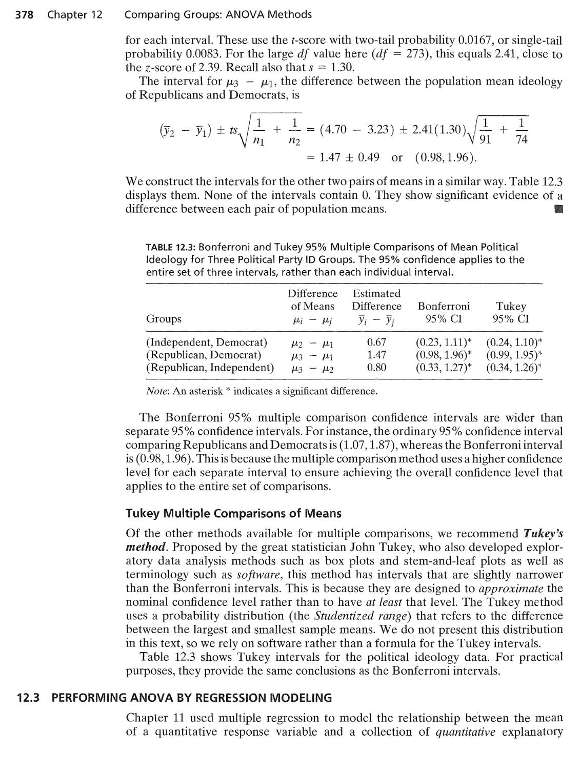
• Methods for contingency tables that are more informative than chi-squared,
such as cell residuals and analyses that utilize category orderings
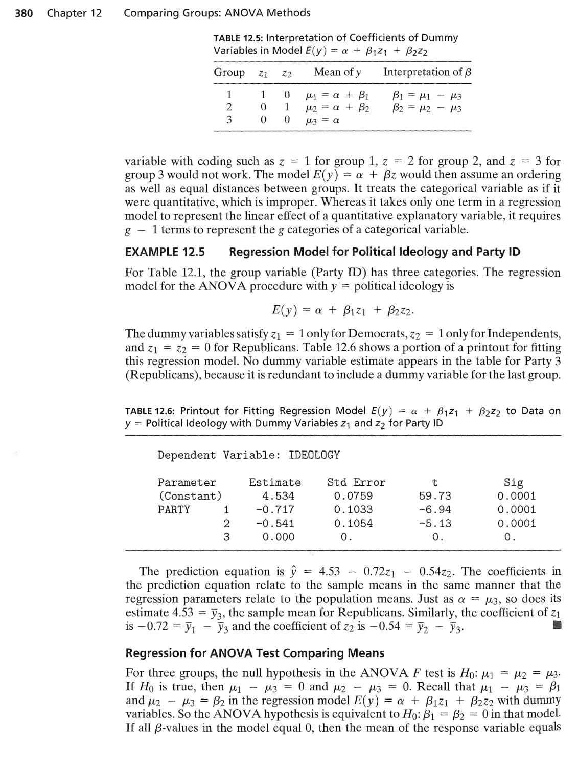
e Controlling for variables, and issues dealing with causation
• The generalized linear modeling approach, encompassing ordinary
regression, analysis of variance and covariance, gamma regression for nonnegative
responses with standard deviation proportional to the mean, logistic
regression for categorical responses, and loglinear association models for contingency
tables
I beheve that the student who works through this book successfully will acquire a
solid foundation in applied statistical methodology.
Acknowledgments
I am grateful to Barbara Finlay for her contributions to the first two editions of this
text. I hope that the combination of our respective fields of expertise provides a book
that is statistically sound as well as relevant to the social sciences.
I thank those who invested a considerable amount of time in helping this book to
reach fruition. Thanks to Sarah Streett for updating data in many of the examples
and exercises, to Jackie Miller for her excellent job on accuracy checking, and to
Traci Douglas for serving as Production Editor. Thanks to Arne Bathke, David Most,
Youqin Huang, and Michael Lacy for providing comments for this edition. Other
individuals who provided advice or data sets include Roslynn Brain, Beth Chance,
Brent Coull, Alfred DeMaris, Mary Gray, Brian Gridley, Ralitza Gueorguieva,
John Henretta, Ira Horowitz, Harry Khamis, Bernhard Klingenberg, Jacalyn Levine,
Michael Radelet, Paula Rausch, Euijung Ryu, Paul Smith, Robert Wilson, and Zoe
Zihak. Thanks also to the many people whose comments helped in the preparation
of the first three editions, especially Burke Grandjean, Susan Reiland, Maureen
Hallinan, Shirley Scritchfield, Sonja Wright, Douglas Zahn, Jeff Witmer, E. Jacquelin
Dietz, Dorothy K. Davidson, and Mary Sue Younger. My editors for this and the
previous edition, Petra Recter and Ann Heath at Prentice Hall, provided outstanding
support and encouragement.
Finally, extra special thanks to my wife, Jacki Levine, for assistance with editing
and style in the third edition and with overall encouragement during the preparation
of the fourth edition.
Alan Agresti
Gainesville, Florida
XIII
CHAPTER 1
Introduction
1.1 INTRODUCTION TO STATISTICAL METHODOLOGY
1.2 DESCRIPTIVE STATISTICS AND INFERENTIAL STATISTICS
1.3 THE ROLE OF COMPUTERS IN STATISTICS
1A CHAPTER SUMMARY
1.1 INTRODUCTION TO STATISTICAL METHODOLOGY
The past quarter-century has seen a dramatic increase in the use of statistical
methods in the social sciences. There are many reasons for this. More research in
the social sciences has taken on a quantitative orientation. Like research in other
sciences, research in the social sciences often studies questions of interest by analyzing
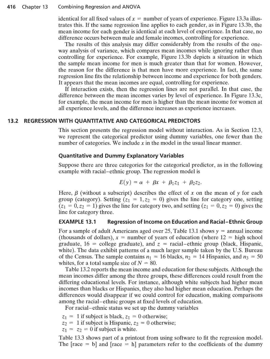
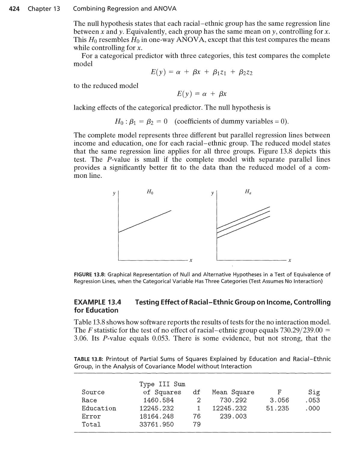
evidence provided by empirical data. The growth of the Internet has resulted in an
increase in the amount of readily available quantitative information. Finally, with the
evolution of evermore powerful computers, software, and statistical methodology,
new methods are available that can more realistically address the questions that arise
in social science research.
Why Study Statistics?
The increased use of statistics is evident in the changes in the content of articles
published in social science research journals and reports prepared in government and
private industry. A quick glance through recent issues of journals such as American
Political Science Review and American Sociological Review reveals the fundamental
role of statistics in research. For example, to learn about which factors have the
greatest impact on student performance in school or to investigate which factors
affect people's political beliefs or the quahty of their health care or their decision
about when to retire, researchers collect information and process it using statistical
analyses. Because of the role of statistics in many research studies, more and more
academic departments require that their majors take statistics courses.
These days, social scientists work in a wide variety of areas that use statistical
methods, such as governmental agencies, business organizations, and health care
facilities. For example, social scientists in government agencies dealing with human
welfare or environmental issues or public health policy invariably need to use
statistical methods or at least read reports that contain statistics. Medical sociologists often
must evaluate recommendations from studies that contain quantitative investigations
of new therapies or new ways of caring for the elderly. Some social scientists help
managers to evaluate employee performance using quantitative benchmarks and to
determine factors that help predict sales of products. In fact, increasingly many jobs
for social scientists expect a knowledge of statistical methods as a basic work tool. As
the joke goes, "What did the sociologist who passed statistics say to the sociologist
who failed it? T'U have a Big Mac, fries, and a Coke.' "
2 Chapter 1 Introduction
But an understanding of statistics is important even if you never use statistical
methods in your career. Every day you are exposed to an explosion of information,
from advertising, news reporting, political campaigning, surveys about opinions on
controversial issues, and other communications containing statistical arguments.
Statistics helps you make sense of this information and better understand the world.
You will find concepts from this text helpful in judging the information you will
encounter in your everyday life.
We realize you are not reading this book in hopes of becoming a statistician. In
addition, you may suffer from math phobia and feel fear at what lies ahead. Please
be assured that you can read this book and learn the primary concepts and methods
of statistics with little knowledge of mathematics. Just because you may have had
difficulty in math courses before does not mean you will be at a disadvantage here.
To understand this book, logical thinking and perseverance are more important
than mathematics. In our experience, the most important factor in how well you do
in a statistics course is how much time you spend on the course—attending class,
doing homework, reading and re-reading this text, studying your class notes, working
together with your fellow students, getting help from your professor or teaching
assistant—not your mathematical knowledge or your gender or your race or whether
you feel fear of statistics at the beginning.
Don't be frustrated if learning comes slowly and you need to read a chapter a few
times before it starts to make sense. Just as you would not expect to take a single
course in a foreign language and be able to speak that language fluently, the same is
true with the language of statistics. Once you have completed even a portion of this
text, however, you will better understand how to make sense of statistical information.
Data
Information gathering is at the heart of all sciences, providing the observations used
in statistical analyses. The observations gathered on the characteristics of interest are
collectively called data.
For example, a study might conduct a survey of 1000 people to observe
characteristics such as opinion about the legalization of marijuana, political party affihation,
political ideology, how often attend religious services, number of years of education, annual
income, marital status, race, and gender. The data for a particular person would
consist of observations such as (opinion = do not favor legalization, party = Republican,
ideology = conservative, religiosity = once a week, education = 14 years, annua)
income in range 40-60 thousand dollars, marital status = married, race = white,
gender — female). Looking at the data in the right way helps us learn about how such
characteristics are related. We can then answer questions such as, "Do people who
attend church more often tend to be more politically conservative?"
To generate data, the social sciences use a wide variety of methods, including
surveys, experiments, and direct observation of behavior in natural settings. In addition,
social scientists often analyze data already recorded for other purposes, such as police
records, census materials, and hospital files. Existing archived collections of data are
called databases. Many databases are now available on the Internet. A very important
database for social scientists contains results since 1972 of the General Social Survey.
EXAMPLE 1.1 The General Social Survey (GSS)
Every other year, the National Opinion Research Center at the University of Chicago
conducts the General Social Survey (GSS). This survey of about 2000 adults provides
data about opinions and behaviors of the American public. Social scientists use it to
investigate how adult Americans answer a wide diversity of questions, such as, "Do
you believe in life after death?," "Would you be willing to pay higher prices in order
Section 1.1 Introduction to Statistical Methodology 3
to protect the environment?," and "Do you think a preschool child is likely to suffer
if his or her mother works?" Similar surveys occur in other countries, such as the
General Social Survey administered by Statistics Canada, the British Social Attitudes
Survey, and the Eurobarometer survey and European Social Survey for nations in the
European Union.
It is easy to get summaries of data from the GSS database. We'll demonstrate, using
a question it asked in one survey, "About how many good friends do you have?"
• Go to the Web site sda.berkeley.edu/GSS/ at the Survey Documentation and
Analysis site at the University of California, Berkeley.
• Click on New SDA.
• The GSS name for the question about number of good friends is NUMFREND.
Type NUMFREND as the Row variable name. Click on Run the table.
Now you'll see a table that shows the possible values for 'number of good friends'
and the number of people and the percentage who made each possible response. The
most common responses were 2 and 3 (about 16% made each of these responses). ¦
What Is Statistics?
In this text, we use the term "statistics" in the broad sense to refer to methods for
obtaining and analyzing data.
Statistics
Statistics consists of a body of methods for obtaining and analyzing data.
Specifically, statistics provides methods for
1. Design: Planning how to gather data for research studies
2. Description: Summarizing the data
3. Inference: Making predictions based on the data
Design refers to plarming how to obtain the data. For a survey, for example,
the design aspects would specify how to select the people to interview and would
construct the questionnaire to administer.
Description refers to summarizing data, to help understand the information they
provide. For example, an analysis of the number of good friends based on the GSS data
might start with a list of the number reported for each of the people who responded
to that question that year. The raw data are a complete listing of observations, person
by person. These are not easy to comprehend, however. We get bogged down in
numbers. For presentation of results, instead of hsting all observations, we could
summarize the data with a graph or table showing the percentages reporting 1 good
friend, 2 good friends, 3,..., and so on. Or we could report the average number of
good friends, which was 6, or the most common response, which was 2. Graphs, tables
and numerical summaries are called descriptive statistics.
Inference refers to making predictions based on data. For instance, for the GSS
data on reported number of good friends, 6.2% reported having only 1 good friend.
Can we use this information to predict the percentage of the more than 200 million
adults in the U.S. at that time who had only 1 good friend? A method presented in
this book allows us to predict that that percentage is no greater than 8%. Predictions
made using data are called statistical inferences.
Description and inference are the two types of statistical analysis—ways of
analyzing the data. Social scientists use descriptive and inferential statistics to answer
questions about social phenomena. For instance, "Is having the death penalty
4 Chapter 1 Introduction
available for punishment associated with a reduction in violent crime?" "Does
student performance in schools depend on the amount of money spent per student,
the size of the classes, or the teachers' salaries?"
1.2 DESCRIPTIVE STATISTICS AND INFERENTIAL STATISTICS
Section 1.1 explained that statistics consists of methods for designing studies and
analyzing data collected in the studies. Methods for analyzing data include descriptive
methods for summarizing the data and inferential methods for making predictions. A
statistical analysis is classified as descriptive or inferential, according to whether its
main purpose is to describe the data or to make predictions. To explain this distinction
further, we next define the population and the sample.
Populations and Samples
The entities that a study observes are called the subjects for the study. Usually the
subjects are people, such as in the GSS, but they might instead be families, schools,
cities, or companies, for instance.
Population and Sample
The population is the total set of subjects of interest in a study. A sample Is the subset of
the population on which the study collects data.
In the 2004 GSS, the sample was the 2813 adult Americans who participated in the
survey. The population was all adult Americans at that time—more than 200 million
people.
The ultimate goal of any study is to learn about populations. But it is almost always
necessary, and more practical, to observe only samples from those populations. For
example, the GSS and polling organizations such as the Gallup poll usually select
samples of about 1000-3000 Americans to collect information about opinions and
beliefs of the population of all Americans.
Descriptive Statistics
Descriptive statistics summarize the information in a collection of data.
Descriptive statistics consist of graphs, tables, and numbers such as averages and
percentages. The main purpose of descriptive statistics is to reduce the data to simpler
and more understandable forms without distorting or losing much information.
Although data are usually available only for a sample, descriptive statistics are
also useful when data are available for the entire population, such as in a census. By
contrast, inferential statistics apply when data are available only for a sample but we
want to make a prediction about the entire population.
Inferential Statistics
Inferential statistics provide predictions about a population, based on data from a sample
of that population.
EXAMPLE 1.2 Belief in Heaven
In two of its surveys, the GSS asked, "Do you beheve in heaven?" The population of
interest was the collection of all adults in the United States. In the most recent survey
Section 1.2 Descriptive Statistics and Inferential Statistics 5
in which this was asked, 86% of the 1158 sampled subjects answered yes. We would
be interested, however, not only in those 1158 people but in the entire population of
all adults in the U.S.
Inferential statistics provide a prediction about the larger population using the
sample data. An inferential method presented in Chapter 5 predicts that the
population percentage that believe in heaven falls between 84% and 88%. That is, the
sample value of 86% has a "margin of error" of 2%. Even though the sample size
was tiny compared to the population size, we can conclude that a large percentage of
the population beheved in heaven. ¦
Inferential statistical analyses can predict characteristics of entire populations quite
weU by selecting samples that are small relative to the population size. That's why
many polls sample only about a thousand people, even if the population has millions
of people. In this book, we'll see why this works.
In the past quarter-century, social scientists have increasingly recognized the
power of inferential statistical methods. Presentation of these methods occupies a
large portion of this textbook, beginning in Chapter 5.
Parameters and Statistics
Parameters and Statistics
A parameter is a numerical summary of the population. A statistic is a numerical summary
of the sample data.
Example 1.2 estimated the percentage of Americans who beheve in heaven.
The parameter was the population percentage who believed in heaven. Its value
was unknown. The inference about this parameter was based on a statistic—the
percentage of the 1158 subjects interviewed in the survey who answered yes, namely,
86%. Since this number describes a characteristic of the sample, it is a descriptive
statistic.
In practice, the main interest is in the values of the parameters, not the values of
the statistics for the particular sample selected. For example, in viewing results of a
poll before an election, we're more interested in the population percentages favoring
the various candidates than in the sample percentages for the people interviewed.
The sample and statistics describing it are important only insofar as they help us make
inferences about unknown population parameters.
An important aspect of statistical inference involves reporting the likely precision
of the sample statistic that estimates the population parameter. For Example 1.2 on
behef in heaven, an inferential statistical method predicted how close the sample
value of 86% was likely to be to the unknown percentage of the population beUeving
in heaven. The reported margin of error was 2 %.
When data exist for an entire population, such as in a census, it's possible to find
the actual values of the parameters of interest. Then there is no need to use inferential
statistical methods.
Defining Populations: Actual and Conceptual
Usually the population to which inferences apply is an actual set of subjects. In
Example 1.2, it was adult residents of the U.S. Sometimes, though, the
generalizations refer to a conceptual population—one that does not actually exist but is
hypothetical.
6 Chapter 1 Introduction
For example, suppose a consumer organization evaluates gas mileage for a new
model of an automobile by observing the average number of miles per gallon for five
sample autos driven on a standardized 100-mile course. Their inferences refer to the
performance on this course for the conceptual population of all autos of this model
that will be or could hypothetically be manufactured.
1.3 THE ROLE OF COMPUTERS IN STATISTICS
Over time, ever more powerful computers reach the market, and powerful and easy-
to-use software is further developed for statistical methods. This software provides
an enormous boon to the use of statistics.
Statistical Software
SPSS (Statistical Package for the Social Sciences), SAS, MINITAB, and Stata are
the most popular statistical software on college campuses. It is much easier to apply
statistical methods using these software than using hand calculation. Moreover,
many methods presented in this text are too complex to do by hand or with hand
calculators.
Most chapters of this text, including all those that present methods requiring
considerable computation, show examples of the output of statistical software. One
purpose of this textbook is to teach you what to look for in output and how to interpret
it. Knowledge of computer programming is not necessary for using statistical software
or for reading this book.
The text appendix explains how to use SPSS and SAS, organized by chapter. You
can refer to this appendix as you read each chapter to learn how to use them to
perform the analyses of that chapter.
Data Files
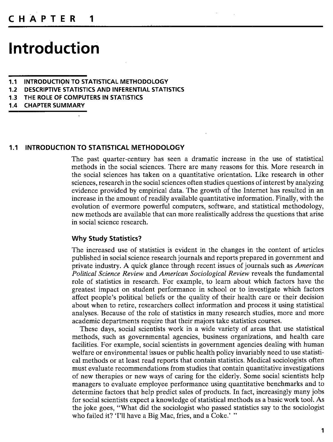
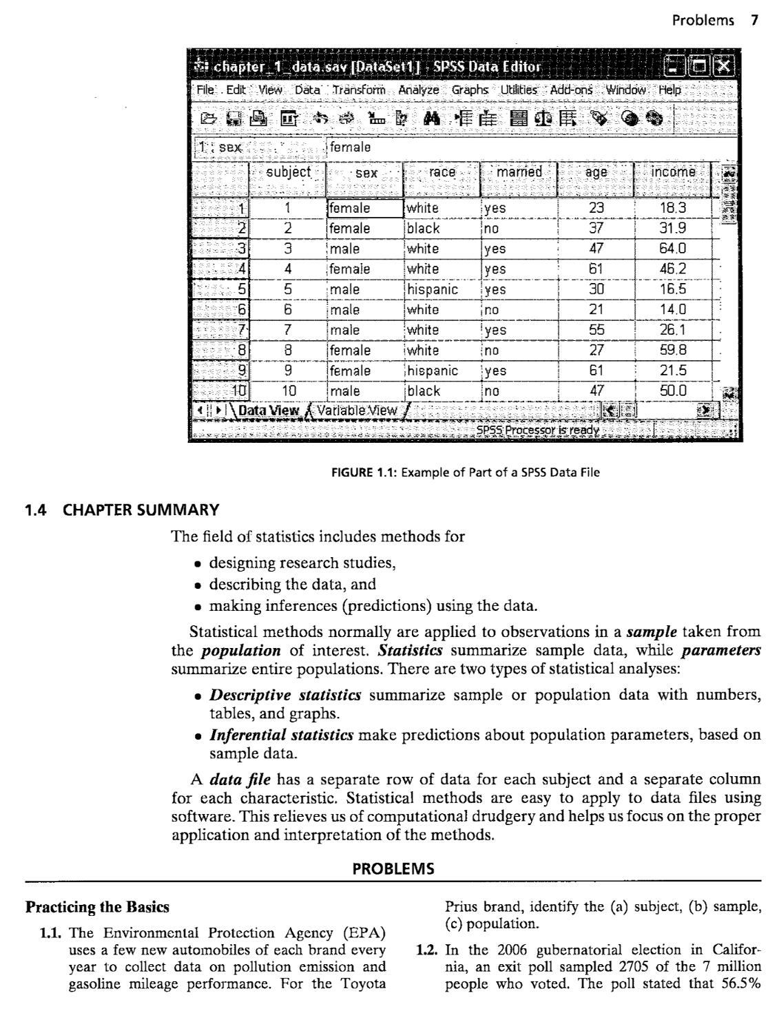
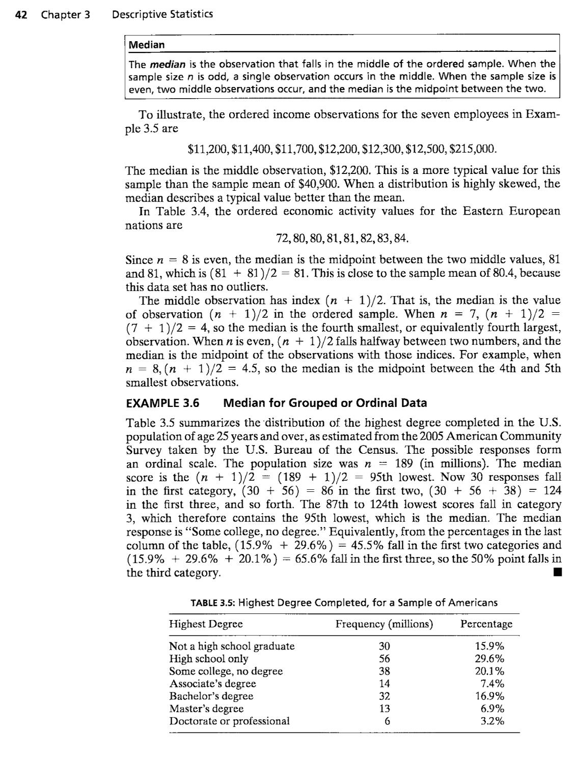
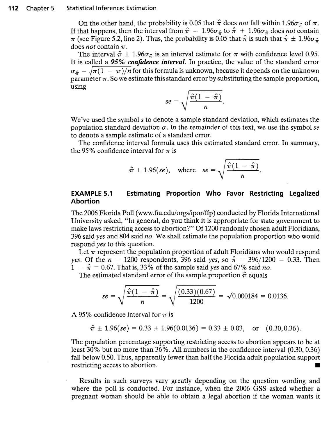
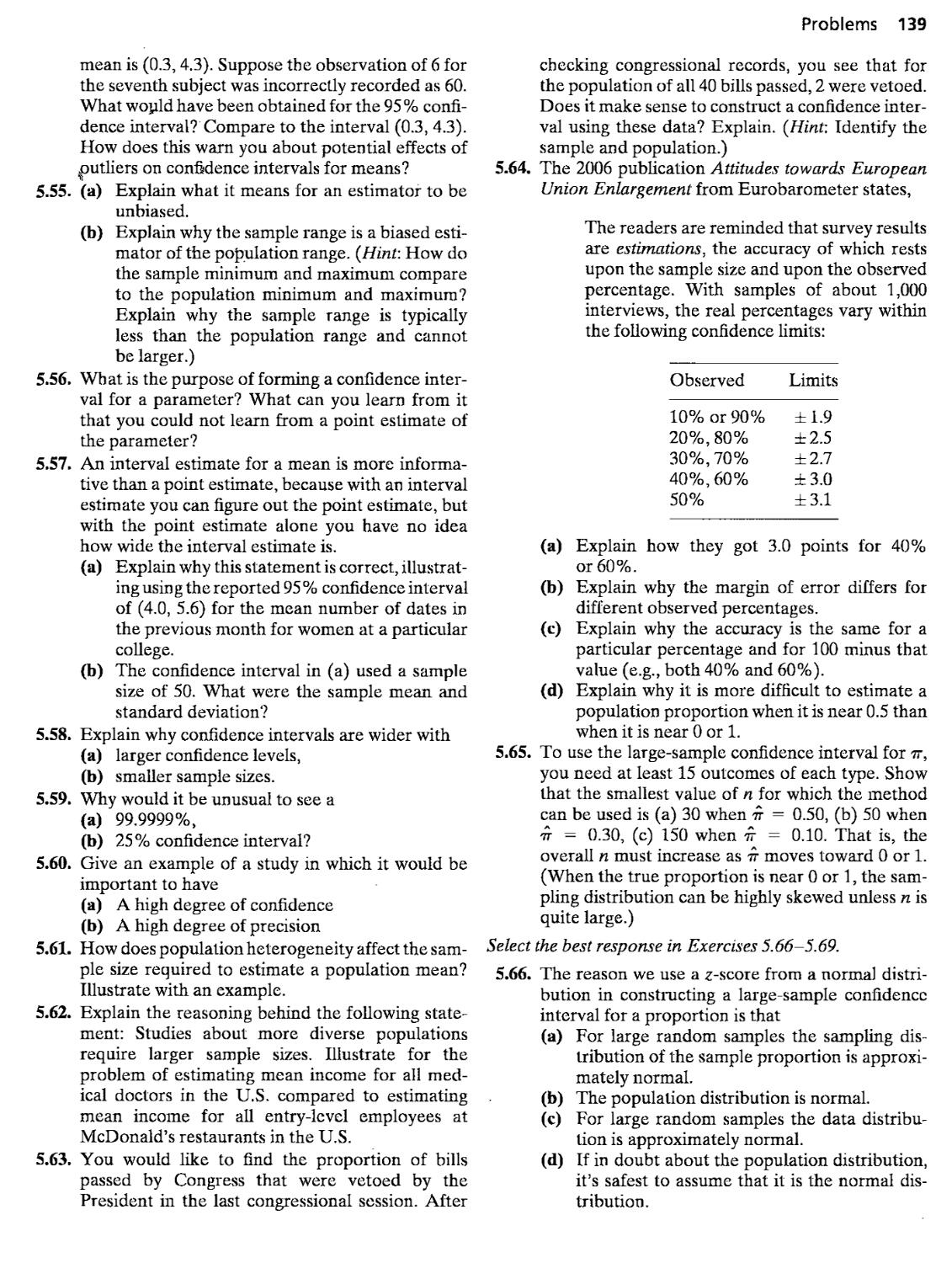
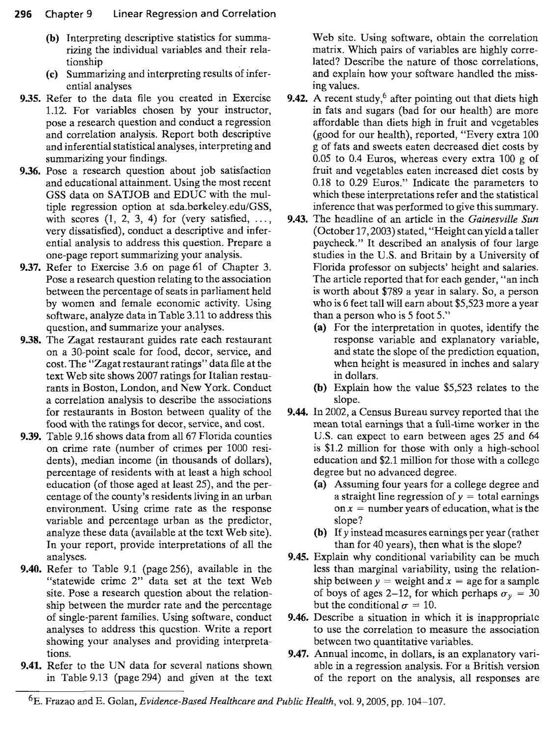
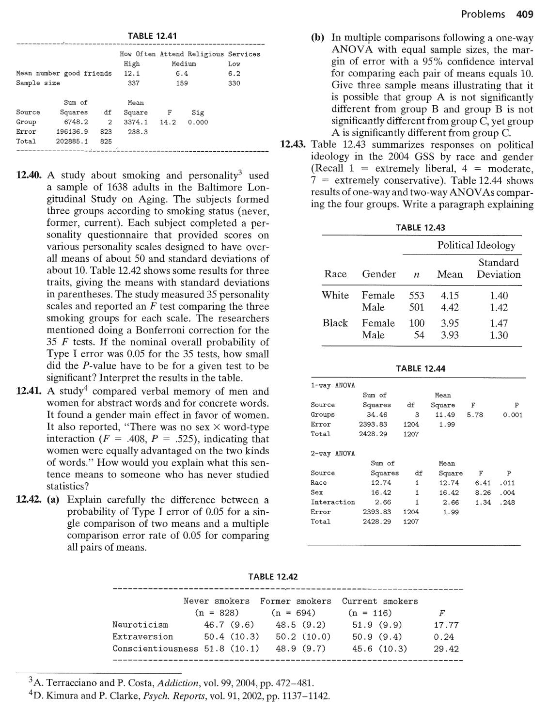
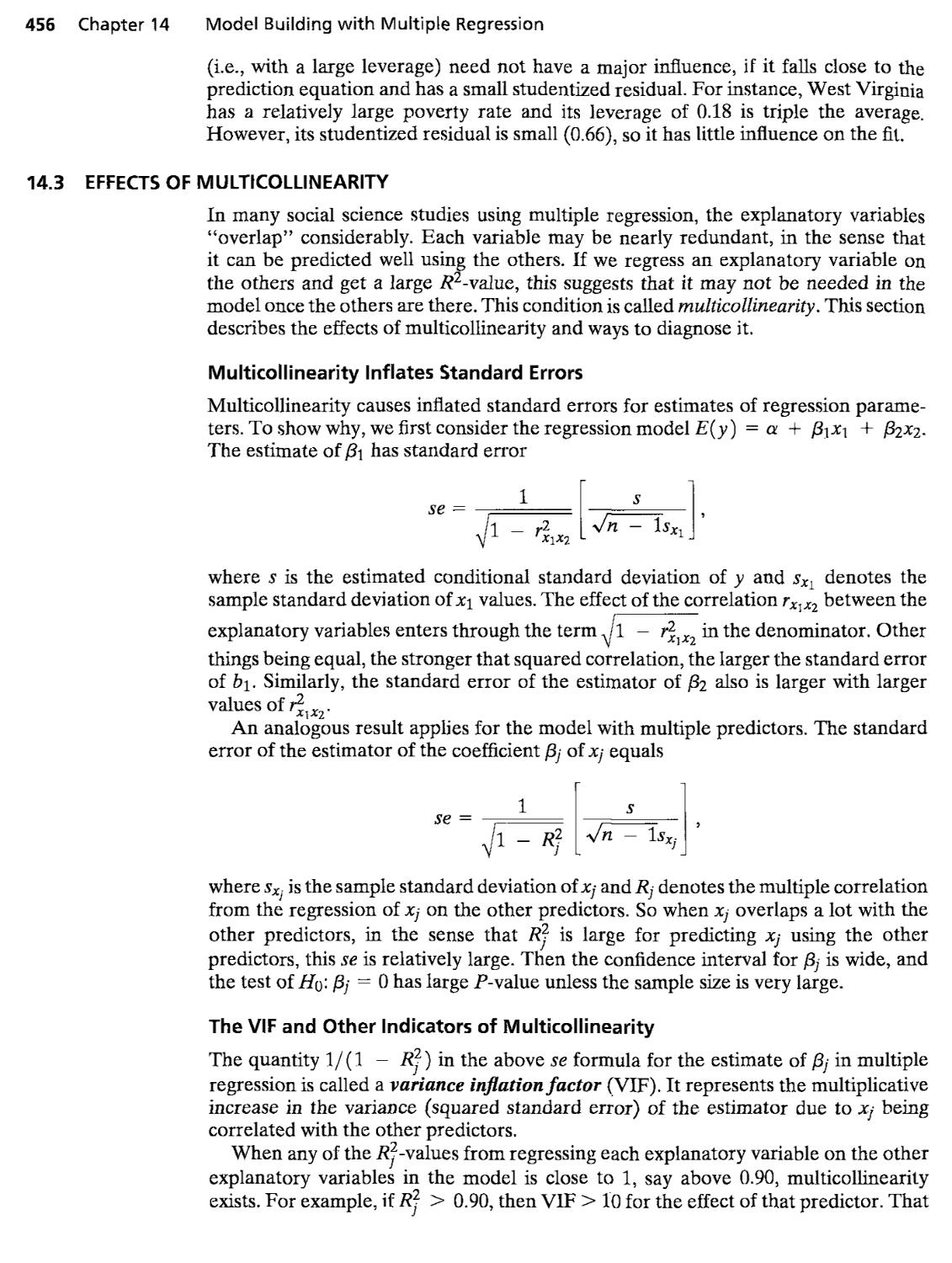
Figure 1.1 shows an example of data organized in a data file for analysis by statistical
software. A data file has the form of a spreadsheet:
• Any one row contains the observations for a particular subject in the sample.
• Any one column contains the observations for a particular characteristic.
Figure 1.1 is a window for editing data in SPSS. It shows data for the first ten
subjects in a sample, for the characteristics sex, racial group, marital status, age, and
annual income (in thousands of dollars). Some of the data are numerical, and some
consist of labels. Chapter 2 introduces the types of data for data files.
Uses and Misuses of Statistical Software
A note of caution: The easy access to statistical methods using software has dangers
as well as benefits. It is simple to apply inappropriate methods. A computer performs
the analysis requested whether or not the assumptions required for its proper use are
satisfied.
Incorrect analyses result when researchers take insufficient time to understand
the statistical method, the assumptions for its use, or its appropriateness for the
specific problem. It is vital to understand the method before using it. Just knowing
how to use statistical software does not guarantee a proper analysis. You'll need a
good background in statistics to understand which method to select, which options
to choose in that method, and how to make valid conclusions from the output. The
main purpose of this text is to give you this background.
Problems 7
|:|i}4i^;pfiQi3«g
File. Edit' View Data'
]^U'^-B---^
i:;sex.
;¦"¦¦¦"¦¦"¦
• '¦ 1
i 2
1- •:. • . -3
¦ -¦- ¦ .4
•6
)'¦.: :
... -8
'^¦"^
:¦•¦.. 10
• ¦ subject ;
1
2
TransFbrm Analyze Graph
female
sex- ¦ •
female
female
• race ¦ ¦'
white
black
3 imale white
4 ifemaie
5
6
7
8
9
10
male
male
white
hispanic
s Utiiities' '• Add-on^ . Window.' Help ¦
fe siteS-.^-%-^-|:'
¦ marrle'd ¦
yes
. ^. ' age' ' ;
Bjl^
'• Income -¦ ¦¦'^,
23 : 18.3
no 37
yes
yes
yes
white Ino
male white lyes
female iwhite jno
female jhispanic (yes
47
61
30
21
55
27
B1
male ibiack ino \ A7
..A L
31.9
64.0
46.2
16,5
14.0
26.1
59.8
21.5
50.0
<51; H \pata View J Variafble View/¦;.:. .;¦.;.•.¦.; ^: .¦:.:;.:: :::KI|
-^-4
..
;
i
:¦
^i
FIGURE 1.1: Example of Part of a SPSS Data File
1.4 CHAPTER SUMMARY
The field of statistics includes methods for
• designing research studies,
• describing the data, and
• making inferences (predictions) using the data.
Statistical methods normally are applied to observations in a sample taken from
the population of interest. Statistics summarize sample data, while parameters
summarize entire populations. There are two types of statistical analyses:
• Descriptive statistics summarize sample or population data with numbers,
tables, and graphs.
• Inferential statistics make predictions about population parameters, based on
sample data.
A data file has a separate row of data for each subject and a separate column
for each characteristic. Statistical methods are easy to apply to data files using
software. This relieves us of computational drudgery and helps us focus on the proper
application and interpretation of the methods.
PROBLEMS
Practicing the Basics
1.1. The Environmental Protection Agency (EPA)
uses a few new automobiles of each brand every
year to collect data on pollution emission and
gasoline mileage performance. For the Toyota
Prius brand, identify the (a) subject, (b) sample,
(c) population.
1.2. In the 2006 gubernatorial election in
California, an exit poll sampled 2705 of the 7 million
people who voted. The poll stated that 56.5%
8 Chapter 1 Introduction
reported voting for the Republican candidate,
Arnold Schwarzenegger. Of all, 7 million voters,
55.9% voted for Schwarzenegger.
(a) For this exit poll, what was the population and
what was the sample?
(b) Identify a statistic and a parameter.
1.3. The student government at the University of
Wisconsin conducts a study about alcohol abuse among
students. One hundred of the 40,858 members of
the student body are sampled and asked to
complete a questionnaire. One question asked is, "On
how many days in the past week did you consume
at least one alcoholic drink?"
(a) Identify the population of interest.
(b) For the 40,858 students, one characteristic
of interest was the percentage who would
respond zero to this question. This value is
computed for the 100 students sampled. Is it a
parameter or a statistic? Why?
1.4. The Institute for Public Opinion Research at
Florida International University has conducted
the FIU/Florida Poll (www.fiu.edu/orgs/ipor/ffp)
of about 1200 Floridians annually since 1988 to
track opinions on a wide variety of issues. The poll
reported in 2006 that 67% of Floridians believe that
state govermnent should not make laws restricting
access to abortion. Is 67% the value of a statistic,
or of a parameter? Why?
1.5. A GSS asked subjects whether astrology—the
study of star signs—has some scientific truth (GSS
question SCITEST3). Of 1245 sampled subjects,
651 responded definitely or probably true, and 594
responded definitely or probably not true. The
proportion responding definitely or probably true was
651/1245 = 0.523.
(a) Describe the population of interest.
(b) For what population parameter might we want
to make an inference?
(c) What sample statistic could be used in making
this inference?
(d) Does the value of the statistic in (c) necessarily
equal the parameter in (b)? Explain.
1.6. Go to the GSS Web site, sda.berkeley.edu/GSS/.
By entering TVHOURS as the Row variable, find
a summary of responses to the question, "On a
typical day, about how many hours do you personally
watch television?"
(a) What was the most common response?
(b) Is your answer in (a) a descriptive statistic, or
an inferential statistic?
1.7. Go to the GSS Web site, sda.berkeley.edu/GSS/.
By entering HEAVEN as the Row variable, you
can find the percentages of people who said
definitely yes, probably yes, probably not, and
definitely not when asked whether they believed
in heaven.
(a) Report the percentage who gave one of the
yes responses.
(b) To obtain data for a particular year such as
1998, enter YEARA998) in the Selection filter
option box before you chck on Run the Table.
Do this for HEAVEN in 1998, and report the
percentage who gave one of the yes responses.
(This question was asked only in 1991 and
1998.)
(c) Summarize opinions in 1998 about belief in
hell (variable HELL in the GSS). Was the
percentage of yes responses higher for HEAVEN
or HELL?
1.8. The Current Population Survey (CPS) is a monthly
survey of households conducted by the U.S.
Census Bureau. A CPS of 60,000 households indicated
that of those households, 8.1% of the whites,
22.3% of the blacks, 20.9% of the Hispanics, and
10.2% of the Asians had annual income below
the poverty level (Statistical Abstract of the United
States, 2006).
(a) Are these numbers statistics, or parameters?
Explain.
(b) A method from this text predicts that the
percentage of all black households in the United
States having income below the poverty level
is at least 21% but no greater than 24%.
What type of statistical method does this
illustrate-—-descriptive or inferential? Why?
1.9. A BBC story (September 9, 2004) about a poll in
35 countries concerning whether people favored
George W. Bush or John Kerry in the 2004 U.S.
Presidential election stated that Kerry was clearly
preferred. Of the sample from Germany, 74%
preferred Kerry, 10% preferred Bush, with the rest
undecided or not responding. Multiple choice: The
results for Germany are an example of
(a) descriptive statistics for a sample.
(b) inferential statistics about a population.
(c) a data file.
(d) a population.
1.10. Construct a data file describing the criminal
behavior of five inmates in a local prison. The
characteristics measured were race (with observations for the
five subjects: white, black, white, Hispanic, white),
age A9, 23, 38, 20, 41), length of sentence in years
B,1^0, 2, 5), whether convicted on a felony (no,
no, yes, no, yes), number of prior arrests (values 2,
0,8,1,5), mraiber of prior convictions A,0,3,1, 4).
Concepts and Applications
1.11. The "Student survey" data file at
www.stat.ufi.edu/^aa/social/data.html
Problems 9
shows responses of a class of social science graduate
students at the University of Florida to a
questionnaire that asked about GE ¦= gender, AG = age
in years, HI = high school GPA (on a four-
point scale), CO ^ college GPA, DH ~ distance
(in miles) of the campus from your home town,
DR = distance (in miles) of the classroom from
your current residence, NE = number of times
a week you read a newspaper, TV = average
number of hours per week that you watch TV,
SP = average number of hours per week that
you participate in sports or have other physical
exercise, VE = whether you are a vegetarian
(yes, no), AB = opinion about whether
abortion should be legal in" the first three months
of pregnancy (yes, no), PI = political
ideology A ^ very liberal, 2 ^ liberal, 3 = slightly
liberal, 4 = moderate, 5 ^ slightly
conservative, 6 ^ conservative, 7 = very conservative),
PA = political affiliation (D = Democrat, R =
Republican, I = independent), RE = how often
you attend religious services (never, occasionally,
most weeks, every week), LD = belief in life after
death (yes, no), AA = support affirmative action
(yes, no), AH = number of people you know
who have died from AIDS or who are HIV + .
You will use this data file for exercises in future
chapters.
(a) Practice accessing a data file for statistical
analysis with your software by going to this
Web site and copying this data file. Print a
copy of the data file. How many observations
(rows) are in the data file?
(b) Give an example of a question that could be
addressed using these data with (i) descriptive
statistics, (ii) inferential statistics.
1.12. Using a spreadsheet program (such as Microsoft
Office Excel) or statistical software, your instructor
will help the class create a data file consisting of
the values for class members of characteristics such
as those in the previous exercise. One exercise in
each chapter will use this data file.
(a) Copy the data file to your computer and print
a copy.
(b) Give an example of a question that you
could address by analyzing these data with (i)
descriptive statistics, (ii) inferential statistics.
1.13. For the statistical software your inst3"uctor has
chosen for your course, find out how to access the
software, enter data, and print any data files that
you create. Create a data file using the data in
Figure 1.1 in Section 1.3, and print it.
1.14. Illustrating with an example, explain the difference
between
(a) a statistic and a parameter.
(b) description and inference as two purposes for
using statistical methods.
1.15. You have data for a population, from a census.
Explain why descriptive statistics are helpful but
inferential statistics are not needed.
1.16. A sociologist wants to estimate the average age
at marriage for women in New England in the
early eighteenth century. She finds within her state
archives marriage records for a large Puritan village
for the years 1700-1730. She then takes a sample of
those records, noting the age of the bride for each.
The average age in the sample is 24.1 years. Using
a statistical method from Chapter 5, the sociologist
estimates the average age of brides at marriage for
the population to be between 23.5 and 24.7 years.
(a) What part of this example is descriptive?
(b) What part of this example is inferential?
(c) To what population does the inference refer?
1.17. In a recent survey by Eurobarometer of Europeans
about energy issues and global warming,^ one
question asked, "Would you be willing to pay more for
energy produced from renewable sources than for
energy produced from other sources?" The
percentage of yes responses varied among countries
between 10% (in Bulgaria) to 60% (in
Luxembourg). Of the 631 subjects interviewed in the UK,
45% said yes. It was predicted that for all 48 mil-
hon adults in the UK, that percentage who would
answer yes falls between 41 % and 49%. Identify in
this discussion (a) a statistic, (b) a parameter, (c) a
descriptive statistical analysis, (d) an inferential
statistical analysis.
1.18. Go to the Web site for the Gallup poll,
www.gaUuppoll.com. From information hsted on
or linked from the homepage, give an example of
a (a) descriptive statistical analysis, (b) inferential
statistical analysis.
1.19. Check whether you have access to JSTOR (Journal
Storage) at your school by visiting www.jstor.org. If
so, click on Browse and then Sociology or another
discipline of interest to you. Select a journal and a
particular issue, and browse through some of the
articles. Find an article that uses statistical
methods. In a paragraph of 100-200 words, explain how
descriptive statistics were used.
^Attitudes towards Energy, published January 2006 at eceuropa.eu/public opinion
CHAPTER2
Sampling and Measurement
2.1 VARIABLES AND THEIR MEASUREMENT
2.2 RANDOMIZATION
2.3 SAMPLING VARIABILITY AND POTENTIAL BIAS
2.4 OTHER PROBABILITY SAMPLING METHODS*
2.5 CHAPTER SUMMARY
To analyze social phenomena with a statistical analysis, descriptive methods
summarize the data and inferential methods use sample data to make predictions about
populations. In gathering data, we must decide which subjects to sample. Selecting a
sample that is representative of the population is a primary topic of this chapter.
Given a sample, we must convert our ideas about social phenomena into data
through deciding what to measure and how to measure it. Developing ways to
measure abstract concepts such as achievement, intelligence, and prejudice is one
of the most challenging aspects of social research. A measure should have validity,
describing what it is intended to measure and accurately reflecting the concept. It
should also have reliability, being consistent in the sense that a subject will give the
same response when asked again. Invahd or unreliable data-gathering instruments
render statistical manipulations of the data meaningless.
The first section of this chapter introduces definitions pertaining to measurement,
such as types of data. The other sections discuss ways, good and bad, of selecting the
sample.
2.1 VARIABLES AND THEIR MEASUREMENT
Statistical methods help us determine the factors that explain variability among
subjects. For instance, variation occurs from student to student in their college grade
point average (GPA). What is responsible for that variability? The way those students
vary in how much they study per week? in how much they watch TV per day? in their
IQ? in their college board score? in their high school GPA?
Variables
Any characteristic we can measure for each subject is called a variable. The name
reflects that values of the characteristic vary among subjects.
Variable
A variable is a characteristicthatcan vary in value among subjects in a sample or population.
Different subjects may have different values of a variable. Examples of variables
are income last year, number of siblings, whether employed, and gender. The values
the variable can take form the measurement scale. For gender, for instance, the
11
12 Chapter 2 Sampling and Measurement
measurement scale consists of the two labels, female and male. For number of siblings
it is 0,1, 2, 3,....
The valid statistical methods for a variable depend on its measurement scale. We
treat a numerical-valued variable such as annual income differently than a variable
with a measurement scale consisting of categories, such as (yes, no) for whether
employed. We next present ways to classify variables. The first type refers to whether
the measurement scale consists of categories or numbers. Another type refers to the
number of levels in that scale.
Quantitative and Categorical Variables
A variable is called quantitative when the measurement scale has numerical values.
The values represent different magnitudes of the variable. Examples of quantitative
variables are a subject's annual income, number of siblings, age, and number of years
of education completed.
A variable is called categorical when the measurement scale is a set of categories.
For example, marital status, with categories (single, married, divorced, widowed), is
categorical. For Canadians, the province of residence is categorical, with the
categories Alberta, British Columbia, and so on. Other categorical variables are whether
employed (yes, no), primary clothes shopping destination (localmall, local downtown,
Internet, other), favorite type of music (classical, country, folk, jazz, rock), religious
affiliation (Protestant, Catholic, Jewish, Muslim, other, none), and political party
preference.
For categorical variables, distinct categories differ in quality, not in numerical
magnitude. Categorical variables are often called qualitative. We distinguish between
categorical and quantitative variables because different statistical methods apply to
each type. Some methods apply to categorical variables and others apply to
quantitative variables. For example, the average is a statistical summary for a quantitative
variable, because it uses numerical values. It's possible to find the average for a
quantitative variable such as income, but not for a categorical variable such as religious
affiliation or favorite type of music.
Nominal, Ordinal, and Interval Scales of Measurement
For a quantitative variable, the possible numerical values are said to form an interval
scale. Interval scales have a specific numerical distance or interval between each
pair of levels. Annual income is usually measured on an interval scale. The interval
between $40,000 and $30,000, for instance, equals $10,000. We can compare outcomes
in terms of how much larger or how much smaller one is than the other.
Categorical variables have two types of scales. For the categorical variables
mentioned in the previous subsection, the categories are unordered. The scale does
not have a "high" or "low" end. The categories are then said to form a nominal scale.
For another example, a variable measuring primary mode of transportation to work
might use the nominal scale with categories (automobile, bus, subway, bicycle, walk).
Although the different categories are often called the levels of the scale, for a
nominal variable no level is greater than or smaller than any other level. Names
or labels such as "automobile" and "bus" for mode of transportation identify the
categories but do not represent different magnitudes. By contrast, each possible value
of a quantitative variable is greater than or less than any other possible value.
A third type of scale falls, in a sense, between nominal and interval. It
consists of categorical scales having a natural ordering of values. The levels form an
ordinal scale. Examples are social class (upper, middle, lower), political
philosophy (very liberal, slightly liberal, moderate, slightly conservative, very conservative).
Section 2.1 Variables and Their Measurement 13
government spending on the environment (too little, about right, too much), and
frequency of religious activity (never, less than once a month, about 1-3 times a
month, every week, more than once a week). These scales axe not nominal, because
the categories are ordered. They are not interval, because there is no defined distance
between levels. For example, a person categorized as very conservative is more
conservative than a person categorized as slightly conservative, but there is no numerical
value for how much more conservative that person is.
In summary, for ordinal variables the categories have a natural ordering, whereas
for nominal variables the categories are unordered. The scales refer to the actual
measurement and not to the phenomena themselves. Place of residence may indicate
a geographic place name such as a county (nominal), the distance of that place from a
point on the globe (interval), the size of the place (interval or ordinal), or other kinds
of variables.
Quantitative Aspects of Ordinal Data
As we've discussed, levels of nominal scales are quaUtative, varying in quality, not in
quantity. Levels of interval scales are quantitative, varying in magnitude. The position
of ordinal scales on the quantitative-qualitative classification is fuzzy. Because their
scale is a set of categories, they are often analyzed using the same methods as nominal
scales. But in many respects, ordinal scales more closely resemble interval scales.
They possess an important quantitative feature: Each level has a greater or smaller
magnitude than another level.
Some statistical methods apply specifically to ordinal variables. Often, though,
it's helpful to analyze ordinal scales by assigning numerical scores to categories.
By treating ordinal variables as interval rather than nominal, we can use the more
powerful methods available for quantitative variables.
For example, course grades (such as A, B, C, D, E) are ordinal. But we treat
them as interval when we assign numbers to the grades (such as 4, 3, 2, 1, 0) to
compute a grade point average. Treating ordinal variables as interval requires good
judgment in assigning scores. In doing this, you can conduct a "sensitivity analysis"
by checking whether conclusions would differ in any significant way for other choices
of the scores.
Discrete and Continuous Variables
One other way to classify a variable also helps determine which statistical methods
are appropriate for it. This classification refers to the number of values in the
measurement scale.
Discrete and Continuous Variables
A variable is discrete if its possible values form a set of separate numbers, sucli as 0, 1, 2,
3, .... It is corytinuous if it can take an infinite continuum of possible real number values.
Examples of discrete variables are the number of siblings and the number of visits
to a physician last year. Any variable phrased as "the number of ..." is discrete,
because it is possible to list its possible values {0,1,2,3,4,...}.
Examples of continuous variables are height, weight, and the amount of time it
takes to read a passage of a book. It is impossible to write down all the distinct
potential values, since they form an interval of infinitely many values. The amount of
time needed to read a book, for example, could take on the value 8.6294473... hours.
Discrete variables have a basic unit of measurement that cannot be subdivided.
For example, 2 and 3 are possible values for the number of sibfings, but 2.5716 is
14 Chapter 2 Sampling and Measurement
not. For a continuous variable, by contrast, between any two possible values there is
always another possible value. For example, age is continuous in the sense that an
individual does not age in discrete jumps. At some well-defined point during the year
in which you age from 21 to 22, you are 21.3851 years old, and similarly for every
other real number between 21 and 22. A continuous, infinite collection of age values
occurs between 21 and 22 alone.
Any variable with a finite number of possible values is discrete. All categorical
variables, nominal or ordinal, are discrete, having a finite set of categories.
Quantitative variables can be discrete or continuous; age is continuous, and number of siblings
is discrete.
For quantitative variables the distinction between discrete and continuous variables
can be blurry, because of how variables are actually measured. In practice, we round
continuous variables when measuring them, so the measurement is actually discrete.
We say that an individual is 21 years old whenever that person's age is somewhere
between 21 and 22. On the other hand, some variables, although discrete, have
a very large number of possible values. In measuring annual family income in
dollars, the potential values are 0, \, 2, 3, ..., up to some very large value in many
millions.
What's the implication of this? Statistical methods for discrete variables are mainly
used for quantitative variables that take relatively few values, such as the number
of times a person has been married. Statistical methods for continuous variables are
used for quantitative variables that can take lots of values, regardless of whether they
are theoretically continuous or discrete. For example, statisticians treat variables such
as age, income, and 10 as continuous.
In summary,
• Variables are either quantitative (numerical valued) or categorical.
Quantitative variables are measured on an interval scale. Categorical variables with
unordered categories have a nominal scale, and categorical variables with
ordered categories have an ordinal scale.
• Categorical variables (nominal or ordinal) are discrete. Quantitative variables
can be either discrete or continuous. In practice, quantitative variables that can
take lots of values are treated as continuous.
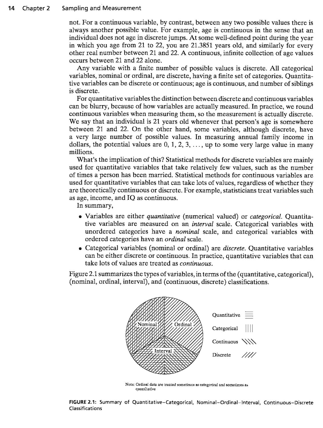
Figure 2.1 summarizes the types of variables, in terms of the (quantitative, categorical),
(nominal, ordinal, interval), and (continuous, discrete) classifications.
Quantitative =^
Categorical 11 11
Continuous ^^^^
Discrete ///^
Note: Ordinal data are vreated sometimes as categorical and somelimes as
quantitative
FIGURE 2.1: Summary of Quantitative-Categorical, Nominai-Ordinal-lntervai, Continuous-Discrete
Classifications
Section 2.2 Randomization 15
2.2 RANDOMIZATION
Inferential statistical methods use sample statistics to make predictions about
population parameters. The quality of the inferences depends on how well the sample
represents the population. This section introduces an important sampling method
that incorporates randomization, the mechanism for achieving good sample
representation.
Simple Random Sampling
Subjects of a population to be sampled could be individuals, families, schools, cities,
hospitals, records of reported crimes, and so on. Simple random sampling is a method
of sampling for which every possible sample has equal chance of selection.
Let n denote the number of subjects in the sample, called the sample size.
Simple Random Sample
A simple random sample of n subjects from a population is one in which each possible
sample of that size has the same probability (chance) of being selected.
For instance, suppose a researcher administers a questionnaire to one randomly
selected adult in each of several households. A particular household contains four
adults—mother, father, aunt, and uncle—identified as M, F, A, and U. For a simple
random sample of n = 1 adult, each of the four adults is equally likely to be
interviewed. You could select one by placing the four names on four identical ballots
and selecting one blindly from a hat. For a simple random sample of n ^ 2 adults,
each possible sample of size two is equally likely. The six potential samples are (M, F),
(M, A), (M, U), (F, A), (F, U), and (A, U). To select the sample, you blindly select
two ballots from the hat.
A simple random sample is often just called a random sample. The simple adjective
is used to distinguish this type of sampling from more complex sampling schemes
presented in Section 2.4 that also have elements of randomization.
Why is it a good idea to use random sampling? Because everyone has the same
chance of inclusion in the sample, so it provides fairness. This reduces the chance that
the sample is seriously biased in some way, leading to inaccurate inferences about
the population. Most inferential statistical methods assume randomization of the sort
provided by random sampling.
How to Select a Simple Random Sample
To select a random sample, we need a Ust of all subjects in the population. This list is
called the sampling frame. Suppose you plan to sample students at your school. The
population is all students at the school. One possible sampling frame is the student
directory.
The most common method for selecting a random sample is to A) number the
subjects in the sampHng frame, B) generate a set of these numbers randomly, and C)
sample the subjects whose numbers were generated. Using random numbers to select
the sample ensures that each subject has an equal chance of selection.
Random Numbers
Random numbers are numbers that are computer generated according to a scheme
whereby each digit is equally likely to be any of the integers 0,1,2,..., 9 and does not
depend on the other digits generated.
16 Chapter 2 Sampling and Measurement
Line/Col.
TABLE 2.1: Part of a Table of Random Numbers
A)
B) C) D) E)
F)
G) (8)
10480 15011 01536 02011 81647 91646 69179 14194
22368 46573 25595 85393 30995 89198 27982 53402
24130 48360 22527 97265 76393 64809 15179 24830
42167 93093 06243 61680 07856 16376 39440 53537
37570 39975 81837 16656 06121 91782 60468 81305
77921 06907 11008 42751 27756 53498 18602 70659
Source: Abridged from William H. Beyer, ed.. Handbook of Tables for Probability
and Statistics, 2nd ed., © The Chemical Rubber Co., 1968. Used by permission of the
Chemical Rubber Co.
Table 2.1 shows a table containing random numbers. The numbers fluctuate
according to no set pattern. Any particular number has the same chance of being
a 0, 1, 2, ..., or 9. The numbers are chosen independently, so any one digit chosen
has no influence on any other selection. If the flrst digit in a row of the table is a
9, for instance, the next digit is still just as likely to be a 9 as a 0 or 1 or any other
number. Random numbers are available in published tables and can be generated
with software and many statistical calculators.
Suppose you want to select a simple random sample oin = 100 students from a
university student body of size 30,000. The sampling frame is a directory of these
students. Select the students by using five-digit sequences to identify them, as follows:
1. Assign the numbers 00001 to 30000 to the students in the directory, using 00001
for the first student in the list, 00002 for the second student, and so on.
2. Starting at any point in the random number table, or by generating random
numbers using software or a calculator, choose successive five-digit numbers
until you obtain 100 distinct numbers between 00001 and 30000.
3. Include in the sample the students with assigned numbers equal to the random
numbers selected.
For example, for the first column of five-digit numbers in Table 2.1, the first three
random numbers are 10480, 22368, and 24130. The first three students selected are
those numbered 10480, 22368, and 24130.
In selecting the 100 five-digit numbers, skip numbers greater than 30000, such as
the next three five-digit numbers in Table 2.1, since no student in the directory has an
assigned number that large. After using the first column of five-digit numbers, move
to the next column of numbers and continue. If the population size were between
1000 and 9999, you would use four digits at a time. The colunm (or row) from which
you begin selecting the numbers does not matter, since the numbers have no set
pattern. Most statistical software can do this all for you.
Collecting Data with Sample Surveys
Many studies select a sample of people from a population and interview them to collect
data. This method of data collection is called a sample survey. The interview could
be a personal interview, telephone interview, or self-administered questionnaire.
The General Social Survey (GSS) is an example of a sample survey. It gathers
information using personal interviews of a random sample of subjects from the U.S.
adult population to provide a snapshot of that population. (The survey does not
use simple random sampling but rather a method discussed later in the chapter that
Section 2.2 Randomization 17
incorporates multiple stages and clustering but is designed to give each family the
same chance of inclusion.) National polls such as the Gallup Poll are also sample
surveys. They usually use telephone interviews. Since it is often difficult to obtain
a sampling frame, many telephone interviews obtain the sample with random digit
dialing.
A variety of problems can cause responses from a sample survey to tend to
favor some parts of the population over others. Then results from the sample
are not representative of the population. We'll discuss some potential problems in
Section 2.3.
Collecting Data with an Experiment
In some studies, data result from a planned experiment. The purpose of most
experiments is to compare responses of subjects on some outcome measure, under
different conditions. Those conditions are levels of a variable that can influence the
outcome. The scientist has the experimental control of being able to assign subjects
to the conditions.
For instance, the conditions might be different drugs for treating some illness. The
conditions are called treatments. To conduct the experiment, the researcher needs
a plan for assigning subjects to the treatments. These plans are called experimental
designs. Good experimental designs use randomization to determine which treatment
a subject receives.
In the late 1980s, the Physicians' Health Study Research Group at Harvard Medical
School designed an experiment to analyze whether regular intake of aspirin reduces
mortahty from heart disease. Of about 22,000 male physicians, half were randomly
chosen to take an aspirin every other day. The remaining half took a placebo, which
had no active agent. After five years, rates of heart attack were compared. By using
randomization to determine who received which treatment, the researchers knew
the groups would roughly balance on factors that could affect heart attack rates,
such as age and quality of health. If the physicians could decide on their own which
treatment to take, the groups might have been out of balance on some important
factor. Suppose, for instance, younger physicians were more likely to select aspirin.
Then, a lower heart attack rate among the aspirin group could occur merely because
younger subjects are less likely to suffer heart attacks.
Collecting Data with an Observational Study
In social research, it is rarely possible to conduct experiments. It's not possible to
randomly assign subjects to the groups we want to compare, such as levels of gender or
race or educational level or annual income. Many studies merely observe the outcomes
for available subjects on the variables without any experimental manipulation of the
subjects. Such studies are called observational studies. The researcher measures
subjects' responses on the variables of interest but has no experimental control over
the subjects.
With observational studies, comparing groups is difficult because the groups may
be imbalanced on variables that affect the outcome. This is true even with random
sampling. For instance, suppose we plan to compare black students, Hispanic students,
and white students on some standardized test. If white students have a higher average
score, a variety of variables might account for that difference, such as parents'
education or parents' income or quality of school attended. This makes it difficult to
compare groups with observational studies, especially when some key variables may
not have been measured in the study.
18 Chapter 2 Sampling and Measurement
Establishing cause and effect is central to science. But it's not possible to establish
cause and effect definitively with a nonexperiniental study, whether it be an
observational study with an available sample or a sample survey using random sampling.
With an observational study, there's the strong possibility that the sample does not
well reflect the population. With an observational study or a sample survey, there's
always the possibility that some unmeasured variable could be responsible for
patterns observed in the data. With an experiment that randomly assigns subjects to
treatments, those treatments should roughly balance on any unmeasured variables.
For example, in the heart attack study mentioned above, the doctors taking aspirin
would not tend to be younger or of better health than the doctors taking placebo.
Because a randomized experiment balances the groups being compared on other
factors, it's possible to study cause and effect more accurately with an experiment
than with an observational study.
Whether or not a study is experimental, it's important to incorporate randomization
in any study that plans to make inferences. This randomization could take the form of
randomly selecting a sample for a survey, or randomly allocating subjects to different
treatments for an experimental study.
2.3 SAMPLING VARIABILITY AND POTENTIAL BIAS
Even if a study wisely uses randomization, the results of the study still depend
on which subjects are sampled. Two researchers who separately select random
samples from some population may have little overlap, if any, between the two
sample memberships. Therefore, the values of sample statistics will differ for the two
samples, and the results of analyses based on these samples may differ.
Sampling Error
Suppose the Gallup, Harris, Zogby, and Pew polling organizations each randomly
sample 1000 adult Canadians, in order to estimate the percentage of Canadians
who give the prime minister's performance in office a favorable rating. Based on
the samples they select, perhaps Gallup reports an approval rating of 63%, Harris
reports 68%, Zogby 65%, and Pew 64%. These differences could reflect slightly
different question wording. But even if the questions are worded exactly the same,
the percentages would probably differ somewhat because the samples are different.
For conclusions based on statistical inference to be worthwhile, we should know
the potential sampling error—-how much the statistic differs from the parameter it
predicts because of the way results naturally exhibit variation from sample to sample.
Sampling Error
The sampling error of a statistic equals the error that occurs when we use a statistic based
on a sample to predict the value of a population parameter.
Suppose that the actual percentage of the population of adult Canadians who give
the prime minister a favorable rating is 66%. Then the Gallup organization, which
predicted 63%, had a sampling error of 63% - 66% = —3%. The Harris organization,
which predicted 68%, had a sampling error of 68% - 66% = 2%. In practice, the
sampling error is unknown, because the values of population parameters are unknown.
Random sampling protects against bias, in the sense that the sampling error tends
to fluctuate about 0, sometimes being positive (as in the Harris poll) and sometimes
being negative (as in the Gallup poll). Random sampling also allows us to predict
the likely size of the sampling error. For sample sizes of about 1000, we'll see that
Section 2.3 Sampling Variability and Potential Bias 19
the sampling error for estimating percentages is usually no greater than plus or
minus 3%. This bound is the margin of error. Variability also occurs in the values of
sample statistics with nonrandom sampling, but the extent of the sampling error is
not predictable as it is with random samples.
Sampling Bias: Nonprobability Sampling
Other factors besides sampling error can cause results to vary from sample to sample.
These factors can also possibly cause bias. We next discuss three types of bias. The
first is called sampling bias.
For simple random sampling, each possible sample of n subjects has the same
probability of selection. This is a type of probability sampling method, meaning that
the probability any particular sample will be selected is known. Inferential statistical
methods assume probability sampling. Nonprobability sampling methods are ones
for which it is not possible to determine the probabilities of the possible samples.
Inferences using such samples have unknown rehability and result in sampling bias.
The most common nonprobabihty sampling method is volunteer sampling. As the
name implies, subjects volunteer to be in the sample. But the sample may poorly
represent the population and yield misleading conclusions. For instance, a mail-in
questionnaire published in TV Guide posed the question, "Should the President have
the Line Item Veto to eliminate waste?" Of those who responded, 97% said yes. For
the same question posed to a random sample, 71% said yes.^
Examples of volunteer sampling are visible any day on many Internet sites and
television news programs. Viewers register their opinions on an issue by voting over
the Internet. The viewers who respond are unlikely to be a representative cross section,
but will be those who can easily access the Internet and who feel strongly enough to
respond. Individuals having a particular opinion might be much more likely to respond
than individuals having a different opinion. For example, one night the ABC program
Nightline asked viewers whether the United Nations should continue to be located
in the United States. Of more than 186,000 respondents, 67% wanted the United
Nations out of the United States. At the same time, a poll using a random sample of
about 500 respondents estimated the population percentage to be about 28%. Even
though the random sample had a much smaller size, it is far more trustworthy.
A large sample does not help with volunteer sampling—the bias remains. In
1936, the newsweekly Literary Digest sent over 10 million questionnaires in the mail
to predict the outcome of the presidential election. The questionnaires went to a
relatively wealthy segment of society (those having autos or telephones), and fewer
than 25% were returned. The journal used these to predict an overwhelming victory
by Alfred Landon over Franklin Roosevelt. The opposite result was predicted by
George Gallup with a much smaller sample in the first scientific poll taken for this
purpose. In fact, Roosevelt won in a landslide.
Unfortunately, volunteer samphng is sometimes necessary. This is often true in
medical studies. Suppose a study plans to investigate how weh a new drug performs
compared to a standard drug, for subjects who suffer from high blood pressure. The
researchers are not going to be able to find a sampling frame of all who suffer from
high blood pressure and take a simple random sample of them. They may, however,
be able to sample such subjects at certain medical centers or using volunteers. Even
then, randomization should be used wherever possible. For the study patients, they
can randomly select who receives the new drug and who receives the standard one.
-'^D. M. Wilbur, Public Perspective, available at roperweb.ropercenter.uconn.edu. May-June
1993.
20 Chapter 2 Sampling and Measurement
Even with random sampling, sampling bias can occur. One case is when the
sampling frame suffers from undercoverage: It lacks representation from some
groups in the population. A telephone survey will not reach prison inmates or
homeless people or people too poor to afford a telephone, whereas famihes that
have many phones will tend to be over-represented. Responses by those not having
a telephone might tend to be quite different from those actually sampled, leading to
biased results.
Response Bias
In a survey, the way a question is worded or asked can have a large impact on the
results. For example, when a New York Times/CBS News poll in 2006 asked whether
the interviewee would be in favor of a new gasoline tax, only 12% said yes. When
the tax was presented as reducing U.S. dependence on foreign oil, 55% said yes, and
when asked about a gas tax that would help reduce global warming, 59% said yes.^
Poorly worded or confusing questions result in response bias. Even the order in
which questions are asked can influence the results dramatically. During the Cold
War, a study asked, "Do you think the U.S. should let Russian newspaper reporters
come here and send back whatever they want?" and "Do you think Russia should
let American newspaper reporters come in and send back whatever they want?" The
percentage of yes responses to the first question was 36% when it was asked first and
73% when it was asked second.^
In an interview, characteristics of the interviewer may result in response bias.
Respondents might lie if they think their belief is socially unacceptable. They may be
more likely to give the answer that they think the interviewer prefers. An example
is provided by a study on the effect of the interviewer's race. Following a phone
interview, respondents were asked whether they thought the interviewer was black
or white (all were actually black). Perceiving a white interviewer resulted in more
conservative opinions. For example, 14% agreed that "American society is fair to
everyone" when they thought the interviewer was black, but 31% agreed to this when
they thought the interviewer was white."^
Nonresponse Bias: Missing Data
Some subjects who are supposed to be in the sample may refuse to participate, or
it may not be possible to reach them. This results in the problem of nonresponse
bias. If only half the intended sample was actually observed, we should worry about
whether the half not observed differ from those observed in a way that causes biased
results. Even if we select the sample randomly, the results are questionnable if there
is substantial nonresponse, say, over 20%.
For her book Women in Love, author Shere Hite surveyed women in the United
States. One of her conclusions was that 70% of women who had been married at
least five years have extramarital affairs. She based this conclusion on responses
to questionnaires returned by 4500 women. This sounds like an impressively large
sample. However, the questionnaire was mailed to about 100,000 women. We cannot
know whether the 4.5% of the women who responded were representative of
the 100,000 who received the questionnaire, much less the entire population of
American women. This makes it dangerous to make an inference to the larger
population.
^Column by T. Friedman, New York Times, March 2, 2006.
^See Crosson A994).
^Washington Post, June 26,1995.
Section 2.4 Other Probability Sampling Methods* 21
Missing data is a problem in almost all large studies. Some subjects do not provide
responses for some of the variables measured. Even in censuses, which are designed
to observe everyone in a country, some people are not observed or fail to cooperate.
Most software ignores cases for which observations are missing for at least one
variable used in an analysis. This results in wasted information and possible bias.
Statisticians have recently developed methods that replace missing observations by
predicted values based on patterns in the data. See Allison B002) for an introduction
to ways of dealing with missing data.
Summary of Types of Bias
In summary, sample surveys have potential sources of bias:
• Sampling bias occurs from using nonprobability samples or having undercov-
erage.
• Response bias occurs when the subject gives an incorrect response (perhaps
lying), or the question wording or the way the interviewer asks the questions is
confusing or misleading.
• Nonresponse bias occurs when some sampled subjects cannot be reached or
refuse to participate or fail to answer some questions.
In any study, carefully assess the scope of conclusions. Evaluate critically the
conclusions by noting the makeup of the sample. How was the sample selected? How
large was it? How were the questions worded? Who sponsored and conducted the
research? The less information that is available, the less you should trust it.
Finally, be wary of any study that makes inferences to a broader population than
is justified by the sample chosen. Suppose a psychologist performs an experiment
using a random sample of students from an introductory psychology course. With
statistical inference, the sample results generalize to the population of all students in
the class. For the results to be of wider interest, the psychologist might claim that the
conclusions extend to all college students, to all young adults, or even to all adults.
These generalizations may well be wrong, because the sample may differ from those
populations in fundamental ways, such as in average age or socioeconomic status.
2.4 OTHER PROBABILITY SAMPLING METHODS*
Section 2.2 introduced simple random sampling and explained its importance to
statistical inference. In practice, other probability sampling methods that have elements
of randomness are sometimes preferable to simple random sampling or are simpler
to obtain.
Systematic Random Sampling
Systematic random sampling selects a subject near the beginning of the sampHng
frame list, skips several names and selects another subject, skips several more names
and selects the next subject, and so forth. The number of names skipped at each stage
depends on the desired sample size. Here's how it's done:
Systematic Random Sample
Denote the sample size by n and the population size by N. Let k = N/n, the population size
divided by the sample size. A systematic random sample A) selects a subject at random
from the first k names in the sampling frame, and B) selects every ^h subject listed after
that one. The number k is called the skip number.
22 Chapter 2 Sampling and Measurement
Suppose you want a systematic random sample of 100 students from a population
of 30,000 students listed in a campus directory. Then, n = 100 and A^ = 30,000,
so k = 30,000/100 = 300. The population size is 300 times the sample size, so
you need to select one of every 300 students. You select one student at random,
using random numbers, from the first 300 students in the directory. Then you
select every 300th student after the one selected randomly. This produces a sample
of size 100. The first three digits in Table 2.1 are 104, which falls between 001
and 300, so you first select the student numbered 104. The numbers of the other
students selected are 104 + 300 = 404, 404 + 300 = 704, 704 + 300 = 1004,
1004 + 300 = 1304, and so on. The 100th student selected is Hsted in the last
300 names in the directory.
In sampling from a sampling frame, it's simpler to select a systematic random
sample than a simple random sample because it uses only one random number. This
method typically provides as good a representation of the population, because for
alphabetic listings such as directories of names, values of most variables fluctuate
randomly through the list. With this method, statistical formulas based on simple
random sampling are usually valid.
A systematic random sample is not a simple random sample, because all samples
of size n are not equally likely. For instance, unlike in a simple random sample, two
subjects listed next to each other on the hst cannot both appear in the sample.
Stratified Random Sampling
Another probability sampling method, useful in social science research for studies
comparing groups, is stratified sampling.
Stratified Random Sample
A stratified random sample 6mdes the population into separate groups, called strata, and
tlien selects a simple random sample from each stratum.
Suppose a study in Cambridge, Massachusetts plans to compare the opinions
of registered Democrats and registered Republicans about whether government
should guarantee health care to aU citizens. Stratifying according to pohtical party
registration, the study selects a random sample of Democrats and another random
sample of Republicans.
Stratified random sampling is called proportional if the sampled strata proportions
are the same as those in the entire population. For example, if 90% of the population
of interest is Democrat and 10% is Republican, then the sampling is proportional if
the sample size for Democrats is nine times the sample size for Republicans.
Stratified random sampHng is called disproportional if the sampled strata
proportions differ from the population proportions. This is useful when the population size
for a stratum is relatively small. A group that comprises a smaU part of the population
may not have enough representation in a simple random sample to allow precise
inferences. It is not possible to compare accurately Democrats to Republicans, for
example, if only 10 people in a sample size of 100 are Republican. By contrast, a
disproportional stratified sample size of 100 might randomly sample 50 Democrats
and 50 Republicans.
To implement stratification, we must know the stratum into which each subject
in the sampling frame belongs. This usually restricts the variables that can be used
for forming the strata. The variables must have strata that are easily identifiable.
For example, it would be easy to select a stratified sample of a school population
Section 2.4 Other Probability Sampling Methods* 23
using grade level as the stratification variable, but it would be difficult to prepare an
adequate sampling frame of city households stratified by household income.
Cluster Sampling
Simple, systematic, and stratified random sampling are often difficult to implement,
because they require a complete sampling frame. Such lists are easy to obtain for
sampling cities or hospitals or schools, for example, but more difficult for sampling
individuals or famihes. Cluster sampling is useful when a complete listing of the
population is not available.
Cluster Random Sample
Divide the population into a large number of dusters, such as city blocks. Select a simple
random sample of the clusters. Use the subjects in those clusters as the sample.
For example, a study might plan to sample about 1% of the families in a city, using
city blocks as clusters. Using a map to identify city blocks, it could select a simple
random sample of 1% of the blocks and then sample every family on each block.
A study of patient care in mental hospitals in Ontario could first randomly sample
mental hospitals (the clusters) and then collect data for patients within those hospitals.
What's the difference between a stratified sample and a cluster sample? A stratified
sample uses every stratum. The strata are usually groups we want to compare. By
contrast, a cluster sample uses a sample of the clusters, rather than all of them. In
cluster sampling, clusters are merely ways of easily identifying groups of subjects. The
goal is not to compare the clusters but rather to use them to obtain a sample. Most
clusters are not represented in the eventual sample.
Figure 2.2 illustrates the distinction among sampling subjects (simple random
sample), sampling clusters of subjects (cluster random sample), and sampling subjects
from within strata (stratified random sample). The figure depicts ways to survey 40
students at a school, to make comparisons among Freshmen, Sophomores, Juniors,
and Seniors.
Multistage Sampling
When conducting a survey for predicting elections, the Gallup Organization often
identifies election districts as clusters and takes a simple random sample of them. But
then it also takes a simple random sample of households within each selected election
Simple Random
Cluster
Stratified
, •¦' • •
.¦¦¦•¦ . • ..•¦..
. ; -¦ ¦ ¦¦ ¦¦ ¦¦• •¦•.:•:
¦? • •• •.
¦ ¦•'....¦.'•, ' ¦•
'-¦'¦ ¦''¦¦)':-'i''-.--
' 'm ¦¦ m ¦ ¦ ¦ m ¦
¦ • • • : . .
• ¦ ¦ • • *
Fresh. Soph. Jnr. Snr.
FIGURE 2.2: Ways of Randomly Sampling 40 Students. The figure is a schematic for a simple random
sample, a cluster random sample of 8 clusters of students who live together, and a stratified random
sample of 10 students from each class (Fr, So, Ju, Sr).
24 Chapter 2 Sampling and Measurement
district. This is more feasible than sampling every household in the chosen districts.
This is an example of multistage sampling, which uses combinations of sampUng
methods.
Here's an example of a multistage sample:
• Treat counties (or census tracts) as clusters and select a random sample of a
certain number of them.
• Within each county selected, take a cluster random sample of square-block
regions.
• Within each region selected, take a systematic random sample of every tenth
house.
• Within each house selected, select one adult at random for the sample.
Multistage samples are common in social science research. They are simpler to
implement than simple random sampling but provide a broader sampling of the
population than a single method such as cluster sampling.
For statistical inference, stratified samples, cluster samples, and multistage samples
use different formulas from the ones in this book. Cluster sampling requires a
larger sample to achieve as much inferential precision as simple random sampling.
Observations within clusters tend to be similar, because of the tendency of subjects
living near one another to have similar values on opinion issues and on economic
and demographic variables such as age, income, race, and occupation. So we need
more data to obtain a representative cross section. By contrast, the results for
stratified sampling may be more precise than those stated in this textbook for simple
random sampling. Books specializing in sampling methodology provide further details
(Scheaffer et al, 2005; Thompson, 2002).
2.5 CHAPTER SUMMARY
Statistical methods analyze data on variables, which are characteristics that vary
among subjects. The statistical methods used depend on the type of variable:
• Numerically measured variables, such as family income and number of children
in a family, are quantitative. They are measured on an interval scale.
• Variables taking value in a set of categories are categorical. Those measured
with unordered categories, such as religious affiliation and province of residence,
have a nominal scale. Those measured with ordered categories, such as social
class and political ideology, have an ordinal scale of measurement.
• Variables are also classified as discrete, having possible values that are a set
of separate numbers (such as 0, 1, 2, ...), or continuous, having a continuous,
infinite set of possible values. Categorical variables, whether nominal or ordinal,
are discrete. Quantitative variables can be of either type, but in practice are
treated as continuous if they can take a large number of values.
Much social science research uses observational studies, which use available
subjects to observe variables of interest. One should be cautious in attempting to conduct
inferential analyses with data from such studies. Inferential statistical methods require
probability samples, which incorporate randomization in some way. Random
sampling allows control over the amount of sampling error, which describes how results
can vary from sample to sample. Random samples are much more likely to be
representative of the population than are nonprobability samples such as volunteer samples.
• For a simple random sample, every possible sample of size n has the same
chance of selection.
Problems 25
• Here are other examples of probability sampling: Systematic random sampling
takes every /cth subject in the sampling frame list. Stratified random sampUng
divides the population into groups (strata) and takes a random sample from
each stratum. Cluster random sampling takes a random sample of clusters of
subjects (such as city blocks) and uses subjects in those clusters as the sample.
Multistage sampling uses combinations of these methods.
Chapter 3 introduces statistics for describing samples and corresponding
parameters for describing populations. Hence, its focus is on descriptive statistics.
PROBLEMS
Practicing the Basics
2.1. Explain the difference between
(a) Discrete and continuous variables
(b) Categorical and quantitative variables
(c) Nominal and ordinal variables
Why do these distinctions matter for statistical
analysis?
2.2. Identify each variable as categorical or
quantitative:
(a) Number of pets in family
(b) County of residence
(c) Choice of auto (domestic or import)
(d) Distance (in miles) commute to work
(e) Choice of diet (vegetarian, nonvegetarian)
A) Time spent in previous month browsing the
World Wide Web
(g) Ownership of personal computer (yes, no)
(h) Number of people you have known with AIDS
@, 1,2, 3, 4 or more)
(i) Marriage form of a society (monogamy, polyg-
¦ yny, polyandry)
2.3. Which scale of measurement (nominal, ordinal, or
interval) is most appropriate for
(a) Attitude toward legalization of marijuana
(favor, neutral, oppose)
(b) Gender (male, female)
(c) Number of children in family @,1, 2,...)
(d) Political party affiHation (Democrat, RepubU-
can. Independent)
(e) Rehgious affiHation (Cathohc, Jewish,
Protestant, MusHm, other)
(f) Political philosophy (very liberal, somewhat
liberal, moderate, somewhat conservative,
very conservative)
(g) Years of school completed @,1,2,3,...)
(h) Highest degree attained (none, high school,
bachelor's, master's, doctorate)
(i) CoUege major (education, anthropology,
physics, sociology,...)
(i) Test score @-100 range for scores)
(k) Employment status (employed full time,
employed part time, unemployed)
2.4. Which scale of measurement is most appropriate
for
(a) Occupation (plumber, teacher, secretary,...)
(b) Occupational status (blue collar, white collar)
(c) Social status (lower, middle, upper class)
(d) Statewide murder rate (number of murders
per 1000 population)
(e) County population size (number of people)
(jF) Population growth rate (in percentages)
(g) Community size (rural, small town, large town,
small city, large city)
(h) Annual income (thousands of dollars peryear)
A) Attitude toward affirmative action (favorable,
neutral, unfavorable)
(j) Lifetime number of sexual partners
2.5. Which scale of measurement is most appropriate
for "attained education" measured as
(a) Number of years @,1, 2, 3,...)
(b) Grade level (elementary school, middle
school, high school, college, graduate school)
(c) School type (pubhc school, private school)
2.6. Give an example of a variable that is (a)
categorical, (b) quantitative, (c) ordinal scale, (d) nominal
scale, (e) discrete, (f) contmuous, (g) quantitative
and discrete.
2.7. A poll conducted by YouGov for the British
newspaper The Daily Telegraph in June 2006 asked a
random sample of 1962 British adults several
questions about their image of the U.S. One question
asked, "How would you rate George W. Bush as
a world leader?" The possible choices were (great
leader, reasonably satisfactory leader, pretty poor
leader, terrible leader),
(a) Is this four-category variable nominal, or
ordinal? Why?
(b) Is this variable continuous, or discrete? Why?
(c) Of the 93% of the sample who responded,
the percentages in the four categories were
1% (great leader), 16%, 37%, 46% (terrible
leader). Are these values statistics, or
parameters? Why?
2.8. A survey asks subjects to rate five issues according
to their importance in determining voting intention
26 Chapter 2 Sampling and Measurement
for U.S. senator, using the scale (very important,
somewhat important, unimportant). The issues are
foreign policy, unemployment, inflation, the arms
race, and civil rights. The evaluations can be treated
as five variables: foreign policy evaluation,
unemployment evaluation, and so on. These variables
represent what scale of measurement?
2.9. Which of the following variables could
theoretically be measured on a continuous scale? (a)
Method of contraception used, (b) length of tune of
residence in a state, (c) task completion time, (d)
mtelligence, (e) authoritarianism, (f) alienation,
(g) county of residence.
2.10. Which of the following variables are continuous
when the measurements are as fine as possible?
(a) Age of mother, (b) number of children in
family, (c) income of spouse, (d) population of cities,
(e) latitude and longitude of cities, (f) distance of
home from place of employment, (g) number of
foreign languages spoken.
2.11. A class has 50 students. Use the column of the first
two digits in the random number table (Table 2.1)
to select a simple random sample of three students.
If the students are numbered Ol to 50, what are the
numbers of the three students selected?
2.12. A local telephone directory has 400 pages with 130
names per page, a total of 52,000 names. Explain
how you could choose a simple random sample of
5 names. Using the second column of Table 2.1 or
software or a calculator, select 5 random numbers
to identify subjects for the sample.
2.13. Explain whether an experiment or an
observational study would be more appropriate to
investigate the following:
(a) Whether or not cities with higher
unemployment rates tend to have higher crime
rates
(b) Whether a Honda Accord or a Toyota Camry
gets better gas mileage
(c) Whether or not higher college GPAs tend to
occur for students who had higher scores on
college entrance exams
(d) Whether or not a special coupon attached to
the outside of a catalog makes recipients more
likely to order products from a mail-order
company
2.14. A study is planned to study whether passive
smoking (being exposed to secondhand cigarette smoke
on a regular basis) leads to higher rates of lung
cancer.
(a) One possible study is to take a sample of
children, randomly select half of them for
placement in an environment where they are
passive smokers, and place the other half in
an environment where they are not exposed
to smoke. Then 60 years later the observation
is whether each has developed lung cancer.
Would this study be an experimental study or
an observational study? Why?
(b) For many reasons, including time and ethics,
it is not possible to conduct the study in (a).
Describe a way that is possible, and indicate
whether it would be an experimental or
observational study.
2.15. Table 2.2 shows the result of the 2000 Presidential
election and the predictions of several
organizations in the days before the election. The sample
sizes were typically about 2000. The percentages
for each poll do not sum to 100 because of
voters reporting as undecided or favoring another
candidate.
(a) What factors cause the results to vary
somewhat among organizations?
(b) Identify the samphng error for the Gallup poll.
TABLE 2.2
Poll
Gallup
Harris
ABC
CBS
NBC
Pew Research
Actual vote
Predicted Vote
Gore
46
47
45
45
44
47
48.4
Bush
48
47
48
44
47
49
47.9
Nader
4
5
3
4
3
4
2.7
Source: www.ncpp.org/
2.16. The BBC in Britain requested viewers to call the
network and indicate their favorite poem. Of more
than 7500 callers, more than twice as many voted
for Rudyard Kiphng's // than for any other poem.
The BBC reported that this was the clear favorite.
(a) Explain what it means to call this a "volunteer
sample."
(b) If the BBC truly wanted to determine Brits'
favorite poem, how could it more reliably
do so?
2.17. A Roper Poll was designed to determine the
percentage of Americans who express some doubt
that the Nazi Holocaust occurred. In response to
the question, "Does it seem possible or does it
seem impossible to you that the Nazi
extermination of the Jews never happened?" 22% said it
was possible the Holocaust never happened. The
Roper organization later admitted that the
question was worded in a confusing manner. When the
poll asked, "Does it seem possible to you that the
Nazi extermination of the Jews never happened,
or do you feel certain that it happened?" only 1%
Problems 27
said -it was possible it never happened.^ Use this
example to explain the concept of response bias.
2.18. Refer, to £xercise 2.12 about selecting 5 of 52,000
names on 400 pages of a directory.
(a) Select five numbers to identify subjects for a
systematic random sample of five names from
the directory.
(b) Is cluster sampling applicable? How could it be
carried out, and what would be the advantages
and disadvantages?
2.1.9. You plan to sample from the 5000 students at a
college, to compare the proportions of men and
women who believe that the legal age for alcohol
should be changed to 18. Explain how you would
proceed if you want a systematic random sample
of 100 students.
2.20. You plan to sample from the 3500 undergraduate
students enroUed at the University of Rochester,
to compare the proportions of female and male
students who would like to see the U.S. have a
female President.
(a) Suppose that you use random numbers to
select students, but you stop selecting females
as soon as you have 40, and you stop selecting
males as soon as you have 40. Is the resulting
sample a simple random sample? Why or why
not?
(b) What type of sample is the sample in (a)?
What advantage might it have over a simple
random sample?
2.21. Clusters versus strata:
(a) With a cluster random sample, do you take
a sample of (i) the clusters? (ii) the subjects
within every cluster?
(b) With a stratified random sample, do you take
a sample of (i) the strata? (ii) the subjects
within every stratum?
(c) Summarize the main differences between
cluster sampling and stratified sampling m terms
of whether you sample the groups or sample
from within the groups that form the clusters
or strata.
Concepts and Applications
2.22. Refer to the Student survey data file introduced
in Exercise 1.11 (page 8). For each variable in the
data set, indicate whether it is:
(a) Categorical or quantitative
(b) Nominal, ordinal, or interval
2.23. Repeat the previous exercise for the data file
created in Exercise 1.12 (page 9).
2.24. You are directing a study to determine the factors
that relate to good academic performance at your
school.
(a) Describe how you might select a sample of 100
students for the study.
(b) List some variables that you would measure.
For each, provide the scale you would use
to measure it, and indicate whether
statistical analysis could treat it as (i) categorical or
quantitative, (ii) nominal, ordinal, or interval,
(iii) continuous or discrete.
(c) Give an example of a research question that
could be addressed using data on the variables
you listed in (b).
2.25. With quota sampling a researcher stands at a street
corner and conducts interviews until obtaining a
quota representing the relative sizes of various
groups in the population. For instance, the quota
might be 50 factory workers, TOO housewives, 60
elderly people, 30 blacks, and so forth. Is this a
probability or nonprobability sampling method?
Explain, and discuss potential advantages or
disadvantages of this method. (Professional pollsters
such as Gallup used this method until 1948, when
they incorrectly predicted that Dewey would defeat
Truman in a landslide in the presidential election.)
2.26. When the Yankelovich pollmg organization
asked,^ "Should laws be passed to eliminate all
possibilities of special interests giving huge sums
of money to candidates?" 80% of the sample
answered yes. When they posed the question,
"Should laws be passed to prohibit interest groups
from contributing to campaigns, or do groups
have a right to contribute to the candidate they
support?" only 40% said yes. Explain what this
example illustrates, and use your answer to
differentiate between sampling error and response bias
in survey results.
2.27. In each of the following situations, evaluate
whether the method of sample selection is
appropriate for obtaining information about the
population of interest. How would you improve the
sample design?
(a) A newspaper wants to determine whether its
readers beheve that government expenditures
should be reduced by cutting benefits for the
disabled. They provide an Internet address
for readers to vote yes or no. Based on 1434
Internet votes, they report that 93% of the
city's residents beheve that benefits should be
reduced.
(b) A congresswoman reports that letters to her
office are running 3 to 1 in opposition to
^Newsweek, July 25,1994.
"Source: A Mathematician Reads the Newspaper, by J. A. Paulos, Basic Books, 1995, p. 15.
28 Chapter 2 Sampling and Measurement
the passage of stricter gun control laws. She
concludes that approximately 75% of her
constituents oppose stricter gun control laws.
(c) An anthropology professor wanted to
compare attitudes toward premarital sex of
physical science majors and social science majors.
She administered a questionnaire to her
large class of Anthropology 437, Comparative
Human Sexuality. She found no appreciable
difference between her physical science and
social science majors in their attitudes, so she
concluded that the two student groups were
about the same in their relative acceptance of
premarital sex.
(d) A questionnaire was mailed to a simple
random sample of 500 household addresses in a
city. Ten were returned as bad addresses, 63
were returned completed, and the rest were
not returned. The researcher analyzed the 63
cases and reported that they represent a
"simple random sample of city households."
(e) A principal in a large high school is
interested in student attitudes toward a proposed
achievement test to determine whether a
student should graduate. She lists all of the
lirst-period classes, assigning a number to
each. Then, using a random number table,
she chooses a class at random and interviews
every student in that class about the proposed
test.
2.28. A content analysis of a daily newspaper studies the
percentage of newspaper space devoted to news
about entertainment. The sampling frame consists
of the daily editions of the newspaper for the
previous year. What potential problem might there
be in using a systematic sample with skip number
equal to 7 or a multiple of 7?
2.29. In a systematic random sample, eveiy subject has
the same chance of selection, but the sample is not
a simple random sample. Explain why.
2.30. With a total sample of size 100, we want to compare
Native Americans to other Americans on the
percentage favoring legalized gambhng. Why might
it be useful to take a disproportional stratified
random sample?
2.31. In a cluster random sample with equal-sized
clusters, every subject has the same chance of selection.
However, the sample is not a simple random
sample. Explain why not.
2.32. Find an example of results of an Internet poll. Do
you trust the results of the poll? If not, explain why
not.
2.33. To sample residents of registered nursing homes
in Yorkshire, UK, I construct a list of all nursing
homes in the county, which I number from 1 to 110.
Beginning randomly, I choose every tenth home
on the Hst, ending up with 11 homes. 1 then obtain
Hsts of residents from those 11 homes, and I select
a simple random sample from each list. What kinds
of sampUng have I used?
For multiple-choice questions 2.34-2.37, select the best
response.
2.34. A simple random sample of size n is one in which:
(a) Every nth member is selected from the
population.
(b) Each possible sample of size n has the same
chance of being selected.
(c) There must be exactly the same proportion of
women in the sample as is in the population.
(d) You keep sampling until you have a fixed
number of people having various characteristics
(e.g., males, females).
(e) A particular minority group member of the
population is less lilcely to be chosen than a
particular majority group member.
(f) All of the above
(g) None of the above
2.35. If we use random numbers to take a simple random
sample of 50 students from the 20,000 students at
a university,
(a) It is impossible to get the random number
11111, because it is not a random sequence.
(b) If we get 20001 for the first random number,
for the second random number that number
is less likely to occur than the other possible
five-digit random numbers.
(c) The draw 12345 is no more or less likely than
the draw 11111.
(d) Since the sample is random, it is
impossible that it will be non-representative, such as
having only females in the sample.
2.36. Crosson A994, p. 168) described an analysis of
published medical studies involving treatments for
heart attacks. In the studies having
randomization and strong controls for bias, the new therapy
provided improved treatment 9% of the time. In
studies without randomization or other controls for
bias, the new therapy provided improved treatment
58% of the time. Select the correct response(s).
(a) This result suggests it is better not to use
randomization in medical studies, because it is
harder to show that new ideas are beneficial.
(b) Many newspaper articles that suggest that a
particular food, drug, or environmental agent
is harmful or beneficial should be viewed
skeptically, unless we learn more about the
statistical design and analysis for the study.
(c) This result suggests that you should be
skeptical about pubUshed results of medical studies
that are not randomized, controlled studies.
Problems 29
(d) Controlling for biases, both suspected and
unsuspected, is necessary in medical research
but not in social research, because the socia]
sciences deal in subjective rather than
objective truth.
2.37.,, A recent GSS* asked subjects if they supported
' legalizing abortion in each of seven different
circumstances. The percentage who supported
legalization varied between 45% (if the woman wants
it for any reason) to 92% (if the woman's health
is seriously endangered by the pregnancy). This
indicates that
(a) Responses can depend greatly on the question
wording.
(b) Surveys sample only a small part of the
population and can never be trusted.
(c) The sample must not have been randomly
selected.
(d) The sample must have had problems with bias
resulting from subjects not telling the truth.
2.38. An interviewer stands at an entrance to a
popular shopping mall and conducts interviews. True
or false: Because we cannot predict who will be
interviewed, the sample obtained is an example of
a random sample. Explain.
2.39. In a recent Miss America beauty pageant,
television viewers could cast their vote on whether to
cancel the swimwear parade by phoning a
number the network provided. About 1 million viewers
called and registered their opinion, of whom 79%
said they wanted to see the contestants dressed as
bathing beauties. True or false: Since everyone
had a chance to call, this was a simple
random sample of all the viewers of this program.
Explain.
*2.40. An interval scale for which ratios are valid is called
a ratio scale. Such scales have a well-defined 0
point, so, for instance, one can regard the value 20
as twice the quantity of the value 10. Explain why
annual income is measured on a ratio scale, but
temperature (in Fahrenheit or Centigrade) is not.
Is IQ, as a measure of intelligence, a ratio-scale
variable?
•"Exercises marked with an asterisk are of greater difficulty or introduce new and optional material.
CHAPTER 3
Descriptive Statistics
3.1 DESCRIBING DATA WITH TABLES AND GRAPHS
3.2 DESCRIBING THE CENTER OF THE DATA
3.3 DESCRIBING VARIABILITY OF THE DATA
3.4 MEASURES OF POSITION
3.5 BIVARIATE DESCRIPTIVE STATISTICS
3.6 SAMPLE STATISTICS AND POPULATION PARAMETERS
3.7 CHAPTER SUMMARY
We've seen that statistical methods are descriptive or inferential. The purpose of
descriptive statistics is to summarize data, to make it easier to assimilate the
information. This chapter presents basic methods of descriptive statistics.
We first present tables and graphs that describe the data by showing the number of
times various outcomes occurred. Quantitative variables also have two key features
to describe numerically:
• The center of the data—a typical observation
• The variability of the data—the spread around the center
We'll learn how to describe quantitative data with statistics that summarize the
center, statistics that summarize the variability, and finally with statistics that specify
certain positions in the data set that summarize both center and variability.
3.1 DESCRIBING DATA WITH TABLES AND GRAPHS
Tables and graphs are useful for all types of data. We'll begin with categorical
variables.
Relative Frequencies: Categorical Data
For categorical data, we list the categories and show the frequency (the number of
observations) in each category. To make is easier to compare different categories, we
also report proportions or percentages, also called relative frequencies.
Relative Frequency
The relative frequency for a category is the proportion or percentage of the observations
that fall in that category.
The proportion equals the number of observations in a category divided by the total
number of observations. It is a number between 0 and 1 that expresses the share
of the observations in that category. The percentage is the proportion multiplied
by 100.
31
32 Chapter 3 Descriptive Statistics
EXAMPLE 3.1 Household Structure in the U.S.
Table 3.1 lists the different types of households in the United States in 2005. Of 111.1
milhon households, for example, 24.1 milhon were a married couple with children.
The proportion 24,1/111.1 ~ 0.22 were a married couple with children.
TABLE 3.1: U.S. Houselioid Structure, 2005
Type of Family
Number (millions) Proportion Percentage
MaiTied couple with children
Married couple, no children
Single householder, no spouse
Living alone
Other households
24.1
31.1
19.1
30.1
6.7
0.22
0.28
0.17
0.27
0.06
22
28
17
27
6
Total
111.1
1.00
100
Source: U.S. Census Bureau, 2005 American Community Survey, Tables BllQOl,
C11003.
A percentage is the proportion multiphed by 100. That is, the decimal place is
moved two positions to the right. For example, since 0.22 is the proportion of families
that are married couples with children, the percentage is 100@.22) — 22%. Table 3.1
shows the proportions and percentages for all the categories. ¦
The sum of the proportions equals 1.00. The sum of the percentages equals 100.
(In practice, the values may sum to a slightly different number, such as 99.9 or 100.1,
because of rounding.)
It is sufficient in such a table to report the percentages (or proportions) and
the total sample size, since each frequency equals the corresponding proportion
multiphed by the total sample size. For instance, the frequency of married couples
with children equals 0.22A11.1) = 24 milhon. When presenting the percentages but
not the frequencies, always also include the total sample size.
Frequency Distributions and Bar Graphs: Categorical Data
Table 3.1 lists the categories for household structure and the number of households
of each type. Such a listing is called &. frequency distribution.
Frequency Distribution
A frequency distribution is a listing of possible values for a variable, togetlier with tine
number of observations at eacli value. A corresponding relative frequency distribution
lists the possible values together with their proportions or percentages.
To construct a frequency distribution for a categorical variable, list the categories and
count the number of observations in each.
To more easily get a feel for the data, it's helpful to look at a graph of the relative
frequency distribution. A bar graph has a rectangular bar drawn over each category.
The height of the bar shows the relative frequency in that category. Figure 3.1 is a
bar graph for the data in Table 3.1. The bars are separated to emphasize that the
variable is categorical rather than quantitative. Since household structure is a nominal
variable, there is no particular natural order for the bars. The order of presentation
for an ordinal variable is the natural ordering of the categories.
Section 3.1 Describing Data with Tables and Graphs 33
Relative
frequency
of household
structure
0.3 n
0.2-
0.1
0.0
Married,
no
children
Married,
with
children
Living
alone
Single
householder
Other
FIGURE 3.1: Relative Frequency of U.S. Household Structure Types, 2005
Another type of graph, the pie chart, is a circle having a "slice of the pie" for each
category. The size of a shce represents the percentage of observations in the category.
The bar graph is more precise than the pie chart for visual comparison of categories
with similar relative frequencies.
Frequency Distributions: Quantitative Data
Frequency distributions and graphs also are useful for quantitative variables. The
next example illustrates.
EXAMPLE 3.2 Statewide Violent Crime Rates
Table 3.2 lists all 50 states in the United States and their 2005 violent crime rates.
This rate measures the number of violent crimes in that state in 2005 per 10,000
population. For instance, if a state had 12,000 violent crimes and a population size of
2,300,000, its violent crime rate was A2,000/2,300,000) X 10,000 - 52. It is difficult
to learn much by simply reading through the violent crime rates. Tables, graphs, and
numerical measures help us more fully absorb the information in these data.
First, we can summarize the data with a frequency distribution. To do this, we
divide the measurement scale for violent crime rate into a set of intervals and count
the number of observations in each interval. Here, we use the intervals {0-11,12-23,
24-35, 36-47, 48-59, 60-71, 72-83}. The values Table 3.2 reports were rounded,
so for example the interval 12-23 represents values between 11.5 and 23.5. Counting
the number of states with violent crime rates in each interval, we get the frequency
distribution shown in Table 3.3. We see that considerable variability exists in the
violent crime rates.
Table 3.3 also shows the relative frequencies, using proportions and percentages.
For example, 3/50 = 0.06 is the proportion for the interval 0-11, and 100@.06) = 6
is the percentage. As with any summary method, we lose some information as the cost
of achieving some clarity. The frequency distribution does not identify which states
have low or high violent crime rates, nor are the exact violent crime rates known. ¦
The intervals of values in frequency distributions are usually of equal width. The
width equals 12 in Table 3.3. The intervals should include all possible values of the
34 Chapter 3 Descriptive Statistics
TABLE 3.2: List of States with Violent Crime Rates Measured as Number
of Violent Crimes per 10,000 Population
Alabama
Alaska
Arizona
Arkansas
CaJifornia
Colorado
Connecticut
Delaware
Florida
Georgia
Hawaii
Idaho
Illinois
Indiana
Iowa
Kansas
Kentucky
43
59
51
46
58
34
31
66
73
45
27
24
56
35
27
40
26
Louisiana
Maine
Maryland
Massachusetts
Michigan
Minnesota
Mississippi
Missouri
Montana
Nebraska
Nevada
New Hampshire
New Jersey
New Mexico
New York
North Carohna
North Dakota
65
11
70
47
51
26
33
47
36
29
61
15
37
66
46
46
8
Ohio
Oklahoma
Oregon
Pennsylvania
Rhode Island
South Carolina
South Dakota
Tennessee
Texas
Utah
Vermont
Virginia
Washington
West Virginia
Wisconsin
Wyoming
33
51
30
40
29
79
17
69
55
25
11
28
35
26
22
26
TABLE 3.3: Frequency Distribution and Relative Frequency Distribution for Violent
Crime Rates
Violent Crime
Rate
0-11
12-23
24-35
36-47
48-59
60-71
72-83
Total
Frequency
3
3
18
11
7
6
2
50
Relative
Frequency
0.06
0.06
0.36
0.22
0.14
0.12
0.04
1.00
Percentage
6
6
36
22
14
12
4
100.0
variable. In addition, any possible value must fit into one and only one interval; that
is, they should be mutually exclusive.
Histograms
A graph of a relative frequency distribution for a quantitative variable is caUed a
histogram. Each interval has a bar over it, with height representing the number of
observations in that interval. Figure 3.2 is a histogram for the violent crime rates.
Choosing intervals for frequency distributions and histograms is primarily a matter
of common sense. If too few intervals are used, too much information is lost. For
example. Figure 3.3 is a histogram of violent crime rates using the intervals 0-29,
30-59, 60-89. This is too crude to be very informative. If too many intervals are
used, they are so narrow that the information presented is difficult to digest, and the
histogram may be irregular and the overall pattern of the results may be obscured.
Ideally, two observations in the same interval should be similar in a practical sense.
To summarize annual income, for example, if a difference of $5000 in income is not
considered practically important, but a difference of $15,000 is notable, we might
Section 3.1 Describing Data with Tables and Graphs 35
0.4-1
Relative
Frequency
0.3
0.2
0.1
0.0
0-11 12-23 24-35 36-47 48-59 60-71 72-83
Violent Crime Rate (per 10,000)
FIGURE 3,2: Histogram of Relative Frequencies for Statewide Violent Crime Rates
0.6 1
Relative
Frequency
0.4-
0.2-
0-29 30-59 60-89
Violent Crime Rate (per 10,000)
FIGURE 3.3: Histogram of Relative Frequencies for Violent Crime Rates, Using Too Few Intervals
choose intervals of width less than $15,000, such as $0-$9999, $10,000-$19,999,
$20,000-$29,999, and so forth. Statistical software can automatically choose intervals
for us and construct frequency distributions and histograms.
For a discrete variable with relatively few values, a histogram has a separate bar
for each possible value. For a continuous variable or a discrete variable with many
possible values, you need to divide the possible values into intervals, as we did with
the violent crime rates.
Stem-and-Leaf Plots
Figure 3.4 shows an alternative graphical representation of the violent crime rate data.
This figure, called a stem-and-leaf plot, represents each observation by its leading
digit(s) (the stem) and by its final digit (the leaf). Each stem is a number to the left of
the vertical bar and a leaf is a number to the right of it. For instance, on the second
line, the stem of 1 and the leaves of 1,1, 5, and 7 represent the violent crime rates 11,
11,15,17. The plot arranges the leaves in order on each line, from smallest to largest.
36 Chapters Descriptive Statistics
Stem
0
1
2
3
4
5
6
7
8
1
2
0
0
1
1
0
1
4
1
0
1
5
3
5
5
3
3
1
6
9
7
6
3
5
5
6
6
4
6
6
9
Leaf
6
5
6
8
6
5
6
9
7
6
7
7
7
7
8
9
9
FIGURE 3,4; Stem-and-leaf Plot for Violent Crime Rate Data in Table 3.2
A Stem-and-leaf plot conveys similar information as a histogram. Turned on its
side, it has the same shape as the histogram. In fact, since the stem-and-leaf plot
shows each observation, it displays information that is lost with a histogram. From
Figure 3.4, the largest violent crime rate was 79 and the smallest was 8 (shown as 08
with a stem of 0 and leaf of 8). It is not possible to determine these exact values from
the histogram in Figure 3.2.
Stem-and-leaf plots are useful for quick portrayals of smaU data sets. As the sample
size increases, you can accommodate the increase in leaves by sphtting the stems.
For instance, you can list each stem twice, putting leaves of 0 to 4 on one line and
leaves of 5 to 9 on another. When a number has several digits, it is simplest for
graphical portrayal to drop the last digit or two. For instance, for a stem-and-leaf
plot of annual income in thousands of dollars, a value of $27.1 thousand has a stem
of 2 and a leaf of 7 and a value of $106.4 thousand has a stem of 10 and leaf
of 6.
Comparing Groups
Many studies compare different groups on some variable. Relative frequency
distributions, histograms, and stem-and-leaf plots are useful for making comparisons.
EXAMPLE 3.3 Comparing Canadian and U.S. Murder Rates
Stem-and-leaf plots can provide visual comparisons of two small samples on a
quantitative variable. For ease of comparison, the results are plotted "back to back."
Each plot uses the same stem, with leaves for one sample to its left and leaves for
the other sample to its right. To illustrate. Figure 3.5 shows back-to-back stem and
leaf plots of recent murder rates (measured as the number of murders per 100,000
population) for the 50 states in the U.S. and for the provinces of Canada. From this
figure, it is clear that the murder rates tended to be much lower in Canada, varying
between 0.7 (Prince Edward Island) and 2.9 (Manitoba) whereas those in the U.S.
varied between 1.6 (Maine) and 20.3 (Louisiana). ¦
Population Distribution and Sample Data Distribution
Frequency distributions and histograms apply both to a population and to
samples from that population. The first type is called the population distribution, and
the second type is called a sample data distribution. In a sense, the sample data
distribution is a blurry photo of the population distribution. As the sample size
increases, the sample proportion in any interval gets closer to the true
population proportion. Thus, the sample data distribution looks more like the population
distribution.
Section 3.1 Describing Data with Tables and Graphs 37
Canada
3 2
9 7 6 3 2
7
1
0
Stem
0
1
2
3
4
5
6
7
8
9
10
11
12
13
14
15
16
17
18
19
20
United States
6
0
0
4
0
0
5
0
0
2
3
7
1
3
7
3
1
6
2
3
3
8
2
3
3
9
4
3
4
4
3
4
5
4
8
6
6
4
4
4
8
9
6
6 8 9 9 9
9
9
FIGURE 3,5: Back-to-Back Stem-and-Leaf Plots of Murder Rates from U.S. and Canada, Both share the
same stems, with Canada leafs to the left and U.S. leafs to the right.
For a continuous variable, imagine the sample size increasing indefinitely, with
the number of intervals simultaneously increasing, so their width narrows. Then,
the shape of the sample histogram gradually approaches a smooth curve. This text
uses such curves to represent population distributions. Figure 3.6 shows two sample
histograms, one based on a sample of size 100 and the second based on a
sample of size 500, and also a smooth curve representing the population distribution.
Even if a variable is discrete, a smooth curve often approximates well the
population distribution, especially when the number of possible values of the variable is
large.
a) 100 measurements
b) 500 measurements
c) Population
Relative
Frequency
Relative
Frequency
Relative
Frequency
\A
k
Lovv^ High
Values of the Variable
'Lovf High
Values ol" the Variable
Low High
Values of the Variable
FIGURE 3.6: Histograms for a Continuous Variable. We use smooth curves to represent population
distributions for continuous variables.
The Shape of a Distribution
One way to summarize a sample or a population distribution is to describe its shape.
A group for which the distribution is bell-shaped is fundamentally different from
38 Chapter 3 Descriptive Statistics
a group for which the distribution is U-shaped, for example. See Figure 3.7. In the
U-shaped distribution, the highest points (representing the largest frequencies) are
at the lowest and highest scores, whereas in the bell-shaped distribution, the highest
point is near the middle value. A U-shaped distribution indicates a polarization on
the variable between two sets of subjects. A bell-shaped distribution indicates that
most subjects tend to fall near a central value.
Relative
frequency
Relative
frequency
Low High
Values of the Variable
Low
High
Values of the Variable
FIGURE 3.7: U-Shaped and Bell-Shaped Frequency Distributions
The distributions in Figure 3.7 are symmetric: The side of the distribution below a
central value is a mirror image of the side above that central value. Most distributions
encountered in the social sciences are not symmetric. Figure 3.8 illustrates. The parts
of the curve for the lowest values and the highest values are called the tails of
the distribution. Often, as in Figure 3.8, one tail is much longer than the other. A
distribution is said to be skewed to the right or skewed to the left, according to which
tail is longer.
Relative
Irequency
/ \ Skewed to the
/ \right
Income
Relative
frequency
Skewed to the / \
left / \
Exam Score
FIGURE 3.8: Skewed Frequency Distributions. The longer tail indicates the direction of skew.
To compare frequency distributions or histograms for two groups, you can give
verbal descriptions using characteristics such as skew. It is also helpful to make
numerical comparisons such as, "On the average, the murder rate for U.S. states is
5.4 higher than the murder rate for Canadian provinces." We now turn our attention
to numerical descriptive statistics.
3.2 DESCRIBING THE CENTER OF THE DATA
This section presents statistics that describe the center of a frequency distribution for
a quantitative variable. The statistics show what a typical observation is like.
Section 3.2 Describing the Center of the Data 39
The Mean
The best known and most commonly used measure of the center is the mean.
Mean
The mean is the sum of the observations divided by the number of observations.
The mean is often called the average.
EXAMPLE 3.4 Female Economic Activity in Europe
Table 3.4 shows an index of female economic activity for the countries of South
America and of Eastern Europe in 2003. The number specifies female employment as
a percentage of male employment. In Argentina, for instance, the number of females
in the work force was 48% of the number of males in the work force. (The value was
83 in the United States and in Canada.)
TABLE 3.4: Female Economic Activity in South
America and Eastern Europe; Female Employment
as a Percentage of Male Employment
South America
Country Activity
Argentina 48
Bolivia 58
Brazil 52
Chile 50
Colombia 62
Ecuador 40
Guyana 51
Paraguay 44
Peru 45
Uruguay 68
Venezuela 55
Eastern Europe
Country
Czech repubhc
Estonia
Hungary
Latvia
Lithuania
Poland
Slovakia
Slovenia
Activity
83
82
72
80
80
81
84
81
Source: Human Development Report 2005, United
Nations Development Programme.
For the eight observations for Eastern Europe, the sum equals
83 + 82 + 72 + 80 + 80 + 81 + 84 + 81 - 643.
The mean female economic activity equals 643/8 = 80.4. By comparison, you can
check that the mean for the 11 South American countries equals 573/11 = 52.1.
Female economic activity tends to be considerably lower in South America than in
Eastern Europe. ¦
We use the following notation for the mean in formulas for it and for statistics that
use the mean.
40 Chapters Descriptive Statistics
Notation for Observations and Sample Mean
The sample size is symbolized by n. For a variable denoted by y, its observations are
denoted byyi,y2,.. .,yn- The sample mean is denoted byy.
The symboly for the sample mean is read as "_y-bar." Throughout the text, letters near
the end of the alphabet denote variables. The n sample observations on a variable y
are denoted by yi for the first observation, yj the second, and so forth. For example,
for female economic activity in Eastern Europe, n = 8 and the observations are
y^ = 83, y2 = 82,... ,y8 ^ 81. A bar over a letter represents the sample mean for
that variable. For instance, x represents the sample mean for a variable denoted by x.
The definition of the sample mean says that
y
_ yi + yi +
+ yn
The symbol S (uppercase Greek letter sigma) represents the process of summing.
For instance, Sj^i represents the sum>i + y2 + ¦ ¦ ¦ + >'„. This symbol stands for the
sum of the ^^-values, where the index i represents a typical value in the range 1 to n.
To illustrate, for the Eastern European data,
^yt = yi + y2 + ¦•• + yg = 83 + S>2 + ¦¦¦ + 81 = 643.
The symbol is sometimes even further abbreviated as 2_y. Using this summation
symbol, we have the shortened expression for the sample mean of n observations,
n
Properties of the Mean
Here are some properties of the mean:
• The formula for the mean uses numerical values for the observations. So the
mean is appropriate only for quantitative variables. It is not sensible to compute
the mean for observations on a nominal scale. For instance, for religion measured
with categories such as (Protestant, Catholic, Jewish, Other), the mean reUgion
does not make sense, even though these levels may sometimes be coded by
numbers for convenience. Similarly, we cannot find the mean of observations
on an ordinal rating such as excellent, good, fair, and poor, unless we assign
numbers such as 4, 3, 2,1 to the ordered levels, treating it as quantitative.
• The mean can be highly influenced by an observation that falls weU above or
well below the bulk of the data, called an outlier.
EXAMPLE 3.5 Effect of Outlier on Mean Income
The owner of Leonardo's Pizza reports that the mean annual income of employees in
the business is $40,900. In fact, the annual incomes of the seven employees are $11,200,
$11,400, $11,700, $12,200, $12,300, $12,500, and $215,000. The $215,000 income is the
salary of the owner's son, who happens to be an employee. The value $215,000 is
an outlier. The mean computed for the other six observations alone equals $11,883,
quite different from the mean of $40,900 including the outUer. ¦
This example shows that the mean is not always typical of the observations in the
sample. This commonly happens with small samples when at least one observation is
Section 3.2 Describing the Center of the Data 41
much larger or much smaller than the others, such as in highly skewed
distributions.
• The mean is pulled in the direction of the longer tail of a skewed distribution,
relative to most of the data.
In Example 3.5, the large observation $215,000 results in an extreme skewness
to the right of the income distribution. This skewness pulls the mean above six
of the seven observations. In general, the more highly skewed the distribution,
the less typical the mean is of the data.
• The mean is the point of balance on the number line when an equal weight is at
each observation point.
For example. Figure 3.9 shows that if an equal weight is placed at each Eastern
European observation on female economic activity from Example 3.4, then the
line balances by placing a fulcrum at the point 80.4. The mean is the center of
gravity (balance point) of the observations. This means that the sum of the
distances to the mean from the observations above the mean equals the sum of the
distances to the mean from the observations below the mean.
70 75 80j 85
y - 80.4
FIGURE 3,9: The Mean as the Center of Gravity, for Eastern Europe Data from Example 3.4. The line
balances with a fulcrum at 80.4.
•
Denote the sample means for two sets of data with sample sizes ni and ^2
by yi and y2- The overall sample mean for the combined set of {n\ + ^2)
observations is the weighted average
niy^ + n2y2
ni + ^2
The numerator niy^ + ^.-2^2 is the sum of all the observations, since ny — ^y
for each set of observations. The denominator is the total sample size.
To illustrate, for the female economic activity data in Table 3.4, the South
American observations have n\ = 11 and y^ = 52.1, and the Eastern European
observations have ^2 = 8 and y2 = 80.4. The overall mean economic activity for the
19 nations equals
- _ ^1^1 + ^2^2 _ 11E2.1) + 8(80.4) _ E73 + 643) _ 1216
^ ni + n2 11 + 8 19 19
The weighted average of 64 is closer to 52.1, the value for South America, than to
80.4, the value for Eastern Europe. This happens because more observations come
from South America than Eastern Europe.
The Median
The mean is a simple measure of the center. But other measures are also informative
and sometimes more appropriate. Most important is the median. It sphts the sample
into two parts with equal numbers of observations, when they are ordered from
lowest to highest.
42 Chapters Descriptive Statistics
Median
The median is the observation that falls in the middle of the ordered sample. When the
sample size n is odd, a single observation occurs in the middle. When the sample size is
even, two middle observations occur, and the median is the midpoint between the two.
To illustrate, the ordered income observations for the seven employees in
Example 3.5 are
$11,200, $11,400, $11,700, $12,200, $12,300, $12,500, $215,000.
The median is the middle observation, $12,200. This is a more typical value for this
sample than the sample mean of $40,900. When a distribution is highly skewed, the
median describes a typical value better than the mean.
In Table 3.4, the ordered economic activity values for the Eastern European
nations are
72,80,80,81,81,82,83,84.
Since 77 = 8 is even, the median is the midpoint between the two middle values, 81
and 81, which is (81 + 81)/2 = 81. This is close to the sample mean of 80.4, because
this data set has no outliers.
The middle observation has index [n + l)/2. That is, the median is the value
of observation {n + l)/2 in the ordered sample. When n = 7, {n + l)/2 =
G + l)/2 = 4, so the median is the fourth smallest, or equivalently fourth largest,
observation. When n is even, {n + 1 )/2 falls halfway between two numbers, and the
median is the midpoint of the observations with those indices. For example, when
n = S,{n + l)/2 ^ 4.5, so the median is the midpoint between the 4th and 5th
smallest observations.
EXAMPLE 3.6 Median for Grouped or Ordinal Data
Table 3.5 summarizes the distribution of the highest degree completed in the U.S.
population of age 25 years and over, as estimated from the 2005 American Community
Survey taken by the U.S. Bureau of the Census. The possible responses form
an ordinal scale. The population size was n ^ 189 (in milhons). The median
score is the {n + l)/2 - A89 + l)/2 = 95th lowest. Now 30 responses fall
in the first category, C0 + 56) = 86 in the first two, C0 + 56 + 38) - 124
in the first three, and so forth. The 87th to 124th lowest scores fall in category
3, which therefore contains the 95th lowest, which is the median. The median
response is "Some college, no degree." Equivalently, from the percentages in the last
column of the table, A5.9% + 29.6%) - 45.5% faU in the first two categories and
A5.9% + 29.6% + 20.1%) - 65.6% fall in the first three, so the 50% point falls in
the third category. ¦
TABLE 3,5: Highest Degree Completed, for a Sample of Americans
Highest Degree
Not a high school graduate
High school only
Some college, no degree
Associate's degree
Bachelor's degree
Master's degree
Doctorate or professional
Frequency (millions)
30
56
38
14
32
13
6
Percentage
15.9%
29.6%
20.1%
7.4%
16.9%
6.9%
3.2%
Section 3.2 Describing the Center of the Data 43
Properties of the Median
The median, like the mean, is appropriate for quantitative variables. Since it
requires only ordered observations to compute it, it is also valid for ordinal-scale
data, as the previous example showed. It is not appropriate for nominal-scale
data, since the observations cannot be ordered.
For symmetric distributions, such as in Figure 3.7, the median and the mean
are identical. To illustrate, the sample of observations 4, 5, 7, 9,10 is symmetric
about 7; 5 and 9 fall equally distant from it in opposite directions, as do 4 and
10. Thus, 7 is both the median and the mean.
For skewed distributions, the mean lies toward the direction of skew (the longer
tail) relative to the median. See Figure 3.10.
Relative
Frequency
Mean
Median
Values of the Variable
Mean
Median
Values of the Variable
FIGURE 3.10: The Mean and the Median for Skewed Distributions. The mean is pulled in the direction
of the longer tail.
For example, consider the violent crime rates of Table 3.2. The median is 36.5.
The mean is y - 40.2, somewhat larger than the median. Figure 3.2 showed that
the violent crime rate values are skewed to the right. The mean is larger than
the median for distributions that are skewed to the right. Income distributions
tend to be skewed to the right. For example, household income in the United
States in 2005 had a mean of about $61,000 and a median of about $44,000 (U.S.
Bureau of the Census).
The distribution of grades on an exam tends to be skewed to the left when some
students perform considerably poorer than the others. In this case, the mean is
less than the median. For example, suppose that an exam scored on a scale of 0
to 100 has a median of 88 and a mean of 76. Then most students performed quite
weU (half being over 88), but apparently some scores were very much lower in
order to bring the mean down to 76.
The median is insensitive to the distances of the observations from the middle,
since it uses only the ordinal characteristics of the data. For example, the
following four sets of observations all have medians of 10:
Setl:
Set 2
Set 3
Set 4
8, 9, 10, 11, 12
8, 9, 10, 11, 100
0, 9, 10, 10, 10
8, 9, 10, 100, 100
• The median is not affected by outliers. For instance, the incomes of the seven
employees in Example 3.5 have a median of $12,200 whether the largest
observation is $20,000, $215,000, or $2,000,000.
44 Chapter 3 Descriptive Statistics
Median Compared to Mean
The median is usually more appropriate than the mean when the distribution is highly
skewed, as we observed with the Leonardo's Pizza employee incomes. The mean can
be greatly affected by outliers, whereas the median is not.
For the mean we need quantitative (interval-scale) data. The median also applies
for ordinal scales (see Example 3.6). To use the mean for ordinal data, we must assign
scores to the categories. lnTable3.5, if we assign scores 10,12,13,14,16,18,20 to the
categories of highest degree, representing approximate number of years of education,
we get a sample mean of 13.4.
The median has its own disadvantages. For discrete data that take relatively few
values, quite different patterns of data can have the same median. For instance,
Table 3.6, from a GSS, summarizes the 365 female responses to the question, "How
many sex partners have you had in the last 12 months?" Only six distinct responses
occur, and 63.8% of those are 1. The median response is 1. To find the sample mean,
to sura the 365 observations we multiply each possible value by the frequency of its
occurrence, and then add. That is,
^yt - 102@) + 233A) + 18B) + 9C) + 2D) + 1E) = 309.
The sample mean response is
n 365
If the distribution of the 365 observations among these categories were @, 233,18, 9,
2,103) (i.e., we shift 102 responses from 0 to 5), then the median would still be 1, but
the mean would shift to 2.2. The mean uses the numerical values of the observations,
not just their ordering.
TABLE 3.6: Number of Sex Partners Last Year, for Female Respondents in GSS
Response Frequency Percentage
0 102 27.9
1 233 63.8
2 18 4.9
3 9 2.5
4 2 0.5
5 I 0.3
The most extreme form of this problem occurs for binary data, which can take
only two values, such as 0 and 1. The median equals the more common outcome,
but gives no information about the relative number of observations at the two levels.
For instance, consider a sample of size 5 for the variable, number of times married.
The observations A, 1, 1, 1, 1) and the observations @, 0, 1, 1, 1) both have a
median of 1. The mean is 1 for A, 1, 1, 1, 1) and 3/5 for @, 0, 1, 1, 1). When
observations take values of only 0 or 1, the mean equals the proportion of observations
that equal 1. Generally, for highly discrete data, the mean is more informative than
the median.
In summary,
• If a distribution is highly skewed, the median is usually preferred because it
better represents what is typical.
Section 3.2 Describing the Center of the Data 45
• If the distribution is close to symmetric or only mildly skewed or if it is discrete
with few distinct values, the mean is usually preferred, because it uses the
numerical values of all the observations.
The Mode
Another measure, the mode, indicates the most common outcome.
Mode
The mode is the value that occurs most frequently.
The mode is most commonly used with highly discrete variables, such as with
categorical data. In Table 3.5, on the highest degree completed, for instance, the
mode is "High school only," since the frequency for that category is higher than the
frequency for any other rating. In Table 3.6, on the number of sex partners in the last
year, the mode is 1.
Properties of the Mode
• The mode is appropriate for all types of data. For example, we might measure
the mode for religion in Australia (nominal scale), for the rating given a teacher
(ordinal scale), or for the number of years of education completed by Hispanic
Americans (interval scale).
• A frequency distribution is called bimodal if two distinct mounds occur in the
distribution. Bimodal distributions often occur with attitudinal variables when
populations are polarized, with responses tending to be strongly in one direction
or another. For instance, Figure 3.11 shows the relative frequency distribution of
responses in a General Social Survey to the question, "Do you personally think
it is wrong or not wrong for a woman to have an abortion if the family has a very
low income and cannot afford any more children?" The relative frequencies in
the two extreme categories are higher than those in the middle categories.
50
Percent
40
30-
20
10
Not Wrong Almost Always
Wrong Only Always Wrong
at AH Sometimes Wrong
FIGURE 3.11: Bimodal Distribution for Opinion about Whether Abortion Is Wrong
• The mean, median, and mode are identical for a unimodal, symmetric
distribution, such as a bell-shaped distribution.
46 Chapter 3 Descriptive Statistics
The mean, median, and mode are complementary measures. They describe
different aspects of the data. In any particular example, some or all their values may be
useful. Be on the lookout for misleading statistical analyses, such as using one statistic
when another would be more informative. People who present statistical conclusions
often choose the statistic giving the impression they wish to convey. Recall
Example 3.5 (p. 40) on Leonardo's Pizza employees, with the extreme outlying income
observation. Be wary of the mean when the distribution may be highly skewed.
3.3 DESCRIBING VARIABILITY OF THE DATA
A measure of center alone is not adequate for numerically describing data for a
quantitative variable. It describes a typical value, but not the spread of the data about
that typical value. The two distributions in Figure 3.12 illustrate. The citizens of nation
A and the citizens of nation B have the same mean annual income ($25,000). The
distributions of those incomes differ fundamentally, however, nation B being much
less variable. An income of $30,000 is extremely large for nation B, but not especially
large for nation A. This section introduces statistics that describe the variability of a
data set.
Relative
Frequency
Nation B
10 20 30 40
Yearly Income (thousands of dollars)
FIGURE 3.12: Distributions with the Same Mean but Different Variability
The Range
The difference between the largest and smallest observations is the simplest way to
describe variability.
Range
The range is the difference between the largest and smallest observations.
Fornation A, fromFigure 3.12, therange of income values is about $50,000 — 0 =
$50,000. For nation B, the range is about $30,000 - $20,000 = $10,000. Nation A has
greater variability of incomes.
The range is not, however, sensitive to other characteristics of data variability.
The three distributions in Figure 3.13 all have the same mean ($25,000) and range
($50,000), but they differ in variability about the center. In terms of distances of
observations from the mean, nation A has the most variability, and nation B the least.
The incomes in nation A tend to be farthest from the mean, and the incomes in nation
B tend to be closest.
Section 3.3 Describing Variability of the Data 47
Nation B
Relative
Frequency
10 20 30 40
Yearly Income (thousands of dollars)
.50
FIGURE 3.13: Distributions witli tine Same Mean and Range, but Different Variability about the Mean
Standard Deviation
Other measures of variability are based on the deviations of the data from a measure
of center such as their mean.
Deviation
The deviation of an observation y,- from the sample mean y is (y/ - y), the difference
between them.
Each observation has a deviation. The deviation is positive when the observation
falls above the mean. The deviation is negative when the observation falls below the
mean. The interpretation of y as the center of gravity of the data implies that the sum
of the positive deviations equals the negative of the sum of negative deviations. Thus,
the sum of all the deviations about the mean, ^{yi — y), equals 0. Because of this,
measures of variability use either the absolute values or the squares of the deviations.
The most popular measure uses the squares.
Standard Deviation
The standard deviation s of n observations is
_ lj.{yi - y)^ _ /sum of squared deviations
V n - 1 Y samp\e size - 1
This is the positive square root of the variance s^, which is
.2 _ 2;(y,- - yJ _ (yi - yJ + ^y^ ^ yf + ... + (y^ _
n - 1 n - 1
The variance is approximately an average of the squared deviations. The units of
measurement are the squares of those for the original data, since it uses squared
deviations. This makes the variance difficult to interpret. It is why we use instead its
square root, the standard deviation.
The expression '^{yi — y)^ in these formulas is called a sum of squares. It
represents squaring each deviation and then adding those squares. It is incorrect to
first add the deviations and then square that sum; this gives a value of 0. The larger
the deviations, the larger the sum of squares and the larger s tends to be.
48 Chapters Descriptive Statistics
Although its formula looks complicated, the most basic interpretation of the
standard deviation s is quite simple: 5 is a sort of typical distance of an observation from
the mean. So the larger the standard deviation s, the greater the spread of the data.
EXAMPLE 3.7 Comparing Variability of Quiz Scores
Each of the following sets of quiz scores for two small samples of students has a mean
of 5 and a range of 10:
Sample 1: 0, 4, 4, 5, 7,10
Sample 2: 0, 0,1, 9,10,10.
By inspection, sample 1 shows less variability about the mean than sample 2, Most
scores in sample 1 are near the mean of 5, whereas all the scores in sample 2 are quite
far from 5.
For sample 1,
^iyi - yf = @ - 5J + D - 5J + D - 5J + E - 5J
+ G - 5J + A0 - 5J - 56,
so the variance equals
^2 ^ ^i - y)
1 6-1
The standard deviation for sample 1 equals s = vll-2 = 3.3. For sample 2, you can
verify that s^ = 26.4 and s ^ V26.4 = 5.1. Since 3.3 < 5.1, the standard deviations
tell us that sample 1 is less variable than sample 2. ¦
Statistical software and many hand calculators can find the standard deviation. You
should do the calculation yourself for a few small data sets to get a feel for what this
measure represents. The answer you get may differ slightly from the value reported
by software, depending on how much you round off in performing the calculation.
Properties of tlie Standard Deviation
• s > 0.
m s ~ 0 only when all observations have the same value. For instance, if the ages
for a sample of five students are 19,19,19,19,19, then the sample mean equals
19, each of the five deviations equals 0, and 5 = 0. This is the minimum possible
variability.
• The greater the variabihty about the mean, the larger is the value of s. For
example, Figure 3.5 shows that murder rates are much more variable among
U.S. states than among Canadian provinces. In fact, the standard deviations are
s = 4.0 for the United States and s ^ 0.8 for Canada.
• The reason for using (« — 1), rather than «, in the denominator of 5'(and ^2) is
a technical one regarding inference about population parameters, discussed in
Chapter 5. When we have data for an entire population, we replace {n - 1) by
the actual population size; the population variance is then precisely the mean
of the squared deviations. In that case, the standard deviation can be no larger
than half the range.
• If the data are rescaled, the standard deviation is also rescaled. For instance, if
we change annual incomes from dollars (such as 34,000) to thousands of dollars
(such as 34.0), the standard deviation also changes by a factor of 1000 (such as
from 11,800 to 11.8).
Section 3.3 Describing Variability of the Data 49
Interpreting the Magnitude of s
A distribution with s — 5.1 has greater variabiUty than one with s = 3.3, but how do
we interpret how large s = 5.1 is? We've seen that a rough answer is that 5 is a typical
distance of an observation from the mean. To illustrate, suppose the first exam in
your course, graded on a scale of 0 to 100, has a sample mean of 77. A value of .s = 0
in unlikely, since every student must then score 77. A value such as 5 = 50 seems
implausibly large for a typical distance from the mean. Values of s such as 8 or 12
seem much more realistic.
More precise ways to interpret s require further knowledge of the shape of the
frequency distribution. The following rule provides an interpretation for many data sets.
Empirical Rule
If the histogram of tine data is approximately bell shaped, then
1. About 68% of the observations fall between y - sandy + s.
2. About 95% of the observations fall between y - 2s and y + 2s.
3. All or nearly all observations fall between y - 3s and y + 3s.
The rule is called the Empirical Rule because many distributions seen in practice
(that is, empirically) are approximately bell shaped. Figure 3.14 is a graphical portrayal
of the rule.
About 68% ol" measurements
y + 35
About 95% of measurements
All or nearly all measurements
FIGURE 3.14: Empirical Rule: Interpretation of the Standard Deviation for a Bell-Shaped Distribution
EXAMPLE 3.8 Describing a Distribution of SAT Scores
The Scholastic Aptitude Test (SAT, see www.coUegeboard.com) has three portions:
Critical Reading, Mathematics, and Writing. For each portion, the distribution of
scores is approximately bell shaped. Each portion has mean about 500 and standard
deviation about 100. Figure 3.15 portrays this. By the Empirical Rule, for each
portion, about 68% of the scores fall between 400 and 600, because 400 and 600
are the numbers that are one standard deviation below and above the mean of 500.
About 95% of the scores fall between 300 and 700, the numbers that are two standard
deviations from the mean. The remaining 5% fall either below 300 or above 700. The
distribution is roughly symmetric about 500, so about 2.5% of the scores fall above
700 and about 2.5% fall below 300. ¦
The Empirical Rule applies only to distributions that are approximately bell-
shaped. For other shapes, the percentage falling within two standard deviations of
the mean need not be near 95%. It could be as low as 75% or as high as 100%. The
50 Chapter 3 Descriptive Statistics
95% of scores
FIGURE 3.15: A Bell-Shaped Distribution of Scores for a Portion of the SAT, with IVIean 500 and Standard
Deviation 100
Empirical Rule may not work well if the distribution is highly skewed or if it is highly
discrete, with the variable taking few values. The exact percentages depend on the
form of the distribution, as the next example demonstrates.
EXAMPLE 3.9 Familiarity with AIDS Victims
A GSS asked, "How many people have you known personally, either living or
dead, who came down with AIDS?" Table 3.7 shows part of a computer printout
for summarizing the 1598 responses on this variable. It indicates that 76% of the
responses were 0.
TABLE 3.7: Frequency Distribution of the Number of People Known Personally with AIDS
AIDS Frequency Percent
N
Mean
Std Dev
0
1
2
3
4
5
6
7
8
1598
0.47
1.09
1214
204
85
49
19
13
5
8
1
76.0
12.8
5.3
3.1
1.2
0.8
0.3
0.5
0.1
The mean and standard deviation are y = 0.47 and s ^ 1.09. The values 0 and 1
both fall within one standard deviation of the mean. Now 88.8% of the distribution
falls at these two points, or within y ± s. This is considerably larger than the 68% that
the Empirical Rule states. The Empirical Rule does not apply to this distribution,
Section 3.4 Measures of Position 51
because it is not even approximately bell shaped. Instead, it is highly skewed to the
right, as you can check by sketching a histogram for Table 3.7. The smallest value in
the distribution @) is less than one standard deviation below the mean; the largest
value in the distribution (8) is nearly seven standard deviations above the mean. ¦
Whenever the smallest or largest observation is less than a standard deviation
from the mean, this is evidence of severe skew. For instance, a recent statistics exam
having scale from 0 to 100 had y = 86 and s = 15. The upper bound of 100 was less
than one standard deviation above the mean. The distribution was highly skewed to
the left.
The standard deviation, like the mean, can be greatly affected by an outlier,
especially for small data sets. For instance, the murder rates shown in Figure 3.5 for
the 50 U.S. states have y ^ 7.3 and s = 4.0. The distribution is somewhat irregular,
but 68% of the states have murder rates within one standard deviation of the mean
and 98% within two standard deviations. Now suppose we include the murder rate
for the District of Columbia, which equaled 78.5, in the data set. Then y = 8.7 and
s — 10.7. The standard deviation more than doubles. Now 96.1 % of the murder rates
(all except D.C. and Louisiana) fall within one standard deviation of the mean.
3.4 MEASURES OF POSITION
Another way to describe a distribution is with a measure of position. This tells us the
point at which a given percentage of the data fall below (or above) that point. As
special cases, some measures of position describe center and some describe variability.
Quartiles and Other Percentiles
The range uses two measures of position, the maximum value and the minimum value.
The median is a measure of position, with half the data falling below it and half above
it. The median is a special case of a set of measures of position called percentiles.
Percentile
The pth percentile is the point such that p% of the observations fall below or at that point
and A00 - p)% fall above it.
Substituting p = 50 in this definition gives the 50th percentile. This is the median.
The median is larger than 50% of the observations and smaller than the other
A00 - 50) = 50%. Two other commonly used percentiles are the/ower^Marfz76? and
the upper quartile.
Lower and Upper Quartiles
The 25th percentile is called the lower quartile. The 75th percentile is called the upper
quartile. One quarter of the data fall below the lower quartile. One quarter fall above the
upper quartile.
The quartiles result from p = 25 andp = 75 in the percentile definition. The lower
quartile is the median for the observations that fall below the median, that is, for the
bottom half of the data. The upper quartile is the median for the observations that
fall above the median, that is, for the upper half of the data. The quartiles together
with the median split the distribution into four parts, each containing one-fourth of
the observations. See Figure 3.16.
52 Chapter 3 Descriptive Statistics
Interquartile
range
L"^^,^ Median ^PPer
quartile quartile
FIGURE 3.16: The Quartiles and the Interquartile Range
For the violent crime rates in Table 3.2, the sample size is n = 50 and the
median equals 36.5. As with the median, the quartiles can easily be found from the
stem-and-leaf plot of the data (Figure 3.4), which was
Stem
0
I
2
3
4
5
6
7
8
1
2
0
0
1
1
0
1
4
1
0
1
5
3
5
5
3
3
1
6
9
7
6
3
5
5
6
6
4
6
6
9
Leaf
6
5
6
8
6
5
6
9
7
6
7
7
7
7
8
9
9
The lower quartile is the median for the 25 observations below the median. It is
the 13th smallest observation, or 27. The upper quartile is the median for the 25
observations above the median. It is the 13th largest observation, or 51.
In sunmiary, since
lower quartile = 27, median = 36.5, upper quartile ^ 51,
roughly a quarter of the states had violent crime rates (i) below 27, (ii) between 27
and 36.5, (iii) between 36.5 and 51, and (iv) above 51. The distance between the upper
quartile and the median, 51 — 36.5 = 14.5, exceeds the distance 36.5 - 27 = 9.5
between the lower quartile and the median. This commonly happens when the
distribution is skewed to the right.
Software can easily find quartiles as well as other percentiles. In practice, percentiles
other than the median are usually not reported for small data sets.
Measuring Variability: Interquartile Range
The difference between the upper and lower quartiles is called the interquartile
range, denoted by IQR. This measure describes the spread of the middle half of the
observations. For the U.S. violent crime rates in Table 3.2, the interquartile range
IQR = 51 - 27 = 24. The middle half of the murder rates fall within a range of 24.
Like the range and standard deviation, the IQR increases as the variabihty increases,
Section 3.4 Measures of Position 53
and it is useful for comparing variability of different groups. For example, 12 years
earlier in 1993, the quartiles of the U.S. statewide violent crime rates were 33 and 77,
giving an IQR of 77 - 33 = 44 and showing quite a bit more variability.
An advantage of the IQR over the ordinary range or the standard deviation is
that it is not sensitive to outliers. The U.S. violent crime rates range from 8 to 79, so
the range is 71. When we include the observation for D.C., which was 161, the IQR
changes only from 24 to 28. By contrast, the range changes from 71 to 153.
For bell-shaped distributions, the distance from the mean to either quartile is
about 2/3rd of a standard deviation. Then IQR is roughly D/3M. The msensitivity
of the IQR to outhers has recently increased its popularity, although in practice the
standard deviation is still much more common.
Box Plots: Graphing a Five-Number Summary of Positions
The median, the quartiles, and the maximum and minimum are five positions often
used as a set to describe center and spread. For instance, software reports the
following five-number summary for the violent crime rates (where Ql = lower
quartile, Q3 = upper quartile, regarding the median as the second quartile):
1007. Max
757. Q3
507c Med
257c Ql
07, Min
79.0
51.0
36.5
27.0
8.0
The five-number summary provides a simple description of the data. It is the
basis of a graphical display called the box plot that summarizes both the center
and the variability. The box of a box plot contains the central 50% of the
distribution, from the lower quartile to the upper quartile. The median is marked by a
line drawn within the box. The Hnes extending from the box are called whiskers.
These extend to the maximum and minimum, except for outliers, which are marked
separately.
Figure 3.17 shows the box plot for the violent crime rates, in the format provided
with SPSS software. The upper whisker and upper half of the central box are longer
than the lower ones. This indicates that the right tail of the distribution, which
corresponds to the relatively large values, is longer than the left tail. The plot reflects
the skewness to the right of violent crime rates. (Some software also plots the mean
on the box plot, representing it by a + sign.)
40
80
violent
120
160
FIGURE 3.17: Box Plot of Violent Crime Rates of U.S. States and D.C.
Side-by-side box plots are useful for comparing two distributions. Figure 3.5 showed
side-by-side stem-and-leaf plots of U.S. and Canadian murder rates. Figure 3.18 shows
54 Chapter 3 Descriptive Statistics
Murder
Rate
20-
15-
10 -
5-
n _
0
1
1
[
+
—~i
i
1
1 1
1 + 1
1
U.S. Canada
FIGURE 3.18: Box Plots for U.S. and Canadian Murder Rates
the side-by-side box plots. These side-by-side box plots reveal that the murder rates
in the U.S. tend to be much higher and have much greater variabihty.
Outliers
Box plots identify outliers separately. To explain this, we now present a formal
definition of an outher.
Outlier
An observation is an outlier if it falls more than 1.5(IQR) above the upper quartile or nnore
than 1.5(IQR) below the lower quartile.
In box plots, the whiskers extend to the smallest and largest observations only if
those values are not outliers; that is, if they are no more than 1.5(IQR) beyond the
quartiles. Otherwise, the whiskers extend to the most extreme observations within
1.5(IQR), and the outliers are marked separately. For instance, the statistical software
SAS marks by an O (O for outher) a value between 1.5 and 3.0(IQR) from the box
and by an asterisk (*) a value even farther away.
Figure 3.18 shows one outher for the U.S. with a very high murder rate. This is
the murder rate of 20.3 (for Louisiana). For these data, the lower quartile ^ 3.9 and
upper quartile = 10.3, so IQR ^ 10.3 - 3.9 = 6.4. Thus,
Upper quartile + 1.5(IQR) = 10.3 + 1.5F.4) = 19.9.
Since 20.3 > 19.9, the box plot highlights the observation of 20.3 as an outlier.
Why highhght outhers? It can be informative to investigate them. Was the
observation perhaps incorrectly recorded? Was that subject fundamentally different from
the others in some way? Often it makes sense to repeat a statistical analysis without
an outlier, to make sure the conclusions are not overly sensitive to a single
observation. Another reason to show outliers separately in a box plot is that they do not
provide much information about the shape of the distribution, especially for large
data sets.
In practice, the 1.5AQR) criterion for an outher is somewhat arbitrary. It is better
to regard an observation satisfying this criterion as a potential outher rather than a
Section 3.5 Bivariate Descriptive Statistics 55
definite outlier. When a distribution has a long right tail, some observations may fall
more than 1.5 IQR above the upper quartile even if they are not separated far from
the bulk of the data.
How Many Standard Deviations from the iVlean? The z-Score
Another way to measure position is by the number of standard deviations that a
point falls from the mean. For example, the U.S. murder rates shown in the box
plot in Figure 3.18 have a mean of 7.3 and a standard deviation of 4.0. The value of
20.3 for Louisiana falls 20.3 - 7.3 = 13.0 above the mean. Now, 13 is 13/4 = 3.25
standard deviations. The Louisiana murder rate is 3.25 standard deviations above the
mean.
The number of standard deviations that an observation falls from the mean is
called its z-score. For the murder rates of Figure 3.18, Louisiana has a z-score of
20.3 — 7.3 Observation — Mean
4.0 Standard Deviation
= 3.25.
By the Empirical Rule, for a bell-shaped distribution it is very unusual for
an observation to fall more than three standard deviations from the mean. An
alternative criterion regards an observation as an outlier if it has a ^-score larger than
3 in absolute value. By this criterion, the murder rate for Louisiana is an outlier.
We'll study ^-scores in more detail in the next chapter. We'U see they are especially
useful for bell-shaped distributions.
3.5 BIVARIATE DESCRIPTIVE STATISTICS
In this chapter we've learned how to summarize categorical and quantitative variables
graphically and numerically. In the next three chapters we'll learn about basic ideas of
statistical inference for a categorical or quantitative variable. Most studies have more
than one variable, however, and Chapters 7-16 present methods that can handle two
or more variables at a time.
Association between Response and Explanatory Variables
With multivariable analyses, the main focus is on studying associations among the
variables. There is said to be an association between two variables if certain values
of one variable tend to go with certain values of the other.
For example, consider "religious affihation," with categories (Protestant, Catholic,
Other) and "ethnic group," with categories (Anglo-American, African-American,
Hispanic). In the United States, Anglo-Americans are more likely to be Protestant
than are Hispanics, who are overwhelmingly Catholic. African-Americans are even
more likely to be Protestant. An association exists between religious affiliation and
ethnic group, because the proportion of people having a particular religious affiliation
changes as ethnic group changes.
An analysis of association between two variables is called a bivariate analysis,
because there are two variables. Usually one is an outcome variable on which
comparisons are made at levels of the other variable. The outcome variable is called
the response variable. The variable that defines the groups is called the explanatory
variable. The analysis studies how the outcome on the response variable depends
on or is explained by the value of the explanatory variable. For example, when we
describe how religious affiliation depends on ethnic group, religious affiliation is the
response variable. In a comparison of men and women on income, income is the
56 Chapter 3 Descriptive Statistics
response variable and gender is the explanatory variable. Income may depend on
gender, not gender on income.
Often, the response variable is called the dependent variable and the explanatory
variable is called the independent variable. The terminology dependent variable
refers to the goal of investigating the degree to which the response on that variable
depends on the value of the other variable. We prefer not to use these terms,
since independent and dependent are used for so many other things in statistical
methods.
Comparing Two Groups Is a Bivariate Analysis
Chapter 7 will present descriptive and inferential methods for comparing two groups.
For example, suppose we'd like to know whether men or women have more good
friends, on the average. A GSS reports (for variable NUMFREND) that the mean
number of good friends is 7.0 for men {s = 8.4) and 5.9 for women {s = 6.0). The
two distributions have similar appearance, both being skewed to the right and with a
median of 4.
Here, this is an analysis of two variables—number of good friends and gender. The
response variable, number of good friends, is quantitative. The explanatory variable,
gender, is categorical. In this case, it's common to compare means on the response
variable for the categories of the categorical variable. Graphs are also useful, such as
side-by-side box plots.
Bivariate Categorical Data
Chapter 8 will present methods for analyzing association between two categorical
variables. Table 3.8 is an example of such data. This table results from answers to
two questions on the 2006 General Social Survey. One asked whether homosexual
relations are wrong. The other asked about the fundamentalism/Hberahsm of the
respondent's religion. A table of this kind, called a contingency table, displays the
number of subjects observed at combinations of possible outcomes for the two
variables. It displays how outcomes of a response variable are contingent on the
category of the explanatory variable.
TABLE 3.8: CfDss-Classificati
Religion
Fundamentalist
Liberal
Always
Wrong
416
213
on of Religion and Opinion about Homosexual Relations
Opinion about Homosexual Relations
Almost Always Sometimes
Wrong Wrong
26 22
29 52
Not Wrong
at All
83
292
Total
547
586
Table 3.8 has eight possible combinations of responses. (Another possible outcome,
"moderate" for the religion variable, is not shown here.) We could list the categories
in a frequency distribution or construct a bar graph. Usually, though, it's more
informative to do this for the categories of the response variable, separately for
each category of the explanatory variable. For example, if we treat opinion about
homosexual relations as the response variable, we could report the percentages in the
four categories for homosexual relations, separately for each religious category.
Section 3.5 Bivariate Descriptive Statistics 57
Consider those who report being fundamentalist. Since 416/547 = 0.76, 76%
believe homosexual relations are always wrong. Likewise, you can check that 5%
believe they are almost always wrong, 4% believe they are sometimes wrong, and
15% believe they are not wrong at all. For those who report being liberal, since
213/586 = 0.36, 36% believe homosexual relations are always wrong. Likewise,
you can check that 5% believe they are almost always wrong, 9% believe they are
sometimes wrong, and 50% believe they are not wrong at all. There seems to be a
definite association between opinion about homosexuality and religious beliefs, with
religious fundamentahsts being more negative about homosexuality. Chapter 8 will
show many other ways of analyzing data of this sort.
Bivariate Quantitative Data
When both variables are quantitative, a plot we've not yet discussed,is helpful.
Figure 3.19 shows an example using the software SPSS to plot data from 38 nations
on fertility (the mean number of children per adult woman) and the percentage
of the adult population using cell phones. (The data are shown later in the text in
Table 9.13.) Here, values of cell-phone use are plotted on the horizontal axis, called
the X-axis, and values of fertihty are plotted on the vertical axis, called the y-axis.
The values of the two variables for any particular observation form a point relative
to these axes. To portray graphically the sample data, we plot the 38 observations
as 38 points. For example, the point at the top left of the plot represents Pakistan,
which had a fertility of 6.2 children per woman but cell-phone use of only 3.5%. This
graphical plot is called a scatterplot.
s
1
6.0-
5.0-
4.0-
3.0-
2.0-
O
0
o
o
o
o
o
o
o
o
o o
o °
o
o
o
oo
o
o oo ^ Q
O O °°QD
25
50
cell_phone
75
100
FIGURE 3.19: Scatterplot for Fertility and Percentage Using Cell Phones, for 38 Nations. The data are in
Table 9.13 in Chapter 9.
58 Chapter 3 Descriptive Statistics
The scatterplot shows a tendency for nations with higher cell-phone use to have
lower levels of fertiUty. In Chapter 9 we'll learn about two ways to describe such as a
trend. One way, called the correlation, describes how strong the association is, in terms
of how closely the data follow a straight line trend. For Figure 3.19, the correlation
is —0.63. The negative value means that fertility tends to go down as cell-phone use
goes up. By contrast, cell-phone use and GDP (gross domestic product, per capita)
have a positive correlation of 0.83. As one goes up, the other also tends to go up.
The correlation takes values between —1 and +1. The larger it is in absolute value,
that is, the farther from 0, the stronger the association. Cell-phone use is a bit more
strongly associated with GDP than with fertility, because the correlation of 0.83 is
larger in absolute value than the correlation of —0.63.
The second useful tool for describing the trend is regression analysis. This provides
a straight-line formula for predicting the value of the response variable from a given
value of the explanatory variable. For Figure 3.19, this equation is
Predicted fertility = 3.4 - 0.02 (cell-phone use).
For a country with no cell-phone use, the predicted fertility is 3.4 - 0.02@) = 3.4
children per mother. For a country with 100% of adults using ceU phones, the
predictedfertility isonly 3.4 - 0.02A00) = 1.4 children per mother.
Chapter 9 shows how to find the correlation and the regression line. Later chapters
show how to extend the analysis to handle categorical as well as quantitative variables.
Analyzing More than Two Variables
This section has taken a quick look at analyzing associations between two variables.
One important lesson from later in the text is that, just because two variables have
an association does not mean there is a causal connection. For example, having more
people in a nation using cell phones does not mean this is the reason the fertility rate
is lower (for example, because people are talking on cell phones rather than doing
what causes babies.) Perhaps high values on cell-phone use and low values on fertility
are both a by-product of a nation being more economically advanced.
Most studies have several variables. The second half of this book (Chapters 10-16)
shows how to conduct multivariate analyses. For example, to study what affects the
number of good friends, we might want to simultaneously consider gender, age,
whether married, educational level, whether attend religious services regularly, and
whether live in urban or rural setting.
3.6 SAMPLE STATISTICS AND POPULATION PARAMETERS
Of the measures introduced in this chapter, the mean y is the most commonly
reported measure of center and the standard deviation s is the most common measure
of spread. We'll use them frequently in the rest of the text.
Since the values y and s depend on the sample selected, they vary in value from
sample to sample. In this sense, they are variables. Their values are unknown before
the sample is chosen. Once the sample is selected and they are computed, they
become known sample statistics.
With inferential statistics, we shall distinguish between sample statistics and the
corresponding measures for the population. Section 1.2 introduced the iermparameter
for a summary measure of the population. A statistic describes a sample, while a
parameter describes the population from which the sample was taken. In this text,
lowercase Greek letters usually denote population parameters and Roman letters
denote the sample statistics.
Section 3.7 Chapter Summary 59
Notation for Parameters
/u, (Greek mu) and a (Greek lowercase sigma) denote the mean and standard deviation of
a variable for the population.
We call /J, and a the population mean and population standard deviation. The
population mean is the average of the observations for the entire population. The
population standard deviation describes the variability of those observations about
the population mean.
Whereas the statistics y and s are variables, with values depending on the sample
chosen, the parameters /x and cr are constants. This is because jjl and a refer to just one
particular group of observations, namely, the observations for the entire population.
The parameter values are usually unknown, which is the reason for sampling and
calculating sample statistics to estimate their values. Much of the rest of this text deals
with ways of making inferences about unknown parameters (such as /x) using sample
statistics (such as y). Before studying these inferential methods, though, you need to
learn some basic ideas of.probability, which serves as the foundation for the methods.
Probability is the subject of the next chapter.
3.7 CHAPTER SUMMARY
This chapter introduced descriptive statistics—ways of describing data to summarize
key characteristics of the data.
3.7.1 Overview of Tables and Graphs
• Afrequency distribution summarizes the counts for possible values or intervals
of values. A relative frequency distribution reports this information using
percentages or proportions.
• A bar graph uses bars over possible values to portray a frequency distribution
for a categorical variable. For a quantitative variable, a similar graphic is called
a histogram. It shows whether the distribution is approximately bell shaped,
U shaped, skewed to the right (longer tail pointing to the right), or whatever.
• The stem-and-leaf plot is an alternative portrayal of data for a quantitative
variable. It groups together observations having the same leading digit (stem),
and shows also their final digit (leaf). For small samples, it displays the individual
observations.
• The box plot portrays the quaxtiles, the extreme values, and any outliers. The
box plot and the stem-and-leaf plot also can provide back-to-back comparisons
of two groups.
Stem-and-leaf plots and box plots, simple as they are, are relatively recent
innovations in statistics. They were introduced by the great statistician John Tukey (see
Tukey 1977), who also introduced the terminology "software." See Cleveland A994)
and Tufte B001) for other innovative ways to present data graphically.
3.7.2 Overview of Measures of Center
Measures of center describe the center of the data, in terms of a typical observation.
• The mean is the sum of the observations divided by the sample size. It is the
center of gravity of the data.
• The median divides the ordered data set into two parts of equal numbers of
observations, half below and half above that point.
60 Chapter 3 Descriptive Statistics
• The lower quarter of the observations fall below the lower quartile, and the
upper quarter fall above the upper quartile. These are the 25th and 75th
percentiles. The median is the 50th percentile. The quartiles and median split
the data into four equal parts. They are less affected than the mean by outliers
or extreme skew.
• The mode is the most commonly occurring value. It is valid for any type of data,
though usually used with categorical data or discrete variables taking relatively
few values.
3.7.3 Overview of Measures of Variability
Measures of variability describe the spread of the data.
• The range is the difference between the largest and smallest observations, The
interquartile range is the range of the middle half of the data between the upper
and lower quartiles. It is less affected by outHers.
• The variance averages the squared deviations about the mean. Its square root,
the standard deviation, is easier to interpret, describing a typical distance from
the mean.
• The Empirical Rule states that for a bell-shaped distribution, about 68% of
the observations fall within one standard deviation of the mean, about 95%
fall within two standard deviations, and nearly all, if not all, fall within three
standard deviations.
Table 3.9 summarizes the measures of center and variability. A statistic summarizes
a sample. A parameter summarizes a population. Statistical inference uses statistics
to make predictions about parameters.
TABLE 3.9: Summary of Measures of Center and Variability
Measure
Center
Mean
Median
Mode
Variability
Definition
y = ^yi/n
Middle observation of ordered
sample
Most frequently occurring value
Interpretation
Standard deviation s = ^^{yi — yY/in — 1)
Range
Difference between largest and
smallest observation
Center of gravity
50th percentile, splits sample
into two equal parts
Most likely outcome, valid for
all types of data
Empirical Rule: If bell shaped,
68 %, 95 % within s, 2s of y
Greater with more variability
Interquartile range Difference between upper quartile
G5th percentile) and lower
quartile B5th percentile)
Encompasses middle half of
data
3.7.4 Overview of Bivariate Descriptive Statistics
Bivariate statistics are used to analyze data on two variables together.
• Many studies analyze how the outcome on a response variable depends on the
value of an explanatory variable.
Problems 61
For categorical variables, a contingency table shows the number of observations
at the combinations of possible outcomes for the two variables.
For quantitative variables, a scatterplot graphs the observations, showing a
point for each observation. The response variable is plotted on the >'"axis and
the explanatory variable is plotted on the x-axis.
For quantitative variables, the correlation describes the strength of straight-line
association. It falls between —1 and +1 and indicates whether the response
variable tends to increase (positive correlation) or decrease (negative correlation)
as the explanatory variable increases.
A regression analysis provides a straight-line formula for predicting the value
of the response variable using the explanatory variable. We study correlation
and regression in detail in Chapter 9.
PROBLEMS
Practicing the Basics
3.1. Table 3.10 shows the number (in millions) of the
foreign-born population of the United States in
2004, by place of birth.
(a) Construct a relative frequency distribution.
(b) Sketch the data in a bar graph.
(c) Is 'Tlace of birth" quantitative or categorical?
(d) Use whichever of the following measures is
relevant for these data: mean, median, mode.
TABLE 3.10
Place of Birth
Europe
Asia
Caribbean
Central America
South America
Other
Total
Number
4.7
8.7
3.3
12.9
2.1
2.6
34.3
Source: Statistical. Abstract of
the United States, 2006.
3.2. According to www.adherents.com, m 2006 the
number of followers of the world's five largest
religions were 2.1 billion for Christianity, 1.3
billion for Islam, 0.9 bilUon for Hinduism, 0.4 billion
for Confucianism, and 0.4 billion for Buddhism.
(a) Construct a relative frequency distribution.
(b) Sketch a bar graph.
(c) Can you find a mean, median, or mode for
these data? If so, do so and interpret.
3.3. A teacher shows her class the scores on the
midterm exam in the stem-and-leaf plot:
6 15 8 8
7101136779
8 I 1223334677789
9 I 011234458
(a) Identify the number of students and the
minimum and maximum scores.
(b) Sketch a histogram with four intervals.
3.4. According to the 2005 American Community
Survey, in 2005 the United States had 30.1 million
households with one person, 37.0 million with two
persons, 17.8 milUon with three persons, 15.3
million with four persons, and 10.9 miUion with five or
more persons.
(a) Construct a relative frequency distribution.
(b) Sketch a histogram. What is its shape?
(c) Report and interpret the (i) median, (ii) mode
of household size.
3.5. Copy the 005 statewide crime" data file from
the text Web site (www.stat.ufl.edu/~aa/social/
data.html). Use the variable, murder rate (per
100,000 population). In this exercise, do not use
the observation for D.C. Using software,
(a) Construct a relative frequency distribution.
(b) Construct a histogram. How would you
describe the shape of the distribution?
(c) Construct a stem-and-leaf plot. How does this
plot compare to the histogram in (b)?
3.6. The OECD (Organization for Economic
Cooperation and Development) consists of advanced,
industrialized countries that accept the principles
of representative democracy and a free market
economy. Table 3.11 shows UN data for OECD
nations on several variables: gross domestic
product (GDP, per capita in U.S. dollars), percent
unemployed, a measure of inequahty based on
comparing wealth of the richest 10% to the poorest
10%, public expenditure on health (as a percentage
of the GDP), thenumber of physicians per 100,000
people, carbon dioxide emissions (per capita, in
metric tons), the percentage of seats in parliament
held by women, and female economic activity as
62 Chapter 3 Descriptive Statistics
TABLE 3.11: UN Data for OECD Nations, Available as "OECD data" File at Text Web Site
Nation
Australia
Austria
Belgium
Canada
Denmark
Finland
France
Germany
Greece
Iceland
Ireland
Italy
Japan
Luxembourg
Netherlands
New Zealand
Norway
Portugal
Spain
Sweden
Switzerland
United Kingdom
United States
GDP
30,331
32,276
31,096
31,263
31,914
29,951
29,300
28,303
22,205
33,051
38,827
28,180
29,251
69,961
31,789
23,413
38,454
19,629
25,047
29,541
33,040
30,821
39,676
Unemp.
5.1
5.8
8.4
6.8
4.9
8.6
10.0
9.3
10.6
2.5
4.3
7.7
4.4
4.6
6.2
3.6
4.6
7.5
9.1
5.6
4.1
4.8
5.1
Inequal.
12.5
6.9
8.2
9.4
8.1
5.6
9.1
6.9
10.2
9.4
11.6
4.5
9.2
12.5
6.1
15
10.3
6.2
9
13.8
15.9
Health
6.4
5.1
6.3
6.9
7.5
5.7
7.7
8.7
5.1
8.8
5.8
6.3
6.4
6.2
6.1
6.3
8.6
6.7
5.5
8
6.7
6.9
6.8
Physicians
247
338
449
214
293
316
337
337
438
362
279
420
198
266
315
237
313
342
330
328
361
230
256
C02
18
8.6
8.3
17.9
10.1
13
6.2
9.8
8.7
7.6
10.3
7.7
9.7
22
8.7
8.8
9.9
5.6
7.3
5.9
5.6
9.4
19.8
Women Pari.
28.3
32.2
35.7
24.3
36.9
37.5
13.9
30.5
13
33.3
14.2
16.1
10.7
23.3
34.2
32.2
37.9
21.3
30.5
45.3
24.8
18.5
15
Fern. Econ.
79
75
72
83
84
86
79
76
66
87
72
61
65
68
76
81
87
79
65
87
79
79
8]
Source: hdr.undp.org/statistics/data
Unemp. ^ % Unemployed, Inequal. ^ Measure of inequality, Women pari.
Fern. econ. = Female economic activity (% of male rate).
% of seats in parliament held by women.
a percentage of the male rate. These data are the
"OECD data" file at the text Web site.
(a) Construct a stem-and-leaf plot of the GDP
values, by rounding and reporting the values
in thousands of dollars (e.g., replacing $19,629
by 20).
(b) Construct a histogram corresponding to the
stem-and-leaf plot in (a).
(c) Identify the outlier in each plot.
3.7. Recently, the statewide number of abortions per
1000 women 15 to 41 years of age, for states in the
Pacific region of the United States, were:
Washington, 26; Oregon, 17; CaUfomia, 236; Alaska, 2; and
Hawaii, 6 {Statistical Abstract of the United States,
2006).
(a) Find the mean.
(b) Find the median. Why is it so different from
the mean?
3.8. Global warming seems largely a result of human
activity that produces carbon dioxide emissions
and other greenhouse gases. The Human
Development Report 2005, published by the United Nations
Development Programme, reported per capita
emissions in 2002 for the eight largest countries
in population size, in metric tons A000 kilograms)
per person: Bangladesh 0.3, Brazil 1.8, China 2.3,
India 1.2, Indonesia 1.4, Pakistan 0.7, Russia 9.9,
United States 20.1.
(a) For these eight values, find the mean and the
median.
(b) Does any observation appear to be an outUer?
Discuss its impact on how the mean compares
to the median.
3.9. A Roper organization survey asked, "How far
have environmental protection laws and
regulations gone?" For the possible responses not far
enough, about right, and too far, the percentages
of responses were 51%, 33%, and 16%.
(a) Which response is the mode?
(b) Can you compute a mean or a median for these
data? If so, do so; if not, explain why not.
3.10. A researcher in an alcoholism treatment center, to
study the length of stay in the center for first-time
patients, randomly selects ten records of
individuals institutionaUzed within the previous two years.
The lengths of stay, in days, were 11, 6, 20, 9, 13, 4,
39,13, 44, and 7.
(a) Construct a stem-and-leaf plot.
(b) Find the mean and the standard deviation, and
interpret.
(c) For a similar study 25 years ago, lengths of
stay for ten sampled individuals were 32, 18,
Problems 63
(d)
55, 17, 24, 31, 20, 40, 24, 15. Compare results
to those in the new study using (i) a back-to-
back stem-and-Ieaf plot, (ii) the mean, (iii) the
standard deviation. Interpret any differences
you find.
Actually, thp iiew study also selected one other
record. That patient is still institutionalized
after 40 days. Thus, that patient's length of
stay is at least 40 days, but the actual value
is unknown. Can you calculate the mean or
median for the complete sample of size 11
including this partial observation? Explain.
(This observation is said to be censored,
meaning that the observed value is "cut short" of
its true, unknown value.)
3.11. Access the GSS at sda.berkeley.edu/GSS. Entering
TVHOURS for the variable and yearB006) in the
selection filter, you obtain data on hours per day
of TV watching in the U.S. in 2006.
(a) Construct the relative frequency distribution
for the values 0,1, 2, 3, 4, 5, 6, 7 or more.
How would you describe the shape of the
distribution?
Explain why the median is 2.
The mean is larger than 2. Why do you think
this is?
(b)
(c)
(d)
3.12. Table 3.12 shows 2003 female economic activity
(number of women m labor force per 100 men in
labor force), for countries in Western Eui'ope.
Construct a back-to-back stem-andTeaf plot of these
values contrasted with those from South America
in Table 3.4. What is your interpretation?
3.13. According to Statistics Canada, in 2000 household
income in Canada had median $46,752 and mean
$71,600. What would you predict about the shape
of the distribution? Why?
3.14. Table 3.13 summarizes responses of 2333 subjects
in the 2006 General Social Survey to the question,
"About how often did you have sex during the last
12 months?"
(a) Report the median and the mode. Interpret.
(b) Treat this scale in a quantitative maimer by
assigning the scores 0, 0.1, 1.0, 2.5, 4.3, 10.8,
and 17 to the categories, for approximate
monthly frequency. Find the sample mean,
and interpret.
TABLE 3.13
How Often Had Sex
Not at all
Once or twice
About once a month
2 or 3 times a month
About once a week
2 or 3 times a week
More than 3 times a week
Frequency
595
205
265
361
343
430
134
3.15. The 2004 GSS asked respondents "How often do
you read the newspaper?" The possible responses
were (every day, a few times a week, once a
week, less than once a week, never), and the
counts in those categories were C58, 222, 134,
121, 71).
(a) Identify the mode and the median response.
(b) Let y = number of times you read the
newspaper in a week, measured as described above.
For the scores G,3,1,0.5,0) for the categories,
find y. How does it compare to the mean of
4.4 for the 1994 GSS?
3.16. According to the U.S. Bureau of the Census, 2005
American Community Survey, the median earnings
in the past 12 months was $32,168 for females and
$41,965 for males, whereas the mean was $39,890
for females and $56,724 for males.
(a) Does this suggest that the distribution of
income for each gender is symmetric, or
skewed to the right, or skewed to the
left? Explain.
(b) The results refer to 73.8 milhon females and
83.4 million males. Find the overall mean
income.
TABLE 3.12
Country
Austria
Belgmm
Cyprus
Denmark
Finland
France
Female Econ.
Activity
66
67
63
85
87
78
Country
Germany
Greece
Ireland
Italy
Luxembourg
Netherlands
Female Econ.
Activity
71
60
54
60
58
68
Country
Norway
Portugal
Spain
Sweden
U.K.
Female Econ.
Activity
86
72
58
90
76
Source: Human Development Report, 2005, United Nations Development Programme.
64 Chapter 3 Descriptive Statistics
3.17. In 20G3 in the United States, the median family
income was $55,800 for white families, $34,400 for
black famiUes, and $34,300 for Hispanic famiUes
{Statistical Abstract of the United States, 2006).
(a) Identify the response variable and the
explanatory variable for this analysis.
(b) Is enougli information given to find the median
when all the data are combined from the three
groups? Why or why not?
(c) If the reported values were means, what else
would you need to know to find the overall
mean?
3.18. The GSS has asked, "During the past 12 months,
how many people have you known personally that
were victims of homicide." Table 3.14 shows a
printout from analyzing responses.
(a) Is the distribution bell shaped, skewed to the
right, or skewed to the left?
(b) Does the Empirical Rule apply to this
distribution. Why or why not?
(c) Report the median. If 500 observations shift
from 0 to 6, how does the median change?
What property does this illustrate for the
median?
3.19. As of October 2006, an article in wikipedia.org on
"Minimum wage" reported (in U.S. dollars) the
minimum wage per hour for five nations: $10.00
in Australia, $10.25 in New Zealand, $10.46 in
France, $10.01 in the U.K., $5.15 in the U.S. Find
the median, mean, range, and standard deviation
(a) excluding the U.S., (b) for all five observations.
Use the data to explain the effect of outhers on
these measures.
3.20. National Geographic Traveler magazine recently
presented data on the annual number of vacation
days averaged by residents of eight different
countries. They reported 42 days for Italy, 37 for France,
35 for Germany, 34 for Brazil, 28 for Britain, 26
for Canada, 25 for Japan, and 13 for the United
States.
(a) Find the mean and standard deviation.
Interpret.
(b) Report the live-number summary. {Hint: You
can find the lower quartile by finding the
median of the four values below the median.)
3.21. The Human Development Index (HDI) is an index
the United Nations uses to give a summary rating
for each nation based on life expectancy at birth,
educational attainment, and income. In 2006, the
ten nations (in order) with the highest HDI
rating, followed in parentheses by the percentage of
seats in their parliament held by women (which is
a measure of gender empowerment) were Norway
38, Iceland 33, Austraha 28, Ireland 14, Sweden 45,
Canada 24, Japan 11, United States 15, Switzerland
25, Netherlands 34. Find the mean and standard
deviation, and interpret.
3.22. The Human Development Report 2006, published
by the United Nations (UN), showed life
expectancies by country. For Western Europe, the values
reported were
Denmark 77, Portugal 77, Netherlands
78, Finland 78, Greece 78, Ireland 78,
UK 78, Belgium 79, France 79,
Germany 79, Norway 79, Italy 80, Spain 80,
Sweden 80, Switzerland 80.
For Africa, the values reported (many of which
were substantially lower than five years earlier
because of the prevalence of AIDS) were
Botswana 37, Zambia 37, Zimbabwe
37, Malawi 40, Angola 41, Nigeria 43,
Rwanda 44, Uganda 47, Kenya 47, Mah
48, South Africa 49, Congo 52,
Madagascar 55, Senegal 56, Sudan 56, Ghana 57.
(a) Which group of life expectancies do you think
has the larger standard deviation? Why?
(b) Find the standard deviation for each group.
Compare them to illustrate that s is larger for
the group that shows more spread.
K
1370
Mean
0.146
VICTIMS
0
1
2
3
4
5
6
TABLE 3.14
Frequency
1244
81
27
11
4
2
1
Std Dev Max
0.546
6
Percent
90.8
5.9
2.0
0.8
0.3
0.1
0.1
Q3
0
Med
0
qi
0
Min
0
Problems 65
3.23. A report indicates that teacher's annual salaries
in Ontario have a mean of $50,000 and standard
deviation of $10,000 (Canadian dollars). Suppose
the distribution has approximately a bell shape.
(a) Give an interval of values that contains about
(i) 68%;,(ii) 95%, (iii) all or nearly all salaries.
(b) Would a salary of $100,000 be unusual? Why?
3.24. Excluding the U.S., the national mean number of
hoHday and vacation days in a year for OECD
nations (see Exercise 3.6) is approximately bell
shaped with a mean of 35 days and standard
deviation of 3 days.^
(a) Use the Empirical Rule to describe the
variability.
(b) The observation for the U.S. is 19. If this is
included with the other observations, will the
(i) mean increase, or decrease, (ii) standard
deviation increase, or decrease?
(c) Using the mean and standard deviation for
the other countries, how many standard
deviations is the U.S. observation from the mean?
3.25. For GSS data on "the number of people you
know who have committed suicide," 88.8% of the
responses were 0, 8.8% were 1, and the other
responses took higher values. The mean equals
0.145, and the standard deviation equals 0.457.
(a) What percentage of observations fall within
one standard deviation of the mean?
(b) Is the Empirical Rule appropriate for the
distribution of this variable? Why or why not?
3.26. The first exam in your Statistics course is graded
on a scale of 0 to TOO, and the mean is 76. Which
value is most plausible for the standard deviation:
-20, 0,10, or 50? Why?
3.27. Grade point averages of graduating seniors at the
University of Rochester must fall between 2.0 and
4.0. Consider the possible standard deviation
values: -10.0,0.0,0.4,1.5,6.0.
(a) Which is the most realistic value? Why?
(b) Which value is impossible! Why?
3.28. According to the U.S. Census Bureau, the U.S.
nationwide median selUng price of homes sold in
2005 was $184,100. Which of the following is the
most plausible value for the standard deviation:
(a) -15,000, (b) 1,000, (c) 10,000, (d) 60,000, (e)
1,000,000? Why?
3.29. For all homes in Gainesville, Florida, the
residential electrical consumption^ for the year 2006 had
a mean of 10,449 and a standard deviation of 7489
kilowatt-hours (kWh). The maximum usage was
336,240 kWh.
(a) What shape do you expect this distribution to
have? Why?
(b) Do you expect this distribution to have any
outliers? Explain.
3.30. Residential water consumption (in thousands of
gallons) in GainesviUe, Florida in 2006 had a mean
of 78 and a standard deviation of 119. What shape
do you expect this distribution to have? Why?
3.31. Accordmgto Statistical Abstract of the United States
2006, mean salary (in dollars) of secondary school
teachers in 2004 in the United States varied among
states with a five-number summary of
100% Max
757, Q3
50% Med
25% Ql
0% Min
61,800 (Illinois)
48,850
42.700
39,250
33,100 (South Dakota)
(a) Find and interpret the range.
(b) Find and interpret the interquartile range.
3.32. Refer to the previous exercise.
(a) Sketch a box plot.
(b) Based on (a), predict the direction of skew for
this distribution. Explain.
(c) If the distribution, although skewed, is
approximately bell shaped, which value is most
plausible for the standard deviation:
(i) 100, (ii) 1000, (iii) 7000, (iv) 25,000?
Explain.
3.33. Table 3.15 shows part of a computer printout for
analyzing the murder rates (per 100,000) in the
005 statewide crime" data file at the text Web
site. The first column refers to the entire data set,
and the second column deletes the observation for
D.C. For each statistic reported, evaluate the effect
of including the outlying observation for D.C.
3.34. During a recent semester at the University of
Florida, computer usage^ of students having
accounts on a mainframe computer was
summarized by a mean of 1921 and a standard deviation
of 11,495 kilobytes of drive usage.
(a) Does the Empirical Rule apply to this
distribution? Why?
(b) The five-number summary was minimum = 4,
Ql - 256, median = 530, 03 = 1105, and
maximum = 320,000. What does this suggest
about the shape of the distribution? Why?
(c) Use the X.5(IQR) criterion to determine if any
outliers are present.
^ Source: Table 8.9 in www.stateofworkingamerica.org, from The Economic Policy Institute.
^Data supplied by Todd Kamhoot, Gainesville Regional Utilities.
^Data supplied by Dr. Michael Conlon, University of Florida.
66 Chapter 3 Descriptive Statistics
TABLE 3.15
Variable = MURDER
M 51
Mean 5.6
Std Dev 6.05
Quartlies
iOO°/o Max 44
75'/, Q3 6
50% Med 5
257. Ql 3
07. Min 1
Range 43
qs-qi 3
Mode 3
N
Mean
Std Dev
Quart:
1007. Max
757. Q3
507. Med
257. qi
Oy. Min
Range
Q3-qi
Mode
50
4.8
2.57
Lies
13
6
5
3
1
12
3
3
3.35. For each of the following, sketch what you expect
a histogram to look like, and explain whether the
mean or the median would be greater.
(a) The selling price of new homes in 2008
(b) The number of children ever born per woman
age 40 or over
(c) The score on an easy exam (mean ^ 88,
standard deviation - 10, maximum possible =
100)
(d) The number of cars owned per family
(e) Number of months in which subject drove a
car last year
3.36. For each of the following variables, indicate
whether you would expect its relative frequency
histogram to be bell shaped, U shaped, skewed to
the right, or skewed to the left.
(a) Exam score of easy exam, with mean = 88,
standard deviation = 10, minimum = 65,
lower quartile = 77, median ^ 85, upper
quartile = 91, maximum^ 100)
(b) IQ for the general population
(c) Number of times arrested in past year
(d) Time needed to complete difficult exam
(maximum time is 1 hour)
(e) Age at death.
(f) Weekly church contribution (median is $10
and mean is $17)
(g) Attitude toward legalization of abortion
3.37. For parts (a), (b), and (f) of the previous exercise,
sketch box plots that would be plausible for the
variable.
3.38. The January 2007 unemployment rates of the 27
countries in the European Union ranged from
3.2 (Denmark) to 12.6 (Poland), with lower
quartile = 5.0, median = 6.7, upper quartile =
7.9, mean = 6.7, and standard deviation = 2.2.
Sketch a box plot, labeling which of these values
are used in the plot.
3.39. For the student survey data on nmnber of times
a week reading a newspaper, referred to in
Exercise 1.11, Figure 3.20 shows a computer printout of
the stem-and-leaf plot and the box plot.
(a) From the box plot, identify the minimum,
lower quartile, median, upper quartile, and
maximum.
(b) Identify these five numbers using the stem-
and-leaf plot.
(c) Do the data appear to contain any outhers? If
so, identify.
(d) The standard deviation is one of the following
values^—0.3,3,13,23. Which do you think it is,
and why?
Boxplot
0
Stem
14
13
12
11
10
9
8
7
e
5
4
3
2
1
0
Leaf
00
0
000000000
000
000000000
0000
0000000000000
000000000
000000
0000
FIGURE 3.20
* ir
3.40. Infant mortality rates (number of infant deaths,
per 1000 live births) are reported by the UN.
In Xh&k 2006 report, the values for Africa had a
five-number summary of
min ^ 54, Ql ^ 76, median ^ 81,
Q3 = 101, max = 154.
The values for Western Europe had a five-number
summary of
min ^ 3,Q1 = 4, median ^ 4, Q3 = 4, max = 5.
Sketch side-by-side box plots, and use them to
describe differences between the distributions.
(The plot for Europe shows that the quartiles, like
the median, are less useful when the data are highly
discrete.)
3.41. In 2004, the five-number summary for the statewide
percentage of people without health insurance had
a minimum of 8.9% (Minnesota), Ql = 11.6,
Med = 14.2, Q3 = 17.0, and maximum of 25.0%
(Texas) [Statistical Abstract of the United States,
2006).
(a) Sketch a box plot.
Problems 67
(b) Do you think that the distribution is
symmetric, skewed to the right, or skewed to the left?
Why?
3.42. High school graduation rates in the U.S. in 2004
had a minimum of 78.3 (Texas), lower quartile of
,83.6, median cl 87.2, upper quartile of 88.8, and
^ maximum of 92.3 (Minnesota) (Statistical Abstract
of the United States, 2006).
(a) Report and interpret the range and the
interquartile range.
(b) Are there any outliers according to the
1.5(IQR) criterion?
3.43. Using software, analyze the murder rates from the
005 statewide crime" data file at the text website.
(a) Using the data set without D.C., find the
five-number summary.
(b) Construct a box plot, and interpret.
(c) Repeat the analyses, including the D.C.
observation, and compare results.
3.44. A report by the OECD'^ indicated that annual
water consumption for nations in the OECD (see
Exercise 3.6) was skewed to the right, with values
(in cubic meters per capita) having a median of
about 500 and ranging from about 200 in Denmark
to 1700 in the U.S. Consider the possible values for
the IQR: -10, 0, 10, 350, 1500. Which is the most
reahstic value? Why?
3.45. Accordmg to values from \.he Human
Development Report, published by the United Nations
(hdr.undp.org), carbon dioxide emissions in 2005
for the 25 nations in the European Union (EU) as
of 2005 had a mean of 8.3 and standard deviation of
3.3, in metric tons per capita. All values were below
12, except Luxembourg which had a value of 21.1.
(a) How many standard deviations above the
mean was the value for Luxembourg?
(b) Sweden's observation was 5.8. How many
standard deviations below the mean was it?
(c) The carbon dioxide emissions were 16.5 for
Canada and 20.1 for the U.S. Relative to the
distribution for the EU, find and interpret the
z-score for (i) Canada, (ii) the U.S.
3.46. The United Nations publication Energy
Statistics Yearbook (unstats.un.org/unsd/energy) lists
consumption of energy. For the 25 nations that
(b)
(c)
3.47.
made up the EU in 2006, the energy values (in
kilograms per capita) had a mean of 4998 and a
standard deviation of 1786.
(a) Italy had a value of 4222. How many standard
deviations from the mean was it?
The value for the U.S. was 11,067. Relative to
the distribution for the EU, find its z-score.
Interpret.
If the distribution of EU energy values were
bell shaped, would a value of 11,067 be
unusually high? Why?
A study compares Democrats and Republicans
on their opinions about national health insurance
(favor or oppose).
(a) Identify the response variable and the
explanatory variable.
(b) Explain how the data could be summarized in
a contingency table.
3.48. Table 3.16 shows reported happiness for those
subjects in the 2004 GSS who said that they attend
religious services rarely or frequently (variables
ATTEND and HAPPY).
(a) Identify the response variable and the
explanatory variable.
At each level of rehgious attendance, find the
percentage who reported being very happy.
Does there seem to be an association between
these variables? Why?
For recent United Nations data for several nations,
a prediction equation relating fertility (the mean
number of children per adult woman) and
percentage of people using the Internet is
Predicted fertility = 3.2 - 0.04 (Internet use).
(a) Compare the predicted fertility of a nation
with 50% use of the Internet (the United
States) to a nation with 0% use (Yemen).
The correlation is -0.55. Explain what the
negative value represents.
3.50. Refer to the previous exercise. A prediction
equation relating fertility and percentage of people
using contraceptive methods is:
Predicted fertility = 6.6
- 0.065 (contraceptive use)
and the correlation is —0.89.
(b)
(c)
3.49.
(b)
Religious Attendance
Nearly every week or more
Never or less than once a year
Very Happy
200
72
TABLE 3.16
Happiness
Pretty Happy
220
185
Not Too Happy
29
53
Total
449
310
^OECD Key Environmental Indicators 2005.
68 Chapter 3 Descriptive Statistics
(a) What type of pattern would you expect for the
points in a scatterplot for these data?
(b) Which variable seems to be more strongly
associated with fertility—Internet use or
contraceptive use? Why?
3.51. For the data for OECD nations in Table 3.11 in
Exercise 3.6, use software to construct a
scatterplot relating y = carbon dioxide emissions and
X —
(a)
GDP.
Based on this plot, would you expect the
correlation between these variables to be positive
or negative? Why?
(b) Do you see an observation that falls apart
from the others? Identify the nation.
3.52. Refer to the previous exercise. The correlation
with carbon dioxide emissions is G.03 for female
economic activity and — 0.52 with number of
physicians. Which variable is more strongly associated
with carbon dioxide emissions? Why?
3.53. What is the difference between the descriptive
measures symbohzed by
(a) y and jxl
(b) s and cr?
Concepts and Applications
3.54. For the "Student survey" data file at the text Web
site (see Exercise 1.11 on page 8), use software to
conduct graphical and numerical summaries for
(a) distance from home town,
(b) weekly houis of TV watching. Describe the
shapes of the distributions, and summarize
your findings.
3.55. Refer to the data file your class created for Exercise
1.12 (page 9). For variables chosen by your
instructor, conduct descriptive statistical analyses. In your
report, give an example of a research question that
could be addressed using your analyses,
identifying response and explanatory variables. Summarize
and interpret your findings.
3.56. Table 3.17 shows annual gun death rates
(including homicide, suicide, and accidental deaths) per
100,000 population in advanced industrialized
nations. Prepare a report in which you summarize
the data using graphical and numerical methods
from this chapter.
3.57. For the 005 statewide crime" dataset at the text
Web site, consider violent crime rate and
percentage with income below the poverty level. Pose
a research question for these variables relating
to the direction of their association, identifying
the response variable and explanatory variable.
Using software, construct a scatterplot and find the
correlation. Interpret, and indicate what the
scatterplot and correlation suggest about the research
question.
3.58. Refer to Exercise 3.6. Pose a research question
relating to the correlation between pubhc
expenditure on health and the number of physicians per
100,000 people. Using software, analyze data in
Table 3.11 to address this question, and summarize
your analyses and conclusions.
3.59. Zagat restaurant guides publish ratings of
restaurants for many large cities around the world (see
www.zagat.com). The review for each restaurant
gives a verbal summary as well as a G-to-30-point
rating of the quality of food, decor, service and the
cost of a diimer with one drink and tip. Figure 3.21
shows side-by-side box plots of the cost for Itahan
restaurants in Boston, London, and New York
(Little Italy and Greenwich Village neighborhoods).
Summarize what you learn from these plots.
3.60. Refer to the previous exercise. The data are
available in the "Zagat data" file at the text Web site.
For the 83 restaurants listed in London, the
quality of food rating has a correlation of 0.61 with
decor rating, 0.81 with service rating, and 0.53 with
cost rating. Summarize what you learn from these
correlations.
3.6L Exercise3.21 introduced the Human Development
Index (HDI). Go to hdr.undp.org/statistics/data/
and get the latest HDI ratings for Sub-Saharan
African nations and separately for Westernized
TABLE 3.17
Nation
Australia
Austria
Belgium
Canada
Denmark
Finland
France
Germany
Gun
Deaths
1.7
3.6
3.7
3.1
1.8
4.4
4.9
1.5
Nation
Greece
Iceland
Ireland
Italy
Japan
Luxembourg
Netherlands
New Zealand
Gun
Deaths
1.8
2.7
1.5
2.0
0.1
1.9
0.8
2.3
Nation
Norway
Portugal
Spain
Sweden
Switzerland
U.K.
U.S.
Gun
Deaths
2.6
2.1
0.7
2.1
6.2
0.3
9.4
Source: Small Arms Survey, Geneva, 2007.
Problems 69
NY
^ London
Boston
o o
SS*-<PJIl
«.«*«'
!f*«Wi!> )sa »«:
f.#««*
¥».*iK*
as&mfi.^
?****
s*«*.*
¦IS***^
«»»*
?'«*•»!
S***f
«*««••!
r.iifv£.»:.l»:'£.».t)'.X»
25
50
75
Cost
100
125
FIGURE 3.21
nations listed at the site as "High-income OECD."
(One way to do this is to dick on "Access a wide
range of data tools" and then "Build table" and
make the appropriate choices.) Using graphical
and numerical methods of this chapter, summarize
the data.
3.62. The incomes of players on the New York Yankees
baseball team in 2006 can be summarized by the
numbers^ $2,925,000 and $7,095,078. One of these
was the median and one was the mean. Which
value do you think was the mean? Why?
3.63. In 2001, the U.S. Federal Reserve sampled about
4000 households to estimate overall net worth of
a family. The Reserve reported the summaries
$86,100 and $395,500. One of these was the mean,
and one was the median. Which do you think was
the median? Why?
3.64. A U.S. Federal Reserve study in 2000
indicated that for those families with annual incomes
above $100,000, their median net worth was about
$500,000 both in 1995 and in 1998, but their
mean net worth rose from $1.4 miUion in 1995
to $1.7 milUon in 1998. A newspaper story about
this said that the mean uses "a calculation that
captures the huge gains made by the wealthiest
Americans." Why would the median not
necessarily capture those gains?
3.65. The fertility rate (mean number of children
per adult woman) varies in Western European
countries between a low of 1.3 (Italy and Spain)
and a high of 1.9 (Ireland). For each woman, the
number of children is a whole number, such as
0 or 1 or 2. Explain why it makes sense to
measure a mean number of children per adult woman
(which is not a whole number); for example, to
compare these rates among European countries or
with Canada A.5), the U.S. B.0), and Mexico B.4).
3.66. According to a report from the U.S. National
Center for Health Statistics, for males age 25-34 years,
2% of their heights are 64 inches or less, 8% are 66
inches or less, 27% are 68 inches or less, 39% are
69 inches or less, 54% are 70 inches or less, 68%
are 71 inches or less, 80% are 72 inches or less,
93% are 74 inches or less, and 98% are 76 inches
or less. These are called cumulative percentages.
(a) Find the median male height.
(b) Nearly all the heights fall between 60 and 80
inches, with fewer than 1 % falling outside that
range. If the heights ai-e approximately bell
shaped, give a rough approximation for the
standard deviation. Explain your reasoning.
3.67. Give an example of a variable for which the mode
applies, but not the mean or median.
3.68. Give an example of a variable having a distribution
that you expect to be
(a) approximately symmetric,
(b) skewed to the right.
'http://usat0day.com/sp0TtsA5aseb all/salaries/
70 Chapter 3 Descriptive Statistics
(c) skewed to the left,
(d) bimodal,
(e) skewed to the right, with a mode and median
of 0 but a positive mean.
3.69. To measure center, why is the
(a) median sometimes preferred over the mean?
(b) Mean sometimes preferred over the median?
In each case, give an example to illustrate your
answer.
3.70. To measure variabihty, why is
(a) The standard deviation 5' usually preferred
over the range?
(b) The IQR sometimes preferred to s7
3.71. Answer true or false to the following:
(a) The mean, median, and mode can never all be
the same.
(b) The mean is always one of the data points.
(c) The median is the same as the second quartile
and the 50th percentile.
(d) For 67 sentences for murder recently imposed
using U.S. Sentencing Commission guidelines,
the median length was 160 months and the
mean was 251 months. This distribution is
probably skewed to the right.
For multiple-choice problems 3.72-3.74, select the best
response.
3.72. In Canada, based on the 2001 census, for the
categories (Catholic, Protestant, Other Christian,
Muslim, Jewish, None, Other) for rehgious
affiliation, the relative frequencies were D2%, 28%,
4%, 2%, 1%, 16%, 7%) {Statistics Canada).
(a) The median religion is Protestant.
(b) Only 2.7% of the subjects fall within one
standard deviation of the mean,>
(c) The mode is Catholic.
(d) The Jewish response is an outher.
3.73. The 2004 GSS asked whether having sex before
marriage is (always wrong, almost always wrong,
wrong only sometimes, not wrong at all). The
response counts in these four categories were B38,
79,157, 409). This distribution is
(a) Skewed to the right
(b) Approximately bell shaped
(c) Bimodal
(d) Shape does not make sense, since the variable
is nominal
3.74. In a study of graduate students who took the
Graduate Record Exam (GRE), the Educational
Testing Service reported that for the quantitative
exam, U.S. citizens had a mean of 529 and standard
deviation of 127, whereas the non-U.S. citizens had
a mean of 649 and standard deviation of 129.
(a) Both groups had about the same amount of
variability in their scores, but non-U.S. citizens
performed better, on the average, than U.S.
citizens.
(b) If the distribution of scores was approximately
bell shaped, then almost no U.S. citizens
scored below 400.
(c) If the scores range between 200 and 800, then
probably the scores for non-U.S. citizens were
symmetric and bell shaped.
(d) A non-U.S. citizen who scored three standard
deviations below the mean had a score of 200.
3.75. A teacher summarizes grades on the midterm
exam by
Min = 26, Ql = 67, Median - 80,
Q3 = 87, Max - 100,
Mean - 76, Mode - 100,
Standard dev. = 76, IQR - 20.
She incorrectly recorded one of these. Which one
do you think it was? Why?
3.76. Ten people are randomly selected in Florida
and another ten people are randomly selected
in Alabama. Table 3.18 provides suimnary
information on mean income. The mean is higher in
Alabama both in rural areas and in urban areas.
Which state has the larger overall mean income?
(The reason for this apparent paradox is that mean
urban incomes are larger than mean rural incomes
for both states and the Florida sample has a higher
proportion of urban residents.)
State
Florida
Alabama
TABLE 3.18
Rural
$26,000 {n - 3)
$27,000 (« = 8)
Urban
$39,000 {n
$40,000 [n
= 7)
-2)
3.77. Refer to Table 3.2 (page 34). Explain why the
mean of these 50 observations is not necessarily
the same as the violent crime rate for the entue
U.S. population.
3.78. For a sample with mean y, adding a constant c t6
each observation changes the mean to y + c, and
the standard deviation 5 is unchanged. Multiplying
each observation by c changes the mean to cy and
the standard deviation to \c\s.
(a) Scores on a difficult exam have a mean of 57
and a standard deviation of 20. The teacher
boosts all the scores by 20 points before
awarding grades. Report the mean and standard
deviation of the boosted scores.
(b) Suppose that annual income of Canadian
lawyers has a mean of $100,000 and a standard
deviation of $30,000. Values are converted to
Problems 71
British pounds for presentation to a British
audience. If one British pound equals $2.00,
report the mean and standard deviation in
British currency.
(c) Observations from, a survey that asks about
the number ©f miles travelled each day on
mass transit are to be converted to kilometer
units A mile = 1.6 kilometers). Explain how
to find the mean and standard deviation of the
converted observations.
*3.79. Showthat2(yj - y) must equal Of or any collection
of observations yi,>'2, • • • ,yn-
*3.80. The Russian mathematician Tchebysheff proved
that for any k > 1, the proportion of observations
that fall more than k standard deviations from the
mean can be no greater than 1/k^. This holds for
any distribution, not just bell-shaped ones.
(a) Find the upper bound for the proportion of
observations falling (i) more than two standard
deviations from the mean, (ii) more than three
standard deviations from the mean, (iii) more
than ten standard deviations from the mean.
(b) Compare the upper bound for k = 2 to
the approximate proportion falling more than
two standard deviations from the mean in
a bell-shaped distribution. Why is there a
difference?
*3.81. The least squares property of the mean states that
the data fall closer to y than to any other number
c, in the sense that the sum of squares of
deviations of the data about their mean is smaller than
the sum of squares of their deviations about c.
That is,
5;(y^ - y? < 2C'^ - 0'.
If you have studied calculus, prove this property by
treating/(c) = '^{yi - c)^ as a function of c and
deriving the value of c that provides a minimum.
{Hint: Take the derivative of/(c) with respect to
c and set it equal to zero.)
CHAPTER4
Probability Distributions
4.1 INTRODUCTION TO PROBABILITY
4.2 PROBABILITY DISTRIBUTIONS FOR DISCRETE AND CONTINUOUS VARIABLES
4.3 THE NORMAL PROBABILITY DISTRIBUTION
4.4 SAMPLING DISTRIBUTIONS DESCRIBE HOW STATISTICS VARY
4.5 SAMPLING DISTRIBUTIONS OF SAMPLE MEANS
4.5 REVIEW: POPULATION. SAMPLE DATA, AND SAMPLING DISTRIBUTIONS
4.7 CHAPTER SUMMARY
Compared to most mathematical sciences, statistics is young. Most methods discussed
in this book were developed within the past century. By contrast, probability,
the subject of this chapter, has a long history. For instance, mathematicians used
probability in France in the seventeenth century to evaluate various gambling
strategies. Probability is a highly developed subject, but this chapter limits attention
to the basics that we'll need for statistical inference.
Following a brief introduction to probability in Section 4.1, Sections 4.2 and 4.3 intro-
duce probability distributions, which provide probabilities for all the possible outcomes
of a variable. The normal distribution, described by a bell-shaped curve, is the most
important probability distribution for statistical analysis. Sections 4.4 and 4.5 introduce
the sampling distribution, a fundamentally important type of probability distribution
for statistical inference. It enables us to predict how close a sample mean falls to the
population mean. We'll see that the main reason for the importance of the normal
distribution is the remarkable result that sampling distributions are often bell shaped.
4.1 INTRODUCTION TO PROBABILITY
In Chapter 2 we learned that randomness is a key component of good ways to gather
data. Consider a hypothetical random sample or randomized experiment. For each
observation, the possible outcomes are known, but it's uncertain which will occur.
Probability as a Long-Run Relative Frequency
For a particular possible outcome for a random phenomenon, the probability of that
outcome is the proportion of times that the outcome would occur in a very long
sequence of observations.
Probability
With a random sample or randomized experiment, the probability an observation has a
particular outcome is the proportion of times that outcome would occur in a very long
sequence of observations.
Later in this chapter, we'll analyze data for the 2006 California gubernatorial
election, for which the winner was the Republican candidate, Arnold Schwarzenegger.
73
74 Chapter 4 Probability Distributions
Imagine the process of interviewing a random sample of voters in that election and
asking whom they voted for. As we interview more and more people, the sample
proportion who say they voted for Schwarzenegger gets closer and closer to the population
proportion who voted for him. They are the same after we have interviewed everyone
in the population of all voters. Suppose that population proportion is 0.56. Then, the
probability that a randomly selected person voted for Schwarzenegger is 0.56.
Why does probability refer to the long run'} Because you need a large number of
observations to accurately assess a probability. If you sample only ten people and they
are all right-handed, you can't conclude that the probability of being right-handed
equals 1.0.
This book defines a probability as a proportion, so it is a number between 0 and 1.
In practice, probabilities are often expressed also as percentages, then falling between
0 and 100. For example, if a weather forecaster says that the probability of rain today
is 70%, this means that in a long series of days with atmospheric conditions like those
today, rain occurs on 70% of the days.
This long-run approach to defining probability is not always helpful. If you decide
to start a new business, you won't have a long run of trials with which to estimate
the probabihty that the business is successful. You must then rely on subjective
information rather than solely on objective data. In the subjective approach, the
probability of an outcome is defined to be your degree of belief that the outcome
will occur, based on the available information. A branch of statistics uses subjective
probability as its foundation. It is called Bayesian statistics, in honor of a British
clergyman (Thomas Hayes) who discovered a probability rule on which it is based.
This approach is beyond our scope in this text.
Basic Probability Rules
It's not the purpose of this text to go into detail about the many rules for finding
probabilities. Here, we'U briefly mention four rules that are especially useful. We
won't try to explain them with precise, mathematical reasoning, because for our
purposes it suffices to have an intuitive feel for what each rule says.
Let P{A) denote the probability of a possible outcome or set of outcomes denoted
by the letter A. Then
1. P(notA) = 1 - P(A).
If you know the probability a particular outcome occurs, then the probability it
does not occur is 1 minus that probability. Suppose A represents the outcome
that a randomly selected voter cast his or her vote for Schwarzenegger. If
P{A) = 0.56, then 1 - 0.56 = 0.44 is the probability of not voting for
Schwarzenegger, that is, voting instead for the Democratic candidate or some
other candidate on the ballot.
2. If A and B are distinct possible outcomes (with no overlap), then P(A or B) =
P(A) + P{B).
Suppose you take a survey to estimate the population proportion of people who
believe that embryonic stem cell research should be banned by the federal
government. Let A represent your getting a sample proportion estimate that is much
too low, being more than O.IO below the population proportion. Let B represent
your sample proportion estimate being much too high—at least 0.10 above the
population proportion. Using methods from this chapter, perhaps you find that
P{A) = P{B) = 0.03. Then the overall probability your sample proportion is
in error by more than 0.10 (without specifying the direction of error) is
P{AotB) = P{A) + P{B) = 0.03 + 0.03 = 0.06.
Section 4.2 Probability Distributions for Discrete and Continuous Variables 75
3. If A and ^ are possible outcomes, then P(A and B) = PiA) X P(BgivenA).
From U.S. Census data, the probability that a randomly selected American
adult is married equals 0.56. Of those who are married, General Social Surveys
indicate that the probabihty a person reports being very happy when asked to
choose among (very happy, pretty happy, not too happy) is about 0.40; that is,
given you are married, the probability of being very happy is 0.40. So
P(married and very happy) =
P(married) X P(very happy given married) = 0.56 X 0.40 = 0.22.
About 22% of the adult population is both married and very happy.
In some cases, A and B are "independent," in the sense that whether one occurs
does not depend on whether the other does. That is, P{B given A) = P{B),so
the previous rule simplifies:
4. IfA and £ are independent, then P(A and £) = P(A) X P(B),
For example, an inference method presented in the next chapter often is used
with the probability of a correct inference set at 0.95. Suppose A represents an
inference about men in the population of interest (such as a prediction about the
proportion of men who vote for Schwarzenegger) being correct. Let B represent
a separate inference about women being correct. Then, since these are
independent samples and inferences, the probability that both inferences are correct is
P{A and 5) - P{A) X P{B) = 0.95 X 0.95 = 0.90.
4.2 PROBABILITY DISTRIBUTIONS FOR DISCRETE AND CONTINUOUS VARIABLES
A variable can take at least two different values. For a random sample or randomized
experiment, each possible outcome has a probability that it occurs. The variable itself
is sometimes then referred to as a random variable. This terminology emphasizes that
the outcome varies from observation to observation according to random variation
that can be summarized by probabilities. We'll continue to use the simpler "variable"
terminology.
Recall from Section 2.1 that a variable is discrete if the possible outcomes are
a set of separate values, for example, a variable expressed as "the number of..."
with possible values 0, 1, 2, It is continuous if the possible outcomes are an
infinite continuum. A probability distribution lists the possible outcomes and their
probabilities. We'll next see how this is done for discrete and for continuous variables.
Probability Distributions for Discrete Variables
The probability distribution of a discrete variable assigns a probability to each possible
value of the variable. Each probability is a number between 0 and 1. The sum of the
probabilities of all possible values equals 1.
Let P{y) denote the probability of a possible outcome for a variable y. Then
O^P{y) <1 and ^^nyP{y) = 1,
where the sum is over all the possible values of the variable.
EXAMPLE 4.1 Ideal Number of Children for a Family
Let y denote the response to the question, "What do you think is the ideal number of
children for a family to have?" This is a discrete variable, taking the possible values
0,1,2, 3, and so forth. According to results from a GSS for a randomly chosen person
in the U.S. the probability distribution of y is approximately as Table 4.1 shows. The
76 Chapter 4 Probability Distributions
TABLE 4.1: Probability
Distribution of y = Ideal
Number of Children for a
Family
y
0
1
2
3
4
5
Total
P{y)
0-01
0.03
0.60
0.23
0.12
0.01
1.0
table displays the recorded >'-values and their probabilities. For instance, PD), the
probability that y = 4 children is regarded as ideal, equals 0.12. Each probability in
Table 4.1 is between 0 and 1, and the sura of the probabilities equals 1. ¦
A histogram can portray the probability distribution. The rectangular bar over
a possible value of the variable has height equal to the probabihty of that value.
Figure 4.1 is a histogram for the probability distribution of the ideal number of
children, from Table 4.1. The bar over the value 4 has height 0.12, the probability of
the outcome 4.
Probability
0.6
0.4
0.2
0.0
12 3 4 5
Ideal Number of Children
FIGURE 4.1: Histogram for the Probability Distribution of the ideal Number of Children for a Family
Probability Distributions for Continuous Variables
Continuous variables have an infinite continuum of possible values. Probabihty
distributions of continuous variables assign probabilities to intervals of numbers. The
probabihty that a variable falls in any particular interval is between 0 and 1, and the
probability of the interval containing all the possible values equals 1.
A graph of the probability distribution of a continuous variable is a smooth,
continuous curve. The area under the curve for an interval of values represents the
probabihty that the variable takes a value in that interval.
Section 4.2 Probability Distributions for Discrete and Continuous Variables 77
EXAMPLE 4.2 Commuting Time to Woric
A recent study about commuting time for workers in the U.S. who commute to work^
measured y = travel time (in minutes). The probability distribution of y provides
probabilities such as P(y < 10), the probability that travel time is less than 10 minutes,
6rPC0 < ;; < 60), the probability that travel time is between 30 and 60 minutes.
Figure 4.2 portrays the approximate probability distribution of y. The shaded area
inthefigurerefers to the region of values higher than 45. This area equals 15% of the
total iarea under the curve, representing the probability of 0.15 that commuting time
is more than 45 minutes. Those regions in which the curve has relatively high height
have the values most likely to be observed. ¦
Probability
= Area under Curve
45 60 75 90 105
Commuting Time (minutes)
FIGURE 4.2: Probability Distribution of Commuting Time to Worlc. Tine area under the curve between
two points represents tine probability of tliat interval of values.
Parameters Describe Probability Distributions
Most probabihty distributions have formulas for calculating probabilities. For
others, tables or graphs provide the probabilities. Section 4.3 shows how to calculate
probabilities for the most important probability distribution.
Section 3.1 introduced Xh&population distribution of a variable. This is, equivalently,
the probability distribution of the variable for a subject selected randomly from the
population. For example, if 0.12 is the population proportion of adults who believe
the ideal number of children is 4, then the probabihty that an adult selected randomly
from that population believes this is also 0.12.
Like a population distribution, a probability distribution ]iaiS parameters describing
center and variability. The mean describes center and the standard deviation describes
variability. The parameter values are the values these measures would assume, in
the long run, if the randomized experiment or random sample repeatedly took
observations on the variable y having that probabihty distribution.
For example, suppose we take observations from the distribution in Table 4.1.
Over the long run, we expect y = 0 to occur 1 % of the time, y ^ 1 to occur 3 % of the
time, and so forth. In 100 observations, for instance, we expect about
one 0, 3 I's, 60 2's, 23 3's, 12 4's, and one 5.
^Journey to Work, issued 2004 by U.S. Census Bureau.
78 Chapter 4 Probability Distributions
In that case, since the mean equals the total of the observations divided by the sample
size, the mean equals
AH + CI + F0J + B3K + 12D) + 1E) ^ 245 ^ ^ 45
100 100
This calculation has the form
0@.01) + 1@.03) + 2@.60) + 3@.23) + 4@.12) + 5@.01),
the sum of the possible outcomes times their probabilities. In fact, for any discrete
variable y, the mean of its probability distribution has this form.
Mean of a Probability Distribution (Expected Value)
The mean of the probability distribution for a discrete variable y is
M = 2y^(y).
The sum is taken over all possible values of the variable. This parameter is also called the
expected value ofy and is denoted by £(y).
For Table 4.1, for example,
At = ^yP{y) ^ 0^@) + 1PA) + 2P{2) + 3P{3) + 4PD) + 5PE)
-0@.01) + 1@.03) + 2@.60) + 3@.23) + 4@.12) + 5@.01)
- 2.45.
This is also the expected value of y, E{y) = fi = 2.45. The terminology reflects
that E{y) represents what we expect for the average value of )/ in a long series of
observations.
The standard deviation of a probability distribution, denoted by o", measures its
variability. The larger the value of a, the more spread out the distribution. In a rough
sense, or describes how far the variable y tends to fall from the mean of its distribution.
The Empirical Rule (Section 3.3) helps us to interpret a. If a probability distribution
is approximately bell shaped, about 68% of the probabihty falls between jjl — a and
/JL + a, about 95% falls between /jl — 2a and /a + 2a, and all or nearly all falls
between jjl - 3a and /jl + 3a. For example, suppose commuting time to work for
a randomly selected worker in Toronto has a bell-shaped probability distribution
with fjL = 24 minutes and a = S minutes. Then there's about a 95% chance that
commuting time falls between 24 — 2(8) = 8 minutes and 24 + 2(8) = 40 minutes.
The standard deviation is the square root of the variance of the probability
distribution. The variance measures the average squared deviation of an observation
from the mean. That is, it is the expected value of (y — fi)^. We shall not need to
compute this measure, so we do not study its formula here (Exercise 4.55 shows the
formula for a for the discrete case).
4.3 THE NORMAL PROBABILITY DISTRIBUTION
Some probability distributions are important because they approximate well the
distributions of variables in the real world. Some are important because of their uses
in statistical inference. This section introduces the normal probability distribution,
which is important for both reasons. Its bell-shaped curve describes well many
histograms of data for variables that are continuous or take a large number of
Section 4.3 The Normal Probability Distribution 79
possible values. It is the most important distribution for statistical inference, because
we'll see it is still useful even when the sample data are not bell shaped.
Normal Distribution
Tine normal distribution is symmetric, bell shaped, and characterized by its mean fi and
standard deviation a. The probability within any particular number of standard deviations
of/x is the same for all normal distributions. This probability equals 0.68 within 1 standard
deviation, 0.95 within 2 standard deviations, and 0.997 within 3 standard deviations.
Each normal distribution is specified by two parameters—its mean /jl and standard
deviation a. For any real number for fi and any nonnegative number for a, there is
a nojmal distribution having that mean and standard deviation. Figure 4.3 illustrates.
Essentially the entire distribution falls between /jl - 3cr and /jl + 3a-.
.68
/^. ¦:¦: \< X
<-v^ ¦!¦: }< \
¦:¦:: y. :i^ :i^ :h: :¦¦' \^^- '^'[
¦yi y. ¦<, y. :¦: ;^" >^- ¦¦¦¦¦
:¦]'.y. y. y.y ¦'"¦ y- ¦'¦¦
¦y y \--. 7:y '^¦¦- ¦¦'¦¦ ¦¦¦¦
:.i. ::i. ::¦; ::¦::::: ::• ;::¦ ¦:::¦
Sail — 2a
<
.95
.997
^t + o"
^t + 2cr jjL + 2a
—>
FIGURE 4.3: For Every Normal Distribution, the Probability Equals (Rounded) 0.68 within a of ix, 0.95
within 2a of (x, and 0.997 within 3o- of /x
For example, heights of adult females in North America have approximately a
normal distribution with mean ix = 65.0 inches and standard deviation a = 3.5.
The probability is nearly 1.0 that a randomly selected female has height between
fji — 3o- = 65.0 — 3C.5) = 54.5 inches and/U, + 3cr = 65.0 + 3C.5) = 75.5 inches.
Adult male height has a normal distribution with /jl = 70,0 and a — 4.0 inches.
So the probability is nearly 1.0 that a randomly selected male has height between
/x - 3cr = 70.0 - 3D.0) = 58 inches and/x + 3a = 70.0 + 3D.0) - 82 inches.
See Figure 4.4.
62 65
70 72
FIGURE 4,4: Normal Distributions for Women's Height {/jl = 65, cr = 3.5) and for Men's Height (jj.
70, a - 4.0)
80 Chapter 4 Probability Distributions
Tabulated Normal Tail Probabilities
For the normal distribution, for each fixed number e, the probabihty falling within.
z standard deviations of the mean depends only on the value of z. This is the area
under the bell-shaped normal curve between jx — zcr and (x + zo-. For every normal
distribution, this probability is 0.68 for ^ ^ 1, 0.95 for z = 2, and nearly 1.0 for z = ?>.
For a normal distribution, the probability concentrated within zcr of /a is the same
for all normal curves even if z is not a whole number—for instance z = 1.43 instead
of 1, 2, or 3. Table A in Appendix A, also shown next to the inside back cover,
determines probabilities for any region of values. It tabulates the probability for the
values falling in the right tail, at least z standard deviations above the mean. The left
margin column of the table lists the values for z to one decimal point, with the second
decimal place listed above the columns.
z
0.0
1.4
1.5
TABLE 4.2: Part of Tab!
.00
.5000
.0808
.0668
.01
.4960
.0793
.0655
.02
.4920
.0778
.0643
e A Di<
splaying Norma!
Right-Tail Probabilities
Second Decimal Place of z
.03
.4880
.0764
.0630
.04 .05
.4840 .4801
.0749 .0735
.0618 .0606
.06
.4761
.0722
.0594
.07
.4721
.0708
.0582
.08
.4681
.0694
.0571
.09
.4641
.0681
.0559
Table 4.2 displays a small excerpt from Table A. The probability for z = 1.43 falls
in the row labeled 1.4 and in the column labeled .03. It equals 0.0764. This means
that for every normal distribution, the right-tail probability above /x + lA?>a (that
is, more than 1.43 standard deviations above the mean) equals 0.0764.
Since the entries in Table A are probabilities for the right half of the normal
distribution above /x + zcr, they fall between 0 and 0.50. By the symmetry of the normal curve,
these right-tail probabilities also apply to the left tail below fx - zcr. For example,
the probability below /a — 1.43cr also equals 0.0764. The left-tail probabilities, called
cumulative probabilities^ are given by many calculators and software.
Normal Probabilities and the Empirical Rule
The probabilities in Table A apply to the normal distribution and also apply
approximately to other bell-shaped distributions. This table yields the probabilities for the
Empirical Rule. That rule states that for bell-shaped histograms, about 68% of the
data fall within 1 standard deviation of the mean, 95% within 2 standard deviations,
and all or nearly all within 3 standard deviations.
For example, the value two standard deviations above the mean has a ^-value of
2.00. The normal curve probability listed in Table A opposite z = 2.00 is 0.0228. The
right-tail probability above /x + 2a equals 0.0228 for every normal distribution. The
left-tail probability below ix - 2a also equals 0.0228, by symmetry (see Figure 4.5).
The total probability more than two standard deviations from the mean is 2( 0.0228) =
0.0456. Since the probability more than two standard deviations from the mean
equals 0.0456, the probability between/A — 2o-and)Lt + 2o-(i.e., within two standard
deviations of the mean) equals 1 — 0.0456 = 0.9544. (Here, we've used rule A) of
the probability rules at the end of Section 4.1, that P(not ^4) = 1 - P{A).) When a
Section 4.3 The Normal Probability Distribution 81
FIGURE 4.5: The Probability within Two Standard Deviations of the Mean for a Normal Distribution Is
1 - 2@.0228), Which Is about 0.95
variable has a normal distribution, 95% of the observations fall within two standard
deviations of the mean.
The probabihty equals 0.50 above the mean, since the normal distribution is
symmetric about (ji. So the probability between fi and /a + 2cr or between ix — la and ^
equals 0.50 — 0.0228 — 0.4772, also shown in Figure 4.5. Again, we see that the total
probabihty within two standard deviations of the mean equals 2@.4772) = 0.9544, or
about 95%.
The approximate percentages in the Empirical Rule are the actual percentages for
the normal distribution, rounded to two decimal places. For instance, with Table A
you can verify that the probabihty within one standard deviation of the mean of a
normal distribution equals 0.68. {Hint: Let z ~ 1.00.) The Empirical Rule stated the
percentages as being approximate rather than exact. Why? Because that rule referred
to all approximately hell-shaped distributions, not just the normal. Not all bell-shaped
distributions are normal, only those described by the mathematical formula shown in
Exercise 4.56 at the end of the chapter. We won't need that formula, but we will use
the probabiHties tabulated for it in Table A throughout the text.
Finding z-Values for Certain Tail Probabilities
Many inferential methods use ^-values corresponding to certain normal curve
probabilities. This entails the reverse use of Table A. Starting with a tail probability, which
is listed in the body of Table A, we find the ^-value that provides the number of
standard deviations that that number fahs from the mean.
To illustrate, let's find the ^-value having a right-tail probability of 0.025. We look up
0.025 in the body of Table A. It corresponds to ^ = 1.96. This means that a probabihty
of 0.025 falls above/x + 1.96o-. Similarly, a probability of 0.025 falls below/>t — 1.96o-.
So a total probability of 0.025 + 0.025 = 0.050 falls more than 1.96a-from/x. We saw
in the previous subsection that 95% of a normal distribution falls within two standard
deviations of the mean. More precisely, 0.9544 falls within 2.00 standard deviations,
and here we've seen that 0.950 falls within 1.96 standard deviations.
To check that you understand this reasoning, verify that the z-value for a right-tail
probability of A) 0.05 is z = 1.64, B) 0.01 is ^ - 2.33, C) 0.005 is ^ - 2.58. Show
that 90% of a normal distribution falls between ^ - 1.64o-and/A + 1.64cr.
EXAMPLE 4.3 Finding the 99th Percentile of IQ Scores
Stanford-Binet IQ scores have approximately a normal distribution with mean = 100
and standard deviation = 16. What is the 99th percentile of IQ scores? In other
words, what is the IQ score that falls above 99% of the scores?
82 Chapter 4 Probability Distributions
To answer this, we need to find the value of z such that /a + ^o- falls above 99% of
a normal distribution. We use the normal curve probability in the right tail beyond the
99th percentile. Then we can use Table A to find the ^-value corresponding to that
probability. Now, for ^c + 2<t to represent the 99th percentile, the probability below
/LL + zcr must equal 0.99, by the definition of a percentile. So 1% of the distribution is
above the 99th percentile. The right-tail probability equals 0.01, as Figure 4.6 shows.
99th percentile
= /A + 2.33cr
FIGURE 4.6: The 99th Percentile for a Normal Distribution Has 99% of the Distribution below that Point
and 1% above It
The body of Table A does not contain the tail probability of exactly 0.0100. The
tail probability = 0.0102 corresponds to ^ = 2.32, and tail probability = 0.0099
corresponds to z = 2.33. We could interpolate, but it is sufficient to use the z-value
rounded to two decimal places. We select the one having probability closer to the
desired value of 0.0100. Thus, the 99th percentile is 2.33 standard deviations above
the mean. In summary, 99% of any normal distribution is located below y. + 2.33tr,
no more than 2.33 standard deviations above the mean.
For the IQ scores with mean =^ 100 and standard deviation = 16, the 99th
percentile equals
/x + 2.33o- = 100 + 2.33A6) = 137.
That is, about 99% of IQ scores fall below 137. ¦
To check that you understand the reasoning above, show that the 95th percentile
of a normal distribution is /^ + 1.64a, and show that the 95th percentile for the IQ
distribution equals 126.
z-Score Is Number of Standard Deviations from IVIean
The z symbol in a normal table refers to the distance between a possible value y of
a variable and the mean ^t of its probability distribution, in terms of the number of
standard deviations that y falls from (x.
EXAMPLE 4.4 z-Scores for College Board Test Scores
Scores on each portion of the Scholastic Aptitude Test (SAT), a college entrance
examination, have traditionally been approximately normal with mean /j, = 500
and standard deviation a = 100. The test score of y = 650 has a z-score of
z = 1.50, because 650 is 1.50 standard deviations above the mean. In other words,
y = 650 = fi + zo- = 500 + z{100), where z - 1.50. ¦
For sample data, Section 3.4 introduced the ^-score as a measure of position. Let's
review how to find it. The distance between y and the mean /u, equals y - /jl. The
z-score expresses this difference in units of standard deviations.
Section 4.3 The Normal Probability Distribution 83
z-Score
The Z'Score for a value y of a variable is the number of standard deviations that y falls
from ix. It equals
^ Observation - Mean ^ y - y-
Standard Deviation a
To illustrate, whence = 500 and o- = 100, an observation of 3^ = 650 has the z-score of
y - /x _ 650 - 500
a
100
= 1.50.
Positive z-scores occur when the number y falls above the mean ix. Negative z-scores
occur when the number y falls below the mean. For example, for SAT scores with
jji = 500 and a = 100, a value of y ^ 350 has a z-score of
z =
y - /JL _ 350 - 500
O"
100
1.50.
The test score of 350 is 1.50 standard deviations below the mean. The value y - 350
falls below the mean, so the z-score is negative.
Table A contains only positive z-values. Since the normal distribution is symmetric
about the mean, the left-tail probability below —z equals the right-tail probabihty
above +z. Looking up z = 1.50 in Table A, we see that the probability that a SAT
score falls below 350 is 0.0668, as Figure 4.7 shows. Fewer than 7% of the scores are
below 350, and fewer than 7% faU above 650.
.4332
I.5O0-
FIGURE 4.7: Norma! Distribution for SAT Scores
The next example shows that z-scores provide a useful way to compare positions
for different normal distributions.
EXAMPLE 4,5 Comparing SAT and ACT Test Scores
Suppose that when you applied to college, you took a SAT exam, scoring 550. Your
friend took the ACT exam, scoring 30. Which score is better?
We cannot compare the test scores of 550 and 30 directly, because they have
different scales. We convert them to z-scores, analyzing how many standard deviations
each falls from the mean. If SAT has fx = 500 and a = 100, a SAT score of >' = 550
converts to a z-score of
(y - IJi) _ E50 ~ 500)
z =
(J
100
0.50.
84 Chapter 4 Probability Distributions
The ACT has approxiinately /^ = 18 and a = 6, so ACT = 30 converts to a z-score
of C0 - 18)/6 = 2.0.
The ACT score of 30 is relatively higher than the SAT score of 650, because 30 is 2.0
standard deviations above its mean whereas 550 is only 0.5 standard deviations above
its mean. The SAT and ACT scores both have approximate normal distributions.
FromTable A, ^ = 2.0hasaright-tailprobability of 0.0228 and z = 0.5 has a right-tail
probability of 0.3085. Of all students taking the ACT, only about 2% scored higher
than 30, whereas of all students taking the SAT, about 31% scored higher than 550.
In this relative sense, the ACT score is higher. ¦
Here's a summary of how we've used z-scores:
Using z-Scores to Find Probabilities ory-Values
• If we have a value y and need to find a probability, convert y to a z-score
using z ^ {y - ijl)/(x, and use a table of normal probabilities to convert it to
the probability of interest.
• If we have a probability and need to find a value of y, convert the probability
to a tail probability and find the z-score using a normal table, and then
evaluate y ^ /u, + zo-.
For example. Example 4.6 used the equation z "^ {y — i^)/o- to determine how
many standard deviations an SAT test score fell from the mean. Example 4.3 used
the equation y ~ fJu + zcr X.o find a percentile score for a normal distribution of IQ
scores.
The Standard Normal Distribution
Many inferential statistical methods use a particular normal distribution, called the
standard normal distribution.
Standard Normal Distribution
The standard normal distribution is the normal distribution with mean /x
deviation a = '\.
0 and standard
For the standard normal distribution, the number falling z standard deviations
above the mean is /x + za- - 0 + ^A) = z. It is simply the z-score itself. For
instance, the value of 2 is two standard deviations above the mean, and the value of
— 1.3 is 1.3 standard deviations below the mean. The original values are the same as
the z-scores. See Figure 4.8.
When the values for an arbitrary normal distribution are converted to z-scores,
those z-scores are centered around 0 and have a standard deviation of 1. The z-scores
have the standard normal distribution.
z-Scores and the Standard Normal Distribution
If a variable has a normal distribution, and if its values are converted to z-scores by
subtracting the mean and dividing by the standard deviation, then the z-scores have the
standard normal distribution.
Section 4.4 Sampling Distributions Describe How Statistics Vary 85
2o-
FIGURE 4,8: The Standard Normal Distribution Has Mean 0 and Standard Deviation 1. Its ordinary scores
are the same as its z-scores.
Suppose we convert each SAT score 3; to a z-score by using z — {y — 500)/100.
For instance, y — 650 converts to z = 1.50, and y = 350 converts to z = —1.50. Then
the entire set of z-scores has a normal distribution with a mean of 0 and a standard
deviation of 1. This is the standard normal distribution.
Many inferential methods convert values of statistics to z-scores and then to normal
curve probabihties. We use z-scores and normal probabilities often throughout the
rest of the book.
4.4 SAMPLING DISTmBUTIONS DESCRIBE HOW STATISTICS VARY
We've seen that probability distributions summarize probabilities of possible
outcomes for a variable. So far, this chapter has treated these distributions as known.
In practice, they are rarely known. We use sample data to make inferences about
the parameters of those distributions. However, probability distributions with fixed
parameter values are useful for many of those inferential methods. Let's look at an
example that illustrates the connection between statistical inference and probability
calculations with known parameter values.
EXAMPLE 4.6 Predicting an Election from an Exit Poll
Television networks sample voters on election day to help them predict the winners
early. For the fall 2006 election for Governor of CaHfornia, CNN^ reported results of
an exit poll of 2705 voters. CNN stated that 56.5 % reported voting for the Republican
candidate, Arnold Schwarzenegger. In this example, the probability distribution for
a person's vote would state the probability that a randomly selected voter voted for
Schwarzenegger. This equals the proportion of the population of voters who voted
for him. When the exit poll was taken, this was an unknown population parameter.
To judge whether this is sufficient information to predict the outcome of the
election, the network can ask, "Suppose only half the population voted for
Schwarzenegger. Would it then be surprising that 56.5 % of the sampled individuals voted for him?"
If this would be very unlikely, the network infers that Schwarzenegger received more
than half the population votes. The inference about the election outcome is based on
finding the probability of the sample result under the supposition that the population
parameter, the percentage of voters preferring Schwarzenegger, equals 50%. ¦
2www.cnn.com/ELECTION/2(H6
86 Chapter 4 Probability Distributions
Nearly 7 million people voted in this race. The exit poll sampled only 2705 voters,
yet TV networks used it to predict that Schwarzenegger would win. How could there
possibly have been enough information from this poll to make a prediction? We next
see justification for making a prediction.
Simulating tlie Estimation Process
A simulation can tell us how well an exit poll result approximates the population
proportion voting for a candidate. We simulate the vote of a voter randomly chosen
from the population by selecting a two-digit random number from a random number
table (such as Table 2.2) or software. Suppose exactly 50% of the population voted
for Schwarzenegger and 50% voted for the Democratic candidate, Phil Angehdes.
Identify all 50 two-digit numbers between 00 and 49 as Repubhcan votes and all 50
two-digit numbers between 50 and 99 as Democrat votes. Then each candidate has a
50% chance of selection on each choice of two-digit random number.
For instance, the first two digits of the first column of Table 2.2 provide the random
numbers 10, 22, 24, 42, 37, 77, and so forth. So of the first 6 voters selected, 5 voted
Republican (i.e., have numbers between 00 and 49). Selecting 2705 two-digit numbers
simulates the process of observing the votes of a random sample of 2705 voters of the
much larger population (which is actually treated as infinite in size).
Using a computer, we selected 2705 random two-digit numbers and got 1334
Repubhcan votes and 1371 Democrat votes. (You can try this yourself with applets
available on the Internet. See Exercise 4.41.) The sample proportion of Republican
votes was 1334/2705 = 0.493, quite close to the population proportion of 0.50. This
particular estimate was good. Were we merely lucky? We repeated the process and
selected 2705 more two-digit random numbers. This time the sample proportion of
Republican votes was 0.511, also quite good. We next programmed the computer to
perform this process of picking 2705 people a million times so we could search for a
pattern in the results. Figure 4.9 shows a histogram of the milhon values of the sample
proportion. Nearly all the simulated proportions fell between 0.47 and 0.53; that is,
within 0.03 of the population proportion of 0.50. Apparently a sample of size 2705
provides quite a good estimate of a population proportion.
Relative
Frequency
0.4
0.3
0.2
0.1
0.0
.45
1
.47 .48 .49 .50 .51
Sample Proportion
.52 .53
.54
.55
FIGURE 4.9: Results of Simulating the Sample Proportion Favoring the Republican Candidate, for Random
Samples of 2705 Subjects from a Population in which Half Voted for Each Candidate. In nearly all cases,
the sample proportion fell within 0.03 of the population proportion of 0.50.
Section 4.4 Sampling Distributions Describe How Statistics Vary 87
In summary, if half the population of voters had voted for Schwarzenegger, we
would have expected between about 47% and 53% of voters in an exit poll of size
2705 to have voted for him. So it would have been very unusual to observe 56.5%
voting for him, as happened in the actual exit poll. If less than half the population
voted for Schwarzenegger, it would have been even more unusual to observe this.
This is the basis of the network's prediction, from its exit poll, that Schwarzenegger
won the election.
It is possible to perform this simulation using any population proportion value. For
instance, we could simulate sampling when the population proportion voting for the
Republican is 0.45 by letting the 45 random numbers between 00 and 44 represent
Republican votes and the 55 between 45 and 99 represent Democrat votes. Likewise,
we could change the size of each random sample in the simulation to study the impact
of the sample size. From results of the next section, for a random sample of size 2705,
the sample proportion is very likely to fall within 0.03 of the population proportion,
regardless of its value.
Representing Sampling Variability by a Sampling Distribution
Voter preference is a variable, varying among voters. Likewise, so is the sample
proportion voting for a given candidate a variable: Before the sample is obtained,
its value is unknown, and that value varies from sample to sample. If several
random samples of size n = 2705 each were selected, a certain predictable amount of
variation would occur in the sample proportion values. A probability distribution with
appearance similar to Figure 4.9 describes the variation that occurs from repeatedly
selecting samples of a certain size n and forming a particular statistic. This distribution
is called a sampling distribution. It also provides probabilities of the possible values
of the statistic for a single sample of size n.
Sampling Distribution
A sampling distribution of a statistic is the probability distribution that specifies
probabilities for the possible values the statistic can take.
Each sample statistic has a sampling distribution. There is a sampling distribution
of a sample mean, a sampling distribution of a sample proportion, a sampling
distribution of a sample median, and so forth. A sampling distribution is merely a
type of probability distribution. Unlike the distributions studied so far, a sampling
distribution specifies probabihties not for individual observations but for possible
values of a statistic computed from the observations. A sampling distribution allows
us to calculate, for example, probabilities about the sample proportion of individuals
who voted for the Republican in an exit poll. Before the voters are selected for the exit
poll, this is a variable. It has a sampling distribution that describes the probabilities
of the possible values.
The sampling distribution is important in inferential statistics because it helps us
predict how close a statistic falls to the parameter it estimates. From Figure 4.9, for
instance, with a sample of size 2705 the probability is apparently high that a sample
proportion falls within 0.03 of the population proportion.
EXAMPLE 4.7 Constructing a Sampling Distribution
It is sometimes possible to construct the sampling distribution without resorting
to simulation or complex mathematical derivations. To illustrate, we construct the
sampling distribution of the sample proportion, for an exit poll of 77 ^ 4 voters from
88 Chapter 4 Probability Distributions
a population in which half voted for each candidate. For each voter, define the y
variable representing the vote as follows:
^^ = 1, vote for the Republican
y = Q, vote for the Democrat.
We use a symbol with four entries to represent the _y-values for a potential sample
of size 4. For instance, A, 0, 0, 1) represents a sample in which the first and fourth
subjects voted for the Republican and the second and third subjects voted for the
Democrat. The 16 possible samples are
A,1,1,1) A,1,1,0) A,1,0,1) A,0,1,1)
@,1,1,1) A,1,0,0) A,0,1,0) A,0.0,1)
@,1,1,0) @,1,0,1) @,0,1,1) A,0,0,0)
@,1,0,0) @,0,1,0) @,0,0,1) @,0,0,0).
Since half the population voted for each candidate, the 16 samples are equally likely.
Now let's construct the sampling distribution of the proportion of the sample that
voted for the Republican candidate. For a sample of size 4, that proportion can be
0, 0.25, 0.50, 0.75, or 1.0. The proportion 0 occurs with only one of the 16 possible
samples, @, 0, 0, 0), so its probability equals 1/16 = 0.0625. The proportion 0.25
occurs for four samples, A, 0, 0, 0), @, 1, 0, 0), @, 0, 1, 0), and @, 0, 0, 1), so
its probability equals 4/16 = 0.25. Based on this reasoning. Table 4.3 shows the
probability for each possible sample proportion value.
TABLE 4.3: Sampling Distribution of Sample
Proportion, for Random Sample of Size n = 4
when Population Proportion Is 0.50. For
example, a sample proportion of 0.0 occurs for
only 1 of 16 possible samples, namely @, 0, 0, 0),
so its probability is 1/16 - 0.0625.
Sample
Proportion Probability
0.0 0.0625
0.25 0.2500
0.50 0.3750
0.75 0.2500
1.0 0.0625
Figure 4.10 portrays the sampling distribution of the sample proportion for n ^ 4.
It is much more spread out than the one in Figure 4.9 for samples of size n = 2705,
which falls nearly entirely between 0.47 and 0.53. With such a small sample {n = 4),
the sample proportion need not be near the population proportion. This is not
surprising. In practice, samples are usually much larger than n = 4. We used a small
value in this example so it was simpler to write down all the potential samples and
find probabilities for the sampling distribution. ¦
With the two possible outcomes denoted by 0 and 1, Section 3.2 observed that the
proportion of times that 1 occurs is the sample mean of the data. For instance, for
the sample @,1, 0, 0) in which only the second subject voted for the Republican, the
sample mean equals @ + 1 + 0 + 0)/4 = 1/4 - 0.25, the sample proportion voting
Section 4.5 Sampling Distributions of Sample IVIeans 89
0.5
Probability
0.4
0.3
0.2
0.1
0.0
.25 .50 .75
Sample Proportion
1.0
FIGURE 4.10: Sampling Distribution of Sample Proportion, for Random Sample of Size n
Population Proportion Is 0.50
4 wlien
for the Republican. So Figure 4.10 is also an example of a sampling distribution
of a sample mean. Section 4.5 provides some general results about the sampling
distribution of the sample mean.
Repeated Sampling Interpretation of Sampling Distributions
Sampling distributions portray the sampling variability that occurs in collecting data
and using sample statistics to estimate parameters. If different polling organizations
each take their own exit poll and estimate the population proportion voting for the
Republican candidate, they will get different estimates, because the samples have
different people. Likewise, Figure 4.9 describes the variability in sample proportion
values that occurs in selecting a huge number of samples of size n = 2705 and
constructing a histogram of the sample proportions. By contrast, Figure 4.10 describes
the variability for a huge number of samples of size n = 4.
A sampling distribution of a statistic based on n observations is the relative
frequency distribution for that statistic resulting from repeatedly taking samples of
size n, each time calculating the statistic value. It's possible to form such a distribution
empirically, as in Figure 4.9, by repeated sampling or through simulation. In practice,
this is not necessary. The form of sampling distributions is often known theoretically,
as shown in the previous example and in the next section. We can then find
probabilities about the value of the sample statistic for one sample of the given size n.
4.5 SAMPLING DISTRIBUTIONS OF SAMPLE MEANS
Because the sample mean y is used so much, its sampling distribution merits special
attention. In practice, when we analyze data and find y, we don't know how close
it falls to the population mean fi, because we do not know the value of fi. Using
information about the spread of the sampling distribution, though, we can predict
how close it falls. For example, the sampling distribution might tell us that with high
probability, y falls within 10 units of ix.
In this section we'll learn two main results about the sampling distribution of
the sample mean. One provides formulas for the center and spread of the sampling
distribution. The other describes its shape.
90 Chapter 4 Probability Distributions
Mean and Standard Error of Sampling Distribution of y
The sample mean y is a variable, because its value varies from sample to sample.
For random samples, it fluctuates around the population mean fx, sometimes being
smaller and sometimes being larger. In fact, the mean of the sampling distribution
of y equals fx. If we repeatedly took samples, then in the long run, the mean of the
sample means would equal the population mean fx.
The spread of the sampling distribution of y is described by its standard deviation,
which is caUed the standard error of y.
Standard Error
Tine standard deviation of the sampling distribution of y is called the standard error of y.
The standard error of y is denoted by o-y.
The standard error describes how y varies from sample to sample. Suppose we
repeatedly selected samples of size n from the population, finding y for each set of n
observations. Then, in the long run, the standard deviation of the y-values would equal
the standard error. The symbol ay (instead of cr) and the terminology standard error
(instead of standard deviation) distinguish this measure from the standard deviation
a of the population distribution.
In practice, we don't need to take samples repeatedly to find the standard error of
y, because a formula is available. For a random sample of size n, the standard error
of y depends on n and the population standard deviation cr by
o-y
a
Figure 4.11 displays a population distribution having cr =^ 10 and shows the
sampling distribution of y for n = 100, for which the standard error is cry = aj yfh —
10/ VlOO = 1.0. The sampling distribution has only a tenth of the spread of the
population distribution. This means that individual observations tend to vary much
more than sample means vary from sample to sample.
Sampling distribution for n = 100
n'^ (standard error a-y = —^
Population distribution
(/x- 100,0-= 10)
/
—I 1 1— 1 —n 1 I—
70 80 90 100 110 120 130 140
At = 100
FIGURE 4.11: A Population Distribution and the Sampling Distribution of y torn = 100
Section 4.5 Sampling Distributions of Sample Means 91
In summary, the following result describes the center and spread of the sampling
distribution of y:
Mean and Standard Error of y
Consider a random sample of size n from a population having mean /jl and standard
deviation a. The sampling distribution of y gives the probabilities for the possible values
of y. It has mean ^and standard error ay = a/ y/n.
EXAMPLE 4.8 Standard Error of Sample Proportion in Election Exit Poll
Following Example 4.7 (page 85), we conducted a simulation to investigate how much
variability to expect from sample to sample in an exit poll of 2705 voters. Instead of
conducting a simulation, we can get similar information directly by finding a standard
error. Knowing the standard error helps us answer the following question: If half the
population voted for each candidate, how much would a sample proportion for an
exit poll of 2705 voters tend to vary from sample to sample?
As in Example 4.8, let the variable y equal 1 for a vote for the Republican and
0 for a vote for the Democrat. Figure 4.12 shows the distribution for which half the
population voted for the Republican, so that P{\) = 0.50 and P{Q] = 0.50. The
mean of the distribution equals 0.50, which is the population proportion voting for the
Republican. (Or, from the formula,/A = I.yP{y) = 0@.50) + 1@.50) = 0.50.) The
squared deviation ofy from the mean, [y - /j,)^, equals @ - 0.50)^ = 0.25 when
y = 0 and it equals A - 0.50)^ = 0.25 when y = 1. The variance is the expected
value of this squared deviation. Thus, it equals a^ = 0.25. So the standard deviation
of the population distribution of y equals a = VO.25 ^ 0.50.
For a sample, the mean of the 0 and 1 values is the sample proportion of voters
who voted for the Republican. Its sampling distribution has mean that is the mean of
the population distribution of y, namely, /x ^ 0.50. For repeated samples of a fixed
size n, the sample proportions fluctuate around 0.50, being larger about half the time
and smaller half the time. The standard deviation of the sampling distribution is the
standard error. For a sample of size 2705, this is
CTt
0.50
-^705
0.01.
Probability
0.6
0.5 ^
0.4
0.3
0.2 H
0.1
0.0
FIGURE 4.12: The Population Distribution when y = 0 or 1, with Probability 0.50 Each. This is the
distribution for a vote, with 1 = vote for Republican candidate and 0 = vote for Democratic candidate.
92 Chapter 4 Probability Distributions
A result from later in this section says that this samphng distribution is bell shaped.
Thus, with probabihty close to 1.0 the sample proportion falls within three standard
errors of /x, that is, within 3@.01) = 0.03 of 0.50, or between 0.47 and 0.53. For a
random sample of size 2705 from a population in which 50% voted for the Republican,
it would be extremely surprising if fewer than 47% or more than 53% voted for the
RepubHcan. We've now seen how to get this result either using simulation, as shown
in Figure 4.9, or using the information about the mean and standard error of the
sampling distribution. ¦
Effect of Sample Size on Sampling Distribution and Precision of Estimates
The standard error gets smaller as the sample size n gets larger. The reason for this
is that the denominator ( y/n) of the standard error formula ay = a/ -^/n increases as
n increases. For instance, when the population standard deviation is cr = 0.50, we've
just seen that the standard error is 0.01 when n = 2705. When n = 100, a less typical
size for a poll, the standard error equals
o- 0.50 0.50 ^,,c
(Ty - -— ~ — , = 0.05.
V^ V« Vioo
With/? = 100, since three standard errors equals 3@.05) = 0.15, the probability is
very high that the sample proportion falls within 0.15 of 0.50, or between 0.35 and 0.65.
Figure 4.13 shows the sampling distributions of the sample proportion when
n = 100 and when n = 2705. As n increases, the standard error decreases and the
sampling distribution gets narrower. This means that the sample proportion tends to
fall closer to the population proportion. It's more likely that the sample proportion
closely approximates an unknown population proportion when n — 2705 than when
n = 100. This agrees with our intuition that larger samples provide more precise
estimates of population characteristics.
In summary, error results from estimating /x by y, because we sampled only part
of the population. This error, which is the sampling error, tends to decrease as the
sample size n increases. The standard error is fundamental to inferential procedures
that predict the sampling error in using y to estimate /x.
n = 2705
0.35 0.40 0.45 0.50 0.55 0.60 0.65
Sample proportion
FIGURE 4.13: The Sampling Distributions of the Sample Proportion, when n = 100 and when n = 2705.
These refer to sampling from the population distribution in Figure 4.12.
Section 4.5 Sampling Distributions of Sample Means 93
Sampling Distribution of Sample Mean Is Approximately Normal
For the population distribution for the vote in an election, shown in Figure 4.12, the
outcome has only two possible values. It is highly discrete. Nevertheless, the two
sampling distributions shown in Figure 4.13 have bell shapes. This is a consequence
of the second main result of this section, which describes the shape of the sampling
distribution of y. This result can be proven mathematically, and it is often called the
Central Limit Theorem.
Central Limit Theorem
For random sampling with a large sample size n, tlie sampling distribution of the sample
mean y is approximately a normal distribution.
Here are some implications and interpretations of this result:
• The approximate normality of the sampling distribution applies no matter what
the shape of the population distribution. This is quite remarkable. For large
random samples, the sampling distribution of y is approximately normal even
if the population distribution is highly skewed, U shaped, or highly discrete
such as the binary distribution in Figure 4.12. We'U see that this enables us
to make inferences even when the population distribution is highly irregular.
This is helpful, because many social science variables are very skewed or highly
discrete.
Figure 4.14 displays sampling distributions of y for four different shapes for
the population distribution, shown at the top of the figure. Below them are
Population distributions
M
Sampling distributions of}'
« = 2
c^. t^_ [A.
30
FIGURE 4.14: Four Different Population Distributions and the Corresponding Sampling Distributions
of y. As n increases, the sampling distributions get narrower and have more of a bell shape.
94 Chapter 4 Probability Distributions
portrayed the sampling distributions for random samples of sizes n = 2,5, and
30. As n increases, the sampling distribution has more of a bell shape.
• How large n must be before the sampling distribution is bell shaped largely
depends on the slcewness of the population distribution. If the population
distribution is bell shaped, then the sampling distribution is bell shaped for
all sample sizes. The rightmost panel of Figure 4.14 illustrates. More skewed
distributions require larger sample sizes. For most cases, a sample size of about
30 is sufficient (although it may not be large enough for precise inference).
So, in practice for random sampling, the sampling distribution is nearly always
approximately bell shaped.
• We could verify the Central Limit Theorem empirically by repeatedly selecting
random samples, calculating y for each sample of n observations. Then the
histogram of the y-values would be approximately a normal curve about /j, with
standard error equal to or/ ^, the population standard deviation divided by the
square root of the sample size of each sample.
• Knowing that the sampling distribution of y is approximately normal helps us
to find probabihties for possible values of y. For instance, y almost certainly
falls within 3o-y = 3cr/ v^ of y.. We'll see that reasoning of this nature is vital to
inferential statistical methods.
EXAMPLE 4.9 Is Sample Mean Income of Migrant Workers Near Population
Mean?
For the population of migrant workers in California, suppose that weekly income has
a distribution that is skewed to the right with a mean of ^t = $380 and a standard
deviation of o- = $80. A researcher, unaware of these values, plans to randomly
sample 100 migrant workers and use the sample mean income y to estimate /a. What
is the sampling distribution of the sample mean? What is the probabihty that y falls
above $400?
By the Central Limit Theorem, the sampling distribution of the sample mean y
is approximately normal, even though the population distribution is skewed. The
sampling distribution has the same mean as the population distribution, namely,
/A = $380. Its standard error is
(Tyj = = —:—— = 8.0 doUars.
v^ Vioo
Thus, it is highly likely that y falls within about $24 (three standard errors) of fx.
For the normal sampling distribution with mean 380 and standard error 8, the
possible y value of 400 has a ^-score of
z = D00 - 380)/8 - 2.5.
From a table of normal probabihties (such as Table A), the corresponding right-tail
probabihty above 400 is 0.0062. It is very unlikely that the sample mean would fall
above $400. ¦
This last example is unrealistic, because it used the value of the population mean ^t.
In practice, this would be unknown. However, the sampling distribution of y provides
the probability that the sample mean falls within a certain distance of the population
mean ix, even when /x is unknown. We illustrate for the study of income of California
migrant workers. Let's calculate the probability that the sample mean weekly income
y faUs within $10 of the true mean income ij, for all such workers.
Section 4.6 Review: Population, Sample Data, and Sampling Distributions 95
Now the sampling distribution of y is approximately normal in shape and is centered
about /J,. We saw in the previous example that when n ^ 100, the standard error is
(Ty = $8.0. Hence, the probability that y falls within $10 of /u- is the probability that
a normally distributed variable falls within 10/8 = 1.25 standard deviations of its
mean. That is, the number of standard errors that /li + 10 (or (x — 10) falls from ix is
1.25,
as Figure 4.15 shows. From a normal table, the probability that y falls more than 1.25
standard errors from /x (in either direction) is 2@.1056) = 0.21. Thus, the probability
that y falls no more than $10 from /x equals 1 — 0.21 = 0.79.
^ ifJL + 10) -
z
8
- /A _
_ 10
8
l.25ay
FIGURE 4.15: Sampling Distribution of y for Unknown /j. and Standard Error ay = 8
This example is still unrealistic, because it used the population standard deviation
G. In practice, we'd estimate this value. The next chapter shows that, to conduct
inference, we can estimate a by the sample standard deviation s.
To get a feel for the Central Limit Theorem and how sampling distributions
become more bell shaped as n increases, it can be very helpful to use an applet on the
Internet. We strongly recommend that you try Exercises 4.41 and 4.42.
4.6 REVIEW: POPULATION, SAMPLE DATA, AND SAMPLING DISTRIBUTIONS
Sampling distributions are fundamental to statistical inference and methodology
presented in the rest of this text. Because of this, we now review and elaborate
on the distinction between the sampling distribution and the two types of
distributions presented in Section 3.1—the population distribution and the sample data
distribution.
Here is a capsule description of the three types of distribution:
• Population distribution: This is the distribution from which we select the
sample. It is usually unknown. We make inferences about its characteristics,
such as the parameters jjl and a that describe its center and spread. Denote the
population size by N.
• Sample data distribution: This is the distribution of data that we actually
observe; that is, the sample observations yi,y2,...,yn- We can describe it by
statistics such as the sample mean y and sample standard deviation s. The
larger the sample size n, the closer the sample data distribution resembles the
population distribution, and the closer the sample statistics such as y fall to
the population parameters such as jU,.
96 Chapter 4 Probability Distributions
• Sampling distribution of a statistic: This is the probability distribution for the
possible values of a sample statistic, such as y. A sampling distribution describes
the variability that occurs in the statistic's value among samples of a certain
size. This distribution determines the probability that the statistic falls within a
certain distance of the population parameter it estimates.
EXAMPLE 4.10 Three Distributions for a General Social Survey Item
In 2006, the GSS asked about the number of hours a week spent on the World Wide
Web, excluding e-mail (variable denoted WWWHR). The sample data distribution
for the n = 2778 subjects in the sample was very highly skewed to the right.
It is described by the sample mean y = 5.7 and sample standard deviation s =
10.5.
Because the GSS cannot sample the entire population of adult Americans (A^ of
about 200 million), we don't know the population distribution. Because the sample
data distribution had a large sample size, probably the population distribution looks
like it. Most likely the population distribution would also be highly skewed to the
right. Its mean and standard deviation would be similar to the sample values. Values
such as /A ^ 6.0 and cr ^ 10.3 would be realistic.
If the GSS repeatedly took random samples of 2778 adult Americans, the sample
mean time y spent on the WWW would vary from survey to survey. The sampling
distribution describes how y would vary. For example, if the population has mean
Ij, = 6.0 and standard deviation a = 10.3, then the sampling distribution of y also has
mean 6.0, and it has a standard error of
a 10.3 ^ ^^
ay - —— - , — 0.20.
^ V^ V^778
Unlike the population and sample data distributions, the sampling distribution
would be bell shaped and narrow. Nearly all of that distribution would fall within
3 @.20) = 0.6 of the mean of 6.0. So it's very likely that any sample of size 2778 would
have a sample mean within 0.6 of 6.0. In summary, the sample data and population
distributions are highly skewed and spread out, whereas the sampHng distribution of
y is approximately normal and has nearly all its probability in a narrow range. ¦
In reahty, the GSS uses a multistage cluster sample rather than a simple random
sample. Because of this, the true standard error is actually a bit larger than given by this
formula. (This is discussed in Appendix A of the codebook at sda.berkeley.edu/GSS.)
It's beyond the scope of this text to adjust standard errors for clustering effects.
For purposes of illustration, we'll treat GSS data as if they come from a simple
random sample, keeping in mind that in practice some adjustment may be necessary
as explained at the GSS website.
EXAMPLE 4.11 Three Distributions for Exit Poll Example
We consider, once again, the variable y = vote in the 2006 California gubernatorial
election for a randomly selected voter. Let }; ^ 1 for Repubhcan and _y = 0 for
another candidate. In fact, of the 6,921,442 adult residents of California who voted,
55.9% voted for Schwarzenegger. So the probability distribution for y has probability
0.559 a.t y = 1 and probability 0.441 at _y = 0. The mean of this distribution is
fi = 0.559, which is the population proportion of votes for Schwarzenegger. From
a formula we'll study in the next chapter, the standard deviation of this distribution
equals a — 0.497.
Section 4.6 Review: Population, Sample Data, and Sampling Distributions 97
The population distribution of candidate preference consists of N = 6,921,442
values of y, 44.1% of which are 0 and 55.9% of which are 1. This distribution is
described by the parameters /x = 0.559 and a = 0.497. Figure 4.16 portrays this
distribution, which is highly discrete (binary). It is not at all bell shaped.
Probability
0.6 n
0.5
0.4
0.3-
0.2-
0.1-
0.0-
Proportion
0.6
0.5-
0.4
0.3
0.2-1
0.1
0.0
0 fji = .559 1
Population Distribution
0 y = .565 1
Sample Data Distribution
FIGURE 4.16: The Population {N = 6,921,442) and Sample Data (n = 2705) Distributions of Vote in 2006
California Gubernatorial Election, where 1 = Schwarzenegger and 0 = Other Candidates
Before all the votes were counted, the population distribution was unknown. When
polls closed, CNN reported results of an exit poU of size n = 2705 to predict the
outcome. A histogram of the 2705 votes in the sample describes the sample data
distribution. Of the 2705 voters, 56.5% said they voted for Schwarzenegger (i.e., have
y = 1) and 43.5% said they voted for another candidate (;; = 0). Figure 4.16 also
displays the histogram of these sample data values. Like the population distribution,
the sample data distribution concentrates at 3^ — 0 and y — 1. It is described
by sample statistics such as y = 0.565, which is the sample proportion voting for
Schwarzenegger. The larger the sample size, the more this sample data distribution
tends to resemble the population distribution, since the sample observations are a
subset of the population values. If the entire population is sampled, as when all the
votes are counted, then the two distributions are identical.
For a random sample of size n — 2705, the sampling distribution of y is
approximately normal. Its mean is /a — 0.559 and its standard error is
(TV =
a
0.497
^ VT705
= 0.01.
Figure 4.17 portrays this sampUng distribution, relative to the population distribution
of votes.
By contrast, the population distribution and sample data distribution of votes
are concentrated at the values 0 and 1. The sampling distribution looks completely
different from them, being much less spread out and bell shaped. The population and
sample data distributions of the vote are not bell shaped. They are highly discrete,
concentrated at 0 and 1. With n = 2705 the sample proportion can take a large number
of values between 0 and 1, and its sampling distribution is essentially continuous,
being approximately normal by the Central Limit Theorem. ¦
Effect of Sample Size on Sample Data and Sampling Distributions
We've seen that the sampling distribution is more nearly normal in shape for larger
values of n. For sampling only one observation (n = 1), y = yi, and the sampling
98 Chapter 4 Probability Distributions
Population distribution
Sampling distribution
of3J(« = 2705)
.559
FIGURE 4.17: The Population Distribution (where y = 1 Is Vote for Schwarzenegger and y
for Other Candidate) and the Sampling Distribution of y for d - 2705
0 Is Vote
distribution of y is the same as the probability distribution for one observation ony.
This is simply the population distribution of y, which need not be the least bit normal.
As n increases, the samphng distribution of y assumes more of a bell shape. For
n > 30, the approximation is usually good. As the sample size n approaches the
population size A^, the normal sampling distribution of y gets narrower and eventually
converges to a spike at the single number jjl. When the entire population is sampled,
y = (JL with probability 1 (i.e., the two measures are the same), and the sampling
distribution concentrates at the point /x.
Figure 4.17 showed a great difference between the population distribution and the
sampling distribution of y (for n = 2705). Note also the great difference between the
sample data distribution (Figure 4.16) and the sampling distribution (Figure 4.17).
The sample data distribution looks much like the population distribution, more so
as the sample size increases. The sampling distribution, on the other hand, has a
bell-shaped appearance and gets narrower as n increases. As Figure 4.16 shows, the
sample values of y can be only 0 or 1. On the other hand, sample mean values
(which are sample proportions) can fall between 0 and 1. According to the sampling
distribution of y for n = 2705, it is practically impossible that a random sample of
that size has a sample mean anywhere near 0 or 1; nearly all the probability falls
between 0.53 and 0.59 (within about three standard errors of the mean of the sampling
distribution).
The Key Role of Sampling Distributions in Statistical Inference
We've seen that, by the Central Limit Theorem, we can often use the normal
distribution to find probabilities about y. The next two chapters will show that
statistical inferences rely on this theorem.
The result about sample means having approximately normal sampling
distributions, for large random samples, is important also because similar results hold for
many other statistics. For instance, most sample statistics used to estimate
population parameters have approximately normal samphng distributions, for large random
samples. The primary reason for the key role of the normal distribution is that so
many statistics have approximately normal sampling distributions.
Problems 99
4.7 CHAPTER SUMMARY
For an observation in a random sample or a randomized experiment, the probability
of a particular outcome is the proportion of times that the outcome would occur in a
long sequence of observations.
• A probability distribution specifies probabihties for the possible values of a
variable. We let P{y) denote the probability of the value y. The probabihties
are nonnegative and sum to 1.0.
• Probabihty distributions have summary parameters, such as the mean fx and
standard deviation a. The mean for a probability distribution of a discrete
variable is
This is also called the expected value oiy.
• The normal distribution has a graph that is a symmetric bell-shaped curve
specified by the mean ^^ and standard deviation a. For any z, the probability
faUing within z standard deviations of the mean is the same for every normal
distribution.
• The z-score for an observation y equals
z = {y - /^)/o-.
It measures the number of standard deviations that y falls from the mean fx. For
a normal distribution, the z-scores have the standard normal distribution, which
has mean = 0 and standard deviation = 1.
• A sampling distribution is a probability distribution of a sample statistic, such as
the sample mean or sample proportion. It specifies probabilities for the possible
values of the statistic for all the possible samples.
• The sampling distribution of the sample mean y centers at the population mean
/Lt. Its standard deviation, called the standard error, relates to the standard
deviation a of the population by cry = a/ ^. As the sample size n increases,
the standard error decreases, so the sample mean tends to be closer to the
population mean.
• The Central Limit Theorem states that for large random samples, the sampling
distribution of the sample mean is approximately normal. This holds no matter
what the shape of the population distribution. The result applies also to
proportions, since the sample proportion is a special case of the sample mean
for observations coded as 0 and 1 (such as for two candidates in an election).
The beU shape for the sampling distribution of many statistics is the main reason
for the importance of the normal distribution. The next two chapters show how the
Central Limit Theorem is the basis of methods of statistical inference.
PROBLEMS
Practicing the Basics 4.2. A GSS estimates the probability that an American
adult believes in heaven is 0.85.
4.1. In a GSS, in response to the question, "Do you (a) Estimate the probability that an American
believe in life after death?" 907 people answered adult does not believe in heaven.
yes and 220 answered no. Based on this survey, (b) Of those who believe in heaven, about 84%
estimate the probability that a randomly selected believe in hell. Estimate the probability a
aduh in the United States beheves in life after randomly chosen American adult beheves in
death. both heaven and hell.
100 Chapter 4 Probability Distributions
4.3. In 2000, the GSS asked subjects whether they
are a member of an environmental group
(variable GRNGROUP) and whether they would be
very willing to pay much higher prices to protect
the environment (variable GRNPRICE). Table 4.4
shows results.
(a) Explain why 96/1117 ^ 0.086 estimates the
probabihty that a randomly selected
American adult is a member of an environmental
group.
(b) Show that the estimated probabihty of being
very willing to pay much higher prices to
protect the environment is (i) 0.312, given that
the person is a member of an environmental
group, (ii) 0.086, given not a member of an
environmental group.
(c) Show that the estimated probability a person
is both a member of an environmental group
and very willing to pay much higher prices to
protect the environment is 0.027 (i) directly
using the counts in the table, (ii) using the
probability estimates from (a) and (b).
(d) Show that the estimated probability that a
person answers yes to both questions or no to
both questions is 0.862.
TABLE 4.4
Pay Higher Prices
Yes
No Total
Member of Yes 30
Environmental No 88
Group
Total 118
66
933
999
96
1021
1117
4.4. Let y = number of languages in which a
person is fluent. According to Statistics Canada,
for residents of Canada this has probability
distribution P{0) = 0.02, P(l) = 0.81, P{2) -
0.17, with negUgible probabihty for higher values
of _y.
(a) Is y a discrete or a continuous variable? Why?
(b) Construct a table showing the probability
distribution of y.
(c) Find the probability a Canadian is not
multilingual.
(d) Find the mean of this probability
distribution.
4.5. Let y denote the number of people known
personally who were victims of homicide within the
past 12 months. According to results from recent
General Social Surveys, for a randomly chosen
person in the U.S. the probability distribution ofy is
approximately: fCO) - 0.91,PA) - 0.06,^B) =
0.02,P{3) =0.01.
(a) Explain why it is not valid to find the mean of
this probability distribution as @ + 1 + 2 +
3)/4 = 1.5.
(b) Find the correct mean of the probability
distribution.
4.6. A ticket for a statewide lottery costs $1. With
probability 0.0000001, you win a million dollars
($1,000,000), and with probability 0.9999999 you
win nothing. Let y denote the winnings from
buying one ticket. Construct the probability
distribution iory. Show that the mean of the distribution
equals 0.10, corresponding to an expected return
of 10 cents for the dollar paid.
4.7. Let y be the outcome of selecting a single digit
from a random number table.
(a) Construct the probability distribution for y.
(This type of distribution is called a uniform
distribution because of the uniform spread of
probabilities across the possible outcomes.)
(b) Find the mean of this probability distribution.
(c) The standard deviation a of this distribution is
one of the following: 0.4, 2.9, 7.0,12.0. Which
do you think is correct? Why?
4.8. For a normal distribution, find the probability that
an observation falls
(a) At least one standard deviation above the
mean
(b) At least one standard deviation below the
mean
(c) At least 0.67 standard deviations above the
mean
4.9. For a normally distributed variable, verify that the
probabihty between:
(a) fL - a and ix + a equals 0.68
(b) AC - 1.96o-and/x + 1.96o-equals 0.95
(c) /A — 3o- and /jl + 3a equals 0.997
(d) fji - 0.61a-and/JL + 0.67o-equals 0.50
4.10. Find the z-value for which the probability that a
normal variable exceeds /jl + za equals
(a) 0.01
(b) 0.025
(c) 0.05
(d) 0.10
(e) 0.25
(t) 0.50
4.11. Find the z-value such that for a normal distribution
the interval from /j. - za to /jl + za contains
(a) 50%
(b) 90%
(c) 95%
(d) 98%
(e) 99 % of the probability.
4.12. Find the z-values corresponding to the
(a) 90th,
(b) 95th,
(c) 98th, and
Problems 101
(d) 99th percentiles of a normal distribution.
4.13. Show that if z is the number such that the
interval from /x — zcr to /A + zcr contains 90% of a
normal distribution, then fx + Z(t equals the 95th
percentile.
4.14. If z is the positive number such that the interval
from/i - zo-XojJi. + zrr contains 50% of a normal
distribution, then
(a) Which percentile is (i) /x + zcr? (ii) /x - z(t1
(b) Find this value of z.
(c) Using this result, explain why the upper quar-
tile and lower quartile of a normal distribution
are /x + 0.67t7- and jx - 0.67cr.
4.15. What proportion of a normal distribution falls in
the following ranges?
(a) Above a z-score of 2.10
(b) Below a z-score of —2.10
(c) Above a z-score of -2.10
(d) Between z-scores of —2.10 and 2.10
4.16. Find the z-score for the number that is less than
only 1% of the values of a normal distribution.
4.17. Mensa is a society of high-IQ people whose
members have a score on an IQ test at the 98th percentile
or higher.
(a) How many standard deviations above the
mean is the 98th percentile?
(b) For the normal IQ distribution with mean 100
and standard deviation 16, what is the IQ score
for the 98th percentile?
4.18. According to a recent Current Population Reports,
self-employed individuals in the United States
work an average of 45 hours per week, with
a standard deviation of 15. If this variable is
approximately normally distributed, what
proportion averaged more than 40 hours per week?
4.19. The Mental Development Index (MDI) of the Bay-
ley Scales of Infant Development is a standardized
measure used in studies with high-risk infants. It
has approximately a normal distribution with a
mean of 100 and a standard deviation of 16.
(a) What proportion of children have a MDI of at
least 120?
(b) Find the MDI score that is the 90th percentile.
(c) Find and interpret the lower quartile, median,
and upper quartile of MDI.
4.20. For 5459 pregnant women using Aarhus
University Hospital in Denmark in a two-year period who
reported information on length of gestation until
birth, the mean was 281.9 days, with standard
deviation 11.4 days.^ A baby is classified as premature
if the gestation time is 258 days or less.
(a) If gestation times are normally distributed,
what proportion of babies would be born
prematurely?
(b) The actual proportion born prematurely
during this period was 0.036. Based on this
information, how would you expect the distribution
of gestation time to differ from nonnal?
4.21. Suppose that the weekly use of gasoline for motor
travel by adults in North America is approximately
normally distributed, with a mean of 16 gallons and
a standard deviation of 5 gallons.
(a) What proportion of adults use more than
20 gallons per week?
(b) Assuming that the standard deviation and the
normal form would remain constant, to what
level must the mean reduce so that only 5%
use more than 20 gallons per week?
(c) If the distribution of gasoline use is not
actually normal, how would you expect it to deviate
from normal?
4.22. On the midterm exam in introductory statistics, an
instructor always gives a grade of B to students who
score between 80 and 90. One year, the scores have
approximately a normal distribution with mean 83
and standard deviation 5. About what proportion
of the students get a B?
4.23. For an SAT distribution (/x - 500, a - 100) and an
ACT distribution (/x = 21, cr = 4.7), which score
is relatively higher, SAT = 600 or ACT = 29?
Explain.
4.24. Suppose that property taxes on homes in Iowa
City, Iowa have an approximately normal
distribution with a mean of $2500 and a standard deviation
of $1500. The property tax for one particular home
is $5000.
(a) Find the ^-score corresponding to that value.
(b) What proportion of the property taxes exceed
$5000?
(c) If the true distribution is not normal, how do
you think it deviates from normal? Why?
4.25. An energy study in Gainesville, Florida, found that
in March 2006, household use of electricity had a
mean of 673 and a standard deviation of 556 kWh
(kilowatt-hours).
(a) K the distribution were normal, what
percentage of the households had use above 1000
kWh?
(b) Do you think the distribution is truly normal?
Why or why not?
4.26. Five students, Ann, Betty, Clint, Douglas, and
Edward, are rated equally qualified for admission
to law school, ahead of other applicants.
However, all but two positions have been filled for
the entering class. Since the admissions committee
can admit only two more students, it decides to
randomly select two of these five candidates. For
^British Medical Journal, Vol. 307,1993, p. 234.
102 Chapter 4 Probability Distributions
this strategy, let y ^ number of females
admitted. Using the first letter of the name to denote a
student, the different combinations that could be
admitted are (A,B), (A, C), (A,D), (A, E), (B, C),
(B, D), (B, E), (C, D), (C, E), and (D, E).
(a) Construct the probability distribution for y.
(b) Construct the sampling distribution of the
sample proportion of the students selected
who are female.
4.27. Construct the sampling distribution of the sample
proportion of heads, for flipping a balanced coin:
(a) Once.
(b) Twice. {Hint: The possible samples are (H, H),
(H,T),(T,H),(T,T).)
(c) Three times. (Hint: There are 8 possible
samples.)
(d) Four times. (Hint: There are 16 possible
samples.)
(e) Describe how the shape of the sampling
distribution seems to be changing as the number
of flips increases.
4.28. The probability distribution associated with the
outcome of rolling a balanced die has probability
1/6 attached to each mteger, {1,2,3,4,5,6}. Let
{yi,y2) denote the outcomes for rolling the die
twice.
(a) Enumerate the 36 possible (y\,y2) pairs (e.g.,
B,1) represents a 2 followed by a 1).
(b) Treating the 36 pairs as equally likely,
construct the sampling distribution for the sample
mean y of the two numbers rolled.
(c) Construct a histogram of the (i) probabihty
distribution for each roll, (ii) sampling
distribution of y in (b). Describe their shapes.
(d) What are the means of the two distributions
in (c)? Why are they the same?
(e) Explain why the sampUng distribution of y
has relatively more probability near the
middle than at the minimum and maximum values.
(Hint: Note there are many more (yi,y2) pairs
that have a sample mean near the middle than
near the minimum or maximum.)
4.29. An exit poll of 2293 voters in the 2006 Ohio
Senatorial election indicated that 44% voted for
the Republican candidate, Mike DeWine, and
56% voted for the Democratic candidate, Sherrod
Brown.
(a) If actually 50% of the population voted for
DeWine, find the standard error of the sample
proportion voting for him, for this exit poll.
(Recall fi'om Example 4.8 on page 91 that the
population standard deviation is 0.50.)
(b) If actually 50% of the population voted for
DeWine, would it have been surprising to
obtain the results in this exit poll? Why?
(c) Based on your answer in (b), would you be
willing to predict the outcome of this election?
Explam.
4.30. According to Current Population Reports, the
population distribution of number of years of
education for self-employed individuals in the United
States has a mean of 13.6 and a standard deviation
of 3.0. Find the mean and standard error of the
sampling distribution of y for a random sample of
(a) 9 residents,
(b) 36 residents,
(c) 100 residents. Describe the pattern as n
increases.
4.31. Refer to Exercise 4.6. The mean and standard
deviation of the probability distribution for the lottery
winnings y are ^ = 0.10 and a = 316.23. Suppose
you play the lottery 1 million times. Let y denote
your average winnings.
(a) Find the mean and standard error of the
sampling distribution of y.
(b) About how likely is it that you would "come
out ahead," with your average winnings
exceeding $1, the amount you paid to play
each time?
4.32. According to recent General Social Surveys
(variable PARTNERS), in the United States the
distribution ofy — number of sex partners you havehad
in the past 12 months has a mean of about 1.1 and
a standard deviation of about 1.1. Suppose these
are the population mean and standard deviation.
(a) Does y have a normal distribution? Explain.
(b) For a random sample of 2400 adults (the size
of the 2006 GSS for this variable), describe the
sampling distribution of y by giving its shape,
mean, and standard error.
(c) Refer to (b). Report an interval within which
the sample mean would almost surely fall.
4.33. The scores on the Psychomotor Development
Index (PDI), a scale of infant development, are
approximately normal with mean 100 and standard
deviation 15.
(a) An infant is selected at random. Find the
probability that PDI is below 90.
(b) A study uses a random sample of 25 infants.
Specify the sampling distribution of the
sample mean PDI, and find the probabihty that
the sample mean is below 90.
(c) Would you be surprised to observe a PDI score
of 90? Would you be surprised to observe a
sample mean PDI of 90? Why?
(d) Sketch the population distribution for PDI.
Superimpose a sketch of the sampling
distribution for « = 25.
4.34. A study plans to sample randomly 100 government
records of farms in Ontario to estimate the mean
Problems 103
acreage of farms in that province. Results from an
earlier study suggest that 200 acres is a reasonable
guess for the population standard deviation of farm
size.
(a) Find the probability that the sample mean
acreage fall^ within 10 acres of the population
mean acreage.
(b) If in reality the population standard deviation
is larger than 200, would the probabihty be
larger or smaller, than you found in (a)?
4.35. According to the U.S.- Census Bureau, in 2000 the
number of people in a household had a mean of 2.6
and a standard deviation of 1.5. Suppose the
Census Bureau instead had estimated this mean using
a random sample of 225 homes, and that sample
had a mean of 2.4 and standard deviation of 1.4.
(a) Identify the variable y.
(b) Describe the center and spread of the
population distribution.
(c) Describe the center and spread of the sample
data distribution.
(d) Describe the center and spread of the
sampling distribution of the sample mean for 225
homes. What does that distribution describe?
4.36. The distribution of family size in a particular tribal
society is skewed to the right, widi /a ^ 5.2 and
(J = 3.0. These values are unknown to an
anthropologist, who samples families to estimate mean
family size. For a random sample of 36 families, she
gets a mean of 4.6 and astandard deviation of 3.2.
(a) Identify the population distribution. State its
mean and standard deviation.
(b) Identify the sample data distribution. State its
mean and standard deviation.
(c) Identify the sampling distribution of y. State
its mean and standard error and explain what
it describes.
4.37. Refer to the previous exercise.
(a) Find the probability that her sample mean
falls within 0.5 of the population mean.
(b) Suppose she takes a random sample of size
100. Find the probability that the sample mean
falls within 0.5 of the true mean, and compare
the answer to that in (a).
(c) Refer to (b). K the sample were truly random,
would you be surprised if the anthropologist
obtained y = 4.0? Why? (This could well
happen if the sample were not random.)
4.38. At a university, 60% of the 7400 students are
female. The student newspaper reports results of
a survey of a random sample of 50 students about
various topics involving alcohol abuse, such as
participation in binge drinking. They report that
their sample contained 26 females.
(a) Explain how you can set up a variable y to
represent gender.
(b) Identify the population distribution of gender
at this university.
(c) Identify the sample data distribution of gender
for this sample.
(d) The sampling distribution of the sample
proportion of females m the sample is
approximately a normal distribution with mean 0.60
and standard error 0.07. Explain what this
means.
4.39. Sunshine City was designed to attract retired
people. Its current population of 50,000 residents has
a mean age of 60 years and a standard deviation of
16 years. The distribution of ages is skewed to the
left, reflecting the predominance of older
individuals. A random sample of 100 residents of Sunshine
City has y = 58.3 and 5 = 15.0.
(a) Describe the center and spread of the
population distribution.
(b) Describe the center and spread of the sample
data distribution. What shape does it probably
have?
(c) Find the center and spread of the sampling
distribution of y for n = 100. What shape
does it have and what does it describe?
(d) Explain why it would not be unusual to
observe a person of age 40 in Sunshine City,
but it would be highly unusual to observe a
sample mean of 40, for a random sample size
of 100.
4.40. Refer to the previous exercise.
(a) Describe the sampUng distribution of y for a
random sample of size n = 1.
(b) Describe the sampling distribution of y if you
sample all 50,000 residents.
Concepts and Applications
4.41. You can use an applet on a computer or on the
Internet to repeatedly generate random samples
from artificial populations and analyze them to
study the properties of statistical methods. To try
this, go to wv^^w.prenhall.com/agresti and use the
sampling distribution applet. Select binary for the
parent population, setting the population
proportion as 0.50. Select for the sample size n = 100.
(a) Simulate once (setting the number of
simulations A'' ^ 1 and clicking on Sample) and
report the counts and the proportions for the
two categories. Did you get a sample
proportion close to 0.50? Perform this simulation of
a random sample of size 100 ten times, each
time observing from the graphs the counts
and the corresponding sample proportion of
yes votes. Summarize.
(b) Now plot the results of simulating a random
sample of size 100 and finding the sample
104 Chapter 4 Probability Distributions
proportion 1000 times, by setting N ^ 1000
on the menu. How does this plot reflect the
Central Limit Theorem?
4.42. Refer to the previous exercise.
(a) For this applet, select the skewed
population distribution. Take 1000 samples of size
30 each. How does the empirical distribution
of sample means compare to the population
distribution? What does this reflect?
(b) Repeat, this time choosing a sample size of
only 2 for each sample. Why is the sampling
distribution not symmetric and bell-shaped?
4.43. {Class Exercise) Refer to Exercises 1.11 and 1.12
(page 8). Using the population defined by your class
or using the student survey, the instixictor will select
a variable, such as weekly time watching television.
(a) Construct a histogram or stem-andTeaf plot
of the population distribution of the variable
for the class.
(b) Using a random number table, each
student should select nine students at random
and compute the sample mean response for
those students. (Each student should use
different random numbers.) Plot a histogram
of the sample means obtained by all the
students. How do the spread and shape
compare to the histogram m (a)? What does this
illustrate?
4.44. (Class Exercise) Table 4.5 provides the ages of all
50 heads of households in a small Nova Scotian
fishing village. The distribution of these ages is
characterized by jia ^ 47.18 and a ^ 14.74.
(a) Construct a stem-and-leaf plot of the
population distribution.
(b) Using a random number table, each
student should select nine random numbers
between 01 and 50. Using these numbers, each
student should sample nine heads of
households and compute their sample mean age.
Plot the empirical sampling distribution of the
y-values. Compare it to the distribution in (a).
(c) What do you expect for the mean of the y-
values in a long run of repeated samples of
size 9?
(d) What do you expect for the standard
deviation of the y-values in a long run of repeated
samples of size 9?
4.45. {Class Exercise) For a single toss of a coin, let
_y ^ 1 for a head and _y - 0 for a tail. This simulates
the vote in an election with two equally-preferred
candidates.
(a) Construct the probability distribution for y,
and find its mean.
(b) The coin is flipped ten times, yielding six heads
and four tails. Construct the sample data
distribution.
(c) Each student in the class should flip a coin 10
times and calculate the proportion of heads
in the sample. Summarize the empirical
sampling distribution by plotting the proportions
for all students. Describe the shape and spread
of the sampling distribution compared to the
distributions in (a) and (b).
(d) If we performed the experiment of flipping
the coin 10 times a very large number of
times, what would we get for the (i) mean and
(ii) standard deviation of the sample
proportion values? You can use 0.50 as the standard
deviation of the distribution in (a).
4.46. (a) Which distribution does the sample data
distribution tend to resemble more closely—the
sampling distribution or the population
distribution? Explain.
(b) Explain carefully the difference between a
sample data distribution and the sampling
TABLE 4.5
Name
Alexander
Bell
Bell
Bok
Clancy
Cochran
Fairchild
Finney
Fisher
Francey
Fricker
Gaughan
Graham
Age
50
45
23
28
67
62
41
68
37
60
41
70
47
Name
Griffith
Grosvenor
Ian
Jansch
Keelaghan
Lavin
Lunny
MacColl
McCusker
McCusker
McDonald
McDonald
McDonald
Age
66
51
57
40
36
38
81
27
37
56
71
39
46
Name
McTell
MacLeod
McNeil
McNeil
McNeil
McNeil
Mitchell
Muir
Oban
Reid
Renbourn
Rogers
Rush
Age
49
30
28
31
45
43
43
54
62
- 67
48
32
42
Name
Staines
Stewart
Stewart
Thames
Thomas
Todd
Trickett
Trickett
Tyson
Watson
Young
Age
33
36
25
29
57
39
50
64
76
63
29
Problems 105
distribution of y. Illustrate your answer for
a variable y that can take only values of 0
and 1.
4.47. The falestinian Central Bureau of Statistics
(www.pcbs.gov.ps) asked mothers of age 20-24
about the ideal number of children. For those
living on the Gaza Strip, the probabiUty
distribution is approximately P{1) - 0.01, PB) - 0,10,
P{3) - 0.09, PD) - 0.31, PE) - 0.19, and P{6
or more) ^ 0.29.,
(a) Because the last category is open-ended, it
is not possible to calculate the mean exactly.
Find a lower bound for the mean.
(b) Explain why you can find the median of the
distribution, and find it.
4.48. For a normal distribution, show that
(a) The upper quartile equals /a + 0.67fr.
(b) According to the 1.5(IQR) criterion, an
outlier is an observation falling more than 2.7
standard deviations below or above the mean,
and this happens for only 0.7% of the data.
4.49. In an exit poll of 1336 voters m the 2006
Senatorial election in New York State, 67% said they
voted for Hillary Clinton. Based on this
information, would you be willing to predict the winner of
the election? Explain your reasoning.
4.50. For an election exit poll for a Senatorial election,
find the standard error of the sample proportion
voting for a candidate for whom the population
proportion is 0.50, when7z - 100,1000, and 1.0,000...
In each case, predict an interval within which the
sample proportion is almost certain to fall. Notice
that the interval shrinks in width as the sample size
increases. This is a consequence of the law of large
numbers, which states that the sample proportion
tends to get closer and closer to the population
proportion as n increases indefinitely.
Select the correct response(s) in multiple-choice questions
4.51-4.52. (There may he m.ore than one correct answer.)
4.51. The standard error of a statistic describes
(a) The standard deviation of the sampling
distribution of that statistic.
(b) The standard deviation of the sample data.
(c) How close that statistic is Ukely to fall to the
parameter that it estimates.
(d) The variabihty in the values of the statistic for
repeated random samiples of size n.
(e) The error that occurs due to nonresponse and
measurement errors.
4.52. The Central Limit Theorem implies that
(a) All variables have bell-shaped sample data
distributions if a random sample contains at
least about 30 observations.
(b) Population distributions are normal whenever
the population size is large.
(c) For large random samples, the sampUng
distribution of y is approximately normal,
regardless of the shape of the population distribution.
(d) The sampling distribution looks more like
the population distribution as the sample size
increases.
(e) All of the above
4.53. True or False: As the sample size increases, the
standard error of the sampling distribution of y
increases. Explain your answer.
*4.54. Lake Wobegon Junior College admits students
only if they score above 400 on a standardized
achievement test. Applicants from group A have
a mean of 500 and a standard deviation of 100
on this test, and applicants from group B have a
mean of 450 and a standard deviation of 100. Both
distributions are approximately normal, and both
groups have the same size.
(a) Find the proportion not admitted for each
group.
(b) Of the students who are not admitted, what
proportion are from group B?
(c) A state legislator proposes that the college
lower the cutoff point for admission to 300,
. thinking that the proportion of the students
who are not admitted who are from group B
would decrease. If this pohcy is implemented,
determine the effect on the answer to (b), and
comment.
*4.55. The standai-d deviation of a discrete probability
distribution is
h(y
i^fP(y)-
(a) Supp(:5sey ^ IwithprobabihtyO.SOandy = 0
with probability 0.50, such as in Example 4.8
(page 91). Show that a = 0.50.
(b) Suppose y = 1 with probability it and y ^ 0
with probabihty 1 — tt, where tt represents
a number between 0 and 1. Show that /a ^ vr
and that or = ^7r(l — tt).
(c) Show that the standard error of a sample
proportion for a random sample of size n equals
^7r{l - 7r)/«.
*4.56. The curve for a normal distribution with mean jjl
and standard deviation a has mathematical
formula
lira
Show that this curve is symmetric, by shcjwing that
for any constant c, the curve has the same value
at y = /x -t- c as at _y = /a — c. (The integral of
/(y) for y between/[x + ^o" and cx) equals the tail
probabihty tabulated in Table A.)
106 Chapter 4 Probability Distributions
*4.S7. The standard error formula crj ^ a/ y/n treats
the population size A^ as infinitely large relative to
the sample size n. The formula for ay for ?i finite
population size N is
N - n
N
1 I y/n
The term ^(A^ - n)/{N - 1) is called the finite
population correction.
(a) When n ^ 300 students are selected from a
college student body of size A'^ = 30,000, show
that o-y = 0.995cr/ ^/n. (In practice, n is
usually small relative to A^, so the correction has
little influence.)
(b) Jf. n = N (i.e., we sample the entire
population), show that ay = 0. In other words, no
sampling error occurs, because y = jx.
(c) For n ^ 1, explain why the sampling
distribution of y and its standard error are identical
to the population distribution and its standard
deviation.
CHAPTER 5
Statistical Inference: Estimation
5.1 POINT AND INTERVAL ESTIMATION
5.2 CONFIDENCE INTERVAL FOR A PROPORTION
5.3 CONFIDENCE INTERVAL FOR A MEAN
5.4 CHOICE OF SAMPLE SIZE
5.5 CONFIDENCE INTERVALS FOR MEDIAN AND OTHER PARAMETERS^
5.6 CHAPTER SUMMARY
This chapter shows how to use sample data to estimate population parameters. With
quantitative variables, we estimate the population mean. A study dealing with health
care issues, for example, might estimate population parameters such as the mean
amount of money spent on prescription drugs during the past year and the mean
number of visits to a physician. With categorical variables, we estimate population
proportions for the categories. The health care study might estimate the proportions
of people who (have, do not have) medical insurance and the proportions who (are
satisfied, are not satisfied) with their health care.
We first learn about two types of estimates of parameters. Then, Sections 5.2 and
5.3 apply them to population means and proportions. Section 5.4 finds the sample size
needed to achieve the desired precision of estimation. Section 5.5 discusses estimation
of medians and other parameters.
5.1 POINT AND INTERVAL ESTIMATION
There are two types of estimates of parameters:
• A. point estimate is a single number that is the best guess for the parameter.
• An interval estimate is an interval of numbers around the point estimate, within
which the parameter value is believed to fall.
For example, a GSS asked, "Do you believe there is a life after death?" For 1958
subjects sampled, the point estimate for the proportion of all Americans who would
respond yes equals 0.73. An interval estimate predicts that the population proportion
responding yes falls between 0.71 and 0.75. That is, it predicts that the point estimate
of 0.73 falls within a margin of error of 0.02 of the true value. Thus, an interval
estimate helps us gauge the probable precision of a point estimate.
The term estimate alone is often used as short for point estimate. The term estimator
then refers to a particular type of statistic for estimating a parameter and estimate
refers to its value for a specific sample. For example, the sample proportion is an
estimator of a population proportion. The value 0.73 is the estimate for the population
proportion believing in life after death.
Point Estimation of Parameters
Any particular parameter has many possible estimators., For a normal population
distribution, for example, the center is the mean and the median, since that distribution
107
108 Chapter 5 Statistical Inference: Estimation
is symmetric. So, with sample data, two possible estimators of that center are the
sample mean and the sample median.
Estimates are the most common statistical inference reported by the mass media.
For example, a Gallup poll in January 2007 reported that 36% of the American public
approved of President George W. Bush's performance in office. This is an estimate
rather than a parameter, because it was based on interviewing a sample of about 1000
people rather than the entire population.
Unbiased and Efficient Point Estimators
A good estimator has a sampling distribution that A) is centered around the parameter
and B) has as small a standard error as possible.
An estimator is unbiased if its sampling distribution centers around the parameter.
Specifically, the parameter is the mean of the sampling distribution. From Section 4.4,
for random samphng the mean of the sampling distribution of the sample meany equals
the population mean /x. Thus, y is an unbiased estimator of the population mean fi.
Figure 5.1 illustrates. For any particular sample, the sample mean may underestimate
/x or may overestimate it. If the sample mean were found repeatedly with different
samples, however, the overestimates would tend to counterbalance the underestimates.
By contrast, a biased estimator tends to underestimate the parameter, on the
average, or it tends to overestimate the parameter. For example, the sample range is
typically smaller than the population range and it cannot be larger, because the sample
minimum and maximum cannot be more extreme than the population minimum and
maximum. Thus, the sample range tends to underestimate the population range. It is
a biased estunatdr of the population range.
Suppose a population distribution is skewed to the right, as shown in Figure 5.1,
and you want to estimate the population mean. If you are worried about the effects
of outhers, you might decide to estimate it using the sample median rather than the
sample mean. However, the population median is less than the population mean in
that case, and the sample median also tends to be less than the population mean /x. So
the sample median is a biased estimator of /a, tending on the average to underestimate
/JL. It's better to use the sample mean, perhaps calculating it after deleting any extreme
outher if it has undue influence or may reflect an error in recording the data.
A second preferable property for an estimator is a relatively small standard error.
An estimator having standard error smaller than those of other estimators is said to be
efficient. An efficient estimator falls closer, on the average, than other estimators to
Sampling distribution of
Sampling distribution^ ^| \ | |^ y (unbiased)
of sample median ' ~*
(biased)
Population distribution
FIGURE 5.1: Sampling Distributions of Two Estimators of the Population Mean, for a Skewed Population
Distribution
Section 5.1 Point and Interval Estimation 109
the parameter. For example, when a population distribution is normal, the standard
error of the sample median is 25 % larger than the standard error of the sample mean.
The sample mean tends to be closer than the sample median to the population center.
The sample mean is an efficient estimator. The sample median is inefficient.
In summary, a good estimator of a parameter is unbiased, or nearly so, and efficient.
Statistical methods use estimators that possess these properties.
Estimators of Mean, Standard Deviation, and Proportion
It is common, but not necessary, to use the sample analog of a population parameter
as its estimator. For instance, to estimate a population proportion, the sample
proportion is an estimator that is unbiased and efficient. For estimating a population
mean /jl, the sample mean y is unbiased. It is efficient for the most common population
distributions. Likewise, we use the sample standard deviation s' as the estimator of
the population standard deviation a.
The symbol " " " over a parameter symbol is often used to represent an estimate
of that parameter. The symbol " " " is called a caret and is usually read as hat. For
example, /x is read as mu-hat. Thus, /2 denotes an estimate of the population mean /x.
IViaximum Lilcelihood Metliod of Estimation^
The most important contributions to modern statistical science were made by a British
statistician and geneticist, R. A. Fisher A890-1962). While working at an agricultural
research station north of London, he developed much of the theory of point estimation
as well as methodology for the design of experiments and data analysis.
For point estimation, Fisher advocated the maximum likelihood estimate. This
estimate is the value of the parameter that is most consistent with the observed data,
in the following sense: If the parameter equaled that number (i.e., the value of the
estimate), the observed data would have had greater chance of occurring than if the
parameter equaled any other number. For instance, a recent survey of about 1000
adult Americans reported that the maximum likelihood estimate of the population
proportion who believe in astrology is 0.37. Then the observed sample would have
been more likely to occur if the population proportion equals 0.37 than if it equaled
any other possible value.
For many population distributions, such as the normal, the maximum likelihood
estimator of a population mean is the sample mean. The primary point estimates
presented in this book are, under certain population assumptions, maximum likelihood
estimates. Fisher showed that, for large samples, maximum likelihood estimators
have three desirable properties:
• They are efficient, for relatively large samples: Other estimators do not have
smaller standard errors and do not tend to fall closer to the parameter.
• They have little, if any, bias, with the bias diminishing as the sample size
increases.
• They have approximately normal sampling distributions.
Confidence Interval Is Point Estimate ± Margin of Error
To be truly informative, an inference about a parameter should provide not only
a point estimate but should also indicate how close the estimate is likely to fall to
the parameter value. For example, since 1988 each year the Florida Poll conducted
by Florida International University (www.fiu.edu/orgs/ipor/ffp) has asked about
1200 Floridians whether sexual relations between two adults of the same sex is wrong.
110 Chapter 5 Statistical Inference: Estimation
The percentage saying this is always wrong has decreased from 74% in 1988 to 54%
in 2006. How accurate are these estimates? Within 2%? Within 5%? Within 10%?
The information about the precision of a point estimate determines the width of an
interval estimate of the parameter. This consists of an interval of numbers around the
point estimate. It is designed to contain the parameter with some chosen probability
close to 1. Because interval estimates contain the parameter with a certain degree of
confidence, they are referred to as confidence intervals.
Confidence Interval
A confidence interval for a parameter is an interval of numbers within which the parameter
is believed to fall. The probability that this method produces an interval that contains the
parameter is called the confidence level. This is a number chosen to be close to 1, such as
0.95 or 0.99.
The key to constructing a confidence interval is the sampling distribution of
the point estimator. Often, the sampling distribution is approximately normal. The
normal distribution then determines the probabihty that the estimator faUs within
a certain distance of the parameter. With probability about 0.95, the estimator faUs
within two standard errors. Almost certainly it falls within three standard errors. The
smaller the standard error, the more precise the estimator tends to be.
In practice, often the sampling distribution is approximately normal. Then, to
construct a confidence interval, we add and subtract from the point estimate some
multiple (a z-score) of its standard error. This multiple of the standard error is the
margin of error. That is,
A confidence interval has the form: Point estimate ± Margin of error.
To construct a confidence interval having "95% confidence," we take the point
estimate and add and subtract a margin of error that equals about two standard
errors. We'll see the details in the next two sections.
5.2 CONFIDENCE INTERVAL FOR A PROPORTION
For categorical data, an observation occurs in one of a set of categories. This type
of measurement occurs when the variable is nominal, such as preferred candidate
(Democrat, Republican, Independent), or ordinal, such as opmion about government
spending (increase, keep the same, decrease). It also occurs when inherently
continuous variables are measured with categorical scales, such as when annual income has
categories ($0-$24,999, $25,000-$49,999, $50,000-$74,999, at least $75,000).
To summarize categorical data, we record the proportions (or percentages) of
observations in the categories. For example, a study might provide a point or interval
estimate of
• The proportion of Americans who have health insurance
• The proportion of Canadians who favor independent status for Quebec
• The proportion of Australians who are unemployed
The Sample Proportion and Its Standard Error
Let TT denote a population proportion.^ Then tt falls between 0 and 1. Its point
estimator is the sample proportion. We denote the sample proportion by tt, since it
estimates tt.
¦^Here, it is not the mathematical constant, 3.1415.
Section 5.2 Confidence Interval for a Proportion 111
Recall that the sample proportion is a mean when we let _y = 1 for an
observation in the category of interest and y = 0 otherwise. (See the discussion
about Table 3.6 on page 44 and following Example 4.7 on page 87.) Similarly,
the population proportion tt is the mean /jl of the probability distribution having
probabilities
P(l) = TT and P@) = 1 - TT.
The standard deviation of this probabihty distribution is o- = ^7r(l — tt).
(Exercise 4.55 in Chapter 4 derived this formula.) Since the formula for the standard error
of a sample mean equals cry = a/ Vn, the standard error a^ of the sample proportion
Tris
(T-
(J
14n^
7r(l — tt)
As the sample size increases, the standard error gets smaller. The sample proportion
then tends to fall closer to the population proportion.
Large-Sample Confidence Interval for a Proportion
Since the sample proportion -n- is a sample mean, the Central Limit Theorem apphes:
For large random samples, the sampling distribution of tt is approximately normal
about the parameter tt it estimates. Figure 5.2 illustrates.
Recall that 95 7o of a normal distribution falls within two standard deviations of the
mean, or, more precisely, 1.96 standard deviations. We've just seen that the standard
error of the sample proportion is a^ = ^7r(l -~ 7r)/n. So, with probability 0.95,
77- falls within 1.96ct^ units of the parameter tt, that is, between ir — 1.96cr^ and
TT + 1.96cr^, as Figure 5.2 shows.
Once the sample is selected, if tt does fall within 1.96cr^ units of tt, then the interval
fromTT — 1.96o-^t0 77- + 1.96cr^ contains tt. See line 1 of Figure 5.2. In other words,
with probability 0.95 a 'u- value occurs such that the interval tt ± 1.96cr^ contains the
population proportion tt.
Line 1
Line 2
95% confidence interval
does not contain v
TT - 1.96cr.
95% confidence
interval contains it
TT + 1.96cr^
FIGURE 5,2: Sampling Distribution of tt and Possible 95% Confidence Intervals for tt
112 Chapter 5 Statistical Inference: Estimation
On the other hand, the probability is 0.05 that tt does not fall within 1.96a^ of tt.
If that happens, then the interval from-n- - 1.96a-^tO'^ + 1.96cr^ does ?zor contain
77 (see Figure 5.2, line 2). Thus, the probability is 0.05 that tt is such that tt ± 1.96a^
does not contain tt.
The interval tt ± 1.96cr^ is an interval estimate for tt with confidence level 0.95.
It is called a 95% confidence interval. In practice, the value of the standard error
cr^ ^ ^7r(l - 7r)/n for this formula is unknown, because it depends on the unknown
parameter tt. So we estimate this standard error by substituting the sample proportion,
using
\j n
We've used the symbol s to denote a sample standard deviation, which estimates the
population standard deviation a. In the remainder of this text, we use the symbol se
to denote a sample estimate of a standard error.
The confidence interval formula uses this estimated standard error. In summary,
the 95% confidence interval for tt is
'n- ± 1.96{se), where
EXAMPLE 5.1 Estimating Proportion Who Favor Restricting Legalized
Abortion
The 2006 Florida Poll (www.flu.edu/orgs/ipor/ffp) conducted by Florida International
University asked, 'Tn general, do you think it is appropriate for state government to
make laws restricting access to abortion?" Of 1200 randomly chosen adult Floridians,
396 said yes and 804 said no. We shall estimate the population proportion who would
respond yes to this question.
Let TT represent the population proportion of adult Floridians who would respond
yes. Of the n = 1200 respondents, 396 said yes, so tt = 396/1200 = 0.33. Then
1 — TT — 0.67. That is, 33% of the sample said yes and 67% said no.
The estimated standard error of the sample proportion tt equals
se
^^TZE ^ /@.33)@.67) ^ ^^^^^^ ^ ^^^3g
\l n V 1200
A 95% confidence interval for tt is
if ± 1.96{se) = 0.33 ± 1.96@.0136) = 0.33 ± 0.03, or @.30,0.36).
The population percentage supporting restricting access to abortion appears to be at
least 30% but no more than 36%. All numbers in the confidence interval @.30, 0.36)
fall below 0.50. Thus, apparently fewer than half the Florida adult population support
restricting access to abortion. ¦
Results in such surveys vary greatly depending on the question wording and
where the poll is conducted. For instance, when the 2006 GSS asked whether a
pregnant woman should be able to obtain a legal abortion if the woman wants it
Section 5,2 Confidence Interval for a Proportion 113
for any reason (variable ABANY), 1155 said no and 784 said yes. You can check
that the 95% confidence interval for the population proportion saying no equals
@.57,0.62).
EXAMPLE 5.2 Estimating Proportion Who "Oppose" from Proportion Wiio
"Favor"
In the Florida Poll, for estimating the population proportion who supported restricting
access to abortion, we obtained 56 = 0.0136 for the point estimate'n- = 0.33. Similarly,
the estimated standard error for 1 ~ tt = 0.67, the proportion of voters who say no
to restricting access to abortion, is
se = ^/(l - ir)^ln = ^/@.67)@.33)/1200 - 0.0136.
Both proportions have the same se.
A 95% confidence interval for the population proportion of no responses to
restricting access to abortion is
0.67 ± 1.96@.0136) = 0.67 ± 0.03, or @.64,0.70).
Now 0.64 = 1 - 0.36 and 0.70 - 1 - 0.30, where @.30, 0.36) is the 95%
confidence interval for nr. Thus, inferences for the proportion 1 - tt follow directly from
those for the proportion tt by subtracting each endpoint of the confidence interval
from 1.0. ¦
If you construct a confidence interval using a hand calculator, don't round off
while doing the calculation or your answer may be affected, but do round off
when you report the final answer. Likewise, in reporting results from software
output, you should use only the first two or three significant digits. Report the
confidence interval as @.30, 0.36) or @.303, 0.357) rather than @.303395, 0.356605).
Software's extra precision provides accurate calculations in finding se and the
confidence interval. However, the extra digits are distracting in reports and not
useful. They do not tell us anything extra in a practical sense about the population
proportion.
Controlling the Confidence Level
With a confidence level of 0.95, that is, "95% confidence," there is a 0.05 probability
that the method produces a confidence interval that does not contain the parameter
value. In some applications, a 5% chance of an incorrect inference is unacceptable.
To increase the chance of a correct inference, we use a larger confidence level, such
as 0.99.
EXAMPLE 5.3 Finding a 99% Confidence Interval
For the data in Example 5.1 (page 112), let's find a 99% confidence interval for
the population proportion who favor laws restricting access to abortion. Now, 99%
of a normal distribution occurs within 2.58 standard deviations of the mean. So
the probability is 0.99 that the sample proportion rr falls within 2.58 standard
errors of the population proportion tt. A 99% confidence interval for tt is -n- ±
2.58(.se).
114 Chapter 5 Statistical Inference: Estimation
In Example 5.1, the sample proportion was 0.33, with se = 0.0136. So the 99%
confidence interval is
ir ± 2.58(^e) = 0.33 ± 2.58@.0136) = 0.33 ± 0.04, or @.29,0.37).
Compared to the 95% confidence interval of @.30, 0.36), this interval estimate is
less precise, being a bit wider. To be more sure of enclosing the parameter, we must
sacrifice precision of estimation by using a wider interval. ¦
The general form for the confidence interval for a population proportion tt is
TT ± z{se), with se = V'"'(l — 'Tr)/n,
where z depends on the confidence level. The higher the confidence level, the greater
the chance that the confidence interval contains the parameter. High confidence
levels are used in practice, so that the chance of error is small. The most common
confidence level is 0.95, with 0.99 used when it is more crucial not to make an
error.
The z-value multipHed by se is the margin of error. With greater confidence, the
confidence interval is wider because the z-score in the margin of error is larger—for
instance, z = 1.96 for 95% confidence and z = 2.58 for 99% confidence.
Why do we settle for anything less than 100% confidence? To be absolutely 100%
certain of a correct inference, the interval must contain all possible values for rr.
A 100% confidence interval for the population proportion in favor of limiting access
to abortion goes from 0.0 to 1.0. This is not helpful. In practice, we settle for less
than perfection in order to estimate much more precisely the parameter value. In
forming a confidence interval, we compromise between the desired confidence that
the inference is correct and the desired precision of estimation. As one gets better,
the other gets worse. This is why you would not typically see a 99.9999% confidence
interval. It would usually be too wide to say much about where the population
parameter falls (its z-value is 4.9).
Larger Sample Sizes Give Narrower Intervals
We'd expect to be able to estimate a population proportion vr more precisely with
a larger sample size. The margin of error is z{se), where se = ^-^A — 77-)/n.
The larger the value of n, the smaller the margin of error and the narrower the
interval.
To illustrate, suppose that tt = 0.33 in Example 5.1 on estimating the proportion
who favor restricting legalized abortion was based on « = 300, only a fourth as
large as the actual sample size of n = 1200. Then the estimated standard error of
7T- is
se = ^n{l - ^)/n - ^@.33)@.67)/300 = 0.027,
twice as large as the se in Example 5.1. The resulting 95% confidence interval is
ir ± 1.96[se) = 0.33 ± 1.96@.027) = 0.33 ± 0.067.
This is twice as wide as the confidence interval formed from the sample of size
n = 1200.
Since the margin of error is inversely proportional to the square root of n, and since
^/4n = 2y/n, the sample size must quadruple in order to double the precision (i.e.,
halve the width). Section 5.4 shows how to find the sample size needed to achieve a
certain precision.
Section 5.2 Confidence Interval for a Proportion 115
In summary, this subsection and the previous one showed the following:
The width of a confidence interval
1. Increases as the confidence level increases
4: 2. Decreases as the sample size increases
These properties apply to all confidence intervals, not just the one for a proportion.
Error Probability = 1 — Confidence Level
The probability that an interval estimation method yields a confidence interval
that does not contain the parameter is called the error probability. This equals 1
minus the confidence level. For confidence level 0.95, the error probability equals
1 — 0.95 = 0.05. The Greek letter a (alpha) denotes the error probabihty, and 1 — a
is the confidence level. For an error probability of a = 0.05, the confidence level
equals 1 — a = 0.95.
The z-value for the confidence interval is such that the probability is a that tt falls
more than z standard errors from tt. The z-value corresponds to a total probabihty of
a in the two tails of a normal distribution, or a/2 (half the error probabihty) in each
tail. For example, for a 95% confidence interval, a = 0.05, and the z-score is the one
with probability a/2 = 0.05/2 = 0.025 in each tail. This is z = 1.96.
Confidence Level Is Long-Run Proportion Correct
The confidence level for a confidence interval describes how the method performs
when used over and over with many different random samples. The unknown
population proportion 77- is a fixed number. A confidence interval constructed from
any particular sample either does or does not contain tt. If we repeatedly selected
random samples of that size and each time constructed a 95 % confidence interval,
then in the long run about 95% of the intervals would contain tt. This happens
because about 95% of the sample proportions would fall within 1.96(.V£?) of tt, as
does the tt in line 1 of Figure 5.2 (page 111). Saying that a particular interval contains
IT with "95% confidence" signifies that in the long run 95% of such intervals would
contain tt. That is, 95% of the time the inference is correct.
Figure 5.3 shows the results of selecting ten separate samples and calculating
the sample proportion for each and a 95% confidence interval for the population
proportion. The confidence intervals jump around because tt varies from sample to
sample. However, nine of the ten intervals contain the population proportion tt. On
the average, only about 1 out of 20 times does a 95% confidence interval fail to
contain the population parameter.
In practice, we select only one sample of some fixed size n and construct one
confidence interval using the observations in that sample. We do not know whether
that confidence interval truly contains tt. Our confidence in that interval is based
on long-term properties of the procedure. We can control, by our choice of the
confidence level, the chance that the interval contains tt. If an error probability of
0.05 makes us nervous, we can instead form a 99% confidence interval, for which the
method makes an error only 1 % of the time.
Large Sample Size Needed for Validity of Method
In practice, the probability that the confidence interval contains tt is approximately
equal to the chosen confidence level. The approximation is better for larger samples.
116 Chapter 5 Statistical Inference: Estimation
Sampling distribution of tt
FIGURE 5.3: Ten 95% Confidence Intervals for a Population Proportion it. In the long run, only 5% of
the intervals fail to contain tt.
As n increases, the sampling distribution of vf is more closely normal in form,
by the Central Limit Theorem. This is what allows us to use ^-scores from the
normal distribution in finding the margin of error. Also as n increases, the estimated
standard error se = >/'77-(l — tt)//! gets closer to the true standard error a^ =
^77-(l - 7r)/«.
For this reason, the confidence interval formula apphes with large random samples.
How large is "large"? A general guideline states you should have at least 15
observations both in the category of interest and not in it. Tliis is true in most social
science studies. In Example 5.1, the counts in the two categories were 396 and 804, so
the sample size requirement was easily satisfied. Section 5.4 and Exercise 5.77 show
methods that work well when the guideline is not satisfied.
Here is a summary of the confidence interval for a proportion:
Confidence Interval for Population Proportion tt
For a random sample, a confidence interval for a population proportion tt based on a
sample proportion vf is
TT ± z{se), which is tt ± z.
7rA — tt)
The z-value is such that the probability under a normal curve within z standard errors of
the mean equals the confidence level. For 95% and 99% confidence intervals, z equals 1.96
and 2.58. The sample size n should be sufficiently large that at least 15 observations are in
the category and at least 15 are not in it.
5.3 CONFIDENCE INTERVAL FOR A MEAN
We've learned how to construct a confidence interval for a population proportion
for categorical data. We now learn how to construct one for the population mean for
quantitative data.
Section 5.3 Confidence Interval for a Mec,^ i^g
Estimated Standard Error for the Margin of Error
Like the confidence interval for a proportion, the confidence interval for a mean has
the form
Point estimate ± Margin of error,
where the margin of error is a multiple of the standard error. The point estimate
of the population mean fx is the sample mean, y. For large random samples, by the
Central Limit Theorem, the sampling distribution of y is approximately normal. So,
for large samples, we can again find a margin of error by multiplying a z-score from
the normal distribution times the standard error.
From Section 4.5, the standard error of the sample mean equals
a
v^
where a is the population standard deviation. Like the standard error of a sample
proportion, this depends on an unknown parameter, in this case a. In practice,
we estimate a by the sample standard deviation s. So, confidence intervals use the
estimated standard error
se — s/ ¦s/n.
EXAMPLE 5.4 Estimating Mean Number of Sex Partners
Some General Social Surveys ask respondents how many sex partners they have had
since their eighteenth birthday. In 2006, when asked how many male sex partners
they've had, the 231 females in the sample between the ages of 20 and 29 reported
a mean of 4.96. A computer printout summarizes the results for this GSS variable
(denoted by NUMMEN):
Variable n Mean StDev SE Mean 95.0% CI
NUMMEN 231 4.96 6.81 0.45 D.1, 5.8)
How did software get the standard error reported? How do we interpret it and the
confidence interval shown?
The sample standard deviation is 5 - 6.81. The sample size is n = 231. So the
estimated standard error of the sample mean is
se = s/y/n = 6.81/ V^ = 0.45.
In several random samples of 231 women in this age group, the sample mean number
of male sex partners would vary from sample to sample with a standard deviation of
about 0.45.
The 95% confidence interval reported of D.1,5.8) is an interval estimate of /j,, the
mean number of male sex partners since the 18th birthday for the population of adult
women in the U.S. of age between 20 and 29. We can be 95% confident that this
interval contains ^t. The point estimate of /a is 5.0, and the interval estimate predicts
that /Lt is no smaller than 4.1 and no greater than 5.8.
This example highUghts a couple of things to keep in mind in doing statistical
analyses: First, the sample mean of 5.0 and standard deviation of 6.8 suggests that the
118 Chapter 5 Statistical Inference: Estimation
distribution of the variable NUMMEN is very highly skewed to the right. The mean
may be misleading as a measure of center. In fact, a look at the entire distribution
of NUMMEN in 2006 (at the GSS Web site) reveals that the median response was 3,
perhaps a more useful summary. It's also worth noting that the mode was 1, with 23%
of the sample.
Second, the margin of error in confidence intervals refers only to sampling error.
Other potential errors include those due to nonresponse or measurement error (lying
or giving an inaccurate response). If such errors are not neghgible, the margin of error
is actually larger than reported by software using standard statistical formulas.
Finally, as mentioned in Chapters 2 and 4, the GSS uses a multistage design that
incorporates cluster sampling. ^ For this design, the estimates are not quite as precise
as a simple random sample would provide. For simphcity of exposition, in this text
we're acting as if the GSS were a simple random sample. ¦
How did software find the margin of error for the confidence interval in the previous
example? As with the proportion, for a 95% confidence interval this is roughly two
times the estimated standard error. We'll next find the precise margin of error by
multiplying se by a score that is very similar to a z-score unless n is quite small.
The t Distribution
We'll now learn about a confidence interval that apphes for any random sample size.
To achieve this generahty, it has the disadvantage of assuming that the population
distribution is normal. In that case, the sampling distribution of y is normal even for
small sample sizes. (The right panel of Figure 4.14 on page 93, which showed sampling
distributions for various population distributions, illustrated this.)
Suppose we knew the exact standard error of the sample mean, cry = a/ ¦s/n. Then,
with the additional assumption that the population is normal, with any n we could
use the formula
y ± z(Ty, which is y ± zcr/ v^,
for instance, with z = 1.96 for 95% confidence. In practice, we don't know the ;?o/?m-
lation standard deviation a, so we don't know the exact standard error. Substituting
the sample standard deviation s for a to get the estimated standard error, se - sj yjn,
then introduces extra error. This error can be sizeable when n is small. To account
for this increased error, we must replace the z-score by a slightly larger score, called
a ^score. The confidence interval is then a bit wider. The r-score is like a z-score,
but it comes from a bell-shaped distribution that is slightly more spread out than the
standard normal distribution. This distribution is called the t distribution.
Properties of the t Distribution
Here are the the main properties of the t distribution:
• The t distribution is bell shaped and symmetric about a mean of 0.
• The standard deviation is a bit larger than 1. The precise value depends on what
is called the degrees of freedom, denoted by df. The t distribution has a slightly
different spread for each distinct value of df, and different f-scores apply for
each df value.
'Seesda.berkeley.edu/D3/GSS06/Doc/gs06.htm
Section 5.3 Confidence Interval for a Mean 119
• For inference about a population mean, the degrees of freedom equal df =
n — I, one less than the sample size.
• The t distribution has thicker tails and is more spread out than the standard
normal distribution. The larger the df value, however, the more closely it
resembles the standard normal. Figure 5.4 illustrates. When df is about 30 or
more, the two distributions axe nearly identical.
Standard normal distribution
(mean 0, variance 1)
t distribution, df= 6
t distribution, df ~2
FIGURE 5,4: t Distribution Relative to Standard Normal Distribution. The t gets closer to the normal
as the degrees of freedom (df) increase, and the two distributions are practically identical when
df > 30.
• A f-score multiplied by the estimated standard error gives the margin of error
for a confidence interval for the mean.
Table B at the end of the text lists ^scores from the t distribution for various
right-tail probabilities. Table 5.1 is an excerpt from that table. The column labelled
f 025 has probability 0.025 in the right tail and a two-tail probability of 0.05. This is the
^score used in 95% confidence intervals.
To illustrate, when the sample size is 29, the degrees of freedom are df = n — \ —
28. With df = 28, we see that ?.o25 = 2.048. This means that 2.5 % of the t distribution
falls in the right tail above 2.048. By symmetry, 2.5% also falls in the left tail below
— ^.025 = —2.048. See Figure 5.5. When df ^ 28, the probability equals 0.95 between
TABLE 5.1: Part of Table B Displaying t-Scores. The scores have
right-tail probabilities of 0.100, 0.050, 0.025, 0.010, 0.005, and
0.001.
df
1
10
28
30
100
infinity
80%
^.100
3.078
1.372
1.313
1.310
1.290
1.282
90%
f.oso
6.314
1.812
1.701
1.697
1.660
1.645
Confidence Level
95%
^.025
12.706
2.228
2.048
2.042
1.984
1.960
98%
^.010
31.821
2.764
2.467
2.457
2.364
2.326
99%
^.005
63.657
3.169
2.763
2.750
2.626
2.576
99.8%
^.001
318.3
4.144
3.408
3.385
3.174
3.090
120 Chapter 5 Statistical Inference: Estimation
-2.048 -1.701
(-f.025) (-^.05)
1.701 2.048
(f.05) (^.02.^)
FIGURE 5.5: t Distribution witfi df = 28
—2.048 and 2.048. These are the r-scores for a 95% confidence interval when n = 29.
The confidence interval isy± 2.Q48{s!e).
t-Scores in the Confidence Interval for a Mean
Confidence intervals for a mean resemble those for proportions, except that they use
the t distribution instead of the standard normal.
Confidence Interval for Population Mean fx
For a random sample from a normal population distribution, a 95% confidence interval
for ix is
y =t f.025(^^)' with se ^ s/V",
where c/f ^ n - 1 for the t-score.
Like the confidence interval for a proportion, this confidence interval has margin of
error that is a score multiplied by the estimated standard error. The main difference is
the substitution of the ^score for the z-score. The t method also makes the assumption
of a normal population distribution. This is mainly relevant for small samples. In
practice, the population distribution may not be close to normal, and we discuss the
importance of this assumption later in the section.
EXAMPLE 5,5 Estimating Mean Weight Change for Anorexic Girls
This example comes from an experimental study that compared various treatments
for young girls suffering from anorexia, an eating disorder. For each girl, weight was
measured before and after a fixed period of treatment. The variable of interest was
the change in weight, that is, weight at the end of the study minus weight at the
beginning of the study. The change in weight was positive if the girl gained weight
and negative if she lost weight. The treatments were designed to aid weight gain. The
weight changes for the 29 girls undergoing the cognitive behavioral treatment were^
1.7, 0.7, -0.1, -0.7, -3.5, 14.9, 3.5, 17.1, -7.6, 1.6,
11.7, 6.1, 1.1, -4.0, 20.9, -9.1, 2.1, 1.4, -0.3, ^3.7,
-1.4, -0.8, 2.4, 12.6, 1.9, 3.9, 0.1, 15.4, -0.7.
'Courtesy of Prof, Brian Everitt, Institute of Psychiatry, London.
Section 5.3 Confidence Interval for a Mean 121
Software used to analyze the data reports the summary results:
Variable Number of Cases Mean SD SE of Mean
CHANGE 29 3.01 7.31 1.36
Thus, n = 29 girls received this treatment. Their mean weight change was y = 3.01
pounds with a standard deviation (SD) of .v = 7.31. The sample mean had an estimated
standard error of se = s/ y/n = 7.31/ y/23 ^ 1.36 (reported as SE of Mean).
Let /Lt denote the population mean change in weight for the cognitive behavioral
treatment, for the population represented by this sample. If this treatment has a
beneficial effect, then /jl is positive. Since n = 29, df = n - 1 ^ 28. For a 95%
confidence interval, we use r 025 = 2.048. The 95% confidence interval is
y ± txJ5ise) = 3.01 ± 2.048A.36) - 3.0 ± 2.8, or @.2,5.8).
With 95% confidence, we infer that this interval contains the population mean
weight change. It appears that the mean weight change is positive, but it may be
rather small in practical terms. However, this experimental study used a volunteer
sample, because it is not possible to identify and randomly sample a population of
anorexic girls. Because of this, inferences are tentative and "95% confidence" in
the results may be overly optimistic. The results are more convincing if researchers
can argue that the sample was representative of the population. The study did
employ randomization in assigning girls to three therapies (only one of which
is considered here), which is reassuring for analyses conducted later in the text
comparing therapies.
Another caveat about our conclusion is shown by Figure 5.6, a histogram that
software shows for the data. This reveals that the data are skewed to the right. The
assumption of a normal population distribution may be violated—more about that
later. The median weight change is only 1.4 pounds, somewhat less than the mean of
3.0 because of the skew to the right. The sample median is another indication that the
size of the effect could be small. ¦
Frequency
+
10 +
+
8 +
+
6 +
+
4 +
+
2 +
*****
*****
*****
*****
*****
*****
*****
*****
*****
*****
*****
*****
*****
*****
*****
*****
*****
*****
*****
*****
*****
*****
*****
*****
*****
*****
*****
(-12,-6) (-5,0)
@,6)
F,12) A2,18) A8,24)
We ight_change
FIGURE 5.6: Histogram of Weight Change Values for Anorexia Study
Effect of Confidence Level and Sample Size
We've used the t distribution to find a 95% confidence interval. Other confidence
levels use the same formula but with a different r-score.
Let a denote the error probability. Tliis is the probability that the method yields a
confidence interval that does not contain /jl. The confidence interval uses the t-score
122 Chapter 5 Statistical Inference: Estimation
with tail probability a/2 in each tail. For a 99% confidence interval, for instance,
a = 1 - 0.99 = 0.01, so a/2 = 0.005, and the appropriate r-score is txY)s for the
specified df value.
To be safer in estimating the population mean weight change for the anorexia
study in Example 5.5, we could instead use a 99% confidence interval. Since df — 28
when n = 29, the r-score is roo5 = 2.763. The standard error does not change. The
99% confidence interval is
y ± 2J63{se) = 3.01 ± 2.763A.36), which is (-0.7,6.8).
The confidence interval is wider than the 95% interval of @.2, 5.8). This is the cost of
having greater confidence. The 99% confidence interval contains 0. This tells us it is
plausible, at the 99% confidence level, that the population mean change is 0, that is,
that the therapy may not result in any change in the mean weight.
Like the width of the confidence interval for a proportion, the width of a confidence
interval for a mean also depends on the sample size n. Larger sample sizes result in
narrower intervals.
Robustness for Violations of Normal Population Assumption
The assumptions for the confidence interval for a mean are A) that randomization
is used for collecting the sample, and B) that the population distribution is normal.
Under the normality assumption, the sampling distribution of y is normal even for
small n. Likewise, the z-score measuring the number of standard errors that y falls
from /x then has the standard normal distribution. In practice, when we use the
estimated standard error se = sf v^ (rather than the true one, a/ y/n), the number of
se that y faUs from [x has the t distribution.
The confidence interval in Example 5.5 estimated the mean weight change for
anorexic girls. The histogram of the weight change data shown above is not precise
when n is as small as in that example {n = 29), but it showed evidence of skew.
Generally, the normal population assumption seems worrisome, because many variables
in the social sciences have distributions that are far from normal.
A statistical method is said to be robust with respect to a particular assumption
if it performs adequately even when that assumption is violated. Statisticians have
shown that the confidence interval for a mean using the t distribution is robust
against violations of the normal population assumption. Even if the population
is not normal, confidence intervals based on the t distribution still work quite
well, especially when n exceeds about 15. As the sample size gets larger, the normal
population assumption becomes less important because of the Central Limit Theorem.
The sampling distribution of the sample mean is then bell shaped even when the
population distribution is not. The actual probability that the 95% confidence interval
method provides a correct inference is close to 0.95 and gets closer as n increases.
An important case when the method does not work well is when the data are
extremely skewed or contain extreme outliers. Partly this is because of the effect
on the method, but also because the mean itself may not then be a representative
summary of the center. For this reason, the confidence interval about number of sex
partners reported in Example 5.4 (page 117) has limited usefulness.
In practice, assumptions are rarely perfectly satisfied. Thus, knowing whether a
statistical method is robust when a particular assumption is violated is important.
The t confidence interval method is not robust to violations of the randomization
assumption. The t method, like all inferential statistical methods, has questionable
validity if the method for producing the data did not use randomization.
Section 5.3 Confidence Interval for a Mean 123
Standard Normal Is t Distribution with df= Infinity
Look at the table of f-scores (Table B in the Appendix), part of which was shown
in Table 5.1. As df increases, you move down the table. The f-score decreases and
gets closer and closer to the z-score for a standard normal distribution. This reflects
the t distribution becoming less spread out and more similar in appearance to the
standard normal distribution as df increases. You can think of the standard normal
distribution as a ? distribution with df=oo (infinity).
For instance, when df increases from 1 to 100 in Table 5.1, the ^score ^025 with
right-tail probability equal to 0.025 decreases from 12.706 to 1.984. The z-score with
right-tail probability of 0.025 for the standard normal distribution is z = 1.96. The
^scores are not printed for df > 100, but they are close to the z-scores. The last
row of Table 5.1 and Table B lists the z-scores for various confidence levels, opposite
df = 00.
You can get r-scores for any df value using software and many calculators, so you
are not restricted to Table B. For df values larger than shown in Table B (above 100),
you can use a z-score to approximate the ^score. For a 95% confidence interval you
will then use
y ± 1.96{se) instead of y ± tQ25{s^)-
You will not get exactly the same result that software would give, but it will be close
enough for practical purposes. For instance, to get the confidence interval for the
mean number of sex partners in Example 5.4, for which the GSS sample had n - 231,
software uses the ^score for df = 231 — 1 = 230, which is 1.97. This is very close to
the z-score of 1.96 from the standard normal distribution.
Why does the t distribution look more like the standard normal distribution as n
(and hence df) increases? Because s is increasingly precise as a point estimate of a in
approximating the true standard error a/ v^ by se — s/ V^. The additional sampling
error for small samples results in the t sampling distribution being more spread out
than the standard normal.
The t distribution has just celebrated its 100th anniversary. It was discovered in
1908 by the statistician and chemist W. S. Gosset. At the time, Gosset was employed
by Guinness Breweries in Dublin, Ireland, designing experiments pertaining to the
selection, cultivation, and treatment of barley and hops for the brewing process.
Due to company pohcy forbidding the pubhshing of trade secrets, Gosset used the
pseudonym Student in articles he wrote about his discovery. The t distribution became
known as Student's t, a name still sometimes used today. Confidence intervals were
not introduced, however, until a series of articles by Jerzy Neyman and Egon Pearson
beginning in 1928.
A Caveat about Using Software
The examples in this section used output from statistical software to help us analyze
data. We'll do this increasingly in future chapters as we cover methods that require
substantial computation. You should use software yourself for some of the exercises
to get a feel for how researchers analyze data in practice. Any particular software has
a huge number of options and it's easy to misuse it. Just because results appear on an
output window does not mean they are the correct ones or that the assumptions were
sufficiently met to do that analysis.
When you start to use software for a given method, we suggest that you first use it
for the example of that method in this book. Note whether you get the same results,
as a way to check whether you are using the software correctly.
124 Chapter 5 Statistical Inference: Estimation
5.4 CHOICE OF SAMPLE SIZE
Polling organizations such as the Gallup poll take samples that typically contain about
a thousand subjects. This is large enough for a sample proportion estimate to have a
margin of error of about 0.03. At first glance, it seems astonishing that a sample of this
size from a population of perhaps many miUions is adequate for predicting outcomes
of elections, summarizing opinions on controversial issues, showing relative sizes of
television audiences, and so forth.
Recall that the margin of error for a confidence interval depends on the standard
error of the point estimate. Thus, the basis for this inferential power lies in the
formulas for the standard errors. As long as the sampling is properly executed, good
estimates result from relatively small samples, no matter how large the population
size (in fact, the methods actually treat the population size as infinite; see Exercise 57
in Chapter 4). Polling organizations use sampling methods that are more complex
than simple random samples, often involving some clustering and/or stratification.
However, the standard errors under their sampling plans are approximated reasonably
well either by the formulas for simple random samples or by inflating those formulas
by a certain factor (such as by 25%) to reflect the sample design effect.
Before data collection begins, most studies attempt to determine the sample size
that wiU provide a certain degree of precision in estimation. A relevant measure is
the value of n for which a confidence interval for the parameter has margin of error
equal to some specified value. This section shows how they do this. The key results
for finding the sample size are as follows:
• The margin of error depends directly on the standard error of the sampling
distribution of the point estimator.
• The standard error itself depends on the sample size.
Sample Size for Estimating Proportions
To determine the sample size, we must decide on the margin of error desired. In
some studies, highly precise estimation is not as important as in others. An exit poU
in a close election requires a precise estimate to predict the winner. If, on the other
hand, the goal is to estimate the proportion of residents of Syracuse, New York, who
have health insurance, a larger margin of error might be acceptable. So we must first
decide whether the margin of error should be about 0.03 (three percentage points),
0.05, or whatever.
We must also specify the probability with which the margin of error is achieved.
For example, we might decide that the error in estimating a population proportion
should not exceed 0.04, with 0.95 probability. This probability must be stated, since
with any sample size the error is no more than 0.04 v^\\h some probability, though
perhaps a small one.
The next example illustrates sample size determination for estimating a population
proportion.
EXAMPLE 5.6 Sample Size for a Survey on Single-Parent Children
A social scientist wanted to estimate the proportion of school children in Boston
who live with only one parent. Since her report was to be published, she wanted a
reasonably precise estimate. However, since her funding was limited, she did not want
to collect a larger sample than necessary. She decided to use a sample size such that,
with probability 0.95, the error would not exceed 0.04. So she needed to determine n
such that a 95% confidence interval for tt equals tt ± 0.04.
Section 5.4 Choice of Sample Size 125
Since the sampling distribution of the sample proportion tt is approximately
normal, tt falls within 1.96 standard errors of tt with probability 0.95. Thus, if the
sample size is such that 1.96 standard errors equals 0.04, then with probability 0.95, tt
falls within 0.04 units of tt. See Figure 5.7.
.95
.04
1.960--
7r + .04
>
FIGURE 5.7: Sampling Distribution of tt with the Error of Estimation No Greater than 0.04, with
Probability 0.95
Recall that the true standard error is a^ = ^77-(l — 7r)/«. How do we find the
value of n that provides a value of o-^ for which 0.04 = 1.96cr^? We must solve for n
in the expression
0.04 = 1.96.
7r(l — tt)
Multiplying both sides of the expression by v^ ^^^ dividing both sides by 0.04, we
get
^ 1.96^77A - 77)
Squaring both sides, we obtain the result
0.04
A.96J7r(l - tt)
@.04J
Now we face a problem. We want to select n for the purpose of estimating the
population proportion tt, but this formula requires the value of tt. This is because
the spread of the sampling distribution depends on tt. The distribution is less spread
out, and it is easier to estimate tt, if tt is close to 0 or 1 than if it is near 0.50. Since
TT is unknown, we must substitute an educated guess for it in this equation to solve
for n.
The largest possible value for 77-A — tt) occurs when tt = 0.50. Then 7r(l — tt) =
0.25. In fact, 7r(l ~ tt) is fairly close to 0.25 unless tt is quite far from 0.50. For
example, 7r(l - tt) = 0.24 when tt = 0.40 or tt = 0.60, and 7r(l — tt) = 0.21 when
77- = 0.70 or 77 = 0.30. Thus, another possible approach is to substitute tt ^ 0.50 in the
above equation. This yields
_ A.96J77A - 77) _ A.96J@.50)@.50)
@.04)^
@.04)^
600.
This approach ensures that with confidence level 0.95, the margin of error will not
exceed 0.04, no matter what the value of 77. ¦
126 Chapter 5 Statistical Inference: Estimation
Obtaining n by setting tt = 0.50 is the "safe" approach. But this n value is
excessively large if tt is not near 0.50. Suppose that based on other studies the social
scientist believed that ir was no higher than 0.25. Then an adequate sample size is
_ A.96J17A - tt) _ A.96J@.25)@.75) _
450.
@.04J @.04J
A sample size of 600 is larger than needed. With it, the margin of error for a 95%
confidence interval would be less than 0.04.
Sample Size Formula for Estimating Proportions
We next provide a general formula for determining the sample size. Let M denote
the desired margin of error. The formula also uses a general ^-score (in place of 1.96)
determined by the probability with which the error is no greater than M.
Sample Size for Estimating a Population Proportion tt
The random sample size n having margin of error M in estimating it by the sample
proportion tt is _ ,
The z-score is the one for a confidence interval with the desired confidence level, such as
z = 1.96 for level 0.95. You need to guess tt or take the safe approach of setting ir ^ 0.50.
7r(l — 77-)
To illustrate, suppose the study about single-parent children wanted to estimate
the population proportion to within 0.08 with a probability of at least 0.95. Then the
margin of error equals M = 0.08, and z ~ 1.96. The required sample size using the
safe approach is
n = 7r(l — tt)
@.50)@.50)
L96
0.08
- 150.
This sample size of 150 is one-fourth the sample size of 600 necessary to guarantee a
margin of error no greater than M = 0.04. Reducing the margin of error by a factor
of one-half requires quadrupling the sample size.
Sample Size for Estimating Means
An analogous result holds for estimating a population mean jjl. We want to determine
how large n needs to be so that the sampling distribution of y has margin of error
A/. Figure 5.8 illustrates. It shows how the sampling distribution gets narrower as
n increases until, at the required n, 95% falls within the chosen margin of error. A
derivation using the large-sample normal sampHng distribution of y yields the following
result:
Sample Size for Estimatlrig a Population Mean fi
The random sample size n having margin of error M in estimating /a by the sample mean
yis .,¦..¦...¦¦¦..¦..¦¦¦
2 f Z
M
The z-scbre is the one for a confidence interval with the desired confidence level, such as
z = 1.96 for level 0.95. You need to guess the population standard deviation u.
Section 5.4 Choice of Sample Size 127
Sampling
Distribution
of y
100 200 300 400 500 600 700 TSOO
Required n
Sample Size
FIGURE 5,8: Determining n So That y Has Probability 0.95 of Falling within a Margin of Error of M Units
of the Population Mean /jl
The greater the spread of the population distribution, as measured by its standard
deviation a, the larger the sample size needed to achieve a certain margin of error. If
subjects have little variation (i.e., a is small), we need less data than if they are highly
heterogenous. In practice, a is unknown. We need to substitute an educated guess
for it, perhaps based on a previous study.
A slight complication is that since we don't know a, for inference we actually use
the t distribution rather than the standard normal. But if we don't know n, we also
don't know the degrees of freedom and the ^score. We saw in Table B, however,
that unless df is small, the f-score is close to the ^-score. So we won't worry about
this complication. The approximation of replacing an unknown r-score in the sample
size formula by a z-score is usually rnuch less than that involved in having to use an
educated guess for a.
EXAMPLE 5.7 Estimating Mean Education of Native Americans
A study is planned of elderly Native Americans. Variables to be studied include
educational level. How large a sample size is needed to estimate the mean number of
years of attained education correct to within 1 year with probability 0.99?
Suppose the study has no prior information about the standard deviation of
educational attainment for Native Americans. As a guess, perhaps nearly all values
of this variable fall within a range of about 15 years, such as between 5 and 20 years.
If this distribution is approximately normal, then since the range from /x — 3cr to
jjL + 3a contains nearly all of a normal distribution, the range of 15 would equal
about 6a. Then, 15/6 — 2.5 is a guess for a.
Now, for 99% confidence, the error probability is 0.01. The z-score is the one with
probability 0.01/2 = 0.005 in each tail, which is 2.58. Since the desired margin of
error is M = 1 year, the required sample size is
a
-
mJ
{2.5y
2.58
1
42.
A more cautious approach would select a larger value for a. For example, if
the range from 5 to 20 years encloses only about 95% of the education values, we
could treat this as the range from ijl — 2a to fi + 2a and set 15 = 4cr. Then
a = 15/4 = 3.75 and n - C.75JB.58/1J - 94. If a is actually less than 3.75, the
margin of error of a 99 % confidence interval with n = 94 observations will be even
less than 1. ¦
128 Chapter 5 Statistical Inference: Estimation
These sample size formulas apply to simple and systematic random sampling.
Cluster samples and complex multistage samples must usually be larger to achieve
the same precision, whereas stratified samples can often be smaller. In such cases,
you should seek guidance from a statistical consultant.
Other Considerations in Determining Sample Size
We have seen that the necessary sample size depends on the desired precision
and confidence. Precision refers to the margin of error. Confidence refers to the
probability that the confidence interval will contain the parameter. We've also seen
that sample size depends on the variability in the population. For estimating means,
the required sample size increases as a increases. In most social surveys, large samples
A000 or more) are necessary, but for homogeneous populations (e.g., residents of
nursing homes), smaller samples are often adequate due to reduced population
variability.
From a practical point of view, other considerations also affect the sample size.
One consideration is the complexity of analysis planned. The more complex the
analysis, such as the more variables analyzed simultaneously, the larger the sample
needed. To analyze a single variable using a mean, a relatively small sample might
be adequate. Planned comparisons of several groups using complex multivariate
methods, however, require a larger sample. For instance, Example 5.7 showed we
may be able to estimate mean educational attainment quite well with only 42 people.
But if we also wanted to compare the mean for several ethnic and racial groups and
study how the mean depends on other variables such as gender, parents' income and
education, and size of the community, a larger sample would be needed.
Another consideration concerns time, money, and other resources. Larger samples
are more expensive and more time consuming. They may require greater resources
than are available. For example, sample size formulas might suggest that 1000 cases
provide the desired precision. Perhaps you can afford to gather only 400. Should you
go ahead with the smaller sample and sacrifice precision and/or confidence, or should
you give up unless you find additionaljesources? You may need to answer questions
such as, "Is it really crucial to study all groups, or can I reduce the sample by focusing
on a couple of groups?"
In summary, no simple formula can always give an appropriate sample size. While
sample size is an important matter, its choice depends on resources and the analyses
planned. This requires careful judgment. A final caveat: If the study is carried out
poorly, or if data are never obtained for a substantial percentage of the sample, or
if some subjects lie, or if some observations are incorrectly recorded by the data
collector or by the statistical analyst, then the actual probability of accuracy to within
the specified margin of error may be much less than intended. When someone claims
to achieve a certain precision and confidence, be skeptical unless you know that the
study was substantially free of such problems.
Wiiat If You Have Only a Small Sample?*
Sometimes, because of financial or ethical factors, it's just not possible to take as
large a sample as we'd Hke. If n must be small, how does that affect the validity of
confidence interval methods? The t methods for a mean can be used with any n.
When n is small, though, you need to be cautious to look for extreme outUers or
great departures from the normal population assumption (such as implied by highly
skewed data). These can affect the results and the validity of usuig the mean as a
summary of center.
Section 5.5 Confidence Intervals for Median and Other Parameters* 129
Recall that the confidence interval formula for a proportion requires at least
15 observations of each type. Otherwise, the sampling distribution of the sample
proportion need not be close to normal, and the estimate se = ^'7r(l — TT)/n of the
true standard error •^7r(l - 7r)/n may be poor. As a result, the confidence interval
fiprmula works poorly, as the next example shows.
EXAMPLE 5.8 What Proportion of Students Are Vegetarians?
For a,class project, a student randomly sampled 20 fellow students at the University
of Florida to estimate the proportion at that university who were vegetarians. Of
the 20 students she sampled, none were vegetarians. Let ir denote the population
proportion of vegetarians at the university. The sample proportion was tt = 0/20 =
0.0.
When -^ = 0.0, then se = ^n{l - n)/n = ^@.0)A.0)/20 = 0.0. The 95%
confidence interval for the population proportion of vegetarians is
u ± 1.96{se) = 0.0 ± 1.96@.0), whichis 0.0 ± 0.0, or @.0,0.0).
The student concluded she could be 95% confident that tt falls between 0 and 0. But
this confidence interval formula is valid only if the sample has at least 15 vegetarians
and at least 15 nonvegetarians. The sample did not have at least 15 vegetarians, so
the method is not appropriate. ¦
For small samples, the confidence interval formula is still valid if we use it after
adding 4 artificial observations, 2 of each type. The sample of size « = 20 in
Example 5.8 had 0 vegetarians and 20 nonvegetarians. We can apply the confidence
interval formula with 0 + 2 = 2 vegetarians and 20 + 2 ^ 22 nonvegetarians.
The value of the sample size for the formula is then n = 24. Applying the formula,
we get
^ - 2/24 - 0.083, se = ^-^A - 'fr)/n - ^@.083)@.917)/24 - 0.056.
The resulting 95% confidence interval is
-^ ± 1.96{se), whichis 0.083 ± 1.96@.056), or (-0.03,0.19).
A proportion cannot be negative, so we report the interval as @.0, 0.19). We can be
95% confident that the proportion of vegetarians at the University of Florida is no
greater than 0.19.
Why do we add 2 to the counts of the two types? The reason is that the confidence
interval then approximates one based on a more complex method (described in
Exercise 5.77) that does not require estimating the standard error.^
5.5 CONFIDENCE INTERVALS FOR MEDIAN AND OTHER PARAMETERS*
We've focused so far on estimating means and proportions. Chapter 3 showed, though,
that other statistics are also useful for describing data. These other statistics also have
samphng distributions. For large random samples, their sampling distributions are
also approximately normal and are the basis of confidence intervals for population
measures. We illustrate in this section for the median.
^See article by A. Agresti and B. Coull (who proposed this confidence interval), American
Statistician, vol. 52,1998, pp. 119-126.
130 Chapters Statistical Inference: Estimation
Inefficiency of tlie Sample iVIedian for Normal Data
When the population distribution is normal and the sample is random, the standard
error of the sample median has formula similar to the one for the sample mean. The
standard error equals 1.25cr/ y/n.
The population median for a normal distribution equals the population mean jjl. So
the sample median and sample mean are both point estimates of the same number.
The sample median is not as efficient as the sample mean because its standard error
is 25% larger. When the population distribution is approximately normal, the sample
mean is a better estimator of the center of that distribution. This is one reason the
mean is more commonly used than the median in statistical inference.
When the population distribution is highly skewed, the population median is often
a more useful summary than the population mean. We use the sample median to
estimate the population median. However, the standard error formula 1.25a/ y/n is
vahd only when the population distribution is approximately normal.
Large-Sample Confidence Interval for Median
The confidence inten^al for the median discussed next is vahd for large samples {n at
least about 20-30). It requires no assumption about the population distribution other
than it is essentially continuous. Its logic utilizes ideas of this chapter.
By definition, the probability tt that a randopily selected observation falls below
the median is 0.50. So, for a random sample of size n, the sample proportion tt
falling below the median has mean 0.50 and standard error a^ = ^7r(l — Tr)/n ~
^0.50@.50)//2 "= 0.50/ v^. In particular, the probability is about 0.95 that the sample
proportion of observations falHng below the median is within two standard errors, or
1/ y/n, of 0.50. The sample number of observations falling below the median is n times
the sample proportion. So the probability is about 0.95 that the number of observations
falling below the median is within n( 1/ ^) ¦= ^/h of half the sample and the number
of observations falling above the median is within n[\J ^/n) = y/n of half the sample.
Now, for an ordered sample of size n, the median is the middle measurement,
which has index [n + l)/2. The observation with index [n + l)/2 — y/n is the
lower endpoint of a 95% confidence interval for the median. The observation with
index (« + l.)/2 + >/« is the upper endpoint.
EXAMPLE 5.9 Estimating Median Shelf Time in a Library
A librarian at the University of Florida wanted to estimate various characteristics of
books in one of the university's special collections. Among the questions of interest
were, "How old is a typical book in the collection?" and "How long has it been since
a typical book has been checked out?" We suspected that the distributions of such
variables might be heavily skewed to the right. So we used the median to describe
the center.
Table 5.2 shows data on P = number of years since publication of book and
C ^ number of years since book checked out, for a systematic random sample of 54
books from the collection. Figure 5.9 shows a SPSS box plot for the P values. The five
starred values represent extreme outhers faUing more than 3.0 IQR above the upper
quartile. The sample median, which is 17, is more representative of the data than the
sample mean of 22.6. Let's construct a 95% confidence interval for the population
median of the distribution of P.
Section 5.5 Confidence Intervals for Median and Other Parameters* 131
TABLE 5.2: Number of Years since Publication (P) and Number
of Years since Checked Out (C) for 54 Books
C P C P C P C P C P
1
30
7
11
1
2
4
2
4
2
92
3
30 ,
19
140
5
97
4
19
13
19
92
9
0
5
2
1
0
11
10
17
11
4
9
17
5
19
22
10
11
10
71
11
44
4
2
47
5
1
1
5
10
8
6
1
4
7
47
8
11
21
20
10
19
6
5
1
0
3
2
5
7
14
0
0
7
1
18
12
15
10
19
7
14
18
17
20
54
1
1
9
11
2
4
5
10
48
4
5
13
17
18
3
19
43
17
48
4
80
publication_years
FIGURE 5,9: Box Plot for Number of Years since Publication for Sample of Library Books
For n ^ 54, the endpoints of a 95% confidence interval have indices
n + 1
± yjn
54 + 1
± V54 = 27.5 ± 7.3, or B0.2,34.8).
The confidence interval consists of the 20th smallest and 35th smallest B0th largest)
values of the variable.
For a smaU sample such as this, it is simple to identify ordered values from a
stem-and-leaf plot. Table 5.3 shows the part of this plot for the smallest 44 of the
54 observations, sphtting stems into two. The 20th smallest observation equals 11
and the 35th smallest observation equals 19. The 95% confidence interval equals
A1,19). We can be 95% confident that the median time since publication is at least
132 Chapter 5 Statistical Inference: Estimation
TABLE 5,3: Lower Part of Stem-and-Leaf Plot for Number of Years
since Publication. This does not show the long right tail of the
distribution, which is not needed to find the confidence interval
for the median.
Stem
0
0
1
1
2
3
5
0
5
0
3
5
0
7
0
4
5
0
7
1
4
5
0
7
2
4
6
1
7
7
1
8
Leaf
7 8 9
12 3
8 8 9
3
9
4
9
9
9
9
9
11 years and no greater than 19 years. To get a narrower interval, we need, a larger
sample size. ¦
The Bootstrap
For some parameters, it is not possible to write down a confidence interval formula
that works weU regardless of the population distribution or sample size or sampling
method. For such cases, a recent computational invention called the bootstrap is
useful. This method treats the sample distribution as if it were the true population
distribution. You sample n observations from this distribution, where each of the
original n data points has probability 1/n of selection for each "new" observation. For
this "new" sample of size n, you then construct the point estimate of the parameter.
You repeat this samphng process a large number of times, for instance selecting 1000
separate samples of size n.
The generated sampling distribution of the point estimate values provides
information about the true parameter. With the percentile method of bootstrapping, the
95% confidence interval for the parameter is the 95% central set of estimate values.
These are the ones falling between the 2.5th percentile and 97.5th percentile of
the generated samphng distribution. This is a computationally intensive process, but
easily feasible with modern computing power.
5.6 CHAPTER SUMMARY
This chapter presented methods of estimation, focusing on the population mean /x
for quantitative variables and the population proportion ir for categorical variables.
• A point estimate is the best single guess for the parameter value. The point
estimates of the population mean /a, standard deviation a, and proportion tt are
the sample values, y, s, and tt.
• An interval estimate, called a confidence interval, is an interval of numbers
within which the parameter is believed to fall. Confidence intervals for a
population mean jx and for a population proportion it have the form
Point estimate ± Margin of error,
with Margin of error =^ score X [se),
where se is the estimated standard error. The score multiplied by se is a
z-score from the normal distribution for confidence intervals for
proportions and a ^score from the t distribution for confidence intervals for a
mean.
Problems 133
• The probability that the method yields an interval that contains the parameter
is called the confidence level. This is controlled by the choice of the z- or r-score
in the margin of error. Increasing the confidence level entails the use of a larger
score and, hence, the sacrifice of a wider interval.
• The t distribution looks like the standard normal distribution, having a mean
of 0 but being a bit more spread out. Its spread is determined by the degrees of
/ree^/om, which equal n — 1 for inference about a mean.
• The width of a confidence interval also depends on the standard error of the
sampling distribution of the point estimate. Larger sample sizes produce smaller
standard errors and narrower confidence intervals and, hence, more precise
estimates.
Confidence intervals assume random sampling. For large samples, they do not need
an assumption about the population distribution because the sampling distribution
is roughly normal even if the population is highly nonnormal, by the Central Limit
Theorem. Table 5.4 summarizes estimation methods.
TABLE 5,4: Summary of Estimation Methods for Means and Proportions
Sample Size
Point Estimated Confidence to Estimate
Parameter Estimate Standard Error Interval to Within M
Mean (x
Proportion rr
y
rr
se
se = -
_ s
j-a-^i—a-)
y ± t{se)
TT ± zise]
-•^fej
Note:z — 1.96for95%conJidence;forerrorprobabilitya;andconfidencelevel(l — a),
Z-score or ^score has right-tail probability a/2 (e.g., a/2 — 0.025 for 95% confidence).
Table 5.4 also shows formulas for the sample size needed to achieve a desired
margin of error M. You must select M and the confidence level, which determines the
z-score. Also, you must substitute a guess for the population standard deviation a to
determine the sample size for estimating a population mean /a. You must substitute
a guess for the population proportion tt to determine the sample size for estimating
TT. Substituting n = 0.50 guarantees that the sample size is large enough to give the
desired precision and confidence.
PROBLEMS
Practicing the Basics
5.1. Of 577,006 people involved in motor vehicle
accidents in Florida in a recent year, 412,878 were
wearing seat belts {Source: Florida Department of
Highway Safety and Motor Vehicles). Find a point
estimate of the population proportion of Florida
motorists wearing seat belts.
5.2. In response to the GSS question in 2006 about
the number of hours daily spent watching TV,
the responses by the seven subjects who identified
themselves as Hindus were 2, 3, 2,1, 0,1, 4, 3.
(a) Find a point estimate of the population mean
for Flindus.
(b) The margin of error for this point estimate is
1.1. Explain what this represents.
5.3. An Associated Press story (March 8, 2006) about
a survey commissioned by the American Medical
Association of a nationwide random sample of 644
college women or graduates ages 17 to 35 estimated
that a proportion of 0.74 of women on Spring Break
use drinking as an excuse for outrageous behavior,
including public nudity and dancing on tables. Find
the standard error of this estimate, and interpret.
5.4. A national survey conducted in July 2006 by Pew
Forum on Religion & Pubhc Life asked whether
the subject favored allowing homosexual couples
134 Chapter 5 Statistical Inference: Estimation
to enter into civil unions—legal agreements that
would give them many of the same rights as
married couples. Of 2G03 adults interviewed, 54% said
yes, 42% said no, and 4% had no opinion. Find the
estimated standard eiTor for the sample proportion
answering yes. Interpret it.
5.5. When polled in 2006 and asked whether Turkey
should be included in the European Union if it met
all conditions set by the EU, the percentage who
saidyei'was 51% in Denmark (n - 1008) and 42%
in the UK {n = 1312). For the Denmark result,
the report stated that the margin of error is plus or
minus 3.1%. Explain how they got this result.
5.6. One question (coded EQUALIZE) on a recent
GSS asked, "Do you think that it should be
government's responsibility to reduce income differences
between the rich and the poor?" Those
answering yes included 90 of the 142 subjects who called
themselves "strong Democrat" in poUtical party
identification and 26 of the 102 who called
themselves "strong Repubhcan."
(a) Find the point estimate of the population
proportion who would answer yes for each group.
(b) The 95% confidence interval for the
population proportion of yes responses is @.55,
0.71) for strong Democrats and @.17,0.34) for
strong Republicans. Explain how to interpret
the intervals.
5.7. The GSS asks whether you agree or disagree with
the following statement: "It is much better for
everyone involved if the man is the achiever
outside the home and the woman takes care of the
home and family" (variable FEFAM). The sample
proportion agreeing was 0.66 in 1977 and 0.36 in
2004 (n = 883).
(a) Show that the estimated standard error in 2004
was 0.016.
(b) Show that the margin of error for a 95%
confidence interval using the estimate in 2004 was
0.03. Interpret.
(c) Construct the 95% confidence interval for
2004, and interpret it.
5.8. A recent GSS asked, "If the wife m a family wants
children, but the husband decides that he does not
want any children, is it all right for the husband
to refuse to have children?" Of 598 respondents,
366 said yes and 232 said no. Show that a 99%
confidence interval for the population proportion
who would say yes is @.56, 0.66).
5.9. In 2006, the Florida Poll conducted by Florida
International University asked whether current
environmental regulations are too strict or not
too strict. Of 1200 respondents, 229 said they were
too strict. Find and interpret a (a) 95%, (b) 99%
confidence interval for a relevant parameter at the
time of that survey.
5.10. When a recent GSS asked whether the goverrunent
should impose strict laws to make industry do less
damage to the environment, a 95% confidence
interval for the population proportion
responding yes was @.87, 0.90). Would a 99% confidence
interval be wider or shorter? Why?
5.11. State the ^-score used in finding a confidence
interval for a proportion with confidence level
(a) 0.98
(b) 0.90
(c) 0.50
(d) 0.9973.
5.12. In the 2006 GSS, respondents were asked whether
they favored or opposed the death penalty for
people convicted of murder. Software shows results:
X
1885
n
2815
Sample prop
0.6696
95.0% CI
CO.652, 0.687)
Here, x refers to the number of the respondents
who were in favor.
(a) Show how to obtain the value reported under
"Sample prop."
(b) Can you conclude that more than half of all
American adults are in favor? Why?
(c) Find a 95% confidence interval for the
proportion of American adults who opposed the
death penalty from the confidence interval
shown for the proportion in favor.
5.13. The GSS has asked respondents, "Do you think
the use of marijuana should be made legal or not?"
View results for all years at sda.berkeley.edu/GSS
by entering the variables GRASS and YEAR.
(a) Of the respondents in 2004, what
proportion said legal and what proportion said not
legall
(b) Is there enough evidence to conclude whether
a majority or a minority of the population
support legalization? Explain your reasoning.
(c) Describe any trend you see since about 1986
in the proportion favoring legalization.
5.14. When the 2000 GSS asked whether human beings
developed from earlier species of animals (variable
SCITEST4), 53.8% of 1095 respondents answered
that this was probably or definitely not true. Find a
99% confidence interval for the corresponding
population proportion, and indicate whether you can
conclude that a majority of Americans felt this way.
5.15. A study by the U.S. National Center for Health
Statistics provided a point estimate of 25.5% for the
percentage of adult Americans who were currently
smokers. The sample size was 42,000. Assuming
that this sample has the characteristics of a random
sample, construct and interpret a 99% confidence
interval for the population proportion of
smokers. {Note: When n is very large, even confidence
intervals with large confidence levels are naiTow.)
Problems 135
5.16. In the exit poll discussed in the previous chapter
(page 85), of the 2705 voters sampled, 56.5% said
they voted for Schwarzenegger. Is there enough
evidence to predict the winner of the election?
Base your decision on a 95% confidence interval,
stating needed assumptions for that decision.
5.17. For an ejdt poll of people who voted in a
gubernatorial election, 40% voted for Jones and 60%
for Smith. Assuming this is a random sample of all
voters, construct a 99% confidence interval for the
proportion of votes that Jones received, if the
sample size was (a) 400, (b) 40. In each case, indicate
whether you would be willing to predict the
winner. Explain how and why the sample size affects
the inference.
5.18. In 2003 the Harris PoU reported results of a survey
about religious behefs. Of 2201 American adults
surveyed, 27% believed in reincarnation. Treating
this as a random sample, a 95% confidence interval
for the population proportion of American adults
beheving in reincarnation is @.25, 0.29). Without
doing any calculation, explain how the interval
would change if the sample size had been only a
fourth as large, n = 550.
5.19. Report the t-score that multiplies by the standard
error to form a
(a) 95% confidence interval with 5 observations
(b) 95% confidence interval with 15 observations
(c) 95% confidence mterval with 25 observations
(d) 95% confidence interval with df = 25
(e) 99% confidence interval with (i/ = 25
5.20. Find and interpret the 95% confidence interval for
/x, if y = 70 and .y ^ 10, based on a sample size of
(a) 5
(b) 20.
5.21. The 2004 GSS asked male respondents how many
female partners they have had sex with since
their eighteenth birthday. The median — 6 and
mode = 1 A6.0% of the sample). A computer
printout summarizes other results:
Variable n Mean StDev SE Mean
mJMWQMEN 1007 24.745 52.554 1.656
95,oy. CI
B1.5, 28.0)
(a) Show how software got the standard error
reported, and interpret.
(b) Interpret the reported confidence interval.
(c) State a factor that might make you
skeptical about the usefulness of this confidence
interval.
5,22. A GSS asked, "What do you think is the ideal
number of children for a family to have?" The 497
females who responded had a median of 2, mean
of 3.02, and standard deviation of 1.81.
(a) Report the point estimate of the population
mean.
(b) Find and interpret the standard error of the
sample mean.
(c) The 95% confidence intei"valis B.9,3.2).
Interpret.
(d) Is it plausible that the population mean = 2.0?
Explain.
5.23. Refer to the previous exercise. For the 397 males
in the sample, the mean was 2.89 and the standard
deviation was 1.77.
(a) Show that the standard error of the sample
mean is 0.089.
(b) Show that the 95% confidence interval for the
population mean is B.7,3.1), and explain what
"95% confidence" means.
5.24. Example 5.5 (page 120) analyzed data from a study
that compared therapies for anorexia. For the 17
girls who received the family therapy, the changes
in weight during the study were
11,11,6,9,14,-3,0,7,22,-5,-4,13,13,9,4,6,11.
(a) Verify that y ~ 7.29 and 5' = 7.18 pounds.
(b) Verify that the standard error of the sample
mean was 1.74.
(c) To use the t distribution, expiam why df = 16
and a 957o confidence interval uses the f-score
of 2.120.
(d) Let /x denote the population mean change
in weight for this therapy. Verify that the
95% confidence interval for /x is C.6, 11.0).
Interpret.
5.25. The 2004 GSS asked, "On the average day about
how many hours do you personally watch
television?" Software reports:
Variable M
TVHOURS 892
Me am
2.76
SE Mean
0.08
95.07. CI
B.60, 2.93)
What's wrong with the interpretation, "In the
long run, 95% of the time subjects watched
between 2.60 and 2.93 hours of TV a day"? State
the correct interpretation.
5.26. In response to the GSS question in 2006 about
the nmnber of hours daily spent watching TV, the
responses by the 15 subjects who identified
themselves as Buddhist were 0, 0, 0,1,1, 1, 2, 2, 2, 2, 2,
3,4,4,5.
(a) Estimate the mean, standard deviation, and
standard error.
(b) Construct a 95% confidence interval for the
population mean.
(c) Specify the assumptions for the method. What
can you say about their validity for these data?
5.27. The GSS has asked subjects, "How long have you
hved in the city, town or community where you
live now?" The responses of 1415 subjects in one
135 Chapter 5 Statistical Inference: Estimation
survey had a median of 16 years, a mean of 20.3
and a standard deviation of 18.2.
(a) Do you think that the population distribution
is normal? Why or why not?
(b) Based on your answer in (a), can you construct
a 99% confidence interval for the population
mean? If not, explain why not. If so, do so and
interpret.
5.28. A recent GSS asked, "How many days in the
past 7 days have you felt sad?" The 816 women
who responded had a median of I, mean of 1.81,
and standard deviation of 1.98. The 633 men who
responded had a median of 1, mean of 1.42, and
standard deviation of 1.83.
(a) Find a 95% confidence interval for the
population mean for women. Interpret.
(b) Explain why the y- and ^-values suggest that
this variable does not have a normal
distribution. Does this cause a problem with the
confidence interval method in (a)? Explain.
5.29. The 2004 GSS asked respondents how many sex
partners they had in the previous 12 months.
Software reports:
Variable N
partners 2198
Meaui
1.130
StDev SE Mean
1.063 0.0227
95.0'/. CI
A.09, 1.18)
(a) Interpret the confidence interval reported.
(b) Based on these results, explain why the
distribution was probably skewed to the right.
Explain why the skew need not cause a
problem with the validity of the confidence interval,
unless there are extreme outliers.
5.30. For the "Florida student survey" data file
mentioned in Exercise 1.11, software reports the results
for responses on the number of times a week the
subject reads a newspaper:
Variable
N
60
Mean
4.1
Std Dev
3.0
SE Mean
0.387
95.07. CI
C.32, 4.88)
(a) Interpret the confidence interval shown.
(b) Does it seem plausible that the population
distribution of this variable is normal? Why?
(c) Explain the implications of the term "robust"
regarding the normaHty assumption for this
analysis.
5.31. The GSS asks respondents to rate their political
views on a seven-point scale, where 1 = extremely
liberal, 4 = moderate, and 7 = extremely
conservative. A researcher analyzing data from the 2004
GSS gets software output:
Variable W
Polviews 1294
Mean
4.23
StDev SE Mean 99°/. CI
1.39 0.0387 D.13, 4.33)
(a) Show how to construct the confidence interval
from the other information provided.
(b) Would the confidence interval be wider or
narrower (i) if you constructed a 95% confidence
interval, (ii) if you found the 99% confidence
interval only for those who called themselves
strong Democrats on political party
identification (PARTYID), for whom the mean was
3.50 with standard deviation 1.51?
(c) What assumption are you making about the
scale of measurement for political ideology
when you use the sample mean and standard
deviation?
5.32. At sda.berkeley.edu/GSS, consider responses to
the question, "On how many days in the past 7
days have you felt lonely?" (coded LONELY) for
the most recent survey in which this was asked.
(a) Find a point estimate of the population mean.
(b) Construct the 95% confidence interval, and
interpret.
5.33. A study estimates the mean annual family income
for families living in public housing in Chicago.
For a random sample of 30 families, the annual
incomes (in hundreds of dollars) are
83 90 77 100 83 64 78 92 73 122
96 60 85 86 108 70 139 56 94 84
111 93 120 70 92 100 124 59 112 79.
(a) Construct a stem-and-leaf plot of the incomes.
What do you predict about the shape of the
population distribution?
(b) Find and interpret point estimates of /x and cr,
the population mean and standard deviation.
(c) Construct and interpret a 95% confidence
interval for /jl.
5.34. A hospital administrator wants to estimate the
mean length of stay for all inpatients in that
hospital. Based on a systematic random sample of
100 records of patients for the previous year, she
reports that' 'The sample mean was 5.3. In repeated
random samples of this size, the sample mean could
be expected to fall within 1.0 of the true mean about
95% of the time."
(a) Construct and interpret a 95% confidence
interval for the mean.
(b) The administrator decides that this interval is
too wide, and she prefers one of only half this
width. How large a sample size is needed?
5.35. To estimate the proportion of traffic deaths in
California last year that were alcohol related,
determine the necessary sample size for the
estimate to be accurate to within 0.06 with probability
0.90. Based on results of a previous study, we
expect the proportion to be about 0.30.
5.36. A television network plans to predict the outcome
of an election between Jacalyn Levin and Roberto
Problems 137
Sanchez. They will do this with an exit poll on
election day. They decide to use a random sample
size for which the margin of error is 0.04 for 95%
confidence intervals for population proportions.
(a) What sample size should they use?
(b) If the pollsters think that the election will be
close, they might use a margin of error of
0.02. How large should the sample size be?
(Note that reducing the margin of error by
50% requires quadrupling n.)
5.37. A public health unit wants to sample death records
for the past year in Toronto to estimate the
proportion of the deaths that were due to accidents.
Health officials want the estimate to be accurate to
within 0.02 with probabihty 0.95.
(a) Find the necessary sample size if, based on
previous studies, officials believe that this
proportion does not exceed 0.10.
(b) Suppose that in determirung the necessary
sample size, officials use the safe approach
that sets tt = 0.50 in the appropriate formula.
Then how many records need to be sampled?
Compare the result to the answer in part (a),
and note the reduction in sample size that
occurs by making an educated guess for tt.
5.38. A poll in Canada indicated that 48% of Canadians
favor imposing the death penalty (Canada does
not have it). A report by Amnesty International
on this and related polls (www.amnesty.ca) did not
report the sample size but stated, "Polls of this size
are considered to be accurate within 2.5 percentage
points 95% of the time." About how large was the
sample size?
5.39. The June 2003 report Views of a Changing World
conducted by the Pew Global Attitudes Project
(www.people-press.org) discussed changes in views
of the U.S. by other countries. In the largest
Muslim nation, Indonesia, a poll conducted in May
2003 after the Iraq war began reported that 83%
had an unfavorable view of America, compared to
36% a year earlier. The 2003 result was reported
to have a margin of error of 3 percentage points.
Find the approximate sample size for the study.
5.40. An estimate is needed of the mean acreage of
farms in Manitoba, Canada. The estimate should
be correct to within 100 acres with probability 0.95.
A preliminary study suggests that 500 acres is a
reasonable guess for the standard deviation of farm
size.
(a) How large a sample of farms is required?
(b) A random sample is selected of the size found
in (a). The sample has a standard deviation of
300 acres, rather than 500. What is the margin
of error for a 95 % confidence interval for the
mean acreage of farms?
5.41. A social scientist plans a study of adult South
Africans living in townships on the outskirts of
Cape Town, to investigate educational attainment
(the number of years of education completed) in
the black community. Many of the study's
potential subjects were forced to leave Cape Town in
1966 when the government passed a law
forbidding blacks to live in the inner cities. Under the
apartheid system, black South African children
were not required to attend school, so some
residents had very Httle education. How large a sample
size is needed so that a 95% confidence interval
for the mean educational attainment has margin
of error equal to 1 year? There is no information
about the standard deviation of educational
attainment, but researchers expect that nearly all values
fall between 0 and 18 years.
5.42. How large a sample size is needed to estimate the
mean annual income of Native Americans correct
to within $1000 with probabihty 0.99? Suppose
there is no prior information about the standard
deviation of annual income of Native Americans,
but we guess that about 95 % of their incomes are
between $6000 and $50,000 and that this
distribution of mcomes is approximately mound shaped.
5.43. An anthropologist wants to estimate the
proportion of children in a tribe in the Philippines who die
before reaching adulthood. For famihes she knew
who had children born between 1980 and 1985,
3 of 30 children died before reaching adulthood.
Can you use the ordinary large-sample formula to
construct a 95 % confidence interval for the
population proportion? Why or why not? Construct an
appropriate confidence interval, and interpret.
5.44. You randomly sample five students at your school
to estimate the proportion of students who hke
tofu. None of the five students say they like it.
(a) Find the sample proportion who like it and its
standard error. Does the usual interpretation
of AC make sense?
(b) Why is it not appropriate to use the ordinary
confidence interval formula (from Section
5.1) for these data? Use a" more appropriate
approach, and interpret.
5.45. Refer to Exercise 5.33. Construct a 95% confidence
interval for the median annual income of the public
housing residents. Interpret.
5.46. Refer to Example 5.9 (page 130). Construct a 95%
confidence interval for the median time since a
book was last checked out. Interpret.
Concepts and Applications
5.47. You can use an applet to repeatedly generate
random samples and construct confidence intervals, to
138 Chapter 5 Statistical Inference: Estimation
illustrate their behavior when used for many
samples. To try this, go to www.prenhall.com/agresti
and use the confidence intervals for a proportion
applet. At the menu, set the population proportion
value (labeled asp) to 0.50 and set the sample size
to 200. Chck on Simulate. The software will
generate TOO samples of size 200 each. For each sample it
displays the 95% and 99% confidence intervals for
the population proportion and highhghts the 95%
intervals that fail to contain the parameter value. It
also counts the number of intervals that contained
the parameter value and the number that did not.
(a) in your simulation, what percentage of the 100
95% confidence intervals generated actually
contained the parameter value? How many
would be expected to contain the parameter?
(b) To get a feel for what happens "in the
long run," click on Simulate 49 more times
E0 times total). You will then have formed
50 X 100 - 5000 separate 95% confidence
intervals. What percentage actually contained
the true parameter value? You should see
that close to 95% of the confidence intervals
contained the true parameter.
5.48. Refer to the previous exercise. Using the
confidence interval for a proportion applet, let's check
that the confidence interval for a proportion may
work poorly with smaU samples. Set n = 10 and
IT ^ 0.90. CUck on Simulate to generate 100
random samples, each of size 10, forming confidence
intervals for ir for each one.
(a) How many intervals failed to contain the true
value, TT = 0.90? How many would you expect
not to contain the true value? What does this
suggest? (Notice that many of the intervals
contain only the value 1.0, which happens
when TT = 1.0.)
(b) To see that this is not a fluke, now click on
Simulate 49 more times so you will have a total
of 5000 confidence intervals. What percentage
contain tt ~ 0.90? (Note: For every
interval formed, the number of failures is smaUer
than 15, so the large-sample formula is not
adequate.)
(c) Using the sampling distribution applet at the
same website, select the Binary population
distribution. Use your mouse to click on the
first bar and change the proportion of I's in
the population to 0.90. (This is the value of the
parameter tt.) Specify A' ^ 1 random sample
of size « = 10. Click on S'flimp/e and it will
generate the sample of size 10 and find the sample
proportion and plot it on a histogram of
sample proportions. Keep clicking on Sample 100
times, so you will have generated sample
proportions for 100 samples of size 10 each. Look
at the empirical sampling distribution of the
sample proportion values. Is it bell shaped
and symmetric? Use this to help explain why
Lh.e confidence interval performs poorly in this
case.
5.49. Refer to the "Student survey" data file
(Exercise 1.11 on page 8). Using software, construct and
interpret a 95% confidence interval for (a) the
mean weekly number of hours spent watching TV,
(b) the proportion believing in life after death.
Interpret.
5.50. Refer to the data file created in Exercise 1.12
(page 9). For variables chosen by your instructor,
pose a research question, and conduct inferential
statistical analyses using basic estimation
methods. Summarize and interpret your findings, and
explain how you could use them to answer the
research question.
5.51. In 2006, the GSS asked about the number of hours
a week spent on the World Wide Web,
excluding e-mail (variable denoted WWWHR). State a
research question you could address about this
response variable and a relevant explanatory
variable. Go to sda.berkeley.edu/GSS and analyze the
data. Prepare a short report summarizing your
analysis and answering the question you posed.
5.52. A recent GSS asked married respondents, "Did
you live with your husband/wife before you got
married?" The responses were 57 yes, 115 no
for those who called themselves politically liberal;
and 45 yes, 238 no for those who called
themselves politicaly conservative. Analyze these data,
identifying the response variable and explanatory
variable. Summarize your analysis in a report of no
more than 300 words.
5.53. When subjects in a recent GSS were asked whether
they agreed with the following statements, the
(yes, no) counts under various conditions were as
follows:
¦ Women should talce care of running their
homes and leave running the country up to
men: B75,1556)
• It is better for everyone mvolved if the man is
the achiever outside the home and the woman
takes care of the home and the family: F27,
1208)
• A preschool child is likely to suffer if her
mother works: G76,1054)
Analyze these data. Prepare a one-page report
stating assumptions, showing results of description
and inference, and summarizing conclusions.
5.54. The observations on TV watching for the seven
Mushms in the GSS in arecent year were 0,0,2,2,2,
4, 6. A 95% confidence interval for the population
Problems 139
mean is @.3, 4.3). Suppose the observation of 6 for
the seventh subject was incorrectly recorded as 60.
What woyld have been obtained for the 95 %
confidence interval? Compare to the interval @.3, 4.3).
How does this warn you about potential effects of
joutHers on confidence intervals for means?
¦Si
5.55. (a) Explain what it means for an estimator to be
unbiased.
(b) Explain why the sample range is a biased
estimator of the population range. (Hint: How do
the sample minimum and maximum compare
to the population minimum and maximum?
Explain why the sample range is typically
less than the population range and cannot
be larger.)
5.56. What is the purpose of forming a confidence
interval for a parameter? What can you learn from it
that you could not learn from a point estimate of
the parameter?
5.57. An interval estimate for a mean is more
informative than a point estimate, because with an interval
estimate you can figure out the point estimate, but
with the point estimate alone you have no idea
how wide the interval estimate is.
(a) Explain why this statement is correct,
illustrating using the reported 95 % confidence interval
of D.0, 5.6) for the mean number of dates in
the previous month for women at a particular
college.
(b) The confidence interval in (a) used a sample
size of 50. What were the sample mean and
standard deviation?
5.58. Explain why confidence intervals are wider with
(a) larger confidence levels,
(b) smaller sample sizes.
5.59. Why would it be unusual to see a
(a) 99.9999%,
(b) 25% confidence interval?
5.60. Give an example of a study in which it would be
important to have
(a) A high degree of confidence
(b) A high degree of precision
5.61. How does population heterogeneity affect the
sample size required to estimate a population mean?
Illustrate with an example.
5.62. Explain the reasoning behind the following
statement: Studies about more diverse populations
require larger sample sizes. Illustrate for the
problem of estimating mean income for all
medical doctors in the U.S. compared to estimating
mean income for all entry-level employees at
McDonald's restaurants in the U.S.
5.63. You would like to find the proportion of bills
passed by Congress that were vetoed by the
President in the last congressional session. After
checking congressional records, you see that for
the population of all 40 bills passed, 2 were vetoed.
Does it make sense to construct a confidence
interval using these data? Explain. {Hint: Identify the
sample and population.)
5.64. The 2006 pubUcation Attitudes towards European
Union Enlargement from Eurobarometer states,
The readers are reminded that survey results
are estimations, the accuracy of which rests
upon the sample size and upon the observed
percentage. With samples of about 1,000
interviews, the real percentages vary within
the following confidence hmits:
Observed
10% or 90%
20%, 80%
30%, 70%
40%, 60%
50%
Limits
±1.9
±2.5
±2.7
±3.0
±3.1
(a)
(b)
(c)
(d)
Explain how they got 3.0 points for 40%
or 60%.
Explain why the margin of error differs for
different observed percentages.
Explain why the accuracy is the same for a
particular percentage and for 100 minus that
value (e.g., both 40% and 60%).
Explain why it is more difficult to estimate a
population proportion when it is near 0.5 than
when it is near 0 or 1.
5.65. To use the large-sample confidence interval for tt,
you need at least 15 outcomes of each type. Show
that the smallest value of n for which the method
can be used is (a) 30 when tt ^ 0.50, (b) 50 when
-;;¦ - 0.30, (c) 150 when ^ = 0.10. That is, the
overall n must increase as tt moves toward 0 or 1.
(When the true proportion is near 0 or 1, the
sampling distribution can be highly skewed unless n is
quite large.)
Select the best response in Exercises 5.66-5.69.
5.66. The reason we use a z-scoxe. from a normal
distribution in constmcting a large-sample confidence
interval for a proportion is that
(a) For large random samples the sampling
distribution of the sample proportion is
approximately normal.
The population distribution is normal.
For large random samples the data
distribution is approximately normal.
If in doubt about the population distribution,
it's safest to assume that it is the normal
distribution.
(b)
(c)
(d)
140 Chapter 5 Statistical Inference: Estimation
5.67. Increasing the confidence level causes the width of
a confidence interval to
(a) increase
(b) decrease
(c) stay the same.
5.68. Other things being equal, quadrupling the sample
size causes the width of a confidence interval to
(a) double
(b) halve
(c) be one quarter as wide
(d) stay the same.
5.69. Based on responses of 1467 subjects in General
Social Surveys, a 95% confidence interval for
the mean number of close friends equals F.8,
8.0). Which of the following interpretations is
(are) correct?
(a) We can be 95% confident that y is between
6.8 and 8.0.
(b) We can be 95% confident that /jl is between
6.8 and 8.0.
(c) Ninety-five percent of the values of y ^
number of close friends (for this sample) are
between 6.8 and 8.0.
(d) If random samples of size 1467 were
repeatedly selected, then 95% of the time y would
fall between 6.8 and 8.0.
(e) If random samples of size 1467 were
repeatedly selected, then in the long run 95% of the
confidence intervals formed would contain the
true value of /x.
5.70. A random sample of 50 records yields a 95%
confidence interval for the mean age at first marriage
of women in a certain county of 21.5 to 23.0 years.
Explain what is wrong with each of the following
interpretations of this interval.
(a) If random samples of 50 records were
repeatedly selected, then 95% of the time the sample
mean age at first marriage for women would
be between 21.5 and 23.0 years.
(b) Ninety-five percent of the ages at first
marriage for women in the county are between
21.5 and 23.0 years.
(c) We can be 95 % confident that y is between
21.5 and 23.0 years.
(d) If we repeatedly sampled the entire
population, then 95% of the time the population
mean would be between 21.5 and 23.5 years.
5.71. Refer to the previous exercise. Provide the proper
interpretation.
*5.72. For a random sample of n subjects, explain why
it is about 95% likely that the sample proportion
has error no more than 1/ y/n in estimating the
population proportion. (Hint: To show this / ^
Rule," find two standard errors when tt ^ 0.50,
and explain how this compares to two standard
errors at other values of vr.) Using this result, show
that n ~ 1/A/^ is a safe sample size for estimating
a proportion to within M with 95% confidence.
*5.73. You know the sample mean of n observations.
Once you know G7 — 1) of the observations, show
that you can find the remaining one. In other
words, for a given value of y, the values of (n — 1)
observations determine the remaining one. In
summarizing scores on a quantitative variable, having
(n - 1) degrees of freedom means that only that
many observations are independent.
*5.74. Find the standard error of the sample proportion
when TT = 0 or TT — 1. What does this reflect?
*5.75. Let TT be the probability a randomly selected voter
prefers the Republican candidate. You sample 2
people, and neither prefers, the Republican. Find
the point estimate ot tt. Does this estimate seem
sensible? Why? (The Bayesian estimator is an
alternative one that uses a subjective approach,
combining the sample data with your prior behefs about tt
before seeing the data. For example, if you believed
TT was equally likely to fall anywhere from 0 to 1,
the Bayesian estimate adds two observations, one
of each type, thus yielding the estimate 1/4.)
*5.76. To encourage subjects to make responses on
sensitive questions, the method of randomized response
is often used. The subject is asked to flip a coin, in
secret. If it is a head, the subject tosses the coin
once more and reports the outcome, head or tails.
If, instead, the first flip is a tail, the subject reports
instead the response to the sensitive question; for
instance, reporting the response head if the true
response is yes and reporting the response tail if the
true response is no. Let vr denote the true
probability of the yes response on the sensitive question.
(a) Explain why the numbers in Table 5.5 are the
probabilities of the four possible outcomes.
(b) Let p denote the sample proportion of
subjects who report head for the second response.
Explain why iv = 2p ~ 0.5 estimates tt,
(c) Using this approach, 200 subjects are asked
whether they have ever knowingly cheated on
their income tax. Report the estimate of vr if
the number of reported heads equals (i) 50,
(ii) 70, (iii) 100, (iv) 150.
First Coin
Head
Tail
TABLE 5.5
Second Response
Head Tail
0.25 0.25
ttII A - 17I2
'^5.11. To construct a large-sample confidence interval for
a proportion tt, it is not necessary to substitute ir
for the unknown value of tt in the formula for the
standard error of tt. A less approximate method
finds the endpoints for a 95% interval by
determining the TT values that are 1.96 standard errors
from the sample proportion, by solving for tt in the
equation
l'^
1.96.
7r(l — 77)
Problems 141
For Example 5.8 (page 129) with no vegetarians
in a sample of size 20, substitute ir and n in this
equation and show that the equation is satisfied at
TT = 0 and at TT ^ 0.161. So the confidence interval
is @, Q.16T).
CHAPTER6
Statistical Inference: Significance Tests
6.1 THE FIVE PARTS OF A SIGNIFICANCE TEST
6.2 SIGNIFICANCE TEST FOR A MEAN
6.3 SIGNIFICANCE TEST FOR A PROPORTION
6.4 DECISIONS AND TYPES OF ERRORS IN TESTS
6.5 LIMITATIONS OF SIGNIFICANCE TESTS
6.6 CALCULATING P (TYPE II ERROR)*
6.7 SMALL-SAMPLE TEST FOR A PROPORTION—THE BINOMIAL DISTRIBUTION*
6.8 CHAPTER SUMMARY
An aim of many studies is to check whether the data agree with certain predictions.
The predictions typically result from the theory that drives the research. These
predictions are hypotheses about the study population.
Hypothesis
In statistics, a hypothesis is a statement about a population. It is usually a prediction that
a parameter describing some characteristic of a variable takes a particular numerical value
or falls in a certain range of values.
Examples of hypotheses are the following: "For workers in service jobs, the mean
income is the same for women and for men," and "There is no difference between
Democrats and Republicans in the probabilities that they vote with their party
leadership," and "Half or more of adult Canadians are satisfied with their national
health service."
A significance test uses data to summarize the evidence about a hypothesis. It
does this by comparing point estimates of parameters to the values predicted by the
hypothesis. The following example illustrates concepts behind significance tests.
EXAMPLE 6.1 Testing for Gender Bias in Selecting Managers
A large supermarket chain in Florida selected some employees to receive
management training. A group of women employees claimed that males were picked at a
disproportionally high rate for such training. The company denied this claim.-^ A
similar claim of gender bias was made about promotions and pay for women who
work for Wal-Mart.^ How could the women employees statistically back up their
assertion?
Suppose the employee pool for potential selection for management training is
half male and half female. Then the company's claim of a lack of gender bias is a
hypothesis. It states that, other things being equal, at each choice the probabihty of
selecting a female equals 1/2 and the probability of selecting a male equals 1/2. If the
^ Tampa Tribune, April 6,1996.
^New York Times, February 7,2007.
143
144 Chapter 6 Statistical Inference: Significance Tests
employees truly are selected for management training randomly in terms of gender,
about half the employees picked should be females and about half should be male.
The women's claim is an alternative hypothesis that the probability of selecting a
male exceeds 1/2.
Suppose that nine of the ten employees chosen for management training were
male. We might be inclined to believe the women's claim. However, we should
analyze whether these results would be unlikely, if there were no gender bias. Would
it be highly unusual that 9/10 of the employees chosen would have the same gender
if they were truly selected at random from the employee pool? Due to sampling
variation, not exactly 1/2 of the sample need be male. How far above 1/2 must the
sample proportion of males chosen be before we believe the women's claim? ¦
This chapter introduces statistical methods for summarizing evidence and making
decisions about hypotheses. We first present the parts that all significance tests have in
common. The rest of the chapter presents significance tests about population means
and population proportions. We'll also learn how to find and how to control the
probability of an incorrect decision about a hypothesis.
6,1 THE FIVE PARTS OF A SIGNIFICANCE TEST
Now let's take a closer look at the significance test method, also called a hypothesis
test, or test for short. All tests have five parts: assumptions, hypotheses, test statistic,
F-vahie, and conclusion.
Assumptions
Each test makes certain assumptions or has certain conditions for the test to be valid.
These pertain to the following:
• Type of data: Like other statistical methods, each test applies for either
quantitative data or categorical data.
• Randomization: Like the confidence interval method of statistical inference, a
test assumes that the data were obtained using randomization, such as a random
sample.
• Population distribution: For some tests, the variable is assumed to have a
particular distribution, such as the normal distribution.
• Sample size: The validity of many tests improves as the sample size increases.
Hypotheses
Each significance test has two hypotheses about the value of a parameter.
Null Hypothesis, Alternative Hypothesis
The null hypothesis is a statement that tine parameter takes a particular value. The
alternative hypothesis states tliat the parameter falls in some alternative range of values.
Usually the value in the null hypothesis corresponds, in a certain sense, to no effect. The
values in the alternative hypothesis then represent an effect of some type.
Notation for Hypotheses
The symbol Hq represents the null hypothesis. The symbol Ha represents the alternative
hypothesis.
Section 6.1 The Five Parts of a Significance Test 145
Consider Example 6.1 about possible gender discrimination in selecting
management trainees. Let rr denote the probability that any particular selection is a male.
The company claims that ir = 1/2. This is an example of a null hypothesis, no effect
referring to a lack of gender bias. The alternative hypothesis reflects the skeptical
women employees' behef that this probability actually exceeds 1/2. So the hypotheses
are Hq: tt = 1/2 and Ha', tt > 1/2. Note that Hq has a single value whereas //« has a
range of values.
A significance test analyzes the sample evidence about the null hypothesis, Hq.
The test investigates whether the data contradict Hq, hence suggesting that Ha is
true. The approach taken is the indirect one of proof by contradiction. The null
hypothesis is presumed to be true. Under this presumption, if the data observed
would be very unusual, the evidence supports the alternative hypothesis. In the study
of potential gender discrimination, we presume the null hypothesis value of tt = 1/2
is true. Then we determine if the sample result of selecting 9 men for management
training in 10 choices would be unusual, under this presumption. If so, then we may
be inclined to believe the women's claim. But if the difference between the sample
proportion of men chosen (9/10) and the //q value of 1/2 could easily be due to
ordinary sampling variability, there's not enough evidence to accept the women's
claim.
A researcher usually conducts a test to gauge the amount of support for the
alternative hypothesis. Thus, Ha is sometimes called the research hypothesis. The
hypotheses are formulated before collecting or analyzing the data.
Test Statistic
The parameter to which the hypotheses refer has a point estimate. The test statistic
summarizes how far that estimate falls from the parameter value in T/q. Often this
is expressed by the number of standard errors between the estimate and the Hq
value.
P-Value
To interpret a test statistic value, we create a probability summary of the evidence
against //q- This uses the sampling distribution of the test statistic, under the
presumption that H\) is true. The purpose is to summarize how unusual the observed test
statistic value is compared to what Hq predicts.
Specifically, if the test statistic falls well out in a tail of the sampling distribution in
a direction predicted by Ha, then it is far from what //q predicts. We can summarize
how far out in the tail the test statistic falls by the tail probability of that value and of
more extreme values. These are the possible test statistic values that provide at least
as much evidence against Hq as the observed test statistic, in the direction predicted by
Ha- This probability is called the P-value.
P-value
The P-value is the probability that the test statistic equals the observed value or a value
even more extreme in the direction predicted by Hg. It is calculated by presuming that Hq
is true. The P-value is denoted by P.
A small P-value (such as P = 0.01) means that the data observed would have
been unusual, if Hq were true. The smaller the P-value, the stronger the evidence is
against Hq.
146 Chapter 6 Statistical Inference: Significance Tests
Probability
.30
,25
.20
,15
.10
.05
/
,/
.3 .4 .5 .6
Sample Proportion
1.0
FIGURE 6.1: The /'-Value Equals the Probability of the Observed Data or Even More Extreme Results.
It is calculated under the presumption that Hq is true, so a very small P-value gives strong evidence
against Hq.
For Example 6.1 on potential gender discrimination in choosing managerial
trainees, tt is the probability of selecting a male. We test Hq: it = 1/2 against
Ha. TT > 1/2. One possible test statistic is the sample proportion of males selected,
which is 9/10 = 0.9C. The values for the sample proportion that provide this much or
even more extreme evidence against Hq: tt ^ 1/2 and in favor of Ha: tt > 1/2 are
the right-tail sample proportion values of 0.90 and higher. See Figure 6.1. A formula
from Section 6.7 calculates this probability as 0.01, so the P-value equals P = 0.01. If
the selections truly were random with respect to gender, the probability is only 0.01
of such an extreme sample result, namely, that nine or all ten selections would be
males. Other things being equal, this small P-value provides considerable evidence
against Hq: tt = 1/2 and supporting the alternative Hg: it > 1/2 of discrimination
against females.
By contrast, a moderate to large P-value means the data are consistent with Hq. A
P-value such as 0.26 or 0.83 indicates that, if Hq were true, the observed data would
not be unusual.
Conclusion
The P-value summarizes the evidence against Hq. Our conclusion should also interpret
what the f-value tells us about the question motivating the test. Sometimes it is
necessary to make a decision about the validity of Hq. If the P-value is sufficiently
small, we reject Hq and accept Ha-
Most studies require very small F-values, such as F ^ 0.05, in order to reject Hq.
In such cases, results are said to be significant at the 0.05 level. This means that if Hq
were true, the chance of getting such extreme results as in the sample data would be
no greater than 0.05.
Making a decision by rejecting or not rejecting a null hypothesis is an optional
part of the significance test. We defer discussion of it until Section 6.4. Table 6.1
summarizes the parts of a significance test.
Section 6.2 Significance Test for a Mean 147
TABLE 6,1: Tlie Five Parts of a Statistical Significance Test
1. Assumptions
Type of data, randomization, population distribution, sample size condition
2. Hypotheses
Null hypothesis, Hq (parameter value for "no effect")
Alternative hypothesis, Ha (alternative parameter values)
3. Test statistic
Compares point estimate to Hq parameter value
4. P-value
Weight of evidence against Hfj; smaller P is stronger evidence
5. Conclusion
Report P-value
Formal decision (optional; see Section 6.4)
6.2 SIGNIFICANCE TEST FOR A MEAN
For quantitative variables, significance tests usually refer to the population mean /jl.
The five parts of the significance test follow:
The Five Parts of a Significance Test for a Mean
1. Assumptions
The test assumes the data are obtained using randomization, such as a random sample.
The quantitative variable is assumed to have a normal population distribution. We'll
see that this is mainly relevant for small sample sizes and certain types of //«.
2. Hypotheses
The null hypothesis about a population mean /x has the form
Hq: fi =>o,
where /u-o is a particular value for the population mean. In other words, the
hypothesized value of /u, in Hq is a single value. This hypothesis usually refers to no effect
or no change compared to some standard. For example, Example 5.5 in the previous
chapter (page 120) estimated the population mean weight change /a for teenage girls
after receiving a treatment for anorexia. The hypothesis that the treatment has no
effect is a null hypothesis, //q: /a = 0. Here, the i/o value /aq for the parameter ^j. is 0.
The alternative hypothesis contains alternative parameter values from the value
in Hq. The most common alternative hypothesis is
Ha : jJi "^ IJiQ, such as Ha', fj^ ^ 0.
This alternative hypothesis is called two sided, because it contains values both below
and above the value listed in Hq. For the anorexia study, Ha', /x =^ 0 states that the
treatment has some effect, the population mean equaling some value other than 0.
3. Test Statistic
The sample mean y estimates the population mean fx. When the population
distribution is normal, the sampling distribution of y is normal about /x. This is also
approximately true when the population distribution is not normal but the random
sample size is relatively large, by the Central Limit Theorem.
148 Chapter 6 Statistical Inference: Significance Tests
FIGURE 6.2: Sampling Distributionof y if Hq: |U. = i^o Is True. For large random samples, it is approximately
normal, centered at the null hypothesis value, iulq.
Under the presumption that Ho: fj, = ix[] is true, the center of the sampUng
distribution of y is the value /u-o, as Figure 6.2 shows. A value of y that falls far out
in the tail provides strong evidence against //q, because it would be unusual if truly
/A = ixQ. The evidence about //q is summarized by the number of standard errors that
y falls from the null hypothesis value /xq.
Recall that the true standard error is cry ^ a/ y/n. As in Chapter 5, we substitute
the sample standard deviation s for the unknown population standard deviation a to
get the estimated standard error, se = s/ sfn. The test statistic is the r-score
^ — y A'-o where se —
se -Jn
The farther y falls from /xo, the larger the absolute value of the t test statistic. Hence,
the larger the value of |fl, the stronger the evidence against R^-
We use the symbol t rather than z because, as in forming a confidence interval, using
s to estimate cr in the standard error introduces additional error. The null sampling
distribution of the t test statistic is the t distribution, introduced in Section 5.3. It looks
like the standard normal distribution, having mean equal to 0 but being more spread
out, moreso for smaller n. It is specified by its degrees of freedom, df = n — 1.
4. P-Value
The test statistic summarizes how far the data fall from Hq. Different tests use
different test statistics, though, and simpler interpretations result from transforming
it to the probability scale of 0 to 1. The P-value does this.
We calculate the P-value under the presumption that Hq is true. That is, we give the
benefit of the doubt to Ho, analyzing how unusual the observed data would be if Hq
were true. The P-value is the probability that the test statistic equals the observed value
or a value in the set of more extreme values that provide even stronger evidence against
Hq. For //«: /x 7^ /xo, the more extreme t values are the ones even farther out in the tails
of the t distribution. So the P-value is the two-tail probability that the t test statistic is at
least as large in absolute value as the observed test statistic. This is also the probability
that y falls at least as far from /xq in either direction as the observed value of y.
Figure 6.3 shows the sampling distribution of the t test statistic when Hq is true. A
test statistic value of t = [y - ixo)/se = 0 results when y = /xq. This is the ?-value
most consistent with Ho. The P-value is the probability of a f test statistic value at
least as far from this consistent value as the one observed. To illustrate its calculation,
suppose t = 0.68 for a sample size of 186. (This is the result in Example 6.2) This
r-score means that the sample mean y falls 0.68 estimated standard errors above /xq.
Section 6.2 Significance Test for a Mean 149
P = Sum of tail probabilities
= 2@.25) = 0.50
Sampling distribution of t
when Hf) is true
(t distribution)
/^o
FIGURE 6.3: Calculation of P-Value when t - 0.68, for Testing Hq: fj, = /jlq against Ha', jx 9^ (xq. Tine
P-value is the two-tail probability of a more extreme result than the observed one.
The P-value is the probability that t > 0.68 or t < -0.68 (i.e., |fl > 0.68). Since
n = 186, df = n - 1 = 185 is large, and the t distribution is nearly identical to the
standard normal. From Table A, the probability in one tail above 0.68 is about 0.25,
so the two-tail probability is about f* = 2@.25) = 0.50.
A more precise P-value calculation with the t distribution using software gives
P-value = 0.4973545. Round such a value, say to 0.50, before reporting it. Reporting
the P-value with many decimal places, such as 0.4973545, makes it seem as if more
accuracy exists than actually does. In practice, the sampling distribution is only
approximately the t distribution, because the population distribution is not exactly
normal as is assumed with the t test.
5. Conclusion
Finally, the study should interpret the P-value in context. The smaller P is, the
stronger the evidence against Ho and in favor of Ha.
EXAMPLE 6.2 Political Conservatism and Liberalism
Some political commentators have remarked that citizens of the United States are
increasingly conservative, so much so that many treat liberal as a dirty word. We
can study political ideology by analyzing response to certain items on the GSS.
For instance, that survey asks (with the POLVIEWS item) where you would place
yourself on a seven-point scale of political views ranging from extremely liberal, point
1, to extremely conservative, point 7. Table 6.2 shows the scale and the distribution
of responses among the levels for the 2006 survey. Results are shown separately
according to the three categories for the variable labelled as RACE in the GSS.
TABLE 6.2: Responses of Subjects on a Scale of Political Ideology
Response
1. Extremely liberal
2. Liberal
3. Slightly liberal
4. Moderate, middle of road
5. Slightly conservative
6. Conservative
7. Extremely conservative
Black
10
21
22
74
21
27
n
n - 186
Race
White
36
109
124
421
179
176
28
n = 1073
Other
1
13
13
27
9
7
2
n = 72
150 Chapters Statistical Inference: Significance Tests
Political ideology is an ordinal scale. Often, we treat such scales in a quantitative
manner by assigning scores to the categories. Then we can use quantitative summaries
such as means, allowing us to detect the extent to which observations gravitate toward
the conservative or the liberal end of the scale.
If we assign the category scores shown in Table 6.2, then a mean below 4 shows
a propensity toward liberalism, and a mean above 4 shows a propensity toward
conservatism. We can test whether these data show much evidence of either of these
by conducting a significance test about how the population mean compares to the
moderate value of 4. We'll do this here for the black sample and in Section 6.5 for the
entire sample.
1. Assumptions: The sample is randomly selected. We are treating political
ideology as quantitative with equally spaced scores. The t test assumes a normal
population distribution for political ideology. We'll discuss this assumption
further at the end of this section.
2. Hypotheses: Let ^u, denote the population mean ideology for black Americans,
for this seven-point scale. The null hypothesis contains one specified value for
IJL: Since we conduct the analysis to check how, if at all, the population mean
departs from the moderate response of 4, the null hypothesis is
U[)\iL = 4.0.
The alternative hypothesis is then
Ha-.fi^ 4.0.
The null hypothesis states that, on the average, the population response
is poHtically "moderate, middle of road." The alternative states that the
mean falls in the liberal direction (/x < 4) or in the conservative direction
(/x > 4).
3. Test statistic: The 186 observations in Table 6.2 for blacks are summarized
5y y = 4.075 and s = 1.512. The estimated standard error of the sampling
distribution of y is
s 1.512 p....
se = -—; ~ , — 0.111.
V^ VT86
The value of the test statistic is
t = >^ - W ^ 4.075 - 4.0 ^ Q ^g
se 0.111
The sample mean falls 0.68 estimated standard errors above the null hypothesis
value of the mean. The df value is 186 — 1 == 185.
4. P-value: The f-value is the two-tail probability, presuming Hq is true, that t
would exceed 0.68 in absolute value. From the t distribution with df = 185
(or its standard normal approximation), this two-tail probability is P = 0.50.
If the population mean ideology were 4.0, then the probability equals 0.50 that
a sample mean for n = 186 subjects would fall at least as far from 4.0 as the
observed y of 4.075.
5. Conclusion: The P-value of F = 0.50 is not small, so it does not contradict Hq.
If Hq were true, the data we observed would not be unusual. It is plausible that
the population mean response for black Americans in 2006 was 4.0, not leaning
toward the conservative or hberal direction. ¦
Section 6.2 Significance Test for a Mean 151
Correspondence between Two-Sided Tests and Confidence Intervals
Conclusions using two-sided significance tests are consistent with conclusions using
confidence intervals. If a test says that a particular value is believable for the
parameter, then so does a confidence interval.
EXAMPLE 6.3 Confidence Interval for Mean Political Ideology
For the data in Example 6.2, let's construct a 95% confidence interval for the
population mean political ideology. With df = 185, the multiple of the standard error
{se = 0.111) is ? 025 = 1.97. Since y = 4.075, the confidence interval is
y ± 1.97(A'e) - 4.075 ± 1.97@.111) = 4.075 ± 0.219, or C.9,4.3).
At the 95% confidence level, these are the plausible values for /x.
This confidence interval indicates that /x may equal 4.0, since 4.0 falls inside the
confidence interval. Thus, it is not surprising that the f-value {F = 0.50) in testing
Hq: /x — 4.0 against Ha', fi "^ 4.0 in Example 6.2 was not small. In fact;
• Whenever the P-value P > 0.05 in a two-sided test, a 95% confidence interval
for fi necessarily contains the Hq value of /x. "^
By contrast, suppose the P-value = 0.02 in testing Ho: /j, = 4.0. Then a 95%
confidence interval would tell us that 4.0 is implausible for /x, with 4.0 falling outside
the confidence interval.
a Whenever P < 0.05 in a two-sided test, a 95% confidence interval for /x does
not contain the Ho value of/x.
Section 6.4 discusses further the connection between the two methods. ¦
One-Sided Significance Tests
A different alternative hypothesis is sometimes used when a researcher predicts a
deviation from Ho in a particular direction. It has the form
Ha', fi > i^-o or Ha'-1^ < M-
The alternative //«: ;a > /xo is used to detect whether /x is larger than the particular
value fXQ, whereas Ha', /x < /xq is used to detect whether /x is smaller than that value.
These hypotheses are called one sided. By contrast, the two-sided Ha is used to detect
any type of deviation from Ho. This choice is made before analyzing the data.
For Ha'. iJ^ > /xo, the F-value is the probability (presuming ^o is true) of a r-score
above the observed r-score; that is, to the right of it on the real number line. These
^scores provide more extreme evidence than the observed value in favor of Ha',
jx > [XO. So P equals the right-tail probability under the t curve, as Figure 6.4 portrays.
A r-score of 0.68 results in P = 0.25 for this alternative.
For Ha', /x < /XQ, the f-value is the left-tail probability, {below) the observed
f-score. A r-score of t = —0.68 results in P = 0.25 for this alternative. A r-score of
0.68 results in P = 1 - 0.25 - 0.75.
EXAMPLE 6.4 Mean Weight Change in Anorexic Girls
Example 5.5 in Chapter 5 (page 120) analyzed data from a study comparing treatments
for teenage girls suffering from anorexia. For each girl, the study observed her change
in weight while receiving the therapy. Let /x denote the population mean change in
152 Chapter 6 Statistical Inference: Significance Tests
Sampling distribution of t,
/ when Hn is true
Observed t
FIGURE 6.4: Calculation of P-value in Testing Hq: (jl = ij.q against Ha', y^ > AtQ. The P-value is tine
probability of values to the right of the observed test statistic.
weight for the cognitive behavioral treatment. If this treatment has beneficial effect,
as expected, then /j, is positive. To test for no treatment effect versus a positive mean
weight change, we test Hq: /jl = 0 against Ha', /to > 0.
Software (SPSS) used to analyze the data reports:
Variable Number of Cases Mean SD SE of Mean
CHANGE 29 3.007 7.309 1.357
For the n = 29 girls, the sample mean weight change of 3.007 pounds had an estimated
standard error of se ^ 1.357. The test statistic equals
y
m
se
3.007 - 0
1.357
2.22.
For this one-sided Ha, the P-value is the right-tail probability above 2.22. Why do we
use the right tail? Because Ha'. /U, > 0 has values above (that is, to the right of) the
null hypothesis value of 0. It's the positive values of t that support this alternative
hypothesis.
Now, for n = 29, df = n ~ \ ^ 28. From Table B, t = 2.048 yields P = 0.025
for the one-sided Ha and t = 2.467 yields P = 0.01. The observed t = 2.22 is
between 2.048 and 2.467, so the P-value is between 0.01 and 0.025. Figure 6.5
illustrates. Table B is not detailed enough to provide the exact P-value. When
software performs the analysis, the output reports the actual P-value rather than
bounds for it. Most software reports the P-value for a two-sided alternative as the
f 025 ^ 2.048 t = 2.22 ^u^ = 2.467
FIGURE 6.5: For df = 2S. t = 2.22 Has a Tail Probability between 0.01 and 0.025
95% CI
Lower Upper
.227 5.787
t-value
2.22
df
28
2-Tail Sig
.035
Section 6.2 Significance Test for a Mean 153
defaiilt, unless you request otherwise. SPSS reports results for the two-sided test and
confidence interval as
Mean
3.01
SPSS reports P = 0.035 (under -Tail Sig"). The one-sided P-value is half this, or
about P = 0.02. There is relatively strong evidence against Hq. It seems that the
tre-atment has an effect.
The significance test concludes that the mean weight gain was not equal to 0. But
the 95% confidence interval of @.2, 5.8), shown also in the SPSS output, is more
informative. It shows just how different from 0 the population mean change is likely
to be. The effect could be very small. Also, keep in mind that this experimental
study (like many medically oriented studies) had to use a volunteer sample. So these
results are highly tentative, another reason that it is silly for studies like this to report
P-values to several decimal places. ¦
Implicit One-Sfded Hq for One-Sided Ha
From Example 6.4, the one-sided P-value = 0.017. So, if /a = 0, the probability
equals 0.017 of observing a sample mean weight gain of 3.01 or greater. Now, suppose
iu, < 0; that is, the population mean weight change is negative. Then the probability
of observing y s 3.01 would be even smaller than 0.017. For example, a sample value
of y ^ 3.01 is even less likely when /a ^ -5 than when /x = 0, since 3.01 is farther
out in the tail of the sampling distribution of y when /a = — 5 than when /u. = 0. Thus,
rejection of i/o: /a ^ 0 in favor of Ha. fju > 0 also inherently rejects the broader null
hypothesis of Hq: ^t < 0. In other words, one concludes that /a =^ 0 is false and that
^t < 0 is false.
The Choice of One-Sided versus Two-Sided Tests
In practice, two-sided tests are more common than one-sided tests. Even if a researcher
predicts the direction of an effect, two-sided tests can also detect an effect that falls
in the opposite direction. In most research articles, significance tests use two-sided
P-values. Partly this reflects an objective approach to research that recognizes that an
effect could go in either direction. In using two-sided P-values, researchers avoid the
suspicion that they chose Ha when they saw the direction in which the data occurred.
That is not ethical.
Two-sided tests coincide with the usual approach in estimation. Confidence
intervals are two-sided, obtained by adding and subtracting some quantity from the point
estimate. One can form one-sided confidence intervals; for instance, concluding that
a population mean is at least equal to 7 (i.e., between 7 and oo). In practice, though,
one-sided intervals are rarely used.
In deciding whether to use a one-sided or a two-sided //«in a particular exercise or
in practice, consider the context. An exercise that says "Test whether the mean has
changed" suggests a two-sided alternative, to allow for increase or decrease. "Test
whether the mean has increased" suggests the one-sided Ha', /jl > /JiQ.
In either the one-sided or two-sided case, hypotheses always refer to population
parameters, not sample statistics. So never express a hypothesis using sample statistic
notation, such as Hq: y = 0. There is no uncertainty or need to conduct statistical
inference about sample statistics such as y, because we can calculate their values
exactly from the data.
154 Chapter 6 Statistical Inference: Significance Tests
The a-Level: Using the P-Value to Make a Decision
A significance test analyzes the strength of the evidence against the null hypothesis,
H[). We start by presuming that Hq is true. We analyze whether the data would
be unusual if Hq were true by finding the P-value. If the P-value is small, the data
contradict Ho and support Ha- Generally, researchers do not regard the evidence
against i/o as strong uiiless jP is very small, say, P < 0.05 or P < 0.01.
Why do smaller P-values indicate stronger evidence against //q? Because the data
would then be more unusual if Hq were true. When Hq is true, the P-value Is roughly
equally likely to fall anywhere between 0 and 1. By contrast, when Hq is false, the
P-value is more likely to be near 0 than near 1.
In practice, it is sometimes necessary to decide whether the evidence against Hq is
strong enough to reject it. The decision is based on whether the P-value falls below
a prespecified cutoff point. It's most common to reject //q if P ^ 0.05 and conclude
that the evidence is not strong enough to reject HqHP > 0.05. The boundary value
0.05 is called the a-level of the test.
-Level
The a-level is a number such that we reject Hq if the P-value is less than or equal to it. The
a-!evel is also called the s»gn/f/cance level. In practice, the most common a-leveis are 0.05
and 0.01.
Like the choice of a confidence level for a confidence interval, the choice of
a reflects how cautious you want to be. The smaller the a-level, the stronger the
evidence must be to reject Hq. To avoid bias in the decision-making process, you
select a before analyzing the data.
EXAIVIPLE 6.5 Adding Decisions to Previous Examples
Let's use a = 0.05 to guide us in making a decision about Hq for the examples of this
section. Example 6.2 (page 149) tested Hq: /jl = 4.0 about mean political ideology.
With sample mean y ^ 4.075, the P-value was 0.50. The P-value is not small, so if
truly fL = 4.0, it would not be unusual to observe); = 4.075. Since P = 0.50 > 0.05,
there is insufficient evidence to reject Hq. It is beUeveable that the population mean
ideology was 4.0.
Example 6.4 tested Hq: /x = 0 about the mean weight gain for teenage girls
suffering from anorexia. The P-value was 0.017. Since P ^ 0.017 < 0.05, there is
sufficient evidence to reject Hq in favor of Ha- /x > 0. We conclude that the treatment
results in an increase in mean weight. Such a conclusion is sometimes phrased as,
"The increase in the mean weight is statistically significant at the 0.05 level." Since
P = 0.017 is not less than 0.010, the result is not significant at the 0.010 level. In
fact, the P-value is the smallest level for a at which the results are significant. So, with
P-value = 0.017, we reject Hq if a = 0.02 or 0.05 or 0.10, but not if a = 0.015 or 0.010
or 0.001. ¦
Table 6.3 summarizes significance tests for population means.
Robustness for Violations of Normality Assumption
The t test for a mean assumes that the population distribution is normal. This ensures
that the sampling distribution of the sample mean y is normal (even for small n) and,
after using s to estimate cr in finding the se, the t test statistic has the t distribution.
As the sample size increases, this assumption of a normal population becomes less
Section 5.2 Significance Test for a Mean 155
TABLE 6.3: The Five Parts of Significance Tests for Population Means
1. Assumptions
Quantitative variable
Randomization
Normal population (robust, especially for two-sided Ha, large n)
2. Hypotheses
Ha'. ^ ^ )Xo (or Ha. ja > ;U0 OI Ha. jX < I^q)
3. Testjtatistic
f = Z c£ where se = ¦—
se y/n
4. jP-value
In t curve, use
P = Two-tail probability for i/fl: fi ^f^ /jlq
P ^ Probability to right of observed r-value for Ha. fi > fio
P = Probability to left of observed f-value for Hg. //, < /aq
5. Conclusion
Report P-value. Smaller P provides stronger evidence against
Hq and supporting Ha. Can reject Hq HP ^ a-level.
important. We've seen that when n is roughly about 30 or higher, an approximate
normal sampling distribution occurs for y regardless of the population distribution,
by the Central Limit Theorem (Section 4.5).
From Section 5.3, a statistical method is robust if it performs adequately even when
an assumption is violated. Statisticians have shown that two-sided inferences for a
mean using the t distribution are robust against violations of the normal population
assumption. Even if the population is not normal, two-sided t tests and confidence
intervals still work quite well. The test does not work so well for a one-sided test with
small n when the population distribution is highly skewed.
Figure 6.6 shows a histogram and a box plot of the data from the anorexia study of
Example 6.4 (page 151). Figure 6.6 suggests skew to the right. The box plot highhghts
(as outliers) six girls who had considerable weight gains. As just mentioned, a two-
sided t test works quite well even if the population distribution is skewed. However,
this plot makes us wary about using a one-sided test, since the sample size is not large
(n =^ 29). Given this and the discussion in the previous subsection about one-sided
versus two-sided tests, we're safest with that study to report a two-sided P-value of
b
Change in Weight
10 15 20 25
***:!:*
Box Plot
FIGURE 6,6: Histogram and Box Plot of Weight Change for Anorexia Sufferers
156 Chapter 6 Statistical Inference: Significance Tests
0.035. Also, as Example 5.5 (page 120) noted, the median may be a more relevant
summary for these data.
6.3 SIGNIFICANCE TEST FOR A PROPORTION
For a categorical variable, the parameter is the population proportion for a category.
For example, a significance test could analyze whether a majority of the population
support embryonic stem-cell research by testing Bq\ it = 0.50 against Hq. it > 0.50,
where tt is the population proportion ir supporting it. The test for a proportion,
like the test for a mean, finds a P-value for a test statistic measuring the number of
standard errors a point estimate falls from a //q value.
The Five Parts of a Significance Test for a Proportion
1. Assumptions
Like other tests, this test assumes the data are obtained using randomization, such
as a random sample. The sample size must be sufficiently large that the sampling
distribution of tt is approximately normal. For the most common case, in which the
//q value of 77 is 0.50, a sample size of at least 20 is sufficient. We'll give a precise
guideline in Section 6.7, which presents a small-sample test.
2. Hypotheses
The null hypothesis of a test about a population proportion has form
Hq : TT — TTQ, such as Hq : tt = 0.50.
Here, ttq denotes a particular proportion value between 0 and 1, such as 0.50. The
most common alternative hypothesis is
Ha'. IT 1^ TTQ, such as Ha'.TT ¥" 0.50.
This two-sided alternative states that the population proportion differs from the value
in ^0-The one-5iVie(i alternatives
Ha '• TT > TTQ and Ha : TT < TTQ
apply when the researcher predicts a deviation in a certain direction from the Ho
value.
3. Test Statistic
From Section 5.2, the sampling distribution of the sample proportion tt has mean tt
and standard error a^ = ^7r(l ~ 7r)/n. When Hq is true, tt = ttq, so the standard
error is seo = -^770A — 7ro)/n. We use the notation seQ to indicate that this is the
standard error under the presumption that Hq is true.
The test statistic is
z =
TT — TTQ
seQ
where seo = ^7ro(l — 7ro)/«.
This measures the number of standard errors that the sample proportion 'n- falls from
TTQ. For large samples, if Hq is true, the sampling distribution of the z test statistic is
the standard normal distribution.
Section 6.3 Significance Test for a Proportion 157
The test statistic has a similar form as in tests for a mean:
Form of Test Statistic
_ Estimate of parameter -
Standard
null hypothesis val
error of estimator
ue of parameter
Here, the estimate tt of the proportion replaces the estimate y of the mean, and the
null hypothesis proportion ttq replaces the mill hypothesis mean /xq.
4. P-Value
The P-Value is a one- or two-tail probability, as in tests for a mean, except using the
normal rather than the t distribution. For Ha. tt # ttq, P is the two-tail probability. See
Figure 6.7. This probability is double the single-tail probability beyond the observed
z-value.
^ *^ Sampling distribution of z = ———
y^ ^\ when /¦/() is true
/ \ (standard normal distribution)
0 Observed z.
FIGURE 6.7: Calculation of P-Value in Testing Hq\ tt = ttq against Ha', u 5^ ttq. The two-sided alternative
hypothesis uses a two-tail probability.
For one-sided alternatives, the P-value is a one-tail probabihty. Since
Hair > TTQ predicts that the population proportion is larger than the Hq value, its
P-value is the probability above (i.e., to the right) of the observed z-value. For
Ha : TT < TTQ, the P-value is the probability below (i.e., to the left) of the observed
^-value.
5. Conclusion
As usual, the smaller the P-value, the more strongly the data contradict Hq and support
Ha- When we need to make a decision, we reject Ho if P ^ a for a prespecified a-level
such as 0.05.
EXAMPLE 6.6 Reduce Services or Raise Taxes?
These days, whether at the local, state, or national level, government often faces the
problem of not having enough money to pay for the various services that it provides.
One way to deal with this problem is to raise taxes. Another way is to reduce services.
Which would you prefer? When the Florida Poll^ asked a random sample of 1200
Floridians in 2006, 52% said raise taxes and 48% said reduce services.
Let TT denote the population proportion in Florida who would choose raising taxes.
IfTT- < 0.50, this is a minority of the population, whereas if TT > 0.50, it is a majority.
^ www.fiu.edu/orgs/ipor/ffp.
1S8 Chapter 6 Statistical Inference: Significance Tests
To analyze whether ir is in either of these ranges, we test Hq\ tt — 0.50 against
Ha. TT ^ 0.50.
The estimate of tt is tt — 0.52. Presuming Hq: tt = 0.50 is true, the standard error
U(l-^o) /@.50)@.50)^^^^^
\l n V 1200
The value of the test statistic is
^ - TTo 0.52 - 0.50 , ^^
z = = = 1.39.
seo 0.0144
From Table A, the two-tail P-value is P = 2@.0823) - 0.16. If Hq is true (i.e., if
TT = 0.50), the probability equals 0.16 that sample results would be as extreme in one
direction or the other as in this sample.
This P-value is not small, so there is not much evidence against Hq. It seems
believable that tt = 0.50. With an a-level such as 0.05, since P ^ 0.16 > 0.05, we
would not reject Hq. We cannot determine whether those favoring raising taxes are a
majority or minority of the population. ¦
In the standard error formula, ^7r(l - Tr)/n, note we substituted the null
hypothesis value TTo — 0.50 for the population proportion tt. The parameter values in
sampling distributions for tests presume that Hq is true, since the P-value is
based on that presumption. This is why, for tests, we use ^^o "^ ^7ro(l - 7ro)/n
rather than the estimated standard error, se = ^7r(l — 7r)/n. With the estimated
se, the normal approximation for the sampling distribution of z is poorer. This
is especially true for proportions close to 0 or 1. The validity of the P-value
is then poorer. By contrast, the confidence interval method does not have a
hypothesized value for ir, so that method uses the estimated se rather than a Hq
value.
Never "Accept Hq"
In Example 6.6, about raising taxes or reducing services, the P-value of 0.16 was not
small. So Hq: it = 0.50 is plausible. In this case, the conclusion is sometimes reported
as, "Do not reject Hq,'' since the data do not contradict Hq.
We say "Do not reject Hq" rather than "Accept //q" The population proportion
has many plausible values besides the number in Hq. For instance, a 95% confidence
interval for the population proportion tt who support raising taxes rather than
reducing services is
^ ± 1.96ji(i^l) = 0.52 ± 1,96J(^^^KM), or @.49,0.55).
M n V 1200
This interval shows a range of plausible values for tt. Even though insufficient
evidence exists to conclude that tt ^ 0.50, it is improper to conclude that tt — 0.50.
In summary, Hq contains a single value for the parameter. When the P-value is
larger than the a-level, saying "Do not reject Hq" instead of "Accept J^o" emphasizes
that that value is merely one of many believable values. Because of sampling
variability, there is a range of believable values, so we can never accept Hq. The
Section 6,4 Decisions and Types of Errors in Tests 159
reason "accept Ha" terminology is permissible for Ha is that when the P-value is
sufficiently small, the entire range of believable values for the parameter fall within
the range of values Ha specifies.
Effect of Sample Size on P-Values
In Example 6.6, on raising taxes or cutting services, suppose tt = 0.52 had been
based onn = 4800 instead of « = 1200. The standard error then decreases to 0.0072
(half as large), and you can verify that the test statistic z = 2.77. This has two-sided
P-value - 0.006. That P-value provides strong evidence against Hq: tt - 0.50 and
suggests that a majority support raising taxes rather than cutting services. In that case,
though, the 95% confidence interval for ir equals @.506, 0.534). This indicates that tt
is quite close to 0.50 in practical terms.
A given difference between an estimate and the Hq value has a smaller P-value as
the sample size increases. The larger the sample size, the more certain we can be that
sample deviations from Hq are indicative of true population deviations. In particular,
notice that even a small difference between tt and ttq (or between y and /xq) can yield
a small P-value if the sample size is very large.
6.4 DECISIONS AND TYPES OF ERRORS IN TESTS
When we need to decide whether the evidence against Hq is strong enough to reject it,
we've seen that we reject HqHP^ a, for a prespecified a-level. Table 6.4 summarizes
the two possible conclusions for a-level = 0.05. The null hypothesis is either rejected
or not rejected. If Hq is rejected, then Ha is accepted. If 7:^0 is not rejected, then Hq is
plausible, but other parameter values are also plausible. Thus, Hq is never accepted.
In this case, results are inconclusive, and the test does not identify either hypothesis
as more valid.
TABLE 6.4: Possible Decisions in a Significance
Test with a-Level ^ 0.05
Conclusion
P-Value Hq Ha
P < 0.05 Reject Accept
P > 0.05 Do not reject Do not accept
It is better to report the P-value than to indicate merely whether the result is
"statistically significant." Reporting the P-value has the advantage that the reader
can tell whether the result is significant at any level. The P-values of 0.049 and 0.001
are both "significant at the 0.05 level," but the second case provides much stronger
evidence than the first case. Likewise, P-values of 0.049 and 0.051 provide, in practical
terms, the same amount of evidence about Hq. It is a bit artificial to call one result
"significant" and the other "nonsignificant."
Type I and Type II Errors for Decisions
Because of sampling variability, decisions in tests always have some uncertainty. The
decision could be erroneous. There are two types of potential errors, conventionally
called Type I and Type H errors.
160 Chapter 6 Statistical inference: Significance Tests
Type I and Type II Errors
When Hq is true, a Type I error occurs if Hq is rejected.
When Hq is false, a Type II error occurs if Hq is not rejected.
There are four possible results. These refer to the two possible decisions cross-
classified with the two possibilities for whether Hq is true. See Table 6.5.
TABLE 6,5: The Four Possible Results of Making a Decision in a Test.
Type I and Type II Errors Are the Two Possible Incorrect Decisions
Decision
Reject Hq
Do not reject Hq
Condition of Hq
Hq tme
Hq false
Type I error
Correct decision
Correct decision
Type 11 error
Rejection Regions
The collection of test statistic values for which the test rej ects Hq is called the rejection
region. For example, the rejection region for a test of level a = 0.05 is the set of test
statistic values for which P < 0.05.
For two-sided tests about a proportion, the two-tail F-value is < 0.05 whenever the
test statistic jz| > 1.96. In other words, the rejection region consists of values of z
resulting from the estimate falhng at least 1.96 standard errors from the Hq value.
Tiie a-Level Is tiie Probability of Type I Error
When Hq is true, let's find the probability of Type I error. Suppose a — 0.05.
We've just seen that for the two-sided test about a proportion, the rejection region is
\z\ ^ 1.96. So the probability of rejecting Hq is exactly 0.05, because the probability
of the values in this rejection region under the standard normal curve is 0.05. But this
is precisely the a-level.
The probability of a Type I error is the a-ievel for the test.
With OL = 0.05, if Hq is true, the probability equals 0.05 of making a Type I error
and rejecting that (true) Hq. We control P (Type 1 error) by the choice of a. The
more serious the consequences of a Type I error, the smaller a should be. In practice,
a = 0.05 is most common, just as an error probability of 0.05 is most common with
confidence intervals (that is, 95% confidence). However, this may be too high when
a decision has serious implications.
For example, consider a criminal legal trial of a defendant. Let Hq represent
innocence and //« represent guilt. The jury rejects Hq and judges the defendant to
be guilty if it decides the evidence is sufficient to convict. A Type I error, rejecting
a true Hq, occurs in convicting a defendant who is actually innocent. In a murder
trial, suppose a convicted defendant gets the death penalty. Then, if a defendant is
actually innocent, we would hope that the probabiUty of conviction is much smaller
than 0.05.
When we make a decision, we don't know whether we've made a Type I or Type II
error, just as we don't know whether a particular confidence interval truly contains
the parameter value. However, we can control the probability of an incorrect decision
for either type of inference.
Section 6.4 Decisions and Types of Errors in Tests 161
As P (Type I Error) Goes Down, P (Type II Error) Goes Up
In an ideal world, Type I or Type II errors would not occur. In practice, errors do
happen. We've all read about defendants who were convicted but later determined to
be innocent. When we make a decision, why don't we use an extremely small /'(Type
i error), such as o; = 0.000001? For instance, why don't we make it almost impossible
to convict someone who is really innocent?
When we make a smaller in a significance test, we need a smaller /"-value to reject
Hq. It then becomes harder to reject Hq. But this means that it will also be harder
ev6n if Hq is false. The stronger the evidence required to convict someone, the more
likely we will fail to convict defendants who are actually guilty. In other words, the
smaller we make P (Type I error), the larger P (Type II error) becomes; that is, the
probabihty of failing to reject Hq even though it is false.
If we tolerate only an extremely small P(Type I error), such as a = 0.000001, the
test may be unlikely to reject Hq even if it is false—for instance, we may be unlikely
to convict someone even if he or she is guilty. This reasoning reflects the fundamental
relation:
• The smaller P(Type I error) is, the larger P(Type II error) is.
Section 6.6 shows that P(Type II error) depends on just how far the true parameter
value falls from Hq- If the parameter is nearly equal to the value in Hq, P(Type II
error) is relatively high. If it falls far from H^, P(Type II error) is relatively low. The
farther the parameter faUs from the Hq value, the less likely the sample is to result in
a Type II error.
For a fixed P(Type I error), P(Type II error) depends also on the sample size n.
The larger the sample size, the more likely we are to reject a false Hq. To keep both
P(Type I error) and P(Type II error) at low levels, it may be necessary to use a very
large sample size. The P(Type II error) may be quite large when the sample size is
small, unless the parameter falls quite far from the Hq value.
Except in Section 6.6, we shall not calculate P(Typen error), because such
calculations are complex. In practice, making a decision requires setting only a, the
P(Type I error).
Equivalence between Confidence Intervals and Test Decisions
We now elaborate on the equivalence between decisions from two-sided tests and
conclusions from confidence intervals, first alluded to in Example 6.3 (page 151).
Consider the large-sample test of
Hq : fi = jjlq versus Ha '¦ fJL ^ {jlq.
When P < 0.05, Hq is rejected at the a = 0.05 level. This happens when the test
statistic t = [y ~ }Ji>Q)lse is greater than about 1.96 in absolute value (when n is
large), which means that y falls more than 1.96E'^) from yu-o-But if this happens, then
the 95% confidence interval for fx, namely, y ± 1.96[se), does not contain the null
hypothesis value ijlq. See Figure 6.8. These two inference procedures are consistent.
In testing Hq: fi = /jlq against Hg: fx ^ /iq, suppose we reject Hq at tlie 0.05 a-level. Then
tine 95% confidence interval for /^ does not contain /aq. The 95% confidence interval for /u,
consists of those /aq values for which we do not reject Hq: /a = /xq at the 0.05 a-level.
In Example 6.2, about mean poHtical ideology, the P-value for testing Hq: (x ~ 4.0
against Ha. /U, t^ 4.0 was P = 0.50. At the a = 0.05 level, we do not reject Hq: jjl = 4.0.
162 Chapter 6 Statistical Inference: Significance Tests
Sampling distribution ofy,
/ when //q is true
y region in which .025 / \ .025 y region in which
//(J is rejected / / \ \ ^ /-/y is rejected
y
/Lto - 1.96Cve) fxu /^o + 1.96E6) |
Observed 'y
^ ' i
y-1.96Eg) j/ + 1.96Ee)
FIGURE 6.8: Relationship between Confidence Interval and Significance Test. The 95% confidence
interval does hot contain the Hq value //.q when the sample mean falls more than 1.96 standard errors
from /AQ, in which case the test statistic \z\ > 1.96 and the P-value < 0.05.
It is'believable that /x — 4.0. Example 6.3 showed that a 95% confidence interval for
fjL is C.9,4.3), which contains fio = 4.0.
Rejecting i?o at a particular a-level is equivalent to the confidence interval for /x
with the same error probability not containing fiQ. For example, if a 99% confidence
interval does not contain 0, then we would reject Hq: ^t = 0 in favor of Ha', /a t^ 0
at the a = 0.01 level with the test. The a-level is both P(Type I error) for the
test and the probability that the confidence interval method does not contain the
parameter.
Making Decisions versus Reporting the P-Value
The formal approach to hypothesis testing that this section has discussed was
developed by the statisticians Jerzy Neyman and Egon Pearson in the late 1920s and early
1930s. In summary, this approach formulates null and alternative hypotheses, selects
an a-level for the P(Type I error), determines the rejection region of test statistic
values that provide enough evidence to reject Hq, and then makes a decision about
whether to reject Hq according to what is actually observed for the test statistic value.
With this approach, it's not even necessary to find a F-value. The choice of a-level
determines the rejection region, which together with the test statistic determines the
decision.
The alternative approach of finding a P-value and using it to summarize evidence
against a hypothesis is due to the great British statistician R. A. Fisher. He advocated
merely reporting the P-value rather than using it to make a formal decision about Hq.
Over time, this approach has gained favor, especially since software can now report
precise P-values for a wide variety of significance tests.
This chapter has presented an amalgamation of the two approaches (the decision-
based approach using an a-level and the P-value approach), so you can interpret a
P-value yet also know how to use it to make a decision if that is needed. These days,
most research articles merely report the P-value rather than a decision about whether
Section 6.5 Limitations of Significance Tests 163
to reject Hq. From the P-value, readers can view the strength of evidence against Hq
and make their own decision, if they want to.
6.5 LIMITATIONS OF SIGNIFICANCE TESTS
A significance test makes an inference about whether a parameter differs from the
Hq value and about its direction from that value. In practice, we also want to know
whether the parameter is sufficiently different from the Hq value to be practically
important. We'll see next that a test does not tell us as much as a confidence interval
about practical importance.
Statistical Significance versus Practical Significance
It's important to distinguish between statistical significance and practical significance.
A small f-value, such as P ^ 0.001, is highly statistically significant. It provides strong
evidence against Hq . It does not, however, imply an important finding in any practical
sense. The smaU P-value merely means that if Hq were true, the observed data would
be very unusual. It does not mean that the true parameter value is far from Hq in
practical terms.
EXAMPLE 6.7 Mean Political Ideology for Ail Americans
The mean political ideology of 4.08 in Example 6.2 refers to a sample of black
Americans. The table also showed results for white and other categories. For a scoring
of 1.0 through 7.0 for the ideology categories with 4.0 = moderate, the entire sample
of 1331 observations has a mean of 4.12 and a standard deviation of 1.38. It appears
that, on the average, conservatism was only slightly higher for the combined sample
than for blacks alone D.12 versus 4.08).
As in Example 6.2, we test Hq: jjl = 4.0 against Ha. fi ^ 4.0 to analyze whether the
population mean differs from the moderate ideology score of 4.0. Now, se = s/ v^ =
1.38/71331 = 0.038, and
^ ^ y " fJJQ ^ 4.12 - 4.0 ^32
se 0.038
The two-sided /*-value is P = 0.001. There is very strong evidence that the true mean
exceeds 4.0; that is, that the true mean falls on the conservative side of moderate.
But on a scale of 1.0 to 7.0, 4.12 is close to the moderate score of 4.0. Although the
difference of 0.12 between the sample mean of 4.12 and the Hq mean of 4.0 is highly
significant statistically, the magnitude of this difference is small in practical terms.
The mean response on political ideology for all Americans is essentially a
moderate one. ¦
In Example 6.2, the sample mean ideology of 4.08 for n — 186 black Americans
had P - 0.50, not much evidence against Hq. But if y = 4.08 had been based on
n = 18,600 (that is, 100 times as large as n was), again with s = 1.51, we would have
instead found z = 6.79 and a two-sided P-value of P = 0.00000000001. This is highly
statistically significant, but not practically significant. For practical purposes, a mean
of 4.08 on a scale of 1.0 to 7.0 for political ideology does not differ from 4.00.
164 Chapter 6 Statistical Inference: Significance Tests
We've seen that, with large sample sizes, P-values can be small even when the
point estimate falls near the /fo-value. The size of P merely summarizes the extent
of evidence about H{), not how far the parameter falls from Hq. Always inspect the
difference between the estimate and the //q-value to gauge the practical implications
of a test result.
Significance Tests Are Less Useful tlian Confidence intervals
Null hypotheses containing single values are rarely true. That is, rarely is the
parameter exactly equal to the value listed in Hq. With sufficiently large samples, so
that a Type TI error is unhkely, these hypotheses will normally be rejected. What is
more relevant is whether the parameter is sufficiently different from the ^o-value to
be of practical importance.
Although significance tests can be useful, most statisticians believe they have been
overemphasized in social science research. It is preferable to construct confidence
intervals for parameters instead of performing only significance tests. A test merely
indicates whether the particular value in Hq is plausible. It does not tell us which
other potential values are plausible. The confidence interval, by contrast, displays
the entire set of believable values. It shows the extent to which Hq may be false by
showing whether the values in the interval are far from the i/o-value. Thus, it helps
us to determine whether rejection of H{] has practical importance.
To illustrate, for the political ideology data in the previous example, a 95%
confidence interval for /a is y ± 1.96[se) = All ± 1.96@.038), or D.05, 4.20). This
indicates that the difference between the population mean and the moderate score of
4.0 is small. Although the P-value of P = 0.001 provides very strong evidence against
Hq: /a = 4.0, in practical terms the confidence interval shows that Hq is not wrong by
much. By contrast, if y had been 6.125 (instead of 4.125), the 95 % confidence interval
would equal F.05, 6.20). This indicates a substantial difference from 4.0, the mean
response being near the conservative score rather than the moderate score.
When a P-value is not small but the confidence interval is quite wide, this forces
us to realize that the parameter might well faU far from Hq even though we cannot
reject it. This also supports why it does not make sense to "accept //q," as Section 6.3
discussed.
The remainder of the text presents significance tests for a variety of situations. It
is important to become familiar with these tests, if for no other reason than their
frequent use in social science research. However, we'U also introduce confidence
intervals that describe how far reality is from the //o-value.
Misinterpretations of Significance Tests and P-Values
We've seen it is improper to "accept //q-" We've also seen that statistical significance
does not imply practical significance. Here's some other possible misinterpretations
of significance tests:
• It is misleading to report results only if they are statistically significant. Some
research journals have the pohcy of publishing results of a study only if the
P-value < 0.05. Here's a danger of this policy: Suppose there truly is no effect,
but 20 researchers independently conduct studies. We would expect about
20@.05) = 1 of them to obtain significance at the 0.05 level merely by chance.
(When Hq is true, about 5% of the time we get a P-value below 0.05 anyway.)
If that researcher then submits results to a journal but the other 19 researchers
do not, the article published will be a Type I error. It will report an effect when
there really is not one.
Section 6.5 Limitations of Significance Tests 165
• Some tests may be statistically significant just by chance. You should never scan
software output for results that are statistically significant and report only those.
If you run 100 tests, even if all the null hypotheses are correct, you would expect
to get P-values < 0.05 about 100@.05) ^ 5 times. Be skeptical of reports of
significance that might merely reflect ordinary random variability.
• It is incorrect to interpret the P-value as the probability that Hq is true. The
P-value is jP(test statistic takes value like observed or even more extreme),
presuming that Ho is true. It is not P{Hq true). Classical statistical methods
calculate probabilities about variables and statistics (such as test statistics)
that vary randomly from sample to sample, not about parameters. Statistics
have sampling distributions; parameters do not. In reality, Hq is not a matter
of probabihty. It is either true or not true. We just don't know which is
the case.
• True effects may be smaller than reported estimates. Even if a statistically
significant result is a real effect, the true effect may be smaller than reported.
For example, often several researchers perform similar studies, but the results
that get attention are the most extreme ones. The researcher who decides to
publicize the result may be the one who got the most impressive sample result,
perhaps way out in the tail of the sampling distribution of all the possible results.
See Figure 6.9.
True Reported
Effect Effect
FIGURE 6.9: When Many Researchers Conduct Studies, the Statistically Significant Result Published Often
Overestimates the True Effect
EXAMPLE 6.8 Are Many Medical "Discoveries" Actually Type I Errors?
In medical studies, suppose that a true effect exists only 10% of the time. Suppose
also that when an effect truly exists, there's a 50% chance of making a Type II error
and faiUng to detect it. These were the hypothetical percentages used in an article in
a medical journal.'^ The authors noted that many medical studies have a high Type II
error rate because they are not able to use a large sample size. Assuming these rates,
could a substantial percentage of medical "discoveries" actually be Type I errors?
Figure 6.10 is a tree diagram showing what we'd would expect with 1000 medical
studies that test various hypotheses. If a true effect exists only 10% of the time; this
would be the case for 100 of the 1000 studies. We do not get a small enough f-value to
4j. Sterne, G. Smith, and D. R. Cox, British MedicalJournal, vol. 322,2001, pp. 226-231.
166 Chapters Statistical Inference: Significance Tests
1000 _
Studies
True
Effect
Yes A00)
No (900)
Decision
Reject Ho?
Yes E0)
No E0)
Tjfpe II Error
Yes D5)
Type I Error
No (855)
Given that Ho Is Rejected,
P (Type I error) = 45/D5 + 50) =
= 0.47
FIGURE 6.10: Tree Diagram of 1000 Hypothetical Medical Studies. This assumes a true effect exists 10%
of the time and a 50% chance of a Type II error when an effect truly exists.
detect this true effect 50% of the time, that is, in 50 of these 100 studies. An effect will
be reported for the other 50 of the 100 that do truly have an effect. For the 900 cases
in which there truly is no effect, with the usual significance level of 0.05 we expect 5 %
of the 900 studies to incorrectly reject Hq. This happens for @.05)900 = 45 studies.
So, of the 1000 studies, we expect 50 to report an effect that is truly there, but we
also expect 45 to report an effect that does not actually exist. So a proportion of
45/D5 + 50) = 0.47 of medical studies that report effects are actually reporting
Type 1 errors.
The moral is to be skeptical when you hear reports of new medical advances, The
true effect may be weaker than reported, or there may actually be no effect at all. ¦
6,6 CALCULATING P (TYPE II ERROR)*
We've seen that decisions in significance tests have two potential types of error. A
Type I error results from rejecting Hq when it is actually true. Given that Hq is
true, the probability of a Type I error is the a-level of the test; when a ^ 0.05, the
probability of rejecting Hq equals 0.05.
When Hq is false, a Type II error results from not rejecting it. This probability has
more than one value, because Ha contains a range of possible values. Each value in
Ha has its own P(Type II error). This section shows how to calculate P(Type II error)
at a particular value.
EXAMPLE 6.9 Testing whether Astrology Really Works
One scientific test of the pseudo-science astrology used the following experiment^:
For each of 116 adult subjects, an astrologer prepared a horoscope based on the
positions of the planets and the moon at the moment of the person's birth. Each
subject also filled out a California Personality Index survey. For each adult, his or
her birth data and horoscope were shown to an astrologer with the results of the
personality survey for that adult and for two other adults randomly selected from the
experimental group. The astrologer was asked which personality chart of the three
subjects was the correct one for that adult, based on his or her horoscope.
Let TT denote the probability of a correct prediction by an astrologer. If the
astrologers' predictions are like random guessing, then it = 1/3. To test this against
the alternative that the guesses are better than random guessing, we can test Hq-.tt =
'S. Carlson, Nature, vol. 318,1985, pp. 419-425.
Section 6.6 Calculating P (Type II Error)* 167
1/3 against //«: rr > 1/3. The alternative hypothesis reflects the astrologers' belief
that they can predict better than random guessing. In fact, the National Council for
Geocosmic Research, which supplied the astrologers for the experiment, claimed it
would be 0.50 or higher. So let's find P(Type II error) if actually tt = 0.50, for an
a - 0.05-level test. That is, if actually tt = 0.50, we'll find the probability we'd fall to
reject Hq: '^ = 1/3.
To determine this, we'U first find the sample proportion values for which we would
not reject Hq. For the test of H(y. tt = 1/3, the sampling distribution of 'tt is the curve
shown on the left in Figure 6.11. With n = 116, this curve has standard error
seo = V^roCl - 'rrQ)/n = V[(V3)B/3)]/116 - 0.0438.
ForHa-TT > 1/3, we get a P-value of 0.05 if the test statistic 2 = 1.645. That is, 1.645
is the z-score that has a right-tail probabihty of 0.05. So we fail to reject H[), getting a
P-value above 0.05, if z < 1.645. In other words, we fall to reject //q: tt == 1/3 if the
sample proportion tt falls less than 1.645 standard errors above 1/3, that is, if
^ < 1/3 + 1.645(j'eo) = 1/3 + 1.645@.0438) = 0.405.
So the right-tail probability above 0.405 is a = 0.05 for the curve on the left in
Figure 6.11.
Sampling distribution of 17
when TT = - {Hq true)
\ Sampling distribution of tt
y when TT = 0.50 (//q false)
H<^ is not rejected when
-77- = 0.50 (//o false)
FIGURE 6.11: Calculation of P(Type II Error) for Testing Hq: tt = 1/3 against Ha. tt > 1/3 at a = 0.05
Level, when True Proportion is tt = 0.50. A Type II error occurs if tt < 0.405, since then P-value >0.05
even though Hq is false.
To find /'(Type II error) if tt actually equals 0.50, we must find /'(-^ < 0.405)
when TT = 0.50. This is the left-tail probability below 0.405 for the curve on the right
in Figure 6.11 (which is the curve that applies when tt = 0.50). When vr = 0.50, the
standard error for a sample size of 116 is /[@.50)@.50)/116 - 0.0464. (This differs a
bit from se^ for the test statistic, which uses 1/3 instead of 0.50 for vr.) For the normal
distribution with a mean of 0.50 and standard error of 0.0464, the tt value of 0.405 has
a z-score of
0.405 - 0.50
0.0464
= -2.04.
The probability that tt < 0.405 is the probabilility that a standard normal variable
falls below -2.04. From Table A, the left-tail probabihty below -2.04 equals 0.02.
So, for a sample of size 116, the probability of not rejecting Hq: tt = 1/3 is 0.02, if in
fact TT = 0.50.
168 Chapter 6 Statistical Inference: Significance Tests
In other words, if astrologers truly had the predictive power they claimed, the
chance of failing to detect this with this experiment would have only been about 0.02.
To see what actually happened in the experiment, see Exercise 6.17. ¦
The probability of Type II error increases when the parameter value moves closer
to Hq. To verify this, you can check that P(Type II error) = 0.54 at tt = 0.40. So, if
the parameter falls near the Hq value, there may be a substantial chance of failing to
reject Hq. Likewise, the farther the parameter falls from Hq, the less likely a Type 11
error. Figure 6.12 plots f*(Type II error) for the various n values in //«.
1.0-
P (Type II Error) = ,54
when TT = .40
P (Type II Error)
Decreases as tt Gets
Farther above H^
Value of 1/3
0.40
0.50
FIGURE 6.12: Probability of Type II Error for Testing Hgi-nr = 1/3 against Ha:-n- > 1/3 at a = 0.05 Level,
Plotted for the Potential ir Values in Ha
For a fixed a-level and alternative parameter value, P(Type II error) decreases
when the sample size increases. If you can obtain more data, you will be less likely to
make this sort of error.
Tests with Smaller a Have Greater P (Type II error)
As Section 6.4 discussed, the smaller a = /'(Type I error) is in a test, the larger
P(Type II error) is. To illustrate, suppose Example 6.9 used a = 0.01. Then you
can verify that /"(Type II error) = 0.08, compared to P(Type II error) = 0.02 when
a = 0.05.
The reason that extremely small values are not normally used for a, such as
a = 0.0001, is that P(Type II error) is too high. We may be unlikely to reject Hq even
if the parameter falls far from the null hypothesis. In summary, for fixed values of
other factors,
• P(Type II error) decreases as
— the parameter value is farther from Hq.
— the sample size increases.
— f (Type I error) increases.
The Power of a Test
When Hq is false, you want the probability of rejecting Hq to be high. The probability
of rejecting Hq is called the power of the test. For a particular value of the parameter
from within the Ha range.
Power = 1 — P (Type II error).
In Example 6.9, for instance, the test of Hq: it = 1/3 has P(Type II error) = 0.02 at
TT = 0.50. Therefore, the power of the test at tt = 0.50 equals 1 - 0.02 - 0.98.
Section 6.7 Small-Sample Test for a Proportion—The Binomial Distribution* 169
The power increases for values of the parameter falhng farther from the //q value.
Just as the curve for P(Type II error) in Figure 6.12 decreases as tt gets farther above
TT{) = 1/3, the curve for the power would increase.
In practice, studies should ideally have high power. Before granting financial
support for a planned study, many research agencies expect principal investigators to
show that reasonable power (usually, at least 0.80) exists at values of the parameter
that are considered practically significant.
When you read that results of a study are insignificant, be skeptical if no information
is given about the power. The power may be low, especially if /2 is small. For further
details about calculating P(Type II error) or power, see Cohen A988).
6.7 SMALL-SAMPLE TEST FOR A PROPORTION—THE BINOMIAL DISTRIBUTION*
For a population proportion tt. Section 6.3 presented a significance test that is valid
for large samples. The sampling distribution of the sample proportion tt is then
approximately normal, which justifies using a z test statistic.
For small n, the sampling distribution of tt occurs at only a few points. If « = 5, for
example, the only possible values for the sample proportion tt are 0,1/5, 2/5, 3/5, 4/5,
and 1. A continuous approximation such as the normal distribution is inappropriate.
In addition, we'll see that the closer the tt is to 0 or 1 for a given sample size, the more
skewed the actual sampling distribution becomes.
This section introduces a small-sample test for proportions. It uses the most
important probability distribution for discrete variables, the binomial.
The Binomial Distribution
For categorical data, often the following conditions hold:
1. Each observation falls into one of two categories.
2. The probabilities for the two categories are the same for each observation. We
denote the probabilities by tt for category 1 and A — tt) for category 2.
3. The outcomes of successive observations are independent. That is, the outcome
for one observation does not depend on the outcomes of other observations.
Flipping a coin repeatedly is a prototype for these conditions. For each flip, we
observe whether the outcome is head (category 1) or tail (category 2). The
probabilities of the outcomes are the same for each flip @.50 for each if the coin is balanced).
The outcome of a particular flip does not depend on the outcome of other flips.
Now, for n observations, let x denote the number that occur in category 1. For
example, forn-S coin flips, x ~ number of heads could equal 0, 1, 2, 3, 4, or 5.
When the observations satisfy the above conditions, the probability distribution of x
is the binomial distribution.
The binomial variable x is discrete, taking one of the integer values 0,1,2,...,«.
The formula for the binomial probabihties follows:
Probabilities for a Binomial Distribution
Denote the probability of category 1, for each observation, by ir. For n independent
observations, the probability of x outcomes in category 1 is
P(x) - '^ -7:^A - 7t)"~\ X = 0,1,2 n.
x\{n - x)!
The symbol n! is called n factorial. It represents n! ^ 1 X 2 x 3-- X n. For example,
1! - 1, 2! = 1 X 2 - 2, 3! - 1 X 2 X 3 = 6, and so forth. Also, 0! is defined to be 1.
170 Chapter 6 Statistical Inference: Significance Tests
For particular values for tt and n, substituting the possible values for x into the
formula for P{x) provides the probabilities of the possible outcomes. The sum of the
probabilities equals 1.0.
EXAMPLE 6.10 Gender and Selection of Managerial Trainees
Example 6.1 (page 143) discussed a case involving potential bias against females
in selection of management trainees for a large supermarket chain. The pool of
employees is half female and half male. Ten trainees are supposedly selected at
random from this pool. If they are truly selected at random, how many females would
we expect?
The probability that any one person selected is a female is 77 = 0.50, the proportion
of available trainees who are female. Similarly, the probability that any one person
selected is male is A - tt) = 0.50. Letx ^ number of females selected. This has the
binomial distribution with /r = 10 and it = 0.50. For each x between 0 and 10, the
probability that x of the ten people selected are female equals
pfx) - — @.50)^@.50)^"-^, jc = 0,1,2,..., 10.
^ ^ jc!A0 - x)r ^ ^ '
For example, the probability that no females are chosen {x = 0) equals
P@) = ^^@.50)^@.50I" ^ @.50I° ^ Q qq;j^_
0!10! ^ ^ ^ ^ ^
Recall that any number raised to the power of 0 equals 1. Also, 0! — 1, and the
10! terms in the numerator and denominator cancel, leaving P{0) ^ @.50I°. jj^g
probability that exactly one female is chosen equals
P{1) = —@.50I@.50)'^ = 10@.50)@.50)^ - 0.010.
This computation simplifies considerably by using 10!/9! — 10, since 10! is just 9!
multiplied by 10. Table 6.6 lists the entire binomial distribution for n = 10, tt ^ 0.50.
In Table 6.6, the probability is about 0.98 that x falls between 2 and 8, inclusive.
The least likely values for x are 0, 1, 9, and 10, which have a combined probability
of only 0.022. If the sample were randomly selected, somewhere between about two
and eight females would probably be selected. It is especially unlikely that none or
ten would be selected.
The probabilities for females determine those for males. For instance, the proba-
bihty that nine of the ten people selected are male equals the probability that one of
the ten selected is female. ¦
TABLE 6,6: The Binomial Distribution for
n = 10, TT = 0.50. The binomial variable
X can take any value between 0 and 10.
P{x) X F{x)
0
1
2
3
4
5
0.001
0.010
0.044
0.117
0.205
0.246
6
7
8
9
10
0.205
0.117
0.044
0.010
0.001
Section 6.7 Smail-Sample Test for a Proportion—The Binomial Distribution* 171
Properties of the Binomial Distribution
The binomial distribution is perfectly symmetric only when tt = 0.50. In Example
6.10 with n = 10, for instance, since the population proportion of females equals 0.50,
X = TO has the same probability as x = 0.
The sample proportion tt relates to x by
TT
x/n.
Foj example, toix = 1 female chosen out of n. = 10, tt - 1/10 = 0.10. The sampling
distribution of it is also symmetric when tt = 0.50. When tt i^ 0.50, the distributions
are skewed, the degree of skew increasing as tt gets closer to 0 or 1. Figure 6.13
illustrates for the sampling distribution of tt. For instance, when tt — 0.10, the sample
proportion t^ can't fall much below 0.10 since it must be positive, but it could fall
considerably above 0.10.
The binomial distribution has mean and standard deviation
/A
= niT, a = ^mril — tt).
For example, suppose the chance of a female in any one selection for management
training is 0.50, as the supermarket chain claims. Then, out of 10 trainees, we expect
fi = n'7r = 10@.50) - 5.0 females.
Probability
Probability
7r = .l
Probability
7r = .l
ft
« = 10
. . ^-^ r TT
0 t .5 1.0
n = 50
V"'T""' 1 r #
0 f .5 1.0
7r = .l
Probability
7r = .5
^
^
0 TT = .5 1.0
Probability
7r = .5
n = 100
Probability
77= .5
0 I .5 1.0
-17=- .1
I ' f r -rr
0 IT = .5 1.0
FIGURE 6.13: Sampling Distribution of-^ when tt = 0.10 or 0.50, forn = 10,50,100
172 Chapter 6 Statistical Inference: Significance Tests
EXAMPLE 6.11 How Much Variability Can an Exit Poll Show?
Example 4.6 (page 85) discussed an exit poll of 2705 voters for the 2006 California
gubernatorial election. Let x denote the number in the exit poll who voted for Arnold
Schwarzenegger. In the population of nearly 7 million voters, 55.9% voted for him. If
the exit poll was randomly selected, then the binomial distribution for x has n = 2705
and 77 = 0.559. The distribution is described by
/x = 2705@.559) = 1512, a - V2705@.559)@.441) = 26.
Almost certainly, x would fall within 3 standard deviations of the mean. This is
the interval from 1434 to 1590. In fact, in that exit poU, 1528 reported voting for
Schwarzenegger. ¦
We've seen (Sections 5.2, 6.3) that the sampling distribution of the sample
proportion TT has mean tt and standard error a^ = -^77A — 7r)/n. To get these, we divide
the binomial mean fi = nn and standard deviation a = ^mr{l — tt) by n, since vr
divides x by n.
The binomial distribution and the sampling distribution of tt are approximately
normal for large n. This approximation is the basis of the large-sample test of Section
6.3. How large is "large"? A guideline is that the expected number of observations
should be at least 10 for both categories. For example, if tt — 0.50, we need at
least about n = 20, because then we expect 20@.50) — 10 observations in one
category and 20A - 0.50) = 10 in the other category. For testing Hq: tt = 0.90 or
Ho : TT = 0.10, we need n > 100. The sample size requirement reflects the fact that a
symmetric beU shape for the sampling distribution of 77 requires larger sample sizes
when 7r is near 0 or 1 than when tt is near 0.50.
The Binomial Test
If the sample size is not large enough to use the normal test, we can use the
binomial distribution directly. Refer to Example 6.10 (page 170) about potential
gender discrimination. For random sampling, the probability tt that a person selected
for management training is female equals 0.50. If there is bias against females, then
77 < 0.50. Thus, we can test the company's claim of random sampling by testing
Hq-.tt = 0.50 versus Ha : it < 0.50.
Of the ten employees chosen for management training, let x denote the number
of women. Under Hq, the sampling distribution of x is the binomial distribution with
n = 10 and 77 = 0.50. Table 6.6 tabulated it. As in Example 6.1 (page 143), suppose
x ^ 1. The P-value is then the left-tail probability of an outcome at least this extreme;
that is, X = 1 or 0. From Table 6.6, the i'-value equals
P = F{0) + P{1) = 0.001 + 0.010 - 0.011.
If the company selected trainees randomly, the probability of choosing one or fewer
females is only 0.011. This result provides evidence against the null hypothesis of a
random selection process. We can reject Hq for a = 0.05, though not for a = 0.010.
Even if we suspect bias in a particular direction, the most even-handed way
to perform a test uses a two-sided alternative. For Ha. tt t^ 0.50, the P-value is
2@.011) = 0.022. This is a two-tail probabihty of the outcome that one or fewer of
either sex is selected. Figure 6.14 shows the formation of this P-value.
Section 6.8 Chapter Summary 173
PiX)
.30
.25
.20
15-\
.10
.05
0
P - 2 (.001 + .010)
= .022
.001 .010
1 ^
0 1
Binomial sampling
distribution oix when
H^ is true
.010 .001
FIGURE 6.14: Calculation of P-Value in Testing AVq: tt = 0.50 against H^: tt ^ 0.50, when n = 10 and
X = 1
The assumptions for the binomial test are the three conditions for the binomial
distribution. Here, the conditions are satisfied. Each observation has only two possible
outcomes, female or male. The probability of each outcome is the same for each
selection, 0.50 for selecting a female and 0.50 for selecting a male (under //q).
For random sampling, the outcome of any one selection does not depend on any
other one.
In the rare cases that the population size is small, the binomial conditions are not all
satisfied. To illustrate, suppose a population contains only four persons, of whom two
are female. If we randomly sample two separate individuals, the second observation
has different probabihties than the first. For example, if the first person selected was
female, then the probability that the second person selected is female equals 1/3, since
1 female remains among the 3 subjects. Thus, the probabilities are not the same for
each selection, which the binomial requires. For the successive observations to have
essentially the same probabihties and be independent, the population size must be
much larger than the sample size. The sample size should be no more than about 10%
as large as the minimum of the population numbers of subjects in the two categories.
This is usually easily satisfied in practice.
6.8 CHAPTER SUMMARY
Statistical inference uses sample data to make predictions about population
parameters. Chapters 5 and 6 have introduced two inference methods—estimation and
significance tests. The estimation method called confidence intervals provides a range
of the most plausible values for a parameter. A significance test judges whether a
particular value for the parameter is plausible. Both methods utilize the sampling
distribution of the estimator of the parameter.
Significance tests have five parts:
1. Assumptions:
• Tests for means apply with quantitative variables, whereas tests for
proportions apply with categorical variables.
• Tests assume randomization, such as a random sample.
• Large-sample tests about proportions require no assumption about the
population distribution, because the Central Limit Theorem implies
approximate normality of the sampling distribution of the sample proportion. This
174 Chapter 6 Statistical Inference: Significance Tests
justifies using the z test statistic. Small-sample tests for proportions use the
binomial distribution.
• Tests for means use the t distribution for the t test statistic. The test
assumes the population distribution is normal. In practice, two-sided
tests (like confidence intervals) are robust to violations of the
normality assumption, especially for large samples because of the Central Limit
Theorem.
2. Null and alternative hypotheses about the parameter: The null hypothesis has
form Ho', fx = ^o for a mean and Hq: tt = ttq for a proportion. Here, /jlq and
TTo denote values hypothesized for the parameters, such as 0.50 in Hq: it = 0.50.
The most common alternative is two sided, such as Ha', tt ^ 0.50. Hypotheses
such as Ha'. TT > 0.50 and Ha', it < 0.50 are one sided, designed to detect
departures from Hq in a particular direction.
3. A test statistic describes how far the point estimate falls from the H[] value.
The z statistic for proportions and t statistic for means measure the number of
standard errors that the point estimate (tt or y) falls from the //o-value.
4. The P-value describes the weight of evidence the data provide about Hq.
m The P-value is calculated by presuming that Hq is true. It equals the
probabihty that the test statistic equals the observed value or a value even
more extreme.
• The "more extreme" results are determined by the alternative hypothesis.
For two-sided Ha, the F-value is a two-tail probability.
• Small P-values result when the point estimate falls far from the Hq value,
so that the test statistic is large. When the F-value is small, it would be
unusual to observe such data if Hq were true. The smaller the f*-value, the
stronger the evidence against Hq.
5. A conclusion based on the sample evidence about Hq: We report and interpret
the P-value. Sometimes it is necessary to make a decision. If the P-value is less
than or equal to a fixed a-level (such as a = 0.05), we reject Hq. Otherwise, we
carmot reject it.
When we make a decision, two types of errors can occur.
• When Hq is true, a Type I error results if we reject it.
• When Hq is false, a Type II error results if we fail to reject it.
The choice of a, the cutoff point for the P-value in making a decision, equals P(Type
I error). Normally, we choose small values such as en ^ 0.05 or 0.01. For fixed a,
P(Type II error) decreases as the distance increases between the parameter and the
Hq value or as the sample size increases.
Table 6.7 summarizes the five parts of the tests this chapter presented.
Sample size is a critical factor in both estimation and significance tests. With
small sample sizes, confidence intervals are wide, making estimation imprecise. Small
sample sizes also make it difficult to reject false null hypotheses unless the true
parameter is far from the null hypothesis value. P(Type II error) may be high for
parameter values of interest.
To introduce estimation and significance tests. Chapters 5 and 6 presented inference
about a single parameter for a single variable. In practice, it is usually artificial to
have a particular fixed number for the Hq value of a parameter. One of the few
times this happens is when the response score results from taking a difference of two
Problems 175
TABLE 6.7: Summary of Significance Tests for Means and Proportions
Parameter
Mean
Proportion
1. Assumptions
2. Hypotheses
3. Test statistic
4. /'-value
5. Conclusion
Random sample,
quantitative variable
normal population
Hq: ^ = /^o
Ha', f^ "^ ^0
Ha. /x > /xo
Ha'.^l < /AO
/^o
with
se
>
,df ^ n - 1
Random sample,
categorical variable
null expected counts at least 10
Hq: tt ^ 770
Ha'. IT ^ TTQ
Ha. 77- > TTO
Ha- TT < TTQ
TTQ
with
seo
scQ = ^7ro(l - 7ro)/«
Two-tail probability in sampling distribution for two-sided test
(/fo: /"< ^ /^o "I" fJa- 7r 7^ TTO); One-tail probability for one-sided test
Reject Hq if P-value <ff-level such as 0.05
values, such as the change in weight in Example 6.4 (page 151). In that case, /jlq - 0
is a natural baseline. Significance tests much more commonly refer to comparisons of
means for two samples than to a fixed value of a parameter for a single sample. The
next chapter shows how to compare means or proportions for two groups.
PROBLEMS
Practicing the Basics
6.1. For (a)-(c), is it a null hypothesis, or an alternative
hypothesis?
(a) In Canada, the proportion of adults who favor
legalized gambling equals 0.50.
(b) The proportion of all Canadian college
students who are regular smokers now is less
than 0.24 (the value it was ten years ago).
(c) The mean IQ of all students at Lake Wobegon
High School is larger than 100.
(d) Introducing notation for a parameter, state the
hypotheses in (a)-(c) in terms of the
parameter values.
6.2. You want to know whether adults in your country
think the ideal number of children is equal to 2, or
higher or lower than that.
(a) Define notation and state the nuU and
alternative hypotheses for studying this.
(b) For responses in a recent GSS to the question,
"What do you think is the ideal number of
children to have?", software shows results:
Report the test statistic value, and show how
it was obtained from other values reported in
the table.
(c) Explain what the /'-value represents and
interpret its value.
6.3. For a test of Hq: /jl ^ 0 against //«: /x # 0 with
n = 1000, the t test statistic equals 1.04.
(a) Find the P-value and interpret it. (Note: You
can use the standard normal to approximate
the t distribution.)
(b) Suppose t = -2.50 rather than 1.04. Find
the /'-value. Does this provide stronger, or
weaker, evidence against the null hypothesis?
Explain.
(c) When t - 1.04, find the P-value for (i) //«:
At > 0, (ii) Ha: /Lt < 0.
6.4. The P-value for a test about a mean with « = 25 is
F - 0.05.
(a) Find the t test statistic value that has this P-
value for (i) Z/^: /a ^ 0, (ii) //«: /x > 0,
(iii)//fl:/x < 0.
Test of mu = 2.0 vs mu not =2.0
Variable N Mean StDev SE Mean
Children 1302 2.490 0.850 0.0236
T
20.80
P-valne
0.0000
176 Chapter 6 Statistical Inference: Significance Tests
(b) Does this P-value provide stronger, or weaker,
evidence against the null hypothesis than
P - 0.01? Explain.
6.5. Find and interpret the P-value for testmg //q:
/x ^ 100 against H^: jx ^ 100, if a sample has
(a) n = 400, y= 103,5 = 40.
(b) n - 1600, y - 103, s = 40. Comment on the
effect of n on the results of a significance test.
6.6. Example 6.4 (page 151) described a study about
therapies for teenage girls suffering from anorexia.
For the 17 girls who received the family therapy,
the changes in weight were
11,11,6,9,14, -3,0,7,22, -5, -4,13,13,9,4,6,11.
Part of an SPSS printout for the data shows:
Lower
3.60
Upper
t-value
df
2-Ta.il Sig
.0007
Fill in the missing results.
6.7. According to a union agreement, the mean income
for all senior-level assembly-line workers in a large
company equals $500 per week. A representative
of a women's group decides to analyze whether
the mean income /x- for female employees matches
this norm. For a random sample of nine female
employees, y = $410 and s ^ $90.
(a) Test whether the mean income of female
employees differs from $500 per week. Include
assumptions, hypotheses, test statistic, and P-
value. Interpret the result.
(b) Report the P-value for ff^:/a < 500. Interpret.
(c) Report and mterpret the P-value for Ha'.
IX > 500. {Hint: The /'-values for the two
possible one-sided tests must sum to 1.)
6.8. By law, an industrial plant can discharge no more
than 500 gallons of waste water per hour, on the
average, into a neighboring lake. Based on other
infractions they have noticed, an environmental
action group believes this limit is being exceeded.
Monitoring the plant is expensive, and a random
sample of four hours is selected over a period of a
week. Software reports:
Variable No. Cases Mean SD SE of Mean
WASTE 4 1000.0 400.0 200.0
(a) Test whether the mean discharge equals 500
gallons per hour against the alternative that
the limit is bemg exceeded. Find the /'-value
and interpret.
(b) Explain why the test may be highly
approximate or even invahd if the population
distribution of discharge is far from normal.
(c) Explain how your one-sided analysis implicitly
tests the broader null hypothesis that jjl ^ 500.
6.9. In response to the statement "A preschool child
is likely to suffer if his or her mother works," the
response categories (Strongly agree. Agree,
Disagree, Strongly disagree) had counts (91, 385, 421,
99) for responses in a GSS. To treat this ordinal
variable as quantitative, we assign scores to the
categories. For the scores B,1, -1, -2), which treat
the distance between Agree and Disagree as twice
the distance between Strongly agree and Agree
or between Disagree and Strongly disagree,
software reports:
M
996
Mean
-0.052
Std Dev
1.253
Std Err
0.0397
(a) Set up null and alternative hypotheses to test
whether the population mean response differs
from the neutral value, 0.
(b) Find the test statistic and /"-value. Interpret,
and make a decision about ^Oj using a = 0.05.
(c) Based on (b), can you "accept" Hq: /jl = 01
Why or why not?
(d) Construct a 95% confidence interval for /a.
Show the correspondence between whether 0
falls in the interval and the decision about Hq.
6.10. In Example 6.2 on political ideology (page 149),
suppose we use the scores (-3, -2, -1, 0, 1, 2,
3) instead of the scores A, 2, 3, 4, 5, 6, 7) used
there. We then test PIq: ix - 0. Explain the effect
of the change in scores on (a) the sample mean
and standard deviation, (b) the test statistic, (c) the
/'-value and interpretation.
6.11. Results of 99% confidence intervals for means are
consistent with results of two-sided tests with which
Qf-level? Explain the connection.
6.12. Foratestof//o:7r = 0.50, the z test statistic equals
1.04.
(a) Find the P-value for//«: 77 > 0.50.
(b) Find the P-value for /f«: tt ^ 0.50.
(c) Find the P-value for//«: 17 < 0.50.
(d) Do any of the P-values in (a), (b), or (c) give
strong evidence against HqI Explain.
6.13. For a test of Hq: it = 0.50, the sample proportion
is 0.35 based on a sample size of 100.
(a) Show that the test statistic is z ^ —3.0.
(b) Find and mterpret the P-value for Ha'.
TT < 0.50.
(c) For a significance level of a ^ 0.05, what
decision do you make?
(d) If the decision in (c) was in error, what type
of error was it? What could you do to reduce
the chance of that type of error?
Problems 177
6.14. Same-sex marriage was legalized across Canada
by the Civil Marriage Act enacted in 2005. Is this
supported by a majority, or a mmority, of the
Canadian population? A poll conducted for the Globe
and Mail newspaper in July 2005 of 1000 Canadians
asked whether tkis bill should stand or be repealed.
The responses were 55% should stand, 39% should
repeal, 6% don't know. Let v denote the
population proportion of Canadian adults who believe
it should stand. For testing Hq : tt ~ 0.50 against
Ha-.TT ^ 0.50:
(a) Find the standard error, and interpret.
(b) Find the test statistic, and interpret.
(c) Find the i*-value, and interpret in context.
6.15. When a recent GSS asked, "Would you be willing to
pay much higher taxes in order to protect the
environment?" (variable GRNTAXES), 369 people
answered yes and 483 answered no. Software shows
the following results to analyze whether a majority
or minority of Americans would answer yes:
Test of proportion = 0.5 vs not =0.5
N Sample prop 95°/. CI Z-Value P-Value
852 0.4331 @.400, 0.466) -3.91 0.000
(a) Specify the hypotheses that are tested.
(b) Report and interpret the test statistic value.
(c) Report and interpret the P-value as a
probability.
(d) Explain an advantage of the confidence
interval shown over the significance test.
6.16. A Pew Research Center poll (May 14, 2003) of
1201 adults asked, "AH in all, do you think
affirmative action programs designed to increase the
number of black and minority students on college
campuses are a good thing or a bad thing?" Sixty
percent said good, 30% said bad, and 10% said
don't know. Let vr denote the population
proportion who said it is good. Fmd the /'-value for testing
Hq: tt = 0.50 against //«: tt # 0.50. Interpret.
6.17. In the scientific test of astrology discussed in
Example 6.9 (page 166), the astrologers were correct
with 40 of their 116 predictions. Test Hq: tv ^ 1/3
against //«: tt > 1/3. Find the P-value, make a
decision using a = 0.05, and interpret.
6.18. The previous exercise analyzed whether
astrologers could predict the correct personality chart for
a given horoscope better than by random guessing.
In the words of that study, what would be a
(a) Type I error,
(b) Type II error?
6.19. A mayoral election in Madison, Wisconsin, has
two candidates. Exactly half the residents currently
prefer each candidate.
(a) For a random sample of 400 voters, 230 voted
for a particular candidate. Are you wiUing to
predict the winner? Why?
(b) For a random sample of 40 voters, 23 voted for
a particular candidate. Would you be willing
to predict the winner? Why? (The sample
proportion is the same in (a) and (b), but the
sample sizes differ.)
6.20. The authorship of an old document is in doubt.
A historian hypothesizes that the author was a
journalist named Jacalyn Levine. Upon a
thorough investigation of Levine's known works, it
is observed that one unusual feature of her
writing was that she consistently began 6% of her
sentences with the word whereas. To test the
historian's hypothesis, it is decided to count the number
of sentences in the disputed document that begin
with whereas. Out of the 300 sentences, none do.
Let IT denote the probability that any one sentence
written by the unknown author of the document
begins with whereas. Test Hq: it = 0.06 against
Ha. 77 i= 0.06. What assumptions are needed for
your conclusion to be vaHd? (F. Mosteller and
D. L. Wallace conducted this type of
investigation to determine whether Alexander Hamilton
or lames Madison authored 12 of the Federalist
Papers. See Inference and Disputed Authorship:
The Federalist, Addison-Wesley, 1964.)
6.21. A multiple-choice test question has four
possible responses. The question is difficult, with none
of the four responses being obviously wrong, yet
with only one correct answer. It first occurs on an
exam taken by 400 students. Test whether more
people answer the question correctly than would
be expected just due to chance (i.e., if everyone
randomly guessed the correct answer).
(a) Set up the hypotheses for the test.
(b) Of the 400 students, 125 correctly answer the
question. Find the f-value and interpret.
6.22. Example 6.4 (page 151) tested a therapy for
anorexia, using Hq: jjl = 0 and Ha- IJ^ > 0 about
the population mean weight change.
(a) In the words of that example, what would be
a (i) Type I error, (ii) Type II error?
(b) The /"-value was 0.017. If the decision for a =¦
0.05 were in error, what type of error is it?
(c) Suppose instead a ^ 0.01. What decision
would you make? If it is in error, what type of
error is it?
6.23. Jones and Smith separately conduct studies to test
//[): /x = 500 against Hq: /a # 500, each with
n = 1000. Jones gets y = 519.5, with se = 10.0.
Smith gets J = 519.7, with .ye - 10.0.
(a) Show that t - 1.95 and P-value = 0.051 for
Jones. Show that t = 1.97 and /'-value ^
0.049 for Smith.
178 Chapter 6 Statistical Inference: Significance Tests
(b) Using a = 0.050, for each study indicate
whether the resuU is "statistically significant."
(c) Using this example, explain the misleading
aspects of reporting the result of a test as
"P < 0.05" versus 'T > 0.05," or as "reject
Hq" versus "Do not reject //q." without
reporting the actual /'-value.
6.24. Jones and Smith separately conduct studies to test
Hq: it = 0.50 against Hq: tt i^ 0.50, each with
n = 400. Jones gets ^ - 220/400 - 0.550. Smith
gets ^ = 219/400 = 0.5475.
(a) Show that z ^ 2.00 and P-value - 0.046 for
Jones. Show that z = 1.90 and P-value =
0.057 for Smith.
(b) Using a = 0.05, indicate in each case whether
the result is "statistically significant."
Interpret.
(c) Use this example to explain why important
information is lost by reporting the result of
a test as 'T-value < 0.05" versus "P-value >
0.05," or as "reject Hq" versus "Do not reject
Hq'\ without reporting the P-value.
(d) The 95% confidence interval for ir is @.501,
0.599) for Jones and @.499, 0.596) for Smith.
Explain how this method shows that, in
practical terms, the two studies had very similar
results.
6.25. A study considers whether the mean score /a on
a college entrance exam for students in 2007 is
any different from the mean of 500 for students in
1957. Test 7/o:m ^500 against//«:/x ?t 500, if for a
nationwide random sample of 10,000 students who
took the exam in 2007, y ^ 497 and s - 100. Show
that the result is highly significant statistically, but
not practically significant.
6.26. A report released on September 25, 2006 by the
Collaborative on Academic Careers in Higher
Education indicated that there is a notable gap between
female and male academics in their confidence that
tenure rules are clear, with men feeling more
confident. The 4500 faculty members in the survey were
asked to evaluate policies on a scale of 1 to 5 (very
unclear to very clear). The mean response about
the criteria for tenure was 3.51 for females and 3.55
for males, which was indicated to meet the test for
statistical significance, with the mean for females
being significantly less than the mean for males.
Use this study to explain the distinction between
statistical significance and practical significance.
6.27. Refer to Example 6.8 on "medical discoveries"
(page 165). Using a tree diagram, approximate
P(Type I error) under the assumption that a
tine effect exists 20% of the time and that
/'(Type II error) - 0.30.
6.28. A decision is planned in a test of Hq: fx = 0
against Ha: fi > 0, using a = 0.05. K /a = 5,
/'(Type II error) = 0.17.
(a) Explain the meaning of this last sentence.
(b) If the test used a = 0.01, would /'(Type II
error) be less than, equal to, or greater than
0.17? Explain.
(c) If/A ^ 10, would/'(Type II error) be less than,
equal to, or greater than 0.17? Explain.
6.29. Let TT denote the proportion of schizophrenics who
respond positively to treatment. A test is conducted
ofHQ:TT = 0.50 against/ffli 77 > 0.50, for a sample
of size 25, usmg a = 0.05.
(a) Find the region of sample proportion values
for which Hq is rejected.
(b) Suppose that TT - 0.60. Find/'(Type II error).
6.30. Studies have considered whether neonatal sex
differences exist in behavioral and physiological
reactions to stress. One study^ evaluated changes in
heart rate for a sample of infants placed in a
stressful situation. The sample mean change in heart rate
was small for males compared to females: —1.2
compared to 10.7, each with standard deviations of
about 18. Suppose we are skeptical of the result for
males and plan a larger experiment to test whether
the mean heart rate increases when male infants
undergo the stressful experience. Let /x denote the
population mean of the difference in heart rates,
after versus before the stress. We'll test Hq: /a = 0
against Ha: /ix > 0, at the a = 0.05 level using
77 ^ 30 infant males. Suppose the standard
deviation is 18. Find /'(Type II error) if/x = 10 by
showing (a) a test statistic of t ~ 1.699 has a P-value of
0.05, (b) we fail to reject Hq if y < 5.6, (c) ttiis
happens if y falls more than 1.33 standard errors below
10, (d) this happens with probabiUty about 0.10.
6.31. Refer to the previous exercise.
(a) Find P(Type II error) if /jl = 5. How does
/'(Type II error) depend on the value of /x?
(b) FindP(Type II error) if/x = 10 and a = 0.01.
How does /'(Type II error) depend on a?
(c) How does /'(Type II error) depend on n?
6.32. A jiu-y Hst contains the names of all individuals
who may be called for jury duty. The proportion of
women on the list is 0.53. A jury of size 12 is selected
at random from the Hst. None selected are women.
(a) Find the probability of selecting 0 women.
(b) Test the hypothesis that the selections are
random against the alternative of bias against
women. Report the P-value, and interpret.
6.33. A person claiming to possess extrasensory
perception (ESP) says she can guess more often than not
the outcome of a flip of a balanced coin in another
room, not visible to her.
^M. Davis and E. Emory, Child Development, vol. 66,1995, pp. 14-27.
Problems 179
(a) Introduce appropriate notation, and state
hypotheses for testing her claim.
(b) Of i5 coin flips, she guesses the correct result 4
times. Find the P-value and interpret.
6.34. In a CNN exit poll of 1336 voters in the 2006
Senatorial election In New York State, let x — number
in exit poll who voted for the Democratic
candidate, Hillary Clinton.
(a) Explain why this scenario would seem to
satisfy the three' conditions needed to use the
binomial distribution.
(b) If the population proportion voting for Chn-
ton had been 0.50, find the mean and standard
deviation of the probabihty distribution of x.
(c) For (b), using the normal distribution
approximation, give an interval in which x would
almost certainly fall.
(d) Actually, the exit poll had x = 895. Explain
how you could make an inference about
whether it is above or below 0.50.
6.35. In a given year, the probability that an
American female dies in a motor vehicle accident equals
0.0001 (Statistical Abstract of the United States).
(a) In a city having 1 million females, find the
mean and standard deviation of a; = number
of deaths from motor vehicle accidents. State
the assumptions for these to be valid. (Hint:
Find jjL and a for the binomial distribution.)
(b) Would it be surprising if .^ = 0? Explain.
(Hint: How many standard deviations is 0
from the expected value?)
(c) Based on the normal approximation to the
bmomial, fmd an interval within which x has
probability 0.95 of occurring.
(d) The probability for American males is 0.0002.
Repeat (a) for males, and compare results to
those for females.
Concepts and Applications
6.36. You can use an applet to repeatedly generate
random samples and conduct significance tests, to
illustrate their behavior when used for many
samples. To try this, go to the significance test for a
proportion applet at www.prenhall.com/???. Set
the null hypothesis as Hq: it ^ 1/3 for a one-sided
test (it > 1/3) with sample size 116, a case Example
6.9 (page 166) on the astrology experiment
considered. At the menu, set the true proportion value
to 0.33.
(a) Click Simulate and 100 samples of this size
will be taken, with the /'-value found for each
sample. What percentage of the tests were
significant at the 0.05 significance level?
(b) To get a feel for what happens "in the long
run," do this simulation 50 times, so you will
have a total of 5000 samples of size 116. What
percentage of the samples resulted in a Type I
error? What percentage would you expect to
do so, resulting in a Type I error?
(c) Next, change tt to 0.50, so Hq is actually
false. Simulate 5000 samples. What
percentage of times did you make a Type II error? By
Example 6.9 this should happen only about 2%
of the time.
6.37. Refer to the "Student survey" data file (Exercise
1.11 on page 8).
(a) Test whether the population mean political
ideology differs from 4.0. Report the /'-value,
and interpret.
(b) Test whether the proportion favoring
legalized abortion equals, or differs from, 0.50.
Report the P-value, and interpret.
6.38. Refer to the data file your class created in
Exercise 1.12 (page 9). For variables chosen by your
instructor, state a research question and conduct
inferential statistical analyses. Also use graphical
and numerical methods presented earlier in this
text to describe the data and, if necessary, to check
assumptions for your analyses. Prepare a report,
summarizing and interpreting your findings.
6.39. A study considered the effects of a special class
designed to improve children's verbal skills. Each
child took a verbal skills test before and after
attending the class for three weeks. Let 3/ — second
exam score - first exam score. The scores on^^ for
a random sample of four children having
learning problems were 3, 7, 3, 3. Conduct inferential
statistical methods to determine whether the class
has a positive effect. Summarize your analyses
and interpretations in a short report. (Note: The
scores could improve merely from the students
feeling more comfortable with the testing process.
A more appropriate design would also administer
the exam twice to a control group that does not
take the special class, comparing the changes for
the experimental and control groups using methods
of Chapter 7.)
6.40. The 49 students in a class at the University of
Florida made blinded evaluations of pairs of cola
drinks. For the 49 comparisons of Coke and Pepsi,
Coke was preferred 29 times. In the population
that this sample represents, is this strong evidence
that a majority prefers one of the drinks? Refer to
the following printout.
Test of parameter = 0.50 vs not =0.50
N Sample prop 95.0°/. CI -Z-Value P-Value
49 0.5918 @.454, 0.729) 1.286 0.1985
180 Chapter 6 Statistical Inference: Significance Tests
Explain how each result on this printout was
obtained. Summarize results m a way that would be
clear to someone who is not familiar with statistical
inference.
6.41. In the 1990s, the U.S. Justice Department and
other groups studied possible abuse by
Philadelphia police officers in their treatment of mhiorities.
One study, conducted by the American Civil
Liberties Union, analyzed whether African-American
drivers were more likely than others in the
population to be targeted by police for traffic stops.
Researchers studied the results of 262 police car
stops during one week in 1997. Of those, 207 of the
drivers were African-American, or 79 % of the total.
At that time, Philadelphia's population was 42.2%
African-American. Does the number of African-
Americans stopped give strong evidence of possible
bias, being higher than you'd expect if we take into
account ordinary random variation? Explain your
reasoning in a report of at most 250 words.
6.42. An experiment with 26 students in an IsraeH
classroom consisted of giving everyone a lottery ticket,
and then later asking if they would be wiUing to
exchange their ticket for another one, plus a small
monetary incentive. Only 7 students agreed to the
exchange. In a separate experiment, 31 students
were given a new pen and then later asked to
exchange it for another pen and a small
monetary incentive. All 31 agreed.^ Conduct inferential
statistical methods to analyze the data.
Summarize your analyses and interpretations in a short
report.
6.43. Ideally, results of a statistical analysis should not
depend greatly on a single observation. To check
this, it's a good idea to conduct a sensitivity study:
Redo the analysis after deleting an outlier from
the data set or changing its value to a more
typical value, and check whether results change
much. Eor the anorexia data shown in Example 5.5
(page 120), the weight change of 20.9 pounds was a
severe outher. Suppose this observation was
actually 2.9 pounds but was incorrectly recorded. Redo
the one-sided test of Example 6.4 (page 151), and
summarize the influence of that observation.
6.44. In making a decision in a test, a researcher worries
about the possibility of rejecting Hq when it is
actually true. Explain how to control the probability of
this type of error.
6.45. Consider the analogy between making a decision
in a test and making a decision about the innocence
or guilt of a defendant in a criminal trial.
(a) Explain what Type I and Type II errors are in
the trial.
(b) Explain intuitively why decreasing P{Type I
error) increases i'(Type II error).
(c) Defendants are convicted if the jury finds them
to be guilty "beyond a reasonable doubt."
A jury interprets this to mean that if the
defendant is innocent, the probability of being
found guilty should be only 1 in a billion.
Describe any problems this strategy has.
6.46. Medical tests for diagnosing conditions such as
breast cancer are fallible, just hke decisions in
significance tests. Identify (Hq true, Hq false) with
disease (absent, present), and (Reject Hq, Do not
reject Hq) with diagnostic test (positive, negative),
where a positive diagnosis means that the test
predicts that the disease is present. Explain the
difference between Type I and Type II errors in this
context. Explain why decreasing P(Type I error)
increases /'(Type II error), in this context.
6.47. An article in a sociology journal that deals with
changes in religious beUefs over tune states,
"For these subjects, the difference in their mean
responses on the scale of rehgiosity between age 16
and the current survey was significant (P < 0.05)."
(a) Explain what it means for the result to be
"significant."
(b) Explain why it would have been more
informative if the authors provided the actual /'-value
rather than merely indicating that it is below
0.05. What other information might they have
provided?
6.48. An article in a poUtical science journal states that
"no significant difference was found between men
and women in their voting rates (P = 0.63)." Can
we conclude that the population voting rates are
identical for men and women? Explain.
6.49. You conduct a significance test using software. The
output reports a P-value of 0.4173545. In
summarizing your analyses in a research article, explain
why it makes more sense to report P = 0.42 rather
than P = 0.4173545.
6.50. A research study conducts 60 significance tests. Of
these, 3 are significant at the 0.05 level. The authors
write a report stressing only the three "significant"
results, not mentioning the other 57 tests that were
"not significant." Explain what is misleading about
their report.
6.51. Some journals have a pohcy of publishing research
results only if they achieve statistical significance
at the 0.05 a-level.
(a) Explain the dangers of this.
(b) When medical stories in the mass media report
supposed large dangers or benefits of certain
agents (e.g., coffee drinking, fiber in cereal),
later research often suggests that the effects
"^M. Bar-Hillel and E. Neter, /. Personality and Social Psych., vol. 70,1996, pp. 17-27.
Problems 181
are smaller than first believed, or may not even
exist. Explain why.
Select the correcfresponse(s) in Exercises 6.52-6.56. (More
than one may be correct.)
6.52. We analyze whether the true mean discharge
of wastewater per hour from an industrial plant
exceeds the company claim of 1000 gallons. For
the decision in the one-sided test using a ~ 0.05:
(a) If the plant is not exceeding the limit, but
actually (X = 1000, there is only a 5% chance that
we will conclude that they are exceeding the
hmit.
(b) If the plant is exceeding the limit, there is only
a 5% chance that we will conclude that they
are not exceeding the limit.
(c) The probability that the sample mean equals
exactly the observed value would equal 0.05 if
Hq were true.
(d) If we reject Hq, the probability that it is
actually true is 0.05.
(e) All of the above.
6.53. The P-value for testing Hq: /jl ^ 100 against Ha',
ix^ lOOisP = 0.001. This indicates that
(a) There is strong evidence that fx = 100.
(b) There is strong evidence that/x # 100.
(c) There is strong evidence that/x > 100.
(d) There is strong evidence that /x < 100.
(e) If ix were equal to 100, it would be unusual to
obtain data such as those observed.
6.54. In the previous exercise, suppose the test statistic
t - 3.29.
(a) There is strong evidence that /u, ^ 100.
(b) There is strong evidence that /jl > 100.
(c) There is strong evidence that ^t < 100.
6.55. A 95 % confidence interval for /x is (96,110). Which
two statements about significance tests for the same
data are correct?
(a) In testing Hq: fx = 100 against Ha', jx # 100,
P > 0.05.
(b) In testing Hq: /x = 100 against Ha: jx i- 100,
P < 0.05.
(c) In testing Hq: jx = ixq against Ha', fx # [xq,
P > 0.05 if fXQ is any of the numbers inside
the confidence interval.
(d) In testing Hq: /x = jxq against Ha- ^ ^ Mo,
P > 0.05 if jXQ is any of the numbers outside
the confidence interval.
6.56. Let j8 denote P(Type II error). For an a ^ 0.05-
level test of. Hq: /x = 0 against Ha: /x > 0 with
« = 30 observations, C ^ 0.36 at /x ^ 4. Then
(a) At IX = 5,13 > 0.36.
(b) If a - 0.01, then at /x - 4, ;S > 0.36.
(c) If « - 50, then at /x == 4, /8 > 0.36.
(d) The power of the test is 0.64 at /x ^ 4.
(e) This must be false, because necessarily a +
^ = 1.
6.57. Answer true or false for each of the following, and
explain your answer:
(a) P(Type II error) = 1 - P(Type I error).
(b) If we reject PIq using or ^ 0.01, then we also
reject it using a - 0.05.
(c) The P-value is the probabihty that PIq is true.
(Hint: Do we find probabilities about variables
and their statistics, or about parameters?)
(d) An article in an anthropology journal reports
P = 0.063 for testing Hq: /x = 0 against //«:
/x 7^ 0. If the authors had instead reported
a 95% confidence interval for [x, then the
interval would have contained 0, and readers
could have better judged just which values are
plausible for /x.
6.58. Explain the difference between one-sided and two-
sided alternative hypotheses, and explain how this
affects calculation of the P-value.
6.59. Explain why the terminology "do not reject Hq" is
preferable to "accept Hq."
6.60. Your friend plans to survey students in your
college to study whether a majority feel that the legal
age for drinking alcohol should be reduced. He has
never studied statistics. How would you explain to
him the concepts of
(a) null and alternative hypotheses,
(b) P-value,
(c) ck'-level,
(d) Type II error?
6.61. A random sample of size 40 has y = 120. The P-
value for testing//o"/"- " 100 against H^:/x ?^ 100 is
P = 0.057. Explain what is incorrect about each of
the following interpretations of this P-value, and
provide a proper interpretation.
(a) The probability that the null hypothesis is
correct equals 0.057.
(b) The probability that y - 120 if Hq is true
equals 0.057.
(c) If in fact /x=7^ 100, the probabihty equals 0.057
that the data would be at least as contradictory
to Hq as the observed data.
(d) The probability of Type I error equals 0.057.
(e) We can accept Hq at the a = 0.05 level.
(f) We can reject Hq at the a ^ 0.05 level.
*6.62. Refer to the previous exercise and the P-value of
0.057.
(a) Explain why the P-value is the smallest a-
level at which Hq can be rejected; that is, P
equals the smallest level at which the data are
significant.
(b) Refer to the correspondence between results
of confidence intervals and two-sided tests.
When the P-value is 0.057, explain why the
182 Chapter 6 Statistical Inference: Significance Tests
94.3% confidence interval is the
narrowest confidence interval for /x that contains
/xo = 100.
*6.63. A researcher conducts a significance test every
time she analyzes a new data set. Over time, she
conducts 100 tests.
(a) Suppose Hq is true in every case. What is the
distribution of the number of times she rejects
Ho at the 0.05 level?
(b) Suppose she rejects Hq in five of the tests. Is
it plausible that Hq is correct in every case?
Explain.
*6.64. Each year in Liverpool, New York, a public
librarian estimates the mean number of times the books
in that hbrary have been checked out in the
previous year. To do this, the librarian randomly samples
computer records for TOO books and forms a 95%
confidence interval for the mean. This has been
done for 20 years.
(a) Find the probability that all the confidence
intervals contain the true means. {Hint: Use
the binomial distribution.)
(b) Find the probability that at least one
confidence interval does not contain the true mean.
*6.65. Suppose you wanted to test Hq: it ^ 0.50, but of
the n — 30 observations, 0 were in the category of
interest. If you found the z test statistic using the
se ~ ^7f(l - 7r)/n for confidence mtervals, show
what happens to the test statistic. Explain why
the seo = ^7ro(l — '7ro)/« is more appropriate for
tests.
*6.66. You test//f): TT ^ 0.50 against//„: tt- > 0.50, using
a = 0.05. In fact, Ha is true. Explain why /"(Type
II error) increases toward 0.95 as tt moves down
toward 0.50. (Assume n and a stay fixed.)
*6.67. Refer to the ESP experiment in Exercise 6.33, with
n = 5.
(a) For what value(s) of a; ^ number of correct
guesses can you reject Hq: tt = 0.50 in favor
of Ha. IT > 0.50, using a = 0.05?
(b) For what value(s) of X can you reject i/f) using
a. ^ 0.01? (A''ofe: For small samples, it may not
be possible to achieve very small P-values.)
(c) Suppose you test Hq using a ~ 0.05. If
TT = 0.50, what is P(Type 1 error)? {Note: For
discrete distributions, P(Type I error) may be
less than intended. It is better to report the
P-value.)
CHAPTER 7
Comparison of Two Groups
7.1 PRELIMINARIES FOR COMPARING GROUPS
7.2 CATEGORICAL DATA: COMPARING TWO PROPORTIONS
7.3 QUANTITATIVE DATA: COMPARING TWO MEANS
7.4 COMPARING MEANS WITH DEPENDENT SAMPLES
7.5 OTHER METHODS FOR COMPARING MEANS*
7.6 OTHER METHODS FOR COMPARING PROPORTIONS*
7.7 NONPARAMETRIC STATISTICS FOR COMPARING GROUPS*
7.8 CHAPTER SUMMARY
The comparison of two groups is a very common type of analysis in the social
and behavioral sciences. A study might compare mean income for men and women
having similar jobs and experience. Another study might compare the proportions of
Americans and Canadians who favor certain gun control laws. Means are compared
for quantitative variables and proportions are compared for categorical variables.
Section 7.1 introduces some basic concepts for comparing groups. Section 7.2
illustrates these for comparing proportions and Section 7.3 for comparing means. The
rest of the chapter shows some alternative methods useful for special cases.
7.1 PRELIMINARIES FOR COMPARING GROUPS
Do women tend to spend more time on housework than men? If so, how much more?
In Great Britain in 2005, the Time Use Survey^ studied how a random sample of Brits
spend their time on a typical day. For those who reported working full time. Table 7.1
reports the mean and standard deviation of the reported average number of minutes
per day spent on cooking and washing up. We use Table 7.1 to present some basic
concepts for comparing groups.
TABLE 7.1: Cooking and Washing Up IVIinutes, per Day, for a
National Survey of IVIen and Women Working Full Time in
Great Britain
Sex
Men
Women
Sample Size
1219
733
Cooking and Washing Up Minutes
Mean Standard Deviation
23 32
37 16
Bivariate Analyses with Response and Explanatory Variables
Two groups being compared constitute a binary variable —a variable having only two
categories, sometimes also called dichotomous. In a comparison of mean housework
www, statistics, gov.uk
183
184 Chapter 7 Comparison of Two Groups
time for men and women, men and women are the two categories of the binary
variable, sex. Methods for comparing two groups are special cases of bivariate
statistical methods —an outcome variable of some type is analyzed for each category of a
second variable.
From Section 3.5 (page 55), recall that an outcome variable about which
comparisons are made is called a response variable. The variable that defines the groups is
called the explanatory variable. In Table 7.1, time spent cooking and washing up is
the response variable. The sex of the respondent is the explanatory variable.
Dependent and Independent Samples
Some studies compare means or proportions at two or more points in time. For
example, a longitudinal study observes subjects at several times. An example is the
Framingham Heart Study, which every two years since 1948 has observed many health
characteristics of more than 5000 adults from Framingham, Massachusetts. Samples
that have the same subjects in each sample are called dependent samples.
More generally, two samples are dependent when a natural matching occurs
between each subject in one sample and a subject in the other sample. Usually this
happens when each sample has the same subjects. But matching can also occur when
the two samples have different subjects. An example is a comparison of housework
time of husbands and wives, the husbands forming one sample and their wives the
other.
More commonly, comparisons use independent samples. This means that the
observations in one sample are independent of those in the other sample. The subjects
in the two samples are different, with no matching between one sample with the other
sample. An example is Table 7.1. Subjects were randomly selected and then classified
on their sex and measured on how much time they spend in various activities. The
samples of men and women were independent.
Suppose you plan to analyze whether a tutoring program improves mathematical
understanding. One study design administers a math achievement test to a sample
of students both before and after they go though the program. The sample of test
scores before the program and the sample of test scores after the program are then
dependent, because each sample has the same subjects.
Another study design randomly splits a class of students into two groups, one of
which takes the tutoring program (the experimental group) and one of which does not
(the control group). After the course, both groups take the math achievement test,
and mean scores are compared. The two samples are then independent, because they
contain different subjects without a matching between samples.
These two studies are experimental. As mentioned at the end of Section 2.2, many
social science studies are instead observational. For example, many comparisons of
groups result from dividing a sample into subsamples according to classification on
a variable such as sex or race or political party. Table 7.1 is an example of this.
Such cases are examples of cross-sectional studies, which use a single survey to
compare groups. If the overall sample was randomly selected, then the subsamples
are independent random samples from the corresponding subpopulations.
Why do we distinguish between independent and dependent samples? Because
the standard error formulas for statistics that compare means or compare
proportions are different for the two types of sample. With dependent samples, matched
responses are likely to be associated. In the study about a tutoring program, the
students who perform relatively well on one exam probably tend to perform well
on the second exam also. This affects the standard error of statistics comparing the
groups.
Section 7.1 Preliminaries for Comparing Groups 185
Difference of Estimates and Their Standard Error
To compare two populations, we can estimate the difference between their
parameters. To compare population means fii and fij, we treat /X2 — ^ti as a parameter and
estimate it by the difference of sample means, ^2 ~ ^i- For Table 7.1, the estimated
difference between the population mean daily cooking and washing up time for
women and for men equals yj - y^ = 37 — 23 = 14 minutes.
The sampling distribution of the estimator ^2 — y^ has expected value/Lt2 — mi.
For large random samples, or for small random samples from normal population
dis'tributions, this sampling distribution has a normal shape, as Figure 7.1 portrays.
Normal sampling distribution
Mean = /i2 - /^i
yi-yi
FIGURE 7.1: For Random Samples, the Sampling Distribution of the Difference between the Sample
Means 72 ~ yi Is Approximately Normal about/l(,2 - ^\
An estimate has a standard error that describes how precisely it estimates a
parameter. Likewise, so does the difference between estimates from two samples
have a standard error. For Table 7T, the standard error of the sampling distribution
ofy2 ~ yi describes how precisely ^2 — ^i " 14 estimates/X2 - /^i. If many studies
had been conducted in Britain comparing daily cooking and washing up time for
women and men, the estimate y2 — y\ would not have equaled 14 minutes for each
of them. The estimate would vary from study to study. The standard error describes
the variabiUty of the estimates from different potential studies of the same size.
The following general rule enables us to find the standard error when we compare
estimates from independent samples:
Standard Error of Difference Between Two Estimates
For two estimates from independent samples that have estimated standard errors se-\ and
562, fbe sampling distribution of their difference has
estimated standard error ^ y(sei J + E62)^.
Each estimate has sampling error, and the variabilities add together to determine
the standard error of the difference of the estimates. The standard error formula for
dependent samples differs from this formula, and Section 7.4 presents it.
Recall that the estimated standard error of a sample mean equals
s
se = —~,
where s is the sample standard deviation. Let n\ denote the sample size for the first
sample and ni the sample size for the second sample. Let s\ and S2 denote the standard
186 Chapter 7 Comparison of Two Groups
deviations. The difference y-i — y^ between two sample means with independent
samples has estimated standard error
se = -l^sexY + {se2Y =
For example, from Table 7.1, the estimated standard error of the difference of 14
minutes between the sample mean cooking and washing up time for women and men
equals
se = ,\--^ + --^= ^\ ^^^^^^ + i^ = 1.1.
For such large sample sizes, the estimate ^2 — Fi would not vary much from study to
study.
From the formula, the standard error of the difference is larger than the standard
error for either sample estimate alone. Why is this? In practical terms, (jj ~ yi)
is often farther from (/X2 "- Ml) than yi is from (jli or ^2 is from ijlz- For instance,
suppose /xi ^ /A2 = 30 (unknown to us), but the sample means are y^ = 23 and
^2 = 37. Then the errors of estimation were
y^ - /xi = 23 - 30 = -7 and y2 - /X2 = 37 - 30 = 7,
each estimate being offbyadistanceof7.Buttheestimate(y2 — y-i) = 37 — 23 = 14
falls 14 from (/X2 — jjl^) = 0. The error of size 14 for the difference is larger than
the error of size 7 for either mean individually. Suppose a sample mean that falls 7
away from a population mean is well out in the tail of a sampling distribution for
a single sample mean. Then a difference between sample means that falls 14 away
from the difference between population means is well out in the tail of the sampling
distribution for ^2 - Ji-
The Ratio of Parameters
Another way to compare two proportions or two means uses their ratio. The ratio
equals 1.0 when the parameters are equal. Ratios farther from 1.0 represent larger
effects.
In Table 7.1, the ratio of sample mean cooking and washing up time for women
and for mean is 37/23 ^ 1.61. The sample mean for women was 1.61 times the sample
mean for men. This can also be expressed by saying that the mean for women was
61% higher than the mean for women.
The ratio of two proportions is often called the relative risk, because it is often
used in pubUc health applications to compare rates for an undesirable outcome for
two groups. The ratio is often more informative than the difference when both
proportions are close to zero.
For example, according to recent data from the United Nations, the annual
gun homicide rate is 62.4 per one million residents in the U.S. and 1.3 per
one million residents in Britain. In proportion form, the results are 0.0000624
in the U.S. and 0.0000013 in Britain. The difference between the proportions is
0.0000624 ~ 0.0000013 = 0.0000611, extremely small. By contrast, the ratio is
0.000624/0.0000013 = 624/13 = 48. The proportion of people killed by guns in the
U.S. was 48 times the proportion in Britain. In this sense, the effect is large.
Software can form a confidence interval for a population ratio of means or
proportions. The formulas are complex, and we will not cover them in this text.
Section 7.2 Categorical Data: Comparfng Two Proportions 187
7.2 CATEGORICAL DATA: COMPARING TWO PROPORTIONS
Let's now learn how to compare proportions inferentially. Let tti denote the
proportion for the first population and tt2 the proportion for the second population. Let rr\
and 77-2 denote the sample proportions. You may wish to review Sections 5.2 and 6.3
on inferences for proportions in the one-sample case.
EXAMPLE 7.1 Does Prayer Help Coronary Surgery Patients?
A study used patients at six U.S. hospitals who were to receive coronary artery bypass
graft surgery.^ The patients were randomly assigned to two groups. For one group,
Christian volunteers were instructed to pray for a successful surgery with a quick,
healthy recovery and no complications. The praying started the night before surgery
and continued for two weeks. The response was whether medical complications
occurred within 30 days of the surgery. Table 7.2 summarizes results.
TABLE 7.2: Whether Complications Occurred for Heart
Surgery Patients Who Did or Did Not Have Group Prayer
Prayer
Yes
No
Complications
315
304
No Complications
289
293
Total
604
597
Is there a difference in complication rates for the two groups? Let tti denote the
probabihty for those patients who had a prayer group. Let 7T2 denote the probability
for the subjects not having a prayer group. From Table 7.2, the sample proportions
equal
-^1 = — = 0.522, ^2 = ^ - 0.509. ¦
604 597
We compare the probabilities using their difference, 7r2 — ttx. The difference of
sample proportions, rrj - tti, estimates 7r2 — tti. If «i and n2 are relatively large,
the estimator 772 - "^i has a sampling distribution that is approximately normal. See
Figure 7.2. The mean of the sampling distribution is the parameter 772 — vri to be
estimated.
Normal sampling distribution:
Mean = 7r2 - 77i
Standard error:
772 ~ '"
1.96 se
FIGURE 7.2: For Large Random Samples, the Sampling Distribution of the Estimator-^2 ~ '^1 of the
Difference of Proportions Is Approximately Normal
From the rule in the box in Section 7.1 (page 185), the standard error of the
difference of sample proportions equals the square root of the sum of squared
'H. Benson et al., American Heart Journal, vol. 151, 2006, pp. 934-952.
188 Chapter 7 Comparison of Two Groups
standard errors of the separate sample proportions. Recall that the estimated standard
error of a single sample proportion is
se =
7r{l — 77)
Therefore, the difference between two proportions has estimated standard error
V ^2
For Table 7.2, -^2 — '^i has estimated standard error
^^ ^ ^ /@.522)@.478) ^ @.509)@.491) ^ ^^^^88.
604
597
For samples of these sizes, the difference in sample proportions would not vary much
from study to study.
Confidence Interval for Difference of Proportions
As with a single proportion, the confidence interval takes the point estimate and adds
and subtracts a margin of error that is a z-score times the estimated standard error,
such as
for 95% confidence.
Confidence Interval for
For large, independent random samples, a confidence interval for the difference
between two population proportions is
G72 - TT]) ± z{se), where se = . I —^ ^ + ^^ ^'
ni 02
The z-score depends on the confidence level, such as 1.96 for 95% confidence.
The sample is large enough to use this formula if, for each sample, at least ten
observations fall in the category for which the proportion is estimated, and at least
ten observations do not fall in that category. Most studies easily satisfy this.
EXAMPLE 7.2 Prayer and Coronary Surgery Patients, Continued
For Table 7.2, we estimate the difference 772 ~ vri between the probability of
complications for the non-prayer and prayer patients. Since ttj = 0.522 and
jf2 — 0.509, the estimated difference equals t:^ - tt^ = —0.013. There was a
drop of 0.013 in the proportion who had complications among those not receiving
prayer.
To determine the precision of this estimate, we form a confidence interval.
Previously we determined that j'e = 0.0288. A 95% confidence interval for 7r2 — tti is
(^2 - ^1) ± 1.96Ee), or @.509 - 0.522) ± 1.96@.0288)
= -0.013 ± 0.057 or (-0.07,0.04).
Section 7.2 Categorical Data: Comparing Two Proportions 189
It seems that the difference is close to 0, so the probability of complications is similar
for the two groups. ¦
Interpreting a Confidence Interval Comparing Proportions
When the confidence interval for 7r2 — tti contains 0, as in the previous example,
it is plausible that 772 — tti — 0. That is, it is behevable that tti = 772. Insufficient
evidence exists to conclude which of tti or ttj is larger. For the confidence interval
for TTo — TTi of ( — 0.07,0.04), we infer that ir^ may be as much as 0.07 smaller or as
much as 0.04 larger than 771.
When a confidence interval for 77-2 ~ tti contains only negative values, this suggests
that 77-2 — TTi is negative. In other words, we infer that tt2 is smaller than tti. When
a confidence interval for 7r2 — tti contains only positive values, we conclude that
77-2 ~ TTi is positive; that is, 7r2 is/arg^r than TTi.
Which group we call Group 1 and which we call Group 2 is arbitrary. If we let
Group 1 be the nonprayer group rather than the prayer group, then the estimated
difference would be +0.013 rather than —0.013. The confidence interval would have
been (-0.04, 0.07), the negatives of the endpoints we obtained. Similarly, it does
not matter whether we form a confidence interval for 7r2 - tt] or for tti - tt2- If
the confidence interval for 772 — '"'1 is (-0.07,0.04), then the confidence intervalfor
7ri - 772 is (-0.04,0.07).
The magnitude of values in the confidence interval tells you how large any true
difference is. If all values in the confidence interval are near 0, such as the interval
(-0.07,0.04), we infer that tt2 — tti is small in practical terms even if not exactly
equal to 0.
As in the one-sample case, larger sample sizes contribute to a smaller se, a smaller
margin of error, and narrower confidence intervals. In addition, higher confidence
levels yield wider confidence intervals. For the prayer study, a 99 % confidence interval
equals (-0.09, 0.06). This is wider than the 95% confidence interval of (-0.07, 0.04).
Significance Tests about 772-77-1
To compare population proportions 771 and 772, a significance test specifies H[)\ 771 =
772.For the difference of proportions parameter, this hypothesis is Hq: 772 — 771 = 0,
no difference, or no effect.
Under the presumption for //q that 771 = 772, we estimate the common value of
771 and 772 by the sample proportion for the entire sample. Denote this by tt. To
illustrate, for the data in Table 7.2 from the prayer study, -^i — 315/604 = 0.522 and
^2 = 304/597 = 0.509. For the entire sample,
^ = C15 + 304)/F04 + 597) = 619/1201 = 0.515.
The proportion tt is called a pooled estimate, because it pools together observations
from the two samples.
The test statistic measures the number of standard errors between the estimate
and the Hq value. Treating 772 ~ 771 as the parameter, we test that 772 — 771 = 0;
that is, the null hypothesis value of the parameter 772 — 771 is 0. The estimated value
of 772 — '" Js U2 — TT\. The test statistic is
Estimate — null hypothesis value [112 ~ -^i) - 0
z = —— -— -— -— ¦
Standard error se^
Rather than use the standard error from the confidence interval, you should use an
alternative formula based on the presumption stated in Hq that 77^ = 772. We use the
190 Chapter 7 Comparison of Two Groups
notation seo, because it is a se that holds under Hq. This standard error is
/Trfl — it) '^A — 'n-)
seo ^ A / ^ ~ + -^
^{1 - n)(~ + —
For Table 7.2, the standard error estimate for the test equals
seo
'^A - '^)|— + — ) - Jo.515@.485)r— + —]
¦s\ \ni n2j \l ^V604 597 J
= VO.000832 = 0.0288.
The test statistic for Ho'-tti = 7r2 equals
, = ^2 - ^i ^ 0.509 - 0.522 ^ _^ ^^
.9^0 0.0288
The P-value depends in the usual way on whether the test is two sided, //«;
TTi ^ 772 (i.e., 7r2 - '" =?^ 0), or onesided,//«: TTi > 77-2 (i.e., 7r2 — tti < 0)or/7Q:
TTi < 77-2 G72 " '"'i > 0). Most common is thc two-sided alternative. Its P-valuc is
the two-tail probability from the standard normal distribution that falls beyond the
observed test statistic value. A z-score of -0.43 has two-sided -P-value equal to 0.67.
There is not much evidence against Ho-
In summary, it is plausible that the probability of complications is the same for the
prayer and nonprayer conditions. However, this study does not disprove the power of
prayer. Apart from the fact that we cannot accept a null hypothesis, the experiment
could not control many factors, such as whether friends and family were also praying
for the patients.
The z test for comparing proportions works quite well even for relatively small
sample sizes. We'll give detailed guidelines in Section 8.2 when we study a more
general test for comparing several groups. For simplicity, you can use the guideline
for confidence intervals comparing proportions, namely that each sample should have
at least 10 outcomes of each type. In practice, two-sided tests are robust and work
well if each sample has at least five outcomes of each type.
Contingency Tables and Conditional Probabilities
Table 7.2 is an example of a contingency table. Each row is a category of the
explanatory variable (whether prayed for) which defines the two groups compared.
Each column is a category of the response variable (whether comphcations occurred).
The cells of the table contain frequencies for the four possible combinations of
outcomes.
The parameters tti and 772 estimated using the contingency table are called
conditional probabilities. This term refers to probabilities for a response variable
evaluated under two conditions, namely the two levels of the explanatory variable.
For instance, under the condition that the subject is being prayed for, the conditional
probability of developing complications is estimated to be 315/604 = 0.52.
This section has considered binary response variables. Instead, the response
could have several categories. For example, the response categories might be (No
complications, Slight complications, Severe complications). Then we could compare
the two groups in terms of the conditional probabilities of observations in each of
the three categories. Likewise, the number of groups compared could exceed two.
Section 7.3 Quantitative Data: Comparing Two Means 191
Chapter 8 shows how to analyze contingency tables having more than two rows or
columns.
7.3 QUANTITATIVE DATA: COMPARING TWO MEANS
To compare two population means /jby and 1^2, we can make inferences about their
difference. You may wish to review Sections 5.3 and 6.2 on inferences for means in
the one-sample case.
Confidence Interval for/X2 - j^i
For large random samples, or for small random samples from normal population
distributions, the sampling distribution of (^2 ~ ^i) has a normal shape. As usual,
inference for means with estimated standard errors uses the t distribution for test
statistics and for the margin of error in confidence intervals. A confidence interval
takes the point estimate and adds and subtracts a margin of error that is a ^score
times the standard error.
Confidence Interval for/A2 ~ /*i
For independent random samples from two groups that have normal population
distributions, a confidence interval for /u,2 - /^i is
{Yi ~ y^) ^ ^(se), winerese
L + !2_
The t-score is chosen to provide the desired confidence level.
The formula for the degrees of freedom for the f-score, called the Welch-
Satterthwaite approximation, is complex. The df depends on the sample standard
deviations Si and S2 as well as the sample sizes n^ and n2. If s^ = S2 and n^ — n2,
it simplifies to df = {ni + ^2 - 2). This is the sum of the df values for separate
inference about each group; that is, fii!/ ~ (ni — 1) + («2 — 1) = «i + n2 — 2.
Generally, df falls somewhere between rii + n2 — 2 and the minimum of (ni — 1)
and («2 ~ !)¦ Software can easily find this df value, the ?-score, and the confidence
interval.
In practice, the method is robust to violations of the normal population assumption.
This is expecially true when both rii and ^2 are at least about 30, by the Central Limit
Theorem. As usual, you should be wary of extreme outliers or of extreme skew that
may make the mean unsuitable as a summary measure.
EXAMPLE 7.3 Comparing Housework Time of Men and Women
For Table 7.1 (page 183), on the daily time full-time workers spend cooking and
cleaning up, denote the population mean in Britain by /xi for men and fi2 for women.
That table reported sample means of 23 minutes for 1219 men and 37 minutes for 733
women, with sample standard deviations of 32 and 16. The point estimate of /X2 — /u-i
equals y2 ~" ^i ~ 37 — 23 — 14. Section 7.1 found that the estimated standard error
of this difference equals
733
192 Chapter 7 Comparison of Two Groups
The sample sizes are very large, so the f-score for the margin of error is essentially
the ^-score. So the 95% confidence interval for />t2 — fi} is
(^2 - yi) ± 1.96E^) = 14 ± 1.96A.09), or 14 ± 2, which is A.2,16).
We can be 95% confident that the population mean amount of daily time spent on
cooking and washing up is between 12 and 16 minutes higher for women than men. ¦
Interpreting a Confidence Interval Comparing Means
The confidence interval A2, 16) contains only positive values. Since we took the
difference between the mean for women and the mean for men, we can conclude
that the population mean is higher for women. A confidence interval for /X2 — /^i
that contains only positive values suggests that /X2 - l^i is positive, meaning that
(ji2 is larger than /jli . A confidence interval for fjL2 — /^i that contains only negative
values suggests that fi2 is smaller than /aj. When the confidence interval contains 0,
insufficient evidence exists to conclude which of ix\ or )ul2 is larger. It is then plausible
that /xi = jjL2.
The identification of which is group 1 and which is group 2 is arbitrary, as is whether
we estimate />t2 — Ati or /Jii — 1x2. For instance, a confidence interval of A2,16) for
/X2 — /tti is equivalent to one of ( — 16,—12) for ^1 — /X2.
Significance Tests about 1x2 - |Ji^
To compare population means fxi and /X2, we can also conduct a significance test ofHo'-
fxi = /Lt2. For the difference of means parameter, this hypothesis is Hq: /j^i — fJt^i = ^
(no effect).
As usual, the test statistic measures the number of standard errors between the
estimate and the Hq value,
Estimate of parameter — null hypothesis value of parameter
Standard error of estimate
Treating ^t2 — /iti as the parameter, we test that/a2 — /xi = 0. Its estimate is y2 ~ yi-
The standard error is the same as in a confidence interval. The t test statistic is
t = slz hi ^ where se =
se
EXAMPLE 7.4 Test Comparing Mean Housework for Men and Women
Using the data from Table 7.1 (page 183), we now test for a difference between the
population mean cooking and washing up time, ixi for men and /X2 for women. We test
Hq-./jli = /X2against/fa:^ti 7^/a2-We'veseenthattheestimatey2 - y^ ^ 37 — 23 = 14
has^e = 1.09.
The test statistic equals
^ ^ jyi - yi) - 0 ^ C7 - 23) ^ ^^ g
se 1.09
With large samples, since the t distribution is essentially the same as the standard
normal, t = 12.8 is enormous. It gives a P-value that is 0 to many decimal places.
We conclude that the population means differ. The sample means show that the
difference takes the direction of a higher mean for women. ¦
Section 7.4 Comparing Means with Dependent Samples 193
In practice, significance tests are much more common for two-sample comparisons
than for one-sample analyses. It is usually artificial to test whether the population
mean equals one particular value, such as in testing Hq: /jl = jjlq. However, it is often
relevant to test whether a difference exists between two population means, such as in
testing Hq: /xi = /X2. For instance, we may have no idea what to hypothesize for the
mean amount of housework time for men, but we may want to know whether that
mean (whatever its value) is the same as, larger than, or smaUer than the mean for
women.
Correspondence between Confidence Intervals and Tests
For meahs, the equivalence between two-sided tests and confidence intervals
mentioned in Sections 6.2 and 6.4 also applies in the two-sample case. For example, since
the two-sided P-value in Example 7.4 is less than 0.05, we reject Hq: /a2 — /ai — 0 at
the a ^ 0.05 level. Similarly, a 95% confidence interval for /X2 — /xi does not contain
0, the Hq value. That interval equals A2,16).
As in one-sample inference, confidence intervals are more informative than tests.
The confidence interval tells us not only that the population mean differs for men
and women, but it shows us just how large that difference is Hkely to be, and in which
direction.
7.4 COMPARING MEANS WITH DEPENDENT SAMPLES
Dependent samples occur when each observation in sample 1 matches with an
observation in sample 2. The data are often called matched pairs data because of this
matching.
Paired Difference Scores for Matched Samples
Dependent samples commonly occur when each sample has the same subjects.
Examples are longitudinal observational studies that observe a person's response
at several points in time and experimental studies that take repeated measures
on subjects. An example of the latter is a cross-over study, in which a subject
receives one treatment for a period and then the other treatment. The next example
illustrates.
EXAMPLE 7.5 Cell Phone Use and Driver Reaction Time
A recent experiment-^ used a sample of college students to investigate whether cell
phone use impairs drivers' reaction times. On a machine that simulated driving
situations, at irregular periods a target flashed red or green. Participants were
instructed to press a brake button as soon as possible when they detected a red
light. Under the cell phone condition, the student carried out a conversation about
a political issue on the cell phone with someone in a separate room. In the control
condition, they listened to a radio broadcast or to books-on-tape while performing
the simulated driving.
For each student, for a particular condition the outcome recorded in Table 7.3
is their mean response time (in milliseconds) over several trials. Figure 7.3 shows
box plots of the data for the two conditions. Student 28 is an outlier under each
condition. ¦
^Data courtesy of David Strayer, University of Utah. See D. Strayer and W. Johnston, Psych.
Science, vol. 21,2001, pp. 462-466.
194 Chapter 7 Comparison of Two Groups
TABLE 7.3: Reaction Times (in Milliseconds) on Driving Skills Task and Cell
Phone Use (Yes or No). The difference score is the reaction time using the cell
phone minus the reaction time not using it, such as 636 - 504 = 32
milliseconds.
Cell Phone?
Cell Phone?
Student
:i
2
3
4
5
6
7
8
9
10
11
12
13
14
15
16
No
604
556
540
522
459
544
513
470
556
531
599
537
619
536
554
467
Yes
636
623
615
672
601
600
542
554
543
520
609
559
595
565
573
554
Difference
32
67
75
150
142
56
29
84
-13
-11
10
22
-24
29
19
87
Student
17
18
19
20
21
22
23
24
25
26
27
28
29
30
31
32
No
525
508
529
470
512
487
515
499
448
558
589
814
519
462
521
543
Yes
626
501
574
468
578
560
525
647
456
688
679
960
558
482
527
536
Difference
101
-7
45
-2
66
73
10
148 .
8
130
90
146
39
20
6
-7
-cellphone -
Cell phone -
?'»!«
f-^^
400 500 600 700 800 900 1000
Reaction time
FIGURE 7.3: Box Plots of Observations for the Experiment on the Effects of Cell Phone Use on Reaction
Times
For matched-pairs data, each observation in one sample pairs with an observation
in the other sample. For each pair, we form
Difference — Observation in sample 2 — Observation in sample 1.
Table 7.3 shows the difference scores for the cell phone experiment.
Section 7.4 Comparing Means with Dependent Samples 195
Let y^i denote the sample mean of the difference scores. This estimates i^d, the
population mean difference. In fact, the parameter /jid is identical to /a2 — /^i,
the difference between the population means for the two groups. The mean of
the differences equals the difference between the means.
For matched-pairs data, the difference between the means of the two groups equals the
mean of the difference scores.
Inferences Comparing Means Using Paired Differences
We can base analyses about /X2 — /xi on inferences about /xa, using the single sample
of difference scores. This simplifies the analysis, because it reduces a two-sample
problem to a one-sample problem.
Let n denote the number of observations in each sample. This equals the number
of difference scores. The confidence interval for (Xd is
Here, y^ and Sd are the sample mean and standard deviation of the difference scores,
and t is the t-score for the chosen confidence level, having <:// — n — 1. This confidence
interval has the same form as the one Section 6.3 presented for a single mean. We
apply the formula to the single sample of n differences rather than the original two
sets of observations.
For testing HoijU-i = /X2, weexpress the hypothesis in terms of the difference scores
as Ho: fJ^d = 0, The test statistic is
t = -^— , where se = saf Vn.
se
This compares the sample mean of the differences to the null hypothesis value of 0,
in terms of the number of standard errors between them. The standard error is the
same one used for a confidence interval. Since this test uses the difference scores for
the pairs of observations, it is called a. paired-difference t test.
EXAMPLE 7.6 Cell Phones and Driver Reaction Time, Continued
We now analyze the matched-pairs data in Table 7.3 for the driving and cell phone
experiment. The mean reaction times were 534.6 milliseconds without the cell phone
and 585.2 milliseconds while using it. The 32 difference scores C2, 67, 75, ...) from
Table 7.3 have a sample mean of
y^ = C2 + 67 + 75 + ¦•• + (-7))/32 = 50.6.-
This equals the difference between the sample means of 585.2 and 534.6 for the two
conditions. The sample standard deviation of the 32 difference scores is
/C2 - 50.6)^ + F7 - 50.6)^ + • • • _ ^^ ^
Sd -\ / JZ.D.
V 32-1
The standard error of y^^ is se = Sd/ yfn = 52.5/ v32 ^ 9.28.
For a 95% confidence interval for ixd ~ ti-i - /^i with df = n - 1 = 31, we use
^.025 ^ 2.04. The confidence interval equals
y^ ± 2.04(^e) = 50.6 ± 2.04(9.28), whichis C1.7,69.5).
196 Chapter 7 Comparison of Two Groups
We infer that the population mean reaction time when using cell phones is between
about 32 and 70 milliseconds higher than when not using cell phones. The confidence
interval does not contain 0. We conclude that the population mean reaction time is
greater when using a cell phone.
Next consider the significance test oi Hq: /jl^ = 0 (and hence equal population
means for the two conditions) against Ha', fid ^ 0. The test statistic is
se 9.28
with df = 31. The two-tail P-value equals 0.000005. There is extremely strong
evidence that mean reaction time is greater when using a cell phone. Table 7.4 shows
how SPSS software reports these results for its paired-samples t test option. ¦
TABLE 7.4: SPSS Printout for Matched-Pairs Analysis Comparing Driver Reaction Times with
and without Cell Phone Use
t-tests for Paired Samples
Number of
Variable pairs Mean SD SE of Mean
NQ-CELL PHONE 534.56 66.45 11.75
32
CELL PHONE 585.19 89.65 15.85
Paired Differences
Mean SD SE of Mean t-value df 2-tail Sig
50.63 52.49 9.28 5.46 31 0.000
95% CI C1.70, 69.55)
Paired-difference inferences make the usual assumptions for t procedures: The
observations (the difference scores) are randomly obtained from a population
distribution that is normal Confidence intervals and two-sided tests work well
even if the normality assumption is violated (their robustness property), unless
the sample size is small and the distribution is highly skewed or has severe
outliers. For the study about driving and cell phones, one subject was an outlier on
both reaction times. However, the difference score for that subject, which is the
observation used in the analysis, is not an outlier. The article about the study
did not indicate whether the subjects were randomly selected. The subjects in
the experiment were probably a volunteer sample, so inferential conclusions are
tentative.
Independent versus Dependent Samples
Using dependent samples can have certain benefits. First, known sources of potential
bias are controlled. Using the same subjects in each sample, for instance, keeps many
other factors fixed that could affect the analysis. Suppose younger subjects tend to
have faster reaction times. If group 1 has a lower sample mean than group 2, it is
not because subjects in group 1 are younger, because both groups have the same
subjects.
Section 7.5 Other Methods for Comparing Means* 197
Second, the standard error of 3^2 ~ ^i ^^Y ^^ smaller with dependent samples.
In the cell phone study, the standard error was 9.3. If we had observed independent
samples with the same scores as in Table 7,3, the standard error of ^2 ~ y-i would
have been 19.7. This is because the variability in the difference scores tends to be
less than the variability in the original scores when the scores in the two samples are
strongly correlated. In fact, for the data in Table 7.3, the correlation (recall Section
3.5) between the no-cell phone reaction times and the cell phone reaction times is
0.81, showing a strong positive association.
7.5 OTHER METHODS FOR COMPARING MEANS*
Section 7.3 presented inference comparing two means with independent samples.
A sHghtly different inference method can be used when we expect similar variabiHty
for the two groups. For example, under a null hypothesis of "no effect," we often
expect the entire distributions of the response variable to be identical for the two
groups. So we expect standard deviations as well as means to be identical.
Comparing Means while Assuming Equal Standard Deviation
In comparing the population means, this method makes the additional assumption
that the population standard deviations are equal, that is, ai = 0-2. For it, a simpler
df expression holds for an exact t distribution for the test statistic. Although it
seems disagreeable to make an additional assumption, confidence intervals and two-
sided tests are fairly robust against violations of this and the normality assumption,
particularly when the sample sizes are similar and not extremely small.
The common value a of a^ and 0-2 is estimated by
^^ Kn, - 1L + {n2 - l>i _ ^{yy - y^f + J^{y2 ~ y2)\
Here, 2(>'i - yy )^ denotes the sum of squares about the mean for the observations
in the first sample, and5](>'2 — y2)^ denotes the sum of squares about the mean for
the observations in the second sample. The estimate s pools information from the
two samples to provide a single estimate of variability. It is called the pooled estimate.
The term inside the square root is a weighted average of the two sample variances.
When ni - n2, it's the ordinary average. The estimate s falls between ^i and S2- With
s as the estimate of ay and 0-2, the estimated standard error of 3/2 — yi simplifies to
1,2
721
+
^
n2
^^
^\
\
1^
+
1
«2
se =
The confidence interval for /X2 ~ l^i has the usual form
(yi - yi) ± Kse).
The r-score comes from the t table for the desired confidence level, with df =
n-i + n2 - 2. The df equals the total number of observations G21 + 722) minus the
number of parameters estimated in order to calculate s (namely, the two means, /x^
and IJL2, estimated by y^ and y2).
To test Hq: /jli =1x2, the test statistic has the usual form,
se
198 Chapter 7 Comparison of Two Groups
Now, se uses the pooled formula, as in the confidence interval. The test statistic has
the t distribution with df = n\ + n2 — 2.
EXAMPLE 7.7 Comparing a Therapy to a Control Group
Examples 5.5 (page 120) and 6.4 (page 151) described a study that used a cognitive
behavioral therapy to treat a sample of teenage girls who suffered from anorexia.
The study observed the mean weight change after a period of treatment. Studies of
that type also usually have a control group that receives no treatment or a standard
treatment. Then researchers can analyze how the change in weight compares for the
treatment group to the control group.
In fact, the anorexia study had a control group. Teenage girls in the study were
randomly assigned to the cognitive behavioral treatment (Group 1) or to the control
group (Group 2). Table 7.5 summarizes the results. (The data for both groups are
shown in Table 12.21 on page 396.)
TABLE 7.5: Summary of Results Comparing Treatment
Group to Control Group for Anorexia Study
Group Sample Size Mean Standard Deviation
Treatment 29 3.01 7.31
Control 26 -0.45 7.99
If Ho is true that the treatment has the same effect as the control, then we
would expect the groups to have equal means and equal standard deviations.
For these data, the pooled estimate of the assumed common standard deviation
equals
{ni - l)sl + (»2 - l)sl _ /28G.31J + 25G.99)^
V Ml + /^2 - 2 V 29 + 26-2
= 7.64.
'3092.2
V 53
Now, y-| ~ y2 = 3.01 - (-0.45) = 3.46 has an estimated standard error of
se = sj^ + -^ = 7.64;/— + — = 2.06.
29 26
Let /Lti and /X2 denote the mean weight gains for these therapies for the hypothetical
populations that the samples represent. We test Hq: fiy — 1x2 against //«: fxi ^ /a2.
The test statistic equals
se 2.06
This statistic has cff = n^ + ^2 - 2 = 29 + 26 - 2 = 53. From the r-table (Table B),
the two-sided/"-value is/' = 0.10. There is only weak evidence of better success using
the cognitive behavioral therapy.
When df = 53, the t-score for a 95% confidence interval for (/^i - 1x2) is
^,025 = 2.006. The interval is
{y-^ - 3/2) ± K^e) = 3.46 ± 2.006B.06), whichis3.46 ± 4.14, or (-0.7,7.6).
Section 7.5 Other Methods for Comparing Means* 199
We conclude that the mean weight change for the cognitive behavioral therapy could
be as much as 0.7 pound lower or as much as 7.6 pounds higher than the mean weight
change for the control group. Since the interval contains 0, it is plausible that the
population means are identical. This is consistent with the P-value exceeding 0.05 in
the test. If the population mean weight change is less for the cognitive behavioral
git)up than for the control group, it is just barely less (less than 1 pound), but if the
population mean change is greater, it could be nearly 8 pounds greater. Since the
sample sizes are not large, the confidence interval is relatively wide. ¦
Completely Randomized versus Randomized Blocic Design
The anorexia study used a completely randomized experimental design: Subjects
were randomly assigned to the two therapies. With this design, there's the chance
that the subjects selected for one therapy might differ in an important way from
subjects selected for the other therapy. For moderate to large samples, factors that
could influence results (such as initial weight) tend to balance by virtue of the
randomization. For small samples, an imbalance could occur.
An alternative experimental design matches subjects in the two samples, such as by
taking two girls of the same weight and randomly deciding which girl receives which
therapy. This matched-pairs plan is a simple example of a randomized block design.
Each pair of subjects forms a block, and within blocks subjects are randomly assigned
to the treatments. With this design, we would use the methods of the previous section
for dependent samples.
Inferences Reported by Software
Table 7.6 illustrates the way SPSS reports results of two-sample t tests. The table
shows results of two tests for comparing means, differing in terms of whether they
assume equal population standard deviations. The t test just presented assumes that
o"! ^ 0-2. The t statistic that software reports for the "equal variances not assumed"
case is the t statistic of Section 7.3,
When ni ~ n2, the "equal variances" and "unequal variances" test statistics are
identical. They are usually similar if n^ and nj are close or if si and S2 are close.
TABLE 7.6: SPSS Output for Performing Two-Sample t Tests
t-test for Equality of Means
Sig. Mean Std. Error
t df B-tailed) Difference Difference
WEIGHT Equal 1.68 53 0.099 3.46 2.06
CHANGE variances
assumed
Equal 1.67 50 0.102 3.46 2.07
variances
not assumed
200 Chapter 7 Comparison of Two Groups
If the data show evidence of a potentially large difference in standard deviations
(with, say, one sample standard deviation being at least double the other), it is better
to use the approximate t test (Section 7.3) that does not make the ai - ai assumption.
It can yield a t statistic value much different from the method that assumes (t\ — 0-2
if 51 and 52 are quite different and the sample sizes are unequal.
Many texts and most software present a statistic denoted by F for testing that
the population standard deviations are equal. It's not appropriate to conduct this test
in order to determine which t method to use. In fact, we don't recommend this test
even if your main purpose is to compare variability of two groups. The test assumes
that the population distributions are normal, and it is not robust to violations of that
assumption.
Effect Size
In Example 7.7, on the anorexia study, Is the estimated difference between the mean
weight gains of 3.46 large or small in practical terms? Keep in mind that the size of
an estimated difference depends on the units of measurement. These data were in
pounds, but if converted to kilograms the estimated difference would be 1.57 and if
converted to ounces it would be 55.4.
A standardized way to describe the difference divides it by the estimated standard
deviation for each group. This is called the effect size. With sample means of 3.01 and
— 0.45 pounds and an estimated common standard deviation of 5* = 7.64 pounds, the
standardized difference is
T.rr . ¦ yi ~ y2 3.01 - (-0.45) „ ,^
Effect size = ^^^——^ = — -^^- ^ = 0.45.
s 7.64
The difference between the sample means is less than half a standard deviation, a
relatively small difference. We would obtain the same value for the effect size if we
measured these data in different units, such as kilograms or ounces.
A Model for Means
In the second half of this book, we'll learn about advanced methods for analyzing
associations among variables. We'll base analyses exphcitly on a model. For two
variables, a model is a simple approximation for the true relationship between those
variables in the population.
Let N{iJi,(r) denote a normal distribution with mean {j, and standard deviation
cr. Let yi denote a randomly selected observation from group 1 and y2 a randomly
selected observation from group 2. The hypothesis tested above for comparing means
under the assumption ai = a2 can be expressed as the model
Hq: Both yI and ya have a N{ijl, ct) distribution.
Ha', yi has aN{iJii,a) distribution, y2 has a N{fi2,(T) distribution, with fii 7^ /a2.
Under Hq, the population means are equal, with some common value /jl. Under Ha,
the population means differ. This is a special case of a model Chapter 12 uses for
comparing several means.
Sampling distributions and resulting inferences are derived under the assumed
model structure. But models are merely convenient simplifications of reality. We do
not expect distributions to be exactly normal, for instance. One of the key parts of
becoming more comfortable using statistical methods is becoming knowledgeable
about which assumptions are most important in a model and how to check such
Section 7.6 Other Methods for Comparing Proportions* 201
assumptions. Generally, there are benefits to using simpler models. They have fewer
parameters to estimate, and inferences can be more powerful. However, when such a
model is badly in error, we're better off using a more complex model.
The first significance test we discussed for comparing means used a slightly more
complex model,
Hq: y\ has aN{fji,a-[) distribution, y2 has a N{iJi,a2) distribution.
Ha'yi has ?iN{fX{,(T\) distribution,3^2 has a N{iJi2,o-2) distribution, with/ai ^ ^2-
Again, under ^o the population means are equal. But now, no assumption is made
about the standard deviations being equal. If there is reason to expect the standard
deviations to be very different, or if the data indicate this (with one of the sample
standard deviations being at least double the other), then we're better off using
analyses based on this model. If the data show that even this model is badly in error,
such as when the sample data distributions are so highly skewed that the mean is an
inappropriate summary, we're better off using a different model yet. The final section
of this chapter presents a model that does not assume normality.
7.6 OTHER METHODS FOR COMPARING PROPORTIONS*
Section 7.2 presented large-sample methods for comparing proportions with
independent samples. This section presents methods for comparing proportions with
A) dependent sample and B) small samples.
Comparing Dependent Proportions
Section 7.4 presented dependent-samples methods for comparing means. The
following example illustrates dependent-samples methods for comparing proportions.
EXAMPLE 7.8 Comparing Two Speech Recognition Systems
In recent years there have been impressive improvements in systems for automatically
recognizing speech. When you call many service centers these days, before speaking
with a human being you are asked to answer various questions verbally, whereas in
the past you had to use the telephone dial pad.
Research in comparing the quality of different speech recognition systems often
uses as a benchmark test a series of isolated words, checking how often each system
makes errors recognizing the word. Table 7.7 shows an example^ of one such test,
comparing two speech recognition systems, called generalized minimal distortion
segmentation (GMDS) and continuous density hidden Markov model (CDHMM).
TABLE 7.7: Results of Benchmark Test Using 2000
Words for Two Speech Recognition Systems
GMDS
Correct
Incorrect
Total
CDHMM
Correct
1921
16
1937
Incorrect
58
5
63
Total
1979
21
2000
'^From S. Chen and W. Chen, IEEE Transactions on Speech and Audio Processing, vol. 3,1995,
pp. 141-145.
202 Chapter 7 Comparison of Two Groups
The rows of Table 7.7 are the (correct, incorrect) categories for each word using
GMDS. The columns are the same categories for CDHMM. The row marginal counts
A979, 21) are the (correct, incorrect) totals for GMDS. The column marginal counts
A937, 63) are the totals for CDHMM.
We will compare the proportion of correct responses for these two speech
recognition systems. The samples are dependent, because the two systems used the same
2000 words. We'll regard these 2000 words as a random sample of the possible
words on which the systems could have been tested. Let tti denote the
population proportion correct for GMDS, and let tti denote the population proportion
correct for CDHMM. The sample estimates are tti = 1979/2000 = 0.9895 and
^2 = 1937/2000 - 0.9685.
If the proportions correct were identical for the two systems, the number of
observations in the first row of Table 7.7 would equal the number of observations
in the first column. The first cell (the one containing 1921 in Table 7.7) is common
to both the first row and first column, so the other cell count in the first row would
equal the other cell count in the first column. That is, the number of words judged
correctly by GMDS but incorrectly by CDHMM would equal the number of words
judged incorrectly by GMDS but correctly by CDHMM. We can test Hq: tti = ttz
using the counts in those two cells. If Hq is true, then of these words, we expect 1/2 to
be correct for GMDS and incorrect for CDHMM and 1/2 to be incorrect for GMDS
and correct for CDHMM.
As in the matched-pairs test for a mean, we reduce the inference to one about a
single parameter. For the population in the two cells just mentioned, we test whether
half are in each cell. In Table 7.7, of the 58 + 16 =^ 74 words judged correctly
by one system but incorrectly by the other, the sample proportion 58/74 = 0.784
were correct with GMDS. Under the null hypothesis that the population proportion
is 0.50, the standard error of the sample proportion for these 74 observations is
^@.50)@.50)/74 - 0.058.
From Section 6.3, the z statistic for testing that the population proportion equals
0.50 is
_ sample proportion - Ho proportion _ 0.784 - 0.50 . ^o
Z -^ ~——~~ —— — ——— — 4.00.
Standard error 0.058
The two-sided P-value equals 0.000. This provides strong evidence against Hq :
TTi — 772. Based on the sample proportions, the evidence favors a greater population
proportion of correct recognitions by the GMDS system. ¦
McNemar Test for Comparing Dependent Proportions
A simple formula exists for this z test statistic for comparing two dependent
proportions. For a table of the form of Table 7.7, denote the cell counts in the two relevant
cells by n^j for those in row 1 and in column 2 and by ^21 for those in row 2 and in
column 1. The test statistic equals
^ _ ^^12 - «21
V«12 + «21
When ni2 + «2i exceeds about 20, this statistic has approximately a standard normal
distribution when Hq is true. This test is often referred to as McNemar's test. For
smaller samples, use the binomial distribution to conduct the test.
Section 7.6 Other Methods for Comparing Proportions* 203
For Table 7.7, the McNemar test uses riu ^ 58, the number of words correctly
recognized by GMDS and incorrectly by CDHMM, and «2i = 16, the number for the
reverse. The test statistic equals
, . ^_iL . 4.88.
V58 + 16
The F-value is 0.000.
Confidence Interval for Difference of Dependent Proportions
A confidence interval for the difference of proportions is more informative than a
significance test. For large samples, this is
G7-2 - -^i) ± z{se),
where the standard error is estimated using
se = ^[nn + «2i) - («12 - «2i )V«/«-
For Table 7.7, ni = 1979/2000 - 0.9895 and ^2 = 1937/2000 = 0.9685. The
difference ^1 ~ -^2 = 0.9895 - 0.9685 = 0.021. For n - 2000 observations with
n\2 - 58and«2i = 16,
se - VE8 + 16) - E8 - 16J/2000/2000 = 0.0043.
A 95% confidence interval for 771 - 772 equals 0.021 ± 1.96@.0043), or @.013,
0.029). We conclude that the population proportion correct with the GMDS system is
between about 0.01 and 0.03 higher than the population proportion correct with the
CDHMM system. In summary, the difference between the population proportions
seems to be quite small,
Fisher's Exact Test for Comparing Proportions
The inferences for proportions with independent samples introduced in Section 7.2
are valid for relatively large samples. We next consider small-sample methods.
The two-sided significance test for comparing proportions with z test statistic works
quite well if each sample has at least about 5-10 outcomes of each type (i.e., at least
5-10 observations in each cell of the contingency table). For smaller sample sizes,
the sampHng distribution of '^2 - tti may not be close to normality. You can then
compare two proportions tt; and 772 using a method called Fisher's exact test, due to
the eminent statistician R. A. Fisher.
The calculations for Fisher's exact test are complex and beyond the scope of this
text. The principle behind the testis straightforward, however, as Exercise 7.57 shows.
Statistical software provides its P-value. As usual, the P-value is the probability of
the sample result or a result even more extreme, under the presumption that Hq is
true. For details about Fisher's exact test, see Agresti B007, pp. 45-48).
EXAMPLE 7.9 Depression and Suicide among HIV Infected Persons
A recent study^ examined rates of major depression and suicidality for HIV infected
and uninfected persons in China. The study used a volunteer sample. In an attempt to
^H. Jin et al., J. Affective Disorders, vol. 94, 2006, pp. 269-275.
204 Chapter 7 Comparison of Two Groups
TABLE 7.8: Comparison of HIV-infected and Uninfected Subjects on WInetlier Have Ever
Attempted Suicide
HIV suicide
lyes I no I Total
positive I 10 i 18 I 28
negative I 1 I 22 I 23
Total 11 40 51
STATISTICS FOR TABLE OF HIV BY SUICIDE
Statistic Prob
Fisher's Exact Test (Left) 0.9995
(Right) 0.0068
B-Tail) 0.0075
make the sample more representative, subjects were recruited from clinics in two very
different regions of China, one urban and one ruraL Table 7.8 shows results based
on a diagnostic interview asking whether the subject had ever attempted suicide. The
table also shows output from conducting Fisher's exact test.
Denote the population proportion who had ever made a suicide attempt by tti
for those who were HIV positive and by 772 for those who were HIV negative.
Then -^i = 10/28 = 0.36 and -^2 = 1/23 = 0.04. We test Fq: tti - 772 against
Ha'. TT] > 772. One of the four counts is very small, so to be safe we use Fisher's
exact test.
On the printout, the right-sided alternative refers to//«: TT;! — 772 > 0; that is, ifa;
77^ > 772. The f-value ~ 0.0068 gives very strong evidence that the population
proportion attempting suicide is higher for those who are HIV positive. The P-value for the
two-sided alternative equals 0.0075. This is not double the one-sided P-value because,
except in certain special cases, the sampling distribution (called the hypergeometric
distribution) is not symmetric. ¦
Small-Sample Estimation Comparing Two Proportions
From Section 7.2, the confidence interval for comparing proportions with large
samples is
{^2 - ^1) ± z[se), where5. ^ /iliijLlll + ^^(l - ^2)^
V «1 «2
A simple adjustment of this formula so that it works better, even for small samples,
adds one observation of each type to each sample. For the data in Table 7.8
for Example 7.9, we replace the cell counts A0, 18, 1, 22) by A1, 19, 2, 23).
Section 7.7 Nonparametric Statistics for Comparing Groups* 205
Then the adjusted estimates are tt] = A0 + l)/B8 + 2) - 0.367 and ^2 =
A + l)/B3 + 2) = 0.080. The adjusted standard error (using ni = 30andn2 = 25)
equals 0.108, and a 95% confidence interval is
@.367 - 0.080) ± 1.96@.103), or 0.287 ± 0.203, whichis @.08,0.49).
Not surprisingly, with such small samples the interval is very wide.
7.7 NONPARAMETRIC STATISTICS FOR COMPARING GROUPS*
We have seen that many statistics have large-sample normal sampling distributions,
even when population distributions are not normal. In fact, with random sampling,
nearly all parameter estimators have normal distributions for large sample sizes.
Small samples, though, often require additional assumptions. For instance, inferences
for means using the t distribution assume normal population distributions.
A body of methods exist that make no assumption about the shape of the
population distribution. These methods are called nonparametric. They contrast
with the traditional (so-called parametric) methods that assume normal populations.
Nonparametric methods are useful, for instance, when the normality assumption for
methods using the t distribution is badly violated. They are primarily useful for small
samples, especially for one-sided tests, as parametric methods may then work poorly
when the normal population assumption is badly violated. They are also useful when
the two groups have highly skewed distributions, because then the mean may not be
a meaningful summary measure.
Wilcoxon-Mann-Whitney Test
To Illustrate, consider the t distribution method for comparing means that assumes
normal population distributions with identical standard deviations (Section 7.5).
These assumptions are mainly relevant for small samples, say when n\ or ^2 is less
than about 20-30. Most nonparametric comparisons of groups also assume identical
shapes for the population distributions, but the shapes are not required to be normal.
The model for the test is then,
//q: Both yi and y2 have the same distribution.
Ha- The distributions for y\ and y2 have the same shape, but the one for yi is shifted up
or shifted down compared to the one for yj.
The most popular test of this type is called the Wilcoxon test. This test is an
ordinal-level method, in the sense that it uses only the rankings of the observations.
The combined sample of ny + n2 measurements are ranked from 1 to ni + n2,
and the means of the ranks are computed for observations in each sample. The test
statistic compares the sample mean ranks. For large samples, a z test statistic has
an approximate standard normal distribution. For small samples, an exact P-value is
based on how unusual the observed difference between the mean ranks is (under the
presumption that 77o is true) compared to the differences between the mean ranks
for all other possible rankings.
Another nonparametric test is the Mann-Whitney test. It views all the pairs of
observations, such that one observation is from one group and the other observation
is from the other group. The test statistic is based on the number of pairs for which the
observation from the first group was higher. This test is equivalent to the Wilcoxon
test, giving the same P-value. (Frank Wilcoxon developed equivalent tests as Henry
Mann and D. R. Whitney at about the same time in the late 1940s.)
206 Chapter 7 Comparison of Two Groups
For Example 7.5, comparing weight changes for a cognitive behavioral therapy
group and a control group in the anorexia study (page 198), the parametric t test had a
two-sided P-value of 0.10. The large-sample version of the Wilcoxon-Mann-Whitney
test reports similar results, with a two-sided P-value of 0.11.
Some software also can report a corresponding confidence interval for the
difference between the population medians. The method assumes that the two population
distributions have the same shape, but not necessarily bell shaped. The median weight
change was 1.4 pounds for the cognitive behavioral therapy group and —0.35 pound
for the control group. Software reports a 95% confidence interval for the difference
between the medians of ( — 0.6,8.1) pounds.
Effect Size: Proportion of Better Responses for a Group
Section 7.5 mentioned that the size of the difference between two groups is sometimes
summarized by the effect size, which for two samples is defined as {yi — 'y-i )/s. When
the distributions are very skewed or have outHers, the means are less useful and this
effect size summary may be inappropriate. A nonparametric effect size measure is the
proportion of pairs of observations (one from each group) for which the observation
from the first group was higher. If yi denotes a randomly selected observation from
group 1 and y2 a randomly selected observation from group 2, then this measure
estimates/'()'i > y2).
To illustrate, suppose the anorexia study had 4 girls, 2 using a new therapy and 2
in a control group. Suppose the weight changes were
Therapy group {yi): 4,10
Control group {y2)'.2,6.
There are four pairs of observations, with one from each group:
yi = 4,3/2 = 2 (Group 1 is higher)
yi = 4,)^2 = 6 (Group 2 is higher)
yi — 10,^2 — 2 (Group 1 is higher)
yi — 10,3/2 — 6 (Group 1 is higher).
Group 1 is higher in 3 of the 4 pairs, so the estimate of P{yi > ^2} is 0.75. If two
observations had the same value, we would count it as yi being higher for 1/2 the pair
(rather than 1 or 0).
Under Hq of no effect, P{yi > 3^2) - 0.50. The farther ^C^1 > 3;2) falls from 0.50,
the stronger the effect. For the full anorexia data set analyzed in Example 7.7 on
page 198, the sample estimate of ^C^1 > ^2) is 0.63. The estimated probability that
a girl using the cognitive behavioral therapy has a larger weight gain than a girl using
the control therapy is 0.63.
When the two groups have normal distributions with the same standard deviation,
a connection exists between this effect size and the parametric one, {/jli — /x2 )/(t. For
example,when(/xi - /A2)/o- ^ 0,thenf*C'i >3'2) = 0.50;when(/^i — /Lt2)/a- = 0.5,
then P{yi > 3^2) = 0-64; when (/ai — /x2)/(r = 1, then P{yi > 3^2) ^ 0.71; when
(/xi - jjL2)/(T = 2, then P{yi > 3^2) = 0.92. The effect is relatively strong if
P{yi > ^2) is larger than about 0.70 or smaller than about 0.30.
Treating Ordinal Variables as Quantitative
Social scientists often use parametric statistical methods for quantitative data with
variables that are only ordinal. They do this by assigning scores to the ordered
Section 7.7 Nonparametric Statistics for Comparing Groups* 207
categories. Example 6.2 (page 149), on poUtical ideology, showed an example of this.
Sometimes the choice of scores is straightforward. For categories (liberal, moderate,
conservative) for political ideology, any set of equally spaced scores is sensible, such
as A, 2, 3) or @, 5, 10). When the choice is unclear, such as with categories (not
too happy, pretty happy, very happy) for happiness, it is a good idea to perform a
sensitivity study. Choose two or three reasonable sets of potential scores, such as
@, 5,10), @, 6,10), @,7,10), and check whether the ultimate conclusions are similar
for each. If not, any report should point out how conclusions depend on the scores
chosen.
Alternatively, nonparametric methods are valid with ordinal data. The reason is
that nonparametric methods do not use quantitative scores, but rather rankings of the
observations, and rankings are ordinal information. However, this approach works
best when the response variable is continuous (or nearly so), so each observation has
its own rank. When used with ordered categorical responses, such methods are often
less sensible than using parametric methods that treat the response as quantitative.
The next example illustrates.
EXAMPLE 7.10 Alcohol Use and Infant Malformation
Table 7.9 refers to a study of maternal drinking and congenital malformations.
After the first three months of pregnancy, the women in the sample completed a
questionnaire about alcohol consumption. Following childbirth, observations were
recorded on presence or absence of congenital sex organ malformations. Alcohol
consumption was measured as average number of drinks per day.
Is alcohol consumption associated with malformation? One approach to
investigate this is to compare the mean alcohol consumption of mothers for the cases
where malformation occcurred to the mean alcohol consumption of mothers for the
cases where malformation did not occur. Alcohol consumption was measured by
grouping values of a quantitative variable. To find means, we assign scores to alcohol
consumption that are midpoints of the categories; that is, 0, 0.5,1.5, 4.0, 7.0, the last
score (for >6) being somewhat arbitrary. The sample means are then 0.28 for the
absent group and 0.40 for the present group, and the t statistic of 2.56 has P-value of
0.01. There is strong evidence that mothers whose infants suffered malformation had
a higher mean alcohol consumption.
An alternative, nonparametric, approach assigns ranks to the subjects and uses
them as the category scores. For aU subjects in a category, we assign the average of
the ranks that would apply for a complete ranking of the sample. These are called
midranks. For example, the 17,114 subjects at level 0 for alcohol consumption share
ranks 1 through 17,114. We assign to each of them the average of these ranks, which
is the midrank A + 17,114)/2 = 8557.5. The 14,502 subjects at level <1 for alcohol
consumption share ranks 17,115 through 17,114 + 14,502 = 31,616, for a midrank of
TABLE 7.9: Infant Malformation and Mother's Alcohol Consumption
Malformation
Absent
Present
Total
0
17,066
48
17,114
Alcohol Consumption
<1
14,464
38
14,502
1-2
788
5
793
3-5
126
1
127
>6
37
1
38
Source: Graubard, B. L, and Korn, E. L., Biometrics, vol.43, 1987,
pp. 471-476.
208 Chapter 7 Comparison of Two Groups
A7,115 + 31,616)/2 ^ 24,365.5. Similarly the midranks for the last three categories
are 32,013, 32,473, and 32,555.5. Used in a large-sample Wilcoxon test, these scores
yield much less evidence of an effect {P = 0.55).
Why does this happen? Adjacent categories having relatively few observations
necessarily have similar midranks. The midranks (8557.5, 24,365.5, 32,013, 32,473,
32,555.5) are similar for the final three categories, since those categories have
considerably fewer observations than the first two categories. A consequence is that
this scoring scheme treats alcohol consumption level 1-2 (category 3) as much closer
to consumption level > 6 (category 5) than to consumption level 0 (category 1). This
seems inappropriate. It is better to use your judgment by selecting scores that reflect
well the distances between categories. ¦
Although nonparametric methods have the benefit of weaker assumptions, in
practice social scientists do not use them as much as parametric methods. Partly this
reflects the large sample sizes for most studies, for which assumptions about population
distributions are not so vital. In addition, nonparametric methods for multivariate
data sets are not as thoroughly developed as parametric methods. Most nonparametric
methods are beyond the scope of this text. For details, see Hollander and Wolfe A999).
7.8 CHAPTER SUMMARY
This chapter introduced methods for comparing two groups. For quantitative response
variables, mferences apply to the difference /A2 — /^i between population means. For
categorical response variables, inferences apply to the difference ttj — tti between
population proportions.
In each case, the significance test analyzes whether 0 is a plausible difference. If the
confidence interval contains 0, it is plausible that the parameters are equal. Table 7.10
TABLE 7.10: Summary of Comparison IVIethods for Two Groups, for Independent
Random Samples
Type of Response Variable
Categorical Quantitative
Estimation
1. Parameter irj - Try jxj — /^i
2. Point estimate 77-2 — -n-i yi ~ Ji
.2 ji
3. Standard error ^^ ^ hil^zA + bS^illl. ^g ^ /^ + i
4. Confidence interval (-^^2 ~ ^i) i z{se) (y2 - Ji) ± K^^)
Significance testing
1. Assumptions Randomization Randomization
^10 observations in each Normal population dist.'s
category, for each group (robust, especially for large n's)
2. Hypotheses Hq: tt] = ttz Ho: ix\ = /X2
G72 - 771 = 0) (At2 - Ml - 0)
Ua. TTi^ ^ JT2 Ha-1^1 ^ fl2
3. Test statistic z = "tLiz^ ^ ^ y^jiZi
set) se
4. P-value Two-tail probability from standard normal or t
(Use one tail for one-sided alternative)
Problems 209
summarizes the methods for independent random samples, for which observations in
the two samples are not matched. This is the most common case in practice.
• Both for differences of proportions and differences of means, confidence
intervals have the form
Estimated difference ± (score)Ee)
using a ^-score for proportions and f-score for means. In each case, the test
statistic equals the estimated difference divided by the standard error.
• For dependent samples, each observation in one sample matches with an
observation in the other sample. For quantitative variables, we compare means
by analyzing the mean of difference scores computed between the paired
observations. The paired-difference confidence interval and test procedures are
the one-sample methods of Chapters 5 and 6 applied to the difference scores.
• Another approach for comparing means makes the extra assumption that the
normal population distributions have equal standard deviations. This approach
pools the standard deviations from the two samples to find a common estimate.
• For comparing proportions, with independent samples the small-sample test
is Fisher's exact test. For dependent samples, McNemar's test compares the
number of subjects who are in category 1 in the first sample and category 2 in
the second sample to the number of subjects who are in category 2 in the first
sample and category 1 in the second.
• Nonparametric statistical methods make no assumption about the shape of the
population distribution. Most such methods use the ranks of the observations.
At this stage, you may feel confused about which method to use for any given
situation. It may help if you use the following checklist. Ask yourself, is the analysis
about
• Means or proportions (quantitative or categorical response variable)?
• Independent samples or dependent samples?
• Confidence interval or significance test?
PROBLEMS
Practicing the Basics
7.1. An Associated Press story (Feb. 23, 2007) about
UCLA's annual survey of college freshmen
indicated that 73 % of college freshmen in 2006
considered being financially well off to be very important,
compared to 42% in 1966 (the first year the survey
was done). It also reported that 81% of 18- to 25-
year-olds in the U.S. see getting rich as a top goal
in life. Are the sample percentages of 42% in 1966
and 73% in 2006 based on independent samples or
dependent samples? Explain.
7.2. Transatlantic Trends is an armual survey of
American and European public opinion (see
www.transatlantictrends.org), with a random
sample of about 1000 adults from each of 13 European
countries each year. In 2002, 38% of
Europeans expressed a positive attitude about President
George W. Bush's handling of international affairs.
In 2006,18% expressed a positive attitude.
(a) Explain what it would mean for these results
to be based on (a) independent samples, (b)
dependent samples.
(b) If we compare results in 2002 and 2006,
identify die response variable and the explanatory
variable, and specify whether the response
variable is quantitative or categorical.
7.3. The National Health Interview Survey (www.cdc.
gov/nchs) estimated that current cigarette smokers
were 41.9% of American adults in 1965 and 21.5%
in 2003.
(a) Estimate the difference between the
proportions who smoked in the two years.
(b) Suppose the standard error were reported as
0.020 for each proportion. Find the standard
error of the difference. Interpret.
210 Chapter 7 Comparison of Two Groups
7.4. When a recent Eurobarometer survey asked
subjects in each European Union country whether they
would be wiUing to pay more for energy produced
from renewable sources than for energy produced
from other sources, the proportion answering yes
varied ft'om a high of 0.52 in Denmark {n = 1008)
to a low of 0.14 in Lithuania (n ^ 1002). For
this survey:
(a) Estimate the difference between Dermiark
and Lithuania in the population proportion
of yes responses.
(b) From the se ^ ^'J7(l — tt)/}! formula in
Chapter 5, the proportion estimates have
se ^ 0.0157 for Denmark and se = 0.110
for Lithuania. Use these to find the se for the
difference estimate in (a). Interpret this se.
7.5. The National Center for Health Statistics recently
estimated that the mean weight for adult American
women was 140 pounds in 1962 and 164 pounds in
2002.
(a) Suppose these estimates had standard errors
of 2 pounds each year. Estimate the increase
in mean weight in the population from 1962
to 2002, and fmd and interpret the standard
error of that estimate.
(b) Show that the estimated mean in 2002 was 1.17
times the estimated mean in 1962. Express this
in terms of the percentage increase.
(c) The estimated mean weights for men were
166 pounds in 1962 and 191 in 2002. Find and
interpret the difference and the ratio.
7.6. The U.S. Census Bureau reported that in 2002 the
median net worth in the U.S. was estimated to be
about $89,000 for white households and $6000 for
black households.
(a) Identify the response variable and the
explanatory variable.
(b) Compare the groups using a (i) difference,
(ii) ratio.
7.7. According to the U.S. Department of Justice, in
2002 the incarceration rate in the nation's prisons
was 832 per 100,000 male residents, and 58 per
100,000 female residents.
(a) Find the relative risk of being incarcerated,
comparing males to females. Interpret.
(b) Find the difference of proportions
incarcerated. Interpret.
(c) Which measure do you think better suirmia-
rizes these data? Why?
7.8. According to the U.S. National Center for Health
Statistics, the annual probability that a male
between the ages of 20 and 24 is a homicide
victim is about 0.00164 for blacks and 0.00015 for
whites.
(a) Compare these rates using the difference of
proportions.
(b) Compare these rates using the relative risk.
(c) Which of the two measures seems to better
summarize results when both proportions are
very close to 0? Explain.
7.9. An Associated Press story (August 7, 2006) about
a research study regarding the impact on teens of
sexual lyrics in songs reported, "Teens who said
they listened to lots of music with degrading sexual
messages were almost twice as likely to start
having intercourse ... within the following two years
as were teens who listened to little or no sexually
degrading music." The reported percentages were
51% and29%.
(a) A 95% confidence interval for the difference
between corresponding population
proportions was @.18, 0.26). Explain how to
interpret it.
(b) The P-value is <0.001 for testing the null
hypothesis that the corresponding population
proportions are equal. Interpret.
7.10. For a random sample of Canadians, 60%
indicate approval of the prime minister's performance.
A similar poll a month later has a favorable rating
of 57%. A 99% confidence interval for the change
in the population proportions is (-0.07,0.01).
Explain why (a) there may have been no change
in support, (b) if a decrease in support occurred, it
may have been fairly important, (c) if an increase
in support occurred, it was probably so small as to
be substantively unimportant.
7.11. The College Alcohol Study at the Harvard School
of Pubhc Health has interviewed random samples
of students at 4-year colleges several times since
1993. Of the students who reported drinking
alcohol, the percentage who reported that drinking "to
get drunk" is an important reason for drmking was
39.9% of 12,708 students in 1993 and 48.2% of 8783
students in 2001.^ For comparing results in 1993
and 2001:
(a) Show that the standard error for the estimated
difference between the corresponding
population proportions in 2001 and in 1993 equals
0.0069.
(b) Show that the 95% confidence interval for the
difference is @.07, 0.10). Interpret.
7.12. In the study mentioned in the previous exercise, the
percent who said they had engaged in unplanned
sexual activities because of drinking alcohol was
19.2% in 1993 and 21.3% in 2001.
(a) Specify assumptions, notation, and hypotheses
for a two-sided test comparing the
corresponding population proportions.
^Journal of American College Health, vol. 50,2002, pp. 203-217.
Problems 211
(b) The test statistic z ^ 3.8 and the P-value ~
0.0002. Interpret the P-value.
(c) Some^ might argue that the result in (b)
reflects statistical significance but not practical
significance. Explain the basis oi' this
argument, and e^xplain why you learn more from
the 95% confidence interval, which is @.009,
0.033).
7.13. For the Time Use Survey reported in Table 7.1
(page 183), of those-working full time, 55% of
1219 men and 74% of 733 women reported
spending some time on cooking and washing up during
a typical day. Find and interpret a 95%
confidence interval for the difference in participation
rates.
7.14. Table 7.11 summarizes responses from General
Social Surveys in 1977 and in 2006 to the
question (FEFAM), "It is much better for everyone
involved if the man is the achiever outside the
home and the woman takes care of the home and
family." Let tt\ denote the population proportion
who agreed with this statement in 1977, and let tt2
denote the population proportion in 2006.
(a) Show that iry ~ 712 ~ 0.30, with standard
error 0.0163.
(b) Show that the 95% confidence interval for
TTi - 77-2 is @.27, 0.33). Interpret.
(c) Explain how results would differ for
comparing the proportions who did not agree in the
two years.
Year
1977
2006
TABLE 7.11
Agree Disagree
989 514
704 1264
Total
1503
1968
7.15. Refer to the previous exercise on a woman's role. In
2004, of 411 male respondents, 153 C7.2%) rephed
yes. Of 472 female respondents, 166 C5.2%)
replied yes.
(a) Set up notation and specify hypotheses for the
hypothesis of no difference between the
population proportions of males and of females
who would respond yes.
(b) Estimate the population proportion
presuming Hq, find the standard error of the
sample difference of proportions, and find the
test statistic.
(c) Find the P-value for the two-sided alternative.
Interpret.
(d) Of 652 respondents having less education than
a college degree, 40.0% replied yes. Of 231
respondents having at least a college degree.
7.16.
25.6% replied yes. Which variable, gender
or educational level, seems to have had the
greater influence on opinion? In other words,
did opinion tend to differ more between men
and women or between the most and least
educated?
In a survey conducted by "Wright State University,
senior high school students were asked if they had
ever used marijuana. Table 7.12 shows software
output. Treating these observations as a random
sample from the population of interest:
(a) State a research question that could be
addressed with this output.
(b) Interpret the reported confidence interval.
(c) Interpret the reported P-value.
Sample
1. Female
2. Male
TABLE 7.12
yes N
445 1120
515 1156
Sample prop
0.3973
0.4455
estimate for p(l) - pB): -0.0482
95% CI for p(l) - pB): ( -0.0887, -0.0077)
Test for difference = 0 (vs not = 0):
z = -2.33 P-value = 0.020
7.17. A study of compulsive buying behavior
(uncontrolled urges to buy) conducted a national
telephone survey in 2004 of adults ages 18 and over.^
Of 800 men, 44 were judged to be compulsive
buyers according to the Compulsive Buying Scale. Of
1501 women, 90 were judged to be compulsive
buyers. Conduct an inference to analyze whether one
sex is more likely than the other to be a compulsive
buyer. Interpret.
7.18. Table 7.13 shows results from a recent General
Social Survey on two variables, sex and whether
one believes in an afterlife (AFTERLIF).
Conduct all steps of a significance test, using a = 0.05,
to compare the population proportions of females
and males who would respond yes to belief in
an afterlife. If you have made an error in your
decision, what type of error is it, Type I or
Type II?
Sex
Female
Male
TABLE 7.13
Behef in Afterlife
Yes No or Undecided
435 147
375 134
Total
582
509
'^Koran et al., Amer. J. Psychiatry, vol. 163, 2006, p. 1806.
212 Chapter 7 Comparison of Two Groups
7.19. A GSS reported that the 486 females had a mean
of 8.3 close friends (s = 15.6) and the 354 males
had a mean of 8.9 close friends (^ — 15.5).
(a) A 95% confidence interval for the difference
between the population means for males and
for females is (-1.5, 2.7). Interpret.
(b) For each sex, does it seem like the
distribution of number of close friends is normal?
Explain why this does not invalidate the result
in (a), but may affect the usefulness of the
interval.
7.20. Table 7.14 summarizes the number of hours spent
in housework per week by gender, based on the
2002 GSS (variable RHHWORK).
(a) Estimate the difference between the
population means for women and men.
(b) Show that the estimated standard error of the
sample difference is 0.81. Interpret.
(c) Show that a 99% confidence interval for the
difference is B.3, 6.5). Interpret.
Gender
Men
Women
TABLE 7.14
Housework Hours
Standard
Sample Size Mean Deviation
292 8.4 9.5
391 12.8 11.6
7.21. A 30-raonth study evaluated the degree of
addiction that teenagers form to nicotine once they
begin experimenting with smoking.^ The study
used a random sample of 332 seventh-grade
students in two Massachusetts cities who had ever
used tobacco by the start of the study. The response
variable was constructed from the Hooked on
Nicotine Checkhst (HONG). This is a Hst of ten
questions such as "Have you ever tried to quit
but couldn't?" The HONG score is the total
number of questions to which a student answered yes.
The higher the score, the greater the dependence
on nicotine. There were 75 smokers and 257 ex-
smokers at the end of the study. The HONG means
describing nicotine addiction were 5.9 {s = 3.3)
for the smokers and 1.0 (s = 2.3) for the ex-
smokers.
(a) Find and interpret a point estimate to compare
HONG means for smokers and ex-smokers.
(b) Software reports a 95 % confidence interval of
D.1,5.7). Interpret.
(c) Was the HONG sample data distribution for
ex-smokers approximately normal? How does
this affect inference?
7.22. Refer to Exercise 7.17, on compulsive buying
behavior. The total credit card balance had a
mean of $3399 and standard deviation of $5595
for 100 compulsive buyers and a mean of $2837
and standard deviation of $6335 for 1682 other
respondents.
(a) Estimate the difference between the means
for compulsive buyers and other respondents,
and find its standard error.
(b) Gompare the population means using a two-
sided significance test. Interpret.
7.23. A recent GSS asked, "How many days in the past 7
days have you felt sad?" Software reported sample
means of 1.8 for females and 1.4 for males, with a
95% confidence interval comparing them of @.2,
0.6), a t statistic of 4.8, and a P-value of 0.000.
Interpret these results.
7.24. For the 2006 GSS, a comparison of females and
males on the number of hours a day that the
subject watched TV gave:
Group
Females
Males
N
1117
870
Mean
2.99
2.86
StDev
2.34
2.22
SE Mean
0.070
0.075
(a) Gonduct all parts of a significance test to
analyze whether the population means differ
for females and males. Interpret the /'-value,
and report the conclusion for a-level =
0.05.
(b) If you were to construct a 95% confidence
interval comparing the means, would it
contain 0? Answer based on the result of (a),
without finding the interval.
(c) Do you think that the distribution of TV
watching is approximately normal? Why or
why not? Does this affect the validity of your
inferences?
7.25. For the 2004 GSS, Table 7.15 shows software
output for evaluating the number of hours of TV
watching per day by race.
TABLE 7.15
Race N
Black 101
White 724
Mean
4.09
2.59
StDev
3.63
2.31
SE Mean
0.3616
0.0859
Difference = mu (Black) - mu (White)
Estimate for difference : 1.50
95% CI for difference: @.77, 2.23)
T-Test of difference = 0: T-value = 4.04,
P-value = 0.000
^J. DiFranza et ah, Archives of Pediatric and Adolescent Medicine, vol. 156,2002, pp. 397-403.
Problems 213
(a)
(b)
(c)
Interpret the reported confidence interval.
Can you conclude that one population mean
is higher? If so, which one? Explain.
Interpret the reported P-value.
Explain the connection between the result
of the significance test and the result of the
confidence interval.
(c)
7.26.
A study^ compared personality characteristics
between adult children of alcoholics and a control
group matched on age and gender. For the 29
pairs of women, the authors reported a mean of
24.8 on the well-being measure for the children
of alcoholics, and a mean of 29.0 for the control
group. They reported t ^ 2.67 for the test
comparing the means. Assuming that this is the result
of a dependent-samples analysis, identify the df
for the t test statistic, report the P-value, and
interpret.
7.27. A paired-difference experiment^^ deaUng with
response latencies for noise detection under two
conditions used a sample of twelve 9-month-old
children and reported a sample mean difference
of 70.1 and standard deviation of 49.4 for the
differences. In their discussion, the authors reported
a t statistic of 4.9 havmg P < 0.01 for a two-
sided alternative. Show how they constructed the t
statistic, and confirm the P-value.
7.28. As part of her class project, a student at the
University ofFlorida randomly sampled 10 fellow students
to investigate their most common social activities.
As part of the study, she asked the students to state
how many times they had done each of the
following activities during the previous year: Going to
a movie, going to a sporting event, or going to a
party. Table 7.16 shows the data.
(a) To compare the mean movie attendance and
mean sports attendance using statistical
inference, should we treat the samples as
independent or dependent? Why?
(b) For the analysis in (a), software shows results;
movies
sports
Difference
M
10
10
10
Mean
13.000
9.000
4.000
StDev
13.174
8.380
16.166
SE Mean
4.166
2.650
5.112
95°/, CI for mean difference: (-7.56, 15.56)
T-Test of mean difference = 0 (vs not = 0):
T-Valne =0.78 P-Value = 0.454
Interpret the 95% confidence interval shown.
Show how the test statistic shown on the
printout was obtained from the other information
given. Report the /'-value, and interpret in
context.
Student
1
2
3
4
5
6
7
8
9
10
TABLE 7.16
Movies
10
4
12
2
12
7
45
1
25
12
Activity
Sports
5
0
20
6
2
8
12
25
0
12
Parties
25
10
6
52
12
30
52
2
25
4
7.29. Refer to the previous exercise. For comparing
parties and sports, software reports a 95% confidence
interval of (-3.33,28.93) and a P-value of 0.106.
(a) Interpret the P-value.
(b) Explain the connection between the results of
the test and the confidence interval.
7.30. A clinical psychologist wants to choose between
two therapies for treating mental depression. For
six patients, she randomly selects three to receive
therapy A, and the other three receive therapy B.
She selects small samples for ethical reasons;
if her experiment indicates that one therapy is
superior, that therapy will be used on her other
patients having these symptoms. After one month
of treatment, the improvement is measured by the
change in score on a standardized scale of
mental depression severity. The improvement scores
are 10, 20, 30 for the patients receiving therapy
A, and 30, 45, 45 for the patients receiving
therapy B.
(a) Using the method that assumes a cormnon
standard deviation for the two therapies,
show that the pooled s ^ 9.35 and se = 1.6A.
(b) When the sample sizes are very small, it may be
worth sacrificing some confidence to achieve
more precision. Show that the 90%
confidence interval for (/X2 - yL\) is C.7, 36.3).
Interpret.
(c) Estimate and sunmiarize the effect size.
7.31. Refer to the previous exercise. To avoid bias from
the samples being unbalanced with such small n,
the psychologist redesigned the experiment. She
^D. Baker and L. Stephenson, Journal of Clinical Psychology, vol. 51,1995, p. 694.
l^J. Morgan and J. Saffran, Child Development, vol. 66,1995, pp. 911-936.
214 Chapter 7 Comparison of Two Groups
forms three pairs of subjects, such that the patients
matched m any given pair are similar in health and
socioeconomic status. For each pair, she randomly
selects one subject for each therapy. Table 7.17
shows the improvement scores, and Table 7.18
shows results of using SPSS to analyze the data.
(a) Compare the means by (i) finding the
difference of the sample means for the two
therapies, (ii) finding the mean of the
difference scores. Compare.
(b) Verify the standard deviation of the
differences and standard error for the mean
difference.
(c) Verify the confidence interval shown for the
population mean difference. Interpret.
(d) Verify the test statistic, df, and P-value for
comparing the means. Interpret.
Pair
1
2
3
TABLE 7.17
Therapy A Therapy B
10 30
20 45
30 45
7.32. A study^^ of bulimia among college women
considered the effect of childhood sexual abuse on various
components of a FamUy Environment Scale. For
a measure of family cohesion, the sample mean
for the bulimic students was 2.0 for 13 sexually
abused students and 4.8 for 17 nonabused students.
Table 7.19 shows software results of a two-sample
comparison of means.
(a) Assuming equal population standard
deviations, construct a 95% confidence interval for
the difference in mean family cohesion for
sexually abused students andnonabused students.
Interpret.
(b) Explain how to interpret results of significance
tests from this printout.
TABLE 7.19
Variable: COHESION
ABUSED N Mean Std Dev Std Error
yes
no
13
17
Variances
Unequal
Equal
2
2
2,
4.
T
.89
.73
,0
8
DF
27.5
28
2
3
.1 0.58
.2 0.78
P-valne
0.007
0.011
7.33. For the survey of students described in Exercise
1.11, the responses on political ideology had a
mean of 3.18 and standard deviation of 1.72 for
the 51 nonvegetarian students and a mean of 2.22
and standard deviation of 0.67 for the 9 vegetarian
students. When we use software to compare the
means with a significance test, we obtain
Variances
DF
P-value
Unequal
Equal
2.915
1.636
30.9
58.0
0.0066
0.1073
Explain why the results of the two tests differ so
much, and give your conclusion about whether the
population means are equal.
7.34. In 2006, the GSS asked about the number of hours
a week spent on the World Wide Web (WWW-
TIME). The 1569 females had a mean of 4.9 and
standard deviation of 8.6. The 1196 males had
a mean of 6.2 and standard deviation of 9.9. Use
these results to make an inference comparing males
and females on WWWTIME in the population,
assuming equal population standard deviations.
7.35. Two new short courses have been proposed for
helping students who suffer from severe math
phobia, scoring at least 8 on a measure of math phobia
that falls between 0 and 10 (based on responses to
t-tests for
Variable
THERAPY A
THERAPY B
TABLE 7.18
Paired Samples
Miimber
pairs
3
of
Mecin
20.000
40.000
SD SE of Mean
10.000 5.774
8.660
5.000
Paired Differences
Mean SD SE of Mean t-value
20.0000 5.00 2.887 6.93
95% CI G.58, 32.42)
11
df
2
J. Kern and T. Hastings, /. Clinical Psychology, vol. 51,1995, p. 499.
2-tail Si^
0.020
Problems 215
10 questions). A sample of ten such students were
randomly allocated to the two courses. Following
the cojLirse, the drop in math phobia score was
recorded. The sample values were
Course A:
Course B:
0, 2, 2, 3, 3
3,6,6,7,8.
(a)
(b)
(c)
(d)
Make an inferential comparison of the means,
assuming equal population standard
deviations. Interpret your results.
Using software, report and interpret the
P-value for the two-sided Wilcoxon test.
Find and interpret the effect size (yg — yy^)/s.
Estimate and interpret the effect size P{yB >
7.36. A GSS asked subjects whether they believed in
heaven and whether they believed in hell. Of 1120
subjects, 833 believed in both, 160 believed in
neither, 125 believed in heaven but not in hell, and 2
believed in hell but not in heaven.
(a) Display the data in a contingency table, cross
classifying behef in heaven {yes, no) with belief
in hell (yes, no).
Estimate the population proportion who
beUeve in heaven and the population
proportion who believe in hell.
Show all steps of McNemar's test to compare
the population proportions, and interpret.
Construct a 95% confidence interval to
compare the population proportions, and
interpret.
7.37. A GSS asked subjects their opinions about
government spending on health and government spending
on law enforcement. For each, should it increase,
or should it decrease? Table 7.20 shows results.
(a) Find the sample proportion favoring increased
spending, for each item.
Test whether the population proportions are
equal. Report the ^-value, and interpret.
Construct a 95% confidence interval for the
difference of proportions. Interpret.
(b)
(c)
(d)
(b)
(c)
7.39.
live from their children. Consider Table 7.21, which
shows whether an older subject lives with a child
at a given time and then again four years later.
The author expected that as people aged and their
health deteriorated, they would be more likely to
live with children. Do these data support this belief?
Justify your answer with an inferential analysis.
TABLE 7.21
First
Survey
Yes
No
Four Years Later
Yes No
423 138
217 2690
A study'-^ investigated the sexual orientation of
adults who had been raised as children in lesbian
famines. Twenty-five children of lesbian mothers
and a control group of 20 children of
heterosexual mothers were seen at age 10 and again at age
about 24. At the later time, they were interviewed
about their sexual identity, with possible response
Bisexual/Lesbian/Gay or Heterosexual. Table 7.22
shows results, in the form of a SAS printout for
conducting Fisher's exact test.
(a) Why is Fisher's exact test used to compare the
groups?
(b) Report and interpret the P-value for the
alternative that the population proportion
identifying as bisexual/lesbian/gay is higher for those
with lesbian mothers.
TABLE 7.22
IDENTITY
MOTHER I B/L/G I HETERD | Total
Lesbian | 2 I 23 I 25
Heterosx | 0 t 20 I 20
Total 2 43 45
Health
Spending
Increase
Decrease
TABLE 7.20
Law Enforcement Spending
Increase Decrease
292 25
14 9
STATISTICS FOR TABLE OF MOTHER
Statistic
Fisher's Exact Test (Left)
(Right)
B-Tail)
BY
IDENTITY
Prob
1.000
0.303
0.495
7.38. A study'^ used data from the Longitudinal Study
of Aging to investigate how older people's health
and social characteristics influence how far they
7.40. Refer to the previous problem. The young adults
were also asked whether they had ever had
a same-gender sexual relationship. Table 7.23
^^M. Silverstein, Demography, vol. 32,1995, p. 35.
^^S. Colcmbok and F. Tasker, Developmental Psychology, vol. 32,1996, pp. 3-11.
216 Chapter 7 Comparison of Two Groups
shows results. Use software to test whether the
probability of this is higher for those raised by
lesbian mothers. Interpret.
Mother
Lesbian
Heterosexual
TABLE 7.23
Same-Gender Relationship
Yes No
6 19
0 20
Concepts and Applications
7.41. For the "Student survey" data file (Exercise 1.11
on page 8), compare poHtical ideology of students
identifying with the Democratic party and with the
RepubHcan
(a) Using graphical and numerical summaries.
(b) Using inferential statistical methods.
Interpret.
7.42. Using software with the student survey data set
(Exercise 1.11), construct a confidence interval and
conduct a test:
(a) To compare males and females in terms of
opinions about legalized abortion. Interpret.
(b) To compare the mean weekly time spent
watching TV to the mean, weekly tune in sports
and other physical exercise.
7.43. For the data file created in Exercise 1.12, with
variables chosen by your instructor, state a research
question and conduct inferential statistical
analyses. Prepare a report that summarizes your findings.
In this report, also use graphical and numerical
methods to describe the data and, if necessary, to
check assumptions you make for your analysis.
7.44. Exercise 3.6 in Chapter 3 on page 61 showed data
on carbon dioxide emissions, a major
contributor to global warming, for advanced industrialized
nations. Is there a difference between European
and non-European nations in their emission levels?
Conduct an investigation to answer this question.
7.45. Pose null and alternative hypotheses about the
relationship between time spent on the Internet
(WWWHR for the GSS) and a binary predictor
available at the GSS that you believe may be
associated with Internet use. Using the most recent GSS
data on these variables at sda.berkeley.edu/GSS,
conduct the test. Prepare a short report
summarizing your analysis. {Note: The GSS Web site enables
you to compare means for groups, by clicking on
"Comparison of means.")
7.46. Browse one or two daily newspapers such as The
New York Times (hard copy or online). Copy an
article about a research study that compared two
groups. Prepare a short report that answers the
following questions:
(a) What was the purpose of the research study?
(b) Identify explanatory and response variables.
(c) Can you tell whether the statistical analysis
used A) independent samples or dependent
samples, or B) a comparison of proportions
or a comparison of means?
7.47. A recent study-*^^ considered whether greater levels
of TV watching by teenagers were associated with
a greater likehhood of committing aggressive acts
over the years. The researchers randomly sampled
707 families in two counties in northern New York
State and made follow-up observations over 17
years. They observed whether a sampled teenager
later conducted any aggressive act against another
person, according to a self report by that person
or by their mother. Of 88 cases with less than 1
hour per day of TV watching, 5 had committed
aggressive acts. Of 619 cases with at least 1 hour
per day of TV, 154 had committed aggressive acts.
Analyze these data, summarizing your analyses in
a short report.
7.48. When asked by the GSS about the number of
people with whom the subject had discussed matters
of importance over the past six months (variable
NUMGIVEN), the response of 0 was made by
8.9% of 1531 respondents in 1985 and by 24.6%
of 1482 respondents in 2004. Analyze these data
inferentially and interpret.
7.49. A study^^ compared substance use, delinquency,
psychological well-being, and social support among
various family types, for a sample of urban African-
American adolescent males. The sample contained
108 subjects from single-mother households and 44
from households with both biological parents. The
youthsrespondedtoabattery of questions that
provides a measure of perceived parental support. This
measure had sample means of 46 {s ^ 9) for the
single-mother households and 42 (s = 10) for the
households with both biological parents. Consider
the conclusion, "The mean parental support was
4 units higher for the single-mother households. If
the true means were equal, a difference of this size
could be expected only 2% of the time. For
samples of this size, 95% of the time one would expect
this difference to be within 3.4 of the true value."
(a) Explain how this conclusion refers to the
results of (i) a confidence interval, (u) a test.
(b) Describe how you would explain the results
of the study to someone who has not studied
inferential statistics.
^"^J. G. Johnson et al.. Science, vol. 295,2002, pp. 2468-2471.
"^¦^M. Zimmerman et al.. Child Development, vol. 66,1995, pp. 1598-1613.
Problems 217
7.50. The results in Table 7.24 are from a study'^ of
physical attractiveness and subjective well-being.
A sample pf college students were rated by a panel
on their physical attractiveness. The table presents
the number of dates in the past three months for
students rate-d in the top or bottom quartile of
attractiveness. Analyze these data, and interpret.
7.51. A report A2/04/2002) by the Pew Research Center
on What the World Thinks in 2002 reported that
"the American public is strikingly at odds with
publics around the world in its views about the U.S.
role in the world and the global impact of
American actions." Conclusions were based on polls in
several countries. In Pakistan, in 2002 the
percentage of interviewed subjects who had a favorable
view of the U.S. was 10%, and the percentage who
thought the spread of American ideas and customs
was good was 2% (« = 2032).
(a) Do you have enough information to make an
inferential comparison of the proportions? K
so, do so. If not, what else would you need to
know?
(b) For a separate survey in 2000, the estimated
percentage who had a favorable view of the
U.S. was 23%. To compare inferentiaUy the
percentages in 2000 and 2002, what more
would you need to know?
7.52. A Time Magazine article titled "Wal-Mart's
Gender Gap" (July 5, 2004) stated that in 2001 women
managers at Wal-Mart earned $14,500 a year less,
on the average, than their male counterparts. If you
were also given the standard errors of the annual
mean salaries for male and female managers at
Wal-Mart, would you have enough information to
determine whether this is a "statistically
significant" difference? Explain.
7.53. The International Adult Literacy Sui-vey
(www.nifl.gov/nifl/facts/IALS.html) was a 22-
country study in which nationally representative
samples of adults were interviewed and tested at
home, using the same literacy test having scores
that could range from 0-500. For those of age
16-25, some of the mean prose literacy scores were
UK 273.5, New Zealand 276.8, Ireland 277.7, U.S.
277.9, Denmark 283.4, Australia 283.6, Canada
286.9, Netherlands 293.5, Norway 300.4, Sweden
312.1. The Web site does not provide sample sizes
or standard deviations. Suppose each sample size
was 250 and each standard deviation was 50. How
far apart do two sample means have to be before
you feel confident that an actual difference exists
between the population means? Explain your
reasoning, giving your conclusion for Canada and
the U.S.
7.54. Table 7.25 compares two hospitals on the
outcomes of patient admissions for severe pneumonia.
Although patient status is an ordinal variable, two
researchers who analyze the data treat it as an
interval variable. The first researcher assigns the
scores @, 5,10) to the three categories. The second
researcher, beheving that the middle category is
much closer to the third category than to the first,
uses the scores @,9,10). Each researcher calculates
the means for the two institutions and identifies the
institution with the higher mean as the one having
more success in treating its patients. Find the two
means for the scoring system used by (a) the first
researcher, (b) the second researcher. Interpret.
(Notice that the conclusion depends on the
scoring system. So if you use methods for quantitative
variables with ordinal data, take care in selecting
scores.)
TABLE 7.25
Patient Status
Released
Died in After
Hospital Lengthy Stay
Hospital A 1 29
Hospital B 8 8
Released
After
Brief Stay
0
14
7.55. From Example 6.4 (page 151) in Chapter 6, for
the cognitive behavioral therapy group the sample
mean change in weight of 3.0 pounds was
significantly different from 0. However, Example 7.7
(page 198) showed it is not significantly different
from the mean change for the control group, even
though that group had a negative sample mean
change. How do you explain this paradox? {Hint:
From Sections 7.1 and 7.3, how does the se value
for estimating a difference between two means
Attractiveness
More
Less
No.
Mean
9.7
9.9
TABLE 7.24
Dates, Men
Std. Dev.
10.0
12.6
n
35
36
No.
Mean
17.8
10.4
Dates, Women
Std. Dev. n
\A2 33
16.6 27
16
E. Diener et al., Journal of Personality and Social Psychology, vol. 69,1995, pp. 120-129.
218 Chapter 7 Comparison of Two Groups
compare to the se value for estimating a single
mean?)
7.56. A survey by the Harris Poll of 2201 Americans in
2003 indicated that 51 % believe in ghosts and 31 %
believe in astrology.
(a) Is it valid to compare the proportions using
inferential methods for independent samples?
Explain.
(b) Do you have enough information to compare
them using inferential methods for dependent
samples? Explain.
7.57. A pool of six candidates for three managerial
positions includes three females and three males. Table
7.26 shows the results.
(a) Denote the three females by Fi, F2, F3 and
the three males by M\, M2, M3. Identify the
20 distinct samples of size three that can be
chosen from these six individuals.
(b) Let TTi denote the sample proportion of
males selected and -^2 the sample
proportion of females. For Table 7.26, ni - tt2 =
B/3) - A/3) - 1/3. Of the 20 possible
samples, show that 10 have-^1 — -^2 — V^-Thus,
if the three managers were randomly selected,
the probability would equal 10/20 - 0.50 of
obtaining tti - 77-2 > 1/3. In fact, this is the
reasoning that provides the one-sided /'-value
for Fisher's exact test.
(c) Find the P-value if all three selected are male.
Interpret.
Gender
Male
Female
TABLE 7.26
Chosen for Position
Yes No
2 1
1 2
7.58. Describe a situation in which it would be more
sensible to compare means using dependent samples
than independent samples.
7.59. An Associated Press story (Feb. 1, 2007) about
a University of Chicago survey of 1600 people of
ages 15 to 25 in several Midwest U.S. cities
indicated that 58% of black youth, 45% of Hispanic
youth, and 23 % of white youth reported listening
to rap music every day.
(a) True or false: If a 95% confidence interval
comparing the population proportions for
Hispanic and white youths was @.18, 0.26), then
we can infer that at least 18 % but no more than
26% of the corresponding white population
hstens daily to rap music.
(b) The study reported that 66% of black
females and 57% of black males agreed
that rap music videos portray black women
m bad and offensive ways. True or false:
Because both these groups had the same race,
inferential methods comparing them must
assume dependent rather than independent
samples.
7.6(). True or false? If a 95% confidence interval for
(/X2 — f^i) contains only positive numbers, then
we can conclude that both /xi and 1x2 are positive.
7.61. True or false? If you know the standard error of
the sample mean for each of two independent
samples, you can figure out the standard error of the
difference between the sample means, even if you
do not know the sample sizes.
In Exercises 7.62-7.64, select the correct response(s). More
than one may be correct.
7.62. A 99% confidence interval for the difference
TT2 — TTi between the proportions of men and
women in California who are alcohohcs equals
@.02, 0.09).
(a) We are 99% confident that the proportion of
alcohohcs is between 0.02 and 0.09.
(b) We are 99% confident that the proportion
of men in California who are alcohohcs is
between 0.02 and 0.09 larger than the
proportion of women in California who are.
(c) At this confidence level, there is insufficient
evidence to infer that the population
proportions are different.
(d) We are 99% confident that a minority of
California residents are alcoholics.
(e) Since the confidence interval does not contain
0, it is impossible that tti ^ tt2.
7.63. To compare the population mean annual incomes
for Hispanics {/jli) and for whites {1x2) having jobs
in construction, we construct a 95% confidence
interval for /X2 — /u-i.
(a) If the confidence interval is C000, 6000), then
at this confidence level we conclude that the
population mean income is higher for whites
than for Hispanics.
(b) If the confidence interval is (-1000,3000),
then the corresponding a = 0.05 level test of
Hq: fii — fjij against Ha'. Mi 7^ /X2 rejects Hq.
(c) If the confidence interval is (-1000,3000),
then it is plausible that /xi = /u,2.
(d) If the confidence interval is (-1000,3000),
then we are 95% confident that the
population mean annual income for whites is between
$1000 less and $3000 more than the population
mean aimual income for Hispanics.
7.64. The Wilcoxon test differs from parametric
procedures (for means) in the sense that
(a) It appHes directly to ordinal as well as interval
response variables.
Problems 219
(b) It is unnecessary to assume that the population
distribution is normal.
(c) Random s^mpUng is not assiraied.
*7.65. A test consists of 100 true-false questions. Joe
did not study, so on each question, he randomly
guesses the correct response.
(a) Fmd the probability that he scores at least
70, thus passing the exam. (Hint: Use the
sampling distribution for the proportion of correct
responses.)
(b) Jane studied a little and has a 0.60 chance
of a correct response for each question. Find
the probability that her score is nonetheless
lower than Joe's. {Hint: Use the sampling
distribution of the difference of sample
proportions.)
(c) How do the answers to (a) and (b) depend on
the number of questions? Explain.
*7.66. Let yn denote the observation for subject / at time
1, yi2 the observation for subject / at time 2, and
yi = yi2 - yii- _
(a) Letting y^, y2, and y^ denote the means of
these observations, show that y^ ^ ^2 ~ ^i-
(b) Is the median difference (i.e., the median of
the yi values) equal to the difference between
the medians of the yn and yi2 values? Show
that this is true, or give a counterexample to
show that it is false.
CHAPTER 8
Analysing Association between
Categorical Variables
8.1 CONTINGENCY TABLES
8.2 CHI-SQUARED TEST OF INDEPENDENCE
8.3 RESIDUALS: DETECTING THE PATTERN OF ASSOCIATION
8.4 MEASURING ASSOCIATION IN CONTINGENCY TABLES
8.5 ASSOCIATION BETWEEN ORDINAL VARIABLES*
8.6 INFERENCE FOR ORDINAL ASSOCIATIONS*
8.7 CHAPTER SUMMARY
Recall that we say there is an association between two variables if the distribution of
the response variable changes in some way as the value of the explanatory variable
changes. In comparing two groups, an association exists if the population means or
population proportions differ between the groups.
This chapter presents methods for detecting and describing associations between
two categorical variables. The methods of this chapter help us answer a question
such as, "Is there an association between happiness and whether one is religious?"
The methods of Chapter 7 for comparing two proportions are special cases of ones
considered here in which both variables have only two categories.
Section 8.1 introduces terminology for categorical data analysis and defines
statistical independence, a type of lack of association. Section 8.2 presents a significance
test for determining whether two categorical variables are associated, and Section 8.3
follows up that test by a residual analysis that describes the nature of that association.
Section 8.4 shows how to determine whether the association is strong enough to have
practical importance. Sections 8.5 and 8.6 present specialized analyses for ordinal
variables.
8.1 CONTINGENCY TABLES
Data for the analysis of categorical variables are displayed in contingency tables. This
type of table displays the number of subjects observed at all combinations of possible
outcomes for the two variables.
EXAMPLE 8.1 Gender Gap in Political Beliefs
In recent years in the United States political commentators have discussed whether
a "gender gap" exists in pohtical beliefs. Do women and men tend to differ in their
political thinking and voting behavior? To investigate this, we study Table 8.1, from
the 2004 GSS. The categorical variables are gender and political party identification
(SEX and PARTYID in the GSS). Subjects indicated whether they identified more
strongly with the Democratic or Republican party or as Independents.
Table 8.1 contains responses for 2771 subjects, cross-classified by their gender and
party ID. Table 8.1 is called a 2 X 3 (read -by-3") contingency table, meaning that
221
222 Chapter 8 Association between Categorical Variables
TABLE 8.1: Party Identifkation (ID) and Gender, for GSS Data
Gender
Females
Males
Total
Party Identification
Democrat Independent Republican
573 516 422
386 475 399
959 991 821
Total
1511
1260
2771
it has two rows and three columns. The row totals and the column totals are called
the marginal distributions. The sample marginal distribution for party identification,
for instance, is the set of marginal frequencies (959, 991, 821). ¦
Percentage Comparisons
Constructing a contingency table from a data file is the first step in investigating
an association between two categorical variables. To study how party identification
depends on gender, we convert the frequencies to percentages within each row,
as Table 8.2 shows. For example, a proportion of 573/1511 = 0.38, or 38% in
percentage terms, identify themselves as Democrat. The percentage of males who
identify themselves as Democrat equals 31% C86 out of 1260). It seems that females
are more likely than males to identify as Democrats.
TABLE 8.2: Party Identification and Gender: Percentages Computed
within Rows of Table 8,1
Gender
Females
Males
Party Identification
Democrat Independent Republican
38% 34% 28%
31% 38% 32%
Total
100%
101%
n
1511
1260
The two sets of percentages for females and males are called the conditional
distributions on party identification. They refer to the sample data distribution of
party ID, conditional on gender. The females' conditional distribution on party ID
is the set of percentages C8, 34, 28) for (Democrat, Independent, Republican). The
percentages sum to 100 in each row, except possibly for rounding. Figure 8.1 portrays
graphically the two conditional distributions.
In a similar way, we could compute conditional distributions on gender for each
party ID. The first column would indicate that 60% of the Democrats are females
and 40% are males. In practice, it is standard to form the conditional distribution for
the response variable, withm categories of the explanatory variable. In this example,
party ID is a response variable, so Table 8.2 reports percentages withm rows, which
tells us the percentage of (Democrats, Independents, Republicans) for each gender.
Another way to report percentages provides a single set for all cells in the table,
using tlie total sample size as the base. To illustrate, in Table 8.1, of the 2771 subjects,
573 or 21% fall in the cell (Female, Democrat), 386 or 14% fall in the cell (Male,
Democrat), and so forth. This percentage distribution is called the sample joint
distribution. It is useful for comparing relati\^e frequencies of occurrences for combinations
of variable levels. When we distinguish between response and explanatory variables,
though, conditional distributions are more informative than the joint distribution.
Section 8.1 Contingency Tables 223
50
Percent
40
30
20-
10
M
M
M
Democrat Independent Republican
Party Identification
FIGURE 8.1: Portrayal of Conditional Distributions on Party ID in Table 8.2 for Females and Males
Guidelines in Forming Contingency Tables
Here are some guidelines when finding proportions or percentages in contingency
tables. First, as just noted, find them for the response variable within the categories of
the explanatory variable. We'll construct the table so that the column variable is the
response variable, as in Table 8.1. So we find proportions within each row, dividing
each cell count by the row total.
Second, clearly label the variables and their categories, and give the table a title
that identifies the variables and other relevant information. Third, include the total
sample sizes on which the percentages or proportions are based. That way, readers
can determine the cell frequencies, if they are not listed, and they can find standard
errors to analyze the precision of sample proportion estimates.
Independence and Dependence
Whether an association exists in Table 8.1 is a matter of whether females and males
differ in their conditional distributions on party ID. We answer the question "Is party
ID associated with gender?" with reference to the concepts of statistical independence
and dependence.
Statistical Independence and Statistical Dependence
Two categorical variables are statistically independent if the population conditional
distributions on one of them are identical at each category of the other. The variables are
statistically dependent if the conditional distributions are not identical.
In other words, two variables are statistically independent if the percentage of the
population in any particular category of one variable is the same for all categories of
the other variable. In Table 8.2, the two conditional distributions are not identical.
But that table describes a sample, and the definition of statistical independence refers
to the population. If those observations were the entire population, then the variables
would be statistically dependent.
For simplicity, we usually use the term independent rather than statistically
independent. Table 8.3 is a hypothetical contingency table showing independence. The
table contains the population data for two variables—party ID and ethnic group.
224 Chapter 8 Association between Categorical Variables
TABLE 8.3: Population Cross-Classification Exhibiting Statistical Independence.
The conditional distribution is the same in each row, D4%, 14%, 42%).
Ethnic Group
White
Black
Hispanic
Democrat
440 D4%)
44 D4%)
110 D4%)
Party Identification
Independent
140A4%)
14 A4%)
35 A4%)
Republican
420 D2%)
42D2%)
105 D2%)
Total
1000 A00%)
100 A00%)
250 A00%)
The percentage of Democrats is the same for each ethnic group, 44%. Similarly, the
percentage of Independents and the percentage of Republicans is the same for each
ethnic group. The probability that a person has a particular party ID is the same for
each ethnic group, and so party ID is independent of ethnic group.
Statistical independence is a symmetric property between two variables: If the
conditional distributions within rows are identical, then so are the conditional
distributions within columns. In Table 8.3, for example, you can check that the conditional
distribution within each column equals G4%, 7%, 19%).
EXAMPLE 8.2 What's Associated with Belief in Life after Death?
In recent General Social Surveys, the percentage of Americans who express a behef in
life after death (variable AFTERLIF in the GSS) has been about 80%. This has been
true both for females and for males and true for those who classify their race as black,
white, or other. Thus, it appears that behef in life after death may be statistically
independent of variables such as gender and race. On the other hand, whereas about
80% of Catholics and Protestants beheve in an afterlife, only about 40% of Jews and
50% of those with no religion believe in an afterlife. We can't be sure, not having
data for the entire population, but it seems that behef in life after death and religion
are statistically dependent. ¦
8.2 CHI-SQUARED TEST OF INDEPENDENCE
Table 8.1 contains sample data. The definition of statistical independence refers
to the population. Two variables are independent if the population conditional
distributions on the response variable are identical. Since Table 8.1 refers to a sample,
it provides evidence but does not definitively answer whether party ID and gender
are independent. Even if they are independent, we would not expect the sample
conditional distributions to be identical. Because of sampling variability, we expect
sample percentages to differ from the population percentages.
We next study whether it is plausible that party ID and gender are independent.
If they are truly independent, could we expect sample differences such as Table 8.2
shows between females and males in their conditional distributions merely by sampling
variation? Or would differences of this size be unlikely? To address this with a
significance test, we test the following:
H^: The variables are statistically independent.
Ha'. The variables are statistically dependent.
The test requires randomization—for example, random sampling or a randomized
experiment. The sample size must be large, satisfying a condition stated later in
the section.
Section 8.2 Chi-Squared Test of Independence 225
Expected Frequencies for independence
The chi-squared test compares the observed frequencies in the contingency table with
values that satisfy the null hypothesis of independence. Table 8.4 shows the observed
frequencies from Table 8.1, with the values (in parentheses) that satisfy Hq. These //q
values have the same row and column totals as the observed frequencies, but satisfy
independence. They are called expected frequencies.
TABLE 8.4; Party Identification by Gender, with Expected
Frequencies in Parentheses
Gender
Female
Male
Total
Democrat
573 E22.9)
386 D36.1)
959
Party Identification
Independent
516 E40.4)
475 D50.6)
991
Republican
422 D47.7)
399 C73.3)
821
Total
1511
1260
2771
Observed and Expected Frequencies
Let fo denote an observed frequency in a cell of the table. Let fg denote an expected
frequency. This is the count expected In a cell if the variables were Independent. It equals
the product of the row and column totals for that cell, divided by the total sample size.
For instance, the cell in the upper left-hand corner refers to Females who identify
as Democrats. For it,/o — 573. Its expected frequency is/g = A511)(959)/2771 =
522.9, the product of the row total for Females and the column total for Democrats,
divided by the overall sample size.
Let's see why this rule makes sense. In the entire sample, 959 out of 2771 people
C4.6%) identify as Democrats. If the variables were independent, we would expect
34.6% of males and 34.6% of females to identify as Democrats. For instance, 34.6%
of the 1511 Females should be classified in the Democrat category. The expected
frequency for the cell is then
fe = (-^ J1511 = 0.346A511) = 522.9.
Chi-Squared Test Statistic
The test statistic for Hq: independence summarizes how close the expected frequencies
fall to the observed frequencies. Symbolized by x^, it is called the chi-squared statistic.
It equals
2_^{fo -fef
X
fe
The summation is taken over all cells in the contingency table. For each cell, we square
the difference between the observed and expected frequencies and then divide that
square by the expected frequency. This is the oldest test statistic in use today; it was
introduced by the British statistician Karl Pearson in 1900.
When H[) is true, fo and fe. tend to be close for each cell, and x^ is relatively small.
If ii'o is false, at least some /„ and fe values tend not to be close, leading to large
{fo — fe)^ values and a large test statistic. The larger the x^ value, the greater the
evidence against Hq: independence.
225 Chapter 8
Association between Categorical Variables
Substituting the/^ andfe values from Table 8.2 into the formula for x^^ we get
r^^S
ifo - fef
fe
E73 - 522.9J , E16 - 540.4)^ , D22 - 447.7)^
—— + ——— + - —
522.9
540.4
447.7
C86 - 436.1J ^ D75 - 450.6J ^ C99 - 373.3)^
436.1
4.8 + ¦¦¦ + 1.8 = 16.2.
450.6
373.3
The calculation is messy, but it is simple to get x^ using software. We next study how
to interpret its magnitude.
The Chi-Squared Distribution
The sampling distribution of the x^ test statistic indicates how large x^ must be
before strong evidence exists that Hq is false. For large sample sizes, the sampling
distribution is the chi-squaredprobability distribution. The name of the test and the
symbol for the test statistic refer to the name of the sampling distribution. Here are
the main properties of the chi-squared distribution:
• It is concentrated on the positive part of the real line. The x^ ^^st statistic cannot
be negative, since it sums squared differences divided by positive expected
frequencies. The minimum possible value, x^ = 0, would occur if fo = fe in
each cell.
• It is skewed to the right.
• The precise shape of the distribution depends on the degrees of freedom (df).
The mean /ji — df and the standard deviation a = ^2df. Thus, the distribution
tends to shift to the right and become more spread out for larger df values. In
addition, as df increases, the skew lessens and the chi-squared curve becomes
more bell shaped. See Figure 8.2.
FIGURE 8.2: The Chi-Squared Distribution. The curve has larger mean and standard deviation as the
degrees of freedom increase.
Section 8.2 Chi-Squared Test of Independence 227
For testing Hq: independence with a table having r rows and c columns,
df={r- l)(c - 1).
For a 2 X 3 table, r = 2 and c = 3 and d!/ = B - 1)C - 1) - 1 X 2 = 2.
Larger numbers of rows and columns produce larger df values. Since larger
tables have more terms in the summation for the x^ l^^st statistic, the x^ values
also tend to be larger.
The larger the x^ value, the stronger the evidence against Hq: independence.
The F-value equals the right-tail probability above the observed x^ value. It
measures the probability, presuming Hq is true, that x'^ is at least as large as the
observed value. Figure 8.3 depicts the P-value.
FIGURE 8.3: The P-Value for the Chi-Squared Test of Independence Is the Right-Tail Probability, above
the Observed Value of the Test Statistic
Table C at the back of the text Hsts chi-squared values for various right-tail
probabilities. These are x^ t^st statistic values that have P-values equal to those
probabilities. For example, Table C reports that when df = 2, x^ = 5.99 has P-value
= 0.05, and x^ == 9.21 has P-value - 0.01.
EXAMPLE 8.3 Chi-Squared Statistic for Party ID and Gender
To apply the chi-squared test to Table 8.4, we test the following:
Hq: Party ID and gender are statistically independent.
Ha'. Party ID and gender are statistically dependent.
Previously, we obtained test statistic ;^^ = 16.2. In Table C, for <i/ = 2,16.2 falls above
13.82, the chi-squared value having right-tail probability 0.001. Thus, we conclude
that P < 0.001. Software indicates that P = 0.0003. This provides extremely strong
evidence against Hq. It seems likely that party ID and gender are associated in
the population. If the variables were independent, it would be highly unusual for a
random sample to have this large a x^ statistic. ¦
Sample Size Requirements
The chi-squared test, like one- and two-sample z tests for proportions, is a large-
sample test. The chi-squared distribution is the sampling distribution of the x^ test
statistic only if the sample size is large. A rough guideline for this requirement is that
the expected frequency fe should exceed 5 in each cell. Otherwise, the chi-squared
distribution may poorly approximate the actual distribution of the x^ statistic. p/
228 Chapter 8 Association between Categorical Variables
For 2X2 contingency tables, a small-sample test of independence is Fisher's exact
test, discussed in Section 7.5. This test extends to tables of arbitrary size r X c but
requires specialized software, such as SAS (the EXACT option in PROC FREQ) or
SPSS (the Exact module).
If you have such software, you can use the exact test for any sample size. You don't
need to use the chi-squared approximation. For Table 8.4, the exact test also gives
P-value = 0.0003. Table 8.5 summarizes the five parts of the chi-squared test.
TABLE 8.5: The Five Parts of the Chi-Squared Test of Independence
1. Assumptions: Two categorical variables, Tandom. sampling, /<, ^ 5 in all ceDs
2. Hypotheses: Hq'. Statistical independence of variables
Ha'. Statistical dependence of variables
3. Test statistic: / == S i^JlJl£, where/, = (Row total)(Column total)
f Total sample size
4. P-value: P = right-tail probability above observed x^ value,
for chi-squared distribution with rf/= [r — l)(c — 1)
5. Conclusion: Report P-value
If decision needed, reject Hq at a-level '\f P < a
Using Software to Conduct Chi-Squared Tests
The chi-squared test of independence is computationally messy enough that you
should use software to conduct it. Table 8.6 illustrates output for Table 8.1. SPSS lists
the P-value under Asymp. Sig., short for asymptotic significance, where the
"asymptotic" refers to a large-sample method. Most software also reports an alternative test
statistic, called the likelihood-ratio statistic, which usually provides similar results.
Chapter 15 introduces this statistic.
TABLE 8.6: Printout for Chi-Squared Test of Independence
GENDER PARTYID
I democrat I indep I repub | Total
female Count | 573 I 5i6 I 422 | 1511
Expected Count I 522.9 | 540.4 I 447.7 |
male Count | 386 I 475 1 399 | 1260
Expected Count | 436.1 | 450.6 I 373.3 |
Total 959 991 821 2771
Statistic
Value
df
Pearson Chi-Square 16.202 2
Likelihood Ratio 16.273 2
Asymp. Sig,
000
000
Interpretation of Degrees of Freedom
The df in a chi-squared test has the following interpretation: Given the marginal
totals, the cell counts in a rectangular block of size (r — 1) X (c — 1) within the
contingency table determine the other cell counts.
Section 8.3 Residuals: Detecting the Pattern of Association 229
To illustrate, in Table 8.1, suppose we know the two frequencies 573 and 516 in
the upper-left-hand part of the table. This is a block of size 1x2, shown in Table 8.7.
Then, given the marginal totals, we can determine all the other cell counts. For
instance, since 573 of the 959 Democrats are female, the other 959 - 573 = 386 must
be male. Since 516 of the 991 Independents are female, the other 991 - 516 = 475
must be male. Also, since the total of the female row is 1511, and since the first
two cells contain 1089 (i.e., 573 + 516) subjects, the remaining cell must have
1511 — 1089 ~ 422 observations. From this and the fact that the last column has 821
observations, there must be 821 - 422 = 399 observations in the second ceU in that
column.
TABLE 8.7: Illustration of Degrees of Freedom; a Block of
{r - 1)(c - "[) CeW Counts Determ'me the Others
Gender
Female
Male
Total
Party Identification
Democrat Independent Republican
573 516 —
959 991 821
Total
1511
1260
2771
Once the marginal frequencies are fixed in a contingency table, a block of only
[r — 1) X {c ~ 1) cell counts is free to vary, since these cell counts determine
the remaining ones. The degrees of freedom value equals the number of cells in this
block, so fif/"^ (z" - l)(c - 1). We'll see another way to interpret rf/at the end of
Section ^.3.
Chi-Squared Tests and Treatment of Categories
In the chi-squared test, the value of the x^ test statistic does not depend on which
is the response variable and which is the explanatory variable (if either). The steps
of the test and the results are identical either way. When a response variable is
identified and the population conditional distributions are identical, they are said to
be homogeneous. The chi-squared test of independence is then often referred to as
a test of homogeneity. For example, party ID is a response variable and gender is
explanatory, so we can regard the chi-squared test applied to these data as a test of
homogeneity of the conditional distributions of party ID.
The chi-squared test treats the classifications as nominal. That is, x^ takes the same
value if the rows or columns are reordered in any way. If either classification is ordinal
or grouped interval, the chi-squared test does not use that information. In that case,
it is usually better to apply stronger statistical methods designed for the higher level
of measurement. Section 8.6 presents a test of independence for ordinal variables.
8.3 RESIDUALS: DETECTING THE PATTERN OF ASSOCIATION
The chi-squared test of independence, like other significance tests, provides limited
information. If the P-value has moderate size (e.g., P > 0.10), it is plausible that the
variables are independent. If the F-value is very small, strong evidence exists that
the variables are associated. The chi-squared test tells us nothing, however, about
the nature or strength of the association. The test does not indicate whether all cells
deviate greatly from independence or perhaps only one or two of the cells do so. Th
next two sections introduce methods to learn more about the association.
230 Chapter 8 Association between Categorical Variables
Residual Analysis
A cell-by-cell comparison of observed and expected frequencies reveals the nature
of the evidence about the association. The difference (/„ — fe) between an observed
and expected cell frequency is called a residual.
The counts on party ID and gender are shown again below in Table 8.8. For the first
cell, the residual equals 573 - 522.9 = 50.1.Theresidualispositivewhen,asinthiscell,
the observed frequency/o exceeds the value/g that independence predicts. The residual
is negative when the observed frequency is smaller than independence predicts.
How do we know whether a residual is large enough to indicate a departure from
independence that is unlikely to be due to mere chance? A standardized form of the
residual that behaves like a z-score provides this information.
Standardized Residual
The standardized residual for a cell
, _ ^0 - f e _
equals
fo - fe
SP ^jfe{'\ - row proportion)A - co
Here, se denotes the standard error of fo ~ fe, presuming
residual is the number of standard errors that {fo - fe) falls
expect when Hq is true.
umn proportion)
Hq is true. The standardized
from the value of 0 that we
The se uses the marginal proportions for the row and the column in which the cell
falls. When Hq: independence is true, the standardized residuals have a large-sample
standard normal distribution. They fluctuate around a mean of 0, with a standard
deviation of about 1.
We use the standardized residuals in an informal manner to describe the pattern
of the association among the cells. A large standardized residual provides evidence
against independence in that cell. When Hq is true, there is only about a 5% chance
that any particular standardized residual exceeds 2 in absolute value. When we
inspect many cells in a table, some standardized residuals could be large just by
random variation. Values below -3 or above +3, however, are very convincing
evidence of a true effect in that cell.
EXAMPLE 8.4 Standardized Residuals for Gender and Political ID
Table 8.8 displays the standardized residuals for testing independence between gender
and party affihation. For the first cell, for instance, fo = 573 and fe = 522.9. The first
row and first column marginal proportions equal 1511/2771 = 0.545 and 959/2771 =
0.346. Substituting into the formula, the standardized residual
fo - fe
M^
rowprop.)(l
573 - 522.9
column prop.)
4.0.
^[522.9A - 0.545)A - 0.346)]
Since the standardized residual exceeds 3.0, this cell has more observations than we'd
expect if the variables were truly independent.
Table 8.8 exhibits very large positive residuals for female Democrats and male
Repubhcans. This means there were more female Democrats and male Republicans
than the hypothesis of independence predicts. The table exhibits relatively large
negative residuals for female Repubhcans and male Democrats. There were fewer
Section 8.3 Residuals: Detecting the Pattern of Association 231
TABLE 8,8: Standardized Residuals (in Parentheses)
for Testing Independence between Party ID and
Gender
Party Identification
Gender Democrat Independent Republican
Female 573 D.0) 516 (-1.9) 422 (-2.1)
Male 386 (-4.0) 475 A.9) 399 B.1)
female Republicans and male Democrats than we'd expect if party affiliation were
independent of gender.
For each party ID, Table 8.8 contains only one nonredundant standardized residual.
The one for females is the negative of the one for males. The observed counts and the
expected frequencies have the same row and column totals. Thus, in a given column,
if fo > fe in one cell, the reverse must happen in the other cell. The differences
fa — fe have the same magnitude but different sign in the two cells, implying the
same pattern for their standardized residuals. ¦
Along with the x^ statistic, most statistical software can provide standardized
residuals. See the text appendix for details.
Chi-Squared and Difference of Proportions for 2x2 Tables
As Section 7.2 showed, 2x2 contingency tables often compare two groups on a
binary response variable. The outcomes could be, for example, (yes, no) on an opinion
question. For convenience, we label the two possible outcomes for that binary variable
by the generic labels success and failure.
Let TTi represent the proportion of successes in population 1, and let 7r2 represent
the proportion of successes in population 2. Then A — tti) and A - 7r2) are the
proportions of failures. Table 8.9 displays the notation. The rows are the groups to be
compared and the columns are the response categories.
TABLE 8.9: 2x2 Table for Comparing Two Groups
on a Binary Response Variable
Group
1
2
Proportion Making Each Response
Success Failure
TTl 1 — TTl
772 1 — 7r2
Total
1.0
1.0
If the response variable is statistically independent of the populations considered,
then TTI = 7r2. The null hypothesis of independence corresponds to the homogeneity
hypothesis, Hq: tti - 7r2. In fact, the chi-squared test of independence is equivalent to
a test for equality of two population proportions. Section 7.2 presented a z test statistic
for this, based on dividing the difference of sample proportions by its standard error,
^ 'TT2 - ^1
se
The chi-squared statistic relates to this z. statistic by x^ = ^-
232 Chapter 8 Association between Categorical Variables
The chi-squared statistic for 2X2 tables has df ^ 1. Its P-value from the chi-
squared distribution is the same as the f-value for the two-sided test with the z
test statistic. This is because of a direct connection between the standard normal
distribution and the chi-squared distribution with df - V. Squaring 2-scores with
certain two-tail probabilities yields chi-squared scores with df - 1 having the same
right-tail probabilities. For instance, z = 1.96 is the z-score with a two-tail probabihty
of 0.05. The square of this, A.96)^ = 3.84, is the chi-squared score for df = 1 with a
f-value of 0.05. (You can check this in Table C.)
EXAMPLE 8.5 Women's and Men's Roles
Table 8.10 summarizes responses from General Social Surveys in 1977 and in 2006 to
the statement (FEFAM), 'Tt is much better for everyone involved if the man is the
achiever outside the home and the woman takes care of the home and family." You
can check that the sample proportions agreeing with the statement were tti = 0.658
in 1977, '772 — 0.358 in 2006, the se for the test comparing them equals 0.0171, and the
2 test statistic for//o:7ri - 7r2 is z = @.658 - 0.358)/0.0171 - 17.54. You can also
check that the chi-squared statistic for this table is x^ = 307.6. This equals the square
of the z test statistic. Both statistics show extremely strong evidence against the null
hypothesis of equal population proportions. ¦
TABLE 8.10: GSS Responses to the Statement, "It
is much better for everyone involved if the man
is the achiever outside the home and the
woman tal<es care of the home and family,"
with Standardized Residuals in Parentheses
Year Agree Disagree Total
1977 989 A7.5) 514 (-17.5) 1503
2006 704 (-17.5) 1264 A7.5) 1968
Standardized Residuals for 2 x 2 Tables
Let's follow up the test for Table 8.10 with a residual analysis. Table 8.10 also shows
the standardized residuals. Those in the first column suggest that more subjects agreed
with the statement in 1977 and fewer agreed in 2006 than we'd expect if opinion
were independent of the year of the survey. Notice that every standardized residual
equals either +17.5 or —17.5. The absolute value of the standardized residual is 17.5
in every cell.
For chi-squared tests with 2x2 tables, df = 1. This means that only one piece of
information exists about whether an association exists. Once we find the standardized
residual for one cell, other standardized residuals in the table have the same absolute
value. In fact, in 2 X 2 tables, each standardized residual equals the z test statistic
(or its negative) for comparing the two proportions. The square of each standardized
residual equals the x^ test statistic.
Chi-Squared Needed for Larger Tables Than 2X2
For a 2 X 2 table, why should we ever do a z test if we can get the same result
with chi-squared? An advantage of the z test is that it also applies with one-sided
alternative hypotheses, such as Ha', iry > 7r2- The direction of the effect is lost in
squaring z and using x'^-
Section 8.4 Measuring Association in Contingency Tables 233
Why do we need the -x^ statistic? The reason is that a z statistic can only compare a
single estimate to a single Ho value. Examples are a z statistic for comparing a sample
proportion to a H^ proportion such as 0.5, or a difference of sample proportions to a
//() value of 0 for 772 — tti. When a table is larger than 2X2 and thus df > 1, we
need more than one difference parameter to describe the association. For instance,
suppose Table 8.10 had three rows, for three years of data. Then //q: independence
corresponds to tti = 772 = 773, where tt^ is the population proportion agreeing with
the statement in year L The comparison parameters are (tti — 772), (tti — 773), and
G72 — 'TTs). We could use a z statistic for each comparison, but not a single z statistic
for the overall test of independence.
We can interpret the df value in a chi-squared test as the number of parameters
needed to determine all the comparisons for describing the contingency table. For
instance, for a 3 x 2 table for comparing three years on a binary opinion response,
df — 2. This means we need to know only two parameters for making comparisons
to figure out the third. For instance, if we know (tti - 772) and (tt^ — 773), then
G72 — 773) = G71 - 773) - G71 — 772).
8.4 MEASURING ASSOQATION IN CONTINGENCY TABLES
The main questions normally addressed in analyzing a contingency table are as
follows:
• Is there an association? The chi-squared test of independence addresses this
question. The smaller the P-value, the stronger the evidence of association.
• How do the data differ from what independence predicts? The standardized
residuals highlight the cells that are more likely or less likely than expected
under independence.
• How strong is the association? To summarize this, we use a statistic such as a
difference of proportions, forming a confidence interval to estimate the strength
of association in the population.
Analyzing the strength of the association reveals whether the association is important
or whether it is statistically significant but practically insignificant. This section
presents two ways to measure strength of association for contingency tables.
Measures of Association
Measure of Association
A measure of association is a statistic or a parameter that summarizes the strength of the
dependence between two variables.
Let's first consider what is meant by strong versus weak association. Table 8.11
shows two hypothetical contingency tables relating race to opinion about allowing
civil unions for same-sex couples. Case A, which exhibits statistical independence,
represents the weakest possible association. Both whites and blacks have 60% in favor
and 40% opposed to civil unions. Opinion is not associated with race. By contrast,
case B exhibits the strongest possible association. All whites favor allowing civil
unions, whereas all blacks oppose it. In this table, opinion is completely dependent
on race. For these subjects, if we know their race, we know their opinion.
A measure of association describes how similar a table is to the tables representing
the strongest and weakest associations. It takes a range of values from one extreme
234 Chapter 8 Association between Categorical Variables
TABLE 8.11: Cross-Classification of Opinion about Same-Sex Civil Unions, by Race,
Showing (A) No Association, (B) Maximum Association
Case A
Race
White
Black
Total
Opinion
Favor
360
240
600
Oppose
240
160
400
Total
600
400
1000
CaseB
Opinion
Favor
600
0
600
Oppose
0
400
400
Total
600
400
1000
to another as data range from the weakest to strongest association. It is useful for
comparing associations, to determine which is stronger.
Difference of Proportions
As Sections 7.2 and 8.3 discussed, many 2x2 tables compare two groups on a
binary variable. In such cases, an easily interpretable measure of association is the
difference between the proportions for a given response category. For example, we
could measure the difference between the proportions of whites and blacks who favor
allowing same-sex civil unions. For Table 8.11(A), this difference is
360
600
240
400
0.60 - 0.60 = 0.0.
The population difference of proportions is 0 whenever the conditional distributions
are identical, that is, when the variables are independent. The difference is 1 or -1 for
the strongest possible association. For Table 8.11(B), for instance, the difference is
600
600
_0_
400
1.0,
the maximum possible absolute value for the difference.
This measure falls between -1 and +1. In practice we don't expect data to take
these extreme values, but the stronger the association, the larger the absolute value of
the difference of proportions. The following contingency tables illustrate the increase
in this measure as the degree of association increases:
Cell Counts:
Difference
of Proportions:
25 25
25 25
0
30 20
20 30
.2
35 15
15 35
.4
40 to
10 40
¦6
45 5
5 45
.8
50 0
0 50
1.0
For the second table, for instance, the proportion falling in the first column equals
30/C0 + 20) = 0.60 in row land 20/B0 + 30) = 0.40 in row 2, for a difference of
0.60 - 0.40 = 0.20.
Clii-Squared Does Not Measure Association
A large value for x^ i^i the test of independence suggests that the variables are
associated. It does not imply, however, that the variables have a strong association.
This statistic summarizes how close the observed frequencies are to the frequencies
expected if the variables were independent. It merely indicates, however, how much
Section 8.4 Measuring Association
TABLE 8,12: Cross-Classifications of Opinion on Legalized
Race, Showing Weak but Identical Associations
ngency Tables 237
A
B
White
Black
Yes
49
51
No
51
49
100 :100
P-value =
Total
100
100
200
.08
:0.78
Yes No Total
98 102 200
102 98 200
200 200 40C
A'2 ^ 0.16
P-value = 0.69
00
Q.
6
Af- -
P-value
^ce of offender
-7 = 79.2. For
variable.
t.ural
en
0.005
evidence there is that the variables are dependent, not how strong that dependence
is. For a given association, larger x^ values occur for larger sample sizes. As with any
significance test, large test statistic values can occur with weak effects, if the sample
size is large.
For example, consider the hypothetical cases in Table 8.12. The association in each
table is very weak—the conditional distribution for whites on opinion D9% favor,
51% oppose) is nearly identical to the conditional distribution for blacks E1% favor,
49% oppose). All three tables show exactly th'e same degree of association, with
the difference between the proportions of blacks and whites who favor legalizing
same-sex civil unions being 0.51 - 0.49 = 0.02 in each table.
For the sample of size 200 in case A, x^ ^ 008, which has a P-value = 0.78. For
the sample of size 400 in case B, x^ = 0.16, for which P = 0.69. So, when the cell
counts double, x^ doubles. Similarly, for the sample size of 20,000 A00 times as large
asn = 200) in case C, x^ = 8.0 A00 times as large as x^ = 0.08), and P = 0.005.
In summary, for a fixed percentage assignment to the cells of a contingency
table, x^ is directly proportional to the sample size—larger values occur with larger
sample sizes. Like other test statistics, the larger the x^ statistic, the smaller the
P-value and the stronger the evidence against the null hypothesis. However, a small
f-value can result from a weak association when the sample size is large, as case C
shows.
The Odds Ratio*
The difference of proportions is easily interpretable. Several other measures are also
reported by statistical software. This subsection presents the most important one for
categorical data analysis, the odds ratio.
For a binary response variable, recall that we use success to denote the outcome of
interest and failure the other outcome. The odds of success are defined to be
Odds
Probability of success
Probability of failure
If the probability of success = 0.75, then the probability of failure equals 1 —
0.75 = 0.25, and the odds of success = 0.75/0.25 = 3.0. If P(success) = 0.50, then
odds - 0.50/0.50 = 1.0. If F(success) = 0.25. then odds = 0.25/0.75 = 1/3. The
odds are nonnegative, with value greater than 1.0 when a success is more likely than
a failure. When odds = 3.0, a success is three times as likely as a failure; we expect
about three successes for every failure. When odds = 1/3, a failure is three times as
likely as a success; we expect about one success for every three failures.
236 Chapter 8 Association between Categorical Variables
The probability of an outcome relates to the odds of the outcome by
Probability — ———¦.
Odds + 1
For instance, when odds = 3, probability - 3/C + 1) = 0.75.
The ratio of odds from the two rows of a 2 X 2 table is called the odds ratio. For
instance, if the odds = 4.5 in row 1 and the odds = 3.0 in row 2, then the odds ratio
equals 4.5/3.0 = 1.5. The odds of success in row 1 then equal 1.5 times the odds of
success in row 2. We denote the odds ratio by the Greek letter 6 (theta).
EXAMPLE 8.6 Race of Murder Victims and Offenders
For murders in the United States in 2005 having a single victim and single offender.
Table 8.13 cross classifies the race of the victim by the race of the offender. We treat
race of victim as the response variable. For white offenders, the proportion of victims
who were white equals 3150/3380 = 0.932 and the proportion who were black equals
230/3380 = 0.068. The odds of a white victim equaled 0.932/0.068 = 13.7. This
equals C150/3380)/B30/3380) = 3150/230. So we can calculate the odds by the
ratio of the counts in the two cells in row 1, without converting them to proportions.
TABLE 8.13: Cross-Classification of Race
of Victim and Race of Offender
Race of
Offender
White
Black
Race of Victim
White
3150
516
Black
230
2984
Total
3380
3500
Source: www.fbj.gov
The value 13.7 means that for white offenders, there were 13.7 white victims
for every 1 black victim. For black offenders, the odds of a white victim equaled
516/2984 = 0.173. This means there were 0.173 white victims for every 1 black victim.
Equivalently, since 2984/516 = 1/0.173 = 5.8, black offenders had 5.8 black victims
for every white victim.
For Table 8.13, the odds ratio equals
Odds for white offenders 13.7
e
79.2.
Odds for black offenders 0.173
For white offenders, the odds of a white victim were about 79 times the odds of a
white victim for black offenders. ¦
In summary.
Odds and Odds Ratio
Tine estimated odds for a binary response equal the number of successes divided by the
number of failures.
The odds ratio is a measure of association for 2x2 contingency tables that equals the
odds in row 1 divided by the odds in row 2.
Properties of the Odds Ratio*
In Table 8.13, suppose we treat race of offender, rather than race of victim, as the
response variable. When victims were white, the odds the race of offender was white
Section 8.4 Measuring Association in Contingency Tables 237
equaled 3150/516 = 6.10. When victims were black, the odds the race of offender
was white equaled 230/2984 = 0.077. The odds ratio equals 6.10/0.077 = 79.2. For
each choice of the response variable, the odds ratio is 79.2. In fact,
• The odds ratio takes the same value regardless of the choice of response variable.
Since the odds ratio treats the variables symmetrically, the odds ratio is a natural
measure when there is no obvious distinction between the variables, such as when
both are response variables.
• The odds ratio 9 equals the ratio of the products of cell counts from diagonally
opposite cells.
For Table 8.13, for instance,
^_ C150X2984) „ ^^ ^
B30 X 516)
Because of this property, the odds ratio is also called the cross-product ratio.
• The odds ratio can equal any nonnegative number.
• When the success probabilities are identical in the two rows of a 2 X 2 table
(i.e., TTi = 77-2), then 6 — 1.
When TTj — 772, the odds are also equal. The odds of success do not depend on the
row level of the table, and the variables are then independent, with 6 — 1. The value
6 = 1 for independence serves as a baseline for comparison. Odds ratios on each side
of 1 reflect certain types of associations.
• When 6 > 1, the odds of success are higher in row 1 than in row 2.
For instance, when 6 = 4, the odds of success in row 1 are four times the odds of
success in row 2.
• When 0 < 1, the odds of success are/ower in row 1 than in row 2.
• Values of 6 farther from 1.0 in a given direction represent stronger associations.
An odds ratio of 4 is farther from independence than an odds ratio of 2; and ah odds
ratio of 0.25 is farther from independence than an odds ratio of 0.50.
• Two values for ^ represent the same strength of association, but in opposite
directions, when one value is the reciprocal of the other.
For instance, 6* = 4.0 and 6^ = 1/4.0 = 0.25 represent the same strength of association.
When 9 = 0.25, the odds of success in row 1 are 0.25 times the odds of success in
row 2. Equivalently, the odds of success in row 2 are 1/0.25 = 4.0 times the odds of
success in row 1. When the order of the rows is reversed or the order of the columns
is reversed, the new value of 6 is the reciprocal of the original value. This ordering of
rows or columns is usually arbitrary, so whether we get 4.0 or 0.25 for the odds ratio
is simply a matter of how we label the rows and columns.
In interpreting the odds ratio, be careful not to misinterpret it as a ratio of
probabilities. An odds ratio of 79.2 does not mean that tt; is 79.2 times 172. Instead,
6 = 79.2 means that the odds in row 1 equal 79.2 times the odds in row 2. The odds
ratio is a ratio of two odds, not a ratio of two probabilities. That is,
,, Odds in row 1 '^i/(l - '^1] . tti
6 = = —'— —^, not -^.
Odds in row2 tt2/{'^ — tti) '^2
The ratio ttxItt^ is itself a useful measure. Section 7.1 introduced this measure, often
called the relative risk.
238 Chapter 8 Association between Categorical Variables
The sampling distribution of the sample odds ratio 6 is highly skewed unless the
sample size is extremely large, in which case the distribution is approximately normal.
See Exercise 8.45 for the method of constructing confidence intervals for odds ratios.
Odds Ratios for r x c Tables*
For contingency tables with more than two rows or more than two columns, the
odds ratio describes patterns in any 2X2 subtable. We illustrate using GSS data on
political party ID and race, shown in Table 8.14.
TABLE 8.14: GSS Data from 2004 on Party Identification and Race
Gender
Black
White
Democrat
250
640
Party Identification
Independent
106
783
Republican
17
775
Consider first the 2X2 subtable formed from the first two columns. The sample
odds ratio equals B50 X 783)/A06 X 640) = 2.89. The odds that a black's response
was Democrat rather than Independent equal 2.89 times the odds for whites. Of those
subjects who responded Democrat or Independent, blacks were more likely than
whites to respond Democrat.
The sample odds ratio for the last two columns of this table equals A06 X
775)/A7 X 783) = 6.17. The odds that a black's response was Independent
rather than Republican equal 6.2 times the odds for whites. Of those subjects
who responded Independent or Republican, blacks were much more likely than
whites to respond Independent.
Finally, for the 2X2 subtable formed from the first and last columns, the sample
odds ratio equals B50 x 775)/A7 X 640) = 17.81. The odds that a black's response
was Democrat rather than Republican equal 17.8 times the odds for whites. Of those
subjects who responded Democrat or Republican, blacks were much more likely than
whites to respond Democrat. This is a very strong effect, far from the independence
odds ratio value of 1.0.
The odds ratio value of 17.8 for the first and last columns equals B.89)F.17), the
product of the other two odds ratios. For 2x3 tables, df = 2, meaning that only
two bits of information exist about the association. Two of the odds ratios determine
the third.
Summary Measures of Association for r x c Tables*
Instead of studying association in 2 X 2 subtables, it's possible to summarize
association in the entire table by a single number. One way to do this summarizes how
well we can predict the value on one variable based on knowing the value on the
other variable. For example, party ID and race are highly associated if race is a
good predictor of party ID; that is, if knowing their race, we can make much better
predictions about people's party ID than if we did not know it.
For quantitative variables, the correlation is such a summary measure. We'll study a
similar summary measure of this type for ordinal variables (called gamma) in the next
section. These measures describe an overall trend in the data. For nominal variables,
when r or c exceed 2, it is usually an oversimplification to describe the table with a
single measure of association. In that case, too many possible patterns of association
Section 8.5 Association between Ordinal Variables* 239
exist to describe an r X c table well by a single number. Nominal measures based on
predictive power (called tau and lambda) and gamma for ordinal data were defined
in 1954 by two prominent statistician-social scientists, Leo Goodman and William
Kruskal. Most software for analyzing contingency tables prints their measures and
several others. Some nominal measures, such as the contingency coefficient and
Cramer's V, are difficult to interpret (other than larger values representing stronger
association) and, in our view, not especially useful.
We do not present the summary nominal measures in this text. We believe you get
a better feel for the association by making percentage comparisons of conditional
distributions, by viewing the pattern of standardized residuals in the cells of the table, by
constructing odds ratios in 2 X 2 subtables, and by building models such as those
presented in Chapter 15. These methods become even more highly preferred to summary
measures of association when the analysis is multivariate rather than bivariate.
8.5 ASSOCIATION BETWEEN ORDINAL VARIABLES*
We now turn our attention to other analyses of contingency tables that apply when the
variables are ordinal. The categories of ordinal variables are ordered. Statistical
analyses for ordinal data take this ordering into account. This section introduces a popular
ordinal measure of association, and Section 8.6 presents related methods of inference.
EXAMPLE 8.7 How Strongly Associated Are Income and Happiness?
Table 8.15 is a contingency table with ordinal variables. These data, from the
2004 GSS, refer to the relation between family income (FINRELA) and happiness
(HAPPY). This table shows results for black Americans, and Exercise 8.13 analyzes
data for white Americans.
Let's first get a feel for the data by studying the conditional distributions on
happiness. Table 8.15 shows these in parentheses. For instance, the conditional
distribution B4%, 54%, 22%) displays the percentages in the happiness categories for
subjects with family income below average. Only 22% are very happy, whereas 36% of
the subj ects at the highest income level are very happy. Conversely, a lower percentage
(9%) of the high-income group are not too happy compared to those in the lowest
income group B4%). The odds ratio for the four corner cells is A6 X 8)/A5 x 2) =
4.3. It seems that subjects with higher incomes tended to have greater happiness. ¦
TABLE 8,15: Family Income and Happiness for a GSS Sample
Happiness
Not Too Pretty Very
Family Income Happy Happy Happy Total
Below average 16 B4%) 36 E4%) 15 B2%) 67 A00.0%)
Average 11 A6%) 36 E3%) 21 C1%) 68 A00.0%)
Above average 2 (9%) 12 E5%) 8 C6%) 22 A00.0%)
Total 29 84 44 157
Ordinal data exhibit two primary types of association between variables x and
y—positive and negative. Positive association results when subjects at the high end of
the scale on x tend also to be high on y, and those who are low on x tend to be low on
y. For example, a positive association exists between income and happiness if those
with low incomes tend to have lower happiness, and those with high incomes tend
240 Chapter 8 Association between Categorical Variables
to have greater happiness. Negative association occurs when subjects classified high
on X tend to be classified low on y, and those classified low on x tend to be high on
y. For example, a negative association might exist between religious fundamentalism
and tolerance toward homosexuality—the more fundamentahst in religious beliefs,
the less tolerance toward homosexuality.
Concordance and Discordance
Many ordinal measures of association are based on the information about the
association provided by all the pairs of observations.
Concordant Pair, Discordant Pair
A pair of observations is concordant if the subject who is higher on one variable also is
higher on the other variable.
A pair of observations is discordant if the subject who Is higher on one variable is lower
on the other.
In Table 8.15, we regard Not too happy as the low end and Very happy as the high
end of the scale on >' = happiness, and Below average as low and Above average
as high on X = family income. By convention, we construct contirigency tables for
ordinal variables so that the low end of the row variable is the first row and the low
end of the column variable is the first column. (There is no standard, however, and
other books or software may use a different convention.)
Consider a pair of subjects, one of whom is classified (below average, not too
happy), and the other of whom is classified (average, pretty happy). The first subject
is one of the 16 classified in the upper-left-hand cell of Table 8.15, and the second
subject is one of the 36 classified in the middle cell. This pair of subjects is concordant,
since the second subject is higher than the first subject both in happiness and in
income. The subject who is higher on one variable is also higher on the other. Now,
each of the 16 subjects classified (below average, not too happy) can pair with each
of the 36 subjects classified (average, pretty happy). So there are 16 X 36 ^ 576
concordant pairs of subjects from these two cells.
By contrast, each of 36 subjects in the cell (below average, pretty happy) forms a
discordant pair when matched with each of the 11 subjects in the ceU (average, not
too happy). The 36 subjects have lower income than the other 11 subjects, yet they
have greater happiness. All 36 X 11 = 396 of these pairs of subjects are discordant.
Concordant pairs of observations provide evidence of positive association since,
for such a pair, the subject who is higher on one variable also is higher on the other.
On the other hand, the more prevalent the discordant pairs, the more evidence there
is of a negative association.
Notation for Numbers of Concordant and Discordant Pairs
Let C denote the total number of concordant pairs of observations, and let D denote the
total number of discordant pairs of observations.
A general rule for finding the number of concordant pairs C is this: Start at the
corner of the table for the low level for each variable (the cell in row 1 and column 1
for Table 8.15). Multiply that cell count by the count in every cell that is higher on both
variables (those cells below and to the right in Table 8.15). Similarly, for every other
cell, multiply the cell count by the counts in cells that are higher on both variables.
(For the cells in the row or in the column at the highest level of a variable, such as
Section 8.5 Association between Ordinal Variables* 241
row Above average or column Very happy in Table 8.15, no observations are higher
on both variables.) The number of concordant pairs is the sum of these products.
In Table 8.15, the 16 subjects in the first cell are concordant when matched with
the C6 + 21 + 12 + 8) subjects below and to the right who are higher on each
variable. Similarly, the 36 subjects in the second cell in the first row are concordant
when matched with the B1 + 8) subjects who are liigher on each variable, and so
forth. Thus,
C = 16C6 + 21 + 12 + 8) + 36B1 + 8) + 11A2 + 8) + 36(8) = 2784.
Table 8.16 portrays this calculation of the total number of concordant pairs.
TABLE 8.16: Illustration of Calculation of Number of Concordant Pairs, C
NTH PH VH NTH PH VH NTH PH VH NTH PH VH
Below
Average
Above
16
36
12
21
8
36
21
8
11
12
8
36
8
C = 16C6+21-1-12 +8) + 36B1 + 8)
+ 11A2 + S)
+ 36(8) = 2784
To find the total number of discordant pairs D, start at the corner of the table
that is the high level of one variable and the low level of the other. For example,
the 15 subjects in the cell (below average, very satisfied) form discordant pairs when
paired with the A1 + 36 + 2 + 12) subjects below and to the left in the table who
are higher on income but lower on happiness. Multiply the count in each cell by the
counts in all cells that are higher on income but lower in job satisfaction. The total
number of discordant pairs is
D = 15A1 + 36 + 2 + 12) + 21B + 12) + 36A1 + 2) + 36B) = 1749.
Table 8.17 portrays the calculation of the number of discordant pairs.
TABLE 8.17: Illustration of Calculation of Number of Discordant Pairs, D
NTH PH VH NTH PH VH NTH PH VH NTH PH VH
Below
Average
Above
¦11
2
36
12
15
2
12
21
11
2
36
2
36
D = 15A1 + 36 +2+12) + 21B + 12)
+ 36A1 + 2)
+ 36B) = 1749
In summary, Table 8.15 has C = 2784 and D = 1749. More pairs show evidence
of a positive association (i.e., concordant pairs) than show evidence of a negative
association (discordant pairs).
Gamma
A positive difference for C — D occurs when C > D. This indicates a positive
association. A negative difference forC — D reflects a negative association.
Larger sample sizes have larger numbers of pairs with, typically, larger absolute
differences in C — Z). Therefore, we standardize this difference to make it easier
242 Chapter 8 Association between Categorical Variables
to interpret. To do this, we divide C - D hy the total number of pairs that are
either concordant or discordant, C + D. This gives the measure of association called
gamma. Its sample formula is
^ C - D
y "^ ¦ ¦
C + D
Here are some properties of gamma:
• The value of gamma falls between -1 and +1.
• The sign of gamma indicates whether the association is positive or negative.
• The larger the absolute value of gamma, the stronger the association.
A table for which gamma equals 0.60 or —0.60 exhibits a stronger association than
one for which gamma equals 0.30 or -0.30, for example. The value +1 represents
the strongest positive association. This occurs when there are no discordant pairs
(D = 0), so all the pairs reveal a positive association. Gamma equals — 1 when C ^ 0,
so all pairs reveal a negative association. Gamma equals 0 when C — D.
For Table 8.15, C = 2784 and D = 1749, so
y = ^i^™? ^ 0.228.
2784 + 1749
This sample exhibits a positive association between family income and happiness.
The higher the family income, the greater the happiness tends to be. However, the
sample value is closer to 0 than to 1, so the association is relatively weak.
The calculation of gamma is rather messy. Most statistical software can find gamma
for you.
Gamma Is a Difference between Two Ordinal Proportions
Another interpretation for the magnitude of gamma follows from the expression
C - D C D
7
C + D C + D C + D
Now (C + D) is the total number of pairs that are concordant or discordant. The
ratio C/(C + D) is the proportion of those pairs that are concordant,-D/(C + D)
is the proportion of the pairs that are discordant, and y is the difference between the
two proportions.
For example, suppose y = 0.60. Then, since 0.80 and 0.20 are the two proportions
that sum to 1 and have a difference of 0.80 - 0.20 = 0.60, 80% of the pairs are
concordant and 20% are discordant. Similarly, y = —0.333 indicates that 1/3 of the
pairs are concordant and 2/3 of the pairs are discordant, since 1/3 + 2/3 = 1 and
1/3 - 2/3 = -0.333.
For Table 8.15, out of the 2784 + 1749 = 4533 pairs that are concordant or
discordant, the proportion 2784/4533 = 0.614 are concordant and the proportion
1749/4533 = 0.386 are discordant; y ^ 0.228 is the difference between these
proportions.
Common Properties of Ordinal Measures
Gamma is one of several ordinal measures of association. Others are Kendall's tau-b
and tau-c. Spearman's rho-b, and rho-c, and Somers' d. All these measures are
similar in their basic purposes and characteristics. For lack of space, we do not define
these other measures, but we will list some common properties. These properties also
Section 8.5 Inference for Ordinal Associations* 243
hold for the correlation for quantitative variables, which was introduced in Section 3.5
and will be used extensively in the next chapter.
• Ordinal measures of association take values between —1 and +1. The sign tells
us whether the association is positive or negative.
• If the variables are statistically independent, then the population values of
ordinal measures equal 0.
• The stronger the association, the larger the absolute value of the measure.
Values of 1.0 and —1.0 represent the strongest associations.
• With the exception of Somers' d, the ordinal measures of association named
above do not distinguish between response and explanatory variables. They
take the same value when variable y is the response variable as when it is the
explanatory variable.
So far, we have discussed the use of ordinal measures only for description. The
next section presents statistical inference, namely, confidence intervals and tests for
ordinal data.
8.5 INFERENCE FOR ORDINAL ASSOCIATIONS''
The chi-squared test of whether two categorical variables are independent treats the
variables as nominal. Other tests are usually more powerful when the variables are
ordinal. This section presents such a test and shows how to construct confidence
intervals for ordinal measures of association such as gamma. The inferences are best
appHed to a large random sample. As a rough guideline, each of C and D should
exceed about 50.
Confidence Intervals for Measures of Association
Confidence intervals help us gauge the strength of the association in the population.
Let y denote the population value of gamma. For sample gamma, y, its sampling
distribution is approximately normal about y. Its standard error se describes the variation in
y values around y among samples of the given size. The formula for se is complicated
but it is reported by most software. A confidence interval for y has the form
y ± z{se).
EXAMPLE 8.8 Association between Income and Happiness
For the data in Table 8.15 on family income and happiness, y = 0.228. We'll see in
Table 8.18 that this has se = 0.114. A 95% confidence interval for y is
7 ±1.96(^6), or 0.228 ± 1.96@.114), or 0.228 ± 0.223,
which equals @.005,0.45). We can be 95% confident that y is no less than 0.005
and no greater than 0.45. It is plausible that essentially no association exists between
income and happmess, but it is also plausible that a moderate positive association
exists. We need a larger sample size to estimate this more precisely. ¦
Test of Independence Using Gamma
Next we'll consider a test of independence that treats the variables as ordinal. As in the
chi-squared test, the null hypothesis is that the variables are statistically independent.
We express the test in terms of gamma, but a similar approach works with other
244 Chapter 8 Association between Categorical Variables
ordinal measures of association. The alternative hypothesis can take the two-sided
form Ha', y # 0 or a one-sided form, Ha. 7 > 0 or Ha- y < 0, when we predict the
direction of the association.
The test statistic has the z statistic form. It takes the difference between y and
the value of 0 that gamma takes when //q: independence is true and divides by the
standard error,
y - 0
z ^ .
se
This test statistic has approximately the standard normal distribution when //q is true.
Some software also reports a se and/or related /"-value that holds only under Hq.
EXAMPLE 8.9 Testing Independence between income and Happiness
Does Table 8.15 relating family income and happiness suggest these variables are
associated in the population? The chi-squared test of independence has )^ = 3.82
with df = 4, for which the P-value equals 0.43. This test does not show any evidence
of an association. The chi-squared test treats the variables as nominal, however, and
ordinal-level methods are more powerful if there is a positive or negative trend.
Table 8.18 shows a printout for the analysis of Table 8.15. The y = 0.228 value has
se =" 0.114, labelled as Asymp. std. error, where Asymp. stands for "asympotic" or
"large-sample." The test statistic equals
, = i^ = P-228 - 0 = 2.00.
se 0.114
From the standard normal table, the P-wslne for Ha', y ^ 0 equals 0.046. (SPSS reports
a P-value of 0.050, based on using a different standard error in the test statistic that
only applies under T/q.)
TABLE 8.18: Part of a Computer Printout for Analyzing Table 8.17
Pearson Chi-Square
Value
Gamma 0.2283
Value DF Asjnnp. Sig.
3.816 4 0.431
Asymp. Std. Error Approx. sig.
0.1139 0.050
This test shows some evidence of an association. Since the sample value of gamma
was positive, it seems that a positive association exists between income and iiappiness.
The test for //ai y > 0 has P = 0.023 (or 0.025 using the null se). ¦
Ordinal Tests versus Pearson Chi-Squared Test
The z test result for these data providing evidence of an association may seem
surprising. The chi-squared statistic of x^ = 3.82 with df = 4 provided no evidence
{P = 0.43).
A test of independence based on an ordinal measure is usually preferred to the
chi-squared test when both variables are ordinal. The x^ statistic ignores the ordering
Section 8.6 Inference for Ordinal Associations* 245
of the categories, taking the same value no matter how the levels are ordered.
If a positive or negative trend exists, ordinal measures are usually more powerful
for detecting it. Unfortunately, the situation is not clear cut. It is possible for the
chi-squared test to be more powerful even if the data are ordinal.
To explain this, we first note that the null hypothesis of independence is not
equivalent to a value of 0 for population gamma. Although independence implies
7 = 0, the converse is not true. Namely, y may equal 0 even though the variables are
not statistically independent. For example. Table 8.19 shows a relationship between
two variables that does not have a single trend. Over the first two columns there is a
positive relationship, since y increases when x increases. Over the last two colunms
there is a negative relationship, as y decreases when x increases. For the entire table,
C = 25B5 + 25) = 1250 = D, so y = 0. The proportion of concordant pairs equals
the proportion of discordant pairs. However, there is not independence, because the
conditional distribution on y for the low level of x is completely different from the
conditional distribution on y for the high level of x.
TABLE 8.19: A Relationship for Which Ordinal Measures of
Association Equal 0. The variables are dependent even
though gamma equals 0.
Level oix
Low
High
Very low
25
0
Level of y
Low High
0 0
25 25
Very high
25
0
Thus, an ordinal measure of association may equal 0 when the variables are
statistically dependent but the dependence does not have an overall positive or
overall negative trend. The chi-squared test can perform better than the ordinal test
when the relationship does not have a single trend. In practice, most relationships
with ordinal variables have primarily one trend, if any. So the ordinal test is usually
more powerful than the chi-squared test.
Similar Inference Methods for Other Ordinal Measures
The inference methods for gamma apply also to other ordinal measures of association.
For a confidence interval, take the sample value and add and subtract a ^-score times
the standard error, which is available using software. Test results are usually similar
for any ordinal measure based on the difference between the numbers of concordant
pairs and discordant pairs, such as gamma or Kendall's tau-fo.
An alternative approach to detect trends assigns scores to the categories for each
variable and uses the correlation and a z test based on it. (Section 9.5 presents a closely
related test.) Some software reports this as a test of linear-by-linear association.
Whenever possible, it is better to choose the categories for ordinal variables
finely rather than crudely. For instance, it is better to use four or five categories
than only two categories. Standard errors of measures tend to be smaller with more
categories, for a given sample size. Thus, the finer the categorizations, the shorter
the confidence interval for a population measure of association tends to be. In
addition, finer measurement makes it more vahd to treat the data as quantitative and
use the more powerful methods presented in the following chapter for quantitative
variables.
246 Chapter 8 Association between Categorical Variables
Mixed Ordinal-Nominal Contingency Tables
For a cross-classification of an ordinal variable with a nominal variable that has only
two categories, ordinal measures of association are still valid. In that case, the sign of
the measure indicates which level of the nominal variable is associated with higher
responses on the ordinal variable. For instance, suppose gamma = —0.12 for the
association in a 2 X 3 table relating gender (female, male) to happiness (not too
happy, pretty happy, very happy). Since the sign is negative, the "higher" level of
gender (i.e., male) tends to occur with lower happiness. The association is weak,
however.
When the nominal variable has more than two categories, it is inappropriate to
use an ordinal measure such as gamma. There are specialized methods for mixed
nominal-ordinal tables, but it is usually simplest to treat the ordinal variable as
quantitative by assigning scores to its levels. The methods of Chapter 12, which
generalize comparisons of two means to several groups, are then appropriate. Section 15.4
presents a modeling approach that does not require assigning scores to ordinal
response variables.
8.7 CHAPTER SUMMARY
This chapter introduced analyses of association for categorical variables:
• By describing the counts in contingency tables using percentage distributions,
called conditional distributions, across the categories of the response variable.
If the population conditional distributions are identical, the two variables are
statistically independent—the probability of any particular response is the
same for each level of the explanatory variable.
• By using chi-squared to test Hq: independence between the variables. The x^
test statistic compares each observed frequency/» to the expected frequency/g
satisfying Hq, using
Je
The test statistic has a large-sample chi-squared distribution. The degrees of
freedom depend on the number of rows r and the number of columns c, through
df = {r — l)(c — 1). The P-value is the right-tail probability above the
observed value of x^-
• By describing the pattern of association using standardized residuals for the
cells in the table. A standardized residual reports the number of standard
errors that (/"„ — fe) falls from 0. A value larger than about 2 or 3 in absolute
value indicates that that cell provides evidence of association in a particular
direction.
• By describing the strength of association. For 2X2 tables the difference of
proportions is useful, as is the odds ratio, the ratio of odds from the two rows.
Each odds measures the proportion of successes divided by the proportion of
failures. When there is independence, the difference of proportions equals 0 and
the odds ratio equals 1. The stronger the association, the farther the measures
fall from these baseline values.
This chapter also presented methods for analyzing association between two ordinal
variables.
Problems 247
• Many ordinal measures of association use the numbers of concordant pairs
(the subject who is higher on x also is higher on y) and discordant pairs (the
subject who is higher on x is lower on y).
• Of the pairs that are concordant or discordant, gamma equals the difference
between the proportions of the two types. Gamma falls between —1 and +1,
with larger absolute values indicating stronger association. When the variables
are independent, gamma equals 0.
The chi-squared test treats the data as nominal. When the variables are ordinal,
methods that use the ordinality (such as a ^ test based on sample gamma) are more
powerful for detecting a positive or negative association trend.
The next chapter introduces similar methods for describing and making inferences
about the association between two quantitative variables.
PROBLEMS
Practicing the Basics
8.1. GSS surveys routinely show that in the United
States, about 40% of males and 40% of females
believe that a women should be able to get an
abortion if she wants it for any reason (variable
ABANY).
(a) Construct a contingency table showing the
conditional distribution on whether
unrestricted abortion should be legal (yes, no) by
gender.
(b) Based on these results, does statistical
independence seem plausible between gender and
opinion about unrestricted abortion? Explain.
8.2. Whether a woman becomes pregnant in the next
year is a categorical variable with categories (yes,
no), and whether she and her partner use
contraceptives is another categorical variable with categories
(yes, no). Would you expect these variables to be
statistically independent, or associated? Explain.
8.3. Every year, a large-scale poll of college
freshmen conducted by the Higher Education Research
Institute at UCLA asks their opinions about a
variety of issues. In 2002, 46% of men and 35% of
women in the survey of 283,000 college freshmen
indicated support for legalization of marijuana.
(a) K results for the population of college
freshmen were similar to these, would gender and
opinion about legalizing marijuana be
independent, or dependent?
(b) Display hypothetical population percentages
in a contingency table for which these
variables would be independent.
8.4. Some political analysts claimed that during the
presidency of George W. Bush, the popularity
of the U.S. decreased dramatically around the
world. In America Against the World: How We
Are Different and Why We Are Disliked} the
Pew Research Center summarized results of 91,000
interviews conducted in 51 nations. In Germany,
for example, the study reported that those having
favorable opinions of the U.S. changed between
2000 and 2006 from 78% to 37%. Show how to
construct a contingency table relating opinion about
the U.S. by year of survey, for Germany. For this
table, identify the response variable, the
explanatory variable, and the conditional distributions.
8.5. Based on current estimates of how well
mammograms detect breast cancer. Table 8.20 shows what
to expect for 100,000 adult women over the age of
40 in terms of whether a woman has breast cancer
and whether a mammogram gives a positive result
(i.e., indicates that the woman has breast cancer).
Construct the conditional distributions for the
mammogram test result, given the true disease
status. Does the mammogram appear to be a
good diagnostic tool?
Construct the conditional distribution of
disease status, for those who have a positive test
result. Use this to explain why even a good
diagnostic test can have a high false positive
rate when a disease is not common.
TABLE 8.20
(a)
(b)
Breast
Cancer
Yes
No
Diagnostic Test
Positive Negative
860 140
11,800 87,120
8.6. Data posted at the FBI Web site (www.fbi.gov)
indicated that of aU blacks slain in 2005, 91 % were
slam by blacks, and of all whites slain in 2005, 83%
^Kohut, A. and Stokes, B. B006). America Against the World: How We Are Different and Why We Are Disliked. Times
Books.
248 Chapter 8 Association between Categorical Variables
were slain by whites. Let y denote race of victim
and X denote race of murderer.
(a) Which conditional distributions do these
statistics refer to, those of y at given levels
oix or those of x at given levels oiyl Set up a
contingency table showing these distributions.
(b) Are x and y independent or dependent?
Explain.
8.7. How large a x^ value provides a f-value of 0.05
for testing independence for the following table
dunensions?
a) 2X2 bKx3 cJx5 dMX5
eK X 9
8.8. Show that the contingency table in Table 8.21 has
four degrees of freedom by showing how the four
cell counts given determine the others.
TABLE 8.21
10
30
20
40
60
100
40
50 80 70
8.9. In 2000 the GSS asked whether a subject is willing
to accept cuts in the standard of living to help the
environment (GRNSOL), with categories (very
willing, fairly willing, neither willing nor unwilling,
not very willing, not at all willing). When this was
cross-tabulated with sex, x^ ^ 8.0.
(a) What are the hypotheses for the test to which
refers?
(b) Report the df value on which x^ is based.
(c) What conclusion would you malce, using a
significance level of (i) 0.05, (ii) 0.10? State your
conclusion in the context of this study.
8.10. Table 8.22 refers to a survey of senior high school
students in Dayton, Ohio.
(a) Construct conditional distributions that treat
cigarette smoking as the response
variable. Interpret.
(b) Test whether cigarette use and alcohol use are
statistically independent. Report the /'-value
and interpret.
TABLE 8.22
Alcohol
Use
Yes
No
Cigarette Use
Yes No
1449 500
46 281
8.11. Are people happier who believe in life after death?
Go to the GSS Web site sda.berkeley.edu/GSS and
download the contingency table for the 2006 survey
relating happiness and whether you beheve in Ufe
after death (variables HAPPY and POSTLIFE,
with YEARB006) in the 'selection filter').
(a) State a research question that could be
addressed with the output.
(b) Report the conditional distributions, using
happiness as the response variable, and
interpret.
(c) Report the x^ value and its /'-value. (You can
get this by checking 'Statistics'.) Interpret.
(d) Interpret the standardized residuals. (You can
get them by checking 'z-statistic'.)
8.12. In the GSS, subjects who were married were asked
the happiness of their marriage, the variable coded
as HAPMAR.
(a) Go to sda.berkeley.edu/GSS/ and construct
a contingency table for 2006 relating
HAPMAR to family income measured as (above
average, average, below average), by entering
FINRELA(r: 1-2; 3; 4-5) as the row variable
and YEARB006) in the selection filter. Use
a table or graph with conditional distributions
to describe the association.
(b) By checking 'Statistics,' you request the chi-
squared statistic. Report it and its df and
/'-value, and interpret.
8.13. The sample in Table 8.15 is 157 black
Americans. Table 8.23 shows cell counts and standardized
residuals for income and happiness for white
subjects in the 2004 GSS.
(a) Explain how to interpret the Pearson chi-
squared statistic and its associated P-value.
(b) Explain how to interpret the standardized
residuals in the four corner cells.
TABLE 8.23
Source: Thanks to Professor Harry
Khamis for providing these data.
Rows: income
below
average
above
All
Cell Content
Pearson
Chi-
Columns: happiness
not
62
5.34
47
.73
22
-2.37
131
s :
Square
pretty
187
3.43
270
-0,57
127
-2.88
584
Count
very
45
-7,40
181
2.B3
118
4.73
131
All
294
498
267
1059
Standardized residual
=72.15,
DF = 4,
P-Value = 0.000
Problems 249
8.14. table 8.24 shows SPSS analyses with the 2004 GSS,
for variables party ID and race.
(a) Report the expected frequency for the first
cell, and show how SPSS obtained it.
(b) Test the hypothesis of mdependence between
party ID and race. Report the test statistic and
P-value and interpret.
(c) Use the standardized residuals (labelled ADJ
RES here for "adjusted residuals" to describe
the pattern of association.
RACE
Count
Exp
Adj
black
white
Val
Res
TABLE 8.24
PARTY^
democr
250
129.1
14.2
640
760.9
-14.2
ID
indep
106
129.0
-2.7
783
760.0
2.7
repub
17
114.9
-11.9
1775
677.1
11.9
Row
Total
373
2198
Column Total 890 889 792 2571
Cbi-Square Value DF Significance
Pearson 234.73 2 0.0000
8.15. For a 2 X 4 cross classification of gender and
religiosity (very, moderately, slightly, not at all) for
recent GSS data, the standardized residual was 3.2
for females who are very religious, —3.2 for males
who are very religious, —3.5 for females who are
not at all religious, and 3.5 for males who are not at
all religious. All other standardized residuals fell
between —1.1 and 1.1. Interpret.
8.16. Table 8.25 is from the 2006 General Social Survey,
cross-classifying happiness (PIAPPY) and marital
status (MARITAL).
TABLE 8.25
Marital
Status
Very
Happy
Pretty
Happy
Not Too
Happy
Married
Widowed
Divorced
Separated
Never
Married
600 A3.1)
63 (-2.2)
93 (-6.1)
19 (-2.7)
144 (-7.4)
720 (-5.4)
142 (-0.2)
304 C.2)
51 (-1.2)
459 D.2)
93 (-10.0)
51 C.4)
88 C.6)
31 E.3)
127 D.0)
(a) Software reports that )(^ ^ 236.4. Interpret.
(b) Table 8.25 also shows, in parentheses, the
standardized residuals. Summarize the
association by indicating which marital statuses have
(c)
8.17.
8.18.
strong evidence of (i) more, (ii) fewer people
in the population in the very happy category
than if the variables were independent.
Compare the married and divorced groups by
the difference in proportions in the very happy
category.
In a VSA 7bdfly/Gallup poll in July 2006, 82%
of Republicans approved of President George W.
Bush's performance, whereas 9% of Democrats
approved. Would you characterize the
association between political party affihation and opinion
about Bush's performance as weak, or strong?
Explain why.
In a recent GSS, the death penalty for subjects
convicted of murder was favored by 74% of whites
and 43 % of blacks. It was favored by 75 % of males
and 63% of females. In this sample, which variable
was more strongly associated with death penalty
opinion—race or gender? Explain why.
8.19. Refer to Exercise 8.10, on alcohol use and cigarette
use.
Describe the strength of association using
the difference between users and nonusers
of alcohol in the proportions who have used
cigarettes. Interpret.
Describe the strength of association using
the difference between users and nonusers
of cigarettes in the proportions who have used
alcohol. Interpret.
Describe the strength of association using the
odds ratio. Interpret. Does the odds ratio value
depend on your choice of response variable?
8.20. Table 8.26 cross-classifies 68,694 passengers in
autos and Ught trucks involved in accidents in
the state of Maine by whether they were wearing
a seat belt and by whether they were injured or
killed. Describe the association using
(a) The difference between two proportions,
treating whether injured or killed as the
response variable.
(b) The odds ratio.
(a)
(b)
(c)
Seat
Belt
TABLE 8.26
Injury
Yes No
Yes 2409 35,383
No 3865 27,037
Source: Thanks to Dr. Cristanna Cook,
Medical Care Development, Augusta, Maine, for
supplying these data.
8.21. According to the Substance Abuse and Mental
Health Archive, a 2003 national household survey
on di-ug abuse indicated that for Americans aged
250 Chapter 8 Association between Categorical Variables
26-34, 51% had used marijuana at least once in
their lifetime, and 18% had used cocaine at least
once.
(a) Find the odds of having used (i) marijuana,
(ii) cocaine. Interpret.
(b) Find the odds ratio comparing marijuana use
to cocaine use Interpret.
8.22. According to the U.S. Department of Justice, m
2004 the incarceration rate in the nation's
prisons was 1 per 109 male residents, 1 per 1563
female residents, 1694 per 100,000 black
residents, and 252 per 100,000 white residents (Source:
www.ojp.usdoj.gov/bjs).
(a) Find the odds ratio between whether
incarcerated and (i) gender, (ii) race. Interpret.
(b) According to the odds ratio, which has the
stronger association with whether
incarcerated, gender or race? Explain.
8.23. Refer to Table 8.1 (page 222) on political party
ID and gender. Find and interpret the odds ratio
for each 2x2 subtable. Explain why this analysis
suggests that the last two columns show essentially
no association.
8.24. For college freshmen in 2004, the percent who
agreed that homosexual relationships should be
legally prohibited was 38.0% of males and 23.4%
of females (www.gseis.ucla.edu/heri/american_
freshman.html).
(a) The odds ratio is 2.01. Explain what is wrong
with the interpretation, "The probability of a
yes response for males is 2.01 times the proba-
biUty of a yes response for females." Give the
correct interpretation.
(b) The odds of a yes response equaled 0.613
for males. Estimate the probability of a yes
response for males.
(c) Based on the odds of 0.613 for males and the
odds ratio of 2.01, show how to estimate the
probability of a yes response for females.
8.25. Table 8.27 cross-classifies happiness with family
income for the subsample of the 2004 GSS that
identified themselves as Jewish.
(a) Find the number of (i) concordant pairs,
(ii) discordant pairs.
(b) Find gamma and interpret.
INCOME Below
Average
Above
TABLE 8.27
Not_too
1
0
2
HAPPY
Pretty
2
5
4
Very
1
2
0
(c) Show how to express gamma as a difference
between two proportions.
8.26. For the 2006 GSS, y = 0.22 for the relationship
¦ between job satisfaction (SATJ OB; categories very
dissatisfied, little dissatisfied, moderately satisfied,
very satisfied) and family income (FINRELA;
below average, average, above average).
(a) Would you consider this a very strong or
relatively weak association? Explain.
(b) Of the pairs that are concordant or discordant,
what proportion are concordant? Discordant?
(c) Is this a stronger or a weaker association than
the one between job satisfaction and
happiness (variable HAPPY), which has y - 0.40?
Explain.
8.27. A study on educational aspirations of high school
students^ measured aspirations using the scale
(some high school, high school graduate, some
college, college graduate) and famUy income with
three ordered categories. Software provides the
results shown in Table 8.28.
(a) Use gamma to surrmiarize the association.
(b) Test independence of educational aspirations
and family income using the chi-squared test.
Interpret.
(c) Find the 95% confidence interval for gamma.
Interpret.
(d) Conduct an alternative test of independence
that takes category ordering into account.
Why are results so different from the chi-
squared test?
Statistic
TABLE 8.28
DF Value
Prob
Chi-Square
Statistic
Gcunma
6 8.871 0.181
Value ASE
0.163 0.080
8.28. Refer to Exercise 8.13, on happiness and income.
The analysis there does not take into account the
ordinality of the variables. Using software:
(a) Summarize the strength of association by
finding and interpreting gamma.
(b) Construct and interpret a 95% confidence
. interval for the population value of ganrnia.
Concepts and Applications
8.29. Refer to the "Student survey" data file
(Exercise 1.11 on page 8). Using software, create and
^S. Crysdale, Intern. J. Compar. Social., vol. 16,1975, pp. 19-36.
analyze descriptively and inferentially the
contingency table relating opinion about abortion and
(a) political affiliation, (b) religiosity.
8.30. Refer to the data file you created in Exercise
1.12. For variables chosen by your instructor, pose
a researcji question and conduct descriptive and
inferential statistical analyses. Interpret and
summarize your findings in a short report.
8.31. In 2002 the GSS asked how housework was shared
between the -respondent and his or her spouse
(HHWKFAIR). Possible responses were 1 = I do
much more than my fair share, 2 = I do a bit more
than ray fair share, 3 ^ I do roughly my fair share,
4 ^ I do a bit less than my fair share, 5 ^ I do
much less than my fair share. Table 8.29 shows
results according to the respondent's sex. State a
research question that could be addressed with this
output, and prepare a one-page report
summarizing what you learn. (The "Adj. Residual" is the
standardized residual.)
8.32. Pose a research question about attitude regarding
homosexual relations and political ideology. Using
the most recent GSS data on HOMOSEX and
POLVIEWS, conduct a descriptive and inferential
analysis to address this question. Prepare a short
report summarizing your analysis.
8.33. Several sociologists have reported that racial
prejudice varies according to religious group. Examine
this using Table 8.30, for white respondents to
the 2002 GSS. The variables are
Fundamentalism/Liberalism of Respondent's Religion (FUND)
and response to the question (RACMAR), "Do
you think there should be laws against marriages
between blacks and whites?" Analyze these data.
Prepare a report, describing your analyses and
providing interpretations of the data.
Religious
Preference
Fundamentalist
Moderate
Liberal
None
Total
Problems 251
TABLE 8.30
Laws i
Favor
39
21
17
16
93
against Marriage
Oppose
142
248
236
74
700
Total
181
269
253
90
793
8.34. For 2006 GSS data, of those identifying as
Democrats, 616 classified themselves as liberal
and 262 as conservative. Of those identifying as
Republicans, 94 called themselves Hberal and 721
called themselves conservative. Using methods
presented in this chapter, describe the strength
of association.
8.35. A study^ of American armed forces who had
served in Iraq or Afghanistan found that the event
of being attacked or ambushed was reported by
1139 of 1961 Army members who had served
in Afghanistan, 789 of 883 Army members who
had served in Iraq, and 764 of 805 Marines who
had served in Iraq. Summarize these data using
conditional distributions and measures of
association.
8.36. Shortly before a gubernatorial election, a poll asks
a random sample of 50 potential voters the
following questions:
Do you consider yourself to be a Democrat
(D), a Republican (R), or Independent (I)?
If you were to vote today, would you
vote for the Democratic candidate (D), the
sex female
male
Pearson Chi-
Gainma
Count
'/, within sex
Adj. Residual
Count
% within sex
Adj. Residual
Value
-Square 155.8
Value
.690
TABLE 8.29
1
121
31. U
8.0
18
6.27,
-8.0
df
4
Asymp.
HHWKFAIR
2
108
27.8°/
5.9
28
9.6'/.
-5.9
Asymp. S:
.000
3
135
34.7'/,
-4.2
148
50.9%
4.2
ig-
, Std. Error
.038
4
19
4.9*/
-7.1
68
23.47.
7.1
5
6
1.57.
-4.9
29
10.07,
4.9
Total
389
100.07,
291
100.07.
^C. Hoge et al., New England!. Medic, vol. 351,2004, pp. 13-21,
252 Chapter 8 Association between Categorical Variables
Republican (R), or would you be undecided
(U) about how to vote?
Do you plan on voting in the election? Yes
(Y) or no (N)?
For each person interviewed, the answers to the
three questions are entered in a data file. For
example, the entry (D, U, N) represents a
registered Democrat who is undecided and who does
not expect to vote. Table 8.31 summai-izes results
of the 50 interviews. Using software, create a data
file and conduct the following analyses:
(a) Construct the 3X3 contingency table relating
party affiliation to intended vote. Report the
conditional distributions on intended vote for
each of the three party affihations. Are they
very different?
(b) Report the result of the test of the
hypothesis that intended vote is independent of party
affihation. Provide the test statistic and the
i'-value, and interpret the result.
(c) Supplement the analyses in (a)-(b) to
investigate the association more fully. Interpret.
TABLE 8.31
(D, U, N)
A,D,N)
(I, D, N)
(D, R, N)
(R, R, Y)
(D, D. Y)
(R, R, Y)
{R, R, Y)
(D, D, Y)
(R.R.Y)
(R, R, Y)
(R, R, Y)
(D, D, Y)
(R, D, N)
(D, D, N)
(D, R. Y)
(R, R, Y)
(I. U, Y)
(I.R,Y)
(D, D, Y)
(T.D.Y)
A, U, N)
(D,D.Y)
(D, U, N)
(D.D.Y)
(I, U, N)
(D, U, N)
(D, D, Y)
(R, R, Y)
(I, D, Y)
(I, U, N)
(D, U, Y)
(I,D,Y)
(D, D, Y)
(I.D,Y)
(D, D, N)
(I, R, N)
(D, R, Y)
(I,D,Y)
A,R.N)
(R, U, N)
(D, R, N)
(R, U, N)
(R, R, Y)
(R, R, N)
(D, D, Y)
(LRY)
(D, D, N)
(R, R, N)
(R, R, Y)
8.37. (a) When the sample size is very large, we have
not necessarily established an important result
when we show a statistically significant
association. Explain.
The remarks in Sections 8.3 and 8.4 about
small F-values not necessarily referring to an
important effect apply for any significance test.
Explain why, discussing the effect of n on
standard errors and the sizes of test statistics.
(b)
8.38. Answer true or false for the following. Explain
your answer.
(a) Even when the sample conditional
distributions in a contingency table are only slightly
different, when the sample size is very large
it is possible to have a large x^ test
statistic and a very small P-value for testing //r:
independence.
(b) If the odds ratio = 2.0 between gender
(female, male) and opinion on some issue
(c)
(d)
(e)
(b)
(c)
(d)
(favor, oppose), then the odds ratio = -2.0 if
we measure gender as (male, female).
Interchanging two rows in a contingency table
has no effect on the chi-squared statistic.
Interchanging two rows in a contingency table
has no effect on garmna.
If 7 = 0 for two variables, then the variables
are statistically independent.
8.39. The correct answer in Exercise 8.38(c) imphes that
if the chi-squared statistic is used for a contingency
table having ordered categories in both directions,
then (select the correct response(s))
(a) The statistic actually treats the variables as
nominal.
Information about the ordering is ignored.
The test is usually not as powerful for detecting
association as a test statistic based on numbers
of concordant and discordant pairs.
The statistic cannot differentiate between
positive and negative associations.
8.40. Each subject in a sample of 100 men and 100
vi^omen is asked to indicate wliich of the following
factors (one or more) are responsible for increases
in crime committed by teenagers: A—the
increasing gap in income between the rich and poor,
B—the increase in the percentage of single-parent
famihes, C—insufficient time that parents spend
with their children, D—criminal penalties given
by courts are too lenient, E—increasing problems
with drugs in society, F—increasing levels of
violence shown on TV. To analyze whether responses
differ by gender of respondent, we cross-classify
the responses by gender, as Table 8.32 shows.
(a) Is it valid to apply the chi-squared test of
independence to these data? Explain.
Explain how this table actually provides
information needed to cross-classify gender with
each of six variables. Construct the
contingency table relating gender to opinion about
whether the increasing gap in income is
responsible for increases in teenage crime.
(b)
Gender
Men
Women
TABLE 8.32
ABC
60 81 75
75 87 86
D
63
46
E
86
82
F
62
83
*8.41. Table 8.33 exhibits the maximum possible
association between two binary variables for a sample of
size n.
(a) Show that }^ ~ n for this table and, hence,
that the maximum value of )^ for 2X2 tables
is n.
Problems 253
(b) The phi-squared measure of association for
2X2 contingency tables has sample value
^2^^
Expkin why this measure falls between 0 and
1, with a population value of 0 corresponding
to independence. (It is a special case, for 2X2
tables, of the Goodman and Kruskal tau
measure and'of the r^ measure introduced in the
next chapter.)
TABLE 8.33
n/2
0
0
n/1
*8.42. For 2X2 tables, gamma simplifies to a
measure first proposed about 1900 by the statistician
G. Udiiy Yule, who also introduced the odds ratio.
In that special case, gamma is called Yule's Q.
(a) Show that for a generic table with counts
¦ (a,b) in row 1 and (c,d) in row 2, the
number of concordant pairs equals ad, the
number of discordant pairs equals be, and
Q ^ [ad - hc)/{ad + he).
Show that the absolute value of gamma equals
1 for any 2X2 table in which one of the cell
frequencies is 0.
Construct a 3 X 3 table for each of the following
conditions:
(a) Gamma equals 1. (Hint: There should be no
discordant pairs.)
(b)
*8.43.
(b) Gamma equals —1.
(c) Gamma equals 0.
*8.44. A chi-squared variable with degrees of freedom
equal to df has representation zl + ... + z^f,
where zi,..., Zdf are independent standard normal
variates.
(a) If z is a test statistic that has a standard normal
distribution, what distribution does z^ have?
Explain how to get the chi-squared values for
df = 1 in Table C from ^-scores in the
standard nonnal table (Table A). Illustrate for the
chi-squared value of 6.63 having P-value 0.01.
The chi-squared statistic for testing Hq:
independence between belief in an afterUfe (yes,
no) and happiness (not too happy, pretty
happy, very happy) is ;t'| in a 2 X 3 table
for men and ;^2 ^n a 2 X 3 table for women.
If Hq is true for each gender, then what is the
(b)
(c)
probability distribution of xi
+
xP
*8.45. For a 2 X 2 table with cell counts a,b,c,d, the
sample log odds ratio log0 has approximately a
normal sampling distribution with estimated
standard error
se
1+1+1+1
The antilogs of the endpoints of the confidence
interval for log@) are endpoints of the confidence
interval for 6. For Table 8.13 on page 236, show
that se ^ 0.0833 and the 95% confidence interval
for the odds ratio is F7.3, 93.2). Interpret.
CHAPTER 9
Linear Regression and Correlation
9.1 LINEAR RELATIONSHIPS
9.2 LEAST SQUARES PREDICTION EQUATION
9.3 THE LINEAR REGRESSION MODEL
9.4 MEASURING LINEAR ASSOCIATION: THE CORRELATION
9.5 INFERENCES FOR THE SLOPE AND CORRELATION
9.6 MODEL ASSUMPTIONS AND VIOLATIONS
9.7 CHAPTER SUMMARY
Chapter 8 presented methods for analyzing association between categorical response
and explanatory variables. This chapter presents methods for analyzing quantitative
response and explanatory variables.
Table 9.1 shows data from Statistical Abstract of the United States for the 50 states
and the District of Columbia (D.C.) on the following:
• Murder rate: The number of murders per 100,000 people in the population
•
Violent crime rate: The number of murders, forcible rapes, robberies, and
aggravated assaults per 100,000 people in the population
• Percentage of the population with income below the poverty level
• Percentage of families headed by a single parent
For these quantitative variables, violent crime rate and murder rate are natural
response variables. We'll treat the poverty rate and percentage of single-parent
families as explanatory variables for these responses as we study methods for
analyzing relationships between quantitative variables in this chapter and in some
exercises. The text Web site contains two datasets on these and other variables that
we will also analyze in exercises in this and later chapters.
We analyze three different, but related, aspects of such relationships:
1. We investigate whether there is an association between the variables by testing
the hypothesis of statistical independence.
2. We study the strength of their association using the correlation measure of
association.
3. We estimate a regression equation that predicts the value of the response
variable from the value of the explanatory variable. For instance, such an
equation predicts a state's murder rate using the percentage of its population
living below the poverty level.
The analyses are collectively called a regression analysis. Section 9.1 shows how to
use a straight line for the regression equation, and Section 9.2 shows how to use data
to estimate the line. Section 9.3 introduces the linear regression model, which takes
into account variability of the data about the regression line. Section 9.4 uses the
correlation and its square to describe the strength of association. Section 9.5 presents
2S5
256 Chapter 9 Linear Regression and Correlation
TABLE 9,1: Statewide Data Used to Illustrate Regression Analyses
State
AK
AL
AR
AZ
CA
CO
CT
DE
FL
GA
HI
lA
ID
IL
IN
KS
KY
LA
MA
MD
ME
MI
MN
MO
MS
Violent
Crime
761
780
593
715
1078
567
456
686
1206
723
261
326
282
960
489
496
463
1062
805
998
126
792
327
744
434
Murder
Rate
9.0
11.6
10.2
8.6
13.1
5.8
6.3
5.0
8.9
:il.4
3.8
2.3
2.9
11.42
7.5
6.4
6.6
20.3
3.9
12.7
1.6
9.8
3.4
11.3
13.5
Poverty
Rate
9.1
17.4
20.0
15.4
18.2
9.9
8.5
10.2
17.8
13.5
8.0
10.3
13.1
13.6
12.2
13.1
20.4
26.4
10.7
9.7
10.7
15.4
11.6
16.1
24.7
Single
Parent
14.3
11.5
10.7
12.1
12.5
12.1
10.1
11.4
10.6
13.0
9.1
9.0
9.5
11.5
10.8
9.9
10.6
14.9
10.9
12.0
10.6
13.0
9.9
10.9
14.7
State
MT
NC
ND
NE
NH
NJ
NM
NV
NY
OH
OK
OR
PA
RI
SC
SD
TN
TX
UT
VA
VT
WA
WI
WV
WY
DC
Violent
Crime
178
679
82
339
138
627
930
875
1074
504
635
503
418
402
1023
208
766
762
301
372
114
515
264
208
286
2922
Murder
Rate
3.0
11.3
1.7
3.9
2.0
5.3
8.0
10.4
13.38
6.0
8.4
4.6
6.8
3.9
10.3
3.4
10.2
11.9
3.1
8.3
3.6
5.2
4.4
6.9
3.4
78.5
Poverty
Rate
14.9
14.4
11.2
10.3
9.9
10.9
17.4
9.8
16.4
13.0
19.9
11.8
13.2
11.2
18.7
14.2
19.6
17.4
10.7
9.7
10.0
12.1
12.6
22.2
13.3
26.4
Single
Parent
10.8
11.1
8.4
9.4
9.2
9.6
13.8
12.4
12.7
^ 11.4
11.1
11.3
9.6
10.8
12.3
9.4
11.2
11.8
10.0
10.3
11.0
11.7
10.4
9.4
10.8
22.1
statistical inference for a regression analysis. The final section takes a closer look at
assumptions and potential pitfalls in using regression.
9.1 LINEAR RELATIONSHIPS
Notation for Response and Explanatory Variables
Let/denote the response variable and let x denote the exp/anato/y variable.
We shall analyze how values of y tend to change from one subset of the population
to another, as defined by values of x. For categorical variables, we did this by
comparing the conditional distributions of y at the various categories of x, in a
contingency table. For quantitative variables, a mathematical formula describes how
the conditional distribution of y varies according to the value of x. This formula
describes how y = statewide murder varies according to the level of jc = percent
below the poverty level. Does the murder rate tend to be higher for states that have
higher poverty levels?
Linear Functions
Any particular formula might provide a good description or a poor one of how y
relates to x. This chapter introduces the simplest type of formula—a straight line. For
it, y is said to be a linear function of a;.
Section 9.1 Linear Relationships 257
Linear Function
The formula y ^ a + px expresses observations on y as a linear function of observations
on X. The formula has a straight line graph with slope /3 (beta) and y-intercept a (alpha).
EXAMPLE 9.1 Example of a Linear Function
3 + 2jc is a linear function. It has the form y
a + I3x with CK = 3
The formula y
and p = 2. The >'-intercept equals 3 and the slope equals 2.
Each real number x, when substituted into the formula y = 3 + 2x, yields a
distinct value for y. For instance, x — 0 has ;; = 3 + 2@) = 3, and x — 1 has
3^ = 3 + 2A) = 5. Figure 9.1 plots this function. The horizontal axis, the AT-ojcis, lists
the possible values of jc. The vertical axis, the y-axis, lists the possible values of _y. The
axes intersect at the point where x = 0 and ^^ = 0, called the origin. ¦
0 12 3 4 5
FIGURE 9.1: Graph of the Straight Liney = 3 + 2x. The y-intercept is 3 and the slope is 2.
Interpreting the y-lntercept and Slope
At X = 0, the equation y = a + px simplifies to y = a + l3x'^a + jS@) = a.
Thus, the constant a in this equation is the value of y when x = 0. Now, points on
the y-axis have jc ^ 0, so the line has height a at the point of its intersection with
the ^^-axis. Because of this, a is called the y-intercept. The straight line y = 3 + 2x
intersects the >'-axis at a = 3, as Figure 9.1 shows.
The slope ^ equals the change in y for a one-unit increase in x. That is, for two x-
values that differ by 1.0 (such as a; = OandA; = 1), the _y-values differ by ;8. For the hne
y ~ 3 + 2x,y = 3atx = Oand>' = 5atj: = 1. These y values differ by |S = 5-3 = 2.
Two .;c-values that are 10 units apart differ by lO^S in their y-values. For example,
whenx = 0,y = 3,andwhenx = 10,y = 3 + 2A0) = 23,and23 - 3 - 20 - 10/S.
Figure 9.2 portrays the interpretation of the y-intercept and slope.
To draw the straight line, we find any two separate pairs of {x,y) values on the
graph and then draw the line through the points. To illustrate, let's use the points just
discussed: (x = 0, y = 3) and (x = 1, y = 5). The point on the graph with (x = 0,
y = 3) is three units up the y-axis. To find the point with (x = 1, y = 5), we start at
the origin (x ^ 0,y = 0) and move one unit to the right on the x-axis and five units
upward parallel to the y-axis (see Figure 9.1). After plotting the two points, drawing
the straight line through the two points graphs the function y = 3 + 2x.
258 Chapter 9 Linear Regression and Correlation
a+ 10/3
Q!H-;8 -
FIGURE 9,2: Graph of the Straight Liney ="q + ySx. The y-intercept is a and the slope is/S,
EXAMPLE 9.2 Straight Lines for Predicting Violent Crime
For the 50 states, consider the variables y ^ violent crime rate and x = poverty
rate. We'll see that the straight line y = 210 + 25x approximates their relation. The
_y-intercept equals 210. This represents the violent crime rate at poverty rate x = 0
(unfortunately, there are no such states). The slope equals 25. When the percentage
with income belov^^ the poverty level increases by 1, the violent crime rate increases
by about 25 crimes a year per 100,000 population.
By contrast, if instead x = percentage of the population Uving in urban areas, the
straight line approximating the relationship is }; = 26 + 8x. The slope of 8 is smaller
than the slope of 25 when poverty rate is the predictor. An increase of 1 in the percent
below the poverty level corresponds to a greater change in the violent crime rate than
an increase of 1 in the percent urban. Figure 9.3 shows the lines relating the violent
crime rate to poverty rate and to urban residence. Generally, the larger the absolute
value of ;S, the steeper the line. ¦
If jS is positive, then y increases as x increases—the straight line goes upward, like
the two Hnes just mentioned. Then large values of y occur with large values of x,
and small values of y occur with small values of x. When a relationship between two
variables follows a straight line with jS > 0, the relationship is said to be positive.
If jS is negative, then y decreases as x increases. The straight line then goes downward,
andtherelationshipissaidtobene^afivg. For instance, the equation}' = 1756 — 16x,
which has slope —16, approximates the relationship between y ^ violent crime rate
and X = percentage of residents who are high school graduates. For each increase of
1.0 in the percent who are high school graduates, the violent crime rate decreases by
about 16. Figure 9.3 also shows this line.
When /8 ^ 0, the graph is a horizontal Hne. The value of _y is constant and does not
vary as x varies. If two variables are independent, with the value ofy not depending
on the value of x, a straight line with ^8 = 0 represents their relationship. The line
y ^ 800 shown in Figure 9.3 is an example of a line with p = 0.
Models Are Simple Approximations for Reality
As Section 7.3 explained, a model is a simple approximation for the relationship
between variables in the population. The linear function is the simplest mathematical
Section 9.2 Least Squares Prediction Equation 259
2000
1600-
1200
y = 800 (;8 - 0)
400
80 100
FIGURE 9,3: Graphs of Lines Showing Positive Relationships (;S > 0), a Negative Relationship (fi < 0),
and Independence {^ = 0)
function. It provides the simplest model for the relationship between two quantitative
variables. For a given value of x, the model y = a + fix predicts a value for y. The
better these predictions tend to be, the better the model.
As we mentioned in Section 3.4 and will explain further at the beginning of Chapter
10, association does not imply causation. For example, consider the interpretation of
the slope in Example 9.2 of "When the percentage with income below the poverty
level increases by 1, the violent crime rate increases by about 25 crimes a year per
100,000 population." This does not mean that if we had the abihty to go to a state and
increase the percentage of people living below the poverty level from 10% to 11%,
we could expect the number of crimes to increase in the next year by 25 crimes per
100,000 people. It merely means that based on current data, if one state had a 10%
poverty rate and one had a 11% poverty rate, we'd predict that the state with the
higher poverty rate would have 25 more crimes per year per 100,000 people. But, as
we'll see in Section 9.3, a sensible model is actually a bit more complex than the one
we've presented so far.
9.2 LEAST SQUARES PREDICTION EQUATION
Using sample data, we can estimate the linear model. The process treats a and j3 in
the equation;; = a + /Sx as unknown parameters and estimates them. The estimated
linear function then provides predicted >'-values at fixed values for x.
A Scatterplot Portrays the Data
The first step of model fitting is to plot the data, to reveal whether a model with a
straight line trend makes sense. The data values {x,y) for any one subject form a
point relative to the x- and )^-axes. A plot of the n observations as n points is called
a scatterplot.
EXAMPLE 9.3 Scatterplot for Statewide Murder Rate and Poverty
For Table 9.1, let x = poverty rate and y = murder rate. To check whether a straight
line approximates the relationship well, we first construct a scatterplot for the 51
observations. Figure 9.4 shows this plot.
260 Chapter 9 Linear Regression and Correlation
Murder Rate
80
60-
40
0 20
0
MD
10
15
20
25
¦ Poverty
Rate
FIGURE 9.4: Scatterplot for y = Murder Rate and x = Percentage of Residents below the Poverty Level,
for 50 States and D.C. Box plots are shown for murder rate to the left of the scatterplot and for poverty
rate below the scatterplot.
Each point in Figure 9.4 portrays the values of poverty rate and murder rate for a
given state. For Maryland, for instance, the poverty rate is jc = 9.7, and the murder
rate is 3^ — 12.7. Its point [x,y) - (9.7,12.7) has coordinate 9.7 for the x-axis and
12.7 for the y-axis. This point is labeled MD in Figure 9.4.
Figure 9.4 indicates that the trend of points seems to be approximated well by a
straight line. Notice, though, that one point is far removed from the rest. This is the
point for the District of Columbia (D.C). For it, the murder rate was much higher
than for any state. This point lies far from the overall trend. Figure 9.4 also shows box
plots for these variables. They reveal that D.C. is an extreme outlier on murder rate.
In fact, it falls 6.5 standard deviations above the mean. We shall see that outliers can
have a serious impact on a regression analysis. ¦
The scatterplot provides a visual check of whether a relationship is approximately
linear. When the relationship seems highly nonlinear, it is not sensible to use a straight
line model. Figure 9.5 illustrates such a case. This figure shows a negative relationship
FIGURE 9,5: A Nonlinear Relationship, for Which It is Inappropriate to Use a Straight Line Model
Section 9.2 Least Squares Prediction Equation 261
over part of the range of x values, and a positive relationship over the rest. These
cancel each other out using a straight line model. For such data, a different model,
presented in Section 14.5, is appropriate.
Prediction Equation
When the scatterplot suggests that the model y = a + ^xis reaUstic, we use the data
to estimate this line. The notation
y — a + bx
represents a sample equation that estimates the linear model. In the sample equation,
the 3^-intercept (a) estimates the }^-intercept a of the model and the slope {b) estimates
the slope ^S. Substituting a particular .x:-value into a + bx provides a value, denoted
by y, that predicts ;; at that value of x. The sample equation y — a + bxis called the
prediction equation, because it provides a prediction y for the response variable at
any value of jc.
The prediction equation is the best straight line, falling closest to the points in the
scatterplot, in a sense discussed later in this section. The formulas for a and b in the
prediction equation y = a + bx are
If an observation has both x- and >'-values above their means, or both x~ and >'-values
below their means, then {x — x){y — y) is positive. The slope estimate b tends to be
positive when most observations are like this, that is, when points with large x-values
also tend to have large };-values and points with small x-values tend to have small
^'-values. Figure 9.4 is an example of such a case.
We shall not dwell on these formulas or even illustrate how to use them, as they are
messy for hand calculation. Anyone who does any serious regression modeling uses
a computer or a calculator that has these formulas programmed. To use statistical
software, you supply the data file and usually select the regression method from a
menu. The appendix at the end of the text provides details.
EXAMPLE 9.4 Predicting Murder Rate from Poverty Rate
For the 51 observations on 3^ = murder rate and x = poverty rate in Table 9.1,
SPSS software provides the results shown in Table 9.2. Murder rate has y = 8.7
and s = 10.7, indicating that it is probably highly skewed to the right. The box plot
for murder rate in Figure 9.4 shows that the extreme outlying observation for D.C.
contributes to this.
TABLE 9.2: Part of SPSS Printout for Fitting Linear Regression Model to Observations for 50
States and D.C. on x = Percent in Poverty and y ^ Murder Rate
Variable
MURDER
POVERTY
Mean Std Deviation
8.727 10.718
14.259 4.584
(Constant)
POVERTY
B Std. Error
-10.1364 4.1206
1.3230 0.2754
262 Chapter 9 Linear Regression and Correlation
The estimates of a and j8 are listed under the heading "B," the symbol that
SPSS uses to denote an estimated regression coefficient. The estimated y-intercept
is fl ^ —10.14, listed opposite "(Constant)." The estimate of the slope is ft = 1.32,
listed opposite the variable name of which it is the coefficient in the prediction
equation, "POVERTY." Therefore, the prediction equation \^ y = a + bx =
-10.14 + 1.32x.
The slope h = 1.32 is positive. So the larger the poverty rate, the larger is the
predicted murder rate. The value 1.32 indicates that an increase of 1 in the percentage
living below the poverty rate corresponds to an increase of 1.32 in the predicted
murder rate.
Similarly, an increase of 10 m the poverty rate corresponds to a 10A.32) = 13.2-
unit increase in predicted murder rate. If one state has a 12% poverty rate and another
has a 22% poverty rate, for example, the predicted annual number of murders per
100,000 population is 13.2 higher in the second state than the first state. Since the
mean murder rate is 8.7, it seems that poverty rate is an important predictor of
murder rate. This differential of 13 murders per 100,000 population translates to 130
per million or 1300 per 10 milUon population. If the two states each had populations
of 10 milhon, the one with the higher poverty rate would be predicted to have 1300
more murders per year. ¦
Effect of Outliers on the Prediction Equation
Figure 9.6 plots the prediction equation from Example 9.4 over the scatterplot. The
diagram shows that the observation for D.C. is a regression outlier—it falls quite
far from the trend that the rest of the data follow. This observation seems to have a
substantial effect. The line seems to be pulled up toward it and away from the center
of the general trend of points.
Murder
Rate
80
60
40
Prediction equation
•Prediction equation
deleting D.C.
15 20
Poverty Rate
FIGURE 9.6: Prediction Equations Relating IVlurder Rate and Percentage in Poverty, with and without
D.C. Observation
Let's now refit the line using the observations for the 50 states but not the one
for D.C. Table 9.3 shows that the prediction equation equals y = -0.86 + 0.58a:.
Figure 9.6 also shows this line, which passes more directly through the 50 points. The
slope is 0.58, compared to 1.32 when the observation for D.C. is included. The one
outlying observation has the impact of more than doubling the slope!
Section 9.2 Least Squares Prediction Equation 263
TABLE 9.3: Part of Printout for Fitting Linear Model to 50 States (but not D.C.) on x = Percent
in Poverty and y = IVIurder Rate
Regression
Residual
Total
Sum of
Squares
307.342
470.406
777.749
MURDER
1 9.0000
2 11.6000
3 10.2000
4 8.6000
Mean
df Square
1 307.34
48 9.80
49
PREDICT
4.4599
9.3091
10.8281
8.1406
RESIDUAL
4.5401
2.2909
-0.6281
0.4594
Unstandardized
Coefficients
B
(Constant) -.857
POVERTY .584
An observation is called influential if removing it results in a large change in the
prediction equation. Unless the sample size is large, an observation can have a strong
influence on the slope if its x-value is low or high compared to the rest of the data and
if it is a regression outlier.
In summary, the line for the data set including D.C. seems to distort the relationship
for the 50 states. It seems wiser to use the equation based on data for the 50 states
alone rather than to use a single equation both for the 50 states and D.C. This line for
the 50 states better represents the overall trend. In reporting these results, we would
note that the murder rate for D.C. falls outside this trend, being much larger than this
equation predicts.
Prediction Errors Are Called Residuals
The prediction equation j^ = -0.86 + 0.58x predicts murder rates using x = poverty
rate. For the sample data, a comparison of the actual murder rates to the predicted
values checks the goodness of the prediction equation.
For example, Massachusetts had x = 10.7 and y = 3.9. The predicted murder rate
(J)atjc - 10.7 is; = -0.86 + 0.58x = -0.86 + 0.58A0.7) - 5.4. The prediction
error is the difference between the actual y-value of 3.9 and the predicted value of 5.4,
or 3; — j^ = 3.9 — 5.4 = —1.5. The prediction equation overestimates the murder
rate by 1.5. Similarly, for Louisiana, ;t = 26.4 and y = -0.86 + 0.58B6.4) = 14.6.
The actual murder rate is y ^ 20.3, so the prediction is too low. The prediction error
i^y - y = 20.3 - 14.6 = 5.7. The prediction errors are called res'irfaa/^'.
Residual
For an observation, tine difference between an observed value and tine predicted value of
the response variable, y - y, is called the residual.
Table 9,3 shows the murder rates, the predicted values, and the residuals for the
first four states in the data file. A positive residual results when the observed value y
is larger than the predicted value y,soy - y > 0. A negative residual results when
the observed value is smaller than the predicted value. The smaller the absolute value
of the residual, the better is the prediction, since the predicted value is closer to the
observed value.
264 Chapter 9 Linear Regression and Correlation
20-
Murder
Rate
15 20
Poverty Rate
FIGURE 9.7: Prediction Equation and Residuals. A residual is a vertical distance between a point and the
prediction line.
In a scatterplot, the residual for an observation is the vertical distance between its
point and the prediction line. Figure 9.7 illustrates this. For example, the observation
for Louisiana is the point with {x,y) coordinates B6.4, 20.3). The prediction is
represented by the point B6.4, 14.6) on the prediction line obtained by substituting
X = 26.4 into the prediction equation y ^ —0.86 + 0.58a:. The residual is the
difference between the observed and predicted points, which is the vertical distance
y - y- 20.3 - 14.6 = 5.7,
Prediction Equation Has Least Squares Property
Each observation has a residual. If the prediction line falls close to the points in the
scatterplot, the residuals are small. We summarize the size of the residuals by the sum
of their squared values. This quantity, denoted by SSE, equals
In other words, the residual is computed for every observation in the sample, each
residual is squared, and then SSE is the sum of these squares. The symbol SSE is an
abbreviation for siim of squared errors. This terminology refers to the residual being
a measure of prediction error from using y to predict y. Some software (such as SPSS)
calls SSE the residual sum of squares. It describes the variation of the data around
the prediction line.
The better the prediction equation, the smaller the residuals tend to be and, hence,
the smaUer SSE tends to be. Any particular equation has corresponding residuals and a
value of SSE. The prediction equation specified by the formulas for the estimates a and
bofa and C has the smallest value of SSE out of all possible linear prediction equations.
Least Squares Estimates
Tine least squares estimates a and b are the values that provide the prediction equation
y ^ a + fax for which the residual sum of squares, SSE = '^{y ~ y)^, is a minimum.
Section 9.3 The Linear Regression Model 265
The prediction line y — a + bx is called the least squares line, because it is the
one with the smallest sum of squared residuals. If we square the residuals (such as
those in Table 9.3) for the least squares line j^ = —0.86 + 0.58x and then sum them,
we get
SSE = ^{y - y)^ - D.54)^ + B.29)^ + ¦ • • = 470.4.
This value is smaller than the value of SSE for any other straight line predictor, such
as y = -0.88 + 0.60x. In this sense, the data fall closer to this line than to any other
line.
Software for regression lists the value of SSE. Table 9.3 reports it in the "Sum of
Squares" column, in the row labeled "Residual." In some software, such as SAS, this
is labeled as "Error" in the sum of squares column.
Besides making the errors as small as possible in this summary sense, the least
squares line
• Has some positive residuals and some negative residuals, but the sum (and
mean) of the residuals equals 0
• Passes through the point, (jc,y)
The first property tells us that the too-low predictions are balanced by the too-high
predictions. Justasdeviationsof observations from theirmeanysatisfy^C)^ — y) — ^,
so is the prediction equation defined so that '^{y - y) =0. The second property
tells us that the line passes through the center of the data.
9.3 THE LINEAR REGRESSION MODEL
For the model y = a + fix, each value of x corresponds to a single value of ;;. Such a
model is said to be deterministic. It is unrealistic in social science research, because
we do not expect all subjects who have the same x-value to have the same };-value.
Instead, the _y-values vary.
For example, let x = number of years of education and y — annual income.
The subjects having x = 12 years of education do not all have the same income,
because income is not completely dependent upon education. Instead, a probability
distribution describes annual income for individuals with x = 12. This distribution
refers to the variability in the y values at a fixed value of x, so it is a conditional
distribution. A separate conditional distribution applies for those with jc = 13 years
of education, and others apply for those with other values of x. Each level of
education has its own conditional distribution of income. For example, the mean
of the conditional distribution of income would likely be higher at higher levels of
education.
A probabilistic model for the relationship allows for variability in y at each value
of X. We now show how a linear function is the basis for a probabilistic model.
Linear Regression Function
A probabilistic model uses a + fix to represent the mean of y-values, rather than y
itself, as a function of x. For a given value of x, a + fix represents the mean of the
conditional distribution of y for subjects having that value of x.
Expected Value of y
Let E{y) denote the mean of a conditional distribution of y. The symbol E represents
expected value, w/hich is another term for the mean.
266 Chapter 9 Linear Regression and Correlation
We now use the equation
E{y) = a + I3x
to model the relationship between x and the mean of the conditional distribution of
y. For y = annual income, in dollars, and x = number of years of education, suppose
E{y) = —5000 + 3000;:. For instance, those having a high school education (a; = 12)
have a mean income of E{y) = -5000 + 3000A2) = 31,000 dollars. The model
states that the mean income is 31,000, rather than stating that every subject with
X — 12 has income 31,000 dollars. The model allows different subjects having x — 12
to have different incomes.
An equation of the form E{y) = a + fSx that relates values of jc to the mean of
the conditional distribution of y is called a regression function.
Regression Function
A regression function is a mathematical function that describes how the mean of the
response variable changes according to the value of an explanatory variable.
The function £(>') = a + j8a; is called a/mea/'regression function, because it uses
a straight line to relate the mean of y to the values of x. The y-intercept a and the
slope j8 are called the regression coefficients for the linear regression function.
In practice, the parameters of the linear regression function are unknown. Least
squares provides the sample prediction equation y — a + 6.x;. At a fixed value of x,
y = a + bx estimates the mean of y for all subjects in the population having that
value of jc.
Describing Variation about tlie Regression Line
The linear regression model has an additional parameter a describing the standard
deviation of each conditional distribution. That is, a measures the variabihty of the
y values for all subjects having the same x-value. We refer to a as the conditional
standard deviation.
A model also assumes a particular probability distribution for the conditional
distribution of _y. This is needed to make inference about the parameters. For
quantitative variables, the most common assumption is that the conditional distribution of
y is normal at each fixed value of x.
EXAIVIPLE 9.5 Describing How Income Varies, for Given Education
Again, suppose E{y) = -5000 + 3000x describes the relationship between mean
annual income and number of years of education. Suppose also that the conditional
distribution of income is normal, with <t = 13,000. According to this model, for
individuals with x years of education, their incomes have a normal distribution with a
mean of £:(;;) = -5000 + 3000x and a standard deviation of 13,000.
Those having a high school education (x = 12) have a mean income of E{y) =
-5000 + 3000A2) - 31,000 dollars and a standard deviation of 13,000 dollars.
So about 95% of the incomes fall within two standard deviations of the mean,
that is, between 31,000 - 2A3,000) = 5000 and 31,000 + 2A3,000) = 57,000
dollars. Those with a college education {x = 16) have a mean annual income of
E{y) = -5000 + 3000A6) - 43,000 dollars, with about 95% of the incomes falling
between $17,000 and $69,000.
The slope j8 ^ 3000 impHes that mean income increases $3000 for each year
increase in education. Figure 9.8 shows this regression model. That figure shows the
conditional income distributions at a; = 8,12, and 16 years. ¦
Section 9.3 The Linear Regression Model 257
E(,y)
100,000 -
E{y)
8 10 12 14 16 18 20
FIGURE 9.8: The Regression Model E[y)
(in Dollars) to x = Education (in Years)
5000 + 3000X, with a = 13,000, Relating y - Income
In Figure 9.8, each conditional distribution is normal, and each has the same
standard deviation, cr ^ 13,000. In practice, the distributions would not be exactly
normal, and the standard deviation need not be the same for each. Any model never
holds exactly in practice. It is merely a simple approximation for reality. For sample
data, we'll learn about ways to check whether a particular model is realistic. The most
important assumption is that the regression equation is linear. The scatterplot helps us
check whether this assumption is badly violated, as we'll discuss later in the chapter.
Mean Square Error: Estimating Conditional Variation
The ordinary linear regression model assumes that the standard deviation cr of the
conditional distribution of y is identical at the various values oix. The estimate of a
uses the numerical value for SSE = '^{y — y)^, which measures sample variability
about the least squares Hne. The estimate is
SSE _ my - yy
n — 2
If the constant variation assumption is not valid, then s provides a measure of average
variability about the line.
EXAMPLE 9.6 TV Watcliing and Grade Point Averages
A survey^ of 50 college students in an introductory psychology class observed self-
reports of y = high school GPA and x = weekly number of hours viewing television.
The study reported y = 3.44 - 0.03a:. For the data, software reports the following:
Regression
Residual
Total
Sum of Squares
3.63
11.66
15.29
df
1
48
49
Mean Square
3.63
.24
^ www.iusb.edu/~joumal/2002/hershberger/hershberger.html
268 Chapter 9 Linear Regression and Correlation
The residual sum of squares in using x to predict y was SSE ^ 11.66. The estimated
conditional standard deviation is
SSE / 11.66 _Q 45
50 -
At any fixed value x of TV viewing, the model predicts that GPAs vary around a
mean of 3.44 - 0.03x with a standard deviation of 0.49. At x = 20, for instance, the
conditional distribution ofGPAisestimated to haveameanof3.44 — 0.03B0) = 2.83
and standard deviation of 0.49. ¦
The term {n — 2) in the denominator of s is the degrees of freedom (df) for
the estimate. In general, when a regression equation has p unknown parameters,
then df = n -p. The equation E{y) = a + ^x has two parameters (a and )8),
so df = n - 2. The table in the preceding example lists SSE = 11.66 and its
df ^ n ~ 2 = 50 — 2 = 48. The ratio of these, s^ = 0.24, is hsted on the printout
in the "Mean Square" column. Some software calls this the MSE, short for mean
square error. Its square root is the estimate of the conditional standard deviation of ;^,
namely s ^ VO.24 = 0.49. (SPSS lists this under the rather misleading heading "Std.
Error of the Estimate")
Conditionai Variation Tends to be Less than Marginal
Variation
From Sections 3.3 and 5.1, a point estimate of the population standard deviation of a
variable y is
V «-1 ¦
This is the standard deviation of the marginal distribution of y, because it uses only
the y-values. It ignores values of x. To emphasize that this standard deviation depends
on values of y alone, the remainder of the text denotes it by Sy in a sample and cry in
a population. It differs from the standard deviation of the conditional distribution of
y, for a fixed value of x.
The sum of squares "^{y — y)^ in the numerator of Sy is called the total sum of
squares. In the preceding table for the 50 student GPAs, it is 15.29. Thus, the marginal
standard deviation of GPA is Sy = ^15.29/E0 — 1) ^ 0.56. Example 9.6 showed
that the conditional standard deviation is 0.49.
Typically, less spread in 3;-values occurs at a fixed value of x than totaled over aU
such values. We'll see that the stronger the association between x and 3^, the less the
conditional variability tends to be relative to the marginal variability.
For example, the marginal distribution of college GPAs (y) at your school may
primarily fall between 1.0 and 4.0. Perhaps a sample has a standard deviation
of Sy = 0.60. Suppose we could predict college GPA perfectly using x = high
school GPA, with the prediction equation y = 0.40 + 0.90x. Then SSE would
be 0, and the conditional standard deviation would be s = 0. In practice, perfect
prediction would not happen. However, the stronger the association in terms of less
prediction error, the smaller the conditional variability would be. See Figure 9.9,
which portrays a marginal distribution that is much more spread out than each
conditional distribution.
Section 9.4 Measuring Linear Association: The Correlation 269
College GPA
4.0 Hi
3.5 -
3.0-
2,5-
2.0-
1.5-
1.0
0.5
0.0
Margin ill
Distribution
2.2 2.4 2.6 2.8 3.0 3.2 3.4 3.6 3.8 4.0
Conditional Distributions
High School
GPA
FIGURE 9.9: Marginal and Conditional Distributions. The marginal distribution shows the overall
variability in y values, whereas the conditional distribution shows how y varies at a fixed value
of X.
9.4 MEASURING LINEAR ASSOCIATION: THE CORRELATION
The linear regression model uses a straight line to describe the relationship.
This section introduces two measures of the strength of association between the
variables.
The Slope and Strength of Association
The slope b of the prediction equation tells us the direction of the association. Its
sign indicates whether the prediction line slopes upward or downward as x increases,
that is, whether the association is positive or negative. The slope does not, however,
directly tell us the strength of the association. The reason for this is that its numerical
value is intrinsically linked to the units of measurement.
For example, consider the prediction equation j; = —0.86 + 0.58.;cfor>' = murder
rate and x — percent living below the poverty level. A one-unit increase in x
corresponds to ab = 0.58 increase in the predicted number of murders per 100,000
people. This is equivalent to a 5.8 increase in the predicted number of murders per
1,000,000 people. So, if murder rate is the number of murders per 1,000,000 population
instead of per 100,000 population, the slope is 5.8 instead of 0.58. The strength of the
association is the same in each case, since the variables and data are the same. Only
the units of measurement for y differed. In summary, the slope b doesn't directly
indicate whether the association is strong or weak, because we can make b as large or
as small as we like by an appropriate choice of units.
The slope is useful for comparing effects of two predictors having the same units.
For instance, the prediction equation relating murder rate to percentage living in
urban areas is 3.28 + 0.06x. A one-unit increase in the percentage living in urban
areas corresponds to a 0.06 predicted increase in the murder rate, whereas a one-unit
increase in the percentage below the poverty level corresponds to a 0.58 predicted
increase in the murder rate. An increase of 1 in percent below the poverty level has a
much greater effect on murder rate than an increase of 1 in percent urban.
270 Chapter 9 Linear Regression and Correlation
The measures of association we now study do not depend on the units of
measurement. Like the measures of association Chapter 8 presented for categorical data,
their magnitudes indicate the strength of association.
The Correlation
Section 3.5 introduced the correlation between quantitative variables. This is a
standardized version of the slope. Its value, unlike that of the ordinary slope b, does
not depend on the units of measurement. The standardization adjusts the slope b for
the fact that the standard deviations of x and y depend on their units of measurement.
The correlation is the value the slope would take for units such that the variables
have equal standard deviations.
Let Sx and Sy denote the marginal sample standard deviations of x and y.
Sx
j,{x ~ xy
n ~ 1
and
S(y - yy
n - 1
Correlation
The correlation, denoted by r, relates to the slope b of the prediction equation y
a + jbx by
5x
When the sample spreads are equal {sx = 5'^,), r = b. For example, when the
variables are standardized by converting their values to ^-scores, both standardized
variables have standard deviations of 1.0. Because of the relationship between r and
b, the correlation is also called the standardized regression coefficient for the model
E{y) "^ a + I3x. In practice, it's not necessary to standardize the variables, but it
is often useful to interpret the correlation as the value the slope would equal if the
variables were equally spread out.
The point estimate r of the correlation was proposed by the British statistical
scientist Karl Pearson in 1896, just four years before he developed the chi-squared
test of independence for contingency tables. In fact, this estimate is sometimes called
the Pearson correlation.
EXAMPLE 9.7 Correlation between IVIurder Rate and Poverty Rate
For the data for the 50 states in Table 9.1, the prediction equation relating y = murder
rate to j: = poverty rate is y = -0.86 + 0.58x. Software tells us that Sx = 4.29 for
poverty rate and Sy = 3.98 for murder rate. The correlation equals
\sy) V3.98J
@.58) - 0.63.
We will interpret this value after studying the properties of the correlation. ¦
Properties of tlie Correlation
• The correlation is vaUd only when a straight line is a sensible model for the
relationship. Since r is proportional to the slope of a linear prediction equation,
it measures the strength of the linear association between x and y.
Section 9.4 Measuring Linear Association: The Correlation 271
— 1 < r < 1. The correlation, unlike the slope b, must fall between —1 and +1.
The reason will be seen later in the section.
r has the same sign as the slope b. Since r equals b multiphed by the ratio of
two (positive) standard deviations, the sign is preserved. Thus, r > 0 when the
variables are positively related, and r < 0 when the variables are negatively
related.
r — 0 for those lines having b = 0. When r ~ 0, there is not a linear increasing
or linear decreasing trend in the relationship.
r = ±1 when all the sample points fall exactly on the prediction line. These
correspond to perfect positive and negative linear associations. There is then no
prediction error when the prediction equation _y = fl + to predicts 3^.
The larger the absolute value of r, the stronger the linear association. Variables
with a correlation of —0.80 are more strongly hnearly associated than variables
with a correlation of 0.40. Figure 9.10 shows scatterplots having various values
for r.
r = l
— X
r= -1
^
FIGURE 9.10: Scatterplots for Different Correlations
• The correlation, unlike the slope b, treats x and y symmetrically. The prediction
equation using y to predict x has the same correlation as the one using x to
predict y.
• The value of r does not depend on the variables' units.
For example, if y is the number of murders per 1,000,000 population instead of
per 100,000 population, we obtain the same value of r = 0.63. Also, when murder
rate predicts poverty rate, the correlation is the same as when poverty rate predicts
murder rate, r = 0.63 in both cases.
The correlation is useful for comparing associations for variables having different
units. Another potential predictor for murder rate is the mean number of years of
education completed by adult residents in the state. Poverty rate and education have
different units, so a one-unit change in poverty rate is not comparable to a one-unit
change in education. Their slopes from the separate prediction equations are not
comparable. The correlations are comparable. Suppose the correlation of murder
rate with education is -0.30. Since the correlation of murder rate with poverty rate is
0.63, and since 0.63 > | - 0.30|,murderrate is more strongly associated with poverty
rate than with education.
Many properties of the correlation are similar to those of the ordinal measure of
association gamma (Section 8.5). It falls between —1 and +1, it is symmetric, and
larger absolute values indicate stronger associations.
272 Chapter 9 Linear Regression and Correlation
We emphasize that the correlation describes linear relationships. For curvihnear
relationships, the best-fitting prediction line may be completely or nearly horizontal,
and r = 0 when b = 0. See Figure 9.11. A low absolute value for r does not then
imply that the variables are unassociated, but that the association is not linear.
Good fit using
curvilinear
function
a + bx{b = 0)
FIGURE 9.11: Scatterplot for Which r = 0, Even Though There Is a Strong Curvilinear Relationship
Correlation implies Regression toward the Mean
Another interpretation of the correlation relates to its standardized slope property.
We can rewrite the equality
r = {sx/sy]b as Sxb
rs.
Now the slope b is the change in y for a one-unit increase in x. An increase in x of
Sx units has a predicted change of Sxb units. (For instance, if Sx = 10, an increase of
10 units in x corresponds to a change in y of 10b.) See Figure 9.12. Since Sxb = rsy,
an increase of 5;^ iii^ ^ corresponds to a predicted change of r standard deviations in
the y values. The larger the absolute value of r, the stronger the association, in the
sense that a standard deviation change in x corresponds to a greater proportion of a
standard deviation change in ;;.
FIGURE 9,12: An Increase of 5^ Units in x Corresponds to a Predicted Change of r5y Units iny
EXAMPLE 9.8 Child's Height Regresses toward the Mean
The British scientist Sir Francis Galton discovered the basic ideas of regression and
correlation in the 1880s. After multiplying each female height by 1.08 to account for
Section 9.4 Measuring Linear Association: The Correlation 273
gender differences, he noted that the correlation between x = parent height (the
average of father's and mother's height) and y = child's height is about 0.5. From the
property just discussed, a standard deviation change in parent height corresponds to
half a standard deviation change in child's height.
For parents of average height, the child's height is predicted to be average. If,
on the other hand, parent height is a standard deviation above average, the child
is predicted to be half a standard deviation above average. If parent height is two
standard deviations below average, the child is predicted to be one standard deviation
below average (because the correlation is 0.5).
Since r is less than 1, a y-value is predicted to be fewer standard deviations from
its mean than x is from its mean. Tall parents tend to have tall children, but on
the average not quite so tall. For instance, if you consider all fathers with height
7 feet, perhaps their sons average 6 feet 5 inches—taller than average, but not so
extremely tall; if you consider all fathers with height 5 feet, perhaps their sons average
5 feet 5 inches—shorter than average, but not so extremely short. In each case,
Galton pointed out the regression toward the mean. This is the origin of the name for
regression analysis. ¦
For X = poverty rate and y = murder rate for the 50 states, the correlation is
r = 0.63. So a standard deviation increase in the poverty rate corresponds to a
predicted 0.63 standard deviation increase in murder rate. By contrast, r = 0.37
between the poverty rate and the violent crime rate. This association is weaker. A
standard deviation increase in poverty rate corresponds to a smaller change in the
predicted violent crime rate than in the predicted murder rate (in standard deviation
units).
r-Squared: Proportional Reduction in Prediction Error
A related measure of association summarizes how well x can predict y. If we can
predict}/much better by substituting j:-values into the prediction equation); = a + bx
than without knowing the x-values, the variables are judged to be strongly associated.
This measure of association has four elements:
• Rule 1 for predicting y without using x.
m Rule 2 for predicting y using information on x.
• A summary measure of prediction error for each rule, Ei for errors by rule 1
and E2 for errors by rule 2.
• Thedifferencein the amount of error with the two rules is £1 — £'2-Converting
this reduction in error to a proportion provides the definition
Ea — E7
Proportional reduction in error = —^-- -.
El
Rule 1 (Predicting y without using x): The best predictor is y, the sample
mean.
Rule 2 (Predicting 3; using x): When the relationship between x and y is
linear, the prediction equation y = a + bx provides the best predictor of
y. For each subject, substituting the x-value into this equation provides the
predicted value of 3;.
274 Chapter 9 Linear Regression and Correlation
Prediction Errors: The prediction error for each subject is the difference
between the observed and predicted values of _y. The prediction error using
rule lisy — y, and the prediction error using rule 2 is y — j^, the residual,
For each predictor, some prediction errors are positive, some are negative,
and the sum of the errors equals 0. We summarize the prediction errors by
their sum of squared values,
£¦ ^ 2^ (observed;; value — predictedy value) .
For rule 1, the predicted values all equal y. The total prediction error equals
E^-^{y -yf.
This is the total sum of squares of the y-values about their mean. We denote this by
TSS. For rule 2, the predicted values are the y-values from the prediction equation.
The total prediction error equals
E2^^[y - y) ¦
We have denoted this by SSE, called the sum of squared errors or the residual sum
of squares.
When X and y have a strong linear association, the prediction equation provides
predictions (y) that are much better than y, in the sense that the sum of squared
prediction errors is substantially less. Figure 9.13 shows graphical representations of
the two predictors and their prediction errors. For rule 1, the same prediction (y)
apphes for the value of y, regardless, of the value of x. For rule 2 the prediction
changes as x changes, and the prediction errors tend to be smaller.
Rulel
Prediction error
{y-
Predictor for
rule 1
y)
\
Sum of squared errors
TSS - £i
Rule 2
Prediction error
Predictor for
rule 2
' Sum of squared errors
SSE = £2
FIGURE 9,13: Graphical Representation of Rule 1 and Total Sum of Squares E-\
2 and Residual Sum of Squares Ej = SSE = ^[y - y)^
TSS = 2{y - yf- Rule
Definition of Measure: The proportional reduction in error from using the
linear prediction equation instead of y to predict y is
J. _ c-l
C;\2
£2 _ TSS ~ SSE _ 2(y - yr - 2(y - y)
El
TSS
ny - y)
v^2
It is called r-squared, or sometimes the coe^cient of determination.
The notation r^ is used for this measure because, in fact, the proportional reduction
in error equals the square of the correlation r. We don't need to use the sums of
Section 9.4 Measuring Linear Association: The Correlation 275
squares in its definition to find r^, as we can square the correlation. Its defining
formula is useful for interpreting r^, but it is not needed for its calculation.
EXAMPLE 9.9 r^ for Murder Rate and Poverty Rate
The correlation between poverty rate and murder rate for the 50 states is r == 0.629.
Therefore, r'^ = @.629)^ = 0.395. For predicting murder rate, the linear prediction
equation}^ ^ -0.86 + 0.58a: has 39.5% less error thany.
Software for regression routinely provides tables that contain the sums of squares
that compose r^. For example, part of Table 9.3 showed
Slim of Squares
Regression 307.342
Residual 470.406
Total 777.749
The sum of squared errors using the prediction equation is SSE ^ ^{y — y)^ ^ 470.4,
and the total sum of squares is TSS = ^{y - y)^ = 777.7. Thus,
2 TSS - SSE 777.7 - 470.4 307.3 ^ .^^
r = -——-——— = = = 0.395.
TSS 777.7 777.7
In practice, it is unnecessary to perform this computation, since software reports r or
r^ or both. ¦
Properties of r-Squared
The properties of r^ follow directly from those of the correlation r or from its
definition in terms of the sums of squares.
• Since — 1 < r < 1, r^ falls between 0 and 1.
• The minimum possible value for SSE is 0, in which case r^ — TSS/TSS — 1. For
SSE ^ 0, all sample points must fall exactly on the prediction line. In that case,
there is no prediction error using x to predict y. This condition corresponds to
r-±l.
• When the least squares slope b ^ 0, the _y-intercept a equals y (because
a = y — bx, which equals y when b = 0). Then y = y for all x. The two
prediction rules are then identical, so that SSE - TSS and r^ = 0.
• Like the correlation, r^ measures the strength of linear association. The closer
r^ is to 1, the stronger the linear association, in the sense that the more effective
the least squares line y = a + bxis compared to y in predicting y.
• r^ does not depend on the units of measurement, and it takes the same value
when X predicts y as when y predicts x.
Sums of Squares Describe Conditional and Marginal
Variability
To summarize, the correlation r falls between ~1 and +1. It indicates the direction
of the association, positive or negative, through its sign. It is a standardized slope,
equaling the slope when x and y are equally spread out. A one standard deviation
change in x corresponds to a predicted change of r standard deviations in y. The
square of the correlation has a proportional reduction in error interpretation related
to predicting y using y = a + bx rather than y.
276 Chapter 9 Linear Regression and Correlation
The total sum of squares, TSS = ^[y ~ y)-^, summarizes the variability of the
observations on y, since this quantity divided by « — 1 is the sample variance s'^
of the 3;-values. Similarly, SSE — '^[y ~ y)^ summarizes the variability around the
prediction equation, which refers to variability for the conditional distributions. When
r^ = 0.39, the variability in y using x to make the predictions (via the prediction
equation) is 39% less than the overall variabihty of the y values. Thus, the r^ result is
often expressed as "the poverty rate explains 39% of the variabihty in murder rate"
or 9% of the variance in murder rate is explained by its linear relationship with
the poverty rate." Roughly speaking, the variance of the conditional distribution of
murder rate for a given poverty rate is 39% smaller than the variance of the marginal
distribution of murder rate.
This interpretation has the weakness, however, that variability is summarized by
the variance. Many statisticians find r^ to be less useful than r, because (being based
on sums of squares) it uses the square of the original scale of measurement. It's easier
to interpret the original scale than a squared scale. This is also the advantage of the
standard deviation over the variance.
When two variables are strongly associated, the variation in the conditional
distributions is considerably less than the variation in the marginal distribution.
Figure 9.9 illustrated this.
9.5 INFERENCES FOR THE SLOPE AND CORRELATION
Sections 9.1-9.3 showed how a linear regression model can represent the form of
relationships between quantitative variables. Section 9.4 used the correlation and
its square to describe the strength of the association. These parts of a regression
analysis are descriptive. We now present inferential methods for the regression
model.
A test of whether the two quantitative variables are statistically independent
has the same purpose as the chi-squared test for categorical variables. A
confidence interval for the slope of the regression equation or the correlation tells
us about the size of the effect. These inferences enable us to judge whether
the variables are associated and to estimate the direction and strength of the
association.
Assumptions for Statistical Inference
Statistical inferences for regression make the following assumptions:
• The study used randomization, such as a simple random sample in a survey.
• The mean of _y is related to X by the linear equation £(y) — a + ^x.
• The conditional standard deviation cr is identical at each jc-value.
• The conditional distribution of 3; at each value of a: is normal.
The second assumption states that the linear regression function is vahd. The
assumption about a common a is one under which the least squares estimates are
the best possible estimates of the regression coefficients.^ The assumption about
normality assures that the test statistic for a test of independence has a t sampling
distribution. In practice, none of these assumptions is ever satisfied exactly. In
the final section of the chapter we'll see that the important assumptions are the
first two.
^Under the assumptions of normality with common a, least squares estimates are special cases
of maximum likelihood estimates, introduced in Section 5.1,
Section 9.5 Inferences for the Slope and Correlation 277
Test of Independence
Under the above assumptions, suppose the population mean of ^^ is identical at each
jc-value. In other words, the normal conditional distribution of y is the same at each
x-value. Then, the two quantitative variables are statistically independent. For the
linear regression function E{y) = a + ftx, this means that the slope j8 = 0 (see
Figure 9.14). The null hypothesis that the variables are statistically independent is
Ho: p = 0.
E (>') = a (all x)
FIGURE 9.14: x and y Are Statistically Independent when the Slope (i
£(y) = a + ^x
0 in the Regression Model
We can test independence against Ha'. /8 ^ 0, or a one-sided alternative, Ha'. jS > 0
or Ha'. j8 < 0, to predict the direction of the association. The test statistic equals
se
where se is the standard error of the sample slope b. The form of the test statistic is the
usual one for a r or z test. We take the estimate b of the parameter p, subtract the null
hypothesis value (|S = 0), and divide by the standard error of the estimate b. Under
the assumptions, this test statistic has the t sampling distribution with df = n — 2.
The degrees of freedom are the same as the df of the conditional standard deviation
estimate s.
The formula for the standard error of b is
se —
V2(^ - ^y
where s
SSE
This depends on the point estimate s of the standard deviation of the conditional
distributions of >». The smaller 5 is, the more precisely 6 estimates jS. A small 5' occurs
when the data points show little variability about the prediction equation. Also,
the standard error of b is inversely related to 'Z{x — x)^, the sum of squares of
the observed x-values about their mean. This sum increases, and hence b estimates
j3 more precisely, as the sample size n increases. (The se also decreases when the
x-values are more highly spread out, but the researcher usually has no control over
this except in designed experiments.)
The P-value for //„: ^S ^ 0 is the two-tail probability from the t distribution.
Software provides the f-value. For large df, recall that the t distribution is similar to
278 Chapter 9 Linear Regression and Correlation
the standard normal, so the P-value can be approximated using the normal probability
table.
EXAMPLE 9.10 Regression for Selling Price of Homes
What affects the selling price of a house? Table 9.4 shows observations on home sales
in Gainesville, Florida, in fall 2006. This table shows data for 8 homes. The entire file
for 100 home sales is the "house selling price" data file at the text Web site. Variables
listed are selling price (in dollars), size of house (in square feet), annual taxes (in
dollars), number of bedrooms, number of bathrooms, and whether the house is newly
built. For now, we use only the data ony = selling price and x = size of house.
TABLE 9.4: Selling Prices and Related Factors for a Sample of Home Sales in
Gainesville, Florida
Home
1
2
3
4
5
6
7
8
Selling Price
279,900
146,500
237,700
200,000
159,900
499,900
265,500
289,900
Size
2048
912
1654
2068
1477
3153
1355
2075
Taxes
3104
1173
3076
1608
1454
2997
4054
3002
Bedrooms
4
2
4
3
3
3
3
3
BathTooms
2
1
2
2
3
2
2
2
New
no
no
no
no
no
yes
no
yes
Note: For the complete file for 100 homes, see the text Web site.
Since these 100 observations come from one city alone, we cannot use them to
make inferences about the relationship between x and y in general. We treat them as
a random sample of a conceptual population of home sales in this market in order to
analyze how these variables seem to be related.
Figure 9.15 shows a scatterplot, which displays a strong positive trend. The model
E{y) = a + I3x seems appropriate. Some of the points at high levels of size are
600000
500000
400000
300000
200000
100000
1000 2000 3000 4000
si/c
FIGURE 9.15; Scatterplot and Prediction Equation fory = Selling Price (in Dollars) and x = Size of House
(in Square Feet)
Section 9.5 Inferences for the Slope and Correlation 279
regression outliers, however, and one point falls quite far below the overall trend. We
discuss this abnormahty in Section 14.5, which introduces an alternative model that
does not assume constant variabihty around the regression line.
Table 9.5 shows part of a SPSS printout for a regression analysis. The prediction
equationis)^ = -50,926 + 126.6x. The predicted selling price increases by ft = 126.6
dollars for an increase in size of a square foot. Figure 9.15 also superimposes the
prediction equation over the scatterplot. In SPSS, "Beta" denotes the estimated
standardized regression coefficient. For the regression model of this chapter, this
is the correlation; it is not to be confused with the population slope, ^S, which is
unknown.
TABLE 9.5: Information from SPSS Printout for Regression Analysis of y ^ Selling Price and
X = Size of House
N
price 100
size 100
Regression
Residual
Total
R Square
.695
(Constant)
size
Mean
155331.00
1629.28
Sum of
Squares df
7.057E+11 1
3.094E+11 98
10.15E+11 99
Std. Deviation
101262.21
666.94
Mean Square
7.057E+11
3157352537
Std. Error of the Estimate
56190.324
Unstandardized
Coefficients
L Standardized
Coefficients
B Std. Error Beta
-50926.3 14896.
126.594 8.
373
468 .834
t
-3.
14.
,42
,95
Sig.
.001
.000
Table 9.5 reports that the standard error of the slope estimate is se = 8.47. This is
listed under "Std. Error" for the size predictor. This value estimates the variability in
sample slope values that would result from repeatedly selecting random samples of
100 house sales in Gainesville and calculating prediction equations.
For testing independence, //q: j8 = 0, the test statistic is
se
126.6
8.47
14.95,
shown in the last row of Table 9.5. Since n = 100, its degrees of freedom are
df = n — 2 - 9H. This is an extremely large test statistic. The f*-value, listed in
Table 9.5 under the heading "Sig", is 0.000 to three decimal places. This refers to
the two-sided alternative Ha'. j8 ^ 0. It is the two-tailed probabihty of at statistic at
least as large in absolute value as the absolute value of the observed t, \t\ — 14.95,
presuming Hq is true.
Table 9.6 shows part of a SAS printout for the same analysis. The two-sided
f-value, hsted under the heading "Pr >\t\," is <0.0001 to four decimal places. (It is
280
Chapter 9
Linear Regression and Correlation
TABLE 9.6: Part o1
Source
Model
Error
Corrected
Variable
Intercept
size
PaSAS
Total
DF
1
1
Printout for Regression Analysis of Selling Price an
Sum of
DF Squares
1 7.05729E11
98 3.094205E11
99 1.01515E12
Mean
Square
7.05729E11
3157352537
Root MSE 56,190.3
Parameter Standard
Estimate Error
-50926 14896
126.59411 8.46752
t Value
-3.42
14.95
d Size of House
Pr > lt|
0.0009
<.0001
actually 0.0000000... to a huge number of decimal places, but SAS reports it this way
rather than 0.0000 so you don't think the /"-value is exactly 0.)
Both the SAS and SPSS printouts also contain a standard error and t test for the
>'-intercept. We won't use this information, since rarely is there any reason to test the
hypothesis that a y-intercept equals 0. For this example, the y-intercept does not have
any interpretation, since houses of size jc = 0 do not exist.
In summary, there is extremely strong evidence that size of house has a positive
effect on selling price. On the average, selling price increases as size increases. This is
no surprise. Indeed, we would be shocked if these variables were independent. For
these data, estimating the size of the effect is more relevant than testing whether it
exists. ¦
Confidence Interval for the Slope
A small P-value for Hq'. )S = 0 suggests that the regression Une has a nonzero slope.
We should be more concerned with the size of the slope j8 than in knowing merely
that it is not 0. A confidence interval for j8 has the formula
h ± t[se).
The f-score is the value from Table B, with df = n — 2, for the desired confidence
level. The form of the interval is similar to the confidence interval for a mean
(Section 5.3), namely, take the estimate of the parameter and add and subtract a t
multiple of the standard error. The se is the same as se in the test about ^8.
EXAMPLE 9.11 Estimating the Slope for House Selling Prices
For the data on x — size of house and y — selling price, b = 126.6 and se = 8.47.
The parameter ^ refers to the change in the mean selling price (in dollars) for each
I-square-foot increase in size. For a 95% confidence interval, we use the to25 value for
df = n - 2 = 9H, which is /025 = 1-984. (Table B shows r 025 = 1.984 for df = 100.)
The interval is
b ± t_025{se) - 126.6 ± 1.984(8.47)
= 126.6 ± 16.8 or A10,143).
Section 9.5 Inferences for the Slope and Correlation 281
We can be 95% confident that C falls between 110 and 143. The mean selling price
increases by between $110 and $143 for a 1-square-foot increase in house size. ¦
In practice, we make inferences about the change in E{y) for an increase in x that
is a relevant portion of the actual range of jc-values. If a one-unit increase in x is too
§maU or too large in practical terms, the confidence interval for j3 can be adjusted
to refer to a different change in x. To obtain the confidence interval for a constant
multiple of the slope (such as 100^8, the change in the mean of y for an increase of
100 jmits in x), multiply the endpoints of the confidence interval for jS by the same
constant.
For Table 9.4, x ^ size of house has x = 1629 and Sx = 669. A change of 1 square
foot in size is small. Let's estimate the effect of a 100-square-foot increase in size.
The change in the mean of y is lOOjS. The 95% confidence interval for j8 is A10,
143), so the 95% confidence interval for 100/8 has endpoints 100A10) - 11,100 and
100( 143) =^ 14,300. We infer that the mean selling price increases by at least $11,100
and at most $14,300, for a 100-square-foot increase in house size. For example,
assuming that the linear regression model is valid, we conclude that the mean is
between $11,100 and $14,300 higher for houses of 1700 square feet than for houses of
1600 square feet.
Reading the Computer Printout
Let's take a closer look at the printouts in Tables 9.5 and 9.6. They contain some
information we have not yet discussed. For instance, in the sum of squares table, the
sum of squared errors (SSE) is 3.094 times 10^^ This is a huge number because the
y-values are very large and their deviations are squared. The estimated conditional
standard deviation of y is
s = ^SSB/{n ~ 2) = 56,190.
SAS labels this "Root MSB" for square root of the mean square error. SPSS
misleadingly labels it "Std. Error of the Estimate." This is a poor label, because s
refers to a conditional standard deviation of selling prices (for a fixed house size), not
a standard error of a statistic.
The sum of squares table also reports the total sum of squares, TSS = 2(> ~ y)^ =
10.15 X 10^^. From this value and SSE,
2 TSS — SSE ^ ^r,^
r = = 0.695.
TSS
This is the proportional reduction in error in using house size to predict selling price.
Since the slope of the prediction equation is positive, the correlation is the positive
square root of this value, or 0.834. A strong positive association exists between these
variables.
The total sum of squares TSS partitions into two parts, the sum of squared errors,
SSE - 3.094 X 10^\ and the difference between TSS and SSE, TSS - SSE =
7.057 X 10^^. This difference is the numerator of the r^ measure. SPSS calls this the
regression sum of squares. SAS calls it the model sum of squares. It represents the
amount of the total variation TSS in y that is explained by x in using the least squares
line. The ratio of this sum of squares to TSS equals r^.
The table of sums of squares has an associated list of degrees of freedom values.
Thedegreesof freedom for the total sum of squares TSS ^ ^{y - y)^isn - 1 = 99,
since TSS refers to variability in the marginal distribution of y, which has sample
282 Chapter 9 Linear Regression and Correlation
variance s^ — TSS/{n — 1). The degrees of freedom for SSE equals « ~ 2 = 98,
since SSE refers to variability in the conditional distribution of y, which has variance
estimate s^ — SSE/(« — 2) for a model having two parameters. The regression (or
model) sum of squares has df equal to the number of explanatory variables in the
regression model, in this case 1. The sum of df for the regression sum of squares and
df for the residual sum of squared errors SSE equals df ~ n - 1 for the total sum of
squares, in this case 1 + 98 — 99.
Inference for the Correlation*
The correlation /' = 0 in the same situations in which the slope ^ = 0. Let p (Greek
letter rho) denote the correlation value in the population. Then p = 0 precisely when
jS = 0. In fact, a test of //q: p = 0 using the sample value r is equivalent to the t test
of //o- j8 = 0 using the sample value h.
The test statistic for testing Ho: p ^ 0 is
/(T- r2)/(n - 2)
This provides the same value as the test statistic t ~ hjse. Use either statistic to test
Hq\ independence, since each has the same t sampling distribution with df — n — 2
and yields the same jP-value. For example, the correlation of ^ =^ 0.834 for the house
selling price data has
0.834
V(l - r2)/(« - 2) V(l - 0.695)/98
14.95.
This is the same t test statistic as Example 9.10 (page 278) had for testing Hq: j8 == 0.
For a set of variables, software can report the correlation for each pair in a
correlation matrix. This matrix is a square table listing the variables as the rows and
again as the columns. Table 9.7 shows the way software reports the correlation matrix
for the variables selling price of home, size, taxes, and number of bedrooms. The
TABLE 9.7: Correlation Matrix for House Selling Price Data. Value under correlation is
two-sided P-value for testing Hq: p ^ 0
Correlations / P-value for Ho: Rho=0
price
size
taxes
price
1.00000
0.83378
<.0001
0.84198
<.0001
0.39396
size
0.83378
<.0001
1.00000
0.81880
<.0001
0.54478
taxes
0.84198
<-0001
0.81880
<.0001
1.00000
0.47393
bedrooms
0.39396
<.0001
0.54478
<.0OOl
0.47393
<.0001
1.00000
Section 9.6 Mode! Assumptions and Violations 283
correlation between each pair of variables appears twice. For instance, the correlation
of 0.834 between selling price and size of house occurs both in the row for "PRICE"
and column for "SIZE" and in the row for "SIZE" and column for "PRICE." The
P-value for testing Ho', p = 0 against Ha', p =5^ 0 is listed beneath the correlation.
The correlations on the diagonal running from the upper left-hand corner to the
lower right-hand corner of a correlation matrix all equal 1.000. This merely indicates
that the correlation between a variable and itself is 1.0. For instance, if we know the
value of >', then we can predict the value of >; perfectly.
, Constructing a confidence interval for the correlation p is more complicated
than for the slope /S. The reason is that the sampling distribution of r is not
symmetric except when p = 0. The lack of symmetry is caused by the restricted
range [-1,1] for r values. If p is close to 1.0, for instance, the sample r cannot fall
much above p, but it can fall well below p. The sampling distribution of r is then
skewed to the left. Exercise 9.64 shows how to construct confidence intervals for
correlations.
Missing Data
In a correlation analysis, some subjects may not have observations for one or more of
the variables. For example. Table 9.13 in the exercises lists 10 variables for 40 nations.
Observations on a few of the variables, such as hteracy rate, are missing for several
nations.
For statistical analyses, some software deletes all subjects for which data are
missing on at least one variable. This is called listwise deletion. Other software only
deletes a subject for analyses for which that observation is needed. For example, this
approach uses a subject in finding the correlation for two variables if that subject
provides observations for both variables, regardless of whether the subject provides
observations for other variables. This approach is called/7fli>ivwe deletion. With this
approach, the sample size can be larger for each analysis.
These days, more sophisticated and better strategies exist than both of these. They
are not yet available in most software, and they are beyond the scope of this text. For
details, see Allison B002).
9.6 IVIODEL ASSUIN/IPTIONS AND VIOLATIONS
We end this chapter by reconsidering the assumptions underlying linear regression
analysis. We discuss the effects of violating these assumptions and the effects of
influential observations. Finally, we show an alternate way to express the model.
Which Assumptions Are Important?
The linear regression model assumes that the relationship between x and the mean of
y follows a straight line. The actual form is unknown. It is almost certainly not exactly
linear. Nevertheless, a linear function often provides a decent approximation for the
actual form. Figure 9.16 illustrates a straight line falling close to an actual curvilinear
relationship.
The inferences discussed in the previous section are appropriate for detecting
positive or negative linear associations. Suppose that instead the true relationship
were U-shaped, such as in Figure 9.5. Then the variables would be statistically
dependent, since the mean of 3^ would change as the value of x changes. The t test of
//q: ^ = 0 might not detect it, though, because the slope b of the least squares line
would be close to 0. In other words, a small f-value would probably not occur even
though an association exists. In summary, 13 = 0 need not correspond to independence
284 Chapter 9 Linear Regression and Correlation
True E{y)
Linear approximatitm a + I3x
for true regression function E (y)
FIGURE 9,16: A Linear Regression Equation as an Approximation for Nonlinear Reiationslnip
if the assumption of a linear regression model is violated. For this reason, you should
always construct a scatterplot to check this fundamental assumption.
The least squares line and r and /-^ are valid descriptive statistics no matter what
the shape of the conditional distribution of 3^-vaIues for each x-value. However, the
statistical inferences in Section 9.5 also assume that the conditional distributions of
y are A) normal, with B) identical standard deviation a for each x-value. These
assumptions are also not exactly satisfied in practice. For large samples, the normality
assumption is relatively unimportant, because an extended Central Limit Theorem
impHes that sample slopes and correlations have approximately normal sampling
distributions. If the assumption about common a is violated, other estimates may
be more efficient than least squares (that is, having smaller se values), but ordinary
inference methods are still approximately vahd.
The random sample and straight line assumptions are very important. If the true
relationship deviates greatly from a straight line, for instance, it does not make sense
to use a slope or a correlation to describe it. Chapter 14 discusses ways of checking
the assumptions and making modifications to the analysis, if necessary.
Extrapolation Is Dangerous
It is dangerous to apply a prediction equation to values of x outside the range of
observed values. The relationship might be far from linear outside that range. We
might get poor or even absurd predictions by extrapolating beyond the observed range.
To illustrate, the prediction equation y = -0.86 + 0.58x in Section 9.2 relating x
= poverty rate to y — murder rate was based on observed poverty rates between 8.0
and 26.4. It is not valid to extrapolate much below or above this range. The predicted
muidei rate for a poverty rate ofx = 0% is j' ^ -0.86. This is an impossible value
for murder rate, which cannot be negative.
Influential Observations ^
The least squares method has a long history and is the standard way to fit prediction
equations to data. A disadvantage of least squares, however, is that individual
observations can unduly influence the results. A single observation can have a large
effect if it is a regression outlier—having x-value relatively large or relatively small
and falling quite far from the trend that the rest of the data follow.
Section 9.6 Mode! Assumptions and Violations 285
Figure 9.17 illustrates this. The figure plots observations for several African and
Asian nations on y = crude birth rate (number of births per 1000 population size) and
X = number of televisions per 100 people. We added to the figure an observation on
these variables for the United States, which is the outlier that is much lower than the
other countries in birth rate but much higher on number of televisions. Figure 9.17
shows the prediction equations both without and with the U.S. observation. The
prediction equation changes from }^ — 29.8 — 0.024xto3^ = 31.2 — 0.195^:. Adding
only a single point to the data set causes the prediction line to tilt dramatically
•downward.
Prediction equation
without United States
Prediction equation
with United States
FIGURE 9.17: Prediction Equations for y
Observation for United States
Birth Rate and x = Television Ownership, with and without
Section 9.2 showed a not-so-extreme version of this. The slope of the prediction
equation more than doubled when we included the observation for D.C. in the data
set about statewide murder rates.
When a scatterplot shows a severe regression outlier, you should investigate the
reasons for it. An observation may have been incorrectly recorded. If the observation
is correct, perhaps that observation is fundamentally different from the others in
some way, such as the U.S. observation in Figure 9.17. It may suggest an additional
predictor for the model, using methods of Chapter 11. It is often worthwhile to refit
the model without one or two extreme regression outliers to see if those observations
have a large effect on the fit, as we did following Example 9.4 (page 261) with the
D.C. observation for the murder rates.
Observations that have a large influence on the model parameter estimates can
also have a large impact on the correlation. For instance, for the data in Figure 9.17,
the correlation is -0.935 when the U.S. is included and —0.051 when it is deleted
from the data set. One point can make quite a difference, especially when the sample
size is small.
Factors Influencing the Correlation
Besides being influenced by outliers, the correlation depends on the range of x-values
sampled. When a sample has a much narrower range of variation in x than the
population, the sample correlation tends to underestimate drastically (in absolute
value) the population correlation.
286 Chapter 9 Linear Regression and Correlation
Figure 9.18 shows a scatterplot of 500 points that is regular and has a correlation
of r ^ 0.71. Suppose, instead, we had only sampled the middle hah of the points,
roughly between x values of 43 and 57. Then the correlation equals only r == 0.33,
considerably lower. For the relation between housing price and size of house,
portrayed in Figure 9.15, r = 0.834. If we sampled only those sales in which house size
is between 1300 and 2000 square feet, which include 44 of the 100 observations, r
decreases to 0.254.
90-
80-
70-
60-
50-
40-
30-
20-
"•
•
.
20 30 40 50 60 70
80
FIGURE 9.18: The Correlation is Affected by the Range of x-Values. The correlation decreases from 0.71
to 0.33 using only points with x between 43 and 57.
The correlation is most appropriate as a summary measure of association when
the sample (A;,_y)-values are a random sample of the population. This way, there is a
representative sample of the x variation as well as the y variation.
EXAMPLE 9.12 Does the SAT Predict College GPA?
Consider the association between x = score on the SAT college entrance exam and
y = college GPA at end of second year of college. The strength of the correlation
depends on the variability in SAT scores in the sample. If we study the association only
for students at Harvard University, the correlation will probably be weak, because
the sample SAT scores will be concentrated very narrowly at the upper end of the
scale. By contrast, if we randomly sampled from the population of all high school
students who take the SAT and placed those students in the Harvard environment,
students with poor SAT scores would tend to have low GPAs at Harvard. We would
then observe a much stronger correlation. ¦
Other aspects of regression, such as fitting a prediction equation to the data and
making inferences about the slope, remain valid when we randomly sample y within
a restricted range of A:-values. We simply limit our predictions to that rang^. The
slope of the prediction equation is not affected by a restriction in the range of a;. For
Figure 9.18, for instance, the sample slope equals 0.97 for the full data and 0.96 for
the restricted middle set. The correlation makes most sense, however, when both x
and y are random, rather than only 3^.
Regression Model with Error Terms*
Recall that at each fixed value of x, the regression model permits values of y to fluctuate
around their mean, E{y) = a + Cx. Any one observation may fall above that mean
Section 9.6 Model Assumptions and Violations 287
(i.e., above the regression line) or below that mean (below the regression line). The
standard deviation a summarizes the typical sizes of the deviations from the mean.
An alternative formulation for the model expresses each observation on y, rather
than the mean E{y) of the values, in terms oix. We've seen that the deterministic model
y = a + I3x is unrealistic, because of not allowing variability of 3^-values. To allow
variability, we include a term for the deviation of the observation y from the mean,
y = a + px + e.
The term denoted by 8 (the Greek letter epsilon) represents the deviation of y from
the mean, a + /Bx. Each observation has its own value for e.
If 8 is positive, then a + ^x + eis larger than a + ftx, and the observation falls
above the mean. See Figure 9.19. If 8 is negative, the observation falls below the mean.
When 8 = 0, the observation falls exactly at the mean. The mean of the 8-values is 0.
a + (ix
FIGURE 9.19: Positive and Negative e-Vaiues Correspond to Observations above and below the Mean of
the Conditional Distribution
For each x, variability in the ^^-values corresponds to variability in e. The s term is
called the error term, since it represents the error that results from using the mean
value (a + px)ofyata certain value of x to predict the individual observation.
In practice, we do not know the n values for e, just like we do not know the
parameter values and the true mean a + /8x. For the sample data and their prediction
equation, let e be such that
y = a + bx + e.
That is, >' = j) + e, so that e = y — y. Then e is the residual, the difference between
the observed and predicted values of y. Since y = a + j8x + 8, the residual e
estimates 8. We can interpret s as a population residual. Thus, e is the difference
between the observation y and the mean a + j3jc of all possible observations on y at
that value of x. Graphically, 8 is the vertical distance between the observed point and
the true regression line.
In summary, we can express the regression model either as
E{y)
+ ^x or as y ^ a + I3x +
We use the first equation in later chapters, because it connects better with regression
models for response variables assumed to have distributions other than the normal.
288 Chapter 9 Linear Regression and Correlation
Models for discrete quantitative variables and models for categorical variables are
expressed in terms of their means, not in terms of >' itself.
Models and Reality
We emphasize again that the regression model approximates the true relationship.
No sensible researcher expects a relationship to be exactly linear, with exactly normal
conditional distributions at each x and with exactly the same standard deviation of
^'-values at each x-value. By definition, models merely approximate reality.
If the model seems too simple to be adequate, the scatterplot or other diagnostics
may suggest improvement by using other models introduced later in this text. Such
models can be fitted, rechecked, and perhaps modified further. Model building is an
iterative process. Its goals are to find a realistic model that is adequate for describing
the relationship and making predictions but that is still simple enough to interpret
easily. Chapters 11-15 extend the model so that it applies to situations in which the
assumptions of this chapter are too simplistic.
9.7 CHAPTER SUMMARY
Chapters 7-9 have dealt with the detection and description of association between
two variables. Chapter 7 showed how to compare means or proportions for two
groups. When the variables are statistically independent, the population means
or proportions are identical for the two groups. Chapter 8 dealt with association
between two categorical variables. Measures of association such as the difference of
proportions, the odds ratio, and gamma describe the strength of association. The
chi-squared statistic for nominal data or a z statistic based on sample gamma for
ordinal data tests the hypothesis of independence.
This chapter dealt with association between quantitative variables. A new element
studied here was a regression model to describe the/orm of the relationship between
the explanatory variable x and the mean E{y) of the response variable. The major
aspects of the analysis are as follows:
• The linear regression equation E{y) = a + Cx describes the form of the
relationship. This equation is appropriate when a straight line approximates the
relationship between x and the mean of ;;.
• A scatterplot views the data and checks whether the relationship is
approximately linear. If it is, the least squares estimates of the y-intercept a and the
slope C provide the prediction equation y - a + bx closest to the data in terms
of a sum of squared residuals.
• The correlation r and its square describe the strength of the linear association.
The correlation is a standardized slope, having the same sign as the slope but
falling between -1 and +1. Its square, r^, gives the proportional reduction in
variability about the prediction equation compared to the variability about y.
• For inference about the relationship, a t test using the slope or correlation tests'
the null hypothesis of independence, namely, that the population slope and
correlation equal 0. A confidence interval for the slope estimates the size of the
effect.
Table 9.8 summarizes the methods studied in the past three chapters.
Chapter 11 introduces the multiple regression model, a generalization that
permits several explanatory variables in the model. Chapter 12 shows how to include
categorical predictors in a regression model. Chapter 13 includes both categorical
Problems 289
TABLE 9.8: Summary of Tests of Independence and Measures of Association
Measurement Levels of Variables
Nominal
Ordinal
Interval
Null hypothesis Hq: Independence Hq\ Independence Hq: Independence {^ = 0)
Test statistic
Measure of
association
X
772
(/o-/.)-
^ y
fc
,df ^ n - 2
TTl
C-D
C-\-D
Odds ratio
r^-
TSS-SSE
TSS
and quantitative predictors. Chapter 14 introduces models for more complex
relationships, such as nonhnear ones. Finally, Chapter 15 presents regression models for
categorical response variables. Before discussing these multivariate models, however,
we introduce in the next chapter some new concepts that help us to understand and
interpret multivariate relationships.
PROBLEMS
Practicing the Basics
9.1. For the following variables in a regression analysis,
which variable more naturally plays the role of x
(explanatory variable) and which plays the role of
y (response variable)?
(a) College grade point average (GPA) and high
school GPA
(b) Number of children and mother's education
level
(c) Annual income and number of years of
education
(d) Annual income and assessed value of home
9.2. Sketch plots of the following prediction equations,
for values of x between 0 and 10:
(a) y~-
(b) y =
(c) y--
(d) y--
(e) y-
@ y =
= 7 + O.Sx
= 7 + X
= 1 - X
= 7 - 0.5x
= 7
= X
9.3. Anthropologists often try to reconstruct
information using partial human remains at burial sites. For
instance, after finding a femur (thighbone), they
may want to predict how tall an individual was. An
equation they use to do this h y = 61.4 + 2.4a:,
where y is the predicted height and x is the length
of the femur, both in centimeters.^
(a) Identify the )^-intercept and slope of the
equation. Interpret the slope.
(b) A femur found at a particular site has length
of 50 cm. What is the predicted height of the
person who had that femur?
9.4. The OECD (Organization for Economic
Cooperation and Development) consists of 20 advanced,
industrialized countries. For these nations,"^ the
prediction equation relating)^ = child poverty rate
in 2000 to ;c = social expenditure as a percent of
gross domestic product is y = 22 — 1.3a:. The y-
valuesrangedfrom2.8% (Finland) to21.9% (U.S.).
The A:-values ranged from 2% (U.S.) to 16%
(Denmark).
(a) Interpret the 3^-intercept and the slope.
(b) Find the predicted poverty rates for the U.S.
and for Denmark.
(c) The correlation is —0.79. Interpret.
9.5. Look at Figure 2 m www.ajph.org/cgi/reprint/93/4/
652?ck-nck, a scatterplot for U.S. states with
correlation 0.53 between a: = child poverty rate and y =
child mortality rate. Approximate the y-intercept
and slope of the prediction equation shown there.
9.6. A study^ of mail survey response rate patterns of
the elderly found aprediction equation relating^: ^
age (between about 60 and 90) and y ^ percentage
of subjects responding of y = 90.2 - 0.6a:.
(a) Interpret the slope.
(b) Find the predicted response rate for a (i) 60-
year-old, (ii) 90-year-old.
9.7. For recent UN data from 39 countries on y = per
capita carbon dioxide emissions (metric tons per
¦^S. Junger, Vanity Fair, October 1999.
^Source: Figure 8H in www.stateofworkingameTica.org
^D. Kaldenberg et al.. Public Opinion Quarterly, Vol. 58,1994, p. 68.
290 Chapter 9 Linear Regression and Correlation
capita) and x ~ per capita gross domestic
product (GDP, in dollars), the prediction equation was
y - 1.26 + 0.346X.
(a) Predict y at the (i) minimum x-value of 0.8,
(ii) maximum:« = 34.3.
(b) For the U.S., x - 34.3 and y = 19.7. Find the
predicted carbon dioxide response value. Find
the residual and interpret.
(c) For Switzerland, x = 28.1 and y = 5.7. Find
the predicted carbon dioxide response value
and residual. Interpret.
9.8. A college admissions officer uses regression to
approximate the relationship between y = college
GPA and x = high school GPA (both measured
on a four-point scale) for students at that college.
(a) Which equation is more realistic: y =
0.5 + 7.0a:, or y - 0.5 + 0.7x? Why?
(b) Suppose the prediction equation is y = x.
Identify the _y-intercept and slope, and
interpret the slope.
9.9. For the data in Table 9.1 on;^ ^ violent crime rate
and X = poverty rate, the prediction equation is
y - 209.9 + 25.5%.
Interpret the y-intercept and the slope.
Find the predicted violent crime rate and
the residual for Massachusetts, which had
X = 10.7 andy = 805. Interpret.
Two states differ by 10.0 in their poverty rates.
Find the difference in their predicted violent
crime rates.
What is the sign of the correlation between
these variables? Why?
9.10. In the 2000 Presidential election in the U.S.,
the Democratic candidate was Al Gore and
the Repubhcan candidate was George W. Bush.
(a)
(b)
(c)
(d)
In Palm Beach County, Florida, initial election
returns reported 3407 votes for the Reform party
candidate, Pat Buchanan. Some political analysts
thought that most of these votes may have
actually been intended for Gore (whose name was
next to Buchanan's on the ballot) but wrongly
cast for Buchanan because of the design of the
"butterfly ballot" used in that county, which some
voters found confusing. For the 67 counties in
Florida, Figure 9.20 is a scatterplot of the county-
wide vote for the Reform party candidates in 2000
(Buchanan) and in 1996 (Perot).
(a) The top point is for Palm Beach comity. What
does it suggest?
(b) The prediction equation fitted to all but
the observation for Palm Beach county is
y - 45.7 - 0.02414^:. In Palm Beach county,
X = 30,739. Find the predicted Buchanan vote
and the residual, and interpret.
(c) Why is the top point, but not each of the two
rightmost points, considered a regression
outlier? (Note: Statistical analyses predicted that
fewer than 900 of the 3407 votes were truly
intended for Buchanan. Bush won the state by
537 votes and, with it, the Electoral College
and the election. Other factors that played
a role were 110,000 disqualified "overvote"
ballots in which people mistakenly voted for
more than one Presidential candidate—with
Gore marked on 84,197 ballots and Bush
on 37,731—often because of confusion from
names being listed on more than one page of
the ballot, and 61,000 "undervotes" caused by
factors such as "hanging chads" from manual
punch-card machmes.)
3500
S 3000-
a
I 2500-1
I 2000-
^ 1500-
S 1000
.a
I 500
0-1
^fc-;c<-'
••.
10000 20000 30000
Number of Votes for Perot
40000
FIGURE 9.20: Scatterplot of Florida Countywide Vote for Reform Party Candidates Pat Buchanan in 2000 and Ross Perot in 1996
Problems 291
9.11. Figure 9.21 is a scatterplot relating y ^ percent of
people using cell phones and x ^ per capita gross
domestic product (GDP) for nations listed in the
Human Development Report.
(a) Give the approximate x- and y-coordinates for
the natipn that has the highest (i) cell-phone
use, (ii) GDP.
(b) The least squares prediction equation is _y =
-0.13 + 2.62JC. For the U.S., x = 34.3 and
y ~ 45.1. Find the predicted cell-phone use
and the residual. Interpret the residual.
(c) Is the correlation positive, or negative?
Explain what it means for the correlation to
have this sign.
100.00
80.00
60,00
U 40.00
20.00
0.00
• • • ••
• '.'
• ••
0.00 10.00 20.00 30.00 40.00
GDP
FIGURE 9.21
^ . . .
9.12. For nations listed in the Human Development
Report, the correlation with percent of people using
the Internet is 0.888 for per capita gross domestic
product (GDP, a summary description of a nation's
wealth), 0.818 for percent using cell phones, 0.669
for literacy rate, - 0.551 for fertility rate (the mean
number of children per adult woman), and 0.680
for per capita emissions of caibon dioxide.
(a) Explain how to interpret the sign of the
correlation between Internet use and (i) GDP, (ii)
fertility rate.
(b) Which variable has the (i) strongest, (ii)
weakest linear association with Internet use?
9.13. A report summarizmg the results of a study on
the relationship between a verbal aptitude test
X and a mathematics aptitude test y states that
3c = 480, y - 500,sx = 8Q,Sy - 120, and r - 0.60.
Using the formulas for the correlation and for
the least squares estimates, find the prediction
equation.
9.14. Table 9.16 in Exercise 9.39 shows countywide
data for several variables in Florida. For those
counties. Table 9.9 shows part of the printout for
the regression analysis relating)' ~ median income
(thousand of dollars) to x = percent of residents
with at least a high school education.
(a) Report the prediction equation, and interpret
the slope.
(b) County A has 10% more of its residents than
county B with at least a high school
education. Find their difference in predicted median
incomes.
(c) Find the correlation. Interpret using (i) the
sign, (ii) the magnitude, (iii) the standardized
slope. : -: .- ¦¦¦¦¦¦¦¦
(d) Find r^. Explain how to interpret it.
9.15. A high school student analyzes whether a
relationship exists between x = number of books read for
pleasure in the previous year and y ^ daily
average number, of. hours spent watching television.
For her three best friends. Table 9.10 shows the
, observations.
(a) Construct a scatterplot. From inspection of the
plot, state the prediction equation, and
interpret. {Note: You can do this without using the
least squares formulas.)
(b) By inspection, report the sample correlation
between ;c and y, and interpret.
TABLE 9.10
X
0
5
10
y
5
3
1
TABLE 9.9
Variable
INCOME
EDUC
Mean
24.51
69.49
Std Dev
4.69
8.86
Parameter
Variable Estimate
(Constant) -4.63
EDUC 0.42
292 Chapter 9 Linear Regression and Correlation
9.16. For the student survey data set described in
Exercise 1.11, the sample correlation between y ~
political ideology (scored 1 to 7, with higher values
representing more conservatism) and x ^ number
oftimesaweekreadinganewspaperisr = -0.066.
(a) Would you conclude that the sample
association is strong or weak?
(b) Interpret the square of the correlation.
(c) When mispredicted using jc = religiosity (how
often attend religious services, scored 0,1,2,3),
the sample correlation is r ^ 0.580. Which of
these two explanatory variables seems to have
a stronger linear relationship with yl Explain.
9.17. For the study in Example 9.6 (page 267) of
y = high school GPA and x — weekly number
of hours viewing television, y = 3.44 - 0.03j:.
(a) The study reported that r-squared = 0.237.
Interpret.
(b) Report and interpret the correlation.
(c) Suppose you found the correlation only for
those students having TV watching of no more
than 3 hours per week. Would you expect the
correlation to be stronger, or weaker, than for
all students? Why?
9.18. For students who take Statistics 101 at Lake
Wobegon College in Minnesota, both a; == midterm exam
score and y = final exam score have mean = 75
and standard deviation ^ 10.
(a) The prediction equation is y = 30 + 0.60j:.
Find the predicted final exam score for a
student who has (i) midterm score ^ lOO, (ii)
midterm score = 50. Note that the predicted
final exam score regresses from the midterm
score toward the mean.
(b) Show that the correlation equals 0.60.
(c) If instead y ^^ x, show that r = 1.0.
(d) If instead y = 75 (i.e., slope - 0), show that
r = 0.0.
9.19. The prediction equation relating x = years of
education and y ^ annual income (in dollars) is
y ^ -20,000 + 4000jc, and the correlation equals
0.50. The standard deviations were 2.0 for x and
16,000 for y.
(a) Show how to find the correlation from the
slope.
(b) Results were translated to units of euros, at
a time when the exchange rate was $1.25 per
euro. Find the prediction equation and the
correlation.
9.20. An article in the September 16, 2006 issue of The
Economist showed a scatterplot for many nations
relating}^ = annual oil consumption per person (in
barrels) and x ^ GDP per person (in thousands
of dollars). The {x,y) values shown on the plot
were approximately C, 1) India, (8, 2) China, (9,
4) Brazil, A0, 7) Mexico, A1, 8) Russia, B0, 18)
South Korea, B9, 12) Italy, C0, 13) France, C1,
11) Britain, C1,12) Germany, C1,16) Japan, C4,
26) Canada, and D1, 26) the U.S. Using software,
(a) Find and interpret the prediction equation.
(b) Find and interpret the correlation.
(c) Find and interpret the predicted value and
residual for Canada.
9.21. For 2004 GSS data, the correlation matrix for
subject's education (EDUC), mother's
education (MAEDUC), and father's education (PAE-
DUC) is
EDUC
EDUC 1.00
PAEDUC .40
MAEDUC .38
PAEDUC MAEDUC
.40 .38
1.00 .65
.65 i.OO
Interpret this matrix, identifying the pair of
variables with the strongest association and giving the
implication of the sign of each correlation.
9.22. In the UN Human Development Report, one
variable measured was x = percentage of adults
who use contraceptive methods. Table 9.11 shows
part of a printout for a regression analysis using
y = fertility (mean number of children per adult
woman), for 22 nations listed in that report. For
those nations x had a mean of 60.0 and standard
deviation of 20.6.
(a) State a research question that could be
addressed with this output.
(b) Report the prediction equation and find the
predicted fertility when (i) X = 0, (ii)x ^ 100.
Show how the difference between these can
be obtained using the slope.
(c) Find and interpret r and r^.
(d) What do your analyses say about the question
in (a)?
TABLE 9.11
Predictor
Constant
CONTRA
Source
Regression
Coef SE Coef
6.6633 0.4771
-0.064843 0.007539
Sum of Squares
37.505
Residual Error 10.138
Total
47.644
t
13.97
-8.60
df
1
20
21
Sig.
0.000
0.000
9.23. For data on several nations, we want to describe
whether percentage of people using the Internet is
more strongly associated with per capita GDP or
with the fertiHty rate.
(a) Can we compare the slopes when GDP and
fertility each predict Internet use in separate
regression equations? Why or why not?
Problems 293
(b) Let X = GDP (thousands of dollars per
capita). For recent data on 39 nations from the
UN, for y ^ percentage using cell phones, y =
-0.13 ¦+ 2.62jc:, whereas for y ^ percentage
using Internet, y = —3.61 + 1.55;c. Why does
it make .sense to compare these slopes, thus
concluding that a one-unit increase in GDP
has a slightly greater impact on the
percentage using cell phones than on the percentage
using the Internet?
9.24. For the house sales data in Table 9.4, Table 9.12
shows a regression analysis relating selling price to
number of bedrooms.
(a) Report the prediction equation, and interpret
the slope.
(b) Using the sample slope and the standard
deviations, find the correlation. Interpret its value.
(c) Report i^, and interpret its value.
(d) Construct a 95% confidence interval for ;8,
and interpret.
(e) Interpret the value labeled "Root MSB,"
9.25. Refer to the 005 statewide crime" data set at the
text Web site. For all 51 observations, use software
to analyze the relationship between y ~ murder
rate and a: ^ poverty rate.
(a) Construct a scatterplot. Does there seem to
be a positive or a negative relationship?
(b) Report the prediction equation, and find the
predicted murder rate and the residual for
D.C. Interpret.
(c) Based on the scatterplot, would you regard
D.C. as a regression outUer? Refit the model
without it, and note the effect on the slope.
9.26. Refer to the data at the text Web site, shown in
Table 9.16 in Exercise 9.39, giving county-wide
data for several variables in Florida. For those
(a)
(b)
(c)
(d)
(e)
data, use software to analyze y ^ crime rate and
X ^ percentage living in an urban environment.
Construct a stem-and-leaf plot and a box plot
for y. Interpret.
Show that y -- 24.5 + 0.56a:. Interpret the
y-intercept and slope.
Find the predicted crime rate and the residual
for Alachua County. Interpret.
Using the slope, find the difference in
predicted crime rates between counties that are
100% urban and counties that are 0% urban.
Interpret.
Report and interpret the correlation and r^.
9.27. Table 9.13, which is the "UN data" file at the
text Web site, shows United Nations data from
2005 for several nations on a human development
index (HDI, which has components referring to
life expectancy at birth, educational attainment,
and income per capita), the fertility rate (births
per woman), percentage of women using
contraception, percentage using cell phones, percentage
using the Internet, per capita gross domestic
product (GDP, in dollars), carbon dioxide emissions
per capita (metric tons), female life expectancy,
female adult hteracy rate, and female economic
activity rate (number of women in labor force
per 100 men in labor force). This exercise uses
y = fertility rate and x = female economic
activity. Table 9.14 shows part of a SPSS printout for a
regression analysis.
(a) State a research question that could be
addressed with this printout.
Report the prediction equation, and interpret.
Report r and r^, and interpret.
What do your analyses suggest about the
question posed in (a)?
(b)
(c)
(d)
TABLE 9.12
Variable
price
bedrooms
N Mean Std Dev
100 155331 101262.2
100 3.000 0.651339
Source
Model
Error
DF
1
98
Sum of
Squares
1.575534E+11
8.57b962E+ll
Total 99 1.01515E+12
Mean
Square
1.575534E+11
8750981211
Root MSE 93547 R-Square 0.1552
Parameter Standard
Variable Estimate Error t Sig.
Intercept -28412 44303 -0.64 0.5228
bedrooms 61248 14435 4.24 <.0001
294 Chapter 9 Linear Regression and Correlation
TABLE 9.13: UN Data for Several Nations, Available as "UN Data" File at Text Web site
Nat ion
Algeria
Argent ina
Australia
Austria
Belgium
Brazil
Canada
Chile
China
Denmsirk
Egypt
Finland
France
Germany
Greece
India
Iran
Ireland
Israel
Japan
Malaysia
Mexico
Netherlands
NevrZealand
Nigeria
Norway
Pakistan
Philippines
Russia
SaudiArabia
SouthAfrica
Spain
Sweden
Switzerland
Turkey
UnitKingdom
US
VletNam
Yemen
HDI
0.72
0.86
0.96
0.94
0.95
0.79
0.95
0.85
0.76
0.94
0.66
0.94
0.94
0.93
0.91
0.60
0.74
0.95
0.92
0.94
0.80
0.81
0.94
0.93
0.45
0.96
0.53
0.76
0.80
0.77
0.66
0.93
0.95
0.95
0.75
0.94
0.94
0.70
0.49
Fert
2.5
2.4
1.7
1.4
1.7
2.3
1.5
2
1.7
1.8
3.3
1.7
1.9
1.3
1.3
3.1
2.1
1.9
2.9
1.3
2.9
2.4
1.7
2
5.8
1.8
4.3
3.2
1.3
4.1
2.8
1.3
1.6
1.4
2.5
1.7
2
2.3
6.2
Cont
64
76
51
78
77
75
84
78
60
77
75
75
48
73
68
56
55
68
79
75
13
74
28
49
73
32
56
81
78
82
64
84
76
79
21
Cell
4.5
71.9
87.9
79.3
26.4
41.9
51.1
21.5
88.3
8.4
91.0
69.6
78.5
90.2
2.5
5.1
88.0
96.1
67.9
44.2
29.5
76.8
64.8
2.6
90.9
1.8
27.0
24.9
32.1
36.4
91.6
98.0
84.3
39.4
91,2
54.6
3.4
3.5
Inter
56.7
46.2
38.6
27.2
6.3
54.1
4.4
53.4
36.6
47.3
15.0
1.7
7.2
31.7
48.3
34.4
12.0
52.2
52.6
0.6
34.6
6.7
23.9
39.8
8.5
55.6
4.3
GDP
2090
3524
26275
31289
29096
2788
27079
4591
1100
39332
1220
31058
29410
29115
15608
564
2066
38487
16481
33713
4187
6121
31532
19847
428
48412
555
989
3018
9532
3489
20404
33676
43553
3399
30253
37648
482
565
C02
2.9
3.5
18.3
7.8
6.8
1.8
16.5
3.6
2.7
8.9
2.1
12.0
6.2
9.8
8.5
1.2
5.3
11.0
11.0
9.4
6.3
3.7
9.4
8.7
0.4
12.2
0.7
0.9
9.9
15.0
7.4
7.3
5.8
5.7
3.0
9.2
20.1
0.8
0.7
Life
72.4
78.2
82.8
81.8
82.0
74.6
82.4
80.9
73.5
79.4
72.1
81.7
83.0
81.5
80.9
65.0
71.9
80.3
81.7
85.4
75.6
77.5
81.1
81.3
43.6
81.9
63.2
72.5
72.1
73.9
50.2
83.2
82.4
83.2
71.1
80.6
80.0
72.6
61.9
Liter FemEc
60.1
97.2
88.6
95.6
86.5
43.6
88.3
47.8
70.4
95.6
85.4
88.7
59.4
35.2
92.7
99.2
69.3
80.9
81.1
86.9
28.5
41
48
79
66
67
52
83
50
86
85
46
87
78
71
60
50
39
54
69
68
62
49
68
81
56
86
44
62
83
29
59
58
90
67
63
76
83
91
37
Source: Human Development. Report, 2005 available at hdr.undp.org/statistics/data
TABLE 9.14; Fertility Rate Regressed on Female Economic Activity
R Square
(Constant)
FEMEC
B
4.845
-0.039
0.3207
Std. Error
0.619
0.00928
t
7.82
-4.18
Sig.
0.000
0.000
Problems 295
9.28. Refer to the previous exercise. Now let the
percentage using contraceptives be the explanatory
variable for predicting fertility. Using software with
the data at the text Web site,
(a) Construct a stera-and-leaf plot or box plot for
fertility^and describe its distribution.
(b) Construct a scatterplot. Does a linear model
seem appropriate?
(c) Fit the model, and interpret the parameter
estimates.
(d) Can you compare the slopes of the prediction
equations with the two predictors to
determine which has the stronger effect? Explain.
(e) Which variable, contraceptive use or women's
econamic activity, seems to have the stronger
association with fertility? Explain.
9.29. For 2428 observations from the 2004 GSS on
y = number of years of education (EDUC) and
X = number of years of mother's education (MAE-
DUC),y = 10.5 + Q.294x,m\.hse = 0.0149.
(a) Test the null hypothesis that these variables
are independent, and interpret.
(b) Find a 95% confidence interval for the
population slope. Interpret.
(c) The correlation equals 0.37. Explain
"regression toward the mean" in terms of these
variables.
9.30. A study was conducted using 49 Catholic female
undergraduates at Texas A&M University. The
variables measured refer to the parents of these
students. The response variable is the number
of children that the parents have. One of the
explanatory variables is the mother's educational
level, measured as the number of years of
formal education. For these data, x = 9.88,5^ =
3.11,y — 3.35,Sy — 2.19, the prediction equation
vs, y - 5.40 - Q2Qlx, the standard error of the
slope estimate is 0.079, and SSE - 201.95.
(a) Find the predicted numbers of children for
women with (i) 8, (ii) 16 years of education.
(b) Find the correlation and interpret its value.
(c) Test the null hypothesis that mean number
of children is independent of mother's
educational level, and report and interpret the
/'-value.
(d) Sketch a potential scatterplot such that the
analyses you conducted above would be
inappropriate.
9.31. Is pohtical ideology associated with income?
When GSS data for 779 cases in 2004 were
used to regress y ^ political views (POLVIEWS,
using scores 1-7 with 1 = extremely liberal and
7 = extremely conservative) on:« ^ respondent's
income (RINCOME, using scores 1-12 for the 12
income categories), we get the results shown in
Table 9.15.
(a) Show all steps of the test of the hypothesis
that political views are independent of income.
Interpret.
(b) What is SPSS reporting under "Beta" in this
printout? How would you interpret this value?
TABLE 9.15: Political Views Regressed on Income
R Square 0.00024
B Std. Error Beta t Sig.
Constant 4.12668 0.18271 22.58 0.000
RINCGME 0.00739 0.01706 0.01554 0.43 0.665
9.32. Refer to the previous exercise. When political
ideology is regressed on a; = number of hours
spent in the home on religious activity in the past
month (RELHRSl), we obtain
Constant
RELHRSl
B
4.0115
0.0064
SE B
0.0422
0.0020
Beta
0.087
t
95.10
3.20
Sig.
0.0000
0.0015
(a) Report and interpret the /'-value for testing
the hypothesis that these variables are
independent.
(b) Use these results to illustrate that statistical
significance does not imply practical
significance.
9.33. For the data for OECD nations in Table 3.11
on page 62, use software to construct a
scatterplot relating y = carbon dioxide emissions
and X = GDP.
(a) Based on this plot, identify a point that may
have large influence in determining the
correlation. Show that the correlation drops from
0.64 to 0.41 if you remove this observation
from the data set.
(b) Suppose you constructed this plot using UN
data for all data, rather than only the highly
economically advanced nations that form the
OECD. Would you expect the correlation to
be weaker, about the same size, or stronger?
Why?
Concepts and Applications
9.34. For the "Student survey" data file (Exercise 1.11
on page 00), conduct regression analyses
relating @ y ~ political ideology and x ^ reUgiosity,
(ii) y = high school GPA and x = hours of TV
watching. Prepare a report
(a) Using graphical ways of portraying the
individual variables and their relationship
296 Chapter 9 Linear Regression and Correlation
(b) Interpreting descriptive statistics for
summarizing the individual variables and their
relationship
(c) Summarizing and interpretmg results of
inferential analyses
9.35. Refer to the data file you created in Exercise
1.12. For variables chosen by your instructor,
pose a research question and conduct a regression
and correlation analysis. Report both descriptive
and inferential statistical analyses, interpreting and
summarizing your findings.
9.36. Pose a research question about job satisfaction
and educational attainment. Using the most recent
GSS data on SATJOB and EDUC with the
multiple regression option at sda.berkeley.edu/GSS,
with scores A, 2, 3, 4) for (very satisfied, ...,
very dissatisfied), conduct a descriptive and
inferential analysis to address this question. Prepare a
one-page report summarizing your analysis.
9.37. Refer to Exercise 3.6 on page 61 of Chapter 3.
Pose a research question relating to the association
between the percentage of seats in parliament held
by women and female economic activity. Using
software, analyze data in Table 3.11 to address this
question, and summarize your analyses.
9.38. The Zagat restaurant guides rate each restaurant
on a 30--point scale for food, decor, service, and
cost. The "Zagat restaurant ratings" data file at the
text Web site shows 2007 ratings for Italian
restaurants in Boston, London, and New York. Conduct
a correlation analysis to describe the associations
for restaurants in Boston between quality of the
food with the ratings for decor, service, and cost.
9.39. Table 9.16 shows data from all 67 Florida counties
on crime rate (number of crimes per 1000
residents), median income (in thousands of dollars),
percentage of residents with at least a high school
education (of those aged at least 25), and the
percentage of the county's residents living in an urban
environment. Using crime rate as the response
variable and percentage urban as the predictor,
analyze these data (available at the text Web site).
In your report, provide interpretations of all the
analyses.
9.40. Refer to Table 9.1 (page 256), available in the
"statewide crime 2" data set at the text Web
site. Pose a research question about the
relationship between the murder rate and the percentage
of single-parent families. Using software, conduct
analyses to address this question. Write a report
showing your analyses and providing
interpretations.
9.41. Refer to the UN data for several nations shown
in Table 9.13 (page 294) and given at the text
Web site. Using software, obtain the correlation
matrix. Which pairs of variables are highly
correlated? Describe the nature of those correlations,
and explain how your software handled the
missing values.
9.42. A recent study,^ after pointing out that diets high
in fats and sugars (bad for our health) are more
affordable than diets high in fruit and vegetables
(good for our health), reported, "Every extra 100
g of fats and sweets eaten decreased diet costs by
0.05 to 0.4 Euros, whereas every extra TOO g of
fruit and vegetables eaten increased diet costs by
0.18 to 0.29 Euros." Indicate the parameters to
which these interpretations refer and the statistical
inference that was performed to give this summary.
9.43. The headline of an article in the Gainesville Sun
(October 17,2003) stated, "Height can yield a taller
paycheck." It described an analysis of four large
studies in the U.S. and Britain by a University of
Florida professor on subjects' height and salaries.
The article reported that for each gender, "an inch
is worth about $789 a year in salary. So, a person
who is 6 feet tall will earn about $5,523 more a year
than a person who is 5 foot 5.""
(a) For the interpretation in quotes, identify the
response variable and explanatory variable,
and state the slope of the prediction equation,
when height is measured in inches and salary
in dollars.
(b) Explain how the value $5,523 relates to the
slope.
9.44. In 2002, a Census Bureau survey reported that the
mean total earnings that a full-time worker in the
U.S. can expect to earn between ages 25 and 64
is $1.2 milhon for those with only a high-school
education and $2.1 million for those with a college
degree but no advanced degree.
(a) Assuming four years for a college degree and
a straight line regression of y ^ total earnings
on j: = number years of education, what is the
slope?
(b) If y instead measures earnings per year (rather
than for 40 years), then what is the slope?
9.45. Explain why conditional variability can be much
less than marginal variability, using the
relationship between y = weight and x — age for a sample
of boys of ages 2-12, for which perhaps ay ^ 30
but the conditional a = 10.
9.46. Describe a situation in which it is inappropriate
to use the correlation to measure the association
between two quantitative variables.
9.47. Annual income, in dollars, is an explanatory
variable in a regression analysis. For a British version
of the report on the analysis, all responses are
^E. Frazao and E. Golan, Evidence-Based Healthcare and Public Health, vol. 9,2005, pp. 104-107.
Problems 297
TABLE 9.16
County
ALACHUA
^AKER
feAY
BRADFORD
BREVARD
BROWARD
CALHOUN
CHARLOTTE
CITRUS
CLAY
COLLIER
COLUMBIA
DADE
DESOTO
DIXIE
DUVAL
ESCAMBIA
FLAGLER
FRANKLIN
GADSDEN
GILCHRIST
GLADES
GULF
HAMILTON
HARDEE
HENDRY
HERNANDO
HIGHLANDS
HILLSBOR.
HOLMES
INDTANR.
JACKSON
JEFFERSON
Crime
Rate
104
20
64
50
64
'94
8
35
27
41
55
69
128
69
49
97
70
34
37
52
15
62
19
6
57
47
44
56
110
5
58
32
36
Median
Income
22.1
25.8
24.7
24.6
30.5
30.6
18.6
25.7
21.3
34.9
34.0
22.0
26.9
21.0
15.4
28.5
25.2
28.6
17.2
20.0
20.6
20.7
21.9
18.7
22.1
24.9
22.7
21.1
28.5
17.2
29.0
19.5
21.8
High
School
82.7
64.1
74.7
65.0
82.3
76.8
55.9
75.7
68.6
81.2
79.0
69.0
65.0
54.5
57.7
76.9
76.2
78.7
59.5
59.9
63.0
57.4
66.4
58.4
54.8
56.6
70.5
68.2
75.6
57.1
76.5
61.6
64.1
Percent
Urban
73.2
21.5
85.0
23.2
91.9
98.9
0.0
80.2
31.0
65.8
77.6
31.1
98.8
44.6
0.0
98.8
85.9
63.1
30.2
28.8
0.0
0.0
35.2
0.0
16.7
44.7
61.3
24.8
89.2
16.8
83.0
21.7
22.3
County
LAFAYETTE
LAKE
LEE
LEON
LEVY
LIBERTY
MADISON
MANATEE
MARION
MARTIN
MONROE
NASSAU
OKALOOSA
OKEECH.
ORANGE
OSCEOLA
PALM B.
PASCO
PINELLAS
POLK
PUTNAM
SANTA R.
SARASOTA
SEMINOLE
ST JOHNS
ST LUCIE
SUMTER
SUWANEE
TAYLOR
UNION
VOLUSIA
WAKULLA
WALTON
WASHINGTON
Crime
Rate
0
42
59
107
45
8
26
79
64
53
89
42
37
51
93
78
90
42
70
84
83
43
58
56
54
58
37
37
76
6
62
29
18
21
Median
Income
20.7
23.4
28.4
27.3
18.8
22.3
18.2
26.0
22.5
31.8
29.4
30.2
27.9
21.4
30.3
27.3
32.5
21.5
26.3
25.2
20.2
27.6
29.9
35.6
29.9
27.7
19.6
19.8
21.4
22.8
24.8
25.0
21.9
18.3
High
School
58.2
70.6
76.9
84.9
62.8
56.7
56.5
75.6
69.6
79.7
79.7
71.2
83.8
59.1
78.8
73.7
78.8
66.9
78.1
68.0
64.3
79.9
71.7
78.5
81.3
84.6
64.3
63.8
62.1
67.7
75.4
71.6
66.5
60.9
Percent
Urban
0.0
43.2
86.1
82.5
0.0
0.0
20.3
88.7
39.6
83.2
73.2
44.9
84.0
30.1
93.1
66.4
94.7
67.4
99.6
70.3
15.7
57.2
92.1
44.4
93.2
92.8
19.3
23.6
41.8
0.0
83.9
0.0
20.9
22.9
Source: Dr. Larry Winner, University of Florida.
converted to British pounds sterling A pound
equals about 2.0 dollars, as of 2007).
(a) How, if at all, does the slope of the prediction
equation change?
(b) How, if at all, does the correlation change?
9.48. State the assumptions (a) in using the regression
equation E{y) = a + fix Xo represent the
relationship between two variables and (b) in making
inferences about that equation using the least
squares prediction equation. Which assumptions
are most critical?
9.49. Refer to the previous exercise. In view of these
assumptions, indicate why such a model would or
would not be good in the following situations.
(a) X = time, y ^ percentage unemployed
workers in the United States. {Hint: Does this
continually tend to increase or decrease?)
(b) X - income, y = charitable contributions
within the previous year, (//mt: Would poor
people show as much variation as wealthy peo-
pie?)
(c) X = age, y = annual medical expenses.
{Hint: Suppose expenses tend to be
relatively high for the newborn and for the
elderly.)
(d) X — per capita income, y = life expectancy,
for nations. {Hint: The increasing trend
eventually levels off.)
298 Chapter 9 Linear Regression and Correlation
9.50. For a class of 100 students, the teacher takes the
10 students who perform poorest on the midterm
exam and enrolls them in a special tutoring
program. The overall class mean is 70 both on the
midterm and final, but the mean for the specially
tutored students increases from 50 to 60. Can we
conclude that the tutoring program was successful?
Explain.
9.51. A study by the Readership Institute^ at
Northwestern University used survey data to analyze
how reader behavior was influenced by the Iraq
war. The response variable was a Reader Behavior
Score (RBS), a combined measure summarizing
newspaper use frequency, time spent with the
newspaper, and how much was read.
Comparing RBS scores prewar and during the war, the
study noted that there was a significant increase
in reading by Hght readers (mean RBS changing
from 2.05 to 2.32, P < 0.001) but a significant
decrease in reading by heavy readers (mean RBS
changing from 5.87 to 5.66, P < 0.001). Would
you conclude that the Iraq war caused a change
in reader behavior, or could there be some other
explanation?
9.52. Refer to Exercise 9.39. For these counties, the
correlation between high school education rate and
median income equals 0.79. Suppose we also have
data at the individual level as well as aggregated
for a county. Sketch a scatterplot to show that at
the individual level, the correlation could be much
weaker. (Hint: Show that lots of variability could
exist for individuals, yet the summary values for
counties could fall close to a straight line. Thus,
it is misleading to extend results from the
aggregate level to individuals. Making predictions about
individuals based on the behavior of aggregate
groups is known as the ecological fallacy. See W.
S. Robinson, American Sociological Review, vol.
15,1950, p. 351.)
9.53. For which student body do you think the
correlation between high-school GPA and college GPA
would be higher: Yale University or the University
of Bridgeport, Connecticut? Explain why.
9.54. Explain why the correlation between x — number
of years of education and y == annual income is
Ukely to be smaller if we use a random sample of
adults who have a college degree than if we use a
random sample of all adults.
9.55. Explain carefully the interpretations of the
standard deviations (a) 5'^, (b) Sx, (c) s = square root
ofMSE, (dMefor6.
9.56. We can regard the problem studied m Chapter 5
of estimating a single mean /jl as estimating the
parameter in the simple model, E{y) = /a, with
a single parameter. Use this fact to explain why
the estimate Sy of the standard deviation of the
marginal distribution has d[/= n - 1.
9.57. The statistician George Box, who had an illustrious
academic career at the University of Wisconsin, is
often quoted as saying, "All models are wrong,
but some models are useful." Why do you think
that, in practice, (a) all models are wrong, (b) some
models are not useful?
9.58. The variables y ^ annual income (thousands of
dollars), xi = number of years of education, and
X2 = number of years experience in job are
measured for all the employees having city-funded jobs,
in Knoxville, Tennessee. The following prediction
equations and correlations apply.
(i.)y = 10 + l.Ojci, r = 0.30
(ii.) y = 14 + 0.4a;2, r = 0.60
The correlation is -0.40 between a:i andA:2. Which
of the following statements are true? (Hint: Seven
of the statements are true.)
(a) The strongest sample association is between y
and X2 ¦
(b) The weakest sample association is between xi
andj:2-
(c) The prediction equation using X2 to predict xi
has negative slope.
(d) A standard deviation increase in education
corresponds to a predicted increase of 0.3
standard deviations in income.
(e) There is a 30% reduction in error in using
education, instead of y, to predict income.
(f) Each additional year on the job corresponds
to a $400 increase in predicted income.
(g) When xi is the predictor of y, the sum of
squared residuals (SSE) is larger than when
X2 is the predictor ofy.
(h) The predicted mean income for employees
having 20 years of experience is $4000 higher
than the predicted mean income for
employees having 10 years of experience.
(i) If A' = 8 for the model using xi to predict y,
then it is not unusual to observe an income of
$70,000 for an employee who has 10 years of
education.
(j) It is possible that 5^ = 12.0 and ^^i - 3.6.
(k) It is possible that 3^ = 20 and xi = 13.
Select the best response(s) in Exercises 9.59-9.61. (More
than one response may be correct.)
9.59. One can interpret r = 0.30 as follows;
(a) A 30% reduction in error occurs in using x to
predict y.
^http://w ww.readership.org/consumers/data/FINAL_war _study.pdf
Problems 299
(b) A 9% reduction in error occurs in. using x to
predict y compared to using y to predict y.
(c) 9%.of the time j) = y.
(d) y changes 0.30 units for every one-unit
increase mx.
(e) When x predicts y, the average residual is 0.3.
(f) X changes exactly 0.30 standard deviations
when y changes one standard deviation.
9.60. The correlation is inappropriate as a measure of
association between two quantitative variables
(a) When different people measure the variables
using different units
(b) When the relationship is highly nonUnear.
(c) When the data points fall exactly on a straight
line
(d) When the slope of the prediction equation is
0 using nearly aU the data, but a couple of
outliers are extremely high on y at the high
end of the x scale
(e) When y tends to decrease as x increases
(f) When we have data for the entire population
rather than a sample
(g) When the sample has a much narrower range
of X-values than does the population
9.61. The slope of the least squares prediction equation
and the correlation are similar in the sense that
(a) They do not depend on the units.
(b) They both must fall between -1 and +1.
(c) They both have the same sign.
(d) They both equal 1 when there is the strongest
association.
(e) Their squares both have proportional
reduction in error interpretations.
(f) They have the same t statistic value for testing
Hq: Independence.
(g) They both can be strongly affected by severe
outliers.
*9.62. A study in 2000 by the National Highway Traffic
Safety Administration estimated that 73% of
people wear seat belts, that failure to wear seat belts led
to 9200 deaths in the previous year, and that that
value would decrease by 270 for every 1
percentage point gain in seat belt usage. Let j = predicted
number of deaths in a year and x = percentage
of people who wear seat belts. Find the prediction
equation that yields these results.
*9.63. Observations on both x and y are standardized,
having estimated means of 0 and standard
deviations of 1 (see Section 4.3). Show that the
prediction equation has the form y = rx, where r is the
sample correlation between x and y. That is, for
the standardized variables, the ^'-intercept equals
0 and the slope is the same as the correlation.
*9.64. A confidence interval for a population
correlation p requires a mathematical
transformation of r for which the sampling distribution
is approximately normal. This transformation is
T{r) - (l/2)log,[(l + r)/(l - r)], where log,
denotes the natural (base-e) logarithm. The
transformation of the population value p is denoted
by 7'(p). The variable T{r) is approximately
normally distributed about T[p) with standard
error (ti = 1/ Vw — 3. A confidence interval
for T{p) is T{r) ± za-j- Once we get the end-
points of the interval for T{p), we substitute
each endpoint for T in the inverse
transformation p = {e^'^ — l)/(e^-^ -f- 1), where e denotes
the exponential function (the inverse of the natural
log function). These two values form the endpoints
of the confidence interval for p.
(a) For the correlation of 0.8338 for the data on
house selling price and size of house shown
partly in Table 9.4, show that T{r) - 1.20.
Show that the standard error of T[ r) is 0.1015.
(b) Show that a 95% confidence interval for T{p)
is A.00,1.40).
(c) Show that the corresponding confidence
interval for p is @.76, 0.89). (Unless r = 0, the
confidence interval for p is not symmetric
about the point estimate r, because of the
nonsymmetry of the sampling distribution
of r.)
(d) A confidence interval for the population value
p2 Qj p. foi^QYvs directly by squaring the limits
of the confidence interval for p. Find and
interpret this confidence interval. {Note: When a
confidence interval for p contains 0, the lower
endpoint of the confidence interval for p^ is
0 and the upper endpoint is the larger of the
squared endpoints of the confidence interval
for p.)
*9.65. Refer 11 the previous exercise. Let p\ and p2
denote ti '^ population correlation values between
two variaL es for two separate populations. Let
ri and rj denote sample values for independent
random samples from the populations. To test Hq:
Pi — P2> the test statistic is
T2
ST.
with st2-T\
n\ - 3
«2
where Ti and T2 are the transformed values of r\
and rj. If Hq is true, this test statistic has
approximately the standard normal distribution. In Table
9.4, the correlation between housing price and
size of home is rj = 0.96 for the 11 new homes
and ^2 = 0.76 for the 89 older homes. Find the
P-value for testing//q: Pi ^ P2 against//a^pi ^P2-
Interpret.
300 Chapter 9 Linear Regression and Correlation
*9.66. Refer to the formula a — y - hx for the y-
intercept.
(a) Show that substituting x = ^ into the
prediction equation y = a + bx yields the predicted
_y-value of y ^ y- Show that this means that
the least squares prediction equation passes
through the point with coordinates {x,y), the
center of gravity of the data.
(b) Show that an alternative way of expressing the
regression model is as (y — y) = b{x — x).
(c) Let y = final exam score and x = midtenn
exam score. Suppose the correlation is 0.70
and the standard deviation is the same for
each set of scores. Show that (y - y) =
0.70(jc — 3c); that is, the predicted difference
between your final exam grade and the class
mean is 70% of the difference between your
midterm exam score and the class mean, so
your score is predicted to regress toward the
mean.
*9.67. Alternative formulas for defining the correlation
use terms similar to those in the equation for h:
S(^ - x){y - y)
^[j.{x -xf]\^{y -yf]
( X — X
Roughly, the correlation is the average cross-
product of the z-score for x times the 2-score for y.
Using this formula, explain why (a) the correlation
has the same value when x predicts y as when y
predicts X, (b) the correlation does not depend on the
units of measurement. {Note: For the population,
the correlation is often defined as
Covariance of x and y
(Standard deviation of a;) (Standard deviation of 3^)
The covariance between x and y is the average of
the cross-products {x - fJix)iy — l^y) about the
population means.)
'^9.68. The values ofy are multiplied by a constant c. From
their formulas, show that the standard deviation Sy
and the least squares slope h are also then multi-
pHed by c. Thus, show that r ~ bs^/sy remains the
same, so that r does not depend on the umts of
measurement.
*9.69. Suppose that the linear regression model £(};) =
a + /8a: with normality and constant standard
deviation a is truly appropriate. Then the interval of
numbers
^ ¦"'' ^' n ^{x - xf
predicts where a new observation on y will fall at
that value of x. This interval, which for large n is
roughly y ± 2s, is a 95% prediction interval for y.
To make an inference about the mean oiy (rather
than a single value of ^y) at that value of jc, one can
use the confidence interval
^ " n 2(a: - xf
For large n near x this is roughly y ± Is^l/n. The
f-value in these intervals is based or\ df ^ n — 2.
Most software has options for calculating these
formulas. Refer to the "house selling price" data
file at the text Web site.
(a) Using software, find a 95% prediction interval
at house size x = 2000.
Using software, find a 95% confidence
interval for the mean selling price at house size
JC = 2000.
Explain intuitively why a prediction interval
for a single observation is much wider than a
confidence interval for the mean.
Explain how prediction intervals would likely
be in error if, in fact, (i) the variability in
housing prices tends to increase as house size
increases, (ii) the response variable is highly
discrete, such as _y = number of children in
Exercise 9.30.
(b)
(c)
(d)
CHAPTER 10
Introduction to Multivariate Relationships
10.1 ASSOCIATION AND CAUSALITY
10.2 CONTROLLING FOR OTHER VARIABLES
10.3 TYPES OF MULTIVARIATE RELATIONSHIPS
10.4 INFERENTIAL ISSUES IN STATISTICAL CONTROL
10.5 CHAPTER SUMMARY
Chapters 7-9 introduced methods for analyzing the association between two variables.
In most social science research, these analyses are but the first step. Subsequent steps
use multivariate methods to include in the analysis other variables that might influence
that association.
For instance, Examples 8.1 and 8.3 showed that political party identification in the
U.S. is associated with gender, with men more likely than women to be Republicans.
To analyze why this is so, we could analyze whether differences between men and
women in political ideology (measured on a conservative-liberal scale) could explain
the association. For example, perhaps men tend to be more conservative than women,
and being conservati ^e tends to be associated with being Republican. If we compare
men to women just or those classified as liberal in political ideology, and then again
just for those classuled as conservative, is it still true that men are more likely than
women to be Republicans? Or could the difference between men and women on
political party ID be explained by some other factor, such as income, or educational
level, or religion?
Several types of research questions require adding variables to the analysis.
These questions often involve notions of causal connections among the variables.
Section 10.1 discusses causation and outlines methods for testing causal assumptions.
Section 10.2 introduces statistical control, a fundamental tool for studying how an
association changes or possibly even disappears after we remove the influence of
other variables. Section 10.3 shows types of multivariate relationships that statistical
control can reveal.
10.1 ASSOCIATION AND CAUSALITY
Causality is central to the scientific endeavor. Most people are familiar with this
concept, at least in an informal sense. We know, for instance, that being exposed to
a virus can cause the flu and that smoking can cause lung cancer. But how can we
judge whether there is a causal relationship between two social science variables?
For instance, what causes juvenile delinquency? Being poor? Coming from a single-
parent home? A lack of moral and religious training? Genetic factors? A combination
of these and other factors? We now look at some guidelines that help us assess a
hypothesis of the form, ''X causes Y." (In this chapter, to emphasize that we are
considering probabilistic properties of the variables rather than their particular values,
we use uppercase notation for the variables.)
301
302 Chapter 10 Multivariate Relationships
Causal relationships usually have an asymmetry, with one variable having an
influence on the other, but not vice versa. An arrow drawn between two variables X
and Y, pointing to the response variable, denotes a causal association between the
variables. Thus,
X ^Y
specifies that X is an explanatory variable having a causal influence on Y. For example,
suppose we suspect that being a Boy Scout has a causal effect on being a juvenile
delinquent, scouts being less likely to be delinquents. We are hypothesizing that
S ^ D, where 5 (for Scouting) and D (for Delinquency) denote the binary variables
"whether a Boy Scout (yes, no)" and "whether a juvenile delinquent (yes, no)."
If we suspect that one variable is causally related to another, how do we analyze
whether it actually is? A relationship must satisfy three criteria to be considered a
causal one. These criteria, which we'll discuss below, are
• Association between the variables
• An appropriate time order
• The elimination of alternative explanations
If all three are met, then the evidence supports the hypothesized causal relationship.
If one or more criteria are not met, then we conclude there is not a causal relationship.
Association
The first criterion for causality is association. We must show that X and Y are
associated to support the hypothesis that X causes Y.liX -^ Y, then as X changes,
the distribution of Y should change in some way. If scouting causes lower delinquency
rates, for example, then the population proportion of delinquents should be higher
for nonscouts than for scouts. For sample data a statistical test, such as a chi-squared
test for categorical data or a t test for the regression slope or for a comparison of
means for quantitative data, analyzes whether this criterion is satisfied.
Association by itself cannot establish causality.
Association does not imply causation.
The remainder of this section explains why.
Time Order
The second criterion for causahty is that the two variables have the appropriate time
order, with the cause preceding the effect. Sometimes this is just a matter of logic.
For instance, race, age, and gender exist prior to current attitudes or achievements,
so any causal association must treat them as causes rather than effects.
In other cases, the causal direction is not as obvious. Consider scouting and
delinquency. It is logically possible that scouting reduces delinquency tendencies.
On the other hand, it is also possible that delinquent boys avoid scouting but
nondelinquent boys do not. Thus, the time order is not clear, and both possibilities,
S —^ D and D -^ S, are plausible. Just showing that an association exists does not
solve this dilemma, because a lower proportion of delinquents among scout members
is consistent with both explanations.
When a research study is experimental rather than observational, the time order
can be fixed. For instance, does a new drug have a beneficial effect in treating a
disease? We could randomly assign subjects suffering from the disease to receive
either the drug or a placebo. Then, to analyze whether the drug assignment may
Section 10.1 Association and Causality 303
have a causal influence on the response outcome, we would observe whether the
proportion successfully treated was significantly higher for the drug treatment group.
The outcome for a subject (success or not) is observed after the treatment, so the time
order is certain.
It's difficult to study cause and effect when two variables do not have a time
order but are measured together over time. The variables may be associated merely
because they both have a time trend. Suppose that both the divorce rate and the
crime rate have an increasing trend over a 10 year period. They will then have a
positive correlation; Higher crime rates occur in years that have higher divorce rates.
This does not imply that an increasing divorce rate causes the crime rate to increase.
They would also be positively correlated with all other variables that have a positive
time trend, such as average selling price of homes, percentage of people who use cell
phones, and number of Internet searches on Google.
Elimination of Alternative Explanation
Suppose two variables are associated and have the proper time order to satisfy a
casual relation. This is still insufficient to imply causality. There may be an alternative
explanation for the association.
For example, airline pilots turn on the "fasten seat belt" sign just before their
planes encounter turbulence- We observe an association, greater turbulence occurring
when the sign is on than when it is off. There's usually also the appropriate time
order, the sign coming on, followed by turbulence shortly afterward. But this does
not imply that turning on the sign causes turbulence.
An alternative explanation for an association is responsible for rejecting many
hypotheses of causal relationships. Many alternative explanations involve an
additional variable Z or set of variables. For example, there may be a variable Z that
causes both X and Y. The relationship may be spurious, as defined in Section 10.3,
both X and Y being dependent on Z.
With observational data, it's easy to find associations, but those associations are
often explained by other variables that may not have been measured in a study.
For example, some medical studies have found associations between coffee drinking
and various responses, such as the likelihood of a heart attack. But after taking into
account other variables associated with the extent of coffee drinking, such as country
of residence, occupation, and levels of stress, such associations have disappeared or
weakened considerably.
This criterion for causality of eliminating an alternative explanation is the most
difficult to achieve. We may think we've found a causal relationship, but we may
merely have not thought of a particular reason that can explain the association.
Because of this, we can n&vtr prove that one variable is a cause of another. We can
disprove causal hypotheses, however, by showing that empirical evidence contradicts
at least one of these three criteria.
Association, Causality, and Anecdotal Evidence
The association between smoking and lung cancer is one that is now regarded as
having a causal link. The association is moderately strong, there is the proper time
order (lung cancer following a period of smoking), and no alternative explanation has
been found to explain the relationship. In addition, the causal link has been bolstered
by biological theories that explain how smoking could cause lung cancer.
Sometimes you hear people give anecdotal evidence to attempt to disprove causal
relationships. "My Uncle Reg is 85 years old, he still smokes two packs of cigarettes
304 Chapter 10 Multivariate Relationships
a day, and he's as healthy as a horse." An association does not need to be perfect
however, to be causal. Not all people who smoke two packs of cigarettes a day will
get lung cancer, but a much higher percentage of them will do so than people who are
nonsmokers. Perhaps Uncle Reg is still in fine health, but that should not encourage
us to tempt the fates by smoking two packs a day. Anecdotal evidence is not enough
to disprove causality unless it can deflate one of the three criteria for causality.
10.2 CONTROLLING FOR OTHER VARIABLES
A fundamental component to evaluating whether X could cause Y is searching for an
alternative explanation. We do this by studying whether the association between X
and Y remains when we remove the effects of other variables on this association. In a
multivariate analysis, a variable is said to be controlled when its influence is removed.
A laboratory experiment controls variables that could affect the results by holding
their values constant. For instance, an experiment in chemistry or physics might
control temperature and atmospheric pressure by holding them constant in a laboratory
environment during the course of the experiment. A lab experiment investigating the
effect of different doses of a carcinogen on mice might control the age and diet of the
mice.
Statistical Control in Social Research
Unlike laboratory sciences, social research is usually observational rather than
experimental. We cannot fix values of variables we might like to control, such as intelligence
or education, before obtaining data on the variables of interest. But we can
approximate an experimental type of control by grouping together observations with equal
(or similar) values on the control variables. Social class or a related variable such
as education or income is often a prime candidate for control in social research. To
control education, for instance, we could group the sample results into those subjects
with less than a high school education, those with a high school education but no
college education, those with some college education, and those with at least one
college degree. This is statistical control, rather than experimental control.
The following example illustrates statistical control in a social science setting,
holding a key variable constant.
EXAMPLE 10.1 Causal Effect of Height on Math Achievement?
Do tall students tend to be better than short students in learning math skifls? We
might think so looking at a random sample of students from Lake Wobegon school
district who take a math achievement test. The correlation is 0.81 between height and
math test score. Taller students tend to have higher scores.
Is being tail a causal influence on math achievement? Perhaps an alternative
explanation for this association is that the sample has students of various ages. As
age increases, both height and math test score would tend to increase. Older students
tend to be taller, and older students tend to have stronger math knowledge.
We can remove the effects of age from the association by statistical control, studying
the association between height and math test score for students of the same age. That
is, we control for age by analyzing the association separately at each age level. Then
variation in age cannot jointly cause both variation in height and in test score.
In fact, the achievement test was administered to students from grades 2,5, and 8 at
Lake Wobegon, so the sample contained considerable variability in the students' ages.
Figure 10.1 shows a scatterplot of the observations, with labels indicating the grade
for each student. The overall pattern of points shows a strong positive correlation.
Section 10.2 Controlling for Other Variables 305
I0+-+-
60 +
M
A 40 +
T
H
88 8
8 88
5 5 5
5 55 5 5
5 5 5
5 5
5 5 5 5 5 5
2 2 2 2
20 + 2 22 22 2 2 2
2 2 2
2 2
0 +
35
40
45
50
+—
55
60
65
70
HEIGHT
FIGURE 10.1: Printout Showing Relationship between Height and Math Achievement Test Score, with
Observations Labeled by Grade Level. Students at a particular grade level have about the same age.
with higher math scores at higher heights. View the points within a fixed grade level
(for which age is approximately constant), however, and you see random variation,
with no particular pattern of increase or decrease. The correlation between height
and math test score is close to zero for students of about the same age. Height does
not have a causal effect on test score, because the association disappears when age is
held constant. ¦
In summary, we control a variable by holding its value constant. We can then
study the relationship between X and Y for cases with equal (or similar) values of
that variable. The variable controlled is called a control variable. In holding the
control variable constant, we remove the influence of that variable on the association
between X and Y.
Types of Association for Statistical Control
The scatterplot in Figure 10.1 describes the association between two quantitative
variables, controlling for a third variable. We can describe association between a
quantitative variable and a categorical variable by comparing means. For example,
at your school suppose the mean income for male faculty is higher than the mean
income for female faculty. Suppose male professors tend to be older and more
experienced, relatively few female professors having been hired until recent years.
Then this difference would diminish and could even disappear if we control for
academic rank or for number of years since received highest degree. See Exercise 18
for an example of this type. If relatively more female faculty are in low-salary colleges
(Arts and Science, Education) and relatively more male faculty are in high-salary
colleges (Medical School, Law, Engineering), this difference would diminish and
possibly disappear if we control for college of employment.
To study the association between two categorical variables, while controlling for
a third variable, we form contingency tables relating those variables separately for
306 Chapter 10 Multivariate Relationships
subjects at each level of that control variable. The separate tables that display the
relationships within the fixed levels of the control variable are called partial tables.
EXAMPLE 10.2 Statistical Control for Scouting and Delinquency
Table 10.1 is a hypothetical table relating scouting to dehnquency. The percentage
of delinquents among scout members is lower than among nonscouts. This table is
bivariate, meaning that it contains data only on two variables. All other variables are
ignored. None is controlled.
TABLE 10,1: Contingency Table Relating Scouting and
Delinquency
Boy Scout
Yes
No
Delinquency
Yes
36 (9%)
60 A5%)
No
364 (91%)
340(85%)
Total
400
400
In seeking a possible explanation for the association, let's control for church
attendance. Perhaps boys who attend church are more likely than nonattenders to be
scouts, and perhaps boys who attend church are less likely to be dehnquent. Then
the difference in delinquency rates between scouts and nonscouts might be due to
variation in church attendance.
To control for church attendance, we examine the association between scouting
and delinquency within partial tables formed by various levels of church attendance.
Table 10.2 shows partial tables for three levels: Low = no more than once a year,
Medium — more than once a year but less than once a week. High = at least
once a week. Adding these three partial tables together produces the bivariate table
(Table 10.1), which ignores church attendance. For instance, the number of Boy
Scouts who are delinquents is 36 = 10 + 18 + 8.
TABLE 10.2: Contingency Table Relating Scouting and Delinquency, Controlling for Church
Attendance
Church Attendance
Low
Medium
High
Delinquency
Yes
Scout
No
Yes
10 B0%)
40 B0%)
No
40 (80%)
160 (80%)
Yes
18 A2%)
18 A2%)
No
132(88%)
132 (88%)
Yes
8 D%)
2 D%)
No
192 (96%)
48 (96%)
In each partial table, the percentage of deUnquents is the same for scouts as
for nonscouts. Controlling for church attendance, no association appears between
scouting and delinquency. These data provide an alternative explanation for the
association between scouting and delinquency, making us skeptical of any causal
links. The alternative explanation is that both these variables depend on church
attendance. Youngsters who attend church are less hkely to be delinquents and more
likely to be scouts. For a fixed level of church attendance, scouting has no association
with delinquency. Since the association can be explained by a dependence on church
attendance, no causal link exists between scouting and delinquency. ¦
Section 10.3 Types of Multivariate Relationships 307
Some of the examples in this chapter use artificial data in order to clarify
relationships and to make it simpler to explain the concepts. In practice, some distortion
occurs because of sampling variation. Even if an association between two variables
truly disappears under a control, sample partial tables would not look exactly like
those in Table 10.2. Because of sampling variation, they would not show a complete
lack of association. Moreover, few associations disappear completely under a control.
There may be some causal connection between two variables, even within each partial
table, but not as strong as the bivariate table suggests.
Be Wary of Lurking Variables
It is not always obvious which variables require control in a study. Knowing about
the theory and previous research in a field of study helps a researcher to know which
variables to control. A potential pitfall of almost all social science research is the
possibility that an important variable was not included in the study. If you fail to
control for a variable that strongly influences the association between the variables
of primary interest, you will obtain misleading results.
A variable that is not measured in a study (or perhaps even known about to the
researchers) but that influences the association of interest is sometimes referred to as
a lurking variable. In interpreting the positive correlation between height and math
achievement in Example 10.1 (page 304), we'd be remiss if we failed to realize that
the correlation could be due to a lurking variable, such as age of student.
When you read about a study that reports an association, see if you can think of a
lurking variable that could be responsible for that association. For example, suppose
a study reports a positive correlation between individuals' college GPA and then-
income later in life. Is doing well in school responsible for the higher income? An
alternative explanation is that high GPA and high income could both be caused by a
lurking variable such as individuals' tendency to work hard.
10.3 TYPES OF MULTIVARIATE RELATIONSHIPS
Section 10.2 showed that an association may change dramatically when we control for
another variable. This section describes types of multivariate relationships that often
occur in social science research. We denote the response variable by Y. In practice,
there may be several explanatory variables and control variables, and we denote them
Spurious Associations
An association between Xy and Y is said to be spurious if both variables are dependent
on a third variable X2, and their association disappears when X2 is controlled. Such
an association results from the relationship of Xi and Y with the control variable
X2, rather than indicating a causal connection. The ^1 y association disappears when
we remove the effect of X2 by holding it constant. Showing that the association
between two variables is spurious disproves the hypothesis of a causal connection
between them.
EXAMPLE 10.3 Examples of Spurious Associations
The association between height and mathematics achievement test score in Example
10.1 disappears at fixed levels of age. That association is spurious, with age being a
common cause of both height and math achievement.
Table 10.1 (page 306) displayed an association between scouting and delinquency.
Controlling for church attendance, the partial tables in Table 10.2 (page 306) showed
308 Chapter 10 Multivariate Relationslnips
no association. This is also consistent with spuriousness. Table 10.2 shows that as
church attendance increases, the percentage of delinquents decreases (compare
percentages across the partial tables) and the percentage of scout members increases.
By the nature of these two associations, it is not surprising that Table 10.1 exhibits
lower overall delinquency rates for scouts than nonscouts. |
Figure 10.2 graphically depicts a spurious association, using Xi = height and
Y = math test score. They are associated only because they both depend on a
common cause, X2 = age. As X2 changes, it produces changes simultaneously in Xi
and Y, so that Xi and Y are associated. In fact, they are associated only because of
their common dependence on the third variable (age).
FIGURE 10.2: Graphical Depiction of a Spurious Association between Xi and V. The association disappears
when we control for X2, which causally affects both Xq and /,
EXAMPLE 10.4 Do Fewer Vacations Cause Increased Risk of Death?
When an association is observed between two variables, later studies often attempt to
determine whether that association might be spurious by controlling for variables that
could be a common cause. For example, some studies have observed an association
between frequency of vacationing and quality of health. In particular, a study using a
20-year follow-up of women participants in the Framingham Heart Study found^ that
less frequent vacationing was associated with greater frequency of deaths from heart
attacks.
A later study^ questioned whether this could be a spurious association, explained
by the effects of socioeconomic status (SES). For example, perhaps higher SES is
responsible both for lower mortality and for more frequent vacations. But after
controlling for education, family income, and other potentially important variables
with a much larger data set, this study also observed higher risk of heart disease and
related death for those who took less vacation time. Perhaps the association is not
spurious, unless researchers find another variable to control such that the association
disappears. ¦
Cliain Relationsliips
Spurious associations are not the only ones for which the association disappears when
we control for a third variable. Another way is with a chain of causation, in which
X\ affects X2, which in turn affects Y. Figure 10.3 depicts the chain. Here, Xi is an
indirect, rather than direct, cause of Y. Variable X2 is called an intervening variable
(or sometimes a mediator variable).
Zi —> x^ —>Y
FIGURE 10.3: A Chain Relationship, in Which Xi Indirectly Affects /through an Intervening Variable X2
^E. D. Eaker et al., Amer. J. Epidemiology, vol. 135,1992, pp. 835-864.
^B. B. Gump and K. A. Matthews, Psychosomatic Medicine, vol. 62,2000, pp. 608-612.
Section 10.3 Types of Multivariate Relationships 309
EXAMPLE 10.5 Is Education Responsible for a Long Life?
A New York Times article (by G. Kolata, January 3, 2007) summarized research
studies dealing with human longevity. It noted that consistently across studies in
many nations, life length was positively associated with educational attainment. Many
researchers believe education is the most important variable in explaining how long
a person lives. Is having more education responsible for having a longer life?
Establishing causal connections are difficult. In some societies, perhaps the
causation could go in the other direction, with sick children not going to school or dropping
out early because they were ill. Many researchers believe there could be a chain
of causation, perhaps with income as an intervening variable. For example, perhaps
having more education leads to greater wealth, which then (possibly for a variety of
reasons, such as access to better health care) leads to living longer. Figure 10.4 depicts
this causal chain model.
Education
Income
Life length
FIGURE 10.4: Example of a Chain Relationship. Income is an intervening variable, and the association
between education and life length disappears when it is controlled.
Support for this model occurs if the association between education and fife length
disappears after controUing for income; that is, if within fixed levels of income (the
intervening variable), no significant association occurs. If this happens, education
does not directly affect life length, but it is an indirect cause through income. ¦
For both spurious relationships and chain relationships, an association between Y
and Xi disappears when we control for a third variable, X2. The difference between
the two is in the causal order among the variables. For a spurious association, X2 is
causally prior to both Xi and Y (as in Figure 10.2), whereas in a chain association X2
intervenes between the two (as in Figure 10.3).
To illustrate, a study^ of mortality rates in the U.S. found that states that had more
income inequality tended to have higher age-adjusted mortality rates. However, this
association disappeared after controlling for the percentage of a state's residents that
had at least a high school education. Might this reflect a chain relationship or a spurious
relationship? Greater education could tend to result in less income inequality, which
could in turn tend to result in lower mortality rates. Thus, the chain relationship
Education
Income inequality
Mortality rate
is plausible. For the relationship to be spurious, education would need to have a
causal effect on both income inequality and mortality. This is also plausible. Just from
viewing the association patterns, we don't know which provides a better explanation.
Multiple Causes
Response variables in social science research almost always have more than one
cause. For instance, a variety of factors likely have causal influences on responses
'a. MuUer, BMJ, vol. 324,2002, pp. 23-25.
310 Chapter 10 Multivariate Relationships
such as y = juvenile delinquency or y = length of life. Figure 10.5 depicts Xi and
X2 as separate causes of Y. We say that Y has multiple causes.
FIGURE 10,5: Graphical Depiction of Multiple Causes of Y
Sometimes variables that are separate causes of Y are themselves statistically
independent. That is, they are independent causes. For instance, Xi = gender and
X2 = race are essentially statistically independent. If they both have effects on
juvenile delinquency, with delinquency rates varying both according to gender and
race, they are likely to be independent causes.
In the social sciences, most explanatory variables are associated. Both being poor
and being from a single-parent family may cause delinquency, but those factors are
themselves probably associated. Because of complex association linkages, when we
control for a variable X2 or a set of variables X2, X3,..., the Xi Y association usually
changes somewhat. Often the association decreases somewhat, although usually it
does not completely disappear as in a spurious or chain relationship. Sometimes this
is because Xi has direct effects on Y and also indirect effects through other variables.
Figure 10.6 illustrates. For instance, perhaps being from a single-parent family has
direct effects on delinquency but also indirect effects through being more likely to be
poor. Most response variables have many causes, both direct and indirect.
FIGURE 10.6: Graphical Depiction of Direct and Indirect Effects of Xi on /
Suppressor Variables
So far, we have discussed examples in which an association disappears or changes
when we control for another variable. By contrast, occasionally two variables show
no association until a third variable is controlled. That control variable is called a
suppressor variable.
EXAMPLE 10.6 Age Suppresses the Association between
Education and Income
Is educational level positively related with income? Table 10.3 shows such a
relationship, measured as binary variables, controlling for age. In each partial table, the
TABLE 10.3: Partial Tables Relating Education and Income, Controlling for Age
Education.
Income
High
Low
Age -
High
125
25
^ Low
Low
225
125
% High
35.7%
16.7%
Age -
High
125
225
High
Low
25
125
% High
83.3%
64.3%
Section 10.3 Types of Multivariate Relationships 311
percentage of subjects at the high level of income is greater when education is high
than when education is low.
Suppose now that we ignore age, adding these two partial tables together. The
bivariate table for education and income is the first panel of Table 10.4. Every count
equals 250. Both when education is high and when education is low, the percentage
having a high income is 50%. For the bivariate table, no association exists between
education and income.
TABLE 10.4: Bivariate Tables Relating Education, Income, and Age
Education
High
Low
Income
High Low
250 250
250 250
Age
High
Low
Income
High Low
350 150
150 350
Age
High
Low
Education
High Low
150 350
350 150
A look at the other two bivariate tables in Table 10.4 reveals how this could happen.
Age is positively associated with income but negatively associated with education.
Older subjects tend to have higher income, but they tend to have lower education.
Thus, when we ignore rather than control age, we give an inadvertent boost to the
relative numbers of people at high incomes with low educational levels and at low
incomes with high educational levels. ¦
Because of the potential for suppressor variables, it can be informative to control
for other variables even when bivariate analyses do not show an association. However,
see Pedhazur A997, pp. 186-188) for a discussion of the importance of having some
theoretical reason for expecting suppression effects.
Statistical Interaction
Often the effect of an explanatory variable on a response variable changes according
to the level of another explanatory variable or control variable. When the true effect
of Xi on y changes at different levels oiXj, the relationship is said to exhibit statistical
interaction.
Statistical Interaction
Statistical interaction exists between Xi and Xj in their effects on Y when the true effect
of one predictor on / changes as the value of the other predictor changes.
EXAMPLE 10.7 Interaction between Education and Gender in Modeling
Income
Consider the relationship between Y = annual income (in thousands of dollars) and
X^ — number of years of education, by X2 ~ gender. Many studies in the U.S.
have found that the slope for a regression equation relating Y to Xi is larger for
men than for women. Suppose that in the population, the regression equations are
E{y) = -10 + 4xi for men and E{y) = —5 + 2jci for women. On the average,
income for men increases by $4000 for every year of education, whereas for women
it increases by $2000 for every year of education. That is, the effect of education
on income varies according to gender, with the effect being greater for men than
for women. So there is interaction between education and gender in their effects on
income. ¦
312 Chapter 10 Multivariate Relationships
EXAMPLE 10.8 Interaction between SES and Age in Quality of Health
An article"^ using a sample of Canadians from the National Population Health Survey
noted that quality of health (measured by self-rated and health indexes) tends to be
positively correlated with SES (measured by years of education and armual household
income). Moreover, the association strengthens with age. For example, the gap in
health between low SES and high SES levels tends to be larger at older ages. Thus,
there is interaction between SES and age in their effects on health. |
To assess whether a sample shows evidence of interaction, we can compare the
effect of Xi on Y at different levels of X2. When the sample effect is similar at
each level of X2, it's simpler to use statistical analyses that assume an absence of
interaction. The interaction is worth noting when the variability in effects is large.
For instance, perhaps the association is positive at one level of X2 and negative at
another, or strong at one level and weak or nonexistent at another. In future chapters
we'll learn how to analyze inferentially whether sample data provide strong evidence
of interaction in the population.
Figure 10.7 depicts a three-variable relationship having statistical interaction. Here,
X2 affects the relationship between X\ and Y. When this happens, then likewise Xi
affects the relationship between X2 and Y.
FIGURE 10.7: Graphical Depiction of Statistical Interaction. The effect of one predictor on Y depends on
the level of the other predictor.
Suppose there is no interaction between Xi and X2 in their effects on Y. This
does not mean that Xi and X2 have no association. There can be a lack of statistical
interaction even when all the variables are associated. For instance, Tables 10.2 and
10.3 showed no interaction—in each case the association was similar in each partial
table. However, in each case the predictors were associated, with each other and with
the response. In Table 10.3, for instance, age was negatively associated with education
and positively associated with income.
Summary of Multivariate Relationships
In summary,
• For spurious relationships (i.e., X2 affects bothXi and Y) and chain relationships
{X2 intervenes between X\ and Y), the XiY association disappears when we
control for ^2-
• For multiple causes, an association may change under a control but does not
disappear.
• When there is a suppressor variable, an association appears only under the
control.
• When there is statistical interaction, an association has different strengths and/or
directions at different values of a control variable.
This list does not exhaust the possible association structures. It is even possible
that, after controlling for a variable, each association in a partial table has the
''S. G. Prus, Canadian J. on Aging, vol. 23, Supplement, 2004, pp. S145-S153.
Section 10.4 Inferential Issues in Statistical Control 313
opposite direction as the bivariate association. This is called Simpson's paradox and
is illustrated in Exercises 10.14,10.29, and 10.30.
Confounding Makes Assessing Effects Difficult
When two explanatory variables both have effects on a response variable but are also
associated with each other, there is said to be confounding. It is difficult to determine
whether either of them truly causes the response, because a variable's effect could be at
least partly due to its association with the other variable. We usually observe a different
effect on Y for a variable when we control for the other variable than when we ignore it.
Confounding is inevitable in social science research. It is the main reason it is
difficult to study many issues of importance, such as what causes crime or what causes
the economy to improve or what causes students to succeed in school.
10.4 INFERENTIAL ISSUES IN STATISTICAL CONTROL
To conduct research well, you must select the key variables, determine which variables
to control, choose an appropriate model, and analyze the data and interpret the results
properly. The first three sections of this chapter have bypassed inferential matters
to avoid confusing them with the new concepts presented. We now discuss some
inferential issues in studying associations while controlling other variables.
Effects of Smaller Sample Size in Partial Analyses
Suppose we control for X2 in studying the X^ Y association. The sample size at a fixed
level of Z2 may be much smaller than in the full data set. Even if no reduction in
association occurs relative to the full data, standard errors of parameter estimators
tend to be larger. Thus, confidence intervals for those parameters at fixed levels of
X2 tend to be wider, and test statistic values tend to be smaller.
For categorical data, for example, we could compute the x^ statistic within a
particular partial table to test whether the variables are independent at that level of
X2- This x^ value may be small relative to the x^ value for the bivariate XiY table.
This could be due partly to a weaker association, but it could also reflect the reduction
in sample size. Section 8.4 showed that larger sample sizes tend to produce larger x^
values, for a particular degree of association.
Effects of Categorization in Controlling a Variable
For simplicity, the control variables in the examples of this chapter had only a few
categories. In practice, avoid overly crude categorizations of quantitative control
variables. The greater the number of control levels, the more nearly constant the control
variable is within each partial table. Unless the control variable naturally has only
two levels (e.g., gender), it is usually better to use at least three or four partial tables.
On the other hand, it's preferable not to use too many partial tables, because then
each one may have a small sample size. Separate estimates may have large standard
errors, resulting in imprecise inferences within the partial tables and comparisons
of associations between tables. Fortunately, the advanced model-building methods
presented in the rest of the text allow us to conduct statistical control and assess
patterns of association and interaction without necessarily performing separate
analyses at the various combinations of levels of the control variables.
Comparing and Pooling Measures
It is often useful to compare parameter values describing the effect of a predictor on
a response at different levels of a control variable. You can construct a confidence
314 Chapter 10 Multivariate Relationships
interval for a difference between two parameter values in the same way as Chapter 7
showed for a difference of proportions or a difference of means. Suppose that the two
sample estimates are based on independent random samples, with standard errors sei
and se2. Then Section 7.1 noted that the standard error for the difference between
the estimates is ¦s[{seiy^+{se^. For large random samples, most estimates have
approximately normal sampling distributions. Then a confidence interval for the
difference between the parameters is
(Estimate2 - Estimatei) ± eVEei)^ + {se2]^.
If the interval does not include 0, the evidence suggests that the parameter values
differ.
EXAMPLE 10.9 Comparing Happiness Associations for Men and Women
Is there a difference between men and women in the association between happiness
and marital happiness? For data from the 2004 GSS on variables HAPPY and
HAPMAR, the sample value of gamma for the 3X3 table relating these two ordinal
variables is 0.674 (se = 0.0614, n = 326) for males and 0.689 {se = 0.0599, n = 350)
for females.
A 95% confidence interval for the difference between the population values of
gamma is
@.689 - 0.674) ± 1.96^@.0614J + @.0599J, or 0.015 ± 0.168,
which is (— 0.153,0.183). It is plausible that the population gamma values are identical.
If they are not, they are not very different. ¦
When the association between two variables is similar in the partial analyses, we
can form a measure that summarizes the strength of the association, conditional on
the control variable. This is referred to as a measure of partial association. The rest
of the text shows how to do this in various situations, using models that handle aU the
variables at once.
10.5 CHAPTER SUMMARY
It is necessary to use a multivariate analysis to study effects on a response variable well.
To demonstrate a causal relationship, we must show association between variables,
ensure proper time order, and eliminate alternative explanations for the association.
To consider alternative explanations, we introduce control variables. We perform
statistical control by analyzing associations while keeping the values of control
variables essentially constant. This helps us to detect
• Spuriousness, in which X2 jointly affects both Y and X\
• Chain relationships, in which X2 is an intervening variable, so that Xi affects
Y indirectl)^ through its effects on X2
• Suppressor variables, in which the XiY association appears only after
controlling for X2
• Statistical interaction, in which the effect of Xi on Y varies according to the
value of X2
Table 10.5 summarizes some possible relationships. The remainder of this text
presents statistical methods for multivariate relationships. As you learn about these
methods, be careful not to overextend your conclusions: Realize the limitations in
Problems 315
TABLE 10.5: Some Three-Variable Relationships
Graph
^Y
Xi~^X2-
^2
i
Xi—>y
X2 V
^1
Xi >Y
Name of Relationship
Spurious Xi Y association
—> Y Cham relationship; X2
intervenes; Xi indirectly causes Y
Interaction
Multiple causes
Both direct and indirect
effects of X\ on Y
What Happens after
Controlhng for X2
Association between Xi and Y
disappears.
Association between X\ and Y
disappears.
Association between X]^ and Y
varies according to level of X2.
Association between X^ and Y
does not change.
Association between Xi and Y
changes, but does not disappear.
making causal inferences with inferential data, and keep in mind that any inferences
you make must usually be tentative because of assumptions that may be violated or
lurking variables that you did not include in your analyses. For further discussion of
these points in the context of regression modeling, see Berk B004), Freedman B005),
and Pedhazur A997).
PROBLEMS
Practicing the Basics
10.1. State the three criteria for a causal relationship. For
each, describe a relationship between two variables
that is not causal because that criterion would be
violated.
10.2. A young child wonders what causes women to have
babies. For each woman who lives on her block, she
observes whether her hair is gray and whether she
has young children. The four women with gray hair
do not have young children, whereas all five women
not having gray hair have young children. Noticing
this association, the child concludes that not having
gray hair is what causes women to have children.
(a) Form the contingency table displaying the
data.
(b) Use this example to explain why association
does not imply causation.
10.3. For all fires in Chicago last year, data are
available on X = number of firefighters at the fire
and Y = cost of damages due to the fire. The
correlation is positive.
(a) Does this mean that having more
firefighters at a fire causes the damage to be worse?
Explain.
(b) Identify a third variable that could be a
common cause of X and Y. Construct a
hypothetical scatterplot (like Figure 10.1), identifying
points according to their value on the third
variable, to illustrate your argument.
10.4. Cities in the U.S. have a positive correlation
between Y - crime rate and X = size of police
force. Does this imply that X causes 7? Explain.
10.5. An association exists between college GPA and
whether a college student has ever used marijuana.
Explain how
(a) The direction of a causal arrow might go in
either direction.
(b) A third variable might be responsible for the
association.
10.6. Explain what it means to control for a variable; use
an example to illustrate.
10.7. Explain what is meant by a spurious association;
draw a scatter diagram to illustrate.
(a) Illustrate using X^i = shoe size, X2 = age, and
Y = number of books one has ever read, for
children from schools in Winnipeg, Canada.
(b) Illustrate using Xy ^ height, Xz ^ gender,
and Y ~ annual income, for a random
sample of adults. Suppose that, overall, men tend
316 Chapter 10 Multivariate Relationslnips
to be taller and have higher income, on the
average, than females.
10.8. Figure 9.17 on page 285 of Chapter 9 showed a
negative correlation between birth rate and
television ownership. Identify a variable to help explain
how this association could be spurious.
10.9. An Associated Press story (February 15, 2002)
quoted a study at the University of California at
San Diego that reported, based on a nationwide
survey, that those who averaged at least 8 hours
sleep a night were 12% more likely to die within
six years than those who averaged 6.5 to 7.5 hours
of sleep a night.
(a) Explain how the subject's age could be
positively associated both with time spent sleeping
and with an increased death rate and hence
could explain the association between sleeping
and the death rate.
(b) If the association disappears when we control
for subject's age, do you think age is more
lilcely to be a common cause or an intervening
variable?
10.10. A study found that children who eat breakfast
get better math grades than those who do not eat
breakfast. This result was based on the association
between X — whether eat breakfast (yes, no) and
y ^ grade in last math course taken. How might
this result be spurious, and how could you check
for that possibility?
10.11. Suppose race is related to frequency of juvenile
arrests, with black juveniles more likely to be
arrested than white juveniles. A possible chain
relationship explanation is that A) race affects family
income, with blacks tending to have lower family
incomes than whites, and B) being poor increases
the chance of being arrested as a juvenile. Show a
figure to portray the chain relationship. To support
this explanation, what would need to happen to
the difference between the arrest rates for whites
and blacks after controlling for family income?
10.12. A study at your university finds that of those who
applied to its graduate school last year, the
percentage admitted was higher for the male applicants
than for the female applicants. However, for each
department that received applications, the
percentage admitted was lower for the male appli,
cants than for the female appHcants. How could
this possibly happen? In your answer, explain
what plays the role of the response variable
the explanatory variable, the control variable, the
bivariate table, and the partial tables. (Exercise
12 in Chapter 15 shows data that have similar
behavior.)
10.13. Table 10.6 relates occupational level (white collar
blue collar) and political party choice, controlling
for income.
(a) Construct the bivariate table between
occupational level and poHtical party, ignoring
income. Is there an association? If so, describe
it.
(b) Do the partial tables display an association?
Interpret them.
(c) Using the nature of the association between
income and each of the other variables,
explain why the bivariate table has such
different association than the partial tables.
(d) Construct a chain diagram that might explain
the relationships, identifying the intervening
variable.
(e) Show that the data are also consistent with
a spurious association, and draw the
corresponding diagram. Which diagram seems
more appropriate? Why?
10.14. In murder trials^ in 20 Florida counties in two
years, the death penalty was given in 19 out of 151
cases in which a white killed a white, in 0 out of 9
cases in which a white killed a black, in 11 out of
63 cases in which a black killed a white, and in 6
out of 103 cases in which a black Icilled a black.
(a) Construct partial tables relating defendant's
race and the death penalty verdict,
controlling for victim's race. In those tables, compare
the proportions of white and black defendants
who received the death penalty.
(b) Construct the bivariate table, ignoring victim's
race. Describe the association, and compare
to (a).
Party
Democrat
Republican
High
White
Collar
45
405
Income
Blue
Collar
5
45
TABLE 10.6
Medium
High Income
White
Collar
100
300
Blue
CoUar
25
75
Medium
Low Income
White
Collar
75
25
Blue
Collar
300
100
Low Income
White
Collar
45
5
Blue
Collar
405
45
^From M. Radelet, American Sociological Review, vol. 46,1981, pp. 918-927.
Problems 317
(t)
(d)
(e)
Simpson's paradox states that the associations
in partial tables can all have a different
direction than the association in the bivariate table.
Show that" these data satisfy Simpson's
paradox, with white defendants having a lower or
higher chancQ, of the death penalty than black
defendants according to whether we control
victim's race.
By describing how victim's race is associated
with each of these variables, explain why the
partial association differs as it does from the
bivariate association.
For these variables, indicate whether each of
the following diagrams seems to provide a
reasonable model. Give your reasoning. (Here,
P = death penalty, D = defendant's race,
V = victim's race.)
P
(ii.) D —^ V —^ P
(i.) V
/
\
D
(iii.)
D
(iv.)
D
^ P
10.15. For the data on house sales shown partly in Table
9.4 on page 278, the number of bedrooms has a
moderately strong positive correlation with selling
price. Controlling for size of home, however, this
association diminishes greatly.
(a) Explain how this could happen, illustrating
with a diagram showing potential direct and
indirect effects of number of bedrooms on
selhng price.
(b) Explain what it means to say that there is
confounding in the effects of size of home and
number of bedrooms in their effects on the
selling price.
10.16. For Table 9.16 in Exercise 9.39 on page 297 in
Chapter 9, giving countywide data in Florida for
several variables, a moderate positive correlation
{r = 0.47) exists between crime rate and percent
who are high school graduates. The percentage
living in urban areas is also strongly correlated
with crime rate {r = 0.68) and with high school
graduation rate {r = 0.79).
(a) Explain why the association between crime
rate and high school graduation rate could
(b)
disappear, or even change direction, when we
control for percentage living in urban areas.
Under the control in (a), if the association
disappears, which type of relationship is more
plausible—a spurious relationship or a chain
relationship? Explain.
10.17. Opposition to the legal availability of abortion is
stronger among the very religious than the non-
religious, and it is also stronger among those
with conservative sexual attitudes than those
with more permissive attitudes. Draw a three-
variable diagram of how these variables might
be related, treating abortion attitude as the
response variable. {Note: More than one diagram
is plausible.)
10.18. Table 10.7 lists the mean salary, in thousands of
dollars, of faculty on nine-month contracts in U.S.
institutions of higher education in 2003-2004, by
gender and academic rank.
(a) Suppose that gender is the explanatory
variable. Identify the response variable and the
control variable.
Describe the bivariate relationship between
gender and salary.
Describe the relationship between gender and
salary, controlling for academic rank.
A hypothesis of interest for these variables is
"Controlling for academic rank, annual salary
and gender are independent." Draw a causal
diagram that is consistent with this hypothesis.
Refer to your interpretation in part (c), and
comment on whether the hypothesis seems
plausible.
The overall difference of 12.1 thousand dollars
between mean income of men and women is
larger than the difference for each academic
rank. Explain how this could be.
(b)
(c)
(d)
(e)
Gender
Females
Males
TABLE 10.8
Math
y^l 7-2
100 50
50 100
Verbal
y=l y=2
50 100
100 50
TABLE 10.7
Gender
Men
Women
Professor
88.3
76.7
Academic Rank
Associate Assistant
63.5 53.7
59.1 49.7
Instructor
51.0
47.4
Overall
67.5
55.4
Source: National Center for Education Statistics, Digest of Education
Statistics, 2004, Table 236.
318 Chapter 10 Multivariate Relationships
10.19. Table 10.8 relates Y = exam score A = below
median, 2 = above median) to gender,
controlling for subject of exam (Math, Verbal). Show that
subject of exam is a suppressor variable.
10.20. When we analyze data for the census tracts in the
greater Los Angeles area, we find no significant
correlation between median tax bill and median lot
size. Yet a considerable positive correlation occurs
when we control for the percentage of the tract
used for business. Explain how the percentage of
the tract used for businesses could be a suppressor
variable if it is positively correlated with median tax
bill and negatively correlated with median lot size.
10.21. According to the U.S. Census Bureau, in 2000
the population median income was estimated to
be $29,661 for white females, $25,736 for black
females, $40,350 for white males, $30,886 for black
males. Compare the difference in median incomes
between males and females for (a) white subjects
(b) black subjects. If these are close estimates
of the population medians, explain why there is
interaction and describe its nature.
10.22. For lower-level managerial employees of a fast-
food chain, the prediction equation relating Y —
annual income (thousands of dollars) to Xi =
number of years experience on the job equals
y = 14.2 + l.ljci for males and i^ = 14.2 + 0.4a;i
for females. Explain how these equations show
evidence of statistical interaction.
10.23. A study of the association between whether a
smoker (yes, no) and whether have had some form
of cancer (yes, no) has odds ratio 1.1 for subjects
of age less than 30, 2.4 for subjects of age 30 to 50,
and 4.3 for subjects of age over 50.
(a) Identify the response variable, explanatory
variable, and control variable.
(b) Does the study show evidence of interaction?
Explain.
10.24. A study of students at Oregon State University
found an association between frequency of church
attendance and favorability toward the
legalization of marijuana. Both variables were measured
in ordered categories. When gender of student was
controlled, the gamma measures for the two partial
tables were
Males: gamma - -0.287, standard error = 0.081
Females: gamma - -0.581, standard error
- 0.091
(a) Interpret the sample gamma values.
(b) These results show a slight degree of ,
Concepts and Applications
10.25. Refer to the "Student survey" data file (Exercise
1.11 on page 7). Construct partial tables relating
opinion about abortion to opinion about life after
death, controlling for attendance at religious
services, measured using the two categories, (Never
or occasionally. Most weeks or every week).
Prepare a report (a) posing and interpreting a possible
arrow diagram, before you analyze the data, for
relationships among the variables; (b)
interpreting the sample associations in the bivariate table
and the partial tables; (c) revising, if necessary,
your arrow diagram based on the evidence in the
sample data.
10.26. For the student survey data (Exercise 1.11), are
there any pairs of variables for which you expect
the association to disappear under control for a
third variable? Explain.
10.27. Using the most recent GSS, construct a
contingency table relating gender (GSS variable SEX)
and party identification (PARTYID). Is there
still a gender gap? Control for political ideology
(POLVIEWS) by forming partial tables for the
most conservative and the most hberal subjects.
Does the association seem to persist for these
subjects?
10.28. Suppose that Xi = father's education is positively
associated with Y = son's income at age 40.
However, for the regression analysis conducted
separately at fixed levels of X2 = son's education, the
correlation does not differ significantly from zero.
Do you thing this is more likely to reflect a chain
relationship or a spurious relationship? Explain.
10.29. Table 10.9 shows the mean number of children
in Canadian famiUes, classified by whether the
family was English speaking or French speaking
and by whether the family lived in Quebec or in
another province. Let Y = number of children
in family, Xi = primary language of family, and
X2 = province (Quebec, others).
(a) Describe the association between Y and Xi,
based on the overall means in this table.
(b) Describe the association between Y and Xi,
controlling for X2.
since the association is somewhat stronger for
females than males.
(c) Construct and interpret a 95% confidence
interval for the difference between the
population gamma values.
Province
Quebec
Other
Overall
TABLE 10.9
Enghsh
1.64
1.97
1.95
French
1.80
2.14
1.85
(c) Explain how it is possible that for each level of
province the mean is higher for French
speaking famihes yet overall the mean is higher
Problems 319
for English speaking families. (This illustrates
Simpson's paradox. See Exercise 10.14.)
10.30. Eighth-grade math scores on the National
Assessment oT Eiducational Progress had means of 277
in Nebraska and 271 in New Jersey. For white
students the means were 281 in Nebraska and
283 in New Jersey. For black students, the means
were 236 in Nebraska and 242 in New Jersey. For
other nonwhite students, the means were 259 in
Nebraska and 260 .in New Jersey.^
(a) Identify the group variable specifying the two
states as the explanatory variable. What is the
response variable and the control variable?
(b) Explain how it is possible for New Jersey to
have the higher mean for each race yet for
Nebraska to have the higher mean when the
data are combined. (This illustrates Simpson's
paradox.).
10.31. Example 7.1 (page 187) discussed a study that
found that prayer did not reduce the incidence of
compHcations for coronary surgery patients.
(a) Just as association does not imply causality, so
does a lack of association not imply a lack of
causality, because there may be an alternative
explanation. Illustrate this using this study.
(b) A summary of this study in Time Magazine
(December 4, 2006, p. 87) noted that "the
prayers said by strangers were provided by
the clergy and were aU identical. Maybe that
prevented them from being truly heartfelt. In
short, the possible confounding factors in this
study made it extraordinary limited." Explain
what the "possible confounding" means, in
the context of this study.
32. A study observes that subjects who say they
exercise regularly reported only half as many serious
iUnesses per year, on the average, as those who say
they do not exercise regularly. The results section
in the article states, "We next analyzed whether
age was a confounding variable affecting this
association." Explain what this sentence means and
how age could potentially explain the association
between exercising and illnesses.
10.33. A research study funded by Wobegon Springs
Mineral Water, Inc., discovers that the probability that
a newborn child has a birth defect is lower for
families that regularly buy bottled water than for
famihes that do not. Does this association reflect a
causal link between drinking bottled water and a
reduction in birth defects? Why or why not?
10.34. The percentage of women who get breast cancer is
higher now than at the beginning of this century.
Suppose that cancer incidence tends to increase
with age, and suppose that women tend to live
longer lives now than earlier in this century. How
might a comparison of breast cancer rates now with
the beginning of this century show different results
from these if we control for the age of the woman?
10.35. The crude death rate is the number of deaths in
a year, per size of the population, multiphed by
1000. According to the U.S. Bureau of the Census,
recently Mexico had a crude death rate of 4.6 (i.e.,
4.6 deaths per 1000 population) while the United
States had a crude death rate of 8.4. Could the
overall death rate be higher in the United States even
if the United States has a lower death rate than
Mexico for people of each specific age? Explain.
10.36. In the United States, median age of residents is
lowest in Utah. At each age level, the death rate
from heart disease is higher in Utah than in
Colorado; yet overall, the death rate from heart disease
is lower in Utah than Colorado. Are there any
contradictions here, or is this possible? Explain.
10.37. A study of the relationship between student's high
school GPA and mother's employment (yes, no)
suspects an interaction with gender of student.
ControlHng gender. Table 10.10 shows results.
(a) Describe the relationship between mother's
employment and GPA for females and for
males. Does this sample show evidence of
statistical interaction? Explain.
(b) A journal article written about the study
states, "Having a mother who is employed
outside the home seems to have positive effects
on daughter's achievement in high school,
but no substantive effect on son's
achievement." Explain how Table 10.10 suggests this
interpretation.
TABLE 10.10: Mean GPA by Mother's
Employment, Controlling for Gender
Gender
Mother
Employed
Mother Not
Employed
Females
Males
2.94
2.72
2.71
2.74
10.38. Give an example of three variables for which the
effect of X\ on Y would be
(a) Spurious, disappearing when Xj is controlled
(b) Part of a chain relationship, disappearing
when an intervening variable X2 is controlled
(c) Weakened, but not eliminated, when X2 is
controlled
(d) Unaffected by controlling X2
(e) Different at different levels oiXj (i.e., showing
interaction)
(f) Confounded with the effect of X2
'H. Wainer and L. Brown, American Statistician, vol. 58, 2004, p. 119.
320 Chapter 10 Multivariate Relationships
10.39. A study of compulsive buying behavior conducted
a national telephone survey in 2004 of adults
ages 18 and overJ The study found that lower
income subjects were more likely to be
compulsive buyers. They reported "Compulsive buyers
did not differ significantly from other respondents
in mean total credit card balances, but the
compulsive buyers' lower income was a confounding
factor." Explain what it means to say that income
was a confounding factor, and explain why a
comparison of the mean total credit card balances
between compulsive and noncompulsive buyers
could change depending on whether income is
controlled.
10.40. A recent study (in Behavior Modification, vol. 29,
2005, p. 677) reported a correlation of 0.68 between
scores on an index of depression and scores on an
index that measures the amount of saturated fat
intake. True or false: You can conclude that if you
increase your saturated fat intake by a standard
deviation, your degree of depression will increase
by more than half a standard deviation.
10.41. A study (in Adolescence, vol. 335, 2000, p. 445)
reported a sample coiTclation of 0.45 between
depression and loneliness and — 0.74 between
loneliness and self-esteem. True or false: By the chain
law, the sample correlation between depression
and self esteem was negative.
Select the best response(s) in Exercises 10.42-10.45.
10.42. For all court trials about homicides in Florida
between 1976 and 1987, the difference of
proportions of whites and blacks receiving the death
penalty was 0.026 when the victim was black and
-0.077 when the victim was white.^ This shows
evidence of
(a) a spurious association,
(b) statistical interaction,
(c) a chain relationhip,
(d) all of these.
10.43. Statistical interaction refers to which of the
following?
(a) Association exists between two variables.
(b) The effect of an explanatory variable on a
response variable changes greatly over the
levels of a control variable.
(c) The partial association is the same at each level
of the control variable, but it is different from
the overall bivariate association, ignoring the
control variable.
(d) For a collection of three variables, each pair
of variables is associated.
(e) All of the above.
10.44. Example 9.10 in the previous chapter used a
data set on house sales to regress Y = selling
price of home (in dollars) io X ^ size of house
(in square feet). The prediction equation was
y = -50,926 + 126.6ji(;. Now we regard size of
house as Xi and also consider X2 = whether the
house is new (yes or no). The prediction equation
relating y to xi has slope 161 for new homes and
109 for older homes. This gives evidence
(a) of interaction between Xi and X2 in their
effects on Y
(b) of a spurious association between selling price
and size
(c) of a chain relationship, whereby whether new
affects size which affects selling price
(d) that size of house does not have a causal effect
on price
10.45. Consider the relationship between Y ^ pohtical
party preference (Democrat, Republican) and
Xi = race (Black, White) and X2 = gender. There
is an association between Y and both Xi and Xi,
with the Democrat preference being more likely
for blacks than whites and for women than men.
(a) Xi and X2 are probably independent causes
of y.
(b) The association between Y and X^ is probably
spurious, controlling for X2.
(c) Since both variables affect Y, there is probably
interaction.
(d) The variables probably satisfy a chain
relationship.
(e) Race is probably a suppressor variable.
(f) None of the above.
^Koran et al., American Journal of Psychiatry, vol. 163,2006, p. 1806.
^M. L. Radelet and G. L. Pierce, Florida Law Review, vol. 43,1991.
C H A P T E R 11
Multiple Regression and Correlation
11.1 THE MULTIPLE REGRESSION MODEL
11.2 EXAMPLE WITH MULTIPLE REGRESSION COMPUTER OUTPUT
11.3 MULTIPLE CORRELATION AND/?2
11.4 INFERENCE FOR MULTIPLE REGRESSION COEFFICIENTS
11.5 INTERACTION BETWEEN PREDICTORS IN THEIR EFFECTS
11.6 COMPARING REGRESSION MODELS
11.7 PARTIAL CORRELATION*
11.8 STANDARDIZED REGRESSION COEFFICIENTS*
11.9 CHAPTER SUMMARY
Chapter 9 introduced regression modeling of the relationship between two
quantitative variables. Multivariate relationships require more complex models containing
several explanatory variables. Some of these may be predictors of theoretical interest,
and some may be control variables.
To predict y = college GPA, for example, it is sensible to use several predictors
in the same model. Possibilities include xi = high school GPA, X2 = math college
entrance exam score, X3 = verbal college entrance exam score, and X4 = rating by
high school guidance counselor. This chapter presents models for the relationship
between a response variable y and a collection of explanatory variables.
A multivariable model provides better predictions of y than does a model with
a single explanatory variable. Such a model also can analyze relationships between
variables while controlhng for other variables. This is important because Chapter
10 showed that after controlling for a variable, an association can appear quite
different from when the variable is ignored. Thus, this model provides information
not available with simple models that analyze only two variables at a time.
Sections 11.1 and 11.2 extend the regression model to a multiple regression model
that can have multiple explanatory variables. Section 11.3 defines correlation and
r-squared measures that describe association between y and a set of explanatory
variables. Section 11.4 presents inference procedures for multiple regression. Section
11.5 shows how to allow statistical interaction in the model, and Section 11.6 presents
a test of whether a complex model provides a better fit than a simpler model. The
final two sections introduce measures that summarize the association between the
response variable and an explanatory variable while controlling other variables.
11.1 THE MULTIPLE REGRESSION MODEL
Chapter 9 modeled the relationship between the explanatory variable x and the mean
of the response variable y by the straight line (linear) equation E{y) ^ a + ^x.
We refer to this model containing a single predictor as a bivariate model, because it
contains only two variables.
321
322 Chapter 11 Multiple Regression and Correlation
The Multiple Regression Function
Suppose there are two explanatory variables, denoted by x\ and X2. As in earlier
chapters, we use lowercase letters to denote observations or particular values of the
variables. The bivariate regression function generalizes to the multiple regression
function
E{y) = a + I3ixi + J82X2.
In this equation, a, Ci, and ^82 are parameters discussed below. For particular values
of xi andx2, the equation specifies the population mean of>'for all subjects with those
values of xi and X2. When there are additional explanatory variables, each has a fix
term, for example, ^(y) = a + ^iXj + ^82X2 + i83X3 + ^84X4 with four predictors,
The multiple regression function is more difficult to portray graphically than the
bivariate regression function. With two explanatory variables, the x\- and X2-axes are
perpendicular but lie in a horizontal plane and the }^-axis is vertical and perpendicular
toboth the X| and X2 axes. The equation £'()^) = a + jS^xi + J82X2 traces a plane (a
flat surface) cutting through three-dimensional space, as Figure 11.1 portrays.
a + ;82;c2(JCi = 0)
]— a + ^iXi + ^2^2
X1X2 Plane
FIGURE 11.1: Graphical Depiction of a Multiple Regression Function with Two Explanatory Variables
The simplest interpretation treats all but one explanatory variable as control
variables and fixes them at particular levels. This leaves an equation relating the
mean ofy to the remaining explanatory variable.
EXAMPLE 11,1 Do Higher Levels of Education Cause Higher Crime Rates?
Exercise 9.39 in Chapter 9 contains recent data on several variables for the 67 counties
in the state of Florida. For each county, let y — crime rate (annual number of crimes
per 1000 population), xi — education (percentage of adult residents having at least
a high school education), and X2 = urbanization (percentage living in an urban
environment).
The bivariate relationship between crime rate and education is approximated by
E{y) = —51.3 + 1.5x1. Surprisingly, the association is modersLtely positive, the
correlation being r = 0.47. As the percentage of county residents having at least a
high school education increases, so does the crime rate.
A closer look at the data reveals strong positive associations between crime rate
and urbanization (r = 0.68) and between education and urbanization {r — 0.79).
This suggests that the association between crime rate and education may be spurious.
Section 11.1 The Multiple Regression Model 323
Perhaps urbanization is a common causal factor. See Figure 11.2. As urbanization
increases, both crime rate and education increase, resulting in a positive correlation
between crime rate and education.
FIGURE 11.2: The Positive Association between Crime Rate and Education IVIay Be Spurious, Explained
by the Effects of Urbanization on Each
The relation between crime rate and both predictors considered together is
approximated by the multiple regression function
E{y) = 58.9 - 0.6x1 + 0-7x2.
For instance, the expected crime rate for a county at the mean levels of education
Cci - 70) and urbanization {x2 = 50) is E{y) = 58.9 - 0.6G0) + 0.7E0) - 52
annual crimes per 1000 population.
Let's study the effect of .x;i, controlling for j:2. We first set j:2 at its mean level of 50.
Then the relationship between crime rate and education is
E{y) = 58.9 - 0.6x1 + 0.7E0) - 58.9 - 0.6;ci + 35.0 = 93.9 - 0.6jci.
Figure 11.3 plots this line. Controlling for X2 by fixing it at 50, the relationship between
crime rate and education is negative rather than positive. The slope decreased and
changed sign from 1.5 in the bivariate relationship to —0.6. At this fixed level of
urbanization, a negative relationship exists between education and crime rate. We use
the termparr/fl/regression equation to distinguish the equation ^(y) = 93.9 - 0.6jci
from the regression equation E{y) ^ —51.3 + 1.5xi for the bivariate relationship
between y and x^. The partial regression equation refers to part of the potential
observations, in this case counties having X2 = 50.
100-
80-
60-
40-
20-
0-
OA" ^«». ^^ <^ ^
1 I 1 I 1
20
40
60
80
100
FIGURE 11.3: Partial Relationships between E{y) and x-\ for the Multiple Regression Equation E{y)
58.9 - 0.6xi -I- 0.7x2-These partial regression equations fix jf2 to equal 50 or 40.
324 Chapter 11 Multiple Regression and Correlation
Next weiixj![:2 at a different level, say a:2 — 40 instead of 50. Then you can check that
E{y) = 86.9 — 0.6jci. Thus, decreasing X2 by 10 units shifts the partial line relating3;
to-Ti downward by 10;S2 = 7.0 units (see Figure 11.3). The slope of—0.6 for the partial
relationship remains the same, so the line is parallel to the original one. Setting xi at
a variety of values yields a collection of parallel lines, each having slope j8i = — 0.6.
Similarly, setting x^ at a variety of values yields a collection of parallel Hnes, each
having slope 0.7, relating the mean of 3; to X2. In other words, controlling for education,
the slope of the partial relationship between crime rate and urbanization is ^2 =^ 0.7.
In summary, education has an overall positive effect on crime rate, but it has a
negative effect when controlling for urbanization. The partial association has the
opposite direction from the bivariate association. This is called Simpson's paradox.
Figure 11.4 illustrates how this happens. It shows the scatterplot relating crime rate
to education, portraying the overall positive association between these variables. The
diagram circles the 19 counties that are highest in urbanization. That subset of points
for which urbanization is nearly constant has a negative trend between crime rate
and education. The high positive association between education and urbanization is
reflected by the fact that most of the highUghted observations that are highest on
urbanization also have high values on education. ¦
Crime
Rate
140
120
100
80
60
40-
20-
0
0
• .
' ¦ %
-
1
. ' 0
I -
0
.0
00
©0
1
I—
Education
50
60
70
80
90
FIGURE 11.4; Scatterplot Relating Crime Rate and Education, Tlie circled points are the counties l^igliest
on urbanization. A regression line fitting the circled points has negative slope, even though the
regression line passing through a//the points has positive slope (Simpson's paradox).
Interpretation of Regression Coefficients
We have seen that for a fixed value of X2, the equation E(y) = a -f jS^Xi + /S2.^2
simplifies to a straight line equation in xi with slope j8i. The slope is the same for
each fixed value of X2. When we fix the value of JC2, we are holding it constant: We are
controlling for X2. That's the basis of the major difference between the interpretation
of slopes in multiple regression and in bivariate regression:
• In multiple regression, a slope describes the effect of an explanatory variable
while controlling effects of the other explanatory variables in the model.
Section 11.1 The Multiple Regression Model 325
• Bivariate regression has only a single explanatory variable. So a slope in bivariate
regression describes the effect of that variable while ignoring all other possible
explanatory variables.
The parameter ^i measures the partial effect of xi on y, that is, the effect of a
one-unit increase in x\, holding X2 constant. The partial effect of xj on y, holding
Xi constant, has slope ^2- Similarly, for the multiple regression model with several
predictors, the beta coefficient of a predictor describes the change in the mean of
y for a one-unit increase in that predictor, controlling for the other variables in the
model. The parameter a represents the mean of y when each explanatory variable
equals 0.
The parameters ^^, C2, ¦ - ¦ are called partial regression coefficients. The adjective
partial distinguishes these parameters from the regression coefficient C in the bivariate
model £C;) = a + jSx, which zg/^ore^ rather than co^^ro/^ effects of other explanatory
variables.
This multiple regression model assumes that the slope of the partial relationship
between y and each predictor is identical for all combinations of values of the other
explanatory variables. This means that the model is appropriate when there is no
statistical interaction, in the sense of Section 10.3. If the true partial slope between y
and xi is very different at X2 — 50 than at X2 = 40, for example, we need a more
complex model. Section 11.5 will show this model.
A partial slope in a multiple regression model usually differs from the slope in the
bivariate model for that predictor, but it need not. With two predictors, the partial
slopes and bivariate slopes are equal if the correlation between xi and X2 equals 0.
When xi and X2 are independent causes of y, the effect of xi on y does not change
when we control for X2.
Prediction Equation and Residuals
Corresponding to the multiple regression equation, software finds a prediction
equation by estimating the model parameters using sample data. For simplicity of
notation, so far we've used just two predictors. In general, let k denote the number of
predictors.
Notation for Prediction Equation
The prediction equation that estimates the multiple regression equation E{y) = a +
/S-jXi + ;62Jf2 + • ¦ • + ^k>(i( is denoted byy ^ a + faix-j + b2X2 + ¦ ¦ • + bj^Xj^.
For multiple regression, it is almost imperative to use computer software to find
the prediction equation. The calculation formulas are complex and are not shown in
this text.
We get the predicted value of >' for a subject by substituting the A:-values for that
subject into the prediction equation. Like the bivariate model, the multiple regression
model has residuals that measure prediction errors. For a subject with predicted
response y and observed response y, the residual is y — y. The next section shows an
example.
The sum of squared errors (SSE),
ssE = 2 (y - yf
325 Chapter 11 Multiple Regression and Correlation
summarizes the closeness of fit of the prediction equation to the response data. Most
software calls SSE the residual sum of squares. The formula for SSE is the same as in
Chapter 9. The only difference is that the predicted value y results from using several
explanatory variables instead of just a single predictor.
The parameter estimates in the prediction equation satisfy the least squares
criterion; The prediction equation has the smallest SSE value of all possible equations
of form y = a + hixi + • • ¦ + bjcXk.
11.2 EXAMPLE WITH MULTIPLE REGRESSION COMPUTER OUTPUT
We illustrate the methods of this chapter with the data introduced in the following
example;
EXAMPLE 11.2 Multiple Regression for Mental Health Study
A study in Alachua County, Florida, investigated the relationship between certain
mental health indices and several explanatory variables. Primary interest focused on
an index of mental impairment, which incorporates various dimensions of psychiatric
symptoms, including aspects of anxiety and depression. This measure, which is the
response variable y, ranged from 17 to 41 in the sample. Higher scores indicate greater
psychiatric impairment.
The two explanatory variables used here are xi = Me events score and X2 =
socioeconomic status (SES). The life events score is a composite measure of both
the number and severity of major life events the subject experienced within the past
three years. These events range from severe personal disruptions such as a death
in the family, a jail sentence, or an extramarital affair, to less severe events such
as getting a new job, the birth of a child, moving within the same city, or having
a child marry. This measure^ ranged from 3 to 97 in the sample. A high score
represents a greater number and/or greater severity of these life events. The SES
score is a composite index based on occupation, income, and education. Measured
on a standard scale, it ranged from 0 to 100. The higher the score, the higher
the status.
Table 11.1 shows data on the three variables for a random sample of 40 adults in
the county. (These data are based on a larger survey. The authors thank Dr. Charles
Holzer for permission to use the study as the basis of this example.) Table 11.2
summarizes the sample means and standard deviations of the three variables.
¦
Scatterplot Matrix for Bivariate Relationships
Plots of the data provide an informal check of whether the relationships are linear.
Most software can construct scatterplots on a single diagram for each pair of the
variables. Figure 11.5 shows the plots for the variables from Table 11.1. This type of
plot is called a scatterplot matrix. Like a correlation matrix, it shows each pair of
variables twice. In one plot, a variable is on the y-axis and in one it is on the x-axis.
Mental impairment (the response variable) is on the y-axis for the plots in the first
row of Figure 11.5, so these are the plots of interest to us. The plots show no evidence
of nonlinearity, and models with linear effects seem appropriate. The plots suggest
that life events has a mild positive effect and SES has a mild negative effect on mental
impairment.
^Developed by E. Paykel et al., Archives of General Psychiatry, vol. 75,1971, pp. 340-347.
Section 11.2 Example with Multiple Regression Computer Output 327
TABLE 11.1: Scores on y ^ Mental Impairment,
x-[ = Life Events, and X2 = Socioeconomic Status
y
17
19
20
20
20
21
21
22
22
23
24
24
25
26
x-i
46
39
27
3
10
44
37
35
78
32
33
18
81
22
X2
84
97
24
85
15
55
78
91
60
74
67
39
87
95
y
26
26
26
27
27
27
27
28
28
28
28
28
29
30
xi
50
48
45
21
55
45
60
97
37
30
13
40
5
59
X2
40
52
61
45
88
56
70
89
50
90
56
56
40
72
y
30
31
31
31
31
32
33
34
34
34
41
41
Xi
44
35
95
63
42
38
45
70
57
40
49
89
X2
53
38
29
53
7
32
55
58
16
29
3
75
TABLE 11,2: Estimated Means and Standard
Deviations of Mental Impairment, Life Events, and
Socioeconomic Status (SES)
Variable
Mean Standard Deviation
Mental Impairment 27.30
Life Events 44.42
SES 56.60
5.46
22.62
25.28
0 20 60 100
A L_l 1 LU-1 U-1 U-ll—1 1 L.
-
~ impairment
-
- . •
1 •'.
- _ •".
1 •'•**¦
.•:':-••
- : ¦':
20 30 40
•I'-i."
.. .'*•
life events
.• • ¦'
* .
" " ': •
• »"•''¦./;•
ses
0 20 60 IC
o
o
rH
. o
o
CM
H
FIGURE 11.5: AScatterplot Matrix: Scatterplots for Pairs of Variables from Table 11.1
Partial Plots for Partial Relationships
The multiple regression model states that each predictor has a linear effect with
common slope, controlling for the other predictors. To check this, we could use
software to plot y versus each predictor, for subsets of points that are nearly constant
on the other predictors. With a single control variable, for example, we could sort
328 Chapter 11 Multiple Regression and Correlation
the observations into four groups using the quartiles as boundaries, and then either
construct four separate scatterplots or mark the observations on a single scatterplot
according to their group. With several control variables, however, keeping thei::!
all nearly constant can reduce the sample to relatively few observations. A more
informative single picture is provided by the partial regression plot. It displays
the relationship between the response variable and an explanatory variable after
removing the effects of the other predictors in the multiple regression model. It does
this by plotting the residuals from models using these two variables as responses and
the other explanatory variables as predictors.
For example, here's how to find the partial regression plot for the effect of xi
when the multiple regression model also has explanatory variables X2 and X3. Find
the residuals from the model using X2 and X3 to predict y. Also find the residuals from
the model using X2 and ^^3 to predict xi. Then plot the residuals from the first analysis
(on the y-axis) against the residuals from the second analysis. For these residuals, the
effects of X2 and x^^ are removed. The least squares slope for the points in this plot
is necessarily the same as the estimated partial slope hi for the multiple regression
model.
Figure 11.6 shows a partial regression plot (from SPSS) for y ~ mental impairment
and xi = life events, controlling for X2 = SES. It plots the residuals on the y-axis
from the model y — 32.2 — O.O86JC2 using X2 to predict y against the residuals
on the jc-axis from the model xi ^ 38.2 + 0.110x2 using X2 to predict x^. Both
axes have negative and positive values, because they refer to residuals. Recall that
residuals (prediction errors) can be positive or negative and have a mean of 0,
Figure 11.6 suggests that the partial effect of life events is approximately linear and
is positive.
20-
10-
0-
10-
0
0 0
0
0 0
0
0
0
0
0 ° ° 00
qOo 0
6> °o
§ 0
0
0
0
0
0
0
-50
-25
0
life events
25
50
FIGURE 11.6: Partial Regression Plot for Mental Impairment and Life Events, Controlling for SES. This
plots the residuals from regressing mental impairment on SES against the residuals from regressing life
events on SES.
Figure 11.7 shows the partial regression plot for SES. It shows that its partial effect
is also approximately linear but is negative. It is simple to obtain partial regression
plots with standard software such as SPSS. (See the appendix.)
Section 11.2 Example with Multiple Regression Computer Output 329
15-
10-
5-
ia 0-
a
BL,
E
-5-1
-10-
-15^
o
o
o
o
o
o
o
o o
o
o° 0 0
. 0
o
o
o
9,
o
0
° o o
0
o
-50
-25
.'0
ses
25
50
FIGURE 11.7: Partial Regression Plot for Mental Impairment and SES, Controlling for Life Events. This plots
the residuals from regressing mental impairment on life events against the residuals from regressing
SES on life events.
Sample Computer Printouts
Tables 11.3 and 11.4 are SPSS printouts of the coefficients table for the bivariate
relationships between mental impairment and the separate explanatory variables.
The estimated regression coefficients faU in the column labelled "B." The prediction
equations are
y = 23.31 + 0.090JC1 and y - 32.17 - 0.086x2.
In the sample, mental impairment is positively related to life events, since the
coefficient of xi @.090) is positive. The greater the number and severity of life events
in the previous three years, the higher the mental impairment (i.e., the poorer the
mental health) tends to be. Mental impairment is negatively related to socioeconomic
status. The greater the SES level, the lower the mental impairment tends to be.
The correlations between mental impairment and the explanatory variables are
modest, 0.372 for life events and -0.399 for SES (listed by SPSS as "Standardized
coefficients;" the "beta" label is misleading and refers to the alternate term beta
weights for standardized regression coefficients).
TABLE 11,3: Bivariate Regression Analysis for y ^ Mental Impairment (IMPAIR) and xi
Events (LIFE)
Life
Model Unstandardized
Coefficients
B Std. Error
1 (Constant) 23.309 1.807
LIFE .090 .036
a Dependent Variable: IMPAIR
Coefficients(a)
Standardized
Coefficients
Beta t
12.901 .000
.372 2.472
Sig.
.018
330 Chapter 11 Multiple Regression and Correlation
TABLE 11.4: BivarJate Regression Analysis for y ^ Mental Impairment and X2 = Socioeconomic
Status (SES)
CoefficientsCa)
Model Unstandardized Standardized
Coefficients Coefficients
B Std. Error Beta t Sig.
1 (Constant) 32.172 1.988 16.186 .000
SES -.086 .032 -.399 -2.679 .011
a Dependent Variable; IMPAIR
Table 11.5 shows part of a SPSS printout for the multiple regression model
E{y) "= a + Pixi + j32X2-The prediction equation is
y = a + bixi + b2X2 ^ 28.230 + 0.103;ci - 0;097.;c2.
TABLE 11.5: Fit of Multiple Regression Model for y ^ Mental impairment, x^ = Life Events
(LIFE), andx2 ^ Socioeconomic Status (SES)
(Constant)
LIFE
SES
Dependent
UnstandaLTdized
Coefficients
B Std. Error
28.230 2.174
.103 .032
-.097 .029
Variable: IMPAIR
Standardized
Coefficients
Beta
.428
>.451
t
12.984
3.177
-3.351
Sig.
.000
.003
.002
Controlling for SES, the sample relationship between mental impairment and life
evQnts is positive, since the coefficient of life events {hi ~ 0.103) is positive.
The estimated mean of mental impairment increases by about 0.1 for every one-
unit increase in the life events score, controlling for SES. Since h^ = —0.097, a
negative association exists between mental impairment and SES, controlling for
life events. For example, over the 100-unit range of potential SES values (from
a minimum of 0 to a maximum of 100), the estimated mean mental impairment
changes by 100(—0.097) — —9.7. Since mental impairment ranges only from 17
to 41 with a standard deviation of S.5, a decrease of 9.7 ^points in the mean is
noteworthy.
From Table 11.1, the first subject in the sample had y ~ 17, x\ = 46, and X2 = 84.
This subject's predicted mental impairment is
y = 28.230 + 0.103D6) - 0.097(84) = 24.8.
The prediction error (residual) is j; — j; = 17 — 24.8 = —7.8.
Table 11.6 summarizes some results of the regression analyses. It shows standard
errors in parentheses below the parameter estimates. The partial slopes for the
multiple regression model are similar to the slopes for the bivariate models. In each
case, the introduction of the second predictor does little to alter the effect of the other
one. This suggests that these predictors may have nearly independent sample effects
on y. In fact, the sample correlation between xi and X2 is only 0.123. The next section
Section 11.3 Multiple Correlation and R^ 331
TABLE 11.6: Summary of Regression IVIodels for IVIental Impairment
Effect
Intercept
Life events
SES
R^
(n)
Multiple
28.230
0.103
@.032)
-0.097
@.029)
0.339
D0)
Predictors in Regression Model
Life Events
23.309
0.090
@.036)
—
0.138
D0)
SES
32.172
—
-0.086
@.032)
0.159
D0)
shows how to measure the joint association of the explanatory variables with the
response variable, and it shows how to interpret the R^ value listed for the multiple
regression model.
11.3 MULTIPLE CORRELATION AND R^
The correlation r and its square describe strength of linear association for bivariate
relationships. This section presents analogous measures for the multiple regression
model. They describe the strength of association between y and the set of explanatory
variables acting together as predictors in the model.
The Multiple Correlation
The explanatory variables collectively are strongly associated with y if the observed
^y-values correlate highly with the j^-values from the prediction equation. The
correlation between the observed and predicted values summarizes this association.
Multiple Correlation
Tine multiple correlation for a regression model is tlie correlation between the observed
y-values and the predicted y-values.
For each subject, the prediction equation provides a predicted value y. So, each
subject has a y-value and a j^-value. For example, above we saw that the first subject
in the sample had y = 17 and y — 24.8. For the first three subjects in Table 11.1, the
observed and predicted y-values are
y y
17 24.8
19 22.8
20 28.7
The sample correlation computed between the y- and y-values is the multiple
correlation. It is denoted by R.
The predicted values cannot correlate negatively with the observed values. The
predictions must be at least as good as the sample mean y, which is the prediction when
all partial slopes = 0, and y has zero correlation with y. So R always falls between
0 and 1. In this respect, the correlation between y and y differs from the correlation
between y and a predictor x, which falls between -1 and +1. The larger the multiple
correlation R, the better the predictions of y by the set of explanatory variables.
332 Chapter 11 Multiple Regression and Correlation
R^\ The Coefficient of Multiple Determination
Another measure uses \he. proportional reduction in error concept, generalizing p- for
bivariate models. This measure summarizes the relative improvement in predictions
using the prediction equation instead of y. It has the following elements:
Rule 1 (Predict y without using x\,... ,Xfc): The best predictor is then the sample
mean, y.
Rule! (Predict y using xi,... ,Xk): The best predictor is the prediction equation
j; ^ fl + bixi + b2X2 + ¦ ¦ ¦ + bkXk.
Prediction Errors: The prediction error for a subject is the difference between the
observed and predicted values of y. With rule 1, the error is ^^ — y. With rule 2, it is
the residual y ~ y.ln. either case, we summarize the error by the sum of the squared
prediction errors. For rule 1, this is TSS = ^(y ~ yY,caW£,d\hQ total sum of squares.
For rule 2, it is SSE = ^{y - y)^, the sum of squared errors using the prediction
equation, called the residual sum of squares.
Definition of Measure: The proportional reduction in error from using the
prediction equation y "^ a + byx^ + ¦ ¦ ¦ + bkXk instead of y to predict y is
called the coefficient of multiple determination or, for simpUcity, R-squared.
/7-Squared: The Coefficient of Multiple Determination
^2_TSS - SSE _S(y -y)^ -
TSS 5:(y-
2(y
-yf
R^ measures the proportion of the total variation in y that is explained by the
predictive power of all the explanatory variables, through the multiple regression
model. The symbol reflects that it is the square of the multiple correlation. The
uppercase notation R^ distinguishes this measure from r^ for the bivariate model.
Their formulas are identical, and r^ is the special case of R^ applied to a regression
model with one explanatory variable. For the multiple regression model to be useful
for prediction, it should provide improved predictions relative not only to y but also
to the separate bivariate models for y and each explanatory variable.
EXAMPLE 11.3 Multiple Correlation and R^ for Mental Impairment
For the data ony = mental impairment, xi — life events, and X2 = socioeconomic
status, introduced in Example 11.2, the prediction equation is y = 28.23 + 0.103xi -
0.097x2. Table 11-5 showed some output for this model. Software also reports ANOVA
(analysis of variance) tables with sums of squares and R and R^ tables. Table 11.7
shows some SPSS output.
From the "Sum of Squares" column, the total sum of squares is TSS = ^{y — y)^ =
1162.4, and the residual sum of squares from using the prediction equation to predict
y is SSE = ^{y - y)^ = 768.2. Thus,
R'
TSS - SSE 1162.4 - 768.2
TSS
1162.4
= 0.339.
Section 11.3 Multiple Correlation and 7?^ 333
TABLE 11.7: ANOVA Table and Model Summary for Regression of Mental Impairment (IMPAIR)
on Life Events (LIFE) and Socioeconomic Status (SES)
Regression
Residual
Total
Sum of
Squares
394.238
768.162
1162.400
Model Suimnary
R R Square
.582 .339
Adjusted R
.303
ANOVA
df Mean Square F Sig.
2
37
39
Square
197.119 9.495 .000
20.761
Std. Error of tlie Estimate
4.556
Predictors: (Constant), SES, LIFE
Dependent Variable: IMPAIR
Using life events and SES together to predict mental impairment provides a 33.9%
reduction in the prediction error relative to using only y. The multiple regression
model provides a substantially larger reduction in error than either bivariate model
(Table 11.6 reported r^ values of 0.138 and 0.159 for them). It is more useful than
those models for predictive purposes.
The multiple correlation between mental impairment and the two explanatory
variables \sR - + V0.339 = 0.582. This equals the correlation between the observed
y- and predicted J-values for the model.
SPSS reports R and R^ in a separate "Model Summary" table, as Table 11.7 shows.
Most software also reports an adjusted version of R^ that is a less biased estimate of
the population value. Exercise 11.61 defines this measure, and Table 11.7 reports its
value of 0.303. ¦
Properties of R and R^
The properties of i?^ are similar to those of r^ for bivariate models.
• R^ falls between 0 and 1.
• The larger the value of R^, the better the set of explanatory variables (xi,..., xk)
collectively predict;;.
• /?^ ^ 1 only when all the residuals are 0, that is, when ally = y, sothatSSE = 0.
In that case, the prediction equation passes through all the data points.
• R^ ^ Q when the predictions do not vary as any of the A:-values vary. In that
case, bi = b2 = • ¦ ¦ = bk - 0, and y is identical to y, since the explanatory
variables do not add any predictive power. When this happens, the correlation
between y and each explanatory variable equals 0.
• R^ carmot decrease when we add an explanatory variable to the model. It is
impossible to explain less variation in y by adding explanatory variables to a
regression model.
• R^ for the multiple regression model is at least as large as the r^-values for the
separate bivariate models. That is, R^ for the multiple regression model is at
334 Chapter 11 Multiple Regression and Correlation
least as large as rj^^ for y sisa. linear function of jci, r^^^ for 3; as a linear functioii
of X2, and so forth.
Properties of the multiple correlation R follow directly from the ones for R^, since
R is the positive square root otR^. For instance, the multiple correlation for the model
E{y) = a + )8ijci + j82:\;2 + /33X3 is at least as large as the multiple correlation for
the model E(}^) = a + ;8ixi + i32X2.
The numerator of R^, TSS — SSE, summarizes the variation in y explained by
the multiple regression model. This difference, which equals ^{y — y)^, is cahed
the regression sum of squares. The ANOVA table in Table 11.7 lists the regression
sum of squares as 394.2. (Some software, such as SAS, labels this the "Model" sum
of squares.) The total sum of squares TSS of the _y-values about y partitions into
the variation explained by the regression model (regression sum of squares) plus the
variation not explained by the model (the residual sum of squares, SSE).
Multicoilinearity with Many Explanatory Variables
When there are many explanatory variables but the correlations among them are
strong, once you have included a few of them in the model, R^ usually doesn't increase
much more when you add additional ones. For example, for the ''house selling price"
data set at the text Web site (introduced in Example 9.10 on page 278), r^ is 0.71 with
the house's tax assessment as a predictor of selling price. Then R^ increases to 0.77
when we add house size as a second predictor. But then it increases only to 0.79 when
we add number of bathrooms, number of bedrooms, and whether the house is new as
additional predictors.
When R^ does not increase much, this does not mean that the additional variables
are uncorrelated with y. It means merely that they don't add much new power for
predicting y, given the values of the predictors already in the model. These other
variables may have small associations with y, given the variables already in the
model. This often happens in social science research when the explanatory variables
are highly correlated, no one having much unique explanatory power. Section 14.3
discusses this condition, called multicoilinearity.
Figure 11.8, which portrays the portion of the total variability in y explained by each
of three predictors, shows a common occurrence. The size of the set for a predictor
in this figure represents the size of its r^-value in predicting y. The amount a set for
a predictor overlaps with the set for another predictor represents its association with
that predictor. The part of the set for a predictor that does not overlap with other
sets represents the part of the variability in y explained uniquely by that predictor.
In Figure 11.8, all three predictors have moderate associations with y, and together
they explain considerable variation. Once x^ and X2 are in the model, however, X3
explains little additional variation in y, because of its strong correlations with xi and
X2- Because of this overlap, R^ increases only shghtly when X3 is added to a model
already containing xi and X2.
For predictive purposes, we gain little by adding explanatory variables to a model
that are strongly correlated with ones already in the model, since R^ will not increase
much. Ideally, we should use explanatory variables having weak correlations with
each other but strong correlations with y. In practice, this is not always possible,
especially if we want to include certain variables in the model for theoretical reasons.
In practice, the sample size you need to do a multiple regression well gets lai'ger
when you want to use more explanatory variables. Technical difficulties caused by
Section 11.4 Inference for Multiple Regression Coefficients 335
^1
TSS
1
^3
^2
FIGURE 11.8: R^ Does Not Increase Much whenx3 Is Added to the Model Already Containing Xi andx2
multicollinearity are less severe for larger sample sizes. Ideally, the sample size should
be at least about 10 times the number of explanatory variables (for example, at least
about 40 for 4 explanatory variables).
11.4 INFERENCE FOR MULTIPLE REGRESSION COEFFICIENTS
The multiple regression function
E{y) = a + /3ixi +
+ l^kXk
describes the relationship between the explanatory variables and the mean of the
response variable. For particular values of the explanatory variables, a + j8ia;i +
• ¦¦ + PkXk represents the mean of y for the population having those values.
To make inferences about the parameters, we formulate the entire multiple
regression model. This consists of this equation together with a set of assumptions:
• The population distribution of y is normal, for each combination of values of
Xi,...,Xk.
• The standard deviation, a, of the conditional distribution of responses on v is
the same at each combination of values oix^,... ,xjc.
• The sample is randomly selected.
Under these assumptions, the true sampling distributions exactly equal those
quoted in this section. In practice, the assumptions are never satisfied perfectly.
Two-sided inferences are robust to the normality and common a assumptions. More
important are the assumptions of randomization and that the regression function
describes well how the mean of y depends on the explanatory variables. We'll see
ways to check the latter assumption in Section 14.2.
Two types of significance tests are used in multiple regression. The first is a
global test of independence. It checks whether any of the explanatory variables
are statistically related to y. The second studies the partial regression coefficients
individually, to assess which explanatory variables have significant partial effects on y.
Testing the Collective Influence of the Explanatory Variables
Do the explanatory variables collectively have a statistically significant effect on the
response variable? We check this by testing
Ho : jSi - i32 =
Hk-^^.
336 Chapter 11 Multiple Regression and Correlation
This states that the mean ofy does not depend on the values of Xi,... ,Xfc. Under the
inference assumptions, this states that y is statistically independent of all k explanatory
variables.
The alternative hypothesis is
Ha : At least one ^Sf ^ 0.
This states that at least one explanatory variable is related to y, controlling for
the others. The test judges whether using xi, • • ,Xfe together to predict y, with the
prediction equation y = a + bixi + • ¦ • + b^Xk, is better than using y.
These hypotheses about {fSi} are equivalent to
Ho : Population multiple correlation ::::: 0 Ha'. Population multiple correlation > 0.
The equivalence occurs because the multiple correlation equals 0 only in those
situations In which all the partial regression coefficients equal 0. Also, Hq is equivalent
to Hq: population /^-squared = 0.
For these hypotheses about the k predictors, the test statistic equals
R^/k
^" A - R^)/[n - {k + !)]•
The sampling distribution of this statistic is called the F distribution. We next study
this distribution and its properties.
The F Distribution
The symbol for the F test statistic and its distribution honors the most eminent
statistician in history, R. A. Fisher, who discovered the F distribution in 1922. Like
the chi-squared distribution, the F distribution can take only noimegative values and
it is somewhat skewed to the right. Figure 11.9 illustrates.
Observed
F
FIGURE 11,9: The F Distribution and the P-Value for F Tests. Larger F values give stronger evidence
against Hq.
The shape of the F distribution is determined by two degrees of freedom terms,
denoted by dfi and df2:
df\ = k, the number of explanatory variables in the model.
dfi = n ~ {k + 1) ^n - number of parameters in regression equation.
The jfirst of these, dfi = k, is the divisor of the numerator term (i?^) in the F test
statistic. The second, df2 = n ~ {k + 1), is the divisor of the denominator terra
A — R^). The number of parameters in the multiple regression model is k + 1,
representing the k beta terms and the alpha term.
Section 11.4 Inference for Multiple Regression Coefficients 337
The mean of the F distribution is approximately^ equal to 1. The larger the
Revalue, the larger the ratio R^/il - R^), and the larger the F test statistic becomes.
Thus, larger values of the F test statistic provide stronger evidence against Hq. Under
the presumption that Hq is true, the P-value is the probabiUty the F test statistic
is larger than the observed i^-value. This is the right-tail probability under the F
distribution beyond the observed F-value, as Figure 11.9 shows.
Table D at the end of the text lists the F scores having P-values of 0.05, 0.01,
and 0.001, for various combinations of dfi and df2- This table allows us to determine
whetherP > 0.05,0.01 < P < 0.05,0.001 < P < 0.01, orP < 0.001. Software for
regression reports the actual P-value.
EXAMPLE 11.4 F Test for Mental Health Impairment Data
In Example 11.2 (page 326), we used multiple regression for « = 40 observations on
y - mental impairment, with k = 2 explanatory variables, Hfe events and SES. The
null hypothesis that mental impairment is statistically independent of life events and
SES is //q: j3i = i32 = 0.
In Example 11.3 (page 332), we found that this model has R^ = 0.339. The F test
statistic value is
F = ^V^ = 0-339/2 ^ g ^
A - R^)l[n - {k + 1)] 0.661/[40 - B + 1)]
The two degrees of freedom terms for the F distribution are df^ = k = 2 and
dfx = n — {k + 1) = 40 — 3 = 37, the two divisors in this statistic.
From Table D, when df\ = 2 and d/2 = 37, the F-value with right-tail probability
of 0.001 falls between 8.25 and 8.77. Since the observed F test statistic of 9.5 falls
above these two, it is farther out in the tail and has smaller tail probability than 0.001.
Thus, the /'-value is P < 0.001. Part of the SPSS printout in Table 11.7 showed the
ANOVA table
Regression
Residual
Sum of Squaxes
394.238
768.162
df
2
37
Mean Square
197.119
20.761
F
9.495
Sig.
.000
in which we see the F statistic. The /'-value, which rounded to three decimal places is
P = 0.000, appears under the heading "Sig" in the ANOVA table.
This extremely small /'-value provides strong evidence against Hq. It suggests that
at least one of the explanatory variables is related to mental impairment. Equivalently,
we can conclude that the population multiple correlation and /<I-squared are positive.
So we obtain significantly better predictions of y using the multiple regression
equation than by using y. ¦
Normally, unless the sample size is small and the associations are weak, this F test
has a small /"-value. If we choose variables wisely for a study, at least one of them
should have some explanatory power.
Inferences for Individual Regression Coefficients
Suppose the /'-value is small for the F test that all the regression coefficients equal 0.
This does not imply that every explanatory variable has an effect on y (controlling for
the other explanatory variables in the model), but merely that at least one of them has
^It equals dfi/ {df2 - 2), which is usually close to 1 unless n is quite small.
338 Chapter 11 Multiple Regression and Correlation
an effect. More narrowly focused analyses judge which partial effects are nonzero and
estimate the sizes of those effects. These inferences make the same assumptions as
the F test, the most important being randomization and that the regression function
describes well how the mean oiy depends on the explanatory variables.
Consider an arbitrary explanatory variable xi, with coefficient ;Sf in the multiple
regressionmodel. The test for its partial effect on}; has/fo^jSj ^ O.li^i = 0, the mean
of y is identical for all values of xi, controlling for the other explanatory variables in
the model. The alternative can be two sided, Hai ^t ^ 0, or one sided, Ha'. Pi > 0 or
Ha'. Pi < 0, to predict the direction of the partial effect.
The test statistic for Hq: Ci = 0, using sample estimate bi of j8j, is
se
where se is the standard error of bi. As usual, the t test statistic takes the best estimate
{bi) of the parameter (^S/), subtracts the Ho-waXue of the parameter @), and divides
by the standard error. The formula for se is complex, but software provides its value.
UHq is true and the model assumptions hold, the t statistic has the t distribution with
df = n ~ {k + l).Thed!/value is the same as d[f2 in the F test.
It is more informative to estimate the size of a partial effect than to test whether it
is zero. Recall that jSj represents the change in the mean of y for a one-unit increase
in Xj, controlling for the other variables. A confidence interval for Pt is
bi ± t{se).
The t score comes from the t table, with df ^^ n — [k + 1). For example, a 95%
confidence interval for the partial effect of Xi is /?i ± t^025{s^)-
EXAMPLE 11.5 Inferences for Separate Predictors of Mental Impairment
For the multiple regression model for y = mental impairment, xi = life events, and
X2 = SES,
E{y) = a + jSiXi + 162X2,
let's consider the effect of fife events. The hypothesis that mental impairment is
statistically independent of life events, controlling for SES, is Hq: j8i = 0. If Hq is
true, the multiple regression equation reduces to E{y) = a + p2^l- If ^0 is false,
then jSi ?^ 0 and the full model provides a better fit than the bivariate model.
Table 11.5 contained the results
(Constant)
LIFE
SES
B
28.230
.103
-.097
Std. Error
2.174
.032 .
.029
t
12.984
3.177
-3.351
Sig.
-000
.003
.002
This tells us that the point estimate of /3i is b\ — 0.103 and has standard error
se = 0.032. The test statistic equals
,.^.^M = 3.18.
se 0.032
This appears under the heading "t" in the table in the row for the variable LIFE.
The statistic has c?/ = n - {k + 1) = 40 - 3 = 37. The i^-value appears under
"Sig" in the row for LIFE. It is 0.003, the probability that the t statistic exceeds 3.18
in absolute value. There is strong evidence that mental impairment is related to life
events, controlling for SES.
Section 11,4 Inference for Multiple Regression Coefficients 339
A 95 % confidence interval for j8i uses ^q 025 — 2.026, the ^value for df = 37 having
a probability of 0.05/2 ^ 0.025 in each tail. This interval equals
bi ± tomsise) = 0.103 ± 2.026@.032), whichis @.04,0.17).
Controlling for SES, we are 95% confident that the change in mean mental impairment
per one-unit increase in life events falls between 0.04 and 0.17. The interval does not
contain 0. This is in agreement with rejecting Hq: Pi = 0 in favor of Ha'. jSi =5^ 0 at the
o; = 0.05 level.
Since this interval contains only positive numbers, the relationship between mental
impairment and Hfe events is positive, controlling for SES. It may be simpler to
interpret the interval @.04, 0.17) by noting that an increase of 100 units in life events
corresponds to anywhere from a 100@.04) = 4 to a 100@.17) = 17 unit increase in
mean mental impairment. The interval is relatively wide because of the small sample
size. ¦
How is the t test for a partial regression coefficient different from the t test of
Ho'- jS = 0 for the bivariate model, E{y) = a + fix, studied in Section 9.5? That t
test evaluates whether y and x are associated, ignoring other variables, because it
applies to the bivariate model. By contrast, the test just presented evaluates whether
variables are associated, controlling for other variables.
A note of caution: Suppose there is multicollinearity, that is, a lot of overlap among
the explanatory variables in the sense that any one is well predicted by the others.
Then possibly none of the individual partial effects has a small P-value, even if R^ is
large and a large F statistic occurs in the global test for the /Ss. Any particular variable
may explain uniquely little of the variation in y, even though together the variables
explain a lot of the variation.
Variability and Mean Squares in the ANOVA Table*
The precision of the least squares estimates relates to the size of the conditional
standard deviation o- that measures variability of y at fixed values of the predictors.
The smaller the variability of y-values about the regression equation, the smaller the
standard errors become. The estimate of <t is
s =
\
n - {k + 1) '
/SSE
V df
The degrees of freedom value is also df for t inferences for regression coefficients, and
it is df2 for the F test about the collective effect of the predictors. (When a model has
only k =" I predictor, df simplifies ion — 2, the term in the s formula of Section 9.3.)
Part of the SPSS prmtout in Table 11.7 showed the ANOVA table
Regression
Residual
Sum of Squares
394.238
768.162
df
2
37
Mean Square
197.119
20.761
F
9.495
Sig
.000
containing the sums of squares for the multiple regression model with the mental
impairment data. We see that SSE = 768.2. Since ^i = 40 for /c = 2 predictors, we
have d!/ - « - (A: + 1) = 40 - 3 - 37 and
'SSE .
df
/768.2
V 37
= V20.76 =
= 4.56
340 Chapter 11 Multiple Regression and Correlation
If the conditional distributions are approximately bell shaped, nearly all mental
impairment scores fall within about 14 units C standard deviations) of the mean
specified by the regression function.
SPSS reports the conditional standard deviation under the heading "Std. Error of
the Estimate" in the Model Summary table that also has the R- and i?^-values (see
Table 11.7). This is a poor choice of label by SPSS, because s refers to the variability
in >'-values, not the variability of a sampling distribution of an estimator.
The square of s, which estimates the conditional variance, is called the mean
square error, often abbreviated by MSE. Software shows it in the ANOVA table
in the "Mean Square" column, in the row labeled "Residual" (or "Error" in some
software). For example, MSE — 20.76 in the above table. Some software (such as
SAS) better labels the conditional standard deviation estimate s as "Root MSE"
because it is the square root of the mean square error.
The F Statistic Is a Ratio of Mean Squares*
An alternative formula for the F test statistic for testing //o : j3i = ¦ ¦ ¦ = jS/c = 0 uses
the two mean squares in the ANOVA table. Specifically,
_ Regression mean square _ 197.1 _ q t-
Residual mean square (MSE) 20.8
This gives the same value as the F test statistic formula based on R^.
The regression mean square equals the regression sum of squares divided by its
degrees of freedom. The df equals k, the number of explanatory variables in the
model, which is dfi for the F test. On the printout shown above, the regression mean
square equals
Regression SS ^ 394.2 ^ ^
dfi 2
Relationship between F and t Statistics'^
We've seen that the F distribution is used to test that all partial regression coefficients
equal 0. Some regression software also lists F test statistics instead of t test statistics
for the tests about the individual regression coefficients. The two statistics are related
and have the same P-values. The square of the t statistic for testing that a partial
regression coefficient equals 0 is an F test statistic having the F distribution with
dfi = 1 and df2^n- {k + 1).
To illustrate, in Example 11.5 (page 338), for Hq: A = 0 and Ha'. j3i ^ 0, the test
statistic was f = 3.18 with ^/ = 37. Alternatively, we could use F = f ^^ 3.18^ = 10.1,
which has the F distribution with dfi = 1 and df2 = 37. The P-value for this F value
is 0.003, the same as Table 11.5 reports for the two-sided t test.
In general, if a statistic has the t distribution with d degrees of freedom, then the
square of that statistic has the F distribution with (i/i = landdfo, = ^. A disadvantage
of the F approach is that it lacks information about the direction of the association.
It cannot be used for one-sided alternative hypotheses.
11.5 INTERACTION BETWEEN PREDICTORS IN THEIR EFFECTS
The multiple regression equation
E{y) = a + /SiJ^i + 1^2X2 + ¦ ¦ • + fik^k
Section 11.5 Interaction between Predictors in Their Effects 341
assumes that the partial relationship between y and each Xi is linear and that the slope
jSf of that relationship is identical for all values of the other explanatory variables.
This implies a parallelism of lines relating the two variables, at various values of the
other variables, as Figure 11.3 illustrated.
This model is sometimes too simple to be adequate. Often, there is interaction,
with the relationship between two variables changing according to the value of a third
variable. Section 10.3 introduced this concept.
Interaction
For quantitative variables, interaction exists between two explanatory variables in their
effects on y when the effect of one variable changes as the level of the other variable
changes.
For example, suppose the relationship between xi and the mean of y is E{y) =
2 + 5x1 when a:2 = 0, it is £'(>') ^ 4 + 15^1 when X2 = 50, and it is ^(y) = 6 + 25x1
when X2 = 100. The slope for the partial effect of xi changes markedly as the fixed
value for X2 changes. There is then interaction between xi and X2 in their effects
ony.
Cross-Product Terms
A common approach for allowing interaction introduces cross-product terms of
the explanatory variables into the multiple regression model. With two explanatory
variables, the model is
E{y) = a + /8ixi + C2X2 + J83X1X2.
This is a special case of the multiple regression model with three explanatory variables,
in which X3 is an artificial variable created as the cross-product X3 = X1X2 of the two
primary explanatory variables.
Let's see why this model permits interaction. Consider how y is related to xi,
controlling for X2. We rewrite the equation in terms of xi as
E{y) - (a + F2x2) + (iSi + j83X2)xi = a' + fS'xi,
where
a' = a + J82X2 and )8' — /81 + ^63x2.
So, for fixed X2, the mean of y changes linearly as a function of xi. The slope of the
relationship is )8' ^ {fii + ^3X2). This depends on the value of X2. As X2 changes, the
slope for the effect of xi changes. In summar}% the mean of _y is a linear function of
xi, but the slope of the line depends on the value of X2.
Note that now we can interpret fix as the effect of xi only when X2 ^ 0.
Unless X2 = 0 is a particular value of interest for X2, it is not particularly
useful to form confidence intervals or perform significance tests about ^2 in this
model.
Similarly, the mean ofy is a linear function of X2, but the slope varies according to
the value of xi. The coefficient ^2 of X2 refers to the effect of X2 only at xi ^ 0.
EXAMPLE 11.6 Interaction Model for Mental Impairment
For the data set on y = mental impairment, xi = life events, and X2 = SES, we
create a third explanatory variable X3 that gives the cross product of xi and X2
342 Chapter 11
Multiple Regression and Correlation
TABLE 11,8: Interaction Model fory ^ Mental Impairment, xi ^ Life Events, andx2 = SES
Regression
Residual
Total
R
.589
(Constant)
LIFE
SES
LIFE*SES
Sinn of
Squares
403.631
758.769
1162.400
DF
3
36
39
R Square
.347
B
26.036649
0.155865
-0.060493
-0.000866
1
Mean
Square
134.544
21.077
3td. Error
3
0
0
0
948826
085338
062675
001297
F
6.383
t
6.594
1.826
-0.965
-0.668
Big
0.0014
Sig
0.0001
0.0761
0.3409
0.5087
for the 40 individuals. For the first subject, for example, xi ^ 46, X2 = 84, so
X3 = 46(84) = 3864. Software makes it easy to create this variable without doing the
calculations yourself. Table 11.8 shows part of the printout for the interaction model.
The prediction equation is
y = 26.0 + 0.156x1 - 0.060x2 - 0.00087xiX2.
Figure 11.10 portrays the relationship between predicted mental impairment and
life events for a few distinct SES values. For an SES score of j:2 — 0, the relationship
between y and xi is
y = 26.0 + 0.156JC1 - 0.060(d) - 0.00087xi@) = 26.0 + 0.156xi.
When X2 = 50, the prediction equation is
y = 26.0 + 0.156x1 - 0.060E0) - 0.00087E0)xi - 23.0 + 0.113xi.
T— 1 Xl
-\ 1—~~i 1 1 r
0 10 20 30 40 50 60 70 80 90 100
FIGURE 11.10: Portrayal of Interaction between Xi and X2 in Their Effects on y
Section 11.5 Interaction between Predictors in Their Effects 343
When X2 = 100, the prediction equation is
;; = 20.0 + 0.069jci.
The higher the value of SES, the smaller the slope between predicted mental
impairment and life events, and so the weaker is the effect of life events. This suggests
that subjects who possess greater resources, in the form of higher SES, are better able
to withstand the mental stress of potentially traumatic life events. ¦
Testing an Interaction Term
For two explanatory variables, the model allowing interaction is
E{y) = a + ^ixi + i82X2 + j^^^ixj. '
The simpler model assuming no interaction is the special case ^3 ^ 0. The hypothesis
of no interaction is Hq: jSs = 0. As usual, the t test statistic divides the estimate of the
parameter (jSs) by its standard error.
From Table 11.8, t - -0.00087/0.0013 = -0.67. The /'-value for //«: {33 ^ 0 is
P = 0.51. Little evidence exists of interaction. The variation in the slope of the
relationship between mental impairment and life events for various SES levels could
be due to sampling variability. The sample size here is small, however, and this makes
it difficult to estimate effects precisely. Studies based on larger sample sizes (e.g.,
Holzer 1977) have shown that interaction of the type seen in this example does exist
for these variables.
In Table 11.8, neither the test of Hq: pi = 0 or of Hq'. jS2 = 0 have small P-values.
Yet the tests of both Hq: /8i = 0 and Hq: {32 = 0 are highly significant for the "no
interaction" model E{y) = a + jS|a:i + /S2a:2; from Table 11.5, the P-values are
0.003 and 0.002. This loss of significance occurs because x^ = ,x:iX2 is quite strongly
correlated with xi and X2, with rj^^xa = 0.779 and rx2X3 ^ 0.646. These substantial
correlations are not surprising, since JC3 — xixo is completely determined by xi and X2-
Since considerable overlap occurs in the variation in y that is explained by x^ and
by xia;2, and also by X2 and xiX2, the partial variabihty explained by each is relatively
small. For example, much of the predictive power contained in x\ is also contained
in X2 and a;ijc2. The unique contribution of xi (or X2) to the model is relatively small,
and nonsignificant, when X2 (or x\) and .x:iX2 are in the model.
When the evidence of interaction is weak, as it is here with a P-value of 0.51, it
is best to drop the interaction term from the model before testing hypotheses about
partial effects such as Hq: /3i = 0 or Hq\ ^2 = 0. On the other hand, if the evidence of
interaction is strong, it no longer makes sense to test these other hypotheses. If there is
interaction, then the effect of each variable exists and differs according to the level of
the other variable.
Centering the Explanatory Variables*
For the mental health data, we've seen that xi and X2 are highly significant in the
model with only those predictors (see Table 11.5) but lose their significance after
entering the interaction term, even though the interaction is not significant (see Table
11.8). We also saw that the coefficients of ;ci and X2 in an interaction model are not
usually meaningful, because they refer to the effect of a predictor only when the other
predictor equals 0.
There is an alternative way to parameterize the interaction model so that it
gives estimates and significance for the effect of xi and X2 similar to those for the
344 Chapter 11 Multiple Regression and Correlation
no-interaction model. The method involves centering the scores for each explanatory
variablearoundO, by subtracting the mean. Let.^f - x-^ ~ /x^, andxf = X2 - Atx2iSo
that each new explanatory variable has a mean of 0. Then we express the interaction
model as
E{y) =-a + jSixf + i32xf + jSBxfxf
Now ^i refers to the effect of x\ at the mean of X2, and ^2 refers to the effect of X2
at the mean of x\. Their estimates are usually similar to the estimated effects for the
no-interaction model
When we rerun the interaction model for the mental health data after centering
the predictors about their sample means, that is, with
LIFE.CEN = LIFE - 44.425 and SES_CEN = SES - 56.60,
we get software output
(Constant)
LIFE.CEN
SES^CEW
LIFE_CEN*SES.
.CEN
B
27.359555
0.106850
-0.098965
-0.000866
Std. Error
0.731366
0.033185
0.029390
0.001297
t
37.409
3.220
-3.367
-0.668
Sig
0.0001
0.0027
0.0018
0.5087
The estimate for the interaction term is the same as for the model with uncentered
predictors. Now, though, the estimates (and standard errors) for the effects of x\
and X2 alone are similar to the values for the no-interaction model. This happens
because the coefficient for a variable represents its effect at the mean of the other
variable, which is typicall}^ similar to the effect for the no-interaction model. Also,
the statistical significance of xi and X2 is similar as in the no-interaction model.
Centering the predictor variables before using them in a model allowing interaction
has two benefits. First, the estimates of the effects of x\ and X2 are more meaningful,
being effects at the mean rather than at 0. Second, the estimates and their standard
errors are similar as in the no-interaction model. The cross-product term with centered
variables does not overlap with the other terms like it does in the ordinary model.
Generalizations and Limitations*
When the number of explanatory variables exceeds two, a model allowing interaction
can have cross-products for each pair of explanatory variables. For example, with
three explanatory variables, an interaction model is
E{y) -= a + jSiXi + ^82X2 + ^-iX^ + i84XiX2 + jSsxiXs + J86X2X3.
This is a special case of multiple regression with six explanatory variables, identifying
X4 = X1X2, X5 = X1X3, and X6 ^ X2X3. Significance tests can judge which, if any, of the
cross-product terms are needed in the model.
When interaction exists and the model contains cross-product terms, it is more
difficult to summarize simply the relationships. One approach is to sketch a collection
of lines such as those in Figure 11.10 to describe graphically how the relationship
between two variables changes according to the values of other variables. Another
possibihty is to divide the data into groups according to the value on a control variable
(e.g., high on X2, medium on X2, low on X2) and report the slope between y and x\
within each subset as a means of describing the interaction.
Section n.6 Comparing Regression Models 345
The interaction terms in the above model are called second order, to distinguish
them from higher-order interaction terms with products of more than two variables
at a time. Such terms are occasionally used in more complex models, not considered
in this chapter.
11.6 COMPARING REGRESSION MODELS
*When the number of explanatory variables increases, the multiple regression model
becomes more difficult to interpret and some variables may become redundant. This
is especially true when some explanatory variables are cross-products of others, to
allow for interaction. Not all predictors may be needed in the model. We next present
a test of whether a model fits significantly better than a simpler model containing only
some of the predictors.
Complete and Reduced Models
We refer to the full model with all the predictors as the complete model. The model
containing only some of these predictors is called the reduced model. The reduced
model is said to be nested within the complete model, which means that it is a special
case of it.
The complete and reduced models are identical if the partial regression coefficients
for the extra variables in the complete model all equal 0. In that case, none of the
extra predictors increases the explained variability in y, in the population of interest.
Testing whether the complete model is identical to the reduced model is equivalent to
testing whether the extra parameters in the complete model equal 0. The alternative
hypothesis is that at least one of these extra parameters is not 0, in which case the
complete model is better than the reduced model.
For instance, a complete model with three explanatory variables and all the
second-order interaction terms is
E{y) = a + jSi^i + 152X2 + ^^x^ + ^a^^^I + f^^x^x^ + fieX2Xz.
The reduced model without the interaction terms is
E{y) = a + jSi^i + )82X2 + )83j:3.
The test comparing the complete model to the reduced model has H<^\ J84 = jSg ^
Comparing Models by Comparing SSE or /?^-Values
The test statistic for comparing two regression models compares the residual sums
of squares for the two models. Denote SSE = 2(>' ~ y)'^ for the reduced model by
SSE^ and for the complete model by SSEf. Now SSE^ ^ SSE^, because the reduced
model has fewer predictors and tends to make poorer predictions. Even if Hq were
true, we would not expect the estimates of the extra parameters and the difference
(SSE^-SSEc) to equal 0. Some reduction in error occurs from fitting the extra terms
because of sampling variability.
The test statistic uses the reduction in error, SSEr - SSEc, that results from adding
the extra variables. An equivalent statistic uses the i^^-values, i?^ ^^^ the complete
model and i^^ for the reduced model. The test statistic equals
^^ (SSE, - SSE,)/^/i ^ [Rl - R',)/dh
SSEc/df2 A - R^,)/df2 '
346 Chapter 11 Multiple Regression and Correlation
Here, dfi is the number of extra terms in the complete model (e.g., 3 in the example
above that adds three interaction terms to get the complete model) and d/2 is the
usual residual 4f for the complete model, which is ci!/2 = n ~ {k + 1). A relatively
large reduction in error (or relatively large increase in R^) yields a large F test statistic
and small P-value. As usual for F statistics, the /'-value is the right-tail probability.
EXAMPLE 11.7 Comparing Models for Mental Impairment
For the mental impairment data, a comparison of the complete model
E{y) = a + jSi^i + J82X2 + J83X1X2
to the reduced model
E{y) -- a + Cixi + 162X2
analyzes whether interaction exists. The complete model has just one additional term,
and the null hypothesis is Hq: J83 = 0.
The sum of squared errors for the complete model is SSEc ^ 758.8 (Table 11.8),
while for the reduced model it is SSE^ - 768.2 (Table 11.7). The difference
SSE, - SSEc = 768.2 ~ 758.8 - 9.4
has dfi — 1 since the complete model has one more parameter. Since the sample size
isn - 40,df2 = n - (A: + 1) = 40 - C + 1) - 36, the 6//for SSE in Table 11.8.
The F test statistic equals
^ _ (SSE, - SSEc)/^/i _ 9.4/1 _ Q ^^
SSBc/df2 758.8/36
Equivalently, the i?^-values for the two models are R^ ^ 0.339 and R^ = 0.347, so
^_{rI - Rf)/dfi _ @347 _ 0339)/! _ ^ ^^
A - Rl)/df2 A - 0.347)/36
From software, the P-value from the F distribution with dfi = 1 and df2 = 36
is P ~ 0.51. There is Httle evidence that the complete model is better. The null
hypothesis seems plausible, so the reduced model is adequate.
When Hq contains a single parameter, the t test is available. In fact, from the
previous section (and Table 11.8), the t statistic equals
se 0.0013
It also has a /'-value of 0.51 for Ha. J83 ^ 0. We get the same result with the t test as
with the F test for complete and reduced models. In fact, the F test statistic equals
the square of the t statistic. (Refer to page 340.) ¦
The t test method is limited to testing one parameter at a time. The F test can
test several regression parameters together to analyze whether at least one of them is
nonzero, such as in the global F test oiH^: ^i = • • • = jS/c =^ 0 or the test comparing
a complete model to a reduced model. F tests are equivalent to t tests only when Ho
contains a single parameter.
Section 11.7 Partial Correlation* 347
11,7 PARTIAL CORRELATION*
Multiple regression models describe the effect of an explanatory variable on the
response variable while controlling for other variables of interest. Related measures
describe the strength of the association. For example, to describe the association
between mental impairment and life events, controlling for SES, we could ask,
"Controlling for SES, what proportion of the variation in mental impairment does
life events explain?"
These measures describe the partial association between y and a particular
predictor, whereas the multiple correlation and R^ describe the association between y
and the entire set of predictors in the model. The partial correlation is based on the
ordinary correlations between each pair of variables. For a single control variable, it
is defined as follows:
Partial Correlation
The sample partial correlation between y and xi, controlling forx^, is
'y^\ ^2
(l - r^x,)(l - r\x^
In the symbol tyxyx-i^ the variable to the right of the dot represents the controlled
variable. The analogous formula for Ty^^-xx (ie., controlhng x\) is
„ '3'^2 'yx\'xxxi
V(i - '^-.)(i - '^.^0
Since one variable is controlled, the partial correlations TyxYX2 ^^id ryx^xx are called
first-order partial correlations.
EXAMPLE 11.8 Partial Correlation Between Education and Crime Rate
Example 11.1 (page 322) discussed a data set for counties in Florida, with y =
crime rate, xi = education, and X2 = urbanization. The pairwise correlations are
ryx^ = 0A6S,ryx2 = 0.678, and rx-^xz "^ 0.791. It was surprising to observe a positive
correlation between crime rate and education. Can it be explained by their joint
dependence on urbanization? This is plausible if the association disappears when we
control for urbanization.
The partial correlation between crime rate and education, controlling for
urbanization, equals
, ^ 'y-'^ - ^y^2^^ix2 ^ 0.468 - 0.678@.791) ^ _^ ^^^
'"" '(l-^k)(l-^U) V(l - 0.6782) A _ 0.7912)
Not surprisingly, ryxyx2 is much smaller than ryx-^- It even has a different direction,
illustrating Simpson's paradox. The relationship between crime rate and education
may well be spurious, reflecting their joint dependence on urbanization. ¦
Interpreting Partial Correlations
The partial correlation has properties similar to those for the ordinary correlation
between two variables, such as a range of — 1 to +1, larger absolute values representing
348 Chapter 11 Multiple Regression and Correlation
• r.
stronger associations, and value free of the units. We list the properties below for
''yxi-.x2' but analogous properties apply to ry^^^.y^^.
ryxiX2 f^lls between —1 and +1.
The larger the absolute value of ryxyx2, the stronger the association between y
and xi, controlling for X2.
The value of a partial correlation does not depend on the units of measurement
of the variables.
^yxx-x2 has the same sign as the partial slope (bi) for the effect of xi in the
prediction equation y = a + b^xi + 62X2. This happens because the same
variable {X2) is controlled in the model as in the correlation.
Under the assumptions for conducting inference for multiple regression (see
the beginning of Section 11.4), ryx^ -x-^ estimates the correlation between y and x\
at every fixed value otx2. If we could controlA;2 by considering a subpopulation
of subjects all having the same value on X2, then ryxyxi estimates the correlation
between y and xi for that subpopulation.
The sample partial correlation is identical to the correlation computed for the
points in the partial regression plot (Section 11.2).
Interpreting Squared Partial Correlations
Like r^ and R^, the square of a partial correlation has a proportional reduction in
error (PRE) interpretation. For example, the square of the value of ryx2-xi tells us
that r^x2Xi '^^ the proportion of variation in y explained by X2, controlling for x^. This
squared measure describes the effect of removing from consideration the portion
of the total sum of squares (TSS) in y that is explained by xi, and then finding the
proportion of the remaining unexplained variation in y that is explained by X2.
Squared Partial Correlation
The square of the partial correlation ryx^x^ represents the proportion of the variation in y
that is explained by x^, out of that left unexplained by x-i. It equals
^ - 'yxi _ Partial proportion explained uniquely by ^2
'yx2-xi
'yx^
Proportion unexplained byxi
Recall from Section 9.4 that rj represents the proportion of the variation in
y explained by x^. The remaining proportion A — r^^^) represents the variation
left unexplained. When X2 is added to the model, it accounts for some additional
variation. The total proportion of the variation in y accounted for by ^i and X2 jointly
is R^ for the model with both x^ and X2 as explanatory variables. So R^ — r^^^ is the
additional proportion of the variability in y explained by X2, after the effects of x\
have been removed or controlled. The maximum this difference could be is 1 - r^^^,
the proportion of variation yet to be explained after accounting for the influence of
xi. The additional explained variation R^ - r'l^^ divided by this maximum possible
difference is a measure that has a maximum possible value of 1. In fact, as the above
formula suggests, this ratio equals the squared partial correlation between y and X2,
controlling for X].
Figure 11.11 illustrates this property of the squared partial correlation. It shows the
ratio of the partial contribution of X2 beyond that of xi, namely, R^ — r^^^, divided
0
I—
Section 11.7 Partial Correlation* 349
Proportion of Explained
Variation in y
r2
Length
.2
Length
P-
Model with {xi,X'^
Model with x^
Partial proportion of
variation explained by X2
H Proportion of variation
. unexplained by x^
FIGURE 11.11: Representation of r^j^ ^^ as the Proportion of Variability That Can Be Explained byx2, of
that Variability Left Unexplained byxi
by the proportion A — rj^^) left unexplained by x\. Similarly, the square of r
equals
yx.\ -x-i
R^
yx2
'yxyX2
y^i
the proportion of variation in y explained by %i, out of that part unexplained by X2.
EXAMPLE 11.9 Partial Correlation of Life Events witli IVIental Impairment
We return to the mental health study, withy = mental impairment, xi = life events,
X2 = SES. Software reports the correlation matrix
IMPAIR
LIFE
SES
IMPAIR
1.000
.372
-.399
LIFE
.372
1.000
.123
SES
-.399
.123
1.000
So ryjc^ = 0.372, ryx2
-0.399, and
^;ci;c2 — 0.123. By its definition, the partial
correlation between mental impairment and life events, controlling for SES, is
^yxrx2
ryxi
^yx2rx,x2 _ 0.372 - (-0.399)@.123)
V^T^^OT:^ VL1-(-0.399PJA- 0.123^)
= 0.463.
The partial correlation, like the correlation of 0.37 between mental impairment and
life events, is moderately positive.
Sincer^^^.^2 — @.463)'^ = 0.21,controllingforSES, 21% of the variation in mental
impairment is explained by life events. Alternatively, since R^ = 0.339 (Table 11.7),
^yx-^ ¦X2
R'
'yx2
yx2
0.339 - (-0.399)^ ^
1 - (-0.399J
0.21,
350 Chapter 11 Multiple Regression and Correlation
Higher-Order Partial Correlations
One reason we showed the connection between squared partial correlation values
and /^-squared is that this approach also works when the number of control variables
exceeds one. For example, with three predictors, let i?^/ ^ ^ s denote the value of
R^. The square of the partial correlation between y and X3, controlling for xi and X2,
relates to how much larger this is than the i?^-value for the model with only xi and X2
?2
as predictors, which we denote by R^, y The squared partial correlation is
d2 n2
V3-^b^2 1 - i?^
In this expression, /?J,. ^ ,. ) — ^^1^ -. is the increase in the proportion of
explained variance from adding JC3 to the model. The denominator 1 - i?J/ ^ > is the
proportion of the variation left unexplained when x\ and x^ are the only predictors in
the model.
The partial correlation Ty^-x^-x^^x-i is called a second-order partial correlation, since
it controls two variables. It has the same sign as ^3 in the prediction equation
5^ = fl + bix\ + h2X2 + ^3X3, which also controls XI and X2 in describing the effect
of X3.
Inference for Partial Correlations
Controlling for a certain set of variables, the slope of the partial effect of a predictor is
0 in the same situations in which the partial correlation between y and that predictor is
0. An alternative formula for the t test for a partial effect uses the partial correlation.
With k predictors in the model, the equivalent t test statistic is
_ partial correlation
^A - squared partial correlation)/[?z — (/c + 1)]
This statistic has the t distribution with df = n - {k + l).It equals the t statistic
based on the partial slope estimate and, hence, has the sanie P-value.
We illustrate by testing that the population partial correlation between mental
impairment and life events, controlling for SES, is 0. From Example 11.9, ryxyxz ~
0.463. There are k = 2 explanatory variables and n = 40 observations. The test
statistic equals
f = ^yj^i -xi ^ 0-463 = 318
V(l - ^yx,«)/[« -ik + 1)]" V[l - @.463J]/37
This equals the test statistic for Hq: j8i = 0 in Table 11.5. Thus, the P-value is also the
same,/' = 0.003.
When no variables are controlled (i.e., the number of explanatory variables is
k = 1), the t statistic formula simplifies to
V(l - r2)/(n - 2)
This is the statistic for testing that the population bivariate correlation equals 0
(Section 9.5). Confidence intervals for partial correlations are more complex. They
Section 11.8 Standardized Regression Coefficients* 351
require a log transformation such as shown for the correlation in Exercise 9.64 in
Chapter 9.
11.8 STANDARDIZED REGRESSION COEFFICIENTS*
As in bivariate regression (recall Section 9.4), the sizes of regression coefficients in
multiple regression models depend on the units of measurement for the variables. To
compare the relative effects of two explanatory variables, it is appropriate to compare
their coefficients only if the variables have the same units. Otherwise, standardized
versions of the regression coefficients provide more meaningful comparisons.
Standardized Regression Coefficient
Tl^e standardized regression coefficient for an explanatory variable represents the change
in the mean of y, in y standard deviations, for a one-standard-deviation increase in that
variable, controlling for the other explanatory variables in the model. We denote them by
^v^l
If JJS2I > |j8*|, for example, then a standard deviation increase in X2 has a greater
partial effect on y than does a standard deviation increase in x\.
The Standardization Mechanism
The standardized regression coefficients represent the values the regression
coefficients take when the units are such that y and the explanatory variables all have equal
standard deviations. We standardize the partial regression coefficients by adjusting
for the differing standard deviation of y and each x/. Let Sy denote the sample standard
deviation of y, and let Sx-^,Sx2, ¦¦ ¦iSxi, denote the sample standard deviations of the
explanatory variables.
EXAMPLE 11.10 Standardized Coefficients for Mental Impairment
The prediction equation relating mental impairment to life events and SES is
y - 28.23 + 0.103%! - 0.097x2.
Table 11.2 reported the sample standard deviations Sy = 5.5,Sx^ — 22.6, and
Sx2 = 25.3. Since the unstandardized coefficient of xi is bi = 0.103, the estimated
standardized coefficient is
.T = ..(^)^ 0.103 (II) ^0.43.
Since b2 = -0.097, the standardized value equals
The estimated change in the mean of y for a standard deviation increase in xi,
controlling for X2, has similar magnitude as the estimated change for a standard
352 Chapter 11
Multiple Regression and Correlation
TABLE 11.9: SPSS Printout for Fit of Multiple Regression Model to Mental Impairment Data
(Constant)
LIFE
SES
Unstandardized
Goeff
B
28.230
.103
-.097
icients
Std. Error
2.174
.032
.029
Standardized
Coefficients
Beta
.428
-.451
t
12.984
3.177
-3.351
Sig.
.000
.003
.002
deviation increase in X2, controlling for x^. However the partial effect of xi is positive,
whereas the partial effect of JC2 is negative.
Table 11.9, which repeats Table 11.5, shows how SPSS reports the estimated
standardized regression coefficients. It uses the heading BETA, reflecting the alternative
name beta weights for these coefficients. ¦
Properties of Standardized Regression Coefficients
For bivariate regression, standardizing the regression coefficient yields the correlation.
For the multiple regression model, the standardized partial regression coefficient
relates to the partial correlation (Exercise 11.65), and it usually takes a similar
value.
UnUke the partial correlation, however, ft* need not faU between —1 and -I-1. A
value \b* \ > 1 occasionally occurs when xt is highly correlated with the set of other
explanatory variables in the model. In such cases, the standard errors are usually
large and the estimates are unreUable.
Since a standardized regression coefficient is a multiple of the unstandardized
coefficient, one equals 0 when the other does. The test of Ho'- jS* = 0 is equivalent to
the t test of Hq: Pt = 0. It is unnecessary to have separate tests for these coefficients. In
the sample, the magnitudes of the {b*} have the same relative sizes as the t statistics
from those tests. For example, the predictor with the greatest standardized partial
effect is the one that has the largest t statistic, in absolute value.
Standardized Form of Prediction Equation*
Regression equations have an expression using the standardized regression
coefficients. In this equation, the variables appear in standardized form.
Notation for Standardized Variables
Let Zy,zxi,.. .,^Xfe denote the standardized versions of the variables y,X'\, ...,Xj^. For
instance, Zy = (y - y)/sy represents tlie number of standard deviations that an observation
on y falls from its mean.
Each subject's scores on >',xi,..., x;t have corresponding z-scoresf or z^,, e;c^,.. .,Zxk-
If a subject's score on xi is such that Zx^ = (^i - x\)/sx-^ = 2.0, for instance, then
that subject falls two standard deviations above the mean xi on that variable.
Let Zy = {y - y)/sy denote the predicted z-score for the response variable. For
the standardized variables and the estimated standardized regression coefficients, the
prediction equation is
Zy = hlzx, + blzx2 + ¦¦¦ + biz.
Xk
Section 11.8 Standardized Regression Coefficients* 353
This equation predicts how far an observation on y falls from its mean, in standard
deviation units, based on how far the explanatory variables fail from their means, in
standard deviation units. The standardized coefficients are the weights attached to
the standardized explanatory variables in contributing to the predicted standardized
response variable.
EXAMPLE 11.11 Standardized Prediction Equation for IVIental Impairment
Example 11.10 found that the estimated standardized regression coefficients for the
life events and SES predictors of mental impairment are 6J ^ 0.43 and ^2 = -0.45.
The prediction equation relating the standardized variables is therefore
Zy = 0A3zxi - 0.45^;c2.
Consider a subject who is two standard deviations above the'mean on Hfe events
but two standard deviations below the mean on SES. This subject has a predicted
standardized mental impairment of
iy = 0.43B) - 0.45(-2) = 1.8.
The predicted mental impairment for that subject is 1.8 standard deviations above
the mean. If the distribution of mental impairment is approximately normal, this
subject might well have mental health problems, since only about 4% of the scores in
a normal distribution fall at least 1.8 standard deviations above their mean. ¦
In the prediction equation with standardized variables, no intercept term appears.
Why is this? When the standardized explanatory variables all equal 0, those variables
all fall at their means. Then y = y,so that
£, = ^^ = 0.
Sy
So this merely tells us that a subject who falls at the mean on each explanatory
variable is predicted to fall at the mean on the response variable.
Cautions in Comparing Standardized Regression Coefficients
To assess which predictor in a multiple regression model has the greatest impact on the
response variable, it is tempting to compare their standardized regression coefficients.
Make such comparisons with caution. In some cases, the observed differences in the
b* may simply reflect sampling error. In particular, when multicoUinearity exists, the
standard errors are high and the estimated standardized coefficients may be unstable.
For a standardized regression coefficient to make sense, the variation in the
predictor variable must be representative of the variation in the population of
interest. It is inappropriate to compare the standardized effect of a predictor to
others if the study purposely sampled values of that predictor in a narrow range. This
comment related to a warning in Section 9.6 about the correlation: Its value depends
strongly on the range of predictor values sampled.
Keep in mind also that the effects are partial ones, depending on which other
variables are in the model. An explanatory variable that seems important in one
system of variables may seem unimportant when other variables are controlled. For
example, it is possible that j^^l > 1^*1 in a model with two explanatory variables, yet
when a third explanatory variable is added to the model, l^^i < \b\\.
It is unnecessary to standardize to compare the effect of the same variable for two
groups, such as in comparing the results of separate regressions for females and males.
354 Chapter 11 Multiple Regression and Correlation
since the units of measurement are the same in each group. In fact, it is usually unwise
to standardize in this case, because the standardized coefficients are more susceptible
than the unstandardized coefficients to differences in the standard deviations of
the predictors. Two groups that have the same value for an estimated regression
coefficient have different standardized coefficients if the standard deviation of the
predictor differs for the two groups.
Finally, if an explanatory variable is highly correlated with the set of other
explanatory variables, it is artificial to conceive of that variable changing while the
othersremainfixedinvalue. As an extreme example,suppose^ = height,xi = length
of left leg, and X2 = length of right leg. The correlation between xi and xj is extremely
close to 1. It does not make much sense to imagine how y changes as xi changes while
X2 is controlled.
11.9 CHAPTER SUMMARY
This chapter generalized the bivariate regression model to include additional
explanatory variables. The multiple regression equation relating a response variable 3^ to a
set of k explanatory variables is
E{y) = a + j8ixi + J82JC2 + ¦¦¦ + ^k^k-
• The {^i} axe^partial regression coefficients. The value jSj is the change in the
mean of y for a one-unit change in xt, controlling for the other variables in the
model.
• The multiple correlation R describes the association between)' and the coUective
set of explanatory variables. It equals the correlation between the observed and
predicted j-values. It falls between 0 and 1.
• R^ ~ (TSS — SSE)/TSS lepiQSQnts IhQ proportional reduction in error fTom
predicting y using the prediction equation 3; = a + bixi + b2X2 + ¦• + hkXk
instead of y. It equals the square of the multiple correlation.
• A partial correlation, such as ryxyxi^ describes the association between two
variables, controlling for others. It falls between -1 and +1.
• The squared partial correlation between y and xi represents the proportion of
the variation in y that can be explained by xt, out of that part left unexplained
by a set of control variables.
• An F statistic tests Hq: p\ = ^2 ~ - " ~ Pk = ^, that the response variable
is independent of aU the predictors. A small P-value suggests that at least one
predictor affects the response.
• Individual t tests and confidence intervals for {pi} analyze partial effects of each
predictor, controlling for the other variables in the model.
• Interaction between xi and X2 in their effects on y means that the effect of either
predictor changes as the value of the other predictor changes. We can aUow this
by introducing cross-products of explanatory variables to the model, such as the
term 133 {X1X2).
• To compare regression models, a complete model and a simpler reduced model,
the F test compares the SSE values or /^^-values.
• Standardized regression coefficients do not depend on the units of measurement.
The estimated standardized coefficient b\ describes the change in y, in y standard
deviation units, for a one-standard-deviation increase in xt, controlling for the
other explanatory variables.
Section 11.9 Chapter Summary 355
To illustrate, with A; = 2 explanatory variables, the prediction equation is
y = a + b\xi + b2X2.
Fixing X2, a straight line describes the relation between y and xi. Its slope bi is the
change in y for a one-unit increase in xi, controlling for X2. The multiple correlation
R is^at least as large as the correlations between y and each predictor. The squared
partial correlation f^x2-xi ^^ ^he proportion of the variation of >' that is explained by X2,
out of that part of the variation left unexplained by xi. The estimated standardized
regression coefficient b* = bi{sxjsy) describes the effect of a standard deviation
change in xi, controlling for X2.
Table 11.10 summarizes the basic properties and inference methods for these
measures and those introduced in Chapter 9 for bivariate regression.
TABLE 11.10: Summary of Bivariate and Multiple Regression
Model
Prediction
equation
Properties
of measures
Tests of no
association
Test statistic
BIVARIATE REGRESSION
E{y) = a + IBx
y — a + bx
b = Slope
r = correlation,
standardized slope,
-1 < r < 1,
r has the same sign as b
p- - PRE measure,
0 < r^ < 1
Ho:/S = Oor/fo:p ^ 0,
y not associated with x
i-b _ r
se ji-,2
df ^n - 2
MULTIPLE REGRESSION
E{y) = a + ^ix\
y = fl + b\X\ +
Simultaneous effect
of xi...,Xk
R = Multiple
correlation,
0 <i? < 1
B} = PRE measure,
0 < /?2 < 1
{y not associated with
Xl,...Xk)
P Regression MS
Residual MS
_ R^/k
(l-/?2)/[«-(^ + l)]'
dfi = k,
df2=n - {k + 1)
+ • • • + likXk
¦¦¦ + hicXk
Partial effect of
onexi
bi = Partial slope
b* =
Standardized
regression
coefficient
Partial correlation,
same sign as bi
andfa^r^^^.^^is
PRE measure
Hq: Ci - 0, or
Hq: popul. partial
corr. = 0,
y not associated
with;cj, controlling
for other x
variables
t~ ^'
se
df = n - {k + 1)
The model studied in this chapter is still somewhat restrictive in the sense that all
the predictors are quantitative. The next chapter shows how to include categorical
predictors in the model.
356 Chapter 11 Multiple Regression and Correlation
PROBLEMS
Practicing the Basics
11.1. For students at Walden University, the
relationship between y = college GPA (with range 0-4.0)
and xi = high school GPA (range 0-4.0) and
X2 ^ college board score (range 2Q0-SQQ) satisfies
E{y) = 0.20 + 0.50a;i + 0.002jc2.
(a) Find the mean college GPA for students
having (i) high school GPA = 4.0 and college
boardscore = 800, (ii)A;i = 3.0andx2 = 300.
(b) Show that the relationship between y and
xi for those students with X2 = 500 is
E{y) = 1.2 + 0.5x1.
(c) Show that when X2 = 600, E{y) = 1.4 +
0.5x1- Thus, increasing X2 by 100 shifts the line
relating y to xi upward by 100j82 = 0.2 units.
(d) Show that setting xi at a variety of values yields
a collection of parallellines, each having slope
0.002, relating the mean of y to X2.
11.2. For recent data in Florida on 3^ = selling price of
home (in dollars), x-[ = size of home (in square
feet), X2 ~ lot size (in square feet), the prediction
equationisy — -10,536 -H 53.8x1 + 2.84x2.
(a) A particular home of 1240 square feet on a lot
of 18,000 square feet sold for $145,000. Find
the predicted selling price and the residual,
and interpret.
(b) For fixed lot size, how much is the house
selling price predicted to increase for each square
foot increase in home size? Why?
11.3. Refer to the previous exercise:
(a) For fixed home size, how much would lot size
need to increase to have the same impact as a
one square foot increase in home size?
(b) Suppose house selling prices are changed
from dollars to thousands of dollars. Explain
why the prediction equation changes to y =
-10.536 + 0.0538x1 + 0.00284x2.
11.4. Use software with the 005 statewide crime" data
file at the text Web site, with murder rate (number
of murders per 100,000 people) as the response
variable and with percent of high school graduates
and the poverty rate (percentage of the
population with income below the poverty level) as
explanatory variables.
(a) Construct the partial regression plots.
Interpret. Do you see any unusual observations?
(b) Report the prediction equation. Explain how
to interpret the estimated coefficients.
(c) Redo the analyses after deleting the D.C.
observation. Describe the influence of this
observation on the predicted effect of poverty
rate. What does this tell you about how
influential outliers can be?
11.5. A regression analysis with recent UN data from
several nations on y = percentage of people
who use the Internet, xi = per capita gross
domestic product (in thousands of dollars), and
X2 = percentage of people using cell phones has
results shown in Table 11.11.
(a) Write the prediction equation.
(b) Find the predicted Internet use for a country
with per capita GDP of $10,000 and 50% using
cell phones.
(c) Find the prediction equations when cell-phone
use is (i) 0 %, (ii) 100%, and use them to
interpret the effect of GDP.
(d) Use the equations in (c) to explain the "no
interaction" property of the model.
(Constant)
GDP
CELLULAR
TABLE 11.11
B
-3.601
1.2799
0.1021
Std. Error
2.506
0.2703
0.0900
t
-1.44
4.74
1.13
Sig
0.159
0.000
0.264
(b)
R Square .796
ANDVA
Sum of Squares DF
Regression. 10316.8 2
Residual Error 2642.5 36
Total 12959.3 38
11.6. Refer to the previous exercise.
(a) Show how to obtain i?-squared from the sums
of squares in the ANOVA table. Interpret it.
7^ = 0.78 when GDP is the sole predictor.
Why do you think R^ does not increase much
when cell-phone use is added to the model,
even though it is itself highly associated with
y (with r = 0.67)? (Hint: Would you expect xi
and X2 to be highly correlated? If so, what's
the effect?)
11.7. Table 9.16 on page 297 showed data from Florida
counties on y ^ crime rate (number per 1000
residents), xi = median income (thousands of
dollars), and X2 = percent in urban environment.
(a) Figure 11.12 shows a scatterplot relating y to
xi. Predict the sign that the estimated effect of
X| has in the prediction equation y ^ a -i-
hxi. Explain.
Figure 11.13 shows a partial regression plot
relating y to xi, controlling for X2. Predict the
sign that the estimated effect of xi has in the
prediction equation y = a + b^xi + b2X2-
Explain.
(b)
c I
R 100 +
I I
M I
E
50 +
0 +
1
I 11
II 1
1 1
1 1 11
13 1
1 1
1 12
1 2 11
1
1 1
1
1 2
1 1
11 1 1
1 1 11 1
2 11
1 1
1 ¦ 11
Problems 357
1 1
1
14 16 18 20 22 24 26 28 30 32 34 36
INCOME
FIGURE 11.12
Partial Regression Residual Plot
-+-
50 +
40 +
30 +
20
10 +
c
R
I
M
E ° +
-10 +
-20 +
-30
-40
1 1
1 1
1 11
I 11
2
I 2
11 11
1
1
1
II 11
I 1
12 11
II 11 11 11
II 1 1 12
4 6
INCOME
10
FIGURE 11.13
(c) Table 11.12 shows part of a printout for
the bivariate and multiple regression
models. Report the prediction equation relating y
to xi, and interpret the slope.
(d) Report the prediction equation relating y to
both xi and X2. Interpret the coefficient of xi,
and compare to (c).
(e) The correlations are ryx^ — 0A3,ryx^^ =
0-6^,fxiX2 ~ 0-'73. Use these to explain
why the xi effect seems so different in (c)
and (d).
(f) Report the prediction equations relating crime
rate to income at urbanization levels of (i) 0,
(ii) 50, (iii) 100. Interpret.
358 Chapter 11 Multiple Regression and Correlation
TABLE 11.12
TABLE 11.13
(Constant)
INCDME
(Constant)
INCDME
URBAN
B Std. Error
-11.526 16.834
2.609 0.675
B Std. Error
40.261 16.365
-0.809 0.605
0.646 0.111
t
-0.6S5
3.866
t
2.460
-1.OOS
5.811
Sig
O.-i960
0.0003
Sig
0.0166
0.3189
0,0001
11.8. Refer to the previous exercise. Using software with
the "Florida crime" data file at the text website:
(a) Construct box plots for each variable and scat-
terplots and partial regression plots between
y and each of x^ and X2. Interpret these plots.
(b) Find the prediction equations for the (i) bivari-
ate effects of xi and of X2, (ii) multiple
regression model. Interpret.
(c) Find R^ for the multiple regression model,
and show that it is not much larger than r^
for the model using urbanization alone as the
predictor. Interpret.
11.9. Recent UN data from several nations on y = crude
birth rate (number of births per IQOO population
size), X] - women's economic activity (female
labor force as percentage of male), and X2 = GNP
(per capita, in thousands of dollars) has prediction
equation;) - 34.53 - 0.13;ci - {)Mx2.
(a) Interpret the coefficient of jcj.
(b) Sketch on a singie graph the relationship
between y and xi when X2 ~ 0, X2 ^ 10,
and X2 ^ 20. Interpret the results.
(c) The bivariate prediction equation with xy is
y ~ 37.65 - 0.31x1. The correlations are
fyxi ^ -0.58,ryx^ = -0.12, and rx-^x2 ^ 0.58.
Explain why the coefficient of xi in the
bivariate equation is quite different from in the
multiple predictor equation.
11.10. For recent UN data for several nations, a
regression of carbon dioxide use (CO2, a measure of air
pollution) on gross domestic product (GDP) has
a correlation of 0.786. With life expectancy as a
second explanatory variable, the multiple
correlation is 0.787.
(a) Explain how to interpret the multiple
correlation.
(b) For predicting CO2, did it help much to add
life expectancy to the model? Does this mean
that life expectancy is very weakly con-elated
with CO2? Explain.
11.11. Table IT.13 shows a printout from fitting the
multiple regression model to recent statewide data,
excluding D.C., on y = violent crime rate (per
100,000 people), xy - poverty rate
(percentage with income below the poverty level), and
X2 ^ percent Uving in urban areas.
Regression
Residual
Total
B,
.7555
(Constant)
POVERTY
URBAN
Sum of
Squares
2448368.07
1841257.15
4289625.22
B, Square
.5708
DF
2 :
47 ;
49
Std
B Std. Er:
-498.683
32.622
9.112
140
6
1
VIOLENT
VIOLENT 1.
POVERTY
URBAN
0000
3688
5940
Mean Square F
1224184.04 31.24E
39175.68
Sig
! 0.0001
Error of tlae Estimate
197.928
ror t
.988 -3.537
.677 4.885
.321 6.900
Correlations
POVERTY
.3688
1.0000
-.1556
Sig
0.0009
0.0001
0.0001
URBAN
.5940
-.1556
1.0000
(a) Report the prediction equation.
(b) Massachusetts had y = 805, xi = 10.7, and
X2 = 96.2. Find its predicted violent crime
rate. Find the residual, and interpret.
(c) Interpret the fit by showing the prediction
equation relating y and xi for states with (i)
X2 - 0, (ii) X2 = 50, (in) X2 = 100. Interpret.
(d) Interpret the correlation matrix.
(e) Report R^ and the multiple correlation, and
interpret.
11.12. Refer to the previous exercise.
(a) Report the F statistic for testing Hq: ^i ~
^2 — 0, report its dj values and f-value, and
interpret.
(b) Show how to construct the i statistic for testing
//q: /Si = 0, te^orX its df and P-value for //«;
jSi 7^ 0, and interpret.
(c) ComXxucX 3i^S% confidence interval for ^\,
and interpret.
(d) Since these analyses use data for all the states,
what relevance, if any, do the inferences have
in (a)-(c)?
11.13, Refer to the previous two exercises. When we add
x-i ~ percentage of single-parent families to the
model, we get the results in Table 11.14.
(a) Report the prediction equation and interpret
the coefficient of poverty rate.
TABLE 11.14
Variable
Intercept
Poverty
Urban
Single parent
R^
n
Coefficient
-1197.538
18.283
7.712
89.401
0.722
50
Std. Error
6.136
1.109
17.836
Problems 359
(b) Why do you think the effect of poverty rate is
much lower after xt, is added to the model?
11.14. Table 11.15 comes from a regression analysis of
y ^ number of phildren in family, xi ^ mother's
educational level in years (MEDUC), and X2 =
father's socioeconomic status (FSES), for a
random sample of 49 coUe-ge students at Texas A&M
University.
(a) Write the prediction equation. Interpret
parameter estimates.
Report SSE. Use it to explain the least squares
property of this prediction equation.
Explain why it is not possible that rj,;cr;c2 =
0.40.
Can you tell from the table whether Vyx^ is
positive or negative? Explain.
TABLE 11.15
(b)
(c)
(d)
Sum of Squares
Regression
Residual
(Constant)
MEDUC
FSES
31.8
199.3
b
5.25
-0.24
0.02
11.15. The GSS has asked subjects to rate various groups
using the "feeling thermometer." The rating is
between 0 and 100, more favorable as the score
gets closer to 100 and less favorable as the score
gets closer to 0. For a small data set from the
GSS, Table 11.16 shows results of fitting the
multiple regression model with feelings toward Ub-
erals as the response, using explanatory variables
TABLE 11.16
Variable
Intercept
Ideology
Religion
F
R"
Adj. R^
{n)
Coefficient
135.31
-14.07
C.16)**
-2.95
B.26)
13.93"*
0.799
0.742
A0)
pohtical ideology (scores 1 = extremely liberal,
2 ^ liberal, 3 = slightly liberal, 4 ^ moderate,
5 = slightly conservative, 6 - conservative, 7 =
extremely conservative) and religious attendance,
(b)
(c)
(d)
(e)
(f)
using scores A = never, 2 = less than once a year,
3 = once or twice a year, 4 = several times a
year, 5 = about once a month, 6 = 2-3 times a
month, 7 = nearly every week, 8 = every week,
9 = several times a week). Standard errors are
shown in parentheses.
(a) Report the prediction equation and interpret
the ideology partial effect.
Report the predicted value and residual for
the first observation, for which ideology ^ 7,
religion = 9, and feelings = 10.
Report, and explain how to interpret, R^.
Tables of this form often put * by an effect
having/' < 0.05,** by an effect having f* < 0.01,
and *** by an effect having P < 0.001. Show
how this was determined for the ideology
effect, and discuss the disadvantage of
summarizing in this manner.
Explain how the F-value can be obtained from
the i^^-value reported. Report its df values,
and explain how to interpret its result.
The estimated standardized regression
coefficients are —0.79 for ideology and —0.23 for
religion. Interpret.
11.16. Refer to Table 11.5 on page 330. Test Hq: /Sz = 0
that mental impairment is independent of SES,
controlling for life events. Report the test statistic,
and report and interpret the P-value for (a) Ha'.
iSz^O, (b)//„:^2 < 0.
11.17. For a random sample of 66 state precincts, data are
available on
y — Percentage of adult residents who are
registered to vote
x\ — Percentage of adult residents owning homes
XI — Percentage of adult residents who are
nonwhite
x->, = Median family income (thousands of dollars)
X&, = Median age of residents
x^ — Percentage of residents who have lived in the
precinct at least 10 years.
Table 11.17 shows a portion of the printout used
to analyze the data.
(a) Fill in all the missing values in the printout.
(b) Do you think it is necessary to include all five
explanatory variables in the model? Explain.
(c) To what test does the "F" refer? Interpret the
result of that test.
(d) To what test does the t-value opposite xl
refer? Interpret the result of that test.
11.18. Refer to the previous exercise.
(a) Find a 95% confidence interval for the change
in the mean of y for a one-unit increase in
360 Chapter n
Multiple Regression and Correlation
TABLE 11.17
Regression,
Residual
Total
Variable
Intercept
xl
x2
x3
x4
x5
S-um of DF
Square s
2940.0
3753.3
Parameter
Estimate
70.0000
0.1000
-0.1500
0.1000
-0.0400
0.1200
Mean
SquEire
Standard
Error
0.0450
0.0750
0.2000
0.0500
0.0500
Sig R-Square
Root MSE
Sig
the percentage of adults owning homes,
controlling for the other variables. Interpret.
(b) Find a 95% confidence interval for the change
in the mean of y for a 50-unit increase in the
percentage of adults owning homes,
controlling for the other variables. Interpret.
11.19. Use software with the "house selling price" data
file at the text Web site to conduct a multiple
regression analysis of 3^ = sellingpriceof home (dollars),
Xi — size of home (square feet), X2 = number of
bedrooms, JC3 ^ number of bathrooms.
(a) Use scatterplots to display the effects of the
predictors on y. Interpret, and explain how
the highly discrete nature of X2 and JC3 affects
the plots.
(b) Report the prediction equation and
interpret the estimated partial effect of size of
home.
(c) Inspect the correlation matrix, and report the
variable having the (i) strongest association
with 3;, (ii) weakest association witli y.
(d) Report R^ for this model and r^ for the sun-
pier model using x\ alone as the predictor.
Interpret.
11.20. Refer to the previous exercise.
(a) Test the partial effect of number of bathrooms,
and interpret.
(b) Find the partial correlation between selling
price and number of bathrooms, controlling
for number of bedrooms. Compai^e it to the
correlation, and interpret.
(c) Find the estimated standardized regression
coefficients for the model, and interpret.
(d) Write the prediction equation using
standardized variables. Interpret.
11.21. Exercise 11.11 showed a regression analysis for
statewde data on _v ^ violent crime rate, x^ =
poverty rate, and X2 = percent living in urban
areas. When we add an interaction terra, we get
the prediction equation y = 158.9 - lA.llxi -
1.29^2 + 0.76xiX2.
(a) As the percentage living in urban areas
increases, does the effect of poverty rate tend
to increase or decrease? Explain.
(b) Show how to interpret the prediction equation
by finding how it simplifies when X2 = 0, 50,
and 100.
11.22. A study analyzes relationships among y =
percentage vote for Democratic candidate, x\ =
percentage of registered voters who are
Democrats, andA:2 = percentage of registered voters who
vote in the election, for several congressional
elections in 2006. The researchers expect interaction,
since they expect a higher slope between y and xi
at larger values of X2 than at smaller values. They
obtain the prediction equation^ ~ 20 -^ 0.30x-[ -f
0.05x2 + 0.005a;i:«2- Does this equation support
the direction of their prediction? Explain.
11.23. Use software with the "house selling price" data
file to allow interaction between number of
bedrooms and number of bathrooms in their effects on
selling price.
(a) Interpret the fit by showing the prediction
equation relating y and number of bedrooms
for homes with (i) two bathrooms, (ii) three
bathrooms.
(b) Test the significance of the interaction term.
Interpret.
11.24. A multiple regression analysis investigates the
relationship between y = college GPA and several
explanatory variables, using a random sample of
195 students at Slippery Rock University. First,
high school GPA and total SAT score are entered
into the model. The sum of squared errors is
SSE = 20. Next, parents' education and parents'
income are added, to determine if they have an
Problems 361
effect, controlling for high school GPA and SAT.
For this expanded model SSE = 19. Test whether
this complete model is significantly better than the
one containing only high school GPA and SAT.
Report and interpret the P-value.
11.25. Table 11.18 shows results of regressing y = birth
rate (BIRTHS, number of births per 1000
population) on x^^ = women's economic activity (ECON)
and X2 - literacy rate (LITERACY), using UN
data for 23 nations.
(a) Report the value of each of the following:
(i) ryjc, (ii) ryx2 (iii) R^
(iv) TSS (v) SSE (vi) mean square
error (vii) s (viii) Sy
(ix) sefoibi (x) tforHQ-.^i = 0
(xi) P for Hq: fti = 0 against //„: Ci ^ 0
(xii) PforHo-.jSi - 0 against Ha: j8i < 0
(xiii) Ffor//o:j8i - /82 - 0
(xiv) PfoiHQ-.Pi ^132 = 0
(b) Report the prediction equation, and interpret
the signs of the estimated regression
coefficients.
(c) Interpret the correlations ryx^ and ryx2 ¦
(d) Report S?-, and interpret its value.
(e) Report the multiple correlation, and interpret.
(f) Though inference may not be relevant for
these data, report the F statistic for Hq:
I3i = (^2 ^ 0, report its P-value, and interpret.
(g) Show how to construct the t statistic for Hq:
j3i = 0, report its df and P-value for Ha'.
Ci ^ 0, and interpret.
11.26. Refer to the previous exercise.
(a) Find the partial correlation between y and
xi, controlling for X2. Interpret the partial
correlation and its square.
(b) Find the estimate of the conditional standard
deviation, and interpret its'value.
(c) Show how to find the estimated standardized
regression coefficient for xi using the unstan-
dardized estimate and the standard deviations,
and ihterpret its value.
(d) Write the prediction equation using
standardized variables. Interpret.
(e) Find the predicted z-score for a country that
is one standard deviation above the mean on
both predictors. Interpret.
BIRTHS
ECON
LITERACY
Correlation
Sig.B-taiIed)
Regression
Residual
Total
Mean i
22.117
47.826
77.696
BIRTHS
ECON
3td :
10
19
17
LITERACY
BIRTHS
ECON
LITERACY
Sum of
Squares
1825.969
585.424
2411.393
Root MSE CStid. Error o:
DF
2
20
22
TABLE 11.18
Deviation
.469
.872
.665
N
23
23
23
Correlations
BIRTHS
1.00000
-0.61181
-0.81872
0.0019
0.0001
ECON
-0.61181
1.00000
0.42056
0.0019
0.0457
Mean Square F
912.985
29.271
f the Estimate)
31.191
5.410 R
LITER
-0.81872
0.42056
1.00000
0.0001
0.0457
Sig
0.0001
Square 0.7572
Uns'tandardized Coef f.
B • Std. Error
(Constant) 61.713 5.2453
ECDN -0.171 0.0640
LITERACY -0.404 0.0720
Standardized
Coeff. (Beta)
-0.325
-0.682
t
11,
-2
-5,
.765
.676
.616
Sig
0.0001
0.0145
0.0001
362 Chapter 11 Multiple Regression and Correlation
11.27. Refer to Examples 11.1 (page 322) and 11.8
(page 347). Explain why the partial correlation
between crime rate and high school graduation rate
is so different from the bivariate correlation. (This
is an example of Simpson's paradox, which states
that a bivariate association can have a different
direction than a partial association.)
11.28. For a group of 100 children of ages varying from
3 to 15, the correlation between vocabulary score
on an achievement test and height of child is 0.65.
The correlation between vocabulary score and age
for this sample is 0.85, and the correlation between
height and age is 0.75.
(a) Show that the partial correlation between
vocabulary and height, controlling for age,
is 0.036. Interpret.
(b) Test whether this partial correlation is
significantly nonzero. Interpret.
(c) Is it plausible that the relationship between
height and vocabulary is spurious, in the sense
that it is due to their j oint dependence on age?
Explain.
11.29. A multiple regression model describes the
relationship among a collection of cities between
y — murder rate (number of murders per 100,000
residents) and
XI = Number of police officers (per 100,000
residents)
X2 ~ Median length of prison sentence given to
convicted murderers (in years)
xj = Median income of residents of city (in
thousands of dollars)
x/[ — Unemployment rate in city
These variables are observed for a random
sample of 30 cities with population size exceeding
35,000. For the model with these predictors,
software reports the estimated standardized regression
coefficients of -0.075 for xi, -0,125 for JC2, -0.30
for ;c3, and 0.20 for X4.
(a) Write the prediction equation using
standardized variables.
(b) Which explanatory variable has the greatest
partial effect on y7 Explain.
(c) Find the predicted z-score on murder rate for
a city that is one standard deviation above
the mean on x\, xi, and ats, and one standard
deviation below the mean on Xi,. Interpret.
11.30. Exercise 11.11 showed a regression of violent
crime rate on poverty rate and percent Uv-
ing in metropolitan areas. The estimated
standardized regression coefficients are 0.473 for
poverty rate and 0.668 for percent in metropolitan
areas.
(a) Interpret the estimated standardized
regression coefficients.
(b) Express the prediction equation using
standardized variables, and explain how it is used.
Concepts and Applications
11.31. Refer to the "Student survey" data file (Exercise
1.11 on page 8). Using software, conduct a
regression analysis using y ^ political ideology with
predictors number of times per week of newspaper
reading and religiosity. Prepare a report, posing a
research question and summarizing your
graphical analyses, bivariate models and interpretations,
multiple regression models and interpretations,
inferences, checks of effects of outliers, and overall
summary of the relationships.
11.32. Repeat the previous exercise using y = college
GPA with predictors high school GPA and number
of weekly hours of physical exercise.
11.33. Refer to the student data file you created in
Exercise 1.12. Forvariables chosen by your instructor, fit
a multiple regression model and conduct
descriptive and inferential statistical analyses. Interpret
and summarize your findings.
11.34. Refer to the "OECD data" file at the text Web
site, shown in Table 3,11 on page 62 of Chapter 3.
Pose a research question about how at least two of
the variables shown in that table relate to carbon
dioxide emissions. Conduct appropriate analyses
to address that question, and prepare a two-page
report summarizing your analyses and conclusions.
11.35. Using software with the 005 statewide crime"
data file at the text Web site, conduct a
regression analysis of violent crime rate with predictors
poverty rate, the percent living in urban areas, and
percent of high school graduates. Prepare a report
in which you state a research question you could
answer with these data, conduct descriptive and
inferential analyses, and provide interpretations
and summarize your conclusions.
11.36. For the previous exercise, repeat the analysis,
excluding the observation for D.C. Describe the
effect on the various analyses of this observation.
11.37. Table 9.13 on page 294 in Chapter 9 is the "UN
data" data file at the text Web site. Construct a
multiple regression model containing two
explanatory variables that provide good predictions for the
fertility rate. How did you select this model? {Jiint:
One way is based on entries in the correlation
matrix.)
11.38. In about 200 words, explain to someone who has
never studied statistics what multiple regression
does and how it can be useful.
Problems 363
11.39. Analyze the "house selling price" data file at the
text Web site (which were introduced in Example
9.10 on page 278), using selling price of home, size
of hom^e, number of bedrooms, and taxes.
Prepare a short report summarizing your analyses and
conclusions..
11.40. For Example 11.2 on mental impairment, Table
11.19 shows the result of adding reHgious
attendance as a predictor, measured as the approximate
number of times the subject attends a religious
service over the course of a year. Write a short report,
interpreting the information from this table.
TABLE 11.19
Variable
Intercept
Life events
SES
Religious attendance
/?2
(«)
Coefficient
27.422
0.0935
@.0313)**
-0.0958
@.0256)***
-0.0370
@.0219)
0.358
D0)
11.41. A study^ of mortaUty rates found in the U.S. that
states with higher income inequality tended to
have higher mortahty rates. The effect of income
inequaHty disappeared after controlling for the
percentage of a state's residents that had at least
a high school education. Explain how these results
relate to analyses conducted using bivariate
regression and multiple regression.
11.42. A 2002 study"^ relating the percentage of a child's
life spent in poverty to number of years of
education completed by the mother and the percentage
of a child's life spent in a single parent home
reported the results shown in Table 11.20. Prepare
a one-page report explaining how to interpret the
results in this table.
(Constant)
y, single parent
mother school
F 611.6 (df
R 0.453 R
TABLE 11.20
Unstandardized
Coefficients
B Std. Error
56.401 2.121
0.323 .014
-3.330 .152
Standard:
Lzed
Coefficients
Beta
.295
-.290
= 2, 4731) Sig .000
Square 0.205
t
12.
11.
-11.
.662
.362
.294
Sig.
.000
.000
.000
11.43. The Economist magazine^ developed a quality-
of-life index for nations as the predicted value
obtained by regressing an average of life-
satisfaction scores from several surveys on gross
domestic product (GDP, per capita, in dollars), life
expectancy (in years), an index of political
freedom (from 1 = completely free to 7 = unfree),
the percentage unemployed, the divorce rate (on
a scale of 1 for lowest rates to 5 for highest),
latitude (to distinguish between warmer and cold
climes), a political stability measure, gender
equality defined as the ratio of average male and female
earnings, and community life A if country has high
rate of church attendance or trade-union
membership, 0 otherwise). Table 11.21 shows results of the
model fit for 74 countries, for which the multiple
correlation is 0.92. The study used the prediction
equation to predict the quality of life in 2005 for
111 nations. The top 10 ranks were for Ireland,
Switzerland, Norway, Luxembourg, Sweden, Aus-
traUa, Iceland, Italy, Denmark, and Spain. Other
ranks included 13 for the U.S., 14 for Canada, 15
for New Zealand, 16 for Netherlands, and 29 for
the U.K.
TABLE 11.21
Constant
GDP per person
Life expectancy
PoHtical freedom
Unemployment
Divorce rate
Latitude
PoUtical stability
Gender equality
Community life
Coefficient
2.796
0.00003
0.045
-0.105
- 0.022
-0.188
-1.353
0.152
0.742
0.386
Standard
Error
0.789
0.00001
o.on
0.056
0.010
0.064
0.469
0.052
0.543
0.124
t Statistic
3.54
3.52
4.23
-1.87
-2.21
-2.93
-2.89
2.92
1.37
3.13
(a) Which variables would you expect to have
negative effects on quality of life? Is this
supported by the results?
(b) The study states that by itself "GDP explains
more than 50% of the variation in life
satisfaction." How does this relate to a summary
measure of association?
(c) The study reported that "using so-called Beta
coefficients from the regression to derive the
weights of the various factors, life expectancy
^A. MuUer, British Medical Journal, vol. 324, 2002, pp. 23-25.
'^http://www.heritage.org/Research/Family/cda02-05.cfm
^http://www.economist.coni/media/pdf/QU ALITYOFLIFE.pdf
364 Chapter 11 Multiple Regression and Correlation
and GDP were the most important." Explain
what was meant by this.
(d) Although GDP seems to be an important
predictor, in a bivariate sense and a partial sense,
Table 11.21 reports a very small coefficient,
0.00003. Why do you think this is?
(e) The study mentioned other predictors that
were not included because they provided no
further predictive power. For example, the
study stated that education seemed to have
an effect mainly through its effects on other
variables in the model, such as GDP, life
expectancy, and political freedom. Does this
mean there is no association between
education and quality of life? Explain.
11.44. A recent article^ used multiple regression to
predict attitudes toward homosexuality. The
researchers found that the effect of number of years
of education on a measure of tolerance toward
homosexuality varied from essentially no effect for
political conservatives to a considerably positive
effect for poHtical liberals. Explain how this is an
example of statistical interaction, and explain how
it would be handled by a multiple regression model.
11.45. In the study mentioned in the previous exercise, a
separate model did not contain interaction terms.
The best predictor of attitudes toward homosex-
uaUty was educational level, with an estimated
standardized regression coefficient of 0.21. The
authors also reported, "Controlling for other
variables, an additional year of education completed
was associated with a .09 rating unit increase in
attitudes toward homosexuality." In comparing
the effect of education with the effects of other
predictors in the model, such as the age of the
subject, explain the purpose of estimating
standardized coefficients. Explain how to interpret the
one reported for education.
11.46. In Exercise 11.1 on y = college GPA, X[ = high
school GPA, and xj = college board score,
E{y) = 0.20 + 0.50JC1 + 0.002.x:2. True or false:
Since )8i ^ 0.50 is larger than jSj = 0.002, this
impHes that x^ has the greater partial effect on y.
Explain.
11.47. Table 11.22 shows results of fitting various
regression models to data on y ^ college GPA, xi ^ high
school GPA, X2 = mathematics entrance exam
score, and x^ = verbal entrance exam score.
Indicate which of the following statements are false.
Give a reason for your answer.
(a) The correlation between y and xi is positive.
(b) A one-unit increase in x\ corresponds to a
change of 0.45 in the estimated mean of y,
controlling for X2 and ^3.
(c) It follows from the sizes of the estimates for the
thii'd model that x\ has the strongest partial
effect on y.
(d) The value of ^^3 is 0.40.
(e) The partial correlation Ty^^.^^^ is positive.
(f) Controlling for xi, a 100-unit increase in X2
corresponds to a predicted increase of 0.3 in
college GPA.
(g) For the first model, the estimated standardized
regression coefficient equals 0.50.
11.48. In regression analysis, which of the following
statements must be false? Why?
(a) r.
y^
0.01, ry;c, = -0.15, R = 0.2
(b) The value of the residual sum of squares, SSE,
can increase as we add additional variables to
the model.
(c) For the model £();) = a + /8i;ci ,>> is
significantly related to xi at the 0.05 level, but when
X2 is added to the model, y is not significantly
related to X] at the 0.05 level.
(d) The estimated coefficient oixi is positive in the
bivariate model but negative in the multiple
regression model.
(e) When the model is refitted after y is multiplied
by 10, R^, ryx^, fy^^yxj^ and the F statistics and
t statistics do not change.
(f) The F statistic for testing that all the
regression coefficients equal 0 has P < 0.05, but
none of the individual t tests have P < 0.05.
(g) If you compute the standardized regression
coefficient for a bivariate model, you always
get the correlation.
(h) r^y^^ -r2^2 -0.6andi?2 ^ ^2.
(i) The correlation betweeny andy equals - 0.10.
TABLE 11.22
Model
Estimates
E(y) - a + )Sxi E{y) ^a + ^ixi + 1^2x2 E{y) = a + ^Si^i + ^82X2 + /33^3
Coefficient of x\
Coefficient of X2
Coefficient of xj,
R^
0.450
0.25
0.400
0.Q03
0.34
0.340
0.002
0.002
0.38
^T. Shackelford and A, Besser, Individual Differences Research, vol. 5, 2007, pp. 106-114.
Problems 365
(j) For every F test, there is an equivalent test
using the t distribution.
(k) Whenl^il > |ZJ| inamultipleregressionpre-
diption equation, we can conclude that xi has
a stronger effect than xj on y.
A) The estimated standardized regression
coefficient f OF a predictor in a multiple regression
model can be interpreted as the value the
ordinary slope would equal for the linear
prediction equation if that predictor and y were
scaled so they both had the same standard
deviation value.
(m) \iy = 31.3 + 0.15xi - 0.05x2 - 0.002%|%2,
then the estimated effect x\ on y decreases as
X2 increases.
(n) Suppose y = 31.3 + 0.15;ci - 0.05x2 -
0.002x1X2, with xi and X2 taking values
between 0 and 100. Then, since the coefficient
of xiX2 is so small compared to the coefficients
of xi and of X2, we can conclude that the
amount of interaction is negligible.
For Exercises 11.49-11.52, select the correct answer(s) and
indicate why the other responses are inappropriate. (More
than one response may be correct.)
11.49. My ~ 2 + 3xi + 5x2 — 8x3, then controlling for
X2 and X3, the predicted mean change in y when xi
is increased from 10 to 20 equals
(aK (bK0 (cH.3 (d)Cannotbegiven^depends
on specific values of X2 and X3.
11.50. Ifj^ - 2 + 3x1 + 5x2 - 8x3,
(a) The strongest correlation is between>» andx3.
(b) The variable with the strongest partial
influence ony isx2.
(c) The variable with the strongest partial
influence on y is X3, but one cannot tell from this
equation which pair has the strongest
correlation.
(d) None of the above.
11.51. \iy = 2 + 3x1 + 5x2 - 8x3,
(a) ry^^ < 0
(b) ry^y^^ < 0
(C) ryxyX^^X2 < 0
(d) Insufficient information to answer.
(e) Answers (a), (b), and (c) are all correct.
11.52. The F test for comparing a complete model to a
reduced model
(a) Can be used to test the significance of a single
regression parameter in a multiple regression
model
(b) Can be used to test Hq: ^\ = ¦ ¦• ^ ^k ^ 0 in
a multiple regression equation
(c) Can be used to test Hq: No interaction, in the
model
E{y)^ a ¦¥ ^jXi + y32X2 + ^83X3 +
;84XiX2 + iSsXiXs + iS6X2X3
(d) Can be used to test whether the model £'(>') ^
a + )8ixi + /82X2 gives a significantly better
fit than the model £(_y) ^ a + ^-[Xx + ^2^3
11.53. Explain the difference in the purposes of the
correlation, the multiple correlation, and the partial
correlation.
11.54. Let y ^ height, xi ^ length of right leg, X2 ^
length of left leg. Describe what you expect for the
relative sizes ofrx:^x2, fyx2^ ^> and ryx2-xi.
11.55. Give an example of three variables for which you
expect jS ^ 0 in the model E{y) ^ a + jSxi but
f3i = 0 in the model ^(y) ^ a + )8ixi -f- y32X2.
11.56. For the models E{y) = a + jSx and E{y) =
a + pixi + ^2-'!^2, express null hypotheses in terms
of correlations that are equivalent to the following:
(a) W.I3 = 0
(b) Ho:Pi-^P2=0
(c) Ho: 1^2=0
*11.57. Whenever x-\ and X2 are uncorrelated, then R^
for the model £¦(_)/) ^ a + jSjXi + JS2X2 satisfies
R'
Ty^ + ryj^ . In this case, draw a figure that
portrays the variability in y, the part of that vari-
abihty explained by each of xi and X2, and the total
variability explained by both of them together.
*11.58. Which of the following sets of correlations would
you expect to yield the highest R^ value? Why?
(a) ryx^
(b) ryx-^
(c) ryx-.
= 0.4,
= 0.4,
= 0.4,
^yx2
^yx2
^yx2
= 0.4,
= 0.4,
= 0.4,
^XlX2
m.s9.
'X.\X2
= 0.0
= 0.5
1.0
Suppose the correlation between y and xi equals
the multiple correlation between y and xi and X2.
What does this imply about the partial correlation
ry;c2^i? Interpret.
*11.60. Software reports four types of sums of squares in
multiple regression models. The Type I
(sometimes cafled sequential) sum of squares represents
the variability explained by a variable, controUing
for variables previously entered into the model.
The Type III (sometimes called partial) sum of
squares represents the variability explained by that
variable, controlling for all other variables in the
model.
(a) For any multiple regression model, explain
why the Type I sum of squares for xi is the
regression sum of squares for the bivariate
model with xi as the predictor, whereas the
Type I sum of squares for X2 equals the amount
by which SSE decreases when X2 is added to
the model.
366 Chapter 11 Multiple Regression and Correlation
(b) Explain, why the Type I sum of squares for
the last variable entered into a model is the
same as the Type III sum of squares for that
variable.
*11.61. The sample value of R'^ tends to overestimate
the population value, because the sample data fall
closer to the sample prediction equation than to
the true population regression equation. This bias
is greater if n is small or the number of predictors
k is large. A better estimate is adjusted R^,
beyond that explained by x\ and X2 (i.e, r^, A
These correlations (each obtained by controlling
for all other predictors in the model) have the
same ordering as the t statistics for testing partial
effects, and some researchers use them as indices
of importance of the predictors.
(a) In Example 11.2 on mental impairment, show
(b)
pret.
0.20 and r^^^^^^^^ - 0.18.
Interim
adj
R'
{k+ 1)
H-R^l
*11.64.
where s^ is the estimated conditional variance and
s^ is the sample variance of _y. We'll use this
measure in Section 14.1.
(a) Suppose R^ = 0.339 for a model with k - 2
explanatory variables, as in Table 11.5. Find
R1^: when n - 10, 40 (as in the text example),
100, and 1000. Show that Rl^- approaches R^
in value as n increases.
(b) Show that 7?J^^. < 0 when i?^ < k/{n - 1).
This is undesireable, and R^^: is equated to 0 in
such cases. (Also, unlike R^, R^^- can decrease
when we add an explanatory variable to a *ii.55,
model.)
*11.62. Let R^f^ „ X denote R^ for the multiple regres-
sion model with k explanatory variables. Explain
why
_ ^'(^1,.
,Xk)
yix-i,-:Xk-i)
Explain why the squared semipartial
correlation ''^/-^^.^ ) cannot be larger than the squared
partial correlationr^xixi-
The least squares prediction equation provides
predicted values y with the strongest possible
correlation with y, out of all possible prediction
equations of that form. That is, the least squares
equation yields the best prediction of y in the sense
that it represents the linear reduction of jc|,..., x/^
to the single variable that is most strongly
correlated with y. Based on this property, explain why
the multiple correlation cannot decrease when one
adds a variable to a multiple regression model.
{Hint: The prediction equation for the simpler
model is a special case of a prediction equation for
the fuU model that has coefficient 0 for the added
variable.)
Let b] denote the estimated standardized
regression coefficient when Xj is treated as the response
variable and y as an explanatory variable,
controlling for the same set of other variables. Then b^
need not equal b*. The squared partial correlation
between y and xi, which is symmetric in the order
of the two variables, equals
' yxkXi,...^k-\
n2
y{x^,...,Xk_i)
bjbl
*11.63. The numerator R^ - r^^^ of the squared partial
correlation rh^^.^ gives the increase in the
proportion of explained variation from adding X2 to
the model. This increment, denoted by r^,^ .^ s,
is called the squared semipartial correlation. One
can use squared semipartial correlations to
partition the variation in the response variable. For
instance, for three explanatory variables.
(a)
(b)
d2
yx\
+ {R^
yixi,x2)
'yx\ ) ^
^^y{xi,X2,.
X3)
R
y(x],x2)
yx\
+ r:
y{xrxy)
+ r.
y{xyx^,xiy
The toXdii variation in y explained by xy, X2,
and X-}, together partitions into (i) the
proportion explained by x\ (i.e., r}^y.\ (ii) the proportion
explained by xj beyond that explained by x-i (i.e.,
^\{x -x ))' ^^'^ ( ^^^ proportion explained by x-},
From this formula, explain why the partial
correlation must fall between 6* and bi. {Note:
When a — Vbc, a is said to be the geometric
average of b and c.)
Even though b\ does not necessarily fall
between —1 and +1, explain whyZ/*^^ cannot
exceed 1.
*11.66. Chapters 12 and 13 show how to incorporate
categorical predictors m regression xn.odie\&, and this
exercise provides a preview. Table 11.23 shows
part of a printout for a model for the "house
selling price 2" data set at the text Web site, with
y - selling price of home, x\ = size of home, and
X2 "^ whether the house is new A = yes, 0 = no).
Report the prediction equation. By setting
X2 ^ 0 and then 1, construct the two separate
lines for older and for new homes. Note that
the model implies that the slope effect of size
on selling price is the same for each.
(a)
Problems 367
(Constant)
SIZE
NEW
TABLE 11.23
B
-26,089
72.575
19.587
Std. Error
5.977
3.508
3.995
t
-4.365
20.690
4.903
Sig
0.0001
0.0001
0.0001
(b) Since xj takes only the values 0 and 1, explain
why the coefficient of X2 estimates the
difference of mean selling prices between new and
older homes, controlling for house size.
*11.67. Refer to the previous exercise. When we add an
interaction term, we get y - -16.6 + 66.6x1 —
31.8x2 + 29.4(a;iX2).
(a) Interpret the fit by reporting the prediction
equation between selhng price and size of
house separately for new homes {x2 = 1)
and for old homes {x2 ^ 0). Interpret. (This
fit is equivalent to fitting lines separately
to the data for new homes and for old
homes.)
(b) A plot of the data shows an outlier, a new
home with a very high selling price. When
that observation is removed from the data
set and the model is refitted, y = -16.6 +
66.6x1 + 9.0x2 + 5.0(xiX2). Redo (a), and
explain how an outHer can have a large impact
on a regression analysis.
CHAPTER 12
Comparing Groups:
Analysis of Variance (ANOVA) IVIethods
12
1 COMPARIIMG SEVERAL MEANS: THE ANALYSIS OF VARIANCE F TEST
12.2 MULTIPLE COMPARISONS OF MEANS
12.3 PERFORMING ANOVA BY REGRESSION MODELING
12.4 TWO-WAY ANALYSIS OF VARIANCE
12.5 TWO-WAY ANOVA AND REGRESSION
12.6 REPEATED MEASURES ANALYSIS OF VARIANCE*
12.7 TWO-WAY ANOVA WITH REPEATED MEASURES ON A FACTOR*
12.8 EFFECTS OF VIOLATIONS OF ANOVA ASSUMPTIONS
12.9 CHAPTER SUMMARY
Chapter 7 presented methods for comparing the means of two groups. In this chapter
we see how those methods extend for comparing means of several groups.
Chapter 8 presented methods for analyzing association between two categorical
variables. Chapters 9 and 11 presented regression methods for analyzing association
between quantitative variables. Methods for comparing means for several groups
relate to the association between a quantitative response variable and categorical
explanatory variable. The mean of the quantitative response variable is compared
among groups that are categories of the explanatory variable. For example, for
a comparison of mean annual income among blacks, whites, and Hispanics, the
quantitative response variable is annual income and the categorical explanatory
variable is racial-ethnic status.
The inferential method for comparing several means is called the analysis of
variance, abbreviated ANOVA. Section 12.1 shows that the name refers to the
way a significance test focuses on two types of variability in the data. Section 12.2
presents confidence intervals comparing group means. Section 12.3 shows that the
inferences are special cases of a multiple regression analysis. Sections 12.4 and 12.5
extend the methods to incorporate additional explanatory variables—for
example, to compare mean income across categories of both racial-ethnic status and
gender.
Sections 12.1-12.5 present analyses for independent samples. As Section 7.1
explained, when each sample has the same subjects rather than unmatched samples,
the samples are dependent and different methods apply. Sections 12.6 and 12.7 present
such methods.
12.1 COMPARING SEVERAL MEANS: THE ANALYSIS OF VARIANCE F TEST
The great British statistician R. A. Fisher developed the analysis of variance method
in the 1920s. The heart of this analysis is a significance test, using his F distribution,
for detecting differences among a set of population means.
369
370 Chapter 12 Comparing Groups: ANOVA Methods
Assumptions for the f Test Comparing Means
Let g denote the number of groups to compare, such as g = 3 groups as above in
comparing blacks, whites, and Hispanics. The means of the response variable for the
corresponding populations are 1x1,112, ¦ ¦ ¦ ,l^g, such as fjui for mean annual income of
blacks, /X2 for mean annual income of whites, and /ms for mean annual income of
Hispanics. The sample means are yi,y2,...,yg.
The analysis of variance (ANOVA) is an F test for
Hq: Ml = /a2 = ¦ • • = /^g
Ha', at least two of the population means are unequal.
If Hq is false, perhaps all the population means differ, perhaps some differ, or perhaps
merely one mean differs from the others. The test analyzes whether the differences
observed among the sample means could have reasonably occurred by chance, if Hq
were true.
The assumptions for the test are as follows:
® For each group, the population distribution of the response variable y is normal.
® The standard deviation of the population distribution is the same for each group.
Denote the common value by a.
9 The samples from the populations are independent random samples.
Figure 12.1 portrays the first two assumptions. Under these assumptions, the null
hypothesis states that the population distribution does not depend on the group to
which a subject belongs. The ANOVA test is a test of independence between the
quantitative response variable and the categorical explanatory variable.
Group 3
Relative Group 1 /^"\/^^ / /^^\ Group 2
Frequency
FIGURE 12.1: Assumptions about Population Distributions: Normal with Equal Standard Deviations, cr
The assumptions about the population distributions are stringent ones that are
never satisfied exactly in practice. As usual, the random sampling assumption is the
most important one. The last section of this chapter discusses the effects of violating
assumptions.
EXAMPLE 12.1 Political Ideology by Political Party
Table 12.1 summarizes observations on political ideology for three groups, based on
data from subjects age 18-30 in the 2004 GSS. The three groups are the (Democrat,
Independent, Republican) categories of the explanatory variable, political party
identification (ID). Political ideology, the response variable, is measured on a seven-
point scale, ranging from extremely liberal A) to extremely conservative G). For
each party ID, Table 12.1 shows the number of subjects who made each response.
For instance, of 91 Democrats, 9 responded extremely liberal, 20 responded liberal,
..., 0 responded extremely conservative.
Section 12.1 Comparing Several Means: The Analysis of Variance F Test 371
Since Table 12.1 displays the data as counts in a contingency table, we could use
methods for categorical data (Chapter 8). The chi-squared test treats both variables
as nominal, however, whereas political ideology is ordinal. That test is not directed
toward detecting whether responses have a higher or lower mean in some groups
than others. Likewise, the ordinal methods of Chapter 8 (such as the gamma measure
of association) are inappropriate, because they require both variables to be ordinal.
Here, the groups, which are the categories of political party ID, are nominal.
TABLE 12.1: Political Ideology by Political Party ID, for Subjects Age 18-30
Group (Party ID)
Democrat
Independent
Republican
1
9
7
0
2
20
11
2
Political Ideology
3
17
17
7
4
36
48
23
5
4
12
23
6
5
11
17
7
0
5
2
Sample
Size
91
111
74
Mean
3.23
3.90
4.70
Standard
Deviation
1.28
1.43
1.10
Note: For political ideology, 1 = extremely liberal, 2 = liberal, 3 = slightly liberal, 4 = moderate,
5 = slightly conservative, 6 = conservative, 7 = extremely conservative.
When an ordinal response has several categories, in practice it is common to assign
scores to its levels and treat it as a quantitative variable. This is a reasonable strategy
when we would like to focus on a measure of center such as the mean rather than on
the proportions in particular categories. For Table 12.1, for instance, interest might
focus on how liberal or conservative the responses tend to be for each group, in some
average sense, rather than on the proportions falling in each category. We analyze
these data by assigning the scores A, 2, 3, 4, 5, 6, 7) to the levels of political ideology
and then comparing means. The higher the mean score, the more conservative the
group's responses tended to be.
For these scores. Table 12.1 also shows the mean and standard deviation for each
group. The overall sample mean is y = 3.89, quite near the score of 4.0 corresponding
to moderate ideology. We shall test whether the three populations have equal means.
The null hypothesis is Hq: fii = fi2 = 1^3, where /^i is the population mean ideology
for Democrats, ijl2 for Independent, and /as for Republicans. ¦
Variability between and within Groups
Why is a method for comparing population means called an analysis of variance?
The reason is that the test statistic compares the means by using two estimates of
the variance, a^, for each group. One estimate uses the variability between each
sample mean y^ and the overall mean y. The other estimate uses the variability within
each group of the sample observations about their separate means—the observations
from the first group about y^, the observations from the second group about y2, and
so forth.
To illustrate, suppose randomly sampled observations from three groups are as
shown in Figure 12.2a. It seems clear that the means of the populations these samples
represent are unequal. The basis for this conclusion is that the variability between
sample means is large and the variability of the observations within each sample is
small.
By contrast, look at Figure 12.2b. It has the same sample means as in Figure 12.2a,
so the variability between sample means is the same. But in Figure 12.2b the variability
within the groups is much larger than in Figure 12.2a. The sample standard deviation
for each group is much larger in Figure 12.2b. Now it is not clear whether the
372 Chapter 12 Comparing Groups: ANOVA Methods
population means differ. Generally, the greater the variability between sample means
and the smaller the variability within each group, the stronger the evidence against
the null hypothesis of equal population means.
-*-*—5N«^*-^Ne ocjooocxxoo
(a) • Sample 1
* Sample 2
o Sample 3
-*Keee-
(b)
FIGURE 12.2: Two Samples. The means are the same in each case, so variability between groups is the
same, but variability within groups is larger in the second set.
The F Test Statistic Is a Ratio of Two Variance Estimates
For testing Hq: fxi = 112 ~ ''' — f^g, the test statistic is the ratio of the two estimates
of the population variance. The estimate that uses the variability between each sample
mean y^ and the overall sample mean y, is called the between-groups estimate. The
estimate that uses the variability within each sample is called the within-groups
estimate.
The F test statistic has the form
_ Between-groups estimate of variance
Within-groups estimate of variance
This is called the analysis of variance F statistic, or ANOVA F statistic for short.
We'll leave the computational details of the variance estimates for later in the section.
The within-groups estimate is an unbiased estimate of a-^ regardless of whether
Ho is true. Because of this, we'll use it also in the formula for confidence intervals
comparing means. By contrast, the between-groups estimate is unbiased only if Hq
is true. It then takes about the same value as the within-groups estimate. We then
expect values of F near 1.0, apart from sampling error. If Hq is false, however, the
between-groups estimate tends to overestimate a^. It then tends to be larger than the
within-groups estimate, and the F test statistic tends to be larger than 1.0, moreso
with larger samples.
When Hq is true, this F test statistic has an F sampling distribution. As in F tests
for multiple regression parameters (e.g., Section 11.4), the P-value is the right-tail
probability that the F test statistic exceeds the observed F value. The larger the F test
statistic, the smaller the P-value.
EXAMPLE 12.2 F Test Comparing Mean Political Ideology by Party ID
Software displays the results of ANOVA F tests in a table similar to the one used to
display sums of squares in regression analysis. This table is called an ANOVA table.
Table 12.2 shows an ANOVA table for the F test of Hq: /jli = /Ji2 = fJ^s comparing
population mean political ideology for three political party IDs with Table 12.1.
In the ANOVA table,
® The two "mean squares" are the between-groups and within-groups estimates
of the population variance a^.
m The F test statistic is the ratio of the tyvo mean squares.
From the Mean Square column of Table 12.2., the between-groups estimate of
the variance is 44.21 and the within-groups estimate is 1.68. The F test statistic is
Section 12.1 Comparing Several Means: The Analysis of Variance F Test 373
TABLE 12.2: ANOVA Table for Result of F Test for Table 12.1. The F test
statistic is the ratio of mean squares.
Source
Between-Groups (Party ID)
Within-Groups (Error)
Total
Sum of
Squares
88.43
459.52
547.95
df
2
273
275
Mean
Square
44.21
1.68
F
26.3
Sig
.000
F = 44.21/1.68 == 26.3. In other words, the between-groups estimate is more than 25
times the within-groups estimate. Recall that if Hq is true, we expect values of F near
1.0, apart from sampling error. So this test statistic gives strong evidence against Hq:
pci = /X2 = pt-3. Table 12.2 reports that the P-value is 0.000, rounded to three decimal
places. We conclude that a difference exists among the population mean political
ideology values for the three political party IDs. ¦
Within-Groups Estimate of Variance*
Now we'll see how to construct the variance estimates that form the F statistic. Each
estimate is a measure of variability divided by a degrees-of-freedom term.
The within-groups estimate of the population variance a^ pools together the sums
of squares of the observations about their means. Now, for the «i observations from
the first group, ^{y — yi)^ is the sum of squares of the observations about their
mean. This sum of squares has ni — 1 degrees of freedom, the denominator for the
sample variance s^ for group 1. Similarly, for the «2 observations from the second
group, 2(y — 3^2 )^ is the sum of squares of the observations about their sample
mean, with ^2 — 1 degrees of freedom. The sum of these sum-of-squares terms for
all the samples is called the within-groups sum of squares, since the sums of squares
are calculated within each sample.
The within-groups sum of squares has degrees of freedom equal to the sum of the
df values of the component parts:
df = {ni — 1) + (^2 — 1) + • • • + {rig — 1) = (ni + n2 + ¦ ¦ ¦ + rig) — g
— N — g = Total sample size — number of groups,
where N denotes the total sample size. The ratio
2 _ Within-groups sum of squares _ Within-groups SS
' df N - g
is the within-groups estimate of the population variance a^ for the g groups.
This estimate summarizes information about variability from the separate samples.
The estimate of a^ using only the first group is
7_^{y -yif
ni — 1
In Table 12.1, for example, this is the square of the reported standard deviation,
5*1 = 1.28. Similarly, the sample variance for the second group is ^2 = ^{y -
3^2)^/(^2 — 1), and so forth for the remaining groups. Under the assumption that
the population variances are identical, these terms all estimate the same parameter.
374 Chapter 12 Comparing Groups: ANOVA Methods
a^. The numerator and denominator ots^ pool the information from these estimates
by adding their numerators and adding their denominators. The resulting estimate
relates to the separate sample variances by
2 _ (^1 - 1L + (^2 - 1L + ¦¦¦ + (Ug - 1L
N - g
This estimate is a weighted average of the separate sample variances, with greater
weight given to larger samples. With equal sample sizes, s^ is the mean of the g sample
variances.
For the political ideology data in Table 12.1, we could calculate s^ by calculating
the within sum of squares from the raw data. Since Table 12.1 reports the standard
deviations, however, it is simpler to use the formula just given, or better yet, use
software. The sample sizes for the groups are ni — 91,^2 = 111,^^3 = 74, for a total
sample size of A^ = 276. From Table 12.1,
2 =:= (^1 - 1L + (^2 - 1L + ( - 1L
iV - 3
(91 - 1)A.28)^ + A11 - 1)A.43)^ + G4 - 1)A.10)^ ^ 459.5
276 - 3 273
= 1.68.
In summary, the within-groups sum of squares equals 459.5, with df = 273, providing
a within-groups variance estimate of 1.68. The standard deviation estimate ot s =
VL68 = 1.30 summarizes the three sample standard deviations from Table 12.1.
Between-Groups Estimate of Variance*
The estimate of cr^ based on variability between each sample mean and the overall
sample mean equals
^triiiyi - yf _ ^1(^1 - y)^ + ¦¦¦ + rigiy^ - yf
g - 1 g - 1
Exercise 12.57 motivates this formula. Since this estimate describes variability among
g means, its
df = g — 1 = Number of groups — 1,
which is the denominator of the estimate.
The numerator of this estimate is called the between-groups sum of squares. The
squared difference between each sample mean and the overall mean is weighted by
the sample size upon which it is based. When the population means are unequal,
the y^-values tend to be more variable than if the population means are equal. The
farther the population means fall from the i^o- M-i = "'' ^ /^g case, the larger the
between-groups SS (sum of squares), the between-groups estimate, and the F test
statistic tend to be.
For Table 12.1, the overall mean y = 3.89. The between-groups sum of squares
equals
Between-groups SS = — /zi {yi ~ y) + ^2 (}^2 ~ 3^) + ^3 (}^3 ~ yY
= 91C.23 - 3.89J ^ 111C.90 - 3.89)^ + 74(^
= 9.9. AT.
yf
)f + 74D.70 - 3.89J
= 88.43.
Section 12.1 Comparing Several Means: The Analysis of Variance F Test 375
Since g = number of groups = 3, this sum of squares has df = g — 1 = 3-1 = 2.
The between-groups estimate of the variance is
Between-groups SS 88.43
!ri ± = = 44.2.
g - 1 2
Sums of Squares in ANOVA Tables*
Let's now look again at the ANOVA table (Table 12.2) for political ideology and
political party ID. For the F test,
dfi = g - 1 = No. groups - 1 and df2 = N - g
= Total sample size - no. groups.
These are reported in the df column of the table. For these data, dfi=g—l =
3 - l = 2anddf2 = N - g = 276 - 3 = 273.
In the "Between-groups" row of the ANOVA table, the between-groups SS
divided by dfi gives a mean square, 88.43/2 = 44.21. In the "Within-groups" row,
the within-groups SS divided by df2 gives the other mean square, 459.52/273 = 1.68.
The F test statistic for Hq: fii = /X2 = IJL3 is the ratio of the variance estimates, which
is the ratio of the two mean squares, F = 44.21/1.68 = 26.3. The two df terms for
the test are the denominators of the two estimates of the variance.
The sum of the within-groups and between-groups sums of squares is called the
total sum of squares. In fact, this equals
T^^ ^ ^(y ~ yf ^ Between-groups SS + Within-groups SS,
the sum of squares of the combined sample of A/^ observations about the overall mean,
y. Table 12.2 shows that TSS = 547.95 = 88.43 + 459.52.
The ANOVA partitions the total variability about the overall mean, TSS, into
two independent parts. One part, the between-groups SS, is the portion of the total
explained by the difference between each group mean and the overall mean. This
is also called the group sum of squares, and most software replaces the "Between-
groups" label in Table 12.2 by the name of the group variable (e.g., PARTY ID).
The other part, the within-groups SS, is the portion of the total variability that cannot
be explained by the differences among the groups. It represents the variability that
remains after classifying the observations into separate groups. The within-groups
sum of squares is also called the error sum of squares, and most software replaces the
"Within-groups" label in Table 12.2 by "Error." Section 12.3 explains the analogy
between these sums of squares and the sums of squares in regression analysis.
The F Test versus Several t Tests
With two groups. Section 7.5 showed how a t test can compare the means under the
assumption of equal population standard deviations. In fact, if we apply the ANOVA
F test to data from g = 2 groups, the F test statistic equals the square of that t test
statistic. The P-value for the F test is exactly the same as the two-sided P-value for
the t test. We can use either test to conduct the analysis.
With several groups, instead of using the F test, why not use a t test to compare
each pair of means? One reason is that using a single F test rather than multiple t
tests enables us to control the overall probability of type I error. With an a-level of
0.05 in the F test, the probability of incorrectly rejecting a true Hq is fixed at 0.05. By
contrast, when we do a separate t test for each pair of means, a type I error probabiUty
376 Chapter 12 Comparing Groups: ANOVA Methods
applies for each comparison. We do not then control the overall type I error rate
for all the comparisons. The next section shows how these same considerations are
relevant for confidence intervals.
12.2 MULTIPLE COMPARISONS OF MEANS
The analysis of variance F test ot Hq: fii = /X2 — ''" = /Xg is a global test of
independence of the response and explanatory variables, just like the F test of
Hq: ^l — ¦ ¦ ¦ = Ck = 0 for multiple regression models or the chi-squared test for
contingency tables. When the P-value is small, this does not indicate which means
are different or how different they are. Confidence intervals help us to determine
this. Even if the P-value is not small, it still is informative to estimate just how large
differences in means could plausibly be.
Confidence Intervals Comparing Means
In practice, it is more informative to estimate the population means than merely to
test whether they are all equal. We can construct a confidence interval for each mean
or for each difference between a pair of means.
® A confidence interval for /x/ is
In this formula, s is the square root of the within-groups estimate of cr^ that
is the denominator of the ANOVA F test statistic. The ?-value for the chosen
confidence level is based on df for that estimate, df = N — g.
® A confidence interval for
V ^ \/ rii rij
In this formula also, df = N — g for the tabled lvalue. Evidence exists of a
difference between /xj and /xj when the interval does not contain 0. (For g = 2
groups, <i/ = N — g = ni+n2 — 2; this confidence interval then simplifies to the
one Section 7.5 introduced for /X2 — M-i assuming a common standard deviation.)
EXAMPLE 12.3 Comparing Mean Ideology of Democrats and Republicans
For Table 12.1, let's compare population mean ideology of Democrats (group 1)
and Republicans (group 3). From Table 12.1, y^ = 3.23 for ni = 91 Democrats and
^3 = 4.70 for 7^3 = 74 Republicans. From Table 12.2, the estimate of the population
standard deviation is 5- = Vl.68 == 1.30, with J/ = 273. For a 95% confidence interval
with df — 273, the ^score is ?025 = 1-97 (essentially the z.025-score). The confidence
interval for [13 — /xi is
/1 _^ 1
= D.70 - 3.23) ± 1.97A.30)J— + ^
^ ^ ^ ^V91 74
= 1.47 ±0.40 or A.07,1.87).
We infer that population mean ideology was between 1.07 and 1.87 units higher for
Republicans than for Democrats. Since the interval contains only positive numbers,
we conclude that /jl^ - fii > 0; that is, fi^ exceeds [jli. On the average. Republicans
Section 12.2 Multiple Comparisons of Means 377
were more conservative than Democrats, with difference about one to two categories
on the seven-category scale. ¦
Error Rates with Large Mumbers of Confidence Intervals
With g groups, there are g{g — 1 )/2 pairs of groups to compare. When g is relatively
large, the number of comparisons can be very large. Confidence intervals for some pairs
of means may suggest they are different even if all of the population means are equal.
When g = 10, for example, there are g{g — l)/2 = 45 pairs of means. Suppose
we form a 95% confidence interval for the difference between each pair. The error
probability of 0.05 applies for each comparison. For the 45 comparisons, we'd expect
that 45@.05) = 2.25 of the intervals would not contain the true differences of means.
For 95% confidence intervals, the error probability of 0.05 is the probability that
any particular confidence interval will not contain the true difference in population
means. When we form a large number of confidence intervals, the probability that at
least one confidence interval will be in error is much larger than the error probability
for any particular interval. The larger the number of groups to compare, the greater
is the chance of at least one incorrect inference.
Bonferroni Multiple Comparisons of Means
When we plan many comparisons, methods are available that control the probability
that all intervals will contain the true differences. Such methods are called multiple
comparison methods. They fix the probability that all intervals contain the true
differences of population means simultaneously rather than individually.
For example, with a multiple comparison method applied with g = 10 means and
95% confidence, the probability equals 0.95 that all 45 of the intervals will contain the
pairwise differences jxt — /xy. Equivalently, the probability that at least one interval is
in error equals 0.05. This probability is called the multiple comparison error rate.
We first present the Bonferroni multiple comparison method, since it is simple and
applies to a wide variety of situations. The Bonferroni method uses the same formulas
for confidence intervals introduced at the beginning of this section. However, it uses a
more stringent confidence level for each interval, to ensure that the overall confidence
level is sufficiently high.
To illustrate, suppose we'd like a multiple comparison error rate of 0.10, that is,
a probability of 0.90 that all confidence intervals are simultaneously correct. If we
plan four comparisons of means, then the Bonferroni method uses error probability
0.10/4 = 0.025 for each one. That is, it uses a 97.5% confidence level for each interval.
This approach is somewhat conservative: It ensures that the actual overall error rate
is at most 0.10 and that the overall confidence level is at least 0.90. The method is
based on an inequality shown by the Italian probabilist Carlo Bonferroni in 1935.
It states that the probability that at least one of a set of events occurs can be no
greater than the sum of the separate probabilities of the events. For instance, if the
probability of an error equals 0.025 for each of four confidence intervals, then the
probability that at least one of the four intervals will be in error is no greater than
@.025 + 0.025 + 0.025 + 0.025) = 0.10.
EXAMPLE 12.4 Bonferroni Intervals for Political Ideology Comparisons
For the g = 3 party IDs in Table 12.1, let's compare the mean political ideologies: /xi
with /A2, jJbi with )U-3, and /X2 with /X3. We construct confidence intervals (CIs) having
overall confidence level at least 0.95. For a multiple comparison error rate of 0.05 with
three comparisons, the Bonferroni method uses error probability 0.05/3 = 0.0167
378 Chapter 12 Comparing Groups: ANOVA Methods
for each interval. These use the t-score with two-tail probability 0.0167, or single-tail
probability 0.0083. For the large df value here (df = 273), this equals 2.41, close to
the z-score of 2.39. Recall also that s = 1.30.
The interval for jjlo, - ix\, the difference between the population mean ideology
of Republicans and Democrats, is
(^2 - yi) ± ts - + ^ = D.70 - 3.23) ± 2.41A.30) /i- + ^
\l ni n2 V 91 74
= 1.47 ± 0.49 or @.98,1.96).
We construct the intervals for the other two pairs of means in a similar way. Table 12.3
displays them. None of the intervals contain 0. They show significant evidence of a
difference between each pair of population means. ¦
TABLE 12.3: Bonferroni and Tukey 95% Multiple Comparisons of Mean Political
Ideology for Three Political Party ID Groups. The 95% confidence applies to the
entire set of three intervals, rather than each individual interval.
Difference Estimated
of Means Difference Bonferroni Tukey
Groups ixi - fjLj fi - yj 95% CI 95% CI
(Independent, Democrat) fjL2 - /jli 0.67 @.23,1.11)* @.24,1.10)*
(Republican, Democrat) ^3 - /xi 1.47 @.98,1.96)* @.99,1.95)*
(Republican, Independent) fX3 - ^12 0.80 @.33,1.27)* @.34,1.26)^
Note: An asterisk * indicates a significant difference.
The Bonferroni 95% multiple comparison confidence intervals are wider than
separate 95% confidence intervals. For instance, the ordinary 95% confidence interval
comparing Republicans and Democrats is A.07,1.87), whereas the Bonferroni interval
is @.98,1.96). This is because the multiple comparison method uses a higher confidence
level for each separate interval to ensure achieving the overall confidence level that
applies to the entire set of comparisons.
Tukey Multiple Comparisons of Means
Of the other methods available for multiple comparisons, we recommend Tukey^s
method. Proposed by the great statistician John Tukey, who also developed
exploratory data analysis methods such as box plots and stem-and-leaf plots as well as
terminology such as software, this method has intervals that are slightly narrower
than the Bonferroni intervals. This is because they are designed to approximate the
nominal confidence level rather than to have at least that level. The Tukey method
uses a probability distribution (the Studentized range) that refers to the difference
between the largest and smallest sample means. We do not present this distribution
in this text, so we rely on software rather than a formula for the Tukey intervals.
Table 12.3 shows Tukey intervals for the political ideology data. For practical
purposes, they provide the same conclusions as the Bonferroni intervals.
12.3 PERFORMING ANOVA BY REGRESSION MODELING
Chapter 11 used multiple regression to model the relationship between the mean
of a quantitative response variable and a collection of quantitative explanatory
Section 12.3 Performing ANOVA by Regression Modeling 379
variables. The ANOVA models the relationship between the mean of a quantitative
response variable and a categorical explanatory variable; the categories are the
groups compared. In fact, ANOVA is a special case of multiple regression. Artificial
explanatory variables in a regression model can represent the groups.
Regression with Dummy Variables
We set up an artificial variable to equal 1 if an observation comes from a particular
group and 0 otherwise. With three groups, as in the political ideology and party
ID example, we use two artificial variables. The first, denoted by zi, equals 1 for
observations from the first group and equals 0 otherwise. The second, denoted by Z2,
equals 1 for observations from the second group and equals 0 otherwise. That is,
zi = 1 and Z2 = 0: observations from group 1
Zl = 0 and Z2 = 1: observations from group 2
zi = 0 and Z2 = 0: observations from group 3.
It is unnecessary and redundant to create a variable for the last (third) group, because
values of 0 for zi and Z2 identify observations from it.
The artificial variables zi and Z2 are called dummy variables. They indicate the
group for an observation. That is, they give a classification, not a magnitude, for the
categorical predictor. Table 12.4 summarizes the dummy variables for three groups.
TABLE 12.4: The Two
Dummy Variables for
Three Groups
Group
1
2
3
z\
1
0
0
Zl
0
1
0
For the dummy variables just defined, consider the multiple regression equation
E{y) = a + Cizi + ^iZi-
For observations from group 3, zi = Z2 = 0. The equation then simplifies to
E{y) = ce + /3i@) + /32@) = a.
So a represents the population mean /X3 of y for the last group. For observations from
group 1, zi == 1 and Z2 = 0, so
E{y) = a + i8i(l) + ^62@) = a + jSi
equals the population mean ixi for that group. Similarly, a + [^2 equals the population
mean ^(-2 for group 2 (let zi = 0 and Z2 = 1)-
Since a + jSi = /xi and a = 1x3, ^i represents the difference /mi — 1x3. Similarly,
^2 = 1^2 — /^3- Table 12.5 summarizes the parameters of the regression model and
their correspondence with the population means. The /3 coefficient of a dummy
variable represents the difference between the mean for the group that dummy
variable represents and the mean of the group not having its own dummy variable.
Dummy variable coding works because it allows the population means to take
arbitrary values, with no assumed distances between groups. Using a single artificial
380 Chapter 12 Comparing Groups: ANOVA Methods
TABLE 12.5: Interpretation of Coefficients of Dumnriy
Variables in Model f(y) = a + j3'[Z\ + 16222
Group zi Z2 Mean of y Interpretation of ^
fil -= a + Ci
1X2 = a + (^2
[X3 = a
/3l
/32
fxi - ^3
1X2 - fX3
variable with coding such as z = 1 for group 1, z. = 2 for group 2, and z = 3 for
groups would not work. The model E(y) = a + j8z would then assume an ordering
as well as equal distances between groups. It treats the categorical variable as if it
were quantitative, which is improper. Whereas it takes only one term in a regression
model to represent the linear effect of a quantitative explanatory variable, it requires
g — 1 terms to represent the g categories of a categorical variable.
EXAMPLE 12.5 Regression Model for Political Ideology and Party ID
For Table 12.1, the group variable (Party ID) has three categories. The regression
model for the ANOVA procedure with y = political ideology is
E{y) = a + jSizi + J32Z2-
The dummy variables satisfy zi = 1 only for Democrats, Z2 - 1 only for Independents,
and zi = Z2 = 0 for Repubhcans. Table 12.6 shows a portion of a printout for fitting
this regression model. No dummy variable estimate appears in the table for Party 3
(Republicans), because it is redundant to include a dummy variable for the last group.
TABLE 12.6: Printout for Fitting Regression Model £(y) = a + {iiz^ + /32Z2 ^o Data on
y = Political Ideology with Dummy Variables zi and Z2 for Party ID
Dependent Variable: IDEOLOGY
Parameter
(Constant)
PARTY 1
2
3
Estimate
4.534
-0.717
-0.541
0.000
Std Error
0.0759
0.1033
0.1054
0.
t
59.73
-6.94
-5.13
0.
Sig
0.0001
0.0001
0.0001
0.
The prediction equation is y = 4.53 - 0.72zi - 0.54z2- The coefficients in
the prediction equation relate to the sample means in the same manner that the
regression parameters relate to the population means. Just as a = ^13, so does its
estimate 4.53 = y^,, the sample mean for Republicans. Similarly, the coefficient of zi
is —0.72 = yi — 3^3 and the coefficient of Z2 is —0.54 = y2 — ^s- *
Regression for ANOVA Test Comparing Means
For three groups, the null hypothesis in the ANOVA F test is Hq: fxi = 1x2 = IJ^'3-
If Hq is true, then (xi - 1x3 = 0 and 1x2 - a^3 =0. Recall that fxi - 1x3 = pi
and iJi2 — fJ^3 = jS2 in the regression model E{y) = a + Cizi + /32Z2 with dummy
variables. So the ANOVA hypothesis is equivalent to //q: /3i = /Si = 0 in that model.
If all /3-values in the model equal 0, then the mean of the response variable equals
Section 12.3 Performing ANOVA by Regression Modeling 381
a for each group. By setting up dummy variables, we can perform the ANOVA test
using the F test of Tfo: iSi = ^82 = 0 for this regression model.
The assumption from regression analysis that the conditional distributions of y
about the regression equation are normal with constant standard deviation implies
here that the population distributions for the groups are normal, with the same
standard deviation for each group. These are precisely the assumptions for the
ANOVA i^ test.
EXAMPLE 12.6 Regression for Comparing Political Ideology Means by
Party ID
Table 12.7 shows the sums of squares for fitting the regression model with dummy
variables to the data on political ideology and party ID. Notice the similarity
between this and the ANOVA table in Table 12.2. The "between-groups sum of
squares" in ANOVA is the "regression sum of squares" (also called "model sum
of squares" by some software) in the regression analysis. The "within-groups sum
of squares" in ANOVA is the "residual sum of squares" (also called "sum of squared
errors") and denoted by SSE. This is the variability within the groups unexplained
by including parameters in the model to account for the differences between the
means. The sum of squared errors divided by its degrees of freedom is the mean
square error (MSE), which is the within-groups estimate s^ = 1.68 of the variance
of observations for each group. The regression mean square is the between-groups
estimate.
TABLE 12.7: Printout Showing Sums of Squares for Regression Model E{y) = a + /3iz-i + /32Z2
for iVlodeling Political Ideology in Terms of Party ID
Regression
Residual
Total
Sum of
Squares
88.43
459.52
547.95
df
2
273
275
Mean
Square
44.21
1.68
F Value
26.3
Sig
0.000
The ratio of the regression mean square to the mean square error is the F test
statistic {F = 26.3), with dfi = 2 and df2 = 273, for testing Hq: /3i = /32 = 0. This
hypothesis is equivalent to Hq: /mi = 1x2 - ^-3 for the three party IDs. The regression
analysis provides the same F statistic as ANOVA did in Section 12.1. M
Why Use Regression to Do an ANOVA?
Since the ANOVA F test is straightforward and since ANOVA is widely available in
software, why should we care that it can be done using regression? One reason is that
it's useful to have a unified approach for which most statistical methods conducted in
practice are special cases. (In fact, we'll see in Chapter 14 that regression itself is a
special case of a yet more general type of model that can handle response variables
that do not have normal distributions, such as categorical variables.) Another reason
is that being able to handle categorical predictors using a regression model gives us
a mechanism for modeling several predictors that may be categorical or a mixture of
categorical and quantitative. We'll learn about such methods in Section 12.5 and in
the next chapter.
382 Chapter 12 Comparing Groups: ANOVA Methods
12.4 TWO-WAY ANALYSIS OF VARIANCE
We've seen how to compare means for groups that are categories of a categorical
explanatory variable. Sometimes the groups refer to two (or more) categorical
variables. For example, the groups (white men, white women, black men, black
women) result from cross-classifying race and gender. The method for comparing the
mean of a quantitative response variable across categories of each of two categorical
variables is called a two-way ANOVA.
The ANOVA discussed so far, having a single explanatory variable, is called
one-way ANOVA. It ignores other variables. Chapters 10 and 11 showed that such
analyses are usually not as informative as multivariate analyses that control other
variables. The rest of this chapter deals with two-way ANOVA and more complex
methods for categorical explanatory and control variables.
Main Effect Hypotheses in Two-Way ANOVA
Two-way ANOVA compares population means across categories of two explanatory
variables. Each null hypothesis states that the population means are identical across
categories of one categorical variable, controlling for the other one.
To illustrate two-way ANOVA, we analyze mean political ideology using
explanatory variables party ID and gender. Six means result from the 2X3 = 6 combinations
of their categories, as Table 12.8 shows. The subscript labels identify the groups, such
as the population mean [ipD for female Democrats.
TABLE 12.8: A Two-Way Classification of Population Mean
Political Ideology by Party Identification and Gender
Gender
Female
Male
Democrat
f^FD
f^MD
Party Identification
Independent
Republican
f^FR
l^MR
One possible analysis compares the mean political ideology for the three party
IDs, controlling for gender. For females, we compare the means jxpo, fJipi, and fipR
for the three party IDs; for males, we compare fJiMD, I^MI, and ijlmr- Another possible
analysis compares the mean political ideology for males and females, controlling for
party ID, by comparing means within each column of the table.
Table 12.9a displays a set of population means satisfying the null hypothesis that
mean political ideology is identical for the three party IDs, controlling for gender.
TABLE 12.9: Population Mean Political Ideology Satisfying
Main Effect Null Hypotheses: (a) No Effect of Party
Identification, (b) Ho Effect of Gender
Table
(a)
(b)
Gender
Female
Male
Female
Male
Party Identification
Democrat Independent
3.0
5.0
3.0
3.0
3.0
5.0
4.0
4.0
Republican
3.0
5.0
5.0
5.0
Section 12.4 Two-Way Analysis of Variance 383
Table 12.9b displays a set of population means satisfying the null hypothesis that
mean political ideology is identical for the two genders, controlling for party ID. The
effects of individual predictors tested in these two null hypotheses are called main
effects.
F Tests about Main Effects
The F tests for two-way ANOVA have the same assumptions as the F test for one-way
ANOVA: randomization, a normal population distribution for each group, with the
same standard deviation for each group. Now the groups are formed by the cells of
the cross-classification of the two explanatory variables.
The test statistics for two-way ANOVA have complex formulas except when the
sample sizes in all cells are equal. We'll rely on software. As in one-way ANOVA,
the test for a predictor effect uses two estimates of the variance for each group. These
estimates appear in the mean square (MS) column of the ANOVA table. For testing
the main effect for a predictor, the test statistic is the ratio of mean squares,
_ MS for the predictor
MS error
The MS for the predictor is a variance estimate based on between-groups variation
for that predictor. That estimate tends to be inflated when Ho is not true. The MS
error (denoted MSE) is a within-groups variance estimate that is always unbiased and
is also used in confidence intervals.
The variance estimates, listed in an ANOVA table in the Mean Square column,
divide a sum of squares by its df value. The degrees of freedom for the F statistics
are dfi = df for the numerator estimate, and <i/2 = df for MSE. The value of dfi is
always one less than the number of groups being compared; for example, dfi = 2 for
comparing three party IDs. As usual, larger F values give stronger evidence against
Hq, so each P-value is a right-tail probability.
EXAMPLE 12.7 Two-way ANOVA for Political Ideology by Party ID and
Gender
Table 12.10 shows GSS data for political ideology by party ID and gender (with no
restrictions on age). The table also shows the sample means and standard deviations
of political ideology, based on scores A,2, 3, 4, 5, 6,7).
TABLE 12.10: GSS Data on Political Ideology by Party Identification and Gender
Party ID
Democrat
Independent
Republican
Gender
Female
Male
Female
Male
Female
Male
1
5
6
4
4
2
0
Political Ideology
2
30
20
17
16
10
9
3
35
• 25
27
20
17
13
4
98
41
83
59
63
36
5
20
15
16
21
32
33
6
24
15
17
23
33
28
7
3
3
5
1
5
9
Sample
Size
215
125
169
144
162
128
Mean
3.85
3.77
3.95
4.04
4.43
4.66
Std.
Dev.
1.26
1.43
1.24
1.30
1.26
1.31
Software reports Table 12.11 for summarizing the analyses. The mean square error
(MSE) estimates the population variance a^ within each cell. For testing the main
384 Chapter 12 Comparing Groups: ANOVA Methods
TABLE 12.11: ANOVA Table for Two-Way Analysis of Main Effects of Party Identification
and Gender on Mean Political Ideology
Dependent
Source
Model
Error
Total
Source
PARTY
GENDER
Variable: IDEOLOGY
Sum of
Squares
86.693
1569.525
1656.218
Type III SS
84.2516
1.3110
df
3
939
942
Mean
Square
28.898
1.671
df Mean Square
2 42.1258
1
1.3110
F
17.29
F
25.20
0.78
Sig
0.0001
Sig
0.0001
0.3760
effects, it equals
y2 = MSE = ^^^
df
1569.53
939
1.67.
For the null hypothesis of no difference in mean political ideology for the Ihree
party IDs, controlling for gender, Table 12.11 shows that the F test statistic is
F
Party ID mean square __ 42.13
Mean square error
1.67
= 25.2,
with dfi = 2 and df2 = 939. The P-value is 0.0001. Very strong evidence exists of
a difference in mean political ideology among the three party IDs, controlling for
gender. For the nuh hypothesis of no difference in mean political ideology between
females and males, controlling for party ID, the F test statistic is
_ Gender mean square _ 1.31
Mean square error 1.67
= 0.78,
with dfi = 1 and df2 = 939. The P-value is P = 0.38. There is negligible evidence
that mean political ideology varies by gender, within each party ID. ¦
Interaction in Two-Way ANOVA
In practice, before conducting the main effects tests just described, we first test
another null hypothesis. Sections 10.3 and 11.5 showed that the study of interaction is
important whenever we analyze multivariate relationships. An absence of interaction
between two explanatory variables means that the effect of either variable on the
response variable (in the population) does not change for different levels of the
other.
Suppose there is no interaction between gender and party ID in their effects on
political ideology. Then the difference between females and males in population mean
political ideology is the same for each party ID. Table 12.12 shows population means
satisfying this. The difference between females and males in mean political ideology
is -1.0 for each party. Similarly, the difference between each pair of parties in mean
political ideology is the same for each gender. The difference between Republicans
and Democrats, for example, equals 2.0 both for females and for males. Figure 12.3
plots the means for the party ID categories, within each gender. The ordering of
Section 12.4 Two-Way Analysis of Variance 385
TABLE 12.12: Population Means for a Two-Way
Classification, Displaying No Interaction
Gender Democrat Independent Republican
Female
Male
3.0
4.0
3.5
4.5
5.0
6.0
Mean
Political
Ideology
5-
Males
Females
Democrat Independent Republican
Party Identification
FIGURE 12.3: Mean Political ideology, by Party Identification and Gender, Displaying No Interaction
categories on the horizontal axis is unimportant, since party ID is nominal. The
absence of interaction is indicated by the parallel sequences of points.
By contrast, Table 12.13 and Figure 12.4 show population means displaying
interaction. The difference between females and males in mean political ideology is
—2 for Democrats, 0 for Independents, and +2 for Republicans. So the difference
depends on the party ID. Similarly, the party ID effect on ideology differs for females
and males. For females. Republicans are the most conservative, whereas for males.
Democrats are the most conservative.
TABLE 12.13: Population Means for a Two-Way
Classification, Displaying Interaction
Gender Democrat Independent Republican
Females
Males
3.0
5.0
4.0
4.0
5.0
3.0
In Table 12.13, suppose the numbers of males and females are equal for each party
ID. Then the overall mean political ideology, ignoring gender, is 4.0 for each party.
The overall difference in means between any two party IDs equals 0. In a one-way
comparison of mean political ideology by party ID, party ID has no effect. However,
in a two-way comparison, the interaction implies differing party ID effects for males
and females. As in other multivariate analyses, the effect of a predictor can change
dramatically when we control for another variable.
386 Chapter 12 Comparing Groups: ANOVA Methods
Mean
Political
Ideology
5-\
Females
Males
Democrat Independent Republican
Party Identification
FIGURE 12.4: Mean Political Ideology, by Party Identification and Gender, Displaying Interaction
F Test of Hq: No Interaction
Before testing the main effects hypotheses in two-way ANOVA, we first test Hq:
no interaction. The F test statistic is the ratio of a mean square based on the
sample degree of interaction divided by the MSE. A small P-value suggests that
each categorical predictor has an effect on the response, but the size of effect varies
according to the category of the other predictor.
When interaction exists, it is not meaningful to test the main effects hypotheses.
When we reject Hq: no interaction, we conclude that each variable has an effect, but
the nature of that effect changes according to the category of the other variable. It's
then better to compare the means for one predictor separately within categories of
the other. On the other hand, if the evidence of interaction is not strong (i.e., if the
P-value is not small), we then test the two main effect hypotheses.
Table 12.10 showed the sample mean political ideology for the six combinations
of party ID and gender. These means show no obvious evidence of interaction. The
only sample effect that seems substantial is the difference between Republicans and
Democrats, and there the effect seems similar for each gender—namely, a higher
mean for Republicans. In the next section, we'll see that the test of Hq: no interaction
has F — 1.06 and a P-value of P = 0.34. So a lack of interaction is plausible, and the
main effect tests are valid.
Next, it's natural to use confidence intervals to find out more about the party ID
effect, controlling for gender. To do this, it's helpful to study two-way ANOVA in
the context of regression modeling. As in one-way ANOVA, the F tests in two-way
ANOVA are equivalently tests about parameters in a regression model. The next
section shows how to conduct the analyses using multiple regression models with
dummy variables for the categorical predictors.
12.5 TWO-WAY ANOVA AND REGRESSION
To conduct the F tests as special cases of tests about parameters of a multiple
regression model, we set up dummy variables for each predictor. We illustrate
with Table 12.10, using party ID and gender (sex) as predictors of political
ideology.
Section 12.5 Two-Way ANOVA and Regression 387
We use the symbol p for dummy variables for party ID and >s as a dummy variable
for sex (whether a subject is female). That is,
__ f 1 if subject is Democrat
\ 0 otherwise
^ f 1 if subject is Independent
\ 0 otherwise.
Both/»i and/72 equal 0 when the subject is Republican. Also,
_ J 1 if subject is female
0 if subject is male.
It is redundant to include dummy variables for the final categories.
Regression Model Assuming No Interaction
For simplicity, we'll first assume there's no interaction. In practice, we'd check this
assumption first, as we discussed in the previous section. The regression model is
E{y) = a + Cipi + C2P2 + ^3S.
To find the correspondence between the population means and the regression
parameters, we substitute the possible values for the dummy variables. To illustrate,
for Repubhcans (pi = P2 = 0), the mean pohtical ideology is
Males {s = 0):fjL = a + /3i@) + ^2@) + ^83@) = a.
Females (s = 1) : fi = a + jSi(O) + ^82@) + ^3A) = a + /Ss.
For the six combinations of party ID and gender, Table 12.14 shows the population
means in terms of the regression parameters. For each party ID, the difference in
means between females and males equals (S^. That is, the coefficient (83 of the dummy
variable s for sex equals the difference between females and males in mean political
ideology, controlling for party ID. The null hypothesis of no difference between
females and males in the mean, controlling for party ID, is Hq: IS^ = 0.
TABLE 12.14: Population Means of Political Ideology for the Two-Way
Classification of Party ID and Gender (Sex), Assuming No Interaction
p Dummy Variables Population Mean of y
Gender Identification Pi Pi s a + pipi + IB2P2 + Pss
Female
Male
Democrat
Independent
Republican
Democrat
Independent
Republican
1
0
0
1
0
0
0
1
0
0
1
0
1
1
1
0
0
0
« + iSi + iSs
« + iS2 + iSs
a + 133
a + /3i
a + 132
a
The test ofHo'.jB^ = 0 of no gender effect compares the complete model
E{y) = a + /3i/?i + P2P2 + f^3S
to the reduced model.
E{y) = a + Cipi + C2P2-
388 Chapter 12 Comparing Groups: ANOVA Methods
The reduced model lacks the gender effect. The ANOVA table in Table 12.11 showed
Source
PARTY
GENDER
Type III SS
84.2516
1.3110
df
2
1
Mean Square
42.1258
1.3110
F
25.20
0.78
Sig
0.0001
0.3760
The gender sum of squares of 1.31 is the amount of the variation accounted for by
introducing the term C3s into the model, once the other terms are already there. It
represents the difference between the sums of squared errors (SSE) when these terms
are omitted and when they are included. There is a difference of one parameter in
the two models, so this sum of squares has df = 1. The table shows that the F test
statistic equals 0.78, with P-value P = 0.38.
In the complete model, j8i is the difference between the means for Democrats
and Republicans, and j32 is the difference between the means for Independents and
Republicans, controlling for gender. The interpretations are similar to the /3-values
for the regression model for one-way ANOVA, except that here we also control for
gender. The null hypothesis of no differences among the parties in mean political
ideology, controlling for gender, is Hq: jSi = j82 = 0. Table 12.11 or its excerpt above
shows that the F test statistic equals 25.2, with a P-value of 0.0001.
Table 12.15 shows some output for fitting the complete regression model. The
prediction equation is
y = 4.58 - O.llpi - 0.54p2 - 0.08^.
The coefficient of s is —0.08. This is the estimated difference between females and
males in mean political ideology for each party ID. The test of the gender main effect
indicated that this difference is not statistically significant. The coefficient of p\ is
— 0.71. This is the estimated difference between Democrats and Republicans in mean
political ideology for each gender. The coefficient oip2 is —0.54. This is the estimated
difference between Independents and Republicans for each gender. The estimated
difference between Democrats and Independents is (—0.71) — (—0.54) = —0.17
for each gender.
TABLE 12.15: Fit of Regression Model for Two-Way Analysis of Mean Political Ideology by
Party Identification and Gender, Assuming No Interaction. The estimate is 0 at the last level
of each predictor, because a dummy variable for that level is not needed and would be
redundant.
Dependent Variable: IDEOLOGY
Parameter
Intercept
PARTY
GENDER
1
2
3
1
2
B
4.5768
-0.7112
-0.5423
0
-0.0758
0
Std. Error
0.0897
0.1035
0.1054
0.0856
t
51.02
-6.87
-5.15
-0.89
Sig
0.0001
0.0001
0.0001
0.3760
Substituting dummy variable values into the prediction equation yields estimated
means that satisfy the no interaction model. For instance, for female^ Republicans,
pi =/72 = 0 and ^ = 1,80)) = 4.58 - 0.71@) + 0.54@) - 0.08A) = 4.50.
Section 12.5 Two-Way ANOVA and Regression 389
Regression Model with Interaction
The model considered so far is inadequate when there is interaction. Section 11.5
showed that cross-product terms in a multiple regression model can represent
interaction. Here, we take cross-products of dummy variables to obtain a regression
model that allows interaction effects.
The interaction model for the two-way classification of party ID and gender is
E{y) =a + I3ipi + P2P2 + l^3S + MPl X ^) + ^5{P2 X s).
The last two terms use cross-products for the interaction. It is not necessary to take
cross-products of dummy variables from categories of the same categorical predictor,
such as pi X p2. This is because no more than one dummy variable for a given
predictor can be nonzero for any observation, since an observation cannot fall in
more than one category. All such cross-products would equal 0.
Table 12.16 shows an ANOVA table for the model that allows interaction.
The sum of squares for interaction, shown in the row with the product label
PARTY* GENDER, is the amount of variability explained by the two
interaction terms. It equals the difference between SSE without and with these terms in the
model. The interaction mean square is an estimate of a^ based on
Interaction SS 3.64
1.82.
df 2
We test Hq: no interaction, that is, Hq: /34 = ^65 = 0, using
F
Interaction mean square _ 1.82
Mean square error
1.67
1.09.
Here, 4/i = 2 for the interaction SS, because the model allowing interaction has two
extra parameters. As usual, <i/2 value for SSE equals the total sample size minus the
number of parameters in the model. For the complete model, there are 6 parameters,
so df2 ~ 943 — 6 — 937. From the F distribution with df\ = 2 and df2 = 937, the
P-value is P = 0.34.
TABLE 12.16: ANOVA Table for Two-Way Analysis of Mean Political Ideology by Party
Identification and Gender, Allowing Interaction
Dependent
Source
Model
Error
Total
Source
PARTY
GENDER
Variable: IDEOLOGY
PARTY*GENDER
Sum of
Squares
90.332
1565.886
1656.218
Type III SS
87.795
1.488
3.640
df
5
937
942
df
2
1
2
Mean
Square F
18.066 10.
1.671
Mean Square
43.898
1.488
1.820
81
Sig
0.0001
F Sig
26.27 0.0001
0.89 0.3456
1.09 0.3370
There is not much evidence of interaction. It is sensible to remove the cross-product
terms and use the simpler model discussed previously. Since an absence of interaction
390 Chapter 12 Comparing Groups: ANOVA Methods
is plausible, the main effect tests presented in Table 12.11 for party ID and gender
are valid. When there is not significant evidence of interaction, it is better to use the
model without interaction terms in testing the main effects of the predictors and in
constructing confidence intervals for the effects.
Partial Sums of Squares
The sums of squares for party, gender, and their interaction in Tables 12.11 and
12.16 are called partial sums of squares (see Exercise 11.60 in Chapter 11). Some
software labels them as Type III sums of squares. They represent the variability in y
explained by those terms, once the other terms are already in the model. This equals
the difference between the SSE values for the model without those terms and the
model with them.
Suppose each cell in the cross classification of the two predictors has the same
number of observations. This happens with designed experiments that assign the same
number of subjects to each cell. Then the predictors are independent, in the sense (for
contingency tables in Chapter 8) that the counts in the cells of the cross classification
satisfy independence. In this case, these sums of squares explain completely separate
portions of the variability in y. They then sum to the model sum of squares (called
the regression SS by some software). The model sum of squares equals TSS — SSE.
It represents the variability explained together by all the terms in the regression
model.
For survey research with observational data, predictors are rarely independent.
Gender is somewhat associated with party ID, for instance. Because of this, the partial
sum of squares for party ID overlaps somewhat with the partial sum of squares for
gender. Consequently, the Type III sums of squares listed in Tables 12.11 and 12.16
do not add up exactly to the model sum of squares.
When the categorical predictors are associated, the partial sum of squares explained
by a predictor depends on whether the interaction terms are in the model. The partial
sums of squares for party and for gender differ slightly between Tables 12.11 and 12.16.
Multiple Comparisons Following Two-Way ANOVA
In practice, we use confidence intervals to estimate the sizes of effects. Suppose Hq:
no interaction seems plausible. Then we can treat the difference in population means
between two categories for one predictor as the same at each category of the other.
So we construct a single set of comparisons rather than a separate set at each category
of the other variable. In Example 12.6, we estimate the differences in the mean
political ideology between each pair of party IDs, controlling for gender, a total of
three comparisons. We can do this using ordinary confidence intervals for regression
parameters. The form is the usual one of estimate plus and minus a ^score times the
standard error, with df for t being the df value for the mean square error.
For instance, for the model assuming no interaction, ^i = —0.71 is the estimated
difference between Democrats and Republicans in mean political ideology,
controlling for gender. The standard error of this estimate, reported in Table 12.15, is 0.104.
A 95% confidence interval is -0.71± 1.96@.104), or (-0.9, -0.5). Democrats are less
conservative, on the average, for each gender.
The Bonferroni approach (Section 12.2) for one-way ANOVA extends to higher-
way ANOVA. A comparison of all three pairs of party IDs with a multiple comparison
error rate of 0.05 uses error probability 0.05/3 = 0.0167 in determining the ^score for
each interval. For these data, we obtain similar intervals to those shown in Table 12.3
following the one-way ANOVA.
Section 12.6 Repeated Measures Analysis of Variance* 391
When a practically significant degree of interaction exists, it is not appropriate to
make summary comparisons of categories of one variable, controlling for the other.
Instead, compare the pairs of rows separately within each column and/or compare
the pairs of columns separately within each row.
Factorial ANOVA
The methods of two-way ANOVA extend to several predictors. Categorical
explanatory variables in ANOVA are often called factors. A multifactor ANOVA with
observations from all the combinations of the factors is called factorial ANOVA.
For instance, with three factors, three-way ANOVA considers possible interactions
as well as main effects for those factors. For factors denoted by A, B, and C, the full
model contains a main effect for each factor, A X B, A X C, and B X C two-factor
interactions, and the A X B X C three-factor interaction. The regression model has
a set of dummy variables for each factor, cross-products of pairs of dummy variables
for the two-factor interactions, and three-way products of dummy variables from all
three factors for the three-factor interaction.
In three-way ANOVA, we first test the three-factor interaction. If the P-value
is small, we compare pairs of categories for one variable at each combination of
categories of the other two. Otherwise, it's better to drop the three-factor term from
the model and test the two-factor interactions. Suppose, for instance, that the P-value
is small for the A X B interaction but not for the others. After refitting the model
with the main effects and the A X B interaction, we can test the C main effect and
compare pairs of means for various pairs of categories of C. Because of the A X B
interaction, we compare means from categories of A separately at each category of
B, and we compare means from categories of B separately at each category of A.
When you have two or more factors, why not instead perform separate one-way
ANOVAs? For instance, you could compare the mean political ideology for females
and males using a one-way ANOVA, ignoring the information about party ID.
Likewise, you could perform a separate one-way ANOVA to compare the means
for the three party IDs, ignoring the information about gender. The main reason is
that with factorial ANOVA we learn whether there is interaction. When there is, it is
more informative to compare levels of one factor separately at each level of the other
factor. This enables us to investigate how the effect depends on that other factor.
Another benefit of factorial ANOVA is that the residual variability, which affects
the MS error and the denominators of the F test statistics, tends to decrease. When
we use two or more factors to predict a response variable, we usually tend to get
better predictions (that is, less residual variability) than when we use one factor. With
less residual (within-groups) variability, we get larger test statistics, and hence greater
power for rejecting false null hypotheses.
12.6 REPEATED MEASURES ANALYSIS OF VARIANCE^
The methods presented so far assume that the samples in the groups are independent,
each group having a separate sample of subjects. In many studies, however, each
group has the same subjects. Most commonly this happens when there is repeated
measurement of the subjects over time or on several related response variables. The
samples are then dependent, and the analysis must take this into account.
EXAMPLE 12.8 Positive and Negative Influences on Children
A recent GSS asked subjects to respond to the following: "Children are exposed
to many influences in their daily lives. What kind of influence does each of the
392 Chapter 12 Comparing Groups: ANOVA Methods
following have on children? 1. Movies, 2. Programs on network television, 3. Rock
music." The possible responses were (very negative, negative, neutral, positive, very
positive). Table 12.17 shows responses for 12 of the sampled subjects, using scores
(—2, -1,0,1,2) for the possible responses. This is part of a much larger data file for
more than 1000 respondents. We analyze only this small sample here to help explain
the concepts and so you can easily use your own software to try to replicate results. ¦
TABLE 12.17: Opinions about Three Influences
on Children. The scores represent -2 = very
negative, -1 = negative, 0 = neutral,
1 = positive, 2 = very positive.
Subject
1
2
3
4
5
6
7
8
9
10
11
12
Mean
Movies
-1
1
0
2
0
-2
-1
0
-1
1
1
-1
-0.08
Influence
TV
0
0
1
0
-1
-2
-1
1
-1
0
1
-1
-0.25
Rock
-1
0
-2
1
-1
-2
0
_1
-1
1
-1
-2
-0.75
One-Way ANOVA with Repeated Measurement
For Table 12.17, Hq is the same as in ordinary one-way ANOVA: equal population
means for several groups. Is there much evidence that the population means differ for
the three influences? Ordinary ANOVA is inappropriate because the three samples
for the categories of influence are not independent. Each sample has the same subjects.
Suppose we regard the rows of Table 12.17, like the columns, as a factor. Then the
data layout resembles a two-way ANOVA. Each cell cross classifies a subject (a row)
with an influence (a column). A regression model could express the expected response
as a function of 2 dummy variables for the 3 influences and 11 dummy variables for
the 12 subjects. The test comparing population means for the three influences is
then the main effect test for the column variable in the two-way ANOVA. In fact,
this is the appropriate test for data of this sort.
Table 12.18 shows the ANOVA table for a two-way ANOVA. Consider
Hq: Equal population means for the three influences.
The F test statistic is the mean square for influence divided by the mean square error,
which is F = 1.44/0.57 = 2.55. The df values are dfi = 2 and df2 = 22. The P-value
equals P = 0.10. The evidence against Hq is not strong. But with only 12 subjects, if
Hq is false the power is probably low.
Table 12.19 shows that we get similar results if we use specialized software for
repeated measures, such as in SPSS by using the Repeated Measures option after
selecting General Linear Model in the Analyze menu.
Section 12.6 Repeated Measures Analysis of Variance* 393
TABLE 12.18: ANOVA Table for Repeated Measures ANOVA of Opinion Response by Influence
Type. This shows results of using software for two-way ANOVA, treating the subject as a
second factor.
Source
Model
Error
Total
Source
INFLUENCE
SUBJECT
Type
2
24
Sum of
Squares
27.861
12.444
40.306
III SS
.889
.972
df
2
11
df
13
22
35
Mean
Square
2.143
0.566
Mean Square
1
2
.444
.270
F
3.79
F
2.55
4.01
Sig
0.003
Sig
0.101
0.003
Source
Sphericity assumed
Influence
Error
of Squares
2.889
12.444
df
2
22
Square
1.444
.566
TABLE 12.19: Partial SPSS Output for Repeated Measures ANOVA of Opinion Response by
Influence Type
Test of Within-Subjects Effects
Type III Sum Mean
F Sig.
2.55 .101
When there are only two groups, with the same subjects in each, Section 7.4 showed
that inference uses the t distribution with difference scores. For testing equahty of
means, the F statistic from ANOVA then simphfies to the square of the t statistic
from that matched-pairs t test.
The Sphericity Assumption and Compound Symmetry
The traditional repeated measures ANOVA assumes sphericity. Roughly speaking,
this means the following. For each pair of groups, consider the difference between two
observations, one from each group. This difference is a variable, and the sphericity
condition states that the standard deviation of the distribution of this difference
is identical for each pair of groups. It is easier to get a feel for a special case
of sphericity, called compound symmetry. This condition holds when the different
groups have the same standard deviations and when each pair of responses has the
same correlation.
If the sphericity assumption is badly violated, the P-value tends to be too small.
Most software provides a formal significance test (Mauchly's test) of the sphericity
assumption. When the data strongly contradict that assumption, an approximate test
adjusts the degrees of freedom downward for the usual F test statistic, using the
Greenhouse-Geisser adjustment. The technical details for these tests and
adjustments are beyond the scope of this text, but standard software reports these
results.
Using a repeated measurement design can improve precision of estimation. Having
the same subjects in each group helps to eliminate extraneous sources of error. For
instance, other variables that affect the response have the same values for each group,
so differences between group means cannot reflect differences between groups on
394 Chapter 12 Comparing Groups: ANOVA Methods
those variables. Controlling for possibly confounding factors by keeping them fixed
in each row of the data file is referred to as blocking. For details on the linkage of
analysis of variance procedures with experimental designs, see Howell B006), Kirk
A995), and Winer et al. A991).
Corifidence Intervals Comparing Dependent Samples
As usual, we learn more from estimating parameters. Table 12.17 showed the sample
means for the three influences. Since the sample size is small, we weaken the multiple
comparison confidence level a bit so that the intervals are not overly wide. The
90% Bonferroni confidence intervals use error probability 0.10/3 = 0.0333 for each
interval. The error df = 22, and the ^score with probability 0.0333/2 = 0.0167 in
each tail ist = 2.27. The square root of the mean square error equals s = VO.566 =
0.75. Each group has 12 observations, so the margin of error for each confidence
interval is
te /- + - = 2.27@.75),/— + -L = 0.70.
^ Hi Uj V 12 12
For instance, the confidence interval for the difference between the mean on
movies and the mean on rock music is (—0.08) — (—0.75) ± 0.70, or (—0.03,
1.37). It is plausible that the means are equal, but also plausible that the mean
for movies is much more in the positive direction than the mean for rock music.
Table 12.20 shows all three Bonferroni comparisons. It is also plausible that the
mean for TV is much more in the positive direction than the mean for rock music.
Confidence intervals can convey useful information even if the overall test statistic is
not significant.
TABLE 12.20: Bonferroni Multiple Comparison
90% Confidence Intervals for Comparing
Mean Responses for Three Influences
Difference Confidence
Influences of Means Interval
Movies, TV 0.17 (-0.53,0.87)
Movies, Rock 0.67 (-0.03,1.37)
TV, Rock 0.50 (-0.20,1.20)
Fixed Effects and Random Effects
The regression model for the previous analysis is
E{y) = a + jSim + j82? + yis\ + y2S2 + ••• + yiis\\.
Here, y is the rating of an influence, m is a dummy variable for movies (i.e., m = 1
for a response on movies, 0 otherwise), / is a dummy variable for TV (? = 1 for a
response on TV, 0 otherwise), and m = t = 0 for a response on rock music. Similarly,
^1 is a dummy variable for subject 1, equaling 1 for that subject's three responses and
0 otherwise, and likewise for 10 other subject dummy variables. We use y (gamma)
instead of /3 for the coefficients of these terms for convenience, so the index of the
parameter agrees with the index of the dummy variable. As usual, each factor has
one fewer dummy variable than its number of categories.
Section 12.7 Two-Way ANOVA with Repeated Measures on a Factor* 395
A short-hand way of writing this regression model is
E{y) = a + f3j + y/.
Here, /3y denotes the effect for influence ; and 7/ is the effect for subject i, where
/33 = 0 and 712 = 0 for the final category of each variable. This equation expresses
the expected response in the cell in row i and column 7 in terms of a row main effect
and a column main effect. Testing equality of the population mean of y for the three
influences corresponds to testing Hq: Ci = (^2 = 0.
, In this model, the main focus is comparing the influence parameters {jSy}, not
the subject parameters {yi}. The {7;} depend on which subjects are chosen for the
sample. The subject effect is called a random effect, because the categories of the
subject factor represent a random sample of all the possible ones. By contrast,
the factor that defines the groups, influence type, is called & fixed effect. The analyses
use all the categories of interest of a fixed effect rather than a random sample
of them. Models studied in earlier sections of this chapter contained only fixed
effects.
When the classification variables are a mixture of random and fixed effects,
such as in this example, the model is called a mixed model. For more complex
mixed models than this one, the test statistics differ for some tests from their form
when all classification variables are fixed effects. The next section discusses an
important case.
12.7 TWO-WAY ANOVA WITH REPEATED MEASURES ON A FACTOR*
Repeated measurement data sets often have more than one fixed effect. The repeated
measures usually occur across categories of one factor, but the categories of the other
factor(s) have independent samples. The following example illustrates.
EXAMPLE 12.9 Comparing Three Treatments for Anorexia
For 72 young girls suffering from anorexia. Table 12.21 shows their weights before
and after an experimental period. The girls were randomly assigned to receive one of
three therapies during this period. One group, a control group, received the standard
therapy. The study analyzed whether one treatment is better than the others, with
the girls tending to gain more weight under that treatment. Analyses of parts of this
data set were presented on pages 120,151, and 198.
Figure 12.5 shows box plots, graphically describing the response distributions
before and after the experimental period for each treatment. Table 12.22 shows the
summary sample means. The three treatments have similar distributions originally.
This is not surprising, because subjects were randomly allocated to the three groups
at that time. There is some evidence of a greater mean weight gain for the family
therapy group, though there are a few low outlying weight values. ¦
Repeated Measures on One of Two Fixed Effects
Tables 12.21 and 12.22 have two fixed effects. One of them, "Treatment," has
categories (CB = cognitive behavioral, FT = family therapy, C = control). It
defines three groups of girls, represented by three independent samples. The second,
"Time," consists of the two times for observations, (before, after). Each time has the
same subjects, so the samples at its levels are dependent. Time is called a within-
subjects factor, because comparisons of its categories use repeated measurements on
subjects. Treatment is called a between-subjects factor, because comparisons of its
categories use different subjects.
396 Chapter 12 Comparing Groups: ANOVA Methods
TABLE 12.21: Weights of Anorexic Girls, in Pounds, before and after
Receiving One of Three Treatments
Cognitive Behavioral
Weight
Before
80.5
84.9
81.5
82.6
79.9
88.7
94.9
76.3
81.0
80.5
85.0
89.2
81.3
76.5
70.0
80.4
83.3
83.0
87.7
84.2
86.4
76.5
80.2
87.8
83.3
79.7
84.5
80.8
87.4
Weight
After
82.2
85.6
81.4
81.9
76.4
103.6
98.4
93.4
73.4
82.1
96.7
95.3
82.4
72.5
90.9
71.3
85.4
81.6
89.1
83.9
82.7
75.7
82.6
100.4
85.2
83.6
84.6
96.2
86.7
Family Therapy
Weight Weight
Before
83.8
83.3
86.0
82.5
86.7
79.6
76.9
94.2
73.4
80.5
81.6
82.1
77.6
83.5
89.9
86.0
87.3
After
95.2
94.3
91.5
91.9
100.3
76.7
76.8
101.6
94.9
75.2
77.8
95.5
90.7
92.5
93.8
91.7
98.0
Control
Weight
Before
80.7
89.4
91.8
74.0
78.1
88.3
87.3
75.1
80.6
78.4
77.6
88.7
81.3
78.1
70.5
77.3
85.2
86.0
84.1
79.7
85.5
84.4
79.6
77.5
72.3
89.0
Weight
After
80.2
80.1
86.4
86.3
76.1
78.1
75.1
86.7
73.5
84.6
77.4
79.5
89.6
81.4
81.8
77.3
84.2
75.4
79.5
73.0
88.3
84.7
81.4
81.2
88.2
78.8
Source: Thanks to Professor Brian Everitt, Institute of Psychiatry, London,
for these data.
Treatment: Cognitive Behavioral Fanciily Therapy
Time: Before After Before After
0
Control
Before After
FIGURE 12.5: Box Piots for Weights of Anorexic Girls, by Treatment and Time of Measurement
Section 12.7 Two-Way ANOVA with Repeated IVIeasures on a Factor* 397
TABLE 12.22: Sample Mean Weight, by Treatment
and Time of Measurement, in Anorexia Study
Treatment
Cognitive Behavioral (CB)
Family Therapy (FT)
Control (C)
Time
Before
82.7
83.2
81.6
After
85.7
90.5
81.1
Although the two factors (treatment and time) are fixed effects, the analysis differs
from ordinary two-way ANOVA. This is because the repeated measurements on the
within-subjects factor (time) creates a third effect, a random effect for subjects. Each
subject is measured at every category of time. Subjects are said to be crossed with the
time factor. Each subject occurs at only one category of the between-subjects factor
(treatment). Subjects are said to be nested within the treatment factor.
As in ordinary two-way ANOVA, we can test each main effect as well as their
interaction. However, tests about the within-subjects factor (both its main effect and
its interaction with the other fixed effect) use a different error term than the test
about the between-subjects main effect. The ordinary sum of squared errors term
is partitioned into two parts. One part uses the variability between mean scores of
subjects. It forms an error term for testing the between-subjects factor. The other part
is based on how the pattern of within-subject scores varies among subjects. It forms
an error term for any test involving the within-subjects factor.
Figure 12.6 shows the partitioning of the total sum of squares for a two-way
ANOVA with repeated measures on one factor. Software automatically performs
this partitioning and creates F statistics in the proper way for testing the main effects
and interaction.
FIGURE 12.6: Partitioning of Variability in Two-Way ANOVA with Treatment and Time Factors and
Repeated Measures on Time. Tests involving the within-subjects factor (time) use a separate error term.
EXAMPLE 12.10 ANOVA F Tests Comparing Anorexia Treatments
Table 12.23 shows a SPSS printout for the analysis of the anorexia study data.
Each sum of squares summarizes the variation its terms explain in a corresponding
regression model. This is the reduction in SSE when we add terms to the model for
that effect. Since treatment has three categories, it has two dummy variables in the
regression model, and its sum of squares has df = 2. Since time has two levels, it
has one dummy variable, and its sum of squares has df ^ 1. The interaction between
398 Chapter 12 Comparing Groups: ANOVA Methods
F
2.92
5.42
Sig
0.001
0.006
these effects has two terms in the model, based on the cross-product of the two
dummy variables for treatment with the dummy variable for time, so its df = 2.
TABLE 12.23: Printout for Two-Way Analysis of Variance of Table 12.21 with Treatment and
Time Fixed Effects and Repeated Measures on Time
Tests of Within-Subject Effects
Type III Sum
Source of Squares df Mean Square
TIME 366.04 1 366.04
TIME*TREATMENT 307.32 2 153.66
Error(TIME) 1955.37 69 28.34
Tests of Between-Subjects Effects.
Type III Sum
Source of Squares df Mean Square F Sig
TREATMENT 644.23 2 322.12 6.20 0.003
Error 3584.03 69 51.94
The error term for the between-subjects part of the table has df = 69, based on
28 dummy variables for the 29 subjects receiving CB therapy, 16 dummy variables
for the 17 subjects receiving FT, and 25 dummy variables for the 26 subjects in group
C B8 + 16 + 25 = 69). The remaining variability, not accounted for by this error
term or by the main effects and interaction terms, is the error sum of squares for
testing the within-subjects effects.
The TIME*TREATMENT row of the ANOVA table indicates that the interaction
is highly significant. The P-value = 0.006. The difference between population means
for the two times differs according to the treatment, and the difference between
population means for a pair of treatments varies according to the time. Because of
the significant interaction, we do not test the main effects. We need, instead, to use
confidence intervals to describe the interaction. ¦
Follow-Up Confidence Intervals
Table 12.22 showed the sample means for the six combinations of the two factors.
The evidence of interaction is clear. The sample means for the three treatments are
similar at the initial time. At the second time, by contrast, the mean for the control
group is similar to its mean at the initial time, but the mean is larger for the other two
treatments than their initial means, especially for the FT group.
To construct confidence intervals comparing means at the two times, for each
treatment, the appropriate common standard deviation estimate is the square root
of the mean square error from the within-subjects analysis. From Table 12.23, this
equals V28.34 = 5.3, with df = 69. We illustrate by constructing a 95% confidence
interval comparing the two means for family therapy (FT), which 17 girls received at
each time. The ^score for 95% confidence when df — 69 equals 1.99. The confidence
interval has margin of error equal to this ^score times the root mean square error
times the square root factor involving the inverse of each sample size A7 for each
time). This interval equals
(90.5 - 83.2) ± 1.99E.3)^/— + —, or 7.3 ± 3.6, or C.6,10.9).
Section 12.7 Two-Way ANOVA with Repeated IVieasures on a Factor* 399
For the FT therapy, we conclude that the population mean weight is between 3.6
and 10.9 pounds higher following the treatment period. Similarly, a 95% confidence
interval comparing the two means equals @.2,5.8) for the CB therapy and (-3.4,2.5)
for the control group. There is evidence of an increase, albeit a small one, for the CB
therapy, but no evidence of change for the control group.
To make between-subjects comparisons of treatments, for each time, one cannot
use the root mean square error from the between-subjects analysis. The reason is that
these separate comparisons involve both the treatment main effect and the interaction,
and these two sources of variation have different error terms in the repeated measures
ANOVA. At a particular time, however, the subjects in the three treatments are
independent samples. Thus, we can compare three means at a given time using a
one-way ANOVA F test or using confidence intervals for those data alone.
For instance, for the 72 observations at time = after, the F test statistic for the
one-way ANOVA comparing the three means is 8.6, with dfi = 2 and df2 = 69.
The P-value is 0.0004, very strong evidence of a difference among the treatment
means. For this one-way ANOVA, the square root of MSB equals s = 7.3. The
95% confidence interval for the difference of means between the FT and the CB
treatments, based on the 17 + 29 observations for the two groups, equals
(90.5 - 85.7) ± 1.99G.3) /— + —, or 4.8 ± 4.4, or @.4,9.2).
We conclude that, at the follow-up time, the mean weight is between 0.4 and 9.2
pounds higher with the FT treatment than with the CB treatment. The true means
may be essentially equal, but if they differ, the advantage could be quite noticeable
for the family therapy. Table 12.24 shows the confidence intervals for each pair of
treatments.
TABLE 12.24: 95% Confidence Intervals Comparing
Treatment Means after the Treatment Period
Treatments Difference of Confidence Bonferroni
Compared Sample Means Interval Interval
FT - CB 4.8
FT - C 9.4
CB - C 4.6
@.4, 9.2)
D.9,13.9)
@.7, 8.5)
(-0.7,10.3)
C.8,15.0)
(-0.2,9.4)
In summary, there is evidence that the mean weight increases during the
experimental period for both noncontrol treatments. There is marginal evidence that the
mean is higher after the experiment for the FT treatment than for the CB treatment.
At this stage, further interest may relate to whether the change in means, between
time = after and time = before, differed for the two noncontrol treatments. That
is, do the difference scores for the FT treatment have a significantly higher mean
that the difference scores for the CB treatment? The difference scores have a mean
of (90.5 - 83.2) = 7.3 for the FT treatment and (85.7 - 82.7) = 3.0 for the CB
treatment, and we used these as the basis of separate confidence intervals for the
mean change. Since the two groups are independent samples, the variance of the
difference of these means is the sum of the variances. A 95% confidence interval for
the difference between the mean changes in weight is
h
17
+
1
17
+
1
29
+
1
29
G.3 - 3.0) ±1.99E.3)./-^ + — + — + —, or4.3 ± 4.6, or (-0.3,8.8).
400 Chapter 12 Comparing Groups: ANOVA Methods
Although the mean change could be considerably larger for the FT treatment, it is
also plausible that the mean changes could be identical.
Bonferroni Multiple Comparisons of Treatments
To control the overall error rate for several comparisons, we can use the Bonferroni
multiple comparison method. Suppose we use three confidence intervals to compare
treatments at time = after, and three intervals to compare times within the treatments.
To ensure at least 90% confidence for the entire set, since 0.10/6 = 0.0167, we use a
98.33% confidence interval for each individual comparison.
Such intervals are wider than the ones just reported, since they use a ?-score of 2.45
instead of 1.99. Table 12.24 shows them for the pairwise comparisons of treatments
at time = after. With this more conservative approach, only the difference between
the FT and C treatments is significant, with the interval not containing 0.
More Complex Repeated Measures Analyses
Two-way ANOVA with repeated measures on a factor extends to more complex
designs. Suppose, for example, that a study has three factors. A, B, and C, with
repeated measures on C. That is, subjects are crossed with C but nested within
combinations of levels of A and B. The between-subjects effects, namely, the A and B
main effects and the A X B interaction, are tested with a mean square error based on
variability between subjects. All effects involving the within-subjects factor C, namely
the C main effect, the A X C interaction, the B X C interaction, and the A X B X C
interaction, are tested with a separate mean square error.
In some studies with two fixed effects, repeated measures occur on both factors.
For instance, we may observe the same subjects for each treatment at each of several
times. Then subjects (a random effect) are crossed with both factors (fixed effects),
and an observation occurs for every subject at every combination of factor levels. As
in ordinary two-way ANOVA, the effects of interest refer to the fixed effects—their
main effects and interaction. The complicating factor is that each test requires a
separate mean square error, but software can easily conduct this analysis.
Repeated Measures at More than Two Times
In Example 12.8 the repeated measurements occur at two times. When observations
are made at several times, the repeated measures ANOVA is more complex. In
particular, the results depend on assumptions about the correlation structure of
the repeated measurements. The standard test for the within-subject effect assumes
sphericity, as in one-way repeated measures ANOVA. Tests of the between-subjects
effects are not affected by violation of the sphericity assumption, so no adjustment is
needed for that F test.
Alternative multivariate ANOVA (MANOVA) approaches to testing the within-
subjects effects (such as the Wilks lambda likelihood-ratio test) make fewer assumptions
but often have weaker power. Other recently developed methods allow more
varied types of random effects modeling of the correlation structure for the repeated
responses, providing options other than sphericity. We'll discuss such approaches
in Section 16.1.
12.8 EFFECTS OF VIOLATIONS OF ANOVA ASSUMPTIONS
Each ANOVA method presented in this chapter assumes (in addition to
randomization) that the groups have population distributions that are normal with identical
standard deviations. These are stringent assumptions. As in ordinary regression
assumptions, they are never exactly satisfied in practice.
Section 12.8 Effects of Violations of ANOVA Assumptions 401
Robustness of F Tests
Moderate departures from normality of the population distributions can be tolerated.
The F distribution still provides a good approximation to the actual sampling
distribution of a F test statistic. This is particularly true for larger sample sizes,
since the sampling distributions then have weaker dependence on the shape of the
population distribution. Moderate departures from equal standard deviations can
also be tolerated. When the sample sizes are identical for the groups, the F test is
very robust to violations of this assumption.
Constructing histograms for each sample data distribution helps to check for
extreme deviations from these assumptions. Misleading results may occur in the
F tests if the population distributions are highly skewed and the sample size is
small, or if there are relatively large differences among the population standard
deviations (say, the largest sample standard deviation is several times as large
as the smallest one) and the sample sizes are unequal. Section 14.5 discusses
alternative regression approaches for such gross violations. When the
distributions are very highly skewed, the mean may not even be an appropriate summary
measure.
Confidence intervals, like tests, are not highly dependent on the normality
assumption. When the standard deviations are quite different, with the ratio of the largest
to smallest exceeding about 2, it is preferable to use formulas for intervals based on
separate standard deviations for the groups rather than a single pooled value. For
instance, the confidence interval method presented in Section 7.3 for two groups does
not assume equal standard deviations.
As in other inferences, the quality of the sample is most crucial. In one-way
ANOVA, for instance, conclusions may be invahd if the observations in the separate
groups compared are not independent random samples. ANOVA procedures are not
robust to violations of sampling assumptions.
Let's consider the validity of the assumptions for two-way ANOVA for the data
in Table 12.10 on political ideology classified by party ID and gender. The sample
standard deviations are similar for the six groups (between 1.24 and 1.43). Also,
the sample sizes are large A25 and up), so the normality assumption is not crucial.
The fuh GSS sample was randomly obtained, so we may regard the six samples as
independent random samples. ANOVA is suitable for these data.
The Kmskal-Wallis Test: A Nonparametric Approach
The Kruskal-WaUis test is an alternative to one-way ANOVA for comparing several
groups. It is a nonparametric method, not requiring the normality assumption. The
test statistic uses only the ordinal information in the data. It ranks the observations
and compares mean ranks for the various groups. The test statistic is larger when
the differences among the mean ranks are larger. It has an approximate chi-squared
distribution with (i/ = g — 1.
This test is especially useful for small samples in which the effects of severe
departures from normality may be influential. We shall not present the test statistic
here. Its result is similar to that of a chi-squared test for the effect of a categorical
predictor in a model for an ordinal response presented in Section 15.4. In practice,
it is more informative to use a modeling approach, because the model parameter
estimates give us information about the sizes of effects. In addition, the modeling
strategy adapts better to multivariate analyses.
Nonparametric tests also exist for more complex analyses. For instance, Friedman's
test is an alternative to the F test of Section 12.6 comparing groups when the same
subjects occur in each. An advantage of the parametric methods is that they more
402 Chapter 12 Comparing Groups: ANOVA Methods
easily generalize to multivariate modeling and to estimation of effects, which are
more important than significance testing. Lehmann A975) is a good source for details
about nonparametric methods.
12.9 CHAPTER SUMMARY
This chapter presented analysis of variance (ANOVA) methods for comparing
several groups according to their means on a quantitative response variable. The
groups are categories of one or more categorical explanatory variables.
® One-way ANOVA methods compare means for categories of a single
explanatory variable.
• Two-way ANOVA methods compare means across categories of each of two
explanatory variables. Assuming no interaction, the main effects describe the
effect of each predictor while controlling for the other one.
® Multiple comparison methods provide confidence intervals for the difference
between each pair of means, while controlling the overall error probability. The
Bonferroni method does this using an error probability for each comparison
that equals the desired overall error probability divided by the number of
comparisons.
• Analysis-of-variance methods are special cases of multiple regression analyses.
Dummy variables in the regression model represent categories that define
the groups. Each dummy variable equals 1 for a particular category and 0
otherwise.
Ordinary ANOVA methods compare groups with independent random samples
from the groups. For some studies, different samples instead have the same subjects,
such as when an experiment observes subjects repeatedly over time. Methods for
repeated measures ANOVA result from regression models with random effects that
represent the effects of the random sample of observed subjects. Such methods treat
within-subjects effects (for repeated measurements on subjects) differently from
between-subjects effects (for independent samples of subjects).
Chapters 9 and 11 presented regression models for a quantitative response
variable when the explanatory variables are also quantitative. This chapter has modeled
a quantitative response variable as a function of categorical explanatory variables.
Table 12.25 summarizes the statistical tests discussed in Sections 12.1,12.4, and 12.6.
TABLE 12.25: ANOVA Tests for Comparing Several Groups on a Response Variable
Element
of Test
One-way ANOVA
Two-Way ANOVA
Repeated Measures
ANOVA
1. Samples
2. Hypotheses
3. Test statistic F
Independent
Hq: Identical means
Ha'. At least two means
not equal
Between-groups MS
Within-groups MS
F distribution
dfi=g - 1
df2 = N - g
Independent
Hq: Identical row means
Hq: Identical col. means
Hq: No Interaction
F
Effect MS
MS error
F distribution
dfi = df for effect
df2 ~ df for error
Dependent
Hq: Identical means
Ha'. At least two
means not equal
F
Effect MS
MS error
F distribution
dfx = df for effect
dfi — df for error
4. P-value
Right-tail probability
Right-tail probability Right-tail probability
Problems 403
Models of the next chapter include both quantitative and categorical
explanatory variables.
PROBLEMS
Practicing the Basics
12.1. A study^ of American armed forces who had served
in Iraq or Afghanistan reported that of those who
had been in a firefight, the P-value was 0.001 for
comparing the number of firefights reported by
soldiers deployed in Afghanistan, soldiers deployed
in Iraq, and Marines deployed in Iraq. Explain
how this relates to analysis of variance, identifying
the response variable, the explanatory variable,
and hypotheses that could be tested to yield this
P-value.
12.2. A GSS asked subjects how many good friends they
have. Is this associated with the,respondent's
astrological sign (the 12 symbols o^ the Zodiac)? The
ANOVA table for the GSS data reports F = 0.61
based ondfi = 11, df2 = 813.
(a) Specify the null and alternative hypotheses for
the ANOVA.
(b) B ased on what you know about the F
distribution, would you guess that F = 0.61 provides
strong evidence against HqI Explain.
(c) Software reports a P-value of 0.82. Explain
how to interpret it.
12.3. For GSS data comparing the reported number of
good friends for those who are (married, widowed,
divorced, separated, never married), an ANOVA
table reports F = 0.80.
(a) Specify the null and alternative hypotheses for
the ANOVA.
(b) B ased on what you know about the F
distribution, would you guess that F = 0.80 provides
strong evidence against HqI Explain.
(c) Software reports a P-value of 0.53. Explain
how to interpret it.
12.4. A recent GSS asked, "What is the ideal number of
kids for a family?" Do responses tend to depend
on religious affiliation? Results of an ANOVA
are shown in Table 12.26, for religion categories
(Protestant, Catholic, Jewish, Other or none).
(a) Specify the hypotheses tested in this table.
TABLE 12.26
Source
Religion
Error
Total
SS
11.72
922.82
934.54
df
3
1295
1298
Mean Square
3.91
0.71
F
5.48
Sig
0.001
12.5.
(c) Based on (b), can you conclude that every pair
of religious affiliations has different
population means for ideal family size? Explain.
A recent GSS asked, "How often do you go to
a bar or tavern?" Table 12.27 shows descriptive
statistics and an ANOVA for comparing the mean
reported number of good friends at three levels of
this variable.
(a) State the (i) hypotheses, (ii) test statistic value,
(iii) P-value, (iv) decision for an a = 0.05-
level test.
(b) Does any aspect of the summary here suggest
that an assumption for the ANOVA test may
be badly violated? Explain.
Meaji no.
Standard
good friends
deviation
Sample size
Source
Group
Error
Total
Sum of
Squares
1116.8
77171.8
78288.5
TABLE 12.27
How often go
to bar or
Very often Occasional
df
2
419
421
12.1
21.3
41
Mean
Square
558.4
184.2
6.4
10.2
166
F
3.03
tavern?
Never
6.2
14.0
215
Sig
0.049
12.6. Table 12.28 shows scores on the first quiz
(maximum score 10 points) in a beginning French course.
Students in the course are grouped as follows:
Group A: Never studied foreign language before,
but have good English skills
Group B: Never studied foreign language before;
have poor English skills
Group C: Studied other foreign language
TABLE 12.28
Group A Group B Group C
9
10
5
(b) Report the F test statistic value and the
P-value. Interpret the P-value.
(a)
(b)
Table 12.29 provides resuhs of an ANOVA.
Report the assumptions, hypotheses, test
statistic, and P-value. Interpret the P-value.
Suppose that the first observation in the
second group was actually 9, not 1. Then the
standard deviations are the same as reported
^C. Hoge et al. New England!. Medic, vol. 351, 2004, pp. 13-21.
404 Chapter 12
Comparing Groups: ANOVA Methods
TABLE 12.29
Source
Between Groups
Within Groups
Total
Group
Grp 1
Grp 2
Grp 3
n
3
2
3
Sum of
Squares
30.000
30.000
60.00
Mean
6.0000
3.0000
8.0000
Mean
df Square
2 15.000
5 6.00
7
Standard !
Deviation
2.0000
2.8284
2.6458
F
2.5000
Standard
Error
1.1547
2.0000
1.5275
Sig
0.1768
in the table, but the sample means are 6, 7,
and 8 rather than 6, 3, and 8. Do you think
the F test statistic would be larger, the same,
or smaller? Explain your reasoning, without
doing any calculations.
(c) Suppose you had the same means as shown in
the table but the sample standard deviations
were 1.0, 1.8, and 1.6, instead of 2.0, 2.8, and
2.6. Do you think the F test statistic would
be larger, the same, or smaller? Explain your
reasoning.
(d) Suppose you had the same means and
standard deviations as shown in the table but the
sample sizes were 30, 20, and 30, instead of
3, 2, and 3. Do you think the F test statistic
would be larger, the same, or smaller? Explain
your reasoning.
(e) In (b), (c), and (d), would the P-value be
larger, the same, or smaller? Why?
12.7. Use software to reproduce the ANOVA results
reported in the previous exercise.
12.8. A consumer protection group compares three
types of front bumpers for a brand of automobile.
A test is conducted by driving an automobile into a
concrete wall at 15 miles per hour. The response is
the amount of damage to the car, as measured by
the repair costs, in hundreds of dollars. Due to the
potentially large costs, the study conducts only two
tests with each bumper type. Table 12.30 shows the
results.
TABLE 12.30
Bumper A Bumper B
1 2
3 4
Bumper C
11
15
(a) Find the within-groups sum of squares and the
associated variance estimate.
(b) Find the between-groups sum of squares and
its associated variance estimate.
(c) Test the hypothesis that the mean repair costs
are the same for the three types of bumpers.
Report the null and alternative hypotheses,
test statistic, df values, and P-value. Display
results in an ANOVA table, and interpret.
12.9. Refer to the previous exercise. Construct 94%
multiple comparison confidence intervals for the
differences in mean repair costs for each pair of
bumpers. Interpret the results, and indicate which
types of bumpers are judged to be different in mean
repair cost.
12.10. In a study to compare customer satisfaction at
service centers for PC technical support in San Jose
(California), Toronto (Canada), and Bangalore
(India), each center randomly sampled 100
people who called during a two-week period. Callers
rated their satisfaction on a scale of 0 to 10,
with higher scores representing greater
satisfaction. The sample means were 7.6 for San Jose, 7.8
for Toronto, and 7.1 for Bangalore. Table 12.31
shows the results of an ANOVA.
TABLE 12.31
Source
Group
Error
Total
Sum of Squares
26.00
140.00
60.00
df
2
297
299
Mean Square
13.00
0.47
F
27.6
Sig
0.000
(a) Explain how to obtain the F test statistic value
reported in the table from the mean square
values shown. Report the dfi and df2 values
for the F distribution, and report and interpret
the P-value.
(b) Explain why the margin of error for separate
95% confidence intervals is the same @.19)
for comparing the population means for each
pair of cities. Construct and interpret the three
intervals.
(c) The margin of error for Bonferroni or for
Tukey 95% multiple comparison confidence
intervals is 0.23. Why is it different than in (b),
and what is an advantage of this approach?
Problems 405
(d) With dummy variables to represent the
service centers, the prediction equation is >» =
7.1 + O.Szi + 0.7z2-Show how the terms in
this equation relate to the sample means of
7.6, 7.8, and 7.1.
12.11. The 2004 GSS jisked 1829 subjects how many hours
per day they watched TV, on the average. The
sample means were 2.75 for whites {n = 1435), 4.14
for blacks (n = 305), and 2.61 for other {n = 89).
The 95% confidence interval comparing the
population means is A.1, 1.7) for blacks and whites,
(—0.4, 0.7) for whites and the other category, and
@.9, 2.1) for blacks and the other category. Based
on the confidence intervals, indicate which pairs of
means are significantly different, and interpret.
12.12. A recent GSS asked, "Would you say that you are
very happy, pretty happy, or not too happy?"
(variable HAPPY). The same GSS also asked, "About
how many good friends do you have?" (variable
NUMFREND). Table 12.32 summarizes results.
(a) State a research question you could answer
with these data.
(b) Interpret the result of the F test.
(c) Software reports Tukey 95 % confidence
intervals of @.3, 5.7) comparing very happy and
pretty happy, (-2.3,6.5) comparing very
happy and not too happy, and ( — 5.1,3.3)
comparing pretty happy and not too happy.
Interpret, and indicate which groups are
significantly different.
12.13. For g groups with n = 100 each, we plan to
compare all pairs of population means. We want the
probability to equal at least 0.80 that the entire set
of confidence intervals contain the true differences.
For the Bonferroni method, which tabled ?-score
should we use for each interval if (a) g = 10,
(b) g = 57 Describe how the r-score depends on
the number of groups, and explain the implication
regarding width of the intervals.
12.14. A psychologist compares the mean amount of time
of REM sleep for subjects under three conditions.
She uses three groups of subjects, with four subjects
in each group. Table 12.33 shows a SAS printout
for the analysis. Interpret all the information on
this printout.
Source
Model
Error
Total
DF
2
9
11
TABLE 12.33
Sum of
Squares
72.000
408.000
480.000
Mean
Square
36.000
45.333
F Value
0.79
Pr > F
0.4813
Bonferroni T tests for variable: TIME
Alpha= 0.05 df= 9 MSE= 45.33333
Critical Value of T= 2.93
Minimum Significant Difference= 13.965
Means with the same letter are not significantly different.
Bon Grouping Mean N GROUP
A 18.000 4 3
A
A 15.000 4 2
A
A 12.000 4 1
12.15. Refer to the previous exercise.
(a) Set up dummy variables for a regression model
so that an F test for the regression parameters
is equivalent to the ANOVA F test. Express
Hq both in terms of population means and
regression parameters.
(b) The prediction equation obtained in fitting the
regression equation from (b) is _y = 18 —
6zi - 3z2-Show how the parameter estimates
relate to the sample means in Table 12.33.
12.16. Exercise 12.8 showed an ANOVA for an
experiment comparing three bumpers, with sample mean
damages of 2 for Bumper A, 3 for Bumper B, and
13 for Bumper C (in hundreds of dollars).
(a) Set up the regression model with dummy
variables for the ANOVA.
(b) Show the correspondence between the null
hypothesis for the means in ANOVA and the
null hypothesis for the regression parameters.
(c) Report the prediction equation you would
obtain for the model in (a). (If you're not
sure, use regression software to find it.)
Mean
Standard
TABLE 12.32
Very happy
deviation
Sample size
Source
Group
Error
Total
10.4
17.8
276
Sum of Squares df
1626.8
193900.9
195527.7
2
828
830
Pretty happy
7.4
13.6
468
Mean Square
813.4
234.2
Not too happy
8.3
15.6
87
F Sig
3.47 0.032
406 Chapter 12 Comparing Groups: ANOVA Methods
12.17. When we use the 2004 GSS to evaluate how the
mean number of hours a day watching TV depends
on sex and race, we get the results shown in
Table 12.34. The sample means were 2.71 for white
females, 2.79 for white males, 4.13 for black females,
and 4.16 for black males. Explain how these results
are compatible with the results of the tests shown.
TABLE 12.34
Source
Sex
Race
Error
Total
SS
2.22
489.65
11094.16
11583.81
df
1
1
1737
1739
MS
2.22
489.65
6.39
F
0.35
76.62
Sig
0.555
0.000
12.18.
A recent GSS asked, "What is the ideal number
of kids for a family?" Table 12.35 shows results of
using the GSS to evaluate the effects of gender and
race.
(a) Explain how to interpret the results of the F
tests.
(b) Let 5 = 1 for females and 0 for males, and let
r = 1 for blacks and 0 for whites. The no
interaction model has y = 2.42 + 0.04^ + 0.37r.
Find the estimated mean for each
combination of gender and race. Explain how these
means satisfy "no interaction."
Source
Gender
Race
Error
Total
SS
0.25
16.98
868.67
886.12
TABLE 12.35
df
1
1
1246
1248
MS
0.25
16.98
0.70
F
0.36
24.36
P-valu6
0.550
0.000
12.19. Table 12.15 on page 388 gave the prediction
equation y = 4.58 - 0.71;?! - 0.54p2 - 0.08^ relating
political ideology to party ID and to sex. Find the
estimated means for the six cells, and show that
they satisfy a lack of interaction.
12.20. A regression analysis of college faculty salaries^
included several predictors, including a dummy
variable for gender (male = 1) and a dummy
variable for race (nonwhite = 1). For annual income
measured in thousands of dollars, the estimated
coefficients were 0.76 for gender and 0.62 for race.
At particular settings of the other predictors, the
estimated mean salary for white females was 30.2
thousand. Find the estimated means for the other
three groups.
12.21. When we use the 2004 GSS and regress y =
number of hours per day watching TV on >y = sex
A = male, 0 = female) and religious affihation
(ri = 1 for Protestant, ^2 = 1 for Catholic, rs = 1
for Jewish, ri = r2 = ^3 = 0 for none or other),
we get j) = 2.4 + 0.2^ + 0.5ri + 0.8r2 - O.Irs.
(a) Interpret the coefficient of ri.
(b) State a corresponding model for the
population, and indicate which parameters must
equal zero for y to be independent of religious
affiliation, for each sex.
12.22. In the U.S., the current population mean hourly
wage for males is about $22 for white-collar jobs,
$11 for service jobs, and $14 for blue-collar jobs.
For females the means are $15 for white-collar
jobs, $8 for service jobs, and $10 for blue-collar
jobs.
(a) Identify the response variable and the two
factors.
(b) Show these means in a two-way classification
of the two factors.
(c) Compare the differences between males and
females for (i) white-collar jobs (ii) blue-collar
jobs. Explain why there is interaction, and
describe it.
12.23. The U.S. Census Bureau recently stated the
population median income to be $29,661 for white
females, $25,736 for black females, $40,350 for
white males, $30,886 for black males.
(a) Identify the response variable and the two
factors, and show these medians in a two-way
classification of the factors.
(b) Explain why there is interaction in terms of
the median.
(c) Show four population median incomes that
would satisfy Hq: no interaction.
12.24. Table 12.36 summarizes responses on political
ideology in the 2004 GSS by religion and sex. The
P-value is 0.03 for testing Hq: no interaction.
Religion
Protestant
Catholic
Jewish
None
Female
Female
Female
Female
TABLE 12.36
Political
Mean
4.23
4.10
2.59
3.34
Ideology
Std Dev.
1.34
1.33
1.22
1.34
Male
Male
Male
Male
Political Ideology-
Mean Std. Dev.
4.44 1.41
4.22 1.42
3.82 1.68
3.58 1.42
'M. Bellas, American Sociological Review, vol. 59,1994, p. 807.
Problems 407
Explain what this means in the context of this
example, and indicate one place in the table that
may be responsible for the small P-value.
12.25. Table ll37 shows resuhs of an ANOVA on
y - depression index and the predictors
gender and marital status (married, never married,
divorced). State the sample size and fill in the
blanks in the ANOVA table. Interpret results.
TABLE 12.37
Sum of Mean
Source Squares df Square F Sig
Gender
Marital status
Interaction
Error
Total
100
200
100
4000
205
(b)
(c)
12.26. Use software with Table 12.10 on page 383.
(a) Fit the no interaction model, and verify the
results given there.
Fit the interaction model. Show how the
difference between SSE for this model and SSE
for the no interaction model relates to the
numerator sum of squares for testing Hq: no
interaction.
Using the prediction equation for the
interaction model, find the six estimated cell means,
and compare them to the sample means. {Note:
The model uses six parameters to summarize
six means, so it has a perfect fit.)
12.27. The prediction equation y = 16 + 2s + 3r +
8{s X r) relates y = annual income (thousands of
dollars), s = sex E = 1 for men, s = 0 for women),
and r - race (r = 1 for whites, r = 0 for blacks).
By finding the four predicted means for this
equation, show that the coefficient 8 of the interaction
term is the amount by which the mean for one of
the four groups must increase or decrease for the
interaction to disappear.
12.28. For the 2000 GSS, Table 12.38 shows sample
means of political ideology classified by gender
and by race. For Hq: no interaction, software
reports F = 21.7, dfi = 1 and df2 = 2508, and
P-value = 0.001.
TABLE 12.38
Race
Gender
Female
Male
Black
4.06 (n = 256)
3.74 (n = 139)
White
4.04 (n = 1144)
4.25 (n = 973)
(a) Suppose that instead of the two-way ANOVA,
you performed a one-way ANOVA with
(b)
12.29.
gender as the predictor and a separate one-way
ANOVA with race as the predictor. Suppose
the ANOVA for gender does not show a
significant effect. Explain how this could happen,
even though the two-way ANOVA showed a
gender effect for each race. (Hint: Will the
overall sample means for females and males
be more similar than they are for each race?)
Summarize what you would learn about the
gender effect from a two-way ANOVA that
you would fail to learn from a one-way
ANOVA.
Refer to Table 12.17 on page 392 about three
influences on children.
(a) Using software, conduct the repeated
measures analyses of Section 12.6.
(b) Suppose you scored the influence categories
(-3,-2,0,2,3). What would this assume
about the response categories? Repeat the
analyses using these scores. Are the
conclusions sensitive to the choice of scores?
12.30. Recently the GSS asked respondents, "Compared
with ten years ago, would you say that American
children today are A) much better off, B)
better off, C) about the same, D) worse off, or E)
much worse off?" Table 12.39 shows responses
for ten of the subjects on three issues: quality
of their education, safety of the neighborhoods
they live in, and getting health care when they
need it.
(a) For each of the following, indicate whether it
is a fixed effect, random effect, or response
variable: (i) opinion, (ii) issue, (iii) subject.
(b) Test the hypothesis that the population means
are equal. Report the P-value, and interpret.
TABLE 12.39
Status of Children
Subject Education Neighborhood Health Care
1
2
3
4
5
6
7
8
9
10
12.31. Refer to the previous exercise. The first five
respondents were female, and the last five were male.
Analyze these data using both gender and issue as
factors.
408 Chapter 12 Comparing Groups: ANOVA Methods
12.32. The GSS asks respondents to rate various groups
using the "feehng thermometer" on a scale of 0
(most unfavorable) to 100 (most favorable). We
plan to study how the mean compares for
rating liberals and rating conservatives, for ratings
in 2006 and ratings in 1986. Explain why a two-
way ANOVA using time A986, 2006) and group
rated (Liberal, Conservative) as factors would
require methods for repeated measures. Identify
the within-subjects and between-subjects factors.
12.33. Table 12.40 shows results of using SAS for
analyzing the anorexia data of Table 12.21.
(a) Explain how to use the information in this
table to test Hq: no interaction between
treatment and time.
(b) Explain why it does not make sense to conduct
the tests of the main effects.
12.34. Using software, conduct the repeated measures
ANOVA of the anorexia data in Table 12.21
(page 396), available at the text Web site.
Concepts and Applications
12.35. Refer to the "Student survey" data file
(Exercise 1.11 on page 8), with response variable the
number of weekly hours engaged in sports and
other physical exercise. Using software, conduct
an analysis of variance and follow-up estimation,
and prepare a report summarizing your analyses
and interpretations using
(a) Gender as a predictor
(b) Gender and whether a vegetarian as
predictors
12.36. For y = number of times used public
transportation in previous week and x = number of cars in
family (which takes value 0, 1, or 2 for the given
sample), explain the difference between
conducting a test of independence of the variables using
the ANOVA F test for comparing three means and
using a regression t test for the coefficient of the
number of cars in an ordinary regression model with
a linear effect for number of cars. Give an example
of three population means for which the regression
test would be less appropriate than the ANOVA
test. (Hint: What does the regression linear model
assume that the ANOVA F test does not?)
12.37. Go to the GSS Web site sda.berkeley.edu/GSS,
and click on Comparison of Means under
Analysis. Conduct an ANOVA for the most receni year
available to compare the mean political ideology
(POLVIEWS) by (a) the categories (lower,
working, middle, upper) for social class (CLASS), (b)
the nine regions of the country (REGION). Report
results and interpret.
12.38. A recent GSS asked, "How often do you attend
religious services?" Table 12.41 shows results of
ANOVA for comparing three levels of this variable
(at least 2-3 times a month for the "high" group,
several times a year to about once a month for the
"medium" group, and at most once a year for the
"low" group); on the mean number of good friends.
Use the reported results to make inferences (a
significance test and estimation). Summarize your
analyses and interpretations.
12.39. An experiment used four randomly selected groups
of five individuals each. The overall sample mean
was 60.
(a) What did the data look like if the one-way
ANOVA for comparing the means had test
statistic F = 0?
(b) What did the data look like if F = oo?
TABLE 12.40
Repeated Measures Analysis of Variance
Tests of Hypotheses for Between Subjects Effects
Value Pr > F
6.20 0.0033
Source DF ANOVA SS
TREATMNT 2 644.23
Error 69 3584.03
Mean Square F ^
322.12
51.94
Univariate Tests of Hypotheses for Within Sul
Source: TIME
DF ANOVA SS Mean Square
1 275.0069444 275.0069444
Source: TIME*TREATMNT
DF ANOVA SS Mean Square
2 307.3218334 153.6609167
Source: Error(TIME)
DF ANOVA SS Mean Square
69 1955.3712221 28.3387134
F Value Pr > F
9.70 0.0027
F Value Pr > F
5.42 0.0065
Problems 409
TABLE 12.41
How Often Attend Religious Services
High Medium Low
Mean number good friends 12.1 6.4 6.2
Sample size 337 159 330
Source
Group
Error
Total
Sum of
Squares
6748.2
196136.9
202885.1
df
2
823
825
Mean
Square
3374.1
238.3
F
14.2
Sig
0.000
12.40. A study about smoking and personality-^ used
a sample of 1638 adults in the Baltimore
Longitudinal Study on Aging. The subjects formed
three groups according to smoking status (never,
former, current). Each subject completed a
personality questionnaire that provided scores on
various personality scales designed to have
overall means of about 50 and standard deviations of
about 10. Table 12.42 shows some results for three
traits, giving the means with standard deviations
in parentheses. The study measured 35 personality
scales and reported an F test comparing the three
smoking groups for each scale. The researchers
mentioned doing a Bonferroni correction for the
35 F tests. If the nominal overall probability of
Type I error was 0.05 for the 35 tests, how small
did the P-value have to be for a given test to be
significant? Interpret the results in the table.
12.41. A study"^ compared verbal memory of men and
women for abstract words and for concrete words.
It found a gender main effect in favor of women.
It also reported, "There was no sex X word-type
interaction {F = .408, P = .525), indicating that
women were equally advantaged on the two kinds
of words." How would you explain what this
sentence means to someone who has never studied
statistics?
12.42. (a) Explain carefully the difference between a
probability of Type I error of 0.05 for a
single comparison of two means and a multiple
comparison error rate of 0.05 for comparing
all pairs of means.
(b) In multiple comparisons following a one-way
ANOVA with equal sample sizes, the
margin of error with a 95% confidence interval
for comparing each pair of means equals 10.
Give three sample means illustrating that it
is possible that group A is not significantly
different from group B and group B is not
significantly different from group C, yet group
A is significantly different from group C.
12.43. Table 12.43 summarizes responses on political
ideology in the 2004 GSS by race and gender
(Recall 1 = extremely liberal, 4 = moderate,
7 = extremely conservative). Table 12.44 shows
results of one-way and two-way ANO VAs
comparing the four groups. Write a paragraph explaining
Race
White
Black
TABLE 12
Gender
Female
Male
Female
Male
n
553
501
100
54
L43
Political Ideology
Mean
4.15
4.42
3.95
3.93
Standard
Deviation
1.40
1.42
1.47
1.30
TABLE 12.44
l-way ANOVA
Source
Groups
Error
Total
2-way ANOVA
Source
Race
Sex
Interaction
Error
Total
Sum of
Squares
34.46
2393.83
2428.29
df
3
1204
1207
Mean
Square F
11.49 5.7
1.99
P
0.001
Sum of
Squares
12.74
16.42
2.66
2393.83
2428.29
df
1
1
1
1204
1207
Mean
Square
12.74
16.42
2.66
1.99
F
6.41
8.26
1.34
P
.011
.004
.248
TABLE 12.42
Never smokers Former smokers
(n = 828) (n = 694)
Neuroticism 46.7 (9.6) 48.5 (9.2)
Extraversion 50.4 A0.3) 50.2 A0.0)
Conscientiousness 51.8 A0.1) 48.9 (9.7)
Current smokers
(n = 116)
51.9 (9.9)
50.9 (9.4)
45.6 A0.3)
F
17.77
0.24
29.42
3 A. Terracciano and P. Costa, Addiction, vol. 99, 2004, pp. 472-481.
^D. Kimura and P. Clarke, Psych. Reports, vol. 91, 2002, pp. 1137-1142.
410 Chapter 12 Comparing Groups: ANOVA Methods
what you learn from the two-way ANOVA that
you cannot learn from the one-way ANOVA.
12.44. Table 7.24 on page 217 summarized a study that
reported the mean number of dates in the past
three months. For men, the mean was 9.7 for the
more attractive and 9.9 for the less attractive. For
women, the mean was 17.8 for the more
attractive and 10.6 for the less attractive. Identify the
response variable and the factors, and indicate
whether these data appear to show interaction.
Explain.
12.45. Construct a numerical example of means for a two-
way classification under the following conditions:
(a) Main effects are present only for the row
variable.
(b) Main effects are present for each variable,
with no interaction.
(c) Interaction effects are present.
(d) No effects of any type are present.
12.46. The null hypothesis of equality of means for a
factor is rejected in a two-way ANOVA. Does this
imply that the hypothesis will be rejected in a
oneway ANOVA F test if the data are collapsed over
the levels of the second variable? Explain.
12.47. For a two-way classification of means by factors A
and B, at each level of B the means are equal for
the levels of A. Does this imply that the overall
means are equal at the various levels of A,
ignoring B? Explain the implications, in terms of how
results may differ between two-way ANOVA and
one-way ANOVA.
12.48. The 25 women faculty in the humanities division of
a college have a mean salary of $66,000, whereas
the five in the science division have a mean salary
of $80,000. On the other hand, the 20 men in the
humanities division have a mean salary of $65,000,
and the 30 men in the science division have a mean
salary of $79,000.
(a) Construct a table of sample mean incomes for
the 2X2 cross-classification of gender and
division of college. Find the overall means for
men and women. Interpret.
(b) Discuss how the results of a one-way
comparison of mean incomes by gender would differ
from the results of a two-way comparison of
mean incomes by gender, controlling for
division of college. {Note: This reversal of which
gender has the higher mean salary, according
to whether one controls division of college,
illustrates Simpson's paradox. See Exercise
10.14 in Chapter 10.)
12.49. A random sample of 26 female graduate students
at the University of Florida were surveyed about
their attitudes toward abortion. Each received a
score on abortion attitude according to how many
from a list of eight possible reasons for abortion she
would accept as a legitimate reason for a woman
to seek abortion. Table 12.45 displays the scores,
classified by religion and church attendance. Using
software, analyze the data and report your findings.
12.50. True or false? Suppose that for subjects aged under
50, there is little difference in mean annual medical
expenses for smokers and nonsmokers, but for
subjects aged over 50 there is a large difference. Then
there is no interaction between smoking status and
age in their effects on annual medical expenses.
Select the correct response(s) in Exercises 12.51-12.54.
(More than one response may be correct.)
12.51. Analysis of variance and regression are similar in
the sense that
(a) They both assume a quantitative response
variable.
(b) They both have F tests for testing that the
response variable is statistically independent
of the explanatory variable(s).
(c) For inferential purposes, they both assume
that the response variable y is normally
distributed with the same standard deviation at
all combinations of levels of the explanatory
variable(s).
(d) They both provide ways of partitioning the
variation in y into "explained" and
"unexplained" components.
12.52. One-way ANOVA provides relatively more
evidence that Hq: jxi = • • • = [Xgi^ false
(a) The smaller the between-groups variation and
the larger the within-groups variation
TABLE 12.45
Church
Attendance
Frequent
Infrequent
Religion
Fundamentalist
0, 3, 4, 0, 3
2, 0, 1, 1
4,3,4
Nonfundamentalist
2,5,1,2
3,3
6, 8, 6, 4
6, 3, 7, 4
Problems 411
(b) The smaller the between-groups variation and *12.55.
the smaller the within-groups variation
(c) The larger the between-groups variation and
the smaller the within-groups variation
(d) The larger the between-groups variation and
the largt-r the within-groups variation *12.56.
12.53. For four means, a multiple comparison method
provides 95% confidence intervals for the
differences between the six pairs. Then
(a) For each confidence interval, there is a 0.95
chance that it contains the population
difference.
(b) P(all six confidence intervals are correct) =
0.70.
(c) P(all six confidence intervals are correct) =
0.95.
(d) P(all six confidence intervals are correct) =
@.95)^
(e) P(at least one confidence interval does not *12.57.
contain the true difference) = 0.05.
(f) The confidence intervals are wider than
separate 95% confidence intervals for each
difference.
12.54. Interaction terms are needed in a two-way
ANOVA model when
(a) Each pair of variables is associated.
(b) Both explanatory variables have significant
effects in the model without interaction
terms.
(c) The difference in means between two
categories of one explanatory variable varies
greatly among the categories of the other
explanatory variable.
(d) The mean square for interaction is huge
compared to the mean square error.
You know the sample mean, standard
deviation, and sample size for each of three groups.
Can you conduct an ANOVA F test comparing
the population means, or would you need more
information?
You form a 95 % confidence interval in five
different situations, with independent samples.
(a) Find the probability that (i) all five intervals
contain the parameters they are designed to
estimate, (ii) at least one interval is in error.
{Hint: Use the binomial distribution.)
(b) If you use confidence level 0.9898 for each
interval, the probability that all five
intervals contain the parameters equals exactly
0.95. Explain why. {Hint: What is @.9898)^?)
Compare 0.9898 to the confidence
coefficient for each interval in the Bonferroni
method.
This exercise motivates the formula for the
between-groups variance estimate in one-way
ANOVA. Suppose the sample sizes all equal n and
the population means all equal [x. The sampling
distribution of each y^ then has mean [x and variance
a^/n. The sample mean of the y^ values is y.
(a) Treating yi,y2,..-,yg^?>g observations having
sample mean y, explain why
2C^/ - yf/is - 1)
estimates the variance a^/n of the sampling
distribution of the yj-values.
(b) Using (a), explain why 2 «(y( - y)'^/{g - 1)
estimates cr^. For the unequal sample size case,
replacing n by ni yields the between-groups
estimate.
CHAPTER 13
Combining Regression and ANOVA:
Quantitative and Categorical Predictors
13.1 COMPARIMG MEANS AND COMPARING REGRESSION LINES
13.2 REGRESSION WITH QUANTITATIVE AND CATEGORICAL PREDICTORS
13.3 PERMITTING INTERACTION BETWEEN QUANTITATIVE AND CATEGORICAL PREDICTORS
13.4 INFERENCE FOR REGRESSION WITH QUANTITATIVE AND CATEGORICAL PREDICTORS
13.5 ADJUSTED MEANS*
13.6 CHAPTER SUMMARY
Chapter 11 introduced multiple regression to analyze the relationship between a
quantitative response variable and quantitative explanatory variables. Chapter 12
showed that multiple regression can also handle categorical explanatory variables, as
in analysis of variance with dummy variables. Not surprisingly, multiple regression
can also handle simultaneously quantitative and categorical explanatory variables.
Thfe model combines elements of ordinary regression analysis, for which the
predictors are quantitative, and analysis of variance, for which the predictors are
categorical.
Controlling for a Covariate
One-way ANOVA compares the mean of the response variable for several groups.
Two-way ANOVA compares means while controlling for another categorical variable.
In many applications, it's useful to compare means while controlling for a quantitative
variable. For example, in comparing mean income for men and women, we might
control for possibly differing levels of job experience between men and women. The
quantitative control variable is called a covariate. The use of regression for this type
of comparison is often called analysis of covariance. It is one of the many statistical
contributions of R. A. Fisher, the brilliant British statistician.
Because effects may change after controlling for a variable, the results of analysis
of covariance may differ from the results of analysis of variance. For instance, job
experience is usually positively correlated with income. If men tend to have higher
levels of experience than women at a particular job, the results of a comparison
of mean income for men and women will depend on whether we control for
experience.
For simplicity, this chapter illustrates concepts using a single categorical predictor
and a single quantitative predictor, but the basic ideas extend to multiple predictors.
The first section shows graphic representations of the potential effects. Sections 13.2
and 13.3 show that regression models with dummy variables provide the basis for the
analyses. Sections 13.4 and 13.5 present inferences for the models. Section 13.6 shows
how to adjust the sample means of y to reflect their predicted values after controlling
for the covariate.
413
414 Chapter 13 Combining Regression and ANOVA
13.1 COMPARING MEANS AND COMPARING REGRESSION LINES
In this chapter we denote a quantitative explanatory variable by x and a
categorical explanatory variable by z. When a categorical predictor has two categories,
z is a dummy variable; when it has several categories, we use a set of dummy
variables.
The analysis of the effect of the quantitative predictor x has a regression flavor.
It refers to the regression of 3^ on x within each category of the categorical variable,
treating z as a control variable. The analysis of the effect of the categorical predictor
has an ANOVA flavor. It refers to comparing the means of y for the groups defined
by the categorical variable, treating x as the control variable.
Comparing Regression Lines
Table 9.4 on page 278 introduced a data file on 3; = selling price of homes. One
quantitative predictor is x = size of home. One categorical predictor is z = whether
a house is new A = yes, 0 = no). Studying the effect of x on y while controlling
for z is equivalent to analyzing the regression of y on x separately for new and
older homes. We could find the best-fitting straight line for each set of points, one
line for new homes and a separate line for older homes. We could then compare
characteristics of the lines, for instance, whether they climb with similar or different
slopes.
In this context, no interaction means that the true slope of the line relating expected
selling price to the size of home is the same for new and older homes. Equality of
slopes implies that the regression lines are parallel (see Figure 13.1a). When the
y-intercepts are also equal, the regression lines coincide (see Figure 13.1b). If the rate
of increase in selling price as a function of size of home differed for new and existing
homes, then the two regression lines would not be parallel. There is then interaction
(see Figure 13.1c).
(a) No interaction
z = 0 or 1
(b) No interaction, with
identical j-intercepts
— z = 0
(c) Interaction
FIGURE 13.1: Regression Lines between Two Quantitative Variables, within Categories of a Categorical
Variable with Two Categories
The effect of x while controlling for z may differ in substantial ways from the
bivariate relationship. For instance, the effect could disappear when we control for
z. Figure 13.2 displays a set of points having an overall positive relationship when
z is ignored. Within each category of z, however, the regression line relating y to
X is horizontal. The overall positive trend is due to the tendency for the categories
with high (low) scores on y to have high (low) scores on x also. Example 10.1 in
Chapter 10 (page 304) presented an example of this type, with y = math achievement
and X = height. The categorical variable was grade of school, with students coming
from grades 2, 5, and 8.
Section 13.1 Comparing Means and Comparing Regression Lines 415
Overall
relationship
Partial
relationships
* Category 1
o Category 2
• Category 3
FIGURE 13.2: An Association between Two Quantitative Variables that Disappears after Controlling for
a Categorical Variable
Comparing Means on y. Controlling for x
Likewise, the effect of the categorical variable z may change substantially when we
control for x. For example, consider the relationship between y = annual income
and z = gender for managerial employees of a chain of fast-food restaurants. From a
two-sample comparison of men and women, mean annual income is higher for men
than for women. In this company, annual income of managers tends to increase with
X = number of years of experience. In addition, only recently have women received
many managerial appointments, so on the average they have less experience than the
men. In summary, men tend to have greater experience, and greater experience tends
to correlate with higher income. Perhaps this is why the overall mean annual income
is higher for men. A chain relationship may exist, with gender affecting experience,
which itself affects income. The difference between the mean incomes of men and
women could disappear when we control for experience.
To study whether the difference in mean incomes can be explained by differing
experience levels of men and women, we compare mean incomes for men and women having
equal levels of experience. If there is no interaction, then the regression line between
income and experience for the male employees is parallel to the one for the female
employees. In that case, the difference between mean incomes for men and women is
(a) No interaction (b) No interaction, with (c) Interaction
identical regression lines
FIGURE 13.3: y = Inconne by x = Number of Years Experience and z = Gender
416 Chapter 13 Combining Regression and ANOVA
identical for all fixed values of x = number of years of experience. Figure 13.3a
illustrates this. If the same regression line applies to each gender, as in Figure 13.3b, the
mean income for each gender is identical at each level of experience. In that case, no
difference occurs between male and female incomes, controlling for experience.
The results of this analysis may differ considerably from the results of the
oneway analysis of variance, which compares mean incomes while ignoring rather than
controlling for experience. For example. Figure 13.3b depicts a situation in which
the sample mean income for men is much greater than that for women. However,
the reason for the difference is that men have more experience. In fact, the same
regression line fits the relationship between income and experience for both genders.
It appears that the mean incomes are equal, controlling for experience.
If interaction exists, then the regression lines are not parallel. In that case, the
difference between the mean incomes varies by level of experience. In Figure 13.3c,
for example, the mean income for men is higher than the mean income for women at
all experience levels, and the difference increases as experience increases.
13.2 REGRESSION WITH QUANTITATIVE AND CATEGORICAL PREDICTORS
This section presents the regression model without interaction. As in Section 12.3,
we represent the categorical predictor using dummy variables, one fewer than the
number of categories. We include x in the model in the usual linear manner.
Quantitative and Dummy Explanatory Variables
Suppose there are three categories for the categorical predictor, as in the following
example with racial-ethnic group. The regression model is
E{y) = a + Cx + Cizi + ^iZi-
Here, j8 (without a subscript) describes the effect of x on the mean of y for each
group (category). Setting (zi = 1,Z2 = 0) gives the line for category one, setting
(zi = 0, Z2 = 1) gives the line for category two, and setting {zi = 0, Z2 = 0) gives the
line for category three.
EXAMPLE 13.1 Regression of Income on Education and Racial-Ethnic Group
For a sample of adult Americans aged over 25, Table 13.1 shows y — annual income
(thousands of dollars), x - number of years of education (where 12 = high school
graduate, 16 = college graduate), and z = racial-ethnic group (black, Hispanic,
white). The data exhibit patterns of a much larger sample taken by the U.S. Bureau
of the Census. The sample contains ni = 16 blacks, ^2 = 14 Hispanics, and no, = 50
whites, for a total sample size of A^ = 80.
Table 13.2 reports the mean income and education for these subjects. Although the
mean incomes differ among the three groups, these differences could result from the
differing educational levels. For instance, although white subjects had higher mean
incomes than blacks or Hispanics, they also had higher mean education. Perhaps the
differences would disappear if we could control for education, making comparisons
among the racial-ethnic groups at fixed levels of education.
For racial-ethnic status we set up the dummy variables
Zi = 1 if subject is black, zi = 0 otherwise;
Z2 = 1 if subject is Hispanic, Z2 = 0 otherwise;
Zi ^ Z2 = 0 if subject is white.
Table 13.3 shows part of a printout from using software to fit the regression model.
The [race = b] and [race = h] parameters refer to the coefficients of the dummy
Section 13.2 Regression with Quantitative and Categorical Predictors 417
TABLE 13.1: Observations on y = Annual Income (in Thousands
of Dollars) and x = Number of Years of Education, for Three
Racial-Ethnic Groups
Black
y
16
18
26
16
34
22
42
42
16
20
66
26
20
30
20
30
X
10
7
9
11
14
12
16
16
9
10
16
12
10
15
10
19
Hisp
y
32
16
20
58
30
26
20
40
32
22
20
56
32
30
anic
X
16
11
10
16
12
10
8
12
10
11
10
14
12
11
White
y
30
48
40
84
50
38
30
76
48
36
40
44
30
60
24
88
46
X
14
14
7
18
10
12
12
16
16
11
11
12
10
15
9
17
16
White
y
62
24
50
32
34
52
24
22
20
30
24
120
22
82
18
26
104
X
16
10
13
10
16
18
12
14
13
14
13
18
10
16
12
12
14
White
y
50
50
22
26
46
22
24
64
28
32
38
44
22
18
24
56
X
16
14
11
12
16
9
9
14
12
12
14
12
12
10
12
20
Note: The data are in the "Income, education, and racial-ethnic
status" data file at the text Web site.
TABLE 13.2: Mean Income and Education, by Racial-Ethnic Group
Black Hispanic White Overall
Mean income y^ = 27.8 y2 = 31.0 y^ = 42.4 y = 37.6
Mean education xi = 12.2 X2 = 11.6 x^ = 13.1 x = 12.7
Sample size ni = 16 «2 = 14 ns = 50 N = 80
TABLE 13.3: Printout for Fitting Model Assuming No Interaction to Table 13.1 on y = Income
and Explanatory Variables Education and Racial-Ethnic Status (with Dummy Variables for
Black and Hispanic Categories)
Parameter
Intercept
education
[race = b]
[race = h]
[race = w]
B
-15.663
4.432
-10.874
-4.934
0
Std. Error
8.412
.619
4.473
4.763
t
-1.862
7.158
-2.431
-1.036
Sig
.066
.000
.017
.304
95% Coni
Lower
-32.4
3.2
-19.8
-14.4
:. Int.
Upper
1.09
5.7
-2.0
4.6
race=w parameter is set to zero because it is redundant
R-Squared = .462
418 Chapter 13
Combining Regression and ANOVA
variables zi for blacks and Z2 for Hispanics. The prediction equation is
y = -15.7 + 4.4x - 10.9zi - 4.9z2.
For blacks, zi = 1 and zi = 0, so the prediction equation is
y = -15.7 + 4.4x - 10.9A) - 4.9@) = -26.6 + 4.4x.
The prediction equations for the other two racial-ethnic groups are
y = -20.6 + 4.4x (Hispanics)
y = -15.7 ± 4Ax (whites).
Figure 13.4 is a scatterplot showing the prediction equations for the three groups.
The lines are parallel, since they each have the same slope, 4.4. This is the coefficient
of X in each prediction equation. M
Income
120-
100-
80-
60-
40-
20-
0 J
*
Qx*
''>'
*
1
*
e
*
*
*
*
*
*
*
s
*
*
*
O
*
*
0
*
*
*
*
1
o
1
White (>) = -15.7 + A Ax)
Hispanic {y = -20.6 + 4.4x)
Black {y = -26.6 + 4Ax)
* White
o Black
• Hispanic
Education
10
15
20
FIGURE 13.4: Plot of Prediction Equation for Model Assuming No Interaction. Each line has the same
slope, so the lines are parallel.
Interpretation of Parameters: No Interaction Model
Let's consider parameter interpretation. For category 1, zi
relationship between x and the mean of y is
1 and Z2 = 0. Then the
E{y) = a + I3x + )Si(l) + /32@)
= {a + jSi) + /3x.
The mean of y is linearly related to x with slope jS and ^'-intercept a + /3i. Similarly,
for category 2, E{y) = (a 4- j82) + jSx. In the last category, all the dummy variables
equal 0, and the regression equation reduces to E{y) = a + /3x.
The coefficient j8 of x is the slope of the regression line for each category. The
equation E{y) = a + j8x is the regression equation for the final category. The
coefficients of the dummy variables tell us how the }^-intercept changes for the other
categories. For instance, (Si (the coefficient of zi) is the difference between the
^y-intercept for the first and the final categories. Since the regression lines are parallel,
jSi is the vertical distance between those two regression lines at any fixed value ofx.
Section 13.3 Permitting Interaction Between Predictors 419
That is, controlling for x, fii is the difference between the means of y for the first
and last categories. Table 13.4 displays the separate equations and the parameter
interpretations. Figure 13.5 graphically displays the model.
TABLE 13.4: Summary of Regression Equations and Parameters for Model with
No Interaction, when Categorical Predictor Has Three Categories
Difference From
Mean of Category 3,
Category y-Intercept Slope Mean £(y) at Fixed x Controlling for x
1
2
3
a
a
a
+
+
Pi
^2
13
P
)8
{a
{a
+
+
M
^2)
a
+
+
+
I3x
jSx
px
Pi
P2
0
a + p
« + i3:
= (a + I3i) + fix (category 1)
'x (category 3)
) + ySx (category 2)
FIGURE 13.5: Graphic Portrayal of a Model with No Interaction, when the Categorical Predictor Has
Three Categories
In summary, the coefficients of the dummy variables estimate differences in means
between each category and the final category, which does not have its own dummy
variable. Analogous results hold for sample prediction equations. Example 13.1
(page 416) had prediction equation
y = -15.7 + 4.4x - 10.9zi - 4.9z2,
where z\ is a dummy variable for blacks and zi is one for Hispanics. The coefficient
—10.9 of zi is the vertical distance between the lines for blacks and whites. This means
that the estimated mean annual income is $10,900 lower for blacks than for whites,
at each fixed level of education. Similarly, the coefficient —4.9 of Z2 represents the
difference ( — $4900) between the estimated mean income for Hispanics and whites,
controlling for education.
13,3 PERMITTING INTERACTION BETWEEN QUANTITATIVE AND CATEGORICAL PREDICTORS
The analysis of covariance model that allows no interaction has the same slope for
the effect of x in each category of the categorical predictor. The model permitting
interaction allows different slopes. To allow interaction, as usual we take cross
products of the explanatory variables.
420 Chapter 13 Combining Regression and ANOVA
EXAMPLE 13.2 Regression of Income on Education and Racial-Ethnic Group,
Permitting Interaction
For Table 13.1, let's now allow interaction between education and racial-ethnic
group in their effects on income. The model has dummy variables zi and zi for the
first two racial-ethnic groups (blacks and Hispanics) and their cross-products x Y. z\
and X X Z2 with the education predictor. Software provides the results shown in
Table 13.5.
TABLE 13.5: Printout for Fitting Interaction Model to Table 13.1 on Income, Education, and
Racial-Ethnic Status (with Dummy Variables for Black and Hispanic Categories)
Parameter
Intercept
education
[race=b]
[race=h]
[race=¥]
[race=b]*education
[race=h.] *education
[race=¥]*education
B
-25.869
5.210
19.333
9.264
0
-2.411
-1.121
0
Std. Error
10.498
.783
18.293
24.282
1.418
2.006
t
-2.464
6.655
1.057
.382
-1.700
-.559
Sig
.016
.000
.294
.704
.093
.578
race=w parameters are set to zero because they are redundant
R-Squared 0.482
From Table 13.5, the overall prediction equation is
y = -25.9 + 5.2JC + 19.3zi + 9.3z2 - 2.4(x X zi) - l.l(x X zi).
The prediction equation with both dummy variables equal to zero (zi = Z2 = 0)
refers to the final racial-ethnic category, namely, whites. For that group,
y = -25.9 + 5.2x + 19.3@) + 9.3@) - 2.4x@) - llx{Q) = -25.9 + 5.2x.
For the first category (blacks), zi = 1 and Z2 = 0, and
y = -6.6 + 2.8x.
For the second category (Hispanics), zi = 0,Z2 = 1, and
y = -16.6 + 4.1x.
The coefficient of zi (i.e., 19.3) again describes the difference between the y-
intercepts for the first and the last category. However, this is the difference only at
X = 0, since the equations have different slopes. Since the coefficient of x (i.e., 5.2)
represents the slope for the last (third) category, the coefficient of (x X zi) (i.e., —2.4)
represents the difference in slopes between the first and last categories. The two lines
are parallel only when that coefficient equals 0. Similarly, for the second category,
the coefficient of Z2 is the difference between the y-intercepts for the second and the
last category, and the coefficient of (x X Z2) is the difference between their slopes.
Table 13.6 summarizes the interpretations of the estimated parameters in the model.
Section 13.3 Permitting Interaction Between Predictors 421
TABLE 13.6: Summary of Prediction Equation y = -25.9 + 5.2x + 19.3z-i + 9.322 ~
2.4(x X zi) - 1.1(x X Z2) Allowing Interaction fory = Income, x = Education, and
Racial-Ethnic Status (z-j = 1 for Blacks and Z2 ~ 1 for Hispanics)
Difference From
Category 3 of
Category
}^-Intercept
Slope
Prediction Equation
y-Intercept Slope
1(Black)
2 (Hispanic)
3 (White)
-25.9 + 19.3
-25.9 + 9.3
-25.9
5.2 -
5.2 -
5.2
- 2.4
- 1.1
(-25.9 + 19.3) + E.2 -
(-25.9 + 9.3) + E.2 -
-25.9 + 5.2x
- 2.4)x
l.l)x
19.3
9.3
0
-2.4
-1.1
0
Figure 13.6 plots the three prediction equations. The sample slopes are all positive.
Over nearly the entire range of education values observed, whites have the highest
estimated mean income, and blacks have the lowest.
Income
White {y = -25.9 + 5.2x)
Hispanic {y = —16.6 + 4.1x)
Black (y = -6.6 + 2.8x)
* White
o Black
® Hispanic
Education
5 10 15 20
FIGURE 13.6: Plot of Prediction Equations for Model with Interaction Terms
When interaction exists, the difference between means of y for two groups varies
as a function of x. For example, the difference between the estimated mean of y for
whites and Hispanics at a particular x-value is
(-25.9 + 5.2x) - (-16.6 + 4.1x) = -9.3 + l.lx.
This depends on the value of x. As x changes, the difference in the estimated means
changes. In this case, the difference between the estimated means is larger at higher
levels of education. Figure 13.6 shows that the difference between the mean incomes
of whites and blacks also gets larger at higher education levels. ¦
Comparing R or /?^ for Different Models
To summarize how much better the model permitting interaction fits, we can check
the increase in I^ or in the multiple correlation R. Recall that B? represents the
proportional reduction in error from using the prediction equation to predict the
response instead of using the overall mean y.
422 Chapter 13 Combining Regression and ANOVA
From the printout for the no-interaction model (Table 13.3), R^ = 0.462. From
the printout for the interaction model (Table 13.5), R^ = 0.482. The corresponding
multiple correlation values are VO.462 = 0.680 and VO.482 = 0.695. There is
little gained by fitting the more complex model, as R^ and R do not increase
much.
Regression with Multiple Categorical and Quantitative Predictors
It is straightforward to generalize the regression models to include additional
predictors of either type. To introduce additional quantitative variables, add a jSx term for
each one. To introduce another categorical variable, add a set of dummy variables for
its categories. To permit interaction, introduce cross-product terms: cross-products of
X terms for interaction between quantitative predictors, cross-products between an x
and a set of dummy variables for interaction between a quantitative and categorical
predictor, and cross-products between dummy variables for interaction between two
categorical predictors.
When there are several predictors, the number of potential models is quite large
when we consider the possible main effect and interaction terms. When a variable
occurs in an interaction term, recall that it is inappropriate to use the main effect term
to summarize its effect, because that variable's effect changes as the value changes of
a variable with which it interacts. Also, some variables may overlap considerably in
the variation they explain in the response variable, so it may be possible to simplify
the model by dropping some terms. We can use inference, as described in the next
section, to help us select a model.
13.4 INFERENCE FOR REGRESSION WITH QUANTITATIVE AND CATEGORICAL PREDICTORS
This section presents significance tests and the following section presents estimation
methods for analysis of covariance models. As in other multivariable models, we first
test the hypothesis of no interaction. If a lack of interaction is plausible, then further
analyses of the main effects treat the regression lines as parallel.
We test hypotheses about model parameters using the F test comparing
complete and reduced regression models, introduced in Section 11.6. For instance,
the test of no interaction compares the complete model containing the
interaction terms to the reduced model deleting them. The test statistic for comparing
models is
(SSE, - SSEe)/rf/i _ {Rl - R])ldh
F
SSBc/df2 A - R^,)/df2
where SSE,- and SSE^ are the residual sums of squares (i.e., the sum of squared
errors) for the reduced and complete models, dfi equals the difference between the
number of terms in the two models, and df2 is the df value for the mean square for the
complete model. Equivalently, we can use the second expression for the i?^-values
of the complete and reduced models. Software presents such tests in an ANOVA
table.
Test of No Interaction
For testing Hq: no interaction, the model under Hq is the reduced model
without the cross-product terms, which has a common slope for all lines. Figure 13.7
depicts the hypotheses for this test. This test has a small F-value if the
addition of the cross-product interaction terms provides a significant improvement in
the fit.
Section 13.4 Inference with Quantitative and Categorical Predictors 423
FIGURE 13.7: Graphical Representation of Null and Alternative Hypotheses in a Test of No Interaction,
when the Categorical Predictor Has Three Categories
EXAMPLE 13.3 Testing Interaction of Education and Racial-Ethnic Group in
Their Effects on Income
For Table 13.1, we now test Hq: No interaction between education and racial-ethnic
group, in their effects on income. The complete model
E{y) =a + px + j8izi + /32Z2 + iS3(x X zi) + fiA{x X zi),
contains two interaction terms. The null hypothesis is Hq: C3 = C4 = 0.
Table 13.7 shows how software summarizes sums of squares explained by various
sets of terms in the model with interaction terms. The variability explained by the
interaction terms, 691.8, equals the difference between the SSE values without and
with those terms in the model. These sums of squares are partial sums of squares,
also called Type III sums of squares by some software (see Section 12.5 and Exercise
11.60 in Chapter 11). They represent the variability explained after the other terms
are already in the model.
TABLE 13.7: Computer Printout of Partial Sunns of Squares Explained by Education,
Racial-Ethnic Group, and Their Interaction, in the Analysis of Covariance Model Permitting
Interaction
Source
Race
Education
Race*Education
Error
Total
Type III Sum
of Squares
267.319
6373.507
691.837
17472.412
33761.950
df
2
1
2
74
79
Mean Square
133.659
6373.507
345.918
236.114
F
.566
26.993
1.465
Sig
.570
.000
.238
For H{): No interaction, the F test statistic is the ratio of the interaction mean
square to the MSE. Table 13.7 shows that the test statistic is F = 345.9/236.1 = 1.46,
with a P-value of 0.24. There is not much evidence of interaction. We are justified in
using the simpler model without cross-product terms. ¦
Test for Effect of Categorical Variable, Controlling for x
Possibly the model can be simplified further, if either of the main effects are not
significant. Here, we test the main effect for the categorical predictor, racial-ethnic group.
424 Chapter 13 Combining Regression and ANOVA
The null hypothesis states that each racial-ethnic group has the same regression line
between x and y. Equivalently, each group has the same mean on y, controlling for x.
This i^o resembles Hq, in one-way ANOVA, except that this test compares the means
while controlling for x.
For a categorical predictor with three categories, this test compares the complete
model
E{y) = a + I3x + [3iZi + ^iZi
to the reduced model
E{y) ^^ a + ^x
lacking effects of the categorical predictor. The null hypothesis is
Ho : ]8i = jS2 = 0 (coefficients of dummy variables = 0).
The complete model represents three different but parallel regression lines between
income and education, one for each racial-ethnic group. The reduced model states
that the same regression line applies for all three groups. Figure 13.8 depicts this
test. The P-value is small if the complete model with separate parallel lines
provides a significantly better fit to the data than the reduced model of a
common line.
Hp,
H„
FIGURE 13.8: Graphical Representation of Null and Alternative Hypotheses in a Test of Equivalence of
Regression Lines, when the Categorical Variable Has Three Categories (Test Assumes No Interaction)
EXAMPLE 13.4
for Education
Testing Effect of Racial-Ethnic Group on Income, Controlling
Table 13.8 shows how software reports the results of tests for the no interaction model.
The F statistic for the test of no effect of racial-ethnic group equals 730.29/239.00 =
3.06. Its F-value equals 0.053. There is some evidence, but not strong, that the
TABLE 13.8: Printout of Partial Sums of Squares Explained by Education and Racial-Ethnic
Group, in the Analysis of Covariance Model without Interaction
Source
Race
Education
Error
Total
Type III Sum
of Squares
1460.584
12245.232
18164.248
33761.950
df
2
1
76
79
Mean Square
730.292
12245.232
239.003
F
3.056
51.235
Sig
.053
.000
Section 13.4 Inference with Quantitative and Categorical Predictors 425
regressions of y on x are different for at least two of the racial-ethnic groups. The
sample sizes for two of the three groups are very small, so this test does not have
much power. I
Comparison with Results of ANOVA
The test just described compares the mean of y among categories of a categorical
variable, controlling for x. This is a different test than one-way ANOVA, because
of the control for x. Table 13.9 shows the table for one-way ANOVA with these data.
The P-value equals 0.018. Somewhat stronger evidence exists of a difference among
the means when we ignore, rather than control for, education.
TABLE 13.9: ANOVA Printout for Fitting Model E{y) = a + /3iz-| + JS2Z2 Corresponding to
One-Way ANOVA of Income by Racial-Ethnic Group
Source
Race
Error
Total
Type III Sum
of Squares
3352.470
30409.480
33761.950
df
2
77
79
Mean
Square
1676.235
394.928
F
4.244
Sig
.018
Chapter 12 showed that ANOVA methods partition the total sum of squares
2(j — y)^ about the overall sample mean into component parts. The analysis of
covariance, by contrast, partitions the term 2^(x — x){y — y) into component parts
(Snedecor and Cochran, 1967). This term measures the covariation between x and y
(Exercise 9.67 in Chapter 9). That is, it measures the way in which x and y vary jointly
around their means x and y. The cross-product (x - x){y - y) for an observation
summarizes the amount by which those observations are both above or both below
their means (in which case it is positive), or one above and the other below their
means (in which case the cross-product is negative). The name analysis of covariance
originates from this representation of the method.
Test for Effect of x. Controlling for Categorical Variable
Assuming no interaction, we have tested for the effect of the categorical variable.
Alternatively, we could test for the effect of the quantitative variable. This tests
Hq: fi = 0 in the model
E{y) = a + /3x + /3iZi + /32Z2-
The hypothesis states that the straight line relating x to the mean of y has slope 0
for each category of the categorical variable. The null model in which /3 = 0 is the
model for one-way ANOVA. Thus, testing the effect of x corresponds to comparing
the models for analysis of variance and analysis of covariance.
Since Hq specifies a value for a single parameter, we can perform the test using
the t test. From Table 13.3, the estimated slope of 4.432 has a standard error of 0.619.
The test statistic equals t = 4.432/0.619 = 7.2, which has a P-value of 0.000. The
evidence is very strong that the true slope is positive. Equivalently, the square of
this t statistic equals the F statistic of 51.2 reported for the effect of education in
Table 13.8.
Table 13.10 summarizes the hypotheses, residual sums of squares, and i?^-values
for the models of this section. In bivariate models, education is a good predictor
of income {R^ = 0.42), considerably better than racial-ethnic group {R^ = 0.10).
426 Chapter 13
Combining Regression and ANOVA
TABLE 13.10: Summary of Comparisons of Four JVlodels
Analysis of
Covariance
Interaction
Analysis of
Covariance
No Interaction
Bivariate
Regression
One-Way
ANOVA
E{y) = a + fix E{y) = a + /3x E{y) = a + j8x E{y) = a
+Cizi + fcz2 +/3l^l + I32Z2 +^1^1 + /32^2
+;83(xzi) + I34{XZ2)
SSE
i?2
Hq: No interaction
F = 1.5,P = 0.24
Hq: Pi = 132 = 0
(Equal means, cont.
foTx)
F = 3.1,P = 0.053
Ho:/3 = 0
(Zero slopes)
F = 51.2,P = 0.000
17472.4
0.48
Complete
model
—
—
18164.2
0.46
Reduced
model
Complete
model
Complete
model
9812.4
0.42
—
Reduced
model
—
30409.5
0.10
—
—
Reduced
model
There is some further reduction in error from using three parallel lines, rather than
one line, to predict income (R^ = 0.46). This is summarized by the second test in
the table, referring to the marginal evidence of the effect of the categorical predictor,
controlling for the quantitative predictor. There is a highly significant effect of the
quantitative predictor, controlling for the categorical one, as summarized by the third
test. However, a small and insignificant reduction in error occurs by allowing different
slopes for the three lines {R^ = 0.48), the first test listed in the table.
13.5 ADJUSTED MEANS*
As usual, we learn more by estimating parameters than by testing hypotheses. This
section shows how to summarize and compare means on y for the categories of the
categorical predictor while controlling for the quantitative covariate. These analyses
can be useful when a model assuming no interaction is adequate.
Adjusting Response Means, Controlling for the Covariate
To summarize the means of y for the groups while taking into account the groups'
differing means on the covariate, we can report the values expected for the means if
the groups all had the same mean on x. These values, which adjust for the groups'
differing distributions on x, are called adjusted means.
Adjusted Mean
The adjusted mean of y for a particular group is the regression function for that group
evaluated at the overall mean of the x-values for all the groups. It represents the expected
value for y at the mean of x for the combined population.
Figure 13.9 illustrates the adjusted means. Since adjusted means are relevant when
the no interaction model applies, this figure shows parallel lines. Let /x^ denote the
Adjusted mean,
category 1
Section 13.5 Adjusted Means* 427
Category 3
Category 1
Category 2
Adjusted means
FIGURE 13.9: Population Adjusted Means, when a Categorical Explanatory Variable Has Three Categories
mean of x for the combined population. The adjusted mean of _y for a particular group
equals that group's regression function evaluated at ijlx.
The sample adjusted mean of y for a group is the prediction equation for that
group evaluated at x, the overall sample mean of x. This estimates the value
expected for the group's mean of y if the mean of x for the group had equaled the
overall mean.
Notation for Adjusted Means
Denote the sample adjusted mean for group / by y|-. This is the value of the prediction
equation for group / evaluated atx.
EXAMPLE 13.5 Adjusted Mean Incomes, Controlling for Education
From Table 13.3, the prediction equation for the model assuming no interaction is
y = -15.7 + 4Ax - 10.9zi - 4.9z2.
Table 13.11 lists the prediction equations for the three racial-ethnic groups. The table
also shows the unadjusted mean incomes and the adjusted mean incomes, controlling
for education.
TABLE 13.11: Sample Unadjusted Mean Incomes, Adjusted
Means (Controlling for Education), and Prediction Equations
for Model Assuming No Interaction
Group
Blacks
Hispanics
Whites
y =
y =
y =
Prediction
Equation
-26.54 + 4A3x
-20.60 + 4A3x
-15.66 + 4A3x
Mean
of X
12.2
11.6
13.1
Mean
of y
27.8
31.0
42.5
Adjusted
Mean of y
29.7
35.6
40.6
For blacks, for instance, the prediction equation is
y = -26.54 + 4.43x.
428 Chapter 13 Combining Regression and ANOVA
From Table 13.2, the mean education for the combined sample of 80 observations is
X = 12.7. So the sample adjusted mean income for blacks, controlling for education, is
y'^ = -26.54 + 4.43x = -26.54 + 4.43A2.7) = 29.7.
Similarly, the sample adjusted means for Hispanics and whites are
y'2 = -20.60 + 4.43A2.7) = 35.6,
y'^ = -15.66 + 4.43A2.7) = 40.6.
The adjustment process adjusts an ordinary sample mean upward or downward
according to whether mean education for the group is below or above average. For
whites, for instance, the adjusted mean income of 40.6 is smaller than the unadjusted
mean of 42.5. The reason is that the mean education for whites (xs = 13.1) is larger
than the mean education for the combined sample (x = 12.7). Since a positive
relationship exists between income and education, the model predicts that whites
would have a lower mean income if their mean education were lower (equal to
X = 12.7). m
Comparing Adjusted Means
The coefficients of the dummy variables in the "no interaction" model refer to
differences between adjusted means. To illustrate, the estimated difference between
adjusted mean incomes of blacks and whites is y^ — y''^ ~ 29.7 — 40.6 = —10.9 (i.e.,
— $10,900). This is precisely the coefficient of the dummy variable zi for blacks in the
above prediction equation. Similarly, the estimated difference between the adjusted
means of Hispanics and whites equals y2 ~ )^3 ~ —4.9, which is the coefficient of zi-
Figure 13.10 depicts the sample adjusted means. The vertical distances between the
lines represent the differences between these adjusted means.
Income
White C) = -15.7 + 4.4x)
Hispanic {y = -20.6 + 4Ax)
Black {y = -26.6 + 4.4x)
Education
10 x = 12.7 15
FIGURE 13.10: Sample Adjusted Means on Income, Controlling for Education, for Three Racial-Ethnic
Groups
Since the groups had different means on the covariate (education), the adjusted
means and their differences are not the same as the unadjusted means and differences.
Section 13.5 Adjusted Means* 429
For example, from Table 13.11, ^2 - ys - 31.0 - 42.5 = -11.5 is the unadjusted
difference in mean income between Hispanics and whites. This is somewhat larger
than the adjusted difference of —5.0. If whites and Hispanics had the same average
educational level, the model predicts that the difference in their mean incomes would
be less than half as large as it actually is in this sample.
Graphical Interpretation
Figure 13.11 depicts the relationship between the adjusted and unadjusted means.
The figure depicts the line for the first group, but the same reasoning applies to any
group. The prediction equation predicts a value of y^- at the x-value of x = xt for
group i. In particular, the prediction line for the first category passes through the
point with coordinates (xi,yi). In other words, the unadjusted mean y^ is the value of
the prediction equation for that group evaluated at the x-value of xi, the mean of the
x-values/or that group alone [see the point {xi, yi) in Figure 13.11].
yi
FIGURE 13.11: Graphical Depiction of Sample Adjusted and Unadjusted Means for the First Group. The
ordinary mean is the predicted value at the mean of x for that group alone, whereas the adjusted mean
is the predicted value at the mean x for all the data.
The adjusted mean y[ for the first group is the value of that prediction equation
evaluated at the overall mean x for the combined sample. Hence, the prediction
line for that category also passes through the point (x, y[), as Figure 13.11 shows.
The difference between the x-coordinates for the points (x, y[) and (xi, yi) is the
horizontal distance x - xi, indicated in the figure. Denoting the slope of the sample
prediction equation by b, the vertical change in the line over the x distance of x — xi
isb{x — xi). That is, the predicted change in the y direction for a (x - xi) change in
the x-direction isb{x — xi). This vertical change is precisely the difference y[ — y^
between the y coordinates of the points (x, y[) and (xi, y^).
In summary, the difference between the adjusted and unadjusted means for the
first group equals
y[ - yi = b{x - xi).
Equivalently,
y'l
= yi + b{x - xi).
430 Chapter 13 Combining Regression and ANOVA
The process of controlling for x takes the sample mean for y and adjusts it by
multiplying the difference (x — xi) in the means of x by the slope b of the prediction
equation.
If the slope b is positive, then the sample mean y^ is adjusted upward if x > xi
(i.e., if X — xi > 0), as in Figure 13.11. This predicts that the mean of 3^ would have
been larger had the distribution of x-values for that group had as large a mean as the
combined samples. If group 1 is above average on x (i.e., xi > x), then b{x — xi) is
negative when ^ > 0, so the mean is adjusted downward.
Similar reasoning applies to other groups. Figure 13.12 depicts the adjustment
process on income for the three racial-ethnic groups. The mean is adjusted down for
whites and up for blacks and Hispanics.
X X3
•Men
o Women
(a) No interaction
(b) No interaction, with
identical regression lines
(c) Interaction
FIGURE 13.12: Adjustment Process for Income by Racial-Ethnic Group, Controlling for Education
The difference between a group's adjusted and unadjusted means depends directly
on the difference between x for the combined sample and x/ for that group. The
adjusted means are similar to the unadjusted means if the Xj-values are close to the
overall x, or if the slope b of the prediction equations is small.
Multiple Comparisons of Adjusted Means
Following an analysis of variance, the Bonf erroni method compares all pairs of means
simultaneously with a fixed overall confidence level. This method extends directly
to multiple comparison of adjusted means. Software for multiple regression reports
standard errors for these estimates. We can form t confidence intervals using these
estimates and their standard errors.
Parameter
[race = b]
[race = h]
B
-10,
-4.
.874
,934
Section 13.5 Adjusted Means* 431
EXAMPLE 13.6 Confidence Intervals for Comparing Adjusted Mean Incomes
Let's construct 95% confidence intervals for differences between the three pairs
of adjusted mean incomes, using the Bonferroni multiple comparison approach.
The error probability for each interval is 0.05/3 = 0.0167. The /^-score with single-tail
probability 0.0167/2 = 0.0083 and <i/ = 76 (which is <i/for SSE for the no-interaction
model) is 2.45.
The estimated difference between adjusted mean incomes of Hispanics and whites
is the coefficient of the dummy variable zi for Hispanics in the prediction equation.
Table 13.3 showed the racial-ethnic effects
Std. Error t Sig
4.473 -2.431 .017
4.763 -1.036 .304
so this coefficient is —4.934 and has a standard error of 4.763. The Bonferroni
confidence interval equals
-4.934 ± 2.45D.763), or (-16.6,6.7).
Controlling for education, the difference in mean incomes for Hispanics and whites
is estimated to fah between -$16,600 and $6700. Since the interval contains 0, it is
plausible that the true adjusted mean incomes are equal. The sample contained only
14 Hispanics, so the interval is wide.
Similarly, from Table 13.3, the confidence interval comparing blacks and whites is
-10.874 ± 2.45D.473), or (-21.8,0.1). To get the standard error for the estimate
bi — b2 = ( — 10.87 — (—4.93)) = —5.94 comparing blacks and Hispanics, we could
fit the model with one of these categories as the baseline category lacking a dummy
variable. Or, we could use the general expression to get se from the values sei for hi
and 562 for ^2 as
se ^^|{self + {362)^ - 2Cov(bi,Z>2),
where CovEi,Z?2) is taken from the covariance matrix of the parameter estimates,
which software can provide. For these data, the standard error for hi — ^2 equals
5.67, and the confidence interval is ( — 19.8, 8.0).
Table 13.12 summarizes the comparisons. We can be 95% confident that all three
of these intervals contain the differences in population adjusted means. None of the
intervals show a significant difference, which is not surprising because the F test of the
group effect in the previous section had a P-value of 0.053. Nonetheless, the intervals
show that the adjusted means could be quite a bit smaller for blacks or Hispanics than
for whites. More precise estimation requires a larger sample. H
TABLE 13.12: Bonferroni Multiple Comparisons of Differences in
Adjusted Mean Incorhe by Racial-Ethnic Group, Controlling for
Education
Racial-Ethnic Estimated Difference 95% Bonferroni
Groups in Adjusted Means Confidence Intervals
Blacks,Whites y^ - y^ = -10.9 (-21.8,0.1)
Hispanics, Whites y'2 - ^3 ^ ~4.9 (-16.6,6.7)
Blacks, Hispanics ^i - 3^2 = -5.9 (-19.8,8.0)
432 Chapter 13 Combining Regression and ANOVA
For the model with no interaction, testing for identical adjusted means is equivalent
to testing whether the regression lines are identical. That is, two parallel lines are
identical if their corresponding adjusted means are equal. Therefore, just as confidence
intervals reveal which pairs of adjusted means are significantly different, so do they
reveal which pairs of lines are significantly different. For example, if the interval for
the difference between a pair of adjusted means does not contain 0, then the regression
lines between y and x for those two categories are judged to have different intercepts.
A Caution about Hypothetical Adjustment
Adjusted means can be useful for comparing several groups by adjusting for
differences in the means of a covariate x. Use them with caution, however, when the means
on X are greatly different. The control process is a hypothetical one that infers what
would happen if all groups had the same mean for x. If large differences exist among
the groups in their means on x, the results of this control may be purely speculative.
We must assume A) that it makes sense to conceive of adjusting the groups on this
covariate and B) that the relationship between y and x would continue to have the
same linear form within each category as the x mean shifts for each category.
To illustrate, recall the relationship between annual income and experience and
gender shown in Figure 13.3b (page 415). The same line fits the relationship between
income and experience for each gender, so it is plausible that the adjusted means
are equal. However, nearly all the women have less experience than the men. The
conclusion that the mean incomes are equal, controlling for experience, assumes that
the regression line shown also applies to women with more experience than those in the
sample and to men with less experience. If it does not, then the conclusion is incorrect.
Figure 13.13 portrays a situation in which the conclusion would be misleading. The
dotted lines show the relationship for each group over the x-region not observed.
At each fixed x-value, a difference persists between the means of y. In practice, in
nonexperimental research we cannot manipulate x-values to force groups to have the
same means on covariates, so inferences about what would happen if this could be
done are merely speculative.
Whenever we use adjusted means, we should check the degree to which the
distributions differ on the mean of x. Excessively large differences may mean that
Income
True regression
curve for men
for small x
True regression
curve for women
for large x
' Men
o Women
Experience
FIGURE 13.13: A Situation in Which Adjusted IVIeans Are iVIisleading, Comparing Mean Incomes for Men
and Women while Controlling for Experience
Problems 433
the conclusions need strong qualification. On the other hand, if relatively small
differences exist among the xt, then controlling for x has little effect. The results of
the comparisons of adjusted means are then similar to the results of the comparisons
of unadjusted means in an analysis of variance.
13.6 CHAPTER SUMMARY
This chapter showed that multiple regression can describe the relationship between
a quantitative response variable and both quantitative and categorical explanatory
variables. When the method is used to compare the mean ofy for different categories
while controlling for a quantitative covariate, it is called the analysis of covariance.
® The multiple regression model has linear terms (such as /3x) for quantitative
predictors and dummy variable terms for categorical predictors.
® There is no interaction if the slope of the line relating x to the mean of y is
the same for each group. The model then provides a set of parallel lines. We
allow interaction and different slopes by entering cross products of quantitative
predictors with dummy variables in the model.
® Adjusted means summarize the means on y for the groups while controlling for
X. They represent the model's prediction for the means ofy at the overall mean
of the x-values.
Adjusted means are meaningful only when there is no interaction. One can test the
hypothesis of no interaction, as well as the hypothesis of equal adjusted means (or,
equivalently, identical regression lines), using an F test for the relevant parameters in
the model. For further details about the methods of this chapter, see Blalock A979)
and Snedecor and Cochran A967).
PROBLEMS
Practicing the Basics
13.1. The regression equation relating y = education
(number of years completed) to race (z = 1 for
whites, z = 0 for nonwhites) in a certain country is
E{y) = 11 + 2z. The regression equation relating
education to race and to father's education (x) is
E{y) =3 + 0.8x - 0.6z.
(a) Ignoring father's education, find the mean
education for whites, the mean education
for nonwhites, and the difference between
them.
(b) Plot the relationship between x and the mean
of 3^ for whites and for nonwhites.
(c) Controlling for father's education, find the
difference between the mean education of whites
and nonwhites.
(d) Find the mean education for whites and for
nonwhites, when father's education equals 12
years.
13.2. Table 9.13 on page 294 showed data for several
nations on various indices. Let y = percentage
who use the Internet, x = per capita GDP (in
thousands of dollars), and z = whether the nation
is a Western nation A = yes, 0 = no).
(a) The prediction equation for the effect of z is
y — 10.5 + 30.4z. Interpret the coefficients.
(b) The prediction equation for the effects of x
and z is _y = 8.3 + 0.73;c + 10.9z. Interpret
the coefficients.
(c) Explain how the coefficient of z could be so
different in (a) and (b).
13.3. A regression analysis for the 100th Congress
predicted the proportion of each representative's
votes on abortion issues that took the "pro-choice"
position (R. Tatalovich and D. Schier, American
Politics Quarterly, vol. 21, 1993). The prediction
equation was
y = 0.350 + Qmiid + 0.094r + 0.005nw
+ 0.005mc + 0.063^ - 0.167;?,
where r = religion A for non-Catholics), 5 = sex(l
for women),p = politicalparty(l for Democrats),
id = ideology is the member's ADA score (ranging
from 0 at most conservative to 100 at most liberal),
nw = nonwhite is the percentage nonwhite of the
member's district, and inc = income is the median
family income of the member's district.
434 Chapter 13 Combining Regression and ANOVA
(b)
(c)
(a) Interpret the coefficient for party.
(b) Using standardized variables, tlie prediction
equation is
iy = 0.83z,-d + 0.21zr + 0.18z„M.
+ OmZinc + 0.03Z, - O.lSZp.
Comment on the relative sizes of the partial
effects. Interpret the coefficient of ideology.
13.4. For data^ from 27 automotive plants on y =
number of assembly defects per 100 cars and
X = time to assemble each vehicle (in hours, falling
between 12 and 54), y = 61.3 + 035x. Adding
z — whether facility is Japanese A = yes, 0 = no)
to the model, y = 105.0 - 0.78x - 36.2z.
(a) Interpret the estimated partial effects.
Explain why these equations satisfy Simpson's
paradox, which states that a partial effect can
have the reverse sign from the bivariate effect.
For these data, x values tended to be lower for
the Japanese plants. Explain how this could be
responsible for Simpson's paradox occurring.
13.5. Based on a national survey, Table 13.13 shows
results of a prediction equation reported for
y = alcohol consumption, measured as the
number of alcoholic drinks the subject drank during the
past month (D. Umberson and M. Chen, American
Sociological Review, vol. 59,1994, p. 152).
(a) Setting up dummy variables / for whether
father died in the past three years, s for sex,
and {mi,m2,mo,) for the four categories of
marital status, and letting x = alcohol
consumption three years ago, report the
prediction equation.
Find the predicted alcohol consumption for
a divorced male whose father died in the
previous three years and whose
consumption three years previously was ten drinks
per month.
TABLE 13.13
(b)
Explanatory Variable
Estimate
Std.
Error
13.6. For the survey in the previous exercise, the sample
size was 1417.
(a) Test the null hypothesis that sex has no effect
on the response, controlling for the other
predictors. Interpret.
(b) Construct a 95% confidence interval for the
sex effect, controlling for the other predictors.
Interpret.
(c) Marital status has three estimates. Dividing
the coefficient of the divorced dummy
variable by its standard error yields a t statistic.
What hypothesis does it test?
(d) What would you need to do to test the effect
of marital status (all categories at once),
controlling for the other variables?
13.7. For the "house selling price" data file at the text
Web site, Table 13.14 shows results of modeling
y = selling price (in dollars) in terms of size of
home (in square feet) and whether the home is
new A = yes; 0 = no).
(a) Report and interpret the prediction equation,
and form separate equations relating selling
price to size for new and for not new homes.
(b) Find the predicted selling price for a home of
3000 square feet that is (i) new, (ii) not new.
TABLE 13.14
Parameter
Intercept
size
new
B
-40230.
116.
57736,
.867
.132
.283
Std. Error
14696.140
8.795
18653.041
-2
13
3
t
.738
.204
.095
Sig
.007
.000
.003
13.8. Refer to the previous exercise. Table 13.15 shows
results of fitting the model allowing interaction,
where new*size refers to the cross-product term.
(a) Report the, lines relating predicted selling
price to size for homes that are (i) new, (ii)
not new.
(b) Find the predicted selling price for a home of
3000 square feet that is (i) new, (ii) not new.
(c) Find the predicted selling price for a home of
1500 square feet that is (i) new, (u) not new.
Comparing to (b), explain how the difference
Intercept
Death of father @ = no)
Sex @ = male)
Divorced, separated
Widowed
Never married
Alcohol consumption,
three years ago
8.3
9.8
-5.3
7.0
2.0
1.2
0.501
2.9
1.6
2.0
3.6
2.4
0.023
m preaiciea sej
home increases.
Parameter
Intercept
size
new
new*size
nng prices en
TABLE 13.15
B
-22227.808
104.438
-78527.502
61.916
Std. Error
15521.110
9.424
51007.642
21.686
anges as :
t
-1.432
11.082
-1.540
2.855
Size oi
Sig
.155
.000
.127
.005
^Source: S. Chatterjee et al., A Casebook for a First Course in Statistics and Data Analysis, Wiley, 1995.
Problems 435
13.9. Replicate all the analyses shown in Sections
13.2-13.4 using the "Income, education, and
racial-ethnic status" data file at the text Web site.
13.10. The printouts in Table 13.16 show results of fitting
two models to data from a study of the relationship
betweefl. y = percentage of adults voting,
percentage of adults registered to vote, and racial-ethnic
representation, for a random sample of 40 precincts
in the state of Texas for a gubernatorial election.
Racial-ethnic representation of a precinct is the
group (Anglo, black, or Mexican American) having
the strongest representation in a precinct.
(a) State a research question that could be
addressed using these data.
(b) Report the prediction equation for the model
assuming no interaction. Interpret the
parameter estimates.
(c) Report the prediction equation for the model
allowing interaction. Interpret the
parameter estimates and describe the nature of the
estimated interaction.
(d) Test whether the regression lines for the three
categories have the same slope. Report the
test statistic and P-value, and interpret.
(e) For the model assuming no interaction, test
whether the mean voting percentages are
equal for the three categories of racial-ethnic
representation, controlling for percentage
registered. Report the test statistic and P-value,
and interpret.
(f) Report the test statistic and P-value for
testing the null hypothesis that percentage voting
and percentage registered are independent,
controlling for racial-ethnic representation.
Interpret.
(g) Summarize what you have learned about
the question posed in (a) from your
analyses.
13.11. Refer to the previous exercise. The means of
percentage registered for the three categories are
xi = 76.2, X2 = 49.5, X3 = 39.7. The overall mean
X = 60.4.
(a) Find the adjusted mean on percentage
voting for Anglos. Compare it to the unadjusted
mean of 52.3, and interpret.
(b) Sketch a plot of the no interaction model for
these data, and identify on it the unadjusted
and adjusted means for Anglos.
MO INTERACTION MODEL
Source
race
register
Source
Model
Error
Total
Type III Sum
of Squares
40.08
2317.43
Sum of
Squares
7936.734
673.166
8609.900
INTERACTION MODEL
Source
race*regi
Source
Model
Error
Total
df
3
36
39
Type III Sum
of Squares
ster 53.79
Sum of
Squares
7990.523
619.377
8609.900
df
5
34-
39
TABLE 13.16
df Mean
2
1
Mean
Square
2645.578
18.699
df
2
Mean
Square
1598.105
18.217
Square F
20.04 1.07
2317.43 123.93
Parameter
INTERCEPT
REGISTER
RACE
Mean Square
27.89 1,
Parameter
INTERCEPT
REGISTER
RACE
Sig
.354
.000
Estimate
a
b
ma
F
,47
REGISTER*RACE
-2.7786
0.7400
-1.3106
-2.8522
0.0000
Sig
.243
Estimate
-8.245
0.878
a 6.974
b 9.804
ma 0.000
a -0.175
b -0.283
ma 0.000
436 Chapter 13 Combining Regression and ANOVA
13.12. Table 13.1 did not report the observations for ten
Asian Americans. Their {x,y) values were
Subject 123456789 10
Education 16 14 12 18 13 12 16 16 14 10
Income 70 42 24 56 32 38 58 82 36 20
Conduct the analyses for the no-interaction model
shown in Sections 13.2 and 13.4, after adding these
data to the 'Tncome, education, and racial-ethnic
status" data file at the text Web site. Summarize
your analyses, and interpret.
13.13. Refer to the previous exercise. Conduct the
analyses for the interaction model and for comparing
that model to the no-interaction model, as shown
in Sections 13.3 and 13.4, after adding these data.
13.14. Exercise 13.1 reported the regression equation
relating y = education to race (z = 1 for
whites) and to father's education (x) of E{y) =
3 + 0.8x — 0.6z. The mean education is 11 for
nonwhites and 13 for whites. The overall mean of
father's education is 12 years.
(a) Find the adjusted mean educational levels for
whites and nonwhites, controlling for father's
education.
(b) Explain why the adjusted means differ as they
do from the unadjusted means.
Concepts and Applications
13.15. Refer to the "Student survey" data file (Exercise
1.11). Using software, prepare a report
presenting graphical, descriptive, and inferential analyses
with
(a) y = political ideology and the predictors
religiosity and whether a vegetarian
(b) y = college GPA with predictors high school
GPA, gender, and religiosity
13.16. Refer to the data file your class created in
Exercise 1.12. For variables chosen by your instructor,
use regression analysis as the basis of descriptive
and inferential statistical analyses. Summarize your
findings in a report in which you state the research
question posed and describe and interpret the fitted
models and the related analyses.
13.17. Refer to the "OECD data" file at the text Web site,
shown in Table 3.11 on page 62. Pose a research
question about how GDP and whether a nation is in
Europe relates to carbon dioxide emissions.
Conduct appropriate analyses to address that question,
and prepare a report summarizing your analyses
and conclusions.
13.18. An article^ on predicting attitudes toward
homosexuality used GSS data to model a response
variable with a four-point scale in which
homosexual relations were scaled from 1 = always
13.19.
wrong to 4 = never wrong, with xi = education
(in years), X2 = age,jC3 = political conservative
A = yes,0 = no), X4 = religious fundamentalist
A = yes,0 = no), and X5 = whether live in same
city as when age 16 A = yes,0 = no). The
prediction equation allowing interaction between xi and
^3 is
y = 0.94 + 0.13x1 - 0.01x2 + l-lOxs
- 0.15x5 - 0.12(xi X X3).
0.38x4
(a)
(b)
Report the prediction equations for political
conservatives and nonconservatives. Explain
how these suggest that greater education
corresponds to less negative views about
homosexuality for nonconservatives but may have
no effect for conservatives.
The model without interaction had fit
y
1.53 + 0.09x1 - 0.01x2 -- 0.49x3
- 0.39x4 - 0.15x5.
Summarize the effect of each predictor.
Table 13.17 shows results of fitting a regression
model to data on salaries (in dollars) of about
35,000 college professors. Four predictors are
categorical (binary), with dummy variable defined in
parentheses. Write a short report, interpreting the
effects of the predictors.
TABLE 13.17
Variable
Estimate (Std. Error)
Years of experience
Terminal degree
(Ph.D. = 1)
Degree quality
Research productivity
Marital status
(married = 1)
Race
(non white = 1)
Gender
(female = 1)
Intercept
162.7 B.0)
264.0 D0.1)
616.8 C4.5)
616.5 G.7)
850.3 E1.2)
-310.3 A07.0)
-1863.7F2.1)
10,033.2
Source: N. Langton and J. Pfeffer, American
Sociological Review, vol. 59,1994, p. 236.
13.20. Table 13.18 is a printout based on GSS data.
The response variable is an index of attitudes
toward premarital, extramarital, and homosexual
sex. Higher scores represent more permissive
attitudes. The categorical explanatory variables are
race @ for whites, 1 for blacks), gender @ for
-T. Shackelford and A. Besser, Individual Differences Research, vol. 5, 2007, pp. 106-114.
Problems 437
TABLE 13.18
Analysis of Variance
Sum of Squares df Mean Square F
Regression 2583.326 12 215.277 54.098
Residual 4345.534 1092 3.979
R Square
0.373
Variable
(Constant)
RACE
AGE
SEX
EDUC
REGION
ATTEND
Rl
R2
R3
R4
R5
FREESPCH
B
9.373
0.993
-0.029
-0.289
0.073
0.617
-0.286
-0.296
-0.605
-1.187
-0.127
0.521
-0.465
Std. Error
0.2040
0.0042
0.1230
0.0223
0.1401
0.0255
0.2826
0.2782
0.3438
0.2856
0.4417
0.0581
Beta
0.125
-0.189
-0.058
0.092
0.115
-0.304
-0.049
-0.113
-0.128
0.023
0.034
-0.227
t
4.869
-6.957
-2.353
3.281
4.403
-11.217
-1.048
-2.174
-3.454
0.446
1.179
-8.011
Sig
.000
.000
.019
.001
.000
.000
.295
.030
.001
.656
.238
.000
males, 1 for females), region @ for South, 1
for non-South), and rehgion (ri = 1 for liberal
Protestant sect, r2 = 1 for conservative Protes- 13.22.
tant, r3 = 1 for fundamentalist Protestant sect,
r4 = 1 for Catholic, r^ - 1 for Jewish; no religious
affiliation when ri = ¦ ¦ ¦ = r^ = 0). The
quantitative explanatory variables are age, education
(number of years), attendance at church (higher
values represent more frequent attendance), and a
variable for which higher values represent greater
intolerance of freedom of speech for atheists and
communists.
(a) Based on the parameter estimates, give a
profile of a person you would expect to be (i) least
permissive, (ii) most permissive, with respect
to sexual attitudes.
(b) Summarize the main conclusions that you
make from studying this printout.
13.21. A researcher studies factors associated with fer- 13.23.
tility (a woman's number of children) in a Latin
American city. Of particular interest is whether
migrants from other cities or migrants from rural,
areas differ from natives of the city in their family
sizes. The groups to be compared are urban natives,
urban migrants, and rural migrants. Since fertility
is negatively related to educational level, and since
education might differ among the three groups, it is
decided to control that variable. Table 13.19 shows
data for a random sample of married women above
age 45. Analyze these data. In your report, provide
graphical presentations as well as interpretations
for all your analyses, and present a summary of the
main results.
Analyze the "house selling price 2" data file at the
text Web site by modeling selling price in terms of
size of house and whether it is new.
(a) Fit the model allowing interaction, and test
whether the interaction term is needed in the
model.
(b) Figure 13.14 shows a scatterplot, labeling the
points by a 1 when the home is new and a
0 when it is not. The observation with the
highest selling price is a new home that is
somewhat removed from the general trend of
points. Fit the interaction model after
removing this single observation. Again, test whether
the interaction term is needed in the model.
Note what a large impact one observation can
have on the conclusions.
For the 005 statewide crime" data file at the text
Web site let z be a dummy variable for whether a
state is in the South, with z = 1 for AL, AR, FL,
GA, KY, LA, MD, MS, NC, OK, SC, TN, TX, VA,
WV.
(a) Not including the observation for D.C.,
analyze the relationship between y = violent
crime rate and z, both ignoring and
controlling for X = poverty rate. Summarize your
analyses and results.
(b) Repeat the analysis with D.C. in the data
set, setting z = 1 for it. Is this observation
influential?
438 Chapter 13 Combining Regression and ANOVA
Urban Natives
Education Fertility
TABLE 13.19
Urban Migrants
Education Fertility
Rural Migrants
Education Fertility
300 +
P I
R I
I I
C I
E 200 +
100 +
0
0
1-
1
2
4
5
7
8
8
8
9
10
11
12
7
5
5
4
7
4
4
3
5
2
3
3
4
3
3
0
0
0
1
2
2
3
4
7
7
8
11
11
11
12
12
12
7
6
7
5
2
6
3
6
4
4
4
3
3
4
4
2
3
0
0
0
0
1
2
3
3
4
5
6
6
7
7
8
8
8
9
9
10
4
6
10
8
7
8
5
6
7
7
8
6
4
5
4
6
5
3
7
4
0
1100
mil 00 0
mil 10001
10000 100 0
0 00000 0
00
0
-+ +-
0 +
._+ + +—
3.0 3.5 4.0
0.0
0.5
1.0
1.5
2.0
SIZE
2.5
FIGURE 13.14
13.24. You have two groups, and you want to compare
their regressions of y on x, in order to test the
hypothesis that the true slopes are identical for
the two groups. Explain how you can do this using
regression modeling.
13.25. In analyzing GSS data relating y — frequency of
having sex in the past year to frequency of going to
bars, DeMaris B004, p. 62) noted that the slope for
unmarried subjects is more than double the slope
for married subjects. Introducing notation, state a
model that you think would be appropriate.
13.26. Let y = death rate and x = mean age of
residents, measured for each county in Louisiana and
in Florida. Sketch a hypothetical scatterplot,
identifying points for each state, when the mean death
rate is higher in Florida than in Louisiana when
Problems 439
mean age is ignored but lower when it is controlled.
{Hint: When you fit a line for each state, the line
should be higher for Louisiana but the _y-values for
Florida should have an overall higher mean.)
13.27. Draw a scatterplot with sets of points
representing two j;roups such that Hq: equal means would
be rejected in a one-way AN OVA but not in an
analysis of covariance.
13.28. A regression model is fitted to annual income
(thousands of dollars), using predictors age and
marital status. Table 13.20 shows the sample mean
incomes and the adjusted means for the model.
How could the adjusted means be so different
from the unadjusted means? Draw a sketch to help
explain.
Group
Married
Divorced
Single
TABLE 13.20
Mean
Age
44
35
26
Mean
Income
40
30
20
Adjusted Mean
Income
30
30
30
In Exercises 13.29-13.30, select the correct response(s).
13.29. In the model £(y) = a + jiix + /32Z, where z is
a dummy variable,
(a) The categorical predictor has two categories.
(b) One line has slope ySi and the other has slope
i82.
(c) ^2 is the difference between the mean of y for
the second and first categories of the
categorical variable.
(d) jS2 is the difference between the mean of y for
the second and first categories of the
categorical variable, controlling for x.'
13.30. In the United States, the mean annual income for
blacks {ixi) is smaller than for whites (/X2), the mean
number of years of education is smaller for blacks
than for whites, and annual income is positively
related to number of years of education. Assuming
that there is no interaction, the difference in the
mean annual income between whites and blacks,
controlling for education, is
(a) Less than ^t2 ^ fJ^i
(b) Greater than ya2 — )U,i
(c) Possibly equal to ^12 — /^i
13.31. Summarize the differences in purpose of a one-way
analysis of variance and an analysis of co variance.
*13.32. Suppose we use a centered variable for the covari-
ate and express the interaction model when the
categorical predictor has two categories as
E{y) = a + I3i{x - iXx) + PiZ + Psix - ij.x)Xz.
Explain how to interpret /32, and explain how this
differs from the interpretation for the model
without a centered covariate.
CHAPTER 14
Model Building with Multiple Regression
14.1 MODEL SELECTION PROCEDURES
14.2 REGRESSION DIAGNOSTICS
14.3 EFFECTS OF WlULTlCOLLINEARITY
14.4 GENERALIZED LINEAR MODELS
14.5 NONLINEAR RELATIONSHIPS: POLYNOMIAL REGRESSION
14.6 EXPONENTIAL REGRESSION AND LOG TRANSFORMS*
147 CHAPTER SUMMARY
This chapter introduces tools for building regression models and evaluating the effects
on their fit of unusual observations or highly correlated predictors. It also shows ways
of modeling variables that badly violate the assumptions of straight line relationships
with a normal response variable.
Section 14.1 discusses criteria for selecting a regression model by deciding which
of a possibly large collection of variables to include in the model. Section 14.2
introduces methods for checking regression assumptions and evaluating the influence
of individual observations. Section 14.3 discusses effects of multicoUinearity—^such
strong "overlap" among the explanatory variables that no one of them seems useful
when the others are also in the model. Section 14.4 introduces a generalized model
that can handle response variables having distributions other than the normal.
Sections 14.5 and 14.6 introduce models for nonlinear relationships.
14.1 MODEL SELECTION PROCEDURES
Social research studies usually have several explanatory variables. For example,
for modeling mental impairment, potential predictors include income, educational
attainment, an index of life events, social and environmental stress, marital status,
age, self-assessment of health, number of jobs held in previous five years, number of
relatives who live nearby, number of close friends, membership in social organizations,
frequency of church attendance, and so forth.
Usually, the regression model for the study includes some explanatory variables
for theoretical reasons. Others may be included for exploratory purposes, to check
whether they explain much variation in the response variable. The model might also
include terms to allow for interactions. In such situations, it can be difficult to decide
which variables to use and which to exclude.
Selecting Explanatory Variables for a Model
One possible strategy may be obvious: Include every potentially useful predictor
and then delete those terms not making signiiicant partial contributions at some
preassigned a-level. Unfortunately, this usually is inadequate. Because of correlations
among the explanatory variables, any one variable may have little unique predictive
power, especially when the number of predictors is large. It is conceivable that few,
441
442 Chapter 14 Mode! Building with Multiple Regression
if any, explanatory variables would make significant partial contributions, given that
all of the other explanatory variables are in the model.
Here are two general guidelines for selecting explanatory variables: First, include
enough of them to make the model useful for theoretical purposes and to obtain
good predictive power. Second, as a counterbalance to the first goal, keep the model
simple. Having extra variables in the model that add httle predictive power, perhaps
because of overlapping a lot with the other variables, has disadvantages. The model
may be more difficult to interpret because it has many more parameters to be
estimated. This can result in inflated standard errors of the parameter estimates
and may make it impossible to assess the partial contributions of variables that are
important theoretically. To avoid multicolUnearity (Section 14.3), it is helpful for
the explanatory variables to be correlated with the response variable but not highly
correlated among themselves.
Related to this second goal, it is best not to build complex models if the data set is
small. If you have only 25 observations, you won't be able to untangle the complexity
of relationships among 10 variables. Even with large data sets, it is difficult to build
"behevable" models containing more than about 10 explanatory variables, and with
small to moderate sample sizes (say, 100 or less) it is safest to use relatively few
predictors.
In attempting to obtain good predictive power, "Maximize i?^" is not a sensible
criterion for selecting a model. Because R^ cannot decrease as you add variables to
a model, this approach would lead you to the most complex model in the set being
considered.
Keeping these thoughts in mind, no unique or optimal approach exists for selecting
predictors. For k potential predictors, since each can be either included or omitted
(two possibilities for each variable), there are 2^ potential subsets. For k — 2, for
example, there are 2^ ^ 2^ = 4 possible models: one with both x^ and X2, one with x-^
alone, one with X2 alone, and one with neither variable. The set of potential models
is too large to evaluate practically if k is even moderate; ]i k ^ 1 there are 2^ = 128
potential models.
Most software contains automated variable selection procedures that scan the
explanatory variables to choose a subset for the model. These routines construct a
model by sequentially entering or removing variables, one at a time according to
some criterion. This takes much less time than fitting and comparing all 2^ possible
regression models. For any particular sample and set of variables, however, different
procedures may select different subsets of variables, and there is no guarantee of
selecting a sensible model. Among the most popular automated variable selection
methods are backward elimination, forward selection, and stepwise regression.
Backward Elimination
Backward elimination begins by placing all of the predictors under consideration
in the model. It deletes one at a time until reaching a point where the remaining
variables all make signfficant partial contributions to predicting y. For most software,
the variable deleted at each stage is the one that is the least significant, having the
largest P-value in the significance test for its effect.
Specifically, here's the sequence of steps for backward elimination: The initial
model contains all potential explanatory variables. If all variables make significant
partial contributions at some fixed a-level, according to the usual t test or F test, then
that model is the final one. Otherwise, the explanatory variable having the largest
P-value, controlling for the other variables in the model, is removed. Next, for the
model with that variable removed, the partial contributions of the variables remaining
Section 14.1 Model Selection Procedures 443
in the model are reassessed, controlling for the other variables still in the model. If
they are all significant, that model is the final model. Otherwise, the variable having
the largest F-value is removed. The process continues until each remaining predictor
explains a significant partial amount of the variability in y.
EXAMPLE 14.1 Selecting Predictors of Home Selling Price
We refer to the TOO observations in the "house selling price" data file at the text Web
site, which were introduced in Example 9.10 on page 278. We use y = selling price of
home, with explanatory variables the size of the home (denoted SIZE), annual taxes
(TAXES), number of bedrooms (BEDS), number of bathrooms (BATHS), and a
dummy variable for whether the home is new (NEW). We use backward elimination
with these variables as potential predictors, requiring a variable to reach significance
at the a = 0.05 level for inclusion in the model.
Table 14.1 shows the first stage of the process, fitting the model containing all
the predictors. The variable making the least partial contribution to the model is
BATHS. Its P-value (F - 0.85) is the largest, and R^ (not shown in Table 14.1)
decreases least by dropping it from the model (from 0.7934 to 0.7933). Although
number of bathrooms is moderately correlated with the selling price {r = 0.56), the
other predictors together explain most of the same variability in selling price. Once
those variables are in the model, number of bathrooms is essentially redundant.
TABLE 14.1: Model Fit at Initial Stage of Backward Elimination for Predicting Home Selling
Price
Variable
(Constant)
SIZE
NEW
TAXES
BATHS
BEDS
B
4525.75
68.35
41711.43
38.13
-2114.37
-11259.1
Std. Error
24474.05
13.94
16887.20
6.81
11465.11
9115.00
t
4.90
2.47
5.60
-.18
-1.23
Sig
.000
.015
.000
.854
.220
When we refit the model after dropping BATHS, the only nonsignificant variable
is BEDS, having a t statistic of -1.31 and P-value — 0.19. Table 14.2 shows the
third stage, refitting the model after dropping BATHS and BEDS as predictors. Each
variable now makes a significant contribution, controlling for the others in the model.
Thus, this is the final model. Backward elimination provides the prediction equation
y= -21,353.8 + 61.7(SIZE) + 46,373.7(NEW) + 37.23(TAXES).
Other things being equal, an extra thousand square feet of size increases the selling
price by about 62 thousand dollars, and having a new home increases it by about
TABLE 14.2: Model Fit at Third Stage of Backward Elimination for Predicting Home Selling
Price
Variable
(Constant)
SIZE
MEW
TAXES
B
-21353.8
61.70
46373.70
37.23
, Std. Error
13311.49
12.50
16459.02
6.74
Std. Coeff
0.406
0.144
0.466
t
4.94
2.82
5.53
Sig
.000
.006
.000
444 Chapter 14 Model Building with Multiple Regression
46 thousand. Using standardized variables, the equation is
2y = 0A06ZS + 0.144Ziv + 0A64zt-
If we had included interactions in the original model, we would have ended up
with a different final model. However, the model given here has the advantage of
simplicity, and it has good predictive power (R^ = 0.790, compared to 0.793 vdth
all the predictors). In fact, the adjusted R^ value (discussed later in this section)
rI^- = 0.783 for this model is higher than R^^- = 0.782 for the original model. ¦
Forward Selection and Stepwise Regression Procedures
Whereas backward elimination begins with all the potential explanatory variables in
the model, forward selection begins with none of them. It adds one variable at a time
to the model until reaching a point where no remaining variable not yet in the model
makes a significant partial contribution to predicting y. At each step, the variable
added is the one that is most significant, having the smallest P-value. For quantitative
predictors, this is the variable having the largest t test statistic, or equivalently the
one providing the greatest increase in R^.
To illustrate, consider again the data on selling prices of homes. Table 14.3 depicts
the process. The variable most highly correlated with selling price is TAXES, so it is
added first. Once TAXES is in the model, SIZE provides the greatest boost to R^,
and it is significant (P — 0.000), so it is the second variable added. Once both TAXES
and SIZE are in the model, NEW provides the greatest boost to R^ and it is significant
{P = 0.006), so it is added next. At this stage, BEDS gives the greatest boost to R^
(from 0.790 to 0.793), but it does not make a significant contribution {F - 0.194), so
the final model does not include it. In this case, forward selection reaches the same
final model as backward elimination.
TABLE 14.3: Steps of Forward Selection for Predicting Home Selling Price
Step
0
1
2
3
4
Variables
in Model
None
TAXES
TAXES, SIZE
TAXES, SIZE, NEW
TAXES, SIZE, NEW, BEDS
i'-Value
for New Terra
0.000
0.000
0.006
0.194
R^
0.000
0.709
0.772
0.790
0.793
Once forward selection provides a final model, not all the predictors appearing
in it need necessarily be significantly related to y. The variability in y explained by
a variable entered at an early stage may overlap with the variabihty explained by
variables added later, so it may no longer be significant. Figure 14.1 illustrates. The
figure portrays the portion of the total variability in y explained by each of three
predictors. Variable xi explains a similar amount of variability, by itself, as X2 or X3.
However, X2 and ^3 between them explain much of the same variation that xi does.
Once X2 and X3 are in the model, the unique variabihty explained by x^ is minor.
Stepwise regression is a modification of forward selection that drops variables from
the model if they lose their significance as other variables are added. The approach
is the same as forward selection except that at each step, after entering the new
variable, the procedure drops from the model any variables that no longer make
Section 14.1 Model Selection Procedures 445
FIGURE 14.1: Variability in y Explained byxi, X2, andx3. Shaded portion is amount explained byx-i that
is also explained byx2 andx3.
significant partial contributions. A variable entered into the model at some stage may
eventually be eliminated because of its overlap with variables entered at later stages.
For the home sales data, stepwise regression behaves the same way as forward
selection. At each stage, each variable in the model makes a significant contribution,
so no variables are dropped. For these variables, backward elimination, forward
selection, and backward elimination all agree. This need not happen.
Limitations and Abuses of Automatic Selection Procedures
It seems appealing to have a procedure that automatically selects variables according
to estabhshed criteria. But any variable selection method should be used with caution
and should not substitute for careful thought. There is no guarantee that the final
model chosen will be sensible.
For instance, when it is not known whether explanatory variables interact in their
effects on a response variable, one might specify all the pairwise interactions as well as
the main effects as the potential explanatory variables. In this case, it is inappropriate
to remove a main effect from a model that contains an interaction composed of that
variable. Yet most software does not have this safeguard.
To illustrate, we used forward selection with the home sales data, including the
five predictors from above as well as their 10 cross-product interaction terms. The
final model had R^ = 0.866, using four interaction terms (SIZE X TAXES, SIZE X
NEW, TAXES X NEW, BATHS X NEW) and the TAXES main effect. It is
inappropriate, however, to use these interactions as predictors without the SIZE, NEW, and
BATHS main effects.
Also, a variable selection procedure may exclude an important predictor that really
should be in the model according to other criteria. For instance, using backward
elimination with the five predictors of home selling price and their interactions,
TAXES was removed. In other words, at a certain stage, TAXES explained an
insignificant part of the variation in selling price. Nevertheless, it is the best single
predictor of selling price, having r^ = 0.709 by itself. (Refer to step 1 of the forward
selection process in Table 14.3.) Since TAXES is such an important determinant of
selling price, it seems sensible that any final model should include it as a predictor.
Although /"-values provide a guide for making decisions about adding or dropping
variables in selection procedures, they are not the true P-values for the tests conducted.
We add or drop a variable at each stage according to a minimum or maximum P-value,
but the sampling distribution of the maximum or minimum of a set of f or F statistics
differs from the sampling distribution for the statistic for an a priori chosen test.
446 Chapter 14 Model Building with Multiple Regression
For instance, suppose we add variables in forward selection according to whether
the f-value is less than 0.05. Even if none of the potential prediqtors truly affect y,
the probability is considerably larger than 0.05 that at least one of the separate test
statistics provides a /'-value below 0.05 (Exercise 14.48). At least one variable that is
not really important may look impressive merely due to chance.
Similarly, once we choose a final model with a selection procedure, any inferences
conducted with that model are highly approximate. In particular, P-values are likely
to appear smaller than they should be and confidence intervals are likely to be too
narrow, since the model was chosen that most closely reflects the data, in some sense.
The inferences are more beheveable if performed for that model with a new set
of data.
Exploratory versus Explanatory (Theory Driven) Research
There is a basic difference between explanatory and exploratory modes of model
selection. In explanatory research, there is a theoretical model to test using multiple
regression. We might test whether a hypothesized spurious association disappears
when other variables are controlled, for example. In such research, automated
selection procedures are usually not appropriate, because theory dictates which
variables are in the model.
In exploratory research, by contrast, the goal is not to examine theoretically
specified relationships but merely to find a good set of predictors. This approach
searches for predictors that give a large R^, v^thout concern about theoretical
explanations. Thus, educational researchers might use a variable selection procedure
to search for a set of test scores and other factors that predict well how students
perform in college. They should be cautious about giving causal interpretations to
the effects of the different variables. For example, possibly the "best" predictor
of students' success in college is whether their parents use the Internet for voice
communication (vd^th a program such as SKYPE).
In summary, automated variable selection procedures are no substitute for careful
thought in formulating models. For most scientific research, they are not appropriate.
Indices for Selecting a Model: Adjusted R^, PRESS, and Cp
Instead of using an automated algorithm such as backward elimination to choose
a method, we could ourselves try to identify a set of potentially adequate models
and then use some established criterion to select among them. We have seen that
maximizing R^ is not a sensible criterion for selecting a model, because the most
complicated model will have the largest /?^-value. This reflects that fact that R^ has
an upward bias as an estimator of the population value of R^. This bias is small for
large n but can be considerable with small n or with many predictors.
In comparing predictive power of different models, it is often more helpful to use
adjusted R^ instead of R^. This equals
'^y ^y
where i'2 = 2(y - y)'^/T^ — (k + 1)] is the estimated conditional variance (i.e.,
the mean square error, MSB) and 5-?; = 2)(>' - y)V(^ "~ 1) is the sample variance
of y. This is a less biased estimator of the population R^. Unhke ordinary R^, if a
term is added to a model that is not especially useful, then R^^: may even decrease.
Section 14.1 Model Selection Procedures 447
This happens when the new model has poorer predictive power, in the sense of a
larger value of s^, the MSE. For example, if the new model has the same value of
SSE = ^{y - i;J, then ^2 will increase because the number of predictors k (which
is in the denominator Qfs^) has increased.
One possible criterion for selecting a model is to choose the one having the greatest
value oiR^^:. (This is, equivalently, the model with smallest MSE value.) Table 14.4
shows the 7?^^. values for five models for the house selling price data, in the order in
which a model is built by forward selection (reverse order for backward elimination).
According to this criterion, the selected model is the one with all the predictors except
BATHS, which has /?2^. = 0.785.
TABLE 14.4: Model Selection Criteria for Models for Home Selling Price
Variables in Model
TAXES
TAXES, SIZE
TAXES, SIZE, NEW
TAXES, SIZE, NEW, BEDS
TAXES, SIZE, NEW, BEDS, BATHS
/?2
0.709
0.772
0.790
0.793
0.793
^?dj
0.706
0.767
0.783
0.785
0.782
PRESS
3.17
2.73
2.67
2.85
2.91
Cp
36.4
9.6
3.7
4.0
6.0
Note: Actual PRESS equals value reported times 10-^^
Various other criteria have been proposed for selecting a model. Most of these
criteria attempt to find the model for which the predicted values tend to be closest to
the true expected values, in some average sense. One type of method for doing this
uses cross-validation. For a given model, you fit the model using some of the data
and then analyze how well its prediction equation predicts the rest of the data. For
example, the method described next analyzes how well each observation is predicted
when all the observations except that one are used to fit the model.
Suppose we fit one of the models from Table 14.4 to the house selling price data
using all the data except observation 1. Using the prediction equation we get, let
y{\^ denote the predicted selling price for observation 1. That is, we find a prediction
equation using the data for observations 2, 3, ..., 100, and then we substitute the
values of the explanatory variables for observation 1 into that prediction equation
to get J(i). Likewise, let y{^2) denote the prediction for observation 2 when we fit
the model to observations 1, 3, 4, ..., 100, leaving out observation 2. In general,
for observation i, we leave it out in fitting the model and then use the resulting
prediction equation to get j^^/^, Then [yt — >^^ j)) is a type of residual, measuring how
far observation i falls from the value predicted, for it using the prediction equation
generated by the other 99 observations.
In summary, for a model for a data set with n observations, we fit the model n
times, each time leaving out one observation and using the prediction equation to
predict that observation. We then get n predicted values and corresponding prediction
residuals. Th& predicted residual sum of squares, denoted by PRESS, is
PRESS = 2(y.- - .no)"-
The smaller the value of PRESS, the better the predictions tend to be, in a summary
sense. According to this criterion, the best-fitting model is the one with the smallest
value of PRESS.
448 Chapter 14 Model Building with Multiple Regression
Table 14.4 shows the PRESS values for five models for the house selling price data.
According to this criterion, the selected model is the one with predictors TAXES,
SIZE, and NEW, which has the minimum PRESS = 2.67. (The ;;-values were in
dollars, so squared residuals tended to be huge numbers, and the actual PRESS
values are the numbers reported multiplied by 10^^.) This was also the model selected
by backward elimination and by forward selection.
A related approach reports a statistic that describes how well each model fits
compared to the full model with all the predictors. Roughly speaking, it attempts to
find the simplest model that has a relatively small expected value of 5^ — E{y]f-^
which measures the distance between a predicted value and the true mean of y at
the given values of the explanatory variables. When you have a full model that you
beheve has sufficient terms as to eliminate important bias, you can use this statistic
to search for a simpler mode) that also has little bias. The statistic is denoted by Cp,
where p denotes the number of parameters in the regression model (including the
y-intercept). For a given number of parameters p, smaller values of Cp indicate a
better fit. For the full model, necessarily Cp = p. A simpler model than the full one
that has Cp close to p provides essentially as good a fit, apart from sampling error.
Models having values of Cp considerably larger thanp do not fit as well. In using Cp
to help select a model, the goal is to have the smallest number of predictors necessary
to give a value of Cp close to p. For that number of predictors, the selected model is
the one with the minimum value of Cp.
Consider the models in Table 14.4. The full model shown on the last line of that
table has five predictors and p — 6 parameters, so it has Cp — 6.0. The model
removing BATHS has p = 5 parameters and has Cp ^ 4.0. The model removing
BEDS hasp — 4 parameters and has Cp - 3.7. Since Cp is then close to p = 4, this
model seems to fit essentially as well as the full model, apart from sampling error.
The simpler models listed in the table have Cp considerably larger than/? {Cp = 9.6
with p = 3 and Cp = 36 A with p = 2) and provide poorer fits.
Some software does not report PRESS or Cp but does present a measure that has
a similar purpose. The AIC, short for Akaike information criterion, also attempts to
find a model for which the {yt} tend to be closest to {E{yi)} in an average sense.
Its formula, not considered here, penalizes a model for having more parameters than
are useful for getting good predictions. The AIC is also scaled in such a way that
the lower the value, the better the model. The "best" model is the one with smallest
AIC. An advantage of AIC it that it is also useful for models that assume nonnormal
distributions for y, in which case a sum of squared errors may not be a useful summary.
14.2 REGRESSION DIAGNOSTICS
Once we have selected predictors for a model, how do we know that model fits
the data adequately? This section introduces diagnostics that indicate A) when
model assumptions are grossly violated and B) when certain observations are highly
influential in affecting the model fit or inference about model parameters.
Recall that inference about parameters in a regression model makes these
assumptions:
• The true regression function has the form used in the model (e.g., Unear).
• The conditional distribution of 3^ is normal.
• The conditional distribution of y has constant standard deviation throughout
the range of values of the explanatory variables. This condition is called
homoscedasticity.
• The sample is randomly selected.
Section 14.2 Regression Diagnostics 449
In practice, the assumptions are never perfectly fulfilled, but the regression model
can still be useful. It is adequate to check that no assumption is grossly violated.
Examine the Residuals
Several checks of assumptions use the residuals, y — y. They represent the deviations
of the observations from the prediction equation values.
One type of check concerns the normahty assumption. If the observations are
normally distributed about the true regression equation with constant conditional
standard deviation o-, then the residuals should be approximately normally
distributed. To check this, plot the residuals about their meai\ value 0, using a
histogram or stem-and-leaf plot. They should have approximately a bell shape
about 0.
A standardized version of the residual equals the residual divided by a standard
deviation that describes how^ much residuals vary because of ordinary sampling
variability. In regression, this is called^ a studentized residual. Under the normality
assumption, a histogram of these residuals should have the appearance of a standard
normal distribution (bell shaped with mean of 0 and standard deviation of 1). If the
model holds, studentized residuals between about 2 and 3 in absolute value may be
worthy of notice, but about 5% are this large simply by chance.
If a studentized residual is larger than about 3 in absolute value, the observation
is a potential outher and should be checked. If an outlier represents a measurement
error, it could cause a major bias in the prediction equation. Even if it is not an
error, it should be investigated. It represents an observation that is not typical of the
sample data, and it may have too much impact on the model fit. Consider whether
there is some reason for the peculiarity. Sometimes the outliers differ from the other
observations on some variable not included in the model, and once that variable is
added, they cease to be outliers.
EXAIVIPLE 14.2 Residuals for Modeling Home Selling Price
For the data of Table 9.4 (page 278) with y = selling price, variable selection
procedures in Example 14.1 (page 443) suggested the model having predictors SIZE
of home, TAXES, and whether NEW. The prediction equation is
y = -21,353.8 + 61.7(SIZE} + 46,373.7(NEW) + 37.2(TAXES).
Figure 14.2 is a histogram of the studentized residuals for this fit, as plotted by
SPSS. No severe nonnormality seems to be indicated, since they are roughly bell
shaped about 0. However, the plot indicates that two observations have relatively
large residuals. On further inspection, we find that observation 6 had a seUing price
of $499,900, which was $168,747 higher than the predicted selling price for a new
home of 3153 square feet with a tax bill of $2997. The residual of $168,747 has a
studentized value of 3.88. Likewise observation 64 had a selling price of $225,000,
which was $165,501 lower than the predicted selling price for a non-new home of 4050
square feet with a tax bill of $4350. Its residual of -$165,501 has a studentized value
of -3.93.
A severe outlier on y can substantially affect the fit, especially when the values of
the explanatory variables are not near their means. So we refitted the model without
^ Some software^ such as SPSS, reports also a standardized residual that is slightly different than
this. It divides the ordinary residual by the square root of the mean square error, which is slightly
larger than the standard error of the residual.
450 Chapter 14 Model Building with Multiple Regression
25%
20% -
g 15%
u
10%
5%
E^ ^3 rfl
jtat - - - -
^»..'i»^V-»ii
¦^•"^ *^'**= **
*#3
^«<<TFW5*!»*
I^Sa
-2.00000 0.00000 2,
Studentized Residual
00000
FIGURE 14.2: Histogram of Studentized Residuals for Multiple Regression Model Fitted to Housing Price
Data, with Predictors Size, Taxes, and New
these two observations. The i?^-value changes from 0.79 to 0.83, and the prediction
equation changes to
y= -32226 + 68.9(SIZE) + 20436(NEW) + 38.3(TAXES).
The parameter estimates are similar for SIZE and TAXES, but the estimated effect
of NEW drops from 46,374 to 20,436. Moreover, the effect of NEW is no longer
significant, having a P-value of 0.17. Because the estimated effect of NEW is affected
substantially by these two observations, we should be cautious in making conclusions
about its effect. Of the TOO homes in the sample, only 11 were new. It is it difficult to
make precise estimates about the NEW effect with so few new homes, and results are
highly affected by a couple of unusual observations. ¦
Plotting Residuals against Explanatory Variables
The normality assumption is not as important as the assumption that the model
provides a good approximation for the true relationship between the predictors and
the mean of y. If the model assumes a linear effect but the effect is actually strongly
nonlinear, the conclusions will be faulty.
For bivariate models, the scatterplot provides a simple check on the form of
the relationship. For multiple regression, it is also useful to construct a scatterplot
of each explanatory variable against the response variable. This displays only the
bivariate relationships, however, whereas the model refers to the partial effect of
each predictor, with the others held constant. The partial regression plot introduced
in Section 11.2 provides some information about this. It provides a summary picture
of the partial relationship.
For multiple regression models, plots of the residuals (or studentized residuals)
against the predicted values y or against each explanatory variable also help us check
Section 14.2 Regression Diagnostics 451
for potential problems. If the residuals appear to fluctuate randomly about 0 with
no obvious trend or change in variation as the values of a particular xi increase,
then no violation of assumptions is indicated. The pattern should be roughly hke
Figure 14.3a. In Figure 14.3c, y tends to be below y for very small and very large
^/-values (giving negative residuals) and above y for medium-sized ^rvalues (giving
positive residuals). Such a scattering of residuals suggests that>' is actually nonlinearly
related to xi. Sections 14.5 and 14.6 show how to address nonlinearity.
,•••••
(a) Assumptions satisfied (b) Nonconstant standard deviation (c) Nonlinear term needed
FIGURE 14.3: Possible Patterns for Residuals (e). Plotted against an Explanatory Variable x
In practice, most response variables can take only nonnegative values. For such
responses, a fairly common occurrence is that the variability increases dramatically
as the mean increases. For example, consider y = annual income (in dollars), using
several predictors. For those subjects having E{Y) = $10,000, the standard deviation
of income is probably much less than for those subjects having E{Y) = $200,000.
Plausible standard deviations might be $4000 and $80,000. When this happens, the
conditional standard deviation of y is not constant, whereas ordinary regression
assumes that it is. An indication that this is happening is when the residuals are more
spread out as the _yrvalues increase. If we were to plot the residuals against a predictor
that has a positive partial association with y, such as number of years of education,
the residuals would then be more spread out for larger values of the predictor, as in
Figure 14.3b.
Figure 14.4 is a residual plot for the model relating selling price of home to size,
taxes, and whether new. It plots the residuals against size. There is some suggestion
of more variabihty at the higher size values. It does seem sensible that selling prices
would vary more for very large homes than for very small homes. A similar picture
occurs when we plot the residuals against taxes.
If the change in variability is severe, then a method other than ordinary least
squares provides better estimates with more valid standard errors. Section 14.4
presents a generalized regression model that allows the variability to be greater when
the mean is greater.
In practice, residual patterns are rarely as neat as the ones in Figure 14.3. Don't let a
few outliers or ordinary sampling variabihty influence too strongly your interpretation
of a plot. Also, the plots described here just scratch the surface of the graphical tools
now available for diagnosing potential problems. Fox A991) described a variety of
modern graphical displays.
Time Series Data
Some social research studies collect observations sequentially over time. For
economic variables such as a stock index or the unemployment rate, for example, the
observations often occur daily or monthly. The observations are then usually recorded
452 Chapter 14 Model Building with Multiple Regression
4.00000 -
2.[KH00
s
Qi
'S 0.00000
-2.00000
-4.00000 -
1000
2000
3000
4000
Size
FIGURE 14.4: Scatterpiot of Studentized Residuals of Home Selling Price Plotted against Size of Home,
for Model with Predictors Size, Taxes, and Whether Home Is New
in sequence, rather than randomly sampled. Sampling subjects randomly from some
population ensures that one observation is not statistically dependent on another,
and this simplifies derivations of sampling distributions and their standard errors.
However, neighboring observations from a time sequence are usually correlated
rather than independent. For example, if the unemployment rate is relatively low in
January 2008, it is probably also relatively low in February 2008.
A plot of the residuals against the time of making the observation checks for
this type of dependence. Ideally, the residuals should fluctuate in a random pattern
about 0 over time rather than showing a trend or periodic cycle. The methods
presented in this text are based on independent observations and are inappropriate
when time effects occur. For example, when observations next to each other tend
to be positively correlated, the standard error of the sample mean is larger than
the cr/ ^ formula that applies for independent observations. Books specializing
in time series or econometrics, such as Kennedy B004), present methods for time
series data.
Detecting Influential Observations: Leverage
Least squares estimates of parameters in regression models can be strongly influenced
by an outUer, especially when the sample size is small. A variety of statistics summarize
the influence each observation has. These statistics refer to how much the predicted
values y or the model parameter estimates change when the observation is removed
from the data set. An observation's influence depends on two factors: A) how far the
response on y falls from the overaU trend in the sample, and B) how far the values of
the explanatory variables fall from their means.
The first factor on influence (how far an observation falls from the overall trend)
is measured by the residual for the observation y — y. The larger the residual, the
farther the observation falls from the overall trend. We can search for observations
Section 14.2 Regression Diagnostics 453
with large studentized residuals (say, larger than about 3 in absolute value) to find
observations that may be influential.
The second factor on influence (how far the explanatory variables fall from
their means) is summarized by the leverage of the observation. The leverage is a
nonnegative statistic such that the larger its value, the greater weight that observation
recedes in determining the j;-values (hence, it also is sometimes called a hat value).
The formula for the leverage in multiple regression is complex. For the bivariate
model, the leverage for observation i simplifies to
1 ^ (^/ - ^?
hi ^ - +
2(x - ^)''
So the leverage gets larger as the x-value gets farther from the mean, but it gets smaller
as the sample size increases. When calculated for each observation in a sample, the
average leverage equals ;?/«, where/? is the number of parameters in the model.
Detecting Influential Observations: DFFIT and DFBETA
Most statistical software reports other diagnostics that depend on the studentized
residuals and the leverages. Two popular ones are called DFFIT and DFBETA.
For a given observation, DFBETA summarizes the effect on the model parameter
estimates of removing the observation from the data set. For the effect jSy of Xj,
DFBETA equals the change in the estimate i^j due to deleting the observation. The
larger the absolute value of DFBETA, the greater the influence of the observation on
that parameter estimate. Each observation has a DFBETA value for each parameter
in the model.
DFFIT summarizes the effect on the fit of deleting the observation. It summarizes
more broadly the influence of an observation, as each observation has a single DFFIT
value whereas it has a separate DFBETA for each parameter. For observation /,
DFFIT equals the change in the predicted value due to deleting that observation
(i.e., yi - y[i))- The DFFIT value has the same sign as the residual. The larger its
absolute value, the greater the influence that observation has on the fitted values.
Cook's distance is an alternative measure with the same purpose, but it is based on
the effect that observation i has on all the predicted values.
EXAMPLE 14.3 DFBETA and DFFIT for an Influential Observation
Example 14.2 (page 449) showed that observations 6 £md 64 were influential on the
equation for predicting home selling price using size of home, taxes, and whether the
house is new. The prediction equation is
y= -21,354 + 61.7(SIZE) + 46,373.7(NEW) + 37.2(TAXES).
For observation 6, the DFBETA values are 12.5 for size, 16,318.5 for new, and —5.7
for taxes. This means, for example, that if this observation is deleted from the data
set, the effect of NEW changes from 46,373.7 to 46,373.7 - 16,318.5 = 30,055.2.
Observation 6 had a predicted selling price oi y = 331,152.8. Its DFFIT value is
29,417.0, This means that if observation 6 is deleted from the data set, then y at the
predictor values for observation 6 changes to 331,152.8 - 29,417.0 = 301,735.8. This
analysis also shows that this observation is quite influential. ¦
Some software reports standardized versions of the DFBETA and DFFIT
measures. The standardized DFBETA divides the change in the estimate ^y due to
454 Chapter 14 Model Building with Multiple Regression
deleting the observation by the standard error of J3j for the adjusted data set. For
observation i, the standardized DFFIT equals the change in the predicted value due to
deleting that observation, divided by the standard error of y for the adjusted data set.
In practice, you scan or plot these diagnostic measures to see if some observations
stand out from the rest, having relatively large values. Each measure has approximate
cutoff points foi noteworthy observations. A leverage larger than about 3p/n (three
times the average leverage) indicates a potentially large influence. A standardized
DFBETA larger than 1 suggests a substantial influence on that parameter estimate.
However, the leverages, DFBETA, and DFFIT tend to decrease as n increases, so
normally it is a good idea to examine observations having extreme values relative to
the others. Individual data points tend to have less influence for larger sample sizes.
EXAMPLE 14.4 Influence Diagnostics for Crime Data
Table 9.1 in Chapter 9 (page 256) listed y ^ murder rate for the 50 states and
the District of Columbia (D.C). The data are shown again in Table 14.5. That
table also showed data on xi = percentage of families below the poverty level and
X2 — percentage of single-parent families.
The least squares fit of the multiple regression model is
y = -40.7 + 0.32x1 + 3.96x2.
Table 14.5 shows the influence diagnostics for the fit of this model, including the
standardized versions of DFBETA and DFFIT. The studentized residuals all fall in a
reasonable range except the one for the last observation (D.C), which equals 14.2.
The observed murder rate of 78.5 for D.C. falls far above the predicted value of
55.3, causing a large positive residual. This is an extreme outher. In addition, the
leverage for D.C. equals 0.54, more than three times as large as any other leverage
and nine times the average leverage otp/n = 3/51 = 0.06. Since D.C. has both a
large studentized residual and a large leverage, it has considerable influence on the
model fit.
Not surprisingly, DFFIT for D.C. is much larger than for the other observations.
This suggests that the predicted values change considerably if we refit the model after
removing this observation. The DFBETA value for the single-family predictor X2 is
much larger for D.C. than for the other observations. Thi.s suggests that the effect
of X2 could change substantially with the removal of D.C. By contrast, DFBETA for
poverty is not so large.
These diagnotics suggest that the D.C. observation has a large influence, particularly
on the coefficient of X2 and on the fitted values. The prediction equation for the model
fitted without the D.C. observation is
y = -14.6 + 0.36x1 + 1-52x2.
Not surprisingly, the estimated effect of xi did not change much, but the coefficient
of X2 is now less than half as large. The standard error of the coefficient of X2 also
changes dramatically, decreasing from 0.44 to 0.26. ¦
An observation with a large studentized residual does not have a major influence
if its values on the explanatory variables do not fall far from their means. Recall that
the leverage summarizes how far the explanatory variables fall from their means. For
instance, New Mexico has a relatively large negative studentized residual (—2.25)
but a relatively small leverage @.046), so it does not have large values of DFFIT or
DFBETA. Similarly, an observation far from the mean on the explanatory variables
Section 14.2 Regression Diagnostics 455
TABLE 14.5: Influence Diagnostics for JVIodel Using Poverty Rate and Single-Parent
Percentage to Predict Murder Rate for 50 U.S. States and District of Columbia
Dbs
AK
AL
AR
A2
CA
CO
CT
DE
FL
GA
HI
lA
ID
IL
IN
KS
KY
LA
MA
MD
ME
MI
MN
MO
MS
MT
NC
ND
KE
NH
NJ
MM
NV
NY
OH
?K
OR
PA
HI
SC
SD
TN
TX
UT
VA
VT
WA
WI
WV
WY
DC
Dep Var
MURDER
9.0
11.6
10.2
8.6
13.1
5.8
6.3
5.0
8.9
11.4
3.8
2.3
2.9
11.4
7.5
6.4
6.6
20.3
3.9
12.7
1.6
9.8
3.4
11.3
13.5
3.0
11.3
1.7
3.9
2.0
5.3
8.0
10.4
13.3
6.0
8.4
4.6
6.8
3.9
10.3
3.4
10.2
11.9
3.1
8.3
3.6
5.2
4.4
6.9
3.4
78.5
Predict
Value
18.88
10.41
8.07
12.16
14.63
10.41
2.04
7.73
6.97
15.12
-2.07
-1.74
1.12
9.21
5.99
2.71
7.79
26.74
5.91
9.95
4.72
15.72
2.23
7.62
25.40
6.84
7.87
-3.83
-0.15
-1.07
0.82
19.53
11.57
14.85
8.62
9.62
7.84
1.55
5.67
13.99
1.07
9.92
11.60
2.34
3.21
6.08
9.52
4.53
3.60
6.34
55.28
Residual
-9.88
1.18
2.13
-3.55
-1.53
-4.61
4.25
-2.73
1.92
-3.72
5.87
4.04
1.77
2.18
1.50
3.68
-1.19
-6.44
-2.01
2.74
-3.12
-5.92
1.16
3.67
-11.90
-3.84
3.42
5.53
4.05
3.07
4.47
-11.53
-1.17
-1.55
-2.62
-1.22
-3.24
5.24
-1.77
-3.69
2.32
0.27
0.29
0.75
5.08
-2.48
-4.32
-0.13
3.29
-2.94
23.22
Student
Res id
-2.04
0.22
0.40
-0.65
-0.28
-0.87
0.79
-0.50
0.35
-0.69
1.11
0.75
0.32
0.40
0.27
0.68
-0.22
-1.29
-0.37
0.51
-0.57
-1.10
0.21
0.67
-2.45
-0.70
0.62
1.04
0.75
0.57
0.83
-2.25
-0.22
-0.28
-0.48
-0.22
-0.59
0.97
-0.32
-0.68
0.43
0.05
0.05
0.13
0.94
-0.46
-0.80
-0.02
0.66
-0.54
14.20
Leverage
h
0.162
0.031
0.079
0.022
0.034
0.060
0.051
0.043
0.048
0.042
0.059
0.045
0.035
0.020
0.023
0.029
0.088
0.161
0.033
0.060
0.031
0.033
0.029
0.027
0.126
0.023
0.020
0.057
0.039
0.044
0.035
0.046
0.069
0.028
0.022
0.067
0.027
0.034
0.028
0.038
0.042
0.060
0.029
0.032
0.039
0.040
0.029
0.023
0.178
0.021
0.536
Dffits
-0.895
0.039
0.117
-0.099
-0.053
-0.220
0.185
-0.107
0.080
-0.145
0.279
0.164
0.063
0.058
0.043
0.117
~0.070
-0.568
-0.068
0.130
-0.104
-0.204
0.037
0.115
-0.933
-0.108
0.090
0.259
0.153
0.123
0.158
-0.499
-0.060
-0.048
-0.072
-0.061
-0.101
0.183
-0.056
-0.137
0.091
0.013
0.009
0.025
0.192
-0.094
-0.139
-0.003
0.307
-0.079
15.271
POVERTY
Dfbeta
0.714
0.024
0.100
-0.005
-0.027
0.174
-0.130
0.079
0.059
0.071
-0.153
-0.034
0.012
-0.013
-0.014
0.013
-0.061
-0.412
0.042
-0.104
0.058
0.035
-0.007
0.059
-0.623
-0.033
0.009
0.016
-0.047
-0.039
-0.041
-0.017
0.048
-0.005
0.024
-0.051
0.054
0.036
0.029
-0.084
0.036
0.010
0.005
-0.010
-0.119
0.067
0.078
0.000
0.274
0.006
-0.485
SINGLE
Dfbeta
-0.761
-0.011
-0.069
-0.025
-0.004
-0.134
0.015
-0.045
-0.047
-0.105
-0.058
-0.081
-0.040
0.011
-0.000
-0.062
0.043
-0.055
-0.014
0.077
-0.008
-0.124
-0.013
-0.049
-0.151
0.039
-0.013
-0.184
-0.056
-0.047
-0.058
-0.308
-0.040
-0.019
-0.015
0.031
-0.029
-0.115
-0.006
0.008
-0.067
-0.006
-0.001
-0.004
0.010
-0.028
-0.059
0.001
-0.229
0.012
12.792
456 Chapter 14 Model Building with Multiple Regression
(i.e., with a large leverage) need not have a major influence, if it falls close to the
prediction equation and has a small studentized residual. For instance, West Virginia
has a relatively large poverty rate and its leverage of 0.18 is triple the average.
However, its studentized residual is small @.66), so it has little influence on the fit.
14.3 EFFECTS OF MULTICOLLINEARITY
In many social science studies using multiple regression, the explanatory variables
"overlap" considerably. Each variable may be nearly redundant, in the sense that
it can be predicted well using the others. If we regress an explanatory variable on
the others and get a large R^-value, this suggests that it may not be needed in the
model once the others are there. This condition is called multicollinearity. This section
describes the effects of multicollinearity and ways to diagnose it.
Multicollinearity Inflates Standard Errors
Multicollinearity causes inflated standard errors for estimates of regression
parameters. To show why, we first consider the regression model £(>') = a + PiX\ + jS2X2.
The estimate of jSi has standard error
1
se =
v«"^n[;
'Xl
where s is the estimated conditional standard deviation of y and Sx^ denotes the
sample standard deviation of jci values. The effect of the correlation rxYX2 between the
explanatory variables enters through the term Jl - r^^^^
things being equal, the stronger that squared correlation, the larger the standard error
of bi. Similarly, the standard error of the estimator of ^2 also is larger with larger
values of r? „ .
X^X2
An analogous result applies for the model with multiple predictors. The standard
error of the estimator of the coefficient /8y of x/ equals
se =
1 - Rj
4n — 1^;
where Sx-^ is the sample standard deviation of xy and Rj denotes the multiple correlation
from the regression of xy on the other predictors. So when xy overlaps a lot with the
other predictors, in the sense that /?? is large for predicting xy using the other
predictors, this se is relatively large. Then the confidence interval for jSy is wide, and
the test otH{): Pj — 0 has large P-value unless the sample size is very large.
The VIF and Other Indicators of Multicollinearity
The quantity 1/ A - RJ) in the above se formula for the estimate of jSy in multiple
regression is called a variance inflation factor (VIF). It represents the multiphcative
increase in the variance (squared standard error) of the estimator due to xj being
correlated with the other predictors.
When any of the /^-values from regressing each explanatory variable on the other
explanatory variables in the model is close to 1, say above 0.90, multicollinearity
exists. For example, if RJ > 0.90, then VIF > 10 for the effect of that predictor. That
Section 14.3 Effects of Multicollinearity 457
is, the variance of tlie estimate of /8y inflates by a factor of more than 10. The standard
error inflates by a factor of more than VlO ~ 3.2, compared to the standard error for
uncorrelated predictors.
To describe the extent to which multicolhnearity exists, most software can display
the variance inflation factor
VIF = 1/A - Rj)
for each predictor. For example, for the model selected in Section 14.1 that predicts
house selling price using taxes, size, and whether the house is new, SPSS reports as
"cCfllinearity statistics"
TAXES
SIZE
NEW
VIF
3.082
3.092
1.192
The standard error for whether new is not affected much by correlation with the
other predictors, but the other two standard errors multiply by a factor of roughly
V3A = 1.76.
Suppose a predictor is in the model primarily as a control. That is, we want to
control its effects in studying effects of the variables of primary interest, but we do
not need precise estimates of its effect on the response variable. Then, it is not crucial
to worry about the VIF value for this predictor variable.
Even without checking VIFs, various types of behavior in a regression analysis can
indicate potential problems due to multicollinearity. A warning sign occurs when the
estimated coefficient for a predictor already in the model changes substantiafly when
another variable is introduced. For example, perhaps the estimated coefficient of xi
is 2.4 for the bivariate model, but when X2 is added to the model, the coefficient of xi
changes to 25.9.
Another indicator of multicollinearity is when a highly significant R^ exists between
y and the explanatory variables, but individually each partial regression coefficient
is not significant. In other words, Hq: /8i = • • ¦ = j8/c = 0 has a small P-value in the
overall F test, but Hq: j8i = 0, Hq: ^2 = 0, and so forth do not have small P-values
in the separate t tests. Thus, it is difficult to assess individual partial effects when
severe multicollinearity exists. Other indicators of multicollinearity are surprisingly
large standard errors or standardized regression coefficients that are larger than 1 in
absolute value (which is impossible for partial correlations).
Since a regression coefficient in a multiple regression model represents the effect
of an explanatory variable when other variables are held constant, it has less meaning
when multicollinearity exists. If \rxiX2\ is high, then as xi changes, X2 also tends to
change in a linear manner, and it is somewhat artificial to envision xi or X2 as being held
constant. Thus, the coefficients have dubious interpretations when multicollinearity
exists.
Remedial Actions when Multicollinearity Exists
Here are some remedial measures to reduce the effects of multicollinearity. First,
since it may not make sense to study partial effects when the explanatory variables
are highly correlated, you could use simple bivariate regression models to analyze the
relationship between y and each xi separately.
A better solution is to choose a subset of the explanatory variables, removing those
variables that explain a small portion of the remaining unexplained variation in y. If
X4 and JC5 have a correlation of 0.96, it is only necessary to include one of them in the
458 Chapter 14 Model Building with Multiple Regression
model. You could use an automated variable selection procedure to select a subset
of variables, but this is primarily helpful for purely exploratory research.
Alternatively, when several predictors are highly correlated and are indicators of
a common feature, you could construct a summary index by combining responses
on those variables. For example, suppose that a model for predicting y = opinion
about president's performance in office uses 12 predictors, of which three refer to
the subject's opinion about whether a woman should be able to obtain an abortion
A) when she cannot financially afford another child, B) when she is unmarried, and
C) anytime in the first three months. Each of these items is scaled from 1 to 5,
with a 5 being the most conservative response. They are likely to be highly positively
correlated, contributing to multicollinearity. A possible summary measure for opinion
about abortion averages (or sums) the responses to these items. Higher values on that
summary index represent more conservative responses. If the items were measured
on different scales, we could first standardize the scores before averaging them.
Socioeconomic status is a variable of this type, summarizing the joint effects of
education, income, and occupational prestige.
Often multicollinearity occurs when the predictors include interaction terms. Since
cross-product terms are composed of other predictors in the model, it is not surprising
that they tend to be highly correlated with the other terms. Section 11.5 noted that the
effects of this are diminished if we center the predictors by subtracting their sample
means before entering them in the interaction model.
Other procedures, beyond the scope of this chapter, can handle multicollinearity.
For example, factor analysis (introduced in Chapter 16) is a method for creating
artificial variables from the original ones in such a way that the new variables can be
uncorrelated. In most applications, though, it is more advisable to use a subset of the
variables or create some new variables directly, as just discussed.
Multicolhnearity does not adversely affect all aspects of regression. Although
multicollinearity makes it difficult to assess partial effects of explanatory variables,
it does not hinder the assessment of their joint effects. If newly added explanatory
variables overlap substantially with ones already in the model, then R and R^ will
not increase much, but the fit will not be poorer. So the presence of multicollinearity
does not diminish the predictive power of the equation. For further discussion of the
effects of multicollinearity and methods for dealing with it, see DeMaris B004), Fox
A991), and Kutner et al B004).
14.4 GENERALIZED LINEAR MODELS
The models presented in this book are special cases of generalized linear models.
This is a broad class of models that includes ordinary regression models for response
variables assumed to have a normal distribution, alternative models for continuous
variables that do not assume normality, and models for discrete response variables
including categorical variables. This section introduces generalized linear models. We
use the acronym GLM.
Nonnormal Distributions for a Response
As in other regression models, a GLM identifies a response variable y and a set of
explanatory variables. The regression models discussed in the past six chapters are
GLMs that assume that y has a normal distribution.
In many apphcations, the potential outcomes for y are binary rather than
continuous. Each observation might be labeled as a success or failure, as in the methods for
proportions presented in Sections 5.2, 6.3, and 7.2. For instance, consider a study of
Section 14.4 Generalized Linear Models 459
factors that influence votes in presidential elections. For each subject, the response
variable indicates the preferred candidate in the previous presidential election—the
Democratic or the Republican candidate. The study uses predictors in a model for
subjects' decisions about the preferred candidate. In this case, models usually assume
a binomial distribution for y. The next chapter presents a GLM for binary data, called
logistic regression.
In some applications, each observation is a count. For example, consider a study
of factors associated with family size. The response for a given married couple is
their number of children. The study constructs a model that uses several explanatory
variables to predict the number of children. Two distributions not discussed in this
text, called the Poisson and the negative binomial, are often assumed for y in GLMs
for count data.
Binary outcomes and counts are examples of discrete variables. Regression models
that assume normal distributions are not optimal for models with discrete responses.
Even when the response variable is continuous, the normal distribution is not
necessarily optimal. When each observation must take a positive value, for instance,
the distribution is often skewed to the right with greater variability when the mean
is greater. In that case, a GLM can assume a gamma distribution for y, as discussed
later in this section.
The Link Function for a GLIVI
Denote the expected value of y, which is the mean of its probability distribution, by
fi = E{y). As in ordinary regression models, in a GLM /x varies according to values
of explanatory variables, which enter hnearly as predictors on the right-hand side of
the model equation. However, a GLM allows a function g( joo) of the mean rather than
just the mean fi itself on the left-hand side. The GLM formula states that
g(^) = a + pixi + 132X2 + • ¦ • + CkXk.
The function g(/x) is called the link function, because it links the mean of the response
variable to the explanatory variables.
The simplest possible link function is g(/x) = ix. This models the mean directly
and is called the identity link. It specifies a linear model for the mean response,
11 = OL + ^ij:i + ^82x2 + • • • + ^kXk-
This is the form of ordinary regression models.
Other link functions permit the mean to relate nonlinearly to the predictors. For
instance, the link function g{ix) = log(/x) models the log of the mean. The log
function applies to positive numbers, so this log link is appropriate when ^ cannot
be negative, such as with count data. A GLM that uses the log link is often called a
loglinear model. It has form
log(^) = a + jSixi + ^2x2 + ¦•¦ + CkXk.
The final section of this chapter shows an example of this model.
For binary data, the most common link function is g(/A) = log[/x/(l — /x)]. This
is called the logit link. It is appropriate when /x faUs between 0 and 1, such as a
probability, in which case At/A - /U,) is the odds. When y is binary, this hnk is used
in models for the probability of a particular outcome, for instance, to model the
probabihty that a subject votes for the Democratic candidate. A GLM using the logit
link is called a logistic regression model.
Mociei Building yy^'
if any, expla^
#'2
a[l:Gf.th.e.oJ
o
Q.
^Regression
tming a Normal Distribution
s are special cases of GLMs. They assume a normal
the mean directly, using the identity hnk, g(/x) = /a. A
Igression in two ways: First, y can have a distribution other
ian model a function of the mean. Both generaUzations
^discrete responses.
Sloped in the 1970s, the traditional way of analyzing
1 transforming the y-values. The goal is to find trans-
h approximately normal distribution, with constant
iels of the predictors. Square root or log transforms
If the goals of normahty and constant variation are
ssion methods using least squares are apphcable with
ctice, this usually does not work well. A transform
ion may not produce normality, or else simple Un-
¦y variables may fit poorly on that scale. Moreover,
lean response on the scale of the transformed vari-
,, and there can be technical problems such as taking
^»virixti^" or 0.
With the GLM approach, it is not necessary to transform data and use normal
methods. This is because the GLM fitting process utilizes a powerful estimation
method {maximum likelihood, see Section 5.1) for which the choice of distribution
for y is not restricted to normahty. In addition, in GLMs the choice of link function
is separate from the choice of distribution for 3^. If a certain link function makes
sense for a particular type of data, it is not necessary that it also stabilize variation or
produce normality.
We introduce the concept of GLMs to unify a wide variety of statistical methods.
Ordinary regression models as well as models for discrete data (Chapter 15) are special
cases of one highly general model. In fact, the same fitting method yields parameter
estimates for all GLMs. Using GLM software, there is tremendous flexibility and
power in the model-building process. You pick a probability distribution that is most
appropriate for y. For instance, you might select the normal option for a continuous
response or the binomial option for a binary response. You specify the variables that
are the predictors. Finally, you pick the link function, determining which function of
the mean to model. The appendix provides examples.
The next chapter introduces the most important GLM for binary response
variables—the logistic regression model. The next subsection shows the use of GLMs for
data with nonconstant variation, and the final section of the chapter shows a GLM
for modeling the log link of the mean as a way of handling nonlinearity.
GLi\^s for a Response Assuming a Gamma Distribution
For Example 14.2, on selling prices of homes. Figure 14.4 (page 452) showed a
tendency for greater variabiUty at higher home size values. Small homes show little
variability in selling price, whereas large homes show high variability. Large homes
are the ones that tend to have higher selhng prices, so variability in y increases as its
mean increases.
This phenomenon often happens for positive-valued response variables. When the
mean response is near 0, less variation occurs than when the mean response is high.
For such data, least squares is not optimal. It is identical to maximum Ukelihood for
a GLM in which y is assumed to have a normal distribution with the same standard
deviation a at all values of predictors.
Section 14.4 Generalized Linear Models 461
An alternative approach for data of this form assumes a distribution for y for
which the standard deviation increases as the mean increases (i.e., that permits
heteroscedasticity). The family of gamma distributions has this property. Its standard
deviation increases proportionally to the mean: When the mean doubles, the standard
deviation doubles. The gamma distribution is concentrated on the positive part of
the line. It exhibits skewness to the right, like the chi-squared distribution, which
is a special case of the gamma. (Technically, GLMs use the gamma family that
has a constant shape parameter determining the shape of the distribution. Software
estimates this parameter. SPSS reports the inverse of the estimated shape parameter.
It refers to it as a scale parameter, terminology that conflicts with what's called the
scale parameter in other sources.)
With GLMs, you can fit a regression model assuming a gamma distribution for y
instead of a normal distribution. Even if the data are close to normal, this alternative
fit is more appropriate than the least squares fit when the standard deviation increases
proportionally to the mean.
EXAMPLE 14.5 Gamma GLM for Home Selling Price
The least squares fit of the model to the data on y = selling price using predictors
size of home, taxes, and whether new, discussed in Example 14.1 (page 443), is
y^ -21,353.8 + 61.7(S1ZE) + 46,373.7(NEW) + 37.2(TAXES).
However, Example 14.2 (page 449) showed that two outlying observations had a
substantial effect on the NEW estimate. Figure 14.4 showed that the variability in
selling prices seems to increase as its mean does. This suggests that a model assuming
a gamma distribution may be more appropriate. For the gamma distribution, the
standard deviation increases as the mean does.
We can use software^ to fit the GLM assuming a gamma distribution for y. For the
GLM fit of the same model form, but assuming a gamma distribution, we get
y = -940.0 + 48.7(SIZE) + 32,868.0(NEW) + 37.9(TAXES).
The estimated effect of TAXES is similar, but the estimated effect of SIZE is weaker
and the estimated effect of NEW is much weaker. Moreover, the effect of NEW is
no longer significant, as the ratio of the estimate to the standard error is 1.53. This
result is similar to what Example 14.3 (page 453) obtained after deleting observation
6, an outlier corresponding to a large, new house with an unusually high selling price.
The outliers are not as influential for the gamma fit, because that model expects more
variabihty in the data when the mean is larger.
SPSS reports a scale parameter estimate of 0.0707. The larger this value, the greater
the degree of skew in the gamma distributions estimated for the model. The estimated
standard deviation a of the conditional distribution of Y relates to the estimated
conditional mean /2 by
a - Vscale/2 - VO.0707/2 = 0.266/1.
For example, at predictor values such that the estimated mean selling price is /2 =
$100,000, the estimated standard deviation of selluig prices is a- - 0.266( $100,000) =
$26,600. By contrast, at predictor values such that /I ^ $400,000, a ^ 0.266
($400,000) = $106,400, four times as large. (SAS identifies the scale parameter as the
^Such as the Generalized Linear Models option in the Analyze menu of SPSS, or PROC
GENMOD in SAS.
462 Chapter 14 Model Building with Multiple Regression
inverse of what SPSS does, so it reports an estimated scale parameter of 1/0.0707 ==
14.14. The parameter that S AS estimates is actually the shape parameter for the gamma
distribution. So, with SAS, you use a = fL/ Vscale = /x/ \/l4.14.) ¦
The traditional method of dealing with variability that increases with the mean is to
transform the data, applying the log or square root to the )'-values. Then the variability
is more nearly constant, and least squares works well. There is a fundamental flaw
with this approach. If the original relationship is linear, it is no longer linear after
applying the transformation. If we fit a straight line and then transform back to
the original scale, the fit is no longer linear. Although this approach is still used in
many statistical methods textbooks, the gamma GLM approach is more elegant and
preferable because of maintaining the linear relationship. Another approach that is
preferable to transforming the data is the use of weighted least squares, which gives
more weight to observations over regions that show less variability. For further details
about generalized linear models, see GUI B000) and King A989).
14.5 NONLINEAR RELATIONSHIPS: POLYNOMIAL REGRESSION
The ordinary regression model assumes that relationships are linear. The multiple
regression model assumes that the partial relationship between the mean of y and
each quantitative explanatory variable is linear, controlling for other explanatory
variables. Although social science relationships are not exactly linear, the degree of
nonlinearity is often so minor that they can be reasonably well approximated with
linear equations.
Occasionally, though, such a model is inadequate, even for approximation. A
scatterplot may reveal a highly nonlinear relationship. Alternatively, the theoretical
formulation of an expected relationship might predict a nonhnear relationship. For
example, you might expect y = annual medical expenses to have a curvilinear
relationship with x = age, being relatively high for the very young and the very
old but lower for older children and young adults (Figure 14.5a). The relationship
between x = per capita income and y = life expectancy for a sample of countries
might be approximately a linearly increasing one, up to a certain point. However,
beyond a certain level, additional income would probably result in little, if any,
improvement in life expectancy (Figure 14.5b).
Medical
Expenses
Life
Expectancy
(a) Age (b) Per Capita GNP
FIGURE 14.5: Two Nonlinear Relationships
Undesirable consequences may result from using straight line regression to describe
relationships that are curvilinear. Measures of association designed for linearity, such
as the correlation, may underestimate the true association. Estimates of the mean
of y at various x-values may be badly biased, since the prediction hne may poorly
Section 14.5 Nonlinear Relationships: Polynomial Regression 463
approximate the true regression curve. This section and the following one present
ways of modeling nonlinear relationships.
Two approaches are commonly used. The first of these uses a polynomial regression
function. The class of polynomial functions includes a diverse set of functional
patterns, including straight lines. The second approach uses a generalized linear
me)del with a link function such as the logarithm. For example, for certain curvilinear
relationships, the logarithm of the mean of the response variable is linearly related
to the explanatory variables. The final section of the chapter discusses this second
approach.
Quadratic Regression IVIodels
A polynomial regression function for a response variable y and single explanatory
variable x has form
E{y) =a + C^x + Pjx^ + ¦¦¦ + ^,,x'\
In this model, x occurs in powers from the first {x = x^) to some integer k. For
k ^ 1, this is the straight line E{y) = a + pix. The index k, the highest power in the
polynomial equation, is caUed the degree of the polynomial function.
The polynomial function most commonly used for nonlinear relationships is the
second-degree polynomial
E{y) =a + I3xx + ^2X^.
This is called a quadratic regression model. The graph of this function is parabolic, as
Figure 14.6 portrays. It has a single bend, either increasing and then decreasing or else
decreasing and then increasing. The shape of the paraboUc curve is symmetric about
a vertical axis, with its appearance when increasing a mirror image of its appearance
when decreasing.
,62 > 0 (convex)
;82 < 0 (concave)
FIGURE 14.6: Graphs of Two Second-Degree Polynomials (Quadratic Functions) and a Tliird-Degree
Polynomial (Cubic Function)
If a scatterplot reveals a pattern of points with one bend, then a second-degree
polynomial usually improves upon the straight line fit. A third-degree polynomial
E{y) = a + I3ix + ^2^^ + /Ssx^, called a cM6/c_/Mncfion, is a curvilinear function
having two bends. See Figure 14.6. In general, a /cth-degree polynomial has {k - 1)
bends. Of the polynomial models, the linear and quadratic equations are most useful.
Rarely is it necessary to use higher than a second-degree polynomial to describe the
trend.
464 Chapter 14 Model Building with Multiple Regression
EXAMPLE 14.6 Fertility Predicted Using Gross Domestic Product (GDP)
Table 14.6 shows values reported by the United Nations in 2005 for several nations
on J' == fertihty rate (the mean number of children per adult woman) and x ~ per
capita gross domestic product (GDP, in dollars). Fertility tends to decrease as GDP
increases. However, a straight line model may be inadequate, since it might predict
negative fertility for sufficiently high GDP. In addition, some demographers predict
that after GDP passes a certain level, fertility rate may increase, since the nation's
wealth makes it easier for a parent to stay home and take care of children rather than
work. In the following model fitting, we will measure GDP in tens of thousands of
dollars (e.g., for the U.S., 3.7648 rather than 37,648) to make the coefficients more
interpretable.
TABLE 14.6; Data on Fertility Rate and Per Capita Gross Domestic Product GDP (in Dollars)
Nation
Algeria
Argentina
Australia
Austria
Belgium
Brazil
Canada
Chile
China
Denmark
Egypt
Finland
France
GDP
2090
3524
26275
31289
29096
278«
27079
4591
1100
39332
1220
31058
29410
Fertility
Rate
2.5
2.4
1.7
1.4
1.7
2.3
1.5
2.0
1.7
1.8
3.3
1.7
1.9
Nation
Germany
Greece
India
Iran
Ireland
Israel
Japan
Malaysia
Mexico
Netherlands
New Zealand
Nigeria
Norway
GDP
29115
15608
564
2066
38487
16481
33713
4187
6121
31532
19847
428
48412
Fertility
Rate
1.3
1.3
3.1
2.1
1.9
2.9
1.3
2.9
2.4
1.7
2.0
5.8
1.8
Nation
Pakistan
Philippines
Russia
vS Africa
Saudi Ar.
Spain
Sweden
Switzerland
Turkey
UK
US
Viet Nam
Yemen
GDP
555
989
3018
3489
9532
20404
33676
43553
3399
30253
37648
482
565
Fej-tdity
Rate
4.3
3.2
13
2.8
4.1
1.3
1.6
1.4
2.5
1.7
2.0
2.3
6.2
Source: Human Development Report, 2005 available at hdr.undp.org/statistics/data
Figure 14.7, a scatterplot for the 39 observations, shows a clear decreasing trend.
The linear prediction equation is j) — 3.04 — 0.415x, and the correlation equals
-0.56. This prediction equation gives absurd predictions for very large x-values; y is
negative for x > 7.3 (i.e., $73,000). However, the predicted values are positive over
the range of x-values for this sample.
To allow for potential nonlinearity and for the possibility that fertility rate may
increase for sufficiently large GDP, we could fit a quadratic regression model to these
data. We would use the second-degree polynomial, rather than higher, because we
expect at most one bend in the relationship, that is, a decrease followed potentially
by an increase. ¦
Interpreting and Fitting Quadratic Regression Models
The quadratic regression model
E{y) = a + I3ix + fi2X^
plotted for the possible values of a, jSj, and ^2 describes the possible parabolic shapes.
Unlike straight lines, for which the slope remains constant over all .x;-values, the mean
change in y for a one-unit increase in x depends on the value of x. For example, a
straight line drawn tangent to the parabola in Figure 14.8 has positive slope for small
values of jc, zero slope where the parabola achieves its maximum value, and negative
Section 14.5 Nonlinear Relationships: Polynomial Regression 465
Fertility
o Observed
Linear
Quadratic
FIGURE 14.7: Scatterplot and Best-Fitting Straight Line and Second-Degree Polynomial for Data on
Fertility Rate and Per Capita GDP
,6 V^ ^i<^for concave sliape
FIGURE 14.8: Interpretation of Parameters of Second-Degree Polynomial E{y) = a + ^¦\x + ^2^^
slope for large values of x. The rate of change of the line varies to produce a curve
having a smooth bend.
The sign of the. coefficient ^2 of the x^-term determines whether the function
is bowl shaped (opens up) relative to the x-axis or mound shaped (opens down).
Bowl-shaped functions (also called convex functions) have ^2 ^ 0- Mound-shaped
functions (also called concave functions) have ^2 < 0. See Figure 14.8.
As usual, the coefficient a is the y-intercept. The coefficient jSi of x is the slope of
the line that is tangent to the parabola as it crosses the y axis. If ^i > 0, for example,
then the parabola is sloping upward at x = 0 (as Figure 14.8 shows). At the point at
which the slope is zero, the relationship changes direction from positive to negative
or from negative to positive. This happens at x = -^¦\/{2^2)- This is the x-value
at which the mean of y takes its maximum if the parabola is mound-shaped and its
minimum if it is bowl shaped.
To fit quadratic regression models, we treat them as a special case of the multiple
regression model
E{y) - a + )8ixi + ^62X2 = ce + fi^x + P2X^
456 Chapter 14 Model Building with Multiple Regression
with two explanatory variables. We identify xi with the explanatory variable x and X2
with.itssquare,A:^. The data for the modelfit consist ofthe}/-valuesforthe subjects in the
sample, the:):-values (calledxj), and an artificial variable (^2) consisting of the squares of
the x-values. Software can create these squared values for us. It then uses least squares
to find the best fitting function out of the class of all second-degree polynomials.
EXAMPLE 14.7 Quadratic Regression for Fertility and GDP
Table 14.7 shows part of a printout for the quadratic regression of y ^ fertility rate
on X = GDP. Here, GDP2 denotes an artificial variable constructed as the square of
GDP. The prediction equation is
y = 3.28 - 1.054X + 0.163;c^.
Figure 14.7 plots the linear and quadratic prediction equations in the scatter diagram.
Since the coefficient 0.163 of x^ is positive, the graph is bowl shaped (convex). Also,
since the coefficient —1.054 of x is negative, the curve is decreasing as it crosses
the >'-axis.
TABLE 14,7: Part of Printout for Second-Degree Polynomial Model for y = Fertility Rate and
X = GDP
Variable
INTERCEP
GDP
GDP2
R-square
B
3.278
-1.054
.163
0.375
Std. Error
.257
0.366
0.090
t
12.750
-2.880
1.810
Sig
.000
.007
.079
A bowl-shaped quadratic equation takes its minimum at x = ~)8i/B^2). For
these data, we estimate this point to be x = 1.054/[2@.163)] - 3.23. The predicted
fertility rate increases as GDP increases above this point (i.e., $32,300). ¦
Description and Inference about the Nonlinear Effect
For a polynomial model, R^ for multiple regression describes the strength of the
association. In this context, it describes the proportional reduction in error obtained
from using the polynomial model, instead of y, to predict y. Comparing this measure
to r^ for the straight line model indicates how much better a fit the curvilinear model
provides. Since the polynomial model has additional terms besides x, R^ always is
at least as large as r^. The difference R^ — r^ measures the additional reduction in
prediction error obtained by using the polynomial instead of the straight line.
For Table 14.6, the best-fitting straight line prediction equation has r^ — 0.318.
That line is also plotted in Figure 14.7. From Table 14.7 for the quadratic model,
R^ = 0.375. The best quadratic equation explains about 6% more variability in y than
does the best-fitting straight line equation.
If/32 — 0,thequadraticregression equation £(;;) — a + Pix + )S2X^ reduces to the
linear regression equation £(>>) = a + j3ix. Therefore, to test the null hypothesis that
the relationship is linear against the alternative that it is quadratic, we test Hq: C2 = 0.
The usual t test for a regression coefficient does this, dividing the estimate of ^2 by its
standard error. The assumptions for applying inference are the same as for ordinary
regression: randomization for gathering the data, a conditional distribution of >'-values
that is normal about the mean, with constant standard deviation cr at all x-values.
Section 14.5 Nonlinear Relationships: Polynomial Regression 467
The set of nations in Table 14.6 is not a random sample of nations, so inference is not
relevant. If it had been, the printout in Table 14.7 shows that t = 0.163/0.090 - 1.81,
with df = 37. The P-value for testing Hq: ^2 -= 0 against Ha'. j32 ^ 0 is P = 0.08. In
this sense, the quadratic prediction equation apparently provides weak evidence of a
better fit than the straight line equation.
Cautions in Using Polynomial Models
Some cautions are in order before you take the conclusions in this example too
seriously. The scatterplot (Figure 14.7) suggests that the variability in fertility rates is
considerably higher for nations with low GDPs than it is for nations with high GDPs.
The fertihty rates show much greater variability when their mean is higher. A GLM
that permits nonconstant standard deviation by assuming a gamma distribution for
_y, discussed in Section 14.4, provides somewhat different results, including stronger
evidence of nonlinearity (Exercise 14.14).
In fact, before we conclude that fertility rate increases above a certain value, we
should realize that other models for which this does not happen are also consistent
with these data. For instance, Figure 14.7 suggests that a "piecewise linear" model
that has a Hnear decrease until GDP is about $25,000 and then a separate, nearly
horizontal, line beyond that point fits quite well. A more satisfactory model for these
data is one discussed in the next section of this chapter for exponential regression.
Unless a data set is very large, several models may be consistent with the data.
In examining scatterplots, be cautious not to read too much into the data. Don't
let one or two outUers suggest a curve in the trend. Good model building foUows the
principle of parsimony: Models should have no more parameters than necessary to
represent the relationship adequately. One reason is that simple models are easier to
understand and interpret than complex ones. Another reason is that when a model
contains unnecessary variables, the standard errors of the estimates of the regression
coefficients tend to inflate, hindering efforts at making precise inferences. Estimates of
the conditional mean of y also tend to be poorer than those obtained with well-fitting
simple models.
When a polynomial regression model is valid, the regression coefficients do not
have the partial slope interpretation usual for coefficients of multiple regression
models. It does not make sense to refer to the change in the mean of y when x^ is
increased one unit and x is held constant. Similarly, it does not make sense to interpret
the partial correlations r^i.^^ or r 2 as measures of association, controlling for jc or
x^. However, the coefficient r^ 2. does measure the proportion of the variation in y
unaccounted for by the straight line model that is explained by the quadratic model.
In Example 14.6 (page 464), applying the formula for r^^^.^^ from Section 11.7 yields
^ ^^ - 'j. ^ 0.375 - 0.318 ^
>" ' 1 - /-i 1 - 0.318
Of the variation in y unexplained by the Unear model, about 8% is explained by the
introduction of the quadratic term.
Nonlinear relationships are also possible when there are several explanatory
variables. For example, the model
E{y) = a + /8i;ci + ^62.^2 + ftx^
allows nonlinearity in X2. For fixed xi, the mean of y is a quadratic function of JC2. For
fixed X2, the mean of y is a linear function of x\ with slope j3i. This model is a special
468 Chapter 14 Model Building with Multiple Regression
case of multiple regression with three explanatory variables, in which X3 is the square
of xi. Models allowing both nonlinearity and interaction are also possible.
Nonparametric Regression'^
Recent advances make it possible to fit models to data without assuming particular
functional forms, such as straight lines or parabolas, for the relationship. These
approaches are nonparametric^ in terms of having fewer (if any) assumptions about
the functional form and the distribution of y. It is helpful to look at a plot of a fitted
nonparametric regression model to learn about trends in the data.
One nonparametric regression method, called generalized additive modeling, is a
further generalization of the generalized hnear model. It has the form
gM ="/l(^l) + fiixi) + ••• + fk{xk),
where /i,... ,fk are unspecified and potentially highly complex functions. The GLM
is the special case in which each of these functions is linear. The estimated functional
form of the relationship for each predictor is determined by a computer algorithm,
using the sample data. As in GLMs, with this model you can select a particular link
function g and also a distribution for y. This model is useful for smoothing data to
reveal overall trends.
Nonparametric regression is beyond the scope of this text. At this time, some
statistical software do not yet have routines for generalized additive models. Many
have related nonparametric smoothing methods that usually provide similar results.
Popular smoothers are LOESS (sometimes also denoted by LOWESS and called
"locally weighted scatterplot smoothing") and kernel methods that get the prediction
at a particular point by smoothly averaging nearby values. The smoothed value is
found by fitting a low-degree polynomial while giving more weight to observations
near the point and less weight to observations further away. You can achieve greater
smoothing by choosing a larger bandwidth, essentially by letting the weights die out
more gradually as you move away from each given point.
Figure 14.9 shows two plots of nonparametric regression fits for the fertility rate
data of Table 14.6. The first plot employs greater smoothing and has a curved,
£ 4.0
(b)
FIGURE 14.9: Fits of Nonparametric Regression Model to Smooth tlie Fertility Rate Data of Table 14.6.
Fit (a) employs greater smoothing (bandwidth = 5 in SPSS) than fit (b) (bandwidth = 1 in SPSS).
Section 14.6 Exponential Regression and Log Transforms* 469
decreasing trend. It is evident that the response may not eventually increase, as a
quadratic mode) predicts. The next section discusses a mode) that provides a more
satisfactory fit for these data.
14.6 EXPONENTIAL REGRESSION AND LOG TRANSFORMS*
Although polynomials provide a diverse collection of functions for modeling nonlin-
earity, other mathematical functions are often more appropriate. The most important
case is when the mean of the response variable is an exponential function of the
explanatory variable.
Exponential Regression Function
An exponential regression function Inas the form f(y) = a^^
In this equation, the explanatory variable appears as the exponent of a parameter.
Unlike a quadratic function, an exponential function can take only positive values,
and it continually increases (if j8 > 1) or continually decreases (if )8 < 1). In either
case, it has a convex shape, as Figure 14.10 shows. We provide interpretations for the
model parameters later in this section.
FIGURE 14.10: The Exponential Regression Function E{y) = a^
For the exponential regression function, the logarithm of the mean is linearly
related to the explanatory variable. That is, if /x = E{y) = ajS^, then
log(/x) = loga + (log/8 )x.
The right-hand side of this equation has the straight line form a' + ji'x with intercept
a' = log(Q!) the log of the a parameter and slope jS' = log(j8) the log of the ji
parameter for the exponential regression function. This model form is the special case
of a generalized linear model (GLM) using the log hnk function. If the model holds,
a plot of the log of the y-values should show approximately a linear relation with x.
(Don't worry if you have forgotten your high school math about logarithms. You will
not need to know this in order to understand how to fit or interpret the exponential
regression model.)
It is simple to use GLM software to estimate the parameters in the model
log[£(>')] = a' + ^'x. The antilogs of these estimates are the estimates for the
parameters in the exponential regression model E{y) = q;j3^, as shown Example 14.8.
EXAMPLE 14.8 Exponential Population Growth
Exponential regression is often used to model the growth of a population over time.
If the rate of growth remains constant, in percentage terms, then the size of that
470 Chapter 14 Model Building with Multiple Regression
population grows exponentially fast. Suppose that the population size at some fixed
time is a and the growth rate is 2% per year. After 1 year, the population is 2%
larger than at the beginning of the year. This means that the population size grows by
a multiplicative factor of 1.02 each year. The population size after 1 year is aA.02).
Similarly, the population size after 2 years is
(Population size at end of lyear)A.02) - [aA.02)]1.02 - a{imf.
After 3 years, the population size is aA.02)^. After x years, the population size
is q:A.02)^. The population size after x years follows an exponential function a^^
with parameters given by the initial population size a. and the rate of growth factor,
/8 = 1.02, corresponding to 2% growth.
Table 14.8 shows the U.S. population size (in millions) at 10-year intervals beginning
in 1890. Figure 14.11 plots these values over time. Table 14.8 also shows the natural
logarithm of the population sizes. (This uses the base e, where e = 2.718... is an
irrational number that appears often in mathematics. The model makes sense with
logs to any base, but software fits the GLM using natural logs, denoted by log^ or
by LN.) Figure 14.12 plots these log of population size values over time. The log
population sizes appear to grow approximately linearly. This suggests that population
growth over this time period was approximately exponential, with a constant rate
of growth. We now estimate the regression curve, treating time as the explanatory
variable x.
TABLE 14.8: Population Sizes and Log Population
Sizes by Decade from 1890 to 2000, with Predicted
Values for Bxponentia\ Regression Model
Year
1890
1900
1910
1920
1930
1940
1950
1960
1970
1980
1990
2000
No. Decades
since 1890
X
0
1
2
3
4
5
6
7
8
9
10
11
Population
Size
y
62.95
75.99
91.97
105.71
122.78
131.67
151.33
179.32
203.30
226.54
248.71
281.42
logg(y)
4.14
4.33
4.52
4.66
4.81
4.88
5.02
5.19
5.31
5.42
5.52
5.64
y
71.5
81.1
92.0
104.4
118.5
134.4
152.5
173.0
196.3
222.6
252.6
286.6
Source:: U.S. Census Bureau.
For convenience, we identify the time points 1890,1900,... ,2000 as times 0,1,
...,11; that is, x represents the number of decades since 1890. We use software
to estimate the generalized linear model log(/.t) ^ a' + p'x, assuming a normal
distribution for^'. The prediction equation, for natural logs, is
loge(A) = 4.2698 + 0.1262X.
Antilogs of these estimates are the parameter estimates for the exponential regression
model. For natural logs, the antilog function is the exponential function e^. That is,
Section 14.6 Exponentiai Regression and Log Transforms* 471
y = antilog D,27 + 0.13x)
= 71.5A.1345)^
12 3 4 5 6 7 8 9 10 11
Number of Decades Since 1890
FIGURE 14.11: U.S. Population Size since 1890
, 5.6-1
Log
Population 5 4
Size
5.2
5.0
4.8
4.6
4.4 H
4.2
4.0
4.27 + 0.13a:
^1—~i 1 1 I 1—~i 1 1 1 r
0 12 3456789 10 11
Number of Decades Since 1890
FrGURE 14.12: Log Population Sizes since 1890
antilogD.2698) = e^^^^S = 71.507, and antilog@.1262) = e°-i262 = i_i^4s. (Most
calculators have an e^ key that provides these antilogs.) Thus, for the exponential
regression model E{y) = a^^, the estimates are a = 71.507 and /§ = 1.1345. The
prediction equation is
y = a0^ = 71.507A.1345)^.
The predicted initial population size (in 1890) is a = 71.5 milhon. The predicted
population size x decades after 1890 equals y = 71.507A.1345)^. For 2000, for
instance, x = 11, and the predicted population size is >» = 71.507A.1345)^^ =
286.6 milHon. Table 14.8 shows the predicted values for each decade. Figure 14.11
plots the exponential prediction equation.
The predictions are quite good. The total sum of squares of population size
values about their mean equals TSS = 55,481, whereas the sum of squared errors
472 Chapter 14 Model Building with IVIuJtiple Regression
about the prediction equation is SSE = 275. The proportional reduction in error is
E5,481 - 275)/55,481 = 0.995. ¦
A caution: The fit of the model log[-E(>')] = a' + P'x that you get with GLM
software will not be the same as you get by taking logarithms of all the 3^-values and
then fitting a straight line model using least squares. The latter approach-^ gives the fit
for the model £[log(y)] ^ a' + p'x. For that model, taking antilogs does not take
you back to E{y), because E[\og{y}] is not equivalent to \og[E{y)]. So in software
it is preferable to use a generalized Hnear modeling option rather than an ordinary
regression option.
Interpreting Exponential Regression Models
Now let's take a closer look at how to interpret parameters in the exponential
regression model, £C^) — ajS'*^.Theparameterarepresents the mean of^ywhenx — 0.
The parameter ft represents the multiplicative change in the mean ofy for a one-unit
increase in x. The mean of y at jc == 10 equals j8 multiplied by the mean of y at x ^ 9.
For instance, for the equation y = 71.507A.1345)^, the predicted population size at
a particular date equals 1.1345 times the predicted population size a decade earlier.
By contrast, the parameter C in the linear model E{y) — a + Cx represents the
additive change in the mean of y for a one-unit increase in x. In the linear model, the
mean of y at x = 10 equals j8 plus the mean ofyn.tx = 9. The prediction equation for
the linearmodel(i.e.,identity link)fitted to Table 14.8equalsy = 49.56 + 19.50a;, This
model predicts that the population size increases by 19.50 miUion people every decade.
In summary, for the linear model, E{y) changes by the same quantity for each
one-unit increase in x, whereas for the exponential model, E{y) changes by the same
percentage for each one-unit increase. For the exponential regression model with
Table 14.8, the predicted population size is multipHed by 1.1345 each decade. This
equation corresponds to a predicted 13.45% growth per decade.
Suppose the growth rate is 15% per decade, to choose a rounder number. This
corresponds to a multiplicative factor of 1.15. After five decades, the population
grows by a factor of A.15)^ = 2.0. That is, after five decades, the population size
doubles. If the rate of growth remained constant at 15% per decade, the population
would double every 50 years. After 100 years, the population size would be quadruple
the original size; after 150 years it would be 8 times as large; after 200 years it would
be 16 times its original size; and so forth.
The exponential function with jS > 1 has the property that its doubling time is a
constant. As can be seen from the sequence of population sizes at 50-year intervals,
this is an extremely fast increase even though the annual rate of growth A.4%
annually for a decade increase of 15%) seems small. In fact, the world population has
been following an exponential growth pattern, with recent rate of growth over 15%
per decade.
EXAMPLE 14.9 Exponential Regression for Fertility Rate Data
When j8 < 1 in the exponential regression model, j8' = log()8) < 0 in the log
transformed GLM. In this case, the mean of y decreases exponentially fast as x
increases. The curve then looks like the second curve in Figure 14.10.
In Example 14.6 with Table 14.6 (page 464), we modeled y = fertility rate for
several countries, with x = per capita GDP. The nonparametric regression curve
^For example, as SPSS would give by selecting Regression in the Analyze menu, followed by the
choice of Curve Estimation with the Exponential option.
Section 14.7 Chapter Summary 473
(Figure 14.9) had appearance m^uch like an exponentially decreasing curve. In fact,
the exponential regression model provides a good fit for those data. Using the GLM
with log linlc for y = fertility rate and x = per capita GDP and assuming a normal
distribution for y, we get the prediction equation
logg(A) = 1-148 - 0.206X.
Taking antilogs yields the exponential prediction equation
J = a/S^ - el-148(g-0.206);c ^ 3.15@.81)^.
The predicted fertility rate at GDP value x + 1 equals 81% of the predicted fertility
rate at GDP value x; that is, it decreases by 19% for a $10,000 increase in per capita
GDP.
With this fit, the correlation between the observed and predicted fertihty rates
equals 0.59, nearly as high as the value of 0.61 achieved with the quadratic model,
which has an extra parameter. If we expect fertility rate to decrease continuously as
GDP increases, the exponential regression model is a more realistic model than the
quadratic regression model of Section 14.5, which predicted increasing fertility above
a certain GDP level. Also, unlike the straight line model, the exponential regression
model cannot yield negative predicted fertility rates.
Since the scatterplot in Figure 14.7 suggests greater variability when the mean
fertility rate is higher, it may be even better to assume a gamma distribution for y
with this exponential regression model. The prediction equation is then
logg(A) = 1-112 - O.IVXt, forwhich y = e^-^l2(g-0.i77>)X ^ 3.04@.84)^.
This gives a slightly shallower rate of decrease than the fit 3.15@.81)^ obtained
assuming a normal response. ¦
Transforming the Predictor to Acliieve Linearity
Other transformations of the response mean or of explanatory variables are useful in
some situations. For example, suppose y tends to increase or decrease over a certain
range of A:-values, but once a certain A;-vaIue has been reached, further increases m x
have less effect on y, as in Figure 14.5b. For this concave increasing type of trend, x
behaves like an exponential function of y. Taking the logarithms of the j:-values often
linearizes the relationship. Another possible transform for this case is to invert the
A:-values (i.e., use 1/x as the explanatory variable).
14.7 CHAPTER SUMMARY
This chapter discussed issues about building regression models. We have seen how to
check assumptions of the basic regression model and how to ease some restrictions
of this model.
• When a large number of terms might serve as explanatory variables, the
backward elimination and forward selection procedures use a sequential algorithm
to select variables for the model. These are exploratory in purpose and should
be used with caution.
• Plots of the residuals check whether the model is adequate and whether the
assumptions for inferences are reasonable. Observations having a large leverage
and large studentized residual have a strong influence on the model fit. The
474 Chapter 14 Model Building with Multiple Regression
DFBETA and DFFIT diagnostics describe which observations have a strong
influence on the parameter estimates and the model fit.
Multicollinearity, the condition by which the set of explanatory variables
contains some redundancies, causes inflation of standard errors of estimated
regression coefficients and makes it difficult to evaluate partial effects.
Generalized linear models allow the response variable to have a distribution
other than the normal, such as the binomial for binary data and the gamma for
positive responses having greater variation at greater mean values. Such models
also permit modeling a function of the mean, called the link function.
Nonlinear relationships are modeled through the use oi polynomial
(particularly quadratic) functions and exponential functions. Quadratic functions have
a parabolic appearance, whereas exponential functions have a convex
increasing or convex decreasing appearance. The exponential regression model is a
generalized linear model for the log of the mean.
PROBLEMS
Practicing the Basics
14.1. For Example 11.2 (page 326) on y "= mental
impairment, a:i = life events, and Jt2 ^ SES, Table
11.5 showed the output
B Std. Error t Sig.
(Constant) 28.230 2.174 12.984 .000
LIFE .103 .032 3.177 .003
SES -.097 .029 -3.351 .002
and Table 11.8 showed the output for the
interaction model,
B Std. Error t Sig
(Constant) 26.036649 3.948826 6.594 0.0001
LIFE 0.155865 0.085338 1.826 0.0761
SES -0.060493 0.062675 -0.965 0.3409
LIFE*SES -0.000866 0.001297 -0.668 0.5087
Table 11.4 showed that SES had P-value 0.011 in
the bivariate model containing only that predictor.
and Table 11.3 showed that LIFE had /'-value of
0.018 in the bivariate model containing only that
predictor. Select explanatory variables from the set
xi, X2-, XT, = x\X2, with a = 0.05
(a) Using backward elimination
(b) Using forward selection
14.2. Table 11.21 on page 363 showed results of a
multiple regression using nine predictors of the quality
of life in a country.
(a) In backward elimination with these nine
predictors, can you predict which variable would
be deleted (i) first? (ii) second? Explain,
(b) In forward selection with these nine
predictors, can you predict which variable would be
added first? Explain.
14.3. For the "house selling price 2" data file at the text
Web site, Table 14.9 shows a correlation matrix
and a model fit using four predictors of selling
price. With these four predictors.
(a) For backward elimination, which variable
would be deleted first? Why?
TABLE 14.9
Correlation coefficients
price
size
beds
baths
new
Variable
INTERCEP
SIZE
BEDS
BATHS
NEW
1
0
0
0
0
price
.00000
.89881
.59027
.71370
.35655
Estimate
-41.795
64.761
-2.766
19.203
18.984
size
0.89881
1.00000
0.66911
0.66248
0.17629
Std. Error
12.104
5.630
3.960
5.650
3.873
beds
0.59027
0.66911
1.00000
0.33380
0.26721
t
3.45
11.50
0.70
3.40
4.90
0,
0.
0
0,
0,
baths
0.71370
0.66248
0.33380
1.00000
0.18207
Sig
,0009
.0001
.4868
,0010
,0001
0.
0,
0,
0,
1,
new
.35655
,17629
,26721
,18207
,00000
Problems 475
(b)
(c)
For forward selection, which variable would
be added first? Why?
Why do you think that BEDS has such a large
P-value in the multiple regression model, even
though it has a substantial correlation with
PRICE?
14.4. Refer to'the previous exercise. Using software
with this data file and these four predictors, find
the model that would be selected using each of the
following criteria: (a) R^^^., (b) PRESS, (c) Cp.
14.5. Use software with the "statewide crime 2" data file
at the text Web site, excluding the observation for
D.C. Let y ^ murder rate. For the five predictors
in that data file (excluding violent crime rate), with
0.10 in tests,
Use backward elimination to select a model.
Interpret.
Use forward selection to select a model.
Interpret.
Use stepwise regression. Interpret.
Compare results of the three selection
procedures. How is it possible that a variable
(percent with a high school education) can be
the first variable dropped in (a) yet the second
added in (b)?
Now include the D.C. observation. Repeat
(a) and (b), and compare to results excluding
D.C. What does this suggest about the
influence outliers can have on automatic selection
procedures?
14.6. Figure 14.13 is a plot of the residuals versus
the predicted y-values for the model discussed
a —
(a)
(b)
(c)
(d)
(e)
in Example 13.1 (page 416) relating income to
education and racial-ethnic group. The numbers
indicate the number of cases at each point. What
does this plot suggest?
14.7. For the 2005 data for the 21 nations in Table 9.13
not missing observations on literacy, Table 14.10
shows a printout of various diagnostics from
fitting the multiple regression model relating fertility
(mean number of births per woman) to literacy
rate and women's economic activity.
(a) Study the studentized residuals. Are there any
apparent outliers?
(b) Which, if any, observations have relatively
large leverage values?
(c) Based on the answers in (a) and (b), does it
seem as if any observations may be especially
influential? Explain.
(d) Study the DFFIT values. Identify an
observation that may have a strong influence on the
fitted values.
(e) Study the DFBETA values. Identify an
observation that is influential for the literacy
estimate but not for the economic activity
estimate.
14.8. For the 005 statewide crime" data file, fit the
linear regression model with y ^ violent crime
rate and x — percent urban for all 51
observations.
(a) Plot the studentized residuals. Are there any
clear regression outliers?
(b) Are there any observations with noticeable
leverage?
+ +.
40 +
0 +
1 1
4 12
12 13
2
2
11
2
5
2
1
21
1
2
1
-40 +
10
—+-
20
30 40
PP.EDICTED Y
50 GO
—H
70
FIGURE 14.13
476 Chapter 14 Model Building with Multiple Regression
TABLE 14.10
Obs
1
2
6
8
9
11
15
16
17
19
21
22
25
27
28
29
30
31
35
38
39
Residual
-1.1374
0.2782
-0.1299
-0.1695
-0.5515
-0.9491
-1.0803
-0.9529
-1.1469
0.8765
0.4208
-0.0490
2.2503
-0.2954
1.0084
-0.4741
0.7329
0.1204
-0.1409
0.1027
1.2868
Studentized
Residual
-1.3088
0.3216
-0.1424
-0.1921
-0.6682
-1.1198
-1.2174
-1.1093
-1.3358
0.9912
0.4559
-0.0543
3.0631
-0.3522
1.1396
-0.5551
0.8843
0.1292
-0.1517
0.1294
1.7217
Leverage
h
0.0935
0.1792
0.0915
0.1490
0.2378
0.1589
0.0665
0.1372
0.1118
0.0982
0.0596
0.1102
0.0867
0.2273
0.0808
0.1901
0.2165
0.0512
0.0571
0.3124
0.2847
DFFIT
-0.4204
0.1503
-0.0452
-0.0804
-0.3732
-0.4868
-0.3249
-0.4424
-0.4738
0.3270
0.1148
-0.0191
0.9438
-0.1910
0.3380
-0.2689
0.4648
0.0300
-0.0373
0.0872
1.0862
DFBETA
fem^econ
0.1989
-0.1001
0.0235
0.0496
-0.3215
-0.0620
0.0285
-0.1055
0.3516
0.0799
0.0142
0.0119
0.3476
-0.0300
-0.0232
-0.1750
-0.4057
0.0015
-0.0119
0.0780
0.0098
Literacy
0.0726
0.1226
-0.0302
-0.0640
0.1017
0.3707
-0.1583
0.3435
-0.1326
0.1407
0.0336
-0.0133
-0.6337
0.1562
0.1929
-0.0323
0.1705
0.0057
-0.0014
-0.0270
-0.8342
(c) Based on (a) and (b), does it seem as if any
observations may be particularly influential?
Explain.
(d) Study the DFFIT values. Which, if any,
observations have a strong influence on the fitted
values?
(e) Study the DFBETA values. For each term,
which if any observations have a strong
influence on the parameter estimate?
(f) Remove the observation that seems most
influential, and refit the model. Is the
prediction equation substantively different in any
way?
14.9. In Exercise 14.3, backward elimination and
forward selection choose the model with predictors
SIZE, BATHS, and NEW.
(a) Fit this model with the "house selling price
2" data set, Inspect the leverages, DFFIT,
and DFBETA values for SIZE. Refit the
model without the three highly influential
observations. Compare the prediction
equation, standard errors, and R^ to the fit for the
complete data set. Summarize the influence of
the influential observations.
(b) For this model, report the VIF values.
Interpret them, and indicate whether the degree of
multicollinearity is severe.
14.10. For the "house selling price 2" data file, fit the
model toy = selling price (in thousands of dollars)
using house size (in thousands of square feet),
whether the house is new, and their interaction.
(a) Show that the interaction term is highly
significant.
(b) Show that observation 5 is highly influential in
affecting the fit in (a).
(c) Show that the interaction effect is not
significant when observation 5 is removed from the
data set.
(d) Now fit the model in (a) using a GLM
assuming a gamma distribution for y. Note how the
estimated interaction effect differs
considerably from that in (a), and note that is not
significant. (Observation 5, highly influential
for ordinary least squares, is not so influential
in this analysis. See also Exercise 13.22.)
14.11. Three variables have population correlations
Px:x2 = 0-85, pyx^ = 0.65, and pyx2 = 0.65. For
these, the partial correlations are pyxyx2 "^ Pyxrxi
- 0.244. In a sample, r^^x2 = 0.90, Ty^^ = 0.70
and ryx2 ^ 0,60, not far from the population
values. For these, the sample partial correlations are
^yxiX2 ^ 0-46 and ryx2-xi = —0.10. What does this
large difference suggest about standard errors of
partial correlations when multicollinearity exists?
(An unwary observer might conclude that the
partial effects oixi and X2 have opposite signs and that
the partial effect of xi is much stronger, when they
are identical in the population.)
Problems 477
(b)
(c)
14.12. y ^ height,;ti ^ lengthof leftleg, andx2 = length
of right leg are measured for 100 adults. The model
E{y) ^ a ^ ^\x\ -V ;e2X2 is fitted to the data, and
neither //q: ^x = 0 nor Hq: ^2 - 0 have P-values
below 0.05.
(a) Does this imply that length of leg is not a good
predictor of height? Why?
Does this imply that Hq: jBi = i32 ^ 0 would
not have a /'-value below 0.05? Why?
Suppose ryx^ -^ 0.901, ryx2 = 0.902, and
^jciX2 ^ 0.999. Using forward selection and the
potential predictors xi and xz with a = 0.05
for tests, which model would be selected?
Why?
14.13. Refer to the plot of residuals in Figure 14.13 for
Exercise 14.6.
(a) Explain why a more valid fit may result from
assuming that income has a gamma
distribution, rather than a normal distribution.
Table 14.11 shows results for the normal GLM
and the gamma GLM. Summarize how results
differ for the two models.
Interpret the scale parameter estimate by
estimating the standard deviation of income when
its conditional mean is (i) 20, (ii) 50 thousand
dollars.
14.14. Refer to the data from Example 14.6 on fertility
rates and GDP (page 464). To allow for greater
variation at higher values of mean fertility, fit a
quadratic GLM with a gamma distribution for
fertility rate and the identity link function. Find the
GDP value at which predicted fertility rate takes
its minimum value. Compare estimates and their
significance to those using least squares.
14.15. Table 14.12 shows the results of fitting two models
to 54 observations on y ^ mental health score,
Xi = degree of social interaction, and xj = SES.
The variables xi and X2 are measured on scales of
0-100, and larger >'-scores represent better mental
health. The variable symbol xl**2 represents x^,
and xl * x2 represents ;cij:2-
(a) When model 1 is fitted, which best describes
the result over the range 0-100 of .x;|-values?
(b)
(c)
i) y is a bowl-shaped function of x\, first
decreasing and then increasing.
ii) y is an increasing bowl-shaped function of
^1-
iii) _y is a mound-shaped function of jC|, first
increasing and then decreasing.
iv) y is an increasing mound-shaped function
of Xl.
(b) When model 2 is fitted, which best describes
the result over the observed ranges?
i) y is a linear function of xi with positive slope
that is the same for all X2.
ii) y is a linear function of x\ with positive
slope for some values of a;2 and negative slope
for others.
iii) y is a linear function of xi with
positive slope, but the magnitude of that slope is
smaller for larger values of X2.
iv) y is a quadratic function of xi and X2 ¦
TABLE 14.12
Model Variable Estimate
1. Intercept 15
xl 0.200
xl**2 -.001
Model Variable
2. Intercept
xl
x2
xl*x2
Estimate
16
0.07
0.04
-.0006
14.16. Sketch the following mathematical functions on
the same set of axes, for values of j: between 0 and
4. Use these curves to describe how the coefficients
of :c and x^ affect their shape.
(a) y = 10 + 4x (b) y - 10 -f 4x + x^
(c) y ^10 + ix - x^ (d) y - 10 - 4.x;
(e) y = 10 - 4x + x^ (r)y ^ 10 - 4x - x^
14.17. For the "house selling price" data file, Table 14.13
shows results of fitting the quadratic regression
model.
(a) Interpret the coefficients of this equation.
What shape does it have?
(b) Find the predicted selling price for homes with
(i) s ^ 1000 square feet, (ii) s = 2000 square
Parameter
Intercept
education
[race = b]
[race = h]
[race = w]
TABLE 14.11
NORMAL GLM
B
-15.663
4.432
-10.874
-4.934
0
se
8.412
.619
4.473
4.763
Sig
.066
.000
.017
.304
GAMMA GLM
B se
-1.927 5.169
3.289 .412
-8.905 2.842
-5.953 3.187
0
(Scale) .117
Sig
.709
.000
.002
.062
478 Chapter 14 Model Building with Multiple Regression
feet, (iii) s = 3000 square feet. Explain why
the effect of a 1000-square-foot increase in s
increases as s increases.
TABLE 14.13
Variable
Intercept
size
sizG*size
Estimate
5507.551
65.156
.014
Std. Error
35626.650
36.289
.008
t
.155
1.795
1.740
Sig
.877
.076
.085
14.18. Refer to the previous exercise.
(a) Using size as a straight line predictor, r^ =
0.695, whereas R^ — 0.704 for the quadratic
model. Is the degree of nonlinearity major
or minor? Is the Unear association strong,
or weak?
(b) Test whether the quadratic model gives a
significantly better fit than the straight line
model. Interpret.
14.19. The "statewide crime 2" data file at the text
Web site illustrates how a single observation can
be highly influential in determining whether the
model should allow nonlinearity.
(a) With all 51 observations, fit the quadratic
model between y — murder rate and x =
percentage in poverty. Test whether the
quadratic term is needed. Report the jP-vaiue,
and interpret.
(b) Refit the model, deleting the observation
for D.C. Report the P-value for testing the
quadratic term, and interpret.
(c) Compare (a) and (b), and use the scatter-
plot to explain how a single observation can
have a large impact on whether the quadratic
term seems needed. Show how you would be
warned of this by influence diagnostics for the
fit in (a).
14.20. For data from 1995 to 2001 on y number of people
(in millions) worldwide using the Internet, the
prediction equation y = 20.34A.77)^ fits well, where
X = number of years since 1995.
(a) Predict the number using the Internet in (i)
1995 (take jc = 0),(iiJ001.
(b) Interpret the estimate 1.77.
(c) Illustrate the dangers of extrapolation, by
predicting;; in 2010.
(d) The straight line model fitted to the data gives
y = -51 + 81a:. Explain why this model is
inappropriate for these data.
14.21. For data between October 2002 and September
2006 given in the article "Wikipedia: Modelling
Wikipedia's growth" at en.wikipedia.org, the
number of English-language articles in Wikipedia was
well approximated by y = 100,000B.1)-'^, where a:
is the time (in years) since January 1, 2003.
(a) Interpret the values 100,000 and 2.1 m this
prediction equation.
(b) If this equation continues to hold, predict
the number of English Wikipedia articles in
(i) January 1, 2008, (ii) January 1, 2013. What
is the danger of doing extrapolation such as
in (ii)?
14.22. For United Nations data on y = world
population size (billions) between 1900 and 2000, the
exponential regression model with x ^ number of
years since 1900 gives y = 1.4193A.014)^.
(a) Explain why the model fit corresponds to a
rate of growth of 1.4% per year.
(b) Show that the predicted population size (i)
doubles after 50 years, (ii) quadruples after
100 years.
(c) The correlation equals 0.948 between y and x
and 0.985 between log(y) and x. Based on this,
which model seems more appropriate? Why?
14.23. Draw rough sketches of the following
mathematical functions on the same set of axes, for x between
0 and 35.
(a) y ^ 6A.02)-'^. {y = predicted world
population size in billions x years from now, if there
is a 2% rate of growth every year.)
(b) y = 6@.95)^. (What does this represent?)
(c) Use these plots to explain the effect of whether
/3 > lor)8 < 1 in the model £(y) = a^"".
14.24. Consider the formula >! = 4B)^.
(a) Plot y for integer x between 0 and 5.
(b) Plot loggj) against x. Report the intercept and
slope of this line.
14.25. For white men in the United States, Table 14.14
presents the nmnber of deaths per thousand
individuals of a fixed age within a period of a year.
(a) Plot X = age against y = death rate and
against logy. What do these plots suggest
about a good model for the relationship?
(b) Find the correlation between (i) x and y, (ii)
X and log(>'). What do these suggest about an
appropriate model?
(c) Using generalized linear models, find the
prediction equation for the model log[E(y)] =
a + I3x.
(d) Find the prediction equation for y. Interpret
the parameter estimates.
TABLE 14.14
Age Death Rate (per thousand)
30
40
50
60
70
80
3
6
14
27
60
125
Problems 479
14.26. Considerthe fertility and GDP data in Table 14.6
on page 464.
(a) Using GLM software, fit the exponential
regression model, assuming fertility rate has
a (i) normal, (ii) gamma distribution.
Interpret the effect of GDP on fertility rate for the
gamma fit.
(b) What advantages does the exponential
regression model have over the quadratic model?
Concepts and Applications
14.27. Refer to the "Student survey" data file (Exercise
1.11).
(a) Conduct and interpret a regression analysis
using y - political ideology, selecting
predictors from the variables m that file. Prepare
a report describing the research question(s)
posed, analyses and diagnostic checks that
you conducted, and indicate how you selected
a final model. Interpret results.
(b) Repeat the analysis, using y ^ college GPA.
14.28. Refer to the data file the class created in Exercise
1.12. Select a response variable, pose a research
question, and build a model using other variables
in the data set. Interpret and summarize your fmd-
ings.
14.29. Analyze the 005 statewide crime" data set at
the text Web site, deleting the observation for
D.C., with y ~ violent crime rate. Use methods of
this chapter. Prepare a report describing the
analyses and diagnostic checks that you conducted,
and mdicate how you selected a model. Interpret
results.
14.30. Refer to Table 11.1 and Example 11.2 (page 326).
Conduct an analysis of residuals and influence
diagnostics for the model predicting mental
impairment using life events and SES, using the "mental
impairment" data file at the text website.
14.31. Table 14.15 shows population size of Florida, by
decade, from 1830 to 2000. Analyze these data.
Year
1830
1840
1850
1860
1870
1880
1890
1900
1910
TABLE 14.15
Population
34,730
54,477
87,445
140,424
187,748
269,493
391,422
528,542
752,619
Year
1920
1930
1940
1950
1960
1970
1980
1990
2000
Population
968,470
1,468,211
1,897,414
2,771,305
4,951,560
6,791,418
9,746,324
12,937,926
15,982,378
Source: U.S. Census Bureau.
14.32. Consider the "UN data" file at the text Web site.
Using methods presented in this chapter,
(a) Find a good model relating x = per capita
GDP to _y = fife expectancy. {Hint: What
does a plot of the data suggest?)
(b) Find a good prediction equation for y =
fertility. Explain how you selected variables
for the model.
14.33. Give an example of a response variable and a
pair of explanatory variables for which an
automated variable selection procedure would
probably produce a model with only one predictor.
Explain.
14.34. A sociologist's first reaction upon studying
automated variable selection routines was that they
had the danger of leading to "crass empiricism"
in theory building. From a theoretical
perspective, describe the dangers with such methods.
What guidelines would you suggest for avoiding
these problems?
14.35. Give an example of two variables you expect to
have a nonlinear relationship. Describe the pattern
you expect for the relationship, and explain how to
model that pattern.
14.36. You plan to model coital frequency in the previous
month as a function of age, for a sample of subjects
with ages between 20 and 90. For the ordinary
bivariate model, explain what might be
inappropriate about the (a) constant standard deviation
assumption, (b) straight line assumption. State a
model that you think might be more vahd. (See
DeMaris [2004, p. 204] for a data set with these
variables.)
14.37. Using the formula s/5yJ(« - 1)A - i??)forthe
standard error of the estimator of jBj in multiple
regression, explain how precision of estimation is
affected by
(a) MulticolHnearity
(b) The conditional variability of the response
variable
(c) The variability of the explanatory variables
(d) The sample size
14.38. A recent newpaper article quoted a planner in a
Florida city as saying, "This city has been growing
at the rate of 4.2% per year. That's not slow growth
by any means. It corresponds to 42% growth per
decade." Explain what is incorrect about this
statement. If, in fact, the current population size of the
city is 100,000 and in each of the next 10 years
the city increases in size by 4.2% relative to the
previous year, then
(a) What is the population size after a decade?
(b) What percentage growth occurs for the
decade?
480 Chapter 14 Model Building with Multiple Regression
14.39. Example 14.8 showed a predicted U.S.
population size (in millions) x decades after 1890 of
y = 71.51A.1345)^.
(a) Show this is equivalent to 1.27% predicted
growth per year. [Hint: {1.0121)'^^ - 1.1345.]
(b) Explain why the predicted U.S. population
size X years after 1890 is 71.51 A.0127 y.
14.40. You invest $1000 in a savings account with interest
compounded annually at 10%.
(a) How much money do you have after x years?
(b) How long does it take your savings to double
in size?
For multiple choice problems 14.41-14.44, select the
correct response(s).
14.41. In the model £(;;) = a + /3tx + |82a:2, the
coefficient ^2
(a) Is the mean change in )^ as x^ is increased one
unit with x held constant
(b) Is a curvature coefficient that describes
whether the regression equation is bowl
shaped or mound shaped
(c) Equals 0 if the relationship between y and x is
linear
(d) Equals 0 if the population value of 1^ for this
model equals p^^
14.42. The log transformation of the mean response in
regression is useful when
(a) E{y) is approximately a logarithmic function
oix.
(b) E[y)\^ approximately an exponential function
oix.
(c) log £'(>') is approximately a linear function
of X.
(d) Unit changes in x have a multipHcative, rattier
than additive, effect on the mean oiy.
14.43. Forward selection and stepwise regression are
similar in the sense that, if they have the same a-level
for testing a term,
(a) They always select the same final regression
model.
(b) They always select the same initial regression
model (when they enter the first explanatory
variable).
(c) Any variable not in the final model does
not have a significant partial association with
y, controlling for the variables in the final
model.
(d) It is impossible that all the variables listed
for potential inclusion are in the final
model.
14.44. Evidence of multicollinearity exists in a multiple
regression fit when
(a) Strong intercorrelations occur among
explanatory variables.
(b) The /^^-value is very large.
(c) The F test oi Hq: /Si = ¦¦¦ ^ /i;, = 0 has a
small P-value, but the individual t tests of Hq-.
)8i = 0,..., Hq: /Sjt = 0 do not.
(d) A predictor variable has VIF ^ 12.
14.45. True or false?
(a) Adjusted R^ can possibly decrease when an
explanatory variable is added to a regression
model.
(b) Possible effects of an influential observation
include changing a correlation from positive
to negative, a i'-value from 0.01 to 0.99, and
R^ from 0.01 to 0.99.
(c) When multicollinearity exists, one can still
obtain good estimates of regression
parameters, but R^ may be adversely afected.
(d) It y = annual medical expenses relates to
x = age by E{y) = 1400 - 22x 4- Q.Ax^,
then the change in the mean of y for every
unit change in x equals —22.
14.46. Select the best response for each of the following
terms (not every response is used):
Heteroscedasticity
Multicollinearity
Forward selection
Interaction
Exponential model
Stepwise regression
Studentized residual
Generalized linear model
(a) The mean of y multiplies by j8 for each unit
increase in x.
(b) The log of E{y) is Hnearly related to the log
of jc.
(c) A residual plot indicates that the residuals
are much more spread out at high x than at
low j:.
(d) The bivariate effect of xi on y differs from the
partial effect of JCi on y, controlling for X2.
(e) There are strong intercorrelations among
explanatory variables.
(£) At each stage, the variable considered for
entry into the model has the smallest /'-value
in the test of its partial effect on y.
(g) The response variable need not be normal,
and we can model a function of the mean as a
linear function of the predictors.
(h) At each stage after entering a new variable,
aU variables in the model are retested to see if
they still have a significant partial effect on y.
(i) The slope between E(y) and xi changes as the
value of a:2 changes.
(j) This measures the number of standard errors
that an observation falls from its predicted
value.
Problems 481
*14.47. Show that using a cross-product term to model
interaction assumes that the slope of the
relationship between y and x\ changes linearly as X2
changes. How would you suggest modeUng
interaction if, instead, the slope of the linear relationship
between y and xi first increases as X2 changes from
low to moderate values and then decreases as X2
changes from moderate to high values?
*14.48. Forward selection is used with ten potential
predictors for y. In reality, none are truly correlated
with y or with each other. For a random sample,
show that the probability equals 0.40 that at least
one is entered into the regression model, when
the criterion for admission is a P-value below 0.05
for the t test. {Hint: Use the binomial
distribution.)
CHAPTER 15
Logistic Regression: Modeling Categorical
Responses
15.1 LOGISTIC REGRESSION
15.2 MULTIPLE LOGISTIC REGRESSION
15.3 INFERENCE FOR LOGISTIC REGRESSION MODELS
15.4 LOGISTIC REGRESSION MODELS FOR ORDINAL VARIABLES*
15.5 LOGISTIC MODELS FOR NOMINAL RESPONSES*
15.6 LOGLINEAR MODELS FOR CATEGORICAL VARIABLES*
15.7 MODEL GOODNESS-OF-FIT TESTS FOR CONTINGENCY TABLES*
15.8 CHAPTER SUMMARY
The regression models studied in the past six chapters assume that the response
variable is quantitative. This chapter presents generalized linear models for response
variables that are categorical.
Sections 15.1-15.3 present the logistic regression model for binary response
variables—variables having only two possible outcomes. For instance, logistic regression
can model
® A voter's choice in a presidential election (Democrat or Republican), with
predictor variables political ideology, annual income, education level, and
religious affiliation
® Whether a person uses illegal drugs (yes or no), with predictors education level,
whether employed, religiosity, marital status, and annual income
Multicategory versions of logistic regression can handle ordinal response variables
(Section 15.4) and nominal response variables (Section 15.5). Section 15.6 introduces
loglinear models, which describe association structure among a set of categorical
response variables. Section 15.7 shows how to check the goodness of fit of models to
contingency table data. The models of this chapter use the odds ratio to summarize
associations.
15.1 LOGISTIC REGRESSION
For a binary response variable y, denote its two categories by 1 and 0. Commonly the
generic terms success and failure are used for these two outcomes. Recall (from the
discussion of Table 3.6 on page 44 and Example 4.7 on page 87) that the mean of 0 and
1 outcomes equals the proportion of outcomes that equal 1. Regression models for
binary response variables describe the population proportions. The population
proportion of successes also represents the probability P{y = 1) for a randomly selected
subject. This probability varies according to the values of the explanatory variables.
Models for binary data ordinarily assume a binomial distribution for the response
variable (Section 6.7). This is natural for binary outcomes. The models are special
cases of generalized linear models (Section 14.4).
483
484 Chapter 15 Logistic Regression: Modeling Categorical Responses
Linear Probability Model
For a single explanatory variable, the simple model
P{y =-1) =- a + /3x
implies that the probability of success is a linear function of x. This is called the linear
probability model.
This model is simple but often inappropriate. As Figure 15.1 shows, it implies that
probabilities fall below 0 or above 1 for sufficiently small or large x values, whereas
probabilities must fall between 0 and 1. The model may be valid over a restricted
range of x values, but it is rarely adequate when the model has several predictors.
P(y = 1)
FIGURE 15.1: Linear and Logistic Regression Models for a @, 1) Response, for which f (y) Is P{y = 1)
The Logistic Regression Model for Binary Responses
Figure 15.1 also shows more realistic response curves, which have an S-shape. With
these curves, the probability of a success falls between 0 and 1 for all possible x-values.
These curvilinear relationships are described by the formula
log
1 - P{y^ 1)
a + Cx.
The ratio P{y = 1)/[1 — P{y = 1)] equals the odds, a measure Section 8.4
introduced. For instance, when P{y = 1) = 0.75, the odds equals 0.75/0.25 = 3.0,
meaning that a success is three times as likely as a failure. Software uses natural
logarithms (base e, often denoted LN) in fitting the model. However, we won't
need to use (or understand) logarithms to interpret the model and conduct inference
using it.
This formula uses the log of the odds, log [P{y = 1)/A — P(y = 1))], called the
logistic transformation, or logit for short. The model is abbreviated as
logit[P{y = 1)] = a + Cx.
It is called the logistic regression model.
When the logit follows this straight line model, the probability P{y = 1) itself
follows a curve such as in Figure 15.1. The parameter j3 indicates whether the curve
goes up or goes down as x increases. For j8 > 0, P{y = 1) increases as x increases,
as in curve A) in Figure 15.1. For C < 0,P{y = 1) decreases as x increases, as in
curve B) in Figure 15.1. If /3 = 0, P{y = 1) does not change as x changes, so the
Section 15.1 Logistic Regression 485
curve flattens to a horizontal straight hne. The steepness of the curve increases as |j8|
increases. For instance, |/3| for curve B) is greater than C for curve A).
When P{y = 1) = 0.50, the odds ^(y = 1)/[1 - P{y = 1)] = 1, and log[P{y =
1)/A - P(y = 1))] = 0. So to find the value of x at which P{y = 1) = 0.50, we
equate this log odds value of 0 to a + fSx and then solve for x. We then find that
ply = 1) = 0.50 when X = -a/(B.
Most software uses maximum likelihood (see Section 5.1) to fit the model. This
method is more appropriate for binary data than least squares.
EXAMPLE 15.1 Income and Having Travel Credit Cards
Table 15.1 shows data for a sample of 100 adults randomly selected for an Itahan
study on the relation between annual income and having a travel credit card, such as
American Express or Diners Club. At each level of annual income (in thousands of
euros), the table indicates the number of subjects in the sample and the number of
those having at least one travel credit card. Let x = annual income and y = whether
have a travel credit card A = yes, 0 = no). For instance, for the five observations at
X = 30, _y = 1 for two subjects and y = 0 for three subjects.
TABLE 15.1: Annual Income (in Thousands of Euros) and Possessing a Travel Credit Card. For
example, of the five subjects with income 30 thousand euros, two possessed a travel credit
card.
Income
12
13
14
15
16
17
19
20
Number
Cases
1
1
8
14
9
8
5
7
Credit
Cards
0
0
2
2
0
2
1
0
Income
21
22
24
25
26
29
30
32
Number
Cases
2
1
2
10
1
1
5
6
Credit
Cards
0
1
0
2
0
0
2
6
Income
34
35
39
40
42
47
60
65
Number
Cases
3
5
1
1
1
1
6
1
Credit
Cards
3
3
0
0
0
0
6
1
Source: Thanks to R. Piccarreta, Bocconi University, Milan. The data were originally recorded in
Italian lira but have been converted to euros.
Software provides results shown in Table 15.2 (heavily edited). The logistic
prediction equation is
logit[P{y = 1)] = -3.518 + 0.105x.
Since the estimate 0.105 of /3 is positive, the estimated probability of having a credit
card increases at higher levels of income. Figure 15.2 shows the prediction curve.
The estimated probability equals 0.50 atx = —«/jS = C.518)/@.105) = 33.5. The
TABLE 15.2: Logistic Regression Model Output for the Italian Credit Card Data of Table 15.1.
The Exp(B) term refers to exponentiating the estimate of .1054 to get an odds ratio, as
explained at the end of this section.
income
Constant
B
.1054
-3.5179
S.E.
.0262
.7103
Exp(B)
1.111
485 Chapter 15 Logistic Regression: Modeling Categorical Responses
estimated probability of tiaving a credit card is below 0.50 for incomes below 33.5
thousand euros and above 0.50 for incomes above this level. ¦
P{y = l)
Income
0 12 24 36 48 60 72
FIGURE 15.2: Logistic Regression Prediction Curve for Example 15.1
Logistic Regression Equation for Probabilities
An alternative equation for logistic regression expresses the probability of success
directly. It is
P{y = 1)
^ _j_ ga+Kjc
Here, e raised to a power represents the antilog of that number, using natural logs.
(Most calculators have an e^ key that provides these antilogs, and software can report
estimated probabilities based on the fit of the model.) We use this formula to estimate
values of P{y == 1) at particular predictor values.
From the estimates in Table 15.2, a person with annual income x thousand euros
has estimated probability of having a credit card equal to
P{y = 1) =
-3.52+0.105X
I + g-3.52+0.105x
For subjects with income x = 12, the lowest income level in this sample, the estimated
probability equals
P{y = 1)
,-3.52+0.105A2^
,-2.26
I + ^-3.52+0.105A2) I + g-2.26
0.104
1.104
= 0.094.
For X = 65, the highest income level in this sample, the estimated probability
equals 0.97.
Interpreting the Logistic Regression IVtodel
We've seen how to estimate the probability of success, and we've seen that the sign
of jS tells us whether it is increasing or decreasing as x increases. How else can we
interpret /3? Unlike in the linear probability model, jS is not the slope for the change
in P{y = 1) as X changes. Since the curve for P{y = 1) is S-shaped, the rate at which
the curve climbs or descends changes according to the value of x.
The simplest way to use fi to interpret the steepness of the curve uses a straight
line approximation to the logistic regression curve. A straight line drawn tangent to
the curve has slope ^P{y = 1)[1 - P{y = 1)], where P[y = 1) is the probability at
that point. Figure 15.3 illustrates. The slope is greatest when P{y = 1) = 1/2, where
Section 15.1 Logistic Regression 487
it is /3( 1/2)A/2) = 13/4. So when P{y = 1) is near 1/2, one-fourth of the jS effect
parameter in the logistic regression model is the approximate rate at which P{y = 1)
changes per one-unit increase in x.
1
Piy = 1)
1
l3P(y = l)[l-P{y = l)]\
FIGURE 15.3: A Line Drawn Tangent to a Logistic Regression Curve Has Slope f3P{y = 1 )[1 - P{y = 1)]
For the Italian credit card and income data, (B — 0.105. When the estimated
probability of a credit card is P{y = 1) = 1/2, a line drawn tangent to the curve at that
point has slope equal to j8/4 = 0.105/4 = 0.026. The rate of change in P{y = 1) for
a one-thousand-euro increase in annual income is )S/4 = 0.026. At the sample mean
income of x = 25, the estimated probability of a credit card is P{y = 1) = 0.29. Then
^P{y = 1)[1 - P{y = 1)] = 0.105@.29)@.71) = 0.022, so a one-thousand-euro
increase in annual income relates approximately to a 0.022 increase in the estimated
probability of having a credit card.
Software can also fit the linear probability model, P{y — 1) = a + f3x. The least
squares fit is P{y = 1) = -0.159 + 0.019x. This formula also has about a 0.02
increase in P{y — 1) per thousand-euro increase in income. However, it provides
quite different predictions at the low end and high end of the income scale. For
instance, it provides the absurd prediction P(}^ = 1) > Iwhenx ^ 61.
Another way to describe the effect of x compares P{y = 1) at two different values
of X. We've seen that when x increases from its smallest to its largest value in the
sample, P{y = 1) increases from 0.09 to 0.97. This is a strong effect, as there is a very
large change in P{y = 1). An alternative is to instead evaluate P{y = 1) at values of
X that are less affected by outliers, such as the upper and lower quartiles.
Interpretation Using the Odds and Odds Ratio
Another interpretion of the logistic regression parameter C uses the odds ratio
measure of association (Section 8.4). Applying antilogs to both sides of the logistic
regression equation log [P{y = 1)/A — P{y = 1))] = a + /3x yields the model
expressed in terms of the odds,
1 - P{y = l)
The right-hand side of this equation has the exponential regression form studied in
Section 14.6, a constant multiplied by another constant raised to the x power. This
exponential relationship implies that every unit increase in x has a multiplicative
effect of e^ on the odds.
In Example 15.1, the antilog of jS is e^ = gOi^^ = 1.11. When annual income
increases by one thousand euros, the estimated odds of owning a credit card multiply
488 Chapter 15 Logistic Regression: Modeling Categorical Responses
by 1.11; that is, they increase by 11%. When x = 25, for example, the estimated odds
of owning a travel credit card are 1.11 times what they are when x = 24. When x = 25,
Estimated odds = ^^l ^ ^^ = ,-3.518+0.105B5) ^ q^^^^
1 - P(y = l)
whereas when x = 26,
Estimated odds - ^^^. ^ ^^ = ,-3.5i8+o.i05B6) ^ q^^q,
1 - P(); = l)
which is 1.11 times the value of 0.414 at x = 25. In other words, e^-^^^ = 1.11 =
0.460/0.414 is an estimated odds ratio, equaling the estimated odds at jc = 26 divided
by the estimated odds at x = 25.
Odds ratios also apply to changes in x other than 1. For example, a 10-unit change
in X corresponds to a change of 10^8 in the log odds and a multiplicative effect of
eW = (e^)io on the odds. When x = 30, the odds equal A.11 )i° = 2.9 times the
odds when x = 20.
Most software can report odds ratio estimates and estimated probabilities.
Table 15.2 reports the estimated odds ratio for a one-unit increase in x under
the heading Exp(B), which is notation for exponentiating the income estimate
of 0.1054.
15.2 MULTIPLE LOGISTIC REGRESSION
Logistic regression can handle multiple predictors. The multiple logistic regression
model has the form
logit[PC; = 1)] = a + iSiXi + • ¦ • + CkXk.
The formula for the probability itself is
Piy = 1) =
I + ga+/3iXi + --+l3kXk
Exponentiating a beta parameter provides the multiplicative effect of that predictor
on the odds, controlling for the other variables. The farther a jSj falls from 0, the
stronger the effect of the predictor x/, in the sense that the odds ratio falls farther
from 1.
As in ordinary regression, cross-product terms allow interactions between pairs of
explanatory variables. Square terms allow probabilities to increase and then decrease
(or the reverse) as a predictor increases. To include categorical explanatory variables,
set up dummy variables, as the next example illustrates.
EXAMPLE 15.2 Death Penalty and Racial Predictors
Table 15.3 is a three-dimensional contingency table from a study^ of the effects of
racial characteristics on whether individuals convicted of homicide receive the death
penalty. The variables in Table 15.3 are death penalty verdict, the response variable,
having categories (yes, no), and the explanatory variables race of defendant and race
of victims, each having categories (white, black). The 674 subjects were defendants in
indictments involving cases with multiple murders in Florida between 1976 and 1987.
^M. L. Radelet and G. L. Pierce, Florida Law Review, vol. 43,1991, pp. 1-34.
Section 15.2 Multiple Logistic Regression 489
TABLE 15.3: Death Penalty Verdict by Defendant's Race and
Victims' Race, for Cases with Multiple Murders in Florida
Defendant's
Race
White
Black
Victims'
Race
Wliite
Black
White
Black
Death
Yes
53
0
11
4
Penalty
No
414
16
37
139
Percent
Yes
11.3
0.0
22.9
2.8
For each of the four combinations of defendant's race and victims' race, Table 15.3
also lists the percentage of defendants who received the death penalty. For white
defendants, the death penalty was imposed 11.3% of the time when the victims
were white and 0.0% of the time when the victims were black, a difference of
11.3% — 0.0% = 11.3%. For black defendants, the death penalty was imposed
22.9% — 2.8% = 20.1% more often when the victims were white than when the
victims were black. Thus, controlling for defendant's race by keeping it fixed, the
percentage of yes death penalty verdicts was considerably higher when the victims
were white than when they were black.
Now consider the association between defendant's race and the death penalty
verdict, controlling for victims' race. When the victims were white, the death penalty
was imposed 22.9% — 11.3% = 11.6% more often when the defendant was black
than when the defendant was white. When the victims were black, the death penalty
was imposed 2.8% more often when the defendant was black than when the defendant
was white. In summary, controlling for victims' race, black defendants were somewhat
more likely than white defendants to receive the death penalty.
For y = death penalty verdict, let y = 1 denote the yes verdict. Since defendant's
race and victims' race each have two categories, a single dummy variable can represent
each. Let <i be a dummy variable for defendant's race and v a dummy variable for
victims' race, where
<i = 1, defendant = white; d = 0, defendant = black,
V = 1, victims = white; v = 0, victims = black.
The logistic model with main effects for these predictors is
logit[PC; = 1)] = a + /3i^ + )S2V,
where jSi represents the effect of defendant's race, controlling for victims' race and
/32 represents the effect of victims' race, controlling for defendant's race. Here e^i
is the odds ratio between the response variable and defendant's race, controlling
for victims' race, and e^^ is the odds ratio between the response and victims' race,
controlling for defendant's race.
Table 15.4 shows output for the model fit (based on using the generalized linear
models option from the Analyze menu in SPSS). The prediction equation is
logit[P(}; = 1)] = -3.596 - 0.868J + 2.404v.
Since d = 1 for white defendants, the negative coefficient of d means that the
estimated odds of receiving the death penalty are lower for white defendants than for
black defendants. Since v = 1 for white victims, the positive coefficient of v means
490 Chapter 15 Logistic Regression: Modeling Categorical Responses
TABLE 15.4: Parameter Estimates for Logistic Model for Death Penalty Data. Estimates equal
0 for the "black" category of each predictor because its dummy variable value is 0.
(Intercept)
[defendant=white]
[def endant=black]
Evict ini=white]
[victim=black]
B
-3.596
-.868
0
2.404
0
Std. Error
.5069
.3671
.6006
Exp(B)
.027
.420
11.072
that the estimated odds of receiving the death penalty are higher when the victims
were white than when they were black.
The formula for the estimated probability of the death penalty is
^-3.596-0.868d+2.404v
P{y = 1) =
I + g-3.596-0.868<i+2.404v
For instance, when the defendant is black and the victims were white, d = 0 and
V = 1, so
„-3.596-0.868@)+2.404A) ^-1.192 0 ^04
^^ " ' I _|_ g-3.596-0.868@)+2.404A) ^ i + g-1.192 ~ ^304 "
This is close to the sample proportion of 0.229 (Table 15.3). The estimated
probabilities, unlike sample proportions, perfectly satisfy the model. The closer the sample
proportions fall to the estimated probabilities, the better the model fits.
The antilog of jSi, namely, e'^i = g-0.868 = 0.42, is the estimated odds ratio between
defendant's race and the death penalty, controlling for victims' race. The estimated
odds of the death penalty for a white defendant equal 0.42 times the estimated odds
for a black defendant. We list white before hlack in this interpretation, because the
dummy variable was set up with ^ = 1 for white defendants. If we instead let J = 1
for black defendants rather than white, then we get ^1 = 0.868 instead of —0.868.
Then e^-^^^ = 2.38, which is 1/0.42; that is, the estimated odds of the death penalty
for a black defendant equal 2.38 times the estimated odds for a white defendant,
controlling for victims' race.
For victims'race, e^"^^"^ = 11.1. Since v = 1 for >v/iiYe victims, the estimated odds of
the death penalty when the victims were white equal 11.1 times the estimated odds when
the victims were black, controlling for defendant's race. This is a very strong effect.
This model assumes that both explanatory variables affect the response variable,
but with a lack of interaction: The effect of defendant's race on the death penalty
verdict is the same for each victims' race and the effect of victims' race is the same for
each defendant's race. This means that the estimated odds ratio between each
predictor and the response takes the same value at each category of the other predictor. For
instance, the estimated odds ratio of 11.1 between victims' race and the death penalty
is the same when the defendants were white as when the defendants were black. ¦
Effects on Odds
The parameter estimates for the logistic regression model are linear effects, but on
the scale of the log of the odds. It is easier to understand effects on the odds scale
than the log odds scale. The antilogs of the parameter estimates are multiplicative
effects on the odds.
Section 15.2 Multiple Logistic Regression 491
To illustrate, for the data on the death penalty, the prediction equation
log[P{y = 1)/A - P{y = 1))] = -3.596 - 0.868^ + 2.404v
refers to the log odds (i.e., logit). The corresponding prediction equation for the
odds is
odds = ^-3-596-0.868(i+2.404v ^ g-3.596g-0.868<ig2.404v
For white defendants, d = 1, and the estimated odds equal e-3.596g-0.868g2.404v p^j.
black defendants, d = 0, and the estimated odds equal e-3-596g2.404v ^^^^ estimated
odds for white defendants divided by the estimated odds for black defendants equal
g-0.868 = Q 42. This shows why the antilog of the coefficient for d in the prediction
equation is the estimated odds ratio between defendant's race and death penalty
verdict, for each fixed victims' race. The effect of defendant's race being white is to
multiply the estimated odds of a yes death penalty verdict by e-o.868 ^ q 42 compared
to its value for black defendants. The actual values of the odds depend on victims'
race, but the ratio of the odds is the same for each.
The logit model expression for the log odds is additive, but taking antilogs yields a
multiplicative expression for the odds. In other words, the antilogs of the parameters
are multiplied to obtain odds. We can use this expression to calculate odds estimates
for any combination of defendant's race and victims' race. For instance, when the
defendant is black (d = 0) and the victims were white (v = 1), the estimated odds of
the death penalty are
odds = g-3.596-0.868J+2.404v ^ g-3.596-0.868@)+2.404(l) ^ g-1-192 = 0 304
Since the formula for the estimated probability of the death penalty is
I . ^-3.596-0.868c?+2.404v
P(y = 1) = —^ ,
^•^ ^ I -^ g-3.596-0.868rf+2.404v'
we see that this probability relates to the estimated odds by
P{y = 1) = ___Odd^.
1 + Odds
This is a formula we first used in Section 8.4. For instance, when the estimated
odds = 0.304, as in this example when d = 0 and v = 1, then P{y = 1) =
0.304/A + 0.304) = 0.233. This is the estimated probability of the death penalty
found above following the discussion of Table 15.4.
EXAMPLE 15.3 Factors Affecting First Home Purchase
Table 15.5 summarizes logistic regression results from a study^ of how family
transitions relate to first home purchase by young married households. The response
variable is whether the subject owns a home A = yes, 0 = no). The parameter
P{y = 1) is the probability of home ownership.
The model contains several explanatory variables. Two variables measure current
income: husband's earnings and wife's earnings. Two variables measure marital
duration: the number of years the respondent has been married and marital status
two years after the year of observation. The latter is a categorical variable with levels
(married, married with a working wife, single), single being the omitted category for
^From J. Henretta, Social Forces, vol. 66,1987, pp. 520-536.
492 Chapter 15 Logistic Regression: Modeling Categorical Responses
TABLE 15.5: Results of Logistic Regression for the Probability
of Home Ownership
Variable
Intercept
Husband earnings ($10,000)
Wife earnings ($10,000)
No. years married
Married in 2 years A = yes)
Working wife in 2 years A =
No. children
Add child in 2 years A = yes^
Head's education (no. years)
Parents' home ownership A =
yes)
)
= yes)
Estimate
-2.870
0.569
0.306
-0.039
0.224
0.373
0.220
0.271
-0.027
0.387
Std. Error
—
0.088
0.140
0.042
0.304
0.283
0.101
0.140
0.032
0.176
the two dummy variables. Two variables measure presence of children: the number of
children age 0-17 in the household and a dummy variable for whether the family has
more children age 0-17 two years after the year of observation. The other variables
are the household head's education and a dummy variable for whether the subject's
parents owned a home in the last year that the subject lived in the parental home.
In Table 15.5, the ratio of the estimate to its standard error exceeds 2 for four of
the predictors. Other things being fixed, the probability of home ownership increases
with husband's earnings, wife's earnings, the number of children, and parents' home
ownership. For instance, each additional child had the effect of multiplying the
estimated odds of owning a home by ^0.220 _ ^^ 25; that is, the estimated odds increase
by 25%. A $10,000 increase in earnings had the effect of multiplying the estimated
odds of owning a home by e^-^^'^ = 1.77 if the earnings add to husband's income and
^ygO.306 ^ 1.36 for wife's income.
From Table 15.5, number of years married, marital status in two years, and head's
education show little evidence of an effect, given the other variables in the model.
We could refit the model without these predictors. This more parsimonious model
may yield better estimates of the effects of the significant variables. ¦
Effects on Probabilities
We've seen that we can summarize the effects of predictors by estimating odds
ratios. Many researchers find it easier to get a feel for the effects by viewing
summaries that use the probability scale. Such summaries can report estimated
probabilities at particular values of a predictor of interest. This evaluation is done
at fixed values of the other predictors, such as at their means or at certain values of
interest.
Alternatively, you can report the change in the estimated probability P(y = 1)
when a predictor increases by a certain amount, such as A) by a fixed value (e.g., 1),
B) by a standard deviation, C) over its range from its lowest to greatest value, or D)
over its inter-quartile range from the lower quartile to the upper quartile. Approach
D) is, unlike A), not affected by the choice of scale and, unlike B) and C), not
affected by outliers.
To illustrate, let's investigate the effect of husband's earnings for the preceding
example. Consider the estimated probability P{y = 1) of home ownership when
wife's earnings = $50,000, years married = 3, the wife is working in two years,
number of children = 0, add child in two years = 0, head's education = 16 years,
Section 15.3 Inference for Logistic Regression Models 493
and parents' home ownership = 0. When husband's earnings = $20,000,
^-2.870+0.569B)+0.306E)-0.039C)+0.373(l)-0.027A6)
p(y = I) = 1 =0 41
^-^ ^ I ^ g-2.870+0.569B)+0.306E)-0.039C)+ 0.373A)-0.027A6)
Then P{y = 1) increases to 0.55 if husband's earnings increase to $30,000, to 0.79 if
they increase to $50,000, and to 0.98 if they increase to $100,000. The effect seems
quite strong.
15.3 INFERENCE FOR LOGISTIC REGRESSION MODELS
We next discuss statistical inference for logistic regression. As usual, inference
assumes randomization for gathering the data. It also assumes a binomial distribution
for the response variable. The model identifies y as having a binomial distribution
and uses the logit link function for P{y = 1), which is the mean oty.
Wald and Likelihood-Ratio Tests of Independence
For the bivariate logistic regression model
logit[PC; = 1)] = a + jSx,
Hq: (S = 0 states that x has no effect on P{y = 1). This is the independence
hypothesis. Except for very small samples, we can test Hq using a z test statistic,
dividing the maximum likelihood estimate jS by its standard error. Some software
reports the square of this statistic, called a Wald statistic. This has a chi-squared
distribution with df = l.lt has the same P-value as the z statistic for the two-sided
Ha: /3 # 0.
Most software can also report another test for this hypothesis. Called the
likelihood-ratio test, in general it is a way to compare two models, a full model
and a simpler model. It tests that the extra parameters in the full model equal zero.
For example, for bivariate logistic regression it tests Hq: C = 0 by comparing the
model logit[P(}; = 1)] = a + j6x to the simpler model logit[P{y = 1)] = a. The
test uses a key ingredient of maximum likelihood inference, the likelihood
function. Denoted by £, this gives the probability of the observed data as a function of
the parameter values. The maximum likelihood estimates maximize this function.
(Specifically, the estimates are the parameter values for which the observed data are
most likely; see Section 5.1.)
Let £o denote the maximum of the likelihood function when Hq is true, and let £i
denote the maximum without that assumption. The formula for the likelihood-ratio
test statistic is
-21og(M = (-21og£o) - (-21og£i).
It compares the maximized values of (—21og£) when Hq is true and when it need
not be true. There is a technical reason for using —2 times the log of this ratio,
namely, that the test statistic then has approximately a chi-squared distribution for
large samples. The df value equals the number of parameters in the null hypothesis.
For testing Hq: ^ = 0 with large samples, the Wald test and likelihood-ratio test
usually provide similar results. For small to moderate sample sizes, the likelihood-
ratio statistic often tends to be larger and gives a more powerful test than the Wald
statistic. To be safe, use it rather than the Wald statistic.
494 Chapter 15 Logistic Regression: Modeling Categorical Responses
EXAMPLE 15.4 Inference for Income and Travel Credit Cards
Table 15.6 shows inference results for Example 15.1 (page 485) about how the
probability of having a travel credit card depends on income level. Hq: fS = 0 states
that the probability of having a travel credit card is the same at all income levels.
TABLE 15.5: Logistic Regression Inference for Italian Credit Card Data
income
Constant
-3
B
.1054
.5179
S.E.
.0262
.7103
Wald
16,
24,
,24
,53
df
1
1
Sig.
.000
.000
95%
1,
CI f
,056
or
1.
exp
.170
(B)
From the table, C = 0.1054 has an estimated standard error of 0.0262. The z test
statistic equals z = 0.1054/0.0262 = 4.02. This has a P-value of 0.000 for Ha. ^ ^ 0.
Table 15.6 reports the square of this statistic, the Wald statistic. This chi-squared
statistic equals 16.2, with df = 1, and has the same P-value. There is strong evidence
of a positive association between income and having a travel credit card.
The likelihood-ratio test otHo: [3 = 0 compares the maximized value of (-21og€)
for this model, logit[P(>' = 1)] = a + Cx, to its maximized value for the simpler
model with C = O.ln its Model Summary, SPSS reports a —21og£ value of 97.23 for
the model. Compared to the model with only an intercept term, SPSS reports (e.g., if
the model is built with the "ForwardiLR" method) that the change in — 21og£ would
be 26.59 with df = 1. This is the likelihood-ratio test statistic. It also has a P-value of
0.000.
The result of these tests is no surprise. We would expect subjects with higher
incomes to be more likely to have travel credit cards. As usual, confidence intervals
are more informative. We could obtain confidence intervals for /3 or for P{y = 1)
at various values of x. The formula for a confidence interval for P{y = 1) is beyond
the scope of this text but is simple with some software (e.g., SAS, as the appendix
shows). A 95% confidence interval for the probability of having a credit card equals
@.04, 0.20) at the lowest income level of 12, @.20, 0.40) at the mean income level of
25, and @.78, 0.996) at the highest income level of 65. ¦
Inference in Multiple Logistic Regression
For testing the partial effect of a predictor in a multiple logistic regression model,
the parameter estimate divided by its standard error is a z test statistic. The square
of that, the Wald statistic, is a chi-squared statistic with df — 1. Most software also
reports likelihood-ratio tests, which compare the (—Hog I) values with and without
the predictor in the model. This is particularly useful if a categorical predictor has
several levels, in which case it has several dummy variables and the test of its effect
equates several parameters to 0 in Hq-
EXAMPLE 15,5 Inference for Death Penalty and Racial Predictors
For the death penalty data. Example 15.2 (page 488) used the model
logit[P{y = l)] = a + I3id + C2V,
with dummy variables d and v for defendant's race and victims' race. If Ci = 0, the
death penalty verdict is independent of defendant's race, controlling for victims' race.
In that case, the odds ratio between the death penalty verdict and defendant's race
equals e^ = 1 for each victims' race.
Section 15.3 Inference for Logistic Regression Models 495
Software (SPSS) shows the resuhs
Std. Wald
B Error Chi-Sq. Sig. 95% CI for Exp(B)
(Intercept) -3.596 .5069 50.33 .000
[defendant=white] -.868 .3671 5.59 .018 .20 .86
Evictim=¥hite] 2.404 .6006 16.03 .000 3.41 35.93
The defendant's race effect of —0.868 has a standard error of 0.367. The z test
statistic for Hq: Pi = 0 is z = -0.868/0.367 = -2.36, and the Wald statistic equals
( -2.36)^ = 5.59 (shown in the table). For the two-sided alternative, either statistic
has a P-value of 0.018. Similarly, the test of Hq: (^2 ~ 0 has P = 0.000 and provides
extremely strong evidence of a victims' race effect.
The parameter estimates are also the basis of confidence intervals for odds ratios.
Since the estimates refer to log odds ratios, after constructing the interval for a ^j we
take antilogs of the endpoints to form the interval for the odds ratio. For instance,
since the estimated log odds ratio of 2.404 between victims' race and the death
penalty has a standard error of 0.601, a 95% confidence interval for the true log odds
ratio is
2.404 ± 1.96@.601), or A.23,3.58).
From applying the antilog (i.e., exponential function, e^) to each endpoint, the
confidence interval for the odds ratio equals (e^-^^, e^-^^) = C.4,35.9), shown in the table.
For a given defendant's race, when the victims were white, the estimated odds of the
death penalty are between 3.4 and 35.9 times the estimated odds when the victims
were black.
Most software can also provide confidence intervals for probabilities. Ninety-five
percent confidence intervals for the probability of the death penalty are @.14, 0.37)
for black defendants with white victims, @.01, 0.07) for black defendants with black
victims, @.09, 0.15) for white defendants with white victims, and @.003, 0.04) for
white defendants with black victims. ¦
Likelihood-Ratio Test Comparing Logistic Regression Models
To compare a model with a set of predictors to a simpler model having fewer
predictors, the likelihood-ratio test uses the difference in the values of (—21og£) for
the two models. This is an approximate chi-squared statistic with df given by the
number of extra parameters in the full model. This test is an analog of the F test for
comparing complete and reduced regression models (Section 11.6).
To illustrate, the model in Example 15.3 about home ownership (page 491)
has (—21og^) = 2931.2. After adding five variables to the model relating to the
housing market, such as the median sale price of existing homes in the area,
-21og£ drops to 2841.1. The difference B931.2 - 2841.1) = 90.1 is a chi-squared
statistic with df = 5, since the more complex model has five additional parameters.
This shows extremely strong evidence of a better fit for the more complex model
(P < 0.0001). So at least one of these variables provides an improvement in predictive
power.
A comparison of the (—21og£) values for a model and for the model containing
only an intercept term tests the joint effects of all the predictors. This test is a chi-
squared analog for binary data of the F test in regression oiHo : Ci = ¦ • ¦ = jSk = 0
that none of the predictors have an effect on y.
496 Chapter 15 Logistic Regression: Modeling Categorical Responses
15.4 LOGISTIC REGRESSION MODELS FOR ORDINAL VARIABLES*
Many applications have a categorical response variable with more than two categories.
For instance, the GSS recently asked subjects whether government spending on the
environment should increase, remain the same, or decrease. An extension of logistic
regression can handle ordinal response variables.
Cumulative Probabilities and Their Logits
Let y denote an ordinal response variable. Let P{y ^ /) denote the probability that
the response falls in category / or below (i.e., in category 1, 2, ..., or /). This is
called a cumulative probability. With four categories, for example, the cumulative
probabilities are
Piy = l),P{y^2)
P{y < 3) = P{y -
- P{y = 1) + P{y = 2),
1) + P{y = 2) + P{y = 3),
and the final cumulative probability uses the entire scale, so P{y < 4) = 1.
A c-category response has c cumulative probabilities. The order of forming the
cumulative probabilities reflects the ordering of the response scale. The probabilities
satisfy
^(y < 1) < P(y < 2) < • ¦ • < P{y < c) = 1.
The odds of response in category / or below is the ratio
Pjy ^ i)
P{y > i)
For instance, when the odds equal 2.5, the probability of response in category ; or
below equals 2.5 times the probability of response above category/. Each cumulative
probability can convert to an odds.
A popular logistic model for an ordinal response uses logits of the cumulative
probabilities. With c = 4, for example, the logits are
logit[P();<l)] = log
P{y = 1)
P{y > 1)
log
logit[P(>; ^ 2)] = log
Pjy ^ 2)
P{y > 2)
logit[PC; < 3)] = log
Pjy ^ 3)
P{y > 3)
= log
P(y - 1)
_P(y = 2) + P(y = 3) + P(y = 4)
lUg
'P{y = l) + P{y = 2)
P{y = 3) + P{y = 4)_
P{y = l) + P{y = 2) + P{y = 3)'
P{y = 4)
Since the final cumulative probability necessarily equals 1.0, we exclude it from the
model. These logits of cumulative probabilities are called cumulative logits. Each
cumulative logit regards the response as binary by considering whether the response
is at the low end or the high end of the scale, where "low" and "high" have a different
definition for each cumulative logit.
Cumulative Logit Models for an Ordinal Response
A model can simultaneously describe the effect of an explanatory variable on all the
cumulative probabilities for y. For each cumulative probability, the model looks like
Section 15.4 Logistic Regression Models for Ordinal Variables* 497
an ordinary logistic regression, where the two outcomes are low
below" and high = "above category;." This model is
logit[PC; < ;•)] = aj - [Sx, j = l,2,...,c - 1.
"category / or
For c = 4, for instance, this single model describes three relationships: the effect of x
on the odds that y < 1 instead of y > 1, the effect of x on the odds that y ^ 2 instead
of y > 2, and the effect of x on the odds that 3^ ^ 3 instead of y > 3. The model
requires a separate intercept parameter aj for each cumulative probability. Since the
cumulative probabilities increase as; increases, so do {aj}.
Why is the model written with a minus sign before C1 This is not necessary, but it is
how the model is parameterized by some software, such as SPSS. That way, if )8 > 0,
then when x is higher, cumulative probabilities are lower. But cumulative probabilities
being lower means it is less likely to observe relatively low values and thus more
likely to observe higher values of y. So this parameterization accords with the usual
formulation of a positive association, in the sense that a positive j8 corresponds to a
positive association (higher x tending to occur with higher _y). Statistical software for
fitting the model has no standard convention. Software (such as SAS) that specifies
the model as logit[P(_y < ;)] = aj + f3x will report the opposite sign for JB. You
should be careful to check how your software defines the model so you interpret E
properly.
The parameter of main interest, /3, describes the effect of x on y. When j8 = 0,
each cumulative probability does not change as x changes, and the variables are
independent. The effect of x increases as |jS| increases. In this model, /3 does not have
a ;¦ subscript. It has the same value for each cumulative logit. In other words, the
model assumes that the effect of x is the same for each cumulative probability. This
cumulative logit model with this common effect is often called the proportional odds
model.
Figure 15.4 depicts the model for four response categories with a quantitative
predictor. The model implies a separate S-shaped curve for each of the three
cumulative probabilities. For example, the curve for P{y < 2) has the appearance
of a logistic regression curve for a binary response with pair of outcomes (y ^ 2)
and {y > 2). At any fixed x-value, the three curves have the same ordering as the
cumulative probabilities, the one for P{y < 1) being lowest.
Piy^i)
FIGURE 15.4: Depiction of Curves for Cumulative Probabilities in Cumulative Logit Model
The size of |jS| determines how quickly the curves climb or drop. The common
value for ^ means that the three response curves have the same shape. In Figure 15.4,
the curve for P{y < 1) is the curve for P{y ^2) moved to the right and the curve
498 Chapter 15 Logistic Regression: Modeling Categorical Responses
for P{y ^3) moved even further to the right. To describe the association, we can
form e~^ d& di muhipHcative effect of a one-unit increase in x on the odds for the
cumulative probabilities: For each /, the odds that 3; < / multiply by e~^ for each
one-unit increase in x. (It is e"^ rather than e^ because of the negative sign attached
to fi in the model formula.)
Model fitting treats the observations as independent from a multinomial
distribution. This is a generalization of the binomial distribution from two to multiple
outcome categories. Software estimates the parameters using all the cumulative
probabilities at once. This provides a single estimate jS for the effect of x, rather than the
three separate estimates we'd get by fitting the model separately for each cumulative
probability. If you reverse the order of categories of y (i.e., listing from high to low
instead of from low to high), the model fit is the same but the sign of j8 reverses.
EXAMPLE 15.6 Comparing Political Ideology of Democrats and Republicans
Do Republicans tend to be more conservative than Democrats? Table 15.7, for the
subjects of age 18-30 in the 2004 GSS, relates political ideology to party affiliation. We
treat political ideology, which has a five-point ordinal scale, as the response variable.
In Chapter 12, on ANOVA methods, we treated political ideology as quantitative by
assigning scores to categories. Now we treat it as ordinal by using a cumulative logit
model.
TABLE 15.7: Political Ideology by Party Affiliation
Party
Affiliation
Democratic
Republican
Very
Liberal
29
2
Slightly
Liberal
17
7
Political Ideology
SHghtly
Moderate Conservative
36 4
23 23
Very
Conservative
5
19
Let X be a dummy variable for party affiliation, with x = 1 for Democrats and
X = 0 for Republicans. Table 15.8 shows results of fitting the cumulative logit model.
The table reports four intercept parameter estimates, because the response variable
(political ideology) has five categories. These estimates are not as relevant as the
estimated effect of the explanatory variable (party affiliation), which is ^ ~ —2.241.
Since the dummy variable x is 1 for Democrats and since high values of y represent
greater conservatism, the negative JS value means that Democrats tend to be less
conservative than Republicans. Democrats are more likely than Republicans to fall
toward the liberal end of the political ideology scale.
TABLE 15,8: Printout for Cumulative Logit Model Fitted to Table 15.7
INTERCPl
INTERCP2
INTERCP3
INTERCP4
PARTY
[ideology=l]
[ideology=2]
[ideology=3]
Cideology=4]
Estimate
-3.051
-2.150
-.183
.983
-2.241
Std. Error
.336
.300
.226
.250
.338
Wald
82.30
51.28
.66
15.41
44.05
df
1
1
1
1
1
Sig.
.000
.000
.418
.000
.000
Section 15.4 Logistic Regression Models for Ordinal Variables* 499
We can also interpret ^ = —2.241 by exponentiating ~j8 to form an estimated
odds ratio for cumulative probabilities. For any fixed ;, the estimated odds that a
Democrat's response is in the liberal direction rather than the conservative direction
(i.e., y ^ ]' rather than y > j) equal e~^ = ^2.241 ^ 94 times the estimated odds
for Republicans. Specifically, this odds ratio applies to each of the four cumulative
probabilities for Table 15.7.
To illustrate, using the second of the four cumulative probabilities, the estimated
odds that a Democrat is very liberal or shghtly liberal, rather than moderate, sHghtly
conservative, or very conservative, are 9.4 times the estimated odds that a Republican
is very liberal or slightly liberal, rather than moderate, slightly conservative, or very
conservative. The value 9.4 is far from the no effect value of 1.0. The sample has a
strong association. Democrats tending to be more liberal than Republicans. ¦
Inference for Effects on an Ordinal Response
When jS = 0 in the cumulative logit model, the variables are independent. We test
independence by testing Hq: C = 0. As usual, the z test statistic divides J3 by its
standard error. The square of that ratio is the Wald statistic, which is chi-squared with
df = 1. Better yet, the likelihood-ratio test is based on the difference in (—21og£)
values with and without the predictor in the model. Most software can report both
these tests.
From Table 15.8, the effect of party affiliation has estimate C = —2.241 and
standard error = 0.338. So z = —2.241/0.338 = 6.63 and the Wald statistic equals
F.63)^ = 44.0. Not reported here is the likelihood-ratio test statistic for this
hypothesis, which equals 51.8, based on df = 1. This is the difference between values
of (— 21og£) for the model with only the intercept terms E07.8) and the full model
D56.1). With either statistic, the P-value is 0.000 for testing Hq: /3 = 0 (independence
of political ideology and party) against Ha'. (S ^ 0. These tests and C provide strong
evidence that Democrats are politically more liberal than Republicans.
This test of independence takes into account the ordering of the response
categories. It is usually more powerful than tests of independence that ignore the ordering,
such as the Pearson chi-squared test of Section 8.2. When there truly is dependence,
the ordinal test usually yields a smaller P-value.
A confidence interval for the odds ratio describes the association for the cumulative
logit model. Since JS = —2.241 with se = 0.338, the 95% confidence interval for the
population log odds ratio represented by —C equals 2.241 ± 1.96@.338), or A.58,
2.90). The confidence interval for the odds ratio is {e^-^^,e^-^^), or D.9, 18.2). The
odds that a Democrat's response falls in the liberal direction are more than about five
times the odds for Republicans. To illustrate, using the second of the four cumulative
probabilities, we conclude that the odds that a Democrat is very liberal or slightly
liberal, rather than moderate, slightly conservative, or very conservative, fall between
4.9 and 18.2 times the odds for a Republican.
Invariance to Choice of Response Categories
When the cumulative logit model fits well, it also fits well with similar effects for
any collapsing of the response categories. For instance, if a model for categories
(Very liberal. Slightly liberal. Moderate, Slightly conservative, Very conservative) fits
well, approximately the same estimated effects result when we fit the model to the
data after collapsing the response scale to (Liberal, Moderate, Conservative). This
invariance to the choice of response categories is a nice feature of the model. Two
500 Chapter 15 Logistic Regression: Modeling Categorical Responses
researchers who use different response categories in studying an association should
reach similar conclusions.
To illustrate, we collapse Table 15.7 to a three-category response, combining the
two liberal categories and combining the two conservative categories. The estimated
effect of party affiliation changes only from —2.241 (standard error = 0.338) to
—2.258 (standard error = 0.343). Some loss of efficiency occurs in collapsing ordinal
scales, resulting in larger standard errors. In practice, when observations are spread
fairly evenly among the categories, the efficiency loss is minor unless the collapsing is
to a binary response. It is usually inadvisable to collapse ordinal data to binary.
The cumulative logit model implies trends upward or downward among
distributions of y at different values of explanatory variables. When x refers to two groups,
as in Table 15.7, the model fits well when subjects in one group tend to make higher
responses on the ordinal scale than subjects in the other group. The model does not
fit well when the response distributions differ in their variability rather than their
average. If Democrats tended to be primarily moderate in political ideology while
Republicans tended to be both very conservative and very liberal (i.e., at the two
extremes of the scale), then the Republicans' responses would show greater
variability than the Democrats'. The two political ideology distributions would be quite
different, but the model would not detect this if the average responses were similar.
Extensions of the Model for Multiple Predictors
Cumulative logit models can handle multiple explanatory variables, which can be
quantitative and/or categorical. When an explanatory variable is categorical, dummy
variables represent the categories.
To check the fit of the model, we can analyze whether extra terms, such as
interactions, provide a significant improvement in the model fit. One way to do this
uses a likelihood-ratio test of whether the extra parameters equal 0. Some software
also provides a chi-squared test for the proportional odds assumption that the C
effects are the same for all cumulative probabilities.
As in other statistical endeavors, there is danger in putting too much emphasis
on statistical tests, whether of effects or of goodness of fit. Results are sensitive to
sample size, more significant results tending to occur with larger sample sizes. Test
statistics merely indicate the level of parsimony that is possible. It is important to
supplement the tests with estimation methods that describe the strength of effects
and with residual analyses that detect parts of the data for which the overall trend
fails to hold.
Ordinal Predictor in a Logistic Regression Model
This section has focused on modeling ordinal response variables. It is usually advisable
to treat ordinal explanatory variables in a quantitative manner, for any type of
regression model.
To illustrate, for Table 15.7, let's now treat party affiliation as the response variable
and political ideology as the explanatory variable. Let 3^ = 1 if the subject identifies as
a Democrat. Rather than assign dummy variables for the categories of x = political
ideology, we could assign scores to the categories and assume
logit[P{y = 1)] = a + (Bx.
The assignment of scores means that ideology is treated as a quantitative variable.
The model is more parsimonious and simpler to interpret than if we used dummy
variables.
Section 15.5 Logistic Models for Nominal Responses* 501
For Table 15.7, it seems sensible to assign equally spaced scores, such as
{1,2,3,4,5}. The prediction equation for the probability that party affiliation is
Democrat is then
\ogit[P{y = 1)] = 3.404 - 1.062x.
For this prediction equation, ^-1062 = q 35 jg ^j^^ multiplicative effect of a single
category increase in conservatism on the odds of being a Democrat instead of
Republican. The odds of being classified Democrat multiply by 0.35 for every category
increase in conservatism. Thus, the probability of being a Democrat decreases
considerably as conservatism increases.
15.5 LOGISTIC MODELS FOR NOMINAL RESPONSES"
For nominal response variables, an extension of the binary logistic regression model
provides an ordinary logistic model for each pair of response categories. The models
simultaneously use all pairs of categories by specifying the odds of outcome in one
category instead of another. The order of listing the categories is irrelevant, because
the model treats the response scale as nominal.
Baseline-Category Logits
Logit models for nominal response variables pair each category with a baseline
category. Most software uses the last category as the baseline. With three response
categories, for example, the baseline-category logits are
log
P{y = 3)
log
P(y = 2)
P{y = 3)
For c outcome categories, the baseline-category logit model with a predictor x is
log
Pjy = J)
P{y = c)
PjX, j
,c - 1.
Given that the response falls in category j or the last category, this models the log
odds that the response is /. It looks like an ordinary logistic regression model, where
the two outcomes are category; and category c.
Each logit has its own parameters. Software for multicategory logit models fits
all the equations simultaneously, again assuming independent observations from
multinomial distributions.
EXAMPLE 15.7 Belief in Afterlife by Sex and Race
Table 15.9, from a GSS, has y = belief in life after death, with categories (Yes,
Undecided, No), and explanatory variables sex and race. Let s = 1 for females and 0
for males, and r = 1 for blacks and 0 for whites. With no as the baseline category for
y, the model is
'P{y = l)
log
log
Piy = 3)
P{y = 2)
= ai + pfs + /3f r,
= a2 + iSf^ + fB^r.
P{y = 3)
The S and R superscripts identify the sex and race parameters.
502 Chapter 15
Logistic Regression: Modeling Categorical Responses
TABLE 15.9: Belief in Afterlife by Sex and Race
Race
Black
White
Sex
Female
Male
Female
Male
Belief in Afterlife
Yes
64
25
371
250
Undecided No
9 15
5 13
49 74
45 71
The model assumes a lack of interaction between sex and race in their effects
on belief in life after death. Table 15.10 shows the parameter estimates. The first
equation refers to the odds of a yes rather than a no response on belief in the afterlife.
We see that ^\ — 0.419 and ^^ ~ —0.342. Since the dummy variables are 1 for
females and for blacks, given that a subject's response was yes or no, the estimated
probability of a yes response was higher for females than for males (given race) and
lower for blacks than for whites (given sex).
TABLE 15.10: Output for Baseline-Category Logit Model Fitted to Table 15.9. First equation
uses belief categories (yes, no) and second equation uses belief categories (undecided, no).
Estimates for second category of race and sex are 0 because of parameter redundancy (not
having their own dummy variable).
Belief
1 Intercept 1
[sex=female]
[sex=male]
[race=black]
[race=white]
2 Intercept
[sex=female]
[sex=male]
[race=black]
[race=white]
The reference category
B
.225
.419
0
.342
0
.487
.105
0
.271
0
is 3.
Std. Error
.128
.171
.237
.183
.247
.354
The effect parameters represent log odds ratios with the baseline category. For
instance, ^\ = 0.419 is the conditional log odds ratio between sex and response
categories 1 and 3 (yes and no), given race. For females, the estimated odds of
response yes rather than no on life after death are ^0.419 ^ ^ 52 times those for males,
controlling for race. For blacks, the estimated odds of response yes rather than no on
life after death are e'^-^^^ = 0.71 times those for whites, controlling for sex. ¦
The choice of the baseline category is arbitrary. We can use the equations for a
given choice to get equations for any pair of categories. For example, using properties
of logarithms,
log
P{y = 2)
log
P{y = 1)
P{y = 3)
log
ny = 2)
P{y = 3)
Section 15.6 Loglinear Models for Categorical Variables* 503
So to get the prediction equation for the log odds of behef yes instead of undecided
in the previous example, we take
A.225 + 0.4195 - 0.342r) - (-0.487 + 0.105^ - 0.271r) = 1.71 + 0.3145 - 0.071r.
For example, the odds of response yes instead of undecided are higher for females
(for whom 5 = 1) than males E = 0).
Inference applies as in ordinary logistic regression, except now to test the effect of
a predictor we consider all its parameters for the various equations. In Example 15.7
(page 501), the test of the sex effect has Hq: iSf = jSf = 0. The likelihood-ratio
test compares the model to the simpler model dropping sex as a predictor. The test
statistic equals 7.2. It has df = 2, since i/o has 2 parameters. The P-value of 0.03
shows evidence of a sex effect. By contrast, the effect of race is not significant, the
likelihood-ratio statistic equaling 2.0 on df = 2. This partly reflects the larger standard
errors that the effects of race have, due to a much greater imbalance between sample
sizes in the race categories than in the sex categories.
15.6 LOGLINEAR MODELS FOR CATEGORICAL VARIABLES*
Logistic regression models are similar in structure to ordinary regression models,
both types predicting a response variable using explanatory variables. By contrast,
loglinear models are appropriate for contingency tables in which each classification
is a response variable. Loglinear analysis resembles a correlation analysis more than
a regression analysis. The log-linear focus is on studying associations between pairs
of variables rather than modeling the response on one of them in terms of the others.
Loglinear models are special cases of generalized linear models that assume
Poisson distributions for cell counts in contingency tables. The Poisson distribution is
defined for discrete variables, such as counts, that can take nonnegative integer values.
Equivalently, given the overall sample size, they assume a multinomial distribution
for the counts in the cells of the contingency table.
The loglinear model formulas express the logs of cell expected frequencies in terms
of dummy variables for the categorical variables and interactions between those
variables. The actual model formulas can be cumbersome, and this section instead
uses a symbolic notation that highlights the pairs of variables that are associated.
Exercise 15.39 shows why the models are called loglinear models.
EXAMPLE 15.8 Students' Use of Alcohol, Cigarettes, and Marijuana
Table 15.11 is from a survey by the Wright State University School of Medicine and
the United Health Services in Dayton, Ohio. The survey asked senior high school
students in a nonurban area near Dayton, Ohio, whether they had ever used alcohol,
cigarettes, or marijuana. Table 15.11 is a 2 X 2 X 2 contingency table that cross
classifies responses on these three items.
In this table, all three variables are response variables, rather than one a response
and the others explanatory. The models presented in this section describe their
association structure. They analyze whether each pair of variables is associated and
whether the association is the same at each category of the third variable. ¦
A Hierarchy of Loglinear Models for Three Variables
Loglinear models apply to contingency tables with any number of dimensions. We
use three-way tables to introduce basic ideas, illustrating for Table 15.11. Denote the
three variables by X, Y, and Z. (In this section, to emphasize that we are considering
504 Chapter 15 Logistic Regression: Modeling Categorical Responses
TABLE 15.11: Alcohol (A), Cigarette (C), and
Marijuana (M) Use for High School Seniors
Alcohol
Use
Yes
No
Cigarette
Use
Yes
No
Yes
No
Marijuana Use
Yes No
911 538
44 456
3 43
2 279
Source: I am grateful to Professor Harry Khamis,
Wright State University, for these data.
probabilistic properties of the variables rather than their particular values, we use
uppercase notation for the variables.)
Loglinear models describe conditional associations in partial tables that relate
two of the variables while controlling for the third one. A pair of variables could be
statistically independent at each category of the third variable. In other words, the
population version of each partial table could satisfy independence. In that case, the
pair is said to be conditionally independent, and the odds ratios equal 1 in the partial
tables. Or associations might exist in some or all of the partial tables. We now introduce
a hierarchy of five loglinear models, ordered in terms of the extent of association.
1. All three pairs of variables are conditionally independent. That is,
X is independent of Y, controlling for Z;
X is independent of Z, controlling for Y;
Y is independent of Z, controlling for X.
2. Two of the pairs of variables are conditionally independent. For example,
X is independent of Z, controlling for Y;
Y is independent of Z, controlling for X;
X and Y are associated, controlling for Z.
3. One of the pairs of variables is conditionally independent. For example,
X is independent of Z, controlling for Y;
X and Y are associated, controlling for Z;
Y and Z are associated, controlling for X.
4. No pair of variables is conditionally independent, but the association between
any two variables is the same at each category of the third. We then say there is
homogeneous association.
5. All pairs of variables are associated, but there is interaction. That is, the
association between each pair varies according to the category of the third
variable. (Recall Section 10.3.)
Each model has a symbol that indicates the pairs of variables that are associated.
Associated variables appear together in the symbol. For instance, {XY, Z) denotes the
model for case 2 in which X and Y are associated but the other two pairs are
conditionally independent. The symbol (XY, XZ, YZ) denotes the model for case 4, in which
all three pairs are associated. Table 15.12 lists the symbols for the models described
above. All the models provide some structure for the pattern of association except for
the one symbolized by (XYZ). This model fits any sample three-way table perfectly,
allowing the associations to be nonhomogeneous. It is called the saturated model.
Section 15.6 Loglinear Models for Categorical Variables* 505
TABLE 15.12: Some Loglinear Models for Three-Dimensional Contingency
Tables
Model Symbol Interpretation
{X, Y, Z) All pairs are conditionally independent.
(XY, Z) X and Y the only associated pair.
(XY, YZ) X and Z the only conditionally independent pair.
(XY, YZ, XZ) Each pair associated, controlling for the third variable.
Homogeneous association.
(XYZ) All pairs associated, but nonhomogeneous (interaction).
Odds Ratio Interpretations for Loglinear Models
Interpretations of associations in loglinear models, like those in logistic regression
models, can use the odds ratio. In 2 X 2 contingency tables, independence is equivalent
to a population odds ratio of 1.0. In a three-way table, conditional independence
between X and Y means that the population odds ratios in the XY partial tables all
equal 1.0. Homogeneous association means that the population odds ratios in the XY
partial tables are identical at each category of Z.
For instance, a 2 X 2 X 3 table consists of three partial tables each of size 2X2,
with two categories for X and two categories for Y measured at three levels of Z.
Suppose the XY population odds ratio is 1.0 at the first level of Z, 1.0 at the second
level of Z, and 1.0 at the third level of Z. Then X and Y are conditionally independent,
and loglinear model (XZ, YZ) holds. If the population odds ratio = 2.2 at the first
level of Z, 2.2 at the second level of Z, and 2.2 at the third level of Z, then there is
conditional association but it is homogeneous. So model {XY,XZ, YZ) holds. When
the XY odds ratios are the same at all levels of Z, necessarily the XZ odds ratios
are the same at all levels of Y and the YZ odds ratios are the same at all levels
ofX.
In fitting loglinear models, software provides expected frequencies having odds
ratios that perfectly satisfy the model. If the model fits well, these odds ratios help us
interpret the associations implied by the model.
EXAMPLE 15.9 Estimated Odds Ratios for Substance Use Data
Denote the variables in Table 15.11 by A for alcohol use, C for cigarette use, and M
for marijuana use. Table 15.13 contains expected frequencies for the loglinear model
(AC, AM, CM). This model permits an association for each pair of variables. But
it assumes homogeneous association, in the sense that the odds ratio between two
TABLE 15.13: Expected Frequencies for Loglinear
Model {AC, AM, CM) for Alcohol (A). Cigarette (C),
and Marijuana (M) Use for High School Seniors
Alcohol
Use
Yes
No
Cigarette
Use
Yes
No
Yes
No
Marijuana
Yes
910.4
44.6
3.6
1.4
Use
No
538.6
455.4
42.4
279.6
506 Chapter 15 Logistic Regression: Modeling Categorical Responses
variables is the same at each level of the third variable. The expected frequencies are
very close to the observed counts, so the model seems to fit well.
Let's study the estimated association between cigarette use and marijuana use,
controlling for alcohol use, using the expected frequencies. For those who used
alcohol, the estimated odds ratio between C and M equals
910.4 X 455.4 _ ^^^
538.6 X 44.6
Similarly, for those who had not used alcohol, the estimated odds ratio between C
and M equals
3.6 X 279.6
42.4 X 1.4
17.3.
For each category of ^4, students who have smoked cigarettes have estimated odds
of having smoked marijuana that are 17.3 times the estimated odds for students who
have not smoked cigarettes. The model assumes homogeneous association, so the
estimated odds ratio is the same at each category oiA.
Software for loglinear models provides tables of model parameter estimates from
which one can obtain estimated odds ratios. Table 15.14 illustrates. (Software also
provides estimates for intercept and main effect parameters. They are not shown here,
because interpretations use the interaction terms to describe conditional associations.)
For each pair of variables, the association parameter estimate refers to the log odds
ratio. For the CM conditional association, therefore, the estimated odds ratio at each
level oiA equals e^-^^s ^ y]3. Similarly, the estimated odds ratio equals e^054 = 73
between A and C at each level of M, and the estimated odds ratio equals e2-986 _ ^9 g
between ^4 and M at each level of C. The estimated conditional association is very
strong between each pair of variables. ¦
TABLE 15.14: Printout of Association Parameter (Log Odds Ratio) Estimates for Loglinear
IVIodel {AC, AM, CM) for Substance Use Data
Parameter
A*C
A*M
C*M
Estimate
2.0545
2.9860
2.8479
Std. Error
0.1741
0.4647
0.1638
z
11.80
6.43
17.38
Sig.
.000
.000
.000
The model {AC, AM, CM) permits conditional association for each pair of
variables. Other possible loglinear models for these data delete at least one of the
associations. To illustrate the association patterns implied by some of these models,
Table 15.15 presents estimated conditional odds ratios for the expected frequencies
for the models. For example, the entry 1.0 for the AC conditional association for
model {AM, CM) is the common value of the estimated AC odds ratios at the two
categories of M. This model implies conditional independence between alcohol use
and cigarette use, controlling for marijuana use. It has estimated odds ratios of 1.0 for
the AC conditional association.
Table 15.15 shows that estimated conditional odds ratios equal 1.0 for each pairwise
term not appearing in a model, such as the AC association in model {AM, CM). The
odds ratios for the sample data are those reported for the saturated model {ACM),
which provides a perfect fit. For that model, the odds ratios between two variables
Section 15.7 Model Goodness-of-Fit Tests for Contingency Tables* 507
TABLE 15.15: Summary of Estimated Conditional
Odds Ratios for Various Loglinear Models Fitted
to Substance Use Data
Model
{A,C,M)
{AC,M)
{AM, CM)
{AC, AM, CM)
{ACM) Level 1
{ACM) Level 2
Conditional Odds Ratio
AC
1.0
17.7
1.0
7.8
13.8
7.7
AM
1.0
1.0
61.9
19.8
24.3
13.5
CM
1.0
1.0
25.1
17.3
17.5
9.7
are not the same at each level of the third variable, so they are reported separately
for each level. In each case, they are strong at both levels.
Table 15.15 shows also that estimated conditional odds ratios can vary dramatically
from model to model. This highlights the importance of good model selection. An
estimate from this table is informative only to the extent that its model fits well. The
next section shows how to check model goodness of fit.
15.7 MODEL GOODNESS-OF-FIT TESTS FOR CONTINGENCY TABLES*
A goodness-of-fit test for a model is a test of the null hypothesis that that model
truly holds in the population of interest. Section 8.2 introduced the chi-squared test of
independence for contingency tables. That test is a goodness-of-fit test for the loglinear
model they states that the two categorical variables are statistically independent. The
chi-squared statistic compares the observed frequencies to the expected frequencies
that satisfy the independence model. Likewise, logistic regression and loglinear models
for multidimensional contingency tables have chi-squared goodness-of-fit tests.
Chi-Squared Goodness-of-Fit Statistics
Each model for a contingency table has a set of cell expected frequencies, which are
numbers that perfectly satisfy the model and give the best fit to the observed counts.
The model goodness of fit is tested by comparing the expected frequencies, denoted
by {fe}, to the observed frequencies {fo}- Chi-squared test statistics summarize the
discrepancies. Larger differences between the {fo} and {fe} yield larger values of the
test statistics and stronger evidence that the model is inadequate.
Two chi-squared statistics, having similar properties, are commonly used to do this.
The Pearson statistic
{fo - fe?
x' = ^
fe
was introduced in Section 8.2 for testing independence. Another statistic, the
likelihood-ratio statistic, is
G^ = 22/olog('|j
It equals the difference between the (-21og£) values for the model being tested and
for the most complex model possible. Software for generalized linear models calls
this statistic the deviance. Both x^ and G^ statistics equal 0 when there is a perfect fit
508 Chapter 15 Logistic Regression: Modeling Categorical Responses
(i.e., all fo = fe). Since large values indicate a poor fit, the P-value for testing a model
is the right-tail probability above the observed value.
If the model truly holds, both test statistics have approximate chi-squared
distributions. The degrees of freedom (df) for the statistics depend on the model fitted.
The df resemble the error df in regression, equaling the number of responses
modeled on the left-hand side of the equation minus the number of parameters on the
right-hand side of the model. For logistic regression models, for instance, the number
of responses modeled is the number of sample logits for the model. This equals the
number of combinations of levels of explanatory variables having observations on the
binary response, since there is one logit for each combination. Thus, df = number
of logits modeled — number of parameters. The simpler the model, in the sense of
fewer parameters, the larger the df for the test.
The chi-squared approximation is better for larger sample sizes. The Pearson
statistic is preferred when the expected frequencies average between about 1 and 10,
but neither statistic works well if most of the expected frequencies are less than
about 5. It is not appropriate to use these tests if any of the predictors are not
categorical. The chi-squared sampling distributions result only when they are applied
to contingency tables with relatively large counts.
EXAMPLE 15.10 Logistic Model Goodness of Fit for Death Penalty Data
Examples 15.2 (page 488) and 15.5 (page 494) used the model
logit[P(y = 1)] = a + /3iJ + C2V
to describe how the probability of the death penalty depends on defendant's race d
and victims' race v. A goodness-of-fit test analyzes whether this model with main
effects is adequate for describing the data (Table 15.3). The more complex model
containing the interaction term is necessary if the main effects model fits poorly.
Software automatically finds the model expected frequencies and the goodness-
of-fit statistics. For instance, this model estimated a probability of 0.233 that a black
defendant receives the death penalty for having white victims. Table 15.3 showed
there were 48 such black defendants, so the expected number receiving the death
penalty equals 48@.233) = 11.2. This is the expected frequency for the cell in the
table having observed frequency 11.
The df equal the number of logits minus the number of parameters in the model.
The death penalty data have four logits, one for each combination of defendant's race
and victims' race. The model has three parameters, so both goodness-of-fit statistics
have
df = Number of logits — number of parameters = 4 — 3 = 1.
Table 15.16 shows the results of chi-squared goodness-of-fit tests for the logistic
model for the death penalty data. The null hypothesis for the tests is that the logistic
TABLE 15.16: Goodness-of-Fit Tests for Logistic Model with Main Effects Fitted to Death
Penalty Data
Likelihood Ratio
Pearson Chi-Square
Goodness-of-Fit Tests
Value df Sig.
.380 1 .538
.198 1 .656
Section 15.7 Model Goodness-of-Fit Tests for Contingency Tables* 509
model with main effects truly holds; that is, no interaction occurs between defendant's
race and victims' race in their effects on the death penalty verdict. The Pearson test
statistic is )^ = 0.20 and the likelihood-ratio test statistic is G^ = 0.38. These test
statistic values are small, so neither F-value is small. The model fits the data well. The
null hypothesis that the model holds is plausible. ¦
Standardized Residuals
The chi-squared statistics provide global measures of lack of fit. When the fit is poor,
a closer look at the cells of the table may reveal the nature of the lack of fit. Most
software for logistic and loglinear models reports standardized residuals (sometimes
called adjusted residuals), which make a cell-by-cell comparison of/o and /g. Each
standardized residual has form
Standardized residual = ¦'^
Standard error of {fo — fe)
When the model truly holds, standardized residuals behave like standard normal
variables. A large standardized residual (say, exceeding 3 in absolute value) provides
strong evidence of lack of fit in that cell. The standardized residuals presented in
Section 8.3 are special cases for the bivariate model of independence.
For the logistic model for the death penalty data, the standardized residuals all
equal ±0.44. They are small and provide no evidence of lack of fit. This is not
surprising, since the goodness-of-fit statistics are small. In fact, when df = 1 for the
goodness-of-fit test, only one standardized residual is nonredundant, and the square
of any of them equals the x^ test statistic.
Loglinear Model Goodness of Fit
The same goodness-of-fit formulas apply to loglinear models. Likewise, standardized
residuals compare individual cell counts to expected frequencies satisfying the model.
Examples 15.8 (page 503) and 15.9 (page 505) used loglinear models to describe
associations among alcohol use, cigarette use, and marijuana use, for high school
students. Table 15.17 displays results of Pearson x^ and likelihood-ratio G^ goodness-
of-fit tests for various loglinear models, ranging from the model (A, C,M) for which
each pair of variables is independent to the model (AC, AM, CM) for which each
pair is associated but the association between two variables is the same at each level
of the third. The smaller the chi-squared statistics, the better the fit. Small P-values
contradict the null hypothesis that the model is adequate. It is usually preferable to
select the simplest model that provides a decent fit to the data. If no model fits well,
the standardized residuals highlight cells contributing to the lack of fit.
The chi-squared distribution falls on the positive part of the line with mean equal
to the df value. Hence, a value such as G^ = 1286.0 based on df = 4 falls way
out in the right-hand tail. It h^s a tiny P-value and indicates a very poor fit. From
Table 15.17, the only model that passes the goodness-of-fit test is (AC,AM, CM).
This model allows association between all pairs of variables but assumes that the odds
ratio between each pair is the same at each category of the third variable. The models
that lack any associations fit poorly, having P-values of 0.000.
Comparing Models by Comparing G^-Values
Table 15.17 illustrates two important properties of the likelihood-ratio G^ statistic.
First, G^ has similar properties as the SSE (sum of squared residuals) measure in
510 Chapter 15 Logistic Regression: Modeling Categorical Responses
TABLE 15.17: Goodness-of-Fit Tests for Logiinear
Models of Alcohol {A), Cigarette (C), and Marijuana
(M) Use, with Likelihood-ratio (G^) and Pearson {x^)
Chi-Squared Test Statistics
Model
{A, CM)
{A, CM)
{C,AM)
{m,ac)
{AC, AM)
{AC, CM)
{AM, CM)
{AC, AM, CM)
G2
1286.0
534.2
939.6
843.8
497.4
92.0
187.8
0.4
/
1411.4
505.6
824.2
704.9
443.8
80.8
177.6
0.4
df
4
3
3
3
2
2
2
1
P-Value
.000
.000
.000
.000
.000
.000
.000
0.54
regression. Both compare observed responses to values expected if a model holds,
and both cannot increase as the model becomes more complex. For instance, {A, CM)
is a more complex model than {A,C,M), since it allows one association. Hence, it
provides a better fit and its G^-value is smaller. Similarly, G^ drops further for model
{AC, CM) and further yet for {AC, AM, CM). The Pearson x^ statistic, unlike the
likelihood-ratio G^, does not have this property. It could increase as a model gets
more complex, although in practice this rarely happens.
The second property of G^ refers to model comparison. This was first discussed
at the end of Section 15.3. Section 11.6 introduced an F test comparing complete
and reduced regression models, based on the reduction in SSE. A similar test
comparing models for categorical responses uses the reduction in G^-values. To test
the null hypothesis that a model truly holds versus the alternative hypothesis that
a more complex model fits better, the test statistic is the difference in G^-values.
This difference is identical to the difference in (—21og£) values for the two models.
It is a chi-squared statistic with degrees of freedom equal to the difference in df
values for the two G^-values. This is the likelihood-ratio test for comparing the
models.
To illustrate, we compare models {AC, CM) and {AC, AM, CM). We test the null
hypothesis that the reduced model {AC, CM) is adequate against the alternative
that the more complex model {AC,AM, CM) is better. The likelihood-ratio test
analyzes whether we can drop the AM association from model {AC, AM, CM). The
test statistic is the difference between their G^-values, 92.0 — 0.4 = 91.6, based on
<i/ = 2 — 1 = 1. This chi-squared statistic has a P-value of P = 0.000. So model
{AC, AM, CM) fits significantly better than {AC, CM).
It is not possible to use G^ to compare a pair of models such as {A, CM) and
{AC, AM). Neither is a special case of the other, since each allows association that
the other excludes.
Connection between Logistic and Logiinear Models
Any logistic regression model for a contingency table has an equivalent logiinear
model. That logiinear model contains the same associations as the logistic model
does between the response variable and the explanatory variables, and it
contains the most general term for describing relationships among the explanatory
variables.
Section 15.8 Chapter Summary 511
EXAMPLE 15.11 Loglinear Models for Death Penalty Data
Examples 15.2 (page 488) and 15.5 (page 494) used a logistic model for the death
penalty data having main effects for defendant's race and victims' race. It provides a
good fit, with G^ = 0.38 and / = 0.20 based on df = 1.
Let D = defendant's race, V = victims' race, and P = death penalty verdict. For
that logistic model, P is the response variable, and D and V have effects on P but
without interaction. It has precisely the same fit as the loglinear model that also allows
an association between D and P and between V and P and has a term to allow an
association between the explanatory variables D and V. That is the loglinear model
(DP, VP, DV) that allows associations for each pair of variables. That loglinear model
has the same values for G^ and x'^ for testing fit, the same expected frequencies,
and the same estimated odds ratios between each predictor and the death penalty
outcome. You can check this, as an exercise, by using software to fit this loglinear
model to the data (Table 15.3). ¦
Distinction between Logistic and Loglinear Models
Logistic models distinguish between a single response variable and a set of
explanatory variables. By contrast, loglinear models treat every variable as a response
variable. Although designed for a different purpose, logistic models imply
association patterns among variables that are equivalent to ones expressed by loglinear
models. For data in contingency tables, similar conclusions result with the two
approaches.
Most applications have a single response variable. It is then more natural to use a
logistic regression model than a loglinear model. The logistic analysis focuses on the
effects of the predictors on the response, much as in ordinary regression modeling.
For that reasqn, logistic regression is more important in practice. That is also why we
gave it more attention than loglinear models in this chapter.
15.8 CHAPTER SUMMARY
Chapter 8 presented methods for analyzing association between two categorical
variables. The methods of this chapter showed how to model a categorical response
variable in terms of possibly several explanatory variables.
® For binary response variables, the logistic regression model describes how the
probability of a particular category depends on explanatory variables. It uses a
linear model for the iogit transform of the probability, which is the log of the
odds. For a quantitative explanatory variable, an S-shaped curve describes how
the probability changes as the predictor changes.
m The antilog of a ^ parameter estimate in logistic regression is a
multiplicative effect on the odds for the response variable, for each one-unit increase
in the predictor variable of which it is a coefficient. Thus, for logistic
regression the odds ratio is a natural measure of the nature and strength of an
association.
® A parameter value of /3 = 0 corresponds to a predictor having no effect on
the response. To test /fo: C — 0, the Wald test uses the squared ratio of C
to its standard error. The likelihood-ratio test compares values of (—21og£)
for models with and without that term, where i is the maximized likelihood
function. The large-sample distribution of these test statistics is chi-squared with
df = l.
512 Chapter 15 Logistic Regression: IViodeling Categorical Responses
• For ordinal response variables, an extension of logistic regression uses
cumulative logits, which are logits of cumulative probabilities. The model is called
a cumulative logit model. The effects of predictors are the same for each
cumulative probability.
m For nominal response variables, an extension of logistic regression forms logits
by pairing each category with a baseline category. Each logit equation has
separate parameters.
# LogUnear models are useful for investigating association patterns among a set of
categorical response variables. They consider possible conditional independence
patterns and use conditional odds ratios to describe association.
® For models for contingency tables, Pearson and likelihood-ratio chi-squared
statistics test the goodness of fit of the model to the data.
Karl Pearson introduced the chi-squared test for bivariate contingency tables
in 1900. The models presented in this chapter did not become popular until near
the end of the 1900s. They are examples of generalized linear models, which
apply to discrete as well as continuous response variables. The statistician and
sociologist Leo Goodman is responsible for many of the developments in this
area. Social scientists now have available a wide variety of tools for analyzing
categorical data.
PROBLEMS
Practicing the Basics
15.1.
15.2.
A logistic regression model describes how the
probability of voting for the Republican candidate in
a presidential election depends on x, the voter's
total family income (in thousands of dollars) in
the previous year. The prediction equation for a
particular sample is
log
P(y = i;
1 - P(y = i;
= -1.00 + 0.02x.
Identify (i and interpret its sign.
Find the estimated probability of voting for the
Republican candidate when (i) income = 10
thousand, (ii) income = 100 thousand.
At which income level is the estimated
probability of voting for the Republican candidate
(i) equal to 0.50? (ii) greater than 0.50?
For the region of x values for which P{y = 1)
is near 0.50, give a linear approximation for
the change in the probability for an increase
of one thousand dollars in income.
Explain the effect of a thousand dollar
increase in family income on the odds of voting
Republican.
Refer to the previous exercise. When the
explanatory variables are xi ~ family income, X2 =
number of years of education, and s = sex A =
male, 0 = female), the prediction equation is
logit[P(>; = 1)] = -2.40 + 0.02x1 + 0.08x2 + 0.205.
(a)
(b)
(c)
(d)
(e)
For this sample, xi ranges from 6 to 157 with a
standard deviation of 25, and X2 ranges from 7 to
20 with a standard deviation of 3.
(a) Find the estimated probability of voting
Republican for (i) a man with 16 years of
education and income 30 thousand dollars,
(ii) a woman with 16 years of education and
income 30 thousand dollars.
(b) Convert the probabilities in (a) to odds, and
find the odds ratio, the odds for men divided
by the odds for females. Interpret.
(c) Show how the odds ratio in (b) relates 1o the
sex effect in the prediction equation.
(d) Holding the other variables constant, find the
estimated effect on the odds of voting
Republican of
i) A standard deviation change in X2
ii) A standard deviation change in x\
Which predictor has the larger standardized
effect? Interpret.
15.3. A sample of 54 elderly men are given a
psychiatric examination to determine whether symptoms
of senility are present. A subtest of the Wechsler
Adult InteUigence Scale (WAIS) is the
explanatory variable. The WAIS scores range from 4 to
20, with a mean of 11.6. Higher values indicate
more effective intellectual functioning. Table 15.18
shows results.
(a) Show (i) P{y = 1) = 0.50 at x = 7.2, (ii)
P{y = '^) < 0.50forX > 7.2.
(b) Estimate the probability of senility at x = 20.
TABLE 15.18
Problems 513
Variable
INTERCEPT
WAIS
B
2.0429
-0.2821
Std. Error
1.0717
0.1007
Wald Chi-square
3.6338
7.8487
Sig.
0.0566
0.0051
(c) The fit of the linear probabihty model is
^(¦y = 1) = 0.847 - 0.05Ix. Estimate the
probability of senility at x = 20. Does this
make sense?
(d) Test Hq:{5 = Q against Ha : P ^ 0. Report and
interpret the P-value.
15.4. Refer to the previous exercise. One of the WAIS
subtests, called Picture completion, asks questions
about 20 pictures that have one vital detail missing.
It is considered a test of attention to fine detail.
The observations for 20 subjects on {x,y), where
X = picture completion score and y — symptoms
of senility A = yes), are
G,1),E,1),C,1),(8,1)A,1),B,1)(9,1),C,1),
F,1), D,1), F,0), (9,0), G,0), G,0), A0,0),
A2,0),A4,0),(8,0),(8,0),A1,0).
(a) Using software, estimate the logistic
regression equation.
(b) Estimate the probability that symptoms of
senility are present when (i) x = 0, (ii) x = 20.
(c) Over what range of x-scores is the estimated
probability of senility greater than 0.50?
(d) Estimate the effect of a one-unit increase in x
on the odds that senility symptoms exist.
15.5. The final subsection of Section 15.2 used estimated
probabilities to describe the effect of husband's
earnings on the decision to buy a home. Perform a
similar analysis to describe the effect of wife's
earnings, when husband's earnings = $50,000, years
married = 3, the wife is working in two years,
number of children = 0, add child in two years = 0,
head's education = 16 years, and parents' home
ownership = 0. Interpret.
15.6. Table 12.1 in Chapter 12 reported GSS data on
political ideology by party affiliation of
Democrat
Republican
1
9
0
2
20
2
3
17
7
4
36
23
5
4
23
6
5
17
7
0
2
Use logistic regression to describe the effect of
ideology on the probability of being a Democrat.
(a) Report the prediction equation, and
estimate the probability of Democratic affiliation
at ideology level (i) 1 = extremely liberal,
(ii) 7 = extremely conservative.
(b) Use the model to test whether the variables
are independent. Report the test statistic and
P-value, and interpret.
(c) Use the odds ratio to describe the effect on
party affiliation of a change in ideology from
(i) 1 = extremely liberal to 2 = liberal, (ii)
1 = extremely liberal to 7 = extremely
conservative.
(d) Construct and interpret a 95% confidence
interval for the population odds ratio in (c),
case (i).
15.7. A study of mother's occupational status and
children's schooling^ reported the prediction equation
logit[P(); = 1)] = 0.75 + 0.356 + 0.13/ + 0.09m
+ 0.30/O + 0.21mo - 0.92me - 0.16^,
where y = 1 ii the child obtains a high school
degree, b = respondent's year of birth, / =
father's education, m = mother's education @
to 17), fo = father's occupational level, mo =
mother's occupationallevel(l to 9), me = whether
mother employed A = yes), s = number of
siblings. All effects were significant at the 0.01
level.
(a) Interpret the coefficient of mother's
education.
(b) Interpret the coefficient of whether mother
employed.
(c) The author reported that a one-point increase
in mother's occupational level is associated
with a 23% increase in the odds of a high
school diploma. Explain how he made this
interpretation.
15.8. Let P{y = 1) denote the probability that a
randomly selected respondent supports current laws
legalizing abortion, estimated using sex of
respondent {s = 0, male; s = 1, female), religious
affiliation (ri = 1, Protestant, 0 otherwise; r2 = 1,
Catholic, 0 otherwise; ^1 = ^2 = 0, Jewish),
and political party affiliation (pi = 1, Democrat,
0 otherwise; P2 = ^, Republican, 0 otherwise.
Pi = P2 ~ 0, Independent). The logistic model
with main effects has prediction equation
logit[PC; = 1)] = 0.11 + 0.16s - 0.57ri
- 0.66r2 + 0.47/71.
^M. Kalmin, American Sociological Review, vol. 59,1994, p. 257.
514 Chapter 15 Logistic Regression: Modeling Categorical Responses
(a) Give the effect of sex on the odds of
supporting legahzed abortion; that is, if the odds of
support for females equal 0 times the odds of
support for males, report 9.
(b) Give the effect of being Democrat instead of
Independent on the estimated odds of support
for legalized abortion.
(c) Give the effect of being Democrat instead of
Republican on the estimated odds of support
for legalized abortion.
(d) Find the estimated probability of
supporting legalized abortion, for (i) female Jewish
Democrats, (ii) male Cathohc Republicans.
15.9. Table 15.19 shows results of a study on the effects of
AZT in slowing the development of AIDS
symptoms. In the study, 338 veterans whose immune
systems were beginning to falter after infection
with the AIDS virus were randomly assigned
either to receive AZT immediately or to wait until
their T cells showed severe immune weakness.
The response is whether they developed AIDS
symptoms during the three-year study. Software
reports the fit of the logistic model with main
effects:
Parameter Estimate
Intercept -1.0736
[azt=yes] -0.7195
[race=black] 0.0555
Std. Error Wald Chi-Square Sig
0.2629 16.6705 .0001
0.2790 6.6507 .0099
0.2886 0.0370 .8476
TABLE 15.19
Race
White
Black
AZT Use
Yes
No
Yes
No
Symptoms
Yes No
14 93
32 81
11 52
12 43
Source: The New York Times, February
15,1991.
(a) Set up dummy variables, and report the
prediction equation.
(b) Interpret the signs of the azt and race
estimates.
(c)
(d)
(e)
15.10,
(b)
(c)
(d)
For white veterans without immediate AZT
use, estimate the probability of AIDS
symptoms.
Find the estimated conditional odds ratio
between AZT use and the development of
symptoms. Interpret.
Test for the effect of AZT use. Interpret.
For Table 15.11 on page 504, Table 15.20 shows
a SAS printout for a logistic model treating
marijuana use as the response variable,
(a) Set up dummy variables and report the
prediction equation. Interpret the signs of the effects
of alcohol use and cigarette use.
Why are the estimates in the table equal to 0
at the second category of each predictor?
Estimate the probability of having used
marijuana (i) for those who have not used alcohol
or cigarettes, (ii) for those who have used both
alcohol and cigarettes.
Show how to convert the coefficient for
alcohol use to an estimated odds ratio. Interpret.
15.11. A sample of inmates being admitted to the
Rhode Island Department of Corrections were
asked whether they ever injected drugs and were
tested for hepatitis C virus (HCV). The
number who reported injecting drugs were 306 of
the 887 men who tested HCV positive, 61 of the
3044 men who tested HCV negative, 110 of the
197 women who tested HCV positive, and 13 of
the 288 women who tested HCV negative. The
authors^ concluded that the prevalence of HCV
may be underestimated by testing only those who
reported injecting drugs.
(a) Report the results as a contingency table.
Define dummy variables and specify a model
for which the odds ratios between HCV status
and whether injected drugs are identical in
the population for each sex.
Fit the model in (b), and report the model-
based estimate of the odds ratio in (b).
15.12. Table 15.21 refers to individuals who applied for
admission into graduate school at the University
of California in Berkeley. Data^ are presented for
(b)
(c)
Parameter
INTERCEPT
ALCOHOL
ALCOHOL
CIGARETT
CIGARETT
yes
no
yes
no
DF
1
1
0
1
0
TABLE 15.20
Estimate
-5.309
2.986
0.000
2.848
0.000
Std Err
0.4752
0.4647
0.0000
0.1638
0.0000
ChiSquare
124.820
41.293
0.
302.141
0.
Pr
0.
0.
0,
> Chi
.0001
.0001
0.
.0001
0.
^G. Macolino et al., American Journal of Public Health, vol. 95, 2005, pp. 1739-1740.
^From D. Freedman, R. Pisani, and R. Purves, Statistics, W. W. Norton, 1978, p. 14.
Problems 515
five of the six largest graduate departments at the
university. The variables are
A: Whether admitted (yes, no)
S: Sex of applicant (male, female)
D: Department to which application was sent
{Di,D2,D3,D4,D5)
(a)
(b)
(c)
Construct the two-way table for sex and
whether admitted, collapsing the table over
department. Find the odds ratio and interpret.
Treating A as the response and D and S as
categorical predictors, fit the logit model having
main effects. Report the prediction equation.
Interpret the coefficient of S in this equation
by finding the estimated conditional odds ratio
between A and S, controlling for D.
Contrast the model estimated conditional
odds ratio between A and S in (b) with the
odds ratio reported in (a). Explain why they
differ so much, satisfying Simpson's paradox.
TABLE 15.21
Department
Di
D2
D3
Da
Ds
Sex
M
F
M
F
M
F
M
F
M
F
Admitted
Yes
353
17
120
202
138
131
53
94
22
24
No
207
8
205
391
279
244
138
299
351
317
15.13. Refer to Table 8.15 on page239 in Chapters.
Treating happiness as the response variable,
Table 15.22 shows results of fitting the
cumulative logit model, using scores A, 2, 3) for
income and the chi-squared test of independence
of Chapter 8.
(b)
(c)
(d)
(a) Why does the table report two intercept
estimates?
Report and interpret the income effect.
Using the model, test the hypothesis of no
income effect. Report the test statistic and
P-value, and interpret.
Suppose we instead used the Pearson chi-
squared test of independence. Report the test
statistic and P-value, and compare results to
those in (c). Why are they so different?
15.14. Using software, replicate the results in Section 15.4
for Example 15.6 on political ideology and party
affiliation.
15.15. Table 15.23 refers to passengers in autos and light
trucks involved in accidents in the state of Maine.
The table classifies subjects by sex, location of
accident, seat-belt use, and a response variable having
categories A) not injured, B) injured but not
transported by emergency medical services, C) injured
and transported by emergency medical services but
not hospitalized, D) injured and hospitalized but
did not die, E) injured and died.
(a) Fit a cumulative logit model having main
effects for gender (g = 1 for males and 0
for females), location (r = 1 for rural and
0 for urban), and seat-belt use (s = 1 for
yes and 0 for no). State the prediction
equation. Interpret the sign of the effect for each
predictor.
(b) Report and interpret an odds ratio describing
the effect of wearing a seat belt.
(c) Construct a 95% confidence interval for the
true odds ratio for the effect of wearing a seat
belt. Interpret.
(d) Conduct a test of the hypothesis of no effect
of seat belt use on the response, controlling
for gender and location. Report the P-value
and interpret.
15.16. For the previous exercise, fit the model that also has
the three two-way interactions. Use a likelihood-
ratio test to compare this model to the main effects
model. Interpret. [Hint: The test statistic is the
difference between the (~21og€) values.]
TABLE 15.22
INTERCPl [liappy=l]
INTERCP2 [happy=2]
INCOME
Statistic
Pearson Chi-square
Estimate
-.792
1.681
.418
'Std. Error Wald df
.415 3.63 1
.435 14.94 1
.223 3.53 1
DF Value Sig.
4 3.816 0.431
Sig.
.057
.000
.060
516 Chapter 15 Logistic Regression: Modeling Categorical Responses
Gender
Female
Male
Location
Urban
Rural
Urban
Rural
TABLE 15.23
Seat Belt
No
Yes
No
Yes
No
Yes
No
Yes
1
7287
11,587
3246
6134
10,381
10,969
6123
6693
Resp
2
175
126
73
94
136
83
141
74
onse
3
720
577
710
564
566
259
710
353
4
91
48
159
82
96
37
188
74
5
10
8
31
17
14
1
45
12
Source: Dr. Cristanna Cook, Medical Care Development, Augusta, Maine.
15.17. A baseline-category logit model fit predicting
preference for President (Democrat, Republican,
Independent) using x = annual income (in $10,000
dollars) is log[PC; = 1)/Hy = 3)] = 3.3 - 0.2x
andlog[P(y = 2)/P{y = 3)] = 1.0 + 0.3jc.
(a) Use an estimated odds ratio to describe how
the choice between Republican and
Independent depends on income.
(b) Explain how to get the prediction equation
for log[P(>' = 1I P{y = 3)]. Interpret its
slope.
15.18. For a sample of people in Ithaca, New York,
consider the most recent time each person shopped
for clothes. You plan to model the choice to
shop downtown (the Ithaca Common), at the
Pyramid/Triphammer mall, or on the Internet, as
a function of several variables, such as annual
income, whether a student, and distance of
residence from downtown. Explain the type of model
you would use, and why.
15.19. Refer to the 3 X 7 table in Table 12.1 (page
371) on party identification and political
ideology.
(a) Fit a baseline-category logit model, treating
party affiliation as the response. Interpret the
political ideology effect for each pair of party
IDs.
(b) Fit a cumulative logit model, treating political
ideology as the response. Interpret the party
ID effects.
15.20. Using software, replicate the results in Section 15.5
for Example 15.7 (page 501) on belief in life after
death, sex, and race.
15.21. Consider the fit of the model {AC,AM, CM) to
Table 15.11 (page 504) for the survey of high school
seniors.
(a) Use the expected frequencies in Table 15.13 to
estimate the conditional odds ratios between
A and M at each level of C
(b) Show how to obtain the estimated odds ratio
in (a) from the parameter estimates for the
model in Table 15.14.
(c) By contrast, what is the estimated conditional
odds ratio between A and M for the loglinear
model denoted by {AC, CM)?
15.22. Refer to the loglinear model analyses reported
in Section 15.6 for use of marijuana, alcohol, and
cigarettes. Use software to replicate all the analyses
shown there.
15.23. Consider a four-way cross-classification of
variables W, X, Y, and Z. State the symbol for the
loglinear model in which
(a) All pairs of variables are independent.
(b) X and Y are associated but other pairs of
variables are independent.
(c) All pairs of variables are associated, but the
conditional associations are homogeneous.
15.24. For the logistic model reported in Exercise 15.9 on
AZT use and AIDS, software reports a Pearson
goodness-of-fit statistic equal to 1.39 with df = 1,
with P-value 0.24. Specify Hq for this test, and
interpret the P-value.
15.25. Refer to the survey data for high school seniors in
Table 15.11 (page 504).
(a) Specify a logistic regression model for the
response of whether the student has used
marijuana that would have fit exactly the same as
the loglinear model {AC, AM, CM).
(b) The Pearson and likelihood-ratio goodness-
of-fit statistics for the model in (a) both equal
0.4, with df — 1. Interpret.
Concepts and Applications
15.26. Refer to the "Student survey" data file
(Exercise 1.11). Using software, conduct and interpret
a logistic regression analysis using y = opinion
about abortion with predictors
(a) political ideology
(b) sex and political ideology
Problems 517
15.27. Refer to the data file you created in Exercise
1.12. For variables chosen by your instructor, fit a
Iqgistic regression model and conduct descriptive
and inferential statistical analyses. Interpret and
summarize your findings.
15.28. The datli given in Exercise 10.14 in Chapter 10
came from an early study on the death penalty
and racial characteristics. Analyze those data using
methods of this chapter. Summarize your main
findings in a way that you could present to the
general public, using as little technical jargon as
possible.
15.29. According to The Independent newspaper
(London, March 8, 1994), the Metropolitan Police in
London reported 30,475 people as missing in the
year ending March 1993. For those of age 13 or
less, 33 of 3271 missing males and 38 of 2486
missing females were still missing a year later. For ages
14-18, the values were 63 of 7256 males and 108
of 8877 females; for ages 19 and above, the values
were 157 of 5065 males and 159 of 3520 females.
Analyze and interpret these data. (Thanks to Dr.
P. M. E. Altham for showing me these data.)
15.30. In a study of whether an educational program
makes sexually active adolescents more likely
to obtain condoms, adolescents were randomly
assigned to two experimental groups. The
educational program, involving a lecture and videotape
about transmission of the HIV virus, was provided
to one group but not the other. In logistic regression
models, factors observed to influence a teenager
to obtain condoms were sex, socioeconomic status,
lifetime number of partners, and the experimental
group. Table 15.24 summarizes results.
(a) Find the parameter estimates for the fitted
model, using A, 0) dummy variables for the
first three predictors.
TABLE 15.24
Variables
Group (education
versus none)
Sex (males versus
females)
SES (high versus
low)
Lifetime number of
Partners
Odds
Ratio
4.04
1.38
5.82
3.22
95% Confidence
Interval
A.17,13.9)
A.23,12.88)
A.87,18.28)
A.08,11.31)
Source: V. I. Rickert et al.. Clinical Pediatrics, vol.
31,1992, pp. 205-210.
15.31.
J.^«<3i^«
(b) Explain why either the estimate of 1.38 for
the odds ratio for sex or the corresponding
confidence interval seems incorrect. The
confidence interval is based on taking antilogs of
endpoints of a confidence interval for the log
odds ratio. Show that if the reported
confidence interval is correct, then 1.38 is actually
the log odds ratio, and the estimated odds
ratio equals 3.98.
A Canadian survey of factors associated with
whether a person is a hunter of wildlife showed
the results in Table 15.25. Explain how to interpret
the results in this table. The study abstract^ stated,
"Men are 10 times more likely to hunt wildlife
than females." Comment on how this conclusion
was reached, and whether it is correct.
A study^ compared the relative frequency of
mental health problems of various types among
U.S. Army members before deployment to Iraq,
U.S. Army members after serving in Iraq, U.S.
Army members after serving in Afghanistan, and
U.S. Marines after serving in Iraq. The study
stated, "Potential differences in demographic
factors among the four study groups were controlled
for in our analysis with the use of logistic
regression." For this study, identify the response variable,
the primary explanatory variable, and likely
control variables.
15.33. A 2006 report (http://www.oas.samhsa.gov/) by the
Office of Applied Studies for the Substance Abuse
and Mental Health Services Administration about
factors that predict marijuana use stated, "Multiple
logistic regression also confirmed that the risk of
recent marijuana initiation increased with
increasing age among youths aged 12 to 14, but the risk
decreased with increasing age among those aged
15 to 25." What does this suggest about the way
that age appears in the model used?
15.34. Refer to the data in Exercise 8.16 (page 249) in
Chapter 8 on happiness and marital status. Using
a cumulative logit model, analyze and interpret
these data.
15.35. Refer to Table 15.4 on page 489. Show that the
association between the defendant's race and the
death penalty verdict satisfies Simpson's paradox.
What causes this?
15.36. For a person, \&X y = 1 represent death during
the next year and >> = 0 represent survival. For
adults in the U.K. and in the U.S., the
probability of death is well approximated by the model,
logit[FC; = 1)] = -10.5 + O.lx, where x = age
in years. Show how the probability of death in the
^By R. Mitchell, Crossing Boundaries, vol. 1, 2001,107-117.
^C Hoge et al., New England Journal of Medicine, vol. 351, 2004,13-21.
518 Chapter 15 Logistic Regression: Modeling Categorical Responses
TABLE 15.25
Constant
Male
Live in rural area
Not married
Not employed
Age: 15 to 29
Age: 50 or more
Education up to HS
Naturalist club member
B
-5.04
2.34
0.98
-0.04
-0.36
0.21
-0.27
0.38
1.64
S.E.
0.16
0.15
0.10
0.12
0.12
0.13
0.12
0.10
0.11
Wald
943.1
259.9
106.2
0.1
8.8
2.5
4.7
14.9
228.6
Sig
.000
.000
.000
.717
.003
.113
.030
.000
.000
Exp(B)
10.39
2.67
.96
.70
1.24
.77
1.46
.42
next year increases as x increases from 20 to 60
to 100.
15.37. State tlie symbols for the loglinear models for
categorical variables that are implied by the causal
diagrams in Figure 15.5.
(b)
X-
(c)x
-^z
(e)
X-
-^Y
-^Y
FIGURE 15.5
*15.38. For the logistic regression model, from the linear
approximation ji/A for the rate of change in the
probability at the x-vdluQ for which P{y = 1) =
0.50, show that 1/|/S| is the approximate distance
between the x-values at which P{y = 1) = 1/4 (or
P{y = 1) = 3/4) and at which P{y = 1) = 1/2.
Thus, the larger the value of \j3\, the less the
x-distance over which this change in probability
occurs.
*15.39. For a two-way contingency table, let r, denote the
rth row total, let Cj denote the yth column total,
and let n denote the total sample size. Section 8.2
showed that the cell in row i and column ; has
/e = riCj/n for the independence model. Show that
the log of the expected frequency has an additive
formula with terms representing the influence of
the ith row total, the /th column total, and the
sample size. This formula is the loglinear model
for independence in two-way contingency tables.
*15.40. Explain what is meant by the absence of statistical
interaction in modeling the relationship between a
response variable y and two explanatory variables
xi and X2 in each of the following cases. Use graphs
or tables to illustrate.
(a) y, xi, and X2 are quantitative.
(b) y and x\ are quantitative; X2 is categorical.
(c) y is quantitative; xi and X2 are categorical.
(d) y, xi, and X2 are binary.
(e) y is binary, xi and X2 are quantitative.
CHAPTER 16
An Introduction
to Advanced Methodology
16.1 LONGITUDINAL DATA ANALYSIS*
16.2 MULTILEVEL (HIERARCHICAL) MODELS''
16.3 EVENT HISTORY MODELS*
16.4 PATH ANALYSIS*
16.5 FACTOR ANALYSIS*
16.6 STRUCTURAL EQUATION MODELS*
16.7 MARKOV CHAINS*
This final chapter introduces some advanced statistical methods. An introductory text
such as this does not have space to present them in detail. However, a social science
researcher is likely to see reference to these methods, and it is helpful to have at least
a rudimentary understanding of their nature and purposes. Rather than presenting
technical details, we provide an explanation of A) what the method is used for, and
B) the types of results that can occur and their interpretations.
16.1 LONGITUDINAL DATA ANALYSIS"
Sections 12.6 and 12.7 introduced ANOVA methods for comparing means of
dependent samples. Such data most commonly result from studies that observe subjects
repeatedly over time, that is, in longitudinal studies. A few types of methods are
available for such data. They vary in the assumptions they make and in how they
model the correlation structure of the repeated observations.
Sections 12.6 and 12.7 presented traditional repeated measures ANOVA. This type
of ANOVA has limitations:
® Observations on all subjects need to be made at the same time points.
® The method cannot deal with missing data. Subjects with any missing
observations get dropped from the analysis. This can lead to significant bias when the
missing data are considerable.
® The correlations among observations on the same subject are assumed to satisfy
a sphericity structure, which is implied by common variability at all times and
the same correlation between each pair of observations.
MANOVA: Multivariate Analysis of Variance
A more general type of ANOVA does not make restrictive assumptions about the
correlation pattern. It treats the set of repeated measures on a subject as a multivariate
vector of responses. By doing this, standard methods are available that are designed for
multivariate response data. Such methods can test hypotheses comparing the means
without needing to make any assumption about the correlation structure. The tests
519
520 Chapter 16 An Introduction to Advanced Methodology
are called MANOVA, short for multivariate analysis of variance. The particular
MANOVA test referred to by most software as Wilks' lambda is a likelihood-ratio
test, the idea of which was introduced in Section 15.3.
The MANOVA approach has its own disadvantages, however. The main one
is that it often loses power as the sacrifice for having weaker assumptions. If the
assumptions for traditional repeated measures ANOVA are not badly violated, that
method has higher power for testing effects. MANOVA loses power because it
requires estimating a larger number of parameters. In addition, MANOVA also
has the first two disadvantages mentioned above for traditional repeated measures
ANOVA: Observations need to be made at the same times, and subjects with any
missing observations get dropped from the analysis.
Mixed Effects Models with Random Effects
A method developed more recently than traditional ANOVA and MANOVA does
not have the disadvantages just discussed. This method allows varied types of modeling
of the correlation structure for the repeated responses. It permits observations at
different time points. It can accommodate subjects in the analysis when some of their
observations are missing. It assumes that the missing data are missing at random. This
means that the probability an observation is missing does not depend on the value of
the unobserved response. As usual, inference assumes normality, and this assumption
becomes less important with larger sample sizes.
This method uses an alternative type of model that expUcitly includes random
effects for the subjects. As explained in Section 12.6, a model for repeated measures
data can include a dummy variable for each subject. The coefficient of a dummy
variable represents the effect for a particular subject. For example, a positive effect
means that each observation for that subject tends to be higher than the average
for all the subjects who share the same values as that subject for the predictors.
The subject factor consists of all these subject-specific effects. The effects are called
random effects, because the subjects observed are regarded as a random sample of aU
the possible subjects who could have been sampled.
The distinction between random effects and other parameters in the model is
that the random effects are treated as unobserved random variables rather than as
parameters. That is, the terms in the model for the subjects are assumed to come from
a particular probability distribution, usually the normal distribution with unknown
variance. This is helpful, because otherwise the number of parameters that need to
be estimated could be enormous (when n is large) if each subject term were treated
as a parameter rather than as a random effect.
The models also include fixed effects (ordinary parameters) for the predictor
variables (such as treatment) for which the analyses use all the categories of interest.
Because the classification variables are a mixture of random and fixed effects, the
model is called a mixed model.
An appealing aspect of the random effects approach to modeling is the freedom
of using various correlation structures for the repeated measures on a subject.
One possibihty is the exchangeability structure. This assumes that all the pairwise
correlations are equal for the responses of a subject at the different times. In practice,
often observations closer together in time tend to be more highly correlated than
observations farther apart. The autoregressive structure is a way to permit this. With
it, if p denotes the correlation for observations one unit apart in time, then the
correlation is p^ for observations two imits apart in time, p^ for observations three
units apart, and so forth. It's also possible to use an unstructured approach that makes
Section 16.1 Longitudinal Data Analysis* 521
no assumption about the correlation pattern. In any of these cases, the correlations
are themselves parameters to be estimated using the data.
One-Way Repeated Measures ANOVA Using Random Effects
Let's first consider the case of one-way ANOVA with repeated measures of subjects.
That is, there is one within-subjects factor but no between-subjects factor. This case
was considered with traditional repeated measures ANOVA in Section 12.6. For T
times, the mixed model with random effects is
E{y) =a + Si + li^h + P2t2 + ¦¦¦ + PT-\tT-l,
where Si is a random effect for subject /, t\ is a dummy variable for time 1, ti is
a dummy variable for time 2, and so forth. Time is a fixed effect. When T =" 2,
for example, the purpose of the study may be to compare means before and after
receiving some treatment. The parameters of main interest to be estimated are the
fixed effects {j8f}. The subject terms in the model correspond to a random intercept
that gets added to the ordinary intercept term.
If we expect a linear trend in the means over time, we could replace the 7 — 1
fixed effects terms for the T times by ^t, thus using one slope parameter instead
of r — 1 separate time parameters. Mixed models can then have a second type of
random effect term to allow the slopes to vary by subject around a mean of jS, that is,
to allow a random slope as well as a random intercept.
The model just described for a within-subjects comparison of T means extends
to allow between-subjects effects in addition to the within-subjects effects. The next
example illustrates.
EXAMPLE 16.1 Quality of Life witli Treatments for Alcohol Dependence
Gueorguieva and Krystal B004) analyzed data from a clinical trial for the effect of
using a particular drug (naltrexone) in addition to psychosocial therapy in treating 627
veterans suffering from chronic, severe alcohol dependence. The response variable
was a financial satisfaction score. This was the average of four items on a quahty of life
scale, for which each item had potential values 1 (terrible) to 7 (delighted). For each
subject, this response was observed initially and then after 4, 26, 52, and 78 weeks.
The three treatments were 12 months of the drug, 3 months of the drug followed by
9 months of placebo, or 12 months of placebo. This is the between-subjects factor.
Table 16.1 shows the sample mean satisfaction scores for the 3X5 combinations of
treatment and time.
This data set is the sort we analyzed in Section 12.7 using ANOVA with two factors
and repeated measures on one of them. Here, the repeated measures occur across
TABLE 16.1: Sample Mean Satisfaction for Subjects Suffering Alcohol
Dependence, by Treatment and Time of Measurement. Treatment is a
between-subjects factor and time is a within-subjects factor.
Treatment
Long-term drug
Short-term drug
Placebo
Initial
3.9
3.7
3.6
4 Weeks
4.0
4.0
3.9
Time
26 Weeks
4.3
4.1
3.9
52 Weeks
4.5
4.3
4.2
78 Weeks
4.4
4.3
4.3
522 Chapter 16 An Introduction to Advanced Methodology
the five levels of time. Let's consider the model
E{y) = a + Si + ^ih + Pit! + P3t3 + ^Ak + Ml + Ml + ^ih X di
+ iSs^l X' d2 + 189^2 X flfi + jSiorz X £^2 + j8ll^3 X £^1 + )8i2^3 X t:^2
+ i8l3?4 X rfi + i8i4^4 X ^2,
where Si is the effect for subject /, {t\,t2, h-> k} are dummy variables for the first four
times and {6/1,^2} are dummy variables for the two drugs.
The traditional repeated measures ANOVA, using the Greenhouse-Geisser
adjustment to account for violation of the sphericity assumption, shows no evidence of a
treatment-by-time interaction (P-value = 0.69) and no evidence of a treatment effect
(P-value ^ 0.80). There is strong evidence of a time effect (P-value < 0.001), not
surprising from viewing the means in Table 16.1. We conclude that although satisfaction
seems to improve over time, it may well improve just as fast for placebo as for either
drug treatment. However, complete results for all five times were available for only
211 of the 627 subjects. This analysis used only the complete cases, thus ignoring the
data for the 416 subjects who had some missing data.
With the mixed model approach, we treat si as a random effect for subject i. Then
it is not necessary to ignore the data for the subjects missing some observations. This
results in greater power. When used with an unstructured pattern for the correlations,
there is then slight evidence of a treatment effect (f-value = 0.07). There is still no
evidence of interaction (P-value = 0.63) and very strong evidence of a time effect
(F-value < 0.001).
This example shows the benefit of a mixed model approach when there are many
missing observations. The traditional approach would discard much information, such
that evidence about the treatment effect changes from marginal {P = 0.07) to very
weak (P = 0.80). ¦
With mixed models, it's possible to use the data to predict the individual subject
effects. This permits us to predict time trends at the subject level. In contrast to
traditional approaches, the predicted response at each time point varies among
subjects in a given treatment group.
More generally, in mixed models, the random effects can represent clusters rather
than subjects. For example, in a study that samples families and observes the subjects
in each family, a cluster consists of subjects from the same family. For given values of
explanatory variables, two subjects in the same family tend to be more alike than two
subjects in different families. Identifying the families in the model using a random
effect for each family accounts for the correlation among subjects within a family.
More and more software can fit mixed models assuming various correlation
structures for repeated measures. An example is PROC MIXED in SAS. The
analysis requires some sophistication to avoid inappropriate models. You should seek
a statistician's guidance before attempting to use these methods. For further details,
see Fitzmaurice et al. B004), Hedeker and Gibbons B006), and Gueorguieva and
Krystal B004). If there are no missing data, the observations are taken at the same
time, and common correlations seems like a plausible assumption, it is simpler to use
traditional repeated measures ANOVA. If the sample size is smaU, this approach is
also preferable, when its assumptions are not badly violated.
The above examples refer to continuous responses and modeling the mean. Similar
approaches have been developed for categorical responses and modeling proportions
using logits. For example, it is possible to include random effects in a logistic regression
model to account for within-subject associations in studies with repeated measures
Section 15.2 Multilevel (Hierarchical) Models* 523
on a binary variable. For discussion of ways of handling categorical responses in
longitudinal studies, see Agresti B007, Chapters 9 and 10).
16.2 MULTILEVEL (HIERARCHICAL) MODELS"
Random effects are useful for various types of models in addition to models for
longitudinal data. An example is hierarchical models that describe observations
having a nested nature: Units at one level are contained within units of another level.
Hierarchical data are common in certain application areas, such as in educational
studies.
For example, a study of student performance might measure, for each student,
performance on each exam in a battery of exams. Students are nested within schools.
The model could describe how the expected response for a subject depends on
explanatory variables as well as how the expected response for a school depends on
explanatory variables. That is, the model could analyze the effect of characteristics of
a student (such as performance on past exams) and of characteristics of the school the
student attends. Just as two observations for the same student (on different exams)
might tend to be more alike than two observations for different students, so might two
students in the same school tend to have more-alike observations than two students
from different schools. This could be because students within a school tend to be
similar on various socioeconomic indices.
Modeling Observations at Two Levels
Hierarchical models contain terms for the different levels of units. For the example
just mentioned, the model would contain terms for predicting an expected student
response and terms for predicting the expected response within a school. Level 1
refers to measurements at the student level, and level 2 refers to measurements at the
school level. Models having a hierarchical structure of this sort are called multilevel
models.
Multilevel models often have a large number of terms. To limit the number of
parameters, the model treats terms for the sampled units on which there are multiple
observations as random effects rather than fixed effects. The random effects can enter
the model at each level of the hierarchy.
For example, random effects for students and random effects for schools refer
to different levels of the model. Level 1 random effects can account for variability
among students in student-specific characteristics not measured by the explanatory
variables. These might include student ability and parents' socioeconomic status. The
level 2 random effects account for variability among schools due to school-specific
characteristics not measured by the explanatory variables. These might include the
quality of the teaching staff, the degree of drug-related problems in the school, and
characteristics of the district for which the school enrolls students.
EXAMPLE 16,2 A Two-Level Model for Student Achievement
An educational study analyzes factors that affect student performance on a statewide
achievement test. Denote the test score for student t in school i by yu. We'll consider a
model having two levels, one for students and one for schools. When there are many
schools and we can regard them as approximately a random sample of schools that
the study could have analyzed, we use random effects for the schools.
The level 1 model (i.e., student level) would include a term for school i and
explanatory variables that have values that vary among students, such as xi ^
performance on an achievement test taken in an earlier grade, X2 = GPA, X3 = race,
524 Chapter 16 An Introduction to Advanced Methodology
and X4 = whether the student has failed any grades. The level 1 model is
E{yit) = a + 8i + l^iXy + ^62^2 + 183^3 + J84X4,
where 5/ is the effect for each student attending school /.
The level 2 model (i.e., school level) provides a linear predictor for the level 2 term
5/ in the level 1 model. That level 2 model has explanatory variables that vary only
at the school level, such as wi = per-student expenditure of school i, W2 = teacher's
average salary, and w^, = median income of famihes in the school district. For
example, the level 2 model might be
8i = Si + yiivi + 72^2 + 73^3-
The term st is a random effect for school i.
Substituting the level-two model into the level 1 model, we obtain
E{yit) = a + Si + yiwi + 72 W2 + 73W'3 + P\Xi + ^2X2 + J83X3 + (^^x^.
Each student in school i shares the random effect si. This is a mixed model, having a
random effect term for schools and fixed effects consisting of explanatory variables for
the schools and explanatory variables for the subjects. It can be fitted with software
for mixed models or with specialized software for multilevel models (such as HLM
andMLwiN). ¦
More generally, random effects can enter into each level of the model. For example,
suppose there are several observations per student, such as a score for each exam in
a battery of tests. Then the model can include random effects for students as well as
for schools. More generally yet, a multilevel model can have more than two levels.
For further details, see Gelman and Hill B006), Raudenbush and Bryk B002), and
Snijders and Bosker A999).
16.3 EVENT HISTORY MODELS*
Some studies have the objective of modeling a response variable that observes how
long it takes until a certain type of event occurs. For instance, the response might be
how long a person works before retiring from the work force, the age of a person
when first marrying, the length of time before someone just released from prison is
rearrested, or how long a person lives after being diagnosed with AIDS.
As in ordinary regression, models for the time to some event include effects of
explanatory variables. A model for the length of time before rearrest, for instance,
might use predictors such as number of previous arrests, whether employed, marital
status, age at the time of release, and educational level.
The modeling of events occurring over time using a set of explanatory variables is
called event history analysis. Early development of event history models took place
in the 1980s in biostatistics, for modeling the length of time that a patient survives
after undergoing a particular medical treatment. In this contQxt, the analysis is called
survival analysis. For example, survival analysis can model the amount of time until
death for a patient who has had a heart transplant, using explanatory variables such
as age at the time of the operation, overall quality of health, body-mass index, and
whether the patient is or has been a smoker.
Section 16.3 Event History Models* 525
Censored Data and Time-Varying Covariates
In event history analyses, the data for each subject consists of an observation of the
length of time until the event of interest occurs. Two complicating factors occur that
are not an issue in ordinary regression modeling.
First, for some subjects, the event has not yet occurred by the end of the observation
period for the study. We cannot observe the actual time to the event for those subjects,
but instead only lower bounds on those times. For instance, a study of the effects
of various explanatory variables on retirement age may use a sample of adults aged
at least 65. Some subjects in this sample may not have retired yet. If a 68-year-old
person has not yet retired, we know only that the response variable (retirement age)
takes value at least 68.
An observation of this type in which we know only a region of values in which it
falls is said to be censored. Methods for event history analysis have special ways of
handling censored data. Ignoring censored data and fitting models using only data
for subjects having fully observed responses can result in a severe bias in parameter
estimation.
Second, some explanatory variables for predicting the time to the event may
change value over time. For instance, a study of criminal recidivism that models the
length of time until rearrest may observe each month whether a person has been
rearrested (the event of interest) and use explanatory variables such as whether the
subject is working and whether the subject is married or living with a partner. For a
particular subject, the value of explanatory variables of this type could vary over time.
An explanatory variable that can vary over time is called a time-dependent covariate.
Advanced methods for fitting event history models can handle both time-dependent
and time-independent covariates.
The Rate of Occurrence of an Event
We've considered the length of time until a particular event occurs as the response
of interest. The most popular event history model describes, however, the rate of
occurrence of the event.
Consider, for instance, a study about health problems of subjects admitted to a
nursing home. The response is the length of time after admission before a subject
requires special medical care that necessitates admission to a hospital. At a particular
setting for the explanatory variables, the sample contains five subjects. The time
until requiring special medical care equals 0.5 year for the first subject, 0.2 year for
the second, 1.3 years for the third, and 0.1 year for the fourth. The fifth subject is
a censored observation, not requiring any special medical care during the 0.4 year
she had been in the home when the observation period for the study ended. Then,
for these five subjects, the total number of occurrences of the event of interest is
4, and the total observation time is @.5 + 0.2 + 1.3 + 0.1 + 0.4) -- 2.5 years.
The sample rate of occurrence is 4/2.5 = 1.6. That is, the rate of occurrence equals
1.6 events per year of observation time. The sample number of events equals 1.6
times the total amount of time for which the entire sample of subjects were under
observation.
The model formula refers to the rate of occurrence of the event rather than to
the time elapsed before the event occurs. In the literature, the rate is usually called
the hazard rate and denoted by h. The above calculation for a sample hazard rate
imphcitly assumes that this rate is constant over time. In practice, this is often not
realistic. Models can allow the hazard rate to depend on time as weU as on values of
explanatory variables.
526 Chapter 16 An Introduction to Advanced Methodology
The Proportional Hazards Model
Let h{t) denote the hazard rate at time f, such as t years after admission to a nursing
home. The standard model for the hazard rate and a set of explanatory variables has
the form
log^@ - a{t) + I3ixi + 132X2 + ¦¦' + l3kXk-
The model applies to the log of the hazard rate, because the hazard rate must
be positive. Linear functions for the hazard rate itself have the disadvantage
that they might provide negative predicted values, much like the linear
probability model for a binary response variable. In the form of the model written
here, the explanatory variables are time independent, but they can also be time
dependent.
The intercept parameter a{t) is allowed to depend on time t. This permits the
hazard rate itself to be time varying. Usually the primary focus is on estimating
the effects of the explanatory variables on the hazard rate, not on modeling the
dependence of the hazard rate on time. The geriatric study, for instance, could
estimate the effects on the hazard rate of gender and age of subject. For this reason,
it is common to allow a{t) to be an arbitrary, unspecified function. The main
focus of the analysis is on estimating {jSy} to make inferences about the covariate
effects.
How do we interpret the covariate effects? Consider the effect of xi on the hazard
rate due to increasing it by one unit while holding the other predictors constant.
Denote the hazard rates at a fixed value xi and at X] +1 by hi and /i2- Then
iog;z2@ - iog^i@ ^ Ht) + /Si(xi + 1) + ¦•• + /3jtx;t]
- [«@ + jSiXi + •¦¦ + PkXk] ^ Pi.
So j8] is the change in the log hazard rate for a one-unit change in xi, holding the other
predictors fixed. But log/z2@ ~ logM@ = log[/i2@/^i@]'^^d exponentiating
both sides,/i2@/^l@ = e^^ or
h2{t)^e^^hi{t).
That is, increasing xi by one unit has the effect of multiplying the hazard rate by e^i.
Effects are multiplicative, as in other models that use the log to achieve linearity, such
as exponential regression and logistic regression models.
The equation h2{t) ^ e^'^hi{t) illustrates that the hazard rate at one setting of
explanatory variables is proportional to the hazard rate at another setting. The same
proportionality constant appUes at each time t. Because of this property, this form of
model is called a proportional hazards model. It is simple to interpret effects for such
models, because the effect of any explanatory variable on the hazard rate is identical
at all times.
In 1972 the British statistician Sir David Cox proposed and showed how to
fit this form of proportional hazards model in which the dependence of the
hazard on time, through «(?), is arbitrary. The model is called the Cox proportional
hazards model. It is nonparametric, in the sense that it makes no assumption
about the probability distribution of the time to the event but instead focuses on
the effects of the explanatory variables. More specialized models of proportional
hazards form (or other forms) make parametric assumptions about this
distribution- This is useful if the distribution of the time to the event is an important
focus of the study, as it is, for example, in analyzing time to failure of electronic
components.
Section 16.4 Path Analysis* 527
EXAMPLE 16.3 Modeling Time to Marital Dissolution
An article on modeling family dynamics with event history techniques analyzed data
from the National Survey of Families and Households. A national probability sample
of about 13,000 subjects were interviewed, and then a follow-up survey interviewed
10,000 of these subjects approximately six years later. The purpose was to analyze
factors that affect the hazard rate for marital separation. The response outcome for
each subject married at the beginning of the study is the number of months from then
until the couple separates. People who are still in their marriage or widowed at the
end of the study provide censored observations.
Table 16.2 summarizes the fit of the model. The final column of the table shows the
exponentiated estimates of the regression parameters, which provide the hazard rate
ratios. For instance, since e^-^^^ — 1.42, the estimated dissolution rate for blacks was
1.42 times the rate for whites. This is the strongest of the effects shown in the table.
TABLE 16.2: Estimated Effects on Hazard Rate for Marital
Dissolution, Based on Cox Proportional Hazards IVIodel
Variable Estimate Std. Error P-Value e^
Age at marriage
Year married
Race (black = 1)
Gender (male = 1)
-0.086
0.048
0.353
-0.065
0.0050
0.0017
0.0423
0.0375
0.000
0.000
0.000
0.083
0.917
1.049
1.423
0.937
Source: T. B, Heaton and V. R. A. Call, Journal of Marriage &
Family, vol. 57,1995, p. 1078.
As in logistic regression, significance tests of model parameters can use Wald
statistics or likehhood-ratio statistics. For instance, for Hq: no gender effect, the Wald
test statistic z = -0.065/0.0375 = -1.73 has two-sidedP-value^0.083.Equivalently,
the square of this statistic is a chi-squared statistic with df = 1. M
Several software programs now exist for fitting event history models, such as the
SURVIVAL option with COX REGRESSION suboption on the ANALYZE menu
in SPSS. See Allison A984), DeMaris B004, Chap. 11), and Yamaguchi A991) for
introductions to this topic.
16.4 PATH ANALYSIS*
Path analysis uses regression models to represent theories of causal relationships
among a set of variables. Statistically, it consists merely of a series of regression
analyses, but there are advantages to conducting the analyses within the path analytic
framework. The primary advantage is that the researcher must specify explicitly the
presumed causal relationships among the variables. This can help contribute logically
to sensible theories of variable relationships.
Association is one characteristic of a cause-effect relationship. As Section 10.1
discussed, however, it is not sufficient to imply causation. Two variables that are both
causally dependent on a third variable may themselves be associated. Neither is a
cause of the other, however, and the association disappears when the third variable
is controlled. Path analyses utilize regression models that include appropriate control
variables.
An explanatory variable .;t is a possible cause of a response variable y if the proper
time order occurs and if changes in x give rise to changes in y, even when all relevant
528 Chapter 16 An Introduction to Advanced Methodology
variables are controlled. If the association between two variables disappears under a
control, a direct causal relationship does not exist between them. If the association
does not disappear, though, the relationship is not necessarily causal. The association
could disappear when other variables are controlled. So we can prove noncausality
but we can never prove causality. A hypothesis of a causal relationship is bolstered,
though, if the association remains after controls are introduced.
Path Diagrams
Theoretical explanations of cause-effect relationships often hypothesize a system
of relationships in which some variables, believed to be caused by others, may
in turn have effects on 5'^et other variables. A single multiple regression model is
insufficient for that system, since it can handle only a single response variable. Path
analysis utilizes the number of regression models necessary to include all proposed
relationships in the theoretical explanation.
EXAMPLE 16.4 Paths to Educational Attainment
Suppose a theory specifies the following:
1. A subject's educational attainment depends on several factors, including the
subject's intelligence, the subject's motivation to achieve, and the parent's
income level.
2. The subject's motivation to achieve itself depends on several factors, including
general intelligence level and the parent's educational level.
3. The parent's income itself depends in part on the parent's educational level.
Figure 16.1 shows a graphic summary of the theory just outlined. The figure is
called a path diagram. Such diagrams generalize the causal diagrams introduced in
Chapter 10.
Parent's
education
Parent's
income
Child's
achievement
motivation
0
Child's
intelUgence
Child's
educational
attainment
FIGURE 16,1: Example of Preliminary Path Diagram for Educational Attainment
In path diagrams, a cause-effect relationship is represented by a straight arrow
pointing toward the effect (response) variable and leading from the causal
(explanatory) variable. The response variables of the regression equations are the variables to
which the arrows point. The explanatory variables for an equation with a particular
response variable are those variables with arrows pointing toward that response
variable. In Figure 16.1, parent's income is modeled as depending on parent's education;
child's educational attainment as depending on parent's income, child's intelligence,
and child's achievement motivation; and child's achievement motivation as depending
on parent's education and child's intelhgence. A curved line, with arrows in both
directions, connects parent's education and child's intelligence. This indicates that
the two variables may be associated but the model does not address their causal
relationship (if any). ¦
Section 15.4 Path Analysis* 529
Path Coefficients
Ordinarily in a path diagram, each arrow has a number written over it. These numbers
are standardized regression coefficients for the regression equation for the response
variable to which the arrows point. In the context of path analysis, they are called
path coefficients. Figure 16.1 has three sets of coefficients to be estimated, since it
refers to three separate response variables.
Denote the standardized versions of the variables in this figure by E, A, and / for
child's educational attainment, achievement motivation, and intelligence, and by Pe
and Pi for parent's education and income. Also, for two variables x and y, let jS*
denote the standardized regression coefficient for the effect of x on y. Then Figure
16.1 corresponds to the three regression equations
E{E) - ^%jl + ^l^A + ^lp,Pi A)
E{A)=fi\,I + (^Ip.Pe B)
E{Pi) = P*p,p,Pe. C)
For example, the coefficient of the path leading from parent's education to child's
achievement motivation is the estimate of the standardized regression coefficient jS^p^
from the multiple regression model B) having child's achievement motivation as the
response variable and parent's education and child's intelligence as the explanatory
variables. Parent's income, in this model, depends only on parent's education [see
C)]. The path coefficient for that arrow is the standardized bivariate regression
coefficient, which is the ordinary correlation.
The path coefficients show the direction and relative sizes of effects of explanatory
variables, controlling for other variables in the sequence. Their interpretation is
that of standardized regression coefficients in multiple regression (Section 11.8).
For instance, a value of 0.40 means that a one standard deviation increase in the
explanatory variable corresponds to a predicted increase of 0.40 standard deviations
in the response variable, controlling for the other explanatory variables in that
model.
Every response variable has a residual variable path attached to it in the path
diagram. This represents the variation unexplained by its explanatory variables. Each
residual variable represents the remaining portion A - R^) of the unexplained
variation, where R^ denotes the i?-squared value for the regression equation for that
response variable. Its path coefficient equals vl — R^.
Direct and Indirect Effects
Most path models have variables that are dependent on some other variables but are,
in turn, causes of other response variables. These variables are intervening variables
(Section 10.3), since they occur in sequence between other variables. In Figure 16.1,
child's achievement motivation intervenes between child's intelligence and child's
educational attainment. If this causal theory is correct, child's intelligence affects his
or her educational attainment in part through its effect on achievement motivation.
An effect of this type, operating through an intervening variable, is said to be indirect.
Figure 16.1 also suggests that child's inteUigence has a direct effect on educational
attainment, over and above its effect through achievement motivation. An important
reason for using path analysis is that it studies the direct and indirect effects of a
variable.
On the other hand, Figure 16.1 suggests that parent's education does not have a
direct effect on child's educational attainment. It affects this response only through its
530 Chapter 16 An Introduction to Advanced Methodology
effects on parent's income and child's achievement motivation. So if we add parent's
education as a predictor to the multiple regression model A) for response E, its effect
should not be significant when parent's income and child's achievement motivation
are also in the model.
The regression analyses conducted as part of the path analysis reveal whether
significant evidence exists of the various effects. If intelligence affects educational
attainment directly, as well as indirectly through its effect on motivation, then all
three coefficients of parts of paths leading from intelligence to educational attairmient
should be significant. The direct effect would be verified by a significant partial effect
for inteUigence in the multiple regression model A) containing intelligence,
achievement motivation, and parent's income as predictors of educational attainment. The
indirect effect would he verified by a significant partial effect for achievement
motivation in that model, and a significant partial effect for intelligence on achievement
motivation in the multiple regression model B) also containing parent's education as
a predictor for achievement motivation.
In conducting the regression analyses, if we find a nonsignificant path, we can
erase that path from the diagram and perform the appropriate analyses again to
reestimate the coefficients of the remaining paths. For small samples, though, keep
in mind that a sample effect may not be significant even if it is of sufficient size to
be noteworthy. To conduct a sophisticated path analysis analyzing several direct and
indirect associations with any degree of precision requires a large sample size.
EXAMPLE 16.5 Completed Path Diagram for Educational Attainment
Figure 16.2 shows the path diagram from Figure 16.1 with the path coefficients added.
The residual variables for the three response variables are denoted by R\, R2, and R^.
If 28% of the child's educational attainment were explained by its three predictors,
for example, then the path coefficient of the residual variable Ri for the child's
educational attainment would be Vl — 7?^ = Vl — 0.28 = 0.85.
Parent's
education
.41
Child's
intelligence
1
Parent's
income
^3
1
Child's
achievement
motivation
1
Child's
educational
attainment
.24
FIGURE 16,2: Path Diagram for Child's Educational Attainment, with Path Coefficients Added
Figure 16.2 suggests that of the three direct predictors of child's educational
attainment, the child's achievement motivation had the strongest partial effect. The
child's intelligence has a moderate indirect effect through increasing achievement
motivation, as well as a direct effect. Parent's income is not as directly important as
the child's achievement motivation or intelligence, but the parent's educational level
has an important effect on the child's achievement motivation. Such conclusions are
highly tentative if the path coefficients have substantial sampling error. ¦
Section 16.4 Path Analysis* 531
Path Decompositions
A causal diagram is a way of hypothesizing what's responsible for an association
between two variables. One of the fundamental results of path analysis decomposes
the correlation between two variables in terms of component parts dealing with the
various paths between those two variables.
It is easiest to illustrate this idea using a simple causal diagram. For three variables,
consider the model of a chain relationship, introduced in Section 10.3. Specifically,
^ z
According to this model, the correlation between x and y is explained by the
intervening variable, z- Controlling for z, that association should disappear.
The partial correlation (Section 11.7)
_ Pxy " PzxPzy
Pxyz
7A - p?.)(i - Pi,)
measures the association between x and y, controlling for z. For the partial correlation
Pxy z to equal 0, it is necessary that
pxy — PzxPzy-
That is, the correlation between x and y decomposes into the correlation between
the intervening variable and x times the correlation between the intervening variable
andy.
A generalization of this formula holds for more complex path diagrams. Specifically,
let /8J-f denote the path coefficient for the model in which zi is a response variable and
a: is a predictor for it. Suppose that the [zi] also serve as predictors of y in a separate
model. Then the correlation between x and ;; decomposes into
Pxy = '^^IxPziy^
i
where the sum is over all variables zt that have a direct path to y. The simpler
expression pxy — PzxPzy given previously for the chain relationship x > z ^ y
is a special case of this with only one zt variable, namely, z- In that case, since x is
the only variable in the model predicting z, the path coefficient of x on z is just the
correlation between them.
How is the general decomposition useful? The equation predicts what the
correlation should be if the causal diagram is correct. For sample data, we can compute
the correlation predicted by this formula by substituting the sample estimates into
the right-hand side. We then compare this predicted correlation to the actual sample
correlation. If the difference between the two cannot be explained by sampling error,
then the results refute the causal hypothesis that the diagram represents.
For the chain model, for instance, Vxy should be close to r^xriy', that is, the partial
correlation rxyz should be close to zero. The t test for i^o- Pxyz = 0 (Section 11.7) is
a way of testing the model.
In summary, the basic steps in a path analysis are as follows:
1. Set up a preliminary theory to be tested, drawing the path diagram without the
path coefficients.
2. Conduct the necessary regression modeling to estimate the path coefficients and
the residual coefficients.
532 Chapter 16 An Introduction to Advanced Methodology
3. Evaluate the model, checking whether the sample results agree with it. Then
reformulate the model, possibly erasing nonsignificant paths. The revised model
may be the basis for future research. That research would fit models for the
amended diagram and reestimate path coefficients for that diagram.
A Caveat about Causal Modeling
We must add an important caveat here. For the path analysis decomposition formula
to truly hold, we must assume that the unmeasured variables that represent the
residual variation for each response variable are uncorrelated with the predictors
in the regression model for that response. In Figures 16.1 and 16.2, for instance,
all the other variables that affect child's educational attainment are assumed to
be uncorrelated with parent's income, child's achievement motivation, and child's
intelligence. In practice, it's doubtful that this would be exactly true.
The real world that social scientists study is never quite as simple as a causal
diagram portrays. In any particular example, such a diagram is a crude approximation
for reality. The true diagram would be highly complex. A large number of variables
would likely play a role, with paths between nearly all pairs.
An analogous remark applies to regression models. Parameter estimates in
prediction equations refer to the particular variables in the model. If we added other
explanatory variables that affect the response variable, those estimated effects would
change somewhat, because undoubtedly the added variables would be somewhat
correlated with the predictors originally in the model. This is a fundamental
characteristic of all social science research. No matter what you report, someone can
argue that different results would occur if you had included other variables in your
model.
Finally, even if data are consistent with a particular path diagram, this does not
imply that the causal system represented by the diagram truly holds. Statistical
methods can not directly test the hypothesized causal order. Path analysis does not
infer causation from association, but merely provides structure for representing and
estimating assumed causal effects. For further details about path analysis, see Duncan
A966), Freedman B005, Chapter 5), Land A969), and Pedhazur A997, Chapter 18).
For discussion of some of the pitfalls in attempting to use regression modeling to
discover causal relationships, we recommend the books by Berk B004), Freedman
B005), and Pedhazur A997).
16.5 FACTOR ANALYSIS*
Factor analysis is a multivariate statistical method used for a wide variety of purposes.
These include
1. Revealing patterns of interrelationships among variables
2. Detecting clusters of variables, each of which contains variables that are strongly
intercorrelated and hence somewhat redundant
3. Reducing a large number of variables to a smaller number of statistically
uncorrelated variables, the factors of factor analysis
The third use is helpful for handling several variables that are highly intercorrelated.
For example, suppose a multiple regression model has severe multicollinearity, partly
due to the large number of predictor variables used to measure each concept of
interest. Factor analysis can transform a collection of highly correlated explanatory
variables that are indicators of the same type to one or two factors having nearly
as much predictive power. Each factor is an artificial combination of the original
Section 16.5 Factor Analysis* 533
variables, however, and how useful this is depends on the interpretability of the
factors.
The Factor Analytic Model
The model for factor analysis expresses the expected values of a set of observable
variables ;ci,..., x^ as linear functions of a set of unobserved variables, called/actors.
The user specifies the number of factors, which we denote by m. This must be less
than the number of variables k. The process uses standardized variables, and in fact
uses only the correlation matrix for the variables.
The model consists of k equations. Each one expresses a standardized variable
in terms of the m factors. Roughly speaking, the model says that the variables can
be replaced by a smaller set of factors. The factors in the factor analysis model
are artificial, unobserved variables. They are merely convenient summaries of the
observed variables. In statistics, unobserved variables such as factors are sometimes
referred to as latent variables.
The correlation of a variable with a factor is called the loading of the variable
on that factor. After conducting a factor analysis, software shows a matrix with a
row for each variable and a column for each factor that shows these factor loadings.
The sum of squared loadings for a variable is called the variable's communality. It
represents the proportion of its variability that is explained by the factors. Ideally,
high communality is achieved for each variable using relatively few factors.
The fitting process also can provide equations that express the factors as linear
functions of the observed variables. The coefficients in the equations depend on the
sample correlations between the pairs of variables. For example, the first factor might
relate to standardized versions of seven observed variables by
/i = 0.93;ci + 0.78JC2 - 0.1^3 + 0.02x4 + 0.14x5 - 0.06x6 - O.lSxy.
This equation indicates that f\ primarily summarizes information provided by xi and
X2- The factor equations convert values on the k variables for each subject to a smaller
set of scores on the m factors.
Fitting the Factor Analysis Model
The researcher selects the number of factors believed adequate to explain the
relationships among the observed variables. The researcher can often form a good
hunch about this number by inspecting the correlation matrix for the observed
variables. If different sets of variables cluster, with strong correlations between pairs
of variables within each set but small correlations between variables from different
sets, then one could let the number of factors equal the number of clusters.
An exploratory form of factor analysis searches for an appropriate number
of factors. Guidance for this is provided by eigenvalues. The eigenvalue for a
particular factor summarizes the percentage of variability of the variables explained
by that factor. Factors are added to the model until additional factors provide little
improvement in explained variability. A more structured, so-called confirmatory
analysis, preselects a particular value for the number of factors. It may also assume
particular structure for the factor loadings, such as taking some of them to equal 0.
The fitting process assumes that the response variables have a multivariate normal
distribution. In particular, this impHes that each individual variable has a normal
distribution, and the regression relationship between each pair of variables is linear. In
practice, this is unrealistic. There is a tendency for most users to go ahead and use this
method regardless of the distributions, but these strong assumptions should make you
534 Chapter 16 An Introduction to Advanced Methodology
wary about using the method with highly nonnormal variables (e.g., binary) or without
a careful check of the effect of any obvious outhers on the ultimate conclusions.
With most exploratory factor analysis, there are so many parameters (factor
loadings) that no unique solution exists. The parameters are said to be unidentified.
For example, with given values of two variables and one factor, there are many
possible solutions for the parameter estimates in
Different solutions can give different estimated factor loadings but correspond to the
same fit. After obtaining an initial solution for the factor loadings, factor analytic
procedures treat each row of m factor loadings as a point in m-dimensional space
and can "rotate" the estimates to obtain more meaningful factors with simpler factor
structure. The purpose of the rotation is to bring most loadings of a variable close to
0, so that each variable is highly correlated with only one or two factors. This makes
it easier to interpret each factor as representing the effects of a particular subset
of variables. The rotated solution reproduces the observed correlations among the
observed variables just as well as the original solution.
Often, one factor is strongly related to all the variables. Ideally, after rotation, the
structure of the factor loadings might appear as shown in Table 16.3. Entries of 0 in
that table represent factor loadings that are not significantly different from zero. The
first factor is associated with all the variables, the second factor provides information
contained in a;i , X2, X3, and the third factor provides information contained in x^,xs, x^,.
TABLE 16.3: Simple Structure for Factor
Loadings of Seven Variables on Three
Factors
Factor
Variable
1
2
3
4
5
6
7
1
*
*
*
*
*
*
*
2
*
*
*
0
0
0
0
3
0
0
0
*
*
*
0
*Denotes a significantly nonzero loading.
In its simplest form, the fitting process derives the factors so that the correlation
equals zero between each pair of them. It is also possible to use rotations for which
the resulting factors are correlated (i.e., nonorthogonal rotations). This is often more
plausible for social science applications.
EXAMPLE 16.6 Factor Analysis of Election Variables
The correlations in Table 16.4 refer to the following eight variables, measured in an
election for 147 districts in Chicago:
1. Percentage vote for Democratic candidate in mayoral election
2. Percentage vote for Democratic candidate in presidential election
3. Percentage of straight party votes
4. Median rental cost
Section 16.5 Factor Analysis* 535
5. Percentage homeownership
6. Percentage unemployed
7. Percentage moved in last year
8. Percentage completed more than ten years of school
TABLE 16.4: Correlation Matrix for Eigint Variables IN^easured for 147 Districts in Chicago
Election
Variable Number
Variable
Number
1
2
3
4
5
6
7
8
1
1.0
0.84
0.62
-0.53
0.03
0.57
-0.33
-0.66
2
1.0
0.84
-0.68
-0.05
0.76
-0.35
-0.73
3
1.0
-0.76
0.08
0.81
-0.51
-0.81
4
1.0
-0.25
-0.80
0.62
0.88
5
1.0
0.25
-0.72
-0.36
6
1.0
-0.58
-0.84
7
1.0
0.68
8
1.0
Source: Reprinted from Harman A967, pp. 165-166) by permission of The University of
Chicago Press.
The table shows that variables 1, 2, 3, and 6 are highly positively correlated, as are
variables 4,7, and 8. This suggests that two factors can represent these eight variables.
Fitting the factor analysis model using the principal factor solution with two factors
yields the estimated factor loadings shown in Table 16.5. The table of factor loadings has
k = S rows, one for each observed variable, and m = 2 columns, one for each factor.
TABLE 16,5: Factor Loadings for a Two-Factor
Solution for tine Correlations in Table 16.4
Loadings
Variable
Number
1
2
3
4
5
6
7
8
Factor 1
0.69
0.88
0.87
-0.88
0.28
0.89
-0.66
-0.96
Factor 2
-0.28
-0.48
-0.17
-0.09
0.65
0.01
-0.56
-0.15
CommunaHty
0.55
1.00
0.79
0.78
0.50
0.79
0.75
0.94
The first factor is said to be bipolar because it contains high positive and high
negative loadings. The positive correlations occur with variables 1, 2, 3, and 6, for
which high scores tend to occur in districts with a heavily Democratic vote. Perhaps
this factor summarizes the traditional Democratic vote. Factor 2, which is highly
positively correlated with variable 5 and negatively correlated with variable 7, is
interpreted as a measure of home permanency. As the score on factor 2 for a district
increases, the percentage of homeownership tends to increase, and the percentage of
those who have moved in the previous year tends to decrease.
Figure 16.3 plots the loadings of the variables on the two factors. Each point in
Figure 16.3 represents a particular variable. For example, the point labeled 4 has as
536 Chapter 16 An Introduction to Advanced Methodology
Loading on
factor 2
1
E)
-li
•D)
(8)
(V)
~1
F)
. , Loading on
, I factor 1
• C)
0).
B)
FIGURE 16.3: Plot of Loadings from Table 16.S of the Eight Variables on the Two Factors
A;-coordinate the loading of variable 4 on factor 1 ( — 0.88) and as y-coordinate the
loading of variable 4 on factor 2 (-0.09). The plots shows that variables 1, 2, 3, and
6 cluster together, having similar pairs of loadings. Also, variables 4, 7, and 8 cluster
together. The relatively large values for the communalities tell us that the factors
explain most of the variation in the original variables.
Further analyses of these data might replace the eight variables with these two
factors. They seem to have a clear interpretation. They are uncorrelated, so no
redundancies occur when both are used in regression analyses. Two equations
express each factor in terms of the eight variables, and these equations provide scores
on the two factors for the 147 districts. ¦
A confirmatory factor analysis provides a stronger hypothesized structure before
analyzing the data. For example, we could specify a structure such as in Table 16.3,
such that certain factor loadings are constrained to equal 0. This makes it easier to
interpret the ultimate factors. Chi-squared tests are available for checking a particular
structure by testing that a set of parameters takes certain fixed values.
Latent Class Models for Categorical Responses
Analogs of factor analysis have been developed for categorical response variables.
The simplest such model is the latent class model. It states that there is an unobserved
latent categorical variable that explains the associations among the observed variables.
Conditional on an observation falling in a particular latent category, responses on the
observed variables are statistically independent.
EXAMPLE 16.7 Latent Class Model for Abortion Attitudes
The GSS asks subjects whether they favor or oppose legalization of abortion under
various conditions, such as whenever the woman wants it (variable ABANY), when
the baby would have a birth defect (ABDEFECT), when the woman does not want any
more children (ABNOMORE), when the mother's health is in danger (ABHLTH),
when the woman is too poor to have more children (ABPOOR), when the woman is
pregnant because of rape (ABRAPE), and when the woman is single and does not
want to get married (ABSINGLE). Perhaps an underlying latent variable describes
one's basic attitude toward legalized abortion, such that given the value of that latent
variable, responses on these variables are conditionally independent.
One possible latent class model would have a single latent variable with three
categories. This would result from hypothesizing that there is a class for those who
Section 16.6 Structural Equation Models* 537
nearly always oppose legalized abortion regardless of the situation, a second class for
those who nearly always favor legalized abortion, and a third class for those whose
response depends on the situation. ¦
This basic latent class model extends in various ways. For example, there could
be two latent factors, each with its own categories. Or a latent variable model has
a latent characteristic that varies continuously and is assumed to have a normal
distribution.
Origin and Controversy
Factor analysis was originally developed early in the twentieth century by psycho-
metricians in an attempt to construct a factor or factors measuring intelligence.
Charles Spearman postulated the existence of a single factor that measures general
intelligence. Later, L. L. Thurstone and others hypothesized a set of group factors,
each of which could be measured using a battery of tests of similar nature. For an
entertaining and highly critical look at the history of this subject and the variety of
potential pitfalls in using factor analysis to attempt to measure intelligence, see Gould
A981).
A danger with factor analysis is making the error of reification—acting as if
a factor truly measures a characteristic of interest to us. In fact, we don't know
this.
Also, there are statistical dangers in using this method. In any analysis dealing
with unmeasured variables such as artificial factors, you could identify patterns in
a factor loading matrix as suggesting certain interpretations for the factors, when
actually those patterns are largely due to sampling error. One check you can do
for this is to split your data set randomly into two parts and then conduct a factor
analysis with each. If the results seem inconsistent in some ways, then any predictions
should be very tentative and serve mainly to suggest models to check with other data
sets.
For a long time, the statistical basis of factor analysis was shaky. It was not possible,
for instance, to report valid standard errors for factor loadings. Recently, maximum
likelihood methods have been developed that improve on many of the older methods
for performing factor analysis. There has also been increasing emphasis on using
factor analysis in more of a confirmatory than exploratory mode, as described in the
following section. This forces a researcher to think more carefully about reasonable
factor structure before performing the analysis. Then spurious conclusions are less
likely. For further details, see Afifi et al. B003), DeMaris B002), Hagenaars and
McCutcheon B006), Harman A967), and Thompson B004).
16,6 STRUCTURAL EQUATION MODELS'
A very general model combines elements of both path analysis and factor analysis.
The model is called a covariance structure model because it attempts to explain the
variances and correlations among the observed variables. This explanation takes the
form of a causal model relating a system of factors, some of which may be created as
in factor analysis and some of which may be observed variables.
Covariance structure models have two components. The first is a measurement
model. It resembles a factor analysis, deriving a set of unobser^^ed factors from
the observed variables. The second component is a structural equation model. It
resembles a path analysis, specifying regression models for the factors derived in the
measurement model.
538 Chapter 16 An Introduction to Advanced Methodology
Measurement Model
The measurement model specifies how the observed variables relate to a set of
unobserved factors, the latent variables. This part of the analysis resembles a
factor analysis, except that the modehng has more highly specified structure. The
measurement model assigns each latent variable, a priori, to a specific set of observed
variables. This is accomplished by forcing certain factor loadings to equal 0, so that
the latent variables are uncorrelated with other variables.
The measurement model addresses the fact that the observed variables, being
subject to measurement error and problems with vahdity and rehability, are imperfect
indicators of the concepts of true interest. For example, a study might use responses to
a battery of items on a questionnaire dealing with racist attitudes as crude indicators
of racism. Factor analyzing them may produce a single latent variable that is a better
general measure of racism than any single item. A purpose of creating latent variables
is to operationalize characteristics that are difficult to measure well, such as prejudice,
anxiety, and conservatism.
Structural Equation Model
The structural equation model uses regression models to specify causal relationships
among the latent variables. One or more of the latent variables are identified as
response variables, and the others are identified as explanatory variables. The latent
response variables can be regressed on the latent explanatory variables as well as
on other latent response variables. Unlike ordinary path analysis, this approach
allows the fitting of models with two-way causation, in which latent variables may be
regressed on each other.
EXAMPLE 16.8 Covariance Structure Model for Intelligence, SES,
and Achievement
Figure 16.4, based on an example in Pedhazur A997), illustrates a covariance structure
model. The model analyzes the effects of inteUigence and socioeconomic status on
achievement. The observed variables are the indicators of intelligence, x\ ^ Wechsler
score and X2 — Stanford-Binet IQ score; the indicators of socioeconomic status,
X2, — father's education, X4 — mother's education, and X5 — parents' total income;
and the indicators of achievement, y^ = verbal score and y2 = quantitative score on
an achievement test. The achievement indicators are the response variables.
In Figure 16.4, rectangles represent observed variables and circles represent latent
variables. An intelligence latent variable applies only to xi and X2, the indicators of
FIGURE 16,4; A Covariance Structure Model for Achievement, Intelligence, and Socioeconomic Status
Latent Variables. It is based on five observed explanatory variables and two observed response variables.
Section 16.6 Structural Equation Models* 539
intelligetice. A socioeconomic status latent variable applies only to X2, x^, and x^, its
indicators. An achievement latent variable applies only to yy and y2, the indicators
of achievement. The figure depicts the dependence of the observed variables on the
latent variables. The paths among the latent variables indicate that achievement is
directly dependent on inteUigence and socioeconomic status and that an association
^exists between intelligence and socioeconomic status.
As in any regression model, a variable is not completely determined by others
in the system. In Figure 16.4, the d (delta) and 6 (epsilon) terms pointing to the
observed variables are error terms, representing the variation in these variables that
is unexplained by the latent variables in the measurement error model. (Recall the
representation of regression models with error terms shown in Section 9.6.) The ^
(zeta) symbol represents unexplained variation in the structural equation model, the
achievement latent variable not being completely determined by the inteUigence and
socioeconomic status latent variables. ¦
Special Cases of Covariance Structure Models
Covariance structure models have the attractive features of flexibility and generaUty.
A regression parameter can be forced to take a fixed value, such as 0. It is then called
a fixed parameter. Or a parameter can be forced to equal another in the system.
It is then called a constrained parameter. Or it can be completely unknown, a free
parameter.
In Figure 16.4, in the measurement model the factor loadings of the intelligence
indicators xi and X2 on the socioeconomic status and achievement latent variables
equal 0. So those factor loadings are fixed parameters. Similarly, the factor loadings
of the socioeconomic status indicators on the intelUgence and achievement latent
variables equal 0, and the factor loadings of the achievement indicators on the
socioeconomic status and inteUigence latent variables equal 0. By contrast, in the
structural equation part of the model, the regression coefficients of intelligence and
socioeconomic status on achievement are free parameters.
To treat an observed variable as perfectly measured, we take the corresponding
latent variable to be identical to that observed variable. This assumes a lack of error
in that part of the measurement model. Ordinary regression models are special cases
of covariance structure models that have a single response variable and treat all
variables as perfectly measured.
Suppose we treat aU the observed variables as response variables and concentrate
on how to represent them by a set of latent variables. Then the model provides a
structured type of factor analysis. The analysis is confirmatory: It has the purpose
of confirming a hypothesized factor-loading pattern for prespecified latent variables.
For instance, in an article dealing with racism, conservatism, affirmative action,
and intellectual sophistication,^ the authors created a factor from five measured
indicators of racism. Many other variables were measured in the study, such as
educational level, political conservatism, and affirmative action attitude, but those
variables were forced to have loadings of 0 on the factor for racism. A chi-squared
test indicated that the five indicators of racism were adequately represented by a
single factor.
Confirmatory factor analysis contrasts with the exploratory nature of ordinary
factor analysis. In an exploratory factor analysis, such as the one in Example 16.6 on
page 534, we do not judge the number of important factors and their relationships
with the observed variables until after viewing the matrix of factor loadings. With
^ J. Sidanius el ai., Journal of Personality and Social Psychology, vol. 70,1996, p. 476.
540 Chapter 15 An Introduction to Advanced Methodology
exploratory factor analysis, there is greater danger of going on a fishing expedition
that produces results that seem interesting but may largely reflect sampling error.
Fitting Covariance Structure Models
The covariance between two variables x and y is the average cross product of their
deviations about their means. Its population value is defined as
Cov(x,>') = E[{x - lJ.x){y - lly)\ = pxyO-xO-y.
That is, the covariance is completely determined by the correlation and the marginal
standard deviations. A covariance matrix summarizes covariances for each pair in a
set of variables. The entry in row i and column / is the covariance between variables i
and/. If we use standardized variables, then the standard deviations equal 1, and the
covariance matrix is identical to the correlation matrix.
Maximum likelihood is the standard method for fitting covariance structure models
and estimating parameters. Software for fitting the models uses the sample covariation
among the observed variables to estimate parameters in the measurement model and
in the structural equation model. Parameters in the structural equation model are
usually the ones of ultimate interest. In the above example, these include the
regression coefficients of the intelhgence and socioeconomic status latent variables
on the achievement latent variable.
As in ordinary regression, inference assumes normally distributed responses. A
parameter estimate divided by its standard error is an approximate z test statistic for
a significance test. The interpretation of the magnitude of an estimate depends on
whether variables are measured in the original units or in standardized form.
Unless the model fixes sufficiently many parameters, the parameters are not
identifiable. This means there are no unique estimates, a situation that always
happens with ordinary factor analysis. It is best to fix enough parameters so that
this does not happen. Software provides guidance about whether identifiabihty is
achieved. If it is not achieved, try setting additional factor loadings equal to zero
or replacing a factor by observed variables in the structural equation part of the
model.
Covariance structure models require specialized software. LISREL is a well-
known program that fits the model using maximum likehhood. The software name is
an acronym for linear structural re/ationships. Another popular program is EQS.
Checking Model Fit
The covariance structure model and its pattern of fixed, constrained, and free
parameters determines a particular pattern that the true covariance matrix of the
observed variables should satisfy. How can we check the fit of the covariance structure
model to the data? One way uses a large-sample chi-squared test to compare the
sample covariance matrix to the estimated covariance matrix implied by the model
fit. The test statistic measures how close the sample covariance matrix falls to its
estimated value assuming that the model holds. The larger the statistic, the poorer
the fit.
Such a goodness-of-fit test provides only a rough guide. First, the test assumes
multivariate normality of the observed variables, which is at best a rough
approximation for reality. Second, like other chi-squared tests, the test of fit is a global test.
If the model fits poorly, it does not indicate what causes the lack of fit. It can be
more informative to view standardized residuals that compare individual elements of
the sample and model-based covariance matrix. Third, as in any test, keep in mind
Section 15J Markov Chains* 541
the dependence of results on sample size. A result may be statistically significant, for
large n, without being practically significant.
An alternative and more informative way to check the fit is as in ordinary regression
models: Compare a given model to a more complex model with additional structure
that may be relevant. To test whether the more complex model gives a better fit than
4he reduced model, the test statistic uses the difference in goodness-of-fit chi-squared
statistics for the two models.
Good aspects of covariance structure models compared to unstructured factor
analysis are that A) the models force researchers to provide theoretical
underpinnings to their analyses, and B) inferential methods provide a check of the fit of
the theoretical model to the data. However, the model is complex. Any model
with latent variables may require a large sample size to obtain good estimates
of effects, even for a relatively modest system of variables such as Figure 16.4
portrays.
In summary, covariance structure models provide a versatile format for conducting
a variety of useful analyses in social science research. The frequency of their use
by social scientists has increased in recent years. Nonetheless, the complexity of the
model implies that results that seem interesting are highly tentative because of the
many sources of variation. We recommend that you seek guidance from a statistician
or well-trained social science methodologist before using this method. For further
details, see Bentler A980), Bollen A989), DeMaris B002), Joreskog and Sorbom
A997), Long A983), and Pedhazur A997).
16.7 MARKOV CHAINS^
Researchers are sometimes interested in sequences of responses over time. A study of
voting patterns in presidential elections might analyze data in which subjects indicate
the party for which they voted in each of the past several elections. A sequence of
observations that varies randomly is called a stochastic process. The possible values
for the process at each step are the states of the process. For example, the possible
states for the vote in an election might be (Democrat, Republican, Other, Did not
vote). Stochastic models describe sequences of observations on a variable.
One of the simplest stochastic processes is the Markov chain. It is appropriate
if, given the behavior of the process at times t,t — l,t — 2,..., 1, the probability
distribution of the outcome at time t + 1 depends only on the outcome at time t. In
other words, given the outcome at time f, the outcome at time r + 1 is statistically
independent of the outcome at all times previous to time t.
The Markov property is not that the state at time ? + 1 is independent of the
states at time t ~ 1, t — 2, and so on; rather only that conditional on the value of
the process at time t, they are independent. Letting yi,y2, ¦ ¦ ¦ denote the successive
states of the chain, yt-i^i may be associated with yt-i,yt'2, ¦ ¦ -, hut given yt, yt+i is
statistically independent otyt-i,yt^2, Associations may exist, but the conditional
associations (e.g., between y^+i and yt-i, controlling for >';) do not.
EXAMPLE 16.9 Modeling Social Class Mobility
A study of male social class mobility considers a three-generation period, labeled
by grandfather, father, and son. The study follows a family line by considering the
sequence of firstborn sons at age 40 years. In each generation, the possible states of
the process are upper, middle, and lower.
Suppose this process behaves like a Markov chain. Then, for example, for all fathers
in a given class (such as upper), the social class of the son is statistically independent
of the social class of the grandfather. Using the vertical slash | to represent given or
542 Chapter 16 An Introduction to Advanced Methodology
conditioned on, the following four probabilities would be identical;
Pr(son in M | father in U, grandfather in L)
Pr(son in M | father in U, grandfather in M)
Pr(son in M | father in U, grandfather in U)
Pr(son in M | father in U) ¦
Transition Probabilities
The common probability in the above example is called the transition probability of
moving from the upper class to the middle class in one generation. Denote it by Pum-
A Markov chain model studies questions such as the following:
• What is the probability of moving from one particular state to another in a
particular amount of time?
• How long, on the average, does it take to move from one particular state to
another?
• Are the transition probabilities between each pair of states constant over time?
If they are, the process is said to have stationary transition probabilities.
• Is the process a Markov chain, or is the dependence structure more complex?
The properties of a Markov chain depend on the transition probabilities. These are
studied with the transition probability matrix, denoted by P. For an i'-state chain, this
matrix is an 5' X 5 table. The entry in the cell in row i and column; is the probability
that, given that the chain is currently in state i, at the next time period it is in state/.
Table 16.6 shows the format for a transition probability matrix for the social
mobility example, with a set of potential transition probabihties. The row labels refer
to the father's class, and the column labels refer to the son's class. From the table,
given that the father is in the upper class, then the probability is Puu — 0.45 that
the son is in the upper class, Pum "^ 0.48 that the son is in the middle class, and
PuL = 0.07 that the son is in the lower class. The sum of the probabilities within each
row of the matrix equals 1.0.
TABLE 16,6: Sample Format for Transition Probability Matrix P
Time t + 1
U M L U M L
V ( Puu Pum Pul \ U ( 0.45 0.48 0.07 \
Time t M Pmu Pmm Pml = -^ 0-05 0.70 0.25
L \ Plu Plm Pll I L \ 0.01 0.50 0.49 j
In practice, we estimate the transition probabilities by the sample proportion of
the transitions from each state into each other state. If there are 200 father-son pairs
with the father in the upper class, and if for 90 of these pairs the son is in the upper
class, thenPf/c; = 90/200 - 0.45.
In social science applications, it is usually unreahstic to expect transition
probabilities to be stationary. This hmits the usefulness of simple Markov chain models. For
sample data, chi-squared tests are available of the assumptions of Markov
dependence and stationary transition probabihties. Although the Markov chain model is
too simphstic by itself to have much practical use, it often forms a component of a
more complex and reahstic model. For examples, see Bartholomew A982), Goodman
A962), and Scheaffer and Young B008).
PROBLEMS
Problems 543
16.1. Summarize advantages of using a model with
random effects io .analyze repeated measures data
compared to using traditional repeated measures
ANOVA.
16.2. Exj^ain what is metint by the term mixed model,
and explain the distinction between a fixed effect
and a random effect.
16-3. Section 16.1 noted that mixed models can use data
for subjects when at least one of their observations
is missing. However, the method assumes the data
art missing at random. In Example 16.1 (page 521),
suppose that subjects who drop out of the study
become, over time, less financially satisfied.
(a) Explain why the missing at random
assumption would be violated.
(b) Explain why the time effect may be
overestimated using only the data observed.
(c) Describe a dropout pattern such that estimates
of the treatment effect would be biased.
16.4. Explain what a multilevel model does. Describe an
application in which this type of model would be
useful.
16.5. Refer to Table 16.2 on page 527. Interpret the
estimated effect of gender on the hazard rate. Test the
effect of race, and interpret.
16.6. A study of recidivism takes a sample of records
of people who were released from prison in 2000.
The response variable, measured when records are
reviewed in 2008, is the number of months until the
person was rearrested. In the context of this study,
explain what is meant by a censored observation.
16.7. In studying the effect of race on job dismissals in
the federal bureaucracy, a study^ used event
history analysis to model the hazard rate regarding
termination of employment. In modeling
involuntary terminations using a sample of size 2141, study
authors reported P < 0.001 in significance tests for
the partial effects of race and age. They reported
an estimated effect on the hazard rate of e^ = 2.13
for the coefficient of the dummy variable for being
black. Explain how to interpret.
16.8. Let / = annual income, E ^ attained educational
level, / ^ number of years experience in job,
M - motivation, A ^ age, G = gender, and
P = parents' attained educational level. Construct
a path diagram showing your opinion about the
likely relationships among those variables. Specify
the regression models you would need to fit to
estimate the path coefficients for that diagram.
16.9. UN data are available for most nations on
B = birth rate, G = per capita gross domestic
product, L = percent literate, 2' = percent of
homes having a television, and C = percent using
contraception. Draw a path diagram relating these
variables. Specify the regression models you would
need to fit to estimate path coefficients for your
diagram.
16.1(). The 005 statewide crime" dataset at the text
Web site has data on murder rate, percentage
urban, percentage of high school graduates, and
percentage in poverty. Do not use the observation
for D.C. Construct a realistic path diagram for
these variables. By fitting the appropriate models
for these data, estimate the path coefficients, and
construct the final path diagram. Interpret.
16.11. Refer to Example 1 of Chapter 11 (page 322), on
the data for the 67 counties in Florida on y = crime
rate,A;i = percentage ofhigh school graduates, and
X2 = percentage living in an urban environment.
Consider the spurious causal model for the
association between crime rate and percentage of high
school graduates, controlling for percentage urban.
Using the "Florida crime" dataset at the text Web
site, determine whether the data ai'e consistent
with this model.
16.12. Refer to the 005 statewide crime" dataset at the
text Web site.
(a) Conduct a factor analysis. How many factors
seem appropriate? Interpret the factors, using
the estimated factor loadings.
(b) Remove the observation for D.C, and repeat.
How sensitive are the estimated factor
loadings and your identification of factors to that
one observation?
16.13. Construct a diagram representing the
following covariance structure model: Three observed
response variables are described by a single latent
variable, and that latent variable is regressed on
four observed predictors.
16.14. Construct a diagram representing the following
covariance structure model, for variables
measured for each state. The latent response variable
is based on two observed indicators, violent crime
rate and murder rate. The two predictor variables
for that latent variable are the observed values of
percentage of residents in poverty and
percentage of single-parent families. These are treated as
perfectly measured.
16.15. Refer to the previous exercise. Using software, fit
this model to the "statewide crime 2" dataset at
the text Web site. Interpret results.
'C. Zwerling and H. Silver, American Sociological Review, vol. 57,1992, p. 651.
544 Chapter 16 An Introduction to Advanced Methodology
16.16. Construct a diagram representing a covariance
structure model for the following: In the
measurement model, a single factor represents violent
crime rate and murder rate and a single factor
represents percentage of high school graduates,
percentage in poverty, and percentage of single-
parent families. In the structural equation model,
the first factor depends on the second factor as well
as on the percentage of urban residents.
16.17. Construct a diagram representing a covariance
structure model for the following: A religiosity
factor is based on two indicators from the GSS
about frequency of church attendance and
frequency of praying. An education factor is based
on two indicators from the GSS about educational
attainment and parents' education. A political
conservatism factor is based on two indicators from
the GSS about pohtical ideology. A government
activism factor is based on three indicators from the
GSS about the extent that government should be
involved in reducing income inequality and
helping the poorest members of society. The structural
equation model predicts the political conservatism
factor using the education factor and religiosity
factor, predicts the government activism factor by
the other three factors, and allows an association
between the education and religiosity factors.
16.18. A variable is measured at three times, yi at time 1,
y2 at time 2, and y^ at time 3. Suppose the chain
relationship holds, with y\ affecting y2, which in
turn affects ^3. Does this sequence of observations
satisy Markov dependence? Explain.
16.19. What is wrong with this statement?: "For a Markov
chain model, yt is independent oiyt-2-"
APPENDIX A
SPSS and SAS for Statistical Analyses
Major statistical software packages have procedures for nearly all the methods
presented in this text. This appendix illustrates software use for these methods.
There is insufficient space to discuss all the major packages, and we focus on
SPSS and SAS. We discuss basic use of the software rather than the great variety of
options provided by the procedures. For ease of reference, the material both for SAS
and SPSS is organized by chapter of presentation in this text. The full data files for
examples and exercises having large data sets are available at
http://www.stat.ufl.edu/~aa/social/data.html
INTRODUCTION TO SPSS
SPSS for Windows has a graphical user interface that makes requesting statistical
procedures simple. In this windows environment, SPSS provides menus and dialog
boxes to save you the work of preparing code to request analyses. Our discussion
below applies to version 15.0. It can help to have access to a manual such as Norusis
B006) or Green and Salkind B007). You can also get lots of help directly from the
SPSS program or at sites such as http://www.ats.ucla.edu/stat/spss/.
As of version 15,0, most of the methods described below are available in a special
student version of SPSS. The GENERAL LINEAR MODEL and
GENERALIZED LINEAR MODELS options in the ANALYZE menu, mentioned below for
Chapters Tl~15, are available in an add-on module, "SPSS Advanced Models."
Particular options for modeling categorical responses (such as logistic regression and a
multinomial logistic model for nominal responses) are available with another add-on,
"SPSS Regression Models." These two add-ons are also part of the "SPSS Graduate
Pack" that is more advanced than the ordinary student version.
Starting and Using SPSS
When you start a session, you see a Data Editor window that contains a menu bar
with a wide variety of separate menus. These include a FILE menu for creating a
new file or opening an existing one, an ANALYZE menu that displays options for
selecting a statistical method, a GRAPHS menu for creating a graph of some type,
and menus for choosing other special features. The Data Editor window displays the
contents of the data file. You use this to enter the data or edit existing data. The
Output window shows results of the analyses after you request them from the menus.
You can edit and save this for later use or printing. Other windows are available for
charts and plotting data. Using the windows environment is mostly self-explanatory,
but online help is readily available.
Data files have the form of a spreadsheet, each column containing a variable and
each row the observations for a particular subject. You can enter the data set while
in SPSS. Or you can simply call up an existing data set, which might be an ASCII
file that you created with a separate editor or a file created with a spreadsheet or
database program. Select FILE on the menu bar in the appHcation window and
545
APPENDIX B
Answers to Selected Odd-Numbered
Exercises
Chapter 1
1. a. An individual automobile b. All automobiles of that type used in the EPA
tests c. All automobiles of that type that are or may be manufactured
3. a. All students at the University of Wisconsin b. A statistic, since calculated
only for the 100 sampled students
5. a. All adult Americans b. Proportion of all adult Americans who would answer
definitely or probably true c. Sample proportion 0.523 estimates population
proportion d. No, it is an estimate of the population value but will not equal it
exactly, because the sample is only a very small subset of the population.
7. a. 85.7% b.85.8% c. 74.4%, higher for HEAVEN
9. a
15. Inferential statistics are used when you have data only for a sample and need to
make predictions about the entire population.
17. a. The percentage in the Eurobarometer sample for a country who say "yes."
b. The population percentage (or proportion) in a country who would say "yes."
c. 45% of 631 sampled in the UK say "yes." d. The prediction that between
41% and 49% of the UK population would say "yes."
Chapter 2
3. a. Ordinal b. Nominal c. Interval d. Nominal e. Nominal f. Ordinal
g. Interval
h. Ordinal i. Nominal j. Interval k. Nominal
S. a. Interval b. Ordinal c. Nominal
7. a. Ordinal b. discrete c. Statistics, because they apply to a sample of size 1962,
not the entire population
9. b, c, d, e, f 11. Students numbered 10, 22, 24.
13. a. observational b. experimental c. observational d. experimental
15. a. Different organizations choose different samples, and so there is samphng
variability (i.e., results naturally vary from sample to sample). They may also
have used slightly different sampling methods and question wording, b. The
difference between the predicted percentage and the actual percentage was
-2.4 for Gore, 0.1 for Bush, and 1.3 for Nader.
19. Skip number is k = 5000/100 = 50. Pick a number at random between 01 and
50. Suppose it is 10, Then the first selection is the subject numbered 10; the next
is numbered 10 + 50 = 60; next is 60 + 50 = 110; last is 4910 + 50 - 4960.
567
568 Appendix B Answers to Selected Odd-Numbered Exercises
21. a. (i) yes, (ii) no b. (i) no, (ii) yes c. Cluster: Samples all subjects in some of
the groups; Stratified: Samples some subjects in all of the groups
25. Nonprobability
29. Because of skipping names, two subjects listed next to each other on the hst
cannot both be in the sample, so not all samples are equally likely.
31. Every possible sample is not equally likely. For example, the probability is 0 of
a sample for which everyone is in the same cluster.
33. Cluster sampling followed by simple random sampling
35. c 37. a 39. False
Chapter 3
1. c. categorical d. Mode — Central America
3. a. 33 students, minimum = 65, maximum = 98
7. a. Mean - 57.4 b. Median = 17, very different because the outlier (California)
affects the mean but not the median
9. a. Not far enough b. Median = not far enough, mean requires scores for
categories
5. b. 16.6 c.12.0 d. 13.9 e. Mean = 27.6, Median = 24.0, Standard deviation-
12.4; the lengths of stay tended to be longer 25 years ago f. Of the 11
observations, the middle in magnitude is 13.0, the median; cannot calculate mean, but
substituting 40 for censored observation gives lower bound for it of 18.7.
7. b. Median = 2 or 3 times a month. Mode — Not at all. c. Mean = 4.5
9. a. Mean = 73.2 b. Median = 16, very different because the outlier (California)
affects the mean but not the median
13. Skewed right, which pulls mean out in light tail above median
15. a. Mode — every day, median = a few times a week
17. a. Response = family income in 2003, explanatory = racial-ethnic group
(white, black, Hispanic) b. No c. The sample size for each group
19. a. median = $10.13, mean = $10.18, range - $0.46, standard deviation = $0.22
b. median = $10.01, mean = $9.17, range = $5.31, standard deviation = $2.26.
The small outlier drags the mean down, but increases the range and standard
deviation substantially
21. Mean = 26.7, standard deviation = 11.1
23. a. (i) $40,000 to $60,000, (ii) $30,000 to $70,000, (iii) $20,000 to $80,000
b. Yes, it would be five standard deviations above the mean, which would be
very unusual for a bell-shaped distribution.
25. a. 88.8 b. No, the distribution is extremely skewed to the right.
27. a. 0.4 b. -10.0
29. a. Skewed to right b. Yes, the maximum is 43.5 standard deviations above the
mean.
31. a. $28,700 b. $9600
33. The large outlying observation increases the mean somewhat, increases the
standard deviation moreso, and has a very strong effect on increasing the
maximum and the range. The quartiles are unaffected.
35. Expect mean to be greater than median in cases a, b, d, since distributions
are probably skewed to right; expect median to be greater in cases c, e since
distributions are probably skewed to left.
Appendix B Answers to Selected Odd-Numbered Exercises 569
39. a. minimum = 0, lower quartile = 2, median = 3, upper quartile = 5,
maximum = 14 c. outliers at 12 and 14 d. 3
41. b. Skewed right
43. a. min - 1, LQ = 3, Median = 5, UQ = 6, max = 13 b.min = 1, LQ -
3, Median = 5, UQ = 6, max ^ 44, so the very large value affects only the
maximum.
45. a. 3.88 b. 0.76 c. (i) 2.48, (ii) 3.58
47. a. Response: opinion about health insurance (favor or oppose); Explanatory:
political party (Democratic, Repubhcan)
49. a. 1.2 and 3.2 b. Nations with higher use of the Internet tend to have lower
fertility rates.
51. a. posi.tive b. Luxembourg is extremely high on both variables.
53. a. Sample mean and population mean b. Sample standard deviation and
population standard deviation
63. Median = $86,100
67. Any nominal variable, such as religious affiliation
69. a. Mean can be misleading with very highly skewed distributions or extreme out-
hers in one direction, b. Median can be uninformative with highly discrete data.
71. a.F b.F C.T d.T 73. c
75. Standard deviation
77. Population sizes vary by state, and the overall rate gives more weight to states
with larger population sizes, whereas the mean of the 50 measurements gives
the same weight to each state.
Chapter 4
1. 0.80
3. b. (i) 30/96 = 0.312, (ii) 88/1021 = 0.086 c. (i) 30/1117, (ii) @.086)@.312)
d. C0 + 933)/1117
5. b.0.13
7. a.P@) =P(l) = ... - P(9) = 0.1 b.4.5 c. 2.9
9. a. z = 1.0 gives tail probability 0.1587, thus two-tail probability 2@.1587) -
0.317, or probability between/x — o-and/A + a-equal to 1 - 0.317=^0.683.
11. a. 0.67 b.1.64 c. 1.96 d.2.33 e. 2.58
13. 5% is in each tail, for which z = 1-64, and thus /jl + 1.64a is the 95th percentile.
15. a. 0.018 b. 0.018 c. 0.982 d. 0.964
17. a. 2.05 b. 133
19. a. 0.106 b. 120.5 c. 89,100, 111
21. a. 0.21 b. 11.8 c. skewed right
23. a. The ACT score, which is z ^ 1.7 standard deviations above mean, compared
to SAT score which is z = 1.0 standard deviations above mean
25. a. 27.8% b. No, probably skewed right since mean is only 1.2 standard deviations
above 0.
27. a.P@) =P(l) = 0.5 b.P(O) = 0.25,P@.5) -0.5,P(l) =0.25
c.P@) = 0.125,P(l/3} = 0.375,PB/3) - 0.375,P(l) = 0.125
d.P@) = 0.0625,P@.25) = 0.250,P@.50) = 0.375,P@.75) = 0.250,
P(l) — 0.0625 e. Becoming more bell shaped
570 Appendix B Answers to Selected Odd-Numbered Exercises
29. a. 0.0104 b. Yes, the sample proportion would be 5.7 standard errors below the
mean, which would happen very rarely, c. Predict that Brown won
31. a. Mean = 0.10, standard error of >^ is o-/ V^ ^ 316.23/ VI, 000,000 = 0.316.
b. For the sampling distribution of the sample mean, 1.0 has a z-score of
A.0 - 0.10)/0.316 = 2.85. The probability that the average exceeds 1.0 is the
probability that a z-score exceeds 2.85, which equals 0.002.
33. a. z = -0.67, probability 0.25 b. By CLT, approximately normal with mean
100 and standard error 15/v^ - 3.0. z = -3.33, probability - 0.0004 below
90. c. No (only 0.67 standard deviations below mean). Yes, since probability is
only 0.0004 of sample mean of 90 or less.
35. a. Number of people in a household b. mean = 2.6, standard deviation ==1.5
c. mean = 2.4, standard deviation — 1.4 d. mean = 2.6, standard error = 0.1
37. a. Standard error = 3.0/v^ = 0.50; distance of 0.5 has z-score of 0.5/0.5 =
1.00, and 0.68 of a normal curve falls within 1.00 standard errors of mean,
b. Standard error = 3.0/v^^ = 0.30; 0.5 has z-score of 0.5/0.3 = 1.67, and
0.90 of a normal curve falls within 1.67 standard errors of mean. c. Yes, because
4.0fallsD.0 — 5.2)/0.3 = -4.0 standard errors from mean, which is extremely
unlikely for a normal distribution.
39. a. Skewed left, mean 60, standard deviation 16
b. Mean 58.3, standard deviation 15.0, probably skewed left (It looks like the
population distribution).
c. Mean 60, standard error 1.6, normal (by CLT)
d. An observation of 40 is 1.25 standard deviations below the mean, which is not
unusual, but a sample mean of 40 is 12.5 standard errors below the mean of the
sampling distribution of the sample mean (extremely unusual).
47. a. 4.41 b.4
49. If half of population voted for Clinton, sample proportion would be 12.4 standard
errors above 0.50, extremely unlikely. Predict Clinton won.
51. a, c, d 53. False
55. a.o-2 = @ - 0.5J@.5) + A - 0.5J@.5) - 0.25, and o- = 0.50
b./x - 0A - tt) + lGr) = TT
c. Substitute a = yJTr{l ~ tt) (from (b)) in standard error a/ yfh.
57. a. Finite population correction - ^C0,000 - 300)/C0,000 - 1) = v/a99 -
0.995.
b. Finite population correction ~ 0, so cty = 0.
c. For n = \, the sample mean is a single observation from the population, so
the samphng distribution is the same as the population distribution.
Chapter 5
1. 0.716 3. 0.017 5. ^@.51)@.49)/1008 = 0.0157, and margin of error -
2@.0157) - 0.031
7. a. ^@.36)@.64)/883 = 0.016 b. 1.96@.016) = 0.03 c. 0.36 ± 0.03, or @.33,
0.39)
9. 95% CI is 0.19 ± 1.96@.0113), which is @.17, 0.21), and 99% CI is 0.19 ±
2.58@.0113), which is @.16, 0.22)
11. a. 0.02 probability in two tails, so 0.01 in each tail, or z = 2.33.
b. 1.64 c.0.67 d.3.0
Appendix B Answers to Selected Odd-Numbered Exercises 571
13. a. 0.364, 0.636 b. The 95% confidence interval of @.33, 0.40) suggests that a
minority supports legalization, c. The proportion has somewhat of an increasing
trend.
15. 0.255 ± 2.58@.002), or @.25, 0.26)
17. a. 0.40 ± 2.58^@.40)@ 60)/400 - 0.40 ±0.06, or @.34,0.46). Can predict Jones
loses, because the interval consists entirely of numbers below 0.50, corresponding
to Jones receiving a minority of the vote.
b. 0.40 ± 2.58^@.40)@.60)/40 = 0.40 ± 0.20, or @.20, 0.60). We would not
predict a winner, because the interval contains numbers both below and above
0.50. The point estimate is the same as in (a), but the interval is much wider
because the sample size is so much smaller.
19. a. 2.776 b. 2.145 c. 2.064 d. 2.060 e. 2.787
21. a. 52.554/\/l007 c. The large standard deviation relative to the mean suggests
the distribution is highly skewed to the right, and there may be extreme outliers.
23. a.l.77/V397 b.2.89± 1.97@.089) is B.7, 3.1)
25. The confidence interval is a prediction about the population mean, not about
where values of y fall for individual subjects. We can be 95% confident
that the population mean TV watching falls between 2.60 and 2.93 hours
per day.
27. a. No, the mean exceeds the median and is only 20.3/18.2 = 1.1 standard
deviations above 0, so the distribution is probably skewed to the right, b. Yes,
since n is so large, the sampling distribution is normal by the Central Limit
Theorem. The interval is 20.3 ± 2.58A8.2)/ V1415, or A9.2,21.5).
29. b. The variable cannot take negative values, but the standard deviation has
similar size as the mean. Although the population distribution and sample data
distribution are probably skewed right, the sampling distribution of the sample
mean is bell-shaped by the Central Limit Theorem.
31. a. 4.23 ± 2.58@.0387) is 4.23 ± 0.10, or D.13, 4.23)
b. (i) narrower, (ii) wider c. Interval scale, with equal spacings between each
pair of adjacent categories
33. a.
5
6
7
8
9
10
11
12
13
69
04
003789
33456
022346
008
12
024
9
It is probably roughly mound shaped, b. >' = 90.0, s = 20.7
c. se = 20.1/y/30 = 3.77, so 95% confidence interval is 90.0 ±2.045C.77) =
90.0 ± 7.7, or (82.3, 97.7)
35. n = A.64J@.30)@.70)/@.06J - 157
37. a.« = A.96J@.1)@.9)/@.02J - 864 b. n = A.96J@.5)@.5)/@.02J =
2401
39. n - A.96J@.83)@.17)/@.03J - 602
572 Appendix B Answers to Selected Odd-Numbered Exercises
41. If 0 to 18 encompasses the mean plus and minus about three standard
deviations, then the standard deviation is approximately 3, and we need
n = A.96JCJ/A)^ = 35.
43. No, do not have at least 15 in one of the categories (death before adulthood).
Use formula after adding 2 outcomes of each type to get tt = 5/34 - 0.147,
with^e = ^@.147)@.853)/34 = 0.0607 and CI 0.147 ± 1.96@.0607), or @.028,
0.266).
45. Indices of the n = 30 ordered observations for the interval are {n + l)/2 ±
y/n = 15.5 ± 5.5, or 10 and 21. The 10th smallest observation is 79 and the 21st
smallest A0th largest) is 96. The confidence interval is ($7900, $9600).
49. a. 7.27 ± 2.00F.72)/v^, or E.5, 9.0) b. ^ = 31/60 = 0.517, and CI is
0.517 ± 1.96^@.517)@.483)/60, or @.39, 0.64).
57. b.y - 4.8,5 - 2.89
59. a. It would usually be too wide to be very useful, since we must use such a large
2-score (z = 3.9) or f-score in forming the interval, b. A 25% confidence interval
has too low a chance of containing the unknown parameter value.
61. The greater the heterogeneity, the greater the value of a. Hence, the larger the
sample size needed, since n is directly proportional to a^. It would require a larger
sample to estimate mean age to within 1 year than to estimate mean number of
years of education to within 1 year, since age is much more variable.
63. No, statistical inference is needed when you have only a sample from the
population, but here you have data for the entire population.
65. a. With n "= 30 and tt = 0.50, there were 30@.50) = 15 in each category, which
is the minimum needed to use this method.
67. a 69.b, e
71. We are 95 % confident that the population mean age at first marriage fell between
21.5 and 23.0. If random samples of 50 records were repeatedly selected, then
in the long run 95% of the confidence intervals formed would contain the
population mean.
73. yn^ ny - {yi + y2 + ¦-¦ + yn-i) 75.-^ = 0.0
Chapter 6
1. a. null b. alternative c. alternative A.Hq:tt = 0.50, Ha. ir < 0.24, Ha'. fJi > 100
3. a. 2@.149) = 0.30, so it is plausible that the population mean equals 0.
b. 2@.0062) = 0.012, which is much stronger evidence against the null. Smaller
P-values give stronger evidence.
c. 0.149, 0.851
5. a. f - A03 - 100)/2 = 1.50, P = 2@.067) = 0.134 b. t = 3.00, P = 0.003.
An effect of a given size has smaller P-value when the sample size is larger.
7. a. Ho: /x = 500, Ha. ^x, + 500, t - D10 - 500)/30 = -3.0, df = 8,0.01 < P <
0.02 (actual value is 0.017, which we could report ai P = 0.02); there is strong
evidence that the mean differs from 500, and a 95% confidence interval would
suggest that it is less than 500.
h,P = 0.01, very strong evidence that mean less than 500. c. P = 0.99
9. n. Ho : fjL = Q, Ha : iJi ^ Ob. Standard error = 1.253/V996 = 0.0397, t =
(-0.052 - 0)/0.0397 - -1.31, P = 0.19. Do not reject//q. It is plausible that
true mean = 0.
Appendix B Answers to Selected Odd-Numbered Exercises 573
c. No, the CI in (d) shows that many values are plausible other than 0. We can
never accept//q.
d. (—0.13,0.03), and 0 in CI corresponds to not rejecting Hq in (b).
11. a ^ 0.01; when reject at o: ^ 0.01 level, the 99% CI does not contain Hq value
of parameter.
13. a.z = @.35 - 0.50)/^@.50)@.50)/100 = -3.0 b.P - 0.00135, which gives
strong evidence in favor of Ha that tt < 0.50.
c. Reject Hq and conclude that it < 0.50.
d. Type I error. Use smaller a level.
15. a. Hq: tt — 0.5,Ha', vr =?^ 0.5 h. z = —3.9 means the sample proportion is 3.9
standard errors below the Hq value of 0,5. c. If Hq were true, the probability
of getting a sample proportion at least 3.9 standard errors from 0.5 would be
0.000 (rounded to three decimal places), d. This shows how far from 0.5 the
population proportion may plausibly fall.
17. z - @.345 - 0.333)/^@.333)@.667)/116 = 0.26, P-value = 0.40. Cannot
reject Hq, and it is plausible that the astrologers are randomly guessing.
19. a. ^ = 230/400 = 0.575,.yeo = v'@.5)@.5)/400 = 0.025,^ = @.575 - 0.5)/
0.025 = 3.0, P-value = 2(.00135) - .003 in testing Hq : ir = 0.5 against
7/fl : TT ^ 0.5, giving strong evidence that tt < 0.5.
b. '^ - 23/40 = 0.575 agam, but^eo = ^@.5)@.5)/40 = 0.079, z = @.575 -
0.5)/0.079 = 0.95, P-value - 2@.17) - 0.34. We would not predict a winner,
since there is a moderate probability @.34) of one or the other candidate having
at least 23 supporters out of a random sample of size 40, even if exactly half the
population favored each candidate.
21. a. Hq: tt = 0.25, Ha', tt > 0.25, where it - population proportion correctly
answering the question.
b. '^ - 125/400 = 0.3125, seo - 7@.25)@.75)/400 - 0.022, z = @.3125 -
0.25)/0.022 = 2.84, for which F = .002. There is very strong evidence against
Hq. We conclude that the proportion answering correctly is greater than would
be expected just due to chance.
23. a. Jones gets t = E19.5 - 500)/10.0 - 1.95 and P = 0.051; Smith gets
t = E19.7 - 500)/10.0 = 1.97 andP = 0.049.
b. For a = 0.05, Jones does not reject Hq but Smith does. Only Smith's study is
significant at the 0.05 level.
c. These two studies give such similar results that they should not yield different
conclusions. Reporting the actual P-value shows that each study has moderate
evidence against Hq.
25. t = D97 - 500)/[100/VlO,000] = -3.0, P-value = 0.003, which is highly
statistically signficant, yet 497 is so close to 500 as to be practically indistinguishable
from it.
27. 40/D0 + 140) = 0.22
29. n.'ii-^ 0.5 + 1.64^0.5@.5)/25 = 0.664 gives z ^ 1-64 and P < .05.
h.z = @.664 - 0.60)/0.1 = 0.64; fail to reject if f < 0.664, which happens
with probability 0-74.
31. a. 0.49; P(Type II error) gets larger as /x gets closer to the value in Hq.
b. 0.16, compared to 0.045 when a = 0.05. The P(Type II error) increases as a
decreases, for a fixed value in Ha.
c. P(Type II error) decreases as n increases, for a fixed value in Hq.
574 Appendix B Answers to Selected Odd-Numbered Exercises
33. a. Let tt = probability she guesses correctly on a particular flip. We test Hq:
77 — 0.5 against T:/^: it > 0.5.
b. Find the right-tail probability for the binomial distribution with n — 5 and
TT = 0.5. That is, the /^-value is PD) + P[S) = 5/32 + 1/32 = 0.19. This
outcome is not unusual if she does not actually possess ESP. Her claim is not
convincing.
35. a. Binomial mean and standard deviation for n ^ 1,000,000 and tt = 0.0001 are
fjL = 1,000,000@.0001) = 100 ando- = ^1000000@.0001)@.9999) = 10.0
b.Yes,Ois@ — 100)/10.0 ^ —10 standard deviations from the expected value.
c. Region within two standard deviations of the mean is (80,120).
d. ;a — 200, a = 14.1, values tend to be larger and more variable than for
females.
37. a. y = 3.033, s = 1.64, z = -4.57, P < 0.0001, so there is strong evidence that
political ideology differs from 4.0. The sample mean suggests that /jl < 4.0.
b. 77- = 0.783, for which z ^ 5.32 and P < 0.0001. There is very strong evidence
that the proportion favoring legalized abortion differs from 0.50 (in fact, is larger
than 0.50).
39. y = 4.0,5 = 2.0,t = D.0 - 0)/1.0 = 4.0,df = 3,0.01 < P < 0.025 for//«:
/x > 0 (actual P = 0.014); moderately strong evidence that /a > 0.
43. y = 2.39,5 = 6A5,se = 1.20, r = 1.99, P = 0.056 for//«:/x ^^ 0. This observation
makes difference in terms of whether the two-sided test is significant at the 0.05
level.
45. a. A Type I error occurs when one convicts the defendant, when he or she is
actually innocent; a Type II error occurs when one acquits the defendant even
though he or she is actually guilty.
b. To decrease P(Type I error), one gives the defendant additional rights and
makes it more difficult to introduce evidence that may be inadmissible in some
way. This makes it more likely that the defendant will not be convicted, hence
that relatively more guilty parties will be incorrectly acquitted.
c. You will be unlikely to convict someone even if they are truly guilty.
47. a. The P-value is less than 0.05. If Hq were true, the probability of getting a
sample result like the observed or even more extreme (more contradictory to
Hq) would be less than 0.05. Thus, the data suggest that Hq is false, meaning
that the population mean has changed.
h. P = 0.001 would provide much more evidence against Hq than P = 0.04, for
instance, yet both are significant at the 0.05 level. It would also be informative
to report the sample mean and standard error, so the reader can construct a
confidence interval of any specified confidence level, if desired.
49. Assumptions are never exactly satisfied, so the actual sampling distribution is
only approximated by the nominal one (standard normal or t), and it is overly
optimistic to report P-values to several decimal places.
51. a. For each test, the probability equals 0.05 of falsely rejecting Hq and
committing a Type I error. For 20 tests, the number of false rejections has the
binomial distribution with n = 20 and rr = 0.05. The expected number of
false rejections is the binomial mean, }x = rnr = 20@.05) = 1. That is,
we expect about 1 researcher to reject Hq, and the result of this study may
then be the one published. This policy encourages the publishing of Type I
errors.
b. Of all the studies conducted, the one with the most extreme or unusual results
is the one that gets substantial attention. That result may be an unusual sample,
Appendix B Answers to Selected Odd-Numbered Exercises 575
with the sample mean far from the actual population mean. Further studies in
later research would reveal that the true mean is not so extreme.
53. b, e 55. a, c 57. F, T, F, T
59. The value in Ho is only one of many plausible values for the parameter. A
confidence interval would display a range of possible values for the parameter.
The terminology "Accept Hq'' makes it seem as if the null value is the only
plausible one.
61. a. Ho either is, or is not, correct. It is not a variable, so one cannot phrase
probability statements about it.
b.If Ho is true, the probability that y > 120orthaty < 80 (i.e., that y is at least
20 from /aq ^ 100, so that \z\ is at least as large as observed) is 0.057.
c. This is true if '> = 100" is substituted for "/x ^ 100."
d. The probability of Type I error equals a (which is not specified here), not
the P-value. The P-value is compared to a in determining whether one can
reject//q.
e. Better to say, "We do not reject Hq at the a = 0.05 level."
f. No, we need P ^ 0.05 to be able to reject Hq.
63. a. Binomial, n = 100, tt = 0.05
b. No, if T/q is correct each time, the probability she would get a f-value ^.05
all five times is @.05)^ - 0.0000003.
65. Would get tt = 0.0, se = 0.0, and z = -oo. This cannot happen using scq.
67. a. .;c - 5, P-value = 1/32 = 0.03. b. No value of x has P-value < 0.01. c. 1/32,
the probability of x such that the P-value is ^ 0.05.
Chapter 7
1. Independent samples 3. 0.204, ^@.02J + @.02J ^ o.028
5. 24 pounds, se = ^BJ + BJ = 2.83 b. 164/140 = 1.17, which is 17% higher
c. Difference = 25 pounds, ratio = 1.15
7. a. 832/58 = 14.3 b. 0.00832 - 0.00058 - 0.00774 c. relative risk
9. a. We can be 95% confident that the population proportion who have started
sexual intercourse is between 0.18 and 0.26 higher for those who listen to lots of
music with degrading sexual messages than for those who listen to httle or none.
b. Extremely strong evidence that the population proportion who have started
sexual intercourse is higher for those who hsten to lots of music with degrading
sexual messages.
11. a. 7@.399)@.601)/12708 + @.482)@.518)/8783 = 0.0069 b. 0.083 ± 1.96
@.0069) = @.07,0.10)
13. 0.19 ± 1.96@.0216) = @.15,0.23)
15. h.TT = 0.36, se = 0.0324, z = 0.62. c.P = 0.53. d. Educational level, for which
the estimated difference is 0.14, compared to 0.02 for gender.
17. 95% confidence interval comparing proportions for women and men is @.060 —
0.055) ±1.96@.010), which is (-0.015,0.025). The population proportions could
be the same, and if they differ, the difference is quite small.
19. a. We can be 95% confident that the mean number of close friends for males
is between 1.5 lower and 2.7 higher than the mean number of close friends for
females.
b. The standard deviations exceeding the mean suggests that the distributions
may be highly skewed to the right. This does not affect the method, because the
576 Appendix B Answers to Selected Odd-Numbered Exercises
sampling distribution of the difference between the sample means is
approximately bell-shaped for such large sample sizes. Extreme skew may make
the means less useful than the medians, especially if there are also extreme
outliers.
21. a. Difference between sample means = 4.9. b. We can be 95% confident that
the population mean HONC score is between 4.1 and 5.7 higher for smokers
than for ex-smokers, c. Probably highly skewed to the right. This does not affect
inference, because the sampling distribution of the difference between sample
means would be bell-shaped for such large samples.
23. There is strong evidence that the population mean is slightly higher for females,
but the confidence interval shows that the difference is small.
25. a. Can conclude that population mean is higher for blacks.
b. If population means were equal, it would extremely unlikely to observe a
difference as large as we did or even larger.
c. The 95% CI does not contain 0, and the null hypothesis of a 0 difference
between the population means would be rejected at the a — 0.05 level (since
the P-value is smaller than 0.05).
27. Estimated standard error is 49.4/\/l2 - 14.3, and test statistic is? ^ 70.1/14.3 =
4.9.
29. a. The evidence is weak against ^o of equal population means, b. The 95%
confidence interval contains 0, and the hypothesis of 0 difference between
population means is not rejected at the 0.05 level.
31. a. 20 in each case c. 20 ± 4.303B.887), which is 20 ± 12.4, or G.6, 32.4)
d.t = 20/2.887 - 6.93, df = 3-1 = 2, P = 2@.01) = 0.02, so relatively
strong evidence that therapy B has higher population mean improvement scores.
33. The sample standard deviations are quite different, so we might not trust the
results based on assuming equal variances. The approximate test without that
assumption shows very strong evidence (P < 0.01) that the population means
differ.
35. a. t = -4.0 (df = 8) and two-sided P-value = 0.004. There is very strong
evidence that the mean drop was higher for course B. A 95% confidence
intervalfor the difference in means is B.0 ~ 6.0) ± 2.306A), or ( — 6.3,—1.7).
c. 4.0/1.58 = 2.5. The difference between the sample means is 2.5 standard
deviations, which is quite large.
d. There are 5 X 5 — 25 pairs of observations. B is higher on 23 pairs and gets
1/2 credit for the two pairs with yB = 3 and y^ ^ 3, so the estimated probabihty
is 24/25 = 0.96. This is a very strong effect.
37. a.^1 = A08 + 157)/294 = 265/294 = 0.90 for environment, ^2 = 113/294 =
0.38 for cities.
b.McNemarstatistic^ = («12 - i)/V"i2 + ^^21 = E - 157)/\/5 + 157 =
— 152/12.7 ~ —11.9. The P-value is essentially 0. There is extremely strong
evidence that the proportion supporting increased spending is higher for the
environment.
c. @.90 - 0.38) ± 1.96@.031) = 0.52, or @.46, 0.58). We conclude that the
population proportion of approval is between 0.46 and 0.58 higher for spending
on the environment.
39. a. The groups have small samples, with only 2 and 0 observations in the B/L/G
category, b. P-value = 0.30, so not much evidence that the probabilities differ
for the two groups.
Appendix B Answers to Selected Odd-Numbered Exercises 577
49. a. (i) 95% CI 4 ± 3.4, or @.6, 7.6) comparing population mean parental support
for single-mother households and households with both biological parents, (ii)
P-value = 0.02 for testing equality of population means.
51. a. The samples are dependent, so you need to know the sample proportions for
the four possible sequences of responses on the two questions (i.e., (favorable,
good), (favorable, not good), (unfavorable, good), (unfavorable, not good)).
b. The sample size for the 2000 survey
S3. Each standard error is 3.16. The standard error for the difference between
two sample means is ^C.16)^ + C.16)^ = 4.47. The margin of error for
a 95% confidence interval comparing two means is about 2D.47) = 8.9.
For comparing Canada and the U.S., the interval would be 9.0 ± 8.9, or
@.1, 17.9), so we conclude an actual difference exists between the population
means.
55. Since se for the difference is y E^1 )^ + {se^ Y, the se for comparing two means
is larger than the se for estimating one of those means. The same is true for the
margins of error.
57. a.
Number Males Possible Samples
In Sample Of Size 3
0 {Fi,F2,F3)
1 {MuFuF2) (Mi,Fi,F3) (Mi,/^2,/^3)
1 iM2,Fi,F2) {M2,Fi,F3) (M2,F2,F3)
1 iM3,Fi,F2) {M3,FuF3) {M3,F2,F3)
2 {FiMiMi) {FuMuM3) (Fi,M2,M3)
2 {F2,MuM2) (F2,Mi,M3) iF2,M2,M3)
2 {F3,Mi,M2) iF3,Mi,M3) {F3,M2,M3)
3 (Mi,M2,M3)
b. Each of the 20 samples is equally likely. The 10 samples with 2 or 3 males
chosen have ^^ ~ ^2 ^ 1/3. c. P = 1/20 - 0.05.
59. a. False b. False 61. True 63. a, c, d
65. a. The sample proportion correct has approximately a normal sampling
distribution with mean 0.5 and standard error ^0.5@.5)/100 = 0.05. A score of 70 has
z = @.7 - 0.5)/0.05 = 4.0. The probability of a score of at least 70 is about
0.00003.
b. The sampling distribution of the difference between Jane's and Joe's
proportions is approximately normal with mean 0.6 — 0.5 = 0.1 and standard error
V^^"^^ + ^^^^ = 0.07. The probability the difference is negative is the
probability that a z-score is less than @ - 0.1)/0.07 = -1.43, which is 0.08.
c. The standard errors decrease as the number of questions increases, and the
probabilities decrease.
Chapter 8
1. a. D0%, 60%) in each row b.Yes
3. a. Dependent, b. D0%, 60%) in each row
578 Appendix B Answers to Selected Odd-Numbered Exercises
5. a. For those with breast cancer, the conditional proportion is 0.86 for a positive
test and 0.14 for a negative test. For those not having breast cancer, the
conditional proportion is 0.12 for a positive test and 0.88 for a negative test. Yes,
it seems to perform well as a diagnostic tool. b. Of those who test positive, the
conditional probability of actual breast cancer is 860/12,660 — 0.068. The 12%
of false diagnoses for those who do not have breast cancer are much larger in
number than the 86% of correct diagnoses for those who have it, because the
number having it is relatively very small.
7. 3.84 {df = 1), b. 9.49 {df = 4) c. 9.49 d. 26.30 e. 26.30
9. a. Hq: GRNSOL is independent of sex, //«: GRNSOL and sex are statistically
dependent. h.df = 4foT2 X 5 table c. (i) Cannot reject H{), (ii) Reject Hq
13. a. Extremely strong evidence of association between income and happiness.
b. The count in the first cell was 5.34 standard errors larger than we'd expect if
the variables were independent. More people were (below average in income,
not happy) and (above average in income, very happy) than we'd expect if
variables were independent. Fewer people were (below average in income, very
happy) and (above average in income, not happy) than we'd expect if variables
were independent.
15. More females are very religious and more males are not at all religious than we'd
expect if variables were independent. Fewer females are not at all religious and
fewer males are very religious than we'd expect if variables were independent.
17. Very strong, as difference between proportions approving was 0.73.
19. a. 0.60 b.0.33 c. 17.7, no
21. a. 1.04, 0.22 b. 4.7
23. 1.37 for Democrat and Independent, 1.40 for Democrat and Republican, 1.03
for Independent and Republican
23. a. (i) 15, (ii) 27 b. -0.29 c. 15/42 - 27/42
25. a. Sample gamma = 0.163, a weak positive association. There is a slight tendency
for students with higher family incomes to have higher aspirations.
b. Test statistic x^ ^ S.S7, df ^ 6. The P-value of P = 0.18 does not provide
much evidence against the null hypothesis of independence of aspirations and
family income.
c. A 90% confidence interval for the population value of gamma is 0.163 ±
1.96( .080) - 0.163 ± 0.157, or @.006,0.320). It seems that the population value
of gamma is positive, although the association may be very weak since the
interval contains values very close to 0.
d. Test based on ganmia has test statistic ^ — 0.163/0.080 ~ 2.04, and two-sided
P-value 2@.0207) = 0.04. There is evidence of a positive association. The chi-
squared test ignores the ordinal nature of the variables and does not detect this
evidence.
37. a. Size of x^ is directly proportional to n, for a particular set of cell proportions;
small P can occur for large n even when association is weak in practical terms.
b. The standard error for y or -^ or a comparison of two values gets smaller as
the sample size increases. So, for a given size of effect, the test statistic tends to
be larger as the sample size is.
39. a, b, c, d
41. a. Each expected frequency equals n/4. Substituting into x^ formula gives the
result, b. Since x^ cannot exceed n, (f>^ cannot exceed 1. Similarly, since x^
cannot be negative, neither can (jp-.
Appendix B Answers to Selected Odd-Numbered Exercises 579
43.
a.
Low
Medium
High
L
10
0
0
M
0
10
0
H
0
0
10
b.
L
0
0
10
M
0
10
0
H
10
0
0
c. L
10
5
10
M
10
15
5
H
10
5
10
45. 'CI for log odds ratio of 4.37 ± 1.96@.0833) exponentiates to CI for odds ratio of
F7.3,93.2).
Chapter 9
1. y = college GPA in (a), number of children in (b), annual income in (c), and
assessed value of home in (d).
3. a. 3^-intercept — 61.4, slope = 2.4, predicted height increases 2.4 cm for each 1
cm increase in femur length, b. 181.4 cm
5. >'-intercept about 18, slope about 0.5
7. a. (i) 1.5, (ii) 13.1 h. y = 13.1, residual = 6.6, carbon dioxide emissions much
higher than predicted for level of GDP. c. y - 11.0, residual = -5.3, carbon
dioxide emissions much lower than predicted for level of GDP.
9. a. 209.9 = predicted violent crime rate for state with poverty rate = 0,
25.5 = increase in predicted violent crime rate for an increase of 1 in percentage
below the poverty level.
b. y = 482.8, 805 - 482.8 = 322.2, so violent crime rate much higher than
predicted for this level of poverty.
c. 10B5.5) -255
d. Positive, since it has same sign as the slope.
11. a. (i) x^20,y = 87, (ii) x ^ 36, y = 41 b. y = 89.7, residual - -44.6,
much lower use of cell phones that predicted for that GDP level, c. Positive, so
cell-phone use tends to increase as GDP increases.
13. r = b{sx/sY), so b = risy/sx) = 0.60A20/80) - 0.90; a -- y - bx =
500 - 0.9D80) = 68. Thus, j} - a + &;c = 68 + 0.9a:.
15. z.y = 5.0 — 0.4a;; predicted daily number of hours watching television decreases
by 0.4 for an increase of 1 in number of books read.
b. r = —1, since the line has a negative slope and passes through all the data
points.
17. a. There is a 23.7% reduction in error in predicting GPA using TV watching
(with the linear prediction equation), compared to using the sample mean TV
watching, b. - VO.237 = -0.49 c. Weaker
19. a. 4000B/16,000) =0.50 b. J - -16,000 + 3200x, with correlation 0.50
21. Strongest association between PAEDUC and MAEDUC, each variable has
tendency to increase as another variable increases.
23. a. No, fertility and GDP have different units, b. Units are same for cell-phone
use and Internet use.
25. a. Positive b.y - -5.18 + 1.13x,D.C.hasy = 15.7 and residual 28.3. c. 0.585
Yes. Now, slope = 0.49, less than half as large.
27. Ky = 4.845 - 0.039a: c. r = -0.57, r^ = 0.32
580 Appendix B Answers to Selected Odd-Numbered Exercises
29. a. t = 19.7, P-value ^ 0 to many decimal places, extremely strong evidence of a
positive association b. @.265, 0.323) c. When mother's education is a certain
number of standard deviations from the mean, the predicted education is 37%
of that many standard deviations from its mean.
31. a. Hq: jS = 0, //«: )S 7^ 0, f - 0.00739/0.1706 = 0.43, P-value = 0.66, plausible
that variables are independent, as shown also by 95% CI for jS of (-0.03,0.04)
b. the correlation = 0.0155
33. b. Stronger, because the correlation tends to be larger when the range of x values
observed is larger.
43. 2i,y = salary, x - height, slope = $789 b. 7($789)
47. a. New slope = old slope divided by 2.0. b. Correlation does not change.
49. a. Over time,;; would fluctuate rather than follow linear trend.
b. Much more variability in y at high levels of x. c. Relationship may be
U-shaped rather than Unear.
d. As X increases, y tends to increase but eventually levels off.
51. Regression toward the mean
53. Bridgeport, because of more variability inx = high school GPA values
55. a. Sample standard deviation of y scores b. Sample standard deviation of x
scores c. Estimated standard deviation of conditional distribution oiy at each
fixed value of x d. Estimated standard error of sample slope b
59. a.b 61.c,f, g
63. r = b{sx/sy) = b{l/l) = ft, so slope ^ correlation. Formula for >'-intercept is
a = y - bx = Q — ft@) = 0, so prediction equation is >> = 0 + rx = rx.
67. a. Interchange x and y in the formula and you get the same value.
b. If the units of measurement change, the z-score does not. For instance, if the
values are doubled, then the deviation of an observation from the mean doubles,
but so does the standard deviation, and the ratio of the deviation to the standard
deviation does not change.
69. c. As the sample size increases, the width of the confidence interval for the
mean goes to 0, and we can estimate the mean nearly perfectly. However large
the sample size, even if we know the true mean, we cannot predict individual
observations. They fluctuate around the mean with a certain variability that
does not depend on the sample size.
d. (i) For instance, the width of the prediction interval is the same at an x-value
that is c units above x as it is at an x value that is c units below x. But if the
variability increases, the interval should be wider above the mean than below
the mean.
Chapter 10
3. a. No, perhaps more firefighters are caUed to fires that are more severe, involving
larger buildings, b. Z = size of structure that burned
5. b. A third variable dealing with a factor such as the subject's natural curiosity or
inquisitiveness could be positively associated with both variables. Subjects who
tend to be higher in this characteristic might tend to have higher GPAs and to
be more likely to experiment with marijuana.
7. a. Positive correlation between shoe size and number of books read is explained
by age, which is strongly positively correlated with each of these.
9. b. Common cause
Appendix B Answers to Selected Odd-Numbered Exercises 581
11. The difference would need to disappear (except for sampling error) after family
income is controlled.
13. a.
White C. Blue C.
Democrat 265 735
Republican 735 265
Yes, the percentage of white collar occupations is 26.5% for Democrats and
73.5% for Republicans.
b. No, conditional distributions are identical in each partial table; differences of
proportions = 0 and odds ratio = 1 in each table. Controlling for income, the
variables are independent.
c. Income tends to be higher for Republicans than Democrats, and it tends to
be higher for white-collar than blue-collar occupations.
d. Occupation affects income, which affects party choice
e. Income jointly affects occupation and party choice. Chain relationship is more
appropriate, since it is more plausible that occupation affects income than the
reverse.
15. b. Size of home and number of bedrooms are both associated with selling price
but also associated with each other. Because size of home is associated both
with number of bedrooms and selling price, the effect of number of bedrooms
on selling price depends on whether we control for size of home.
19. Ignoring the subj ect of the exam, there is no association, but there is a substantial
association in each partial table.
21. a. $10,689, b. $51.50, so the effect of gender is greater for whites than for blacks.
23. a. Response = whether have cancer, explanatory = whether a smoker,
control = age
b. Yes, the association is stronger for older subjects. Smoking seems to have
a stronger effect for older subjects, who have presumably been smoking for a
longer period.
29. a. Mean number of children higher for families for which English is the primary
language.
b. For each province, the mean number of children is higher for families for
which French is the primary language.
c Most French-speaking families are in Quebec, where the means are lower
regardless of language, and most Enghsh-speaking families are in other
provinces.
31. a. Plausibly prayer has an effect only if done by a relative of the patient.
b. Other variables could be associated with whether one prayed and with
whether the patient had comphcations.
33. Socioeconomic status may be a common cause of birth defects and of buying
bottled water.
35. Yes, because the U.S. may have relatively more people who are old.
37. a. For females, mean GPA is higher for those with an employed mother. For
males, mean GPA is about the same for those with an employed mother as for
those with an nonemployed mother. Since the results differ according to gender,
there is evidence of interaction.
582 Appendix B Answers to Selected Odd-Numbered Exercises
b. The two means are about equal for males, yet for females the mean is higher
for those with an employed mother.
39. Income is associated with whether one is a compulsive buyer, and both these
variables are associated with credit card balance. So, the effect of whether one
is a compulsive buyer on the credit card balance depends on whether income is
controlled.
41. False 43. b 45. a
Chapter 11
1. a.{i)E{y) = 0.2 + 0.5D.0) + 0.001(800) = 3.0; (ii) 2.0
h.E{y) = 0.2 + 0.5x1 + 0.002E00) = 1.2 + 0.5xi
c.E{y)^ = 0.2 + 0.5x1 + 0.002F00) = 1.4 + 0.5xi
d. For instance, consider xi = 3 for which £"(};) = 1.7 + 0.002x2; by contrast,
when xi = 2, E{y) — 1.2 + .002x2, having a different _y-intercept but the same
slope of 0.002.
3. a. 18.9 square feet b. The y-intercept is 10.536 thousand dollars, and a 1-unit
change in xi or X2 has only 1/1000 of the impact in thousands of dollars.
5. a. }) = -3.601 + 1.280x1 + 0.102x2 b. 14.3% c. y = -3.601 + 1.280xi,
y = 6.61 + 1.280x1, so at a fixed value of cell-phone use, Internet use is
predicted to increase by 1.28% for each thousand-dollar increase in per capita
GDP. d. The effect of xi is the same (slope 1.28) at each fixed value of X2.
7. a. Positive b. Negative
c.y = —11.5 + 2.6x1; predicted crime rate increases by 2.6 (per 1000 residents)
for every thousand-dollar increase in median income.
d. y = 40.3 — 0.81x1 + 0.65x2; predicted crime rate decreases by 0.8 for each
thousand-dollar increase in median income, controlling for level of urbanization.
Compared to (c), effect is weaker and has different direction.
e. Urbanization is highly positively correlated both with income and with crime
rate. This makes overall bivariate association between income and crime rate
more positive than the partial association.
f. {i)y = 40.3 - 0.81x1, (ii) y = 40.3 - O.Slxli + 0.65E0) = 73 - 0.81xi,
(iii) y = 105 — 0.81xi. The slope stays constant, but at a fixed level of X], the
crime rates are higher at higher levels of X2.
9. a. — 0.13 = change in predicted birth rate for unit increase in women's economic
activity, controlling for GNP.
b. Parahel lines, so effect of xi the same at each level of X2, but at fixed xi,
predicted birth rates lower at higher levels of X2.
c. xi and X2 are moderately positively correlated and explain some of the same
variation in y. Controlling for X2, the effect of xi weakens.
11. a.y = -498.7 + 32.6xi + 9.1x2
h.y = -498.7 + 32.6A0.7) + 9.1(96.2) = 725.5; residual = 805 - 725.5 =
79.5, so observed violent crime rate somewhat higher than model predicts.
c.{i)y = -498.7 + 32.6xi, (ii) y = -43.1 + 32.6xi, (iii) j) = 412.5 + 32.6xi
d. Violent crime rate tends to increase as poverty rate increases or as percent in
metropolitan areas increases; weak negative association between poverty rate
and percent in metropolitan areas.
e. R^ = 0.57 = PRE in using xi and X2 together to predict y, R = •\/0.57 =
0.76 = correlation between observed and predicted _y-values.
Appendix B Answers to Selected Odd-Numbered Exercises 583
13. a.y = -1197.5 + 18.3jci + 7.7x2 + 89.4x3
b. xi and X3 are highly positively correlated, and explain some of the same
variability in y\ controlling for X3, the effect of xi weakens.
15. 2i,y = 135.3 - 14.07x1 - 2.95x2
h.y = 135.3 - 14.07G) - 2.95(9) = 10.3, residual = 10 - 10.3 = -0.3
c. R^ = 0.799; 80% reduction in error by predicting 3^ using xi and X2 instead of
y-
d.t= -14.07/3.16 = -4.45, df = 10 - 3 = 1, P < 0.01 for two-sided test.
Better to show actual P-value, since (for instance) 0.049 is not practically
different from 0.051.
e. Using R^,F = [0.799/2]/[(l - 0.799)/A0 - 3)] = 13.9,dfi = 2,^/2 =
1,P < 0.01; strong evidence that at least one predictor has an effect on y.
f. Ideology appears to have a stronger partial effect than religion; a standard
deviation increase in ideology has a 0.79 standard deviation predicted decrease
in feelings, controlling for religion.
17. a. df values are 5, 60, 65, regression sum of squares = 813.3, regression
mean square = 813.3/5 = 162.7, residual mean square = 2940.0/60 = 49,
F = 162.7/49 = 3.3 with dfi = 5,df2 = 60, the P-value (Prob > F) is 0.01,
R^ = 0.217, Root MSE = 7.0, t values are 2.22, -2.00,0.50, -0.80,2.40, with
P-values (Sig) 0.03, 0.05, 0.62, 0.43, 0.02.
b. No, could probably drop X3 or X4, or both, since the P-values are large for
their partial tests.
c. The test of Hq : (^i ^ (^2 = ¦.. = ^5 = 0.
There is very strong evidence that at least one predictor has an effect on y.
d. Test of /fo : jSi = 0; P = 0.03, so there is considerable evidence that xi has
an effect on y, controlling for the other xs.
21. a. Increases h. y = 158.9 - 14.1xi,y = 94.4 + 23.3x1,}) = 29.9 + 61.3xi.
The effect of xi moves toward the positive direction and becomes greater as X2
increases.
25. a. (i) -0.612, (ii) -0.819, (iii) 0.757, (iv) 2411.4, (v) 585.4, (vi) 29.27, (vii) 5.41,
(viii) 10.47, (ix) 0.064, (x) -2.676, (xi) 0.0145, (xii) 0.007, (xiii) 31.19, (xiv) 0.0001
h.y = 61.7 - 0.17x1 - 0.40x2; 61.7 = predicted birth rate at ECON = 0 and
LITER = 0 (may not be useful), -0.17 = change in predicted birth rate for 1
unit increase in ECON, controlling for LITER, —0.40 = change in predicted
birth rate for l-unit increase in LITER, controlling for ECON.
c. —0.612; there is a moderate negative association between birth rate and
ECON; -0.819; there is a strong negative association between birth rate and
LITER.
d. R^ = B411.4 - 585.4)/2411.4 = 0.76; there is a 76% reduction in error in
using these two variables (instead of y) to predict birth rate.
e. P = VO.76 = 0.87 = correlation between observed y-values and the
predicted values y.
LF = 31.2, dfi = 2,df2 = 20, P = 0.0001; at least one of ECON and LITER
has a significant effect.
g. t = -0.171/0.064 = -2.68,4f = 20,P = 0.014; there is strong evidence of a
relationship between birth rate and ECON, controlling for LITER.
27. Urbanization is highly positively correlated with both variables. Even though
there is a weak association between crime rate and high school graduation rate at
a fixed level of urbanization (since partial correlation = —0.15), as urbanization
increases, so do both of these variables tend to increase, thus producing an
584 Appendix B Answers to Selected Odd-Numbered Exercises
overall moderate positive association (correlation = 0.47) between crime rate
and high school graduation rate.
29, a. £3; = -0.075^;,, - 0.125z^2 " 0.30z;,3 + Q>.2Qzx,
b. X3 has the greatest partial effect in standardized units.
ciy = -0.075A) - 0.125A) - 0.30A) + 0.20(-l) = -0.7, so the city is
predicted to be 0.7 standard deviations below the mean in murder rate.
43. a. Political freedom, unemployment, divorce rate, and latitude had negative
partial effects, b. R^ > 0.50 c. Estimated standardized regression coefficients
highest for life expectancy and GDP. A one standard deviation increase in
these predictors (controlling for the others) had a greater impact than other
predictors, d. GDP measured in per capita dollars, and a dollar change is
extremely small, e. No, merely that whatever effect education has disappears
after controlling for the other predictors in the model.
45. Different predictors have different units of measurement. Controlling the other
predictors, a standard deviation increase in education corresponds to a 0.21
standard deviation increase in the predicted value oiy.
47. b. The partial change is 0.34, not 0.45, which is the overall change ignoring rather
than controlling the other variables.
c. Cannot tell, since variables have different units of measurement.
d. False, since this cannot exceed 0.38, the P?' value for the model with X3 and
other variables in the model.
49. b 51. c
53. Correlation measures linear association between two variables, multiple
correlation measures correlation between a response variable and the predicted value
given by a set of explanatory variables from the estimated regression equation,
partial correlation measures association between two variables while controlling
for one or more other variables.
55, For a sample of children of various ages, y = score on vocabulary achievement
test, xi = height, X2 = age.
59. ^yx2xi' ^^^ hence its square root, equal 0.
61. a. 0.150, 0.303, 0.325, 0.338
65, a. Let b denote the minimum of the two standardized estimates, and let B
denote the maximum. Then the squared partial correlation equals bB, and
bB < BB = B^ and bB > bb = b^. Thus, since the partial correlation has the
same sign as the standardized coefficient, it falls between b and B.
b. Because the partial correlation must fall between —1 and -hi, and its square
must fall between 0 and 1.
67. a. For new homes, j' = —48.4 -1- 96.0xi
For older homes, _y = —16.6 + 66.6x1
For new homes, the effect of size is greater than for older homes,
b. For new homes, 3) = —7.6 + 71.6x1
For older homes, y = —16.6 + 66.6x1, now only a slightly smaller effect of size
than for new homes.
Chapter 12
1. y = number of reported firefights, explanatory variable is group (soldiers in
Afghanistan, soldiers in Iraq, Marines in Iraq). Null hypothesis is that population
mean number of firefights is the same for the three groups.
Appendix B Answers to Selected Odd-Numbered Exercises 585
3. a. Hq: ixi = A2 = M-s — fJ^i = 1^5, Ha'. At least two population means unequal.
b. No, when Hq is true one expects F values around 1.
c. If Hq were true, the probability of getting a F test statistic of 0.80 or larger is
0.53, so there is not evidence against Hq.
5. a. (i) Hq: fii = 1x2 = /J^s, Ha- At least two population means unequal, (ii)
F = 3.03, (iii) P-value = 0.049. At the a = 0.05 level, there is barely enough
evidence to reject Hq and conclude that at least two population means differ.
b. For each group, the standard deviation is larger than the mean, suggesting
the population distributions may have considerable skew to the right. ANOVA
assumes normal population distributions.
9. Each CI is an ordinary 98% CI, and has plus and minus part 4.541 /4.O i + -
9.1; only A and B are not significantly different.
11. a. Each pair except white and other, e.g., we can be 95% confident that the
population mean time watching TV is between 1.1 and 1.7 hours higher for
blacks than for whites.
13. For 10 groups, there are 10(9)/2 == 45 comparisons. Using the Bonferroni
method with error probability 0.20/45 = 0.0044 for each guarantees at least
80% confidence for the entire set. Since df is very large (990), the /^-score is
very close to the z-score with single-tail probability 0.0022, which is 2.84. For 5
groups, there are 10 comparisons. The Bonferroni method with error probability
0.02 for each uses the ^score with single-tail probability 0.01, which is 2.33. The
?-score increases, and the confidence intervals tend to be wider, as the number
of groups increases.
15. a.E{y) = a + /3izi + J82Z2, where zi = 1 group 1 and 0 otherwise and Z2 = 1
for group 1 and 0 otherwise. Hq : /mi = /jl2 = 1^3 equivalent to ifo : jSi = /32 = 0
b. 18 is mean for group 3, —6 is difference between mean for group 1 and group
3, and —3 is difference between mean for group 2 and group 3.
17. Large differences between sample means for whites and blacks of a given sex
but small differences for females and males of a given race correspond to small
P-value for race but not for sex.
19. Females (s = 1): 3.79, 3.96, 4.50, Males (s = 0): 3.87, 4.04, 4.58. The difference
between the estimated means for males and females is 0.08 for each party ID.
21. a. The estimated difference in mean TV watching between the Protestant and
none or other categories of religion, controlling for sex.
h.E{y) =a + Cis + f32n + ^3^2 + iS4r3,need^2 = jSs = ^84 = 0
23. a. Response variable = income, factors = sex and race.
b. (i) $10,689 (ii) $5150. The difference is much greater for whites than blacks,
suggesting interaction between sex and race in their effects on income.
c. $30,000 for white females, $25,000 for black females, $40,000 for white males,
$35,000 for black males
25. n = 206, SSE = 3600, df values are 1, 2, 2, 200, Mean Square values are 100,
100,50,18, F-values are 5.6,5.6,2.8, P-values are P < 0.05, P < 0.01, P > 0.05
27. Predicted means 16 for black women, 19 for white women, 18 for black men, 29
for white men. If the predicted value for men changes to 29 — 8 = 21, there is
no interaction.
29. a. Treats the distance between very negative and negative, and between positive
and very positive, as double the distance between negative and neutral and the
distance between neutral and positive.
586 Appendix B Answers to Selected Odd-Numbered Exercises
31. Between-subjects: gender; within-subjects: issue. For test of interaction, F =
1.23, P = 0.32. For sex main effect, F = 0.26, P = 0.62. For issue effect,
F = 9.48, P = 0.002. The margin of error for each interval comparing means for
the issues is 2.12@.719)J— + — = 0.7. The sample means for the issues are
2.5, 3.8, and 2.7, so the mean for safety of neighborhoods is significantly higher
than the other two means.
39. a. Each of the four sample means equal 60, so the between-groups SS = 0 and
F = 0.
b. Within each group, all five observations are identical. Then the within-groups
SS = 0, so the mean square error = 0 and the F statistic is infinite.
45.
a. 10 10 b. 10 20 c, 10 20 d. 10 10
20 20 30 40 30 60 10 10
47. No, not unless at each level of B, the sample sizes are equal for each level of A.
51. a, b, c, d 53. c, e, f
55. You have enough information. The sample standard deviations can be combined
to obtain the pooled (within-groups) estimate. The between-groups estimate
can be calculated from the separate sample means, since the overall mean is a
weighted average of their values.
Chapter 13
1. a. 13,11, difference = 2 c. -.6 d. 12.0,12.6
3. a. The predicted proportion of pro-choice votes was 0.167 lower for Democrats,
controlling for the other predictors.
b. Ideology seems to be, by far, the most important predictor of proportion of
pro-choice votes. A standard deviation increase in ideology corresponds to a
0.83 standard deviation predicted increase in the response, controlling for the
other variables in the model.
5. a.y = 8.3 + 9.8/ - 5.3^ + 7.0mi + 2.0m2 + 1.2m3 + 0.501x
h.y = 8.3 + 9.8A) + 7.0A) + .501A0)^30.1
7. a. j) = -40,230.9 + 116.1x + 57,736.3z, where z = 1 for new and 0 for
not new. For new homes, y = 17,505.4 + 116.Ix and for not new homes,
y = -40,230.9 + 116.1x.
b. $365,901 for new homes, $308,165 for not new homes
11. a. Anglos: -4.09 + 0.74F0.4) = 40.6. From ANOVA model, unadjusted mean
for Anglos equals 26.6 + 25.7 = 52.3.
13. a. F = 1.43, dfi = 3, df2 = 82, P - 0.24
b.F = 2.06, dfi = 3,df2 = 85,P = 0.11
c. Test statistic t = 7.9, df = 85,P = 0.0001
d. The standard error of this estimate equals 2.20, and the t score for 94%
Bonferroni confidence intervals is identical to the ordinary t score (when df =
85) for a 99% interval, which is 2.63. The interval is -5.36 ± 2.63B.20), or
(-11.1,0.4).
25. E{y) = a + jSix + f32Z + ^^{xz), where x = frequency of going to bars,
z = 1 for married subjects and z = 0 for unmarried subjects.
27. See Figure 13.3b. 29. a, d
Appendix B Answers to Selected Odd-Numbered Exercises 587
Chapter 14
1. a. No interaction model with LIFE and SES predictors b. No interaction model
with LIFE and SES predictors
3. a. BEDS, because it is least significant in the model with all the predictors.
b, SIZE, because it is most highly correlated with selling price and would have
the smallest P-value.
c. BEDS can be predicted well knowing SIZE, BATHS, and NEW, so it does
not uniquely explain much variability in selling price.
7. a. Observation 25 b. Most noticeably, observations 38 and 39 c. No observations
have both large studentized residuals and large leverage, d. Observation 39
e. Observation 39
11. Partial correlations, like partial regression coefficients, have large standard
errors when there is multicoUinearity.
13. a. The variability increases as y increases, which the gamma distribution allows
but the ordinary normal model (i.e., normal distribution with constant standard
deviation) does not.
b. For the gamma model, the estimated education effect is a bit weaker and
there is stronger evidence of a difference between Hispanics and whites.
c, (i) 20VO.II7 = 6.8 thousand dollars, (ii) 17.1 thousand dollars
17. a. Continually increasing and "bowl shaped." b. (i) $84,764, (ii) $192,220, (iii)
$327,877, because with the increasing bowl shape the curve keeps climbing
more quickly as s increases.
21. a. 100,000 = predicted number of articles January 1,2003, and predicted number
is multiplied by 2.1 for each successive year.
b. (i) 4,084,101 (ii) 166,798,810
23. a. Predicted world population size (in billions) x years from now if there is a 5%
decrease in population size each year.
c. ^ > 1 ever increasing, (B < 1 ever decreasing.
25. a. Death rate changes more quickly at higher ages, and there appears to be a
linear relation between age and log of death rate, which suggest exponential
model.
c.log(/I) = -1.146 + 0.0747X
d. y = 0.318A.0776)^^. The death rate increases by 7.8% for each additional
year of age.
33. y = height, xi = length of left leg, X2 = length of right leg.
35. In the U.S., for each of the past 60 years, y = the cumulative federal deficit,
X = year. This might be well modeled by an exponential regression model.
37. Precision improves (i.e., the standard error of bj decreases) when (a)
multicoUinearity, as described by Rj, decreases, (b) conditional variability of the
response variable decreases, (c) the variability of xy increases, (d) the sample
size increases.
39. A1.27 % growth rate per year corresponds to a multiplicative effect after 10 years
of A.0127I° = 1.1345, or 13.45%. Or, to find the yearly multiplicative factor
corresponding to a 10-year multiplicative effect of 1.1345, set 1.1345 = p^^,
and solve for/3; then logA.1345) = 101og(/3), so log(/3) = log( 1.1345)/10 =
0.01262, andj8 = e*^i262 ^ i.oi27.
b. If the growth rate is 1.27% per year, then after x years, the multiplicative
effect is A.0127)^.
588 Appendix B Answers to Selected Odd-Numbered Exercises
41. b, c, d 43. b 45a. True b. True c. False d. False
47. E{y) = a + j8ixi + /32X2 + JS3X1X2 + C4X1X2
Chapter 15
1. a. Estimated probability of voting Republican increases as income increases.
b.(i)e-l-0+0-02(l0)/[i + e-l-0+0.02(l0)-|^ 0.31, (ii) 0.73
c. (i) 1.00/0.02 = 50 thousand, (ii) above 50 thousand
d.p7T{l - tt) = 0.02@.5)@.5) = 0.005
e. Odds multiply by e^-^^ = 1.02 for each thousand dollar increase in family
income.
3. a. 2.043/0.282 = 7.2
h.P{y = 1) = e2-043-0.282B0)/|--i^ + g2.043-0.282B0)j ^ o.027
c.P{y = 1) = 0.847 - 0.051B0) = -0.17; no, probability cannot be negative.
d. z = -0.282/0.101 = -2.80, Wald = (-2.80)^ = 7.8,P = 0.005, strong
evidence of a negative association between WAIS and senility.
5. P{y — 1) = 0.60 when wife's earnings = $20,000 and increases to 0.95 when
wife's earnings = $100,000.
7. a. The probability the child obtains a high school degree increases with mother's
education. Estimated odds of degree multiplied by e^-^^ = 1.09 for each one-unit
increase in mother's education, controlling for other variables.
b. Probability of degree is lower when mother is employed. Estimated odds of
degree when mother is employed equal e~o.92 _ q 40 times odds when mother
is not employed.
c. e^-^^ = 1.23, which corresponds to a 23% increase in the odds.
9. a. Let r = 1 for black, 0 for white, let a = 1 for AZT = yes and 0 for AZT = no.
Prediction equation is logit[P(); = 1)] = -1.074 - 0.7195a + .0555r.
b. Estimated probability of AIDS symptoms decreases with AZT use (given
race) and is slightly higher for blacks, given AZT use.
c.P{y = 1) = e-i-O^Vll + e-i-O'^4] = 0.25
d. e~0'720 = 0.49, so estimated odds of AIDS symptoms for those using AZT
are 0.49 times estimated odds for those not using AZT, controlling for race.
e. Wald statistic is (-0.720/0.279J = 6.65,df = 1 (P = .01), so strong
evidence that AIDS symptoms are less likely for those using AZT, controlling
for race.
13. a. There are 3 categories of happiness and 2 cumulative probabilities in
the model. The logit for each cumulative probability has its own intercept
term.
b. j8 = 0.418, so happiness tends to increase with income.
c. Wald statistic - @.418/0.223J = 3.53, with df = 1, P-value = 0.06 for Ha.
iS ^ 0 and 0.03 for H^: /3 > 0
d. x^ = 3.8, df = 4, P-value = 0.43. The cumulative logit model treats the
response as ordinal and predictor as quantitative and results in much stronger
evidence of an effect than the ordinary Pearson chi-squared test of independence,
which treats both variables as nominal.
15. a. C = —0.54 for gender, 0.77 for location, —0.82 for seat belt. Controlling for
the other predictors, the chance of a more serious injury is lower for males,
higher in the rural location, and lower for those wearing seat belts.
Appendix B Answers to Selected Odd-Numbered Exercises 589
b. e-0.824 ^ Q 44. fQj. those wearing seat belts, the estimated odds of injury more
serious than any fixed category are 0.44 times the estimated odds for those not
wearing seat behs.
c. The interval (-0.878, -0.770) for the /3 coefficient of seat-belt use has
exponentiated endpoints @.42, 0.46), which form the interval for this odds ratio.
d. Wald statistic = 891.5, df — 1. Extremely strong evidence of effect.
17. a. e^-^ = 1.35, so estimated odds of voting Republican (given that one votes
either for Republican or independent) multiply by 1.35 for each $10,000 increase
in annual income.^
b.log[PC; = 2)l'P{y = 1)] = A.0 + 0.3x) - C.3 - 0.2x) = -2.3 + 0.5x.
Given one votes for Republican or Democratic candidate, odds of voting
Republican increase with income, by multiplicative factor of e^-^ = 1.65 for each
$10,000 increase in annual income.
23. &.(W,X,Y,Z), h.(XY,W,Z), c.(WX,WY,WZ,XY,XZ,YZ)
25. a. logit[P(_y = 1)] — a + fiia + /32C, where a and c are dummy variables for
alcohol and cigarette use A for yes and 0 for no)
b. The model fits well.
29. The logistic model with additive factor effects for age and gender fits well
(Pearson x^ = 0.1, <i/ = 2). The estimated odds of females still being missing
are e^-^^ = 1.46 times those for males, given age. The estimated odds are
considerably higher for those aged at least 19 than for the other two age groups,
given gender.
31. e^-^^ = 10.4, but this is a ratio of ot/ii^, not probabilities (which the "more likely"
interpretation suggests). The odds that a male is a hunter are estimated to be
10.4 times the odds that a female is a hunter, controlling for the other variables.
33. The effect of age is increasing and then decreasing. If age is in the model as a
quantitative variable (rather than with categories), this might be described by a
quadratic term for age.
35. At each level of victims' race, black defendants were more likely to get the
death penalty. Adding together the two partial tables (and hence ignoring
rather than controlling victims' race), white defendants were more likely to
get the death penalty. The association changes direction, so Simpson's paradox
holds.
37. a. (XZ, YZ) b. (XZ, YZ), c. (XZ, YZ), d. (XY, XZ, YZ), e. (XYZ), there
is interaction, the effect of X on Y varying according to the level of Z.
39. log(/e) = log(ri) -f- log(cy) — log(n), which has the form log(/e) = a + f3i + yy
with main effects for the two classications.
Chapter 16
1. Can use various correlation structures for the repeated measures on a subject,
and do not need to delete subjects for which some observations are missing.
5. Estimated hazard rate for males is 0.94 times the rate for females. For test of
race effect, z = 0.353/0.0423 = 8.3, P < 0.0001; extremely strong evidence that
the rate is higher for blacks.
7. The estimated rate of termination for blacks was 2.13 times the estimated rate
for whites, controlling for the other predictors.
9. G, L, T, and C all have direct effects on B, and G also has indirect effects
through its effects on L, T, and C. One would need to fit the bivariate models for
590 Appendix B Answers to Selected Odd-Numbered Exercises
L predicting G, T predicting G, and C predicting G, and the multiple regression
model with G, L, T, and C all affecting B.
11. Yes, the effect of percentage of high school graduates weakens considerably
(and is not statistically significant) after controlling for percentage urban.
19. yt is conditionally independent otyt-2, given the outcome of _yf_i.
Tables
A NORMAL CURVE TAIL PROBABILITIES
B T DISTRIBUTION
C CHI-SQUARED DISTRIBUTION
D F DISTRIBUTION
591
592 Tables
TABLE A: Normal curve tail probabilities. Standard normal probability in right-hand tail (for
negative values of z, probabilities are found by symmetry).
Probability
z
0.0
0.1
0.2
0.3
0.4
0.5
0.6
0.7
0.8
0.9
1.0
1.1
1.2
1.3
1.4
1.5
1.6
1.7
1.8
1.9
2.0
2.1
2.2
2.3
2.4
2.5
2.6
2.7
2.8
2.9
3.0
3.5
4.0
4.5
5.0
.00
.5000
.4602
.4207
.3821
.3446
.3085
.2743
.2420
.2119
.1841
.1587
.1357
.1151
.0968
.0808
.0668
.0548
.0446
.0359
.0287
.0228
.0179
.0139
.0107
.0082
.0062
.0047
.0035
.0026
.0019
.00135
.000233
.0000317
.00000340
.000000287
.01
.4960
.4562
.4168
.3783
.3409
.3050
.2709
.2389
.2090
.1814
.1562
.1335
.1131
.0951
.0793
.0655
.0537
.0436
.0352
.0281
.0222
.0174
.0136
.0104
.0080
.0060
.0045
.0034
.0025
.0018
.02
.4920
.4522
.4129
.3745
.3372
.3015
.2676
.2358
.2061
.1788
.1539
.1314
.1112
.0934
.0778
.0643
.0526
.0427
.0344
.0274
.0217
.0170
.0132
.0102
.0078
.0059
.0044
.0033
.0024
.0017
Second Decimal Place oi
.03
.4880
.4483
.4090
.3707
.3336
.2981
.2643
.2327
.2033
.1762
.1515
.1292
.1093
.0918
.0764
.0630
.0516
.0418
.0336
.0268
.0212
.0166
.0129
.0099
.0075
.0057
.0043
.0032
.0023
.0017
.04
.4840
.4443
.4052
.3669
.3300
.2946
.2611
.2296
.2005
.1736
.1492
.1271
.1075
.0901
.0749
.0618
,0505
.0409
.0329
.0262
.0207
.0162
.0125
.0096
.0073
.0055
.0041
.0031
.0023
.0016
.05
.4801
.4404
.4013
.3632
.3264
.2912
.2578
.2266
.1977
.1.711
.1469
.1251
.1056
.0885
.0735
.0606
.0495
.0401
.0322
.0256
.0202
.0158
.0122
.0094
.0071
.0054
.0040
.0030
.0022
.0016
z
.06
.4761
.4364
.3974
.3594
.3228
.2877
.2546
.2236
.1949
.1685
.1446
.1230
.1038
.0869
.0722
.0594
.0485
.0392
.0314
.0250
.0197
.0154
.0119
.0091
.0069
.0052
.0039
.0029
.0021
.0015
.07
.4721
.4325
.3936
.3557
.3192
.2843
.2514
.2206
.1922
.1660
.1423
.1210
.1020
.0853
.0708
.0582
.0475
.0384
.0307
.0244
.0192
.0150
.0116
.0089
.0068
.0051
.0038
.0028
.0021
.0015
.08
.4681
.4286
.3897
.3520
.3156
.2810
.2483
.2177
.1894
.1635
.1401
.1190
.1003
.0838
.0694
.0571
.0465
.0375
.0301
.0239
.0188
.0146
.0113
.0087
.0066
.0049
.0037
.0027
.0020
.0014
.09
.4641
.4247
.3859
.3483
.3121
.2776
.2451
.2148
.1867
.1611
.1379
.1170
.0985
.0823
.0681
.0559
.0455
.0367
.0294
.0233
.0183
.0143
.0110
.0084
.0064
.0048
.0036
.0026
.0019
.0014
Source: R. E. Walpole, Introduction to Statistics (New York: Macmillan, 1968).
Tables 593
TABLE B: t Distribution Critical Values
Probability
df
1
2
3
4
5
6
7
8
9
10
11
12
13
14
15
16
17
18
19
20
21
22
23
24
25
26
27
28
29
30
40
50
60
80
100
00
80%
^.100
3.078
1.886
1.638
1.533
1.476
1.440
1.415
1.397
1.383
1.372
1.363
1.356
1.350
1.345
1.341
1.337
1.333
1.330
1.328
1.325
1.323
1.321
1.319
1.318
1.316
1.315
1.314
1.313
1.311
1.310
1.303
1.299
1.296
1.292
1.290
1.282
90%
^.050
6.314
2.920
2.353
2.132
2.015
1.943
1.895
1.860
1.833
1.812
1.796
1.782
1.771
1.761
1.753
1.746
1.740
1.734
1.729
1.725
1.721
1.717
1.714
1.711
1.708
1.706
1.703
1.701
1.699
1.697
1.684
1.676
1.671
1.664
1.660
1.645
Confidence Level
95%
98%
Right-Tail Probability
^0^
12.706
4.303
3.182
2.776
2.571
2.447
2.365
2.306
2.262
2.228
2.201
2.179
2.160
2.145
2.131
2.120
2.110
2.101
2.093
2.086
2.080
2.074
2.069
2.064
2.060
2.056
2.052
2.048
2.045
2.042
2.021
2.009
2.000
1.990
1.984
1.960
^,010
31.821
6.965
4.541
3.747
3.365
3.143
2.998
2.896
2.821
2.764
2.718
2.681
2.650
2.624
2.602
2.583
2.567
2.552
2.539
2.528
2.518
2.508
2.500
2.492
2.485
2.479
2.473
2.467
2.462
2.457
2.423
2.403
2.390
2.374
2.364
2.326
99%
^.005
63.656
9.925
5.841
4.604
4.032
3.707
3.499
3.355
3.250
3.169
3.106
3.055
3.012
2.977
2.947
2.921
2.898
2.878
2.861
2.845
2.831
2.819
2.807
2.797
2.787
2.779
2.771
2.763
2.756
2.750
2.704
2.678
2.660
2.639
2.626
2.576
99.8%
^.001
318.289
22.328
10.214
7.173
5.894
5.208
4.785
4.501
4.297
4.144
4.025
3.930
3.852
3.787
3.733
3.686
3,646
3.611
3.579
3.552
3.527
3.505
3.485
3.467
3.450
3.435
3.421
3.408
3.396
3.385
3.307
3.261
3.232
3.195
3.174
3.091
Source: "Table of Percentage Points of the f-Distribution." Computed by Maxine Merrington,
Biometrika, 32 A941): 300. Reproduced by permission of the Biometrika trustees.
594 Tables
TABLE C Chi-Squared Distribution Values for Various Right-Tail Probabilities
Probability
df
1
2
3
4
5
6
7
8
9
10
.11
12
13
14
15
16
17
18
19
20
25
30
40
50
60
70
80
90
100
0.250
1.32
2.77
4.11
5.39
6,63
7.84
9.04
10.22
11.39
12.55
13.70
14.85
15.98
17.12
18.25
19.37
20.49
21.60
22.72
23.83
29.34
34.80
45.62
56.33
66.98
77.58
88.13
98.65
109.1
0.100
2.71
4.61
6.25
7.78
9.24
10.64
12.02
13.36
14.68
15,99
17.28
18.55
19.81
21.06
22.31
23,54
24.77
25.99
27.20
28.41
34,38
40.26
51.80
63.17
74.40
85.53
96.58
107.6
118.5
Right
0.050
3,84
5.99
7.81
9.49
11.07
12.59
14.07
15.51
16.92
18.31
19.68
21.03
22.36
23.68
25.00
26.30
27.59
28.87
30.14
31.41
37,65
43.77
55.76
67.50
79.08
90,53
101.8
113.1
124.3
Tail Probability
0.025
5.02
7.38
9.35
11.14
12.83
14.45
16.01
17.53
19.02
20.48
21.92
23,34
24.74
26.12
27.49
28.85
30,19
31.53
32.85
34.17
40.65
46,98
59.34
71.42
83.30
95.02
106.6
118.1
129.6
0.010
6.63
9.21
11.34
13.28
15.09
16,81
18.48
20.09
21.67
23.21
24.72
26.22
27.69
29.14
30.58
32.00
33.41
34.81
36.19
37.57
44.31
50.89
63.69
76.15
88.38
100.4
112.3
124.1
135.8
0.005
7.88
10.60
12.84
14.86
16.75
18.55
20,28
21.96
23.59
25.19
26.76
28.30
29.82
31.32
32.80
34.27
35.72
37.16
38.58
40.00
46.93
53.67
66.77
79.49
91.95
104.2
116.3
128.3
140,2
0.001
10.83
13.82
16.27
18.47
20.52
22.46
24.32
26.12
27.88
29.59
31.26
32.91
34.53
36.12
37.70
39.25
40.79
42.31
43.82
45.32
52.62
59.70
73,40
86.66
99.61
112.3
124.8
137.2
149.5
Source: Calculated using StaTable, software from Cytel Software, Cambridge, MA,
TABLED: FDistribution
Tables 595
df2
1
2
3
4
5
6
7
8
9
10
11
12
13
14
15
16
17
18
19
20
21
22
23
24
25
26
27
28
29
30
40
60
120
oo
1
161.4
18.51
10.13
7.71
6.61
5.99
5.59
5.32
5.12
4.96
4.84
4.75
4.67
4.60
4.54
4.49
4.45
4.41
4.38
4.35
4.32
4.30
4.28
4.26
4.24
4.22
4.21
4.20
4.18
4.17
4.08
4.00
3.92
3.84
2
199.5
19.00
9.55
6.94
5.79
5.14
4.74
4.46
4.26
4.10
3.98
3.88
3.80
3.74
3.68
3.63
3.59
3.55
3.52
3.49
3.47
3.44
3.42
3.40
3.38
3.37
3.35
3.34
3.33
3.32
3.23
3.15
3.07
2.99
3
215.7
19.16
9.28
6.59
5.41
4.76
4.35
4.07
3.86
3.71
3.59
3.49
3.41
3.34
3.29
3.24
3.20
3.16
3.13
3.10
3.07
3.05
3.03
3.01
2.99
2.98
2.96
2.95
2.93
2.92
2.84
2.76
2.68
2.60
4
224.6
19.25
9.12
6.39
5.19
4.53
4.12
3.84
3.63
3.48
3.36
3.26
3.18
3.11
3.06
3.01
2.96
2.93
2.90
2.87
2.84
2.82
2.80
2.78
2.76
2.74
2.73
2.71
2.70
2.69
2.61
2.52
2.45
2.37
a = .05
dfi
5
6
230.2 234.0
19.30
9.01
6.26
5.05
4.39
3.97
3.69
3.48
3.33
3.20
3.11
3.02
2.96
2.90
2.85
2.81
2.77
2.74
2.71
2.68
2.66
2.64
2.62
2.60
2.59
2.57
2.56
2.54
2.53
2.45
2.37
2.29
2.21
19.33
8.94
6.16
4.95
4.28
3.87
3.58
3.37
3.22
3.09
3.00
2.92
2.85
2.79
2.74
2.70
2.66
2.63
2.60
2.57
2.55
2.53
2.51
2.49
2.47
2.46
2.44
2.43
2.42
2.34
2.25
2.17
2.09
8
238.9
19.37
8.84
6.04
4.82
4.15
3.73
3.44
3.23
3.07
2.95
2.85
2.77
2.70
2.64
2.59
2.55
2.51
2.48
2.45
2.42
2.40
2.38
2.36
2.34
2.32
2.30
2.29
2.28
2.27
2.18
2.10
2.02
1.94
12
243.9
19.41
8.74
5.91
4.68
4.00
3.57
3.28
3.07
2.91
2.79
2.69
2.60
2.53
2.48
2.42
2.38
2.34
2.31
2.28
2.25
2.23
2.20
2.18
2.16
2.15
2.13
2.12
2.10
2.09
2.00
1.92
1.83
1.75
24
249.0
19.45
8.64
5.77
4.53
3.84
3.41
3.12
2.90
2.74
2.61
2.50
2.42
2.35
2.29
2.24
2.19
2.15
2.11
2.08
2.05
2.03
2.00
1.98
1.96
1.95
1.93
1.91
1.90
1.89
1.79
1.70
1.61
1.52
oo
254.3
19.50
8.53
5.63
4.36
3.67
3.23
2.93
2.71
2.54
2.40
2.30
2.21
2.13
2.07
2.01
1.96
1.92
1.88
1.84
1.81
1.78
1.76
1.73
1.71
1.69
1.67
1.65
1.64
1.62
1.51
1.39
1.25
1.00
Source: From Table V of R. A. Fisher and F, Yates, Statistical. Tables for Biological, Agricultural
and Medical Research, published by Longman Group Ltd., London, 1974. (Previously published by
Oliver & Boyd, Edinburgh.) Reprinted by permission of the authors and publishers.
A GUroE TO CHOOSING A STATISTICAL METHOD
Quantitatiye Response Variable (Analyzing Means)
1. If jnb other variables, use descriptive methods of Chapter 3 and inferential
methods of Section 5.3 (confidence interval) and Section 6.2 (significance test)
for a mean.
2. Categorical explanatory variable: If two levels, use methods for comparing two
means'from Section 7.3 (two independent samples) or Section 7.4 (two
dependent samples). If several levels, use ANOVA methods for comparing several
means from Sections 12.1-3 (several independent samples) or Section 12.6
(several dependent samples). These are equivalent to regression methods with
dummy variables for predictors. If several categorical variables, use ANOVA
methods of Sections 12.4-5 or 12.7 or use regression with dummy variables.
3. Quantitative explanatory variable: Use regression and correlation methods of
Chapter 9. If several quantitative predictors, use multiple regression methods of
Chapters 11 and 14.
4. Quantitative and categorical explanatory variables: Use analysis of covariance
methods of Chapter 13, which are regression methods with dummy variables for
categorical predictors.
Categorical Response Variable (Analyzing Proportions)
1. If no other variable, use descriptive methods of Section 3.1 and inferential
methods of Section 5.2 (confidence interval) and Section 6.3 (significance test)
for proportions.
2. Categorical explanatory variable: Use contingency table methods of Chapter 8,
with Section 7.2 for special case of comparing proportions for two groups and
Sections 8.5-6 for ordinal classifications.
3. If binary response with quantitative explanatory variable or multiple quantitative
and/or categorical predictors, use logistic regression methods of Chapter 15.
4. If ordinal response with quantitative and/or categorical predictors, use ordinal
logit model of Section 15.4.