Handbook of Partial Least Squares. Concepts, methods and application - Vinzi V.E., Chin W.W., Henseler J., Wang H.

Springer Handbooks of Computational Statistics
Handbook of Partial Least Squares: Concepts, Methods and Applications
Editorial: Perspectives on Partial Least Squares
2.1.3 PLS Path Modeling with Classification Issues
2.1.4 PLS Path Modeling for Customer Satisfaction Studies
2.2 Part II: Applications to Marketing and Related Areas
1.2 A Second Order Factor Model, the ``Basic Design''
1.3 Distributional Assumptions: Multinormality or ``Distribution Free''?
1.4 On the PLS-Algorithms: Convergence Issues and Functional Properties of Fixed Points
1.5 Correlations, Structural Parameters, Loadings
1.6 Two Suggestions for Further Research
2 PLS Path Modeling: From Foundations to Recent Developments and Open Issues for Model Assessment and Improvement
2.2 PLS Path Modeling: Basic Algorithm and Quality Indexes
2.3.2 Hypothesis Testing on the Whole Set of Path Coefficients
3 Bootstrap Cross-Validation Indices for PLS Path Model Assessment
PLS Path Modeling: Extensions
PLS Path Modeling with Classification Issues
PLS Path Modeling for Customer Satisfaction Studies
PLS Regression
4.1.3 Computation of the Vector of Weights wj Using Mode A or Mode B Options
4.1.4 Some Considerations on the Criteria
4.2.2 Use of Mode B with Centroid and Factorial Schemes
4.3 Multi-block Analysis Methods and PLS Path Modeling
4.4.2 Principal Component Analysis of Each Block
4.4.3 PLS Confirmatory Factor Analysis
4.4.4 Use of the MAXDIFF/MAXBET Algorithms
4.4.5 Use of Hierarchical PLS Path Model
5 Use of ULS-SEM and PLS-SEM to Measure a Group Effect in a Regression Model Relating Two Blocks of Binary Variables
5.2.2 Use of Multiple Regression on the Latent Variables
5.2.3 Use of Bootstrap on the ULS-SEM RegressionCoefficients
5.3 Application
6 A New Multiblock PLS Based Method to Estimate Causal Models: Application to the Post-Consumption Behavior in Tourism
6.4 PLS Regression Methods
6.4.2 Multiblock PLS Method
6.4.3 Multiblock PLS Path Modeling Method
7 An Introduction to a Permutation Based Procedure for Multi-Group PLS Analysis: Results of Tests of Differences on Simulated Data and a Cross Cultural Analysis of the Sourcing of Information System Services Between Germany and the USA
7.4 Cross-Cultural Analysis of an Information Systems Outsourcing Model
7.4.3 Effectiveness Factors
7.4.4 Social Influences and Constraints
8.5 Marketing Example Using Empirical Data
8.7 Appendix
8.7.2 PLS Path Modeling Results for Experimental Data
8.7.3 PLS Path Modeling Results for the Examplewith Empirical Data
9 Prediction Oriented Classification in PLS Path Modeling
9.3.2.1 Classification in PLS Regression
9.4.2 Results for the Overall PLS Model and for PLS-TPM Segmented Data
10 Conjoint Use of Variables Clustering and PLS Structural Equations Modeling
10.1.3 Divisive Methods
10.2 Application to Structural Equation Modeling
10.3.3 PLS Structural Models
10.3.4 Results and Interpretations
11.1.3 Question Order
11.1.4 Data Collection Method
11.4 Considerations Concerning Specification of a Customer Satisfaction Model
12 A Case Study of a Customer Satisfaction Problem: Bootstrap and Imputation Techniques
12.2 Missing Data and Imputation Techniques
13 Comparison of Likelihood and PLS Estimators for Structural Equation Modeling: A Simulation with Customer Satisfaction Data
14 Modeling Customer Satisfaction: A Comparative Performance Evaluation of Covariance Structure Analysis Versus Partial Least Squares
14.5.3 Three-way Interactions
14.6 Discussion
14.6.2 Model Fit and Parameter Estimate Accuracy
14.6.3 Sample Size, Independent Variable Correlation, and Number of Measures
14.7 Conclusion
15.1.5 Design and Sampling
15.1.6 Organization of the Remaining Parts of the Chapter
15.2 Work-Flow of Data Mining
15.2.4 Centering and Scaling
15.2.5 Overview and Cluster Analysis
15.2.6 Classification and Discriminant Analysis
15.2.7 Relationships and Predictive Modeling
15.3 A Chemical Data Mining Example: ChemGPS
15.3.3 ChemGPS and Its Use in Data Mining
15.3.4 Discussion of Example
15.4.2 Obtaining an Overview of the Data
15.4.3 Ascertaining Homogeneity and Representativity
15.4.4 Block-Modeling Using the Hierarchical Approach
15.4.5 Linking and Contrasting Blocks of Data,and Information Transfer
15.4.6 Predictive Modeling
15.5 A Spectroscopic Data Integration Example:Carrageenan
15.5.2 Mixture Design to Get Representative Y-Datain the Training and Test Sets
15.5.3 The Three Blocks of Spectral Data
15.5.4 Pre-Processing of Spectral Data
15.5.5 Hierarchical Model Structure
15.5.6 Scaling of Data
15.5.7 Base Level OPLS Models
15.5.8 Top Level OPLS Model Summarizing the 10 Y-Predictive Score Variables
15.5.9 Top Level PCA Model Summarizing the 12 Y-Orthogonal Score Variables
15.5.10 Discussion of Example
15.6 Combining the Concepts: The Novartis PAT Example
15.6.3 Nine Base Level Batch Models
15.6.4 Top Level Batch Model
15.6.5 Discussion and Epilogue
16 Three-Block Data Modeling by Endo- and Exo-LPLS Regression
16.2.4 Cross-validation and Jackknifing
16.2.5 Visualization of Model Fit
16.3.2 Comparing Results from Endo- and Exo-LPLSR
17 Regression Modelling Analysis on Compositional Data
17.2.3 Linear Combination and Logcontrast
17.3 Simple Linear Regression Model of Compositional Data
17.3.2 Simple Linear Regression Model of Compositional Data
17.3.3 Case Study on Simple Linear Regression Modelof Compositional Data
17.4 Multiple Linear Regression Model of Compositional Data
17.4.2 Multiple Linear Regression Model of Compositional Data
17.4.3 Multiple Linear Regression Model for Predictingthe Employment structure
17.5 PLS Path Modelling on Compositional Data
17.5.1.2 The Algorithm of PLS Path Modelling
17.5.2 PLS Path Modelling on Compositional Data
17.5.3 PLS Path Modelling for Analyzing the Employment structure
17.6 Comparison of the Three Models of Compositional Data
Part II Applications to Marketing and Related Areas
18.2 Misspecification of Marketing Studies
18.5 Recommendations on the Use of PLS for Success Factor Studies in Marketing
19 Applying Maximum Likelihood and PLS on Different Sample Sizes: Studies on SERVQUAL Model and Employee Behavior Model
19.4 Relevant SEM Analysis Characteristics
19.5.2 Comparing Data in a Small Sample: The Employee Behavior Model
19.6 Conclusions and Implications for Researchers
20.7 Summary, Conclusions, and Limitations
21 An Application of PLS in Multi-Group Analysis: The Need for Differentiated Corporate-Level Marketing in the Mobile Communications Industry
21.2 Corporate-Level Marketing and Reputation
21.2.2 The Concept of Corporate Reputation
21.2.2.2 The Dimensionality of Reputation
21.2.3 Antecedents and Consequences of Reputation
21.2.4 Stakeholder-Specific Reputation Management
21.3 Operationalization and Measures
21.4 PLS Path Modeling in Multiple Groups
21.5 Data and Results
21.5.2 Sample Demographics
21.5.4 The Overall Model and the Moderating Effect of Stakeholder Groups
21.5.4.2 Differences Between Stakeholder Groups
22.2 Literature Review and Conceptual Model
22.4 Empirical Study
22.4.2 Data Analysis
23 Reframing Customer Value in a Service-Based Paradigm: An Evaluation of a Formative Measure in a Multi-industry, Cross-cultural Context
23.3 Toward a Conceptualization of Service Value
23.3.2 Operationalizing Service Value
23.4 Methodology
23.5.3 Salience of Service Value Components across Contexts
23.5.4 Salience of Service Value Components Across Cultures
23.6.2 Usage of Reflective or Formative Components in Operationalizing Customer Value
23.6.3 Inclusion of Service Components in Conceptualizing Customer Value
24 Analyzing Factorial Data Using PLS: Application in an Online Complaining Context
24.2 Online Service Recovery: Significance and Literature Review
24.3.2 Sampling Procedure and Sample Characteristics
24.3.3 Analytical Results
25 Application of PLS in Marketing: Content Strategies on the Internet
25.2 Resource-Strategy-Relationship Model
26.5 Results
26.5.2 Discriminant Validity
27 Using PLS to Investigate Interaction Effects Between Higher Order Branding Constructs
27.2 Introduction
27.3 Literature Review and Model Development
27.4 Methodology
27.4.2 The Brands Studied
27.5.2 Common Method Bias
27.5.3 Initial Results Obtained with Covariance-Based Methods
28.3 Degree of Emphasis on Covariance Explanation
28.5 Exploratory in Nature
28.6 High Model Complexity as Criterion
28.10 Higher Order Molar and Molecular Construct Scores
28.11 Determinate Scores/Indices for Predictive Relevance
28.12 Eschewing the ``True'' Model for Prediction Focus
28.13 Ease of Model Specification and Model Interpretation
28.14 Clear Reporting
28.15 Two Step Approach for Reporting Results
28.16 Model Evaluation: Measurement Model Results
28.17 Model Evaluation: Structural Model Results
29.2.1.2 Evaluation of Formative Measurement Models
29.2.2 Evaluation of the Structural Equation Model
30 Testing Moderating Effects in PLS Path Models: An Illustration of Available Procedures
30.2 PLS Path Modeling and Moderating Effects
30.3.2 Determining Moderating Effects Through Group Comparisons
30.3.4 Three-Way Interactions
30.4 Measurement Model Considerations
30.4.2 Moderating Effects with at Least One Formative Construct: The Two-Stage Approach
30.4.3 Moderating Effects with Categorical Variables
30.4.4 The Scaling of the Interacting Variables
30.5.2 Determining the Strength of Moderating Effects
30.6 A Framework for Determining Moderating Effects in PLS Path Models
31 A Comparison of Current PLS Path Modeling Software: Features, Ease-of-Use, and Performance
31.3.2.2 Multi-collinearity
31.3.2.3 Resampling Methods
31.3.3 Ease-of-Use
31.4 Comparison Based on Simulated Data
Автор: Vinzi V.E. Chin W.W. Henseler J. Wang H.
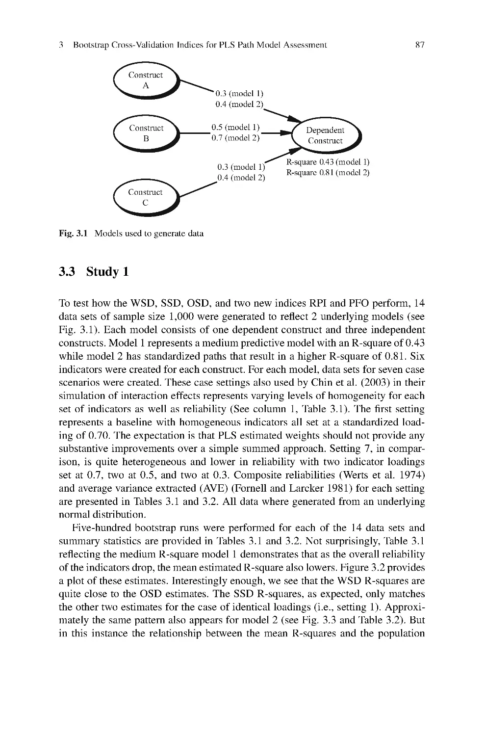
Теги: mathematics statistics springer publisher calculations computational statistics partial least squares
ISBN: 978-3-540-32825-4
Год: 2010
Похожие
Geomorphological Mapping Methods and Applications
Handbook of Usability and User Experience UX
Introduction to Development Engineering - A Framework with Applications from the Field
Languages, compilers, and run-time systems for scalable computers 4th international workshop, LCR '98, Pittsburgh, PA, USA, May 28-30, 1998 selected papers
Текст
                    Springer Handbooks of Computational Statistics
Series Editors
James E. Gentle
Wolfgang K. Härdle
Yuichi Mori
For further volumes:
http://www.springer.com/series/7286

Vincenzo Esposito Vinzi
Wynne W. Chin
J rg Henseler
Huiwen Wang
Editors
Handbook of
Partial Least Squares
Concepts, Methods and Applications
13

Editor-in-Chief
ESSEC Business School of Paris and
Singapore
Department of Information Systems &
Decision Sciences
Avenue Bernard Hirsch - B.P. 50105
95021 Cergy-Pontoise Cedex France
vinzi@essec.fr
Nijmegen School of Management
Institute for Management Research
Radboud Universiteit Nijmegen
6500 HK Nijmegen
The Netherlands
j.henseler@fm.ru.nl
Editors
Bauer Faculty Fellow
Department of Decision and
Information Sciences
C.T. Bauer College of Business
334 Melcher Hall, room 280D
University of Houston
Houston, Texas 77204-6282
wchin@uh.edu
School of Economic Management
BeiHang University
37, XueYuan Road, HaiDian District
Beijing 100191
P. R. China
wanghw@vip.sina.com
ISBN 978-3-540-32825-4
e-ISBN 978-3-540-32827-8
DOI 10.1007/978-3-540-32827-8
Printed on acid-free paper
Springer is part of Springer Science+Business Media (www.springer.com)
Springer Heidelberg Dordrecht London New York
Vincenzo Esposito Vinzi
J rg Henseler
Huiwen Wang
Wynne W. Chin
Co er design: deblik, Berlin, Germany
Library of Congress Control Number: 2009943435
©Springer-Verlag Berlin Heidelberg 2010
This work is subject to copyright. All rights are reserved, whether the whole or part of the material is
concerned, specifically the rights of translation, reprinting, reuse of illustrations, recitation, broadcasting,
reproduction on microfilm or in any other way, and storage in data banks. Duplication of this publication
The use of general descriptive names, registered names, trademarks, etc. in this publication does not imply,
or parts thereof is permitted only under the provisions of the German Copyright Law of September 9, 1965,
in its current version, and permission for use must always be obtained from Springer. Violations are liable
to prosecution under the German Copyright Law.
even in the absence of a specific statement, that such names are exempt from the relevant protective laws
and regulations and therefore free for general use.

Contents
Editorial: Perspectives on Partial Least Squares ............................... 1
Vincenzo Esposito Vinzi, Wynne W. Chin, J¨
org Henseler,
and Huiwen Wang
Part I Methods
PLS Path Modeling: Concepts, Model Estimation and Assessment
1 Latent Variables and Indices: Herman Wold’s Basic
Design and Partial Least Squares ........................................... 23
Theo K. Dijkstra
2 PLS Path Modeling: From Foundations to Recent
Developments and Open Issues for Model Assessment
and Improvement ............................................................. 47
Vincenzo Esposito Vinzi, Laura Trinchera, and Silvano Amato
3 Bootstrap Cross-Validation Indices for PLS Path Model
Assessment .................................................................... 83
Wynne W. Chin
PLS Path Modeling: Extensions
4 A Bridge Between PLS Path Modeling
and Multi-Block Data Analysis ............................................. 99
Michel Tenenhaus and Mohamed Hanaﬁ
5 Use of ULS-SEM and PLS-SEM to Measure a Group
Effect in a Regression Model Relating Two Blocks
of Binary Variables ...........................................................125
Michel Tenenhaus, Emmanuelle Mauger,
and Christiane Guinot
v

vi
Contents
6 A New Multiblock PLS Based Method to Estimate Causal
Models: Application to the Post-Consumption Behavior
in Tourism .....................................................................141
Francisco Arteaga, Martina G. Gallarza, and Irene Gil
7 An Introduction to a Permutation Based Procedure
for Multi-Group PLS Analysis: Results of Tests
of Differences on Simulated Data and a Cross Cultural
Analysis of the Sourcing of Information System Services
Between Germany and the USA ............................................171
Wynne W. Chin and Jens Dibbern
PLS Path Modeling with Classiﬁcation Issues
8 Finite Mixture Partial Least Squares Analysis:
Methodology and Numerical Examples ....................................195
Christian M. Ringle, Sven Wende, and Alexander Will
9 Prediction Oriented Classiﬁcation in PLS Path Modeling ...............219
Silvia Squillacciotti
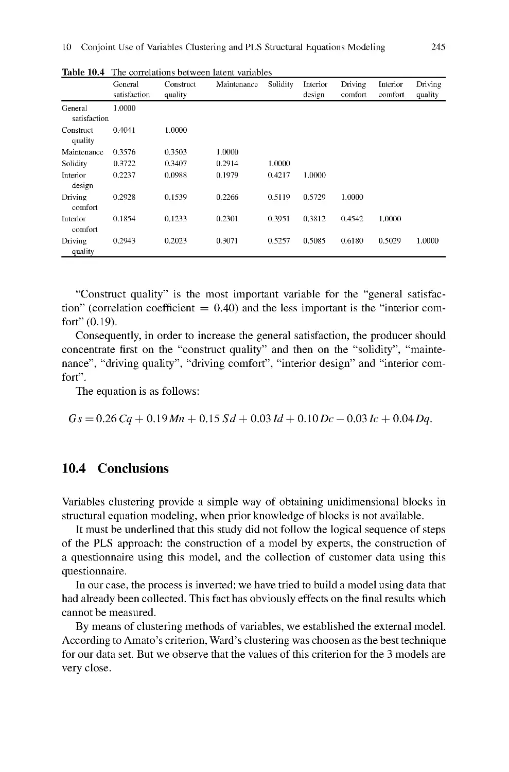
10 Conjoint Use of Variables Clustering and PLS Structural
Equations Modeling ..........................................................235
Valentina Stan and Gilbert Saporta
PLS Path Modeling for Customer Satisfaction Studies
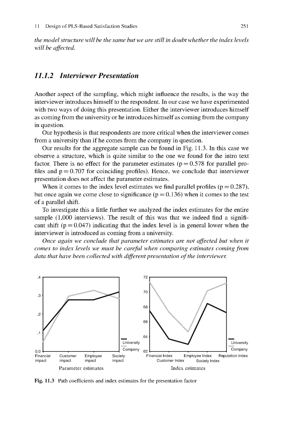
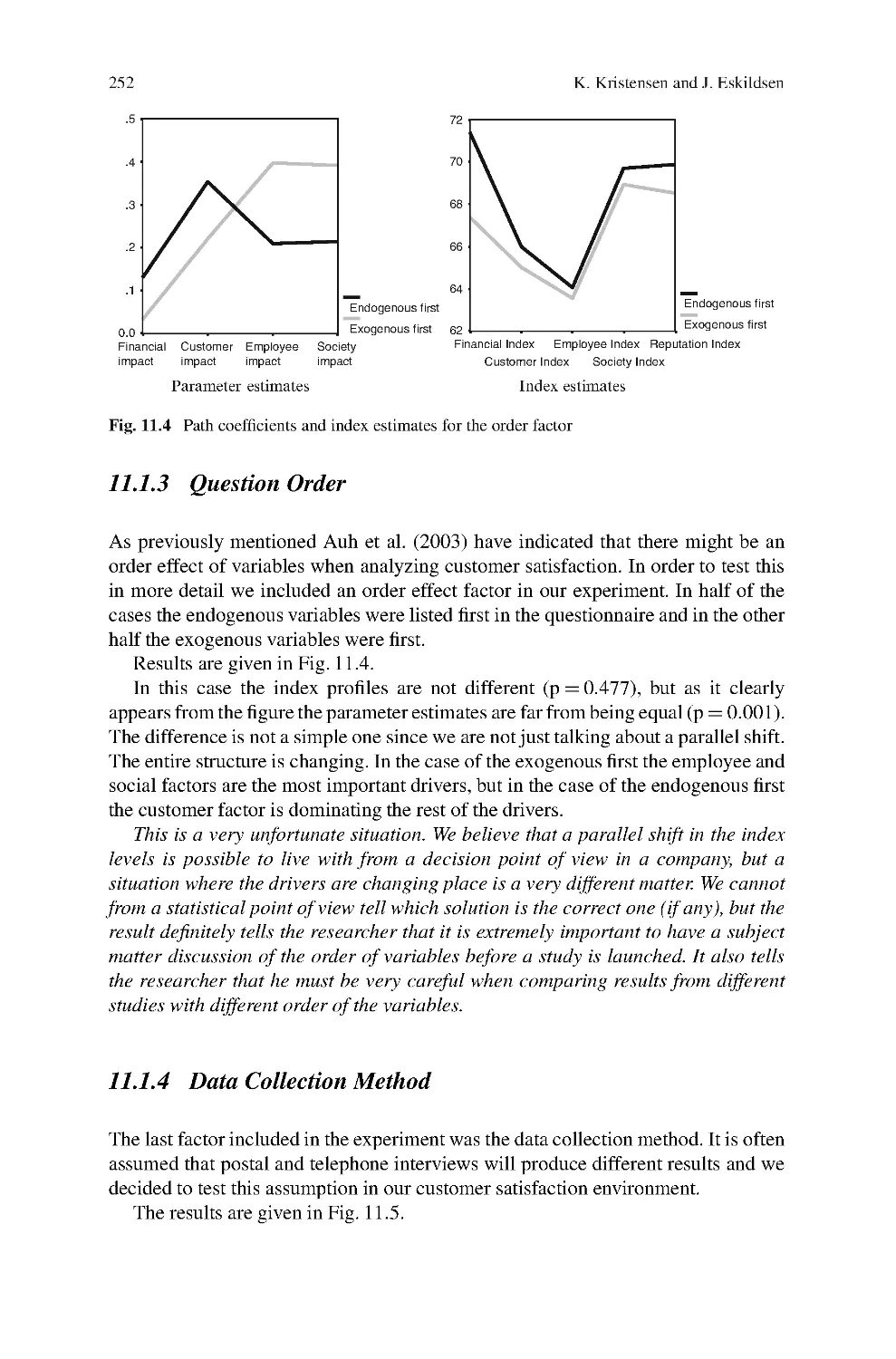
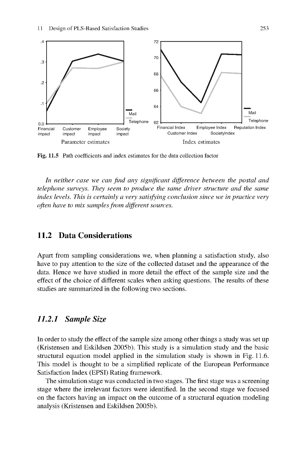
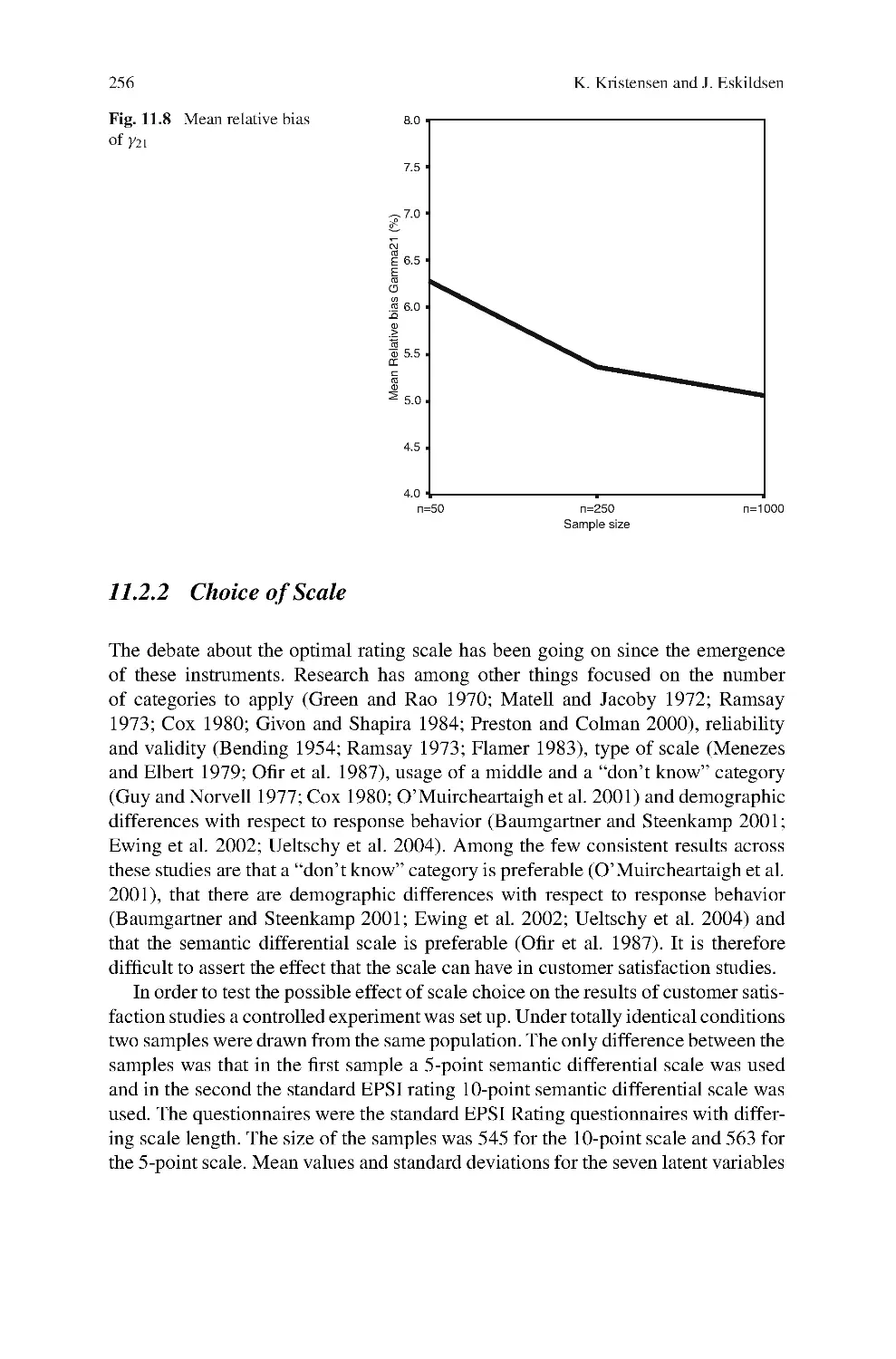
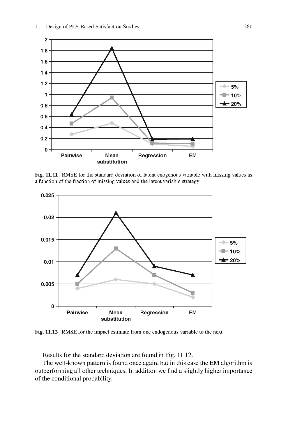
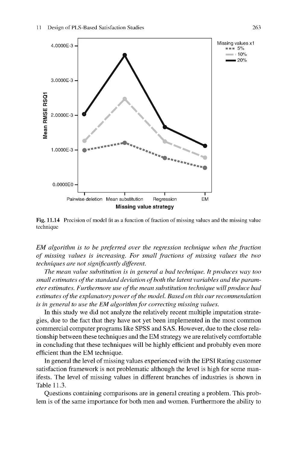
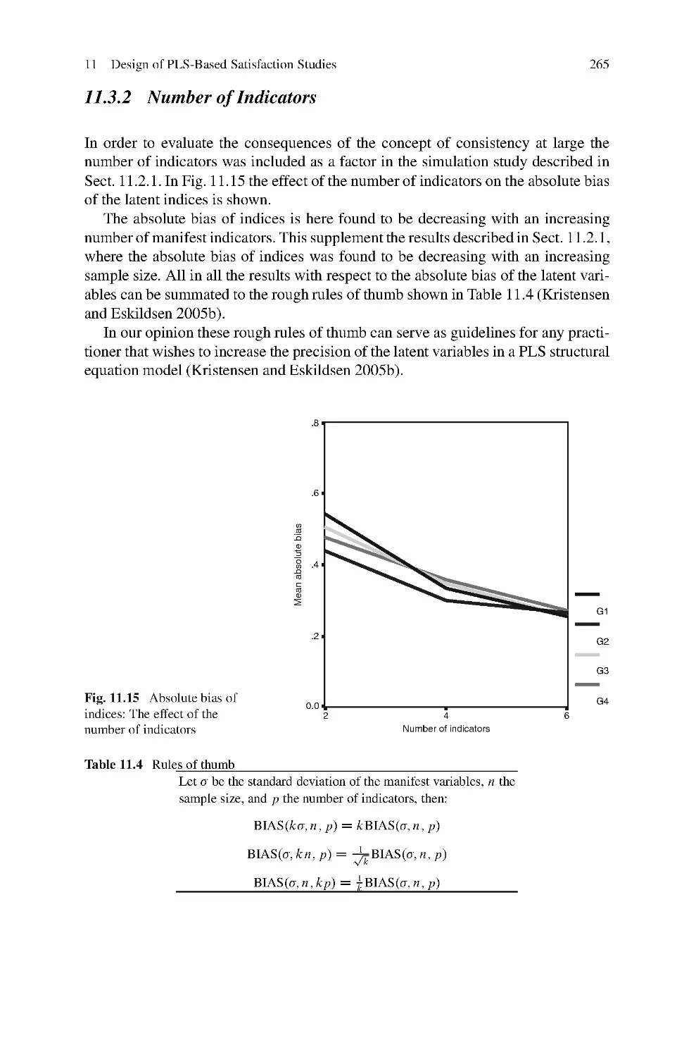
11 Design of PLS-Based Satisfaction Studies .................................247
Kai Kristensen and Jacob Eskildsen
12 A Case Study of a Customer Satisfaction Problem:
Bootstrap and Imputation Techniques .....................................279
Clara Cordeiro, Alexandra Mach´
as, and Maria Manuela Neves
13 Comparison of Likelihood and PLS Estimators
for Structural Equation Modeling: A Simulation
with Customer Satisfaction Data ...........................................289
Manuel J. Vilares, Maria H. Almeida, and Pedro S. Coelho
14 Modeling Customer Satisfaction: A Comparative
Performance Evaluation of Covariance Structure Analysis
Versus Partial Least Squares ................................................307
John Hulland, Michael J. Ryan, and Robert K. Rayner

Contents
vii
PLS Regression
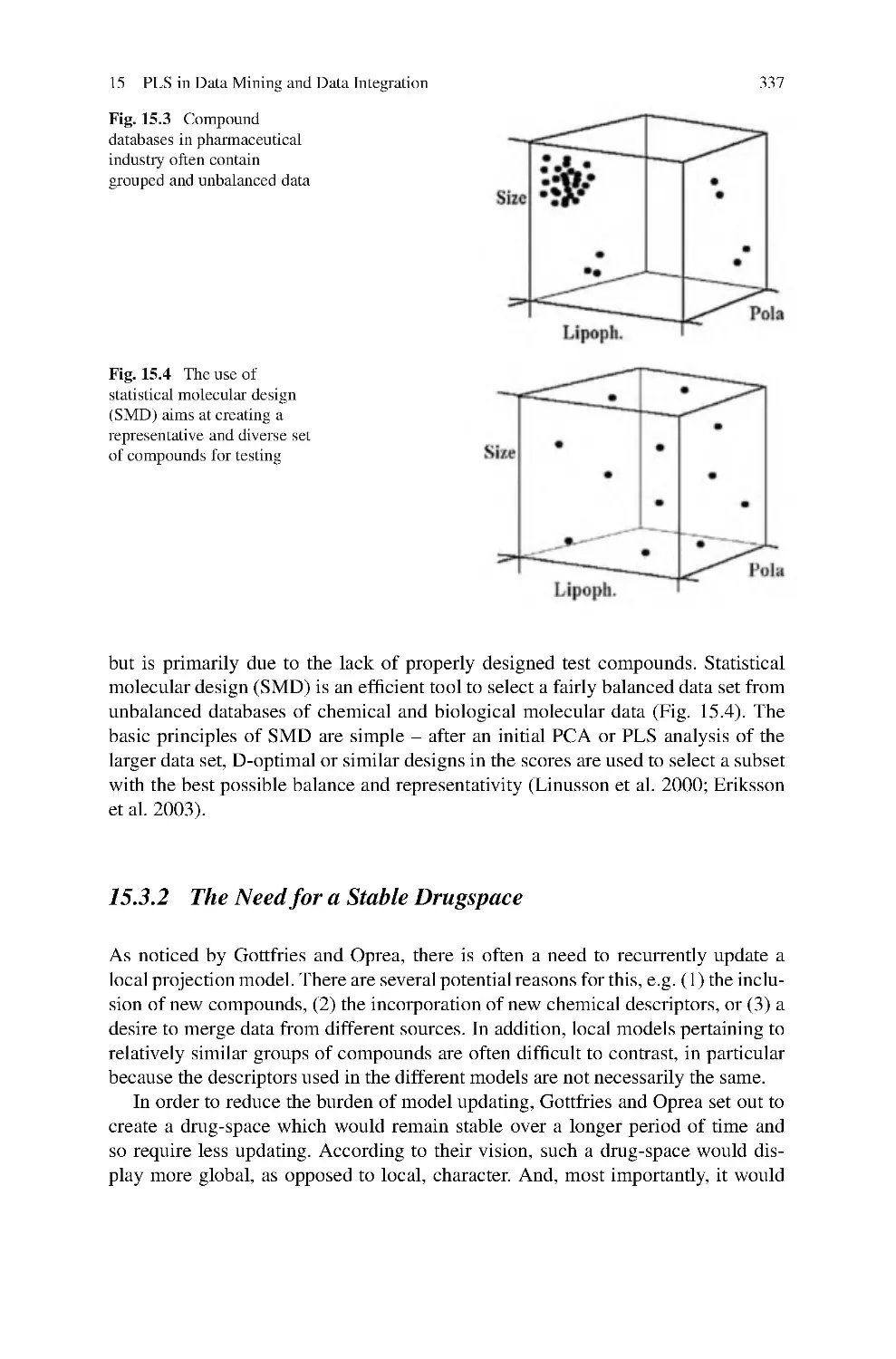
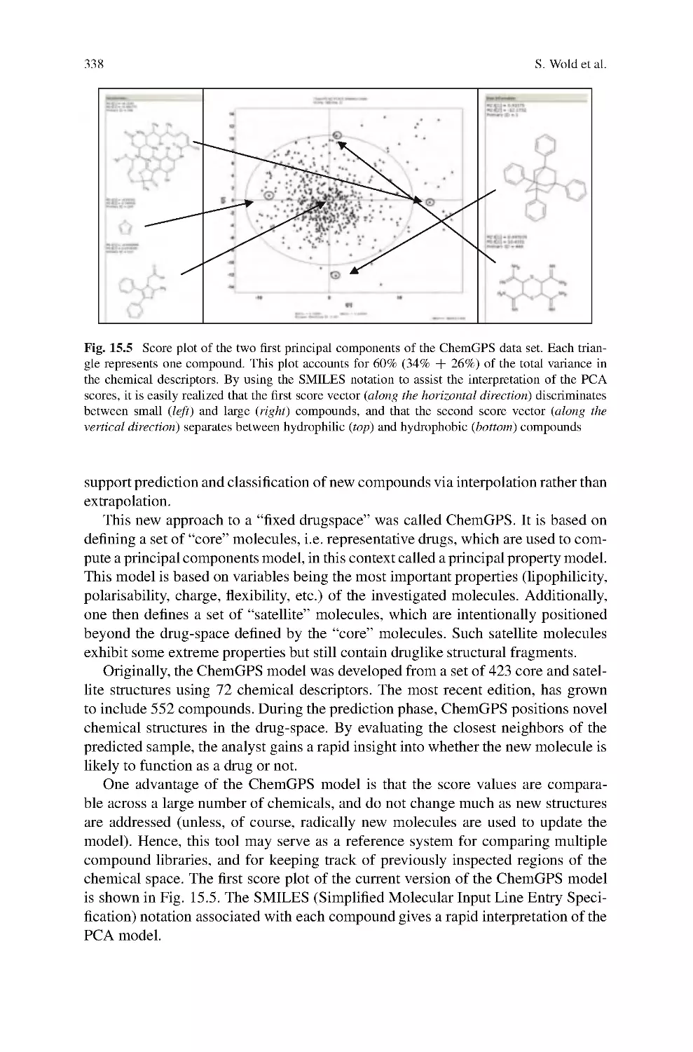
15 PLS in Data Mining and Data Integration ................................327
Svante Wold, Lennart Eriksson, and Nouna Kettaneh
16 Three-Block Data Modeling by Endo- and Exo-LPLS
Regression .....................................................................359
Solve Sæbø, Magni Martens, and Harald Martens
17 Regression Modelling Analysis on Compositional Data ..................381
Part II Applications to Marketing and Related Areas
18 PLS and Success Factor Studies in Marketing ............................409
S¨
onke Albers
19 Applying Maximum Likelihood and PLS on Different
Sample Sizes: Studies on SERVQUAL Model
and Employee Behavior Model..............................................427
Carmen Barroso, Gabriel Cepeda Carri ´
on, and Jos´
eL.Rold´
an
20 A PLS Model to Study Brand Preference: An Application
to the Mobile Phone Market .................................................449
Paulo Alexandre O. Duarte and M´
ario Lino B. Raposo
21 An Application of PLS in Multi-Group Analysis:
The Need for Differentiated Corporate-Level Marketing
in the Mobile Communications Industry ..................................487
Markus Eberl
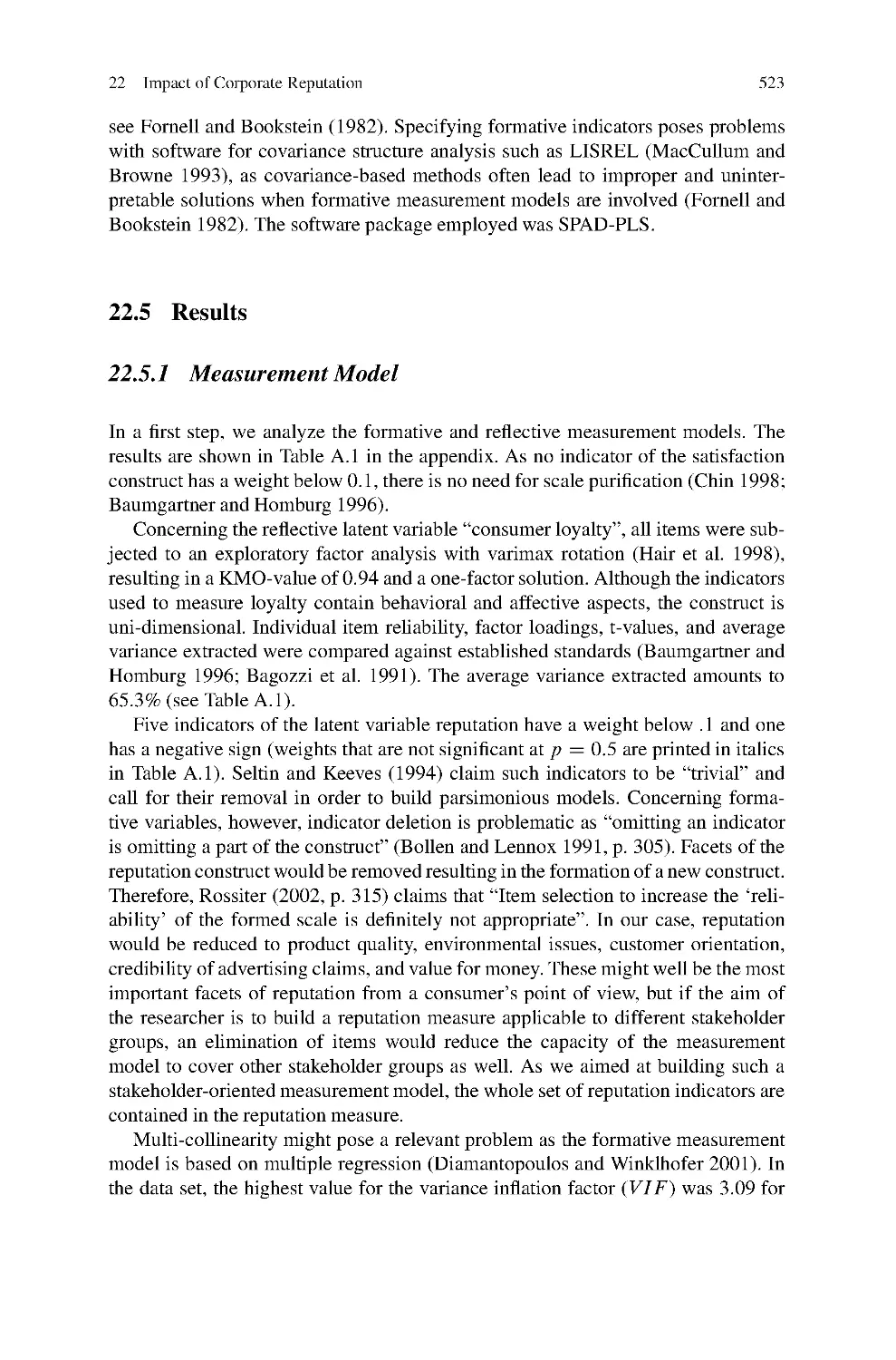
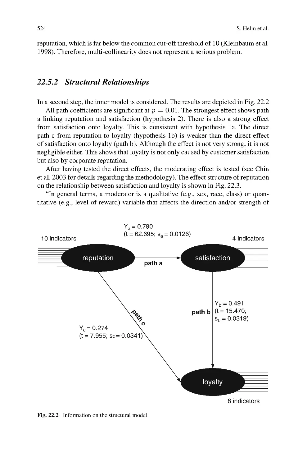
22 Modeling the Impact of Corporate Reputation
on Customer Satisfaction and Loyalty Using Partial Least
Squares ........................................................................515
Sabrina Helm, Andreas Eggert, and Ina Garnefeld
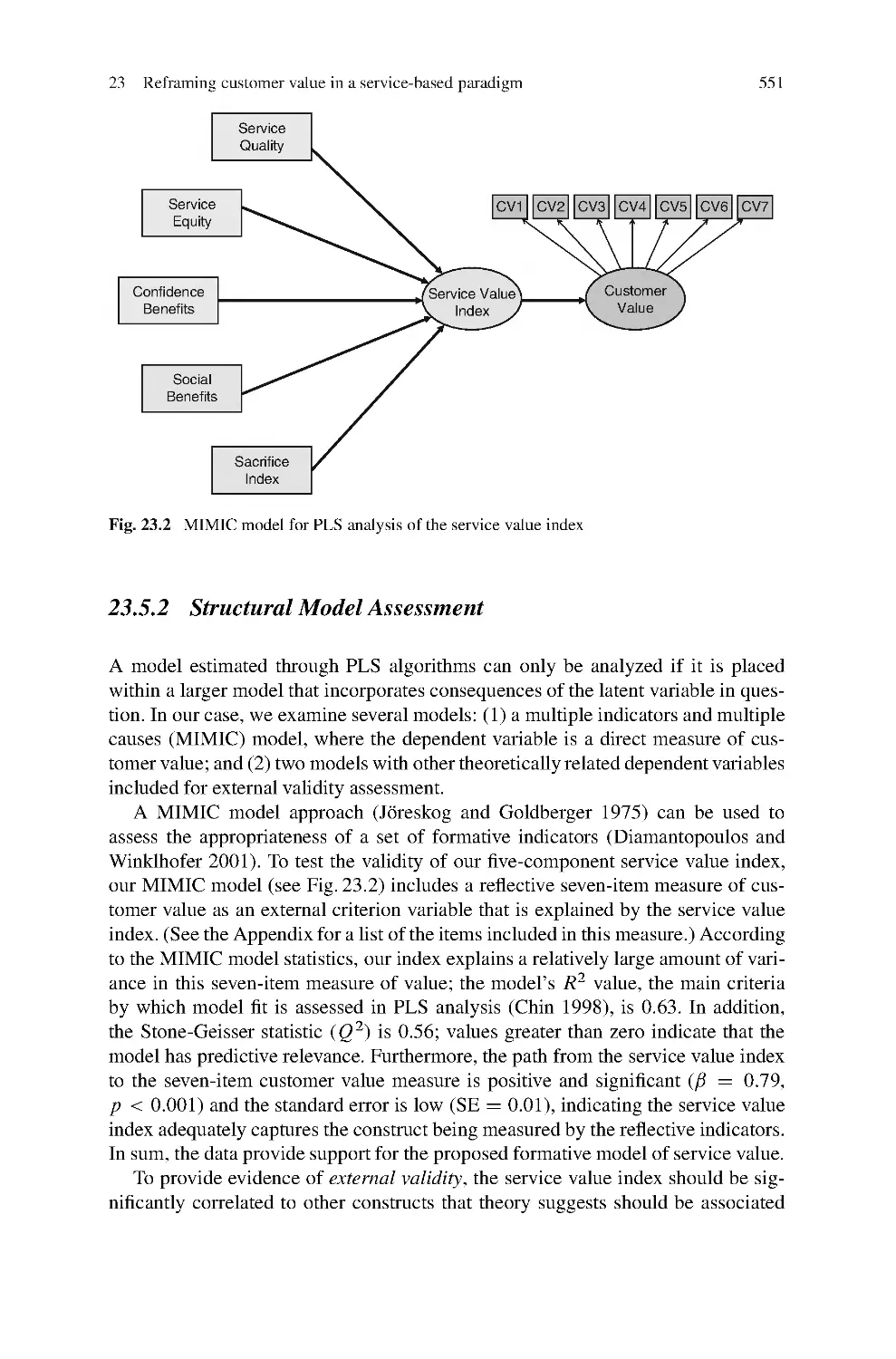
23 Reframing Customer Value in a Service-Based
Paradigm: An Evaluation of a Formative Measure
in a Multi-industry, Cross-cultural Context ...............................535
David MartKın Ruiz, Dwayne D. Gremler, Judith H. Washburn,
and Gabriel Cepeda Carri´
on
24 Analyzing Factorial Data Using PLS: Application
in an Online Complaining Context .........................................567
Sandra Streukens, Martin Wetzels, Ahmad Daryanto,
andKodeRuyter
Huiwen Wang, Jie Meng, and Michel Tenenhaus

viii
Contents
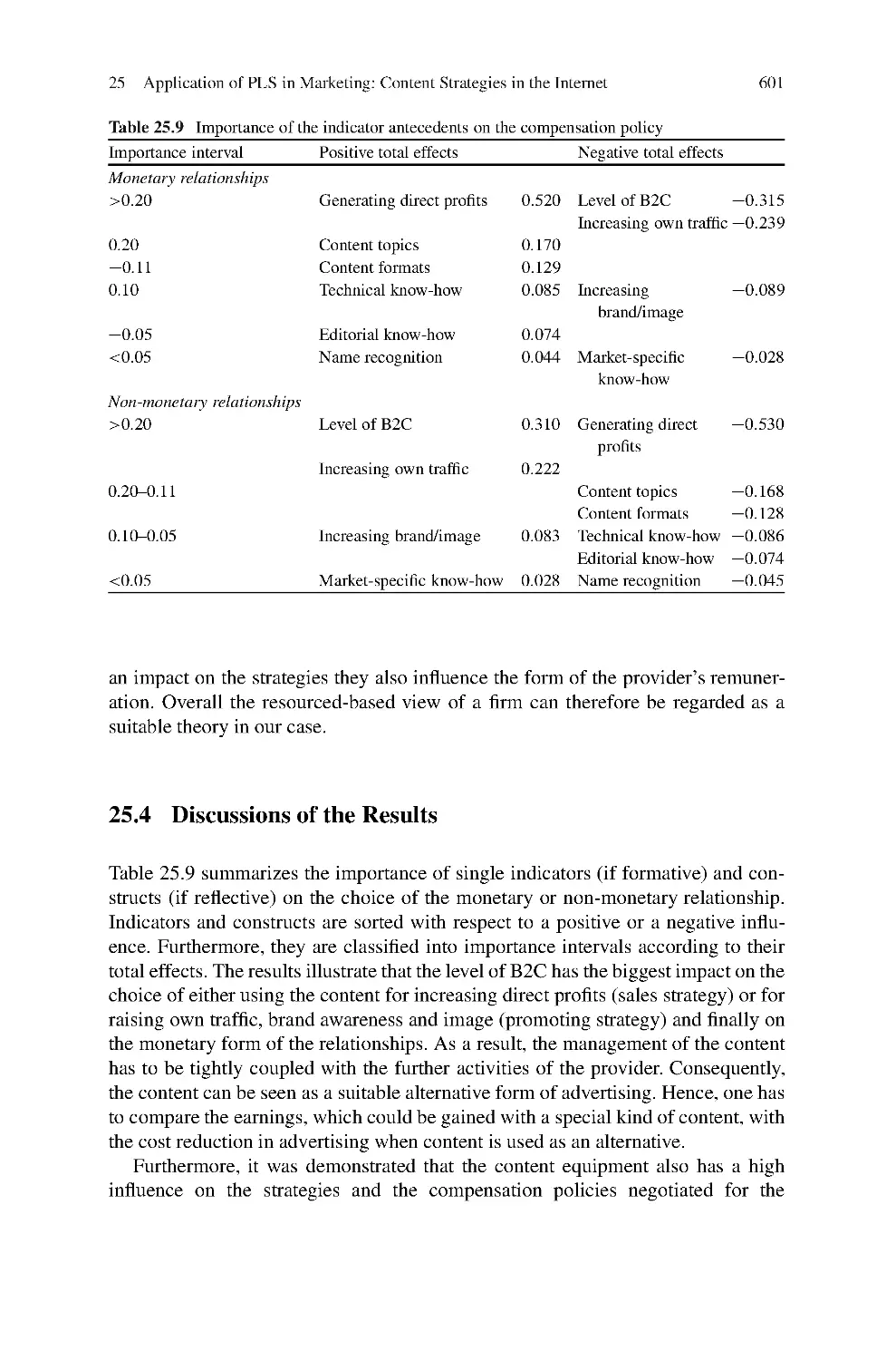
25 Application of PLS in Marketing: Content Strategies
on the Internet ................................................................589
Silvia Boßow-Thies and S¨
onke Albers
26 Use of Partial Least Squares (PLS) in TQM Research:
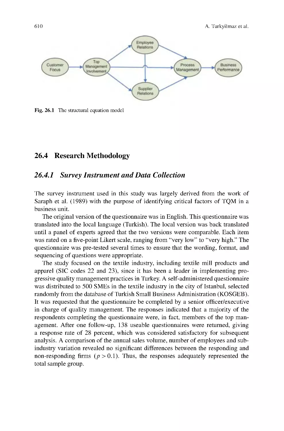
TQM Practices and Business Performance in SMEs .....................605
Ali Turkyilmaz, Ekrem Tatoglu, Selim Zaim,
and Coskun Ozkan
27 Using PLS to Investigate Interaction Effects Between
Higher Order Branding Constructs ........................................621
Bradley Wilson
Part III Tutorials
28 How to Write Up and Report PLS Analyses ...............................655
Wynne W. Chin
29 Evaluation of Structural Equation Models Using
the Partial Least Squares (PLS) Approach ................................691
Oliver G ¨
otz, Kerstin Liehr-Gobbers, and Manfred Krafft
30 Testing Moderating Effects in PLS Path Models:
An Illustration of Available Procedures ....................................713
J¨
org Henseler and Georg Fassott
31 A Comparison of Current PLS Path Modeling Software:
Features, Ease-of-Use, and Performance ...................................737
Dirk Temme, Henning Kreis, and Lutz Hildebrandt
32 Introduction to SIMCA-P and Its Application ............................757
33 Interpretation of the Preferences of Automotive
Customers Applied to Air Conditioning Supports
by Combining GPA and PLS Regression ..................................775
Laure Nokels, Thierry Fahmy, and S´
ebastien Crochemore
Index .................................................................................791
Zaibin Wu, Dapeng Li, Jie Meng, and Huiwen Wang

List of Contributors
S¨
onke Albers Institute of Innovation Research, Christian-Albrechts-University
at Kiel, Westring 425, 24098 Kiel, Germany, albers@bwl.uni-kiel.de
Maria H. Almeida Faculty of Economics, New University of Lisbon, Campus de
Campolide, 1099-032 Lisbon, Portugal, mhalmeida@fe.unl.pt
Silvano Amato Dipartimento di Matematica e Statistica, Universit`
a degli Studi di
Napoli “Federico II”, Via Cintia 26, Complesso Monte S. Angelo, 80126 Napoli,
Italy, silvano.amato@gmail.com
Francisco Arteaga Department of Statistics, Universidad Cat ´
olica de Valencia
San Vicente Martir, Guillem de Castro, 175, Valencia 46008, Spain,
francisco.arteaga@ucv.es
Carmen Barroso Management and Marketing Department, University of Seville,
Ram ´
on y Cajal, 1, 41018 Sevilla, Spain, barroso@us.es
Silvia Boßow-Thies Capgemini Telecom Media and Networks Deutschland
GmbH, Neues Kanzler Eck 21, 10719 Berlin, Germany,
silvia.bossow- thies@capgemini.com
Gabriel Cepeda Carri´
on Departamento de Administraci´
on de Empresas y
Marketing, Universidad de Sevilla, Ram ´
on y Cajal, 1, 41018 Sevilla, Spain,
gabi@us.es
Wynne W. Chin Department of Decision and Information Sciences, Bauer
College of Business, University of Houston, TX, USA, wchin@uh.edu
Pedro S. Coelho ISEGI – New University of Lisbon, Campus de Campolide,
1070-032 Lisbon, Portugal, psc@isegi.unl.pt
Clara Cordeiro Department of Mathematics, FCT, University of Algarve,
Campus de Gambelas, 8005-139 Faro, Portugal, ccordei@ualg.pt
S´ebastien Crochemore Materials Engineering Department, Technocentre
Renault 1, avenue du Golf, API TCR LAB 252, 78 288 Guyancourt Cedex,
France, sebastien.crochemore@renault.com
ix

x
List of Contributors
Ahmad Daryanto Department of Business Analysis, Systems and Informa-
tion Management, Newcastle Business School, City Campus East,
Northumbria University, Newcastle upon Tyne, NE1 8ST, UK,
ahmad.daryanto@northumbria.ac.uk
Ko de Ruyter Department of Marketing and Marketing Research, Maastricht
University, P.O. Box 616 6200 MD, The Netherlands, k.deruyter@mw.unimaas.nl
Jens Dibbern Department of Information Engineering, Institute of Information
Systems, University of Bern, Engehaldenstr. 8, Room 204, 3012 Bern, Switzerland,
jens.dibbern@iwi.unibe.ch
Theo K. Dijkstra SNS Asset Management, Research and Development,
Pettelaarpark 120, P.O. Box 70053, 5201 DZ ’s-Hertogenbosch, The Netherlands,
theo.dijkstra@snsam.nl
and
University of Groningen, Economics and Econometrics, Zernike Complex, P.O.
Box 800, 9700 AV, Groningen, The Netherlands, t.k.dijkstra@rug.nl
Paulo Alexandre de Oliveira Duarte Departamento de Gest˜
ao e Economia,
Universidade da Beira Interior, Estrada do Sineiro, 6200-209 Covilh˜
a, Portugal,
pduarte@ubi.pt
Markus Eberl Senior Consultant Models and Methods, TNS Infratest Forschung
GmbH, Landsberger Straße 338, 80687 M ¨
unchen, Germany,
markus.eberl@tns-infratest.com
Andreas Eggert University of Paderborn, Warburger Str. 100, 33098 Paderborn,
Germany, andreas.eggert@notes.upb.de
Lennart Eriksson Umetrics Inc, 17 Kiel Ave, Kinnelon, NJ 07405, USA,
Lennart.eriksson@umetrics.com
Jacob Eskildsen School of Business, University of Aarhus, Haslegaardsvej 10,
8210 Aarhus V, Denmark, Eskildsen@asb.dk
Vincenzo Esposito Vinzi Dept. of Information Systems and Decision Sciences
ESSEC Business School of Paris,
Avenue Bernard Hirsch – B.P. 50105, 95021 Cergy-Pontoise, Cedex, France,
vinzi@essec.fr
Thierry Fahmy Addinsoft, 40 rue Damr´
emont, 75018 Paris, France,
fahmy@xlstat.com
Georg Fassott Department of Marketing, University of Kaiserslautern, Postfach
30 49, 67653 Kaiserslautern, Germany, fassott@wiwi.uni-kl.de
Martina Gonz ´
alez Gallarza Faculty of Economics, Department of Marketing,
Universitat de Valencia, Avenida de los Naranjos s/n, Valencia 46022, Spain,
martina.gallarza@uv.es
Ina Garnefeld University of Paderborn, Warburger Str. 100, 33098 Paderborn,
Germany, ina.garnefeld@notes.upb.de

List of Contributors
xi
Irene Gil Department of Marketing, Universitat de Val`
encia, Avenida de los
Naranjos s/n, Valencia 46022, Spain, irene.gil@uv.es
Oliver G ¨
otz University of M ¨
unster, Marketing Centrum M ¨
unster, Institute
of Marketing, Am Stadtgraben 13-15, 48143 M ¨
unster, Germany,
o.goetz@uni-muenster.de
Dwayne D. Gremler Department of Marketing, College of Business
Administration, Bowling Green State University, Bowling Green, OH 43403,
USA, gremler@cba.bgsu.edu
Christiane Guinot Biometrics and Epidemiology unit, C.E.R.I.E.S, 20 rue Victor
Noir, 92521 Neuilly sur Seine, France, christiane.guinot@ceries-lab.com
and
Computer Science Laboratory, Ecole Polytechnique, University of Tours, France
Mohamed Hanaﬁ Unit ´
e Mixte de Recherche (ENITIAA-INRA) en Sensom ´
etrie
et Chimiom´
etrie, ENITIAA, Rue de la G´
eraudi`
ere – BP 82225, Nantes 44322,
Cedex 3, France, hanaﬁ@enitiaa-nantes.fr
Sabrina Helm University of Arizona, John and Doris Norton School of Family and
USA, helm@email.arizona.edu
J¨
org Henseler Nijmegen School of Management, Radboud University Nijmegen,
P.O. Box 9108, 6500 HK Nijmegen, The Netherlands, j.henseler@fm.ru.nl
Lutz Hildebrandt Institute of Marketing, Humboldt University Berlin, Unter den
Linden 6, 10099 Berlin, Germany, hildebr@wiwi.hu-berlin.de
John Hulland Katz Business School, University of Pittsburgh, Pittsburgh,
PA 15260, USA, jhulland@katz.pitt.edu
Nouna Kettaneh NNS Consulting, 42 Pine Hill Rd, Hollis, NH 03049, USA,
nouna@nnsconsulting.com
Manfred Krafft University of M ¨
unster, Marketing Centrum M ¨
unster,
Institute of Marketing, Am Stadtgraben 13-15, 48143 M ¨
unster, Germany,
mkrafft@uni-muenster.de
Henning Kreis Marketing-Department, Freie Universit ¨
at Berlin, School
of Business and Economics, Otto-von-Simson-Str. 19, 14195 Berlin, Germany,
henning.kreis@fu-berlin.de
Kai Kristensen School of Business, University of Aarhus, Haslegaardsvej 10,
8210 Aarhus V, Denmark, kak@asb.dk
Dapeng Li Agricultural Bank of China, Beijing 100036, China,
zh.ldp@intl.abocn.com
Kerstin Liehr-Gobbers Hering Schuppener Consulting, Kreuzstraße 60, 40210
D¨
usseldorf, Germany, kliehr@heringschuppener.com
Consumer Sciences, 650 N. Park Ave, P.O. Box 210078, Tucson, AZ 85721-0078,

xii
List of Contributors
Alexandra Mach´
as Polytechnic Institute of Lisbon, Escola Superior de
Comunicac
¸˜
ao Social Campus de Benﬁca do IPL, 1549-014 Lisboa, Portugal,
amachas@escs.ipl.pt
Harald Martens Norwegian Food Research Institute, Matforsk, 1430 ˚As, Norway,
harald.martens@matforsk.no
and
Faculty of Life Sciences, Department of Food Science, University of Copenhagen,
Rolighedsvej 30, 1958 Frederiksberg C, Denmark
and
Norwegian University of Life Sciences, IKBM/CIGENE, P.O. Box 5003, 1432 ˚As,
Norway
Magni Martens Norwegian Food Research Institute, Matforsk, 1430 ˚As, Norway,
magni.martens@matforsk.no
and
Faculty of Life Sciences, Department of Food Science, University of Copenhagen,
Rolighedsvej 30, 1958 Frederiksberg C, Denmark
Emmanuelle Mauger Biometrics and Epidemiology unit, C.E.R.I.E.S, 20 rue
Victor Noir, 92521 Neuilly sur Seine, France, emmanuelle.mauger@ceries-lab.com
Maria Manuela Neves Department of Mathematics, Instituto Superior de
Agronomia, Technical University of Lisbon (TULisbon), Tapada da Ajuda,
1349-017 Lisboa, Portugal, manela@isa.utl.pt
School of Statistics, Central University of Finance and Economics,
Beijing 100081, China, mengjie517@126.com
Laure Nokels Materials Engineering Department, Technocentre Renault, 1,
avenue du Golf, API TCR LAB 2 52, 78 288 Guyancourt Cedex, France,
laure.nokels@renault.com
Coskun Ozkan Department of Industrial Engineering, Kocaeli University,
Veziroglu Yerleskesi, 41040 Kocaeli, Turkey, coskun ozkan@yahoo.com
M´
ario Lino Barata Raposo Departamento de Gest˜
ao e Economia, Universidade
da Beira Interior, Estrada do Sineiro, 6200-209 Covilh˜
a, Portugal, mraposo@ubi.pt
Robert K. Rayner Market Strategies International, 20255 Victor Parkway, Suite
400, Livonia, MI 48152, USA, bob rayner@marketstrategies.com
Christian M. Ringle University of Hamburg, Institute for Industrial Management
and Organizations, Von-Melle-Park 5, 20146 Hamburg, Germany,
c.ringle@smartpls.de
and
University of Technology Sydney, Centre for Management and Organization
Jos ´eL.Rold´
an Management and Marketing Department, University of Seville,
Ram ´
on y Cajal, 1, 41018 Sevilla, Spain, jlroldan@us.es
Meng Jie
Studies, P.O. Box 123, Broadway NSW 2007, Australia

List of Contributors
xiii
David Mart´ın Ruiz Escuela Universitaria de Estudios Empresariales, 41012
Sevilla, Spain, dmartin@us.es
Michael J. Ryan Ross School of Business, University of Michigan, P.O. Box 105,
Bass Harbor, ME 04653, USA, mikeryan@umich.edu
Solve Sæbø Department of Chemistry, Biotechnology and Food Science (IKBM),
Norwegian University of Life Sciences, P.O. Box 5003, 1432 ˚As, Norway,
solve.sabo@umb.no
Gilbert Saporta Conservatoire National des Arts et M´
etiers, Chaire de Statistique
Appliqu´
ee, case 441, 292 rue Saint Martin, 75141 Paris, Cedex 03, France,
gilbert.saporta@cnam.fr
Silvia Squillacciotti EDF R&D, D ´
epartement ICAME, 1 avenue du G´
en´
eral de
Gaulle, 92141 Clamart, France, silvia.fagnoni@edf.fr
Valentina Stan Groupe ESSCA Angers, 1 Rue Lakanal – BP 40348, 49003
Angers, Cedex 01, France, valentina titu@yahoo.fr
Sandra Streukens Department of Marketing and Strategy, Universiteit Hasselt,
Campus Diepenbeek, Agoralaan Gebouw DBE 3590 Diepenbeek, Belgium,
sandra.streukens@uhasselt.be
Ekrem Tatoglu Faculty of Economics and Administrative Sciences, Chair of
International Trade and Business, Bahcesehir University, Besiktas, Istanbul, Turkey,
ekremt@bahcesehir.edu.tr
Dirk Temme Chair of Retailing and Service Management, Schumpeter School
of Business and Economics, Bergische Universit¨
at Wuppertal, Gaußstr. 20, 42097
Wuppertal, Germany, Temme@wiwi.uni-wuppertal.de
Michel Tenenhaus Department of SIAD, HEC School of Management, 1 rue de
la Lib´
eration, 78351 Jouy-en-Josas, France, tenenhaus@hec.fr
Laura Trinchera Dipartimento di Matematica e Statistica, Universit`
a degli Studi
di Napoli “Federico II”, Via Cintia, 26 – Complesso Monte S. Angelo, 80126
Napoli, Italy, ltrinche@unina.it
Ali Turkyilmaz Department of Industrial Engineering, Fatih University,
Buyukcekmece, 34500 Istanbul, Turkey, aturkyilmaz@fatih.edu.tr
Manuel J. Vilares ISEGI – New University of Lisbon, Campus de Campolide,
1070-032 Lisbon, Portugal, mjv@isegi.unl.pt
School of Economics and Management, Beihang University, 37
Xueyuan Road, Haidian District, Beijing 100083, China, wanghw@vip.sina.com
Judith H. Washburn John H. Sykes College of Business, University of Tampa,
401 W. Kennedy Blvd., UT Box 48F, Tampa, FL 33606, USA, jwashburn@ut.edu
Sven Wende University of Hamburg, Institute for Industrial Management
and Organizations, Von-Melle-Park 5, 20146 Hamburg, Germany,
s.wende@smartpls.de
Wang Huiwen

xiv
List of Contributors
Martin Wetzels Department of Marketing and Marketing Research, Maastricht
University, P.O. Box 616 6200 MD, The Netherlands, m.wetzels@mw.unimaas.nl
Alexander Will University of Hamburg, Institute for Industrial Management and
Organizations, Von-Melle-Park 5, 20146 Hamburg, Germany,
mail@alexwill.de
Bradley Wilson School of Media and Communication, RMIT University, 124
LaTrobe Street, GPO Box 2476V, Melbourne, Victoria 3000, Australia,
brad.wilson@rmit.edu.au
Svante Wold NNS Consulting, 42 Pine Hill Rd, Hollis, NH 03049, USA,
sbwold@gmail.com
School of Economics and Management, Beihang University, 37
Xueyuan Road, Haidian District, Beijing 100083, China, binship@126.com
Selim Zaim Department of Management, Fatih University, Buyukcekmece,
Istanbul 34500, Turkey, szaim@fatih.edu.tr
Wu Zaibin

Editorial: Perspectives on Partial Least Squares
Vincenzo Esposito Vinzi, Wynne W. Chin, J ¨
org Henseler, and Huiwen Wang
1 Partial Least Squares: A Success Story
This Handbook on Partial Least Squares (PLS) represents a comprehensive presen-
tation of the current, original and most advanced research in the domain of PLS
methods with speciﬁc reference to their use in Marketing-related areas and with a
discussion of the forthcoming and most challenging directions of research and per-
spectives. The Handbook covers the broad area of PLS Methods from Regression
to Structural Equation Modeling, from methods to applications, from software to
interpretation of results. This work features papers on the use and the analysis of
latent variables and indicators by means of the PLS Path Modeling approach from
the design of the causal network to the model assessment and improvement. More-
over, within the PLS framework, the Handbook addresses, among others, special
and advanced topics such as the analysis of multi-block, multi-group and multi-
structured data, the use of categorical indicators, the study of interaction effects,
the integration of classiﬁcation issues, the validation aspects and the comparison
between the PLS approach and the covariance-based Structural Equation Modeling.
V. Esposito Vinzi
ESSEC Business School of Paris, Avenue Bernard Hirsch – B.P. 50105,
95021 Cergy-Pontoise, France
e-mail: vinzi@essec.fr
W.W. Chin
Department of Decision and Information Sciences, Bauer College of Business, University of
Houston, TX, USA
e-mail: wchin@uh.edu
J. Henseler
Nijmegen School of Management, Radboud University Nijmegen, P.O. Box 9108, 6500 HK
Nijmegen, The Netherlands
e-mail: j.henseler@fm.ru.nl
H. Wang
School of Economics and Management, Beihang University, 37 Xueyuan Road, Haidian District,
Beijing 100083, China
e-mail: wanghw@vip.sina.com
V. Esposito Vinzi et al. (eds.), Handbook of Partial Least Squares, Springer Handbooks
of Computational Statistics, DOI 10.1007/978-3-540-32827-8 1,
c

 Springer-Verlag Berlin Heidelberg 2010
1

2
V. Esposito Vinzi et al.
Most chapters comprise a thorough discussion of applications to problems from
Marketing and related areas. Furthermore, a few tutorials focus on some key aspects
of PLS analysis with a didactic approach. This Handbook serves as both an intro-
duction for those without prior knowledge of PLS but also as a comprehensive
reference for researchers and practitioners interested in the most recent advances
in PLS methodology.
Different Partial Least Squares (PLS) cultures seem to have arisen following
the original work by Herman Wold (1982): PLS regression models (PLS-R, Wo l d
et al. 1983; Tenenhaus 1998) and PLS Path Modeling (PLS-PM, Lohm ¨
oller 1989;
Tenenhaus et al. 2005). As a matter of fact, up to now, the two cultures are somehow
oriented to different application ﬁelds: chemometrics and related ﬁelds for PLS-
R; econometrics and social sciences for PLS-PM. While experiencing this internal
diversity, most often the PLS community has to cope also with external diversities
due to other communities that, grown up under the classical culture of statistical
inference, seem to be quite reluctant in accepting the PLS approach to data analysis
as a well-grounded statistical approach.
Generally speaking, PLS-PM is a statistical approach for modeling complex mul-
tivariable relationships among observed and latent variables. In the past few years,
this approach has been enjoying increasing popularity in several sciences. Struc-
tural Equation Models include a number of statistical methodologies allowing the
estimation of a causal theoretical network of relationships linking latent complex
concepts, each measured by means of a number of observable indicators. From the
standpoint of structural equation modeling, PLS-PM is a component-based approach
where the concept of causality is formulated in terms of linear conditional expec-
tation. Herman Wold (1969, 1973, 1975b, 1980, 1982, 1985, 1988) developed PLS
as an alternative to covariance-based structural equation modeling as represented
by LISREL-type models (J¨
oreskog, 1978) with, preferably, maximum likelihood
estimation. He introduced PLS as a soft modeling technique in order to emphasize
the difference in methodology for estimating structural equation models (Fornell
and Bookstein, 1982; Schneeweiß, 1991). Soft modeling refers to the ability of
PLS to exhibit greater ﬂexibility in handling various modeling problems in situ-
ations where it is difﬁcult or impossible to meet the hard assumptions of more
traditional multivariate statistics. Within this context, ”soft” is only attributed to
distributional assumptions and not to the concepts, the models or the estimation
techniques (Lohm ¨
oller, 1989). As an alternative to the classical covariance-based
approach, PLS-PM is claimed to seek for optimal linear predictive relationships
rather than for causal mechanisms thus privileging a prediction-relevance oriented
discovery process to the statistical testing of causal hypotheses. From the stand-
point of data analysis, PLS-PM may be also viewed as a very ﬂexible approach
to multi-block (or multiple table) analysis. Multi-block situations arise when a
few sets of variables are available for the same set of samples. Tenenhaus and
Hanaﬁ (2007) show direct relationships between PLS-PM and several techniques
for multi-block analysis obtained by properly specifying relationships in the struc-
tural model and by mixing the different estimation options available in PLS-PM.
This approach clearly shows how the data-driven tradition of multiple table analysis

Editorial
3
can be merged in the theory-driven tradition of structural equation modeling to
allow running analysis of multi-block data in light of current knowledge on con-
ceptual relationships between tables. In both structural equation modeling and
multi-block data analysis, PLS-PM may enhance even further its potentialities,
and provide effective added value, when exploited in the case of formative epis-
temic relationships between manifest variables and their respective latent variables.
In PLS-PM latent variables are estimated as linear combinations of the manifest
variables and thus they are more naturally deﬁned as emergent constructs (with
formative indicators) rather than latent constructs (with reﬂective indicators). As
a matter of fact, formative relationships are more and more commonly used in the
applications, especially in the marketing domain, but pose a few problems for the
statistical estimation. This mode is based on multiple OLS regressions between
each latent variable and its own formative indicators. As known, OLS regression
may yield unstable results in presence of important correlations between explana-
tory variables, it is not feasible when the number of statistical units is smaller than
the number of variables nor when missing data affect the dataset. Thus, it seems
quite natural to introduce a PLS-R external estimation mode inside the PLS-PM
algorithm so as to overcome the mentioned problems, preserve the formative rela-
tionships and remain coherent with the component-based and prediction-oriented
nature of PLS-PM. Apart from the external estimation module, the implementation
of PLS-R within PLS-PM may be extended also to the internal estimation mod-
ule (as an alternative OLS regression) and to the estimation of path coefﬁcients
for the structural model upon convergence of the PLS-PM algorithm and estima-
tion of the latent variable scores. Such an extensive implementation, that might
well represent a playground towards the merging of the two PLS cultures, opens
a wide range of new possibilities and further developments: different dimensions
can be chosen for each block of latent variables; the number of retained compo-
nents can be chosen by referring to the PLS-R criteria; the well established PLS-R
validation and interpretation tools can be ﬁnally imported in PLS-PM; new opti-
mizing criteria are envisaged for multi-block analyses; mutual causality with the
so-called feedback relationships may be more naturally estimated and so on so
forth.
Each chapter of this Handbook focuses on statistical methodology but also on
selected applications from real world problems that highlight the usefulness of
PLS Methods in Marketing-related areas and their feasibility to different situa-
tions. Beside presenting the most recent developments related to the statistical
methodology of the PLS-PM approach, this Handbook addresses quite a few open
issues that, also due to their relevance in several applications, are of major impor-
tance for improving and assessing models estimated by PLS-PM. This work ﬁnally
wishes to convey the idea that, when exploring and modeling complex data struc-
tures, PLS-PM has the promising role of being the basis for merging the two
PLS cultures while also beneﬁting those external cultures traditionally grounded
on either data-driven or theory-driven approaches. There are several reasons for
the increasing popularity of PLS Path Modeling. They are mainly related to the
ﬂexible methodological framework provided by this approach that well adapts

4
V. Esposito Vinzi et al.
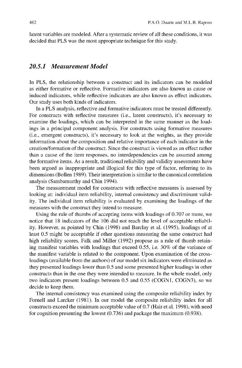
Fig. 1 The PLS handbook’s editors in Beijing (April 2006). From left to right: J ¨
org Henseler as the
Prince, Vincenzo Esposito Vinzi (Editor-in-Chief) as the Emperor, Huiwen Wang as the Empress,
and Wynne W. Chin as the Minister
to several application ﬁelds. For instance, national customer satisfaction indices
(e.g. the Swedish Barometer of Satisfaction by Fornell (1992), the American Cus-
tomer Satisfaction Index by Fornell et al. (1996)) have become the application par
excellence of PLS Path Modeling. Many other applications are found in Strategic
Management (Birkinshaw et al., 1995; Hulland, 1999), Knowledge Management
(Gray and Meister, 2004), Information Technology Management (Gefen and Straub,
1997; Yi and D avis , 2003; Venkatesh and Agarwal, 2006) as well as within var-
ious disciplines of Marketing, such as Relationship Marketing (Reinartz et al.,
2004), Business-to-Business Marketing (Ulaga and Eggert, 2006) and International
Marketing (Singh et al., 2006), just to mention a short, and by no means exhaustive,
list of references.
2 The Handbook in a Nutshell
This Handbook consists of three parts featuring 33 papers selected after three rounds
of a peer reviewing process. In the ﬁrst part, contemporary methodological develop-
ments of PLS analysis are the focus. The second part contains a set of applications
of PLS in the ﬁeld of Marketing as well as in related ﬁelds. The pedagogical
contributions in the third part reﬂect tutorials on key aspects of PLS analysis.

Editorial
5
2.1 Part I: Methods of Partial Least Squares
2.1.1 PLS Path Modeling: Concepts, Model Estimation, and Assessment
Theo K. Dijkstra: Latent Variables and Indices – Herman Wold’s Basic Design and
Partial Least Squares
In this chapter it is shown that the PLS-algorithms typically converge if the covari-
ance matrix of the indicators satisﬁes (approximately) the ‘basic design’, a factor
analysis type of model. The algorithms produce solutions to ﬁxed point equations;
the solutions are smooth functions of the sample covariance matrix of the indicators.
If the latter matrix is asymptotically normal, the PLS estimators will share this
property. The probability limits, under the basic design, of the PLS-estimators for
loadings, correlations, multiple R2’s, coefﬁcients of structural equations et cetera
will differ from the true values. But the difference is decreasing, tending to zero,
in the ‘quality’ of the PLS estimators for the latent variables. It is indicated how to
correct for the discrepancy between true values and the probability limits. The con-
tribution deemphasizes the ‘normality’-issue in discussions about PLS versus ML:
in employing either method one is not required to subscribe to normality; they are
‘just’ different ways of extracting information from second-order moments.
Dijkstra also proposes a new ‘back-to-basics’ research program, moving away
from factor analysis models and returning to the original object of constructing
indices that extract information from high-dimensional data in a predictive, useful
way. For the generic case one would construct informative linear compounds, whose
constituent indicators have non-negative weights as well as non-negative loadings,
satisfying constraints implied by the path diagram. Cross-validation could settle
the choice between various competing speciﬁcations. In short: it is argued for an
upgrade of principal components and canonical variables analysis.
Vincenzo Esposito Vinzi, Laura Trinchera, and Silvano Amato: PLS Path
Modeling: From Foundations to Recent Developments and Open Issues for Model
Assessment and Improvement
In this chapter the Authors ﬁrst present the basic algorithm of PLS Path Modeling by
discussing some recently proposed estimation options. Namely they introduce the
development of new estimation modes and schemes for multidimensional (forma-
tive) constructs, i.e. the use of PLS Regression for formative indicators, and the use
of path analysis on latent variable scores to estimate path coefﬁcients Furthermore,
they focus on the quality indexes classically used to assess the performance of the
model in terms of explained variances. They also present some recent developments
in PLS Path Modeling framework for model assessment and improvement, includ-
ing a non-parametric GoF-based procedure for assessing the statistical signiﬁcance
of path coefﬁcients. Finally, they discuss the REBUS-PLS algorithm that enables
to improve the prediction performance of the model by capturing unobserved

6
V. Esposito Vinzi et al.
heterogeneity. The chapter ends with a brief sketch of open issues in the area that,
in the Authors’ opinion, currently represent major research challenges.
Wynne W. Chin: Bootstrap Cross-validation Indices for PLS Path Model
Assessment
The goal of PLS path modeling is primarily to estimate the variance of endogenous
constructs and in turn their respective manifest variables (if reﬂective). Models with
signiﬁcant jackknife or bootstrap parameter estimates may still be considered invalid
in a predictive sense. In this paper, Chin attempts to reorient researchers from the
current emphasis of assessing the signiﬁcance of parameter estimates (e.g., loadings
and structural paths) to that of predictive validity. Speciﬁcally, his paper examines
how predictive indicator weights estimated for a particular PLS structural model are
when applied on new data from the same population. Bootstrap resampling is used
to create new data sets where new R-square measures are obtained for each endoge-
nous construct in a model. Chin introduces the weighted summed (WSD) R-square
representing how predictive the original sample weights are in a new data context
(i.e., a new bootstrap sample). In contrast, the Simple Summed (SSD) R-square
examines the predictiveness using the simpler approach of unit weights. From this,
Chin develops his Relative Performance Index (RPI) representing the degree to
which the PLS weights yield better predictiveness for endogenous constructs than
the simpler procedure of performing regression after simple summing of indicators.
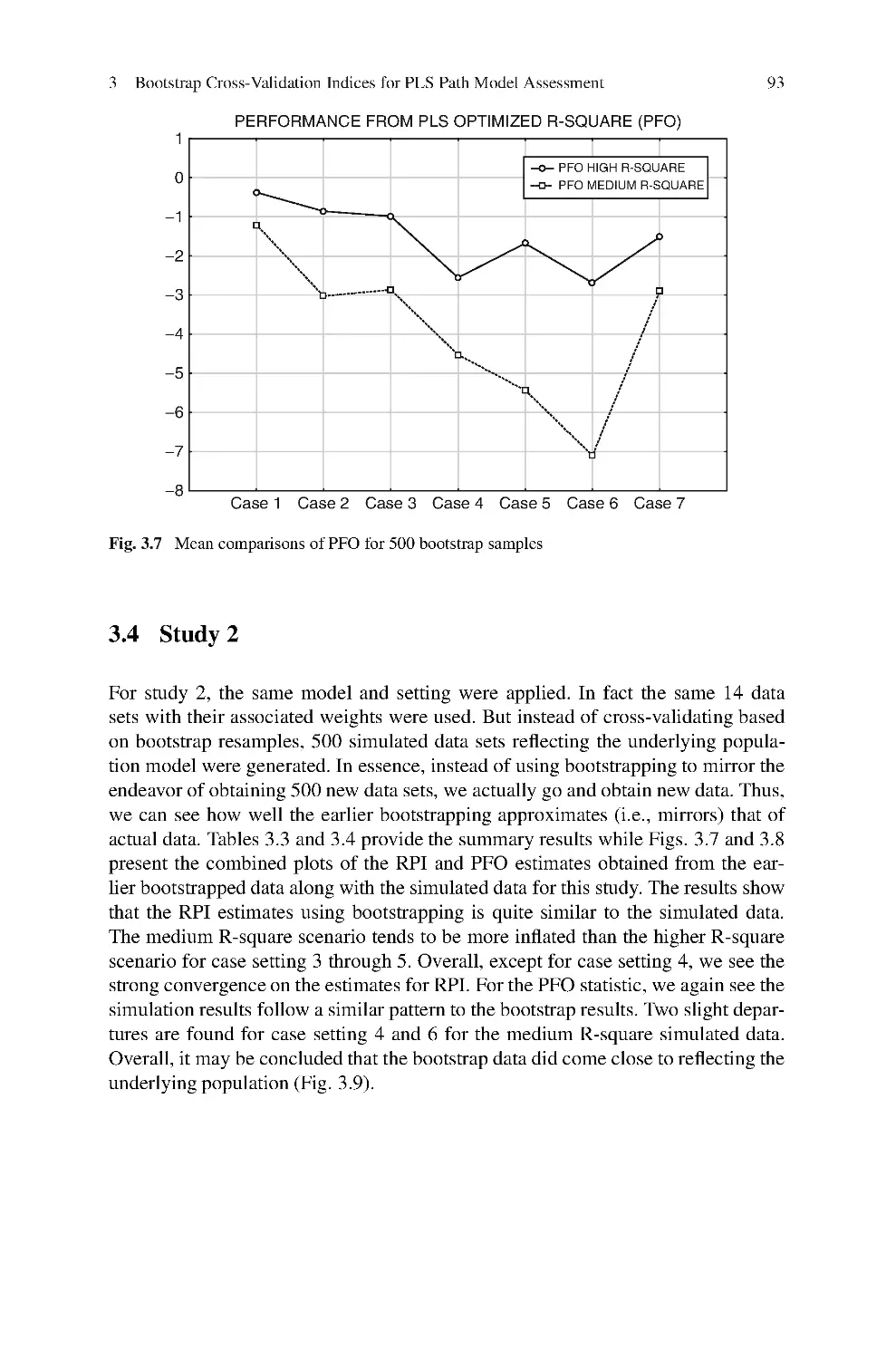
Chin also introduces a Performance from Optimized Summed Index (PFO) to con-
trast the WSD R-squares to the R-squares obtained when the PLS algorithm is used
on each new bootstrap data set. Results from 2 simulation studies are presented.
Overall, in contrast to Q-square which examines predictive relevance at the indica-
tor level, the RPI and PFO indices are shown to provide additional information to
assess predictive relevance of PLS estimates at the construct level. Moreover, it is
argued that this approach can be applied to other same set data indices such as AVE
(Fornell and Larcker, 1981) and GoF (Tenenhaus, Amato, and Esposito Vinzi, 2004)
to yield RPI-AVE, PFO-AVE. RPI-GoF, and PFO-GoF indices.
2.1.2 PLS Path Modeling: Extensions
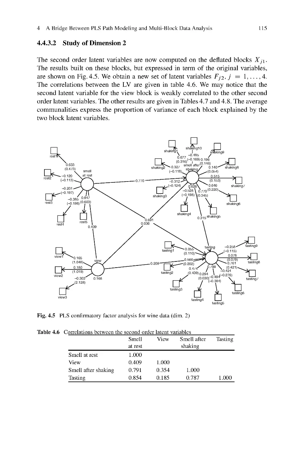
Michel Tenenhaus and Mohamed Hanaﬁ: A Bridge Between PLS Path Modeling
and Multiblock Data Analysis
A situation where J blocks of variables X1;:::;XJ are observed on the same set
of individuals is considered in this paper. A factor analysis approach is applied to
blocks instead of variables. The latent variables (LV’s) of each block should well
explain their own block and at the same time the latent variables of same order
should be as highly correlated as possible (positively or in absolute value). Two path
models can be used in order to obtain the ﬁrst order latent variables. The ﬁrst one

Editorial
7
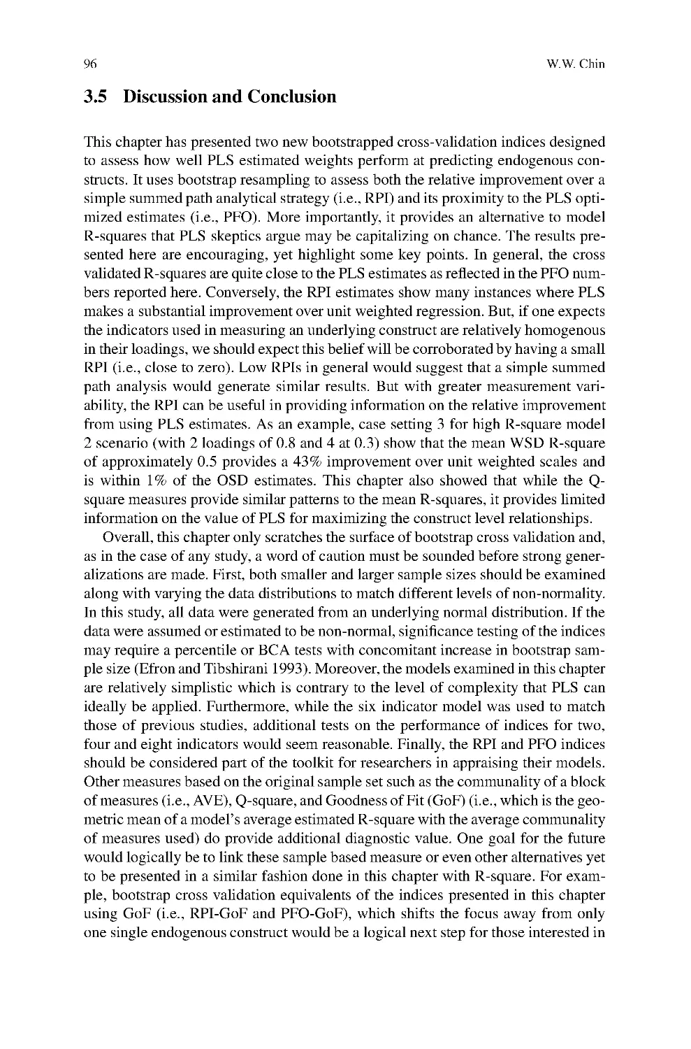
is related to conﬁrmatory factor analysis: each LV related to one block is connected
to all the LV’s related to the other blocks. Then, PLS Path Modeling is used with
mode A and centroid scheme. Use of mode B with centroid and factorial schemes
is also discussed. The second model is related to hierarchical factor analysis. A
causal model is built by relating the LV’s of each block Xj to the LV of the super-
block XJ C1 obtained by concatenation of X1;:::;XJ . Using PLS estimation of
this model with mode A and path-weighting scheme gives an adequate solution for
ﬁnding the ﬁrst order latent variables. The use of mode B with centroid and factorial
schemes is also discussed. The higher order latent variables are found by using the
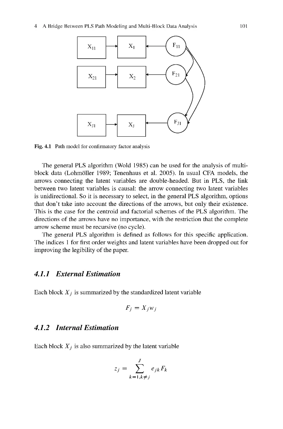
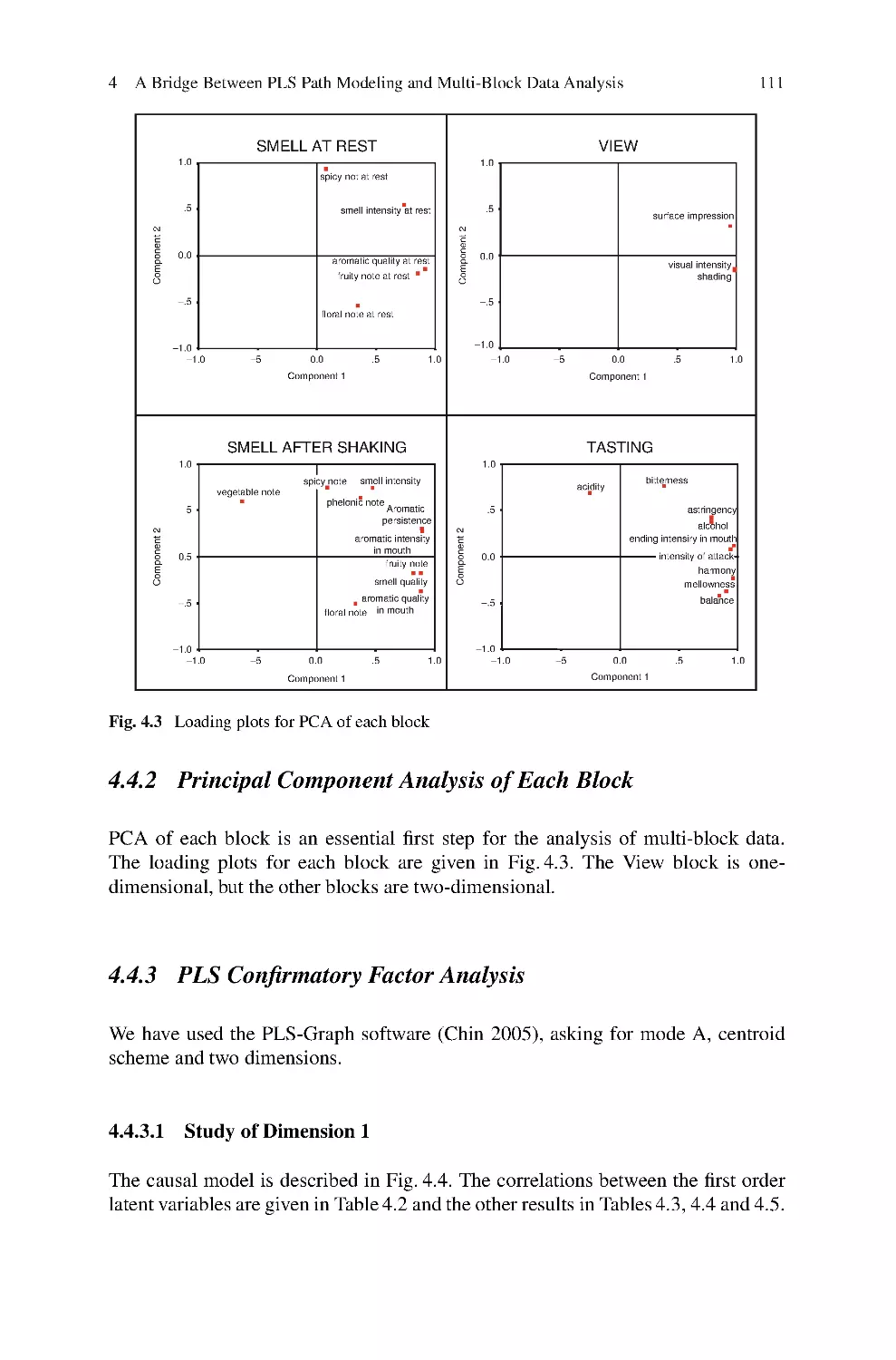
same algorithms on the deﬂated blocks. The ﬁrst approach is compared with the
MAXDIFF/MAXBET Van de Geer’s algorithm (1984) and the second one with the
ACOM algorithm (Chessel and Hanaﬁ, 1996). Sensory data describing Loire wines
are used to illustrate these methods.
Michel Tenenhaus, Emmanuelle Mauger, and Christiane Guinot: Use of ULS-SEM
and PLS-SEM to Measure a Group Effect in a Regression Model Relating Two
Blocks of Binary Variables
The objective of this constribution is to describe the use of unweighted least
squares structural equation modelling and partial least squares path modelling in
a regression model relating two blocks of binary variables when a group effect can
inﬂuence the relationship. These methods were applied on the data of a question-
naire investigating sun exposure behaviour addressed to a cohort of French adult
in the context of the SU.VI.MAX epidemiological study. Sun protection and expo-
sure behaviours were described according to gender and class of age (less than 50
at inclusion in the study versus more than 49). Signiﬁcant statistical differences
were found between men and women, and between classes of age. This paper illus-
trates the various stages in the construction of latent variables or scores, based on
qualitative data. These kind of scores is widely used in marketing to provide a quan-
titative measure of the phenomenon studied before proceeding to a more detailed
analysis.
Arteaga Francisco, Martina G. Gallarza, and Irene Gil: A New Multiblock PLS
Based Method to Estimate Causal Models. Application to the Post-consumption
Behavior in Tourism
This chapter presents a new method to estimate causal models based on the Multi-
block PLS method (MBPLS) from Wangen and Kowalski (1988). The new method
is compared with the classical LVPLS algorithm from Lohm ¨
oller (1989), using an
academic investigation on the post-consumption behaviour of a particular proﬁle of
university students. The results for both methods are quite similar, but the explained
percentage of variance for the endogenous latent variables is slightly higher for
the MBPLS based method. Bootstrap analysis shows that conﬁdence intervals are
slightly smaller for the MBPLS based method.

8
V. Esposito Vinzi et al.
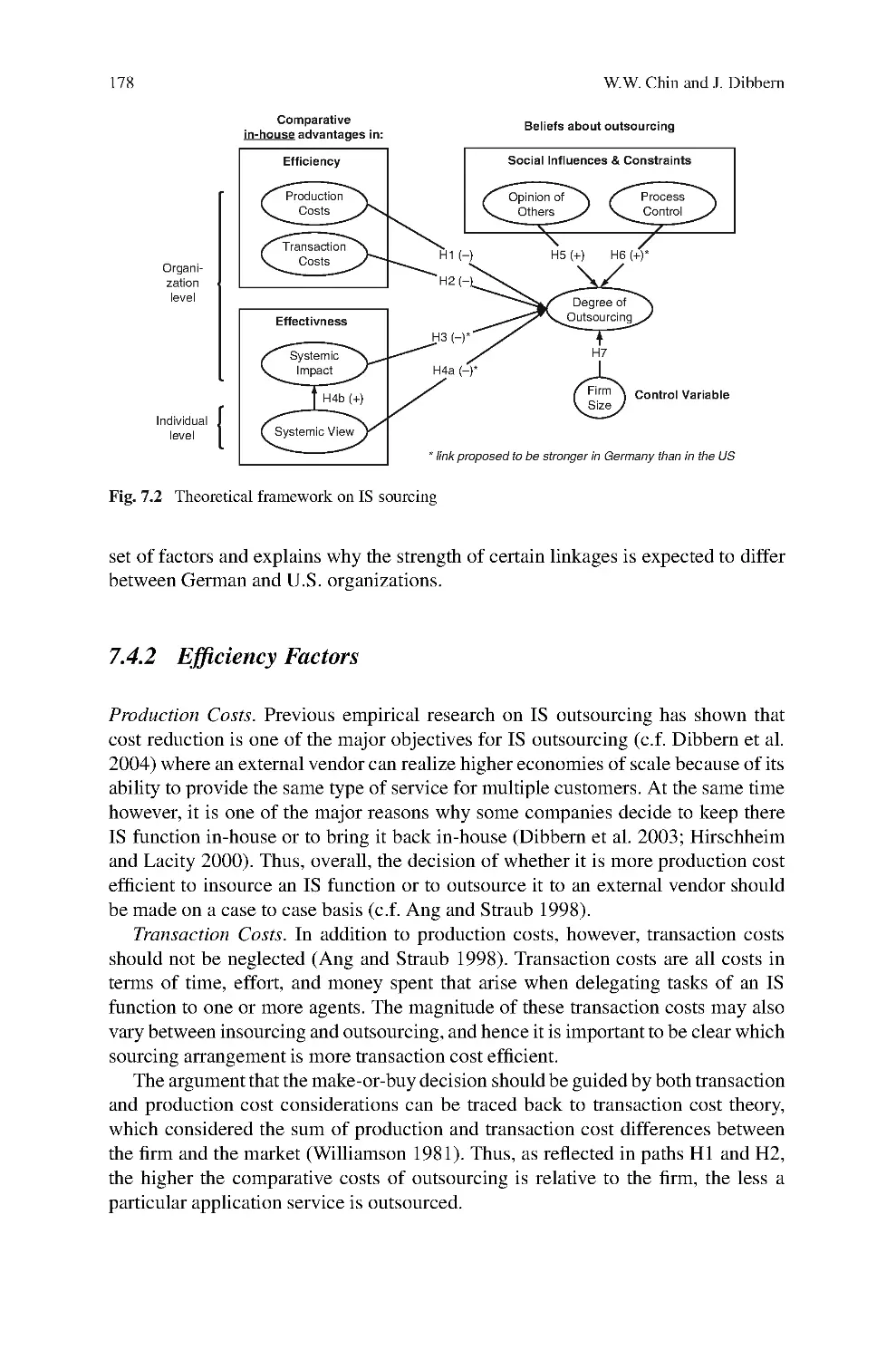
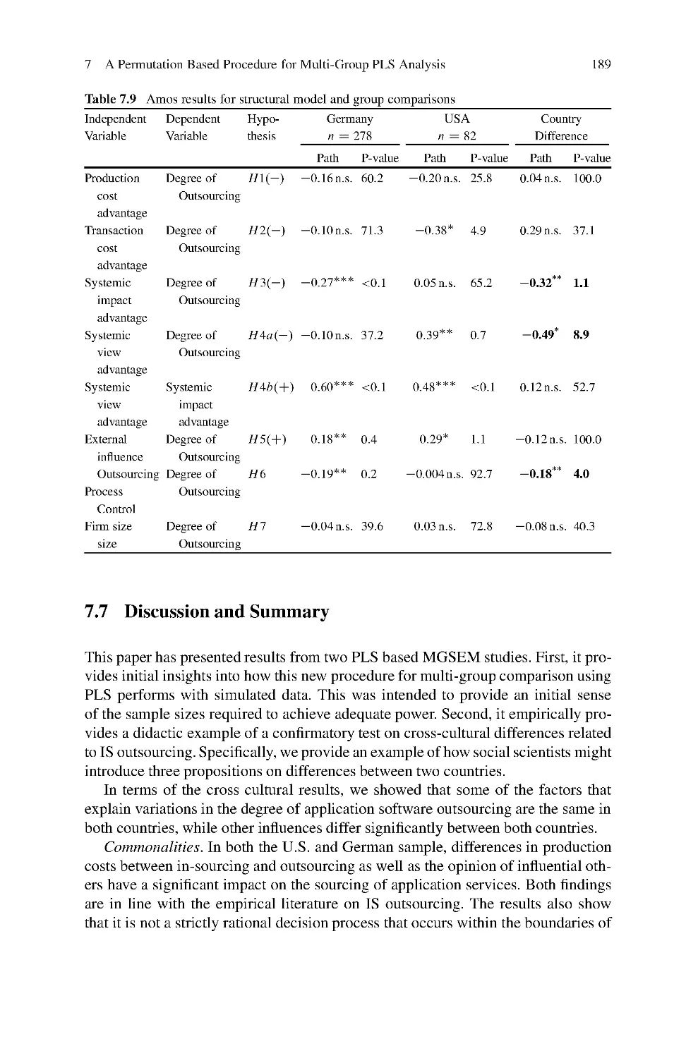
Wynne W. Chin and Jens Dibbern: A Permutation Based Procedure for
Multi-Group PLS Analysis – Results of Tests of Differences on Simulated Data and
a Cross Cultural Analysis of the Sourcing of Information System Services Between
Germany and the USA
This paper presents a distribution free procedure for performing multi-group PLS
analysis. To date, multi-group comparison of PLS models where differences in
path estimates for different sampled populations have been relatively naive. Often,
researchers simply examine and discuss the difference in magnitude of particular
model path estimates for two or more data sets. Problems can occur if the assump-
tion of normal population distribution or similar sample size is not tenable. This
paper by Chin and Dibbern presents an alternative distribution free approach via an
approximate randomization test - where a subset of all possible data permutations
between sample groups is made. The performance of this permutation procedure is
applied on both simulated data and a study exploring the differences of factors that
impact outsourcing between the countries of US and Germany.
2.1.3 PLS Path Modeling with Classiﬁcation Issues
Christian M. Ringle, Sven Wende, and Alexander Will: Finite Mixture Partial Least
Squares Analysis: Methodology and Numerical Examples
In a wide range of applications for empirical data analysis, the assumption that
data is collected from a single homogeneous population is often unrealistic. In
particular, the identiﬁcation of different groups of consumers and their appropri-
ate consideration in partial least squares (PLS) path modeling constitutes a critical
issue in marketing. The authors introduce a ﬁnite mixture PLS software imple-
mentation, which separates data on the basis of the estimates’ heterogeneity in
the inner path model. Numerical examples using experimental as well as empirical
data allow the veriﬁcation of the methodology’s effectiveness and usefulness. The
approach permits a reliable identiﬁcation of distinctive customer segments along
with characteristic estimates for relationships between latent variables. Researchers
and practitioners can employ this method as a model evaluation technique and
thereby assure that results on the aggregate data level are not affected by unobserved
heterogeneity in the inner path model estimates. Otherwise, the analysis provides
further indications on how to treat that problem by forming groups of data in order
to perform a multi-group path analysis.
Silvia Squillacciotti: Prediction oriented classiﬁcation in PLS Path Modeling
Structural Equation Modeling methods traditionally assume the homogeneity of all
the units on which a model is estimated. In many cases, however, this assumption
may turn to be false; the presence of latent classes not accounted for by the global
model may lead to biased or erroneous results in terms of model parameters and

Editorial
9
model quality. The traditional multi-group approach to classiﬁcation is often unsat-
isfying for several reasons; above all because it leads to classes homogeneous only
with respect to external criteria and not to the theoretical model itself.
In this paper, a prediction-oriented classiﬁcation method in PLS Path Modelling
is proposed. Following PLS Typological Regression, the proposed methodology
aims at identifying classes of units showing the lowest distance from the models
in the space of the dependent variables, according to PLS predictive oriented logic.
Hence, the obtained groups are homogeneous with respect to the deﬁned path model.
An application to real data in the study of customers’ satisfaction and loyalty will
be shown.
Valentina Stan and Gilbert Saporta: Conjoint use of variables clustering and PLS
structural equations modeling
In the PLS approach, it is frequently assumed that the blocks of variables satisfy the
assumption of unidimensionality. In order to fulﬁll at best this assumption, this con-
tribution uses clustering methods of variables. illustrate the conjoint use of variables
clustering and PLS path modeling on data provided by PSA Company (Peugeot
Citro ¨
en) on customer satisfaction. The data are satisfaction scores on 32 manifest
variables given by 2922 customers.
2.1.4 PLS Path Modeling for Customer Satisfaction Studies
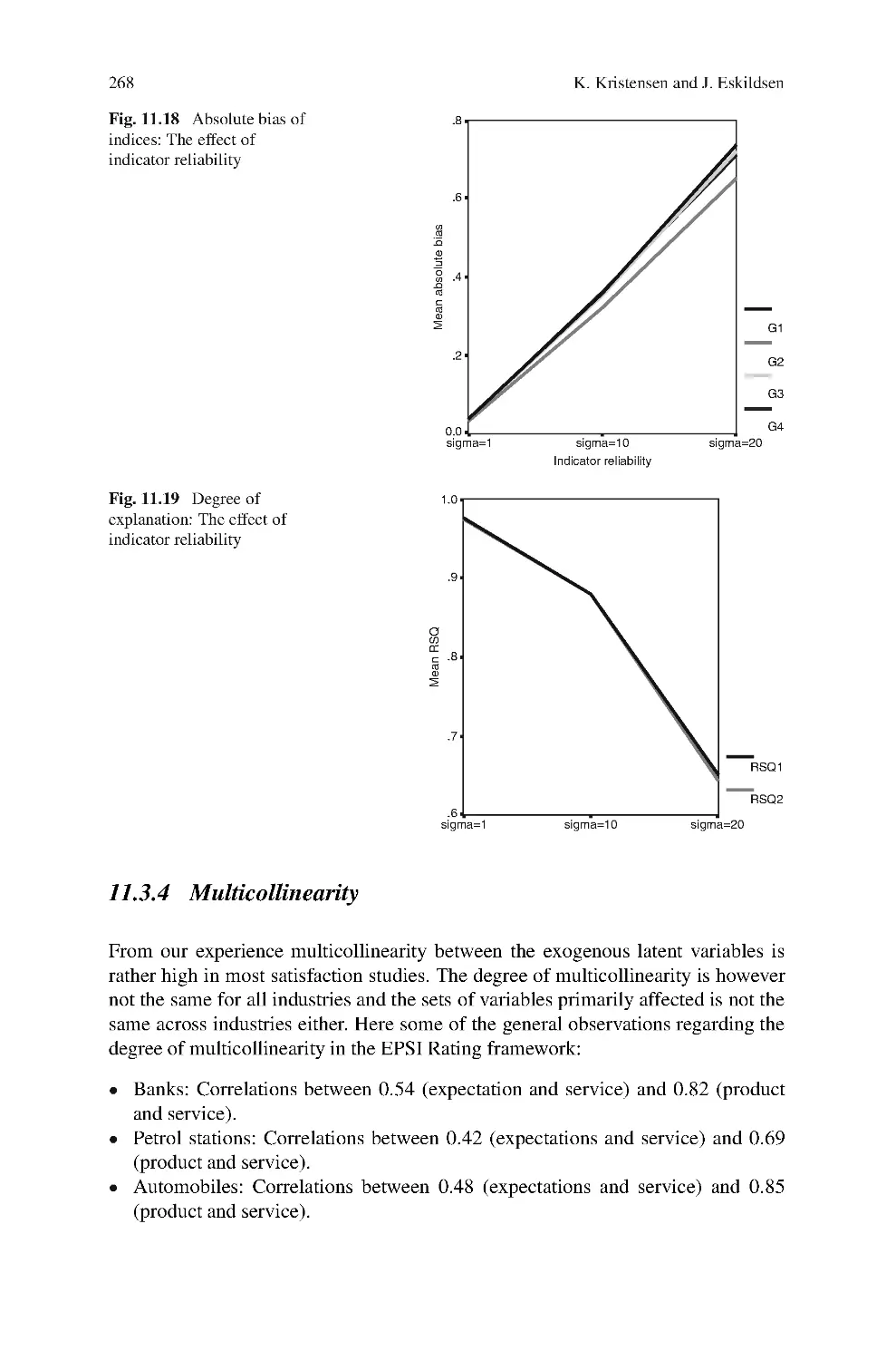
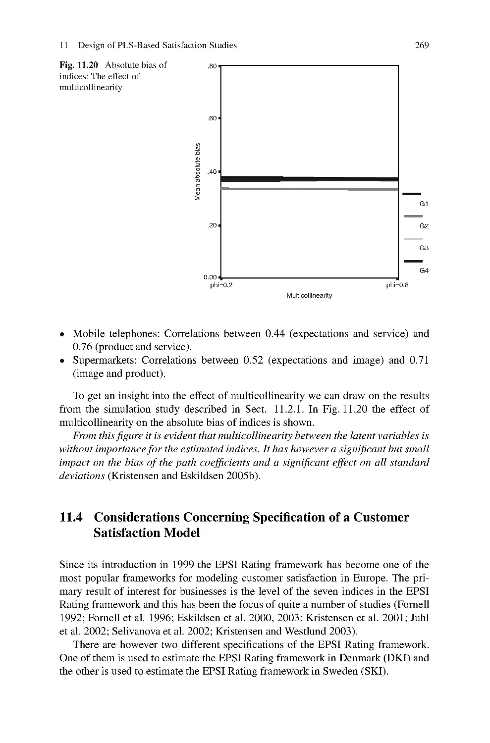
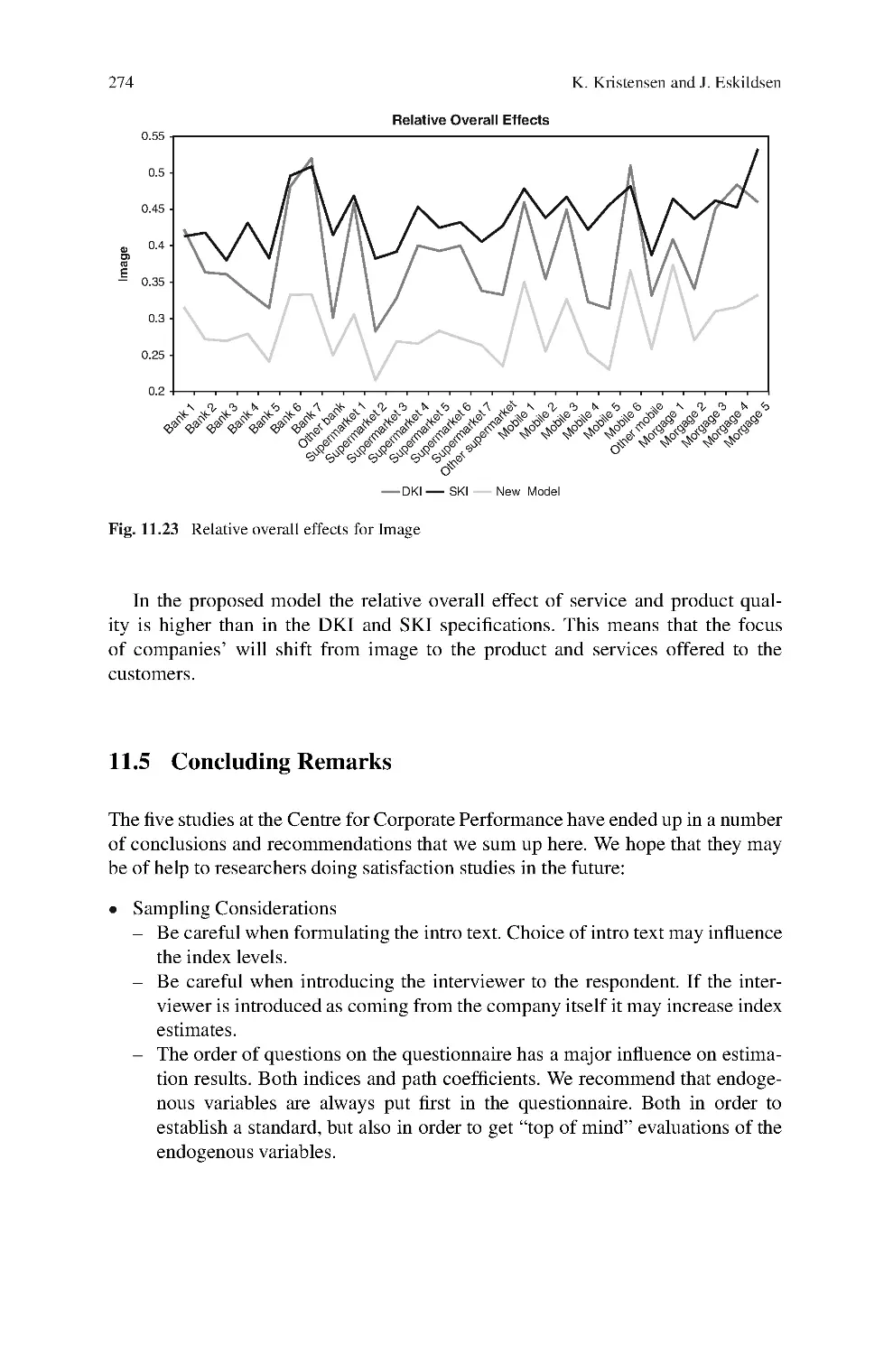
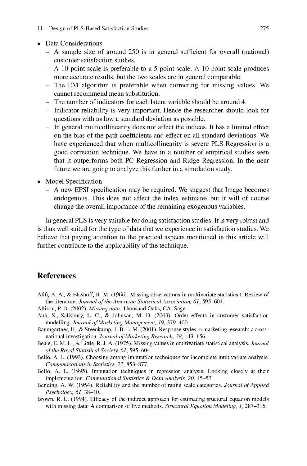
Kai Kristensen and Jacob K. Eskildsen: Design of PLS-based Satisfaction Studies
This chapter focuses on the design of PLS structural equation models with respect
to satisfaction studies. The authors summarize the ﬁndings of previous studies,
which have found the PLS technique to be affected by aspects as the skewness
of manifest variables, multicollinearity between latent variables, misspeciﬁcation,
question order, sample size as well as the size of the path coefﬁcients. Moreover,
the authors give recommendations based on an empirical PLS project conducted
at the Aarhus School of Business. Within this project ﬁve different studies have
been conducted, covering a variety of aspects of designing PLS-based satisfaction
studies.
Clara Cordeiro, Alexandra Mach ´
as, and Maria Manuela Neves: A Case Study of a
Customer Satisfaction Problem – Bootstrap and Imputation Techniques
Bootstrap is a resampling technique proposed by Efron. It has been used in many
ﬁelds, but in case of missing data studies one can ﬁnd only a few references. Most
studies in marketing research are based in questionnaires, that, for several reasons
present missing responses. The missing data problem is a common issue in market
research. Here, a customer satisfaction model following the ACSI barometer from

10
V. Esposito Vinzi et al.
Fornell will be considered. Sometimes, not all customer experience all services or
products. Therefore, one may have to deal with missing data, taking the risk of
reaching non-signiﬁcant impacts of these drivers on CS and resulting in inaccurate
inferences. To estimate the main drivers of Customer Satisfaction, Structural Equa-
tion Models methodology is applied. For a case study in mobile telecommunications
several missing data imputation techniques were reviewed and used to complete the
data set. Bootstrap methodology was also considered jointly with imputation tech-
niques to complete the data set. Finally, using Partial Least Squares (PLS) algorithm,
the authors could compare the above procedures. It suggests that bootstrapping
before imputation can be a promising idea.
Manuel J. Vilares, Maria H. Almeida, and Pedro Sim ˜
oes Coelho: Comparison of
Likelihood and PLS Estimators for Structural Equation Modeling – A Simulation
with Customer Satisfaction Data
Although PLS is a well established tool to estimate structural equation models,
more work is still needed in order to better understand its relative merits when com-
pared to likelihood methods. This paper aims to contribute to a better understanding
of PLS and likelihood estimators’ properties, through the comparison and evalua-
tion of these estimation methods for structural equation models based on customer
satisfaction data. A Monte Carlo simulation is used to compare the two estima-
tion methods. The model used in the simulation is the ECSI (European Customer
Satisfaction Index) model, constituted by 6 latent variables (image, expectations,
perceived quality, perceived value, customer satisfaction and customer loyalty). The
simulation is conducted in the context of symmetric and skewed response data and
formative blocks, which constitute the typical framework of customer satisfaction
measurement. In the simulation we analyze the ability of each method to adequately
estimate the inner model coefﬁcients and the indicator loadings. The estimators are
analyzed both in terms of bias and precision. Results have shown that globally PLS
estimates are generally better than covariance-based estimates both in terms of bias
and precision. This is particularly true when estimating the model with skewed
response data or a formative block, since for the model based on symmetric data
the two methods have shown a similar performance.
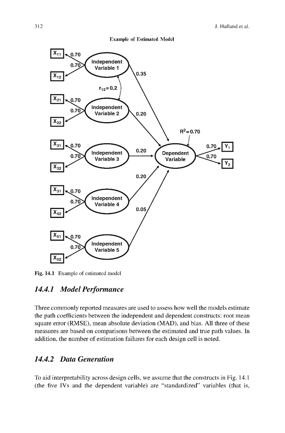
John Hulland, M.J. Ryan, and R.K. Rayner: Modeling Customer Satisfaction: A
Comparative Performance Evaluation of Covariance Structure Analysis versus
Partial Least Squares
Partial least squares (PLS) estimates of structural equation model path coefﬁcients
are believed to produce more accurate estimates than those obtained with covari-
ance structure analysis (CVA) using maximum likelihood estimation (MLE) when
one or more of the MLE assumptions are not met. However, there exists no empir-
ical support for this belief or for the speciﬁc conditions under which it will occur.

Editorial
11
MLE-based CVA will also break down or produce improper solutions whereas PLS
will not. This study uses simulated data to estimate parameters for a model with 5
independent latent variables and 1 dependent latent variable under various assump-
tion conditions. Data from customer satisfaction studies were used to identify the
form of typical ﬁeld-based survey distributions. Our results show that PLS produces
more accurate path coefﬁcients estimates when sample sizes are less than 500, inde-
pendent latent variables are correlated, and measures per latent variable are less
than 4. Method accuracy does not vary when the MLE multinormal distribution
assumption is violated or when the data do not ﬁt the theoretical structure very well.
Both procedures are more accurate when the independent variables are uncorrelated,
but MLE estimations break down more frequently under this condition, especially
when combined with sample sizes of less than 100 and only two measures per latent
variable.
2.1.5 PLS Regression
Swante Wold, Lennart Eriksson, and Nouna Kettaneh-Wold: PLS in Data Mining
and Data Integration
Data mining by means of projection methods such as PLS (projection to latent struc-
tures), and their extensions is discussed. The most common data analytical questions
in data mining are covered, and illustrated with examples.
1. Clustering, i. e., ﬁnding and interpreting “natural” groups in the data,
2. Classiﬁcation and identiﬁcation, e. g., biologically active compounds vs. inactive,
3. Quantitative relationships between different sets of variables, e. g., ﬁnding vari-
ables related to quality of a product, or related to time, seasonal or/and geograph-
ical change.
Sub-problems occurring in both (1) to (3) are discussed.
1. Identiﬁcation of outliers and their aberrant data proﬁles,
2. Finding the dominating variables and their joint relationships, and
3. Making predictions for new samples.
The use of graphics for the contextual interpretation of results is emphasized. With
many variables and few observations – a common situation in data mining – the risk
to obtain spurious models is substantial. Spurious models look great for the training
set data, but give miserable predictions for new samples. Hence, the validation of
the data analytical results is essential, and approaches for that are discussed.
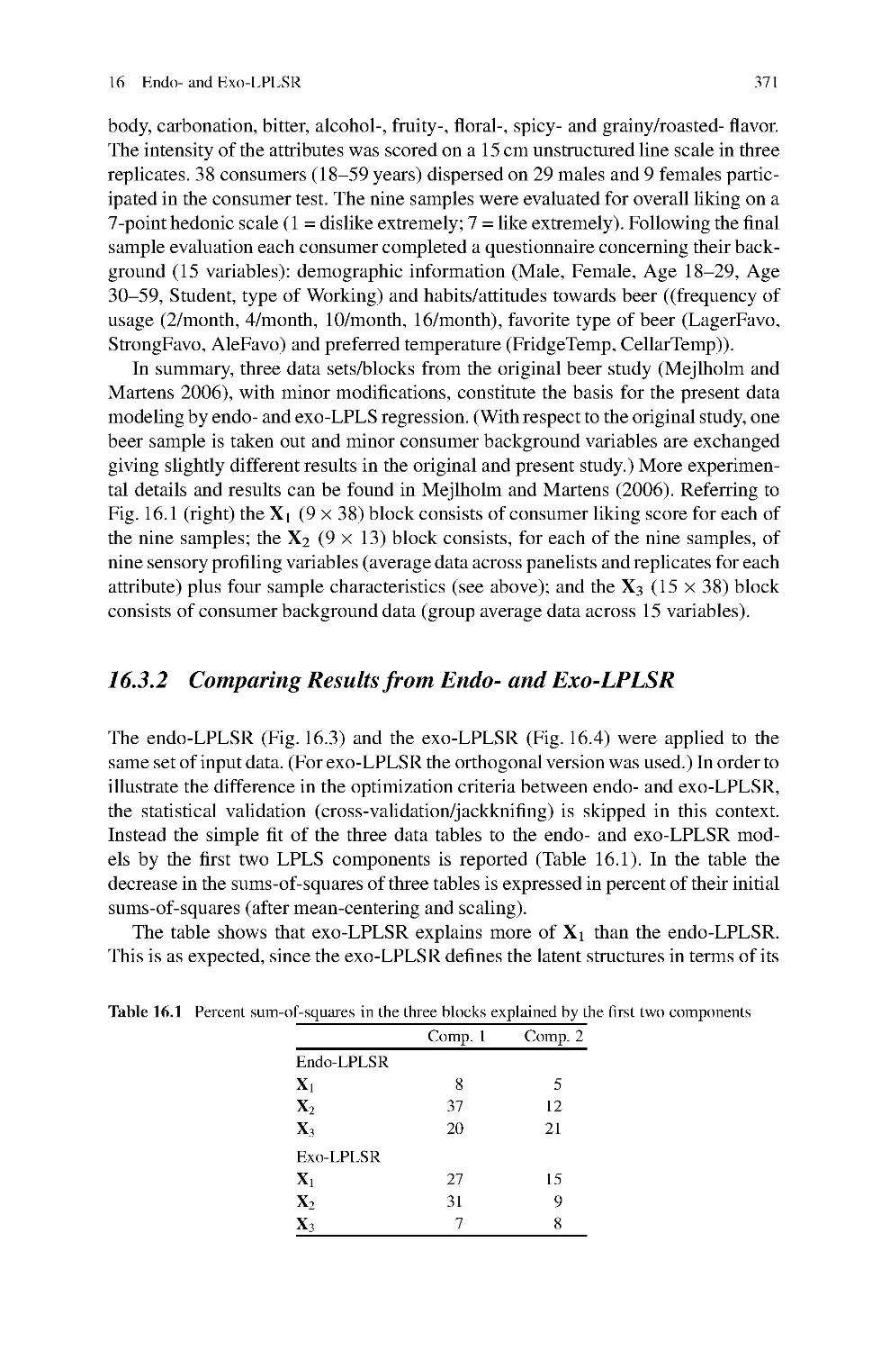
Solve Sæbø, Harald Martens, and Magni Martens: Three-block Data Modeling by
Endo- and Exo-LPLS Regression
In consumer science it is common to study how various products are liked or
ranked by various consumers. In this context, it is important to check if there are

12
V. Esposito Vinzi et al.
different consumer groups with different product preference patterns. If systematic
consumer grouping is detected, it is necessary to determine the person character-
istics, which differentiate between these consumer segments, so that they can be
reached selectively. Likewise it is important to determine the product characteristics
that consumer segments seem to respond differently to.
Consumer preference data are usually rather noisy. The productspersons data
table (X1) usually produced in consumer preference studies may therefore be sup-
plemented with two types of background information: a productsproduct-property
data table (X2)a
ndape
r
s
o
n
person-property data table (X3). These additional
data may be used for stabilizing the data modelling of the preference data X1 sta-
tistically. Moreover, they can reveal the product-properties that are responded to
differently by the different consumer segment, and the person-properties that char-
acterize these different segments. The present chapter outlines a recent approach to
analyzing the three types of data tables in an integrated fashion and presents new
modelling methods in this context.
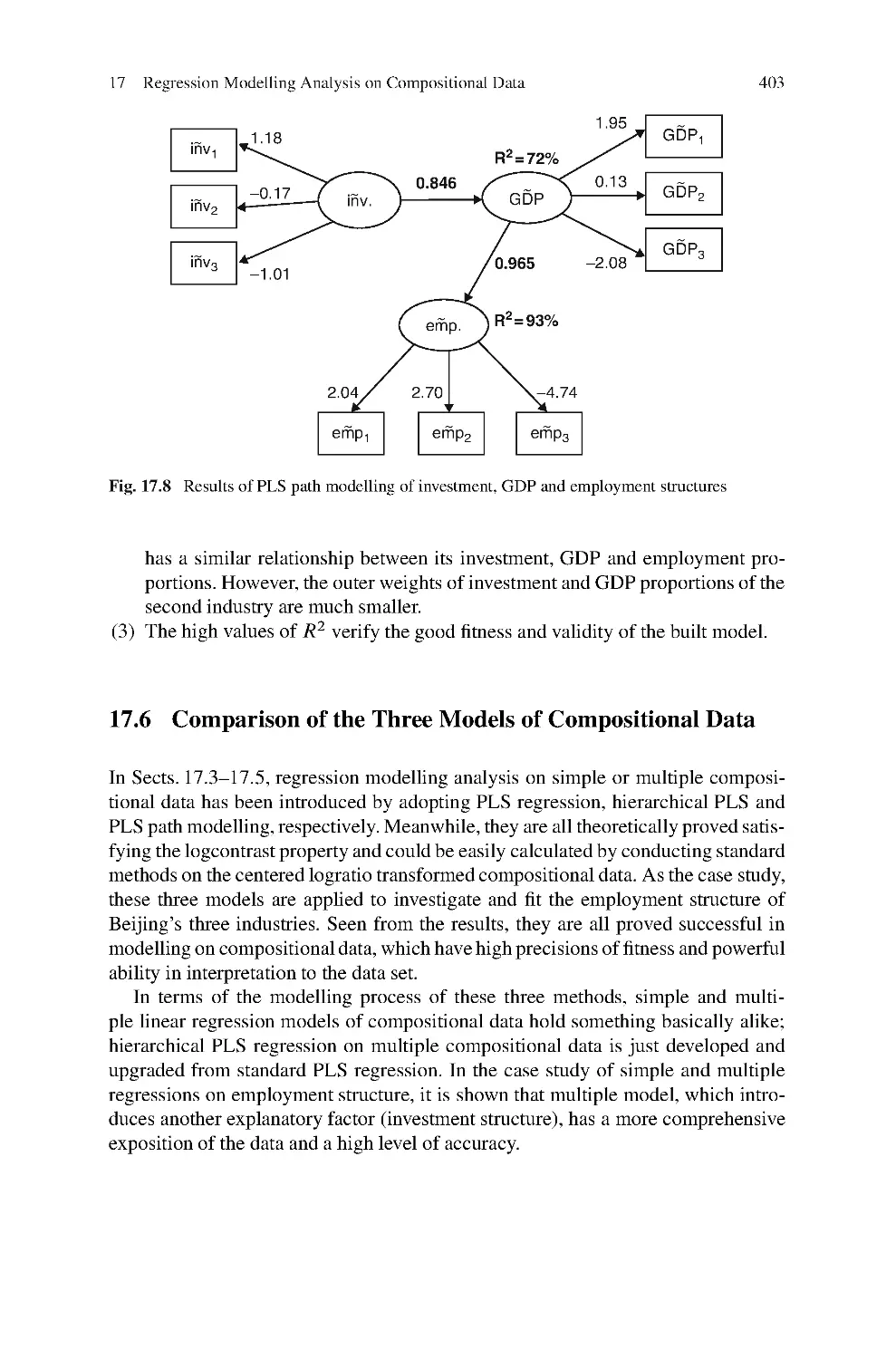
on Compositional Data
In data analysis of social, economic and technical ﬁelds, compositional data is
widely used in problems of proportions to the whole. This paper develops regres-
sion modelling methods of compositional data, discussing the relationships of one
compositional data to one or more than one compositional data and the interrelation-
ship of multiple compositional data. By combining centered logratio transformation
proposed by Aitchison (1986) with Partial Least Squares (PLS) related techniques,
that is PLS regression, hierarchical PLS and PLS path modelling, respectively, par-
ticular difﬁculties in compositional data regression modelling such as sum to unit
constraint, high multicollinearity of the transformed compositional data and hier-
archical relationships of multiple compositional data, are all successfully resolved;
moreover, the modelling results rightly satisﬁes the theoretical requirement of log-
contrast. Accordingly, case studies of employment structure analysis of Beijing’s
three industries also illustrate high goodness-of-ﬁt and powerful explainability of
the models.
2.2 Part II: Applications to Marketing and Related Areas
S¨
onke Albers: PLS and Success Factor Studies in Marketing
While in consumer research the “Cronbachs ˛ - LISREL”-paradigm has emerged for
a better separation of measurement errors and structural relationships, it is shown
in this chapter that studies which involve an evaluation of the effectiveness of mar-
keting instruments require the application of PLS. This is because one no longer
Huiwen Wang, Jie Meng, and Michel Tenenhaus: Regression Modelling Analysis

Editorial
13
distinguishes between constructs and their reﬂecting measures but rather between
abstract marketing policies (constructs) and their forming detailed marketing instru-
ments (indicators). It is shown with the help of examples from literature that many
studies of this type applying LISREL have been misspeciﬁed and had better made
use of the PLS approach. The author also demonstrates the appropriate use of PLS
in a study of success factors for e-businesses. He concludes with recommendations
on the appropriate design of success factor studies including the use of higher-order
constructs and the validation of such studies.
Carmen Barroso, Gabriel Cepeda Carri ´
on, and Jos´
eL.Rold´
an: Applying
Maximum Likelihood and PLS on Different Sample Sizes – Studies on Servqual
Model and Emloyee Behaviour Model
Structural equation modeling (SEM) has been increasingly utilized in marketing
and management areas. This rising deployment of SEM suggests addressing com-
parisons between different SEM approaches. This would help researchers to choose
which SEM approach is more appropriate for their studies. After a brief review
of the SEM theoretical background, this study analyzes two models with differ-
ent sample sizes by employing two different SEM techniques to the same set of
data. The two SEM techniques compared are: Covariance-based SEM (CBSEM),
speciﬁcally maximum likelihood (ML) estimation, and Partial Least Square (PLS).
After the study ﬁndings, the paper provides insights in order to suggest to the
researchers when to analyze models with CBSEM or PLS. Finally, practical sug-
gestions about PLS use are added and we discuss whether they are considered by
researchers.
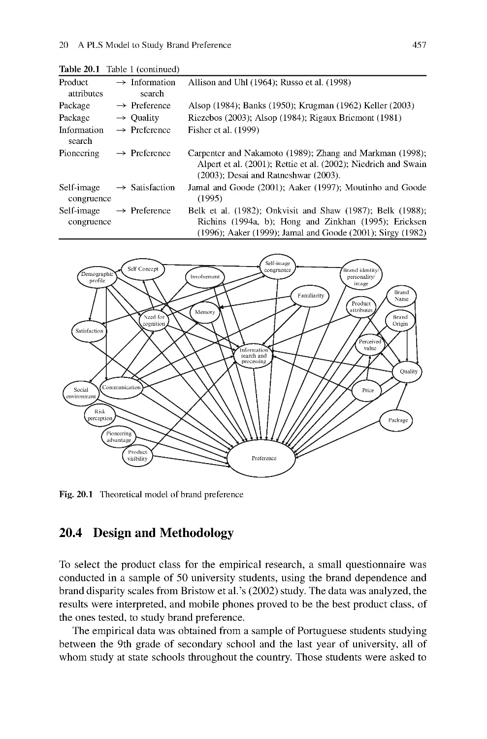
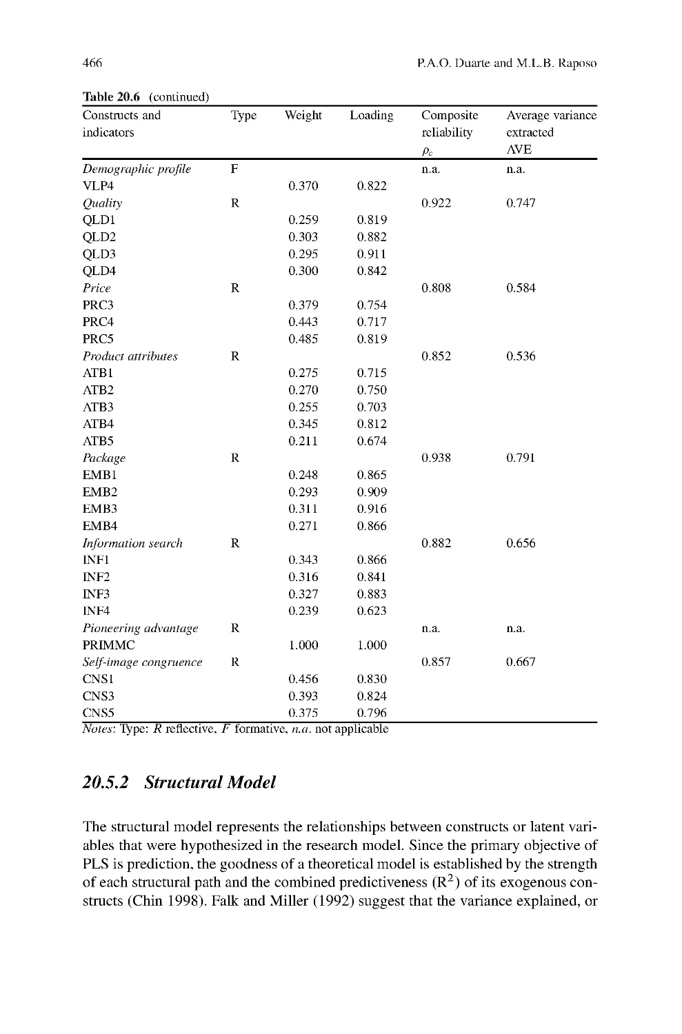
Paulo Alexandre O. Duarte and Mario Lino B. Raposo: A PLS Model to Study
Brand Preference – An Application to the Mobile Phone Market
Brands play an important role in consumers’ daily life and can represent a big asset
for companies owning them. Due to the very close relationship between brands and
consumers, and the speciﬁc nature of branded products as an element of consumer
life style, the branded goods industry needs to extend its knowledge of the pro-
cess of brand preference formation in order to enhance brand equity. This chapter
shows how Partial Least Squares (PLS) path modeling can be used to successfully
test complex models where other approaches would fail due to the high number of
relationships, constructs and indicators, here with an application to brand preference
formation for mobile phones. With a wider set of explanatory factors than prior stud-
ies, this one explores the factors that contribute to the formation of brand preference
using a PLS model to understand the relationship between those and consumer pref-
erence on mobile phone brands. The results reveal that brand identity, personality,
and image, together with self-image congruence have the highest impact on brand
preference. Some other factors linked to the consumer and the situation also affect
preference, but in a lower degree.

14
V. Esposito Vinzi et al.
Markus Eberl: An Application of PLS in Multi-group Analysis – The Need for
Differentiated Corporate-level Marketing in the Mobile Communications Industry
The paper focuses on the application of a very common research issue in marketing:
the analysis of the differences between groups’ structural relations. Although PLS
path modeling has some advantages over covariance-based structural equation mod-
eling (CBSEM) regarding this type of research issue – especially in the presence of
formative indicators – few publications employ this method. This paper therefore
presents an exemplary model that examines the effects of corporate-level marketing
activities on corporate reputation as a mediating construct and, ﬁnally, on customer
loyalty. PLS multi-group analysis is used to empirically test for differences between
stakeholder groups in a sample from Germany’s mobile communications industry.
Sabrina Helm, Andreas Eggert, and Ina Garnefeld: Modelling the Impact of
Corporate Reputation on Customer Satisfaction and Loyalty Using PLS
Reputation is one of the most important intangible assets of a ﬁrm. For the most
part, recent articles have investigated its impact on ﬁrm proﬁtability whereas its
effects on individual customers have been neglected. Using data from consumers
of an international consumer goods producer, this paper (1) focuses on measuring
and discussing the relationships between corporate reputation, consumer satisfac-
tion, and consumer loyalty and (2) examines possible moderating and mediating
effects among the constructs. We ﬁnd that reputation is an antecedent of satisfac-
tion and loyalty that has hitherto been neglected by management. Furthermore, we
ﬁnd that more than half of the effect of reputation onto loyalty is mediated by sat-
isfaction. This means that reputation can only partially be considered a substitute
for a consumer’s own experiences with a ﬁrm. In order to achieve consumer loyalty,
organizations need to create both, a good reputation and high satisfaction.
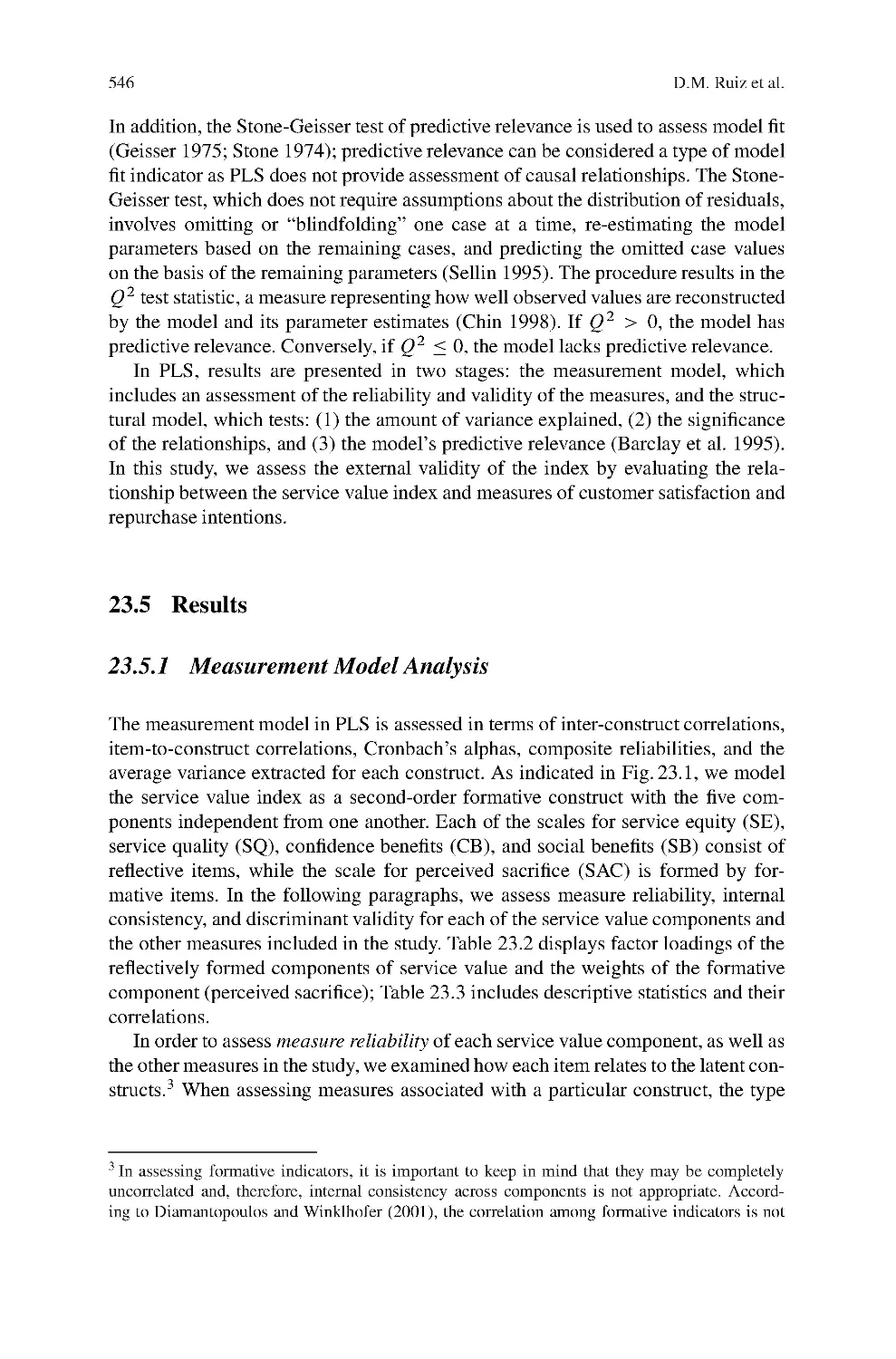
David Mart´ın Ru´ız, Dwayne D. Gremler, Judith H. Washburn, and Gabriel Cepeda
Carri ´
on: Reframing Customer Value in a Service-based Paradigm: An Evaluation
of a Formative Measure in a Multi-industry, Cross-cultural Context
Customer value has received much attention in the recent marketing literature, but
relatively little research has speciﬁcally focused on inclusion of service components
when deﬁning and operationalizing customer value. The purpose of this study is to
gain a deeper understanding of customer value by examining several service ele-
ments, namely service quality, service equity, and relational beneﬁts, as well as
perceived sacriﬁce, in customers’ assessments of value. A multiple industry, cross-
cultural setting is used to substantiate our inclusion of service components and to
examine whether customer value is best modeled using formative or reﬂective mea-
sures. Our results suggest conceptualizing customer value with service components
can be supported empirically, the use of formative components of service value can

Editorial
15
be supported both theoretically and empirically and is superior to a reﬂective oper-
ationalization of the construct, and that our measure is a robust one that works well
across multiple service contexts and cultures.
Sandra Streukens, Martin Wetzels, Ahmad Daryanto, and Ko de Ruyter: Analyzing
Factorial Data Using PLS: Application in an Online Complaining Context
Structural equation modeling (SEM) can be employed to emulate more traditional
analysis techniques, such as MANOVA, discriminant analysis, and canonical corre-
lation analysis. Recently, it has been realized that this emulation is not restricted to
covariance-based SEM, but can easily be extended to components-based SEM, or
partials least squares (PLS) path analysis. This chapter presents a PLS path mod-
eling apllication to a ﬁxed-effects, between-subjects factorial design in an online
complaint context.
Silvia Thies and S ¨
onke Albers: Application of PLS in Marketing: Content
Strategies in the Internet
In an empirical study the strategies are investigated that content providers follow in
their compensation policy with respect to their customers. The choice of the policy
can be explained by the resource-based view and may serve as recommendations.
The authors illustrate how a strategy study in marketing can be analyzed with the
help of PLS thereby providing more detailed and actionable results. Firstly, complex
measures have to be operationalized by more speciﬁc indicators, marketing instru-
ments in this case, which proved to be formative in the most cases. Only by using
PLS it was possible to extract the inﬂuence of every single formative indicator on the
ﬁnal constructs, i. e. the monetary form of the partnerships. Secondly, PLS allows
for more degrees of freedom so that a complex model could be estimated with a
number of cases that would not be sufﬁcient for ML-LISREL. Thirdly, PLS does
not work with distributional assumptions while signiﬁcance tests can still be car-
ried out with the help of bootstrapping. The use of PLS is recommended for future
strategy studies in marketing because it is possible to extract the drivers at the indi-
cator level so that detailed recommendations can be given for managing marketing
instruments.
Ali T¨
urkyilmaz, Ekrem Tato ˘glu, Selim Zaim, and Cos¸kun ¨
Ozkan: Use of PLS in
TQM Research – TQM Practices and Business Performance in SMEs
Advances in structural equation modeling (SEM) techniques have made it possible
for management researchers to simultaneously examine theory and measures. When
using sophisticated SEM techniques such as covariance based structural equation
modeling (CBSEM) and partial least squares (PLS), researchers must be aware of

16
V. Esposito Vinzi et al.
their underlying assumptions and limitations. SEM models such as PLS can help
total quality management (TQM) researchers to achieve new insights. Researchers
in the area of TQM need to apply this technique properly in order to better under-
stand the complex relationships proposed in their models. This paper makes an
attempt to apply PLS in the area of TQM research. In doing that special emphasis
was placed on identifying the relationships between the most prominent TQM con-
structs and business performance based on a sample of SMEs operating in Turkish
textile industry. The analysis of PLS results indicated that a good deal of support has
been found for the proposed model where a satisfactory percentage of the variance
in the dependent constructs is explained by the independent constructs.
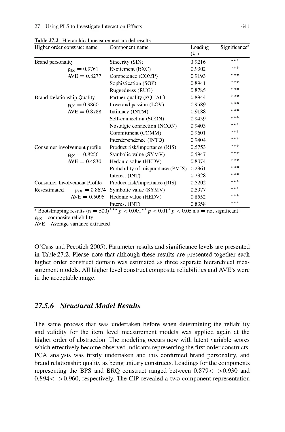
Bradley Wilson: Using PLS to Investigate Interaction Effects Between Higher
Order Branding Constructs
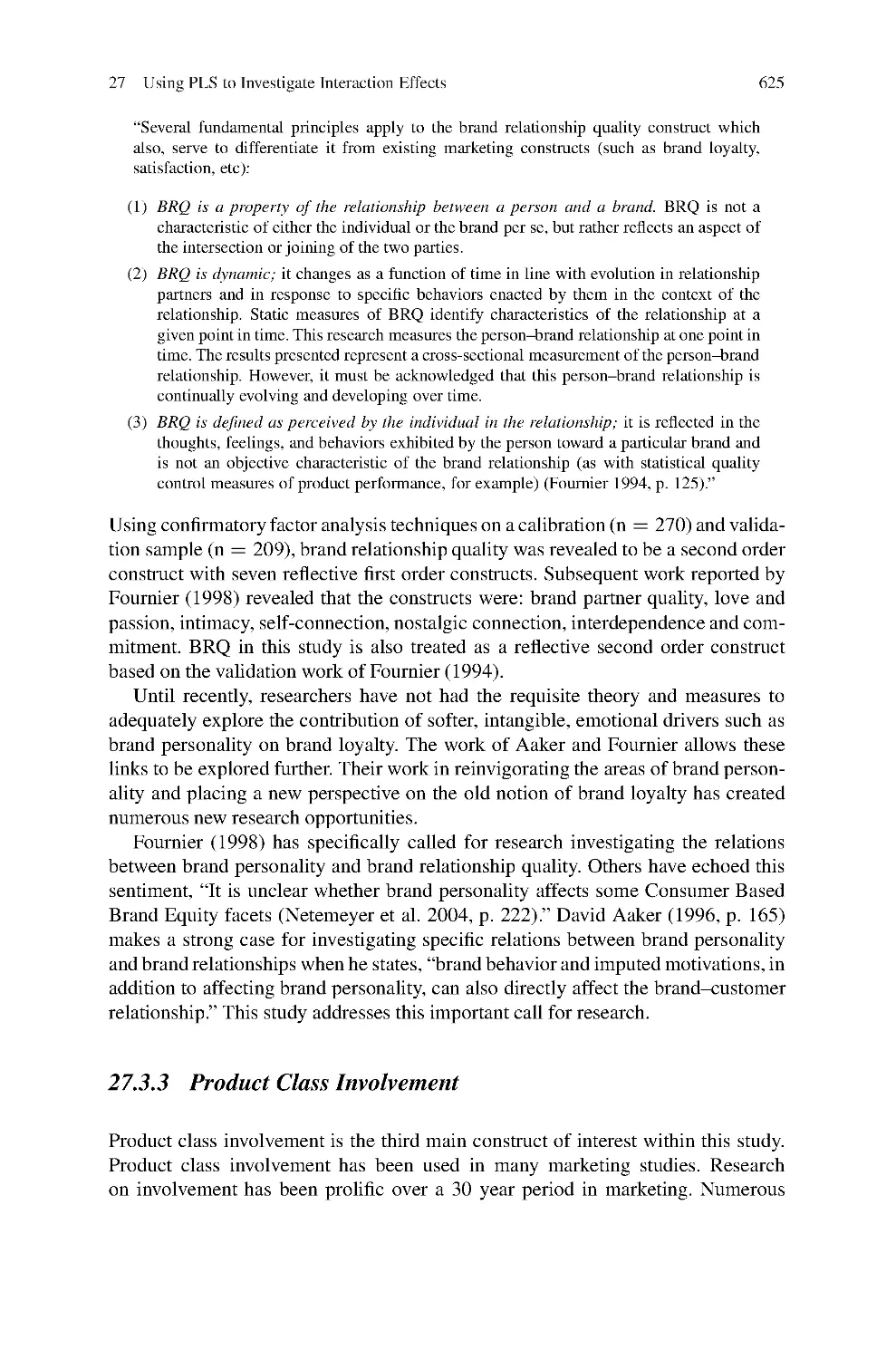
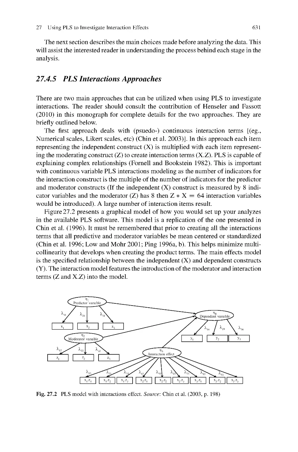
This chapter illustrates how PLS can be used when investigating causal models with
moderators at a higher level of abstraction. This is accomplished with the presen-
tation of a marketing example. This example speciﬁcally investigates the inﬂuence
of brand personality on brand relationship quality with involvement being a mod-
erator. The literature is reviewed on how to analyse moderational hypotheses with
PLS. Considerable work is devoted to the process undertaken to analyse higher order
structures. The results indicate that involvement does moderate the main effects
relationship between brand personality and brand relationship quality.
2.3 Part III: Tutorials
Wynne W. Chin: How to Write Up and Report PLS analyses
The objective of this paper is to provide a basic framework for researchers inter-
ested in reporting the results of their PLS analyses. Since the dominant paradigm
in reporting Structural Equation Modeling results is covariance based, this paper
begins by providing a discussion of key differences and rationale that researchers
can use to support their use of PLS. This is followed by two examples from the
discipline of Information Systems. The ﬁrst consists of constructs with reﬂective
indicators (mode A). This is followed up with a model that includes a construct
with formative indicators (mode B).
Oliver G ¨
otz, Kerstin Liehr-Gobbers, and Manfred Krafft: Evaluation of Structural
Equation Models using the Partial Least Squares Approach
This paper gives a basic comprehension of the partial least squares approach. In this
context, the aim of this paper is to develop a guide for the evaluation of structural

Editorial
17
equation models, using the current statistical methods methodological knowledge by
speciﬁcally considering the Partial-Least-Squares (PLS) approach’s requirements.
As an advantage, the PLS method demands signiﬁcantly fewer requirements com-
pared to that of covariance structure analyses, but nevertheless delivers consistent
estimation results. This makes PLS a valuable tool for testing theories. Another
asset of the PLS approach is its ability to deal with formative as well as reﬂec-
tive indicators, even within one structural equation model. This indicates that the
PLS approach is appropriate for explorative analysis of structural equation models,
too, thus offering a signiﬁcant contribution to theory development. However, little
knowledge is available regarding the evaluating of PLS structural equation models.
To overcome this research gap a broad and detailed guideline for the assessment
of reﬂective and formative measurement models as well as of the structural model
had been developed. Moreover, to illustrate the guideline, a detailed application of
the evaluation criteria had been conducted to an empirical model explaining repeat
purchasing behaviour.
J¨
org Henseler and Georg Fassott: Testing Moderating Effects in PLS Path Models:
An Illustration of Available Procedures
Along with the development of scientiﬁc disciplines, namely social sciences, hypoth-
esized relationships become more and more complex. Besides the examination of
direct effects, researchers are more and more interested in moderating effects. Mod-
erating effects are evoked by variables, whose variation inﬂuences the strength or
the direction of a relationship between an exogenous and an endogenous variable.
Investigators using partial least squares path modeling need appropriate means to
test their models for such moderating effects. Henseler and Fassott illustrate the
identiﬁcation and quantiﬁcation of moderating effects in complex causal structures
by means of Partial Least Squares Path Modeling. They also show that group com-
parisons, i.e. comparisons of model estimates for different groups of observations,
represent a special case of moderating effects, having the grouping variable as a
categorical moderator variable. In their contribution, Henseler and Fassott provide
profound answers to typical questions related to testing moderating effects within
PLS path models:
1. How can a moderating effect be drawn in a PLS path model, taking into account
that available software only permits direct effects?
2. How does the type of measurement model of the independent and the moderator
variables inﬂuence the detection of moderating effects?
3. Before the model estimation, should the data be prepared in a particular manner?
Should the indicators be centered (having a mean of zero), standardized (having
a mean of zero and a standard deviation of one), or manipulated in any other
way?
4. How can the coefﬁcients of moderating effects be estimated and interpreted?
And, ﬁnally,
5. How can the signiﬁcance of moderating effects be determined?

18
V. Esposito Vinzi et al.
Borrowing from the body of knowledge on modeling interaction effect within mul-
tiple regression, Henseler and Fassott develop a guideline on how to test moderating
effects in PLS path models. In particular, they create a graphical representation of
the necessary steps and decisions to make in form of a ﬂow chart. Starting with the
analysis of the type of data available, via the measurement model speciﬁcation, the
ﬂow chart leads the researcher through the decisions on how to prepare the data
and how to model the moderating effect. The ﬂow chart ends with the bootstrap-
ping, as the preferred means to test signiﬁcance, and the ﬁnal interpretation of the
model outcomes which are to be made by the researcher. In addition to this tutorial-
like contribution on the modelation of moderating effects by means of Partial
Least Squares Path Modeling, readers interested in modeling interaction effects can
ﬁnd many modelling examples in this volume, particularly in the contributions by
Chin & Dibbern; Eberl; Guinot, Mauger, Malvy, Latreille, Ambroisine, Ezzedine,
Galan, Hercberg & Tenenhaus; Streukens, Wetzels, Daryanto & de Ruyter; and
Wilson.
Dirk Temme, Henning Kreis, and Lutz Hildebrandt: Comparison of Current PLS
Path Modeling Software – Features, Ease-of-Use, and Performance
After years of stagnancy, PLS path modeling has recently attracted renewed interest
from applied researchers in marketing. At the same time, the availability of soft-
ware alternatives to Lohm ¨
oller’s LVPLS package has considerably increased (PLS-
Graph, PLS-GUI, SPAD-PLS, SmartPLS). To help the user to make an informed
decision, the existing programs are reviewed with regard to requirements, method-
ological options, and ease-of-use; their strengths and weaknesses are identiﬁed.
Furthermore, estimation results for different simulated data sets, each focusing on a
speciﬁc issue (sign changes and bootstrapping, missing data, and multi-collinearity),
are compared.
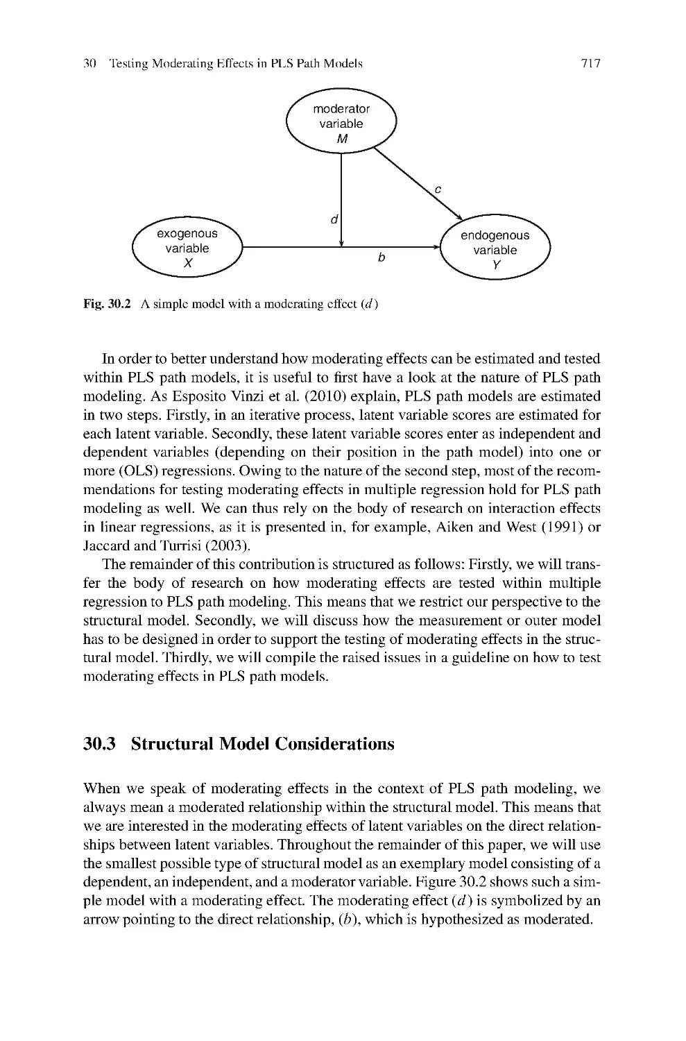
Application
SIMCA-P is a kind of user-friendly software developed by Umetrics, which is
mainly used for the methods of principle component analysis (PCA) and partial
least square (PLS) regression. This paper introduces the main glossaries, analysis
cycle and basic operations in SIMCA-P via a practical example. In the application
section, this paper adopts SIMCA-P to estimate the PLS model with qualitative
variables in independent variables set and applies it in the sand storm prevention in
Beijing. Furthermore, this paper demonstrates the advantage of lowering the wind
erosion by Conservation Tillage method and shows that Conservation Tillage is
worth promotion in Beijing sand storm prevention.
Zaibin Wu, Jie Meng, and Huiwen Wang: Introduction to SIMCA-P and Its

Editorial
19
Laure Nokels, Thierry Fahmy, and Sebastien Crochemore: Interpretation of the
Preferences of Automotive Customers Applied to Air Conditioning Supports by
Combining GPA and PLS Regression
A change in the behavior of the automotive customers has been noticed throughout
the last years. Customers feel a renewed interest in the intangible assets of perceived
quality and comfort of environment. A concrete case of study has been set up to ana-
lyze the preferences for 15 air conditioning supports. Descriptive data obtained by
ﬂash proﬁling with 5 experts on the photographs of 15 air conditioning supports are
treated by Generalized Procrustes Analysis (GPA). The preferences of 61 customers
are then explained by Partial Least Squares (PLS) regression applied to the factors
selected from the GPA. The results provided by the XLSTAT GPA and PLS regres-
sion functions help to quickly identify the items that have a positive or negative
impact on the customers’ preferences, and to deﬁne products that ﬁt the customers’
expectations.
Acknowledgements The PLS Handbook Editors are very grateful to Rosaria Romano and Laura
Trinchera from the University of Naples Federico II (Italy) for their endeavor and enthusiasm as
editorial assistants and to the more than 50 referees for their highly professional contribution to
the three rounds of the peer reviewing process. A special thank goes also to the owners and the
staff of the Hotel San Michele in Anacapri (Island of Capri, Italy) for offering a very peaceful and
inspiring summer environment during the completion of the editorial work.
References
Birkinshaw, J., Morrison, A., and Hulland, J. (1995). Structural and Competitive Determinants of
a Global Integration Strategy. Strategic Management Journal, 16(8):637–655.
Fornell, C. (1992). A National Customer Satisfaction Barometer. The Swedish Experience. Journal
of Marketing, 56(1):6–21.
Fornell, C. and Bookstein, F. L. (1982). Two structural equation models: LISREL and PLS applied
to consumer exit-voice theory. Journal of Marketing Research, 19(4):440–452.
Fornell, C. , Johnson, M., Anderson, E., Cha, J. , and Bryant, B. (1996). The American Customer
Satisfaction Index: Nature, Purpose, and Findings. Journal of Marketing, 60(4):7–18.
Gefen, D. and Straub, D. (1997). Gender Differences in the Perception and Use of E-Mail: An
Extension to the Technology Acceptance Model. MIS Quarterly, 21(4):389–400.
Gray, P. H. and Meister, D. B. (2004). Knowledge sourcing effectiveness. Management Science,
50(6):821–834.
Hulland, J. (1999). Use of Partial Least Squares (PLS) in Strategic Management Research: A
Review of Four Recent Studies. Strategic Management Journal, 20(2):195–204.
J¨
oreskog, K. G. (1978). Structural analysis of covariance and correlation matrices. Psychometrika,
43(4):443–477.
Lohm ¨
oller, J. -B. (1989). Latent Variable Path Modeling with Partial Least Squares. Physica,
Heidelberg.
Reinartz, W. J. , Krafft, M. , and Hoyer, W. D. (2004). The Customer Relationship Manage-
ment Process: Its Measurement and Impact on Performance. Journal of Marketing Research,
41(3):293–305.
Schneeweiß, H. (1991). Models with latent variables: LISREL versus PLS. Statistica Neerlandica,
45(2):145–157.

20
V. Esposito Vinzi et al.
Singh, N. , Fassott, G. , Chao, M. , and Hoffmann, J. (2006). Understanding international web site
usage. International Marketing Review, 23(1):83–97.
Tenenhaus, M. (1998). La R´
egression PLS: th´
eorie et pratique. Technip, Paris.
Tenenhaus, Esposito Vinzi, V., Chatelin, Y.-M., and Lauro, C. (2005). PLS path modeling.
Computational Statistics & Data Analysis, 48(1):159–205.
Ulaga, W. and Eggert, A. (2006). Value-Based Differentiation in Business Relationships: Gaining
and Sustaining Key Supplier Status. Journal of Marketing, 70(1):119–136.
Venkatesh, V. and Agarwal, R. (2006). Turning visitors into customers: a usability-centric
perspective on purchase behavior in electronic channels. Management Science, 52(3):367–382.
Wangen, L. and Kowalski, B. (1988). A multiblock partial least squares algorithm for investigating
complex chemical systems. Journal of Chemometrics, 3:3–20.
Wold, H. (1973). Nonlinear iterative partial least squares (NIPALS) modelling. some current
developments. In Krishnaiah, P. R., editor, Proceedings of the 3rd International Symposium
on Multivariate Analysis, pages 383–407, Dayton, OH.
Wold, H. (1975a). Modeling in complex situations with soft information. In Third World Congress
of Econometric Society.
Wold, H. (1975b). Soft modelling by latent variables: The non-linear iterative partial least squares
(NIPALS) approach. In Perspectives on Probability and Statistics, Festschrift (65th Birthday)
for M. S. Bartlett, pages 117–142.
Wold, H. (1980). Model construction and evaluation when theoretical knowledge is scarce: Theory
and application of PLS. In Kmenta, J. and Ramsey, J. B., editors, Evaluation of Econometric
Models, pages 47–74. Academic Press, New York.
Wold, H. (1982). Soft modeling: The basic design and some extensions. In J ¨
oreskog, K. G. and
Wold, H., editors, Systems Under Indirect Observations: Part I, pages 1–54. North-Holland,
Amsterdam.
Wold, H. (1985). Partial Least Squares, volume 6, pages 581–591. John Wiley & Sons, New York
et al.
Wold, H. (1988). Speciﬁcation, predictor. In Kotz, S. and Johnson, N. L., editors, Encyclopedia of
Statistical Sciences, volume 8, pages 587–599. Wiley, New York.
Wold, H. and Lyttkens, E. (1969). Nonlinear iterative partial least squares (NIPALS) estimation
procedures. Bulletin of the International Statistical Institute, 43:29–51.
Wold, S., Martens, H., and Wold, H. (1983). The multivariate calibration problem in chemistry
solved by the PLS method. In In: Ruhe, A. , Kagstrom, B. (Eds.), Proceedings of the Conference
on Matrix Pencils. Lectures Notes in Mathematics, Heidelberg. Springer.
Yi, M. and Davis, F. (2003). Developing and Validating an Observational Learning Model of
Computer Software Training and Skill Acquisition. Information Systems Research, 14(2):
146–169.

Part I
Methods
PLS Path Modeling: Concepts, Model Estimation
and Assessment
Chapters 1–3
PLS Path Modeling: Extensions
Chapters 4–7
PLS Path Modeling with Classiﬁcation Issues
Chapters 8–10
PLS Path Modeling for Customer Satisfaction Studies
Chapters 11–14
PLS Regression
Chapters 15–17

Chapter 1
Latent Variables and Indices: Herman Wold’s
Basic Design and Partial Least Squares
Theo K. Dijkstra
Abstract In this chapter it is shown that the PLS-algorithms typically converge if
the covariance matrix of the indicators satisﬁes (approximately) the “basic design”,
a factor analysis type of model. The algorithms produce solutions to ﬁxed point
equations; the solutions are smooth functions of the sample covariance matrix of
the indicators. If the latter matrix is asymptotically normal, the PLS-estimators
will share this property. The probability limits, under the basic design, of the
PLS-estimators for loadings, correlations, multiple R’s, coefﬁcients of structural
equations et cetera will differ from the true values. But the difference is decreas-
ing, tending to zero, in the “quality” of the PLS estimators for the latent variables. It
is indicated how to correct for the discrepancy between true values and the probabil-
ity limits. We deemphasize the “normality”-issue in discussions about PLS versus
ML: in employing either method one is not required to subscribe to normality; they
are “just” different ways of extracting information from second-order moments.
We also propose a new “back-to-basics” research program, moving away from
factor analysis models and returning to the original object of constructing indices
that extract information from high-dimensional data in a predictive, useful way.
For the generic case we would construct informative linear compounds, whose
constituent indicators have non-negative weights as well as non-negative loadings,
satisfying constraints implied by the path diagram. Cross-validation could settle the
choice between various competing speciﬁcations. In short: we argue for an upgrade
of principal components and canonical variables analysis.
T.K. Dijkstra
SNS Asset Management, Research and Development, Pettelaarpark 120, P. O. Box 70053,
5201 DZ ’s-Hertogenbosch, The Netherlands
e-mail: theo.dijkstra@snsam.nl
and
University of Groningen, Economics and Econometrics, Zernike Complex, P.O. Box 800,
9700 AV, Groningen, The Netherlands
e-mail: t.k.dijkstra@rug.nl
V. Esposito Vinzi et al. (eds.), Handbook of Partial Least Squares, Springer Handbooks
of Computational Statistics, DOI 10.1007/978-3-540-32827-8 2,
c

 Springer-Verlag Berlin Heidelberg 2010
23

24
T.K. Dijkstra
1.1 Introduction
Partial Least Squares is a family of regression based methods designed for the anal-
ysis of high dimensional data in a low-structure environment. Its origin lies in the
sixties, seventies and eighties of the previous century, when Herman O.A. Wold
vigorously pursued the creation and construction of models and methods for the
social sciences, where “soft models and soft data” were the rule rather than the
exception, and where approaches strongly oriented at prediction would be of great
value. The author was fortunate to witness the development ﬁrsthand for a few years.
Herman Wold suggested (in 1977) to write a PhD-thesis on LISREL versus PLS
in the context of latent variable models, more speciﬁcally of “the basic design”.
I was invited to his research team at the Wharton School, Philadelphia, in the fall
of 1977. Herman Wold also honoured me by serving on my PhD-committee as a
distinguished and decisive member. The thesis was ﬁnished in 1981. While I moved
into another direction (speciﬁcation, estimation and statistical inference in the con-
text of model uncertainty) PLS sprouted very fruitfully in many directions, not only
as regards theoretical extensions and innovations (multilevel, nonlinear extensions
et cetera) but also as regards applications, notably in chemometrics, marketing, and
political sciences. The PLS regression oriented methodology became part of main
stream statistical analysis, as can be gathered from references and discussions in
important books and journals. See e. g. Hastie et al. (2001), or Stone and Brooks
(1990), Frank and Friedman (1993), Tenenhaus et al. (2005), there are many others.
This chapter will not cover these later developments, others are much more knowl-
edgeable and are more up-to-date than I am. Instead we will go back in time and
return to one of the real starting points of PLS: the basic design. We will look at
PLS here as a method for structural equation modelling and estimation, as in Tenen-
haus et al. (2005). Although I cover ground common to the latter’s review I also
offer additional insights, in particular into the distributional assumptions behind the
basic design, the convergence of the algorithms and the properties of their outcomes.
In addition, ways are suggested to modify the outcomes for the tendency to over- or
underestimate loadings and correlations. Although I draw from my work from the
period 1977–1981, which, as the editor graciously suggested is still of some value
and at any rate is not particularly well-known, but I also suggest new developments,
by stepping away from the latent variable paradigm and returning to the formative
years of PLS, where principal components and canonical variables were the main
source of inspiration.
In the next section we will introduce the basic design, somewhat extended beyond
its archetype. It is basically a second order factor model where each indicator is
directly linked to one latent variable only. Although the model is presented as “dis-
tribution free” the very fact that conditional expectations are always assumed to be
linear does suggest that multinormality is lurking somewhere in the background.
We will discuss this in Sect. 1.3, where we will also address the question whether
normality is important, and to what extent, for the old “adversary” LISREL. Please
note that as I use the term LISREL it does not stand for a speciﬁc well-known sta-
tistical software package, but for the maximum likelihood estimation and testing

1 Latent Variables and Indices
25
approach for latent variable models, under the working hypothesis of multivariate
normality. There is no implied value judgement about other approaches or packages
that have entered the market in the mean time. In Sect. 1.3 we also recall some rele-
vant estimation theory for the case where the structural speciﬁcation is incorrect or
the distributional assumptions are invalid.
The next section, number 4, appears to be the least well-known. I sketch a proof
there, convincingly as I like to believe, that the PLS algorithms will converge from
arbitrary starting points to unique solutions, ﬁxed points, with a probability tend-
ing to one when the sample size increases and the sample covariance matrix has
a probability limit that is compatible with the basic design, or is sufﬁciently close
to it.
In Sect. 1.5 we look at the values that PLS attains at the limit, in case of
the basic design. We ﬁnd that correlations between the latent variables will be
underestimated, that this is also true for the squared multiple correlation coefﬁcients
for regressions among latent variables, and the consequences for the estimation of
the structural form parameters are indicated; we note that loadings counterbalance
the tendency of correlations to be underestimated, by overestimation. I suggest ways
to correct for this lack of consistency, in the probabilistic sense.
In the Sect. 1.6, we return to what I believe is the origin of PLS: the construction
of indices by means of linear compounds, in the spirit of principal components and
canonical variables. This section is really new, as far as I can tell. It is shown that for
any set of indicators there always exist proper indices, i. e. linear compounds with
non-negative coefﬁcients that have non-negative correlations with their indicators.
I hint at the way constraints, implied by the path diagram, can be formulated as
side conditions for the construction of indices. The idea is to take the indices as
the fundamental objects, as the carriers or conveyers of information, and to treat
path diagrams as relationships between the indices in their own right. Basically, this
approach calls for the replacement of fullblown unrestricted principal component
or generalized canonical variable analyses by the construction of proper indices,
satisfying modest, “theory poor” restrictions on their correlation matrix. This section
calls for further exploration of these ideas, acknowledging that in the process PLS’s
simplicity will be substantially reduced.
The concluding Sect. 1.7 offers some comments on McDonald’s (1996) thought
provoking paper on PLS; the author gratefully acknowledges an unknown referee’s
suggestion to discuss some of the issues raised in this paper.
1.2 A Second Order Factor Model, the “Basic Design”
Manifest variables, or indicators, are observable variables who are supposed to con-
vey information about the behavior of latent variables, theoretical concepts, who
are not directly observable but who are fundamental to the scientiﬁc enterprise
in almost any ﬁeld, see Kaplan (1946). In the social sciences factor models are
the vehicle most commonly used for the analysis of the interplay between latent

26
T.K. Dijkstra
and manifest variables. Model construction and estimation used to be focussed
mainly on the speciﬁcation, validation and interpretation of factor loadings and
underlying factors (latent variables), but in the seventies of the previous cen-
tury the relationships between the factors themselves became a central object of
study. The advent of optimization methods for high-dimensional problems, like the
Fletcher-Powell algorithm, see Ortega and Rheinboldt (1970) e. g., allowed research
teams to develop highly ﬂexible and user-friendly software for the analysis, estima-
tion and testing of second order factor models, in which relationships between the
factors themselves are explicitly incorporated. First Karl G. J¨
oreskog from Uppsala,
Sweden, and his associates developed LISREL, then later, in the eighties, Peter
M. Bentler from UCLA designed EQS, and others followed. However, approaches
like LISREL appeared to put high demands on the speciﬁcation of the theoretical
relationships: one was supposed to supply a lot of structural information on the the-
oretical covariance matrix of the indicators. And also it seemed that, ideally, one
needed plenty of independent observations on these indicators from a multinormal
distribution! Herman O. A. Wold clearly saw the potential of these methods for the
social sciences but objected to their informational and distributional demands, which
he regarded as unrealistic for many ﬁelds of inquiry, especially in the social sciences.
Moreover, he felt that estimation and description had been put into focus, at the
expense of prediction. Herman Wold had a lifelong interest in the development of
predictive and robust statistical methods. In econometrics he pleaded forcefully for
“recursive modelling” where every single equation could be used for prediction and
every parameter had a predictive interpretation, against the current of mainstream
“simultaneous equation modelling”. For the latter type of models he developed the
Fix-Point estimation method, based on a predictive reinterpretation and rewriting of
the models, in which the parameters were estimated iteratively by means of simple
regressions. In 1966 this approach was extended to principal components, canonical
variables and factor analysis models: using least squares as overall predictive crite-
rion, parameters were divided into subsets in such a way that with any one of the
subsets kept ﬁxed at previously determined values, the remaining set of parameters
would solve a straightforward regression problem; roles would be reversed and the
regressions were to be continued until consecutive values for the parameters differed
less then a preassigned value, see Wo ld (1966)butalsoWol d (1975). The ﬁnaliza-
tions of the ideas, culminating into PLS, took place in 1977, when Herman Wold
was at the Wharton School, Philadelphia. Incidentally, since the present author was
a member of Herman Wold’s research team at the Wharton School in Philadelphia
in the fall of 1977, one could be tempted to believe that he claims some of the
credit for this development. In fact, if anything, my attempts to incorporate struc-
tural information into the estimation process, which complicated it substantially,
urged Herman Wold to intensify his search for further simpliﬁcation. I will try to
revive my attempts in the penultimate section. . .
For analytical purposes and for comparisons with LISREL-type of alternatives
Herman Wold put up a second order factor model, called the “basic design”. In the
remainder of this section we will present this model, somewhat extended, i.e. with
fewer assumptions. The next section then takes up the discussion concerning the

1 Latent Variables and Indices
27
“multivariate normality of the vector of indicators”, the hard or “heroic” assumption
of LISREL as Herman Wold liked to call it. Anticipating the drift of the argument:
the difference between multinormality and the distributional assumptions in PLS is
small or large depending on whether the distance between independence and zero
correlation is deemed small or large. Conceptually, the difference is large, since two
random vectors X and Y are independent if and only if “every” real function of X
is uncorrelated with “every” real function of Y , not just the linear functions. But
any one who has ever given a Stat1 course knows that the psychological distance is
close to negligible. . .
More important perhaps is the fact that multinormality and independence of the
observational vectors is not required for consistency of LISREL-estimators, all that
is needed is that the sample covariance matrix S is a consistent estimator for the
theoretical covariance matrix †. The existence of † and independence of the obser-
vational vectors is more than sufﬁcient, there is in fact quite some tolerance for
dependence as well. Also, asymptotic normality of the estimators is assured without
the assumption of multinormality. All that is needed is asymptotic normality of S ,
and that is quite generally the case. Asymptotic optimality, and a proper interpre-
tation of calculated standard errors as standard errors, as well as the correct use
of test-statistics however does indeed impose heavy restrictions on the distribution,
which make the distance to multinormality, again psychologically spoken, rather
small, and therefore to PLS rather large. . .
There is however very little disagreement about the difference in structural infor-
mation, PLS is much more modest and therefore more realistic in this regard than
LISREL. See Dijkstra (1983, 1988, 1992) where further restrictions, relevant for
both approaches, for valid use of frequentist inference statistics are discussed, like
the requirement that the model was not speciﬁed interactively, using the data at
hand.
Now for the “basic design”.
We will take all variables to be centered at their mean, so the expected values are
zero, and we assume the existence of all second order moments. Let  be a vec-
tor of latent variables which can be partitioned in a subvector n of endogenous
latent variables and a subvector x of exogenous latent variables. These vectors
obey the following set of structural equations with conformable matrices B and 
and a (residual) vector  with the property that E.j x/ D 0:
n DBnCxC
(1.1)
The inverse of .I B/ is assumed to exist, and the (zero-) restrictions on B ,  and
the covariance matrices of x and  are sufﬁcient for identiﬁcation of the structural
parameters. An easy consequence is that
E.njx/D.I B/1x …x
(1.2)
which expresses the intended use of the reduced form, prediction, since no function
of x will predict n better than …x in terms of mean squared error. Note that the

28
T.K. Dijkstra
original basic design is less general, in the sense that B is sub-diagonal there and
that for each i larger than 1 the conditional expectation of i given x and the ﬁrst
i 1 elements of n is zero. In other words, originally the model for the latent
variables was assumed to be a causal chain, where every equation, whether from
the reduced or the structural form, has a predictive use and interpretation.
Now assume we have a vector of indicators y which can be divided into subvec-
tors, one subvector for each latent variable, such that for the i -th subvector yi the
following holds:
yi DiiCi
(1.3)
where i is a vector of loadings, with as many components as there are indicators
for i , and the vector i is a random vector of measurement errors. It is assumed that
E.yi j i / D i i so that the errors are uncorrelated with the latent variable of the
same equation. Wold assumes that measurement errors relating to different latent
variables are uncorrelated as well. In the original basic design he assumes that the
elements of each i are mutually uncorrelated, so that their covariance matrix is
diagonal. We will postulate instead that Vi  Ei >
i has at least one zero element
(or equivalently, with more than one indicator, because of the symmetry and the fact
that is a covariance matrix, at least two zero elements). To summarize:
†ij  Eyiy>
j Dijijfori¤j
(1.4)
where ij stands for the correlation between i and j , adopting the convention that
latent variables have unit variance, and
†ii D i>
i CVi:
(1.5)
So the ij ’s and the loading vectors describe the correlations at the ﬁrst level, of
the indicators, and the structural equations yield the correlations at the second level,
of the latent variables. It is easily seen that all parameters are identiﬁed: equation
(4) determines the direction of i apart from a sign factor and (5) ﬁxes its length,
therefore the ij ’s are identiﬁed (as well as the Vi ’s), and they on their turn allow
determination of the structural form parameters, given † of course.
1.3 Distributional Assumptions: Multinormality
or “Distribution Free”?
The (extended) basic design does not appear to impose heavy constraints on the
distribution of the indicators: the existence of second order moments, some zero
conditional expectations and a linear structure, that’s about it. Multinormality seems
conceptually way off. But let us take an arbitrary measurement equation
yi DiiCi
(1.6)

1 Latent Variables and Indices
29
and instead of assuming that E.i j i / D 0,weleti and i be stochastically
independent, which implies a zero conditional expectation. As Wold assumes the
elements of i to be uncorrelated, let us take them here mutually independent.
For E.i j yi / we take it to be linear as well, so assuming here and in the sequel
invertibility of matrices whenever this is needed
E.ijyi/D>
i.†ii/1yi />
iV1
iyi
(1.7)
If now all loadings, all elements of i , differ from zero, we must have multinor-
mality of the vector .yi I i I i / as follows from a characterization theorem in Kagan
et al. (1973), see in particular theorem 10.5.3. Let us modify and extend each mea-
surement equation as just described, and let all measurement errors be mutually
independent. Then for one thing each element of  will be normal and , the vector
obtained by stacking the i ’s, will be multinormal.
If we now turn to the structural equations, we will take for simplicity the special
case of a complete causal chain,whereB is square and lower diagonal and the ele-
ments of the residual vector  are mutually independent. A characterization due to
Cram ´
er states that when the sum of independent variables is normal, all constituents
of this sum are normal, and Cram ´
er and Wold have shown that a vector is multinor-
mal if and only if every linear function of this vector is normal. Combining these
characterizations one is easily led to the conclusion that .yI I I / is multinormal.
See Dijkstra (1981) for a more elaborate discussion and other results.
So, roughly, if one strengthens zero conditional expectations to independence and
takes all conditional expectations to be linear, one gets multinormality. It appears
that psychologically PLS and multinormality are not far apart. But the appreciation
of these conditions is not just a matter of taste, or of mathematical/statistical matu-
rity. Fundamentally it is an empirical matter and the question of their (approximate)
validity ought to be settled by a thorough analysis of the data. If one has to reject
them, how sad is that? The linear functions we use for prediction are then no longer
least squares optimal in the set of all functions, but best linear approximations only
to these objects of desire (in the population,that is). If we are happy with linear
approximations, i.e. we understand them and can use them to good effect, then who
cares about multinormality, or for that matter about linearity of conditional expec-
tations? In the author’s opinion, normality has a pragmatic justiﬁcation only. Using
it as a working hypothesis in combination with well worn “principles”, like least
squares or, yes, maximum likelihood, often leads to useful results, which as a bonus
usually satisfy appealing consistency conditions.
It has been stated and is often repeated, seemingly thoughtlessly, that LISREL
is based on normality, in the sense that its use requires the data to be normally dis-
tributed. This is a prejudice that ought to be cancelled. One can use the maximum
entropy principle, the existence of second order moments, and the likelihood prin-
ciple to motivate the choice of the ﬁtting function that LISREL employs. But at the
end of the day this function is just one way of ﬁtting a theoretical covariance matrix
†./to a sample covariance matrix S , where the ﬁt is determined by the difference

30
T.K. Dijkstra
between the eigenvalues of S† 1 and the eigenvalues of the identity matrix. To
elaborate just a bit:
If we denote the p eigenvalues of S† 1 by 
1;
2;:::;
p the LISREL ﬁtting
function can be written as Pi Dp
i D1 .
i log 
i 1/. Recall that for real positive num-
bers 0  x log x 1 everywhere with equality only for x D 1. Therefore the
LISREL criterion is always nonnegative and zero only when all eigenvalues are
equal to 1. The absolute minimum is reached if and only if a  can be found such
that S D †./.SoifS D †./ for some  and identiﬁability holds, LISREL
will ﬁnd it. Clearly, other functions of the eigenvalues will do the trick, GLS is one
of them. See Dijkstra (1990) for an analysis of the class of Swain functions. The
“maximum likelihood” estimator b
 is a well-behaved, many times differentiable
function of S , which yields  when evaluated at S D †./. In other words, if S
is close to †./ the estimator is close to  and it is locally a linear function of S .
It follows that when S tends in probability to its “true value”, †./,thenb
 will do
the same and moreover, if S is asymptotically normal, then b
 is.
Things become more involved when the probability limit of S , plim(S ), does
not satisfy the structural constraints as implied by the second order factor model
at hand, so there is no  for which †./ equals plim(S ). We will summarize in
a stylized way what can be said about the behavior of estimators in the case of
Weighted Least Squares, which with proper weighting matrices include LISREL,
i. e. maximum likelihood under normality, and related ﬁtting functions as well. The
result will be relevant also for the analysis of reduced form estimators using PLS.
To simplify notation we will let ./stand for the vector of non-redundant ele-
ments of the smooth matrix function †./and s does the same for S . We will let s
stand for plim(S ). Deﬁne a ﬁtting function F.s;./j W/by
F.s;./j W/ .s .//> W.s .//
(1.8)
where W is some symmetric random matrix of appropriate order whose plim, W ,
exists as a positive deﬁnite matrix (non-random matrices can be handled as well).
The vector  varies across a suitable set, non-empty and compact or such that F has
a compact level set. We postulate that the minimum of F s;  ./ j W is attained
in a unique point  s; W , depending on the probability limits of S and W .One
can show that F tends in probability to F s;  ./ j W uniformly with respect
to  . This implies that the estimator b
.s;W/ argmin.F/ will tend to  s;W
in probability. Different ﬁtting functions will produce different probability limits, if
the model is incorrect. With sufﬁcient differentiability and asymptotic normality we
can say more (see Dijkstra 1981 e. g.), using the implicit function theorem on the
ﬁrst-order conditions of the minimization problem. In fact, when
pn .s s/
vec W W! N0;VssVsw
Vws Vww (1.9)

1 Latent Variables and Indices
31
where n is the number of observations, vec stacks the elements columnwise and
the convergence is in distribution to the normal distribution, indicated by N,andwe
deﬁne:
  @=@>
(1.10)
evaluated at  s; W ,andM is a matrix with typical element Mij :
Mij @2>=@i@jW  s
(1.11)
and e
V equals by deﬁnition
h>W; s > ˝ >iVss Vsw
Vws Vww W
s ˝  (1.12)
with  and its partial derivatives in M and e
V also evaluated at the same point
 s;W , then we can say thatpnb
.s;W/  s; W  will tend to the normal
distribution with zero mean and covariance matrix , say, with
 >WCM 1e
V >WCM 1:
(1.13)
This may appear to be a somewhat daunting expression, but it has a pretty clear
structure. In particular, observe that if s D   s; W ,inothe
rw
o
rds
,if the
structural information contained in † is correct, then M becomes 0 and e
V which
sums 4 matrices looses 3 of them, and so the asymptotic covariance of the estimator
b
.s;W/reduces to:
>W 1 >WVssW >W 1
(1.14)
which simpliﬁes even further to
>V 1
ss1
(1.15)
whenWDV 1
ss . In the latter case we have asymptotic efﬁciency: no other ﬁtting
function will produce a smaller asymptotic covariance matrix. LISREL belongs to
this class, provided the structure it implicitly assumes in Vss is correct. More pre-
cisely, it is sufﬁcient when the element in Vss corresponding with the asymptotic
covariance between sij and skl equals ikjl C iljk. This is the case when the
underlying distribution is multinormal. Elliptical distributions in general will yield
an asymptotic covariance matrix that is proportional to the normal Vss,sotheyare
efﬁcient as well. The author is unaware of other suitable distributions. So LISREL
rests for inference purposes on a major assumption, that is in the opinion of the
author not easily met. If one wants LISREL to produce reliable standard errors, one
would perhaps be well advised to use the bootstrap. By the way, there are many
versions of the theorem stated above in the literature, the case of a correct model is

32
T.K. Dijkstra
particularly well covered. In fact, we expect the results on asymptotic efﬁciency to
be so well known that references are redundant.
To summarize, if the model is correct in the sense that the structural constraints
on † are met, and S is consistent and W has a positive deﬁnite probability limit
then the classical ﬁtting functions will produce estimators that tend in probability
to the true value. If the model is not correct, they will tend to the best ﬁtting value
as determined by the particular ﬁtting function chosen. The estimators are normal,
asymptotically, when S and W are (jointly), whether the structural constraints are
met or not. Asymptotic efﬁciency is the most demanding property and is not to
be taken for granted. A truly major problem that we do not discuss is model uncer-
tainty, where the model itself is random due to the interaction between speciﬁcation,
estimation and validation on the same data set, with hunches taken from the data
to improve the model. This wreaks havoc on the standard approach. No statistics
school really knows how to deal with this. See for discussions e. g. Leamer (1978),
Dijkstra (1988)orHastie et al. (2001).
In the next sections we will see that under the very conditions that make LISREL
consistent, PLS is not consistent, but that the error will tend to zero when the qual-
ity of the estimated latent variables, as measured by their correlation with the true
values, tends to 1 by increasing the number of indicators per latent variable.
1.4 On the PLS-Algorithms: Convergence Issues
and Functional Properties of Fixed Points
The basic approach in PLS is to construct proxies for the latent variables, in the
form of linear compounds, by means of a sequence of alternating least squares
algorithms, each time solving a local, linear problem, with the aim to extract the
predictive information in the sample. Once the compounds are constructed, the
parameters of the structural and reduced form are estimated with the proxies replac-
ing the latent variables. The particular information embodied in the structural form
is not used explicitly in the determination of the proxies. The information actually
used takes the presence or absence of variables in the equations into account, but
not the implied zero constraints and multiplicative constraints on the reduced form
(:the classical rank constraints on submatrices of the reduced form as implied by the
structural form).
There are two basic types of algorithms, called mode A and mode B, and a third
type, mode C, that mixes these two. Each mode generates an estimated weight vector
b
w, with typical subvector b
wi of the same order as yi . These weight vectors are
ﬁxed points of mappings deﬁned algorithmically. If we let Sij stand for the sample
equivalent of †ij , and signij for the sign of the sample correlation between the
estimated proxies b
ib
w>
i yi andb
jb
w>
j yj ,andCi is the index set that collects
the labels of latent variables which appear at least once on different sides of the
structural equations in which i appears, we have for mode A:
b
wi /X
jCi
signij Sij b
wjandb
w>
i Siib
wi D1:
(1.16)

1 Latent Variables and Indices
33
As is easily seen the i -th weight vector is obtainable by a regression of the i -th
subvector of indicators yi on the scalar b
ai  PjCi signij b
j , so the weights
are determined by the ability of b
ai to predict yi . It is immediate that when the
basic design matrix † replaces S the corresponding ﬁxed point wi ; say, is propor-
tional to i . But note that this requires at least two latent variables. In a stand-alone
situation mode A produces the ﬁrst principal component, and there is no simple rela-
tionship with the loading vector. See Hans Schneeweiss and Harald Mathes (1995)
for a thorough comparison of factor analysis and principal components. Mode A
and principal components share a lack of scale-invariance, they are both sensitive to
linear scale transformations. McDonald (1996) has shown essentially that mode A
corresponds to maximization of the sum of absolute values of the covariances of the
proxies, where the sum excludes the terms corresponding to latent variables which
are not directly related. The author gratefully acknowledges reference to McDonald
(1996) by an unknown referee.
For mode B we have:
b
wi/S1
iiX
jCi
signij Sij b
wj andb
w>
i Siib
wiD1:
(1.17)
Clearly, b
wi is obtained by a regression that reverses the order compared to mode
A: here b
ai , deﬁned similarly, is regressed on yi . So the indicators are used to pre-
dict the sign-weighted sum of proxies. With only two latent variables mode B will
produce the ﬁrst canonical variables of their respective indicators, see Wold (1966,
1982) e. g. Mode B is a genuine generalization of canonical variables: it is equiva-
lent to the maximization of the sum of absolute values of the correlations between
the proxies, b
w>
i Sijb
wj , taking only those i and j into account that correspond to
latent variables which appear at least once on different sides of a structural equa-
tion. A Lagrangian analysis will quickly reveal this. The author noted this, in 1977,
while he was a member of Herman Wold’s research team at the Wharton School,
Philadelphia. It is spelled out in his thesis (1981). Kettenring (1971) has introduced
other generalizations, we will return to this in the penultimate section. Replacing
S by † yields a weight vector wi proportional to † 1
ii i , so that the “population
proxy” i  w>
i yi has unit correlation with the best linear least squares predictor
for i in terms of yi . This will be true as well for those generalizations of canonical
variables that were analyzed by Kettenring (1971). Mode B is scale-invariant, in the
sense that linear scale transformations of the indicators leave b
i and i undisturbed.
Mode C mixes the previous approaches: some weight vectors satisfy mode A,
others satisfy mode B type of equations. As a consequence the products of mode C
mix the properties of the other modes as well. In the sequel we not dwell upon this
case. Sufﬁce it to say that with two sets of indicators, two latent variables, mode C
produces a variant of the well-known MIMIC-model.
Sofar we have simply assumed that the equations as stated have solutions, that
they actually have ﬁxed points, and the iterative procedure to obtain them has been
merely hinted at. To clarify this, let us discuss a simple case ﬁrst. Suppose we have
three latent variables connected by just one relation 3 D ˇ311 Cˇ322 plus a least
squares residual, and let us use mode B. The ﬁxed point equations specialize to:

34
T.K. Dijkstra
b
w1Db
c1S 1
11 sign13 S13b
w3
(1.18)
b
w2Db
c2S 1
22 sign23 S23b
w3
(1.19)
b
w3Db
c3S 1
33 sign13 S31b
w1 C sign23 S32b
w2:
(1.20)
The scalar b
ci forces b
wi to have unit length in the metric of Sii.The iterations start
with arbitrary nonzero choices for the b
wi ’s, which are normalized as required, the
sign-factors are determined, and a cycle of updates commences: inserting b
w3 into
(18) and (19) gives updated values for b
w1andb
w2, which on their turn are inserted
into (20), yielding an update for b
w3, then new sign-factors are calculated, and we
return to (18) et cetera. This is continued until the difference between consecutive
updates is insigniﬁcant. Obviously, this procedure allows of small variations, but
they have no impact on the results. Now deﬁne a function G,sayby
G.w3;S/ c3S 1
33 c1S31S 1
11 S13 C c2S32S 1
22 S23 w3
(1.21)
where c1 is such that c1S 1
11 S13w3 has unit length in the metric of S11, c2 is deﬁned
similarly, and c3 gives G unit length in the metric of S33. Clearly G is obtained by
consecutive substitutions of (18) and (19) into (20). Observe that:
G.w3;†/ D w3
(1.22)
for every value of w3 (recall that w3 / † 1
33 3). A very useful consequence is that
the derivative of G with respect to w3 , evaluated at .w3 ;†/equals zero. Intuitively,
this means that for S not too far away from †, G.w3 ;S/maps two different vectors
w3 , which are not too far away from w3 ; on points which are closer together than
the original vectors. In other words, as a function of w3 ;G.w3;S/ will be a local
contraction mapping. With some care and an appropriate mean value theorem one
may verify that our function does indeed satisfy the conditions of Copson’s Fixed
point theorem with a parameter,seeCopson (1979), Sects. 80–82. Consequently, G
has a unique ﬁxed point b
w3 .S/ in a neighborhood of w3 for every value of S in a
neighborhood of †,anditcan be found by successive substitutions: for an arbitrary
starting value sufﬁciently close to w3 the ensuing sequence of points converges to
b
w3 .S/ which satisﬁes b
w3.S/DG.b
w3 .S/; S/. Also note that if plim.S/ D † then
the ﬁrst iterate from an arbitrary starting point will tend to w3 in probability, so if
the sample is sufﬁciently large the conditions for a local contraction mapping will
be satisﬁed with an arbitrarily high probability. Essentially, any choice of starting
vector will do. The mapping b
w3 .S/ is continuous, in fact it is continuously differ-
entiable, as follows quickly along familiar lines of reasoning in proofs of implicit
function theorems. So asymptotic normality is shared with S . The other weight
vectors are smooth transformations of b
w3 .S /, so they will be well-behaved as well.
It is appropriate now to point out that what we have done with mode B for three
latent variables can also be done for the other modes, and the number of latent
variables is irrelevant: reshufﬂe (16) and (17), if necessary, so that the weights cor-
responding to the exogenous latent variables are listed ﬁrst; we can express them
in terms of the endogenous weight vectors, wn , say, so that after insertion in the

1 Latent Variables and Indices
35
equations for the latter a function G.wn ;S/ can be deﬁned with the property that
G.wn ;†/ D wn and we proceed as before. We obtain again a well-deﬁned ﬁxed
point b
w .S/ by means of successive substitutions: Let us collect this in a theorem
(Dijkstra, 1981; we ignore trivial regularity assumptions that preclude loading vec-
tors like i to consist of zeros only; and similarly, we ignore the case where †ij is
identically zero for every jCi ):
Theorem 1.1. If plim.S / D † where † obeys the restrictions of the basic design,
then the PLS algorithms will converge for every choice of starting values to unique
ﬁxed points of (16) and (17) with a probability tending to one when the number
of sample observations tends to 1: These ﬁxed points are continuously differen-
tiable functions of S , their probability limits satisfy the ﬁxed point equations with S
replaced by †. They are asymptotically normal when S is.
As a ﬁnal observation in this section: if plim.S/ D † which is not a basic design
matrix but comes sufﬁciently close to it, then the PLS-algorithms will converge in
probability to the ﬁxed point deﬁned by b
w .†/. We will again have good numerical
behavior and local linearity.
1.5 Correlations, Structural Parameters, Loadings
In this section we will assume without repeatedly saying so that plim.S / D † for a
† satisfying the requirements of the extended basic design except for one problem,
indicated below in the text. Recall the deﬁnition of the population proxy i  w>
iyi
where wi  plim .b
wi / depends on the mode chosen; for mode A wi is proportional
to i and for mode B it is proportional to † 1
ii i . Its sample counterpart, the sample
proxy, is denoted by b
ib
w>
i yi : In PLS the sample proxies replace the latent vari-
ables. Within the basic design, however, this replacement can never be exhaustive
unless there are no measurement errors. We can measure the quality of the proxies
by means of the squared correlation between i and i W R2 .i ; i / D w>
ii2.
In particular, for mode A we have
R2
A.i;i/D >
ii2
>
i †iii
(1.23)
and for mode B:
R2
B.i;i/D>
i†1
ii i
(1.24)
as is easily checked. It is worth recalling that the mode B population proxy is propor-
tional to the best linear predictor of i in terms of yi , which is not true for mode A.
Also note that the Cauchy-Schwarz inequality immediately entails that R2
A is always
less than R2
B unless i is proportional to † 1
ii i or equivalently, to V 1
i i;fordiag-
onal Vi this can only happen when all measurement error variances are equal. For
every mode we have that

36
T.K. Dijkstra
R2 i;j D w>
i†ijwj 2D2
ij R2.i;i/ R2 j;j
(1.25)
and we observe that in the limit the PLS-proxies will underestimate the squared
correlations between the latent variables. This is also true of course for two-block
canonical variables: they underestimate the correlation between the underlying
latent variables eventhough they maximize the correlation between linear com-
pounds. It is not typical for PLS of course. Methods like Kettenring’s share this
property. The error depends in a simple way on the quality of the proxies, with
mode B performing best.
The structural bias does have consequences for the estimation of structural form
and reduced form parameters as well. If we let R stand for the correlation matrix
of the latent variables, R does the same for the population proxies, and K is the
diagonal matrix with typical element R.i ; i /; we can write
RDKRKCI K2:
(1.26)
So conditions of the Simon-Blalock type, like zero partial correlation coefﬁcients,
even if satisﬁed by R will typically not be satisﬁed by R. Another consequence is
that squared multiple correlations will be underestimated as well: the value that
PLS obtains in the limit, using proxies, for the regression of i on other latent
variables never exceeds the fraction R2 .i ; i / of the “true” squared multiple corre-
lation coefﬁcient. This is easily deduced from a well-known characterization of the
squared multiple correlation: it is the maximum value of 1 ˇ>Rˇ with respect to
ˇ where R is the relevant correlation matrix of the variables, and ˇ is a conformable
vector whose i -th component is forced to equal 1 (substitution of the expression for
R quickly yields the upper bound as stated). The upper bound can be attained only
when the latent variables other than i are measured without ﬂaw.
In general we have that the regression matrix for the population proxies equals
…,say,with
…DRnxR 1
xx D Kn…RxxKxR 1
xx
(1.27)
where subscripts indicate appropriate submatrices, the deﬁnitions will be clear. Now
we assumed that B and  could be identiﬁed from …: It is common knowledge in
econometrics that this is equivalent to the existence of rank restrictions on submatri-
ces of …: But since R differs from R these relations will be disturbed and … will not
satisfy them, except on sets of measure zero in the parameterspace. This makes the
theory hinted at in Sect. 1.3 relevant. With p replacing s,and replacing  for max-
imum similarity, if so desired, we can state that classical estimators for the structural
form parameters will asymptotically center around .B ;/ say, which are such that
.I B/ 1  ﬁts … “best”. “Best” will depend on the estimation procedure cho-
sen and … varies with the mode. In principle, the well-known delta method can
be used to get standard errors, but we doubt whether that is really feasible (which
is something of an understatement). The author, Dijkstra (1982, 1983), suggested
to use the bootstrap as a general tool. Later developments, such as the stationary
bootstrap for time series data, has increased the value of the method even more, but

1 Latent Variables and Indices
37
care must be used for a proper application; in particular, one should resample the
observations on the indicators, not on the sample proxies, for a decent analysis of
sampling uncertainty.
Turning now to the loadings, some straightforward algebra easily yields that both
modes will tend to overestimate them in absolute value, mode B again behaving
better than mode A, in the limit that is. The loadings are in fact estimated by
b
i  Siib
wi:
(1.28)
and the error covariance matrices can be calculated as
b
ViSii b
ib
>
i:
(1.29)
(Note that b
Vib
wi D 0; so the estimated errors are linearly dependent, which will have
some consequences for second level analyses, not covered here). Inserting popula-
tion values for sampling values we get for mode A that i , the probability limit of
b
i , is proportional to †iii : For mode B we note that i is proportional to i with
a proportionality factor equal to the square root of 1 over R2 .i ; i/: Mode B, but
not mode A, will reproduce †ij exactly in the limit. For other results, all based on
straightforward algebraic manipulations we refer to Dijkstra (1981).
So in general, not all parameters will be estimated consistently. Wold, in a report
that was published as Chap. 1 in J¨
oreskog and Wo l d (1982), introduced the auxiliary
concept of ‘consistency at large’ which captures the idea that the inconsistency will
tend to zero if more indicators of sufﬁcient quality can be introduced for the latent
variables. The condition as formulated originally was
hE w>
ii2i
w>
ii
1
2
!0:
(1.30)
This is equivalent to R2 .i ; i / ! 1: Clearly, if these correlations are large, PLS
will combine numerical expediency with consistency. If the proviso is not met in
a sufﬁcient degree the author (Dijkstra, 1981) has suggested to use some simple
“corrections”. E. g. in the case of mode B one could ﬁrst determine the scalar b
fi say
that minimizes, assuming uncorrelated measurement errors,
tracehSii diag .Sii/ hf 2
ib
ib
>
i diagf 2
ib
ib
>
i ii2 (1.31)
for all real fi and which serves to rescale b
i .Weget
b
f2
iD
b
>
i Sii diag .Sii/b
i
b
>
ihb
ib
>
i diagb
ib
>
i ib
i
:
(1.32)

38
T.K. Dijkstra
One can check that b
fib
i tends in probability to i : In addition we have that
p limb
f2
i  equals R2
B .i ; i / . So one could in principle get consistent estimators
for R, the correlation matrix of the latent variables by reversing (25) so to speak.
But a more direct approach can also be taken by minimization of
tracehSij rij b
fib
fjb
ib
>
ji> hSij rij b
fib
fjb
ib
>
j i (1.33)
for rij . This produces the consistent estimator
b
rij 
b
>
i Sijb
j
b
fib
fjb
>
ib
ib
>
jb
j:
(1.34)
With a consistent estimator for R we can also estimate B and  consistently. We
leave it to the reader to develop alternatives. The author is not aware of attempts in
the PLS-literature to implement this idea or related approaches. Perhaps the devel-
opment of second and higher order levels has taken precedence over reﬁnements
to the basic design because that just comes naturally to an approach which mimics
principal components and canonical variables so strongly. But clearly, the bias can
be substantial if not dramatic, whether it relates to regression coefﬁcients, correla-
tions, structural form parameters or loadings as the reader easily convinces himself
by choosing arbitrary values for the R2 .i ; i /’s; even for high quality proxies the
disruption can be signiﬁcant, and it is parameter dependent. So if one adheres to the
latent variable paradigm, bias correction as suggested here or more sophisticated
approaches seems certainly to be called for.
1.6 Two Suggestions for Further Research
In this section we depart from the basic design with its adherence to classical factor
analysis modelling, and return so to speak to the original idea of constructing indices
by means of linear compounds. We take the linear indices as the fundamental objects
and we read path diagrams as representing relationships between the indices in their
own right. What we try to do here is to delineate a research program that should
lead to the construction of proper indices, more about them below, that satisfy the
restrictions implied by a path diagram. In the process PLS will loose a lot of its
simplicity: proper indices impose inequality restrictions on the indices, and we will
no longer do regressions with sums of sign weighted indices, if we do regressions at
all, but with sums that somehow reﬂect the pattern of relationships. The approach is
highly provisional and rather unﬁnished.
As a general principle indicators are selected on the basis of a presumed
monotonous relationship with the underlying concept: they are supposed to reﬂect
increases or decreases in the latent variable on an empirically relevant range (without

1 Latent Variables and Indices
39
loss of generality we assume that indicators and latent variable are supposed to vary
in the same direction). The ensuing index should mirror this: not only the weights
(the coefﬁcients of the indicators in the index) but also the correlations between the
indicators and the index ought to be positive, or at least non-negative. In practice, a
popular ﬁrst choice for the index is the ﬁrst principal component of the indicators,
the linear compound that best explains total variation in the data. If the correlations
between the indicators happen to be positive, Perron-Frobenius’ theorem tells us that
the ﬁrst principal component will have positive weights, and of course it has positive
correlations with the indicators as well. If the proviso is not met we cannot be certain
of these appealing properties. In fact, it often happens that the ﬁrst principal com-
ponent is not acceptable as an index, and people resort to other weighting schemes,
usually rather simple ones, like sums or equally weighted averages of the indicators.
It is not always checked whether this simple construct is positively correlated with
its indicators.
Here we will establish that with every non-degenerate vector of indicators is
associated a set of admissible indices: linear compounds of the indicators with non-
negative coefﬁcients whose correlations with the indicators are non-negative. The
set of admissible or proper weighting vectors is a convex polytope, generated by a
ﬁnite set of extreme points. In a stand-alone situation, where the vector of indicators
is not linked to other indicator-vectors one could project the ﬁrst principal compo-
nent on this convex polytope in the appropriate metric, or choose another point in the
set,e.g. the point whose average squared correlation with the indicators is maximal.
In the regular situation, with more than one block of manifest variables, we propose
to choose weighting vectors from each of the admissible sets, such that the ensuing
correlation matrix of the indices optimizes one of the distance functions suggested
by Kettenring (1971), like: GENVAR (the generalized variance or the determinant of
the correlation matrix), MINVAR, its minimal eigenvalue or MAXVAR, its maximal
eigenvalue. GENVAR and MINVAR have to be minimized, MAXVAR maximized.
The latter approach yields weights such that the total variation of the corresponding
indices is explained as well as possible by one factor. The MINVAR-indices will
move more tightly together than any other set of indices, in the sense that the vari-
ance of the minimum variance combination of the indices will be smaller, at any rate
not larger, than the corresponding variance of any other set of indices. GENVAR is
the author’s favorite, it can be motivated in terms of total variation, or in terms of
the volume of (conﬁdence) ellipsoids; see Anderson (1984, in particular Chap. 7.5),
or Gantmacher (1977, reprint of 1959, in particular Chap. 9, Sect. 5). Alternatively,
GENVAR can be linked to entropy. The latent variables which the indices repre-
sent are supposed to be mutually informative, in fact they are analyzed together for
this very reason. If we want indices that are mutually as informative as possible,
we should minimize the entropy of their distribution. This is equivalent to the min-
imization of the determinant of their covariance or correlation matrix, if we adopt
the “most neutral” distribution for the indicators that is consistent with the existence
of the second order moments: the normal distribution. (The expression “most neu-
tral” is a non-neutral translation of “maximum entropy”...).Also, aspointedoutby
Kettenring (1971), the GENVAR indices satisfy an appealing consistency property:

40
T.K. Dijkstra
the index of every block, given the indices of the other blocks, is the ﬁrst canonical
variable of the block in question relative to the other indices; so every index has
maximum multiple correlation with the vector of the other indices.
For the situation where the latent variables are arranged in a path diagram, that
embodies a number of zero constraints on the structural form matrices (the matrix
linking the exogenous latent variables to the endogenous latent variables, and the
matrix linking the latter to each other), we suggest to optimize one of Ketten-
ring’s distance functions subject to these constraints. Using Bekker and Dijkstra
(1990) and Bekker et al. (1994) the zero constraints can be transformed by symbolic
calculations into zero constraints and multiplicative constraints on the regression
equations linking the endogenous variables to the exogenous latent variables. In
this way we can construct admissible, mutually informative indices, embedded in a
theory-based web of relationships.
Now for some detail.
1.6.1 Proper Indices
Let † be an arbitrary positive deﬁnite covariance or correlation matrix of a random
vector X of order p by 1,wherep is any natural number. We will prove that there
is always a p by 1 vector w with non-negative elements, adding up to 1, such that
the vector †w that contains the covariances between X and the “index” w>X ,has
no negative elements as well (note that at least one element must be positive, since
the positive deﬁniteness of † and the fact that the weights add up to one preclude
the solution consisting of zeros only). Intuitively, one might perhaps expect such
a property since the angle between any w and its image †w is acute due to †’s
positive deﬁniteness.
Considertheset: ˚xRpWx0;>x D1;†x0
(1.35)
where  is a column vector containing p ones. The deﬁning conditions can also be
written in the form Ax  b with
A 26
6
64C{>
{>
I
†
37
7
75and b 26
64C1100
37
75
(1.36)
where I is the p by p identity matrix, and the zero vectors in b each have p com-
ponents. Farkas’ lemma (see e. g. Alexander Schrijver 2004, in particular corollary
2.5a in Sect. 2.3.) implies that the set
fxRpWAxbg
(1.37)

1 Latent Variables and Indices
41
is not empty if and only if the set
˚yR2pC2 Wy 0;y>AD0;y>b<0
(1.38)
is empty. If we write y> as y1;y2; u>; v> where u and v are both of order p by 1,
we can express y>A D 0 as
v⊺†Cu⊺C.y2 y1/{⊺D0
(1.39)
and the inequalities in (1.38) require that u and v must be non-negative and that
y2 y1 is positive. If we postmultiply (1.39)byv we get:
v>†vCu>vC.y2 y1/ {>vD0
(1.40)
which entails that v is zero and therefore from (1.39)thatu as well as y2 y1 are
zero. (Note that this is true even when † is just positive semi-deﬁnite). We conclude
that the second set is empty, so the ﬁrst set is nonempty indeed! Therefore there are
always admissible indices for any set of indicators. We can describe this set in some
more detail if we write the conditions in “standard form” as in a linear programming
setting. Deﬁne the matrix A as:
A {⊺ 0⊺
†I
(1.41)
where { is again of order p by 1, and the dimensions of the other entries follow from
this. Note that A has 2p columns. It is easily veriﬁed that the matrix A has full
rowrankpC1if†ispositivedeﬁnite.Alsodeﬁne apC1by1vectorbas 1I0,
a 1 stacked on top of p zeros, and let s be a p by 1 vector of “slack variables”. The
original set can now be reframed as:
xRp ;sRp W A x
sD b;x 0; s  0 (1.42)
Clearly this is a convex set, a convex polytope in fact, that can be generated by
its extreme points. The latter can be found by selecting p C 1 independent columns
from A, resulting in a matrix AB , say, with B for “basis”, and checking whether the
product of the inverse of AB times b has nonnegative elements only (note that A 1
Bb
is the ﬁrst column of the inverse of AB ). If so, the vector xI s containing zeros
corresponding to the columns of A which were not selected, is an extreme point of
the enlarged space .x; s/. Since the set is bounded, the corresponding subvector x
is an extreme point of the original .x/-space. In principle we have to evaluate 2p
pC1
possible candidates. A special and trivial case is where the elements of † are all
non-negative: all weighting vectors are acceptable, and, as pointed out before, the
ﬁrst principal component (suitably normalized) is one of them.

42
T.K. Dijkstra
1.6.2 Potentially Useful Constraints
As indicated before we propose to determine for every block of indicators its set of
admissible proper indices, and then choose from each of these sets an index such
that some suitable function of the correlation matrix of the selected indices is opti-
mized; we suggested the determinant (minimize) or the ﬁrst eigenvalue (maximize),
and others. A useful reﬁnement may be the incorporation of a priori constraints on
the relationships between the indices. Typically one employs a pathdiagram that
embodies zero or multiplicative constraints on regression coefﬁcients. It may hap-
pen e.g. that two indices are believed to be correlated only because of their linear
dependence on a third index, so that the conditional correlation between the two
given the third is zero: 23:1, say, equals 0. This is equivalent to postulating that the
entry in the second row and third column of the inverse of the correlation matrix
of the three indices is zero (see Cox and Nanny Wermuth (1988), in particular the
Sects. 3.1–3.4). More complicated constraints are generated by zero constraints on
structural form matrices. E. g. the matrix that links three endogenous latent variables
to each other might have the following structure:
B D24ˇ11 00
ˇ21 ˇ22 ˇ23
0ˇ
32 ˇ33 35
(1.43)
and the effect of the remaining exogenous latent variables on the ﬁrst set is cap-
tured by
 D24 0
12

21 0
0035
(1.44)
Observe that not all parameters are identiﬁable, not even after normalization (ˇ23
will be unidentiﬁable). But the matrix of regression coefﬁcients, of the regressions
of the three endogenous latent variables on the two endogenous latent variables,
taking the given structure into account, satisﬁes both zero constraints as well as
multiplicative constraints. In fact, this matrix, …; say, with …  B 1, can be
parameterized in a minimal way as follows (see Bekker et al. (1994), Sect. 5.6):
… D240
3
1 14
2 2435
(1.45)
So …11 D 0 and …21…32 …22…31 D 0: These restrictions should perhaps not
be wasted when constructing indices. They can be translated into restrictions on
the inverses of appropriate submatrices of the correlation matrix of the latent vari-
ables. Bekker et al. (1994) have developed software for the automatic generation of
minimal parameterizations.

1 Latent Variables and Indices
43
Some small scale experiments by the author, using the constraints of proper-
ness and those implied by a path diagram, were encouraging (to the author), and
only a few lines of MATLAB-code were required. But clearly a lot of develop-
ment work and testing remains to be done. For constructing and testing indices
a strong case can be made for cross-validation, which naturally honoures one of
the purposes of the entire exercise: prediction of observables. It ﬁts rather natu-
rally with the low-structure environment for which PLS was invented, with its soft
or fuzzy relationships between (composite) variables. See e. g. Geisser (1993)and
Hastie et al. (2002) for cross-validation techniques and analyses. Cross-validation
was embraced early by Herman Wold. He also saw clearly the potential of the related
Jackknife-method, see Wo l d (1975).
1.7 Conclusion
I have described and analyzed some of PLS’ properties in the context of a latent
variable model. It was established that one may expect the algorithms to converge,
from essentially arbitary starting values, to unique ﬁxed-points. As a function of the
sample size these points do not necessarily converge to the parameters of the latent
variable model, in fact their limits or theoretical values may differ substantially from
the “true” value if the quality of the proxies is not (very) high. But in principle
it is possible to adjust the PLS-estimators in a simple way to cancel the induced
distortions, within the context of the (extended) basic design. I also outlined an
approach where the indices are treated as the fundamental objects, and where the
path diagrams serve to construct meaningful, proper indices, satisfying constraints
that are relatively modest.
There are other approaches construed as alternatives to PLS. One such approach,
as pointed out by a referee, is due to McDonald (1996) who designed six methods
for the estimation of latent variable models as the basic design. These methods all
share a least squares type of ﬁtting function and a deliberate distortion of the under-
lying latent variable model. His method I e. g. minimizes the sum of squares of the
difference between S and †./ as a function of  ,where contains the loadings
as well as the structural parameters of the relationships between the latent variables,
and where all measurement error variances are aprioritaken to be zero. Once the
optimal value for  is obtained, weighting vectors for the composites are chosen pro-
portional to the estimated loading vectors. McDonald applies his methods as well as
PLS to a particular, simple population correlation matrix, with known parameters.
Method I is the favorite of the referee who referred me to McDonald (1996), but
McDonald himself carefully avoids to state his overall preferences. Clearly, one set
of parameters is no basis for a well-established preference, as McDonald takes care
to point out on page 254, and again on page 262: the results will typically be rather
parameter dependent. I think it is relevant to note the fact, which is not difﬁcult
to show, that Method I’s loading vectors based on true parameters, their probability
limits, are typically not proportional to the true loadings, as opposed to PLS mode B.

44
T.K. Dijkstra
Table 2 of McDonald (1996) conﬁrms this. Moreover, the ensuing proxies are not
proportional to the best linear predictors of the latent variables (in terms of their
direct indicators), again unlike PLS mode B. A necessary and sufﬁcient condition
for proportionality in the context of the basic design with unrestricted correlations
between the latent variables, is that the loading vectors are eigenvectors of the cor-
responding error covariance matrices; if the latter are diagonal the unique factors of
each block should have identical variances.
One reviewer of McDonald’s paper, apparently a member of the “PLS-camp”,
suggested that among users of PLS there is an emerging consensus that PLS repre-
sents a philosophy rather different from the standard philosophy of what quantitative
behavioral science is doing: PLS is mainly prediction-oriented whereas the tradi-
tional approach is mainly inference-oriented. I tend to agree with this reviewer, if
only for the fact that in each and every one of Wold’s contributions to statistics
“prediction” and “predictive speciﬁcations” are central, key terms. And there is also
the embryonic PLS-model of principal components, which served as one of the
starting points of PLS (or NIPALS as it was called then in 1966): loadings as well
as “latent” variables are viewed and treated as parameters to be estimated with a
least squares “prediction” criterion leading to linear compounds as estimates for
the latent variables. So in this context at least, the approach appears to be entirely
natural. But I would maintain that it is still in need of serious development and
explication. Somehow the latent variable model, the basic design, seems to have
interfered in a pernicious way by posturing as the unique and proper way to analyze
and model high-dimensional data; this may have (as far as I can see) impeded further
developments. Without wanting to sound presumptuous, my contribution contained
in Sect. 1.6 can be seen as an attempt to revive what I believe to be the original
program. Perhaps PLS could re-orient itself by focussing on (proper) index build-
ing through prediction-based cross-validation. McDonald clearly disagrees with the
reviewer of his paper about the prediction versus inference issue, and counters by
claiming that, if it were true, since “we cannot do better than to use multivariate
regressions or canonical variate analysis”, one would expect to see a preference
among PLS users for multivariate regressions, or if they must use a path model they
should prefer mode B to mode A. Since this does not seem to happen in practice
he infers the invalidity of the reviewer’s statement. McDonald has a point when the
true parameters are known, but not when they are subject to estimation. If the goal
is prediction, this goal is as a rule served best by simplifying the maintained model
even more than we would do if description were just what we were after. In fact,
predictors based on a moderately incorrect version of the “true model” usually out-
perform those constructed on the basis of a more elaborate, more correct version,
see Dijkstra (1989) or Hastie et al. (2002). In other words, one can certainly not
dismiss path models and indices if prediction is called for.
The ﬁnal issue raised by McDonald at the very end of his paper concerns the
use and appropriateness of latent variable models (in what follows the emphasis is
mine). He contends that because of factor score indeterminacy, a small number of
indicators makes a latent variable model quite inappropriate; indeed, we need lots
of them if we want to do any serious work using the model (this is an “inescapable

1 Latent Variables and Indices
45
fact”). But if we have a large number of indicators per latent variable, a simple aver-
age of the former will do an adequate job in replacing the latter, so we then no longer
need the model (in other words, the model is either inappropriate or redundant). In
my opinion this point of view is completely at odds with the notion of an acceptable
model being a useful approximation to part of reality, latent variable modelling is
no exception. If a model is to be any good for empirical explanation, prediction or
otherwise, it should not be a complete and correct speciﬁcation. See among many
e. g. Kaplan (1946, 1964), or Hastie et al. (2002). A suitable methaphor is a map,
that by its very nature must yield a more or less distorted picture of “angles and
distances”; maps that are one-to-one can’t get us anywhere. The technical merits of
McDonald’s paper are not disputed here, but the philosophical and methodological
content I ﬁnd hard to understand and accept.
The reviewer of the present chapter concludes from McDonalds results that “PLS
was a mistake, and Method I should have been invented instead. PLS should simply
be abandoned”. I disagree. I contend that PLS’ philosophy potentially has a lot to
offer. In my view there is considerable scope in the social sciences, especially in
high-dimensional, low-structure, fuzzy environments, for statistical approaches that
specify and construct rather simple “index-models” through serious predictive test-
ing. PLS in one version or the other still appears to have untapped sources, waiting
to be exploited.
References
Anderson, T. W. (1984). An introduction to multivariate statistical analysis. New York: Wiley.
Bekker, P. A. , & Dijkstra, T. K. (1990). On the nature and number of the constraints on the reduced
form as implied by the structural form. Econometrica, 58 , 507–514.
Bekker, P. A. , Merckens, A. , & Wansbeek, T. J. (1994). Identiﬁcation, Equivalent models, and
computer algebra. Boston: Academic.
Copson, E. T. (1968). Metric spaces. Cambridge: Cambridge University Press.
Cox, D. R., & Wermuth, N. (1998). Multivariate dependencies- models, analysis and interpreta-
tion. Boca Raton: Chapman & Hall.
Dijkstra, T. K. (1981). Latent variables in linear stochastic models, PhD-thesis, (second edition
(1985), Amsterdam: Sociometric Research Foundation).
Dijkstra, T. K. (1982). Some comments on maximum likelihood and partial least squares methods,
Research Report UCLA, Dept. Psychology, a shortened version was published in 1983.
Dijkstra, T. K. (1983). Some comments on maximum likelihood and partial least squares methods.
Journal of Econometrics, 22 , 67–90.
Dijkstra, T. K. (1988). On model uncertainty and its statistical implications. Heidelberg: Springer.
Dijkstra, T. K. (1989). Reduced form estimation, hedging against possible misspeciﬁcation.
International Economic Review, 30(2), 373–390.
Dijkstra, T. K. (1990). Some properties of estimated scale invariant covariance structures.
Psychometrika, 55 , 327–336.
Dijkstra, T. K. (1992). On statistical inference with parameter estimates on the boundary of the
parameter space. British Journal of Mathematical and Statistical Psychology, 45, 289–309.
Frank, I. E., & Friedman, J. H. (1993). A statistical view of some chemometric regression tools.
Technometrics, 35, 109–135.
Gantmacher, F. R. (1977). The theory of matrices, Vol. 1. New York: Chelsea.

46
T.K. Dijkstra
Geisser, S. (1993). Predictive inference: an introduction.New York: Chapman&Hall.
Hastie, T. , Tibshirani, R. , & Friedman, J. (2002). The elements of statistical learning. New York:
Springer.
J¨
oreskog, K. G., & Wold, H. O. A. (Eds.), (1982). Systems under indirect observation, Part II.
Amsterdam: North-Holland.
Kagan, A. M., Linnik, Y. V., & Rao, C. R. (1973). Characterization problems in mathematical
statistics. New York: Wiley.
Kaplan, A. (1946). Deﬁnition and speciﬁcation of meaning. The Journal of Philosophy, 43,
281–288.
Kaplan, A. (1964). The conduct of inquiry. New York: Chandler.
Kettenring, J. R. (1971). Canonical analysis of several sets of variables. Biometrika, 58, 433–451.
Leamer, E. E. (1978). Speciﬁcation searches. New York: Wiley.
McDonald, R. P. (1996). Path analysis with composite variables. Multivariate Behavioral
Research, 31(2), 239–270.
Ortega, J. M., & Rheinboldt, W. C. (1970). Iterative solution of nonlinear equations in several
variables. New York: Academic.
Schrijver, A. (2004). A course in combinatorial optimization. Berlin: Springer.
Schneeweiss, H., & Mathes, H. (1995). Factor analysis and principal components. Journal of
Multivariate Analysis, 55, 105–124.
Stone, M. , & Brooks, R. J. (1990). Continuum regression: cross-validated sequentially constructed
prediction embracing ordinary least squares, partial least squares and principal components
regression. Journal of the Royal Statistical Society, Series B (Methodological), 52, 237–269.
Tenenhaus, M., Esposito Vinzi, V., Chatelin, Y.-M., & Lauro, C. (2005). PLS path modelling.
Computational Statistics & Data Analysis, 48, 159–205.
Wold, H. O. A. (1966). Nonlinear estimation by iterative least squares procedures. In David, F. N.
(Ed.), Research Papers in statistics, Festschrift for J. Neyman, (pp. 411–414). New York: New
York.
Wold, H. O. A. (1975). Path models with latent variables: the NIPALS approach. In H. M. Blalock,
A. , Aganbegian, A., F. M.Borodkin, R. Boudon, V. Capecchi, (Eds.), Quantitative Sociology,
(pp. pp. 307–359). New York: Academic.
Wold, H. O. A. (1982). Soft modelling: the basic design and some extensions. in J¨
oreskog,
K
.G
.
,&W
o
l
d
,H
.O
.A
.(e
d
s),Systems under indirect observation, Part II, pp. 1–5.
Amsterdam: Northholland.

Chapter 2
PLS Path Modeling: From Foundations
to Recent Developments and Open Issues
for Model Assessment and Improvement
Vincenzo Esposito Vinzi, Laura Trinchera, and Silvano Amato
Abstract In this chapter the authors ﬁrst present the basic algorithm of PLS Path
Modeling by discussing some recently proposed estimation options. Namely, they
introduce the development of new estimation modes and schemes for multidimen-
sional (formative) constructs, i.e. the use of PLS Regression for formative indicators,
and the use of path analysis on latent variable scores to estimate path coefﬁcients
Furthermore, they focus on the quality indexes classically used to assess the perfor-
mance of the model in terms of explained variances. They also present some recent
developments in PLS Path Modeling framework for model assessment and improve-
ment, including a non-parametric GoF-based procedure for assessing the statistical
signiﬁcance of path coefﬁcients. Finally, they discuss the REBUS-PLS algorithm
that enables to improve the prediction performance of the model by capturing unob-
served heterogeneity. The chapter ends with a brief sketch of open issues in the area
that, in the Authors’ opinion, currently represent major research challenges.
2.1 Introduction
Structural Equation Models (SEM) (Bollen 1989; Kaplan 2000) include a number
of statistical methodologies meant to estimate a network of causal relationships,
deﬁned according to a theoretical model, linking two or more latent complex
concepts, each measured through a number of observable indicators. The basic idea
is that complexity inside a system can be studied taking into account a causality
network among latent concepts, called Latent Variables (LV), each measured by
V. Esposito Vinzi
ESSEC Business School of Paris, Department of Information Systems and Decision Sciences,
Avenue Bernard Hirsch - B.P. 50105, 95021 Cergy-Pontoise, Cedex, France
e-mail: vinzi@essec.fr
L. Trinchera and S. Amato
Dipartimento di Matematica e Statistica, Universit`
a degli Studi di Napoli “Federico II”, Via Cintia,
26 - Complesso Monte S. Angelo, 80126 Napoli, Italy
e-mail: ltrinche@unina.it, silvano.amato@gmail.com
V. Esposito Vinzi et al. (eds.), Handbook of Partial Least Squares, Springer Handbooks
of Computational Statistics, DOI 10.1007/978-3-540-32827-8 3,
c

 Springer-Verlag Berlin Heidelberg 2010
47

48
V. Esposito Vinzi et al.
several observed indicators usually deﬁned as Manifest Variables (MV). It is in this
sense that Structural Equation Models represent a joint-point between Path Analy-
sis (Tukey 1964; Alwin and Hauser 1975) and Conﬁrmatory Factor Analysis (CFA)
(Thurstone 1931).
The PLS (Partial Least Squares) approach to Structural Equation Models, also
known as PLS Path Modeling (PLS-PM) has been proposed as a component-based
estimation procedure different from the classical covariance-based LISREL-type
approach. In Wo l d ’s (1975a) seminal paper, the main principles of partial least
squares for principal component analysis (Wold 1966) were extended to situations
with more than one block of variables. Other presentations of PLS Path Modeling
given by Wold appeared in the same year (Wold 1975b,c).Wo l d (1980) provides
a discussion on the theory and the application of Partial Least Squares for path
models in econometrics. The speciﬁc stages of the algorithm are well described in
Wo l d (1982)andinWo ld (1985). Extensive reviews on the PLS approach to Struc-
tural Equation Models with further developments are given in Chin (1998)andin
Tenenhaus et al. (2005).
PLS Path Modeling is a component-based estimation method (Tenenhaus 2008a).
It is an iterative algorithm that separately solves out the blocks of the measurement
model and then, in a second step, estimates the path coefﬁcients in the structural
model. Therefore, PLS-PM is claimed to explain at best the residual variance of
the latent variables and, potentially, also of the manifest variables in any regression
run in the model (Fornell and Bookstein 1982). That is why PLS Path Modeling is
considered more as an exploratory approach than as a conﬁrmatory one. Unlike the
classical covariance-based approach, PLS-PM does not aim at reproducing the sam-
ple covariance matrix. PLS-PM is considered as a soft modeling approach where
no strong assumptions (with respect to the distributions, the sample size and the
measurement scale) are required. This is a very interesting feature especially in
those application ﬁelds where such assumptions are not tenable, at least in full. On
the other side, this implies a lack of the classical parametric inferential framework
that is replaced by empirical conﬁdence intervals and hypothesis testing procedures
based on resampling methods (Chin 1998; Tenenhaus et al. 2005) such as jackknife
and bootstrap. It also leads to less ambitious statistical properties for the esti-
mates, e.g. coefﬁcients are known to be biased but consistent at large (Casseletal.
1999, 2000). Finally, PLS-PM is more oriented to optimizing predictions (explained
variances) than statistical accuracy of the estimates.
In the following, we will ﬁrst present the basic algorithm of PLS-PM by dis-
cussing some recently proposed estimation options and by focusing on the quality
indexes classically used to assess the performance (usually in terms of explained
variances) of the model (Sect. 2.2). Then, we will present a non-parametric GoF-
based procedure for assessing the statistical signiﬁcance of path coefﬁcients
(Sect. 2.3.1). Finally, we will present the REBUS-PLS algorithm that enables to
improve the prediction performance of the model in presence of unobserved hetero-
geneity (Sect. 2.4). This chapter ends with a brief sketch of open issues in the area
that, in our opinion, currently represent major research challenges (Sect. 2.5).

2 PLS Path Modeling: Foundations, Recent Developments and Open Issues
49
2.2 PLS Path Modeling: Basic Algorithm and Quality Indexes
2.2.1 The Algorithm
PLS Path Modeling aims to estimate the relationships among Q (q D 1;:::;Q)
blocks of variables, which are expression of unobservable constructs. Essentially,
PLS-PM is made of a system of interdependent equations based on simple and mul-
tiple regressions. Such a system estimates the network of relations among the latent
variables as well as the links between the manifest variables and their own latent
variables.
Formally, let us assume P variables (p D 1;:::;P) observed on N units (n D
1;:::;N). The resulting data (xnp q ) are collected in a partitioned data table X :
X D X1;:::;Xq;:::;XQ
where X q is the generic q-th block made of Pq variables.
As well known, each Structural Equation Model is composed by two sub-models:
the measurement model and the structural model. The ﬁrst one takes into account the
relationships between each latent variable and the corresponding manifest variables,
while the structural model takes into account the relationships among the latent
variables.
In the PLS Path Modeling framework, the structural model can be written as:
jDˇ0jCX
qWq!jˇqjqCj
(2.1)
where j .j D 1;:::;J/is the generic endogenous latent variable, ˇqj is the generic
path coefﬁcient interrelating the q-th exogenous latent variable to the
j -th endogenous one, and j is the error in the inner relation (i.e. disturbance term
in the prediction of the j -th endogenous latent variable from its explanatory latent
variables).
The measurement model formulation depends on the direction of the relation-
ships between the latent variables and the corresponding manifest variables (Fornell
and Bookstein 1982). As a matter of fact, different types of measurement model are
available: the reﬂective model (or outwards directed model), the formative model
(or inwards directed model) and the MIMIC model (a mixture of the two previous
models).
In a reﬂective model the block of manifest variables related to a latent variable is
assumed to measure a unique underlying concept. Each manifest variable reﬂects (is
an effect of) the corresponding latent variable and plays a role of endogenous vari-
able in the block speciﬁc measurement model. In the reﬂective measurement model,
indicators linked to the same latent variable should covary: changes in one indicator
imply changes in the others. Moreover, internal consistency has to be checked, i.e.
each block is assumed to be homogeneous and unidimensional. It is important to

50
V. Esposito Vinzi et al.
notice that for the reﬂective models, the measurement model reproduces the fac-
tor analysis model, in which each variable is a function of the underlying factor.
In more formal terms, in a reﬂective model each manifest variable is related to the
corresponding latent variable by a simple regression model, i.e.:
xpq Dp0CpqqCpq
(2.2)
where pq is the loading associated to the p-th manifest variable in the q-th block
and the error term pq represents the imprecision in the measurement process. Stan-
dardized loadings are often preferred for interpretation purposes as they represent
correlations between each manifest variable and the corresponding latent variable.
An assumption behind this model is that the error pq has a zero mean and is
uncorrelated with the latent variable of the same block:
E.xpqjq/ D p0 C pqq:
(2.3)
This assumption, deﬁned as predictor speciﬁcation, assures desirable estimation
properties in classical Ordinary Least Squares (OLS) modeling.
As the reﬂective block reﬂects the (unique) latent construct, it should be homoge-
neous and unidimensional. Hence, the manifest variables in a block are assumed to
measure the same unique underlying concept. There exist several tools for checking
the block homogeneity and unidimensionality:
(a) Cronbach’s alpha: this is a classical index in reliability analysis and represents
a strong tradition in the SEM community as a measure of internal consistency.
A block is considered homogenous if this index is larger than 0:7 for conﬁrma-
tory studies. Among several alternative and equivalent formulas, this index can
be expressed as:
˛ D Pp¤p0 cor.xpq; xp0q/
Pq C Pp¤p0 cor.xpq; xp0q/  Pq
Pq1
(2.4)
where Pq is the number of manifest variables in the q-th block.
(b) Dillon-Goldstein’s (or J¨
oreskog’s) rho (Wertz et al. 1974) better known as
composite reliability: a block is considered homogenous if this index is larger
than 0:7
D
.PPq
pD1 pq/2
.PPq
pD1 pq/2 C PPq
pD1.1 2
pq/ :
(2.5)
(c) Principal component analysis of a block: a block may be considered unidi-
mensional if the ﬁrst eigenvalue of its correlation matrix is higher than 1,
while the others are smaller (Kaiser’s rule). A bootstrap procedure can be
implemented to assess whether the eigenvalue structure is signiﬁcant or rather
due to sampling ﬂuctuations. In case unidimensionality is rejected, eventual

2 PLS Path Modeling: Foundations, Recent Developments and Open Issues
51
groups of unidimensional sub-blocks can be identiﬁed by referring to patterns
of variable-factor correlations displayed on the loading plots.
According to Chin (1998), Dillon-Goldstein’s rho is considered to be a better indica-
tor than Cronbach’s alpha. Indeed, the latter assumes the so-called tau equivalence
(or parallelity) of the manifest variables, i.e. each manifest variable is assumed to
be equally important in deﬁning the latent variable. Dillon-Goldstein’s rho does not
make this assumption as it is based on the results from the model (i.e. the loadings)
rather than the correlations observed between the manifest variables in the dataset.
Cronbach’s alpha actually provides a lower bound estimate of reliability.
In the formative model , each manifest variable or each sub-block of manifest
variables represents a different dimension of the underlying concept. Therefore,
unlike the reﬂective model, the formative model does not assume homogeneity nor
unidimensionality of the block. The latent variable is deﬁned as a linear combination
of the corresponding manifest variables, thus each manifest variable is an exogenous
variable in the measurement model. These indicators need not to covary: changes in
one indicator do not imply changes in the others and internal consistency is no more
an issue. Thus the measurement model could be expressed as:
qD
Pq
X
pD1
!pqxpq C q
(2.6)
where !pq is the coefﬁcient linking each manifest variable to the corresponding
latent variable and the error term q represents the fraction of the corresponding
latent variable not accounted for by the block of manifest variables. The assumption
behind this model is the following predictor speciﬁcation:
E.qjxpq/ D
Pq
X
pD1
!pqxpq:
(2.7)
Finally, the MIMIC model is a mixture of both the reﬂective and the formative
models within the same block of manifest variables.
Independently from the type of measurement model, upon convergence of the
algorithm, the standardized latent variable scores ( Oq) associated to the q-th latent
variable (q) are computed as a linear combination of its own block of manifest
variables by means of the so-called weight relation deﬁned as:
Oq D
Pq
X
pD1
wpqxpq
(2.8)
where the variables xpq are centred and wpq are the outer weights. These weights
are yielded upon convergence of the algorithm and then transformed so as to pro-
duce standardized latent variable scores. However, when all manifest variables are

52
V. Esposito Vinzi et al.
observed on the same measurement scale and all outer weights are positive, it is
interesting and feasible to express these scores in the original scale (Fornel 1992).
This is achieved by using normalized weights Q
wpq deﬁned as:
Q
wpq D
wpq
PPq
pD1 wpq
with Pq
X
pD1
Q
wpqD18qWPq>1:
(2.9)
It is very important not to confound the weight relation deﬁned in (2.8) with
a formative model.Theweight relation only implies that, in PLS Path Modeling,
any latent variable is deﬁned as a weighted sum of its own manifest variables. It
does not affect the direction of the relationship between the latent variable and its
own manifest variables in the outer model. Such a direction (inwards or outwards)
determines how the weights used in (2.8) are estimated.
In PLS Path Modeling an iterative procedure permits to estimate the outer
weights (wpq) and the latent variable scores (bq). The estimation procedure is
named partial since it solves blocks one at a time by means of alternating single
and multiple linear regressions. The path coefﬁcients (ˇqj ) are estimated afterwards
by means of a regular regression between the estimated latent variable scores in
accordance with the speciﬁed network of structural relations. Taking into account
the regression framework of PLS Path Modeling, we prefer to think of such a
network as deﬁning a predictive path model for the endogenous latent variables
rather than a causality network. Indeed, the emphasis is more on the accuracy of
predictions than on the accuracy of estimation.
The estimation of the outer weights is achieved through the alternation of the
outer and the inner estimation steps, iterated till convergence. It is important to
underline that no formal proof of convergence of this algorithm has been pro-
vided until now for models with more than two blocks. Nevertheless, empirical
convergence is usually observed in practice.
The procedure works on centred (or standardized) manifest variables and starts
by choosing arbitrary initial weights wpq. Then, in the outer estimation stage, each
latent variable is estimated as a linear combination of its own manifest variables:
q /˙
Pq
X
pD1
wpqxpq D˙Xqwq
(2.10)
where q is the standardized (zero mean and unitary standard deviation) outer esti-
mate of the q-th latent variable q , the symbol / means that the left side of the
equation corresponds to the standardized right side and the “˙” sign shows the sign
ambiguity. This ambiguity is usually solved by choosing the sign making the outer
estimate positively correlated to a majority of its manifest variables. Anyhow, the
user is allowed to invert the signs of the weights for a whole block in order to make
them coherent with the deﬁnition of the latent variable.

2 PLS Path Modeling: Foundations, Recent Developments and Open Issues
53
In the inner estimation stage, each latent variable is estimated by considering its
links with the other Q0 adjacent latent variables:
#q/Q0X
q0 D1
eqq0 q0
(2.11)
where # q is the standardized inner estimate of the q-th latent variable q and
each inner weight (eqq0 ) is equal (in the so-called centroid scheme) to the sign of
the correlation between the outer estimate q of the q-th latent variable and the
outer estimate of the q0 latent variable q0 connected with q . Inner weights can be
obtained also by means of other schemes than the centroid one. Namely, the three
following schemes are available:
1. Centroid scheme (the Wold’s original scheme): take the sign of the correlation
between the outer estimate q of the q-th latent variable and the outer estimate
q0 connected with q .
2. Factorial scheme (proposed by Lohm ¨
oller): take the correlation between the
outer estimate q of the q-th latent variable and the outer estimate q0 connected
with q .
3. Structural or path weighting scheme: take the regression coefﬁcient between q
and the  q0 connected with q if q plays the role of dependent variable in
the speciﬁc structural equation, or take the correlation coefﬁcient in case it is
a predictor.
Even though the path weighting scheme seems the most coherent with the direction
of the structural relations between latent variables, the centroid scheme is very often
used as it adapts well to cases where the manifest variables in a block are strongly
correlated to each other. The factorial scheme, instead, is better suited to cases where
such correlations are weaker. In spite of different common practices, we strongly
advice to use the path weighting scheme. Indeed, this is the only estimation scheme
that explicitly considers the direction of relationships as speciﬁed in the predictive
path model.
Once a ﬁrst estimate of the latent variables is obtained, the algorithm goes on by
updating the outer weights wpq .
Two different modes are available to update the outer weights. They are closely
related to, but do not coincide with, the formative and the reﬂective modes:
 Mode A : each outer weight wpq is updated as the regression coefﬁcient in the
simple regression of the p-th manifest variable of the q-th block (xpq)onthe
inner estimate of the q-th latent variable # q . As a matter of fact, since # q is
standardized, the generic outer weight wpq is obtained as:
wpq D cov xpq;#q
(2.12)
i.e. the regression coefﬁcient reduces to the covariance between each manifest
variable and the corresponding inner estimate of the latent variable. In case the
manifest variables have been also standardized, such a covariance becomes a
correlation.

54
V. Esposito Vinzi et al.
 Mode B : the vector wq of the weights wpq associated to the manifest variables
of the q-th block is updated as the vector of the regression coefﬁcients in the
multiple regression of the inner estimate of the q-th latent variable # q on the
manifest variables in X q :
wq D X0qXq 1X0q#q
(2.13)
where X q comprises the Pq manifest variables xpq previously centred and
scaled by p1=N .
As already said, the choice of the outer weight estimation mode is strictly related
to the nature of the measurement model. For a reﬂective (outwards directed) model
the Mode A is more appropriate, while Mode B is better for a formative (inwards
directed) model.Furthermore,Mode A is suggested for endogenous latent variables,
while Mode B for the exogenous ones.
In case of a one-block PLS model, Mode A leads to the same results (i.e. outer
weights, loadings and latent variable scores) as for the ﬁrst standardized principal
component in a Principal Component Analysis (PCA). This reveals the reﬂective
nature of PCA that is known to look for components (weighted sums) explaining
the corresponding manifest variables at best. Instead, Mode B coherently provides an
indeterminate solution when applied to a one-block PLS model. Indeed, without an
inner model, any linear combination of the manifest variables is perfectly explained
by the manifest variables themselves.
It is worth noticing that Mode B may be affected by multicollinearity between
manifest variables belonging to the same block. If this happens, PLS regression
(Tenenhaus 1998; Wold et al. 1983) may be used as a more stable and better inter-
pretable alternative to OLS regression to estimate outer weights in a formative
model, thus deﬁning a Mode PLS (Esposito Vinzi 2008, 2009; Esposito Vinzi and
Russolillo 2010). This mode is available in the PLSPM module of the XLSTAT
software 1 (Addinsoft 2009). As a matter of fact, it may be noticed that Mode A
consists in taking the ﬁrst component from a PLS regression, while Mode B takes
all PLS regression components (and thus coincides with OLS multiple regression).
Therefore, running a PLS regression and retaining a certain number (that may be
different for each block) of signiﬁcant PLS components is meant as an intermediate
1 XLSTAT-PLSPM is the ultimate PLS Path Modeling software implemented in XLSTAT (http://
www.xlstat.com/en/products/xlstat-plspm/), a data analysis and statistical solution for Microsoft
Excel. XLSTAT allows using the PLS approach (both PLS Path modeling and PLS regression)
without leaving Microsoft Excel. Thanks to an intuitive and ﬂexible interface, XLSTAT-PLSPM
permits to build the graphical representation of the model, then to ﬁt the model, to display the
results in Excel either as tables or graphical views. As XLSTAT-PLSPM is totally integrated
with the XLSTAT suite, it is possible to further analyze the results with the other XLSTAT
features. Apart from the classical and fundamental options of PLS Path Modeling, XLSTAT-
PLSPM comprises several advanced features and implements the most recent methodological
developments.

2 PLS Path Modeling: Foundations, Recent Developments and Open Issues
55
mode between Mode A and Mode B. This new Mode PLS adapts well to formative
models where the blocks are multidimensional but with fewer dimensions than the
number of manifest variables.
The PLS Path Modeling algorithm alternates the outer and the inner estimation
stages by iterating till convergence. Up to now convergence has been proved only
for path diagrams with one or two blocks (Lyttkens et al. 1975). However, for multi-
block models, convergence is practically always encountered in practice.
Upon convergence, the estimates of the latent variable scores are obtained
according to 2.8. Thus, PLS Path Modeling provides a direct estimate of the latent
variable individual scores as aggregates of manifest variables that naturally involve
measurement error. The price of obtaining these scores is the inconsistency of the
estimates.
Finally, structural (or path) coefﬁcients are estimated through OLS multiple/
simple regressions among the estimated latent variable scores. PLS regression can
nicely replace OLS regression for estimating path coefﬁcients whenever one or more
of the following problems occur: missing latent variable scores, strongly correlated
latent variables, a limited number of units as compared to the number of predictors
in the most complex structural equation. A PLS regression option for path coefﬁ-
cients is implemented in the PLSPM module of the XLSTAT software (Addinsoft
2009). This option permits to choose a speciﬁc number of PLS components for each
endogenous latent variable.
A schematic description of the PLS Path Modeling algorithm by L ¨
ohmoller
(with speciﬁc options for the sake of brevity) is provided in Algorithm 1.This
is the best known procedure for the computation of latent variable scores and it
is the one implemented in the PLSPM module of the XLSTAT software. There
exists a second and less known procedure initially proposed in Wo l d (1985). The
L¨
ohmoller’s procedure is more advantageous and easier to implement. However,
the Wold’s procedure seems to be more interesting for proving convergence proper-
ties of the PLS algorithm as it is monotonically convergent (Hanaﬁ 2007). Indeed, at
present PLS Path Modeling is often blamed not to optimize a well identiﬁed global
scalar function. However, very promising researches on this topic are on going and
interesting results are expected soon (Tenenhaus 2008b; Tenenhaus and Tenenhaus
2009).
In Lohm ¨
oller (1987)andinLohm ¨
oller (1989) Wold’s original algorithm was
further developed in terms of options and mathematical proprieties. Moreover, in
Tenenhaus and Esposito Vinzi (2005) new options for computing both inner and
outer estimates were implemented together with a speciﬁc treatment for missing
data and multicollinearity while enhancing the data analysis ﬂavour of the PLS
approach and its presentation as a general framework to the analysis of multiple
tables.
A comprehensive application of the PLS Path Modeling algorithm to real data
will be presented in Sect. 2.4.2 after dealing with the problem of capturing unob-
served heterogeneity for improving the model prediction performance.

56
V. Esposito Vinzi et al.
Algorithm 1 : PLS Path Modeling based on L ¨
ohmoller’s algorithm with the follow-
ing options: centroid scheme, standardized latent variable scores, OLS regressions
Input: X D X 1 ;:::;X q ; :::;X Q,i.e.Q blocks of centred manifest variables;
Output: wq, Oq, j;
1: for all q D 1;:::;Qdo
2: initialize wq
3: q /˙PPq
pD1 wpqxpq D˙Xqwq
4: eqq0 D sig ncor q; q0  following the centroid scheme
5: #q /PQ0
q0D1 eqq0 q0
6: update wq W
(a) wpq D cov.xpq ; # q/ for Mode A (outwards directed model)
(b) wq DX0qXq
N  1X0q#q
N  for Mode B (inwards directed model)
7: end for
8: Steps 1–7 are repeated until convergence on the outer weights is achieved, i.e. until:
maxfwpq;current iteration wpq;previous iterationg <
where  is a convergence tolerance usually set at 0:0001 or less
9: Upon convergence:
(1) for each block the standardized latent variable scores are computed as weighted
aggregates of manifest variables:
Oq / Xqwq;
(2) for each endogenous latent variable j (j D 1;:::;J), the vector of path coefﬁcients is
estimated by means of OLS regression as:
jDO0O1 O0Oj;
where O includes the scores of the latent variables that explain the j -th endogenous latent
variable j ,and Oj is the latent variable score of the j -th endogenous latent variable
2.2.2 The Quality Indexes
PLS Path Modeling lacks a well identiﬁed global optimization criterion so that there
is no global ﬁtting function to assess the goodness of the model. Furthermore, it
is a variance-based model strongly oriented to prediction. Thus, model validation
mainly focuses on the model predictive capability. According to PLS-PM structure,
each part of the model needs to be validated: the measurement model,thestructural
model and the overall model. That is why, PLS Path Modeling provides three differ-
ent ﬁt indexes: the communality index, the redundancy index and the Goodness of
Fit (GoF) index.

2 PLS Path Modeling: Foundations, Recent Developments and Open Issues
57
For each q-th block in the model with more than one manifest variable (i.e. for
each block with Pq >1) the quality of the measurement model is assessed by means
of the communality index:
ComqD1
Pq
Pq
X
pD1
cor2xpq; Oq8q W Pq >1:
(2.14)
This index measures how much of the manifest variables variability in the q-th
block is explained by their own latent variable scores Oq . Moreover, the commu-
nality index for the q-th block is nothing but the average of the squared correlations
(squared loadings in case of standardized manifest variables) between each manifest
variable in the q-th block and the corresponding latent variable scores.
It is possible to assess the quality of the whole measurement model by means of
the average communality index, i.e:
ComD 1
PqWPq >1 Pq X
qWPq>1 PqComq:
(2.15)
This is a weighted average of all the Q block-speciﬁc communality indexes
(see (2.14)) with weights equal to the number of manifest variables in each block.
Moreover, since the communality index for the q-th block is nothing but the average
of the squared correlation in the block, then the average communality is the average
of all the squared correlations between each manifest variable and the corresponding
latent variable scores in the model, i.e.:
ComD 1
PqWPq >1 Pq X
qWPq >1
Pq
X
pD1
cor2xpq; Oq:
(2.16)
Let us focus now on the structural model. Although the quality of each structural
equation is measured by a simple evaluation of the R2 ﬁt index, this is not sufﬁcient
to evaluate the whole structural model. Speciﬁcally, since the structural equations
are estimated once the convergence is achieved and he latent variable scores are esti-
mated, then the R2 values only take into account the ﬁt of each regression equation
in the structural model.
It would be a wise choice to replace this current practice by a path analysis on the
latent variable scores considering all structural equations simultaneously rather than
as independent regressions. We see two advantages in this proposal: the path coef-
ﬁcients would be estimated by optimizing a single discrepancy function based on
the difference between the observed covariance matrix of the latent variable scores
and the same covariance matrix implied by the model; the structural model could be
assessed as a whole in terms of a chi-square test related to the optimized discrepancy
function. We have noticed, through several applications, that such a procedure does
not actually change the prediction performance of the model in terms of explained

58
V. Esposito Vinzi et al.
variances for the endogenous latent variables. Up to now, no available software has
implemented the path analysis option in a PLS-PM framework.
In view of linking the prediction performance of the measurement model to
the structural one, the redundancy index computed for the j -th endogenous block,
measures the portion of variability of the manifest variables connected to the j -th
endogenous latent variable explained by the latent variables directly connected to
the block, i.e.:
Redj D Comj  R2Oj ; OqWq!j:
(2.17)
A global quality measure of the structural model is also provided by the average
redundancy index, computed as:
RedD1
J
JX
j D1 Redj
(2.18)
where J is the total number of endogenous latent variables in the model.
As aforementioned, there is no overall ﬁt index in PLS Path Modeling. Never-
theless, a global criterion of goodness of ﬁt has been proposed by Tenenhaus et al.
(2004): the GoF index. Such an index has been developed in order to take into
account the model performance in both the measurement and the structural model
and thus provide a single measure for the overall prediction performance of the
model. For this reason the GoF index is obtained as the geometric mean of the
average communality index and the average R2 value:
GoF DpComR2
(2.19)
where the average R2 value is obtained as:
R2D1
J R2Oj ; OqWq!j:
(2.20)
As it is partly based on average communality, the GoF index is conceptually
appropriate whenever measurement models are reﬂective. However, communalities
may be also computed and interpreted in case of formative models knowing that, in
such a case, we expect lower communalities but higher R2 as compared to reﬂective
models. Therefore, for practical purposes, the GoF index can be interpreted also
with formative models as it still provides a measure of overall ﬁt.
According to (2.16)and(2.20)theGoF index can be rewritten as:
GoF D
v
u
u
utPqWPq >1 PPq
pD1 Cor2 xpq; Oq
PqWPq >1 Pq
 PJjD1 R2Oj ; OqWq !j
J
:
(2.21)

2 PLS Path Modeling: Foundations, Recent Developments and Open Issues
59
A normalized version is obtained by relating each term in (2.21) to the corre-
sponding maximum value. In particular, it is well known that in principal component
analysis the best rank one approximation of a set of variables X is given by the
eigenvector associated to the largest eigenvalue of the X 0X matrix. Furthermore,
the sum of the squared correlations between each variable and the ﬁrst principal
component of X is a maximum.
Therefore, if data are mean centred and with unit variance, the left term under
the square root in (2.21) is such that PPq
pD1 cor2 xpq ; Oq  1.q/,where1.q/ is
the ﬁrst eigenvalue obtained by performing a Principal Component Analysis on the
q-th block of manifest variables. Thus, the normalized version of the ﬁrst term of
the GoF is obtained as:
T1D 1
PqWPq >1 Pq X
qWPq >1
PPq
pD1 cor2xpq; Oq
1.q/
:
(2.22)
In other words, here the sum of the communalities in each block is divided by
the ﬁrst eigenvalue of the block itself.
As concerning the right term under the square root in (2.19), the normalized
version is obtained as:
T2D1
J
JX
jD1
R2Oj ; OqWq !j
2j
(2.23)
where j is the ﬁrst canonical correlation of the canonical analysis between Xj
containing the manifest variables associated to the j -th endogenous latent variable,
and a matrix containing the manifest variables associated to all the latent variables
explaining j .
Thus, according to (2.21), (2.22)and(2.23), the relative GoF index is:
GoFrel D
v
u
u
ut1
PqWPq >1 Pq X
qWPq >1
PPq
p D1 Cor2 xpq ; Oq
1.q/
1
J
JX
jD1
R2Oj ; OqWq!j
2j
:
(2.24)
This index is bounded between 0 and 1. Both the GoF and the relative GoF are
descriptive indexes, i.e. there is no inference-based threshold to judge the statistical
signiﬁcance of their values. As a rule of thumb, a value of the relative GoF equal to
or higher than 0:90 clearly speaks in favour of the model.
As PLS Path Modeling is a soft modeling approach with no distributional
assumptions, it is possible to estimate the signiﬁcance of the parameters trough
cross-validation methods like jack-knife and bootstrap (Efron and Tibshirani 1993).
Moreover, it is possible to build a cross-validated version of all the quality indexes

60
V. Esposito Vinzi et al.
(i.e. of the communality index, of the redundancy index, and of the GoF index) by
means of a blindfolding procedure (Chin 1998; Lohm ¨
oller 1989).
Bootstrap conﬁdence intervals for both the absolute and the relative Goodness of
Fit Indexes can be computed. In both cases the inverse cumulative distribution func-
tion (cdf)oftheGoF (ΦGoF ) is approximated using a bootstrap-based procedure. B
(usually > 100/ re-samples are drawn from the initial dataset of N units deﬁning the
bootstrap population. For each of the B re-samples, the GoF b index is computed,
with b D 1 B . The values of GoF b are then used for computing the Monte Carlo
approximation of the inverse cdf, ΦB
GoF . Thus, it is possible to compute the bounds
of the empirical conﬁdence interval from the bootstrap distribution at the .1 ˛/
conﬁdence level by using the percentiles as:
hΦB
GoF .˛=2/ ; ΦB
GoF .1 ˛=2/i:
(2.25)
Several applications have shown that the variability of the GoF values is mainly
due to the inner model while the outer model contribution to GoF is very stable
across the different bootstrap re-samples.
2.3 Prediction-Based Model Assessment
In this section we present a non-parametric GoF -based bootstrap validation proce-
dure for assessing the statistical signiﬁcance of path coefﬁcients (individually or by
sub-sets).
In order to simplify the discussion we will refer to a very simple model with only
three latent variables: 1; 2 and 3 (see Fig. 2.1). The structural relations deﬁned
in Fig. 2.1 are formalized by the following equations:
2 Dˇ02Cˇ121C2
3 Dˇ03Cˇ131Cˇ232C3
(2.26)
where ˇqj (q D 1; 2 and j D 2; 3) stands for the path coefﬁcient linking the
q-th latent variable to the j -th endogenous latent variable, and j is the error term
associated to each endogenous latent variable in the model.
Fig. 2.1 Path diagram of the
structural model speciﬁed in
(2.26)
β13
ξ1
ξ2
ξ3
β12
β23

2 PLS Path Modeling: Foundations, Recent Developments and Open Issues
61
Equation (2.26) deﬁnes a structural model with only three latent variables and
with three structural paths. In the following, ﬁrst we present a non-parametric infer-
ential procedure based on the GoF index to assess the statistical signiﬁcance of a
single path coefﬁcient (Sect. 2.3.1). Then, we discuss the case of an omnibus test on
all the path coefﬁcients or on sub-sets of theirs (Sect. 2.3.2).
2.3.1 Hypothesis Testing on One Path Coefﬁcient
Here we want to test if a generic path coefﬁcient ˇqj is different from 0, i.e.
H0WˇqjD0
H1 Wˇqj¤0
(2.27)
The null hypothesis of ˇqj D 0 is tested against the alternative hypothesis that
ˇqj ¤ 0, thus a two-tailed test is performed.
In order to perform this hypotesis testing procedure, we need to deﬁne a proper
test statistic and the corresponding distribution under the null hypothesis. In par-
ticular, the GoF index will be used to test the hypotheses set in (2.27), while the
corresponding distribution under the null hypothesis will be obtained by using a
bootstrap procedure.
Let GoFH0 be the GoF value under the null hypothesis, Φ be the inverse cumu-
lative distribution function (cdf )oftheGoFH0 , F be the cdf of X ,andΦ.B / be
the B -sample bootstrap approximation of Φ. In order to approximate Φ by means of
Φ.B/ we need to deﬁne a B -sample bootstrap estimate of F under the null hypoth-
esis(O
FH0.b/ ), i.e. such that the null hypothesis is true. Remembering that X is the
partitioned matrix of the manifest variables, the sample estimates of F are deﬁned
on the basis of p.x0n/ D 1
N ,wheren D 1;2;:::;N and p.x 0n/ is the probability to
extract the n-th observation from the matrix X .
Suppose we want to test the null hypothesis that no linear relationship exists
between 2 and 3. In other words, we want to test the null hypothesis that the
coefﬁcient ˇ23 linking 2 to 3 is equal to 0:
H0Wˇ23D0
H1 Wˇ23¤0
(2.28)
In order to reproduce the model under H0 the matrix of the manifest variables asso-
ciated to 3 ,i.e.X 3, can be deﬂated by removing the linear effect of X 2,whereX 2
is the block of manifest variables associated to 2 . In particular, the deﬂated matrix
X 3.2/ is obtained as:
X3.2/ D X3 X2 X02X2 1 X02X3:
(2.29)
Thus, the estimate of F under the null hypothesis is O
F X1;X2;X3.2/.

62
V. Esposito Vinzi et al.
Once the estimate of cdf of X under the null hypothesis is deﬁned, the B-sample
bootstrap approximation Φ.B/ of Φ is obtained by repeating B times the following
procedure.
For each b: b D 1;2:::;B:
1. Draw a random sample from O
F X1;X2;X3.2/.
2. Estimate the model under the null hypothesis for the sample obtained at the
previous step.
3. Compute the GoF value, GoF .b/
H0.
The choice of B depends on several aspects such as: the sample size, the number
of manifest variables and the complexity of the structural model. Usually, we prefer
to choose B  1000.
The decision on the null hypothesis is taken by referring to the inverse cdf of
GoFH0 . In particular, the test is performed at a nominal size ˛, by comparing the
GoF value for the model deﬁned in (2.26), computed on the original data, to the
.1 ˛/th percentile of Φ.B/.IfGoF > Φ.B/
.1 /, then we reject the null hypothesis.
A schematic representation of the procedure to perform a non-parametric Boot-
strap GoF -based test on a single path-coefﬁcient is given in Algorithm 2.
Algorithm 2 : Non-parametric Bootstrap GoF-based test of a path-coefﬁcient
Hypotheses on the coefﬁcient ˇqj :
H0 Wˇqj D0
H1 Wˇqj¤0
(2.30)
1: Estimate the speciﬁed structural model on the original dataset (bootstrap population) and
compute the GoF index.
2: Deﬂate the endogenous block ofmanifest variable Xj:Xj.q/ D Xj XqX0qXq 1 X0qXj.
3: Deﬁne B large enough.
4: for all b D 1;:::;B do
5: Draw a sample from O
F X1;X2;X3.2/.
6: Estimate the model under the null hypothesis.
7: Compute the GoF value named GoFH b
0.
8: end for
9: By comparing the original GoF index to the inverse cdf of GoFH0 accept or reject H0 .
2.3.2 Hypothesis Testing on the Whole Set of Path Coefﬁcients
The procedure described in Sect. 2.3.1 can be easily generalized in order to test a
sub-set of path coefﬁcients or all of them at the same time. If the path coefﬁcients are
tested simultaneously, then this omnibus test can be used for an overall assessment
of the model. This test is performed by comparing the default model speciﬁed by the
user to the so-called baseline models, i.e the saturated model and the independence

2 PLS Path Modeling: Foundations, Recent Developments and Open Issues
63
or null model. The saturated model is the least restrictive model where all the struc-
tural relations are allowed (i.e. all path coefﬁcients are free parameters). The null
model is the most restrictive model with no relations among latent variables (i.e.
all path coefﬁcients are constrained to be 0). Following the structure of the model
deﬁned in ﬁgure 2.1, the null model is the model where W ˇ12 D ˇ13 D ˇ23 D 0,
while the saturated model coincides with the one in ﬁgure 2.1. More formally:
H0 Wˇ12 Dˇ13 Dˇ23 D0
H1 WAtleastoneˇqj¤0
(2.31)
As for the simple case described in Sect. 2.3.1 we need to properly deﬂate X in
order to estimate Φ.B/. In particular, each endogenous block X j has to be deﬂated
according to the speciﬁed structural relations by means of orthogonal projection
operators. In the model deﬁned by (2.26), the block of manifest variables linked
to 2 (X 2) has to be deﬂated by removing the linear effect of 1 on 2 , while the
block of the manifest variables linked to 3 (X 3) has to be deﬂated by removing the
linear effect of both 1 and 2. However, since 2 is an endogenous latent variable,
the deﬂated block X 2.1/ has to be taken into account when deﬂating X 3 .Inother
words, the deﬂation of the block X 2 is obtained as:
X2.1/ D X2 X1 X01X1 1X01X2
while, the deﬂation of the block X 3 is obtained as:
X3.1;2/ D X3 X1;X2.1/X1;X2.1/0X1;X2.1/1X1;X2.1/0 X3:
As we deal with a recursive model, it is always possible to build blocks that verify
the null hypothesis by means of a proper sequence of deﬂations.
The algorithm described in Sect. 2.3.1 and in Algorithm 2 can be applied to
O
F X 1 ;X 2.1/;X 3.1;2/ in order to construct an inverse cdf of Φ.B/ such that H0 is
true. The test is performed at a nominal conﬁdence level ˛, by comparing the GoF
value for the model deﬁned in (2.26)tothe.1 ˛/th percentile of Φ.B/ built upon
O
F X 1 ;X 2.1/;X 3.1;2/.IfGoF > Φ.B /
.1 /, then the null hypothesis is rejected. By com-
paring the GoF value obtained for the default model on the bootstrap population
with the GoF .b/
H0 obtained from bootstrap samples (b D 1;2;:::;B), an empirical
p-value can be computed as:
p-value D PB
bD1 Ib
B
(2.32)
where
Ib D(1 if GoF .b/
H0GoF
0 otherwise
(2.33)
and B is the number of Bootstrap re-samples.

64
V. Esposito Vinzi et al.
As stated in (2.31), the above procedure tests the null hypothesis that all path
coefﬁcients are equal to zero against the alternative hypothesis that at least one of
the coefﬁcients is different from zero. By deﬁning a proper deﬂation strategy, tests
on any sub-set of path coefﬁcients can be performed. Stepwise procedures can also
be deﬁned in order to identify a set of signiﬁcant coefﬁcients.
2.3.3 Application to Simulated Data
In this subsection we apply the procedures for testing path coefﬁcients to simulated
data.
Data have been generated according to the basic model deﬁned in Fig. 2.2.This
model is a simpliﬁed version of the one deﬁned in Fig. 2.1.
According to Fig. 2.2, the structural model is speciﬁed by the equation:
3 Dˇ03Cˇ131Cˇ232C3
(2.34)
Three different tests have been performed on the simulated data-set. In particular,
we perform a test:
1. Onthewholemodel: H0 Wˇ13 Dˇ23 D0
H1 WAtleastoneˇqj¤0
(2.35)
2. On the coefﬁcient ˇ13
H0Wˇ13D0
H1 Wˇ13¤0
(2.36)
3. On the coefﬁcient ˇ23
H0Wˇ23D0
H1 Wˇ23¤0
(2.37)
2.3.3.1 Simulation Scheme
The following procedure has been used in order to simulate the manifest variables
for the model in Fig. 2.2 with a sample size of 50 units:
Fig. 2.2 Path diagram of the
structural model speciﬁed by
(2.34)
β13
ξ1
ξ2
ξ3
β23

2 PLS Path Modeling: Foundations, Recent Developments and Open Issues
65
1. For each exogenous block, three manifest variables have been randomly gener-
ated according to a multivariate normal distribution. In particular, the manifest
variables linked to the latent variable 1 come from a multivariate normal dis-
tribution with means equal to 2 and standard deviations equal to 1:5 for every
manifest variable. The manifest variables of block 2 come from a multivariate
normal distribution with means equal to 0 and standard deviations equal to 1 for
every manifest variable.
2. The exogenous latent variables 1 and 2 have been computed as a standardized
aggregate of the manifest variables obtained in the ﬁrst step. An error term (from
a normal distribution with zero mean and standard deviation equal to 1=4 of the
manifest variables’ standard deviation) has been added to both exogenous latent
variables.
3. The manifest variables corresponding to the endogenous latent variable 3 have
been generated as a standardized aggregate of 1 and 2 plus an error term (from
a normal distribution with zero mean and standard deviation equal to 0:25).
2.3.3.2 Results
Ta b le 2.1 reports the path coefﬁcients and the GoF values obtained by running the
PLS-PM algorithm on the simulated dataset.
According to the procedure described in Sect. 2.3.2 we need to deﬂate the data
in different ways in order to perform the three different types of tests. Namely, in
order to perform the ﬁrst test (H0 W ˇ13 D ˇ23 D 0) we need to deﬂate the block
X3 with regards to X2 and X1 (Test 1), while the second test (H0 W ˇ13 D 0)is
performed by deﬂating the block X 3 only with regards to X 1 (Test 2) and the last
test (H0 W ˇ23 D 0) is performed by deﬂating the block X 3 with regards to X 2
(Test 3).
Under each null hypothesis, bootstrap resampling has been performed to obtain
the bootstrap approximation Φ.B/ of Φ. Bootstrap distributions have been approxi-
mated by 1,000 pseudo-random samples.
The histograms of the bootstrap approximations of the GoF distributions under
the null hypotheses for Test 1, Test 2 and Test 3 are shown in Figs. 2.3–2.5,
respectively. These histograms seem to reveal fairly normal distributions.
Tab l e 2.2 reports the values of the critical thresholds computed for test sizes
˛ D 0:10 and ˛ D 0:05 on the bootstrap distribution for the three different tests.
The p values, computed according to the formula in (2.32), are also shown. On
this basis, the null hypotheses for Test 1 and Test 2 have been correctly rejected by
the proposed procedure. Nevertheless, the proposed test accepts the null hypothesis
for Test 3 even if this hypothesis is false. This is due to the very weak value for the
corresponding path coefﬁcient, i.e. ˇ23 D 0:05.
Table 2.1 Results from the
simulated data-set
ˇ13
0.94
ˇ23
0.05
GoF (Absolute) 0.69

66
V. Esposito Vinzi et al.
Fig. 2.3 Histogram of the
bootstrap approximation of
the GoF distribution under the
null hypothesis in Test 1
50
45
40
35
30
25
20
15
10
5
00.1 0.2 0.3 0.4 0.5 0.6 0.7 0.8
Fig. 2.4 Histogram of the
bootstrap approximation of
the GoF distribution under the
null hypothesis in Test 2
50
45
40
35
30
25
20
15
10
5
00.15 0.2 0.25 0.3 0.35 0.4 0.45 0.5 0.55 0.6 0.65
Fig. 2.5 Histogram of the
bootstrap approximation of
the GoF distribution under the
null hypothesis in Test 3
40
35
30
25
20
15
10
5
00.45 0.5 0.55 0.6
0.7 0.75
0.65
0.8 0.85 0.9
Table 2.2 Thresholds and
p-values from bootstrap
distributions (1,000
re-samples)
˛ D 0:10 ˛ D 0:05 p-value
Test 1
0.46
0.49
0
Test 2
0.47
0.50
0
Test 3
0.74
0.77
0.27
Further researches are needed to investigate features of the GoF distribution as
well as the statistical power of the proposed tests and their sensitivity with respect
to the size of the coefﬁcients, the sample size and the complexity of the structural
model.
2.4 Heterogeneity in PLS Path Modeling
In this section we discuss how to improve the prediction performance and the
interpretability of the model by allowing for unobserved heterogeneity.
Indeed, heterogeneity among units is an important issue in statistical analysis.
Treating the sample as homogeneous, when it is not, may seriously affect the quality
of the results and lead to biased interpretation. Since human behaviors are complex,
looking at groups or classes of units having similar behaviors will be particularly

2 PLS Path Modeling: Foundations, Recent Developments and Open Issues
67
hard. Heterogeneity can hardly be detected using external information, i.e. using
aprioriclustering approach, especially in social, economic and marketing areas.
Moreover, in several application ﬁelds (e.g. marketing) more attention is being
given to clustering methods able to detect groups that are homogeneous in terms of
their responses (Wedel and Kamakura 2000). Therefore, response-based clustering
techniques are becoming more and more important in statistical literature.
Two types of heterogeneity could be affecting the data: observed and unobserved
heterogeneity (Tenenhaus et al. 2010; Hensler and Fassott 2010; Chin and Dibbern
2007). In the ﬁrst case the composition of classes is known apriori, while in the
second case information on the number of classes or on their composition is not
available.
So far in this paper we have assumed homogeneity over the observed set of units.
In other words, all units are supposed to be well represented by a unique model
estimated on the whole sample, i.e. the global model.
In a Structural Equation Model, the two cases of observed and unobserved het-
erogeneity match with the presence of a discrete moderating factor that, in the ﬁrst
case is manifest, i.e. an observed variable, while in the second case is latent, i.e. an
unobserved variable (Chin and Dibbern 2007).
Usually heterogeneity in Structural Equation Models is handled by ﬁrst forming
classes on the basis of external variables or on the basis of standard clustering tech-
niques applied to manifest and/or latent variables, and then by using the multi-group
analysis introduced by J¨
oreskog (1971)andS¨
orbom (1974). However, heterogeneity
in the models may not be necessarily captured by well-known observed variables
playing the role of moderating variables (Hahn et al. 2002). Moreover, post-hoc
clustering techniques on manifest variables, or on latent variable scores, do not take
at all into account the model itself. Hence, while the local models obtained by cluster
analysis on the latent variable scores will lead to differences in the group averages
of the latent variables but not necessarily to different models, the same method per-
formed on the manifest variables is unlikely to lead to different and well-separated
models. This is true for both the model parameters and the means of latent vari-
able scores. In addition, aprioriunit clustering in Structural Equation Models is
not conceptually acceptable since no structural relationship among the variables is
postulated: when information concerning the relationships among variables is avail-
able (as it is in the theoretical causality network), classes should be looked for while
taking into account this important piece of information. Finally, even in Structural
Equation Models, the need is pre-eminent for a response-based clustering method,
where the obtained classes are homogeneous with respect to the postulated model.
Dealing with heterogeneity in PLS Path Models implies looking for local models
characterized by class-speciﬁc model parameters.
Recently, several methods have been proposed to deal with unobserved hetero-
geneity in PLS-PM framework (Hahn et al. 2002; Ringle et al. 2005; Squillacciotti
2005; Trinchera and Esposito Vinzi 2006; Trinchera et al. 2006; Sanchez and
Aluja 2006, 2007; Esposito Vinzi et al. 2008; Trinchera 2007). To our best knowl-
edge, ﬁve approaches exist to handle heterogeneity in PLS Path Modeling: the
Finite Mixture PLS, proposed by Hahn et al. (2002) and modiﬁed by Ringle et al.

68
V. Esposito Vinzi et al.
(2010) (see Chap. 8 of this Handbook), the PLS Typological Path Model pre-
sented by Squillacciotti (2005) (see Chap. 10 of this Handbook) and modiﬁed by
Trinchera and Esposito Vinzi (2006)andTrinchera et al. (2006), the PATHMOX by
Sanchez and Aluja (2006), the PLS-PM based Clustering (PLS-PMC) by Ringle and
Schlittgen (2007) and the Response Based Unit Segmentation in PLS Path Modeling
(REBUS-PLS) proposed by Trinchera (2007)andEsposito Vinzi et al. (2008).
In the following we will discuss the REBUS-PLS approach in detail.
2.4.1 The REBUS-PLS Algorithm
A new method for unobserved heterogeneity detection in PLS-PM framework was
recently presented by Trinchera (2007)andEsposito Vinzi et al. (2008). REBUS-
PLS is an iterative algorithm that permits to estimate at the same time both the unit
membership to latent classes and the class speciﬁc parameters of the local models.
The core of the algorithm is a so-called closeness measure (CM ) between units
and models based on residuals (2.38). The idea behind the deﬁnition of this new
measure is that if latent classes exist, units belonging to the same latent class will
have similar local models. Moreover, if a unit is assigned to the correct latent class,
its performance in the local model computed for that speciﬁc class will be better
than the performance of the same unit considered as supplementary in the other
local models.
The CM used in the REBUS-PLS algorithm represents an extension of the dis-
tanceusedinPLS-TPMbyTrinchera et al. (2006), aiming at taking into account
both the measurement and the structural models in the clustering procedure. In
order to obtain local models that ﬁt better than the global model, the chosen close-
ness measure is deﬁned according to the structure of the Goodness of Fit (GoF )
index, the only available measure of global ﬁt for a PLS Path Model. According to
the DmodY distance used in PLS Regression (Tenenhaus 1998) and the distance
used by Esposito Vinzi and Lauro (2003) in PLS Typological Regression all the
computed residuals are weighted by quality indexes: the importance of residuals
increases while the quality index decreases. That is why the communality index and
the R2 values are included in the CM computation.
In a more formal terms, the closeness measure (CM )ofthen-th unit to the
k-th local model, i.e. to the latent model corresponding to the k-th latent class, is
deﬁned as:
CMnk D
v
u
u
u
u
u
u
u
ut
PQ
qD1 PPq
pD1 e2
npqk
Com.Oqk ;xpq/
PN
nPQ
qD1 PPq
pD1" e2
npqk
Com.Oqk ;xpq/#
.Ntk1/

PJjD1" f2
njk
R2Oj ; OqWq !j#
PN
nPJ
jD124 f2
njk
R2Oj ; OqWq !j35
.N tk 1/ (2.38)

2 PLS Path Modeling: Foundations, Recent Developments and Open Issues
69
where:
Com xpq; qk is the communality index for the p-th manifest variable of the q-th
block in the k-th latent class;
enp q k is the measurement model residual for the n-th unit in the k-th latent class,
corresponding to the p-th manifest variable in the q-th block, i.e. the communality
residuals;
fnj k is the structural model residual for the n-th unit in the k-th latent class, corre-
sponding to the j -th endogenous block;
N is the total number of units;
tk is the number of extracted components. Since all blocks are supposed to be
reﬂective, the value of tk will always be equal to 1.
As for the GoF index, the left-side term of the product in (2.38) refers to the
measurement models for all the Q blocks in the model, while the right-side term
refers to the structural model. It is important to notice that both the measurement and
the structural residuals are computed for each unit with respect to each local model
regardless of the membership of the units to the speciﬁc latent class. In computing
the residual from the k-th latent model, we expect that units belonging to the k-th
latent class show smaller residuals than units belonging to the other .K 1/ latent
classes.
As already said, two kinds of residuals are used to evaluate the closeness between
a unit and a model: the measurement or communality residuals and the struc-
tural residuals. For a thorough description of the REBUS-PLS algorithm and the
computation of the communality and the structural residuals, refer to the original
REBUS-PLS papers (Trinchera 2007; Esposito Vinzi et al. 2008).
The choice of the closeness measure in (2.38) as a criterion for assigning units
to classes has two major advantages. First, unobserved heterogeneity can now be
detected in both the measurement and the structural models. If two models show
identical structural coefﬁcients, but differ with respect to one or more outer weights
in the exogenous blocks, REBUS-PLS is able to identify this source of heterogene-
ity, which might be of major importance in practical applications. Moreover, since
the closeness measure is deﬁned according to the structure of the Goodness of Fit
(GoF ) index, the identiﬁed local models will show a better prediction performance.
The CM expressedby(2.38) is only the core of an iterative algorithm allowing
us to obtain a response-based clustering of the units.
As a matter of fact, REBUS-PLS is an iterative algorithm (see Fig. 2.6). The ﬁrst
step of the REBUS-PLS algorithm involves estimating the global model on all the
observed units, by performing a simple PLS Path Modeling analysis. In the sec-
ond step, the communality and the structural residuals of each unit from the global
model are obtained. The number of classes (K ) to be taken into account during
the successive iterations and the initial composition of the classes are obtained by
performing a hierarchical cluster analysis on the computed residuals (both from the
measurement and the structural models). Once the number of classes and their initial
composition are obtained, a PLS Path Modeling analysis is performed on each class
and K provisional local models are estimated. The group-speciﬁc parameters com-
puted at the previous step are used to compute the communality and the structural

70
V. Esposito Vinzi et al.
Fig. 2.6 A schematic representation of the REBUS-PLS algorithm
residuals of each unit from each local model. Then the CM of each unit from each
local model is obtained according to (2.38). Each unit is, therefore, assigned to the
closest local model, i.e. to the model from which it shows the smallest CM value.
Once the composition of the classes is updated, K new local models are estimated.
The algorithm goes on until the threshold of a stopping rule is achieved.
Stability on class composition from one iteration to the other is considered as
a stopping rule. The authors suggest using the threshold of less than 5% of units
changing class from one iteration to the other as a stopping rule. Indeed, REBUS-
PLS usually assures convergence in a small number of iterations (i.e. less than 15).
It is also possible not to deﬁne a threshold as a stopping rule and run the algorithm
until the same groups are formed in successive iterations. In fact, if no stopping
rule is imposed once the “best” model is obtained in the REBUS-PLS viewpoint,
i.e. once each unit is correctly assigned to the closest local model, the algorithm
provides the same partition of the units at successive iterations.
If the sample size is large, it is possible to have such boundary units that change
classes time after time at successive iterations. This leads to obtaining a series of
partitions (i.e. of local model estimates) that repeat themselves in successive iter-
ations. In order to avoid the “boundary” unit problem the authors suggest always
deﬁning a stopping rule.
Once the stability on class composition is reached, the ﬁnal local models are
estimated. The class-speciﬁc coefﬁcients and indexes are then compared in order
to explain differences between detected latent classes. Moreover the quality of the
obtained partition can be evaluated through a new index (i.e. the Group Quality
Index - GQI ) developed by Trinchera (2007). This index is a reformulation of the
Goodness of Fit index in a multi-group perspective, and it is also based on residuals.
A detailed presentation of the GQI , as well as a simulation study aiming at assess-
ing GQI properties, can be found in Trinchera (2007). The GQI index is equal to
the GoF in the case of a unique class, i.e. when K D 1 and n1 D N .Inotherwords,
the Group Quality Index computed for the whole sample as a unique class is equal to

2 PLS Path Modeling: Foundations, Recent Developments and Open Issues
71
the GoF index computed for the global model. Instead, if local models performing
better than the global one are detected, the GQI index will be higher than the GoF
value computed for the global model.
Trinchera (2007) performed a simulation study to assess GQI features. In par-
ticular, it is suggested that a relative improvement of the GQI index from the
global model to the detected local models higher than 25% can be considered as
a satisfactory threshold to prefer the detected unit partition to the aggregate data
solution. Finally, the quality of the detected partition can be assessed by a permu-
tation test (Edgington 1987) involving T random replications of the unit partition
(keeping constant the group proportions as detected by REBUS-PLS) so as to yield
an empirical distribution of the GQI index.
The GQI obtained for the REBUS-PLS partition is compared to the percentiles
of the empirical distribution to decide whether local models are performing sig-
niﬁcantly better than the global one. Trinchera (2007) has shown that, in case
of unobserved heterogeneity and apart from the outlier solutions, the GQI index
computed for the aggregate level is the minimum value obtained for the empirical
distribution of the GQI .
If external concomitant variables are available, an ex-post analysis on the detected
classes can be performed so as to characterize the detected latent classes and
improve interpretability of their composition.
So far, REBUS-PLS is limited to reﬂective measurement models because the
measurement residuals come from the simple regressions between each manifest
variable in a block and the corresponding latent variable. Developments of the
REBUS-PLS algorithm to the formative measurement models are on going.
2.4.2 Application to Real Data
Here, we present a simple and clear example to show the REBUS-PLS ability to cap-
ture unobserved heterogeneity on empirical data. We use the same data as in Ringle
et al. (2010). This dataset comes from the Gruner&Jahr’s Brigitte Communication
Analysis performed in 2002 that speciﬁcally concerns the Benetton fashion brand.
REBUS-PLS has been performed using a SAS-IML macro developed by Trinchera
(2007).
The Benetton dataset is composed of ten manifest variables observed on 444
German women. Each manifest variable is a question in the Gruner&Jahr’s Brigitte
Communication Analysis of 2002. The women had to answer each question using a
four-point scale from “low” to “high”.
The structural model for Benetton’s brand preference, as used by Ringle et al.
(2010), consists of one latent endogenous Brand Preference variable, and two latent
exogenous variables, Image and Character. All manifest variables are linked to
the corresponding latent variable via a reﬂective measurement model. Figure 2.7
illustrates the path diagram with the latent variables and the employed manifest
variables. A list of the used manifest variables with the corresponding meanings is
shown in Table 2.3.

72
V. Esposito Vinzi et al.
Modernity
Style of living
Trust
Impression
Brand name
Fashion 2
Trends
Fashion 1
Character
Image
Brand
Preference
Brand usage
Sympathy
Fig. 2.7 Path diagram for Benetton data
Ta b l e 2 . 3 Manifest (MV) and latent variables (LV) deﬁnition for Benetton data
LV Name
MV Name
Concepts
Image
Modernity
It is modern and up to date
Style of living
Represents a great style of life
Trust
This brand can be trusted
Impression
I have a clear impression of this brand
Character
Brand name
A brand name is very important to me
Fashion 2
I often talk about fashion
Trends
I am interested in the latest trends
Fashion1
FashionisawaytoexpresswhoIam
Brand
Sympathy
Sympathy
Preference
Brand usage
Brand usage
A PLS Path Modeling analysis on the whole sample has been performed with
standardized manifest variables. As it is obvious, the global model estimates are
consistent with the ones obtained by Ringle et al. in their study (see Chap. 8).
Since all the blocks in the model are supposed to be reﬂective, then they should
be homogeneous and unidimensional. Hence, ﬁrst of all we have to check for block
homogeneity and unidimensionality. Table 2.4 shows values of the tools presented in
Sect. 2.2.1 for checking the block homogeneity and unidimensionality. According to
Chin (1998), all the blocks are considered homogenous, i.e. the Dillon-Goldstein’s
rho is always larger than 0:7. Moreover, the three blocks are unidimensional as only
the ﬁrst eigenvalues for each block are greater than one. Therefore, the reﬂective
model is appropriate.
A simple overview of the global model results is proposed in Fig. 2.8. According
to the global model results Image seems to be the most important driver for
Brand Preference, with a path coefﬁcient equal to 0:423. The inﬂuence of the

2 PLS Path Modeling: Foundations, Recent Developments and Open Issues
73
Ta b l e 2 . 4 Homogeneity and unidimensionality of MVs blocks
LV Name
#ofMVs
Cronbach’s ˛
D.G.’s  PCA eigenvalues
Image
4
0.869
0.911
2.873
0.509
0.349
0.269
Character
4
0.874
0.914
2.906
0.479
0.372
0.243
Brand preference
2
0.865
0.937
1.763
0.237
Fig. 2.8 Global model results from Benetton data obtained by using a SAS-IML macro
exogenous latent variable Character is considerably weaker (path coefﬁcient of
0:177). Nevertheless, the R2 value associated with the endogenous latent variable
Brand Preference is quite low, being equal to 0:239. Ringle et al. (2010) consider
this value as a moderate level for a PLS Path Model. In our opinion, an R2 value of
0:239 has to be considered as unsatisfactory, and could be used as a ﬁrst sign of pos-
sible unobserved heterogeneity in the data. Looking at the measurement models, all
the relationships in the reﬂective measurement models have high factor loadings (the
smallest loading has a value of 0:795,seeTable2.5). In Fig. 2.8 the outer weights
used for yielding standardized latent variable scores are shown. In the Brand Pref-
erence block, Sympathy and Brand Usage have similar weights. Instead, differences
arise in both exogenous blocks. Finally, the global model on Benetton data shows
a value for the absolute GoF equal to 0:424 (see Table 2.6). The quite low value
of the GoF index might also suggest that we have to look for more homogeneous
segments among the units.

74
V. Esposito Vinzi et al.
Ta b l e 2 . 5 Measurement model results for the global and the local models obtained by
REBUS-PLS
Global Class 1 Class 2 Class 3
Number of units
444
105
141
198
Outer weights
Modernity
0:250
0:328
0:278
0:291
Image
Style of living
0:310
0:264
0:314
0:270
Trust
0:321
0:284
0:315
0:375
Impression
0:297
0:292
0:267
0:273
Outer weights
Brand name
0:343
0:342
0:262
0:298
Character
Fashion2
0:292
0:276
0:345
0:314
Trends
0:258
0:266
0:323
0:335
Fashion1
0:282
0:314
0:213
0:231
Outer weights
Sympathy
0:555
0:549
0:852
0:682
Brand preference
Brand Usage
0:510
0:637
0:575
0:547
Standardized loadings
Modernity
0:795
0:827
0:810
0:818
Image
Style of living
0:832
0:834
0:860
0:735
Trust
0:899
0:898
0:890
0:895
Impression
0:860
0:865
0:840
0:834
Standardized loadings
Brand name
0:850
0:832
0:842
0:822
Character
Fashion2
0:894
0:846
0:929
0:908
Trends
0:859
0:850
0:902
0:878
Fashion1
0:801
0:819
0:788
0:762
Standardized loadings Sympathy
0:944
0:816
0:819
0:855
Brand preference
Brand Usage
0:933
0:867
0:526
0:762
Communality
Modernity
0:632
0:685
0:657
0:668
Image
Style of living
0:693
0:695
0:740
0:541
Trust
0:808
0:806
0:792
0:801
Impression
0:739
0:748
0:706
0:696
Communality
Brand name
0:722
0:692
0:709
0:676
Character
Fashion2
0:799
0:715
0:864
0:825
Trends
0:738
0:722
0:814
0:770
Fashion1
0:642
0:670
0:620
0:581
Communality
Sympathy
0:891
0:666
0:671
0:730
Brand preference
Brand Usage
0:871
0:752
0:277
0:581
A more complete outline of the global model results is provided in Table 2.5 for
the outer model and in Table 2.6 for the inner model. These tables contain also the
class-speciﬁc results in order to make it easier to compare the segments.
Performing REBUS-PLS on Benetton data leads to detecting three different
classes of units showing homogeneous behaviors. As a matter of fact, the clus-
ter analysis on the residuals from the global model (see Fig. 2.9) suggests that we
should look for two or three latent classes. Both partitions have been investigated.
The three classes partition is preferred as it shows a higher Group Quality Index.
Moreover, the GQI index computed for the two classes solution (GQI D 0:454)
is close to the GoF value computed for the global model (i.e. the GQI index in
the case of only one global class, GoF D 0:424). Therefore, the 25% improvement

2 PLS Path Modeling: Foundations, Recent Developments and Open Issues
75
Ta b l e 2 . 6 Structural model results for the global model and the local models obtained by
REBUS-PLS
Global
Class 1
Class 2
Class 3
Number of units
444
105
141
198
Path
Image
0:423
0:420
0:703
0:488
Coefﬁcients
0:331I 0:523 0:225I 0:565 0:611I 0:769 0:314I 0:606
on brand
Character
0:177
0:274
0:319
0:138
preference
0:100I 0:257 0:078I 0:411 0:201I 0:408 0:003I 0:311
Redundancy Brand preference 0:210
0:207
0:322
0:180
R2
0:239
0:292
0:680
0:275
Brand preference
0:166I 0:343 0:162I 0:490 0:588I 0:775 0:195I 0:457
R2
Image
0:81
0:67
0:79
0:90
contributions Character
0:19
0:33
0:21
0:10
GoF value
0:424
0:457
0:682
0:435
0:354I 0:508 0:325I 0:596 0:618I 0:745 0:366I 0:577
0.150
0.125
0.100
0.075
0.050
0.025
0.000
Fig. 2.9 Dendrogramme obtained by a cluster analysis on the residuals from the global model
(Step 3 of the REBUS-PLS algorithm)
foreseen for preferring the partition in two classes is not achieved. Here, only the
results for the three classes partition are presented.
The ﬁrst class is composed of 105 units, i.e around 24% of the whole sample.
This class is characterized by a path coefﬁcient linking the latent variable Character
to the endogenous latent variable Brand Preference higher than the one obtained for
the global model. Moreover, differences in unit behaviors arise also with respect to
the outer weights in the Brand Preference block, i.e. Brand Usage shows a higher
weight than Sympathy.TheGoF value for this class (0:457) is similar to the one for
the global model (0:424). Figure 2.10 shows the estimates obtained for this class.
The second class, instead, shows a deﬁnitely higher GoF value of 0:682 (see
Tabl e 2.6). This class is composed of around 32% of the whole sample, and

76
V. Esposito Vinzi et al.
Fig. 2.10 Local model results for the ﬁrst class detected by the REBUS-PLS algorithm on
Benetton data
Fig. 2.11 Local model results for the second class detected by the REBUS-PLS algorithm on
Benetton data
is characterized by a much higher path coefﬁcient associated to the relationship
between the Image and the Brand Preference. Looking at the measurement model
(see Table 2.5), differences arise in the Brand Preference block and in the Character
block. As a matter of fact, the communality index (i.e. the square of the correlation)
between the manifest variable Brand Usage and the corresponding latent variable
Brand Preference is really lower than the one obtained for the global model as well
as for the ﬁrst local model described above. Other differences for this second class
may be detected by looking at the results provided in Fig. 2.11.

2 PLS Path Modeling: Foundations, Recent Developments and Open Issues
77
Fig. 2.12 Local model results for the third class by the REBUS-PLS algorithm on Benetton data
Finally, the results for the third class are presented in Fig. 2.12. This class is com-
posed of 198 units., i.e. more than 44% of the whole sample. It is characterized by
a very weak relationship between the latent variable Character and the endogenous
latent variable Brand Preference. Moreover, the 95% bootstrap conﬁdence interval
shows that this link is close to be non signiﬁcant as the lower bound is very close
to0(seeTable2.6). Differences arise also with respect to the measurement model,
notably in the Image block. As a matter of fact, in this class the manifest variable
Style of living shows a very low correlation compared with the other models (both
local and global).
Nonetheless, the quality index values computed for this third local model are only
slightly different from the ones in the global model (R2 D 0:275 and GoF D 0:435).
The three classes solution shows a Group Quality Index equal to 0:531.Inorder
to validate the REBUS-PLS based partition, an empirical distribution of the GQI
values is yielded by means of permutations. The whole sample has been randomly
divided 300 times into three classes of the same size as the ones detected by REBUS-
PLS. The GQI has been computed for each of the random partitions of the units.
The empirical distribution of the GQI values for a three classes partition is then
obtained (see Fig. 2.13). As expected, the GQI value from the REBUS-PLS parti-
tion is deﬁnitely an extremely high value of the distribution thus showing that the
REBUS-PLS based partition is better than a random assignment of the units into
three classes.
Moreover, in Fig. 2.14, it is possible to notice that the GQI computed for the
global model (i.e. the GoF value) is a very small value in the GQI distribution.
Therefore, the global model has to be deﬁnitely considered as being affected by
heterogeneity.
Ringle et al. (2010) apply FIMIX-PLS to Benetton data (see Chap. 8) and iden-
tify only two classes. The ﬁrst one (80:9% of the whole sample) is very similar to

78
V. Esposito Vinzi et al.
Hystogram (GQI)
0.9
0.8
0.7
0.6
0.5
0.4
0.3
0.2
0.100.4
0.42 0.44 0.46 0.48
GQI
0.5
0.52
GQI for REBUS clustering
0.54
Fig. 2.13 Empirical distribution of the GQI computed on 300 random partitions of the original
sample in three classes
Fig. 2.14 Descriptive statistics for the GQI empirical distribution
the global model results in terms of path coefﬁcients. Nevertheless, the R2 value
associated to the endogenous latent variable Brand Preference is equal to 0:108.
This value is even smaller than for the global model (R2 D 0:239). The second
detected class, instead, is similar to the second class obtained by REBUS-PLS. As
a matter of fact, also in this case the exogenous latent variable Image seems be the
most important driver for Brand Preference, showing an R2 close to 1.
In order to obtain local models that are different also for the measurement
model, Ringle et al. (2010) apply a two-step strategy. In the ﬁrst step they simply
apply FIMIX-PLS. Successively they use external/concomitant variables to look
for groups overlapping the FIMIX-based ones. Nevertheless, also in this two-step
procedure the obtained results are not better than the ones provided by the REBUS-
PLS-based partition. As a matter of fact, the R2 value and the GoF value for the ﬁrst
local model are smaller than for the global model. The local model for the largest
class (80% of the whole sample) performs worse than the global model, and worse
than all the REBUS-PLS based local models.
The REBUS-PLS algorithm turned out to be a powerful tool to detect unobserved
heterogeneity in both experimental and empirical data.

2 PLS Path Modeling: Foundations, Recent Developments and Open Issues
79
2.5 Conclusion and Perspectives
In the previous sections, where needed, we have already enhanced some of the on
going research related to the topics of interest for this chapter. Namely, the devel-
opment of new estimation modes and schemes for multidimensional (formative)
constructs, a path analysis on latent variable scores to estimate path coefﬁcients,
the use of GoF -based non parametric tests for the overall model assessment, a
sensitivity analysis for these tests, the generalization of REBUS-PLS to capturing
heterogeneity in formative models.
We like to conclude this chapter by proposing a short list of further open issues
that, in our opinion, currently represent the most important and promising research
challenges in PLS Path Modeling:
 Deﬁnition of optimizing criteria and unifying functions related to classical or
modiﬁed versions of the PLS-PM algorithm both for the predictive path model
between latent variables and for the analysis of multiple tables.
 Possibility of imposing constraints on the model coefﬁcients (outer weights,
loadings, path coefﬁcients) so as to include any information available a priori
as well as any hypothesis (e.g. equality of coefﬁcients across different groups,
conjectures on model parameters) in the model estimation phase.
 Speciﬁc treatment of categorical (nominal and ordinal) manifest variables.
 Speciﬁc treatment of non-linearity both in the measurement and the structural
model.
 Outliers identiﬁcation, i.e. assessment of the inﬂuence of each statistical unit on
the estimates of the outer weights for each block of manifest variables.
 Development of robust alternatives to the current OLS-based PLS Path Modeling
algorithm.
 Development of a model estimation procedure based on optimizing the GoF
index, i.e. on minimizing a well deﬁned ﬁt function.
 Possibility of specifying feedback relationships between latent variables so as to
investigate mutual causality.
The above mentioned issues represent fascinating topics for researchers from
both Statistics and applied disciplines.
There is nothing vague or fuzzy about soft modeling;
the technical argument is entirely rigorous
Herman Wold
Acknowledgements The participation of V. Esposito Vinzi to this research was supported by the
Research Center of the ESSEC Business School of Paris. The participation of L. Trinchera to
this research was supported by the MIUR (Italian Ministry of Education, University and Research)
grant “Multivariate statistical models for the ex-ante and the ex-post analysis of regulatory impact”,
coordinated by C. Lauro (2006).

80
V. Esposito Vinzi et al.
References
Addinsoft (2009). XLSTAT 2009. France: Addinsoft. http://www.xlstat.com/en/products/
xlstat-plspm/
Alwin, D. F. , and Hauser, R. M. (1975). The decomposition of effects in path. American
Sociological Review, 40, 36–47.
Bollen, K. A. (1989). Structural equations with latent variables. New York: Wiley.
Cassel, C., Hackl, P., and Westlund, A. (1999). Robustness of partial least-squares method for
estimating latent variable quality structures. Journal of Applied Statistics, 26, 435–446.
Cassel, C. , Hackl, P. , and Westlund, A. (2000). On measurement of intangible assets: a study of
robustness of partial least squares. Total Quality Management, 11, 897–907.
Chin, W. W. (1998). The partial least squares approach for structural equation modeling. in G. A.
Marcoulides (Ed.), Modern methods for business research (pp. 295–236). London: Lawrence
Erlbaum Associates.
Chin, W. W., and Dibbern, J. (2007). A permutation based procedure for multigroup PLS analysis:
results of tests of differences on simulated data and a cross cultural analysis of the sourc-
ing of information system services between germany and the USA. In: V. Esposito Vinzi,
W. Chin, J. Hensler, and H. Wold (Eds.,) Handbook PLS and Marketing. Berlin, Heidelberg,
New York: Springer.
Edgington, E. (1987). Randomization test. New York: Marcel Dekker.
Efron, B., and Tibshirani, R. J. (1993). An introduction to the bootstrap.N
e
wY
o
r
k
:
Chapman&Hall.
Esposito Vinzi, V. (2008). The contribution of PLS regression to PLS path modelling: forma-
tive measurement model and causality network in the structural model. In: Joint Statistical
Meetings (JSM) 2008, American Statistical Association, Denver, Colorado, United States of
America, August 7th 2008.
Esposito Vinzi, V. (2009). PLS path modeling and PLS regression: a joint partial least squares
component-based approach to structural equation modeling. In: IFCS@GFKL – Classiﬁcation
as a Tool for Research (IFCS 2009) , University of Technology, Dresden, Dresden, Germany,
March 14th 2009 (Plenary Invited Speaker).
Esposito Vinzi, V., and Lauro, C. (2003). PLS regression and classiﬁcation. In Proceedings of the
PLS’03 International Symposium, DECISIA, France, pp. 45–56.
Esposito Vinzi, V., and Russolillo, G. (2010). Partial least squares path modeling and regression.
In E. Wegman, Y. Said, and D. Scott (Eds.), Wiley interdisciplinary reviews: computational
statistics. New York: Wiley.
Esposito Vinzi, V., Trinchera, L., Squillacciotti, S., and Tenenhaus, M. (2008). Rebus-pls: a
response-based procedure for detecting unit segments in pls path modeling. Applied Stochastic
Models in Business and Industry (ASMBI), 24, 439–458.
Fornell, C. (1992). A national customer satisfaction barometer: the swedish experience. Journal of
Marketing, 56, 6–21.
Fornell, C., and Bookstein, F. L. (1982). Two structural equation models: LISREL and PLS
appliead to consumer exit-voice theory. Journal of Marketing Research, 19, 440–452.
Hahn, C. , Johnson, M. , Herrmann, A., and Huber, F. (2002). Capturing customer heterogeneity
using a ﬁnite mixture PLS approach. Schmalenbach Business Review, 54, 243–269.
Hanaﬁ, M. (2007). PLS path modeling: computation of latent variables with the estimation mode
B. Computational Statistics, 22, 275–292.
Hensler, J. , and Fassott, G. (2010). Testing moderating effects in PLS path models: An illustra-
tion of available procedures. In V. Esposito Vinzi, W. Chin, J. Henseler, and H. Wang (Eds.),
Handbook Partial Least Squares. Heidelberg: Springer.
J¨
oreskog, K. (1971). Simultaneous factor analysis in several populations. Psychometrika, 57,
409–426.
Kaplan, D. (2000). Structural equation modeling: foundations and extensions. Thousands Oaks,
California: Sage.

2 PLS Path Modeling: Foundations, Recent Developments and Open Issues
81
Lohm ¨
oller, J. (1987). LVPLS program manual, version 1.8, Technical report. Zentralarchiv f ¨
ur
Empirische Sozialforschung, Universit¨
atZuK¨
oln, K¨
oln.
Lohm ¨
oller, J. (1989). Latent variable path modeling with partial least squares. Heildelberg:
Physica-Verlag.
Lyttkens, E., Areskoug, B., and Wold, H. (1975). The convergence of NIPALS estimation pro-
cedures for six path models with one or two latent variables. Technical report, University of
G¨
oteborg.
Ringle, C., and Schlittgen, R. (2007). A genetic algorithm segmentation approach for uncovering
and separating groups of data in PLS path modeling. In ‘PLS’07: 5th International Symposium
on PLS and Related Methods, Oslo, Norway, pp. 75–78.
Ringle, C., Wende, S., and Will, A. (2005). Customer segmentation with FIMIX-PLS. In T. Aluja,
J. Casanovas, V. Esposito Vinzi, A. Morineau, and M. Tenenhaus Eds. , Proceedings of PLS-05
International Symposium, SPAD Test&go, Paris, pp. 507–514.
Ringle, C., Wende, S., and Will, A. (2010). Finite mixture partial least squares analysis: Method-
ology and numerical examples. In V. Esposito Vinzi, W. Chin, J. Henseler, and H. Wang (Eds.),
Handbook Partial Least Squares. Heidelberg: Springer.
Sanchez, G., and Aluja, T. (2006). Pathmox: a PLS-PM segmentation algorithm, in V. Esposito
Vinzi, C. Lauro, A. Braverma, H. Kiers, and M. G.Schmiek (Eds.), Proceedings of KNEMO
2006, number ISBN 88-89744-00-6, Tilapia, Anacapri, p. 69.
Sanchez, G., and Aluja, T. (2007). A simulation study of PATHMOX (PLS path modeling seg-
mentation tree) sensitivity. In 5th International Symposium - Causality explored by indirect
observation,Oslo,Norway.
S¨
orbom, D. (1974). A general method for studying differences in factor means and factor structures
between groups. British Journal of Mathematical and Statistical Psychology, 27, 229–239.
Squillacciotti, S. (2005). Prediction oriented classiﬁcation in PLS path modelling. In T. Aluja,
J. Casanovas, V. Esposito Vinzi, A. Morineau, and M. Tenenhaus, (Eds.), Proceedings of
PLS- 05 International Symposium, SPAD Test&go, Paris, pp. 499–506.
Tenenhaus, M. (1998). La R´
egression PLS: th´
eorie et pratique. Paris: Technip.
Tenenhaus, M. (2008a). Component-based structural equation modelling. Total Quality Manage-
ment & Business Excellence, 19, 871–886.
Tenenhaus, M. (2008b). ‘Structural equation modelling for small samples. HEC Paris: Jouy-en-
Josas,Working paper, no. 885.
Tenenhaus, M., and Esposito Vinzi, V. (2005). PLS regression, PLS path modeling and general-
ized procrustean analysis: a combined approach for PLS regression, PLS path modeling and
generalized multiblock analysis. Journal of Chemometrics, 19, 145–153.
Tenenhaus, M. , and Tenenhaus, A. (2009). A criterion-based PLS approach to SEM. In 3rd
Workshop on PLS Developments, ESSEC Business School of Paris, France, May 14th 2009.
Tenenhaus, M., Amato, S., and Esposito Vinzi, V. (2004). A global goodness-of-ﬁt index for PLS
structural equation modelling. Proceedings of the XLII SIS Scientiﬁc Meeting, Vol. Contributed
Papers, CLEUP, Padova, pp. 739–742.
Tenenhaus, M., Esposito Vinzi, V., Chatelin, Y., and Lauro, C. (2005). PLS path modeling.
Computational Statistics and Data Analysis, 48, 159–205.
Tenenhaus, M., Mauger, E., and Guinot, C. (2010). Use of ULS-SEM and PLS-SEM to measure
a group effect in a regression model relating two blocks of binary variables. In V. Espos-
ito Vinzi, W. Chin, J. Henseler, and H. Wang (Eds.), Handbook Partial Least Squares.
Heidelberg: Springer.
Thurstone, L. L. (1931). The theory of multiple factors. Ann Arbor, MI: Edwards Brothers.
Trinchera, L. (2007). Unobserved Heterogeneity in structural equation models: a new approach in
latent class detection in PLS path modeling. PhD thesis, DMS, University of Naples.
Trinchera, L. , and Esposito Vinzi, V. (2006). Capturing unobserved heterogeneity in PLS path
modeling. In Proceedings of IFCS 2006 Conference, Ljubljana, Sloveny.
Trinchera, L. , Squillacciotti, S., and Esposito Vinzi, V. (2006). PLS typological path modeling :
a model-based approach to classiﬁcation. In V. Esposito Vinzi, C. Lauro, A. Braverma, H. Kiers,

82
V. Esposito Vinzi et al.
and M. G.Schmiek (Eds.), Proceedings of KNEMO 2006, ISBN 88-89744-00-6, Tilapia,
Anacapri, p. 87.
Tukey, J. W. (1964). Causation, regression and path analysis. In Statistics and mathematics in
biology.NewYork:Hafner.
Wedel, M., and Kamakura, W. A. (2000). , Market segmentation – conceptual and methodological
foundations, 2 edn. Boston: Kluwer.
Wertz, C., Linn, R. , and J ¨
oreskog, K. (1974). Intraclass reliability estimates: Testing structural
assumptions. Educational and Psychological Measurement, 34(1), 25–33.
Wold, H. (1966). Estimation of principal component and related models by iterative least squares.
In P. R. Krishnaiah (Ed.), Multivariate analysis, (pp. 391–420). New York: Academic Press.
Wold, H. (1975a). PLS path models with latent variables: the nipals approach. In H. M. Blalock,
A. Aganbegian, F. M. Borodkin, R. Boudon, and V. Cappecchi (Eds.), Quantitative sociology:
international perspectives on mathematical and statistical modeling. New York: Academic
Press.
Wold, H. (1975b). Modelling in complex situations with soft infromation. Third World Congress
of Econometric Society, Toronto, Canada.
Wold, H. (1975c). Soft modeling by latent variables: the nonlinear iterative partial least squares
approach. In J. Gani (Ed.), Perspectives in probability and statistics, papers in honor of
M. S. Bartlett (pp. 117–142). London: Academic Press.
Wold, H. (1980). Model construction and evaluation when theoretical knowledge is scarce. In
J. Kmenta, & J. B. Ramsey (Eds.), Evaluation of econometric models, pp. 47–74.
Wold, H. (1982). Soft modeling: the basic design and some extensions. In K. G. J ¨
oreskog,
and H. Wold, (Eds.), Systems under indirect observation, Part II (pp. 1–54). Amsterdam:
North-Holland.
Wold, H. (1985). Partial least squares. In S. Kotz, and N. L. Johnson, (Eds.), Encyclopedia of
Statistical Sciences, Vol. 6 (pp. 581–591). New York: Wiley.
Wold, S., Martens, H. , and Wold, H. (1983). The multivariate calibration problem in chemistry
solved by the PLS method. In: A. Ruhe, & B. Kagstrom (Eds.), Proceedings of the Conference
on Matrix Pencils, Lectures Notes in Mathematics. Heidelberg: Springer.

Chapter 3
Bootstrap Cross-Validation Indices for PLS
Path Model Assessment
Wynne W. Chin
Abstract The goal of PLS path modeling is primarily to estimate the variance of
endogenous constructs and in turn their respective manifest variables (if reﬂective).
Models with signiﬁcant jackknife or bootstrap parameter estimates may still be con-
sidered invalid in a predictive sense. In this chapter, the objective is to shift from that
of assessing the signiﬁcance of parameter estimates (e.g., loadings and structural
paths) to that of predictive validity. Speciﬁcally, this chapter examines how pre-
dictive indicator weights estimated for a particular PLS structural model are when
applied on new data from the same population. Bootstrap resampling is used to cre-
ate new data sets where new R-square measures are obtained for each endogenous
construct in a model. The weighted summed (WSD) R-square represents how well
the original sample weights predict when given new data (i.e., a new bootstrap sam-
ple). In contrast, the simple summed (SSD) R-square examines the predictiveness
using the simpler approach of unit weights. Such an approach is equivalent to per-
forming a traditional path analysis using simple summed scale scores. A relative
performance index (RPI) based on the WSD and SSD estimates is created to repre-
sent the degree to which the PLS weights yield better predictiveness for endogenous
constructs than the simpler procedure of performing regression after simple sum-
ming of indicators. In addition, a Performance from Optimized Summed Index
(PFO) is obtained by contrasting the WSD R-squares to the R-squares obtained
when the PLS algorithm is used on each new bootstrap data set. Results from two
studies are presented. In the ﬁrst study, 14 data sets of sample size 1,000 were cre-
ated to represent two different structural models (i.e., medium versus high R-square)
consisting of one endogenous and three exogenous constructs across seven different
measurement scenarios (e.g., parallel versus heterogenous loadings). Five-hundred
bootstrap cross validation data sets were generated for each of 14 data sets. In study
2, simulated data based on the population model conforming to the same scenarios
in study 1 were used instead of the bootstrap samples in part to examine the accu-
racy of the bootstrapping approach. Overall, in contrast to Q-square which examines
W.W. Chin
Department of Decision and Information Sciences, Bauer College of Business,
University of Houston, TX, USA
e-mail: wchin@uh.edu
V. Esposito Vinzi et al. (eds.), Handbook of Partial Least Squares, Springer Handbooks
of Computational Statistics, DOI 10.1007/978-3-540-32827-8 4,
c

 Springer-Verlag Berlin Heidelberg 2010
83

84
W.W. Chin
predictive relevance at the indicator level, the RPI and PFO indices are shown to
provide additional information to assess predictive relevance of PLS estimates at
the construct level. Moreover, it is argued that this approach can be applied to other
same set data indices such as AVE (Fornell C, Larcker D, J Mark Res 18:39–50,
1981) and GoF (Tenenhaus M, Amato S, Esposito Vinzi V, Proceedings of the
XLII SIS (Italian Statistical Society) Scientiﬁc Meeting, vol. Contributed Papers,
739–742, CLEUP, Padova, Italy, 2004) to yield RPI-AVE, PFO-AVE. RPI-GoF, and
PFO-GoF indices.
3.1 Introduction
PLS path modeling is a components based methodology that provides determinate
construct scores for predictive purposes. Its goal is primarily to estimate the variance
of endogenous constructs and in turn their respective manifest variables (if reﬂec-
tive). To date, a large portion of the model validation process consists of parameter
inference where signiﬁcance of estimated parameters are tested (Chin 1998). Yet,
models with signiﬁcant jackknife or bootstrap parameter estimates may still be con-
sidered invalid in a predictive sense. In other words, to what extent will the estimated
weights from the PLS analysis predict in future situations when we have new data
from the same underlying population of interest? If we develop a consumer based
satisfaction scale to predict brand loyalty, for example, will the weights derived to
form the satisfaction scale be as predictive. In this chapter, the objective is to shift
the focus from that of assessing the signiﬁcance or accuracy of parameter estimates
(e.g., weights, loadings and structural paths) to that of predictive validity. Specif-
ically, this chapter presents a bootstrap re-sampling process intended to provide a
sense as to how efﬁcacious the indicator weights estimated for a particular PLS
structural model are in predicting endogenous constructs when applied on new data.
Predictive sample reuse technique as developed by Geisser (1974)andStone
(1975) represent a synthesis of cross-validation and function ﬁtting with the per-
spective “that prediction of observables or potential observables is of much greater
relevance than the estimation of what are often artiﬁcial constructs-parameters”
(Geisser 1975, p. 320). For social scientists interested in the predictive validity of
their models, the Q-square statistic has been the primary option. This statistic is
typically provided as a result of a blindfolding algorithm (Chin 1998, pp. 317–
318) where portions of the data for a particular construct block (i.e., indicators
by cases for a speciﬁc construct) are omitted and cross-validated using the esti-
mates obtained from the remaining data points. This procedure is repeated with a
different set of data points as dictated by the blindfold omission number until all
sets have been processed. Two approaches have been used to predict the holdout
data. A communality-based Q-square takes the construct scores estimated for the
target endogenous construct (minus the holdout data) to predict the holdout data.
Alternatively, a redundancy-based Q-square uses the scores for those antecedent
constructs that are modeled as directly impacting the target construct. In both

3 Bootstrap Cross-Validation Indices for PLS Path Model Assessment
85
instances, a Q-square relevance measure is obtained for the endogenous construct
in question. This relevance measure is generally considered more informative than
the R-square and the Average Variance Extracted statistics since the latter two have
the inherent bias of being assessed on the same data that were used to estimate its
parameters and thereby raises the issue of data overﬁtting.
As Chin (1995, p. 316) noted over a decade ago “alternative sample reuse meth-
ods employing bootstrapping or jackkniﬁng have yet to be implemented.” This still
seems to be the case. Moreover, the Q-square measure is meant to help assess pre-
dictive validity at the indicator level, while there is still need for indices that help
provide information regarding the predictive validity of a PLS model at the con-
struct level. With that in mind, this chapter presents a bootstrap reuse procedure for
cross-validating the weights derived in a PLS analysis for predicting endogenous
constructs. It is meant to answer questions concerning the value of the weights pro-
vided in a PLS analysis as it relates to maximizing the R-square of the key dependent
constructs of a model.
Standard cross validation involves using a sample data set for training followed
by test data set from the same population to evaluate predictiveness of the model
estimates. As Picard and Cook (1984, p. 576) noted in the context of regression
models is that “when a model is chosen because of qualities exhibited by a particu-
lar set of data, predictions of future observations that arise in a similar fashion will
almost certainly not be as good as might naively be expected. Obtaining an ade-
quate estimator of MSE requires future data and, in the extreme, model evaluation
is a long-term, iterative endeavor. To expedite this process, the future can be con-
structed by reserving part of the present, available data.” Their approach is to split
the existing data into two part (not necessarily of equal size) to see how the ﬁtted
model in part one performs on the reserved set for validation. Such an approach
has been applied in chemometrics to determine the number of components in a PLS
models (Du et al. 2006; Xu et al. 2004; Xu and Liang 2001). This approach is argued
as a consistent method in determining the number of components when compared
to the leave-one-out cross validation, but requires more than 50% of samples left
out to be accurate (Xu and Liang 2001), although it can underestimate the predic-
tion ability of the model selected if a large percentage of samples are left out for
validation (Xu et al. 2004).
Here we differ by using the original sample set as the training set to estimate a
given PLS model and then employ bootstrap re-sampling to create new data sets.
The indicator weights derived from the original sample set are used on the new
bootstrap samples and R-square measures are examined for each endogenous con-
struct in the model. The weighted summed (WSD) R-square represents how well the
original sample weights predict given new data (i.e., a new bootstrap sample). As
comparison, we also calculate the Simple Summed (SSD) R-square which reﬂects
the predictiveness using the simpler approach of unit weights. Such an approach
is equivalent to what many social scientists normally do – that being to create unit
weighted composite scores for each construct in order to run a traditional path analy-
sis. The relative performance index (RPI) based on the WSD and SSD R-squares can
then calculated to represent the degree to which the PLS weights from the original

86
W.W. Chin
sample provide greater predictiveness for endogenous constructs than the simpler
procedure of performing regression after simple summing of indicators.
For each bootstrap sample set, a standard PLS run can also be completed. The
R-squares obtained from running the model in question on each bootstrap data
set would represent optimized summed (OSD) R-squares as dictated by the PLS
algorithm and thus should generally be greater than the WSD or SSD R-squares.
A performance from optimized summed index (PFO) can then be obtained by
contrasting the WSD to the OSD R-squares.
3.2 General Procedure
The speciﬁc steps for calculating the RPI and PFO indices are as follows1:
1. Take original sample set model run, record original sample weights and R-square
for each endogenous construct in the model.
2. Create N bootstrap samples where each sample will be used to obtain three
different R-squares for each endogenous construct (i.e., OSD, WSD, and SSD
R-squares).
3. For each bootstrap sample, run PLS algorithm and record the R-square for
each endogenous construct. This will be labeled the optimized summed (OSD)
R-square.
4. Standardize each bootstrap sample data and apply the original sample weights to
calculate the WSD set of construct scores. Unit weights are applied to calculate
the SSD set of construct scores.
5. To obtain the WSD and SSD R-squares, replace each construct in the graph with
the single indicator from your calculation in step 4. Estimate and record R-square
twice. The R-square resulting from the use the weights from the original run will
be labeled the Weighted Summed (WSD) R-square. The third R-square repre-
sents the baseline level of unit weights and is labeled the Simple Summed (SSD)
R-square.
6. Calculate relative performance index (RPI) of using original samples weights
(WSD R-square) over simple summed regression. (SSD R-square).
RPI D 100  .WSD R-square SSD R-square/
SSD R-square
:
7. Calculate Performance from PLS optimized summed (PFO) by examining how
the WSD R-square differs from the OSD R-square.
PFO D 100  .OSD R-square WSD R-square/
WSD R-square
:
1 This is based on the assumption that the default unit variance, no location algorithm is employed.

3 Bootstrap Cross-Validation Indices for PLS Path Model Assessment
87
0.3 (model 1)
0.4 (model 2)
0.5 (model 1)
0.7 (model 2)
0.3 (model 1)
0.4 (model 2)
Dependent
Construct
Construct
A
Construct
B
Construct
C
R-square 0.43 (m odel 1)
R-square 0.81 (m odel 2)
Fig. 3.1 Models used to generate data
3.3 Study 1
To test how the WSD, SSD, OSD, and two new indices RPI and PFO perform, 14
data sets of sample size 1,000 were generated to reﬂect 2 underlying models (see
Fig. 3.1). Each model consists of one dependent construct and three independent
constructs. Model 1 represents a medium predictive model with an R-square of 0.43
while model 2 has standardized paths that result in a higher R-square of 0.81. Six
indicators were created for each construct. For each model, data sets for seven case
scenarios were created. These case settings also used by Chin et al. (2003)intheir
simulation of interaction effects represents varying levels of homogeneity for each
set of indicators as well as reliability (See column 1, Table 3.1). The ﬁrst setting
represents a baseline with homogeneous indicators all set at a standardized load-
ing of 0.70. The expectation is that PLS estimated weights should not provide any
substantive improvements over a simple summed approach. Setting 7, in compar-
ison, is quite heterogeneous and lower in reliability with two indicator loadings
set at 0.7, two at 0.5, and two at 0.3. Composite reliabilities (Werts et al. 1974)
and average variance extracted (AVE) (Fornell and Larcker 1981) for each setting
are presented in Tables 3.1 and 3.2. All data where generated from an underlying
normal distribution.
Five-hundred bootstrap runs were performed for each of the 14 data sets and
summary statistics are provided in Tables 3.1 and 3.2. Not surprisingly, Table 3.1
reﬂecting the medium R-square model 1 demonstrates that as the overall reliability
of the indicators drop, the mean estimated R-square also lowers. Figure 3.2 provides
a plot of these estimates. Interestingly enough, we see that the WSD R-squares are
quite close to the OSD estimates. The SSD R-squares, as expected, only matches
the other two estimates for the case of identical loadings (i.e., setting 1). Approxi-
mately the same pattern also appears for model 2 (see Fig. 3.3 and Table 3.2). But
in this instance the relationship between the mean R-squares and the population

88
W.W. Chin
Ta b l e 3 . 1 Statistics for 500 bootstrap resamples for medium R-square Model 1 of 0.43
Composite Average
R-square R-square R-square
RPI
PFO Q-square Q-square
reliability variance
OSD
WSD
SSD
OSD
SSD
extracted
Setting 1: All
loadingssetat0.7 0.85
0.49 Mean 0:332
0:328 0:324 1:28
1:20 0:08
0:07
SE
0:025
0:025
0:025 0:34
0:59 0:03
0:03
T- s t a t 13:511 13:199 13:107 3:77
2:05 2:64
2:52
Setting 2: 3 loadings
set 0.7, 3 at 0.3
0.68
0.29 Mean 0:250
0:242
0:184 31:97
3:03 0:02
0:04
SE
0:022
0:023
0:021 6:48
1:59 0:02
0:03
T- s t a t 11:286 10:627 8:773 4:94
1:91 0:78
1:39
Setting 3: 2 loadings
set 0.8, 4 at 0.3
0.64
0.27 Mean 0:282
0:274
0:165 66:58
2:86 0:01
0:03
SE
0:021
0:022
0:021 11:34
1:97 0:02
0:02
T- s t a t 13:731 12:356 8:048 5:87
1:46 0:28
1:67
Setting 4: 1 loading
set 0.8, 5 at 0.3
0.52
0.18 Mean 0:229 0:219 0:135 63:52
4:52 0:04
0:07
SE
0:021
0:023
0:020 11:21
2:67 0:07
0:04
T- s t a t 10:986 9:578 6:643 5:67
1:69 0:57
1:89
Setting 5: 2 loadings
set 0.7, 4 at 0.3
0.59
0.22 Mean 0:190
0:180
0:123 48:11
5:43 0:06
0:08
SE
0:020
0:021
0:020 12:73
2:99 0:03
0:04
T- st a t 9:426 8:521 6:101 3:78
1:82 1:93
2:19
Setting 6: 2 loadings
setat0.6,4at0.3
0.54
0.18 Mean 0:164
0:153
0:124 23:90
7:10 0:08
0:09
SE
0:020
0:020
0:019 7:52
3:05 0:02
0:02
T-stat 8:341
7:621 6:609 3:18
2:33 4:42
4:52
Setting 7: 2 loadings
setat0.7,2at0.5,
and2at0.3
0.67
0.28 Mean 0:259 0:252
0:219 15:08
2:90 0:01
0:03
SE
0:023
0:023
0:023 3:43
1:34 0:05
0:05
T- s t a t 11:365 10:720 9:472 4:40
2:16 0:24
0:53
Standardized paths set at 0.3, 0.5, and 0.3 for constructs A, B, and C respectively

3 Bootstrap Cross-Validation Indices for PLS Path Model Assessment
89
Ta b l e 3 . 2 Statistics for 500 bootstrap resamples for high R-square Model 2 of 0.81
Composite Average
R-square R-square R-square
RPI
PFO Q-square Q-square
reliability variance
OSD
WSD
SSD
OSD
SSD
extracted
Setting 1: All
loadingssetat0.7 0:85
0:49 Mean 0:603
0:601
0:599 0:37
0:37 0:31
0:30
SE
0:020
0:020
0:020 0:14
0:20 0:03
0:03
T- s t at 30:179 29:767 29:457 2:67
1:87 8:92
8:84
Setting 2: 3 loadings
set 0.7, 3 at 0.3
0:68
0:29 Mean 0:519 0:515
0:406 26:80
0:86 0:16
0:13
SE
0:021
0:022
0:024 3:46
0:68 0:05
0:04
T- st a t 24:687 23:473 17:147 7:75
1:26 3:51
3:14
Setting 3: 2 loadings
set 0.8, 4 at 0.3
0:64
0:27 Mean 0:500
0:495
0:345 43:99
0:98 0:14
0:09
SE
0:022
0:023
0:024 5:52
0:99 0:03
0:03
T- s t a t 23:080 21:551 14:177 7:97
1:00 4:68
2:74
Setting 4: 1 loading
set 0.8, 5 at 0.3
0:52
0:18 Mean 0:331
0:323
0:193 68:23
2:56 0:02
0:01
SE
0:021
0:023
0:021 10:08
2:18 0:03
0:04
T- st a t 15:658 13:774 9:088 6:77
1:17 0:62
0:34
Setting 5: 2 loadings
set 0.7, 4 at 0.3
0:59
0:22 Mean 0:399 0:393
0:298 32:21
1:68 0:07
0:05
SE
0:024
0:025
0:024 4:38
1:21 0:04
0:03
T- s t a t 16:826 15:955 12:442 7:36
1:39 1:94
1:46
Setting 6: 2 loadings
setat0.6,4at0.3
0:54
0:18 Mean 0:322
0:313
0:266 17:78
2:68 0:02
0:01
SE
0:021
0:022
0:021 3:58
1:31 0:03
0:03
T- s t a t 15:098 14:376 12:717 4:97
2:05 0:72
0:35
Setting 7: 2 loadings
setat0.7,2at0.5,
and2at0.3
0:67
0:28 Mean 0:409 0:403
0:337 19:85
1:51 0:09
0:07
SE
0:022
0:023
0:023 3:15
0:93 0:03
0:04
T- s t a t 18:362 17:324 14:693 6:31
1:62 2:58
1:79
Standardized paths set at 0.3, 0.5, and 0.3 for constructs A, B, and C respectively

90
W.W. Chin
MEAN R-SQUARES
(medium R-square setting)
0.10
0.14
0.18
0.22
0.26
0.30
0.34
0.38
Case1 Case2 Case3 Case4 Case5 Case6 Case7
RSQ_OSD
RSQ_WSD
RSQ_SSD
Fig. 3.2 Mean comparison of 500 bootstrap samples for Model 1
0.15 Case1 Case2 Case3 Case4 Case5 Case6 Case7
0.25
0.35
0.45
0.55
0.65
RSQ_OSD
MERN R-SQUARES
(high R-square setting)
RSQ_WSD
RSQ_SSD
Fig. 3.3 Mean comparison of 500 bootstrap samples
based average variance extracted and composite reliability is more apparent. For
example, case setting 5 has a higher average communality and scale reliability than
case settings 4 and 6. These differences, in turn, are reﬂected in better estimates of
the structural paths and higher mean R-squares.
Figure 3.4 provides a plot of the RPI across the two models and seven set-
tings. Both model yielded somewhat similar results with model 2 being slightly

3 Bootstrap Cross-Validation Indices for PLS Path Model Assessment
91
5
–10
10
20
30
40
50
60
70
80
Case1 Case2 Case3 Case4 Case5 Case6 Case7
RELATIVE PERFORMANCE INDEX TO SIMPLE SUMMED REGRESSION (RPI)
MEDIUM R-Square 0.43
HIGH R-Square 0.81
Fig. 3.4 Mean of RPI for 500 bootstrap samples
more consistent with the average communality of its indicators. Again, in agree-
ment with the earlier R-square results, the average RPI for the baseline setting is not
substantively different from zero. The relative percentage improvement over simple
summed path analysis did reach 68% in the case of setting 4. As comparison, redun-
dancy based Q-squares were also estimated for each data set. Figures 3.5 and 3.6 are
plots of models 1 and 2 respectively using OSD and SSD weights. Since the objec-
tive of this measure is for evaluating predictiveness as the indicator level, we see the
Q-square tends to drop as the indicator reliabilities go lower. On average, the OSD
based Q-squares are slightly higher and follows the pattern of the mean R-squares.
But the differences were not that dramatic. We also note that when the higher struc-
tural paths are higher as in Model 2, the Q square becomes more in line with the
magnitude of the composite reliability and communality of the construct. For exam-
ple, case 5 is now higher than either cases 4 or 6. This reﬂects the stronger linkage
for the antecedent constructs in conjunction with the reliability of the indicators in
predicting individual item responses. But, as expected, it provides little information
on the strength of relationship at the construct level. The plot of PFO (see Fig. 3.7)in
conjunction with the plot of the RPI provides a sense as to how well the PLS model
performs. For case settings 3 through 5, for example, we see that the PLS supplied
weights provide improvements over unit weighting regression in the range of 50%.
In terms of the distance from the PLS optimized OSD R-square, the performance of
the PLS estimated weights was never more than 5% from the optimized.

92
W.W. Chin
0.00
–0.04
–0.08
–0.12
0.04
0.08
0.12
Case1 Case2 Case3 Case4 Case5 Case6 Case7
QSQ_OSD
QSQ_SSD
Q-SQUARE PLS OPTIMIZED SUMMED VERSUS SIMPLE SUMMED
(medium R-square setting)
Fig. 3.5 Q-square comparison (omission distance of 7)
Q-SQUARE PLS OPTIMIZED SUMMED VERSUS SIMPLE SUMMED
(high R-square setting)
–0.05
0.00
0.05
0.10
0.15
0.20
0.25
0.30
0.35
Case1 Case2 Case3 Case4 Case5 Case6 Case7
QSQ_OSD
QSQ_SSD
Fig. 3.6 Q-square comparison (omission distance of 7)

3 Bootstrap Cross-Validation Indices for PLS Path Model Assessment
93
PERFORMANCE FROM PLS OPTIMIZED R-SQUARE (PFO)
–8
–7
–6
–5
–4
–3
–2
–1
0
1
Case1 Case2 Case3 Case4 Case5 Case6 Case7
PFO HIGH R-SQUARE
PFO MEDIUM R-SQUARE
Fig. 3.7 Mean comparisons of PFO for 500 bootstrap samples
3.4 Study 2
For study 2, the same model and setting were applied. In fact the same 14 data
sets with their associated weights were used. But instead of cross-validating based
on bootstrap resamples, 500 simulated data sets reﬂecting the underlying popula-
tion model were generated. In essence, instead of using bootstrapping to mirror the
endeavor of obtaining 500 new data sets, we actually go and obtain new data. Thus,
we can see how well the earlier bootstrapping approximates (i.e., mirrors) that of
actual data. Tables 3.3 and 3.4 provide the summary results while Figs. 3.7 and 3.8
present the combined plots of the RPI and PFO estimates obtained from the ear-
lier bootstrapped data along with the simulated data for this study. The results show
that the RPI estimates using bootstrapping is quite similar to the simulated data.
The medium R-square scenario tends to be more inﬂated than the higher R-square
scenario for case setting 3 through 5. Overall, except for case setting 4, we see the
strong convergence on the estimates for RPI. For the PFO statistic, we again see the
simulation results follow a similar pattern to the bootstrap results. Two slight depar-
tures are found for case setting 4 and 6 for the medium R-square simulated data.
Overall, it may be concluded that the bootstrap data did come close to reﬂecting the
underlying population (Fig. 3.9).

94
W.W. Chin
Ta b l e 3 . 3 Statistics for 500 simulated samples for medium R-square model of 0.43
R-square OSD R-square WSD R-square SSD RPI PFO
Setting 1: All
loadings set at 0.7 Mean
0:318
0:314
0:314
0:11 1:31
SE
0:024
0:025
0:025
0:33 0:57
T-stat
13:060
12:707
12:720
0:34 2:28
Setting 2: 3 loadings
set 0.7, 3 at 0.3 Mean
0:253
0:244
0:200 22:49 3:66
SE
0:023
0:023
0:023
5:53 1:69
T-stat
11:044
10:416
8:873
4:07 2:17
Setting 3: 2 loadings
set 0.8, 4 at 0.3 Mean
0:267
0:261
0:180 46:33 2:22
SE
0:023
0:024
0:022
9:12 1:71
T-stat
11:818
10:975
8:031
5:08 1:30
Setting 4: 1 loading
set 0.8, 5 at 0.3 Mean
0:194
0:173
0:118 48:01 10:67
SE
0:020
0:021
0:019 10:87 4:03
T-stat
9:757
8:125
6:315
4:42 2:65
Setting 5: 2 loadings
set 0.7, 4 at 0.3 Mean
0:212
0:202
0:152 33:67 4:71
SE
0:022
0:023
0:021
8:44 2:42
T-stat
9:748
8:989
7:353
3:99 1:95
Setting 6: 2 loadings
set at 0.6, 4 at 0.3 Mean
0:167
0:150
0:127 19:18 9:79
SE
0:020
0:020
0:019
6:78 3:43
T-stat
8:265
7:477
6:692
2:83 2:85
Setting 7: 2 loadings
set at 0.7, 2 at 0.5,
and2at0.3
Mean
0:237
0:226
0:198 14:73 4:45
SE
0:023
0:023
0:022
3:98 1:61
T-stat
10:449
9:931
9:057
3:70 2:77
Standardized paths set at 0.3, 0.5, and 0.3 for constructs A, B, and C respectively
Ta b l e 3 . 4 Statistics for 500 simulated samples for high R-square model of 0.81
R-square OSD R-square WSD R-square SSD RPI PFO
Setting 1: All
loadings set at 0.7 Mean
0:592
0:589
0:590
0:07 0:43
SE
0:018
0:019
0:019
0:15 0:21
T-stat
32:117
31:734
31:787
0:48 2:09
Setting 2: 3 loadings
set 0.7, 3 at 0.3 Mean
0:465
0:462
0:374 23:51 0:77
SE
0:023
0:024
0:025
3:67 0:73
T-stat
19:962
19:133
15:112
6:41 1:06
Setting 3: 2 loadings
set 0.8, 4 at 0.3 Mean
0:490
0:482
0:335 44:26 1:56
SE
0:022
0:023
0:023
5:23 1:04
T-stat
22:672
20:948
14:316
8:47 1:50
Setting 4: 1 loading
set 0.8, 5 at 0.3 Mean
0:352
0:345
0:219 58:41 1:93
SE
0:020
0:022
0:021
8:26 1:89
T-stat
17:245
15:393
10:254
7:07 1:02
Setting 5: 2 loadings
set 0.7, 4 at 0.3 Mean
0:388
0:374
0:286 31:21 3:60
SE
0:024
0:025
0:025
4:77 1:42
T-stat
16:371
15:105
11:488
6:54 2:53
Setting 6: 2 loadings
set at 0.6, 4 at 0.3 Mean
0:299
0:281
0:237 18:87 5:90
SE
0:024
0:025
0:024
4:12 2:02
T-stat
12:387
11:370
9:873
4:58 2:92
Setting 7: 2 loadings
set at 0.7, 2 at 0.5,
and2at0.3
Mean
0:433
0:428
0:369 16:25 1:20
SE
0:023
0:024
0:024
3:06 0:85
T-stat
18:909
17:960
15:347
5:31 1:41
Standardized paths set at 0.3, 0.5, and 0.3 for constructs A, B, and C respectively

3 Bootstrap Cross-Validation Indices for PLS Path Model Assessment
95
RELATIVE PERFORMANCE INDEXED TO SIMPLE SUMMED REGRESSION (RPI)
–10
0
10
20
30
40
50
60
70
80
Case1 Case2 Case3 Case4 Case5 Case6 Case7
RPI HIGH R-SQUARE SIMULATION
RPI MEDIUM R-SQUARE
RPI HIGH R-SQUARE
RPI MEDIUM R-SQUARE SIMULATION
Fig. 3.8 Mean comparison of RPI for 500 bootstrap samples and simulated data
PERFORMANCE FROM PLS OPTIMIZED R-SQUARE (PFO)
–12
–10
–8
–6
–4
–2
0
2
Case1 Case2 Case3 Case4 Case5 Case6 Case7
PFO MEDIUM R-SQUARE
PFO HIGH R-SQUARE
PFO MEDIUM R-SQUARE SIMULATION
PFO HIGH R-SQUARE SIMULATION
Fig. 3.9 Mean comparison of PFO for 500 bootstrap samples and simulated data

96
W.W. Chin
3.5 Discussion and Conclusion
This chapter has presented two new bootstrapped cross-validation indices designed
to assess how well PLS estimated weights perform at predicting endogenous con-
structs. It uses bootstrap resampling to assess both the relative improvement over a
simple summed path analytical strategy (i.e., RPI) and its proximity to the PLS opti-
mized estimates (i.e., PFO). More importantly, it provides an alternative to model
R-squares that PLS skeptics argue may be capitalizing on chance. The results pre-
sented here are encouraging, yet highlight some key points. In general, the cross
validated R-squares are quite close to the PLS estimates as reﬂected in the PFO num-
bers reported here. Conversely, the RPI estimates show many instances where PLS
makes a substantial improvement over unit weighted regression. But, if one expects
the indicators used in measuring an underlying construct are relatively homogenous
in their loadings, we should expect this belief will be corroborated by having a small
RPI (i.e., close to zero). Low RPIs in general would suggest that a simple summed
path analysis would generate similar results. But with greater measurement vari-
ability, the RPI can be useful in providing information on the relative improvement
from using PLS estimates. As an example, case setting 3 for high R-square model
2 scenario (with 2 loadings of 0.8 and 4 at 0.3) show that the mean WSD R-square
of approximately 0.5 provides a 43% improvement over unit weighted scales and
is within 1% of the OSD estimates. This chapter also showed that while the Q-
square measures provide similar patterns to the mean R-squares, it provides limited
information on the value of PLS for maximizing the construct level relationships.
Overall, this chapter only scratches the surface of bootstrap cross validation and,
as in the case of any study, a word of caution must be sounded before strong gener-
alizations are made. First, both smaller and larger sample sizes should be examined
along with varying the data distributions to match different levels of non-normality.
In this study, all data were generated from an underlying normal distribution. If the
data were assumed or estimated to be non-normal, signiﬁcance testing of the indices
may require a percentile or BCA tests with concomitant increase in bootstrap sam-
ple size (Efron and Tibshirani 1993). Moreover, the models examined in this chapter
are relatively simplistic which is contrary to the level of complexity that PLS can
ideally be applied. Furthermore, while the six indicator model was used to match
those of previous studies, additional tests on the performance of indices for two,
four and eight indicators would seem reasonable. Finally, the RPI and PFO indices
should be considered part of the toolkit for researchers in appraising their models.
Other measures based on the original sample set such as the communality of a block
of measures (i.e., AVE), Q-square, and Goodness of Fit (GoF) (i.e., which is the geo-
metric mean of a model’s average estimated R-square with the average communality
of measures used) do provide additional diagnostic value. One goal for the future
would logically be to link these sample based measure or even other alternatives yet
to be presented in a similar fashion done in this chapter with R-square. For exam-
ple, bootstrap cross validation equivalents of the indices presented in this chapter
using GoF (i.e., RPI-GoF and PFO-GoF), which shifts the focus away from only
one single endogenous construct would be a logical next step for those interested in

3 Bootstrap Cross-Validation Indices for PLS Path Model Assessment
97
a global cross validation index since GoF is “meant as an index for validating a PLS
model globally” (Tenenhaus et al. 2005).
References
Chin, W. W. (1995). Partial least squares is to LISREL as principal components analysis is to
common factor analysis. Technology Studies, 2, 315–319.
Chin, W. W. (1998). The partial least squares approach for structural equation modeling. In
G. A. Marcoulides (Ed.), Modern methods for business research (pp. 295–336). New Jersy:
Lawrence Erlbaum.
Chin, W. W., Marcolin, B. L., & Newsted, P. R. (2003). A partial least squares latent variable
modeling approach for measuring interaction effects: Results from a monte carlo simula-
tion study and electronic mail emotion/adoption study. Information Systems Research, 14(2),
189–217.
Du, Y.-P, Kasemsumran, S., Maruo, K., Nakagawa, T., & Ozaki, Y. (2006). Ascertainment of the
number of samples in the validation set in Monte Carlo cross validation and the selection of
model dimension with Monte Carlo cross validation. Chemometrics and Intelligent Laboratory
Systems, 82, 83–89.
Efron, B., & Tibshirani, R. J. (1993). An introduction to the bootstrap (monographs on statistics
and applied probability #57). New York: Chapman & Hall.
Fornell, C., & Larcker, D. (1981). Evaluating structural equation models with unobservable
variables and measurement error. Journal of Marketing Research, 18, 39–50.
Geisser, S. (1974). A predictive approach to the random effect model. Biometrika, 61(1), 101–107.
Geisser, S. (1975). The predictive sample reuse method with applications. Journal of the American
Statistical Association, 70, 320–328.
Picard, R. R., & Cook, R. D. (1984). Cross-validation of regression models. Journal of the
American Statistical Association, 79(387), 573–585.
Stone, M. (1975). Cross-validatory choice and assessment of statistical predictions. Journal of the
Royal Statistical Society, Series B, 36(2), 111–133.
Tenenhaus, M., Amato, S., & Esposito Vinzi, V. (2004). A global Goodness-of-Fit index for
PLS structural equation modelling. In Proceedings of the XLII SIS (Italian Statistical Society)
Scientiﬁc Meeting, vol. Contributed Papers (pp. 739–742). Padova, Italy: CLEUP.
Tenenhaus, M. , Esposito Vinzi, V. , Chatelin, Y. M. , & Lauro, C. (2005). PLS path modelling,
computational statistics and data analysis (Vol. 48, No. 1, pp. 159–205). The Netherlands:
North-Holland.
Xu, Q. -S. , & Liang, Y. -Z. (2001). Monte Carlo cross valiation. Chemometrics and Intelligent
Laboratory Systems, 56, 1–11.
Xu, Q.-S, Liang, Y.-Z, & Du, Y. -P. (2004). Monte Carlo cross-validation for selecting a model
and estimating the prediction error in multivariate calibration. Journal of Chemometrics, 18,
112–120.
Werts, C. E., Linn, R. L., & J¨
oreskog, K. G. (1974). Intraclass reliability estimates: Testing
structural assumptions. Educational and Psychological Measurement, 34(1), 25–33.

Chapter 4
A Bridge Between PLS Path Modeling
and Multi-Block Data Analysis
Michel Tenenhaus and Mohamed Hanaﬁ
Abstract A situation where J blocks of variables X1;:::;XJ are observed on the
same set of individuals is considered in this paper. A factor analysis approach is
applied to blocks instead of variables. The latent variables (LV’s) of each block
should well explain their own block and at the same time the latent variables of
same order should be as highly correlated as possible (positively or in absolute
value). Two path models can be used in order to obtain the ﬁrst order latent vari-
ables. The ﬁrst one is related to conﬁrmatory factor analysis: each LV related to
one block is connected to all the LV’s related to the other blocks. Then, PLS path
modeling is used with mode A and centroid scheme. Use of mode B with centroid
and factorial schemes is also discussed. The second model is related to hierarchical
factor analysis. A causal model is built by relating the LV’s of each block Xj to
the LV of the super-block XJ C1 obtained by concatenation of X1;:::;XJ .Using
PLS estimation of this model with mode A and path-weighting scheme gives an
adequate solution for ﬁnding the ﬁrst order latent variables. The use of mode B with
centroid and factorial schemes is also discussed. The higher order latent variables
are found by using the same algorithms on the deﬂated blocks. The ﬁrst approach
is compared with the MAXDIFF/MAXBET Van de Geer’s algorithm (1984) and
the second one with the ACOM algorithm (Chessel and Hanaﬁ, 1996). Sensory data
describing Loire wines are used to illustrate these methods.
Introduction
In this paper, we consider a situation where J blocks of variables are observed on the
same set of n individuals. The block Xj contains kj variables . All these variables
are supposed to be centered and are often standardized in practical applications. We
M. Tenenhaus
Department SIAD, HEC School of Management, 1 rue de la Lib´
eration,
78351 Jouy-en-Josas, France
e-mail: tenenhaus@hec.fr
M. Hanaﬁ
Unit´
e Mixte de Recherche (ENITIAA-INRA) en Sensom ´
etrie et Chimiom ´
etrie, ENITIAA,
RuedelaG´
eraudi`
ere – BP 82225, Nantes 44322, Cedex 3, France
e-mail: hanaﬁ@enitiaa- nantes.fr
V. Esposito Vinzi et al. (eds.), Handbook of Partial Least Squares, Springer Handbooks
of Computational Statistics, DOI 10.1007/978-3-540-32827-8 5,
c

 Springer-Verlag Berlin Heidelberg 2010
99

100
M. Tenenhaus and M. Hanaﬁ
can follow a factor analysis approach on tables instead of variables. We suppose
that each block Xj is summarized by m latent variables (LV’s) plus a residual Xjm.
Each data table is decomposed into two parts:
Xj D hFj1pTj1 C CFjmpTjmi C Xjm
The ﬁrst part of the decomposition is Fj1pTj1 C CFjmpTjm where the Fjh’s are
n-dimension column vectors and the pjh’s are kj -dimension column vectors. The
latent variables (also called scores, factors or components) Fj1;:::;Fjm should
well explain the data table Xj and, at the same time, the correlations between the
scores of same order h should be as high as possible in absolute value, or in positive
value to improve interpretation. These scores play a similar role as the common
factors in factor analysis (Morrison 1990). The second part of the decomposition is
the residual Xjm which represents the part of Xj not related to the other blocks in a
m dimensions model, i.e., the speciﬁc part of Xj . The residual Xjm is the deﬂated
block Xj of order m.
To obtain ﬁrst order latent variables that well explain their own blocks and are
at the same time well correlated, covariance-basedcriteriahavetobeused.Several
existing strategies can be used, among them the MAXDIFF/MAXBET (Van de Geer
1984)andACOM(Chessel and Hanaﬁ 1996) algorithms or other methods (Hanaﬁ
and Kiers 2006). In the present paper, it is shown how to use PLS path modeling
for the analysis of multi-block data with these objectives. PLS path modeling offers
two path models that can be used to obtain the ﬁrst order latent variables. In the ﬁrst
strategy, the LV of each block is connected to all the LV’s of the other blocks in
such a way that the obtained path model is recursive (no cycles). This is a conﬁrma-
tory factor analysis model with one factor per block (Long 1983). Then, PLS path
modeling is used with mode A and centroid scheme. In the second strategy, a hierar-
chical model is built by connecting each LV related to block Xj to the LV related to
the super-block XJ C1 , obtained by concatenation of X1;:::;XJ . PLS estimation of
this model with mode A and path-weighting scheme gives an adequate solution for
ﬁnding the ﬁrst order latent variables. The use of mode B with centroid and factorial
schemes is also discussed for both strategies. The higher order latent variables are
found by using the same algorithms on the deﬂated blocks. These approaches will
be compared to the MAXDIFF/MAXBET and ACOM algorithms.
Sensory data about Loire wines will be used to illustrate these methods. PLS-
Graph (Chin 2005) has been used to analyze these data and the ouputs of this
software will be discussed in details.
4.1 A PLS Path Modeling Approach to Conﬁrmatory
Factor Analysis
A causal model describing the conﬁrmatory factor analysis (CFA) model with one
factor per block is given in Fig. 4.1.

4 A Bridge Between PLS Path Modeling and Multi-Block Data Analysis
101
X11
X21
XJ1
XJ
FJ1
X2
F21
X1
F11
Fig. 4.1 Path model for conﬁrmatory factor analysis
The general PLS algorithm (Wold 1985) can be used for the analysis of multi-
block data (Lohm ¨
oller 1989; Tenenhaus et al. 2005). In usual CFA models, the
arrows connecting the latent variables are double-headed. But in PLS, the link
between two latent variables is causal: the arrow connecting two latent variables
is unidirectional. So it is necessary to select, in the general PLS algorithm, options
that don’t take into account the directions of the arrows, but only their existence.
This is the case for the centroid and factorial schemes of the PLS algorithm. The
directions of the arrows have no importance, with the restriction that the complete
arrow scheme must be recursive (no cycle).
The general PLS algorithm is deﬁned as follows for this speciﬁc application.
The indices 1 for ﬁrst order weights and latent variables have been dropped out for
improving the legibility of the paper.
4.1.1 External Estimation
Each block Xj is summarized by the standardized latent variable
Fj D Xjwj
4.1.2 Internal Estimation
Each block Xj is also summarized by the latent variable
zjD
JX
kD1;k¤j ejkFk

102
M. Tenenhaus and M. Hanaﬁ
where the coefﬁcients ejk are computed following two options:
– Factorial scheme: the coefﬁcient ejk is the correlation between Fj and Fk .
– Centroid scheme: the coefﬁcient ejk is the sign of this correlation.
A third option exists, the path-weighting scheme, but is not applicable for the
speciﬁc path model described in Fig. 4.1 because it takes into account the direction
of the arrows.
4.1.3 Computation of the Vector of Weights wj Using Mode A or
Mode B Options
For mode A
The vector of weights wj is computed by PLS regression of zj on Xj , using only
the ﬁrst PLS component:
wj/XT
jzj
(4.1)
where / means that the left term is equal to the right term up to a normalization.
In PLS path modeling, the normalization is chosen so that the latent variable Fj D
Xj wj is standardized.
For mode B
The vector of weights wj is computed by OLS regression of zj on Xj :
wj /.XT
j Xj/ 1XT
jzj
(4.2)
The PLS algorithm
The algorithm is iterative. We begin by an arbitrary choice of weights wj .In
the software PLS-Graph (Chin 2005), the default is to choose all the initial weights
equal to 1. We get the external estimations, then the internal ones, choosing between
the factor and centroid schemes. Using equation (4.1) if mode A is selected or
(4.2) if mode B is preferred, we get new weights. The procedure is iterated until
convergence which is always observed in practice.
4.1.4 Some Considerations on the Criteria
For mode A and centroid scheme
Using optimality properties of PLS regression, we can deduce that the weight
vector wj is obtained in two steps:
1. By maximizing the criterion
Cov.Xj e
wj;
JX
kD1;k¤j ejkFk/
(4.3)
subject to the constraints

e
wj

D1forallj.

4 A Bridge Between PLS Path Modeling and Multi-Block Data Analysis
103
2. By normalizing e
wj in order to obtain a standardized latent variable Fj :
wjD
e
wj
sj
where sj is the standard deviation of Xj e
wj.
Criterion (4.3) can also be written as
JX
kD1;k¤j ejkCov.Xj e
wj;Fk/DqVar.Xje
wj/ JX
kD1;k¤j
ˇˇCor.Xj e
wj ;Xke
wk/ˇˇ (4.4)
We may conclude that PLS path modeling of the causal model of Fig. 4.1, with
mode A and centroid scheme, aims at maximizing the following global criterion
JX
jD1qVar.Xje
wj/ JX
kD1;k¤j
ˇˇCor.Xj e
wj ;Xke
wk/ˇˇ
(4.5)
subject to the constraints

e
wj

 D 1 for all j . Therefore, we may conclude that
the choice of mode A and centroid scheme leads to latent variables that are well
explaining their own block and are well correlated (in absolute value) with the other
blocks. The properties and the solution of this optimization problem are currently
investigated and will be reported elsewhere.
The higher order latent variables are obtained by replacing the blocks Xj by the
deﬂated blocks Xjm in the algorithm. Therefore, the latent variables related to one
block are standardized and uncorrelated.
For mode B with centroid and factorial schemes
Using two different approaches and practical experience (i.e., computational
practice), Mathes (1993)andHanaﬁ (2007) have shown that use of mode B with
centroid scheme leads to a solution that maximizes the criterion
X
j;k
ˇˇCor.Xj wj ;Xk wk/ˇˇ
(4.6)
In the same way, they have concluded that use of mode B with factorial scheme
leads to a solution that maximizes the criterion
X
j;k Cor2.Xj wj ;Xkwk/
(4.7)
This last criterion corresponds exactly to the “SsqCor” criterion of Kettenring
(1971). Hanaﬁ (2007) has proven the monotone convergence of criteria (4.6) and
(4.7) when the Wold’s algorithm is used instead of the Lohm R
oller’s one.

104
M. Tenenhaus and M. Hanaﬁ
The proof of the convergence of the PLS algorithm for mode A is still an open
question for a path model with more than two blocks. Nevertheless, when mode B
and centroid scheme are selected for each block, Hanaﬁ and Qannari (2005)have
proposed a slight modiﬁcation of the algorithm in order to guarantee a monotone
convergence. The modiﬁcation consists in the replacement of the internal estimation
zjD
JX
kD1;k¤j sign.Cor.Fj ;Fk//  Fk
by
zjD
JX
kD1
sign.Cor.Fj ;Fk//  Fk
This modiﬁcation does not inﬂuence the ﬁnal result.
The MAXDIFF/MAXBET algorithm
Van de Geer introduced the MAXDIFF method in 1984. It comes to maximize
the criterion
JX
j;kD1;k¤j Cov.Xj e
wj ;Xke
wk/
D
JX
j;kD1;k¤j qVa r .Xj e
wj /pVa r .Xke
wk/Cor.Xj e
wj ;Xke
wk/ (4.8)
subject to the constraints

e
wj

D1forallj.
The MAXBET method is a slight modiﬁcation of the MAXDIFF algorithm. In
MAXBET, the following criterion
JX
j;kD1 Cov.Xj e
wj ;Xke
wk/
D
JX
jD1Var.Xje
wj/C JX
j;kD1;k¤j qVa r.Xj e
wj/pVa r.Xke
wk/Cor.Xj e
wj ;Xke
wk/
(4.9)
is maximized instead of (8).
Let’s describe the MAXBET algorithm. The algorithm is iterative:
1. Choose arbitrary weight vectors e
wj with unit norm.
2. For each j , the maximum of (4.9) is reached by using PLS regression of
PJ
kD1 Xke
wk on Xj . Therefore new weight vectors are deﬁned as

4 A Bridge Between PLS Path Modeling and Multi-Block Data Analysis
105
e
wjD XT
jPJ
kD1 Xke
wk



XT
jPJ
kD1 Xke
wk



3. The procedure is iterated until convergence.
Proof of the monotonic convergence of the MAXBET algorithm has been ini-
tially proposed by Te n Be rge (1988). Chu and Watterson (1993) completed this
previous property by showing that the MAXBET algorithm always converges.
Hanaﬁ and Ten Berge (2003) showed that the computation of the global optimal
solution is guaranteed in some speciﬁc cases.
The MAXDIFF algorithm is similar to the SUMCOR algorithm (see table 1
below) with the covariance criterion replacing the correlation criterion. It would
be rather useful to maximize criteria like
JX
j;kD1;k¤j
ˇˇCov.Xj e
wj ;Xke
wk/ˇˇ
or
JX
j;kD1;k¤j Cov2.Xj e
wj ;Xke
wk/
subject to the constraints

e
wj

 D 1 for all j . The second criterion has recently been
introduced by Hanaﬁ and Kiers (2006) as MAXDIFF B criterion. The ﬁrst criterion
appears new. The computation of the solution for both criteria can be performed
by using one monotonically convergent general algorithm proposed by Hanaﬁ and
Kiers (2006).
4.2 The Hierarchical PLS Path Model
It is rather usual to introduce a super-block XJ C1 obtained by concatenation of
the original blocks X1;:::;XJ W XJ C1 D X1 ;:::;XJ . The hierarchical model
proposed by Wol d (1982) is described in Fig. 4.2. In this section too, the index 1 is
removed for ﬁrst order weights and latent variables.
Lohm ¨
oller (1989) has studied the use of mode A and of the path-weighting
scheme for estimating the latent variables of the causal model described in
Fig. 4.2. He has shown that a solution of the stationary equations related to this
model is obtained for the ﬁrst standardized principal component YJ C1 of the super-
block XJ C1 and for variables Yj ’s deﬁned as the standardized fragments of YJ C1
related to the various blocks Xj . In practice, he has noted that the PLS algorithm
converges toward the ﬁrst principal component.

106
M. Tenenhaus and M. Hanaﬁ
X11
X21
XJ1
X2
XJ
.
.
.
F11
F21
X1
XJ
...
FJ+1,1
XJ+1,1
FJ1
X1
Fig. 4.2 Path model for hierarchical model
Lohm ¨
oller has called “Split Principal Component Analysis” this calculation of
the ﬁrst principal component and of its fragments. Let’s describe the PLS algorithm
for this application.
4.2.1 Use of Mode A with the Path-Weighting Scheme
1. The latent variable FJ C1 is equal, in practical applications, to the ﬁrst standard-
ized principal component of the super-block XJ C1 .
2. The latent variable Fj D Xj wj is obtained by PLS regression of FJ C1 on block
Xj , using only the ﬁrst PLS component:
wj/XT
j FJC1
So, it is obtained by maximizing the criterion
Cov.Xj e
wj ;FJ C1/
(4.10)
subject to the constraint

e
wj

 D 1, and standardization of Xj e
wj:
Fj DXjwj;
wherewjDe
wj =sj and sj is the standard deviation of Xj e
wj.
3. We can check that the correlation between Fj and FJ C1 is positive:
wj/XT
jFJC1)FT
jFJC1DwTjXT
jFJC1/wTjwj>0
4. The ACOM algorithm of Chessel and Hanaﬁ (1996) consists in maximizing the
criterion

4 A Bridge Between PLS Path Modeling and Multi-Block Data Analysis
107
JX
j D1 Cov2.Xj wj ;XJ C1wJ C1/
(4.11)
D
JX
jD1 Va r.Xj wj/Va r.XJ C1wJ C1/Cor2.Xj wj ;XJ C1wJ C1/
subject to the constraints

wj

DkwJC1kD1.
It leads to the ﬁrst principal component XJ C1wJ C1 of XJ C1 a
ndtotheﬁr
st
PLS component in the PLS regression of XJ C1wJ C1 on Xj . This is exactly the
solution that has been obtained above for the hierarchical path model with mode A
and path-weighting scheme, up to a normalization. This leads to latent variables that
are at the same time well explaining their own block and as positively correlated as
possible to the ﬁrst principal component of the whole data table. The higher order
latent variables are obtained by replacing the blocks Xj by the deﬂated blocks Xjm
in the algorithm.
4.2.2 Use of Mode B with Centroid and Factorial Schemes
Using the results by Mathes (1993)andHanaﬁ (2005) on the stationnary equations
of the PLS algorithm, and practical experience, it is possible to conclude that use of
mode B with centroid scheme leads to a solution that maximizes the criterion
JX
jD1Cor.Xj wj ;XJC1wJC1/
(4.12)
Furthermore, the optimal solution has the following property:
XJC1wJC1 /
JX
jD1Xjwj
(4.13)
This is exactly the SUMCOR criterion proposed by Horst (1961). A known property
of this method is that a solution that maximizes (4.12) also maximizes
JX
j;kD1 Cor.Xj wj ;Xk wk/
(4.14)

108
M. Tenenhaus and M. Hanaﬁ
In Tenenhaus et al. (2005), it was also shown that use of mode B with factorial
scheme leads to a solution that maximizes the criterion
JX
j D1 Cor2.Xj wj ;XJ C1wJ C1/
This is exactly the criterion used by Carroll (1968) for generalized canonical
correlation analysis.
4.3 Multi-block Analysis Methods and PLS Path Modeling
Several methods for analyzing multi-block data sets, related to PLS path modeling,
have been proposed in this paper. It is useful to clarify the place of these methods
among the most well known methods for multi-block analysis. In Table 4.1,we
summarize methods which optimize a criterion and give, when the case applies,
their PLS equivalences. Let’s give some explanations on the criteria appearing in
table 4.1:
(a) ﬁrst Cor.Fj ;Fk/ is the ﬁrst eigenvalue of block LV correlation matrix.
(b) last Cor.Fj ;Fk/ is the last eigenvalue of block LV correlation matrix.
(c) b
Fj is the prediction of F in the regression of F on block Xj .
(d) The reduced block number j is obtained by dividing the block Xj by the square
root of ﬁrst Cor.xjh;xj`/ :
(e) The transformed block number j is computed as Xj .1=n/X T
j Xj 1=2:
Methods 1–7 are all generalizations of canonical correlation analysis. Method 1
has to be preferred in cases where positively correlated latent variables are sought.
The other methods 2–7 will probably give very close results in practical situations.
Consequently, PLS path modeling, applied to a conﬁrmatory or hierarchical model,
leads to useful LV’s summarizing the various blocks of variables.
Methods 8–11 are generalizations of PLS regression. Methods 8 and 9 are only
interesting when positively correlated latent variables are sought.
Methods 12 and 14–16 have a common point: the auxiliary variable is the ﬁrst
principal component of a super block obtained by concatenation of the original
blocks, or of transformed blocks to make them more comparable. Three of them
have a PLS solution. As mode A is equivalent to a PLS regression with one compo-
nent, it is worth noticing that these methods can be applied in a situation where the
number of variables is larger than the number of individuals. Furthermore identical
latent variables are obtained when block principal components are used instead of
the original variables.
As a ﬁnal conclusion for this theoretical part, we may consider that PLS path
modeling appears to be a uniﬁed framework for Multi-block data analysis.

4 A Bridge Between PLS Path Modeling and Multi-Block Data Analysis
109
Ta b l e 4 . 1 Multi-block analysis methods with a criterion to be optimized and PLS approach
Method
Criterion
PLS path
model
Mode Scheme
(1)SUMCOR
(Horst 1961)
Max Pj;k Cor.Fj ;Fk/
or
MaxPj Cor Fj;Pk Fk
Hierarchical
B
Centroid
(2) MAXVAR
(Horst 1961)or
GCCA
(Carroll 1968)
Max ˚œﬁrst Cor.Fj ;Fk / (a)
or
Max Pj Cor2.Fj ;Fj C1/
Hierarchical
B
Factorial
(3)SsqCor
(Kettenring 1971) Max Pj;k Cor2.Fj ;Fk /
Conﬁrmatory
B
Factorial
(4)GenVar
(Kettenring 1971) Min ˚det Cor.Fj ;Fk /
(5)MINVAR
(Kettenring 1971) Min ˚œlast Cor.Fj ;Fk / (b)
(6) Lafosse (1989) Max Pj Cor2 Fj ; Pk Fk
(7) Mathes (1993)
or Hanaﬁ (2005)
Max Pj;k jCor.Fj ;Fk /j
Conﬁrmatory
B
Centroid
(8) MAXDIFF
(Van de Geer, 1984
& Ten Berge,
1988)
Maxall kwj kD1 Pj ¤k Cov.Xj wj ;Xk wk/
(9) MAXBET (Va n
de Geer, 1984 &
Ten Berge, 1988)
Maxall kwj kD1 Pj;k Cov.Xj wj ;Xk wk/
(10) MAXDIFF B
(Hanaﬁ and
Kiers 2006)
Maxall kwj kD1 Pj ¤k Cov2.Xj wj ;Xk wk/
(11)(Hanaﬁ and
Kiers 2006)
Maxall kwj kD1 Pj ¤k jCov.Xj wj ;Xkwk/j
(12)ACOM
(Chessel and
Hanaﬁ 1996)or
Split PCA
(Lohm ¨
oller 1989)
Maxall kwj kD1 Pj Cov2.Xj wj ;Xj C1wj C1/
or
MinF;pj Pj



Xj FpTj



2
Hierarchical
A
Path-
weighting
(13) CCSWA
(Hanaﬁ et al.,
2006) or HPCA
(Wold et al., 1996)
Maxall kwj kD1;Var.F /D1 Pj Cov4.Xj wj ;F/
or
MinkF kD1 Pj



XjXT
j jFFT


2
(14) Generalized
PCA (Casin 2001) MaxPj R2.F;Xj/Ph Cor2xjh; O
Fj(c)
(15)MFA(Escoﬁer
and Pag`
es 1994)
MinF;pj Pj





1
rœﬁrsthCor.xjh;xjl/ Xj FpTj






2
Hierarchical
(appliedtothe
reduced Xj )
(d)
AP
a
t
h
-
weighting
(16) Oblique
maximum variance
method
(Horst 1965)
MinF;pj Pj




Xj1nXT
j Xj 1=2 FpTj



2 Hierarchical
(appliedtothe
transformed
Xj )(e)
AP
a
t
h
-
weighting

110
M. Tenenhaus and M. Hanaﬁ
4.4 Application to Sensory Data
In this section we are going to present in details the application on a practical
example of one method described in the previous sections: PLS conﬁrmatory fac-
tor analysis with mode A and centroid scheme. We will also mention more brieﬂy
the MAXDIFF/MAXBET algorithms and PLS hierarchical model with mode A and
path-weighting scheme. On these data they practically yield the same latent vari-
able estimates as the PLS conﬁrmatory factor analysis. We have used sensory data
about wine tasting that have been collected by C. Asselin and R. Morlat and are
fully described in Escoﬁer and Pag`
es (1988). This section can be considered as
a tutorial on how to use PLS-Graph (Chin 2005) for the analysis of multi-block
data.
4.4.1 Data Description
A set of 21 red wines with Bourgueil, Chinon and Saumur origins are described by
27 variables grouped into four blocks:
X1 D Smell at rest
Rest1 D smell intensity at rest, Rest2 D aromatic quality at rest, Rest3 D fruity
note at rest, Rest4 D ﬂoral note at rest, Rest5 = spicy note at rest
X2 D View
View1 D visual intensity, View2 D shading (from orange to purple), View3 D
surface impression
X3 = Smell after shaking
Shaking1 D smell intensity, Shaking2 D smell quality, Shaking3 D fruity note,
Shaking4 D ﬂoral note, Shaking5 D spicy note, Shaking6 D vegetable note,
Shaking7 D phenolic note, Shaking8 D aromatic intensity in mouth, Shaking9
D aromatic persistence in mouth, Shaking10 D aromatic quality in mouth
X4 D Tasting
Tasting1 D intensity of attack, Tasting2 D acidity, Tasting3 D astringency, Tast-
ing4 D alcohol, Tasting5 D balance (acidity, astringency, alcohol), Tasting6 D mell-
owness, Tasting7 D bitterness, Tasting8 D ending intensity in mouth, Tasting9 D
harmony
Two other variables are available and will be used as illustrative variables: (1)
the global quality of the wine and (2) the soil with four categories, soil 3 being the
reference one for this kind of wine. These data have already been analyzed by PLS
and GPA in Tenenhaus and Esposito Vinzi (2005).

4 A Bridge Between PLS Path Modeling and Multi-Block Data Analysis
111
spicy not at rest
smell intensity at rest
SMELL AT REST
SMELL AFTER SHAKING
aromatic quality at rest
fruity note at rest
floral note at rest
spicy note
vegetable note
phelonic note
fruity note
smell quality
floral note
smell intensity
Aromatic
persistence
aromatic intensity
in mouth
aromatic quality
in mouth
Component 1
–1.0
–5
0.0
.5
1.0
Component 1
–1.0
–5
0.0
.5
1.0
1.0
.5
0.0
–.5
–1.0
Component 2
1.0
5
0.5
–.5
–1.0
Component 2
TASTING
acidity
bitterness
astringency
alcohol
ending intensiry in mouth
intensity of attack
harmony
mellowness
balance
Component 1
–1.0
–5
0.0
.5
1.0
1.0
.5
0.0
–.5
–1.0
Component 2
VIEW
surface impression
visual intensity
shading
Component 1
–1.0
–5
0.0
.5
1.0
1.0
.5
0.0
–.5
–1.0
Component 2
Fig. 4.3 Loading plots for PCA of each block
4.4.2 Principal Component Analysis of Each Block
PCA of each block is an essential ﬁrst step for the analysis of multi-block data.
The loading plots for each block are given in Fig. 4.3. The View block is one-
dimensional, but the other blocks are two-dimensional.
4.4.3 PLS Conﬁrmatory Factor Analysis
We have used the PLS-Graph software (Chin 2005), asking for mode A, centroid
scheme and two dimensions.
4.4.3.1 Study of Dimension 1
The causal model is described in Fig. 4.4. The correlations between the ﬁrst order
latent variables are given in Table 4.2 and the other results in Tables 4.3, 4.4 and 4.5.

112
M. Tenenhaus and M. Hanaﬁ
smell
at rest
0.710
(0.297)
rest1
rest2
rest3
rest5
rest4
view1
view2
view3
0.733
0.983
(0.333)
0.980
(0.323)
0.953
(0.374) 0.537
view
0.444
0.544
0.410
0.245
(0.032)
0.847
0.207
(0.074)
–0.551
(–0.109)
0.438
(0.086)
0.926
(0.208)
0.925
(0.212)
0.821
(0.162)
0.575
(0.149)
0.842
(0.173)
0.787
(0.160)
smell after
shaking
shaking3
shaking4
tasting1
tasting
tasting2
tasting3
tasting4 tasting5
tasting6
tasting7
tasting8
tasting9
0.780
0.937
(0.154)
0.231
(–0.027)
0.791
(0.155) 0.904
0.788
(0.149) 0.829
(0.142)
0.887
(0.153)
0.398
(0.072)
0.949
(0.168)
0.971
(0.173)
shaking5
shaking6
shaking7
shaking8
shaking9
shaking10
shaking1
shaking2
–0.239
0.913
(0.427)
0.844
(0.353)
0.425
(0.236) 0.029
(0.027)
Fig. 4.4 PLS conﬁrmatory factor analysis for wine data (dim. 1)
Ta b l e 4 . 2 Correlations between the ﬁrst order latent variables
Smell at rest View Smell after
shaking
Tasting
Smell at rest
1.000
View
0.733
1.000
Smell after shaking
0.870
0.843
1.000
Tasting
0.739
0.892
0.917
1.000
Ta b l e 4 . 3 Results for the ﬁrst dimension (Inner model)
Inner Model
Block
Mult. RSq.a/
AvCommun.b/
Smell at rest
0.7871
0.4463
View
0.8077
0.9449
Smell after shaking
0.9224
0.4646
Tasting
0.9039
0.6284
Average
0.8553
0.5692
(a) R2 of each LV with all the other LVs, not a standard output of PLS-
Graph
(b) Average gives the average of block communalities weighted by the
number of MV by block

4 A Bridge Between PLS Path Modeling and Multi-Block Data Analysis
113
Ta b l e 4 . 4 Results for the ﬁrst dimension (Outer model)
Outer Model
Variable
Weight.a/
Loading.b/
Communality.c/
Smell at rest
rest1
0:2967
0:7102
0.5044
rest2
0:4274
0:9132
0.8340
rest3
0:3531
0:8437
0.7118
rest4
0:2362
0:4247
0.1804
rest5
0:0268
0:0289
0.0008
View
view1
0:3333
0:9828
0.9660
view2
0:3229
0:9800
0.9604
view3
0:3735
0:9531
0.9085
Smell after shaking
shaking1
0:1492
0:5745
0.3300
shaking2
0:1731
0:8422
0.7094
shaking3
0:1604
0:7870
0.6194
shaking4
0:0324
0:2448
0.0599
shaking5
0:0735
0:2069
0.0428
shaking6
0:1089
0:5515
0.3042
shaking7
0:0857
0:4377
0.1916
shaking8
0:2081
0:9263
0.8581
shaking9
0:2119
0:9250
0.8556
shakin10
0:1616
0:8214
0.6748
Tasting
tasting1
0:1537
0:9373
0.8786
tasting2
0:0270
0:2309
0.0533
tasting3
0:1545
0:7907
0.6252
tasting4
0:1492
0:7883
0.6215
tasting5
0:1424
0:8292
0.6876
tasting6
0:1529
0:8872
0.7872
tasting7
0:0719
0:3980
0.1584
tasting8
0:1733
0:9709
0.9426
tasting9
0:1678
0:9494
0.9013
a. Weights of standardized original MV for LV 1 construction
b. Correlation between original MV and LV 1
c. Communality D R2 between MV and ﬁrst LV
The communalities are the square of the correlations between the manifest variables
and the ﬁrst dimension latent variable of their block. The four latent variables Fj1
are well correlated with the variables related to the ﬁrst principal components of
each block.
The quality of the causal model described in ﬁgure 4 can be measured by a
Goodness-of-Fit (GoF) index. It is deﬁned by the formula

114
M. Tenenhaus and M. Hanaﬁ
Ta b l e 4 . 5 First dimension latent variables
Latent variables
Smell
at rest
View
Smell after
shaking
Tasting
2EL
0:224
0:522
0:146
0:425
1CHA
0:904
1:428
1:060
0:730
1FON
0:946
0:721
0:653
0:176
1VAU
2:051
2:136
2:303
2:290
1DAM
2:290
0:742
1:460
0:963
2BOU
0:391
0:966
0:325
0:801
1BOI
1:029
0:338
0:937
0:815
3EL
0:533
0:105
0:255
0:433
DOM1
0:796
0:292
0:185
0:121
1TUR
0:980
0:458
0:521
0:527
4EL
0:436
0:007
0:522
0:536
PER1
0:639
1:151
0:400
0:506
2DAM
0:975
0:764
0:915
0:929
1POY
0:204
1:327
0:522
1:174
1ING
0:648
0:557
0:592
0:632
1BEN
0:248
0:286
0:007
0:245
2BEA
1:055
0:067
1:428
0:297
1ROC
0:355
0:374
0:098
0:149
2ING
1:660
2:606
2:559
2:961
T1
0:791
0:604
0:135
0:375
T2
0:076
0:579
0:365
0:180
GoF .1/ D
v
u
u
ut1
Ppj D1 kj
JX
jD1
kjX
kD1 Cor2.xjk;Fj1/ 
v
u
u
ut1
J
JX
jD1R2.Fj1IfFk1;k¤jg/
D pAvCommun.1/  pAverage Mult.RSq.1/
D p0:5692  0:8553 D 0:6977
(4.15)
where AvCommun.1/ and Average Mult.RSq.1/ are given in table 4.3.
The ﬁrst term of the product measures the quality of the outer model and the
second term the one of the inner model. The GoF index for the model described in
ﬁgure 4 and for dimension 1 is equal to 0.6977.
Using the bootstrap procedure of PLS-Graph (results not shown), we have
noticed that the weights related to rest5 (Spicy note at rest), shaking4 (Floral note),
shaking5 (Spicy note), shaking7 (Phenolic note), tasting2 (Acidity) and tasting7
(Bitterness) are not signiﬁcant (jtj <2). It may be noted on ﬁgure 3 that these
items are precisely those that are weakly contributing to component 1 and highly
contributing to component 2 in the PCA of each block.

4 A Bridge Between PLS Path Modeling and Multi-Block Data Analysis
115
4.4.3.2 Study of Dimension 2
The second order latent variables are now computed on the deﬂated blocks Xj1.
The results built on these blocks, but expressed in term of the original variables,
are shown on Fig. 4.5. We obtain a new set of latent variables Fj2;j D 1;:::;4.
The correlations between the LV are given in table 4.6. We may notice that the
second latent variable for the view block is weakly correlated to the other second
order latent variables. The other results are given in Tables 4.7 and 4.8. The average
communalities express the proportion of variance of each block explained by the
two block latent variables.
smell
at rest
0.633
(0.473)
rest1
rest2
rest3
rest5
rest4
view1
view2
view3
0.409
0.165
(1.048)
0.180
(1.019)
–0.303
(2.128) 0.168
view
0.036
0.770
0.209
–0.528
(–0.198)
0.626 0.770
(0.345)
0.646
(0.220)
0.515
(0.153)
0.140
(0.054)
(0.146)
0.196
–0.485
(–0.169)
0.677
(0.316)
0.327
(–0.118)
–0.312
(–0.124)
smell after
shaking
shaking3
shaking4
tasting1
tasting
tasting2
tasting3
tasting4 tasting5
tasting6
tasting7
tasting8
tasting9
0.315
0.055
(0.110)
0.566
(0.202)
0.474
(0.439) 0.799
0.294
(0.030)–0.494
(–0.384)
–0.424
(–0.276)
0.761
(0.421)
–0.258
(–0.115)
0.078
(0.079)
shaking5
shaking6
shaking7
shaking8
shaking9
shaking10
shaking1
shaking2
0.691
–0.120
(–0.113)
–0.201
(–0.197)
–0.385
(–0.198) 0.947
(0.603)
Fig. 4.5 PLS conﬁrmatory factor analysis for wine data (dim. 2)
Ta b l e 4 . 6 Correlations between the second order latent variables
Smell
at rest View Smell after
shaking
Tasting
Smell at rest
1.000
View
0.409 1.000
Smell after shaking 0.791 0.354
1.000
Tasting
0.854 0.185
0.787
1.000

116
M. Tenenhaus and M. Hanaﬁ
Ta b l e 4 . 7 Results for the second dimension (Inner model)
Inner Model
Block
Mult.RSq
AvCommun
Smell at rest
0:8071
0:7465
View
0:2972
0:9953
Smell after shaking
0:6844
0:7157
Tasting
0:7987
0:8184
Average
0:6469
0:7867
Ta b l e 4 . 8 Results for the second dimension (Outer model)
Outer Model
Variable
Weight.a/
Loading.b/
Communality.c/
Smell at rest
rest1
0:4729
0:6335
0:9057
rest2
0:1128
0:1202
0:8484
rest3
0:1971
0:2014
0:7524
rest4
0:1977
0:3845
0:3283
rest5
0:6032
0:9469
0:8975
View
view1
1:0479
0:1648
0:9932
view2
1:0192
0:1798
0:9927
view3
2:1285
0:3026
1:0000
Smell after shaking
shaking1
0:3161
0:6772
0:7886
shaking2
0:1179
0:3269
0:8162
shaking3
0:1235
0:3120
0:7168
shaking4
0:1977
0:5283
0:3390
shaking5
0:3449
0:7701
0:6359
shaking6
0:2199
0:6459
0:7214
shaking7
0:1529
0:5153
0:4572
shaking8
0:0537
0:1401
0:8777
shaking9
0:1459
0:1961
0:8940
shaking10
0:1686
0:4853
0:9103
Tasting
tasting1
0:1096
0:0554
0:8817
tasting2
0:2017
0:5658
0:3735
tasting3
0:4391
0:4739
0:8498
tasting4
0:0302
0:2935
0:7076
tasting5
0:3838
0:4943
0:9319
tasting6
0:2756
0:4239
0:9668
tasting7
0:4213
0:7611
0:7376
tasting8
0:0789
0:0781
0:9487
tasting9
0:1145
0:2578
0:9678
a. Weights of standardized original MV for LV2 construction
b. Correlation between original MV and LV2
c. Communality D R2 between MV and two ﬁrst LV’s

4 A Bridge Between PLS Path Modeling and Multi-Block Data Analysis
117
Ta b l e 4 . 9 Results for the second dimension latent variables
Latent variables
Smell
at rest
View
Smell after
shaking
Tasting
2EL
0:436
0:556
0:744
0:943
1CHA
0:909
0:019
1:077
0:866
1FON
0:168
0:091
0:687
1:012
1VAU
0:695
1:018
0:504
1:393
1DAM
0:171
0:085
0:313
0:157
2BOU
0:067
0:260
0:953
0:443
1BOI
0:145
0:219
0:174
0:171
3EL
0:625
1:540
1:631
0:008
DOM1
0:008
0:291
0:470
0:506
1TUR
0:708
0:595
0:176
0:294
4EL
0:199
0:990
0:258
0:615
PER1
0:174
1:933
0:386
0:279
2DAM
0:932
0:981
0:085
0:939
1POY
0:704
1:156
0:011
0:673
1ING
0:448
1:636
0:489
0:217
1BEN
0:309
0:417
1:150
0:713
2BEA
1:599
1:967
0:029
0:275
1ROC
0:236
1:298
0:809
0:096
2ING
0:699
0:747
0:543
1:125
T1
2:112
0:088
2:396
1:950
T2
3:039
0:854
2:477
2:882
The GoF index for this second model is deﬁned as:
GoF.2/ D
v
u
u
ut1
Ppj D1 kj
JX
jD1
kjX
kD1 Cor2.xjk;Fj2/ 
v
u
u
ut1
J
JX
j D1 R2.Fj2I fFk2;k ¤ j g/
D pAvCommun.2/ AvCommun.1/  pAverage Mult:RSq.2/
D p.0:7867 0:5692/  0:6469 D 0:3751
where AvCommun.2/ and Average Mult.RSq.2/ are given in table 4.7. This for-
mula comes from the deﬁnition of AvCommun.2/ and from the fact that the latent
variables Fj1 and Fj2 are uncorrelated:
AvCommun.2/
D1
Ppj D1 kj
JX
jD1
kjX
kD1 R2.xjkI Fj1;Fj2/
D1
Ppj D1 kj
JX
jD1
kjX
kD1 Cor2.xjk;Fj1/ C 1
Ppj D1 kj
JX
jD1
kjX
kD1 Cor2.xjk;Fj2/

118
M. Tenenhaus and M. Hanaﬁ
The data can be visualized in a global component space by using the ﬁrst prin-
cipal component of the four ﬁrst order components F11;F21 ;F31;F41 and the ﬁrst
principal component of the three second order components F12;F32 ;F42 .Wehave
not used the second component of the view block because this component is not
related with the other second components (Table 4.6). This graphical display is given
in Fig. 4.6. The loading plot is given in Fig. 4.7. The various mapping (Fj1;Fj2)are
given in Fig. 4.8.
Discussion
From global criterion (4.5), tables 2 and 6, PLS Conﬁrmatory factor analysis
comes here to carry out a kind of principal component analysis on each block such
that the same order components are as positively correlated as possible. So, for each
dimension h, the interpretations of the various block components Fjh;j D 1;:::;J
can be related.
In table 4.10 and in ﬁgure 4.7 the “Smell at rest”, “View”, “Smell after shaking”
and “Tasting” loadings with the global components are displayed. It makes sense as
the correlations of the variables with the block components and the global compo-
nents are rather close. The global quality judgment on the wines has been displayed
as an illustrative variable. This loading plot is quite similar to the one obtained by
multiple factor analysis (Escoﬁer and Pag`
es 1988, p. 117). So, we may keep their
interpretation of the global components.
The ﬁrst dimension is related with “Harmony” and “Intensity”. For this kind
of wine, it is known that these wine characteristics are closely related. The sec-
ond dimension is positively correlated with “Bitterness”, “Acidity”, “Spicy” and
“Vegetable” notes and negatively correlated with “Floral” note. Soil however is
3.5
3.0
2.5
2.0
1.5
1.0
.5
0.0
–.5
–1.0
–1.5
Global component 2
2ING 1CHA
1TUR
1FON
1ROC DOM11ING
4EL
3EL
1VAU
T2
T1
Soil
PER1
2BOU
1BEN
2EL 2BEA
1BOI
1POY
2DAM
1DAM
Reference
Soil 4
Soil 2
Soil 1
–3
Global component 1
–2
–1
0
1
2
Fig. 4.6 Wine and soil visualization in the global component space

4 A Bridge Between PLS Path Modeling and Multi-Block Data Analysis
119
1.0
.8
.6
.4
.2
–.0
–.2
–.4
–.6
Floral note
Floral note
at rest
Fruity note
at rest
Intensity of attack
Ending intensity in mouth
Phelonic note
Alcohol
Surface impression
Aromatic intensity in mouth
Aromatic quality at rest
Aromatic persistence
Shading
Visual intensity
Astringency
Smell intensity at rest
Smell intensity
Spicy note
Bitterness
Spicy note at rest
Vegetable note
Acidity
Correlation with global component 2
Harmony
Mellowness
Aromatic quality in mouth
Fruity note
Smell quality GLOBAL QUALITY
Correlation with global component 1
–.6
–.4
–.2
–.0
.2
.4
.6
.8
1.0
Balance
Fig. 4.7 Loading plot for the wine data
very predictive of the quality of wine: an analysis of variance of the global qual-
ity judgment on the soil factor leads to F D 5:327 with p-value D .009. This point
is illustrated in ﬁgure 6. All the reference soils are located in the “good” quadrant.
It can also be noted that the second dimension is essentially due to two wines from
soil 4: T1 and T2. They are in fact the same wine presented twice to the tasters. In an
open question on aroma recognition, aromas “mushrooms” and “underwood” were
speciﬁcally mentioned for this wine.
4.4.4 Use of the MAXDIFF/MAXBET Algorithms
On this example, the PLS conﬁrmatory factor analysis model and MAXDIFF/
MAXBET give practically the same latent variables for the various blocks. The
correlations between the latent variables on the same block for both approaches are
all above .999. So it is not necessary to go further on this approach.
4.4.5 Use of Hierarchical PLS Path Model
The causal model estimated with mode A and path-weighting scheme is described
in ﬁgure 4.9. The correlations between the latent variables are given in table 4.11.

120
M. Tenenhaus and M. Hanaﬁ
2.5
2.0
1.5
1.0
.5
0.0
–.5
–1.0
–1.5
–2.0
–2.5
–3
F21
F22
–2
–1
0
1
2
4
3
2
1
0
–1
–2
3
2
1
0
–1
3.5
3.0
2.5
2.0
1.5
1.0
.5
0.0
–.5
–1.0
–1.5
–4
F41
F42
F31
F32
–3
2ING
–2
–1
0
1
2
–2 –3
–2
–1
0
1
2
–3
–2
F11
SMELL AT REST
SMELL AFTER SHAKING
TASTING
VIEW
F12
–1
1CHA
1TUR
DOM1
2ING
1FON
3EL
1VAU
2BOU 4EL 1BOI
2EL
1ROC
PER1
T1
T2
1ING
1BEN
2DAM
1POY
2BEA
T2 T1
3EL
1VAU
T1
4EL
2BOU
PER1
3EL 1ING
1BOI
2BEA
1ROC
1DAM
1POY
DOM1
1BEN
1BEN
2EL
1TUR
1CHA
2DAM
1FON
T2
PER1
1TUR 1POY
4EL
2DAM 2BEA
1DAM
1BOI
1ING
DOM1
2EL
2BOU
1ROC
1FON
1CHA
1VAU
2ING
1DAM
1VAU
2ING
1CHA
1TUR
1BEN
1FON
4EL
1ROC
2BEA
1ING
2DAM
1DAM
DOM1
1BOI 2BOU
T1
T2
2EL
1POY
3EL
PER1
0123
Fig. 4.8 Wine visualization with respect to four aspects
On this example, the PLS hierarchical model and the PLS conﬁrmatory factor
analysis model give the same latent variables for the various blocks. The correla-
tions between the latent variables on the same block for both approaches are all
above .999. The correlation between the ﬁrst principal component of the four ﬁrst
order components of the PLS conﬁrmatory factor analysis and the global score of
the hierarchical PLS path model is equal to .995. So it is not necessary to go further
on this approach.
4.5 Conclusion
There were two objectives in this paper. The ﬁrst one was to show how PLS path
modeling is a uniﬁed framework for the analysis of multi-block data. The second
one was to give a tutorial on the use of PLS-Graph for multi-block data analysis.
We can now give some guidelines for the selection of a method. There are three
types of methods with respect to the uniﬁed general framework: (1) generalized
canonical correlation analysis, (2) generalized PLS regression and (3) split-PCA.

4 A Bridge Between PLS Path Modeling and Multi-Block Data Analysis
121
Ta b l e 4 . 1 0 Correlations between the original variables and the global components 1 and 2
(Variables clearly related to second dimension are in italic)
Correlation with Correlation with
global component 1 global component 2
Smell intensity at rest (Rest1)
0:60
0:68
Aromatic quality at rest (Rest2)
0:83
0:07
Fruity note at rest (Rest3)
0:71
0:15
Floral note at rest (Rest4)
0:44
0:33
Spicy note at rest (Rest5)
0:04
0:86
Visual intensity (View1)
0:88
0:24
Shading (View2)
0:86
0:24
Surface impression (View3)
0:95
0:08
Smell intensity (Shaking1)
0:63
0:62
Smell quality (Shaking2)
0:78
0:38
Fruity note (Shaking3)
0:73
0:34
Floral note (Shaking4)
0:17
0:50
Spicy note (Shaking5)
0:29
0:70
Vegetable note (Shaking6)
0:50
0:61
Phelonic note (Shaking7)
0:39
0:32
Aromatic intensity in mouth (Shaking8)
0:92
0:02
Aromatic persistence in mouth (Shaking9)
0:93
0:14
Aromatic quality in mouth (Shaking10)
0:74
0:53
Intensity of attack (Tasting1)
0:84
0:07
Acidity (Tasting2)
0:17
0:41
Astringency (Tasting3)
0:80
0:49
Alcohol (Tasting4)
0:78
0:22
Balance (Tasting5)
0:77
0:50
Mellowness (Tasting6)
0:83
0:41
Bitterness (Tasting7)
0:38
0:70
Ending intensity in mouth (Tasting8)
0:93
0:07
Harmony (Tasting9)
0:90
0:23
GLOBAL QUALITY
0:74
0:46
If the main objective is to obtain high correlations in absolute value between factors,
mode B has to be preferred and methods number 2, 3, or 7 mentioned in table 1 will
probably give very close results. If positive correlations are wished, then method
number 1 is advised: PLS-graph appears to be a software where SUMCOR Horst’s
algorithm is available. For data with many variables and high multicolinearity inside
the blocks, it is preferable (and mandatory when the number of variables is larger
than the number of individuals) to use a generalized PLS regression method. The
ACOM Chessel & Hanaﬁ’s algorithm seems to be the most attractive one and is
easy to implement with PLS-graph (hierarchical PLS path model with mode A and
path weighting scheme). Furthermore, ACOM will give the same results using the
original MV’s or the block principal components. That means that ACOM can still
be used when the number of variables is extremely high. Multi-block analysis is
very common in sensory analysis. We have given a detailed application in this ﬁeld.
We have commented the various outputs of PLS-Graph so that the reader should be

122
M. Tenenhaus and M. Hanaﬁ
rest2
rest3
rest4
rest5
view1
view2
view3
0.687
(0.262)
0.917
(0.428)
0.851
(0.361)
0.438
(0.242) –0.006
(0.002)
0.983
(0.336)
0.981
(0.328)
0.952
(0.365)
0.138
0.329
0.797
(0.161)
0.280
(0.051) 0.167
(0.058)
–0.585
(–0.123)
0.415
(0.085)
0.916
(0.200)
0.916
(0.206)
0.846
(0.172)
0.540
(0.133)
Smell after
shaking
0.856
(0.178)
Global
1.000
0.400
0.937
(0.158)
–0.246
(–0.036) 0.760
(0.143) 0.780
(0.143) 0.840
(0.149)
0.897
(0.158)
0.383
(0.066)
0.955
(0.169)
0.969
(0.172)
shaking4
shaking5
shaking6
shaking7
shaking8
shaking9
shaking10
shaking1
shaking2
shaking3
tasting9
tasting8
tasting7
tasting6
tasting5
tasting4
tasting3
tasting2
tasting1
Tasting
0.189
View
Smell
at rest
rest1
Fig. 4.9 Hierarchical PLS path modeling of the wine data
Ta b l e 4 . 1 1 Correlations between the ﬁrst LV’s for the hierarchical PLS model
Smell
at rest View Smell after
shaking
Tasting
Smell at rest
1:000
View
0:726 1:000
Smell after shaking 0:866 0:828
1:000
Tasting
0:736 0:887
0:917
1:00
Global
0:855 0:917
0:972
0:971
able to re-apply these methods for him(her)self. As a ﬁnal conclusion to this paper,
we mention our conviction that PLS path modeling will become a standard tool for
multi-block analysis. We hope that this paper will contribute to reach this objective.
References
Carroll, J. D. (1968). A generalization of canonical correlation analysis to three or more sets
of variables”, Proceedings of the 76th Convenction of American Psychological Association,
pp. 227–228.
Casin, P. A. (2001). A generalization of principal component analysis to K sets of variables.
Computational Statistics & Data Analysis, 35, 417–428.

4 A Bridge Between PLS Path Modeling and Multi-Block Data Analysis
123
Chin, W. W. (2005). PLS-Graph User’s Guide, C.T. Bauer College of Business. USA: University
of Houston.
Chessel, D. & Hanaﬁ M. (1996). Analyses de la Co-inertie de K nuages de points. Revue de
Statistique Appliqu ´
ee, 44(2), 35–60.
Chu, M. T. & Watterson, J. L (1993). On a multivariate eigenvalue problem, Part I : Algebraic
theory and a power method. SIAM Journal on Scientiﬁc Computing, 14,(5), 1089–1106.
Escoﬁer, B. & Pag`
es J. (1988). Analyses factorielles simples et multiples. Paris: Dunod.
Escoﬁer, B. & Pag`
es J. (1994). Multiple factor analysis, (AFMULT package), Computational
Statistics & Data Analysis, 18, 121–140.
Hanaﬁ, M. (2007). PLS path modelling: Computation of latent variables with the estimation mode
Hanaﬁ, M. & Kiers H. A. L (2006). Analysis of K sets of Data with differential emphasis between
and within sets. Computational Statistics and Data Analysis, 51(3), 1491–1508.
Hanaﬁ, M., Mazerolles G. , Dufour E. & Qannari E. M. (2006). Common components and speciﬁc
weight analysis and multiple co-inertia analysis applied to the coupling of several measurement
techniques. Journal of Chemometrics, 20, 172–183.
Hanaﬁ, M. & Qannari E. M. (2005). An alternative algorithm to PLS B problem. Computational
Statistics and Data Analysis, 48, 63–67.
Hanaﬁ, M. & Ten Berge, J. M. F (2003). Global optimality of the MAXBET Algorithm.
Psychometrika, 68(1), 97–103.
Horst, P. (1961). Relations among m sets of variables, Psychometrika, 26, 126–149.
Horst, P. (1965). Factor analysis of data matrices. Holt, Rinehart and Winston: New York.
Kettenring, J. R. (1971). Canonical analysis of several sets of variables. Biometrika, 58, 433–451.
Lafosse, R. (1989). Proposal for a generalized canonical analysis. In R. Coppi & S. Bolasco (Eds.),
Multiway data analysis (pp. 269–276). Amsterdam: Elsevier Science.
Lohm ¨
oller, J. B. (1989). Latent Variables Path Modeling with Partial Least Squares, Physica-
Verlag, Heildelberg.
Long, J. S. (1983). Conﬁrmatory Factor Analysis, Series: Quantitative Applications in the Social
Sciences, Thousand Oaks, CA: Sage.
Mathes, H. (1993). Global optimisation criteria of the PLS-algorithm in recursive path models with
latent variables. In K. Haagen, D. J. Bartholomew, M. Deister (Eds), Statistical modelling and
latent variables. Amsterdam: Elsevier.
Morrison, D. F. (1990). Multivariate statistical methods, New York: McGrawHill.
Ten Berge, J. M. F (1988). Generalized approaches to the MAXBET and the MAXDIFF problem
with applications to canonical correlations. Psychometrika, 42, 1, 593–600.
Tenenhaus, M. & Esposito Vinzi V. (2005). PLS regression, PLS path modeling and generalized
Procustean analysis: a combined approach for multiblock analysis. Journal of Chemometrics,
19, 145–153.
Tenenhaus, M., Esposito Vinzi V., Chatelin Y.-M., Lauro C. (2005). PLS path modeling. Compu-
tational Statistics & Data Analysis, 48, 159–205.
Van de Geer, J.P. (1984). Linear relations among K sets of variables, Psychometrika, 49, 1, 79–94.
Wold, H. (1982). Soft modeling: The basic design and some extensions, in Systems under indirect
observation, Part 2,K.G.J¨
oreskog & H. Wold (Eds), North-Holland, Amsterdam, 1–54.
Wold, H. (1985). Partial Least Squares. In Encyclopedia of Statistical Sciences, vol. 6, S. Kotz and
N.L. Johnson (Eds), John Wiley & Sons, New York, 581–591.
Wold, S., Kettaneh N. & Tjessem K. (1996). Hierarchical multiblock PLS and PC models for easier
model interpretation and as an alternative to variable selection. Journal of Chemometrics, 10,
463–482.
B. Computational Statistics, 22(2), 275–292.

Chapter 5
Use of ULS-SEM and PLS-SEM to Measure
a Group Effect in a Regression Model
Relating Two Blocks of Binary Variables
Michel Tenenhaus, Emmanuelle Mauger, and Christiane Guinot
Abstract The objective of this paper is to describe the use of unweighted least
squares (ULS) structural equation modeling (SEM) and partial least squares (PLS)
path modeling in a regression model relating two blocks of binary variables, when
a group effect can inﬂuence the relationship. Two sets of binary variables are avail-
able. The ﬁrst set is deﬁned by one block X of predictors and the second set by
one block Y of responses. PLS regression could be used to relate the responses Y
to the predictors X , taking into account the block structure. However, for multi-
group data, this model cannot be used because the path coefﬁcients can be different
from one group to another. The relationship between Y and X is studied in the
context of structural equation modeling. A group effect A can affect the measure-
ment model (relating the manifest variables (MVs) to their latent variables (LVs))
and the structural equation model (relating the Y -LV to the X -LV). In this paper,
we wish to study the impact of the group effect on the structural model only, sup-
posing that there is no group effect on the measurement model. This approach has
the main advantage of allowing a description of the group effect (main and inter-
action effects) at the LV level instead of the MV level. Then, an application of this
methodology on the data of a questionnaire investigating sun exposure behavior is
presented.
M. Tenenhaus
Department SIAD, HEC School of Management, 1 rue de la Lib´
eration,
78351 Jouy-en-Josas, France
e-mail: tenenhaus@hec.fr
E. Mauger
Biometrics and Epidemiology unit, CERIES, 20 rue Victor Noir,
92521 Neuilly sur Seine, France
e-mail: emmanuelle.mauger@ceries-lab.com
C. Guinot
Biometrics and Epidemiology unit, CERIES, 20 rue Victor Noir,
92521 Neuilly sur Seine, France
e-mail: christiane.guinot@ceries-lab.com
and
Computer Science Laboratory, Ecole Polytechnique, University of Tours, France
V. Esposito Vinzi et al. (eds.), Handbook of Partial Least Squares, Springer Handbooks
of Computational Statistics, DOI 10.1007/978-3-540-32827-8 6,
c

 Springer-Verlag Berlin Heidelberg 2010
125

126
M. Tenenhaus et al.
5.1 Introduction
The objective of this paper is to describe the use of unweighted least squares
structural equation modeling (ULS-SEM) and partial least squares path model-
ing (PLS-SEM) in a regression model relating a response block Y to a predictor
block X , when a group effect A can affect the relationship. A structural equation
relates the response latent variable (LV)  associated with block Y to the pre-
dictor latent variable  associated with block X , taking into account the group
effect A. In usual applications, the group effect acts on the measurement model
as well as on the structural model. In this paper, we wish to study the impact of
the group effect on the structural model only, supposing that there is no group
effect on the measurement model. This constraint is easy to implement in ULS-
SEM, but not in PLS-SEM. This approach has the main advantage of allow-
ing a description of the group effect (main and interaction effects) at the LV
level instead of the manifest variable level. We propose a four-step methodology:
(1) Use of ULS-SEM with constraints on the measurement model, (2) LV esti-
mates are computed in the framework of PLS: the outer LV estimates b and b

are computed using mode A and, as inner LV estimates, the ULS-SEM LVs,
(3) Analysis of covariance relating the dependent LV b
 to the independent terms
b, A (main effect) and A  b (interaction effect), and (4) Tests on the structural
model, using bootstrapping.
These methods were applied on the data of a questionnaire investigating sun
exposure behavior addressed to a cohort of French adults in the context of the
SU.VI.MAX epidemiological study. Sun protection behavior was described accord-
ing to gender and class of age (less than 50 at inclusion in the study versus more
or equal to 50). This paper illustrates the various stages in the construction of latent
variables, also called scores, based on qualitative data.
5.2 Theory
Chin, Marcolin and Newsted(2003) proposed to use the PLS approach to relate the
response block Y to the predictor block X with a main effect A and an interac-
tion term A  X added to the model as described in Fig. 5.1. In this example, the
group variable A has two values, and A1 and A2 are two dummy variables describ-
ing these values. Ping (1995) has studied the same model in the LISREL context.
A path model equivalent to the one described in Fig. 5.1 is given in Fig. 5.2,where
the redundant manifest variables have been removed. This model in Fig. 5.2 seems
easier to estimate using ULS procedure than the model shown in Fig. 5.1,afte
r
removal of the redundant MVs: a negative variance estimate has been encountered in
the presented application for the Fig. 5.1 model, and not for the Fig. 5.2 model. The
study of the path coefﬁcients related to the arrows connecting X  A1 , X  A2 and A
to Y in Fig. 5.2 gives some insight on the main group effect A and on the interaction
effect A  X . However, this model can be misleading because the blocks X  Ah

5 ULS-SEM and PLS-SEM to Measure Group Effects
127
x1
x2
x3
A1
A2
A1*x1
A1*x2 A1*x3 A2*x1 A2*x2 A2*x3
y3
y2
Y
A
x
y1
A*X
Fig. 5.1 Two-block regression model with a group effect (Ping 1995; Chin et al. 2003)
x2*A1
X*A1
x3*A1
x1*A2
x2*A2
x3*A2
X*A2
Y
A
A1
y3
y2
y1
x1*A1
Fig. 5.2 Two-block regression model with main effect and interaction [Group effect for measure-
ment and structural models]

128
M. Tenenhaus et al.
x1*A1
x2*A1
X*A1
Y
A
A1
x3*A1
x1*A2
X*A2
x2*A2
x3*A2
W3
W2
W1
C3
y1
y2
y3
C2
C1
W3
W2
W1
λ2
λ3
a1
λ1
Fig. 5.3 Two-block regression model with main effect and interaction [Group effect for the
structural model only]
do not represent the product of the group effect A with the latent variable related to
the X block. In this model the inﬂuence of the group effect A on the measurement
and the structural models are confounded. Henseler and Fassot (2006) propose a
two-stage PLS approach: (1) Computing the LV scores LV .X/ and LV .Y / using
PLS on the model described in Fig. 5.1 without the interaction term and (2) Using
the LV scores to carry out an analysis of covariance of LV .Y / on LV .X/; A and
A  LV .X /. In this paper, we propose a methodology to compute the LV scores
taking into account the interaction term.
The main hypothesis that we need to do in this paper is that there is no group
effect on the measurement model. The regression coefﬁcients wjh in the regression
equations relating the MVs to their LVs are all equal among the X  Ah blocks. This
model is described in Fig. 5.3. These equality constraints cannot be obtained with
PLS-Graph Chin (2005) nor with other PLS softwares. But, a SEM software like
AMOS 6.0 Arbuckle (2005) could be used to estimate the path coefﬁcients subject
to these equality constraints with the ULS method.
5.2.1 Outer Estimate of the Latent Variables in the PLS Context
Using the model described in Fig. 5.3, it is possible to compute the LV estimates in
a PLS way using the ULS-SEM weights wj . For each block, the weight wj is equal
to the regression coefﬁcient of h, LV for the block X  Ah, in the regression of the

5 ULS-SEM and PLS-SEM to Measure Group Effects
129
manifest variable Xj Ah on the latent variable h:
Cov.Xj Ah;h/
Var.h/ D Cov.wj h C "jh;h/
Var.h/ D wj
(5.1)
Therefore, in each block, these weights are proportional to the covariances between
the manifest variables and their LVs. With mode A, using the ULS-SEM latent
variables as LV inner estimates, the LV outer estimate bh for block X  Ah is given
by the variable
bh /Xj wj.XjAh XjAh/
(5.2)
where / means that the left term is equal to the right term up to a normalization to
unit variance. This approach is described in Tenenhaus et al. (2005).
When all the X variables have the same units and all the weights wj are positive,
Fornell et al. (1996) suggest computing the LV estimate as a weighted average of
the original MVs:
b
bh DXj b
wjXjAh D bAh
(5.3)
where b
wj D wj=Pkwk andbDPjb
wjXj DXb
w: The LV estimate has values
between 0 and 1 when the X variables are binary.
In the same way, the LV outer estimate for block Y is given by
b
h /Xk
ck.Yk Yk/
(5.4)
When all the weights ck are positive, they are normalized so that they sum up to 1.
We obtain, keeping the same notation for the “Fornell”  LV estimate,
b
h DXk
b
ckYk DYb
c
(5.5)
where b
ck D ck= P` c`: ThisLVha
sals
ov
alu
e
sbetw
e
e
n0a
nd1whe
ntheY
variables are binary.
5.2.2 Use of Multiple Regression on the Latent Variables
The structural equation of Fig. 5.3, relating  to  and taking into account the
group effect A, is now estimated in the PLS framework by using the OLS multiple
regression:
b
Dˇ0Cˇ1A1Cˇ02bA1Cˇ03bA2C"
Dˇ0Cˇ1A1Cˇ02bA1Cˇ03b.1 A1/C"
(5.6)
Dˇ0Cˇ1A1Cˇ03bC.ˇ02 ˇ03/bA1C"

130
M. Tenenhaus et al.
The regression equation of b
 on b, taking into account the group effect A, is ﬁnally
written as follows:
b
Dˇ0Cˇ1A1Cˇ2bCˇ3bA1C"
(5.7)
Consequently, there is a main group effect if the regression coefﬁcient of A1 is
signiﬁcantly different from zero and an interaction effect if the regression coefﬁcient
of bA1 is signiﬁcantly different from zero.
This approach can be generalized without difﬁculties if the group effect has more
than two categories. In this approach ULS-SEM is only used to produce weights w
and c that lead to the latent variables b and b
. The regression coefﬁcients of model
(5.7) are estimated by ordinary least squares (OLS), independently of the ULS-SEM
parameters.
5.2.3 Use of Bootstrap on the ULS-SEM Regression
Coefﬁcients
Denoting the latent variables for the model in Fig. 5.3 as follows:
 is the LV related to block Y
1istheLVrelatedtoblockXA1
2istheLVrelatedtoblockXA2
3 is the LV related to block A
the theoretical model related to the model shown in Fig. 5.3 can be described by
(5.8):
D11C22C33Cı
(5.8)
The test for a main effect A is equivalent to the test H0 W 3 D 0: The test for an
interaction effect X  A is equivalent to the test H0 W 1 D 2: Conﬁdence intervals
of the regression coefﬁcients of model (5.8) can be constructed by bootstrapping
using AMOS 6.0. These intervals can be used to test the main group effect and the
interaction effect.
5.3 Application
5.3.1 Introduction
Ultraviolet radiations are known to play a major role in the development of skin
cancers in humans. Nevertheless, in developed countries an increase in sun exposure
has been observed over the last ﬁfty years due to several sociological factors: longer

5 ULS-SEM and PLS-SEM to Measure Group Effects
131
holidays duration, traveling facilities and tanning being fashionable. To estimate
the risk of skin cancer occurrence and of skin photoageing related to sun expo-
sure behavior, a self-administered questionnaire was speciﬁcally developed in the
context of the SU.VI.MAX cohort Guinot et al. (2001). The SU.VI.MAX study
(SUppl´
ements en VItamines et Min´
eraux Anti-oXydants) is a longitudinal cohort
study conducted in France, which studies the relationship between nutrition and
health through the main chronic disorders prevalent in industrialized countries. It
involves a large sample of middle-age men and women right across the country
recruited in a “free-living” adult population Hercberg et al. (1998). The study objec-
tives, design and population characteristics have been described elsewhere Hercberg
et al. (1998b). The information collected on this cohort offers the opportunity to
conduct cross-sectional surveys using self-reported health behavior and habits ques-
tionnaires, such as those used to study the sun exposure behavior of French adults
Guinot et al. (2001).
5.3.2 Material and Methods
Dermatologists and epidemiologists contributed to the deﬁnition of the question-
naire, which was in two parts, the ﬁrst relating to sun exposure behavior over the
past year and the second to sun exposure behavior evaluated globally over the sub-
jects’ lifetime. The questionnaire was addressed in 1997 to the 12,741 volunteers
who were included in the cohort. Over 64% of the questionnaires were returned and
analyzed (8,084 individuals: 4,825 women and 3,259 men).
In order to characterize the sun exposure of men and women, various synthetic
variables characterizing sun exposure behavior were previously generated Guinot
et al. (2001). Homogeneous groups of variables related to sun exposure behavior
were obtained using a variable clustering method. Then, a principal component anal-
ysis was performed on these groups to obtain synthetic variables called “scores”. A
ﬁrst group of binary variables was produced to characterize sun protection behavior
over the past year (block Y with 6 variables). A second group of binary variables was
produced to characterize lifetime sun exposure behavior (block X : 11 variables):
intensity of lifetime sun exposure (4 variables), sun exposure during mountain sports
(2 variables), sun exposure during nautical sports (2 variables), sun exposure during
hobbies (2 variables), and practice of naturism (1 variable).
The objective of this research was to study the relationship between sun protec-
tion behavior over the past year of the individuals and their lifetime sun exposure
behavior taking into account the group effects gender and class of age.
The methodology used was the following.
Firstly, the possible effect of gender has been studied. This analysis was carried
out in four parts:
1st part. Because of the presence of dummy variables, the data are not multi-
normal. Therefore, ULS-SEM was carried out using AMOS 6.0 with the option
Method D ULS. So, two weight vectors were obtained: a weight vector c for the

132
M. Tenenhaus et al.
sun protection behavior over the past year and a weight vector w for lifetime sun
exposure behavior.
2nd part. Using these weights, two scores were calculated: one for the sun
protection behavior and one for lifetime sun exposure behavior.
3rd part. Then, to study the possible gender effect on sun protection behavior over
the past year, an analysis of covariance was conducted using PROC GLM (SAS
software release 8.2 (SAS Institute Inc, 1999)) on lifetime sun exposure behavior
score, gender and the interaction term between gender and lifetime sun exposure
behavior score.
4th part. Finally, the results of the last testing procedure were compared with
those obtained using the regression coefﬁcient conﬁdence intervals for model (5.8)
calculated by bootstrapping (ULS-option) with AMOS 6.0.
Secondly, the possible effect of age was studied for each gender using the same
methodology.
5.3.3 Results
The results are presented as follows. The relationship between sun protection behav-
ior over the past year and lifetime sun exposure behavior has been studied, ﬁrstly
with the gender effect (step 1), and secondly with the age effect for each gender
(step 2a and step 2b). Finally, three different “lifetime sun exposure” scores were
obtained, as well as three “sun protection over the past year” scores.
Step 1. Effect of Gender
ULS-SEM allowed to obtained weights c for the sun protection behavior over the
past year and weights w for the lifetime sun exposure behavior. The AMOS results
are shown in Fig. 5.4.
Then, the scores were calculated using the normalized weights on the original
binary variables. The sun protection behavior over the past year was called “Sun
protection over the past year score 1” (normalized weight vector c1 showninTable
5.1). For example, the value c11 D 0:24 was obtained by dividing the original
weight 1.00 (shown in Fig. 5.4)bythesumofallthec1 weights (4:22 D 1:00 C
0:84 C C0:46). The lifetime sun exposure behavior score was called “Lifetime
sun exposure score 1” (normalized weight vector w1 shown in Table 5.2).
To study the possible effect of gender on sun protection behavior, an analysis
of covariance was then conducted relating the “Sun protection over the past year
score 1” to the “Lifetime sun exposure score 1”, “Gender” and the interaction term
“Gender*Lifetime sun exposure score 1”. The results of this analysis are given in
Table 5.3.
The LV “Sun protection over the past year score 1” is signiﬁcantly related
to the “Lifetime sun exposure score 1” (t-test D 9.61, p<0.0001), to “Gender”

5 ULS-SEM and PLS-SEM to Measure Group Effects
133
Men: Sun exposure of body and face
2.73
2.73
2.22
2.22
1.44
1.44
3.97
3.97
2.05
2.05
1.00
1.00
1.23
1.23
.65
.65
2.56
2.56
1.33
1.33
.63
λ1
1.15 λ3
–.13
λ2
1.84
.63
.46
.40
.60
.92
.84
1.00
Men
Women: Sun exposure of body and face
Men: Sun exposure between
11 a.m. and 4 p.m.
Women: Sun exposure between
11 a.m. and 4 p.m.
Men: Basking in the sun is important
or very important
Women: Basking in the sun is important
or very important
Men: Intensity of sun exposure
moderate or severe
Women: Intensity of sun exposure
moderate or severe
Men: Sun exposure during practice
of mountain sports
Women: Sun exposure during practice
of mountain sports
Men: Nb of days of mountain sport
activities > 200 days
Women: Nb of days of mountain sport
activities > 200 days
Men: Nb of days of nautical sports
> 400 days
Men: Nb of days of nautical sports
> 400 days
Men: Sun exposure during practice
of hobbies
Women: Sun exposure during practice
of hobbies
Men: Nb of days of lifetime hobby
> 900 days
Women: Nb of days of lifetime hobby
> 900 days
Men: Practice of naturism
during lifetime
Women: Practice of naturism
during lifetime
Sun protection products used
while suntanning
Sun protection products used besides
voluntarily sun exposure periods
Sun protection products used throughout
voluntarily sun exposure periods
Sun protection products used for the body
hasaSPF>15
Sun protection products used for the face
hasaSPF>15
Sun protection products applied several times
during sun exposure
Sun protection
Sun
Exposure
(Men)
Sun
Exposure
(Women)
d
Men: Sun exposure during practice
of nautical sports
Women: Sun exposure during practice
of nautical sports
Fig. 5.4 Two block regression model for relating sun protection behavior over the past year to the
lifetime sun exposure behaviors with a gender effect acting on the structural model and not on the
measurement model
Ta b l e 5 . 1 Normalized weight vector c1 for the “Sun protection over the past year score 1” (Effect
of gender)
C 0.24 If sun protection products used while sun tanning
C 0.20 If sun protection products used throughout voluntarily sun exposure periods
C 0.22 If sun protection products applied regularly several times during sun exposure periods
C 0.14 If the sun protection product used for the face has a SPFa over 15
C 0.09 If the sun protection product used for the body has a SPFa over 15
C 0.11 If sun protection products used besides voluntarily sun exposure periods
a SPF: Sun Protection Factor
(t-test D 8.15, p<0.0001) and to “Gender*Lifetime sun exposure score 1”
(t-test D 4.87, p<0.0001). Generally, men tend to use less sun protection prod-
ucts than women; furthermore, this difference between men and women increases
as lifetime sun exposure increases.
These results are conﬁrmed by the bootstrap analysis of model (5.8) given in
Ta b le 5.4. The 95% Conﬁdence Interval (CI) for the regression coefﬁcient 3 is
[ 0.181, 0.084]. Therefore there is a signiﬁcant “Gender” effect. The 95% CI for
the regression coefﬁcients 1 and 2 do not overlap. Therefore we may conclude

134
M. Tenenhaus et al.
Ta b l e 5 . 2 Normalized weight vector w1 for the “Lifetime sun exposure score 1” (Effect of gender)
C
0.14
If sun exposure of the body and the face
C
0.11
If sun exposure between 11 a.m. and 4 p.m.
C
0.07
If basking in the sun is declared important or extremely important
C
0.20
If self-assessed intensity of sun exposure is declared moderate or severe
C
0.10
If sun exposure during practice of mountain sports
C
0.05
If the number of days of lifetime mountain sports activities > 200 daysa
C
0.06
If sun exposure during practice of nautical sports
C
0.03
If the number of days of lifetime nautical sports activities > 400 daysa
C
0.13
If sun exposure during practice of hobbies
C
0.07
If the number of days of lifetime hobby activities > 900 daysa
C
0.03
If practice of naturism during lifetime
a Median value of the duration was used as a threshold for dichotomisation
Ta bl e 5. 3 SAS output of analysis of covariance for “Sun protection over the past year score 1”
on “Lifetime sun exposure score 1” (score x1 protect), gender and interaction
Parameter
Estimate
Standard Error t Value Pr>jt j
Intercept
0.0729460737 B 0:01213456 6:01 <:0001
Score x1 protect
0.2473795070 B 0:02574722 9:61 <:0001
GENDER
Women 0.1269948620 B 0:01557730 8:15 <:0001
GENDER
Men 0.0000000000 B
–
–
–
Score x1 protec*GENDER Women 0.1613712617 B 0:03316612 4:87 <:0001
Score x1 protec*GENDER Men 0.0000000000 B
–
–
–
Ta b l e 5 . 4 AMOS output for 95% CI of regression coefﬁcients for Fig. 5.4 “Sun protection over
the past year score 1” on “Lifetime sun exposure score 1”
Coefﬁcients
Estimate Lower Upper
œ1
Sun exposure (men) ! Sun protection 1:155 0:950 1:360
œ2
Sun exposure (women) ! Sun protection 1:839 1:596 2:080
œ3
Men
! Sun protection 0:129 0:181 0:084
that 1 ¤ 2 . There is a signiﬁcant interaction effect “Gender*Sun Exposure”on
“Sun Protection”. But this last approach does not produce any p-value.
Step 2. Effect of Age
As the relationship between the sun protection behavior over the past year and the
lifetime sun exposure depends on gender, the effect of age was studied for each
gender. Thus, the variable age was dichotomized. This variable called “Age50”is
equal to 0 if less than 50 at inclusion in the SU.VI.MAX study and equal to 1 if
more or equal to 50. However, in Figs. 5.5 and 5.6, this variable is called “Age50”
to make the interpretation easier.

5 ULS-SEM and PLS-SEM to Measure Group Effects
135
W ≥ 50: Sun exposure of body and face
3.32
3.32
2.69
2.69
1.98
1.98
4.30
4.30
2.12
2.12
1.00
1.00
1.11
1.11
.57
.57
2.28
Age≥50
Sun
Exposure
(W≥50)
Sun
Exposure
(W<50)
Sun protection
2.28
1.10
1.10
.71
1.00
.88
.97
.62
.42
.48
d
.71
W ≥ 50: Sun exposure between
11 a.m. and 4 p.m.
W ≥ 50: Basking in the sun is important
or very important
W ≥ 50: Intensity of sun exposure
moderate or severe
W ≥ 50: Sun exposure during practice
of mountain sports
W ≥ 50: Nb of days of mountain sport
activities > 200 days
W ≥ 50: Sun exposure during practice
of nautical sports
W ≥ 50: Nb of days of nautical sports
> 400 days
W ≥ 50: Sun exposure during practice
of hobbies
W ≥ 50: Nb of days of lifetime hobby
> 900 days
W ≥ 50: Practice of naturism
during lifetime
Sun protection products used
while suntanning
Sun protection products used throughout
voluntarily sun exposure periods
Sun protection products applied several times
during sun exposure
Sun protection products used for the face
hasaSPF>15
Sun protection products used for the body
hasaSPF>15
Sun protection products used besides
voluntarily sun exposure periods
W < 50: Practice of naturism
during lifetime
W < 50: Nb of days of lifetime hobby
> 900 days
W < 50: Sun exposure during practice
of hobbies
W < 50: Nb of days of nautical sports
> 400 days
W < 50: Sun exposure during practice
of nautical sports
W < 50: Nb of days of mountain sport
activities > 200 days
W < 50: Sun exposure during practice
of mountain sports
W < 50: Intensity of sun exposure
moderate or severe
W < 50: Basking in the sun is important
or very important
W < 50: Sun exposure between
11 a.m. and 4 p.m.
W < 50: Sun exposure of body and face
λ1
1.93 λ3
–.12
λ2
–.93
Fig. 5.5 Two block regression model for relating sun protection behavior over the past year to the
lifetime sun exposure behaviors for women with an age effect acting on the structural model and
not on the measurement model
Step 2a. Effect of age for women
Using the same methodology, a sun protection over the past year score (“Sun pro-
tection over the past year score 2”) and a lifetime sun exposure score (“Lifetime
sun exposure score 2”) were obtained (normalized weights shown in Tables 5.5 and
5.6, in columns c2andw2, respectively; normalized weights in c1andw1arethe
same as in Tables 5.1 and 5.2 and are given here again for comparison purpose). The
AMOS results are shown in Fig. 5.5.
Then, to study the age effect on the sun protection over the past year for women,
an analysis of covariance was conducted relating the “Sun protection over the past
year score 2” to the “Lifetime sun exposure score 2”, “Age50” and the interaction
term “Age50*Lifetime sun exposure score 2”. The results are given in Table 5.7.The
LV “ Sun protection over the past year score 2” is signiﬁcantly related to “Lifetime
sun exposure score 2” (t-test D 15.3, p < 0.0001) and to “Age50” (t-test D 4.95,
p < 0.0001), but not to the interaction term (t-test D 0.43, p D 0.6687). Women less
than 50 tend to use more sun protection products than women over or equal to 50.
These results are conﬁrmed by the bootstrap analysis of model (5.8) given in
Tabl e 5.8. The 95% CI for the regression coefﬁcient 3 is [ 0.187, 0.049].

136
M. Tenenhaus et al.
M ≥ 50: Sun exposure of body and face
2.16
1.75
.87
3.53
1.90
1.00
1.35
.76
2.82
1.62
.56
λ1
1.03 λ3
–.02
λ2
1.49
1.00
.59
.73
.50
.43
.20
.56
1.62
2.82
.76
1.35
1.00
1.90
3.53
.87
1.75
2.16
M < 50: Sun exposure of body and face
M ≥ 50: Sun exposure between
11 a.m. and 4 p.m.
M < 50: Sun exposure between
11 a.m. and 4 p.m.
M ≥ 50: Basking in the sun is important
or very important
M < 50: Basking in the sun is important
or very important
M ≥ 50: Intensity of sun exposure
moderate or severe
M < 50: Intensity of sun exposure
moderate or severe
M ≥ 50: Sun exposure during practice
of mountain sports
M < 50: Sun exposure during practice
of mountain sports
M ≥ 50: Nb of days of mountain sport
activities > 200 days
M < 50: Nb of days of mountain sport
activities > 200 days
M ≥ 50: Sun exposure during practice
of nautical sports
M < 50: Sun exposure during practice
of nautical sports
M ≥ 50: Nb of days of nautical sports
> 400 days
M < 50: Nb of days of nautical sports
> 400 days
M ≥ 50: Sun exposure during practice
of hobbies
M < 50: Sun exposure during practice
of hobbies
M ≥ 50: Nb of days of lifetime hobby
> 900 days
M < 50: Nb of days of lifetime hobby
> 900 days
M ≥ 50: Practice of naturism
during lifetime
M < 50: Practice of naturism
during lifetime
Sun protection products used
while suntanning
Sun protection products used besides
voluntarily sun exposure periods
Sun protection products used throughout
voluntarily sun exposure periods
Sun protection products used for the body
hasaSPF>15
Sun protection products applied several times
during sun exposure
Sun protection products used for the face
hasaSPF>15
Sun protection
d
Sun
Exposure
(M≥50)
Age≥50
Sun
Exposure
(M<50)
Fig. 5.6 Two block regression model for relating sun protection behavior over the past year to the
lifetime sun exposure behaviors for men with an age effect acting on the structural model and not
on the measurement model
Ta b l e 5 . 5 Normalized weights for the sun protection behavior over the past year scores
c1c2c3
Sun protection products used while suntanning
0:24 0:23 0:29
Sun protection products used throughout voluntarily sun exposure periods 0:20 0:20 0:17
Sun protection products applied regularly several times during sun exposure 0:22 0:22 0:21
Sun protection product used for the face has a SPF over 15
0:14 0:14 0:14
Sun protection product used for the body has a SPF over 15
0:09 0:10 0:12
Sun protection products used besides voluntarily sun exposure periods
0:11 0:11 0:06
Therefore there is a signiﬁcant “Age50” effect. The 95% CI for the regression coef-
ﬁcients 1 and 2 do overlap. Therefore we may conclude that 1 D 2.There
is no signiﬁcant interaction effect “Age50*Sun Exposure”on“Sun Protection” f or
women.
Step 2b. Effect of age for men
The normalized weights c3 for computing the sun protection over the past year
score (“Sun protection over the past year score 3”) are given in Table 5.5,a
nd

5 ULS-SEM and PLS-SEM to Measure Group Effects
137
Ta b l e 5 . 6 Normalized weights for the lifetime sun exposure scores
w1
w2
w3
Sun exposure of the body and the face
0:14
0:16
0:12
Sun exposure between 11 a.m. and 4 p.m.
0:11
0:13
0:10
Basking in the sun important or extremely important
0:07
0:09
0:05
Self-assessed intensity of sun exposure moderate or severe
0:20
0:20
0:19
Sun exposure during practice of mountain sports
0:10
0:10
0:10
Number of days of mountain sports activities > 200 days
0:05
0:05
0:05
Sun exposure during practice of nautical sports
0:06
0:05
0:07
Number of days of nautical sports activities > 400 days
0:03
0:03
0:04
Sun exposure during practice of hobbies
0:13
0:11
0:15
Number of days of lifetime hobby activities > 900 days
0:07
0:05
0:09
Practice of naturism during lifetime
0:03
0:03
0:03
Ta b l e 5 . 7 SAS output of analysis of covariance for “Sun protection over the past year score 2”
on “Lifetime sun exposure score 2” (score x2 protect women), age and interaction
Parameter
Estimate Standard Error t Value Pr>jtj
Intercept
0.2275434886 B 0:01269601 17:92 <:0001
score x2 protect women
0.4056820480 B 0:02651644 15:30 <:0001
age50
C50 years 0:1090996349 B 0:02206033 4:95 <:0001
age50
50 years 0.0000000000 B
–
–
–
score x2 protect women age50 C50 years 0.0197448010 B 0:04613877 0:43 0:6687
score x2 protect women age50 50 years 0.0000000000 B
–
–
–
Ta b l e 5 . 8 AMOS output for 95% CI of regression coefﬁcients for ﬁgure 5 “Sun protection over
the past year score 2” on “Lifetime sun exposure score 2” (for women)
Coefﬁcients
Estimate Lower Upper
œ1
Sun exposure (women  50) ! Sun protection 1:929 1:546 2:280
œ2
Sun exposure (women < 50) ! Sun protection 1:929 1:628 2:223
œ3
Age50
! Sun protection 0:124 0:187 0:049
the normalized weights w3 for lifetime sun exposure score (“Lifetime sun exposure
score 3”) in Table 5.6. The AMOS results are shown in Fig. 5.6.
The results of the analysis of covariance relating the “Sun protection over the
past year score 3” to the “Lifetime sun exposure score 3”, “Age50” and the interac-
tion term “Age50*Lifetime sun exposure score 3” are shown in Table 5.9.TheLV
“Sun protection over the past year score 3” is signiﬁcantly related to “Lifetime sun
exposure score 3” (t-test D 8.28, p<0.0001) and tends to be related to the interaction
term “Age50*Sun protection over the past year score 3” (t-test D 1.95, p D 0.05),
but not to “Age50” (t-test D 1.41, p D 0.1576).
The sun protection behavior of men less than 50 tends to increase more rapidly
with the level of lifetime sun exposure than the one of men over or equal to 50.
The 95% CI for the regression coefﬁcient 3 is [ 0.104, 0.075]. Therefore there
is no signiﬁcant “Age50” effect. The 95% CI for the regression coefﬁcients 1 and
2 do overlap. We may conclude that 1 D 2 and, therefore, that there is no

138
M. Tenenhaus et al.
Ta b l e 5 . 9 SAS output of analysis of covariance for “Sun protection over the past year score 3”
on “Lifetime sun exposure score 3” (score x3 protect men), age and interaction
Parameter
Estimate
Standard Error t Value Pr>jt j
Intercept
0.1070220420 B 0:01677764 6:38 <:0001
score x3 protect men
0.2962098256 B 0:03577279 8:28 <:0001
age50
C50 years 0:0315335922 B 0:02230895 1:41 0:1576
age50
50 years 0.0000000000 B
–
–
–
score x3 protect men age50 C50 years 0:0923178930 B 0:04726879 1:95 0:0509
score x3 protect men age50 50 years 0.0000000000 B
–
–
–
These results are partially conﬁrmed by the bootstrap analysis of model (5.8) given in Table 5.10
Ta b l e 5 . 1 0 AMOS output for 95% CI of regression coefﬁcients for ﬁgure 6 “Sun protection over
the past year score 3” on “Lifetime sun exposure score 3” (for men)
Coefﬁcients
Estimate Lower Upper
œ1
Sun exposure (men  50) ! Sun protection 1:034 0:728 1:395
œ2
Sun exposure (men < 50) ! Sun protection 1:485 1:136 1:895
œ3
Age50
! Sun protection 0:017 0:104 0:075
signiﬁcant interaction effect “Age50*Sun Exposure” on “Sun Protection” for men.
But this procedure does not control the risk ˛.
On the other hand, the previous procedure tends to give too small p-values
because the LV estimates have been constructed to optimize the relationship.
A bootstrap procedure on the ﬁrst approach will probably give more reliable results.
5.4 Discussion
A major issue is the stability of the scores.
The lifetime sun exposure weights (Table 5.6), lead to scores highly correlated
for women and men:
For women: Cor(“Lifetime sun exposure score 1”, “Lifetime sun exposure score
2”) D 0.99.
For men: Cor(“Lifetime sun exposure score 1”,“Lifetime sun exposure score
3”) D 0.99.
The weights obtained for the sun protection over the past year scores are summa-
rized in Table 5.5. The correlations between the scores are all above 0.99:
For women: Cor(“Sun protection over the past year score 1”,“Sun protection
over the past year score 2”) D 0.99.
For men: Cor(“Sun protection over the past year score 1”,“Sun protection over
the past year score 3”) D 0.99.

5 ULS-SEM and PLS-SEM to Measure Group Effects
139
5.5 Conclusion
A software like AMOS is oriented toward the estimation of the path coefﬁcients of
a structural equation model, when a software like PLS-Graph is oriented toward the
production of latent variables or scores. It is possible to use the results of AMOS
to construct scores using the PLS methodology. In this paper, we propose a way
to take into account interactions in the structural equations, independently from the
measurement model. This procedure follows four parts:
1 Use of AMOS to compute the weights of the manifest variables subject to the
constraint that the weights related to the same manifest variable are equal in the
various groups.
2 Computation of the PLS LV estimates using the weights issued from AMOS.
3 Study of the interaction through an analysis of covariance relating the response
block latent variable to the predictor block latent variable, the group effect and
the interaction crossing the predictor block latent variable and the group effect.
4 Use of the bootstrapping possibilities of AMOS 6.0 to produce conﬁdence
intervals of the structural equation regression coefﬁcients.
When the manifest variables are numerical, it is recommended to use the maxi-
mum likelihood (ML) option of AMOS. When the manifest variables are binary (it
is the case in this paper) the unweighted least squares (ULS) should be preferred as
ML estimation supposes multinormality.
In this paper, this methodology has been applied on a large dataset, and its
simplicity and efﬁciency have been well demonstrated. Its generalization to more
complex path models should be straightforward.
Acknowledgements The authors wish to thank Pr Denis Malvy and Dr Khaled Ezzedine for their
comments and advices. We thank the staff who participated in or assisted practically in carrying
out the SU.VI.MAX study, in particular Pr Serge Hercberg and Dr Pilar Galan.
References
Arbuckle, J. L. (2005). AMOS 6.0. Spring House, PA: AMOS Development Corporation.
Chin, W. W. (2005). PLS-Graph user’s guide. Houston, USA: C.T. Bauer College of Business,
University of Houston.
Chin, W. W., Marcolin, B. L., & Newsted, P. R. (2003). A Partial Least squares latent variable
modeling approach for measuring interaction effects: results from a Monte Carlo simulation
study and an electronic-mail emotion/adoption study. Information Systems Research, 14(2),
189–217.
Fornell, C., Johnson, M. D. , Anderson, E. W., Cha, J., & Bryant B. E. (1996). The American
Customer satisfaction index: nature, purpose and ﬁndings. Journal of Marketing, 60, 7–18.
Guinot, C., Malvy, D., Latreille, J., Preziosi, P., Galan, P., Vaillant, L., Tenenhaus, M., Hercberg, S.,
& Tschachler, E. (2001). Sun exposure behaviour of a general adult population in France. In:
J. Ring, S. Weidinger, U. Darsow (Eds.), Skin and Environment – Perception and Protection
(pp. 1099–1106), 10th EADV Congress, Munich. ISBN 88-323-1411-8, Monduzzi editore
S.p.A., Bologna.

140
M. Tenenhaus et al.
Henseler, J., & Fassot, G. (2006). Testing moderating effects in PLS path models. In: Esposito
Vinzi, V., Chin, W. W. , Henseler, J., & Wang, H. (Eds.), Handbook PLS and Marketing. Berlin,
Heidelberg, New York: Springer.
Hercberg, S., Galan, P. , Preziosi, P., Roussel, A. -M., Arnaud, J., Richard, M.-J., Malvy, D. ,
Paul-Dauphin, A. , Brianc
¸ on, S., & Favier, A. (1998). Background and rationale behind the
SU.VI.MAX. study, a prevention trial using nutritional doses of a combination of antioxidant
vitamins and minerals to reduce cardiovascular diseases and cancers. International Journal for
Vitamin and Nutrition Research, 68(1), 3–20.
Hercberg, S., Preziosi, P. , Brianc
¸ on, S., Galan, P., Triol, I., Malvy, D., Roussel, A.-M., & Favier, A.
(1998). A primary prevention trial using nutritional doses of antioxidant vitamins and minerals
in cardio-vascular diseases and cancers in a general population: “The SU.VI.MAX. study” -
Design, methods and participants characteristic. Controlled Clinical Trials, 19(4), 336–351.
Hercberg, S., Galan, P. , Preziosi, P., Bertrais, S., Mennen, L., Malvy, D. , Roussel, A.-M. , Favier,
A., & Brianc
¸ on, S. (2004). The SU.VI.MAX study: a randomized, placebo-controlled trial of
the health effects of antioxidant vitamins and minerals. Archives of Internal Medicine, 164(21),
2325–2342.
Ping, R. A. (1995). A Parsimonious estimating technique for interaction and quadratic latent
variables. Journal of Marketing Research, 32, 336–347.
SAS Institute Inc. (1999). SAS/STAT User’s Guide, Version 8. Cary, NC: SAS Institute Inc.
Tenenhaus, M. , Esposito Vinzi V., Chatelin, Y. M., & Lauro, C. (2005). PLS path modeling.
Computational Statistics and Data Analysis, 48(1), 159–205.

Chapter 6
A New Multiblock PLS Based Method
to Estimate Causal Models: Application
to the Post-Consumption Behavior in Tourism
Francisco Arteaga, Martina G. Gallarza, and Irene Gil
Abstract This study presents a new algorithm for estimating causal models based
on multiblock PLS method. This new algorithm is tested in a particular post-
consumption behavior with the aim of validating a complex system of relations
between antecedents of value, perceived value, satisfaction and loyalty. The results
are compared with the classical LVPLS method: both methods support the pro-
posed structural relations, but the explained variance is slightly higher with the new
algorithm.
6.1 Introduction
Partial least squares regression (PLS) and derived methods are successfully applied
in a wide variety of scientiﬁc research areas, with some speciﬁc characteristics in
speciﬁc applications. The PLS algorithm that is applied in causal modeling tech-
niques and the PLS algorithm that is applied in chemometrics applications are very
different in their implementation. The ﬁrst usually apply the LVPLS method which
computational aspects have been developed by Lohm ¨
oller (1987, 1989) and the sec-
ond apply the non-linear iterative partial least squares (NIPALS) algorithm (Geladi
and Kowalski 1986; Wold et al. 1987; Martens and Naes 1989).
F. Arteaga
Department of Statistics, Universidad Cat ´
olica de Valencia San Vicente Martir,
Guillem de Castro, 175, Valencia 46008, Spain
e-mail: francisco.arteaga@ucv.es
M. G. Gallarza
Faculty of Economics, Department of Marketing, Universitat de Valencia,
Avenida de los Naranjos s/n, Valencia 46022, Spain
e-mail: martina.gallarza@uv.es
I. Gil
Department of Marketing, Universitat de Val`
encia, Avenida de los Naranjos s/n,
Valencia 46022, Spain
e-mail: irene.gil@uv.es
V. Esposito Vinzi et al. (eds.), Handbook of Partial Least Squares, Springer Handbooks
of Computational Statistics, DOI 10.1007/978-3-540-32827-8 7,
c

 Springer-Verlag Berlin Heidelberg 2010
141

142
F. Arteaga et al.
The aim of this work is to adapt a multiblock PLS method used in chemomet-
ric applications (Gerlach et al. 1979; Frank et al. 1984; Frank and Kowalski 1985;
Wold et al. 1987; Wangen and Kowalski 1988; Westerhuis and Coenegracht 1997;
Westerhuis et al. 1998), to deal with the causal modeling estimation problem and to
compare the estimations from the new method with the analogous from the classic
LVPLS method. We are also interested in the performance of both methods.
The ﬁrst part of this work starts with a primer on causal modeling, useful to intro-
duce the problem nature and the notation; we then review the standard partial least
squares path modeling algorithm (PLSPM) to estimate causal models and follow by
reviewing the PLS regression method as it is used in other applications as chemo-
metrics or pharmaceutical applications, from the two blocks PLS to the multiblock
PLS method, and then we adapt the multiblock PLS method to deal with causal mod-
els, yielding the MultiBlock PLS path modeling method (MBPLSPM). In the second
part, we compare both methods (PLSPM and MBPLSPM) over a post-consumption
behavior application and, with the aim to conﬁrm the conclusions obtained, we com-
pare both methods over a simulated example. Finally we present the conclusions.
Notation is detailed in Appendix 1.
6.2 Causal Modeling
In our context a Causal Model consists of a set of concepts difﬁcult to mea-
sure directly (value, loyalty, satisfaction :::) that present different linear relations
between them. To study and conﬁrm these relations we need to build a scale for each
concept. A scale is a set of observable variables related to the concept that altogether
gives us an indirect measure of it. Because of this, the concepts are called constructs
and the variables from the scale are called indicators. The constructs are also called
latent variables (LV) and the indicators are called manifest variables (MV).
The set of linear relations between the constructs is the so called structural model
and the set of relations between each construct and its indicators is the so called
measurement model.
In Fig. 6.1 we can see the structural model for a particular study of the post-
consumption behavior with nine constructs and eleven linear relations.
In this work we assume that the manifest and the latent variables have zero mean
and standard deviation one. Lohm ¨
oller (1987), in his software LVPLS 1.8, proposes
new options for the PLS algorithm and, in particular, proposes the above men-
tioned standardization for the manifest variables when three conditions matches:
the variable scales are comparable, the means are not interpretable and variance is
not related whit variable importance. This standardization yields also in a simplest
representation of the model equations.
We represent a causal model as a set of B standardized random latent variables,
b , related between them in a way that some of them are caused by a subset of the
other latent variables that are its precedents, i.e., we assume that each caused latent
variable can be expressed as a linear combination of a subset of the other latent
variables, plus a zero mean error term not correlated with them.

6 A New Multiblock PLS Based Method to Estimate Causal Models
143
; LOYALTY
6 PLAY
7
AESTHETICS
8 EFFORT
AND TIME
: SATISFACT.
5 SOCIAL
VALUE
4 SERVICE
QUALITY
3 EFFICIENCY
9 PERCEIVED
VALUE
Fig. 6.1 Representation of the structural model for a particular study of the post-consumption
behavior
The structural model leads to a set of linear equations relating the latent variables
between them:
b DX
i¤bˇbii Cb:
(6.1)
The residual b is a zero mean random term not correlated with the latent variables
i that cause b (prediction speciﬁcation condition).
For the structural model in Fig. 6.1 we can write three structural equations:
7 Dˇ722Cˇ733Cˇ744Cˇ755Cˇ766C7
8 Dˇ833Cˇ844Cˇ877C8 9 Dˇ911Cˇ922Cˇ988C9 :
(6.2)
The latent variables are latent because they are not directly measurable and this is
why we need a set of manifest variables (the above mentioned scale) that altogether
give us an indirect measure of it. That is, knowing the value for the manifest vari-
ables associated to a latent variable, we can assign a value for the latent variable.
Each latent variable has a set of manifest variables that are measured over n subjects;
that is the reason why the data consist of B matrices X1; X2 ;:::;XB with n rows
and k1 ;k2 ;:::;kB columns respectively. For each matrix Xb , we need to obtain a
vector with the value of the bth latent variable for the n individuals. Each block of
variables constitutes the measurable face of a latent variable and it is interesting the
way in which the variables xbj with j D 1;2;:::;kb (block Xb) are connected with
the latent variable b . This is the so called measurement model.
There are three ways to relate each manifest variable with its latent variable, but
for our proposal we only employ the so called reﬂective way where each manifest

144
F. Arteaga et al.
Fig. 6.2 In the reﬂective way
each MV comes from a linear
transformation of their LV,
plus a zero mean random term
not correlated with the LV
lb1
xb1 xb1
xb2 xb2
xbKb xbKb
lbKb
xb
lb2
lb1xb + eb1
lb2xb + eb2
lbKbxb + ebKb
variable is related to its latent variable by a simple regression:
xbj D bjb C ebj:
(6.3)
The residual ebj is a zero mean random term not correlated with the latent variable b
(again the prediction speciﬁcation condition). This implies that in the reﬂective way
each block of manifest variables is unidimensional (Hulland 1999) in the meaning
of factor analysis, because all the manifest variables for a latent variable are linear
transformations of the same latent variable plus a zero mean random term.
The name reﬂective is due to the fact that each manifest variable xbj constitutes
a reﬂect of its latent variable b .
In Fig. 6.2 we illustrate the reﬂective way for the bth latent variable b .
6.3 PLS Path Modeling
Lohm ¨
oller (1987, 1989) developed the computational aspects in the LVPLS soft-
ware application. The algorithm employed in this work, that we call LVPLS method,
is described by Guinot et al. (2001) and it is showed below.
The algorithm consists of alternating two types of estimation of the latent vari-
ables until they converge to the same results. The types of estimation are the external
estimation (each latent variable is estimated from their manifest variables) and the
internal estimation (each latent variable is estimated from the previous external
estimation of the other latent variables).
In the algorithm the external estimation for the bth latent variable is denoted by
yb and the internal estimation is denoted by zb .
To begin, each external estimation yb is made by assigning the ﬁrst column of
the Xb matrix (Xb is the n by Kb matrix that accommodates the value for the Kb
variables measured over the n individuals).
The internal estimation zb of Ÿb is deﬁned as:
zb D0@X
jW bj¤0dbjyj C X
jW jb¤0 djbyj1A
:
(6.4)

6 A New Multiblock PLS Based Method to Estimate Causal Models
145
for each b, yb = first column of Xb
wb=1
n
Non
Yes
yb = (Xbwb)*
Estimate b bj as the coefficient of
yj in the PLS regression of yb on
all the yj ‘s with non zero bbj.
yb=zb?
XTzb
zb = dbjyj + djbyj
j:bbj 0
j:bjb 0
*
Fig. 6.3 Schedule for the LVPLS method, with the structural scheme for the internal estimation
and with mode A for the weights estimation
In this formula and in the following text, the asterisk means that the variable in
parentheses is standardized.
In (4) we divide the sum into two parts. In the ﬁrst part dbj is the regression coefﬁ-
cient of yj in the multiple regression of yb on all the yj ’s related to the predecessors
of b , and in the second part djb is the correlation between yj and yb . This is the
so called structural or path weighting scheme, proposed by Lohm ¨
oller (1987)inhis
software LVPLS 1.8.
The external estimation yb of Ÿb is deﬁned by:
yb D.Xbwb/ :
(6.5)
In (5), wb are the weights that determinate the inﬂuence of each manifest variable in
the construction of the latent variable yb . The coordinates of the vector wb are the
correlations between variables xbj and the previous internal estimation zb .Thisway
of calculating the weights is the so called “mode A,” that is appropriated when the
manifest variables are collinear as it is the case in the reﬂective way.
We alternate the internal and external estimations until they match (within desired
precision).
When the algorithm ends we can calculate the path coefﬁcients, that is, for
each b, estimate the ˇbj values as the coefﬁcient of yj in the single component PLS
regression of yb on all the yj ’s related to the precedents of Ÿb .
In Fig. 6.3 we can see a scheme useful for a better understanding of the LVPLS
algorithm.

146
F. Arteaga et al.
6.4 PLS Regression Methods
In the previous section we describe the PLS path modeling method as it is used in
marketing research: the LVPLS method. In the following sections we describe the
multiblock PLS method and its adaptation to deal with causal models. We begin by
describing the basic two-blocks PLS method (Sect. 6.4.1) for comparing it with the
multiblock extension of the method (Sect. 6.4.2). Finally, we adapt the multiblock
PLS method to deal with causal models, yielding the multiblock PLS path modeling
method (MBPLSPM) (Sect. 6.4.3) as an alternative to the LVPLS above descript
(Sect. 6.3).
6.4.1 Two-Blocks PLS Method
Partial least squares (PLS) is a regression method mainly developed by Herman
Wold and co-workers (Wold 1982, 1985). Stone and Brooks (1990)showhowPLS
can be considered as a two stage process in which the set of k predictor variables
are ﬁrst linearly transformed into a new set of A.A < K/ factors which have maxi-
mal covariance with the response variable subject to them being orthogonal to each
other. To known the history of PLS the reader can see Geladi (1988). For a tutorial
on PLS refer to Geladi and Kowalski (1986).
In two blocks PLS method we start from two data matrices X and Y. X is an
N K matrix andYis anN M matrix, withoutassumptions aboutN,K orM.
In general, we can suppose that X and Y are centered (each column has zero mean)
and scaled (the variance for each column is one) matrices. Figure 6.4 shows the
algorithm and the arrow scheme for the PLS method. This is the known non-linear
iterative partial least squares (NIPALS) algorithm (Geladi and Kowalski 1986; Wo l d
et al. 1987; Martens and Naes 1989).
The data matrices X (descriptors) and Y (responses) are represented by their
latent variables t and u respectively. The corresponding weights w and c are obtained
by multiplying the latent variables through the speciﬁc matrix, being w normalized
to length one. New values for the latent variables are obtained from the weights. This
is repeated until convergence of u. From this algorithm we obtain the latent variables
t and u that summarize X and Y respectively maximizing their covariance. Loadings
p are calculated to obtain the residuals on X, XRES D X tpT, and we employ c to
obtain the residuals on Y, Y RES D Y tcT. The residual matrices XRES and YRES
can be used as the original X and Y matrices to obtain new t and u latent variables,
but in our case we are only interested in the ﬁrst set of latent variables (remember
that the reﬂective way for the measurement model implies the unidimensionality of
the blocks, in the meaning of factor analysis).
6.4.2 Multiblock PLS Method
When the number of variables is large, and additional information is available we
can block the descriptor variables into several conceptually meaningful blocks, to
improve the interpretability of the model.

6 A New Multiblock PLS Based Method to Estimate Causal Models
147
u
t
2
13
4
PT
wT
cT
Y
X
p = XTt/tTt
...go to step 1 until u converges.
4.u=Yc/cTc
3.c=YTt
2.t=Xw
1.w=XTuw=w/
0.u=firstcolumnofY
w
Fig. 6.4 Algorithm and arrow scheme of the two blocks PLS method
Many multiblock PLS algorithms have been presented in the literature, Gerlach
et al. (1979), Frank et al. (1984), Frank and Kowalski (1985), Wold et al. (1987),
Wangen and Kowalski (1988),Westerhuis and Coenegracht (1997), Westerhuis et al.
(1998) study and compare different variations from the original multiblock PLS
algorithm.
In the multiblock PLS method, as in the previously descript two-blocks PLS
method, we distinguish between the I descriptor blocks, Xi , with i D 1;:::;I,
and the response block, Y. The latent variables for the i th descriptor block, with
i D 1;:::;I, is denoted by ti and for the response block by u.
In Fig. 6.5 we can see the algorithm and the arrow scheme for the basic
multiblock PLS algorithm.
In this algorithm a start latent variable u is regressed on each block Xi i D
1;:::;I to give the block variable weights wi , that are normalized to length one
and multiplied through the block to give the block latent variable ti .TheI latent
variables are combined into the super block T and a two-blocks PLS cycle between
T and Y is performed to give the combined weight wT, which is also normalized
to length one, and the combined latent variable tT. We repeat this until convergence
on u.
6.4.3 Multiblock PLS Path Modeling Method
The presented multiblock PLS method can be adapted to deal with more general
linear models. In particular it is interesting to considerer the possibility of blocking
also the response variables and the existence of blocks of variables that are simul-
taneously descriptor variables and response variables as in the causal models above
mentioned.
Wangen and Kowalski (1988) introduced a multiblock PLS algorithm that was
based on an algorithm originally presented by Wold et al. (1984). We adapt the Wan-
gen and Kowalski multiblock PLS method as an alternative to the LVPLS method,
yielding the multiblock PLS path modeling (MBPLSPM) method.

148
F. Arteaga et al.
t1
X1
X2
XI
1
1
1
tT
u
TY
4
cT
t2
tI
WT1
WT2
WTI
WTT
2
2
1
3
0.u=firstcolumnofY
1.fori=1toI
2.T=[t1t2...tI]
5
6
2
wi=XT
iuwi=wi/wi ti=Xiwi
3. wT
T=TTuwT=wT/ wT
6.u=Yc/cTc
... go to step 1 until u converges.
5.c=YTtT/tTTtT
4.tT=TwT
Fig. 6.5 Algorithm and arrow scheme of the multiblock PLS method
MBPLSPM is an extension of the PLS regression method useful to deal with
causal models, where there can be more than one set of predictors and more com-
plex relations: various predictor blocks, various predicted blocks and various blocks
which are simultaneously predictor and predicted.
In two-blocks PLS and Multiblock PLS methods we denote by Xb the descrip-
tor blocks and by Y the response blocks, also we call tb the latent variable for a
descriptor block Xb and by u the latent variable for a response block Y.Now,inthe
MBPLSPM method, there can be several predictor blocks, several response blocks
and several blocks that are simultaneously predictor and response blocks, because

6 A New Multiblock PLS Based Method to Estimate Causal Models
149
of this, in the MBPLSPM method we denote by B the overall number of blocks
and by Xb ;b D 1;:::;B, the blocks. We assume that the blocks numeration in the
model is logically speciﬁed from left (1, 2, :::) to right .B 2; B 1; B/,thatis,if
ablocki is the precedent of another block j , necessarily i<j. Left end blocks are
deﬁned as blocks that only predict, right end blocks are blocks that are predicted but
do not predict and interior blocks both predict and are predicted. The left end blocks
are also called exogenous blocks and the interior blocks altogether with the right
end blocks are also called endogenous blocks. If we considerer the causal model in
Fig. 6.1, we can see six left end or exogenous blocks (from block 1 to block 6), two
interior blocks (blocks 7 and 8) and an unique right end block (block 9). The three
last blocks are endogenous blocks.
In MBPLSPM each block Xb has associated two latent variables, tb and ub ,
instead of one, as in the previous methods. The ﬁrst latent variable, tb , summarizes
the information contained in block Xb considering that it must predict the Xj blocks
with ˇjb ¤ 0. The second latent variable, ub , summarizes the information contained
in block Xb considering that it must be predicted by the Xj blocks with ˇbj ¤ 0.
If Xb is a predictor block, we are only interested in tb ,ifXb is a response block,
we are only interested in ub ,butifXb is simultaneously a predictor and a response
block, we are interested in both latent variables.
MBPLSPM Algorithm
Step 0. Initialization
For b increasing from 1 to B: tb and ub D the ﬁrst column of Xb
Step 1. Backward phase
For b decreasing from B to 1
if Xb predicts no blocks then: set tb D ub
if Xb predicts only the block Xkb then: wb D XT
bukb ) tb D .Xbwb/
(remember that the asterisk means that the variable in parentheses is stan-
dardized)
if Xb predicts Nb >1blocks then: Ub D ub1 ; ub2;:::;ubNb
cUbDUT
btb)uUbDUbcUb)wbDXT
buUb ) tb D .Xbwb/
Step 2. Forward phase
For b increasing from 1 to B
if Xb is predicted by no other blocks, then: set ub D tb
if Xb is predicted by one block Xkb, then: cb D XT
btkb ) ub D.Xbcb/
if Xb is predicted by Nb >1blocks, then: Tb D tb1 ; tb2;:::;tbNb
wTbDTT
bub )tTb DTbwTb )cb DXTbtTb )ub D.Xbcb/
After completing one backward plus forward cycle (Steps 1 and 2 respectively),
all the right end blocks ub vectors are tested for convergence. If, within desired

150
F. Arteaga et al.
precision, these ub are the same as they were during the previous iteration, go to
step 3, otherwise return to step 1.
Step 3. Path coefﬁcients calculation
For each b, estimate the ˇbj values as the coefﬁcient of tj in the PLS
regression of tb on all the tj ’s related to the precedents of b .
In the multiblock PLS algorithm from Wangen and Kowalski (1988) the loading
vectors w and c are standardized and the scores t and u are not. Nevertheless, fol-
lowing current causal modeling practice, we standardize only the latent variables t
and u. This is also useful to make easier the comparison with the LVPLS algorithm.
Westerhuis et al. (1998) study and compare different variations from the original
multiblock PLS algorithm, but only with blocks that are exclusively predictor or
predicted blocks, not including blocks that perform simultaneously both functions.
In a complete cycle of the algorithm (backward and forward phases) each block
is taken into account in all their roles played. For instance, if we think in block 9 in
our model from Fig. 6.1, the relevant part of the model is reduced to the submodel
in Fig. 6.6.
Blocks 1, 2 and 8 are clearly related with block 9 because they predict it. Block
7 is also related with block 9 because when we estimate the latent variable for block
2, precedent of block 9, we need to take into account that block 2 is also precedent
of block 7.
In backward phase we see that block 1 and block 8 only predict block 9 and then
we estimate t1 and t8 from u9:
w1DXT
1u9)t1 D.X1w1/ ;
w8DXT
8u9)t8 D.X8w8/ :
1 EFFICIENCY
2 SERVICE
QUALITY
3 SOCIAL
VALUE
4 PLAY
5 AESTHETICS
6 EFFORT AND
TIME
9 LOYALTY
8 SATISFACT
7 PERCEIVED
VALUE
Fig. 6.6 Reduced model including only the blocks and paths that are explicitly related with block
9 in the MBPLSPM algorithm. Grey part of the ﬁgure corresponds to blocks and links not explicitly
related with block 9 in the algorithm

6 A New Multiblock PLS Based Method to Estimate Causal Models
151
Block 2 predicts block 9, but block 2 also predicts block 7, then we estimate t2 from
U2Du7u9:
cU2DUT
2t2)uU2DU2cU2)w2DXT
2uU2 ) t2 D.X2w2/ :
In forward phase we see that block 9 is predicted by blocks 1, 2 and 8 and we
estimate u9 from T9 D t1 t2 t8:
wT9DTT
9u9)tT9DT9wT9)c9DXT
9tT9 ) u9 D .X9c9/ :
The previous description shows that we need both phases (backward and forward)
to consider the different roles played by block 9 in relation to the other blocks in the
structural model, and this is also true for the other blocks.
For better understanding the MBPLSPM algorithm, Figs. 6.7–6.9 show how the
MBPLSPM algorithm deal with three different situations in a hypothetic causal
model. The ﬁrst is a single link (Fig. 6.7), the second consists of various prece-
dents for a block (Fig. 6.8) and the last consists of various consequents for a block
(Fig. 6.9).
In Fig. 6.8 the expression ObT3 D uT
3 tT3
tT
T3 tT3 comes from an ordinary least squares
regression model but in our implementation we have changed this for a PLS
regression model.
The expression ObU1 D uT
U1 t1
tT1 t1 comes from an ordinary least squares regression
model but in our implementation we have changed this for a PLS regression model.
1
2
1
3
forward phase
backward phase
4
2
b21
b21
t1
u2
wT1
cT2
X1
X2
1w1=XT1u2
2 t1=(X1w1)*
3 c2=XT2t1
4 u2=(X2c2)*
b21
ˆ uT2t1
tT1 t1
Fig. 6.7 MBPLSPM algorithm dealing with a single link. b21 is the estimation for the
coefﬁcient ˇ21

152
F. Arteaga et al.
X1
X3
t1
u3
bT3
X2
t2
T3
tT3
wT2
wT1
wT T3
cT3
1
24
forward phase
backward phase
1
3
b31
2 b32
ˆ
ˆ
ˆ
ˆ
ˆ
3c3 =XT3tT3
1 wT3 = TT3u3
2 tT3 = T3wT3
*
4u3=X3c3
wT3 1 bT3
wT3 2 bT3
b32
b31
bT3
t1 t2
3
uT3 tT3
tTT3tT3
T3=
Fig. 6.8 MBPLSPM dealing with various precedents for a block. wT3.j /, with j D 1; 2,isthe
j th coordinate of vector wT3 . b31 and b32 are the estimations for the coefﬁcients ˇ31 and ˇ32
respectively

6 A New Multiblock PLS Based Method to Estimate Causal Models
153
X1
X3
t1
u3
bU1
X2
u2
U1
uU1
wT1
cT2
cT3
cTU1
1
2
3
4
back ward phase
forward phase
2
1
b31 3
b21
1
*
ˆ
ˆ
ˆ
ˆ
ˆ
4
3 w1 = XT1uU1
2 uU1 = U1cU1
1 cU1=UT1t1
U
b21 = cU1(1)bU1
b31 = cU1 (2)bU1
b
U1= u2 u3
t1 = X1w1
uTU1t1
tT1t1
Fig. 6.9 MBPLSPM dealing with various consequents for a block. cU1.j /, with j D 1; 2,is
the j th coordinate of vector cU1 . b21 and b31 are the estimations for the coefﬁcients ˇ21 and ˇ31
respectively

154
F. Arteaga et al.
6.5 The Data Set
For the purposes of the paper, the empirical setting is grounded on services mar-
keting research, where the efforts and discussions made for the last decades have
enabled researchers to obtain a better understanding of the conceptual and method-
ological relationships between service quality, perceived value and customer satis-
faction. Links and associations between service quality and customer satisfaction
have been investigated deeply (Ngobo 1997; Giese and Cote 2000; Oliver 1997;
Caruana et al. 2000; Brady et al. 2002; Grace and O’Cass 2005). Value has been
a rather neglected aspect in customer’s assessment of services during the nineties
(Petrick 2002; Lin et al. 2005). Although since 2000, both academically and man-
agerially the interest on value research has been deeply tackled. Consequently, in
recent years, most modern theoretical proposals take discussion to a higher order
of perceived value, where “value becomes a superordinate concept subsuming qual-
ity” (Oliver 1999, p. 58), or where “customer satisfaction management needs to be
backed-up with in-depth learning about customer value” (Woodruff 1997, p. 139).
The range of empirical studies on methodological links among service quality,
perceived value and customer satisfaction is very wide: Fig. 6.10 proposes a review
that shows links and constructs. As in recent years a special interest on the loyalty
behavior has emerged, we have also considered the loyalty construct, along with the
other three classical constructs (quality, satisfaction and value). Since 1999, tourism
services are one of the most preferred ﬁelds for exploring and assessing post con-
sumption behavior (e.g. Oh 1999, 2000, 2003; Petrick et al. 2001; Gallarza and Gil
2006).
As Fig. 6.10 shows, generally, the link between quality and value provides the
widest consensus among authors, quality being an input of value. Methodologically,
the quality-satisfaction proposal is more common as Fig. 6.10 shows, with some
remarkable exceptions such as Bolton and Drew (1991). Regarding the discussion
on the relative superiority of value or satisfaction, although some authors propose a
satisfaction-value link (e.g. Petrick et al. 2001; Chiou 2004), most of them consider
value as the best and most complete antecedent of satisfaction (Fornell et al. 1996,
McDougall and Levesque 2000; Babin and Kim 2001). Furthermore, the cumulative
insights of services literature support the general notion that both value and satisfac-
tion contribute to loyalty as positive behavioral intention (Parasuraman and Grewal
2000; Cronin et al. 2000). Consequently, even with some exceptions as Fig. 6.10
shows, we could say that a certain consensus exists in the literature regarding a nat-
ural chain between quality, value and satisfaction, which has led, in recent years,
to customer loyalty as a ﬁnal outcome. This theoretical chain of constructs has
led to an important research on the assessment of links between quality, value and
satisfaction, with causal modeling as a natural methodological approach.
In the present study, we explore relationships between classical constructs (ser-
vice quality, satisfaction, perceived value and loyalty) as a post-consumption
sequence. Additionally, given the multidimensional nature of consumption value
(Sheth et al. 1991; Babin et al. 1994; Parasuraman and Grewal 2000) we postulate
that positive and negative value dimensions can have positive and negative effects

6 A New Multiblock PLS Based Method to Estimate Causal Models
155
Perceived
Quality
Perceived
Value
Satisfaction
Loyalty
12, 13
4, 7, 9, 10, 12, 14–20
3
1–9, 20
8, 12, 14, 19
7, 9, 13–17, 19
4, 7–10
5,8,9
4, 7–11, 14–18, 20
1 Zeithaml (1988)
11 Babin and Kim (2001)
2 Dodds, Monroe and Grewal (1991) 12 Petrick et al. (2001)
3 Bolton and Drew (1991)
13 Oh (2003)
4 Fornell et al. (1996)
14 Ch io u (2004)
5 Sirohi, McLaughlin and Wittink (1998) 15 Yang and Peterson (2004)
6 Oliv er (1999)
16 Lin and Wang (2006)
7 Oh (1999)
17 Grace and O'Cas s (2005)
8 Oh (2000)
18 Lin et al. (2005)
9 Cronin, Brady and Hult (2000)
19 Duman & Mattila (2005)
10 McDougall and Levesque (2000) 20 Galla rza & Gil (2006)
Author s :
Fig. 6.10 Constructs and links in post consumption behavior: a review
on some of these constructs. Following Holbrook’s theory, the eight cells of his
typology could be considered as positive value inputs. Hence, among positive value
dimensions, we consider efﬁciency, quality, play,andaesthetics as more represen-
tative of an individualistic approach of consumer behavior study and social value as
a representation of all social interactions when consuming (Holbrook 1999; Oliver
1999).
Concerning the negative inputs, according to Gallarza and Gil (2006)weintro-
duce time and effort invested as the main cost of consuming, directly related to
perceived value.

156
F. Arteaga et al.
According to Holbrook’s typology, the affective vs cognitive nature of value
dimensions allows us to consider potential links among cognitive antecedents (efﬁ-
ciency and service quality) and both loyalty and value and affective antecedents
(social value and play) and both satisfaction and loyalty. More precisely, we consid-
ered the following links supported by the following hypothesis:
H1: Perceptions of efﬁciency are related positively to loyalty.
H2(a): Perceptions of service quality are related positively to perceived value.
H2(b): Perceptions of service quality are related positively to loyalty.
H3(a): Perceptions of play are related positively to perceived value.
H3(b): Perceptions of play are related positively to satisfaction.
H4: Perceptions of aesthetics are related positively to perceived value.
H5(a): Perceptions of social value are related positively to perceived value.
H5(b): Perceptions of social value are related positively to satisfaction.
H6: Perceptions of time and effort spent are related negatively to perceived value.
Additionally, according to the aforementioned discussion on the primacy of
major consumer behavioral constructs, we propose a sequential relationship between
perceived value, satisfaction and loyalty: so, we also postulated that:
H7: Perceived value is related positively to satisfaction and
H8: Satisfaction is related positively to loyalty.
A combination of sources was used in the construction of scales (see Appendix 2):
Holbrook (1999) as a conceptual proposal on value dimensionality, literature review
on tourism behavior and previous qualitative techniques (three in deep interviews
and ﬁve group discussions).
Concerning endogenous variables, satisfaction was measured using a previously
applied and reliable scale (Cronin et al. 2000). The perceived value scale came form
the same source but an additional indicator was included, according to Zeithaml’s
deﬁnition of value as a trade-off between get and give elements. For the loy-
alty scale, according to tourism services literature we measured several behavioral
intentions: we have considered both the visit to the same destination and to other
destinations in the same area (Murphy et al. 2000), but also a positive word of mouth
(Kozak and Rimmington 2000), both to the destination and to the agency (Petrick
et al. 2001). We also conducted a pilot study among students and thus we made a few
corrections and adjustment in the wording and structure of the questionnaire. A ﬁve-
point Liker-type scale was used for the nine latent constructs (44 indicators). The
data were taken from an academic investigation on the post-consumption behavior
of a convenience sample of university students: 273 undergraduate students who
travel in the spring break of their third and/or ﬁfth year at university. See Fig. 6.1
for the representation of the structure described by the hypothesis.

6 A New Multiblock PLS Based Method to Estimate Causal Models
157
6.6 The Causal Model Estimated
In this section we estimate the model with the known Lohm ¨
oller’s LVPLS method
and with the multiblock PLS Path Modeling method, that for short is called the
MBPLS based method, or simply MBPLS. The aim is to compare the estimations
and the performance of both methods.
In Table 6.1 we give the statistics for checking the unidimensionality of each
block.
Except for the second eigenvalue of blocks Social Value and Loyalty, that are
bigger than one, all these statistics lead to an acceptation of the unidimensionality
of all but two blocks. Nevertheless, because the Cronbach’s ’ is bigger than 0.70 for
both blocks, we consider all the blocks as unidimensional ones.
The estimated coefﬁcients for the structural relations, the ˇ’s, built from the
hypothesis are show in Table 6.2.
We can see that there are not great differences between both sets of estimations
as it happens with the outer weights (see Table 6.3), that are the factors used to build
each latent variable from their manifest variables, and with the correlations between
the manifest variables and their latent variables (see Table 6.4).
Ta b l e 6 . 1 Check for block unidimensionality
1st principal component 2nd principal component
Cronbach’s ’ Eigenvalue Expl. var. (%) Eigenvalue Expl. var. (%)
1 Efﬁciency
0:7348
2:259
56:47
0:796
19:90
2 Service quality
0:9418
6:151
68:34
0:868
9:64
3 Social value
0:7251
2:442
48:84
1:304
26:08
4Play
0:8471
2:749
68:72
0:555
13:89
5 Aesthetics
0:8156
2:193
73:10
0:474
15:80
6 Effort and time spent 0:7962
3:193
45:61
0:899
12:84
7 Perceived value
0:8872
2:448
81:60
0:306
10:20
8 Satisfaction
0:8709
2:384
79:48
0:333
11:10
9 Loyalty
0:8043
3:050
50:84
1:337
22:28
Ta b l e 6 . 2 Estimated coefﬁcients with both methods for the structural relations
From
To
Estimated coefﬁcients
LVPLS
MBPLS
1 Efﬁciency
9 Loyalty
0:2362
0:2628
2 Service quality
7 Perceived value
0:1737
0:1730
2 Service quality
9 Loyalty
0:1133
0:1375
3 Social value
7 Perceived value
0:2998
0:2998
3 Social value
8 Satisfaction
0:2490
0:2483
4 Play
7 Perceived value
0:3330
0:3305
4 Play
8 Satisfaction
0:3361
0:3358
5 Aesthetics
7 Perceived value
0:1248
0:1249
6 Effort and time spent
7 Perceived value
0:1655
0:1765
7 Perceived value
8 Satisfaction
0:3417
0:3395
8 Satisfaction
9 Loyalty
0:5506
0:5133

158
F. Arteaga et al.
Ta b l e 6 . 3 Outer weights for both methods
Outer weight
LVPLS
MBPLS
Efﬁciency
Efﬁciency 1
0:0152
0:0214
Efﬁciency 2
0:0200
0:0163
Efﬁciency 3
0:0221
0:0206
Efﬁciency 4
0:0225
0:0226
Service quality
Service quality 1
0:0078
0:0077
Service quality 2
0:0076
0:0092
Service quality 3
0:0084
0:0086
Service quality 4
0:0082
0:0079
Service quality 5
0:0084
0:0076
Service quality 6
0:0083
0:0069
Service quality 7
0:0083
0:0081
Service quality 8
0:0087
0:0096
Service quality 9
0:0077
0:0078
Social value
Social value 1
0:0208
0:0216
Social value 2
0:0208
0:0198
Social value 3
0:0184
0:0203
Social value 4
0:0130
0:0092
Social value 5
0:0116
0:0130
Play
Play 1
0:0172
0:0157
Play 2
0:0177
0:0167
Play 3
0:0198
0:0192
Play 4
0:0184
0:0213
Aesthetics
Aesthetics 1
0:0227
0:0177
Aesthetics 2
0:0240
0:0268
Aesthetics 3
0:0242
0:0259
Effort and time
Effort and time 1
0:0127
0:0056
Effort and time 2
0:0115
0:0053
Effort and time 3
0:0118
0:0144
Effort and time 4
0:0146
0:0154
Effort and time 5
0:0150
0:0177
Effort and time 6
0:0137
0:0170
Effort and time 7
0:0098
0:0115
Perceived value
Perceived value 1
0:0227
0:0234
Perceived value 2
0:0216
0:0204
Perceived value 3
0:0228
0:0234
(continued)

6 A New Multiblock PLS Based Method to Estimate Causal Models
159
Table 6.3 (continued)
Outer weight
LVPLS
MBPLS
Satisfaction
Satisfaction 1
0:0220
0:0209
Satisfaction 2
0:0234
0:0224
Satisfaction 3
0:0226
0:0246
Loyalty
Loyalty 1
0:0124
0:0114
Loyalty 2
0:0125
0:0113
Loyalty 3
0:0172
0:0154
Loyalty 4
0:0134
0:0158
Loyalty 5
0:0144
0:0179
Loyalty 6
0:0151
0:0132
Ta b l e 6 . 4 Correlations with both methods between manifest and latent variables
Corr. with the LV
LVPLS
MBPLS
Efﬁciency
Efﬁciency 1
0:566
0:647
Efﬁciency 2
0:745
0:700
Efﬁciency 3
0:825
0:801
Efﬁciency 4
0:839
0:832
Service quality
Service quality 1
0:792
0:797
Service quality 2
0:767
0:782
Service quality 3
0:847
0:854
Service quality 4
0:827
0:818
Service quality 5
0:852
0:844
Service quality 6
0:843
0:832
Service quality 7
0:847
0:846
Service quality 8
0:878
0:879
Service quality 9
0:780
0:781
Social value
Social value 1
0:837
0:850
Social value 2
0:836
0:832
Social value 3
0:741
0:763
Social value 4
0:525
0:478
Social value 5
0:466
0:459
Play
Play 1
0:782
0:765
Play 2
0:800
0:791
Play 3
0:897
0:898
Play 4
0:833
0:854
(continued)

160
F. Arteaga et al.
Table 6.4 (continued)
Corr. with the LV
LVPLS
MBPLS
Aesthetics
Aesthetics 1
0:820
0:779
Aesthetics 2
0:868
0:888
Aesthetics 3
0:876
0:889
Effort and time
Effort and time 1
0:668
0:575
Effort and time 2
0:607
0:515
Effort and time 3
0:619
0:663
Effort and time 4
0:767
0:761
Effort and time 5
0:791
0:807
Effort and time 6
0:719
0:758
Effort and time 7
0:514
0:540
Perceived value
Perceived value 1
0:897
0:900
Perceived value 2
0:911
0:906
Perceived value 3
0:902
0:904
Satisfaction
Satisfaction 1
0:883
0:877
Satisfaction 2
0:904
0:900
Satisfaction 3
0:887
0:897
Loyalty
Loyalty 1
0:745
0:715
Loyalty 2
0:656
0:618
Loyalty 3
0:809
0:771
Loyalty 4
0:681
0:738
Loyalty 5
0:658
0:722
Loyalty 6
0:712
0:681
The path coefﬁcients .ˇij/ have been estimated with both algorithms (see
Table 6.2). For assessing signiﬁcativity of the estimations, as we have no previ-
ous hypothesis about the data distribution, we used the bootstrap method (Efrom
and Tibshirani 1993), taking 10,000 samples with replacement of 273 individuals
from the original sample. It is shown in Table 6.5 the bootstrap conﬁdence intervals
for the estimated coefﬁcients with both methods (from the 2.5 to the 97.5 percentile
of the 10,000 values obtained for each coefﬁcient with both methods).
We see again that the two methods lead to similar results, but in all the eleven
cases the conﬁdence interval width is smaller for the MBPLS based method, that
is, there is less uncertainty for the estimated coefﬁcients with the MBPLS based
method than the calculated with the LVPLS method.
In order to compare the performance of both algorithms, it is interesting to
calculate the explained variance percentage for the endogenous latent variables

6 A New Multiblock PLS Based Method to Estimate Causal Models
161
Ta b l e 6 . 5 Bootstrap conﬁdence intervals for the path coefﬁcients with both methods
From
To
Bootstrap percentiles
LVPLS
MBPLS
P2;5
P97;5
P2;5
P97;5
1 Efﬁciency
9 Loyalty
0:1585 0:3157 0:1944 0:3406
2 Service quality
7 Perceived value 0:1129 0:2262 0:1144 0:2236
2 Service quality
9 Loyalty
0:0189 0:1982 0:0518 0:2146
3 Social value
7 Perceived value 0:2466 0:3484 0:2505 0:3457
3 Social value
8 Satisfaction
0:2053 0:2850 0:2072 0:2840
4 Play
7 Perceived value 0:2777 0:3816 0:2785 0:3742
4 Play
8 Satisfaction
0:3000 0:3726 0:3000 0:3708
5 Aesthetics
7 Perceived value 0:0569 0:1990 0:0650 0:1970
6 Effort and time spent 7 Perceived value 0:1035 0:2222 0:1307 0:2320
7 Perceived value
8 Satisfaction
0:2995 0:3859 0:2972 0:3815
8 Satisfaction
9 Loyalty
0:4577 0:6384 0:4256 0:5938
Ta b l e 6 . 6 Estimated R2 for the endogenous constructs and its bootstrap conﬁdence intervals
Latent variable
LVPLS
MBPLS
Estimated Bootstrap percentiles Estimated Bootstrap percentiles
R2 (%) P2:5.%/ P97:5.%/R
2.%/ P2:5.%/ P97:5.%/
7 Perceived value 48:07 38:29
58:10
49:42 40:93
59:57
8 Satisfaction
59:32 49:48
68:43
59:41 49:71
68:55
9 Loyalty
52:82 44:28
61:84
53:50 45:65
62:55
.R2/, which is slightly higher when applying the MBPLS based method than when
applying the LVPLS algorithm (see Table 6.6).
Again the conﬁdence interval width is smaller for the MBPLS based method than
the correspondent to the LVPLS method.
In order to highlight the signiﬁcativity of the slight difference between the R2
value from the MBPLS and the LVPLS methods R2
MBPLS R2
LVPLS we can see the
bootstrap distribution function for this difference (see Fig. 6.11).
As Fig. 6.11 shows, the explained variance for the 7th latent variable (perceived
value) is higher with the MBPLS algorithm than with LVPLS algorithm for the
99.70% of the samples; for the 8th latent variable (satisfaction) this percentage
reaches 70.34% and 93.58% for the 9th latent variable (loyalty).
As a conclusion, we can afﬁrm that our hypothesis were all supported. The R2
values are quite high, and every path is signiﬁcant. Among predictors, the impact
of play dimension on perceived value is quite high (0.33); but play dimension also
provides a strong link with satisfaction (0.34), showing a clear prominence of the
affective dimension of the tourism experience investigated. Social value is also rel-
evant for the perceived value (0.30) and for satisfaction (0.25). The more cognitive
antecedents (efﬁciency and service quality) are linked to loyalty behavior (0.26
and 0.14 respectively), as a willingness to recommend and/or repurchase. Besides,

162
F. Arteaga et al.
R2 (M BPLS)-R2 (LVPLS) dis tributio n functio n
7 Perceived Value
8 Satisfaction
9 Loyalty
0%–0.01
0.00
0.01
0.02
0.03
0.04
0.05
10%
20%
30%
40%
50%
60%
70%
80%
90%
100%
Fig. 6.11 Estimated distribution function for the R2 difference between the two methods for the
10,000 bootstrap samples
affective antecedents (play and social value) are better predictors of both customer
satisfaction and perceived value.
Concerning the proposal of investigating the quality–value–satisfaction–loyalty
chain, the study indicates a clear pattern: perceived value is then a mediator between
quality and satisfaction, satisfaction being the behavioral consequence of perceived
value, and leading also to loyalty behavior. Thus, the consumer evaluation inves-
tigated is well modeled in a complex system where positive and negative value
dimensions have effects on three behavioral constructs: satisfaction, perceived value
and loyalty.
6.7 Simulated Data
In order to conﬁrm the slight superiority of the MBPLS based method from the R2
criterion we use simulated data from a hypothetic causal model (see Fig. 6.12).
The model has four latent variables and there are ﬁve structural relations summa-
rized in three equations:
2 Dˇ211C2
3 Dˇ311Cˇ322C3:
4 Dˇ411Cˇ433C4

6 A New Multiblock PLS Based Method to Estimate Causal Models
163
ξ2
ξ1
ξ3
ξ4
b21
b32
b31
b41
b43
Fig. 6.12 Hypothetic model
To generate the four latent variables we follow the next process:
1. Select a value for each one of the ﬁve coefﬁcients and calculate the covariance
matrix S,beingVa r .b/ D 1 for all b.
By example, if ˇ21 D 0:7I ˇ31 D 0:2I ˇ32 D 0:6I ˇ41 D 0:3I ˇ43 D 0:7,
results:
S D26
641:000 0:700 0:620 0:734
0:700 1:000 0:740 0:728
0:620 0:740 1:000 0:886
0:734 0:728 0:886 1:000
37
75
2. Generate n D 150 samples from a multivariate normal distribution with zero
mean and covariance matrix S, obtaining L D flibg,a150by4m
atrixwith
lib being the value of the b latent variable for the i th subject.
3. To build X DX1 X2 X3 X4,whereXb D lb 0:6 0:7 0:8 0:9C Eb,being
Eb a 150 by 4 matrix which elements are normal with zero mean and standard
deviation 0.9 and lb the bth column of L.
4. To centre and autoscale the X matrix to obtain 16 columns (4 manifest variables
for each one of the 4 latent variables) with zero mean and standard deviation one.
5. To apply the LVPLS and MBPLS methods on X and calculate the correspondent
R2 values for the three endogenous latent variables (2;3 and 4).
Following the previous process we generate a set of four blocks of manifest variables
for 150 individuals that verify the hypothesis for a casual model with the reﬂective
way. We can now estimate the model with both methods and, in particular, we can
measure the performance of the estimation from the R2 statistic for the endogenous
blocks.
We are interested in the distribution for the difference R2
MBPLS R2
LVPLS,andfor
this we apply the Monte Carlo method, that is, we run the previous process, from
step one to step four, 1,000 independent times, obtaining 1,000 independent values
for the difference R2
MBPLS R2
LVPLS, this is, a sample for the difference, from which
we can estimate its distribution function from their percentiles (see Fig. 6.13).

164
F. Arteaga et al.
R2 (MBPLS)-R2(LVPLS) distribution function
LV2
LV3
LV4
0%
10%
20%
30%
40%
50%
60%
70%
80%
90%
100%
–1.0%
–0.5%
0.0%
0.5%
1.0%
1.5%
2.0%
Fig. 6.13 Monte Carlo distribution function for the difference between the explained variance
with both methods
As Fig. 6.13 shows, the explained variance for LV2 is higher with the MBPLS
algorithm than with LVPLS algorithm for the 72.35% of the samples; for LV3 this
percentage reaches 87.44% and 95.86% for LV4. This conﬁrms that the MBPLS
based method is slightly superior to the classic LVPLS under the R2 criterion.
The hypothetic structural model from Fig. 6.10, the path coefﬁcients selected
in step 0 of the algorithm (ˇ21 D 0:7; ˇ31 D 0:2; ˇ32 D 0:6; ˇ41 D 0:3
and ˇ43 D 0:7), the size of the blocks (150 by 4), the coefﬁcients for the mea-
sure model (0.6, 0.7, 0.8 and 0.9) and the standard deviation for the residuals (0.9)
selected in step 2 of the algorithm are a particular election. As the exposed results
can be affected by this election, we have proved a variety of different situations (not
shown), yielding that the slight superiority of the MBPLS based method over the
classic LVPLS method is repeated in all cases.
6.8 Summary and Conclusions
In this work we have presented a new method to estimate causal models based on the
multiblock PLS method from Wangen and Kowalski (1988). The new method has
been compared with the classical LVPLS algorithm from Loh¨
omoller (1985), using
an academic investigation on the post-consumption tourism behavior of a particular
proﬁle of university students.
The results for both methods are quite similar (see Tables 6.2–6.4), but the
explained percentage of variance (the R2 coefﬁcient) for the endogenous latent
variables is slightly higher for the MBPLS based method (see Table 6.6).

6 A New Multiblock PLS Based Method to Estimate Causal Models
165
From a bootstrap analysis we have built the conﬁdence intervals for the estimated
coefﬁcients of the structural model (see Table 6.5)andfortheR2 coefﬁcient cor-
respondent to the endogenous latent variables (see Table 6.6), showing that in both
cases the uncertainty is slightly smaller for the MBPLS based method.
We have also estimated the distribution function for the difference R2 .MBPLS/
R2 .LVPLS/ of the endogenous latent variables (see Fig. 6.10), showing that this
difference is positive for a majority of the bootstrap samples: 99.7% for the 7th
latent variable (perceived value), 70.34% for the 8th latent variable (satisfaction)
and 93.5% for the 9th latent variable (loyalty).
To conﬁrm these results we have built a hypothetic causal model ﬁxing the
coefﬁcients for the structural model and simulating 1,000 independent sets of
data adding normal distributed noise. We have applied both methods on each
data set and have built the Monte Carlo distribution function for the difference
R2 .MBPLS/ R2 .LVPLS/ for the three endogenous latent variables (see Fig. 6.12),
obtaining that the explained variance for LV2 is higher with the MBPLS algorithm
than with LVPLS algorithm for the 72.35% of the samples; for LV3 this percent-
age reaches 87.44% and 95.86% for LV4, conﬁrming the slightly superiority of the
MBPLS based method to the classic LVPLS under the R2 criterion.
Appendix 1 Notation
b Unknown latent variable for the bth block
xbj j th measured variable for b
ˇij path coefﬁcient that indicates the inﬂuence of construct j over construct i
bj Unknown coefﬁcient of b in the explained part of xbj in reﬂective way
ebj White noise part of xbj in reﬂective way, not correlated with b
b White noise part of b not correlated with the precedents of b
yb External estimation of the latent variable for block b in LVPLS method
zb Internal estimation of the latent variable for block b in LVPLS method
dbj With non null ˇbj: regression coefﬁcient of yj in the multiple regression of
yb on all the yj ’s related to the predecessors of b
djb With non null ˇjb: correlation between yj and yb
X Descriptor data in two-blocks PLS method
Y Response block in two-blocks and multiblock PLS methods
Xi Descriptor block in multiblock PLS method
Xb Descriptor and response blocks in the new MBPLSPM method
tuti Latent variable for X, Y and Xi , respectively
tb ub Pair of latent variables for Xb
wwi Weight of variables in block X (two-blocks PLS) and Xi (multiblock PLS)
wb Weight of variables in predictor block Xb
c
Weight of variables in block Y
cb Weight of variables in predicted block Xb
T Super block containing all the ti ’s in multiblock PLS method

166
F. Arteaga et al.
Tb Super block containing all tb ’s for blocks that predict Xb in MBPLSPM
Ub Super block containing all ub ’s for blocks predicted by Xb in MBPLSPM
wT Weight of latent variables in super block T
tT Super latent variable summarizing super block T
tTb Super latent variable summarizing super block Tb
uUb Super latent variable summarizing super block Ub
n
Number of individuals in all blocks
Kb Number of variables in block Xb
Appendix 2 Scales and Sources Used
See Table 6.7.
Ta b l e 6 . 7 Scales and sources used in the questionnaire
Efﬁciency (5 items)
Holbrook (1999), Heung
and Qu (2000) C focus
groups
Information received during the trip (maps, timetables,
:::)was
Infrastructures destination were
Gastronomy at destination was
Lodging facilities at destination where
Service quality (9 items)
Cronin et al. (2000)
Provide service reliably, consistently and dependently
Provide service in a timely manner
Competent employees (knowledgeable and skillful)
Approachable employees and easy to contact
Courteous, polite and respectful employees
Employees listen to me and we understood each other
Employees were trustworthy, believable and honest
Employees make the effort to understand my needs
Employees were neat and clean
Social value (5 items)
Adaptated from Sweeney
and Soutar (2001) C
focus groups
Reinforce my feeling of belonging to the group
A better knowledge of my classmates
Being socially accepted in the group
Relationship with other tourists outside the group
Relationship with residents
Play (4 items) Holbrook
(1999), Babin and Kim
(2001) C focus groups
I enjoyed the leisure (pubs, bars, :::)
I enjoyed my free time
The leisure was pleasurable
I had fun in the destination
(continued)

6 A New Multiblock PLS Based Method to Estimate Causal Models
167
Table 6.7 (continued)
Aesthetics (4 items)
Adapted from Gallarza
et al. (2002), Holbrook
(1999) C focus groups
The city, its streets, buildings were :::
Exhibitions, museums concerts were :::
The beauty of the art (monuments) was :::
Time and effort spent (7
items) General tourism
literature C focus groups
Cost of time planning and preparing
Time spent in return trip
Cost of time losses
Cost associated with the time invested in the trip
Opportunity cost associated with the trip
Effort made for leaving tasks and works to do
Mental effort made for leaving family and friends
Perceived value (3 items)
Zeithaml (1988), Cronin
et al. (2000)
Overall, the value of this experience is
Comparing what I gave up and what I received :::
The experience has satisﬁed my needs and wants
Satisfaction (3 items)
Cronin et al. (2000)
My choice to purchase this trip was a wise one
I did the right thing when I purchased this trip
This experience is exactly what I needed
Loyalty (6 items) Adaptated
from Murphy et al.
(2000), Kozak and
Rimmington (2000),
Petrick et al. (2001)
Likelihood to return to same destination in next 5 years
Likelihood to return to same area in next 5 years
Likelihood to recommend the destination to friends and
relatives
Likelihood to recommend the agency to friends and
relatives
Same situation, same choice of agency
Same situation, same choice of destination
Acknowledgements The authors are grateful to the Spanish Ministry of Science and Technology
for ﬁnancial support for this work (SEJ2007-66054).
References
Babin, B. J., Darden, W. R., & Grifﬁn, M. (1994). Work and/or fun: Measuring hedonic and
utilitarian shopping value. Journal of Consumer Research, 20(Marzo), 644–656.
Babin, B. J. , & Kim, K. (2001). International students travel behaviour: A model of the travel-
related consumer/dissatisfaction process. Journal of Travel and Tourism Marketing, 10(1),
93–106.

168
F. Arteaga et al.
Bolton, R., & Drew, J. (1991). A multistage model of customers’ assessments of service quality
and value. Journal of Consumer Research, 17, 375–384.
Brady, M. K., Cronin, J. J. , & Brand, R. R. (2002). Performance-only measurement of service
quality: A replication and extension. Journal of Business Research, 55, 17–31.
Caruana, A., Money, A. H., & Berthon, P. R. (2000). Service quality and satisfaction – the
moderating role of value. European Journal of Marketing, 34(11/12), 1338–1353.
Chiou, J. S. (2004). The antecedents of consumers’ loyalty toward internet service providers.
Information and Management, 41, 685–695.
Cronin, J. J., Brady, M. K., & Hule, G. T. M. (2000). Assessing the effects of quality, value and
customer satisfaction on consumer behavioural intentions in service environments. Journal of
Retailing, 76(2), 193–218.
Efrom, B. , & Tibshirani, R. (1993). Introduction to the bootstrap. New York: Chapman-Hall.
Fornell, C., Johnson, M. D., Anderson, E. W., Cha, J., & Everitt Bryant, B. (1996). The American
customer satisfaction index: Nature, purpose, and ﬁndings. Journal of Marketing, 60, 7–18.
Frank, I. E., Feikema, J., Constantine, N., & Kowalski, B. R. (1984). Prediction of product quality
from spectral data using the partial least-squares method. Journal of Chemical Information and
Computer Science, 24, 20–24.
Frank, I. E., & Kowalski, B. R. (1985). A multivariate method for relating groups of measurements
connected by a causal pathway. Analytica Chimica Acta, 167, 51–63.
Gallarza, M. G., Gil, I., & Calder ´
on, H. (2002). Destination image: Towards a conceptual
framework. Annals of Tourism Research, 29(1), 56–78.
Gallarza, M. G. , & Gil, I. (2006). Value dimensions, perceived value, satisfaction and loyalty: An
investigation of university students’ travel behavior. Tourism Management, 27(3), 437–452.
Geladi, P. (1988). Notes on the history and nature of partial least squares (PLS) modeling. Journal
of Chemometrics, 2, 231–246.
Geladi, P. , & Kowalski, B. R. (1986). Partial least-squares regression: A tutorial. Analytica Chimica
Acta, 185, 1–17.
Gerlach, R. W. , Kowalski, B. R. , & Wold, H. (1979). Partial least squares path modeling with latent
variables. Analytica Chimica Acta, 112, 417–421.
Giese, J. L., & Cote, J. A. (2000). Deﬁning consumer satisfaction. Academy of Marketing Science
Review (on line), 00(01), 1–34.
Grace, D. & O’Cass, A. (2005). An examination of the antecedents of re-patronage intentions
across different retail store formats, Journal of Retailing and Consumer Services, 12, 227–243.
Guinot, C., Latreille, J., & Tenenhaus, M. (2001). PLS path modelling and multiple table analysis.
Application to the cosmetics habits of women in Ile-de-France. Chemometrics and Intelligent
Laboratory Systems, 36, 247–259.
Heung, V. C. S. , & Qu, H. (2000). Hong Kong as a travel destination: An analysis of Japanese
tourist’ satisfaction levels, and the likelihood of them recommending Hong Kong to others.
Journal of Travel and Tourism Marketing, 9(1/2), 57–80.
Holbrook, M. B. (1999). Consumer value. A framework for analysis and research. London:
Routledge.
Hulland, J. (1999). Use of partial least squares (PLS) in strategic management research: A review
of four recent studies. Strategic Management Journal, 20, 195–204.
Kozak, M., & Rimmington, M. (2000). Tourist satisfaction with Mallorca, Spain, as an off-season
holiday destination. Journal of Travel Research, 38(3), 260–269.
Lin, H. H., & Wang, Y. S. (2006). An examination of the determinants of customer loyalty in
mobile commerce contexts. Information and Management, 43, 271–282.
Lin, C. H. , Sher, P. J. , & Shih, H. Y. (2005). Past progress and future directions in conceptualiz-
ing customer perceived value. International Journal of Service Industry Management, 16(4),
318–336.
Lohm ¨
oller, J. B. (1987). LVPLS program manual, version 1.8, Zentralarchiv f ¨
ur Empirische
Sozialforschung, Universit¨
atzuK¨
oln, K¨
oln.
Lohm ¨
oller, J. B. (1989). Latent variables path modeling with partial least squares. Heildelberg:
Physica-Verlag.

6 A New Multiblock PLS Based Method to Estimate Causal Models
169
McDougall, G. H. G., & Levesque, T. (2000). Customer satisfaction with services: Putting
perceived value into the equation. The Journal of Services Marketing, 14(5), 392–410.
Martens, H., & Naes, T. (1989). Multivariate calibration. New York: Wiley.
Murphy, P. E., Pritchard, M. P. , & Smith, B. (2000). The destination product and its impact on
traveller perceptions. Tourism Management, 21, 43–52.
Ngobo, P.V. (1997). Qualit´
epe
r
c
¸ ue et satisfaction des consommateurs: un ´
etat des recherches.
Revue Franc
¸ aise de Marketing, 163, 67–69
Oh, H. (1999). Service quality, customer satisfaction, and customer value: A holistic perspective.
International Journal of Hospitality Management, 18(1), 67–82.
Oh, H. (2000). The effect of brand class, brand awareness, and price on customer value and
behavioral intentions. Journal of Hospitality and Tourism Research, 24(2), 136–162.
Oh, H. (2003). Price fairness and its asymmetric effects on overall price, quality, and value
judgements: The case of an upscale hotel. Tourism Management, 24, 397–399.
Oliver, R. L. (1997). Satisfaction. A behavioural perspective on the consumer.N
e
wY
o
r
k
:
McGraw Hill.
Oliver, R. L. (1999). Value as excellence in the consumption experience. In M. B. Holbrook (Ed.),
Consumer value. A framework for analysis and research. London: Routledge.
Parasuraman, A., & Grewal, D. (2000). The impact of technology on the quality-value-loyalty
chain: A research agenda. Journal of the Academy of Marketing Science, 28(1), 168–174.
Petrick, J. F., Morais, D. D. , & Norman, W. C. (2001). An examination of the determinants of
entertainment vacationers’ intentions to revisit. Journal of Travel Research, 40, 41–48.
Petrick, J. F. (2002). Development of a multi-dimensional scale for measuring the perceived value
of a service. Journal of Leisure Research, 34(2), 119–134.
Sheth, J. N. , Newman, B. I. , & Gross, B. L. (1991). Why we buy what we buy: A theory of
consumption values. Journal of Business Research, 22, 159–170.
Stone, M., & Brooks, R. J. (1990). Continuum regression: Cross-validated sequentially constructed
prediction embracing ordinary least squares, partial least squares and principal components
regression (with discussion). Journal of Royal Statistical Society Series B, 52, 237–269.
Corrigendum (1992) 54, 906–907.
Sweeney, J., & Soutar, G. (2001). Consumer perceived value: The development of a multiple item
scale. Journal of Retailing, 77, 203–207.
Wangen, L. E., & Kowalski, B. R. (1988). A multiblock partial least squares algorithm for
investigating complex chemical systems. Journal of Chemometrics, 3, 3–20.
Westerhuis, J. A., & Coenegracht, P. M. J. (1997). Multivariate modeling of the pharmaceutical
two-step process of wet granulation and tableting with multiblock partial least squares. Journal
of Chemometrics, 11, 379–392.
Westerhuis, J. A., Kourti, T., & MacGregor, J. F. (1998). Analysis of multiblock and hierarchical
PCA and PLS models. Journal of Chemometrics, 12, 301–321.
Woodruff, B. R. (1997). Customer value: The next source for competitive advantage. Journal of
the Academy of Marketing Science, 25(2), 139–153.
Wold, H. (1982). Soft modeling: The basic design and some extensions. In K. G. J ¨
oreskog &
H. Wold (Eds.), Systems under indirect observation, Part 2 (pp. 1–54). Amsterdam: North-
Holland.
Wold, S. , Martens, H. , & Wold, H. (1984). In S. Wold (Ed.), MULDAST Proceedings. Technical
Report on Research Group for Chemometrics, Ume ˚
a University, Sweden.
Wold, H. (1985). Partial least squares. In S. Kotz & N. L. Johnson (Eds.), Encyclopedia of
statistical sciences (Vol. 6, pp. 581–591). New York: Wiley.
Wold, S., Hellberg, S., Lundstedt, T., Sjostrom, M., & Wold, H. (1987) Proceedings of Symposium
on PLS: Theory and Application. Frankfurt am Main, Germany.
Zeithaml, V. A. (1988). Consumer perceptions of price, quality, and value: A means-end model
and synthesis of evidence. Journal of Marketing, 52, 2–22.

Chapter 7
An Introduction to a Permutation Based
Procedure for Multi-Group PLS Analysis:
Results of Tests of Differences on Simulated
Data and a Cross Cultural Analysis
of the Sourcing of Information System
Services Between Germany and the USA
Wynne W. Chin and Jens Dibbern
Abstract To date, multi-group comparison of Partial Least Square (PLS) models
where differences in path estimates for different sampled populations have been
relatively naive. Often, researchers simply examine and discuss the difference in
magnitude of speciﬁc model path estimates from two or more data sets. When eval-
uating the signiﬁcance of path differences, a t -test based on the pooled standard
errors obtained via a resampling procedure such as bootstrapping from each data set
is made. Yet problems can occur if the assumption of normal population or similar
sample size is made. This paper provides an introduction to an alternative distribu-
tion free approach based on an approximate randomization test – where a subset
of all possible data permutations between sample groups is made. The performance
of this permutation procedure is tested on both simulated data and a study explor-
ing the differences of factors that impact outsourcing between the countries of US
and Germany. Furthermore, as an initial examination of the consistency of this new
procedure, the outsourcing results are compared with those obtained from using
covariance based SEM (AMOS 7).
7.1 Introduction
Partial Least Squares (PLS) modeling has been gaining attention among social sci-
entists in recent years (e.g., Chin 1995; Chin and Higgins 1991; Fornell 1982;
Mathieson 1991; Sambamurthy and Chin 1994). One of the reasons is that the
W. W. Chin
Department of Decision and Information Sciences, Bauer College of Business, University
of Houston, TX, USA
e-mail: wchin@uh.edu
J. Dibbern
Department of Information Engineering, Institute of Information Systems, University of Bern,
Engehaldenstr. 8, Room 204, 3012 Bern, Switzerland
e-mail: jens.dibbern@iwi.unibe.ch
V. Esposito Vinzi et al. (eds.), Handbook of Partial Least Squares, Springer Handbooks
of Computational Statistics, DOI 10.1007/978-3-540-32827-8 8,
c

 Springer-Verlag Berlin Heidelberg 2010
171

172
W.W. Chin and J. Dibbern
PLS approach, consistent with standard structural equation modeling precepts, pro-
vides the researcher with greater ability to predict and understand the role and
formation of individual constructs and their relationships among each other (Chin
1998b; Hulland 1999). Moreover, PLS is often considered more appropriate than
covariance-based modeling techniques like LISREL when the emphasis is predic-
tion since it attempts to maximize the explained variance in the dependent construct.
Furthermore, sample size requirements are considerably smaller than the mini-
mum recommended for covariance-based techniques especially for complex models
(Chin and Newsted 1999). In the case of multi-group structural equation model-
ing (MGSEM), advanced procedures for group comparison have been implemented
in covariance-based SEM (e.g., as provided in AMOS 7.0). This approach, how-
ever, can pose high demands on data properties and sample size. Another less
restrictive way of testing structural equation models across groups is the use of the
component-based procedure, partial least squares (PLS).
To date, multi-group comparison of PLS models where differences in path esti-
mates for different sampled populations have been relatively naive. Often, resear-
chers simply examine and discuss the difference in magnitude of particular model
path estimates for two or more data sets (e.g., Thompson et al. 1994). When assess-
ing the signiﬁcance of the differences, a t -test based on the pooled standard errors
obtained via a resampling procedure such as bootstrapping from each sample is
made (e.g., Keil et al. 2000). Yet problems can occur if the assumption of normal
population distribution or similar sample size is not tenable. As an alternative distri-
bution free approach, this paper will present the results of applying an approximate
randomization test – where a subset of all possible data permutations between sam-
ple groups is made. In assessing the signiﬁcance for a two-sided permutation test, we
could examine whether the originally observed difference falls outside of the middle
n% (e.g., 95 or 99 percentile) of the distribution of differences for the subset runs
performed. But typically, a one-sided test is performed to examine the percentage of
subset runs that are greater than the original observed difference. The performance
of this permutation procedure is tested on both simulated data and a study exploring
the differences of factors that impact outsourcing between the countries of US and
Germany. Furthermore, for reasons of curiosity and in order to examine the consis-
tency of this new procedure, the outsourcing results will be compared with those
obtained from using covariance based SEM (AMOS 7).
7.2 The Permutation Procedure
Randomization, or permutation procedures are now the preferred tests of signiﬁ-
cance for non-normal data. These techniques are considered distribution-free tests
in that they require no parametric assumptions. Randomization tests should not be
viewed as alternatives to parametric statistical tests, rather they should be considered
as those tests for that particular empirical form being examined. The availability
of fast computers has made permutation tests increasingly feasible, even for large

7 A Permutation Based Procedure for Multi-Group PLS Analysis
173
data sets. Since such methods require no particular assumptions concerning statisti-
cal distributions (with the exception of the important assumption of independent
observations), permutation tests are increasingly applied even in the context of
traditional statistical tests (e.g. correlation, t -tests, ANOVAs, etc.).
The procedure for a permutation test based on random assignment, as described
by Edgington (1987)andGood (2000), is carried out in the following manner.
1. A test statistic is computed for the data (e.g., contrasting experimental treat-
ment/control or nonexperimental groupings).
2. The data are permuted (divided or rearranged) repeatedly in a manner consistent
with the random assignment procedure. With two or more samples, all observa-
tions are combined into a single large sample before being rearranged. The test
statistic is computed for each of the resulting data permutations.
3. These data permutations, including the one representing the obtained results,
constitute the reference set for determining signiﬁcance.
4. The proportion of data permutations in the reference set that have test statistic
test statistic values greater than or equal to (or, for certain test statistics, less
than or equal to) the value for the experimentally obtained results is the P -value
(signiﬁcance or probability value). For example, if your original test statistic is
greater than 95% of the random values, then you can reject the null hypothesis
atp<0:05.
Determining signiﬁcance on the basis of a distribution of test statistics generated
by permuting the data is characteristic of all permutation tests. When the basis for
permuting the data is random assignment, that permutation test is often called a ran-
domization test. This preceding deﬁnition is broad enough to include procedures
called randomization tests that depend on random sampling as well as randomiza-
tion. The modern conception of a randomization test, however, is a permutation test
that is based on randomization alone, where it does not matter how the sample is
selected.
A permutation test based on randomization, as Edgington (1987) notes “is valid
for any kind of sample, regardless of how the sample is selected.” This is an
extremely important property because the use of nonrandom samples is common in
surveys and experimentation and would otherwise invalidate the use of parametric
statistical tables (e.g., t or F tables). Essentially, the random sampling assumption
underlying these signiﬁcance tables states that all possible samples of n cases within
a speciﬁed population has the same probability of being drawn.
Statisticians going back to Sir Ronald Fisher (1936, p. 59, c.f., Edgington 1987)
have indicated that the randomization test is the correct test of signiﬁcance and that
the corresponding parametric test is valid only to the extent the results yield the same
statistical decision. Fisher, in particular, referred to the application of permuting the
data to determine signiﬁcance. But Efron and Tibshirani (1993, p. 202) noted that
Fisher introduced the idea of permutation testing “more as a theoretical argument
supporting Student’s t -test than as a useful statistical method in its own right.” With
modern computational power available for permutation tests to be used on a routine
basis, the reliance on parametric tests as an approximation is no longer necessary.

174
W.W. Chin and J. Dibbern
0.25
P1
P2
Fig. 7.1 Base model tested with structural paths P1 and P2 varied
Good (2000) clearly articulates that when samples are very large, decisions based
on parametric tests like the t and F tests usually agree with decisions based on the
corresponding permutation test. But with small samples, “the parametric test will be
preferable IF the assumptions of the parametric test are satisﬁed completely” (Good
2000, p. 9). Otherwise, even for large samples, the permutation test is usually as
powerful as the most powerful parametric test and may be more powerful when the
test statistic does not follow the assumed distribution (Noreen 1989, pp. 32–41).
In this paper, we examine the two sample situation where two independent ran-
dom samples G1 =(m1, m2, ..., mi )andG2 =(n1, n2 , ..., nk ) are drawn from
potentially two different probability distributions DG1 and DG2. The test statistic is
the difference in the PLS parameter estimates such as P 1andP 2 as seen in Fig. 7.1
(i.e., e D P1 P2). Having observed sample sets G1 and G2, we test the null
hypothesis H0 of no difference between DG1 and DG2 (i.e., H0 : DG1 D DG2).
7.3 Monte Carlo Design
Figure 7.1 provides the basis for the Monte Carlo generated data. Two exogenous
constructs, labeled X and Z, are created with a correlation of 0.25. Both are mod-
eled to impact the endogenous construct Y . Six indicators were created as measures
reﬂecting each construct. The standardized loadings were set at 0.6 for three indi-
cators and 0.8 for the other three indicators. While not a full factorial design, the
cells studied provides initial information to contrast varying structural path effect
sizes with data normality (normal versus high kurtosis). In addition, asymmetry in

7 A Permutation Based Procedure for Multi-Group PLS Analysis
175
Ta b l e 7 . 1 Power for p < 0:05 signiﬁcance level for path differences (percentages out
of 1,000 runs)
Path setting 1
Path setting 2
Path setting 3
Group 1
Group 1
Group 1
(p1 D 0.5,
(p1 D 0:7,(
p1 D 0:6,
p2 D :03)
p2 D :05)
p2 D :03)
Group 2
Group 2
Group 2
(p1 D 0:3,(
p1 D 0:5,(
p1 D 0:3,
p2 D :05)
p2 D :07)
p2 D :06)
Data
N D 150 (group 1),
82.0 (p1)
90.3 (p1)
Setting 1 N D 150 (group 2)
83.0 (p2)
88.2 (p2)
Data
N D 150 (group 1),
64.9 (p1)
76.9 (p1)
Setting 2 N D 75 (group 2)
68.3 (p2)
76.5 (p2)
Data
N D 150 (group 1) na (p1)
66.6 (p1)
78.8 (p1)
Setting 3 N D 150 (group 2) 66.9 (p2)
67.0 (p2)
79.0 (p2)
non-normal
setting A
setting B
setting C
conditions
sample sizes for the two groups was also tested (150 cases for both versus 150 and
75 for groups 1 and 2 respectively). Data were generated using PreLis 2 (J¨
oreskog
and S¨
orbom 1996). For non-normal data, the generalized Lambda distribution sug-
gested by Ramberg et al. (1979) was used following the procedure described by
Reinartz et al. (2002).
The structural paths were varied symmetrically with the effects for the two causal
paths in group 1 the same, but reversed of group 2. Thus, for example, in the ﬁrst
effect treatment the standardized paths were set for P1 at 0.5 and P2 at 0.3 for
the group 1 and reversed with P1 at 0.3 and P2 at 0.5 for group 2. This pro-
vided the opportunity to see the performance for two paths with the same effect
size differences.
Tabl e 7.1 presents the results for those cells analyzed. Each cell represents the
results of running one million PLS analysis. This is due to the fact that 1,000 Monte
Carlo sample sets were created for each cell to reﬂect that particular condition. Then
1,000 permutations were conducted for each sample to determine the p-value for the
test statistic. The ﬁrst two rows represent results using normal data, whereas the last
row presents results using non-normal data. For the non-normal conditions, the item
skewness ranged from 0.952 to 1.759 and kurtosis (see Table 7.2) ranged from 2.764
to 18.425.
The results in Table 7.1 provide us with an initial sense of the power for detecting
structural path differences for different sample populations. As typical of power
analysis, the sample and effect size was found to have an impact. For the ﬁrst row, we
see that the power for normal data where the population path difference is 0.2 was
detected at the p < 0:05 level approximately 82% of the time. When the difference
in path was increased to 0.3 (i.e., path setting 3), the power went up to 88 for p2
and 90.3 for p1. Conversely, the power dropped when the number of cases for the
second group was lowered from 150 to 75 (i.e., data setting 2). Interestingly enough,

176
W.W. Chin and J. Dibbern
Ta b l e 7 . 2 Level of kurtosis for indicators used for the non-normal runs
setting A
setting B
setting C
g1
g2
g1
g2
g1
g2
X1 8.286
6.176 5.705
6.412
5.356 6.176
X2
7.748
5.503 5.498
5.392
6.410 5.503
X3
7.176
8.151 4.908
5.964
6.970 8.151
X4 9.206
4.407 4.218
6.435
4.544 4.407
X5 8.144
4.295 3.842
6.830
4.205 4.295
X6 8.068
3.880 4.555
6.220
3.784 3.880
Z1
6.927
5.405 4.863
4.775
6.741 5.405
Z2 5.345
7.502 7.297
5.754
5.392 7.502
Z3 5.178
5.545 5.580
5.552
7.350 5.545
Z4 7.566
4.483 3.841
4.211
3.628 4.483
Z5 6.160
5.126 4.232
6.195
3.738 5.126
Z6 6.517
5.667 3.726
4.308
3.978 5.667
Y1 5.713
5.028 5.292
5.823
7.525 5.028
Y2 5.999 4.672 4.489 6.165
4.896 4.672
Y3 5.249 5.248 9.645
6.161
4.990 5.248
Y4 4.847
2.874 2.765
3.610
4.092 2.874
Y5 4.786
3.850 2.818
3.962
3.721 3.850
Y6 4.690
3.056 2.974
3.909 3.899 3.056
Ta b l e 7. 3 Power at p < 0:05 signiﬁcance level for loading differences of 0.2 (percentage out of
1,000 runs for six loadings)
0.8 vs. 0.6
0.8 vs. 0.6
0.8 vs. 0.6
0.9 vs. 0.6
(normal)
(normal)
(non normal) (non normal)
Group1D150, Group1D150, Group1D150, Group1D150,
Group2D150 Group2D75 Group2D75 Group2D75
85.0 – 90.5
76.1 – 77.4
51.2 – 52.1
89.4 – 92.3
this same drop in power can also be achieved if the data was highly non-normal
(i.e., data setting 3). Finally, it seems it is not simply the effect size, but also the
overall magnitude of predictiveness that may make a difference. In a separate run
(not presented in the table), we kept both path differences equal at 0.3, but changed
the model to represent more substantive paths (i.e., 0.7 and 0.4 versus 0.6 and 0.3).
The power increased a corresponding 20%.
The power to detect standardized path loading differences of 0.2 were also exam-
ined (see Table 7.3). Overall, the power ranged from 76 to 90 in the normal data
settings. Under high non-normality, the power dropped to the 50 percentile range.
But when the effect size was increased to 0.3 population difference, the power
dramatically improved moving into the 89.4–92.3 range.
Taken together, these results are suggestive of the countervailing impact that
asymmetry in group sample sizes, degree of non-normality, difference in magnitude
of path effects, and overall predictiveness of the model have upon each other. In
other words, while asymmetry in group sample sizes is expected to lower the power

7 A Permutation Based Procedure for Multi-Group PLS Analysis
177
to detect structural path differences, a more predictive model, on average, may mod-
erate this effect. Ideally, we would like high predictive models with normal data and
sample sizes of 150 or higher for each group.
7.4 Cross-Cultural Analysis of an Information Systems
Outsourcing Model
We now provide a didactic example of the use of the PLS based permutation pro-
cedure in a cross cultural context. The example includes the testing of a model that
explains why companies outsource the development and maintenance of software
applications to external vendors. Over the past 15 years, the practice of informa-
tion systems (IS) outsourcing has grown signiﬁcantly. Many industry watchers have
attributed this growth to the ﬁrst IS outsourcing mega deal in 1989, when Kodak
decided to outsource major parts of their IS infrastructure to IBM, DEC and Busi-
nessland in a 10-year, $250 million deal (Dibbern et al. 2004). However, in spite of
the fact that the outsourcing market has grown globally, there are a number of obvi-
ous differences between countries. First of all, when looking at the overall amount
of money that is spent for IS services, it soon becomes apparent that the U.S. is
still the leading country in terms of IS outsourcing expenditures with three times
more money spent on IS outsourcing than Germany (Murphy et al. 1999; OECD
2000) as an example. Second, there are signiﬁcant differences between countries in
terms of what IS functions are being outsourced (Apte et al. 1997; Barthelemy and
Geyer 2001). This phenomenon is essentially attributed to the increasing practice
of selective outsourcing. That is, rather than outsourcing their entire IS department,
ﬁrms prefer to outsource part or all of particular IS functions, such as data center
operations, help desk services or applications development.
Thus, the question is raised as to why such national differences do exist. Is the
sourcing decision fundamentally different between countries (i.e., is it motivated or
restricted by different factors?) and, if yes, why so? Most research on IS outsourcing
has been conducted in a single country. Indeed the majority of research is U.S.-based
and it is hard to say to what extent these ﬁndings are generalizable across countries.
The few studies with a cross-national perceptive are purely descriptive (Apte et al.
1997; Barthelemy and Geyer 2001).
7.4.1 Theoretical Framework
Figure 7.2 presents a graphical representation of the theoretical model to be tested.
This model suggests that the decision to outsource application services is inﬂuenced
by three distinct sets of variables: efﬁciency variables, effectiveness variables as
well as social inﬂuences and other constraints. In addition, ﬁrm size similar to other
studies is included as a control variable. The discussion below elaborates upon each

178
W.W. Chin and J. Dibbern
Comparative
in-house advantages in:
Beliefs about outsourcing
Control Variable
Social Influences & Constraints
Efficiency
Production
Costs
Opinion of
Others
H1 (–)
H2 (–)
H7
H3 (–)*
H4a (–)*
H5 (+) H6 (+)*
Transaction
Costs
Organi-
zation
level
Individual
level
H4b (+)
Degree of
Outsourcing
Firm
Size
Process
Control
Effectivness
Systemic View
* link proposed to be stronger in Germany than in the US
Systemic
Impact
Fig. 7.2 Theoretical framework on IS sourcing
set of factors and explains why the strength of certain linkages is expected to differ
between German and U.S. organizations.
7.4.2 Efﬁciency Factors
Production Costs. Previous empirical research on IS outsourcing has shown that
cost reduction is one of the major objectives for IS outsourcing (c.f. Dibbern et al.
2004) where an external vendor can realize higher economies of scale because of its
ability to provide the same type of service for multiple customers. At the same time
however, it is one of the major reasons why some companies decide to keep there
IS function in-house or to bring it back in-house (Dibbern et al. 2003; Hirschheim
and Lacity 2000). Thus, overall, the decision of whether it is more production cost
efﬁcient to insource an IS function or to outsource it to an external vendor should
be made on a case to case basis (c.f. Ang and Straub 1998).
Transaction Costs. In addition to production costs, however, transaction costs
should not be neglected (Ang and Straub 1998). Transaction costs are all costs in
terms of time, effort, and money spent that arise when delegating tasks of an IS
function to one or more agents. The magnitude of these transaction costs may also
vary between insourcing and outsourcing, and hence it is important to be clear which
sourcing arrangement is more transaction cost efﬁcient.
The argument that the make-or-buy decision should be guided by both transaction
and production cost considerations can be traced back to transaction cost theory,
which considered the sum of production and transaction cost differences between
the ﬁrm and the market (Williamson 1981). Thus, as reﬂected in paths H1 and H2,
the higher the comparative costs of outsourcing is relative to the ﬁrm, the less a
particular application service is outsourced.

7 A Permutation Based Procedure for Multi-Group PLS Analysis
179
7.4.3 Effectiveness Factors
Focusing solely on efﬁciency, however, neglects the fact that the output of the IS
work could be signiﬁcantly inﬂuenced by the sourcing choice as well. Empirical
ﬁndings have shown that some organizations change their current sourcing arrange-
ment for strategic intents (DiRomualdo and Gurbaxani 1998; McLellan et al. 1995).
The precondition for strategic impacts are variations in the effectiveness of the IS
function.
Systemic Impact. For reaching a high level of IS effectiveness, it is often argued
that beyond producing application software whose features and capabilities meet
the needs of the users, it is even more important to ensure that an organization’s
application software ﬁts synergistically with other IS functions such as data center
operations, network design and maintenance, user support and telecommunications
services. It is often hard to separate the effectiveness of the application software
from that of the overall IS (c.f. Hamilton and Chervany 1981; Pitt et al. 1995).
Accordingly, as tested via path H3, it is important for an organization to examine
whether the systemic impact of application services is higher in-house or with an
external vendor.
Systemic View. In line with the arguments made above and with the resource-
based view (Wade and Hulland 2004), IS workers that feel responsible not only
for their own work, but also for how their work relates to the work of others, may
be viewed as valuable resources. IS executives, when evaluating and comparing
alternative sourcing options, may well consider whether their choice leads to IS
workers with more of an integrative view of the ﬁrm. This is reﬂected in path H4a,
which suggests that the more systemic the view of in-house employees as opposed
to outsourced workers in performing application services, the less these services
are outsourced. Path H4b, in a similar vein, suggests that the impact of the applica-
tion development and maintenance work on overall systems performance is better
achieved in-house, if an organization’s own employees have more of a systemic
view than the personnel of an external service provider.
7.4.4 Social Inﬂuences and Constraints
Opinion of Inﬂuential Others. The preceding factors are based on the assumption
that the sourcing decision represents a rational decision based on efﬁciency and
effectiveness criteria. This view has been partially contradicted by other studies that
show an organizations sourcing decision can be inﬂuenced by various social inﬂu-
ences and constraints (Lacity and Hirschheim 1993; Lacity and Hirschheim 1995).
Overall, these studies support the view that the opinion of others could have a pro-
found impact on the sourcing decision of organizations and this is tested via path H5.
Outsourcing Process Control. A ﬁnal main factor that may explain variations in
the degree of outsourcing application services is extent to which organizations have
control (i.e. unlimited power of direction) over all necessary activities associated

180
W.W. Chin and J. Dibbern
with outsourcing an IS function to an external service provider. These inﬂuences
may limit the ability of the main decision makers to act strictly relationally. Accord-
ingly, one would expect that the less the implementation of an outsourcing decision
is constrained by various forces, the easier it is for an organization to outsource
application services. Path H6 tests for this impact. Finally, in accordance with pre-
vious studies on IS sourcing, ﬁrm size is added as a control variable and tested via
path H7 (Ang and Straub 1998; Sobol and Apte 1995).
7.4.5 Proposed Cultural Differences
The preceding net of hypotheses (see Fig. 7.2) may be viewed as a mid-range theory
that seeks to explain variations in the extent to which organizations outsource appli-
cation services. The question for this study is whether the relationships between
constructs are the same in Germany and the U.S., or whether country speciﬁc fac-
tors affect the generalizability of the proposed linkages. One way of approaching
this question is (1) to identify those cultural dimensions that were found to dif-
fer between Germany and the U.S. in previous cross-cultural research, (2) to select
those dimensions that have an impact on the mid-range theory, and (3) to develop
propositions about how selected linkages will differ between Germany and the U.S.
(based on Lytle et al. 1995).
In following this procedure, three candidates have been identiﬁed that may
account for cross-cultural variation in the theoretical framework. Two of them are
cross-cultural dimensions that refer to relationship characteristics between societal
members, while the third refers to more general patterns of institutions and social
systems (Lytle et al. 1995).
The ﬁrst dimension is individualism-collectivism basedonalargescalesurvey
of approximately 116,000 respondents from 50 different cultural regions worldwide
(Hofstede 1980). The U.S. sample showed the highest individualism ranking of all
the countries, while Germany ranking above the average but signiﬁcantly lower
on the index scale (rank 15 from 50; index 67 as opposed to 91 from the U.S.)
(Hofstede 1983, 1991). Two of seven categories identiﬁed by Triandis (1996) are (1)
the people’s concern about how their decisions could affect others in their collectiv-
ity; and (2) the belief in the correspondence of ones own outcomes, both positive and
negative, with the outcome of others. These two aspects of collectivism can be seen
to be closely related to two constructs in our theoretical model, namely systemic
impact and systemic view.
Another cultural dimension that is closely related to the aspect of systemic view
is the analytical versus integrative view. This dimension was extracted by another
cross cultural study that included about 1000 intercultural trainee programs, plus a
survey of about 30,000 managers of 30 organizations with locations in 50 different
countries (Hampden-Turner and Trompenaars 1993; Trompenaars and Hampden-
Turner 1994). The analytical view reﬂects the extent to which a ﬁrm is perceived as a
collection of tasks, functions, people, and machines rather than as a group of related

7 A Permutation Based Procedure for Multi-Group PLS Analysis
181
persons working together (an integrative viewpoint). Overall, Germany showed a
higher tendency towards an integrative view of an organization than the U.S.
Taking these preceding cultural dimensions together, it can be argued that in
nations such as Germany, where members of organizations show a tendency towards
collectivism and have more of an integrative view of the organization, it matters
greatly for managers to consider how the overall IS function will be affected by
the sourcing choice. By contrast, managers in countries, such as the U.S., where
individual performance is valued higher than collective action, and where man-
agers have more of an analytical view of the organization, the systemic impact
of the sourcing choice may reside to the background. This leads to the following
proposition:
P1: The negative relationship between comparative in-house advantages in sys-
temic impact and the degree of outsourcing (H3-) is stronger in Germany than in
the U.S.
Moreover, German IS managers may be more inclined to consider whether in-
house personnel or the staff of external vendors shows more of a systemic view in
doing their work:
P2: The negative relationship between comparative systemic view advantages of
in-house workers and the degree of outsourcing (H4a-) is stronger in Germany than
in the U.S.
Third, in Germany there are a number of unique legal and legitimized institu-
tional constraints that do not exist in the same form in the U.S. For example, in
Germany, the protection of employee interests is codiﬁed in law. Employee inter-
ests are legally supported by the works constitution act (“Betriebsverfassungsgesetz
BetrVG”) that guarantees the right of employee participation and codetermination
(“Mitbestimmung”) in social, economic, and personnel matters (Richardi 1990).
Overall, these restrictions suggest that in Germany, major organizational deci-
sions, such IS outsourcing, where personnel and social affairs are affected, are more
participative than in the U.S. Accordingly, German managers may be more sensitive
to consider the extent to which they have control over the outsourcing process when
deciding on IS sourcing than their U.S. colleagues:
P3: The impact between the extent to which IS managers believe that they have
control over the outsourcing process and the degree of applications outsourcing is
stronger in Germany than in the U.S.
7.5 Method
7.5.1 Data
Data for this study was gathered via a mailed questionnaire survey. Only companies
with more than 500 employees were considered. The questionnaires were adminis-
tered to the highest ranking IS executives of organizations in the USA and Germany.
Overall, 180 usable questionnaires were returned. Since the survey included both

182
W.W. Chin and J. Dibbern
questions about the development and maintenance of software applications, the sam-
ple for this study includes 278 decisions on the sourcing of software applications in
Germany and 82 cases in the U.S.
7.5.2 Measures
Each of the constructs from our model was measured with a block of indicators
(questionnaire items). Whenever possible, existing measures from prior empirical
studies were adopted. An overview of the constructs and exempliﬁed measurement
items is provided in Table 7.4. Most of the items were measured on a (positive
to negative) ﬁve point Likert scale ranging from “strongly agree” to “strongly dis-
agree”, with “neither agree nor disagree” as a mid-point. For measures of the degree
of outsourcing, respondents were asked to provide percentages ranging form 0%
to 100%. For the construct opinion of others, the semantic differential approach to
measurement was adopted (Osgood et al. 1957), where each response is located
on an evaluative bipolar (negative to positive) dimension, using a seven point Lik-
ert scale. All blocks of indicators were formulated in the reﬂective mode (Chin
1998a; Chin and Newsted 1999; Fornell 1989). The unit of analysis was the respec-
tive application service. The respondents had to answer each question for both the
development and the maintenance of application software.
7.6 Analysis and Results
In the following, the results of the model testing for both the U.S. and Germany will
be presented. This includes the test of (1) the measurement model and (2) the struc-
tural model in both countries, as well as (3) the test of differences in the structural
paths between both countries.
7.6.1 Results of Partial Least Squares Estimation
Measurement Model. In order to check whether the indicators of each construct
measure what they are supposed to measure, tests for convergent and discrimi-
nant validity were performed in both the U.S. and German sample. Before doing
any multigroup comparisons, it is always important to ﬁrst establish the measures
perform adequately in both data samples.
In terms of convergent validity (Bagozzi and Phillips 1982), both indicator reli-
ability and construct reliability were assessed (Peter 1981). Indicator reliability
was examined by looking at the construct loadings. All loadings are signiﬁcant
at the 0.01 level and above the recommended 0.7 parameter value (Signiﬁcance
tests were conducted using the bootstrap routine with 500 resamples (Chin 1998b).

7 A Permutation Based Procedure for Multi-Group PLS Analysis
183
Ta b l e 7 . 4 Questionnaire measures
Construct
Source
Sample Item
Degree of
Outsourcing Based on Dibbern and
Heinzl (2004);
Teng et al. (1995)
For each of the two IS functions, please estimate the
average percentage currently allocated to
external service providers in terms of
1.
...thefunctions total budget (from 0 to 100%)
2.
...totalperson working days.
3.
...totalnumber of people that participate in
doing the work.
Comparative
production
cost
advantage
Based on Ang and
Straub (1998) In doing the actual work required for each of the IS
functions
1.
. . . our internal staff works more cost efﬁcient
than an external service provider.
2.
...we can realize higher economies of scale
internally than an external service provider.
Comparative
transaction
cost
advantage
Based on Ang and
Straub (1998) When delegating i.e. transferring tasks of the
particular IS function
1.
...the costs incurred in negotiating, managing
and coordinating are lower within the ﬁrm than
in case of contracting with an external service
provider.
2.
...lesstransaction costs are incurred for internal
employees than when using an external service
provider.
Comparative
systemic
impact
advantage
Informed by the
notion of task
interdependence
(Pfeffer and
Salancik 1978;
Thompson 1967)
If this IS function is not performed in-house but
externally,
1.
...theintegration of this IS function into the
overall IS function of our organization is
weakened.
2.
...the synergetic effects to other IS functions
will be threatened.
3.
...the overall performance of our entire IS
function will be greatly affected.
Comparative
systemic
view
advantage
See above plus the
individualism-
collectivism
categorization by
Hui and Triandis
(1986)
In doing the actual work required for each of the IS
functions, our own employees tend much more
than personnel of external service providers to
1.
...have a systems view of the organization.
2.
...have an organization wide perspective of how
work in different areas effect one another.
3.
...considerthe task interdependencies in our
organization.
4.
...have an integrated view of the organization.
Outsourcing
Process
Control
Based on Ajzen
(1991); Ajzen and
Fishbein (1980)
When it comes to outsourcing this IS function to an
external service provider
1.
. . . our organization can act unrestrictedly.
2.
...there are no impediments to our organization.
(continued)

184
W.W. Chin and J. Dibbern
Table 7.4 (continued)
Construct
Source
Sample Item
External
Inﬂuences Based on Ajzen
(1991); Ajzen and
Fishbein (1980)
Persons or groups whose opinion is important to our
organization think that outsourcing this particular
IS function is
1.
...bad - good (-3 to +3).
2.
...negative - positive.
3.
...harmful - beneﬁcial.
4.
...foolish - wise.
5.
. . . illogical - logical.
6.
...worthless - valuable.
Firm size
Based on Ang and
Straub (1998) Please estimate your organization’s overall number of
employees.
Ta b l e 7 . 5 Indicator and construct reliability
Construct
Item
Germany
USA
Loading CR AVE Loading CR AVE
Degree of Outsourcing
Out1
0.96 0.97 0.93 0.95 0.97 0.91
Out2
0.96
0.98
Out3
0.96
0.94
Production Cost Advantage Pc1
0.85 0.86 0.75 0.92 0.90 0.82
Pc3
0.88
0.89
Transaction Cost Advantage Tc1
0.90 0.85 0.74 0.70 0.83 0.71
Tc4
0.82
0.97
System Impact Advantage Impact1
0.89 0.91 0.78 0.92 0.94 0.85
Impact2
0.89
0.90
Impact3
0.86
0.94
System View Advantage
EmplOrit1 0.77 0.91 0.71 0.77 0.91 0.73
EmplOri2 0.87
0.77
EmplOri3 0.83
0.91
EmplOri4 0.89
0.89
Opinion of Others
Other1
0.92 0.97 0.82 0.93 0.98 0.87
Other2
0.93
0.92
Other3
0.92
0.93
Other4
0.89
0.97
Other5
0.88
0.96
Other6
0.89
0.90
Process Control
CoPro1
0.94 0.93 0.87 1.00 0.93 0.87
CoPro2
0.94
0.86
Construct reliability and validity was tested using two indices: (1) the composite
reliability (CR) and (2) the average variance extracted (AVE). All the estimated
indices were above the threshold (Bagozzi and Yi 1988)of0.6fo
rCRa
nd0.5
for AVE (see Table 7.5). Finally, the discriminant validity of the construct items

7 A Permutation Based Procedure for Multi-Group PLS Analysis
185
Ta b l e 7 . 6 PLS crossloadings for U.S. sample
PC TC ﬁrm size Out SysImp Control SysView ExtInﬂ
Pc1
0.92 0.39 0.02 0.36 0.53
0.01
0.17
0.30
Pc3
0.89 0.47 0.02 0.31 0.59
0.02
0.36
0.33
Tc1
0.31 0.70 0.02 0.11 0.31
0.15
0.34
0.25
Tc4
0.46 0.97 0.02 0.30 0.36
0.07
0.35
0.20
NoAll
0.02 0.02 1.00 0.16 0.10
0.04
0.06
0.17
Out1
0.28 0.19 0.25 0.95 0.08
0.00
0.06
0.29
Out2
0.36 0.33 0.11 0.98 0.19
0.02
0.01
0.32
Out3
0.41 0.27 0.11 0.94 0.25
0.04
0.01
0.37
Impact1 0.62 0.40 0.16 0.22 0.92
0.17
0.37
0.34
Impact2 0.50 0.31 0.00 0.16 0.90
0.11
0.30
0.44
Impact3 0.56 0.35 0.09 0.14 0.94
0.07
0.44
0.40
CoPro1
0.01 0.10 0.04 0.02 0.13
1.00
0.10
0.01
CoPro2
0.11 0.10 0.03 0.00 0.09
0.86
0.04
0.03
EmplOri1 0.19 0.28 0.12 0.09 0.34
0.19
0.77
0.28
EmplOri2 0.34 0.44 0.05 0.03 0.31
0.01
0.84
0.28
EmplOri3 0.25 0.38 0.12 0.11 0.40
0.04
0.91
0.35
EmplOri4 0.19 0.23 0.08 0.08 0.35
0.12
0.89
0.28
Other1
0.32 0.25 0.17 0.28 0.39
0.05
0.28
0.93
Other2
0.35 0.21 0.23 0.28 0.37
0.07
0.24
0.92
Other3
0.31 0.12 0.14 0.24 0.42
0.05
0.31
0.93
Other4
0.36 0.27 0.15 0.36 0.42
0.05
0.34
0.97
Other5
0.34 0.26 0.17 0.34 0.39
0.02
0.41
0.96
Other6
0.26 0.21 0.08 0.37 0.37
0.10
0.36
0.90
was assured by looking at the cross-loadings. They are obtained by correlating the
component scores of each latent variable with both their respective block of indica-
tors and all other items that are included in the model (Chin 1998b). In Tables 7.6
and 7.7, in the Appendix, the cross loadings for both the USA and Germany are pre-
sented. The loadings on their respective constructs are shadowed. Moving across
the rows reveals that each item loads higher on its respective construct than on
any other construct. Going down a column also shows that a particular constructs
loads highest with its own item. Taken together, this implies discriminant validity
for both samples.
Structural Model. Having gained conﬁdence that the measures work appropriate
for both the U.S. and German sample, the next step is to test the explanatory power
of the entire model on IS sourcing as well as the predictive power of the independent
variables in both countries. The explanatory power is examined by looking at the
squared multiple correlations (R2) of the main dependent variable, the degree of IS
outsourcing. As can be inferred from Fig. 7.3, in Germany 33% (R2 D 0:33)ofthe
variation in the degree of outsourcing are explained by the independent variables,
while in the U.S. 27% (R2 D 0:27) are accounted for. The hypotheses are tested by
examing the magnitude of the standardized parameter estimates between constructs
together with the corresponding t -values that indicate the level of signiﬁcance.

186
W.W. Chin and J. Dibbern
Ta b l e 7 . 7 PLS crossloadings for German sample
PC TC ﬁrm size Out SysImp Control SysView ExtInﬂ
Pc1
0.85 0.57 0.05 0.34 0.40
0.16
0.44
0.25
Pc3
0.88 0.44 0.10 0.38 0.49
0.12
0.42
0.33
Tc1
0.53 0.90 0.12 0.36 0.33
0.14
0.33
0.30
Tc4
0.45 0.82 0.03 0.27 0.40
0.06
0.39
0.29
NoAll
0.09 0.07 1.00 0.01 0.03
0.01
0.13
0.00
Out1
0.40 0.36 0.03 0.96 0.41
0.05
0.35
0.36
Out2
0.41 0.37 0.01 0.96 0.43
0.04
0.38
0.32
Out3
0.38 0.36 0.02 0.96 0.41
0.04
0.37
0.38
Impact1 0.51 0.41 0.03 0.38 0.89
0.24
0.46
0.21
Impact2 0.46 0.36 0.03 0.41 0.89
0.14
0.44
0.28
Impact3 0.40 0.34 0.02 0.35 0.86
0.16
0.41
0.22
CoPro1
0.16 0.11 0.03 0.05 0.18
0.97
0.17
0.05
CoPro2
0.14 0.12 0.07 0.03 0.21
0.90
0.17
0.05
EmplOri1 0.34 0.36 0.08 0.23 0.40
0.15
0.77
0.18
EmplOri2 0.47 0.39 0.17 0.38 0.41
0.08
0.87
0.31
EmplOri3 0.41 0.31 0.03 0.33 0.39
0.22
0.83
0.17
EmplOri4 0.44 0.34 0.14 0.33 0.46
0.15
0.89
0.19
Other1
0.37 0.37 0.03 0.34 0.28
0.07
0.25
0.92
Other2
0.35 0.35 0.03 0.33 0.27
0.07
0.27
0.93
Other3
0.33 0.31 0.01 0.34 0.27
0.03
0.22
0.92
Other4
0.26 0.28 0.03 0.33 0.22
0.09
0.22
0.89
Other5
0.23 0.25 0.03 0.31 0.22
0.06
0.18
0.88
Other6
0.27 0.32 0.04 0.34 0.21
0.02
0.22
0.89
Comparative
in-house advantages in:
Beliefs about outsourcing
Control Variable
Social Influences & Constraints
Efficiency
Production
Costs
Opinion of
Others
Ger: –0.04 n.s.
US: 0.10 n.s.
Ger: –0.016**
US: 0.02 n.s.
Ger: 0.20***
US: 0.30**
Ger: –0.13**
US: –0.29**
Ger: –0.10**
US: –0.20 n.s.
Ger: –0.23***
US: 0.08 n.s.
Ger: –0.15**
US: 0.26**
Ger: 0.49***
US: 0.41***
Organi-
zation
level
Worker
level
Degree of
Outsourcing
Firm
Size
Process
Control
Transaction
Costs
* link proposed to be stronger in Germany than in the US
Effectivness
Systemic
Impact
Systemic View
Fig. 7.3 Structural model ﬁndings for Germany and the U.S.

7 A Permutation Based Procedure for Multi-Group PLS Analysis
187
Ta b l e 7 . 8 PLS results for structural model and group comparisons
Independent Dependent Hypo-
Germany
USA
Country
Variable Variable
thesis
nD278
nD82
Difference
Path P -values Path P -values Path P -value
Production Degree of H1. / 0:13 3:1 0:29 2.0 0.17 n.s. 13.0
cost
Outsourcing
advantage
Transaction Degree of H2. / 0:10 4:8 0:20 n.s. 10.9 0.10 n.s. 25.2
cost
Outsourcing
advantage
Systemic Degree of H3. / 0:23 <0:1 0:08 n.s. 29.5 0.31** 2.5
impact
Outsourcing
advantage
Systemic Degree of H4a. / 0:15 2:4 0:26
1.7 0.40*** 0.3
view
Outsourcing
advantage
Systemic Systemic
H4b.C/ 0.49 <0:1 0:41
<0:1 0.08 n.s. 17.1
view
impact
advantage advantage
External Degree of H5.C/ 0.20 <0:1 0:30
1.0 0.10 n.s. 20.9
inﬂuence Outsourcing
Outsourcing Degree of H6.C/ 0:16 1:3 0:02 n.s. 41.7
0.18* 7.9
Process Outsourcing
Control
Firm size Degree of H7
0.04 n.s. 14:0 0:10 n.s. 25.8 0.14 n.s. 12.0
Outsourcing
t -values were obtained through the bootstrap routine (Chin 1998b). An overview
of the results can be inferred from Table 7.8. Moreover, Fig. 7.3 shows a graphical
representation of the ﬁndings for Germany and the U.S.
The ﬁndings show solid support for the efﬁciency and effectiveness hypotheses
in Germany. All of the path coefﬁcients show the expected negative sign and are
signiﬁcant at the 0.05 (**) or 0.01 (***) level. Notably, perceived comparative in-
house advantages in the systemic impact have the strongest impact (H3 W 0:23,
t D 3:67). The impact of Social Inﬂuences & Constraints is less consistent. While
solid support can be found for the impact of inﬂuential others on the degree of
outsourcing (H5 W 0:20, t D 3:93), the link between decision control and out-
sourcing is negative instead of positive as predicted in the model. Moreover, ﬁrm
size has no impact. In the U.S., the opposite was found, that comparative advan-
tages of in-house workers in the systemic view are positively related to the degree
of outsourcing and not negatively, as predicted. Moreover, in contrast to Germany,
no evidence can be found for the signiﬁcant impact of comparative transaction cost
advantages and systemic impact advantages, as well as for decision control and
ﬁrm size.

188
W.W. Chin and J. Dibbern
Signiﬁcance of Group Differences. The question is, however, whether the
observed differences between Germany and the U.S. are signiﬁcant and whether
those differences are in line with the proposed cultural differences (P1 P3). This
can be inferred from the right column of Table 7.8. It shows the level of probabil-
ity with which the hypotheses that the parameter estimates equal zero (i.e., that the
Null-hypothesis) is true. This probability (scaled from 0 to 100) is also called crit-
ical distance and should be limited to 1% (P<1), 5% (P<5), or 10% (P<10)
(Mohr 1991).
The results show that the path coefﬁcient from systemic impact advantage to
degree of outsourcing (H3) in the structural model for Germany is signiﬁcantly
stronger (P D 2:5) than the corresponding path in the structural model for the U.S.,
supporting P1 at the 0.05 level of signiﬁcance. Moreover, the link between outsourc-
ing process control and degree of outsourcing is signiﬁcantly stronger (P D 7:9)
in Germany than in the U.S., supporting P3 at the 0.1 level of signiﬁcance. Finally,
P2 is supported partially. It was proposed that the negative link between systemic
view advantage and degree of outsourcing were stronger in Germany than in the
U.S. However, the results show that not the strength, but the direction of that link
is signiﬁcantly different between Germany and the U.S. It is negative in Germany,
while positive in the U.S.
Given the results of our earlier simulation, we might conjecture that the asym-
metry in sample size between Germany and U.S. may impact the p-value estimate
for P3. While it was found to be signiﬁcant at the 0.1, it would not be at the 0.05
level of signiﬁcance. The Germany size at n D 278 is larger than our simulated size
of 150 as was the U.S. sample of 82 being slightly larger than the 75 setting we
tested. At an exact 150 versus 75 group sample difference, recall that we found the
power to range from 65 to 68. Thus, we might conjecture that had the U.S. sample
been closer to 150, we would have obtained a multi-group p-value at 0.05.
7.6.2 Results of AMOS Estimation
The AMOS results of the structural model for Germany and the U.S., as well as the
test results for country differences in the structural model are depicted in Table 7.9.
The focus is on comparing the level of signiﬁcance for the differences in structural
paths as provided by AMOS with those from PLS. The comparison reveals strong
agreement between the PLS and AMOS results. Just like in PLS, only the relation-
ships from H3, H4, and H6 show signiﬁcant differences between both countries.
There are only differences in the level of signiﬁcance, e.g. the country difference
for the path coefﬁcient from systemic view advantage to degree of outsourcing is
signiﬁcant at the 0.01 level in Germany (P D 0:3) and at the 0.1 level in the U.S.
(P D 8:9).

7 A Permutation Based Procedure for Multi-Group PLS Analysis
189
Ta b l e 7 . 9 Amos results for structural model and group comparisons
Independent Dependent Hypo-
Germany
USA
Country
Variable
Variable
thesis
nD278
nD82
Difference
Path P-value Path P-value Path P-value
Production Degree of H1. / 0:16 n.s. 60.2
0:20 n.s. 25.8 0.04 n.s. 100.0
cost
Outsourcing
advantage
Transaction Degree of H2. / 0:10 n.s. 71.3
0:38 4.9 0.29 n.s. 37.1
cost
Outsourcing
advantage
Systemic
Degree of H3. / 0:27 <0:1 0:05 n.s. 65.2
0.32** 1.1
impact
Outsourcing
advantage
Systemic
Degree of H4a. / 0:10 n.s. 37.2 0:39 0.7
0.49* 8.9
view
Outsourcing
advantage
Systemic
Systemic
H4b.C/ 0:60 <0:1 0:48 <0:1 0.12 n.s. 52.7
view
impact
advantage
advantage
External
Degree of H5.C/ 0:18 0.4
0:29 1.1
0.12 n.s. 100.0
inﬂuence
Outsourcing
Outsourcing Degree of H6
0:19 0.2
0:004 n.s. 92.7
0.18** 4.0
Process
Outsourcing
Control
Firm size
Degree of H7
0:04 n.s. 39.6 0:03 n.s. 72.8 0.08 n.s. 40.3
size
Outsourcing
7.7 Discussion and Summary
This paper has presented results from two PLS based MGSEM studies. First, it pro-
vides initial insights into how this new procedure for multi-group comparison using
PLS performs with simulated data. This was intended to provide an initial sense
of the sample sizes required to achieve adequate power. Second, it empirically pro-
vides a didactic example of a conﬁrmatory test on cross-cultural differences related
to IS outsourcing. Speciﬁcally, we provide an example of how social scientists might
introduce three propositions on differences between two countries.
In terms of the cross cultural results, we showed that some of the factors that
explain variations in the degree of application software outsourcing are the same in
both countries, while other inﬂuences differ signiﬁcantly between both countries.
Commonalities. In both the U.S. and German sample, differences in production
costs between in-sourcing and outsourcing as well as the opinion of inﬂuential oth-
ers have a signiﬁcant impact on the sourcing of application services. Both ﬁndings
are in line with the empirical literature on IS outsourcing. The results also show
that it is not a strictly rational decision process that occurs within the boundaries of

190
W.W. Chin and J. Dibbern
the IS department, but rather a participative process that recognizes the opinion of
external others.
Country Differences. While efﬁciency matters both in the U.S. and Germany,
effectiveness criteria were found to be treated differently. First of all, while per-
ceived in-house advantages in the systemic impact of an IS function were found
to impede the extent to which application services are outsourced in Germany, the
relationship was found to be irrelevant in the U.S. This obvious country difference
is consistent with our perspective that German managers have more of an inte-
grative view of the organization, where the ﬁrm is viewed as a group of related
persons working together. By contrast, U.S. managers may see the ﬁrm as a collec-
tion of tasks, functions, people, and machines that can be changed and exchanged
more ﬂexibly, without leading to severe consequences for overall ﬁrm performance
(Hampden-Turner and Trompenaars 1993, p. 18).
Second, the results show that in both countries, systemic view is an important
predictor of the extent to which application services are outsourced, however, with
different directional impacts. Germany, with a more integrative view and collec-
tivist culture is less likely (more negative path) to outsource an IS function if they
perceive a systemic view advantage exists for their company employees relative to
outsourced workers. In contrast, the collectivist nature is likely viewed potentially
as a hindrance in the U.S. The analytical nature of the U.S. workforce emphasizes
compartmentalized effort and rotation/shifting of workers when required. Thus, the
more systemic or collectivistic a CIO may perceive his or her company to be, the
greater the desire to minimize this culture through the use of an external workforce.
Another relationship that was found to be culturally sensitive is the link between
outsourcing decision control and degree of outsourcing. It was proposed, that a
higher level of perceived control over the outsourcing process would be positively
related with the degree of outsourcing and that this link would be stronger in
Germany than in the U.S. Interestingly, there was a signiﬁcant difference in the
impact of that link between Germany and the U.S. But unexpectedly, that link was
positive, instead of negative in Germany, while insigniﬁcant in the U.S. In other
words, German organizations show a higher level of outsourcing if IS managers do
not believe that they have full control over all necessary activities associated with
outsourcing. A similar reversed link, albeit in a different organizational context, was
also found in the study from Cordano and Frieze Hanson (2000, p. 637). From their
point of view, this ﬁnding may be explained by the limited power of managers,
which hinders them to act in accordance with their beliefs.
Overall, the PLS MGSEM analysis is shown to provide useful information for
researchers interested in applied areas such as cross cultural studies. Using this tech-
nique, we were able to determine that cultural differences play a substantial role
in IS sourcing decisions and that it is necessary to recognize that behavioral and
institutional differences between countries can signiﬁcantly limit the generalizabil-
ity of mid-range theories of IS sourcing. In terms of our Monte Carlo simulation,
the results, while not surprising, provides a sense of how the effect size, sample
size, normality, and magnitude of prediction impacts the ability to detect an effect.
A future study might involve a more complete assessment of the effect of asymmetry

7 A Permutation Based Procedure for Multi-Group PLS Analysis
191
in the sample size between the two groups with the combined cases ﬁxed at the same
number. Furthermore, we’d recommend a comparison of how the PLS algorithm
compares with a simple summed regression. Our initial test with an asymmetric
sample set of 150 and 75, non-normal condition, and 0.7 and 0.4 path differences
resulted in the PLS algorithm providing a 10 percent higher level in statistical power.
In summary, this paper attempted to illustrate the appropriateness of using a new
non-parametric procedure for conducting MGSEM analysis using PLS. As noted
earlier, such an approach employing randomization tests should not be viewed
as alternatives to parametric statistical tests, rather they should be considered as
those tests for that particular empirical form being examined. Thus, normal theory
MGSEM may be viewed as approximations. This is an extremely important property
in the case of both data distributions and nonrandom samples common in surveys,
which would otherwise invalidate the use of parametric statistical tables (e.g., t or
F tables). Nevertheless, in the case of our outsourcing data set, we did ﬁnd remark-
ably similar results with the AMOS analysis, which provides greater conﬁdence in
a methodological convergent validity sense. Unfortunately, due to page and analyt-
ical constraints, comparison of our Monte Carlo results with those obtained using
AMOS or similar covariance based MGSEM analysis was not performed. What
would be useful in the future is to generate such data conforming to a model with
varying levels of non-normality (both leptokurtic and platykurtic and left and right
skewed) to see how both methods perform.
References
Ajzen, I. (1991). The theory of planned behavior. Organizational behavior and human decision
processes, 50, 179–211.
Ajzen, I., & Fishbein, M. (1980). Understanding attitudes and predicting social behavior.
Englewood Cliffs, NY: Prentice Hall.
Ang, S., & Straub, D. W. (1998). Production and transaction economies and IS outsourcing: a study
of the U.S. banking industry. MIS Quarterly, 22(4), 535–552.
Apte, U. M. , Sobol, M. G. , Hanaoka, S. , Shimada, T. , Saarinen, T., Salmela, T., & Vepsalainen,
A. P. J. (1997). IS outsourcing practices in the USA, Japan and Finland: a comparative study.
Journal of Information Technology, 12, 289–304.
Bagozzi, R. P., & Phillips, L. (1982). Representing and testing organizational theories: a holistic
construal. Administrative Science Quarterly, 27, 459–489.
Bagozzi, R. P., & Yi, Y. (1988). On the evaluation of structural equation models. Journal of the
Academy of Marketing Science, 16, 74–94.
Barthelemy, J. , & Geyer, D. (2001). IT outsourcing: evidence from France and Germany. European
Management Journal, 19(2), 195–202.
Chin, W. W. (1998a). Issues and opinion on structural equation modeling. MIS Quarterly, 22(1),
VII–XVI.
Chin, W. W. (1998b). The partial least squares approach for structural equation modeling. In
G. A. Marcoulides (Ed.), Modern methods for business research (pp. 295–336). Hillsdale, NJ:
Lawrence Erlbaum Associates.
Chin, W. W., & Gopal, A. (1995). Adoption intention in GSS: relative importance of beliefs. The
data base for advances in information systems, 26(2), 42–63.

192
W.W. Chin and J. Dibbern
Chin, W. W., & Newsted, P. R. (1999). Structural equation modeling: analysis with small samples
using partial least squares. In R. Hoyle (Ed.), Statistical strategies for small sample research
(pp. 307–341). Thousand Oaks, CA: Sage.
Compeau, D. R., & Higgins, C. A. (1991). A social cognitive theory perspective on individual
reactions to computing technology. International conference on information systems (ICIS),
New York, 187–198.
Cordano, M., & Frieze Hanson, I. (2000). Pollution reduction preferences of U.S. environmen-
tal managers: applying Ajzen’s theory of planned behavior. Academy of Management Review,
43(4), 627–641.
Dibbern, J., Goles, T., Hirschheim, R. A., & Jayatilaka, B. (2004). Information systems outsourc-
ing: a survey and analysis of the literature. The DATA BASE for Advances in Information
Systems, 35(4), 6–102.
Dibbern, J., & Heinzl, A. (2001). Outsourcing der informationsverarbeitung im mittelstand: test
eines multitheoretischen kausalmodells. Wirtschaftsinformatik, 43(4), 339–350.
Dibbern, J., Heinzl, A. , & Leibbrandt, S. (2003). Interpretation des sourcing der informationsverar-
beitung: hintergr ¨
unde und grenzen ¨
okonomischer einﬂussgr ¨
oßen. Wirtschaftsinformatik, 45(5),
533–540.
DiRomualdo, A., & Gurbaxani, V. (1998). Strategic intent for IT outsourcing. Sloan Management
Review, Summer, 67–80.
Edgington, E. S. (1987). Randomization tests. New York: Marcel Dekker Inc.
Efron, B., & Tibshirani, R. J. (1993). An introduction to the bootstrap. In monographs on statistics
and applied probability, No. 57. New York: Chapman & Hill.
Fornell, C. (1989). The blending of theoretical empirical knowledge in structural equations with
un-observables. In H. Wold (Ed.), Theoretical empiricism: a general rationale for scientiﬁc
model-building (pp. 153–174). New York: Paragon House.
Fornell, C., & Bookstein, F. (1982). Two structural equation models: LISREL and PLS applied to
consumer exit-voice theory. Journal of Marketing Research, 19, 440–452.
Good, P. (2000). Permutation tests, a practical guide to resampling methods for testing hypotheses.
New York: Springer.
Hamilton, S. , & Chervany, N. L. (1981). Evaluating information system effectiveness part I:
comparing evaluation approaches. MIS Quarterly, 5(3), 55–69.
Hampden-Turner, C. , & Trompenaars, A. (1993). The seven cultures of capitalism: value systems
for creating wealth in the United States, Japan, Germany, France, Britain, Sweden, and the
Netherlands. New York: Doubleday.
Hirschheim, R. A., & Lacity, M. C. (2000). The myths and realities of information technology
in-sourcing. Communications of the ACM, 43(2), 99–107.
Hofstede, G. (1980). Culture’s consequences, international differences in work-related values.
Beverly Hills: Sage.
Hofstede, G. (1983). National culture in four dimensions. International Studies of Management
and Organization, 13(2), 46–74.
Hofstede, G. (1991). Cultures and organizations: software of the mind. London: McGraw-Hill.
Hui, C. H., & Triandis, H. C. (1986). Individualism-collectivism: a study of cross-cultural research.
Journal of Cross-Cultural Psychology, 17, 222–248.
Hulland, J. (1999). Use of partial least squares (PLS) in strategic management research: a review
of four recent studies. Strategic Management Journal, 20(2), 195–204.
J¨
oreskog, K., & S ¨
orbom, D. (1996). PRELIS 2: User’s reference guide. Chicago: Scientiﬁc
Software International.
Murphy, C. , Ker, S. , & Chen, S. (1999). IDC: U.S. and worldwide outsourcing markets and trends,
1998–2003. International data corporation, No. 19322
Keil, M., Tan, B. C. Y., Wei, K.
-K. , Saarinen, T., Tuunainen, V., & Wassenaar, A. (2000).
A cross-cultural study on escalation of commitment behavior in software projects. MIS
Quarterly, 24(2), 299–325.
Lacity, M. C., & Hirschheim, R. A. (1993). The information systems outsourcing bandwagon.
Sloan Management Review, 35(1), 73–86.

7 A Permutation Based Procedure for Multi-Group PLS Analysis
193
Lacity, M. C. , & Hirschheim, R. A. (1995). Beyond the information systems outsourcing band-
wagon : the insourcing response. Chichester, New York: Wiley.
Lytle, A. L., Brett, J. M., Barsness, Z. I., Tinsley, C. H., & Maddy, J. (1995). A paradigm for conﬁr-
matory cross-cultural research in organizational behavior. In B. M. Staw and L. L. Cummings
(Eds.), Research in organizational behavior (Vol. 17, pp. 167–214). Greenwich, CT: JAI.
Mathieson, K. (1991). Predicting user intentions: comparing the technology acceptance model with
the theory of planned behavior. Information Systems Research, 2(3), 173–191.
McLellan, K. L., Marcolin, B. L., & Beamish, P. W. (1995). Financial and strategic motivations
behind IS outsourcing. Journal of Information Technology, 10, 299–321.
Mohr, L. B. (1991). Understanding signiﬁcance testing, series: quantitative applications in the
Social Sciences. Newbury Park, CA: Sage.
Noreen, E. W. (1989). Computer intensive methods for testing hypotheses, an introduction.New
York: Wiley.
OECD (2000). Information technology outlook: 2000.Paris:OECD.
Osgood, C. E., Suci, G. J., & Tannenmann, P. H. (1957). The measurement of meaning. Urbana,
IL: University of Illinois Press.
Peter, J. (1981). Reliability: a review of psychometric basics and recent marketing practices.
Journal of Marketing Research, 16, 6–17.
Pfeffer, J. , & Salancik, G. R. (1978). The external control of organizations: a resource dependence
perspective.NewYork:Harper&Row
.
Pitt, L. F., Watson, R. T., & Kavan, C. B. (1995). Service quality: a measure of information systems
effectiveness. MIS Quarterly, 19(2), 173–187.
Ramberg, J. S., Dudewicz, E. J., Tadikamalla, P. R., Pandu, R. , & Mykytka, E.F. (1979).
A probability distribution and its uses in ﬁtting data. Technometrics, 21, 201–214.
Reinartz, W. J. , Echambadi, R., & Chin, W. W. (2002). Generating non-normal data for simula-
tion of structural equation models using Mattson’s method. Multivariate Behavioral Research,
37(2), 227–244.
Richardi, R. (1990). Labour Right. In C. E. Poeschel (Ed.), Handbook of German business
management (Vol. 2, pp. 1278–1290). Stuttgart: Verlag.
Sambamurthy, V., & Chin, W. W. (1994). The effects of group attitudes toward alternative GDSS
designs on the decision-making performance of computer-supported groups. Decision Sciences,
25(2), 215–241.
Sobol, M. G. , & Apte, U. M. (1995). Domestic and global outsourcing practices of America‘s most
effective IS users. Journal of Information Technology, 10, 269–280.
Teng, J. T. C., Cheon, M. J., & Grover, V. (1995). Decisions to outsource information systems
functions: testing a strategy-theoretic discrepancy model. Decision Sciences, 26(1), 75–103.
Thompson, R. L. (1967). Organizations in action. New York: McGraw-Hill.
Thompson, R. L., Higgins, C. A., & Howell, J. M. (1994). Inﬂuence Of experience on personal
computer utlization: testing a conceptual model. Journal of Management Information Systems,
11(1), 167–187.
Triandis, H. C. (1996). The psychological measurement of cultural syndromes. American Psychol-
ogist, 51(4), 407–415.
Trompenaars, A., & Hampden-Turner, C. (1994). Riding the waves of culture : understanding
diversity in global business. Burr Ridge, Ill: Irwin Professional Pub.
Wade, M. , & Hulland, J. (2004). Review: The resource-based view and information systems
research: review, extension, and suggestions for future research. MIS Quarterly, 18(1),
107–142.
Williamson, O. E. (1981). The Economics of organization: the transaction cost approach. American
Journal of Sociology, 87(3), 548–577.

Chapter 8
Finite Mixture Partial Least Squares Analysis:
Methodology and Numerical Examples
Christian M. Ringle, Sven Wende, and Alexander Will
Abstract In wide range of applications for empirical data analysis, the assumption
that data is collected from a single homogeneous population is often unrealistic. In
particular, the identiﬁcation of different groups of consumers and their appropri-
ate consideration in partial least squares (PLS) path modeling constitutes a critical
issue in marketing. In this work, we introduce a ﬁnite mixture PLS software imple-
mentation which separates data on the basis of the estimates’ heterogeneity in the
inner path model. Numerical examples using experimental as well as empirical
data allow the veriﬁcation of the methodology’s effectiveness and usefulness. The
approach permits a reliable identiﬁcation of distinctive customer segments along
with characteristic estimates for relationships between latent variables. Researchers
and practitioners can employ this method as a model evaluation technique and
thereby assure that results on the aggregate data level are not affected by unobserved
heterogeneity in the inner path model estimates. Otherwise, the analysis provides
further indications on how to treat that problem by forming groups of data in order
to perform a multi-group path analysis.
8.1 Introduction
Structural equation modeling (SEM) and path modeling with latent variables (LVP)
are applied in marketing research to measure complex cause-effect relationships
(Fornell and Larcker 1981; Steenkamp and Baumgartner 2000). Covariance structure
C.M. Ringle
University of Hamburg Institute for Industrial Management and Organizations
Von-Melle-Park 5, 20146 Hamburg, Germany
e-mail: c.ringle@smartpls.de
and
University of Technology Sydney Centre for Management and Organisation Studies
PO Box 123, Broadway NSW 2007, Australia
S. Wende and A. Will
University of Hamburg Institute for Industrial Management and Organizations
Von-Melle-Park 5, 20146 Hamburg, Germany
e-mail: s.wende@smartpls.de, mail@alexwill.de
V. Esposito Vinzi et al. (eds.), Handbook of Partial Least Squares, Springer Handbooks
of Computational Statistics, DOI 10.1007/978-3-540-32827-8 9,
c

 Springer-Verlag Berlin Heidelberg 2010
195

196
C.M. Ringle et al.
analysis (CSA) (J¨
oreskog 1978) and partial least squares analysis (PLS) (Lohm ¨
oller
1989) constitute the two corresponding, yet different (Schneeweiß 1991), statistical
techniques for estimating such models. An important research issue in SEM and
LVP is the measurement of customer satisfaction (Fornell et al. 1996; Hackl and
Westlund 2000), which is closely related to the requirement of identifying distinctive
customer segments (ter Hofstede et al. 1999; Wu and Desarbo 2005).
In SEM, segmentation can be achieved based on the heterogeneity of scores for
latent variables in the structural model (DeSarbo et al. 2006). Jedidi et al. (1997)pio-
neer this ﬁeld of research and propose a procedure that blends ﬁnite mixture models
and the expectation-maximization (EM) algorithm (McLachlan and Krishnan 2004;
Wedel and Kamakura 2000). However, this technique extends CSA but is inap-
propriate for PLS path modeling. For this reason, Hahn et al. (2002) propose the
ﬁnite mixture partial least squares (FIMIX-PLS) approach that joins a ﬁnite mixture
procedure with an EM algorithm speciﬁcally regarding the ordinary least squares
(OLS)-based predictions of PLS. Sarstedt (2008) reviews existing segmentation
techniques for PLS path modeling and concludes that FIMIX-PLS can currently
be viewed as the most comprehensive and commonly used approach to capture
heterogeneity in PLS path modeling.
Building on the guiding articles by Jedidi et al. (1997)andHahn et al. (2002),
this paper presents FIMIX-PLS as it is implemented for the ﬁrst time in a statistical
software application (SmartPLS; Ringle et al. 2005). Thereby, this methodology
for segmenting data based on PLS path modeling results is made broadly applica-
ble for research in marketing, management and other social sciences disciplines.
This kind of analysis is typically performed in two stages. In the ﬁrst step, FIMIX-
PLS (see Chap. 8.2) is applied for different numbers of classes using standard PLS
path modelling estimates. If distinctive groups of observations in the overall set of
data cause heterogeneity in the inner PLS path model estimates, FIMIX-PLS results
permit detection of this heterogeneity and provide implications how to treat it by
segmentation. In the second step (see ex post analysis in Chap. 8.3), an explanatory
variable must be uncovered that entails both, similar clustering of data, as indicated
by evaluated FIMIX-PLS outcomes, and interpretability of the formed groups of
observations. Then, correspondingly separated sets of data are used as new input
for segment-speciﬁc LVP computations with PLS facilitating multigroup analysis
(Chin and Dibbern 2010, Chap. 8.7). Both analytical steps frame a comprehensive
application of the FIMIX-PLS approach and are carried out by numerical examples
with experimental (see Chap. 8.4) and empirical data (see Chap. 8.5) in this paper.
The numerical examples reveal some important methodological implications that
have not been addressed, yet.
As segmentation is a key element for marketers to form and improve their tar-
geted marketing strategies, these analyses allow us to demonstrate the potentials
of FIMIX-PLS for identifying homogeneous clusters of consumers with regard to
the beneﬁts they seek or in their response to marketing programs. This research
is important to expand the methodological toolbox for analyzing LVP with PLS.
Like the conﬁrmatory tetrad analysis to empirically test whether a measurement
model is reﬂective or formative (Gudergan et al. 2008), researchers and practitioners

8 Finite Mixture Partial Least Squares Analysis
197
should employ FIMIX-PLS as a standard procedure to evaluate their PLS path mod-
eling results. They thereby assure that outcomes on the aggregate data level are not
affected by unobserved heterogeneity in the inner path model estimates. Otherwise,
the analysis provides further indications on how to treat that problem by form-
ing groups of data in order to perform a multi-group path analysis. Signiﬁcantly
distinctive group-speciﬁc path model estimations impart further differentiated inter-
pretations of PLS modeling results and may foster the origination of more effective
(marketing) strategies (Rigdon et al. 2010; Ringle et al. 2010a; Sarstedt et al. 2009).
8.2 Methodology
The ﬁrst methodological step is to estimate path models by applying the basic PLS
algorithm for LVP (Lohm ¨
oller 1989). Then, FIMIX-PLS is employed as formally
described and discussed by its developers (Hahn et al. 2002) using the estimated
scores of latent variables and their modiﬁed presentation of relationships in the inner
model (see Table 8.7 in the appendix for a description of all of the symbols used in
the equations presented in this paper):
BiCi Di
(8.1)
Segment-speciﬁc heterogeneity of path models is concentrated in the estimated
relationships between latent variables. FIMIX-PLS captures this heterogeneity. The
distributional function for each segment is deﬁned as follows, assuming that i is
distributed as a ﬁnite mixture of conditional multivariate normal densities fijk. /:
i
KX
kD1 kfijk.iji ;Bk;k; k/
(8.2)
Substituting fijk.i ji ;Bk ;k ; k/ results in the following equation:
i
KX
kD1 k" jBkj
Mp2pj kje 1
2.BkiCki/0 1
k .Bk i Cki //# (8.3)
It is sufﬁcient to assume multivariate normal distribution of i . Equations (8.4)
and (8.5) represent an EM-formulation of the likelihood function and the log-
likelihood (lnL) as the corresponding objective function for maximization:
L DYi Yk kf.iji ;Bk;k; k/zik
(8.4)
lnLDXi Xk
zikln.f.iji ;Bk;k; k//CXi Xk
zik ln.k/ (8.5)

198
C.M. Ringle et al.
The EM algorithm is used to maximize the likelihood in this model in order to
ensure convergence. The “expectation” of (8.5) is calculated in the E-step, where zik
is 1 if subject i belongs to class k (or 0 otherwise). The relative segment size k ,the
parameters i , Bk , k and k of the conditional probability function are given, and
provisional estimates (expected values) for zik are computed as follows according
to Bayes’ theorem:
E.zik/ D Pik D kfijk.iji;Bk;k; k/
PK
kD1 kfijk.iji ;Bk;k; k/
(8.6)
Equation (8.5) is maximized in the M-step. Initially, new mixing proportions k
are calculated by the average of adjusted expected values Pik that result from the
previous E-step:
k D PIiD1 Pik
I
(8.7)
Thereafter, optimal parameters for Bk , k ,and k are determined by indepen-
dent OLS regression (one for each relationship between latent variables in the inner
model). ML estimators of coefﬁcients and variances are assumed to be identical
to OLS predictions. The following equations are applied to obtain the regression
parameters for endogenous latent variables:
Ymi D mi
(8.8)
Xmi D .Emi ;Nmi/0
(8.9)
Emi Df1;:::;Amg;Am  1; am D 1;:::;Am ^ am is regressor of m
; else
(8.10)
Nmi Df1;:::;Bmg;Bm  1; bm D 1;:::;Bm ^ bm is regressor of m
; else
(8.11)
The closed form OLS analytic formulation for mk and !mk is given as follows:
mk D .
ammk/;.ˇbmmk/ 0 DPi Pik.X0
miXmi/ 1Pi Pik.X0
miYmi/(8.12)
!mk D cell.m  m/of k D Pi Pik.Ymi Xmimk/.Ymi Xmimk/0
Ik
(8.13)
The M-step computes new mixing proportions. Independent OLS regressions are
used in the next E-step iteration to improve the outcomes for Pik . Based on an a
priori speciﬁed convergence criterion, the EM-algorithm stops whenever the lnL
hardly improves (see Fig. 8.1). This is more a measure of lack of progress than a
measure of convergence, and there is evidence that the algorithm is often stopped
too early (Wedel and Kamakura 2000).
When applying FIMIX-PLS, the EM-algorithm monotonically increases lnL
and converges towards an optimum. Experience shows that FIMIX-PLS frequently

8 Finite Mixture Partial Least Squares Analysis
199
—————————————————————————————-
// initial E-step
set random starting values for Pik;setlastlnL D V ;set0<S <1
repeat do
begin // the M-step starts here
k D PIiD1 Pik
I8k
determine Bk, k, k, 8k
calculate c urrentlnL
 D c urrentlnL lastlnL
// the E-step starts here
ifSthen
begin
Pik D kfijk.iji ;Bk;k; k/
PK
kD1 kfijk.iji ;Bk;k; k/8i;k
lastlnL D c urrentlnL
end
end
until <S
—————————————————————————————-
Fig. 8.1 The FIMIX-PLS algorithm
stops in local optimum solutions, caused by multimodality of the likelihood, so
that the algorithm becomes sensitive to starting values. Moreover, the problem of
convergence in local optima seems to increase in relevance whenever component
densities are not well separated or the number of parameters estimated is large and
the information embedded in each observation is limited (Wedel and Kamakura
2000). This results in relatively weak updates of membership probabilities in the
E-step. Some examples of simple strategies for escaping local optima include ini-
tializing the EM-algorithm from a wide range of (random) values or using sequential
clustering procedures, such as K-means, to obtain an appropriate initial partition of
data. If alternative starting values of the algorithm result in different local optima,
then the solution with the maximum value of likelihood is recommended as best
solution. An issue for future research is to address concerns whether this kind of an
unsystematically selected solution reaches the global optimum.
Another crucial aspect is that FIMIX-PLS only applies mixtures to the regres-
sions in the inner model while this is not possible for the outer model. The
algorithm’s static use of latent variable scores does not entail dynamically form-
ing new groups of data and computing group-speciﬁc outer and inner PLS path
model estimates in every iteration compared to a prediction oriented segmentation
algorithm presented by Squillacciotti (2010), Chap. 9. Eventhough, computational
experiment for various data constellations show that FIMIX-PLS performs better
or equally well compared with those alternative PLS segmentation approaches such
as PLS-GAS (Ringle et al. 2010b), PLS-TPM and REBUS-PLS (Esposito Vinzi
et al. 2007). In FIMIX-PLS, one regression equation for each segment captures the

200
C.M. Ringle et al.
predictor-outcome relationships at the same time that the uncovered segments are
captured in the inner model and, thus, reliably accounts for heterogeneity in the rela-
tionships of latent variables as demonstrated by two numerical in the Chaps. 8.4 and
8.5. Although, FIMIX-PLS results ought not instantaneously be analyzed and inter-
preted. In a second analytical step, the ex-post analysis (see the following chapter),
an explanatory variable must be identiﬁed that allows forming groups of data as indi-
cated by FIMIX-PLS. Then, these a-priori segmented data is used as new inputs for
PLS estimations providing group-speciﬁc latent variables scores as well as results
for the outer and inner measurement models. By this means, concerns on the sub-
ject of static utilization of latent variable scores are relaxed and turned into a key
advantage of this segmentation approach (Sarstedt and Ringle 2010). FIMIX-PLS
is generally applicable for all kinds of PLS path models regardless of whether mea-
surement models for latent variables are operationalized as formative or reﬂective
(see the numerical example in Chap. 8.4).
8.3 Segmentation and Ex Post Analysis
When applying FIMIX-PLS, the number of segments is unknown and the identiﬁ-
cation of an appropriate number of K classes is not straightforward. A statistically
satisfactory solution does not exist for several reasons (Wedel and Kamakura 2000),
i.e., mixture models are not asymptotically distributed as chi-square and do not
allow for the likelihood ratio statistic. For this reason, Hahn et al. (2002) propose
the repeated operation of FIMIX-PLS with consecutive numbers of latent classes
K(e.g.
,1–10) and to compare the class-speciﬁc outcomes for criteria such as the
lnL, the Akaike information criterion (AI C K D 2lnL C 2NK), the consistent
AIC (CAIC K D 2l nL C .l n.I / C 1/NK ) or the Bayesian Information Cri-
terion (BIC K D 2lnL C l n.I /NK ). The results of these heuristic measures
and their comparison for different numbers of classes provide evidence about
an appropriate number of segments. Moreover, an entropy statistic (EN), limited
between 0 and 1, indicates the degree of separation in the individually estimated
class probabilities (Ramaswamy et al. 1993):
ENK D 1 PiPk Pikln.Pik/
Iln.K/
(8.14)
The quality of separation of the derived classes will improve the higher EN is.
Values of EN above 0:5 imply estimates for Pik that permit unambiguous segmenta-
tion. Thus, this criterion is especially relevant for identifying and clustering different
types of customers in the ﬁeld of marketing.
Given these assumptions, FIMIX-PLS is only applicable for additional analytic
purposes, if an explanatory variable can be identiﬁed. An explanatory variable must
facilitate both a-priori clustering of data, as indicated by the evaluated FIMIX-PLS
results, and interpretability of the distinctive groups. This kind of analysis is essen-
tial for exploiting FIMIX-PLS ﬁndings for PLS path modeling, and it is the most

8 Finite Mixture Partial Least Squares Analysis
201
challenging analytical step to accomplish. Hahn et al. (2002) suggest an ex post
analysis of the estimated probabilities of membership using an approach proposed
by Ramaswamy et al. (1993). The additional ﬁndings can be used to a-priori group
data (e.g., into “younger customers” and “older customers”) as well as to compute
and analyze the LVP for each segment. The following numerical examples, which
use experimental and empirical data, document this approach.
8.4 Example Using Experimental Data
Suppose that a market researcher has formulated a LVP on theoretically well
developed cause-effect relationships. The researcher suspects, however, that an
unobserved moderating factor accounts for Heterogeneity or that the data belongs to
a ﬁnite number of segments. In such situations, theoretical assumptions can be used
to identify a-priori moderating factors that account for consumer heterogeneity in
PLS path model. This kind of strategy is not feasible in many marketing applications
(Jedidi et al. 1997), and it gives rise to analytical techniques like FIMIX-PLS.
SmartPLS 2.0 (Ringle et al. 2005) is the ﬁrst statistical software application
for (graphical) path modeling with latent variables employing both the basic PLS
algorithm (Lohm ¨
oller 1989) as well as FIMIX-PLS capabilities for the kind of seg-
mentation proposed by Hahn et al. (2002). Applying this statistical software module
to experimental data for a marketing-related path model demonstrates the potentials
of the methodology for PLS-based research. In terms of heterogeneity in the inner
model, it might be desirable to identify and describe price sensitive consumers (Kim
et al. 1999) and consumers who have the strongest preference for another particular
product attribute (Allenby et al. 1998), e.g., quality. Thus, the path model for our
numerical example with experimental data has one endogenous latent variable, Sat-
isfaction, and two exogenous latent variables, Price and Quality, in the inner model
(DeSarbo et al. 2001; Dillon et al. 1997). The used experimental set of data consist
of the following equally sized segments:
 Price-oriented customers (segment 1) – this segment is characterized by a strong
relationship between Price and Satisfaction and a weak relationship between
Quality and Satisfaction.
 Quality-oriented customers (segment 2) – this segment is characterized by a
strong relationship between Quality and Satisfaction and a weak relationship
between Price and Satisfaction.
Instead of using single item constructs, each exogenous latent variable (Price
and Quality) has ﬁve indicators, and the endogenous latent variable (Satisfaction)is
measured by three manifest variables (Sarstedt and Wilczynski 2009). We use the
correlation matrix in Table 8.1 to generate experimental data. This matrix is partially
adopted with changed variable names from Albers and Hildebrandt (2006)who
compare, among other aspects, results of formative and reﬂective operationalized
PLS path models with experimental data. A Monte Carlo simulation is performed
employing the SEPATH module of the software application STATISTICA 7.1 to

202
C.M. Ringle et al.
Ta b l e 8 . 1 Correlation of manifest variables
Price1 Price2 Price3 Price4 Price5 Quality1 Quality2 Quality3 Quality4 Quality5 Satisfaction1 Satisfaction2 Satisfaction3
Price1
1:00
Price2
0:03 1:00
Price3
0:01 0:15 1:00
Price4
0:06 0:05 0:10 1:00
Price5
0:01 0:08 0:06 0:56 1:00
Quality1
0:02 0:07 0:10 0:05 0:06 1:00
Quality2
0:03 0:05 0:02 0:06 0:01 0:12
1:00
Quality3
0:07 0:02 0:01 0:01 0:04 0:24
0:57
1:00
Quality4
0:02 0:04 0:02 0:00 0:05 0:29
0:49
0:53
1:00
Quality5
0:05 0:02 0:00 0:02 0:01 0:13
0:20
0:29 0:27
1:00
Satisfaction1 0:15 0:14 0:19 0:02 0:01 0:08
0:08
0:03
0:06
0:02
1:00
Satisfaction2 0:19 0:11 0:16 0:04 0:01 0:10
0:04
0:02
0:04
0:01
0:85
1:00
Satisfaction3 0:09 0:14 0:15 0:01 0:04 0:11
0:01
0:00
0:03
0:00
0:89
0:83
1:00

8 Finite Mixture Partial Least Squares Analysis
203
generate manifest variable scores. The ﬁrst one hundred case values are com-
puted for a strong relationship of 0:9 between Price and Satisfaction and a week
relationship of 0:1 between Quality and Satisfaction in the inner path model (seg-
ment 1). Correspondingly, another one hundred cases reﬂect the characteristics of
the quality-oriented segment 2 so that the full set of experimental data includes
200 cases.
PLS path modelling permits both, formative as well as reﬂective operational-
ization of latent variables’ measurement model with manifest variables (Lohm ¨
oller
1989; Ringle et al. 2009). The choice depends on the theoretical foundation and
interpretation of cause-effect relationships (Diamantopoulos and Winklhofer 2001;
Jarvis et al. 2003; Gudergan et al. 2008; Rossiter 2002). Consequently, FIMIX-
PLS must properly perform for this experimental set of data using three different
examples of outer measurement models:
 Reﬂective case – all latent variables have reﬂective indicators.
 Formative case – all latent variables have formative indicators.
 Mixed case – the exogenous latent variables have a formative while the latent
endogenous variable has a reﬂective measurement model.
To begin with, we use reﬂective measurement model for all three latent vari-
ables. FIMIX-PLS employs the estimates of the standard PLS procedure for this
numerical example with experimental data in order to process the latent variable
scores for K D 2 classes. The standard PLS inner model weights in Table 8.2 show
that both constructs, Price and Quality, have a relatively high effect on Satisfac-
tion resulting in a substantial R2 of 0:465. An overview of results is provided
by Table 8.8 in the appendix. However, it is quite misleading to instantaneously
examine and further interpret these good estimates for a PLS path model.
The application of FIMIX-PLS permits additional analysis that lead to differ-
ent conclusions. This procedure identiﬁes two equally sized groups of data that
exhibit segment-speciﬁc path coefﬁcients with the same characteristics as expected
for the experimental set of data (see Table 8.2). Attributable to the experimental
design, segment-speciﬁc regression variances are very low for the latent endoge-
nous variable Satisfaction (0:170 for segment 1 and 0:149 for segment 2) resulting
in corresponding outcomes for R2 at a high level for each segment. Among other
results, SmartPLS 2.0 provides the ﬁnal probability of membership Pik of each case
to ﬁt into one of the two classes. More than 80% of the cases are assigned to the
class they have been intended to belong to in accordance with the design of data
generation in this numerical example. An EN above 0:5 indicates a good separation
of data.
Table 8.2 Inner model weights
Price ! Satisfaction Quality ! Satisfaction
Standard PLS
0:538
0:450
FIMIX-PLS segment 1
0:899
0:009
FIMIX-PLS segment 2
0:113
0:902

204
C.M. Ringle et al.
In the second analytical step, we test the FIMIX-PLS results for segment-speciﬁc
PLS analysis. The FIMIX-PLS probabilities of membership allow splitting the
experimental set of data into two groups. These two sets of data are then sepa-
rately used as input matrices for manifest variables to estimate the path model for
each group with PLS. The FIMIX-PLS results for segment-speciﬁc relationships in
the inner model are essentially re-establish by this supplementary analysis. While
the lower relationship in the inner path model for each group of price- or quality-
oriented consumers remains at a value around 0:1, the higher relationship is at a
value close to 0:9 and R2 is around 0:8 in both cases. An overview of these result is
given by Table 8.8 in the appendix.
FIMIX-PLS reliably identiﬁes two a-priori formed segments in this numerical
example with experimental data and reﬂective operationalization of latent variables
in the PLS path model. However, the question remains, if the methodology also
properly performs for path models with formative measurement model. For this rea-
son, all three latent variables are measured with formative indicators and, in the
mixed case, Price and Quality have a formative measurement model while Satisfac-
tion has reﬂective indicators. The standard inner PLS path model estimates as well
as the FIMIX-PLS results for two segments in these additional analysis (for the for-
mative and the mixed case) are at the same level as indicated for the reﬂective case.
Then, in the second analytical step, we split the experimental set of data according
to the FIMIX-PLS probabilities of membership Pik into two sets of data that are
then used as new input matrices for groups speciﬁc PLS path model estimates. The
computations also provide almost the same estimates for the inner path model rela-
tionships and the R2 of Satisfaction as described before for the reﬂective case (see
Table s 8.9 and 8.10 in the appendix).
As a result from these numerical examples with experimental data, we further
substantiate the earlier stated rationale that FIMIX-PLS is capable to identify and
treat heterogeneity of inner path model estimates by segmentation no matter if
latent variables have formative or reﬂective measurement models. The correspond-
ing group-speciﬁc PLS analysis are important for marketers to further differentiate
interpretations of the path model resulting in more speciﬁc recommendations for the
use of the marketing-mix instruments to effectively target each group of consumers.
8.5 Marketing Example Using Empirical Data
When researchers work with empirical data and do not have a-priori segmentation
assumptions to capture unobserved heterogeneity in the inner PLS path model rela-
tionships, FIMIX-PLS is often not as clear-cut as demonstrated in the foregoing
example that is based on experimental data. Until now, research efforts to apply
FIMIX-PLS and to assess its usefulness for expanding methodological instruments
in marketing was restricted by the unavailability of a statistical software applica-
tion for this kind of analysis. Since such functionalities are provided as presented
in Chap. 8.2, extensive use of FIMIX-PLS with empirical data in future research
ought to furnish additional ﬁndings about the methodology and its applicability. For

8 Finite Mixture Partial Least Squares Analysis
205
this reason, we make use of that technique for a marketing-related path model and
empirical data from Gruner+Jahr’s “Brigitte Communication Analysis 2002”.
Gruner+Jahr is one of the leading publishers of printed magazines in Ger-
many. They have been conducting their communication analysis survey every other
year since 1984. In the survey, over 5; 000 women answer numerous questions on
brands in different product categories and questions regarding their personality. The
women represent a cross section of the German female population. We choose
answers to questions on the Benetton fashion brand name (on a four-point scale
from “low” to “high”) in order to use the survey as a marketing-related example
of FIMIX-PLS-based customer segmentation. We assume that Benetton’s aggres-
sive and provocative advertising in the 1990s resulted in a lingering customer
heterogeneity that is more distinctive and easier to identify compared with other
fashion brands in the Communication Analysis Survey (e.g., Esprit or S.Oliver).
The scope of this paper does not include a presentation of theoretically hypoth-
esized LVP and its PLS-based estimation with empirical data (Bagozzi 1994;
Hansmann and Ringle 2005). Consequently, we do not provide a discussion if
one ought use CSA or PLS to estimate the cause-effect relationship model with
latent variables (Bagozzi and Yi 1994), a line of reasoning if the measurement
models of latent variables should be operationalized as formative or reﬂective
(Diamantopoulos and Winklhofer 2001; Rossiter 2002) or an extensive presentation
of the survey data. Our goal is to demonstrate the applicability of FIMIX-PLS to
empirical data for a reduced cause-effect relationship model on branding (Yo o e t a l .
2000) that principally guides all kinds of LVP analysis in marketing employing this
segmentation technique.
The PLS path model for Benetton’s brand preference consists of one latent
endogenous Brand preference variable, and two exogenous latent variables, Image
and Pe r s o n , in the inner model. All latent variables are operationalized via a reﬂec-
tive measurement model. Figure 8.2 illustrates the path model with the latent
variables and the particular manifest variables from Gruner+Jahr’s “Brigitte Com-
munication Analysis 2002” employed. The basic PLS algorithm (Lohm ¨
oller 1989)
is applied for estimating that LVP using the SmartPLS 2.0 (Ringle et al. 2005)
software application.
We follow the suggestions given by Chin (1998a) and Henseler et al. (2009) for
arriving at a brief evaluation of results. All relationships in the reﬂective measure-
ment model have high factor loadings (the smallest loading has a value of 0:795).
Moreover, results for the average variance extracted (AVE) and c are at good levels
(see Table 8.11 in the appendix). The exogenous latent Image variable (weight of
0:423) exhibits a strong relationship to the endogenous latent Brand preference vari-
able. The inﬂuence of the exogenous latent Pe r s o n variable is considerably weaker
(weight of 0:177). Both relationships are statistically signiﬁcant [tested with the
bootstrapping procedure using individual sign change (Tenenhaus et al. 2005)]. The
endogenous latent variable Brand preference has a R2 of 0:239 and, thus, is at a
moderate level for PLS path models.
The FIMIX-PLS module of SmartPLS 2.0 is applied for customer segmenta-
tion based on the estimated scores for latent variables. Table 8.3 shows heuristic

206
C.M. Ringle et al.
Fig. 8.2 The brand preference model
Ta b l e 8 . 3 Evaluation of FIMIX-PLS results
Number of
lnL
AIC
BIC
CAIC EN
latent classes
KD2
713:233 1448:466 1493:520 1493:545 0:501
KD3
942:215 1954:431 2097:784 2097:863 0:216
KD4
1053:389 2192:793 2450:830 2450:972 0:230
KD5
1117:976 2441:388 2846:874 2847:097 0:214
FIMIX-PLS evaluation criteria for alternative numbers of classes K. According to
these results, the choice of two latent classes seems to be appropriate for customer
segmentation purposes, especially in terms of EN. Compared to EN of 0:43 arrived
at in the only other proﬁcient FIMIX-PLS segmentation presented thus far in lit-
erature by Hahn et al. (2002), our EN result of 0:501 also reaches a proper level
indicating well separable groups of data.
Ta b le 8.4 presents the FIMIX-PLS results for two latent classes. In a large seg-
ment (relative size of 0:809), the explained variance of the endogenous latent Brand
preference variable is at a relatively weak level for PLS models (R2 D 0:108). The
variance is explained by the exogenous latent Image variable, with its weight of
0:343, and the exogenous latent Pe r s o n variable, with its weight of 0:177. A smaller
segment (relative size of 0:191) has a relatively high R2 for Brand preference (value
of 0:930). The inﬂuence of the Pe r s o n variable does not change much for this seg-
ment. However, the weight of the Image variable is more than twice as high and has
a value of 0:759. This result reveals that the preference for Benetton is explained
to a high degree whenever the image of this brand is far more important than the
individuals’ personality.

8 Finite Mixture Partial Least Squares Analysis
207
Ta b l e 8 . 4 FIMIX-PLS disaggregate results for two latent classes
KD1K
D2
Relative segment size
0:809 0:191
R2 (for Brand preference)
0:108 0:930
Path Image to Brand preference 0:343 0:759
Path Pe r s o n to Brand preference 0:177 0:170
Ta b l e 8 . 5 A-priori segmentation based on I like to buy fashion designers’ perfumes
Segment 1 Segment 2
R2 (for Brand preference) 0:204
0:323
Image ! Brand preference 0:394
0:562
Pe r s o n ! Brand preference 0:164
0:104
The next step of FIMIX-PLS involves the identiﬁcation of a certain variable to
form and characterize the two uncovered customer segments. For this reason, we
conducted an ex post analysis for ﬁnite mixture models according to the approach
proposed by Ramaswamy et al. (1993). Among several possible indicators exam-
ined, the most signiﬁcant explanatory variable are: I am very interested in the latest
fashion trends, I get information about current fashion from magazines for women,
Brand names are very important for sports wear and I like to buy fashion design-
ers’ perfumes (t-statistics ranging from 1:462 to 2:177). These variables may be
appropriate for explaining the segmentation of customers into two classes.
Table 8.5 shows PLS results using the I like to buy fashion designers’ perfumes
variable for an a-priori customer segmentation into two classes. Both correspond-
ing outcomes for segment-speciﬁc LVP estimations (see Table 8.12 in the appendix)
satisfy the relevant criteria for model evaluation (Chin 1998a; Henseler et al. 2009).
Segment 1 represents customers that are not interested in fashion designers’ per-
fumes (relative size of 0:777). By contrast, segment 2 (relative size of 0:223)is
characterized by female consumers that are attracted to Benetton and who would
enjoy using Benetton products in other product categories, such as perfumes. From
a marketing viewpoint, these customers are very important to fashion designers who
want to plan for brand extensions.
Except for the I like to buy fashion designers’ perfumes variable, the other four
variables identiﬁed in the ex post analysis to explain the two classes (with reason-
able t-statistics) do not offer much potential for a meaningful a-priori separation of
data into two groups and segment-speciﬁc PLS path modeling. The corresponding
results are at similar levels as the estimates for the full set of data. We therefore
consider reasonable alternatives and test the Customers’ age variable for an a-priori
segmentation of Benetton’s brand preference LVP. The ex post analysis of FIMIX-
PLS results does not furnish evidence for the relevance of this variable (t-statistic
of 0:690). Yet, when creating a customer segment for females over age 28 (seg-
ment 1; relative segment size: 0:793) and for younger women (segment 2; relative
segment size: 0:207), we do achieve a result (see Table 8.6) that is nearly iden-
tical to the a-priori segmentation using I like to buy fashion designers’ perfumes.
The evaluation of results (Chin 1998a; Henseler et al. 2009) substantiates that the
PLS path model estimates are acceptable for each segment (see Table 8.13 in the
appendix).

208
C.M. Ringle et al.
Ta b l e 8 . 6 A-priori segmentation based on Customers’ age
Segment 1 Segment 2
R2 (for Brand preference) 0:172
0:356
Image ! Brand preference 0:364
0:559
Pe r s o n ! Brand preference 0:158
0:110
The ﬁndings that we present for the technique to uncover explanatory variables
proposed by Ramaswamy et al. (1993) depict indistinct outcomes for PLS path mod-
eling. Consequently, reliable procedures for the identiﬁcation of ﬁtting explanatory
variables in the ex post analysis are required and future research must advance on
this essential issue for the applicability of FIMIX-PLS.
Another implication addresses the FIMIX-PLS segment-speciﬁc estimates for
relationships in the inner model and R2 of endogenous latent variables. The pro-
cedure must be executed for successively increased numbers of classes and the
outcomes for evaluation criteria must be compared in order to determine an appro-
priate number of segments. However, segment-speciﬁc FIMIX-PLS results are often
improper for interpretation when a certain number of classes is exceeded. In most
cases, the standardized weights in the inner model are at values higher than one
and/or the unexplained variance of endogenous latent variables exceeds the value
of one (or becomes negative). These kinds of outcomes indicate that the hetero-
geneity in the inner path model cannot appropriately be segmented by FIMIX-PLS
for the chosen number of classes and that the analysis of additional classes may be
stopped. Thus, these ﬁndings allow to further improve this methodology. Hahn et al.
(2002) suggest limiting segment-speciﬁc FIMIX-PLS estimates between reasonable
bounds. Future research must determine if such bounds for FIMIX-PLS computa-
tion impart useful improvements of the methodology regarding the identiﬁcation of
an adequate number of segments.
Our numerical example that uses empirical data demonstrates that FIMIX-PLS
reliably identiﬁes distinctive groups of customers. The larger segment tendencyally
exhibits comparable results to the overall PLS path model estimates. Thus, this
group of individuals is not subject for obtaining additional conclusions. In con-
trast, the smaller segment with a substantial relationship between Image and Brand
preference is of high relevance from a marketing perspective. For these women,
Brand preference of Benetton is foremost explained by aspects that are potentially
under control of marketing activities that aim at creating an exclusive Image for
the brand. Characteristics of the individual Pe rs o n that are more difﬁcult to inﬂu-
ence by marketers are not an important issue for Benetton’s brand preference in this
segment of consumers. Furthermore, two kinds of explanatory variables are uncov-
ered to form and characterize these two groups of data. Females who would like
to buy Benetton’s perfume or, alternatively, younger female consumers account for
the smaller group of data. Hence, the speciﬁc PLS path model outcomes for the a
priori formed smaller group of customers are particularly important for originating
marketing strategies with regard to potential brand extensions or Benetton’s target
group of customers.

8 Finite Mixture Partial Least Squares Analysis
209
8.6 Summary
FIMIX-PLS allows us to capture unobserved heterogeneity in the estimated scores
for latent variables in path models by grouping data. This is advantageous to a pri-
ori segmentation because homogeneous segments are explicitly generated for the
inner path model relationships. The procedure is broadly applicable in business
research. For example, marketing-related path modeling can exploit this approach
for distinguishing certain groups of customers.
In the ﬁrst numerical example involving experimental data, FIMIX-PLS reliably
identiﬁes and separates the two a-priori created segments of price- and quality-
oriented customers no matter what kind of outer measurement model, reﬂective
or formative, is employed. The second numerical example of a marketing-related
path model for Benetton’s brand preference is based on empirical data, and it also
demonstrates that FIMIX-PLS reliably identiﬁes an appropriate number of customer
segments if distinctive groups of customers exist that cause heterogeneity within the
inner model. In this case, FIMIX-PLS enables us to identify and characterize: (1) a
large segment of customers that shows similar results when compared to the orig-
inal model estimation as well as (2) a smaller segment of customers that is highly
important for marketing programs revealing a strong relationship between Image
and Brand preference.
We accordingly conclude that the methodology offers valuable capabilities to
extend and further differentiate PLS-based analysis of LVP in order to develop tar-
geted marketing strategies (Rigdon et al. 2010; Ringle et al. 2010a). Under extreme
circumstances, poor standard PLS results for the overall set of data, caused by the
heterogeneity of estimates in the inner model, may result in signiﬁcant estimates
of the inner relationships and substantial values for R2 of endogenous latent vari-
ables for at least one group after segmentation. (Sarstedt and Ringle 2010; Sarstedt
et al. 2009). Researchers and practitioners should employ FIMIX-PLS as a stan-
dard procedure to evaluate their PLS path modeling results. They thereby assure
that outcomes on the aggregate data level are not affected by unobserved hetero-
geneity in the inner path model estimates. Otherwise, the analysis provides further
indications on how to treat that problem by forming groups of data. Signiﬁcantly
distinctive group-speciﬁc path model estimations impart further differentiated inter-
pretations of PLS modeling results and may foster the origination of more effective
(marketing) strategies.
The initial application and critical review of this new segmentation technique
for partial least squares path modeling ﬁnally allows us to unveil and discuss some
of the problematic aspects (Ringle 2006) and to address signiﬁcant areas of future
research. As pointed out in the foregoing chapters, advances on the problem of local
optimum solutions, not interpretable FIMIX-PLS estimates as well as a reliable
procedure to identify explanatory variables in the ex post analysis are crucial for
the applicability of this approach. In addition, extensive simulations with experi-
mental data and broad use of empirical data are required to further exemplify how
FIMIX-PLS provides additional ﬁndings for PLS path modeling.

210
C.M. Ringle et al.
8.7 Appendix
8.7.1 Description of Symbols
Table 8.7 Table of symbols
Am
number of exogenous variables as regressors in regression m
am
exogenous variable am with am D 1;:::;Am
Bm
number of endogenous variables as regressors in regression m
bm
endogenous variable bm with bm D 1;:::;Bm

am mk regression coefﬁcient of am in regression m for class k
ˇbm mk regression coefﬁcient of bm in regression m for class k
mk ..
am mk/; .ˇbm mk//0 vector of the regression coefﬁcients
!mk
cell.mm/of k
c
constant factor
fijk. / probability for case i given a class k and parameters . /
I
number of cases or observations
i
case or observation i with i D 1;:::;I
J
number of exogenous variables
j
exogenous variable j with j D 1;:::;J
K
number of classes
k
class or segment k with k D 1;:::;K
M
number of endogenous variables
m
endogenous variable m with m D 1;:::;M
Nk
number of free parameters deﬁned as .K 1/ C KR C KM
Pik
probability of membership of case i to class k
R
number of predictor variables of all regressions in the inner model
S
stop or convergence criterion
V
large negative number
Xmi
case values of the regressors for regression m of individual i
Ymi
case values of the regressant for regression m of individual i
zik
zik D 1, if the case i belongs to class k; zik D 0 otherwise
i
random vector of residuals in the inner model for case i
i
vector of endogenous variables in the inner model for case i
i
vector of exogenous variables in the inner model for case i
BM
 M path coefﬁcient matrix of the inner model
M
 J path coefﬁcient matrix of the inner model

difference of c urrentlnL and lastlnL
Bk
M  M path coefﬁcient matrix of the inner model for latent class k
k
M  J path coefﬁcient matrix of the inner model for latent class k
k
M  M matrix for latent class k containing the regression variances
.

1 ;:::;K/, vector of the K mixing proportions of the ﬁnite mixture
k
mixing proportion of latent class k
8.7.2 PLS Path Modeling Results for Experimental Data

8 Finite Mixture Partial Least Squares Analysis
211
Ta b l e 8 . 8 Overview of experimental PLS modeling results (reﬂective case)
Analysis with reﬂective
PLS results for the full
Group 1: PLS results for
Group 2: PLS results for
measurement models
set of experimental data
a-priori segmented experimental data
a-priori segmented experimental data
Price
(loadings) Quality
(loadings) Satisfaction
(loadings) Price
(loadings) Quality
(loadings) Satisfaction
(loadings) Price
(loadings) Quality
(loadings) Satisfaction
(loadings)
Price 1
0:854
0:848
0:730
Price 2
0:872
0:888
0:740
Price 3
0:843
0:829
0:712
Price 4
0:860
0:882
0:871
Price 5
0:890
0:898
0:941
Quality 1
0:862
0:738
0:847
Quality 2
0:864
0:639
0:843
Quality 3
0:892
0:599
0:893
Quality 4
0:880
0:977
0:862
Quality 5
0:903
0:684
0:893
Satisfaction 1
0:877
0:892
0:855
Satisfaction 2
0:861
0:867
0:872
Satisfaction 3
0:907
0:919
0:882
Price -> Satisfaction
0:538
0:873
0:169
Quality -> Satisfaction
0:450
0:077
0:898
AVE
0:746
0:775
0:777
0:756
0:547
0:797
0:646
0:754
0:756
¡c
0:936
0:945
0:913
0:939
0:854
0:777
0:900
0:939
0:903
R2
0:465
0:777
0:843

212
C.M. Ringle et al.
Ta b l e 8 . 9 Overview of experimental PLS modeling results (formative case)
Analysis with formative
PLS results for the full
Group 1: PLS results for
Group 2: PLS results for
measurement models
set of experimental data
a-priori segmented experimental data
a-priori segmented experimental data
Price
(weights) Quality
(weights) Satisfaction
(weights) Price
(weights) Quality
(weights) Satisfaction
(weights) Price
(weights) Quality
(weights) Satisfaction
(weights)
Price 1
0:116
0:127
0:654
Price 2
0:079
0:090
0:115
Price 3
0:017
0:257
0:778
Price 4
0:458
0:326
0:531
Price 5
0:641
0:342
0:928
Quality 1
0:005
0:074
0:001
Quality 2
0:137
0:584
0:160
Quality 3
0:059
0:907
0:320
Quality 4
0:779
0:948
0:362
Quality 5
0:354
0:422
0:289
Satisfaction 1
0:502
0:348
0:382
Satisfaction 2
0:167
0:279
0:411
Satisfaction 3
0:449
0:485
0:357
Price > Satisfaction
0:527
0:875
0:065
Quality > Satisfaction
0:406
0:052
0:892
R2
0:470
0:784
0:835

8 Finite Mixture Partial Least Squares Analysis
213
Ta b l e 8 . 1 0 Overview of experimental PLS modeling results (mixed case)
Analysis with formative and
PLS results for the full
Group 1: PLS results for
Group 2: PLS results for
reﬂective measurement models
set of experimental data
a-priori segmented experimental data
a-priori segmented experimental data
Price
(weights) Quality
(weights) Satisfaction
(loadings) Price
(weights) Quality
(weights) Satisfaction
(loadings)
Price
(weights) Quality
(weights) Satisfaction
(loadings)
Price 1
0:066
0:168
0:647
Price 2
0:037
0:071
0:102
Price 3
0:016
0:248
0:787
Price 4
0:436
0:303
0:539
Price 5
0:659
0:352
0:927
Quality 1
0:098
0:102
0:005
Quality 2
0:109
0:602
0:158
Quality 3
0:078
0:901
0:322
Quality 4
0:785
0:952
0:359
Quality 5
0:384
0:330
0:287
Satisfaction 1
0:881
0:892
0:852
Satisfaction 2
0:862
0:867
0:876
Satisfaction 3
0:902
0:919
0:880
Price -> Satisfaction
0:513
0:873
0:063
Quality -> Satisfaction
0:418
0:053
0:893
AVE
0:777
0:797
0:756
¡c
0:913
0:922
0:903
R2
0:464
0:781
0:835

214
C.M. Ringle et al.
8.7.3 PLS Path Modeling Results for the Example
with Empirical Data
Ta b l e 8 . 1 1 Overview of empirical PLS path modeling results
PLS results for the full set
of empirical data
Image
Person
Brand Preference
I have a clear impression of this brand
0:860
This brand can be trusted
0:899
Is modern and up to date
0:795
Represents a great style of living
0:832
Fashion is a way to express who I am
0:801
I often talk about fashion
0:894
A brand name is very important to me
0:850
I am interested in the latest trends
0:859
Sympathy
0:944
Brand usage
0:930
AVE
0:718
0:725
0:881
c
0:910
0:913
0:937
R2
0:239
Image > Brand preference
0:423
Person > Brand preference
0:177
Relative segment size
1:000

8 Finite Mixture Partial Least Squares Analysis
215
Ta b l e 8 . 1 2 Segment-speciﬁc PLS results for I like to buy:::
Group 1: PLS results for a-priori segmented
Group 2: PLS results for a-priori segmented
empirical data based on the explanatory variable
empirical data based on the explanatory variable
I like to buy fashion designers’ perfumes
I like to buy fashion designers’ perfumes
Image Person
Brand Preference
Image Person
Brand Preference
I have a clear impression of this
brand
0:851
0:873
This brand can be trusted
0:894
0:906
Is modern and up to date
0:783
0:832
Represents a great style of
living
0:821
0:870
Fashionisawaytoexpress
whoIam
0:761
0:788
I often talk about fashion
0:878
0:645
A brand name is very important
to me
0:851
0:747
I am interested in the latest
trends
0:823
0:718
Sympathy
0:949
0:906
Brand usage
0:930
0:934
AVE
0:703
0:687
0:882
0:758 0:528
0:847
c
0:904
0:898
0:938
0:926 0:816
0:917
R2
0:204
0:323
Image > Brand preference
0:394
0:562
Person > Brand preference
0:164
0:104
Relative segment size
0:777
0:223

216
C.M. Ringle et al.
Ta b l e 8 . 1 3 Segment-speciﬁc PLS results for Customers’ age
Group 1: PLS results for a-priori segmented
Group 1: PLS results for a-priori segmented
empirical data based on the
empirical data based on the
explanatory variable Customers’ age
explanatory variable Customers’ age
Image Person
Brand Preference
Image Person
Brand Preference
I have a clear impression of this
brand
0:860
0:850
This brand can be trusted
0:879
0:928
Is modern and up to date
0:777
0:888
Represents a great style of
living
0:807
0:897
Fashionisawaytoexpress
whoIam
0:769
0:849
I often talk about fashion
0:894
0:834
A brand name is very important
to me
0:867
0:752
I am interested in the latest
trends
0:831
0:818
Sympathy
0:936
0:958
Brand usage
0:925
0:940
AVE
0:692 0:708
0:866
0:794 0:663
0:900
c
0:900 0:906
0:928
0:939 0:887
0:948
R2
0:172
0:356
Image -> Brand preference
0:364
0:559
Person -> Brand preference
0:158
0:110
Relative segment size
0:793
0:207

8 Finite Mixture Partial Least Squares Analysis
217
References
Albers, S. , & Hildebrandt, L. (2006). Methodische Probleme bei der Erfolgsfaktorenforschung
– Messfehler, versus reﬂektive Indikatoren und die Wahl des Strukturgleichungs-Modells.
Schmalenbachs Zeitschrift fr betriebswirtschaftliche Forschung, 58(1), 2–33.
Allenby, G. M. , Arora, N., & Ginter, J. L. (1998). On the heterogeneity of demand. Journal
of Marketing Research, 35(3), 384–389.
Bagozzi, R. P. (1994). Structural equation models in marketing research: basic principles. In
R. P. Bagozzi (Ed.), Principles of marketing research (pp. 317–385). Oxford: Blackwell.
Bagozzi, R. P. , & Yi, Y. (1994). Advanced topics in structural equation models. In R. P. Bagozzi,
(Ed.), Principles of marketing research (pp. 1–52). Oxford: Blackwell.
Chin, W. W. (1998). The partial least squares approach to structural equation modeling. In
G. A. Marcoulides, (Ed.), Modern methods for business research (pp. 295–358). Mahwah:
Lawrence Erlbaum Associates.
Chin, W. W., & Dibbern, J. (2010). A permutation based procedure for multi-group PLS analysis:
results of tests of differences on simulated data. In replace V. Esposito Vinzi, W. W. Chin,
J. Henseler, & H. Wang, (Eds.), Handbook of computational statistics (Vol. II): Partial Least
Squares: Concepts, Methods and Applications, 171–193. Berlin: Springer.
DeSarbo, W. S., Anthony Benedetto, C., Jedidi, K., & Song, M. (2006). Identifying sources of
heterogeneity for empirical deriving strategic types: a constrained ﬁnite-mixture structural-
equation methodology. Management Science, 62(6), 909–924.
DeSarbo, W. S., Jedidi, K., & Sinha, I. (2001). Customer value analysis in a heterogeneous market.
Strategic Management Journal, 22(9), 845–857.
Diamantopoulos, A., & Winkelhofer, H. (2001). Index construction with formative indicators: an
alternative to scale development. Journal of Marketing Research, 38(2), 269–277.
Dillon, W. R. , White, J. B., Rao, V. R., & Filak, D. (1997). Good science: use structural equation
models to decipher complex customer relationships. Marketing Research, 9(4), 22–31.
Esposito Vinzi, V. , Ringle, C.M., Squillacciotti, S., Trinchera, L. (2007): Capturing and Treat-
ing Unobserved Heterogeneity by Response Based Segmentation in PLS Path Modeling: A
Comparison of Alternative Methods by Computational Experiments, ESSEC Research Center,
Working Paper No. 07019, ESSEC Business School Paris-Singapore, Cergy Pontoise Cedex
2007.
Fornell, C. , Johnson, M. D. , Anderson, E. W., Jaesung, C. , & Bryant, B. E. (1996). The american
customer satisfaction index: nature, purpose, and ﬁndings. Journal of Marketing, 60(4), 7–18.
Fornell, C., & Larcker, D. F. (1981). Structural equation models with unobservable variables and
measurement error: algebra and statistics. Journal of Marketing Research, 18(3), 328–388.
Gudergan, S., Ringle, C.M., Wende, S., Will, A. (2008): Conﬁrmatory tetrad analysis in PLS path
modeling, in: Journal of Business Research (JBR), Volume 61 (2008), Issue 12, pp. 1238–1249.
Hackl, P., & Westlund, A. H. (2000). On structural equation modeling for customer satisfaction
measurement. Total Quality Management, 11(4/5/6), 820–825.
Hahn, C., Johnson, M. D., Herrmann, A., & Huber, F. (2002). Capturing customer heterogeneity
using a ﬁnite mixture PLS approach. Schmalenbach Business Review, 54(3), 243–269.
Henseler, J., Ringle, C. M., Sinkovics, R. R.: The use of partial least squares path modeling in
international marketing, in: Sinkovics, R. R., Ghauri, P. N. (eds.), Advances in International
Marketing, Vol. 20, Bingley 2009, pp. 277–320.
Hansmann, K., & Ringle, C. M. (2005). Strategies for cooperation. In T. Theurl & E. C. Meyer,
(Eds.), Competitive advantage of the cooperatives’ networks (pp. 131–152). Aachen: Shaker.
Jarvis, C. B., MacKenzie, S. B., & Podsakoff, P. M. (2003). A critical review of construct indica-
tors and measurement model misspeciﬁcation in marketing and consumer research. Journal of
Consumer Research, 30(2), 199–218.
Jedidi, K., Jagpal, H. S., & DeSarbo, W. S. (1997). Finite-mixture structural equation models for
response-based segmentation and unobserved heterogeneity. Marketing Science, 16(1), 39–59.

218
C.M. Ringle et al.
J¨
oreskog, K. G. (1978). Structural analysis of covariance and correlation matrices. Psychometrika,
43(4), 443–477.
Kim, B., Srinivasan, K. , & Wilcox, R. T. (1999). Identifying price sensitve consumers: the relative
merits of domogrphic vs. purchase pattern information. Journal of Retailing, 75(2), 173–193.
Lohm ¨
oller, J. (1989). Latent variable path modeling with partial least squares. Heidelberg: Verlag.
McLachlan, G. J. , & Krishnan, T. (2004). The EM algorithm and extensions. Chichester: Wiley.
Ramaswamy, V., DeSarbo, W. S., Reibstein, D. J. , & Robinson, W. T. (1993). An empirical pooling
approach for estimating marketing mix elasticities with PIMS data. Marketing Science, 12(1),
103–124.
Rigdon, E.E., Ringle, C.M., Sarstedt, M.: Structural Modeling of Heterogeneous Data with Partial
Least Squares, in: Malhotra, N.K. (ed.), Review of Marketing Research, Volume 7, Armonk,
2010, forthcoming.
Ringle, C. M., Wende, S., & Will, A. (2005). SmartPLS 2.0 (beta). http://www.smartpls.de.
Ringle, C. M., Sarstedt, M., Mooi, E. A. (2009a): Response-based segmentation using FIMIX-
PLS: Theoretical foundations and an application to American customer satisfaction index data,
in: Stahlbock, R., Crone, S. F. , Lessmann, S. (eds.): Annals of Information Systems, Special
Issue on Data Mining, Vol. 8, Berlin-Heidelberg 2010, 19–49.
Rossiter, J. R. (2002). The C-OAR-SE procedure for scale development in marketing. International
Journal of Research in Marketing, 19(4), 305–335.
Sarstedt, M. (2008): A review of recent approaches for capturing heterogeneity in partial least
squares path modelling. Journal of Modelling in Management, 3(2): 140–161.
Sarstedt, M., & Wilczynski, P. (2009). More for Less? A Comparison of Single-Item and Multi-
Item Measures. Business Administration Review, 69(2), 211–227.
Sarstedt, M., Schwaiger, M., & Ringle, C. M. (2009). Do we fully understand the critical suc-
cess factors of customer satisfaction with industrial goods? - Extending Festge and Schwaigers
model to account for unobserved heterogeneity, in: Journal of Business Market Management
(JBM), Volume 3 (2009), Issue 3, pp. 185–206.
Sarstedt, M., Ringle, C. M. (2010). Treating unobserved heterogeneity in PLS path modelling:
A comparison of FIMIX-PLS with different data analysis strategies, in: Journal of Applied
Statistics, Vol. 37, 2010, in press.
Schneeweiß, H. (1991). Models with latent variables: LISREL versus PLS. Statistica Neerlandica,
45(2), 145–157.
Squillacciotti, S. (2010). Prediction oriented classiﬁcation in PLS path modeling. In V. Esposito
Vinzi, W. W. Chin, J. Henseler, & H. Wang, (Eds.), Handbook of Computational Statis-
tics (Vol. II): Partial Least Squares: Concepts, Methods and Applications, 219–234. Berlin:
Springer.
Steenkamp, J., & Baumgartner, H. (2000). On the use of structural equation models for marketing
modeling. International Journal of Research in Marketing, 17(2/3), 195–202.
Tenenhaus, M., Vinzi, V. E. , Chatelin, Y. , & Lauro, C. (2005). PLS path modeling. Computational
Statistics & Data Analysis, 48(1), 159–205.
Ter Hofstede, F., Steenkamp, J. E. M., & Wedel, M. (1999). International market segmentation
based on consumer-product relations. Journal of Marketing Research, 36(1), 1–17.
Wedel, M. , & Kamakura, W. (2000). Market segmentation: conceptual and methodological
foundations (2nd ed.). Dordrecht: Kluwer.
Wu, J., & Desarbo, W. S. (2005). Market segmentation for customer satisfaction studies via a new
latent structure multidimensional scaling model. Applied Stochastic Models in Business and
Industry, 21(4/5), 303–309.
Yoo, B., Donthu, N. , & Lee, S. (2000). An examination of selected marketing mix elements and
brand equity. Academy of Marketing Science Journal, 28(2), 195–211.

Chapter 9
Prediction Oriented Classiﬁcation in PLS Path
Modeling
Silvia Squillacciotti
Abstract Structural Equation Modelling methods traditionally assume the homo-
geneity of all the units on which a model is estimated. In many cases, however,
this assumption may turn to be false; the presence of latent classes not accounted
for by the global model may lead to biased or erroneous results in terms of model
parameters and model quality. The traditional multi-group approach to classiﬁcation
is often unsatisfying for several reasons; above all because it leads to classes homo-
geneous only with respect to external criteria and not to the theoretical model itself.
In this paper, a prediction-oriented classiﬁcation method in PLS Path Modelling
is proposed. Following PLS Typological Regression, the proposed methodology
aims at identifying classes of units showing the lowest distance from the models
in the space of the dependent variables, according to PLS predictive oriented logic.
Hence, the obtained groups are homogeneous with respect to the deﬁned path model.
An application to real data in the study of customers’ satisfaction and loyalty will
be shown.
9.1 Introduction
PLS Path Modeling has become one of the reference statistical methodologies in the
analysis of customer satisfaction. It allows to build latent variables (such as customer
satisfaction, or perceived value) from a number of manifest variables measuring
the unobserved complex constructs. The scores for these variables can be com-
puted, thus allowing to build and compare indexes of satisfaction and loyalty among
individuals and in time. The model can be estimated through a “soft modeling” tech-
nique, which avoids some of the main drawbacks found in the Maximum-Likelihood
approach (SEM-ML) (J¨
oreskog 1970), namely the restrictive distributional hypothe-
ses on the observed variables (Tenenhaus et al. 2005). This is certainly an advantage
when working on data from marketing surveys. Hence, PLS Approach to Struc-
tural Equation Modeling is an alternative statistical methodology to the Maximum
S. Squillacciotti
EDF R&D, D´
epartement ICAME, 1 avenue du G ´
en´
eral de Gaulle, 92141 Clamart, France
e-mail: silvia.fagnoni@edf.fr
V. Esposito Vinzi et al. (eds.), Handbook of Partial Least Squares, Springer Handbooks
of Computational Statistics, DOI 10.1007/978-3-540-32827-8 10,
c

 Springer-Verlag Berlin Heidelberg 2010
219

220
S. Squillacciotti
Likelihood Approach. The two techniques are more complementary than compet-
ing, and the choice of one rather than the other should depend on the purpose of
the analysis and the research context (J¨
oreskog and Wold 1982; Lohm ¨
oller 1989).
In three speciﬁc cases, however, PLS may be preferable to ML: when the sample
size is very small, when the data to be analyzed is not multinormal, and when the
complexity of the model to be estimated may lead to improper or non-convergent
results (Bagozzi and Yi 1994). In marketing applications, such as in the analysis
of the drivers of satisfaction and of its links to loyalty, data are very rarely multi-
normal. Moreover, PLS shows the interesting feature of allowing the computation
of “scores” for the latent variables, which can serve as indexes for the underlying
latent concept (for example as a satisfaction index).
EDF (Electricit´
e de France) is greatly concerned with the analysis of customer
satisfaction and with modeling customers’ drivers to satisfaction and loyalty. The
European energy market is undergoing a great number of major changes. Many
European countries have already witnessed the transition from a monopolistic mar-
ket to a competitive one. In France, the energy market is open for all customer
segments except residential customers, who will be free to choose their energy sup-
plier from July 2007. The study of customer satisfaction through adapted models
allows to ﬁnd out which elements may lead to customer satisfaction or customer
non-satisfaction and, hence, to the decision of switching to a new energy provider.
The deﬁnition of a unique model, however, although allowing the global iden-
tiﬁcation of the main drivers of customer satisfaction, may “hide” differences
in customer behavior. As underlined in Ozcan (1998), marketing managers are
interested in ﬁnding ways to exploit opportunities resulting from heterogeneity
in customers’ behavior when deﬁning their strategical and tactical business deci-
sions. When customers do have different behaviors, models accounting for this
heterogeneity allow the deﬁnition of targeted and more efﬁcient strategies.
The traditional approach to segmentation in Structural Equation Modeling con-
sists in estimating separate models for customer segments which have been obtained
either by assigning customers to a priori segments on the basis of demographic
or consumption variables, or through a cluster analysis on the original variables.
None of these approaches, however, is to be considered satisfactory. A limitation to
this “a priori” approach is that very rarely heterogeneity may be captured by well-
known observable variables (Hahn et al. 2002). Clustering procedures, on the other
hand, may be problematic since traditional cluster analysis assumes independence
among variables; preliminary data reduction techniques may also lead to statisti-
cal problems (Jedidi et al. 1997). Apart from the statistical considerations, a priori
segmentation is not conceptually acceptable since no causal structure among the
variables is postulated. Units should be clustered according to all the available infor-
mation, hence in relation with the deﬁned model. In other words, a model-based
clustering method should be used, where the obtained clusters are homogeneous
with respect to the structural causal relationships.
A new technique for the identiﬁcation of groups homogeneous with respect to the
deﬁned model in the framework of PLS Approach to Structural Equation Modeling
(SEM-PLS) is proposed in this paper. The proposed technique, PLS Typological

9 Prediction Oriented Classiﬁcation in PLS Path Modeling
221
Path Modeling (PLS-TPM) allows to take into account the predictive purpose
of PLS techniques when deﬁning the classes. Differently from existing model-
based classiﬁcation methods, PLS-TPM requires no distributional assumptions on
observed and/or latent variables.
Structural Equation Modeling (SEM) is often applied in marketing research,
especially in the analysis of customer satisfaction, in order to measure complex
cause-effect relationships. Two statistical methodologies exist for the estimation
of such models: SEM-ML (Maximum Likelihood Approach to Structural Equation
Modeling), also known as LISREL (LInear Structural RELations (J¨
oreskog 1970))
approach, and PLS (Partial Least Squares (Wold 1975)). The following paragraph
gives an overview of model-based classiﬁcation techniques in the framework of
ML-SEM, while paragraph 3 deals with model-based classiﬁcation in PLS meth-
ods. FIMIX-PLS, which generalizes ﬁnite mixture models to a PLS framework, is
described in paragraph 3.1. PLS-TPM, the methodology proposed by the author, is
introduced in paragraph 3.2.
An empirical application of PLS-TPM to data from a satisfaction survey for an
English energy provider is shown in Chap. 3. Finally, Chap. 4 describes the major
research issues in model-based classiﬁcation in a PLS framework.
9.2 SEM-ML and Classiﬁcation
When group membership is known a priori, traditional standard multi-group meth-
ods (J¨
oreskog 1971, 1973; S¨
orb¨
om 1974) can be used in order to account for
heterogeneity. Basically this technique consists in computing separate models for
each segment, where segments have been deﬁned according to the available apriori
information. Segments can be either deﬁned according to prior knowledge on their
homogeneity according to external variables (such as socio-demographic or con-
sumption variables) or on the basis of a cluster analysis. Unfortunately, background
variables such as demographic or psychographic descriptors are rarely sufﬁcient to
allow to form groups apriori. On the other hand, cluster analysis, besides show-
ing a number of statistical drawbacks (Hahn et al. 2002), is conceptually unﬁt to the
available data structure since it ignores the available information on the relationships
among the variables in the model.
A more sophisticated approach is given by ﬁnite-mixture models in SEM
(DeSarbo and Cron 1988; Jones and Maclachlan 1992; Jedidi et al. 1997). Seg-
mentation is performed by taking into account the deﬁned model and the implied
relationships among variables. In this approach to classiﬁcation, the data is sup-
posed to be the result of the mixture of two or more populations mixed in different
proportions. In other words, each subject is supposed to belong to a segment, each
segment being characterized by a different covariance structure. Hence, data arise
from a mixture of distributions, and the aim is to estimate the probability that each
subject belongs to each of these sub-populations. Distributions that are more fre-
quently used are the multivariate normal or multinomial distribution. The technique

222
S. Squillacciotti
is based on the EM algorithm, which allows the estimation of the posterior probabil-
ities. The posterior probabilities represent a fuzzy classiﬁcation of the observations
in the K segments based on the postulated measurement and structural models.
The main drawbacks of the methodology concern the distributional assumptions,
the risk of encountering a local optimum in the iterations and the identiﬁcation of the
number of classes. The distributional assumptions are required in order to ensure
the model identiﬁcation. They may however be a problematic constraint, especially
in marketing applications where data are rarely normal and more frequently highly
skewed. The risk of falling into a local optimum may be resolved by choosing differ-
ent starting points for the iterations. Finally, the number of classes K is supposed to
be known. However, in a totally exploratory approach, the number of classes is very
rarely known a priori and is, instead, to be worked out by the analysis. The solution
proposed in Jedidi et al. (1997) consists in performing the Finite Mixture Structural
Equation Model with different possible values of K and comparing several global
measures of ﬁt such as Akaike’s Information Criterion (AIC) or Bayesian Infor-
mation Criterion (BIC). However, in terms of quality of results, the ﬁnite-mixture
approach outperforms traditional sequential procedures combining cluster analysis
and multi-group SEM, as it has been demonstrated in a simulation study in G¨
orz
et al. (2000).
9.3 PLS and Classiﬁcation
Traditionally, classiﬁcation in PLS Path Modeling has been performed through
multi-group analysis: groups are deﬁned according to prior knowledge, background
variables, or external analyses. Separate PLS path models are then estimated for
each group, and the results are compared in order to identify, if possible, the
differences among the groups. The existence of groups showing internally homoge-
neous structural models may eventually be validated by means of a partial analysis
criterion as shown in Amato and Balzano (2003).
9.3.1 FIMIX PLS: The PLS Finite Mixture Models
Recently, a different approach to classiﬁcation in PLS Path Modeling has been pro-
posed: the Finite Mixture Partial Least Squares Approach (FIMIX-PLS) (Hahn et al.
2002; Ringle et al. 2005), which generalizes the ﬁnite mixture approach to PLS
Path Modeling. For further details and a complete description of the algorithm, cf.
Chap. 8. The methodology begins with the estimation of the path model through
the traditional PLS-PM algorithm. The information concerning the heterogeneity
of individual behaviors is supposed to be contained in the structural relationships
between the latent variables. The model requires the assumption of multivariate
normal distribution only for the endogenous latent variables ˜i . This assumption is

9 Prediction Oriented Classiﬁcation in PLS Path Modeling
223
sufﬁcient since the endogenous variables are expressed as function of the exogenous
variables Ÿi . The likelihood of the model is maximized through the EM algorithm.
As shown in (Hahn et al. 2002), although the EM algorithm monotonically
increases the lnL and converges towards an optimum, there is a risk of it converging
towards local optima. This risk increases when group densities are not well sep-
arated, when there is a high number of parameters to be estimated and when the
information contained in each observation is limited. Since the convergence of the
EM algorithm depends on the starting values (Wedel and Kamakura 2000) a possi-
ble solution is to initialize the algorithm with different values or to obtain an initial
partition through clustering procedures (for example k-means) (Ringle et al. 2005).
As in the original ﬁnite mixture models described in paragraph 2, in FIMIX-
PLS the number of groups is a priori unknown, and the identiﬁcation of an optimal
number of classes K is not straightforward. The proposed solution to this problem
follows what has already been said concerning “classical” Finite Mixture Models,
and consists in running FIMIX-PLS several times with different possible choices
of values for K. The choice of the best partition will be based on criteria such
as the lnL, the AIC or the BIC indicator. Moreover, an indicator of the degree of
separation for the estimated individual class probabilities, as deﬁned in Ramaswamy
et al. (1993) is available .ENk/. This statistic varies between 0 and 1 (1 indicates
a perfect separation among classes, whereas values very close to 0 indicate that
segments are “fuzzy” and hardly interpretable). Segmentations can be considered
unambiguous with values of EN higher than 0,5 (Ringle et al. 2005).
The main problematic issue in FIMIX-PLS is basically the one described for the
original Finite Mixture Models, related to the EM algorithm: namely the risk of
convergence in local optima. To that we may add the difﬁculty of accepting, under
a strictly theoretical point of view, the imposition of a distributional assumption on
the endogenous latent variable in the framework of PLS Modeling. Finally, FIMIX-
PLS is characterized by static outer models for the groups: in order to ensure the
convergence of the procedure, the outer models (i.e. the loadings) are kept constant
over all the classes. This problem is solved by adding a further step in the overall
classiﬁcation procedure: the “external” analysis. This step consists in searching for
available external descriptive variables leading to the same partition as the one iden-
tiﬁed through FIMIX-PLS. Once the variable(s) identiﬁed, traditional multi-group
analysis is performed over the groups, i.e. new local models are estimated, each hav-
ing its own outer model. We may however remark that experience has shown how
rarely few external variables allow to univocally recover the same groups as those
identiﬁed by a model-based procedure.
9.3.2 PLS Typological Path Modeling (PLS-TPM)
PLS-TPM is a generalization of PLS Typological Regression to a PLS Path mod-
eling framework, i.e. where variables may be grouped in more than two blocks
and blocks are supposed to be linked by means of causal paths. The relationships

224
S. Squillacciotti
existing between PLS Path Modeling and PLS Regression have been widely dis-
cussed in literature (Tenenhaus 1998; Sampson et al. 1989). A brief overview of
classiﬁcation methods in the framework of PLS Regression is however required
in order to better understand the context of this chapter and of the proposed
methodology.
9.3.2.1 Classiﬁcation in PLS Regression
In PLS Regression, classiﬁcation has traditionally been performed through the
SIMCA (Soft Independent Modeling of Class Analogy) approach (Wold et al. 1984).
The technique consists in performing a ﬁrst PLS Regression over all the units in the
data set. Units are then assigned to different classes according to their positions on
the extracted PLS components, and one local model is estimated for each class. The
class membership for a new unit can be determined according to its distance from
the PLS Regression model in the independent variable space (DModX, N).
In a discrimination approach, PLS Discriminant Analysis (PLS-DA) (Sj¨
ostr ¨
om
et al. 1986) searches for the PLS components allowing the best separation of
the classes. This methodology basically consists of a PLS Regression where the
dependent variables are the indicators of the class membership.
The two above methods are however affected by two major drawbacks. In
SIMCA, the predictive purpose of PLS Regression seems to be of minor impor-
tance in the deﬁnition of the classes: classes are deﬁned once and for all and are not
optimized with respect to the model’s predictive performance since the prediction of
a new unit’s class membership depends on the unit’s distance from the local models
in the independent variables space. In PLS Discriminant Analysis, instead, the only
allowed dependent variable is the one containing the class membership information.
More recently, two truly model-based approaches to classiﬁcation in PLS regres-
sion have been proposed: PLS clusterwise regression (Preda and Saporta 2005)and
PLS Typological Regression (PLS-TR) (Esposito Vinzi and Lauro 2003).
As in clusterwise linear regression (Charles 1977; Spaeth 1979), in PLS cluster-
wise regression the points in each clusters are supposed to be generated according to
a linear regression relation. The aim of the method is to simultaneously ﬁnd both the
optimal partition of the data and the regression coefﬁcient for each local regression
model. Hence, in order to maximize the overall ﬁt, the parameters to be estimated are
the number of classes, the regression coefﬁcients for each cluster and the variance
of the residuals within each class. The goal is obtained by minimizing a function of
both the partition and the regression parameters.
Since the estimation of the local models may become a difﬁcult task if the number
of units is low with respect to the number of variables, the use of PLS regression is
particularly useful in this context.
PLS Typological Regression (PLS-TR) (Esposito Vinzi and Lauro 2003). allows
a classiﬁcation of the statistical units in the framework of a traditional PLS Regres-
sion taking into account the predictive purpose of PLS. As in the SIMCA approach, a
PLS Regression is performed over all the units, which are then assigned to different

9 Prediction Oriented Classiﬁcation in PLS Path Modeling
225
classes according to the results of an ascending hierarchical classiﬁcation on the
retained PLS components and a local model is estimated for each class. While
SIMCA stops here, in PLS-TR the distance of each unit from each local model
is computed in the dependent variables space, following the DModY,N index given
in (9.1)(Tenenhaus 1998), where e2
kij is the square of the i -th residual on the j -
th dependent variable for the PLS model relative to group k, J is the number of
dependent variables, mk is the number of retained components in the k-th group,
and Rd.Tk; yj/ is the portion of the j -th dependent variable variance explained by
the components of group k (Tk being the matrix containing the component scores
for the k-th local model).
DModY;Nk D
v
u
u
u
ut PJ
jD1he2
kij =Rd.Tk ;yj /i
.J mk/
PIk
iD1PJ
jD1he2
kij =Rd.Tk ;yj /i
.Ik mk 1/.J mk/
(9.1)
The index DmodY,N in (9.1) represents the distance of the i -th unit from the
estimated PLS Regression model in the dependent variable space. Performing a clas-
siﬁcation according to such distance measure leads to deﬁning classes optimizing
the predictive capacity of the local models.
An iterative process begins: each unit is assigned to the closest local model
according to the distance computed in (9.1). If there are any changes in the class
composition, the local models are re-estimated, the distances computed and the units
eventually re-assigned to a new class. The algorithm stops at convergence, i.e. when
there is no change in the class compositions from one step to the following. A com-
promise model is then computed, which allows the description of the whole set of
units taking into account the existence of different local models. The ﬁnal local
models are hence optimized with respect to their predictivity. Moreover, this tech-
nique may also be used when classes are known a priori in order to validate their
existence and their composition.
9.3.2.2 PLS Typological Path Modeling (PLS-TPM)
The model-based approach to classiﬁcation in PLS Path Modeling proposed in this
paper consists of an extension of PLS Typological Regression to the situation where
more than two variable blocks are available. When dealing with more than two
variable blocks, and wishing to take into account the links among all variable blocks,
PLS Path Modeling is more appropriate than PLS Regression. This is the case for
example in the analysis of customer satisfaction or customer loyalty, where many
latent variables are supposed to interact and impact on satisfaction and/or intentional
loyalty.
The iterative algorithm starts with the estimation of the global PLS Path Model
(over the entire sample). According to the results of the global model, classes are

226
S. Squillacciotti
deﬁned. Local models are then estimated (one for each class), and a measure of the
distance of each unit from each local model is computed. Units are then re-assigned
to the class corresponding to the closest local model: if this causes any changes in
the composition of the classes, the local models are re-estimated and the distances
are computed once again. When there is no change in the composition of the classes
from one step to the following, the obtained local models are compared in terms
of predictivity (R2) and of intensity of the structural links on the ﬁnal endogenous
latent variables.
The distance indicator used for the assignment of the units to the classes is an
adaptation of the DmodY, N index used in PLS Typological Regression. The distance
is given in the following (9.2):
DkD
v
u
u
u
ut PJ
jD1he2
kij =Rd.;yj /i
.J Ak/
PIk
iD1PJ
jD1he2
kij =Rd.;yj /i
.Ik Ak 1/.J Ak/
(9.2)
where:
Ÿ is the generic latent variable;
e2
kij is the residual of the “redundancy” model, i.e. the regression of the ﬁnal
endogenous manifest variables over the exogenous latent variables;
Rd ; yj is the redundancy index for the ﬁnal endogenous manifest variables for
group k;
Ik is the number of units in group k;
Ak is the number of exogenous latent variables in the local model for group k;
J is the number of ﬁnal endogenous manifest variables.
As in Finite Mixture Models and in FIMIX-PLS, in a purely exploratory approach
groups are not known a priori. The initial assignment of the units to classes requires
therefore the deﬁnition of the number K of classes as well as the criterion for assign-
ing each unit to a class. Obviously, in a model-based classiﬁcation, this criterion
should not derive from external analyses but from the global model itself. In PLS
Typological Regression the membership of each unit is decided according to the
results of a clustering procedure on the extracted global model components. Such
a procedure cannot however be extended to PLS Path Modeling given the deep
conceptual differences between the Regression components and the Path Modeling
latent variables. PLS Regression components, obtained by means of a deﬂative pro-
cedure (Tenenhaus 1998), represent statistically independent syntheses of the same
variable blocks, whereas latent variables are usually uni-dimensional combinations
of different variable blocks, often strongly correlated one to the other. Different
options are possible: the initial sample may be progressively partitioned in K classes
according to the distances of the units from the global model (units showing high
distances being considered as badly represented by the global model), or units may
be randomly assigned to a pre-deﬁned number of classes K. The procedure is the
following:

9 Prediction Oriented Classiﬁcation in PLS Path Modeling
227
Step 1: Estimation of the PLS Path Model over the entire sample;
Step 2: Imputation of the units to the K classes according to the global PLS model
results;
Step 3: Estimation of the K local models;
Step 4: Computation of the distance Dk as deﬁned in (7);
Step 5: Attribution of each unit to the closest local model: if there is any change in
the composition of the classes, repeat steps 3, 4, and 5, otherwise move to
step 6.
Step 6: Comparison of the ﬁnal local models.
In a validation approach, where classes are known to exist aprio
riboth in num-
ber and in composition, the procedure may simply be used to verify if the external
segmentation criterion also leads to homogeneity in the estimated local models.
Differently from FIMIX-PLS, PLS-TPM requires no distributional assumptions
either on manifest or latent variables, according to PLS theory. Moreover, both the
inner model and the outer model are dynamically updated each time that the com-
putation of the distances lead to a redeﬁnition of the groups memberships. Hence,
at each step, each class has different component scores, structural coefﬁcients, outer
weights and loadings.
9.4 Empirical Application
9.4.1 Presentation of the Empirical Data and of the Path Model
The described methodology, PLS Typological Path Modeling, will be illustrated
using data from a satisfaction survey on customers of an English energy provider.
The sample includes 791 customers, chosen so as to represent the global churn pro-
portion in the population. Among all the respondents to the survey, in fact, 133
customers have eventually switched to a different energy provider. Knowing that in
the population of the energy provider customers the churn rate is around 17%, the
remaining 83% of the sample (658 customers) have been chosen randomly so as
to be representative of certain criteria in the population (namely socio-demographic
criteria and the length of the relationship with the provider). There were 26 manifest
variables for the path model, divided into 6 blocks:
 Price (2 manifest variables)
 Service (4 manifest variables)
 Communication (4 manifest variables)
 Billing (9 manifest variables)
 Image (9 manifest variables)
 Satisfaction (one manifest variable).
The model chosen to represent the drivers of satisfaction is shown in Fig. 9.1.

228
S. Squillacciotti
service
image
satisfaction
communication
billing
price
Fig. 9.1 Representation of the satisfaction model
There is one ﬁnal endogenous variable (satisfaction), one intermediate endoge-
nous variable (image) and four exogenous variables (price, service, communication,
and billing). All blocks are supposed to be reﬂective. The represented model is a
simpliﬁed version of the model actually in use, not shown for industrial secrecy
reasons. In choosing this model, it has been supposed that the main driver for
churn (effective and not intentional loyalty) is satisfaction: a satisﬁed customer will
choose to stay with his present provider, whereas an unsatisﬁed customer will more
probably “switch” to competitors. Satisfaction, on the other hand, is inﬂuenced by
other latent constructs which indirectly, through satisfaction, affect churn (price,
perceived image, perceived quality of the service, communication, billing).
In a traditional approach to classiﬁcation in PLS Path Models, one would have
computed two separate models, one for “loyal” customers, and the other for “switch-
ing” customers. This procedure, however, does not guarantee that the chosen exter-
nal variable leads to homogeneous models in a predictive sense. Through PLS
Typological Path Modeling we wish to ﬁnd out classes which are homogenous with
respect to the proposed satisfaction model (i.e. in each class customers should have
the same main drivers for satisfaction). Classes can then be characterized by the
dichotomous variable representing churn (customer has switched/customer has not
switched).
9.4.2 Results for the Overall PLS Model and for PLS-TPM
Segmented Data
First of all, the parameters for the global model shown in Fig. 9.1 have been esti-
mated. Results (structural coefﬁcients and R2)areshowninTable9.1.ThePLSPath
Models have all been estimated through SPAD R

 (version 6.0.1) PLS Path Modeling
module.

9 Prediction Oriented Classiﬁcation in PLS Path Modeling
229
Ta b l e 9 . 1 PLS Path Modeling results for the global model. All coefﬁcients are signiﬁcant with
Prob > jTjD0:000
Block
Factor
Regression coefﬁcient
Student’s T
Image
R2 D 0:76
Communication
0.28
8.78
Billing
0.24
9.53
Service
0.19
6.54
Price
0.29
9.37
Satisfaction
R2 D 0:39
Price
0:26
5:76
Image
0.39
8.64
Ta b l e 9 . 2 PLS path modeling results for the initial local model for class 1. All coefﬁcients are
signiﬁcant with Prob > jTjD0:000
Block
Factor
Regression coefﬁcient
Student’s T
Image
R2 D 0:78
Communication
0.31
7:52
Billing
0.26
7:44
Service
0.21
5:634
Price
0.22
5:37
Satisfaction
R2 D 0:42
Price
0:23
3:73
Image
0.45
7:33
Ta b l e 9 . 3 PLS path modeling results for the initial local model for class 2. All coefﬁcients are
signiﬁcant with Prob > jTjD0:000
Block
Factor
Regression coefﬁcient
Student’s T
Image
R2 D 0:73
Communication
0.24
4.87
Billing
0.21
5.93
Service
0.18
3.91
Price
0.35
7.68
Satisfaction
R2 D 0:34
Price
0:30
4:44
Image
0.32
4.74
In a totally exploratory approach to the research of classes, we have chosen to
randomly assign customers to K D 2 classes of approximately the same size. In
step 1, class 1 includes 390 customers and class 2, 401 customers. Tables 9.2 and
9.2 show the results for the initial local models respectively for class 1 and 2.
In a prediction-oriented classiﬁcation, we expect the ﬁnal local models to be at
least as predictive (in terms of R2) as the starting local models (Tables 9.2 and 9.3)
and more predictive than the global one (Table 9.1).

230
S. Squillacciotti
Ta b l e 9 . 4 PLS path modeling results for the ﬁnal local model for class 1. All coefﬁcients are
signiﬁcant with Prob > jTjD0; 000
Block
Factor
Regression coefﬁcient
Student’s T
Image
R2 D 0:81
Communication
0.25
4:62
Billing
0.29
6:82
Service
0.19
4:52
Price
0.29
5:96
Satisfaction
R2 D 0:86
Price
0:65
16:53
Image
0.31
7:83
Ta b l e 9 . 5 PLS path modeling results for the ﬁnal local model for class 2. All coefﬁcients are
signiﬁcant with Prob > jTjD0:000
Block
Factor
Regression coefﬁcient
Student’s T
Image
R2 D 0:78
Communication
0.34
7:12
Billing
0.19
597
Service
0.29
4:57
Price
0.18
3:72
Satisfaction
R2 D 0:57
Price
0:38
5:65
Image
0.59
6:37
In the subsequent steps, distances between the units and the local models accord-
ing to (7) have been computed in SAS R
 (version 8) [SAS99]. After 29 iterations
the ﬁnal local model results for classes 1 (221 customers) and 2 (570 customers) are
shown in Tables 9.4 and 9.5.
Latent variables showing the higher impacts on satisfaction are in bold. Customer
satisfaction in class 1 seem to be more strongly inﬂuenced by items connected to
money (price and billing). In class 2, instead, satisfaction seems to depend more
on less “material” drivers such as communication, perceived quality of service and
image. Both local models show higher predictivity (R2) for satisfaction than both the
initial local models and the global one. The local model for class 2, however, is less
predictive for satisfaction (R2 D 0; 57). This may be due to a higher heterogeneity
in this class (570 units vs. 221 in class 1).
The characterization of the classes with respect to the external variable (switched/
not switched) leads to the following results: 107 lost customers (80% of all lost
customers are in class 1), and 26 lost customers (20% of all lost customers) are in
class 2. Although the low number of lost customers (representing 17% of the total
sample) leads to be cautious in the characterization of the classes, we may conclude
that customers more likely to churn are more sensible to monetary issues such as
price and billing.

9 Prediction Oriented Classiﬁcation in PLS Path Modeling
231
9.5 Conclusions and Future Research
PLS-TPM is a really model-based, prediction-oriented classiﬁcation technique,
allowing both the discovery of previously unknown classes and the validation of
the existence of supposed ones. According to PLS theory, it does not require any
distributional assumption for observed or latent variables.
However, a number of open problems are currently under investigation and rep-
resent interesting future research directions. The ﬁrst subject to deal with concerns
the choice of the number of classes: the empirical application shows a lower predic-
tivity for the ﬁnal model for class 2, which may be due to the existence of a third
class, hidden by the initial choice of two classes.
The choice of the number of classes in model-based classiﬁcation methods repre-
sents a frequently dealt with issue in literature, also when limiting our overview to a
PLS framework. In PLS model-based regression techniques described in paragraph
3.2 the solution to the problem is rather straightforward. In PLS-TR the ascen-
dant hierarchical classiﬁcation on the PLS components allows easily to identify the
number of classes according to the classical statistical criteria. In PLS clusterwise
regression, the number of classes is identiﬁed simultaneously with the local model
coefﬁcients by minimization of a criterion which is function of both the partition
and the local model parameters. In a SEM-PLS framework, instead, the solution is
less immediate. In FIMIX-PLS the problem is solved by running the algorithm sev-
eral times with different choices of k and by selecting the partition leading to the
best separated classes. In practical applications however the choice is often not so
simple since some values of the number of classes may lead to impossible solutions
(for example variances higher than 1) or to excessively unbalanced class effectives.
However, in PLS-TPM the choice is even harder. Although it is possible to run the
method with different values for k, no indication may be given on how to choose the
best partition, except the consistency of the obtained solutions (interpretable results
for the local models, balanced classes, acceptable R2,etc.).
Although not affected by the same convergence problems as FIMIX methods
based on the EM algorithm, the convergence of the procedure is under study: it
should be veriﬁed if the ﬁnal partition is robust to the initial assignment of the units
to the classes (be it random or based on a priori knowledge).
Finally, a more theoretical research issue concerns the deﬁnition itself of model-
based heterogeneity: in FIMIX-PLS, “segment speciﬁc heterogeneity of path mod-
els is concentrated in the estimated relationships between latent variables” (Ringle
et al. 2005). In other words, the information concerning the differences between the
groups is supposed to be carried only in the different intensities of the structural
coefﬁcients. In PLS-TPM, instead, heterogeneity is not only concentrated in the
structural model, but takes into account the overall theoretical model (structural and
outer model). This feature allows to identify classes which, although having similar
path coefﬁcients, may differ with respect to the importance of the manifest variables
in the blocks.
Both methods, however are based on the strong assumption that the structural
model remains the same for all groups. This may not always be true: differences

232
S. Squillacciotti
among groups may also depend on the existence, in each group, of a different struc-
tural model (for example some latent variables may not be linked in one group).
Comparison among groups with different structural models may be problematic,
especially in a PLS framework, given the absence of a global quality indicator (such
as chi-square in ML-SEM). Moreover, this issue requires further investigations in
PLS-TPM with respect to the redeﬁnition of the distance proposed in (9.2).
References
Amato, S. Balzano, S. (2003). Exploratory approaches to group comparison. Proceedings of the
PLS’03 International Symposium, DECISIA, France.
Bagozzi, R. P., Yi, Y. (1994). Advanced topics in structural equation models, In R. P. Bagozzi (Ed.)
Principles of Marketing Research, pp. 317–385.
Charles, C. (1977). R´
egression Typologique et reconnaissance des formes. Th`
ese de Doctorat,
Universit ´
eParisIX.
DeSarbo, W. S., Cron, W. L. (1988). A maximum likelihood methodology for clusterwise linear
regression. Journal of Classiﬁcation, 5, 249–282.
Esposito Vinzi, V. , Lauro, C. (2003) PLS regression and classiﬁcation, Proceedings of the PLS’03
International Symposium, DECISIA, France.
G¨
orz, N., Hildebrandt, L., Annacker, D. (2000). Analyzing multigroup data with structural equation
models. Discussion Papers of Interdisciplinary Research Project 373, Paper provided by Hum-
boldt Universitat zu Berlin in its series Quantiﬁkation und Simulation Okonomischer Prozesse;
11. ISSN 1436–1086.
Hahn, C. , Johnson, M., Herrmann, A. , Huber, F. (2002). Capturing customer heterogeneity using a
ﬁnite mixture PLS approach. Schmalenbach Business Review, 54, 243–269.
Jedidi, K., Harshanjeet, S. J., De Sarbo W. S. (1997). STEMM: A general ﬁnite mixture structural
equation model. Journal of Classiﬁcation, 14, 23–50.
Jones, P. , Maclachlan, G. (1992). Fitting ﬁnite mixture models in a regression context. Australian
Journal of Statistics, 32, 233–240.
J¨
oreskog, K. G. (1970). A general method for analysis of covariance structure. Biometrika, 57,
239–251.
J¨
oreskog, K. G. (1971). Simultaneous factor analysis in several populations. Psychometrika, 36,
409–426.
J¨
oreskog, K. G. (1973). A general method for estimating a linear structural equation system. In
A.S. Goldberger & O. D. Duncan (Eds.), Structural Equation Models in the Social Sciences,
New York: Academic Press, 85–112.
J¨
oreskog, K. G., Wold, H. (1982). The ML and PLS techniques for modelling with latent variables:
Historical and comparative aspects. Amsterdam, North Holland
Lohm ¨
oller, J.-B. (1989). Latent variable path modelling with partial least squares. Heidelberg:
Physica-Verlag.
Ozcan, K. (1998). Modelling consumer heterogeneity in marketing science. Working Paper,
Department of Marketing – University of Michigan Business School.
Preda, C., Saporta, G. (2005). Clusterwise PLS regression on a stochastic process. Computational
Statistics and Data Analysis, 49, 99–108.
Ramaswamy, V. , DeSarbo, W. S., Reibstein, D. J., Robinson, W. T. (1993). An empirical pooling
approach for estimating marketing mix elasticities with PIMS data. Marketing Science, 12,
130–124.
Ringle, C. M., Wende, S., Will, A. (2005). Customer segmentation with FIMIX-PLS. Proceedings
of the PLS’05 International Symposium, France: SPAD Test&go.
SAS Institute Inc. (1999). SAS/STAT R

 User’s Guide, Version 8, Cary, NC: SAS Institute Inc.

9 Prediction Oriented Classiﬁcation in PLS Path Modeling
233
S¨
orb ¨
om, D. (1974). A general method for studying differences in factor means and factor structure
between groups. British Journal of Mathematical and Statistical Psychology, 28, 138–151.
Sampson, P. D., Streissguth, A. P. , Barr, H. M. , Bookstein, F. L. (1989). Neurobehavioural effects of
prenatal alcohol: Part II. Partial Least Squares, Neurotoxicology and teratology, 11, 477–491.
Sj¨
ostr ¨
om, M., Wold, S., S ¨
odestr ¨
om, B. (1986). PLS discriminant plots. Proceedings of PARC in
Practice, North Holland: Elsevier.
Spaeth, H. (1979). Clusterwise linear regression. Computing, 22, 367–373.
Tenenhaus, M., Esposito Vinzi, V. , Chatelin, Y. -M. , Lauro, C. (2005). PLS path modeling.
Computational Statistics and Data Analysis, 48, 159–205.
Tenenhaus, M. (1998). La R´
egression PLS: Th´
eorie et Pratique. (Ed.) Paris: Technip.
Wold, S., Albano, C., Dunn, W. J., Edlund, U. , Esbensen, K., Geladi, P. et al. (1984). Multivariate
data analysis in chemistry. SIAM Journal of Scientiﬁc and Statistical Computing, 5, 735–744.
Wedel, M., Kamakura, W. A. (2000). Market segmentation: Conceptual and methodological
foundations. Boston: Kluwer.
Wold, H. (1975). Soft Modelling by latent variables: The Non-Linear Iterative Partial Least Squares
(NIPALS) approach. In J. Gani (Ed.), Perspectives in probability and statistics: Papers in honour
of M.S. Bartlett on the occasion of his sixty-ﬁfth birthday, pp. 117–142. London: Applied
Probability Trust, Academic.

Chapter 10
Conjoint Use of Variables Clustering and PLS
Structural Equations Modeling
Valentina Stan and Gilbert Saporta
Abstract In PLS approach, it is frequently assumed that the blocks of variables
satisfy the assumption of unidimensionality. In order to fulﬁll at best this hypothesis,
we use clustering methods of variables. We illustrate the conjoint use of variables
clustering and PLS structural equations modeling on data provided by PSA Com-
pany (Peugeot Citro ¨
en) on customers’ satisfaction. The data are satisfaction scores
on 32 manifest variables given by 2,922 customers.
10.1 Clustering of Variables
There are two main methodologies: hierarchical methods and direct partitioning
methods. Hierarchical methods are either agglomerative or divisive. Partitioning
methods usually require that the number of groups should be deﬁned beforehand
and will not be used here.
A good partition is such that the variables of the same class are correlated as
much as possible.
We will use here algorithms which provide clusters which are as unidimensional
as possible, and where correlations between variables of the same clusters are larger
than correlations between variables of different clusters. This means that blocks of
variables should be as homogeneous as possible, but are not independent.
One may distinguish two cases, depending on whether the sign of the correlation
coefﬁcient is important or not (i.e. if negative values show a disagreement between
variables).
V. Stan
Groupe ESSCA Angers, 1 Rue Lakanal – BP 40348, 49003 Angers, Cedex 01, France
e-mail: valentina titu@yahoo.fr
G. Saporta
Conservatoire National des Arts et M´
etiers, Chaire de Statistique Appliqu´
ee, case 441,
292 rue Saint Martin, 75141 Paris, Cedex 03, France
e-mail: gilbert.saporta@cnam.fr
V. Esposito Vinzi et al. (eds.), Handbook of Partial Least Squares, Springer Handbooks
of Computational Statistics, DOI 10.1007/978-3-540-32827-8 11,
c

 Springer-Verlag Berlin Heidelberg 2010
235

236
V. Stan and G. Saporta
10.1.1 Agglomerative Hierarchical Clustering Methods
10.1.1.1 Methods Derived from Clustering of Statistical Units
(Nakache and Confais 2005)
Various dissimilarity measures can be used, based on the usual correlation coefﬁ-
cient like:
1 rjj0 or1 ˇˇrjj0 ˇˇ if the sign of the correlation is not importantI sjj0 D cos 1.rjj0/:
Then we use the following strategies of aggregation: single linkage, average linkage,
complete linkage, Ward’s criteria etc.
10.1.1.2 The VARHCA Method (Vigneau and Qannari 2003)
Let C1;C2 ::::Ck be k blocks (or clusters) of manifest variables and Y1, Y2 ::: :Yk
the standardized latent variables (ﬁrst principal component) associated respectively
with each cluster. Manifest variables are centred, but not necessarily standardized.
The following hierarchical procedure aims at locally optimizing the criterion T
deﬁned by:
TDn
kX
rD1
pX
jD1ırj cov2 xj;Yr where ırj D1ifxj 2Cr
0 otherwise
– At the ﬁrst level of the hierarchy, each variable forms a cluster by itself; then,
T0D
pP
jD1var xj ;
– At level i, one merges the two clusters giving the minimal variation of T:
TDTi 1 TiD.A/
1 C.B/
1 .A[B/
1
where .A/
1 ;.B/
1 ;.A[B/
1
are the largest
eigenvalues of the covariance matrices of the variables in clusters A, B and A [ B.
10.1.2 Cutting Trees
The resulting tree should be cut at a suitable level to get a partition. We use here
a criterion of unidimensionality of the groups to obtain this cut. Starting from the
root of the tree, we ﬁrst realize a cut in 2 classes and verify the hypothesis of unidi-
mensionality by using the Cronbach’s ’ or the Dillon–Goldstein’s ¡.Ifthesevalues
are close to 1, then the hypothesis of unidimensionality is accepted. Otherwise, we
proceed to a cut at the following level of the tree, and so on. We repeat the procedure
until we obtain classes satisfying the unidimensionality criteria.

10 Conjoint Use of Variables Clustering and PLS Structural Equations Modeling
237
10.1.3 Divisive Methods
SAS VARCLUS procedure is one of the best known. At ﬁrst step one performs a
PCA with all manifest variables. If there is only one principal component with an
eigenvalue greater than 1, there is only one cluster.
Otherwise one considers the ﬁrst two principal components: each manifest vari-
able is associated with the principal component to which it is the closest, in regard
to the squared linear correlation coefﬁcient, thus forming two groups of variables.
If the second eigenvalue of a group is greater than 1, this group is divided in turn,
according to the same method, and so on, until each group has only one principal
component.
10.2 Application to Structural Equation Modeling
Let p variables be observed upon n units. The p variables are partitioned in J sub-
sets or blocks of kj variables which are presumed to be pertinent for describing the
phenomenon. Each of these blocks is designed to describe a theme of the general
phenomenon. We shall designate these blocks by Xj and we shall consider them as
matrices with dimension .n  kj/ (Tenenhaus et al. 2005).
In the following, we shall always suppose that each block is associated with
only one latent variable (unidimensionality). In order to obtain unidimensional
blocks, we propose to use some of the clustering methods, previously presented
in Sect. 10.1. Therefore we can identify the blocks by the same name as their
latent variable. The latent variable corresponding to the Xj block will be designated
by Ÿj.
In the following, we study the speciﬁc case where there are no pre-deﬁned causal
relationships between the latent variables. We use the blocks obtained by each
method to build the causality scheme.
With the help of experts we propose relationships between latent variables with
the aim of explaining the general satisfaction of the customers, and we therefore
establish the inner model. To choose the best model from many, we use the global
quality criterion developed by Amato et al. (2004):
GoF D qcommunality  R2
where communality is the average of the communality of each block and measures
the quality of the external model. R2 is the average of R2 for each endogenous latent
variable.
The R2 measures the quality of the inner model and is calculated for each
endogenous variable according to latent variables which explain it.
The software used is PLSX module of SPAD.

238
V. Stan and G. Saporta
10.3 Practical Application
10.3.1 The Questionnaire
The data obtained are satisfaction scores scaled between 1 and 10 on 32 services
for a car. 2,922 customers participated. Manifest variables are the followings
(Table 10.1).
Table 10.1 Manifest variables
Variable
General satisfaction
Sat01h
General quality
Sat02h
Quality–price ratio
Sat03h
Absence of small, irritating defects
Sat04h
Absence of noise and vibrations
Sat05h
General state of the paintwork
Sat06h
Robustness of commands, buttons
Sat33h
Solidity and robustness
Sat08h
Lock, door and window mechanisms
Sat09h
Inside space and seat modularity
Sat34h
Inside habitability
Sat11h
Dashboard: quality of materials and ﬁnishing
Sat12h
Insider: quality of mat. and ﬁnishing
Sat13h
Front seat comfort
Sat14h
Driving position
Sat15h
Visibility from driver’s seat
Sat16h
Radio–CD-ROM
Sat17h
Heating–ventilation
Sat18h
Boot capacity
Sat19h
Security
Sat20h
Braking
Sat21h
Acceleration
Sat22h
Handling
Sat23h
Suspension comfort
Sat24h
Silence in rolling
Sat25h
Maniability
Sat26h
Direction
Sat27h
Gears
Sat28h
Mechanic reliability
Sat29h
Oil consumption
Sat30h
Mechanic’s efﬁciency in solving problems
Sat31h
Maintenance cost and repairs
Sat32h

10 Conjoint Use of Variables Clustering and PLS Structural Equations Modeling
239
10.3.2 Clustering Variables
We have used 1 rjj0 as distance. We have applied 6 clustering methods of variables:
single linkage, average linkage, complete linkage, Ward’s criterion, VARCLUS
and VARHCA. Single linkage and average linkage did not provide well separated
clusters, so they are eliminated.
For Ward’s criterion, the tree shows that a partition in 8 classes is reasonable and
for complete linkage in 6 classes. The partition obtained by cutting VARHCA tree
into 7 clusters is here exactly the same as the partition given by VARCLUS. The
Cronbach’s ’ coefﬁcients show that the obtained blocks are unidimensional.
In the following, we present the blocks for complete linkage, Ward’s criterion
VARCLUS and VARHCA:
In Table 10.2 we can observed that the blocks “solidity” and “driving quality”
are identical for all methods. “General satisfaction” has the same composition for
complete linkage, VARCLUS and VARHCA, but partition issued from Ward’s cri-
terion is more logical, according to experts. By comparison with the other methods,
complete linkage groups in a single block the variables which form the blocks “inte-
rior design,” “driving comfort,” “interior comfort” in Ward’s criterion, VARCLUS
and VARHCA. For VARCLUS and VARHCA, the variables which are associated
to the block “maintenance” in Ward’s criterion and complete linkage, are in the
same block with “quality–price ratio”. Complete linkage is the only method which
realizes a distinct block for the variable “quality-price ratio.”
The tree for Ward’s criterion (partition in 8 classes):
sat 30h
sat 29h
sat 28h
sat 27h
sat 26h
sat 25h
sat 24h
sat 23h
sat 22h
sat 21h
sat 20h
sat 18h
sat 17h
sat 16h
sat 15h
sat 14h
sat 13h
sat 12h
sat 19h
sat 34h
sat 11h
sat 33h
sat 09h
sat 08h
sat 06h
sat 32h
sat 31h
sat 05h
sat 04h
sat 03h
sat 02h
sat 01h
0.00 0.02 0.04 0.06 0.08 0.10 0.12 0.14 0.16 0.18 0.20

240
V. Stan and G. Saporta
Table 10.2 Blocks of manifest variables after Ward’s criterion, complete linkage, VARCLUS and VARHCA
Ward’s criterion
Complete linkage
VARCLUS and VARHCA
Block
MV Block
MV Block MV Block
MV Block MV Block MV Block
MV Block
MV Block MV
General
satisfaction
(Gs)
Sat01h
Solidity
(Sd)
Sat06h
Driving
quality
(Dq)
Sat20h General
satisfaction
(Gs)
Sat01h
Comfort
(Cf)
Sat11h
Driving
quality
(Dq)
Sat20h General
satisfaction
(Gs)
Sat01h
Solidity
(Sd)
Sat06h
Driving
quality
(Dq)
Sat20h
Sat02h
Sat08h
Sat21h
Sat02h
Sat34h
Sat21h
Sat02h
Sat08h
Sat21h
Sat03h
Sat09h
Sat22h
Sat04h
Sat12h
Sat22h
Sat04h
Sat09h
Sat22h
Construct
quality
(Cq)
Sat04h
Sat33h
Sat23h
Sat05h
Sat13h
Sat23h
Sat05h
Sat33h
Sat23h
Quality –
price ratio
(Qpr)
Sat05h
Driving
comfort
(Dc)
Sat12h
Sat24h
Sat03h
Sat14h
Sat24h Quality –
price (Qp)
Sat03h
Driving
comfort
(Dc)
Sat12h
Sat24h
Maintenance
(Mn)
Sat31h
Sat13h
Sat25h Maintenance
(Mn)
Sat31h
Sat15h
Sat26h
Sat31h
Sat13h
Sat25h
Sat32h
Sat14h
Sat26h
Sat32h
Sat16h
Sat27h
Sat32h
Sat14h
Sat26h
Interior
design
(Id)
Sat11h
Sat15h
Sat27h
Solidity
(Sd)
Sat06h
Sat19h
Sat25h Interior
design
(Id)
Sat11h
Sat15h
Sat27h
Sat34h
Sat16h
Sat28h
Sat08h
Sat17h
Sat28h
Sat19h
Sat16h
Sat28h
Sat19h Interior
comfort (Ic) Sat17h
Sat29h
Sat09h
Sat18h
Sat29h
Sat34h Interior
comfort (Ic) Sat17h
Sat29h
Sat18h
Sat30h
Sat33h
Sat30h
Sat18h
Sat30h

10 Conjoint Use of Variables Clustering and PLS Structural Equations Modeling
241
The tree for complete linkage (partition in 6 classes):
sat 30h
sat 29h
sat 28h
sat 25h
sat 27h
sat 26h
sat 24h
sat 23h
sat 22h
sat 21h
sat 20h
sat 18h
sat 17h
sat 19h
sat 16h
sat 15h
sat 14h
sat 13h
sat 12h
sat 34h
sat 11h
sat 33h
sat 09h
sat 08h
sat 06h
sat 32h
sat 31h
sat 03h
sat 05h
sat 04h
sat 02h
sat 01h
0.0
0.2
0.4
0.6
0.8
1.0
1.2
1.4
1.6
The tree for VARHCA et VARCLUS (partition in 7 classes)
SAT 01H
SAT 02H
SAT 04H
SAT 05H
SAT 32H
SAT 03H
SAT 31H
SAT 34H
SAT 11H
SAT 19H
SAT 15H
SAT 14H
SAT 16H
SAT 13H
SAT 12H
SAT 09H
SAT 08H
SAT 33H
SAT 06H
SAT 29H
SAT 28H
SAT 24H
SAT 23H
SAT 27H
SAT 26H
SAT 21H
SAT 20H
SAT 22H
SAT 25H
SAT 30H
SAT 18H
SAT 17H
106.6
96.60
86.60
76.60
66.60
56.60
46.60
36.60
26.60

242
V. Stan and G. Saporta
10.3.3 PLS Structural Models
The clustering techniques provide blocks but not the relationships between them.
With the help of experts we then propose relations between blocks, so as to
explain the latent variable “general satisfaction”. The following ﬁgures give the 3
causality schemes (Figs. 10.1–10.3):
The values of Amato’s criterion GoF are:
– For Ward’s criterion: GoF D 0:48
– For complete linkage: GoF D 0:42
– For VARCLUS: GoF D 0:47
Ward’s clustering gives the best result and will be selected.
10.3.4 Results and Interpretations
10.3.4.1 The Measurement Model
After convergence of the PLS algorithm, one obtains the ﬁnal weights which allow
us to link the manifest variables with the latent variables. An example for “general
satisfaction”:
Gs D 0;22Sat01hC0;57Sat02hC0;48Sat03h:
This table presents only correlations larger than the mean of the absolute values
(0.3333) (Table 10.3).
Dq
Mn
Ic
0,50
Id
0,51
Gs
Cq
Sd
Dc
0,19
0,36
0,40
0,22
0,57
0,62
0,53
0,29
0,29
Fig. 10.1 Causality scheme after Ward’s clustering

10 Conjoint Use of Variables Clustering and PLS Structural Equations Modeling
243
0,56
Qpr
Mn
Gs
Cf
Sd
Dq
0,24
0,68
0,52
0,40
0,27
0,40
0,33
Fig. 10.2 Causality scheme after complete linkage clustering
Dq
Ic
Id
Gs
Qp
Sd
Dc
0,52
0,62
0,51
0,57
0,16
0,41
0,51
0,25
0,46
0,16
0,27
0,50
Fig. 10.3 Causality scheme after VARCLUS or VARCHA clustering
Analyzing the correlations, we observe that all latent variables are well corre-
lated with their own manifest. So, the manifest variables “describe” their latent
appropriately and the blocks are therefore validated.
10.3.4.2 The Structural Model
The R2 coefﬁcients between connected latent variables are:
R2.Driving comfortISd; Id/ D 0:42
R2.Driving qualityISd; Id; Dc; Ic/ D 0:5
R2 .General satisf actionI Cq;Mn
;Sd;Id;Dc
;Ic;Dq/D 0:27

244
V. Stan and G. Saporta
Table 10.3 Correlations between manifest and latent variables
Variables General
satisfaction Construct
quality Maintenance Solidity Interior
design Driving
comfort Interior
comfort Driving
quality
Sat01h 0.6442
0.3588
Sat02h 0.8706
0.4011
0.3731
Sat03h 0.7397
Sat04h 0.3667
0.8780
Sat05h
0.8449
Sat31h
0.3828 0.8739
Sat32h
0.8332
Sat06h
0.6534
0.3428
Sat08h
0.7867 0.3558 0.4223
0.4605
Sat09h
0.7057
0.3493
0.3707
Sat33h
0.7061
0.3420
Sat11h
0.3597 0.8801 0.5249
0.4442
Sat34h
0.4039 0.8286 0.4816
0.4088
Sat19h
0.7015 0.3651
0.3774
Sat12h
0.4308 0.4684 0.7711 0.3480 0.4782
Sat13h
0.4305 0.4502 0.7903 0.3396 0.4522
Sat14h
0.3756 0.4351 0.8122 0.3461 0.4786
Sat15h
0.3914 0.4611 0.8283 0.3851 0.5367
Sat16h
0.3444 0.3971 0.6595 0.3403 0.4455
Sat17h
0.3508 0.8110 0.3895
Sat18h
0.3434 0.3506 0.4086 0.8665 0.4514
Sat20h
0.4589 0.4924 0.5299 0.4713 0.7315
Sat21h
0.3909 0.3453 0.3952 0.3760 0.6739
Sat22h
0.3349 0.3944 0.3349 0.6757
Sat23h
0.3737 0.3685 0.4458 0.3690 0.7716
Sat24h
0.3685 0.3647 0.4789 0.3379 0.7362
Sat25h
0.3840
0.6218
Sat26h
0.3908 0.3724 0.4791 0.3593 0.7837
Sat27h
0.3902 0.3594 0.4880 0.3751 0.7841
Sat28h
0.3573
0.4048
0.6396
Sat29h
0.5690
Sat30h
0.4743
For “general satisfaction,” the R2 coefﬁcient generated by the other latent variables
is 27%, and we consider that as satisfactory because there are 2,922 individuals
(Table 10.4).
The correlations between the latent variables are given below:
Analyzing the correlations between the latent variables, we can see that to
improve “driving quality”, the producer should concentrate on “driving comfort”
(correlation coefﬁcient D 0:62), on the “solidity” (0.53) and on the “interior design”
(0.51).
In order to obtain a good “driving comfort”, the producer could concentrate on
“interior design” (0.57) and on “solidity” (0.51).
Given the causality scheme, the determination of “general satisfaction” is a
complex procedure in which almost all the latent variables are directly involved.

10 Conjoint Use of Variables Clustering and PLS Structural Equations Modeling
245
Table 10.4 The correlations between latent variables
General
satisfaction Construct
quality
Maintenance Solidity Interior
design Driving
comfort Interior
comfort Driving
quality
General
satisfaction 1.0000
Construct
quality 0.4041
1.0000
Maintenance 0.3576
0.3503
1.0000
Solidity
0.3722
0.3407
0.2914
1.0000
Interior
design 0.2237
0.0988
0.1979
0.4217 1.0000
Driving
comfort 0.2928
0.1539
0.2266
0.5119 0.5729 1.0000
Interior
comfort 0.1854
0.1233
0.2301
0.3951 0.3812 0.4542 1.0000
Driving
quality 0.2943
0.2023
0.3071
0.5257 0.5085 0.6180 0.5029 1.0000
“Construct quality” is the most important variable for the “general satisfac-
tion” (correlation coefﬁcient D 0:40) and the less important is the “interior com-
fort” (0.19).
Consequently, in order to increase the general satisfaction, the producer should
concentrate ﬁrst on the “construct quality” and then on the “solidity”, “mainte-
nance”, “driving quality”, “driving comfort”, “interior design” and “interior com-
fort”.
The equation is as follows:
GsD0:26CqC0:19MnC0:15SdC0:03IdC0:10Dc 0:03IcC0:04Dq:
10.4 Conclusions
Variables clustering provide a simple way of obtaining unidimensional blocks in
structural equation modeling, when prior knowledge of blocks is not available.
It must be underlined that this study did not follow the logical sequence of steps
of the PLS approach: the construction of a model by experts, the construction of
a questionnaire using this model, and the collection of customer data using this
questionnaire.
In our case, the process is inverted: we have tried to build a model using data that
had already been collected. This fact has obviously effects on the ﬁnal results which
cannot be measured.
By means of clustering methods of variables, we established the external model.
According to Amato’s criterion, Ward’s clustering was choosen as the best technique
for our data set. But we observe that the values of this criterion for the 3 models are
very close.

246
V. Stan and G. Saporta
For the chosen model, a hierarchy of the inﬂuence of the latent variables on
general satisfaction can be established using the structural model:
I. Construct quality; II. Solidity; III. Maintenance; IV. Driving quality, V. Driving
comfort, VI. Interior design, VII. Interior comfort.
The results obtained are satisfactory: R2 D 27% for a large sample of almost
3,000 respondents.
References
Amato, S., Esposito Vinzi, V., & Tenenhaus, M. (2004). A global goodness-of-ﬁt index for PLS
structural equation modeling. Oral Communication to PLS Club, HEC School of Management,
France, March 24.
Nakache, J. P., & Confais J. (2005) Approche pragmatique de la classiﬁcation. Ed. Technip, Paris.
Tenenhaus, M., Esposito Vinzi, V. , Chatelin, Y. -M. , & Lauro, C. (2005). PLS path modeling.
Computational Statistics and Data Analysis, 48(1), 159–205.
Vigneau, E. , & Qannari, E. M. (2003). Clustering of variables around latent component –
application to sensory analysis. Communications in Statistics, Simulation and Computation,
32(4), 1131–1150.

Chapter 11
Design of PLS-Based Satisfaction Studies
Kai Kristensen and Jacob Eskildsen
Abstract In this chapter we focus on design of PLS structural equation model-
ing with respect to satisfaction studies in general. Previous studies have found the
PLS technique to be affected by things as the skewness of manifest variables, mul-
ticollinearity between latent variables, misspeciﬁcation, question order, sample size
as well as the size of the path coefﬁcients (Cassel et al. 1999; Auh et al. 2003;
Eskildsen and Kristensen 2005; Kristensen and Eskildsen 2005a,b). In this chapter
we expand on these contributions in order to provide the reader with recommenda-
tions on all aspects included in designing PLS-based satisfaction studies.
The recommendations are based on an empirical PLS project conducted at the
Aarhus School of Business, Center for Corporate Performance. Within this project
ﬁve different studies have been conducted that cover a variety of aspects of design-
ing PLS-based satisfaction studies.
The data used in subsequent sections comes from a variety of sources. In relation
to the empirical PLS project at the Aarhus School off Business the following ﬁve
different studies have been conducted:
 Scale study
 Empirical experiment
 Simulation study – data collection
 Simulation study – missing values
 Empirical study of model speciﬁcation for a customer satisfaction model
11.1 Data Collection Considerations
When planning a satisfaction study one of the ﬁrst things to consider will be the
practical aspects of data collection. Among these we ﬁnd things like the design of
the questionnaire and the sampling method.
K. Kristensen and J. Eskildsen
School of Business, University of Aarhus, Haslegaardsvej 10, 8210 Aarhus V, Denmark
e-mail: kak@asb.dk, Eskildsen@asb.dk
V. Esposito Vinzi et al. (eds.), Handbook of Partial Least Squares, Springer Handbooks
of Computational Statistics, DOI 10.1007/978-3-540-32827-8 12,
c

 Springer-Verlag Berlin Heidelberg 2010
247

248
K. Kristensen and J. Eskildsen
It has for some time been assumed that the practical design of a satisfaction study
may inﬂuence the results. Auh, Salisbury and Johnson have for instance suggested
that there may be an order effect of the variables (Auh et al. 2003). Other studies
have suggested that factors like the intro text and presentation of the interviewer as
well as sampling technique may also have an effect.
To analyze this, an experimental design was set up to test the inﬂuence that the
practical design of a satisfaction study may have on the results. Recently it has been
suggested that there may be an order effect of the variables (Auh et al. 2003)and
local studies in the Nordic countries have suggested that factors like the intro text
and presentation of the interviewer may also have an effect. Furthermore it has been
suggested that the data collection technique may also inﬂuence the results.
The theoretical framework used as the basis for this study is the so-called
Reputation Excellence (REEX) Index shown in Fig. 11.1 (Eskildsen et al. 2004b;
Kristensen and Eskildsen 2005a).
The Reputation Excellence Index is estimated on the basis of 18 generic state-
ments that cover the areas shown in Table 11.1.
In order to carry out the test an experimental design was set up with the following
eight factors:
Sampling method
 Telephone
 Postal
Presentation of researcher
 Company itself
 The University
Intro text
 Corporate level
 Local level
Fig. 11.1 The REEX model
FINANCIAL
PERSPECTIVE
CUSTOMER
PERSPECTIVE
EMPLOYEE
PERSPECTIVE
SOCIETAL
PERSPECTIVE
REPUTATION
EXCELLENCE
INDEX

11 Design of PLS-Based Satisfaction Studies
249
Table 11.1 Generic REEX
statements
Perspective
Statements
Financial perspective
Financially sound
Financially successful
Customer perspective
Value for money
Quality of products
Quality of service
Innovative
Employee perspective
Competent employees
Competent management
Good working conditions
Society perspective
Trustworthiness
Cares for the environment
Social commitment
REEX
A well-run company
Customer-oriented company
Good place to work
A responsible company
Likes the company
Trust the company
Order of questions on questionnaire
 Endogenous ﬁrst
 Exogenous ﬁrst
A half fraction of a 24 design was used; i.e. eight combinations were used. The
combinations were chosen according to an orthogonal main effects plan. For each
combination approximately 125 respondents were interviewed and for each combi-
nation the latent model was estimated using PLS estimation. Data were analyzed on
both aggregate level and on individual subject level using proﬁle analysis.
11.1.1 Intro Text
Any questionnaire used for satisfaction studies will contain an intro text, which
explains the background and context of the study. In relation to this we have in a
number of Nordic customer satisfaction and similar studies experienced that there
is a tendency that the results may be affected by the way that you introduce the
respondent to your study. Especially we have seen that for larger companies, results
seem to depend on whether you ask the respondent to focus on the head ofﬁce or on
the local outlet when answering the questions.
In order to put this to a more rigorous test we have in the study included two
versions of the intro text: One focusing on the corporate level and one focusing on
the local level.

250
K. Kristensen and J. Eskildsen
Reputation Index
Employee Index
Society Index
Customer Index
Financial Index
72
70
68
66
64
62
60
Corporate level
Local level
Society
impact
Employee
impact
Parameter estimates
Index estimates
Customer
impact
Financial
impact
.4
.3
.2
.1
0.0
Corporate level
Local level
Fig. 11.2 Path coefﬁcients and index estimates for the intro text factor
As described previously we used a simple society satisfaction model to do the
test. This model has four exogenous variables corresponding to the right hand
side of the European Foundation for Quality Management (EFQM) Excellence
model (ﬁnancial results, customer results, employee results and society results) and
one endogenous variable describing company reputation. Each latent variable has
approximately ﬁve manifest indicators.
In Fig. 11.2 above parameter estimates for the model and average index estimates
are given for the eight runs of the experiment. To the left you will ﬁnd the parameter
estimates and to the right the index estimates.
The conclusion concerning the parameters is quite clear. When performing a
proﬁle analysis, the p-value for parallel proﬁles is 0.388, and the p-value for coin-
ciding proﬁles is 0.519. Both are far from being signiﬁcant. Hence the conclusion
is that, for the parameter estimates, the proﬁles are identical. The intro text does not
inﬂuence the parameter estimates.
When it comes to the index estimates the picture is a little unclear. The pro-
ﬁles are indeed parallel (p D 0.825) which clearly can be seen from the diagram,
but there seems to be a tendency that the answers for corporate level have been
shifted upwards. To be strict the shift is not signiﬁcant (p D 0.122), but since the
sample size is rather small (eight runs at the aggregate level) and since we have
observed this tendency in other studies, we have decided not to reject the hypothesis
totally.
Furthermore, theoretically, it makes good sense that the corporate levels should
be higher than the local levels. Reputation at the corporate level is clearly based
on advertising campaigns, TV commercials, newspaper articles and the like, while
reputation at local level will be much more inﬂuenced by your own actual experi-
ence.
Thus our recommendation is to be careful when formulating the intro text and
when comparing results from studies with different texts. We are not in doubt that

11 Design of PLS-Based Satisfaction Studies
251
the model structure will be the same but we are still in doubt whether the index levels
will be affected.
11.1.2 Interviewer Presentation
Another aspect of the sampling, which might inﬂuence the results, is the way the
interviewer introduces himself to the respondent. In our case we have experimented
with two ways of doing this presentation. Either the interviewer introduces himself
as coming from the university or he introduces himself as coming from the company
in question.
Our hypothesis is that respondents are more critical when the interviewer comes
from a university than if he comes from the company in question.
Our results for the aggregate sample can be found in Fig. 11.3. In this case we
observe a structure, which is quite similar to the one we found for the intro text
factor. There is no effect for the parameter estimates (p D 0.578 for parallel pro-
ﬁles and p D 0.707 for coinciding proﬁles). Hence, we conclude that interviewer
presentation does not affect the parameter estimates.
When it comes to the index level estimates we ﬁnd parallel proﬁles (p D 0.287),
but once again we come close to signiﬁcance (p D 0.136) when it comes to the test
of a parallel shift.
To investigate this a little further we analyzed the index estimates for the entire
sample (1,000 interviews). The result of this was that we indeed ﬁnd a signiﬁ-
cant shift (p D 0.047) indicating that the index level is in general lower when the
interviewer is introduced as coming from a university.
Once again we conclude that parameter estimates are not affected but when it
comes to index levels we must be careful when comparing estimates coming from
data that have been collected with different presentation of the interviewer.
Society
impact
Employee
impact
Customer
impact
Parameter estimates
Index estimates
Financial
impact
.4
.3
.2
.1
0.0
University
Company
Reputation Index
Employee Index
Society Index
Customer Index
Financial Index
72
70
68
66
64
62
University
Company
Fig. 11.3 Path coefﬁcients and index estimates for the presentation factor

252
K. Kristensen and J. Eskildsen
Reputation Index
Society Index
Employee Index
Customer Index
Financial Index
72
70
68
66
64
62
Endogenous first
Exogenous first
Society
impact
Employee
impact
Customer
impact
Parameter estimates
Index estimates
Financial
impact
.5
.4
.3
.2
.1
0.0
Endogenous first
Exogenous first
Fig. 11.4 Path coefﬁcients and index estimates for the order factor
11.1.3 Question Order
As previously mentioned Auh et al. (2003) have indicated that there might be an
order effect of variables when analyzing customer satisfaction. In order to test this
in more detail we included an order effect factor in our experiment. In half of the
cases the endogenous variables were listed ﬁrst in the questionnaire and in the other
half the exogenous variables were ﬁrst.
Results are given in Fig. 11.4.
In this case the index proﬁles are not different (p D 0.477), but as it clearly
appears from the ﬁgure the parameter estimates are far from being equal (p D 0.001).
The difference is not a simple one since we are not just talking about a parallel shift.
The entire structure is changing. In the case of the exogenous ﬁrst the employee and
social factors are the most important drivers, but in the case of the endogenous ﬁrst
the customer factor is dominating the rest of the drivers.
This is a very unfortunate situation. We believe that a parallel shift in the index
levels is possible to live with from a decision point of view in a company, but a
situation where the drivers are changing place is a very different matter. We cannot
from a statistical point of view tell which solution is the correct one (if any), but the
result deﬁnitely tells the researcher that it is extremely important to have a subject
matter discussion of the order of variables before a study is launched. It also tells
the researcher that he must be very careful when comparing results from different
studies with different order of the variables.
11.1.4 Data Collection Method
The last factor included in the experiment was the data collection method. It is often
assumed that postal and telephone interviews will produce different results and we
decided to test this assumption in our customer satisfaction environment.
The results are given in Fig. 11.5.

11 Design of PLS-Based Satisfaction Studies
253
Reputation Index
Employee Index
SocietyIndex
Customer Index
Financial Index
72
70
68
66
64
62
Mail
Telephone
Society
impact
Employee
impact
Customer
impact
Parameter estimates
Index estimates
Financial
impact
.4
.3
.2
.1
0.0
Mail
Telephone
Fig. 11.5 Path coefﬁcients and index estimates for the data collection factor
In neither case we can ﬁnd any signiﬁcant difference between the postal and
telephone surveys. They seem to produce the same driver structure and the same
index levels. This is certainly a very satisfying conclusion since we in practice very
often have to mix samples from different sources.
11.2 Data Considerations
Apart from sampling considerations we, when planning a satisfaction study, also
have to pay attention to the size of the collected dataset and the appearance of the
data. Hence we have studied in more detail the effect of the sample size and the
effect of the choice of different scales when asking questions. The results of these
studies are summarized in the following two sections.
11.2.1 Sample Size
In order to study the effect of the sample size among other things a study was set up
(Kristensen and Eskildsen 2005b). This study is a simulation study and the basic
structural equation model applied in the simulation study is shown in Fig. 11.6.
This model is thought to be a simpliﬁed replicate of the European Performance
Satisfaction Index (EPSI) Rating framework.
The simulation stage was conducted in two stages. The ﬁrst stage was a screening
stage where the irrelevant factors were identiﬁed. In the second stage we focused
on the factors having an impact on the outcome of a structural equation modeling
analysis (Kristensen and Eskildsen 2005b).

254
K. Kristensen and J. Eskildsen
122.5*Beta(4,3)
G1
G2
G3
G4
ex1
ex2
ex3
ex4
ey3
ey4
ey1
ey2
lx11
lx32
lx42
lx21
lx21
ly11
ly32 ly42
g21 = .25
g22 = .75
g11 = .50
x1
x2
x3
x4
y3
y4
b12 = .50
f12
z1
z2
y1
y2
Fig. 11.6 The simulation model
In the screening stage we applied an orthogonal main effect plan with 7 factors
in 27 runs with 25 replications for each run. Each replication has a number of obser-
vations varying between 50, 250 and 1,000. In this stage the following factors was
included:
 Exogenous distribution (Beta vs. Normal)
 Multicollinearity between latent exogenous variables
 Indicator validity (bias – G1)
 Indicator reliability (standard deviation within a block – G1)
 Structural model speciﬁcation error
 Sample size
 Number of manifest indicators in each block
In the second stage we focused on the resulting four most interesting factors
being multicollinearity, reliability, sample size and the number of manifest indi-
cators. This resulted in a full factorial design with 4 factors in 54 runs with 25
replications for each run – a total of 585.000 observations. The four factors were
included in the second stage study with the following levels:
 Multicollinearity:  D [0.2;0.8].
 Reliability (G1):  D [1; 10; 20].
 Sample size: n D [50; 250; 1,000].
 Number of manifest indicators: p D [2;4;6].
In order to assess the effect of the four factors the following response variables
have been retained for all 25 replications for each of the 54 runs:
 Absolute bias of indices
 Standard deviation of indices
 Bias of path coefﬁcients
 Standard deviation of path coefﬁcients
 R2 ,AVEandRMSE.

11 Design of PLS-Based Satisfaction Studies
255
The measure RMSE is given as:
RMSE Dsn
P
iD1
nP
jD1. ij ./ij/2
n.n 1/
;i¤j ^ ./D RXY0
: correlations matrix between the manifest variables
./: parameterized correlations matrix between the manifest variables
: matrix of loadings between latent and manifest variables according to model
structure
RXY: Latent correlations matrix
The ﬁnal response variable for each of the 54 runs is an average of the response
variables from the 25 replications (Kristensen and Eskildsen 2005b).
In Fig. 11.7 the effect that the sample size has on the mean absolute bias of the
latent constructs.
The absolute bias of indices is here found to be decreasing with an increasing
sample size. The indices are however not the only part of the model affected by the
sample size.
In Fig. 11.8 below we show the effect of the sample size on the relative bias of

21 the path coefﬁcient between the latent variables G1 and G3 in Fig. 11.6.
From Fig. 11.8 it appears as if the beneﬁt of increasing the sample size more or
less fades out when the sample size reaches 250.
The general recommendation for practitioners is therefore that a sample size of
250 is sufﬁcient to ensure a reasonable level of bias of the path coefﬁcient in a PLS
structural equation model (Kristensen and Eskildsen 2005b).
Fig. 11.7 Absolute bias of
indices: The effect of sample
size
n=1000
n=250
n=50
Sample size
Mean absolute bias
0.8
0.6
0.4
0.2
0.0
G1
G2
G3
G4

256
K. Kristensen and J. Eskildsen
Fig. 11.8 Mean relative bias
of 
21
Mean Relative bias Gamma21 (%)
Sample size
n=1000
n=250
n=50
8.0
7.5
7.0
6.5
6.0
5.5
5.0
4.5
4.0
11.2.2 Choice of Scale
The debate about the optimal rating scale has been going on since the emergence
of these instruments. Research has among other things focused on the number
of categories to apply (Green and Rao 1970; Matell and Jacoby 1972;Ra
m
s
ay
1973;Cox1980; Givon and Shapira 1984; Preston and Colman 2000), reliability
and validity (Bending 1954;Ramsay1973;Flamer1983), type of scale (Menezes
and Elbert 1979; Oﬁr et al. 1987), usage of a middle and a “don’t know” category
(Guy and Norvell 1977;Cox1980; O’Muircheartaigh et al. 2001) and demographic
differences with respect to response behavior (Baumgartner and Steenkamp 2001;
Ewing et al. 2002; Ueltschy et al. 2004). Among the few consistent results across
these studies are that a “don’t know” category is preferable (O’Muircheartaigh et al.
2001), that there are demographic differences with respect to response behavior
(Baumgartner and Steenkamp 2001; Ewing et al. 2002; Ueltschy et al. 2004)and
that the semantic differential scale is preferable (Oﬁr et al. 1987). It is therefore
difﬁcult to assert the effect that the scale can have in customer satisfaction studies.
In order to test the possible effect of scale choice on the results of customer satis-
faction studies a controlled experiment was set up. Under totally identical conditions
two samples were drawn from the same population. The only difference between the
samples was that in the ﬁrst sample a 5-point semantic differential scale was used
and in the second the standard EPSI rating 10-point semantic differential scale was
used. The questionnaires were the standard EPSI Rating questionnaires with differ-
ing scale length. The size of the samples was 545 for the 10-point scale and 563 for
the 5-point scale. Mean values and standard deviations for the seven latent variables

11 Design of PLS-Based Satisfaction Studies
257
Table 11.2 Results from the rating scale experiment
Latent Variable
Mean
Signiﬁcance Standard deviation Signiﬁcance
Ten
Five
Two
Ten
Five
Two
points points
tailed
points points
tailed
Image
63.6
64.0
0.740
18.1
19.5
0.069
Expectations
73.3
75.1
0.128
19.2
20.1
0.476
Products
64.2
64.3
0.879
19.1
20.5
0.274
Service
66.9 66.4
0.703
21.2
23.4
0.014
Value
54.4
54.4
0.958
19.7
22.4
0.005
Satisfaction
65.2
65.2
0.970
19.3
21.5
0.013
Loyalty
57.5
58.7
0.355
21.7
23.6
0.054
0
0.1
0.2
0.3
0.4
0.5
–20
20-40
40-60
60-80
80-100
Observed
Normal
Beta 10
Fig. 11.9 Comparison of observed and theoretical distributions
in the EPSI rating framework on the two scales standardized to 0–100 are shown in
Table 11.2.
From Table 11.2 it is evident that there is no signiﬁcant difference between the
mean values of the aggregate variables. This means that the choice of scale has no
inﬂuence on the level of the customer satisfaction index or the loyalty index. As
expected the standard deviation of the 10-point scale is smaller than the standard
deviation of the 5-point scale with Image, Expectations and Products as possible
exceptions. The difference is on the average approx. 10% and the reason for this
difference is that the underlying distributions are discrete.
A comparison of the observed distribution of the 10-point scale with theoreti-
cal distributions of satisfaction is shown in Fig. 11.9. The beta distribution or the
doubly truncated normal distribution seems to give the closest approximation to the
distribution but even here there is a signiﬁcant difference in both cases.
Regardless of the choice of scale it is well known that there are demographic
differences with respect to age, gender, education and the degree of urbanization
when it comes to customer satisfaction. Customer satisfaction is increasing with

258
K. Kristensen and J. Eskildsen
age, decreasing with education as well as decreasing with the degree of urbanization.
Furthermore women are in general more satisﬁed than men.
However, we did not ﬁnd any interaction effects between the choice of scale and
age, gender, education and the degree of urbanization. It is therefore our general
conclusion that the demographic interpretation of customer satisfaction studies will
not be seriously affected by the choice of scale.
Our general conclusion is that a 10-point scale is preferable to a 5-point scale.
This is due to a smaller standard deviation and to the fact that an increasing num-
ber of points will bring the scale closer to a continuous scale and thus closer to
the assumption of most of the statistical techniques used by the practitioner. On the
other hand we did not ﬁnd any differences between the mean values of the standard-
ized 5- and 10-point scales. In practice this means that it will be possible to compare
results from satisfaction studies using these different scales.
11.3 Data Analysis Considerations
11.3.1 Treatment of Missing Values
Methods for Handling Missing Values
Previous research has investigated the consequences of methods for handling non-
response in structural equation modeling based on traditional likelihood estimation
(Brown 1994; Olinsky et al. 2003).
These studies generally ﬁnd that pair-wise or list-wise deletion as well as mean
substitution is outperformed by the more sophisticated techniques such as EM sub-
stitution (Brown 1994; Olinsky et al. 2003). Similar ﬁndings have been reported
when it comes to traditional regression analysis as well as other multivariate statis-
tical techniques (Aﬁﬁ and Elashoff 1966; Beale and Little 1975; Bello 1993, 1995;
Schafer 1997; Allison 2002). Little has however been done in relation to PLS.
Based on these previous ﬁndings we have therefore included the following
techniques in a simulation study (Kristensen and Eskildsen 2005a):
 Pairwise deletion
 Mean substitution
 Regression based substitution
 EM substitution
These techniques are all available in the SPSS Missing Value module. Fur-
thermore previous research has shown that the quality of the imputations can be
negatively affected if the assumption of missing at random is breached (Greenless
et al. 1982). We will therefore incorporate this into the simulation study as well.
Finally it has been shown that the Missing Value Package in SPSS may deliver
biased results (von Hippel 2004) and since our PLS algorithm is based on SPSS we

11 Design of PLS-Based Satisfaction Studies
259
will also be able to assess whether or not these biases has an effect on the outcome
of a PLS analysis.
The basic structural equation model applied is the same as the one previously
applied (see Fig. 11.6). All the manifest variables are generated as a function of the
latent variables plus an error term that is (0.10) normally distributed.
A full experimental design was conducted, i.e. 24 runs with 25 replicates in
each and each replicate consisting of 250 observations yielding a total of 150.000
observations. The following factors were thus studied (Kristensen and Eskildsen
2005a):
 The probability of missing values for one group of manifest variables (x1). (5%;
10%; 20%)
 The conditional probability of missing values for another group of manifest
variables within the same latent variable (x2) given the ﬁrst group. (25%; 50%)
 The method of handling missing values (Pairwise deletion; Mean substitution;
Regression; EM algorithm)
In order to assess the effect of the three factors the following response variables
have been retained for all 25 replications for each of the 54 runs:
 Absolute bias of indices
 Standard deviation of indices
 Bias of path coefﬁcients
 Standard deviation of path coefﬁcients
 R2 ,AVEandRMSE.
The ﬁnal response variable for each of the 24 runs is an average of the response
variables from the 25 replications.
Results
In the missing value simulation study our analysis is based on four basic research
assumptions or hypothesis coming from the existing missing value literature (Kris-
tensen and Eskildsen 2005a):
1. We assume that the RMSE of both latent variable estimates and parameter esti-
mates will depend heavily on both the fraction of missing values and the missing
value strategy.
2. We assume that the effect is not limited to the latent variable with missing values
but is transmitted to the endogenous variables, but to a smaller extent.
3. We assume that the RMSE is affected by the interaction between the fraction of
missing values and the missing value strategy.
4. We assume that the EM and regression techniques outperform mean value
substitution and pair-wise deletion.

260
K. Kristensen and J. Eskildsen
0
0.1
0.2
0.3
0.4
0.5
0.6
0.7
0.8
0.9
5%
10%
20%
Pairwise
Mean
substitution Regression
EM
Fig. 11.10 RMSE for a latent exogenous variable with missing values as a function of the fraction
of missing values and the latent variable strategy
Some of the results of our analysis of the latent variable estimates are shown in
Fig. 11.10 above. First of all it will be seen that the size of the fraction of missing
values has a tremendous effect on the precision. As a rule of thumb we may say that
when the fraction is doubled the RMSE is increased by 50%. It will also be seen that
when it comes to the latent variable estimate (mean value) all techniques including
mean value substitution perform better than doing nothing (pairwise deletion), and
in this particular case there is no statistical difference between the techniques. The
reduction in RMSE is around 75% when applying a technique instead of just using
pairwise deletion.
When it comes to the RMSE of the standard deviation we see another picture.
This appears from Fig. 11.11. Again we ﬁnd a signiﬁcant effect of fraction and
strategy as well as an interaction. This time, however, mean value substitution is
the big problem. It performs signiﬁcantly worse than all other techniques including
pairwise deletion. Regression and EM are by far the preferred techniques.
We ﬁnd similar effects for endogenous variables. The effects are, however, very
small and they are not of any practical importance in our case.
When we look at the parameter estimates we ﬁnd results very similar to the ones
described above. In all cases analyzed we have signiﬁcant effects for the fraction of
missing values, the missing value technique, and the interaction between the two.
The size of the conditional probability is of small importance.
As an illustration we give the values forˇ12, the impact from the ﬁrst to the
second endogenous variable.
In this case we again ﬁnd that mean substitution is the worst performer. The
difference between the rest is very small.

11 Design of PLS-Based Satisfaction Studies
261
0
0.2
0.4
0.6
0.8
1
1.2
1.4
1.6
1.8
2
Pairwise
Mean
substitution Regression
EM
5%
10%
20%
Fig. 11.11 RMSE for the standard deviation of latent exogenous variable with missing values as
a function of the fraction of missing values and the latent variable strategy
0
0.005
0.01
0.015
0.02
0.025
5%
10%
20%
Pairwise
Mean
substitution Regression
EM
Fig. 11.12 RMSE for the impact estimate from one endogenous variable to the next
Results for the standard deviation are found in Fig. 11.12.
The well-known pattern is found once again, but in this case the EM algorithm is
outperforming all other techniques. In addition we ﬁnd a slightly higher importance
of the conditional probability.

262
K. Kristensen and J. Eskildsen
EM
Regression
Mean substitution
Pairwise deletion Missing value strategy
1.5000E-3
1.2000E-3
9.0000E-4
6.0000E-4
3.0000E-4
0.0000E0
Mean rsbeta12
Missing values x1
20%
10%
5%
Fig. 11.13 RMSE for the standard deviation of parameter beta12
So far our results conﬁrm our hypothesis. In general the regression and EM tech-
niques are outperforming other techniques, and it seems as if the EM algorithm
due to the interaction is the most preferable technique when the fraction of missing
values is increasing (within the limits that we have analyzed).
As a ﬁnal example of the results let us look at the model ﬁt by analyzing the
ﬁrst coefﬁcient of determination in the model, that is the regression from the two
exogenous variables to the ﬁrst endogenous variable. The results are shown in
Fig. 11.14.
There is a tendency that mean substitution is exaggerating the explanatory power.
This exaggeration is an increasing function of the fraction of missing values.
Again the regression technique and the EM algorithm are performing well and are
producing results very close to the true result.
Concluding remarks concerning missing values
In order to give some guidelines for the choice of technique this study has compared
four different methods of handling missing values in a customer satisfaction like
PLS model.
The results show that the regression technique and the EM algorithm in gen-
eral are outperforming the other techniques. There is, however, a tendency that the

11 Design of PLS-Based Satisfaction Studies
263
EM
Regression
Mean substitution
Pairwise deletion
Missing value strategy
4.0000E-3
3.0000E-3
2.0000E-3
1.0000E-3
0.0000E0
Mean RMSE RSQ1
Missing values x1
20%
10%
5%
Fig. 11.14 Precision of model ﬁt as a function of fraction of missing values and the missing value
technique
EM algorithm is to be preferred over the regression technique when the fraction
of missing values is increasing. For small fractions of missing values the two
techniques are not signiﬁcantly different.
The mean value substitution is in general a bad technique. It produces way too
small estimates of the standard deviation of both the latent variables and the param-
eter estimates. Furthermore use of the mean substitution technique will produce bad
estimates of the explanatory power of the model. Based on this our recommendation
is in general to use the EM algorithm for correcting missing values.
In this study we did not analyze the relatively recent multiple imputation strate-
gies, due to the fact that they have not yet been implemented in the most common
commercial computer programs like SPSS and SAS. However, due to the close rela-
tionship between these techniques and the EM strategy we are relatively comfortable
in concluding that these techniques will be highly efﬁcient and probably even more
efﬁcient than the EM technique.
In general the level of missing values experienced with the EPSI Rating customer
satisfaction framework is not problematic although the level is high for some man-
ifests. The level of missing values in different branches of industries is shown in
Table 11.3.
Questions containing comparisons are in general creating a problem. This prob-
lem is of the same importance for both men and women. Furthermore the ability to

264
K. Kristensen and J. Eskildsen
Table 11.3 The level of missing values
Supermarkets
Banks
Automobiles
Petrol Stations
Below 10% for
Relative comparisons
19outof22
13 out of 22 have
all items
are problematic.
items have
missing values
40–50% missing values
missing values
below 10%
below 5%
8 have missing
values between
10% and 20%
do comparisons is decreasing with age and increasing with education. In general the
number of missing values is low except for
 Image (Questions about corporate creativity)
 Products (Questions about technical aspects, e.g. the internet and similar techni-
cal matters. Likewise comparisons to other products give problems)
 Service (Questions about comparisons to other companies)
In general the population may be segmented into three groups when we are
talking about missing values:
 A small group (approx. 2%), which in general has a large number of missing
values on all questions.
 A relatively large group (approx. 38%), which has missing, values when it comes
to comparisons. This group does not have any problems regarding the rest of the
questions.
 A very large group (approx. 60%) where the number of missing values is low
and where the causes seem to be random.
In general the number of missing values is lower for women than for men. The
only area where we observe the opposite is questions about value (e.g. value for
money).
Thus, our study of the Danish EPSI Rating material has shown that in general the
fraction of missing values for most questions and most industries is below 20%. In
a few cases the fraction may be a high as 50%, but in these cases the missing values
are to be considered as structural and not random. For these cases the problem has
to be remedied by reformulating the questions. In the random cases the problem can
be dealt with by using one of the existing missing value correction techniques. On
the other hand the 2% group mentioned in the segmentation poses a problem. This
group has a very large number of missing values. The validity and reliability of the
answers from this group should in general be questioned, and we propose that this
group is simply excluded from the analysis in order to prevent contamination of the
rest of the dataset.

11 Design of PLS-Based Satisfaction Studies
265
11.3.2 Number of Indicators
In order to evaluate the consequences of the concept of consistency at large the
number of indicators was included as a factor in the simulation study described in
Sect. 11.2.1.InFig.11.15 the effect of the number of indicators on the absolute bias
of the latent indices is shown.
The absolute bias of indices is here found to be decreasing with an increasing
number of manifest indicators. This supplement the results described in Sect. 11.2.1,
where the absolute bias of indices was found to be decreasing with an increasing
sample size. All in all the results with respect to the absolute bias of the latent vari-
ables can be summated to the rough rules of thumb shown in Table 11.4 (Kristensen
and Eskildsen 2005b).
In our opinion these rough rules of thumb can serve as guidelines for any practi-
tioner that wishes to increase the precision of the latent variables in a PLS structural
equation model (Kristensen and Eskildsen 2005b).
Fig. 11.15 Absolute bias of
indices: The effect of the
number of indicators
6
4
2
Mean absolute bias
.8
.6
.4
.2
0.0
G1
G2
G3
G4
Number of indicators
Table 11.4 Rules of thumb
Let  be the standard deviation of the manifest variables, n the
sample size, and p the number of indicators, then:
BIAS.k ; n; p/ D kBIAS.;n;p/
BIAS.;kn;p/D 1
pk BIAS.;n;p/
BIAS.;n;kp/D 1k BIAS.;n;p/

266
K. Kristensen and J. Eskildsen
Fig. 11.16 Mean relative
bias of 
 21: The effect of the
number of indicators
Number of indicators
6
4
2
Mean Relative bias Gamma21 (%)
8.0
7.5
7.0
6.5
6.0
5.5
5.0
4.5
4.0
Fig. 11.17 Degree of
explanation: The effect of the
number of indicators
6
4
2
1.00
.90
.80
.70
.60
Number of indicators
Mean RSQ
RSQ1
RSQ2
The number of indicators also has an impact on other aspects of a PLS model. In
Fig. 11.16 the impact that the number of indicators has on the mean relative bias of

21 is shown.
From Fig. 11.16 it appears as if the beneﬁt of increasing the number of indicators
decreases when the number of indicators reaches 4. The same goes for the degree of
explanation (R2/ which is shown in Fig. 11.17.
The general recommendation for practitioners is therefore that a sample size of
250 and 4 indicators for each latent variable is sufﬁcient to ensure a reasonable
level of bias of the path coefﬁcient in a PLS structural equation model (Kristensen
and Eskildsen 2005b).

11 Design of PLS-Based Satisfaction Studies
267
11.3.3 Question Reliability
Although many satisfaction studies are based on generic measurement system such
as the EPSI Rating framework the reliability of the individual constructs differs
across industries and furthermore some of the manifest variables are may need
rethought in relation to speciﬁc industries. Table 11.5 highlights some of our
experiences from different industries.
As Table 11.5 indicates that “comparison to ideal” from the satisfaction construct
tend to have a much lower level than the other manifests in some industries. In
general the level of “comparison to ideal” is lower than the other manifests from the
satisfaction construct but it is not equally problematic in all branches of industry.
In order to evaluate the consequences of different levels of indicator reliabil-
ity we can again turn towards the results from the simulation study described in
Sect. 11.2.1. Figure 11.6 shows the effect of indicator reliability in the mean absolute
bias of the constructs.
As Fig. 11.18 shows the mean absolute bias seems to increase linearly with
decreasing indicator reliability. Decreasing indicator reliability also has an effect
on the on the degree of explanation (R2/ which is evident from Fig. 11.19.
Not only does the R2 decrease when the indicator reliability decreases it seems
to do so disproportionally.
All in all indicator reliability has an enormous inﬂuence on all measured
responses, i.e. bias, standard deviation and ﬁt measures. Furthermore several cases
of two-factor interaction with multicollinearity, sample size, and the number of
indicators were found (Kristensen and Eskildsen 2005b).
Table 11.5 Reliability and choice of manifests
Industry
Experiences
Supermarkets
In the satisfaction construct the “comparison to ideal” may cause a
problem. Much lower level than the two other questions
The value for money indicator and the assortment indicator may cause
a problem since they reﬂect the type of supermarket
The question about opening hours which is classiﬁed as belonging to
the service block should possibly be re-classiﬁed
Banks
In the satisfaction construct the “comparison to ideal” may cause a
problem. Much lower level than the two other questions
Automobiles
Reasonable reliability
No need for changes
Petrol Stations
High reliability
No need for changes

268
K. Kristensen and J. Eskildsen
Fig. 11.18 Absolute bias of
indices: The effect of
indicator reliability
sigma=20
sigma=10
sigma=1
Mean absolute bias
.8
.6
.4
.2
0.0
G1
G2
G3
G4
Indicator reliability
Fig. 11.19 Degree of
explanation: The effect of
indicator reliability
sigma=20
sigma=10
sigma=1
Mean RSQ
1.0
.9
.8
.7
.6
RSQ1
RSQ2
11.3.4 Multicollinearity
From our experience multicollinearity between the exogenous latent variables is
rather high in most satisfaction studies. The degree of multicollinearity is however
not the same for all industries and the sets of variables primarily affected is not the
same across industries either. Here some of the general observations regarding the
degree of multicollinearity in the EPSI Rating framework:
 Banks: Correlations between 0.54 (expectation and service) and 0.82 (product
and service).
 Petrol stations: Correlations between 0.42 (expectations and service) and 0.69
(product and service).
 Automobiles: Correlations between 0.48 (expectations and service) and 0.85
(product and service).

11 Design of PLS-Based Satisfaction Studies
269
Fig. 11.20 Absolute bias of
indices: The effect of
multicollinearity
phi=0.8
phi=0.2
Mean absolute bias
.80
.60
.40
.20
0.00
Multicollinearity
G1
G2
G3
G4
 Mobile telephones: Correlations between 0.44 (expectations and service) and
0.76 (product and service).
 Supermarkets: Correlations between 0.52 (expectations and image) and 0.71
(image and product).
To get an insight into the effect of multicollinearity we can draw on the results
from the simulation study described in Sect. 11.2.1.InFig.11.20 the effect of
multicollinearity on the absolute bias of indices is shown.
From this ﬁgure it is evident that multicollinearity between the latent variables is
without importance for the estimated indices. It has however a signiﬁcant but small
impact on the bias of the path coefﬁcients and a signiﬁcant effect on all standard
deviations (Kristensen and Eskildsen 2005b).
11.4 Considerations Concerning Speciﬁcation of a Customer
Satisfaction Model
Since its introduction in 1999 the EPSI Rating framework has become one of the
most popular frameworks for modeling customer satisfaction in Europe. The pri-
mary result of interest for businesses is the level of the seven indices in the EPSI
Rating framework and this has been the focus of quite a number of studies (Fornell
1992; Fornell et al. 1996; Eskildsen et al. 2000, 2003; Kristensen et al. 2001; Juhl
et al. 2002; Selivanova et al. 2002; Kristensen and Westlund 2003).
There are however two different speciﬁcations of the EPSI Rating framework.
One of them is used to estimate the EPSI Rating framework in Denmark (DKI) and
the other is used to estimate the EPSI Rating framework in Sweden (SKI).

270
K. Kristensen and J. Eskildsen
In 1989, Sweden became the ﬁrst country in the world to establish a uniform,
cross-company and cross-industry methodology for measuring customer satisfac-
tion and customer loyalty. This national measurement instrument for customer satis-
faction and customer loyalty is called the Swedish Customer Satisfaction Barometer
(SCSB).
SCSB was adopted and adapted for use in the American Customer Satisfaction
Index (ACSI) in 1994 and the successful experiences of the Swedish and Amer-
ican customer satisfaction indices inspired moves towards establishing a uniform
methodology for measuring customer satisfaction and customer loyalty in Europe.
Based on the recommendations from a feasibility study (Grigoroudis and Siskos
2004) and by the work provided by the ECSI (European Customer Satisfaction
Index) Technical Committee (ECSI Technical Committee 1998) the EPSI Rating
framework for measuring customer satisfaction and customer loyalty was designed.
A pilot study was conducted in 1999 and measurements have so far been imple-
mented in a small set of industries in a sample of the European countries.
As previously stated there are now two different speciﬁcations of the EPSI Rating
framework. One of them is used to estimate the EPSI Rating framework in Denmark
(DKI) and the other is used to estimate the EPSI Rating framework in Sweden (SKI).
The two different speciﬁcations are shown in the ﬁgure below.
The experiences from the EPSI Rating initiative have shown that both model
speciﬁcations are associated with both advantages as well as disadvantages.
The SKI speciﬁcation only has one exogenous variable. This means that the only
area in which a company is with respect to its image since the model captures the
structural part of the variation in the remaining variables according to predictor
speciﬁcation (Wold 1980, 1985; Fornell and Cha 1994). The DKI speciﬁcation on
the other hand has the advantage of having four exogenous variables.
The DKI speciﬁcation is however rather unstable meaning that quite a lot of the
inner relationships is insigniﬁcant in the individual analyses. This is typically not
a problem to the same degree with the SKI speciﬁcation (Eskildsen and Kristensen
2005).
The ideal speciﬁcation would thus be one that could combine the advantages of
the DKI and the SKI speciﬁcation.
In a recent study it has been argued that the image variable in the EPSI framework
should be modeled as an outcome of customer satisfaction (Johnson et al. 2001).
This argument is based on the notion that corporate image will have been affected
by the customers’ most recent experiences but this can be said for all the other
variables in the EPSI framework as well. If we are to keep a non-recursive structure
the only viable option is to model image as a mediating variable between the actual
consumption experience and the cumulative post-consumption evaluation of value
and satisfaction (Fig. 11.21).
Furthermore the study was argued that the image variable could be used instead
of measuring expectations. The argument is that since the pre purchase expectations
are collected post-purchase what is really being collected is the customers percep-
tion of corporate image (Johnson et al. 2001). The problem with this argument is that
the image construct in the EPSI Rating framework is much broader than the expecta-
tion construct which only encompasses expectations with products and services and

11 Design of PLS-Based Satisfaction Studies
271
Image
Perceived
Value
Customer
Satisfaction
Customer
Loyalty
Expectations
Product
Quality
Service
Quality
Image
Perceived
Value
Customer
Satisfaction
Customer
Loyalty
Expectations
Product
Quality
Service
Quality
DKI
SKI
Fig. 11.21 The two different model speciﬁcations
nothing more. It would therefore probably make more sense to keep the expectation
variable as an antecedent to value and corporate image.
Previous studies has shown that there is a strong relationship between product
/service quality and value and satisfaction (Eskildsen et al.2004a). If we are to model
image as a mediating variable between the actual consumption experience and the
cumulative post-consumption evaluation of value and satisfaction then product /ser-
vice quality must affect image as well. The authors’ proposal for a common EPSI
Rating speciﬁcation is shown in Fig. 11.22 (Eskildsen and Kristensen 2005).

272
K. Kristensen and J. Eskildsen
Image
Perceived
Value
Customer
Satisfaction
Customer
Loyalty
Expectations
Product
Quality
Service
Quality
Fig. 11.22 New model speciﬁcation
In order to test the consequences of different model speciﬁcations an empirical
study was set up and the data used in the analysis comes from the 2004 EPSI Rating
study in Denmark in the following industries:
 mobile phone operators
 supermarkets
 banks
 mortgage providers
All in all there are 15 companies included in the study with approx. 250 responses
for each company. For each company three different model speciﬁcations have been
estimated using PLS. The latent variables are identical in each of the three speciﬁ-
cations and the relationship between latent and manifest variables are reﬂective by
nature.
In order to assess the standard deviation of the outer weights bootstrapping was
applied and 1,000 replications were conducted for each company in the analysis.
The overall results from this empirical study are given in Table 11.6 below. As the
table indicates there are no major differences between the three model speciﬁcations
when it comes to the customer satisfaction index as well as the models’ ability to
explain the customer satisfaction construct.
Table 11.6 Results for the 3 model speciﬁcations
DKI
SKI New Model
Index – customer satisfaction
72.02
71.78
71.66
R2 – customer satisfaction
0.708
0.705
0.705
R2 – average
0.661
0.585
0.639
GoF
0.688
0.647
0.676

11 Design of PLS-Based Satisfaction Studies
273
Table 11.7 Results for the outer weights (bootstrapped)
Industry Statement
Average
Average
Average
Maximum
outer
maximum
standard
ratio
weight
difference
deviation
d/std.
Supermarkets
Overall satisfaction
0.4018
0.0043
0.0258
0.3553
Fulﬁllment of expectations
0.4040
0.0041
0.0254
0.3818
Comparison to ideal
0.4299
0.0034
0.0265
0.2560
Banking
Overall satisfaction
0.3813
0.0027
0.0155
0.4491
Fulﬁllment of expectations
0.3684
0.0022
0.0143
0.3255
Comparison to ideal
0.3902
0.0045
0.0159
0.6855
Mobile telecom
Overall satisfaction
0.3708
0.0046
0.0167
0.5659
Fulﬁllment of expectations
0.3940
0.0036
0.0171
0.3078
Comparison to ideal
0.3966
0.0031
0.0179
0.3607
Morgage providers
Overall satisfaction
0.3869
0.0038
0.0184
0.2452
Fulﬁllment of expectations
0.3783
0.0026
0.0195
0.4730
Comparison to ideal
0.4107
0.0034
0.0198
0.2370
Furthermore the new model speciﬁcation seems to capture the ability of the DKI
speciﬁcation in relation to the Tennenhaus/Vinzi overall goodness of ﬁt index (GoF)
as well as the average degree of explanation in the model (Eskildsen and Kristensen
2005).
Although there are no apparent differences with respect to the reported indices
the outer weights for the three manifest variables may very well be different in the
three speciﬁcations. Whether or not such differences were found in the study case
can be seen from Table 11.7.
As Table 11.7 indicates the average maximum differences among the outer
weights within each industry are very small. The maximum ratio between the dif-
ferences and the standard deviation were found to be only 0.6855 and there are thus
no signiﬁcant differences between the outer weights from the three different model
speciﬁcations.
Another important aspect in this context is how the results of the companies will
change if the model speciﬁcation is altered. From Table 11.6 it is evident that the
customer satisfaction index is virtually the same no matter what speciﬁcation is
applied.
This is however not the case when it comes to the relative overall effect of the
image construct on customer satisfaction. This is shown in Fig. 11.23 below.
From this ﬁgure it is clear that the relative overall effect of the image construct
is reduced when it becomes an endogenous latent variable. This is something that
needs to be considered before changing the way the EPSI Rating framework is
speciﬁed (Eskildsen and Kristensen 2005).

274
K. Kristensen and J. Eskildsen
Relative Overall Effects
0.2
0.25
0.3
0.35
0.4
0.45
0.5
0.55
Bank 1
Bank 2
Bank 3
Bank 4
Bank 5
Bank 6
Bank 7
Other bank
Supermarket 1
Supermarket 2
Supermarket 3
Supermarket 4
Supermarket 5
Supermarket 6
Supermarket 7
Other supermarket
Mobile 1
Mobile 2
Mobile 3
Mobile 4
Mobile 5
Mobile 6
Other mobile
Morgage 1
Morgage 2
Morgage 3
Morgage 4
Morgage 5
Image
DKI SKI New Model
Fig. 11.23 Relative overall effects for Image
In the proposed model the relative overall effect of service and product qual-
ity is higher than in the DKI and SKI speciﬁcations. This means that the focus
of companies’ will shift from image to the product and services offered to the
customers.
11.5 Concluding Remarks
The ﬁve studies at the Centre for Corporate Performance have ended up in a number
of conclusions and recommendations that we sum up here. We hope that they may
be of help to researchers doing satisfaction studies in the future:
 Sampling Considerations
– Be careful when formulating the intro text. Choice of intro text may inﬂuence
the index levels.
– Be careful when introducing the interviewer to the respondent. If the inter-
viewer is introduced as coming from the company itself it may increase index
estimates.
– The order of questions on the questionnaire has a major inﬂuence on estima-
tion results. Both indices and path coefﬁcients. We recommend that endoge-
nous variables are always put ﬁrst in the questionnaire. Both in order to
establish a standard, but also in order to get “top of mind” evaluations of the
endogenous variables.

11 Design of PLS-Based Satisfaction Studies
275
 Data Considerations
– A sample size of around 250 is in general sufﬁcient for overall (national)
customer satisfaction studies.
– A 10-point scale is preferable to a 5-point scale. A 10-point scale produces
more accurate results, but the two scales are in general comparable.
– The EM algorithm is preferable when correcting for missing values. We
cannot recommend mean substitution.
– The number of indicators for each latent variable should be around 4.
– Indicator reliability is very important. Hence the researcher should look for
questions with as low a standard deviation as possible.
– In general multicollinearity does not affect the indices. It has a limited effect
on the bias of the path coefﬁcients and effect on all standard deviations. We
have experienced that when multicollinearity is severe PLS Regression is a
good correction technique. We have in a number of empirical studies seen
that it outperforms both PC Regression and Ridge Regression. In the near
future we are going to analyze this further in a simulation study.
 Model Speciﬁcation
– A new EPSI speciﬁcation may be required. We suggest that Image becomes
endogenous. This does not affect the index estimates but it will of course
change the overall importance of the remaining exogenous variables.
In general PLS is very suitable for doing satisfaction studies. It is very robust and
is thus well suited for the type of data that we experience in satisfaction studies. We
believe that paying attention to the practical aspects mentioned in this article will
further contribute to the applicability of the technique.
References
Aﬁﬁ, A. A. , & Elashoff, R. M. (1966). Missing observations in multivariate statistics I. Review of
the literature. Journal of the American Statistical Association, 61, 595–604.
Allison, P. D. (2002). Missing data. Thousand Oaks, CA: Sage.
Auh, S., Salisbury, L. C. , & Johnson, M. D. (2003). Order effects in customer satisfaction
modelling. Journal of Marketing Management, 19, 379–400.
Baumgartner, H., & Steenkamp, J.-B. E. M. (2001). Response styles in marketing research: a cross-
national investigation. Journal of Marketing Research, 38, 143–156.
Beale, E. M. L., & Little, R. J. A. (1975). Missing values in multivariate statistical analysis. Journal
of the Royal Statistical Society, 61, 595–604.
Bello, A. L. (1993). Choosing among imputation techniques for incomplete multivariate analysis.
Communications in Statistics, 22, 853–877.
Bello, A. L. (1995). Imputation techniques in regression analysis: Looking closely at their
implementation. Computational Statistics & Data Analysis, 20, 45–57.
Bending, A. W. (1954). Reliability and the number of rating scale categories. Journal of Applied
Psychology, 61, 38–40.
Brown, R. L. (1994). Efﬁcacy of the indirect approach for estimating sructural equation models
with missing data: A comparison of ﬁve methods. Structural Equation Modeling, 1, 287–316.

276
K. Kristensen and J. Eskildsen
Cassel, C., Hackl, P., & Westlund, A. H. (1999). Robustness of partial least-squares method for
estimating latent variable quality structures. Journal of Applied Statistics, 26(4), 435–446.
Cox, E. P. (1980). The optimal number of response alternatives for a scale. Journal of Marketing
Research, 17(4), 407–422.
ECSI Technical Committee. (1998). European customer satisfaction index: foundation and struc-
ture for harmonized national pilot projects. Report, October.
Eskildsen, J. K., & Kristensen, K. (2005). The consequences of different model speciﬁcations when
estimating national customer satisfaction indices using PLS. In PLS ’05, Barcelona.
Eskildsen, J. K. , Kristensen, K., Juhl, H. J., & Østergaard, P. (2004a). The drivers of customer
satisfaction & loyalty. Total Quality Management & Business Excellence, 15(5–6), 859–868.
Eskildsen, J. K., Kristensen, K. , Vestergaard, T. , & Schmidt-Laugesen (2004b). Corporate reputa-
tion as a strategic performance measure. Edinburgh, Scotland: Performance Measurement and
Management: Public and Private.
Eskildsen, J. K., Kristensen, K., & Westlund, A. H. (2003). The predictive power of intangibles.
Measuring Business Excellence, 7(2), 46–54.
Eskildsen, J. K., Martensen, A. , Grønholdt, L., & Kristensen, K. (2000). Benchmarking student
satisfaction in higher education based on the ECSI methodology. Sinergie - Rapporti di ricerca,
9(18), 385–402.
Ewing, M. T., Caruana, A., & Zinkhan, G. M. (2002). On the cross-national generalisability and
equivalence of advertising response scales developed in the USA. International Journal of
Advertising, 21, 323–343.
Flamer, S. (1983). Assessment of the multitrait-multimethod matrix validity of Likert scales via
conﬁrmatory factor analysis. Multivariate Bevavioral Research, 18, 275–308.
Fornell, C. (1992). A national customer satifaction barometer: the Swedish experience. Journal of
Marketing, 56(1), 6–21.
Fornell, C., & Cha, J. (1994). Partial least squares. In: R. P. Bagozzi (Ed.), Advanced methods of
marketing research. Cambridge: Blackwell.
Fornell, C., Johnson, M. D., Anderson, E. W., Cha, J., & Bryant, B. E. (1996). The American
customer satisfaction index: nature, purpose and ﬁndings. Journal of Marketing, 60(4), 7–18.
Givon, M. M. , & Shapira, Z. (1984). Response to rating scales: a theoretical model and its
application to the number of categories problem. Journal of Marketing Research, 21, 410–419.
Green, P. E., & Rao, V. (1970). Rating scales and information recovery – how many scales and
response categories to use? Journal of Marketing, 34(3), 33–39.
Greenless, J. S. , Reece, W. S. , & Zieschang, K. D. (1982). Imputation of missing values when
the probability of response depends on the variable being imputed. Journal of the American
Statistical Association, 77(378), 251–261.
Grigoroudis, E. , & Siskos, Y. (2004). A survey of customer satisfaction barometers: some results
from the transportation-communications sector. European Journal of Operational Research,
152, 334–353.
Guy, R. F., & Norvell, M. (1977). The neutral point on a Likert Scale. The Journal of Psychology,
95, 199–204.
Johnson, M. D., Gustafsson, A., Andreassen, T. W., Lervik, L. , & Cha, J. (2001). The evolution
and future of national customer satisfaction index models. Journal of Economic Psychology,
22, 217–245.
Juhl, H. J. , Kristensen, K., & Østergaard, P. (2002). Customer satisfaction in European food
retailing. Journal of Retailing and Consumer Services, 9, 327–334.
Kristensen, K. , & Eskildsen, J. K. (2005a). Missing values, partial least squares and the estimation
of customer satisfaction. PLS ’05, Barcelona.
Kristensen, K., & Eskildsen, J. K. (2005b). PLS structural equation modelling for customer sat-
isfaction measurement: some empirical and theoretical results. In: F. W. Bliemel, A. Eggert,
G. Fassott, & J. Henseler (Eds.), Handbuch PLS-Pfadmodellierung - Methode, Anwendung,
Praxisbeispiele (pp. 5–24), Sch¨
affer-Poeschel.

11 Design of PLS-Based Satisfaction Studies
277
Kristensen, K., Eskildsen, J. K., & Juhl, H. J. (2001). Benchmarking as a strategic tool. In: M.
Christensen (Ed.), Benchmarking across boundaries (in danish) (pp. 1–19). Copenhagen: Jurist
og Økonomforbundets forlag.
Kristensen, K. , & Westlund, A. H. (2003). Valid and reliable measurements for sustainable non-
ﬁnancial reporting. Total Quality Management, 14(2), 161–170.
Matell, M. G., & Jacoby, J. (1972). Is there an optimal number of alternatives for Likert-scale
items? Journal of Applied Psychology, 60, 10–13.
Menezes, D., & Elbert, N. F. (1979). Alternative semantic scaling formats for measuring store
image: An evaluation. Journal of Marketing Research, 16, 80–87.
O’Muircheartaigh, C., Krosnick, J. A., & Helic, A. (2001). Middle alternatives, acquiescence, and
the quality of questionnaire data. The Harris School University of Chicago: Paper Series 10.3.
USA.
Oﬁr, C. , Reddy, S. K., & Bechtel, G. G. (1987). Are semantic response scales equivalent?
Multivariate Bevavioral Research, 22, 21–38.
Olinsky, A. , Chen, S. , & Harlow, L. (2003). The comparative efﬁcacy of imputation methods for
missing data in structural equation modelling. European Journal of Operational Research, 151,
53–79.
Preston, C. C., & Colman, A. M. (2000). Optimal number of response categories in rating scales:
reliability, validity, discriminating power, and respondent preferences. Acta Psychologica, 104,
1–15.
Ramsay, J. O. (1973). The effect of number of categories in rating scales on precision of estimation
of scale values. Psychometrika, 38, 513–532.
Schafer, J. L. (1997). Analysis of incomplete multivariate data. Boca Raton, FL: Chapman & Hall.
Selivanova, I., Hallissey, A., Letsios, A. , & Ekl ¨
of, J. (2002). The EPSI rating initiative. European
Quality, 9(2), 10–25.
Ueltschy, L. C., Laroche, M., Tamilia, R. D., & Yannopoulos, P. (2004). Cross-cultural invariance
of measures of satisfaction and service quality. Journal of Business Research, 57, 901–912.
von Hippel, P. T. (2004). Biases in SPSS 12.0 missing value analysis. The American Statistician,
58(2), 160–164.
Wold, H. (1980). Model construction and evaluation when theoretial knowledge is scarce: theory
and application of partial least squares. In: J. Kmenta, & J. B. Ramsey (Eds.), Evaluation of
econometric models (pp. 47–74). New York: Academic.
Wold, H. (1985). Partial least squares. In: S. Kotz, & N. Johnson (Eds.), Encyclopedia of statistical
sciences (pp. 581–591). New York: Wiley.

Chapter 12
A Case Study of a Customer Satisfaction
Problem: Bootstrap and Imputation Techniques
Clara Cordeiro, Alexandra Mach ´
as, and Maria Manuela Neves
Abstract Bootstrap is a resampling technique proposed by Efron (The Annals of
Statistics 7:1–26, 1979). It has been used in many ﬁelds, but in case of missing data
studies one can ﬁnd only a few references.
Most studies in marketing research are based on questionnaires, that, for several
reasons present missing responses. The missing data problem is a common issue in
market research. Here, a customer satisfaction model following the ACSI barome-
ter from Fornell (Journal of Marketing 60(4):7–18, 1996; The American customer
satisfaction index: methodology report. Michigan: University of Michigan Business
School, 1998) will be considered. Sometimes not all customers experience all ser-
vices or products. Therefore, we may have to deal with missing data, taking the risk
of reaching non-signiﬁcant impacts of these drivers on Customer Satisfaction and
resulting in inaccurate inferences. To estimate the main drivers of Customer Sat-
isfaction, Structural Equation Models methodology is applied (Peters and Enders,
Journal of Targeting Measurement and Analysis for Marketing 11(1):81–95, 2002).
For a case study in mobile telecommunications several missing data imputation
techniques were reviewed and used to complete the data set. Bootstrap methodol-
ogy was also considered jointly with imputation techniques to complete the data set.
Finally, using Partial Least Squares (PLS) algorithm we could compare the above
procedures. It suggests that bootstrapping before imputation can be a promising
idea.
C. Cordeiro
Department of Mathematics, FCT, University of Algarve, Campus de Gambelas, 8005-139 Faro,
Portugal
e-mail: ccordei@ualg.pt
A. Mach´
as
Polytechnic Institute of Lisbon, Escola Superior de Comunicac
¸˜
ao Social Campus de Benﬁca do
IPL, 1549-014 Lisboa, Portugal
e-mail: amachas@escs.ipl.pt
M. M. Neves
Department of Mathematics, Instituto Superior de Agronomia, Technical University of Lisbon
(TULisbon), Tapada da Ajuda, 1349-017 Lisboa, Portugal
e-mail: manela@isa.utl.pt
V. Esposito Vinzi et al. (eds.), Handbook of Partial Least Squares, Springer Handbooks
of Computational Statistics, DOI 10.1007/978-3-540-32827-8 13,
c

 Springer-Verlag Berlin Heidelberg 2010
279

280
C. Cordeiro et al.
12.1 Introduction
From the last years, organizations have given a special attention to monitor sat-
isfaction scores. A wide spread of Customer Satisfaction Models (CSM) (Smith
and Smith-Langﬁeld 2004) has been developed to produce strategic insights using
several methodologies to collect data and to estimate adequate models. Organiza-
tions gain conscious of the correlation between customer satisfaction and loyalty to
their ﬁnancial results and market share. In our days, the best practices in business
organizations, taking globalization and high competition environment, goes beyond
the excellence of quality of products and services to customers. Strategic market-
ing planning includes targets for satisfaction indexes and customer retention (Chan
et al. 2003).
Statisticians have joined efforts with marketers to develop advanced models
of satisfaction that include the evaluation of all touch points that each customer
experiences when establishes an interaction with the organization.
For all these reasons, internal and personalized models have been implemented
and gained a high magnitude inside the organization. For the referred importance,
there is a huge need of obtaining a major validity and reliability, in order to reach
higher credibility and conﬁdence in CSM.
Bring up better methods to estimate Customer Satisfaction (CS) is one of the
latest issues. Structural Equation Models (SEM) provide a combination of conﬁr-
matory factorial analysis and regression models, to be applied to data obtained from
a CS survey when a theoretical model can not be considered.
Many articles have already compared the robustness of Maximum Likelihood
methods (like LISREL or AMOS) with Partial Least Squares (PLS) (Vin zi e t al.
2003), i.e., should we estimate SEM based on a covariance structure or on a variance
structure of data (Dijkstra 2000; Tenenhaus 2003; Loughlin and Coenders 2004)?
The data quality and the SEM design are now more complex and even more
crucial. Only ensuring the good quality of data, SEM and CSM can be considered a
true strategic instrument for the organizations and the base for a marketing planning.
The main objective of this article is to bring into discussion a situation that occurs
in survey studies and can affect the quality of estimators and the validation of the
model- the missing data problem. Missing values emerge from the non-response on
our customer satisfaction questionnaire. Sometimes there are some difﬁculties to
answer certain top of mind questions or perceptions. Some questions have a higher
probability for non-response due to a certain social-demographic proﬁle of the indi-
vidual or other cultural aspects besides the non-experience in certain issues asked in
the questionnaire.
Most data analysis procedure were not designed for dealing with missing data.
Various imputation methods are used in practice. In this study we discuss and com-
pare several methods presented in the literature to treat missing data in market
research, see Sect. 12.2.
The bootstrap methodology has been considered by Efron (1994)andShao and
Sitter (1996) for missing data. Here a different approach is considered: bootstrap

12 A Case Study of a Customer Satisfaction Problem
281
followed by an imputation technique is applied to a mobile telecommunication case
study.
12.2 Missing Data and Imputation Techniques
The problem of missing data or incomplete data is frequently found in many data
bases. The missing values arise due to a lack of response or missing response. Such
as no value, not admissible and so on. Many studies in marketing research are based
on questionnaires. Some practitioners classify the item non-response in the ques-
tionnaire as a missing value. The non-response pattern of these missing values is a
haphazard one and is said to be missing completely at random (MCAR) if the prob-
abilities of observing some components and unobserving the others do not depend
neither on the observed data nor on the unobserved data. That is, if the probability
that the observations are missing is not related to either Y0 or Ym ,whereY0 repre-
sents the observed values in Y(the input data matrix) and Ym represents the missing
values in Y. So,
P.YjY0/ D P.YjYm/:
Missing data creates difﬁculties in statistical analysis because the techniques used
are not designed for them, therefore, missing data reduces statistical power. This
implies that, estimates calculated from incomplete data set can be biased. How-
ever, many statistical studies contain data structures with partially observed data.
The sources of missingness of some of the variables may vary from the totally
randomness to the strong dependence on the true values of the variables.
In order to solve the problem of missing data have been proposed some missing
data techniques or data imputation algorithms for transforming the incomplete data
to a complete data set. These algorithms ﬁll out the missing data values, by exam-
ining the range of probable values for each variable and calculating many possible
values randomly. So, using these methods we end up with a credible data set and the
results often produce more accurate estimates and/or can be dealt with by the usual
computer programs.
Listwise and Pairwise are methods that can be used with any statistical analysis.
They are quick and easy to implement. These methods delete the cases or variables
with missing data. They are not considered in this work because a large amount
of data is lost, the sample size decreases, and thus, reduces statistical power. Our
preference is for methods that do not discard information and allow to complete the
data set.
Rubin (1976) was the ﬁrst to describe the mechanism that result in missing
observations and to handle with incomplete data. Rubin proposed drawing multi-
ple random imputations of the missing data rather than a single best-ﬁt imputation.
Variability of results between the randomly imputed data sets can then be used to
assess the true accuracy of an estimate.
Several imputation methods are presented in literature Roth (1994)andSchafer
and Graham (2002), some of them are summarized above:

282
C. Cordeiro et al.
Estimation Methods: These methods use the information based on non-missing data
to replace the missing responses. The most used is the Mean Imputation (Mean).
This method uses the available observations and ﬁll the missing values with the
calculated mean of those observations. It is simple to implement but underestimates
the variance and inﬂates the adjusted R2 value. It distorts the underlying distribution
of the sample and it only works for quantitative features (for qualitative features, the
mode would be a good alternative). Besides this, it is a good option when the data
are both missing completely at random and normally distributed.
Nearest Neighbor Method: The missing values are replaced by the values of a
Nearest Neighbor. The method tries to ﬁnd the complete cases most similar to the
incomplete case. The similarity can be measured in many ways, such as k-Nearest
Neighbor method (KNN), SRPI (simple response pattern imputation), correlation
(KNNc), etc. The k-Nearest Neighbor works by ﬁnding the k complete cases most
similar/nearest to the incomplete case where the similarity is measured by some
distance parameter.
Hot-Deck Imputation (HDI): This strategy has become popular in survey research.
The principle is that researchers should replace a missing value with a value selected
with replacement from the sample observed. Hence, the data set that will yield the
imputed score is termed hot because is currently in use by the computer. Proponents
argue that hot-deck imputation tends to increase accuracy over simple techniques
strategies because missing data values are replaced by realistic values. The values
sampled preserve the distributional data characteristics opposite to the estimative
method. This approach is particularly helpful when data are missing in certain
patterns.
The disadvantages of Hot-Deck procedure is: there is little theoretical or empiri-
cal work to determine their accuracy; and the number of classiﬁcation variables may
become unmanageable in large surveys.
Multiple Imputation (MI): The statistical method most used to deal with missing
data is the multiple imputation (Rubin 1976). This technique replaces each missing
value with a pointer of m values. The m values (3  m  10) come from m possible
scenarios or imputation procedures based either on the observed information or on
historical or posterior follow-up registers.
Multiple Imputation has the advantage of using complete-data methodologies for
the analysis and allows to reproduce the uncertainty due to the sampling variability
assuming that the reasons for non-response are known as well as the variability due
to the uncertainty about the reasons of non-response.
A big disadvantage is that this method is difﬁcult to implement and is computa-
tionally demanding.
Maximum Likelihood (ML): It is a method that estimates the parameters of a model
by the value that maximizes the likelihood function. This method begins with the
likelihood function for the data, witch is the probability of obtaining that particular
sample of the data given the chosen probability model.
Expectation-Maximization (EM): When the full-data model and the ignorability
assumption are correct, all information about the parameters is contained in the
observed-data likelihood, but this expression can be complicate and special tools

12 A Case Study of a Customer Satisfaction Problem
283
are required. Dempster et al. (1977) proposed the Expectation-Maximization (EM)
algorithm. This is a general method for obtaining the maximum likelihood estimates
of the parameters in missing data. It can be summarized in four steps:
1. Replace missing values by estimated values.
2. Estimate parameters of the variables distribution.
3. Re-estimate missing values assuming that the new parameters estimates are true.
4. Re-estimate parameters in an iterative procedure until convergence.
This converge could be very slow if there is a huge amount of missing data.
The last three methods assume a model for the missing data and that inferences
are based on the likelihood function. The parameters are estimated using parametric
approaches like the maximum likelihood and they are computationally demanding.
The importance of choosing the best imputation method to handle missing data
refers basically to the possible solutions that a researcher has at his disposal. So,
the consequences for not choosing the best imputation method are reﬂected in the
quality of the estimators and the quality of the model.
12.3 Bootstrap Methodology
Resampling methods are an important tool in statistical inference and they became
more popular since the advance of computers. Bootstrap is one of these resampling
methods. The bootstrap is a computer-intensive method that provides answers to
a large class of statistical inference problems. This methodology was introduced
by Efron (1979) with the objective of providing solutions in situations where the
traditional methods failed. The bootstrap involves the drawing of samples with
replacement from the original data or from an appropriate model, usually for pur-
poses of making inferences about how samples behave when draw from a population
(see Efron and Tibshirani 1993; Mooney and Duval 1993; Davison and Hinkley
1997 for more details).
The principal reference for resampling in missing data problems is given by
Efron (1994). Efron discusses the relationship between bootstrap and the theory
of multiple imputation (Rubin 1976) and presents computationally efﬁcient ways
of executing them. In this article, Efron shows some differences and similarities
between bootstrap and the imputation approaches.
The missing data techniques described in the previous section, were used and
compared via empirical measures when a bootstrap procedure was previously real-
ized. The whole computation procedures were implemented using R software and
their packages.
In bootstrap application we considered each sampled unit as a vector of responses
and the procedure considered is the following:
Step 1: Matrix rows are resampled with replacement
Step 2: A bootstrap matrix is obtained
Step 3: An imputation technique is used (using each method described in Sect. 12.2)

284
C. Cordeiro et al.
Step 4: For the complete matrix and for each variable the mean is computed
Step5:Gotostep1
The process is repeated r times and ﬁnally a new mean using the values of step 4 is
obtained and the initial matrix is completed with the values.
Performing a missing data technique, for example the Hot-Deck Imputation,the
bootstrap can be carried out without auxiliary information. So the HDI imputes
Ym by an i.i.d. sample select from Yo with replacement. The key in applying the
bootstrap to complex survey data with imputed non-respondents is that the bootstrap
data set should be imputed in the same way as the original data set.
12.4 Case Study
The data come from a market survey conducted for the mobile telecommunication
sector in Portugal. About 250 mobile telecom customers were interviewed in 2003,
for each of the 3 mobile companies. Criterions for respondents selection, sample
size and queries that integrated the CSM followed the ACSI model. Image was
also included as in the ECSI/EPSI model (Fornell et al. 1996; 1998). The ACSI
model assesses customer satisfaction and loyalty. Perceived value, perceived quality,
expectations and image represent the antecedents of customer satisfaction.
Structural Equation Models (SEM) methodology is applied to estimate the main
drivers of Customer Satisfaction (CS) in a mobile telecommunication sector. CS is
considered to be explained by a set of latent variables reﬂecting dimensions of brand
perception and real experience with products and services provided by the mobile
operator. Although we are dealing with latent variables that reﬂect measurement
indicators, this does not mean that all customer will experience all services and
all products. Therefore, we may have to deal with missing data, taking the risk of
reaching non signiﬁcant impacts of these drivers on CS or resulting in inaccurate
inferences.
Partial Least Squares (PLS) algorithm (Chin and Todd 1995; Chin 1998)usedto
estimated SEM model, lead to the best estimators when we are dealing with small
samples and free distribution, compared with other methodologies based on Maxi-
mum Likelihood. PLS was used to estimate the Customer Satisfaction Model (CSM)
for mobile telecommunication sector, which includes an inner structural model and
an outer measurement model.
But, sometimes there is a problem with PLS application. This algorithm does not
work in the presence of missing data, so in this case the data must be fulﬁll whenever
a missing value is found. The Mean Imputation is the ad hoc procedure adopted for
the ECSI/EPSI model, but there are many others missing data imputation techniques
(see Sect. 12.2).
The bootstrap resampling method is considered to give an answer to the prob-
lem of small sample size in SEM, in case of missing observations. Bootstrap
and the imputation methods are going to work together in an extensive computer
performance.

12 A Case Study of a Customer Satisfaction Problem
285
In the case study, the missing data imputation is done separately for each of three
mobile brands considered and for each of the scenarios described above.
Scenario 1: Let X D .xij / denote a .n  k/ rectangular data matrix, the input
data matrix, were n is the number of individuals and k the number of
variables in the questionnaire. The X matrix have a 10% non-response
rate.
Scenario 2: Now, consider another matrix M D .mij /, .n  k/,havingaMCAR
pattern deﬁned as mij D 0 if it is missing, and mij D 1 otherwise.
A new matrix Y D .yij /, n  k, is constructed with X data, that is,
if mij D 0 then yij D NA,otherwise,ifmij D 1 then yij D xij .In
this case, the non-response rate is must higher (50%) and Y is the input
matrix.
The missing data techniques described in the Sect. 12.2, were used for the two
scenarios and also used after a bootstrap procedure. Using the results, we intend to
obtain estimates for the missing data in order to perform the PLS methodology, that
is know as an efﬁcient method, reducing the biases of estimators (Cassel et al. 2000).
The bootstrap procedure described in Sect. 12.3 was repeated r D 5,000 times
and at the end, the missing values in matrix X or Y, are replaced with new estimates.
Then, the PLS estimation is performed.
The PLS output gives many statistical tools for evaluating the model adjustment
such as: communalities, redundancies, residual variance, percentage of variance
explained (R2), etc. The results for these last two statistical measures denoted by
R2
S and VarS are the following:
At a Customer Satisfaction level and for scenario 1,valuesofR2
S and VarS are
similar for all missing data methods (Tables 12.1 and 12.2). So for this case, it seems
that the use of the bootstrap does not bring up any improvement in this study.
Table 12.1 R2S in scenario 1
Methods Without bootstrap With bootstrap
Mean
59.8
59.8
ML
59.8
60.2
MI
62.8
59.7
KNN
63.6
59.8
KNNc
62.6
59.8
HDI
56.7
59.8
Table 12.2 Av. Residual
VarS in scenario 1
Methods Without bootstrap With bootstrap
Mean
0.76
0.76
ML
0.75
0.75
MI
0.73
0.76
KNN
0.72
0.76
KNNc
0.74
0.75
HDI
0.84
0.76

286
C. Cordeiro et al.
Table 12.3 R2S in scenario 2
Methods Without bootstrap With bootstrap
Mean
35.6
35.7
ML
36.2
34.7
MI
60.1
36.2
KNN
26.3
35.6
KNNc
77.5
35.9
HDI
21.3
35.6
Table 12.4 Av. Residual
VarS in scenario 2
Methods Without bootstrap With bootstrap
Mean
0.66
0.68
ML
0.67
0.68
MI
0.58
0.68
KNN
0.81
0.66
KNNc
0.63
0.66
HDI
0.55
0.66
For the worst case in analysis (50% non-response), Tables 12.3 and 12.4, there
are some differences among the missing data techniques. The bootstrap used with
Multiple Imputation and the k-Nearest Neighbor, based in the correlation (KNNc),
does not give good results. On the other hand, the k-Nearest Neighbor and Hot-Deck
Imputation present better results with bootstrap application. Indeed, the R2
S is higher
and the residual variance is lower compared with the other imputation methods.
No one of these methods are a perfect solution for missing data problems. But,
to use the bootstrap, can be an idea to improve the performance of these methods.
Some research is in progress, namely some simulations covering several percentages
of missing values are now being realized.
12.5 Conclusion
For estimating a standard CSM with missing data using PLS, the Mean Imputation
is the ad hoc procedure adopted for ECSI/EPSI model. Here is proposed to use the
bootstrap methodology followed by several imputation techniques and results are
compared on base of two empirical measures.
The simplest nonparametric bootstrap approach is used. The rows in the data
are resampled with replacement from the original data. A nonparametric bootstrap
matrix is obtained and an estimate is calculated for each variable in the study.
For a real data matrix with a 10% missing data rate several missing data impu-
tation methods has been performed combined with resampling techniques. Another
missing data rate was simulated and the previous methods were used.
It seems that combining data imputation methods and resampling methods may
conduct to improve the results. An extensive simulation study is in progress.

12 A Case Study of a Customer Satisfaction Problem
287
References
Cassel, C. , Hackl, P., & Westhund, A. (2000). On measurement of tangible Assets, a study of
robusteness of Partial Least Squares. Total Quality Management, 11, 897–907.
Chan, L., Hui, Y., Lo, H. , & Tse, S., et al. (2003). Consumer satisfaction index: New practice and
ﬁndings. European Journal of Marketing, 37, 872–898.
Chin, W. (1998). In G. Marcoulides (Ed.), The partial least squares approach for structural
equation modeling. Mahwah: Lawrence Erlbaum.
Chin, W., & Todd, P. (1995). On the use, usefulness, and ease of use of structural equation modeling
in MIS research: a note of caution. MIS Quarterly, 19(2), 237–246.
Davison, A., & Hinkley, D. (1997). Bootstrap methods and their application. Cambridge Series in
Statistical and Probabilistic Mathematics. Cambridge: Cambridge University Press.
Dempster, A. P. , Laird, N. M., & Rubin, D. B. (1977). Maximum likelihood estimation from
incomplete data via the EM algorithm. Journal of the Royal Statistical Society, B, 39, 1–38.
Dijkstra, T. (1983). Some comments on Maximum likelihood and partial least squares methods.
Journal of Econometrics, 22, 67–90.
Efron, B. (1979). Bootstrap methods: another look at the Jackknife. The Annals of Statistics, 7,
1–26.
Efron, B. (1994). Missing Data, imputation, and the bootstrap. Journal of American Statistical
Association, 89(426), 463–475.
Efron, B., & Tibshirani, R. J. (1993). An introdution to the bootstrap. London: Chapman and Hall.
Fornell, C., Anderson, E., Johnson, M., Bryant, B., & Cha, J. (1996). The American Customer
Satisfaction Index: Nature, purpose and ﬁndings. Journal of Marketing, 60(4), 7–18.
Fornell, C., Johnson, M., Anderson, E., Cha, J. , & Bryant, B. (1998). The American customer
satisfaction index: methodology report. Michigan: University of Michigan Business School.
Loughlin, C., & Coenders, G. (2004). Estimation of the European customer satisfaction index:
maximum likelihood versus partial least squares. Application to postal services. Total Quality
Management and Business Excellence, 17, 1231–1255 .
Mooney, C., & Duval, R. (1993). Bootstrapping: a nonparametric approach to statistical inference.
New York: Sage.
Peters, C., & Enders, C. (2002). A primer for the estimation of structural equation models in the
presence of missing data: Maximum likelihood algorithms. Journal of Targeting Measurement
and Analysis for Marketing, 11(1), 81–95.
Roth, P. (1994). Missing data: a conceptual review for applied psychologists. Personnel
Psychology, 47(3), 537–560.
Rubin, D. (1976). Inference and missing data. Biometrika, 63(3), 581–592.
Schafer, J., & Graham, J. (2002). Missing data: our view of the state of the art. Psychological
Methods, 7(2), 147–177.
Shao, J., & Sitter, R. (1996). Bootstrap for Imputed Survey Data. Journal of the American
Statistical Association, 91(435), 1278–1288.
Smith, D., & Smith-Langﬁeld, K.: Structural Equation Modeling in Management accounting
research: citical analysis and opportunities. Journal of Accounting Literature, 23, 49–86.
Tenenhaus, M. (2003). Comparison between PLS and LISREL approaches for structural equation
modeling: application to the measure of customer satisfaction. In: DECISIA (Ed.) PLS and
Related Methods. Proceedings of the PLS03 International Symposium.
Vinzi, V.E., Lauro, C. , & Tenenhaus, M. (2003). PLS Path Modeling. In: DECISIA (Ed.), PLS and
related methods. Proceedings of the PLS03 International Symposium.

Chapter 13
Comparison of Likelihood and PLS Estimators
for Structural Equation Modeling: A Simulation
with Customer Satisfaction Data
Manuel J. Vilares, Maria H. Almeida, and Pedro S. Coelho
Abstract Although PLS is a well established tool to estimate structural equation
models, more work is still needed in order to better understand its relative merits
when compared to likelihood methods. This paper aims to contribute to a better
understanding of PLS and likelihood estimators’ properties, through the compar-
ison and evaluation of these estimation methods for structural equation models
based on customer satisfaction data. A Monte Carlo simulation is used to com-
pare the two estimation methods. The model used in the simulation is the ECSI
(European Customer Satisfaction Index) model, constituted by 6 latent variables
(image, expectations, perceived quality, perceived value, customer satisfaction and
customer loyalty). The simulation is conducted in the context of symmetric and
skewed response data and formative blocks, which constitute the typical frame-
work of customer satisfaction measurement. In the simulation we analyze the
ability of each method to adequately estimate the inner model coefﬁcients and
the indicator loadings. The estimators are analyzed both in terms of bias and pre-
cision. Results have shown that globally PLS estimates are generally better than
covariance-based estimates both in terms of bias and precision. This is particularly
true when estimating the model with skewed response data or a formative block,
since for the model based on symmetric data the two methods have shown a similar
performance.
13.1 Introduction
Covariance based methods are undoubtedly the most well-known methods to esti-
mate Structural Equation Models (SEM), with the result that many social researchers
use the terms (SEM and covariance based methods) synonymously.
M.J. Vilares and P.S. Coelho
ISEGI – New University of Lisbon, Campus de Campolide, 1070-032 Lisbon, Portugal
e-mail: mjv@isegi.unl.pt, psc@isegi.unl.pt
M.H. Almeida
Faculty of Economics, New University of Lisbon, Campus de Campolide, 1099-032 Lisbon,
Portugal
e-mail: mhalmeida@fe.unl.pt
V. Esposito Vinzi et al. (eds.), Handbook of Partial Least Squares, Springer Handbooks
of Computational Statistics, DOI 10.1007/978-3-540-32827-8 14,
c

 Springer-Verlag Berlin Heidelberg 2010
289

290
M.J. Vilares et al.
Partial Least Squares (PLS) methods constitute one alternative to estimating
SEM. However in spite of the growing usage of PLS methods in several ﬁelds (for
instance in customer satisfaction measurement), these methods are still often seen as
ad hoc algorithms that have generally not been formally analysed (McDonald 1996).
Several authors (Chin 1998; Fornell and Bookstein 1982) argue that PLS presents
several advantages when compared to covariance based methods. In fact it is argued
that some conditions should be met in order for these later methods to produce con-
sistent parameter estimates, namely the data should follow a speciﬁc multivariate
distribution and have independence of observations. Moreover, indicators are typ-
ically required to be reﬂective and unique case values for latent variables cannot
be obtained.
In contrast, beyond being based on simpler algorithms, PLS methods do not
require any assumptions regarding the joint distribution of indicators or the indepen-
dence of observations. On the other hand, unique case values for the latent variables
can be estimated. Also indicators can be modeled in either direction (i.e. formative
or reﬂective).
However there is neither a formal proof nor a simulation study in the framework
of a realistic model that show these advantages of PLS techniques over covariance
based methods. The main goal of this paper is to ﬁll such gap. In Fornell and Book-
stein (1982) the two kinds of estimation methods are compared using survey data,
but authors used an extremely simple model (with only three latent variables: two
endogenous and one exogenous) and only focused on the conditions that may cause
improper maximum likelihood (ML) estimates. In Casseletal.(2000) a simulation
study is conducted to access the performance of PLS estimates. The authors have
used a simpliﬁed version of ECSI (European Customer Satisfaction Index) model
and accessed the robustness of PLS estimators in the presence of multicolinearity
between manifest or latent variables, in presence of skewness of manifest variables,
and in the presence of misspeciﬁcation (erroneous omission of manifest and latent
variables). Nevertheless, covariance-based estimates are not obtained in this study
and therefore the relative merits of PLS can not be determined.
In our paper, we will study the effects of two assumptions: the symmetry of the
distribution and the reﬂective modeling of the indicators. Thus we compare how the
two kinds of methods (PLS and covariance based methods) perform both when these
assumptions hold and when they are violated, i.e. when the distribution of the obser-
vations is skewed and some indicators follow a formative scheme. We shall perform
this analysis in the framework of the ECSI (European Customer Satisfaction Index)
model. In fact, the interest in the performance of the two methods in the context of
skewness of response and the formative nature of some blocks in the model is partic-
ularly justiﬁed when we deal with customer satisfaction data. This formative nature
of blocks is common in marketing applications and according to Hulland (1998)
tends to result in slightly better overall model quality. Fornell and Bookstein (1982)
and Tenenhaus (2003, pp. 253–4), give criteria for choosing between a reﬂective
and a formative scheme.
The structure of the remaining part of the paper is as follows. Section 13.2
presents the ECSI model. Two different estimation procedures for structural equation

13 Comparison of Likelihood and PLS Estimators for SEM
291
models are presented in Sect. 13.3: Subsects. 13.3.1 and 13.3.2 present the covari-
ance based methods and PLS, respectively. The organization of the simulation study,
including the data generating process is shown in Sect. 13.4. Section 13.5 presents
and analysis the main results obtained in this simulation. The paper concludes with
the discussion presented in Sect. 13.6.
13.2 The ECSI Model
The ECSI model is a framework that aims to harmonize the national customer satis-
faction indices in Europe. It was an adaptation of the Swedish Customer Satisfaction
Barometer (Fornel 1992) and of the ACSI-American Customer Satisfaction Index
(Fornell et al. 1998). The ECSI model is presented in detail in ECSI (1998)and
some of the more relevant issues discussed there are brieﬂy presented in this sec-
tion. A comparison between ECSI and ACSI models can be found in Vilares and
Coelho (2005).
The ECSI model is composed of two sub-models: the structural model and the
measurement model. The structural model includes the relations between the latent
or non-observable variables and is represented in Fig. 13.1. Customer satisfaction
is the central variable of this model, having as antecedents or drivers the corpo-
rate image of the company, customer expectations, perceived quality of products
and services and perceived value. The main consequent of customer satisfaction as
speciﬁed by the model is customer loyalty. The coefﬁcients of the structural model
(also named path coefﬁcients) give the direct impact on a latent variable when there
Image
Expectations
Perceived
value
Perceived
quality
Satisfaction
(ECSI)
Loyalty
lx1
ly12
ly13
t4
t5
t1
b41
b31
b32
b43
b54
b42
b41
b21
lx5
...
ly21
ly25
ly31 ly32
ly41 ly42 ly43 ly51 ly52 ly53
...
Fig. 13.1 The ECSI model

292
M.J. Vilares et al.
is a change in an antecedent latent variable. The model therefore consists of one
exogenous latent variable (image) and ﬁve endogenous variables.
The measurement model deﬁnes the relations between the latent variables and
the observed indicators or manifest variables. As it is well known, one may have
three kinds of measurement models:
 A reﬂective model when the observed indicators are assumed to be the reﬂex of
the latent variables (the arrow is directed to the observed indicator from its latent
variable)
 A formative model when the observed indicators are assumed to cause or form
the latent variables (the arrows are directed to the latent variables from their
indicators)
 A mixed model when some of the latent variables (in general, the exogenous
ones) use a formative model, while others adopt a reﬂective model
All the indicators are obtained through the administration of a questionnaire to
customers, using a scale from 1 to 10 where the value 1 expresses a very negative
customer perception and the value 10 a very positive one.
The ECSI structural and measurement models may be formally described by the
equations shown in appendix.
13.3 Estimation Procedures
The model to estimate is composed of (13.2)to(13.4) if one adopts a reﬂective
scheme for the measurement model, or by (13.2), (13.5)and(13.6) if the formative
scheme is used.
The estimation of ECSI model as well as of other Structural Equation Models
faces several difﬁculties, of which we emphasize:
 The latent variables are not observed
 The measurement indicators that correspond to responses to a customer sat-
isfaction questionnaire may not follow a normal distribution. The frequency
distribution of these indicators is in general not symmetric and typically presents
skewness to the right
 The measurement variables often present some level of multicollinearity
 Some blocks can hardly be seen as reﬂective. This is the case of the exogenous
latent variable (image), where theory behind the measurement model suggests
that the latent variable may be of a formative nature, i.e. the indicators may be
viewed as the cause of the latent variable
Two families of methods have been used to estimate this type of models: the PLS
methods and the covariance-based methods. We will present in this section a brief
introduction of these two groups of methods.

13 Comparison of Likelihood and PLS Estimators for SEM
293
13.3.1 Covariance Based Methods
This group of methods is the most widely adopted. According to Ridgon (1998), the
different covariance based methods are variations on the minimization of a common
general discrepancy function:
F D.S †/TW 1.S †/
(13.1)
Where S is a vector of the unique (non-redundant) elements of the sample covari-
ance or correlation matrix, † is a parallel vector of elements from the model-implied
matrix, and W is a matrix of weights. Different estimation methods correspond to
different matrices W . The two most widely used estimation methods are the Gen-
eralized Least Squares (GLS) (with W as the variance and covariance matrix of the
residuals) and the Maximum Likelihood (ML) Method (that uses the ﬁtting function
ln j†jCtrace.S=†/ ln.jSj/ p, with p being the number of indicators).
There are several programs available that are able to minimize different discrep-
ancy functions. Among these programs the most well known is LISREL (Linear
Structural Relations) that is a ML implementation. LISREL is so much associ-
ated with the estimation of structural equation models that it is often confused with
SEM itself.
ML methods produce asymptotically unbiased, consistent and efﬁcient estima-
tors under the empirical conditions that the indicators follow a multivariate normal
distribution, the sample is large and independence of observations exists (Bollen
1989).
When these assumptions are violated, these methods may produce, according to
several authors (Fornell and Bookstein 1982; Chin 1998) improper solutions such as
negative variance estimates. Moreover, these methods do not provide unique values
for individual case values of latent variables, since there is an inﬁnite set of possible
scores that are consistent with the parameter estimates. Finally, all the indicators
must be treated in a reﬂective manner because the model otherwise would create a
situation where we are unable to explain the covariances of all indicators, which is
the rationale for this approach (Chin 1998).
13.3.2 PLS Methods
PLS for structural equation modeling may be seen as a distribution free method,
since no assumptions are made about the distribution of measurement variables
or about the independence of observations. The PLS approach has two stages: the
ﬁrst estimates the observations of the latent variables (case-values) with an iterative
scheme. The second estimates the parameters of the structural equations and mea-
surement model. In opposition to covariance-based methods, PLS aims to minimize
the residual variance of the dependent variables (both latent and measurement
variables).

294
M.J. Vilares et al.
PLS is supported by an iterative process that iterates between two approximations
to the latent variables: the inner approximation and the outer approximation. In each
iteration the outer approximation produces an estimate for each latent variable as a
weighted mean of their manifests. The inner approximation produces another esti-
mate for the latent variables. Here each variable is obtained as a combination of the
external approximation of the other latent variables directly connected to it. Various
weighting schemes have been used in this context, the best well-known being: the
centroid, the factor and the path weighting schemes. The two estimations are iter-
ated until convergence is reached (using a stopping rule based on relative change
from previous iteration). From this process each latent variable is determined both
by the inner and outer structure, in such a way that both the inner residual variances
from (13.2) and the outer residual variances from (13.3)–(13.4)or(13.5)–(13.6)are
minimized.
Finally, case values for the latent variables are obtained, allowing using Ordi-
nary Least Squares (OLS) to estimate, in a non-iterative way, the structural model
coefﬁcients, the measurement model loadings, as well as mean scores and location
parameters for all variables. The adoption of OLS is possible since model (13.2)is
recursive and as a consequence the matrix of the parameters of endogenous variables
is triangular.
The case values of the latent variables are inconsistent due to the fact that they are
estimated as aggregates of the observed or manifest variables (cf. outside approxi-
mation), which include a measurement error. The bias of estimates will tend to zero
as the number of indicators per block and sample size both increase. This limiting
case is termed “consistency at large” and this property has been argued as a justi-
ﬁcation for using PLS as an estimation method to estimate LISREL parameters in
case where the number of manifest variables is large (Schneeweiss 1990).
PLS is the estimation method adopted for estimating ECSI model. There are
several presentations of the PLS methodology in this framework (Cassel et al. 2000;
ECSI 1998). More general descriptions of the PLS methodology may be found in
Fornell and Cha (1994), Lom ¨
oller (1989), Tenenhaus (2003)andVilares and Coelho
(2005).
13.4 The Simulation Study
13.4.1 Introduction
Due to the complexity of SEM models and PLS and covariance-based methods, the
analysis of their relative merits and their robustness when some of their assumptions
are violated can hardly be assessed in an analytical form. This is a fertile ground for
the use of simulation studies.
Thus, we use a Monte Carlo simulation with three models: one where all blocks
are reﬂective and the measurement variables show a symmetric distribution (referred
as base model); a model in which the measurement variables continue to show a

13 Comparison of Likelihood and PLS Estimators for SEM
295
symmetric distribution, but the block corresponding to the exogenous latent variable
(image) is formative; and ﬁnally a model of reﬂective nature, but where measure-
ment variables show an asymmetric right skewed distribution. As already remarked,
the two chosen violations were intended to be typical of customer satisfaction data
that frames the study.
The simulation aims to analyze the quality of PLS and ML estimates of structural
model coefﬁcients (matrices and ) and of measurement model coefﬁcients (ƒy ,
ƒx and  ) in the context of the three variants: base model, formative model and
skewed data. The PLS and ML estimators of model coefﬁcients are analyzed in
terms of bias and precision (as measured by the mean square errors). The bias of an
estimator of a generic coefﬁcient ˇij is obtained as B ij D K 1 XK
kD1. Oˇij;k ˇij /
and the mean square error by MSE ij D K 1XK
kD1. Oˇij;k ˇij /2,whe
r
eK
represents the number of replicates in the simulation and Oˇij ;k the estimate of ˇij
obtained with replicate k by one estimation method (PLS or ML). The simulation
was run using the SAS system. The PLS approach was implemented using a SAS
macro and the ML estimation using CALIS procedure.
The simulation error regarding the estimators’ biases is small and varies between
0.00 and 0.02 when estimating the indicators loadings and between 0.00 and 0.10
when approaching the structural coefﬁcients.
13.4.2 The Data Generating Process
The starting point of our simulation is the ECSI model (cf. Fig. 13.1). Data are
generated according to the ECSI model, where we have assumed that the coefﬁcients
of both models (structural and measurement models) are known. Thus the postulated
structural model is:
1 D0:91C1
2 D0:81C2
3 D0:31C0:72C3
4 D0:31C0:11C0:42C0:33C4
5 D0:31C0:74C5
where 1 is the exogenous variable image, and 1 5 are endogenous variables
that represent customer expectations, perceived quality, perceived value, customer
satisfaction and customer loyalty.
The measurement models for the endogenous variables are of reﬂective form,
assuming the following values for the parameters: 1j D 1:2; 0:8; 1:0 for j D
1;2;3,2j D 0:8;1:1;1:0;0:7;0:9forj D 1;:::;5,3j D1:2;0:75forj D1;2,
4j D1:1;0:8;0:6forj D1;2;3and5j D 0:9;0:7;0:6forj D 1;2;3.Forthe
base model and the skewed data model the measurement scheme for the exogenous

296
M.J. Vilares et al.
variable is reﬂective assuming the following values for parameters:
xj D 1:00; 0:75; 1:15; 0:90; 0:80 for j D 1;:::;5:
For the formative model, we have adopted a formative scheme for the exogenous
latent variable:
1 D 0:4x1 C 0:25x2 C 0:15x3 C 0:1x4 C 0:1x5 C ı:
The values for inner and outer model coefﬁcients were chosen in order to be as
similar as possible to the ones that would be obtained with real world data. For
that we have observed typical estimates of model coefﬁcients obtained thought the
estimation of ECSI model applied to different companies and sectors, and postulated
a model structure consistent with those estimates.
For the base model the cases of the exogenous latent variable (1) were generated
using a ˇ.4; 4/ symmetric distribution in the interval 1; 10 and all the errors both in
the inner and outer models (i , "ij and ı) were generated using a ˇ.3; 3/ symmetric
distribution in the interval 1:5; 1:5. For the formative model we used the same
symmetric distributions ˇ.4; 4/ and ˇ.3; 3/, but we started by generating the cases
of the 5 measurement variables associated with the exogenous block. Finally, in the
skewed data model we used a right skewed distribution ˇ.10; 4/ both for the cases of
the exogenous latent variable (1) and the errors (i , "ij and ı). In the three models
the values of the measurement variables were converted into scores in a ten point
scale 1–10, which is the scale used in ECSI and ACSI questionnaires. Figure 13.2
shows the frequency distribution of generated data for the exogenous variable both
in the symmetric (a) and skewed data context (b).
For the simulation we have generated 1,000 data sets of 250 observations for
each one of the three models, resulting in a total of 750,000 observations for the
21 measurement variables. The choice of a sample size of 250 observations was
motivated by the fact that this is the sample size used in ECSI and ACSI to estimate
the satisfaction models at company level. For each one of the 1,000 replicates the
123456
(a)
7891
0 123456
(b)
7891
0
Fig. 13.2 Frequency distributions for the exogenous variable (Image): (a) beta distribution
ˇ.4; 4/;(b) beta distribution ˇ.10; 4/

13 Comparison of Likelihood and PLS Estimators for SEM
297
three subsets of 250 observations (generated by three different models) are used
to estimate inner and outer models coefﬁcients ( , , ƒy , ƒx and  ) using both
ML and PLS methods. For each model and estimation procedure the 1,000 sets
of estimates are then compared with true values and used to obtain ML and PLS
estimators biases and mean square errors.
13.5 Simulation Results
The goal of our simulation study is to analyze and compare Maximum Likeli-
hood and PLS estimators’ properties for structural equation models (SEM) based
on customer satisfaction data, both in terms of bias and precision.
Simulation results are shown in Tables 13.1 and 13.2.Table13.1 shows the bias
of model parameters (loadings and inner model coefﬁcients) both for the PLS and
ML techniques and for the three model formulations (base model, formative exoge-
nous latent variable and skewed response data). The precision of the estimates is
assessed through the mean square errors of these parameters that are presented in
Ta b le 13.2. In both tables the simple averages of the absolute bias and the averages
of mean square errors for the inner and outer structures are also shown.
13.5.1 Base Model
Looking at Table 13.1 it is possible to observe that when the base model is adopted,
the PLS and ML estimators presented on average similar biases when estimating
the outer structure. The average of absolute bias is 0.10 for PLS and 0.11 for ML.
PLS shows smaller biases for most of the indicator loadings. The only exceptions
are those that belong to the Image block (exogenous variable) and to the Loyalty
block (the last latent variable in the model) where PLS shows a poor performance
in terms of bias.
In the inner structure context, the superiority of PLS performance in terms of bias
is increased signiﬁcantly as the absolute bias reaches on average 0.07 compared to
0.12 reached by ML. This method is better than PLS only in the estimation of the
coefﬁcients that relate to the following latent variables: Expectations with Satisfac-
tion (ˇ41), Value with Satisfaction (ˇ43), Image with Loyalty (5) and Satisfaction
with Loyalty (ˇ54).
Of special interest is the fact that while there is a tendency of PLS to overesti-
mate loadings, a negative bias tends to be observed in the same structure when the
likelihood estimator is used. In contrast, we can ﬁnd some evidence of the opposite
situation in the inner structure context, with a tendency of underestimation for PLS
and overestimation for ML.
Mean square errors for the base model can be found in the ﬁrst two columns
of Table 13.2. The PLS estimator shows better precision than the ML estimator in

298
M.J. Vilares et al.
Table 13.1 Bias
Base model
Image Formative
Skewed data
Parameter
PLS
ML
PLS
ML
PLS
ML
Indicator loadings
x1
0:08
0:04
0:08
0:14
x2
0:06
0:03
0:08
0:11
x3
0:09
0:05
0:07
0:17
x4
0:07
0:04
0:08
0:13
x5
0:07
0:03
0:08
0:12
11
0:01
0:16
0:01
0:63
0:02
0:17
12
0:00
0:11
0:01
0:42
0:01
0:11
13
0:01
0:13
0:01
0:52
0:01
0:14
21
0:09
0:09
0:09
0:19
0:10
0:15
22
0:12
0:12
0:12
0:26
0:10
0:21
23
0:11
0:11
0:11
0:23
0:10
0:20
24
0:08
0:08
0:08
0:16
0:10
0:14
25
0:10
0:19
0:10
0:03
0:10
0:13
31
0:02
0:23
0:01
0:44
0:00
0:34
32
0:01
0:15
0:01
0:27
0:03
0:21
41
0:20
0:26
0:19
1:01
0:18
0:39
42
0:15
0:19
0:14
0:74
0:15
0:28
43
0:11
0:14
0:11
0:55
0:13
0:21
51
0:32
0:08
0:31
0:83
0:30
0:01
52
0:25
0:06
0:25
0:64
0:25
0:01
53
0:21
0:05
0:21
0:55
0:23
0:01
Average (abs)
0:10
0:11
0:11
0:47
0:10
0:16
Inner model coefﬁcients
1
0:03
0:21
0:26
1:55
0:01
0:06
ˇ21
0:05
0:17
0:06
0:22
0:06
0:00
ˇ31
0:04
0:04
0:01
0:00
0:06
0:25
ˇ32
0:15
0:29
0:17
0:12
0:17
0:52
4
0:04
0:14
0:17
0:92
0:02
0:33
ˇ41
0:06
0:03
0:11
2:07
0:07
0:11
ˇ42
0:09
0:16
0:17
1:93
0:09
0:32
ˇ43
0:08
0:02
0:06
1:71
0:09
0:07
5
0:07
0:06
0:09
2:35
0:10
0:11
ˇ54
0:15
0:12
0:07
0:03
0:18
0:22
Average (abs)
0:07
0:12
0:12
1:09
0:09
0:20
the estimation of all the inner coefﬁcients and the majority of the outer coefﬁcients.
On average, PLS mean square errors reach 0.02 and 0.01 in the outer and inner
structures against the ML mean square errors that are on average 0.03 and 0.05,
respectively. As with bias, it is in the inner model estimation that PLS shows a
better relative performance.

13 Comparison of Likelihood and PLS Estimators for SEM
299
Table 13.2 Mean Square Error
Base model
Image Formative
Skewed data
Parameter
PLS
ML
PLS
ML
PLS
ML
Indicator loadings
x1
0.01
0.00
–
–
0.01
0.04
x2
0.00
0.00
–
–
0.01
0.02
x3
0.01
0.00
–
–
0.01
0.05
x4
0.01
0.00
–
–
0.01
0.03
x5
0.01
0.00
–
–
0.01
0.03
11
0.00
0.03
0.00
0.43
0.00
0.17
12
0.00
0.02
0.00
0.19
0.00
0.08
13
0.00
0.02
0.00
0.29
0.00
0.12
21
0.01
0.02
0.01
0.06
0.01
0.06
22
0.02
0.03
0.01
0.12
0.01
0.12
23
0.01
0.03
0.01
0.10
0.01
0.10
24
0.01
0.01
0.01
0.05
0.01
0.05
25
0.01
0.04
0.01
0.07
0.01
0.03
31
0.00
0.13
0.00
0.26
0.00
0.18
32
0.00
0.05
0.00
0.10
0.00
0.07
41
0.04
0.08
0.04
1.02
0.03
0.20
42
0.02
0.04
0.02
0.54
0.02
0.11
43
0.01
0.02
0.01
0.30
0.02
0.06
51
0.10
0.01
0.10
0.68
0.09
0.08
52
0.06
0.01
0.06
0.41
0.06
0.05
53
0.05
0.01
0.04
0.30
0.05
0.04
Average
0.02
0.03
0.02
0.31
0.02
0.08
Inner model coefﬁcients
1
0.00
0.05
0.07
2.80
0.00
0.04
ˇ21
0.00
0.03
0.00
0.10
0.00
0.09
ˇ31
0.01
0.02
0.00
0.03
0.01
0.19
ˇ32
0.03
0.13
0.03
0.16
0.03
0.44
4
0.01
0.05
0.03
1.00
0.00
0.19
ˇ41
0.01
0.02
0.02
4.89
0.01
0.09
ˇ42
0.01
0.13
0.03
5.24
0.01
0.25
ˇ43
0.01
0.03
0.01
3.51
0.01
0.07
5
0.01
0.02
0.01
8.26
0.01
0.06
ˇ54
0.03
0.03
0.01
0.02
0.04
0.09
Average
0.01
0.05
0.02
2.60
0.01
0.15
Moreover, we conclude that the PLS estimators are generally more efﬁcient not
only due to smaller absolute biases but also due to smaller estimator variances. The
exceptions are again the loadings belonging to the ﬁrst and last blocks (Image and
Loyalty) where the mean square errors of PLS exceed the ones obtained thought
ML. This is exclusively explained by the higher bias already reported.

300
M.J. Vilares et al.
13.5.2 Formative Measurement Model
Biases for PLS and ML estimators when a formative measurement model is adopted
for the exogenous latent variable (Image) are shown in 3rd and 4th columns of Table
13.1. Note that ML estimates were obtained considering all blocks as reﬂective and,
therefore, ignoring the formative nature of the exogenous variable, while PLS esti-
mators explicitly consider this formative block. This may constitute an “unfair”
context for the benchmark of ML and PLS estimators, but allows to understand
the effect of ignoring the formative nature of a block on estimators properties. As
the exogenous block is modelled differently within each of the estimation methods
(ML and PLS), in Tables 13.1 and 13.2 results regarding the estimation of indi-
cators loadings for this block are omitted. For PLS it can be seen that biases for
outer coefﬁcients are similar to the ones observed in the reﬂective context. For the
inner coefﬁcients some tendency for a bias increase is observed, having an average
absolute bias of 0.12 against 0.07 in the base model. Also, the higher bias increases
observed in the inner structure estimation are usually associated with the formative
block (Image). PLS estimates continue to show a tendency for the overestimation of
the outer structure and the underestimation of the inner structure.
On the other hand, the bias of the ML estimation is drastically increased both
in the outer and inner structure. In the outer structure the average absolute bias
is now four times higher and in the inner structure it has increased from 0.12 to
1.09. Also ML has originated some extremely biased estimates reaching 2.35 for
the Image-Loyalty impact. These extreme estimates are generally associated with
impacts involving the Image block, which is not surprising due to the impossibil-
ity of ML methods to consider the formative nature of this block (cf. Sect. 13.3.1).
Finally, we can observe that there is a downward bias tendency for ML in the outer
structure and for overestimation of the structural path estimates. Remember that this
pattern is the opposite of that observed in PLS estimates. As a result of these behav-
iors PLS signiﬁcantly outperforms the ML method in terms of bias when estimating
both structures.
Regarding the mean square errors in the formative model (columns 3 and 4 of
Table 13.2) it can be observed that of the PLS estimators remain with a preci-
sion similar to the one observed in the base model when estimating both the inner
and outer structure. However the mean square errors of the ML estimators increase
severely, especially in the inner structure, where the mean square error reaches in
average the value 2.6. Moreover, ML estimates produce more extreme values, with
the mean square error reaching 8.26 for the image-loyalty impact. Consequently,
the precision of ML estimates when approximating both inner and outer struc-
tures is without exception drastically worse than PLS estimates. In accordance with
what was remarked in Sect. 13.3.1, we have also obtained some improper solutions
(negative variance estimates) with ML methods applied to data generated with a for-
mative block. In those cases we have imposed restrictions to the estimation, setting
a lower bound of zero for all variance estimates.

13 Comparison of Likelihood and PLS Estimators for SEM
301
13.5.3 Skewed Response Data
This simulation study also analyses the impact of skewed response data on PLS and
ML estimation when a reﬂective measurement model for the ﬁrst block is adopted.
Last two columns of Table 13.1 show the bias of PLS and ML estimators when
we use skewed response data. Looking at the outer coefﬁcients results, we can
observe that the average of the absolute bias of PLS estimators remains near 0.10
as in the base model. In fact, PLS estimates for the indicator loadings show simi-
lar biases when using symmetric or skewed response data. On the other hand, ML
shows an increase in average absolute bias (from 0.11 to 0.16). Now, ML estimates
only outperform PLS when approaching the loadings of loyalty indicators (the last
block in the model). A similar pattern arises when analysing inner model estimates.
Bias for PLS estimates now show a modest increase when compared to the base
model (0.07 to 0.09). The bias for ML in the estimation of inner model coefﬁcients
(0.20 on average) is much higher than the one observed with PLS and increases sig-
niﬁcantly when compared to the base model (from 0.12 to 0.20). Also, ML estimates
have shown a higher bias increase than PLS when we move from base model to the
skewed data model. We can observe that the general overestimation bias tendency
of PLS in the outer structure and the general underestimation tendency of PLS in
the structural path estimates are still noticeable with asymmetric response data. ML
also shows an overestimation tendency when approaching inner model coefﬁcients.
The MSE results for the skewed data model are shown in last columns of
table 13.2. We conclude that while the PLS estimators assure on average the same
precision in the base model and in the skewed data model (0.02 and 0.01 respectively
in the outer and inner coefﬁcients), the ML estimators are not able to maintain the
same precision level when we move to skewed data. In the outer structure, the mean
square error changes from 0.03 to 0.08 and in the inner structure from 0.05 to 0.15.
This degradation in precision is signiﬁcant, although not as high as the one origi-
nated by the formative model. This evolution takes place not only due to the bias
increase, but also because the variance of the ML estimators increases signiﬁcantly
more than the PLS estimators in the presence of skewed data, making the ML esti-
mation less efﬁcient. Consequently, when we move from symmetric to skewed data
the advantage of PLS over ML in terms of precision is signiﬁcantly increased.
Note that the models used in the simulation included different number of indica-
tors. In fact we have included a block with two indicators (perceived value), three
blocks with three indicators (expectations, satisfaction and loyalty) and two blocks
with ﬁve indicators (image and perceived quality). Globally it can be seen that PLS
always produces good estimates for perceived value loadings. This is an interesting
result, since PLS is presented as being “consistent at large” requiring both sample
size and the number of indicators per block to increase in order to approach the true
values. So, globally, with the sample sizes typically used when estimating customer
satisfaction models (about 250 observations), PLS also seems to show robustness to
estimating the loadings in blocks with a small number of measurement variables.

302
M.J. Vilares et al.
13.6 Discussion
Although the covariance-based procedures are by far the most well known tech-
niques among structural equation modeling, the PLS approach can also be a very
useful tool that can be applied by researchers.
Our paper gives some insights into the quality of PLS estimation when applied
to a structural equation model representing customer satisfaction data. We have pos-
tulated a model similar to the ECSI model composed by 6 latent variables (Image,
Expectations, Quality, Value, Satisfaction and Loyalty). Within a simulation study
we have evaluated both PLS and ML estimates in terms of bias and precision when
estimating the inner and outer model coefﬁcients. We have used a reﬂective with
symmetric data as base model, but also two variants: one where the exogenous
variable (Image) is formative and other where data is obtained with a right-skewed
distribution. These are both situations that are typical of customer satisfaction data.
Results have shown that globally PLS estimates are generally better than ML esti-
mates both in terms of bias and precision. Nevertheless, in the base model (reﬂective
model with symmetric data) the quality of the two estimation methods is very sim-
ilar, especially in what regards the estimation of indicator loadings. On the other
hand, it is when a formative latent variable is introduced that PLS method shows the
most signiﬁcant gains when compared to the covariance-based method.
We have also concluded that within the generated simulation PLS approach was
very robust both to the inclusion of formative blocks and skewed data. In the for-
mative model, PLS have shown modest increase in bias and mean square errors
specially when estimating outer structure. Nevertheless, the robustness of the PLS
estimation procedure was even more conspicuous with respect to skewed response
distributions. In our simulation both precision and bias remained almost unchanged,
or have shown very modest increases when compared to the results generated by
symmetric data.
On the other hand, the ML estimators were much more sensitive to the vari-
ous potential deﬁciencies in data and in the model speciﬁcation. When asymmetric
data is used and especially if a formative block is used, the quality of the estimates
decreases drastically. This result underlines the fact that when a formative block is
wrongly taken as reﬂective ML may render poor and sometimes extreme estimates
for some model coefﬁcients.
This is not a surprise since the covariance-based approach for SEM, typically
makes the underlying assumption that the observed variables follow a normal
multivariate distribution. In addition, it only allows for reﬂective measurement
schemes.
It should also be emphasized that globally, and for the sample size used in the
simulation (250 observations), PLS also seems to show a high robustness for esti-
mating indicator loadings in blocks with a small number of measurement variables.
Obviously, this conclusion can’t be generalized without further research.
Finally, it is also noticeable that generally PLS has shown a tendency for over-
estimation of the outer model and for underestimation of the inner model structure.
The ML method showed exactly the opposite tendency, with overestimation of the

13 Comparison of Likelihood and PLS Estimators for SEM
303
path coefﬁcients and a general underestimation of the indicator loadings. The only
exception was in the context of skewed data where the ML method no longer showed
a systematic underestimation of the outer model.
Note that PLS is usually presented as a useful tool when the primary interest
is to obtain indicator weights and produce the predictions of the latent variables.
On the other hand covariance-based methods are usually presented as useful when
the interest is to obtain model coefﬁcients. Since, in this simulation, we compare
the ability of the two methods to reproduce the inner model coefﬁcients and the
outer model loadings, it can be argued that it runs in a framework that favors the
covariance-based methods. Therefore, we may conclude that PLS can be used as an
alternative to ML estimators even when the primary interest of the research relates to
obtaining and interpreting model coefﬁcients and sample sizes are relatively large.
Moreover, it appears that practitioners should use PLS as a preferable choice over
ML methods when using skewed data and one or more blocks in the model can
be considered as having a formative nature, situations that are typical in market-
ing research framework. In this later contexts PLS signiﬁcantly outperforms ML
estimators, and practitioners using PLS methods may more likely obtain accurate
coefﬁcient estimates and achieve a better understanding of the structures underlying
the data they have collected.
A major limitation of this simulation is the fact that we have not considered dif-
ferent levels of skewness in the data set. Further research should be done in order to
understand how different levels of skewness in the measurements variables affect the
properties of the two estimators (PLS and ML). Also, some work should be done in
understanding the estimators’ properties with small sample sizes. In fact, although
satisfaction models in the context of national customer satisfaction indexes are usu-
ally estimated with a sample size consistent with the one used in our simulation, in
the industry context it is usual to try to estimate models for market segments where
the available sample sizes are signiﬁcantly smaller. Finally, future work should also
access the performance of both methods, ML and PLS, in the presence of multicolin-
earity and or model misspeciﬁcation. In fact, with real world applications, erroneous
omissions of model coefﬁcients or manifest and latent variables are common. Also
erroneous inclusions of non-existent relationships between variables may arise. This
is fertile ground to a more in dept study of ML and PLS performance.
Appendix
Structural Model
The model consists of ﬁve equations (i.e. the same number of endogenous variables)
that can be written in a compact form as:
D CC
(13.2)
where  is a vector (5  1) of endogenous latent variables (all except Image),  is
the exogenous latent variable (Image), and  are impact matrices and  is a vector

304
M.J. Vilares et al.
(5  1) of speciﬁcation errors. We shall assume the usual properties about these
errors (zero mean, homoscedasticity and zero covariance between the errors).
More speciﬁcally the matrices of structural coefﬁcients and  are the
following:
D26
6
6
6
64
00000
ˇ21 0000
ˇ31 ˇ32 000
ˇ41 ˇ42 ˇ43 00
000ˇ
540
37
7
7
7
75;  D26
6
6
6
64
1
00
4
5
37
7
7
7
75:
with :image;1 : customer expectations; 2: perceived quality of products and
services; 3 : perceived value; 4 customer satisfaction; 5: customer loyalty.
Measurement Model
When the model is considered reﬂective, the equations are:
yDƒyC"
(13.3)
xDƒxC
(13.4)
E."/DE./DE."j/DE.j/D0:
where y0 D .y1;y2;:::;yp/ and x0 D .x1 ;x2;:::;xq/ are the manifest endoge-
nous and exogenous variables, respectively. ƒy and ƒy are the corresponding
parameters matrices (loadings) and " and ı are speciﬁcation errors.
Representing by y 01 D .yi1;:::;yiHi / the vector of manifest variables related to
the latent endogenous variable i and by x0 D .x1;:::;xG/ the vector of manifest
variables related to the latent exogenous variable , we can also write the model in
the form:
yij DyijiC"ij,i D1;:::;5;jD1;:::;Hi
xj DxjCıj,jD1;:::;G
where Hi is the number of manifest variables associated with variable i and G the
number of manifest variables associated with variable .
If the model is considered formative, we have for the endogenous variable i and
for the exogenous variable  the following equations:
iD
HX
lD1 ilyl C ıi , i D 1;:::;5
(13.5)
D
GX
lD1 lxl C ı
(13.6)

13 Comparison of Likelihood and PLS Estimators for SEM
305
where il and l are coefﬁcients of the formative model and ıi and ı are
speciﬁcation errors.
References
Bollen, K. A. (1989). Structural equations with latent variables. New York: Wiley.
Cassel, C., Hackl, P., & Westlund, A. (2000). On measurement of intangibles assets: a study of
robustness of partial least squares. Total Quality Management, 7, 897–907.
Chin, W. W. (1998). The partial least squares approach to structural equation modeling. In
G. A. Marcoulides (Ed.), Modern methods for business research, Chap.10. New Jersey:
Lawrence Erlbaum Associates.
Dijkstra, T. (1983). Some comments on maximum likelihood and partial least squares methods.
Journal of Econometrics, 22, 67–90.
ECSI: European Customer Satisfaction Index. (1998). Report prepared for the ECSI Steering
Committee.
Fornell, C. (1992). A national customer satisfaction barometer: the Swedish experience. Journal
of Marketing, 56, 6–21.
Fornell, C. , & Bookstein, F. L. (1982). The two structural equation models: LISREL and PLS
applied to customer exit-voice theory. Journal of Marketing Research, 19, 440–452.
Fornell, C., & Cha, J. (1994). Partial least squares. In R. P. Bagozzi (Ed.), Advanced methods of
marketing research. MA, Cambridge: Blackwell.
Fornell, C., Johnson, M. D., Anderson, E. W. , Cha, J. , & Everitt Bryant, B. (1998). The American
customer satisfaction index: nature, purpose and ﬁndings. Journal of Marketing, 60, 7–18.
Hulland, J. (1998). Use of partial least squares in strategic management research. Comportamento
Organizacional e Gesto, 4(1), 181–202.
Lom ¨
oller, J. B. (1989). Latent variable path modelling with partial least squares. Heidelberg:
Physica.
Mcdonald, R. P. (1996). Path analysis with composite variables. Multivariate Behavioral Research,
31(2), 239–270.
Ridgon, R. E. (1998). Structural equation modelling. In G. A. Marcoulides (Ed.), Modern methods
for business research. MahWah, NJ: Lawrence Erlbaum Associates.
Schneeweiss, H. (1990). Models with latent variables: LISREL versus PLS. Contempororary
Mathematics, 112, 33–40.
Tenenhaus, M. (1999). Lapproche PLS. Revue de Statistique Applique, 47(2), 5–40.
Tenenhaus, M. (2003). Comparison between PLS and LISREL approaches for structural equa-
tion models. In Vilares, Tenenhaus, Coelho Vinzi, Morinau (Eds.), PLS and related methods.
Proceedings of the PLS03 International Conference.
Vilares, M. J. , & Coelho, P. S. (2005). A Satisfac
¸˜
ao e a Lealdade do Cliente - Metodologias de
Avaliac
¸˜
ao, Gest˜
aoeAn´
alise. Escolar Editora.

Chapter 14
Modeling Customer Satisfaction:
A Comparative Performance Evaluation
of Covariance Structure Analysis Versus
Partial Least Squares
John Hulland, Michael J. Ryan, and Robert K. Rayner
Abstract Partial least squares (PLS) estimates of structural equation model path
coefﬁcients are believed to produce more accurate estimates than those obtained
with covariance structure analysis (CVA) using maximum likelihood estimation
(MLE) when one or more of the MLE assumptions are not met. However, there
exists no empirical support for this belief or for the speciﬁc conditions under which
it will occur. MLE-based CVA will also break down or produce improper solutions
whereas PLS will not. This study uses simulated data to estimate parameters for a
model with ﬁve independent latent variables and one dependent latent variable under
various assumption conditions. Data from customer satisfaction studies were used
to identify the form of typical ﬁeld-based survey distributions. Our results show that
PLS produces more accurate path coefﬁcients estimates when sample sizes are less
than 500, independent latent variables are correlated, and measures per latent vari-
able are less than 4. Method accuracy does not vary when the MLE multinormal
distribution assumption is violated or when the data do not ﬁt the theoretical struc-
ture very well. Both procedures are more accurate when the independent variables
are uncorrelated, but MLE estimations break down more frequently under this con-
dition, especially when combined with sample sizes of less than 100 and only two
measures per latent variable.
J. Hulland
Katz Business School, University of Pittsburgh, Pittsburgh, PA 15260, USA
e-mail: jhulland@katz.pitt.edu
Ross School of Business, University of Michigan,
P.O. Box 105, Bass Harbor, ME 04653, USA
e-mail: mikeryan@umich.edu
R.K. Rayner
Market Strategies International, 20255 Victor Parkway, Suite 400, Livonia, MI 48152, USA
e-mail: bob rayner@marketstrategies.com
V. Esposito Vinzi et al. (eds.), Handbook of Partial Least Squares, Springer Handbooks
of Computational Statistics, DOI 10.1007/978-3-540-32827-8 15,
c

 Springer-Verlag Berlin Heidelberg 2010
307
M. J. Ryan

308
J. Hulland et al.
14.1 Introduction
Causal modeling techniques allow researchers to simultaneously examine theory
and measures. They permit the explicit inclusion of measurement error and an
ability to incorporate abstract and unobservable constructs (Fornell 1982). Bagozzi
(1980) suggests that causal models provide researchers with four key beneﬁts: (1)
they make the assumptions, constructs, and hypothesized relationships in a theory
explicit; (2) they add a degree of precision to a theory, since they require clear deﬁni-
tions of constructs, operationalizations, and functional relationships; (3) they permit
a more complete representation of complex theories; and (4) they provide a formal
framework for constructing and testing both theories and measures.
The most commonly employed causal modeling techniques involve covariance
structure analysis (CVA), using software such as LISREL (J¨
oreskog 1973; J¨
oreskog
and S¨
orbom 1993), AMOS (Arbuckle 1994), and EQS (Bentler 1995). However,
CVA approaches are poorly suited to dealing with small data samples (Fornell 1982)
and can yield non-unique or otherwise improper solutions or simply break down,
particularly when sample sizes are small or the number of indicators per construct is
low (Fornell and Bookstein 1982). An alternative causal modeling approach known
as partial least squares (PLS) avoids some of these limitations (Barclay et al. 1995;
Hulland 1999; Lohm ¨
oller 1989; Lohm ¨
oller and Wold 1984; Wold 1966, 1980, 1982,
1985; Chin 1998; Dijkstra 1993).
Given the assumptions of multivariate normality, large sample sizes, and well-
speciﬁed models (Bagozzi 1980), covariance-based coefﬁcients (typically estimated
using a maximum likelihood estimation – or MLE – technique) should more closely
match true model parameters than estimates derived with PLS. The opposite should
be true when the MLE assumptions are not met (Wold 1982). Since the MLE
assumptions can often be difﬁcult to achieve in both theoretical and applied market-
ing research (e.g., customer satisfaction) contexts, Wold’s assertion has implications
for the accuracy of parameter estimates obtained using either of the two approaches.
To our knowledge, no one has produced empirical evidence showing the degree to
which assumption violations favor either PLS or MLE-based CVA. The primary
focus of this paper is to speciﬁcally address this issue, using simulated data, but
based on distributions typically encountered in the ﬁeld.
The remainder of the paper is organized as follows. First, we review the two tech-
niques, followed by a detailed discussion of the conditions under which either PLS
or CVA should produce more accurate path coefﬁcient estimates. We then describe
our simulation study, designed to systematically assess the effects of various factors
(e.g., sample size, estimation technique and number of indicators per construct) on
causal model parameter estimates, followed by a presentation of the results. Finally,
we discuss our ﬁndings and their implications for future research.

14 Modeling Customer Satisfaction: A Comparative Performance Evaluation
309
Table 14.1 Comparison of partial least squares and covariance-based analysis
Criterion
PLS
CVA
Objective
Prediction oriented
Parameter oriented
Approach
Variance based
Covariance based
Assumptions
Nonparametric
Parametric
Parameter estimates
Consistent at large
Consistent
Latent variable scores
Explicitly estimated
Indeterminate
Model complexity allowed
High complexity
Small to moderate
Minimum sample size
20–100
200–800
Note: Adapted from Chin and Newsted (1998)
14.2 Background
Path analysis and causal modeling, introduced by Wright (1934), has been adopted
and reﬁned in many disciplines. For example, Goldberger (1973) in economics,
Asher (1976)a
ndMcArdle (1980) in political science, James et al. (1982)in
psychology, Duncan (1966) in sociology, and J¨
oreskog (1970) in statistics all con-
tributed to early causal modeling development1. Collectively, this work has become
known as latent variable structural equation modeling using maximum-likelihood
estimation procedures or as covariance structure analysis (CVA). Structural equa-
tion modeling is based on the notions that valid construct operationalization re-
quires multiple measures, conceptual models must precede empirical testing, and
theoretical variables should be ordered and their effects decomposed. Applications
are ubiquitous in the social sciences with Lenk’s (2000) citation search returning
2,463 entries.
Marketing and customer satisfaction researchers have been traditional users and
developers of CVA models (e.g., Bagozzi 1977, 1980, 1982, 1984; Bagozzi and Yi
1989, 1994; Bagozzi et al. 1991; Beardon et al. 1982; Fornell 1982, 1983, 1992;
Fornell and Larcker 1981; Hulland et al. 1996; Lenk 2000; Sharma et al. 1989).
PLS has also seen a number of marketing applications (e.g., Barclay 1991; Fornell
1992; Green et al. 1995; Johnson and Fornell 1987; Plouffe et al. 2001a, b; Qualls
1987; Smith and Barclay 1997; Zinkhan et al. 1987) and some extensions (Bagozzi
and Yi 1989; Bagozzi et al. 1991; Fornell and Bookstein 1982). The basic PLS and
MLE submodels are well known (Bagozzi 1980; Chin and Newsted 1998; Fornell
and Cha 1993) and will not be repeated here.
The variance-based approach of PLS shifts emphasis from theory testing to
predictive modeling, since the objective of PLS is to maximize prediction in the
endogenous constructs rather than explain the covariances of all of the indicators
used in a model (Fornell 1989; Falk and Miller 1992). As summarized in Table 14.1,
researchers believe that PLS is best suited to situations where the primary modeling
objective is prediction, when the focus is on explaining variance, when paramet-
ric assumptions do not hold, when explicit latent variable scores are desired, when
model complexity is high, and when sample sizes are small.
1 For recent applications in Psychology see MacCallum and Austin (2000).

310
J. Hulland et al.
14.3 Expected Effects
PLS is acknowledged to be more robust than MLE, but is believed to produce
biased estimates, overestimating measurement model coefﬁcients and underesti-
mating path coefﬁcients. On the other hand, it is widely held that MLE should
produce more accurate results, especially if its assumptions are largely met.2 PLS
estimates are known to be biased. In some cases, the differences resulting from use
of the two different approaches will be small. For example, Fornell and Bookstein
(1982) reported high correlations between PLS and MLE-based CVA estimates.
Nonetheless, it remains an empirical matter to determine whether MLE-based CVA
or PLS will produce more accurate coefﬁcient estimates under a variety of different
assumption violations.
14.3.1 Model Assumptions Thought to Affect Accuracy
MLE maximizes the probability of observing the data given a hypothesized model
assuming multivariate normality of variables. It is important to note that normal-
ity violations impact parameter estimates, not merely inferential statistics. PLS,
on the other hand, uses a series of interdependent OLS regressions to minimize
residual variances without making any distributional assumptions. Consequently,
PLS should be more accurate than MLE-based CVA if variables distributions are
skewed and the increased accuracy is not offset by the bias inherent in PLS. Since
skewed distributions are often found in ﬁeld-based surveys of customer satisfac-
tion, this suggests that more frequent use of PLS by satisfaction researchers may be
warranted.
The multivariate normality assumption can be relaxed with elliptical estima-
tion or asymptotic distribution-free estimation (Browne 1984). However, these
procedures typically require sample sizes in excess of 200 (depending on the num-
ber of parameter estimates). Large samples are typically not used by academic
researchers, especially in experiments, and may be unavailable, prohibitively expen-
sive, or impractical to obtain due to multiple segments in commercial research. Yet a
substantial body of evidence shows that causal models estimated using covariance-
based approaches and based on small samples often lead to poor model ﬁt and
inadmissible solutions (e.g., Anderson and Gerbing 1984; Boomsma 1983; Chou
and Bentler 1995; Dillon et al. 1987; Hu and Bentler 1995). MacCallum et al. (1996)
have suggested that under exploratory conditions minimum samples sizes of 200 to
400 cases are needed.
2 The accuracy depends on data characteristics. As noted by Schneeweiss (1990, p. 38), PLS will
generate consistent parameter estimates when “blocks of manifest variables are related to each
other.” Conversely, PLS estimates based on data drawn from a covariance-based model may be
inconsistent.

14 Modeling Customer Satisfaction: A Comparative Performance Evaluation
311
The PLS procedure is believed to be preferable when sample sizes are small.
Wo l d (1985) reports estimation results based on a sample of 10 cases. Fornell and
Bookstein (1982) used a sample of 24 cases with 28 manifest variables included in
their model. In contrast, a large number of parameter estimates relative to sample
size can lead to non-convergent or improper solutions in MLE-based CVA (Gerb-
ing and Anderson 1987). For example, Ryan and Rayner (1998) found frequent
MLE failures using simulated data for a model with 15 latent variables when the
sample size was less than 1,000. Since PLS does not suffer from non-convergent
or improper solutions, it does not break down when estimating large models with
small samples. However, it remains to be seen if PLS produces more accurate esti-
mates than MLE-based CVA given convergence and proper solutions and, if so,
what sample size is needed before MLE-based CVA outperforms PLS.
PLS provides the best prediction of a speciﬁed set of variable relationships with-
out requiring the strong measurement models demanded by MLE-based CVA. For
example, Ryan and Rayner (1998) found consistent MLE failures when models
contained only two measures per latent variable. They also found that when mea-
surement model loadings approached .70, PLS estimates were more accurate than
MLE estimates, whereas the results converged when loadings were .90. It appears,
therefore, that one would favor PLS estimates when model measurement is not
strong. However, it is unknown how this effect would behave under different sample
sizes or normality violations or whether model ﬁt and colinearity conditions produce
different empirical results. To address these unanswered questions, we conducted an
extensive simulation study, as described in the next section.
14.4 Simulation Study
A series of Monte Carlo simulations were used to study the effects of various
design factors on alternate measures of path estimation accuracy. The design factors
that were varied across cells are the following: estimation approach (PLS versus
AMOS), sample size (50, 100, 200, 500, and 1,000), data distribution (MVN ver-
sus extreme), number of measurement items per construct (2, 4, and 6), correlations
among the independent constructs (low versus high), and R-squared for the depen-
dent construct (low versus high). The study design is full-factorial, with 240 separate
design cells and 50 replications conducted per cell.
To aid interpretability, other factors are held constant across all conditions. Load-
ings between measures and constructs are set at 0.70 in all cases, and only reﬂective
epistemic relationships are used. All models incorporate the same structure: ﬁve
independent constructs are causally linked to a single dependent construct (Fig. 14.1
shows the structure of a typical model). The true path values between the indepen-
dent constructs and the dependent construct are set to be 0.35, 0.2, 0.2, 0.2, and 0.05.
In our experience, these values are typical of the relative magnitudes of effects that
are observed in many applied research contexts (e.g., customer satisfaction studies).

312
J. Hulland et al.
Example of Estimated Model
X11
X12
X21
X22
X31
X32
X31
X42
X51
X52
Independent
Variable 1
Independent
Variable 2
Independent
Variable 3
Independent
Variable 4
Independent
Variable 5
Dependent
Variable
0.70
0.70
0.70
0.70
0.70
0.70
0.70
0.70
0.70
0.70
0.70 Y1
Y2
0.70
0.35
0.20
0.20
0.20
0.05
r12 = 0.2
R2 = 0.70
Fig. 14.1 Example of estimated model
14.4.1 Model Performance
Three commonly reported measures are used to assess how well the models estimate
the path coefﬁcients between the independent and dependent constructs: root mean
square error (RMSE), mean absolute deviation (MAD), and bias. All three of these
measures are based on comparisons between the estimated and true path values. In
addition, the number of estimation failures for each design cell is noted.
14.4.2 Data Generation
To aid interpretability across design cells, we assume that the constructs in Fig. 14.1
(the ﬁve IVs and the dependent variable) are “standardized” variables (that is,

14 Modeling Customer Satisfaction: A Comparative Performance Evaluation
313
they have zero means and standard deviations of one), with the speciﬁed correla-
tion structure among the IVs (0.2 or 0.8).3 Consequently, the path coefﬁcients are
standardized regression coefﬁcients (or beta weights).
Initially, ﬁfty separate random samples were generated using MATLAB for each
of 60 multivariate normal (MVN) design cells (5 sample sizes by 2 levels of
correlation among the IVs by 2 levels of R-squared values by 3 levels number of
measurement items per construct). For a given design cell, data sets for the simu-
lations were built up by a process that started with the generation of ﬁve IVs with
the desired sample size and correlation structure. Of course the actual sample values
were not exactly mean zero and standard deviation one, and so, in the next step these
variables were standardized, in the usual way.
Then, the dependent variable was computed as a weighted average of the ﬁve
standardized variables, using path D (0.35, 0.20, 0.20, 0.20, 0.05) as weights, but
with the addition of an error component that was drawn from a univariate normal
distribution. Speciﬁcally, the dependent variable was determined according to:
DV D 0:35IV1 C 0:20IV2 C 0:20IV3 C 0:20IV4 C 0:05IV5 C e
D modelCe;
where e is an error term with standard deviation chosen to satisfy the equation
R squared D var.model/=var.DV/
D var.model/= var.model/ C var.e/ :
Once the DV was computed, it too was standardized. However, this had the effect of
reducing the expected size of the path coefﬁcients by a constant value that depends
on C (the 5  5 correlation matrix for the IVs) and the R-squared value for the
model. To see this, note that standardization of DV involves multiplication of the
DV equation by the factor 1/sqrt(var(DV)). Also, we have:
var.model/ D path’  C  path:
Therefore, in order to have all of the path estimates comparable directly to the true
path coefﬁcients, estimates were weighted by the constant (path’  C  path/R-
squared)0:5 before computing deviations. Finally, the values for the observed items
(the X’s and Y’s in Fig. 14.1) were computed from the standardized constructs, with
coefﬁcients set equal to 0.7 in all cases. Before estimation, the observed items were
also standardized.
3 For example, if the intra-correlations among the IVs is 0.8, the 5  5 correlation matrix, C, has
diagonal values of 1.0 and off-diagonal values of 0.8.

314
J. Hulland et al.
14.4.3 Design Factors
Estimation Method: The generated data were analyzed using AMOS 4.0 and PLS
Graph version 3.0 (Chin 2001).
Sample Size: Random samples of 50, 100, 200, 500, or 1,000 cases were gen-
erated for individual design cells. These values were chosen since many published
rules of thumb for deciding on a minimum sample size recommend at least 150
to 200 observations. Sample sizes of 50 and 100 fall below such thresholds, while
sample sizes of 500 and 1,000 fall above them. Use of a 200 case sample size allows
us to also assess how well the estimation methods perform for the most frequently
recommended minimum sample size.
Between – (IV) Construct Correlations: For each design cell, the underlying
independent constructs were generated to have expected intra-correlations of either
0.2 or 0.8. These values span the range of intra-correlation values among the IVs
typically found in practical applications.
Distribution of variables: The data sets originally generated for the MVN cell
conditions were transformed directly into extreme distribution data sets, so that the
results obtained across the two types of distributions would be directly compara-
ble. This transformation was done in two stages. First, we examined consumers’
responses to satisfaction measures from commercial market research drawn from
three different industries: information technology, electrical utilities, and health-
care. (In all three cases, multiple measures of satisfaction were used. In the ﬁrst
two industries, 0–10 scales anchored at both ends were used, while in healthcare,
1–5 scales anchored at both ends were used.) Speciﬁcally, we looked at the skewness
and kurtosis values associated with the distributions of these responses across the
three industries. Table 14.2 summarizes our ﬁndings, both by industry and overall.
Using skewness and kurtosis values of 1.2 and 4.8 (respectively), the power
transformation approach recommended by Fleishman (1978) was then employed to
create the extreme distribution data sets.4 By using this approach, we ensured both
that the extreme distribution results can be compared directly to the MVN results
and that these results are typical of what a customer satisfaction researcher would
expect in the ﬁeld.
Table 14.2 Average Kurtosis and Skewness values for commercial research measures of customer
satisfaction in the IT, electrical utility, and healthcare industries
Industry
Skewness
Kurtosis
Information technology (3)
0:810
3.471
Electrical utility (2)
1:088
3.932
Healthcare (3)
1:635
6.986
Average
1:178
4.796
4 Fleishman’s approach requires positive values for both skewness and kurtosis. Since skewness
is symmetric about a mean of zero, we used the absolute value obtained from the empirical data
reported in Table 2.

14 Modeling Customer Satisfaction: A Comparative Performance Evaluation
315
Number of Items per Construct: The number of indicators per construct was
set at 2, 4 or 6 for an individual design cell. All constructs (both dependent and
independent) in a particular cell were constrained to have the same number of
indicators.
R-Squared: A cursory review of studies published in the past decade, taken
together with our own experience, suggests that customer models typically report
R-square values in the range 0.3 to 0.7. We used the two extreme values from this
range in our simulation design.
14.5 Results
The RMSE, MAD, and bias performance measures calculated for the 50 replication
runs conducted for each of the 240 design cells were used as inputs to three separate
MANOVA assessments (one each for the sets of RMSE, MAD, and bias measures).
For each MANOVA, ﬁve separate dependent measures were used, representing each
of the ﬁve path coefﬁcients. Initially, the MANOVAs included all main effects as
well as all higher order interaction terms that included the design variable repre-
senting the estimation approach employed (i.e., AMOS or PLS). It quickly became
apparent that the four-way and ﬁve-way interaction terms in all three MANOVAs
were not signiﬁcant, and these were dropped from subsequent analyses. The models
were then further trimmed to eliminate any three-way interaction terms not signif-
icant in any of the three MANOVAs. F-values for the various components retained
in the resulting trimmed models are reported in Table 14.3. (All main effect and
two-way interaction terms were retained in these models, whether signiﬁcant or not.)
14.5.1 Main Effects
AsshowninTable14.3, most of the main effects of the design factors on the RMSE,
MAD and bias performance measures are signiﬁcant. The mean values for these
performance measures across the different levels of the design factors are reported
in Table 14.4. In addition, Table 14.4 reports the number of times we were unable to
obtain a model solution for each main effect level.
Somewhat surprisingly, whether the data follow an MVN or extreme distribution
has no effect on model estimation performance. In contrast, the estimation approach
used, the correlations between the independent constructs, the number of indicators,
and the sample size are all observed to have a strong main effect on model perfor-
mance. Finally, the R-squared valued has a signiﬁcant effect on MAD, but not on
either RMSE or bias. Each of these ﬁndings is described in more detail below.
Estimation technique: RMSE, MAD, and bias are all signiﬁcantly higher when
AMOS is used to estimate the models than when PLS is employed. Furthermore,

316
J. Hulland et al.
Table 14.3 Summary of trimmed model F-values (based on Wilk’s ƒ) for RMSE, MAD, and Bias
measures
Component
RMSE
MAD
Bias
NORMAL
0.70
0.75
0.82
AMOS
27.32
26.30
36.02
HIIVCORR
31.72
35.04
38.29
HIRSQUARE
1.74
2.73
2.00
NUMIND
3.15
4.75
5.97
SAMSIZE
14.73
17.33
14.55
AMOSNORMAL
0.54
0.40
0.47
AMOSHIIVCORR
25.08
24.12
25.15
AMOSHIRSQUARE
0.98
1.43
2.58
AMOSNUMIND
3.00
3.49
3.74
AMOSSAMSIZE
9.36
10.30
12.86
AMOSHIIVCORRHIRSQUARE
1.62
2.34
2.43
AMOSHIIVCORRNUMIND
2.38
2.78
2.59
AMOSHIIVCORRSAMSIZE
8.48
8.67
9.19
Notes:
p<0:05,p<0:01,p<0:001
NORMAL D 1 if data are MVN, 0 if extreme distribution
AMOS D 1 if MLE was used to estimate the model, 0 if PLS was used
HIIVCORR D 1 if the IV correlation was 0.8, 0 if it was 0.2
HIRSQUARE D 1 if the DV R-square value was 0.7, 0 if it was 0.3
NUMIND D 2,4,or6;and
SAMSIZE D 50, 100, 200, 500, or 1,000
all model estimation failures occur with AMOS.5 In contrast, model solutions are
always obtained with PLS.
Independent Construct Correlations: As would be expected, when the correla-
tions between the IVs are low, RMSE, MAD, and bias are all signiﬁcantly lower than
when the inter-IV correlations are high. However, most of the estimation failures
using AMOS occur when the inter-IV correlations are low.
Model R-Square: MAD is observed to be signiﬁcantly lower when a higher
R-square is employed. RMSE and bias are also better under a higher R-square,
but the differences in these values versus the lower R-square condition are not
signiﬁcant.
Number of Indicators: A signiﬁcant and systematic decrease in RMSE, MAD,
and bias is observed as the number of indicators used to measure each construct
increases from 2 to 4, and then to 6. Furthermore, the vast majority of model esti-
mation failures using AMOS occur when only two indicators are used; conversely,
AMOS always works when 6 indicators are employed.
Sample Size: As the sample size is increased, model performance systemat-
ically and signiﬁcantly improves for all three performance measures. Moreover,
5 Out of the 6000 models we attempted to run using AMOS, 235 could not be successfully esti-
mated, representing a failure rate of 3.9%. As will be described later, these failures occur under
speciﬁc design conditions rather than uniformly across all conditions.

14 Modeling Customer Satisfaction: A Comparative Performance Evaluation
317
Table 14.4 Average RMSE, MAD, Bias Values, and total number of estimation failures, by main
effect
Main effect
n
RMSE
MAD
Bias
Percentage of
failures
NORMAL D 0
120
0.341
0.207
0.120
2:03
NORMAL D 1 (MVN) 120
0.266
0.169
0.091
1:88
AMOS D 0 (PLS)
120
0.104
0.085
0:019
0
AMOSD1
120
0.502
0.291
0.231
3:92
HIIVCORR D 0
120
0.083
0.065
0:007
3:40
HIIVCORR D 1
120
0.524
0.312
0.218
0:52
HIRSQUARE D 0
120
0.359
0.225
0.137
2:08
HIRSQUARE D 1
120
0.248
0.151
0.075
1:83
NUMIND D 28
0
0.437
0.260
0.166
5:68
NUMIND D 48
0
0.273
0.175
0.096
0:20
NUMIND D 68
0
0.201
0.130
0.055
0
SAMSIZE D 50
48
0.682
0.406
0.299
5:79
SAMSIZE D 100
48
0.406
0.242
0.151
3:29
SAMSIZE D 200
48
0.242
0.155
0.075
0:58
SAMSIZE D 500
48
0.117
0.080
0.009
0:12
SAMSIZE D 1000
48
0.070
0.057
0:005
0
Notes:
1. n in this Table refers to the number of deign cells, with 50 replications run for each cell
2. The percentage of failures reported is the proportion of model estimations that were unsuccessful
out of the 50n attempted. For example, out of the 6,000 (50  120) normal distribution models that
we attempted to run, a total of 122 were not successful
the incidence of AMOS model failure systematically declines as the sample size
is increased. However, some model estimation failures result even with a sample
size of 500.
14.5.2 Two-way Interactions
Three of the ﬁve interactions between estimation technique and the other design
factors are signiﬁcant across all three model performance measures, as reported
in Table 14.3. Somewhat surprisingly, there is not a signiﬁcant interaction between
chosen estimation technique and data distribution (i.e., the AMOS  NORMAL
interaction term is not signiﬁcant). In addition to the three interactions that are
signiﬁcant across all three performance measures, the estimation technique – R-
square interaction term (i.e., AMOS  HIRSQUARE) has a signiﬁcant effect on bias
(only). Figure 14.2 visually summarizes the nature of the three signiﬁcant two-way
interactions affecting RMSE.6
Estimation technique by IV correlation: As panel (a) in Fig. 14.2 shows, when
the inter-IV correlation is low, both AMOS and PLS result in similar RMSE values.
However, when the inter-IV correlation is high, the AMOS model estimates have a
6 For all three performance measures, the effects of the two-way and three-way interactions were
very similar, so in our discussion we focus only on the RMSE results.

318
J. Hulland et al.
(b) Approach * Number of indicators
0
0.2
0.4
0.6
0.8
1
6
24
(c) Approach * Sample size
0
0.2
0.4
0.6
0.8
1
50
1.2
100 200 500 1000
Amos
PLS
Significant Two-way Interactions (RMSE)
(a) Estimation approach * IV correlation
0
0.2
0.4
0.6
0.8
1
Low
High
Fig. 14.2 Signiﬁcant two-way interactions (RMSE). (a) Estimation approach  IV correlation.
(b) Approach  Number of indicators. (c) Approach  Sample size
much higher level of RMSE. In contrast, the RMSE values obtained using PLS are
quite similar regardless of the level of inter-IV correlation.
Estimation technique by number of indicators: As noted previously, RMSE sys-
tematically declines as the number of indicators per construct is increased. However,
as shown in Fig. 14.2b, combined with this main effect there is also a systematic
effect of estimation technique on RMSE. Speciﬁcally, the AMOS model parame-
ter estimates lead to consistently higher RMSE values than PLS, regardless of the
number of indicators per construct.

14 Modeling Customer Satisfaction: A Comparative Performance Evaluation
319
Estimation technique by sample size: As shown in Fig. 14.2c, RMSE is relatively
insensitive to sample size when PLS is used. In contrast, when AMOS is employed
RMSE depends critically on sample size, with very large errors (i.e., greater than
1.0 on average) observed for a sample size of 50.
14.5.3 Three-way Interactions
Two three-way interactions have a signiﬁcant effect on all three sets of estima-
tion performance measures: (1) estimation technique by number of indicators by
IV correlation (AMOS  HIIVCORR  NUMIND), and (2) estimation technique
by sample size by IV correlation (AMOS  HIIVCORR  SAMSIZE). These
interactions are visually summarized (for RMSE) in Fig. 14.3. In addition, the three-
way interaction between estimation technique, IV correlation, and model R-square
(AMOS  HIIVCORR  HIRSQUARE) has a signiﬁcant effect on MAD and bias,
but not RMSE.
Estimation technique by IV correlation by number of indicators: Fig. 14.3ashows
that RMSE is relatively stable (and low) when PLS is used (regardless of the level
of inter-IV correlation involved) or when AMOS is used under the low inter-IV
correlation condition. However, use of AMOS when the IV correlations are high
leads to higher RMSE values, particularly when fewer indicators per construct are
used. Model estimation failure using AMOS is also much higher when the inter-IV
correlation is high and the number of indicators is small.
Estimation technique by IV correlation by sample size: Similarly, RMSE is rel-
atively invariant when PLS is used, or when AMOS is used under the low inter-IV
correlation condition. However, when the inter-IV correlation is high and AMOS is
employed, RMSE is strongly dependent on sample size. Extreme errors are observed
when the sample size is small (n D 50, 100), but even when moderate sample sizes
(n D 200, 500) are used, AMOS leads to notably larger RMSE values than does
PLS when the inter-IV correlation is high.
Estimation technique by IV correlation by sample size: Both the MAD and
bias (but not RMSE) measures are strongly affected when AMOS is used under
the high inter-IV correlation condition, regardless of whether R-square is low or
high, but both are more severely affected when the model R-square is low. In con-
trast, the estimation performance measures are relatively stable regardless of model
R-square whenever PLS is used or when AMOS is employed in the low between-IV
correlation condition.
14.6 Discussion
14.6.1 Multivariate Normal Versus Skewed Distributions
The results suggest that the type of distribution is not a factor in deciding whether
to use PLS or an MLE-based approach to causal modeling. Neither failure rate nor

320
J. Hulland et al.
(a) Estimation approach * Number of indicators * IV correlation
Significant Three-way Interactions (RMSE)
0
0.2
0.4
0.6
0.8
1
6
2
4
1.2
1.4
(b) Estimation approach * Sample size * IV correlation
0
0.2
0.4
0.6
0.8
1
1.2
1.4
1.6
1.8
2.0
2.2
50
100
200
500 1000
Amos, High IV Correlation
Amos, Low IV Correlation
PLS, High IV Correlation
PLS, Low IV Correlation
Fig. 14.3 Signiﬁcant three-way interactions (RMSE). (a) Estimation approach  Number of
indicators  IV correlation. (b) Estimation approach  Sample size  IV correlation
parameter estimation accuracy vary signiﬁcantly across normal or extremely skewed
distributions, whether distribution is considered separately or in combination with
other factors. This result is surprising, since the distribution free assumption of PLS
in estimating parameters is frequently touted as an advantage of using it rather than
MLE. Our results suggest that normality should not be a consideration in choosing
which procedure to use.
14.6.2 Model Fit and Parameter Estimate Accuracy
The degree of model ﬁt (i.e., R-square) is a minor factor, affecting MAD to some
extent whether considered separately or in combination with other factors. Our

14 Modeling Customer Satisfaction: A Comparative Performance Evaluation
321
results, which suggest that either method will yield comparably accurate esti-
mates whether or not the data strongly ﬁt the theoretical structure, run counter to
conventional wisdom.
14.6.3 Sample Size, Independent Variable Correlation,
and Number of Measures
Our ﬁnding that small sample size and a limited number of indicators per con-
struct result in high model inadmissibility (when the independent constructs are
only weakly correlated with one another) or extremely biased parameter estimates
(when the independent constructs are highly inter-correlated) is consistent with a
study by Marsh and Hau (1998). They recommend the use of at least four or ﬁve
indicators per construct, particularly when sample sizes drop below 100. Our results
suggest that even with six indicators per construct, MLE-based CVA produces rel-
atively high estimate errors when the independent constructs are highly correlated
with one another (a condition not studied by Marsh and Hau).
PLS errors are considerably lower than those generated by MLE-based CVA
when 2 or 4 indicators per construct are used, when sample sizes are below 500,
and when high between-IV correlations exist. In contrast, PLS errors remain rel-
atively constant in the face of high correlations down to sample sizes of 100 and
across 2, 4, or 6 indicators. Thus, PLS can be thought of as an estimation technique
that is highly robust across different model characteristics.
14.7 Conclusion
For the situations modeled here, PLS appears to generally produce more accurate
structural equation path estimates than does MLE. The accuracy gap widens con-
siderably in favor of PLS with 4 or 2 indicators and sample sizes below 500 in the
face of high correlations. It appears that sample sizes of at least 1,000, low correla-
tions among the independent variables, and 6 indicators per construct are needed to
produce accurate MLE path estimates.
One main reason for this may be that even if the model speciﬁcation is exactly
correct, and the errors are normally distributed, the coefﬁcient estimates from
MLE – for relatively small samples – can have relatively larger standard errors than
those from PLS because of the relation:
MSE D Variance C .Bias/2
Thus, PLS can perform better for small sample situations; while there is a slight
bias to PLS estimates, the variance of PLS estimates can be much smaller than the

322
J. Hulland et al.
variance of the MLE estimates. In such cases, the total MSE will be smaller for PLS
than for MLE estimation.
It must be acknowledged that the ﬁndings upon which these conclusions are
drawn are based on a rather simple causal model. Use of more complex models
(e.g., more independent variables, the addition of moderator variables, multiple
dependent variables, direct and indirect paths) would seem likely to exacerbate the
differences reported here as they entail more parameters relative to sample size and
create the need for long questionnaires that may introduce other elements of error
and bias (e.g., measurement error, sampling bias). On the other hand, related studies
both in this book (i.e., Vilares et al. 2010; Barraso et al. 2010) and elsewhere (e.g.,
Chin et al. 2003) also show empirical support for use of PLS over MLE models in
speciﬁc situations (particularly in situations involving small samples and a smaller
number of indicators per construct).
In summary, PLS appears to be the preferred estimation method when the
researcher’s purpose is either to guide management in the allocation of scarce
resources or to determine the relative relationships among latent variables in a the-
oretical structure. In addition, PLS models do not break down as do MLE models,
especially when sample sizes are 100 or less, there are 2 indicators per construct,
and independent variable correlations are low.
Acknowledgements John Hulland is Associate Professor of Marketing at the Katz Graduate
School of Business, University of Pittsburgh. Michael J. Ryan is Professor Emeritus at the Ross
School of Business, University of Michigan. Robert K. Rayner is Vice President, Market Strate-
gies, Inc. The authors appreciate ﬁnancial support for this work from the Richard Ivey School of
Business, the Katz Graduate School of Business, and the Social Sciences and Humanities Council
of Canada. We also appreciate the very helpful comments made on earlier versions of the paper
by Michel Wedel and Fred Feinberg. Finally, we are extremely grateful for the study design and
estimation assistance provided by Sungjin Hong.
References
Anderson, J. C. , & Gerbing, D. W. (1984). The effect of sampling error on convergence, improper
solutions, and goodness-of-ﬁt indices for maximum likelihood conﬁrmatory factor analysis.
Psychometrika, 49, 155–173.
Arbuckle, J. (1994). AMOS – Analysis of moment structures. Psychometrika, 59(1), 135–137.
Asher, H. B. (1976). Causal modeling. Beverly Hills: Sage
Bagozzi, R. P. (1977). Structural equation lModels in experimental research. Journal of Marketing
Research, 14, 209–226.
Bagozzi, R. P. (1980). Causal models in marketing. New York, NY: Wiley.
Bagozzi, R. P. (1982). Introduction to the special issue on causal modeling. Journal of Marketing
Research, 19, 403.
Bagozzi, R. P. (1984). A prospectus for theory construction in marketing. Journal of Marketing,
48, 11–29.
Bagozzi, R. P. , & Yi, Y. (1989). On the use of structural equation models in experimental designs.
Journal of Marketing Research, 26, 271–284.
Bagozzi, R. P, & Yi, Y. (1994). Advanced topics in structural equation models. In R. P. Bagozzi
(Ed.), Advanced Methods of Marketing Research (pp. 1–78). Cambridge: Blackwell Business.

14 Modeling Customer Satisfaction: A Comparative Performance Evaluation
323
Bagozzi, R. P., Yi, Y. , & Singh, S. (1991). On the use of structural equation models in experimental
designs: two extensions. International Journal of Research in Marketing, 8, 125–140.
Barclay, D. W. (1991). Interdepartmental conﬂict in organizational buying: the impact of the
organizational context. Journal of Marketing Research, 28, 145–159.
Barclay, D. W. , Higgins, C. A., & Thompson, R. (1995). The partial least squares (pls) approach
to causal modeling: personal computer adoption and use as an illustration. Technology Studies,
2, 285–323.
Barroso, C. , Carri ´
on, G. C., & Rold´
an, J. L. (2010). Applying maximum likelihood and PLS
on different sample sizes: studies on SERVQUAL model and employee behavior model. In
V. Esposito Vinzi, W. Chin, J. Henseler, & H. Wang (Eds.), Handbook Partial Least Squares.
Berlin: Springer.
Beardon, W. O. , Sharma, S., & Teel, J. (1982). Sample size effects on chi square and other statistics
used in evaluating causal models. Journal of Marketing Research, 19, 425–30.
Bentler, P. M. (1995). EQS structural equations program manual. Encino, California: Multivariate
Software.
Boomsma, A. (1983). On the robustness of LISREL (maximum likelihood estimation) against
small sample size and non-normality. Amsterdam: Sociometric Research Foundation.
Chin, W. W. (1998). The partial least squares approach for structural equation modeling. In
G. A. Marcoulides (Ed.), Modern Methods for Business Research (pp. 295–336). Mahwah,
NJ: Erlbaum.
Chin, W. W. (2001). PLS-Graph Manual Version 3.0, http://disc-nt.cba.uh.edu/chin.
Chin, W. W. , & Newsted, P. R. (1998). Structural equation modeling analysis with small samples
using partial least squares. In R. H. Hoyle (Ed.), Statistical strategies for small sample research
(pp. 307–341). Newberry Park, California: Sage.
Chin, W. W., Marcolin, B. L. , & Newsted, P. R. (2003). A partial least squares latent variable mod-
eling approach for measuring interaction effects: results from a monte carlo simulation study
and an electronic-mail emotion/adoption study. Information System Research, 14(2), 189–217.
Chou, C. P. , & Bentler, P. M. (1995). Estimates and tests in structural equation modeling. In R.
H. Hoyle (Ed.), Structural equation modeling: concepts, issues, and applications (pp. 37–55).
Newberry Park, California: Sage.
Dillon, W. R. , Kumar, A. , & Mulani, N. (1987). Offending estimates in covariance structure anal-
ysis: comments on the causes of and solutions to heywood cases. Psychological Bulletin, 101,
126–135.
Dijkstra, T. (1983). Some comments on maximum likelihood and partial least squares methods.
Journal of Econometrics, 22, 67–90.
Duncan, O. D. (1966). Path analysis sociological examples. American Journal of Sociology, 72,
1–16.
Falk, R. F., & Miller, N. B. (1992). A Primer for Soft Modeling. Akron, Ohio: University of Akron
Press.
Fleishman, A. I. (1978). A method for simulating non-normal distributions. Psychometrika, 43(4),
521–532.
Fornell, C. (1982). A second generation of multivariate analysis,Vol.1,NewYork:Praeger.
Fornell, C. (1983). Issues in the application of covariance structure analysis. Journal of Consumer
Research, 9, 443–448.
Fornell, C. (1989). The blending of theoretical and empirical knowledge in structural equations
with unobservables. In H. Wold (Ed.), Theoretical Empiricism (pp. 153–173). New York:
Paragon.
Fornell, C. (1992). A national customer satisfaction barometer: the swedish experience. Journal of
Marketing, 56, 6–21.
Fornell, C., & Cha, J. (1993). Partial least squares, Unpublished working paper. Ann Arbor:
University of Michigan Business School.
Fornell, C., & Larcker, D. (1981). Evaluating structural equation models with unobservable
variables and measurement error. Journal of Marketing Research, 18, 39–50.

324
J. Hulland et al.
Fornell, C., & Bookstein, F. (1982). Two structural equation models: LISREL and PLS applied to
consumer exit-voice theory. Journal of Marketing Research, 19, 440–452.
Gerbing, D. W., & Anderson, J. C. (1987). Improper solutions in the analysis of covariance struc-
tures: their interpretability and a comparison of alternative respeciﬁcations. Psychometrika, 52,
99–111.
Goldberger, A. S. (1973). Structural equation models: an overview. In A. S. Goldberger, & O.
D. Duncan (Eds.), Structural equation models in the social sciences (pp. 1–18). New York:
Seminar Press.
Green, D. H. , Barclay, D. W., & Ryans, A. B. (1995). Entry strategy and long-term performance:
conceptualization and empirical examination. Journal of Marketing, 59(October), 1–16.
Hu, L. T., & Bentler, P. M. (1995). Evaluating model ﬁt. In R. H. Hoyle (Ed.), Structural Equation
Modeling Concepts, Issues, and Applications (pp. 76–99). Newberry Park, California: Sage.
Hulland, J. S. (1999). Use of partial least squares (PLS) in strategic management research: a review
of four recent studies. Strategic Management Journal, 20, (2), 195–204.
Hulland, J. S. , Chow, Y. H. , & Lam, S. Y. (1996). Use of causal models in marketing research: a
review. International Journal of Research in Marketing, 13(2), 181–197.
James, L. R., Mulaik, S. A., & Brett, J. M. (1982). Causal analysis: assumptions, models, and
data. Beverly Hills: Sage.
Johnson, M., & Fornell, C. (1987). The nature and methodological implication of the cognitive
representation of products. Journal of Consumer Research, 14, 214–228.
J¨
oreskog, K. G. (1970). A general method for analysis of covariance structures. Biometrika, 57,
239–251.
J¨
oreskog, K. G. (1973). A general method for estimating a linear structural equation system. In A.
S. Goldberger, & O. D. Duncan (Eds.), Structural equation models in the social sciences (pp.
85–112). New York: Seminar Press.
J¨
oreskog, K. G., & S ¨
orbom, D. (1993). LISREL 8: Structural Equation Modeling with the SIMPLIS
Command Language. Hillsdale, N.J.: Lawrence Erlbaum Associates.
Lenk, P. (2000). Bayesian path analysis, Unpublished working paper. Ann Arbor: University of
Michigan Business School.
Lohm ¨
oller, J. -B. (1989). Latent variable path modeling with partial least squares. Heidelberg:
Verlag.
Lohm ¨
oller, J.-B., & Wold, H. (1984). Introduction to PLS estimation of path models with latent
variables, including some recent developments on mixed scales variables. In G. Melischek,
K. Rosengren, & J. Stappers (Eds.), Cultural indicators: an international symposium. Wei n ,
Germany: Sonderbruck.
MacCallum, R. C. , & Austin, J. T. (2000). Applications of structural equation modeling in
psychological research. Annual Review of Psychology, 202–220.
MacCallum, R. C., Browne, M. W., & Sugawara H. M. (1996). Power analysis and determination
of sample size for covariance structure modeling. Psychological Methods, 1, 130–149.
Marsh, H. W., & Hau, K.-T. (1998). Conﬁrmatory factor analysis: strategies for small sample sizes.
In R. H. Hoyle (Ed.), Statistical strategies for small-sample research (pp. 251–284). Newbury
Park, California: Sage.
McArdle, J. J. (1980). Causal modeling applied to psychonomic systems simulation. Behavioral
Research Methods and Instrumentation, 12, 193–209.
Plouffe, C. R., Vandenbosch, M., & Hulland, J. (2001). Intermediating technologies and multi-
group adoption: a comparison of consumer and merchant adoption intentions towards a new
electronic payment system. Journal of Product Innovation Management, 18, 65–81.
Plouffe, C. , Hulland, J. S. , & Vandenbosch, M. (2001). Research Report: richness versus parsimony
in modeling technology adoption decisions – understanding merchant adoption of a smart card-
based payment system. Information Systems Research, 12(2), 208–222.
Qualls, W. J. (1987). Household decision behavior: the impact of husbands’ and wives’ sex role
orientation. Journal of Consumer Research, 14, 264–279.
Ryan, M. J., & Rayner, B. (1998). Estimating structural equation models with PLS. Paper presented
at the American Marketing Association Advanced Research Techniques Forum, Keystone, CO.

14 Modeling Customer Satisfaction: A Comparative Performance Evaluation
325
Schneeweiss, H. (1990). Models with latent variables: LISREL versus PLS. Contemporary
Mathematics, 112, 33–40.
Sharma, S., Durvasula, S., & Dillon W. R. (1989). Some results on the behavior of alternative
covariance structure estimation procedures in the presence of non-normal data. Journal of
Marketing Research, 26, 214–221.
Smith, J. B., & Barclay, D. W. (1997). The effects of organizational differences and trust on the
effectiveness of selling partner relationships. Journal of Marketing, 61, 3–21.
Vilares, M. J. , Almeida, M. H., & Coelho, P. S. (2010). Comparison of likelihood and PLS esti-
mators for structural equation modeling: a simulation with customer satisfaction data. In V.
Esposito Vinzi, W. Chin, J. Henseler, & H. Wang (Eds.), Handbook Partial Least Squares.
Berlin: Springer.
Wold, H. (1966). Nonlinear estimation by iterative least squares procedures. In F. N. David (Ed.),
Festschrift for J. Neyman: Research Papers in Statistics (pp. 411–444). London: Wiley.
Wold, H. (1980). Model construction and evaluation when theoretical knowledge is scarce: theory
and application of partial least squares. In J. Kmenta, & J. B. Ramsey (Eds.), Evaluation of
Econometric Models. New York: Academic Press.
Wold, H. (1982). Soft modeling: the basic design and some extensions. In K. G. Joreskog, & H.
Wo l d (Ed s .), Systems Under Indirect Observations: Causality, Structure, Prediction,Pa
rt2,
(pp. 1–54). North-Holland: Amsterdam.
Wold, H. (1985). Systems analysis by partial least squares. In P. Nijkamp, L. Leitner, & N. Wrigley
(Eds.), Measuring the Unmeasurable (pp. 221–251). Dordrecht, Germany: Marinus Nijhoff.
Wright, S. (1934). The method of path coefﬁcients. Annals of Mathematical Statistics, 5, 161–215.
Zinkhan, G. M., Joachimsthaler, E., & Kinnear, T. C. (1987). Individual differences and marketing
decision support system usage and satisfaction. Journal of Marketing Research, 24, 208–214.

Chapter 15
PLS in Data Mining and Data Integration
Svante Wold, Lennart Eriksson, and Nouna Kettaneh
Abstract Data mining by means of projection methods such as PLS (projection
to latent structures), and their extensions is discussed. The most common data
analytical questions in data mining are covered, and illustrated with examples.
(a) Clustering, i.e., ﬁnding and interpreting “natural” groups in the data
(b) Classiﬁcation and identiﬁcation, e.g., biologically active compounds vs inactive
(c) Quantitative relationships between different sets of variables, e.g., ﬁnding vari-
ables related to quality of a product, or related to time, seasonal or/and geo-
graphical change
Sub-problems occurring in both (a) to (c) are discussed.
(1) Identiﬁcation of outliers and their aberrant data proﬁles
(2) Finding the dominating variables and their joint relationships
(3) Making predictions for new samples
The use of graphics for the contextual interpretation of results is emphasized.
With many variables and few observations (samples) – a common situation in
data mining – the risk to obtain spurious models is substantial. Spurious models
look great for the training set data, but give miserable predictions for new samples.
Hence, the validation of the data analytical results is essential, and approaches for
that are discussed.
S. Wold, N. Kettaneh
NNS Consulting, 42 Pine Hill Rd, Hollis, NH 03049, USA
e-mail: sbwold@gmail.com, nouna@nnsconsulting.com
L. Eriksson
Umetrics Inc, 17 Kiel Ave, Kinnelon, NJ 07405, USA
e-mail: Lennart.eriksson@umetrics.com
V. Esposito Vinzi et al. (eds.), Handbook of Partial Least Squares, Springer Handbooks
of Computational Statistics, DOI 10.1007/978-3-540-32827-8 16,
c

 Springer-Verlag Berlin Heidelberg 2010
327

328
S. Wold et al.
15.1 Introduction
15.1.1 General Considerations and Scope of Chapter
Data mining and integration refer to the use of historical data from large, multiple
and diverse databases for some speciﬁc purpose, usually classiﬁcation or predictive
modeling (regression). Data mining involves a wide variety of data analytical
approaches, ranging from traditional exploratory data analysis to the application of
a collection of fancy data analytical tools to massive amounts of messy and incom-
plete data sets. Data integration entails the amalgamation of data of different shapes
from multiple parts of a system, usually sitting in separate data bases, in an attempt
to provide the basis for a holistic understanding of the whole system.
Our objective is to discuss data mining and data integration by means of projec-
tion methods, notably PLS, getting an efﬁcient, simple and interpretable approach
to this difﬁcult problem area. We shall advocate the use of principal component
analysis (PCA) for the analysis of one data table and projections to latent structures
(PLS) for the analysis of the two-block (X/Y) problem. A thorough discussion of
the two-block PLS method as used in chemometrics is found in Wold et al. (2001).
Extensions of the basic PCA and PLS methodologies play an important role in
data mining and data integration. These methods involve hierarchical PCA & PLS
(Eriksson et al. 2002; Wold et al. 1996), batch PLS (Wold et al. 1998) and orthogonal
PLS (OPLS) (Trygg and Wold 2002).
The transparent properties of projection methods and their extensions to the han-
dling of missing data, noise in X & Y, and multicollinearities while still providing
results that are meaningful and have a faithful graphical representation – make these
methods ideal for data mining and integration. For example, the scores of a PCA or
PLS model provide summaries of the original variables that are optimal in a cer-
tain sense. Hence, they are ideal for information transfer from one block of data to
another and hence provide a straight forward mechanism for data integration.
15.1.2 Data Analytical Challenges
Historical data often reside in large, multiple and diverse databases, and it is usu-
ally far from trivial to prepare the data for analysis. This involves synchronizing
and linking different records, to achieve data providing a reliable, representative
and interpretable picture of the whole system or process. Aligning and shifting
data consumes considerable effort, while the actual data analysis, is relatively
straightforward.
As an example, one of the greatest challenges pharmaceutical companies face
when rolling out process analytical technology (PAT) relates to the ability to orga-
nize and concatenate measured data. The approach in pharmaceutical manufacturing
has very much been to store data securely in vast data bases but rarely, if ever,

15 PLS in Data Mining and Data Integration
329
retrieve and use them. Indeed, previous regulatory environments did not provide
incentives for analysis of manufacturing processes because implementing improve-
ments would have required costly and time consuming re-validation. The current
state of pharmaceutical data infrastructure reﬂects this situation. However, integrat-
ing, synchronizing and aligning data from all relevant sources is a pre-requisite
before any data analysis can begin.
We emphasize that this chapter deals with the problems encountered after the
data collection phase, which may be the most difﬁcult and critical in itself. We
here describe data mining and data integration based on PCA and PLS. However, as
pointed out below, data mining and data integration are terms carrying different con-
notations and meanings to different people. Depending on the context, the research
ﬁeld, the data analytical culture, etc., the emphasis of the data analysis may vary,
and different data analytical tools including hard to interpret “black boxes” are used
(Hand 1998; Buydens et al. 1999).
15.1.3 A Few Words on Data Mining
Data mining is a multi-faceted task and in many cases the goals are unclear.
Large, scattered data sets are common (see Fig. 15.1 for an example). Following
Hand (1998), we shall here discuss the typical data mining problem as one with
the following characteristics:
Fig. 15.1 First score plot of a PCA model of a GPCR (G-protein coupled receptors) data set. Each
point is one GPCR sequence. In total, there are 897 sequences, distributed across 12 classes. Each
GPCR is characterized by 675 sequence descriptor variables. The smallest class has 4 members
and the largest 302. The dataset shows strong groupings. Any data mining effort must consider the
clustering and the varying cluster size

330
S. Wold et al.
 Large datasets (databases) – many records, cases, observations, and possibly
also many variables, indicators, features, etc.;
 Secondary analysis – the data were collected for another objective than the one
underlying the present analysis;
 Heterogeneous data – the data are clustered in unknown ways, and relationships
between variables may change between clusters;
 Non-independence – both observations (rows) and variables (columns) are often
dependent and/or correlated, but in different ways and degrees in different parts
of the data;
 Selection bias – different categories of cases have different amounts of data
recorded;
 Drift in the data – data measured at different times have different means and
variances and relationships;
 Non-numeric data – qualitative variables, or just pieces of unorganized text are
often mixed with quantitative variables.
Data mining also has a certain common set of objectives that occur in various com-
binations. These objectives can be translated to ﬁnding models or patterns, where
the former are seen as global (stable in time) and the latter being temporary and of
short duration (Hand 1998). We see no principal difference between models that are
local in time or local in, for instance, geographical space, and hence we will discuss
local models and patterns as synonymous.
Hence, we can deﬁne a number of “data mining unit operations” (DUOs), which
are similar to those of ordinary data analysis, but often modiﬁed to take into account
the peculiarities of the data mining situation, as listed above.
These DUOs may be categorized as:
a) data cleaning and pre-processing;
b) overview and cluster analysis;
c) classiﬁcation and discrimination;
d) relationships and predictive modeling.
These DOUs are ampliﬁed upon below (see Sect. 15.2).
15.1.4 A Few Words on Data Integration
Data integration seeks to integrate data from multiple parts of a system or process,
so that the essence of the system or process can be readily understood (see Fig. 15.2
for an example). The main data analytical objectives are usually to reveal:
 how the different blocks of data are related (correlated),
 which parts of the system or process provide overlapping information,
 which data blocks provide unique information, and
 which sources of data are most useful from a predictive and interpretative
viewpoint.

15 PLS in Data Mining and Data Integration
331
Fig. 15.2 Raw spectra from the Carrageenan dataset. Measurements from three distinct data
blocks, i.e. spectra from three different instruments, are to be integrated
One relevant example is systems biology, which tries to gather information from a
multitude of compartments in a biological system. Another example is PAT in phar-
maceutical manufacturing. Here the aim is to collate relevant process information
ranging from raw material, intermediate measurements to ﬁnal conditions, in order
to enhance product quality and lower production costs.
The different data structures to integrate and analyze may vary considerably,
from simple two-block (X/Y) problems to the analysis of multi-block (X/Y/Z/:::)
and multi-way (batches) problems, and extensions thereof. Due to its intrinsic
multi-block nature, the problems of data integration are often well addressed by hier-
archical modeling techniques. With this approach to data integration, the objective
is primarily to achieve a condensed overview of the system or process, an overview
which may or may not have a predictive focus on ﬁnal endpoint data (Y-data).
Hierarchical extensions of the PCA and PLS methods are especially apt at han-
dling data from many sources. Score vectors of models of each source are used as
the variables in “upper” models. These hierarchical (blocked) PCA and PLS models,
are much simpler than the multi-block PLS models used in the social and economic
sciences. Our experience is that this use of scores of blocks of data as variables in
“upper” models is an indispensable tool in data mining and data integration. Both
for providing summaries of the blocks, and for sequential information transfer from
one block to another when the blocks are nested chronologically.
Part of the data integration may also be to uncover which information is common
in several data blocks, and which is unique to a speciﬁc block. The recent extensions
of two-block PLS, namely OPLS and O2-PLS, answer this type of questions by
separating the variation in each block into parts that are related to the other block,
and parts that are orthogonal to the other block (Trygg and Wold 2002).
In many systems, information (correlation) can ﬂow in more than one direction;
for example, it is known that genes inﬂuence the metabolic output (genes ! metabo-
lites), but metabolites also inﬂuence the expression of the genes (metabolites !
genes). Thus, with the O-PLS methods, it is possible not only to focus on the cor-
relation between the different data tables, but also to capture the non-correlating
information among these data tables.

332
S. Wold et al.
Moreover, in very complex data integration problems, with vast arrays of data,
possibly also containing noisy variables and missing data, we have found the
combination of hierarchical modeling and OPLS to be very powerful. The
hierarchical models provide a compact summary of the different data blocks which
can then be interrogated and contrasted using OPLS and O2-PLS.
15.1.5 Design and Sampling
As in any data analytical activity, good experimental design and sampling are crucial
to ensure representative and meaningful data. With the large numbers of observa-
tions usually prevailing in data mining and data integration applications, sampling
according to simple multivariate designs is particularly useful (Eriksson et al. 2004).
In many applications, including the analysis of large molecular data sets, a clus-
ter analysis followed by multivariate designs in the separate clusters works well
(Eriksson et al. 2000). An example of multivariate design in spectroscopy was
presented by Svensson (Svensson et al. 1997). These multivariate designs, usually
based on the scores of a PCA or PLS model, aid in selecting a representative sub-
set of the observations. An important new design type in this area is the D-optimal
onion design family (Olsson et al. 2004a,b;Eriksson et al. 2004).
Reducing a large number of (sometimes unevenly scattered) observations to only
those close to the points of a suitable experimental design, results in a more bal-
anced, more informative and easier data analysis. This approach is in contrast to the
standard data mining philosophy of analyzing all data with the hope of mining a few
valuable nuggets of information. A by-product of applying design to reduce data is
that outliers and other anomalies are quickly ﬁltered out, solving another common
problem encountered in data mining.
15.1.6 Organization of the Remaining Parts of the Chapter
Separate sections are devoted to work-ﬂow descriptions and accounts of pertinent
examples. Thus, in Sect. 15.2 the work-ﬂow of data mining is rolled out, which is
followed by a data mining application (Sect. 15.3). Similarly, Sect. 15.4 (work-ﬂow)
and Sect. 15.5 (application) discuss and exemplify the data integration concept.
Finally, Sect. 15.6 provides an interesting example where the two concepts are
combined. The last section, Sect. 15.7, provides concluding remarks.
15.2 Work-Flow of Data Mining
This section describes an appropriate work-ﬂow for data mining. We re-iterate that
we start from the point where the data have been collected, but the data mining has
yet to begin. In general one has the choice between looking at all the data, or a

15 PLS in Data Mining and Data Integration
333
small sub-sample. In addition, if the models are to be used for predictive purposes,
it makes sense to select a representative test set and set this aside for subsequent
validation.
15.2.1 Outliers, Trimming and Winsorising
The larger the dataset, the greater the likelihood that the data are dominated by
outliers. These are data points that lie a long way away from the bulk of the data
and often severely distorting the results of the analysis. Hence, outliers may also
compromise the model interpretability. Since, the vast majority of large datasets do
contain outliers, these need to be identiﬁed and eliminated from the training set
before the modeling begins.
With both PCA and PLS, severe outliers are easily identiﬁed in score plots (or
Hotelling’s T2 plots if the number of components exceeds 2 or 3). Moderate outliers
are identiﬁed by examining the row residual standard deviations of X, often called
DModX or distance to the model. The severe outliers are extreme cases and must
be addressed. Moderate outliers, on the other hand, have a smaller impact (lower
leverage) on the model, and need not be excluded from the analysis.
With large and complex data sets, however, the repetitive use of PCA and PLS for
data cleaning becomes tedious, and then faster approaches are needed. The simple
approaches of trimming and winsorising remove most, if not, all of the serious out-
liers and hence are particularly useful for pre-processing large data sets (Kettaneh
et al. 2005).
Trimming and winsorising involve the separate sorting of each variable and
removing or modifying a small percentage of the extreme values (typically between
1 and 5%). Note that only the extreme elements of a single variable are modiﬁed at
each step – the whole observation (row) is not removed. With trimming, the extreme
elements are simply set to “missing” introducing between 2% and 10% of missing
values in the data. With winsorising, the extreme elements are replaced with values
closer to the mean, e.g. 3 standard deviations (computed in a robust way) or the “last
good value” with process data.
15.2.2 Representative and Diverse Data (the Training Set)
It is important to recognize that any model must be based on a representative set of
observations to be interpretable. A model based on a dataset exhibiting particular
properties may not necessarily be predictively viable with respect to data with dif-
ferent properties. The training set, used to build the model, and the test set, used to
validate the model, must contain observations that are similar chemically, biologi-
cally, technically, etc. This must also be so for the prediction set for which routine
large-scale predictions will be made.

334
S. Wold et al.
With the large numbers of observations usually available in a data mining
application, sampling according to simple multivariate designs is very useful, see
e.g., (Kettaneh et al. 2005; Wold et al. 2004). In many cases, including large molec-
ular data sets, a cluster analysis followed by separate multivariate designs in the
separate clusters works well (Eriksson et al. 2000). These multivariate designs are
usually based on the scores of a PCA or PLS of the trimmed/winsorized data set,
selecting a subset of the observations according to a D-optimal or onion design
(similar to space ﬁlling), see e.g., (Olsson et al. 2004a,b).
15.2.3 Selection of Test Data (Validation Set, Prediction Set)
Also, to create a diverse and representative test set, sampling according to a suitable
experimental design is a practical approach. As discussed above, such a design is
usually based on the scores of an initial PCA or PLS model of the dataset. With
manufacturing data, however, the test set occurs naturally with each additional unit
or batch produced, thus providing a strong validation of the goodness of the model.
15.2.4 Centering and Scaling
The standard procedure in most data analyses is to standardize variables by subtract-
ing their averages and dividing by their standard deviations. This shifts the data to
the origin in multidimensional space and gives each variable equal importance. This
also corresponds to working with the correlation matrix as opposed to the covariance
matrix.
However, in some datasets there are other more natural reference points. For
example, in processes the set points of controlled variables provide obvious and
interpretable reference values. For uncontrolled process variables, using averages
may still be the best approach. In QSAR, the unsubstituted compound (H) is often
a natural reference point while in biological trials the average of the “controls” may
be preferred.
Analogously, range scaling (dividing by the permissible range) is sometimes
warranted with process and biomedical data. This references all variation to the
maximum allowed, facilitating interpretation of the results.
In data mining it may make sense to apply centering and scaling as described
above ﬁrst, followed by a separate centering and scaling of any clusters that emerge.
This again makes the cluster models and their differences easier to interpret.
15.2.5 Overview and Cluster Analysis
An initial PCA or PLS analysis followed by a 2D or 3D plot of the scores often
serves as a good overview of the dataset and shows how the observations are

15 PLS in Data Mining and Data Integration
335
grouped. Such groups may indicate a discrete change in some process condition,
which eventually might be linked to variable product quality. For large datasets the
score plots are often cluttered, and a more formal cluster analysis may be warranted
(Maitra 2001; Naes and Mevik 1999). In the present examples, no cluster analysis
seems to be needed.
15.2.6 Classiﬁcation and Discriminant Analysis
Many data mining applications concern classiﬁcation and discriminant analysis, i.e.
to recognize pre-deﬁned groups (classes) in the data, ﬁnding out if these are well
separated and by which variables, and how well additional observations not con-
tained in the training set can be classiﬁed. The most popular data analysis methods
seem to be classiﬁcation trees (CT), linear and quadratic discriminant analysis (LDA
and QDA), neural networks (NN), and support vector machines (SVM). With the
exception of SVM, all of these methods are based on a regression-like step with
inversion of the variance covariance matrix, hence requiring independent variables,
which is never the case in data mining. There seems to be a ﬁxation to methods
which need more observations than variables and with such methods a preliminary
variable reduction step is therefore required. This runs the risk of discarding critical
information, as well as ending up with spurious models.
This is somewhat surprising given the multivariate and correlated nature of data
mining datasets for which methods such as PLS-DA and SIMCA (based on one PCA
or PLS model per class) were speciﬁcally developed (Albano et al. 1978; Sj¨
ostr ¨
om
et al. 1986). These methods work perfectly well even when there are more variables
than observations and so no prior variable selection is required.
A major advantage of PLS compared with LDA, QDA, NN, and SVM is the
model that PLS makes of the X-space. The loading maps and similarities between
variables in the loading space indicate which variables have similar information
content and hence may be mechanistically related. Analogously, the score plot of
the X-model shows similarities and dissimilarities between the observations (cases,
samples) and sub-groups of the classes related to secondary patterns due to, e.g.,
sex, age, nutritional status, etc. Thus, PCA and PLS models yield much richer
results than the other methods, leading the scientist in new directions and stimulating
creative thinking (Munck 2005).
15.2.7 Relationships and Predictive Modeling
The search for and estimation of quantitative relationships in data mining is very
similar to classiﬁcation. Again, regression-like methods dominate the scene – regres-
sion trees (RT), step-wise multiple regression (SWMLR), neural networks (NN),
and support vector machines (SVM). Again, given the properties of the datasets

336
S. Wold et al.
in question, the popularity of these methods makes little sense. The assumption of
independence of the X-variables, is rarely realistic.
The major advantage of getting an interpretable model of X, with scores, load-
ings, and residuals is the same in this type of analysis as in classiﬁcation discussed
above. Hence, PLS is the preferred choice. Finally, the ease with which PLS mod-
els can be extended to hierarchical models and non-linear models while retaining
interpretability and predictive power makes PLS a suitable tool for data mining.
15.3 A Chemical Data Mining Example: ChemGPS
15.3.1 Background and Objectives
The objective with this investigation is the characterization of molecular structures
for compound subset selection and prioritization. We are indebted to Prof. Johan
Gottfries at AstraZeneca R&D, M ¨
olndal, Sweden, for granting us permission to use
this dataset, which was originally published in Oprea and Gottfries (2001).
Some 10 years ago, combinatorial chemistry evolved as a potentially expedi-
tious route to large sets of molecules with promising pharmacological activity.
Using combinatorial approaches, it became possible to synthesize chemical libraries
containing in the order of 102–109 compounds, i.e., to maximize the number of com-
pounds within a given time-frame (Oprea and Gottfries 2001). Today, however, it is
realized that there is no strict correlation between the number of compounds and
their joint information content. Rather, it is important which compounds are made –
their ensemble should provide optimal information. This necessitates some kind of
multivariate design as the guiding principle for their selection.
A set of informative compounds needs to be based on their molecular similar-
ity and diversity. The compounds must be dissimilar enough to provoke a change
in the pharmacological activity proﬁle, yet sufﬁciently similar to show the same
pharmacological mechanism, and hence be possible to model in a single QSAR
model. Multivariate characterization and design is an approach whereby a set of
representative and diverse compounds can be constructed or selected. A key step in
this approach is the application of PCA to the X-matrix containing a multitude of
measured and computed molecular descriptors.
Unfortunately, many corporate databases of compounds represent scattered data
rendering the selection of diverse subsets more difﬁcult than it should be (Fig. 15.3).
This is because the compounds are often heterogeneous and contain strong groups,
plus outliers, discontinuities, and other undesirable properties. An initial PCA is
useful in the sense that it will often point to such problematic structure in the
data. A pre-requisite for subset selection using, e.g. D-optimal onion design, is a
homogenous dataset devoid of outliers and subgroups.
The clustered and unbalanced nature of such databases does not only arise
because of the varying molecular architecture of different pharmaceutical projects,

15 PLS in Data Mining and Data Integration
337
Fig. 15.3 Compound
databases in pharmaceutical
industry often contain
grouped and unbalanced data
Fig. 15.4 The use of
statistical molecular design
(SMD) aims at creating a
representative and diverse set
of compounds for testing
but is primarily due to the lack of properly designed test compounds. Statistical
molecular design (SMD) is an efﬁcient tool to select a fairly balanced data set from
unbalanced databases of chemical and biological molecular data (Fig. 15.4). The
basic principles of SMD are simple – after an initial PCA or PLS analysis of the
larger data set, D-optimal or similar designs in the scores are used to select a subset
with the best possible balance and representativity (Linusson et al. 2000; Eriksson
et al. 2003).
15.3.2 The Need for a Stable Drugspace
As noticed by Gottfries and Oprea, there is often a need to recurrently update a
local projection model. There are several potential reasons for this, e.g. (1) the inclu-
sion of new compounds, (2) the incorporation of new chemical descriptors, or (3) a
desire to merge data from different sources. In addition, local models pertaining to
relatively similar groups of compounds are often difﬁcult to contrast, in particular
because the descriptors used in the different models are not necessarily the same.
In order to reduce the burden of model updating, Gottfries and Oprea set out to
create a drug-space which would remain stable over a longer period of time and
so require less updating. According to their vision, such a drug-space would dis-
play more global, as opposed to local, character. And, most importantly, it would

338
S. Wold et al.
Fig. 15.5 Score plot of the two ﬁrst principal components of the ChemGPS data set. Each trian-
gle represents one compound. This plot accounts for 60% (34% C 26%) of the total variance in
the chemical descriptors. By using the SMILES notation to assist the interpretation of the PCA
scores, it is easily realized that the ﬁrst score vector (along the horizontal direction) discriminates
between small (left)a
ndla
rge(right) compounds, and that the second score vector (along the
vertical direction) separates between hydrophilic (top) and hydrophobic (bottom) compounds
support prediction and classiﬁcation of new compounds via interpolation rather than
extrapolation.
This new approach to a “ﬁxed drugspace” was called ChemGPS. It is based on
deﬁning a set of “core” molecules, i.e. representative drugs, which are used to com-
pute a principal components model, in this context called a principal property model.
This model is based on variables being the most important properties (lipophilicity,
polarisability, charge, ﬂexibility, etc.) of the investigated molecules. Additionally,
one then deﬁnes a set of “satellite” molecules, which are intentionally positioned
beyond the drug-space deﬁned by the “core” molecules. Such satellite molecules
exhibit some extreme properties but still contain druglike structural fragments.
Originally, the ChemGPS model was developed from a set of 423 core and satel-
lite structures using 72 chemical descriptors. The most recent edition, has grown
to include 552 compounds. During the prediction phase, ChemGPS positions novel
chemical structures in the drug-space. By evaluating the closest neighbors of the
predicted sample, the analyst gains a rapid insight into whether the new molecule is
likely to function as a drug or not.
One advantage of the ChemGPS model is that the score values are compara-
ble across a large number of chemicals, and do not change much as new structures
are addressed (unless, of course, radically new molecules are used to update the
model). Hence, this tool may serve as a reference system for comparing multiple
compound libraries, and for keeping track of previously inspected regions of the
chemical space. The ﬁrst score plot of the current version of the ChemGPS model
is shown in Fig. 15.5. The SMILES (Simpliﬁed Molecular Input Line Entry Speci-
ﬁcation) notation associated with each compound gives a rapid interpretation of the
PCA model.

15 PLS in Data Mining and Data Integration
339
15.3.3 ChemGPS and Its Use in Data Mining
The PCA model of the ChemGPS dataset can be used for data mining purposes in
the sense that it provides a coherent basis for the selection of a representative and
diverse subset of compounds. As can be seen from Fig. 15.5, the compounds are
not divided into major clusters but are rather spread throughout the chemical space.
This can be attributed to the fact that the compounds were deliberately selected to
span the chemical space of orally active drugs (Oprea and Gottfries 2001).
The ChemGPS model can be used in different ways depending on the objective
of the investigation; two possibilities are:
 to select a small subset of compounds spanned by the training set;
 to identify new compounds with promising pharmaceutical properties, based on
a selection from the training set and prediction of the locations of a test set of
new compounds.
Figure 15.6 suggests the basic principles for the selection of compounds according
to the two possibilities above.
15.3.4 Discussion of Example
The objective of the ChemGPS model is to provide a consistent mapping device that
avoids extrapolations when estimating and positioning the properties of a new set
of compounds or druglike organic molecules. Unlike “conventional” applications of
data mining in chemical space, where all data for all compounds in a database are
analyzed, this approach relies on the modeling of a subset of compounds deliber-
ately selected to cover as many aspects as possible of the chemical space spanned by
orally active drugs. This reference set of compounds is homogenous, i.e. does not
contain strong sub-clustering, and provides a ﬁxed universe of orally active drugs.
When new compounds become available in a research project they can be pro-
jected into this ﬁxed universe and their properties be readily understood by looking
at the property proﬁles of compounds situated in the vicinity of the new compounds.
Sometimes outliers are encountered in such a prediction process. If there are several
persistent outliers “of the same type”, this suggests that the new compounds contain
new information which the ChemGPS system is not trained for. Outliers that hold
interesting or extreme properties in some chemical descriptors can therefore be used
to expand the ChemGPS model.
If the number of predicted compounds is large, and it is of relevance to select
a smaller number for continued exploration and testing, then statistical molecular
design can be applied.

340
S. Wold et al.
Investigation: ChemGPS
Onion Plot
No Layer
Layer 3
Selected Runs
10
5
0
M2.t2
M2.t1
–5
–10
–10
0
10
MODDE7-2005-12-19 15:51:41
Layer 1
Layer 4
Layer 2
Layer 5
Centerpoint
Fig. 15.6 Selection of a representative subset of compounds from the ChemGPS training set. The
selection was made using an onion design (Olsson et al. 2004a, b). Equivalently, a set of new
compounds with diverse properties could have been identiﬁed by laying out an onion design, or
similar design, in a set of predicted t-scores including information also for a test set of compounds.
By reducing the large number of (the sometimes unevenly scattered) observations to only those
close to the points of a suitable experimental design, one obtains a more balanced, informative,
and easier to analyze dataset
15.4 Workﬂow of Data Integration
As discussed in the introduction to this chapter, perhaps the most challenging phase
of data integration is data formatting, i.e. the selection, alignment and organiza-
tion of acquired data, such that the various measurements and calculated indices,
possibly drawn from different databases, are matched up and address the same
observation (time point, sample, object, :::) in a meaningful and transparent way.
We do not discuss the data formatting phase itself, but start from the point when the
data are appropriately arranged and ready for multi- and megavariate data analysis.

15 PLS in Data Mining and Data Integration
341
15.4.1 Pre-processing of Data
The main steps of data mining were listed in Sect. 15.2. These principles apply
in data integration as well. Thus, pre-processing of data in terms of trimming, win-
sorizing, centering, scaling, ﬁltering, transformation, etc., is the mandatory ﬁrst step.
A key objective of data pre-processing is to prepare and shape the data into a form
that is suitable for data analysis, a form which should enhance the efﬁciency of the
ensuing modeling.
15.4.2 Obtaining an Overview of the Data
The ﬁrst modeling step is often a PCA overview model of the entire data set. This
will provide a general feeling for what is going on in the dataset, its structure,
whether there are outliers, time trends, groupings, etc.
15.4.3 Ascertaining Homogeneity and Representativity
As with any type of modeling, in data mining and integration, homogeneity and rep-
resentativity are essential for the training set as well as the test and prediction sets.
A homogenous dataset with little clustering and no high leverage points (inﬂuential
outliers) increases the chances of obtaining a viable model.
Representativity implies that the training set contains all the sources of variation
that are expected to inﬂuence the system or process over time, and that it covers
the range of the data expected in the future. This is achieved with sound sampling
strategies and/or DOE. In batch modeling (example 3, see Sect. 15.6) it is crucial
to ensure that sufﬁciently many good batches are included so that the model can be
trained on the mechanistically and practically relevant variation. There should also
be additional good and bad batches set aside as a test set to verify the predictive
ability of the batch model.
15.4.4 Block-Modeling Using the Hierarchical Approach
After the initial overview, removal of outliers, division of observations into pertinent
training and test sets, etc., it may be advisable to compute a local PCA model, and/or
local PLS model if Y-variables are available, for each block of data. The score vec-
tors arising from each of these local models can then be combined to form a new
block of data which is analyzed to explore the relationships between the blocks. This
is the essence of the hierarchical modeling approach to megavariate data (Eriksson
et al. 2006b, Chap. 24).

342
S. Wold et al.
15.4.5 Linking and Contrasting Blocks of Data,
and Information Transfer
Depending on the objective of the data integration, the score variables drawn from
the various block models can be used differently. Some of the options are as follows:
 Linking blocks of data: Here, the score vectors from the lower levels of the hier-
archical model are simply joined together in one X-matrix and then co-analyzed
using PCA or PLS. This analysis will highlight how the different score vari-
ables co-vary, i.e. the degree of information overlap between the different blocks.
When external Y-data are available, such as in QSAR or at the batch level of batch
modeling, PLS or OPLS are used. In that case, the focus of the data analysis is
predictive modeling.
 Contrasting blocks of data: Within the framework of this data analytical objec-
tive, the set of score vectors derived from each of the local models are not put
together as one combined matrix, but are compared and contrasted using either
OPLS or O2-PLS. In this case, the aim is to reveal the unique information resid-
ing within each block, and also which parts of the system or process provide
similar information.
 Information transfer between blocks of data: Since the score variables are optimal
summaries of the original variables, they may also be used for transferring the
information from one block of data to another. This may be of interest in process
modeling and monitoring where one part of a process is followed sequentially
in time by another part, which is followed by a third, and so on, and the output
information at one stage represents the input to the next stage. Here, the variation
in the process parameters and raw material properties at the ﬁrst part/stage of the
process can be summarized by a PCA model. The ﬁrst few scores of this model
are then “sent” further downstream as memory parameters and are glued together
with the next set of process measurements acquired at the second part/stage.
A new PCA or PLS model is then computed and the ﬁrst few score vectors of
this new model are in turn joined with the process and raw material data obtained
for the next process step. In this way, the important process information gathered
upstream in a process is conveniently exported to the later stages of the same
process.
15.4.6 Predictive Modeling
With the relationships among the different blocks of data investigated and under-
stood, the ﬁnal goal of the data analysis is typically to build quantitative predictions
of Y-variables. This step can be carried out using PLS or OPLS. For instance, it
may be of relevance to know which block of data gives the best predictions of the
dependent data. The general comments voiced in Sect. 15.2.7 apply here too.

15 PLS in Data Mining and Data Integration
343
15.5 A Spectroscopic Data Integration Example:
Carrageenan
15.5.1 Background and Objective
Carrageenans are polysaccharides extracted from seaweed. They are used as gelling
and thickening agents in a wide range of products, including food, pharmaceuticals
and cosmetics. Many different types of carrageenans exist, each having different
gelling and thickening properties. In commercial production, the raw material (sea-
weed) contains a mixture of carrageenan types and hence the ﬁnal product is also
a mixture of types. It is therefore important for the carrageenan manufacturers to
know the composition of their products in order to direct speciﬁc products to appro-
priate application areas, and, if necessary, perform chemical modiﬁcation prior to
release.
We here develop a calibration model of carrageenan composition based on spec-
tral data of three types, namely near infrared (NIR), IR and Raman. A secondary
objective was to understand which type of spectral data provided the best basis
for predicting carrageenan content in real samples. We are indebted to Jan Larsen,
CPKelco A/S, Denmark, and co-workers for granting us permission to use this
dataset. This original reference is Dyrby et al. (2004).
15.5.2 Mixture Design to Get Representative Y-Data
in the Training and Test Sets
A ﬁve-constituent mixture design in six levels was laid out resulting in 128 pow-
der samples. The ﬁve Y-variables represent the relative amounts of each of the ﬁve
carrageenan types (Lambda, Kappa, Iota, Mu and Nu) in each mixture sample. As
the ﬁve production samples used for mixing the 128 samples were not totally pure,
the Y-variables are not exactly at the design levels of 0, 20, 40, 60, 80 and 100%.
Furthermore, the Carrageenan types Mu and Nu are not found in natural seaweed at
higher purity than about 20%. One ﬁfth of the samples (26 samples) was set aside as
a test set (Dyrby et al. 2004) leaving 102 samples in the training set (calibration set).
15.5.3 The Three Blocks of Spectral Data
For each of the 128 samples, three blocks of spectral data were acquired (Fig. 15.2):
 NIR spectra, 1,100–2,500 nm, 699 variables
 IR spectra, 550–4;000 cm 1, 662 variables
 Raman spectra, 3;600–200 cm 1, 3,401 variables

344
S. Wold et al.
Fig. 15.7 Standard normal variate (SNV) pre-processed spectral data of the Carrageenan applica-
tion. Compare with Fig. 15.2
As seen, the Raman block is more than ﬁve times wider than the IR block. If these
blocks were modeled together, the Raman block might dominate the smaller blocks
for purely numerical reasons. The raw spectra were plotted above in Fig. 15.2.
15.5.4 Pre-Processing of Spectral Data
Prior to the data analysis, the spectra were SNV transformed to remove baseline
variation (Barnes et al. 1989) and mean-centered. The SNV ﬁltered data are plotted
in Fig. 15.7. In comparison with the raw spectra (cf. Fig. 15.2), the ﬁltered spectra
are much better matched.
15.5.5 Hierarchical Model Structure
The hierarchical model is outlined in Fig. 15.8. Three OPLS models will be devel-
oped at the base level, one for each spectral block versus the same Y-block. This
enables a good categorization of the base level score variables, i.e., to uncover which
are predictive for Y and which are not. The top level modeling will then be pursued
in two directions, one that further examines the Y-predictive score variables, and
another which concentrates on the Y-orthogonal variation only (Fig. 15.8).
15.5.6 Scaling of Data
Different scalings were used for the base and top level models. In all base level
models, Pareto scaling was used (Wold et al. 1993). The reason for this was that

15 PLS in Data Mining and Data Integration
345
Fig. 15.8 Hierarchical model structure used when separating Y-predictive and Y-orthogonal spec-
tral variation. The lower level consists of three OPLS models. On the upper level there are two
models, the ﬁrst is an OPLS model targeting the Y-predictive spectral variation and the second is a
PCA model addressing the Y-orthogonal spectral variation
inside each X-block variables of similar origin were used. In all top level models,
Unit Variance scaling was used. This to make scores of different origin (arising from
different spectral measurement techniques) comparable.
15.5.7 Base Level OPLS Models
The three base level OPLS models had 3 predictive and 4 orthogonal components
(NIR block), 4 predictive and 3 orthogonal (IR block), and 3 predictive and 5 orthog-
onal (Raman block). The predictive components use 76.8 (NIR), 72.6 (IR) and
78.6% (Raman) of the X-variance. Between 95% (NIR and IR) and 84% (Raman)
of the variation in the Carrageenan proportions (Y) are explained by the different
models. Hence, the Raman spectra contain less information about Y than the NIR
and IR spectra.
15.5.8 Top Level OPLS Model Summarizing the 10 Y-Predictive
Score Variables
Next, the 10 .3 C 4 C 3/ predictive score variables – originating from the three
base level OPLS models – were concatenated to form the top level predictive
X-matrix (Fig. 15.8). The top level OPLS model comprised 4 predictive components
displaying an explained and predicted Y-variance of 98%, i.e., slightly higher values
than the corresponding ones of the three base level models. Figure 15.9 illustrates

346
S. Wold et al.
Fig. 15.9 Prediction results for the top level model for one representative response (Lambda).
(left) Relationship between observed and predicted proportions of Lambda constituent for the
training set samples. (right) Relationship between observed and predicted proportions of Lambda
constituent for the prediction set samples
Fig. 15.10 Scores (left) and loadings (right) of the ﬁrst two components of the top level Car-
rageenan OPLS model. The mixture design structure of the underlying design is easy to see. In
the loading plot $M3 refers to the NIR base level model, $M4 to the IR model, and $M5 to the
Raman model
the predictive power of the model, and Fig. 15.10 provides plots of its scores and
loadings.
When evaluating the estimation (training set) and prediction (prediction set)
errors of Y (no detailed results provided), two interesting observations can be made.
First and foremost, the prediction results of the prediction set well match the result
for the training set, i.e., the RMSEP and RMSEE values are similar. This suggests

15 PLS in Data Mining and Data Integration
347
the top level model is not overtrained and has sound predictive power (see also
Fig. 15.9). Secondly, the ﬁfth and last response, relating to the proportions of Nu, is
more challenging to model and predict than the other four Y-variables.
The structure of the underlying mixture design is clearly evident in Fig. 15.10
(scores t1 vs t2). The extreme vertices of the simplex design are deﬁned by the
amounts of the Lambda, Kappa and Iota carrageenan types. Recall that these species
were varied in the largest ranges, i.e., from 0 to 100% in the nominal metric (see
Sect. 15.5.2).
Interestingly, the loadings reveal that each of the three predictive NIR score vari-
ables accounts for one of these three main constituents. The Mu and Nu constituents,
which were varied in smaller proportions (between 0 and 20% on the nominal
scale), dominate the model in the third and fourth components. In particular, the
Nu carrageenan species is almost exclusively described by the fourth score of the
IR model.
15.5.9 Top Level PCA Model Summarizing the 12 Y-Orthogonal
Score Variables
The top level PCA model – investigating the Y-orthogonal variation in X only –
comprised two components explaining 33% of the variance. The scores of these two
components are plotted in Fig. 15.11 together with the ﬁrst two orthogonal scores
of the three base level OPLS models. A systematic shift among the observations is
seen in the top level model, which is clearly due to structure in the NIR and IR data,
but not the Raman data (Fig. 15.11).
The line plot of the ﬁrst component of this “orthogonal” top level PCA model
shows a strong time trend (Fig. 15.12). Hence, there is a trend in the spectral data
that is not associated with changes in Y. This trend is weak during the two ﬁrst days
of the measurement campaign, while the scores of day 3 are markedly higher than
for the other three days. The group contribution plot shown in Fig. 15.13 conﬁrms
that this shift is due to variation in the NIR and IR spectra, but not the Raman
spectra.
Figure 15.14 displays how features seen in the upper level group contribution plot
(Fig. 15.13) can be related back to the spectral domain; the line plot of the loading
p4O of the base level NIR model suggests that the main area of Y-orthogonal spectral
variation is located around 1970 nm (i.e., in the water region).
15.5.10 Discussion of Example
As seen in the carrageenan analysis, integrating and contrasting blocks of data from
different sources is greatly facilitated by the hierarchical modeling approach. The
obvious advantages being simplicity and transparency. Other advantages are:

348
S. Wold et al.
Fig. 15.11 (upper left) Score plot of the two ﬁrst scores of the top level PCA model of the
Y-orthogonal base model scores. (upper right) Score plot of the two ﬁrst orthogonal scores of
the base level NIR model. (lower left) Score plot of the two ﬁrst orthogonal scores of the base
level IR model. (lower right) Score plot of the two ﬁrst orthogonal scores of the base level Raman
model. The same observations (samples) are marked throughout all four plots
 blocks of very different widths (i.e., containing radically different number of
variables) are given equal opportunity to inﬂuence the top level model;
 different observations can be outliers in different base level models;
 the loading plot of the top level model is less cluttered and easier to interpret but
the information represented by the scores is still easily accessible.
The hierarchical models – based on the three OPLS lower level models – enables
a partitioning of the spectral data into predictive and orthogonal components. A
detailed analysis of the orthogonal variation revealed systematic shifts in the NIR
and IR spectra between the different days of the sampling campaign. A close-up
interpretation suggests this day-to-day shift to be linked to varying moisture con-
tent. NIR and IR measurements are more affected by such variations than Raman
spectroscopy.

15 PLS in Data Mining and Data Integration
349
Hi-Carra_NIR_IR_Raman_SNV.M7(PCA-Class(1)), PCA Top level only score vars
t[Comp. 1]
38D
4
3
2
1
0
–1
t[1]
–2
–3
–4
01
0
Day 1
Day 2
R2X[3] = 1.306015
Day 3
Day 4
20
30
40
50
Num 60
70
80
90
100
Z8D
Z8D
38D
Fig. 15.12 Score line plot of t1 of the hierarchical PCA model of the Y-orthogonal base model
scores. Systematic shifts between the different sampling days are obvious
–3
–2
–1
0
1
2
$M3.t4(NIR
$M3.t5(NIR
$M3.t6(NIR
$M3.t7(NIR
$M4.t5(IR
$M4.t6(IR
$M4.t7(IR
$M5.t4(Ram
$M5.t5(Ram
$M5.t6(Ram
$M5.t7(Ram
$M5.t8(Ram
Score Contrib(Obs Group- Obs Group),
Weight=p1
Var ID (Primary)
Hi-Carra_NIR_IR_Raman_SNV.M7 (PCA-Class(1)), PCA Top level only orth score vars
Score Contrib(Obs Group - Obs Group), Weight=p[1]
Fig. 15.13 Group contribution plot between the day 3 and day 4 samples. This plot conﬁrms that
the “jump” seen in t1 arises because of anomalies in the NIR and IR spectra
15.6 Combining the Concepts: The Novartis PAT Example
15.6.1 Background
The last dataset employed to illustrate some of the concepts (read: data mining and
data integration) described in this chapter comes from a feasibility study of produc-
tion data of Novartis in Suffern, NY, USA. We are grateful to James Cheney, John
Sheehan, and Fritz Erni for granting us permission to show this example.

350
S. Wold et al.
–0.10
–0.05
–0.00
0.05
0.10
1102
1300
1500
1700
1900
2100
2300
p[4]O
Wavelength
Hi-Carra_NIR_IR_Raman_SNV.M3 (OPLS), NIR vs Y
p[Comp. 4]
R2X[4] = 0.0922266
Fig. 15.14 Line plot of p4o – the loading of the ﬁrst Y-orthogonal component – of the base level
NIR model. This plot suggests the region around 1970 nm to contribute a large fraction of the
non-correlating variation
In this pharmaceutical production process, the manufactured tablets recently
showed a tendency to dissolve too slowly (dissolution rate less than 90). Process
variables and analytical data of the raw materials were available for a period of
just over 2 years. In the ﬁrst phase of the investigation, only raw material data plus
dynamic process data of the dryer were included because the latter was suspected of
causing the dissolution problems.
The process data comprise Ntot D 5743 observations with 6 process variables
(e.g. temperature, air ﬂow, etc.) C process time for each. These observations are
divided into Nbat D 313 batches, which in turn are divided into 2 phases (process
steps). In addition, data for seven raw materials (excipients) are available for each
batch, as well as summary data for other process steps (granulation, solvent addition,
ﬁlm coating), giving 298 variables in total. Finally, 21 quality measurements are
available for each batch, where the dissolution rate is the most important.
Note that these data reside in different databases and are unaligned and unsyn-
chronized so a key part of the data analysis is to ensure that the batches are
comparable and that the right raw material data are aligned with the right batch.
15.6.2 Workﬂow to Synchronize Data
In this case, the data have different dimensions and sizes and it is therefore neces-
sary to align them to put them on a comparable footing. Getting the different types
of data into a single data structure was made according to the principles of hierar-
chical and batch-wise analysis of process data outlined in Wold et al. (1996, 1998).
Figure 15.15 shows an overview of the models’ structure.

15 PLS in Data Mining and Data Integration
351
 Step 1. First, the data of the two phases were arranged in accordance with
Fig. 15.16. Two separate PLS models were made, one for each phase (step) of
the process using local process time as y (Fig. 15.16).
 Step 2. Subsequently, the original process variables were chopped up in one piece
per batch, transposed, aligned by linear time warping, and used as descriptors of
the process dynamics. The resulting matrix, with one line per batch, was then
subjected to a PLS analysis with y D dissolution rate. This gave 2 lower level
models (Fig. 15.15).
 Step 3. The data for each raw material (one row per batch) were ﬁtted in separate
PLS models with y D dissolution rate. This gave an additional 7 lower level
models (Fig. 15.15).
36 score
variables
Raw material 1
Raw material 2
PLS
PLS
y=dissolution rate
y=dissolution rate
Raw material 3
Raw material 4
Raw material 5
Raw material 6
Raw material 7
Step 3 meas.
Step 4 meas.
Fig. 15.15 Overview of the modeling workﬂow to get a synchronized data structure. The structure
seen is a combination of batch analysis and hierarchical modeling. Each row is one batch
B1
B2
Time
B3
…
Bn
Variables
Batches
X
Y
Fig. 15.16 The initial three-way data table of Batch data is unfolded by preserving the direction
of the variables. This gives a two-way matrix with N  J rows and K columns. Each row contains
data points xijk from a single batch observation (batch i, time j, variable k). If regression is made
against local batch time, the resulting PLS scores reﬂect linear .t1/, quadratic .t2/, and cubic .t3/
relationships to local batch time

352
S. Wold et al.
 Step 4. The scores resulting from the 9 lower level PLS models developed in
steps 2 and 3, in total 36 score variables, were used as variables in the “top
hierarchical” batch model, again with y D dissolution rate (Fig. 15.15).
The net result of the ﬁrst three steps was that all the data were combined into a
single, consistent and synchronized structure. This allows the PLS estimation of
the relationship between y D dissolution rate and X D all data from the process,
including raw materials, summarized steps, and the full dynamics of the dryer.
15.6.3 Nine Base Level Batch Models
The PLS analysis was, as described in Sect. 15.6.2, divided into two hierarchical
levels. At the base level, 9 separate PLS models were built, each with the same
y-variable (dissolution rate), while the X-variables were from the two process steps
and the 7 raw materials. These 9 base models resulted in between 3 and 6 compo-
nents each and a total of 36 score vectors. The models had R2 X values of between
0.62 and 0.93 with an average of 0.72. The average R2 Y was 0.15.
15.6.4 Top Level Batch Model
The 36 base level score vectors were then used as X-variables (UV-scaled) in the
top level hierarchical PLS model. The resulting two-component PLS model had
R2X D 0:25; R2Y D 0:44 and Q2Y D 0:39. The X-scores are plotted in Fig. 15.17
and the relationship between observed and predicted dissolution rate is shown in
Fig. 15.18. The score plot clearly contains clusters and, by coloring by time, it
becomes evident that later batches with poor dissolution properties are clustered
to the left (negative end of t1).
The model was validated by a permutation test (Fig. 15.19), and, more dramat-
ically, by a ﬁnal model including more complete process data and its real on-line
predictions (Fig. 15.20). The top model PLS weights of the two components are
plotted in Fig. 15.21. Several raw materials as well as one phase of the dryer are
indicated as important for the changes in y D dissolution rate.
15.6.5 Discussion and Epilogue
This example of hierarchical PLS modeling/process data mining demonstrated that
much of the process quality variation could be explained and understood. This led
to the start of a much larger project looking at all relevant data for both off-line
modeling and on-line monitoring.

15 PLS in Data Mining and Data Integration
353
Fig. 15.17 Score scatter plot of t1=t2 . A high proportion of late batches with poor dissolution
properties are clustered in the left-hand region of the plot
Fig. 15.18 Agreement between measured and predicted dissolution rate for the training set

354
S. Wold et al.
Fig. 15.19 Validation plot based on 999 permutations of the y-vector followed by the ﬁtting of a
PLS model between X (unperturbed) and the permuted y. The horizontal axis shows the correlation
between the original and the permuted y, and the vertical axis the values of R2 (upper line, light)
and Q2 (lower line, dark). The plot where all Q2 values of the permuted y models are below zero
is a clear indication that the original model does not happen by coincidence
About a year after the ﬁrst feasibility study, a system collecting, integrating,
aligning, and synchronizing all process and raw material measurements was in place
at Novartis, Suffern. A ﬁnal PLS model was developed from all these data giving
a remarkably good (and validated) relationship with dissolution rate (Fig. 15.20).
This model was put on-line and has faithfully predicted dissolution rate for several
months now (large points in Fig. 15.20).
In summary, this shows that good models can be obtained, even when dealing
with very complex processes, provided that relevant data are available from all
pertinent parts of the process and that these data are properly aligned and analyzed.
15.7 Summary and Discussion
Process data provide a very satisfactory testing ground for data mining and data
integration because, although the data are numerous, they are often of high precision
and the rewards are substantial. The PLS analysis of process data, both dynamic and
point data, provides models that are interpretable and easily validated. The hierarchi-
cal approach to PLS modeling provides additional useful tools for data formatting
and alignment, making it possible to integrate data of different shapes and types in
the same ﬁnal model.

15 PLS in Data Mining and Data Integration
355
Fig. 15.20 Observed y D dissolution rate on the vertical axis plotted versus the predicted y from
the top hierarchical PLS model later developed from more complete process data. Large points are
predictions for new batches. R2 D 0:82
Fig. 15.21 PLS-weights (w) for the ﬁrst (horizontal axis) and second components (vertical axis)
of the hierarchical top PLS model
Process data are usually fairly linear since manufacturing processes are well con-
trolled and have a limited range of variation. In other areas such as structure-activity
modeling, however, non-linear PLS models have been shown to compare well with

356
S. Wold et al.
other non-linear approaches. Supported by appropriate multivariate cluster analyses
(not shown here), PLS, OPLS and hierarchical and non-linear extensions form a
comprehensive tool-box for successful data mining and integration.
Faced with large unbalanced databases containing clusters and gross outliers, a
combination of appropriate pre-processing and DOE can often facilitate a difﬁcult
modeling situation and hence contribute to a successful data mining and integration.
In summary, PLS (and PCA) are suitable for data mining because they can deal
with complex, collinear, incomplete, noisy, and numerous data as they are. This is in
contrast to regression-like methods such as linear discriminant analysis, regression
and classiﬁcation trees, and neural networks, which break down when the variables
are collinear and too numerous.
Also, the modeling of the X-block(s) by PLS provides and additional source for
diagnostics (outliers, process upsets, drift, trends) and understanding. The X-matrix
contains the data describing the process, the spectra, the molecular properties, and
the interpretation of the patterns in loading plots and score plots is invaluable for the
understanding of the investigated system or process.
With computer intensive data analytical tools such as cross-validation and jack-
kniﬁng, and permutation tests, rigorous inference and predictions can be made as
easily for large and complex data sets as by the use of classical statistics for small
and well behaved data sets. This opens the way for the efﬁcient and proﬁtable use of
the information inherent in complex data to better understand our complex world,
and perhaps sometimes even improve it.
References
Albano, C., Dunn, W. G., III, Edlund, U., Johansson, E., Nord´
en, B., & Sj¨
ostr ¨
om, M., et al. (1978).
Four levels of pattern recognition. Analytica Chemica Acta, 103, 429–443.
Barnes, R. J. , Dhanoa, M. S. , & Lister, S. J. (1989). Standard normal variate transformation and
de-trending of near-infrared diffuse reﬂectance spectra. Applied Spectroscopy, 43, 772–777.
Buydens, L. M. C. , Reijmers, T. H., Beckers, M. L. M. , & Wehrens, R. (1999). Molecular data
mining: A challenge for chemometrics. Chemometrics and Intelligent Laboratory Systems, 49,
121–133.
Dyrby, M., Petersen, R. V. , Larsen, J. , Rudolf, B. , Nørgaard, L., & Engelsen, S. B. (2004). Towards
on-line monitoring of the composition of commercial carrageenan powders. Carbohydrate
Polymers, 57, 337–348.
Eriksson, L. , Johansson, E., M ¨
uller, M. , & Wold, S. (2000). On the selection of training set in
environmental QSAR when compounds are clustered. Journal of Chemometrics, 14, 599–616.
Eriksson, L. , Johansson, E. , Lindgren, F. , Sj¨
ostr ¨
om, M., & Wold, S. (2002). Megavariate analysis
of hierarchical QSAR data. Journal of Computer-Aided Molecular Design, 16, 711–726.
Eriksson, L., Jaworska, J., Worth, A., Cronin, M., McDowell, R. M., & Gramatica, P. (2003).
Methods for reliability, uncertainty assessment, and applicability evaluations of classiﬁcation
and regression based QSARs. Environmental Health Perspectives, 111, 1361–1375.
Eriksson, L., Antti, H., Gottfries, J., Holmes, E., Johansson, E., Lindgren, F., et al. (2004). Using
chemometrics for navigating in the large data sets of genomics. Proteomics and Metabonomics,
Analytical and Bioanalytical Chemistry, 380, 419–429.
Eriksson, L. , Johansson, E., Kettaneh-Wold, S., Trygg, J., Wikstr ¨
om, C. , & Wold, S. (2006a).
Multi- and megavariate data analysis. Part I. Basic principles and applications. Second revised

15 PLS in Data Mining and Data Integration
357
and enlarged edition, Umetrics Academy, 2006. ISBN-10: 91–973730–2–8. ISBN-13: 978–91–
973730–2–9.
Eriksson, L. , Johansson, E. , Kettaneh-Wold, S., Trygg, J., Wikstr ¨
om, C., & Wold, S. (2006b).
Multi- and megavariate data analysis. Part II. Advanced applications and method extension.
Second revised and enlarged edition, Umetrics Academy, 2006. ISBN-10: 91–973730–3–6.
ISBN-13: 978–91–973730–3–6.
Hand, D. J. (1998). Data mining: Statistics and more? American Statistician, 52, 112–188.
Kettaneh, N., Berglund, S., & Wold, S. (2005). PCA and PLS with very large data sets.
Computational Statistics & Data Analysis, 48, 69–85.
Linusson, A., Gottfries, J., Lindgren, F., & Wold, S. (2000). Statistical molecular design of building
blocks for combinatorial chemistry. Journal of Medicinal Chemistry, 43, 1320–1328.
Maitra, R. (2001). Clustering massive data sets with applications in software metrics and
tomography. Technometrics, 43, 336–346.
Munck, L. (2005). The revolutionary aspect of exploratory chemometric technology. The universe
and the biological cell as computers. A plea for cognitive ﬂexibility in mathematical modelling.
Gylling: Narayana Press.
Naes, T., & Mevik, B. H. (1999). The ﬂexibility of fuzzy clustering illustrated by examples. Journal
of Chemometrics, 13, 435–444.
Olsson, I. M. , Gottfries, J., & Wold, S. (2004a). D-optimal onion design in statistical molecular
design. Chemometrics and Intelligent Laboratory Systems, 73, 37–46.
Olsson, I. M., Gottfries, J., & Wold, S. (2004b). Controlling coverage of D-optimal onion designs
and selections. Journal of Chemometrics, 18, 548–557.
Oprea, T. I., & Gottfries, J. (2001). Chemography: The art of navigating in chemical space. Journal
of Combinatorial Chemistry, 3, 157–166.
Sj¨
ostr ¨
om,M.
,Wold,S.
,&S¨
oderstr ¨
om, M. (1986). PLS discriminant plots, In E. S. Gelsema &
L. N. Kanal (Eds.), Pattern recognition in practice II (pp. 461–470). North-Holland: Elsevier
Science.
Svensson, O., Josefsson, M. , & Langkilde, F. W. (1997). Classiﬁcation of chemically modiﬁed
celluloses using a near-infrared spectrometer and soft independent modeling of class analogy.
Applied Spectroscopy, 51, 1826–1835.
Trygg, J., & Wold, S. (2002). Orthogonal projections to latent structures (OPLS). Journal of
Chemometrics, 16, 119–128.
Wold, S. , Johansson, E., & Cocchi, M. (1993). PLS. In H. Kubinyi (Ed.), 3D-QSAR in drug design,
theory, methods, and applications (pp. 523–550). Ledien: ESCOM Science.
Wold, S., Kettaneh, N., & Tjessem, K. (1996). Hierarchical multiblock PLS and PC models for
easier model interpretation and as an alternative to variable selection. Journal of Chemometrics,
10, 463–482.
Wold, S., Kettaneh, N., Frid´
en, H., & Holmberg, A. (1998). Modeling and diagnostics of batch pro-
cesses and analogous kinetic experiments. Chemometrics and Intelligent Laboratory Systems,
44, 331–340.
Wold, S. , Sj¨ostr¨
om, M., & Eriksson, L. (2001). PLS-regression: A basic tool of chemometrics.
Chemometrics and Intelligent Laboratory Systems, 58, 109–130.
Wold, S., Josefson, M., Gottfries, J., & Linusson, A. (2004). The utility of multivariate design in
PLS modeling. Journal of Chemometrics, 18, 156–165.

Chapter 16
Three-Block Data Modeling by Endo-
and Exo-LPLS Regression
Solve Sæbø, Magni Martens, and Harald Martens
Abstract In consumer science it is common to study how various products are
liked or ranked by various consumers. In this context, it is important to check if
there are different consumer groups with different product preference patterns. If
systematic consumer grouping is detected, it is important to determine the person
characteristics which differentiate between these consumer segments, so that they
can be reached selectively. Likewise it is important to determine the product char-
acteristics that consumer segments seem to respond differently to.
Consumer preference data are usually rather noisy. The products  persons
data table (X1) usually produced in consumer preference studies may therefore be
supplemented with two types of background information: a products  product-
property data table (X2)a
ndape
r
s
o
n person-property data table (X3). These
additional data may be used for stabilizing the data modeling of the preference data
X1 statistically. Moreover, they can reveal the product-properties that are responded
to differently by the different consumer segments, and the person-properties that
characterize these different segments. The present chapter outlines a recent approach
to analyzing the three types of data tables in an integrated fashion and presents new
modeling methods in this context.
S. Sæbø
Department of Chemistry, Biotechnology and Food Science (IKBM), Norwegian University of Life
Sciences, P.O. Box 5003, 1432 ˚As, Norway
e-mail: solve.sabo@umb.no
M. Martens
Norwegian Food Research Institute, Matforsk, 1430 ˚As, Norway
e-mail: magni.martens@matforsk.no
and
Faculty of Life Sciences, Department of Food Science, University of Copenhagen, Rolighedsvej
30, 1958 Frederiksberg C, Denmark
H. Martens
Norwegian Food Research Institute, Matforsk, 1430 ˚As, Norway
e-mail: harald.martens@matforsk.no
and
Faculty of Life Sciences, Department of Food Science, University of Copenhagen, Rolighedsvej
30, 1958 Frederiksberg C, Denmark
and
Norwegian University of Life Sciences, IKBM/CIGENE, P.O. Box 5003, 1432 ˚As, Norway
V. Esposito Vinzi et al. (eds.), Handbook of Partial Least Squares, Springer Handbooks
of Computational Statistics, DOI 10.1007/978-3-540-32827-8 17,
c

 Springer-Verlag Berlin Heidelberg 2010
359

360
S. Sæbø et al.
Fig. 16.1 The L-shaped matrix systems of endo-LPLSR (left) and exo-LPLSR (right). In both
cases the columns of X1 and the columns of X3 are related, as well as the rows of X1 and the rows
of X2 . In endo-LPLSR the corner matrix X1 is the regressand, whereas it serves as a regressor in
exo-LPLSR
16.1 Introduction
The LPLSR approach was presented by Martens et al. (2005) as a method for explor-
ing consistent patterns of co-variation between three data matrices arranged in an
L-shaped (“corner-shaped”) system, where X2 and X3 give additional descriptions
of the rows and of the columns in X1, respectively. The LPLSR is a horizontal-and-
vertical extension of the ordinary PLS regression (PLSR) (Wold et al. 1983), and is
a formalized version of an early development by Wold et al. (1987), which was not
pursued by those authors. The version of LPLSR presented at PLS’01 at Capri, Italy
in 2001, is here named “endo-LPLSR”, where “endo” reﬂects the inward-pointed
regression of a single response matrix from two outer regressors as illustrated in
Fig. 16.1 (left). Martens et al. (2005) used endo-LPLS regression to model con-
sumers’ liking data of apples, and later Mejlholm and Martens (2006) adopted the
method in a study of Danish beer liking data.
A subset of this consumer science data set on beer liking will be used here for
the purpose of comparing the endo-LPLSR with a new, but related method, here
called “exo-LPLSR”. The exo-LPLSR gives more emphasis on the consumer liking
data X1, at the expense of the product- and consumer descriptors X2 and X3.The
exo-LPLSR approach shares the L-shaped or corner-shaped structure with the endo-
version, but is characterized by a simultaneous outward (“exo”) regression of two
regressands from a single regressor matrix, as shown in Fig. 16.1 (right). We have
arranged the matrices differently for endo- and exo-LPLSR since it is conventional
to place the regressand to the left of the regressor.
The direction of regression (endo or exo) may be based on causal assumptions,
or merely a choice of convenience if the purpose is data exploration. Since the data
matrices involved will serve different purposes for the two methods (regressand
or regressor), they will simply be denoted by X1 (corner matrix), X2 and X3 to
avoid any confusion (Fig. 16.2). The function of each matrix should be clear from

16 Endo- and Exo-LPLSR
361
Xa−1
2
(N×J)
Xa−1,a−1
1
(N×K)
Xa−1
3
(L×K)
t21
t22
t11
t12
t31
t32
¯
x1N .
¯
x1.K
¯
¯
x1..
¯
x2
¯
x3
Fig. 16.2 The t-vectors are identiﬁed by the iterative NIPALS algorithm. The mean vectors are
used in the initial centering of the matrices as given in (16.1)–(16.3)
the context. The reversed L-shape in Fig. 16.1 (right) will be used throughout the
remainder of this chapter for both LPLSR-methods, since the usual endo-LPLSR
setup can be reached by swopping X2 and X3 and transposing the matrices.
The endo-LPLSR algorithm, as it is presented in Martens et al. (2005), may be
based on a singular value decomposition (SVD) of a matrix product of X1 .N  K/,
X2 .N  J/and X3 .L  K/. In fact, also the exo-LPLSR algorithm may be worked
out from a SVD of the same three matrices. As an alternative to SVD the iterative
NIPALS algorithm can be used to extract singular vectors from some data matrix
X, as outlined in Martens and Martens (2001) for a Principal Component Analysis.
SVD- and NIPALS- extractions of singular vectors have also been used in parallel
in PLSR for the analysis of the relationship between two data matrices Y and X.The
singular vectors used in PLSR are those of the matrix product X>Y. Also the endo-
and exo- LPLSR algorithms may alternatively be based on NIPALS extractions of
latent vectors.
In the following NIPALS-based LPLSR algorithms are presented since this best
illustrates the differences and similarities between the endo- and the exo- versions.
However, the relations to the SVD solutions will be remarked. For instance, if both
X2 and X3 are non-informative (e.g. equal to identity N  N and K  K matrices),
the exo-LPLSR reduces to a PCA of X1 (after double-centering). If only X2 or X3
is non-informative, the exo-LPLSR reduces to a two-block PLSR of X2 (“Y”) vs X1
(“X”), or X>
3 (“Y”) vs X>
1 (“X”).

362
S. Sæbø et al.
Some alternatives to LPLSR do exist for analysis of such three-block data. The
elements in X1 may be strung out as an .NK  1/ vector and regressed on an .NK 
.J C L// matrix representing X2 and X3 as main effects; this model can also be
extended to include multiplicative interactions. The weakness of this approach is
that it may preclude consumer/product segmentation, as described by Martens et al.
(2005). A two-step approach for using the X3-information together with the X1
and X2 data is to fold the information from X3 with X>
1 in order to give the X3-
information a dimension N , common with X1 and X2 . Kubberød et al. (2002)ﬁrst
estimated the reduced-rank regression coefﬁcient matrix B1;3 between X>
3 andX>
1
by PLSR, and secondly regressed both X1 and B>
1;3 on X2 by a second PLSR. Thybo
et al. (2002) used a similar two-step approach, but in order to simplify the analysis,
they replaced the regression coefﬁcient matrix B1;3 by the matrix of correlation
coefﬁcients R1;3 between the N rows in X1 and the L columns in X3, correlated
over K elements. In either case, the three-block interpretations were meaningful.
But these two-step procedures are cumbersome and somewhat nontransparent with
regard to optimization criterion and variable weighting. The optimization criterion
used for model estimation using a two-step method must necessarily also be a two-
step criterion. The LPLSR is more transparent in that respect since it can be based
on latent vectors extracted from a single matrix product of all three data matrices.
This is in analogy to how the two-step criterion of Principal Component Regression
relates to the one-step criterion of PLSR in two-block modeling.
This chapter is organized as follows: Section 16.2 describes the mathematics of
the two LPLSR methodologies, in terms of data preprocessing (16.2.1), the endo-
LPLSR (16.2.2), the exo-LPLSR (16.2.3), and outlines associated topics in model
validation (16.2.4) and visualization (16.2.5). In Sect. 16.3 these methodologies are
applied to the consumer science data set on beer liking, in terms of data description
(16.3.1) and a comparison of endo- and exo-LPLSR (16.3.2). Section 16.4 puts the
LPLSR developments into the more general framework of Domino-PLS regression
(Martens 2005) and outlines methods to improve the methodologies further.
16.2 LPLS Regression
16.2.1 Data Pre-processing and Extraction of Latent Variables
Preceding the extraction of latent vectors, the columns of X2 and the rows of X3 are
typically centered by:
X0
2 DX2 1NN
x>
2
(16.1)
X0
3DX3 N
x31>
K;
(16.2)
where N
x2 is the J -vector of column-means of X2 ,and N
x3 is the L-vector of row-
means of X3. The corner matrix X1 is subject to a double centering across both

16 Endo- and Exo-LPLSR
363
rows and columns:
X00
1 DX1 1NN
x>
1:K N
x1N:1>
KC1NN
N
x1::1>
K;
(16.3)
where N
x1:K is the K-vector of column means, N
x1N: is the N -vector of row means
and N
N
x1:: is the overall mean of X1 , respectively. If the column variables of X2 and
the row variables of X3 are internally very different in scale, it may be natural to
perform a standardization to yield a common variance equal to 1 before proceeding.
LPLSR is here presented as algorithms with sequential extractions of latent struc-
tures. At each extraction step the iterative NIPALS algorithm is used to identify
latent structures. In analogy with ordinary PLSR, it is assumed that a relatively small
set A of latent structures is sufﬁcient for capturing the majority of the variability in
the response variables.
Set a (a D 1;:::;A) of latent variables is identiﬁed by iteratively projecting
the data matrices onto a set of vectors t11, t12 , t21 , t22, t31 and t32,asshownin
Fig. 16.2. The iterative algorithm starts out by choosing an arbitrary J -vector t21
onto which Xa 1
2 is projected, giving the N -vector t22:
t22DXa 1
2 t21.t>
21t21/ 1
As indicated by arrows in Fig. 16.2, the NIPALS-iterations continue by projecting
Xa1;a1
1
onto t22 to construct t12. Further, the vectors t32, t31 and t11 are found
by the appropriate projections, and ﬁnally the ﬁrst round is completed by project-
ingXa 1
2 onto t11 to give an update of t21 . These steps are repeated until minimal
change is traced in the latent t-vectors. The set of t-vectors found upon convergence
is deﬁned as set a of latent variables, ta
11;:::;ta
32 . These six t-vectors (two for each
of the three matrices) will, depending on the chosen LPLSR method, serve as either
weights or bi-linear modeling parameters.
The A sets of such latent variables form the basis for the bi-linear models deﬁned
in both LPLSR-approaches, as described next.
16.2.2 Endo-LPLSR
The basic steps of the endo-LPLSR algorithm described below are illustrated in
Fig. 16.3. This version of endo-LPLSR is based on a sequential NIPALS extraction
of latent variables. Auxiliary loadings are then estimated to ensure proper deﬂation
at each step.
The endo-LPLSR algorithm
For latent vectors extraction a D 1;:::;A
1. Find t-vectors ta
22 and ta
31 by the iterative algorithm described above and as shown
in Fig. 16.2, cycling through Xa 1;a 1
1
,Xa 1
2 andXa 1
3 .LetT22 D .t1
22;:::;ta
22/
and T31 D .t1
31;:::;ta
31/.

364
S. Sæbø et al.
X03
(N×M)
X100
(P×M)
X20
(P×L)
TT31
TT12
TT21
PT2
P3
T32
T11
T22
F
Fig. 16.3 The estimation steps of the regression parameters of the endo-LPLSR algorithm. At step
a the T-variables and the P-loadings contain a columns, and D is a (a  a)matrix
2. Compute X2-andX3-loadings by projection onto orthogonal column matrices
T22 and T31:
P2 D.X0
2/>T22.T22>T22/ 1
(16.4)
P3DX0
3T31.T31>T31/ 1 ;
(16.5)
and a kernel loadings matrix for X1, D (a  a), deﬁned by
D D .T22>T22/ 1T22>X00
1 T31.T31>T31/ 1
3. Deﬂate the data matrices by the contribution of the scores identiﬁed to form
residual matrices
Xaa
1 DX00
1 T22DT>
31
Xa
2DX0
2 T22P>
2
Xa
3DX0
3 P3T>
31
end
The double-centered response matrix X00
1 may upon completion of A extractions be
expressed in terms of the latent components and the kernel loadings matrix D:

16 Endo- and Exo-LPLSR
365
X00
1 D T22DT>
31CEA
1;
where the E-matrix contains the residual variation in the observed variables which
is not accounted for by the orthogonal latent variables in T22 and T31.
The model for X00
1 may alternatively be expressed in terms of the original
variables:
X00
1 DX0
2CX0
3CEA
1;
(16.6)
where C is a .J  L/ matrix of regression coefﬁcients estimated by
OC D V1DV>
3 ; where
V1 D T21.P>
1T21/1
V3 D T32.P>
3T32/1
In Martens et al. (2005) the reduced-rank linear model for X00
2 was expressed in
terms of a set of latent variables deﬁned from singular value decompositions of
matrix products of type
Gendo D X>
2 X1X>
3
It can be shown that the ﬁrst left-hand and the ﬁrst right-hand singular vectors found
by SVD(Ga 1
endo ) (input for iteration a) are proportional to ta
21 and ta
32, and further that
the X2 -andX3-relevant latent variables are proportional to ta
22 and ta
31, respectively.
Hence, the NIPALS and the sequential SVD versions of endo-LPLSR are equivalent
given proper convergence in the NIPALS steps.
An alternative endo-LPLSR based on extracting all A sets of latent vectors simul-
taneously by SVD of Gendo is described in Martens et al. (2005) as an analogy
to the PLSR of Bookstein et al. (1996). However, the maximum number of latent
components which can be extracted is limited to the rank of Gendo .
16.2.3 Exo-LPLSR
The basic idea of exo-LPLSR was proposed by Martens (2005) as a method for a
bi-directional regression of two regressands from a single regressor. A sequential
algorithm based on NIPALS extractions is presented below, and the basic steps are
shown in Fig. 16.4.
The exo-LPLSR algorithm
For latent vectors extraction a D 1;:::;A
1. Find t-vectors ta
11 and ta
12 by the NIPALS algorithm as shown in Fig. 16.2,
cycling through Xa 1;a 1
1
,Xa1
2 andXa1
3 .Le
tT11 D .t1
11;:::;ta
11/ and
T12 D .t1
12 ;:::;ta
12/

366
S. Sæbø et al.
T32
P12
T11
T22
X03
(N×M)
X100
(P×M)
X20
(P×L)
TT31
PT11
TT12
TT21
PT2
F
P3
Fig. 16.4 The estimation steps of the regression parameters of the exo-LPLSR algorithm. At step
a the T-variables and the P-loadings contain a columns, and D is a (a  a)matrix
2. Compute X2 -andX3-loadings
P2 D.X0
2/>T11.T11>T11/ 1
P3DX0
3T12.T12>T12/ 1 ;
and a kernel loadings matrix D (a  a), deﬁned by
D D .T11>T11/ 1T11>X00
1 T12.T12>T12/ 1 :
Also construct X1-loadings in both X2 -andX3-directions (used for construction
of regression coefﬁcients in (16.11)).
P11 D .X00
1 />T11.T11>T11/ 1
P12 D X00
1 T12.T12>T12/ 1 :
3. Deﬂate the data matrices by the contribution of the scores identiﬁed to form
residual matrices
Xa
2DX0
2 T11P>
2
Xa
3DX0
3 P3T>
12
Xaa
1 DX00
1 T11DT>
12
end

16 Endo- and Exo-LPLSR
367
The exo-LPLSR algorithm described above does not return orthogonal scores, that
is, T>
11T11 and T>
12T12 are non-diagonal. To account for this P2 and P3 must be
recomputed (step 3) and the total contribution from all a scores subtracted from
the original centered matrices (step 5) at each iteration of the algorithm. (For endo-
LPLSR the scores are orthogonal and the loadings may alternatively be computed
sequentially.)
The bi-linear models for X0
2andX0
3 after A extractions are given by
X0
2 D T11P>
2 CEA
2
(16.7)
X0
3DP3T>
12CEA
3:
(16.8)
For the purpose of prediction and interpretation it may be more convenient to
express the models in terms of the original variables in X00
1:
X0
2DX00
1B2CEA
2
(16.9)
X0
3DB>
3 X00
1 CEA
3;
(16.10)
where the regression coefﬁcients are estimated by
OB2 D T31.P>
11T31/ 1P>
2
(16.11)
OB3 D T22.P>
12T22/ 1P>
3:
(16.12)
The exo-way of modeling is reasonable if some degree of connectivity may be
assumed between the two regressands. The latent score vector t11, used to model X2 ,
is a linear combination of the columns of X1 where the weights are inﬂuenced by
X3 through t31 . Likewise, the weights used to construct the scores t12 for modeling
X3 are inﬂuenced by X2 through t22.
The difference between endo- and exo-LPLSR for model formulation and param-
eter estimation is apparent when Figs. 16.3 and 16.4 are compared. The latent
t-vectors used for modeling the regressand(s) are consequently those vectors deﬁned
as linear combinations of rows or columns of the regressor(s). This is in analogy
with ordinary PLSR and, of course, necessary for prediction purposes.
Alternative exo-LPLSR approaches
Exo-LPLSR with sequential extraction of orthogonal scores may be achieved by
alternatively deﬂating X1 by
Xaa
1DXa1;a1
1
ta
11.pa
11/> pa
12.ta
12/> C ta
11da.ta
12/> ; (16.13)
where the loadings pa
11, pa
12 and d a are computed as in step 4 of the exo-LPLSR
algorithm, using only step a vectors ta
11 and ta
12. Here the total variation in Xa 1;a 1
1

368
S. Sæbø et al.
captured in both directions (rows and columns) by the scores ta
11 and ta
12, is sub-
tracted. However, the two score-vectors may capture overlapping variability. This
overlap is equal to the cross term ta
11d a.ta
12/> being added at the deﬂation step.
Note the similarity between (16.13) and the double centering in the pre-processing
step for X1 (16.3). Exo-LPLSR with orthogonal scores may be a better choice for
visualization using correlation loadings plots, as discussed below in Sect. 16.2.5.
In its original form (Martens 2005) exo-LPLSR was deﬁned through an SVD of
the matrix product of type
Gexo D X1X>
3 X3X>
1 X2X>
2 X1:
The motivation for this approach was to combine PLS regressions in both X2 -and
X3-directions. The last part of this matrix product, X>
1 X2X>
2 X1, is recognized as the
basis for eigenvector extraction for a regular PLS regression between X1 and X2 .
Likewise the ﬁrst part, X1X>
3 X3X>
1 , partially overlapping with the former, is a
corresponding basis for PLS regression between X>
1 andX>
3.
Also for exo-LPLSR there is a direct correspondence between the SVD of Gexo
and the latent t-vectors identiﬁed by NIPALS. The ﬁrst left-hand singular vector of
SVD(Ga 1
exo ) is proportional to ta
11 and the ﬁrst right-hand singular vector is propor-
tional to ta
12 . Hence, exo-LPLSR based on sequential NIPALS extractions or SVD
extractions are equivalent.
The SVD approach may, on the other hand, facilitate simultaneous extraction of
all A score-vectors. Deﬁne G0
exo by
G0
exo D X00
1 .X0
3>X0
3X00
1 >X0
2X0
2>/X00
1 DX00
1 G0exoX00
1
Perform SVD on G0
exo to obtain
G0
exo D ULV>
and deﬁne T11 as the ﬁrst A columns of U and T12 as the ﬁrst A columns of V.The
maximum number of latent vectors which can be extracted, is limited to the rank of
G0
exo. The linear models for the centered regressands are subsequently expressed in
terms of the orthogonal score-vectors as given by (16.7) with loadings computed as
in step 3 of the exo-LPLSR algorithm. Finally, models expressed in terms of X00
1
are as given by (16.9), but with regression coefﬁcients estimated by
OB2 D G0exoX00
1T12L1
AT>
11X0
2
(16.14)
OB3 D G0exo>X00
1 >T11L 1
AT>
12X0
3>;
(16.15)
where LA is the square sub-matrix of L with the A ﬁrst (and largest) singular values
on the diagonal. The coefﬁcient estimates given by (16.14) will for A>1typically
differ from those given by (16.11) since the scores of the two algorithms span
different subspaces of the full variable space.

16 Endo- and Exo-LPLSR
369
16.2.4 Cross-validation and Jackkniﬁng
Predictors for the regressands in endo- and exo-LPLSR may be constructed from
(16.6)and(16.9). This gives the opportunity to perform model validation on predic-
tion performance, for instance, by test set prediction or by cross-validation (Stone
1974) . Further, just as in ordinary PLS-regression, cross-validation may be used
to ﬁnd the optimal model complexity through the number A of latent components.
In endo-LPLSR cross-validation can be performed in three ways; 1) by holding out
rows of X2 and X1, 2) By holding out columns of X1 and X3 , or 3) by a combination
of both holding out rows and columns. Usually the nature of the data will give guid-
ance to how to perform the cross-validation. Typically either rows or columns of X1
represent random selections from some population (i.e. persons, objects), and often
the purpose of cross-validation is to assess some general predictive property of the
model for new objects from this population. In exo-LPLSR prediction may be per-
formed in two directions, but it is reasonable to perform cross-validation separately
for the two cases. An alternative to regular cross-validation is bootstrap validation
(see e.g. Chap. 3).
In many implementations of PLS-regression the signiﬁcance of regression
coefﬁcients is determined by jackkniﬁng (Martens and Martens 2001), which
conveniently can be performed without much extra computational cost during cross-
validation. Jackknife-testing is straightforwardly implemented also in LPLSR as
soon as a proper cross-validation setup has been identiﬁed.
16.2.5 Visualization of Model Fit
The ﬁtted models from the various LPLSR approaches described above, should be
evaluated to verify that the results are reasonable in light of prior knowledge of
the phenomenon studied. The so-called correlation loadings plot is frequently used
for graphical model evaluation (Martens and Martens 2001). Correlation loadings
are unit-free loading-vectors corresponding to the loadings found in the LPLSR
algorithms. For instance, the X2 loadings P2, as found in (16.4) for endo-LPLSR,
are transformed to correlations R2 between the columns of X0
2 and the score vectors
T22 .Forvariablej in X0
2 the correlation loading along latent component a (element
j; a in R2)isdeﬁnedby
ra
2;j D
x0
2;j >ta
22
.x0
2;j>x0
2;j /1=2.ta
22 >ta
22/1=2
(16.16)
Correspondingly, R3 are the correlation loadings deﬁned as the correlations between
the rows of X0
3 and the columns of T31. Further, correlation loadings R11 and R12
may be explored, although their analogues P11 and P12 are not used in the model
ﬁt. R11 is here deﬁned as the correlations between the columns of X00
1 and the

370
S. Sæbø et al.
X2-relevant score vectors T22, whereas R12 are the correlation between the rows
of X0
1 and the X3- relevant scores T31. Correlation loadings for evaluating the exo-
LPLSR ﬁt are computed similarly, the only difference being that the scores T22
and T31 are replaced by T11 and T12, respectively. If the scores are orthogonal,
the distance of the correlation loadings from the origin can be interpreted as the
proportion of explained variance. In that respect the orthogonal exo-LPLSR should
be used for visualizations, since the correlation loadings from the non-orthogonal
version do not have this interpretation and may end up outside the unit circle.
Typically the correlation loadings along the two ﬁrst latent components are plot-
ted for all or some of R2, R3, R11 and R12 in the same plot. The correlation plot
summarizes in an apprehensible manner the main systematic patterns of covariation
between the three data matrices.
For data exploration it can be useful to construct correlation plots from both
endo- and exo-LPLSR. If the endo- and the exo- analyses give rise to similar
correlation loadings plots, the X2 -andX3-relevant patterns in X1 should not be
very different from the X1 -relevant patterns in X2 and the X1-relevant patterns in
X3, respectively. This two-way data exploration is analogous to how Martens and
Martens (2001)usedPLSRtoregressbothX on Y and Y on X in two block mod-
eling. In cases where the corner-matrix in LPLSR represents empirical data (e.g.
consumer response to products) and the off-corner matrices hold “design infor-
mation” about consumers and products, the endo-LPLSR may be considered as a
three-block generalization of ANOVA-modeling via PLSR. The exo-LPLSR, on the
other hand, may represent a three-block generalization of PLS discriminant analysis.
16.3 Real Data Example
16.3.1 Beer Liking Data
After examining the theoretical properties of endo- and exo-LPLS regression in the
previous sections, it may be enlightening to study a real data example. We shall
use data from a Danish beer study (Mejlholm and Martens 2006) which constitute
suitable data sets for comparing the two approaches from a data exploration point
of view.
Nine commercially available Danish beers, selected to span a relevant space with
respect to new and established products on the market, were used as samples. The
chosen samples represented three types of beer namely; Lager (named L1, L2, L3
with %alcohol range 4.6-5.8), Strong lager (named S1, S2, S3 with %alcohol range
7.1-7.7) and Ale (named A1, A2, A3 with %alcohol range 5.7-7.3). From this,
four beer sample characteristics were made for each of the nine samples: Design
variables L, S, A as well as %alcohol.
The same beer samples were used for sensory proﬁling and a consumer liking
test (Meilgaard et al. 1999). A trained panel consisting of nine members carried out
the sensory proﬁling in an accredited sensory laboratory, evaluating the following
nine sensory attributes concerning appearance, taste and ﬂavor: color (darkness),

16 Endo- and Exo-LPLSR
371
body, carbonation, bitter, alcohol-, fruity-, ﬂoral-, spicy- and grainy/roasted- ﬂavor.
The intensity of the attributes was scored on a 15 cm unstructured line scale in three
replicates. 38 consumers (18–59 years) dispersed on 29 males and 9 females partic-
ipated in the consumer test. The nine samples were evaluated for overall liking on a
7-point hedonic scale (1 = dislike extremely; 7 = like extremely). Following the ﬁnal
sample evaluation each consumer completed a questionnaire concerning their back-
ground (15 variables): demographic information (Male, Female, Age 18–29, Age
30–59, Student, type of Working) and habits/attitudes towards beer ((frequency of
usage (2/month, 4/month, 10/month, 16/month), favorite type of beer (LagerFavo,
StrongFavo, AleFavo) and preferred temperature (FridgeTemp, CellarTemp)).
In summary, three data sets/blocks from the original beer study (Mejlholm and
Martens 2006), with minor modiﬁcations, constitute the basis for the present data
modeling by endo- and exo-LPLS regression. (With respect to the original study, one
beer sample is taken out and minor consumer background variables are exchanged
giving slightly different results in the original and present study.) More experimen-
tal details and results can be found in Mejlholm and Martens (2006). Referring to
Fig. 16.1 (right) the X1 (9  38) block consists of consumer liking score for each of
the nine samples; the X2 (9  13) block consists, for each of the nine samples, of
nine sensory proﬁling variables (average data across panelists and replicates for each
attribute) plus four sample characteristics (see above); and the X3 (15  38)block
consists of consumer background data (group average data across 15 variables).
16.3.2 Comparing Results from Endo- and Exo-LPLSR
The endo-LPLSR (Fig. 16.3) and the exo-LPLSR (Fig. 16.4) were applied to the
same set of input data. (For exo-LPLSR the orthogonal version was used.) In order to
illustrate the difference in the optimization criteria between endo- and exo-LPLSR,
the statistical validation (cross-validation/jackkniﬁng) is skipped in this context.
Instead the simple ﬁt of the three data tables to the endo- and exo-LPLSR mod-
els by the ﬁrst two LPLS components is reported (Table 16.1). In the table the
decrease in the sums-of-squares of three tables is expressed in percent of their initial
sums-of-squares (after mean-centering and scaling).
The table shows that exo-LPLSR explains more of X1 than the endo-LPLSR.
This is as expected, since the exo-LPLSR deﬁnes the latent structures in terms of its
Table 16.1 Percent sum-of-squares in the three blocks explained by the ﬁrst two components
Comp. 1 Comp. 2
Endo-LPLSR
X1
85
X2
37
12
X3
20
21
Exo-LPLSR
X1
27
15
X2
31
9
X3
78

372
S. Sæbø et al.
bi-linear components from X1,(T11, T12,Fig.16.4), while the endo-LPLSR deﬁnes
them from the X2 -andX3 -components T22 and T31 (Fig. 16.3). Moreover, it shows
that the product descriptor data in X2 are in general better modeled than the person
descriptor data in X3, in particular in the exo-LPLSR case.
Bi-linear models are generally well suited for graphical inspection of the main
patterns of co-variation in data tables; this is also the case for the LPLSR methods.
Figures 16.5 and 16.7 show the results for the endo- and exo-LPLSR, respectively.
−1.0 −0.5
0.0
0.5
1.0
−1.0 −0.5
0.0
0.5
1.0
Comp 1
Comp 2
−1.0 −0.5
0.0
0.5
1.0
−1.0 −0.5
0.0
0.5
1.0
Comp 1
Comp 2
−1.0 −0.5
0.0
0.5
1.0
−1.0 −0.5
0.0
0.5
1.0
Comp 1
Comp 2
−1.0 −0.5
0.0
0.5
1.0
−1.0 −0.5
0.0
0.5
1.0
Comp 1
Comp 2
A1
A2
S1
A3
S2
L1
S3
L2 L3
Lager
Strong
Ale
%Alcohol
Color
Carbonation
Alcohol
Body
Fruity
Floral
Spicy
Grainy/roasted
Bitter
Male
Female
Student
Working
LagerFavo
StrongFavo
AleFavo
FridgeTemp
CellarTemp
2/month
4/month
10/month
>16/month
Age18−29
Age30−59
A1
A2 S1
A3
S2
L1
S3
L2
L3
X1colmean
M
M
M
M
M
M
M
M
F
M
M
M
F
M
M
F
F
M
F
F
M
F
M
M
F
M
M
M
M
M
MM
M
M
M
F
M
M
X1rowmean
Fig. 16.5 Endo-LPLSR modeling of the beer liking data: Correlation loadings for the two ﬁrst
latent structures. Abscissa: latent variable #a=1, ordinate: #a=2. Upper left: Product descriptors
(columns in X2) correlations to column 1 and 2 in T22 . The 9 products are positioned by the corre-
lations between the 9  9 identity matrix I9 and T22 . Upper right: Person descriptors (rows in X3)
correlations to T>
31 . Lower left: Product likings (rows in X1) correlations to T>
31 . The row of column
means in the input X1 , i.e. the average liking level for the different persons, is also correlated to
T>
31 , and named “X1colmean”. Lower right: Person likings (columns in X1) correlations to T22.
The column of row means in the input X1 , i.e. the average liking level for the different beers, is
also correlated to T22 , and named “X1rowmean”

16 Endo- and Exo-LPLSR
373
−1.0
−0.5
0.0
0.5
1.0
−1.0
−0.5
0.0
0.5
1.0
Comp 1
Comp 2
M
M
M
M
M
M
M
M
F
M
M
M
F
M
M
F
F
M
F
F
M
F
M
M
F
M
M
M
M
M
MM
M
M
M
F
M
M
A1
A2
S1
A3
S2
L1
S3
L2
L3
X1rowmean
X1colmean
A1
A2
S1
A3
S2
L1
S3
L2 L3
Lager
Strong
Ale
%Alcohol
Color
Carbonation
Alcohol
Body
Fruity
Floral
Spicy
Grainy/roasted
Bitter
Male
Female
Student
Working
LagerFavo
StrongFavo
AleFavo
FridgeTemp
CellarTemp
2/month
4/month
10/month
>16/month
Age18−29
Age30−59
Fig. 16.6 Combination of all endo-LPLSR subplots of Fig. 16.5. The product indicators from the
leftmost subﬁgures of Fig. 16.5 are connected by dashed lines
It is important to attain both a detailed interpretation of the patterns within each of
the three data tables and an integrative overview of how the three tables’ patterns
are related. Therefore, the correlation loadings method of Martens and Martens
(2001) was extended to all the component parameters in LPLSR, as described in
Martens et al. (2005). Hence, the four subplots in Figs. 16.5 and 16.7 show results
for the individual data tables, while Figs. 16.6 and 16.8 superimpose the subplots
for overview.
Each of the axes in correlation loadings plots represent the simple correlation
coefﬁcient between a key LPLSR component vector and the corresponding vectors
in the input data (rows or columns in the X00
1 ,X0
2orX0
3 submitted to LPLSR, conf.
(16.16)). In endo-LPLSR the key component vectors are deﬁned as the ﬁrst two
vectors in T22 and T31 (Fig. 16.3), while in exo-LPLSR they are deﬁned as the
ﬁrst two vectors in T11 and T12 (Fig. 16.4). The unit circle in the plots represent
100% explained variance using these two components, while the origin represent
0% explained variance.

374
S. Sæbø et al.
A1
A2 S1
A3
S2
L1
S3
L2
L3
Lager
Strong
Ale
%Alcohol
Color
Carbonation
Alcohol
Body
Fruity
Floral
Spicy
Grainy/roasted
Bitter
−1.0 −0.5
0.0
0.5
1.0
−1.0 −0.5
0.0
0.5
1.0
o
Comp 1
Comp 2
−1.0 −0.5
0.0
0.5
1.0
−1.0 −0.5
0.0
0.5
1.0
o
Comp 1
Comp 2
−1.0 −0.5
0.0
0.5
1.0
−1.0 −0.5
0.0
0.5
1.0
Comp 1
Comp 2
−1.0 −0.5
0.0
0.5
1.0
−1.0 −0.5
0.0
0.5
1.0
Comp 1
Comp 2
Male
Female
Student
Working
LagerFavo
StrongFavo
AleFavo
FridgeTemp
CellarTemp
2/month
4/month
10/month
>16/month
Age18−29
Age30−59
A1
A2
S1
A3
S2
L1
S3
L2
L3
X1colmean
M
M
M
M
M
M
M
M
F
M
M
M
F
M
M
F
F
M
F
F
M
F
M
M
F
M
M
M
M
M
M
M
M
M
M
F
M
M
X1rowmean
Fig. 16.7 Exo-LPLSR modeling of the beer liking data: Correlation loadings for the two ﬁrst
latent structures. Abscissa: latent variable #a=1, ordinate: #a=2. Upper left: Product descriptors
(columns in X2) correlations to column 1 and 2 in T11 . The 9 products are positioned by the corre-
lations between the 9  9 identity matrix I9 and T11 . Upper right: Person descriptors (rows in X3)
correlations to T>
12 . Lower left: Product likings (rows in X1) correlations to T>
12 . The row of column
means in the input X1 , i.e. the average liking level for the different persons, is also correlated to
T>
12 , and named “X1colmean”. Lower right: Person likings (columns in X1) correlations to T11.
The column of row means in the input X1 , i.e. the average liking level for the different beers, is
also correlated to T11 , and named “X1rowmean”
This quantitative interpretation is possible because the LPLSR algorithms are
here deﬁned to ensure that the key LPLSR component vectors are orthogonal (i.e.
T>
11T11=diag, T>
12T12=diag, T>
22T22 =diag, T>
31T31=diag; otherwise some points
might have ended outside the unit circle). Moreover, in order to maintain that the ﬁrst
two component patterns found in the different data tables really reﬂect the same two
latent structures, the coupling between the structures should be weak. This means
that the kernel loadings matrix D in Figs. 16.3 and 16.4 should be close to diagonal.
Table 16.2 shows that this is the case for the present data; not only for the exo-
LPLSR (where orthogonality was ensured by (16.13)), but also for the endo-LPLSR.

16 Endo- and Exo-LPLSR
375
−1.0
−0.5
0.0
0.5
1.0
−1.0
−0.5
0.0
0.5
1.0
Comp 1
Comp 2
M
M
M
M
M
M
M
M
F
M
M
M
F
M
M
F
F
M
F
F
M
F
M
M
F
M
M
M
M
M
M
M
M
M
M
F
M
M
A1
A2
S1
A3
S2
L1
S3
L2
L3
X1rowmean
X1colmean
A1
A2 S1
A3
S2
L1
S3
L2
L3
Lager
Strong
Ale
%Alcohol
Color
Carbonation
Alcohol
Body
Fruity
Floral
SpicyGrainy/roasted
Bitter
Male
Female
Student
Working
LagerFavo
StrongFavo
AleFavo
FridgeTemp
CellarTemp
2/month
4/month
10/month
>16/month
Age18−29
Age30−59
Fig. 16.8 Combination of all exo-LPLSR subplots of Fig. 16.7. The product indicators from the
leftmost subﬁgures of Fig. 16.5 are connected by dashed lines
Table 16.2 The kernel loadings matrix D from endo-and exo-LPLSR of the Danish beer data with
two latent components
Comp. 1 Comp. 2
Endo-LPLSR
Comp. 1
0.094
0.010
Comp. 2
0.003
0.128
Exo-LPLSR
Comp. 1
0.119
0
Comp. 2
0
0.170
Hence, a conventional inspection of the individual correlation loadings plots as well
as their superimposed overview plot is warranted.
Figure 16.5 (upper left) shows that the ﬁrst component associated high lev-
els of several sensory descriptors (alcoholic taste, bitter, fruity, spicy, body, color,
grainy/roasted) with Ales and not Lager, while the second component associated

376
S. Sæbø et al.
high levels of the sensory descriptor ﬂoral and the chemical descriptor %Alcohol
and lower levels of carbonation with Strong lager. Hence, the three Lagers L1, L2
and L3 appear to have high carbonation, low %Alcohol and alcoholic and ﬂoral
taste; Ales A1 and A2 and Strong lager S1 are e.g. fruity, spicy and of dark color,
while the Strong lagers S2 and S3 and Ale A3 have somewhat ﬂoral ﬂavor, but little
color.
The ﬁrst component in Fig. 16.5 (upper right) seems to pit people, primarily
female, who verbally claim to have Lager as favorite beer, like to drink beer at
Fridge temperature and drink less than 2 beers/month, against primarily males who
apparently have a tendency to have ale as favorite beer and prefer drinking beer
at room temperature. The second component seems to distinguish older, working
people from younger students.
The likings data in X1 is visualized in Fig. 16.5 (lower left). The ﬁrst component
primarily differentiates the three Lagers against Ales A1 and A2, while the second
component primarily differentiates Strong lagers S2 and S3 against Strong lager S1.
The “average liking of beer” (X1colmean) is to the left of the origin in the plot.
Figure 16.5 (lower right) shows how the 38 individual consumers span the two
ﬁrst components. There is a tendency for more males (M) to the left and more
females (F) to the right. The “average person” with respect to beer liking lies below
the origin in the plot.
The ﬁt of the endo-LPLSR model is summarized in Fig. 16.6. It shows, for
instance, (in the North-West/South-East direction) that males tend to prefer beer
with higher alcohol and bitterness levels than women do. Further, women tend to
drink less than 2 beers per month, claim that they have Lager as favorite, and in
practice show that they prefer Lager (with high carbonation). However, the gen-
der distinction is far from complete. Older people and working people tend to have
higher liking for strong lager than students.
It is important not to lose track of the means used in the mean centering prior to
the model ﬁt. The ﬁgure shows that on the average, the liking of beer (X1colmean)
seems to be higher for men than for women, and stronger for Ale than for Lager, i.e.
those who really like beer tend to Male and to prefer Ale over Strong lager or Lager.
There is conversely a tendency that the average beer-liking person (X1rowmean)
tends to be a young student, and ﬂoral beers are not liked on the average. However,
this just shows how the mean liking vectors project on the LPLSR solutions, these
mean liking vectors should also be studied by themselves.
Figures 16.7 and 16.8 likewise summarize the exo-LPLSR solution. The results
are rather similar to those of the endo-LPLSR in Figs. 16.5 and 16.6, although some
differences may be noticed: First of all, the person descriptors X3 are generally
closer to the origin and further from the unit circle in the exo-LPLSR than in the
endo-LPLSR result, as expected from the theory and as summarized by Table 16.1.
Secondly, the gender difference is far less pronounced in the exo-LPLSR solution.
But the general pattern remains, e.g. that people who say that they prefer lager also
in practice like lagers L1, L2 and L3 well (and sometimes even strong lagers S2 and
S3), that students don’t like Strong Lagers S2 and S3 etc.

16 Endo- and Exo-LPLSR
377
Fig. 16.9 The average liking
score in X1 for the three beer
types Ale, Lager, and Strong
Lager for females and males
Ale
Lager
Strong
Females
Males
06
5
4
3
2
1
In summary we ﬁnd that the general picture is rather similar for both LPLSR
approaches with regard to the interpretation of the correlation loadings plots, which
is an indication that there are consistent patterns of co-variation in the three data
matrices (as discussed in Sect. 16.2.5). The consumer response data in this case
represent a useful consensus between product- and consumer-descriptors. Still, the
two approaches emphasize slightly different aspects of the data, and investigating
both ﬁts may give increased insight.
Finally, a word of caution regarding data centering: The analyst should bear in
mind at all times that the patterns revealed in the correlation loadings plots are rel-
ative to the subtracted row and column means, and the patterns should be veriﬁed
by studying plots of the raw data. For instance, the plots indicate that males score
Ale and Strong Lager beers higher than Lager beer, whereas the opposite should
apply to the females. This is more or less consistent with the mean values shown in
Fig. 16.9. We may also be led to believe that males claim that they have Ale and
Strong Lager as their favorite beers and strongly claim their disliking to Lager beer.
However, in the consumer background data, almost 45% of the males hold Lager
as their favorite over all other beers in the study. The picture of males preferring
Ale and Strong Lager over Lager is generated by the fact that females vote stronger
is disfavor of these beers than males do. No females claim they are in favor of
Ale or Strong Lager, whereas the numbers for males are 7% and 21% respectively.
Hence, it is important to verify the conclusions made from the LPLSR analysis on
the centered data by plotting the raw data.
16.4 Outlook
Extracting and visualizing more than one latent variable makes it possible to over-
come the traditional limitation of rank-1 blocks in reﬂexive path modeling. In
market research it may be seen as a tool for developing path models in more than

378
S. Sæbø et al.
one direction, as demonstrated in this application. In biology it may e.g. be used for
multivariate modeling of how (X1) expressions from K genes in N objects relate to
(X2) J phenotypic descriptors in the same N objects in light of (X3) known func-
tional relationships of the K genes wrt L biological pathways (“gene ontology”)
or L clusters of literature reference (“co-citation correlations”). In particular, the
LPLSR modeling may be seen as a PLS path modeling in two directions - over
objects (e.g. “products”) and over variables (e.g. “persons”). Other extensions of
path modeling are described in Chaps. 4–8.
The endo- and exo-LPLSR approaches may be combined in order to perform
one-directional regressions e.g. from X3 via X1 to X2. This means that X3 serves
as a regressor for X1 , which in turn serves as a regressor for X2 . For instance,
the biological data on gene expression mentioned above should ﬁt nicely into this
framework, where the intention is to model phenotypic data in X2 using the gene
expressions in X1 under the inﬂuence of the background information on gene depen-
dencies in X3. Technically this may be achieved by using t31 as the score-vector for
modeling X3 , and at the same time it serves as weights for deﬁning the scores t11
used for modeling X1 and X2. A reﬁnement of this approach would be to use a
weighted average of t31 and t12 as the weights deﬁning the scores used to model
X1 and X2 . In this way the background information on gene dependencies may be
taken into account to a varying extent.
The one-block PCA, the two-block PLSR and the three-block LPLSR model-
ing approaches may all be seen as special cases of the more general concept of
“Domino-PLS” Martens (2005) , which provides a ﬂexible framework for mul-
tivariate data modeling of very complex systems in various conceptual spaces.
The eigen-analysis of various covariance matrices, e.g. X>
2 X1X>
3 (endo-LPLSR)
or X1X3X>
3X>
1X>
2 X2X1 (exo-LPLSR) links together various rows and columns in
a way that ﬁnd and visualize the major co-variation patterns in such complex data
structures. This methodology can be combined with local re-weighting and cluster-
ing in order to balance global vs local modeling (e.g. global patterns common to
several consumer groups vs local patterns of different consumer groups).
As the two-block PLSR has been extended in a number of ways, Domino-PLS
may be modiﬁed in many ways. One interesting aspect is the removal of “irrelevant
dimensions”. If one or more of the data matrices in Domino-PLS contain types of
variation that are orthogonal to its regressand or regressor “neighbor” in the model
structure, their “ﬁngerprints” may be identiﬁed and effects removed. As shown in
Martens and Næs (1989) for the two-block case, “irrelevant” variation patterns in a
matrix X1, varying independently of the valuable information in another matrix X2 ,
may be identiﬁed by ﬁrst regressing X1 on X2 and then analyzing the X1-residuals
by PCA: The ﬁrst, major PC K-dimensions loading(s) P1;Irrelevant should then give
good estimates of unknown interferences’ patterns; their detrimental effect can be
more or less eliminated from X1 by e.g. projection on P1;Irrelevant . Methods like
Orthogonal Scatter Correction , Direct Orthogonalization and O-PLS are variations
of this theme, similarly developed for the two-block case. Matrix X2 can similarly be
cleaned of J -dimensional X1-irrelevant patterns, P2;Irrelevant. In the case of Domino-
PLS, irrelevant variation patterns can be deﬁned in several more ways as well, e.g.

16 Endo- and Exo-LPLSR
379
in the four-block case between X1 and X3 (L-orN -dimensional) and between X2
and X4 (M -orN -dimensional). This opens up for possibilities for simplifying the
data analysis of complex systems. If any of the input matrices are N-way, instead of
just two-way, the Domino-PLS can be modiﬁed to handle N-way model extensions.
Acknowledgements Thanks to Ole Mejlholm for permission to use the beer data.
References
Bookstein, F. L., Sampson, P. D., Streissguth, A. P., & Barr, H. M. (1996). Exploiting redundant
measurement of dose and developmental outcome: new methods from the behavioral teratology
of alcohol. Developmental Physchology, 32, 404–415.
Kubberød, E. , Ueland, Ø., Rødbotten, M., Westad, F. , & Risvik, E. (2002). Gender speciﬁc
preferences and attitudes towards meat. Food Quality and Preference, 13, 285–294.
Martens, H. (2005). Domino PLS: a framework for multi-directional Path Modelling. In Pro-
ceedings of PLS’05 International Symposium, Aluja, T., Casanovas, J., Esposito Vinzi, V.,
Morineau, A. and Tenenhaus, M. (eds), SPAD Test & Go Group, Paris, pp. 125–132.
Martens, H., Anderssen, E., Flatberg, A. , Gidskehaug, L. H., Høy, M., Westad, F., Thybo, A., &
Martens, M. (2005). Regression of a data matrix on descriptors of both its rows and of its
columns via latent variables: L-PLSR. Computational Statistics & Data Analysis, 48, 103–123.
Martens, H., & Martens, M. (2001). Multivariate analysis of quality. An introduction (Monograph).
New York: Wiley.
Martens, H., & Næs, T. (1989). Multivariate calibration. Chichester, UK: Wiley.
Meilgaard, M., Civille, G. V., & Carr, B. T. (1999). Sensory evaluation techniques, 3rd Edn. New
York: CRC.
Mejlholm, O., & Martens, M. (2006). Beer identity in Denmark. Food Quality and Preference, 17,
108–115.
Stone, M. (1974). Cross-validatory choice and assessment of statistical predictions (with discus-
sion). Journal of the Royal Statistical Society B, 36, 111–147.
Thybo, A. K., Kuhn, B. F., & Martens, H. (2002). Explaining Danish children’s preferences
for apples using instrumental, sensory and demographic/behavioural data. Food Quality and
Preference, 15, 53–63.
Wold, S., Martens, H., & Wold, H. (1983). The multivariate calibration problem in chemistry
solved by the PLS method. In A. Ruhe, & B. K˚
agstrom (Eds.), Proceedings of the Conference
on Matrix Pencils (pp. 286–293), Lecture Notes in Mathematics. Heidelberg: Springer.
Wold, S., Hellberg, S., Lundstedt, T., Sjostrom, M., & Wold, H. (1987). PLS modelling with
latent variables in two or more dimensions. In Proceedings PLS Model Building. Theory and
Applications. Symposium Frankfurt am Main, Sep 1987.

Chapter 17
Regression Modelling Analysis
on Compositional Data
Abstract In data analysis of social, economic and technical ﬁelds, compositional
data is widely used in problems of proportions to the whole. This paper develops
regression modelling methods of compositional data, discussing the relationships
of one compositional data to one or more than one compositional data and the
interrelationship of multiple compositional data. By combining centered logratio
transformation proposed by Aitchison (The Statistical Analysis of Compositional
Data, Chapman and Hall, 1986) with Partial Least Squares (PLS) related techniques,
that is PLS regression, hierarchical PLS and PLS path modelling, respectively, par-
ticular difﬁculties in compositional data regression modelling such as sum to unit
constraint, high multicollinearity of the transformed compositional data and hier-
archical relationships of multiple compositional data, are all successfully resolved;
moreover, the modelling results rightly satisﬁes the theoretical requirement of log-
contrast. Accordingly, case studies of employment structure analysis of Beijing’s
three industries also illustrate high goodness-of-ﬁt and powerful explainability of
the models.
17.1 Introduction
In data analysis of social, economic and technical ﬁelds, compositional data is
widely used in problems of proportions to the whole, such as investment structure,
industrial structure, consumption structure, etc.
H. Wang
School of Economics and Management, Beihang University, 37 Xueyuan Road,
Haidian District, Beijing 100083, China
e-mail: wanghw@vip.sina.com
School of Statistics, Central University of Finance and Economics, Beijing 100081, China
e-mail: mengjie517@126.com
M. Tenenhaus
Department of SIAD, HEC School of Management, 1 rue de la Lib´
eration,
78351 Jouy-en-Josas, France
e-mail: tenenhaus@hec.fr
V. Esposito Vinzi et al. (eds.), Handbook of Partial Least Squares, Springer Handbooks
of Computational Statistics, DOI 10.1007/978-3-540-32827-8 18,
c

 Springer-Verlag Berlin Heidelberg 2010
381
Huiwen Wang, Jie Meng, and Michel Tenenhaus
J. Meng

382
H. Wang et al.
According to the deﬁnition, a compositional data with p components refers to a
non-negative vector X D .x1 ;x2 ;:::;xp/,ofwhichxj .j D 1;2;:::;p/satisfy
pX
jD1
xjD1
(17.1)
Equation (17.1) is also called “sum to unity” constraint which is the basic char-
acteristic of compositional data. The concept of compositional data originally came
from research by Ferrers (1866). Pearson (1897) indicated in an article about spu-
rious correlation that in practice of compositional data analysis, the sum to unity
constraint was often intentionally or unintentionally ignored and some statisti-
cal methods designed for data without constraint were frequently misused, which
sometimes led to disastrous results. Aitchison (1986) published the ﬁrst systemic
work on compositional data – The Statistical Analysis of Compositional Data,
which presented logratio transformation, discussed the theory of logistic-normal
distributions and introduced some related statistical models of compositional data.
Hinkle and Rayens (1994) proposed logcontrast partial least squares (LCPLS)
regression. Zhang (2000) discussed ordinary least squares regression modelling on
compositional data.
Based on the above research, this paper further develops regression modelling
methods on compositional data, including PLS regression models of one depen-
dent compositional variable on one or more than one independent compositional
variables, and PLS path modelling on compositional data.
Conﬁned by the sum to unity constraint, the following problems may arise when
using classic linear regression methods in the modelling process: (1) more than one
dependent variables should be considered in the modelling process; (2) the sum to
unity constraint of compositional data should always be satisﬁed throughout the
modelling; (3) the components of compositional data rang within (0,1), that makes
trouble in prediction of the dependent variable; (4) considering each compositional
data, which is composed of multiple components and represents a thematic mean-
ing, the hierarchical relationship in terms of multiblock variables should be mainly
investigated for the purpose of interpreting.
Studies in this paper show that these problems could be well resolved by com-
bining centered logratio transformation with PLS regression, hierarchical PLS and
PLS path modelling, respectively. The remainder of the paper is organized as fol-
lows: in the next section, some basic related knowledge of compositional data is
introduced; in Sect. 17.3, simple linear regression model of compositional data is
established by integrating centered logratio transformation with “standard” PLS
regression method, which is then used to analyze the relationship of employment
structure on GDP structure in Beijing’s three industries ; afterwards, multiple linear
regression model on compositional data is built in Sect. 17.4 by adopting hierarchi-
cal PLS regression method, and the investment structure in Beijing’s three industries
is further added in the case study as the second independent compositional variable;
in Sect. 17.5, PLS path modelling is employed to explore the direct and indirect con-
nections of multiple compositional data, which is then used to analyze the causal
relationships of the investment, GDP and employment structures in Beijing’s three

17 Regression Modelling Analysis on Compositional Data
383
industries; based on the above studies, a comparison of the three models is given in
Sect. 17.6; ﬁnally, Sect. 17.7 is a conclusion of the contribution.
17.2 Overview of Compositional Data
In this section, deﬁnitions and properties of logratio transformation, compositional
covariance matrix and logcontrast combination are introduced as an overview of
compositional data.
17.2.1 Logratio Transformation
Logratio transformation is ﬁrst introduced by Aitchison (1986), which can be easily
calculated and has some proper mathematic properties.
Deﬁnition 17.2.1 The logratio transformation of a p-part composition is the
.p 1/- dimensional vector given by
O
xjDlogxj
xp ;j
D 1;2;:::;p 1
(17.2)
Obviously, logratio transformation could overcome the “sum to unity” constraint
and it is much easier to model on O
xj .j D 1;2;:::;p 1/ ranging within . 1; C1/.
However, the model has a disadvantage in interpreting, because the asymmetrically
transformed variables cannot rightly match to the original variables. As a result, it
is still difﬁcult to be applied in practice.
Deﬁnition 17.2.2 The centered logratio transformation of a p-part composition is
the p-dimensional vector given by
Q
xjDlog xj
pqQp
iD1 xi
;j
D 1;2;:::;p
(17.3)
Denote Q
X D.Q
x1; Q
x2;:::; Q
xp/, obviously we have Q
xj 2. 1;C1/.
And the reverse transformation of (3) is given by
vj DQ
xjQ
xp ;j
D 1;2;:::;p 1
xjD
evj
1CPp 1
iD1 evi ;j
D 1;2;:::;p 1
(17.4)
xpD
1
1CPp 1
iD1 evi
In centered logratio transformation, every element in Q
XD.Q
x1; Q
x2 ;:::; Q
xp/ is
symmetrical to the components in compositional data X D .x1;x2;:::;xp/, thus it

384
H. Wang et al.
can properly represent every original component and has more powerful ability in
explaining the result. However, there is still a problem that the centered transformed
variables are completely correlated, since
Q
X1p1 D
pX
jD1log xj
pqQp
iD1 xi
D
pX
jD1logxj plog p
v
u
ut pY
iD1
xi
(17.5)
D
pX
jD1logxj log pY
iD1
xi
D0
17.2.2 Compositional Covariance Matrix
Based on the above logratio transformations, Aitchison presented the following
corresponding covariance matrices.
Deﬁnition 17.2.3 The covariance matrix of O
X (Deﬁnition 17.2.1) is termed the
logratio covariance matrix
† D ij Dcovlog xi
xp;logxj
xp i;j D 1;:::;p 1
Deﬁnition 17.2.4 The covariance matrix of Q
X (Deﬁnition 17.2.2) is termed the
centered logratio covariance matrix
 D
ijDcov log xi
g.X/; log xj
g.X// i;j D 1;:::;p
where g.X/ is the geometric mean of the p components of X .
and it should be noticed that elements in every row of  sum to zero.
pX
jD1
ij D
pX
jD1
cov Q
xi; Q
xj/
D cov.Q
xi;
pX
jD1
Q
xj/
D0
Finally, we should emphasize that compositional covariance matrix is the founda-
tion in multiple statistical analysis of compositional data. Both Principal component

17 Regression Modelling Analysis on Compositional Data
385
analysis on compositional data (Aitchison 1986) and LCPLS (Hinkle and Rayens
1994) were established by using the centered logratio covariance matrix. Similarly,
regression models presented below will also follow this way of investigation.
17.2.3 Linear Combination and Logcontrast
As a linear combination to unconstrained Euclidean space, Aitchison proposed a
“logcontrast” to the simplex.
Deﬁnition 17.2.5 A logcontrast for a p-part composition X is any loglinear com-
bination
pX
jD1
aj log xj ; where
pX
jD1
ajD0
(17.6)
Actually, the logcontrast combination of compositional data comes from the
following connection with the linear combination of logratio transformation
p1
X
jD1
aj log xj
xpD
p1
X
jD1
aj logxj logxp
D
p1
X
jD1
ajlogxj Caplogxp
D
pX
jD1
aj log xj
whereapDPp1
j D1 aj . Thus a linear combination of the variates in O
Xcanbe
viewed as a logcontrast.
Moreover, a logcontrast is the same as a contrast in the centered logratio trans-
formed composition
pX
jD1
aj log xj
g.X/ D
pX
jD1
aj log xj log g.X/
D
pX
jD1
aj log xj log g.X/ pX
jD1
aj
(17.7)
D
pX
jD1
aj log xj

386
H. Wang et al.
17.3 Simple Linear Regression Model of Compositional Data
There has been some research on the regression model of compositional data.
Aitchison (1986) ﬁrst made some study in the situation of one dependent com-
positional variable on several independent ordinary variables. By combining com-
positional data analysis with PLS regression, Hinkle and Rayens (1994) proposed
LCPLS with one dependent ordinary variable on one independent compositional
variable. Zhang (2000) discussed ordinary least squares regression of dependent
ordinary variable on independent compositional variable. In this paper, the simple
linear regression model of compositional data involves in studying the relationship
of one dependent compositional variable on one independent compositional vari-
able. Developed from LCPLS (Hinkle and Rayens 1994), the deﬁnition and theorem
for conducting the modelling are presented below.
17.3.1 PLS Algorithm Based on Covariance Matrix
In PLS regression, variables are usually standardized ﬁrstly to overcome the prob-
lem of large scale variance of them, and the modelling process is actually based on
the correlation matrix of the original data. However, as to the compositional data,
on one hand, the components of composition have the same scale of percentage; on
the other hand, as mentioned in Sect. 17.2.2, studies show it is more reasonable to
adopt compositional covariance matrix and the result can meet the logcontrast con-
dition. Therefore, in this part we specially present a PLS algorithm which is directly
based on covariance matrix, so that it’ll be much easier to expand to the analysis of
compositional data.
Let X D .x1;x2 ;:::;xp/ be an .np/ matrix containing n rows of observations
on p explanatory variables and Y D .y1;y2 ;:::;yq/ an .n  q/ matrix contain-
ing n rows of corresponding observations on q response variables. The covariance
structure of fX; Y g is given by
SX D cov.X/D.X N
X/T.X N
X/
s D cov.X;Y/D.X N
X/T.Y N
Y/
PLS produces factors .t1 ;:::;tA/,.u1;:::;uA/ of X and Y , respectively, given by
tkDXwk
ukDYck kD1;:::;A
(17.8)
where W D w1 ;:::;wApA and C D c1;:::;cAqA are weight matrices.
Here, A is the number of components needed to adequately model the data
fX; Y g based on some minimization or stopping rule. The conditions that ensure
uniqueness of the weight matrix are inherent in the following deﬁnition.

17 Regression Modelling Analysis on Compositional Data
387
Deﬁnition 17.3.1 For the data fX; Y g, the PLS factors of X and Y are given by the
matrix equation in (17.8) with
.wk ;ck/ D arg maxncov.X w;Yc/ W
(17.9)
wTwD1;cTc D1;fwTSXwjD0gk 1
j D1o;k D 1;:::;A
where arg max stands for the argument of the maximum, that is to say, the value of
the given argument for which the value of the given expression attains its maximum
value.
Theorem 17.3.1 For the PLS factors given in Deﬁnition 17.3.1, the vector solutions
of (17.9) are:
1. wkC1.k D 0;:::;A 1/ is the eigenvector associated with the largest eigenvalue
of matrix HkssT,whereH0 D I, Hk D I SXWk WT
kS2
XWk 1WT
kSX;
2. ckC1 D sTwkC1
ksTwkC1k
Proof. Suppose that we have the ﬁrst k solution vectors Wk D w1 ;:::;wk of
(17.9), then by using the Lagrange multiplier technique let
kC1.w;c/ D cov.X w;Yc/ 1.wTw 1/ 2.cTc 1/ wTSX Wk
where 1,2 and  D 1;:::;kT are Lagrange multipliers corresponding to the
constraints in (17.9). Since cov.X w;Yc/ D wTsc, we have the vector of partial
derivatives of kC1 with respect to the elements of w,c set equal to zero
@kC1.w;c/
@w
Dsc 21w SXWkD0
(17.10)
@kC1.w;c/
@c
DsTw 22cD0
(17.11)
Premultiplication of (17.10), (17.11) by wT, cT, respectively, and solving for 1,
2 gives
21 D 22 D wTsc D cTsTw D cov.Xw;Yc/D 2
cD1
2sTw
(17.12)
and premultiplication of (17.10) by W T
k SX and solving for  gives
DWT
kS2
XWk 1WT
kSXsc
(17.13)
Using (17.12) and (17.13) to simplify (17.10), results in the eigenvector problem
HkssTw D .2/2w

388
H. Wang et al.
Since cov.X w;Yc/ D 2 is the objective function of being max, w is the eigenvec-
tor associated with the maximal eigenvalue of matrix Hk ssT;andc D s T wkC1
ksTwkC1k is
obtained according to (17.12).
17.3.2 Simple Linear Regression Model of Compositional Data
Following both Aitchison’s contention that the linear combinations of X should be
replaced with logcontrasts and Hinkle and Rayens’s LCPLS, the following devel-
oped deﬁnition of simple linear regression model of one dependent compositional
variable on one independent compositional variable is suggested.
Deﬁnition 17.3.2 For the data fX; Y g,whereX is a p-part composition and Y is a
q-part composition, the logcontrast PLS (LCPLS) factors of X and Y are given by
tk DlogXwk
uk DlogYck kD1;:::;A
where log X D .log x1;:::;log xp/,logY D .log y1;:::;log yq/
.wk ;ck/ D arg maxncov.log Xw; log Yc/ W
wTw D1;cTc D1;1Tw D0;1Tc D0;fwTSlogXwj D0gk 1
j D1o;
k D 1;:::;A
(17.14)
Theorem 17.3.2 The logcontrast PLS factors deﬁned in Deﬁnition 17.3.2 can be
formed by constructing the PLS factors (Deﬁnition 17.3.1) of the centered logratio
transformation of the composition fX; Y g.
Proof. The logratio transformations are Q
X;Q
Y , as deﬁned in Deﬁnition 17.2.2. To
compute the A PLS factors of Q
X;Q
Y given by
tkD Q
Xwk
ukD Q
Yck k D 1;:::;A
we will use the covariance structures of the data f Q
X;Q
Y g.Theseare
XDcov.Q
X/D.Q
XN
Q
X/T. Q
XN
Q
X/

Dcov.Q
X;Q
Y/D.Q
XN
Q
X/T. Q
YN
Q
Y/
From Theorem 17.3.1 the weight vectors deﬁning the factors are given by
Hk

TwkC1 D maxwkC1
ckC1 D 
TwkC1
k
TwkC1k k D 0;:::;A 1
(17.15)

17 Regression Modelling Analysis on Compositional Data
389
whereH0DI,HkDI XWkWT
k2
XWk 1W T
kX.
Now to see how computing the above weights and factors of Q
X;Q
Y is equivalent
to doing LCPLS.
Notice from (17.5) that Q
X1p1 D Q
Y 1q1 D 0n1. This implies
0Dcov.Q
X1; Q
Y/D 1Tcov. Q
X;Q
Y/D 1T
0Dcov.Q
X;Q
Y1/Dcov.Q
X;Q
Y/1D
1
and from (17.15), 1Twk D 1Tck D 0.k D 1;:::;A/,since1TX D 0. Thus the
weight vectors resulting from standard PLS on f Q
X;Q
Y g are contrasts; that is, they
each sum to zero. Using this result and (17.7) we have the following relations
max
wTwD1;cTcD1
1TwD0;1Tc D0
cov.log X w; log Yc/ D max
wTwD1;cTcD1
1TwD0;1TcD0
cov. Q
Xw; Q
Yc/ (17.16)
and
max
O
wTO
wD1;O
cTO
cD1cov.Q
XO
w;Q
YO
c/ max
wTwD1;cTcD1
1TwD0;1TcD0
cov. Q
Xw; Q
Yc/
(17.17)
But the maximizing vectors of the left side of (17.17), subject to the PLS con-
straints, are simply the weight vectors given by (17.15). Thus (17.17) is an equality
and hence the weights and factors of LCPLS are exactly the weights and factors
computed above.
In conclusion, the algorithm of simple linear regression model of compositional
data can be summarized as follows:
1. Take centered logratio transformation on both dependent and independent com-
positional variables
2. Apply PLS on the transformed variables and analyze the regression relationships
of them
3. Take reverse transformations as equation (4) on the estimations from the built
model and the predictions of compositional data can be obtained resultingly
17.3.3 Case Study on Simple Linear Regression Model
of Compositional Data
In this part, regression model of employment structure on GDP structure in Beijing’s
three industries is built to illustrate the modelling process of simple linear regression
on compositional data.
The trendlines of GDP and employment structures in Beijing’s three industries
from 1990 to 2003 are shown in Fig. 17.1, where the solid lines with solid scatters
denote the employment proportions of the three industries and the dash lines with
hollow scatters denote GDP proportions of the three industries.

390
H. Wang et al.
1990
0%
10%
20%
30%
40%
50%
60%
70%
1991 1992 1993 1994 1995 1996 1997 1998 1999
the third
the second
the first
2000 2001 2002 2003
Fig. 17.1 Trendlines of GDP and employment proportions of Beijing’s three industries in
1990–2003
Table 17.1 Weights of LCPLS of employment structure on GDP structure
Independent variables
w1
w2 Dependent variables
c1
c2
Q
GDP 1
0.689 0.439
Q
emp1
0.349 0.675
Q
GDP 2
0.036 0.818
Q
emp2
0.465 0.735
Q
GDP 3
0.725 0.379
Q
emp3
0.814 0.060
RdX
72% 28%
RdY
69% 0.8%
Here what we called GDP or employment structure refers to the proportions of
each industry to the three total value, both of which are obviously compositional
data according to the deﬁnition. Now we establish regression model of employ-
ment structure on GDP structure by applying simple linear regression model of
compositional data in Sect. 17.3.2.
Denote the compositional data GDP and employment structures of the three
industries as GDP D .GDP1;GDP2 ;GDP3/ and emp: D .e mp1;emp2;emp3/;
and their centered logratio transformations as Q
GDPD.Q
GDP 1;
Q
GDP 2;
Q
GDP 3/ and
Q
emp: D. Q
emp1 ;
Q
emp2 ;
Q
emp3/.
Apply PLS regression on the transformed variables. Two weight vectors of
extracted PLS factors are recorded in Table 17.1, satisfying the logcontrast con-
dition. The percentages in the bottom row of the table represent the explainablity
of PLS factors to the independent and dependent variable sets, showing a satisfying
result.
Meanwhile, the loading plot of the ﬁrst two PLS factors in Fig. 17.2 also displays
the relationship between the dependent and independent variables. It is visible that

17 Regression Modelling Analysis on Compositional Data
391
1
0.5
emp2
emp1
emp3
GDP2
GDP3
GDP1
00
–1
–1w1c1
w2c2
0.5
–0.5
–0.5
1
Fig. 17.2 Loading plot of the ﬁrst two PLS factors
Table 17.2 Coefﬁcients of LCPLS of employment structure on GDP structure
Independent variables
Q
emp1
Q
emp2
Q
emp3
Q
GDP 1
0.235
0.020
0.254
Q
GDP 2
0.220
0.254
0.034
Q
GDP 3
0.015
0.274
0.288
R2
47%
93%
95%
employment and GDP proportions of each industry have a high correlation with
each other.
Furthermore, LCPLS regression coefﬁcients of employment structure on GDP
structure are calculated in Table 17.2, meeting logcontrasts as well. The R2 in the
bottom row of the table indicate good ﬁtness of the model.
Finally, reverse transformations are implemented to get the ﬁtted values of the
original employment proportions of the three industries in Fig. 17.3, where the solid
scatters are observed values and the dash lines denote the ﬁtted values from the
LCPLS model.
17.4 Multiple Linear Regression Model of Compositional Data
Multiple linear regression model of compositional data is developed from simple
linear regression model. As it has been mentioned in Sect. 17.1, the hierarchical rela-
tionship should be especially considered when there are more than one composition

392
H. Wang et al.
1990
0%
10%
20%
30%
40%
50%
60%
70%
1991 1992 1993 1994 1995 1996 1997 1998 1999 2000 2001 2002 2003
emp3
emp2
emp1
Fig. 17.3 Observed and ﬁtted values of employment structure in Beijing’s three industries
as independent variables. Therefore, hierarchical PLS regression method could be a
choice for solving the problem.
In this section, we ﬁrst introduce hierarchical PLS regression. And then multiple
linear regression on compositional data is presented. Finally, we add the investment
structure as another independent compositional variable to the model established
in Sect. 17.3.3 to analyze the effect of both GDP and investment structure to the
employment structure in Beijing’s three industries.
17.4.1 Introduction to Hierarchical PLS Regression
Hierarchical PLS regression was ﬁrst introduced by Wold (1996), which is a very
efﬁcient technic in dealing with large numbers of variables in the ﬁeld of complex
data analysis. Although the “standard” PLS regression is still feasible in the mod-
elling on too many variables, the results, such as plots and lists of loadings, weights,
coefﬁcients, VIP, etc., become messy and difﬁcult to interpret. To solve the problem,
researchers attempt to ﬁnd out ways to simplify the variable set. However, modelling
on a subclass of the former set is somewhat unreasonable, for excessively deleting
variables may increase the risk of losing information, receiving fake answers and
misleading interpretation.
A better alternative is to divide the variables into conceptually meaningful blocks,
which leads to two model levels: the upper level where the relationships between
blocks are modelled, and the lower level showing the details of each block. On
each level, PLS regression, principal component analysis (PCA) and other standard

17 Regression Modelling Analysis on Compositional Data
393
models could be used. Therefore, the hierarchical modelling method can obtain a
compactly integrated model (top model) which provides an overview of the whole
and several sub models (base models) which allows “zooming” onto interesting
subsets of data.
Let X D .X1;:::;Xp/ be a p-block of explanatory variable set, where Xj .j D
1;:::;p/ is a sub block with pj variables, that is Xj D .xj1;:::;xjpj /; while
Y D .y1;:::;yq/ is a q corresponding response variable set.
Deﬁnition 17.4.1 The PLS factors in hierarchical PLS regression are given by
tj DXjWj;jD1;:::;p
utop D YCtop
where tj D .tj1;:::;tjAj /, Wj D .wj1;:::;wjAj / are PLS factors and weights
ofXj in each base model of Y on Xj; and utop D .utop
1 ;:::;utop
A/,Ctop D
.C top
1 ;:::;Ctop
A / are factors and weights of Y in the top model of Y on .t1 ;:::;tp/.
Figure 17.4 gives a visualization of hierarchical PLS regression modelling process.
Seen from the modelling process, hierarchical PLS regression is very powerful in
integrating and explaining information of the data set. Compared to the standard
PLS regression, it is more effective and practical in managing high dimensional
data.
Top Model
PLS
PLS1
PLS2
PLSp
Base Models
(t1 ,
,tA )
top
top top
(u1 ,
,uA )
top
(t11,
,t1A1) (t21,
,t2A2)
(tp1,
,tpAp)
X2
Y
,
X1
Xp
Fig. 17.4 Hierarchical PLS modelling

394
H. Wang et al.
17.4.2 Multiple Linear Regression Model of Compositional Data
In this part, we study on the linear regression modelling method of one dependent
compositional variable on more than one independent compositional variables. In
the multiple model, except the “sum to unity” constraint, the hierarchical relation-
ship of multiple compositions with multiple components should be mainly discussed
to enhance the explainablity of the model. For this reason, we could ﬁrst summa-
rize each independent composition and extract its corresponding thematic variables;
then regress the dependent composition on these thematic variables.
One way to carry out the above idea is to combine centered logratio transforma-
tion with hierarchical PLS regression.
Let X D .X1;:::;Xp/ be an independent variable set of p compositions,
where Xj .j D 1;:::;p/ is a composition with pj components, that is Xj D
.xj1;:::; xjpj /; while Y D .y1 ;:::;yq/ is a composition with q components of
corresponding dependent variable set.
Deﬁnition 17.4.2 The logcontrast PLS factors in hierarchical PLS regression are
given by
tj DlogXjWj;jD1;:::;p
utop D log YCtop
where log Xj D .log xj1;:::;log xjpj /, log Y D .log y1;:::;log yq/; tj ,Wj are
logcontrasts PLS factors and weights of Xj in each base model; u,C are logcon-
trasts factors and weights of composition Y in the top model.
Theorem 17.4.1 The logcontrast PLS factors deﬁned in Deﬁnition 17.4.2 can be
formed by constructing the PLS factors (Deﬁnition 17.4.1) of the centered logratio
transformation of the multiple compositions f.X1;:::;Xp/; Y g in hierarchical PLS
regression.
Proof. The logratio transformations are . Q
X1;:::; Q
Xp/; Q
Y . As Deﬁnition 17.4.1, we
have
tjD Q
Xj Wj ;j D 1;:::;p
utopD Q
YCtop
According to Theorem 17.3.2, tj ,Wj are logcontrast factors and weights of compo-
sition Xj in each base model.
Similar to (17.15), c top
j D cov .t1;:::;tp/; Q
Y Twtop
j
kcov .t1;:::;tp/; Q
Y Twtop
j k and 1Tctop
j D 0,since
1Tcov .t1 ;:::;tp/; Q
Y T D cov .t1 ;:::;tp/; Q
Y 1 D cov .t1;:::;tp/; Q
Y1D0.
Using this result and (17.7) we have utop D Q
YCtop D log YCtop.

17 Regression Modelling Analysis on Compositional Data
395
Therefore, the logcontrast factors and weighs of compositional data in hierarchi-
cal PLS regression are exactly those computed in hierarchical PLS regression of the
centered logratio transformation of composition data.
In conclusion, the algorithm of multiple linear regression model of compositional
data can be summarized as follows:
1. Take centered logratio transformation on both dependent and independent com-
positional variables
2. Apply hierarchical PLS on the transformed variables and analyze the regression
relationships of them
3. Take reverse transformations as (4) on the estimations from the built model and
the predictions of compositional data can be obtained resultingly
17.4.3 Multiple Linear Regression Model for Predicting
the Employment structure
In this part, on the basis of simple LCPLS regression model built in Sect. 17.3.3,we
further bring in the investment structure as the second composition of independent
variable, analyze the effects of proportions of investment and GDP to the propor-
tions of employment in Beijing’s three industries, and illustrate the multiple PLS
regression modelling process on compositional data and its validity.
Denote the investment structure of the three industries as inv: D .i nv1;inv2;
inv3/ and its centered logratio transformation as Q
inv: D.Q
inv1; Q
inv2; Q
inv3/; while
the notations of GDP and employment structures are same as those in Sect. 17.3.3.
Conduct hierarchical PLS regression on the transformed data. There are two base
models of Q
emp: on Q
GDP and Q
inv:, and one top model of Q
emp: on the factors
extracted in the base models. The weight vectors and their corresponding percents
of explainablity are recorded in Table 17.3.
Meanwhile, the loading plots are shown in Fig. 17.5, from which we could see
that the employment proportion of the third industry has high correlations with its
GDP and investment proportions in the direction of the ﬁrst factor, and so does it in
the ﬁrst industry; while the correlations in the second industry is weak.
According to the above built hierarchical PLS model, the ﬁtted values of employ-
ment proportions of the ﬁrst, second and third industries could also be calculated,
and the R2 of them are 52%, 95%and92%, respectively. Figure 17.6 shows a good
ﬁtness of the model, where the solid scatters are observed values and the dash lines
denote the ﬁtted values.
Table 17.3 Weights of base models and top models
Base model 1 w11
w12 Base model 2 w21
w22 Top model c1
c2
Q
GDP 1
0.689 0.439
Q
inv1
0.769 0.192 Q
emp1 0.374 0.251
Q
GDP 2
0.036 0.818
Q
inv2
0.146 0.783 Q
emp2 0.441 0.798
Q
GDP 3
0.725 0.379
Q
inv3
0.623 0.591 Q
emp3
0.815 0.547
RdX1
72% 28% RdX2
77% 23% RdY
61% 12%

396
H. Wang et al.
0.5
emp2
emp1
emp3
GDP1
GDP2
GDP3
inv1
inv3
inv2
–0.5
00
1
0.5
–0.5
–1
–1
1
Fig. 17.5 Loading plots of the hierarchical PLS regression
emp3
emp2
emp1
1990
0%
10%
20%
30%
40%
50%
60%
70%
1991 1992 1993 1994 1995 1996 1997 1998 1999 2000 2001 2002 2003
Fig. 17.6 Observed and ﬁtted values of employment structure in Beijing’s three industries
17.5 PLS Path Modelling on Compositional Data
In this section, by employing PLS path modelling, we make further development in
analyzing the more complex interrelationships of multiple compositions. First, PLS
path modelling is introduced. And then PLS path modelling on compositional data
is presented. Finally, as the case study used in Sect. 17.4.3, we apply the model to

17 Regression Modelling Analysis on Compositional Data
397
analyze the causal correlations of the investment, GDP and employment structures
in Beijing’s three industries.
17.5.1 Introduction to PLS Path Modelling
PLS path modelling is originally presented by the founder of PLS regression, Wold
(1985), and further developed by Lohmoller (1989), who also exploited the software
of it. The objective of PLS path modelling is similar to LISREL (LInear Structural
RELations) by Joreskog (1970), which is mainly used to analyze the relationship of
several aggregations. However, different with LISREL in parameter estimation, PLS
path modelling is more practical with fewer assumptions. In fact, there are many
restrictions hardly satisﬁed in LISREL. For example, LISREL modelling is based
on the covariance matrix of the observation variables, variables should obey normal
distribution assumption, and the number of observations should be large enough.
Besides, problems of getting an unexplainable results or computing nonconvergence
may also arise in practice, which severely restrict its application ﬁelds. Compared
to LISREL, PLS path modelling implements an iterative algorithm with a series of
simple or multiple linear regressions, which is veriﬁed more practical and effective.
In PLS path model, a latent variable (LV) is an unobservable variable (or con-
struct) indirectly described by a block of observable variables which are called
manifest variables (MV) or indicators; and the causality model leads to linear equa-
tions relating the LVs between them. Consider p-block of variables X1;:::;Xp ,
where Xj D .xj1;:::;xjpj /.j D 1;:::p/is a block of MVs and j is the related
LV ofXj.
17.5.1.1 The PLS Path Model
A PLS path model is described by two models: (1) a measurement model (also called
outer model) relating the MVs to their own LV and (2) a structural model (also called
inner model) relating some endogenous LVs to other LVs. (An LV is an exogenous
variable if it never appears as a dependent variable, or else an endogenous variable.)
In the measurement model, there are two ways to relate the MVs to their LVs.
(1) The reﬂective way
In the model of the reﬂective way, each MV reﬂects its LV, which can be
expressed by a simple regression
xjhDjh0CjhjC"jh
(17.18)
where "jh is the residual term with the hypothesis of a zero mean and uncorre-
lated with the LV j .

398
H. Wang et al.
(2) The formative way
In the formative way, it is supposed that the LV j is generated by its own MVs,
expressed by a linear combination of its MVs
jD
pjX
hD1
wjhxjh C ıj
(17.19)
where ıj is the residual term with the hypothesis of a zero mean and uncorre-
lated with the MV xjh.
In the structural model, there are a series of linear equations of LVs to
describe their causality relationships
j Dˇj0CX
i¤jˇjii Cj
(17.20)
where j is the residual term satisfying the predictor speciﬁcation hypothesis of
a zero mean and uncorrelated with LVs j .i ¤ j/.
The causality model must be a causal chain, that is there is no loop in the
causality model. Besides, a structural model can be summarized by a 0=1 square
matrix called the inner design matrix, where rows and columns represent the
LVs and a cell .i; j / is ﬁlled with a 1 if LV j explains LV i ,and0 otherwise.
17.5.1.2 The Algorithm of PLS Path Modelling
The algorithm of PLS path modelling is composed of LVs estimation and estimation
of the structural equations.
In the LVs estimation, PLS path modelling iteratively computes LVs and weights
according to the following three steps until convergence.
(1) Outer estimation Yj
The standardized LVs are estimated as linear combinations of their MVs
Yj DXjwj
(17.21)
where wj D wj1;:::;wjpj T is outer weight vector.
(2) Inner estimation Zj
The inner estimation is deﬁned by
ZjDX
iW ji¤0
ejiYi
(17.22)
where ˇji are the coefﬁcients in formula (17.20) and eji D sign r.Yj ;Yi / are
the inner weights.

17 Regression Modelling Analysis on Compositional Data
399
(3) Weights estimation wj
There are two ways to estimate weight vector wj : mode A and mode B.
In mode A, wjh is the regression coefﬁcient of Zj in the simple regression
of xjh on the inner estimation Zj
wjh D cov.xjh;Zj /
(17.23)
In mode B, the weight vector wj is the regression coefﬁcient vector in the multiple
regression of Zj on the MVs
wj D.XT
jXj/ 1XT
jZj
(17.24)
Mode A is appropriate for a block with a reﬂective measurement model and mode
B for a formative one.
In estimation of the structural equations, the structural equations (17.20) are esti-
mated by individual OLS multiple regressions where the LVs j are replaced by
their estimations Oj .
Actually, the above algorithm could be summarized by an optimality criterion.
Deﬁnition 17.5.1 For the multiblock data, the LVs in PLS path model are given by
Yj DXjwj;jD1;:::;p
with wj D arg max ˚cov.Xj w; Ppj
iD1;i¤j ejiYi/ W wTw D 1 .
17.5.2 PLS Path Modelling on Compositional Data
Followed above, it is clear to see that PLS path modelling is usable in extracting
the thematic variables of multiblocks of variables and analyze their path corre-
lations. Therefore, it is adoptable in exploring the interrelationships of multiple
compositions.
Let X D .X1;:::;Xp/ be a group of p compositions, where Xj .j D 1;:::;p/
is a composition with pj components, that is Xj D .xj1;:::;xjpj /.He
r
ew
e
mainly discuss their reﬂective way in the measurement model.
Deﬁnition 17.5.2 For the multiple compositional data, the logcontrast LVs in PLS
path model of multiple compositions are given by
Yj DlogXjwj;jD1;:::;p
where log Xj D .log xj1;:::;log xjpj / wj D arg max ˚cov.log Xj w; Ppj
i D1;i ¤j
ejiYi/WwTw D1;1Tw D0 .
Theorem 17.5.1 The logcontrast LVs of compositional data in PLS path modelling
deﬁned in Deﬁnition 17.5.2 can be formed by constructing LVs in PLS path model
of the centered logratio transformation of the multiple compositions .X1;:::;Xp/.

400
H. Wang et al.
Proof. The logratio transformations are . Q
X1;:::; Q
Xp/.
As the algorithm of PLS path modelling, the outer weight is calculated as mode
AwjDcov.Q
Xj ;Zj /.And
1Twj D 1Tcov. Q
Xj;Zj/D cov.Q
Xj1;Zj/D0
Thus the outer weights resulting from standard PLS path modelling on . Q
X1;:::; Q
Xp/
are contrasts.
Using this result and (17.7) we have the following relations
YjDlogXjwjD Q
Xj wj
max wTwD1;1TwD0cov log Xj w;
pjX
iD1;i¤j ejiYi
D max wTwD1;1TwD0cov Q
Xj w;
pjX
i D1;i¤j ejiYi
D max wTwD1cov Q
Xj w;
pjX
i D1;i¤j ejiYi :
Thus the weights and LVs in PLS path modelling on compositional data deﬁned
in Deﬁnition 17.5.2 are exactly the weights and LVs computed in the PLS path
modelling on the centered logratio transformation of composition data.
In conclusion, the algorithm of PLS path modelling on compositional data can
be summarized as follows:
(1) Take centered logratio transformation on multiple compositional variables
(2) Apply PLS path modelling on the transformed variables and analyze the inter-
relationships of them
17.5.3 PLS Path Modelling for Analyzing the Employment
structure
Here we apply the above model to analyze the interrelationships of investment, GDP
and employment structures in Beijing’s three industries. The data set and variable
notations are same as those in Sect. 17.4.3. Let investment, GDP, employment be
LVs and their proportions of the three industries be the corresponding MVs (seen in
Table 17.4).
According to the rule of macroeconomic theory, investment directly affects
GDP and employment, and indirectly affects employment through GDP. Therefore,
investment can be regarded as an exogenous LV, while GDP and employment as
endogenous LVs. As a result, the initial inner design matrix is shown in Table 17.5
and the corresponding path model graph in Fig. 17.7.

17 Regression Modelling Analysis on Compositional Data
401
Table 17.4 Deﬁnitions of LVs and MVs
Investment structure GDP structure Employment structure
LV
(Q
inv:)(
Q
GDP )(
Q
emp:)
Q
inv1
Q
GDP 1
Q
emp1
MVs
Q
inv2
Q
GDP 2
Q
emp2
Q
inv3
Q
GDP 3
Q
emp3
Table 17.5 Inner design matrix of the structural model (1)
Q
inv:
Q
GDP
Q
emp:
Q
inv:
000
Q
GDP
100
Q
emp:
110
inv1
~
inv2
~
inv3
~
inv.
~
GDP
~
GDP1
~
GDP2
~
GDP3
~
emp1
~
emp2
~
emp3
~
emp.
~
Fig. 17.7 Path model of investment, GDP and employment structures
Table 17.6 is the centered logratio transformed data of the proportions of invest-
ment, GDP and employment in Beijing’s three industries.
According to the model in Fig. 17.7, apply PLS Path model to the data in Table 17.6
and obtain the inner weights of LVs in Table 17.7.
Because the direct effect of Q
inv: to Q
emp: (0:102) is not signiﬁcant, this path could
be removed; then the developed inner design matrix are given in Table 17.8.
Reconduct PLS path modelling based on the modiﬁed design matrix; and the
inner weights of LVs are calculated in Table 17.9.
Meanwhile, the outer weights of LVs on their corresponding MVs are recorded
in Table 17.10, which rightly meet the logcontrast condition.
Resultingly, the PLS path model could be summarized in Fig. 17.8.
From the above results, we could get the following conclusions.
(1) According to the structural model, the investment and GDP structures in Bei-
jing’s three industries greatly inﬂuence it’s employment structure: the direct
effect of Q
inv: to Q
GDP is 0.846, the indirect effect of Q
inv: to Q
emp: through
Q
GDP is 0:846  0:965 D 0:816,and Q
GDPto Q
emp: is 0:965.

402
H. Wang et al.
(2) From the measurement model, the employment proportion of the third industry
plays a great role in the employment structure, and it is actually driven by its
corresponding investment and GDP proportions. Besides, the ﬁrst industry also
Table 17.6 Transformed data of the proportions of investment, GDP and employment
Year
Q
inv:
Q
GDP
Q
emp:
Q
inv1
Q
inv2
Q
inv3
Q
GDP 1
Q
GDP 2
Q
GDP 3
Q
emp1
Q
emp2
Q
emp3
1990 2.172 0.721 1.451 1.093 0.696 0.397 0.722 0.411 0.311
1991 2.152 0.793 1.359 1.202 0.655 0.547 0.730 0.395 0.335
1992 2.145 0.912 1.232 1.276 0.685 0.590 0.804 0.399 0.405
1993 2.880 1.392 1.488 1.348 0.698 0.650 0.976 0.481 0.495
1994 2.790 1.126 1.665 1.273 0.627 0.646 0.928 0.385 0.543
1995 2.808 1.096 1.712 1.390 0.632 0.758 0.956 0.389 0.567
1996 2.958 1.177 1.780 1.474 0.628 0.846 0.929 0.349 0.580
1997 3.818 1.591 2.228 1.539 0.625 0.914 0.940 0.349 0.591
1998 3.556 1.345 2.211 1.594 0.613 0.982 0.888 0.263 0.625
1999 3.427 1.232 2.196 1.640 0.623 1.017 0.849 0.216 0.633
2000 3.032 0.927 2.105 1.709 0.641 1.068 0.861 0.188 0.673
2001 3.305 0.981 2.324 1.774 0.630 1.144 0.893 0.217 0.676
2002 3.352 1.052 2.300 1.816 0.617 1.199 0.988 0.259 0.729
2003 3.314 1.037 2.277 1.927 0.692 1.234 1.057 0.224 0.833
Table 17.7 Inner weights of LVs (1) Q
inv:
Q
GDP
Q
emp:
Q
inv:
000
Q
GDP 0.843
0
0
Q
emp: 0.102 0.879
0
Table 17.8 Inner design matrix of the structural model (2)
Q
inv:
Q
GDP
Q
emp:
Q
inv:
000
Q
GDP
100
Q
emp:
010
Table 17.9 Inner weights of LVs (2) Q
inv:
Q
GDP
Q
emp:
Q
inv:
000
Q
GDP 0.846
0
0
Q
emp:
0
0.965
0
Table 17.10 Outer weights of LVs
Q
inv:
Q
GDP
Q
emp:
Q
inv1 1.18
Q
GDP 1 1.95
Q
emp1 2.04
Q
inv2 0.17
Q
GDP 2 0.13
Q
emp2 2.70
Q
inv3 1.01
Q
GDP 3 2.08
Q
emp3 4.74

17 Regression Modelling Analysis on Compositional Data
403
inv1
~
1.18
–0.17
–1.01
0.846
1.95
0.13
–2.08
0.965
R2 =93%
R2=72%
–4.74
2.70
2.04
inv2
~
emp1
~
emp2
~
emp3
~
inv3
~
inv.
~
GDP
~
GDP1
~
GDP2
~
emp.
~
GDP3
~
Fig. 17.8 Results of PLS path modelling of investment, GDP and employment structures
has a similar relationship between its investment, GDP and employment pro-
portions. However, the outer weights of investment and GDP proportions of the
second industry are much smaller.
(3) The high values of R2 verify the good ﬁtness and validity of the built model.
17.6 Comparison of the Three Models of Compositional Data
In Sects. 17.3–17.5, regression modelling analysis on simple or multiple composi-
tional data has been introduced by adopting PLS regression, hierarchical PLS and
PLS path modelling, respectively. Meanwhile, they are all theoretically proved satis-
fying the logcontrast property and could be easily calculated by conducting standard
methods on the centered logratio transformed compositional data. As the case study,
these three models are applied to investigate and ﬁt the employment structure of
Beijing’s three industries. Seen from the results, they are all proved successful in
modelling on compositional data, which have high precisions of ﬁtness and powerful
ability in interpretation to the data set.
In terms of the modelling process of these three methods, simple and multi-
ple linear regression models of compositional data hold something basically alike;
hierarchical PLS regression on multiple compositional data is just developed and
upgraded from standard PLS regression. In the case study of simple and multiple
regressions on employment structure, it is shown that multiple model, which intro-
duces another explanatory factor (investment structure), has a more comprehensive
exposition of the data and a high level of accuracy.

404
H. Wang et al.
As to the multiple model, hierarchical PLS and PLS path modelling can both
be used in regression analysis on multiblock variables. However, they still hold
different characteristics in aspects of modelling objective, process and results.
(1) They have different modelling assumption. In PLS path modelling, the reﬂective
way in the measurement model requires unidimensionality of each block of
MVs while hierarchical PLS not.
(2) They have different complexity of computation. PLS path modelling adopts an
iterative way to estimate the path coefﬁcients of direct and indirect relationships
of variables, which seems a little complicated; while hierarchical PLS is easy to
be conducted for its straightforward modelling process involving twice standard
PLS regression.
(3) They present different analyzing results. PLS path modelling particularly
emphasizes on the summarizing of each LV to its corresponding MVs and the
direct or indirect effects of LVs; while hierarchical PLS only focuses on the
direct impact of multiblock independent variables to dependent variables except
the interrelations between independent variables themselves. Hence hierarchi-
cal PLS is unavailable in exploring embedded interactions of multiblocks of
variables.
Because of those features mentioned above, we should choose different mod-
els for different purpose in practice. Seen from the case study, hierarchical PLS on
compositional data mainly gives a linear regression model of employment structure
to investment and GDP structures; moreover, it can also detailedly investigate the
extent of investment and GDP proportions of each industry in boosting its employ-
ment proportion, respectively. It is more practical from the view of forecasting. On
the other hand, PLS path modelling on compositional data illustrates upper connec-
tions of summarized variables from a higher level, indicating how the investment
structure indirectly affects employment structure through GDP structure.
17.7 Conclusion
This paper proposes simple, multiple regressions and path modelling on com-
positional data by combining centered logratio transformation with PLS related
technics.
By introducing centered logratio transformation, compositional data can then be
scaled up to a broader range of . 1; C1/. On one hand, it avoids the “sum to
unity” constraint; on the other hand, it rightly represents the characteristic of every
original component and is much more convenient and reasonable in explaining the
result.
By employing PLS related technics to the transformed compositional data, the
evil consequence of complete correlation can be solved effectively. In the sim-
ple regression modelling analysis on compositional data, standard PLS regression
method is conducted on one-to-one composition variables. In the multiple regression

17 Regression Modelling Analysis on Compositional Data
405
modelling analysis, hierarchical meanings of the variables should be mainly consid-
ered. One solution is to adopting hierarchical PLS regression: extracting thematic
variables in each independent composition by the base models; then regressing
dependent composition on the thematic variables by the top model, which can be
easily managed by twice using standard PLS regression. Finally, PLS path mod-
elling can especially analyze the direct and indirect path links of the thematic
variables (LVs).
What’s more, consistent with theories of compositional data, the three models
are all rightly satisfying the logcontrast condition, which veriﬁes their validity and
rationality from a theoretical point of view.
For the case studies, regression modelling procedures of compositional data are
illustrated by analyzing employment structure of Beijing’s three industries from
1990 to 2003. A simple regression model on compositional data of employment
structure to GDP structure in Beijing’s three industries is ﬁrstly established; after-
wards, a multiple regression model is built by further bringing in the second
independent composition – investment structure; ﬁnally, PLS path modelling on
compositional data of investment, GDP and employment structures is presented to
summarize an upper interrelations of them. The results of these three cases verify
the validity and rationality of the models discussed in this paper, which have a high
level of accuracy in prediction applications and are quite powerful in explaining the
relationships of multiple compositional variables.
Acknowledgements This research was supported by the National Natural Science Foundation of
China (NSFC) under grant number 70125003, 70371007, 70531010 and 70521001.
References
Aitchison, J. (1986). The statistical analysis of compositional data. London: Chapman and Hall.
Bayol, M. P., Delafoye, A., Tellier, C., & Tenenhaus, M. (2000). Use of PLS path modeling to
estimate the European consumer satisfaction index (ECSI) model. Statistica Applicata - Italian
Journal of Applied Statistics, 12(3), 361–375.
Chin, W. W. (1998). The partial least squares approach for structural equation modeling. In:
G. A. Marcoulides (Ed.), Modern methods for business research. NJ, USA: Lawrence Erlbaum
Associates.
Chin, W. W., & Newsted, P. R. (1999). Structural equation modeling analysis with small samples
using partial least squares. In: R. Hoyle (Ed.), Statistical strategies for small sample research.
Thousand Oaks, CA, USA: Sage.
Eriksson, L., Johansson, E., Wold, N., & Wold, S. (2001). Multi- and megavariate data analysis–
principles and applications. Umea, Sweden: Umetrics AB.
Ferrers, N. M. (1866). An elementary treatise on trilinear coordinates. London: Macmillan.
Guinot, C., Latreille, J., & Tenenhaus, M. (2001). PLS path modellind and multiple table analysis.
Application to the cosmetic habits of women in Ile-de-France. Chemometrics and Intelligent
Laboratory Systems, 58, 247–259.
Johan, A. W., Theodora, K., & John, F. M. (1998). Analysis of Multiblock and Hierarchical PCA
and PLS models. Journal of Chemometrics, 12, 301–321.
Joreskog, K. G. (1970). A general method for analysis of covariance structure. Biometrika, 57,
239–251.

406
H. Wang et al.
Lohmoller, J. B. (1984). LVPLS Program Manual Version 1.6. Zentralarchiv fr Empirische
Sozialforschung. Koln: Universitat zu Koln.
Lohmoller, J. B. (1989). Latent variables path modeling with partial least squares. Heidelberg:
Physica.
Noonan, R. , & Wold, H. (1982). PLS path modeling with indirectly observed variables: a com-
parison of alternative estimates for the latent variable. In: K. G. Joreskog, & H. Wold (Eds.),
Systems under indirect observation. Amsterdam: North-Holland.
Pages, J., & Tenenhaus, M. (2001). Multiple factor analysis combined with PLS path modelling.
Application to the analysis of relationships between physicochemical variables, sensory proﬁles
and hedonic judgements. Chemometrics and Intelligent Laboratory Systems, 58, 261–273.
Pearson, K. (1897). On a form of spurious correlation which may arise when indices are used in
the measurement of organs. In: M. Emery (Ed.), Mathematical contributions to the theory of
evolution. London: Proceedings of the Royal Society.
Wang, H. W. (1999). Partial least-squares regression method and application. Beijing: National
Defence Industry Press.
Wold, H. (1982). Soft modeling: the basic design and some extensions. In: K. G. Joreskog, &
H. Wold (Eds.), Systems under indirect observation, Part 2. Amsterdam: North-Holland.
Wold, H. (1985). Partial least squares. In: S. Kotz, & N. L. Johnson (Eds.), Encyclopedia of
statistical sciences. New York: Wiley.
Wold, S., Wold, K., & Tjessem, K. (1996). Hierarchical Multiblock PLS and PC Models for easier
model interpretation and as an alternative to variable Selection. Journal of Chemometrics, 10,
463–482.
Wold, S., Trygg, J. , Berglund, A., & Antti, H. (2001). Some recent developments in PLS modeling.
Chemometrics and Intelligent Laboratory Systems, 58, 131–150.
Zhang, Y. T. (2000). The statistical analysis generality of compositional data. Beijing: Science.

Part II
Applications to Marketing
and Related Areas

Chapter 18
PLS and Success Factor Studies in Marketing
S¨
onke Albers
Abstract While in consumer research the “Cronbach’s ’ – LISREL”-paradigm
has emerged for a better separation of measurement errors and structural relation-
ships, it is shown here that studies involving an evaluation of the effectiveness of
marketing or organizational strategies based on structural relationships require the
application of PLS. This is because we no longer distinguish between constructs and
their reﬂecting measures but rather between abstract marketing policies (constructs)
and their forming detailed marketing instruments (indicators). It is shown with the
help of examples from literature that many studies of this type applying LISREL
have been misspeciﬁed and would have better made use of the PLS approach.
I also demonstrate the appropriate use of PLS in a study of success factors for e-
businesses. I conclude with recommendations on the appropriate design of success
factor studies, including the use of higher-order constructs and the validation of such
studies.
18.1 Introduction
Based on research primarily in the area of salesperson behavior, Churchill (1979),
in an inﬂuential article, has advocated a better measurement approach for empir-
ical studies in marketing. He stresses that complex constructs like role conﬂict
or role ambiguity cannot be measured with a single item because each mea-
sure has an idiosyncratic error and will not give a reliable measure. Rather, it
is better to work with multiple measures. This allows the researcher to sepa-
rate the relationships between various constructs from their measurement errors.
According to classical test theory as developed in psychology, Churchill pro-
moted the evaluation of the internal consistency of the items with the help of
Cronbach’s ’ (Cronbach 1951). Furthermore, relationships between constructs can
S. Albers
Institute of Innovation Research, Christian-Albrechts-University at Kiel, Westring 425,
24098 Kiel, Germany
e-mail: albers@bwl.uni-kiel.de
V. Esposito Vinzi et al. (eds.), Handbook of Partial Least Squares, Springer Handbooks
of Computational Statistics, DOI 10.1007/978-3-540-32827-8 19,
c

 Springer-Verlag Berlin Heidelberg 2010
409

410
S. Albers
be modeled by structural equation approaches that can be estimated with the help of
variance–covariance-based approaches like LISREL. This has been the standard in
marketing for many years.
While many studies using this approach were at ﬁrst in the ﬁeld of consumer
behavior research, later studies used the same approach for studies of organiza-
tional effectiveness. Typical examples are studies on market orientation by, e.g.,
Homburg and Pﬂesser (2000), Matsuno et al. (2002), and Zhou et al. (2005). While
the approach by Churchill is mostly applicable to psychological constructs, this
no longer holds for organizational constructs. The reason is that the measurement
approach advocated by Churchill (1979) works with the assumption that constructs
may be operationalized through indicators that reﬂect the construct. However, if one
is interested in the area of organizational and marketing effectiveness in the factors
that drive success, then the constructs have to be operationalized as different aspects
and thus form the construct. Unfortunately, many articles have not paid attention
to this important distinction and have estimated their models under the assumption
of reﬂective indicators (Jarvis et al. 2003; Fassott 2006). This misspeciﬁcation does
not only have consequences with respect to the estimation of parameters, but also to
the selection of the right indicators and to the derivation of the implications of the
results.
I, therefore, describe typical misspeciﬁcations in structural equation modeling
approaches applied in empirical marketing studies in Sect. 18.2. In Sect. 18.3,I
derive the consequences of these misspeciﬁcations, which require a paradigm shift
from the so-called “Cronbach’s ’ – LISREL” approach for mostly psychological
constructs to the derivation of success factor constructs based on content valid-
ity grounds and to estimate the structural equations with the help of Partial Least
Squares (PLS). Section 18.4 describes a prototypical application with recommen-
dations on how to report results. Based on these experiences, I formulate some
recommendations for the design of success factor studies in marketing in Sect. 18.5
and, in Sect. 18.6, present a conclusion.
18.2 Misspeciﬁcation of Marketing Studies
According to Jarvis et al. (2003), 28% of all structural equation modeling articles
in marketing top-A-Journals, especially in Journal of Marketing, use misspeciﬁed
models. This refers to the fact that studies assume reﬂective indicators while they are
in fact different facets and, hence, must be formative. The same is true for articles
in the leading German journals. Fassott (2006) reports that ca. 33% of those articles
use misspeciﬁed models.
The authors of these articles follow a common scheme that can be deduced, for
example, from the articles by Steenkamp and van Trijp (1991), Baumgartner and
Homburg (1996), and Steenkamp and Baumgartner (2000). In Germany an article
by Homburg and Giering (1996) was very inﬂuential and was later misused as a
kind of recipe for empirical work. The basic premise is that the success of market-
ing is due to complex inﬂuences like market orientation and so on. These inﬂuences

18 PLS and Success Factor Studies in Marketing
411
cannot be measured error-free. Rather, it is advisable to measure the construct with
the help of indicators. According to classical test theory, one should use indicators or
items that are reliable and should discriminate between different constructs. There-
fore, tests are done whether the constructs and its operationalizations are supported
by Cronbach’s ’ (Cronbach 1951) and other reliability measures and conﬁrmatory
factor analysis. If the constructs do not comply with the tests, they are puriﬁed in the
sense that indicators that do not correlate sufﬁciently high with the other indicators
of a construct are deleted. Based on these modiﬁed operationalizations of constructs,
the statistical analysis is carried out with the help of LISREL, which tries to ﬁt the
variance–covariance matrix as best as possible. The advantage is that LISREL is
readily available and provides many test statistics to assess the overall model ﬁt. In
the very end, the overall ﬁt was used to support or reject theories. This approach
represented the ruling paradigm for many years, so that Homburg and Baumgartner
(1995, p. 1093) conclude that one cannot get papers accepted that do not follow
these rules.
Only later on, it was pointed out by Diamantopoulos and Winklhofer (2001)
and Rossiter (2002) that this approach may be misleading if a researcher wants to
investigate the drivers of success. In this case, the constructs have to be operational-
ized by formative rather than reﬂective indicators. The misspeciﬁcation of structural
equation models by implicitly assuming reﬂective indicators, although they are actu-
ally formative, can mostly be observed when the articles deal with organizational
constructs like market orientation, customer orientation, and service orientation of
companies, salesforces or employees.
In the following, I want to make a clear distinction between reﬂective and
formative indicators. Figure 18.1 shows that, in principle, a construct can be opera-
tionalized in both ways (Albers and Hildebrandt 2006). The right side of Fig. 18.1
shows reﬂective indicators. In this case, the causal direction is that a construct is
reﬂected by indicators and therefore the causal relationship goes from the construct
to the indicators. This might be appropriate when a researcher wants to test theories
with respect to satisfaction. However, in managerially oriented business studies we
want to ﬁnd out what are the most important drivers of satisfaction that ultimately
lead to the retention of a customer. In this case, we need as many facets of satisfac-
tion as required for a success factor study and the causal relationship goes from the
indicators to the constructs.
In the case of formative indicators, the classical test theory no longer applies.
The items are no longer replaceable and very often do not correlate enough. As
a consequence, researchers who struggled with the requirement of 0.7 for Cron-
bach’s ’, but found that their constructs did not meet this criterion, relaxed this
requirement with the excuse that weaker requirements should be applied to new
constructs (Petersen 1994, p. 382). However, formative constructs need not be cor-
related and could therefore not be tested with test theory at all. If researchers either
tried to delete unreliable items (false puriﬁcation) or assumed the wrong direction
of the relationship, this could lead to misspeciﬁed models (Jarvis et al. 2003).
This misspeciﬁcation is still present in many articles in top-A-journals. I want
to demonstrate this with the help of some examples that are typical for this area.

412
S. Albers
The room is well
equipped
I can find
silence here
The wellness
area is good
The personnel
is friendly
The service is
good
formative
reflective
I feel well in this
hotel
This hotel belongs
to my favorites
I recommend this
hotel to others
Satisfaction
with Hotel
I am always happy
to stay overnight in
this hotel
Fig. 18.1 Satisfaction as a formative and reﬂective construct
Source: Albers and Hildebrandt (2006)
However, it is not my purpose to single out certain authors but rather to discuss the
way the particular methodology applied in these articles was misspeciﬁed:
In a study by Homburg and Pﬂesser (2000), they investigated whether market
orientation is based on an organizational culture that has shared basic values inﬂu-
encing norms, and these in turn inﬂuence artifacts and behaviors, and these in turn
again ﬁnally impact market and ﬁnancial performance. They operationalized their
constructs with the help of 23 aspects that are themselves ﬁrst-order constructs,
which are in turn operationalized by 78 indicators or items. They applied the usual
techniques of Cronbach’s ’ and conﬁrmatory factor analysis (CFA) to purify the
scales of the 23 ﬁrst-order constructs. As they considered their model to be too
complex, the authors tested simpliﬁed alternative measurement models and selected
the one with the best CAIC (consistent Akaike information criterion). Based on a
5-factor model with only one dimension of shared values (out of eight aspects), one
dimension of norms (out of eight aspects), one dimension of market-oriented behav-
iors (20 original items were reduced to 12 items), and two dimensions of artifacts
(out of six), they ﬁnally tested their hypothesized structure. Although this implies a
reﬂective philosophy of construct operationalization, Homburg and Pﬂesser (2000)
report different dimensions (aspects) of their constructs, which is only possible if
one assumes that the ﬁrst-order factors form the second-order constructs. If one
deletes different aspects, then the overall meaning of the constructs has changed
and the results no longer hold for this construct in general but only for this par-
ticular operationalization. While this procedure allows the application of statistical
criteria for construct validation and the ﬁnal application of LISREL with reﬂective
indicators, this would have strongly altered the originally postulated model. If we

18 PLS and Success Factor Studies in Marketing
413
really have different aspects, then they are not interchangeable and could therefore
not be deleted. Deletion of items is only possible if all items stem from a universe
of alternative but interchangeable measures that reﬂect the whole construct but not
special facets or aspects (Rossiter 2002).
The study by Matsuno et al. (2002) investigates whether market orientation and
entrepreneurial proclivity have an inﬂuence on business performance. The authors
develop a structural equation model (SEM) in which entrepreneurial proclivity
inﬂuences market orientation via constructs describing organizational structure (for-
malization, centralization, and departmentalization) while market orientation ﬁnally
impacts business performance. All the constructs have been operationalized with the
help of item batteries that have been puriﬁed according to Cronbach’s ’ and CFA.
The model itself has been estimated by LISREL, assuming reﬂective relationships
between the constructs and indicators.
A closer look at the operationalization of the construct market orientation shows
that nearly all the indicators represent different (formative) aspects of market ori-
entation but are not total reﬂections of the construct. Indeed, on the basis of a
factor analysis Matsuno et al. (2002) ﬁnd three sets of indicators to be sufﬁ-
ciently correlated. They, therefore, argue that this implies that market orientation
is a second-order factor with the sets of correlated indicators as ﬁrst-order factors.
These ﬁrst-order factors are termed intelligence generation, intelligence dissemina-
tion, and responsiveness and are in turn representations of a total of 22 indicators.
In order to run LISREL, the authors determined the values of the three ﬁrst-order
factors by calculating the unweighted mean of the respective indicators. This means
that the model is based on market-orientation with its ﬁrst-order factors as indica-
tors. As these ﬁrst-order factors represent different aspects (otherwise they could
not emerge as different factors in a conﬁrmatory factor analysis), it would have
been mandatory to handle them as formative indicators. Unfortunately, they were
erroneously considered to be reﬂecting indicators of market orientation. In the same
way, entrepreneurial proclivity was operationalized by the unweighted means of the
indicators of the three ﬁrst-order factors innovativeness, risk taking, and proactive-
ness. The authors derive as managerial implication that both constructs positively
affect business performance. However, because of the reﬂective nature of their indi-
cators, they could not give an indication of what drives business performance the
most. Therefore, the value of this investigation is limited.
Zhou et al. (2005) analyze whether market orientation impedes breakthrough
innovations. They work with constructs like market orientation, technology orien-
tation, and entrepreneurial orientation for strategic orientation as well as demand
uncertainty, market turbulence, and competitive intensity for market force. With the
help of covariance-based structural equation modeling, they analyze whether these
factors exert an inﬂuence on either technology-based or market-based innovations
and, ﬁnally, on performance. These factors are constructs and therefore are opera-
tionalized by a total of 54 indicators. Although many of these indicators represent
different aspects, the authors have validated them with the help of conﬁrmatory
factor analysis, leading to the dropping of a number of indicators. As some of
their constructs are second-order factors, they replaced the ﬁrst-order factors by the

414
S. Albers
summated scores of their indicators. In the ﬁnal model, they treated all constructs
as reﬂected by indicators. This is of course not possible given the nature of the indi-
cators representing aspects or drivers but not reﬂections. It is surprising to see that
despite all the articles already published, such as the ones by Diamantopoulos and
Winklhofer (2001), Rossiter (2002), and Jarvis et al. (2003), authors and reviewers
of top-A-journals apparently do not know about this problem of misspeciﬁcation.
The review by Jarvis et al. (2003) also makes it clear that many researchers like
to make a compromise by considering different aspects or drivers with the help
of several ﬁrst-order factors forming one second-order factor while staying in the
tradition of classical test theory by operationalizing the ﬁrst-order factors with the
help of multiple reﬂecting measures. Very often this is the outcome of a process
of an exploratory factor analysis and a puriﬁcation following a conﬁrmatory factor
analysis. Owing to the difﬁculties of handling second-order factors in LISREL as
well as other SEM approaches, authors frequently calculate unweighted means as
measures for the ﬁrst-order factors and continue to work with those by mostly using
regression analysis.
18.3 Consequences of Misspeciﬁcation
The discussion of several applications in top-A-journals in marketing makes clear
that the models suffer from manifold misspeciﬁcations:
(a) Items have been deleted despite their relevance for the construct.
(b) Many constructs are not measured in a general way but only represent the
meaning of their sample of indicators.
(c) The estimation of misspeciﬁed models leads to biased estimates.
(d) In the case of unweighted linear combinations in order to run linear regressions,
the relationships are underestimated because stronger relationships can be found
with a weighting of the indicators.
(e) With the assumption of reﬂective indicators, it is only possible to derive results
for the constructs but not for the differential effect of the indicators. This is espe-
cially a problem in success factor studies where learning that market orientation
has a positive impact on market results (this is a highly plausible conclusion)
is of less concern than which drivers (indicators) are mostly responsible for the
success.
Ad (a) The recommendation by Churchill (1979) to use better measures in marketing
by using multiple items only holds for constructs that are measured by reﬂective
indicators. As each indicator has its idiosyncratic error, it will not give a reliable
measure. Rather, it is better to work with multiple items. However, this also implies
that all multiple measures must come from a universe of equally suitable items and
are drawn randomly from it. Therefore, with the help of classical test theory it can be
checked whether the selected items show internal consistency, e.g., by calculating
Cronbach’s ’ and testing for one-dimensionality. While this procedure very often

18 PLS and Success Factor Studies in Marketing
415
makes sense in the ﬁeld of consumer behavior research, this is generally no longer
true for studies of organizational effectiveness. Here, we are interested, for example,
in ﬁnding out which drivers of the organizational structure and culture that lead
to market orientation have an impact on success. Only this information provides
recommendations on concrete actions that improve business, while the information
that market orientation has a positive impact on success does not tell us what to do.
Therefore, researchers have strived to operationalize their constructs with as many
aspects as extractable from expert interviews. Now, if the so called “Cronbach’s ’ –
LISREL” paradigm (which may also include other reliability measures) is applied,
researchers have found that these indicators are no longer internally consistent or
sufﬁciently intercorrelated. They have, therefore, deleted all items that showed a
low reliability. Authors frequently report that up to 50% of items were deleted.
Ad (b) It can seen from our two examples that authors have either deleted items
that do not show reliability during the puriﬁcation process (see a) or have selected
only some aspects. However, if these items do not represent interchangeable items
drawn randomly, then any selection of indicators alters the meaning of a construct.
Therefore, the ﬁndings can only refer to the special operationalization of this con-
struct in this study and do not allow for any kind of generalization. In essence, under
reﬂective assumptions, one selects the set of maximally intercorrelated items while,
in a formative approach, one tries to avoid intercorrelated items. This means that the
operationalization can differ as much as the sets of items, as both approaches are dis-
tinct. Diamantopoulos and Siguaw (2002) re-analyzed an already published study by
Cadogan et al. (1999) in which reﬂective indicators were erroneously assumed and,
therefore, some of them that did not provide internal consistency were deleted. In
contrast, Diamantopoulos and Siguaw (2002) assumed that the indicators of their
construct export coordination were formative. This allows for the inclusion of many
facets but resulted in multicollinearity. Therefore, the authors eliminated some inter-
correlated indicators. Now, it is no surprise that only 2 indicators out of a pool of 30
indicators are the same according to both methods. This implies that the meaning of
the constructs, even if they have the same name, is drastically altered. In addition,
the authors ﬁnd that the relationship to 14 different export success measures can bet-
ter be explained with the help of the remaining 5 uncorrelated formative indicators
than with the correlated 16 reﬂective indicators.
Ad (c) If one attempts to estimate a model with the help of covariance-based
structural equation modeling approaches like LISREL (J¨
oreskog and S¨
orbom 1996)
or AMOS (Arbuckle 1999), which is based on reﬂective indicators that are actually
formative, then one obtains biased estimators (Jarvis et al. 2003). The puriﬁcation
process may result in model structures that give totally different results com-
pared to true models with formative indicators estimated with the help of PLS
(Wold 1985). The results of a simulation study show that the coefﬁcients explain-
ing the inﬂuence of the various constructs (inner model) are positively biased.
With respect to the level of the coefﬁcients, there is a signiﬁcantly negative rela-
tionship with respect to the level of the intercorrelation of the indicators of the
constructs. However, this result only holds for maximum-likelihood estimations of
variance–covariance models (Jarvis et al. 2003). When comparing LISREL with

416
S. Albers
PLS, Albers and Hildebrandt (2006) found that the coefﬁcients are surprisingly
robust if the models are speciﬁed correctly, while formative models estimated by
PLS and, alternatively, by LISREL under the assumption of reﬂective indicators
lead to completely different conclusions.
Ad (d) Very often the approach of using multiple items for measurement leads
to complex models with large numbers of indicators. As estimation procedures
require a sufﬁcient number of degrees of freedom (ﬁve observations per parame-
ter is an often-used rule), authors have to work with a smaller number of indicators.
Rather than specifying a full model and estimating it with the help of LISREL, these
authors only evaluate the measurement model with the help of conﬁrmatory factor
analysis and then work with indices that comprise the items as unweighted means.
This allows them to apply simple OLS regression to estimate relationships. As the
weights are equal, this means that the explanatory power of the construct is less than
in the weighted case and the structural relationships may be underestimated. We
have also seen in the study by Matsuno et al. (2002) that these authors handle forma-
tive aspects by deﬁning second-order constructs that have different aspects or facets
as ﬁrst-order constructs, which are in turn measured by reﬂective multiple items.
If one collapses one level of this second order construct relationship by forming
indices of unweighted means of indicators and works with the indices as indicators
reﬂecting the construct, then the indicators are not sufﬁciently intercorrelated and
therefore we arrive at a bad model ﬁt.
Ad (e) By assuming reﬂective indicators, it is implied that the indicators are inter-
changeable representations of the construct. Therefore, these studies only argue with
the effects of the constructs. In the case of studies on the inﬂuence of market ori-
entation, one has no knowledge of how to achieve this market orientation. If the
indicators are formative and modeled as such, then one can determine the inﬂu-
ence of the indicators on the construct. However, if reﬂective indicators are used,
no such interpretation is possible. However, it might be argued that we can use
reﬂective indicators if we are only interested in the inﬂuence of a holistic strategy
with highly intercorrelated strategy elements. If we understand the strategy as all
indicators have to be altered in case the construct is altered then the direction of
causality is not crucial. However, the explanation power of the model is limited
because we can only investigate the inﬂuence of a complete strategy and not that
of its components and we cannot be sure whether the strategy has been operational-
ized completely. Moreover, in the case of such strategies, there is no need for a
separation of the measurement model and the structural model because the opera-
tionalization of a strategy cannot involve a measurement error according to classical
test theory. Rather, it can only be incomplete, which would determine the meaning
of the strategy. Insofar, indicators can serve as reﬂective effects of a construct as
well as formative aspects of a construct, depending on the purpose of the study.
Hence, contrary to the intention of Jarvis et al. (2003, p. 203) to provide decision
rules that allow the either reﬂective or formative character of indicators to be deter-
mined unequivocally, it is argued in the preceding paragraph that it is not possible to
assess whether a construct operationalization approach is correct or not. Rather, the
approach (working with holistic strategies or components determining a strategy)

18 PLS and Success Factor Studies in Marketing
417
limits the kind of results obtainable and may lead to an inappropriate model. In the
case of reﬂective indicators, the model might be correct but only allows an analysis
of whether changing all indicators at the same time will lead to more success or not.
Whether single indicators have more importance cannot be the goal of such a study.
In the same way, one cannot evaluate the validity of constructs with formative indi-
cators. Rather, the chosen indicators determine the meaning of the construct and,
thereby, the explanatory power of the model (Albers and Hildebrandt 2006).
18.4 Success Factor Models in Marketing
Success factor studies should concentrate on the impact of success drivers. Insofar,
hypothesis testing takes second place to identifying the differential impact of the
various factors. As success in marketing is driven by many factors, one ﬁrst faces
the problem of selecting the relevant factors. According to Rossiter (2002), this
should be done on the basis of expert interviews and a thorough literature review.
If some of these factors belong to the same domain, they are subsumed under more
abstract constructs that allow for a more aggregate discussion. I only consider stud-
ies that have such structural relationships. In a second step, multicollinearity has
to be removed. In success factor studies, intercorrelated factors do not imply that
indicators reﬂect a construct, but rather that they are the result of applying certain
holistic strategies in practice. As the multicollinearity of indicators within a con-
struct inﬂates the standard error, it is advisable to either remove correlated indicators
or to aggregate them within a single index.
In this way, Albers (2003) investigated which marketing strategies, business
models, characteristics of founders, ﬁnancial incentives, job characteristics, organi-
zational culture, and kind of IT solution have the highest positive impact on business
performance as measured by market share, revenue and proﬁtability. In this study,
the author elicited measures that represent different stages of the success chain:
satisfaction with the achieved level of market share and with its development over
the last 12 months and the same for revenue. Both are, of course, only a prerequi-
site of proﬁtability, which is operationalized by cash-ﬂow and ROI considerations
in order to capture absolute as well as relative effects. In addition, the company’s
judgment of achieved customer satisfaction and the employee ﬂuctuation rate were
questioned. The assumed causal relationships are visualized in Fig. 18.2.
Based on expert interviews and a literature study, 42 indicators were aggregated
to 10 constructs. In the majority, the indicators were measured on 7-point Likert
scales. In addition, the model takes some dummy-variables into account. Details
of the measurement model are given in Albers (2003). On this basis, the following
relationships are assumed: Market share is the heart of all activities and therefore
inﬂuenced by the marketing concept, the communication strategy, and the non-
imitability. In addition, the founders’ network and experience, job attractiveness,
ﬁnancial incentives, and corporate culture inﬂuence the effort of the employees to
ﬁght for market share. In the very end, all these variables explain 30% of the mar-

418
S. Albers
Customer
Satisfaction
Business Model
B2C
Integrated
Unit
Revenue
47%
Market
Share
30%
Cash Flow
ROI
57.4%
Revenue
Sources
Marketing
Concept
Founders`
Network
Founders`
Experience
Job
Attractiveness
Corporate
Culture
Risk
Tolerance
Non
Imitability
Communication
Instruments
Financial
Incentives
Internet IT-
Solution
Future
Assessment
14.2%
Outside
Capital
Employee
Fluctuation
Time Since
Online
0.151
0.196
0.012
0.189
0.147
0.644
–0.056
0.079
0.197
0.374
–0.201
0.054
0.063
0.095
0.187
0.067
0.089
0.196
0.068
–0.047
0.122
0.079
0.031
0.107
0.285
–0.198
0.096
0.095
0.127
0.010
0.073
0.058
0.064
0.125
0
0.212
0.112
0.004
Fig. 18.2 Structure and estimation results of structural equation model
ket share. Market share determines revenue, which is also directly inﬂuenced by
the revenue sources and some other variables, which also inﬂuence market share.
47% of the variance of revenue can, thus, be explained. Revenue, then, determines
proﬁtability. Proﬁtability is also directly inﬂuenced by marketing variables, if they
determine the margins that can be realized, and by variables that have cost con-
sequences like the IT solution and the ﬁnancial incentives. Based on this model,
the explained variance with respect to proﬁtability is 57.4%. Finally, proﬁtability
explains 14.2% of the variance of the future assessment of the operations given
continuing the operations and/or increasing investments.
If we want to investigate data from a broad cross-section of companies, it is advis-
able to include covariates as additional explanatory variables in order to absorb the
heterogeneity of the sample. Since large differences are observed between B2C and
B2B operations, a respective dummy variable is included. Companies had already
reached their break-even if they started earlier, so the time since they ﬁrst went
online was included. In addition, it was taken into account whether the operation was
ﬁnanced by outside capital, which may impose different expectations on proﬁtabil-
ity. Finally, a dummy variable, which distinguishes between start-ups and integrated
units, was included to capture residual variance that can not be explained by the
constructs. The relationships described so far represent a structural equation model
given in Fig. 18.2.
In order to empirically test the relative importance of the various success fac-
tors, Albers (2003) distributed a questionnaire via e-mail (in a few cases also by
fax and surface mail) to 590 companies. The addressees of the companies were

18 PLS and Success Factor Studies in Marketing
419
obtained with the help of an online search for phrases like e-commerce, start-up,
online-shop, etc. Moreover, a systematic search was done of Web newspapers and
shopping indices. The questionnaire was addressed to members of the board, chief
executive ofﬁcers as well as managers of the e-business operations. A total of 191
companies responded, which resulted in a response rate of 32%. Unfortunately, 21
out of 191 companies refused to ﬁll in the necessary information on business suc-
cess. In addition, we excluded another 23 companies because they had more than
4 missing values in the success factors. In the other cases, missing values were
replaced by the mean values of the respective variables. As a result, we can base our
analysis on 147 complete questionnaires. The sample of responses does not claim
to be representative but appears to be typical.
Based on 147 complete questionnaires, Albers estimated a PLS model despite
the unfavorable ratio of observations to parameters of less than 4. This is because
PLS partially estimates parameters per construct so that the degree of freedoms
147 10 1 D 136 was still satisfactory.
The study did not reveal any surprising relationships with respect to the sign of
the regression coefﬁcients. Rather, the derivation of the impact of the various indi-
cators was the goal of this investigation. This means that, ﬁrst of all, the effects
of the various indicators via all paths on the endogenous variable ROI had to be
calculated. By adding up all single effects one obtains the total effect. Table 18.1
presents the results of the impact of the various success factors on success in terms
of standardized regression coefﬁcients. Even better would be to sort the variables in
a matrix with different classes of overall parameter values as well t-values for the
total effect. However, this requires a Monte-Carlo simulation to determine the dis-
tribution of the parameter value over several paths. This has still to be implemented
by current software.
In a similar way, Thies and Albers (2010) investigated the success of drivers of
cooperation strategies between content providers and ecommerce companies.
18.5 Recommendations on the Use of PLS for Success Factor
Studies in Marketing
On the basis of my criticism as well as the description of typical applications of
success factor studies (with constructs and indicators) in marketing, the following
recommendations can be made:
(a) Indicators of success factor studies should be actionable and therefore need to
be formative.
(b) Indicators can only be evaluated by means of content validity.
(c) The application of SEM estimated by PLS is superior to working with indices
and running simple regressions or applying LISREL to indices.
(d) There is no need for second-order constructs.

420
S. Albers
Table 18.1 Total effects of single indicators for ROI (Albers 2003)
Classes
Positive total effects
Negative total effects
>0:15
Time since online
0:2456
Venture capital funded
0:1980
Brand advantage
0:1872
Prior experience in same industry
0:1634
0.05–0.15
Individually developed IT-solution
0:1040
Employee ﬂuctuation
0:0998
Network for data on market and
competition
0:0983
Secure jobs
0:0690
Wide assortment
0:0678
Selling to target group
0:0615
Prior consulting experience
0:0604
0.03–0.05
Career opportunities
0:0571
Margins on sold products
0:0562
Time advantage
0:0512
Prior entrepreneur experience
0:0439
Commercially available IT-solution
0:0501
Public relations
0:0413
Stock options and shares
0:0480
Prior experience in IT-technology
0:0405
Online advertising communication
0:0457
Network for access to suppliers and
customers
0:0342
TV communication
0:0449
IT-solution tested upfront by
customers
0:0310
Open source software or freeware
0:0434
Above average salary
0:0389
Attractive price
0:0382
IT-solution inﬂuenced by lead-user
0:0329

18 PLS and Success Factor Studies in Marketing
421
<0:03
Customer satisfaction
0:0251
Network for acceptance and
references
0:0288
Business model (B2C)
0:0232
Revenue from online-advertising
0:0276
Commissions
0:0192
Print communication
0:0255
Revenue ﬁxed fees
0:0120
Technology and know-how
network
0:0236
Hierarchical decision making
0:0096
Created new brand
0:0214
Autonomous unit
0:0070
Prior experience in ﬁnance and
accounting
0:0150
Risk tolerance
0:0029
Interesting tasks
0:0115
One-to-one marketing
0:0003
Selling brands
0:0109
Radio communication
0:0107
Prior experience in marketing and
sales
0:0088
Continuous education
0:0078
Supply of own ideas
0:0068
Complaint management
0:0057

422
S. Albers
(e) Rather than reporting signiﬁcant coefﬁcients, the impact of indicators should be
reported (standardized b versus t-values).
(f) Owing to structural equations, the total impact of exogenous indicators on
endogenous indicators should be evaluated by counting all paths.
(g) We need ﬁnite mixture programs for the PLS framework to capture unobserved
heterogeneity.
Ad (a) With respect to success factor studies we are not so much interested in sup-
porting hypotheses of the type that a construct such as market orientation has a
positive impact on business performance. Such a relationship is highly plausible.
Valuable information is only generated for the business community if we know the
level of impact that the various drivers of market orientation have. The indicators
should be actionable, which implies that they must form a construct and not reﬂect it.
Ad (b) A set of formative indicators should cover all aspects or facets of a con-
struct. Such indicators can therefore not be drawn randomly from a universe of
interchangeable indicators. This implies that we cannot apply statistical criteria for
the validation of the measurement of a construct. Rather, we can only test con-
tent validity through appropriate reasoning (Rossiter 2002). Although some authors
(Diamantopoulos 2005; Finn and Kayande 2005) have argued that this is unsatis-
factory and should be accompanied by appropriate statistical tests Rossiter (2005)
argues against it. Even the tetrad-test is only a test whether indicators are truly
reﬂective but not a test to prove the contrary (Gudergan et al. 2008).
Ad (c) In order to handle formative indices, we frequently found that authors
aggregate indicators to indices in order to run LISREL or simple OLS regressions.
This implies that the indices have been aggregated by computing the unweighted
mean of all indicators forming a construct. Unfortunately, this has the consequence
that one cannot determine the different impacts of different indicators as drivers.
In addition, equal weights will underestimate the relationship between the con-
struct and a ﬁnal endogenous construct. Besides this, current programs like LISREL
or AMOS also enable the user to include formative indicators but one can esti-
mate many more parameters with PLS because the degree of freedoms in PLS is
determined on the basis of the maximum number of indicators or relationships per
construct.
Ad (d) In the literature, we ﬁnd the second-order constructs approach. Its use has
become popular because it allows for the operationalization on the basis of aspects
or facets (ﬁrst-order factors forming the second-order factor) and at the same time
allows working with multiple items that reﬂect a ﬁrst-order factor and to evaluating
their measurement according to the “Cronbach’s ’ – CFA” paradigm. Unfortu-
nately, a second-order factor can only be handled in SEMs if it is itself reﬂected
by some indicators. One proposal is to use the unweighted sum of all indicators
as a reﬂecting indicator (Jarvis et al. 2003). This practice is questionable because it
means that the construct will be explained by just one indicator and thereby does not
allow for different weights of the different aspects. It is therefore better to refrain
from using the highly abstract second-order construct and work with all the ﬁrst-
order factors as constructs. This will give richer information on the impact of the

18 PLS and Success Factor Studies in Marketing
423
various constructs. Even in this case, it would be better to work with indicators
forming ﬁrst-order factors because this gives actionable results.
Ad (e) The purpose of studies with reﬂective or formative indicators is different.
In the ﬁrst case, the test of theories has been the dominant research goal of studies.
We have seen that a test whether market orientation has a positive impact on business
performance provides limited insights because the relationship is highly plausible
and the result of a signiﬁcance test heavily depends on the number of investigated
cases or other non-controlled effects. Therefore, we get richer information if we
determine the level of impact that different drivers have on business performance.
Insofar, we advocate that signiﬁcance testing is not the main purpose of success
factor studies but that the determination of the parameter levels is. To better visual-
ize the different impacts, it is proposed to present a table with indicators classiﬁed
according to different intervals of importance (total effects) and standard errors.
Ad (f) In the application, it has been proposed to determine not only the direct
effect but also an indicator’s total effect on the endogenous construct via all indi-
rect paths. However, the standard errors of the total effect are not as yet given by
programs like PLS-graph (Chin 1998). Rather, one has to determine via simulation
what the standard error is of the sum of paths with different standard errors per
connection in the graph.
Ad (g) In marketing, it is observed that regression results are heavily distorted
because of heterogeneity across cases. When investigating success and its drivers,
one has to concede that decision units combine drivers in different ways, which
makes it impossible to determine just one uniform relationship. Rather, it will be
found that at least segments of units (cases) behave in a similar way. It is therefore
advisable, to simultaneously determine segments of cases and regression equations
per segment. This is done with the help of ﬁnite mixture regressions. Unfortunately,
there is no program available for PLS that can perform this kind of estimation. So
far, only the program FIMIX has been developed to determine the regression equa-
tions once the weights of the various indicators have been determined beforehand
(Hahn et al. 2002).
18.6 Conclusion
Success factor studies in marketing have traditionally been analyzed with the help
of an approach that not only determines the structural relationships but also the mea-
surement error of complex constructs. Researchers implied reﬂective indicators that
could be validated and estimated according to the traditional “Cronbach’s ’ –LIS-
REL” paradigm. Unfortunately, reﬂective indicators in a structural equation model
do not allow for actionable results. Rather, success factors should consider all facets
of a construct and be treated as formative indicators. If researchers worked with
facets as indicators but treated them as reﬂective misspeciﬁcations are the result.
The item puriﬁcation process may lead to the deletion of important aspects and the
estimation might result in substantial biases.

424
S. Albers
This article proposes a new paradigm for success factor studies in marketing.
In such studies, the signiﬁcance of highly plausible relationships is no longer of
interest. Rather, the differential impact of the various variables in the model as a
whole is of interest. PLS is the most suitable model for such applications, as it
allows for quantifying the total effects of success factors.
References
Albers, S. (2003). Relative advantages of e-business start-ups versus integrated units of bricks-
and-moritar companies. In G. Fandel et al. (Eds.), Modern Concepts of the Theory of the Firm-
Managing Enterprises of the New Economy, Springer, Berlin (pp. 33–57).
Albers, S., & Hildebrandt, L. (2006). Methodological problems in success factor studies – mea-
surement error, formative versus reﬂective indicators and the choice of the structural equation
model. Zeitschrift f¨
ur betriebswirtschaftliche Forschung, 58(2), 2–33.
Arbuckle, J. L. (1999). AMOS user’s guide, version 4.0.
Baumgartner, H., & Homburg, C. (1996). Applications of structural equation modeling in mar-
keting and consumer research: A review. International Journal of Research in Marketing,
22(1), 1–9.
Cadogan, J. W. , Diamantopoulos, A., & Pahud de Mortanges, C. (1999). A measure of export
market orientation: Scale development and cross-cultural validation. Journal of International
Business Studies, 30, 689–707.
Chin, W. W. (1998). The partial least squares approach to structural equation modelling. In
G. A. Marcoulides (Ed.), Modern methods for business research (pp. 295–336). New Jersey:
Lawrence Erlbaum.
Churchill, G. A., Jr. (1979). A paradigm for developing better measures of marketing constructs.
Journal of Marketing, 16(1), 64–73.
Cronbach, L. J. (1951). Coefﬁcient alpha and the internal structure of tests. Psychometrika, 16(3),
297–324.
Diamantopoulos, A. (2005). The C-OAR-SE procedure for scale development in marketing:
A comment. International Journal of Research in Marketing, 22(1), 1–9.
Diamantopoulos, A. , & Winklhofer, H. M. (2001). Index construction with formative indicators:
An alternative to scale development. Journal of Marketing Research, 38, 269–277.
Diamantopoulos, A., & Siguaw, J. A. (2002). Formative vs. reﬂective indicators in measure
development: Does the choice of indicators matter? Cornell School of Hotel Administration,
Working paper.
Fassott, G. (2006). Operationalization of latent variables in structural equation models: Current
status. Zeitschrift f¨
ur betriebswirtschaﬂiche Forschung, 58(2), 67–88.
Finn, A., & Kayande, U. (2005). How ﬁne is C-OAR-SE? A generalizability theory perspective on
Rossiter’s procedure. International Journal of Research in Marketing, 22(1), 11–21.
Gudergan, S. (2008). Conﬁrmatory tetrad analysis in PLS path modeling. In S. P. Gudergan, C. M.
Ringle, S. Wende & A. Will (Eds.). Journal of Business Research, 61(12), 1238–1249. Elsevier.
Hahn, C., Johnson, M. D., Herrmann, A., & Huber, F. (2002). Capturing customer heterogeneity
using a ﬁnite mixture PLS approach. Schmalenbach Business Review, 54, 243–269.
Homburg, C. , & Baumgartner, H. (1995). Die Kausalanalyse als Instrument der Marketing-
forschung. Eine Bestandsaufnahme. Zeitschrift f¨
ur Betriebswirtschaft, 65, 1091–1108.
Homburg, C., & Giering, A. (1996). Konzeptualisierung und Operationalisierung komplexer
Konstrukte. Marketing ZFP, 18(1), 5–24.
Homburg, C., & Pﬂesser, C. (2000). A multiple-layer model of market-oriented organizational
culture: Measurement issues and performance outcomes. Journal of Marketing Research, 37,
449–462.

18 PLS and Success Factor Studies in Marketing
425
Jarvis, C. B., MacKenzie, S. B., & Podsakoff, P. M. (2003). A critical review of construct indicators
and measurement model misspeciﬁcations in marketing and consumer research. Journal of
Consumer Research, 30, 199–218.
J¨
oreskog, K., & S¨
orbom, D. (1996). LISREL 8: User’s reference guide. Scientiﬁc Software
International Inc.
Matsuno, K., Mentzer, J. T. , & ¨Ozsomer, A. (2002). The effects of entrepreneurial proclivity and
market orientation on business performance. Journal of Marketing, 66(3), 18–32.
Petersen, R. A. (1994). A meta-analysis of Cronbach’s coefﬁcient alpha. Journal of Consumer
Research, 21, 381–391.
Rossiter, J. (2002). The C-OAR-SE procedure for scale development in marketing. International
Journal of Research in Marketing, 19, 305–335.
Rossiter, J. (2005). Reminder: A horse is a horse. International Journal of Research in Marketing,
22(1), 23–25.
Steenkamp, J. B., & Baumgartner, H. (2000). On the use of structural equation modeling for
marketing modeling. International Journal of Research in Marketing, 17, 195–202.
Steenkamp, J. B., & van Trijp, H. C. M. (1991). The use of LISREL in validating marketing
constructs. International Journal of Research in Marketing, 8, 283–299.
Thies, S., & Albers, S. (2010). Application of PLS in Marketing: Content strategies in the internet.
In V. Esposito. Vinzi, W. W. Chin, J. Henseler, & H. Wang (Eds.), Handbook Partial Least
Squares. Heidelberg: Springer.
Wold, H. (1985). Partial least squares. In S. Kotz & N. L. Johnson (Eds.), Encyclopedia of
statistical sciences (pp. 581–591). New York: Wiley.
Zhou, K. Z. , Yim, C. K., & Tse, D. K. (2005). The effects of strategic orientations on technology-
and market-based breakthrough innovations. Journal of Marketing, 69(2), 42–60.

Chapter 19
Applying Maximum Likelihood and PLS on
Different Sample Sizes: Studies on SERVQUAL
Model and Employee Behavior Model
Carmen Barroso, Gabriel Cepeda Carri´
on, and Jos´
eL.Rold´
an
Abstract Structural equation modelling (SEM) has been increasingly utilized in
marketing and management areas. This increasing deployment of SEM suggests
that a comparison should be made of the different SEM approaches. This would
help researchers choose the SEM approach that is most appropriate for their studies.
After a brief review of the SEM theoretical background, this study analyzes two
models with different sample sizes by applying two different SEM techniques to
the same set of data. The two SEM techniques compared are: Covariance-based
SEM (CBSEM) – speciﬁcally, maximum likelihood (ML) estimation – and Partial
Least Squares (PLS). After presenting the study ﬁndings, the paper provides insights
regarding when researchers should analyze models with CBSEM and when with
PLS. Finally, practical suggestions concerning PLS use are presented and we discuss
whether researcher considered these.
19.1 Introduction
Marketing and management research has been increasing and adding more sophis-
ticated methodological tools. Owing to a higher elaboration level, marketing and
management researchers have been able to design and test more complex models
to explain reality. Among these methodological tools, structural equation modeling
(SEM, hereafter) is a way to run multiple regressions between variables and latent
variables. LISREL and AMOS are the most popular of the SEM software packages.
In fact, many researchers believe these programs are SEM. Nevertheless, not all
SEM is covariance-based and factorial analysis. Recently, the use of Partial Least
C. Barroso and J. L. Rold´
an
Management and Marketing Department, University of Seville, Ram ´
on y Cajal, 1, 41018 Sevilla,
Spain
e-mail: barroso@us.es, jlroldan@us.es
G. C. Carri ´
on
Departamento de Administraci ´
on de Empresas y Marketing, Universidad de Sevilla, Ram ´
ony
Cajal, 1, 41018 Sevilla, Spain
e-mail: gabi@us.es
V. Esposito Vinzi et al. (eds.), Handbook of Partial Least Squares, Springer Handbooks
of Computational Statistics, DOI 10.1007/978-3-540-32827-8 20,
c

 Springer-Verlag Berlin Heidelberg 2010
427

428
C. Barroso et al.
Squares (PLS) has increased. The PLS objective, unlike that of covariance based
SEM (CBSEM), is latent variable prediction and the method is not covariance-
based but variance-based. PLS tries to maximize the variance explained of the
dependent variables. Many management and marketing researchers have applied
and popularized PLS (e.g., Fornell and Cha 1994; Hulland 1999) since, compared
to CBSEM, it offers many beneﬁts with respect to distribution requirements, type of
variables, sample size and the complexity of the model to be tested. Nevertheless,
the main drawbacks of PLS are its predictive and exploratory nature and that it only
achieves consistency at large (McDonald 1996). However, few papers have been
written about how to be rigorous when applying PLS and how to solve all method-
ological problems that could arise in models when PLS is applied. While there are
various papers and books that explain the PLS theoretical background (Tenenhaus
and Esposito 2005), almost no papers explain and analyze PLS’ real application in
management research. Many relevant authors in the SEM ﬁeld call for concrete sug-
gestions regarding speciﬁc issues such as the deployment of various techniques and
a guideline of when to apply one technique or the other (Vinzi et al. 2006). Other
speciﬁc issues to be addressed by SEM researchers are: (1) identifying the most
adequate technique when several are applicable; (2) analyzing the similarities and
divergences between CBSEM and PLS regarding sample size as a possible cause
for concern.
Following these research suggestions, we address a results comparison estimat-
ing two well-known models of the marketing and management literature, both of
which apply CBSEM-ML (maximum likelihood) and PLS with the goal of show-
ing the similarities and divergences between the two techniques. These two models
provide one more concern regarding the comparison: sample size. The comparative
analysis conclusions permit the clarifying of issues such as: when is PLS more per-
tinent than CBSEM-ML? When does this not matter? We begin with the theoretical
context and an outline of the main SEM concepts on which we anchor this chapter.
Thereafter, we present a theoretical comparison between CBSEM-ML and PLS and
a description of how to analyze models applying SEM. Subsequently, we describe
the two models and their results applying both techniques. Finally, we provide the
implications and conclusions for researchers.
19.2 Structural Equation Modeling
Structural equation modeling (SEM) emerges as a result of the conjunction of two
traditions (Chin 1998a; Goldberger 1971). On the one hand, an econometric per-
spective focused on prediction, on the other, a psychometric approach that models
concepts as latent (unobserved) variables that are indirectly inferred from multiple
observed measures (indicators or manifest variables).
Compared to the ﬁrst generation of multivariate methods,1 SEM approaches, as
a second generation of multivariate analysis (Bagozzi and Fornell 1982), allow to
1 For example, linear regression, principal components analysis, factor analysis, LOGIT, ANOVA,
and MANOVA.

19 Applying Maximum Likelihood and PLS on different Sample Sizes
429
(Chin 1998a; Fornell 1982; Haenlein and Kaplan 2004): (1) explicitly model mea-
surement error for observed variables; (2) incorporate abstract and unobservable
constructs (latent variables) measured by indicators (also called items, manifest
variables, or observed measures); (3) simultaneously model relationships among
multiple predictor (independent or exogenous) and criterion (dependent or endoge-
nous) variables; and (4) combine and test a priori knowledge and hypotheses with
empirical data. In this regard, SEM tends to be conﬁrmatory rather than exploratory.
In a single, systematic, and comprehensive analysis, SEM evaluates
(Diamantopoulos 1994; Gefen et al. 2000): (1) The measurement model, i.e., load-
ings of observed items (indicators or measures) on their expected constructs (latent
variables). The measurement part describes how each of the latent variables is oper-
ationalized via the manifest variables and provides information about the validities
and reliabilities of the latter. (2) The structural model, i.e. the assumed causation in
a set of dependent and independent latent variables. These relationships between the
latent variables reﬂect substantive hypotheses based on theoretical considerations.
Furthermore, the structural model shows the amount of unexplained variance.
SEM permits complicated variable relationships to be expressed through hierar-
chical or non-hierarchical, recursive or non-recursive structural equations to present
a more complete picture of the entire model (Bullock et al. 1994; Hanushek and
Jackson 1977). The intricate causal networks enabled by SEM characterize real-
world processes better than simple correlation-based models. Therefore, SEM is
more suited for the mathematical modeling of complex processes to serve both
theory (Bollen 1989) and practice (Dubin 1976).
The holistic analysis that SEM is capable of performing is carried out via one
of two distinct statistical techniques (Gefen et al. 2000): (1) Covariance-based SEM
(CBSEM) and (2) a variance-based (or components-based) method, i.e. Partial Least
Squares (PLS). The two types of SEM differ in the objectives of their analyses, the
statistical assumptions on which they are based, and the nature of the ﬁt statistics
they produce.
19.3 PLS or Covariance-Based SEM?
PLS and Covariance-Based SEM (CBSEM) have been designed to achieve different
objectives. CBSEM attempts to estimate the parameters of the model (i.e., loadings
and path values) in order to minimize the difference between the sample covariances
and those predicted by the theoretical model. Thus, the parameter estimation pro-
cess tries to reproduce the covariance matrix of the observed measures’ (Chin and
Newsted 1999) overall goodness-of-ﬁt measures to see how well the hypothesized
model ﬁts the data (Barclay et al. 1995). CBSEM emphasizes the overall model ﬁt;
that is, this approach is oriented towards testing a strong theory. Therefore, CBSEM
is best suited for conﬁrmatory research (Gefen et al. 2000).
PLS path modeling focuses on the prediction of the dependent variables (both
latent and manifest). This objective is achieved by maximizing the explained

430
C. Barroso et al.
variance (R2) of the dependent variables. Thus, parameter estimates are obtained
based on the ability to minimize the residual variances of dependent variables. Com-
pared to CBSEM, PLS is more suited for predictive applications and theory building
(exploratory analysis), although PLS can be also used for theory conﬁrmation
(conﬁrmatory analysis).
The decision between these approaches is whether to use SEM for theory testing
and development or for predictive applications (Anderson and Gerbing 1988). In
situations where prior theory is strong and further testing and development are the
goal, covariance-based full-information estimation methods (i.e. Maximum Likeli-
hood (ML) or Generalized Least Squares (GLS)) are more appropriate. However,
for application and prediction, a PLS approach is often more suitable. Indeed, Wo ld
(1979) states that PLS is primarily intended for causal-predictive analysis, where
the problems explored are complex (i.e. models with a large number of variables,
indicators and relationships), and prior theoretical knowledge is scarce. Barclay
et al. (1995, p. 288) conclude: (1) PLS is generally recommended for predictive
research models where the emphasis may be more on theory development. (2)
CBSEM is more suited for conﬁrmatory testing of how well a theoretical model
ﬁts observed data, requiring much stronger theory than PLS.
Chin (1998b, p. 299) makes three basic distinctions for choosing between PLS
and CBSEM: (1) the constructs are modeled as indeterminate or determinate
(deﬁned),2 (2) the extent to which, in the theoretical model and auxiliary theory, the
researcher links measures to constructs, and (3) the researcher is parameter-oriented
or prediction-oriented. If the second option applies best to each question, the PLS
approach is likely to be more suitable.
Certainly, PLS can be a powerful method of analysis because of the minimal
demands on measurement scales,3 sample size, and residual distributions (Fornell
and Bookstein 1982). With reference to CBSEM, PLS avoids two serious prob-
lems which often interfere with meaningful modeling: improper, i.e. inadmissible
solutions4 (Fornell and Bookstein 1982), and factor indeterminacy.5 As a conse-
quence of the use of an iterative algorithm that consists of a series of ordinary
2 According to Fornell (1982, p. 5), a determinate or deﬁned construct is a composite (often called a
component or a derived variable) of its indicators (manifest variables). An indeterminate construct
(often called factor) is a composite of its indicators plus an error term. Deﬁned constructs sacriﬁce
the theoretical desirability of allowing for imprecise measurement for the practical advantage of
construct estimation and direct calculation of component scores. A determinate construct is com-
pletely determined by its indicators and assumes that the combined effect of the indicators is free
from measurement error.
3 Nominal, ordinal, and interval scaled variables are permissible in PLS (Falk and Miller 1992,
p. 32; Wold 1985, p. 234). In this respect, nominal variables should be replaced by a set of Boolean
variables or dummy-coded variables to be admissible in a PLS model (Falk and Miller 1992, p. 67;
Lohm ¨
oller 1989, p. 143).
4 For example, negative estimates of variance and standardized loadings greater than 1. One
possible cause of improper solutions might be failure of the model to ﬁt the data.
5 Factor indeterminacy occurs when case values for the latent variables can not be obtained in
the estimation process. PLS avoids factor indeterminacy by explicitly deﬁning the unobservable

19 Applying Maximum Likelihood and PLS on different Sample Sizes
431
least squares (OLS) analyses, neither is identiﬁcation a problem for recursive
nor does PLS require the measured variables to follow any particular distribution
(Chin 1998b).
PLS is a technique designed to reﬂect the theoretical and empirical conditions
present in the behavioral and social sciences, where these are habitual situations with
no solid theories and scarce knowledge. This kind of modeling is called soft mod-
eling (Wold 1980). Mathematical and statistical procedures underlying the system
are rigorous and robust6 (Wold 1979); however, the mathematical model is soft in
the sense that it makes no measurement, distributional, or sample size assumptions.
The goal to be achieved is milder than hard modeling (i.e. CBSEM, particularly
using maximum-likelihood estimation procedures). In soft modeling, the concept of
causation must be abandoned and replaced by the concept for predictability. While
causation guarantees the ability to control events, predictability allows only a lim-
ited degree of control (Falk and Miller 1992). In CBSEM, each established causal
relationship should be due to a justiﬁcation based on a substantial theory, and the
proposed causality could be simple, circular or complex (Bullock et al. 1994; Hair
et al. 1998). In fact, establishing causation is difﬁcult in research. According to
Cook and Campbell (1979), establishing causation requires the demonstrating of:
association, temporal precedence, and isolation. Therefore, statistical analysis alone
can not prove causation, because it does not establish isolation or temporal order-
ing (Bollen 1989; Bullock et al. 1994). Besides, this problem is more pronounced
in SEM because of the complexity of the structural models and the potential exis-
tence of equivalent models. Given these reasons, SEM methods should be used as
a conﬁrmatory and not as an exploratory method, particularly in the covariance-
based techniques (Bullock et al. 1994; Bollen 1989). Taking into account the nature
of epistemic relationships,7 it should be pointed out that CBSEM was originally
designed to operate with reﬂective indicators (Fornell 1982). In this case, the latent
variable is thought to give rise to what is observed – indicators – (e.g., personal-
ity traits and attitudes). On the other hand, there are so-called formative indicators,
which are manifest variables giving rise to an unobserved theoretical construct (e.g.,
the social status construct could be deﬁned as produced by occupation, income,
location of residence, etc.). It should be highlighted that PLS allows working with
both types of measures (Fornell and Bookstein 1982). In contrast, any attempts to
model formative indicators in CBSEM can lead to identiﬁcation problems, implied
covariances of zero among some indicators, and/or the existence of equivalent mod-
els (MacCullum and Browne 1993). Therefore, authors such as Diamantopoulos
and Winklhofer (2001) suggest the use of PLS as an alternative for incorporating
formative measurement models.
variables. In this way, PLS produces latent variable scores that can be used to predict its own
indicators or other latent variables scores.
6 Monte Carlo simulations show that the PLS method is quite robust against (Cassel et al. 1999):
(1) skew instead of symmetric distributions of manifest variables, (2) multi-collinearity within
blocks of manifest variables and between latent variables; and (3) misspeciﬁcation of the structural
model (omission of regressors).
7 An epistemic relationship describes the link between theory and data.

432
C. Barroso et al.
Concerning the directional relationships among constructs, they can be both
recursive (unidirectional) and nonrecursive (bidirectional). CBSEM allows both,
whereas PLS currently only works with recursive.8
Finally, according to Wo l d (1985), CBSEM and PLS should be considered as
complementary rather than competitive methods, and both have a rigorous rationale
of their own. As JR
oreskog and Wold – parents of LISREL and PLS, respectively –
state: “ML is theory-oriented, and emphasizes the transition from exploratory to
conﬁrmatory analysis. PLS is primarily intended for causal-predictive analysis
in situations of high complexity but low theoretical information” (J¨
oreskog and
Wo l d 1982). Subsequently, Wold distinguished a division of labor between LIS-
REL and PLS: “LISREL is at a premium in small models where each parameter has
operative signiﬁcance, and accurate parameter estimation is important. PLS comes
to the fore in larger models, where the importance shifts from individual variables
and parameters to packages of variables and aggregate parameters” (Wold 1985).
19.4 Relevant SEM Analysis Characteristics
The speciﬁc literature indicates two stages of the SEM analysis (Hair et al. 1998):
measurement model and structural model assessment. The measurement model
deﬁnes the latent variables that the model will use, and assigns observed variables
(indicators) to each. It attempts to analyze whether the theoretical constructs are cor-
rectly measured by the manifest variables. This analysis is carried out with reference
to reliability and validity attributes. The structural model deﬁnes the causal relation-
ships between the latent variables. The structural model is assessed according to
the meaningfulness and signiﬁcance of the hypothesized relationships between the
constructs.
The basic terms used are the following (Diamantopoulos 1994; Falk and Miller
1992; Wold 1985; Barclay et al. 1995): (1) The theoretical construct or latent vari-
able (graphically represented by a circle), which makes a distinction between the
exogenous constructs () that act as predictor or causal variables of the endoge-
nous constructs (). (2) Indicators, measures, manifest or observable variables
(graphically symbolized by squares).
19.4.1 Measurement Model Assessment
The measurement model is evaluated by examining individual item reliability, inter-
nal consistency or construct reliability, average variance extracted analysis, and
discriminant validity.
8 Hui (1978, 1982) developed a ﬁxed-point PLS method to model nonrecursive relations. However,
this algorithm has not been implemented in the present PLS software applications.

19 Applying Maximum Likelihood and PLS on different Sample Sizes
433
In PLS, individual item reliability is assessed by inspecting the loadings (), or
simple correlations of the indicators with their respective latent variable. A widely
accepted rule of thumb has been proposed by Carmines and Zeller (1979). They
indicate that to accept an indicator as a constituent of a construct, the manifest vari-
able should have a loading of 0.707 or more. This implies more shared variance
between the construct and its measures than error variance. Nonetheless, several
researchers think this rule of thumb should not be as rigid at the early stages of
scale development (Chin 1998b) and when scales are applied across different con-
texts (Barclay et al. 1995). In contrast to covariance-based SEM, where including
additional poor indicators will lead to a worse ﬁt, in the case of PLS, the inclu-
sion of weak items will help to extract what useful information is available in the
indicator to create a better construct score. It should not be forgotten that PLS works
with determinate constructs; consequently, worse indicators are factored in by lower
weights (Chin 2002).
Nonetheless, in the case of a construct with formative indicators, the loadings
are misleading because the intraset correlations for each block are never taken into
account in the estimation process that this technique follows to obtain the construct
parameters. Therefore, it makes no sense to compare loadings among manifest vari-
ables within a block. The interpretation of a construct with formative indicators
should be based on the weights (Chin 1998b). Like the canonical correlation anal-
ysis, the weights allow us to understand the make-up of each emergent construct.
That is to say, these provide information on how each dimension or indicator (for-
mative) contributes to the respective construct. However, a concern related to using
formative measures deals with the potential multicollinearity among the formative
items. This would produce instable estimates, and would make it difﬁcult to sepa-
rate the distinct effect of the indicators on the emergent construct (Diamantopoulos
and Winklhofer 2001; Mathieson et al. 2001).
In CBSEM, the item reliability shows the variance rate that such an item and
the construct share, which is equivalent to communality in the exploratory factor
analysis. An indicator should have at least 50% of its variance in common with the
latent variable, establishing a value of 0.5 as an acceptation limit (Sharma 1996).
The construct reliability assessment allows the evaluation of the extent to which
a variable or set of variables is consistent in what it intends to measure (Straub
et al. 2004). As a measure of internal consistency, the composite reliability (c )
developed by J¨
oreskog (1974) fulﬁlls the same task as Cronbach’s alpha. The inter-
pretation of both indexes is similar. Nunnally (1978) suggests 0.7 as a benchmark for
“modest” reliability applicable in early stages of research, and a more strict 0.8 value
for basic research. Nevertheless, as measures of internal consistency, both com-
posite reliability (c) and Cronbach’s alpha, are only applicable to latent variables
with reﬂective indicators (Chin 1998b). However, in an emergent construct with
formative manifest variables, indicators need not covary with one another (Jarvis
et al. 2003). Thus, such measures are not necessarily correlated and, consequently,
traditional reliability and validity assessment have been argued as inappropriate and
illogical for this type of constructs when refering to its indicators (Bollen 1989).

434
C. Barroso et al.
Another measure of reliability is the average variance extracted (AVE, Fornell
and Larcker 1981). This measure quantiﬁes the amount of variance that a con-
struct captures from its manifest variables or indicators relative to the amount due
to measurement error (Chin 1998b). This ratio tends to be more conservative than
composite reliability (c ). AVE values should be greater than 0.50. This means that
50% or more of the indicator variance should be accounted for. Moreover, as in
the previous case, this measure is only appropriate for constructs with reﬂective
indicators.
Finally, discriminant validity indicates the extent to which a given construct dif-
fers from other constructs. To assess discriminant validity, (Fornell and Larcker
1981) suggest that the AVE should be greater than the variance between the con-
struct and other constructs in the model (i.e., the squared correlation between two
constructs).
19.4.2 Structural Model Assessment
In CBSEM, the ﬁrst step consists of analyzing the signiﬁcance achieved by the coef-
ﬁcient estimates (t > 1:96). A non-signiﬁcant parameter indicates the necessity
to re-formulate such a model, taking into account the theoretical basis. Subse-
quently, the researcher should carefully analyze the overall model ﬁt measures (Hair
et al. 1998). For an adequate evaluation of the structural model in PLS, there are two
key indexes: the explained variance in the endogenous variables (R2)andthepath
coefﬁcients (ˇ).
When asked the key question – where are the goodness-of-ﬁt measures? –
regarding a PLS analysis in any SEM-based study, the answer should be that it
is impossible to offer this information. The reason for this answer is based on the
fact that the existing goodness-of-ﬁt measures are related to the model’s ability to
account for the sample covariances and therefore assume that all measures are reﬂec-
tive. Nevertheless, PLS does not have any explicit objective function and allows for
formative indicators, therefore, it is, by design, unable to provide such ﬁt indexes
(Chin 1998a).
In order to estimate the precision of the PLS estimates, nonparametric techniques
of re-sampling should be used. Consequently, jackkniﬁng and bootstrapping 9 are
two approaches commonly used in PLS analysis. Both methods provide the standard
errors and t-statistics of the parameters.
Together with these resampling techniques, the Q2 test, developed by Geisser
(1975)andStone (1974), is used to assess the predictive relevance of the endoge-
nous constructs. This test is an indicator of how well observed values are reproduced
by the model and its parameter estimates. Two types of Q2 can be obtained,
9 See Efron (1982), Efron and Gong (1983), Efron and Tibshirani (1993), and Chapter 3 of this
book for further details.

19 Applying Maximum Likelihood and PLS on different Sample Sizes
435
depending on the form of prediction: cross-validated communality and cross-
validated redundancy (Fornell and Cha 1994). Chin (1998b) suggests using the lat-
ter to examine the predictive relevance of the theoretical/structural model. A Q2
greater than 0 implies that the model has predictive relevance, whereas a Q2 less
than 0 suggests that the model lacks predictive relevance.
19.5 PLS or Covariance-Based SEM?
In order to carry out the proposed comparisons, we strive to achieve the following
objectives:
1. To compare results achieved by means of the same model using covariance-based
SEM (CBSEM-ML) and PLS.
2. To present two very different models with respect to sample size and number of
indicators.
We provide a SERVQUAL model, which possesses many indicators and uses
a large sample, and an employee behavior model, which has less indicators and
uses a smaller sample. These two models are widely referenced in marketing and
management literature.
19.5.1 Comparing Data in a Big Simple: The SERVQUAL
Model and Customer Satisfaction
The service marketing literature devoted much attention to the relationship between
perceived quality service and customer satisfaction as a “loyalty chain” compo-
nent (e.g., Beerli et al. 2004; Bitner and Hubbert 1994; Caruana 2002; Cronin
and Taylor 1992; Spreng and Mackoy 1996; Falk and Miller 1992; Sureshchan-
dar et al. 2002; Tam 2004; Yi 2004; Zeithaml and Berry 1996). These contributions
have illustrated that service quality should be considered an attitude that is highly
related to satisfaction, but not equivalent (Spreng and Mackoy 1996; Taylor and
Baker 1994). Service quality can be deﬁned as the degree and direction of the
discrepancies between service delivery perceptions and customers’ previous expec-
tations (Parasuraman et al. 1988). Nowadays, most researchers agree that service
quality is an antecedent of customer satisfaction (Cronin and Taylor 1992; Zeithaml
and Berry 1996; Bitner and Hubbert 1994). The most used scale of perceived qual-
ity service has been developed by Parasuraman et al. (1985). These authors suggest
an instrument called SERVQUAL, which is applied in numerous studies despite
various criticisms (Teas 1993; Cronin and Taylor 1994). In our study, we use a mod-
iﬁed version of this proposed scale (Parasuraman et al. 1988). This scale contains
22 items belonging to ﬁve underlying factors: “tangibles” (four items); “reliability”
(ﬁve items), “responsiveness” (four items); “security” (four items); “empathy” (ﬁve

436
C. Barroso et al.
items). Customer satisfaction is measured by Maloles’s scale (Maloles 1997). Our
sample consists of 3,624 bank industry customers.
We present the outcomes obtained after applying both techniques (ML estimation
and PLS).
Measurement Model Analysis.
We start our analysis with a conﬁrmatory factor analysis (CFA). As can be observed
(Table 19.1), indicators composing both measurement models (CBSEM-ML and
PLS) are exactly alike in this model. In fact, the cs19 indicator is dropped in
both estimations. According to the concrete values, such as those described in the
theoretical section, it can be observed that the CFA values for CBSEM-ML esti-
mation are slightly lower than those obtained with PLS. The average of the ratio
 (ML)/ (PLS) is 0.9064 for service quality and 0.9929 for customer satisfaction.
Notwithstanding, the indicator hierarchy is very similar in both techniques.
The Composite reliability coefﬁcient (c ) is used to address construct reliabil-
ity on both SEM analyses. It is possible to assess internal consistency through
Cronbach’s alpha (Werts et al. 1974), but we choose composite reliability follow-
ing Barclay et al. (1995) and Fornell and Larcker’s suggestions (Fornell and Larcker
1981), since composite reliability is not inﬂuenced by existent items number in each
scale and uses item loadings extracted from the causal model analyzed. Composite
Table 19.1 Individual item loadgings
Customer satisfaction
Service quality
Service quality
Items
Factor
Items
Factor
Items
Factor
loadings
loadings
loadings
CBSEM PLS
CBSEM PLS
CBSEM PLS
s1
0.838 0.8382 Tangibles 0.610 0.7243 Responsiveness 0.767 0.8854
s2
0.791 0.7811 cs1
0.545 0.6900 cs10
0.649 0.7266
s3
0.714 0.6366 cs2
0.587 0.7330 cs11
0.624 0.7733
s4
0.826 0.7506 cs3
0.695 0.7686 cs12
0.785 0.8237
s5
0.672 0.8421 cs4
0.578 0.7075 cs13
0.516 0.6783
s6
0.672 0.7170 Reliability 0.795 0.8562 Security
0.850 0.8756
s7
0.833 0.8346 cs5
0.703 0.7742 cs14
0.836 0.8770
s8
0.814 0.8378 cs6
0.744 0.8024 cs15
0.792 0.8502
s9
0.871 0.8736 cs7
0.784 0.8320 cs16
0.763 0.8259
cs8
0.802 0.8471 cs17
0.672 0.7555
cs9
0.546 0.6230 Empathy
0.781 0.8355
cs18
0.818 0.8226
cs19
cs20
0.852 0.8474
cs21
0.642 0.7879
cs22
0.700 0.8188

19 Applying Maximum Likelihood and PLS on different Sample Sizes
437
Table 19.2 Composite reliability and AVE coefﬁcients
Construct
Composite
AVE
reliability (c )
CBSEM
PLS
CBSEM
PLS
Tangibles
0.6949
0.8160
0.4010
0.5262
Reliability
0.8498
0.8848
0.5101
0.6082
Responsiveness
0.7096
0.8385
0.4703
0.5661
Security
0.8511
0.8971
0.5896
0.6862
Empathy
0.8420
0.8910
0.5343
0.6715
Service quality
0.8307
0.9382
0.5849
0.7013
Customer satisfaction
0.9295
0.9211
0.6241
0.6296
Table 19.3 CBSEM-ML correlation matrix. Diagonal elements (values in parentheses) are the
square root of the AVE
TANG RELIAB RESPONS SECU EMPAT SERVQ CUSTSAT
TANG (0.633) –
–
–
–
–
–
RELIAB 0.647 (0.714)
–
–
–
–
–
RESPONS 0.721 0.798 (0.685)
–
–
–
–
SECU
0.724 0.773
0.855 (0.767) –
–
–
EMPAT
0.657 0.723
0.746
0.734 (0.730) –
–
SERVQ
–
–
–
–
– (0.764)
–
CUSTSAT
–
–
–
–
–
0.81 (0.79)
reliability values are appropriated for both approaches (CBSEM-ML and PLS). All
values are above or very close to 0.7 (Table 19.2). As can be appreciated, values
for PLS are greater than for CBSEM-ML due to the greater values of the indicators
estimations in PLS.
Regarding the Average Variance Extracted (AVE) for each construct, all values
(except for the tangibles construct with CBSEM-ML) are above 0.5 (Table 19.2),
which means variance explained by indicators exceeds variance explained by error.
Again, the values for PLS are greater than the values for CBSEM-ML. To address
discriminant validity, we compare whether the average variance extracted is greater
than the square correlations between the construct and each of the other constructs
in the model (Fornell and Larcker 1981). This highlights that one construct differs
from the others.
To make the calculation process agile, we carry out a reverse procedure. That
is, to determine construct discriminant validity, we calculate the square root of the
AVE, and it should be greater than each of the construct correlations. These values
are shown in the following tables: (one for CBSEM-ML (Table 19.3) and another
for PLS (Table 19.4), where diagonal elements (values in parentheses) represent the
square root of the AVE.
All constructs satisfy that condition for PLS, whereas the CBSEM-ML estima-
tion presents a problem between the tangibles and reliability dimensions of service

438
C. Barroso et al.
Table 19.4 PLS correlation matrix. Diagonal elements (values in parentheses) are the square root
of the AVE TANG RELIAB RESPONS SECU EMPAT SERVQ CUSTSAT
TANG (0.725) –
–
–
–
–
–
RELIAB 0.502 (0.780)
–
–
–
–
–
RESPONS 0.549 0.712 (0.752)
–
–
–
–
SECU
0.568 0.668
0.751
(0.828) –
–
–
EMPAT 0.646 0.646
0.658
0.655 (0.819) –
–
SERVQ
–
–
–
–
– (0.837)
–
CUSTSAT
–
–
–
–
–
0.814 (0.793)
Tangibles (0.724***)
(Q2 = 0.3930 > 0)
(0.814***) (R2 = 0.662)
R2 = 0.656
(PLS)
CBSEM-ML
0.81***
GFI = 0.961
RGFI = 0.964
RMSR = 0.040
RMSEA = 0.07
t(0.05; 499) = 1.964726835; t(0.01; 499) = 2.585711627; t(0.001; 499) = 3.310124157
*p<.05;**p<.01;***p<.001
0.610***
(0.856***)
(0.885***)
(0.876***)
(0.835***)
0.795***
0.767***
0.850***
0.781***
Responsiveness
Reliability
Empathy
Service
Quality
Customer
Satisfaction
Security
Fig. 19.1 Structural model analysis
quality. Nonetheless, this is a well-known problem in the service quality literature
(Teas 1993; Cronin and Taylor 1994). In our case, we applied an ANOVA analysis to
demonstrate the discriminant validity between both dimensions (see Barroso et al.
2004, for further details).
Structural Model Analysis
The structural model (Fig. 19.1) shows the existent relationships between the con-
structs in both CBSEM-ML and PLS. The goodness-of-ﬁt measures for CBSEM
(excluding 2) indicate that the data ﬁts the model. Thus, GFI is 0.961, above the

19 Applying Maximum Likelihood and PLS on different Sample Sizes
439
desired 0.9 value. This likewise applies to the RGFI value, which rates 0.964, also
above 0.9. Another ﬁt ratio, such as RMSE, reaches 0.07, above the 0.05 thresh-
old. Correlations estimated between the latent variables are 0.81, and SERVQUAL
dimensions values vary between 0.610 and 0.850: all signiﬁcant. The standardized
loadings for every SERVQUAL dimension can be interpreted as the square root
of the composite reliability of the associated dimension. Thus, for example, 72% of
the empathy dimension variation is associated with SERVQUAL, whether or not the
model is considered correct.
From the point of view of the PLS technique (Chin et al. 2003), the model
shows a good predictability, reaching an explained variance (R2) of the depen-
dent variable of 0.662. Furthermore, the predictive measure for the endogenous
construct also achieves a value higher than 0 (Q2 D 0:3930), pointing out that
the model has predictive relevance. Anyhow, we would like to highlight how very
close the path coefﬁcients achieved by the two techniques are: these are clearly
signiﬁcant.
It can be seen that the PLS values for dimension loadings are higher than those
of CBSEM-ML. Hence, in our model, latent variables are something better mea-
sured by PLS than by CBSEM-ML. Another difference in the results that is not
very well noted here, is that the construct correlations are lower for PLS than for
CBSEM-ML. Probably due to sample size, those values are almost coincident in
our case. Both differences justify Chin’s statements (Chin 1995) when results are
compared in the same model using CBSEM-ML and PLS. The extreme similarity
between correlations in such a big sample explains Herman Wold’s (father of PLS)
words when he states that “The PLS estimates are consistent at large in the sense
that they tend to the true values when there is indeﬁnite increase not only in the num-
ber of observed cases, but also in the number of indicators for each latent variable”
(Wold 1985).
19.5.2 Comparing Data in a Small Sample: The Employee
Behavior Model
The employee behavior literature states that both job conﬂict and job ambiguity
are employee satisfaction antecedents (Babin and Boles 1998; Hartline and Ferrell
1996; Mackenzie et al. 1998; Singh 1998). We deﬁne job conﬂict as the degree
to which expectations and requirements in a job are incompatible for two or more
employees. Job ambiguity is deﬁned as the uncertainty level about activities and
tasks that shape a particular job (Rizzo et al. 1970). Both elements constitute what
the literature calls job stress. The literature states that there is a trade-off between
employee satisfaction with a job and both job conﬂict and job ambiguity (Hartline
and Ferrell 1996; Mackenzie et al. 1998). Furthermore, job ambiguity has a positive
relationship with the likelihood of turnover in a organization, and job conﬂict has
a negative link with employee commitment (Brown and Peterson 1993). The job
conﬂict scale is shaped by six items and job ambiguity by ﬁve items. We use Rizzo,

440
C. Barroso et al.
Table 19.5 Individual item loadings
Job
Factor
Job
Factor
Employee
Factor
conﬂict
loadings
ambiguity
loadings
satisfaction
loadings
Items CBSEM PLS Items
CBSEM PLS
Items CBSEM PLS
c1
0.688 0.7174 a1
s1
0.821 0.8633
c2
0.760 0.7146 a2
0.7465
s2
0.696 0.7589
c3
0.421 0.7330 a3
0.720 0.7795
s3
0.630 0.7402
c4
a4
0.726 0.7791
s4
c5
0.747 0.7207 a5
0.7005
s5
0.671 0.7365
c6
0.7323
s6
s7
0.633 0.7140
s8
s9
Table 19.6 Composite reliability and AVE coefﬁcients
Construct
Composite reliability (c )A
V
E
CBSEM-ML PLS CBSEM-ML PLS
Job conﬂict
0.771
0.846
0.483 0.524
Job ambiguity
0.892
0.839
0.512 0.566
Employee satisfaction 0.882
0.875
0.556 0.584
House and Lirtzman’s scale (Rizzo et al. 1970). The scale of employee satisfaction
with a job has been adapted from Babin and Boles (1998). Our sample comprises
176 bank industry employees.
We present the outcomes obtained after applying both techniques (CBSEM-ML
estimation and PLS).
Measurement Model Analysis
We start our analysis with a conﬁrmatory factor analysis. With reference to indi-
vidual item reliability (Table 19.5), we can observe that the ﬁnal list of indicators
included in the measurement model differs in the two methods. After an item trim-
ming process, CBSEM-ML deletes indicators that are maintained by PLS (e.g., c6,
a2 and a5). Another observable difference is the increase in the distance between
the loading estimates as developed by both techniques. It seems that the differences
are more intense when the sample decreases. The average ratio  (ML)/ (PLS) is
0.9132. To compare reliability measures, we use the composite reliability coefﬁ-
cient (c) again. In respect of both methods, all latent variables seem to satisfy the
conditions imposed for composite reliability, as all are above 0.7 (Table 19.6). As
in the previous study, PLS also generates greater measures than the CBSEM-ML
estimation.

19 Applying Maximum Likelihood and PLS on different Sample Sizes
441
Table 19.7 CBSEM-ML correlation matrix. Diagonal elements (values in parentheses) are the
square root of the AVE
Job conﬂict
Job ambiguity
Employee satisfaction
Job conﬂict
(0.694)
Job ambiguity
0.346
(0.715)
Employee satisfaction
0.432
0.508
(0.745)
Table 19.8 PLS Correlation Matrix. Diagonal elements (values in parentheses) are the square root
of the AVE
Job conﬂict
Job ambiguity
Employee satisfaction
Job conﬂict
(0.768)
Job ambiguity
0.194
(0.872)
Employee satisfaction
0.232
0.331
(0.764)
Job Conflict
Job Ambiguity
Employee
Satisfaction
GFI = 0.997
RGFI = 0.998
RMSR = 0.004
RMSEA = 0.046
–0.398**
t(0.05; 499) = 1.964726835; t(0.01; 499) = 2.58711627; t(0.001; 499) = 3.310124157
*p<.05;**p<.01;***p<.001
(–0.324***)
–0.189*
(–0.179*)
(Q2 = –0.1270 < 0) (R2=0.172)
(R2=0.194)
(PLS)
CBM
Fig. 19.2 Structural model analysis
In both methods, all the latent variables seem to satisfy the conditions imposed
for the AVE indexes. As in the previous study, PLS also generates greater measures
than ML. Finally, according to the estimations developed by both the methods, all
the constructs achieve discriminant validity (see Tables 19.7 and 19.8).
Structural Model Analysis
The structural model (Fig. 19.2) shows the existent relationships between the con-
structs in both CBSEM-ML and PLS. Again, according to the CBSEM-ML estima-
tion, the goodness-of-ﬁt indexes (excluding 2) suggests that the data ﬁts the model.
Thus, GFI achieves 0.997, above the desired 0.9 value. This also applies to the RGFI
value. It achieves 0.998, also above 0.9. Another ﬁt ratio, the RMSE, reaches 0.046,
very close to the 0.05 threshold.

442
C. Barroso et al.
The correlations estimated between the latent variables for the CBSEM-ML
approach are 0.189 and 0.398. The PLS values are slightly lower but signiﬁcant
too: these are 0.179 and 0.324 (Fig. 19.2). On the other hand, PLS provides a R2
value very close to CBSEM-ML, whereas the Q2 index ( 0.1270 < 0) indicates no
predictive relevance of the model (Fornell and Cha 1994; Sellin 1989). This outcome
is comprehensible due to the low level of R2 on the dependent variable. Therefore,
we would need new variables and relationships for an increase in the explained
variance of the employee satisfaction construct. The standardized coefﬁcients are
signiﬁcant for CBSEM-ML and PLS. Nevertheless, compared to CBSEM-ML, PLS
underestimates the path coefﬁcients.
It can be observed that PLS loading values are higher than those of CBSEM-ML.
Again, in this model, latent variables are something better measured by PLS than
by CBSEM-ML. Another clear difference between results is construct correlations
are lower for PLS than for ML. Both differences justify Haenlain and Kaplan’s
statements (Haenlein and Kaplan 2004) regarding comparing the same model using
CBSEM-ML and PLS. It seems that when the case number decreases, the regular
differences found return.
19.6 Conclusions and Implications for Researchers
The growing interest in SEM analysis among social researchers leads to the neces-
sity to make comparisons between various SEM techniques. Marketing and man-
agement researchers are not only interested in the main characteristics of each
technique, but they also want to know when the use of a particular technique is
more appropriate (Vinzi et al. 2010). The main goal of this paper is to focus on
addressing the similarities and differences between CBSEM (ML estimation) and
PLS. The ﬁnal objective is to begin a research stream that will help researchers with
their empirical studies. Therefore, our study compares two well-known models in
the management and marketing literature whose main divergences are their indica-
tors numbers and sample size. Obviously, this study constitutes a ﬁrst approximation
to this issue. New studies such as Reinartz et al. (2009) have emerged using Monte
Carlo simulations to compare the behaviour of both techniques (CBSEM vs. PLS).
This stream continues the early contributions by Jarvis et al. (2003)andMackenzie
et al. (2005).
Our ﬁndings lead to the following conclusions: ﬁrst, as many SEM researchers
state, the objectives of the two techniques differ. The main objective of PLS is pre-
diction, while the CBSEM objective is more conﬁrmative. CBSEM considers the
analysis of covariance, while PLS takes the observed variances of dependent as
point of departure. Second, in PLS, hypotheses are derived from a general theory
that does not recognize all relevant variables. Thus, the theory is less sound. The
CBSEM models are based on solid theories that they try to conﬁrm. In sum, taking
into account the predictive or explanatory character of the model to be tested, and
the soundness of the theoretical background, researcher should choose either one
approach or the other.

19 Applying Maximum Likelihood and PLS on different Sample Sizes
443
Third, ﬁndings achieved in our study suggest that when various sample sizes
are utilized, the differences between these two approaches are become evident
(Reinartz et al. 2009). Thus, PLS increases its consistency when the sample size
and number of indicators included in the model are increased. In this case, the out-
comes are very close. Hence, PLS and CBSEM-ML tend to converge in models with
many indicators and large sample sizes. In turn, when the sample size and number of
indicators decrease, PLS’ consistency is reduced and there is a bigger gap between
the outcomes in the two techniques. In conclusion, after our ﬁndings we deduce that
CBSEM-ML is more exigent with data in order to adjust them to the theory utilized.
However, PLS does not discard anything that SEM-ML models assume, both in the
indicators level and in the values of the relationships between the latent variables.
PLS is even more conservative than the CBSEM-ML models in this regard. In com-
parison, PLS tends to increase the factor loadings but to decrease the path coefﬁcient
values.
These study ﬁndings encourage us to continue this research stream. Hence, as
future research streams, we propose analyzing the other recognized differences
between these techniques not covered by this study. First, the inclusion of reﬂec-
tive or formative indicators and their possible inﬂuence on the outcomes of the
ﬁnal model ﬁt. Up to now, both PLS and some software packages with ML esti-
mation (EQS) allow formative indicators. It should be taken into account that in
the management and marketing ﬁeld, there are a relevant number of constructs
whose indicators are formative and not reﬂective. An unsuitable use of techniques
generates misspeciﬁcation problems in models (Jarvis et al. 2003).
Therefore, we consider studying the outcomes of both techniques when the
indicators that link latent variables are formative and not only reﬂective, as very
interesting. Second, considering the complexity level of models. CBSEM and PLS’
different views (conﬁrmatory vs. exploratory) sometimes determines that PLS mod-
els need many constructs and indicators, while CBSEM models (due to their
conﬁrmatory nature) require more parsimony. Thus, previous studies suggest that
CBSEM models tend to be less complex (number of variables implied and ana-
lyzed) than SEM-PLS models. A relevant empirical study could shed light on this
ﬁeld. Finally, our research clariﬁes one of the most discussed questions in social
sciences: which is the more suitable technique for an empirical study?
References
Anderson, J. C., & Gerbing, D. W. (1988). Structural equation modeling in practice: a review and
recommended two-step approach. Psychological Bulletin, 103, 411–423.
Babin, B. J., & Boles, J. S. (1998). Employee behaviour in a service environment: a model and test
of potential differences between men and women. Journal of Marketing, 62, 77–91.
Bagozzi, R. P., & Fornell, C. (1982). Theoretical concepts, measurement, and meaning. In
C. Fornell (Ed.), A second generation of multivariate analysis, Vol. 2 (pp. 5–23). New York:
Praeger.
Barclay, D., Higgins, C. , & Thompson, R. (1995). The partial least squares (PLS) approach to
causal modelling: Personal computer adoption and use as an illustration. Technology Studies
(Special Issue on Research Methodology), 2(2), 285–309.

444
C. Barroso et al.
Barroso, C., Martin, E. M., & Martin, D. (2004). The inﬂuence of employee organizational citi-
zenship behavior on customer loyalty. International Journal of Service Industry Management,
15(1), 27–53.
Beerli, A., Martn, J. , & Quintana, A. (2004). A model of customer loyalty in the retail banking
market. European Journal of Marketing, 38, 253–275.
Bitner, M. J., & Hubbert, A. (1994). Encounter satisfaction versus overall satisfaction versus qual-
ity.InR.T.Rust,&R.L.Oliver(Eds.),Service quality: new directions in theory and practice
(pp. 72–94). Thousand Oaks, CA: Sage.
Bollen, K. A. (1989). Structural equations with latent variables. New York: Wiley.
Brown, S. , & Peterson, A. (1993). Antecedents and consequences of salesperson job satisfaction:
a meta-analysis and assessment of causal effects. Journal of Marketing, 30, 63–77.
Bullock, H. E., Harlow, L. L., & Mulaik, S. A. (1994). Causation issues in structural equation
modeling research. Structured Equation Modeling, 1(3), 253–267.
Carmines, E. G., & Zeller, R. A. (1979). Reliability and validity assessment, N. 07-017, Sage
University Paper Series on Quantitative Applications in the Social Sciences. Beverly Hills,
CA: Sage.
Caruana, A. (2002). Service loyalty: the effects of service quality and the mediating role of
customer satisfaction. European Journal of Marketing, 36, 811–822.
Cassel, C., Hackl, P., & Westlund, A. H. (1999). Robustness of partial least-squares method for
estimating latent variable quality structures. Journal of Applied Statistics, 26(4), 435–446.
Chin, W. W. (1995). Partial least squares is to LISREL as principal components analysis is to
common factor analysis. Technology Studies, 2(2), 315–319.
Chin, W. W. (1998a). Issues and opinion on structural equation modelling. MIS Quarterly, 22(1),
7–15.
Chin, W. W. (1998b). The partial least squares approach to structural equation modelling. In
G. A. Marcoulides (Ed.), Modern methods for business research (pp. 295–336). Mahwah, NJ:
Lawrence Erlbaum.
Chin, W. W. (2002). Exploring some FAQs regarding PLS including to report results. I Workshop
on partial least squares methodology. Seville, Spain: University of Seville.
Chin, W. W. (2003). PLS Graph Version 3.0. Soft Modeling Inc.
Chin, W. W. , & Newsted, P. R. (1999). Structural equation modeling analysis with small samples
using partial least squares. In R. Hoyle (Ed.), Statistical strategies for small samples research
(pp. 307–341). Thousand Oaks, CA: Sage.
Chin, W. W. , Marcolin, B. L. , & Newsted, P. R. (2003). A partial least squares latent variable
modeling approach for measuring interaction effects: Results from a Monte Carlo simulation
study and an electronic-mail emotion/adoption study. Information Systems Research, 14(2),
189–217.
Cook, T. D., & Campbell, D. T. (1979). Quasi experimentation: design and analytical issues for
ﬁeld settings. Chicago: Rand McNally College.
Cronin, J. J., & Taylor, S. A. (1992). Measuring service quality: a reexamination and extension.
Journal of Marketing, 56, 55–68.
Cronin, J. A., & Taylor, S. A. (1994). SERVPERF versus SERVQUAL: Reconciling performance-
based and perceptions-minus-expectations measurement of service quality. Journal of Market-
ing, 58, 125–131.
Diamantopoulos, A. (1994). Modelling with LISREL: A guide for the uninitiated. Journal of
Marketing Management, 10, 105136.
Diamontopoulos, A., & Winklhofer, H. M. (2001). Index construction with formative indicators:
an alternative to scale development. Journal of Marketing Research, 38, 269–277.
Dubin, R. (1976). Theory building in applied areas. In M. D. Dunnette (Ed.), Handbook of
industrial and organizational psychology (pp. 17–26). Chicago: Rand McNally College.
Efron, B. (1982). The Jackknife, the bootstrap and other resampling plans. Philadelphia: Society
for Industrial and Applied Mathematics.
Efron, B., & Gong, G. (1983). A leisurely look at the bootstrap, the jackknife, and cross-validation.
The American Statistician, 37, 36–48.

19 Applying Maximum Likelihood and PLS on different Sample Sizes
445
Efron, B., & Tibshirani, R. J. (1993). An introduction to the bootstrap. No: 57, Monographs on
Statistics and Applied Probability. New York: Chapman and Hall.
Falk, R. F. & Miller, N. B. (1992). A primer for soft modeling. Akron, Ohio: The University of
Akron.
Fornell, C. (1982). A second generation of multivariate analysis: an overview. In C. Fornell (Ed.),
A second generation of multivariate analysis, Vol. 1 (pp. 1–21). New York: Praeger.
Fornell, C., & Bookstein, F. L. (1982). A comparative analysis of two structural equation models:
Lisrel and PLS applied to market data. In C. Fornell (Ed.), A second generation of multivariate
analysis, Vol. 1 (pp. 289–324). New York: Praeger.
Fornell, C., & Cha, J. (1994). Partial least squares. In R. Bagozzi (Ed.), Advanced methods of
marketing (pp. 52–78). Cambridge: Blackwell.
Fornell, C., & Larcker, D. F. (1981). Evaluating structural equation models with unobservable
variables and measurement error. Journal of Marketing Research, 18, 39–50.
Gefen, D. , Straub, D. , & Boudreau, M. (2000). Structural equation modeling and regression: guide-
lines for research practice. Communications of the Association for Information Systems, 7(7),
1–78.
Geisser, S. (1975). The predictive sample reuse method with applications. Journal of the American
Statistical Association, 70(350), 320–328.
Goldberger, A. S. (1971). Econometrics and psychometrics: a survey of communalities. Psychome-
trika, 36, 83–107.
Haenlein, M. , & Kaplan, A. M. (2004). A beginners guide to partial least squares analysis.
Understanding Statistics, 3(4), 283–297.
Hair, J. F., Jr., Anderson, R. E. , Tatham, R. L., & Black, W. C. (1998). Multivariate data analysis
with readings, 5th Edn. Englewood Cliffs, NJ: Prentice Hall.
Hanushek, E. A., & Jackson, J. E. (1977). Statistical methods for social scientists. Orlando, FL:
Academic.
Hartline, M. D., & Ferrell, O. C. (1996). The management of customer-contact service employees:
an empirical investigation. Journal of Marketing, 60, 52–70.
Hui, B. S. (1982). On building partial least squares models with interdependent inner relations. In
K.G.JR
oreskog, & H. Wold (Eds.), Systems under indirect observations: causality, structure,
prediction, Vol. 2 (pp. 249–271). Amsterdam: North-Holland.
Hui, B. S. (1978). The partial least squares approach to path models of indirectly observed vari-
ables with multiple indicators. Unpublished Ph.D. dissertation, Graduate Group in Managerial
Science and Applied Economics, University of Pennsylvania.
Hulland, J. (1999). Use of partial least squares (PLS) in strategic management research: A review
of four recent studies. Strategic Management Journal, 20(2), 195–204.
Jarvis, C. B., MacKenzie, S. B., & Podsakoff, P. M. (2003). Critical review of construct indi-
cators and measurement model misspeciﬁcation in marketing research. Journal of Consumer
Research, 30, 199–218.
JR
oreskog, K. G., & Wold, H. (1982). Systems under indirect observation - causality structure
prediction. Amsterdam: North Holland.
Lohm ¨
oller, J. B. (1989). Latent variables path modeling with partial least squares. Heidelberg:
Physica.
MacCallum, R. C. , & Browne, M. W. (1993). The use of causal indicators in covariance structure
models: some practical issues. Psychological Bulletin, 114, 533–541.
MacKenzie, S. B., Podsakoff, P. M., & Ahearne, M. (1998). Some possible antecedents and
consequences of in-role and extra-role salesperson performance. Journal of Marketing, 62,
87–98.
MacKenzie, S. B., Podsakoff, P. M., & Jarvis, C. B. (2005). The problem of measurement model
misspeciﬁcation in behavioural and organizational research and some recommended solutions.
Journal of Applied Psychology, 90, 710–730.
Maloles, C. M. (1997). The Determinants of Customer Retention. Doctoral Thesis, The City of
University of New York.

446
C. Barroso et al.
Mathieson, K., Peacock, E., & Chin, W. W. (2001). Extending the technology acceptance model:
The inﬂuence of perceived user resources. Data Base for Advances in Information Systems,
32(3), 86–112.
McDonald, R. P. (1996). Path analysis with composite variables. Multivariate Behavioral
Research, 31(2), 239–270.
Nunnally, J. (1978). Psychometric theory, 2nd Edn. New York: McGraw-Hill.
Parasuraman, A., Berry, L. L., & Zeithaml, V. A. (1991). Understanding customer expectations of
service. Sloan Management Review, 32(3), 39–48.
Parasuraman, A., Zeithaml, V. A., & Berry, L. L. (1985). A conceptual model of service quality
and its implications for future research. Journal of Marketing, 49, 41–50.
Parasuraman, A., Zeithaml, V. A., & Berry, L. L. (1988). SERVQUAL: a multiple item scale for
measuring consumer perceptions of service quality. Journal of Retailing, 64(1), 12–40.
Reinartz, W., Haenlein, M., & Henseler, J. (2009). An empirical comparison of the efﬁcacy of
covariance-based and variance-based (SEM). International Journal of Research in Marketing,
26(4) 332–344.
Rizzo, J. R., House, R. J. , & Lirtzman, S. I. (1970). Role conﬂict and ambiguity in complex
organizations. Administrative Science Quarterly, 15, 150–163.
Sellin, N. (1989). Partial least square modeling in research on educational achievement. In
W. Bos, & R. H. Lehmann (Eds.), Reﬂections on educational achievement, Papers in Honour
of T. Neville Postlethwaite (pp. 256–267). New York: Waxmann Munster.
Sharma, S. (1996). Applied multivariate techniques. New York: Wiley.
Singh, J. (1998). Striking a balance in boundary-spanning positions: an investigation of some
unconventional inﬂuences of role stressors and job characteristics on job outcomes of sales-
person. Journal of Marketing, 62, 69–86.
Spreng, R. A., & Mackoy, R. D. (1996). An empirical examination of a model of perceived service
quality and satisfaction. Journal of Retailing, 72(2), 201–214.
Stone, M. (1974). Cross-validatory choice and assessment of statistical predictions. Journal of the
Royal Statistical Society, 36(2), 111–147.
Straub, D., Boudreau, M. C., & Gefen, D. (2004). Validation guidelines for IS positivist research.
Communications of the Association for Information Systems, 14, 380–426.
Sureshchandar G. S., Rajendran C., & Anantharaman R. N (2002). Determinants of customer-
perceived service quality: a conﬁrmatory factor analysis approach. Journal of Services
Marketing, 16(1), 9–34.
Tam, J. L. M. (20 04). Customer satisfaction, service quality and perceived value. Journal of
Marketing Management, 20(7/8), 21–35.
Taylor, S. T., & Baker, T. L. (1994). An assessment of the relationship between service quality and
customer satisfaction in the formation of consumer purchase intentions. Journal of Retailing,
70(2), 163–178.
Teas, R. K. (1993). Expectations, performance evaluation, and consumers perceptions of quality.
Journal of Marketing, 57, 18–34.
Tenenhaus, M. , Vinzi, V. E. , Chatelin, Y.-M. , & Lauro, C. (2005). PLS path modeling. Computa-
tional Statistics & Data Analysis, 48(1), 159-205.
Vinzi, V. E., Tenenhaus, M., Lauro, C. , & Amato, S. (2006). PLS path modeling: recent
developments and open issues for model assessment and improvement, Chap. 2.
Vinzi, V. E. , Trinchera, L., & Amato, S. (2010). PLS path modeling: from foundations to recent
developments and open issues for model assessment and improvement. In: V. Esposito Vinzi,
W.Chin
,J.He
n
sle
r
,a
ndH.Wold(Eds
.
,)Handbook of partial least squares, (pp. 47–82).
Heidelberg: Springer.
Werts, C. E., Linn, R. L., & JR
oreskog, K. G. (1974). Interclass reliability estimates: testing
structural assumptions. Educational and Psychological Measurement, 34, 25–33.
Wold, H. (1979). Model construction and evaluation when theoretical knowledge is scarce: an
example of the use of partial least squares. Cahiers du Dpartement Dconomtrie. Genve: Facult
des Sciences conomiques et Sociales, Universit de Genve.

19 Applying Maximum Likelihood and PLS on different Sample Sizes
447
Wold, H. (1980). Soft modeling: intermediate between traditional model building and data analysis.
Mathematical Statistics, 6, 333–346.
Wold, H. (1985). Systems analysis by partial least squares. In P. Nijkamp, H. Leitner, & N. Wrigley
(Eds.), Measuring the unmeasurable (pp. 221–251). Dordrecht: Martinus Nijhoff.
Yi, Y., & La, S. (2004). What inﬂuences the relationship between customer satisfaction and
repurchase intention? Investigating the effects of adjusted expectations and customer loyalty.
Psychology and Marketing, 21, 351–373.
Zeithaml, V. A., Berry, L. L. , & Parasuraman, A. (1996). The behavioral consequences of service
quality. Journal of Marketing, 60, 31–46.

Chapter 20
A PLS Model to Study Brand Preference:
An Application to the Mobile Phone Market
Paulo Alexandre O. Duarte and M´
ario Lino B. Raposo
Abstract Brands play an important role in consumers’ daily life and can represent a
big asset for companies owning them. Owing to the very close relationship between
brands and consumers, and the speciﬁc nature of branded products as an element of
consumer life style, the branded goods industry needs to extend its knowledge of
the process of brand preference formation in order to enhance brand equity.
This chapter show how Partial Least Squares (PLS) modeling can be used to suc-
cessfully test complex models where other approaches would fail due to the high
number of relationships, constructs and indicators. Here, PLS modeling is applied
to brand preference formation regarding mobile phones.
With a wider set of explanatory factors than prior studies, this one explores the
factors that contribute to the formation of brand preference using a PLS model
to understand the relationship between those and consumer preference for mobile
phone brands.
Despite the exploratory nature of the study, the results reveal that brand identity,
personality and image, together with self-image congruence have the highest impact
on brand preference. Some other factors linked to the consumer and the situation
also affect preference, but to a lesser degree.
20.1 Introduction
Owing to their massive presence in today’s market and the huge diversity of prod-
ucts, brands play an important role in the consumer decision process. Brands
are used to differentiate sellers’ offers, and function as a sign of guarantee for
consumers.
Brands are composed of many different elements, both tangible and intangible
(Gardner and Levy 1955; Levy 1959a,b;Broadbent and Cooper 1987; Keller 2003).
They exist in customers’ minds as a sum of those elements and deliver a variety
P.A.O. Duarte and M.L.B. Raposo
Departamento de Gest˜
ao e Economia, Universidade da Beira Interior, Estrada do Sineiro, 6200-209
Covilh˜
a, Portugal
e-mail: pduarte@ubi.pt, mraposo@ubi.pt
V. Esposito Vinzi et al. (eds.), Handbook of Partial Least Squares, Springer Handbooks
of Computational Statistics, DOI 10.1007/978-3-540-32827-8 21,
c

 Springer-Verlag Berlin Heidelberg 2010
449

450
P.A.O. Duarte and M.L.B. Raposo
of beneﬁts, which can be classiﬁed as satisfying a buyer’s rational and emotional
needs (De Chernatony and McDonald 2001). The importance of brand preference is
emphasized by Zajonc (1980) when he points out that the affective component can
continue to exist, even after the cognitive basis has been erased from a consumer’s
memory.
However, as pointed by Creyer and Ross (1997)andMuthukrishnan and Kardes
(2001), much remains unknown about the formation of preference, especially how
and according to which factors consumers develop preference for one brand. The
majority of research on brand preference is partial by nature, as it is mostly conﬁned
to measuring the impact of one single factor on brand preference, which is an obvi-
ous limitation (Stafford 1966; Hawkins 1970; Ross 1971; Monroe 1976; Dunn and
Murphy 1986; Bushman 1993; Schmitt and Shultz 1995; Sengupta and Fitzsimons
2000; Jamal and Goode 2001; Niedrich and Swain 2003).
This research has three main objectives. First, it attempts to identify and com-
pile the various factors reported in the literature that can inﬂuence brand preference.
Second, it develops a model to study brand preference formation to improve our
understanding of the interaction of the elements involved in the emergence of pref-
erence and which potentially affect the decision choice process. Third, it show
that PLS can be successfully used to test complex models with a large number of
constructs and indicators.
20.2 Theoretical Background
20.2.1 Brand Preference Formation
Over the years several attempts have been made to explain the development of brand
preference, some of them have been labeled as models of consumer behavior. The
Howard and Sheth (1969) model is one example of those models, as it seeks to
explain brand choice behavior.
The literature review of brand preference formation reveals two main theoretical
perspectives, labeled as “archeological” and “architectural” (Payne et al. 1999). The
ﬁrst assumes that there is a well-deﬁned preference and therefore the task of the
researcher is just to uncover or reveal this. On the other hand, the second believes
that preference is formed when the consumer needs to choose, and is produced using
stable values associated with the object being evaluated, and a situation-speciﬁc
component that represents the joint effect of the task and context contingencies.
This second perspective believes that the situation-speciﬁc component is a major
determinant of judgment responses (Payne et al. 1992, 1999).
However, noting that consumers do not always behave in a consistent way when
choosing a brand, a probabilistic perspective of preference emerged (see, e.g., Bass
1974; Srinivasan 1975; Bass and Pilon 1980; Blin and Dodson 1980; Sharma 1981;
DeSarbo and Rao 1984, 1986; Currim and Sarin 1984; Carroll et al. 1990; Russel
and Kamakura 1997).

20 A PLS Model to Study Brand Preference
451
Aware of the complexity of preference, Nowlis and Simonson (1997) state that
there is no single path to brand preference formation. Trying to integrate the var-
ious approaches, Shocker and Srinivasan (1979) stressed that it makes sense to
treat choice as a stochastic process and relate it to a determinist measure of pref-
erence. We believe, just like various other authors (Lehmann 1972; Bettman and
Jones 1972), that the two perspectives are complementary rather than substitutes.
In spite of the discussion, some general stages and elements that appear in every
model can be identiﬁed. The process seems to start with stimuli which are selected,
absorbed and codiﬁed by the consumer, combined with information retrieved from
their memory. This package of data is then processed, a representation is formed
and brand preference is developed and stored in a consumer’s memory. Regardless
of how we look at the process, it is essential to know what those stimuli are and how
they interact with other factors to form brand preference.
To identify the major inﬂuences on brand preference an exhaustive review of the
literature between 1942 and 2005 was conducted to gather information about current
knowledge and, to provide the framework for the brand preference formation model
proposed in this chapter.
For the literature review, the factors were divided into three groups (consumer,
product/brand and situation) following Woodside and Trappey’s (1992)andBelk’s
(1974, 1975a, b) indications that consumer behavior is conditioned by the char-
acteristics of the consumer himself, by the situation, and the object. We assume
that is also true for preference; consequently, the determinants of preference identi-
ﬁed by the literature review were classiﬁed into one of the three groups previously
mentioned.
20.2.2 Consumer-Oriented Factors
Consumer characteristics are the ﬁrst main group of factors of interest for this study.
This group should reﬂect the most important characteristics and dominant inﬂuences
present in individuals and are expected to be responsible for guiding their brand
preference.
For example, Schmitt and Shultz (1995) suggest the existence of an ideal con-
sumer for every brand, based on their characteristics. Relying on this assumption,
we expect to ﬁnd a set of characteristics common to consumers who prefer one
speciﬁc brand.
Following this same thought, several researchers have tried to identify mean-
ingful relationships between demographic characteristics and consumer behavior
(Bass and Talarzyk 1972; Fennell et al. 2003; Jamal and Goode 2001). Practically
all those studies only reveal weak effects of demographic characteristics on con-
sumer behavior (Rossi et al. 1996; Bucklin et al. 1995). Such a case is the inﬂuence
of consumers’ age and gender on brand perception (Elliot 1994; Sethuraman and
Cole 1999). Likewise, Lin (2002) shows that consumers’ values change with age,
gender, education, and social class. Some other factors correlated with preference,

452
P.A.O. Duarte and M.L.B. Raposo
like satisfaction or need for cognition also seems to be linked to the demographic
proﬁle of consumers (Bryant and Cha 1996; Mittal and Kamakura 2001; Jamal and
Goode 2001; Lin 2002).
We feel that demographic variables are important for this, and despite the discus-
sion about their importance, they should be considered when modeling preference.
But it is not only the demographic characteristics that have caught the attention of
researchers. Several authors have been looking for a way to predict preference and
behavior from personality. Unfortunately, the conclusions of those studies are con-
ﬂicting, and lack consensus about the true power of personality to predict consumer
behavior (Evans 1959; Westfall 1962; Birdwell 1968; Kaponin 1960; Shank and
Langmeyer 1994; Alpert 1972; Kassarjian 1971; Horton 1974; Kassarjian 1979). In
any case, in the face of the evidence of the existence of an association between a
consumer’s personality self-concept and brand values, namely brand identity and
personality, we cannot exclude the existence of a possible inﬂuence (Graeff 1996;
Fournier 1998; Aaker 1997, 1999).
Other studies explore the relationship between involvement and preference,
showing that involvement plays an important role in deﬁning how consumers receive
and process information (Bolﬁng 1988; Zhang and Markman 2001; Chernev 2001;
Muthukrishnan and Kardes 2001). For instance, high levels of involvement lead to
different levels of the need for cognition and motivation to search for information
(Witt and Bruce 1972; Celsi and Olson 1988; Maheswaran and Mackie 1992), and
the way it is used and interpreted (Bettman et al. 1975; Jain and Maheswaran 2000).
The predisposition to process information also depends on the need for cogni-
tion. This concept by Cacioppo and Petty (1982) refers to the individual’s tendency
to engage in and enjoy effortful cognitive endeavors. Research on the need for cog-
nition suggests that this characteristic is predictive of the way in which people deal
with tasks and social information and subsequently inﬂuences the way individuals
develop their preference.
A ﬁnal element is the memory and the capacity to store and recall information.
The way information is stored and retrieved from memory also seems to play some
part in generating preference (Costley and Brucks 1992; Haley and Case 1979;
Hutchinson et al. 1994). Brands that are easily remembered seem to be preferred
over brands that are difﬁcult to memorize.
To summarize, we think that is very unlikely, if not impossible, that a single
preference model based on the characteristics of consumers can ﬁt all consumers
and products, in order to be universally applicable. Instead, we feel that the appro-
priateness of a preference model is likely to vary across individuals and products. In
our opinion, despite all the difﬁculties and discussions, the identiﬁcation of the rele-
vant inﬂuences of consumer-related factors on preference, either directly or through
other variables, can be useful and, therefore, those effects should not be ignored.

20 A PLS Model to Study Brand Preference
453
20.2.3 Brand-Related Factors
The second group speciﬁcally addresses the factors related to the object, i.e. the
product and brand attributes. As previously mentioned, products and brands have
a special and personal value for consumers that exceeds the functional value and
is capable of expressing social identities and symbolizing class and status (Bristow
and Asquith 1999).
Prior research suggests that product and brand-related factors, such as brand
name (Zinkhan and Martin 1987; Klink 2001), can affect how consumers look at
brands and the inferences made about quality (Sappington and Wernerfelt 1985).
Perceived quality impacts preference (Morton 1994; Dickerson 1982; Hugstad
and Durr 1986; Stephen et al. 1985; Wall and Heslop 1989; Olsen 2002; Hel-
lier et al. 2003) and is also inﬂuenced by price (Peterson 1970; Zeithaml 1988;
Lichtenstein and Burton 1989; Lichtenstein et al. 1993; Chapman and Wahlers
1999), which inﬂuences preference too (Monroe 1976; Rao and Monroe 1988;
Venkataraman 1981), and by country of origin (Han and Terpstra 1988; Khacha-
turian and Morganosky 1990; Powers and Nooh 1999; Tse and Gorn 1993; Thakor
and Katsanis 1997) which additionally seems to impact perceived value (Ahmed
and D’Astous 1993) and preference (Papadopoulos et al. 1990; Peris et al. 1993;
Kim 1995).
Another important factor is brand identity, personality, and image. Our theoreti-
cal research reveals that this variable seems to interact with self-image congruence
and the preference showed by consumers (Sirgy 1982; Phau and Lau 2001; Jamal
and Goode 2001).
All those factors, together with product attributes (Urban and Hauser 1993), per-
ceived value (Hellier et al. 2003), package (Keller 2003), and familiarity (Meyers-
Levy 1989), appear in the literature on preference.
20.2.4 Situational Factors
This group of factors was the most challenging for three reasons. The ﬁrst was
the difﬁculty experienced with classifying one factor as situational. Second, the
extremely high number of potential situational variables and, ﬁnally, the limited
support found in the literature. However, Belk (1974) stresses that, situational fac-
tors are essential to predict consumer behavior, while Payne et al. (1999) believe
that this component of situational factors has a large impact on preference.
To classify one factor as situational, we use Belk’s (1974, 1975a, b) deﬁnition
that situational factors are those present at a precise moment and place, which do
not result from the consumer or object of choice, but which can, beyond any doubt,
affect consumer behavior.
Owing to the large number of situational factors, and to the difﬁculty in classify-
ing some factors as situational, as was previously mentioned, only a few were used
in this study, speciﬁcally those that appeared the most important in previous studies.

454
P.A.O. Duarte and M.L.B. Raposo
As a result of those limitations, only ﬁve situational factors (communication, social
environment, risk perception, pioneering advantage, and product visibility), which
had proved to be related to preference, were used. For example, several authors
report that a higher level of communication (namely advertising) induces high lev-
els of preference (Paivio 1971; Shepard 1978; Mitchell and Olson 1981; Woodside
and Wilson 1985; Carrol et al. 1990).
The impact of the social environment is supported by the works of Sheth (1968),
Hawkins and Coney (1974)andKeillor et al. (1996). Product visibility is somehow
related to this last factor. Graeff (1997), Dickson (1982)andBecherer et al. (1982)
reported an association between it, the consumption context and the preference for
one brand.
Another factor that emerged from the literature review was risk perception. The
relationship between risk perception and preference appears in the studies of Peter
andRyan(1976), Pras and Summers (1978), Campbell and Goodstein (2001)and
Hellier et al. (2003).
Finally, the pioneering advantage factor is based on the work by Carpenter and
Nakamoto (1989), which suggests that the ﬁrst brand in the market tends to build a
standard for preference which inﬂuences the following brands. These authors’ basic
idea was conﬁrmed by recent studies by Zhang and Markman (1998), Alpert et al.
(2001), Rettie et al. (2002), Niedrich and Swain (2003), and Desai and Ratneshwar
(2003).
Additionally, a construct which reﬂects the information search, acquisition and
processing was included in the model due to the various references to it in the
literature.
20.3 Theoretical Model
The theoretical model was developed by searching in the available literature for vari-
ables reportedly related to brand preference. The review of the literature on brand
preference between 1942 and 2004 reveals a ﬁnal set of 22 principal factors (con-
structs), and a total of 54 relationships that may be signiﬁcant for the development
of brand preference as modeled. The proposed model, with 23 constructs and 106
indicators, incorporates many of the factors and relations that the review indicates as
directly and individually contributing to explain brand preference. Table 20.1 sum-
marizes the most relevant studies supporting the selection of variables and relations
used in the formulation of the model presented in Fig. 20.1. The inclusion of a con-
struct or relation in the model was based on its relevance for the study, the degree
of differentiation, and its effective operationalization. Nevertheless, due to the com-
plexity of the process of brand preference formation, it is assumed that not all the
factors and relations were included, which could be seen as a limitation.

20 A PLS Model to Study Brand Preference
455
Table 20.1 Studies supporting the variables and relations
Path
Studies
Demographic
proﬁle
! Self-concept Lin (2002)
Demographic
proﬁle
! Satisfaction
Bryant and Cha (1996); Mittal and Kamakura (2001);
Olsen (2002)
Demographic
proﬁle
! Need for
cognition
Elliot (1994)
Demographic
proﬁle
! Communication Ginter and Bass (1972)
Demographic
proﬁle
! Preference
Jamal and Goode (2001); Sethuraman and Cole (1999);
Bass and Talarzyk (1972)
Demographic
proﬁle
! Information
search
Mandrik (1996)
Self-concept ! Preference
Landon (1974); Sirgy (1982, 1985); Hughes (1976)
Self-concept ! Self-image
congruence
Gardner and Levy (1955); Levy (1959); Sirgy (1982, 1985)
Satisfaction ! Preference
Taylor and Baker (1994); Hellier et al. (2003); Jamal and
Goode (2001)
Need for
cognition
! Self-concept Malhotra (1988); Sadowski and Cogburn (1997)
Need for cog-
nition
! Social
environment Cacioppo et al. (1996)
Need for cog-
nition
! Preference
Garbarino and Edell (1997)
Need for cog-
nition
! Information
search
Mandrik (1996); Bloch and Richins (1983); Zaichkowsky
(1985); Celsi and Olson (1988)
Need for cog-
nition
! Self-image
congruence
Sadowski and Cogburn (1997); McCrea and John (1992)
Memory ! Preference
Hutchinson et al. (1994); Nedungadi (1990); Ettenson
(1993); Fisher et al. (1999)
Involvement ! Need for
cognition
Antil (1984); Celsi and Olson (1988)
Involvement ! Preference
Zhang and Markman (2001)
Involvement ! Information
search
Witt and Bruce (1972); Celsi and Olson (1988); Mah-
eswaran and Mackie (1992); Bolﬁng (1988); Jain and
Maheswaran (2000)
Communication ! Need for
cognition
Zhang and Buda (1999)
Communication ! Memory
Rheingold (1985); Fisher et al. (1999); Macklin (1996);
Alreck and Settle (1999)
Communication ! Preference
Paivio (1971); Shepard (1978); Mitchell and Olson (1981);
Woodside and Wilson (1985); Carrol et al. (1990);
D’Souza and Rao (1995); Alreck and Settle (1999)
Communication ! Familiarity
Bogart and Lehman (1973); Cobb-Walgren et al. (1995);
Alreck and Settle (1999); Lin et al. (2000)
Communication ! Information
search
Harris and Monaco (1978); Gruenfeld and Wyer (1992);
Creyer and Ross (1997); Garbarino and Edell (1997)
Social envi-
ronment
! Preference
Sheth (1968); Stafford (1966); Hawkins and Coney (1974);
Schmitt and Shultz (1995); Keillor et al. (1996); Ya n g
et al. (2002); Ji (2002)
(continued)

456
P.A.O. Duarte and M.L.B. Raposo
Table 20.1 (continued)
Path
Studies
Risk
! Preference Peter and Ryan (1976); Pras and Summers (1978); Campbell
and Goodstein (2001); Hellier et al. (2003); Muthukrishnan
and Kardes (2001)
Visibility ! Preference Belk (1975); Miller and Ginter (1979); Dickson (1982);
Becherer et al. (1982); Graeff (1997)
Visibility ! Information
search Mandrik (1996)
Familiarity ! Memory Meyer-Levy (1989a,b)
Familiarity ! Preference Monroe (1976); Moreland and Zajonc (1982); Rheingold (1985)
Familiarity ! Information
search Mandrik (1996)
Brand indent/
pers/image
! Preference Birdwell (1968); Ross (1971); Sirgy (1982, 1985); Graeff
(1997); Phau and Lau (2001)
Brand indent/
pers/image
! Self-image
congruence Fournier (1998); Helman and De Chernatony (1999); Sheth,
Newman and Gross (1991)
Brand name ! Preference Klink (2001); Bristow et al. (2002); Venkataraman (1981);
Woodside and Wilson (1985)
Brand name ! Quality
Zinkhan and Martin (1987); Zeithaml (1988); Zaichkowsky and
Vipat (1993); Rao et al. (1999); Srinivasan and Till (2002);
Sappington and Wernerfelt (1985); Jacoby et al. (1977);
Rigaux Bricmont (1981); Zeithaml (1988); Dick et al. (1996)
Brand origin ! Preference Papadopoulos et al. (1990); Peris et al. (1993); Kim (1995);
Thorelli et al. (1989)
Brand origin
Perceived
value
Ahmed and D’Astous (1993)
Brand origin ! Quality
Han and Terpstra (1988); Khachaturian and Morganosky
(1990); Powers and Nooh (1999); Tse and Gorn (1993);
Thakor and Katsanis (1997)
Perceived
value
! Preference Hellier et al. (2003); Morton (1994)
Quality
! Preference Morton (1994); Dickerson (1982); Hugstad and Durr (1986);
Stephen et al. (1985); Wall and Heslop (1989); Olsen (2002);
Hellier et al. (2003)
Quality
! Perceived
value
Morton (1994); Agarwal and Teas (2001); Hellier et al. (2003);
Snoj et al. (2004)
Quality
Information
search Mandrik (1996)
Price
! Preference Monroe (1976); Rao and Monroe (1988); Wheatley et al. (1977)
Price
! Perceived
value
Sivakumar (1996); Chapman and Wahlers (1999)
Price
! Quality
Peterson (1970); Zeithaml (1988); Lichtenstein and Burton
(1989); Lichtenstein et al. (1993); Chapman and Wahlers
(1999)
Price
! Information
search Mandrik (1996)
Product
attributes
! Preference Urban and Hauser (1993); Fisher et al. (1999); Carpenter et al.
(1994); Dhar et al. (1999); Chernev (2001); Zhang and
Markman (2001)
Product
attributes
! Quality
Kirmani and Zeithaml (1993); Richardson et al. (1994); Dick
et al. (1996)
(continued)

20 A PLS Model to Study Brand Preference
457
Table 20.1 Table 1 (continued)
Product
attributes
! Information
search Allison and Uhl (1964); Russo et al. (1998)
Package
! Preference Alsop (1984); Banks (1950); Krugman (1962) Keller (2003)
Package
! Quality
Riezebos (2003); Alsop (1984); Rigaux Bricmont (1981)
Information
search ! Preference Fisher et al. (1999)
Pioneering ! Preference Carpenter and Nakamoto (1989); Zhang and Markman (1998);
Alpert et al. (2001); Rettie et al. (2002); Niedrich and Swain
(2003); Desai and Ratneshwar (2003).
Self-image
congruence
! Satisfaction Jamal and Goode (2001); Aaker (1997); Moutinho and Goode
(1995)
Self-image
congruence
! Preference Belk et al. (1982); Onkvisit and Shaw (1987); Belk (1988);
Richins (1994a,b);Hong and Zinkhan (1995); Ericksen
(1996); Aaker (1999); Jamal and Goode (2001); Sirgy (1982)
Demographic
profile
Product
attributes
Need for
cognition
Involvement
Self Concept
Brand
Origin
Brand
Name
Brand identity/
personality/
image
Price
Perceived
value
Package
Quality
Satisfaction
Communication
Social
environment
Risk
perception
Pioneering
advantage
Product
visibility
Information
search and
processing
Preference
Familiarity
Self-image
congruence
Memory
Fig. 20.1 Theoretical model of brand preference
20.4 Design and Methodology
To select the product class for the empirical research, a small questionnaire was
conducted in a sample of 50 university students, using the brand dependence and
brand disparity scales from Bristow et al.’s (2002) study. The data was analyzed, the
results were interpreted, and mobile phones proved to be the best product class, of
the ones tested, to study brand preference.
The empirical data was obtained from a sample of Portuguese students studying
between the 9th grade of secondary school and the last year of university, all of
whom study at state schools throughout the country. Those students were asked to

458
P.A.O. Duarte and M.L.B. Raposo
state their preference regarding the brand of mobile phone to buy, and to evaluate the
various factors identiﬁed in the literature reviewed, using the multi-item Likert-type
scales, previously selected, adapted and pre-tested for the current context.
A balance was sought between covering the maximum and most important indi-
cators and the extent of the questionnaire. Where several measures were available,
preference was given to those judged most easily read, and those with strong predic-
tive power. Finally, a set of 106 indicators was selected from existing questionnaires
and the handbook of marketing scales. The questions were adapted for readability
prior to pre-testing.
Ta b le 20.2 presents a summary of the studies reviewed to identify the indicators
used to measure the constructs of the model (the full list of measures is available
from the authors).
Table 20.2 Constructs, number of indicators and studies
Construct
Studies
Demographic
proﬁle
Sethuraman and Cole (1999); Jamal and Goode (2001)
Self-concept
Malhotra (1981); Sirgy et al. (1997); Lau and Lee (1999)
Involvement
Traylor (1981); Zaichkowsky (1985); Zinkhan and Martin (1987); Rodgers
and Schneider (1993); Zaichkowsky (1994); D’Astous and Gargouri (2001)
Need for
cognition
Cacioppo et al. (1984)
Memory
Lange and Dahl´
en (2003)
Brand name
Mandrik (1996); Kohli and LaBahn (1997)
Brand identity,
personality
and image
Lewis and Stubbs (1999); Del R´ıo et al. (2001)
Price and
perceived
value
Petroshius and Monroe (1987); Schmitt and Shultz (1995); Agarwal and Teas
(2001); D’Astous and Gargouri (2001); Del R´ıo et al. (2001); Quester and
Lim (2003)
Quality
Dodds et al. (1991); Schmitt and Shultz (1995); Burton et al. (1998); Chapman
and Wahlers (1999); Agarwal and Teas (2001); Ballester and Alem ´
an (2002)
Familiarity
Low and Lamb (2000); D’Astous and Gargouri (2001); Mackay (2001); Lange
and Dahl´
en (2003)
Satisfaction
Lau and Lee (1999); Jamal and Goode (2001)
Self image
congruence Lau and Lee (1999)
Social
environment Lau and Lee (1999); Del R´ıo et al. (2001)
Risk
Mitchell (1992); Agarwal and Teas (2001)
Information
search and
processing
Srinivasan and Ratchford (1991)
Preference
Moschis (1981); Duncan and Nelson (1985); Stayman and Aaker (1988);
Petroshius and Crocker (1989); Costley and Brucks (1992); Sirgy et al.
(1997); Jamal and Goode (2001); Mackay (2001); Quester and Lim (2003);
Hellier et al. (2003).

20 A PLS Model to Study Brand Preference
459
Table 20.3 Sample characterization
Education level
Age
Total
<15
15–18
19–25
26
9th grade
39
97
1
0
137
10th grade
26
3 006
5
11th grade
16
2 306
6
12th grade
03
81
205
0
University students
1
13
132
31
177
Bachelor’s degree
011
94
2
4
University degree
01 157
Total
43
275
168
40
526
Note: Gender is missing for two subjects
The following indicators were used to evaluate: demographic proﬁle, satisfaction,
self-concept, need for cognition (Cacioppo and Petty 1982), involvement, memory,
self-image congruence, communication, social environment, risk perception, pio-
neering advantage (Carpenter and Nakamoto 1989), product visibility, information
search, familiarity, brand identity/personality and image, product attributes, brand
name, brand origin, price, quality, perceived value, and package. Using the guide-
lines proposed by Jarvis et al. (2003), two constructs (demographic proﬁle and
self-concept) were modeled as formative and the remaining as reﬂective.
The sample was stratiﬁed according to the number of students in each grade.
A total of 700 questionnaires were mailed and 542 were received. Of those, 14
were eliminated, for various reasons, resulting in a valid sample of 528 subjects.
Tab le 20.3 presents the participants’ distribution by education level.
To evaluate the strength of brand in the consumer mind, a top-of-mind analysis
(TOMA) was made. A TOMA allows the investigator to explore people’s percep-
tions and immediate associations with a particular issue. It works by asking: what is
the ﬁrst brand that comes to mind when the product class is mentioned? The results
of the TOMA can somehow be regarded as an indicator of brand preference. It is
conceivable that consumers will automatically think of their preferred brand when
a given product category is mentioned.
The TOMA performed in this study reveals that Nokia is the winner by far,
followed by Siemens, as can be seen in Table 20.4.
When looking at the subjects’ ﬁrst brand of mobile phone and their actual
brand an interesting point emerged. Alcatel was the ﬁrst brand for 21.3% of the
respondents, but is the actual brand for only 2.8% (see Table 20.5).
Inversely, the preference for Nokia and Siemens seems to increase as they have
more actual users who had ﬁrst bought another brand. These ﬁndings can be an
especially interesting starting point for Alcatel to try to ﬁnd why they lose so much
market share and cannot retain consumer preference over time.
To assess the predictive power of our theoretical model, a structural equa-
tion modeling (SEM), speciﬁcally Partial Least Squares (PLS) (using PLS-Graph
Version 3.0 by Wynne Chin), was used to evaluate the relationships between the
constructs, and to estimate both the measurement and structural parameters in

460
P.A.O. Duarte and M.L.B. Raposo
Table 20.4 Top-of-mind analysis
Brand
Order of response
Total
1st
2nd
3rd
Alcatel
11
49
95
155
Mitsubishi
11
2
Motorola
14
52
97
163
Panasonic
1236
Philips
1236
Nokia
409
83
20
512
Samsung
11
54
91
156
Sharp
791
6
Siemens
61
207
115
383
Sony Ericsson
15
58
77
150
Sendo
1271
0
Telit
11
Maxon
11
Sagem
1348
Trium
415
Audiovox
22
Total
528
525
523
Note: Some respondents didn’t mention a second or third brand
name
Table 20.5 Comparison between ﬁrst and actual brand
Actual
%
First
%
Alcatel
15
2:84
108
20:7
Mitsubishi
40
:
7
640
:
8
Motorola
24
4:55
57
10:9
Panasonic
10
:
1
961
:
1
Philips
2
0:38
15
2:9
Nokia
312
59:09
147
28:1
Samsung
21
3:98
14
2:7
Sharp
30
:
5
700
:
0
Siemens
111
21:02
87
16:6
Sony Ericsson
23
4:36
40
7:6
Sendo
20
:
3
810
:
2
Maxon
10
:
1
9
Sagem
1
0:19
11
2:1
Trium
7
1:33
12
2:3
Bosh
81
:
5
Aeg
10
:
1
991
:
7
Audiovox
30
:
6
Nec
10
:
2
Total
528
523

20 A PLS Model to Study Brand Preference
461
the proposed structural equation model. The choice of PLS is due to the nature
of the study and the size and complexity of the model. Furthermore, the model
has two constructs measured with formative indicators and PLS is appropriate
for the analyses of measurement models with both formative and reﬂective items
(Diamantopoulos and Winklhofer 2001).
20.5 PLS Analyses
The Partial Least Squares (PLS) was used to evaluate the proposed theoretical
model. PLS is a structural equation modeling (SEM) technique that can simulta-
neously test the measurement model (relationships between indicators or manifest
variables and their corresponding constructs or latent variables) and the struc-
tural model (relationships between constructs). Additionally, PLS has the capacity
to deal with very complex models with a high number of constructs, indicators,
and relationships (Garthwaite 1994; Barclay et al. 1995), what makes it ideal to
our study.
The PLS algorithm generates loadings between reﬂective constructs and their
indicators and weights between formative constructs and their indicators. It also
produces standardized regression coefﬁcients between constructs, and coefﬁcients
of multiple determination .R2/ for all endogenous constructs in the model.
In PLS, the relationship between a construct and its indicators can be modeled
as either formative or reﬂective, which is an advantage compared to the covariance-
based methods. In addition, PLS allows working with small sample sizes and makes
less strict assumptions about the distribution of the data (Chin and Newsted 1999).
However, rather than being viewed as competitive models, PLS and covariance-
based SEM techniques should be viewed as complementary. They differ regarding
the objective (prediction for PLS and theory testing for covariance-based SEM) and
the approach (variance for PLS and covariance for covariance-based SEM) (Chin
and Newsted 1999).
According to J¨
oreskog and Wold (1982), “ML is theory-oriented, and emphasizes
the transition from exploratory to conﬁrmatory analysis. PLS is primarily intended
for causal-predictive analysis in situations of high complexity but low theoretical
information.”
Certain conditions are required to evaluate the appropriateness of PLS com-
pared to its covariance-based counterpart, which can be classiﬁed into four groups
(Falk and Miller 1992): theoretical conditions, measurement conditions, distribu-
tional conditions, and practical conditions. According to these authors, PLS could
be used when there is no strong existing theory, and hypotheses are derived from
a macro-level theory in which all relevant variables are not known, relationships
between constructs are conjectural, some of the manifest variables are categorical
and they may have some degree of unreliability, distribution of the data may not
be normal, sample size is very large or small, and a large number of manifest and

462
P.A.O. Duarte and M.L.B. Raposo
latent variables are modeled. After a systematic review of all these conditions, it was
decided that PLS was the most appropriate technique for this study.
20.5.1 Measurement Model
In PLS, the relationship between a construct and its indicators can be modeled
as either formative or reﬂective. Formative indicators are also known as cause or
induced indicators, while reﬂective indicators are also known as effect indicators.
Our study uses both kinds of indicators.
In a PLS analysis, reﬂective and formative indicators must be treated differently.
For constructs with reﬂective measures (i.e., latent constructs), it’s necessary to
examine the loadings, which can be interpreted in the same manner as the load-
ings in a principal component analysis. For constructs using formative measures
(i.e., emergent constructs), it’s necessary to look at the weights, as they provide
information about the composition and relative importance of each indicator in the
creation/formation of the construct. Since the construct is viewed as an effect rather
than a cause of the item responses, no interdependencies can be assumed among
the formative items. As a result, traditional reliability and validity assessments have
been argued as inappropriate and illogical for this type of factor, referring to its
dimensions (Bollen 1989). Their interpretation is similar to the canonical correlation
analysis (Sambamurthy and Chin 1994).
The measurement model for constructs with reﬂective measures is assessed by
looking at: individual item reliability, internal consistency and discriminant valid-
ity. The individual item reliability is evaluated by examining the loadings of the
measures with the construct they intend to measure.
Using the rule of thumbs of accepting items with loadings of 0.707 or more, we
notice that 18 indicators of the 106 did not reach the level of acceptable reliabil-
ity. However, as pointed by Chin (1998)andBarclay et al. (1995), loadings of at
least 0.5 might be acceptable if other questions measuring the same construct had
high reliability scores. Falk and Miller (1992) propose as a rule of thumb retain-
ing manifest variables with loadings that exceed 0.55, i.e. 30% of the variance of
the manifest variable is related to the component. Upon examination of the cross-
loadings (available from the authors) of our model six indicators were eliminated as
they presented loadings lower than 0.5 and some presented higher loadings in other
constructs than in the one they were intended to measure. In the whole model, only
two indicators present loadings between 0.5 and 0.55 (COGN1, COGN3), so we
decide to keep them.
The internal consistency was examined using the composite reliability index by
Fornell and Larcker (1981). In our model the composite reliability index for all
constructs exceed the minimum acceptable value of 0.7 (Hair et al. 1998), with need
for cognition presenting the lowest (0.736) and package the maximum (0.938).

20 A PLS Model to Study Brand Preference
463
The next step was evaluating discriminant validity. Discriminant validity indi-
cates the extent to which a given construct is different from other latent constructs.
As a means of evaluating discriminant validity, Fornell and Larcker (1981) suggest
the use of the Average Variance Extracted (AVE).
A score of 0.5 for the AVE indicates an acceptable level. (Fornell and Larcker
1981). Table 20.6 shows that the average variances extracted by our measures range
from 0.536 to 0.791 above the acceptable value, except for the need for cognition
construct which has a value of 0.361.
This value may be an effect of tailoring the scale. However, looking at the com-
posite reliability index, the discriminant validity of the constructs (Table 20.7), and
the cross-loading, we decide to keep the construct in the model, as we believed that
it actually measures the respondents’ degree of need for cognition.
Ta b le 20.7 compares the square root of the AVE (diagonal values) with the corre-
lations among the reﬂective constructs. All constructs were more strongly correlated
with their own measures than with any other of the constructs, suggesting good
convergent and discriminant validity.
For adequate discriminant validity, this measure should be greater than the vari-
ance shared between the construct and other constructs in the model. This, according
to Chin (1998), can also be accomplished by examining the loadings and cross-
loadings matrix. In our model the assessment of discriminant validity does not reveal
any problem, as all indicators showed higher loadings with their respective construct
than with any other reﬂective construct.
As formative indicators are not expected to correlate with one another and
therefore traditional measures of validity are not appropriate, Chin (1998) sug-
gests the evaluation of the Variance Inﬂation Factor and condition index to assess
multicollinearity, and the signiﬁcance of the weights (Table 20.8).
Using four conservative criteria by Olmo and Jamilena (2000), we see that the
measures of demographic proﬁle and self-concept components present VIF values
lower than the limit speciﬁed, indicating the absence of multicollinearity.
The condition index conﬁrms the absence of multicollinearity, as its value for
every dimension never exceeds 30.
For formative items, the magnitude and signiﬁcance of the weight indicate the
importance of the contribution of the associated latent variable. The education
level is by far the most important variable in forming the demographic proﬁle. For
the self-concept construct, the level of formality (PERS8) seems to be the most
important variable.
The signiﬁcance of the weight was assessed using the bootstrap procedure.
The results of 500 resamples indicate that several indicators were not signiﬁcant
even at the 0.1 level, but given the exploratory nature of the study and following
Chin’s (1998) recommendation, those items were retained in the model to assess the
strength of the demographic proﬁle.

464
P.A.O. Duarte and M.L.B. Raposo
Table 20.6 Weights, loadings, composite reliability and average variance extracted
Constructs and
Type Weight Loading Composite Average variance
indicators
reliability
extracted
c
AVE
Demographic proﬁle F
n.a.
n.a.
Age
0:219
0:703
Education
0:761
0:836
Gender
0:262
0:289
Family DIM
0:281
0:394
Marit status
0:389
0:113
Resid
0:170
0:012
Self-concept
F
n.a.
n.a.
PERS1
0:143
0:101
PERS2
0:206
0:282
PERS3
0:094
0:207
PERS4
0:223
0:319
PERS5
0:353
0:166
PERS6
0:170
0:168
PERS7
0:205
0:277
PERS8
0:800
0:737
PERS9
0:288
0:360
Satisfaction
R
0.900
0.693
SATGLOB
0:220
0:707
SAT1
0:342
0:858
SAT2
0:303
0:875
SAT3
0:325
0:879
Need for cognition
R
0.736
0.361
COGN2
0:369
0:601
COGN4
0:448
0:710
COGN5
0:307
0:625
COGN1
0:300
0:523
COGN3
0:213
0:525
Memory
R
0.780
0.546
MEM1
0:439
0:750
MEM2
0:542
0:840
MEM3
0:354
0:609
Involvement
R
0.874
0.538
ENV1
0:225
0:768
ENV2
0:203
0:768
ENV3
0:284
0:702
ENV4
0:210
0:593
ENV5
0:197
0:707
ENV6
0:249
0:840
Communication
R
0.913
0.601
COM1
0:230
0:816
COM2
0:213
0:836
COM3
0:170
0:785
COM4
0:209
0:814
(continued)

20 A PLS Model to Study Brand Preference
465
Table 20.6 (continued)
COM5
0:166
0:774
COM6
0:162
0:742
COM7
0:126
0:643
Social environment
R
0.859
0.607
SOC1
0:273
0:759
SOC2
0:191
0:637
SOC3
0:398
0:865
SOC4
0:392
0:835
Perceived risk
R
0.899
0.643
RSC1
0:187
0:679
RSC2
0:251
0:818
RSC3
0:275
0:867
RSC4
0:263
0:842
RSC5
0:264
0:791
Product visibility
R
0.840
0.724
VIS1
0:513
0:811
VIS2
0:657
0:889
Preference
R
0.828
0.616
PREF1
0:455
0:776
PREF2
0:420
0:825
PREF3
0:400
0:752
Familiar
R
0.883
0.659
FAM1
0:313
0:872
FAM2
0:351
0:876
FAM3
0:317
0:858
FAM4
0:242
0:610
Brand identity. image
R
0.908
0.587
IPI1
0:189
0:775
IPI2
0:165
0:750
IPI3
0:178
0:787
IPI4
0:166
0:812
IPI5
0:203
0:719
IPI6
0:173
0:793
IPI7
0:238
0:722
Brand name
R
0.825
0.545
NOM1
0:329
0:786
NOM2
0:365
0:834
NOM3
0:348
0:738
NOM6
0:318
0:568
Brand origin
R
0.835
0.629
ORIG1
0:470
0:830
ORIG2
0:412
0:826
ORIG3
0:376
0:718
Perceived value
R
0.858
0.606
VLP1
0:221
0:573
VLP2
0:310
0:808
VLP3
0:364
0:877
(continued)

466
P.A.O. Duarte and M.L.B. Raposo
Table 20.6 (continued)
Constructs and
Type Weight Loading Composite Average variance
indicators
reliability extracted
c
AVE
Demographic proﬁle
F
n.a.
n.a.
VLP4
0:370
0:822
Quality
R
0.922
0.747
QLD1
0:259
0:819
QLD2
0:303
0:882
QLD3
0:295
0:911
QLD4
0:300
0:842
Price
R
0.808
0.584
PRC3
0:379
0:754
PRC4
0:443
0:717
PRC5
0:485
0:819
Product attributes
R
0.852
0.536
ATB1
0:275
0:715
ATB2
0:270
0:750
ATB3
0:255
0:703
ATB4
0:345
0:812
ATB5
0:211
0:674
Package
R
0.938
0.791
EMB1
0:248
0:865
EMB2
0:293
0:909
EMB3
0:311
0:916
EMB4
0:271
0:866
Information search
R
0.882
0.656
INF1
0:343
0:866
INF2
0:316
0:841
INF3
0:327
0:883
INF4
0:239
0:623
Pioneering advantage R
n.a.
n.a.
PRIMMC
1:000
1:000
Self-image congruence R
0.857
0.667
CNS1
0:456
0:830
CNS3
0:393
0:824
CNS5
0:375
0:796
Notes: Type: R reﬂective, F formative, n.a. not applicable
20.5.2 Structural Model
The structural model represents the relationships between constructs or latent vari-
ables that were hypothesized in the research model. Since the primary objective of
PLS is prediction, the goodness of a theoretical model is established by the strength
of each structural path and the combined predictiveness .R2/ of its exogenous con-
structs (Chin 1998). Falk and Miller (1992) suggest that the variance explained, or

20 A PLS Model to Study Brand Preference
467
Table 20.7 Discriminant validity coefﬁcients
Satis Need Mem Invol Comm Soc En Risk Visibi
Satis 0:832
Need 0:120 0:601
Mem 0:292 0:273 0:739
Invol 0:239 0:286 0:214 0:733
Comm 0:344 0:258 0:455 0:487 0:775
Soc Env 0:365 0:377 0:252 0:378 0:433 0:779
Risk
0:537 0:301 0:319 0:398 0:562 0:452 0:802
Visi bi 0:177 0:401 0:204 0:398 0:343 0:547 0:359 0:851
Prefer 0:302 0:312 0:235 0:463 0:443 0:544 0:489 0:458
Famil 0:273 0:270 0:330 0:252 0:341 0:247 0:335 0:224
Br.Iden 0:433 0:364 0:338 0:388 0:526 0:593 0:499 0:356
Br.Name 0:532 0:273 0:327 0:445 0:580 0:532 0:557 0:360
Br.Orig 0:184 0:416 0:155 0:373 0:327 0:361 0:370 0:449
Va l u e 0:642 0:347 0:273 0:346 0:444 0:467 0:687 0:346
Quality 0:792 0:223 0:351 0:338 0:454 0:498 0:705 0:285
Price 0:253 0:329 0:232 0:361 0:421 0:445 0:525 0:390
Prod At 0:276 0:268 0:389 0:435 0:502 0:337 0:431 0:307
Package 0:076 0:326 0:150 0:437 0:333 0:356 0:282 0:404
Inform 0:214 0:338 0:288 0:439 0:382 0:296 0:363 0:299
Pion. 0:007 0:039 0:015 0:000 0:002 0:031 0:003 0:062
Congr. 0:221 0:391 0:254 0:412 0:436 0:462 0:380 0:450
Prefer Famil Br.Iden Br.Name Br.Orig Value Quality Price
Prefer 0:785
Famil 0:300 0:812
Br.Iden 0:648 0:460 0:766
Br.Name 0:564 0:412 0:655 0:738
Br.Orig 0:425 0:317 0:420 0:426 0:793
Va l u e 0:423 0:294 0:504 0:549 0:280 0:778
Quality 0:432 0:312 0:513 0:587 0:274 0:755 0:864
Price 0:406 0:253 0:434 0:398 0:341 0:420 0:395 0:764
Prod At 0:427 0:528 0:481 0:488 0:470 0:346 0:355 0:347
Package 0:415 0:171 0:349 0:401 0:502 0:168 0:161 0:271
Inform 0:429 0:649 0:494 0:435 0:432 0:315 0:304 0:329
Pion. 0:033 0:003 0:024 0:002 0:020 0:009 0:004 0:068
Congr. 0:590 0:270 0:563 0:538 0:530 0:322 0:331 0:352
Prod At Package Inform Pion. Congruence
Prod At 0:732
Package 0:376 0:889
Inform 0:560 0:331 0:810
Pion. 0:056 0:013 0:073 1:000
Congr. 0:453 0:515 0:434 0:045 0:817
Notes: Diagonal elements are the square root of average variance extracted (AVE) between the
constructs and their measures. Off-diagonal elements are correlations between constructs. For
discriminant validity, diagonal elements should be larger than off-diagonal elements in the same
row and column

468
P.A.O. Duarte and M.L.B. Raposo
Table 20.8 Multicollinearity statistics
Component
Indicator
Tolerance VIF
t -Statistic
Demographic proﬁle Age
0:378
2:648 1:232
Education
0:376
2:656 4:082
Gender
0:929
1:076 1:391
Family dim
0:952
1:050 2:053
Marit status
0:906
1:104 4:254
Residence
0:887
1:127 1:302
Self-concept
PERS1
0:862
1:160 0:763
PERS2
0:943
1:061 1:538
PERS3
0:859
1:165 0:658
PERS4
0:850
1:176 1:423
PERS5
0:916
1:091 1:633
PERS6
0:953
1:049 0:864
PERS7
0:878
1:139 1:667
PERS8
0:938
1:066 4:439
PERS9
0:898
1:113 2:031
Notes:  p < 0:001,  p < 0:01,  p < 0:05 (based on t.499/, two-tailed test)
Table 20.9 Variance explained
Dependent construct
R2
Satisfaction
0:059
Communication
0:049
Need for cognition
0:138
Self-concept
0:096
Social environment
0:143
Memory
0:242
Self-image congruence
0:358
Information search
0:539
Familiarity
0:116
Perceived value
0:589
Quality
0:392
Preference
0:574
R2s, for endogenous variables should be greater than 0.1. The variance explained
for each dependent construct is showed in Table 20.9.
As can be seen, three of the 12 endogenous constructs do not meet Falk and
Miller’s (1992) rule of 0.1. In this study, the ﬁnal dependent construct (preference)
has an R2 value of 0.574, which can be considered satisfactory, taking into account
the complexity of the model. Other constructs in the model also present acceptable
levels of explained variance above the 0.1 level.
After computing the path estimates in the structural model, a bootstrap analysis
was performed to assess the statistical signiﬁcance of the path coefﬁcients. From the
initial set of paths, ﬁve were revealed as signiﬁcant at 0.95, six at the 0.99 level, and
the remaining 18 were signiﬁcant at the 0.999 level, as shown in Table 20.10.

20 A PLS Model to Study Brand Preference
469
Table 20.10 Path coefﬁcient
Path
Path coefﬁcient T statistic Sign
Demographic proﬁle
! Satisfaction
0:104
2:052 
Demographic proﬁle
! Need for cognition
0:205
3:447 
Demographic proﬁle
! Communication
0:221
4:345 
Demographic proﬁle
! Preference
0:099
2:667 
Need for cognition
! Self-concept
0:169
2:103 
Need for cognition
! Social environment
0:377
9:187 
Need for cognition
! Information search
0:088
2:406 
Need for cognition
! Self-image congruence
0:211
4:624 
Involvement
! Need for cognition
0:163
3:148 
Involvement
! Preference
0:119
2:821 
Involvement
! Information search
0:201
5:380 
Communication
! Need for cognition
0:133
2:853 
Communication
! Memory
0:388
9:957 
Communication
! Familiarity
0:341
7:491 
Social environment
! Preference
0:099
1:991 
Risk
! Preference
0:129
2:169 
Visibility
! Preference
0:118
2:901 
Familiarity
! Memory
0:198
4:412 
Familiarity
! Information search
0:463
11:951 
Brand indent/pers/image ! Preference
0:331
6:190 
Brand indent/pers/image ! Self-image congruence
0:480
12:971 
Brand name
! Quality
0:521
10:568 
Quality
! Perceived value
0:690
23:289 
Price
! Perceived value
0:131
3:822 
Price
! Quality
0:192
4:101 
Product attributes
! Information search
0:194
4:890 
Package
! Quality
0:139
3:265 
Self-image congruence ! Satisfaction
0:201
4:247 
Self-image congruence ! Preference
0:195
4:532 
Notes:  p < 0:001,  p < 0:01,  p < 0:05;(basedont.499/, two-tailed test)
Figure 20.2 shows the signiﬁcant paths (at the minimum level of 0.05) for our
model. As can be seen, of the initial 22 constructs, only 7 seem to have a direct and
statistical signiﬁcant impact on brand preference, with brand identity, personality
and image and self image congruence constructs having the strongest inﬂuence.
In PLS, no global criterion is optimized and, consequently, there is no that
allows us to evaluate the overall model. Trying to surpass this problem, Tenenhaus
et al. (2004) propose a global criterion of goodness-of-ﬁt (GoF) that represents an
operational solution for this gap, and can be seen as an index for validating the PLS
model globally. This GoF measure is the geometric mean of the average communal-
ity and the average R2 . The average communality is computed as a weight average
of the different communalities with the number of manifest variables or indicators of
every construct as weights. It is worth noting that single indicator constructs should
not be used for the computation of the average communality, because they lead to
communalities equal to 1 (Tenenhaus et al. 2005).

470
P.A.O. Duarte and M.L.B. Raposo
Demographic
profile
Involvement
0.205
0.099
0.104
0.377
0.133 0.388 0.341
0.099
0.129
0.118
0.221
0.169
0.163
0.119
0.201
0.201
0.195
0.198
0.463
0.480
0.331
0.194
0.131
0.192
0.139
0.690
0.521
0.211
0.088
Self-Concept
R2=0.096
Satisfaction
R2=0.059
Need for
cognition
R2=0.138
Memory
R2=0.242
Self-image
congruence
R2=0.358
Familiarity
R2=0.116
Perceived
Value
R2=0.589
Quality
R2=0.392
Package
Significant relations (p<0.05)
Legend:
Significant relations (p<0.01)
Significant relations (p<0.001)
Price
Brand Identity
personality
and image
Brand
name
Brand
Origin
Product
Attributes
Information search
and processing
R2=0.539
Preference
R2=0.574
Communication
R2=0.049
Social
Environment
R2= 0.143
Risk
Perception
Pioneering
Advantage
Product
Visibility
Fig. 20.2 Statistical signiﬁcance of path coefﬁcients

20 A PLS Model to Study Brand Preference
471
Table 20.11 Communality, redundancy and GoF
Block
R2
Average
commu-
nality
Average
redun-
dancy
Manifest
variables
(MV)
AvComm.
MV
Demog. proﬁle ./
0:2411
6.0000
0:930
Self-concept ./ 0:0957
0:1178
0:0113 9.0000
1:026
Satisfaction
0:0593
0:6941
0:0412
4.0000
2:773
Need for cognition 0:1369
0:3610
0:0494
5.0000
1:804
Memory
0:2421
0:5458
0:1321
3.0000
1:637
Involvement
0:5379
6.0000
3:229
Communication
0:0489
0:6012
0:0294
7.0000
4:206
Social environment 0:1402
0:6102
0:0856
4.0000
2:428
Risk perception
0:6427
5.0000
3:216
Visibility
0:7248
2.0000
1:449
Preference
0:6159
0:4997
0:3077
3.0000
1:847
Familiar
0:1159
0:6588
0:0763
4.0000
2:636
Brand iden/ier/imag
0:5879
7.0000
4:107
Brand name
0:5442
4.0000
2:182
Brand origin
0:6288
3.0000
1:886
Perceived value
0:5892
0:6064
0:3573
4.0000
2:425
Quality
0:3960
0:7466
0:2957
4.0000
2:986
Price
0:5844
3.0000
1:753
Product
0:5360
5.0000
2:680
Package
0:7911
4.0000
3:165
Information search 0:5393
0:6559
0:3537
4.0000
2:624
Pioneering advant.
1:0000
1.0000
Self-image congru. 0:3543
0:6665
0:2361
3.0000
2:001
Average
0:2778
100.00
0:529887
GoF 0.3814
Note: ./ For latent variables (LVs) measured with formative indicators the communalities were
replaced with the R2 obtained through the multiple regression of the LVs scores from internal
estimation, over its own formative manifest variables (MVs)
For our model, the Amato et al. (2004) GoF was 0.3814, as can be seen in
Table 20.11.
Another test applied in PLS models is the Stone-Geisser test of predictive rele-
vance. This test can be used as an additional assessment of model ﬁt in PLS analysis
(Stone 1974; Geisser 1975). The Q2 statistic is a jackknife version of the R2 statis-
tic. According to Chin (1998), the “Q2 represents a measure of how well observed
values are reconstructed by the model and its parameter estimates.” Models with Q2
greater than zero are considered to have predictive relevance. Models with higher
positive Q2 values are considered to have more predictive relevance.
The procedure to calculate the Q2 involves omitting or “blindfolding” one case
at a time and reestimating the model parameters based on the remaining cases, and
predicting the omitted case values on the basis of the remaining parameters (Sellin
1989). The procedure results in the Q2 test statistic.

472
P.A.O. Duarte and M.L.B. Raposo
The Stone-Geisser Q2 can be obtained through the underlying latent variable
score case from which the cross-validated communality is obtained, or through those
latent variables that predict the block in question from which the cross-validated
redundancy is obtained.
The cv-communality measures the capacity of the path model to predict the man-
ifest variables or data points from their own latent variable score, and serves as an
indicator of the quality of the measurement model. The cv-redundancy measures the
capacity of the model to predict the endogenous manifest variables using the latent
variables that predict the block in question, and serve as a sign of the quality of the
structural model (Tenenhaus et al. 2005).
We compute measures of cross-validation to evaluate both the measurement
model (cv-communality H2) and the structural model (cv-redundancy F2). For our
model, blindfolding has been carried out using G D 30. According to Wo l d (1982),
the omission distance should be an integer between the number of indicators and
cases. Chin (1998) indicates that values between 5 and 10 are feasible but, consider-
ing the complexity of the model, we believe that a larger number is preferable. The
results are in Table 20.12.
As can be seen, several blocks do not present an acceptable cross-validated
redundancy index. More, due to blindfolding procedure, the cv-communality and
Table 20.12 Blindfolding results: cv-communality and cv-redundancy
Block
Cv-communality H 2 Cv-redundancy F 2
Demographic proﬁle
0:0049
Self-concept
0:0768
0:0532
Satisfaction
0:4862
0:3575
Need for cognition
0:0660
0:1023
Memory
0:1460
0:0123
Involvement
0:3579
Communication
0:4708
0:3451
Social environment
0:3628
0:1539
Risk perception
0:4657
Visibility
0:2037
Preference
0:2474
0:2884
Familiar
0:4416
0:2067
Brand iden/per/imag
0:4462
Brand name
0:2624
Brand origin
0:2750
Perceived value
0:3650
0:3194
Quality
0:5613
0:1861
Price
0:1962
Product
0:3124
Package
0:6289
Information search
0:4376
0:3017
Pioneering advantage
Self-image congruence
0:3358
0:1244

20 A PLS Model to Study Brand Preference
473
the cv-redundancy measures may be negative, which happens in this study and,
according to Tenenhaus et al. (2005), implies that the corresponding latent variable
has been badly estimated. These results may be attributed to the size and complexity
of the theoretical model proposed.
20.6 Discussion
In keeping with the evidences retrieved from the literature review (Rossi et al. 1996;
Bucklin et al. 1995), the demographic proﬁle in this study shows a small, but sta-
tistical signiﬁcant, impact on brand preference. This impact can be even higher, as
this construct represents several other effects on other components of the model, and
consequently, we think that demographic variables should not be ignored in brand
preference studies.
The need for cognition construct presents a rich set of signiﬁcant relations with
other elements, but these results should be carefully considered given the AVE value
obtained in the measurement model evaluation. Nevertheless, it can be observed that
all the paths, starting with the need for cognition, have negative signs, suggesting
that consumers with a high level of need for cognition, i.e. who appreciate the effort
of thinking over things, tend to pay little attention and assign little importance to,
and rely less on other factors. In line with the indications by Zhang and Buda (1999)
and Sadowski and Cogburn (1997), these results show that the level of need for cog-
nition has the capability of inﬂuencing the way consumers look at the environment
and the stimulus received.
The need for cognition is also inﬂuenced by the importance placed on communi-
cation, suggesting that consumers who place higher importance on communication
are less likely to engage in complex mental processes. On the other hand, commu-
nication shows a positive impact on memory and familiarity, which is consistent
with previous studies. The absence of a direct impact on the preference conﬁrms
Hawkins (1970)a
ndHigie and Sewall’s (1991) doubts about the existence of a
direct link between communication and preference and reinforces the indication
by D’Souza and Rao (1995) that communication itself is not sufﬁcient to increase
brand preference. Nevertheless, communication has a signiﬁcant impact on memory,
as pointed out by Ettenson (1993), on familiarity according to Bogart and Lehman
(1973), Cobb-Walgren et al. (1995), Alreck and Settle (1999), Lin et al. (2000)and
Riezebos (2003), and on the need for cognition, but none of those links directly to
preference, only through other constructs.
Our ﬁndings also suggest that familiarity enhances memory, but contrary to
the observations by Haley and Case (1979)andHutchinson et al. (1994), mem-
ory has a negative impact (non signiﬁcant) on brand preference, suggesting that
preference can be negatively affected by memory capacity, perhaps because con-
sumers with better memories are able to retain more data and produce more complex
comparisons.

474
P.A.O. Duarte and M.L.B. Raposo
More consistent with the evidence from the literature reviewed, namely Witt
and Bruce (1972), Celsi and Olson (1988)andMaheswaran and Mackie (1992),
is the effect of involvement, which exhibits a positive impact on information search,
thus pointing to a high level of involvement inducing a more extensive informa-
tion search. Also, the degree of familiarity and the importance placed on product
attributes display a positive inﬂuence on information search, suggesting that con-
sumers more familiar with the class and those who weighted product attributes more
heavily, tend to place more importance on information search and processing. Con-
versely, consumers with a high need for cognition are less willing to engage in
information search, which could be explained by the conﬁdence they have in on
their own mental skills.
Looking at the attributes related to the brand, we notice that only brand identity,
personality, and image components exhibit a signiﬁcant relation with preference,
suggesting that most consumers use brands as a way of expressing themselves or
their lifestyle and, consequently, they tend to prefer brands whose identity, person-
ality, and image are closer to them, pointing out that a consumer’s relationship with
brands becomes increasingly symbiotic.
Companies have long stimulated consumers to identify with products or brands
and their identity/personality. Brands becomes extremely attractive to consumers,
and so become new friends, who over time become old friends. Consumers prefer
brands with a strong identity, personality and image (Sirgy 1982; Phau and Lau
2001), especially those that reinforce their self-concept. Fournier (1998) has even
identiﬁed a total of 15 types of consumer/brand relationships.
Consequently, the congruence between brand identity, personality and image,
and consumer self-image, called self-image congruence seems to be very important
for brand preference. Many studies (Belk et al. 1982; Onkvisit and Shaw 1987; Belk
1988; Richins 1994a,b; Hong and Zinkhan 1995; Ericksen 1996; Aaker 1999; Jamal
and Goode 2001) have conﬁrmed the importance of self-image congruence, which
our study now conﬁrms. If we look at the path coefﬁcients we notice that brand iden-
tity, personality and image, and self-image congruence have the strongest relations
with preference, stressing the importance of those constructs in the development of
brand preference.
Other constructs related to the brand show strong and signiﬁcant relations, espe-
cially brand name/quality and quality/perceived value, but none have a signiﬁcant
impact on preference.
Finally, of the situational factors, only social environment and product visibility
exhibit a signiﬁcant positive inﬂuence on preference. These ﬁndings suggest that
consumers try to match the brand of their mobile phone with the brands of their
friends and family. A product with social visibility also seems to have a positive
impact on preference, which was previously noted by Graeff (1997).
Several other constructs also show strong relations, namely: communication,
familiarity, brand name, quality, need for cognition, product attributes and demo-
graphic proﬁle, but, as was anticipated, a large number does not exhibit a statistical
signiﬁcant relation with preference. The explanation for this contradiction, in our
opinion, may result from two conditions. First, the product class used in this

20 A PLS Model to Study Brand Preference
475
investigation has different characteristics from the products used in the studies
reviewed, most of which were consumer goods. Second, as was anticipated in the
introduction, we think that the interaction between factors plays a crucial role in the
development of preference. This is, perhaps, an issue that could explain the results
found, because previous studies focus only on the impact of one or a very limited
set of factors on preference.
Consequently, we cannot say that our results are contrary to those found in the lit-
erature; rather, they should serve as a new starting point for investigators to consider,
revise, and extend upon.
In conclusion, these results show that the social environment and the context in
which the product will be used inﬂuence the brand preference for mobile phones.
Further, the results stress the importance of brand identity and its relationship with
the self-image of the consumer for the formation of brand preference and, therefore,
reinforce the conviction of several authors that consumers tend to prefer brands that
are closer to their self-image.
20.7 Summary, Conclusions, and Limitations
The goal of our research was to uncover factors that lead to the formation of brand
preference and improve our understanding of the interaction of those factors. At
the same time, we hope to show that PLS can be successfully used to test big and
complex models, where other statistical techniques would fail.
From the analysis, we were be able to show that several factors contribute to
brand preference, specially those related to brand identity, personality and image
and their congruence with consumer self-image. The ﬁndings of this study are par-
tially supported by the literature, and the estimation model validates 29 of the 54
relationships hypothesized in our conceptual model at the 0.05 signiﬁcance level.
The R-square for the model was 0.574, which we think can be considered very
satisfactory, taking into account its complexity.
In the light of the controversy about the nature of brand preference and consumer
behavior, the results of this investigation support Best’s (1978) vision of a pattern
of preference, which can result in a buying pattern or a pattern of choice behavior.
Nevertheless, we cannot ignore or underestimate the power of situational factors in
determining consumer preference. Consequently, in our opinion, the results of this
research reinforce the conciliatory perspective by Lehmann (1972), Bettman and
Jones (1972), and Shocker and Srinivasan (1979), which points to the integration of
the deterministic and probabilistic approaches.
The main direct effects on brand preference are the self-image congruence and
the identity/personality and image of the brand. In addition to those, the level of
involvement, social environment, risk perception, demographic proﬁle, and prod-
uct visibility also show a positive inﬂuence on brand preference. Several other
constructs present indirect, but signiﬁcant and robust, contributions to explain the
development of brand preference.

476
P.A.O. Duarte and M.L.B. Raposo
On the other side, 15 constructs in this research do not exhibit a direct inﬂuence
on brand preference. Of those, the pioneering advantage and brand origin are the
only ones that do not show a single signiﬁcant relationship with any other construct
in the model.
The results of the demographic variables, as previously noted, follow the evi-
dence from previous studies (e.g., Jamal and Goode 2001); that is to say, present
a small but signiﬁcant relation with preference construct and, consequently, should
not be ignored in future investigations.
In conclusion, our ﬁndings suggest that brand preference formation is a com-
plex process, in which factors should not be considered independently because
interaction plays a determinant role.
These ﬁndings must, of course, be interpreted with extreme caution; moreover,
the model needs to be tested with improved and more objective measures for some
constructs to solve methodological problems associated with the statistical sig-
niﬁcance of those measures. In addition, the model clearly does not include all
the relevant variables. The possible inclusion of more situational, brand-related or
other consumer-related variables to further extend the proposed model should be
actively pursued by future research. Additionally, other relationships currently not
supported by other studies, may be included in the model, for example, the rela-
tionship between brand identity, personality, and image and the perceived value or
perceived quality.
Finally, we believe that this study is important to show how PLS path modeling
can be used to successfully assess complex models and, in our case, provide some
explanation of the relationships between the selected factors and brand preference
formation. Furthermore, it shows that factors that are individually signiﬁcant, can
lose their power when assessed together with other factors due to the interaction
effect. In our opinion, the new insight into the interaction effect provides important
and usable information to managers. Nevertheless, this study needs to be replicated
with new samples of consumers and different products and be improved with the
introduction of new and relevant variables and perhaps the reﬁnement of the scales
used to measure some of the constructs.
References
Aaker, J. L. (1997). Dimensions of brand personality. Journal of Marketing Research, 34(3),
347–356.
Aaker, J. L. (1999). The malleable self: The role of self-expression in persuasion. Journal of
Marketing Research, 36(1), 45–57.
Agarwal, S., & Teas, R. K. (2001). Perceived value: Mediating role of perceived risk. Journal of
Marketing Theory and Practice, 9(4), 1–14.
Ahmed, S. A., & D’Astous, A. (1993). Cross-national evaluation of made-in concept using multiple
cues. European Journal of Marketing, 27(7), 39–52.
Allison, R. I., & Uhl, K. P. (1964). Inﬂuence of beer brand identiﬁcation on taste perception.
Journal of Marketing Research, 1(3), 36–39.

20 A PLS Model to Study Brand Preference
477
Alpert, F., Kamins, M., Sakano, T., Onzo, N., & Graham, J. (2001). Retail buyer beliefs, attitude
and behavior toward pioneer and me-too follower brands: A comparative study of Japan and
the USA. International Marketing Review, 18(2), 160–187.
Alpert, M. I. (1972). Personality and the determinants of product choice. Journal of Marketing
Research, 9(1), 89–92.
Alreck, P. L., & Settle, R. B. (1999). Strategies for building consumer brand preference. Journal
of Product and Brand Management, 8(2), 130–144.
Alsop, R. (1984, November 29). Color grows more important in catching consumers’ eyes. Wa l l
Street Journal (Eastern edition), 37.
Antil, J. H. (1984). Conceptualization and operationalization of involvement. Advances in Con-
sumer Research, 11, 203–209.
Ballester, M. E. D., & Alem ´
an, J. L. M. (2002). Construcci ´
on de un ´ındice de medici´
on con
indicadores formativos. Investigaci ´
on y Marketing, 75, 16–20.
Banks, S. (1950). The measurement of the effect of a new packaging material upon preference and
sales. Journal of Business, 23(2), 71–80.
Barclay, D., Thompson, R. , & Higgins, C. (1995). The partial least squares (PLS) approach to
causal modeling: Personal computer adoption and use as an illustration. Technology Studies,
2(2), 285–309.
Bass, F. M. (1974). The theory of stochastic preference and brand switching. Journal of Marketing
Research, 11(1), 1–20.
Bass, F. M. , & Pilon, T. (1980). A stochastic brand choice framework for econometric modeling of
time series market share behavior. Journal of Marketing Research, 17(4), 486–497.
Bass, F. M., & Talarzyk, W. (1972). An attitude model for the study of brand preference. Journal
of Marketing Research, 9(1), 93–96.
Becherer, R. C., Morgan, F. W. , & Richard, L. M. (1982). Informal group inﬂuence among
situationally/dispositionally-oriented consumers. Journal of the Academy of Marketing Science,
10, (3), 269–281.
Belk, R. W. (1974). An exploratory assessment of situational effects in buyer behavior. Journal of
Marketing Research, 11(2), 156–163.
Belk, R. W. (1988). Possessions and the extended self. Journal of Consumer Research, 15(2),
139–168.
Belk, R. W. (1975a). Situational variables and consumer behavior. Journal of Consumer Research,
2(3), 157–164.
Belk, R. W. (1975b). The objective situation as a determinant of consumer behavior. Advances in
Consumer Research, 2, 427–438.
Belk, R. W., Bahn, K. D., & Mayer, R. N. (1982). Developmental recognition of consumption
symbolism. Journal of Consumer Research, 9(1), 4–17.
Best, R. J. (1978). Validity and reliability of criterion-based preferences. Journal of Marketing
Research, 15(1), 154–160.
Bettman, J. R., & Jones, M. J. (1972). Formal models of consumer behavior: A conceptual
overview. Journal of Business, 45(4), 544–562.
Bettman, J. R., Capon, N., & Lutz, R. J. (1975). Cognitive algebra in multi-attribute attitude
models. Journal of Marketing Research, 12(2), 151–164.
Birdwell, A. E. (1968). A study of the inﬂuence of image congruence on consumer choice. Journal
of Business, 41(1), 76–88.
Blin, J.-M., & Dodson, J. A. (1980). The relationship between attributes, brand preference, and
choice: A stochastic view. Management Science, 26(6), 606–619.
Bloch, P. H. , & Richins, M. L. (1983). A theoretical model for the study of product importance
perceptions. Journal of Marketing, 47(3), 69–81.
Bogart, L., & Lehman, C. (1973). What makes a brand name familiar? Journal of Marketing
Research, 10(1), 17–22.
Bolﬁng, C. P. (1988). Integrating consumer involvement and product perceptions with market
segmentation and positioning strategies. Journal of Consumer Marketing, 5(2), 49–57.
Bollen, K. A. (1989). Structural equations with latent variables. New York: Wiley.

478
P.A.O. Duarte and M.L.B. Raposo
Bristow, D. N., & Asquith, J. A. L. (1999). What’s in a name? An intracultural investigation of His-
panic and Anglo consumer preferences and the importance of brand name. Journal of Product
and Brand Management, 8(3), 185–203.
Bristow, D. N., Schneider, K. C., & Schuler, D. K. (2002). The brand dependence scale: Measuring
consumers’ use of brand name to differentiate among product alternatives. Journal of Product
and Brand Management, 11(6), 343–356.
Broadbent, K., & Cooper, P. (1987). Research is good for you. Marketing Intelligence and
Planning, 5(1), 3–9.
Bryant, B. E. , & Cha, J. (1996). Crossing the threshold. Marketing Research, 8(4), 20–28.
Bucklin, R. E., Gupta, S., & Han, S. (1995). A brand’s eye view of response segmentation in
consumer brand choice behavior. Journal of Marketing Research, 32(1), 66–74.
Burton, S., Lichtenstein, D. R., Netemeyer, R. G., & Garretson, J. A. (1998). A scale for measuring
attitude toward private label products and an examination of its psychological and behavioral
correlates. Journal of the Academy of Marketing Science, 26(4), 293–306.
Bushman, B. J. (1993). What’s in a name? The moderating role of public self-consciousness on
the relation between brand label and brand preference. Journal of Applied Psychology, 78(5),
857–861.
Cacioppo, J. T. , & Petty, R. E. (1982). The need for cognition. Journal of Personality and Social
Psychology, 42, 116–131.
Cacioppo, J. T., Petty, R. E., & Kao, C. F. (1984). The efﬁcient assessment of need for cognition.
Journal of Personality Assessment, 48, 306–307.
Cacioppo, J. T., Petty, R. E., Feinstein, J. A., Jarvis, W., & Blair, G. (1996). Dispositional differ-
ences in cognitive motivation: The life and times of individuals varying in need for cognition.
Psychological Bulletin, 119(2), 197–253.
Campbell, M. C. , & Goodstein, R. C. (2001). The moderating effect of perceived risk on con-
sumers’ evaluations of product incongruity: Preference form the norm. Journal of Consumer
Research, 21(3), 439–449.
Carpenter, G. S., & Nakamoto, K. (1989). Consumer preference formation and pioneering
advantage. Journal of Marketing Research, 25(3), 285–298.
Carpenter, G. S., Glazer, R. , & Nakamoto, K. (1994). Meaningful brands from meaningless dif-
ferentiation: The dependence on irrelevant attributes. Journal of Marketing Research, 31(3),
339–350.
Carroll, J. D., De Soete G., & DeSarbo, W. S. (1990). Two stochastic multidimensional choice
models for marketing research. Decision Sciences, 21(2), 337–356.
Celsi, R. L., & Olson, J. C. (1988). The role of involvement in attention and comprehension
processes. Journal of Consumer Research, 15(2), 210–224.
Chapman, J., & Wahlers, R. (1999). A revision and empirical test of the extended price-perceived
quality model. Journal of Marketing Theory and Practice, 7(3), 53–64.
Chernev, A. (2001). The impact of common features on consumer preferences: A case of
conﬁrmatory reasoning. Journal of Consumer Research, 27, 475–488.
Chin, W. W. (1998). The partial least squares approach to structural equation modeling. In G.
A. Marcoulides (Ed.), Modern methods for business research (pp. 295–336). New Jersey:
Lawrence Erlbaum.
Chin, W., & Newsted, P. R. (1999). Structural equation modeling analysis with small samples
using partial least squares. In R. Hoyle (Ed.), Statistical strategies for small sample research
(pp. 307–341). Thousand Oaks: Sage.
Cobb-Walgren, C., Ruble, C. A., & Donthu, N. (1995). Brand equity, brand preference, and
purchase intent. Journal of Advertising, 24(3), 25–40.
Costley, C. L., & Brucks, M. (1992). Selective recall and information use in consumer preferences.
Journal of Consumer Research, 18(4), 464–474.
Creyer, E. H., & Ross, W. T. (1997). Tradeoffs between price and quality: How a value index
affects preference formation. Journal of Consumer Credit Management, 31(2), 280–302.
Currim, I. S., & Sarin, R. K. (1984). A comparative evaluation of multiattribute consumer
preference models. Management Science, 30(5), 543–561.

20 A PLS Model to Study Brand Preference
479
D’Astous, A. , & Gargouri, E. (2001). Consumer evaluations of brand imitations. European Journal
of Marketing, 35(1/2), 153–167.
De Chernatony, L., & McDonald, M. H. B. (2001). Creating powerful brands. Oxford:
Butterworth-Heinemann.
Del R´ıo, A., V´
azquez, R., & Iglesias, V. (2001). The role of the brand name in obtaining differential
advantages. Journal of Product and Brand Management, 10(7), 452–465.
Desai, K. K., & Ratneshwar, S. (2003). Consumer perceptions of product variants positioned on
atypical attributes. Journal of the Academy of Marketing Science, 34(1), 22–35.
DeSarbo, W. S., & Rao, V. R. (1984). GENFOLD2: A set of models and algorithms for the general
unfolding analysis of preference/dominance data. Journal of Classiﬁcation, 1, 147–186.
DeSarbo, W. S., & Rao, V. R. (1986). A constrained unfolding methodology for product
positioning. Marketing Science, 5(1), 1–19.
Dhar, R., Nowlis, S. M., & Sherman, S. J. (1999). Comparison effects on preference construction.
Journal of Consumer Research, 26, 293–306.
Diamantopoulos, A., & Winklhofer, H. M. (2001). Index construction with formative indicators:
An alternative to scale development. Journal of Marketing Research, 38(2), 269–277.
Dick, A., Jain, A. , & Richardson, P. (1996). How consumers evaluate store brands. Journal of
Product and Brand Management, 5(2), 19–28.
Dickerson, K. G. (1982). Imported versus U.S. produced apparel: Consumer views and buying
patterns. Home Economic Research Journal, 10(3), 241–253.
Dickson, P. R. (1982). Person-situation: Segmentation’s missing link. Journal of Marketing,
46(4), 56–64.
Dodds, W. B. , Monroe, K. B., & Grewal, D. (1991). Effects of price brand and store information
on buyers’ product evaluations. Journal of Marketing Research, 28(3), 307–319.
D’Souza, G., & Rao, R. C. (1995). Can repeating an advertisement more frequently than the
competition affect brand preference in mature market. Journal of Marketing, 59, 32–42.
Duncan, C. P., & Nelson, J. E. (1985). Effect of humor in a radio advertising experiment. Journal
of Advertising, 14(2), 33–40.
Dunn, M. G., & Murphy, P. E. (1986). Research note: The inﬂuence of perceived risk on brand
preference for supermarket products. Journal of Retailing, 62(2), 204–216.
Elliott, R. (1994). Exploring the symbolic meaning of brands. British Food Journal,
5(Special), s13–s19.
Ericksen, M. K. (1996). Using self-congruity and ideal congruity to predict purchase intention: A
European perspective. Journal of Euromarketing, 6(1), 41–56.
Ettenson, R. (1993). Brand names and country-of-origin effects in emerging market economies of
Russia, Poland, and Hungary. International Marketing Review, 10(5), 14–36.
Evans, F. B. (1959). Psychological and objective factors in the prediction of brand choice. Journal
of Business, 32, 340–369.
Falk, R. F., & Miller, N. B. (1992). A primer for soft modeling. Ohio: The University of
Akron Press.
Fennell, G., Allenby, G. M., Yang, S. , & Edwards, Y. (2003). The effectiveness of demographic and
psychographic variables for explaining brand and product category use. Quantitative Marketing
and Economics, 1(2), 223–244.
Fisher, G. W., Carmon, Z., Ariely, D., & Zauberman, G. (1999). Goal-based construction of
preferences: Task goals and the prominence effect. Management Science, 45(8), 1057–1075.
Fornell, C. , & Larcker, D. (1981). Evaluating structural equation models with unobservable
variables and measurement error. Journal of Marketing Research, 18, 39–50.
Fournier, S. (1998). Consumers and their brands: Developing relationship theory in consumer
research. Journal of Consumer Research, 24(3), 343–373.
Garbarino, E. C. , & Edell, J. A. (1997). Cognitive effort, affect and choice. Journal of Consumer
Research, 24(2), 147–158.
Gardner, B. B. , & Levy, S. J. (1955). The product and the brand. Harvard Business Review, 33,
33–39.
Garthwaite, P. H. (1994). An interpretation of partial least squares. (425), 122–127.

480
P.A.O. Duarte and M.L.B. Raposo
Geisser, S. (1975). The predictive sample reuse method with applications. Journal of the American
Statistical Association, 70(350), 320–328.
Ginter, J. L., & Bass, F. M. (1972). An experimental study of attitude change, advertising, and
usage in new product introduction. Journal of Advertising, 1(1), 33–39.
Graeff, T. R. (1996). Using promotional messages to manage the effects of brand and self-image
on brand evaluations. The Journal of Consumer Marketing, 13(3), 4–18
Graeff, T. R. (1997). Consumption situations and the effects of brand image on consumers’ brand
evaluations. Psychology and Marketing, 14(1), 49–70.
Gruenfeld, D. H., & Wyer, R. S., Jr. (1992). Semantics and pragmatics of social inﬂuence: How
afﬁrmations and denials affect beliefs in referent propositions. Journal of Personality and Social
Psychology, 62(1), 38–49.
Hair, J. F. , Jr., Anderson, R. E. , Tatham, R. L., & Black, W. C. (1998). Multivariate data analysis
(5th ed.). London: Prentice Hall International.
Haley, R. I., & Case, P. B. (1979). Testing thirteen attitude scales for agreement and brand
discrimination. Journal of Marketing, 43(4), 20–32.
Han, C. M. , & Terpstra, V. (1988). Country-of-origin effects for uni-national and bi-national.
Journal of International Business Studies, 19(2), 235–255.
Harris, R. J., & Monaco, G. E. (1978). Psychology of pragmatic implications: Information
processing between the lines. Journal of Experimental Psychology, 107(1), 1–27.
Hawkins, D. I. (1970). The effects of subliminal stimulation on drive level and brand preference.
Journal of Marketing Research, 7(3), 322–326.
Hawkins, D. I. , & Coney, K. A. (1974). Peer group inﬂuences on children’s product preferences.
Academy of Marketing Science Review Online, 2(2), 322–331.
Hellier, P. K., Guersen, G. M., Carr, R. A., & Rickard, J. A. (2003). Customer repurchase intention.
A general structural equation model. European Journal of Marketing, 37(11/12), 1762–1800.
Helman, D., & De Chernatony, L. (1999). Exploring the development of lifestyle retail brands. The
Service Industries Journal, 19(2), 49–68.
Higie, R. A., & Sewall, M. A. (1991). Using recall and brand preference to evaluate advertising
effectiveness. Journal of Advertising Research, 31(2), 56–63.
Hong, J. W., & Zinkhan, G. M. (1995). Self-concept and advertising effectiveness: The inﬂuence
of congruency conspicuousness and response mode. Psychology and Marketing, 12(1), 53–77.
Horton, R. L. (1974). The Edwards personal preference schedule and consumer personality
research. Journal of Marketing Research, 11(3), 335–337.
Howard, J. A., & Sheth, J. N. (1969). The theory of buyer behavior. New York: Wiley.
Hughes, R. E. (1976). Self-concept and brand preference: A partial replication. Journal of Business,
49(4), 530–540.
Hugstad, P. S., & Durr, M. (1986). A study of country of manufacturer impact on consumer
perceptions. Journal of the Academy of Marketing Science, 9, 115–119.
Hutchinson, J. W., Raman, K. , & Mantrala, M. K. (1994). Finding choice alternatives in memory:
Probability models of brand name recall. Journal of Marketing Research, 31(4), 441–461.
Jacoby, J., Szybillo, G. J., & Busato-Schach, J. (1977). Information acquisition behavior in brand
choice situations. Journal of Consumer Research, 3(4), 209–216.
Jain, S. P. , & Maheswaran, D. (2000). Motivated reasoning: A depth-of-processing perspective.
Journal of Consumer Research, 26(4), 358–371.
Jamal, A., & Goode, M. M. H. (2001). Consumers and brands: A study of the impact of self-image
congruence on brand preference and satisfaction. Marketing Intelligence and Planning, 19(7),
482–492.
Jarvis, C. B., Mackenzie, S. B., & Podsakoff, P. M. (2003). A critical review of construct indica-
tors and measurement model misspeciﬁcation in marketing and consumer research. Journal of
Consumer Research, 30(2), 199–218.
Ji, M. F. (2002). Children’s relationships with brands: True love or one-night stand? Psychology
and Marketing, 19(4), 369–387.
J¨
oreskog, K. G. , & Wold, H. (1982). The ML and PLS techniques for modeling with latent
variables: Historical and comparative aspects. In H. Wold & K. J ¨
oreskog (Eds.), Systems

20 A PLS Model to Study Brand Preference
481
under indirect observation: Causality, structure, prediction (Vol. 1, pp. 263–270). Amsterdam:
North-Holland.
Kaponin, A. (1960). Personality characteristics of purchasers. Journal of Advertising Research,
1(1), 6–12.
Kassarjian, H. H. (1971). Personality and consumer behavior: A review. Journal of Marketing
Research, 8(4), 409–418.
Kassarjian, H. H. (1979). Personality: The longest fad. Advances in Consumer Research, 6,
122–124.
Keillor, B. D., Parker, R. S., & Schaefer, A. (1996). Inﬂuences on adolescent brand preferences in
the United States and Mexico. Journal of Advertising Research, 36(3), 47–56.
Keller, K. L. (2003). Strategic brand management – building, measuring and managing brand
equity (2nd ed.). New Jersey: Prentice Hall.
Khachaturian, J. L., & Morganosky, M. A. (1990). Quality perceptions by country of origin.
International Journal of Retail and Distribution Management, 18(5), 21–30.
Kim, C. K. (1995). Brand popularity and country image in global competition: Managerial
implications. Journal of Product and Brand Management, 4(5), 21–33.
Kirmani, A., & Zeithaml, V. (1993). Brand equity and advertising: Advertising’s role in building
strong brands. In D. A. Aaker & A. L. Biel (Eds.), Brand equity and advertising: Advertising’s
role in building strong brands (pp. 143–162). New Jersey: Lawrence Erlbaum.
Klink, R. R. (2001). Creating meaningful new brand names: A study of semantics and sound
symbolism. Journal of Marketing Theory and Practice, 9(2), 27–34.
Kohli, C., & Labahn, D. W. (1997). Creating effective brand names: A study of the naming process.
Journal of Advertising Research, 37(1), 67–75.
Krugman, H. E. (1962). The learning of consumer preference. Journal of Marketing, 26(2), 31–33.
Landon, L. E., Jr. (1974). Self concept, ideal self concept, and consumer purchase intentions.
Journal of Consumer Research, 1(2), 44–51.
Lange, F., & Dahl´
en, M. (2003). Let’s be strange: Brand familiarity and ad-brand incongruency.
Journal of Product and Brand Management, 12(7), 449–461.
Lau, G. T., & Lee, S. H. (1999). Consumers’ trust in a brand and the link to brand loyalty. Journal
of Market Focused Management, 4, 341–370.
Lehmann, D. R. (1972). Judged similarity and brand-switching data as similarity measures. Journal
of Marketing Research, 9(3), 331–334.
Levy, S. J. (1959a). Symbols by which we buy. In M. J. Baker (Ed.) (2001), Marketing-critical
perspectives on business and management, II (pp. 432–438). London: Routledge.
Levy, S. J. (1959b). Symbols for sale. Harvard Business Review, 37, 117–124.
Lewis, C., & Stubbs, S. (1999). National expansion of British regional brands: Parallels with
internationalization. Journal of Product and Brand Management, 8(5), 369–386.
Lichtenstein, D. R. , & Burton, S. (1989). The relationship between perceived and objective price-
quality. Journal of Marketing Research, 26(4), 429–443.
Lichtenstein, D. R. , Ridgway, N. M., & Netemeyer, R. G. (1993). Price perceptions and consumer
shopping behavior: A ﬁeld study. Journal of Marketing Research, 30(2), 234–245.
Lin, C.-F. (2002). Segmenting customer brand preference: Demographic or psychographic. Journal
of Product and Brand Management, 11(4), 249–268.
Lin, C., Wu, W. -Y., Wang, Z. -F. (2000). A study of market structure: A brand loyalty and
brand switching behaviors for durable household appliances. International Journal of Market
Research, 42(3), 277–300.
Low, G. S., & Lamb, C. W., Jr. (2000). The measurement and dimensionality of brand associations.
Journal of Product and Brand Management, 9(6), 350–368.
Mackay, M. M. (2001). Evaluation of brand equity measures: Further empirical results. Journal of
Product and Brand Management, 10(1), 38–51.
Macklin, M. C. (1996). Preschoolers’ learning of brand names from visual cues. Journal of
Consumer Research, 23, 251–261.

482
P.A.O. Duarte and M.L.B. Raposo
Maheswaran, D., & Mackie, D. M. (1992). Brand name as a heuristic cue: The effects of
task importance and expectancy conﬁrmation on consumer judgments. Journal of Consumer
Psychology, 1(4), 317–336.
Malhotra, N. K. (1981). A scale to measure self-concepts, person concepts, and product concepts.
Journal of Marketing Research, 18(4), 456–464.
Malhotra, N. K. (1988). Self concept and product choice: An integrated perspective. Journal of
Economic Psychology, 9(1), 1–28.
Mandrik, C. A. (1996). Consumer heuristics: The tradeoff between processing effort and value in
brand choice. Advances in Consumer Research, 23, 301–307.
McCrae, R. R., & John, O. P. (1992). An introduction to the ﬁve-factor model and its application.
Journal of Personality, 60, 175–215.
Meyers-Levy, J. (1989a). The inﬂuence of a brand name’s association set size and word frequency
on brand memory. Journal of Consumer Research, 16(2), 197–207.
Meyers-Levy, J. (1989b). Investigating dimensions of brand name that inﬂuence the perceived
familiarity of brands. Advances in Consumer Research, 16, 258–263.
Miller, K. E., & Ginter, J. L. (1979). An investigation of situational variation in brand choice
behavior and attitude. Journal of Marketing Research, 16(1), 111–123.
Mitchell, A. A. (1982). Models of memory: Implications for measuring knowledge structures.
Advances in Consumer Research, 9, 45–51.
Mitchell, A. A. , & Olson, J. C. (1981). Are product attribute beliefs the only mediator of advertising
effects on brand attitude? Journal of Marketing Research, 18(3), 318–332.
Mittal, V., & Kamakura, W. A. (2001). Satisfaction, repurchase intent, and repurchase behavior:
Investigating the moderating effect of customer characteristics. Journal of Marketing Research,
38(1), 131–142.
Monroe, K. B. (1976). The inﬂuence of price differences and brand familiarity on brand
preferences. Journal of Consumer Research, 3(1), 42–49.
Moreland, R. L., & Zajonc, R. B. (1982). Exposure effects in person perception: Familiarity,
similarity, and attraction. Journal of Experimental Social Psychology, 18, 395–415.
Morton, J. (1994). Predicting brand preference. Marketing Management, 2(4), 32–44.
Moschis, G. P. (1981). Patterns of consumer learning. Journal of the Academy of Marketing
Science, 9(2), 110–126.
Moutinho, L., & Goode, M. (1995). Gender effects to the formation of overall product satisfaction:
A multivariate approach. Journal of International Consumer Marketing, 8(1), 71–91.
Muthukrishnan, A. V., & Kardes, F. R. (2001). Persistent preferences for product attributes:
The effects of the initial choice context and uninformative experience. Journal of Consumer
Research, 28(1), 89–104.
Nedungadi, P. (1990). Recall and consumer consideration sets: Inﬂuencing choice without altering
brand evaluations. Journal of Consumer Research, 17(3), 263–276.
Niedrich, R. W. , & Swain, S. D. (2003). The inﬂuence of pioneer status and experience order on
consumer brand preference: A mediated effects model. Journal of the Academy of Marketing
Science, 31(4), 468–480.
Nowlis, S. M., & Simonson, I. (1997). Attribute-task compatibility as a determinant of consumer
preference reversals. Journal of Marketing Research, 34(2), 205–218.
Olmo, J. M. C. , & Jamilena, D. M. F. (2000). Regresi ´
onlineal.InT.L.Mart´
ınez (coord.), T´
ecnicas
de an´
alisis de datos en investigaci ´
on de mercados (pp. 247–280). Madrid: Editorial Pir´
amide.
Olsen, S. O. (2002). Comparative evaluation and the relationship between quality, satisfaction, and
repurchase loyalty. Journal of the Academy of Marketing Science, 30(3), 240–249.
Onkvisit, S. , & Shaw, J. (1987). Self-concept and image congruence: Some research and
managerial implications. Journal of Consumer Marketing, 4(1), 13–23.
Paivio, A. (1971). Imagery and verbal processes. New York: Holt, Rinehart, and Winston.
Papadopoulos, N., Heslop, L. A., & Bamossy, G. (1990). A comparative image analysis of domestic
versus imported products. International Journal of Research in Marketing, 7(4), 283–294.
Payne, J. W., Bettman, J. R. , & Johnson, E. J. (1992). Behavioral decision research: A constructive
processing perspective. Annual Review of Psychology, 43, 87–131.

20 A PLS Model to Study Brand Preference
483
Payne, J. W. , Bettman, J. R., & Schkade, D. A. (1999). Measuring constructed preferences:
Towards a building code. Journal of Risk and Uncertainty, 19(3), 243–270.
Peris, S. M., Newman, K., Bigne, E., & Chansarkar, B. (1993). Aspects of Anglo-Spanish per-
ceptions arising from country-of-origin image. International Journal of Advertising, 12(12),
131–142.
Peter, J. P., & Ryan, M. J. (1976). An investigation of perceived risk at the brand level. Journal of
Marketing Research, 13(2), 184–188.
Peterson, R. A. (1970). The price-perceived quality relationship: Experimental evidence. Journal
of Marketing Research, 7(4), 525–528.
Petroshius, S. M., & Monroe, K. B. (1987). Effect of product-line pricing characteristics on product
evaluations. Journal of Consumer Research, 13(4), 511–519.
Petroshius, S. M., & Crocker, K. E. (1989). An empirical analysis of spokesperson characteristics
on advertisement and product evaluations. Journal of the Academy of Marketing Science, 17(3),
217–225.
Phau, I., & Lau, K. C. (2001). Brand personality and consumer self-expression: Single or dual
carriageway? Brand Management, 8(6), 428–444.
Powers, T., & Nooh, S., Md. (1999). The impact of country-of-origin on product choice: A
developing country perspective. Journal of Practical Global Business, 1(1), 18–40.
Pras, B., & Summers, J. O. (1978). Perceived risk and composition models for multiattribute
decisions. Journal of Marketing Research, 15(3), 429–437.
Quester, P. , & Lim, A. L. (2003). Product involvement/brand loyalty: Is there a link? Journal of
Product and Brand Management, 12(1), 22–38.
Rao, A. R., & Monroe, K. B. (1988). The moderating effect of prior knowledge on cue utilization
in product evaluations. Journal of Consumer Research, 15(2), 253–264.
Rao, A. R., Qu, L., & Ruekert, R. W. (1999). Signaling unobservable product quality through a
brand ally. Journal of Marketing Research, 36(2), 258–268.
Rettie, R., Hilliar, S., & Alpert, F. (2002). Pioneer brand advantage with UK consumers. European
Journal of Marketing, 36(7/8), 895–913.
Rheingold, H. L. (1985). Development as the acquisition of familiarity. Annual Review of
Psychology, 36, 1–17.
Richardson, P. S. , Dick, A. S., & Jain, A. K. (1994). Extrinsic and intrinsic cue effects on
perceptions of store brand quality. Journal of Marketing, 58(4), 28–36.
Richins, M. L. (1994a). Valuing things: The public and private meanings of possessions. Journal
of Consumer Research, 21(3), 504–521.
Richins, M. L. (1994b). Special possessions and the expression of material values. Journal of
Consumer Research, 21(3), 522–533.
Riezebos, R. (2003). Brand management. A theoretical and practical approach. Essex: Prentice
Hall/Financial Times.
Rigaux-Bricmont, B. (1981). Inﬂuences of brand name and packaging on perceived quality.
Advances in Consumer Research, 9, 472–477.
Rodgers, W. C., & Schneider, K. C. (1993). An empirical evaluation of the kapferer-laurent
consumer involvement proﬁle scale. Psychology and Marketing, 10(1), 333–345.
Ross, I. (1971). Self-concept and brand preference. Journal of Business, 44(1), 38–50.
Rossi, P. E., McCulloch, R. E. , & Allenby, G. M. (1996). The value of purchase history data in
target marketing. Marketing Science, 15(4), 321–340.
Russel, G. J., & Kamakura, W. A. (1997). Modeling multiple category brand preference with
household basket data. Journal of Retailing, 73(4), 439–461.
Russo, J. E., Meloy, M. G., & Husted-Medvec, V. (1998). Predecisional distortion of product
information. Journal of Marketing Research, 35(4), 438–452.
Sadowski, C. J., & Cogburn, H. E. (1997). Need for cognition in the big-ﬁve factor structure.
Journal of Psychology, 131(3), 307–312.
Sambamurthy, V. , & Chin, W. W. (1994). The effects of group attitudes toward alternative GDSS
designs on the decision-making performance of computer-supported groups. Decision Sciences,
25(2), 215–241.

484
P.A.O. Duarte and M.L.B. Raposo
Sappington, D. E. M. , & Wernerfelt, B. (1985). To brand or not to brand? A theoretical and
empirical question. Journal of Business, 58(3), 279–293.
Schmitt, B. H., & Shultz, II, C. J. (1995). Situational effects on brand preference for image
products. Psychology and Marketing, 12(5), 433–446.
Sellin, N. (1989). PLSPath version 3.01 application manual. Germany: Hamburg.
Sengupta, J., Fitzsimons, G. J.(2000). The effects of analysing reasons for brand preferences:
Disruption or reinforcement. Journal of Marketing Research, 37(3), 318–330.
Sethuraman, R. & Cole, C. (1999). Factors inﬂuencing the price premiums that consumers pay for
national brands over store brands. Journal of Product and Brand Management, 8(4), 350–351.
Shank, M. D., & Langmeyer, L. (1994). Does personality inﬂuence brand image? Journal of
Psychology, 128(2), 157–164.
Sharma, S. (1981). The theory of stochastic preferences: Further comments and clariﬁcations.
Journal of Marketing Research, 18(3), 364–369.
Shepard, R. N. (1978). The mental image. American Psychologist, 33(2), 125–137.
Sheth, J. N. (1968). How adults learn brand preference. Journal of Advertising Research, 8(3), 25–
36.
Sheth, J. N., Newman, B. I., & Gross, B. L. (1991). Why we buy what we buy: A theory of
consumption values. Journal of Business Research, 22(2), 159–170.
Shocker, A. D., & Srinivasan, V. (1979). Multiattribute approaches for product concept evaluation
and generation: A critical review. Journal of Marketing Research, 16(2), 159–180.
Sirgy, M. J. (1982). Self-concept in consumer behavior: A critical review. Journal of Consumer
Research, 9(3), 287–300.
Sirgy, M. J. (1985). Using self-congruity and ideal congruity to predict purchase motivation.
Journal of business Research, 13(3), 195–206.
Sirgy, M. J., Grewal, D., Mangleburg, T. F., Park, J. -O., Chon, K. -S. , Claiborne, C. B., et al. (1997).
Assessing the predictive validity of two methods of measuring self-image congruence. Journal
of the Academy of Marketing Science, 25(3), 229–241.
Sivakumar, K. (1996). An empirical investigation of the two roles of price on brand choice. Pricing
Strategy and Practice, 4(2), 15–22.
Snoj, B., Korda, A. P., & Mumel, D. (2004). The relationships among perceived quality, perceived
risk and perceived product value. The Journal of Product and Brand Management, 13(2/3),
156–167.
Srinivasan, N. , & Ratchford, B. T. (1991). An empirical test of a model of external search for
automobiles. Journal of Consumer Research, 18, 233–242.
Srinivasan, S. S., & Till, B. D. (2002). Evaluation of search, experience and credence attributes:
Role of brand name and product trial. Journal of Product and Brand Management, 11(7),
417–431.
Srinivasan, V. (1975). A general procedure for estimating consumer preference distributions.
Journal of Marketing Research, 12(4), 377–389.
Stafford, J. E. (1966). Effects of group inﬂuences on consumer brand preferences. Journal of
Marketing Research, 3, 68–75.
Stayman, D. M., & Aaker, D. A. (1988). Are all the effects of ad-induced feelings mediated by
attitude toward the Ad? Journal of Consumer Research, 15(3), 368–373.
Stephen, K. T., Fox, H. W., & Leonard, M. J. (1985). A comparison of preferences concerning
the purchase of domestics products versus imports: United States and Jamaica. Journal of the
Academy of Marketing Science, 8, 100–104.
Stone, M. (1974). Cross-validatory choice and assessment of statistical predictions. Journal of the
Royal Statistical Society, Series B (Methodological), 36(2), 111–147.
Taylor, S. A., & Baker, T. L. (1994). An assessment of the relationship between service quality and
customer satisfaction in the formation of consumers’ purchase intentions. Journal of Retailing,
70(2), 163–178.
Tenenhaus, M. , Vinzi, V. E. , Chatelin, Y. -M. , & Lauro, C. (2005). PLS path modeling. Computa-
tional Statistics and Data Analysis, 48, 159–205.

20 A PLS Model to Study Brand Preference
485
Tenenhaus, M., Amato, S., and Esposito Vinzi, V. (2004). A global goodness-of-ﬁt index for PLS
structural equation modelling. Proceedings of the XLII SIS Scientiﬁc Meeting, Vol. Contributed
Papers, CLEUP, Padova, pp. 739–742.
Thakor, M. V., & Katsanis, L. P. (1997). A model of brand and country effects on quality
dimensions: Issues and implications. Journal of International Consumer Marketing, 9(3),
79–100.
Thorelli, H. B., Lim, J.-S., & Ye, J. (1989). Relative importance of country of origin, warranty and
retail store image on product evaluations. International Marketing Review, 6(1), 35–46.
Traylor, M. B. (1981). Product involvement and brand commitment. Journal of Advertising
Research, 21(6), 51–56.
Tse, D. K., & Gorn, G. J. (1993). An experiment on the salience of country-of-origin in the era of
global brands. Journal of International Marketing, 1(1), 57–76.
Urban, G. L., & Hauser, J. R. (1993). Design and marketing of new products. Englewood Cliffs,
NJ: Prentice-Hall.
Venkataraman, V. K. (1981). The price-quality relationship in an experimental setting. Journal of
Advertising Research, 21(4), 49–52.
Wall, M., & Heslop, L. A. (1989). Consumer attitudes toward the quality of domestic and imported
apparel and footwear. Journal of Consumer Studies and Home Economics, 13, 337–358.
Westfall, R. (1962). Psychological factors in predicting product choice. Journal of Marketing,
26(2), 34–40.
Wheatley, J. J., Walton, R. G., & Chiu, J. S. Y. (1977). The inﬂuence of prior product experience,
price and brand on quality perception. Advances in Consumer Research, 4, 72–77.
Witt, R. E., & Bruce, G. D. (1972). Group inﬂuence and brand choice congruence. Journal of
Marketing Research, 9(4), 440–443.
Wold, H. (1982), Soft modeling, the basic design and some extensions. In K. G. Jreskog & H. Wold
(Eds.), Systems under indirect observation, I–II. Amsterdam: North-Holland.
Woodside, A., & Trappey, III, R. J. (1992). Finding out why customers shop your store and buy
your brand: Automatic cognitive processing models of primary choice. Journal of Advertising
Research, 32(6), 59–78.
Woodside, A. G., & Wilson, E. J. (1985). Effects of consumer awareness of brand advertising on
preference. Journal of Advertising Research, 25(4), 41–47.
Yang, S., Allenby, G. M., & Fennell, G. (2002). Modelling variation in brand preference: The roles
of objective environment and motivating conditions. Marketing Science, 21(1), 14–31.
Zaichkowsky, J. L. (1985). Measuring the involvement construct. Journal of Consumer Research,
12(3), 341–352.
Zaichkowsky, J. L. (1994). The personal involvement inventory: Reduction, revision, and applica-
tion to advertising. Journal of Advertising, 23(4), 59–70.
Zaichkowsky, J. L., & Vipat, P. (1993). Inferences from brand names. European Advances in
Consumer Research, 1, 534–540.
Zajonc, R. B. (1980). Feeling and thinking: Preferences need no inferences. American Psycholo-
gist, 35, 151–175.
Zeithaml, V. A. (1988). Consumer perceptions of price, quality, and value: A means-end model
and synthesis of evidence. Journal of Marketing, 52, 2–22.
Zhang, S., & Markman, A. B. (1998). Overcoming the early entrant advantage: The role of
alignable and nonalignable differences. Journal of Marketing Research, 35(4), 413–426.
Zhang, S., & Markman, A. B. (2001). Processing product unique features: Alignability and
involvement in preference construction. Journal of Consumer Psychology, 11(1), 13–27.
Zhang, Y., & Buda, R. (1999). Moderating effects of need for cognition on responses to positively
versus negatively framed advertising messages. Journal of Advertising, 28(2), 1–14.
Zinkhan, G. M., & Martin, C. R., Jr. (1987). New brand names and inferential beliefs: Some
insights on naming new products. Journal of Business Research, 15(2), 157–172.

Chapter 21
An Application of PLS in Multi-Group
Analysis: The Need for Differentiated
Corporate-Level Marketing in the Mobile
Communications Industry
Markus Eberl
Abstract The paper focuses on the application of a very common research issue
in marketing: the analysis of the differences between groups’ structural relations.
Although PLS path modeling has some advantages over covariance-based structural
equation modeling (CBSEM) regarding this type of research issue – especially in the
presence of formative indicators – few publications employ this method. This paper
therefore presents an exemplary model that examines the effects of corporate-level
marketing activities on corporate reputation as a mediating construct and, ﬁnally, on
customer loyalty. PLS multi-group analysis is used to empirically test for differences
between stakeholder groups in a sample from Germany’s mobile communications
industry.
21.1 Motivation
The escalating competition in global markets has compelled companies throughout
all industries to analyze their (potential) customer base. Subsequently, the applica-
tion of differentiation strategies has emerged as an extremely successful possibility
in saturated markets (Markwick and Fill 1997). Customer segmentation approaches
have inspired quantitative marketing research to develop methods with which to
identify customer segments. Simultaneously, a growing stream of research has
aimed at broadening the understanding of product- and customer-driven organiza-
tional success factors (Hall 1992; Markwick and Fill 1997; Wilson 1985; We ig e lt
and Camerer 1988). Assets that are intangible by nature can, from a resource-based
view, be a strategic success factor for companies, since they cannot be easily imi-
tated by competitors. For various reasons, which are described later, a company’s
reputation is one of its most interesting intangible assets. Empirical research into the
consequences of intangibles – and especially reputation – has been relatively scarce
M. Eberl
Senior Consultant Models and Methods, TNS Infratest Forschung GmbH,
Landsberger Straße 338, 80687 M ¨
unchen, Germany
e-mail: markus.eberl@tns-infratest.com
V. Esposito Vinzi et al. (eds.), Handbook of Partial Least Squares, Springer Handbooks
of Computational Statistics, DOI 10.1007/978-3-540-32827-8 22,
c

 Springer-Verlag Berlin Heidelberg 2010
487

488
M. Eberl
and is only slowly providing empirical evidence of the theoretically postulated
effects of a “ﬁne” corporate reputation. The aim of this paper is to show that PLS
path modeling can be a helpful tool when the question is whether one should also
segment the relevant interested parties in respect of reputation management.
From a methodological point of view, the problem analyzed in this study is
quite popular, as it boils down to the analysis of differences in structural rela-
tions (e.g., the effect of customer satisfaction on retention) between groups (i.e.
subsamples). Although PLS path modeling has advantages (e.g., the softer distri-
butional assumptions, or the possibility to deal with large numbers of formative
indicators) over covariance-based structural equation modeling (hereafter referred
to as CBSEM) regarding this type of research question, few publications employ
this method. This paper therefore presents a typical PLS application in marketing
research. Research into intangible resources’ outcomes and corporations’ success
factors generally refers to the question of control levers, i.e. which activities man-
agement should preferably undertake in order to achieve a sustainable competitive
advantage from this intangible. These drivers are often formative indicators that
rule out CBSEM approaches in many cases (MacCullum and Browne 1993; Bollen
1989; Eberl 2006).
The model proposed in the following sections deals with the effects of corporate-
level marketing activities on corporate reputation (as an exemplary intangible
resource) and, ﬁnally, on customer loyalty. Reputation will be modeled with two
constructs that mediate the activities’ effect on customer loyalty. (Note that accord-
ing to Baron and Kenny (1986), a moderator is deﬁned as a qualitative (e.g., sex,
race, class) or quantitative (e.g., level of reward) variable that affects the direction
and/or strength of an independent – or predictor – variable and a dependent – or
criterion – variable’s relationship, while a variable functions as a mediator to the
extent that it accounts for the relation between the predictor and the criterion.) We
further introduce a stakeholder group (i.e. a subsample) as a moderator variable into
our model in order to explore the possible need for differentiated marketing activi-
ties in order to gain a high reputation and customer loyalty in different subgroups.
This part of the research is more exploratory in nature and expands the theoretical
knowledge to be gained from the hypothesized relationships between the model con-
structs in the model structure. Owing to the presence of many formative indicators,
PLS path modeling is the only simultaneous method to quantify all relationships,
including the latent variables in this model. The model is to be tested empirically
with a sample from Germany’s mobile communications industry. PLS multi-group
analysis, with parametric t-testing based on the PLS re-sampling technique (Chin
2000), will be used to empirically test for differences between stakeholder groups
in a sample.
The paper is organized as follows: in the next section, the theoretical aspects
of the model are presented, which include the concept of corporate reputation
and the levers for corporate-level marketing. Thereafter, the measures are pre-
sented that were used to capture the latent variables in the model. As mentioned
above, PLS path modeling is the only viable methodology with which to estimate
these. Section 21.4 brieﬂy discusses the methodology of parametric multi-group

21 An Application of PLS in Multi-Group Analysis
489
comparisons of PLS estimates, which will later be employed to explore stakeholder
groups’ moderating inﬂuence. The empirical results are presented in Sect. 21.5,
while the ﬁnal section concludes the paper and presents some implications for
corporate behavior.
21.2 Corporate-Level Marketing and Reputation
21.2.1 Reputation’s Consequences
Companies are becoming increasingly aware that a purely shareholder-oriented
approach to doing business can be problematic. A ﬁrm’s long-term goals are often
not purely ﬁnancially oriented, thus affecting a broader set of stakeholders. Besides,
sustainable competitive advantages can be more easily obtained from intangible
assets than from more product-related sources, as they are much harder to imi-
tate. A company’s reputation is one of those intangibles that are extremely hard
to imitate (Hunt and Morgan 1995). The literature ascribes many potential com-
pany beneﬁts to a “good” reputation: With regard to consumers (Shapiro 1983;
Zeithaml 1988), reputation functions as a risk-reduction mechanism (Kotha et al.
2001), leads to higher product satisfaction (Aaker 1991), and ultimately increases
loyalty (Rogerson 1983). But one has to acknowledge that although the cited authors
agree on the more or less theory-based fact that reputation is a source of competitive
advantage, there has been relatively weak empirical evidence of the consequences
of a “good” reputation (Roberts and Dowling 2002) as well as the marketing levers
that can be used in reputation management.
21.2.2 The Concept of Corporate Reputation
Initially, research into reputation revealed great dissent in respect of the construct’s
deﬁnition. Although many authors have published on the subject, this problem is
still, to some degree, present (Fombrun and van Riel 1997; Gotsi and Wilson 2001).
Consequently, current research is faced with a large number of different deﬁnitions
as well as operationalizations of reputation.
21.2.2.1 Deﬁnitions
The discussion of deﬁnitions – which has been part of reputation research from the
start – has not led to an integrative conceptualization that can be used in all research
areas in which the term “reputation” is relevant (e.g., sociology, signaling theory, or
corporate level marketing). Nevertheless, there are a number of useful deﬁnitions of
“reputation” that are, to some extent at least, based on scientiﬁc work. They differ

490
M. Eberl
with regard to the various interested parties’ point of view as well as regarding
the distinction between “corporate image” and “corporate reputation” (Eberl 2006).
Since the discussion of deﬁnitions is not integral to this paper, only one deﬁnition
will be presented (cf. Gotsi and Wilson, 2001; Eberl, 2006). Although there are still
certain differences, various authors have tried to provide an integrative deﬁnition
of recent conceptualizations. In their cross-disciplinary literature review, Gotsi and
Wilson (2001) deﬁned corporate reputation as “(..) a stakeholder’s overall evaluation
of a company over time. This evaluation is based on the stakeholder’s direct expe-
riences with the company, any other form of communication and symbolism that
provides information about the ﬁrm’s actions and/or a comparison with the actions
of other leading rivals” (Gotsi and Wilson 2001).
21.2.2.2 The Dimensionality of Reputation
Many “reputation indexes” with which to quantify reputation have, however, not
been developed according to scientiﬁc operationalization procedures. Among these
are rankings such as Fortune Magazine’s “America’s/Global Most Admired Com-
panies” indexes (Hutton 1986) (henceforth referred to as AMAC and GMAC), and
a large number of European magazines’ indices like Germany’s “Manager Magazin
Imageproﬁle”. Eidson and Master (2000)aswellasSchwaiger (2004) provide an
overview of the various measurement concepts, all of which have been criticized to
some extent.
An important validity problem in prior reputation research has always been
that reputation’s multidimensionality has not been in accordance with the relevant
conceptualization. This critique is especially valid regarding the Fortune “Most
Admired” indices as formulated by Fryxell and Wang (1994). Fortune presents
two indices: the AMAC (America’s Most Admired Companies) and the GMAC
(Global Most Admired Companies). In the AMAC study, an overall reputation score
is achieved as the mean of eight attributes rated by experts from within the com-
pany’s industry on 11-point scales (Hutton 1986). While AMAC only incorporates
American companies, the GMAC features the 500 largest companies worldwide.
The GMAC overall score is computed from the eight AMAC categories plus one
item that refers to the company’s international activities. An important problem
with these measures is that there is no clear deﬁnition of the concept “reputation”
(Sobol et al. 1992). Fombrun and Shanley (1990) analyzed the reputation measures’
scores and items and concluded that the Fortune scales are problematic because
of their unidimensionality (Brown and Perry 1994), and because ﬁnancial criteria
uniformly determine the Fortune data. While the Fortune surveys marked the kick-
off of reputation research, most authors publishing on the topic agree that there
are other criteria according to which a reputation should be assessed (Dunbar and
Schwalbach 2001; Fombrun and Shanley 1990; Herremans et al. 1993; Weiss et al.
1999; Benjamin et al. 1999; Shenkar and Yuchtman-Yaar 1997; Shamsie 2003).
Balmer (2001a,b, 2003) makes a strong point for corporate branding as a major
research area in twenty-ﬁrst century marketing. A strong corporate brand cannot be

21 An Application of PLS in Multi-Group Analysis
491
easily assessed, but past ﬁnancial performance is a prerequisite for a company to
be held in high esteem, i.e. to be highly reputed (Balmer 2003). A unidimensional
construct would also contradict the deﬁnitional framework given above. Therefore,
a conceptual broadening of the “reputation” construct, as evaluated with the Fortune
data, is necessary.
This broadening is accomplished as follows: for our study, we draw on a def-
inition of reputation as a concept similar to attitudes. Common knowledge from
attitude theory provides us with reputation’s two-dimensionality, which comprises
a cognitive as well as an affective component (Schwaiger 2004). In his empirical
study, Schwaiger (2004) likewise conceptualized reputation: Based on a deﬁni-
tion of corporate reputation as an attitude-related construct – which is consistent
with recent deﬁnitions – he modeled reputation with two dimensions, using a cog-
nitive and an affective component. Twenty-one explanatory variables that formed
antecedents of corporate reputation were gained from open-ended expert inter-
views. After pretesting, a large-scale representative data set (3,300 judgements on
the 21 driver items) from Germany, the United Kingdom, and the United States
was split in half. The ﬁrst half of the sample was used to explore the strength of
these drivers’ inﬂuence on corporate reputation. Cross-validation with the rest of
the sample yielded satisfying results. The model proved to be reliable and valid in
explaining the drivers of reputation. The structure of four constructs that drive repu-
tation has been shown to be robust across different data sets, countries and industries
(e.g. Eberl and Schwaiger 2004, 2005; Eberl 2006).
This paper suggests that it should also be taken into account that it is possi-
ble – through communication – to substitute individuals’ direct experiences with
surrogate experiences and thus allow a reputation to exist within the overall public
(Mahon 2002; Dozier 1993). The term “surrogate experiences” deﬁnes the commu-
nications of other stakeholders’ direct experiences (as customers, employees, media
etc.) with a company to third-party stakeholders. This view is in accordance with
Fishbein’s view of attitudes being ultimately “obtained from direct experiences with
objects and from communications about them received from other sources” (Loudon
and Della Bitta 1993). Note that the concept explicitly allows reputation to vary
within different stakeholder groups.
21.2.3 Antecedents and Consequences of Reputation
While the different concepts of reputation have been thoroughly discussed in liter-
ature, recommendations on how a reputation can actually be managed are scarce.
Some evidence has been provided to show that corporate-level marketing’s activi-
ties (comprising product quality as well as corporate communications and corporate
social responsibility, etc.) actually inﬂuence reputational judgements. Nevertheless,
it is not known whether these judgments affect a company’s customer-speciﬁc mar-
keting objectives (e.g., customer satisfaction and loyalty). Since this paper does not

492
M. Eberl
endeavor to present a complete model for all possible outcomes of reputation, the
focus on satisfaction and loyalty are deemed sufﬁcient at this stage.
This paper argues that isolated corporate-level marketing activities do not directly
inﬂuence consumers’ loyalty decisions. It is far more plausible that individuals
process the perception of a single company activity in the light of existing eval-
uations stored in their minds, which will eventually lead to a conﬁrmation or
contradiction of the existing evaluation called reputation. Hence, reputation is an
important mediator in the analysis of corporate-level marketing activities’ impact
on customer loyalty. It is conceptualized in a two-dimensional way: (1) a dimension
comprising all of the stakeholders’ cognitive evaluations of the company (which
can be labeled “competence”) and (2) a dimension capturing all of the stakehold-
ers’ affective judgments (which can be labeled “likeability”). It is hypothesized
that both dimensions inﬂuence customer satisfaction directly, while the emotional
dimension also inﬂuences loyalty directly. Previous research into the “drivers of rep-
utation” (Schwaiger 2004; Eberl and Schwaiger 2005), i.e. a ﬁrm’s corporate-level
marketing instruments, has identiﬁed four formative constructs that aggregate the
relevant corporate levers (“quality”, “performance”, “attractiveness” and “corporate
social responsibility”). Figure 21.1 displays the relationships taken into account.
The supposition that the two dimensions of reputation are mediators implies the
need to test for their mediating inﬂuence, which a later section describes.
customer satisfaction
competence
likeability
quality
attractiveness
performance
CSR
customer loyalty
corporate reputation
(two reflective dimensions)
consequences of
corporate reputation (reflective)
formative driver constructs of
corporate reputation (antecedents)
Fig. 21.1 Research model

21 An Application of PLS in Multi-Group Analysis
493
21.2.4 Stakeholder-Speciﬁc Reputation Management
The analysis of the path coefﬁcients in the proposed model allows for a detailed
prioritization of marketing activities’ levers on the four driver constructs’ aggregate
level as well as on the more detailed level of the formative indicators used to opera-
tionalize the constructs. Since it is in the very nature of stakeholder groups to have
differing interests in respect of a company, it is plausible that some of those stake-
holder groups will tend to weigh the various aspect of a company’s reputation and
behavior differently, which will lead to marketing activities inﬂuencing reputation
to various degrees. Moreover, it is possible that by assessing companies profession-
ally, and thus on a more cognitive basis, the cognitive components of reputational
aspects will have a relative dominating effect on customer satisfaction and loyalty.
The relative importance of the inﬂuence of reputation’s cognitive dimension com-
pared to that of its affective dimension is key to the model’s interpretation. This
is due to this inﬂuence’s importance, inducing a choice of some marketing levers
over others in reverse: When choosing which corporate-level marketing activity to
emphasize, it will be this activity’s contribution (i.e. the path coefﬁcient) to compe-
tence and likeability that will lead to the company taking concrete measures. And
the relative importance of competence and likeability for satisfaction and loyalty
(i.e. the speciﬁc path coefﬁcient) will provide the answer to whether competence
or likeability will have greater inﬂuence on satisfaction and loyalty. If stakeholder
groups react differently to corporate-level activities, this implies that a company has
to act in a differentiated and segment-speciﬁc way. Consequently, the stakeholder
group should be interpreted as a discrete moderator variable. This moderator may
account for differences in reputation levers’ strength. The analysis of group differ-
ences undertaken in this study therefore seeks to answer two questions of a more
exploratory nature:
(1) Is there such a moderating effect at all, i.e. do drivers of reputation and
satisfaction differ depending on the stakeholders?
(2) Is this an issue for all stakeholder groups and all paths in the hypothesized
model, or are there some levers for reputation management that should be
employed in subgroups only?
21.3 Operationalization and Measures
The operationalization of the four exogenous constructs that drive reputation (“qual-
ity”, “performance”, “attractiveness”, and “corporate social responsibility”) is based
on previous research by Schwaiger (2004)aswellasEberl and Schwaiger (2005),
in which a procedure similar to Rossiter’s C-OAR-SE approach has been applied
(Rossiter 2002). If one ignores this approach’s dogmatic rejection of statistical mea-
sures in the item validation process (cf. the recent critique by Diamantopoulos
2005), it is a good guideline for operationalization. In interviews with experts
from various industries, corporate reputation was brieﬂy deﬁned and discussed to

494
M. Eberl
ensure a common understanding of reputation and the constructs quality, perfor-
mance, attractiveness, and CSR. The experts were then asked to take a broad view
of their organizational environment and think of aspects that could possibly drive
their company’s reputation in the four ﬁelds of organizational quality, the perfor-
mance aspects, the company’s attractiveness, and its responsible behavior. After
gaining 21 items for the four constructs (presented in the appendix), the causal
direction between each indicator and its respective construct was inspected (Chin
1998b; Jarvis et al. 2003; Eberl 2004). It was found that the 21 indicators have to be
speciﬁed as formative. This is not surprising, since the aim of the expert interviews
was to identify drivers, i.e. antecedents of reputation. This is also in accordance with
the intention to model quality, performance, attractiveness, and social responsibility
as driver constructs for corporate reputation and, ultimately, being able to identify
important levers (i.e. the indicators). The measures thus capture the stakeholders’
assessment of 21 levers for corporate-level marketing activities and can be used as
input variables in respect of reputation management and controlling. For example,
corporate social responsibility is captured by the aspects
 “I have the feeling that [company] is not only concerned about proﬁt”
 “[company] is concerned about the preservation of the environment”
 “[company] behaves in a socially conscious way”
 “I have the impression that [company] is forthright in giving information to the
public” and
 “I have the impression that [company] has a fair attitude towards competitors”
Intuitively, it is possible for a company to be forthright in giving information to the
public, while simultaneously not necessarily behaving in a socially conscious way
(in the eyes of the stakeholders). Therefore, these indicators need not necessarily
correlate from a theoretical point of view. The same argument applies to the rest
of the indicators presented here and in the appendix. These aspects represent target
variables for marketing activities. The extent of their effects on customer-speciﬁc
target variables such as customer satisfaction and loyalty is therefore crucial for the
prioritization of such activities.
The three indicators gained in respect of competence as well as the three indi-
cators of likeability were identiﬁed as being exchangeable indications of their
underlying constructs and were treated as reﬂective (Schwaiger 2004). Likeability
was operationalized by the following items:
 “[company] is a company that I can better identify with than with other compa-
nies”
 “[company] is a company that I would more regret not having if it no longer
existed than I would other companies”, and
 “I regard [company] as a likeable company”
The measures of the cognitive dimension of reputation were:
 “[company] is a top competitor in its market”
 “As far as I know, [company] is recognized world-wide” and
 “I believe that [company] performs at a premium level”

21 An Application of PLS in Multi-Group Analysis
495
Finally, the constructs of customer satisfaction and loyalty were operational-
ized with reﬂective measures that are well known in empirical marketing studies
(Zeithaml and Berry 1996): overall satisfaction, intention to repurchase, propensity
for recommendation, and intention to remain a customer in the long-run.
All the items in the study were measured with 7-point rating scales. However, a
reassessment of the speciﬁcation of the constructs likeability, competence, customer
satisfaction, and loyalty via expert interviews could not verify that the measures
have to be speciﬁed in a formative fashion.
21.4 PLS Path Modeling in Multiple Groups
The proposed model presents an application of PLS path modeling in corporate-
level marketing. An interpretation of the path coefﬁcients that determine the four
formative constructs allows corporate-level marketing measures, as represented in
the formative indicators, to be prioritized (MacCullum and Browne 1993). In fact,
the same model would not be identiﬁed in a CBSEM environment.
“Stakeholder group” can be described as a moderator variable in this model. As
such, it is hypothesized as inﬂuencing the other main effects’ strength in the model
(Baron and Kenny 1986) (i.e. the effects of the four exogenous driver constructs as
well as the impact of the two reputational dimensions on customer satisfaction and
loyalty). There are several ways of including moderating effects within PLS path
models.
21.4.1 Moderating Inﬂuences Within Structural Models
One way would be to include an exogenous interaction term within the model. The
model would then not only comprise the main effect under consideration (a)and
the moderator variable’s main effect on the endogenous variable (b), but also an
interaction variable’s effect (c) (predictor  moderator). Proof of moderation would
be provided if path c was found to differ signiﬁcantly from zero (Baron and Kenny
1986). This approach is especially appealing for continuous (and latent) moderator
variables, but cannot be used in path modeling with covariance-based techniques
(CBSEM). These models assume that the correlation between latent variables’ error
terms equals zero. These assumptions would, of course, be violated by the very way
in which the interaction term is constructed. PLS, conversely, has no such restric-
tion, so that the interaction technique is a feasible alternative for testing moderation
in PLS models. Chin et al. (2003) point out that due to PLS’ bias, it is actually
superior to traditional OLS regression in respect of the same model: “While prob-
lematic if not accounted for within covariance-based modeling software such as
LISREL, these correlations may actually help provide a more accurate estimation
of the interaction effect when using PLS” (Chin et al. 2003).

496
M. Eberl
The construction of the interaction term (a  b) is accomplished by formulating
a latent interaction variable. The cross-product of the predictor and moderator vari-
ables’ indicators yields the indicators of the latent interaction variable (Chin et al.
2003). This approach can be applied without any drawbacks if both the predictor
and moderator construct are modeled as having reﬂective indicators. If, however, at
least one of the two constructs is operationalized in a formative fashion, the cross-
product of the indicators must not be applied: “Since formative indicators are not
assumed to reﬂect the same underlying construct (i.e. can be independent of one
another and measuring different factors), the product indicators between two sets
of formative indicators will not necessarily tap into the same underlying interaction
effect” (Chin et al. 2003). It is therefore recommended that in respect of a forma-
tive predictor and/or moderator variable, the latent variable scores of one or both
should, as a ﬁrst step, be estimated in a main effects model and that the latent inter-
action variable should then be constructed as a single-indicator construct via the
product variable of the two latent score variables. One drawback of this approach
is, however, that it is not possible to interpret the moderator variable’s impact on the
predictor variable’s weights (and/or loadings). This is a drawback when conducting
driver analysis
21.4.2 Multiple Group Analysis
The second approach to the analysis of moderating effects in path models is multi-
ple group analysis, which is especially useful for discrete moderator variables (e.g.,
sex, customer status [yes/no], stakeholder group). Group comparisons are also used
in CBSEM environments (J¨
oreskog 1971), but can also be applied in PLS (Chin
2000; Keil et al 2000). Basically, a discrete moderator variable can be interpreted as
dividing the data into groups of subsamples. The same PLS path model can then
be estimated in each of the distinct subsamples. CBSEM models usually report
having used different measures for global ﬁt (based on their hard distributional
assumptions), which allows for a statistical assessment of the group differences in
terms of the structural invariance between the groups. This approach is an easy-to-
apply instrument for testing discrete moderators. Nevertheless, the approach does
have some drawbacks. One of the prerequisites of this parametric testing proce-
dure is that – as in any t-test – the data is largely normal. This is a huge problem
in many applications, since violation of the assumption may lead to biased results.
Recent publications have, however, developed alternatives. Dibbern and Chin (2005)
proposed an alternative distribution-free approach by using a random permutation
procedure in accordance with Edgington (1987)andGood (2000). This rather new
approach to PLS path modeling is a very interesting alternative for further research
on this topic. For more information, see also the paper by Chin in this handbook.
As the approach requires a huge number of simulation runs, and has not, for practi-
cal reasons, been used in practical research to date, it was not adopted in this study
either.

21 An Application of PLS in Multi-Group Analysis
497
It is not possible to compare groups in PLS by using a global criterion. However,
there is a possibility to compare the path coefﬁcients between two groups at a time,
which allows an interpretation of the differences in effects between groups. In the
context of this study, the different mechanisms concerning impact on loyalty can be
revealed by comparing models’ resulting path estimators across groups. According
to Chin, these structural differences can, furthermore, be tested for signiﬁcance with
pair-wise t-tests (Chin 2000). This approach merely requires, that (1) every model
considered has to be acceptable in terms of goodness of ﬁt (not necessarily equal
goodness of ﬁt), (2) the data should not be too non-normal, and (3) there should be
measurement invariance (Chin 2000). The approach uses the re-sampling estimates
for the standard errors of the structural paths in two samples under consideration
gained from the bootstrapping procedure usually used for model evaluation (Chin
1998a). Differences between the path estimators are tested for signiﬁcance with a t-
test. The approach’s test statistic has to be constructed according to the fact whether
the standard errors of the path estimators in the two subgroups are equal or not. If
they are equal, the test statistic is computed as follows (Chin 2000):
tD
Pa thsample1 Pa thsample2
q.m 1/2
.mCn 2/ s:e:2
sample1 C .n 1/2
.mCn 2/ s:e:2
sample2 q 1
mC1
n
tmCn 2
(21.1)
with
Pathsample1=2 original sample estimate for the path coefﬁcient in both
subsamples respectively
m
number of cases in sample 1
n
number of cases in sample 2
s:e:sample1=2 standard error of the path coefﬁcient in both subsamples
respectively
(gained from the re-sampling procedure implemented in PLS)
Should there be evidence of the standard errors’ inequality in the two groups, the
test statistic can be computed as (Chin 2000):
t D Pathsample1 Pathsample2
qs:e:2
sample1 C s:e:2
sample2
(21.2)
Further, the t-test’s degrees of freedom (df ) would then have to be computed as
follows:
df D s:e:2
sample1 C s:e:2
sample22
 s:e:2
sample1
mC1 Cs:e:2
sample2
nC1!2
(21.3)

498
M. Eberl
The groups can be compared pair-wise. If there are moderators with more
than two realizations, the groups have to be compared pairwise before an overall
interpretation of the results is undertaken.
21.5 Data and Results
21.5.1 Germany’s Mobile Communications Market
The model was tested in Germany’s mobile communications market on four major
service providers. Together, they have more than 71 million customers with a mar-
ket penetration rate in 2004 of approximately 82%. The market is, therefore, close
to saturation. Consequently, there has been a steep decline in prices since the begin-
ning of 2003. The market’s increasing competitiveness means that customer loyalty
is an important issue in the industry. It is also difﬁcult to maintain product innova-
tions and product-based competitive advantages. Thus, corporate-level activities are
an important possibility for differentiation. At the same time, the corporations are
facing various stakeholder groups with very different demands (e.g., environmental
issues in respect of the discussion of electromagnetic radiation vs. customers’ con-
cerns regarding availability). Companies in the market therefore face the question
of how the different activities that they could undertake could affect the different
stakeholder groups.
21.5.2 Sample Demographics
Together with experts from the mobile communications industry, four stakeholder
groups were identiﬁed as being most important for the industry: customers, media
representatives and opinion leaders, politicians, and the ﬁnancial community (which
includes analysts and other opinion leaders in the ﬁnancial industry).
Data were collected by means of CATI interviews in February 2005. The sub-
jects rated the indicators of reputation (i.e. competence and likeability) and the
driver constructs of the four service provider companies on 7-point Likert scales.
Each interviewee was asked about his satisfaction with and loyalty regarding his
own service provider. Customers were randomly selected from the general pub-
lic, while the other stakeholders were randomly selected from industry databases.
Since it was difﬁcult to rule out the possibility of a person belonging to various
stakeholder groups at a time, all interviewees belonging to the stakeholder group
“customers” had to be described as being “customers only.” It was believed that in
the other groups, each group’s speciﬁc characteristics would provide politicians or
members of the ﬁnancial community or media with another perspective of looking
at the ﬁrm. Simultaneously, the results would not be distorted by the effects of not
having personal experience with the company.

21 An Application of PLS in Multi-Group Analysis
499
The dataset comprises a total of N D 352 persons representing the four
most important stakeholder groups identiﬁed: representatives of the media
(n D 34; 9:7%), politics (n D 58; 16:5%), the ﬁnancial community (n D 50; 14:2%),
and randomly selected persons representing the general public and customers
(n D 210; 59:7%). The aggregate sample’s demographic characteristics correspond
to the distribution in the total overall population. The demographics of the two
subsamples “politics” and “media” deviate slightly from the aggregate sample’s
demographic characteristics, which is not surprising.
21.5.3 Mediation in the Model
PLS’ estimation of the model and bootstrapping was performed with SmartPLS
(Hansmann and Ringle 2004), employing the centroid weighting scheme and the
construct-level sign change option in the bootstrapping procedure (for a discussion
of weighting schemes applied in the PLS algorithm cf. Lohm ¨
oller 1989 and Chin
and Newsted, 1999).
Before one can assess a stakeholder group’s moderating effects, it is necessary to
clarify whether the two reputational dimensions can at all be justiﬁed as mediators
beyond theoretical aspects. The research model proposed in this paper may be inter-
preted as suggesting that corporate reputation functions as a mediator variable of
the four driver constructs quality, performance, attractiveness, and corporate social
responsibility. While the theoretical point differs somewhat, the mediating structure
presented here is clear. It raises the issue of how reputation can be justiﬁed as a
variable in the model if the latter does not assume that the four drivers have direct
effects on both customer satisfaction and loyalty.
However, the concept of reputation as used in this paper is a rather elaborate
concept that captures a construct and simultaneously allows the analysis of its
drivers. On the other hand, reputation is covered by its two dimensions, and the
drivers used actually capture the aspects that drive reputation. One can interpret the
model as a type of second-order formed construct as deﬁned by Rossiter (2002):
the four constructs quality, performance, attractiveness, and CSR are antecedents
and thus “form” the two reputational constructs competence and likeability. Of
course, in technical terms, reputation is not a second-order construct, as it is also
operationalized by means of unique indicators.
Thus, one surmises that without the “mediator” reputation, the four con-
structs quality, performance, attractiveness, and corporate social responsibility could
explain customer satisfaction and loyalty well, i.e. that the two constructs compe-
tence and likeability are unnecessary and do not contribute to variance explanation
beyond theoretical aspects. Our model’s derivation does not allow us to share this
point of view: starting off with reputation as our focal concept, we incorporated
the four constructs on the left-hand side of our model as antecedents, and customer
satisfaction as an external criterion in order to validate the outcomes of reputation.
Nevertheless, this would not generally rule out the possibility of also taking the four

500
M. Eberl
driver constructs’ direct effects on satisfaction and loyalty into account. Our theoret-
ical assumption therefore aims at perfect mediation. Note that in this case, a direct
relationship between two variables a and b is not signiﬁcantly different from zero
in a model that also takes a mediator variable into account (and, consequently, the
paths a ! b and c ! b)(Baron and Kenny 1986). An example of such a relation-
ship can be found in the stimulus-organism-response (SOR) models that have found
the mediating constructs of the individual to mediate the relationships between the
observable input stimuli and output responses.
To underpin our theoretical assumption of perfect mediation with empirical
results, we therefore tested the mediating effect of corporate reputation’s two dimen-
sions with an alternative model. This alternative model also comprised the driver
constructs’ four direct links to customer satisfaction. Generally, mediation in path
models can be assessed by examining the relationship of the direct link between two
latent variables (c) and the indirect link via the potential mediator variable (path a
from the predictor to the mediator and path b from the mediator to the endogenous
variable). Mediation can be assumed if H0 W a  b D 0 can be rejected. The asymp-
totical normally distributed z D
ab
qb2 s2
aCa2 s2
b (Sobel 1982) can be used as a test
statistic.
VAF (variance accounted for) can be used as a means of assessing the size of the
effect: VAF D a b
a bCc (Shrout and Bolger 2002). The z-test for the overall alternative
model proposed in this paper (n D 352) yielded a signiﬁcant (p<0:1) mediation
effect in respect of likeability as a mediator for attractiveness, quality and CSR’s
inﬂuence on satisfaction. For each of the four driver constructs, at least one of the
two reputational dimensions showed values > 25:89% (even in the case of perfor-
mance, although this was not signiﬁcant). These results are very consistent with
the results of the overall model to be presented later and provide the theoretical
aspects discussed in this section with further evidence from a purely data-oriented
perspective.
From this sections’ results, we conclude that the model structure provided is
appropriate, and these results therefore uphold our rejection of there being direct
effects between the drivers (quality, performance, attractiveness, CSR) and the out-
comes (satisfaction and loyalty). In the next step, we attempt to answer our actual
research question regarding the existence of stakeholder groups’ moderating effects.
21.5.4 The Overall Model and the Moderating Effect
of Stakeholder Groups
Table 21.1 provides a brief overview of the path coefﬁcients in the overall sample
as well as the different stakeholder groups. While all four groups were compared
pairwise, the following section will present a more thorough discussion of the
differences between the stakeholder groups that were found to be signiﬁcant, or
of certain interest to the mobile communications industry.

21 An Application of PLS in Multi-Group Analysis
501
Table 21.1 PLS path estimators for the complete sample and the stakeholder subsamples
n
all stakeholders
media
politicians
ﬁnancial community
general public
352
34
58
50
210
coeff.
t
coeff.
t
coeff.
t
coeff.
t
coeff.
t
quality ! competence
0.453
2.496
0.769
5.633 0.431 2.350
0.472
2.443
0.467 2.746
performance ! competence 0.293
1.853
0.067
0.490 0.306 1.743
0.142
0.735
0.314 2.053
attractiveness ! competence 0.095
0.674
0.207
1.472 0.131 1.137
0.220
1.424
0.037 0.288
csr ! competence
0.021
0.156
0:181
1.585 0.076 0.521
0:042
0.259
0.043 0.304
quality ! likeability
0.393
2.205
0.172
1.055 0.569 3.202
0.355
1.884
0.410 2.514
performance ! likeability
0.124
0.808
0.667
3.966 0.138 0.785
0.111
0.680
0.056 0.324
attractiveness ! likeability
0.158
1.019
0:177
1.124 0.107 0.739
0.352
2.278
0.164 1.039
csr ! likeability
0.160
1.211
0.152
1.014 0.093 0.712
0.078
0.663
0.220 1.638
competence ! satisfaction
0.187
1.071
0.148
0.795 0.078 0.411
0:023
0.157
0.187
1.039
likeability ! satisfaction
0.363
2.497
0.521
4.453 0.473 3.006
0.433
2.937
0.416 2.404
satisfaction ! loyalty
0.524
4.400
0.650
6.563 0.405 3.831
0.480
4.780
0.523 4.834
likeability ! loyalty
0.325
2.731
0.154
1.444 0.479 5.010
0.307
2.938
0.344 2.976

502
M. Eberl
21.5.4.1 Results for the Overall Model
The R2 values of the endogenous reﬂective construct customer loyalty are very
acceptable in respect of the overall model (0.545) as well as regarding each sub-
sample (0.56 for media, 0.59 for politicians and general public and 0.45 for the
ﬁnancial community model). Table 21.2 displays the complete list of all endoge-
nous constructs and submodels’ R2 values in the discussion of differences between
subgroups. The results show that a corporate reputation’s dimensions are actually
good predictors of the latent variable customer loyalty. Figure 21.2 presents the
results of the overall path model.
In contrast to other industries (Schwaiger 2004; Eberl and Schwaiger 2005,
2004), the affective dimension clearly dominates. The t -values of the paths of com-
petence in respect of satisfaction are relatively small compared to those of likeability
in each subsample. This implies that in the mobile communications market, invest-
ments in a favorable assessment of corporate competence do not necessarily pay
Table 21.2 Goodness of ﬁt for endogenous constructs
overall model general public
media
politics
ﬁnancial c.
R2
˛R
2
˛R
2
˛R
2
˛R
2
˛
Competence 0.631 0.777 0.628 0.750 0.788 0.879 0.779 0.815 0.522 0.727
Likeability 0.546 0.824 0.560 0.803 0.576 0.836 0.733 0.844 0.587 0.851
Cust.loyalty 0.545 0.833 0.585 0.850 0.557 0.815 0.587 0.773 0.448 0.840
Satisfaction 0.252 n/a 0.308 n/a 0.372 n/a 0.292 n/a 0.177 n/a
quality
.453
(2.496)*
.293
(1.853)*
.095
(.674) .021
(.156)
.393
(2.205)*
.124
(.808)
.158
(1.019)
.160
(1.211)
.187
(1.071)
.325
(2.731)*
.363
(2.497)*
.524
(4.400)*
performance
attractiveness
CSR
formative driver constructs of
corporate reputation (antecedents)
corporate reputation
(two reflective dimensions)
consequences of
corporate reputation (reflective)
competence
likeability
customer satisfaction
customer loyalty
PLS path estimates
(resampling t-values in brackets)
R 2=.631
R 2=.545
R 2=.252
R 2=.546
Fig. 21.2 Results of the overall model (aggregated dataset) (*: p<0;1)

21 An Application of PLS in Multi-Group Analysis
503
off in terms of an increase in customer satisfaction (and, consequently, in loyalty).
Being regarded as a competent ﬁrm does not pay off in terms of consumer sat-
isfaction. This is consistent with the characteristics of the market’s products: as
discussed, it is very difﬁcult to gain product-based competitive advantages because
the consumer ﬁnds the product “mobile telecommunications” – a rather intangible
product – very difﬁcult to distinguish. The data therefore support the notion that the
emotional component is the driver that the industry should preferably use as a target
variable when conducting corporate-level marketing. This effect can be found when
looking at the aggregate sample of all the stakeholders as well as at that of the four
individual subsamples. Hence, this seems to be an industry effect rather than a stake-
holder group effect. Note that the strength of the relationship between competence
and satisfaction is based on a cross-sectional analysis. It could be hypothesized that
competence may be a penalty factor in the industry, eventually leading to dissatis-
faction if the company falls short of a certain threshold. Since this could also be
an effect of the multicollinearity of reputation’s two dimensions, we also inspected
the correlation between competence and likeability, but found that the correlation
of 0.431 was not a source of interpretational bias. Further, the model only considers
the ﬁrm’s customer-speciﬁc goals. It is plausible that the stakeholders’ good assess-
ment of the cognitive component will have positive consequences in other aspects
of corporate governance. These effects would have to be investigated in a separate
research model. The results of this model suggest that it is more promising for com-
panies to conduct corporate-level marketing activities with the aim of maximizing
likeability instead of competence.
The results of the impact of the four driver constructs quality, performance,
attractiveness, and corporate social responsibility differ quite substantially in the
four stakeholder groups. A discussion of the aggregate sample’s level will therefore
be postponed in favor of a more thorough discussion of the differences between the
stakeholder groups in the next subsection.
21.5.4.2 Differences Between Stakeholder Groups
Prerequisites for employing multiple t-tests for group comparisons
As discussed in Sect. 21.4.1, the procedure of comparing multiple groups with pair-
wise t-tests as performed in this paper is subject to several assumptions about the
data and the model: (1) the data should not be too non-normal, (2) each submodel
considered has to achieve an acceptable goodness of ﬁt, and (3) there should be
measurement invariance (Chin 2000).
We visually inspected normality by means of QQ-plots, which, for brevity’s sake,
are not presented in this paper. Visual inspection of normality is the normal way of
checking distributional assumptions when dealing with quasimetric scales – such as
the symmetric 7-point rating scale that we employed (Bromley 2002). The author
carried out the visual inspection. A later validation by an expert who was unfamil-
iar with the aim of this study did not alter the results. None of the 31 variables

504
M. Eberl
that were used in the analysis were found to deviate strongly from the distributional
assumption. We employed consecutive F-tests to decide on the equality of the stan-
dard errors gained from the resampling procedure implemented in PLS. The test’s
null hypothesis of variance homogeneity was rejected at the 0:05 level in only 4
out of 186 tests; therefore, formula (21.1)(p.497) was employed in respect of all
comparisons.
To check that each submodel considered achieved acceptable ﬁt, we relied on
the R2 values realized in respect of the endogenous constructs in each subgroup,
since there is no other overall parametric criterion in PLS. Table 21.2 shows the R2
values of all endogenous constructs in all subgroups. All values are very acceptable
within the usual boundaries of interpretation. Note that it is not surprising that the
proportion of explained variance for the construct customer satisfaction is lower
than for the other endogenous constructs. A brief look at the literature dealing with
customer satisfaction reveals a huge number of possible determinants of satisfaction,
only one of which refers to intangible assets like corporate reputation. In fact, we
were pleasantly surprised that reputation could explain satisfaction of approximately
20–30% – quite a large percentage. Table 21.2 also displays the reliability values
(coefﬁcient ˛) of the reﬂective constructs. They are also well within the boundaries
usually required for acceptance ( 0:7).
The ﬁnal prerequisite for group comparisons to be made is measurement invari-
ance, i.e. the loadings and weights of the eight constructs’ measurement models
must not differ signiﬁcantly within the model. This is to ensure that the paths
compared in the test are comparable in terms of the causal relationships that they
represent. In this study, the measurement invariance of the constructs is also com-
pared with pair-wise t-tests, i.e. the same procedure of pair-wise comparisons was
followed for all measurement models as well as for the path coefﬁcients later on. At
the 5% level, no difference between any subsample was signiﬁcant, but at the 10%
level, the following differences were found to be signiﬁcantly different: (1) three
indicators of quality between the models for media and politics (p D 0:0533; 0:0692
and 0:0958 respectively), (2) one indicator of quality between the models for media
and ﬁnancial community (p D 0:0829), and (3) one indicator of CSR between the
models for media and politics. We conclude that, in terms of our test procedure,
structural invariance is given for two reasons: (1) the number of signiﬁcant differ-
ences found between the groups is only a very small fraction of all 6  31 D 186
tests performed and (2) the differences appear mainly in respect of the construct
quality, which uses a relatively large number of indicators for operationalization.
We conclude that, between different groups, this formative construct’s content is
not heavily biased by this result. Consequently, we can proceed to the interpretation
of the results of the subgroups.
Interpreting the group differences
Ta b le 21.1 shows the estimated values of the structural relations within the subsam-
ples. Besides the cognitive reputation dimension’s minor effect – which is found in

21 An Application of PLS in Multi-Group Analysis
505
every subsample –, the four stakeholder groups seem, ﬁrst of all, to have rather dif-
ferent levers for the construction of a “good” reputation: Table 21.1 reveals that the
relative importance of quality, performance, attractiveness, and CSR differs quite
substantially within the four subsamples. Hence, one can see the different mecha-
nisms at work in the various stakeholder groups from the path coefﬁcients’ absolute
values and the t-values reported. The pair-wise t-tests performed to test for struc-
tural invariance in keeping with 21.4.1, allow these differences to be analyzed with
respect to signiﬁcance.
As this part of the study is more exploratory in nature, we do not formulate
separate hypotheses for the 12 (paths)  6 (group comparisons) D 72 differences
between groups, but stick to the general rationale, as established in Sect. 21.2.4,
that stakeholders may react differently to corporate-level marketing activities (i.e.
changes in the drivers of reputation). If the path coefﬁcients in two subsamples
are not signiﬁcantly different, one could conclude that the strength of the inﬂu-
ence between the two constructs involved is generalizable (with respect of the two
groups involved). This conclusion could also be interesting for a company, as this
aspect does not have to be treated separately in respect of each of the stakeholder
groups. Of course, if a null-hypothesis cannot be rejected, this does not imply proof
of it in a statistical sense, due to the possibility of beta errors. In terms of this sec-
tion, paths should therefore only be cautiously interpreted as “generalizable between
stakeholder groups.” Nevertheless, because structural equivalence between groups
cannot be rejected, this will also be relevant information for the industry. This
is also valuable information for reputation management. In our study, structural
invariance could not be rejected for a number of paths in pair-wise comparisons,
therefore, for brevity’s sake, we will concentrate on some interesting signiﬁcant
differences in this section. Interpretation of the non-signiﬁcant differences will cer-
tainly be an important aspect of the marketing implications discussion in the next
section.
Two stakeholder groups can be considered “professional judges of corporations”:
the media and the ﬁnancial community. In these two subsamples, performance’s
inﬂuence on reputation’s cognitive dimension is very small. On the other hand,
corporate “quality” aspects are the predominant drivers of “competence” in these
two groups and not in the other stakeholder groups. This is indicative of these two
groups’ wider view of the company.
The importance of the media
Interestingly, the media turn out to be the most interesting subgroup, as more struc-
tural invariance hypotheses can be signiﬁcantly rejected due to this group than
other subsamples. The other stakeholder groups seem a little more homogenous
with respect to implications for corporate behavior. We will consequently discuss
the differences between the media and the other subsamples in a little more depth,
beginning with a look at the resulting path coefﬁcients estimated for the subgroup.
Besides, the media are anyway a very important stakeholder group due to their

506
M. Eberl
quality
.769
(5.633)*
.067
(.490)
.207
(1.472)* –181
(1.585)
.148
(0.795)
.154
(1.444)*
.521
(4.452)*
.650
(6.563)*
.667
(3.966)*
.172
(1.055)*
–.177
(1.124)
.152
(1.014
performance
competence
likeability
customer loyalty
customer satisfaction
R 2=.576
R 2=.372
R 2=.557
PLS path estimates
(resampling t-values in brackets)
R 2=.788
attractiveness
CSR
formative driver constructs of
corporate reputation (antecedents)
corporate reputation
(two reflective dimensions)
consequences of
corporate reputation (reflective)
Fig. 21.3 Results of the model in respect of the subsample media (*: p<0;1)
function as opinion leaders (because we conceptualized reputation as also being
based on communicated messages of interactions with the company, e.g., via the
media). Figure 21.3 presents the estimated path coefﬁcients of this subsample.
Testing the differences between the media and the other subgroups
The media are a very interesting target for the mobile communications ﬁrms’
stakeholder management, since the same marketing levers in terms of corporate
reputation have quite different consequences when compared to the consequences
in other stakeholder groups: The negative effect of perceived CSR activities seems
to express a critical perspective. This is underpinned by the fact that likeability has
a relatively small inﬂuence on customer loyalty.
This perspective is further strengthened when examining the results of the pair-
wise t-tests that tested the differences between the path estimators in the four groups.
Table 21.3 shows the total differences between the media subsample’s path estima-
tors in comparison to those of the other stakeholder groups as well as the results
of the pair-wise t-tests. Negative differences imply that the speciﬁc path is larger
in the media subsample. The differences are very large in many constellations, even
though only some pairs prove to be signiﬁcant. It is very possible that this is an effect
of sample size and the test’s resulting degrees of freedom. For example, the impact
of performance on likeability is signiﬁcantly larger in the media group than in the
politician group (difference D 0.440), or the customers selected from the general
public (difference D 0.525). Yet, only the ﬁrst difference is signiﬁcant. As can be

21 An Application of PLS in Multi-Group Analysis
507
Table 21.3 Differences in path estimators between the “media” group and other groups
differences of path coefﬁcients
politicians
ﬁnancial community
general public
of subsample media to subsample..
diff.
pooled s.e.
p
diff.
pooled s.e.
p
diff.
pooled s.e.
p
quality ! competence
0:286
1:197
0.272 0:274
1:156
0.289 0:234
2:302
0:583
performance ! competence
0:225
1:154
0.369 0:140
1:162
0.589 0:222
2:076
0:563
attractiveness ! competence
0:072
0:847
0.695 0:037
0:984
0.866 0:174
1:746
0:590
csr ! competence
0:198
0:963
0.344 0:130
0:960
0.544 0:201
1:910
0:570
quality ! likeability
0:423
1:210
0.109 0:213
1:183
0.420 0:271
2:217
0:509
performance ! likeability
0:440
1:208
0.095 0:471
1:078
0.053 0:525
2:351
0:228
attractiveness ! likeability
0:180
1:028
0.420 0:420
1:011
0.065 0:276
2:149
0:488
csr ! likeability
0:074
0:944
0.718 0:054
0:836
0.772 0:032
1:828
0:925
competence ! satisfaction
0:038
1:312
0.894 0:147
1:037
0.525 0:042
2:450
0:926
likeability ! satisfaction
0:077
1:027
0.729 0:096
0:903
0.634 0:109
2:337
0:801
satisfaction ! loyalty
0:329
0:686
0.029 0:156
0:689
0.311 0:172
1:575
0:555
likeability ! loyalty
0:250
0:724
0.113 0:171
0:650
0.240 0:121
1:466
0:656

508
M. Eberl
derived from the formula (21.1)onp.497, the pooled standard error used to weigh
the path differences is a function of the respective sample sizes. The large sample
size difference thus leads to an increase in the pooled standard errors. Consequently,
absolute path differences of about 0.5 turn out to be signiﬁcant in a comparison of
the media and ﬁnancial community and not signiﬁcant in a comparison of the media
and general public. It is obvious that the path estimators in the media subsample are
very distinct from the paths in the other stakeholder groups.
Differences between the subsample media’s path coefﬁcients and other subgroups
When comparing the results of the path estimators in Table 21.3, one ﬁnds that in
the media sample, product and corporate quality aspects covered by the formative
driver “quality” explain an overwhelming proportion of the competence assessment
in the group, while performance is a driver of likeability rather than competence.
Interestingly, performance has a larger impact on the assessment of likeability than
corporate social responsibility. The company’s communication and reputation man-
agement should therefore stress performance drivers rather than corporate social
responsibility when communicating with the media. While this may seem coun-
terintuitive at ﬁrst, industry experts provided a possible explanation: as the mobile
communications industry is a relatively young industry, the rise and fall of the new
economy has led to the media regarding mobile communications ﬁrms quite skep-
tically. High organizational performance may therefore be regarded as a sign of
the company’s sustainability, therefore minimizing fears that the company could
be lost.
Furthermore, corporate social responsibility (CSR) as perceived by stakehold-
ers has a negative effect on the judgment of competence in the media and ﬁnancial
analysts sample, while it only has a positive effect on the emotional component
likeability. This is indicative of a very rationalist perspective of the company: media
stakeholders apparently include the cost of CSR activities in their calculations of
corporate competence and disregard their somewhat ﬁnancial assessment of compe-
tence due to corporate social behavior. Conversely, modest CSR may lead to the
assessment of competence increasing; this effect can be observed in stock mar-
kets’ favorable evaluation of rationalization programs. This effect also holds true
for the ﬁnancial community stakeholder group as can be derived from Table 21.1
(p. 501).
Although the t-values are relatively small, an investment in CSR activities and
the communication of those activities to all stakeholders alike would present the
ﬁrm with a trade-off: whilst CSR activities foster the assessment of likeability,
they negatively inﬂuence the assessment of competence. But since competence is
less important for customer satisfaction in the industry, the positive effects of CSR
activities on likeability outweigh the negative effects on loyalty through the media
and ﬁnancial communities’ decreased competence judgment.

21 An Application of PLS in Multi-Group Analysis
509
When, in an undifferentiated fashion, conducting similar corporate-level market-
ing activities as a means of reputation management in respect of all stakeholder
groups, the consequences would differ greatly in respect of each stakeholder group.
Although a positive change in competence would result in a positive change in
respect of customer satisfaction in the media sample, the same initial change in
competence assessment would result in a notably larger change in the ﬁnancial
community subsample.
Further, Table 21.3 (p. 507) reveals that the payoff of a good reputation is lower
for the media than for politicians, which is expressed as a lower path coefﬁcient
for all the relations that have been taken into account. Yet, in the media subgroup,
satisfaction seems to have a signiﬁcantly higher impact on customer loyalty. On
the other hand, the media seem to be a more promising target group for reputation
management than the ﬁnancial community (differences in the path estimators are
greater than zero for all the considered consequences of reputation).
21.6 Marketing Implications
In the ﬁrst place, the overall model’s results make a strong case for corporate rep-
utation management’s effectiveness in terms of customer-speciﬁc goals: corporate
reputation does have a positive impact on customer satisfaction and loyalty. Intan-
gible assets thus play a key role in differentiation, besides mere product-attributed
differentiation. We can therefore underpin the theoretical assumptions regarding the
effects of a positive reputation with these empirical ﬁndings. We further ﬁnd that
the mobile communications industry is to a greater degree subject to reputation’s
affective aspects. This is not surprising, as differentiation via product features is
quite hard to accomplish in this market. This positive link can also be regarded as a
potential threat for companies in the industry: a drop in likeability during communi-
cational crises (e.g., product harm crises, boycotts or scandals) may eventually lead
to a drop in customer satisfaction and loyalty. A strong reputation may provide the
means with which to attenuate the reputational effects of a crisis. Companies look-
ing for control levers need to know which levers can be used to achieve this. The
present study can answer this question through the example of the mobile communi-
cations industry. Companies should pay more attention to the affective reputational
dimension by investing in their likeability. The driver constructs model can also be
used to derive tangible drivers regarding how likeability can be inﬂuenced. This can
be accomplished by interpreting the total effect sizes (through the multiplication of
path coefﬁcients) from the formative driver indicators of likeability (cf. Table 21.4
in the appendix for the weights of the formative indicators on their respective con-
structs in the overall model). One can, consequently, identify those levers that will
show the most impact on likeability (and thus, satisfaction and loyalty).
But the results also advise companies not to act undifferentiatedly regarding
reputation management, and reveal that for corporate-level marketing to be suc-
cessful, management has to prioritize the stakeholder groups in which reputation

510
M. Eberl
management is to be employed, as well as having to monitor which actions are effec-
tive in which groups. In our study, we found a relatively large number of paths that
are generalizable across stakeholder groups. Hence, companies must be very careful
when choosing activities, since some activities will inﬂuence different stakeholder
groups in a different way. We have explored the media subgroup in a little more
detail, as it is not only an important stakeholder group due to its effect on others
via mass communication, but also as this speciﬁc subgroup has a distinct way of
interpreting a company’s activities in terms of reputation. We have found that the
rational antecedental mechanisms of reputation can be generalized between sub-
samples, i.e. the inﬂuence of the four drivers quality, performance, attractiveness,
and CSR on the competence dimension does not differ signiﬁcantly between any
subgroup. When examining the antecedents of the affective dimension likeability,
we simply ﬁnd that the impact of CSR activities (as interpreted by the stakehold-
ers) on likeability can be generalized across all the stakeholders. The other driver
constructs have different impacts on likeability. This ﬁnding is of much importance
for the industry, since we have found that reputation’s likeability dimension is of
greater importance with regard to the generation of customer satisfaction and loy-
alty. Note again that we have shown that satisfaction and loyalty effects in this
model are really effects of reputation, and not merely direct consequences of the
drivers.
Furthermore, it can be observed that in the industry researched, the stakeholder
groups employ different degrees of rationality when constructing decisions regard-
ing satisfaction. Irrationalities like the overall evaluation of a company are more
likely to inﬂuence customers who are not members of other stakeholder groups.
Nevertheless, the results do not suggest that “professional” stakeholder groups
like the media or the ﬁnancial community are more rational regarding all aspects,
they are merely inﬂuenced by other aspects of the company’s reputation. Whether a
company should stress their reputation management’s cognitive or emotional com-
ponents in respect of the various stakeholder groups can be easily deduced from
the path coefﬁcients of the endogenous constructs’ two dimensions in the model.
On examining the coefﬁcients in the measurement model, a company can further
learn which corporate-level marketing action will lead to an increase or decrease
in the two reputational components in which stakeholder group. The model conse-
quently allows the prediction of the different levers’ consequences in each and every
stakeholder group.
PLS path modeling has been demonstrated as a very powerful and reliable tool
for this kind of research question and it allows an analysis to be made of the
differences between groups in even relatively small subsamples.

21 An Application of PLS in Multi-Group Analysis
511
21.7 Appendix
Table 21.4 Indicators for the exogenous constructs
Indicator
Outer weight in
overall model
The products / services offered by ::: are of high quality.
0:144
In my opinion ::: tends to be an innovator, rather than
an imitator with respect to mobile communications
0:135
I think that :::’s products / services offer good value for
money.
0:006
quality
The services ::: offers are good.
0:071
Customer concerns are held in high regards at :::
.
0:017
::: seems to be a reliable partner for customers.
0:100
I have the impression that ::: is forthright in giving
information to the public.
0:086
Iregard::: as a trustworthy company.
0:237
I have a lot of respect for :::
.
0:142
:::is a very well managed company.
0:338
performance :::is an economically stable company.
0:136
I assess the business risk for ::: as modest compared to
its competitors.
0:123
I think that ::: has growth potential.
0:236
:::has a clear vision about the future of the company.
0:147
attractiveness In my opinion ::: is successful in attracting high-quality
employees.
0:287
I could see myself working at :::
.
0:099
I like the physical appearance of :::(company
buildings, shops etc. .)
0:452
CSR
I have the feeling that ::: is not only concerned about
the proﬁt.
0:062
::: behaves in a socially conscious way.
0:364
::: is concerned about the preservation of the
environment.
0:099
I have the impression that ::: has a fair attitude towards
competitors.
0:310
References
Aaker, D. A. (1991). Managing brand equity: capitalizing on the value of a brand name. New York:
Free.
Balmer, J. M. T. (2001a). Corporate identity, corporate branding and corporate marketing: seeing
through the fog. European Journal of Marketing, 35(3–4), 248–291.
Balmer, J. M. T. (2001b). The three virtues and seven deadly sins of corporate branding. Journal
of General Management, 27(1), 1–17.
Balmer, J. M. T. (2003). Corporate brands: what are they? What of them? European Journal of
Marketing, 37(7–8), 972–997.

512
M. Eberl
Baron, R. M., & Kenny, D. A. (1986). The moderator-mediator variable distinction in social psy-
chological research: conceptual, strategic, and statistical considerations. Journal of Personality
and Social Psychology, 51(6), 1173–1182.
Benjamin, B. A., & Podolny, J. M. (1999). Status, quality, and social order in the California wine
industry. Administrative Science Quarterly, 44(3), 563–589.
Bollen, K. A. (1989). Structural equations with latent variables. Free: New York.
Brosius, F. (2002). SPSS 11, Bonn.
Brown, B., & Perry, S. (1994). Removing the ﬁnancial performance halo from fortune’s most
admired companies. Academy of Management Journal, 37(5), 1347–1359.
Chin, W. W. (1998a). The partial least squares approach for structural equation modeling. In:
G. A. Marcoulides (Ed.), Modern methods for business research (pp. 295–336). Mahwah.
Chin, W. W. (1998b). Issues and opinion on structural equation Modelling. MIS Quarterly, 22(1),
7–16.
Chin, W. W. (2000). Frequently asked questions – partial least squares and PLS-graph. http://disc-
nt.cba.uh.edu/chin/plsfaq.htm (accessed 6-10-2005).
Chin, W. W. , Marcolin, B. L. , & Newsted, P. R. (2003). A partial least squares latent variable
modeling approach for measuring interaction Effects: Results from a Monte Carlo Simulation
study and an electronic-mail emotion/adoption study. Information Systems Research, 14(2),
189–217.
Chin, W. W. , & Newsted, P. R. (1999). Structural equation modeling analysis with small samples
using partial least squares. In: R. H. Hoyle (Ed.), Statistical strategies for small sample research
(pp. 307–341). Thousand Oaks: Sage.
Diamantopoulos, A. (2005). How ﬁne is C-OAR-SE? A generalizability theory perspective on
Rossiter’s procedure. International Journal of Research in Marketing, 22(1), 1–9.
Dibbern, J., & Chin, W. W. (2005). Multi-group comparison: testing a PLS-model on the sourc-
ing of application software services across Germany and the U.S.A. using a permutation based
algorithm. In: F. W. Bliemel, A. Eggert, G. Fassott, J. Henseler (Eds.), Handbuch PLS Pfadmod-
ellierung: Methode, Anwendung, Praxisbeispiele (pp. 135–159). Stuttgart: Schffer-Poeschel.
Dozier, D. M. (1993). Image, reputation and mass communication effects. In: W. Armbrecht,
H. Avenarius, & U. Zabel (Eds.), Image and PR. Opladen: Westdt. Verlag.
Dunbar, R. L. M. , & Schwalbach, J. (2001). Corporate reputation and performance in Germany.
Corporate Reputation Review, 3(2), 115–123.
Eberl, M. (2004). Formative und reﬂektive Indikatoren im Forschungsprozess: Entschei-
dungsregeln und die Dominanz des reﬂektiven Modells. Schriften zur Empirischen Forschung
und Quantitativen Unternehmensplanung, 5 Vol. 19.
Eberl, M. (2006). Unternehmensreputation und Kaufverhalten - Methodische Aspekte komplexer
Strukturmodelle. Wiesbaden: DUV.
Eberl, M., & Schwaiger, M. (2004). Struktur und Parameter der Corporate Reputation: Die Branche
als Determinante. Ein internationaler kausalanalytischer Modellvergleich. In: P. Albrecht, E.
Lorenz, B. Rudolph (Eds.), Risikoforschung und Versicherung (pp. 623–654). Karslruhe:
VVW.
Eberl, M., & Schwaiger, M. (2005). Corporate reputation – Disentangling the effects on ﬁnancial
performance. European Journal of Marketing, 39(7–8), 838–854.
Edgington, E. S. (1987). Randomization tests, 2nd Edn. New York: Marcel Dekker.
Eidson, C. , & Master, M. (2000). Top Ten . . . Most admired ... most respected: who makes the call?
Across the Board 37(3), 16–22.
Fombrun, C. J., & Shanley, M. (1990). What’s in a Name? Reputation building and corporate
strategy. Academy of Management Journal, 33(2), 233–258.
Fombrun, C. J. , & van Riel, C. B. M. (1997). The reputational landscape. Corporate Reputation
Review, 1(1), 5–13.
Fryxell, G. E. , & Wang, J. (1994). The Fortune corporate reputation index: reputation for what?
Journal of Management, 20(1), 1–14.

21 An Application of PLS in Multi-Group Analysis
513
Gardberg, N. A., Fombrun, C. J. (2002). The global reputation quotient project: ﬁrst steps towards
a cross-nationally valid measure of corporate reputation. Corporate Reputation Review, 4(4),
303–307.
Good, P. (2000). Permutation tests, a practical guide to resampling methods for testing hypotheses,
2nd edn. Springer: New York.
Gotsi, M., & Wilson, A. M. (2001). Corporate reputation: seeking a deﬁnition. Corporate
Communications, 6(1), 24–30.
Hall, R. (1992). The strategic analysis of intangible resources. Strategic Management Journal,
13(2), 135–144.
Hansmann, K. -W., & Ringle, C. M. (2004). Smart PLS user’s guide. Hamburg: Universitt
Hamburg.
Herremans, I. M. , Akathaporn, P. , McInnes, M. (1993). An investigation of corporate social respon-
sibility, reputation and economic performance. Accounting, Organizations & Society, 18(7–8),
587–604.
Hunt, S. D., & Morgan, R. M. (1995). The comparative advantage theory of competition. Journal
of Marketing, 59(2), 1–15.
Hutton, C. (1986). America’s most admired corporations. Fortune, 113(1), 16–22.
Jarvis, C. B., MacKenzie, S. B., & Podsakoff, P. M. (2003). A critical review of construct indica-
tors and measurement model misspeciﬁcation in marketing and consumer research. Journal of
Consumer Research, 30(3), 199–218.
J¨
oreskog, K. G. (1971). Simultaneous Factor analysis in several populations. Psychometrika,
36(4), 409–426.
J¨
oreskog, K. G., & Goldberger, A. S. (1975). Estimation of a model with multiple indicators and
multiple causes of a single latent variable. Journal of the American Statistical Association,
70(351), 631–639.
Keil, M. , Tan, B. C. Y. , Wei, K.-K., Saarinen, T. , Tuunainen, V., & Wasenarr, A. (2000). A cross-
cultural study on escalation of commitment behavior in software projects. MIS Quarterly, 24(2),
299–325.
Kotha, S., Rajgopal, S., & Rindova, V. (2001). Reputation building and performance: an empirical
analysis of the Top-50 pure internet ﬁrms. European Management Journal, 19(6), 571–586.
Lohm ¨
oller, J.-B. (1989). Latent variables path modeling with partial least squares. Heidelberg:
Springer.
MacCallum, R. C., & Browne, M. W. (1993). The use of causal indicators in covariance structure
models: some practical issues. Psychological Bulletin, 114(3), 533–541.
Mahon, J. F. (2002). Corporate reputation: a research agenda using strategy and stakeholder
literature. Business and Society, 41(4), 415–445.
Marwick, N., & Fill, C. (1997). Towards a framework for managing corporate identity. European
Journal of Marketing, 31(5–6), 396–409.
Loudon, D. L., & Della Bitta, A. J. (1993). Consumer behavior: concepts and applications,4th
Edn. New York: McGraw-Hill.
Roberts, P. W. , & Dowling, G. R. (2002). Corporate reputation and sustained superior ﬁnancial
performance. Strategic Management Journal, 23(12), 1077–1094.
Rogerson, W. P. (1983). Reputation and product quality. The Bell Journal of Economics, 14(2),
508–516.
Rossiter, J. R. (2002). The C-OAR-SE procedure for scale development in marketing. International
Journal of Research in Marketing, 19(4), 305–335.
Schwaiger, M. (2004). Components and parameters of corporate reputation – an empirical study.
Schmalenbach Business Review, 56(1), 46–71.
Shamsie, J. (2003). The context of dominance: an industry-driven framework for exploiting
reputation. Strategic Management Journal, 24(3), 199–215.
Shapiro, C. (1983). Premiums for high quality products as returns to reputations. The Quarterly
Journal of Economics, 98(4), 659–679.
Shrout, P. E. , & Bolger, N. (2002). Mediation in experimental and nonexperimental studies: new
recommendations. Psychological Methods, 7(4), 422–445.

514
M. Eberl
Shenkar, O., & Yuchtman-Yaar, E. (1997). Reputation, image, prestige, and goodwill: an interdis-
ciplinary approach to orgnaizational standing. Human Relations, 50(11), 1361–1381.
Sobel, M. E. (1982). Asymptotic conﬁdence intervals for indirect effects in structural equation
models. Sociological Methodology, 13(1), 290–312.
Sobol, M. G., Farelly, G. E., & Taper, J. S. (1992). Shaping the corporate image – an analytical
guide for executive decision makers. New York: Quorum Books.
Weiss, A. M., Anderson, E. , MacInnes, D. J. (1999). Reputation management as a motivation for
sales structure decisions. Journal of Marketing, 63(4), 74–89.
Weigelt, K. , & Camerer, C. (1988). (1988). Reputation and corporate strategy: a review of recent
theory and applications. Strategic Management Journal, 9(5), 443–454.
Wilson, R. (1985). Reputations in games and markets. In: A. E. Roth (Ed.), Game-theoretic models
of bargaining, (pp. 27–62). Cambridge: Cambridge University Press.
Zeithaml, V. A. (1988). Consumer perceptions of price, quality and value. Journal of Marketing,
52(3), 2–22.
Zeithaml, V. A., Berry, L. L., & Parasuraman, A. (1996). The behavioral consequences of service
quality. Journal of Marketing, 60(2), 31–46.

Chapter 22
Modeling the Impact of Corporate Reputation
on Customer Satisfaction and Loyalty Using
Partial Least Squares
Sabrina Helm, Andreas Eggert, and Ina Garnefeld
Abstract Reputation is one of the most important intangible assets of a ﬁrm.
For the most part, recent articles have investigated its impact on ﬁrm proﬁtabil-
ity whereas its effects on individual customers have been neglected. Using data
from consumers of an international consumer goods producer, this paper (1) focuses
on measuring and discussing the relationships between corporate reputation, con-
sumer satisfaction, and consumer loyalty and (2) examines possible moderating and
mediating effects among the constructs. We ﬁnd that reputation is an antecedent
of satisfaction and loyalty that has hitherto been neglected by management. Fur-
thermore, we ﬁnd that more than half of the effect of reputation onto loyalty is
mediated by satisfaction. This means that reputation can only partially be consid-
ered a substitute for a consumer’s own experiences with a ﬁrm. In order to achieve
consumer loyalty, organizations need to create both, a good reputation and high
satisfaction.
22.1 Introduction
Marketing research relies on hypothetical constructs to explain the behavior of
market actors. This paper focuses on the construct of corporate reputation which
is deemed an important intangible asset and competitive advantage of the ﬁrm
(Fombrun 1996). It may be deﬁned as stakeholders’ overall evaluation of a com-
pany over time (Gotsi and Wilson 2001; Fombrun 1996). Reputation serves as a
point of reference when judging the ﬁrm’s contribution to stakeholders’ own and
S. Helm
University of Arizona, John and Doris Norton School of Family and Consumer Sciences, 650 N.
Park Ave, PO Box 210078, Tucson, AZ 85721-0078, USA
e-mail: helm@email.arizona.edu
A. Eggert and I. Garnefeld
University of Paderborn, Warburger Str. 100, 33098 Paderborn, Germany
e-mail: andreas.eggert@notes.upb.de, ina.garnefeld@notes.upb.de
V. Esposito Vinzi et al. (eds.), Handbook of Partial Least Squares, Springer Handbooks
of Computational Statistics, DOI 10.1007/978-3-540-32827-8 23,
c

 Springer-Verlag Berlin Heidelberg 2010
515

516
S. Helm et al.
the public’s welfare. Therefore, it is decisive for stakeholders’ contributions to the
ﬁrm (Lewis 2001).
In the past, research on reputation mainly focused on reputation as an indis-
pensable condition of market exchange because customers evaluate a ﬁrm’s repu-
tation before entering into a business relationship. How reputation affects already
established relationships, has not been investigated in detail, though.
In order to manage reputation, it seems important to analyze its behavioral
effects. Customers are believed to be more loyal to the products of ﬁrms with a
good reputation (Morley 2002). However, empirical evidence on the effect of reputa-
tion in the formation of customer satisfaction and loyalty is scarce (Andreassen and
Lindestad 1999) and led to divergent ﬁndings (Anderson and Sullivan 1993; Yoon
et al. 1993; Abdullah et al. 2000; Andreassen and Lindestad 1999). Loyalty man-
agement could proﬁt from an investigation of another determinant of the construct.
Therefore, we take this gap in the literature as a starting point.
Additionally, we want to focus the mediating and moderating effects among
these constructs. From a methodological point of view, the paper at hand aims at
illustrating how to quantify mediating and moderating effects in structural equation
models with latent variables. Mediating effects are often hypothesized in structural
equation modeling, but rarely explicitly tested. This leads to a validity problem
regarding the model as a whole and regarding the managerial implications. Moderat-
ing effects are fundamental to the marketing discipline because complex phenomena
are typically subject to contingencies. Identifying and quantifying these contin-
gencies is an important challenge within marketing research. While the literature
frequently proclaims the importance of contingencies, empirical research is rather
limited.
Also, covariance-based measurement approaches such as LISREL fall short of
quantifying moderating effects due to their inherent assumptions. Partial Least
Squares (PLS) is a competing estimation approach for structural equation models.
Using PLS, one can directly assess the strength of latent moderating variables.
Based on a customer survey of an international consumer goods producer, the
paper investigates the interplay of corporate reputation, consumer satisfaction, and
loyalty. The research objectives of the paper are
1. to discuss and assess three hypotheses on the relationships between the three
constructs using partial least squares and
2. to examine possible mediating and moderating effects among the constructs.
In order to address these objectives, the paper is structured as follows: In the next
section, the relevant literature on reputation, satisfaction, loyalty, and their mea-
sures is reviewed. The third section describes the process of scale development. The
fourth section deals with the empirical research design, followed by an overview
of the major research ﬁndings. We discuss the ﬁndings and implications in a sixth
section and conclude by presenting limitations of the present research in a ﬁnal
section.

22 Impact of Corporate Reputation
517
22.2 Literature Review and Conceptual Model
22.2.1 Reputation, Satisfaction, and Loyalty
The growing body of literature has led to an abundance of deﬁnitions of corporate
reputation. Fombrun (1996, p. 72) deﬁnes the construct as “a perceptual representa-
tion of a company’s past actions and future prospects that describes the ﬁrm’s overall
appeal to all of its key constituents when compared with other leading rivals”. Rep-
utation is a socially shared impression, a consensus about how a ﬁrm will behave in
any given situation (Bromley 2002; Sandberg 2002). Morley (2002, p. 8) explains
that “corporate reputation – or image as advertising professionals prefer to term it –
is based on how the company conducts or is perceived as conducting its business”.
While he uses the terms image and reputation synonymously, other authors differ-
entiate the constructs. Middleton and Hanson (2002, p. 4), for example, provide a
cogent summarization of the image construct and deﬁne it to consist of “attitudes
and beliefs about the company held by the company’s stakeholders shaped by the
organisation’s own communication processes”. Markwick and Fill (1997), as well
as Nguyen and Leblanc (2001a), explain that corporate image represents a variable
portrait of a ﬁrm and its products/brands in the mind of a consumer that is mostly
inﬂuenced by the ﬁrm’s promotion efforts that may be altered relatively quickly,
whereas reputation reﬂects the degree of trust in a ﬁrm’s ability and willingness to
meet consumers’ expectations continuously.
In the context of this paper, we focus on the construct of reputation and deﬁne
it as a stakeholder’s overall evaluation of a ﬁrm over time in respect to its handling
of stakeholder relationships (Fombrun 1996). Reputation is a perceptual collective
construct (Wartick 2002) as it relies on an individual’s perception of the public’s
impression about a ﬁrm. In discerning it from the image construct, we follow Balmer
and Gray (1999), who suggest that image is an immediate mental picture that indi-
viduals conceive of an organization. In contrast, reputation is “formed over time;
based on what the organization has done and how it has behaved” (Balmer and
Greyser 2003, p. 177), meaning that it evolves as a result of consistent behavior
that created trust.
The growing interest in reputation has led to the development of a variety of dif-
ferent construct measures. Rankings of companies are the most common approach
to measure reputation. They are usually based on a cluster of different corporate
associations that represent different stakeholders’ expectations regarding the activi-
ties of a ﬁrm. Examples for such social expectations are the delivery of high-quality
products, treating employees fairly, and delivering a good ﬁnancial performance.
Indicators used to measure corporate reputation usually represent one facet of these
expectations. The set of indicators is then aggregated to make up the construct of
reputation in the sense of an index. Examples are Fortune’s annual study on the
Most Admired Companies and the Reputation Institute’s Reputation Quotientsm
(RQsm). Among others, Fombrun (1998), Lewis (2001), and Wartick (2002)have
reviewed the existing measurement approaches, highlighting the Fortunes annual

518
S. Helm et al.
“Most Admired Companies” and the RQsm as the most frequently used and
discussed data sets.
The loyalty construct has gained vast attention in marketing research leading to
several different deﬁnitions and conceptualizations of the construct with varying lev-
els of complexity. According to Oliver (1997, p. 392), customer loyalty is “a deeply
held commitment to re-buy or re-patronize a preferred product or service consis-
tently in the future, despite situational inﬂuences and marketing efforts having the
potential to cause switching behavior”. Dick and Basu (1994, p. 102) understand it
to be the “favorable correspondence between relative attitude and repeat patronage”,
and thus, attitude and repetitive behavior are reﬂected in consumer loyalty. Because
individuals usually act according to an attitudinal predisposition, in modeling the
loyalty construct, we integrate an emotional predisposition of the consumer as well
as a behavioral intention to maintain an ongoing relationship with a ﬁrm (Oliver
1999).
Furthermore, we propose that satisfaction is a main determinant of loyalty. This
means that episodic experiences as a main part of satisfaction are linked to relational
connotations, a notion that is supported by attitude-behavior consistency arguments
(Oliver 1997; Singh and Sirdeshmukh 2000). Consumer satisfaction results from
a favorable correspondence between a consumer’s expectations and his/her experi-
ences with a ﬁrm or its products and services (Churchill and Surprenant 1982). Due
to the importance of satisfaction in explaining loyalty, we include the construct in
our analysis. We focus only on the experience-part of satisfaction though, as expec-
tations can be developed partly on the basis of reputational information about a ﬁrm
which might lead to an overlap of reputation and an expectancy-based satisfaction
construct.
22.2.2 The Relationship Between Reputation, Satisfaction,
and Loyalty
A review of the literature on reputation and loyalty shows inconsistent ﬁndings con-
cerning the causal relationships between both constructs. Fombrun (1996, p. 78)
points out that “reputation breeds customer loyalty”. Nguyen and Leblanc (2001b),
as well as Gray (1986), interpret reputation as an important determinant of loy-
alty. According to Anderson and Weitz (1989), a highly reputable ﬁrm that was
able to build trust will have more loyal customers than less reputable ﬁrms. Finally,
Anderson and Sullivan (1993, p. 132) claim that reputation “determines customers’
sensitivity to short-run deviations in product quality and satisfaction”, indicating
that reputation may compensate for a consumer’s bad experiences or dissatisfaction.
A good reputation guarantees that the ﬁrm will soon return to producing the high
quality products its reputation was built upon. This signalling function of reputation
has been investigated in the literature on the economics of information (Shapiro
1982; Herbig and Milewicz 1994).

22 Impact of Corporate Reputation
519
Besides these conceptual analysis, empirical evidence regarding the relation-
ships between corporate reputation, satisfaction, and loyalty has been established.
Yoon et al. (1993) ﬁnd a positive relationship between corporate reputation and
the intention to buy a ﬁrm’s products. Abdullah et al. (2000) show that, compared
to satisfaction, there is a relatively large impact of a ﬁrm’s image on consumer
loyalty; these authors do not differentiate between image and reputation. Nguyen
and Leblanc (2001b) ﬁnd a signiﬁcant relationship between reputation and loy-
alty. Anderson and Weitz (1992), however, only ﬁnd a partial effect of reputation
on loyalty and commitment in supplier–retailer relationships. Finally, Andreassen
and Lindestad (1999) failed to support the hypothesized direct impact of corporate
image (interpreted synonymously to reputation) on loyalty.
Against the background of these divergent ﬁndings, different causalities appear
to be reasonable. In the context of our research, we posit a positive effect of sat-
isfaction and reputation on loyalty. The positive relationship between consumer
satisfaction and loyalty has been investigated in a number of empirical studies
(Oliver 1999; Anderson and Sullivan 1993; Rust and Zahorik 2003). An explanation
for the impact of satisfaction can be found in social exchange theory (Thibaut and
Kelley 1959). Perceived satisfaction is a stimulus or reinforcement that an individual
repeatedly wants to achieve and which therefore leads to loyalty. A positive rela-
tionship between reputation and loyalty can be explained based on the economics
of information. The consumer is uncertain as to the question whether staying in a
certain business relationship is more proﬁtable than establishing a new one. The
reputation of a ﬁrm serves as a signal to the consumer that is used to reduce his/her
uncertainty. “In a context of imperfect information, the customer has tendency to
use corporate reputation to infer the quality of a speciﬁc product or service offered
by a ﬁrm or to predict its future action” (Nguyen and Leblanc 2001a, p. 233).
We further posit that satisfaction is positively inﬂuenced by corporate reputa-
tion. The existence of a positive relationship between reputation and satisfaction
can be explained by self-perception theory (Bem 1967) and the motivation for self-
afﬁrmation, as well as by Festinger’s (1957) theory of cognitive dissonance. A poor
public reputation might inﬂuence a consumer’s perceptions of his own experiences
with a ﬁrm’s products and services, urging him/her to reconsider his/her perception
and possibly leading to a negative impact on satisfaction. A positive public repu-
tation, on the other hand, conﬁrms and reinforces the consumer’s own experiences
and satisfaction scores.
Therefore, we hypothesize:
H.1: Consumers’ loyalty to a ﬁrm is positively inﬂuenced by
a) the degree of consumer satisfaction (i.e., consumer experiences)
b) the degree of corporate reputation as perceived by the consumer.
H.2: Consumers’ satisfaction as reﬂected in their experiences with a ﬁrm’s offer-
ings is positively inﬂuenced by the degree of reputation as perceived by the
consumer.
As satisfaction is based on consumers’ own experiences with a ﬁrm’s offer-
ings, its link to loyalty should be stronger than the link from reputation to loyalty.

520
S. Helm et al.
Consequently, reputation might also be considered as a moderator of the relationship
between satisfaction and consumer loyalty. According to self-perception theories,
this moderating effect should be positive: The consumer’s own experiences are
reinforced by the reputation of the ﬁrm which is based on the experiences of a mul-
titude of consumers. In an information economic sense, the moderating effect could
be negative, though: good reputation guarantees that even after a lapse in quality,
the ﬁrm will soon return to producing the high quality products its reputation was
built upon. As Anderson and Sullivan (1993) claim, reputation inﬂuences a cus-
tomer’s sensitivity to deviations in product quality and satisfaction indicating that
reputation may compensate a consumer’s bad experiences and therefore serve as a
negative moderator of the relationship between satisfaction and loyalty. Therefore,
we hypothesize:
H.3: Reputation moderates the relationship between satisfaction and loyalty.
Furthermore, satisfaction – especially the consumer’s experiences as a part of the
satisfaction construct – might function as a mediator in the relationship between rep-
utation and loyalty so that (nearly) no direct effect of reputation on loyalty becomes
evident. Consumer’s own experiences are more viable and important in determin-
ing loyalty than experiences communicated by others (i.e., reputation). If this were
the case, reputation could not compensate consumer dissatisfaction. Although the
theoretical foundation remains thin, we hypothesize:
H.4: Satisfaction mediates the effect of reputation on loyalty.
The structural equation model visualizing these relationships is shown in
Fig. 22.1.
+
H1b
+
H2
+
H1a
H3
Fig. 22.1 Basic structural model

22 Impact of Corporate Reputation
521
22.3 Scale Development
A novel measure for reputation was developed due to a lack of consensus on valid
scales (Nguyen and Leblanc 2001a). As the epistemic nature of reputation is thought
to be formative, the methodology proposed by Diamantopoulos and Winklhofer
(2001) for building formative construct measures was followed. It contains four
steps: content and indicator speciﬁcation, test for indicator collinearity, and test for
external validity.
The ﬁrst step includes content speciﬁcation. Drawing on existing scales and the
literature on reputation, satisfaction, and loyalty, we conducted two focus group
interviews with fellow researchers with different academic backgrounds, and forty
individual, in-depths interviews with consumers. In this way, corporate reputation
could be deﬁned taking into account input by the potential respondents (Berens and
van Riel 2004). Potential indicators for the measures were identiﬁed by looking for
items commonly used in prior measurement models and by integrating the results
of the interviews.
In a second step, an item-sorting task (Anderson and Gerbing 1991)sho
wed
how well the items tapped their underlying constructs. Participants consisting of
12 fellow academics were told about the basic research design, the deﬁnition of rep-
utation and two other constructs, i.e., customer satisfaction and loyalty. They were
asked to assign individual items to what they believed to be the correct construct
out of the set of three. Two indices proposed by Anderson and Gerbing (1991)–the
proportion of substantive agreement (psa) and the substantive-validity coefﬁcient
(csv) – were computed for each item to identify those that were difﬁcult to assign to
the corresponding construct. The equations for these calculations are:
psaDnc
N
csvDnc no
N
N number of participants
nc number of correctly allocated items
no highest number of assignments of the item to another construct
For reputation, this led to a reduced item set of 10 as only items with a psa of
above 0.75 and a cs v above 0.5 were kept in the measure.
Finally, questionnaires were administered to 20 consumers in a “think aloud”
answer mode. The ten remaining reputation indicators, four indicators for satisfac-
tion (i.e., experiences), and eight indicators for loyalty were then included in the
ﬁnal survey. In accordance with Rossiter (2002), no statement-based approach was
used. Instead, bipolar, entirely verbalized seven-point scales were used as shown in
Ta b le A.1 in the appendix.
Corporate reputation and satisfaction were modeled with formative indicators,
while loyalty was conceptualized as a reﬂective construct. Conceptualizing

522
S. Helm et al.
reputation as a formative construct means that it is an aggregation of all its indi-
cators such as treatment of employees, commitment to protecting the environment,
etc. (Bollen and Lennox 1991; Jarvis et al. 2003). This implies that because it treats
its employees right, a ﬁrm has a good reputation; because it protects the environ-
ment, it has a good reputation. The same applies to the measure of satisfaction,
which is also seen as a summation of a ﬁrm’s performances such as the quality of
products, customer orientation, etc. As common measures for customer satisfaction
are not conceptualized formatively but reﬂectively (Bettencourt 1997; Mano and
Oliver 1993; Westbrook and Oliver 1981), we also derive a new measure for this
construct.
In accordance with the literature (Andreassen 1994; Oliver 1997), loyalty was
conceptualized as a reﬂective construct. Increasing loyalty of a consumer will usu-
ally result in a variety of different attitudinal and behavioral consequences. The
more loyal, the more often the consumer might refer the products to others, re-buy
products of the same ﬁrm, etc. He or she will show the entirety of the possible
characteristics of loyal customers, including a positive personal disposition towards
the ﬁrm. Loyalty therefore leads to the behavioral indicators which characterizes a
reﬂective construct structure.
22.4 Empirical Study
22.4.1 Research Design and Sample Structure
The procedure and results described below were part of a larger research project that
focused the reputation of an international consumer goods producer (fast-moving
consumer goods such as detergent or cosmetics) and its effects on different stake-
holders. Here, we only discuss the results of the study conducted in the German
consumer sample.
Interviewers of a leading research institute contacted 1,681 consumers following
a random-route design. Personal, computer-aided interviews took place at con-
sumers’ households at 210 sample points all across Germany. In 729 cases, the
household or targeted person refused to take part in the interview, leading to a
response rate of 56.6% (952 cases). Respondents had to be knowledgeable about
the ﬁrm’s reputation and to have actual experience with the ﬁrm as customers, and
were therefore identiﬁed by two ﬁlter questions. This led to an effective sample size
of 45.3% and 762 usable questionnaires.
22.4.2 Data Analysis
Partial least squares (PLS) analysis was used because the model contains formative
and reﬂective constructs; for an overview and a discussion of the features of PLS

22 Impact of Corporate Reputation
523
see Fornell and Bookstein (1982). Specifying formative indicators poses problems
with software for covariance structure analysis such as LISREL (MacCullum and
Browne 1993), as covariance-based methods often lead to improper and uninter-
pretable solutions when formative measurement models are involved (Fornell and
Bookstein 1982). The software package employed was SPAD-PLS.
22.5 Results
22.5.1 Measurement Model
In a ﬁrst step, we analyze the formative and reﬂective measurement models. The
results are shown in Table A.1 in the appendix. As no indicator of the satisfaction
construct has a weight below 0.1, there is no need for scale puriﬁcation (Chin 1998;
Baumgartner and Homburg 1996).
Concerning the reﬂective latent variable “consumer loyalty”, all items were sub-
jected to an exploratory factor analysis with varimax rotation (Hair et al. 1998),
resulting in a KMO-value of 0.94 and a one-factor solution. Although the indicators
used to measure loyalty contain behavioral and affective aspects, the construct is
uni-dimensional. Individual item reliability, factor loadings, t-values, and average
variance extracted were compared against established standards (Baumgartner and
Homburg 1996; Bagozzi et al. 1991). The average variance extracted amounts to
65.3% (see Table A.1).
Five indicators of the latent variable reputation have a weight below .1 and one
has a negative sign (weights that are not signiﬁcant at p D 0:5 are printed in italics
in Table A.1). Seltin and Keeves (1994) claim such indicators to be “trivial” and
call for their removal in order to build parsimonious models. Concerning forma-
tive variables, however, indicator deletion is problematic as “omitting an indicator
is omitting a part of the construct” (Bollen and Lennox 1991, p. 305). Facets of the
reputation construct would be removed resulting in the formation of a new construct.
Therefore, Rossiter (2002, p. 315) claims that “Item selection to increase the ‘reli-
ability’ of the formed scale is deﬁnitely not appropriate”. In our case, reputation
would be reduced to product quality, environmental issues, customer orientation,
credibility of advertising claims, and value for money. These might well be the most
important facets of reputation from a consumer’s point of view, but if the aim of
the researcher is to build a reputation measure applicable to different stakeholder
groups, an elimination of items would reduce the capacity of the measurement
model to cover other stakeholder groups as well. As we aimed at building such a
stakeholder-oriented measurement model, the whole set of reputation indicators are
contained in the reputation measure.
Multi-collinearity might pose a relevant problem as the formative measurement
model is based on multiple regression (Diamantopoulos and Winklhofer 2001). In
the data set, the highest value for the variance inﬂation factor (VIF) was 3.09 for

524
S. Helm et al.
reputation, which is far below the common cut-off threshold of 10 (Kleinbaum et al.
1998). Therefore, multi-collinearity does not represent a serious problem.
22.5.2 Structural Relationships
In a second step, the inner model is considered. The results are depicted in Fig. 22.2
All path coefﬁcients are signiﬁcant at p D 0:01. The strongest effect shows path
a linking reputation and satisfaction (hypothesis 2). There is also a strong effect
from satisfaction onto loyalty. This is consistent with hypothesis 1a. The direct
path c from reputation to loyalty (hypothesis 1b) is weaker than the direct effect
of satisfaction onto loyalty (path b). Although the effect is not very strong, it is not
negligible either. This shows that loyalty is not only caused by customer satisfaction
but also by corporate reputation.
After having tested the direct effects, the moderating effect is tested (see Chin
et al. 2003 for details regarding the methodology). The effect structure of reputation
on the relationship between satisfaction and loyalty is shown in Fig. 22.3.
“In general terms, a moderator is a qualitative (e.g., sex, race, class) or quan-
titative (e.g., level of reward) variable that affects the direction and/or strength of
path a
path b
path c
8 indicators
Yc = 0.274
(t = 7.955; sc = 0.0341)
Yb = 0.491
(t = 15.470;
sb = 0.0319)
Ya = 0.790
(t = 62.695; sa = 0.0126)
10 indicators
4 indicators
Fig. 22.2 Information on the structural model

22 Impact of Corporate Reputation
525
Fig. 22.3 The moderating effect of reputation on the satisfaction-loyalty link
the relation between an independent or predictor variable and a dependent or crite-
rion variable” (Baron and Kenny 1986, p. 1174). Moderator variables are of high
relevance as complex relationships are normally subject to contingencies. However,
they are rarely tested within the context of structural equation modeling.
To test the moderating effect, the inﬂuence of the exogenous variable on the
endogenous variable, the direct effect of the moderating variable on the endogenous
variable and the inﬂuence of the interaction variable on the endogenous variable
are estimated (see Fig. 22.4). The moderator hypothesis is conﬁrmed if the interac-
tion effect (i.e., path c) is signiﬁcant, independently of the magnitude of the path
coefﬁcients a and b (Baron and Kenny 1986).
f2DR2
model with moderator R2
model without moderator
1R2
model without moderator
Considering the contradictory statements found in the literature, we did not
hypothesize on the direction of the effect, i.e., whether reputation enhances or
diminishes the satisfaction-loyalty link. Therefore, a two-sided test of signiﬁcance is
applied. As reputation and satisfaction both are measured using formative scales, the
interaction variable is formed by multiplying the construct coefﬁcients of reputation
and satisfaction (see Fig. 22.5).
A moderating effect can be conﬁrmed if path c is signiﬁcant, independent of
the magnitude of pathes a and b. In our model, we estimate a standardized path
coefﬁcient of 0:039. However, the effect is not signiﬁcant (p < 0:05). The effect
size is calculated as follows (Chin et al. 2003):
f 2 D 0:546 0:545
1 0:546 D 0:0002

526
S. Helm et al.
E3
E1 x M1……….....…. E3 x M3
abc
E1E2
M3
M1M2
Fig. 22.4 Moderator model
Consequently, reputation cannot be considered a moderating variable; hypothesis 3
has to be rejected.
To address hypothesis 4, the mediating effect of satisfaction is analyzed. While
the traditional approach, following Hoyle and Kenny’s (1999) suggestions, rec-
ommends a two-step approach, Iacobucci and Duhachek (2003) argue for the
superiority of a simultaneous assessment of the mediating effect as shown in
Fig. 22.6.
To establish the mediating effect, the indirect effect a  b has to be signiﬁcant.
To test for signiﬁcance, the z-statistic (Sobel 1982) is applied. If the z-value exceeds
1.96 (at p < 0:05) the null hypothesis can be rejected, i.e., there is no indirect effect
of reputation on loyalty via the construct of satisfaction. The z-value is formally
deﬁned as follows:
zD
ab
qb2s2
aCa2s2
bCs2
as2
b
As shown in Fig. 22.2, there is a signiﬁcant effect of reputation onto satisfaction
(0.790, p < 0:001) as well as of satisfaction onto loyalty (0.491, p < 0:001). As
there is also a signiﬁcant direct relationship between reputation and loyalty (0.274,
p < 0:001), satisfaction is established as a partial mediator. This mediating effect is

22 Impact of Corporate Reputation
527
10
indicators
1
indicator
4
indicators
8
indicators
Ya = 0.295
(t = 2.360)
Yb = 0.497
(t = 6.637)
Yc = –0.039
(t = –1.864)
R2 = 0.546
(without interaction
variable: R2 = 0.545)
Fig. 22.5 Information on the moderator model
conﬁrmed by the z-statistic (Sobel 1982):
zD
0:790  0:491
q.0:491/2  .0:013/2 C .0:790/2  .0:032/2 C .0:013/2  .0:032/2 D 14:87
The result shows that reputation has a direct effect on loyalty as well as an
indirect effect via the satisfaction construct
To estimate the magnitude of the indirect effect Iacobucci and Duhachek (2003)
use the VAF (Variance Accounted For) value, which represents the ratio of the
indirect effect to the total effect.
VAFD ab
abCc

528
S. Helm et al.
a
b
c
Fig. 22.6 Illustration of the mediating effect
The magnitude of the indirect effect of reputation via satisfaction is illustrated by
the high VAF value:
VAF D 0:79  0:491
0:79  0:491 C 0:274 D 0:586
A VAF value of 58.6% indicates that more than half of the total effect of
reputation onto loyalty is explained by the indirect effect.
22.6 Discussion
In the past, literature on reputation has been dominated by conceptual research.
The inclusion of reputation in structural equation modeling to examine its inter-
play with other focal constructs has remained an exception. However, in order to
make use of reputation as a strategic asset (Fombrun 1996; Lewis 2001), its link
to other important marketing variables needs to be understood. The present study
contributes to a better knowledge of the interplay between perceived corporate rep-
utation, satisfaction of consumers as manifested in their experiences with the ﬁrm,
and loyalty.
We found that reputation not only inﬂuences a consumer’s own experiences with
the products of the ﬁrm. It also determines consumers’ loyalty. Investing in reputa-
tion should therefore have positive effects on the bonding of customers although

22 Impact of Corporate Reputation
529
such investments usually aim at fostering the esteem the ﬁrm is held in by the
general public, not at improving individual stakeholder relationships. This lever
to improve loyalty has hitherto been neglected and is largely ignored in loyalty
management.
Understanding reputation as a formative construct allows for identifying the
drivers of reputation. Hence, our results cannot only show that loyalty can be
improved by a good reputation but also how a good reputation can be established.
We found value for money and quality of the products as well as the credibility
of advertising claims to be the most important aspects of reputation. Therefore, a
ﬁrm that aims at managing its reputation in order to achieve higher loyalty should
especially concentrate on these key drivers of reputation.
The results also show that more than half of the effect of reputation on loyalty
is mediated by satisfaction. In the absence of satisfaction, even the best reputation
lacks most of its effect on loyalty. Therefore, ﬁrms need to create both, a good
reputation and high satisfaction rates. This is also important considering the acqui-
sition of new customers, a task that has not been covered within the scope of this
research. Lacking own experiences, new customers rely on reputational informa-
tion and word-of-mouth from satisﬁed customers to make a ﬁrst-time purchase
decision.
Reputation was expected to be a moderator for the satisfaction-loyalty link.
However, we found no empirical evidence for this moderating inﬂuence of repu-
tation. This ﬁnding could possibly be due to the study’s limitation to fast-moving
consumer goods. Different ﬁndings in other industry settings may occur. It is
expected that reputation will play an important role in products or services that lead
to higher levels of perceived risk. Furthermore, other ﬁrms within the same industry
and other stakeholders should be investigated.
The present study focused on the importance of reputation in determining con-
sumer satisfaction and loyalty. Reputation has been found to be a determinant of
both constructs, having the strongest effect on loyalty via the satisfaction construct.
This leads to a more thorough understanding of the interplay between the three
constructs.
From a methodological standpoint, the study shows the importance of including
moderator and mediator variables into structural equation modeling. These variables
are often discussed in conceptual literature but empirical testing remains scarce.
One explanation could be the lack of knowledge in identifying and assessing medi-
ators and moderators. To close this gap, this paper aimed at showing a step-by-step
framework for systematically integrating these variables into PLS-path models.
22.7 Limitation
As in any empirical research, the results of the present study cannot be interpreted
without taking into account its limitations. Furthermore, this study generates a set
of researchable issues that might be addressed in future projects.

530
S. Helm et al.
With respect to the hypothesized causality between the constructs investigated
in our study, the suggested directionality needs to be determined by theoretical
arguments. Satisfaction has been interpreted as the experience with a ﬁrm’s offer-
ings made by the individual respondents. Therefore, reputation should be viewed
as an antecedent to this, not an outcome. Experiences with a ﬁrm’s products cannot
immediately affect a ﬁrm’s overall reputation. Only if a number of customers experi-
ence deteriorating quality and disseminate this information in the market, reputation
will deteriorate over time. As reputation is built by word-of-mouth communication
(Yoon et al. 1993; Fombrun 1996), satisfaction levels among consumers and other
stakeholders will eventually impact a ﬁrm’s reputation (besides possible impacts of
the media). This effect may only be studied in a longitudinal design. The same rea-
soning applies to the causality ﬂow between reputation and loyalty. In the long run,
improvements in loyalty (i.e., increases in favorable word-of-mouth, in resources
for investments in product quality due to re- and cross-buying, etc.) will positively
affect reputation, but this effect could not be investigated in this study. The expected
positive long-term effects of satisfaction and loyalty on reputation further strengthen
the importance of a combined reputation and satisfaction management.
The sample was reduced to consumers who were questioned in their role as
customers of one speciﬁc ﬁrm. This randomized sample contained interviewees
who were representative of German consumers. As previously pointed out, a cross-
sectional and even cross-cultural study could provide important insights. Also,
it would be interesting to distinguish between products and services. It is to be
expected that reputation will play an important role in establishing cooperative rela-
tionships with consumers in service settings that are characterized by experience and
credence qualities. This role might be less important in transaction-oriented market
settings, meaning that relationship-orientation or quality might also moderate the
effects of reputation.

22 Impact of Corporate Reputation
531
Appendix A
Ta b l e A . 1 Information on the measurement models
Indicator
Description
Weight/
t-value
Loading
Reputationa
x1
Quality of products
0:2733
51.129
x2
Commitment to protecting the environment
0:2204
31.633
x3
Corporate success
0:0183
0.3245
x4
Treatment of employees
0:0243
0.2915
x5
Customer orientation
0:1287
27.766
x6
Commitment to charitable and social issues
0:0987
14.297
x7
Value for money of products
0:3029
61.554
x8
Financial performance
0:0218
0.3988
x9
Qualiﬁcation of management
0:0308
0.5454
x10
Credibility of advertising claims
0:3023
57.450
Satisfactionb (experience concerning attributes)
y1
Quality of products
0:3330
223.232
y2
Value for money of products
0:2947
188.717
y3
Customer orientation
0:3007
233.442
y4
Adherence to advertising claims
0:3057
232.657
Loyaltyc (y5 to y8: affective loyalty/y9 to y12: behavioral loyalty)
Average variance extracted = 0.653; Composite reliability = 0.938
y5
To what extent do you feel bonded to x?
0:7807
181.585
y6
To what extent would you regret if products
0:8098
192.441
made by x were no longer available?
y7
To what extent are products made by x part of
0:8430
200.218
your everyday life?
y8
To what extent are you loyal to products
0:8577
189.218
made by x?
y9
When shopping next time, are you going to
0:8103
192.146
buy products made by x?
y10
Would you refer products made by x to your
0:7829
177.206
family and friends?
y11
Do you prefer products made by x to products
0:8376
193.390
of competitors?
y12
Are you going to try new products made by x?
0:7368
158.072
a Question: “Concerning the following attributes, does company x have a good or bad reputation in
the public?” Scale: 1 D “very good reputation”, 7 D “very bad reputation”; the scale was entirely
verbalized.
b Question: “How would you rate your experiences with x concerning the following attributes?”
Scale: 1 D “very good experiences”, 7 D “very bad experiences” the scale was entirely verbalized.
c Scale for item y5 to y8: 1D “to a very high extent”, 7 D “not at all”; the scale was entirely
verbalized. Scale for items y9 to y12: 1D “yes, very likely”, 7 D “no, not likely at all”; the scale
was entirely verbalized.

532
S. Helm et al.
References
Abdullah, M. , Al-Nasser, A. , & Husain, N. (2000). Evaluating functional relationship between
image, customer satisfaction and customer loyalty using general maximum entropy. To t a l
Quality Management, 11, 826–829.
Anderson, E., & Sullivan, M. (1993). The antecedents and consequences of customer satisfaction
for ﬁrms. Marketing Science, 12, 125–143.
Anderson, E., & Weitz, B. (1989). Determinants of continuity in conventional industrial channel
dyads. Marketing Science, 8(2), 310–323.
Anderson, E. , & Weitz, B. (1992). The use of pledges to build and sustain commitment in
distribution channels. Journal of Marketing Research, 24(1), 18–34.
Anderson, J., & Gerbing, D. (1991). Predicting the performance of measures in a conﬁrmatory
factor analysis with a pretest assessment of their substantive validities. Journal of Applied
Psychology, 76(5), 732–740.
Andreassen, T. (1994). Satisfaction, loyalty and reputation as indicators of customer orientation in
the public sector. Internatinal Journal of Public Sector Management, 7(2), 16–34.
Andreassen, T. , & Lindestad, B. (1999). The effect of corporate image in the formation of customer
loyalty. Journal of Service Research, 1, 82–92.
Bagozzi, R., Yi, Y., & Phillips, L. (1991). Assessing construct validity in organizational research.
Administrative Science Quarterly, 36(3), 421–458.
Balmer, J., & Gray, E. (1999). Corporate identity and corporate coummunications: Creating a
competitive advantage. Corporate Commincations, 4(4), 171–176.
Balmer, J., & Greyser, S. (2003). Revealing the Corporation. London/New York: Routledge.
Baron, R., & Kenny, D. (1986). The moderator-mediator variable distinction in social psycholog-
ical research: Conceptual, strategic, and statistical considerations. Journal of Personality and
Social Psychology, 51(6), 1173–1182.
Baumgartner, H., & Homburg, C. (1996). Applications of structural equation modeling in market-
ing and consumer research: A review. International Journal of Research in Marketing, 13(2),
139–161.
Bem, D. (1967). Self-perception: An alternative interpretation of cognitive dissonance phenomena.
Psychological Review, 74(3), 183–200.
Berens, G., & van Riel, C. (2004). Corporate associations in the academic literature: Three main
streams of thought in the reputation measurement literature. Corporate Reputation Review,
7(2), 161–178.
Bettencourt, L. (1997). Customer voluntary performance. customers as partners in service delivery.
Journal of Retailing, 3, 383–406.
Bollen, K., & Lennox, R. (1991). Conventional wisdom on measurement: A structural equation
perspective. Psychological Bulletin, 110(2), 305–314.
Bromley, D. (2002). Comparing corporate reputations: League tables, quotients, benchmarks, or
case studies. Corporate Reputation Review, 5(1), 35–50.
Chin, W. (1998). The partial least squares approach to structural equation modeling. In
G. Marcoulides (Ed.), Modern Methods for Business Research (pp. 295–336). Mah-
wah/London: Lawrence Erlbaum.
Chin, W. , Marcolin, B., & Newsted, P. (2003). A partial least squares latent variable modeling
approach for measuring interaction effects: Results from a monte carlo simulation study and an
electronic-mail emotion/adoption study. Information Systems Research, 14(2), 189–217.
Churchill, G., & Surprenant, C. (1982). An investigation into the determinants of customer
satisfaction. Journal of Marketing Research, 19(10), 491–504.
Diamantopoulos, A., & Winklhofer, H. (2001). Index construction with formative indicators: An
alternative to scale development. Journal of Marketing Research, 38, 269–277.
Dick, A., & Basu, K. (1994). Customer loyalty: Toward an integrated conceptual framework.
Journal of the Academy of Marketing Science, 22(2), 99–113.
Festinger, L. (1957). A Theory of Cognitive Dissonance. Stanford CA: Stanford University Press.

22 Impact of Corporate Reputation
533
Fombrun, C. (1996). Reputation. Boston: Harvard Business School Press.
Fombrun, C. (1998). Indices of corporate reputation: an analysis of media rankings and social
monitors ratings. Corporate Reputation Review, 1, 327–340.
Fornell, C., & Bookstein, F. (1982). A comparison analysis of two structural equation models:
Lisrel and pls applied to market data. In C. Fornell (Ed.), A Second Generation of Multivariate
Analysis (pp. 290–312). New York: Greenwood.
Gotsi, M., & Wilson, A. (2001). Corporate reputation: Seeking a deﬁnition. Corporate Communi-
cations, 6, 24–30.
Gray, J. (1986). Managing the Corporate Image. Westport/London: Greenwood Press.
Hair, J., Anderson, R. , Tatham, R., & Black, W. (1998). Multivariate Data Analysis (5th ed.).
Englewood Cliffs: Prentice Hall.
Herbig, P. , & Milewicz, J. (1994). Marketing signals in service industries. Journal of Services
Marketing, 8(2), 19–35.
Hoyle, R. H., & Kenny, D. A. (1999). Sample size, reliability, and tests of mediation. In R. H.,
Hoyle (Ed.), Statistical strategies for small sample research (pp. 195–222). Thousand Oaks:
Sage.
Iacobucci, D., & Duhachek, A. (2003). Mediation analysis – round table acr 2003. Presentation at
the round table of the ACR Conference, Toronto.
Jarvis, C., Mackenzie, S., & Podsakoff, P. (2003). A critical review of construct indicators and mea-
surement model misspeciﬁcation in marketing and consumer research. Journal of Consumer
Research, 30, 199–218.
Kleinbaum, D., Kupper, L., Muller, K., & Nizam, A. (1998). Applied Regression Analysis and
Other Multivariable Methods (3rd ed.). Paciﬁc Grove: Duxbury.
Lewis, S. (2001). Measuring corporate reputation. Corporate Communications, 6, 31–35.
MacCullum, R. , & Browne, M. (1993). The use of causal indicators in covariance structure models:
Some practical issues. Psychological Bulletin, 114(1), 533–541.
Mano, H., & Oliver, R. (1993). Assessing the dimensionality and structure of the consumption
experience: Evaluation, feeling, and satisfaction. Journal of Consumer Research, 20, 451–466.
Markwick, N., & Fill, C. (1997). Towards a framework for managing corporate identity. European
Journal of Marketing, 31(5/6), 396–409.
Middleton, S. , & Hanson, D. (2002). Reputation, research, and the resource bases view: Deter-
mining a suitable methodolgy. In R. H. Hoyle (Ed.), Proceedings of the 6th International
Conference on Corporate Reputation, Identity and Competitiveness. Boston.
Morley, M. (2002). How to Manage Your Global Reputation (2nd ed.). New York: New York
University Press.
Nguyen, N., & Leblanc, G. (2001a). Corporate image and corporate reputation in customers’
retention decision in services. Journal of Retailing and Consumer Services, 8, 227–236.
Nguyen, N., & Leblanc, G. (2001b). Image and reputation of higher education institutions in
students’ retention decisions. The International Journal of Educational Management, 15(6),
303–311.
Oliver, R. (1997). Satisfaction. New York: McGraw-Hill.
Oliver, R. (1999). Whence consumer loyalty? Journal of Marketing, 63, 33–44.
Rossiter, J. (2002). The c-oar-se procedure for scale development in marketing. International
Journal of Research in Marketing, 19(4), 305–335.
Rust, R. T., & Zahorik, A. J. (2003). Customer satisfaction, customer retention,and market share.
Journal of Retailing, 69, 193–215.
Sandberg, K. (2002). Kicking the tires of corporate reputation. Harvard Management Communi-
cation Letter, 5(1), 3–4.
Seltin, N., & Keeves, J. (1994). Path analysis with latent variables. In T. Husn & T. Postleth-
waite (Eds.), The International Encyclopedia of Education (2nd ed. , pp. 4352–4359). Oxford:
Pergamon.
Shapiro, C. (1982). Consumer information, product quality, and seller reputation. Bell Journal of
Economics, 13(1), 20–35.

534
S. Helm et al.
Singh, J., & Sirdeshmukh, D. (2000). Agency and trust mechanisms in consumer statisfaction and
loyalty judgments. Journal of the Academy of Marketing Science, 28(1), 150–167.
Sobel, M. (1982). Asymptotic conﬁdence intervals for indirect effects on structural equation
models. In S. Leinhardt (Ed.), Sociological Methodology (pp. 290–312). Jossy-Bass.
Thibaut, J., & Kelley, H. (1959). The Social Psychology of Groups. New York: Wiley.
Wartick, S. (2002). Measuring corporate reputation. Business & Society, 41(4), 371–392.
Westbrook, R. , & Oliver, R. (1981). Developing better measures of consumer satisfaction. some
preliminary results. Journal of Consumer Research, 18, 84–91.
Yoon, E. , Guffey, H., & Kijewski, V. (1993). The effects of information and company reputation
on intentions to buy a business service. Journal of Business Research, 27, 215–228.

Chapter 23
Reframing Customer Value in a Service-Based
Paradigm: An Evaluation of a Formative
Measure in a Multi-industry, Cross-cultural
Context
David MartKın Ruiz, Dwayne D. Gremler, Judith H. Washburn,
and Gabriel Cepeda Carri ´
on
Abstract Customer value has received much attention in the recent marketing lit-
erature, but relatively little research has speciﬁcally focused on inclusion of service
components when deﬁning and operationalizing customer value. The purpose of this
study is to gain a deeper understanding of customer value by examining several ser-
vice elements, namely service quality, service equity, and relational beneﬁts, as well
as perceived sacriﬁce, in customer assessments of value. A multiple industry, cross-
cultural setting is used to substantiate our inclusion of service components and to
examine whether customer value is best modeled using formative or reﬂective mea-
sures. Our results suggest conceptualizing customer value with service components
can be supported empirically, the use of formative components of service value can
be supported both theoretically and empirically and is superior to a reﬂective oper-
ationalization of the construct, and that our measure is a robust one that works well
across multiple service contexts and cultures.
D.M. Ruiz
Escuela Universitaria de Estudios Empresariales, 41012 Sevilla, Spain
e-mail: dmartin@us.es
D.D. Gremler
Department of Marketing, College of Business Administration, Bowling Green State University,
Bowling Green, OH 43403, USA
e-mail: gremler@cba.bgsu.edu
J.H. Washburn
John H. Sykes College of Business, University of Tampa, 401 W. Kennedy Blvd., UT Box 48F,
Tampa, FL 33606, USA
e-mail: jwashburn@ut.edu
G.C. Carri ´
on
Departamento de Administraci ´
on de Empresas y Marketing, Universidad de Sevilla, Ram ´
ony
Cajal, 1, 41018 Sevilla, Spain
e-mail: gabi@us.es
V. Esposito Vinzi et al. (eds.), Handbook of Partial Least Squares, Springer Handbooks
of Computational Statistics, DOI 10.1007/978-3-540-32827-8 24,
c

 Springer-Verlag Berlin Heidelberg 2010
535

536
D.M. Ruiz et al.
23.1 Introduction
Companies have recognized the strategic relevance of maintaining a solid base of
loyal customers for survival, growth, and ﬁnancial performance (Arnett et al. 2003).
Scholars and successful ﬁrms have highlighted the delivery of customer value as a
key strategy for achieving customer loyalty and reducing defection rates (Parasur-
aman and Grewal 2000). In some sense, customer value creation has emerged as
a new paradigm that is a more comprehensive approach than the focus on service
quality and customer satisfaction in creating and sustaining a competitive advan-
tage (Stewart 2002; Vargo and Lusch 2004; Woodall 2003). Gale (1997) notes, “the
customer value paradigm is newer, includes many of the elements of the customer
satisfaction paradigm, plus additional features, and is more widely adopted.” Sim-
ilarly, Holbrook (1994) points out that “customer value is the fundamental basis
for all marketing activity.” Customer value research is viewed as being in its early
stages and still underdeveloped to the extent that its deﬁnition remains confusing
(Flint et al. 2002).
Customer value has been addressed in the marketing literature for some time, but
only recently has consideration been given to understanding value in the context of
service delivery. It is widely held that customer value leads to competitive advan-
tage (Woodruff 1997) and that value is typically seen as a tradeoff between what
customers receive versus what they give up (e.g., Monroe 1990; Zeithaml’s 1988.
Zeithaml’s (1988) deﬁnition of product value, “consumers’ overall assessment of the
utility of a product based on perceptions of what is received and what is given,” is
representative of how value has been described in tangible goods contexts. However,
relatively little research has speciﬁcally focused on the inclusion of service compo-
nents when deﬁning and operationalizing customer value. Indeed, researchers have
traditionally implied that service value should be conceived as a special case of cus-
tomer value that could lead to a competitive advantage for service providers (e.g.,
Parasuraman and Grewal 2000). More recently, however, Va r g o a n d L u s c h (2004)
have proposed that the traditional goods-based marketing paradigm is evolving into
a service-based paradigm. Following this paradigm shift, we suggest that the con-
ceptualization of customer value should be reframed and extended to include service
elements.
The conceptualization and measurement of customer value has been approached
in different ways in the marketing literature. The unidimensional approach describes
customer value in a global fashion and often operationalizes the construct directly
through single measures of utility or value for money (e.g., Bolton and Drew 1991;
Cronin et al. 1997; Hartline and Jones 1996) or multiple items (e.g., Teas and
Agarwal 2000). However, in conceptualizing customer value in this way, researchers
lose the conceptual richness of the construct. Alternatively, the multidimensional
approach considers customer value as a highly complex concept with many com-
ponents (e.g., de Ruyter et al. 1997; Sheth et al. 1991). Recent studies addressing
customer value have suggested that the construct is too complex to be operational-
ized as unidimensional (Lam et al. 2004; Rust et al. 2000; Wang et al. 2004;
Woodall 2003). A question that arises when taking a multidimensional approach is,
whether customer value should be modeled as consisting of reﬂective or formative

23 Reframing customer value in a service-based paradigm
537
indicators. Indeed, understanding the underlying essence of the construct, whether
it is reﬂective (i.e., changes in the underlying construct cause changes in the indi-
cators) or formative (i.e., indicators impact or cause the underlying construct), is an
essential ﬁrst step in modeling its structure (Jarvis et al. 2003). However, no prior
study has examined whether customer value is better modeled with reﬂective or
formative indicators.
The purpose of our study is to gain a deeper understanding of the customer
value construct by looking at service components, to analyze how customer value
is best measured, and to investigate this conceptualization across contexts and cul-
tures. Speciﬁcally, we examine several service elements, namely service quality,
service equity, and relational beneﬁts (both social and conﬁdence beneﬁts) to see
what role they play in customers’ assessments of value. We conduct our study in a
multiple-industry, multiple-culture setting to validate and generalize the proposed
conceptualization of customer value. Our analysis also examines how customer
value should be modeled by comparing a multidimensional, formative approach
with a unidimensional, reﬂective approach.
23.2 Literature Review
23.2.1 Previous Conceptualizations of Customer Value
Early research on customer value is based in the pricing literature (Dodds and
Monroe 1985), where perceived quality and sacriﬁce are the main components in
determining the perceived value of a product, and extrinsic and intrinsic attributes
are the determinants of quality and sacriﬁce. The widely held view is that “buy-
ers’ perceptions of value represent a tradeoff between the quality or beneﬁts they
perceive in the product relative to the sacriﬁce they perceive by paying the price”
(Monroe 1990, p. 46). Zeithaml’s (1988) customer value model, one of the ﬁrst to
appear in the literature, has been empirically assessed in a variety of different prod-
uct categories and with numerous attribute cues (e.g., Dodds et al. 1991; Grewal
et al. 1998; Kerin et al. 1992; Naylor and Frank 2000; Sweeny and Soutar 2001;
Sweeny et al. 1999; Teas and Agarwal 2000; Yang and Peterson 2004). These stud-
ies, which all conceptualize customer value in a unidimensional manner, have iden-
tiﬁed how different product attributes (e.g., country of origin, perceived risk, price,
perceived quality) relate to customer perceived value and behavioral intentions.
Other scholars have conceptualized customer value as multidimensional. As we
indicate in Table 23.1, many studies have adopted Zeithaml’s (1988) approach
(i.e. tradeoff model) by arguing that customer value consists of various beneﬁts
and sacriﬁces (e.g., Lapierre 2000; Lin et al. 2005). Other frameworks have also
been proposed. For example, Woodruff (1997, p. 142) proposes that customer value
“incorporates both desired and received value and emphasizes that value stems from
customers’ learned perceptions, preferences, and evaluations.” This view depicts
customer value as a hierarchy or means-end chain that begins with customers think-
ing about desired attributes and performance and builds to customers’ goal-directed

538
D.M. Ruiz et al.
Table 23.1 Recent multidimensional approaches used to examine customer value empirically
Author(s) / Context
Type of
Components of customer value(items)
components
de Ruyter et al. (1997)
Reﬂective Beneﬁts components
Sacriﬁce components
emotional value (5),
Hotelservice
practical value (5),
logical value (5)
Grewal et al. (1998)
Reﬂective perceived acquisition
perceived transaction
Bicycles
value (9)
value (3)
Lapierre (2000)
Reﬂective alternative solutions (3), price (5),
ICE Information, communication,
product quality (4),
time/effort/energy (5),
entertainment), distribution, and
product customization (4), conﬂict (3)
ﬁnance services
responsiveness (3),
ﬂexibility (4),
reliability (5),
technical competence (5),
supplier’s image (2),
trust (5),
solidarity (4)
Mathwick et al. (2001)
Reﬂective aesthetics (6),
Internet and catalog shopping
playfulness (5),
service excellence (2),
customer ROI (6)
Sweeny and Soutar (2001)
Reﬂective emotional value (5),
price (4)
Durables
social value (4),
performance/quality (6)
Petrick (2002)
Reﬂective quality (4),
monetary price (6),
Fast food restaurant service
emotional response (5), behavioral price (5)
reputation (5)
Lam et al. (2004)
Reﬂective service quality (5)
price competitiveness
Courier services (business-to-
(5)
business)
Heinonen (2004)
Reﬂective technical value (1),
technical value (1),
Online bill payment service
functional value (1),
functional value (1),
temporal value (1),
temporal value (1),
spatial value (1)a
spatial value (1)
Wang et al. (2004)
Reﬂective functional value (4),
perceived sacriﬁce
Security ﬁrms
social value (3),
(6)
emotional value (5)
Liu et al. (2005)
Reﬂective
core service (3),
economic value (3)
Financial stafﬁng services
support service (4)
Pura (2005)
Reﬂectiveb social value (3),
monetary value (3),
Directory services
emotional value (2),
convenience value (4)
epistemic value (3),
conditional value (2)
(continued)

23 Reframing customer value in a service-based paradigm
539
Table 23.1 (continued)
Author(s) / Context Type of
Components of customer value (items)
components
Lin et al. (2005)
Reﬂective
web site design (5),
monetary sacriﬁce (2)
Web services
and formative fulﬁllment/reliability (3),
security/privacy (3),
customer service (3)
a The value components were each assumed to include an assessment of beneﬁts and sacriﬁces.
b Six value components were investigated independently; the discussion does not suggest a
formative conceptualization.
and purposeful behavior or their satisfaction with the received value; only a hand-
ful of studies have followed this approach, including those by Flint et al. (2002),
Overby et al. (2004), and Woodruff and Gardial (1996). Sheth et al. (1991)pro-
pose ﬁve dimensions of customer value-epistemic, social, functional, emotional,
and conditional dimensions of consumption; and their study serves as a framework
for research conducted by de Ruyter et al. (1997)andSweeny and Soutar (2001).
Finally, Holbrook’s (1994) multidimensional conceptualization suggests that value
not only serves as the basis for a purchase decision, but is also the result of a
particular consumption experience. He proposes a value typology based on three
criteria – extrinsic/intrinsic value, reactive/passive value, and internal/external ori-
entation – that has been tested by other researchers (e.g., Mathwick et al. 2001).
However, of these alternative conceptualizations of value, the most commonly used
framework remains Zeithaml’s (1988) tradeoff model. We adopt her approach and
conceptualize customer value in service contexts as consisting of various beneﬁts
and sacriﬁces.
23.2.2 Service Value
The call for more of a service focus in marketing research has recently been made in
the literature. For example, Va r g o a n d L u s c h (2004, p. 2) argue that “the traditional
dominant, goods-centered view of marketing not only may hinder a full apprecia-
tion for the role of services but also may partially block a complete understanding of
marketing in general.” The service view of marketing is customer-centric, suggest-
ing that value is deﬁned by and cocreated with the customer rather than embedded
in the output (Sheth et al. 2000). Similarly, Gr ¨
onroos (2000, pp. 24–25) states that
“value for customers is created throughout the relationship by the customer, partly
in interactions between the customer and the supplier or service provider. The focus
is on the customers’ value-creating processes where value emerges for customers
and is perceived by them.”
Following these arguments, and consistent with Va r g o a n d L u s c h ’s (2004) sug-
gested service-dominant paradigm, we focus on better understanding customer
value by examining service-related issues. Thus, in this study, we are interested in
examining the customer’s perception of quality and beneﬁts weighed against sacri-
ﬁces in the context of service delivery. From this point forward, we will use the term

540
D.M. Ruiz et al.
service value as a synonym for customer value since our focus is on demonstrating
the role various service components can have in shaping customers’ perceptions of
value. In the next section, we identify major components of service value – in terms
of beneﬁts and sacriﬁces – present in the service delivery process.
23.3 Toward a Conceptualization of Service Value
23.3.1 Service Value Components
In multidimensional approaches, value has been described as depending on a com-
bination of monetary and non-monetary sacriﬁce, quality, performance, and dis-
conﬁrmation experiences that represent a “richer, more comprehensive measure of
customers’ overall evaluation of a service than service quality” (Bolton and Drew
1991, p. 383). We contend that service value is primarily a cognitive consumer
response since most of its components are assessed rationally. Our review of the
literature suggests that customers consider several issues when making cognitive
assessments of service value including service quality, service equity, relational ben-
eﬁts, and perceived sacriﬁce. The following paragraphs brieﬂy discuss each of these
components and argue why, based on our review, they should be considered salient
components of service value.
Service Quality. The delivery of a high-value service offering is generally
expected to be based on customer perceptions of quality (Berry 1995; Gremler and
Brown 1996; Gronroos 1995). If a company’s service delivery is built on a core
physical product (e.g., a cellular phone in wireless communication services), prod-
uct quality will be a component of perceived value for the customer (Rust and Oliver
1994). However, independent of where an offering stands on the goods-services
continuum, perceived service quality is considered to be an essential pillar of value
(Gronroos 1995). Service quality is difﬁcult for competitors to imitate (Parasuraman
and Grewal 2000), and it therefore represents a basis for differentiation (Berry 1995)
and competitive advantage (Reichheld and Earl Sasser 1990) in building service
value.
Service Equity. We suggest that service equity, which is also referred to as ser-
vice image or service brand equity, should be considered as a second component
of service value. Berry and Parasuraman (1991) contend that service image can
be a source of customer value creation as company communications and customer
experiences with the service deﬁne perceptions of the brand. A strong brand can
create feelings of proximity, affection, and trust, and thus contribute signiﬁcantly
to customer perceptions of value. Cultivating brand equity in services is especially
important given the intangible nature of the “invisible purchase” that a service rep-
resents for the customer (Berry 2000). As a consequence, service equity plays the
role of a signaling indicator for the customer in a wide number of service settings
(Singh and Sirdeshmukh 2000). Therefore, service equity is likely to be a salient
dimension of perceived customer value in services, and a path to value creation for
the customer.

23 Reframing customer value in a service-based paradigm
541
Relational Beneﬁts. The beneﬁts derived from an ongoing relationship with
the service provider represent another value component that should be considered
in evaluations of the service delivery process. Gr ¨
onroos (1997) argued that a
relationship has a value of its own, acting as a softener in the case of discrete ser-
vice failures, since the relational customer judges the relationship with the provider
as a whole. Building on the early work of Barnes (1994), Bendapudi and Berry
(1997), and Berry (1995), Gwinner et al. (1998) developed, and empirically sup-
ported, a typology of three relational beneﬁts: conﬁdence beneﬁts, social beneﬁts,
and special treatment beneﬁts. These are all beneﬁts that exist above and beyond
the core service being delivered (Hennig-Thurau 2002). Conﬁdence beneﬁts refer to
customer feelings of trust and anxiety reduction. As customers engage in relational
behavior and accumulate service encounter experiences, their level of uncertainty
decreases as their knowledge of the service provider increases. Social beneﬁts
refer to the friendship, recognition, and fraternization that might arise between the
customer and the service provider; they pertain to the emotional part of the rela-
tionship and are characterized by personal recognition of customers by employees,
the customer’s familiarity with employees, and the creation of friendships between
customers and employees. Because service encounters are mostly social encounters
(Czepiel 1990), Gwinner et al. (1998) found such beneﬁts are often highly valued
by customers. Finally, special treatment refers to functional beneﬁts such as “... the
customer’s perception of preferential treatment, extra attention or personal recog-
nition, and special service not available to other customers” (Gwinner et al. 1998,
p. 105). A number of authors have found that these beneﬁts signiﬁcantly affect cus-
tomer assessments of the service provider (cf. Bolton et al. 2000; Hennig-Thurau
2002; Price and Arnould 1999; Reynolds and Beatty 1999). Therefore, we contend
that relational beneﬁts are part of service value – at least for those customers who
actively participate in an ongoing relationship – since these customers are able to
evaluate such beneﬁts as their experience with the service provider accumulates.
Perceived Sacriﬁce. Finally, customers may face a number of sacriﬁces, which
involve both monetary and non-monetary costs, to obtain a service. The price paid
for the service is the obvious monetary sacriﬁce, which is clearly a component of
service value (Voss et al. 1998). Indeed, price or sacriﬁces have been empirically
tested as either the antecedents or dimensions of value in both product and service
settings (Cronin et al. 1997; Teas and Agarwal 2000). However, although customers
do not always want low prices, they do consistently want the service to be worth the
money expended. For some customers or in some speciﬁc situations, non-monetary
sacriﬁces (e.g., convenience with respect to time, effort, and energy) might be even
more important than monetary sacriﬁces when making choices. For example, time-
constrained consumers patronize convenience stores and increasingly shop online
to save time and effort. In this regard, time spent on making the buying decision
and time spent waiting to access, receive, and complete the service are all rele-
vant (Berry et al. 2002). In conclusion, the literature suggests perceived sacriﬁce –
including both price and non-monetary sacriﬁces – should also be included in a
conceptualization of service value.

542
D.M. Ruiz et al.
23.3.2 Operationalizing Service Value
Because of the multidimensional conceptualization of service value, we propose
that the construct is best operationalized as a formative index. The calculation of
such an index requires the use of formative rather than reﬂective indicators (Arnett
et al. 2003). When reﬂective indicators are used, the latent construct is assumed to
cause the observed indicators; that is, with reﬂective indicators the observed vari-
ables “reﬂect” the changes in the latent construct (Bollen 1989). In comparison,
when a latent construct is measured using formative indicators, the observed indi-
cators are assumed to cause or “form” the latent construct. As such, omitting one
or more formative indicators in effect omits part of the construct. The literature
suggests that each of the service value components discussed earlier, should be
essential to customer perceptions of value. Thus, our index is comprised of mea-
sures that inﬂuence the underlying latent construct rather than being inﬂuenced
by it. Although the use of reﬂectively measured latent constructs dominates much
of the research in marketing (Diamantopoulos and Winklhofer 2001), formative
indexes have a long and rich tradition in social science research (e.g., Cronbach
and Glesser 1953; Warner et al. 1949). Examples of formative indexes used in mar-
keting research include the American Customer Satisfaction Index (Fornell et al.
1996), the Swedish Customer Satisfaction Barometer (Fornell 1992), the Deutsche
Kundenbarometer (Meyer 1994), the job descriptive scale (Futrell 1979), and the
retailer equity index (Arnett et al. 2003).
In this study, we conceptualize and measure service value as an index formed
by the following components: service equity, service quality, relational beneﬁts, and
perceived sacriﬁce. It is appropriate to conceptualize service value as an index since
changes in any of these dimensions would cause a change in the service value index.
Furthermore, a change in one of the observed variables is not necessarily accompa-
nied by changes in any of the other observed dimensions. For example, devoting
more time to reach the dentist’s ofﬁce because of the longer distance to the ofﬁce
from the patient’s home than other such ofﬁces (an indicator of perceived sacriﬁce)
would not necessarily be accompanied by a change in service quality, service equity,
or relational beneﬁts displayed by the service provider. Therefore, the measurement
of service value is modeled as having formative components that cause changes in
the latent construct service value index (see Fig. 23.1).
23.4 Methodology
In view of the earlier discussion, the intent of the present study is threefold: (1)
to identify components expected to be strong indicators of service value – namely,
service quality, service equity, relational beneﬁts, and perceived sacriﬁce; (2) to
compare this multidimensional conceptualization of service value with a direct
(reﬂective) conceptualization of the construct; and (3) to generalize this conceptual-
ization by examining its robustness across differing services and across two cultures.

23 Reframing customer value in a service-based paradigm
543
SE1
Service
Equity
Service
Quality
Service Value
Index
Confidence
Benefits
Social
Benefits
Sacrifice
Index
CB1
CB2
CB3
CB4
CB5
SB1 SB2 SB3 SB4 SB5
SAC1 SAC2 SAC3
SE2 SE3 SE4
SQ1 SQ2 SQ3 SQ4
Fig. 23.1 Service value components
To examine the robustness of the conceptualization across various types of services,
we grouped service organizations into three categories – following Bowen’s (1990)
classiﬁcation of service industries – based on: the degree to which the offering is
directed to the person or the person’s property; whether the service has high, mod-
erate, or low levels of customer contact; and the extent to which the service is highly
customized, moderately customized, or standardized. To examine this conceptu-
alization of service value across cultures, we conducted studies of both U.S. and
Spanish consumers.
23.4.1 Measures and Data Collection
A self-report questionnaire that examines relationships with service providers was
administered to 800 respondents (500 U.S. and 300 Spanish consumers). Respon-
dents in both countries completed one of three questionnaire forms representing the
three categories of service providers suggested by Bowen (1990): Group 1 – high
contact, customized, personalized services (e.g., medical care, barber shop); Group
2 – moderate contact, semi-custom, non-personal services (e.g., dry cleaning, auto
repair); and Group 3 – moderate contact/standardized services (e.g., health club,
fast-food restaurant). Each respondent was asked to report on a service provider with
whom he or she perceived having a strong, established relationship (cf. Gwinner
et al. 1998).

544
D.M. Ruiz et al.
The service value components under evaluation consist of a collection of 23
items that measure each of the components previously described: service quality
(ﬁve items), service equity (ﬁve items), relational beneﬁts – speciﬁcally conﬁdence
beneﬁts (ﬁve items) and social beneﬁts (ﬁve items),1 and perceived sacriﬁce (three
items). All items were taken directly or modiﬁed slightly from previously vali-
dated measures in the literature. Speciﬁcally, the service quality scale was adopted
from Taylor and Baker (1994) and Gremler and Brown (1996); service equity
items were taken from Yoo and Donthu (2001)andHa(1996); relational beneﬁts
(speciﬁcally, conﬁdence beneﬁts and social beneﬁts) items were taken from Gwinner
et al. (1998); and the perceived sacriﬁce measures were from Sweeney and Soutar
(2001) and Blackwell et al. (1999). The scales, presented in the Appendix, are
seven-point Likert scales with anchors “strongly disagree” and “strongly agree.”2
Both reﬂective and formative measures can be associated with a particular con-
struct (Fornell 1982). As indicated earlier, of the service value components we con-
sidered, only perceived sacriﬁce is considered to be a formative construct (formed
by price, time, and effort indicators). Our perceived sacriﬁce index combines both
monetary and non-monetary sacriﬁces measures in a formative way since monetary
sacriﬁces (e.g., price) and non-monetary sacriﬁces (e.g., time) are not necessarily
positively correlated and, in fact, may sometimes be negatively correlated. The
remaining components – service quality, service equity, conﬁdence beneﬁts, and
social beneﬁts – are ﬁrst-order latent constructs measured by reﬂective indicators.
Finally, three other sets of measures were included in the study. To compare
our index with a reﬂective operationalization of the construct, seven items were
included as a direct reﬂective measure of value (Grewal et al. 1998; Sweeny and
Soutar 2001). Two constructs were also included to provide an external validity
assessment, including customer satisfaction – measured with six items based on
Taylor and Baker (1994)andOliver(1980), and repurchase intentions – with three
items based on Zeithaml et al. (1996) and Taylor and Baker (1994).
23.4.2 Respondent Samples
U.S. Sample. Students served as data collectors for this sample, a technique that
has been successfully used in a variety of services marketing studies (e.g., Bitner
et al. 1990; Gwinner et al. 1998; Keaveney 1995). A total of 100 undergraduate
1 We chose to focus on only two of the three relational beneﬁts delineated by Gwinner et al. (1998),
namely conﬁdence beneﬁts and social beneﬁts. This decision was based on the necessity for par-
simony and the desire to avoid weighting the service value construct too heavily on the dimension
of relational beneﬁts.
2 Measures were pretested in both the U.S. (56 respondents) and Spain (66 respondents), fol-
lowing a double translation procedure (from English to Spanish and then back to English). As
a consequence of the pretest results, two items were slightly reworded. In general, items and mea-
surement scales in the pretest worked properly, displaying good reliability with Cronbach’s alphas
all above 0.80.

23 Reframing customer value in a service-based paradigm
545
students from a public university in the midwestern U.S. participated as data collec-
tors as part of a class assignment; a total of 500 questionnaires were distributed to
U.S. customers. Each student distributed ﬁve questionnaires among their network of
acquaintances from each of ﬁve age ranges (i.e., 19–29, 30–39, 40–49, 50–59, and
over 60) and was instructed to collect data from at least two respondents of each gen-
der. Three versions of the questionnaire, representing each of Bowen’s (1990)three
industry groups, were randomly distributed within each data collector’s set of ﬁve.
All questionnaires were collected within 14 days of distribution. Of the 500 ques-
tionnaires, six were not usable as they did not contain a complete set of responses;
thus, 494 responses were usable (170, 158, and 166 per service Industry Groups 1,
2, and 3, respectively).
Spanish Sample. In Spain, two doctoral students trained in ﬁeld research at a
public university in Spain distributed 300 questionnaires to customers, with 254
of the responses deemed usable (55, 107, and 92 per Industry Groups 1, 2, and
3, respectively). As with the U.S. sample, data collectors followed age and gender
quotas to prevent response bias. The industry group quota was not strictly followed,
as it turned out to be difﬁcult for the researchers to identify customers within the
Spanish sample who perceived they had a strong, established relationship with a
service provider from Industry Group 1 – only 55 usable responses were collected
for this group.
In total, we obtained 748 valid questionnaires (225 from Industry Group 1, 265
from Industry Group 2, and 258 from Industry Group 3). The U.S. respondents aver-
aged 45.0 years of age and 56.6% were female; Spanish respondents averaged 30.8
years of age and 57.0% were female. The average length of the customer/service
provider relationship was 10.1 years in the U.S. sample and 5.1 years in the Spanish
sample.
23.4.3 Data Analysis
Data analysis was performed using Partial Least Squares (PLS), a structural equa-
tion modeling technique that uses a principal-component-based estimation approach
(Chin 1998). The use of PLS has certain advantages: (1) it does not suffer from inde-
terminacy problems like other causal modeling techniques using EQS or LISREL;
(2) it is a nonparametric technique and, therefore, does not assume normality of
the data; (3) it does not require as large a sample size as other causal modeling
techniques; and (4) it can be used to estimate models that use both formative and
reﬂective indicators. Research suggests the characteristics of PLS analysis make it
an especially useful tool for index construction (Arnett et al. 2003; Diamantopoulos
and Winklhofer 2001; Fornell et al. 1996).
For index development testing using PLS, Chin (1995,1998) recommends two
procedures: the bootstrapping procedure and the Stone-Geisser test. In bootstrap-
ping, a large number of random samples – Chin (1998) suggests 500 samples gener-
ated from the original dataset by sampling with replacement (Efron and Tibshirani
1993). Path coefﬁcients are estimated with each random sample, and mean param-
eter estimates and standard errors are computed across the total number of samples.

546
D.M. Ruiz et al.
In addition, the Stone-Geisser test of predictive relevance is used to assess model ﬁt
(Geisser 1975; Stone 1974); predictive relevance can be considered a type of model
ﬁt indicator as PLS does not provide assessment of causal relationships. The Stone-
Geisser test, which does not require assumptions about the distribution of residuals,
involves omitting or “blindfolding” one case at a time, re-estimating the model
parameters based on the remaining cases, and predicting the omitted case values
on the basis of the remaining parameters (Sellin 1995). The procedure results in the
Q2 test statistic, a measure representing how well observed values are reconstructed
by the model and its parameter estimates (Chin 1998). If Q2 >0, the model has
predictive relevance. Conversely, if Q2  0, the model lacks predictive relevance.
In PLS, results are presented in two stages: the measurement model, which
includes an assessment of the reliability and validity of the measures, and the struc-
tural model, which tests: (1) the amount of variance explained, (2) the signiﬁcance
of the relationships, and (3) the model’s predictive relevance (Barclay et al. 1995).
In this study, we assess the external validity of the index by evaluating the rela-
tionship between the service value index and measures of customer satisfaction and
repurchase intentions.
23.5 Results
23.5.1 Measurement Model Analysis
The measurement model in PLS is assessed in terms of inter-construct correlations,
item-to-construct correlations, Cronbach’s alphas, composite reliabilities, and the
average variance extracted for each construct. As indicated in Fig. 23.1, we model
the service value index as a second-order formative construct with the ﬁve com-
ponents independent from one another. Each of the scales for service equity (SE),
service quality (SQ), conﬁdence beneﬁts (CB), and social beneﬁts (SB) consist of
reﬂective items, while the scale for perceived sacriﬁce (SAC) is formed by for-
mative items. In the following paragraphs, we assess measure reliability, internal
consistency, and discriminant validity for each of the service value components and
the other measures included in the study. Table 23.2 displays factor loadings of the
reﬂectively formed components of service value and the weights of the formative
component (perceived sacriﬁce); Table 23.3 includes descriptive statistics and their
correlations.
In order to assess measure reliability of each service value component, as well as
the other measures in the study, we examined how each item relates to the latent con-
structs.3 When assessing measures associated with a particular construct, the type
3 In assessing formative indicators, it is important to keep in mind that they may be completely
uncorrelated and, therefore, internal consistency across components is not appropriate. Accord-
ing to Diamantopoulos and Winklhofer (2001), the correlation among formative indicators is not

23 Reframing customer value in a service-based paradigm
547
Table 23.2 Assessment of reﬂective and formative constructs
(A) Reﬂective constructs: factor loadings
Conﬁdence Social
Customer
Service Service (Relational) (Relational) Value (reﬂective Customer Repurchase
Equity Quality Beneﬁts Beneﬁts
measure)
Satisfaction Intentions
SE1 0.83 0.23
0.11
0.22
0.30
0.20
0.03
SE2 0.91 0.23
0.20
0.18
0.26
0.22
0.03
SE3 0.92 0.26
0.24
0.14
0.26
0.23
0.03
SE4 0.82 0.15
0.20
0.12
0.18
0.19
0.01
SQ1 0.21 0.88
0.15
0.31
0.27
0.31
0.03
SQ2 0.22 0.88
0.13
0.13
0.31
0.29
0.05
SQ3 0.27 0.90
0.14
0.21
0.28
0.27
0.04
SQ4 0.26 0.86
0.13
0.15
0.25
0.28
0.03
CB1 0.11 0.11
0.88
0.16
0.09
0.06
0.02
CB2 0.13 0.03
0.88
0.18
0.12
0.14
0.00
CB3 0.19 0.10
0.92
0.18
0.17
0.11
0.00
CB4 0.12 0.09
0.89
0.29
0.15
0.14
0.00
CB5 0.10 0.12
0.86
0.08
0.12
0.17
0.01
SB1 0.22 0.21
0.52
0.89
0.21
0.15
0.06
SB2 0.23 0.21
0.43
0.90
0.18
0.28
0.03
SB3 0.26 0.21
0.32
0.89
0.20
0.19
0.01
SB4 0.08 0.16
0.37
0.84
0.21
0.34
0.02
SB5 0.22 0.25
0.34
0.89
0.28
0.31
0.03
CV1 0.31 0.27
0.19
0.21
0.79
0.42
0.07
CV2 0.11 0.10
0.15
0.04
0.82
0.19
0.02
CV3 0.23 0.26
0.14
0.19
0.88
0.23
0.04
CV4 0.13 0.13
0.13
0.09
0.86
0.19
0.02
CV5 0.24 0.20
0.18
0.19
0.88
0.28
0.03
CV6 0.27 0.18
0.10
0.26
0.78
0.24
0.05
CV7 0.22 0.30
0.14
0.16
0.87
0.22
0.02
SAT1 0.21 0.23
0.24
0.22
0.32
0.90
0.08
SAT2 0.21 0.32
0.20
0.24
0.39
0.95
0.05
SAT3 0.23 0.30
0.21
0.23
0.37
0.92
0.03
SAT4 0.32 0.30
0.19
0.25
0.36
0.93
0.05
SAT5 0.26 0.34
0.15
0.23
0.39
0.96
0.06
SAT6 0.31 0.32
0.19
0.22
0.38
0.95
0.07
RP1 0.02 0.04
0.01
0.04
0.04
0.06
0.92
RP2 0.02 0.02
0.00
0.01
0.02
0.02
0.90
RP3 0.03 0.03
0.02
0.04
0.05
0.04
0.84
(B) Formative constructs: component weights
Component Weights
SAC1
0.51
SAC2
0.57
SAC3
0.12

548
D.M. Ruiz et al.
Table 23.3 Descriptive statistics and correlation matrix
MeanaSDCACRAVE123456789
1. Service
5.72 1.06 0.89 0.92 0.76 (0.87)
equity
2. Service
5.26 1.00 0.90 0.93 0.77 0.62 (0.88)
quality
3. Social
4.30 0.99 0.93 0.95 0.79 0.42 0.41 (0.89)
beneﬁts
4. Conﬁdence 5.34 1.00 0.93 0.94 0.76 0.58 0.66 0.69 (0.87)
beneﬁts
5. Sacriﬁce 3.22 1.12 n.a. n.a. n.a. 0.07c 0.21 0.16 0.19 n.a.
indexb
6. Service
4.77 1.02 n.a. n.a. n.a. 0.76 0.73 0.58 0.85 0.31 n.a.
value indexb
7. Customer 5.31 1.42 0.93 0.94 0.69 0.62 0.70 0.43 0.63 0.37 0.78 (0.83)
valued
8. Customer 5.72 1.32 0.96 0.97 0.83 0.65 0.80 0.46 0.73 0.26 0.86 0.80 (0.91)
satisfaction
9. Repurchase 4.94 1.46 0.87 0.91 0.72 0.62 0.64 0.40 0.61 0.28 0.70 0.65 0.76 (0.85)
intentions
Notes:
a Mean D the average score for all of the items included in this measure; S.D. D Standard
Deviation; CA D Cronbach’s Alpha; CR D Composite Reliability; AVE D Average Variance
Extracted; n.a. D not applicable. The bold numbers on the diagonal are the square root of the
Average Variance Extracted. Off-diagonal elements are correlations among constructs
b Formative construct
c For this correlation, p < 0.05; for all other correlations in the table, p < 0.01
d This construct is formulated using seven reﬂective indicators
of measure dictates whether one looks at the weights when examining formative
measures, or factor loadings when examining reﬂective measures (Mathwick et al.
2001). Table 23.2 shows construct-to-item loadings and cross-loadings of the reﬂec-
tive service value measures. All of the loadings exceed 0.82 for these items and load
more highly on their own construct than on others. The loadings for the direct reﬂec-
tive measures of customer value, as well as for customer satisfaction and repurchase
intentions, are also as expected (i.e., all above 0.70). These results provide strong
support for the reliability of the reﬂective measures.
explained by the measurement model but is exogenously determined. Therefore, internal con-
sistency across components is of minimal importance since two components that might even be
negatively related could both serve as meaningful indicators. As a result, “conventional procedures
used to assess the validity and reliability of scales composed of reﬂective indicators are not appro-
priate for indexes with formative indicators” (Diamantopoulos and Winklhofer 2001, p. 271). In
contrast to formative indicators, reﬂective indicators are essentially interchangeable because they
mirror or reﬂect the latent construct. Omitting a single reﬂective measure will not compromise the
essential nature of the construct. Reﬂective indicators should be internally consistent and changes
in the latent construct cause changes in the reﬂective variable(s). Thus, we examine the internal
consistency within each reﬂective service value component and the other reﬂective constructs in
the study, but not across the service value components.

23 Reframing customer value in a service-based paradigm
549
In the case of formative measures, instead of examining the factor loadings, one
examines factor weights – which represent a canonical correlation analysis and pro-
vide information about how each indicator contributes to the respective construct
(Mathwick et al. 2001). As indicated in Table 23.2, all three formative items for
perceived sacriﬁce signiﬁcantly contribute to the measure (p < 0:01), with time
(weight D 0.57) and money (weight D 0.51) being the major contributors to the
sacriﬁce index, followed distantly by effort (weight D 0.12). A concern with for-
mative measures is the potential multicollinearity among the items (Mathwick et al.
2001), which could produce unstable estimates. Thus, we performed a collinearity
test; the results showed minimal collinearity with the variance inﬂation factor (VIF)
of all items ranging between 1.30 and 1.80, far below the common cut-off threshold
of 5 to 10. These results suggest that the three items are salient contributors to the
perceived sacriﬁce index.
Internal consistency is assessed using two measures: Cronbach’s alpha and com-
posite reliability. Nunnally (1978) suggests 0.70 as a benchmark for a “modest”
reliability applicable in early stages of research and 0.80 as a more “strict” reliability
applicable in basic research. As shown in Table 23.3, both the alpha and compos-
ite reliability of each set of reﬂective measures for each component of the service
value index, as well as each of the other measures included in the study, exceeds
0.89. Additionally, the factor loadings for each of the components of the service
value index are all greater than 0.82, and for all of the other constructs examined,
the loadings are greater than 0.78, suggesting all of the items are good indicators of
their respective components.
Discriminant validity was assessed in two ways. First, we examined the Average
Variance Extracted (AVE) – which indicates the amount of variance that is captured
by the construct in relation to the variance due to measurement error. Values for
AVE should exceed 0.50 (BAR95). As the statistics presented in Table 23.3 indi-
cate, all AVE values are greater than 0.69. Second, we compared the square root
of the AVE (i.e. the diagonal in Table 23.3) with the correlations among constructs
(i.e. the off-diagonal elements in Table 23.3). In Table 23.3, the square root of AVE
for all of the reﬂective constructs exceeds 0.83 and each is greater than the correla-
tion between the constructs; in order to demonstrate discriminant validity, diagonal
elements should be greater than off-diagonal elements (Fornell and Larcker 1981).
These statistics suggest that each construct relates more strongly to its own measures
than to measures of other constructs; that is, all constructs share more variance with
their own measures than with the others. These two sets of ﬁndings provide strong
evidence of discriminant validity among the constructs.
Collectively, these results provide support for the overall quality of our mea-
sures. In particular, the statistics suggest our component measures are reliable, are
internally consistent, and have discriminant validity.
Finally, we assessed the service value index as a formative second-order factor.
The previous discussion provides support for the quality of the measures of the
various service value components. Also of interest are the weights of the ﬁve service
value components. The statistics for all but one of the components were as expected.
As indicated in Table 23.4, the weights for service quality (weight D 0.46), service

550
D.M. Ruiz et al.
Table 23.4 Service value statistics across contexts
Entire Industry Industry Industry U.S. Spanish
sample group 1 group 2 group 3 sample sample
Service value index weightsa
Service quality (SQ) component
0:46 0:46 0:46 0:42 0:44 0:55
Service equity (SE) component
0:34 0:28 0:39 0:28 0:31 0:36
Conﬁdence beneﬁts (CB) component 0:23 0:33 0:16 0:22 0:30 0:13
Social beneﬁts (SB) component
0:00 0:05 0:04 0:00 0:03 0:03
Sacriﬁce (SAC) component
0:30 0:25 0:30 0:43 0:29 0:37
MIMIC model:
Structural path
SV index ! CV (reﬂective measure) 0:79 0:73 0:83 0:77 0:80 0:71
Standard errorb
0:01 0:03 0:02 0:02 0:02 0:03
R2
0:63 0:54 0:69 0:60 0:64 0:51
Q2
0:56 0:56 0:60 0:52 0:60 0:55
External validity model:
Structural path
SV index ! SAT
0:88 0:86 0:88 0:81 0:88 0:77
Standard errorb
0:01 0:02 0:02 0:02 0:01 0:02
R2
0:78 0:74 0:78 0:66 0:78 0:60
Q2
0:74 0:75 0:73 0:73 0:80 0:63
Structural path
SV index ! RP
0:72 0:68 0:69 0:68 0:69 0:58
Standard error
0:02 0:05 0:04 0:04 0:04 0:05
R2
0:51 0:46 0:48 0:46 0:48 0:34
Q2
0:53 0:42 0:56 0:47 0:53 0:41
a All weights are standardized
b Standard error values are estimated using a bootstrapping procedure
Industry Group 1: (High Contact/Customized/Personalized Services) Nice Restaurants, Beauty
Salon, Medical Care Services, Barber Shop, Dental Care, Legal Services, Investment Brokerage
Firms, Financial Consulting/Accounting Services
Industry Group 2: (Moderate Contact/Semi-customized/Non-personal Services) Photo Finishing
Services, Shoe Repair, Laundry and Dry Cleaning Services, Computer Repair, Auto Repair,
Veterinarian Care, Banking Services, Cellular/Mobile Phone Service
Industry Group 3: (Moderate Contact/Standardized Services) Health Club, Airlines, Movie
Theater, Grocery Store, Express Mail Services, Copying/Printing Services, Retail Clothing Store,
Fast Food Restaurant
equity (weight D 0.34), conﬁdence beneﬁts (weight D 0.23), and sacriﬁce (weight
D 0.30) suggest they are major determinants of service value. Surprisingly, the
weight for social beneﬁts was essentially zero (weight D 0.004). We performed a
collinearity test on the index; the results showed minimal collinearity among the ﬁve
components, with the variance inﬂation factor (VIF) of all items ranging between
1.06 and 3.00, far below the common cut-off threshold of 5 to 10. Thus, the ﬁve
service value components are independent from one another. Overall, these results
suggest four of the ﬁve components are salient contributors to the service value
index. In the discussion section, we discuss this ﬁnding further.

23 Reframing customer value in a service-based paradigm
551
Service
Quality
Service
Equity
Confidence
Benefits
Social
Benefits
Sacrifice
Index
Service Value
Index
Customer
Value
CV1 CV2 CV3 CV4 CV5 CV6 CV7
Fig. 23.2 MIMIC model for PLS analysis of the service value index
23.5.2 Structural Model Assessment
A model estimated through PLS algorithms can only be analyzed if it is placed
within a larger model that incorporates consequences of the latent variable in ques-
tion. In our case, we examine several models: (1) a multiple indicators and multiple
causes (MIMIC) model, where the dependent variable is a direct measure of cus-
tomer value; and (2) two models with other theoretically related dependent variables
included for external validity assessment.
A MIMIC model approach (J¨
oreskog and Goldberger 1975) can be used to
assess the appropriateness of a set of formative indicators (Diamantopoulos and
Winklhofer 2001). To test the validity of our ﬁve-component service value index,
our MIMIC model (see Fig. 23.2) includes a reﬂective seven-item measure of cus-
tomer value as an external criterion variable that is explained by the service value
index. (See the Appendix for a list of the items included in this measure.) According
to the MIMIC model statistics, our index explains a relatively large amount of vari-
ance in this seven-item measure of value; the model’s R2 value, the main criteria
by which model ﬁt is assessed in PLS analysis (Chin 1998), is 0.63. In addition,
the Stone-Geisser statistic (Q2) is 0.56; values greater than zero indicate that the
model has predictive relevance. Furthermore, the path from the service value index
to the seven-item customer value measure is positive and signiﬁcant (ˇ D 0:79,
p < 0:001) and the standard error is low (SE D 0.01), indicating the service value
index adequately captures the construct being measured by the reﬂective indicators.
In sum, the data provide support for the proposed formative model of service value.
To provide evidence of external validity, the service value index should be sig-
niﬁcantly correlated to other constructs that theory suggests should be associated

552
D.M. Ruiz et al.
SAT1
Service Value
Index
Service
Quality
Service
Equity
Confidence
Benefits
Social
Benefits
Sacrifice
Index
Customer
Satisfaction
SAT2 SAT3
SAT5 SAT6
SAT4
RP1 RP2 RP3
Repurchase
Intentions
Service Value
Index
Service
Quality
Service
Equity
Confidence
Benefits
Social
Benefits
Sacrifice
Index
Fig. 23.3 External validation models for PLS analysis of the service value index
with the construct (Bagozzi 1994). As indicated earlier and depicted in Fig. 23.3,
we included two constructs in the study – namely, customer satisfaction and repur-
chase intentions – that theory suggests should be related to service value. Consistent
with the services literature (e.g., Cronin et al. 2000), we estimated two models in
which the service value index serves as an antecedent for these two constructs (see
Fig. 23.3). The resulting statistics suggest each model ﬁts the data well: for cus-
tomer satisfaction, R2 D 0.74, and for repurchase intentions, R2 D 0.51. We also
estimated these models using the reﬂective seven-item measure of value. The service
value index outperforms the reﬂective measure as the R2 values are smaller when
value is modeled using reﬂective indicators: for customer satisfaction, R2 D 0.64,

23 Reframing customer value in a service-based paradigm
553
Table 23.5 Comparison of formative and reﬂective measures of customer value
Service value index Customer value
(Formative measure) (Reﬂective measure)
Customer satisfaction
Structural path
Service value ! Customer satisfaction (SAT)
0.86
0.80
Standard errora
0.01
0.01
R2
0.74
0.64
Repurchase intentions
Structural path
Service value ! Repurchase intentions (RP)
0.72
0.65
Standard errora
0.02
0.02
R2
0.51
0.43
a Standard error values are estimated using a bootstrapping procedure
and for repurchase intentions, R2 D 0.43. We conducted an f 2 analysis to compare
the R2 values in the two external validity models for both value measures. The f 2
statistic for a comparison of the customer satisfaction R2 values is 0.64 and for a
comparison of the repurchase intentions R2 values it is 0.43; both f 2 statistics are
greater than 0.35, the level that suggests a substantial difference between each pair
of R2 values (Chin 1998), indicating that the service value index is a substantially
better predictor of these two constructs than the reﬂective measure.
We also examined the path coefﬁcients between the service value index and the
two constructs, using the bootstrapping test mentioned earlier with 500 subsamples
(Chin 1998). As reported in Table 23.5, the coefﬁcients are signiﬁcant (p < 0:001;
SE D 0.01) in each relationship: for customer satisfaction 
 D 0:86, and for repur-
chase intentions 
 D 0:71. These coefﬁcients are greater than those that result from
using a model with a reﬂective measure of value: for customer satisfaction 
 D 0:80,
and for repurchase intentions, 
 D 0:65. As we did with the external validity models
mentioned in the previous paragraph, we conducted an f 2 analysis to compare the
path coefﬁcients in the external validity model for both value measures (formative
and reﬂective). The f 2 statistic for a comparison of the customer satisfaction coefﬁ-
cients is 0.64 and for the repurchase intentions is 0.43; and, as before, both values are
greater than 0.35, the level that suggests a substantial difference between the path
coefﬁcients (Chin 1998), indicating that the service value index is a substantially
better predictor of these two constructs.
Overall, statistics from the MIMIC model and the external validation models
provide evidence in support of the external validity of the service value index.
The external validity results also suggest the superiority of the formative service
value measure compared to the reﬂective measure of the construct, as the R2 values
and path coefﬁcients are all signiﬁcantly greater when using the (formative) service
value index than when using the reﬂective seven-item value measure.

554
D.M. Ruiz et al.
23.5.3 Salience of Service Value Components across Contexts
To assess the salience of the various service value components across service con-
texts, we split the data into three sets corresponding to the three industry groups
described earlier. As displayed in Table 23.4, the relative importance of the service
value components is very consistent and varies minimally across industry contexts.
In particular, the salient role of service quality is not dependent on the context, as
the weight of this component in the index is similar across industry groups. That is,
across the three industry groups, service quality consistently emerges as the most
salient component of service value, with weights ranging from 0.42 to 0.46.
Service equity, perceived sacriﬁce, and conﬁdence beneﬁts also have relatively
consistent weights across the three industry groups. In particular, the range of the
service equity weights, although slightly larger than the range of weights for service
quality, is relatively small; the component weight for semi-customized non-personal
services (Industry Group 2) (weight D 0.39) is a little more than it is for both
high contact (Industry Group 1) (weight D 0.28) or standardized services (Indus-
try Group 30) (weight D 0.28). For perceived sacriﬁce, the range of the weights is
a little greater. As the level of personalization and interpersonal contact decreases
(i.e., going from Industry Group 1 to Industry Group 3), the relative importance of
perceived sacriﬁce increases (with weights of 0.25, 0.30, and 0.43 for Industry
Groups 1, 2, and 3, respectively). Conﬁdence beneﬁts also make a similar contribu-
tion to the service value index across all three industry groups (with weights ranging
from 0.16 to 0.33).
As mentioned earlier, the weight for social beneﬁts is essentially zero when the
entire data set is analyzed. This is also true when looking at the contribution of
social beneﬁts to the service value index across contexts. In general, the weights of
the ﬁve service value components (displayed in Table 23.4) suggest the contributions
of each are relatively consistent – both in terms of the magnitude and the relative
order – across service contexts.
Although the importance of the various components is fairly consistent across the
three industry groups, there is some variation. For example, in standardized services
(Industry Group 3), the weight of perceived sacriﬁce is the largest component of the
service value index (weight D 0.43), matching the contribution of service quality
(weight D 0.42); however, for moderate contact, semi-customized services (Industry
Group 2), the relative weight of perceived sacriﬁce decreases (weight D 0.30),
reaching its lowest level (weight D 0.25) for personalized high-contact services
(Industry Group 1). However, the pattern of weights is, in general, consistent across
contexts.
23.5.4 Salience of Service Value Components Across Cultures
In addition to investigating the service value components across contexts, we also
examined the components across cultures by comparing the U.S. sample with the
Spanish sample. In general, as was the case in looking across the industry groups,

23 Reframing customer value in a service-based paradigm
555
the importance of the service value components is also relatively consistent across
the two cultures. That is, the weights displayed in Table 23.4 suggest the largest
contribution to the service value index is made by service quality, followed by
service equity, perceived sacriﬁce, and conﬁdence beneﬁts. The magnitude of the
weights are fairly similar for each component across cultures, except that conﬁ-
dence beneﬁts appear to be more important in the U.S. (weight D 0.30) than in
Spain (weight D 0.13).
23.6 Discussion
Our review of the literature suggests three salient issues arise when considering
customers’ perceptions of value: whether customer value should be conceptual-
ized as unidimensional or multidimensional, whether the components of customer
value should be modeled as reﬂective or formative, and whether service components
should be included in conceptualizations of the construct. This study contributes to
the literature by addressing these issues. In particular, our study (1) identiﬁes ser-
vice components expected to be strong indicators of customer value – namely,
service quality, service equity, relational beneﬁts (including conﬁdence beneﬁts
and social beneﬁts), and perceived sacriﬁce; (2) demonstrates the superiority of
this multidimensional conceptualization of customer value to a direct (reﬂective)
conceptualization of the construct; and (3) provides evidence in support of the
robustness of this conceptualization by assessing it across differing service contexts
and cultures.
23.6.1 Unidimensional Versus Multidimensional
Conceptualization of Customer Value
The conceptualization of customer value has been approached in different ways
in the marketing literature. The unidimensional approach describes customer value
in a global fashion; using this approach, the construct is often measured directly
by reﬂective items attempting to capture the concept of utility or value for money.
However, this conceptualization of customer value prevents researchers from cap-
turing the conceptual richness of the construct. Alternatively, the multidimensional
approach considers customer value as a highly complex concept with many com-
ponents. We contend, as do many recent studies, that the customer value construct
is too complex to be conceptualized as unidimensional and should be considered
multidimensional.
In support of our claim, we compare a unidimensional conceptualization of the
construct with a multidimensional approach. Following Arnett et al. (2003), we con-
struct a MIMIC model, which includes a reﬂective seven-item measure of customer
value as an external criterion variable, to test the validity of our multidimen-
sional service value construct. The resulting statistics indicate that the service value

556
D.M. Ruiz et al.
index adequately captures the construct being measured by the reﬂective indicators,
providing support for our multidimensional conceptualization of service value.
23.6.2 Usage of Reﬂective or Formative Components
in Operationalizing Customer Value
A question that arises when taking a multidimensional approach is whether cus-
tomer value should be modeled as consisting of reﬂective or formative compo-
nents. A reﬂective approach would suggest that each dimension is (or should be)
highly correlated with the others because changes in the underlying construct cause
changes in the dimensions; a formative approach suggests the various dimensions
may be independent of each other as they cause the underlying construct. The fun-
damental essence of any construct, whether it is reﬂective or formative, is crucial in
modeling the construct’s structure (Jarvis et al. 2003). However, we are not aware
of any prior study that has examined customer value using a formative approach or
has addressed whether the construct is better modeled with reﬂective or formative
components.
To address this gap in the literature, we proposed a formative index of customer
value to capture a more complete portrayal of the construct and compared this to an
operationalization of the construct using reﬂective measures. We found our forma-
tive index signiﬁcantly outperforms a reﬂective measure. In particular, the variance
explained (measured via R2) for customer satisfaction and repurchase intentions is
signiﬁcantly greater when using our index and the magnitude of the path coefﬁ-
cients between the two customer value measures and each of these two constructs
is signiﬁcantly greater with our index. These results suggest that formative index
of customer value is a signiﬁcantly better predictor of these two constructs than a
reﬂective measure of the construct.
23.6.3 Inclusion of Service Components in Conceptualizing
Customer Value
Customer value has received much attention in recent marketing literature, but rel-
atively little attention has been given to the inclusion of service components when
deﬁning and operationalizing customer value. That is, most conceptualizations of
customer value tend to have a product focus, a likely consequence of the tradi-
tional goods-based marketing paradigm that has dominated thought for the past
few decades (Vargo and Lusch 2004). Since service components are generally not
considered in conceptualizations of customer value, we believe the discipline’s con-
ceptualization of the construct is incomplete. Following Vargo and Lusch’s call to
shift to a more service-based paradigm, we have argued in this study that the con-
ceptualization of customer value should be reframed to include service elements,
including service quality, service equity, and relational beneﬁts.

23 Reframing customer value in a service-based paradigm
557
Our conceptualization of customer value was tested across a variety of service
settings and in two countries (the U.S. and Spain); the results are fairly uniform
across contexts and cultures. First, service quality consistently emerges as the major
determinant of service value across both cultures and three industry groups, support-
ing previous literature suggesting quality is an essential pillar of the value creation
process. That is, the evidence conﬁrmed the essential role that service quality plays
in the value perception of service as a major source of competitive advantage for
companies. Second, we found that service equity is also a signiﬁcant component of
service value, especially for moderate-contact, semi-customized services. While the
literature supports the importance of branding in services, to our knowledge, this is
the ﬁrst empirical exploration of the relevance of service equity in the global context
of value. Importantly, this research shows that service quality and service equity are
the consistently signiﬁcant drivers of service value.
Perceived sacriﬁce, the third major component of service value we examined,
generally has a relative weight close to that of service equity. However, the inﬂuence
of perceived sacriﬁce appears to be context-dependent; the importance of sacriﬁce
(weight D 0.43) increases when the service is standardized and nonpersonal in
nature (Industry Group 3), suggesting customers are more sacriﬁce-conscious when
they have fewer interactions with the provider. On the other hand, the relevance
of sacriﬁce for service value decreases when it comes to high-contact, customized
services (weight D 0.25). Perceived sacriﬁce appears to be less important when
the customer has more direct contact with the service provider.
One type of relational beneﬁt we included in our study, conﬁdence beneﬁts,
appears to be relatively more important when the service is more personal in nature
and with a higher level of customer-employee contact (Industry Group 1). Cus-
tomers apparently value feelings of conﬁdence in, and reduced anxiety with, a
service provider when the service is more complex. This ﬁnding is consistent with
the key role that trust plays in high-contact, customized services (such as dental
services, legal services, and ﬁnancial consulting).
One unanticipated ﬁnding is the negligible contribution social beneﬁts appear to
make to the service value index. Although the respondents were asked to evaluate
a service provider with whom they had a strong relationship, they apparently did
not identify service providers where they have a strong interpersonal relationship
with their employees. That is, most respondents did not report having a particu-
larly strong social connection with the service provider – the average social beneﬁts
score of 4.30 is just above the midpoint on the 1 to 7 scale. However, the fact that
social beneﬁts had no impact even for respondents from Industry Group 1 was very
surprising since these customers used services that tend to have signiﬁcantly more
interactions with employees than the other two industry groups. In standardized ser-
vices (Industry Group 3), one could perhaps argue that customers are not interested
in developing close interpersonal relationships, which would explain why social
beneﬁts are irrelevant in this context. Clearly, the insigniﬁcant contribution of social
beneﬁts to customer value needs further investigation.

558
D.M. Ruiz et al.
23.7 Implications
23.7.1 Managerial Implications
This study highlights issues that are directly relevant to managers responsible for
creating or measuring customer value. Consistent with the emergent thinking on
competing through service, our study supports the notion that competitive advantage
is achieved by focusing on the service elements of customer value. In an environ-
ment that is increasingly competitive on a global scale, management efforts directed
toward a better understanding of and measuring customer value, and, in particular,
service value, will improve an organization’s competitive position. Results from this
study can inﬂuence managerial decisions in at least three areas: 1) customer value
measurement, 2) customer value perceptions for global companies, and 3) company
performance on elements of customer value.
Measuring Customer Value. Managers should reexamine current customer value
measures to ensure these tools capture the richness of this multidimensional con-
struct. Our ﬁndings clearly suggest that a simple, direct measure is inadequate for
capturing the complexities of customer value. Our development of a service value
index implies that, for the measure to be comprehensive, it should contain several
service components; omitting these aspects of customer value prevents a complete
understanding of the construct. In addition, we conﬁrm that service value is strongly
correlated with such critical outcomes as customer satisfaction and repurchase
intention.
Customer Value for Global Companies. Global managers can similarly measure
customer value across cultures with conﬁdence. Our study indicates that the value
model is robust across the U.S. and Spanish cultures. While complete generalization
requires further validation, managers can begin to develop improved programs and
measurement instruments with the expectation that customers in different markets
may deﬁne value in similar ways.
Performance on Customer Value Elements. Our study suggests customer percep-
tions of value are inﬂuenced by service elements; therefore, service should be an
integral part of any customer value strategy. Our model clearly demonstrates that
service quality is consistently the strongest driver of service value, across cultures
and across industries. This ﬁnding suggests service quality is the key to improving
customer value perceptions and should be emphasized in all customer encounters.
Managers should also take note of the importance of service equity and begin
to incorporate this component in measures and programs. Service equity elements
are particularly relevant for such service providers as dry cleaners or auto repair
shops (i.e., Industry Group 2 – moderate contact, non-personal services) where
service equity rivals service quality as the most important component of customer
value. The image the company portrays through its communications and customer
interactions plays heavily into customers’ value perceptions. The auto repair shop
that projects an image of integrity, efﬁciency, and professionalism at each customer
contact point will increase its customer value proposition.

23 Reframing customer value in a service-based paradigm
559
Managers must also recognize that the level of importance customers attach to
what they perceive to be sacriﬁces in purchasing and/or using a service is likely
to vary across industries. Our study shows that customers are more “sacriﬁce-
conscious” when consuming impersonal, standardized services and become less so
as the service becomes more personalized. To increase customers’ value percep-
tions, managers – especially those in standardized, moderate-contact industries –
should attempt to reduce customers’ perceptions of sacriﬁce. Movie theater
managers, for example, might allow customers to pre-purchase tickets online,
thereby reducing the sacriﬁce of standing in a long ticket line.
Our ﬁndings on the importance of relational beneﬁts were mixed. Conﬁdence
beneﬁts (e.g., trust, anxiety reduction) are consistently important but the level of
importance varies across industries and cultures. Conﬁdence beneﬁts are more
important when the service is highly personal and involves high contact and, inter-
estingly, in the U.S. in comparison to Spain. Therefore, conﬁdence beneﬁts should
be emphasized for service providers such as doctors, lawyers, and ﬁnancial consul-
tants and should be considered especially vital in the U.S. Visual cues that inspire
trust (e.g., sedate dcor in a lawyer’s ofﬁce) may be more inﬂuential in improving per-
ceived customer value for the lawyer than for the dry cleaner. On the other hand, our
study suggests social beneﬁts may not contribute to customers’ value perceptions in
the manner previously suggested by the literature. Rather, our ﬁndings suggest com-
panies might consider carefully examining the effectiveness of programs designed
to increase customers’ social beneﬁts (e.g., building friendships or familiarity with
employees).
23.7.2 Research Implications
At least three research implications arise from our study. First, researchers should
avoid unidimensional conceptualizations of customer value whenever possible.
Scholars who attempt to capture the essence of customer value by deﬁning it as
a single dimension are likely to have an incomplete portrayal of the construct, limit-
ing the understanding of a customer’s perceptions of value as well as its drivers and
consequences.
Second, scholars who conceptualize customer value as multidimensional but
operationalize it by including reﬂective dimensions are likely to incorrectly specify
the construct. For example, there is no reason why the “what I receive” compo-
nents of customer value (such as service quality) should necessarily be correlated
with the “what I give up” components (such as perceived sacriﬁce). Yet, this
assumption is normally made when the components are considered to be reﬂec-
tive. By using reﬂective measures, previous models of customer value may have
been misspeciﬁed; these misspeciﬁcations can affect the conclusions and evidence
drawn from empirical research (Jarvis et al. 2003). In future studies, we recom-
mend that researchers who intend including multiple dimensions of customer value

560
D.M. Ruiz et al.
consider using a formative approach unless a convincing argument can be made for
a reﬂective approach being appropriate.
Third, given the inﬂuence that the service components of a product’s offering can
have on a customer’s experience, scholars would be well advised to include elements
of service when conceptualizing customer value. Ignoring the service dimensions of
customer value may mean that an important domain of customer value construct is
not being captured.
Our study has provided a framework for conceptualizing customer value to pro-
vide guidance to future researchers in terms of each of these implications. That is,
we have developed a robust, formative index of customer value that (1) is superior
to a reﬂective measure of value, (2) includes relevant service components, and (3)
works well across contexts and cultures.
23.7.3 Limitations and Future Research
We acknowledge certain limitations in this study and suggest some directions for
future research. First, our list of service components may not be exhaustive. In this
study, a primary objective was to ﬁnd a salient group of service components that
is consistent across contexts and consumers. However, other service components of
customer value may be salient in speciﬁc situations or for some types of customers.
For example, special treatment, another of Gwinner et al.’s (1998) relational bene-
ﬁts, may be meaningful in those contexts where a strong service relationship exists
between the provider and customer. Similarly, our division of services into three
groups may have prevented us from looking at individual elements pertaining to
single service industries. Thus, exploring a single context more deeply may identify
some speciﬁc components that have been overlooked. And, as mentioned earlier,
the insigniﬁcant contribution that social beneﬁts – a concept well supported in the
literature – makes to the customer value index needs further investigation.
Second, we did not thoroughly analyze customer value differences across con-
texts. Future study is needed to understand the extent to which value differs not only
among service industries, but also among cultures and customer types. For example,
future studies should examine the extent to which the relative weights of the various
service components differ across cultures. Also, although the importance of the var-
ious service value components is fairly consistent across the three industry groups,
there is some variation. These variations should be explored in future research.
Third, we did not explore the extent to which customer-related variables might
account for differences in the weights of the various value components. Perhaps
some customer characteristics (demographics, psychographics, experience with the
service, etc.) inﬂuence which component of service value is more important. For
example, are some value components more important to female customers, to older
customers, or to customers with extensive experience with a particular type of
service?

23 Reframing customer value in a service-based paradigm
561
Finally, the relative impact of each service value dimension on outcomes of inter-
est to marketers (e.g., customer loyalty, future purchase intentions, word-of-mouth
communication) should be assessed. We examined the relationship between service
value and two such outcomes (customer satisfaction and repurchase intentions), but
only as part of a validity test of the index. Although a positive relationship between
unidimensional conceptualizations of customer value and customer loyalty has been
established (e.g., Cronin et al. 2000), future research should determine the extent
to which the relationship holds when using a multidimensional conceptualization
of value. Other research might explore the relative impact that each service value
dimension has on these marketing outcomes.
APPENDIX
Measurement Items
SQ: Service Quality
SQ1. In general, this company’s service is reliable and consistent.
SQ2. My experience with this company is always excellent.
SQ3. I would say that this company provides superior service.
SQ4. Overall, I think this company provides good service.
SE: Service Equity
SE1. It makes sense to buy this company’s services compared to others, even if
they are the same.
SE2. Even if another company offers the same service, I would still prefer this
company.
SE3. If another company offers services as good as this company’s, I would still
prefer this company.
SE4. If another company is not different from this company in any way, it still
seems smarter to purchase this company’s services.
CB: Conﬁdence (Relational) Beneﬁts
CB1. I have more conﬁdence the service will be performed correctly.
CB2. I have less anxiety when I buy/use the services of this company.
CB3. I believe there is less risk that something will go wrong.
CB4. I know what to expect when I go to this company.
CB5. I feel I can trust this company.
SB: Social (Relational) Beneﬁts
SB1. I am recognized by certain employees.
SB2. I enjoy certain social aspects of the relationship.
SB3. I have developed a friendship with the service provider.
SB4. I am familiar with the employee(s) that perform(s) the service.
SB5. At this company, they know my name.

562
D.M. Ruiz et al.
SAC: Perceived Sacriﬁce
SAC1. The price charged to get this company’s services is high.
SAC2. The time required to receive this company’s services is high.
SAC3. The effort I expend to receive this company’s services is high.
CV: Customer Value (reﬂective measure)
CV1: The value I receive from this company’s services is worth the time, effort
and money I have invested
CV2. This company’s services are reasonably priced.
CV3. This company offers good services for the price.
CV4. I am happy with the price of this company’s services.
CV5. This company makes me feel that I am getting my money’s worth.
CV6: The value of this company’s services compares favorably to other service
providers.
CV7. This company offers good value for the price I pay.
SAT: Customer Satisfaction
SAT1. I am happy with this company’s services.
SAT2. Overall, I am pleased when I purchase this company’s services.
SAT3. Using this company’s services is a satisfying experience.
SAT4. My choice to use this company was a wise one.
SAT5. Overall, I am satisﬁed with this company.
SAT6. I think I did the right thing in deciding to use this company for my service
needs.
RP: Repurchase Intentions
RP1. I intend to continue doing business with this company in the future.
RP2. As long as the present service continues, I doubt that I would switch
companies.
RP3. I will choose this company the next time I need this service.
Note: All items used seven-point Likert scales with anchors 1 (“strongly dis-
agree”) and 7 (“strongly agree”).
References
Arnett, D. B., Laverie D. A., & Meiers, A. (2003). Developing parsimonious retailer equity indexes
using partial least squares analysis: a method and applications. Journal of Retailing, 79(Fall),
161–170.
Bagozzi, R. P. (1994). Advanced methods of marketing research. Cambridge, MA: Blackwell
Business.

23 Reframing customer value in a service-based paradigm
563
Barclay, D. W., Higgins, C. A. , & Thompson, R. L. (1995). The partial least squares (PLS)
approach to causal modeling: personal computer adaptation and use as an illustration.
Technology Studies, 2(2), 285–324.
Barnes, J. G. (1994). Close to the customer: but is it really a relationship? Journal of Marketing
Management, 10(7), 561–570.
Bendapudi, N., & Berry, L. L. (1997). Customers’ motivations for maintaining relationships with
service providers. Journal of Retailing, 73(Spring), 15–37.
Berry, L. L. (1995). On great service: a framework for action. New York: Free.
Berry, L. L. (2000). Cultivating service brand equity. Journal of the Academy of Marketing Science,
28(Winter), 128–137.
Berry, L. L. , & Parasuraman, A. (1991). Marketing services: competing through quality.NewYork:
Free.
Berry, L. L. , Seiders, K., & Grewal, D. (2002). Understanding service convenience. Journal of
Marketing, 66(July), 1–17.
Bitner, M. J., Booms, B. H. , & Tetreault, M. S. (1990). The service encounter: diagnosing favorable
and unfavorable incidents. Journal of Marketing, 54(January), 71–84.
Blackwell, S. A., Szeinbach, S. I., Barnes, J. H., Garner, D. W., & B. Victoria. (1999). The
antecedents of customer loyalty: an empirical investigation of the role of personal and
situational aspects on repurchase decisions. Journal of Service Research, 1(May), 362–375.
Bollen, K. A. (1989). Structural equations with latent variables. New York: Wiley.
Bolton, R., & Drew, J. (1991). A multistage model of customer assessment of service quality and
value. Journal of Consumer Research, 17(March), 375–384.
Bolton, R. N., Kannan, P. K. , & Bramlett, M. D. (2000). Implications of loyalty program mem-
bership and service experiences for customer retention and value. Journal of the Academy of
Marketing Science, 28(Winter), 95–108.
Bowen, J. (1990). Development of a taxonomy of services to gain strategic marketing insights.
Journal of the Academy of Marketing Science, 18(Winter), 43–49.
Chin, W. (1995). Partial least squares is to LISREL as principal components analysis is to common
factor analysis. Technology Studies, 2, 315–319.
Chin, W. (1998). The partial least squares approach to structural equation modeling. In G. A.
Marcoulides (Ed.), Modern methods for business research (pp. 295–336). London: Lawrence
Erlbaum Associates.
Cronbach, L. J. , & Glesser, G. C. (1953). Assessing similarity between proﬁles. Psychological
Bulletin, 50(6), 456–473.
Cronin, J. J., Jr., Brady, M. K., & Hult, G. T. M. (2000). Assessing the effects of quality, value,
and customer satisfaction on consumer behavioral intentions in service environments. Journal
of Retailing, 76(Summer), 193–218.
Cronin, J. J. , Jr. , Brady, M. K. , Brand, R. R., Hightower, R., Jr., & Shemwell, D. J. (1997).
A cross-sectional test of the effect and conceptualization of service value. Journal of Services
Marketing, 11(6), 375–391.
Cudeck, R., & Browne, M. W. (1983). Cross-validation of covariance structures. Multivariate
Behavioral Research, 18, 147–167.
Czepiel, J. A. (1990). Service encounters and service relationships: implications for research.
Journal of Business Research, 20(January), 13–21.
de Ruyter, K., Lemmink, J., Wetzels, M., & Mattson, J. (1997). Carry-over effects in the formation
of satisfaction: the role of value in a hotel service delivery process. In T. A. Swartz, D. E.
Bowen, & D. Iacobucci (Eds.), Advances in services marketing and management (pp. 61–78),
Vol. 6. Greenwich, CT: JAI.
Diamantopoulos, A., & Winklhofer, H. M. (2001). Index construction with formative indicators:
an alternative to scale development. Journal of Marketing Research, 43(May), 269–277.
Dodds, W. B., & Monroe, K. B. (1985). The effect of brand and price information on subjective
product evaluations. In E. Hirschman, & M. Holbrook (Eds.), Advances in Consumer Research
(pp. 85–90), Vol. 12. Provo, UT: Association for Consumer Research.

564
D.M. Ruiz et al.
Dodds, W. B. , Monroe, K. B. , & Grewal, D. (1991). Effects on price, brand, and store information
on buyers’ product evaluations. Journal of Marketing Research, 28(August), 307–319.
Efron, B. , & Tibshirani, R. J. (1993). An introduction to the bootstrap. New York: Chapman and
Hall.
Flint, D. J., Woodruff, R. B. , & Gardial, S. F. (2002). Exploring the phenomenon of customers’
desired value change in a business-to-business context. Journal of Marketing, 86(October),
102–117.
Fornell, C. (1982). A second generation of multivariate analysis. New York: Praeger.
Fornell, C. (1992). A national customer satisfaction barometer: the Swedish experience. Journal
of Marketing, 56(January), 6–21.
Fornell, C., & Larcker, D. F. (1981). Evaluating structural models with unobservable variables and
measurement error. Journal of Marketing Research, 28(February), 39–50.
Fornell, C., Johnson, M. D., Anderson, E. W., Cha, J. , & Bryant, B. E. (1996). The American
customer satisfaction index: nature, purpose, and ﬁndings. Journal of Marketing, 60(October),
7–18.
Futrell, C. M. (1979). Measurement of salespeople’s job satisfaction: convergent and discriminant
validity of corresponding INSCALES and job descriptive index scales. Journal of Marketing
Research, 16(November), 594–597.
Gale, B. (1997). Satisfaction is not enough. Marketing News, 31(22), 18.
Geisser, S. (1975). The predictive sample reuse method with applications. Journal of the American
Statistical Association, 70, 320–328.
Gremler, D. D., & Brown, S. W. (1996). Service loyalty: its nature, importance, and implications.
In B. Edvardsson, S. W. Brown, R. Johnston, et al. (Eds.), Advancing service quality: a global
perspective (pp. 171–180). USA: International Service Quality Association.
Grewal, D. , Monroe, K. B., & Krishnan, R. (1998). The effects of price-comparison advertising on
buyers’ perceptions of acquisition value, transaction value, and behavioral intentions. Journal
of Marketing, 62(April), 46–59.
Gronroos, C. (1995). Relationship marketing: the strategy continuum. Journal of the Academy of
Marketing Science, 23(Fall), 252–254.
Gr¨
onroos, C. (1997). Relationship marketing: interaction, dialogue, and value. Working Paper No.
344, Swedish School of Economics and Business Administration, Finland.
Gr¨
onroos, C. (2000). Service management and marketing. A customer relationship management
approach. New York: Wiley.
Gwinner, K., Gremler, D. D., & Bitner, M. J. (1998). Relational beneﬁts in services industries: the
customer’s perspective. Journal of the Academy of Marketing Science, 26(Spring), 101–114.
Ha, L. (1996). Observations: advertising clutter in consumer magazines: dimensions and effects.
Journal of Advertising Research, 36(July–August), 76–85.
Hartline, M. D., & Jones, K. C. (1996). Employee performance cues in a hotel environment: inﬂu-
ence on perceived service quality, value, and word-of-mouth intentions. Journal of Business
Research, 35(3), 207–215.
Heinonen, K. (2004). Reconceptualizing customer perceived value: the value of time and place.
Managing Service Quality, 13(2/3), 205–215.
Hennig-Thurau, T., Gwinner, K. P., & Gremler, D. D. (2002). Understanding relationship market-
ing outcomes: an integration of relational beneﬁts and relationship quality. Journal of Service
Research, 4(February), 230–247.
Holbrook, M. B. (1994). The nature of customer value: an axiology of services in the consumption
experience. In R. T. Rust, & R. L. Oliver (Eds.), Service quality: new directions in theory and
practice (pp. 21–71). Sage: Thousand Oaks.
Jarvis, C. B., Mackenzie, S. B., & Podsakoff, P. M. (2003). A critical review of construct indica-
tors and measurement model misspeciﬁcation in marketing and consumer research. Journal of
Consumer Research, 30(September), 199–218.
J¨
oreskog, K. G., & Goldberger, A. S. (1975). Estimation of a model with multiple indicators and
multiple causes of a single latent variable. Journal of the American Statistical Association,
70(351), 631–639.

23 Reframing customer value in a service-based paradigm
565
Keaveney, S. M. (1995). Customer switching behavior in service industries: an exploratory study.
Journal of Marketing, 59(April), 71–82.
Kerin, R. A., Jain, A., & Howard, D. J. (1992). Store shopping experience and consumer price-
quality-value perceptions. Journal of Retailing, 68(Winter), 376–397.
Lam, S. Y., Shankar, V. , Krishna Erramilli, M., & Murthy, B. (2004). Customer value, satisfaction,
loyalty, and switching costs: an illustration from a business-to-business service context. Journal
of the Academy of Marketing Science, 32(Summer), 293–311.
Lapierre, J. (2000). Customer-perceived value in industrial contexts. Journal of Business and
Industrial Marketing, 15(2–3), 122–140.
Lin, C.-H., Sher, P. J., & Shih, H. -Y. (2005). Past progress and future directions in conceptualiz-
ing customer perceived value. International Journal of Service Industry Management, 16(4),
318–336.
Mathieson, K. , Peacock, E. , & Chin, W. W. (2001). Extending the technology acceptance model:
the inﬂuence of perceived user resources. The Data Base for Advances in Information Systems,
32(Summer), 86–112.
Mathwick, C., Malhotra, N., & Rigdon, E. (2001). Experiential value: conceptualization, measure-
ment, and application in the catalog and internet shopping environment. Journal of Retailing,
77(Spring), 39–54.
McDougall, G. H. G., & Levesque, T. (2000). Customer satisfaction with services: putting
perceived value into the equation. Journal of Services Marketing, 14(5), 392–410.
Meyer, A. (1994). Das Deutsche Kundenbarometer. Mnchen, Germany: Ludwig-Maximilians-
Universitt Mnchen.
Monroe, K. (1990). Pricing: making proﬁtable decisions. New York: McGraw Hill.
Naylor, G. & Frank, K. E. (2000). The impact of retail sales force responsiveness on consumers’
perceptions of value. Journal of Services Marketing, 14(4), 310–322.
Nunnally, J. C. (1978). Psychometric theory. New York: McGraw-Hill.
Oliver, R. L. (1980). A cognitive model of the antecedents and consequences of satisfaction
decisions. Journal of Marketing Research, 17(November), 460–469.
Overby, J. W. , Gardial, S. F., & Woodruff, R. B. (2004). French versus American consumers’
attachment of value to a product in a common consumption context: a cross-national compari-
son. Journal of the Academy of Marketing Science, 32(4), 437–460.
Parasuraman, A., & Grewal, D. (2000). Serving customers and consumers effectively in the twenty-
ﬁrst century: a conceptual framework and overview. Journal of the Academy of Marketing
Science, 28(Winter), 9–16.
Petrick, J. F. (2002). Development of a multi-dimensional scale for measuring the perceived value
of a service. Journal of Leisure Research, 34(2), 119–134.
Price, L. L. , & Arnould, E. J. (1999). Commercial friendships: service provider-client relationships
in context. Journal of Marketing, 63(October), 38–56.
Pura, M. (2005). Linking perceived value and loyalty in location-based mobile services. Managing
Service Quality, 15(6), 509–538.
Reichheld, F. F., & Earl Sasser, W., Jr. (1990). Zero defections: quality comes to services. Harvard
Business Review, (September–October), 105–111.
Reynolds, K. E. , & Beatty, S. E. (1999). Customer beneﬁts and company consequences of
customer-salesperson relationships in retailing. Journal of Retailing, 75(Spring), 11–32.
Rust, R. T., & Oliver, R. L. (1994). Service quality: insights and managerial implications from
the frontier. In R. T. Rust, & R. L. Oliver (Eds.), Service quality: new directions in theory and
practice (pp. 1–19). Thousand Oaks: Sage.
Rust, R. T., Lemon, K. N. , & Zeithaml, V. A. (2004). Return on marketing: using customer equity
to focus marketing strategy. Journal of Marketing, 68(January), 109–127.
Rust, R. T., Zeithaml, V. A., & Lemon, K. N. (2000). Driving customer equity. New York: Free.
Sellin, N. (1995). Partial least squares modeling in research on education achievement.
In W. Boss, & R. H. Lehmann (Eds.), Reﬂections on education achievement (pp. 256–267).
M¨
unster: Waxmann Verlag.

566
D.M. Ruiz et al.
Sheth, J. N., Newman, B. I., & Gross, B. L. (1991). Why we buy what we buy: a theory of
consumption values. Journal of Business Research, 22(March), 159–170.
Sheth, J. N., Sisodia, R., & Sharma, A. (2000). The antecedents and consequences of customer-
centric marketing. Journal of the Academy of Marketing Science, 28(Winter), 55–66.
Singh, J., & Sirdeshmukh, D. (2000). Agency and trust mechanisms in consumer satisfaction and
loyalty judgments. Journal of the Academy of Marketing Science, 28(Winter), 150–167.
Sirdeshmukh, D., Singh, J., & Sabol, B. (2002). Consumer trust, value, and loyalty in relational
exchanges. Journal of Marketing, 66(January), 15–37.
Sirohi, N., McLaughlin, E. W., & Wittink, D. R. (1998). A model of consumer perceptions and
store loyalty intentions for a supermarket retailer. Journal of Retailing, 74(Summer), 223–245.
Stewart, D. W. (2002). Getting published: reﬂections of an old editor. Journal of Marketing,
66(October), 1–6.
Stone, M. (1974). Cross-validatory choice and assessment of statistical predictions. Journal of the
Royal Statistical Society, Series B, 36(2), 111–147.
Sweeney, J. C., & Soutar, G. N. (2001). Consumer perceived value: the development of a multiple
item scale. Journal of Retailing, 77(Summer), 203–220.
Sweeney, J. C., Soutar, G. N., & Johnson, L. W. (1999). The role of perceived risk in the quality-
value relationship: a study in a retail environment. Journal of Retailing, 75(Spring), 77–105.
Taylor, S. A., & Baker, T. L. (1994). An assessment of the relationship between service quality and
customer satisfaction in the formation of consumers’ purchase intentions. Journal of Retailing,
70(Summer), 163–178.
Teas, R. K. , & Agarwal, S. (2000). The effects of extrinsic product cues on consumers’ percep-
tions of quality, sacriﬁce, and value. Journal of the Academy of Marketing Science, 28(Spring),
278–290.
Vargo, S. L., & Lusch, R. F. (2004). Evolving to a new dominant logic for marketing. Journal of
Marketing, 68(January), 1–17.
Voss, G. B., A. Parasuraman, & Grewal, D. (1998). The roles of price, performance, and expec-
tations in determining satisfaction in service exchanges. Journal of Marketing, 62(October),
46–61.
Wang, Y., Lo, H. P., Chi, R., & Yang, Y. (2004). An integrated framework for customer value and
customer-relationship-management performance: a customer-based perspective from China.
Managing Service Quality, 14(2–3), 169–182.
Warner, W. L., Meeker, M. , & Eells, K. (1949). Social class in America: a dynamic study of
a system that powerfully inﬂuences the lives of all Americans. Chicago: Science Research
Associates.
Woodall, T. (2003). Conceptualising ’value for the customer’: an attributional, structural, and
dispositional analysis. Academy of Marketing Science Review [Online] (12), available:
www.amsreview.org/articles/woodall12-2003.pdf.
Woodruff, R. B. , & Gardial, S. F. (1996). Know your customer: new approaches to customer value
and satisfaction. Cambridge, MA: Blackwell.
Woodruff, R. (1997). Customer value: the next source for competitive advantage. Journal of the
Academy of Marketing Science, 25(Spring), 139–153.
Yang, Z. , & Peterson, R. T. (2004). Customer perceived value, satisfaction, and loyalty: the role of
switching costs. Psychology and Marketing, 21(10), 799–822.
Yoo, B., & Donthu, N. (2001). Developing and validating a multidimensional consumer-based
brand equity scale. Journal of Business Research, 52(April), 1–15.
Zeithaml, V. A. (1988). Consumer perceptions of price, quality, and value: a means-end model and
synthesis of evidence. Journal of Marketing, 52(July), 2–22.
Zeithaml, V. A., Berry, L. L. , & Parasuraman, A. (1996). The behavioral consequences of service
quality. Journal of Marketing, 60(April), 31–46.

Chapter 24
Analyzing Factorial Data Using PLS:
Application in an Online Complaining Context
Sandra Streukens, Martin Wetzels, Ahmad Daryanto, and Ko de Ruyter
Abstract Structural equation modeling (SEM) can be employed to emulate more
traditional analysis techniques, such as MANOVA, discriminant analysis, and canon-
ical correlation analysis. Recently, it has been realized that this emulation is not
restricted to covariance-based SEM, but can easily be extended to components-
based SEM, or partials least squares (PLS) path analysis (Guinot et al. 2001;
Tenenhaus et al. 2005; Wetzels et al. 2005). In this paper, we will apply PLS path
analysis to a ﬁxed-effects, between-subjects factorial design in an online complaint-
handling context. The results of our empirical study reveal that satisfaction with
online recovery is determined by the level of both procedural and distributive jus-
tice. Furthermore, customers’ satisfaction with the way their complaints are handled
has a positive inﬂuence on the customers’ intentions to repurchase and to spread pos-
itive word of mouth. Taking into account the entire chain of effects, we ﬁnd that the
inﬂuence of justice perceptions on behavioral intentions is almost fully mediated by
satisfaction. From a managerial perspective, the results of our study provide insight
into how to design effective complaint-handling strategies in order to maintain a
satisﬁed and loyal customer base.
24.1 Introduction
Structural equation modeling (SEM) has the potential to fundamentally improve
experimental research in social sciences (MacKenzie 2001). Compared to traditional
approaches (i.e., (M)AN(C)OVA) used to analyze data from factorial experimental
S. Streukens
Department of Marketing and Strategy, Universiteit Hasselt, Campus Diepenbeek,
Agoralaan Gebouw DBE 3590 Diepenbeek, Belgium
e-mail: sandra.streukens@uhasselt.be
M. Wetzels and Ko de Ruyter
Department of Marketing and Marketing Research, Maastricht University, P.O. Box 616 6200 MD,
The Netherlands
e-mail: m.wetzels@mw.unimaas.nl, k.deruyter@mw.unimaas.nl
A. Daryanto
Department of Business Analysis, Systems and Information Management, Newcastle Business
School, City Campus East, Northumbria University, Newcastle upon Tyne, NE1 8ST, UK
e-mail: ahmad.daryanto@northumbria.ac.uk
V. Esposito Vinzi et al. (eds.), Handbook of Partial Least Squares, Springer Handbooks
of Computational Statistics, DOI 10.1007/978-3-540-32827-8 25,
c

 Springer-Verlag Berlin Heidelberg 2010
567

568
S. Streukens et al.
designs, the use of SEM offers the following advantages: ability to control for
measurement error and enhanced testing of nomological webs among multiple
dependent variables (cf. MacKenzie 2001). Despite these fundamental strengths,
it appears that the proposed covariance-based SEM approaches to analyzing exper-
imental data perform rather poorly in small sample conditions under non-normality
and do not have the ability to handle complex models (e.g., Bagozzi et al. 1991;
McDonald et al. 2002). Given the fundamental properties of PLS estimation, it
has the potential to offer a method for analyzing data from factorial experimental
designs that offers many of the abovementioned advantages of SEM-based analy-
sis but overcomes the often-encountered drawbacks. Thus, a PLS-based approach
to experimental designs offers a strong methodological tool that can be applied in
many circumstances. In this paper, we show how PLS can be used to analyze data
from factorial experimental designs.
In this chapter, we will apply the proposed PLS approach to data obtained from a
factorial experimental design in an online service recovery context. The signiﬁcance
of this application and the relevant literature will be discussed in Sect. 2. In Sect. 3,
we will demonstrate how PLS can be used to analyze factorial data and how to
interpret the accompanying output. We will end this chapter with a discussion and
conclusion.
24.2 Online Service Recovery: Signiﬁcance and Literature
Review
Several empirical studies indicate that organized service recovery policies are an
important tool in order to maintain satisﬁed and loyal customers (Blodgett et al.
1997; Maxham and Netemeyer 2002; Tax et al. 1998). In contrast to complaint-
handling in traditional (i.e., ofﬂine) services, only limited attention has been paid
to the antecedents and consequences of satisfaction in complaint-handling in online
settings despite the great differences that exist between online and ofﬂine settings
and, therefore, the way complaint management procedures are perceived by cus-
tomers in both settings. First of all, effective complaint management is particularly
important for e-services, as customers can terminate their relationship with the
service provider by just a simple mouse click (Holloway and Beatty 2003). Sec-
ond, Holloway and Beatty (2003) state that satisfaction with complaint recovery
is especially crucial for online service providers as poor service online may hurt
online as well as ofﬂine sales. Third, in an online environment, customers cannot
directly see and touch the product, nor can they directly bring it home after buying
it (Reichheld and Schefter 2000). Fourth, the formation of customer evaluative judg-
ments is different in online settings (Shankar et al. 2003). Fifth, the types of service
failures experienced may be different for the online and ofﬂine environment and cus-
tomers tend to complain more online than in traditional marketplace (Holloway and
Beatty 2003). Finally, given the lack of human interaction in e-services, we cannot

24 Analyzing Factorial Data Using PLS
569
Distributive
Justice
(DJ)
Procedural
Justice
(PJ)
Interaction Effect
(DJ×PJ)
Justice Perceptions
Satisfaction with
Online Recovery
(SAT)
Repurchase
Intentions
(REP)
Word of Mouth
Intent
(WOM)
Fig. 24.1 Conceptual model
simply extrapolate the empirical ﬁndings concerning complaint-handling that were
established in ofﬂine/regular services (Reichheld and Schefter 2000).
The research objectives guiding our work are formulated as follows:
1. To examine how justice perceptions of complaint-handling procedures inﬂuence
key customer evaluative judgments in an online setting.
2. To show how PLS path modeling can be used to analyze factorial design (i.e.,
data from experimental studies).
Figure 24.1 provides an overview of the conceptual model underlying our study.
The relevant literature underlying our conceptual framework will be summarized
below.
Concerning traditional ofﬂine service delivery formats, equity or justice theory
has been proven to be a powerful approach to understand and explain customers’
perceptions regarding companies’ service recovery efforts (e.g., Smith et al. 1999;
Blodgett et al. 1997; Maxham and Netemeyer 2002; Tax et al. 1998). In the litera-
ture two reasons can be distinguished that clarify the signiﬁcant explanatory power
of justice perceptions in understanding customer’s perceptions of service recovery
strategies. First of all, Maxham and Netemeyer (2002) state that implicit promises
of fairness are salient because it is often difﬁcult for customers to evaluate service
before, and sometimes after, the transaction has been made. This is especially true
for (online) complaint management procedures as these are characterized by high
degree of experience quality, meaning that a customer can only evaluate the service
in retrospection (Brush and Artz 1999; Klein 1998). Second, as complaint-handling
can be considered a process (Tax et al. 1998), justice theory provides researchers
with a comprehensive framework to understand customer evaluations as each part of
the complaint-handling process is subject to fairness considerations and each aspect
of a complaint resolution creates a justice episode (Bies 1987; Tax et al. 1998). As
these characteristics apply to online service delivery formats as well, in our opin-
ion, justice theory will also very likely be a strong approach to explain customer’s
post-recovery attitudes and behaviors in an online context.

570
S. Streukens et al.
Building on the principals of equity theory, we believe that the evaluation of
an online recovery process is a function of the recovery process itself (referred to as
procedural justice) and the outcomes of the recovery process (referred to as distribu-
tive justice). The suggested impact of procedural and distributive justice on online
service evaluations is supported by the work of Zeithaml et al. (2000)whostate
that customer evaluative judgments in an online service context are based on what
customers receive as an outcome as well as on how the process of service delivery
takes place.
Procedural justice can be deﬁned as the perceived fairness of the way the com-
plaint is handled (Netemeyer and Maxham 2002). According to Ta x e t al. (1998)
procedural justice is meaningful because it aims to resolve conﬂicts in ways that
encourage the continuation of a relationship even when outcomes are not satisfac-
tory to one/both parties. Flexibility, speed of recovery, accessibility of complaint
procedure, the freedom of the complainant in rejecting or accepting the refund
offered and the extent to which a complainant is free to express their view of the
complaint-handling procedure are important factors in the formation of procedural
justice perceptions (Tax et al. 1998; Blodgett et al. 1997). Although the complaint-
handling in online settings may be different in form, the positive effect of procedural
justice on recovery satisfaction may still hold (Janda et al. 2002; Montoya-Weiss
et al. 2003). Consequently, we hypothesize:
H1 Procedural justice positively affects satisfaction with the online complaint
recovery.
Distributive justice relates to the outcome of the complaint-handling effort. The
degree to which a customer perceives the outcome of complaint-handling as fair in
terms of distributive justice depends on the beneﬁts received and the costs associated
with the experienced service failure (Netemeyer and Maxham 2002). It is reasonable
to assume that the outcome of complaint-handling efforts is itself independent of the
channel through which the service is provided. Based on this assumption, we believe
that the positive relationship between perceived distributive justice and satisfaction
with complaint-handling as empirically supported in ofﬂine service settings can be
extended to an online setting. Therefore, we hypothesize:
H2 Distributive justice positively affects satisfaction with the online complaint
recovery.
It has been empirically demonstrated (e.g., Sparks and McColl-Kennedy 2001)
that in a service recovery context, outcomes and procedures work together to create
a sense of justice. Following the principle of referent cognition theory, Ta x e t al .
(1998) state that the value of a service recovery outcome may be enhanced or com-
prised by the procedures by which the outcome is established. We extend this ﬁnding
to an online service context. The underlying premise is that human-computer inter-
action is fundamentally social and that individuals respond to computers in much the
same way that they respond to human beings (cf. Reeves and Nash 1996). Hence,
we posit:
H3 Perceptions of procedural justice affect the nature of the positive rela-
tionship between distributive justice and satisfaction with the online complaint
recovery.

24 Analyzing Factorial Data Using PLS
571
This study examines the effects of procedural and distributive justice on three
types of customer outcomes: satisfaction, loyalty intentions, and word of mouth
intentions. Ample empirical evidence is available concerning the relevance of these
three outcome variables in a complaint management context (e.g., Maxham and
Netemeyer 2002; Blodgett et al. 1997). In brief, these customer outcomes can be
described as follows: satisfaction is the customer’s overall affective psychological
response based on subjective evaluations of the overall service performance after
organizational recovery efforts (Hess et al. 2003). Word of mouth intent can be
deﬁned as the likelihood that one would favorably recommend doing business with
a certain ﬁrm after a failure and recovery effort, while purchase intent refers to the
degree to which customers intend to purchase a ﬁrm’s products/services in the future
(Netemeyer and Maxham 2002).
Although both satisfaction and behavioral intentions are key constructs in study-
ing the effectiveness of service recovery efforts, consideration of the nomological
web that exists among them is crucial to obtain valid and unbiased estimates of the
effects justice perceptions have on these outcome variables.
Our previously formulated hypotheses state that justice perceptions only have
a direct impact on the formation of satisfaction. This is congruent with the exist-
ing literature (e.g., Maxham and Netemeyer 2002; Wirtz and Mattila 2004)o
n
service recovery, which states that satisfaction mediates the positive impact of jus-
tice perceptions on repurchase intentions and the intention to engage in word of
mouth. Finally, it should be noted that similar to traditional services, the relation-
ship between satisfaction and behavioral intentions is also evidenced in e-services
(Anderson and Srinivasan 2003, Holloway et al. 2005). Overall, the literature cited
above leads to the formulation of the following hypotheses:
H4 Satisfaction with service recovery positively affects repurchase intentions.
H5 Satisfaction with service recovery positively affects the intention to engage in
word of mouth.
H6 Satisfaction with service recovery mediates the relationship between justice
perceptions and (a) repurchase intentions and (b) word of mouth intentions.
24.3 Method
24.3.1 Study Design
In order to test the hypotheses outlined above, a 2  2 between-groups quasi-
experimental design was employed using written scenarios. Subjects were randomly
assigned to the various treatments and were ask asked to read a scenario in which a
customer was dissatisﬁed with a product (a pair of sports shoes starting to fall apart
after only limited use) that s/he bought online and sought to redress from the online
retailer via the website. Sports shoes were chosen as it is a product with which
most subjects are familiar and have at least some experience of purchasing them (cf.
Blodgett et al. 1997).

572
S. Streukens et al.
Manipulations were conducted as follows: under the high distributive justice
condition, the customer received a full refund, whereas under the low distribu-
tive justice condition, the customer was offered a 15% discount on a new pair of
shoes. In respect of procedural justice, we manipulated the scenarios with regard
to when the complainant receives a response from the company and the level of
effort the customer has to exert to obtain this response. Under the high procedural
justice condition the customer received a response within 24 hours of his/her ﬁrst
email, whereas under the low procedural justice condition the customer received an
answer from the company only after ﬁve working days after having sent a second
email.
After having read one of the four scenarios, the respondents were asked to ﬁll
out a questionnaire containing the following measures: to assess whether manip-
ulations indeed achieved the desired effect, we included the items of Blodgett et
al.’s (1997) scale on procedural (3 items) and distributive justice (3 items). Fur-
thermore, we included measures to assess customer satisfaction (Maxham and
Netemeyer 2002; 3 items), repurchase intentions (Blodgett et al. 1997; 3 items)
and word of mouth intent (Maxham and Netemeyer 2002; 3 items). For all con-
structs we used seven-point Likert scales, with higher scores reﬂecting a more
favorable attitude. Table 24.1 provides an overview of the items used to mea-
sure customer satisfaction, repurchase intentions, and word of mouth intent. The
items used for the manipulation checks are presented in the appendix A to this
chapter.
24.3.2 Sampling Procedure and Sample Characteristics
All respondents (n D 147) were students participating in a business research course
at a European university. They were asked to take part in the study and ﬁlled out the
questionnaire during the last 15–20 min of their classes. Participation in the study
was rewarded with a candy bar.
The mean age of the respondents was 23.12 years with a standard deviation of
2.88 years. Furthermore, the proportion of males and females in the sample was
equal (i.e., 49.7% male; 50.3% female). As a results of the international orientation
of the university at which we collected the data, various nationalities are represented
in the sample: Dutch (51.0%), German (35.4%), Belgian (4.1%), and 9.5% of the
respondents were non-European.
24.3.3 Analytical Results
Unless mentioned otherwise, we used PLS-GRAPH version 3.0 to estimate the
parameters in our model, with the number of bootstrap samples J equaling 1,000
and all containing 147 cases. Below, we describe the empirical results pertaining
to our study. First, we assess the measurement properties of the scales used in our
study. More speciﬁcally, we assess whether the multiple-items scales used possess

24 Analyzing Factorial Data Using PLS
573
Table 24.1 Measurement properties
Coefﬁcient t -value p-value
Satisﬁcation
1 D 2:570 2 D 2:570
3D2:570˛D0:95
ave D 0:86
1 Company provided a satisfactory
resolution to problem
0.95
115.79 <0:0001
2 Not satisﬁed with company’s
problem handling ( )
0.90
32.41 <0:0001
3 Regarding the problem resolution
satisﬁed with company
0.90
49.74 <0:0001
Word of mouth
1 D 2:746 2 D 0:161
3D0:093˛D0:97
ave D 0:92
1 Likelihood to spread positive
word-of-mouth about company
0.96
153.04 <0:0001
2 Recommend company to others
0.94
70.97 <0:0001
If asked for advice, recommend
company
0.97
115.83 <0:0001
Repurchase intent
1 D 2:552 2 D 0:271
3D0:177˛D0:95
ave D 0:85
1 Likelihood to shop at this online
retail store in the future
0.92
62.86 <0:0001
2 If this situation happened, would
never shop there again . /
0.91
37.10 <0:0001
3 If this situation happened, would
still shop there in the future
0.94
60.02 <0:0001
Satisfaction 1 D totally disagree; 7 D totally agree
Word of mouth and Repurchase intent 1 D very unlikely; 7 D very likely
favorable psychometric properties in terms of unidimensionality, reliability, conver-
gent and discriminant validity. Second, we discuss how PLS can be used to analyze
factorial data and its relative advantage of existing methods, and apply the suggested
approach to our data.
24.3.3.1 Measurement Properties
In order to assess the psychometric properties of the multiple item scales used in our
study, we follow the procedures suggested by Tenenhaus et al. (2005). The empirical
results related to the analysis of the scale’s measurement properties are summarized
in Table 24.1.

574
S. Streukens et al.
Starting with the assessment of unidimensionality, we conducted a principle com-
ponent analysis (using SAS v8) for each of the three scales. For all three scales,
unidimensionality is evidenced as the ﬁrst eigenvalue (1) of the block of vari-
ables exceeds one and the second eigenvalue (2) is smaller than one (see also
Table 24.1).
The internal consistency of the measurement scales under study is evidenced
by the fact that the composite reliability values, indicated by ˛, all exceed the
recommended cut-off values of 0.70 (Nunnally and Bernstein 1994).
Having substantiated the existence of unidimensionality and the reliability of the
scales used in this study, we proceed by examining whether the scales possess a
substantial degree of within-method convergent validity and discriminant validity.
Within-method convergent validity is evidenced by the large (>0:50) and signiﬁ-
cant item loadings on their respective constructs (cf. Anderson and Gerbing 1988).
Finally, discriminant validity is established as the square root value of average
trait extracted is greater than the correlation coefﬁcient between the two relevant
constructs. Figures regarding the evidence of discriminant validity are provided in
Tabl e 24.2. Furthermore, Table 24.2 provides key descriptive statistics of the scales
used in our study, as well as the correlations and covariances among all pairs of
variables.
Structural Model
The effects of our factorial design are captured by dichotomous variables. As
the number of respondents per cell is not equal, we opted for dummy coding
rather than effects coding the justice manipulations used in our study (cf. Pedhazur
1997).
Prior to the actual analysis of our conceptual model, we ﬁrst need to examine
whether the intended justice manipulations achieved the desired effect. Although
manipulation checks are typically conducted by means of a series of one-way
ANOVAs, they can also be directly performed in PLS by estimating a model that
connects the dichotomous manipulations to the variables intended to measure the
effect of the manipulation as well. For the situation at hand, the model to conduct
manipulation checks in PLS is graphically displayed in Fig. 24.2.
In Fig. 24.2,thev
a
riable
sD.PJ / and D.DJ / represent the dummy coded
manipulations for procedural and distributive justice respectively, and are forma-
tive indicators of a latent construct representing the actual manipulation used in
the study. The constructs “PJ Manipulation Check” and “DJ Manipulation Check”
assess the respondents’ perceptions regarding the manipulations of procedural and
distributive justice. These latter constructs are both assessed by multi-item scales
(see appendix A for details of the scales). The signiﬁcant values of 1 (t D 25:071;
p < 0:0001)and2 (t D 20:359; p < 0:0001) indicate that the procedural justice
and distributive justice manipulations achieved the desired effects.
Below, different types of models are outlined in order to clearly and convinc-
ingly demonstrate the added value of PLS over other methods (i.e., (M)ANOVA
and covariance-based SEM) in analyzing data from factorial designs.

24 Analyzing Factorial Data Using PLS
575
Table 24.2 Correlations, covariance, and descriptive statistics
SAT
WOM
REP
SAT
0.93a
2.67c
2.56
WOM
0.82b
0:96
2.73
REP
0.88
0.84
0:92
Complete sample .n D 147/
Mean
3.93
3.98
4.12
SD
1.63
1.81
1.79
Skewness .SE D 0:200/
0:13
0.07
0:19
Kurtosis .SE D 0:397/
1:20
1:14
1:11
LP –LD.n D 37/
Mean
2.32
5.60
2.37
SD
0.94
1.21
1.23
Skewness .SE D 0:388/
0.61
0:79
0.84
Kurtosis .SE D 0:759/
0:41
0:21
0:08
LP –HD.n D 36/
Mean
4.34
3.61
4.74
SD
1.21
1.30
1.43
Skewness .SE D 0:393/
0:40
0:08
0:51
Kurtosis .SE D 0:768/
0:85
0:98
0:45
HP –LD.n D 38/
Mean
3.53
4.46
3.53
SD
1.48
1.70
1.36
Skewness .SE D 0:383/
0.05
0:11
0:06
Kurtosis .SE D 0:750/
1:25
0:98
0:31
HP –HD.n D 36/
Mean
5.60
2.18
5.91
SD
0.71
0.98
0.75
Skewness .SE D 0:393/
0.38
0.55
0:10
Kurtosis .SE D 0:768/
0:57
0:99
0:91
aSquare root of average variance extracted values are on the diagonal of the matrix.
bCorrelation coefﬁcients are placed in the lower triangle of the matrix.
cCovariances are placed in the upper triangle of the matrix. A correlation/covariance matrix as well
descriptive statistics at the item level of the constructs can be obtained from the ﬁrst author.
The ﬁrst model is a PLS model that exactly replicates a (M)ANOVA estimation
approach (see also Fig. 24.3).1 To achieve this, we propose a path model contain-
ing only latent variables with a single indicator. To capture the design effects,
1 The model in Fig. 24.3 represents a MANOVA approach as typically used in the marketing liter-
ature (e.g. Blodgett et al. 1997): the experimental effects are hypothesized to inﬂuence all outcome
variables and there are no effects hypothesized among the outcome variables. To exactly assess
the hypotheses outlined in this paper following a (M)ANOVA approach one would actually need
separate models: one ANOVA model with satisfaction as an outcome variable and two regres-
sion models to estimate the effects of satisfaction on repurchase intentions and word of mouth
intentions, respectively.

576
S. Streukens et al.
PJ
Manipulation Check
D(PJ)
PJ
Manipulation
DJ
Manipulation Check
DJ
Manipulation
D(DJ)
PJ01
PJ03
PJ02
DJ01
DJ02
DJ03
ρ1
ρ2
Fig. 24.2 Conducting manipulation checks in PLS
PJ×DJ
DJ
PJ
WOM
REP
SAT
D(PJ)×D(DJ)
D(DJ)
D(PJ)
n
i=3
(∑ sati)/n
n
i=3
(∑ repi)/n
n
i=3
(∑ womi)/n
Fig. 24.3 (M)ANOVA using PLS
formative indicators are used, whereas each outcome variable is represented by
a latent variable for which the (reﬂective) indicator is formed by the sum of its
items.
The added value of PLS analysis over traditional MANOVA is that one can allow
for structural paths among the various outcome variables, thereby substantially
diminishing the effects of omitted variable bias. The introduction of covariance-
based SEM approaches to modeling factorial data (Bagozzi and Yi 1989)wasa
giant leap forward in analyzing factorial data, as structural paths among dependent
variables can be taken into account whilst controlling for measurement error. How-
ever, the methodology cannot always be feasibly used in empirical research as it
requires multivariate normal data, large sample sizes and cannot be used for complex
models (Bagozzi et al. 1991). Compared to covariance-based SEM models, the PLS
approach offers the following advantages to analyzing factorial data: ﬁrst of all, PLS
poses less stringent assumptions regarding the distributional characteristics of the
data. Second, its ability to model both reﬂective and formative indicators, whereas

24 Analyzing Factorial Data Using PLS
577
sat1
SAT
WOM
REP
sat2 sat3
rep1 rep2 rep3
wom1 wom2 wom3
PJ
DJ
PJ×DJ
D(PJ)×D(DJ)
D(PJ)
D(DJ)
Fig. 24.4 A PLS approach to modeling factorial data
covariance-based SEM approaches can typically handle only reﬂective indicators.
Third, PLS can be used well in case of small and medium sized samples. Fourth,
PLS can handle more complex designs.
In Fig. 24.4 we outline a PLS model to model factorial data, which also allows for
structural relationships among the outcome variables as outlined in our conceptual
model (see also Fig. 24.1).
Regarding the model presented in Fig. 24.4, the experimental manipulations
are modeled as latent variables with dummy variables as their formative indi-
cators and the outcome variables are modeled as latent variables with multiple
items as their reﬂective2 indicators. As the model presented in Fig. 24.4 pro-
vides us with the most valid representation of the situation at hand, we will only
discuss the empirical results pertaining to this model. Although in the major-
ity of cases that build on the principles of Theory of Reasoned Action (TRA)
developed by Fishbein and Ajzen (1975), the effects of beliefs (i.e., justice) on
behavioral intentions (i.e., repurchase intent and word of mouth) are fully medi-
ated by attitude (i.e., satisfaction with complaint recovery), Bagozzi (1982)pro-
vides empirical support for a model in which attitude only partially mediates
the relationship between beliefs on behavioral intentions. Thus, to increase the
validity of our ﬁndings regarding the mediating role of satisfaction with com-
plaint recovery in our conceptual model, we estimate a model that contains both
indirect and direct effects between the justice manipulations and behavioral inten-
tions.
To assess H6, which states that satisfaction with online recovery mediates the
effect of justice perceptions on behavioral intentions, we use the procedure outlined
2 In respect of the outcome variables, the choice of using reﬂective indicators is guided by the
work of Jarvis et al. (2003). If the guidelines presented by Jarvis et al. (2003) on the speciﬁcation
of indicators suggest the use of formative indicators, this can be readily applied in our suggested
PLS approach to analyze factorial data.

578
S. Streukens et al.
X
x1
Y
y2
y1
y3
X
x1
Y
Z
z1
z2
z3
y1
y2
y3
c
c’
a
b
Fig. 24.5 Hoyle and Kenny’s (1999) mediation test
by Hoyle and Kenny (1999). In summary, the Hoyle and Kenny3 approach requires
the estimation of the two types of models presented in Fig. 24.5.
In terms of the labels used in Fig. 24.5, “X” denotes one of the justice percep-
tions, “Y” the respondent’s behavioral intentions (either repurchase intent or word
of mouth intent), and “Z” reﬂects the possible mediator, in this case satisfaction with
the online recovery.4
Statistical evidence of mediation in a structural equation modeling context
requires the following (cf. Hoyle and Kenny 1999): ﬁrst, evidence of a causal inﬂu-
ence of X on Y (c ¤ 0). Second, a signiﬁcant indirect effect of X on Y (ab ¤ 0),
indicative of a decline in the direct effect of X on Y when the mediator is accounted
for (please note that ab D c c0). If ab ¤ 0 and c0 ¤ 0, M only partially mediates
3 For situations in which the independent variable(s), mediator variable, and/or dependent vari-
able(s) are embedded in a larger nomological network (i.e., have their own additional antecedents
or consequences), the approach by Iacobucci et al. (2007) is preferred over the Hoyle and Kenny
(1999) approach.
4 The form and number of indicators used in the models presented in Fig. 24.5 are chosen to reﬂect
the situation of our study. The Hoyle and Kenny (1999) approach also applies to other forms and
numbers of indicators.

24 Analyzing Factorial Data Using PLS
579
the relationship between X and Y. If ab ¤ 0 and c0 D 0, M fully mediates the effect
ofXonY.
To assess the signiﬁcance of the various effects, we employed a bootstrap
procedure, (J D 1;000 with n D 147). Based on the outcomes of the boot-
strap procedure, we constructed several 95% conﬁdence intervals. The bootstrap
percentile conﬁdence interval is preferred over the standard normal conﬁdence
interval for small sample sizes (n < 400), which are often characterized by a
skewed and leptokurtic sample distribution of the indirect effect ab (Preacher and
Hayes 2006; Shrout and Bolger 2002; Bollen and Stine 1990). A further improve-
ment came from Efron and Tibshirani (1998), who proposed a bias-corrected
bootstrap percentile conﬁdence interval, which corrects for the bias in the cen-
tral tendency of the estimate. A simulation study by MacKinnon et al. (2004)
shows that the bias-corrected version of the bootstrap percentile method outper-
forms the regular bootstrap percentile method in terms of statistical power and
accuracy of the conﬁdence intervals. Computational details on how to construct
(bias corrected) bootstrap percentile conﬁdence interval are presented in appendix
B. The accompanying estimation results of the structural model are presented in
Table 24.3.
Inspection of the estimation results of the structural model reveals the follow-
ing. First of all, we can conclude that our conceptual model is well supported
by the data as indicated by the R-squared values (R2
SAT D 0:54.p < 0:0001/;
R2
REP D 0:77.p < 0:0001/; R2
WOM D 0:67 (p < 0:0001)). Turning to
the individual effects, we see that both distributive and procedural justice have
a signiﬁcant5 inﬂuence on the formation of satisfaction with service recovery in
an online setting. Hence, H1 and H2 are supported. However, we fail to ﬁnd a
signiﬁcant interaction effect of procedural and distributive justice in the devel-
opment of satisfaction. Consequently, H3 is not supported. The crucial role of
satisfaction with recovery in shaping both customers’ repurchase intentions and cus-
tomers’ intentions to spread word of mouth is also reﬂected in the data, thereby
providing support for H4 and H5. In addition to the hypothesized direct effects,
our analysis also reveals a direct inﬂuence of distributive justice on repurchase
intent.
Based on the empirical results we can conclude that the effect of procedural jus-
tice on behavioral intentions is fully mediated by satisfaction, whereas the effect of
distributive justice on behavioral intentions is only partially mediated (41%) by sat-
isfaction with online recovery. Overall, H6 is fully supported for procedural justice
and only partly for distributive justice. Please note that the mediation analysis does
not apply to the interaction effect as there is no effect of PJ  DJ on SAT (i.e.,
aD0).
5 Although the three types of conﬁdence intervals are very consistent for the effects found is this
study, we base our hypothesis testing on the bias-corrected bootstrap percentile conﬁdence interval
given its superior performance as demonstrated by MacKinnon et al. (2004).

580
S. Streukens et al.
Table 24.3 Estimation results structural model
Effects
Estimate SE Standard normal
95% CI
Mean Bootstrap SD
Bootstrap e
Bias corrected
percentile
bootstrap perc.
Direct effects
Proc!sat
0.37
0.08 (0.21;0.53)
(0.21;0.54)
(0.21;0.55) 0.37 0.09
Proc!rep
0.06
0.07 ( 0:09;0.20) ( 0:08;0.18) ( 0:06;0.22) 0.05 0.07
Proc!wom
0.07
0.09 ( 0:11;0.25) ( 0:07;0.29) ( 0:12;0.23) 0.11 0.09
Dist!sat
0.63
0.07 ( 0:48;0.77)
(0.48;0.77)
(0.46;0.76) 0.63 0.07
Dist!rep
0.21
0.07 (0.07;0.35)
(0.06;0.36)
(0.09;0.39) 0.20 0.07
Dist!wom
0.14
0.07 ( 0:01;0.28)
(0.00;0.29)
(0.00;0.28) 0.14 0.07
Proc  dist ! sat
0.01
0.09 ( 0:17;0.19) ( 0:18;0.19) ( 0:06;0.33) 0.01 0.09
Proc  dist ! rep
0.01
0.07 ( 0:14;0.15) ( 0:12;0.14) ( 0:12;0.14) 0.01 0.06
Proc  dist ! wom 0.06
0.08 ( 0:10;0.22) ( 0:19;0.14) ( 0:02;0.22) 0.03 0.08
Sat!rep
0.73
0.06 (0.61;0.85)
(0.62;0.85)
(0.60;0.83) 0.73 0.06
Sat!wom
0.67
0.08 (0.51;0.83)
(0.50;0.79)
(0.52;0.81) 0.65 0.07
Indirect effects
Proc!sat!rep
0.27
0.06 (0.14;0.39)
(0.15;0.41)
(0.15;0.41) 0.27 0.07
Proc!sat!wom
0.25
0.06 (0.13;0.37)
(0.14;0.37)
(0.15;0.39) 0.24 0.06
Dist!sat!rep
0.45
0.06 (0.33;0.58)
(0.34;0.59)
(0.35;0.56) 0.46 0.06
Dist!sat!wom
0.42
0.07 (0.28;0.56)
(0.28;0.55)
(0.30;0:580) 0.41 0.07
Total effects
.dist ! rep/C
.dist ! sat ! rep/ 0.66
0.08 (0.50;0.82) 41% mediation

24 Analyzing Factorial Data Using PLS
581
24.4 Discussion and Conclusion
The use of factorial experimental design is ubiquitous in social sciences. Although
traditional analysis techniques, such as (M)AN(C)OVA, can be considered powerful
for this type of study under certain conditions, they fail to meet some often-
encountered modeling circumstances such as structural dependency among the
outcome variables, non-normal data, and small samples. Although considerable
research has been devoted to developing covariance-based models to overcome the
limitations of these traditional estimation approaches, only limited effort has been
made to show how component-based techniques such as PLS can be used to estimate
these more realistic, but more complex, models of factorial experimental data.
In this paper we showed how PLS can be used to analyze data of factorial
designs. First, we indicated how PLS is related to traditional MANOVA. Compared
to traditional estimation approaches (i.e., MANOVA) the PLS model provides a
more accurate and insightful picture of the phenomenon under study as it allows
researchers to take into account the nomological web that may exist among the
dependent variables. Compared to covariance-based SEM approaches to analyzing
factorial data, the PLS approach offers a much greater practical applicability as it
requires no distributional assumptions regarding the data, can be used well in small
and medium sample sizes, can incorporate both reﬂective and formative indicators,
and does not run into trouble when estimating complex models.
As choosing the best technique for the research design at hand is a critical step
in conducting sound research, it is also important to acknowledge that there are cir-
cumstances in which covariance-based SEM approaches to modeling factorial data
are preferred over PLS path modeling. Based on a Monte Carlo simulation con-
ducted by Hoyle and Kenny (1999), it can be concluded that the bias in parameter
estimates is inversely related to the reliability of the constructs. As covariance-based
SEM techniques allow correcting parameter estimates for measurement error, it is
favored in situations in which the reliability of the measures is less optimal.
Balancing the relative (dis)advantages of covariance-based SEM and PLS, we
can nevertheless state that PLS has the potential to fundamentally improve the
analysis of experimental designs in social sciences.
From a marketing perspective, our work offers the following insights: in con-
trast to studies conducted in ofﬂine service settings, it appears that distributive
and procedural justice have independent positive effects on satisfaction with online
recovery. A possible explanation for this ﬁnding could be due to the inherent dif-
ferences between electronic services and traditional services. Owing to the lack of
human interaction both with employees and other customers, e-service customers
may produce less strong and clear perceptions regarding the procedures in complaint
recovery situations. As such, the prediction based on referent cognitions theory (cf.
Folger 1984; Tax et al. 1998) that perceived procedural injustice will exacerbate
feelings of distributive injustice when customers believe that a better outcome could
have been achieved with a fairer procedure, may not hold.
Taking a look at the individual effects of procedural and distributive justice,
we see that distributive justice has a larger positive impact on the formation of

582
S. Streukens et al.
satisfaction with online recovery than procedural justice. This ﬁnding is in contrast
to empirical results obtained by various researchers (e.g., Maxham and Netemeyer
2002; Tax et al. 1998) in ofﬂine service settings. Again, the difference in the nature
of the interaction between ofﬂine and online service contexts may play a key role
in explaining this ﬁnding. In an ofﬂine context, the costs involved in the actual
complaint recovery procedure may be substantially higher compared to online ser-
vice delivery formats (e.g., traveling to the store, waiting in line). Consequently,
customers may be more likely to form more negative perceptions of procedural jus-
tice in an ofﬂine service delivery format. Drawing on prospect theory (cf. Mittal et
al. 1998), more negative evaluations are weighted more heavily, thereby explain-
ing the larger effect of procedural justice in traditional service delivery formats.
From a different angle, distributive justice in online service complaint-handling may
be easier for customers to evaluate than procedural justice. As a result, customers
may place more weight on the evaluation of distributive justice in developing their
post-recovery attitudes and behaviors. From a practical perspective, the ﬁnding that
customers place more value on distributive justice that on procedural justice pro-
vides managers with insights into setting priorities when developing effective online
recovery strategies.
In line with research conducted in ofﬂine complaint-handling situations, we also
ﬁnd support for positive associations between satisfaction with recovery efforts and
the intent of the customer to again do business with the company. This relationship is
relevant as loyalty intentions are a signiﬁcant antecedent of actual behavior, which
is crucial to a ﬁrm’s long-term survival. In a similar vein, the signiﬁcant positive
relationship between satisfaction with the online recovery and customer’s intent to
engage in word of mouth entails good news for the company, as satisﬁed customers
may persuade others to do business with the company.
Finally, various limitations of the current study need to be recognized, which,
it is hoped, will provide fruitful directions for further research efforts. First of all,
our results relate to a single setting. Although, on the one hand, this allows us to
control for cross-industry difference, on the other hand, it would be interesting
to examine the generalizability of our ﬁndings. Second, in terms of measurement
a cross-sectional approach was pursued. Related work in ofﬂine service settings
demonstrates interesting longitudinal effects (e.g., Maxham and Netemeyer 2002),
which have remained unexplored in online service contexts. Third, our chain of
effects ends with behavioral intentions. Extending this chain with actual behav-
ior or ﬁnancial measures would allow managers to make an economically justiﬁed
analysis of the value and design of effective recovery strategies.
Appendix A
Overview of the items used in the manipulation checks. All items are based on the
work of Blodgett et al. (1997). Conform the work of Blodgett et al. (1997) and other
researchers who employed the scale, the items were modeled as reﬂective indicators.
See Tables 24.4 and 24.5

24 Analyzing Factorial Data Using PLS
583
Table 24.4 Scales and psychometric properties
Coefﬁcient
t -value
p-value
Distributive justice
1D3:5642D0:2133D0:094˛D
0:97 ave D 0:92
1. Taking everything into consideration the
company’s refund offer was quite fair
0.97
139.54
<0:0001
2. Regarding the refund the customer did
not get what s/he deserved . /
0.95
47.88
<0:0001
3. Given the circumstances, I feel that the
company offered adequate compensation
0.96
107.76
<0:0001
Procedural justice
1D2:6692D0:2123D0:119˛D
0:96 ave D 0:92
1. The customer’s complaint was handled in
a very timely manner
0.93
38.16
<0:0001
2. The customer’s complaint was not
resolved as quickly as it should have
been. /
0.96
86.86
<0:0001
3. The customer had to write too many
e-mails in order to resolve the problem
0.95
104.29
<0:0001
Scale anchors: 1 D totally disagree; 7 D totally agree
Table 24.5 Descriptive statistics
LD–LP
HD–LP
LD–HP
HD–HP
Overall
N
37
36
38
36
147
Mean DJ
2:34
5:81
3:00
6:52
4:38
SD DJ
0:89
0:93
1:34
0:61
2:03
Skewness DJ
0:36
0:40
0:63
1:49
0:13
Skewness DJ SE
0:39
0:39
0:38
0:39
0:20
Kurtosis DJ
0:37
0:86
0:27
1:84
1:47
Kurtosis DJ SE
0:76
0:77
0:70
0:77
0:40
Mean PJ
2:14
2:71
6:04
6:79
4:43
SD PJ
0:79
1:13
1:13
0:34
2:22
Skewness PJ
0:56
0:88
1:37
1:49
0:09
Skewness PJ SE
0:39
0:39
0:38
0:39
0:20
Kurtosis PJ
0:62
1:05
0:97
0:98
1:68
Kurtosis PJ SE
0:76
0:77
0:70
0:77
0:40
LD Low distributive justice; HD High distributive justice; LP Low procedural justice; HP High
procedural justice. Data on item level as well as correlation/covariance matrices can be obtained
from the ﬁrst author.

584
S. Streukens et al.
Appendix B
Constructing a Bootstrap Percentile Conﬁdence Interval
The bootstrap percentile interval for parameter ˇ (regardless whether it is a direct
of indirect effect) is constructed by the following steps (Shrout and Bolger 2002;
Bollen and Stine 1990):
1. Using the original data set as a population reservoir, create J bootstrap samples
of N subjects by randomly sampling observations with replacement from the data
set. Parameters J and N can be set in PLSGRAPH via options > resampling.
2. For each bootstrap sample, estimate parameter Oˇ and save the result. The possi-
bility to save bootstrap estimates can also be found under options > resampling in
PLSGRAPH. To proceed with the following step we pasted the bootstrap results
produced by PLSGRAPH into Excel (SPSS is also a good option).
3. Examine the distribution of the bootstrap estimates and determine the .˛=2/ 
100%and.1 ˛=2/  100% percentiles of the distribution. These percentile
represent, respectively, the lower and upper bound of the conﬁdence interval.
Constructing a Bias Corrected Bootstrap Conﬁdence Interval
1. Deﬁne Zlower and Zupper as the corresponding z-scores in a standard normal
distribution.
2. Deﬁne Z0lower and Z0upper as the z-scores that deﬁne the percentile for the bias-
corrected bootstrap conﬁdence interval. Equations B1 and B2 summarizes how
to determine Z0lower and Z0upper .
Z0lower D Z0 C Z0 C Zlower
1O
a.Z0 C Zlower/
(B1)
Z0upper D Z0 C Z0 C Zupper
1O
a.Z0 C Zupper/
(B2)
where Z0 is the z-score corresponding to the percentage of the q bootstrap
estimates that are less than the original sample estimate. To determine Z0 the
following website offer very helpful calculator: http://davidmlane.com/hyperstat/
z table.html.
Furthermore, coefﬁcient O
a is the acceleration constant as is deﬁned as:
O
aD
nP
iD1. i/3
6 nP
i D1 . i /23=2
(B3)

24 Analyzing Factorial Data Using PLS
585
where i is the i th jackknife estimate of the parameter computed after deleting
case i ,and is the average value of the n jackknife estimates.
3. After having computed Z0lower and Z0upper , determine the proportion of the normal
distribution to the left of Z0lower and Z0upper respectively. Again, a handy calculator
can be found on http://davidmlane.com/hyperstat/z table.html.
Assume that the proportion of the normal distribution to the left of Z0lower and
Z0upper is respectively lower and upper , then the limits of the conﬁdence interval
are determined as follows (with J denoting the number of bootstrap samples).
The lower bound is the .a  J/th estimate in the sorted distribution of bootstrap
estimates and the upper bound is the .b  J/th estimate in the sorted distribution
of bootstrap estimates.
We conducted the calculations needed to construct the bias corrected bootstrap
interval in Excel . For more details on the construction of bias corrected boot-
strap conﬁdence intervals see Preacher and Hayes (2006)andEfron and Tibshirani
(1998).
References
Anderson, J. C. & Gerbing, D. W. (1988). Structural equation modeling in practice: a review and
recommended two-step approach. Psychological Bulletin, 103, 411–423.
Anderson, R. E. & Srinivasan, S. S. (2003). E-satisfaction and e-loyalty: a contingency framework.
Psychology and Marketing, 20(2), 123–138.
Bagozzi, R. P. (1982). A ﬁeld investigation of causal relations among cognition, affect, intentions,
and behavior. Journal of Marketing Research, 19(4), 562–583.
Bagozzi, R. P., & Yi, Y. (1989). On the use of structural equation models in experimental designs.
Journal of Marketing Research, 26(3), 271–284.
Bagozzi, R. P., Yi, Y. & Singh, S. (1991). On the use of structural equation models in experimental
designs: two extensions. International Journal of Research in Marketing, 8(2), 125–140.
Bies, R. J. (1987). The predicament of injustice: The management of moral outrage. Research in
Organizational Behavior, 9, 289–319.
Blodgett, J. G., Hill, D. & Tax, S. S. (1997). The effects of distributive, procedural, and interactional
justice on postcomplaint behavior. Journal of Retailing, 73(2), 185–210.
Brush, T. H. & Artz, K. W. (1999). Toward a contingent resource-based theory: the impact of infor-
mation asymmetry on the value of capabilities in veterinary medicine. Strategic Management
Journal, 20(3), 223–250.
Bollen, K. A. & Stine, R. (1990). Direct and indirect effects: classical and bootstrap estimates of
variability. In C. C., Clogg (Ed.), Sociological methods 1990 Vol. 20, (pp. 115–140), Oxford:
Basil Blackwell.
Efron, B., & Tibshirani, R. J. (1998). An introduction to the bootstrap, Boca Raton, FL: Chapman
and Hall.
Fishbein, M., & Ajzen, I. (1975). Belief, attitude, intention and behavior: an introduction to theory
and research. Reading, MA: Addison-Wesley.
Folger, R. (1984), Emerging issues in the social psychology of justice. In R. Folger (Eds.), The
sense of injustice: social psychology perspectives (pp. 4–23), New York: Plenum Press.
Guinot, C., Latreille, J., & Tenenhaus, M. (2001). PLS path modeling and multiple table analysis:
Application to the cosmetic habits of women in Ile-de-France. Chemometrics and Intelligent
Laboratory Systems, 58(2), 247–259.

586
S. Streukens et al.
Hess, J. R. , Jr., Ganesan, S. , & Klein, N.M. (2003). Service failure and recovery: The impact of
relationship factors on customer satisfaction. Journal of the Academy of Marketing Science
31(2), 127–145.
Holloway, B. B., & Beatty, S. H. (2003). Service failures in online retailing: a recovery opportunity.
Journal of Service Research, 6(1), 92–105.
Holloway, B. B., Wang, S., & Parish, J. T. (2005). The role of cumulative online purchasing
experience in service recovery management. Journal of Interactive Marketing 19(3), 54–66.
Hoyle, R. H., & Kenny, D. A. (1999). Sample size, reliability, and tests of statistical mediation. In
R. H., Hoyle (Ed.), Statistical Strategies for Small Sample Research (pp. 197–223), Thousand
Oaks, CA: Sage Publications.
Iacobucci, D., Saldanha N. , & Deng, X. (2007). “A meditation on mediation: Evidence that struc-
tural equations models perform better than regressions” Journal of Consumer Psychology
17(2), 139–153.
Janda, S., Trocchia, P. J., & Gwinner, K. (2002). Customer perceptions of Internet retail service
quality. International Journal of Service Industry Management, 13(5), 412–431.
Jarvis, C. B., MacKenzie, S. B., & Podsakoff, P. M. (2003). A critical review of construct indica-
tors and measurement model misspeciﬁcation in marketing and consumer research. Journal of
Consumer Research, 30(2), 199–218.
Klein, L. R. (1998). Evaluating the potential of interactive media through a new lens: search versus
experience goods. Journal of Business Research, 41(3), 195–203
MacKenzie, S. B. (2001), Opportunities for improving consumer research through latent variable
structural equation modeling. Journal of Consumer Research, 28(1), 159–166.
MacKinnon, D. P., Lockwood, C. M., & Williams, J. (2004). Conﬁdence limits for the indirect
effect: Distribution of the product and resampling methods. Multivariate Behavioral Research,
39(1), 99–128.
McDonald, R. A., Seifert, C. F., Lozeret, S. J. , Givens, S., & Jaccard, J. (2002). The effectiveness
of methods for analyzing multivariate factorial data. Organizational Research Methods, 5(3),
255–274.
Maxham, J. G., & Netemeyer, R. G. (2002). Modeling customer perceptions of complaint handling
over time: The effects of perceived justice on satisfaction and intent. Journal of Retailing, 78(4),
239–252.
Mittal, V., Ross, W. T., & Baldasare, P. M. (1998). The asymmetric impact of negative and pos-
itive attribute level performance on overall satisfaction and repurchase intentions. Journal of
Marketing, 62(1), 33–47.
Montoya-Weiss, M. M., Voss, G. B., & Grewal, D. (2003). Determinants of online channel use and
overall satisfaction with a relational, multichannel service provider. Journal of the Academy of
Marketing Science, 31(4), 448–458.
Nunnally, J. C., & Bernstein, I. H. (1994). Psychometric theory, New York: McGraw-Hill.
Pedhazur, E.J. (1997), Multiple regression in behavioral research: explanation and prediction.
Singapore: Wadsworth/Thomson Learning.
Preacher, K. J., & Hayes, A. F. (2006). Asymptotic and resampling strategies for assessing and
comparing indirect effects in simple and multiple mediater models. Working Paper.
Reichheld, F. F. , & Schefter, P. (2000). E-Loyalty. Harvard Business Review, 78(4), 105–113.
Reeves, B., & Nass, C. I. (1996). The media equation: how people treat computers, television, and
new media like real people and places. Cambridge, UK: Cambridge University Press.
Shrout, P. E. , & Bolger, N. (2002). Mediation in experimental and nonexperimental studies: New
procedures and recommendations. Psychological Methods 7(4), 422–445.
Smith, A. K., Bolton, R. N. , & Wagner, J. (1999). A model of customer satisfaction with service
encounters involving failure and recovery. Journal of Marketing Research 36(3), 356–372.
Sparks, B. A., & McColl-Kennedy, J. (2001). Justice strategy options for increased customer
satisfaction in a services recovery setting. Journal of Business Research 54(3), 209–218.
Shankar, V., Smith, A. K., & Rangaswamy, A. (2003). Customer satisfaction and loyalty in online
and ofﬂine environments. International Journal of Research in Marketing, 20(2), 153–175.

24 Analyzing Factorial Data Using PLS
587
Tax, S. S., Brown, S. W. , & Chandrashekaran, M. (1998). Customer evaluations of service
complaint experiences: Implications for relationship marketing. Journal of Marketing 62(2),
516–533.
Tenenhaus, M., Esposito Vinzi, V. , Chatelin, Y. , & Lauro, C. (2005). PLS path modeling.
Computational Statistics and Data Analysis 48(1), 15–205.
Wirtz, J., & Mattila, A. S. (2004). Consumer responses to compensation, speed of recovery and
apology after a service failure. International Journal of Service Industry Management, 15(2),
150–166.
Wetzels, M. G. M., Lindgreen, A., Ruyter, K. de & Wouters, J. (2005). The effect of corporate
image and service delivery on customer evaluative judgments in service organizations: Ana-
lyzing an experimental study using partial least squares. In Bliemel, F., Eggert, A., Fassott, G.
and J. Henseler (Eds.), Handbuch PLS-pfadmodellerung: Methode, anwendung, praxisbeispiele
(pp. 225–240), Stuttgart: Sch¨
affer-Poeschel Verlag.
Zeithaml, V. A., Parasuraman, A. , & Malhotra, A. (2000). A conceptual framework for understand-
ing e-service quality: implications for future research and managerial practice. (Working Paper
00–115) Cambridge, MA.

Chapter 25
Application of PLS in Marketing:
Content Strategies on the Internet
Silvia Boßow-Thies and S ¨
onke Albers
Abstract In an empirical study the strategies are investigated that content providers
follow in their compensation policy with respect to their customers. The choice of
the policy can be explained by the resource based view and may serve as recommen-
dations. We illustrate how a strategy study in marketing can be analyzed with the
help of PLS thereby providing more detailed and actionable results. First, complex
measures have to be operationalized by more speciﬁc indicators, marketing instru-
ments in our case, which proved to be formative in most cases. Only by using PLS it
was possible to extract the inﬂuence of every single formative indicator on the ﬁnal
constructs, i.e., the monetary form of the partnerships. Second, PLS allows for more
degrees of freedom so that a complex model could be estimated with a number of
cases that would not be sufﬁcient for ML-LISREL. Third, PLS does not work with
distributional assumptions while signiﬁcance tests can still be carried out with the
help of bootstrapping. We recommend the use of PLS for future strategy studies in
marketing because it is possible to extract the drivers at the indicator level so that
detailed recommendations can be given for managing marketing instruments.
25.1 Introduction
Although a high proportion of the population uses the Internet for information and
communication content providers still struggle with the question of how to manage
their product in the most proﬁtable way. It is still very difﬁcult to overcome the
“content for free mentality” of users and to introduce paid content models to the
Internet. Another way to market content is to syndicate different content bundles to
other players in the market who need interesting content to increase the number and
S. Boßow-Thies
Capgemini Telecom Media and Networks Deutschland GmbH, Neues Kanzler Eck 21,
10719 Berlin, Germany
e-mail: silvia.bossow-thies@capgemini.com
S. Albers
Institute of Innovation Research, Christian-Albrechts-University at Kiel, Westring 425,
24098 Kiel, Germany
e-mail: albers@bwl.uni-kiel.de
V. Esposito Vinzi et al. (eds.), Handbook of Partial Least Squares, Springer Handbooks
of Computational Statistics, DOI 10.1007/978-3-540-32827-8 26,
c

 Springer-Verlag Berlin Heidelberg 2010
589

590
S. Boßow-Thies and S. Albers
duration of visits on their website (Werbach 2000). Generally, content providers
can follow two different marketing strategies in this context: On the one hand, a
provider can follow a “sales strategy.” In this case, he aims at generating direct prof-
its through content licensing and regards the Internet as an additional distribution
channel. On the other hand, it might be more effective for some providers to fol-
low a “promoting strategy.” Here, the provider strives to increase his own trafﬁc or
own brand awareness and image with the transfer of his content. According to the
structure-follows-strategy paradigm one can assume that a provider who follows a
sales strategy will primarily be directly paid by his subscribers according to classical
licensing arrangements. Other actors who follow a promoting strategy will only be
rewarded in an indirect way by content branding or the integration of a link leading
to the own website. Here, the transfer of content can be seen as a more cost-effective
alternative to banner advertising. Although syndication is widely used in practice, it
is still not obvious which marketing strategy and compensation policy is accepted
by the different providers.
This article investigates which strategies the players follow and how the choice
of the strategy depends on its antecedents. As the providers differ in several char-
acteristics, it is obvious to presume that the particular content-relevant resources
of the providers might have an impact on their strategies and, consequently, on
the compensation policy. This leads to the theory of the resource based view of
a ﬁrm (RBV). The RBV focuses speciﬁcally on the question of how different
resource endowments determine corporate strategies and, ultimately, on the char-
acteristics of interorganizational relationships (Penrose 1959; Prahalad and Hamel
1990; Wernerfelt 1984).
On the basis of the RBV, several hypotheses are deduced in the second section
of this chapter and an explanatory model is built. In the third section, we illustrate
that PLS can be regarded as an adequate statistical method. Our model contains the
abstract constructs “content relevant resources,” “marketing strategies,” and “com-
pensation policy”, which needs to be operationalized by detailed indicators – here,
marketing instruments. The indicators cause the constructs and can therefore be seen
as formative measures, which can be handled only by PLS in a simple manner. In
this section, we also illustrate the standard procedures which should be undertaken
by using PLS as the method of analysis. Additionally we demonstrate which fur-
ther statistical methods should be used to increase the explanatory power of the PLS
analysis. The results in Sect. 4 show that the marketing strategies and compensation
policies should be implemented on the basis of the intangible resource endowments
of the content providers. Only by using PLS were we able to determine the indi-
vidual inﬂuence of every formative indicator, i.e., the marketing instruments in our
case. We close with a concluding section and an outlook for further research.
25.2 Resource-Strategy-Relationship Model
Although most providers syndicate their content on the Internet, the question of
which marketing strategy and compensation have been accepted has not been
solved. As previous analyses in Table 25.1 show, providers who follow a sales

25 Application of PLS in Marketing: Content Strategies in the Internet
591
Table 25.1 Descriptive illustration of the strategy-structure relationship
Monetary relationships (%) Non-monetary relationships (%)
Sales strategy n D 65
82.5
17.5
Promoting strategy n D 35
23.9
76.1
Non.-mon
Relationships
Know-
how
Content
Equipment
Formats
Topics
Sales
Strategy
Promoting
Strategy
Increasing
Traffic
Name
Recognition
Monetary
Relationships
Level of B2C
Editorial
Market-
specific
Brand
Awareness
Image
Technical
Established
Firm
Generating
Direct Profits
Mere
Non-monetary
Monetary and
Non-Monetary
Mere
Monetary
Charge
for Integration
Traffic
Level of B2C
Increasing
Brand / Image
+
+
+
+
+
+
–
–
–
–
–
–
Fig. 25.1 Resource-strategy-relationship model
strategy also work under non-monetary relationships and vice versa (Thies 2005).
Therefore the question is: which antecedents inﬂuence the providers’ marketing
strategy and compensation policy?
The model of how certain antecedents inﬂuence the choice of a content provider’s
strategy is visualized in Fig. 25.1, which shows two separate submodels. The ﬁrst
one deals with the relationship between different marketing strategies and compen-
sation policies. For these, we assume a good ﬁt according to the structure-follows-
strategy paradigm: A provider with a sales strategy should primarily maintain
monetary partnerships while others who follow a promoting strategy should mainly
have relationships with non-monetary rewards. In this setting, the structure is rep-
resented by the formation of the interorganizational relationship (monetary versus
non-monetary).
The second submodel contains the effects of the antecedents on the strategies
of the content providers. As the providers differ in several characteristics, one can
presume that the particular content-relevant resources of the providers might have an
impact on their strategies and, consequently, on the compensation policy. This leads
to the resource-based view of a ﬁrm (RBV). The resource-based view assumes that
a business combines various resources on the basis of which strategies for gaining
competitive advantages are implemented (Wernerfelt 1984).

592
S. Boßow-Thies and S. Albers
Therefore, several content-relevant resources were identiﬁed in the explanatory
stage of the project by conducting focus interviews. As a result of the qualitative
research, the content-relevant resources could be classiﬁed into physical, organisa-
tional, ﬁnancial and intangible ones (Bamberger and Wrona 1996). According to
the RBV, resources must be proved to be valuable, rare, imperfectly imitable and
non-substitutable to have the potential to create a comparative advantage. Only the
intangible resources, namely the content equipment, content-speciﬁc know-how and
name recognition, fulﬁlled all the mentioned criteria above. Therefore, they need to
be considered in implementing the marketing strategy in the following.
As the mentioned resources are abstract dimensions, they need to be operational-
ized by more detailed indicators. These can be extracted with the help of expert
interviews in a next step (Rossiter 2002).
The content equipment of a provider contains different kinds of content (text,
graphs, pictures, etc.) the provider can syndicate to other players in the market.
Regarding the content equipment of the provider, one can assume that the more
extensive the content equipment suitable for the syndication process, the higher the
possibility to gain a competitive advantage by syndicating the content. If the content
equipment is extensive, the set-up of an additional distributional channel is worth-
while and the provider will follow a sales strategy. However, if a provider only owns
little content that he can syndicate on the Internet, e.g., due to rights of disposal prob-
lems, he would do this to increase his own trafﬁc or brand awareness as well as his
image. Therefore, he would rather follow a promoting strategy. As the expert inter-
views showed, the abstract construct “content equipment” can be operationalized by
the amount of syndicated topics and formats. These indicators are independent of
each other since a provider can syndicate different content topics just as texts and
does not necessarily have to provide the content in various formats. The indicators
form the construct “content equipment”, which thus acts as an index.
Moreover, the content-speciﬁc know-how might be of importance for the imple-
mentation of the providers’ marketing strategy. The content-speciﬁc know-how
incorporates all knowledge areas which are essential to run the syndication busi-
ness. Here, it is essential to cover the single steps of the value production process.
The higher the know-how, the more reasonable it is to concentrate on an additional
distribution channel and to follow a sales strategy. If the level of know-how is low,
the content may only be transferred to a slight extent and the special requirements
have to be handled by the subscriber. Under these circumstances the provider would
rather follow a promoting strategy. As the construct “content-speciﬁc know-how”
is still quite abstract, it also needs to be more speciﬁed by its indicators. To pro-
vide content of high quality and therefore create a competitive advantage, personnel
trained in journalisms are necessary. Additionally, the technical know-how can be
seen as a limiting factor for syndication activities on the Internet. The personnel
must know how to conﬁgure the content from possibly different data formats, main-
tain and transfer the offered product. Moreover, one can assume that it is necessary
to have a deep understanding of the market, the underlying trends and the relevant
players. The outlined indicators are independent from one another, which means
that a provider with a high level of editorial know-how can also have a high level

25 Application of PLS in Marketing: Content Strategies in the Internet
593
of technical or market-speciﬁc know-how, but he does not necessarily have to have
this. Consequently, the indicators form the construct, which means that the construct
“content-speciﬁc know-how” can be regarded as an index.
Furthermore, it can be assumed that the name recognition, the positive awareness,
of a provider might be an important factor in the outlined context, which is reﬂected
by his brand awareness and image, the amount of trafﬁc and the extent to which he
is established in the market. The lower the values of these indicators, the more the
provider depends on an increase in his name recognition. As a result, he requires
increasing trafﬁc, growing brand awarenessaswellasimageandwillfollowapro-
moting strategy. The higher the name recognition, is on the other hand, the less his
dependence and the higher the provider’s preference for generating direct proﬁts. In
this case he will follow a sales strategy. Here the indicators are representations of
the underlying factor and thus represent reﬂective indicators of the construct “name
recognition.”
In addition to the mentioned intangible resources, the provider’s level of B2C
should be taken into account as a control variable referring to the overall strategy of
the provider. The higher the level of B2C, the more the provider will focus on adver-
tising revenue or proﬁts from online or accordant ofﬂine deals and therefore follow
a promoting strategy. Otherwise, the sales strategy will be preferred. As previous
analysis showed, the level of B2C can be measured in a direct way and can be
operationalized as a single item. Figure 25.1 and Table 25.2 give an overview of the
hypotheses.
Table 25.2 Resource-strategy-relationship model hypotheses
Overview of hypotheses
H1 The more extensive the content equipment of the content provider the more likely he will
follow a sales strategy.
H2 The less extensive the content equipment of the content provider the more likely he will
follow a promoting strategy.
H3 The higher the content-speciﬁc know-how of the content provider the more likely he will
follow a sales strategy.
H4 The less the content-speciﬁc know-how of the content provider the more likely he will follow
a promoting strategy.
H5 The higher the name recognition of the content provider the more likely he will follow a
sales strategy.
H6 The less the name recognition of the content provider the more likely he will follow a
promoting strategy.
H7 The higher the level of B2C of the content provider the more likely he will follow a promoting
strategy.
H8 The less the level of B2C of the content provider the more likely he will follow a sales
strategy.
H9 The more the content provider follows a sales strategy the more monetary relationships he
will maintain.
H10 The more the content provider follows a sales strategy the less non-monetary relationships
he will maintain.
H11 The more the content provider follows a promoting strategy the less monetary relationships
he will maintain.
H12 The more the content provider follows a promoting strategy the more non-monetary
relationships he will maintain.

594
S. Boßow-Thies and S. Albers
To test the model, a survey was conducted. A standardized questionnaire was
sent via email to nearly all content providers in the German-speaking market. The
respondents had the opportunity to complete the questionnaires directly on the
screen and send it back via email or to ﬁll out a printed version of the questionnaire
and to fax or post it. Overall 309 companies had been identiﬁed as suitable partic-
ipants in an investigation of the Internet and were ﬁnally contacted. The respective
informants were reminded twice: via email and by phone. Twenty-one indicated that
they would not transfer any content to a partner, which reduced the number of pos-
sible answers to 288. A total of 136 ﬁrms took part in the survey, which led to a
response rate of 47.22 %.
Preliminary analysis showed no bias between early and late respondents. Owing
to the low level of missing values per item, all the indicators could remain in the
analysis. The small number of missing values was replaced by their means.
25.3 Analysis with Partial Least Squares (PLS)
Based on the hypotheses derived from the RBV, the explanatory model was analysed
in a next step. As Fig. 25.1 and Table 25.2 show we hypothesized the relationship
between various constructs. To reduce the complexity and enhance the explanatory
power of the model we operationalized the abstract constructs with more speciﬁc
indicators. As structural equation modelling (SEM) deals with multilevel relation-
ships between latent variables measured by multiple manifest items it seems to be
the appropriate method for statistical analysis of the case at hand.
The procedures for estimating SEM can principally be separated into variance-
covariance-based procedures such as ML-LISREL or AMOS and principal
components-regression-approaches such as PLS. In this case we chose PLS to test
the relationships in the model because it works with less restrictive requirements.
The most widely used variance-covariance-based procedure, ML-LISREL,uses
the maximum likelihood estimation method and therefore several assumptions, have
to be fulﬁlled. Especially in situations of high complexity but low level of informa-
tion, some of the assumptions might be violated (Dupacav ´
a and Wold 1982, p. 293).
Firstly, ML-LISREL needs large sample sizes .N > 200/ and relatively few indi-
cators and constructs for the algorithm to converge (Hair et al. 1998, p. 605). PLS,
however, is applicable to relatively small sample sizes and complex models (Fornell
and Bookstein 1982, p. 450; Wold 1985, p. 590). Regarding our survey, the number
of cases might not be sufﬁcient for ML-LISREL to obtain proper results if the com-
plexity of the model is borne in mind. Secondly, while covariance-based methods
depend on a multivariate normal distribution of the data, PLS makes no distribu-
tional assumptions. Therefore, PLS is also applicable in situations with an explo-
rative character like our analysis where a multivariate normal distribution of the
data cannot be ensured. Thirdly, formative indicators can be handled much simpler
by PLS. This means that the measurement model in PLS may not only include

25 Application of PLS in Marketing: Content Strategies in the Internet
595
reﬂective indicators, which are caused by an underlying construct (Mode A), but
also formative ones, which form the construct (Mode B) and, hence, act as an index
(Diamantopoulos and Winklhofer 2001, p. 269). The PLS algorithm can deal with
both kinds of indicators which leads to mode C if modes A and B are both inte-
grated into one explanatory model. While the estimation of indicators in mode A
follows a series of single regressions with the indicators as the dependent variables,
the estimation of mode B is based on a multiple regression, treating the indicators
as independent variables. The distinction between formative and reﬂective indica-
tors has often been neglected in the literature leading to misspeciﬁed models and
poor results (Albers 2010; Jarvis et al. 2003; Rossiter 2002). Therefore, one really
has to prove whether the change of the direction of one item will necessarily result
in an alteration of the other items in the same direction. If this is not the case, the
indicators cannot be regarded as reﬂective. In our case, most of the variables, e.g.,
the “content-speciﬁc know-how”, are formative measures. Here, the indicators are
independent from one another: A provider with a high level of editorial know-how,
can also have a high level of technical or market-speciﬁc know-how, but it is not
a compulsory relationship. Only the construct “name recognition” is measured in a
reﬂective way. This implies that the values of the indicators brand awareness, image,
established ﬁrm and trafﬁc should co-vary with one another.
Having ensured a theoretically based model with appropriate speciﬁcations, the
PLS analysis can be conducted. The empirical PLS analysis and interpretation of
the results are presented in two steps. In a ﬁrst step, the quality of the measure-
ment model is assessed. Only in the case of reliable and valid measures of the latent
variables can a valuable analysis of the structural model and interpretation be under-
taken (Anderson and Gerbing 1988, p. 417; Hulland 1999, p. 198). As PLS makes
no distributional assumptions, only non-parametric tests can be used to evaluate the
explanatory model (Chin 1998, p. 316).
The quality of reﬂective measures can be assessed by the individual reliability
of the items as well as by the convergent validity and the discriminant validity of
the latent variables (Hulland 1999, p. 198ff.). As formative indicators cause their
constructs, they do not have to be highly correlated with one another. Therefore,
formative indicators have to be evaluated according to their content validity (Chin
1998, p. 367; Hulland 1999, p. 201).
With name recognition, we have only one reﬂective construct (see Fig. 25.1)for
which the usual tests are applied. Regarding the reliability of the items,Table25.3
shows that all loadings exceed the threshold level of 0.707, indicating that more than
50% of the variance in the observed variable is due to the construct (Hulland 1999).
Furthermore, a bootstrap test shows high signiﬁcance levels for all loadings. With
respect to the convergent validity of a construct, Cronbach’s alpha (Cronbach 1951)
and the internal consistency measure (IC), developed by Werts, Linn und J¨
oreskog
(Werts et al. 1974), should be used. Both measures differ in that the IC takes indi-
vidual loadings into account, whereas Cronbach’s alpha assumes a priori that each
indicator contributes equally to its construct (Barclay et al. 1995, p. 297). Neverthe-
less, the interpretation of the measures is similar and 0.707 should be exceeded in
both cases (Hulland 1999, p. 199).

596
S. Boßow-Thies and S. Albers
Table 25.3 Results of the outer model
Proposed Loadings, Observed Signif. -level
effect
weights t -value 1-tail
Content equipment (formative)
Topics
C
0:708 4:274 0:000
Formats
C
0:537 2:542 0:006
Know-how (formative)
Editorial
C
0:664 1:755 0:041
Market-speciﬁc
C 0:254 0:572 0:284
Technical
C
0:767 1:977 0:025
Name recognition (reﬂective)
Brand awareness
C
0:834 3:778 0:000
Strong image
C
0:853 4:153 0:000
Established ﬁrm
C
0:858 3:328 0:000
Sufﬁcient trafﬁc
C
0:722 3:179 0:001
Promoting strategy (formative)
Increasing own trafﬁc
C
0:823 7:338 0:000
Index: increasing brand/image
C
0:307 2:072 0:020
Monetary relationships (form.)
Mere monetary compensation
C
0:997 34:124 0:000
Monetary and non-monetary compensation C
0:403 3:295 0:000
Non-monetary relations (form.)
Mere non-monetary compensation
C
0:992 53:650 0:000
Charge for integration
C
0:125 2:467 0:008
Furthermore, the AV E measure developed by Fornell and Larcker (1981) should
be considered. It measures the amount of variance of the indicator which is
accounted for by the construct relative to the amount due to the measurement error.
Therefore, the AVE should exceed 0.5, indicating that more than 50% of the indi-
cators’ variance can be captured by the construct. In our case, Cronbach’s alpha is
0.841 while the internal consistency measure (IC) is 0.890. Hence, both values meet
the respective marginal values. The same is true for the average variance extracted
(AVE) value of 0.670, which exceeds the required 0.5.
The discriminant validity is the traditional counterpart of the convergent validity.
To evaluate to which extent measures of a given construct differ from other indica-
tors of the latent variables, the AVE-value can be used again. Overall, the average
shared variance of a construct and its indicators should exceed the shared variance
with every other construct of the model. Therefore, the square root of AVE should
surpass the correlation coefﬁcient of the construct with every other construct of the
model, which is the case in the outlined model. Furthermore, as a reﬂective indi-
cator should load higher on its corresponding construct than on the other ones, the
cross-loadings should be examined. Additionally, all indicators of the construct in
question should have a higher loading than the indicators of further constructs. As
there is only one reﬂective construct in the outlined model, the examination of the
cross-loadings is not appropriate in this case.

25 Application of PLS in Marketing: Content Strategies in the Internet
597
The other constructs of the model are caused by formative indicators.Asforma-
tive indicators do not have to be highly correlated with each other, the application
of the mentioned measures is inappropriate. Rather, in order to investigate the qual-
ity of the formative indicators, their content validity has to be evaluated (Albers
2010; Diamantopoulos and Winklhofer 2001; Rossiter 2002, 2005). Diamantopou-
los (2005)andFinn and Kayande (2005), however, plead for generalized measures
in this context. Hence, the effects and the weights resulting from a bootstrapping
should be considered.
Table 25.3 presents signiﬁcant values for the proposed effects and adequate
weightings according to the conducted expert interviews (Chin 1998; Hulland
1999; Rossiter 2002). Only the indicator “market-speciﬁc know-how” shows no
signiﬁcance. An investigation of multicollinearity demonstrates that the formative
indicators “increasing own brand awareness” and “increasing own image” are cor-
related too much. Therefore, an index was created by the means of these items.
We had no further problems with multicollinearity as the Variance Inﬂation Factors
(VIF) were shown to be less than 2.0 in each case. Table 25.4 gives an overview of
the VIFs of formative indicators.
Furthermore, the correlations between the exogenous variables showed to be
relatively low: r (content equipment, know-how) D 0.04; r (content equipment,
name recognition) D 0.19; r (know-how, name recognition) D 0.17. Nevertheless,
in the very end the achieved explained variance .R2/ of the endogenous constructs
determines whether a theoretically sound exogenous construct is operationalized
appropriately.
Based on a sound measurement model, the structural model is estimated. To
evaluate the inner model and test the hypotheses, the path coefﬁcient of the inner
model as well as the R2 and R2adj of the endogenous latent variables have to be
Table 25.4 Overview of VIFs
VIF
Content equipment (formative)
Topics
1:083
Formats
1:083
Know-how (formative)
Editorial
1:018
Market-speciﬁc
1:374
Technical
1:391
Promoting strategy (formative)
Increasing own trafﬁc
1:257
Index: increasing brand/image
1:257
Monetary relationships (form.)
Mere monetary compensation
1:040
Monetary and non-monetary compensation 1:040
Non-monetary relations (form.)
Mere non-monetary compensation
1:000
Charge for integration
1:000

598
S. Boßow-Thies and S. Albers
inspected. Although PLS provides a relatively unbiased estimation of path coef-
ﬁcients, the method follows no distributional assumptions and does not present
signiﬁcance levels. Therefore, a bootstrap, with N D 100 samples, will be run,
providing t-values and 1-tail signiﬁcance levels (Efron and Gong 1983; Efron and
Tibshirani 1993; Hinkley 1988). Table 25.5 presents the R2 and R2adj of the tested
model, which have to be evaluated at ﬁrst.
The results show that a substantial part of the variance of the latent constructs
can be explained, which also refers to a sound measurement of the model. Conse-
quently, the different strategies and monetary form of the relationships are explained
to a comparable extent. Given that regressions with cross-sectional data arrive at an
explained variance of between 30 % and 40 %, the nomological validity of the model
is satisfactory.
A next step can now examine which hypotheses are supported by the analy-
sis. Table 25.6 presents the path coefﬁcient of the inner model along with the
results of the conducted bootstrap. Figure 25.2 shows the results of the inner model
graphically.
Nine of the 12 hypotheses are supported while three show no signiﬁcance. Every
signiﬁcant relationship is characterized by a path coefﬁcient >0:1and can therefore
Table 25.5 R2 und R2 adj of the endogenous variables
R2
R2 adj
Sales strategy
0:300
0:275
Promoting strategy
0:307
0:282
Monetary relationships
0:531
0:523
Non-monetary relationships
0:526
0:518
Table 25.6 Results of the inner model
Hypothesized Path
Observed Signiﬁcance
effect
coefﬁcient t -value level 1-tail
Sales strategy
Content equipment
C
0.294
0.275
0.000
Know how
C
0.176
1.536
0.064
Name recognition
C
0.090
0.845
0.200
Level of B2C
0:355
4.642
0.000
Promoting strategy
Content equipment
0:310
0.317
0.000
Know-how
0:056
0.486
0.314
Name recognition
0.006
0.025
0.483
Level of B2C
C
0.438
4.410
0.000
Monetary relationships
Sales strategy
C
0.524
4.936
0.000
Promoting strategy
0:292
3.064
0.001
Non-mon. relationships
Sales strategy
0:538
5.748
0.000
Promoting strategy
C
0.272
3.561
0.000

25 Application of PLS in Marketing: Content Strategies in the Internet
599
0.52
–0.29
0.27
0.29
–0.31
0.18
–0.06
0,09
0.01
–0.36
0.44
R2= 0.300
R2= 0.307
R2= 0.526
R2= 0.531
Content-
Equipment
Non-Monetary
Relationship
Name
Recognition
Sales Strategy
Promoting
Strategy
Know-how
Monetary
Relationship
Level of B2C
–0.53
Fig. 25.2 Results of the inner model
not be neglected (Seltin and Keeves 1994, p. 4356). The sales strategy of the
provider is inﬂuenced by the level of B2C, the content equipment, and know-how
of the provider in descending order. The same holds for the promoting strategy with
reversed sign, although there is no signiﬁcant relationship between the know-how
and this strategy. Additionally, the name recognition of the provider has no inﬂuence
on either strategy.
For further cross-validation of the model, the data-splitting approach is applied as
simultaneous methods like the Stone-Geisser approach are only applicable for mode
A models (reﬂective constructs). The sample was randomly split into an estimation
sample and a hold-out sample. According to the recommendations of Steckel and
Vanhonacker (Steckel and Vanhonacker 1993), 75 % of the cases were used for the
estimation sample, while 25% created the hold-out sample. As we are consequently
implicitly testing the predictive validity of the model, it is advisable to include only
the relationships with an observed t-value >1. In this case, only relationships that
have a higher information value than white noise are considered (Hansen 1987; Chin
2006). Table 25.7 gives an overview of the results.
High correlations .r/ between the calculated and observed values of the hold-
out sample (0.443–0.852) indicate a good predictive validity of the model and the
generality of the results. The same is shown by the small difference between the
calculated r 2 and the R2 of the hold-out sample.
For managerial purposes it is not so much the signiﬁcance that counts but the
differential effects of the variables. One way is to assess whether a predictor vari-
able has a substantive inﬂuence on the dependent variable, which can be explored
through the effect size f 2:

600
S. Boßow-Thies and S. Albers
Table 25.7 R2 und R2 adj of the endogenous variables
Sales strategy Promoting strategy Monetary relationships Non-monetary relationships
R
0.443
0.515
0.852
0.841
r2
0.197
0.265
0.726
0.708
R2
0.300
0.307
0.531
0.526
Table 25.8 Effect sizes of the latent variables
f2
Rating
Sales strategy
Content equipment
0.120
Small
Know-how
0.041
Small
Name recognition
0.011
Level of B2C
0.174
Middle
Promoting strategy
Content equipment
0.128
Small
Know-how
0.004
Name recognition
0.001
Level of B2C
0.268
Middle
Monetary relationships
Sales strategy
0.371
Large
Promoting strategy
0.115
Small
Non-monetary relationships
Sales strategy
0.416
Large
Promoting strategy
0.105
Small
f 2 D R2included R2excluded
1 R2included :
R2included or R2excluded indicates the R2 of the dependent variable when the indepen-
dent variable is included or excluded as a predictor of the dependent variable. The
higher f2 the greater the inﬂuence of the independent construct whereby values of
0.02, 0.15 and 0.35 can be respectively regarded as small, medium or large (Chin
1998, p. 317). The results are given in Table 25.8.
Another way is to calculate the total effects that single indicators have on
the determination of either a monetary or non-monetary compensation policy.
Tab le 25.9 shows the results. Of course, the total effects of indicator antecedents
can only be computed for formative indicators.
The results show that the providers actually follow two different strategies,
namely a sales and promoting strategy. Both can be regarded as antipodal to each
other as most of the respective path coefﬁcients have roughly the same value, but
with reversed signs. Hence, the providers either aim at an increase in direct proﬁts
and regard the Internet as a further distribution-channel of their content or intend to
improve the own trafﬁc, image and/or name recognition. Here the results of the mea-
surement model show that a growth of trafﬁc is more important than the other goals.
Both strategies are explained by the proposed content relevant resources of the
providers which inﬂuence the strategies to different extents. As the resources have

25 Application of PLS in Marketing: Content Strategies in the Internet
601
Table 25.9 Importance of the indicator antecedents on the compensation policy
Importance interval
Positive total effects
Negative total effects
Monetary relationships
>0:20
Generating direct proﬁts 0:520 Level of B2C
0:315
Increasing own trafﬁc 0:239
0.20
Content topics
0:170
0:11
Content formats
0:129
0.10
Technical know-how
0:085 Increasing
0:089
brand/image
0:05
Editorial know-how
0:074
<0:05
Name recognition
0:044 Market-speciﬁc
0:028
know-how
Non-monetary relationships
>0:20
Level of B2C
0:310 Generating direct
0:530
proﬁts
Increasing own trafﬁc
0:222
0.20–0.11
Content topics
0:168
Content formats
0:128
0.10–0.05
Increasing brand/image 0:083 Technical know-how 0:086
Editorial know-how 0:074
<0:05
Market-speciﬁc know-how 0:028 Name recognition 0:045
an impact on the strategies they also inﬂuence the form of the provider’s remuner-
ation. Overall the resourced-based view of a ﬁrm can therefore be regarded as a
suitable theory in our case.
25.4 Discussions of the Results
Table 25.9 summarizes the importance of single indicators (if formative) and con-
structs (if reﬂective) on the choice of the monetary or non-monetary relationship.
Indicators and constructs are sorted with respect to a positive or a negative inﬂu-
ence. Furthermore, they are classiﬁed into importance intervals according to their
total effects. The results illustrate that the level of B2C has the biggest impact on the
choice of either using the content for increasing direct proﬁts (sales strategy) or for
raising own trafﬁc, brand awareness and image (promoting strategy) and ﬁnally on
the monetary form of the relationships. As a result, the management of the content
has to be tightly coupled with the further activities of the provider. Consequently,
the content can be seen as a suitable alternative form of advertising. Hence, one has
to compare the earnings, which could be gained with a special kind of content, with
the cost reduction in advertising when content is used as an alternative.
Furthermore, it was demonstrated that the content equipment also has a high
inﬂuence on the strategies and the compensation policies negotiated for the

602
S. Boßow-Thies and S. Albers
partnerships although it is lower than the B2C level. The higher the amount of con-
tent suitable for syndication, e.g., without the limitation of property rights, the more
the provider will seek a sales strategy. As indicated in Table 25.9, the content top-
ics are much more important than the formats, as text is still the most syndicated
and demanded kind of content. Like the level of B2C, the content equipment has a
similar impact on both strategies.
The results show that the content-speciﬁc know-how has an impact on the sales
strategy. The more knowledge the provider possesses the more the provider follows
a sales strategy, whereas no relationship could be conﬁrmed between the know-
how and the promotion strategy. As the results also show the impact of the market-
speciﬁc know-how on the strategies and the compensation of the provider can be
ignored while the technical know-how is more important than the editorial know-
how.
Finally we can maintain that name recognition has a negligible impact on the
choice of strategy and compensation policy. As a result, it has not been determined
that ﬁrms with high name recognition, like publishing houses, follow a sales strat-
egy, whereas start-ups with a low level of name recognition primarily embark on a
promoting strategy. To sum up, the choice of strategy is sufﬁciently explained by its
antecedents.
Regarding the ﬁt-problem between the marketing strategies and compensation
policies, it can be shown that the strategies explain a substantial part of the outcomes
“monetary” and “non-monetary partnerships.” Nevertheless, the results illustrate no
deﬁnite link between the strategies and the form of the partnerships. Providers who
follow a sales strategy, also work under non-monetary partnerships and vice versa.
As the results show, the sales strategy has a higher impact on both forms of the
relationship. More providers agree to form a monetary relationship although they
more often follow a promoting strategy than the other way round. This implies that
additional factors might have an impact on the monetary form of the relationship.
Here, one might assume that not only providers, but also the content subscribers
inﬂuence the ﬁnancial form of the relationship and, therefore, their resources and
strategies might also have an impact in this context. This has to be determined in
further investigations.
25.5 Conclusion and Outlook
This article illustrates how a strategy study in marketing can be analyzed with the
help of PLS, thereby providing more detailed and actionable results. We also dis-
cuss additional methods with which the explanatory power of the analysis can be
increased. In our case, PLS turned out to be the adequate statistical method. First,
complex measures had to be operationalized with more speciﬁc indicators – market-
ing instruments in our case –, which proved to be formative in the most cases. Only
by using PLS was it possible to extract the inﬂuence of every single formative indi-
cator on the ﬁnal constructs, i.e., the monetary form of the partnerships. Second,

25 Application of PLS in Marketing: Content Strategies in the Internet
603
PLS allows for more degrees of freedom, so that a complex model could be esti-
mated with a number of cases that would not have been sufﬁcient for ML-LISREL.
Third, PLS does not work with distributional assumptions, while signiﬁcance tests
can still be carried out with the help of bootstrapping. To sum up, we recommend the
use of PLS for future strategy studies in marketing because it is possible to extract
the drivers at the indicator level, allowing detailed recommendations to be made
regarding managing marketing instruments.
Our analysis shows that content providers follow certain strategies in their com-
pensation policy with respect to their customers. The choice of the policy can be
explained by the resource-based view and may serve as recommendations. While
this is based on sales results only, further studies should also include the cost side.
Finally, this analysis is carried out from the viewpoint of the content provider
while the compensation contract is also inﬂuenced by the situation of the content
subscriber, which also has to be taken into account.
References
Albers, S. (2010). PLS and success factor studies in marketing. In V. E. Vinzi, W. W. Chin,
J. Henseler, & H. Wang (Eds.), Handbook of Partial Least Squares. Heidelberg: Springer.
Anderson, J., & Gerbing, D. W. (1988). Structural equation modelling in practice: A review and
recommended two-step approach. Psychological Review, 103 (3), 411–423.
Bamberger, I., & Wrona, T. (1996). The resource based view of a ﬁrm and its importance
for strategic management (in German). Schmalenbachs Zeitschrift f¨
ur betriebswirtschaftliche
Forschung, 48(2), 130–153.
Barclay, D., Higgins, S., & Thompson, R. (1995). The partial least squares approach to causal
modelling personal computer adoption and use as an illustration. Technology Studies, 2(2),
285–374.
Chin, W. W. (1998). The partial least squares approach to structural equation modelling. In:
G. A. Marcoulides (Ed.), Modern methods for business research (pp. 295–336). Mahwah,
NJ: Lawrence Erlbaum.
Chin, W. W. (2010). Bootstrap cross-validation indices for PLS path model assessment. In
V. E. Vinzi, W. W. Chin, J. Henseler, & H. Wang (Eds.), Handbook of Partial Least Squares.
Heidelberg: Springer.
Cronbach, L. J. (1951). Coefﬁcient alpha and the internal structure of tests. Psychometrika, 16(3),
297–324.
Diamantopoulos, A. (2005). The C-OAR-SE procedure for scale development in marketing:
A comment. International Journal of Research in Marketing, 22(1), 1–9.
Diamantopoulos, A. , & Winklhofer, H. M. (2001). Index construction with formative indicators:
An alternative to scale development. Journal of Marketing Research, 38, 269–277.
Dupacav ´
a, J., & Wold, H. (1982). On some identiﬁcation problems in ML modelling of sys-
tems with indirect observations. In K. G. J ¨
oreskog & H. Wold (Eds.), Systems under indirect
observations: Causality, structure, prediction, part 2 (pp. 293–315). New York: Amsterdam.
Efron, B., & Gong, G. (1983). A leisurely look at the bootstrap, the jackknife, and cross validation.
The American Statistican, 37(1), 36–48.
Efron, B., & Tibshirani, R. J. (1993). An introduction to the bootstrap – monographs on statistics
and applied probability. New York: Chapman and Hall.
Finn, A., & Kayande, U. (2005). How ﬁne is C-OAR-SE? A generalizability theory perspective on
rossiter’s procedure. International Journal of Research in Marketing, 22(1), 11–21.

604
S. Boßow-Thies and S. Albers
Fornell, C., & Bookstein, F. L. (1982). Two structural equation models: LISREL and PLS applied
to consumer exit-voice theory. Journal of Marketing Research, 19, 440–452.
Fornell, C., & Larcker, D. F. (1981). Evaluating structural equation models with unobservable
variables and measurement error. Journal of Marketing Research, 18, 39–50.
Hair, J. F., Jr. , Anderson, R. E., Tatham, R. L. , & Black, W. C. (1998). Multivariate data analysis
(5th ed.). Upper Saddle River, NJ: Prentice Hall.
Hansen, G. (1987). Forecasting error and multicollinearty (in German). Jahrbuch f¨
ur
National ¨
okonomie und Statistik, 203(5–6), 517–531.
Hinkley, D. V. (1988). bootstrapping methods. Journal of the Royal Statistical Society, Series B,
50(3), 321–337.
Hulland, J. (1999). Use of partial least squares (PLS) in strategic management research: A review
of four recent studies. Strategic Management Journal, 20, 195–204.
Jarvis, C. B., MacKenzie, S. B., & Podsakoff, P. M. (2003). A critical review of construct indica-
tors and measurement model misspeciﬁcations in marketing and consumer research. Journal
of Consumer Research, 30, 199–218.
Penrose, E. T. (1959). The theory of the growth of the ﬁrm. Oxford: Oxford University Press.
Prahalad, C. K., & Hamel, G. (1990). The core competence of the corporation. Harvard Business
Review, 68, 79–91.
Rossiter, J. (2002). The C-OAR-SE procedure for scale development in marketing. International
Journal of Research in Marketing, 19, 305–335.
Rossiter, J. (2005). Reminder: A horse is a horse. International Journal of Research in Marketing,
22(1), 23–25.
Seltin, N., & Keeves, J. P. (1994). Path analysis with latent variables. In T. Husen & Postleth-
waite,T.N.(Ed.),International encyclopedia of education. (2nd ed., pp. 4352–4359). Oxford:
Pergamon.
Steckel, J. H., & Vanhonacker, W. R. (1993). Cross-validation regression models in marketing
research. Marketing Science, 12(4), 415–427.
Thies, S. (2005). Content-Interaktionsbeziehungen in Internet: Ausgestaltung und Erfolg (engl.:
Content-cooperations on the Internet – forms and performance). DUV: Wiesbaden.
Werbach, K. (2000). Syndication – the emerging model for business in the internet Era. Harvard
Business Review, 78, 85–93.
Wernerfelt, B. (1984). A resource-based view of the ﬁrm. Strategic Management Journal, 5(2),
171–180.
Werts, C. E., Linn, R. L., & J¨
oreskog, K. G. (1974). Interclass reliability estimates: Testing
structural assumptions. Educational and Psychological Measurement, 34, 24–33.
Wold, H. (1985). Partial least squares.In S. Kotz & N. L. Johnson (Eds.), Encyclopedia of statistical
sciences (pp. 581–591). New York: Wiley.

Chapter 26
Use of Partial Least Squares (PLS) in TQM
Research: TQM Practices and Business
Performance in SMEs
Ali Turkyilmaz, Ekrem Tatoglu, Selim Zaim, and Coskun Ozkan
Abstract Advances in structural equation modeling (SEM) techniques have made
it possible for management researchers to simultaneously examine theory and
measures. When using sophisticated SEM techniques such as covariance-based
structural equation modeling (CBSEM) and partial least squares (PLS), researchers
must be aware of their underlying assumptions and limitations. SEM models such
as PLS can help total quality management (TQM) researchers achieve new insights.
Researchers in the area of TQM need to apply this technique properly in order
to better understand the complex relationships proposed in their models. This
paper attempts to apply PLS in the area of TQM research. Consequently, special
emphasis is placed on identifying the relationships between the most prominent
TQM constructs and business performance based on a sample of SMEs operat-
ing in the Turkish textile industry. The analysis of PLS results indicate that a
good deal of support is found for the proposed model where a satisfactory per-
centage of the variance in the dependent constructs is explained by the independent
constructs.
A. Turkyilmaz and S. Zaim
Department of Industrial Engineering, Fatih University, Buyukcekmece,
34500 Istanbul, Turkey
e-mail: aturkyilmaz@fatih.edu.tr, szaim@fatih.edu.tr
E. Tatoglu
Faculty of Economics and Administrative Sciences, Chair of International Trade and Business,
Bahcesehir University, Besiktas, Istanbul, Turkey
e-mail: ekremt@bahcesehir.edu.tr
C. Ozkan
Department of Industrial Engineering, Kocaeli University, Veziroglu Yerleskesi,
41040 Kocaeli, Turkey
e-mail: coskun ozkan@yahoo.com
V. Esposito Vinzi et al. (eds.), Handbook of Partial Least Squares, Springer Handbooks
of Computational Statistics, DOI 10.1007/978-3-540-32827-8 27,
c

 Springer-Verlag Berlin Heidelberg 2010
605

606
A. Turkyilmaz et al.
26.1 Introduction
Advances in structural equation modeling (SEM) techniques have made it possi-
ble for management researchers to simultaneously examine theory and measures.
SEM is a comprehensive statistical approach to testing hypotheses about rela-
tionships between observed and latent variables. It combines features of factor
analysis and multiple regression to study both the measurement and the structural
properties of theoretical models. Such techniques are considered superior to more
traditional statistical techniques such as multiple regression, factor analysis, and
multidimensional scaling. However, researchers should apply these new techniques
appropriately. They must be aware of the underlying assumptions and limitations of
SEM techniques.
SEM is formally deﬁned by two sets of linear equations called the inner and outer
model. The inner model speciﬁes the relationships between unobserved or latent
variables (LVs), while the outer model speciﬁes the relationships between LVs and
their associated observed or manifest variables (MVs).
There are two common statistical approaches for structural model estimation.
The most prominent SEM technique is the maximum likelihood (ML) based covari-
ance structure analysis method the so-called CBSEM (Bollen 1989; J¨
oreskog 1970;
Rigdon 1998). The second approach is the Partial Least Squares (PLS)-based vari-
ance analysis developed by Wo ld (1975, 1982, 1985). These two distinct methods
of SEM differ in terms of their objectives, statistical assumptions and the nature of
the ﬁt statistics they produce (Gefen et al. 2000). The main concern of PLS is, in
general, related to the explanatory power of the path model along with the signiﬁ-
cance level of standardized regression weights. In contrast, the objective of CBSEM
is to show that the complete set of paths as speciﬁed in the model is reasonable, and
that the operationalization of the theory is corroborated and not disconﬁrmed by the
sample data. These two methods also differ with respect to the type of relationship
they support between the observed variables and their associated latent constructs
(i.e. outer model). PLS supports two types of relationships, formative and reﬂective,
whereas CBSEM supports only reﬂective indicators (Fornell and Bookstein 1982).
Although CBSEM has been widely adopted as a powerful approach and has been
used for parameter estimation in most applications of structural modeling, there are
some situations where PLS approach is superior to CBSEM. CBSEM is poorly
suited to deal with small data samples and can provide nonunique or otherwise
improper solutions in some cases (Hulland 1999). Moreover, data from management
research often do not satisfy the requirements of multinormality and interval scal-
ing for maximum likelihood estimation. More fundamentally, two serious problems
often interfere with meaningful covariance structure analysis: inadmissible solutions
and factor indeterminacy (Fornell and Cha 1994; Wold 1985).
PLS is a general method for the estimation of path models involving latent
constructs indirectly measured by multiple indicators (Wold 1982). This tool is
primarily intended for causal-predictive analysis in which the problems explored
are complex and theoretical knowledge is scarce. PLS is an appropriate tech-
nique to use in a theory development situation (Wold 1979). This technique uses a

26 Use of Partial Least Squares (PLS) in TQM Research
607
component-based approach to estimation. Consequently, it places minimal demands
on sample size and residual distributions (Lohm ¨
oller 1989).
While SEM techniques such as CBSEM and PLS can enhance existing method-
ological approaches to conducting quality management research, they should be
applied properly. Most quality management researcher are very familiar with the
fundamentals of covariance-based-type SEM models, whereas current familiarity
with PLS is relatively low in the ﬁeld of quality management, making it difﬁcult for
researchers to properly evaluate its use.
Employing the PLS approach, Cassel et al. (2000) measured the European Cus-
tomer Satisfaction Index (ECSI). In this study, they also used the Monte Carlo
simulation method to evaluate the robustness of partial least squares. The authors
noted that PLS is reasonably robust against multicollinearity, skew response dis-
tributions, and various types of model misspeciﬁcations (Cassel et al. 2000, 1999;
Cassel 2000). In another survey, Kanji (1998) also employed the PLS approach to
develop the Business Excellence Index model that simultaneously measures cus-
tomers’, employers’ and shareholders’ satisfaction within an organization in order to
obtain a comprehensive evaluation of the organizational performance (Kanji 1998;
Kanji and Wallace 2000).
The purpose of this study is to help shape application of PLS in the area of total
quality management (TQM). In doing this special emphasis is placed on investigat-
ing the relationships between TQM practices and the business performance of small
and medium-sized enterprises (SMEs) in Turkey. The rest of this study is organized
as follows: The next section provides a brief review of the theoretical background
of TQM. The third section presents the methodology of the study, followed by the
results. A discussion and conclusions are provided in the ﬁnal section.
26.2 Theoretical Background
Any organization, regardless of its nature, is advised to adopt TQM practices to
generate high quality products or services and to meet the challenge of global com-
petition. Total quality management (TQM) is an integrated management philosophy
aiming at continuous improvement in all functions of an organization to produce
and deliver commodities or services in line with customers’ needs or requirements,
and it covers many important aspects, ranging from customer satisfaction, meet-
ing customers’ requirements, and reducing rework and waste to increased employee
involvement, process management and supplier relations.
TQM helps ﬁrms establish an organizational culture committed to customer sat-
isfaction through continuous improvement. This culture varies from one country
to another and between different industries, but has certain essential principles,
which can be implemented to secure greater market share, increased proﬁts, and
reduced costs (Kanji and Wallace 2000). A review of extant literature on TQM and
continuous improvement programs identiﬁes a number of common aspects, which
include committed leadership, closer customer relationships, benchmarking, sup-
plier relations, increased training, employee empowerment, zero defects mentality,

608
A. Turkyilmaz et al.
ﬂexible manufacturing, process improvement and measurement (Saraph et al. 1989;
Flynn et al. 1995; Anderson et al. 1994; Black and Porter 1996; Demirbag et al.
2006). Furthermore, to determine the critical factors of TQM, various studies were
undertaken and different instruments were developed by individual researchers and
institutions such as the Malcolm Baldrige Award, the EFQM (European Foun-
dation for Quality Management), and the Deming Prize criteria Based on these
studies, a wide range of management issues, approaches, and systematic empirical
investigations have been generated.
Measuring business performance is crucial for the effective management of an
organization. Therefore, to improve business performance, one needs to determine
the extent of TQM implementation and measure its impact on business performance
(Gadenne and Sharma 2002). Traditionally, business performance has been mea-
sured by using ﬁnancial indicators, which may include inter alia proﬁt, market share,
earnings, and growth rate. Kaplan and Norton (1996) emphasized that ﬁnancial
indicators would measure only past performance. Therefore, in order to overcome
the potential shortcomings of traditional business performance systems they added
non-ﬁnancial categories to the traditional performance measurement system.
There is a relatively large body of empirical studies that measures business per-
formance by means of TQM criteria (see, e.g., Benson et al. 1991; Samson and
Terziovski 1998; Flynn et al. 1995; Wilson and Collier 2000; Fynes and Voss 2001;
Montes et al. 2003). These studies explore a variety of theoretical and empirical
issues. If the TQM plan is implemented properly, it has an impact on a wide range
of areas, including better process management, understanding customers’ needs,
improved customer satisfaction, improved internal communication, better problem
solving, and fewer errors.
Large-size ﬁrms have recently had a greater tendency to focus on their core
business areas and have therefore extensively relied on outsourcing. As the quality
of products and services depends extensively on the quality of suppliers’ products
and services, large ﬁrms encourage the application of TQM practices by their suppli-
ers, the majority of which are small and medium-sized enterprises (SMEs). Despite
some attempts to investigate the relationships between TQM practices and the
business performance of SMEs (Ahire and Golhar 1996; McAdam and McKeown
1999; Yusof and Aspinwall 2000; Sun and Cheng 2002; Lee 2004; Demirbag et al.
2006), there is a lack of systematic empirical evidence regarding the level of TQM
implementation and its effect on the business performance of SMEs.
26.3 Variables and the Model
Based on a review and classiﬁcation of the relevant empirical literature, the follow-
ing TQM factors were, in a broad sense, identiﬁed as the most appropriate TQM
constructs within the context of SMEs, which include customer focus, top man-
agement involvement, process management, supplier management, and employee
relations (Lee 2004; Demirbag et al. 2006).
Customer focus (CF), which is considered the major “driver” of TQM practices,
addresses how and how well the organization determines current and emerging

26 Use of Partial Least Squares (PLS) in TQM Research
609
customer requirements and expectations; provides effective customer relationship
management, and determines customer satisfaction (Kaynak 1995). In this study, we
measure the CF construct using the following indicators: in-house market research
activities of the ﬁrm, survey of customer choices, and reviewing the business
environment from the customers’ point of view.
Top management involvement (TMI) is an important factor in TQM implemen-
tation as it improves business performance by inﬂuencing other TQM practices
(Saraph et al. 1989; Ahire et al. 1996; Anderson et al. 1994; Flynn et al. 1995;
Wilson and Collier 2000). In SMEs, the success of TQM applications depends on
a strong leadership that must be initiated by the top management. Quality improve-
ment plans proposed by various gurus primarily emphasize the commitment of top
management. The top management of the ﬁrm determines an appropriate orga-
nizational culture, vision, and quality policy. Managers of organizations should
determine objectives, and set speciﬁc measurable goals to satisfy customer expec-
tations, and improve their organizations’ performance. They must also provide
adequate resources for the implementation of quality efforts.
The employee relations (ER) construct investigated in this study includes a vari-
ety of organizational development (OD) techniques to facilitate changes within
the organization such as employee participation in decisions, employee recogni-
tion, teamwork and the use of effective communications to create an awareness of
organizational goals. These OD techniques are generally considered the most rel-
evant human resource practices in organizations that make effective use of TQM
techniques.
Process Management (PM) is mainly concerned with how the organization
designs and introduces products and services, and integrates production and delivery
requirements (Kaynak 1995). It is therefore vital to the success of an organization.
The PM construct is composed of the following items: availability of quality data,
the extent to which quality data are used as tools for managing quality and the extent
to which quality data and control charts are displayed for the production processes
in the ﬁrm.
Suppliers play a well-recognized key role in quality management and have a
signiﬁcant impact on several quality dimensions. Once it is recognized that the mate-
rials and the components purchased are the main cause of quality problems and that
the blame for this can often be placed on incorrect relations with suppliers, the logi-
cal conclusion is that, in order to achieve adequate quality control of critical inputs,
companies must invest more in forging relations with their suppliers. The construct
supplier relations (SR) is measured by the following items in this study: supplier
selection criteria, longer term relationships, clarity of speciﬁcations, and reliance on
a sufﬁciently small number of dependable suppliers.
Business performance (BF) is the ﬁnal construct used in this study and represents
the performance measure in the latent variable model. All six constructs used in this
study are listed in Appendix A along with their associated indicators.
Drawing on a sample of SMEs in the Turkish apparel industry, we utilize the PLS
method to evaluate the proposed relationships as indicated in Fig. 26.1.

610
A. Turkyilmaz et al.
Fig. 26.1 The structural equation model
26.4 Research Methodology
26.4.1 Survey Instrument and Data Collection
The survey instrument used in this study was largely derived from the work of
Saraph et al. (1989) with the purpose of identifying critical factors of TQM in a
business unit.
The original version of the questionnaire was in English. This questionnaire was
translated into the local language (Turkish). The local version was back translated
until a panel of experts agreed that the two versions were comparable. Each item
was rated on a ﬁve-point Likert scale, ranging from “very low” to “very high.” The
questionnaire was pre-tested several times to ensure that the wording, format, and
sequencing of questions were appropriate.
The study focused on the textile industry, including textile mill products and
apparel (SIC codes 22 and 23), since it has been a leader in implementing pro-
gressive quality management practices in Turkey. A self-administered questionnaire
was distributed to 500 SMEs in the textile industry in the city of Istanbul, selected
randomly from the database of Turkish Small Business Administration (KOSGEB).
It was requested that the questionnaire be completed by a senior ofﬁcer/executive
in charge of quality management. The responses indicated that a majority of the
respondents completing the questionnaire were, in fact, members of the top man-
agement. After one follow-up, 138 useable questionnaires were returned, giving
a response rate of 28 percent, which was considered satisfactory for subsequent
analysis. A comparison of the annual sales volume, number of employees and sub-
industry variation revealed no signiﬁcant differences between the responding and
non-responding ﬁrms .p > 0:1/. Thus, the responses adequately represented the
total sample group.

26 Use of Partial Least Squares (PLS) in TQM Research
611
26.5 Results
26.5.1 PLS Estimation of the Structural Equation Model
Before starting to analyze the path model, the unidimensionality of each construct
in the proposed model was checked, using principal component analysis, Cron-
bach’s alpha, and Dillon-Goldstein’s  (Tenenhaus et al. 2005). According to the
test results, all six constructs were found to be reliable for the path analysis, as
shown in Table 26.1.
In this model, the manifest variables do not differ in nature with respect to their
latent variables, and they should be utilized and improved simultaneously. Thus,
reﬂective representation is more appropriate than a formative one for each construct.
Ta b le 26.2 presents the latent and manifest variables along with the inner and outer
model equations.
26.5.2 Discriminant Validity
Discriminant validity refers to the degree to which measures of different dimen-
sions of TQM are unique from one another. According to Venkatraman (1989),
“this is achieved when measures of each dimension converge on their correspond-
ing true scores (which is unique from other dimensions) and can be tested that the
correlations between pairs of dimensions are signiﬁcantly different from unity.”
Table 26.3 reports the results of 15 pair-wise tests conducted for discriminant
validity. 13 of the 15 tests indicated strong support for the discriminant validity,
while two tests failed to satisfy the criterion for discriminant validity. Therefore,
it is necessary to evaluate if there is evidence to conclude that the dimensions are
identical or not. Venkataraman (1989) states “since the conceptual domains of these
dimensions do not overlap signiﬁcantly and they exhibit different patterns of rela-
tionships with other dimensions, it is possible to accept the distinctive characteristics
of these dimensions.” We can conclude that the discriminant validity criterion is
satisﬁed by these dimensions, as two of the 15 tests did not satisfy this criterion.
PLS procedure uses two-stage estimation algorithms to obtain the weights, load-
ings and path estimates. In the ﬁrst stage an iterative scheme of simple and/or
Table 26.1 Reliability and validity of the constructs
Construct Number of Cronbach’s Dillon-Goldstein’s First
Second
indicators Alpha
rho
eigenvalue eigenvalue
CF
3
0.750
0.860
2.008
0.536
TMI
7
0.902
0.923
4.423
0.705
ER
4
0.826
0.896
2.227
0.446
SR
4
0.818
0.885
2.595
0.622
PM
3
0.835
0.891
2.688
0.503
BP
5
0.862
0.902
3.223
0.578

612
A. Turkyilmaz et al.
Table 26.2 Model variables, parameters and relations
Latent variables and
Manifest variables Outer model
Inner model equations
equations
1 Customer focus
x11 CF1
x1i D 1i1 C ı1i
x12 CF2
x13 CF3
1 Top management involvement y11 TMI1
y1i D 1i1 C "1i
1 D
111C1
y12 TMI2
y13 TMI3
y14 TMI4
y15 TMI5
y16 TMI6
y17 TMI7
2Employee relations
y21 ER1
y2i D 2i1 C "2i
2 Dˇ211C2
y22 ER2
y23 ER3
y24 ER4
3Supplier relations
y31 SM1
y3i D 3i1 C "3i
3 Dˇ311Cˇ322C3
y32 SM2
y33 SM3
y34 SM4
4Process management
y41 PM1
y4i D 4i1 C "4i
4 Dˇ411Cˇ422Cˇ433C4 y42PM2
y43 PM3
5 Business performance
y51 BP1
y5i D 5i1 C "5i
5 Dˇ544C5
y52 BP2
y53 BP3
y54 BP4
y54 BP5
multiple regressions is performed until a solution converges on a set of weights used
for estimating the latent variables scores. The second stage involves the non-iterative
application of PLS regression for obtaining loadings, path coefﬁcients, mean scores,
and location parameters for the latent and manifest variables (Fornell and Cha 1994;
Chin 1998; Tenenhaus et al. 2005).
26.5.3 Outer Model Estimation
PLS results are estimated after 5 iterations using Decisia Spad software. The ﬁnd-
ings of the study were divided into outer and inner model estimations. Table 26.4
presents the estimation results of the outer model including outer weights, cor-
relation between a manifest and its latent variable, communality and redundancy
measures.
AsshowninTable26.4, the correlation values between the manifest variables and
their respective latent variables were found to be very satisfactory. The communality

26 Use of Partial Least Squares (PLS) in TQM Research
613
Table 26.3 Assessment of discriminant validity
Te st ] Description
Chi-squared Chi-squared Difference
Constrained Unconstrained
Model
Model
1
Top management – customer focus
29:171
20:221
8.950**
2 Top management – process management 42:7
31:6
11.1**
3 Top management – employee relations
52:48
49:1
3.38*
4 Top management – supplier relations
69:61
64:9
4.71*
5 Top management – business performance 67:65
57:58
10.030**
6 Customer focus – employee relations
27:3
18:84
8.46**
7 Customer focus – supplier relations
28:16
18:0
10.16**
8 Customer focus – process management
22:66
13:2
9.46**
9 Customer focus – business performance
22:22
12:3
9.92**
10 Employee relations – supplier relations
23:2
15:0
8.2**
11
Employee relations – process management 29:459
28:5
0.959
12 Employee relations – business performance 31:4
29:5
1.9
13 Supplier relations – process management 33:61
13:66
19.95**
14 Supplier relations – business performance 45:46
23:7
21.76**
15 Process management – business performance 29:91
24:9
5.01*
p < 0:01; p < 0:001
measure, which might be considered the R-square value, is the squared correlation
between the manifest variable and its own related latent variable. It measures the
capacity of the manifest variable to describe the related latent variable (Tenenhaus
et al. 2005). A communality measure is expected to be higher than 0.60 for each
manifest variable. In this application, the communality measures of all the manifest
variables were found to be satisfactory, with most of them above the threshold value
of 0.60.
For an endogenous latent variable, redundancy is the capacity of the model to pre-
dict its manifest variables from the indirectly connected latent variable (Tenenhaus
et al. 2005). For such a complex model, the redundancy results are also
satisfactory.
26.5.4 Inner Model Estimation
Once the outer weights of the latent variables have been identiﬁed, the path model or
inner model is estimated by individual OLS multiple regressions (Fornell and Cha
1994; Chin 1998; Tenenhaus et al. 2005).
The full set of 26 variables comprising all six constructs loads signiﬁcantly on
their respective corresponding factors. In addition, all of the hypothesized paths are
signiﬁcant, as shown in Table 26.5. The standardized coefﬁcients of these paths and
the R-square values of each construct are shown in Fig. 26.2. Analysis of the PLS
results indicates that a good deal of support has been found for all of the proposed

614
A. Turkyilmaz et al.
Table 26.4 Outer model estimation results
Latent
Manifest Outer
Correlation Communality Redundancy
variable
variable
weight
Customer
CF1
0.3634 0.8466
0.7167
focus
CF2
0.3472 0.8531
0.7277
CF3
0.2719 0.7441
0.5537
Top management TMI1
0.1329 0.7875
0.6202
0.1961
involvement
TMI2
0.1320 0.7710
0.5945
0.1880
TMI3
0.1833 0.8243
0.6794
0.2149
TMI4
0.1499 0.7946
0.6313
0.1997
TMI5
0.1516 0.8007
0.6411
0.2028
TMI6
0.1530 0.8060
0.6496
0.2055
TMI7
0.1565 0.7724
0.5966
0.1887
Employee
ER1
0.2064 0.7623
0.5812
0.3256
relations
ER2
0.2115 0.7750
0.6007
0.3366
ER3
0.2427 0.8731
0.7624
0.4272
ER4
0.2673 0.8573
0.7350
0.4118
Supplier
SR1
0.2386 0.7079
0.5011
0.1935
relations
SR2
0.2209 0.7624
0.5812
0.2244
SR3
0.2346 0.8225
0.6766
0.2613
SR4
0.3291 0.9084
0.8253
0.3187
Process
PM1
0.2225 0.8542
0.7296
0.1469
management
PM2
0.2716 0.8683
0.7540
0.1518
PM3
0.2934 0.8593
0.7383
0.1487
Business
BP1
0.2642 0.8780
0.7708
0.2518
performance
BP2
0.1936 0.7637
0.5832
0.1905
BP3
0.2177 0.8248
0.6803
0.2223
BP4
0.1381 0.7108
0.5052
0.1651
BP5
0.2186 0.8177
0.6687
0.2185
relationships in the model. The relationships between the TQM constructs, in addi-
tion to the relationship between process management and business performance,
were all found to be positive and signiﬁcant (p<0.01). The R-square values of the
path model are satisfactory, ranging from 0.32 to 0.56, indicating that a satisfactory
percentage of the variance in the dependent constructs is explained by the indepen-
dent constructs. While Fig. 26.2 shows only the signiﬁcant direct effects between
the constructs, Table 26.4 provides the decomposition of these effects between the
constructs.
26.6 Discussion and Conclusions
When using sophisticated SEM techniques such as CBSEM and PLS, researchers
must be aware of their underlying assumptions and limitations. While most resear-
chers have a good basic understanding of CBSEM-type models, their familiarity

26 Use of Partial Least Squares (PLS) in TQM Research
615
Table 26.5 Inner (Path) model estimation results
Construct
Factor
Regression Standard t-value
coefﬁcient deviation
TMI
Intercept
1.5892
R2D0:32 CF
0.5624
0.0725
7.75**
ER
Intercept
0.7564
R2 D 0:38 TMI
0.4487
0.0784
5.72**
SR
Intercept
1.0912
R2 D 0:39 TMI
0.5143
0.0772
6.66**
ER
0.1874
0.0772
2.43*
PM
Intercept
0.2171
R2 D 0:56 TMI
0.3124
0.0760
4.11**
ER
0.2784
0.0671
4.15**
SR
0.3285
0.0748
4.39**
BP
Intercept
1.9390
R2D0:33 PM
0.5716
0.0720
7.94**
p < 0:05; p < 0:01
Fig. 26.2 Path model results
with PLS in the area of quality management slight. SEM models such as PLS can
help TQM researchers achieve new insights. PLS requires a higher level of rigor and
clarity than more traditional methodological approaches. Researchers in the area
of quality management need to master this technique properly in order to better
understand the complex relationships proposed in their models.
By applying PLS in the area of TQM research, this study has sought to investi-
gate the relationships between TQM practices and to identify the direct and indirect
effects of TQM practices on business performance. Consequently, special empha-
sis was placed on identifying the relationships between the most prominent TQM
constructs and business performance based on a sample of SMEs operating in the
Turkish textile industry. The analysis of PLS results indicated that a good deal of
support has been found for the proposed model where a satisfactory percentage of
the variance in the dependent constructs is explained by the independent constructs.
The ﬁndings show that TQM practices start with customer focus. There is
a strong and positive relationship between customer focus and top management

616
A. Turkyilmaz et al.
involvement. Under increasing competitive pressure, the purpose of companies is to
retain their customers. Therefore, determining and meeting customer requirements
are a necessary step to create a better business performance. Delivering quality
to customers in the competitive marketplace emphasizes the need to continually
enhance customer’s satisfaction, which in turn leads many companies to adopt a
more customer-oriented approach. Having a customer focus has now become a key
concern for every company intent on increasing the value of its customer assets and
boosting its business performance.
Top management involvement is necessary when the effectiveness of TQM
implementation is investigated. Effective leadership by top management also indi-
rectly affects ﬁrm performance through the mediating effects of process manage-
ment. In fact, the success of TQM applications hinges on strong leadership that
must be initiated by the top management. Quality improvement plans proposed by
various quality gurus strongly emphasize the top management commitment. The top
management of the organization is directly responsible for determining an appro-
priate organizational culture, vision, and quality policy. Top managers should also
determine objectives, and develop speciﬁc and measurable goals to satisfy customer
expectations and improve their organizations’ performance. In order to enhance
their business performance, managers must convey their priorities and expectations
to their employees. In this study, management leadership has been found to have
a direct and positive relationship with employee relations, supplier relations and
process management.
Supplier relations are another important underlying dimension of TQM practices
to improve business performance. Traditionally, vendors are selected from among
many suppliers due to their ability to meet the quality requirements, delivery sched-
ule, and the price offered. In this approach, suppliers compete aggressively with
one another. The relationship between the buyer and the seller is usually adversar-
ial. This traditional purchasing approach places special emphasis on the commercial
transaction between the supplier and the customer. The main purchasing objective
in this approach is to obtain the lowest possible price by creating strong competition
between the suppliers, and negotiating with them. However, in the modern business
world, many ﬁrms prefer the strategy of few suppliers. The few supplier strategy
implies that a buyer wants to have a long-term relationship and the cooperation of a
few dedicated suppliers. Using few suppliers can create value for the buyer and yield
both lower transaction and production costs. The relationship between the buyer and
the supplier includes speciﬁed work-ﬂow, sharing information through electronic
data interchange and the Internet, and joint planning and other mechanisms that
allow a just in time (JIT) system and TQM in the company.
Based on the survey results, a strong and positive relationship between the top
management involvement and employee relations has been noted. Building qual-
ity awareness among employees, recognition of employees for superior quality
performance, employee-involvement-type programs, and feedback about their per-
formance are very important to achieve successful employee relations. Firm must
develop formal reward and recognition systems to encourage employee involve-
ment, and support teamwork.

26 Use of Partial Least Squares (PLS) in TQM Research
617
Process management, which includes such sub-factors as the availability of qual-
ity data, the extent to which quality data are used as a tool to manage quality, and
the extent to which data and control charts are displayed in work areas, has been
found to have a strong impact on business performance. This might be explained by
the low level of personnel compliance with the implicit and explicit norms and rules
of the workplace. Under such circumstances, the marginal contribution of the inputs
used for process management (inspection, supervision etc.) purposes to the total
quality would be high. This could explain the relatively high value of the process
management-coefﬁcient in the model.
The TQM approach places a great deal of emphasis on the maintenance of pro-
cess control; in other words, it ensures that these processes do not only behave as
expected, but also that the behavior of these processes does not create problems
for the future. Thus, greater attention is paid to controlling the behavior of the pro-
cesses that generate the products than to product conformity control. To achieve this
objective, statistical instruments are used (e.g., the control sheet) in order to deter-
mine whether the machinery and the various production processes are under control.
These instruments are weak when only used by quality control specialists, but they
become extremely powerful when the whole staff learns how to use them and apply
them to their own activities. Consequently, the production personnel receive timely
and visible feedback on quality, i.e. information on the level of quality such as the
percentage of defective items and the frequency of mechanical breakdowns. In par-
ticular, the process data gathered through quality controls are supplied in both a
visible and timely way.
Another important conclusion and a managerial implication of this study is that
SMEs should focus more on reducing variation in the production process to improve
business performance. To improve process performance, top management involve-
ment, supplier relations, and employee relations must be ensured. For SMEs in
Turkey, customer focus or orientation is the most important quality practice for top
management involvement.
APPENDIX
Top Management Involvement
1. Extent to which top executives assume responsibility for quality performance
(current practice)
2. Acceptance of responsibility for quality by major department heads
3. Degree to which top management is evaluated for quality performance
4. Extent to which the top management has objectives for quality performance
5. Degree to which top management considers quality improvement as a way to
increase proﬁts
6. Extent to which top management has developed and communicated a vision
7. Quality is emphasized throughout the company by the senior management

618
A. Turkyilmaz et al.
Supplier Relations
1. Extent to which suppliers are selected based on quality rather than price or
delivery schedule
2. Extent to which longer term relationships are offered to suppliers
3. Clarity of speciﬁcations provided to suppliers
4. Extent to which suppliers are selected based on quality rather than price or
delivery schedule
Process Management
1. Availability of quality data
2. Extent to which quality data are used as tools to manage quality
3. Extent to which quality data, control charts are displayed in work areas
Employee Relations
1. Effectiveness of quality teams or employee involvement type program in com-
pany
2. Amount of feedback provided to the employees on their quality performance
3. Extent to which quality awareness building among employees is on-going
4. Extent to which employees are recognized for superior quality performance
Customer Focus
1. We do a lot in-house market research
2. We often talk with or survey those who can inﬂuence our customer’s choices
3. We periodically review the likely effect of changes in our business environment
Business Performance
1. Investments in R&D aimed at new innovations
2. Capacity to develop a unique competitive proﬁle
3. New product/service development
4. Market development
5. Market orientation
References
Ahire, S. L., Golhar, D. Y., & Waller, M. A. (1996). Development and validation of TQM
implementation constructs. Decision Sciences, 27(1), 23–56.
Anderson, J. C., Rungtusanatham, M., & Schroeder, R. G. (1994). A Theory of quality management
underlying the deming management method. Academy of Management Review, 19(3), 472–509.

26 Use of Partial Least Squares (PLS) in TQM Research
619
Benson, G. P., Saraph, J. V., & Schroeder, R. G. (1991). The effects of organizational context on
quality management: an empirical investigation. Management Science, 37(9), 1107–1124.
Black, S. E., & Porter, L. J. (1996). Identiﬁcation of the critical factors of TQM. Decision Sciences,
27(1), 1–21.
Bollen, K. A. (1989). Structural equations with latent variables.NewYork,NY:Wiley.
Cassel C. M. (2000). Measuring customer satisfaction on a national level using a super-population
approach. Total Quality Management, 11(7), 909–915.
Cassel C. M., Hackl, P. , & Westlund, A. H. (1999). Robustness of partial least squares method for
estimating latent variable quality structures. Journal of Applied Statistics, 26(4), 435–446.
Cassel C. M. , Hackl, P., & Westlund, A. H. (2000). On measurement of intangible assets: a study
of robustness of partial least squares. Total Quality Management, 11(7), 897–907.
Chin, W. W. (1998). The partial least squares approach for structural equation modeling. In G. A.
Marcoulides (Ed.), Modern methods for business research (pp. 295–336). London: Lawrence
Erlbaum Associates.
Demirbag, M., Tatoglu, E., Tekinkus, M. , & Zaim, S. (2006). An analysis of the relationship
between TQM implementation and organizational performance. Journal of Manufacturing
Technology Management, 17(6), 829–847.
Flyyn, B. B., Schroder, R. G., & Sakakibara, S. (1994). A framework for quality management
research and an associated measurement instrument. Journal of Operations Management, 11,
339–366.
Flyyn, B. B., Schroeder, R. G., & Sakakibara, S. (1995). The impact of quality management
practices on performance and competitive advantage. Decision Sciences, 26(5), 659–691.
Fornell, C. , & Cha, J. (1994). Partial least squares. In R. P. Bagozzi (Ed.), Advanced methods in
marketing research (pp. 52–78). Cambridge: Basil Blackwell.
Fornell, C., & Bookstein, F. L. (1982). Two structural equation models: LISREL and PLS applied
to consumer exit-voice theory. Journal of Marketing Research, 19(4), 440–452.
Fynes, B., & Voss, C. (2001). A path analytic model of quality practices, quality performance and
business performance. Production and Operations Management, 10(4), 494–513.
Gadenne, D., & Sharma, B. (2002). An inter-industry comparison of quality management practices
and performance. Managing Service Quality, 12(6), 394–404.
Gefen D. , Straub W. D., & Boudreau M. C. (2000). Structural equation modeling and regression:
guidelines for research practice. Communications of the Association for Information Systems,
4(7).
Hulland, J. (1999). Use of partial least squares (PLS) in strategic management research: a review
of four recent studies. Strategic Management Journal, 20, 195–204.
J¨
oreskog, K. G. (1970). A general method for analysis of covariance structure. Biometrika, 57,
239–251.
Kanji, G. K. (1998). Measurement of business excellence. Total Quality Management, 9(7),
633–643.
Kanji, G. K., & Wallace, W. (2000). Business excellence through customer satisfaction. To t a l
Quality Management, 11(7), 979–998.
Kaplan, R. S., & Norton, D. P. (1996). The balanced scorecard: translating strategy into action.
Boston: Harvard Business School Press.
Kaynak, H. (2003). The relationship between total quality management practices and their effects
on ﬁrm performance. Journal of Operations Management, 21, 405–435.
Lee, C. Y. (2004). Perception and development of total quality management in small manu-
facturers: an exploratory study in China. Journal of Small Business Management, 42(1),
102–115.
McAdam, R., & McKeown, M. (1999). Life after ISO 9000: an analysis of the impact of ISO
9000 and total quality management on small businesses in Northern Ireland. Total Quality
Management, 10(2), 229–241.
Montes, F. J. L. M., Jover, A. V., & Fernandez, L. M. M. (2003). Factors affecting the relationship
between total quality management and organizational performance. International Journal of
Quality and Reliability Management, 20(2), 189–209.

620
A. Turkyilmaz et al.
Ridgon, E. E. (1998). Structural equations modeling. In G. A. Marcoulides (Ed.), Modern methods
for business research (pp. 251–294). Mahwah, NJ: Lawrence Erlbaum Associates.
Samson, D., & Terziovski, M. (1998). The relationship between total quality management practices
and operational performance. Journal of Operations Management, 17, 393–409.
Saraph, J. V., Benson, G. P., & Schroder, R. G. (1989). An instrument for measuring the critical
factors of quality management. Decision Sciences, 20, 810–829.
Sun, H., & Cheng, T. K. (2002). Comparing reasons, practices and effects of ISO 9000 certiﬁcation
and TQM implementation in Norwegian SMEs and large ﬁrms. International Small Business
Journal, 2(4), 421–440.
Tenenhaus, M. , Vinzi, V. E., Chatelin, Y. M., & Lauro, C. (2005). PLS path modeling. Computa-
tional Statistics & Data Analysis, 48, 159–205.
Wilson, D. D., & Collier, D. A. (2000). An empirical investigation of the Malcolm Baldrige
National Quality Award causal model. Decision Sciences, 31(2), 361–390.
Wold, H. (1975). Soft modeling by latent variables: the non-linear iterative partial least squares
(NIPALS) approach. In J. Gani (Ed.), Perspectives in probability and statistics: Papers, in
Honour of M.S. Bartlett on the occasion of his 68th Birthday (pp. 117–142). London: Applied
Probability Trust, Academic.
Wold, H. (1982). Soft modeling: the basic design and some extensions. In K.G. J ¨
oreskog, &
H. Wold (Eds.), Systems under indirect observation, Part 2 (pp. 1–54). Amsterdam: North-
Holland.
Wold, H. (1985). Partial least squares. In S. Kotz, N. L. Johnson (Eds.), Encyclopedia of statistical
sciences, Vol. 6 (pp. 581–591). New York: Wiley.
Yusof, S. M., & Aspinwall, E. (2000). Total quality management implementation frameworks:
comparison and review. Total Quality Management, 1(3), 281–294.

Chapter 27
Using PLS to Investigate Interaction Effects
Between Higher Order Branding Constructs
Bradley Wilson
Abstract This chapter illustrates how PLS can be used when investigating causal
models with moderators at a higher level of abstraction. This is accomplished with
the presentation of a marketing example. This example speciﬁcally investigates the
inﬂuence of brand personality on brand relationship quality with involvement being
a moderator. The literature is reviewed on how to analyze moderational hypothe-
ses with PLS. Considerable work is devoted to the process undertaken to analyze
higher order structures. The results indicate that involvement does moderate the
main effects relationship between brand personality and brand relationship quality.
This chapter makes a unique contribution and applied researchers will appreciate
the descriptive way it is written with regards to analytical process.
27.1 Chapter Overview
Many models in the social sciences have posited the existence of a moderating
variable(s)1 impacting relations between independent and dependent latent vari-
ables. Recent advances in methodology and available software have resulted in
many new approaches for assessing the effect of moderators2 within structural mod-
els (Cortina et al. 2001). This chapter builds on the theoretical contribution in this
monograph of Henseler and Fassott (2010) by applying Partial Least Squares (PLS)
(Chin et al. 1996, 2003) to investigating a marketing example with interaction terms.
The use of PLS in modeling interactions allows more complex models to be inves-
tigated, lowers the sample size required and allows the researcher to ﬂexibly deal
with data that violates distributional assumptions. Given that interaction modeling
1 A moderator is deﬁned as, “a qualitative or quantitative variable that affects the direction
and/or strength of the relation between an independent and dependent or criterion variable”
(Baron and Kenny, 1986, p. 1174).
2 For this chapter the term of moderation and interaction effects are used interchangeably.
B. Wilson
School of Media and Communication, RMIT University, 124 LaTrobe Street,
GPO Box 2476V, Melbourne, Victoria 3000, Australia
e-mail: brad.wilson@rmit.edu.au
V. Esposito Vinzi et al. (eds.), Handbook of Partial Least Squares, Springer Handbooks
of Computational Statistics, DOI 10.1007/978-3-540-32827-8 28,
c

 Springer-Verlag Berlin Heidelberg 2010
621

622
B. Wilson
introduces distributional problems when creating cross product terms and that model
complexity is naturally exacerbated when adding these interaction terms, PLS pro-
vides a ﬂexible means for addressing these concerns. It is not the intention of this
chapter to illustrate further the well known advantages of PLS and its’ algorithm or
utility for investigating moderating effects as these have been discussed previously
by others and within other contributions in this monograph. The contribution of this
work is that it illustrates the use of the Chin et al. (2003) technique to investigate
interaction effects between three second order constructs. Speciﬁcally, this chapter
investigates the role of category involvement (CIP) (Laurent and Kapferer 1985)
moderating the main effects relationship between Brand Personality (BP) (Aaker
1997) and Brand Relationship Quality (BRQ) (Fournier 1994). This work builds on
the call for research by Fournier (1994) indicating that the inﬂuence of Brand Per-
sonality on Brand Relationship Quality needs to be investigated.3 The majority of
studies testing interaction effects with PLS have been limited to other disciplines
outside of marketing (Denham et al. 2003; Khalifa and Cheng 2002; Kwong and
Lee 2002).
27.2 Introduction
The primary goal of this chapter is to illustrate how PLS can be used when investi-
gating models with moderators at a higher level of abstraction. This is accomplished
with the presentation of a marketing example. Firstly, there is a brief outline
of the conceptual development of the theoretical model under investigation. The
main hypotheses are presented. Secondly, the methodology is outlined. Thirdly,
the majority of this chapter presentation is devoted to the process undertaken in
obtaining the results. Before outlining the results, some problematic results initially
obtained whilst analyzing the measurement models with Covariance-Based Struc-
tural Equation Modeling (CBSEM) methods are pragmatically discussed. Fourthly,
PLS results are illustrated with the main effects model compared with the interac-
tions model to assess the utility of the interaction effect. Finally, study limitations
and suggestions for future research of a methodological and theoretical nature are
outlined.
27.3 Literature Review and Model Development
It has been an interest and priority of academics and practitioners alike to investigate
how the softer attributes of a brand’s image (such as brand personality) inﬂuence
and relate to brand loyalty (Aaker and Biel 1993). A brief explanation is given
for the main constructs of interest and a model is subsequently developed. This
3 The author would like to thank Professor Fournier for inspiring this research avenue. A major-
ity of the work highlighted in the literature review stems from ideas developed in her seminal
dissertation and subsequent journal publications.

27 Using PLS to Investigate Interaction Effects
623
work is unique in drawing together two relatively important contributions within
the marketing literature.
27.3.1 Brand Personality
In order to give a richer picture into the conceptual groundings of the model to
be investigated it was decided to selectively investigate the personal relationship,
psychology and marketing literatures. Davis and Todd (1982, p. 93) deﬁned a rela-
tionship as: “a particular state of affairs- one which conveys information about how
two or more persons or objects are connected.” This deﬁnition acknowledges the
ability of people to form relations with objects. Marketers’ have long been trying
to embed their brands with personalities to encourage some degree of person–
brand personality congruence (Sirgy 1982). They use a range of tools to create
brand images and brand personalities. Aakers’ (1995) seminal work on brand per-
sonality has spawned a revisitation of the whole concept. Brand personality as
deﬁned by Aaker (1997, p. 347) is “the set of human characteristics associated with a
brand.” For instance, the use of a celebrity endorser and/or animated characters may
have a personality trait “rub off” effect into the brand (Callcott and Lee 1994). This
may happen by association through an image transfer process (McCracken 1988).
The country of origin, manufacture or ownership all contributes to the creation of
brand personality (Thakor and Kohli 1996). Other “strategies used by advertisers
to imbue a brand with personality traits include: anthropomorphization, personiﬁ-
cation, and the creation of user imagery (Aaker 1997, p. 347).” It could be argued
that a ﬁrm’s processes and how it is distributed impacts on its’ brand personal-
ity. For instance, Dell computers may be considered more innovative and leading
edge as opposed to its other competitors by the way it practises direct market-
ing. The product being often stylishly black in colour communicates elements of
sophistication.
Aaker and Fournier (1995, p. 394) emphasize that, “personality, is used differ-
ently in the context of brands (consumer behavior) than in the context of persons
(psychology). For example, while a person’s personality is determined by multidi-
mensional factors (e.g., appearance, traits and behavior), a brand, by its nature of
being an inanimate object, has a personality that is determined by different factors
(e.g., attributes, beneﬁts, price, user imagery).”
Jennifer Aaker reﬁned a Brand Personality Scale (BPS) initially reﬁned from
“The Big Five” of human personality in her dissertation (Aaker 1995). Her work
based on both exploratory and conﬁrmatory factor analyzes on large brand sets
(37 brands and 20 brands) and large samples (n D 637 and n D 180) identiﬁed
that brand personality was a second order reﬂective representation with ﬁve ﬁrst
order factors: Sincerity (Down-to Earth, Honest, Wholesome, Cheerful), Excite-
ment (Daring, Spirited, Imaginative, Up-to-date), Competence (Reliable, Intelligent,
Successful), Sophistication (Upper Class, Charming) and Ruggedness (Outdoorsy,

624
B. Wilson
Tough). Under each construct there are facets and these are represented in the
brackets.
The brand personality constructs are considered to be the independent constructs
in this research. This study conceptualizes brand personality as a higher order con-
struct. This is in keeping with Aaker (1995) whom established that brand personality
was a reﬂective second order construct using CBSEM methods with a validation
sample.
It is beyond the scope of this presentation to review all of the other research
on brand personality. Numerous studies (Aaker et al. 2001; Bhat and Reddy 1998;
Capara et al. 1998, 2001) have attempted cross-cultural replications, whilst other
studies have focused on applying brand personality to different contexts: corpo-
rate personality (Bromley 2000); non-proﬁt entity personality (Venables et al. 2003)
and sport sponsorship (Deane et al. 2003). It is notable that they also treated brand
personality with reﬂective measures.
27.3.2 Brand Relationship Quality
The second main domain of interest for this study was developed by Fournier (1994,
1995, 1998). Through the use of grounded theory methods and ethnographic tech-
niques she qualitatively illustrated that people in fact do have relationships with
brands.
Her qualitative analysis has also been very convincing in reinforcing the belief
that brands are given animate qualities by their users. This provides further validity
to the notion of people sustaining dyadic relationships with brands and that they
project animate human-like qualities onto inanimate branded objects. Further, qual-
itative work by Andreou (1994), Hanby (1999), and Hess (1998) have argued that
consumers are able to form active and reciprocal consumer–brand relationships,
supporting the validity of the brand-relational metaphor. Understanding consumers
and the relationships they form with brands provides knowledge about the enduring
bonds that develop between a consumer and brand. Some of these relationship and
brand loyalty afﬁliations are developed from childhood (Ji 2002).
At the conclusion of her ethnographic qualitative work, Fournier (1994)inher
dissertation continues to develop an item battery to measure the quality of the
person–brand bond. She termed this Brand Relationship Quality. “Brand relation-
ship quality (BRQ) is best thought of as a customer-based indicator of the strength
and depth of the person–brand relationship. It reﬂects the intensity and viability of
the enduring association between a consumer and a brand (Fournier 1994, p. 124).”
Fournier (1994) considers the multi-faceted measure of brand relationship quality to
be “a reﬁned articulation of the brand loyalty notion.” David Aaker (1996, p. 167)
reemphasizes this point by stating that, “the dimensions can be viewed as variants
of brand loyalty.” The notion of what BRQ is (and what it is not) is best expressed
by a direct quotation from Fournier’s (1994) seminal dissertation work:

27 Using PLS to Investigate Interaction Effects
625
“Several fundamental principles apply to the brand relationship quality construct which
also, serve to differentiate it from existing marketing constructs (such as brand loyalty,
satisfaction, etc):
(1) BRQ is a property of the relationship between a person and a brand. BRQ is not a
characteristic of either the individual or the brand per se, but rather reﬂects an aspect of
the intersection or joining of the two parties.
(2) BRQ is dynamic; it changes as a function of time in line with evolution in relationship
partners and in response to speciﬁc behaviors enacted by them in the context of the
relationship. Static measures of BRQ identify characteristics of the relationship at a
given point in time. This research measures the person–brand relationship at one point in
time. The results presented represent a cross-sectional measurement of the person–brand
relationship. However, it must be acknowledged that this person–brand relationship is
continually evolving and developing over time.
(3) BRQ is deﬁned as perceived by the individual in the relationship; it is reﬂected in the
thoughts, feelings, and behaviors exhibited by the person toward a particular brand and
is not an objective characteristic of the brand relationship (as with statistical quality
control measures of product performance, for example) (Fournier 1994, p. 125).”
Using conﬁrmatory factor analysis techniques on a calibration (n D 270) and valida-
tion sample (n D 209), brand relationship quality was revealed to be a second order
construct with seven reﬂective ﬁrst order constructs. Subsequent work reported by
Fournier (1998) revealed that the constructs were: brand partner quality, love and
passion, intimacy, self-connection, nostalgic connection, interdependence and com-
mitment. BRQ in this study is also treated as a reﬂective second order construct
based on the validation work of Fournier (1994).
Until recently, researchers have not had the requisite theory and measures to
adequately explore the contribution of softer, intangible, emotional drivers such as
brand personality on brand loyalty. The work of Aaker and Fournier allows these
links to be explored further. Their work in reinvigorating the areas of brand person-
ality and placing a new perspective on the old notion of brand loyalty has created
numerous new research opportunities.
Fournier (1998) has speciﬁcally called for research investigating the relations
between brand personality and brand relationship quality. Others have echoed this
sentiment, “It is unclear whether brand personality affects some Consumer Based
Brand Equity facets (Netemeyer et al. 2004, p. 222).” David Aaker (1996, p. 165)
makes a strong case for investigating speciﬁc relations between brand personality
and brand relationships when he states, “brand behavior and imputed motivations, in
addition to affecting brand personality, can also directly affect the brand–customer
relationship.” This study addresses this important call for research.
27.3.3 Product Class Involvement
Product class involvement is the third main construct of interest within this study.
Product class involvement has been used in many marketing studies. Research
on involvement has been proliﬁc over a 30 year period in marketing. Numerous

626
B. Wilson
deﬁnitions and measures for involvement have been constructed. Involvement is
often viewed as a “property of the relationship between a person and a product
category, rather than a speciﬁc possession (Ball and Tasaki 1992, p. 159).” It is gen-
erally accepted that the level of involvement is associated with the level of perceived
personal relevance or importance of a speciﬁc product category to the customer
(Zaichkowsky 1985). Involvement has both intrinsic (enduring) and extrinsic (sit-
uational) elements (Richins and Bloch 1986). Enduring involvement pertains to
the accumulation of knowledge in long term memory compared with situational
involvement which is much more temporal and inﬂuenced by the purchase situation
(Richins and Bloch 1986). The Consumer Involvement Proﬁle (CIP) encompasses
some aspects of both enduring involvement and situational involvement. The CIP
was the scale utilized in this work to measure involvement (Laurent and Kapferer
1985; Kapferer and Laurent 1986).
The original CIP (Laurent and Kapferer 1985) included 19 items (four constructs,
not ﬁve constructs). Initial investigations using three samples with data collected
via in-home interviewing and analyzed using reliability and exploratory factor anal-
ysis found that perceived risk/importance and probability of mispurchase were not
distinct constructs.
Discriminant validity was adequately demonstrated with low between construct
intercorrelations. This was deemed satisfactory. The interest construct was not
investigated in the initial 1985 study and was added after further research. The four
constructs in the Laurent and Kapferer (1985) article for the 14 product categories
under investigation were presented as averages out of 100.
Further studies (Kapferer and Laurent 1985; Kapferer and Laurent 1986)reﬁned
the CIP by including the interest construct. This new structure was examined for
validity and reliability with a sample of 1,568 including some 20 product cate-
gories. Nomological validity was supported by investigation of relationships with
several dependent measures such as: level of extensive decision making, brand
commitment, and reading articles (Bearden et al. 1993).
The ﬁnal CIP was developed to be a multidimensional measure of involvement.
This was in keeping with previous involvement studies that conceptualized involve-
ment as being multidimensional in nature (Arora 1982). The ﬁnal CIP is a collection
of 16 items that measure ﬁve ﬁrst order constructs namely: product risk/importance,
symbolic value, hedonic value, probability of mispurchase, and enduring interest.
Some authors believe that the ﬁnal ﬁve CIP constructs represent antecedents of
involvement (Day et al. 1995; Zaichkowsky 1994). Many scaling methods have
been used with the CIP. Jain and Srinivasan (1990) transformed the original Lik-
ert scale into a semantic differential format. However, the 5-point Likert version of
the scale is implemented in this study. The ﬁnal CIP is a collection of 16 items that
measure ﬁve ﬁrst order reﬂective constructs. This involvement measure was cho-
sen as it provides a richer description tapping the full involvement domain. It is
also a second order representation like the independent and dependent constructs
within the structural model. Therefore, the analysis is undertaken at the same level
of abstraction.

27 Using PLS to Investigate Interaction Effects
627
27.3.4 Hypotheses to be Tested
The need for research for the main effects model of brand personality and brand
relationship quality has previously been outlined. The next major consideration is
establishing the role of product class involvement in this relationship. It has been
shown that consumers are more likely to relate positively to relationship market-
ing tactics when consumers are involved in a product category (Gordon and van
der Sprong 1998). Involvement has been a moderator in numerous marketing stud-
ies (Homburg and Giering 2001; Low and Mohr 2001; Suh and Yi 2006)andis
also treated as a moderator within this study. Product class involvement was also
treated as a moderator when investigating BRQ (Fournier 1994). A conceptualized
structural model demonstrating the moderating role of involvement is represented
diagrammatically in Fig. 27.1.
A review of the literature has resulted in the following hypotheses:
H1 : There is a positive relationship between brand personality and overall
brand relationship quality.
H2 : The relationship between brand personality and overall brand rela
tionship quality is moderated by the level of consumer product class
involvement: that is, the relationship is weaker under conditions of
low product class involvement and stronger under conditions of high
product class involvement.
In Fig. 27.1, the dependent variable (Y) would be brand relationship quality with
the predictor (X) and moderator (Z) variables being brand personality dimensions
and product class involvement, respectively. The necessity to investigate the rela-
tionships at the higher level of abstraction is to ascertain the respective contribution
at the global or macro level. This is deemed appropriate so as to remain consistent
with past contributions and theory derivations. It maintains a level of continuity with
each original individual conceptualization as second order representations. It is also
worthy to address the numerous calls for research. Previously, such issues could not
be explored due to the available methods. This represents a ﬁrst contribution and
exploration using PLS.
The methodology section is presented next.
Brand Personality (η1)
Brand Relationship
Quality (η2)
Moderator:
Product Class
Involvement
Moderating Influence
Direct Structural Relationship
β
Fig. 27.1 Structural model to be tested

628
B. Wilson
27.4 Methodology
27.4.1 The Sample and Data Collection
The data was collected via a national random mail self-completion questionnaire
using Marketing Pro (a national white pages directory with addresses) as the sam-
ple frame. Marketing Pro is a CD ROM directory consolidating some seven million
residential listings, Australia wide. The product categories were selected after four
pretests were completed involving expert opinion, two studies of undergraduate
student product class mentions and another study analyzing awareness and equity
scores from the Australia Scan national survey (Callaghan and Wilson 1998). The
ﬁnal categories (and brands) chosen also considered such issues as: the product class
having national distribution, product class familiarity, and whether the ﬁnal product
classes selected would provide a mix of different involvement levels. The selection
was also mindful of previous brands studied (Fournier 1994).
27.4.2 The Brands Studied
The product classes (and brands) studied included: Cola Soft Drinks (Coca-Cola and
Pepsi), Film (Kodak and Fuji), Airlines (Qantas and Ansett), Credit Cards (Master-
card and Visa), Cars (Ford and Holden), and Athletics Shoes (Nike and Reebok).
Respondents ﬁlled in the questionnaire for two brands, thus violating the assump-
tion of independence between observations that techniques like CBSEM require.
The brands are all large and familiar brands with extensive product ranges. The
brands in this investigation have received years of advertising and marketing sup-
port. The brands are all well established. Therefore, it was believed, they would have
an established brand personality.
It must be noted that each brand personality, given the scope and range of the
brands studied, would be multi-faceted. That is, through years of advertising cam-
paigns and innovations the brands’ chosen have come to stand for multiple brand
personality traits for its’ respective target markets. For instance, if we were to con-
sider a brand such as Levi’s which has product variants directed at very diverse
demographics and various product styles and distribution points, it is easy to con-
sider the brand possessing many personalities. Others have echoed that underlying
the brand personality may be notions of masculinity, ruggedness, rebelliousness
and individualism, however, “one execution cannot necessarily reﬂect every brand
value (Fuller 1995).” In fact, each separate communication may only concentrate
on communicating and enhancing a limited range of brand personality traits at a
time. Only a number of limited messages can be communicated within a 15 or 30
second television execution. This idea would have to be revised in the face of a
targeted marketing campaign containing a series of executions. For example, the
Engineered Levi’s range is very distinct from the range of Levi’s 501’s directed at
those over 40 years of age. Therefore, it is the collection of traits delivered across

27 Using PLS to Investigate Interaction Effects
629
multiple media executions to various target audiences and segments focusing on
many product ranges and distributed accordingly that represents the brands’ holis-
tic personality. This is how large brands develop multiple personalities and this is
considered to represent brand personality strength in this study. This is captured in
the higher level construct developed by Aaker (1995) when modeled as a second
order construct. Niche brand personalities are not represented in this study as only
nationally distributed familiar brands with adequate penetration were sought. This
brand selection was necessary to facilitate respondent recruitment and participation.
27.4.3 The Measures
There were three main item batteries (Brand Personality Scale: 47 items, Brand
Relationship Quality Scale: 62 items, Consumer Involvement Proﬁle: 16 items) used
in this study.4
The Brand Personality Scale of Aaker (1995, 1997) was adapted slightly. In
deciding to add items, a panel of experts consisting of three marketing academics
reviewed the items to determine their relevance to the Australian culture. The panel
was briefed on each construct representing brand personality and discussed the
nuance of each trait descriptor with reference to its’ suitability to the Australian
culture. Two items were added to the scale as it was deemed that Australian respon-
dents would not take out the same meaning from items such as: western and small
town. There was also consensus that the sophistication trait descriptors were not
clear enough. Based on this two items were added to the established 45 items scale.
The items added were: sophisticated and outback. The Brand Personality Scale was
measured on a 5-point modiﬁed semantic differential scale (not at all descriptive –
extremely descriptive).
The same panel of experts was also used to assess the potential for item misin-
terpretation with the other scales. There were no underlying concerns with the CIP
item battery. A 5-point Likert scale was considered appropriate in keeping with the
previous research.
The Brand Relationship Quality Scale implemented within this study was slightly
different to the original scale developed within Fournier’s (1994) dissertation work.
Fournier supplied an extended version that was being subjected to further scale
validation in ongoing research.5 This version of the BRQ scale was conceptually
4 There are a total of 125 possible items (ignoring item deletion) in the main effects model. This in
itself is a complex model. Conventional sample size rules of a minimum of at least ﬁve observations
per item is often recommended (e.g. , Tabachnick and Fidell (1996)), and a ratio of ten or greater
is preferred. This would make the required sample size for CBSEM to be very large. When the
interactions terms are added this model (and required sample size) becomes more complex again.
When such data is non-normal and necessitates ADF estimation the required sample size becomes
unpractically large.
5 The author would like to acknowledge and thank Professor Fournier for her initial support,
inspiration and for supplying the most up to date BRQ scale for investigation.

630
B. Wilson
discussed in Fournier (1998) and is used in this work. There were no signiﬁcant
changes between the two versions. Some constructs had beneﬁted from the reword-
ing of items and the introduction of a few new items. The items used a 7-point
scale which was increased from the 5-point scale in Fourniers’ (1994) original BRQ
scale to allow greater discrimination. The scale was a modiﬁed semantic differential
(Does not describe my feelings toward the brand at all – Does describe my feeling
toward the brand very well).
All measures in this study were treated as being reﬂective in keeping with the
initial mode they were speciﬁed. Fornell and Bookstein (1982, p. 292) believe that
“constructs such as ‘personality’ or ‘attitude’ are typically viewed as underlying fac-
tors that give rise to something that is observed. Their indicators tend to be realized,
then as reﬂective.” Although this statement is referring to human personality its’
applicability can be transferred to brand personality measurement. Similarly, items
within the brand relationship quality and involvement construct are all “attitudinal-
style” items. The panel of experts were in agreement with the items being reﬂective
when briefed on the individual items representing constructs. The work of Jarvis
et al. (2003) was consulted post hoc to conﬁrm whether reﬂective or formative oper-
ationalizations should be applied and all agreed that the constructs should follow
their originally developed conceptualizations. Bollen and Ting (2000) would sug-
gest the implementation of Conﬁrmatory Tetrad analysis as a quantitative test that
is more data driven. This test was not used due to the strong support above.
27.4.4 Proﬁle of Respondents
Data was collected from around Australia. A ﬁnal sample size of 1,290 was obtained.
The ﬁnal response rate was 25.8%. A lottery (similar to Aaker 1995)andasmall
incentive (movie ticket) was utilized to encourage response. The questionnaire was
mailed out with two reminder letters. Reminder letters were sent out when the
responses received had reached a plateau and were starting to decline.
An analysis of the sample characteristics indicates that the sample is representa-
tive of the Australian population. A distribution of the age of respondents revealed
that: 22% were aged 15–34, 51% were aged 35–54 and 27% were aged 55–75. This
is similar to the age distribution within the general populace. The gender split was
53% males and 47% females. Again this mirrored roughly the breakdown within
Australian society. Around half of the sample indicated having at least a high school
education, with a further quarter having undergraduate and another quarter having
completed postgraduate study.
People indicated they had a high level of knowledge and familiarity of the brands
for which they were responding to. Around 43% of total respondents had purchased
the brands under study in the past year and 68% had at least bought and used
the brand at some time in their life. The sample was deemed adequate for further
analysis.

27 Using PLS to Investigate Interaction Effects
631
The next section describes the main choices made before analyzing the data. This
will assist the interested reader in understanding the process behind each stage in the
analysis.
27.4.5 PLS Interactions Approaches
There are two main approaches that can be utilized when using PLS to investigate
interactions. The reader should consult the contribution of Henseler and Fassott
(2010) in this monograph for complete details for the two approaches. They are
brieﬂy outlined below.
The ﬁrst approach deals with (psuedo-) continuous interaction terms [(eg.,
Numerical scales, Likert scales, etc) (Chin et al. 2003)]. In this approach each item
representing the independent construct (X) is multiplied with each item represent-
ing the moderating construct (Z) to create interaction terms (X.Z). PLS is capable of
explaining complex relationships (Fornell and Bookstein 1982). This is important
with continuous variable PLS interactions modeling as the number of indicators for
the interaction construct is the multiple of the number of indicators for the predictor
and moderator constructs (If the independent (X) construct is measured by 8 indi-
cator variables and the moderator (Z) has 8 then Z  X D 64 interaction variables
would be introduced). A large number of interaction items result.
Figure 27.2 presents a graphical model of how you would set up your analyzes
in the available PLS software. This model is a replication of the one presented in
Chin et al. (1996). It must be remembered that prior to creating all the interactions
terms that all predictive and moderator variables be mean centered or standardized
(Chin et al. 1996; Low and Mohr 2001; Ping 1996a, b). This helps minimize multi-
collinearity that develops when creating the product terms. The main effects model
is the speciﬁed relationship between the independent (X) and dependent constructs
(Y). The interaction model features the introduction of the moderator and interaction
terms (Z and X.Z) into the model.
η1
Predictor variable
η2
Moderator variable
η3
Interaction effect
η4
Dependent variable
λ11
x1
λ21
x2
λ31
λ14 λ24
λ34
λ13
λ23
λ33 λ43 λ53 λ63 λ73 λ83
λ93
λ22
λ12
λ32
x3
y1
y2
y3
z1
x1.z1
x1.z2
x1.z3
x2.z1
x2.z2
x2.z3
x3.z1
x3.z2
x3.z3
z2
z3
Fig. 27.2 PLS model with interactions effect. Source: Chin et al. (2003, p. 198)

632
B. Wilson
The second approach involves implementing a multiple group PLS model. This
approach uses dichotomous variables (like occupation, etc) or creates two or more
groups artiﬁcially from continuous variables (Chin 2002). Researchers are often
interested in discrete variables like gender or occupation moderating relations
between constructs of interest (Dick and Sauer 1992).6 The effect of gender as
a moderator has also been explored in email usage behavior (Gefen and Straub
1997). Gender could also be worthy of investigation when investigating relations
between brand personality and brand relationship quality dimensions. It could be
argued that females have “a people-centered approach” (Rigg and Sparrow 1994,
p. 9). It is believed that females are more nurturing and caring. Fournier (1998)
in her qualitative ethnographic study on brand relationships purposively chose this
group. Females may be better able to accept the notion of brands having human-
like personality traits and better afﬁliate with Fournier’s “brand as a relationship
partner” notion. Although not explicitly demonstrated within this paper the mul-
tiple group PLS model could also have applicability to the research domain. Past
research by Chin et al. (1996, 2003) would advise against the use of multiple group
models when researchers have continuous moderator variables at their disposal as it
could result in inadequate power to detect the moderator/interaction effect. It is this
author’s contention that the prevalent use of the two group method in CBSEM may
be a function of the extensive level of expertise required to implement some of the
continuous interaction modeling approaches (see Cortina et al. 2001 for a review).
Implementation of CBSEM when dealing with continuous interactions is very spe-
cialized and often beyond the level of competence for all but the most advanced
covariance modeling users.
Both PLS interactions methods have received scant application in the market-
ing literature. The multiple group approach has been applied in marketing within a
retailing context investigating how different retail store formats inﬂuence purchase
intentions (Grace and O’Cass 2005). The author is not aware of any further appli-
cations within the marketing domain. Both PLS interaction modeling approaches
have numerous operational advantages. When using PLS, “models consisting of
over 200 indicators can be easily executed.... LISREL, conversely, will tend to
reject the model (based on covariance ﬁt). This rejection occurs, in part, because
the model needs to account for more covariances. As the number of indicators
increases and as sample size increases, the power to detect even minor model mis-
speciﬁcations increase (Chin 1998, p. 332).” The use of PLS is often mandatory
in such situations. When all of the interaction terms are included within the model
it becomes very complex which further justiﬁes the use of PLS. For the current
study, both approaches could have been implemented. This study only implements
the continuous interaction term approach.
Furthermore, it must be remembered that the relative newness of this research
area makes PLS applicable. The theoretical model is not well formed and represents
6 The intention of this chapter is not to discuss moderation approaches that utilize the two
group approach through dichotomous (sex) or items that have been artiﬁcially dichotomised (eg. ,
median/mean splits etc).

27 Using PLS to Investigate Interaction Effects
633
a ﬁrst attempt at consolidating both the brand personality and brand relationship
quality theories (with small to moderate sample sizes). Barclay et al. (1995) suggest
that PLS is suitable for “research models where the emphasis may be more on theory
development.” In fact, the presumption that the application of CBSEM to the above
mentioned theories at such an early stage of theoretical development may have been
premature. This is the ﬁrst time the main effects relationship has been investigated
within Australia.
The data was analyzed with PRELIS, PLS-Graph 3.0 and SPAD 6.0. Zumastat
3.1 (an SPSS add-in) was used to create the interaction terms. It must be acknowl-
edged that the author initially utilized CBSEM (Lisrel 8.50) to analyze the involve-
ment construct measurement models (see the results Sect. 27.5.3 for a cursory
discussion).
The next section outlines the results.
27.5 Results
27.5.1 Preliminary Data Analysis
The preliminary data analysis involved missing value analysis and descriptives anal-
ysis. Firstly, missing data patterns were visually inspected. There appeared to be no
one item suffering from extensive missingness. A test to determine the random-
ness of missing data was conducted (Hair et al. 1995). The data set was recoded
with missing values being coded zero and non-missing values being coded one.
A correlation matrix was then run with low correlations indicating a low associa-
tion between the missing data process for pairs of variables. All correlations were
suitably low to suggest the missing data imputation could be considered appropriate.
The choice of missing data imputation was carefully considered. A process
of EM imputation was undertaken due to many reasons. Given that this research
involves interaction modeling with higher order constructs, replacing with the EM
estimated value is believed to have a minor effect on variables undergoing fur-
ther analysis in the structural model. Mean replacement was also considered as
mean centering is recommended when dealing with interaction terms to avoid mul-
ticollinearity between interaction terms (X.Z) however, given that the interaction
terms are created from derived standardized factor scores (after the hierarchi-
cal components measurement models are estimated, see Sect. 27.5.4) this was not
considered a problem (Aiken and West 1991).
Variable distributions were then inspected and statistics calculated to test nor-
mality. Statistics indicated that the normality assumption is violated. There was a
positive skew and leptokurtic distribution to the data (Byrne and Campbell 1999).
This is not uncommon with social science data. For the sake of conserving pre-
sentation space, descriptive statistics at the item level, such as: the mean, standard
deviation, skewness, and kurtosis ﬁgures are omitted from this chapter. However,
the non-normality of the data provides further support for utilizing PLS.

634
B. Wilson
27.5.2 Common Method Bias
Common method bias can arise when using similar scales with the same number of
response options. A similar source can introduce spurious relationships among the
variables. Common method bias could be exacerbated as higher order constructs for
the main measurement models are represented by components measured in a similar
format. Each question is obviously different as are the constructs and all measure-
ment models. A factor analysis (ex post one-factor test) was run to demonstrate
that there is no common factor loading on all measures. This is the same as Har-
mon’s one factor test. The results revealed that there was no common factor loading
on all measures (Podsakoff and Organ 1986). Therefore common method bias was
considered not to be a problem with this dataset.
27.5.3 Initial Results Obtained with Covariance-Based Methods
It was the authors’ original intention to investigate the full structural model with
CBSEM methods. All theoretical constructs had previously undergone what was
believed to be quite solid psychometric testing within their respective countries of
development. There was an adequate level of cross-validation which had also been
completed. Limited work had been done within an Australian context. Due to the
level of theoretical development it was initially deemed prudent to apply CBSEM
methods to the data. The three major domains had also utilized CBSEM methods in
their development or subsequent validation studies. The involvement measurement
model was the ﬁrst theory exposed to CBSEM modeling. This was because it was
the simplest in structure, containing the smallest number of items and constructs.
Given that the data was non-normal a suitable CBSEM estimator was selected.
One of the key assumptions of maximum likelihood estimation in CBSEM is that
the variables in the model need to be multivariate normal (Cortina et al. 2001). Some
authors suggest that maximum likelihood estimation is relatively robust against
violations of normality (Boomsma 1983; Gerbing and Anderson 1985) whilst oth-
ers believe asymptotic distribution-free estimation (ADF, WLS) (Browne 1984)
should be implemented. Using ADF estimation is much more computationally
intensive requiring larger sample sizes. In this case, the sample size is large enough
under conventional rules (Holmes-Smith and Rowe 1994; Steenkamp and van Trijp
1991).7 The LISREL analyzes were run using both ML and ADF estimators. The
polychoric correlation matrix (ML and ADF) with asymptotic covariance matrix
(ADF only) was used as the data input, as is typical when using these estimators
(Rigdon and Ferguson 1991). The involvement measurement model was run as a
Single second order factor model (ﬁve uncorrelated ﬁrst order factors reﬂecting one
7 Minimum required sample size for use of ADF estimation [1:5q.q C 1/ if q>12], where q is
the number of items. So if q D 16,[1:5  16.17/ D 408 required sample size.

27 Using PLS to Investigate Interaction Effects
635
second order involvement factor) and also as a Saturated model (ﬁve correlated ﬁrst
order factors). An inspection of all of the results revealed the presence of negative
unique error variances (Heywood Cases) in all solutions. Despite all other ﬁt statis-
tics being in acceptable ranges (Hoyle 1995) the four solutions could not be utilized
further without puriﬁcation. These results are not surprising as CBSEM models are
often affected by many factors such as: Heywood cases, an inability to converge
to a solution, parameters that are outside reasonable limits, large standard errors of
parameter estimates, and large correlations among parameter estimates (Rindskopf
1984). There were two offending items out of the 16 items producing negative error
estimates. Rindskopf (1984, p. 118) states that, “negative error variance estimates
are often the result of an attempt to compensate for large factor loadings.” The
results revealed this trend with some loadings in the 0.90 range. Negative unique
variance estimates are frequently encountered (J¨
oreskog 1967) in CBSEM. “It is
well-known ..., one thirdof thedatayield one or more nonpositive estimates of the
unique variances (Lee 1980, p. 313)” as modiﬁed from (Dillon et al. 1987, p. 127).
To help rectify these problems, the strategies of Dillon et al. (1987) were followed
such as constraining the error variances to zero, a small positive value, and model
reparameterization through item deletion. All strategies did not solve the problem
satisfactorily (often resulting in non convergence). Other ﬁxes such as using the gen-
eralized least-squares estimator was also implemented with the same results. Model
respeciﬁcation was attempted via merging factors together into a single involvement
construct and a four-factor representation, however, similar results were obtained.
Fornell and Bookstein (1982, p. 444) believe that poor LISREL estimates “sug-
gest several possibilities: (1) the theory is wrong, (2) the data are inaccurate, (3) the
sample size is too small, or (4) covariance structure analysis is not appropriate for
this analysis task.” Previous replication studies would suggest that (1) is unlikely
(Laurent and Kapferer 1985). It is a possibility that the data is inaccurate (2) and
technically it should be tested on split half samples or with a validation sample.
The sample size (3) analyzed was deemed adequate by conventional standards. It is
believed that that CBSEM was not satisfactory in this case due to data distribution
problems. PLS was chosen to overcome the problems experienced above and that it
reﬂects the exploratory nature of this investigation being an investigation of higher
order interactions.
It is heartening that other academics have experienced similar problems,
although, the reporting of such problems is relatively scarce within the litera-
ture.8 In a study on exit-voice theory Fornell and Bookstein (1982) ﬁrstly utilize
CBSEM methods and after coming to improper solutions (negative error vari-
ances and standardized loadings greater than 1), they choose to ﬁnish their analysis
with PLS where the method subsequently converges to a solution. With a PLS
solution they then highlight their structural model results. More recently, whilst
studying mobile phone data for the European Customer Satisfaction Index (ECSI)
8 It is the author’s contention that these CBSEM issues are not as readily reported due to it drawing
a negative connotation to the research in general and editorial reluctance to accept articles with
negative results.

636
B. Wilson
Tenenhaus et al. (2005) analyze a reduced form of the full ECSI model (with less
constructs included) to compare LISREL and PLS estimates due to LISREL non-
convergence of the full ECSI model.9 It appears that CBSEM methods may have
limitations when researchers are investigating complex models with sample size
constraints (Chin and Newsted 1999). PLS practically always converges (Wo l d
1981). PLS is also robust against deviations from the normal distribution (Cassel
et al. 1999) and does not rest on the assumption of observation independence10
(Falk and Miller 1992). PLS also circumvents “inadmissible solutions in the form
of negative variances and out-of-range covariances common in CBSEM” (Chin and
Newsted 1999, p. 309). PLS was deemed most appropriate for the analysis.
27.5.4 Data Analysis Strategy
The modeling strategy employed is partially related to the two-step approach advo-
cated by Anderson and Gerbing (1988). The measurement models are assessed
for adequate validity and unidimensionality prior to commencing the structural
main effects and interactions modeling.11 For this study, the two-step approach
involves: (1) a detailed assessment of the measurement models at the item level
and higher-order level, and (2) includes an analysis of the posited structural rela-
tionships. Reliability and validity was veriﬁed at each stage.
The internal consistency of the measures, i.e., their unidimensionality and reli-
ability, were the ﬁrst properties to be assessed. The indicators used to measure a
construct (or latent variable) must be unidimensional. Convergent validity for the
measures was assessed by running a separate factor analysis for each construct under
9 It must be noted that author’s of such articles evidencing non-convergence problems do not out-
line the speciﬁc causes for non-convergence. This may be due to the numerous possible causes
of such problems including: “(1) sampling ﬂuctuations, (2) model misspeciﬁcation to the extent
that no factor analysis model will ﬁt the data, and (3) “indeﬁniteness” (underidentiﬁcation) of the
model, (4) empirical underidentiﬁcation (Rindskopf, 1984) and (5) outliers/inﬂuential cases. (as
modiﬁed from Chen et al. (2001, p. 470)).”
10 Marketers often carry out attitudinal studies and run the same item battery sometimes many times
for the same individual. Data is often then stacked for analysis. For example, each respondent rates
ﬁvebrandsonthesamescale(Aaker, 1995). This violates the independence of case assumption
in CBSEM. However, Aaker may have minimized such problems by focusing on the brand as the
unit of analysis (not case).
11 In principle, the goal is the same to establish adequate construct validity and unidimensionality,
however, the process is slightly different when undertaking a two-step approach with PLS. With
covariance-based methods the goal is to create adequate congeneric measurement models with the
aim of reducing the number of indicators (item puriﬁcation) and then to create composite single
indicators proportionately weighted by each item factor score. The second stage in covariance
based methods involves evaluating the structural model taking these composite single indicators
and ﬁxing paths and error variances by formula (to allow model identiﬁcation). The researcher
then can estimate the coefﬁcients for the posited structural relations and discuss in relation to
hypotheses.

27 Using PLS to Investigate Interaction Effects
637
investigation. This follows the procedure followed by many researchers utilizing
PLS in recent times (Bontis 1998; Grace and O’Cass 2003, 2005). The analysis is
undertaken to conﬁrm that one dimension represents each reﬂective construct. This
determines if each construct can be regarded as unitary.
As the research involves exploring relationships at a higher level of abstraction
each second order measurement model (three measurement models; brand personal-
ity, involvement, and brand relationship quality) are then estimated separately using
the repeated indicators approach, also known as the hierarchical components model
suggested by Wold (Lohm ¨
oller 1989, p. 130–133; Chin et al. 2003). “In essence,
a second order factor is directly measured by observed variables for all the ﬁrst
order factors. While this approach repeats the number of manifest variables used,
the model can be estimated by the standard PLS algorithm (Reinartz et al. 2003,p.
19).” Standardized latent scores (representing the ﬁrst order constructs) are saved
during this stage of the analysis. The standardized scores are automatically com-
puted in the PLS analysis. These scores are copied into the PLS data ﬁle for further
analysis. These scores subsequently become the observed variables representing the
ﬁrst order constructs in the structural model. Factor scores are frequently estimated
and used as input for further statistical calculations (Field 2005; Hair et al. 1995).
Other researchers have used the PLS repeated indicators approach and utilized latent
construct scores in further analyzes within models in recent times (Reinartz et al.
2004; Venaik 1999; Venaik et al. 2001, 2005; Zhang et al. 2006). The hierarchical
components model is diagrammatically represented in Fig. 27.3 below. The above-
mentioned authors’ did not implement interactions modeling at the second order
level of abstraction.
It is notable that Ping’s (1995, 1996a, b) CBSEM interaction modeling method
has simpliﬁed the creation of interaction terms through the use of composites.
Recently, his work has explored (Ping 2005) the implementation of interactions
modeling at the second order level. He follows his standard approach of creat-
ing composite constructs but does this at the second order level using alternative
speciﬁcations to represent the higher order latent construct (second order latent
variable, summed indicator ﬁrst order latent variable, and factor scored ﬁrst order
latent variable). His work shows there is little difference in overall results between
the composite methods. The J¨
oreskog and Yang (1996) CBSEM method also uses
derived factor scores to simplify the process of interactions analysis (Yang Jonsson
1998).
Item 1
Item 2
Item 3
Item 4
2ndorder Construct
1storder Construct
1storder Construct
Item 1
Item 2
Item 3
Item 4
Fig. 27.3 Conceptual representation of hierarchical components model

638
B. Wilson
Convergent and discriminant validity tests are in essence repeated twice. The
ﬁrst time, is at the item-level when the measurement models for brand personality,
involvement and brand relationship quality are separately investigated. Secondly, the
process is undertaken again at a higher level of abstraction when construct scores
representing ﬁrst order constructs are substituted into the model. This representation
then allows relationships between higher level constructs to be investigated.
Because the derived construct (factor) scores are standardized by nature this helps
avoid computational errors by lowering the correlations between the interaction
terms and their individual components (multicollinearity) (Chin et al. 2003). Inter-
action terms for all X and Z variables were then created using ZumaStat. Finally,
the main effects and moderating relationships (interactions model) are estimated.
Aside from the usual statistics [R2, Average Variance Accounted For (AVA)],
there are some useful statistics to help assist the researcher assess the contribu-
tion the introduction of interaction terms has above and beyond the main effects
relationship. “In formulating and testing for interaction effects using PLS, one needs
to follow a hierarchical process similar to multiple regression where you compare
the results of two models (i.e., one with and one without the interaction construct)
(Limayem et al. 2001, p. 282).” The main effects and interaction models (with all
cross-products variables) are subsequently modeled with the effect size (f 2)ofthe
main effects and interactions model being assessed by the Cohen effect size formula
(Cohen 1988):
f2DR2
model with moderator R2
model without moderator
1R2
model with moderator
(27.1)
The difference in R-squares between the main effects model and interaction model
is calculated to assess the overall effect size f 2 for the interaction where 0.02,
0.15, and 0.35 has been suggested as small, moderate, and large effects respectively
(Cohen 1988). The effect size and signiﬁcance of interaction terms determines the
utility of the interaction model over the main effects model. The critical ratios to
determine structural parameter signiﬁcance were estimated via bootstrapping (Efron
and Tibshirani 1993). The number of samples in the bootstrap procedure was set to
500 exceeding the recommendation of 200 by Chin (1998, p. 320). The following
section outlines results for the measurement models.
27.5.5 Measurement Model Results
In the ﬁrst step, exploratory principal components analysis (PCA) and reliability
analysis (RA) to assess the validity of the model measures for each construct are
completed. In the second step, the measurement model estimated in step one is
used for simultaneously estimating three separate hierarchical measurement models.
Each construct was explored via PCA with varimax rotation. Others have used this
approach (Bontis 1998; Grace and O’Cass 2003). PCA is used extensively within

27 Using PLS to Investigate Interaction Effects
639
consumer research (Baumgartner and Homburg 1996). The initial analysis indi-
cated that the items of each construct were loading appropriately. Falk and Miller
(1992) suggest that loadings of indicators on constructs need to be greater than 0.55.
They believe this level is adequate to establish item reliability. Chin (1998, p. 325)
believes, “loadings of 0.5 and 0.6 may still be acceptable if there exists other indi-
cators in the block for comparison.” The Chin (1998) recommendation is adhered
to here as each construct has multiple measures. Most of the loadings (item reli-
ability) exceeded the more stringent cut-off threshold (0.707) which implies that
more than 50% (0:7072) of the variance in the observed variable is shared with the
construct (Barclay et al. 1995). The remaining loadings satisﬁed the Chin (1998)
requirement of being greater than 0.6. Three items were eliminated in this process.
Correlations between the construct where also inspected and illustrated that items
correlated more highly with like items. The item-level principal components results
and correlation matrix is not presented so as to preserve space.
Ta b le 27.1 presents key statistics such as: Cronbach’s Alpha (Cronbach 1951),
Composite Reliability [often referred to as Internal Consistency (IC) statistic or
Dillon–Goldstein statistics] (Werts et al. 1974) and the Average Variance Extracted
(AVE) (Fornell and Larcker 1981) for each construct.
Cronbach’s Alpha is only reported as a matter of convention and should be not
be given much credence as it is the lower bound estimate of reliability (Raykov
2001). The composite reliability statistic is considered to be a better indicator of
the unidimensionality of a block than the Cronbach’s alpha (Chin 1998, p. 320). All
composite reliabilities were high ranging between 0.8029 and 0.9422. These relia-
bilities provide evidence of unidimensionality and illustrate that the constructs are
suitable for further analysis (Hattie 1985). The calculated values are all above con-
ventional cut offs for reliability >0:70(Nunnally and Bernstein 1994). The AVE
illustrates the amount of variance the items share with the construct it purports to
measure (Fornell and Larcker 1981). It is important that the items share more vari-
ance with its’ measures than with other constructs in a given model. This is the
case with AVE’s ranging between 0.5249 and 0.8116. The results demonstrate ade-
quate convergent validity and unidimensionality. Convergent validity was therefore
satisﬁed. The hierarchical measurement models could now be estimated.
There were three separate measurement models (one each for brand personality,
consumer involvement proﬁle, brand relationship quality) estimated using the hier-
archical components method. This tests whether the ﬁrst order constructs loaded
onto their posited second order constructs.
All loadings and path coefﬁcients between the ﬁrst order and second order con-
structs were inspected and signiﬁcance was assessed via 500 bootstrapped iterations.
Standardized factor scores (latent variable scores in this case as they come to rep-
resent the construct in the structural modeling later) were saved during this stage of
the analysis. All loadings were again above 0.6 as recommended by Chin (1998).
Having computed the latent variable scores an assessment of discriminant valid-
ity was initiated. Discriminant validity was satisﬁed with all correlations between
composite constructs (latent variable scores) being lower than their respective relia-
bility estimates (Gaski 1984; Gaski and Nevin 1985; Grace and O’Cass 2003, 2005;

640
B. Wilson
Table 27.1 Reﬂective measurement model constructs
Construct
Original No. of Inda After No. of Indb Item Loading (œ) rangec Alphad (’)C
o
m
p
R
e
l
e (¡ŸX)A
V
E
f
Brand personality
Sincerity (SIN)
12
11
0.699 !0.806
0.9309
0.9410
0.5946
Excitement (EXC)
12
12
0.657 ! 0.809
0.9259
0.9369
0.5538
Competence (COMP)
9
9
0.645 ! 0.837
0.8986
0.9181
0.5554
Sophistication (SOP)
7
7
0.710 ! 0.843
0.8977
0.9200
0.6202
Ruggedness (RUG)
7
7
0.602 ! 0.821
0.8460
0.8840
0.5249
Brand relationship quality
Partner quality (PQUAL)
11
11
0.699 ! 0.826
0.9316
0.9419
0.5962
Love and passion (LOV)
9
9
0.677 ! 0.858
0.9288
0.9408
0.6426
Intimacy (INTM)
11
9
0.604 ! 0.822
0.8875
0.9108
0.5313
Self-connection (SCON)
7
7
0.781 ! 0.852
0.9227
0.9388
0.6859
Nostalgic connection (NCON)
7
7
0.640 ! 0.822
0.8917
0.9170
0.6081
Commitment (COMM)
9
9
0.704 ! 0.847
0.9304
0.9422
0.6468
Interdependence (INTD)
8
8
0.658 ! 0.849
0.9213
0.9360
0.6541
Consumer involvement proﬁle
Product risk/importance (RIS)
3
3
0.646 ! 0.820
0.6313
0.8029
0.5775
Symbolic value (SYMV)
3
3
0.849 ! 0.914
0.8527
0.9109
0.7726
Hedonic value (HEDV)
3
3
0.898 ! 0.907
0.8840
0.9286
0.8116
Probability of mispurchase (PMIS)
4
4
0.717 ! 0.844
0.8138
0.8789
0.6319
Interest (INT)
3
3
0.636 ! 0.907
0.7378
0.8521
0.6693
a Original Number of indicators; b Number of indicators after deletion ; c Highest and lowest loading after deletion; d Cronbach’s alpha composite; e Reliability
composite Reliability ; f Average variance extracted (AVE)

27 Using PLS to Investigate Interaction Effects
641
Table 27.2 Hierarchical measurement model results
Higher order construct name Component name
Loading
(œi)
Signiﬁcancea
Brand personality
Sincerity (SIN)
0.9216

¡ŸX D 0:9761 Excitement (EXC)
0.9302

AV E D 0:8277 Competence (COMP)
0.9193

Sophistication (SOP)
0.8941

Ruggedness (RUG)
0.8785

Brand Relationship Quality Partner quality (PQUAL)
0.8944

¡ŸX D 0:9860 Love and passion (LOV)
0.9589

AV E D 0:8788 Intimacy (INTM)
0.9188

Self-connection (SCON)
0.9459

Nostalgic connection (NCON) 0.9403

Commitment (COMM)
0.9601

Interdependence (INTD)
0.9404

Consumer involvement proﬁle Product risk/importance (RIS) 0.5753

¡ŸX D 0:8256 Symbolic value (SYMV)
0.5947

AV E D 0:4830 Hedonic value (HEDV)
0.8074

Probability of mispurchase (PMIS) 0.2961

Interest (INT)
0.7928

Consumer Involvement Proﬁle Product risk/importance (RIS) 0.5202

Resestimated ¡ŸX D 0:8674 Symbolic value (SYMV)
0.5977

AV E D 0:5095 Hedonic value (HEDV)
0.8552

Interest (INT)
0.8358

a Bootstrapping results .n D 500/ p < 0:001 p < 0:01p < 0:05 n:s D not signiﬁcant
¡ŸX – composite reliability
AVE – Average variance extracted
O’Cass and Pecotich 2005). Parameter results and signiﬁcance levels are presented
in Table 27.2. Please note that although these results are presented together each
higher order construct domain was estimated as three separate hierarchical mea-
surement models. All higher level construct composite reliabilities and AVE’s were
in the acceptable range.
27.5.6 Structural Model Results
The same process that was undertaken before when determining the reliability
and validity for the item level measurement models was applied again at the
higher order of abstraction. The modeling occurs now with latent variable scores
which effectively become observed indicants representing the ﬁrst order constructs.
PCA analysis was ﬁrstly undertaken and this conﬁrmed brand personality, and
brand relationship quality as being unitary constructs. Loadings for the components
representing the BPS and BRQ construct ranged between 0:879< >0:930 and
0:894< >0:960, respectively. The CIP revealed a two component representation

642
B. Wilson
with the component Probability of Mispurchase loading highly by itself. This was
not surprising as the earlier results showed that this construct had the lowest path
coefﬁcient of 0.2961. This was by far the lowest value compared with the other four
paths reﬂecting the involvement construct. Earlier studies by Laurent and Kapferer
(1985) also found problems with this construct. This variable was deleted. Another
PCA was reestimated and loadings now ranged between 0.546 and 0.849. The
construct is now unitary. This hierarchical measurement model was re-run with-
out the Probability of Mispurchase construct and factor scores were again derived.
Table 27.2 shows the results without this construct and it is evident that this dele-
tion improves composite reliability. Also the AVE is now in an acceptable range.
The latent variable scores derived for the three models could now be used further
in the structural modeling. The composite reliability estimates were all acceptable
(BPS 0.9761, CIP 0.8674, and BRQ 0.9860). Discriminant validity is also satisﬁed
because in no case is the correlation between any variable and another as high as its
reliability coefﬁcient. The results in relation to the outer components of structural
model are all adequate and the critical ratios are all signiﬁcant (p <0:05). The two
structural models (main effects and interaction model) can now be estimated using
PLS.
The structural model coefﬁcient results for Model 1 (Main Effects Model) and
Model 2 (Interaction Model) specifying relationships between the latent variables
(brand personality, involvement, brand relationship quality and interaction term)
are reported in Table 27.3. These coefﬁcients are interpreted just like standardized
regression coefﬁcients (Fornell and Cha 1994).
The results in Table 27.3 demonstrate that the standardized beta coefﬁcients
for brand personality and involvement (0.5571 and 0.1709) with an R2 of 0.3875
for brand relationship quality. The inclusion of the interaction term shows a smaller
beta of 0.1277 increasing the R-square to 0.4027. These results imply that one stan-
dard deviation increase in brand personality will impact brand relationship quality
directly by 0.5571. The R-squares are both high indicating the predictive capacity of
the model. The contribution to R-square illustrates the importance of each construct
and its’ relative contribution to overall R-squared. These results satisfy the require-
ment of Falk and Miller (1992) whom state that the variance in the endogenous
construct explained by any one individual path must exceed 1.5%.
Table 27.3 Structural model results
Structural relation
Model 1 (Main effects)
Model 2 (Interaction model)
Path Coeff Sig. Cont R2 Path Coeff Sig. Cont R2
Brand personality ! BRQ 0.5571
 86.2%
0.5683
 84.5%
CIP ! BRQ
0.1709  13.8%
0.1658
 12.8%
Interaction construct/term
0.1277
 2.7%
R2
0.3880
0.4037
R2 adjusted
0.3875
0.4027
Bootstrapping results .n D 500/ p < 0:001 p < 0:01p < 0:05
Path Coeff D Path coefﬁcient. Cont R2 D Contribution to R2

27 Using PLS to Investigate Interaction Effects
643
To determine the merit of the interaction term being added into the model the
effect size was calculated. This is assessed by inputting R2s of the main effects and
interactions model using the Cohen (1988) effect size formula (27.1):
f 2 D 0:4027 0:3875= 1 0:4027 D 0:0254:
The effect size (f 2) when an interaction is 0.02, 0.15, and 0.35 has been suggested
as small, moderate, and large respectively (Cohen 1988). It is important to under-
stand that a small f 2 does not necessarily imply an unimportant effect. “If there
is a likelihood of occurrence for the extreme moderating conditions and the result-
ing beta changes are meaningful, then it is important to take these situations into
account (Limayem et al. 2001, p. 281).”
In this particular study the effect size has been deemed to be small (0.0254). Pro-
duct Class Involvement does have a role to play. Involvement has a strong positive
impact on BRQ. The interaction between brand personality and level of involve-
ment shows a signiﬁcant positive effect on the strength of BRQ. This would suggest
that these constructs should be modeled together in future studies. The next section
features a discussion and outlines opportunities for further research.
27.6 Discussion
These results are quite positive and show the ﬂexibility of using PLS for interactions
modeling of higher order constructs to overcome CBSEM estimation difﬁculties.
Both hypotheses are supported. It should be noted that a weakness of PLS inter-
actions modeling is that it has a tendency to underestimate structural parameter
estimates. PLS performs better with more indicants per construct. “This implies
caution against putting too much emphasis on PLS loadings when there are few
indicators (Chin et al. 2003, p. 205).” The same situation has been highlighted in
CBSEM interactions modeling with derived factor scores. Yang-Wallentin et al.
(2004, p. 147) results complement Chin et al. (2003) when they state that, the more
indicators a latent variable had, the better the estimated (factor) scores will be. The
above stated problems have been negated somewhat due to the use of an adequate
number of indicators represented in both the initial measurement models and in the
ﬁnal structural model.
This study was quite ambitious in trying to model relationships at a higher order
of abstraction. It represents a ﬁrst attempt. One that will be reﬁned with future val-
idation studies. It provides some preliminary evidence to illustrate (at least for the
brands in this study) that the softer image drivers of brand loyalty do indeed mat-
ter. Some authors’ argue that a brand’s true source of differentiation lies not in the
superiority of functional (physical) attributes of the product. Rather, sustainable dif-
ferentiation is now focused on “softer” intangible issues such as; emotions, feelings,
images, personality, and relationships with the brand (Carpenter et al. 1994). This
research provides valuable support to this viewpoint and is a call to action for brand
custodians to invest further and manage carefully the “softer” emotional elements

644
B. Wilson
of branding. The importance of brand personality is central in this process. Prod-
uct class involvement has also been shown to have a signiﬁcant moderating effect.
This supports others that believe the moderating role of product class involvement
is important (Homburg and Giering 2001).
Other moderators could obviously be explored within the main effects model.
These were not covered in this chapter so as to give a richer description of the
process undertaken within the analysis. This should assist others in replicating the
process with their own data. Implementation of multiple group PLS analysis as
demonstrated in (Chin 2002; Grace and O’Cass 2005; Henseler and Fassott 2010;
Lee 2000) using dichotomous (sex, age) or artiﬁcially dichotimized variables (inter-
personal orientation (Swap and Rubin 1983; Wilson et al. 2003; personal attach-
ment styles (Paulssen and Fournier 2005)) could also provide valuable theoretical
advances and insights.12
27.6.1 Study Limitations and Suggestions for Further Research
There are some study limitations and opportunities for future research worth men-
tioning. The usual caveats concerning the use of single informants and self-reported
data apply to this study and, consequently, some caution is advised when general-
izing the ﬁndings. Although not presented in this chapter, it may also be of interest
to adopt a more ﬁne-grained approach in concert with the higher level analysis
undertaken here to examine other relationships not explored between ﬁrst order
constructs. For instance, future research may wish to examine whether the indi-
vidual independent brand personality constructs at the ﬁrst order level interrelate
with brand relationship quality and its’ individual ﬁrst order constructs. This could
be implemented using regression analysis. Unfortunately, the sample sizes are too
small at the brand level to investigate with conﬁdence.
There are study limitations concerning the scope (12 brands) and the number
of product categories (6 product classes) studied. It is recommended that future
research consider other brands within the product category, extending past the two
most familiar brands and incorporating lower-level brands (or even niche brands)
within the category. As the sample size to number of variables ratio was too low,
contrasts could not be made between brands. A larger longitudinal study is sug-
gested. This could proﬁle the evolving and dynamic changes occurring within a
brand’s personality and help track brand relationships over time. To achieve maxi-
mum faith in the ﬁndings, future researchers should employ an experimental design
to more suitably test causation and eliminate any extrageneous inﬂuences. This
study has been very useful in demonstrating that exploring relations between higher
order constructs is possible. Future researchers are also encouraged to be ambitious
in their plans to investigate such abstract constructs. It may be possible (designs
12 This idea was initially suggested by Professor Fournier.

27 Using PLS to Investigate Interaction Effects
645
permitting) in the future to complete growth curve modeling for there underlying
these constructs with the use of CBSEM or PLS methods. This would be exciting in
allowing insight into understanding brand relationship trajectories.
Further methodological studies with PLS continuous moderators need to imple-
ment Monte Carlo designs to investigate the stability of coefﬁcients estimated and
determine adequate indicator-to-sample size ratios. Chin et al. (2003) have provided
some initial results, but given the substantive literature that exists for CBSEM meth-
ods, such work in the PLS realm is in its’ infancy. This could encompass many
model types of varying strength and complexity. Nonlinear and quadratic terms
could also be explored with PLS. This important task will give PLS methods greater
legitimacy and allow researchers to more conﬁdently understand when (and when
not) to use it.
Chin et al. (2003) have shown that using PLS in interactions modeling leads to
increased power to detect relationships (thus, further minimizing Type I errors) and
allows the researcher to ﬂexibly deal with data that violates distributional assump-
tions. This is notable for this study as the results indicated the interaction effect
size was small according to Cohen (1988) and although no substantive compar-
ison could be implemented with CBSEM interactions methods (due to CBSEM
non-convergence) it is believed that possibly this would not have been unearthed
without the use of the PLS interactions modeling method. These well known advan-
tages make it very suitable for many social research studies. Researchers also need
to be aware that a major weakness of PLS is that being a limited information method
the bias and consistency of parameter estimates are less than optimal. The estimates
will be asymptotically correct under the joint conditions of large sample size and
large number of indicators per latent variable (Chin 1998; Lohm ¨
oller 1989). This
is the consistency at large assumption (Wold 1980). The one Monte Carlo study
with this technique has shown that PLS also has a tendency to underestimate struc-
tural parameter estimates and inﬂate interaction estimates (X  Z). “This implies
caution against putting too much emphasis on PLS loadings when there are few
indicators (i.e., <8)(Chin et al. 2003, p. 205).” The number of indicants used in
this study was consistent with this recommendation. One of the greatest beneﬁts of
using PLS to analyze psychosocial data is that it can deal with complex models.
The illustrated example would not have been able to be explored with other tech-
niques. Again, researchers are urged to run more Monte Carlo PLS studies to gain a
better understanding of the above issues. The Chin et al. (2003) study provides the
only limited guidance available at this time. Researchers are best to err on the side
of caution when interpreting results. There has been over 20 years of Monte Carlo
studies in the CBSEM domain. CBSEM studies have investigated: structural coef-
ﬁcient stability, standard error accuracy and goodness-of-ﬁt statistic behavior for
various population model types. To place the level of development in perspective,
PLS researchers are now just starting to develop their own goodness-of-ﬁt statistics
(Amato et al. 2004). There are many research opportunities.
PLS also has numerous managerial advantages in that variables can be left
in the model (pending adequate reliability and validity is demonstrated) to more
aptly explain the drivers of complex relationships between constructs. Creating

646
B. Wilson
managerial useful benchmarks has been illustrated within a retailing context (Arnett
et al. 2003). Herein, lies one of the strengths of PLS for practitioners. When mar-
keters are investigating such areas as: brand personality, brand associations and
other image dimensions often the utility of such research from the practitioner’s
perspective is based around whether the research allows a rich enough distinc-
tion to determine a “point of difference.” The question a manager would often like
answered is: “How can I make my brand/s different or distinctive?” This is much
more powerful than, “How are my brands similar to other brands?” When statistical
methods inhibit (do not converge or produce nonsense solutions) or reduce the full
ﬂavour of the qualitative nuance underlining such concepts they become less useful
for managers. This provides a strong argument for practitioners preferring the use of
qualitative research methodologies in such substantive domains. Blackston (1992)
in support of qualitative methods when investigating the two-sided nature of brand
relationships concluded, “the use of factor analysis eliminated outlying statements
so that what remains are image statements which represent a sort of lowest common
denominator.” He goes on to state, “we most often discard the very things that would
allow us to see what makes a brand really different or unique (Blackston 1992,
p. 232).” It is acknowledged that the method chosen must address the substantive
research questions under study. However, it is believed that use of the PLS method
in addressing some of the issues mentioned herein allows a balance between greater
substantive insight and the application of standard psychometric principles. This is
most appropriate to most forms of psychosocial research undertaken. It is believed
the use of PLS allows the richer descriptive dimensions to remain relatively intact,
thus, allowing managers a solid baseline from which to implement decisions at the
tactical level. This becomes more pronounced when the researcher decides to use
formative indicants within their models.
27.6.2 Concluding Remarks
This work is the ﬁrst of its’ kind employing a new method (PLS interactions
modeling with higher order constructs) within an important research area. After
overcoming initial difﬁculties with CBSEM methods a solution was obtained with
PLS. This approach was more suitable from a philosophical perspective in that the
theory was relatively new, the model was complex and the work was being under-
taken within a different culture. The PLS approach was better able to deal with
inherent data distribution problems. An exciting era is here. I have highlighted
the importance for further Monte Carlo studies to be undertaken. PLS will also
be increasingly chosen when researchers use formative measures. Malhotra (1996),
in a meta-analytic study on statistical methods implemented in major marketing
journals, illustrated that the use of structural equation methods had increased dra-
matically. His study did not distinguish between PLS and CBSEM methods. A
recent examination of top marketing journals (Journal of Marketing, Journal of
Marketing Research and Journal of Consumer Research) between 2000 and 2003

27 Using PLS to Investigate Interaction Effects
647
(inclusive) indicated that only one article had featured the use of PLS (Goodhue
et al. 2006). It is my contention that PLS will be increasingly used within the mar-
keting domain. In fact, both CBSEM and PLS modeling methods will increasingly
be implemented in marketing studies well into the future. Understanding when each
technique “could and should” be used will be the key.
References
Aaker, D. A., & Biel, A. L. (1993). Brand equity and advertising: advertising’s role in building
strong brands. New Jersey: Lawrence.
Aaker, D. A. (1996). Building strong brands. New York: Free Press.
Aaker, J. L. (1995). Brand personality: conceptualization, measurement and underlying psycho-
logical mechanisms, Doctoral Dissertation, Stanford University.
Aaker, J. L. (1997). Dimensions of brand personality. Journal of Marketing Research, 34(August),
347–356.
Aaker, J. L., & Fournier, S. (1995). A brand as a character, a partner and a person: three perspectives
on the question of brand personality. In F. R. Kardes, & S. Mita (Eds.), Advances in Consumer
Research (pp. 391–395). Provo, UT: Association for Consumer Research.
Aaker, J. L., Benet-Martinez, V., & Garlolera, J. (2001). Consumption symbols as carriers of cul-
ture: a study of Japanese and Spanish brand personality constructs. Journal of Personality and
Social Psychology, 81(5), 492–508.
Aiken, L. S., & West, S. G. (1991). Multiple regression: testing and interpreting interactions.CA,
Beverly Hills: Sage.
Amato, S. , Esposito Vinzi, V., & Tenenhaus, M. (2004). A global goodness-of-ﬁt index for PLS
structural equation modeling. Oral communication to PLS Club, HEC School of Management,
France, March 24.
Anderson, J. C., & Gerbing, D. W. (1988). Structural equation modeling in practice: a review and
recommended two-step approach. Psychological Bulletin, 103(3), 411–423.
Andreou, P. T. (1994). Brand relationships: a new approach to branding, PhD Dissertation.
University of South Hampton.
Arnett, D. B., Laverie, D. A., & Meiers, A. (2003). Developing parsimonious retailer equity
indexes using partial least squares analysis: a method and applications. Journal of Retailing, 79,
61–170.
Arora, R. (1982). Validation of an S-O-R model for situation, enduring, and response components
of involvement. Journal of Marketing Research, 19(November), 505–516.
Ball, A. D., & Tasaki, L. H. (1992). The role and measurement of attachment in consumer behavior.
Journal of Consumer Psychology, 1(2), 155–172.
Barclay, D. , Higgins, C., & Thompson, R. (1995). The partial least squares (PLS) approach to
causal modeling: personal computer adoption and use as an illustration. Technology Studies,
2(2), 285–309.
Baron, R. M., & Kenny, D A. (1986). The moderator-mediator variable distinction in social psy-
chological research: conceptual, strategic and statistical considerations. Journal of Personality
and Social Psychology, 51(6), 1173–1182.
Baumgartner, H., & Homburg, C. (1996). Applications of structural equation modeling in mar-
keting and consumer research: a review. International Journal of Research in Marketing, 13,
139–161.
Bearden, W. O., Netemeyer, R. G., & Mobley, M. E. (1993). Handbook of marketing scales: multi-
item measures for marketing and consumer behavior research. Newbury Park, California: Sage.
Bhat, S., & Reddy, S. K. (1998). Symbolic and functional positioning of brands. Journal
of Consumer Marketing, 15(1), 32–43.

648
B. Wilson
Blackston, M. (1992). Observations: building brand equity by managing the brand’s relationships.
Journal of Advertising Research, 32(May/June), 79–83.
Bollen, K.A. , & Ting, K. (2000). A tetrad test for causal indicators. Psychological Research
Methods, 5, 3–22.
Bontis, N. (1998). Intellectual capital: an exploratory study that develops measures and models.
Management Decision, 36(2), 63–76.
Boomsma, A. (1983). On the robustness of LISREL (maximum likelihood estimation) against small
sample size and nonnormality, Doctoral Dissertation. University of Groningen.
Bromley, D. B. (2000). Psychological aspects of corporate identity, image and reputation.
Corporate Reputation Review, 3(3), 240–252.
Browne, M. W. (1984). Asymptotically distribution-free methods for the analysis of covariance
structures. British Journal of Mathematical and Statistical Psychology, 37, 62–83.
Byrne, B. M., & Campbell, T. L. (1999). Cross-cultural comparisons and the presumption of
equivalent measurement and theoretical structure: a look beneath the surface. Journal of
Cross-Cultural Psychology, 30(5), 555–574.
Callaghan, W. M., & Wilson, B. J. (1998). The role of the category in brand equity studies: a
brand attitudinal segmentation perspective. In Australia and New Zealand Marketing Educators
Conference, Dunedin, New Zealand.
Callcott, M F. , & Lee, W-N. (1994). A content analysis of animation and animated spokes-
characters in television commercials. Journal of Advertising, 23(4), 1–12.
Capara, G V. , Barbaranelli, C., & Gianluigi, G. (1998). Personality as metaphor: extension of the
psychlexical hypothesis and the ﬁve factor model to brand and product personality description.
European Advances in Consumer Research, 3, 61–69.
Caprara, G. V. , Barbaranelli, C., & Gianluigi, G. (2001). Brand personality: how to make the
metaphor ﬁt? Journal of Economic Psychology, 22, 377–395.
Carpenter, G. S. , Glazer, R., & Nakamoto, K. (1994). Meaningful brands from meaningless dif-
ferentiation: the dependance on irrelevant attributes. Journal of Marketing Research, 31(3),
339–350.
Cassel, C. M., Hackl, P. , & Westlund, A. H. (1999). Robustness of partial least-squares method for
estimating the latent variable quality structures. Journal of Applied Statistics, 26(4), 435–446.
Chen, F., Bollen, K. A., Paxton, P., Curran, P. J., & Kirby, J. B. (2001). Improper solutions in
structural equation models: causes, consequences, and strategies. Sociological Methods and
Research, 29(4), 468–508.
Chin, W. W. (1998) The partial least squares approach to structural equation modelling. In
G. A. Marcoulides (Ed.), Modern methods for business research (pp. 295–336). Mahwah, NJ:
Lawrence Erlbaum.
Chin, W. W. (2002). Multigroup analysis with PLS [WWW document]. URL http://disc-
nt.cba.uh.edu/chin/plsfaq/multigroup.htm
Chin, W. W. , Marcolin, B. L., & Newsted, P. R. (1996). A partial least squares latent variable mod-
eling approach for measuring interaction effects: results from a monte carlo simulation study
and voice mail emotion/adoption study. In J. I. DeGross, S. Jarvenpaa, & A. Srinivasan (Eds.),
Proceedings of the Seventeenth International Conference on Information Systems, (pp. 21–41),
Cleveland, Ohio.
Chin, W. W., Marcolin, B. L., & Newsted, P. R. (2003). A partial least squares latent variable
modeling approach for measuring interaction effects: results from a monte carlo simulation
study and an electronic-mail emotion/adoption study. Information Systems Research, 14(2),
189–217.
Chin, W. W., & Newsted, P. R. (1999). Structural equation modeling analysis with small samples
using partial least squares. In R. H. Hoyle (Ed.), Statistical strategies for small sample research
(pp. 307–341). Thousand Oaks, CA: Sage.
Cohen, J. (1988). Statistical Power Analysis for the Behavioral Sciences. Hillsdale,
New Jersey.Lawrence Erlbaum.

27 Using PLS to Investigate Interaction Effects
649
Cortina, J. M., Chen, G. , & Dunlap, W. P. (2001). Testing interaction effects in LISREL:
examination and illustration of available procedures. Organizational Research Methods, 4(4),
324–360.
Cronbach, L. J. (1951). Coefﬁcient alpha and the internal structure of tests. Psychmetrika, 16(3),
297–334.
Davis, K. E., & Todd, M. J. (1982). Friendship and Love Relationships. In K. E. Davis, &
T. Mitchell (Ed.), Advances in descriptive psychology (pp. 79–122). Greenwich, CT: JAI.
Day, E., Royne S. M., & Camacho, A. (1995). Opportunities for involvement research: a scale-
development approach. Journal of Advertising, 24(3), 69–75.
Deane, J., Smith, G., & Adams, A. (2003). Sports sponsorship and brand personality- the
Ryder Cup Team and IBM. International Journal of Sports Marketing and Sponsorship, 5(3),
193–208.
Denham, S. A., Blair, K. A., DeMulder, E., Levitas, J., Sawyer, K. , Auerbach-Major, S. , &
Queenan, P. (2003). Preschool emotional competence: pathway to social competence? Child
Development, 74(1), 238–256.
Dick, A. , & Sauer, P. L. , (1992). Using moderator variables in structural equation models. In
L. McAlister, & M. L. Rothschild (Eds.), Advances in Consumer Research (pp. 637–640).
Provo, UT: Association for Consumer Research.
Dillon, W. R., Mulani, N., & Kumar, A. (1987). Offending estimates in covariance structure anal-
ysis: comments on the causes and solutions to Heywood cases. Psychological Bulletin, 101(1),
126–135.
Efron, B. , & Tibshirani, R. J. (1993). An introduction to the bootstrap. New York: Chapman and
Hall.
Falk, R. F., & Miller, N. B. (1992), A primer for soft modeling. Akron, Ohio: The University of
Akron Press.
Field, A. (2005). Discovering statistics using SPSS, 2nd Edn. London: Sage.
Fornell, C., & Larcker, D. F. (1981). Evaluation structural equation models with unobservable
variables and measurement error. Journal of Marketing Research, 18(February), 39–50.
Fornell, C., & Bookstein, F. L. (1982) Two structural equation models: LISREL and PLS applied
to consumer exit-voice theory. Journal of Marketing Research, 19(November), 440–452.
Fornell, C., & Cha, J. (1994). Partial least squares. In R. P. Bagozzi (Ed.), Advanced methods of
marketing research (pp. 52–78). Oxford: Basil Blackwell.
Fournier, S. (1994). A consumer-brand relationship framework for strategic brand management,
Doctoral Dissertation. University of Florida.
Fournier, S. (1995). Understanding consumer-brand relationships. Harvard Business School
Working Paper, 96–018, 1–57.
Fournier, S. (1998). Consumers and their brands: developing relationship theory in consumer
research. Journal of Consumer Research, 24(March), 343–373.
Fuller, K. (1995). The Levi 501 campaign. Admap, 349(March), 20–23.
Gaski, J. (1984). Theory of power and conﬂict in channels of distribution. Journal of Marketing,
48(Summer), 9–29.
Gaski, J. F. , & Nevin, J. R. (1985). The differential effect of exercised and unexercised power in a
marketing channel. Journal of Marketing Research, 22(May), 130–142.
Gefen, D., & Straub D. (1997). Gender difference in the perception and use of e-mail: an extension
to the technology acceptance model. MIS Quarterly, 21(4), 389–400.
Gerbing, D. W. , & Anderson, J. C. (1985). The effect of sampling error and model characteristics
on parameter estimation for maximum likelihood conﬁrmatory factor analysis. Multivariate
Behavioral Research, 20, 255–271.
Goodhue, D., Lewis, W. , & Thompson, R. (2006). PLS, small sample size, and statistical power
in MIS research. In Proceedings of the 39th Hawaii Conference on Systems Sciences. IEEE
Computer Society, p. 10.
Gordon, M. E., & van der Sprong, F. (1998). Relationship marketing effectiveness: the role of prod-
uct category. In 6th International Colloquium in Relationship Marketing (pp. 1–14). Auckland,
New Zealand: The University of Auckland.

650
B. Wilson
Grace, D., & O’Cass, A. (2003). Child care services: an exploratory study of choice, switching and
search behaviour. European Journal of Marketing, 31(1/2), 107–132.
Grace, D., & O’Cass, A. (2005). An examination of the antecedents of repatronage intentions
across different retail store formats. Journal of Retailing and Consumer Services, 12, 227–243.
Hair, J. F Jnr. , Anderson, R. E., Tatham, R. L. , & Black, W. C. (1995). Multivariate data analysis:
with Readings. New Jersey: Prentice Hall.
Hattie, J. (1985). Methodology review: assessing unidimensionality of tests and items. Applied
Psychological Measurement, 9(2), 139–164.
Hanby, T. (1999). Brands- dead or alive? Journal of the Market Research Society, 41(1), 7–18.
Henseler, J., & Fassott, G. (2010). Testing moderating effects in PLS path models: an illustration
of available procedures. In V. Esposito Vinzi, W. W. Chin, J. Henseler & H. Wang (Eds.),
Handbook of partial squares (pp. 715–737), Heidelberg: Springer.
Hess, J. S. (1998). A multidimensional conceptualization of consumer brand relationships: the
differential impact of relationship dimensions on evaluative relationship outcomes,Do
cto
r
al
Dissertation. University of Colorado, U.S.A.
Holmes-Smith, P., & Rowe, K. J. (1994). The development and use of congeneric measurement
models in school effectiveness research: improving the reliability and validity of composite and
latent variables for ﬁtting multilevel and structural equation models. In International Congress
for School Effectiveness and Improvement. Melbourne: The World Congress Centre.
Homburg, C., & Giering, A. (2001). Personal characteristics as moderators of the relationship
between customer satisfaction and loyalty- an empirical analysis. Psychology and Marketing,
18(1), 43–66.
Hoyle, R. H. (1995). Structural equation modeling: concepts, issues and applications. Thousand
Oaks, California: Sage.
Jain, K., & Srinivasan, N. (1990). An empirical assessment of multiple operationalizations of
involvement. In M. Goldberg, G. Gorn, & R. Pollay (Eds.), Advances in consumer research
(pp. 594–602). The Association for Consumer Research: Provo, UT.
Jarvis, C.B., MacKenzie, S.B., & Podsakoff, P. M. (2003). A critical review of construct indica-
tors and measurement model misspeciﬁcation in marketing and consumer research. Journal of
Consumer Research, 30(September), 199–218.
Ji, M. F. (2002). Children’s relationships with brands: “true love” or “one-night” stand? Psychology
and Marketing, 19(4), 369–387.
J¨
oreskog, K. G. (1967). Some contributions to maximum likelihood factor analysis. Psychometrika,
32, 443–482.
J¨
oreskog, K. G., & Yang, F. (1996). Nonlinear structural equation models: the Kenny-Judd model
with interaction effects. In G. A. Marcoulides, & R. E. Schmacker (Eds.), Advanced structural
modeling: Issues and techniques (pp. 57–88). Mahwah, NJ: Lawrence Erlbaum.
Kapferer, J-N., & Laurent, G. (1985). Consumer’s Involvement Proﬁle: New Empirical Results.
In E. Hirschman, & M Holbrook. (Eds.), Advances in Consumer Research. Prov, UT. The
Association for Consumer Research, 290–295.
Kapferer, J-N. , & Laurent, G. (1986). Consumer involvement proﬁles: a new practical approach to
consumer involvement. Journal of Advertising Research, 25(December–January), 49–56.
Khalifa, M. , & Cheng, S. K. N. (2002). Adoption of mobile commerce: role of exposure. In Pro-
ceedings of the 35th Hawaii International Conference on Systems Science, Vol 9. Hawaii: IEEE
Computer Society.
Kwong, T. C. H., & Lee, M. K. O. (2002). Behavioral intention model for the exchange mode
internet music piracy. In Proceedings of the 35th Hawaii International Conference on Systems
Sciences, Vol 9. Hawaii: IEEE Computer Society.
Laurent, G. , & Kapferer, J-N. (1985). Measuring consumer involvement proﬁles. Journal of
Marketing Research, 12(February), 41–53.
Lee, S. Y. (1980). Estimation of covariance structure models with parameters subject to functional
restraints. Psychometrika, 45, 309–324.
Lee, D. Y. (2000). Retail bargaining behaviour of American and Chinese customers. European
Journal of Marketing, 34(1/2), 190–206.

27 Using PLS to Investigate Interaction Effects
651
Limayem, M., Hirt, S. G., & Chin, W. W. (2001). Intention does not always matter: the contingent
role of habit on IT usage behavior. In Global co-operation in the new millennium. The 9th
European Conference on Information Systems (pp. 274–286). Slovenia: Bled.
Lohm ¨
oller, J-B. (1989). Latent variable path modeling with partial least squares. Heidelberg,
Germany: Physica-Verlag.
Low, G. S., & Mohr, J. J. (2001). Factors affecting the use of information in the evaluation of
marketing communications productivity. Journal of the Academy of Marketing Sciences, 29(1),
70–88.
Malhotra, N. K. (1996). The impact of the academy of marketing science on marketing scholarship:
an analysis of the research. Journal of the Academy of Marketing Science, 24(4), 291–298.
McCracken, G. (1988). Culture and consumption. Bloomington: University Press.
Netemeyer, R. G., Krishnan, B., Pullig, C., Wang, G., Yagci, M., Dean, D., Ricks, J., & Wirth, F.
(2004). Developing and validating measures of facets of customer-based brand equity. Journal
of Business Research, 57(2), 209–224.
Nunnally, J. C. , & Bernstein, I. H. (1994). Psychometric theory. New York: McGraw-Hill.
O’Cass, A. , & Pecotich, A. (2005). The dynamics of voter behavior and inﬂuence in electoral
markets: a consumer behavior perspective. Journal of Business Research, 58, 406–413.
Paulssen, M., & Fournier, S. (2005) Individual difference in consumer relationship – an attach-
ment perspective. In Proceedings of the 34th European Marketing Academy: Rejuvenating
Marketing: Contamination, Innovation, Integration. Milan, Italy.
Ping, R. A. (1995). A parsimonious estimating technique for interaction and quadratic latent
variables. Journal of Marketing Research, 32(August), 336–347.
Ping, R. A. (1996). Latent variable interaction and quadratic effect estimation: a two-step technique
using structural equation analysis. Psychological Bulletin, 119(1), 166–175.
Ping, R. A. (1996). Latent variable regession: a technique for estimating interaction and quadratic
coefﬁcients. Multivariate Behavioral Research, 31(1), 95–120.
Ping, R. A. (2005). Second-order latent variable interactions, and second-order latent variables.
[WWW document: online paper]. URL http://home.att.net/(rpingjr/2NCUTDWN 6.DOC
Podsakoff, P. M., & Organ, D. W. (1986). Self-reports in organizational research: problems and
prospects. Journal of Management, 12(4), 531–544.
Raykov, T. (2001). On the use and utility of the reliability coefﬁcient in social and behavioral
research. Quality and Quantity, 35, 253–263.
Reinartz, W., Krafft, M. , & Hoyer, W. D. (2003). Measuring the customer relationship man-
agement construct and linking it to performance outcomes. INSEAD Working Paper Series.
2003/02/MKT:1–51.
Reinartz, W. , Krafft, M. , & Hoyer, W. D. (2004). The customer relationship management process:
its measurement and impact on performance. Journal of Marketing Research, 41(3), 293–305.
Richins, M. L., & Bloch, P. H. (1986). After the new wears off: the temporal context of product
involvement. Journal of Consumer Research, 13(September), 280–285.
Rigdon, E. E. , & Ferguson Jr., C. E. (1991). The performance of the polychoric correlation coef-
ﬁcient and selected ﬁtting functions in conﬁrmatory factor analysis. Journal of Marketing
Research, 28(November), 491–497.
Rigg, C. , & Sparrow, J. (1994). Gender, diversity and working styles. Wo
m
e
ninMa
n
age
m
e
nt
Review, 9(1), 9–16.
Rindskopf, D. (1984). Structural equation models. Sociological Methods and Research, 13(1),
109–119.
Sirgy, J. M. (1982) Self-concept in consumer behavior: a critical review. Journal of Consumer
Research, 9(December), 287–300.
Steenkamp, J-B. E. M., & van Trijp, H. C. M. (1991). The use of LISREL in validating marketing
constructs. International Journal of Research in Marketing, 8, 283–299.
Suh, J-C., & Yi, Y. (2006). When brand attitudes affect the customer satisfaction-loyalty relations:
the moderating role of product involvement. Journal of Consumer Psychology, 16(2), 145–155.
Swap, W. C. , & Rubin, J. Z. (1983). Measurement of interpersonal orientation. Journal of
Personality & Social Psychology, 44(1), 208–219.

652
B. Wilson
Tabachnick, B. G., & Fidell, L. S. (1996). Using multivariate statistics, 3rd Edn. New York:
HarperCollins College Publishers.
Tenenhaus, M., Esposito Vinzi, V., Chatelin, Y-M., & Lauro, C. (2005). PLS path modeling.
Computational Statistics & Data Analysis, 48(1), 159–205.
Thakor, M. V. , & Kohli, C. S. (1996). Brand origin: conceptualization and review. Journal of
Consumer Marketing, 13(3), 27–42.
Venables, B. T., Rose, G. M., & Gilbert, F. W. (2003). Measuring the brand personality of non-proﬁt
organizations. In Advances in Consumer Research (pp. 379–380). Duluth, MN: Association for
Consumer Research.
Venaik, S. (1999). A model of global marketing in multinational ﬁrms: an empirical investigation,
PhD Dissertation. The Australian Graduate School of Management, Sydney.
Venaik, S., Midgley, D. F., & Devinney, T. M. (2001). Autonomy, networking and interunit learning
in a model of MNC subsidiary innovation and performance. AGSM Working Paper. (May),
1–47.
Venaik, S., Midgley, D. F., & Devinney, T. M. (2005). Dual paths to performance: the impact
of global pressures on MNC subsidiary conduct and performance. Journal of International
Business Studies, 36(6), 655–678.
Werts, C. E., Linn, R. L., & J¨
oreskog, K. G. (1974). Intraclass reliability estimates: testing
structural assumptions. Educational and Psychological Measurement, 34, 25–33.
Wilson, B. , Callaghan, W., & Stainforth, G. (2003). An exploratory study of interpersonal orien-
tation: a dimension worthy of investigation in consumer-brand relationship measurement? In
Proceedings of the Fifth Australasian Services Research Workshop (pp. 74–81). Melbourne,
Monash University.
Wold, H. (1980). Model construction by partial least squares. In J. Kmenta, & J. Ramsey (Eds.),
Evaluation of econometric models (pp. 47–74). London: Academic Press.
Wold, H. (1981). Model construction and evaluation when theoretical knowledge is scarce: the-
ory and application of partial least squares. In J. Kmenta, & J. Ramsey (Eds.), Evaluation of
econometric models (pp. 47–74). New York: Academic Press.
Yang Jonsson, F. (1998). Modeling interaction and nonlinear effects: a step-by-step Lisrel example.
In R. E. Schumacker, & G. A. Marcoulides (Eds.), Interaction and nonlinear effects in structural
equation modeling (pp. 17–42). Mahwah, NJ: Lawrence Erlbaum and Associates.
Yang-Wallentin, F., Schmidt, P., Davidov, E., & Bamberg, S. (2004). Is there any interaction effect
between intention and perceived behavioural control? Methods of Psychological Research
Online, 8(2), 127–157.
Zaichkowsky, J. L. (1985). Measuring the involvement construct. Journal of Consumer Research,
12(December), 341–352.
Zaichkowsky, J. L. (1994). The personal involvement inventory: reduction, revision, and applica-
tion to advertising. Journal of Advertising, 23(4), 59–70.
Zhang, P., Li, N., & Sun, H. (2006). Affective quality and cognitive absorption: extending tech-
nology acceptance research. In Proceedings of the 39thHawaii International Conference on
Systems Sciences. IEEE Computer Society, Vol 11.

Part III
Tutorials

Chapter 28
How to Write Up and Report PLS Analyses
Wynne W. Chin
Abstract The objective of this paper is to provide a basic framework for researchers
interested in reporting the results of their PLS analyses. Since the dominant paradigm
in reporting Structural Equation Modeling results is covariance based, this paper
begins by providing a discussion of key differences and rationale that researchers
can use to support their use of PLS. This is followed by two examples from the
discipline of Information Systems. The ﬁrst consists of constructs with reﬂective
indicators (mode A). This is followed up with a model that includes a construct
with formative indicators (mode B).
28.1 Introduction
This intent of this paper is to provide an introduction with corresponding exam-
ples to assist social scientists interested on how to write up research that employs
PLS path analyses. Due to page limitations, the scope of discussion will be tailored
towards survey based studies with speciﬁc examples from Information Systems
research.
While a number of papers have been written dealing with appropriate reporting
of covariance based SEM analyses (CBSEM) (Hoyle and Panter 1995; Steiger 1988,
2001; McDonald and Moon-Ho 2002), this is less so for Partial Least Squares. At
ﬁrst glance, it would seem that a researcher can simply follow the same process
employed by covariance based SEM researchers. But, unreﬂectively following the
same procedures may also overemphasize or possibly incorporate aspects that are
idiosyncratic to that particular methodology. For example, it can arguably be said
that there tends to be more emphasis spent in CBSEM papers on the adequacy of
how well proposed models account for all item covariances based on the chi-square
statistic and various goodness of ﬁt indices. In contrast, as discussed in more detail
in other papers in this handbook, PLS path analysis does not focus on accounting
W.W. Chin
Department of Decision and Information Sciences, Bauer College of Business,
University of Houston, TX, USA
e-mail: wchin@uh.edu
V. Esposito Vinzi et al. (eds.), Handbook of Partial Least Squares, Springer Handbooks
of Computational Statistics, DOI 10.1007/978-3-540-32827-8 29,
c

 Springer-Verlag Berlin Heidelberg 2010
655

656
W.W. Chin
for measurement item covariances. Rather, depending on the particular model spec-
iﬁed by the researcher, only the variances of dependent variables (item or construct
level) variances are considered. Therefore, since the dominant paradigm is CBSEM
and most reviewers are trained in the use and reporting (at times unreﬂectively) of
CBSEM models, it would seem appropriate to spend a little upfront time discussing
why goodness of ﬁt indices and chi-square statistics are not expected to have as
prominent a role in PLS reports. In addition, other key methodological distinctions
will be presented. It is hoped at the end of this initial discussion, researchers using
PLS will be in better position to provide various reasons justifying both their choice
of using PLS and why lack of usage or reporting of goodness of ﬁt measures should
not necessarily be viewed as a deﬁcit. Then, we begin with an example of report-
ing a model with all reﬂective items. This is followed with one that incorporates
formative measures.
28.2 On Using PLS Versus CBSEM
At this point in time, given that most readers and reviewers of research articles are
likely to have more experience with CBSEM methods than PLS, it can be argued
that researchers employing PLS analysis are obliged to provide some initial discus-
sion as to the rationale for their use of this particular technique. Speciﬁcally, it can be
viewed as an education process in explaining the underlying “raison d’ ˆ
etre” for both
CBSEM and PLS. Often, the cookbook like recipe taught to students on CBSEM
analysis and reporting are continued in a unreﬂective manner when it comes to
expectations for PLS papers. Rather than being competitive, it can be argued that
the use of PLS is often complementary to CBSEM for research endeavors and may
potentially be better suited depending on the speciﬁc empirical context and objec-
tives. For consideration, some of the key issues and/or justiﬁcations used in the
past are:
 Degree of Emphasis on Covariance Explanation
 Soft Distributional Assumptions
 Exploratory in Nature
 Modeling Formative Measurement Items
 Higher Order Molar and Molecular Models
 High Model Complexity as Criterion
 Sample Size Requirement
 Accuracy of Parameter Estimation
 Eschewing the “True” Model for Prediction Focus
 Determinate Scores/Indices for Predictive Relevance
 Ease of Model Speciﬁcation and Model Interpretation
Let’s consider each one in detail.

28 How to Write Up and Report PLS Analyses
657
28.3 Degree of Emphasis on Covariance Explanation
More than a decade ago Chin (1998a) noted that there tends to be an immediate
reliance on the use of overall model ﬁt (or goodness of ﬁt) indices among CBSEM
researchers without consideration of the full suite of information that should also be
used to evaluate the adequacy of the model being considered. In fact, there may be
a mistaken inference among some people between overall model ﬁt and the speciﬁc
term of “goodness of model ﬁt” with “goodness of model.” As Chin (1998a, pp.
xii–xiii) noted:
A ﬁnal issue is the over-reliance towards overall model ﬁt (or goodness of ﬁt) indices.
“Where is the goodness of ﬁt measures?” has become the 90s mantra for any SEM based
study. Yet, it should be clear that the existing goodness of ﬁt measures are related to the
ability of the model to account for the sample covariances and therefore assume that all
measures are reﬂective. SEM procedures that have different objective functions and/or allow
for formative measures (e.g., PLS) would, by deﬁnition, not be able to provide such ﬁt mea-
sures. In turn, reviewers and researchers often reject articles using such alternate procedures
due to the simple fact that these model ﬁt indices are not available.
In actuality, models with good ﬁt indices may still be considered poor based on other
measures such as the R-square and factor loadings. The ﬁt measures only relate to
how well the parameter estimates are able to match the sample covariances. They
do not relate to how well the latent variables or item measures are predicted. The
SEM algorithm takes the speciﬁed model as true and attempts to ﬁnd the best ﬁtting
parameter estimates. If, for example, error terms for measures need to be increased
in order to match the data variances and covariances, this will occur. Thus, models
with low R square and/or low factor loadings can still yield excellent goodness of ﬁt.
Thus, in contrast to the component based algorithm of PLS, CBSEM primarily
focuses on selecting appropriate estimates for the structural paths among latent con-
structs and the corresponding roadmap connecting all item measures. Moreover, the
CBSEM algorithm does not follow the PLS approach which explicitly creates con-
structs scores by weighting sums of items underlying each latent variable. Rather, all
latent variables are viewed as intangible and primarily the conduit connecting item
measures. Loosely speaking, the CBSEM algorithm attempts to provide estimates
for all open structural paths and measurement loadings such that the summation of
all pathways connecting any two items result in an implied covariance is as similar
to those obtained from the sample data.
For example, in Fig. 28.1, the model speciﬁed has one pathway connecting items
B1 and E1. The algorithm attempts to provide the best set of numeric estimates
(i.e., for b1, p1, p3, p4, and e1) such that the product of those estimates along
with construct variances ends up being as similar to the covariance between B1
and E1 obtained from the sample data set. Similarly, the item loadings connecting
E1 and E2 would also yield an implied covariance that must be compared with those
obtained from the actual data set. Thus, the algorithm seeks to ﬁnd the “best” set of
parameters estimates for a given model such that all the implied covariances matches
those observed from the sample data set. As the quote by Chin earlier noted, the

658
W.W. Chin
b1
e1
p1
p2
p3
p4
Construct
D
D1D2D3D4
Construct
A
A1A2A3A4
Construct
B
B1B2B3B4
Construct
E
E1E2E3E4
Construct
C
C1C2C3C4
Fig. 28.1 Hypothetical model explaining item covariances
resulting path and loading estimates may end up being relatively low in magnitude
and yet provide a good overall ﬁt. Chin (1998a,xii)goesontosay:
Therefore, pure reliance of model ﬁt follows a Fisherian scheme similar to ANOVA which
has been criticized as ignoring effect sizes (e.g., Cohen 1990, p. 1309). Instead, closer atten-
tion should be paid to the predictiveness of the model. Are the structural paths and loadings
of substantial strength as opposed to just statistically signiﬁcant? Standardized paths should
be around 0.20 and ideally above 0.30 in order to be considered meaningful. Meehl (1990)
has argued that anything lower may be due to what he has termed the crud factor where
“everything correlate to some extent with everything else” (p. 204) due to “some complex
unknown network of genetic and environmental factors” (p. 209). Furthermore, paths of 10,
for example, represents at best a 1% explanation of variance. Thus, even if they are “real,”
are constructs with such paths theoretically interesting?
A few additional points are worth considering regarding the example in Fig. 28.1.
The overall model ﬁt involves all item covariances. There is no differentiating
between proximity of constructs. As a full information algorithm, CBSEM attempts
to reduce the discrepancy between model implied covariances from estimates with
those obtained from the data. If the choice of estimates provides a larger overall
reduction in discrepancies of implied with observed covariances for construct E
items and construct B items than for construct E items and construct D item, then
it will do so. Thus, there is no relative importance placed on whether a researcher
wishes to explain the covariances of items for neighboring constructs versus those
further separated in a nomological network. Accounting for the covariance for items
B1 and E1, as an example, is equally as important as for D1 and E1.
Also as a full information approach, model misspeciﬁcation can have a substan-
tial impact. For example, including one item that does not belong with a particular
construct can impact estimates obtained throughout the model. Likewise, path esti-
mates can be quite different if a relevant path is left out (e.g., direct path from
construct B to E). It is for these reasons, that CBSEM analysis is not only viewed as
conﬁrmatory in nature, but often considered by many as requiring relatively strong
theoretical and substantive background knowledge for adequate deployment. Model

28 How to Write Up and Report PLS Analyses
659
misspeciﬁcation with missing structural paths or multidimensional items placed
under one construct can ripple through the entire model estimation process. In
contrast, PLS estimates are limited to the immediate blocks a particular construct
is structurally connected. Item weights and loadings for construct D, for exam-
ple, are developed based on the inner weight relationships with constructs A, C,
and E. Construct B being two links removed is not directly used in the PLS iterative
algorithm.
28.4 Soft Distributional Assumptions
Predictor speciﬁcation forms the basis for PLS modeling. Whereas a covariance-
based maximum likelihood (ML) estimation rests on the assumptions of a speciﬁc
joint multivariate distribution and independence of observations, the PLS approach
does not make these hard assumptions. Rather, the PLS technique of model building
uses very general, soft distributional assumptions which often led to this approach
being termed soft modeling.AsLohm ¨
oller (1989) noted: “it is not the concepts nor
the models nor the estimation techniques which are ‘soft,’ only the distributional
assumptions” (p. 64).
Because PLS makes no distributional assumption other than predictor speci-
ﬁcation in its procedure for estimating parameters, traditional parametric-based
techniques for signiﬁcance testing/evaluation would not be appropriate. Wo l d (1980,
1982) argued for tests consistent with the distribution-free/predictive approach of
PLS. In other words, rather than based on covariance ﬁt, evaluation of PLS mod-
els should apply prediction-oriented measures that are also nonparametric. To that
extent, the R-square for dependent LVs, the Stone-Geisser (Stone 1974; Geisser
1975) test for predictive relevance, Fornell and Larcker (1981) average variance
extracted measure, and bootcross validation are used to assess predictiveness, while
resampling procedures such as jack kniﬁng and bootstrapping are used to examine
the stability of estimates.
Chin (1998b, pp. 315–316) also noted that identical distributions are not assumed.
Speciﬁcally, he said:
For any two cases say n and nC1, no assumption is made that the residuals n and nC1 have
the same distribution. Nor is independence of cases required because no speciﬁcation was
made regarding the correlation between two different cases (i.e., Cov n;nC1]). In general,
a sufﬁcient condition for consistency in LS estimates is that as the number of observations
go toward inﬁnity, the sum of the correlations between cases must stay below inﬁnity (i.e.,
Pi jcor.n ;nCi /j <Infinity; Wold 1988, p. 589).
In general, predictor speciﬁcation could be viewed as a least squares counterpart
to the distributional assumptions of ML modeling. At the same time, PLS avoids
the assumptions that observations follow a speciﬁc distributional pattern and that
they must be independently distributed. Therefore, no restrictions are made on the
structure of the residual covariances and under PLS modeling the residual variance
terms are minimized.

660
W.W. Chin
28.5 Exploratory in Nature
As we’ve noted, CBSEM typically employs a full information maximum likeli-
hood estimation process that yields parameter estimates that are consistent and a
chi-square statistic that is correct under the assumption of a “true” model being
tested. But also by employing a full information procedure, a poorly developed
construct where some of the item measures are weak or inappropriately measuring
some other latent construct or a theoretical model with misspeciﬁed paths can bias
other estimates throughout the proposed model. PLS, being a limited-information,
component-based least squares alternative, tends to be less affected. The weights
developed for each construct take into account only those neighboring constructs it
is structurally connected. Because of this, some researcher often use the argument
that they used PLS because both the theoretical knowledge and substantive knowl-
edge for the domain they are studying is limited. As such, some conclude that PLS
is primarily appropriate for exploratory studies where theoretical knowledge is rel-
atively scarce and, possibly and inappropriately believe that CBSEM is superior to
PLS for establishing theoretical models.
In fact, there are other instances beyond initial exploratory stages that PLS is
well suited. It should not be construed that PLS is not appropriate in a conﬁrmatory
sense nor in well researched domains. As to be shown as an example, it may be the
case that the researcher begins with a well established baseline model where both
theory and measures have been rigorously developed. Instead, as an incremental
study, it builds on a prior model by developing both new measures and structural
paths. Depending how extensive the model is, there may be a desire to use PLS to
constrain the new construct and measures to its immediate nomological neighbor-
hood of constructs and avoid possible CBSEM estimation bias that can be affected
by minor modeling or item selection errors.
28.6 High Model Complexity as Criterion
The prior discussion leads to a topic that is rarely ever considered: the objectives
and requirements of the modeling process. Meehl (1990, p. 114), discussing the
concept of verisimilitude (i.e., truth-likeness) from philosophy, noted that models
are always imperfect and vary in the degree to which they approximate reality in
two ways. Incompleteness deals with how well the complexities of the real world are
represented in the model. Falseness examines how well contradictions between the
model and the world are represented. Rozeboom (2005) noted that Meehl’s notion
of verisimilitude urged us to recognize that scientiﬁc theories are never impeccably
veridical in all respects, and practical theory adjudication requires a researcher to
ask not whether a model is true but how a model is true and to what degree it is true.
As Chin et al. (2008, p. 294) note:
Most SEM studies seem to focus on the falsity of a model as opposed to its completeness.
In part because of algorithmic constraints, few SEM models are very complex (i.e., have

28 How to Write Up and Report PLS Analyses
661
a large number of latent variables). Emphasis on model ﬁt tends to restrict researchers to
testing relatively elementary models representing either a simplistic theory or a narrow slice
of a more complex theoretical domain. As an example, Shah and Goldstein (2006), in their
review of 93 SEM-based articles in operations management, found an average of 4.4 latent
variables per model with a range of 1–12 latent variables, and between 3 and 80 manifest
variables with a mean of 14. MacCallum (2003, p. 118) concluded that “the empirical phe-
nomena that yield the population variances and covariances in † are far too complex to be
fully captured by a linear common factor model with a relatively small number of common
factors.”
Blalock (1979, p. 881), in his presidential address concerning measurement and
conceptualization problems in sociology three decades earlier, made the case that
“reality is sufﬁciently complex that we will need theories that contain upwards of
ﬁfty variables if we wish to disentangle the effects of numerous exogenous and
endogenous variables on the diversity of dependent variables that interest us.” He
later stated (Blalock 1986) that in formulating theories and models, there is a natural
incompatibility between generalizability, parsimony, and precision, and that one of
these desired characteristics must be sacriﬁced when conducting research. Blalock,
therefore, argued for excluding the criterion of parsimony in order to allow models
to describe more diverse settings and populations by replacing “constants” reﬂecting
such settings with explanatory variables.
It is under this backdrop of high complexity that PLS, regardless of whether
applied under a strong substantive and theoretical context or limited/exploratory
conditions, comes to the fore relative to CBSEM. Due to the algorithmic nature
requiring inverting of matrices, users often run into difﬁculties handling larger mod-
els with 50 or more items measures using CBSEM. As the model complexity with
associated number of items increase, not only does the chance of obtaining poor
model ﬁts increase, but so will the memory limitations in our current computer sys-
tems where the model either simply will not run or take an extraordinarily long
time.
Thus, the question becomes whether the goal is to explain the covariances of a
relatively small set of measured items based on a few underlying latent constructs
or to focus on the complex interrelationships among a large set of factors that more
closely mirrors the study context. The former may work well in experimental set-
tings, whereas more complex models capturing many factors related to attitudes,
opinions, and behaviors over time could be difﬁcult to fully capture using CBSEM.
In these instances, component-based methods such as PLS or path analysis may be
very useful, especially if one places greater emphasis on the completeness portion
of Meehl’s notion of verisimilitude.
28.7 Sample Size Requirement
A side beneﬁt of the partial nature of the PLS algorithm is that the sample size
requirements when using PLS for complex models are likely much smaller than
required for CBSEM (Chin and Newsted 1999). This can be ascertained as a ﬁrst

662
W.W. Chin
approximation by determining the speciﬁc portion of the model that has the largest
number of predictors for a particular dependent variable and then applying Cohen’s
power tables (1988) relative to the effect sizes one wishes to detect. In other words,
the researcher needs to determine which dependent variable (either at the struc-
tural level or item measure level) has the highest number of predictors (i.e., arrows
directed). Since this represents the largest regression performed during the PLS iter-
ative process, this would be the logical starting point for choosing an adequate
sample to insure an adequate level of accuracy and statistical power. Ideally, if
one wishes to customize the sample size estimation with speciﬁc effect sizes for
the structural paths and include a certain amount of measurement error (normal or
nonnormal), running a Monte Carlos simulation would be a better approach (e.g.,
Majchrak et al., 2005).
Figure 28.2 provides an exaggerated hypothetical example where the PLS algo-
rithm has an advantage to that of CBSEM. As depicted, we have a linear sequential
process connecting 100 constructs each with 100 reﬂective indicators. To estimate
this within a standard CBSEM software requires initially calculating the covariances
among the 10,000 indicators in the model. This represents a lower triangular matrix
of 50,005,000 variances and covariances. This matrix size is prohibitive. Current
computer memory cannot invert a matrix of this size. But within the PLS framework,
we can see that all dependent variables only have one predictor. Therefore, through-
out the PLS iterative process, PLS only performs a series of simple OLS regression
(i.e., correlations). Thus, depending on the effect sizes for paths and loadings, the
case can be made that sample size can be extremely small relative to the complexity
of the model. If you were to use an OLS regression rule of 20 cases per dependent
variable, this particular model would suggest 20 cases is enough. To play it safe,
one might recommend 100 or 200 to improve accuracy. But this amount is several
orders of magnitude better that what can be accomplished with CBSEM even if the
software memory allows it to be estimated.
Construct
1
Ind1 Ind2
Ind 100
Construct
2
Construct
3
Construct
100
Ind1 Ind2
Ind 100
Ind1 Ind2
Ind 100
Ind1 Ind2
Ind 100
Fig. 28.2 Hypothetical example of a model requiring minimal sample size under PLS relative to
CBSEM

28 How to Write Up and Report PLS Analyses
663
28.8 Accuracy of Parameters Estimation
We now come to the case of accuracy of model estimates. Fornell and Bookstein
(1982) have shown that PLS often provides component-based loadings and struc-
tural paths similar to SEM without requiring the distributional assumptions. More-
over, PLS estimates can be obtained with smaller sample sizes relative to model
complexity (as discussed earlier). Yet, critics would often make the case that PLS
estimates are not as efﬁcient or potentially even biased relative to those obtained by
CBSEM. A key argument for this position is that the case values for the constructs
(i.e., PLS estimated scores) are “inconsistent” relative to CBSEM model analy-
sis because PLS components are aggregates of the observed variables and include
measurement error (Chin 1998b). This bias tends to manifest itself in somewhat
higher estimates for loadings and lower structural path estimates. The estimates will
approach the “true” parameter values when both the number of indicators per con-
struct and sample size increase. This limiting case has been termed “consistency at
large” (Wold 1982, p. 25).
What if the underlying population model is not covariance-based? Other
researchers have suggested that these estimated biases were calculated relative to
the covariance-based ML estimation, which presupposes that the underlying model
is “true” and the generated data are covariance-based. Schneeweiss (1990, p. 38)
noted that the consistency-at-large notion is really a “justiﬁcation for using PLS as
an estimation method to estimate LISREL parameters in cases where the number of
manifest variables is large.” He argued that PLS can be seen as a consistent estimator
of parameters and latent variables as long as we ask the question of which popula-
tion parameters we are attempting to estimate. If we are estimating the parameters
for the population model as deﬁned by PLS, then we have the advantage of “treating
PLS as a method to deﬁne parameters and latent variables that are useful for describ-
ing the relations that may exist between blocks of observable (manifest) variables”
(p. 38), even if the data cannot be regarded as stemming from a covariance model.
Under these conditions, PLS will estimate model parameters consistently. If, on the
other hand, the data are generated from a covariance-based model, PLS will pro-
duce inconsistent estimates. To date, papers running Monte Carlo simulation to test
PLS estimation have always employed an underlying covariance-based model for
data generation. No other underlying latent variable generating model (PLS based
or otherwise) have been used.
Therefore, while PLS can be used in a conﬁrmatory sense following a covariance-
based orientation, it can also be used for testing the appropriateness of a block of
indicators in a predictive sense and for suggesting potential relations among blocks
without necessarily making any assumptions regarding which LV model generated
the data. As Wo l d (1980) noted:
The arrow scheme is usually tentative since the model construction is an evolutionary
process. The empirical content of the model is extracted from the data, and the model is
improved by interactions through the estimation procedure between the model and the data
and the reactions of the researcher. Consequently, the researcher should begin with a gener-
ous number of observables-indicators in the various blocks. To use many observables makes

664
W.W. Chin
for rich empirical content of the model and is favorable to the accuracy of the PLS estima-
tion procedure. In the interaction between the data and the original model it will become
apparent which indicators are relevant and which should be omitted. (p. 70)
28.9 Formative Measurement Items
A default assumption for CBSEM analysis is that the items or indicators used to
measure a LV are reﬂective in nature. Such items are viewed as affected by the
same underlying concept (i.e., the LV). Yet a common and serious mistake often
committed by researchers is to inadvertently apply formative indicators (also known
as cause measures) in an SEM analysis. Formative items are multidimensional in
nature, but are the most immediate/antecedent items that produce/form/cause the
LV to exist in its current state. As an initial conceptual approach for sorting through
this, one needs to look at all the items used for a particular construct and determine
whether they are tapping into the same underlying issue or factor. In other words,
if the underlying construct was to change in magnitude, would all its items change
as well? Alternatively, one can do the following thought exercise: Is it necessarily
true that if one of the items (assuming all coded in the same direction) were to
suddenly change in a particular direction, the others will change in a similar manner?
If the answer is no and the items suggest multidimensionality and may, in fact, be
formative. If so, the resulting CBSEM estimates would be invalid.
Figure 28.3 provides a graphical representation of these two modes for modeling
indicators to latent variables. First introduced by Blalock (1964), formative indi-
cators are deﬁned as measures that form or cause the creation or change in an LV
(Chin and Gopal 1995, pp. 58–59; Chin 1998b; Jarvis et al. 2003). Yet, a quarter
century later, Cohen et al. (1990) found that this is a common mistake in psycholog-
ical and sociological journals leading to serious questions concerning the validity of
the results and conclusions. Attempts to explicitly model formative indicators in a
CBSEM analysis have been shown to lead to identiﬁcation problems with efforts to
work around them generally unsuccessful (MacCallum and Browne 1993).
Since PLS explicitly estimates the outer weights to form construct scores, mod-
eling formative indicators is much less problematic. A construct with formative
indicators (whether endogenous or exogenously modeled) must be connected to at
least one other construct to yield meaningful information since the multiple regres-
sion weights that PLS estimates are intended to overlap with neighboring latent
variable blocks. Otherwise, without some structural linkage, the weights would
end up being identical. This differs from modeling reﬂective indicators where the
weights are meant to form the single best score to maximally predict its own
measures (i.e., the ﬁrst principal component).
There has been a mistaken assumption by some that all weights estimated by
PLS are formative in nature. The likely reason is based on the perspective that the
act of performing a weighted summation of items to create a construct score is
the same as forming a construct. While this is technically true in the strict sense,
the direction of the arrows linking measures to construct nonetheless can have a

28 How to Write Up and Report PLS Analyses
665
Reflective indicators
Latent
Construct
Formative indicators
Emergent
Construct
Fig. 28.3 Latent Construct with reﬂective indicators (Mode A) and emergent construct with
formative indicators (Mode B)
dramatic effect on the weights that are produced. In the case of formative indicators,
there is no emphasis on predicting its own measures. Rather, the objective is to
obtain weights that create the best variate or construct score such that it maximally
correlates with the neighboring constructs. Thus, PLS based formative indicators
are inwards directed to maximize the structural portion of the model.
28.10 Higher Order Molar and Molecular Construct Scores
Higher order latent variables are often useful if a researcher wishes to model a
level of abstraction higher than those ﬁrst order constructs used in a basic CBSEM
and PLS model. Due to the determinate nature of the PLS algorithm that explic-
itly weights measurement indicators to create construct scores, two types of higher
order constructs can be modeled: what Chin and Gopal (1995) termed as molar
and molecular higher order constructs. Molecular 2nd order constructs represent a
higher level of abstraction with arrows pointing to its respective ﬁrst order constructs
(see Fig. 28.3). Whereas a second order molar model would have the arrow in the
opposite direction going from the ﬁrst order constructs to the higher second order
one. In the case of CBSEM, researchers are limited only to second order molecular
model. Moreover, an implicit equality constraint is placed among the ratio of the
paths between the ﬁrst and second order LVs (Fig. 28.4).
In the context of PLS, modeling either molecular or molar models is eas-
ily accomplished with existing PLS software. According to Chin et al. (1996,
appendix A):
Second order factors can be approximated using various procedures. One of the easiest
to implement is the approach of repeated indicators known as the hierarchical component
model suggested by Wold (cf. Lohm ¨
oller 1989, pp. 130–133). In essence, a second order
factor is directly measured by observed variables for all the ﬁrst order factors. While this
approach repeats the number of manifest variables used, the model can be estimated by the
standard PLS algorithm. This procedure works best with equal numbers of indicators for
each construct (Fig. 28.5).

666
W.W. Chin
123456
78
910111213141516
123456
78
910111213141516
2nd order
Molecular
Fig. 28.4 Second order molecular model in PLS
123456
78
910111213141516
123456
78
910111213141516
+
2nd order
Molar
Fig. 28.5 Second order molar model in PLS
When considering such models, Chin (1998a) posed several questions that should
be considered. The ﬁrst is the purpose of these models. Is this second order factor
expected to mediate fully the relationship of the ﬁrst order factors when applied in
a theoretical model? To postulate the existence of second order factor that sits in a
vacuum holds little value. Rather, it must be related to other factors in a conceptual
model. Because a second order factor such as a molecular model is modeled as
being at a higher level of abstraction and reﬂected by ﬁrst order factors, it needs to

28 How to Write Up and Report PLS Analyses
667
be related with other factors that are at a similar level of abstraction independent
of whether these other factors are inferred from measured items or other ﬁrst order
factors. Therefore, it is imperative that this be demonstrated by embedding such
second order factor models within a nomological network (i.e., used as a consequent
and/or predictor of other LVs).
Tests of validity for a second order factor model should, by analogy, follow the
same process that is used to examine the validity of ﬁrst order factors. The ﬁrst step
applies the conceptual thought experiment discussed earlier for formative/reﬂective
items, but at this higher order level. In essence, one asks whether the ﬁrst order
factors actually taps into the same underlying second order LV or are factors that
form the second order LV (Chin 1998a).
28.11 Determinate Scores/Indices for Predictive Relevance
While the preceding discussion on higher order constructs indicated how the deter-
minate scores that are provided by the PLS algorithm can provide ﬂexibility in
modeling both molar and molecular higher order constructs, another consideration
is simply the scores at the ﬁrst order level. These scores can be scaled in different
ways (e.g., normalized or 0 to 100 points). But these scores actually are immediately
interpretable from a predictive perspective. CBSEM, in contrast, has an inherent
indeterminacy (Steiger 1979).
28.12 Eschewing the “True” Model for Prediction Focus
The beneﬁts of CBSEM are predicated to a large part on the accuracy of the model
being tested. Being a full-information procedure, we have noted that model ﬁts and
estimates can be inﬂuenced by many sources of error, including simply having one
or two poor measures that do not belong with the other measures for a particu-
lar construct. A model positing that only a single factor can explain the inter-item
covariances with items for other downstream constructs in a nomological network
is likely incorrect. Subsets of items may be correlated because they are mutu-
ally affected by other underlying trait or method factors. Nonlinear relationships
may also exist between the construct and its measures. The key question becomes
how robust are the estimates that are obtained from models that are imperfect
representations of the underlying “real world.”
This leads to a recent statement from Cudeck and Henley (2003, p. 378) who
question the notion of ever uncovering a “real world” by saying:
A realistic perspective is that although a healthy skepticism to complex statistical results is
appropriate, there are no true models to discover... The purpose of a mathematical model
is to summarize data, to formalize the dynamics of a behavioral process, andtomakepre-
dictions. All of this is scientiﬁcally valuable and can be accomplished with a carefully
developed model, even though the model is false. [emphasis added]

668
W.W. Chin
They go on to say (2003, p. 381):
Even more tenable is the viewpoint that there is no population operating model of any kind.
Researchers advocate a model that hopefully makes some sense of results. There is no pre-
tense that the ﬁnal product is true. From this perspective, the purpose of the analysis is
to summarize the data, to describe the change process algebraically, to formalize an
expert’s opinion about development with empirical support, and to make predictions.
These are extremely valuable activities both theoretically and practically. This process dif-
fers from mere armchair theorizing in that a useful model must ﬁt data well and must
make sense scientiﬁcally. If the enterprise is successful, the end result is a structure that
accounts for data and is consistent with someone’s theory of behavior. It actually is not all
that easy to reach these goals. When it can be accomplished, the achievement is no less
impressive because the model is not the truth. [emphasis added]
Such a viewpoint tends to be more akin to the American philosophical perspective of
pragmatism (Menand 2002; Diggins 1994) which holds that both the meaning and
the truth of any idea is a function of its practical outcome. Pragmatism according to
Charles Sanders Peirce focuses on what the truth of statements (i.e., our analytical
claims) means in terms of action (i.e., consequences of truth). Alternatively, William
James’ view of pragmatism loosely equates truth and usefulness as in “if something
is true it is useful, and if it isn’t useful, then talking about its truth doesn’t make
sense.”
28.13 Ease of Model Speciﬁcation and Model Interpretation
Although ease of model speciﬁcation and reduction in the complexity regarding
model identiﬁcation should not be a primary basis for choosing PLS over CBSEM,
it probably is worth considering at the margins. For PLS, as a component based
approach with explicit estimation via indicator weights, a researcher only needs to
specify the block of indicator representing each construct in question and the struc-
tural paths among all constructs. For CBSEM analysis, additional considerations
such as model identiﬁcation, measurement scale adequacy for the discrepancy esti-
mator, setting the metric for each construct, and other SEM constraints need to be
addressed.
The results from a PLS analysis can also be arguably said to be easier to assess.
As long as the individual has a solid understanding of traditional multiple regres-
sion analysis and interpretation, PLS results are similarly interpreted. Rather than
determining whether various model ﬁt indices are appropriate, we focus on variance
explained (i.e., the predictiveness of the model).
Summarizing, decisions or justiﬁcation regarding the use of PLS instead of SEM
depend in part on whether the researcher
 Places less premium on explaining the covariances of all item measures,
 Avoid negative impact due to errors in modeling or item usage,
 Values soft distributional assumptions,
 Sees the research not simply exploratory in nature, but interactive,

28 How to Write Up and Report PLS Analyses
669
 Has formative measurement items,
 Requires ﬂexibility in modeling higher order Molar and Molecular models,
 Is interested in obtaining determinate scores/indices that are predictive
 Has high model complexity,
 Faces relatively smaller sample size,
 Is less concerned with accuracy of parameter estimation or do not hold the
belief in the notion of an underlying covariance based latent variable generating
mechanism,
 Wants to shift the perspective of a “True” Model towards a Prediction Focus, and
 Values Ease of Model Speciﬁcation & Model Interpretation
28.14 Clear Reporting
Before we begin, it is probably useful to reiterate, as in the case of all statistical
analyses, that clear communication of the study context can assist both during the
review process and in building a cumulative tradition for any discipline. Enough
information need to be provided to understand (a) the population from which the
data sample was obtained, (b) the distribution of the data to determine the ade-
quacy of the statistical estimation procedure, (c) the conceptual model to determine
the appropriateness of the statistical models analyzed, and (d) statistical results to
corroborate the subsequent interpretation and conclusions. In addition, the computer
program and version number, and speciﬁc estimation settings different from the
program’s default need to be reported.
In general, PLS models tested can easily be described through graphical repre-
sentation and simple language. The graph needs to provide enough information to
the reader regarding (a) the measurement model, which links LVs to its respective
block of items and (b) the structural model connecting LVs. Luckily, as a component
based approach, recursive models are automatically identiﬁed. Thus, in contrast to
CBSEM, there is no need to articulate other parameter speciﬁcations such as which
variances and paths are ﬁxed and which are freed to be estimated.
28.15 Two Step Approach for Reporting Results
After providing the underlying rationale and justiﬁcation for the use of PLS fol-
lowed by the proposed model, the next step is to present results. In many respects,
this approach is still heavily inﬂuenced by CBSEM reporting (especially the mea-
surement portion) since it follows the notion of an underlying covariance based
latent variable generating mechanism. Nevertheless, a very common approach is to
present results in two phases. The ﬁrst is to focus on the reliability and validity of
the item measures used. The logic is that if you are not conﬁdent that the measures
are representing the constructs of interest, there is little reason to use them to test

670
W.W. Chin
the theoretical model in question. But if the measures are shown to be adequate,
then the validity and results of the theoretical model (i.e., structural portion) is then
presented.
28.16 Model Evaluation: Measurement Model Results
Thus, the ﬁrst part in evaluating a model is to present what is termed the measure-
ment model results. Here, we focus on the reliability and validity of the measures
used to represent each construct. Ideally, this portion provides an evaluation on how
accurate (i.e., reliable) the measures are and also their convergent and discriminant
validities. One approach to obtain the measurement results is to ﬁrst draw all possi-
ble structural links among the constructs you plan to use and then set the PLS inner
weighting option using the factorial scheme. This essentially ignores the direction-
ality of the arrows among constructs and simply performs pair wise correlations to
establish inner weights. Alternatively, if you wish to determine the reliability and
validity of your measures within the context of your actual structural model, you
would report all measurement results, but with the particular structural model you
are testing. Ideally, you should do both and compare both measurement results.
There are two sets of information that results from the preceding setup and
are generally available from standard PLS software. Each set represent tests of
discriminant validity (Chin 1998b). The ﬁrst group of results is meant to show that a
construct is more strongly related its own measures than with any other construct by
examining the overlap in variance. Essentially, the argument is that if a speciﬁc con-
struct is more correlated with another construct than with its own measures, there
is the possibility that the two constructs share the same types of measures and are
not conceptually distinct. Alternatively, it indicates that the two sets of items do a
poor job of discriminating or differentiating the two underlying concepts you believe
exists. To test for this, we compare the square root of the average variance extracted
(AVE) with the correlations among constructs.
AVE was originally proposed by Fornell and Larcker (1981). It attempts to mea-
sure the amount of variance that an LV component captures from its indicators
relative to the amount due to measurement error. AVE is only applicable for mode
A (outward-directed) blocks. The AVE is calculated as follows:
AVE D Pi2varF
Pi2varF CP ii
where œi,F
,a
nd ii, are the factor loading, factor variance, and unique/error
variance respectively.
When all the indicators are standardized, this measure would be the same as
the average of the communalities in the block. Fornell and Larcker (1981) sug-
gested that this measure can also be interpreted as a measure of reliability for the

28 How to Write Up and Report PLS Analyses
671
LV component score and tends to be more conservative than composite reliabil-
ity c . Ideally, AVE should be greater than 0.50 meaning that 50% or more variance
of the indicators should be accounted for.
While many researchers have compared the square root of AVE to construct cor-
relations, you can equivalently compare the average variance extracted with the
squared correlations among constructs. In either case, it provides a basis to see
whether each construct is more highly related to its own measures than with other
constructs. Overall, presenting AVE with squared correlations have two advantages.
It provides a more intuitive interpretation since it represents the percentage overlap
(i.e., shared variance) among constructs and construct to indicators and it is tends
to be easier to distinguish the differences. Table 28.1 provides an example with ten
constructs.
It is typical to also include the composite reliability measure, c , for each block
of indicators. Composite reliability developed by Werts, Linn, and J¨
oreskog (1974)
is a measure of internal consistency and is calculated as follows:
c D .Pi/2 varF
.Pi/2 varF CP ii
;
where œi,F
,a
nd ii, are the factor loading, factor variance, and unique/error
variance respectively.
In comparison to Cronbach’s alpha, this measure does not assume tau equiv-
alency among the measures with its assumption that all indicators are equally
weighted. Therefore, while alpha tends to be a lower bound estimate of reliability,
c is a closer approximation under the assumption that the parameter estimates are
accurate. Finally, c like AVE is only applicable for LVs with reﬂective indicators
(i.e., mode A blocks).
Depending on how much more information one wishes to provide, a table such
as just presented can be a logical place to also include Cronbach alpha statistics as
well as means, standard deviations, number of items and other descriptive statistics
related to the construct scores. Alternatively, it can be in a separate table as depicted
in Table 28.2.
The second and more detailed set of information examines how each item relates
to each construct. Not only should each measure be strongly related to the con-
struct it attempts to reﬂect, but it should not have a stronger connection with another
construct. Otherwise, such a situation would imply that the measure in question is
unable to discriminate as to whether it belongs to the construct it was intended to
measure or to another (ie., discriminant validity problem). Table 28.3 provides an
example from a different data set comparing correlations of each item to its intended
construct (i.e., loadings) and to all other constructs (i.e., cross loadings). As Chin
(1998b) notes, going down a particular construct column, you should expect to see
item loadings to be higher than the cross loadings. Similarly, if you scan across a
particular item row, you should expect to see that any item be more strongly related
to its construct column than any other construct column. If this is found to be the

672
W.W. Chin
Table 28.1 Inter-construct correlations and reliability measures
Correlations of among Constructs
Composite
reliability
Average vari-
ance extracted
Intention
ra
eou
cmpt Image
vis
tr
rd
vlt Attitude
0.963
0.947
intention 1.000
0.962
0.850
ra
0.653 1.000
0.952
0.817
eou
0.596 0.483
1.000
0.949
0.908
cmpt
0.660 0.678
0.549
1.000
0.864
0.758
image
0.212 0.396
0.169
0.284 1.000
0.852
0.688
vis
0.563 0.395
0.415
0.408 0.178 1.000
0.812
0.691
tr
0.629 0.380
0.517
0.456 0.123 0.588 1.000
0.886
0.814
rd
0.586 0.448
0.614
0.475 0.165 0.562 0.549 1.000
0.843
0.761
vlt
0:417 0:403
0:190
0:299 0:164 0:359 0:267 0:257 1.000
0.949
0.853
attitude
0.659 0.566
0.642
0.646 0.309 0.437 0.498 0.560 0:233 1.000
Squared correlations of among Constructs
Composite
Average
intention
ra
eou
cmpt image
vis
tr
rd
vlt
attitude
Reliability
Variance
extracted
0.963
0.897
intention 1.000
0.962
0.722
ra
0.426 1.000
0.952
0.667
eou
0.355 0.233
1.000
0.949
0.824
cmpt
0.435 0.459
0.302
1.000
0.864
0.575
image
0.045 0.157
0.029
0.081 1.000
0.852
0.473
vis
0.317 0.156
0.172
0.167 0.032 1.000
0.812
0.478
tr
0.395 0.144
0.267
0.208 0.015 0.345 1.000
0.886
0.663
rd
0.343 0.201
0.377
0.226 0.027 0.315 0.302 1.000
0.843
0.579
vlt
0.174 0.163
0.036
0.090 0.027 0.129 0.071 0.066 1.000
0.949
0.728
attitude
0.434 0.320
0.412
0.417 0.095 0.191 0.248 0.314 0.055 1.000

28 How to Write Up and Report PLS Analyses
673
Table 28.2 Descriptive statistics for each construct
Construct
Number of items
Mean
Standard deviation
Relative Advantage (ra)
11
5.0265
1.2000
Perceived Ease-of-use (eou)
10
5.3914
1.0608
Compatibility (cmpt)
4
5.0820
1.3162
Image
5
3.2760
1.4037
Visibility (vis)
7
5.4762
.9156
Trialability (tr)
5
4.6516
1.3926
Result Demonstrability (rd)
4
5.3915
1.1158
Voluntariness (vlt)
4
3.0837
1.3502
Attitude
7
5.5677
.9071
Intention
3
6.7584
1.6170
Table 28.3 Outer model loadings and cross loadings
Loadings and cross-loadings for the measurement
(outer) model.
Useful Ease of use Resources Attitude Intention
U1
0.95
0.40
0.37
0.78
0.48
U2
0.96
0.41
0.37
0.77
0.45
U3
0.95
0.38
0.35
0.75
0.48
U4
0.96
0.39
0.34
0.75
0.41
U5
0.95
0.43
0.35
0.78
0.45
U6
0.96
0.46
0.39
0.79
0.48
EOU1 0.35
0.86
0.53
0.42
0.35
EOU2 0.40
0.91
0.44
0.41
0.35
EOU3 0.40
0.94
0.46
0.40
0.36
EOU4 0.44
0.90
0.43
0.44
0.37
EOU5 0.44
0.92
0.50
0.46
0.36
EOU6 0.37
0.93
0.44
0.42
0.33
R1
0.42
0.51
0.90
0.41
0.42
R2
0.37
0.50
0.91
0.38
0.46
R3
0.31
0.46
0.91
0.35
0.41
R4
0.28
0.38
0.90
0.33
0.44
Al
0.80
0.47
0.39
0.98
0.54
A2
0.80
0.44
0.41
0.99
0.57
A3
0.78
0.45
0.41
0.98
0.58
I1
0.48
0.38
0.46
0.58
0.97
12
0.47
0.37
0.48
0.56
0.99
13
0.47
0.37
0.48
0.56
0.99
case, the claim can be made for discriminant validity at the item level. Speciﬁcally,
we can say that each item loads more highly on their own construct than on other
constructs and that all constructs share more variance with their measures than with
other constructs.

674
W.W. Chin
At this point, it is worth noting that while the discriminant validity based on
correlations can be easily determined in our example, this is not necessarily always
the case. In situations where the cross loadings seem to be quite close in magnitude
to the item loading, it may require an alternative presentation where you square all
the loadings and cross loadings. In fact, while the current norm among researchers
is to present loadings and cross loadings, we can argue that presenting the square of
the loadings and cross loadings is more intuitive. For example, while a standardized
loading 0.8 compared to a cross loading of 0.7 may raise concerns among na¨ıve
researchers pointing out that there is a 0.1 difference, providing squared results gives
a more intuitive interpretation since it represents the percentage overlap between an
item and any construct. In our hypothetical example, the item relationship to its
own construct has shared variance of 64% (i.e., 0:80:8), while that shared with
some other item is 49% (i.e., 0:7:07). If we take a look at item U1 as another
example, the shared variance to its own construct is 90% (i.e., 0:950:95) whereas
it only overlaps most at 61% with attitude (i.e., 0:780:78). Since the goal is to have
a strong nomological network where constructs at the structural level are closely
related, this difference seems reasonable.
In addition to discriminant validity, one also needs to examine convergent valid-
ity which is deﬁned as the extent to which blocks of items strongly agree (i.e.,
converge) in their representation of the underlying construct they were created to
measure. In other words, how high are each of the loadings and are they more or
less similar? If you have measures that are mixed and have a wide range (e.g., vary-
ing from 0.5 to 0.9), this would raise concern about whether your measures are
truly a homogenous set that primarily captures the phenomenon of interest. But,
with both a higher average loadings and narrower range such as from 0.7 to 0.9
you would have greater conﬁdence that all items help (i.e., converge) in estimat-
ing the underlying construct. While there is no set range or minimum, the narrower
the range and higher the lowest loading is the more you can assume convergent
validity.
28.17 Model Evaluation: Structural Model Results
Having established the appropriateness of the measures, the next step is to pro-
vide evidence supporting the theoretical model as exempliﬁed by the structural
portion of your model. As discussed earlier, a major emphasis in PLS analysis is
on variance explained as well as establishing the signiﬁcance of all path estimates.
Speciﬁcally, predictive power of the structural model is assessed by the R2 values
of the endogenous constructs. Similar to its counterparts in OLS regression, PLS R2
results represent the amount of variance in the construct in question that is explained
by the model.
Thus, for a given PLS model, we can start by looking at the R-squares for each
dependent LV in the structural model provided by PLS. This is obtained because

28 How to Write Up and Report PLS Analyses
675
the case values of the LVs are determined by the weight relations. The corre-
sponding standardized path estimates can also be examined and interpreted in the
same manner. Finally, the change in R-squares can be explored to see whether the
impact of a particular independent LV on a dependent LV has substantive impact.
Speciﬁcally, the effect size f 2 can be calculated as:
f2DR2
included R2
excluded
1R2
included
(28.1)
where R2
included and R2
excluded are the R-squares provided on the dependent LV
when the predictor LV is used or omitted in the structural equation respectively. f 2
of 0.02, 0.15, and 0.35, similar to Cohen (1988) operational deﬁnitions for multi-
ple regression, can be viewed as a gauge for whether a predictor LV has a small,
medium, or large effect at the structural level.
If you are examining sets of predictors for a dependent construct, where the base-
line model is compared with adding two or more additional LVs, you can perform
an F test which is calculated as follows:
FD
R2
2R2
1
k2 k1
1R2
2
Nk21
With k2 k1; N-k2 1 degrees of freedom
where R2
1 is for the baseline model and R2
2 is the superset model that includes the
additional LVs, k2 is the number of predictors for the superset model and k1 is the
number of predictors for the baseline, and N is the sample size.
In terms of signiﬁcance, the conventional wisdom since Chin (1998b) ﬁrst intro-
duced its use for PLS estimation is to apply bootstrapping. The bootstrap approach
represents a nonparametric approach for estimating the precision of the PLS esti-
mates. N samples sets are created in order to obtain N estimates for each parameter
in the PLS model. Each sample is obtained by sampling with replacement from
the original data set (typically until the number of cases are identical to the origi-
nal sample set). Various approaches for estimating conﬁdence intervals have been
developed (see Efron and Tibshirani 1993, for more details). The simplest is a semi
parametric approach that uses the N bootstrap estimates for each parameter of inter-
est to calculate the standard error and associated t-test. But both a percentile or BCA
approach would be completely distribution free.
An alternative resampling procedure, but less utilized in recent years is the jack-
knife. In general, the jackknife is another inferential technique that assesses the
variability of a statistic by examining the variability of the sample data rather than
using parametric assumptions. Developed in the late 1940s and 1950s, the jackknife
can be used to provide both estimates and compensate for bias in statistical esti-
mates by developing robust conﬁdence intervals. The general approach, in contrast
to bootstrapping, is “delete n cases” where n is typically 1. Parameter estimates are
calculated for each instance and the variation in the estimates are analyzed.

676
W.W. Chin
The basic steps for performing jackknife on a parameter estimate  of the
population value p (e.g., factor weight or loading, structural path) is as follows:
1. Calculate the parameter using the entire sample data. Let’s call this  .
2. Partition the sample into subsamples according to the deletion number d. The
ﬁrst subsample represents the full sample with the ﬁrst d cases removed. The
second subsample has the next d cases deleted. Thus, a full sample set of 100
cases with a deletion number of 2 results in 50 subsamples where each subsample
has 98 cases.
3. For each of the n subsamples (say the ith subsample), calculate the pseudo-
jackknife value Ji as follows:
JiDn™ .n 1/™i
(28.2)
4. Calculate the mean of the pseudovalues to yield the jackknife estimate JM of the
population parameter p as follows:
JMDPJi
n D n .n 1/Pi
n
(28.3)
5. Treat the pseudovalues as approximately independent and identically randomly
distributed (Tukey 1958) and calculate the standard deviation (SD) and standard
error (SE) as follows:
SD DpPi.Ji JM/2
n1
SE DSD
pn
(28.4)
6. The jackknifed t-statistic with n-1 degrees of freedom (where n is the number of
subsamples) is used to test the null hypothesis that p is not different from 0.
t-statistic D .JM 0/
SE
(28.5)
where 0 is normally zero.
Although the pseudovalues are asymptotically independent, Gray and Schucany
(1972, pp. 138–162) advise adjusting the “t-statistic” to account for possible inter-
dependence. If the intraclass correlation between pseudovalues is r, the t-statistic
should be adjusted by multiplying it with the following correction factor:
s1r
1 .n 1/r
(28.6)

28 How to Write Up and Report PLS Analyses
677
Gray and Schucany suggested the use 1/n for r, which results in the correction factor
as follows:
rn1
2n1
(28.7)
Overall, jackknife estimation tends to take less time for standard error estimation
under the joint assumption that the bootstrap procedure utilizes a conﬁdence estima-
tion procedure other than the normal approximation and the number of resamples
are larger than those of the jackknife. Conversely, the jackknife is viewed as less
efﬁcient than the bootstrap because it can be considered as an approximation to the
bootstrap (Efron and Tibshirani 1993, pp. 145–146). In general, both the jackknife
and bootstrap standard errors should converge.
With the preceding discussion in mind, Figs. 28.6 and 28.7 drawn from a study
by George, Hinson, and Chin (2000) provide an example of presenting some of
the structural model results. Figure 28.6 represents a baseline model and Fig. 28.7
incorporates the additional predictor construct labeled attitude. The effect size for
attitude, while signiﬁcant, is considered small at 0.045. But also important is that
attitude mediates the inﬂuence of the construct Ease of Use. While all other struc-
tural paths remain approximately the same both prior and after the inclusion of
attitude, Ease of Use changes from having a signiﬁcant standardized beta of 0.128 to
non-signiﬁcant. This is a sufﬁcient test within the speciﬁc context that attitude fully
0.257***
0.204***
0128***
– 0.113**
– 0.050
0.082
0.107* 0.240***
Intention to
Adopt
R-Square = 0.674
Relative
Advantage
Compatibility
Ease of Use
Voluntariness
Image
Result
Demonstrability
Visibility
Trialability
***p<.005
**p<.01
*p<.05
Fig. 28.6 Structural model with path coefﬁcients (without Attitude)

678
W.W. Chin
0.183**
0.239***
0.152***
0.075
– 0.118**
– 0.070
0.059
0.101* 0.224***
Intention to
Adopt
R-Square = 0.688
Attitude
Relative
Advantage
Compatibility
Ease of Use
Voluntariness
Image
Result
Demonstrability
Visibility
Trialability
***p<.005
**p<.01
*p<.05
Fig. 28.7 Structural model with path coefﬁcients (including Attitude)
mediates the impact of Ease of Use on Intention. In other words, if the inclusion of a
new construct into a model changes the path of an existing construct from signiﬁcant
to non-signiﬁcant, you have established full mediation for this new construct.
To assess the signiﬁcance of indirect effects, one needs to explicitly model the
two paths both directed in and out of the mediating construct. Figure 28.8 represents
a simplistic case of only one indirect path. While the bootstrap results from both
Ease of Use to Attitude and Attitude to Intention is shown to be signiﬁcant, this does
not necessarily guarantee the indirect effect of 0.12 (i.e., 0:650:183) is signiﬁcant.
It is recommended that for assessing the signiﬁcance of indirect paths in a PLS
structural model, you should simply apply the same bootstrapping procedure as done
elsewhere with path analysis.
The two step bootstrapping procedure for testing mediation is as follows:
1. Use the speciﬁc model in question with both direct and indirect paths included
and perform N bootstrap resampling (e.g., 1,000 resamples) and explicitly calcu-
late the product of direct paths that form the indirect path being assessed.
2. Estimate the signiﬁcance using either percentile bootstrap or bias corrected cor-
rected bootstrap which has been shown to have the least biased conﬁdence
intervals, greatest power to detect nonzero effects and contrasts, and the most
accurate overall Type I error (Williams and MacKinnon 2008).

28 How to Write Up and Report PLS Analyses
679
0.183**
0.239***
0.152***
0.075
–0.118**
–0.070
0.059
0.101* 0.224***
Intention to
Adopt
R-Square = 0.688
Attitude
Relative
Advantage
Compatibility
Ease of Use
Voluntariness
Image
Result
Demonstrability
Visibility
Trialability
0.65**
Fig. 28.8 Structural model with indirect path effect through attitude
In the case of our example, using this distribution free procedure, the results did
indicate that the indirect path from Ease of Use to Intention through Attitude was
signiﬁcant .p < 0:005/. Coupled with the fact that the results also showed the direct
effect of Ease of Use to Intention as non-signiﬁcant, we can conclude that Attitude
fully mediates the impact of Ease of Use. Hypothetically, if we had found the direct
effect from Ease of Use to be smaller, but statistically signiﬁcant, we would label
Attitude as a partial mediator.
28.17.1 Q2 Predictive Relevance
Besides looking at the magnitude of the R-square as a criterion for predictive rel-
evance, we can also apply the predictive sample reuse technique as developed by
Stone (1974)andGeisser (1975). This technique represents a synthesis of cross-
validation and function ﬁtting with the perspective that the prediction of observables
or potential observables is of much greater relevance than the estimation of what are
often artiﬁcial construct-parameters (Geisser 1975, p. 320). The sample reuse tech-
nique has been argued as ﬁtting the soft modeling approach of PLS like hand in
glove (Wold 1982, p. 30).

680
W.W. Chin
The PLS adaptation of this approach follows a blindfolding procedure that omits
a part of the data for a particular block of indicators during parameter estima-
tions and then attempts to estimate the omitted part using the estimated parameters.
Speciﬁcally, the blindfolding procedure takes a block of say N cases and K indica-
tors and takes out a portion of the N by K data points. Using an omission distance D,
the ﬁrst point (case 1 indicator 1) is removed and then every other D data point as
we move across each column and row is omitted until we reach the end of the data
matrix. With the remaining data points, estimates are obtained by treating the miss-
ing values via pairwise deletion, mean substitution, or an imputation procedure. The
sum of squares of prediction error (E) is calculated when the omitted data points are
then predicted. The sum of squares errors using the mean for prediction (O) is also
calculated. The omitted data points are returned and we shift over to the next data
point in the data matrix (case 1 indicator 2) as the starting point for a new round of
omission. A new E and O are calculated. This continues until D sets of Es and Os
are obtained. The predictive measure for the block becomes:
Q2D1 PDED
PD OD
(28.8)
Thus, without any loss of freedom, Q2 represents a measure of how well-observed
values are reconstructed by the model and its parameter estimates. Q2 >0implies
the model has predictive relevance whereas Q2 <0represents a lack of predictive
relevance. As in the case of f 2, changes in Q2 can be used to assess the relative
impact of the structural model on the observed measures for each dependent LV:
q2DQ2
included Q2
excluded
1Q2
included
(28.9)
Different forms of Q2 can be obtained depending on the form of prediction. A
cross-validated communality Q2 is obtained if prediction of the data points is made
by the underlying latent variable score, whereas a cross-validated redundancy Q2
is obtained if prediction is made by those LVs that predict the block in question.
One would use the cross-validated redundancy measure to examine the predictive
relevance of one’s theoretical/structural model.
According to Wo l d (1982, p. 33), the omission distance D should be a prime
integer between the number of indicators K and cases N. Furthermore, the choice of
the omission distance D need not be large. Experience shows that D from 5 to 10 is
feasible as long as N is large.
For the model depicted in Fig. 28.6, we obtained a cross-validated redundancy
Q2 of 0.585 and a cross-validated communality Q2 of 0.731. In general, a cross-
validated redundancy Q2 above 0.5 is indicative of a predictive model.
Recently, a global criterion of goodness of ﬁt (i.e., GoF index) has been proposed
by Tenenhaus et al. (2004). The intent is to account for the PLS model performance
at both the measurement and the structural model with a focus on overall prediction
performance of the model. The GoF index is obtained as the geometric mean of the

28 How to Write Up and Report PLS Analyses
681
Table 28.4 GoF index results
GoF
GoF
(Bootstrap) Standard
error
Critical
ratio
(CR)
Lower
bound
(95%)
Upper
bound
(95%)
Absolute 0.672 0.678
0.021
31.904
0.631
0.722
Relative
0.909 0.883
0.018
51.678
0.840
0.916
Outer
model 0.979 0.974
0.011
89.827
0.950
0.988
Inner
model 0.928 0.906
0.015
62.779
0.877
0.939
average communality index and the average R2 value:
GOF D qCommunality  R2
While the utility of this index is likely best applied for models with reﬂective indi-
cators, the case has been made that there is a natural tradeoff when using formative
indicators where the inner model predictiveness is increased as the expense of the
outer model. For more detail, please see the Esposito Vinzi, Trinchera, and Amato
chapter in this book. Table 28.4 presents the results for the same model depicted
in Fig. 28.6 and corroborating the results of the cross-validated redundancy Q2,the
relative GoF was above the 0.90 threshold suggestive of a good model. Finally,
the bootstrap cross validation Relative Performance index (see Chin chapter in this
book) of 23.12 provides yet another example of how the PLS estimates provide
predictive improvement relative to an equally weighted simple summed regression.
Example 2: Application of PLS with a Formative Construct - the Case
of Perceived Resources
As a ﬁnal example of reporting PLS results, we examine a portion of the
results produced by Mathieson et al. (2001) that assesses the adequacy of formative
measures. In their paper, they took a well established model for predicting individual
usage of information technology (IT) and included a new construct called perceived
resources.
The baseline model (see Fig. 28.9) depicts an individual’s intention to use an IT
as predicted by both one’s attitude (in an evaluative sense) toward usage (labeled
Attitude) and one’s cognitive belief that the use of the IT will lead to performance
gains (labeled Usefulness). Attitude is seen as partially mediating the impact of
Usefulness. In addition, one’s belief in the ease of use of the IT is modeled indirectly
impacting intention through the attitude and usefulness. Finally Intention is seen as
leading to actual System Usage. For completeness, the loadings, weights, composite
reliability, AVE, Q2, and other measures as discussed earlier should be presented.
But due to space limitations, we focus primarily on those results used to validate the
R measures.
Mathieson et al. (2001) extended the baseline model in order to enhance pre-
dictiveness under conditions where the ability to use an IT is not entirely under

682
W.W. Chin
0.530*
0.539*
0.138*
0.433*
0.748*
0.045
Behavioral
Intention to
Use
(R2 = 0.332)
Actual System
Usage
(R2 = 0.281)
Attitude
Towards Using
(R2 = 0.668)
Perceived
Usefulness
(R2 = 0.188)
Perceived Ease
of Use
* p<0.05
Fig. 28.9 Baseline model
Table 28.5 The perceived resource instrument. (Fully-anchored Likert scales were used.
Responses to all items ranged from Extremely likely (7) to Extremely unlikely (1).)
General Items
1.
I have the resources, opportunities and knowledge I would need to use a
database package in my job.
2.
There are no barriers to my using a database package in my job.
3.
I would be able to use a database package in my job if I wanted to.
4.
I have access to the resources I would need to use a database package in my
job.
Speciﬁc items
5.
I have access to the hardware and software I would need to use a database
package in my job.
6.
I have the knowledge I would need to use a database package in my job.
7.
I would be able to ﬁnd the time I would need to use a database package in
my job.
8.
Financial resources (e.g., to pay for computer time) are not a barrier for me
in using a database package in my job.
9.
If I needed someone’s help in using a database package in my job, I could get
it easily.
10.
I have the documentation (manuals, books etc.) I would need to use a database
package in my job.
11.
I have access to the data (on customers, products, etc.) I would need to use a
database package in my job.
the volition of the individual. They developed a new construct called perceived
resources. Perceived resources (R) is deﬁned as the extent to which an individual
believes that he or she has the personal and organizational tools needed to use an
IT. Thus, separate from the notion of assessing one’s own ability, R attempts to cap-
ture how the perception of the presence or absence of resources or opportunities can
impact one’s attitude and intention toward using an IT.
Two sets of items were developed to measure R (see Table 28.5). One set of
four indicators (R1 through R4) consisted of reﬂective measures that tap into the
general feeling of having enough resources, whereas the other set (R5 through R11)
attempted to capture a comprehensive set of formative indicators that help create
that perception.

28 How to Write Up and Report PLS Analyses
683
For the R formative measures, the previous recommendations of examining AVE
and correlations, composite reliability, and loadings versus cross loadings do not
apply since formative items are viewed as multidimensional and not similar mea-
sures (in a convergent validity sense) reﬂecting the same underlying construct.
Therefore, we must present other results. The ﬁrst analysis is to compare the two
sets of measures via a two-block redundancy model. The redundancy model is spec-
iﬁed based on the original design of the questions. In other words, one set was
designed with reﬂective indicators in mind whereas the other was meant to be for-
mative. The extent to which both modes of assessing R are successful can be partly
determined by the structural path linking them. In general, we would expect a path
of 0.80 or above to be suggestive of securing an adequate (i.e., comprehensive) set
of formative measures assuming convergent validity (i.e., adequate loadings) for the
reﬂective set. A path of 0.90 or above would indicate an extremely strong result.
Figure 28.10 provides the results of the redundancy analysis. The path of 0.87
between the two modes of assessing R indicates a strong convergence and implies
an adequate coverage of the perceptions in the formative set. The topmost estimate
for each measurement path represents the regression estimates. For the formative
case, the estimates represent the multiple regression weights as opposed to the com-
ponent loadings for the reﬂective case. In turn, the numbers in the parentheses for
the formative block represent the component loadings (simple regression between
the indicator and the LV component scores). Conversely, for the reﬂective block, the
parentheses represent the weights. Bootstrap resampling was performed to examine
the signiﬁcance of the weights for the formative block and loadings for the reﬂec-
tive block. Overall, the loadings for the reﬂective set were uniformly high around
0.9 with a composite reliability c of 0.95 and a AVE of 0.81. Among the forma-
tive measures, R5, R6, R7, and R8 were all signiﬁcant .p < 0:01/ with weights
of 0.59, 0.27, 0.13, and 0.10 respectively. This empirically suggests that the overall
impression of available resources for IT usage is primarily formed by access to
necessary hardware, software, and knowledge.
The interpretation of LVs with formative indicators in any PLS analysis should
be based on the weights. As in the case of a canonical correlation (Harris 1989),
0.589*
(0.930)
0.270*
(0.814)
0.100*
(0.735)
0.027
(0.566)
0.132*
(0.654)
0.022
(0.546)
0.118
(0.602)
0.873*
0.893*
(0.271) 0.904*
(0.261) 0.911*
(0.274) 0.903*
(0.310)
R formative
R reflective
R5. Hardware/
Software
R6. Knowledge
R7. Time
R8. Financial
Resources
R9. Someone's
Help
R10. Documentation
R11. Data
R1
R2
R3
R4
* p<0.05
Fig. 28.10 PLS results for a redundancy model. ( indicates signiﬁcant estimates p < 0:01)

684
W.W. Chin
the weights provide information as to what the makeup and relative importance are
for each indicator in the creation/formation of the component. Because the intraset
correlations for each block was never taken into account in the estimation process,
use of the loadings would be misleading. Comparison of loadings among indica-
tors within a block of formative indicators would therefore be nonsensical. At best,
loadings can be used for identifying which indicator makes the best surrogate for
the component score.
The next step is to examine the validity of the R measures as applied into the
nomological network of the basic model. R (mode A) is placed as a new predic-
tor. Although R was theoretically developed to predict the Attitude and Intention
constructs, structural paths to Usefulness and Ease of Use were also included in an
exploratory sense. Results indicate signiﬁcant paths of 0.22 and 0.51 respectively.
The full structural level results are presented in Fig. 28.11. All paths going from R
were found to be signiﬁcant. But in terms of substantive effects, R had more impact
on Intention than Attitude. This is determined in terms of changes in both the R-
squares and Q2 as measured by f 2 and q2.Thef 2 for intention and attitude were
0.12 and 0.04. Thus, R has an approximately medium effect on Intention above
and beyond the contributions provided by Usefulness and Attitude. The impact on
Attitude, on the other hand, was smaller.
In calculating q2, blindfold analyses were performed with varying omission dis-
tances. Speciﬁcally, D of 7, 37, and 97 were used. The results were very similar (i.e.,
to the third decimal point). The cross-validated redundancy Q2 went from 0.15 to
0.870*
0.216*
0.466*
0.453*
0.107*
0.322*
0.733*
0.003
0.076*
0.510*
0.291*
0.134*
Actual System
Usage
(R2 = 0.295)
Behavioral
Intention to
Use
(R2 = 0.402)
Attitude
Towards Using
(R2 = 0.673)
Perceived
Usefulness
(R2 = 0.222)
Perceived Ease
of Use
(R2 = 0.260)
Perceived
Resources
(reflective)
(R2 = 0.756)
Perceived
Resources
(formative)
* p<0.05
Fig. 28.11 Impact of including perceived resources (reﬂective measures)

28 How to Write Up and Report PLS Analyses
685
0.26 when we included R implying a q2 of 0.15 reﬂecting, again, a medium impact.
Similarly, the q2 for Attitude was small with an effect of 0.026 for Q2 increasing
from 0.60 to 0.61.
The validity of the measurement model was then assessed by examining the load-
ing and cross-loadings (not shown here for space limitation). Because all measures
are reﬂective (i.e., mode A analysis), we can examine the individual loadings for
each block of indicators. All standardized loadings should be greater that 0.707.
This condition was met in the study. But it should also be noted that this rule of
thumb should not be as rigid at early stages of scale development. Loadings of 0.5
or 0.6 may still be acceptable if there exist additional indicators in the block for
comparison basis. The composite reliability c for each construct was also above
0.95.
If items with low loadings in a mode A block are encountered, possible reasons
are (a) that the item is simply unreliable, (b) it may be inﬂuenced by additional
factors such as a method effect or some other concept, or (c) the construct itself is
multidimensional in character (thus items where created capturing different issues).
For the last situation, one might partition the items into more coherent blocks or
simply remove the item. For the ﬁrst situation, keeping the item will likely still
increase predictiveness since the PLS algorithm will still weight it to the extent
it helps minimize residual variance as long as other more reliable indicators exist.
This, of course, assumes the poor loading is due only to noise. This would not be the
case if the indicator cross-loads higher with other LVs. Only in situation (b) would
you have to remove it for lack of discriminant validity.
Finally, we can replace the mode A measures with the mode B measures of R.
If the mode A measures do approximate R well, the pattern of structural relation-
ships we saw with the reﬂective measures should also appear. The only difference
would be an increase in the magnitude of the paths connected to R because mode B
minimizes the residuals at the structural level. The results, as provided in Fig. 28.12,
did occur as expected. In particular, we see the R-square increase from 0.40 to 0.44
for Intention, 0.67–0.69 for Attitude, 0.26–0.35 for Ease of Use, and 0.22–0.324
for Usefulness. While not shown here, a similar analysis can be made to assess the
impact of R to System Usage. In terms of structural paths to the main endogenous
constructs of Attitude, Intention, and System Usage, both sets of measures showed
it had the most substantive impact to Intention. In contrast, both yield the same
conclusion of having lesser impact on Attitude and System Usage.
As we look at the weights and loadings associated with our model using the for-
mative measures of R (see Table 28.6), we notice that only indicators R6, R7, and
R10 have a signiﬁcant impact with 0.23, 0.56, and 0.41 respectively. Substantively,
this would suggest that time is the most important resource, followed by documenta-
tion, and then knowledge in forming an overall perception of resources that facilitate
or hinder using an IT. We also see a difference in the impact of these measures
relative to the earlier Redundancy model. Whereas, in both analyses, knowledge
(R6) and Time (R7) were factors inﬂuential in forming one’s overall perception
of resources, the signiﬁcance of the other factors varied. These results highlight
the importance of the nomological context in which measures are used. Whether

686
W.W. Chin
0.457*
0.419*
0.359*
0.057*
0.163*
0.678*
–0.037
0.190*
0.589*
0.411*
0.184*
Actual System
Usage
(R2 = 0.303)
Behavioral
Intention to
Use
(R2 = 0.438)
Attitude
Towards Using
(R2 = 0.688)
Perceived
Usefulness
(R2 = 0.324)
Perceived Ease
of Use
(R2 = 0.347)
Perceived
Resources
(formative)
* p<0.05
Fig. 28.12 PLS results for the extended model using formative measures
Table 28.6 Outer Model weights and loadings for model using formative R measures (n.s. D
nonsigniﬁcant)Indicator
Weight
Loading
U1
0.1782
0.9494
U2
0.1727
0.9591
U3
0.1740
0.9462
U4
0.1665
0.9555
U5
0.1752
0.9541
U6
0.1822
0.9600
EOU1
0.1764
0.8592
EOU2
0.1846
0.8973
EOU3
0.1843
0.9256
EOU4
0.1909
0.8883
EOU5
0.2003
0.9095
EOU6
0.1763
0.9221
A1
0.3364
0.9778
A2
0.3439
0.9863
A3
0.3408
0.9779
I1
0.3360
0.9644
I2
0.3473
0.9822
I3
0.3433
0.9821
TIMES
0.6746
0.8294
LENGTH
0.6026
0.7360
R5. Hardware/Software
0:0024 (n.s.)
0.5832
R6. Knowledge
0.2284
0.7290
R7. Time
0.5611
0.8549
R8. Financial Resources
0:1015 (n.s.)
0.5597
R9. Someone’s Help
0.0698 (n.s.)
0.5941
R10. Documentation
0.4120
0.7592
R11. Data
0.0874 (n.s.)
0.6847

28 How to Write Up and Report PLS Analyses
687
formative or reﬂective, loadings and weights may change for a given construct as it
is applied in different contexts for which it was originally developed.
In summary, this second example provides both an instance of how PLS can be
used in a conﬁrmatory sense and presenting results for validating formative indi-
cators. An existing theoretical model with an established set of measures was used
as the basis for further theoretical and measurement development. As depicted in
Fig. 28.13, the validation process for the formative items depends on whether you
have access to a validated reﬂective set. Without the reﬂective measures, there would
be less evidence as to whether the researcher was successful in estimating the par-
ticular construct. In a situation where a researcher has only formative measures,
the predictive capabilities of that block of measures would be the primary bases
for validation. If the formative indicators is applied in a theoretical model where
a reﬂective set had been used in the past, a structural pattern comparison can be
made. Speciﬁcally, we would expect that the structural paths linking the emergent
construct with other constructs should follow the same pattern as those estimated in
previous studies that applied the latent construct using reﬂective measures. In our
example, both formative and reﬂective sets of measures were created to estimate the
YES
YES
NO
Redundancy
Analysis
Nomological
Analysis
Nomological
Pattern
Comparison
Nomological
Substitution
Pattern
Comparison
Predictive
Relevance
Prior
Nomological
Net Exist?
Reflective
Items
Exist?
Begin with
Formative
Construct
NO
Fig. 28.13 Formative construct validation roadmap

688
W.W. Chin
same underlying construct. In so doing, results can be presented to show that both
sets converged toward the same LV. The formative set was compared to the reﬂective
set via a redundancy analysis. The reﬂective set, being new, also had to be validated
in the context of the baseline model. This process would follow the same procedure
as in our ﬁrst example. Then a pattern substitutability comparison is made where
the structural paths are compared for each set in the proposed nomological network.
References
Blalock, H. M., Jr. (1964). Causal inferences in nonexperimental research. Chapel Hill, NC:
University of North Carolina Press.
Blalock, H. M. , Jr. (1979). The presidential address: measurement and conceptualization problems:
the major obstacle to integrating theory and research. American Sociological Review, 44, 881–
894.
Blalock, H. M., Jr. (1986). Multiple causation, indirect measurement and generalizability in the
social sciences. Synthese, 68, 13–36.
Chin, W. W. (1998a). Commentary: issues and opinion on structural equation modeling. MIS
Quarterly, 22, vii–xvi.
Chin, W. W. (1998b). The partial least squares approach for structural equation modeling. In
G. A. Marcoulides (Ed.), Modern methods for business research (pp. 295–336). Mahwah,
NJ: Lawrence Erlbaum Associates.
Chin, W. W. , & Gopal, A. (1995). Adoption intention in GSS: Relative importance of beliefs. The
Data Base for Advances in Information Systems, 26(2&3), 42–64.
Chin, W. W., Marcolin, B. L. , & Newsted, P. R. (1996). A partial least squares latent variable mod-
eling approach for measuring interaction effects: Results from a monte carlo simulation study
and voice mail emotion/adoption study. In J. I. DeGross, S. Jarvenpaa, & A. Srinivasan (Eds.)
Proceedings of the Seventeenth International Conference on Information Systems (pp. 21–41).
Chin, W. W., & Newsted, P. R. (1999). Structural equation modeling analysis with small samples
using partial least squares. In R. Hoyle (Ed.), Statistical strategies for small sample research
(pp. 307–341). Thousand Oaks, CA: Sage Publications.
Chin, W. W., Peterson, R. A., Brown, S. P. (2008). Structural equation modeling in marketing:
some practical reminders. Journal of Marketing Theory and Practice, 16(4), 287–298.
Cudeck, R., & Henley, J. J. (2003). A realistic perspective on pattern representation in growth data:
Comment on Bauer and Curran (2003). Psychological Methods, 8, 378–383.
George, B., Hinson, S., & Chin, W. W. (2000). Modeling the Technology Adoption Decision:
The Impact and Generalizability of the Perceived Characteristics Of Innovating Inventory On
Email Adoption. Paper presented at the Diffusion Interest Group in Information Technology
(DIGIT), – December 10, 2000. Brisbane, Australia: Queensland University of Technology.
Cohen, J. (1988). Statistical power analysis for the behavioral sciences. Hillside, NJ: L. Erlbaum
Associates.
Cohen, J. (1990). Things I have learned (so far). American Psychologist, 45(12), 1304–1312.
Cohen, P., Cohen, J. , Teresi, J., Marchi, M. , & Velez, C. N. (1990). Problems in the measurement
of latent variables in structural equations causal models. Applied Psychological Measurement,
14, 183–196.
Diggins, J. P. (1994). The promise of pragmatism: modernism and the crisis of knowledge and
authority. Chicago: The University of Chicago Press.
Efron, B. , & Tibshirani, R. J. (1993). An introduction to the bootstrap (monographs on statistics
and applied probability, #57). New York: Chapman & Hall.
Fornell, C., & Bookstein, F. L. (1982). Two structural equation models: LISREL and PLS applied
to consumer exit-voice theory. Journal of Marketing Research, 19, 440–452.

28 How to Write Up and Report PLS Analyses
689
Fornell, C., & Larcker, D. F. (1981). Evaluating structural equation models with unobserved
variables and measurement error. Journal of Marketing Research, 18, 39–50.
Harris, R. J. (1989). A canonical cautionary. Multivariate Behavioral Research, 24(1), 17–39.
Hoyle, R. H., & Panter, A. T. (1995). Writing about structural equation models. In R. H.
Hoyle (Ed.), Structural equation modeling: concepts, issues, and applications (pp. 158–176).
Thousand Oaks, CA: Sage Publications.
Geisser, S. (1975). The predictive sample reuse method with applications. Journal of the American
Statistical Association, 70, 320–328.
Gray, H. L., & Schucany, W. R. (1972). The generalized jackknife statistic. New York: Marcel
Dekker.
Jarvis, C. B., MacKenzie, S. B., & Podsakoff, P. M. (2003). A critical review of construct indica-
tors and measurement model misspeciﬁcation in marketing and consumer research. Journal of
Consumer Research, 30, 199–218.
Lohm ¨
oller, J.-B. (1989). Latent variable path modeling with partial least squares. Heidelberg:
Physica-Verlag.
MacCallum, R. C. (2003). Working with imperfect models. Multivariate Behavioral Research, 38,
113–139.
MacCallum, R. C. , & Browne, M. W. (1993). The use of causal indicators in covariance structure
models: Some practical issues. Psychological Bulletin, 114(3), 533–554.
Majchrak, A., Beath, C. , Lim, R. , & Chin, W. W. (2005). Managing client dialogues during
information systems design to facilitate client learning. MIS Quarterly, 29(4), 653–672.
Mathieson, K., Peacock, E., & Chin, W. W. (2001). Extending the technology acceptance model:
The inﬂuence of perceived user resources. The Data Base for Advances in Information Systems,
32(3), 86–112.
McDonald, R. P., & Moon-Ho R. H. (2002). Principles and practice in reporting structural equation
analyses. Psychological Methods, 7, 64–82.
Meehl, P. E. (1990). Appraising and amending theories: The strategy of lakatosian defense and two
principles that warrant it. Psychological Inquiry, 1(2), 108–141.
Menand, L. (2002). The metaphysical club: A story of ideas in America. New York: Farrar, Straus
and Giroux.
Rozeboom, W. W. (2005). Meehl on metatheory. Journal of Clinical Psychology, 61, 1317–1354.
Schneeweiss, H. (1990). Models with latent variables: LISREL versus PLS, Contemporary
Mathematics, 112, 33–40.
Shah, R., & Goldstein, S. M. (2006). Use of structural equation modeling in operations manage-
ment research: looking back and forward. Journal of Operations Management, 24, 148–169.
Steiger, J. H. (1979). Factor indeterminacy in the 1930’s and the 1970’s – some interesting parallels.
Psychometrika, 44, 157–167.
Steiger, J. H. (1988). Aspects of person-machine communication in structural modeling of
correlations and covariances. Multivariate Behavioral Research, 23, 281–290.
Steiger, J. H. (2001). Driving fast in reverse, the relationship between software development,
theory, and education in structural equation modeling. Journal of the American Statistical
Association, 96, 331–338.
Stone, M. (1974). Cross-validatory choice and assessment of statistical predictions. Journal of the
Royal Statistical Society, Series B, 36(2), 111–133.
Tenenhaus, M., Amato, S., & Esposito Vinzi, V. (2004). A global goodness-of-ﬁt index for PLS
structural equation modelling, In Proceedings of the XLII SIS Scientiﬁc Meeting (pp. 739–742).
Vol. Contributed Papers, CLEUP, Padova.
Tukey, J. W. (1958). Bias and conﬁdence in not-quite large samples. Annals of Mathematical
Statistics, 29, 614.
Werts, C. E., Linn, R. L., & J¨
oreskog, K. G. (1974). Intraclass reliability estimates: Testing
structural assumptions. Educational and Psychological Measurement, 34, 25–33.
Williams, J., & MacKinnon, D. P. (2008). Resampling and distribution of the product methods for
testing indirect effects in complex models. Structural Equation Modeling, 15, 23–51.

690
W.W. Chin
Wold, H. (1980). Model construction and evaluation when theoretical knowledge is scarce: The-
ory and application of partial least squares. In J. Kmenta & J. B. Ramsey (Eds.), Evaluation
of econometric models. New York: Academic Press.
Wold, H. O. A. (1982). Soft modeling: The basic design and some extensions. In K. G. J ¨
oreskog &
H. O. A. Wold (Eds.), Systems under indirect observations: Causality, structure, prediction,
Pa r t 2 (pp. 1–54). Amsterdam, The Netherlands: North-Holland.
Wold, H. (1988). Speciﬁcation, predictor. In S. Kotz & N. L. Johnson (Eds.), Encyclopedia of
statistical sciences (Vol. 8), New York: Wiley, 587–599.

Chapter 29
Evaluation of Structural Equation Models Using
the Partial Least Squares (PLS) Approach
Oliver G¨
otz, Kerstin Liehr-Gobbers, and Manfred Krafft
Abstract This paper gives a basic comprehension of the partial least squares
approach. In this context, the aim of this paper is to develop a guide for the evalu-
ation of structural equation models, using the current statistical methods method-
ological knowledge by speciﬁcally considering the Partial-Least-Squares (PLS)
approach’s requirements. As an advantage, the PLS method demands signiﬁcantly
fewer requirements compared to that of covariance structure analyses, but never-
theless delivers consistent estimation results. This makes PLS a valuable tool for
testing theories. Another asset of the PLS approach is its ability to deal with forma-
tive as well as reﬂective indicators, even within one structural equation model. This
indicates that the PLS approach is appropriate for explorative analysis of structural
equation models, too, thus offering a signiﬁcant contribution to theory development.
However, little knowledge is available regarding the evaluating of PLS structural
equation models. To overcome this research gap a broad and detailed guideline
for the assessment of reﬂective and formative measurement models as well as of
the structural model had been developed. Moreover, to illustrate the guideline, a
detailed application of the evaluation criteria had been conducted to an empirical
model explaining repeat purchasing behaviour.
29.1 Introduction
The analysis of interdependencies across latent variables concerns empirical
research done in many areas of economy and social sciences, which has led to a
growing interest in the analysis of structural equation models (Baumgartner and
O. G¨
otz and M. Krafft
University of M ¨
unster, Marketing Centrum M ¨
unster,
Am Stadtgraben 13-15, 48143 M ¨
unster, Germany
e-mail: o.goetz@uni-muenster.de, mkrafft@uni-muenster.de
K. Liehr-Gobbers
Hering Schuppener Consulting, Kreuzstraße 60, 40210 D ¨
usseldorf, Germany
e-mail: kliehr@heringschuppener.com
V. Esposito Vinzi et al. (eds.), Handbook of Partial Least Squares, Springer Handbooks
of Computational Statistics, DOI 10.1007/978-3-540-32827-8 30,
c

 Springer-Verlag Berlin Heidelberg 2010
691

692
O. G¨
otz et al.
Homburg 1996, pp. 140). An indication of this development is the growing number
of papers where covariance structure analysis is used in national and international
journals (Krafft et al. 2003, pp. 95; Homburg and Baumgartner 1995, p. 1095). This
may be one of the most popular methods with which to estimate structural equation
models, but it can only be utilized if various requirements concerning data, theory
and the operationalization of latent variables are fulﬁlled. For instance, maximum
likelihood estimation, which is frequently used in covariance structure analysis, is
only efﬁcient and unbiased when the assumption of multivariate normality is met.
Furthermore, a sample size ranging between 150 and 400 is recommended when
maximum likelihood estimation is used in a covariance-based analysis (Hair et al.
2006 p. 740–743). However, the predominant utilization of covariance structure
analysis to analyze reﬂective measurement models has led to a remarkable num-
ber of incorrect speciﬁcations regarding formative measurement models (Fassott
2006, pp. 76–78; Jarvis et al. 2003, pp. 206; Cohen et al. 1990, pp. 184–186; Albers
2010, pp. 411–427). Cohen et al. (1990), for example, examined 15 papers in which
covariance-based approaches had been used and showed that a substantial number
of latent variables had been inadequately speciﬁed by treating formative measure-
ment models as if they were reﬂective measurement models. Another requirement
for covariance structure analysis is to achieve identiﬁcation within the use of for-
mative measurement models (Jarvis et al. 2003, p. 213). An alternative approach to
address these issues is the Partial Least Squares (PLS) approach for the analysis of
structural equation models.
After its initial frequent application in the early 1980s, the PLS approach has
recently attracted renewed interest from applied researchers. Simultaneously, soft-
ware packages with which to analyze structural equation models with PLS have
become more readily available (LVPLS, PLS-Graph, PLS-GUI, SmartPLS, SPAD
PLS). Temme et al. (2010) provides a detailed comparison of current PLS software.
Nevertheless, there is still uncertainty regarding appropriate criteria with which to
evaluate PLS models that contain both reﬂective and formative measures.
This incertitude is emphasized by the following example: While Bollen (1989)
pointed out that traditional validity assessments and classical test theory do not
cover formative indicators, Berscheid et al. (1989) used internal consistency and
indicator reliability as criteria for evaluating a formative construct. Although the
PLS approach’s main advantage lies in the unrestricted coverage of reﬂective and
formative measurement models, few authors have used PLS to analyze formative
constructs. They either unquestioningly apply the same evaluation criteria that they
used for testing reﬂective constructs in respect of formative measurement models,
or state that the existing criteria cannot be used for formative models without pre-
senting alternative, more appropriate criteria (Fornell et al. 1990, pp. 1252; Bontis
1998, p. 69; Hulland 1999, pp. 199–201; Tan et al. 1999, p. 950; Alpert et al. 2001,
pp. 177; Sarkar et al. 2001, pp. 705–710; O’Cass 2002, pp. 69–71; Soo et al. 2002,
p. 37).
Given this background, the objective of this paper is to present guidelines for a
comprehensive evaluation of structural equation models, including both formative
and reﬂective constructs, and taking the current methodological discussion on PLS
into account.

29 Evaluation of Structural Equation Models
693
In Sect. 29.2, the evaluation of PLS models’ quality deals with the question of
the extent to which speciﬁed PLS models are deemed appropriate for describing
the effects between latent variables. For this evaluation, we propose a two-tiered
process (G¨
otz and Liehr-Gobbers 2004). In the ﬁrst step, the reﬂective as well as the
formative measurement models are evaluated in terms of their overall quality. In the
second step, the extent to which the PLS model reproduces the real data structure,
i.e., the indicator values, is evaluated. Subsequent to the examination of model ﬁt
in respect of measurement models, the structural model’s evaluation is presented in
detail.
We demonstrate the procedure in more detail in Sect. 29.3 by using an example
from a study of customer loyalty behavior. The paper concludes with a summary
and outlook in Sect. 29.4.
29.2 Evaluation of the Model Quality
Similar to covariance structure analysis, applying the PLS algorithm requires an
extensive model evaluation. Speciﬁcally, the extent to which a speciﬁed model is
appropriate for describing the effects between the constructs under investigation
needs to be demonstrated. The evaluation of the model quality follows a multi-
level process. After demonstrating how measurement models can be evaluated in
PLS, and stressing the diversity of such an evaluation in a comparison of reﬂective
and formative measurement models, the assessment of the structural model will be
described in detail.
29.2.1 Evaluation of Measurement Models
The measurement or outer model speciﬁes the relationship between observable vari-
ables and the underlying construct. In this context, the search for and investigation
of suitable indicators are an important step with regard to the operationalization of
such a construct (Churchill 1979, pp. 67).
There are different ways of operationalizing a construct. Subject to the hypothe-
sized effect’s direction and the nature of the relationship between latent constructs
and their indicators, one can differentiate between reﬂective and formative indica-
tors. Figure 29.1 clariﬁes this issue: the arrows either point from the construct to the
(reﬂective) indicators, or in the opposite direction from the (formative) indicators to
the shared construct.
A measurement model can either include reﬂective or formative indicators exclu-
sively, or consist of both – reﬂective and formative – indicators, depending on
the observed construct (Fornell and Bookstein 1982, pp. 292–294). The decision
whether a construct should be operationalized with formative and/or reﬂective
indicators should be based on theoretical considerations.

694
O. G¨
otz et al.
ξ1
Reflective Measurement Model
λ11
X1
X2
X3
X4
X5
X6
λ21
λ31
δ1
δ2
δ3
ξ2
π24
π25
π26
r56
r45
r46
Formative Measurement Model
δξ
Fig. 29.1 Comparison of reﬂective and formative measurement models
29.2.1.1 Evaluation of Reﬂective Measurement Models
When a measurement model is operationalized reﬂectively, each indicator repre-
sents an error-afﬂicted measurement. This measurement error can be split into a
random and systematic part. The random part includes all factors that inﬂuence
a construct measurement’s results unsystematically. The systematic measurement
error is, however, not dependent on random measurement errors, but occurs at each
repetition and always at the same level (Churchill 1987, pp. 381). A measure-
ment is totally reliable if the random measurement error is zero. A measurement
is completely valid if both error parts equal zero (Churchill 1987, p. 382).
Starting with this basic deﬁnition, the literature discusses several criteria for
validating reﬂective constructs. The paragraphs that follow describe a detailed
procedure for evaluating reﬂective constructs in respect of the PLS approach.
According to Bagozzi (1979), Churchill (1979)a
ndPeter (1981) four basic
evaluation types can be differentiated:
1. Content validity: According to Bohrnstedt (1970, p. 92), the content validity
reveals to what extent a measurement model’s variables belong to the domain
of the construct. The principal component analysis is an appropriate method for
examining the indicators’ underlying factor structure (Vinzi et al. 2003, pp. 5;
Bohrnstedt 1970, p. 92). After establishing the construct’s indicators in respect
of uni-dimensionality, further evaluation is required regarding the reliability and
validity.
2. Indicator reliability: The indicator reliability speciﬁes which part of an indica-
tor’s variance can be explained by the underlying latent variable. A common
threshold criterion is that more than 50% of an indicator’s variance should be
explained by the latent construct. This implies that for loadings  of the latent
constructs on an indicator variable x or y, values larger than 0.7 are acceptable.
This threshold value also means that the shared variance between a construct and
its indicator is larger than the variance of the measurement error (Vinzietal.
2003, pp. 5; Bohrnstedt 1970, p. 92). Weak loadings are frequently observed in
empirical research, especially when newly developed scales are used (Hulland

29 Evaluation of Structural Equation Models
695
1999, p. 198). However, reﬂective indicators should be eliminated from mea-
surement models if their loadings within the PLS model are smaller than 0.4
(Hulland 1999, p. 198).
3. Construct reliability: Although small indicator reliabilities may point to a given
indicator’s inadequate measurement of a construct, it is usually more impor-
tant that all the construct’s indicators jointly measure the construct adequately
(Bagozzi and Baumgartner 1994, p. 402). This can be assessed by means of the
construct reliability (Rodgers and Pavlou 2003, pp. 24), which requires indicators
assigned to the same construct to reveal a strong mutual association. Subse-
quently, the composite reliability measure (synonymous with factor reliability,
or J¨
oreskog’s rho) can be used to check how well a construct is measured by its
assigned indicators. According to Fornell and Larcker (1981, p. 45), composite
reliability in reﬂective measurement models is deﬁned as follows:
Composite reliability./ D .Pi ij /2
.Pi ij /2 C Pi var."ij / (29.1)
i indicates the loading of indicator variable i of a latent variable, "i indicates the
measurement error of indicator variable i ,andj represents the ﬂow index across
all reﬂective measurement models. The composite reliability can vary between 0
and 1. Values larger than 0.6 are frequently judged as acceptable (e.g., Bagozzi
and Yi 1988, p. 82). The composite reliability is, similar to Cronbach’s alpha, a
measure of a reﬂective construct’s construct reliability, yet it includes the actual
factor loading, whereas the alpha uses equal weighting. Indicators showing weak
correlations with the measurement model’s remaining indicators have to be elimi-
nated.
In academic publications, the most commonly used reliability coefﬁcient is
Cronbach’s alpha, which is a generalized measure of a uni-dimensional, multi-
item scale’s internal consistency (Cronbach 1951; Peterson 1994). This criterion
is deﬁned as:
Cronbach’s alpha W ˛ D  N
N 10B
B
B@1
NP
iD12
i
2
t
1C
C
CA (29.2)
Cronbach’s alpha quantiﬁes how well a set of indicators measures a uni-dimensional
latent construct. If the data have a multidimensional structure, this alpha will usu-
ally be low. In this context, N is equivalent to the number of indicators assigned
to the factor.  2
i indicates the variance of indicator i .  2
t represents the variance
of the sum of all the assigned indicators’ scores. A basic assumption is that the
average covariance among indicators has to be positive. Therefore one can easily

696
O. G¨
otz et al.
see that Cronbach’s alpha varies between 0 and 1. An issue in assessing Cronbach’s
alpha is that correlations among indicators and scale length are critical, inﬂuencing
alpha. In addition, sample size has a signiﬁcant effect on the precision of the estima-
tion of alpha. A common threshold for sufﬁcient values of Cronbach’s alpha is 0.6
(Hair et al. 2006, p. 102). Furthermore, Nunnally (1978, pp. 245) provides a short
discussion about sufﬁcient thresholds for alpha.
4. Convergent validity: In classical test theory convergent validity is based on the
correlation between responses obtained by maximally different methods of mea-
suring the same construct (Peter 1981, p. 136). This involves several problems.
In addition to the practical problem of developing different methods, a major
problem is in selecting “maximally different methods” and avoiding shared
method variance. However, some authors may argue that indicators of a reﬂec-
tive construct can be treated as different methods to measure the latent construct.
A common measure to examine convergent validity is the average variance
extracted (AVE), which is formally deﬁned as follows (Fornell and Larcker 1981,
pp. 45):
AVE D
Pi 2
i
Pi 2
i CPi var."i/
(29.3)
AVE includes the variance of its indicators captured by the construct relative to the
total amount of variance, including the variance due to measurement error. An AVE
of less than 0.5 is considered insufﬁcient, as more variance is due to error variance
than to indicator variance (Homburg and Giering 1996, p. 12; Rodgers and Pavlou
2003, p. 25).
5. Discriminant validity: Besides considering the indicator and construct reliability,
a thorough validation procedure also requires the evaluation of a measurement
(or structural) model’s discriminant validity. Discriminant validity is deﬁned as
the dissimilarity in a measurement tool’s measurement of different constructs. A
necessary condition for discriminant validity is that the shared variance between
the latent variable and its indicators should be larger than the variance shared
with other latent variables (Hulland 1999, p. 199).
According to Fornell and Larcker (1981, p. 46), discriminant validity is proven if a
latent variable’s AVE is larger than the common variances (squared correlations) of
this latent variable with any other of the model’s constructs. After having checked
for discriminant validity, the reﬂective measurement model’s validation process has
been completed.
With the exception of content validity, all the evaluation criteria for reﬂective
measurement models as discussed above are basic PLS-Graph 3.0 outputs.

29 Evaluation of Structural Equation Models
697
29.2.1.2 Evaluation of Formative Measurement Models
In contrast to reﬂective models, formative measurement models reverse the direc-
tion of causality in as far as the indicators form or constitute the latent variable.
This causality reversal demands a different interpretation and evaluation of the
measurement model. Consequently, the statistical evaluation criteria for reﬂec-
tive measurement models cannot be directly transferred to formative measurement
models (Diamantopoulos 1999, pp. 453).
Following the structure of the reﬂective measurement models’ assessment in
2.1.1, a detailed discussion of how to evaluate formative measurement models
follows below:
1. Content validity Contrary to reﬂective measurement models, neither the content
validity nor the uni-dimensionality criterion can, strictly speaking, be used to
assess formative measurement models and/or their quality (Bollen and Lennox,
1991; Cohen et al. 1990; Chin and Gopal, 1995).
Suggested Procedure: In a formative measurement model, content validity should
already be ensured when the model is speciﬁed (i.e., before the data are collected),
because every single indicator measures a speciﬁc facet of the latent construct.
Omitting an indicator would therefore mean omitting a part of the latent construct.
Consequently, all facets of the formative construct should be considered.
The scientiﬁc literature has discussed different approaches to determining
whether a construct has a more formative or reﬂective nature. On the one hand,
expert judgments are deemed appropriate (Diamantopoulos and Winklhofer 2001,
p. 271; Rossiter 2002, p. 306). On the other hand, some researchers provide rules
for determining whether a construct is formative or reﬂective (Chin 1998a,p.9;
Jarvis et al. 2003, p. 203). Nevertheless, the boundaries between formative and
reﬂective speciﬁcations are rather fuzzy. Many latent variables measure – depending
on the context of the study – as either formative or reﬂective. This is emphasized
in the MIMIC model examples below. As an alternative, Bollen and Ting (2000)
propose the tetrad test as a criterion for construct speciﬁcation, which takes into
consideration that formative indicators do not necessarily correlate, whereas reﬂec-
tive indicators do, and is an evaluation of the given data’s correlation structure.
According to this test, a construct cannot be reﬂective if there is no or only a little
correlation. Gudergan et al. (2003), Venaik et al. (2004)andAlbers (2010)present
a detailed description of the tetrad test as well as Bucic and Gudergan (2004), who
applied the vanishing tetrad test to evaluate formative scales.
In this context, it has to be noted that a construct’s reﬂective speciﬁcation can be
excluded if the tetrad test is “positive.” However, if the outcome of the tetrad test is
“negative,” it does not automatically mean that the speciﬁc construct is formative,
as a formative measurement model’s indicators do not have to but may correlate.
Therefore, ultimately, the tetrad test cannot resolve whether a construct should be
speciﬁed formatively or reﬂectively, either.
Nevertheless, if a construct seems to be speciﬁed formatively, all facets of the
construct have to be included. To support this, a pre-test could be applied to measure

698
O. G¨
otz et al.
the extent of the similarity between the a priori intended and the actually occur-
ring indicator assignment (expert validity). Following this step, the indicators must
be assigned to their respective constructs during a pretest. Anderson and Gerbing
(1991, p. 734) recommended measures for evaluating the assignment’s uniqueness
and its relevance in respect of the content, which can be quantiﬁed if based on
experts’ statements.
2. Indicator reliability: Contrary to reﬂective measurement models, the assessment
of formative measurement models’ reliability makes little sense, as a measure-
ment model’s formative indicators do not have to be correlated (Chin 1998b,
p. 306).
Suggested Procedure: Instead of checking the indicator reliability, it is more logical
to compare each indicator’s weights by means of the PLS approach. One could thus
determine which indicators contribute most substantially to the construct (“indicator
relevance”).
Formative constructs’ valid indicators can reveal positive, negative or no corre-
lations. Consequently, the different indicators’ weights must not be interpreted as
factor loadings, but should rather be compared to determine their relative contribu-
tion to the relevant construct (Sambamurthy and Chin 1994, pp. 231). Formative
indicators’ weights are frequently smaller than reﬂective items’ loadings. The PLS
approach optimizes the indicators’ weights to maximize the explained variance of
the dependent variable(s) in the model. Therefore, a formative construct’s rather
small absolute weights should not be misinterpreted as a poor measurement model
(Chin 1998b, p. 307).
While indicators with very small loadings are frequently eliminated within
reﬂective measurement models, this procedure should not be applied in forma-
tive measurement models, as theoretical and conceptual considerations have led to
indicators being assigned to the construct. Another reason is that a measurement
model’s formative indicators do not have to be correlated, so that the elimination
of an indicator with a small weight could lead the omission of a substantial part of
the latent construct (Bollen and Lennox 1991, p. 308; Jarvis et al. 2003, p. 202).
However, the elimination of an indicator from a formative measurement model is
recommended if substantial multicollinearity occurs. After the formative indicators
have been derived from the construct description and have passed a pre-test, they
have to be immediately checked for multicollinearity, which indicates the indica-
tors’ degree of linear dependency. While reﬂective items have to be highly correlated
due to the model’s factor analytic construction, substantial collinearity in formative
models can lead to the results, i.e., the parameter estimations, being highly biased.
Substantial collinearity within indicators consequently complicates ascertaining the
individual indicators’ distinct inﬂuence on the latent construct (Diamantopoulos and
Winklhofer 2001, p. 272). As formative measurement models are based on the prin-
ciples of multiple regression analysis, the beta-coefﬁcients’ standard errors inﬂate
with increasing multicollinearity, and their estimation becomes less reliable (inef-
ﬁciency of estimates). If perfect multicollinearity is given, the regression analysis
cannot be calculated at all (Backhaus et al. 2003, p. 88). Various testing procedures
can be applied to reveal collinearity within a model:

29 Evaluation of Structural Equation Models
699
An inspection of all indicators’ correlation matrix can serve as a ﬁrst indica-
tion of pairwise collinearity. The Variance Inﬂation Factor (VIF) is a metric for
multicollinearity, i.e., collinearity between more than two indicators. The VIF is
calculated as the inverse of the tolerance value (Eckey et al. 2001, p. 93; Hair et al.
2006, pp. 227). The term VIF is derived from the fact that its square root is the
degree to which the standard error has been increased due to multicollinearity. There
is no clear threshold value for multicollinearity. As a rule of thumb, the VIF should
not exceed a value of 10, but, in general, the critical value should be deﬁned indi-
vidually and be based on practical considerations in respect of each analysis. Green
et al. (1988, p. 457), for example, argued that no multiple correlation of a regres-
sion’s variables should exceed the dependent variable’s multiple correlation with the
indicators.
3. Construct reliability: Contrary to the procedure in reﬂective measurement mod-
els, no evaluation is allowed of formative constructs that are based on the internal
consistency measure (Hulland 1999, p. 201). Mathieson et al. (1996) formulated
this circumstance as follows: “Since the latent variable is viewed as an effect
rather than a cause of the item responses, internal consistency is irrelevant.” On
the one hand, a reason for this can be found in the fact that formative indica-
tors do not have to be highly correlated (Krafft 1999, pp. 124; Rossiter 2002,pp
307). On the other hand, the suggestion to eliminate indicators with rather small
weights argues against the application of internal consistency metrics. As stated
earlier, indicators of formative measurement models should not be eliminated
even if they show small weights, as the operationalized construct’s conceptual
domain may otherwise not be fully covered.
Suggested Procedure: Reinartz et al. (2004, pp. 298) suggest using external validity
as an evaluation criterion for formative measurement models, as it is quite often
possible to operationalize a construct formatively as well as reﬂectively. How-
ever, covering a latent construct’s entire scope by means of formative indicators
is hardly possible. In such cases, reﬂective indicators can be used to quantify the
error terms. This MIMIC (Multiple effect indicators for multiple causes) model,
developed by Hauser and Goldberger (1971, pp. 81), provides an opportunity to
measure a construct with both formative and reﬂective indicators. In such a case,
reﬂective indicators serve as formative measurement models’ external validation.
An example of a construct that can be measured both formatively and reﬂectively,
is “drunkenness,” with the construct’s formative indicators being the amount of dif-
ferent alcoholic beverages (e.g., beer, wine, champagne) consumed. The reﬂective
operationalization could be accomplished by measuring the blood alcohol level as
well as the ability to coordinate, articulate, and concentrate. The operationalization
of the construct by means of reﬂective indicators allows the measurement error to be
determined (Chin 1998a, p. 9). In this speciﬁc case, a substantial error term could be
attributed to the fact that the consumption of alcoholic sweets or medicine could also
lead to drunkenness. These indicators were not, however, included in the formative
operationalization. Another example is the operationalization of the construct “prod-
uct quality” (Stone-Romero and Stone 1997). This construct can be operationalized

700
O. G¨
otz et al.
η1
ζ1
δ1
δ2
δ3
δ1
δ2
δ3
Y1
Y2
Y3
λ31
λ21
λ11
π13
π11
π12
X1
X2
X3
r12
r23
r13
Y1
Y2
Y3
λ31
λ21
λ11
η1 ζ1
γ11
δ=0
ξ1
π13
π11
π12
X1
X2
X3
r12
r23
r13
b) Two-construct model
a) MIMIC model
Fig. 29.2 Alternative speciﬁcations for a construct that is operationalized formatively as well as
reﬂectively. Source: Adapted from Diamantopoulos and Winklhofer (2001), p. 272
by means of formative indicators such as “appealing design,” “high-quality func-
tionality,” and “adequate product weight.” Product quality can also be measured by
means of reﬂective indicators to determine the formative operationalization’s error
term. Reﬂective items could, for example, be “the product is of high quality,” “my
quality expectations have been met,” “I will not complain about the product,” and
“my quality expectations have been exceeded.” Figure 29.2 clariﬁes the hypothetical
interrelation.
Currently, only SPAD PLS supports the speciﬁcation of variables by means of
the MIMIC model. An alternative speciﬁcation for quantifying the error terms is
to use the two-construct model (cp. Fig. 29.2, type b) that integrates an additional
“phantom variable” (Rindskopf 1984), which represents the construct’s reﬂective
operationalization (Diamantopoulos and Winklhofer 2001, pp. 272–274). In such a
case, the two-construct model can also be applied to evaluate the formative mea-
surement model. If a strong and signiﬁcant association between the latent and the
phantom variable is conﬁrmed, external validity is proven. If there are no reﬂec-
tive indicators with which to identify the phantom variable, nomological validity
can be investigated by means of the association between the construct opera-
tionalized formatively and another latent variable (“dependent variable”) within
the model (Diamantopoulos and Winklhofer 2001, p. 273). The analyzed structural
relationship should have a thorough theoretical base and be empirically supported.
For instance, in the example presented above, the relationship between “prod-
uct quality” and “customer retention” could be used to validate the formative

29 Evaluation of Structural Equation Models
701
measurement model. If a strong positive relationship is detected between product
quality and customer retention, this can be regarded as an indication of the applied
measurement models’ nomological validity.
4. Convergent validity: and discriminant validity: As formative indicators do not
have to be strongly interrelated, the convergent and discriminant validity (accord-
ing to Fornell and Larcker 1981, p. 46) by no means represents a reasonable
criterion for evaluating formative measurement models.
The ﬁnal evaluation of reﬂective as well as formative measurement models is carried
out in the context of the PLS approach with the help of signiﬁcance tests, which can
be conducted by asymptotic t-statistics generated by resampling techniques (Chin
1998b, pp. 318–320).
For the evaluation of formative measurement models, PLS-Graph 3.0 presents
the following evaluation criteria: the weights of each indicator (indicator relevance),
the intensity and direction as well as the signiﬁcance of all relationships between the
indicators and constructs. The signiﬁcance, intensity and direction of inter-construct
relationships can be used for the evaluation of external (nomological) validity.
29.2.2 Evaluation of the Structural Equation Model
The structural model covers the relationships among hypothetical constructs. Latent
variables that only predict other latent variables are called exogenous variables,
while a latent variable that is a dependent variable in at least one causal relation-
ship is called an endogenous variable. The relationships between constructs are also
hypothesized in accordance with theoretical and logical reasoning. For PLS, the
structural model has to be designed as a causal chain. This model type is known as
a recursive type, i.e., there is no loop in the path model.
In contrast to covariance-based approaches, the PLS method does not allow sta-
tistical tests to measure the calibrated model’s overall goodness, which is mainly
due to the assumption of distribution-free variance. Alternatively, non-parametrical
tests can be applied to evaluate the structural model’s quality. A logical metric for
judging the structural (or inner) model is the endogenous variables’ determination
coefﬁcient (R2). Similar to a multiple regression’s coefﬁcients, the evaluation of
the model’s quality should also be based on the path coefﬁcients’ directions and
signiﬁcance levels (Chin 1998b, p. 316).
The determination coefﬁcient (R2) reﬂects the level or share of the latent con-
struct’s explained variance and therefore measures the regression function’s “good-
ness of ﬁt” against the empirically obtained manifest items (Backhaus et al. 2003,
p. 63). R2 is a normalized term that can assume values between 0 and 1. According
to Backhaus et al. (2003), no generalizable statement can be made about acceptable
threshold values of R2. Whether this determination coefﬁcient is deemed acceptable
or not rather depends on the individual study. However, the larger R2 is, the larger
the percentage of variance explained.

702
O. G¨
otz et al.
The PLS structural model’s individual path coefﬁcients represent standardized
beta coefﬁcients resulting from the least-squares method or estimation. The good-
ness of the path coefﬁcients estimated in PLS can be tested by means of asymptotic
t-statistics, which are also obtained by resampling methods (Venaik et al. 2001,
p. 20). Paths that are insigniﬁcant, or show signs contrary to the hypothesized
direction, do not support a prior hypothesis, while signiﬁcant paths showing the
hypothesized direction empirically support the proposed causal relationship. The
hypotheses are tested by quantifying the structural equation paths’ signiﬁcance
with an appropriate resampling method and by examining all the hypothesized
relationships’ absolute values.
Besides inspecting the R2 metrics of all endogenous variables, the change in the
determination coefﬁcient also shows whether an independent latent variable has a
substantial inﬂuence on the dependent latent variable. Similarly to traditional partial
F-tests, Cohen (1988, p. 410–413) developed the so-called “effect size” f 2. Con-
trary to the F-test, the effect size f 2 does not refer to the sample at all, but to the
basic population of the analysis, therefore no degrees of freedom need be consid-
ered. This is justiﬁed by the fact that if a variance-based structural equation model
“proceeds more naturally with [...]squaredcorrelationvalues,itismoreconvenient
to work directly with f 2 rather than f .” (Cohen 1988, p. 410)
The effect size f 2 is deﬁned as follows:
Effectsize Wf2 D R2
incl R2
excl
1R2
incl
(29.4)
The change in the dependent variable’s determination coefﬁcient is calculated by
estimating the structural model twice, i.e., once with and once without the indepen-
dent latent variable (R2
incl and R2
excl). Values for f 2 of 0.02, 0.15, or 0.35 indicate the
latent exogenous variable’s weak, moderate or substantial inﬂuence on the particular
latent endogenous variable (Cohen 1988, p. 413; Chin 1998b, p. 316).
The model’s predictive validity can be tested by means of the non-parametric
Stone–Geisser test (Geisser 1975, p. 320; Stone 1975; Fornell and Cha 1994, pp.
71–73; Chin 1998a, p. 15). This test uses a so-called “blindfolding” procedure,
which systematically assumes that a part of the raw data matrix is missing during the
parameter estimation. Even with missing values, it is possible to estimate parameter
and construct values. For cross-validation purposes, two data sets are needed: one
set for the model estimation and the other for determining the full model’s predic-
tive validity. The blindfolding procedure removes some data from the sample and
treats these data as missing in the estimation. In the next step, the obtained param-
eter estimates are used to reconstruct the raw data that the blindfolding procedure
assumes are missing. Consequently, the blindfolding technique produces general
cross-validation metrics as well as the parameter estimates’ jackkniﬁng standard
deviation.
Similar to the determination coefﬁcient (R2) in OLS, the Stone–Geisser test cri-
terion Q2 is interpreted without loss of degrees of freedom. It shows how well the
data collected empirically can be reconstructed with the help of the model and the
PLS parameters (Fornell and Cha 1994, p. 72).

29 Evaluation of Structural Equation Models
703
Formally, the Stone–Geisser test criterion can be displayed as:
Stone-Geisser test criterion W Q2j D 1
Pk Ejk
Pk Ojk
(29.5)
The predictive errors are calculated as the difference between the true values of
the data omitted from the blindfolding procedure and the predicted values, using
parameter estimates from the remaining data points. Ejk represents the squares of
the prediction errors, while Ojk represents the squares of the trivial prediction error
provided by the mean of the remaining data from the blindfolding procedure. Index j
indicates the observed endogenous measurement model, and k represents the index
for all indicators of the measurement model. If this test criterion is larger than 0,
the model is considered to have predictive validity, otherwise, the model cannot be
granted predictive relevance (Fornell and Cha 1994, p. 73; Chin, 1998b). The model
can, however, have predictive relevance, if the sum of the remaining residuals from
the model estimation is lower than a trivial estimation. For a detailed description of
the Stone–Geisser test criterion, see Fornell and Cha (1994, pp. 71–73).
With the exception of effect size f 2 , all evaluation criteria discussed in this
section are part of the standard output of PLS-Graph 3.0.
The following section illustrates the PLS approach’s evaluation procedure and
introduces a consumer behavior example to explain repeat purchasing intention by
means of customer satisfaction and the homogeneity of the service offering.
29.3 Empirical Application of Model Quality’s Evaluation
by Means of Partial Least Squares (PLS) Analysis
This section outlines the evaluation of a PLS model’s quality to explain repeat pur-
chasing behavior. The developed model examines the relationship between customer
satisfaction, homogeneity of the service offering and their effect on customer loy-
alty behavior. The focus of this chapter is not centered on the substantive model as
such, but on the evaluation process when the PLS method is applied.
Customer loyalty has long been the focus of interest. Customer satisfaction is a
necessary precondition for customer loyalty, which is in turn a key driver of proﬁt
growth and performance (Kotler 1994; Reichheld 1993; Heskett et al. 1997; Reinartz
and Kumar 2000). Previous studies have focused on speciﬁc determinants of cus-
tomer loyalty, such as the link between service quality and customer loyalty (Bitner
1990; Boulding et al. 1993; Cronin and Taylor 1992), between product quality and
customer loyalty (Woodside and Taylor 1978), customer satisfaction and customer
loyalty (Giering 2000), and the effect of available product and service alternatives on
customer loyalty (Sriram and Mummalaneni 1990). Various deﬁnitions of the term
“customer loyalty” have also evolved (Anderson and Sullivan 1993; Olsen 2002; Yi
and Jeon 2003). This study, however, focuses speciﬁcally on the customer’s repur-
chase intention (Taylor and Baker 1994). Drawing on cognitive dissonance theory

704
O. G¨
otz et al.
Customer Loyalty Behavior
Customer‘s Repurchase Intention
Customer Satisfaction
Homogeneity of the
service offering
Fig. 29.3 Conceptual model to explain customer loyalty
(Festinger 1978), learning theory and risk theory (Sheth and Parvatiyar 1995), cus-
tomer satisfaction and homogeneity of the service offering have been identiﬁed
as constructs that impact customer’s repurchase intention. Figure 29.3 outlines the
conceptual framework.
Customer satisfaction was measured by means of ten formative items, adapted
from Ganesh, Arnold, and Reynolds, which measure different facets of customer
satisfaction (e.g., tariff transparency, issuing of an invoice, reliability of the energy
supply, the qualiﬁcation and friendliness of the employees, and additional services)
as well as by means of one item that measured the overall customer satisfaction
in respect of external validation (Ganesh et al. 2000). Homogeneity of the service
offering was measured by two reﬂective indicators adapted from Burnham et al.
(2003).BasedontheworkofGiering (2000), a three-item scale was constructed in
respect of the customer’s repurchase intention.
To test our customer loyalty model, data were collected for a German energy
supplier by means of a telephone survey. The study focused on a random sample
frame of 300 private customers. Altogether, 273 surveys were usable. The model
was then analyzed by using SPSS 13 and PLS Graph 3.0 (Chin and Fry 2004).
Before the hypotheses could be investigated, each construct was assessed for
reliability and validity. The reﬂective measures (representing the homogeneity of
the service offering and customer repurchase intentions) were deemed satisfactory.
The principal component analysis (PCA) conﬁrmed the uni-dimensionality of
both constructs, indicating a high content validity. The homogeneity of the service
offering and the customer’s repurchase intention’s indicators loaded on one principal
component each (72.5% and 60.4%). Communalities ranged between 0.60 and 0.83.
The loadings of all the PLS analysis’s reﬂective indicators were examined to
assess the indicator reliability. The item loadings ranged between 0.64 and 0.96, in
other words, one indicator’s explained variance was below the 0.5 level, but still
above the 0.4 level. This item was therefore not deleted.
To check how well the reﬂective constructs are measured by their assigned
indicators, internal consistency metrics (e.g., Cronbach’s alpha and composite relia-
bility) can be used. Table 29.1 indicates Cronbach’s alpha (˛), composite reliability
(), and average variance explained (AVE). All common thresholds were thus met
for construct reliability in accordance with the number of indicators. Discriminant
validity was satisﬁed, with the correlation between the homogeneity of the service
offer and customer repurchase intention (r D 0:213) being substantially lower
than the square root of the average variance extracted (AVE).

29 Evaluation of Structural Equation Models
705
Table 29.1 Internal consistency of reﬂective constructs
Construct
No. of Ind. Cron. Alpha (˛)C
o
m
p
R
e
l
(
)A
V
E
Homogeneity of the
service offering
2
0.57
0.79
0.66
Customer’s
repurchase
intention
3
0.80
0.89
0.72
Table 29.2 Goodness of formative measurement model of customer satisfaction
Satisfaction with . . .
Indicator
Weight
t -value
transparency of tariff
cs1
0.18
1.69
price-performance ratio
cs2
0.28
2.53
reliability of energy supply
cs3
0.10
1.42
exposure to renewable energy and
environmental friendliness
cs4
0.03
0.33
issuingofaninvoice
cs5
0.17
1.82
expertise of the employees
cs6
0.23
2.12
information offered (e.g., internet,
customer magazine)
cs7
0.25
2.30
additional services (e.g.,
arrangements, customer card)
cs8
0.04
0.33
friendliness of the employees
cs9
0.13
1.07
reachability in case of problems
cs10
0.12
1.23
The evaluation of reﬂective measurement models, as mentioned in Sect. 29.2.1.1,
is not adequate for formative measurement models. To ensure content validity, a
pre-test was applied to ensure a complete deﬁnition of customer satisfaction as a
formative construct. Experts supported the content validity and approved the a priori
assignment of the indicators to constructs.
The weights of the customer satisfaction indicators were obtained through PLS
estimation. The indicators’ weights and their bootstrap t -statistics (cf. Chin 2010)
are presented in Table 29.2. The variables “satisfaction with price-performance
ratio” and “information offered” contribute most effectively to customer satisfac-
tion.
The elimination of a formative indicator is, however, only recommended if high
multicollinearity occurs. The maximum variance inﬂation factor (VIF) came to 1.99,
which is far below the common cut-off threshold of ten (Hair et al. 2006, p. 230).
The average VIF of 1.59 across all indicators also indicates that with respect to the
ten indicators, collinearity does not seem to pose a problem.
A two-construct model was applied to test the external validity of the formative
measurement model (see Fig. 29.2 in Sect. 29.2.1.2). The postulated strong (0.61)
and signiﬁcant (t -value D 14:37) connection between the formative and reﬂective
measurement model of customer satisfaction conﬁrmed the external validity. The
R2 for the reﬂective construct (phantom variable) (0.37) indicates that much of the

706
O. G¨
otz et al.
0.37
0.61 (p < 0.01)
Customer
Satisfaction
cs3
cs5
cs4
cs2
cs1
cs6
cs7
cs8
cs9
cs10
0.17
0.18 0.28 0.10 0.03
0.23 0.25
0.13 0.12
Customer
Satisfaction (P)
Overall
satisfaction
0.04
Fig. 29.4 External validation of customer satisfaction
Customer Loyalty Behavior
Homogeneity of the
service offering
0.49
(p < 0.01)
–0.10**
(p < 0.05)
Customer‘s Repurchase Intention
R2= 0.27
Customer Satisfaction
Fig. 29.5 Structural model to explain customer loyalty behavior
variance in “overall satisfaction” could be explained by the formative measurement
model. Figure 29.4 illustrates the external validation of customer satisfaction.
The starting point for judging our structural (inner) model is the determina-
tion coefﬁcient (R2). The estimated model ﬁts the survey data well, with an R2
for customer’s repurchase intention equal to 0.27. Thus, our parsimonious model
consists of two factors that are strongly associated with customer loyalty behavior.
Customer satisfaction (0.49, p < 0:01) and homogeneity of the service offering
. 0:10; p < 0:05/ signiﬁcantly inﬂuence repurchase intention. The results of the
model are presented in Fig. 29.5.
The change in the determination coefﬁcient shows whether an independent latent
variable has a substantial inﬂuence on the dependent latent variable. Table 29.3
reports the effect size in respect of the exogenous constructs.
Customer satisfaction seems to be the key explanatory factor in terms of incre-
mental variance explained in the dependent variable.
The predictive relevance of the model was tested by means of the Stone–Geisser
test (see Sect. 29.2.2). Considering the Q2 value of 0.005, which is only slightly
above the common threshold (i.e., larger than zero), and Q2’s standard deviation of
0.28, the predictive relevance of the customer loyalty model seems t o be doubtful.

29 Evaluation of Structural Equation Models
707
Table 29.3 Relative explanatory power (Effect Size)
Construct
R2excluded
Effect size (f 2)
Homogeneity of the service offering
0.262
0.012
Customer satisfaction
0.048
0.306
29.4 Summary
The aim of this paper has been to develop a guide for the evaluation of struc-
tural equation models, using the actual available methodological knowledge by
speciﬁcally considering the PLS approach’s requirements.
It has been established that the PLS method demands signiﬁcantly fewer require-
ments compared to that of covariance structure analyses, but nevertheless delivers
consistent estimation results. This makes PLS a valuable tool for testing theories. In
this context, another advantage of the PLS approach is its ability to deal with for-
mative as well as reﬂective indicators, even within one structural equation model.
This indicates that the PLS approach is appropriate for explorative analyses of
structural equation models, too, and thus offers a signiﬁcant contribution to theory
development.
The procedure that the authors have presented of conceptualizing, operationaliz-
ing and evaluating structural equation models uses the above-mentioned advantages.
The individual steps for the assessment of reﬂective and formative measurement
models as well as structural models have also been described in detail. Moreover, to
illustrate the guideline, an empirical application was undertaken of model quality’s
evaluation to explain repeat purchasing behavior.
In summary, it can be stated that the PLS method expands the spectrum of
structural equation model analysis, indicating a future change of focus in empirical
research. Further conceptual development and empirical validation of the presented
approach should therefore play an important role in future research papers. In
addition, future research should also deal with the theory-based derivation of more
evaluation criteria and the (further) development of adequate software.
References
Albers, S. (2010). PLS and Success Factor Studies in Marketing. In: V. Esposito Vinzi, W. Chin,
J. Hensler, and H. Wold (Eds.,) Handbook of partial least squares, (pp.411–427), Heidelberg:
Springer.
Alpert, F., Kamins, M., Sakano, T., Onzo, N., & Graham, J. (2001). Retail buyer beliefs, attitude
and behavior toward pioneer and me-too follower brands. International Marketing Review, 18,
(2), 160–187.
Anderson, E. W., & Sullivan, M. W. (1993). The antecedents and consequences of customer
satisfaction for ﬁrms. Marketing Science, 12, pp. 125–143.
Anderson, J. C., & Gerbing, D. W. (1991). Predicting the performance of measures in a conﬁrma-
tory factor analysis with a pretest assessment of their substantive validities. Journal of Applied
Psychology, 76, (5), pp. 732–740.

708
O. G¨
otz et al.
Backhaus, K., Erichson, B., Plinke, W., & Weiber, R. (2003). Multivariate analysemethoden: eine
anwendungsorientierte einf¨
uhrung (10th ed.). Berlin: Springer.
Bagozzi, R. P. (1979). The role of measurement in theory construction and hypothesis testing:
toward a holistic model. In O. C. Ferrell, S. W. Brown, C. W. Lamb (Eds.), Conceptual and
theoretical developments in marketing (pp. 15–32). Chicago: American Markting Association.
Bagozzi, R. P. , & Baumgartner, H. (1994). The evaluation of structural equation models and
hypothesis testing. In R. P. Bagozzi (Ed.), Principles of marketing research (pp. 386–422).
Cambridge: Blackwell.
Bagozzi, R. P., & Yi, Y. (1988). On the evaluation of structural equation models. Journal of the
Academy of Marketing Science, 16(1), 74–94.
Baumgartner, H., & Homburg, C. (1996). Applications of structural equation modelling in mar-
keting and consumer research: a review. International Journal of Research in Marketing, 13,
139–161.
Berscheid, E.; Snyder, M. , & Omoto, A. M. (1989). The relationship closeness inventory: assessing
the closenness of interpersonal relationships. Journal of Personality and Social Psychology, 57,
792–807.
Bitner, M. J. (1990). Evaluating service encounters: the effects of physical surroundings and
employee responses. Journal of Marketing, 54(2), 69–82.
Bohrnstedt, G. W. (1970). Reliability and validity assessment in attitude measurement. In G. F.
Summers (Ed.), Attitude measurement (pp. 80–99). London: Rand McNally.
Bollen, K. A. (1989). Structural equations with latent variables. New York: Wiley.
Bollen, K. A. , & Lennox, R. (1991). Conventional wisdom on measurement: a structural equation
perspective. Psychological Bulletin, 110(2), 305–314.
Bollen, K. A., & Ting, K. (2000). A tetrad test for causal indicators. Psychological Methods, 5,
3–22.
Bontis, N. (1998). Intellectual capital: an exploratory study that develops measures and models.
Management Decision, 36(2), 63–76.
Boulding, W., Kalra, A., Staelin, R., & Zeithaml, V. A. (1993). A dynamic process model of service
quality: from expectations to behavioral intentions. Journal of Marketing Research, 30, 7–27.
Bucic, T., & Gudergan, S. P (2004). Formative versus reﬂective measurement implications for
explaining innovation in marketing partnerships. In: Proceedings of the Australia New Zealand
Marketing Academy Conference.
Burnham, T. A. , Frels, J. K., & Mahajan, V. (2003). Consumer switching costs – A typology,
antecedents and consequences. Journal of the Academy of Marketing Science, 31(2), 109–126.
Chin, W., & Fry, T. A. (2004). PLS-Graph 3.0 Build 1126. Houston: Department of Decision and
Information Science, University of Houston.
Chin, W. W. (1998a). Issues and opinion on structural equation modeling. Management Informa-
tion Systems Quarterly, 22(1), 7–16.
Chin, W. W. (1998b). The partial least squares approach to structural equation modeling. In G. A.
Marcoulides (Ed.), Modern methods for business research (pp. 295–336) Mahwah: Lawrence
Erlbaum.
Chin, W.W. (2010). Bootstrap Cross-Validation Indices for PLS Path Model Assessment. In:
V. Esposito Vinzi, W. Chin, J. Hensler, and H. Wold (Eds.,) Handbook of partial least squares,
(pp. 83–97), Heidelberg: Springer.
Chin, W. W., & Gopal, A. (1995). Adoption intention in GSS: relative importance of beliefs. DATA
BASE for Advances in Information Systems, 26(2 & 3), 42–64.
Churchill, G. A. (1979). A paradigm for developing better measures of marketing constructs.
Journal of Marketing, 16, 64–73.
Churchill, G. A. (1987). Marketing research: methodological foundations (4th ed.). Fort Worth:
Dryden Press.
Cohen, J. (1988). Statistical power analysis for the behavioral sciences (2nd ed.). Hillsdale:
Lawrence Erlbaum Associates.

29 Evaluation of Structural Equation Models
709
Cohen, P. , Cohen, J., Teresi, J. , Marchi, M., & Velez, C. N. (1990). Problems in the measurement
of latent variables in structural equations causal models. Applied Psychological Measurement,
14(2), 183–196.
Cronbach, L. J. (1951). Coefﬁcient alpha and the internal structure of tests. Psychometrika, 16,
297–334.
Cronin, J. J. J. , & Taylor, P. A. (1992). Measuring service quality. A Re-examination and Extension,
Journal of Marketing, 56(3), 55–68.
Diamantopoulos, A. (1999). Export performance measurement: reﬂective versus formative indica-
tors. International Marketing Review, 16(6), 444–457.
Diamantopoulos, A. , & Winklhofer, H. M. (2001). Index construction with formative indicators:
an alternative to scale development. Journal of Marketing Research, 38, 269–277.
Eckey, H. F.; Kosfeld, R. Draeger, C. (2001).
¨
Okonometrie (2nd ed.), Wiesbaden: Gabler.
Fassott, G. (2006). Operationalisierung latenter variablen in strukturgleichungsmodellen: eine
standortbestimmung. Zeitschrift f¨
ur betriebswirtschaftliche Forschung, 58, 67–88.
Festinger, L. (1978). Theorie der kognitiven dissonanz. Bern: Verlag Hans Huber.
Fornell, C., & Bookstein, F. L. (1982). A comparative analysis of two structural equation models:
lisrel and pls applied to market data. In C. Fornell (Ed.), A second generation of multivariate
analysis (pp. 289–323). New York, Praeger.
Fornell, C., & Cha, J. (1994). Partial least squares. In R. P. Bagozzi (Ed.), Advanced methods of
marketing research (pp. 52–78). Cambridge: Blackwell.
Fornell, C., & Larcker, D. F. (1981). Evaluating structural equation models with unobservable
variables and measurement errors. Journal of Marketing Research, 18, 39–50.
Fornell, C., Lorange, P., & Roos, J. (1990). The cooperative venture formation process: a latent
variable structural modeling approach. Management Science, 36(10), 1246–1255.
Ganesh, J., Arnold, M. J. , & Reynolds, K. E. (2000). Understanding the customer base of ser-
vice providers: an examination of the difference between switchers and stayers. Journal of
Marketing, 64(30), 1–78.
Geisser, S. (1975). A predictive approach to the random effect model. Biometrika, 61(1), 101–107.
Giering, A. (2000). Der Zusammenhang zwischen Kundenzufriedenheit und Kundenloyalit ¨
at Eine
Untersuchung moderierender Effekte. Wiesbaden: Gabler.
G¨
otz, O. , & Liehr-Gobbers, K. (2004). Analyse von Strukturgleichungsmodellen mit Hilfe der
Partial-Least-Squares (PLS)-Methode. Die Betriebswirtschaft (DBW), 24(6), 716–740.
Green, P. E., Tull, D. S., & Albaum, G. (1988). Research for marketing decisions (5th ed.),
Englewood Cliffs: Prentice-Hall.
Gudergan, S. P.; Devinney, T. Ellis, R. S. (2003). A Competence-innovation framework of non-
equity alliance performance, institute for the study of business markets. University Park: The
Pennsylvania State University.
Hair, J. F. , Black, W. C. , Babin, B. J. , Anderson, R. E., Tatham, R. L. (2006). Multivariate Data
Analysis (6th ed.), Upper Saddle River: Pearson.
Hauser, R. M., & Goldberger, A. S. (1971). The treatment of unobservable variables in path
analysis. In H. L. Costner (Ed.), Sociological methodology (pp. 81–117). London: Jossey-Bass
Heskett, J. L., Sasser, W. E., & Schlesinger, L. A. (1997). The service proﬁt chain.NewYork:The
Free Press.
Homburg, C., & Baumgartner, H. (1995). Die kausalanalyse als instrument der marketing-
forschung: eine bestandsaufnahme. Zeitschrift f¨
ur Betriebswirtschaft, 65(10), 1091–1108.
Homburg, C., & Giering, A. (1996). Konzeptualisierung und operationalisierung komplexer
konstrukte. Marketing ZFP, 18(1), 5–24.
Hulland, J. (1999). Use of partial least squares (PLS) in strategic management research: a review
of four recent studies. Strategic Management Journal, 20(4), 195–204.
Jarvis, C. B., Mackenzie, S. B., & Podsakoff, P. M. (2003). A critical review of construct indi-
cators and measurement model speciﬁcation in marketing and consumer research. Journal of
Consumer Research, 30, 199–218.
Kotler, P. (1994). Marketing management – analysis, planning, implementation and control (8th
ed.), Englewood Cliffs, NJ, Prentice-Hill.

710
O. G¨
otz et al.
Krafft, M. (1999). An empirical investigation of the antecedents of sales force control systems.
Journal of Marketing, 63, 120–134.
Krafft, M., Haase, K., & Siegel, A. (2003). Statistisch- ¨
okonometrische BWL-forschung: entwick-
lung, status quo und perspektiven. In M. Schwaiger; D. Harhoff (Eds.), Empirie und
Betriebswirtschaft (pp. 83–104) Sch¨
affer-Poeschel, Stuttgart: Entwicklungen und Perspektiven.
Mathieson, K. , Peacock, E. , Chin, W. W. (1996). Extending the technology acceptance model: The
inﬂuence of perceived user resources. Alberta, Canada: University of Calgary.
Nunnally, J. C. (1978). Psychometric theory. (2nd ed.), New York: McGraw-Hill Book Company.
O’Cass, A. (2002). Political advertising believability and information source value during elec-
tions. Journal of Advertising, 31(1), 63–74.
Olsen, P. O. (2002). Comparative evaluation and the relationship between quality, satisfaction and
repurchase loyality. Journal of Academy of Marketing Science, 30(3), 240–249.
Peter, J. P. (1981). Construct validity: a review of basic issues and marketing practices. Journal of
Marketing Research, 18, 133–145.
Peterson, R. A. (1994). A meta-analysis of cronbach’s coefﬁcient alpha. Journal of Consumer
Research, 21, 381–391.
Reichheld, F. F. (1993). Loyalty-based management. Harvard Business Review, 71, 64–73.
Reinartz, W., Krafft, M., & Hoyer, W. D. (2004). The customer relationship management process:
its measurement and impact on performance. Journal of Marketing Research, 41, 293–305.
Reinartz, W. Kumar, V. (2000). On the proﬁtability of long-life customers in a noncontractual
setting: an empirical investigation and implications for marketing. Journal of Marketing, 64(4),
17–35.
Rindskopf, D. (1984). Using phantom and imaginery latent variables to parameterize constraints
in linear structural models. Psychometrika, 49 37–47.
Rodgers, W., & Pavlou, P. (2003). Developing a predictive model: a comparative study of the
partial least squares vs maximum likelihood techniques. (Working Paper). Graduate School of
Management, University of California, Riverside.
Rossiter, J. R. (2002). The C-OAR-SE procedure for scale development in marketing. International
Journal of Research in Marketing, 19(4) 305–335.
Sambamurthy, V. , & Chin, W. W. (1994). The effects of group attitudes towards alternative gdss
designs on the decision-making performance of computer-supported groups. Decision Sciences,
25(2) 215–242.
Sarkar, M. B., Echambadi, R., Cavusgil, S. T., & Aulakh, P. S. (2001). The inﬂuence of com-
plementarity, compatibility, and relationship capital on alliance performance. Journal of the
academy of marketing science, 29(4), 358–373.
Sheth, J., & Parvatiyar, A. (1995). Relationship marketing in consumer markets: antecedents and
consequences. Journal of the Academy of Marketing Science, 23(4), 255–271.
Soo, C. W. , Midgley, D. F., & Devinney, T. M. (2002). The Process of Knowledge Creation in
Organizations. (Working Paper). INSEAD, Fontainebleau.
Sriram, V., Mummalaneni, V. (1990). Determinants of Source Loyalty in Buyer-Sellers Relation-
ships. Journal of Purchasing and Materials Management, 26(4), 21–26.
Stone-Romero, E. F., Stone, D. L. (1997). Development of a multidimensional measure of
perceived product quality. Journal of Quality Management, 2(1), 87–111.
Stone, M. (1975). Cross-validatory choice and assessment of statistical predictions. Journal of the
Royal Statistical Society, 36(2), 111–133.
Tan, W. G., Chan, T., & Gable, G. G. (1999). A structural model of software maintainer effective-
ness. In Proceedings of the 10th Australasian Conference on Information Systems, Wellington,
pp. 943–954.
Taylor, P., & Baker, T. (1994). An assessment of the relationship between service quality and
customer satisfaction in the formation of consumers’ purchase intention. Journal of Retailing,
70, 163–178.
Temme, D., Kreis, H. , & Hildebrandt, L. (2010). A Comparison of Current PLS Path Modeling
Software: Features, Ease-of-Use, and Performance. In: V. Esposito Vinzi, W. Chin, J. Hensler,
andH.Wold(Eds.
,)Handbook of partial least squares, (pp. 741–760), Heidelberg: Springer.

29 Evaluation of Structural Equation Models
711
Venaik, S., Midgley, D. F., & Devinney, T. (2004). A new perspective on the integration-
responsiveness pressures confronting multinational ﬁrms. Management International Review,
44(1), 15–48.
Venaik, S., Midgley, D. F., & Devinney, T. M. (2001). Autonomy, Networking and Interunit Learn-
ing in a Model of MNC Subsidiary Innovation and Performance. http://www.agsm.edu.au/
timdev/research/VMD.PDF.
Vinzi, V. E., Lauro, C., & Tenenhaus, M. (2003). PLS Path Modeling. (Working Paper). DMS –
University of Naples, HEC – School of Management, Jouy-en-Josas.
Woodside, A. G., & Taylor, J. L. (1978). Consumer purchase intention of product quality and
national advertising. Journal of Advertising, 7(1), 48–51.
Yi, Y., Jeon, H. (2003). Effects of loyality programs on value perception, program loyalty and
brand loyalty. Journal of Academy of Marketing Science, 31(3), 229–40.

Chapter 30
Testing Moderating Effects in PLS Path
Models: An Illustration of Available Procedures
J¨
org Henseler and Georg Fassott
Abstract Along with the development of scientiﬁc disciplines, namely social sci-
ences, hypothesized relationships become increasingly more complex. Besides the
examination of direct effects, researchers are more and more interested in mod-
erating effects. Moderating effects are evoked by variables whose variation inﬂu-
ences the strength or the direction of a relationship between an exogenous and an
endogenous variable. Investigators using partial least squares path modeling need
appropriate means to test their models for such moderating effects. We illustrate the
identiﬁcation and quantiﬁcation of moderating effects in complex causal structures
by means of Partial Least Squares Path Modeling. We also show that group com-
parisons, i.e. comparisons of model estimates for different groups of observations,
represent a special case of moderating effects by having the grouping variable as a
categorical moderator variable. We provide profound answers to typical questions
related to testing moderating effects within PLS path models:
1. How can a moderating effect be drawn in a PLS path model, taking into account
that the available software only permits direct effects?
2. How does the type of measurement model of the independent and the moderator
variables inﬂuence the detection of moderating effects?
3. Before the model estimation, should the data be prepared in a particular manner?
Should the indicators be centered (by having a mean of zero), standardized (by
having a mean of zero and a standard deviation of one), or manipulated in any
other way?
J. Henseler
Nijmegen School of Management, Radboud University Nijmegen, P.O. Box 9108, 6500 HK
Nijmegen, The Netherlands
e-mail: j.henseler@fm.ru.nl
G. Fassott
Department of Marketing, University of Kaiserslautern, Postfach 30 49,
67653 Kaiserslautern, Germany
e-mail: fassott@wiwi.uni-kl.de
V. Esposito Vinzi et al. (eds.), Handbook of Partial Least Squares, Springer Handbooks
of Computational Statistics, DOI 10.1007/978-3-540-32827-8 31,
c

 Springer-Verlag Berlin Heidelberg 2010
713

714
J. Henseler and G. Fassott
4. How can the coefﬁcients of moderating effects be estimated and interpreted?
And, ﬁnally:
5. How can the signiﬁcance of moderating effects be determined?
Borrowing from the body of knowledge on modeling interaction effect within multi-
ple regression, we develop a guideline on how to test moderating effects in PLS path
models. In particular, we create a graphical representation of the necessary steps to
take and decisions to make in the form of a ﬂow chart. Starting with the analysis of
the type of data available, via the measurement model speciﬁcation, the ﬂow chart
leads the researcher through the decisions on how to prepare the data and how to
model the moderating effect. The ﬂow chart ends with the bootstrapping, as the pre-
ferred means to test signiﬁcance, and the ﬁnal interpretation of the model outcomes.
30.1 Moderating Effects – An Overview
Along with the development of scientiﬁc disciplines, namely social sciences, the
complexity of hypothesized relationships has steadily increased (Cortina 1993). As
Jaccard and Turrisi (2003) established, there are basically six types of relationships
that can occur within causal models: (1) direct effects when an independent vari-
able, X , causes a dependent variable, Y ; (2) indirect effects (also called mediating
effects) when an independent variable, X , has an impact on a third variable, Z,
which then inﬂuences the dependent variable, Y ; (3) spurious effects when a cor-
relation between two variables stems from a common cause, Z; (4) bidirectional
effects when two variables, X and Y , inﬂuence each other; (5) unanalyzed effects;
and (6) moderating effects (also called interaction effects) when a moderator vari-
able inﬂuences the strength of the direct effect between the independent variable,
X , and the dependent variable, Y . Figure 30.1 shows the symbolic representations
of the different causal relationships.
The detection and estimation of direct effects is a central domain of PLS path
modeling and is thus an inherent part of almost all of this volume’s contribu-
tions. The nature of path modeling particularly supports the examination of indirect
effects. A good example of this is the contribution by Helm et al. (2010). Typi-
cally, neither spurious effects and unanalyzed effects nor bidirectional effects are
accounted for in PLS path models. Moreover, the requirement of recursivity in stan-
dard PLS path models (Lohm ¨
oller 1989) inhibits investigating bidirectional effects.
Besides the examination of direct effects, researchers are more and more inter-
ested in moderating effects. Moderating effects are evoked by variables whose
variation inﬂuences the strength or the direction of a relationship between an
exogenous and an endogenous variable (Baron and Kenny 1986, p. 1174). The
causes of moderating effects are called “moderator variables” or just “moderators.”
Moderator variables can either be metric (e. g., consumer psychological constructs
like arousal or intelligence) or categorical (e. g., gender or social class) in nature.
Interestingly, group comparisons, i.e. comparisons of model estimates for different

30 Testing Moderating Effects in PLS Path Models
715
Direct
Causal Relationship
X
Y
Indirect (or Mediated)
Causal Relationship
X
Y
Z
Spurious
Relationship
X
Y
Unanalyzed
Relationship
X
Y
Z
Bidirectional
Causal Relationship
X
Y
Moderated
Causal Relationship
X
Y
M
Fig. 30.1 Examples of causal relationships between latent variables (slight variation of Jaccard
and Turrisi (2003,p.2))
groups of observations, can be regarded as a special case of moderating effects. The
grouping variable is nothing more than a categorical moderator variable.
One example of the examination of moderating effects is a paper by Homburg
and Giering (2001): They ﬁnd that age and income have signiﬁcant effects on
the strength of the relationship between customer satisfaction and customer loy-
alty. In that context, age and income serve as moderator variables. Other examples
are presented in this volume, particularly in the contributions by Chin and Dibbern
(2010), Eberl (2010), Tenenhaus et al. (2010), and Streukens et al. (2010).
In the majority of structural equation models, moderating effects are not taken
into account, although in the literature the importance of moderators for the
understanding of complex relationships is emphasized repeatedly (c. f. Chin et al.

716
J. Henseler and G. Fassott
(2003), p. 193; Homburg and Giering (2001), p. 47). This neglect of moderating
effects leads to a lack of relevance: Relationships that hold true regardless of the con-
text factors are often trivial. For example, marketing researchers and practitioners
will not be surprised that customer satisfaction and customer loyalty usually corre-
late positively. However, serious progress could be achieved in scientiﬁc knowledge
if an answer is found to the question of the circumstances under which this relation-
ship is extremly strong or extremely weak. Research questions of the latter type rely
on the identiﬁcation and quantiﬁcation of moderating effects.
Once a marketing research project has determined that moderating effects should
be accounted for, the question arises of how this should be realized. One of the ﬁrst
frameworks for identifying moderating effects in marketing research was presented
by Sharma et al. (1981). But 20 years later, Irwin and McClelland (2001, p. 101)
still state that the proper use of moderated regression models, under which they
subsumate OLS regression as well as AN(C)OVA, logistic regression and structural
equation modeling, “...is not a minor issue in marketing.” This statement certainly
holds true for other social sciences, too.
30.2 PLS Path Modeling and Moderating Effects
The purpose of this contribution is to illustrate the identiﬁcation and quantiﬁcation
of moderating effects in complex causal structures by means of PLS path modeling.
The use of PLS path modeling in order to identify and quantify other types of causal
relationships is discussed elsewhere in this volume (Esposito Vinzi 2006; Helm et al.
2010).
To date, only a few methodologically oriented articles have been dedicated to the
detection of moderating effects in PLS path models, among them Chin et al. (2003)
and Eggert et al. (2005). Discussions among researchers, for example in internet
forums like www.smartpls.de, show that there is a strong need for clariﬁcation of
how moderating effects can be integrated into PLS path models. Researchers who
want to test moderating effects within PLS path models have to cope with a number
of questions:
 How can a moderating effect as depicted in Fig. 30.2 be drawn in a PLS path
model, taking into account that the available software only permits direct effects?
 How does the type of outer model of the independent and the moderator variables
(outwards directed as in mode A, or inwards directed as in mode B) inﬂuence the
detection of moderating effects?
 Before the model estimation, should the data be prepared in a particular man-
ner? Should the indicators be centered (by having a mean of zero), standardized
(by having a mean of zero and a standard deviation of one), or manipulated in
any other way?
 How can the coefﬁcients of moderating effects be estimated and interpreted?
 How can the signiﬁcance of moderating effects be determined?

30 Testing Moderating Effects in PLS Path Models
717
exogenous
variable
X
endogenous
variable
Y
moderator
variable
M
b
c
d
Fig. 30.2 A simple model with a moderating effect (d )
In order to better understand how moderating effects can be estimated and tested
within PLS path models, it is useful to ﬁrst have a look at the nature of PLS path
modeling. As Esposito Vinzi et al. (2010) explain, PLS path models are estimated
in two steps. Firstly, in an iterative process, latent variable scores are estimated for
each latent variable. Secondly, these latent variable scores enter as independent and
dependent variables (depending on their position in the path model) into one or
more (OLS) regressions. Owing to the nature of the second step, most of the recom-
mendations for testing moderating effects in multiple regression hold for PLS path
modeling as well. We can thus rely on the body of research on interaction effects
in linear regressions, as it is presented in, for example, Aiken and West (1991)or
Jaccard and Turrisi (2003).
The remainder of this contribution is structured as follows: Firstly, we will trans-
fer the body of research on how moderating effects are tested within multiple
regression to PLS path modeling. This means that we restrict our perspective to the
structural model. Secondly, we will discuss how the measurement or outer model
has to be designed in order to support the testing of moderating effects in the struc-
tural model. Thirdly, we will compile the raised issues in a guideline on how to test
moderating effects in PLS path models.
30.3 Structural Model Considerations
When we speak of moderating effects in the context of PLS path modeling, we
always mean a moderated relationship within the structural model. This means that
we are interested in the moderating effects of latent variables on the direct relation-
ships between latent variables. Throughout the remainder of this paper, we will use
the smallest possible type of structural model as an exemplary model consisting of a
dependent, an independent, and a moderator variable. Figure 30.2 shows such a sim-
ple model with a moderating effect. The moderating effect (d ) is symbolized by an
arrow pointing to the direct relationship, (b), which is hypothesized as moderated.

718
J. Henseler and G. Fassott
In general, there are two common approaches to estimate moderating effects
with regression-like techniques: the product term approach and the group com-
parison approach. We will present both approaches and discuss their strengths and
weaknesses.
30.3.1 Moderating Effects as Product Terms
In order to develop the structural equation for the exemplary model, we ﬁrst consider
only the main effects. The main effects of the two independent variables X and M
on the dependent variable Y can be expressed by the following equation:
YDaCbXCcM
(30.1)
Here, a is the intercept, and b and c are the slopes of X and M , respectively.
Note that if you once partially derive equation 30.1 with respect to X and M ,
you receive the change in Y depending on the change in one predictor if the other
predictor is held constant. Obviously, these ﬁrst partial derivatives are b and c,
respectively.
In order to include the moderating effect, its nature has to be clear. Keeping in
mind Baron and Kenny’s (1986, p. 1174) deﬁnition of a moderator as a “...variable
that affects the direction and/or strength of the relation between an independent or
predictor variable and a dependent or criterion variable,” the moderating effect can
easily be added. The idea of a moderating effect is that the slope of the independent
variable is no longer constant, but depends linearly on the level of the moderator.
The structural equation of the model depicted in Fig. 30.2, including the moderating
effect can thus be mathematically formulated as follows:
YDaC.bCd M/XCcM
(30.2)
In this equation, the slope of X depends on the level of M . Equation (30.2) can be
rearranged to have either of the following two forms:
YDaCbXCc MCd.XM/
(30.3)
D.aCc M/C.bCd M/X
(30.4)
Equation (30.3) forms the basis of the following discussion. This equation also
delivers the answer to the question of how moderating effects can be integrated
into a PLS path model. The solution is a so-called interaction term X  M ,a
n
additional latent variable in the structural model covering the product of the inde-
pendent and the moderator variable. Figure 30.3 illustrates this approach. At this
stage, four comments should be made.
Firstly, in general, the regression parameters a, b,andc in formulae (30.2)and
(30.3) will differ from those in formula (30.1). The reason for this is that regression

30 Testing Moderating Effects in PLS Path Models
719
moderator
variable
M
interaction
term
X×M
exogenous
variable
X
endogenous
variable
Y
b
d
c
Fig. 30.3 Transcript of the model in Fig. 30.2 for PLS path models
parameters in regression functions with product terms, as in formulae (30.2)and
(30.3), no longer represent main effects, but single effects. Single effects mean that
they describe the strength of an effect when all the other components of the prod-
uct term have a value of zero. This idea becomes especially clear when looking at
formula (30.4): For a given level of M , Y is expressed by X in the form of a single
regression with intercept a C .c M/and slope .b C d M/.
Secondly, besides controlling for the focal effects b and d , the structural equation
(30.3) should control for the direct effect c, too. Only when all the components
of a product term are included in the regression model in a direct form, does the
product term represent the moderating effect (Irwin and McClelland 2001; Cohen
1978; Cronbach 1987). Sometimes called “reduced” models as in, for example, Y D
a C d .X  M/, are not appropriate to determine moderating effects, because they
would overestimate the size of the moderating effect (Carte and Russell 2003).
Thirdly, note that the formula (30.2) is a type of regression formula and therefore
requires metric data. If the independent or the moderator variable are categorical
with more than two categories (l>2), the respective variable has to be dichotomized
as described in Sect. 30.4.3.
Fourthly, the interaction term, i. e. the product of the independent variable X and
the moderator variable M , is as such commutative. This fact implies that mathe-
matically it does not matter which variable is the independent and which one the
moderator variable. Both the interpretations are equally legitimate.
30.3.2 Determining Moderating Effects Through
Group Comparisons
Especially if either of the independent or moderator variable is not continuous,
an alternative technique for identifying moderating effects in structural equation

720
J. Henseler and G. Fassott
modeling is widely suggested. “If one or both of the interacting variables is discrete,
or can be made so, researchers can apply a ‘multisample’ approach, with the interac-
tion effects becoming apparent as differences in parameter estimates when the same
model is applied to different but related sets of data” (Rigdon et al. 1998,p.1).
When the moderator variable is categorical (as, e. g., sex, race, class) it can be
used as a grouping variable without further reﬁnement. However, when a metrically
scaled variable is used as a grouping variable, it ﬁrst has to be transformed into
a categorical variable. The prevailing technique is dichotomization here, i. e. the
moderating variable is divided into two value categories, “high” and “low”. There
are mainly two ways to dichotomize a latent construct: either using the indicator
values or the construct values. If the indicators have an interpretable mean, the fol-
lowing decision rule can be used to determine to which group each observation
should belong:
 If all indicator values are above the mean, the grouping value is “high”.
 If all indicator values are below the mean, the grouping value is “low”.
 Otherwise, the observation should not be assigned to any group.
While this dichotomization rule is in general ﬁne for reﬂective constructs, it may be
problematic with formative constructs: Formative constructs do not necessarily have
to correlate with one another. Consequently, many observations may be discarded.
In that case, or if the indicators have no interpretable mean, a different decision rule
can be applied:
 If the moderator variable’s latent variable score of an observation lies within the
upper third, the grouping value is set to “high”.
 If the moderator variable’s latent variable score of an observation lies within the
lower third, the grouping value is set to “low”.
 Otherwise, the observation is not assigned to any group.
Another popular method is the so-called median split. Observations whose modera-
tor score is above the median, are said to have a high moderator value; observations
whose moderator score is below the median, are said to have a low moderator value.
The selection of one of the suggested grouping methods for a particular research
question is up to the researcher.
Once the observations are grouped, the model with the direct effects is estimated
separately for each group of observations. Differences in the model parameters
between the different data groups are interpreted as moderating effects. Figure 30.4
depicts the proposed procedure by having a dichotomous (or dichotomized by the
researcher) moderator variable. In this example, the direct relationship b between
the exogenous latent variable X and the endogenous latent variable Y is compared
across G groups. The superscript g symbolizes that all values X .g /, Y .g /,andb.g/
are estimated for every group g (g D 1;:::;G) separately.

30 Testing Moderating Effects in PLS Path Models
721
Cases with moderating
variable being high:
exogenous
variable
X(1)
exogenous
variable
X(2)
Cases with moderating
variable being low:
Moderating effect:
endogenous
variable
Y(1)
endogenous
variable
Y(2)
b(2)
b(1)
d=b(1)−b(2)
Fig. 30.4 Detecting a moderating effect (d ) through group comparisons
30.3.3 Comparison of Both Approaches
The product term approach is a straightforward modelation of a moderating effect if
the moderator inﬂuences the strength of the moderated direct relationship linearly.
As long as the construct measurement is invariant across groups, the product term
approach and the group comparison approach lead to the same results.
Obviously, the group comparison is suboptimal for continuous moderating vari-
ables: Firstly, due to the dichotomization, a part of the moderator variable’s variance
is lost for analysis. Secondly, observations that cannot be unambiguously allocated
to a single group are ignored for analysis. Thirdly, the assignment of observations to
groups is rather arbitrary. Given that the only indication of the moderator effect size
is the parameter difference d D b.1/ b.2/ as depicted in Fig. 30.4, the arbitrariness
of assignation opens the door for manipulation. However, despite these disadvan-
tages, the group comparison approach is quite popular among researchers, probably
because of its ease of use.
One could argue that guidelines developed for structural equation modeling do
also hold for PLS path modeling in particular. For example, in the context of
structural equation modeling, Rigdon et al. (1998, p. 4) regard the product term
approach as the “natural” approach when both interacting variables are continuous,
whereas the group comparison approach is seen as the logical choice when one or
both of the interacting variables are discrete or categorical. Other researchers (e. g.,
Reinecke (1999)) suggest ﬁrst conducting group comparisons in order to obtain a
deeper insight, and thereafter applying the product term approach.
In this respect, we provide differing advice concerning the selection of approaches
to estimate moderating effects within PLS path models: Given that the results of
the product term approach are usually equal or superior to those of the group
comparison approach, we recommend always using the product term approach.
Only if the moderator variable is categorical, or if the researcher wants a quick
overview of a possible moderator effect, could the group comparison approach be
considered.

722
J. Henseler and G. Fassott
30.3.4 Three-Way Interactions
The issues regarding moderating effects discussed so far do not only hold true for
simple moderating effects, but also cover cascaded moderating effects. We speak
of cascaded moderating effects if the strength of a moderating effect is inﬂuenced
by another variable, i. e. the moderating effect is again moderated. In the special
case of three interacting variables, i. e. the independent variable and two moderator
variables, we ﬁnd a so-called three-way interaction.
Returning to the example of the direct relation between customer satisfaction and
customer loyalty, which was moderated by age and income, we could imagine that
the moderating effect of age and income is not constant, but is itself inﬂuenced by
other variables like product category.
We now consider the simplest possible three-way interaction model. It consists
of an independent variable X , two moderator variables, M and N , and the depen-
dent variable, Y . A mathematical representation of the three-way interaction is as
follows:
Y D aX CbM CcN Cd.XM/Ce.X N/Cf.MN/Cg.X M N/ (30.5)
This formula can be expressed by a PLS path model with three direct effects and four
product terms. The path model would thus be comprised of eight latent variables,
including the endogenous variable.
As in the case of a simple moderating effect, all components of the product term
should also be entered into the regression function explicitly. In particular, besides
the three-way interaction term, all single effects and all two-way interaction effects
should be included.
30.4 Measurement Model Considerations
How can the measurement models of all the involved variables contribute to facili-
tating the estimation and testing of moderating effects? The answer to this question
will vary depending on the type of measurement model of the independent and the
moderator variable. Three types of measurement models can be distinguished in the
present context:
 In formative measurement models, the latent variable is regarded as a conse-
quence of its respective indicators (Bollen and Lennox 1991). As the latent
variable is deﬁned by its indicators, changing indicators alters the meaning of the
latent variable (Diamantopoulos and Winklhofer 2001). It is important to recog-
nize that the latent variable values are sensitive to changes in the importance (the
weight) of each indicator, because the indicators can measure different attributes
and/or different components and thus do not have to be correlated.
 In reﬂective measurement models, indicators are regarded as consequences of
the latent variable to which they belong (Jarvis et al. 2003). Having a common

30 Testing Moderating Effects in PLS Path Models
723
cause, reﬂective indicators should be highly correlated. The reﬂective indicators
of a latent variable can be used interchangeably and even to a certain extent be
discarded.
 The latent variable is, in fact, a dummy or effects-coded variable. In this case, the
latent variable and its indicator are one and the same. The latent variable is thus
neither the cause nor the consequence of its indicator.
It is noteworthly that the distinction between the ﬁrst two types is based solely on
the direction of causality. It is not necessarily linked to the choice of the statistical
measurement model, i.e. the selection of Mode A, Mode B, or any other mode.
In this contribution, only non-hierarchical measurement models will be discussed.
However, the generalization of the techniques (described below) to hierarchical
measurement models (as, e. g., assigned to second-order constructs) is straight-
forward. Examples for the estimation of moderating effects between second-order
constructs can be found in the contributions of Streukens et al. (2010) and Wilson
(2010).
30.4.1 Moderating Effects with Reﬂective Constructs: The
Product Indicator Approach
In order to model moderating effects of latent variables in structural equation mod-
els, Kenny and Judd (1984) proposed building product terms between the indicators
of the latent independent variable and the indicators of the latent moderator vari-
able. These product terms serve as indicators of the interaction term in the structural
model. Chin et al. (1996, 2003) were the ﬁrst to transfer this approach to PLS path
modeling. They suggest building the products of each indicator of the independent
latent variable with each indicator of the moderator variable. These product indica-
tors become the indicators of the latent interaction term. If the independent latent
variable has I indicators and the latent moderator variable has J indicators, then
the latent interaction variable will have I J product indicators. Figure 30.5 shows
a simple example of the product indicator approach.
One question which is particularly raised in structural equation modeling is
whether really all possible indicator products should be built and combined in the
interaction term. J¨
oreskog and Wang (1996) show that already one product indicator
is sufﬁcient to estimate the moderating effect. Jonsson (1998) uses several but not
all product terms in order to obtain a better estimate of the interaction term’s stan-
dard error. However, this coincides with a stronger bias of the estimates (Jonsson
1998). In PLS path modeling, statistical inferences are usually based on bootstrap
outcomes of the parameter estimates. As it is the variation of parameter estimates
across bootstrap samples that determines the range of the conﬁdence interval of a
parameter, the correct estimation of the interaction term’s path coefﬁcient should be
prioritized against the estimation of its standard error. As a conclusion, the approach
by Chin et al. (2003) is most promising.

724
J. Henseler and G. Fassott
moderator
variable
M
interaction
term
X×M
exogenous
variable
X
endogenous
variable
Y
b
d
c
x1
x1·m1
x2
y2
x1·m2
x2·m1
x2·m2
m1
m2
y1
Fig. 30.5 Creating the interaction term with product indicators
30.4.2 Moderating Effects with at Least One Formative
Construct: The Two-Stage Approach
If the exogenous variable and/or the moderator variable are formative, the pair-
wise multiplication of indicators is not feasible. “Since formative indicators are not
assumed to reﬂect the same underlying construct (i. e., can be independent of one
another and measuring different factors), the product indicators between two sets
of formative indicators will not necessarily tap into the same underlying interaction
effect” (Chin et al. 2003, Appendix D).
Instead of using the product indicators approach, we recommend a two-stage PLS
approach for estimating moderating effects when formative constructs are involved.
We thereby make use of PLS path modeling’s advantage of explicitly estimating
latent variable scores. The two stages are built up as follows:
Stage 1: In the ﬁrst stage, the main effect PLS path model is run in order to obtain
estimates for the latent variable scores. The latent variable scores are
calculated and saved for further analysis.
Stage 2: In the second stage, the interaction term X  M is built up as the element-
wise product of the latent variable scores of X and M . This interac-
tion term as well as the latent variable scores of X and M are used as
independent variables in a multiple linear regression on the latent variable
scores of Y .
Figure 30.6 illustrates the two-stage approach. Whilst in the ﬁrst stage the latent
variable scores are estimated, these are used in the second stage to determine the
coefﬁcients of the regression function in the form of formula (30.3).
The second stage can be realized by multiple linear regression or be implemented
within PLS path modeling by means of single indicator measurement models.
However, using only a single indicator measurement for the interaction term and
estimating the formative measurement models again is not recommendable, because

30 Testing Moderating Effects in PLS Path Models
725
moderator
variable
M
exogenous
variable
X
endogenous
variable
Y
c
x1
x2
b
d
c
LVS = latent variable scores
Stage1:
Stage2:
m2
m1
d
y1
y2
LVS(X)
LVS(X)×LVS(M)
L VS(M)
LVS(Y)
Fig. 30.6 A two-stage PLS approach to model interaction effects with formative constructs
involved
the latent variable scores of X and M may alter signiﬁcantly. Such an alteration can
have two negative consequences. Firstly, due to the formative measurement, the con-
struct meaning might change in comparison to the main effects model. Secondly, the
element-wise product of the newly estimated latent variable scores of X and M no
longer equals the previously calculated interaction term.
An important characteristic of measurement models in PLS path modeling is that
latent variables with only one indicator are set equal to this indicator, no matter
which type of measurement model is chosen. If all formative interacting variables
are measured by single indicators, the researcher can choose either the product
indicator approach or the two-stage approach.
30.4.3 Moderating Effects with Categorical Variables
The third possible type of measurement model encompasses the case when the
latent variable is a categorical variable described by one indicator. Actually, from
a psychometric point of view, since the PLS path modeling algorithm sets the latent
variable equal to its single indicator, it is questionable whether the variable is really
“latent”. However, for simplicity’s sake, we accept that the latent variable just equals
its respective manifest variable.

726
J. Henseler and G. Fassott
As PLS path modeling is based on ordinary least squares regressions, only inter-
val scaled variables can be analyzed. Therefore, categorical variables with more than
two categories have to be transformed into sets of dichotomous variables. Several
methods for this are suggested in literature; however, we want to focus on the two
most widely used: dummy coding, as shown in Table 30.1, and unweighted effects
coding, as visualized in Table 30.2.
The most often used coding scheme for dichotomizations of categorical variables
is certainly dummiﬁcation, i. e. a categorical variable with 
 categories is dissolved
into 
 1 distinct 0/1-coded variables. One category is arbitrarily designated as the
reference category. The dummy variables indicate the assigned category by a value
of one.
If both the independent variable and the moderator variable are categorical, Aiken
and West (1991) recommend using a different coding scheme: unweighted effects
codes. Table 30.2 shows the corresponding coding scheme for a categorical vari-
able with three categories. The advantage of unweighted effects codes is that they
produce ANOVA-like results, i e. unweighted effects codes focus on the explanation
of group differences.
Figure 30.7 illustrates how a moderating effect evoked by a categorical moderator
variable M with three categories can be drawn and estimated through PLS path
modeling. Obviously, the procedure differs from the product indicators approach for
reﬂective measurement models only in as much as categorical variables with more
than two categories have to be converted into dichotomous variables; consequently,
additional interaction terms have to be eventually considered.
Table 30.1 Three potential dummy variable coding schemes for a categorical variable with three
categories
Original variable M
Comparison group
Category 1
Category 2
Category 3
M1 M2
M1 M2
M1 M2
10
0
1
0
1
0
Categories
2
10
00
0
1
30
1
0
1
0
0
Table 30.2 Three potential coding schemes for variables with unweighted effects codes for a
categorical variable with three categories
Original variable M
Comparison group
Category 1
Category 2
Category 3
M1 M2
M1 M2
M1 M2
1
111
01
0
Categories
2
10
110
1
30
1
0
1
1
1

30 Testing Moderating Effects in PLS Path Models
727
interaction
term two
X×M2
moderator
dummy two
M2
exogenous
variable
X
interaction
term one
X×M1
moderator
dummy one
M1
endogenous
variable
Y
m1
x1·m1
x2·m1
x1
x2
x2·m2
m2
x1·m2
c1
d1
b
d2
c2
y1
y2
Fig. 30.7 Moderator variable as a categorical variable with three categories
It is noteworthy that as M1 and M2 belong to one variable M , it does not
make sense to look for three-way interactions of the kind X  M1  M2 .More-
over, it is generally not possible to disentangle a binary variable’s effect when,
besides the single effect, also higher order effects (e. g., M 2
1 orM1M2)a
r
e
modelled.
30.4.4 The Scaling of the Interacting Variables
Another important question is whether the manifest variables should be standard-
ized or not. From additive regression models it is known that linearly rescaling
a variable – this explicitly comprises standardization – does not inﬂuence either
the statistical test or the interpretation of a regression parameter. However, this
experience is not transferable to regressions containing product terms.
Aiken and West (1991) regard standardized regression coefﬁcients as particularly
problematic in interaction models, because z-scores of products in general do not
equal products of z-scores. In other words: In general, a standardized interaction
term does not equal the product of its standardized factors. It can be concluded that

728
J. Henseler and G. Fassott
in order to get interpretable coefﬁcients for moderating effects, the interaction term
itself must speciﬁcally not be standardized.
Jaccard and Turrisi (2003, p. 68) deliver a smooth illustration of how standard-
ized model parameters can lead to a false conclusion:
“As one illustration of the limitations of standardized coefﬁcients, consider a simple bivari-
ate regression where we regress a measure of income onto the number of years of education
in order to determine the ‘value’ of a year of education. The analysis is conducted in two
differen ethnic groups, African Americans and European Americans. Suppose that the anal-
ysis yielded identical standardized regression coefﬁcients in the two groups, indicating that
for every 1 SD that education changes, income is predicted to change 0.50 SD. One might
conclude from this that the ‘value’ of education is the same in the two groups. Suppose that
the standard deviation for education is 3.0 in both groups but that for income it is 15,000
for European Americans and 6,000 for African Americans. Such a state of affairs yields
unstandardized coefﬁcients of 2,500 European Americans and 1,000 for African Ameri-
cans. Whereas for European Americans an additional year of education is predicted to be
worth $2,500, for African Americans, it is worth only $1,000. There is a clear disparity
between the groups that is not reﬂected in the standardized analysis.”
Obviously, the false conclusion might be drawn when ﬁrstly, the differences the
standard deviation are not taken into account and, secondly, the standard deviation
can be meaningfully interpreted. The researcher must thus be aware of potential
misinterpretations.
On the one hand, centering and especially standardization of indicators are asso-
ciated with problems concerning the interpretation of model outcomes. On the other
hand, centering also has its speciﬁc merits, as we will show.
Multicollinearity is a well-known problem that arises in the context of modeling
moderating effects through multiplicative terms. This multicollinearity can lead to
serious computational problems (Cohen 1978; Pedhazur 1982). However, in contrast
to multicollinearity between two theoretically different variables, which has to be
acknowledged by the researcher, “[t]he multicollinearity in the context of regression
with higher order terms [which comprise interaction terms; the authors] is due to
scaling, and can be greatly lessened by centering variables” (Aiken and West 1991,
p. 35). This is also clearly discussed by Marquardt (1980), Smith and Sasaki (1979),
and Ta t e (1984).
A second reason to center the indicators of the independent and the moderator
variable lies in the interpretation of the single effects. In Fig. 30.2, the coefﬁcient
b represents the slope of the regression of X on Y when M has a value of zero.
If zero were not an existing value on the scale of M , the reference point would
not be a particularly sensible choice. Centering is an appropriate means of shifting
the reference point to the mean and facilitating the interpretation of the parameters
(Aiken and West 1991; Finney et al. 1984).
In PLS path models, the latent variable scores are calculated as linear com-
binations of the corresponding indicators. This characteristic is common to all
measurement models, whether mode A or mode B (see vinzi et al. 2010), mode
C(seeTenenhaus et al. 2005), mode PLS or mode PCA (as implemented in SPAD
PLS, see Temme and Kreis 2010). If one requires a latent variable to be centered,

30 Testing Moderating Effects in PLS Path Models
729
this can thus easily be accomplished by centering all its indicators. However, by
means of this approach it is in general not possible to obtain standardized latent
variables (except for a single indicator measurement when the indicator is standard-
ized). In order to get standardized latent variables, the standardization has to take
place within the PLS estimation algorithm. As this built-in functionality can not
distinguish between exogenous and latent moderator variables, also the moderator
variable would be standardized. Every interaction term’s path coefﬁcient then has to
be manually corrected, taking into account the original variance of the interaction
term.
Whilst centering is advantageous for metric independent and moderator vari-
ables, we have neglected the scaling of the dependent latent variable so far. Is it
recommendable to center or standardize the dependent latent variable and, thus, its
indicators? Aiken and West (1991, p. 35) point out that “[c]hanging the scaling of the
criterion by additive constants has no effect on regression coefﬁcients in equations
containing interactions. By leaving the criterion in its original (usually uncentered
form), predicted scores conveniently are in the original scale of the criterion. There
is typically no reason to center the criterion Y when centering predictors.” How-
ever, when the researcher is only interested in the relative impact of the predictors
and uses standardized indicators for X and M , also the indicators of the dependent
variable Y should be standardized in order to get standardized path coefﬁcients.
30.4.5 Software Support
Most PLS software packages offer several possibilities to standardize the manifest
variables (Temme et al. 2010). Many of them follow Lohm ¨
oller’s suggestion for a
standardization parameter, the so-called METRIC (Tenenhaus et al. 2005)(seeTable
30.3); others allow for a global or project-speciﬁc standardization option. Obviously,
none of the METRICs is designed to center manifest variables but at the same time
leave unchanged their variance. Moreover, it is not possible to standardize or center
only some latent variables (or their indicators), while others, in particular the inter-
action term and eventually the endogenous variable, maintain their original scale.
We therefore recommend to always use METRIC=4 if interaction effects are tested.
In order to get centered manifest variables, the respective mean should be manually
Table 30.3 Lohm ¨
oller’s METRIC (Tenenhaus et al. 2005, p. 170)
Variable Means are Variance reﬂects Mean Variance Rescaling METRIC
scales are interpretable the importance
comparable
of a variable
No
0
1
No
1
Yes
No
No
0
1
Yes
2
Yes
Yes
No
Original 1
Yes
3
Yes
Yes
Yes
Original Original
4

730
J. Henseler and G. Fassott
subtracted from each manifest variable before the manifest variable is integrated into
a PLS path model. If standardization of indicators is desired, the indicators have
to be divided by their respective standard deviations after centering. Researchers
must be cautious not to use in-built standardization mechanisms. Even if the latent
independent and moderator variable are standardized, their product must not be a
posteriori standardized. Otherwise, the path coefﬁcient of the interaction term is not
interpretable.
30.5 Interpreting Moderating Effects
In order to analyze moderating effects, the direct relations of the exogenous and the
moderator variable (effects b and c in Fig. 30.3) as well as the relation of the interac-
tion term (effect d in Fig. 30.3) with the endogenous variable Y are examined. The
hypothesis on the moderating effect is supported if the path coefﬁcient d is signiﬁ-
cant – regardless of the values of b and c (Baron and Kenny 1986, p. 1174). Firstly,
it has to be determined whether the moderating effects really exist in the population
to which the researcher wants to generalize the research results, i.e. a test has to
be done whether the path coefﬁcient capturing the moderating effect differs signif-
icantly from zero. Secondly, the strength of the identiﬁed moderating effect has to
be assessed.
30.5.1 Determining the Signiﬁcance of Moderating Effects
As PLS path modeling does not rely on distributional assumptions, direct inference
statistical tests of the model ﬁt and the model parameters are not available. As a
solution to this, bootstrapping is recommended (Chin 2010). Bootstrapping is a non-
parametric technique for estimating standard errors of the model parameters (Efron
and Tibshirani 1993). The quotient of (1) a model parameter and (2) its standard
deviation is asymptotically Student t distributed. The signiﬁcance of model param-
eters and, in particular, the coefﬁcient of the interaction term, can be determined by
means of respective tables.
In the case of group comparisons, the researcher is interested in whether cer-
tain path coefﬁcients differ across groups. The Chow test is a parametric test that
gives evidence of this (Chow 1978). This issue was discussed in marketing by Bass
and Wittink (1975). Nowadays, the procedure is well described in econometrics
primers (c.f. Gujarati 2003). The input necessary for a Chow test can be obtained
by overall and group-wise bootstrap analyses. However, in the context of PLS path
modeling, the Chow test’s use of distributional assumptions is regarded as subop-
timal. Alternatively, non-parametric approaches can be used. In their contribution,
Chin and Dibbern (2010) present a permutation-based approach that provides the
possibility to test for different path coefﬁcients among groups. As their approach is
distribution-free, it should be the ﬁrst choice.

30 Testing Moderating Effects in PLS Path Models
731
Define Y,X,M
X&M
metric?
X
metric?
Center
xi,mj i,j
Standardize
xi,yk i,k
s2M
meaningful?
s2
X
meaningful?
s2Xands2M
meaningful?
Standardize xi,
mj, yk i,j,k
Standardize
mi,yk i,k
XandM
reflective?
use dummy
coding for M
Yes
Yes
Yes
Yes
Yes
Yes
Yes
Yes
Yes
No
No
No
No
No
No
No
No
No
Indicator
products
model (see
figure 5)
Two-stage
approach
(see
figure 6)
X
formative?
M
formative?
M
metric?
use dummy
coding for X
use unweighted
effects coding
Indicator
products
model (see
figure 7)
Bootstrapping
Interpretation
Two-stage
approach
(see
figure 6)
Indicator
products model
(see figure 7,
swap X and M)
Indicator
products
model (see
figure 5)
Fig. 30.8 Framework for determining moderating effects in PLS path models

732
J. Henseler and G. Fassott
30.5.2 Determining the Strength of Moderating Effects
The estimated path coefﬁcient b describes the exogenous variable’s inﬂuence on the
endogenous variable when the moderator variable is zero (i. e., its mean). The path
coefﬁcient d of the interaction term indicates to which extent the exogenous vari-
able’s inﬂuence on the endogenous variable changes depending on the moderating
variable. In the case of standardized variables, the following interpretation is pos-
sible: If the moderator variable is one, i. e. one standard deviation higher than its
mean, the exogenous variable’s inﬂuence on the endogenous variable is b C d (in
the nomenclature of Fig. 30.3).
Further, the moderating effect can be assessed by comparing the proportion of
variance explained (as expressed by the determination coefﬁcient R2)ofthemain
effect model (i. e. the model without moderating effect) with the R2 of the full model
(i. e. the model including the moderating effect). This idea also underlies the effect
size. Drawing on Cohen (1988, p. 410–414), we suggest calculating the effect size
f 2 with the following formula:
f2DR2
model with moderator R2
model without moderator
1R2
model with moderator
(30.6)
Moderating effects with effect sizes f 2 of 0.02 may be regarded as weak, effect
sizes from 0.15 as moderate, and effect sizes above 0.35 as strong. Chin et al. (2003)
state that a low effect size .f 2/ does not necessarily imply that the underlying mod-
erator effect is negligible: “Even a small interaction effect can be meaningful under
extreme moderating conditions, if the resulting beta changes are meaningful, then it
is important to take these conditions into account” (Chin et al. 2003, p. 211).
30.6 A Framework for Determining Moderating Effects
in PLS Path Models
Within this contribution, several procedures were presented to estimate and test
moderating effects by means of PLS path modeling. The selection of procedures
should be based on the model speciﬁcation as well as the type of data available.
Instead of a verbal summary of the discussed issues, we give a graphical representa-
tion in the form of a ﬂow chart (see Fig. 30.8). Starting with the analysis of the type
of data available, via the measurement model speciﬁcation, this ﬂow chart leads the
researcher through the decisions on how to prepare the data and how to model the
moderating effect. The ﬂow chart ends with bootstrapping, as the preferred means
to test signiﬁcance, and the ﬁnal interpretation of the model outcomes.

30 Testing Moderating Effects in PLS Path Models
733
References
Aiken, L. S., & West, S. G. (1991). Multiple regression: testing and interpreting interactions.
Newbury Park: Sage.
Baron, R. M., & Kenny, D. A. (1986). The moderator-mediator variable distinction in social psy-
chological research: conceptual, strategic, and statistical considerations. Journal of Personality
and Social Psychology, 51(1), 1173–1182.
Bass, F. , & Wittink, D. (1975). Pooling issues and methods in regression analysis with examples
in marketing research. Journal of Marketing Research, 12(4), 414–425.
Bollen, K. A., & Lennox, R. (1991). Conventional wisdom on measurement: A structural equation
perspective. Psychological Bulletin, 110(2), 305–314.
Carte, T. A., & Russell, C. J. (2003). In pursuit of moderation: Nine common errors and their
solutions. MIS Quarterly, 27(3), 479–501.
Chin, W., & Dibbern, J. (2010). A permutation based procedure for multi-group PLS analysis:
results of tests of differences on simulated data and a cross cultural analysis of the sourcing of
information system services between germany and the USA. In: V. Esposito Vinzi, W. Chin, J.
Hensler, and H. Wold (Eds.,) Handbook of partial least squares, Heidelberg: Springer.
Chin, W. W. (2010). Bootstrap cross-validation indices for PLS path model assessment. In
V. Esposito Vinzi, W. W. Chin, J. Henseler, & H. Wang (Eds.), Handbook of Partial Least
Squares. Heidelberg: Springer.
Chin, W. W., Marcolin, B. L., & Newsted, P. N. (2003). A partial least squares latent variable
modeling approach for measuring interaction effects: results from a monte carlo simulation
study and an electronic-mail emotion/adoption study. Information Systems Research, 14(2),
189–217.
Chin, W. W., Marcolin, B. L., & Newsted, P. R. (1996). A partial least squares latent variable mod-
eling approach for measuring interaction effects. Results from a monte carlo simulation study
and voice mail Emotion/Adoption study. In J. I. DeGross, S. Jarvenpaa, & A. Srinivasan (Eds.),
Proceedings of the Seventeenth International Conference on Information Systems, pp. 21–41,
Cleveland, OH.
Chow, G. (1978). Test of equality between sets of coefﬁcients in two linear regressions.
Econometrika, 28, 591–605.
Cohen, J. (1978). Partialed products Are interactions; partialed powers Are curve components.
Psychological Bulletin, 85(4), 858–866.
Cohen, J. (1988). Statistical power analysis for the behavioral sciences. Hillsdale, NJ: Lawrence
Erlbaum.
Cortina, J. M. (1993). Interaction, nonlinearity, and multicollinearity: Implications for multiple
regression. Journal of Management, 19, 915–922.
Cronbach, L. J. (1987). Statistical tests for moderator variables: Flaws in analysis recently
proposed. Psychological Bulletin, 102(3), 414–417.
Diamantopoulos, A., & Winklhofer, H. M. (2001). Index construction with formative indicators:
an alternative to scale development. Journal of Marketing Research, 38(2), 269–277.
Eberl, M. (2010). An application of PLS in multi-group analysis: the need for differentiated
corporate-level marketing in the mobile communications industry. In: V. Esposito Vinzi, W.
Chin,J.Hensler,andH.Wold(Eds.
,)Handbook of partial least squares, Heidelberg: Springer.
Efron, B., & Tibshirani, R. J. (1993). An introduction to the bootstrap. New York: Chapman
& Hall.
Eggert, A., Fassott, G., & Helm, S. (2005). Identiﬁzierung und quantiﬁzierung mediierender und
moderierender effekte in komplexen kausalstrukturen. In F. Bliemel, A. Eggert, G. Fassott, &
J. Henseler (Eds.), Handbuch PLS-Pfadmodellierung. Methode, Anwendung, Praxisbeispiele.
Stuttgart: Sch¨
affer-Poeschel.

734
J. Henseler and G. Fassott
Esposito Vinzi, V. (2010). PLS Path Modeling: From Foundations to Recent Developments and
Open Issues for Model Assessment and Improvement. In V. Esposito Vinzi, W. W. Chin, J.
Henseler, & H. Wang (Eds.), Handbook of Partial Least Squares. Heidelberg: Springer.
Finney, J. W., Mitchell, R. E. , Cronkite, R. C., & Moos, R. H. (1984). Methodological issues in
estimating main and interactive effects: Examples from coping/social support and stress ﬁeld.
Journal of Health and Social Behavior, 25, 85–98.
Guinot, C., Mauger, E., Malvy, D., Latreille, J., Ambroisine, L., Ezzedine, K., Galan, P., Hercberg,
S., & Tenenhaus, M. (2010). Use of ULS-SEM and PLS-SEM to Measure a Group Effect in a
Regression Model Relating Two Blocks of Binary Variables. In V. Esposito Vinzi, W. W. Chin,
J. Henseler, & H. Wang (Eds.), Handbook of Partial Least Squares. Heidelberg: Springer.
Gujarati, D. (2003). Basic econometrics, 4th Edn. New York: McGraw-Hill.
Helm, S., Eggert, A., & Garnefeld, I. (2010). Modelling the impact of corporate reputation on
customer satisfaction and loyalty using PLS. In V. Esposito Vinzi, W. W. Chin, J. Henseler, &
H. Wang (Eds.), Handbook of Partial Least Squares. Heidelberg: Springer.
Homburg, C. , & Giering, A. (2001). Personal characteristics as moderators of the relationship
between customer satisfaction and loyalty: An empirical analysis. Psychology & Marketing,
18(1), 43–66.
Irwin, J. R., & McClelland, G. H. (2001). Misleading heuristics and moderated multiple regression
models. Journal of Marketing Research, 38(1), 100–109.
Jaccard, J., & Turrisi, R. (2003). Interaction effects in multiple regression, 2nd Edn. Thousand
Oaks: Sage.
Jarvis, C. B., MacKenzie, S. B., & Podsakoff, P. M. (2003). A critical review of construct indica-
tors and measurement model misspeciﬁcation in marketing and consumer research. Journal of
Consumer Research, 30(2), 199–218.
Jonsson, F. Y. (1998). Nonlinear structural equation models: The Kenny–Judd model with inter-
action effects. In R. E. Schumacker, & G. A. Marcoulides (Eds.), Interaction and nonlinear
effects in structural equation modeling (pp. 17–42). Mahwah, NJ: Lawrence Erlbaum.
J¨
oreskog, K. G. , & Wang, F. (1996). Nonlinear structural equation models: The Kenny–Judd model
with interaction effects. In G. A. Marcoulides, & R. E. Schumacker (Eds.), Advanced structural
equation modeling: issues and techniques (pp. 57–88). Mahwah, NJ: Lawrence Erlbaum.
Kenny, D. A. , & Judd, C. M. (1984). Estimating the nonlinear and interactive effects of latent
variables. Psychological Bulletin, 96, 201–210.
Lohm ¨
oller, J.-B. (1989). Latent variable path modeling with partial least squares. Heidelberg:
Physica.
Marquardt, D. W. (1980). You should standardize the predictor variables in your regression models.
Journal of the American Statistical Association, 75, 87–91.
Pedhazur, E. J. (1982). Multiple regression in behavioral research. New York: Holt, Rinehart &
Winston.
Reinecke, J. (1999). Interaktionseffekte in Strukturgleichungsmodellen mit der Theorie des
geplanten Verhaltens. Multiple Gruppenvergleiche und Produktterme mit latenten Variablen.
ZUMA-Nachrichten, 23(45), 88–114.
Rigdon, E. E., Schumacker, R. E., & Wothke, W. (1998). A comparative review of interaction
and nonlinear modeling. In R. E. Schumacker, & G. A. Marcoulides (Eds.), Interaction and
nonlinear effects in structural equation modeling, (pp. 1–16). Mahwah, NJ: Lawrence Erlbaum.
Sharma, S. , Durand, R. M., & Gur-Arie, O. (1981). Identiﬁcation and analysis of moderator
variables. Journal of Marketing Research, 18(3), 291–300.
Smith, K. W., & Sasaki, M. S. (1979). Decreasing multicollinearity: a method for models with
multiplicative functions. Sociological Methods and Research, 8, 35–56.
Streukens, S., Wetzels, M. , Daryanto, A., & de Ruyter, K. (2010). Analyzing Factorial Data
Using PLS: Application in an Online Complaining Context. In V. Esposito Vinzi, W. W. Chin,
J. Henseler, & H. Wang (Eds.), Handbook of Partial Least Squares. Heidelberg: Springer.
Tate, R. L. (1984). Limitations of centering for interactive models. Sociological Methods and
Research, 13, 251–271.

30 Testing Moderating Effects in PLS Path Models
735
Temme, C., & Kreis, H. (2010). A Comparison of Current PLS Path Modeling Software: Features,
Ease-of-Use, and Performance. In V. Esposito Vinzi, W. W. Chin, J. Henseler, & H. Wang
(Eds.), Handbook of Partial Least Squares. Heidelberg: Springer.
Tenenhaus, M. , Vinzi, V. E., Chatelin, Y.-M., & Lauro, C. (2005). PLS path modeling. Computa-
tional Statistics & Data Analysis, 48(1), 159–205.

Chapter 31
A Comparison of Current PLS Path Modeling
Software: Features, Ease-of-Use, and
Performance
Dirk Temme, Henning Kreis, and Lutz Hildebrandt
Abstract After years of stagnancy, PLS path modeling has recently attracted
renewed interest from applied researchers in marketing. At the same time, the avail-
ability of software alternatives to Lohm ¨
oller’s LVPLS package has considerably
increased (PLS-Graph, PLS-GUI, SPAD-PLS, SmartPLS). To help the user to make
an informed decision, the existing programs are reviewed with regard to require-
ments, methodological options, and ease-of-use; their strengths and weaknesses are
identiﬁed. Furthermore, estimation results for different simulated data sets, each
focusing on a speciﬁc issue (sign changes and bootstrapping, missing data, and
multi-collinearity), are compared.
31.1 Introduction
When it comes to modeling relationships between latent variables, mainly two dif-
ferent methodological approaches can be distinguished: Covariance structure analy-
sis on the one hand and PLS path modeling (not to be confused with PLS regression)
on the other. Although both methods emerged roughly at the same time, their devel-
opment took a rather diverse course. Since the introduction of the ﬁrst LISREL
version in the early 1970s, the software available for covariance structure analysis
has experienced substantial progress with respect to ease-of-use and methodologi-
cal capabilities. Graphical interfaces in programs like AMOS or LISREL have freed
D. Temme
Chair of Retailing and Service Management, Schumpeter School of Business and Economics,
Bergische Universit¨
at Wuppertal, Gaußstr. 20, 42097 Wuppertal, Germany
e-mail: Temme@wiwi.uni- wuppertal.de
H. Kreis
Marketing-Department, Freie Universit¨
at Berlin, School of Business and Economics,
Otto-von-Simson-Str. 19, 14195 Berlin, Germany
e-mail: henning.kreis@fu-berlin.de
Lutz Hildebrandt
Institute of Marketing, Humboldt University Berlin, Unter den Linden 6, 10099 Berlin, Germany
e-mail: hildebr@wiwi.hu-berlin.de
V. Esposito Vinzi et al. (eds.), Handbook of Partial Least Squares, Springer Handbooks
of Computational Statistics, DOI 10.1007/978-3-540-32827-8 32,
c

 Springer-Verlag Berlin Heidelberg 2010
737

738
D. Temme et al.
the user from having to specify his/her model in matrix or equation form. Simulta-
neously, estimation methods for non-normal/categorical data as well as multi-level,
multi-group, and ﬁnite mixture models have emerged, thus offering a wide range of
possible applications. Meanwhile, covariance structure analysis is arguably one of
the most popular methods used in the social sciences (e.g., marketing).
In contrast, PLS path modeling has, until recently, rarely been applied in market-
ing although its basic algorithms were developed in the 1970s and the ﬁrst software
packages were publicly available in the 1980s (LVPLS (Lohm ¨
oller 1984), PLSPath
(Sellin 1989). The rather limited use of PLS path modeling in the last decades can
be explained to a considerable degree by the lack of progress regarding the soft-
ware’s ease-of-use and methodological options. Recently, however, this situation has
changed tremendously. Currently, researchers can choose between several alterna-
tive software solutions (PLS-GUI, VisualPLS, PLS-Graph, SmartPLS, SPAD-PLS)
which provide a clear improvement especially in terms of user-friendliness. Fur-
thermore, growing need in modeling so-called formative constructs, particularly
in marketing and management/organizational research (e.g., Diamantopoulos and
Winklhofer 2001; Jarvis et al. 2003; MacKenzie et al. 2005), has stimulated great
interest in applying the PLS path modeling approach. Although models with for-
mative constructs can, in principle, also be estimated within covariance structure
analysis (e.g., MIMIC models), doing so causes speciﬁc identiﬁcation problems
whicharenotanissueinPLS(e.g.
,MacCallum and Browne 1993).
Against the background of a growing number of PLS software packages and
an increasing differentiation in the programs’ capabilities, a comprehensive review
would help researchers to decide on the speciﬁc PLS program to be used in their
studies. To the best of our knowledge, no such review of PLS path modeling soft-
ware currently exists. In order to close this gap, we aim at providing an informative
software overview by identifying speciﬁc strengths and weaknesses of the relevant
programs. In the remaining part of the article, we offer a brief description of each
software package; in addition, screenshots will give an impression of how analy-
ses are set up in the different programs. Subsequently, the software is assessed with
respect to the following criteria: requirements, methodological options, and ease-of-
use. Next, estimation results for different simulated data sets, each focusing on a spe-
ciﬁc issue, are compared. Finally, the main conclusions of the study are discussed.
31.2 PLS Path Modeling Software
Besides LVPLS, the software overview includes several more recent software pack-
ages for PLS path modeling: PLS-GUI, VisualPLS, PLS-Graph, SPAD-PLS,a
nd
SmartPLS. Following the description of LVPLS, we will discuss PLS-GUI and Vi s u -
alPLS which are basically graphical interfaces to LVPLS. Finally, the remaining
programs are characterized. In contrast to the former software, these programs are
more or less self-contained implementations of the algorithms developed by Wold
(1982, 1985)andLohm ¨
oller (1987). This review includes those program versions
available to the authors as of August 2006. It should be noted, that all programs

31 A Comparison of Current PLS Path Modeling Software
739
LVPLS
PLS-GUI
Fig. 31.1 Speciﬁcation of Path Models in PLS Software: LVPLS, PLS-GUI
(except LVPLS) are constantly under development and can therefore be expected to
offer additional features in the future.
LVPLS: The DOS-based program LVPLS 1.8 (Lohm ¨
oller 1987) includes two dif-
ferent modules for estimating path models. Whereas LVPLSC analyzes the
covariance matrix of the observed variables, the LVPLSX module is able to pro-
cess raw data. In order to specify the input ﬁle an external editor is necessary. The
input speciﬁcation requires that the program parameters are deﬁned at speciﬁc
positions in the ﬁle – a format which resembles punchcards (see upper panel in
Fig. 31.1). Results are reported in a plain text ﬁle. The program offers blindfold-
ing and jackkniﬁng as resampling methods in case raw data has been analyzed.
When analyzing covariance/correlation matrices, resampling techniques cannot
be applied.
PLS-GUI: The Windows-based PLS-GUI (Li 2005) provides a graphical interface
for LVPLS which supports both the analysis of raw data (LVPLSX) as well as
covariance information (LVPLSC). To specify a model, the user is led through
a stepwise procedure which offers a menu at each step (see lower panel in
Fig. 31.1). Additional options (e.g., weighting schemes, missing data code) are to

740
D. Temme et al.
be chosen in a separate window. The program ﬁnally creates an input ﬁle which
is processed by the executable ﬁle pls.exe of LVPLS. If required, the input ﬁle
can be modiﬁed by the user. The output is the same as for LVPLS. The current
version offers a bootstrap option as an additional feature not provided by LVPLS.
VisualPLS: VisualPLS (Fu 2006a) is a graphical user interface for LVPLS running in
the Windows environment which enables the analysis of raw data only. The path
model is speciﬁed by drawing the latent variables and by assigning the indicators
in a pop-up window (see upper panel in Fig. 31.2). Based on the graphical model,
the program produces a separate LVPLS input ﬁle, which is run by LVPLSX
(pls.exe). Different formats of input data are supported. The results are offered
as LVPLS output (plain text ﬁle) as well as in HTML/Excel format. In addition, a
path model showing the estimated parameters is displayed. Beyond blindfolding
and jackniﬁng, bootstrapping has been integrated. Special support for specifying
moderating effects and second order factors is offered.
PLS-Graph: PLS-Graph (Chin 2003) is a Windows-based program which uses mod-
iﬁed routines of LVPLS, but only processes raw data (LVPLSX). In order to
specify the model, a graphical interface can be used which provides some tools
for drawing a path diagram (see lower panel in Fig. 31.2). Different options (e. g.,
weighting scheme, resampling method) can be chosen from a menu. Although
the generated input ﬁle is a text ﬁle, it can only be processed by PLS-Graph,but
not by LVPLS. Estimation results are presented in ASCII format as well as in a
graphical path model; resampling methods include blindfolding, jackkniﬁng, and
bootstrapping.
SPAD-PLS: This program is part of the comprehensive data analysis software SPAD
(running under Windows) which is offered by the French company Test&Go.
SPAD-PLS (Test&Go 2006) does not process covariance information but needs
raw data instead. Models can be speciﬁed with a menu or graphically in a Java
applet; the remaining settings may be adjusted in additional menu windows (see
upper panel in Fig. 31.3). Different options for handling missing data (but see
section 31.3.2.1) and multi-collinearity are provided. Results are reported both
as a path diagram and as text or Excel ﬁle; blindfolding, jackkniﬁng, and boot-
strapping (including conﬁdence intervals) are available. In the non-graphical
manual mode transformations of latent variables (squares, cross-products) can
be speciﬁed.
SmartPLS: Since SmartPLS (Ringle et al. 2005) is Java-based, it is independent
from the user’s operating system. Again, only raw data can be analyzed. The
model is speciﬁed by drawing the structural model for the latent variables and by
assigning the indicators to the latent variables via “drag & drop” (see lower panel
in Fig. 31.3). The output is provided in HTML, Excel or Latex format, as well as
a parameterized path model. Bootstrapping and blindfolding are the resampling
methods available. Like in VisualPLS, the speciﬁcation of interaction effects is
supported. A special feature of SmartPLS is the ﬁnite mixture routine (FIMIX)

31 A Comparison of Current PLS Path Modeling Software
741
VisualPLS
PLS-Graph
Fig. 31.2 Speciﬁcation of Path Models in PLS Software: VisualPLS, PLS-Graph

742
D. Temme et al.
SPAD-PLS
SmartPLS
Fig. 31.3 Speciﬁcation of Path Models in PLS Software: SPAD-PLS, SmartPLS

31 A Comparison of Current PLS Path Modeling Software
743
(see Chap. 9). Such an option might be of interest if unobserved heterogeneity is
expected in the data (McLachlan and Peel 2000).
31.3 Comparison and Recommendations
In order to support the user in making an informed decision about the software to be
used in his/her study, programs are compared with respect to several features which
can be subsumed under the following headings: requirements (e. g., operating sys-
tem, data), methodological options (e. g., weighting scheme, resampling methods),
and ease-of-use (e.g., speciﬁcation, output format). In addition, we also point to
some issues the researcher should pay attention to when using a speciﬁc program.
The main properties of the programs are summarized in Tables 31.1, 31.2,and31.3.
Table 31.1 Overview of PLS Path Modeling Software (Part 1). Details represent the stage of
development as of August 2006
Features
LVPLS 1.8
PLS-GUI 2.0.1
Lohm ¨
oller (1987)
Li (2005)
Requirements
Operating system
DOS
Windows
Data
Raw data / covariance matrix
Scale level
Metric / binary exogenous variables
Deﬁnition of missing
values (MV)
Individual deﬁnition of MV for
each variable
Common deﬁnition of MV for
all variables
Data format
.inp (ASCII)
.dat (ASCII)
Methodology
Data metric
 Mean=0, Var=1
 Mean=0, Var=1, rescal.
 Mean=1, rescal.
 Original
Missing data treatment
Fixed (pairwise elimination and/or
imputation of means (see Section 31.3.2.1))
Weighting scheme
Factor-, centroid-, or path weighting
Resampling
 Blindfolding
 Blindfolding
 Jackkniﬁng
 Jackkniﬁng
 Bootstrapping
Cross-validation
 CV-redundancy
Not available
 CV-communality
Ease-of-use
Speciﬁcation
Text editor
Quasi graphically
Output
ASCII
Graphical output
Not available
Documentation
Lohm ¨
oller (1984)
Li (2003)
Internet
not available
http://dmsweb.moore.sc.edu/
yuanli/pls-gui/
Availability
Freeware

744
D. Temme et al.
Table 31.2 Overview of PLS Path Modeling Software (Part 2). Details represent the stage of
development as of August 2006
Features
VisualPLS 1.04
PLS-Graph 3.00
Fu (2006a)
Chin (2003)
Requirements
Operating system
Windows
Data
Raw data
Scale level
Metric / binary exogenous variables
Deﬁnition of missing
values (MV)
Common deﬁnition of MV for each variable
Data format
.dat (ASCII), .csv
.raw (ASCII)
Methodology
Data metric
 Mean=0, Var=1
 Mean=0, Var=1, rescal.
 Mean=1, rescal.
 Original
Missing data treatment
Fixed (pairwise elimination and/or
imputation of means (see Section 31.3.2.1))
Weighting scheme
Factor-, centroid-, or path weighting
Resampling
Blindfolding, jackniﬁng, and bootstrapping
Cross-validation
CV-redundancy and CV-communality
Special features
Interaction- and 2nd-order factor
model support
Individual and construct level
sign correction for bootstrapping
Ease-of-use
Speciﬁcation
Graphically
Output
ASCII, Excel, HTML
ASCII
Graphical output
Path diagram
Documentation
Fu (2006b)
Chin (2001)
Internet
http://www2.kuas.edu.tw/prof/
fred/vpls/index.html
http://www.cba.uh.edu/
plsgraph/
Availability
Freeware
31.3.1 Requirements
Comparing the software with respect to their system requirements reveals that users
of UNIX/LINUX or Mac systems have to use the platform-independent SmartPLS
program. Further requirements concern the analyzed data. All programs at present
expect that the indicators of the latent variables are continuous, or – for instance in
the case of rating scales with 5 or more answer categories – approximate a continu-
ous scale. In addition, binary exogenous variables can be included in the analysis. If
only covariance matrices are available as data input, the choice is currently restricted
to LVPLS or PLS-GUI. Except for LVPLS, all programs require a common deﬁnition
of missing values for all variables (e.g., 999). In general, all programs are able to
process ASCII data although some software requires a conversion into speciﬁc data
formats (e.g., .sba in SPAD-PLS). SPAD-PLS also supports data formats of com-
mon software packages like SPSS and SAS which are converted in a data editor or
exchange module.

31 A Comparison of Current PLS Path Modeling Software
745
Table 31.3 Overview of PLS Path Modeling Software (Part 3). Details represent the stage of
development as of August 2006
Features
SPAD-PLS
SmartPLS 2.0 M3
Test&Go (2006)
Ringle et al. (2005)
Requirements
Operating system
Windows
Independent (Java)
Data
Raw data
Scale level
Metric / binary exogenous variables
Deﬁnition of missing
values (MV)
Common deﬁnition of MV for each variable
Data format
.sba (ASCII, SPSS, SAS) .txt (ASCII), .csv
Methodology
Data metric
 Mean=0, Var=1
 Mean=0, Var=1, rescal.
 Mean=1, rescal.
 Original
Missing data treatment Pairwise elimination or
imputation of means,
NIPALS/EM
Casewise elimination or
imputation of means
Weighting scheme
Factor-, centroid-, or path weighting
Resampling
 Blindfolding
 Blindfolding
 Jackkniﬁng
 Bootstrapping
 Bootstrapping
Cross-validation
 CV-redundancy
 CV-redundancy
 CV-communality
 CV-communality
Special features
PLS regression for weights and
path coefﬁcients; conﬁdence
intervals for jackniﬁng and
bootstrapping; contribution to
R2; check of unidimensionality
of latent variables (eigenvalues)
Finite-mixture PLS; Interaction
model support; Cronbach’s
alpha
Ease-of-use
Speciﬁcation
Graphically
Output
ASCII, Excel
HTML, Latex, Excel
Graphical output
Path diagram
Documentation
Vinzi et al. (2004)
Hansmann and Ringle (2004)
Internet
http://www.testandgo.com
http://www.smartpls.de
Availability
Test&Go
Freeware
Not implemented in the test version used for this review
31.3.2 Methodological Options
31.3.2.1 Missing Data
Data sets where at least some values of their variables are missing are ubiquitious in
empirical research. In order to deal with missing data, several alternative approaches
have been proposed (e.g., Little and Rubin 2002). LVPLS offers a speciﬁc treatment
in the case of missing data which combines mean value imputation and pairwise
deletion in the course of the estimation (Lohm ¨
oller 1984; for a more comprehensive
description see Tenenhaus et al. 2005). This missing data treatment is also provided

746
D. Temme et al.
by the graphical interfaces (PLS-GUI, VisualPLS)a
sw
ella
sbyPLS-Graph and
SPAD-PLS. In contrast, SmartPLS offers two options equivalent to some data pre-
processing which either substitute the mean over all available cases of a variable for
the missing values or which delete those cases with missing data (casewise deletion).
Since casewise deletion throws away a lot of useful information and thus leads to
lower efﬁciency, this procedure is not to be recommended. Even the other traditional
methods of dealing with missing data (i.e., pairwise deletion, mean imputation) have
several shortcomings such as computing covariances (mode B) based on different
sample sizes and biased parameter estimates (Allison 2002; Haitovsky 1968), for
example. Meanwhile, more advanced data imputation methods are announced for
the next release of SPAD-PLS which will include an EM algorithm as well as the
NIPALS approach.
31.3.2.2 Multi-collinearity
Multi-collinearity can be a problem both for the estimation of indicator weights
in the case of formative constructs (mode B) and for the estimation of the rela-
tionships among latent variables. Possible means to detect severe multi-collinearity
with respect to formative indicators are inspecting the correlation matrix, calculating
the variance inﬂation factors, or examining the condition index (see, for example,
Chap. 30). SPAD-PLS at present is the only program which addresses the problem
of multi-collinearity by providing a PLS regression routine for estimating weights
(Mode PLS) and path coefﬁcients (PLS regression instead of OLS regression).
PLS regression searches for a set of components which decompose the vector y
of the endogenous variable and the matrix X of explanatory variables in such a way
that the explained covariance between y and X is maximized (for details on PLS
regression see Chap. 16).
31.3.2.3 Resampling Methods
Since one of the appealing features of PLS path modeling is the fact that it does
not rest on any distributional assumptions, signiﬁcance levels for the parameter
estimates which are based on normal theory are, strictly speaking, not suitable.
Therefore, information about the variability of the parameter estimates and hence
their signiﬁcance has to be generated by means of resampling procedures. Whereas
LVPS only offers blindfolding and jackniﬁng, all recent software packages include
a bootstrap option. In order to assess the quality of the estimated model, several
criteria for model validation have been proposed in the literature (for a discussion
see, for example, Tenenhaus et al. (2005) as well as Chaps. 3 and 30). To calculate
cross-validation indices, blindfolding is necessary and now offered by all programs.
Except for PLS-GUI, cross-validated communality and redundancy measures are
also provided in the programs’ output by request.

31 A Comparison of Current PLS Path Modeling Software
747
In order to derive valid standard errors or t -values, applying bootstrapping is
superior to the other two resampling methods (see Chap. 3). Therefore, in the fol-
lowing we will focus on the former. The bootstrap procedure approximates the
sampling distribution of an estimator by resampling with replacement from the orig-
inal sample. An important issue is that in PLS the signs of the latent variables are
indetermined. Since arbitrary sign changes in the parameter estimates of the various
bootstrap samples can increase their standard error to a substantial degree, proce-
dures have been developed to correct for sign reversals (for a more comprehensive
discussion of this issue see Chap. 3). Here, both PLS-Graph and SmartPLS allow
the user to choose between two correction procedures: In the ﬁrst option (individual
sign changes), the sign of each individual outer weight is made equal to the corre-
sponding sign in the original sample. Because this procedure does not check for the
overall coherence of the model as would be done if mental “reverse coding” (Chin
2000) were performed, this option should be used with special care. The second
option (construct level changes) compares the loadings for each latent variable with
the original loadings and reverses the sign of the weights if the absolute value of
the summed difference between the original and the bootstrap loadings is greater
than the absolute value of the sum of the original loadings and the bootstrap load-
ings (Tenenhaus et al. 2005). However, both procedures do not guarantee that sign
changes are properly handled. The graphical interfaces PLS-GUI and VisualPLS
only offer construct level correction. Since SPAD-PLS uses the elements of the ﬁrst
eigenvector of a principal components analysis with predominantly positive signs,
sign control aligns the signs in the bootstrap samples to those of the original sample.
Another possibility to gauge the signiﬁcance of the PLS estimates is to calculate
the conﬁdence intervals from the bootstrap samples. So far this option using the
percentile method is only implemented in SPAD-PLS.
31.3.2.4 Other Features
With respect to the inner weights, all programs offer the weighting schemes for
estimating the inner model (centroid-, factor-, and path weighting) already available
in LVPLS. A topic of special interest is the use of different sets of starting values for
determining the outer weights. The starting values can have an impact on the sign of
the estimated weights or factor loadings and therefore also on the path coefﬁcients
(see the simulation results for data set 1 in Section 31.4). Although this is not a
statistical issue, it is important for the interpretation of the estimation results. None
of the programs currently allow users to specify their own set of starting values.
For those programs with ﬁxed starting values (LVPLS, PLS-GUI, VisualPLS, PLS-
Graph,andSmartPLS), rearranging the order of indicators in a single block is the
only means of exerting an inﬂuence on the sign (Tenenhaus et al. 2005). In SPAD-
PLS, starting values are ﬂexible insofar as the elements of the ﬁrst eigenvector of
a principal components analysis (PCA) with predominantly positive signs are used
(Tenenhaus et al. 2005). SPAD-PLS provides normalized weights if all outer weights
are positive as well as latent variable scores in the original metric.

748
D. Temme et al.
31.3.3 Ease-of-Use
Compared to LVPLS, all recent PLS software is considerably more user-friendly.
This is especially true for programs where the user can specify the model graphically
and where the program displays a parameterized path diagram as output (VisualPLS,
PLS-Graph, SPAD-PLS,andSmartPLS). Particularly mentionable are the following
features: In PLS-Graph, SPAD-PLS,andSmartPLS, it is easy to change the data set
without having to specify the model again. Additionally, it is possible to save the
complete analysis (including data set, model, and results) into a single project ﬁle.
VisualPLS and SmartPLS both give assistance in constructing product indica-
tors for path models with interaction effects. The user can choose between mean
centering and standardizing the corresponding manifest variables. Whereas Vi s u -
alPLS only calculates product terms and includes them as new variables, SmartPLS
directly adds the latent interaction term with its measures to the graphical path
model. The program even modiﬁes the indicator product terms automatically if
the measurement models of the latent predictor/moderator variables are changed.
In the case of reﬂective indicators, the interaction module is a convenient feature.
However, the option should not be used in the case of formative constructs (for a
discussion of estimating interaction effects in PLS path modeling see Chin et al.
(2003) as well as Chaps. 27 and 32).
Most programs provide rich tool boxes which help to improve the layout of
the path diagrams (color, size, text etc.). This especially applies to SPAD-PLS and
SmartPLS. Even though graphical tools are not available under PLS-GUI, model
speciﬁcation is nevertheless fairly easy. For all programs, user manuals document
the application with example data. Additional information on SPAD-PLS,butalso
on PLS path modeling in general, can be accessed on the website www.esisproject.
com of the European Satisfaction Index System (ESIS). Overall, PLS path analyses
can be performed after a few initial practice sessions with all of the recent software.
31.4 Comparison Based on Simulated Data
Since all programs for PLS path modeling more or less use the same basic algo-
rithms, estimation results should not differ for data sets without any “problematic”
characteristics. In order to provoke distinct results, we therefore created three differ-
ent data sets, each focusing on a speciﬁc issue: First, we demonstrate that programs
can produce different solutions with respect to the parameter signs under certain
conditions. Second, parameter estimates differ across programs if missing data are
present. Third, we focus on the case that latent exogenous variables show a substan-
tial degree of multi-collinearity. Since the programs’ capabilities to cope with the
data characteristics described above in part differ, the three simulated data sets have
been analyzed with PLS-GUI, VisualPLS, PLS-Graph, SPAD-PLS,andSmartPLS.
All data simulations have been performed in the statistical environment R.

31 A Comparison of Current PLS Path Modeling Software
749
z1
z2
z3
z4
z5
z6
z7
z8
z9
z10
z11
z12
z13
z15
z14
.35
.15
.25
.20
–.30
–.70
.90
.85
.80
–.20
.35
.50
.90 .95 .80 .70
.80
{1
ε1
δ7
ξ1
ξ2
ξ3
η1
η2
1
2
δ8
δ9
δ10
δ11
δ12
δ13
δ14
δ15
ε2ε3ε4
ε5ε6ε7ε8
{2
{5{6{7{8
{3 {4
.85 .80 .85
.60
.75
.70
.95
.80
.75
.90
Fig. 31.4 Path Model Used for Simulating Data Set 1 (all variables are standardized)
31.4.1 Data Set 1 – Sign Changes and Bootstrapping
Theﬁr
stdatas
et(N D 200) has been generated according to the parameter-
ized path model in Fig. 31.4. Because speciﬁcation issues with respect to the
measurement models for latent variables (reﬂective versus formative models) have
recently been discussed rather intensively in the marketing research literature (e. g.,
Diamantopoulos and Winklhofer 2001; Jarvis et al. 2003), we specify two dif-
ferent kinds of measurement models for the exogenous latent variables (1:fo
r
-
mative/mode B, 2 and 3: reﬂective/mode A). Since formative indicators do not
necessarily imply a speciﬁc pattern of correlations among them (Nunnally and
Bernstein 1994), a negative inﬂuence of the manifest variables x5 and x6 on the
latent variable 1 has been speciﬁed. For both endogenous variables 1 and 2, only
reﬂective measurement models are supposed (mode A).
Comparing the results for the programs used in our study reveals the following:
Absolute parameter values are almost identical across the programs. For speciﬁc
relations, however, the signs differ across the software packages (as reported in
Tabl e 31.4). Whereas PLS-GUI, VisualPLS and SPAD-PLS reproduce the signs of
the population values used for the simulation, PLSGraph and SmartPLS generate
opposite signs for the weights of the indicators x1 to x6. As a consequence, the esti-
mated effect of the exogenous latent variable 1 on the latent endogenous variable 1

750
D. Temme et al.
Table 31.4 Comparisons of the results for Data Set 1 – Estimates and signs for selected parameters
Programs
All
PLS-GUI/ PLS-Graph/
VisualPLS/ SmartPLS
SPAD-PLS
Absolute values
Signs
Measurement
model 1
Weights
x1
0.073
C
x2
0.339
C
x3
0.225
C
x4
0.335
C
x5
-0.345
C
x6
-0.822
C
Structural
model
Path coeff.
1!1
0.447
C
2!1
0.323
C
C
3!1
-0.180
1!2
0.482
C
C
differs likewise. This ﬁnding can be explained by different sets of starting values.
Whereas LVPLS uses the sequence 1;1;:::; 1 as starting values for each block,
SmartPLS, for example, uses the value 1 for all weights of a block. By performing
mental “reverse coding” (Chin 2000), the different solutions can be aligned. Thus,
from a statistical point of view, sign changes across the programs are not an issue,
but applied researchers should be sensitized to think thoroughly about the expected
signs of the relationships between the manifest and latent variables as well as the
effects between the latent variables. A peculiar ﬁnding emerges for VisualPLS:The
signs for the weights of the formative construct 1 and the path coefﬁcient for its
effect on 1 in LVPLS (see Table 31.4) are reversed in the displayed path model.
Since the reversed signs are used in the bootstrap procedure, they are reported in
Table 31.5.
As discussed above, arbitrary sign changes can have a severe inﬂuence on the
bootstrap results if not properly controlled for. Therefore, 500 bootstrap samples
(each with N = 200) have been analyzed with the various programs. Construct
level sign change is applied since for 1 the signs of the weights differ within
the block. The results with respect to the bootstrap means/standard errors and the
t -ratios are reported in Table 31.5. There are substantial differences in the time
needed for the different programs to produce the bootstrap results for our sample.
SPAD-PLS is by far the fastest software (the run took less than 5 s), followed by
SmartPLS and PLSGraph (about 30 s). Both graphical interfaces for LVPLS,i.e.
PLS-GUI and VisualPLS were rather slow in providing the bootstrap estimates
(about 1 min and 40 s).
Whereas the graphical interfaces for LVPLS as well as PLS-Graph and Smart-
PLS produce similar results, both the bootstrap means/standard errors and the
t -ratios of SPAD-PLS in part differ considerably. For example, for the path of 1
to 1 the t -ratio is less than half the ratio which results from the other programs;
the same applies to the weight for x6 . These differences might be explained by the

31 A Comparison of Current PLS Path Modeling Software
751
Table 31.5 Comparisons of the Bootstrap Results for Data Set 1 – selected parameters
Original
Bootstrap
estimate
means
standard errors
t-ratios
PLS- Visual PLS- SPAD- Smart PLS- Visual PLS- SPAD- Smart PLS- Visual PLS- SPAD- Smart
GUI PLS Graph PLS PLS GUI PLS Graph PLS PLS GUI PLS Graph PLS PLS
Measurement model
1
Weights
x1 0.073 0.070 -0.127 -0.056 0.078 -0.073 0.139 0.092 0.144 0.139 0.138 0.525 -0.790 -0.511 0.527 -0.528
x2 0.339 0.325 -0.321 -0.336 0.371 -0.318 0.114 0.123 0.113 0.150 0.119 2.974 -2.763 -3.011 2.260 -2.843
x3 0.225 0.225 -0.222 -0.239 0.242 -0.219 0.125 0.110 0.116 0.135 0.120 1.800 -2.047 -1.941 1.679 -1.887
x4 0.335 0.314 -0.321 -0.305 0.358 -0.303 0.125 0.121 0.139 0.132 0.132 2.680 -2.761 -2.426 2.536 -2.544
x5
-0.345 -0.334 0.317 0.314 -0.366 0.333 0.137 0.134 0.131 0.152 0.138 -2.518 2.577 2.638 -2.271 2.501
x6
-0.822 -0.784 0.794 0.785 -0.881 0.790 0.091 0.086 0.090 0.203 0.092 -9.033 9.575 9.182 -4.048 8.921
Structural
model
Path coeff.
1 ! 1 0.447 0.459 -0.460 -0.459 0.457 -0.460 0.049 0.050 0.048 0.108 0.052 9.122 -8.932 -9.228 4.130 8.666
2 ! 1 0.323 0.321 0.318 0.322 0.323 0.326 0.051 0.055 0.052 0.045 0.054 6.333 5.870 6.169 7.205 5.950
3 ! 1 -0.180 -0.184 -0.182 -0.190 -0.191 -0.181 0.053 0.048 0.056 0.069 0.052 -3.396 -3.779 -3.217 -2.617 3.447
1 ! 2 0.482 0.485 0.482 0.482 0.476 0.486 0.051 0.053 0.053 0.040 0.054 9.451 9.042 9.135 12.103 8.897

752
D. Temme et al.
idiosyncratic way SPAD-PLS determines the starting values for each block and the
corresponding sign control (Tenenhaus et al. 2005, p. 184). However, SPAD-PLS
does not consistently produce the lowest t -ratios.
31.4.2 Data Set 2 – Missing Data
In order to compare the results of the different programs in the case of missing data,
a very simple model is used for data simulation in which a formative construct only
inﬂuences one latent variable measured by reﬂective indicators. Since in LVPLS
missing data treatment depends on whether data is missing on a whole block or just
on some (but not all) manifest variables, two different missing data schemes are
applied. For the formative construct it is assumed that values are missing for only
some manifest variables. In contrast, for the reﬂective endogenous latent variable,
missing data are produced such that values are absent for all of its indicators. Miss-
ing data (about 10 % for each variable) have been generated completely at random
(MCAR).
Since the programs in part offer different options in the case of missing data,
some discrepancies in the results are expected. However, at least the graphical
interfaces for LVPLS (PLS-GUI, VisualPLS) should produce the same results as
Lohm ¨
oller’s program. The actual results nevertheless show unexpected differences.
Obviously, these differences are caused by an incorrect setup of the input ﬁle to
LVPLS. In both interfaces one is allowed to specify one speciﬁc value for missing
data (e.g., -1) which is then used to add a “missing data case” to the data. In the
input ﬁle, this value should exactly correspond to the missing data values in the raw
data. In PLS-GUI and VisualPLS, however, this code is transferred in a way which
does not correspond to the Fortran format speciﬁed for reading the data. If the raw
data has decimal places, this means that the missing data code differs from the miss-
ing values contained in the data. For example, in the following input ﬁle generated
by PLS-GUI the variables have four decimal places. For the given Fortran format,
a value of -1 (for missing data) is written as -10000 whereas the missing data case
includes a -1 instead.
COMMENT
LVPLS input file generated by PLS-GUI 2.0.1
CEND
PLSX
Missing Data - Demonstration
2-2011225521000100
64
10
11
x1
x2
x3
x4
x5
x6
y1
y2
y3
y4
0 011 (2A4,2F2.0)
Ksi .
.
Eta1.
0 0 0 0(2A4,10F8.4)
MISSING
-1
-1
-1 ...
-1
-1
-1
-1
Case 1 -1376 -10000 4377 ...
-3641 4779 -4490 -4477

31 A Comparison of Current PLS Path Modeling Software
753
Case 2 -3732 -12294 -10674 ...
-8361 13691 -5158 -1034
Case 3 6682 12600 -3648 ...
-2730 -9584 -2378 -3407
Case 4 3872 -11195 13664 ...
-1358 10213 -5583 8641
Case 5 7190 -15879 -10000 ...
-10000 -10000 -10000 -10000
Case 6 -17634 -10000 19101 ...
-15699 -8155 -3705 -14140
...
Case 199 4730 -17174 8129 ... 10000 19261 12698 9710
Case 200 -14363 -10805 -1490 ...
-3009 2840 4169 2750
STOP
Correcting the wrong coding in the missing data case of the input ﬁle for LVPLS
produced by the interfaces and running it with the executable PLS ﬁle leads to
the correct results. In PLS-Graph and SPAD-PLS, the missing data procedure is
implemented correctly. The more advanced methods to deal with missing data (EM
algorithm, NIPALS) announced for SPAD-PLS were not available in the test ver-
sion for this review. Since SmartPLS only allows for mean imputation or casewise
deletion, different results emerge compared to the other programs.
31.4.3 Data Set 3 – Multi-collinearity
Multi-collinearity can be a problem for the estimation of the relationships within
(formative) measurement models as well as the effects among the latent variables.
z1
δ1
λz11
λz51
λz62
λz102
λz113
λz153
λ{11
λ{41
λ{52
λ{82
λz164
λz204
λz215
λz255
δ5
δ6
δ10
1
2
δ11
δ15
δ16
δ20
δ21
δ25
z6
z10
z11
z15
z16
z20
{1
ε1
ε4
ε5
ε8
{4
η1
ξ1
ξ2
ξ3
ξ4
ξ5
η2
{5
{8
–.10
–.15
.30
.25
.40
.50
z21
z25
z5
Fig. 31.5 Path Model Used for Simulating Data Set 3 (all variables are standardized)

754
D. Temme et al.
Table 31.6 Comparisons of the Results for Data Set 3 – OLS versus PLS Regression Path
Coefﬁcients
True OLS
PLS
values regression regression
Structural
Model
Path coefﬁcients
1 ! 1 0.50 -0.003 0.029
2 ! 1 -0.15 0.382 0.378
3 ! 1 0.25 0.156 0.114
4 ! 1 0.10 0.288 0.298
5 ! 1 0.30 0.004 0.008
1 ! 2 0.40 0.441 0.441
So far SPAD-PLS is the only program which takes this problem into account by
offering an option to use PLS regression in the estimation of the outer weights
and the path coefﬁcients. Here we only focus on the problem of multicollinearity
at the latent construct level. We therefore compare the results of SPAD-PLS with
PLS regression in the case of multi-collinearity with the results of the remaining
programs based on common OLS regressions. A data set (N D 100) with ﬁve
correlated exogenous latent variables has been created (see the model in Fig. 31.5).
The resulting variance inﬂation factors (VIF) for these constructs are between
VIF = 16 and VIF = 38. According to general rules of thumb (e.g., Kutner et al.
2004), values above VIF = 10 allude to a potentially severe problem of multi-
collinearity. The results reported in Table 31.6 show very similar estimates for the
path coefﬁcients both under OLS and PLS regression. In addition, the highest con-
tribution to R2 is determined for those two exogenous variables which have the
smallest “true” effect size (2 and 4). Given the great discrepancies between the
“true” values and the estimated coefﬁcients, SPAD-PLS does not really seem to cure
the problem of multi-collinearity, at least in our data set.
31.5 Conclusion
In this review on PLS path modeling programs, LVPLS and the more recent software
packages (PLS-GUI, VisualPLS, PLSGraph, SPAD-PLS,andSmartPLS) have been
characterized and compared with each other. A special emphasis has been placed
on the criteria ease-of-use and methodological options. Whereas specifying path
models in LVPLS is rather inconvenient, all recent programs have made a huge step
with respect to ease-of-use, reaching now the same level as the software used in
covariance structure analysis. Individual strengths in user-friendliness have been
identiﬁed, such as supporting the estimation of interaction effects (VisualPLS and
SmartPLS) and helpful export options (SPAD-PLS and SmartPLS).

31 A Comparison of Current PLS Path Modeling Software
755
One main methodological improvement is the bootstrap procedure for assessing
the signiﬁcance of parameter estimates, which is now implemented in all software
packages and supplements the blindfolding and jackniﬁng resampling routines of
LVPLS. A speciﬁc strength of SPAD-PLS is the estimation of bootstrap conﬁdence
intervals for the parameters. Model validation is another important aspect; although
some measures like the goodness-of-ﬁt index (Tenenhaus et al. 2005) have been
discussed in the literature, so far only the blindfolding cross-validation indices
(cv-redundancy and cv-communality) are offered. The performance of the different
programs has also been tested on data sets with missing data and multi-collinearity.
Here, both PLS-GUI and Visual-PLS provide an incorrect missing data code for the
LVPLS input ﬁle. A major improvement in dealing with missing data is expected for
the next release of SPAD-PLS.
Multi-collinearity is a problem both for the estimation of weights in the case
of formative constructs and the estimation path coefﬁcients. To cure this problem,
SPAD-PLS has implemented a PLS regression routine. In our study, results for sim-
ulated data, however, are very similar to those resulting from OLS regression. This
issue should be the subject of a comprehensive Monte Carlo study.
Overall, there is considerable demand for implementations of the various method-
ological advances documented, for example, in this volume.
References
Allison, P. D. (2002). Missing data. Thousand Oaks, CA: Sage.
Chin, W. W. (1993–2003). PLS Graph – Version 3.0. Soft Modeling Inc.
Chin, W. W. (2000). Frequently asked questions – Partial Least Squares & PLS-Graph. http://
disc- nt.cba.uh.edu/chin/plsfac.htm.
Chin, W. W. (2001). PLS-Graph User’s Guide Version 3.0. Houston, Texas: C. T. Bauer College
of Business, University of Houston.
Chin, W. W. , Marcolin, B. L., & Newsted, P. N. (2003). A partial least squares latent variable
modeling approach for measuring interaction effects: Results from a monte carlo simulation
study and an electronic-mail emotion/adoption study. Information Systems Research, 14(2),
189–217.
Diamantopoulos, A. , & Winklhofer, H. (2001). Index construction with formative indicators: an
alternative to scale development. Journal of Marketing Research, 38(2), 269–277.
Fu, J.-R. (2006a). VisualPLS – Partial Least Square (PLS) Regression – An Enhanced GUI for
Lvpls (PLS 1.8 PC) Version 1.04. Taiwan, ROC: National Kaohsiung University of Applied
Sciences.
Fu, J.-R. (2006b). VisualPLS – Partial Least Square (PLS) Regression – An Enhanced GUI for
Lvpls (PLS 1.8 PC) Version 1.04. http://www2.kuas.edu.tw/prof/fred/vpls/index.html.
Haitovsky, Y. (1968). Missing data in regression analysis. Journal of the Royal Statistical Society,
30, 67–82.
Hansmann, K.-W., & Ringle, C. M. (2004). SmartPLS Benutzerhandbuch. Hamburg: Universit ¨
at
Hamburg.
Jarvis, C. B., MacKenzie, S. B., & Podsakoff, P. M. (2003). A critical review of construct indicators
and measurement model misspeciﬁcation in marketing and consumer research. Journal of
Consumer Research, 30, 199–218.

756
D. Temme et al.
Kutner, M. H., Nachtsheim, C. J., Neter, J., & Li, W. (2004). Applied linear statistical models,5th
Edn. Homewood, IL: McGraw-Hill/Irwin.
Li, Y. (2003). PLS-GUI User Manual – A graphic user interface for LVPLS (PLS-PC 1.8) – Version
1.0. Columbia, SC: University of South Carolina.
Li, Y. (2005). PLS-GUI – Graphic user interface for partial least squares (PLS-PC 1.8) – Version
2.0.1 beta. Columbia, SC: University of South Carolina.
Little, R. J. A., & Rubin, D. B. (2002). Statistical analysis with missing data, 2nd Edn. Hoboken,
NJ: Wiley.
Lohm ¨
oller, J.-B. (1984). LVPLS Program Manual - Version 1.6.K
¨
oln: Zentralarchiv f ¨
ur
Empirische Sozialforschung, Universit¨
atzuK¨
oln.
Lohm ¨
oller, J. -B. (1987). PLS-PC: Latent variables path analysis with Partial Least Squares -
Version 1.8 for PCs under MS-DOS.
MacCallum, R. C., & Browne, M. W. (1993). The use of causal indicators in covariance structure
models: Some practical issues. Psychologicval Bulletin, 114, 533–541.
MacKenzie, S. B. , Podsakoff, P. M., & Jarvis, C. B. (2005). The problem of measurement model
misspeciﬁcation in behavioral and organizational research and some recommended solutions.
Journal of Applied Psychology, 90(4), 710–730.
McLachlan, J. , & Peel, D. (2000). Finite mixture models. New York: Wiley.
Nunnally, J. C., & Bernstein, I. H. (1994). Psychometric theory, 3rd Edn. New York: McGraw-Hill.
Ringle, C. M., Wende, S., & Will, A. (2005). SmartPLS – Version 2.0. Hamburg: Universit ¨
at
Hamburg.
Sellin, N. (1989). PLSPATH - Version 3.01. Application Manual. Hamburg: Universit ¨
at Hamburg.
Tenenhaus, M., Vinzi, V. E. , Chatelin, Y.-M., & Lauro, C. (2005). PLS path modeling.
Computational Statistics and Data Analysis, 48(1), 159–205.
Test&Go. (2006). Spad Version 6.0.0. Paris, France.
Vinzi, V.E., Tenenhaus, M., & Chatelin, Y. (2004). ESIS-PLS software. In Demonstration at Club
PLS 2004 Meeting, Jouy-en-Josas, France.
Wold, H. (1982). Soft modeling: The basic design and some extensions. In J ¨
oreskog, K. G., &
Wold, H., (Eds.), Systems under indirect observation. Part II (pp. 1–54). Amsterdam: North-
Holland.
Wold, H. (1985). Partial least squares. In Kotz, S. , & Johnson, N. L., (Eds.), Encyclopaedia of
statistical sciences, Vol 6 (pp. 581–591). New York: Wiley.

Chapter 32
Introduction to SIMCA-P and Its Application
Abstract SIMCA-P is a kind of user-friendly software developed by Umetrics,
which is mainly used for the methods of principle component analysis (PCA) and
partial least square (PLS) regression. This paper introduces the main glossaries,
analysis cycle and basic operations in SIMCA-P via a practical example. In the
application section, this paper adopts SIMCA-P to estimate the PLS model with
qualitative variables in independent variables set and applies it in the stand storm
prevention in Beijing. Furthermore, this paper demonstrates the advantage of lower-
ing the wind erosion by Conservation Tillage method and shows that Conservation
Tillage is worth promotion in Beijing sand storm prevention.
32.1 Introduction to SIMCA-P
32.1.1 About SIMCA-P Software
SIMCA-P is developed by Umetrics, which is mainly used for the methods of princi-
ple component analysis (PCA) and partial least square (PLS) regression. It is a kind
of user-friendly software based on Windows: the operations of models in SIMCA-P
are very convenient to handle and the results can be easily illustrated by plots and
lists, which present the explanations of the models in kinds of forms. At present,
Z. Wu and H. Wang
School of Economics and Management, Beihang University, 37 Xueyuan Road, Haidian District,
Beijing 100083, China
e-mail: binship@126.com, wanghw@vip.sina.com
D. Li
Agricultural Bank of China, Beijing 100036, China
e-mail: zh.ldp@intl.abocn.com
School of Statistics, Central University of Finance and Economics, Beijing 100081, China
e-mail: mengjie517@126.com
V. Esposito Vinzi et al. (eds.), Handbook of Partial Least Squares, Springer Handbooks
of Computational Statistics, DOI 10.1007/978-3-540-32827-8 33,
c

 Springer-Verlag Berlin Heidelberg 2010
757
Zaibin Wu, Dapeng Li, Jie Meng, and Huiwen Wang
J. Meng

758
Z.Wuetal.
SIMCA-P has been a standard tool in PLS regression analysis for researchers in
many ﬁelds of science and technology.
32.1.2 Some Glossaries in SIMCA-P
There are several special glossaries in SIMCA-P system, which would help us to
gain a mastery of the software.
(1) Project. SIMCA-P is organized into projects. A project is a folder including the
models with the relative statistics and results.
(2) List. All the data are listed in tables in the system. The ﬁrst row with the variable
names is marked as the Primary variable ID. The ﬁrst column is marked as
identiﬁcation numbers.
(3) Dataset. The set of processing data is known as a Dataset. A project may contain
several datasets.
(4) Model. Models are mathematical representations of your process and are devel-
oped using the data speciﬁed in the workset and with a speciﬁed model type.
(5) Workset. A workset is the set of data processed by the current active model.
A workset can contain all the data, or be a subset of the primary data, with
a particular treatment of the variables, such as role (predictor variables X, or
responses Y),scaling, transformation, lagging, etc.
(6) Block. A block is a combination of the variables with same role. For example,
the Y block in a PLS model refers to all the dependent variables (responses).
(7) Class. The observations of a dataset can be spitted into different set for different
purposes, known as class.
32.1.3 The Analysis Cycle
It is convenient to do PCA or PLS estimation with SIMCA-P. Users can get the
analysis results after several steps in accordance with the principles of PCA or PLS
methods. The analysis cycles can be summarized as follows.
(1) Start a project. Users should import the primary data form ﬁle or databases to
create a new project.
(2) Preprocess the data. View or modify a SIMCA-P data set. For example, it is easy
to generate new variables as functions of existing ones or from model results.
Users can do similar operations to preprocess the data.
(3) Prepare the workset. The default workset is the whole data set with all variables
as X at the project start, and the default model (unﬁtted) is a principal component
model of X. Users should change the role of the variables to ﬁt other models.
(4) Fit the models. After all the preparing procedures, users can do the estimation.
(5) Detect the outliers. Display the score scatter plot to show the possible presence
of outliers, groups, and other patterns in the data. Users should exclude the
outliers from the workset and go back to step (4) to ﬁt a new model.

32 Introduction to SIMCA-P and Its Application
759
1. Start a project
Import data to
create a project
2. Preprocess the data
View or modify
a SIMCA-P dataset
3. Prepare the workset
Change the role of variable
and specify model type
4. Fit the model
Fit the model
automatically or artificially
5. Detect outliers
Detect outliers and exclude
them if existing
6. Review the fit
Judge the effect and
interpretate the results
7. To do prediction
Specify a dataset
to do prediction
Fig. 32.1 RoadmaptoSIMCA-P
(6) Review the ﬁt. After a ﬁt, the whole spectrum of plots and lists are available
for model interpretation. Users should judge the effect of the ﬁtted model and
decide whether to do prediction.
(7) To do prediction. Build the prediction set from the primary or any secondary
data sets to do prediction.
The above steps can be shown as the above road map (Fig. 32.1).
32.2 The Basic Operations of SIMCA-P
The example below will illustrate the main operations of SIMCA-P. The data in
this example describes the relationship between body condition and sports grade
of people. The predictors reﬂect one’s body condition including avoirdupois, cum-
merbund and pulse. The responses are three grades of physical exercise including
chin-up, curl and high jump. 20 persons have been selected. Table 32.1 shows the
original data set (Jone Neter, used by Tenenhaus 1998).
32.2.1 The Main Window of SIMCA-P
Double click on the SIMCA-P icon on the desktop, the main window opens and
displays as Fig. 32.2. (Note: Before this operation, the project with the above data
in Table 32.1 has been created. Otherwise the active model status window will not
display.)
The main window includes the following parts.
(1) The command menu bar. The name and the folder of a project will be shown in
the title. The menu in the bar includes the entire functions menu.

760
Z.Wuetal.
Table 32.1 Observed data of body condition and sports grade
No avoirdupois cummerbund pulse chin-up curl high jump
1
191
36
50
5
162
60
2
189
37
52
2
110
60
3
193
38
58
12
101
101
4
162
35
62
12
105
37
5
189
35
46
13
155
58
6
182
32
56
4
101
42
7
211
38
56
8
101
38
8
167
34
60
6
125
40
9
176
31
74
15
200
40
10
154
33
56
17
251
250
11
169
34
50
17
120
38
12
166
33
52
13
210
115
13
154
34
64
14
215
105
14
247
46
50
15
050
15
193
36
46
67
031
16
202
37
62
12
210
120
17
176
37
54
46
025
18
157
32
52
11
230
80
19
156
33
54
15
225
73
20
138
33
68
2
110
43
Fig. 32.2 Main window of SIMCA-P

32 Introduction to SIMCA-P and Its Application
761
(2) Standard and shortcut bar. These shortcut buttons are for activating command
menus and plots. Pressing a button will perform a certain task.
(3) Plot and maker bar. Use the buttons in Plot toolbar to insert labels or text in
plot, enlarge and read positions in graphs, get information about observations or
variables, show a regression line in scatter plots or rotate 3D graphs. The main
function of Maker toolbar is to exclude or include the observations or variables
in the active model and create a new model.
(4) The Favorites window. The Favorites window contains commands and plots,
which are marked with different symbols. Double click on a symbol will execute
a command or open a speciﬁed plot.
(5) The Workset bar. The bar displays the variables and observations in the workset
and their status.
(6) The active model status window. The window shows the information about all
the models, such as model name, type, number of components, etc.
(7) The Audit Trail window. The log events are shown in this window.
32.2.2 The Operations of SIMCA-P
The important operations are as followings.
(1) Import the data and create a project
Data can only be imported from ﬁle or data bases, but not by keyboard. The
system supports more than 10 types of ﬁles, such as txt, xls, mat, etc. Select
FilejNewjGet data from ﬁle, a standard dialog box opens to enter the ﬁle type, name
and source address of the data ﬁle to be imported (Fig. 32.3).
After importing the data ﬁle, the ﬁrst page of the import wizard opens (Fig. 32.4).
The row with the variable names is by default marked as the Primary variable ID
and colored in dark green. You can select any other row as the Primary variable
ID. If the Primary variable ID has not been speciﬁed, SIMCA-P creates the Primary
variable ID as Var 1, Var 2, etc. The column with observation numbers or names is
colored in dark yellow. Select any desired column as Primary Observation ID. Data
are colored in white and text are colored in blue.
Fig. 32.3 Import the data ﬁle

762
Z.Wuetal.
Fig. 32.4 Import data wizard
Fig. 32.5 Speciﬁcation of the project
Fig. 32.6 The active model status window
In the Import data wizard, you can do other operations by pressing the buttons
on the left window.
Click on Next, the project speciﬁcation page of the import wizard displays
(Fig. 32.5). Users should specify the project name and the folder to save the work
ﬁle. The ﬁle type is usp. The window still displays other information about the
data set.
Click on Finish and the data set is imported. A project has been created
(Fig. 32.6). The default workset is the whole data set with all variables as X and
scaled to unit variance. The associated model is PCA.
(2) Explore the data
Before ﬁtting the model, you should understand the data comprehensively. Select
DatasetjQuick infojVariables/Observations, a window opens with the name of the

32 Introduction to SIMCA-P and Its Application
763
Fig. 32.7 Usual statistics and dataset
Fig. 32.8 Generate variables
variable/observation and default options (Fig. 32.7). The usual statistics are showed
in the window, such as number, missing values, mean, etc.
In some case, a new variable should be generated from raw data. Select Datasetj
Generate Variable, SIMCA-P opens the wizard window displaying the active data
set in a spreadsheet (Fig. 32.8).
Enter the expression deﬁning the new variable and click on Next. SIMCA-P dis-
plays the new variable, with its formula, statistics and Quick info plots (Fig. 32.9).
Click ﬁnish, and the new variable is added at the end of the active dataset.
(3) Create the workset and set model options
After the primary data set is loaded, all the variables are selected as X variables
(predictors). The active model type is PCX (Principle Component Analysis of the X
variables).
In order to change the role of the variables or observations, you can select
Wo r k s e tjEdit to open the Overview page of the workset dialog with the current
observations and variables and their attributes (Fig. 32.10).
The workset is organized into pages. Select the desired page to change the
attributes of the observations or variables. In order to do PLS estimation, you can
select WorksetjEdit to change roles of variables by marking the variable y and

764
Z.Wuetal.
Fig. 32.9 Info of new variable
Fig. 32.10 Overview page of the workset dialog
Fig. 32.11 Specify variables as responses
clicking on the desired button Y (Fig. 32.11). You can also set class of observations
in the Observations page.
After the above procedures, you can select WorksetjOptions to set the options of
the current active model (Fig. 32.12).
(4) Fit the model
You can select Analysis menu to ﬁt the model. The model is by default non hier-
archical base model. The model type is decided according to the role of variables,
including PCA on X-block, PCA on Y-block, etc. The methods of ﬁt include autoﬁt,

32 Introduction to SIMCA-P and Its Application
765
Fig. 32.12 Model options
Fig. 32.13 Fit the model
Fig. 32.14 Model overview
next component, 2 ﬁrst components, next component, zero component, remove
component and autoﬁt class models (Fig. 32.13).
Select AnalysisjAutoﬁt, SIMCA-P extracts as many components as considered
signiﬁcant. When you ﬁt a model, a plot window opens and displays the cumulative
R2 and Q2 for the X(PCA) or Y(PLS) matrix (Fig. 32.14).
After ﬁtting a model, you can mark the model and click on Active Model
TypejHierarchical Base Model and select scores, residuals, or both as variables in

766
Z.Wuetal.
Fig. 32.15 Hieraarchical base model
Fig. 32.16 t[1]/t[2] scatter plot
another model (Fig. 32.15). The scores, residuals, or both would be added to the
workset to be used as variables in another model.
(5) Detect the outliers
Double click t[1]/t[2] Scatter Plot in Favorite window to display score scatter
plot after ﬁtting (Fig. 32.16). These plots show the possible presence of outliers,
groups, and other patterns in the data. In order to illustrate this plot, we extract two
components.
In Fig. 32.16, observation 14 is outside the 95% conﬁdence region of the model.
This means observation 14 is an outlier. In order to eliminate the effect of obser-
vation 14, you should exclude this observation from the workset. Press Mark item
button in Marker toolbar and mark observation 14, and then press the red arrow but-
ton. Resultingly, observation 14 is excluded from workset and a new unﬁtted model
is created without observation 14 (Fig. 32.17).
(6) Review the results
You can select Analysis to plot or list some statistics, including scores, loading,
coefﬁcients, etc. For example, you can select AnalysisjSummaryjList to show the
individual cumulative R2 and Q2 for each Y variable (Fig. 32.18).
In fact, you can double click a ceratin symbol in Favorites window to execute
a command. The Favorites bar is similar to a customized Navigation Bar. It con-
tains commands and plots. They are marked with different symbols for speciﬁed

32 Introduction to SIMCA-P and Its Application
767
Fig. 32.17 Detect the outliers
Fig. 32.18 Summary of the results
Fig. 32.19 Coefﬁcients Plot
plots/lists and for a command (works on the active model). For example, you can
double click on the Coefﬁcients Plot in Favorites window to show the coefﬁcients
plot (Fig. 32.19).
Besides the results included in Analysis menu and Favorites window, you can
also select Plot/List menu to plot or list all the results. The Plot/List menus allow
you to plot and list input data such as observations and variable values, compute

768
Z.Wuetal.
elements such as scaling weights, variable variances, etc., as well as results such as
loadings, scores, predictions, etc., of all the ﬁtted models.
(7) To do Prediction
After ﬁtting, the workset is by default speciﬁed as prediction set. If you want
to build a prediction set by combining observations from different data sets, or
removes observations from the prediction set, select PredictionsjSpecify Predictions
SetjSpecify.
The observations are displayed in the left window (Fig. 32.20). Select the ones
you want in the prediction set and move them to the right window.
After specifying the prediction set, you can select Predictions menu to obtain
the prediction information about the current model. For example, you can select
Distance to ModeljYBlockjLine Plot to display this plot (Fig. 32.21).
The residual standard deviation of an observation in the Y space is proportional to
the observation distance to the hyper plane of the PLS model in the corresponding
space. SIMCA-P computes the observation distances to the PLS model in the Y
Fig. 32.20 Specify predictions set
Fig. 32.21 Distance to model

32 Introduction to SIMCA-P and Its Application
769
space (DModY) and displays them as line plots. A large DModY value indicates
that the observation is an outlier in the Y space. By default, these distances are
computed after all extracted components.
32.3 Application
In this section, we provide an application of SIMCA-P. Sandstorms have been a
big barrier against the development of the world, which results in an annual global
loss of 48 billion USD, including 6.5 billion USD in China. In recent years, sand
storms in Beijing have caused many serious problems. Investigations showed that
about 70 percent of the sand in these storms are generated by wind erosion of
dry, fallow farmland around the city. Consequently, the study on wind erosion of
soil becomes very important in sand storm prevention (Shen et al. 2000; Li and
Gao 2001; Gao 2002; Zang 2003).
In this research, the Water Content in Soil .x1/, Soil Particle Size.x2/,the Rate of
Straw Mulching .x3/ and the Type of Farmland is deﬁned as four independent vari-
ables (IVs). The Type of Farmland is a qualitative variable (QV) consisting of the
following four categories: sand farmland, traditional tillage farmland, grass farm-
land and Conservation Tillage farmland. These categories are regarded as different
types of farmland. To establish a regression model of Wind Erosion Rate .y/with the
above four IVs, the Type of Farmland should be transformed into four dummy vari-
ables (DVs), D1 ;D2 ;D3;D4.Table32.2 shows the original data set. The sample
size is 16.
Based on the data in Table 32.2, the regression model can be written as follows:
yD uCˇ1x1Cˇ2x2Cˇ3x3C˛1D1C˛2D2C˛3D3C˛4D4 (32.1)
Table 32.2 Wind erosion rate and IVs
No
yx
1
x2
x3
D1D2D3D4
1
11:674
3:623
0:651
12.4
1
0
0
0
2
13:812
3:623
0:651
12.4
1
0
0
0
3
15:260
3:623
0:651
12.4
1
0
0
0
4
12:160
3:623
0:651
12.4
1
0
0
0
5
6:021
6:291
0:266
13.8
0
1
0
0
6
8:598
6:291
0:266
13.8
0
1
0
0
7
10:395
6:291
0:266
13.8
0
1
0
0
8
7:331
6:291
0:266
13.8
0
1
0
0
9
3:689
10:210
0:337
45.4
0
0
1
0
10
5:339
10:210
0:337
45.4
0
0
1
0
11
5:971
10:210
0:337
45.4
0
0
1
0
12
4:893
10:210
0:337
45.4
0
0
1
0
13
2:768
8:883
0:339
58.5
0
0
0
1
14
4:167
8:883
0:339
58.5
0
0
0
1
15
4:357
8:883
0:339
58.5
0
0
0
1
16
4:111
8:883
0:339
58.5
0
0
0
1

770
Z.Wuetal.
Fig. 32.22 Get the data from ﬁle
Fig. 32.23 Import data
It is clear that the following equation always exists in the model (1):
D1CD2CD3CD4D1
(32.2)
The above results show that there is full multicollinearity between the IVs. We
have used SAS 8.0 to obtain the estimation. The system provides the following
notes: the model is not of full rank; the least-squares solutions for the parameters
are not unique; some statistics will be misleading. A reported DF of 0 or B means
that the estimate is biased. Therefore, OLS method is invalid in this case study.
Consequently, we adopted PLS to establish the regression model, which was
executed by SIMCA-P 9.0.
At the beginning, select FilejNewjGet data from ﬁle to import the primary dataset
and create a new project (Fig. 32.22).
The raw data was stored in c:n and the name of the source ﬁle is sand.dif. After
the ﬁle was selected, the window of Import data wizard was displayed (Fig. 32.23).
The ﬁrst row with the variable names is by default marked as the Primary variable
ID. The ﬁrst column is by default marked as identiﬁcation numbers.Click on Next
in Import data wizard when ﬁnished.
After importing the data, we should specify the project name and select the
destination folder to save the project (Fig. 32.24).
After the above procedures, a project has been created. By default all variables
are selected as X. The active model type is PCX (Fig. 32.25).
In order to adopt PLS estimation, we can select WorksetjEdit to change all the
options of the default model in Workset Window. Variables are displayed with their
roles (X, Y or excluded ( )). To change roles, mark the variable y andclickonthe
desired button Y (Fig. 32.26).

32 Introduction to SIMCA-P and Its Application
771
Fig. 32.24 Speciﬁcation of the project
Fig. 32.25 The default model
Fig. 32.26 Change the role of variable y
Fig. 32.27 Change the role of variable y
When we exit the Workset window, the model type has been changed from PCX
to PLS. This model is unﬁtted and is the active model (Fig. 32.27).
SIMCA-P extracts one component according to the cross validation rules after
selecting AnalysisjAutoﬁt. The right plot displays the cumulative R2 and Q2 for the
Y (PLS) matrix after the extracted component (Fig. 32.28).
Double click t[1]/u[1] Scatter Plot in Favorites window to display the t1=u1 plot
(Fig. 32.29).
The plot indicates a good ﬁt corresponding to the small scatter around the straight
line. It proves that there is a strong linear correlation between Wind Erosion Rate
and its IVs. So the linear regression is fundamentally established.

772
Z.Wuetal.
Fig. 32.28 The PLS model
Fig. 32.29 t[1]/u[1] scatter plot
Fig. 32.30 t[1]/t[2] scatter plot
For a better illustration of the regression results, we extracted two components.
The cumulative Q2 for the extracted components is 0.848 and it can explain 72.6%
variation of IVs and 90.2% variation of y.
Double click t[1]/t[2] Scatter Plot in Favorites window to display a two-dimen-
sional score plot (Fig. 32.30).
SIMCA-P draws the conﬁdence ellipse based on Hotelling T2. Observations
situated outside the ellipse are outliers. Figure 32.30 shows no outliers.
Double click Observed vs. Predicted in Favorites window to shows the observed
values vs. the ﬁtted or predicted values (Fig. 32.31).

32 Introduction to SIMCA-P and Its Application
773
Fig. 32.31 Observed vs. Predicted values
Fig. 32.32 Standardized regression coefﬁcients
Figure 32.31 demonstrates that the estimation by PLS is effective. The model
consisting of original variables is estimated as follows:
y D 9:36 0:36x1 C 5:54x2 0:03x3 C 2:11D1 C 0:10D2 0:59D3 1:62D4
(32.3)
Double click Coefﬁcients Plot in Favorites window to show standardized regres-
sion coefﬁcients of the model (Fig. 32.32).
According to Fig. 32.32, the larger the size of soil particle, the more serious the
wind erosion. Furthermore, because Soil Water Content and Straw Mulching Rate
are negatively correlated with Wind Erosion Rate, these are beneﬁcial in easing the
soil wind erosion problem by adding Soil Water Content and increasing the Straw
Mulching Rate. Considering the different kinds of farmland, we conclude that the
Conservation Tillage farmland has the lowest wind erosion rate, while the Sand
farmland has the highest.
Double click w*c[1]/w*c[2] Scatter Plot in Favorites window to show both the X-
weights (w or w*) and Y-weights (c) and thereby the correlation structure between
XandY(Fig.32.33).
Since the Conservation Tillage method cultivates the farmland in a shallow way
and leaves the crop residues on the land surface as much as possible, it is the most
effective way to prevent wind erosion. Additionally, it can increase land coverage

774
Z.Wuetal.
Fig. 32.33 Loading plots of IVs
rate, prevent water and soil loss and enlarge the level of production. Therefore, it is
worthwhile promoting the Conservation Tillage method both for the prevention of
sand storms in the Beijing area and for agricultural production.
32.4 Conclusion
This paper has introduced ﬁtting modes by employing SIMCA-P. It is obvious that
SIMCA-P is an effective tool to conduct multivariate data analysis. In the part of
empirical research, the results show that, compared with OLS, PLS is preferable in
dealing with QVs. In the investigation, the PLS model not only illustrated the factors
of soil wind erosion, which conformed fairly well with reality, but also demonstrated
that Conservation Tillage method is the most effective way to ease soil wind erosion.
The results provide valuable information for Beijing sand storm prevention.
References
UMETRI AB: SIMCA-P for Windows: Maltivariate Modeling, Analysis and SPC of Process Data.
UMETRI AB (1996)
Tenenhaus, M.: La Rgression PLS: Thorie et Pratique. TECHNIP, Paris (1998)
Shen, Y.C., Yang, Q.Y., Jing, K, Xu, J.X.: Sand-storm and Dust-storm in China and Prevention and
Control. Journal of Arid Land Resources and Environment, 14(3), 11–14 (2000)
Li, L.J., Gao, Q.X.: Source Analysis of Beijing Sand-Dust in 2000, Research of Environmental
Sciences, 14(2), 1–4 (2001)
Gao, Q.X.: The Dust Weather of Beijing and Its Impact, China Environmental Science, 22(5),
468–471 (2002)
Zang, Y.: Experimental Study on Soil Erosion by Wind under Conservation Tillage, 19(2), 56–60
(2003)

Chapter 33
Interpretation of the Preferences of Automotive
Customers Applied to Air Conditioning
Supports by Combining GPA and PLS
Regression
Laure Nokels, Thierry Fahmy, and S´ebastien Crochemore
Abstract A change in the behavior of the automotive customers has been noticed
throughout the last years. Customers feel a renewed interest in the intangible assets
of perceived quality and comfort of environment. A concrete case of study has
been set up to analyze the preferences for 15 air conditioning supports. Descrip-
tive data obtained by ﬂash proﬁling with ﬁve experts on the photographs of 15
air conditioning supports are treated by Generalized Procrustes Analysis (GPA).
The preferences of 61 customers are then explained by Partial Least Squares (PLS)
regression applied to the factors selected from the GPA. The results provided by
the XLSTAT GPA and PLS regression functions help to quickly identify the items
that have a positive or negative impact on the customers’ preferences, and to deﬁne
products that ﬁt the customers’ expectations.
33.1 Introduction
Due to an overall standardization of technical performances of cars, the automo-
tive industry concentrates on ergonomics, safety, design and sensations. In order to
create attractive passenger cells and to answer the customers’ expectations, sensory
analysis is integrated into the vehicles’ design.
Sensory analysis allows to measure customers’ preferences, and to describe prod-
ucts on the basis of human perceptions, such as the sight, the touch or the odor
(Crochemore and Nesa 2004).
A study on air conditioning supports is conducted in order to deﬁne, explain and
anticipate the future customers’ behaviors.
L. Nokels and S. Crochemore
Materials Engineering Department, Technocentre Renault, 1, avenue du Golf, API TCR LAB 2 52,
78 288 Guyancourt Cedex, France
e-mail: laure.nokels@renault.com, sebastien.crochemore@renault.com
T. Fahmy
Addinsoft, 40 rue Damr ´
emont, 75018 Paris, France
e-mail: fahmy@xlstat.com
V. Esposito Vinzi et al. (eds.), Handbook of Partial Least Squares, Springer Handbooks
of Computational Statistics, DOI 10.1007/978-3-540-32827-8 34,
c

 Springer-Verlag Berlin Heidelberg 2010
775

776
L. Nokels et al.
33.2 Sensory Methodology
Flash proﬁling is a method that makes it possible to quickly obtain the descriptions
given by a group of judges for a series of products (Dairou and Sieffermann 2002).
In this study, ﬁve sensory experts used their own terms to describe the 15 air
conditioning supports on the basis of one photograph for each support. A total of
99 attributes have been used by the experts, with, for each expert, a minimum of 4
and a maximum of 27. Based on the attributes they chose, the experts ranked the
photographs.
During a second session, 61 customers gave for each air conditioning photogra-
phy a preference rating on a continuous scale (from 0 “Don’t like it” to 10 “Like it
very much”).
33.3 Statistical Methodology
33.3.1 Generalized Procrustes Analysis
A Generalized Procrustes Analysis (GPA) was used in this study on the data
obtained from the experts, in order to homogenize and relate the various attributes,
and to obtain after a Principal Components Analysis (PCA) a reduced number of
factors summarizing them.
GPA is a multivariate data analysis method (Gower 1975) that allows to apply
repeatedly until convergence, three types of transformations (translation, rotation,
rescaling) to a series of m conﬁgurations of n points described in a p-dimensional
space. The transformations are performed in order to reduce the sum of the Euclidean
distances between the m conﬁgurations and the consensus conﬁguration,whichis
the mean of the m conﬁgurations. After these transformation steps, a Principal Com-
ponent Analysis (PCA) is often performed on the consensus conﬁguration in order
to reduce the number of dimensions while concentrating the variability on the ﬁrst
axes. The PCA transformation is then applied to the m conﬁgurations.
Once the GPA algorithm has converged, we obtain three types of results:
– Results that allow evaluating how well the algorithm performed.
– Results on the consensus conﬁguration.
– Results on the m individual conﬁgurations.
GPA has been very early applied to the ﬁeld of sensory data analysis (Harries and
MacFie 1976), where it allows to solve several problems that may arise and make
the analysis difﬁcult:
– Experts might use the rating scales in different ways, either because they tend to
give higher or lower ratings in average, or because the range of the scale they use
is different.

33 Preferences of Automotive Customers Applied to Air Conditioning Supports
777
– Experts might use different descriptors to rate the similar characteristics of the
products.
– Experts might use several descriptors that could be summarized by a single
concept.
The scaling issue is solved by the translation and rescaling steps of the GPA. The
problem of the conceptual similarity between different descriptors can be solved by
the rotation steps. Last, the reduction of the number of dimensions can be solved by
the PCA step.
As is often the case with methods aimed at decreasing the number of dimensions,
the key question is how many dimensions should be kept. The scree plot of the PCA
allows to visually decide how many dimensions should be taken into account, but it
is very empirical and not very reliable after a GPA, as the consensus conﬁguration
is an average of the m conﬁgurations.
A permutation test has been developed by Wu et al. (2002) in order to determine
how many dimensions are signiﬁcant to describe the consensus conﬁguration. The
Wu test is based on an F statistic that measures how much of the variability of the
m initial conﬁgurations is represented by a given factor of the consensus conﬁgura-
tion. Permuting many times the initial conﬁgurations makes it possible to obtain a
distribution for the F statistic. If the observed F statistic is greater than the value that
corresponds to the selected conﬁdence interval, then the dimension should be taken
into account.
Prior to this test, another permutation test had been developed by Wakeling et al.
(1992) to test whether the GPA impact on the variance reduction is signiﬁcant or not.
This test is based on the Rc coefﬁcient that corresponds to the ratio of the variance
of the consensus conﬁguration and the variance before GPA is computed for each
permutation. The rows of each conﬁguration are randomly permuted in order to
obtain a distribution of Rc. The Rc coefﬁcient for the original data is computed
and the corresponding quantile in the distribution obtained from the permutations is
determined, and compared to a signiﬁcance level.
33.3.2 Partial Least Square Regression
A Partial Least Square (PLS) regression is run to explain the standardized cus-
tomers’ preferences using as explanatory variables the factors obtained from the
GPA/PCA steps.
In sensory data analysis it is very common that the number of observations (in
our case observations are products) is much lower than the number of explana-
tory variables. The latter often correspond to experts’ ratings, or physico-chemical
descriptors of the products.
While applying classical linear regression is not possible in such situations, PLS
regression offers a very interesting framework, as it allows to automatically decrease
the number of dimensions by taking into account the covariance structure of both
the explanatory and the dependent variables.

778
L. Nokels et al.
Furthermore, there are often many dependent variables (the consumers’ prefer-
ences). As in our case we will be decreasing the number of explanatory variables
using the GPA, the PLS regression is used here more because it allows to treat simul-
taneously many dependent variables, trying to ﬁnd a common structure within these
variables.
However, that advantage of the PLS regression, that you can model several
dependent variables using the same set of explanatory variables, must be consid-
ered with caution. If your population is too heterogeneous, and if the information
corresponding to the heterogeneity is not carried by the explanatory variables, the
quality of the PLS models might be penalized. This problem was pinpointed by
Tenenhaus et al. (2005). To improve the quality of the PLS models, hierarchical
clustering can be used to cluster the consumers using the t components of the PLS
regression on the whole population. The use of the t components allows considering
the heterogeneity at the model level, and not at the variable level which would be of
little effect.
Some authors make a distinction between the PLS-1 regression where only one
dependent variable is being modeled and the PLS-2 regression where two or more
variables can be modeled. As the PLS-2 algorithm can be applied to the case where
there is only one dependent variable, we will consider later that a PLS regression is
a PLS-2 regression.
To analyze the results of the PLS models we have extensively used here the
outputs of the PLS regression that include several graphical representations that
facilitate the interpretation.
33.4 Application to Air Conditioning Supports
33.4.1 Generalized Procrustes Analysis
A Generalized Procrustes Analysis (GPA) is performed on the descriptive data with
the GPA function of the XLSTAT software (Addinsoft 2006). The GPA function is
available in the XLSTAT-MX and XLSTAT-ADA modules, which are respectively
dedicated to sensory data analysis and multiple tables data analysis techniques.
When ﬂash proﬁling is used to describe products, the number of dimensions that
are spontaneously chosen might vary from one expert to another, leading to very
heterogeneous conﬁgurations in terms of dimensionality. In our case study, from 4
to 27 descriptors have been quoted depending on the expert.
XLSTAT requires that all conﬁgurations have the same number of dimensions.
This issue is easily solved by replacing the missing dimensions by columns of
zeroes, which has no inﬂuence on the results.
When one applies GPA on free proﬁles data, the consensus conﬁguration is
usually not easy to interpret, as it is likely that each dimension of the consensus
conﬁguration is a mixture of heterogeneous concepts. In order to facilitate the

33 Preferences of Automotive Customers Applied to Air Conditioning Supports
779
100%
90%
80%
70%
60%
50%
40%
30%
20%
10%
Initial
After
translation
After rotation
After scaling
0%
Fig. 33.1 Percentage of residual variance after each GPA transformation
interpretation of the results, we ﬁrst analyzed the terms used by the experts, in order
to position identical or close terms in the same column of the conﬁgurations: This
allowed to reduce the number of dimensions from the 99 different terms that were
used by the experts, down to 44 descriptors.
The GPA was highly efﬁcient as it decreased the residual sum of squares down
to 6% of the initial value, as shown in Fig. 33.1.
We can see that most of the variance reduction is provided by the translation.
This indicates that the ﬁve experts tend to use differently the rating scale in terms of
position. The scaling effect is low. This shows that the experts use similar ranges, in
terms of width, of the rating scale.
GPA allows to analyze the results it provides using two point of views: the
objects, here the air conditioning supports, and the conﬁgurations, here the experts.
This is well illustrated by the analysis of the residuals of the objects and conﬁgura-
tions.
The residuals for an object correspond to the sum of squared distances between
the object as described in the various conﬁgurations (after the GPA) and the object
in the consensus conﬁguration, for all the dimensions kept after the PCA. The resid-
uals for a conﬁguration correspond to the sum of squared distances between the
conﬁguration described by the various objects and the consensus conﬁguration, for
all the dimensions kept after the PCA. Figure 33.2 shows the residuals for each air
conditioning support.
We can see on Fig. 33.2 than even after the GPA, there is quite heterogeneity
among the objects, the residuals being sometimes more than three time higher for
some objects.

780
L. Nokels et al.
Residuals by object
Residuals
Object
ABCDEFGH I JKLMNO
400
350
300
250
200
150
100
50
0
Fig. 33.2 Residuals by object
1800
1600
1400
1200
1000
Residuals
Residuals by configuration
Configuration
12345
800
600
400
200
0
Fig. 33.3 Residuals by conﬁguration
The residuals by conﬁguration (Fig. 33.3) indicate that the ﬁrst conﬁguration is
signiﬁcantly more different from the consensus conﬁguration than the four other
ones.
However, this does not tell us whether we can considerer that the GPA was efﬁ-
cient in reaching a consensus or not. In order to verify this assumption, we use the
consensus test developed by Wakeling et al. (1992).
On Fig. 33.4 we see that the Rc coefﬁcient obtained after the GPA is far above
those obtained after 5,000 permutations. However, we can also see there is still some

33 Preferences of Automotive Customers Applied to Air Conditioning Supports
781
500
450
400
350
300
250
200
150
100
50
00
0.2
0.4 Rc
Histogram (Rc / 5000 permutations)
Frequency
Rc = 0.298
0.6
0.8
1
Fig. 33.4 Histogram of the Rc coefﬁcient, and observed Rc coefﬁcient
Scree plot
Axis
F2F3F4F5F6F7F8F9F10F11F12F13F14
F1
0
10
20
30
40
50
60
70
80
90
100
Variability (%)
Fig. 33.5 Percentage of variability carried by the PCA axes
disagreement between the experts, as the value of Rc would be one in the case of a
perfect consensus between the experts.
The permutation test, run to determine the number of dimensions that should be
retained after the PCA step of the GPA, allows us to conclude that four dimensions
should be enough to describe the consensus conﬁguration. The analysis of the eigen-
values, which corresponding scree plot is displayed in Fig. 33.5, shows that the ﬁrst
four factors bring 72% of the total variability.

782
L. Nokels et al.
1
0.75
0.5
0.25
0
–0.25
–0.5
–0.75
–1–1 –0.75 –0.5
nb_rnb_buttons
orange_lights
yellow_lights
dist_sorlcom
blue_screenbck
screen_size
grey_backgd
white_display
black_backgd display_size
nb_press_but2
sym_buttons
nb_press_bt1
tot_nb_buttons
nb_symbols
rect_buttons
nb_rot_buttons
–0.25 0
F1 (29.63 %)
F2 (22.88 %)
Dimensions (axes F1 and F2: 52.51 %)
0.25 0.5 0.75 1
Fig. 33.6 Correlation circle (factors 1 and 2)
On Fig. 33.6 only the dimensions that have a correlation greater than 0.7 or lower
than 0:7 with the four selected factors have been displayed, i.e. 17 dimensions.
The ﬁrst axis obtained from the GPA/PCA is positively correlated with “dis-
play size”, “rectangular buttons”and“number of press buttons1”, but negatively
correlated to “number of rotative buttons”. The descriptors “distance screen to com-
mands”, “orange lights”and“yellow lights” are correlated with the second axis, and
negatively correlated to “number of symbols”.
On Fig. 33.7, we see that the third axis is strongly positively correlated with the
“black screen background”. The fourth axis is positively correlated with “symmetric
buttons”.
33.4.2 Partial Least Square Regression
Before modeling them, the preference scores (ps) corresponding to each customer
have ﬁrst been standardized in order to avoid location and scale effects (Howell
1995); for each consumer j we compute the mean .j / and the standard devia-
tion .j/. The standardized preference score for an air conditioning support i is
computed as follows:
psst.i; j/ D ps.i; j/ .j/
.j/ :

33 Preferences of Automotive Customers Applied to Air Conditioning Supports
783
1
0.75
sym_buttons
grey_backgd
nb_rot_buttons
orange
yellow_lights
tot_nb_buttons
blue_screenbck
screen_size
nb_press but2 display_size
black_backgd
nb_press_bt1
nb_rnd_buttons
nb_symbols
rect_buttons
white_display
dist_scrlcom
lights
Dimensions (axes F3 and F4: 20.41 %)
0.5
0.25
0
–0.25
–0.5
–0.75
–1–1 –0.75 –0.5 –0.25 0
F3 (13.24 %)
F4 (7.16 %)
0.25 0.5 0.75 1
Fig. 33.7 Correlation circle (factors 1 and 2)
Table 33.1 Quality of ﬁt
indexes for the PLS
regression
Index
Comp1
Comp2
Q2 cum
0:010
0:022
R2Y cum
0.170
0.288
R2X cum
0.250
0.500
The standardized preferences of the 61 consumers are modeled using partial least
squares (PLS-2) regression (Wold 1995), with as explanatory variables, the four
factors obtained from the GPA/PCA step.
The regression is performed using the PLS regression function of XLSTAT
(Addinsoft 2006), while taking into account the methodology presented by Tenen-
haus et al. (2005). The ﬁrst two components are chosen to display the results.
The cumulative Q2 amounts to only 0:022 with two components and becomes
even worse with more. We considered that the poor ﬁt of the model was due to the
heterogeneity of the customers’ preferences (Table 33.1).
In order to remove some of the heterogeneity, the customers are grouped using
the Agglomerative Hierarchical Clustering (AHC) function provided by XLSTAT
(Addinsoft 2006). The AHC is run on the four t components, using the Euclidean
distance and the Ward method.
Four groups have been generated (Fig. 33.8). The four groups include respec-
tively 13, 8, 17, and 23 and consumers.
A PLS regression is then run on each group to explain the preferences.

784
L. Nokels et al.
600
500
400
Dendrogram
300
200
Dissimilarity
100
0
Fig. 33.8 Agglomerative Hierarchical Clustering
Table 33.2 Quality of ﬁt
indexes for the PLS
regression on group 1
Index
Comp1
Comp2
Q2 cum
0.267
0.216
R2Y cum
0.392
0.436
R2X cum
0.250
0.500
33.4.2.1 PLS Regression on the Data of the First Group
The quality of this PLS regression for this group is much better than it was for the
whole population: using the ﬁrst two components the cumulative R2 Y reaches 0.436
and the cumulative Q2 equals 0.216 (Table 33.2).
According to the correlation map (Fig. 33.9), this group shows a preference for
the air conditioning photographs F and L, but it clearly rejects B, C, D, and E.
We see that the customers’ preferences of this group are positively correlated with
the ﬁrst factor of the GPA. Using that information we deduce that consumers from
group 1 prefer air conditioning supports with rectangular buttons, a large display,
and buttons to press rather than buttons to rotate.
The analysis of the Variable Importance for Projection (VIP) coefﬁcients con-
ﬁrms that the F1 factor is the most important in the models (Fig. 33.10).
Although we are not interested in using the models in this type of applications, it
can be of interest to have a look at the PLS models. For example, for the consumer
J21, we have a ﬁne model with an R2 of 0.6. The standardized coefﬁcients of the
model are computed in order to allow to determine if they are signiﬁcant or not,
and so that we can compare the coefﬁcients (in linear regression these coefﬁcients
are often referred to as beta coefﬁcients). The conﬁdence intervals are estimated

33 Preferences of Automotive Customers Applied to Air Conditioning Supports
785
1
0.75
Correlations on axes t1 and t2
F2
I
B
J
H
K
F3
ALF
F4
J35
J50
GPA Factors
Consumers
Air cond
J21F1
J70
J23
M
N
DCOJ40
G J11 J48
J29
J27 J62J37
J59
E
0.5
0.25
0
–0.25
t2
–0.5
–0.75
–1–1 –0.75 –0.5 –0.25 0 0.25
t1
0.5 0.75 1
Fig. 33.9 Correlation between the t1 and t2 components with the air conditioning systems ( ), the
consumers ( ) and the GPA factors () (group 1)
1.8
1.6
1.4
1.2
1
0.8
0.6
0.4
0.2
0F1
F2
F4
Variable
VIP
1.8
1.6
1.4
1.2
1
0.8
0.6
0.4
0.2
0
VIP
VIPs (Comp1)
VIPs (Comp2)
F3
F1
F2
F4
Variable
F3
Fig. 33.10 Variable importance for the projection (group 1)
using a jackknife method. Figure 33.11 allows to conﬁrm that only the factor F1 is
signiﬁcant in the model.
33.4.2.2 PLS Regression on the Data of the Second Group
The quality of the PLS regression for this group is poor as shown below (Table 33.3).
This means that either the necessary information to explain the preferences is not
provided by the four GP4 factors, or that a linear model is not suited for that group.

786
L. Nokels et al.
1.5
1
0.5
0
–0.5
–1
F2
F3
F4
Variable
Standardized coefficients
J21 / Standardized coefficients
(95% conf. interval)
F1
Fig. 33.11 Standardized coefﬁcients and 95% conﬁdence intervals (group 1)
Table 33.3 Quality of ﬁt
indexes for the PLS
regression on group 2
Index
Comp1
Comp2
Q2 cum
0:071
0:171
R2Y cum
0.173
0.283
R2X cum
0.250
0.500
Table 33.4 Quality of ﬁt
indexes for the PLS
regression on group 3
Index
Comp1
Comp2
Q2 cum
0.196
0.166
R2Y cum
0.384
0.455
R2X cum
0.250
0.500
33.4.2.3 PLS Regression on the Data of the Third Group
The quality of this PLS regression is almost as good as for the ﬁrst group: using
the ﬁrst two components the cumulative R2 Y reaches 0.455 and the cumulative Q2
equals 0.166 (Table 33.4).
According to the correlation map (Fig. 33.12), this group shows a preference for
the air conditioning photographs F and L, but it clearly rejects B, C, D, and E. We
see that the customers’ preferences of this group are positively correlated with the
fourth factor of the GPA/PCA, and negatively correlated to the second and third
factors.
The analysis of the Variable Importance for Projection (VIP) coefﬁcients indi-
cates that the factor 2 is the most important in the models (Fig. 33.13).
Using what we established earlier for the second factor of the GPA, we under-
stand that this group prefers the systems with symmetric buttons with more symbols,
and with no yellow or orange lights.

33 Preferences of Automotive Customers Applied to Air Conditioning Supports
787
Fig. 33.12 Correlation between the t1 and t2 components with the air conditioning systems ( ),
the consumers ( ) and the GPA factors () (group 3).
1.6
1.4
1.2
1
0.8
0.6
0.4
0.2
0
1.6
1.4
1.2
1
0.8
0.6
0.4
0.2
0
F2
F4
F3
Variable
VIPs (Comp1)
VIPs (Comp2)
VIP
VIP
F1
F2
F4
F3
Variable
F1
Fig. 33.13 Variable importance for the projection (group 3)
33.4.2.4 PLS Regression on the Data of the Fourth Group
The quality of this PLS regression is poor for this group: the cumulative R2 Y
equals only 0.282 using two components and the cumulative Q2 equals 0:065
(Table 33.5). With three components, the cumulative Q2 decreases to 0:202.

788
L. Nokels et al.
Table 33.5 Quality of ﬁt
indexes for the PLS
regression on group 3
Index
Comp1
Comp2
Q2 cum
0:066
0:065
R2Y cum
0.184
0.282
R2X cum
0.250
0.500
Fig. 33.14 Modeling customers’ preferences using GPA/PCA and PLS regression
33.4.3 Conclusion
We developed a methodology that allows to sequentially apply GPA, PCA and PLS
regression to preference data in order to explain the customers’ preferences on the
basis of sensory descriptors. A clustering step was necessary in order to reduce the
heterogeneity of the preference data and to obtain models that can be interpreted.
We believe this approach should be more and more used in the coming years
especially by the growing community of sensory analysts. The methodology used
in this study is summarized on Fig. 33.14.
Future developments should allow to automatically translate the results obtained
after the GPA and PLS steps in the original space of experts terms. As we are here
dealing with linear combines, displaying the PLS models in the original space would
make a lot of sense and would facilitate the interpretation of results.
References
Addinsoft. (2006). XLSTAT, a data analysis and statistical solution for Microsoft Excel. Paris,
France.
Crochemore, S., & Nesa, D. (2004). The use of the sensory analysis to the perception of materials:
How to objectivize tactile. First sino-french workshop on sensory evaluation and intelligent
techniques, dec. 17–19 2003, Shanghai, R.P. Chine.
Dairou, V., & Sieffermann, J. M. (2002). A comparison of 14 jams characterized by conventional
proﬁle and a quick original method, the ﬂash proﬁle. Journal of Food Science, 67(2), 826–834.
Gower, J. C. (1975). Generalized procrustes analysis. Psychometrika, 40(1), 33–51.
Harries, J. M., & MacFie, H. J. H. (1976). The use of a rotational ﬁtting technique in the
interpretation of sensory scores for different characteristics. Journal of Food Technology, 11,
449–456.
Howell, D. C. (1995). Fundamental statistics for behavioural science, 3rd edn. Belmont: Duxbury.

33 Preferences of Automotive Customers Applied to Air Conditioning Supports
789
Tenenhaus M., Pag`
es J., Ambroisine, L. , & Guinot, C. (2005). PLS methodology to study relation-
ships between hedonic judgements and product characterisitcs. Food Quality and Preference,
16(4), 315–325.
Wakeling, I. N., Raats, M. M., & MacFie, H. J. H. (1992). A new signiﬁcance test for consensus in
generalized Procrustes analysis. Journal of Sensory Studies, 7, 91–96.
Wold, S. (1995). PLS for multivariate linear modelling. In: H. van de Waterbeemd (Ed.), QSAR:
Chemometric methods in molecular design, Vol 2 (pp. 195–218). Weinheim, Germany: Wiley-
VCH.
Wu, W., Gyo, Q., de Jong, S., & Massart, D. L. (2002). Randomisation test for the number of
dimensions of the group average space in eneralised Procrustes analysis. Food Quality and
Preference, 13, 191–200.

Index
ACSI Model, 279, 284, 291, 296
AIC, 200
Algorithm, 56, 62
AMAC, 490
AMOS, 172, 188, 191, 415, 422
ANOVA, 370, 574
asymptotic distribution-free estimation, 634
asymptotic efﬁciency, 31
asymptotic normality, 27
Asymptotic unbiaseness, 293
attractiveness, 492
Average Variance Extracted (AVE), 84, 87, 96,
205, 463, 464, 467, 670, 671, 681,
683, 696, 704, 705
average variance extracted analysis, 432
(bias corrected), 579
basic design, 24, 26–28, 44
extended, 28
batch modeling, 341, 342
Batch Models, 352
batch PLS, 328
Bayes’ theorem, 198
beer, 370
Benetton, 205, 206
best linear approximations, 29
best linear predictor, 35, 44
Beta distribution, 296
Bias, 38, 294, 295, 297, 300–302, 310, 312,
315–317, 319, 321, 322
structural, 36
bias-corrected bootstrap percentile conﬁdence
interval, 579
BIC, 200
bidirectional effect, 714
blindfolding, 746
Block, 330–332, 341–344, 347, 348, 758
Block-Modeling, 341
Bootstrap, 31, 36, 205, 279, 280, 283–286,
434, 723, 746, 749, 750
Bootstrap Percentile Conﬁdence Interval, 579,
584
brand personality, 621
Brand Personality Scale, 623
Brand preference, 205, 206, 449–451, 454,
457, 459, 469, 473–483
brand relationship quality, 621
branding, 205
Brigitte Communication Analysis 2002, 205
C-OAR-SE, 493
CAIC, 200
calibration, 343
CALIS Procedure, 295
canonical variables, 26, 33, 36
Case-Values, 290, 293
casewise deletion, 746
causal chain, 28
complete, 29
Causal Model, 142
causal-predictive analysis, 430
cause-effect relationship model, 205
cause-effect relationships, 195, 201
Centering, 334
Centroid Weighting scheme, 294
chain of constructs, 154
characterization theorem, 29
ChemGPS, 336, 338–340
chemometrics, 328
choice of scale, 256
Chow test, 730
churn, 227, 228, 230
Class, 758
Classiﬁcation, 328, 330, 335, 336, 338, 356
Cluster Analysis, 330, 332, 334, 335
clustering, 196, 200
clusterwise regression, 231
791

792
Index
Cohen effect size formula, 638
Communality, 56, 57
average communality, 57, 58
residuals, 69
compact summary, 332
comparative analysis, 428
Comparing results, 435
competence, 492
competitive advantage, 536
Composite Reliability, 50, 51, 462, 464, 695,
704
compositional data, 381
conﬁdence beneﬁts, 541
conﬁdence intervals, 747
conﬁrmatory
anaysis, 461
Conﬁrmatory Factor Analysis, 100, 411–414,
416, 422
consensus conﬁguration, 776
consistency
at large, 37, 294, 301, 439
of LISREL-estimators, 27
property, 39
Construct, 409, 411–415, 418, 422, 423, 493
First-Order Construct, 412, 414, 416, 422
Second-Order Construct, 409, 412–414,
416, 419, 422
operationalization, 493
reliability, 432, 695, 699
consumer heterogeneity, 201
consumer decision process, 449
Consumer Involvement Proﬁle, 626
Content Validity, 419, 694, 697
continuous interaction terms, 631
contribution plot, 347
convergence, 198
convergent, 573
Convergent validity, 574, 696, 701
corporate attractiveness, 492
corporate performance, 492
corporate quality, 492
corporate reputation, 487, 489
corporate social responsibility, 492
corporate-level marketing, 487
correlation loadings, 369
Covariance structure analysis, 196
Covariance-Based Methods, 289, 293, 294,
302, 303
Cronbach’s ’, 409, 411, 412, 422
cross validation, 43, 83–85, 96, 97, 369
cross-loadings, 462, 463
cross-validation indices, 746
CSA, 196
CSR, 492
customer loyalty, 225, 492, 536, 693, 703, 704,
706
Customer satisfaction, 154, 196, 219–221, 225,
230, 279, 280, 284, 285, 307–311,
314, 435, 492, 536, 544, 703, 704,
706, 707
models, 280, 290–292, 301, 303
speciﬁcation of a, 269
paradigm, 536
customer segmentation, 205, 206
customer segments, 196
customer value, 536
customer value paradigm, 536
customers, 498
cv-communality, 472
cv-communality H2 , 472
cv-redundancy F2 , 472
data collection, 252
Data Integration, 327–333, 335, 337, 339–343,
345, 347, 349, 351, 353–355, 357
Data Mining, 327–337, 339, 341, 343, 345,
347, 349, 351–357
Dataset, 758
demographic information, 371
design, 332, 334, 336, 337, 340, 343, 346, 347
designed, 337
determination coefﬁcient (R2), 701, 702, 706
dichotomization, 720, 725
dichotomous variables, 574
direct effect, 714
Direct Orthogonalization, 378
Discriminant, 335, 356
analysis, 370
validity, 432, 463, 573, 574, 696, 701, 704
discrimination, 330
distances, 224–227, 230, 232
distribution free, 24, 28
Distribution Free Method, 290, 293
distributional assumptions, 27, 28
Diverse Data, 333
Domino-PLS, 362, 378
Driver, 220, 227, 228, 230, 411, 414–417, 419,
422, 423
DUOs, 330
E-step, 198
econometric perspective, 428
ECSI Model, 281, 286, 290, 291, 295
Effect
Differential, 414, 423
Effect size (f 2), 707
Total, 423, 424

Index
793
Effectiveness, 409
Marketing, 410
Organizational, 410, 415
Efﬁciency, 293, 299, 301
elliptical distributions, 31
EM algorithm, 196, 198, 746
empirical data, 205
employee commitment, 439
employee satisfaction, 439
employment, 382
EN, 200
Endo-LPLSR, 360, 363
endogenous, 461, 468, 472
latent variable, 27, 201
variables, 156
entropy, 39
entropy statistic, 200
EPSI, see ECSI
EQS, 26
evaluation, 205, 206
ex post analysis, 201, 207
Exo-LPLSR, 360, 365
exogenous, 466
exogenous latent variables, 27, 201
expectation-maximization, 196, 282, 283
experimental data, 201
experimental design, 568, 571, 581
expert validity, 698
explained variance, 434
explanatory variable, 200, 207
exploratory, 449, 461, 463
exploratory data analysis, 328
external validity, 546, 699, 700, 705
external variables, 221, 223
f 2, 675, 680, 684
Facets, 410, 411, 413–416, 422, 423
factor reliability, 695
Factor scores, 637
factorial data, 568, 573, 576, 577, 581
FIMIX-PLS, 196, 197, 203, 205, 207,
221–223, 226, 227, 231, 232
algorithm, 199
results, 204, 206
ﬁnancial community, 498
Financial performance, 608
Finite mixture, 743
models, 196, 221
partial least squares, 196
regressions, 423
Fixed point theorem with a parameter, 34
Formative, 203, 459, 461–463, 466, 471,
479, 655–657, 664, 665, 667, 669,
681–683, 685–687
construct, 521, 523, 529
index, 542
indicators, 536
measurement model, 204, 290, 292, 295,
296, 300, 302, 692–694, 697–701,
704, 705, 707, 749, 753
model, 49, 51, 54
future research, 209
general public, 498
Generalized Least Squares, 30, 293
Generalized Procrustes Analysis, 778
GENVAR, 39
Germany, 498
Global, 229, 230
model, 225, 226, 228, 229
PLS, 225
Goodness of Fit (GoF), 48, 56, 58–63, 70, 469,
471, 680, 681
relative GoF, 59
group comparison approach, 718, 720–721
evaluation, 721
graphical representation, 721
group effect, 126
Group Quality Index (GQI), 70
groups of customers, 208
Gruner+Jahr, 205
hard modelling, 431
Heterogeneity, 48, 67, 68, 71, 196, 197, 201,
220–222, 231, 232, 423, 778
Heterogeneous data, 330
Heywood Cases, 635
hierarchical clustering, 778
hierarchical components model, 637
hierarchical modeling, 331, 332, 341, 347, 351
hierarchical PCA, 328, 349
hierarchical PLS, 352, 355, 382
Hierarchical PLS path model, 105
higher order constructs, 643
Historical data, 328
Homogeneity, 341
hot-deck imputation, 282, 284, 286
Hypothesis testing, 417
identiﬁcation problems, 431
Image, 205, 206
Impact, 422, 424

794
Index
implicit function theorem, 30
improper solutions, 308, 311
imputation techniques, 279–281, 284, 286
Independence of observations, 290, 293
independent, 335
Indicators, 409, 410, 412, 414–417, 419, 422,
423
Actionable Indicators, 419
Formative Indicators, 410, 411, 413,
415–417, 422, 423
Reﬂective Indicators, 410–417, 422, 423
reliability, 694, 698
Indices, 416, 422
admissible, 39
GENVAR, 39
proper, 25, 38, 40, 42
indirect effect, 714
individual item reliability, 432, 462
Information Transfer, 342
Inner Approximation, 294
Inner coefﬁcients, 296, 297, 300–302
inner model, 197, 201
interaction, 631
effect, 126, 621, 714, 748
model, 622
term, 718
Internal Consistency, 49–51, 409, 414, 415,
432, 462
interpretation, 334, 338, 348, 356
interviewer presentation, 251
intro text, 249
item-sorting task, 521
Iterative Scheme, 293, 294
IV correlations, 316–319, 321
Jackknife, 43, 369, 434, 746
jackkniﬁng, 369, 746
job ambiguity, 439
job conﬂict, 439
job stress, 439
K-means, 199
kernel loadings matrix, 364, 374
kurtosis, 314
latent classes, 200, 206
latent construct scores, 637
latent constructs, 156
latent variable scores, 639
Latent Variables, 196, 219–222, 225–227,
230–233, 290–293, 297, 303, 363
LCPLS, 382
Levels of skewness, 303
likeability, 492
likelihood function, 197
likelihood of turnover, 439
likelihood principle, 29
Liker, 156
Likert, 458
linear compounds, 38
LISREL (Linear Structural Relations), 24, 27,
29–32, 293, 294, 409–413, 415,
416, 419, 422, 423, 594, 603
List, 758
listwise deletion, 281
lnL, 197, 200
Loadings, 294, 295, 297, 300–302, 336, 346,
347, 461–464
local, 224
local contraction mapping, 34
Local models, 223–227, 229–231, 330
log-likelihood, 197
logcontrast, 383
logratio transformation, 382
loyal customers, 536
loyalty, 219, 220, 225, 228, 492, 516–519, 528
loyalty behavior, 154
LPLSR, 360
LVP, 195, 201, 205
LVPLS, 141, 739
M-step, 198
main effects model, 622
Manifest variables, 203, 290, 292, 294, 303
manipulation checks, 572, 574, 576, 582
MANOVA, 567, 574–576, 581
Market orientation, 410, 412, 413, 416, 422,
423
Marketing, 204, 205, 208
applications, 201
instruments, 409
policies, 409
programs, 196, 209
strategies, 196, 208, 590
marketing-mix, 204
MAXBET, 104
MAXDIFF, 104
maximum entropy principle, 29
Maximum likelihood, 280, 282–284, 290, 293,
295, 297, 300–303
MAXVAR, 39
MCAR. See Missing completely at random
mean imputation, 284, 286, 745
Mean square error, 295, 297, 300–302

Index
795
Measurement, 409, 416
errors, 409, 423
model, 142, 242, 291–293, 295, 432, 462,
480
Measurement/Outer model, 590, 595
formative indicators, 590
reﬂective indicators, 593
reliability, 595
individual reliability, 595
validity, 595
content, 597
convergent, 595, 596
discriminant, 595, 596
Measures, 409
media, 498
mediating effect, 516, 520, 526, 529, 714
mediating inﬂuences, 499
mediation, 578, 579
mediators, 499
megavariate, 340, 341
MIMIC (Multiple effect indicators for multiple
causes), 697, 699, 700
MIMIC model, 33, 49, 51, 551
MINVAR, 39
Missing completely at random (MCAR), 281,
282, 285
missing data, 279–286, 328, 332, 745, 752
missing values
treatment of, 258
misspeciﬁcations, 559
Mixed measurement modeling, 292
Mixture design, 343
mobile communication, 498
mode
A, 32, 33, 35, 37, 44, 53, 54
B, 32, 33, 35, 37, 43, 44, 54
C, 32, 33
Mode PLS, 54, 55
Model, 224, 225
acceptable, 45
assessment, 48
misspeciﬁcation, 290, 303
uncertainty, 32
of X, 336
model-based classiﬁcation, 221, 226, 231
model-based clustering, 220
moderating effect, 516, 520, 524, 525, 529,
714–748
deﬁnition, 714
equation, 718
graphical representation, 717
interpretation, 730–732
moderator, 495, 714
Molar, 656, 665
molar model, 665, 666
Molecular model, 656, 665, 666, 669
monetary sacriﬁce, 541
Monte Carlo, 175, 191
simulation, 201, 294
study, 645
multi-block, 142, 331
Multi-block analysis, 108, 109
multi-collinearity, 746, 753
multi-group analysis, 172, 189–191, 487, 495
multi-way, 331
multicollinearity, 54, 55, 268, 290, 292, 303,
328, 415, 417, 463, 549
multidimensional, formative approach, 537
multigroup analysis, 196
multinormality, 29
distance to, 27
multiple group PLS analysis, 644
multiple group PLS model, 632
multiple imputation, 282, 283, 286
multiplicative constraints, 40
multivariate, 335, 336, 356
N-way model, 379
nearest neighbor, 282, 286
negative error variances, 635
NIPALS, 141, 361, 363, 746
nomological validity, 700
Non-ﬁnancial performance, 608
non-monetary sacriﬁces, 541
Non-numeric data, 330
nonparametric techniques of re-sampling, 434
Normal distribution, 292, 293, 302
number of indicators, 265, 308, 315, 316, 318,
319, 321, 322
numerical example with experimental data,
201
O-PLS, 378
O2-PLS, 331, 332, 342
OLS regression, 198, 416, 422
onion design, 332, 334, 336, 340
operationalization, 493
OPLS, 328, 331, 332, 342, 344–348, 356
optimized summed OSD, 86
optimized summed PFO, 86
ordinary least squares, 196
orthogonal PLS, 328
Orthogonal scatter correction, 378
orthogonal scores, 367
OSD, 86, 87, 91, 96
Outer approximation, 294
Outliers, 332, 333, 336, 339, 341, 348, 356

796
Index
outsourcing, 172, 177–185, 187–191
Overestimation, 297, 300–302
Partial Least Squares Journal of the American
Statistical Association, 89, 479
pairwise deletion, 281, 745
paragraph, 562
Partial least squares (PLS), 25, 27, 32, 141,
196, 219–228, 231–233, 279, 280,
284–286, 327–329, 331–337, 339,
341–343, 345, 347, 349, 351–357,
410, 416, 419, 422, 423, 449,
450, 459, 461, 462, 466, 469, 471,
475–478, 480, 484, 757
algorithms, 25, 100, 205
alternatives to, 43
approach, 235, 245
clusterwise regression, 224
discriminant analysis, 224
methods, 290, 293, 294, 297, 300–303
multi-group analysis, 487, 495
path modelling, 196, 201, 203, 205, 219,
221–227, 229–231, 233, 382
path modeling module, 228
path modeling software, 738
regression, 54, 55, 68, 382, 746, 754
repeated indicators approach, 637
scores, 351
typological path modeling, 221, 223, 225,
227, 228
typological regression PLS, 223–226
PAT, 328, 331, 349
Path, 455, 456, 469
Path coefﬁcients, 291, 300, 301, 303
path diagram, 38
path model, 201, 377
path modeling with latent variables, 195
patterns, 330, 335, 356
PCA scores, 338
PCR, 362
perceived quality, 537
perceived quality service, 435
perceived sacriﬁce, 541
perceived value, 154
Performance, 412, 413, 422, 423, 492
Performance from optimized, 83
performance index RPI, 86
permutation, 172–175, 177
permutation test, 777
Person, 205, 206
PFO, 83, 84, 87, 91, 93, 95, 96
phantom variable, 700, 705
PLS-Graph, 633, 740
PLS-GUI, 739
PLS-SEM, 126
politics, 498
Pre-processing, 344
Precision, 295, 297, 300–302
predictability, 431
prediction, 333, 334, 338, 339, 341, 342, 346,
352, 355, 356
Prediction oriented classiﬁcation, 219, 221,
223, 225, 227, 229, 231, 233
prediction oriented segmentation algorithm,
199
predictive, 328, 330, 331, 333, 335, 336, 341,
342, 344–348
predictive relevance, 434
predictive validity, 84
predictively, 333
prejudice, 29
Price, 201
Price-oriented customers, 201
principal component, 26, 33, 44
ﬁrst, 39, 41
principal component analysis (PCA), 328, 329,
331–339, 341, 342, 345, 347, 348,
356, 361, 694, 704, 757
probability, 198
probability of membership, 203
process analytical technology, 328
product indicator approach, 723
graphical representation, 724
product term approach, 718–719, 721
evaluation, 721
graphical representation, 719
Proﬁtability, 417, 418
Project, 758
projection methods, 328
projections to latent structures, 328
proportion, 381
proxy, 32
high quality, 38
population, 35
sample, 35
psychometric approach, 428
psychometric properties, 573
Puriﬁcation of scales, 412–415, 423
Q2 , 679–681, 684, 685
qualitative variable, 769
Quality, 201, 492
quality management, 607, 609, 610, 615
Quality-oriented customers, 201
question order, 252
question reliability, 267

Index
797
rank restrictions, 36
REBUS-PLS algorithm, 68, 69
schematic representation, 70
Recursive model, 294
reduced form parameter, 36
Redundancy, 56, 58
reﬂective, 143, 203, 459, 461–463
reﬂective construct, 521, 523
reﬂective measurement model, 203, 205,
692–701, 704, 705, 707
reﬂective measurement modeling, 290, 292,
293–295, 301, 302
Reﬂective model, 49, 50, 54
regression, 328, 335, 351, 356
regression matrix for population proxies, 36
relational beneﬁts, 537, 541
Relative importance, 418
Relative performance index (RPI), 83–87, 90,
91, 93, 95, 96
reliability, 411, 415, 462, 463, 573, 574, 581
repeated indicators approach, 637
representative subset, 332
Representativity, 337, 341
repurchase intention, 544, 703–706
reputation, 487, 515–519, 521, 528
resampling, 746
Resourced based view (RBV), 590, 591, 594,
603
results comparison, 428
reverse coding, 750
RMSE, 312, 315–319
Robustness, 290, 294, 301, 302
sacriﬁce, 537
sample size, 428
sample size effect, 253
Sampling, 332, 334, 341, 348, 349
sandstorm, 769
SAS system, 295
Satisfaction, 201, 220, 228, 492, 516–519,
521, 529
scale, 142
scale-invariance, 33
Scaling, 334
Scores, 328, 331, 332, 334, 336, 337, 340, 342,
345–349, 352
second order construct, 624
second order factor model, 26
segment-speciﬁc PLS analysis, 204
segment-speciﬁc PLS path modeling, 207
segmentation, 196, 205, 207
segmentation of customers, 207
segments, 201
SEM-ML, 428
SEM-PLS, 428
sensory analysis, 775
Sensory data, 110
sensory proﬁling, 370
service brand equity, 540
service components, 536, 537
service contexts, 539
service equity, 537, 540
service image, 540
Service quality, 154, 435, 536, 537, 540
service value, 536
service value index, 553
services marketing research, 154
services marketing studies, 544
several sample sizes, 443
several SEM techniques, 442
sign change, 749, 750
sign correction, 747
SIMCA-P, 757
Simulation, 308, 311, 313, 315, 415
single effect, 719
Skewed, 310, 319, 320
Skewed response data, 290, 292, 295–297,
301–303
skewness, 314
small and medium-sized enterprises (SMEs),
607–610, 615, 617
Small sample sizes, 303
SmartPLS, 499, 740
SmartPLS 2.0, 201, 203, 205
SMD, 337
social beneﬁts, 541
soft modelling, 431
software, 738, 754
SPAD, 633
SPAD-PLS, 740
special treatment beneﬁts, 541
spurious effects, 714
squared correlation, 35
squared multiple correlations, 36
SSD, 83, 85–87, 91
stakeholders, 489, 498
standardization, 727–730
Standardized latent scores, 637
standardized regression coefﬁcients, 434
starting values, 199, 747, 750
STATISTICA 7.1, 201
Statistical molecular design, 337, 339
Stone-Geisser test, 471, 472, 702, 703, 706
Strategy, 416
Structural equation modelling (SEM), 24, 195,
279, 280, 284, 289, 292–294, 297,
302, 410, 413, 416, 419, 423, 594

798
Index
structural equations, 27
structural form parameter, 36
Structural model, 142, 196, 291, 295, 432, 461,
466, 468, 472
Structural relationships, 409, 416, 417, 423
Structural residuals, 69
Structural/Inner model, 597
cross-validation, 599
effect size, 599, 600
predictive validity, 599
total effects, 600, 601
structure, 382
Structure-follows-strategy-paradigm, 590
Success, 410, 415, 417–419
Success factor, 408, 411, 414, 417, 419, 423
Success factor study, 589
sum to unity, 382
SVD endo-LPLSR, 365
SVD exo-LPLSR, 368
SVD LPLSR, 361
symbolic calculations, 40
Symmetric data, 294, 296, 301, 302
systems biology, 331
Test, 60–66
Test theory, 409, 411, 414, 416
Tetrad-test, 422
The service view of marketing, 539
the similarities and differences between
CBSEM (ML estimation) and PLS,
442
theoretical comparison, 428
Theory, 411
three industries, 382
three-way interaction, 722
time trend, 347
Tolerance, 468
Top of the mind, 459
total quality management (TQM), 607–611,
614–617
tourism services, 154
Training set, 333
Trimming, 333, 341
two-block PLS, 328, 331
two-stage approach, 724–725
graphical representation, 725
ULS-SEM, 126
unanalyzed effect, 714
Underestimation, 297, 300, 301, 303
Unidimensionality, 573, 574
unidimensional, reﬂective approach, 537
Validation, 329, 333, 334, 354, 356, 369, 409,
412, 417
validity, 462, 463, 467, 484
value, 539
value-creating processes, 539
vanishing tetrad test, 697
Variables clustering, 235, 237, 239, 241, 243,
245
variance explained, 373
Variance inﬂation factor (VIF), 463, 468, 699,
705
vector of loadings, 28
VisualPLS, 740
Weighted least squares, 30
weights, 461–463, 469
winsorizing, 341
Workset, 758
WSD, 83, 85–87, 96
Y-predictive, 345