: · ι
A
»
\S
И

A First Course in the Numerical Analysis
of Differential Equations
ARIEH ISERLES
Department of Applied Mathematics and Theoretical Physics
University of Cambridge
Cambridge
UNIVERSITY PRESS

Published by the Press Syndicate of the University of Cambridge
The Pitt Building, Trumpington Street, Cambridge CB2 1RP
40 West 20th Street, New York, NY 10011-4211, USA
10 Stamford Road, Oakleigh, Melbourne 3166, Australia
© Cambridge University Press 1996
First published 1996
Library of Congress cataloging in publication data available
British Library cataloging in publication data available
ISBN 0 521 55376 8 Hardback
ISBN 0 521 55655 4 Paperback
Printed by Bell and Bain Ltd., Glasgow

Contents
Preface xi
Flowchart of contents xvii
I Ordinary differential equations 1
1 Euler's method and beyond 3
1.1 Ordinary differential equations and the Lipschitz condition 3
1.2 Euler's method 4
1.3 The trapezoidal rule 8
1.4 The theta method 13
Comments and bibliography 14
Exercises 15
2 Multistep methods 19
2.1 The Adams method 19
2.2 Order and convergence of multistep methods 21
2.3 Backward differentiation formulae 26
Comments and bibliography 29
Exercises 31
3 Runge-Kutta methods 33
3.1 Gaussian quadrature 33
3.2 Explicit Runge-Kutta schemes 37
3.3 Implicit Runge-Kutta schemes 41
3.4 Collocation and IRK methods 42
Comments and bibliography 47
Exercises 50
4 Stiff equations 53
4.1 What are stiff ODEs? 53
4.2 The linear stability domain and A-stability 56
4.3 Α-stability of Runge-Kutta methods 59
4.4 Α-stability of multistep methods 63
Comments and bibliography 68
Exercises 70
vii

viii Contents
5 Error control 73
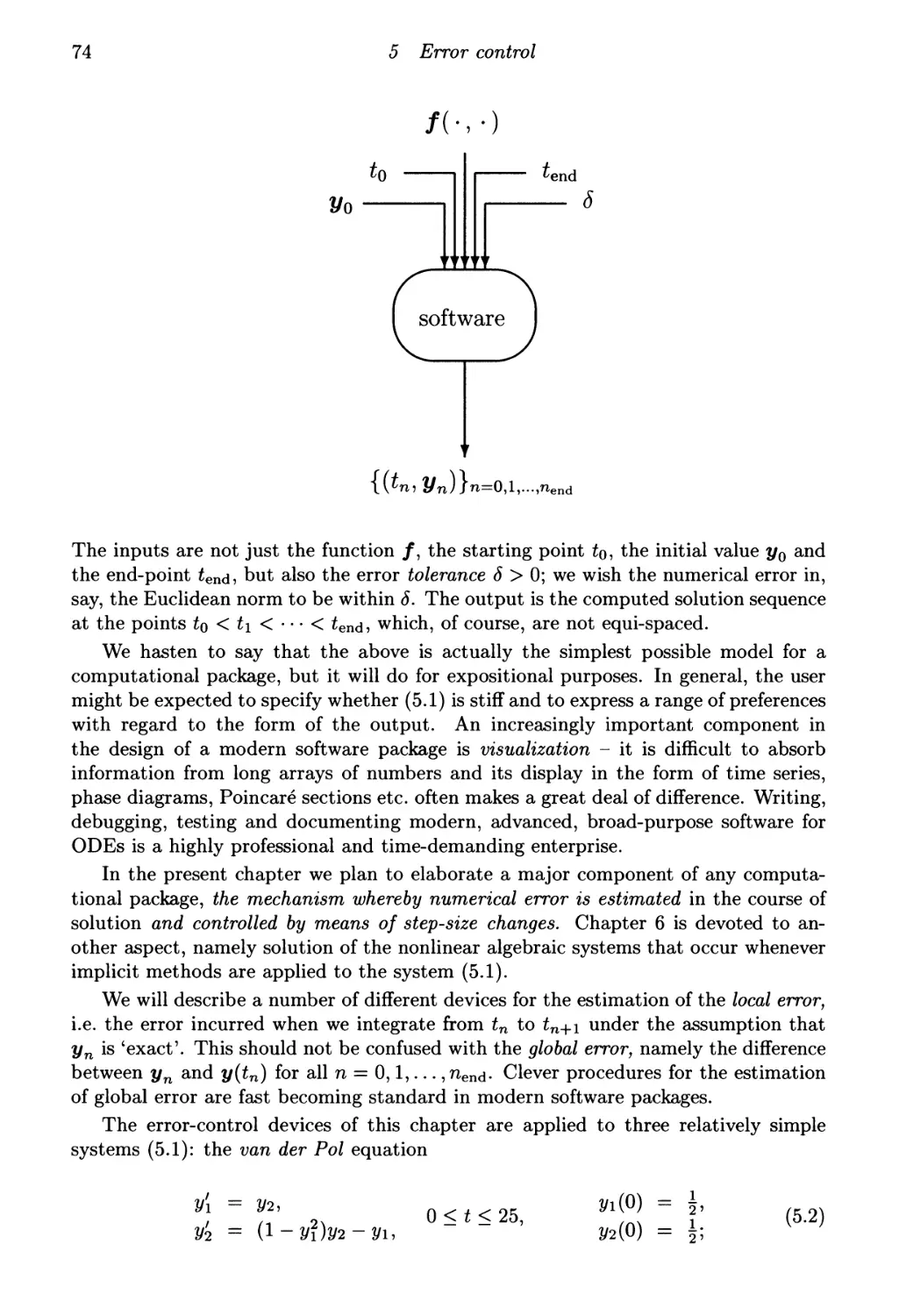
5.1 Numerical software vs numerical mathematics 73
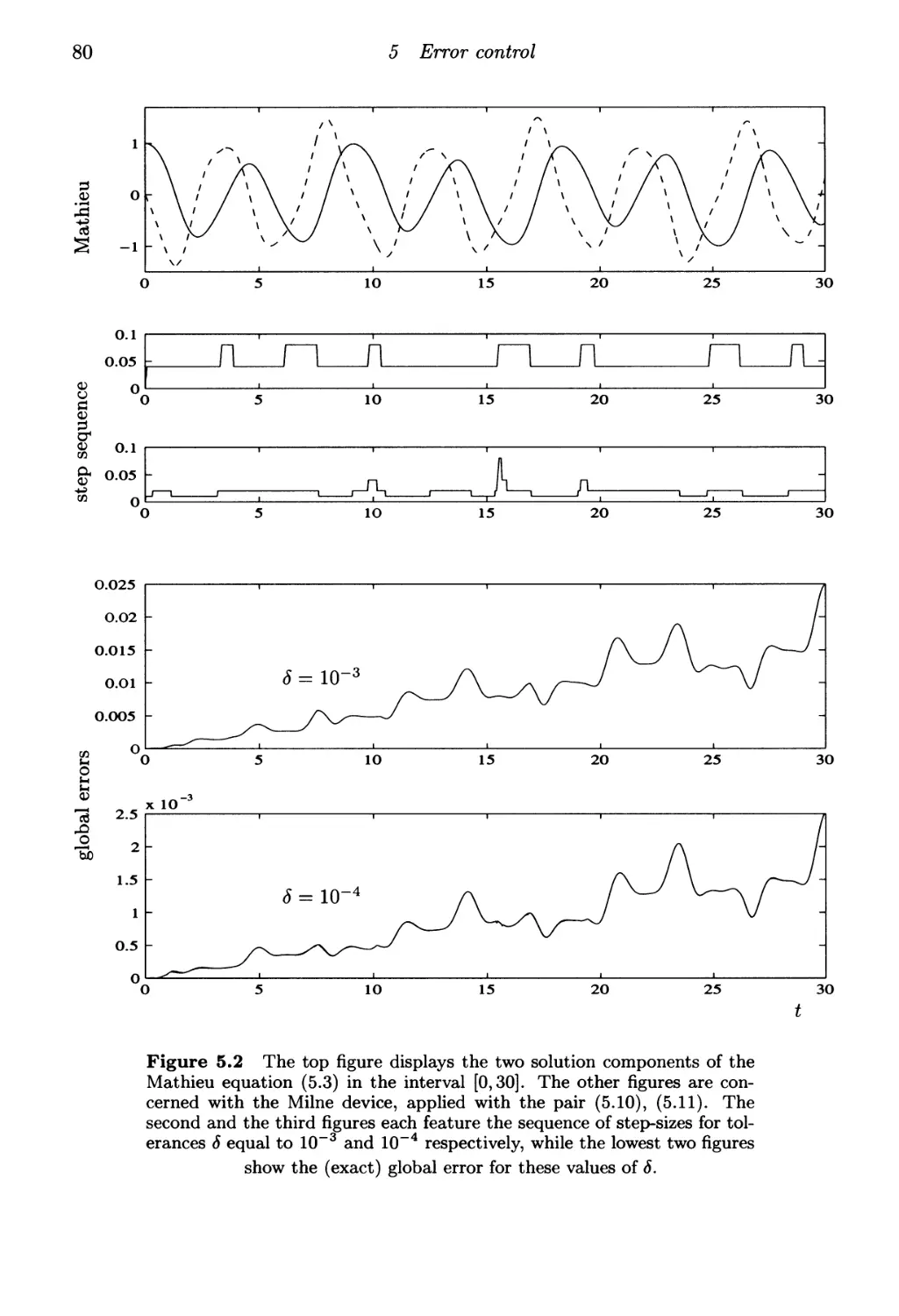
5.2 The Milne device 75
5.3 Embedded Runge-Kutta methods 81
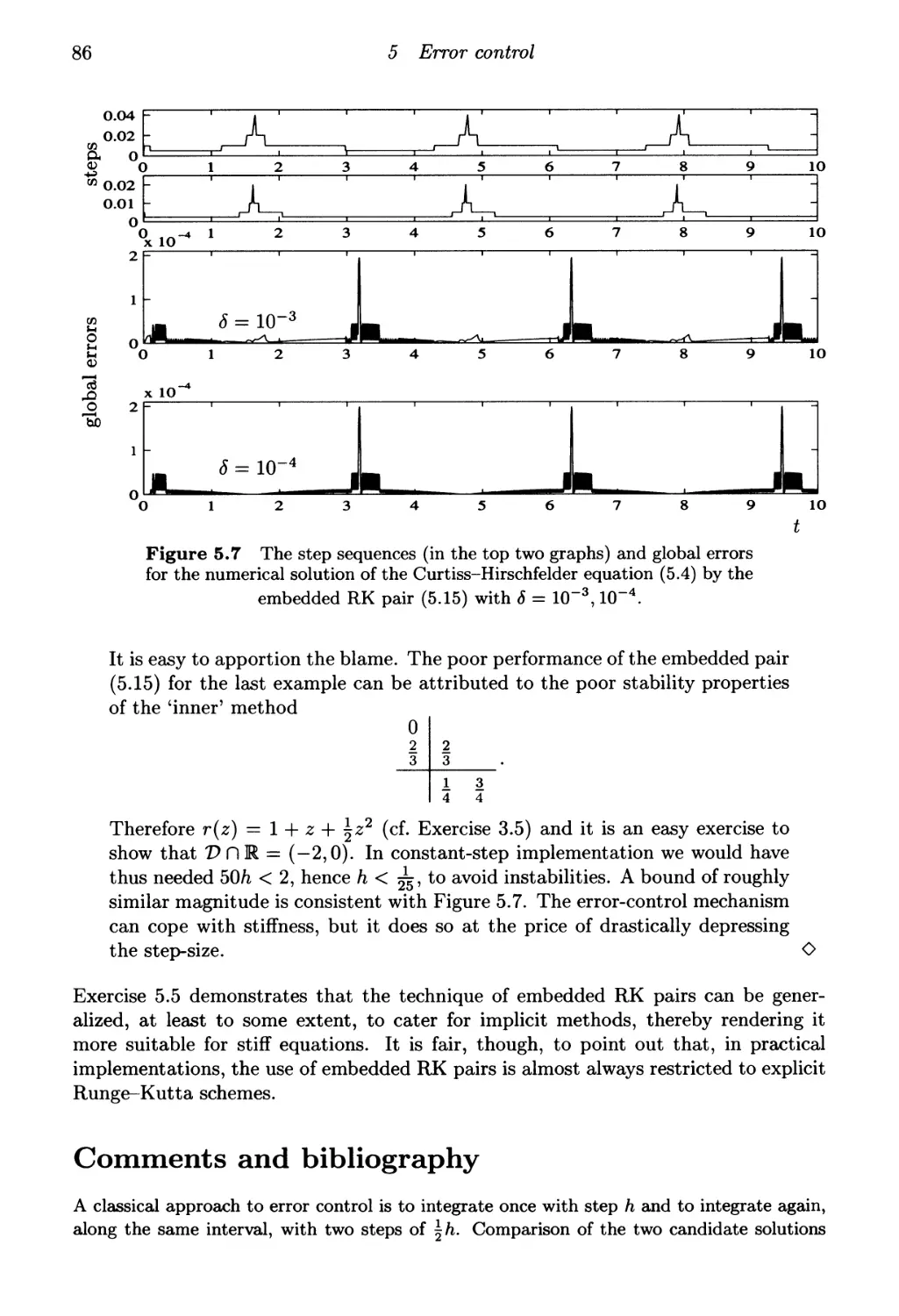
Comments and bibliography 86
Exercises 89
6 Nonlinear algebraic systems 91
6.1 Functional iteration 91
6.2 The Newton-Raphson algorithm and its modification 95
6.3 Starting and stopping the iteration 98
Comments and bibliography 100
Exercises 101
II The Poisson equation 103
7 Finite difference schemes 105
7.1 Finite differences 105
7.2 The five-point formula for V2u = / 112
7.3 Higher-order methods for V2u = / 123
Comments and bibliography 128
Exercises 131
8 The finite element method 135
8.1 Two-point boundary value problems 135
8.2 A synopsis of FEM theory 147
8.3 The Poisson equation 155
Comments and bibliography 163
Exercises 165
9 Gaussian elimination for sparse linear equations 169
9.1 Banded systems 169
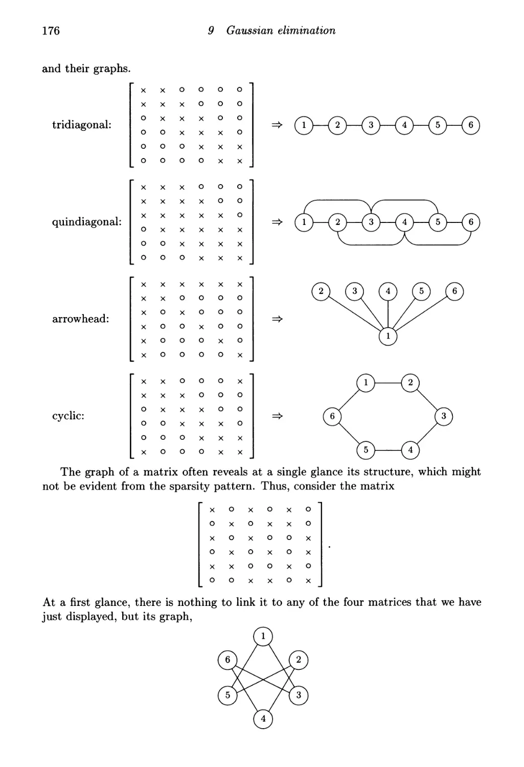
9.2 Graphs of matrices and perfect Cholesky factorization 174
Comments and bibliography 179
Exercises 182
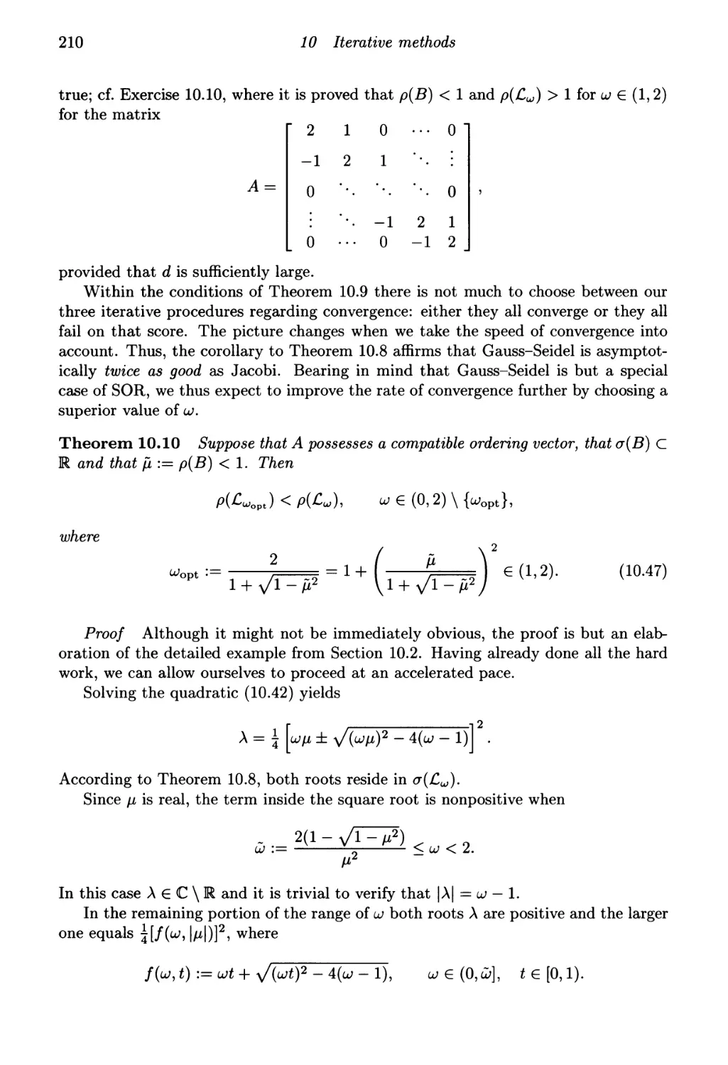
10 Iterative methods for sparse linear equations 185
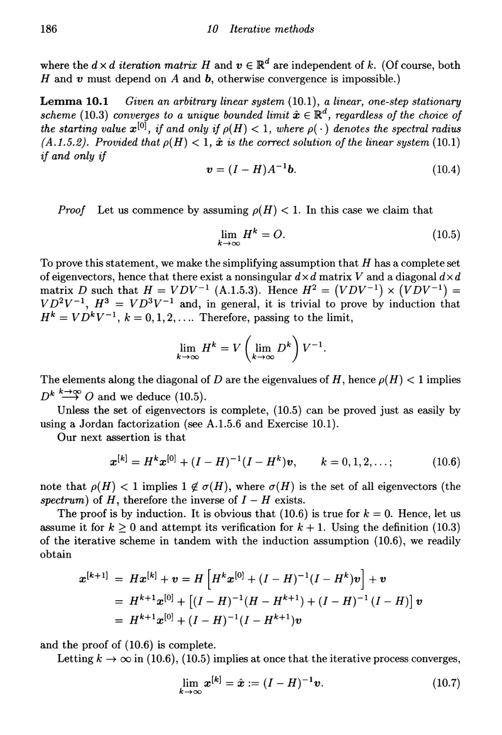
10.1 Linear, one-step, stationary schemes 185
10.2 Classical iterative methods 193
10.3 Convergence of successive over-relaxation 204
10.4 The Poisson equation 214
Comments and bibliography 219
Exercises 224

Contents ix
11 Multigrid techniques 227
11.1 In lieu of a justification 227
11.2 The basic multigrid technique 234
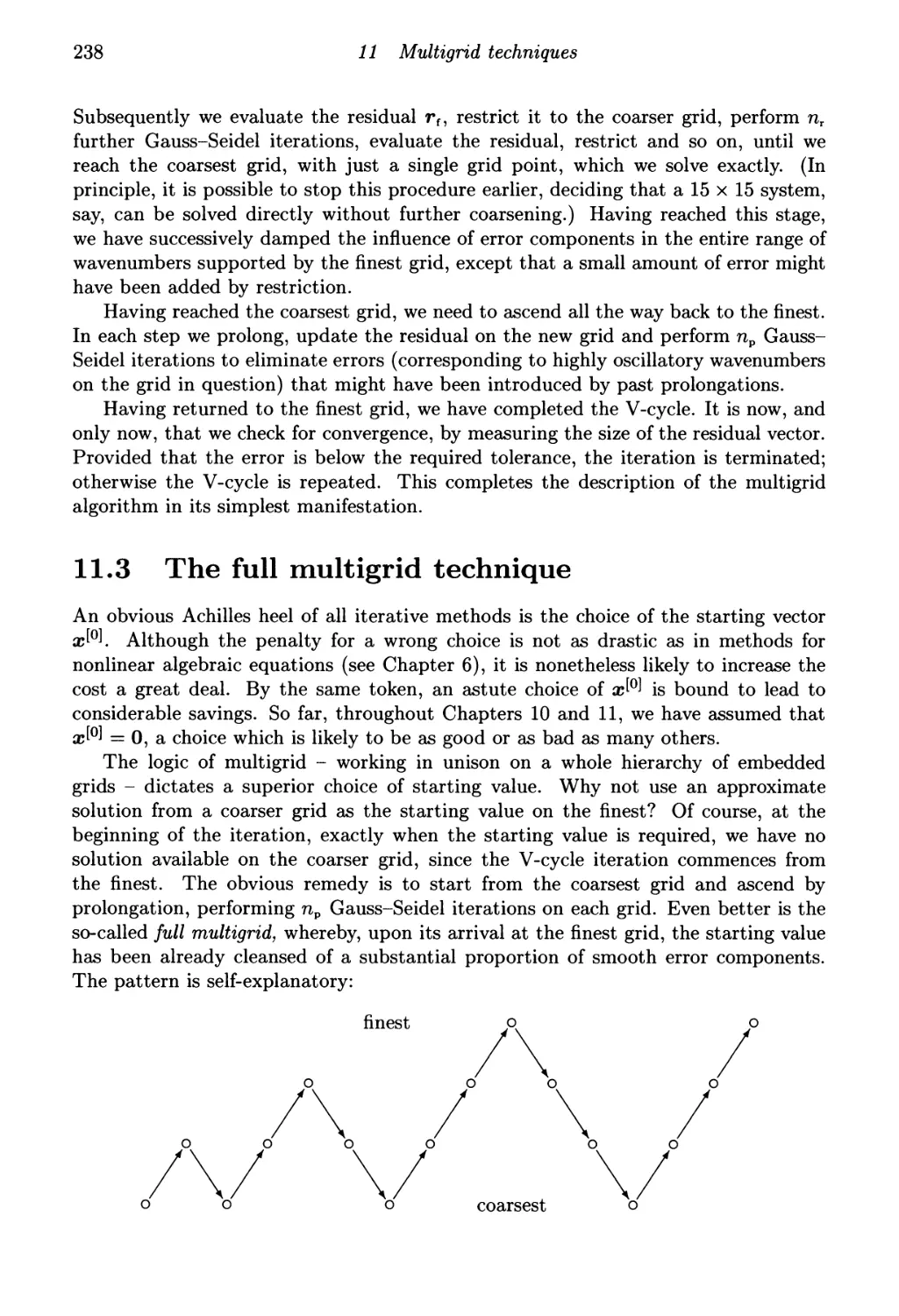
11.3 The full multigrid technique 238
11.4 Poisson by multigrid 240
Comments and bibliography 242
Exercises 243
12 Fast Poisson solvers 245
12.1 TST matrices and the Hockney method 245
12.2 The fast Fourier transform 249
12.3 Fast Poisson solver in a disc 256
Comments and bibliography 262
Exercises 264
III Partial differential equations of evolution 267
13 The diffusion equation 269
13.1 A simple numerical method 269
13.2 Order, stability and convergence 275
13.3 Numerical schemes for the diffusion equation 282
13.4 Stability analysis I: Eigenvalue techniques 287
13.5 Stability analysis II: Fourier techniques 292
13.6 Splitting 297
Comments and bibliography 301
Exercises 303
14 Hyperbolic equations 307
14.1 Why the advection equation? 307
14.2 Finite differences for the advection equation 314
14.3 The energy method 325
14.4 The wave equation 327
14.5 The Burgers equation 333
Comments and bibliography 338
Exercises 342
Appendix: Bluffer's guide to useful mathematics 347
A.l Linear algebra 348
A.1.1 Vector spaces 348
A.1.2 Matrices 349
A.1.3 Inner products and norms 352
A.1.4 Linear systems 354
A. 1.5 Eigenvalues and eigenvectors 357
Bibliography 359

χ Contents
Α.2.2 Approximation theory 362
Α.2.3 Ordinary differential equations 364
Bibliography 365
Index 367

Preface
Books - so we are often told - should be born out of a sense of mission, a wish to
share knowledge, experience and ideas, a penchant for beauty. This book has been
born out of a sense of frustration.
For the last decade or so I have been teaching the numerical analysis of differential
equations to mathematicians, in Cambridge and elsewhere. Examining this extensive
period of trial and (frequent) error, two main conclusions come to mind and both have
guided my choice of material and presentation in this volume.
Firstly, mathematicians are different from other varieties of homo sapiens. It may
be observed that people study numerical analysis for various reasons. Scientists
and engineers require it as a means to an end, a tool to investigate the subject
matter that really interests them. Entirely justifiably, they wish to spend neither
time nor intellectual effort on the finer points of mathematical analysis, typically
preferring a style that combines a cook-book presentation of numerical methods with
a leavening of intuitive and hand-waving explanations. Computer scientists adopt
a different, more algorithmic, attitude. Their heart goes after the clever algorithm
and its interaction with computer architecture. Differential equations and their likes
are abandoned as soon as decency allows (or sooner). They are replaced by discrete
models, which in turn are analysed by combinatorial techniques. Mathematicians,
though, follow a different mode of reasoning. Typically, mathematics students are
likely to participate in an advanced numerical analysis course in their final year of
undergraduate studies, or perhaps in the first postgraduate year. Their studies until
that point in time would have consisted, to a large extent, of a progression of formal
reasoning, the familiar sequence of axiom => theorem => proof => corollary =>
Numerical analysis does not fit easily into this straitjacket, and this goes a long way
toward explaining why many students of mathematics find it so unattractive.
Trying to teach numerical analysis to mathematicians, one is thus in a dilemma:
should the subject be presented purely as a mathematical theory, intellectually
pleasing but arid insofar as applications are concerned or, alternatively, should the audience
be administered an application-oriented culture shock that might well cause it to vote
with its feet?! The resolution is not very difficult, namely to present the material in
a bona fide mathematical manner, occasionally veering toward issues of applications
and algorithmics but never abandoning honesty and rigour. It is perfectly allowable
to omit an occasional proof (which might well require material outside the scope of
the presentation) and even to justify a numerical method on the grounds of
plausibility and a good track record in applications. But plausibility, a good track record,
XI

Xll
Preface
intuition and old-fashioned hand-waving do not constitute an honest mathematical
argument and should never be presented as such.
Secondly, students should be exposed in numerical analysis to both ordinary and
partial differential equations, as well as to means of dealing with large sparse algebraic
systems. The pressure of many mathematical subjects and sub-disciplines is such that
only a modest proportion of undergraduates are likely to take part in more than
a single advanced numerical analysis course. Many more will, in all likelihood, be
faced with the need to solve differential equations numerically in the future course of
their professional life. Therefore, the option of restricting the exposition to ordinary
differential equations, say, or to finite elements, while having the obvious merit of
cohesion and sharpness of focus is counterproductive in the long term.
To recapitulate, the ideal course in the numerical analysis of differential equations,
directed toward mathematics students, should be mathematically honest and rigorous
and provide its target audience with a wide range of skills in both ordinary and
partial differential equations. For the last decade I have been desperately trying to
find a textbook that can be used to my satisfaction in such a course - in vain. There
are many fine textbooks on particular aspects of the subject: numerical methods
for ordinary differential equations, finite elements, computation of sparse algebraic
systems. There are several books that span the whole subject but, unfortunately, at
a relatively low level of mathematical sophistication and rigour. But, to the best of
my knowledge, no text addresses itself to the right mathematical agenda at the right
level of maturity. Hence my frustration and hence the motivation behind this volume.
This is perhaps the place to review briefly the main features of this book.
ik We cover a broad range of material: the numerical solution of ordinary
differential equations by multistep and Runge-Kutta methods; finite difference and
finite element techniques for the Poisson equation; a variety of algorithms for
solving the large systems of sparse algebraic equations that occur in the course
of computing the solution of the Poisson equation; and, finally, methods for
parabolic and hyperbolic differential equations and techniques for their analysis.
There is probably enough material in this book for a one-year, fast-paced course
and probably many lecturers will wish to cover only part of the material. To help
them - and their students - to navigate in the numerical minefield, this preface
is accompanied by a flowchart on page xvii that displays the 'connectivity' of
this book's contents. The darker-shaded items along the centre form the core:
no decent exposition of the subject can afford to avoid these topics. (Of course,
it is entirely legitimate to pick and choose within each chapter!) The boxes
corresponding to optional material are shaded lighter - the incorporation of these
topics is a matter for individual choice. They all contain valuable material but,
in their entirety, might well exceed the capacity and attention span of a typical
advanced undergraduate course.
ik This is a textbook for mathematics students. By implication, it is not a
textbook for computer scientists, engineers or natural scientists. As I have already
argued, each group of students has different concerns and thought modes. Each
assimilates knowledge differently. Hence, a textbook that attempts to be
different things to different audiences is likely to disappoint them all. Nevertheless,

Preface
хш
non-mathematicians in need of numerical knowledge can benefit from this
volume, but it is fair to observe that they should perhaps peruse it somewhat later
in their careers, when in possession of the appropriate degree of motivation and
background knowledge.
On an even more basic level of restriction, this is a textbook, not a monograph or
a collection of recipes. Emphatically, our mission is not to bring the exposition
to the state of the art or to highlight the most advanced developments. Likewise,
it is not our intention to provide techniques that cater for all possible problems
and eventualities.
* An annoying feature of many numerical analysis texts is that they display
inordinately long lists of methods and algorithms to solve any one problem. Thus,
not just one Runge-Kutta method but twenty! The hapless reader is left with an
arsenal of weapons but, all too often, without a clue which one to use and why.
In this volume we adopt an alternative approach: methods are derived from
underlying principles and these principles, rather than the algorithms themselves,
are at the centre of our argument. As soon as the underlying principles are
sorted out, algorithmic fireworks become the least challenging part of numerical
analysis - the real intellectual effort goes into the mathematical analysis.
This is not to say that issues of software are not important or that they are
somehow of a lesser scholarly pedigree. They receive our attention in
Chapter 5 and I hasten to emphasize that good software design is just as challenging
as theorem-proving. Indeed, the proper appreciation of difficulties in software
and applications is enhanced by the understanding of the analytic aspects of
numerical mathematics.
* A truly exciting aspect of numerical analysis is the extensive use it makes of
different mathematical disciplines. If you believe that numerics are a
mathematical cop-out, a device for abandoning mathematics in favour of something
'softer', you are in for a shock. Numerical analysis is perhaps the most extensive
and varied user of a very wide range of mathematical theories, from basic
linear algebra and calculus all the way to functional analysis, differential topology,
graph theory, analytic function theory, nonlinear dynamical systems, number
theory, convexity theory - and the list goes on and on. Hardly any theme in
modern mathematics fails to inspire and help numerical analysis. Hence,
numerical analysts must be open-minded and ready to borrow from a wide range
of mathematical skills - this is not a good bolt-hole for narrow specialists!
In this volume we emphasize the variety of mathematical themes that inspire
and inform numerical analysis. This is not as easy as it might sound, since it
is impossible to take for granted that students in different universities have a
similar knowledge of pure mathematics. In other words, it is often necessary
to devote a few pages to a topic which, in principle, has nothing to do with
numerical analysis per se but which, nonetheless, is required in our exposition.
I ask for the indulgence of those readers who are more knowledgeable in arcane
mathematical matters - all they need is simply to skip few pages

XIV
Preface
* There is a major difference between recalling and understanding a
mathematical concept. Reading mathematical texts I often come across concepts that are
familiar and which I have certainly encountered in the past. Ask me, however,
to recite their precise definition and I will probably flunk the test. The proper
and virtuous course of action in such an instance is to pause, walk to the nearest
mathematical library and consult the right source. To be frank, although
sometimes I pursue this course of action, more often than not I simply go on reading.
I have every reason to believe that I am not alone in this dubious practice.
In this volume I have attempted a partial remedy to the aforementioned
phenomenon, by adding an appendix named 'Bluffer's guide to useful mathematics'.
This appendix lists in a perfunctory manner definitions and major theorems in
a range of topics - linear algebra, elementary functional analysis and
approximation theory - to which students should have been exposed previously but
which might have been forgotten. Its purpose is neither to substitute
elementary mathematical courses nor to offer remedial teaching. If you flick too often
to the end of the book in search of a definition then, my friend, perhaps you
had better stop for a while and get to grips with the underlying subject, using
a proper textbook. Likewise, if you always pursue a virtuous course of action,
consulting a proper source in each and every case of doubt, please do not allow
me to tempt you off the straight and narrow.
* Part of the etiquette of writing mathematics is to attribute material and to refer
to primary sources. This is important not just to quench the vanity of one's
colleagues but also to set the record straight, as well as allowing an interested
reader access to more advanced material. Having said this, I entertain serious
doubts with regard to the practice of sprinkling each and every paragraph in a
textbook with copious references. The scenario is presumably that, having read
the sentence '... suppose that χ € U, where U is a foliated widget [37]', the reader
will look up the references, identify '[37]' with a paper of J. Bloggs in Proc. SDW,
recognize the latter as Proceedings of the Society of Differentiable Widgets, walk
to the library, locate the journal (which will be actually on the shelf, rather
than on loan, misplaced or stolen) All this might not be far-fetched as far as
advanced mathematics monographs are concerned but makes very little sense in
an undergraduate context. Therefore I have adopted a practice whereby there
are no references in the text proper. Instead, each chapter is followed by a section
of 'Comments and bibliography', where we survey briefly further literature that
might be beneficial to students (and lecturers).
Such sections serve a further important purpose. Some students - am I too
optimistic? - might be interested and inspired by the material of the chapter.
For their benefit I have given in each 'Comments and bibliography' section a
brief discussion of further developments, algorithms, methods of analysis and
connections with other mathematical disciplines.

Preface
xv
* Clarity of exposition often hinges on transparency of notation. Thus, throughout
this book we use the following convention.
• Lower-case lightface sloping letters (a, 6, c, a, /?, 7,...) represent scalars;
• Lower-case boldface sloping letters (a, 6, c, a, /3,7,...) represent vectors;
• Upper-case lightface letters (A, B, C, θ, Φ,...) represent matrices;
• Letters in calligraphic font {A, B,C,...) represent operators;
• Shell capitals (A,B,C...) represent sets.
Mathematical constants like i = л/—Ϊ and e, the base of natural logarithms, are
denoted by roman, rather than italic letters. This follows British typesetting
convention and helps to identify the different components of a mathematical
formula.
As with any principle, our notational convention has its exceptions. For
example, in Section 3.1 we refer to Legendre and Chebyshev polynomials by the
conventional notation, Pn and Tn: any other course of action would have caused
utter confusion. And, again as with any principle, grey areas and ambiguities
abound. I have tried to eliminate them by applying common sense but this,
needless to say, is a highly subjective criterion.
This book started out life as two sets of condensed lecture notes - one for students of
Part II (the last year of undergraduate mathematics in Cambridge) and the other for
students of Part III (the Cambridge advanced degree course in mathematics). The task
of expanding lecture notes to a full-scale book is, unfortunately, more complicated than
producing a cup of hot soup from concentrate by adding boiling water, stirring and
simmering for a short while. Ultimately, it has taken the better part of a year, shared
with the usual commitments of academic life. The main portion of the manuscript
was written in Autumn 1994, during a sabbatical leave at the California Institute of
Technology (Caltech). It is my pleasant duty to acknowledge the hospitality of my
many good friends there and the perfect working environment in Pasadena.
A familiar computer proverb states that while the first 90% of a programming
job takes 90% of the time the remaining 10% also takes 90% of the time Writing
a textbook follows similar rules and, back home in Cambridge, I have spent several
months reading and rereading the manuscript. This is the place to thank a long list of
friends and colleagues whose help has been truly crucial: Brad Baxter (Imperial
College, London), Martin Buhmann (Swiss Institute of Technology, Zurich), Yu-Chung
Chang (Caltech), Stephen Cowley (Cambridge), George Goodsell (Cambridge), Mike
Hoist (Caltech), Herb Keller (Caltech), Yorke Liu (Cambridge), Michelle Schatzman
(Lyon), Andrew Stuart (Stanford), Stefan Vandewalle (Louven) and Antonella Zanna
(Cambridge). Some have read the manuscript and offered their comments. Some
provided software well beyond my own meagre programming skills and helped with
the figures and with computational examples. Some have experimented with the
manuscript upon their students and listened to their complaints. Some contributed
insight and occasionally saved me from embarrassing blunders. All have been
helpful, encouraging and patient to a fault with my foibles and idiosyncrasies. None is

XVI
Preface
responsible for blunders, errors, mistakes, misprints and infelicities that, in spite of
my sincerest efforts, are bound to persist in this volume.
This is perhaps the place to extend thanks to two 'friends' that have made the
process of writing this book considerably easier: the T^jX typesetting system and the
Matlab package. These days we take mathematical typesetting for granted but it is
often forgotten that just a decade ago a mathematical manuscript would have been
hand-written, then typed and retyped and, finally, typeset by publishers - each stage
requiring laborious proofreading. In turn, Matlab allows us a unique opportunity to
turn our office into a computational-cum-graphic laboratory, to bounce ideas off the
computer screen and produce informative figures and graphic displays. Not since the
discovery of coffee have any inanimate objects caused so much pleasure to so many
mathematicians!
The editorial staff of Cambridge University Press, in particular Alan Harvey, David
Tranah and Roger Astley, went well beyond the call of duty in being helpful, friendly
and cooperative. Susan Parkinson, the copy editor, has worked to the highest
standards. Her professionalism, diligence and good taste have done wonders in sparing the
readers numerous blunders and the more questionable examples of my hopeless wit.
This is a pleasant opportunity to thank them all.
Last but never the least, my wife and best friend, Dganit. Her encouragement,
advice and support cannot be quantified in conventional mathematical terms. Thank
you!
I wish to dedicate this book to my parents, Gisella and Israel. They are not
mathematicians, yet I have learnt from them all the really important things that have
motivated me as a mathematician: love of scholarship and admiration for beauty and
art.
Arieh Iserles
August 1995

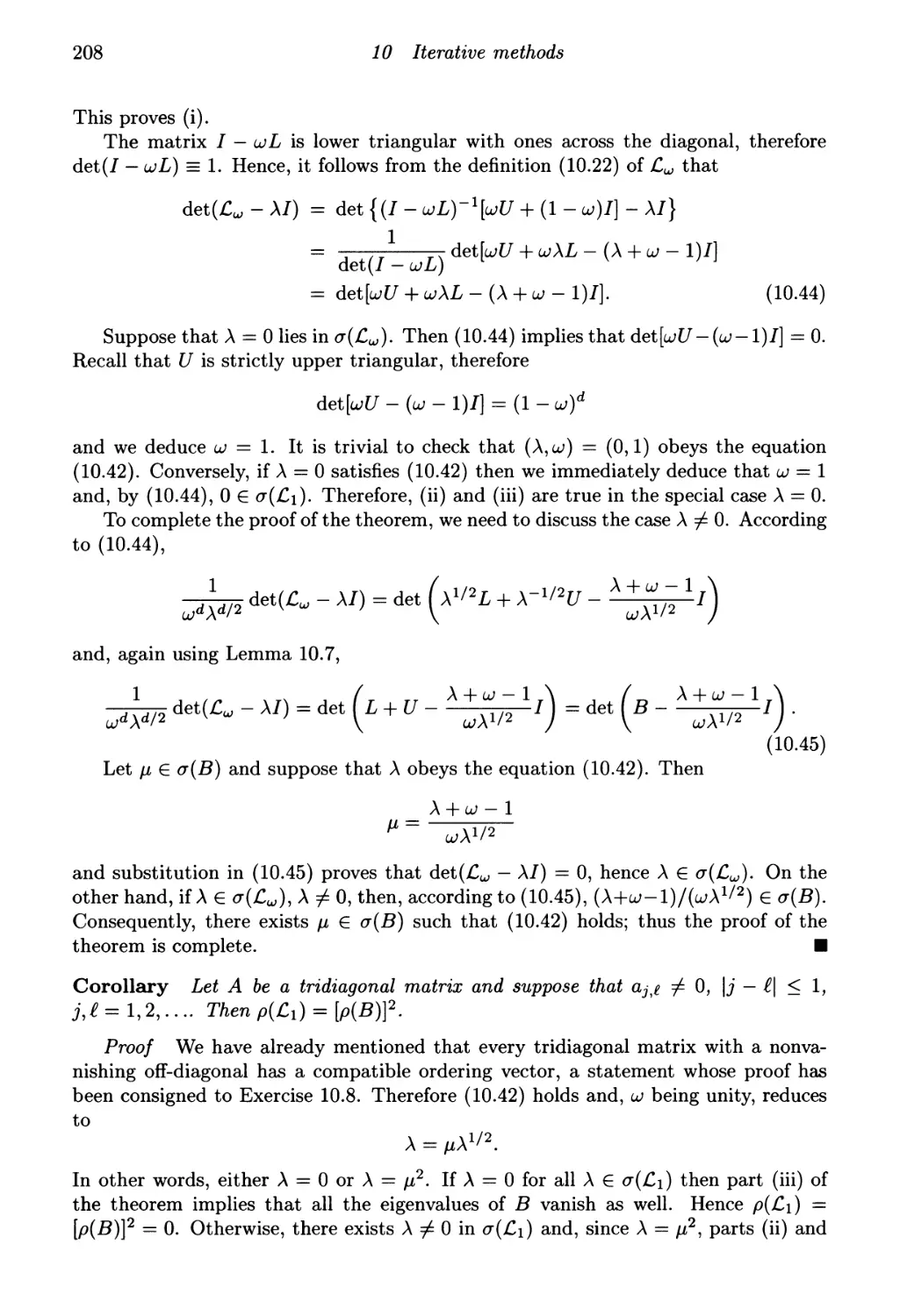
Flowchart of contents
Error
control
β Algebraic
systems
ι ο Finite
elements
1 Introductk
Α λ Multistep methods
О Runge-Kutta methods
4 Stiff equations
7 Finite differences
13 The diffusion equation
14 Hyperbolic equations
q Gaussian
elimination
Jin Iterative
methods
■
'
11 Multigrid
\J л г) Fast
solvers

This page intentionally left blank

PART I
Ordinary differential equations

This page intentionally left blank

1
Euler's method and beyond
1.1 Ordinary differential equations and the Lips-
chitz condition
We commence our exposition of the computational aspects of differential equations by
a close - yet extensive - examination of numerical methods for ordinary differential
equations (ODEs). This is important because of the central role of ODEs in a
multitude of applications. Not less crucial is the critical part that numerical ODEs play
in the design and analysis of computational methods for partial differential equations
(PDEs).
Our goal is to approximate the solution of the problem
y' = /(i,y), t>t0, y(t0) = y0. (1.1)
Here / is a sufficiently well-behaved function that maps [£o,oo) χ R to R and the
initial condition y0 € R is a given vector. R denotes here - and elsewhere in this
book - the d-dimensional real Euclidean space.
The 'niceness' of / may span a whole range of desirable attributes. At the very
least, we insist on / obeying, in a given vector norm || · ||, the Lipschitz condition
||/(i,n5)-/(i,y)||<A||ic-y|| for all x,y€Rd, t>t0. (1.2)
Here λ > 0 is a real constant that is independent of the choice of χ and у - a
Lipschitz constant. Subject to (1.2), it is possible to prove that the ODE system (1.1)
possesses a unique solution.1 Taking a stronger requirement, we may stipulate that
/ is an analytic function - in other words, that the Taylor series of / about every
(£, yQ) € [0, oo) χ Rd has a positive radius of convergence. It is then possible to prove
that the solution у itself is analytic. Analyticity comes in handy, since much of our
investigation of numerical methods is based on Taylor expansions, but it is often an
excessive requirement and excludes many ODEs of practical importance.
In this volume we strive to steer a middle course between the complementary vices
of mathematical nitpicking and of hand-waving. We solemnly undertake to avoid any
needless mention of exotic function spaces that present the theory in its most general
form, whilst desisting from woolly and inexact statements. Thus, we always assume
that / is Lipschitz and, as necessary, may explicitly stipulate that it is analytic.
An intelligent reader could, if the need arose, easily weaken many of our 'analytic'
statements so that they are applicable also to sufficiently-differentiable functions.
1 We refer to the Appendix for a brief refresher course on norms, existence and uniqueness theorems
for ODEs and other useful odds and ends of mathematics.
3

4
1 Euler's method and beyond
1.2 Euler's method
Let us ponder briefly the meaning of the ODE (1.1). We possess two items of
information: we know the value of у at a single point t = to and, given any function
value у € R and time t > to, we can tell the slope from the differential equation.
The purpose of the exercise being to guess the value of у at a new point, the most
elementary approach is to use a linear interpolant. In other words, we estimate y(t)
by making the approximation f(t,y(t)) ~ f(to,y(to)) f°r t ^ [to, to + h], where h > 0
is sufficiently small. Integrating (1.1),
V(t) = y(to) + / /(r, y(r)) dr и y0 + (f - to)/(*o, Уо)· (1-3)
«/ίο
Given a sequence £o> ^i = ^o + h, £2 = ^o + 2/i,..., where h > 0 is the tame step, we
denote by yn a numerical estimate of the exact solution y(in),n = 0,l, Motivated
by (1.3), we choose
У ι = Ι/ο + Λ/(*ο,Ι/0)·
This procedure can be continued to produce approximants at £2, £3 and so on. In
general, we obtain the recursive scheme
1/n+i = У η + Λ/(ίη, 1/η)> η - 0,1,..., (1.4)
the celebrated Enter method.
Euler's method is not only the most elementary computational scheme for ODEs
and, simplicity notwithstanding, of enduring practical importance. It is also the
cornerstone of the numerical analysis of differential equations of evolution. In a deep
and profound sense, all the fancy multistep and Runge-Kutta schemes that we shall
discuss in the sequel are nothing but a generalization of the basic paradigm (1.4).
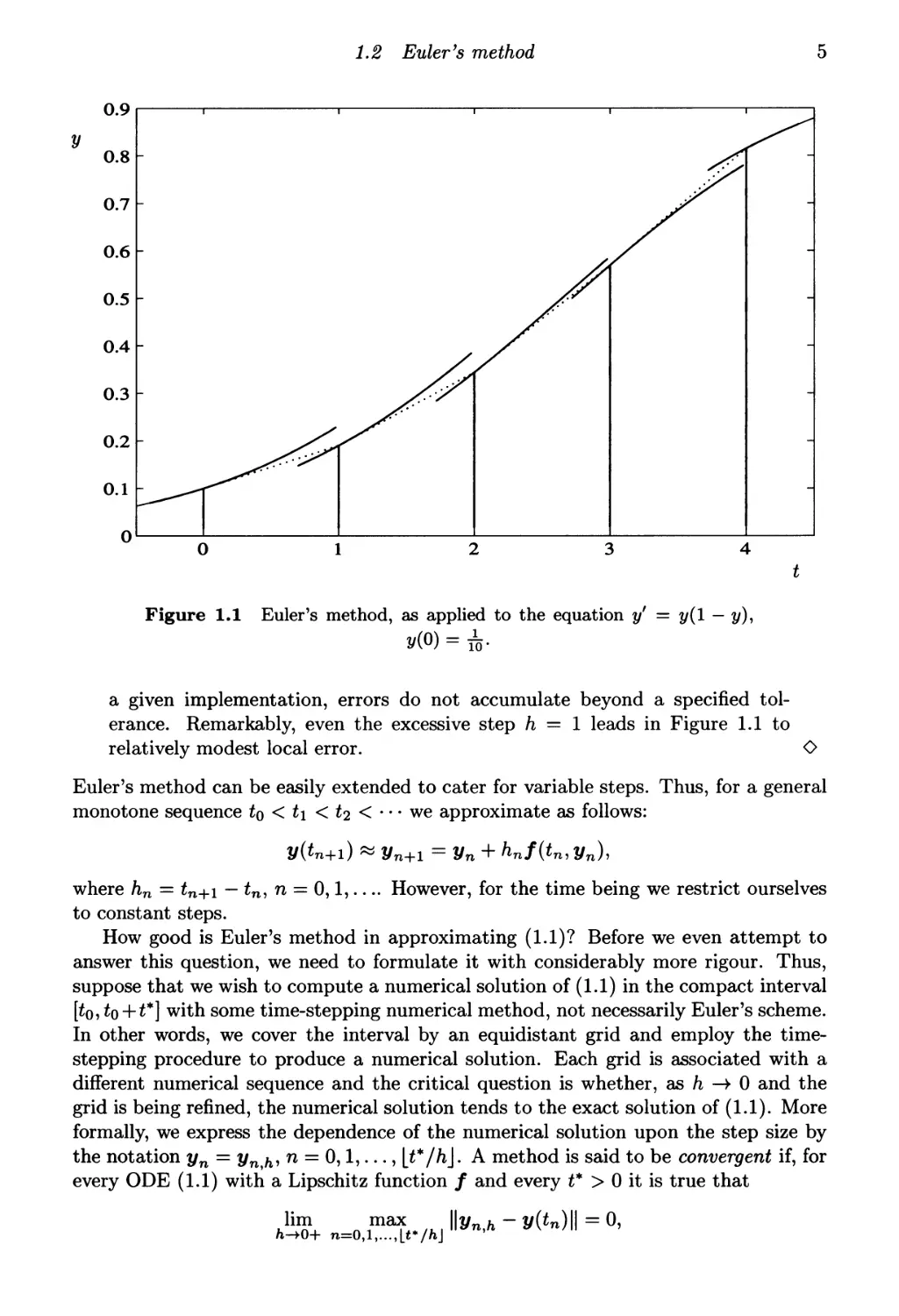
О Graphic interpretation Euler's method can be illustrated pictorially.
Consider, for example, the scalar logistic equation y' = y(l — ?/), y(0) = ^.
Figure 1.1 displays the first few steps of Euler's method, with a grotesquely
large step h = 1. For each step we show the exact solution with initial
condition y(tn) = yn in the vicinity of tn = nh (solid line) and the linear
interpolation via Euler's method (1.4) (dotted line).
The initial condition being, by definition, exact, so is the slope at to. However,
instead of following a curved trajectory, the numerical solution is piece wise-
linear. Having reached £1, say, we have moved to a wrong trajectory (i.e.,
corresponding to a different initial condition). The slope at t\ is wrong -
or, rather, it is the correct slope of a wrong solution! Advancing further, we
might well stray even more from the original trajectory.
A realistic goal of numerical solution is not, however, to avoid errors
altogether; after all, we approximate since we do not know the exact solution
in the first place! An error-generating mechanism exists in every algorithm
for numerical ODEs and our purpose is to understand it and to ensure that, in

1.2 Euler's method
5
0.8
0.7
0.6
0.5
0.4
0.3
0.2
0.1
0
, , , ,j
yS
^r
/^
//
у^Л
I
-
-
-
-
-
-
и
Figure 1.1 Euler's method, as applied to the equation y' = y(l — y),
v(Q) = &·
a given implementation, errors do not accumulate beyond a specified
tolerance. Remarkably, even the excessive step h = 1 leads in Figure 1.1 to
relatively modest local error. О
Euler's method can be easily extended to cater for variable steps. Thus, for a general
monotone sequence to < t\ < ti < · · · we approximate as follows:
l/(*n+l) « l/n+l = Уп + hnf{tn,Vn)i
where hn = tn+\ — tn, η = 0,1, However, for the time being we restrict ourselves
to constant steps.
How good is Euler's method in approximating (1.1)? Before we even attempt to
answer this question, we need to formulate it with considerably more rigour. Thus,
suppose that we wish to compute a numerical solution of (1.1) in the compact interval
[£(b £o + £*] with some time-stepping numerical method, not necessarily Euler's scheme.
In other words, we cover the interval by an equidistant grid and employ the time-
stepping procedure to produce a numerical solution. Each grid is associated with a
different numerical sequence and the critical question is whether, as h -> 0 and the
grid is being refined, the numerical solution tends to the exact solution of (1.1). More
formally, we express the dependence of the numerical solution upon the step size by
the notation yn = yn^ η = 0,1,..., \t*/h\. A method is said to be convergent if, for
every ODE (1.1) with a Lipschitz function / and every t* > 0 it is true that
h-*0+ n=0,l,...,Lt*//iJ

6
1 Euler's method and beyond
where [a\ € Ζ is the integer part of α € R. Hence, convergence means that, for
every Lipschitz function, the numerical solution tends to the true solution as the grid
becomes increasingly fine.2
In the next few chapters we will mention several desirable attributes of numerical
methods for ODEs. It is crucial to understand that convergence is not just another
'desirable' property but, rather, a sine qua поп of any numerical scheme. Unless it
converges, a numerical method is useless!
Theorem 1.1 Euler's method (1.4) is convergent.
Proof We prove this theorem subject to the extra assumption that the function
/ (and therefore also y) is analytic (it is enough, in fact, to stipulate the weaker
condition of continuous differentiability).
Given h > 0 and yn = ynh, η = 0,1,..., [t*/h\, we let еп>л = уп>л - y(tn) denote
the numerical error. Thus, we wish to prove that lim/l_).o+ maxn Цвп^Ц = О.
By Taylor's theorem and the differential equation (1.1),
y(tn+i) - V(tn) + hy'{tn) + 0(h2) = y{tn) + hf{tn,y{tn)) + 0(ft2), (1.5)
and, у being continuously differentiable, the (9 (ft2) term can be bounded (in a given
norm) uniformly for all h > 0 and η < [t*/ft J by a term of the form eft2, where с > 0
is a constant. We subtract (1.5) from (1.4), giving
+ h[f(tn,y(tn) + enM) - f{tn,y(tn))) + 0(ft2).
Thus, it follows by the triangle inequality from the Lipschitz condition and the
aforementioned bound on the О (ft2) reminder term that
l|en+i,h|| < ||en,h|| + Л||/(*п,у(*п) + еп>л) - f{tn,y{tn))\\ + ch2
< (l + ftAJIIe^H + cft2, n = 0,l,...,Lt7ftJ-l, (1.6)
We now claim that
||е„,л|| < jh [(1 + h\)n - 1], η = 0,1,.... (1.7)
The proof is by induction on n. When η = 0 we need to prove that Цео^Ц < О and
hence that βο,/г = 0. This is certainly true, since at to the numerical solution matches
the initial condition and the error is zero.
For general η > 0 we assume that (1.7) is true up to η and use (1.6) to argue that
Κ+ι,λ|| < (1 + ftA)^ft [(1 + h\)n - 1] + eft2 = ^ft [(1 + ftA)n+1 - 1] .
Λ Λ
This advances the inductive argument from η to n+1 and proves that (1.7) is true. The
constant h\ is positive, therefore 1 + h\ < e/lA, and we deduce that (1 + ftA)n < enhx.
2We have just introduced a norm through the back door. This, however, should cause no worry,
since all norms are equivalent in finite-dimensional spaces. In other words, if a method is convergent
in one norm, it converges in all....

1.2 Euler's method
7
The index η is allowed to range in {0,1,..., \t*/h\}, hence (1 + h\)n < e^/h^hX <
etX. Substituting into (1.7), we obtain the inequality
||е„|Л||<^(еГА-1)Л, η = 0,1,...,ίί7Λ].
Since c(el*x — 1)/λ is independent of /ι, it follows that
lim ||еп>л||=0.
0<π/ι<£*
In other words, Euler's method is convergent. ■
О Health warning At first sight, it might appear that there is more to the last
theorem than meets the eye - not just a proof of convergence but also an upper
bound on the error. In principle it is perfectly true and the error of Euler's
method is indeed always bounded by hce1 λ/λ. Moreover, with very little
effort it is possible to demonstrate, e.g. by using the Peano kernel theorem,
that a reasonable choice is с = maxt€[t(bto+t*] ||y"(i)||. The problem with this
bound, unfortunately, is that in an overwhelming majority of practical cases
it is too large by many orders of magnitude. It falls into the broad category
of statements like 'the distance between London and New York is less than 47
light years' which, although manifestly true, fail to contribute significantly to
the sum total of human knowledge.
The problem is not with the proof per se but with the insensitivity of a
Lipschitz constant. A trivial example is the scalar linear equation y' = —100?/,
y(0) = 1. Therefore λ = 100 and, since y(t) = е-100*, с = λ2. We thus derive
the upper bound of 100h(eloot — 1). Letting t* = 1, say, we have
\yn - y(nh)\ < 2.69 χ 1045A. (1.8)
It is easy, however, to show that yn = (1 — 100/i)n, hence to derive the exact
expression
|y„ - y(nh)\ = |(1 - 100ft)n - e-l00nh\
which is smaller by many orders of magnitude than (1.8) (note that, unless
nh is very small, to all intents and purposes e~100nh « 0).
The moral of our discussion is simple. The bound from the proof of Theorem
1.1 must not be used in practical estimation of numerical error! О
Euler's method can be rewritten in the form yn+1 - [yn + hf(tn,yn)] = 0. Replacing
У pi by the exact solution y(tk), к = η, η + 1, and expanding into the first few terms
of the Talyor series about t = to + nh, we obtain
y(*„+i) - [y(tn) + hf(tn,y(tn))}
= [y(tn) + hy'{tn) + 0(h2)] - [y(tn) + hy'{tn)) = 0(h2) .
We say the Euler's method (1.4) is of order one. In general, given an arbitrary
time-stepping method
yn+i = Уп(/, Л, y0, yi,..., Уп)> η = 0,1,...,

8
1 Euler's method and beyond
for the ODE (1.1), we say that it is of order ρ if
V(*n+i) - Уп(/, A, v(*o), v(*i), · · ·, V(tn)) = <9(AP+1)
for every analytic / and η = 0,1, Alternatively, a method is of order ρ if it recovers
exactly every polynomial solution of degree ρ or less.
The order of a numerical method provides us with information about its local
behaviour - advancing from tn to £п+ъ where h > 0 is sufficiently small, we are
incurring an error of (9(/ip+1). Our main interest, however, is in not the local but
the global behaviour of the method: how well is it doing in a fixed bounded interval
of integration as h —> 0? Does it converge to the true solution? How fast? Since
the local error decays as 0(hp+l), the number of steps increases as 0(h~l). The
naive expectation is that the global error decreases as 0(hp), but - as we will see
in Chapter 2 - it cannot be taken for granted for each and every numerical method
without an additional condition. As far as Euler's method is concerned, Theorem 1.1
demonstrates that all is well and the error indeed decays as O(h).
1.3 The trapezoidal rule
Euler's method approximates the derivative by a constant in [£n?£n+i]? namely by its
value at tn (again, we denote tk = to + kh, к — 0,1,...). Clearly, the 'cantilever-
ing' approximation is not very good and it makes more sense to make the constant
approximation of the derivative equal to the average of its values at the end-points.
Bearing in mind that derivatives are given by the differential equation, we thus obtain
an expression similar to (1.3):
V(t) = V(tn)+ f /(r,y(r))dr
Jtn
« V(tn) + W ~ tn){f(tn, y(tn)) + /(fn+1, y(*n+l))}·
This is the motivation behind the trapezoidal rule
Vn+l = У η + |M/(f„,yn) + /(*n+b Vn+l)]· (L9)
To obtain the order of (1.9), we substitute the exact solution,
3/(*η+ΐ)" {у(*п)+|М/(*п,У(*п)) + /(*п+Ь!/(*п+1))]}
= [v(tn) + hy'(tn) + \h2y"(tn) + 0(h3)]
- (y(tn) + \h {y'(tn) + [y'(tn) + hy"{tn) + 0(h2)] }) = 0{h3) .
Therefore the trapezoidal rule is of order two.
Forewarned of the shortcomings of local analysis, we should not jump to
conclusions. Before we infer that the error decays globally as 0(h2), we must first prove that
the method is convergent. Fortunately, this can be accomplished by a straightforward
generalization of the method of proof of Theorem 1.1.
Theorem 1.2 The trapezoidal rule (1.9) is convergent.

1.3 The trapezoidal rule
9
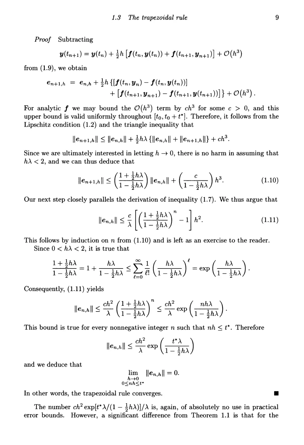
Proof Subtracting
y(tn+1) = y(tn) + Ift [/(fn,y(in)) + /(in+i,y„+i)] + 0(^3)
from (1.9), we obtain
βη+ιίΛ = еп,л + |Л{[/(*п,уп)-/(*п,у(*п))]
+ [/(in+i,y„+i) - /(ίη+ι,»(ίη+ι))] } + 0{h3).
For analytic / we may bound the (D(h3) term by ch3 for some с > 0, and this
upper bound is valid uniformly throughout [to, to +1*]. Therefore, it follows from the
Lipschitz condition (1.2) and the triangle inequality that
||еп+1,л|| < ||еп,л|| + \h\ {||еП|Л|| + ||βη+ι|Λ||} + ch3.
Since we are ultimately interested in letting h —> 0, there is no harm in assuming that
h\ < 2, and we can thus deduce that
\К.Ы\<(\±Щ11е„,Л + (^щ)ь>- (МО)
Our next step closely parallels the derivation of inequality (1.7). We thus argue that
IK,/J < д
/l_+jfcA\n_
\l-±h\)
h2. (1.11)
This follows by induction on η from (1.10) and is left as an exercise to the reader.
Since 0 < h\ < 2, it is true that
l + \h\ _ h\ ^ ι / h\ \e _ ( h\ \
ι - \h\ ~ ι - \h\ ~ ^ a\i - \h\) ~exp \i - \h\)'
.11) yields
„ ch2 /1 + Ш\" ch2 ( nh\ \
l + \h\
Consequently, (1.11) yields
eft2 /1 + |/ιΛ\"< ch2
\h\) - λ 4i-5.
This bound is true for every nonnegative integer η such that nh <t*. Therefore
.2
||e„,h||<^exp(r^)
and we deduce that
lim ||еп,л||=0.
/ι-Ю
0<nh<t*
In other words, the trapezoidal rule converges. ■
The number ch2 exp[t*X/(l - ^h\)]/X is, again, of absolutely no use in practical
error bounds. However, a significant difference from Theorem 1.1 is that for the

10
1 Euler's method and beyond
trapezoidal rule the error decays globally as 0(h2). This is to be expected from a
second-order method if its convergence has been established.
Another difference between the trapezoidal rule and Euler's method is of an entirely
different character. Whereas Euler's method (1.4) can be executed explicitly - knowing
yn we can produce yn+i by computing a value of / and making a few arithmetic
operations - this is not the case with (1.9). The vector υ = yn + \hf(tn,yn) can be
evaluated from known data, but that leaves us in each step with the task of finding
yn_f_1 as the solution of the system of algebraic equations
The trapezoidal rule is thus said to be implicit, to distinguish it from the explicit
Euler's method and its ilk.
Solving nonlinear equations is hardly a mission impossible, but we cannot take it
for granted either. Only in texts on pure mathematics are we allowed to wave a magic
wand, exclaim 'let yn+1 be a solution of ...' and assume that all our problems are
over. As soon as we come to deal with actual computation, we had better specify how
we plan (or our computer plans) to undertake the task of evaluating yn+1. This will be
one of the themes of Chapter 6, which deals with the implementation of ODE methods.
It suffices to state now that the cost of numerically solving nonlinear equations does
not rule out the trapezoidal rule (and other implicit methods) as viable computational
instruments. Implicitness is just one attribute of a numerical method and we must
weigh it alongside other features.
О A 'good' example Figure 1.2 displays the (natural) logarithm of the error
in the numerical solution of the scalar linear equation y' = —y + 2e-i cos 2£,
y(0) = 0 for (in descending order) h = \, h = ^ and h = ^.
How well does the plot illustrate our main distinction between Euler's method
and the trapezoidal rule, namely faster decay of the error for the latter? As
often in life, information is somewhat obscured by extraneous 'noise'; in the
present case the error oscillates. This can be easily explained by the periodic
component of the exact solution y(t) = e_i sin 2t. Another observation is that,
for both Euler's method and the trapezoidal rule, the error, twists and turns
notwithstanding, does decay. This, on the face of it, can be explained by the
decay of the exact solution, but is an important piece of news nonetheless.
Our most pessimistic assumption is that errors might accumulate from step
to step but, as can be seen from this example, this prophecy of doom is often
misplaced. This is a highly nontrivial point which will be debated at greater
length throughout Chapter 4.
Factoring out oscillations and decay, we observe that errors indeed decrease
with h. More careful examination verifies that they increase at roughly the
rate predicted by order considerations. Specifically, for a convergent method
of order ρ we have ||e|| « chp, hence In ||e|| « In с + plnh. Denoting by e^
and e^2) errors corresponding to step sizes h^ and h^ respectively, it follows
that In ||e(2)|| « In ||e^^|| - p\n(h^/h^). The ratio of consecutive step sizes
in Figure 1.2 being five, we expect the error to decay by (at least) a constant
multiple of In 5 « 1.6094 and 2 In 5 « 3.2189 for Euler and the trapezoidal
rule respectively. The actual error decays if anything slightly faster than this. О

1.3 The trapezoidal rule
11
Euler's method
5*
I
5яа
_fi
-5
-10
-15
-20
-25
/
! ' Γ Τ
v--nV·
-
-
-
I
I
4 6
The trapezoidal rule
10
e
5*
|
5*
Й
-5
-10
-15
-20
-^^
^. — —
s
/
~ ■
_ll
|
—
1 1 1
— _^ N. ^ ■ ^^
-*· -^ ^^ ^y """--\
\ V"" "~~^-0N /^
\,\i '♦ ч ^ -·
1/ V \ /'
i 1 ',/. ■
1 1 1
^~—^^
— __ ->_
' ^
- _ "N
vv
-25
Figure 1.2 Euler's method and the trapezoidal rule, as applied to y' =
2e-t cos2£, ϊ/(0) = 0. The logarithm of the error is displayed for h = \ (solid
h = jq (broken line) and h = ^ (broken-and-dotted line).
10
t
-y +
line),
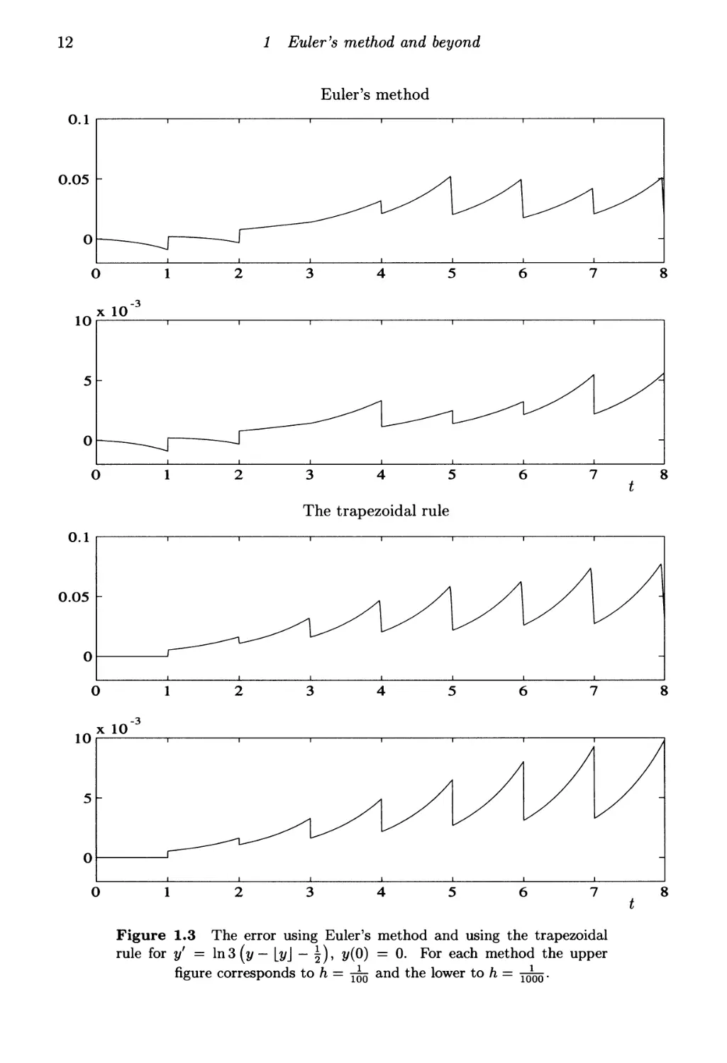
О A 'bad' example Theorems 1.1 and 1.2 and, indeed, the whole numerical
ODE theory, rest upon the assumption that (1.1) obeys the Lipschitz
condition. We can expect numerical methods to underperform in the absence
of (1.2), and this is vindicated by experiment. In Figure 1.3 we display the
numerical solution of the equation y' = ln3 (y — [y\ — ^), y(0) = 0. It is easy
to verify that the exact solution is
y(t) = -n + \ (1 - 3ί_η) , η < t < η + 1, η = 0,1,....
However, the equation fails the Lipschitz condition. In order to demonstrate
this, we let m > 1 be an integer and set χ = ra+ε, ζ = τη—ε, where ε € (θ, \).
Then
2ε
\χ — ζ\
and, since ε can be arbitrarily small, we see that inequality (1.2) cannot be
satisfied with a finite λ.
Figure 1.3 displays the error for ft = -^ and ft = 7^5 · We observe that,
although the error decreases with ft, the rate of decay is just O(h) and, for
the trapezoidal rule, falls short of what can be expected in a Lipschitz case.

12
1 Euler's method and beyond
Euler's method
0.05
0.1
0.05
The trapezoidal rule
Figure 1.3 The error using Euler's method and using the trapezoidal
rule for y' = ln3 (y — [y\ — |), y(0) = 0. For each method the upper
figure corresponds to h = -^ and the lower to h = γ^ο·

1.4 The theta method
13
Moreover, Euler's method outperforms the trapezoidal rule - but when the
ODE is not Lipschitz, all bets are off! О
Two assumptions have led us to the trapezoidal rule. Firstly, for sufficiently small /ι, it
is a good idea to approximate the derivative by a constant and, secondly, in choosing
the constant we should not 'discriminate' between the endpoints - hence the average
V'W ~ |[/(*n,V„) + /(*n+bVn+l)]
is a sensible choice. Similar reasoning leads, however, to an alternative approximant,
y'(t) « f{tn + \h, \{yn + yn+i)) , t € [tn, *n+i],
and to the implicit midpoint rule
Уп+ι =Vn + hf {tn + \K \{Уп + Уп+ι)) · (1-12)
It is easy to prove that (1.12) is second order and that it converges. This is left to the
reader in Exercise 1.1.
The implicit midpoint rule is a special case of the Runge-Kutta method. We defer
the discussion of such methods to Chapter 3.
1.4 The theta method
Both Euler's method and the trapezoidal rule fit the general pattern
yn+i=yn + h[ef(tn,yn) + (l-e)f(tn+1,yn+1)), η = 0,1,..., (1.13)
with θ = 0 and θ = \ respectively. We may contemplate using (1.13) for any fixed
value of θ € [0,1] and this, appropriately enough, is called a theta method. It is explicit
for θ = 0, otherwise implicit.
Although we can interpret (1.13) geometrically - the slope of the solution is
assumed to be piecewise constant and provided by a linear combination of derivatives
at the endpoints of each interval - we prefer the formal route of a Taylor expansion.
Thus, substituting the exact solution y(t),
y(f„+i) - y(tn) - h[6f(tn, y(tn)) + (1 - fl)/(i„+i, y(fn+i))]
= y(fn+i) - V(tn) - h[ey'{tn) + (1 - 0)y'(tn+i)]
= [y(tn) + hy'{tn) + £А2у"(*„) 4- £AV"(*n)] " V(*n)
- h {ey\tn) + (1 - Θ) [y\tn) + hy"{tn) + \h2v"\tnj\ } + 0(h4)
= (Θ - I) h2y"{tn) + (\θ - \) h3y'"(tn) + 0(h4) . (1.14)
Therefore the method is of order two for θ = \ (the trapezoidal rule) and otherwise of
order one. Moreover, by expanding further than strictly required by order
considerations, we can extract from (1.14) an extra morsel of information. Thus, subtracting
the last expression from
Уп+ι -Vn-h [0f(tn, yn) + (1 - 0)/(tn+i, V„+,)] = 0

14
1 Euler's method and beyond
we obtain for sufficiently small h > 0,
+ 0h[f(tn, y(tn) + e„) - f(tn,y(tn))}
+ (1 - 0)/i[/(*„+i, y(i„+i) + en+i)
-/(<n+l.!/(*n+l))] {
\+(e-i)h2y"(tn) + 0{h3), Θφ\.
Considering en+i as an unknown, we apply the implicit function theorem - this is
allowed since / is analytic and, for sufficiently small h > 0, the matrix
I - (i _ g)ftd/(*n+by(*n+i))
is nonsingular. The conclusion is that
^n+l — ^n
- ^h3y'"(tn) + 0(h4), 0=i,
The theta method is convergent for every θ € [0,1], as can be verified with ease by
generalizing the proofs of Theorems 1.1 and 1.2. This is is the subject of Exercise 1.1.
Why, a vigilant reader might ask, bother with the theta method except for the
special values of θ = 0 and θ = |? After all, the first is unique in conferring explicitness
and the second is the only second-order theta method. The reasons are threefold.
Firstly, the whole concept of order is based on the assumption that the numerical
error is concentrated mainly in the leading term of its Taylor expansion. This is
true as h —> 0, except that the step length, when implemented on a real computer,
never actually tends to zero Thus, in very special circumstances we might wish
to annihilate higher-order terms in the error expansion - for example, letting θ = |
gets rid of the (9(/i3) term while retaining the 0(h2) component. Secondly, the theta
method is our first example of a more general approach to the design of numerical
algorithms, whereby simple geometric intuition is replaced by a more formal approach
based on a Taylor expansion and the implicit function theorem. Its study is a good
preparation for the material of Chapters 2 and 3. Finally, the choice θ = 1 is of great
practical relevance. The first-order implicit method
1/n+i =Ι/η + Λ/(*η+ι?Ι/η+ι)? η = 0,1,..., (1.15)
is called the backward Euler's method and is one of the favourite algorithms for the
solution of stiff ODEs. We defer the discussion of stiff equations to Chapter 4, where
the merits of the backward Euler's method and similar schemes will become clear.
Comments and bibliography
We assume very little knowledge of the analytic (as distinguished from the numerical) theory
of ODEs throughout this volume: just the concepts of existence, uniqueness, the Lipschitz
condition and (mainly in Chapter 4) explicit solution of linear initial value systems. A brief

Exercises
15
resume of essential knowledge is reviewed in the Appendix at Section A.2.3, but a diligent
reader will do well to refresh her memory with a thorough look at a reputable textbook, for
example Birkhoff & Rota (1978) or Boyce & DiPrima (1986).
Euler's method, the grandaddy of all numerical schemes for differential equations, is
introduced in just about every relevant textbook (e.g. Conte & de Boor, 1990; Hairer et al.,
1991; Isaacson & Keller, 1966; Lambert, 1991), as is the trapezoidal rule. More traditional
books have devoted considerable effort toward proving, with the Euler-Maclaurin formula
(Ralston, 1965), that the error of the trapezoidal rule can be expanded in odd powers of h (cf.
Exercise 1.8), but it seems that nowadays hardly anybody cares much about this observation,
except for its applications to Richardson's extrapolation (Isaacson & Keller, 1966).
We have mentioned in Section 1.2 the Peano kernel theorem. Its knowledge is marginal
to the subject matter of this book. However, if you want to understand mathematics and
learn a simple, yet beautiful, result in approximation theory, we refer to A.2.2.6 and A.2.2.7
and references therein.
Birkhoff, G. and Rota, G.-C. (1978), Ordinary Differential Equations (3rd ed.), Wiley, New
York.
Boyce, W.E. and DiPrima, R.C. (1986), Elementary Differential Equations and Boundary
Value Problems (4th ed.), Wiley, New York.
Conte, S.D. and de Boor, C. (1980), Elementary Numerical Analysis: An Algorithmic
Approach (3rd ed.), McGraw-Hill Kogakusha, Tokyo.
Hairer, E, Norsett, S.P. and Wanner, G. (1991), Solving Ordinary Differential Equations I:
Nonstiff Problems (2nd ed.) Springer-Verlag, Berlin.
Isaacson, E. and Keller, H.B. (1966), Analysis of Numerical Methods, Wiley, New York.
Lambert, J.D. (1991), Numerical Methods for Ordinary Differential Systems, Wiley, London.
Ralston, A. (1965), A First Course in Numerical Analysis, McGraw-Hill Kogakusha, New
York.
Exercises
1.1 Apply the method of proof of Theorems 1.1 and 1.2 to prove convergence of
the implicit midpoint rule (1.12) and of the theta method (1.13).
1.2 The linear system y' = Ay, y(0) = y0, where Л is a symmetric matrix, is
solved by Euler's method.
a Letting en = yn — y(nh), π = 0,1,..., prove that
Kb < IIV0II2 ma*: |(1 + Λλ)"-β"Λλ|,
Α€σ(Λ;
where σ(Α) is the set of eigenvalues of A and || · Ц2 is the Euclidean matrix
norm (cf. A. 1.3.3).
b Demonstrate that for every -Kx<0 and η = 0,1,... it is true that
enx - \nx2e{n-l)x < (1 4- x)n < enx.

1 Euler's method and beyond
[Hint: Prove first that 1 + χ < ex, \ + χ + \x2 > ex for all χ < 0, and
then argue that, provided \a — 1| and \b\ are small, it is true that (a — b)n >
an -nan-lb]
с Suppose that the maximal eigenvalue of A is Amax < 0. Prove that, as h -¥ 0
and nh -» t € [Ο,Γ],
||en||2 < ^Х1^Хтах1\\Уо\№ < ^\2max\\y0\\2h.
d Compare the order of magnitude of this bound with the upper bound from
Theorem 1.1 in the case
A =
-2 1
1 -2
, t* = 10.
We solve the scalar linear system y' = ay, y(0) = 1.
a Show that the 'continuous output' method
1 + ±a(t -nh) , .
w(*) = Ϊ 171 ZT^n, nh<t<(n+l)h, η = 0,1,...,
1 — ±a(t — nh)
is consistent with the values of yn and yn+\ which are obtained by the
trapezoidal rule.
b Demonstrate that и obeys the perturbed ODE
-a3(t - nh)2
u'(t) = au(t) + 4 г — yn, t € [nh, (n + 1)Л],
1 — ±a(t — nh)
with the initial condition u(nh) = yn. Thus, prove that
u((n + l)h) = eha (l + ±a3 £ ^^f) Уп'
с Let e„ = y„ — y(nh), η = 0,1, — Show that
J0 1 - ±ατ у 4 Jo 1 - 5 a
en+1 = еЛв ( 1 + -4.
In particular, deduce that a < 0 implies that the error propagates subject
to the inequality
\en+i\<eha 1 +
|H3 /V™r2dr j |en| + ±|a|Vn+1>^ /VreT2dr.
Given θ € [0,1], find the order of the method
Уп+ι =Vn + hf (tn + (1 - 6)h, 6yn + (1 - 0)yn+1).

Exercises
17
1.5 Provided that / is analytic, it is possible to obtain from y' = f(t,y) an
expression for the second derivative of y, namely y" = g(t,y), where
9{t'y) = —dr- + -^rf{t'y)-
Find the order of the methods
2/n+i = У η + hf(tn,yn) + \h2g(tn,yn)
and
2/n+i = 2/n + |[/(*n,3/J + /(Wb y„+i)] + ^^2[^(^n, yn) - Л+ьУп+ι)]·
1.6* Assuming that g is Lipschitz, prove that both methods from Exercise 1.5
converge.
1.7 Repeated differentiation of the ODE (1.1), for an analytic /, yields explicit
expressions for functions дш such that
-$Г = 9m(t,V(t)), m = 0,l,...;
hence g0(t,y) = у and gi(t,y) = f(t,y), whereas ^2 nas been already
defined in Exercise 1.5 as g.
a Assuming for simplicity that / = f(y) (i.e., that the ODE system (1.1) is
autonomous), derive g3.
b Prove that the mth Taylor method
2/n+i = Σ ыhk^k(tn, Vn), η - 0,1,...,
k=0
is of order m for m = 1,2,
с Let /(y) = Ay + 6, where the matrix A and the vector b are independent of
t. Find the explicit form of дш for m = 0,1,... and thereby prove that the
mth Taylor method reduces to the recurrence
МёНЧё^-'Ь
η = 0,1,....
1.8 Let / be analytic. Prove that, for sufficiently small h > 0 and an analytic
function ж, the function
x(t + h) - x(t -h)-hf U(x(t - h) + x(t + h)j\
can be expanded into power series in odd powers of h. Deduce that the error
in the implicit midpoint rule (1.13), when applied to autonomous ODEs
y' = /(y) also admits an expansion in odd powers of h. [Hint: First try to
prove the statement for a scalar function f. Once you solve this problem, a
generalization should present no difficulties.]

This page intentionally left blank

2
Multistep methods
2Л The Adams method
A typical numerical method for an initial-value ODE system computes the solution
on a step-by-step basis. Thus, the Euler method advances the solution from to to t\
using y0 as an initial value. Next, to advance from t\ to ti, we discard y0 and employ
yx as the new initial value.
Numerical analysts, however, are thrifty by nature. Why discard a potentially
valuable vector y0? With greater generality, why not make the solution depend on
several past values, provided that these values are available?
There is one perfectly good reason why not - the exact solution of
y' = /(f,y), t>t0, y(to) = Vo (2-1)
is uniquely determined (/ being Lipschitz) by a single initial condition. Any attempt
to pin the solution down at more than one point is mathematically nonsensical or, at
best, redundant. This, however, is valid only with regard to the true solution of (2.1).
When it comes to computation, this redundancy becomes our friend and past values of
у can be put to a very good use - provided, however, that we are very careful indeed.
Let us thus suppose again that yn is the numerical solution at tn = to + nh, where
h > 0 is the step-size, and let us attempt to derive an algorithm that intelligently
exploits past values. To that end, we assume that
2/m = 2/(U + 0(/is+1), m = 0,l,...,n + s-l, (2.2)
where s > 1 is a given integer. Our wish being to advance the solution from £n-s+i
to £n+s, we commence from the trivial identity
y(fn+a) - y(fn+a-i) + / П+8 у'(т)&г = y(t„+e-i) + / "+' /(r,y(r))dr. (2.3)
Jtn+a-\ Jtn+s-1
Wishing to exploit (2.3) for computational ends, we note that the integral on the right
incorporates у not just at the grid points - where approximants are available - but
throughout the interval [£n+s_i,£n+s]. The main idea of an Adams method is to use
past values of the solution to approximate y' in the interval of integration. Thus,
let ρ be an interpolation polynomial (cf. A.2.2.1-A.2.2.5) that matches /(tm,ym) for
m = n,n + l,,...,n + s-l. Explicitly,
s-l
mi Уп+т))
m=0
19

20
2 Multistep methods
where the functions
ίφτη ίφτη
for every ra = 0, l,...,5 — 1, are Lagrange interpolation polynomials. It is an easy
exercise to verify that indeed p(tm) = f(tm, ym) for all m = η, η + 1,..., η + s - 1.
Hence, (2.2) implies that p(im) = yf(tm) + 0(hs) for this range of m. We now use
interpolation theory from A.2.2.2 to argue that, у being sufficiently smooth,
p(t) = y\i) + 0(hs), t € [t„+e_i, t„+e].
We next substitute ρ in the integrand of (2.3), replace y(in+s-i) by yn+s_i there
and, having integrated along an interval of length /ι, we incurr an error of (9(/is+1).
In other words, the method
s-l
Уп+s — Уп+s-l + ), (2-5)
m=0
where
bm = /i"1 / Pm(r) dr = /i"1 / pm(in+s_i + г) dr, m = 0,1,..., s - 1,
is of order ρ = s. Note from (2.4) that the coefficients 6o, 6i,..., 6s_i are independent
of η and of h - thus we can subsequently use them to advance the iteration from tn+s
to £n+s+i and so on.
The scheme (2.5) is called the s-step Adams-Bashforth method.
Having derived explicit expressions, it is easy to state Adams-Bashforth methods
for moderate values of s. Thus, for s = 1 we encounter our old friend, the Euler
method, whereas 5 = 2 gives
Уп+2 = Уп+\ + Л [§/(*п+ьVn+ι) " \f{U,VnJ\ (2·6)
and 5 = 3 gives
2/n+3 = 2/n+2 + Л [fi/(*n+2,yn+2) " !/(<п+ьУп+1) + и/(*п,Уп)] · (2·7)
Figure 2.1 displays the logarithm of the error in the solution of y' = -?/2, y(0) = 1,
by Euler's method and the schemes (2.6) and (2.7). The important information can
be read off the y-scale: when h is halved, Euler's error decreases linearly, the error of
(2.6) decays quadratically and (2.7) displays cubic decay. This is hardly surprising,
since the order of the 5-step Adams-Bashforth method is, after all, 5 and the global
error decays as 0(hs).

2.2 Order and convergence of multistep methods
21
Figure 2.1 The first three Adams-Bashforth methods, as applied to the equation
y' = -y2, ϊ/(0) = 1. Euler's method, (2.6) and (2.7) correspond to the solid, broken
and broken-and-dotted lines respectively.
Adams-Bashforth methods are just one instance of multistep methods. In the
remainder of this chapter we will encounter several other families of such schemes.
Later in this book we will learn that different multistep methods are suitable in
different situations. First, however, we need to study the general theory of order and
convergence.
2·2 Order and convergence of multistep methods
We write a general s-step method in the form
s s
Σ й™Уп+т = h ]Г brnf{tn+rn, Уп+rn), П = 0, 1, . . . , (2.8)
m=0
m=0
where am, 6m, m = 0,1,..., s, are given constants, independent of /ι, η and the
underlying differential equation. It is conventional to normalize (2.8) by letting as = 1.
When bs = 0 (as is the case with the Adams-Bashforth method) the method is said
to be explicit; otherwise it is implicit.
Since we are about to encounter several criteria that play an important role in
choosing the coefficients аш and 6m, a central consideration is to obtain a reasonable

22 2 Multistep methods
value of the order. Recasting the definition from Chapter 1, we note that the method
(2.8) is of order ρ > 1 if and only if
s s
4>(t,y):= ^2amy{t + mh)-hY^bmy\t + mh)^0(hp+l), /ι-> 0, (2.9)
771=0 771=0
for all sufficiently smooth functions у and there exists at least one such function for
which we cannot improve upon the decay rate (9(/ip+1).
The method (2.8) can be characterized in terms of the polynomials
s s
p(w) := V^ аши)ш and a(w) := Y^ 6mwm.
ra=0 rn=0
Theorem 2.1 The multistep method (2.8) is of order ρ > 1 if and only if there
exists с ф 0 such that
p(w) - a(w) \nw = c(w - l)p+1 + 0(\w - l|p+2) , w-> 1. (2.10)
Proof We assume that у is analytic and that its radius of convergence exceeds
sh. Expanding in Taylor series and changing the order of summation,
s oo ι s oo ^
*(f,y) = ^«™Е^№(*)Лк-лЕ^Е/к+1)(()т¥
m=0 fc=0 * m=0 fc=0
= (Ση »(*) + Σ h (Σ m*a- -fc Σ mfc_l6-) /* Vfc)w·
\m=0 / fc=l ' \m=0 k=0 /
Thus, to obtain order ρ it is neccesary and sufficient that
s s s
Σ am = 0, 5Z mk(l™ = k Σ m*~lftm, fc = 1, 2, . . . ,p.
m=0 m=0 m=0 /^ ii\
£ m^+'o,,, ^ (p + 1) Σ mpbm.
ra=0 τη=0
Let w = ez; therefore w —> 1 corresponds to ζ —> 0. Expanding again in a Taylor
series,
-mkzk
p(e«) - za(e^) - £ a™e™ " z Σ 6™e™
τη=0 τη=0
= Σα™ E*imfc*fc -"Σ6- Σ^ϊ1
m=0 \fc=0 ' / m=0 \fc=0 ' /

2.2 Order and convergence of multistep methods
23
Therefore
p{ez) - za(ez) = c/ip+1 + (9(/ip+2)
for some с φ 0 if and only if (2.11) is true. The theorem follows by restoring w = ez.
■
An alternative derivation of the order conditions (2.11) assists in our understanding
of them. The map у м- ψ(ί, у) is linear, consequently ψ(ί, у) = 0(hp+l) if and only
if ip(t, q) = 0 for every polynomial q of degree p. Because of linearity, this is equivalent
to
il>(t,qk) = 0, fc = 0,l,...,p,
where {qo, (/i,..., qp} is a basis of the (p+l)-dimensional space of p-degree polynomials
(cf. A.2.1.2-A.2.1.3). Setting qk(t) = (t - mh)k for к = 0,1,...,ρ we immediately
obtain (2.11).
О Adams-Bashforth revisited... Theorem 2.1 obviates the need for
'special tricks' such as used in our derivation of the Adams-Bashforth methods
in Section 2.1. Given any multistep scheme (2.8), we can verify its order by a
fairly painless expansion into series. It is convenient to express everything in
the currency ξ := w — 1. For example, (2.6) results in
thus order two is validated. Likewise, we can check that (2.7) is indeed of
order three from the expansion
p(w) - a(w)\nw = £ + 2£2 + £3
= §£4 + <?(£5).
О
Nothing, unfortunately, could be further from good numerical practice than to assess
a multistep method solely - or primarily - in terms of its order. Thus, let us consider
the two-step implicit scheme
2/n+2 - 3yn+1 +2yn = h [Щ/(*n+2, Vn+2) " §/(*п+ь Vn+i) - £/(*n, Vn)] · (2·12)
It is easy to ascertain that the order of (2.12) is two. Encouraged by this - and
not being very ambitious - we attempt to use this method to solve numerically the
exceedingly simple equation y' = 0, y(0) = 1. A single step reads 2/n+2 — 3?/n+i +2yn =
0, a recurrence relation whose general solution is yn = c\ + C22n, η = 0,1,..., where
ci,C2 € R are arbitrary. Suppose that c^ φ 0; we need both yo and y\ to launch
time-stepping and it is trivial to verify that c^ φ 0 is equivalent to y\ Φ yo- It is easy
to prove that the method fails to converge. Thus, choose t > 0 and let h —> 0 so that
nh —>· t. Obviously, η —> oo, and this implies that \yn\ —> oo, which is far from the
exact value y(t) = 1.

24
2 Multistep methods
2.5
й
.2
,2 1-5
о
S3
0.5
-
_ \
I I
I "" " 1
1
-~-^·~~~
—
. 1 1 I ,
/
/
/
/
/
Λ - 40 /
/
/
/
/
/
/
/
/
/
/
/
/
/
„^ Λ = ά,,--
™ in
1 1 1 1 i"
0
8
10
12 14
Figure 2.2 The breakdown in the numerical solution of y' — —y, y(0) = 1, by a
nonconvergent numerical scheme, showing how the situation worsens with decreasing
step-size.
The failure in convergence does not require, realistically, that c<i φ 0 be induced
by у ι. Any calculation on a real computer introduces roundoff error which, sooner or
later, is bound to render c^ φ 0 and bring about a geometric growth in the error.
Needless to say, a method that cannot integrate the simplest possible ODE with
any measure of reliability should not be used for more substantial computational
ends. Nontrivial order is not sufficient to ensure convergence! The need thus arises
for a criterion that allows us to discard bad methods and narrow the field down to
convergent multistep schemes.
О Failure to converge Suppose that the linear equation y' = —y, y(0) = 1,
is solved by a two-step method with p(w) = w2 — 2.01u> +1.01, a(w) = 0.995u>
— 1.005. As will be soon evident, this method also fails the convergence
criterion, although not by a wide margin! Figure 2.2 displays three solution
trajectories, for progressively decreasing step-sizes h = ^, ^, ^. In all instances,
in its early stages the solution perfectly resembles the decaying exponential,
but after a while small perturbations grow at an increasing pace and render
the computation meaningless. It is a characteristic of nonconvergent methods
that decreasing the step-size actually makes matters worse! О
We say that a polynomial obeys the root condition if all its zeros reside in the closed
complex unit disc and all its zeros of unit modulus are simple.
Theorem 2.2 (The Dahlquist equivalence theorem) Suppose that the error
in the starting values y1? y2,..., ys-\ tends to zero as h —> 0+. The multistep method

2.2 Order and convergence of multistep methods
25
(2.8) is convergent if and only if it is of order ρ > 1 and the polynomial ρ obeys the
root condition. ■
It is important to make crystal clear that convergence is not simply another
attribute of a numerical method, to be weighed alongside its other features. If a method
is not convergent - and regardless of how attractive it may look - do not use it!
Theorem 2.2 allows us to discard method (2.12) without further ado, since p(w) =
(w — l)(w — 2) violates the root condition. Of course, this method is contrived and,
even were it convergent, it is doubtful whether it would have been of much interest.
However, more 'respectable' methods fail the convergence test. For example, the
method
Уп+З + Т[Уп+2 ~ у[Уп+1 ~ Уп
= h [£/(*п+3,Уп+з) + ϊϊ/(*η+2, V„+2) + П/(*П+Ь Vn+l) + π/(*η, Vn)]
is of order six; it is the only three-step method that attains this order! Unfortunately,
, ч , ,J 19 + 4νΊ5\ / 19-4νΊ5\
p(w) = (w-l) iw + — I iw+ — I
and the root condition fails. On the other hand, note that Adams-Bashforth methods
are safe for all s > 1, since p(w) = ws~1(w — 1).
О Analysis and algebraic conditions Theorem 2.2 demonstrates a state
of affairs that prevails throughout mathematical analysis. Thus, we desire
to investigate an analytic condition, e.g. whether a differential equation has
a solution, whether a continuous dynamical system is asymptotically stable,
whether a numerical method converges. By their very nature, analytic
concepts involve infinite processes and continua, hence one can expect analytic
conditions to be difficult to verify, to the point of unmanageability. For all we
know, the human brain (exactly like a digital computer) might be essentially
an algebraic machine. It is thus an important goal in mathematical analysis
to search for equivalent algebraic conditions. The Dahlquist equivalence
theorem is a remarkable example of this: everything essentially reduces to the
determination whether zeros of a polynomial reside in a unit disc, and this
can be determined in a finite number of algebraic operations! In the course of
this book we will encounter numerous other examples of this state of affairs.
Cast your mind back to basic infinitesimal calculus and you are bound to
recall further instances of analytic problems being rendered into an algebraic
language. О
The multistep method (2.8) has 2s + 1 parameters. Had order been the sole
consideration, we could have utilized all the available degrees of freedom to maximize it. The
outcome, an (implicit) s-step method of order 2s, is unfortunately not convergent for
s > 3 (we have already seen the case s = 3). In general, it is possible to prove that the
maximal order of a convergent s-step method (2.8) is at most 2|_(s + 2)/2j for implicit
schemes and just s for explicit ones; this is known as the Dahlquist first barrier.

26
2 Multistep methods
The usual practice is to employ orders s + 1 and s for s-step implicit and explicit
methods respectively. An easy procedure for constructing such schemes is as follows.
Choose an arbitrary s-degree polynomial ρ that obeys the root condition and such
that p{\) = 0 (according to (2.11), p{\) = ^аш = 0 is necessary for order ρ > 1).
Dividing the order condition (2.10) by Inw we obtain
a(w) = ^- + <D(\w-l\*). (2.13)
inw
(Note that division by \nw shaves off a power of \w — 1| and that the singularity
at w = 1 in the numerator and the denominator is removable.) Suppose first that
ρ = s + 1 and no restrictions are placed on σ. We expand the fraction in (2.13) into
a Taylor series about w = 1 and let σ be the s-degree polynomial that matches the
series up to 0(\w — l|s+1). The outcome is a convergent, s-step method of order
5+1. Likewise, to obtain an explicit method of order s, we let σ be an (s — l)-degree
polynomial (to force 6m = 0) that matches the series up to 0(\w — l\s).
Let us, for example, choose s = 2 and p(w) = w2 — w. Letting, as before, ξ = w — 1,
we have
Thus, for quadratic σ and order 3 we truncate, obtaining
a(w) = 1 + §(«,- 1) + ±(w - l)2 = --L + §«, + ^w2,
whereas in the explicit case σ is linear, ρ = 2, and we recover, unsurprisingly, the
Adams-Bashforth scheme (2.6).
The choice p(w) = ws~1(w — 1) is associated with Adams methods. We have
already seen the explicit Adams-Bashforth schemes, whilst their implicit counterparts
bear the name of Adams-Moulton methods. However, provided that we wish to
maximize the order subject to convergence, without placing any extra constraints on
the multistep method, Adams schemes are the most reasonable choice. After all, if -
as implied in the statement of Theorem 2.2 - large zeros of ρ are bad, it makes perfect
sense to drive as many zeros as we can to the origin!
2.3 Backward differentiation formulae
Classical texts in numerical analysis present several distinct families of multistep
methods. For example, letting p(w) = ws~2(w2 — 1) leads to s-order explicit Nystrom
methods and and to implicit Milne methods of order s + l (cf. Exercise 2.3). However,
in a well-defined yet important situation, certain multistep methods are significantly
better than other schemes of the type (2.8). These are the backward differentiation
formulae (BDFs).

2.3 Backward differentiation formulae
27
An s-order, s-step method is said to be a BDF if a(w) = βνο8 for some β G R\ {0}.
Lemma 2.3 For a BDF we have
-1
β = ( ]Γ - ) and p(w) = β Σ -™3~ш(™ ~ l)m· (2.14)
, τη / *—' m
\m=l / rn=\
Proof The order being ρ = 5, (2.10) implies that
p(w) - βνο3 lnw = 0(\w - l|s+1) , w -> 1.
We substitute ν = iu-1, hence
νβρ(ν_1) = -/31n ν + C?(|v - l|s+1), ν -> 1
Since
(-l)m-l
In ν = mil + (v - 1)] = V ^—* (v - l)m + 0(\v - l|s+1),
we deduce that
3 ( — Л\™>
ν-ρ(ν-1)=β,Σι^-{υ-ΐΓ.
771=1
Therefore
( —l)m i\m_ л\^ ( —1) „„s/ -1 1\m
pH = /*,- 53 ^—^—(« - i)m = β Σ ^-^'(«г1 - ιγ·
*-^ τη ^—' τη
τη=1 τη=1
5 1
= βΥ -w^iw-ir.
^ τη ν '
771=1
To complete the proof of (2.14), we need only to derive the explicit form of β. It
follows at once by imposing the normalization condition as = 1 on the polynomial p.
■
The simplest BDF has been already encountered in Chapter 1: when s = 1 we
recover the backward Euler method (1.15). The next two BDFs are
* = 2 : yn+2 - |yn+1 + \yn = |Λ/(ί„+2,yn+2), (2.15)
5 = 3: yn+3 - ±f yn+2 + £yn+1 - £yn = £Λ/(ίη+3, yn+3). (2.16)
Their derivation is trivial; for example, (2.16) follows by letting s = 3 in (2.14).
Therefore
1
""i + i + έ"11
and
pM = £ [ti;2(ti; - 1) + Щи; - l)2 + ±(w - l)3] = w3 - fxw2 + ±w
2_
1Г Tllu/ И*

28
2 Multistep methods
Figure 2.3 The norm of the numerical solution of (2.17) by the Adams-Bashforth
method (2.6) for h = 0.027 (solid line) and h = 0.0275 (broken line).
Since BDFs are derived by specifying σ, we cannot be assured that the polynomial
ρ of (2.14) obeys the root condition. In fact, the root condition fails for all but a few
such methods.
Theorem 2.4 The polynomial (2.14) obeys the root condition and the underlying
BDF method is convergent if and only ifl<s<6. ■
Fortunately, the 'good' range of s is sufficient for all practical considerations.
Underscoring the importance of BDFs, we present a simple example that
demonstrates the limitations of Adams schemes; we hasten to emphasize that this is by way
of a trailer for our discussion of stiff ODEs in Chapter 4.
Let us consider the linear ODE system
y' =
' -20
10
0
0
10
-20
0
0
-20
10
0
0
10
-20
У,
1/(0) =
(2.17)
We will encounter in this book numerous instances of similar systems; (2.17) is a
handy paradigm for many linear ODEs that occur in the context of discretization of
the partial differential equations of evolution.
Figure 2.3 displays the Euclidean norm of the solution of (2.17) by the second-order
Adams-Bashforth method (2.6), with two (slightly) different step-sizes, h = 0.027 (the
solid line) and h = 0.0275 (the broken line). The solid line is indistinguishable in the

Comments and bibliography
29
figure from the norm of the true solution, which approaches zero as t —> oo. Not so
the norm for h = 0.0275: initially, it shadows pretty well the correct value but, after
a while, it runs away. The whole qualitative picture is utterly false! And, by the way,
things rapidly get considerably worse when h is increased: for h = 0.028 the norm
reaches 2.5 χ 104, while for h = 0.029 it shoots to 1.3 χ 1011.
What is the mechanism that degrades the numerical solution and renders it so
sensitive to small changes in hi At the moment it suffices to state that the quality
of local approximation (which we have quantified in the concept of 'order') is not to
blame; taking the third-order scheme (2.7) in place of the current method would have
only made matters worse. On the other hand, were we to attempt the solution of this
ODE with (2.15), say, and with any h > 0, the norm would have tended to zero in
tandem with the exact solution. In other words, methods such as BDFs are singled
out by a favourable property that makes them the methods of choice for important
classes of ODEs. Much more will be said about this in Chapter 4.
Comments and bibliography
There are several ways of introducing the theory of multistep methods. Traditional texts
have emphasized the derivation of schemes by various interpolation formulae. The approach
of Section 2.1 harks back to this approach, as does the name 'backward differentiation
formula'. Other books derive order conditions by sheer brute force, requiring that the multi-
step formula (2.8) be exact for all polynomials of degree p, since this is equivalent to order
p. This can be expressed as a linear system of ρ + 1 equations in the 2s + 1 unknowns
αο,αϊ,..., αβ_ι, 6o,6i,..., 6*. A solution of this system yields a multistep method of
requisite order (of course, we must check it for convergence!), although this procedure does not
add much to our understanding of such methods.1 Linking order with an approximation of
the logarithm, pace Theorem 2.1, elucidates matters on a considerably more profound level.
This can be shown by the following hand-waving argument.
Given an analytic function #, say, and a number h > 0, we denote gn = g^k\to + /in),
k,n = 0,1,..., and define two operators that map such 'grid functions' into themselves, the
shift operator Sgi, := g„+i and the differential operator Vgn :=(/i+ ,fc,n = 0,l,... (cf.
Section 7.1). Expanding in a Taylor series about to + n/i,
oo / oo \
«if} = Σ ?^θΛ< = Σ^Φ- *.»=ο,ι,....
i=0 ' \£=0 ' /
Since this is true for every analytic g with a radius of convergence exceeding /ι, it follows
that, at least formally, Ε = exp(hV). The exponential of the operator, exactly like the more
familiar matrix exponential, is defined by a Taylor series.
The above argument can be tightened at the price of some mathematical sophistication.
The main problem with naively defining S as the exponential of hV is that, in the
standard spaces beloved by mathematicians, V is not a bounded linear operator. To recover
boundedness we need to resort to a more exotic space.
Let U С С be an open connected set and denote by *4(U) the vector space of analytic
functions defined in U. The sequence {/η}ίϋο> where fn G -4(U), η = 0,1,..., is said to
converge to / locally uniformly in A(V) if fn -> / uniformly in every compact (i.e., closed and
1 Though low on insight and beauty, brute force techniques are occasionally useful in mathematics
just as in more pedestrian walks of life.

30
2 Multistep methods
bounded) subset of U. It is possible to prove that there exists a metric (a 'distance function')
on A(V) that is consistent with locally uniform convergence and to demonstrate, using the
Cauchy integral formula, that the operator V is a bounded linear operator on A(U). Hence,
so is S = exp(hV) and we can justify a definition of the exponential via a Taylor series.
The correspondence between the shift operator and the differential operator is
fundamental to the numerical solution of ODEs - after all, a differential equation provides us with the
action of X>, as well as with a function value at a single point, and the act of numerical solution
is concerned with (repeatedly) approximating the action of S. Equipped with our new-found
knowledge, we should realize that approximation of the exponential plays (often behind the
scenes) a crucial role in designing numerical methods. Later, in Chapter 4, approximants of
the exponential, this time with a matrix argument, will be crucial to our understanding of
important stability issues, whereas the present theme forms the basis for our exposition of
finite differences in Chapter 7.
Applying the operatorial approach to multistep methods, we note at once that
s s / s s \
У^ arny(tn+rn) - h ^2 brny'(tn+rn) = I ^2 a™£™ ~ hV 5Z brnS™ J y(tn)
ra=0 m=0 \m=0 ra=0 /
= [p(£) - hVa(£)]y(tn).
Note that S and V commute (since S is given in terms of a power series in D), and this
justifies the above formula. Moreover, S = exp(hV) means that hV = ln£, where the
logarithm, again, is defined by means of a Taylor expansion (about the identity operator
X). This, in tandem with the observation that lim/l_>o+ £ = Z, is the basis to an alternative
'proof of Theorem 2.1 - a proof that can be made completely rigorous with little effort by
employing the implicit function theorem.
The proof of the equivalence theorem (Theorem 2.2) and the establishment of the first
barrier (cf. Section 2.2) by Germund Dahlquist, in 1956 and 1959 respectively, were important
milestones in the history of numerical analysis. Not only are these results of a great
intrinsic impact but they were also instrumental in establishing numerical analysis as a bona fide
mathematical discipline and imparting a much-needed rigour to numerical thinking. It goes
without saying that numerical analysis is not just mathematics. It is much more! Numerical
analysis is first and foremost about the computation of mathematical models originating in
science and engineering. It employs mathematics - and computer science - to an end. Quite
often we use a computational algorithm because, although it lacks formal mathematical
justification, our experience and intuition tell us that it is efficient and (hopefully) provides the
correct answer. There is nothing wrong with this! However, as always in applied
mathematics, we must bear in mind the important goal of casting our intuition and experience into a
rigorous mathematical framework. Intuition is fallible and experience attempts to infer from
incomplete data - mathematics is still the best tool of a computational scientist!
Modern texts in the numerical analysis of ODEs highlight the importance of a structured
mathematical approach. The classic monograph of Henrici (1962) is still a model of clear
and beautiful exposition and includes an easily digestible proof of the Dahlquist first barrier.
Hairer et al. (1991) and Lambert (1991) are also highly recommended. In general, books on
numerical ODEs fall into two categories: pre-Dahlquist and post-Dahlquist. The first set is
nowadays of mainly historical and antiquarian significance.
We will encounter multistep methods again in Chapter 4. As has been already seen
in Section 2.3, convergence and reasonable order are far from sufficient for the successful
computation of many ODEs. The solution of such equations, commonly termed stiff, requires
numerical methods with superior stability properties.

Exercises
31
Much of the discussion of multistep methods centres upon their implementation. The
present chapter avoids any talk of implementation issues - solution of the (mostly nonlinear)
algebraic equations associated with implicit methods, error and step-size control, the choice
of the starting values y1,y2, · · · >2/s_i· Our purpose has been an introduction to multistep
schemes and their main properties (convergence, order), as well as a brief survey of the
most distinguished members of the multistep methods menagerie. We defer the discussion of
implementation issues to Chapters 5 and 6.
Hairer, E., Norsett, S.P. and Wanner, G. (1991), Solving Ordinary Differential Equations I:
Nonstiff Problems (2nd ed.), Springer-Verlag, Berlin.
Henrici, P. (1962), Discrete Variable Methods in Ordinary Differential Equations, Wiley, New
York.
Lambert, J.D. (1991), Numerical Methods for Ordinary Differential Systems, Wiley, London.
Exercises
2.1 Derive explicitly the three-step and four-step Adams-Moulton methods and
the three-step Adams-Bashforth method.
2.2 Let η(ζ,ιυ) = p(w) - za(w).
a Demonstrate that the multistep method (2.8) is of order ρ if and only if
r/(z,e2) = czp+1 + θ(ζρ+2) , ζ -> 0,
forsomec€R\{0}.
b Prove that, subject to δη(0, \)/dw φ 0, there exists in a neighbourhood of
the origin an analytic function w\(z) such that η(ζ,νϋ\(ζ)) = 0 and
Wl(z)=e2-c(^^S\ z»+1 + 0(ζ"+2), z^O. (2.18)
с Show that (2.18) is true if the underlying method is convergent. [Hint-
Express δη(0, l)/dw in terms of the polynomial p.]
2.3 Instead of (2.3), consider the identity
ptn + s
y(tn+s) = v(tn+s-2) + / /(τ, y(r)) dr.
Jtn+s-2
a Replace /(r,y(r)) by the interpolating polynomial ρ from Section 2.1 and
substitute 2/n+s_2 m place of y(tn+s_2). Prove that the resultant explicit
Nystrom method is of order ρ = s.
b Derive the two-step Nystrom method in a closed form by using the above
approach.

2 Multistep methods
с Find the coefficients of the two-step and three-step Nystrom methods by
noticing that p(w) = ws~2(w2 — 1) and evaluating σ from (2.13).
d Derive the two-step, third-order implicit Milne method, again letting p(w) =
ws~2(w2 — 1) but allowing σ to be of degree s.
Determine the order of the three-step method
Уп+3-Уп = Л[|/(<„+з,Уп+3) + |/(*п+2,Уп+2) + |/(*п+ьУп+1)
+ §/(*n,V„)],
the three-eighths scheme. Is it convergent?
By solving a three-term recurrence relation, calculate analytically the
sequence of values y^, ?/з, ?/4,... that is generated by the midpoint rule
Уп+2 = У п + 2A/(f„+i,yn+1)
when it is applied to the differential equation y' = —y. Starting from the
values yo = 1, y\ = 1 — h, show that the sequence diverges as η —>· oo. Recall,
however, from Theorem 2.1 that the root condition, in tandem with order ρ >
1 and suitable starting conditions, imply convergence to the true solution in
a finite interval as h —> 0+. Prove that this implementation of the midpoint
rule is consistent with the above theorem. [Hint: Express the roots of the
characteristic polynomial of the recurrence relation as exp{±sinh_1 h}.]
Show that the multistep method
Уп+З + <*2Уп+2 + <*1Уп+1 + а0Уп = Λ[/32/(ίη+2, Уп+2)
+ /3i/(in+i,y„+i) + A)/(<n,yn)]
is fourth order only if ao + &2 = 8 and αϊ = —9. Hence deduce that this
method cannot be both fourth order and convergent.
Prove that the BDFs (2.15) and (2.16) are convergent.
Find the explicit form of the BDF for s = 4.
An s-step method with a(w) = ws~1(w + 1) and order s might be superior
to a BDF in certain situations.
a Find a general formula for ρ and /3, along the lines of (2.14).
b Derive explicitly such methods for s = 2 and 5 = 3.
с Are the last two methods convergent?

3
Runge-Kutta methods
3.1 Gaussian quadrature
The exact solution of the trivial differential equation
y' = /(*), t > t0, у (to) = j/o,
whose right-hand side is independent of y, is yo + Jt f(r) dr. Since a very rich theory
and powerful methods exist to compute integrals numerically, it is only natural to
wish to utilize them in the numerical solution of general ODEs
v' = /(*,V), t>to, v(*o) = Vo, (3.1)
and this is the rationale behind Runge-Kutta methods. Before we debate such
methods, it is thus fit and proper to devote some attention to the numerical calculation of
integrals.
It is usual to replace an integral with a finite sum, a procedure known as quadrature.
Specifically, let ω be a nonnegative function acting in the interval (a, 6), such that
< oo, i = 1,2,...
г г
0< / ω(τ)άτ<οο, / τ^ω(τ)άτ\
Ja \J a
ω is dubbed the weight function. We approximate as follows:
/ /(r)a;(r)dr«26^(ci)· <3·2)
where the numbers &i, 62,..., hv and ci, C2,..., cv, which are independent of the
function / (but, in general, depend upon u;, a and 6), are called the quadrature weights
and nodes, respectively. Note that we do not require a and b in (3.2) to be bounded;
the choices a = —00 or b = +00 are perfectly acceptable. Of course, we stipulate
a < b.
How good is the approximation (3.2)? Suppose that the quadrature matches the
integral exactly whenever / is an arbitrary polynomial of degree ρ — 1. It is then easy
to prove, e.g. by using the Peano kernel theorem (cf. A.2.2.6), that, for every function
/ with ρ smooth derivatives,
Ja
ν ι
/(гМг)(1г-^6,/(с,·) < стах|/<*>(*)|,
i=i
33

34
3 Runge-Kutta methods
where the constant с > 0 is independent of /. Such a quadrature formula is said to
be of order p.
We denote the set of all real polynomials of degree m by Pm. Thus, (3.2) is of
order ρ if it is exact for every / € Pp_i.
Lemma 3.1 Given any distinct set of nodes C\,C2,... , c„, it is possible to find a
unique set of weights 61,62,... ,bv such that the quadrature formula (3.2) is of order
ρ > v.
Proof Since P^-i is a linear space, it is necessary and sufficient for order ν that
(3.2) is exact for elements of an arbitrary basis of P„_i. We choose the simplest such
basis, namely {1, £, t2,..., i^-1}, and the order conditions then read
Σ bjcj1 = / rmu(r) dr, m = 0,1,..., ν - 1. (3.3)
3=1 Ja
This is a system of ν equations in the ν unknowns 61,62,... ,6^, whose matrix, the
nodes being distinct, is a nonsingular Vandermonde matrix (cf. A. 1.2.5). Thus, the
system possesses a unique solution and we recover a quadrature of order p> v. ■
The weights 61,62,... ,6^ can be derived explicitly with little extra effort and we
make use of this in the sequel in (3.14). Let
be Lagrange polynomials (cf. A.2.2.3). Because
V
X]Pj(*Mcj)=0(*)
for every polynomial g of degree 1/, it follows that
Σ Ι Ρί(τ)ω(τ)άτο™= ί £>W ω(Τ)άτ= Ι τ™ω(τ)άτ
j = l J° J° j = \ J°
for every m = 0, l,...,i/— 1. Therefore
b3 = / Pj(r)o;(r)dr, j = l,2,...,i/,
-/о
is the solution of (3.3).
A natural inclination is to choose quadrature nodes that are equispaced in [a, 6],
and this leads to the so-called Newton-Cotes methods. This procedure, however, falls
far short of the optimal; by making an adroit choice of ci, C2,..., cv, we can, in fact,
double the order to 2v.

3.1 Gaussian quadrature
35
Each weight function ω determines an inner product (cf. A. 1.3.1) in the interval
(a, 6), namely
</,<?>:= / /(τ)9(τ)ω(τ)άτ,
J a
whose domain is the set of all functions /, g such that
ί\ΐ(τ)?ω(τ)άτ, ί\9(τ)]2ω(τ)άτ
J a J a
< OO.
We say that pm € Pm, pm ^ 0, is an mth orthogonal polynomial (with respect to the
weight function ω) if
(Pm,p) = 0, for every ρ € Pm_i. (3.4)
Orthogonal polynomials are not unique, since we can always multiply рш by a nonzero
constant without violating (3.4). However, it is easy to demonstrate that monic
orthogonal polynomials are unique. (The coefficient of the highest power of t in a monic
polynomial equals one.) Suppose that both рш and рш are monic m-degree orthogonal
polynomials with respect to the same weight function. Then pm — рш € Pm_i and,
by (3.4), (pm,Pm - Pm) = (Pm,Pm - Pm) = 0. We thus deduce from the linearity of
the inner product that (рш — Prn,Pm — Pm) — 0, and this is possible, pace Appendix
subsection A. 1.3.1, only if рш = рш.
Orthogonal polynomials occur in many areas of mathematics; a brief list includes
approximation theory, statistics, representation of groups, theory of (ordinary and
partial) differential equations, functional analysis, quantum groups, coding theory,
mathematical physics and, last but not least, numerical analysis.
О Classical orthogonal polynomials Three families of weights give rise to
classical orthogonal polynomials.
Let a = -1, b = 1 and ω(ί) = (1 - t)a(l + ί)β, where α, β > -1. The
underlying orthogonal polynomials are known as Jacobi polynomials Pm .
We single out for special attention the Legendre polynomials Pm, which
correspond to a = β = 0, and the Chebyshev polynomials Tm, associated with the
choice a — β — —\. Note that for min{a,/3} < 0 the weight function has a
singularity at the endpoints ±1. There is nothing wrong with that, provided
ω is integrable in [0,1]; but this is exactly the reason we require α, β > —1.
The other two 'classics' are the Laguerre and Hermite polynomials. The
Laguerre polynomial Lm is orthogonal with the weight function u{t) = tae_i,
(a, 6) = (0, oo), a > — 1, whereas the Hermite polynomial Hm is orthogonal
in (a, 6) = R with the weight function ω{ί) = e_i .
Why are classical orthogonal polynomials so named? Firstly, they have been
very extensively studied and occur in a very wide range of applications.
Secondly, it is possible to prove that they are singled out by several properties
that, in a well-defined sense, render them the 'simplest' orthogonal
polynomials. For example - and do not try to prove this on your own! - Pm ,
(a)
L\n} and Hm are the only orthogonal polynomials whose derivatives are also
orthogonal with some weight function. О

36
3 Runge-Kutta methods
The theory of orthogonal polynomials is replete with beautiful results which, perhaps
regrettably, we do not require in this volume. However, one morsel of information,
germane to the understanding of quadrature, is about the location of zeros of orthogonal
polynomials.
Lemma 3.2 All m zeros of an orthogonal polynomial рш reside in the interval (a, b)
and they are simple.
Proof Since
rb
ι
J a
Pm(r)u(r) dr = (pm, 1) = 0
and ω > 0, it follows that pm changes sign at least once in (a, 6). Let us thus denote
by #i, xi,..., Xk all the points in (a, b) where pm changes sign. We already know that
к > 1. Let us assume that к < τη — 1 and set
к к
q(t)~l[(t-xj) = Ytqiti.
j=l i=0
Therefore pm changes sign in (a, 6) at exactly the same points as q and the product
pmq does not change sign there at all. The weight function being nonnegative and
prnq ψ 0, we deduce that
rb
Pm(r)q(T)u(r)dT^0.
I
J a
ΐ
J a
On the other hand, the orthogonality condition (3.4) and the linearity of the inner
product imply that
rb к
Pm(r)q(r)dr = ^qi(Pm,tl) =0,
г=0
because к < m — 1. This is a contradiction and we conclude that к > m. Since
each sign-change of рш is a zero of the polynomial and, according to the fundamental
theorem of algebra, each ρ G Pm \ Pm-i has exactly m zeros in C, we deduce that рш
has exactly m simple zeros in (a, 6). ■
Theorem 3.3 Let ci, C2,..., cv be the zeros ofpv and let &i, 62,..., bv be the solution
of the Vandermonde system (3.3). Then
(i) The quadrature method (3.2) is of order 2v;
(ii) No other quadrature can exceed this order.
Proof Let ρ € P21/-1· Applying the Euclidean algorithm to the pair {p,pv} we
deduce that there exist q, r € P^-i such that ρ = pvq + r. Therefore, according to
(3.4),
pb pb pb
Ι ρ(τ)ω(τ)άτ = (p„,q) + / r(r)u;(r)dr= / r(r)u;(r)dr;
J a J a J a
we recall that degg <v — \. Moreover,
V V V V
Σ6Λ) = ^bjPAcj)Q(cj) + ^2bjr(Cj) = ^bjr{Cj)
j=\ j=l j=l j=l

3.2 Explicit Runge-Kutta schemes
37
because Pv(cj) = 0, j = 1,2,..., v. Finally, r € FV-i and Lemma 3.1 imply
г(г)а;(г)(1г = ^6^г(^·).
3 = 1
We thus deduce that
j*b "
/ pjrMTldT^l^), p€P2„-i,
Ja i=i
and the quadrature formula is of order p>2v.
To prove (ii) (and, incidentally, to affirm that ρ = 2ι/, thereby completing the proof
of (i)) we assume that, for some choice of weights 6b 62,..., 6„ and nodes
the quadrature formula (3.2) is of order ρ > 2ι/+1. In particular, it must then integrate
exactly the polynomial
V
p(t):=Y[(t-Ci)2, p€P2„.
i=\
This, however, is impossible, since
Ί2
/*o /*o
Ι ρ(τ)ω(τ)άτ= /
J a J a
П(г-с«)
,г=1
ω(τ)άτ > 0,
ν ν
while
ν
^Ь0р{4) = Y^bj П(с,- - a)2 = 0.
j=l j=l i=l
The proof is complete. ■
The optimal methods of the last theorem are commonly known as Gaussian
quadrature formulae.
In the sequel we require a generalization of Theorem 3.3. Its proof is left as an
exercise to the reader.
Theorem 3.4 Let r €¥„ obey the orthogonality conditions
<r,p) = 0 for every p€Pm_b <r,*m)^0,
for some m € {0,1,..., v}. We let c\,c<i,... ,cv be the zeros of the polynomial r and
choose 61,62,... ,bv consistently with (3.3). The quadrature formula (3.2) has order
p = is + m. ■
3.2 Explicit Runge—Kutta schemes
How do we extend a quadrature formula to the ODE (3.1)? The obvious approach is
to integrate from tn to tn+\ = tn + h:
y(t
n+l
ftn+i /Ί
) = y(tn) + / /(τ, y(r)) dr = y(tn) + h I f(tn + /it, y(tn + hr)) dr,
Jtn Jo

38
3 Runge-Kutta methods
and to replace the second integral by a quadrature. The outcome might have been
the 'method'
1/n+i = У η + h ]Γ bjf(tn + Cjh, y(tn + Cjh)),
3=1
η = 0,1,...,
except that we do not know the value of у at the nodes tn + c\h, tn + C2,..., tn + cvh.
We must resort to an approximation!
We denote our approximant of y(tn + Cjh) by ξ ·, j = 1,2,..., v. To start with, we
let c\ — 0, since then the approximant is already provided by the former step of the
numerical method, £x = yn. The idea behind explicit Runge-Kutta (ERK) methods
is to express each £·, j = 2,3, ...,i/, by updating yn with a linear combination of
/(*n,€i), /(*п + Лс2,€2)> ···' /(^ + cj-i^£j-i)· Specifically, we let
€i = 2/n
€2 = 1/η + Λα2,ΐ/(*η,€ΐ)
€3 = 2/n + /ia3,l/(in,$l) + ^3,2/(in + C2/l,$2)
(3.5)
1/-1
С = Уп + ^Х}°Чг/(*п+сЛ£г)
г=1
Уп+1 = Уп + Л]£^7(*п+сЛ^)·
The matrix A = (aj,i)j,i=i,2,...,i/? where missing elements are defined to be zero, is
called the RK matrix, while
b =
61
62
6,
and
с =
C2
are the .R/f weights and ## noc/es respectively. We say that (3.5) has ν stages.
Confusingly, sometimes the £j are called 'RK stages'; elsewhere this name is reserved
for f(tn + Cjh,£j), j = 1,2,..., s. To avoid confusion, we henceforth desist from using
the phrase 'RK stages'.
How should we choose the RK matrix? The most obvious way consists of expanding
everything in sight into Taylor series about (tn,yn)\ but, in a naive rendition, this is
of strictly limited utility. For example, let us consider the simplest nontrivial case,
ν — 2. Assuming sufficient smoothness of the vector function /, we have
/(*п + с2Л,€2) = f(tn + c2h, yn + a2,ihf(tn,yn))
= f{tn,yn) + h
n df(tn,yn) df(tn,yn)
C2 El +a2,l ^ f(tn,yn)
at
dy
+ 0(h>);

3.2 Explicit Runge-Kutta schemes
39
therefore the last equation in (3.5) becomes
Уп+1 = Уп + М*1+Ы/(*п.Уп)
+ h2b2
(3.6)
c2 ΪΠ 1-^2,1 ^ f{tn,yn)
dt
dy
+ 0(h3).
We need to compare (3.6) with the Taylor expansion of the exact solution about
the same point (tn,yn). The first derivative is provided by the ODE, whereas we can
obtain y" by differentiating (3.1) with respect to t:
У
w,v) + mvimy).
dt
dy
We denote the exact solution at £п+ъ subject to the initial condition yn at tn, by y.
Therefore
1^2
2/(*n+i) = У η + hf(tn, yn) + \h
df(tn,yn) , df(t
П) Уп ) J»/. \
+ ^ ТУтУп)
dt dy
Comparison with (3.6) gives us the condition for order ρ > 2:
6l + &2 = 1, &2C2 = \, «2,1 = C2.
+ 0(/i3).
(3.7)
It is easy to verify that the order cannot exceed two, e.g. by applying the ERK method
to the scalar equation у' = у.
The conditions (3.7) do not define a two-stage ERK uniquely. Popular choices of
parameters are displayed in the RK tableaux
0 1
which are of the following form:
0
2
3
2
3
1
4
3
4
and
0
1
1
1
2
1
2
A naive expansion can be carried out (with substantially greater effort) for ν = 3,
whereby we can obtain third-order schemes. However, this is clearly not a serious
contender in the technique-of-the-month competition. Fortunately, there are
substantially more powerful and easier means of analysing the order of Runge-Kutta methods.
We commence by observing that the condition
i-i
г=1
bj,
.7 = 2,3,...,!/,
is necessary for order one - otherwise we cannot recover the solution of y' = 1. The
simplest device, which unfortunately is valid only for ρ < 3, consists of verifying the
order for the scalar autonomous equation
y' = f(y), t > t0, y(t0) = yo,
(3.8)

40
3 Runge-Kutta methods
rather than for (3.1). We do not intend here to justify the above assertion bur merely to
demonstrate its efficacy in the case ν = 3. We henceforth adopt the 'local convention'
that, unless indicated otherwise, all the quantities are evaluated at tn, e.g. у ~ yn,
f ~ f(Vn) etc. Subscripts denote derivatives.
ξι = У
=> /(ίι) = /;
=> /(&) = f(y + hc2f) = / + hc2fyf + \h2c2fyyf + 0(h3) ;
Ь = 2/ + Л(сз-аз,2)/(6) + Ла3,2/(42)
= у + (c3 - α3|2)/ + Л«з,2/(У + Ас2/) + 0(/ι3)
= 2/ + Ас3/ + /г2аз,2С2/2// + 0(/г3)
=► /(&) = /(2/ + W + /12а3,2с2/у/) + (9(/ι3)
= / + hc3fyf + /ι2 (ic2/,,/2 + а3,2с2/2/) + 0{h3) .
Therefore
Уп+ι = У + hbif + hb2(f + hc2fyf + \h2c\fyyf2)
+ hb3 [f + hc3fyf + h2 (\c2fyyf2 + a3ac2f2f)] + 0(h4)
= Уп + h(bt + b2 + из)/ + h2(c2b2 + с3йз)/у/ + h3 {\{b2c22 + b3c\)fyyf2
+ b3a3t2c2f2f]+0(h4).
Since
У' = /, У" = fyf, У'" = fyyf2 + fyf
the expansion of у reads
Уп+i =y + hf+ \h2fyf + ih3 (fyyf2 + f2f) + Q(h4).
Comparison of the powers of h leads to third-order conditions, namely
61+62 + 63 = !, 62c2 + 63C3 = i b2c\ + 63 c\ = \, 63a3,2c2 = \.
Some instances of third-order, three-stage ERK methods are important enough to
bear an individual name, for example the classical RK method
0
1
2
1
1
2
-1
1
6
2
2
3
1
6
and the Nystrom scheme
0
2
3
2
3
2
3
0
1
4
2
3
3
8
3
8

3.3 Implicit Runge-Kutta schemes
41
Fourth order is not beyond the capabilities of a Taylor expansion, although a
great deal of persistence and care (or, alternatively, a good symbolic manipulator) are
required. The best-known fourth-order, four-stage ERK method is
0
1
2
1
2
1
1
2
0
0
1
6
1
2
0
1
3
1
1
3
1
6
The derivation of higher-order ERK methods requires a substantially more
advanced technique based upon graph theory. It is well beyond the scope of this volume
(but see the comments at the end of this chapter). The analysis is further complicated
by the fact that i/-stage ERKs of order ν exist only for ν < 4. To obtain order five we
need six stages and matters become considerably worse for higher orders.
3.3 Implicit Runge—Kutta schemes
The idea behind implicit Runge-Kutta (IRK) methods is to allow the vector functions
£i?£2> · · · >£i/ t° depend upon each other in a more general manner than that of (3.5).
Thus, let us consider the scheme
V
ij = У η + h Σ <Ъ\*/(*п + c%h, &), j = 1,2,..., ν
lf (3.9)
»n+i = Vn + hY^bjfitn + Cjhttj).
j=\
Here A = (aj,i)j,i=i,2,...,i/ is an arbitrary matrix, whereas in (3.5) it was strictly lower
triangular. We impose the convention
V
which is necessary for the method to be of nontrivial order. The ERK terminology -
RK nodes, RK weights etc. - stays in place.
For general RK matrix A, the algorithm (3.9) is a system of vd coupled algebraic
equations, where у € R . Hence, its calculation faces us with an ordeal altogether of a
different kind than that for the explicit method (3.5). However, IRK schemes possess
important advantages; in particular they may exhibit superior stability properties.
Moreover, as will be apparent in Section 3.4, there exists for every i/>la unique
IRK method of order 2i/, a natural extension of the Gaussian quadrature formulae of
Theorem 3.3.
О A two-stage IRK method Let us consider the method
€i = У η + \h [/(*n,£i) - f(tn + §Λ,£2)] ,
£2 = Уп + пл[3/(*п,€1) + 5/(*п + 1А,€2)], (З.Ю)
Уп+i = yn + lhtfitn^J + Sfitn + lh,^)].

42
3 Runge-Kutta methods
In tableau notation it reads
0
2
3
1
4
1
4
1
4
1
4
5
12
3
4
To investigate the order of (3.10), we again assume that the underlying ODE
is scalar and autonomous - a procedure that is justified since we do not intend
to exceed third order. As before, the convention is that each quantity, unless
explicitly stated to the contrary, is evaluated at yn. Let k\ := /(ξι) and
k2 := /(£2)· Expanding about yn,
fci = / + \hfy(k! - k2) + ±h2fyy(k! - k2)2 + 0{h3),
k2 = f+ j^hfyiSh + bk2) + 288^2/y2/(3A:i + bk2)2 + 0(h3) ,
therefore k\,k2 = / 4- 0(/i). Substituting this on the right-hand side of the
above equations yields ki = f + 0{h2), k2 = f +\hfyf + 0{h2). Substituting
again these enhanced estimates, we finally obtain
*i = f-\h2f2yf + 0{h3),
*2 = / + lhfyf + h2 {У2/ + lfyyf) + 0(h3).
Consequently,
Уп+ι = Уп + h(bih + b2k2)
= y + hf+ \h2jyj + \h\i2yi + fyyf2) + 0(h4) . (3.11)
On the other hand, yf = /, y" = fyf, y"f = f2f2 + fyyf2 and the exact
expansion is
Уп+l =y + hf+ \h2fyf + i/l3(/a2/ + fyyf2) + 0{h4) ,
and this matches (3.11). We thus deduce that the method (3.10) is of order at
least three. It is, actually, of order exactly three, and this can be demonstrated
by applying (3.10) to the linear equation у' = у. О
It is perfectly possible to derive IRK methods of higher order by employing the graph-
theoretic technique mentioned at the end of Section 3.2. However, an important
subset of implicit Runge-Kutta schemes can be investigated very easily and without
any cumbersome expansions by an entirely different approach. This will be the theme
of the next section.
3.4 Collocation and IRK methods
Let us abandon Runge-Kutta methods for a little while and consider instead an
alternative approach to the numerical solution of the ODE (3.1). As before, we assume
that the integration has been already carried out up to (tn,yn) and we seek a recipe

3.4 Collocation and IRK methods
43
to advance it to (£n+i,yn+1), where tn+\ = tn + h. To this end we choose ν distinct
collocation parameters c\, C2,... ,c„ (preferably in [0,1], although this is not essential
to our argument) and seek a ι/th-degree polynomial и (with vector coefficients) such
that
U{tn) = У"> (3.12)
u'{tn + Cjh) = f(tn + Cjh, u(tn + Cjh)), ,7 = 1,2,...,ϊ/.
In other words, и obeys the initial condition and satisfies the differential equation
(3.1) exactly at ν distinct points. A collocation method consists of finding such а и
and setting
»n+l = U(*n+l)·
The collocation method sounds eminently plausible. Yet, you will search for it
in vain in most expositions of ODE methods. The reason is that we have not been
entirely sincere at the beginning of this section: collocation is nothing other than a
Runge-Kutta method in disguise.
Lemma 3.5 Set
«(*)
q(t):=Y[(t-Cj), g<(i):=-«LL, t = 1,2
, ~, .
,*л
and let
a» := / J βίτ\ dr' i, < = 1,2,..., i/, (3.13)
Jo Qi(ci)
bJ-= I ^44d^ j = l,2,...,i/. (3.14)
Jo
The collocation method (3.12) is identical to the IRK method
A
bT
Proof According to Appendix subsection A.2.2.3, the Lagrange interpolation
polynomial
q(t) := У ^(t-tn)/h)
satisfies q(ce) = we, £ = 1,2,..., ι/. Let us choose wi = u'(tn + q/i), £ = 1,2,..., v.
The two (y — l)th-degree polynomials q and u' coincide at ν points and we thus
conclude that q = v!. Therefore, invoking (3.12),
и\ч = 2^, r~]—u \ιη + ceh) = 2^ r~)—f(tn + Cih> u(tn + c*h))·

44
3 Runge-Kutta methods
We will integrate the last expression. Since u(tn) = yn, the outcome is
«(*) = vn + f Σ /(*»+c<fe» ц(*"+c<fe» g'((T~l*")/fe) dr
(t-tn)/h
» f(t-tn)/h / ч
= 2/n + л Σ /(**+c^ w(^ + c^) / ^4dr· (3·15)
We set £.,· := u(tn + c^/i), j = 1,2,..., ι/. Letting t = tn + Cjh in (3.15), the definition
(3.13) implies that
€jг = 3/n + h Σ ai.</(^ + c^' &)> i = l, 2,..., ϊ/,
whereas ί = £n+i and (3.14) yield
V
2/n+i = ti(tn+i) = У η + ^2bjf(tn + с,Л,£,)·
3 = 1
Thus, we recover the definition (3.9) and conclude that the collocation method (3.12)
is an IRK method. ■
О Not every Runge-Kutta method originates in collocation Let ν = 2,
c\ = 0 and c2 = §. Therefore
fl(f) = f(f-§), gi(f) = f-§, g2(*) = *
and (3.13), (3.14) yield the IRK method with tableau
0
2
3
0
1
3
1
4
0
1
3
3
4
Given that every choice of collocation points corresponds to a unique
collocation method, we deduce that the IRK method (3.10) (again, with ν — 2,
c\ = 0 and C2 = |) has no collocation counterpart. There is nothing wrong
in this, except that we cannot use the remainder of this section to elucidate
the order of (3.10). О
Not only are collocation methods a special case of IRK but, as far as actual
computation is concerned, to all intents and purposes the IRK formulation (3.9) is preferable.
The one advantage of (3.12) is that it lends itself very conveniently to analysis and
obviates the need for cumbersome expansions. In a sense, collocation methods are the
true inheritors of the quadrature formulae.
Before we can reap the benefits of the formulation (3.12), we need first to present
(without proof) an important result on the estimation of error in a numerical solution.
It is frequently the case that we possess a smoothly differentiable 'candidate solution'

3.4 Collocation and IRK methods
45
v, say, to the ODE (3.1). Typically, such a solution can be produced by any of a myriad
of approximation or perturbation techniques, by extending (e.g. by interpolation) a
numerical solution from a grid to the whole interval of interest or by formulating
'continuous' numerical methods - the collocation (3.12) is a case in point.
Given such a function v, we can calculate the defect
d(t,v):=v'(t)-f(t,v(t)).
Clearly, there is a connection between the magnitude of the defect and the error
v(t) — y(t): since d(t,y) = 0, we can expect a small value of \\d(t, v)\\ to imply that
the error is small. Such a connection is important, since, unlike the error, we can
evaluate the defect without knowing the exact solution y.
Matters are simple for linear equations. Thus, suppose that
y' = Лу, y(t0) = Ι/ο- (3-16)
We have d(t) = ν' — Av and therefore the linear inhomogeneous ODE
υ' = Αν + d(t), t > t0, v(t0) given.
The exact solution is provided by the familiar variation-of-constants formula,
v(t) = e(i"io)A + / e{t~T)Ad(T) dr, t > f0,
J t0
while the solution of (3.16) is, of course,
y(t) = e(f-f°)Ay0 t > t0.
We deduce that
v(t) - y(t) = e<*-to>A(t;o - Vo) + / е<*-г>лс*(т) dr, t > t0;
thus the error can be expressed completely in terms of the 'observables' Vo — y0
and d.
It is perhaps not very surprising that we can establish a connection between the
error and the defect for the linear equation (3.16) since, after all, its exact solution is
known. Remarkably, the variation-of-constants formula can be rendered, albeit in a
somewhat weaker form, in a nonlinear setting.
Theorem 3.6 (The Alekseev—Grobner lemma) Let υ be a smoothly differen-
tiable function that obeys the initial condition ν (to) = y0. Then
v(t) - y(t) = ί Φ(ί, r, v(r))d(r, v) dr, t > to, (3.17)
J to
where Φ is the matrix of partial derivatives of the solution of the ODE w' = f(t,w),
w(t) = v(t), with respect to ν(τ). ■
The matrix Φ is, in general, unknown. It can be estimated quite efficiently, a
practice which is useful in error control, but this ranges well beyond the scope of this

46
3 Runge-Kutta methods
book. Fortunately, we do not need to know Φ for the application that we have in
mind!
Theorem 3.7 Suppose that
[ д(т)тЫт = 0, j = 0,l,...,m-l, (3.18)
Jo
for some m € {0,1,..., v}. (The polynomial q(t) = Y[^=1(t — ce) has been already
defined in the proof of Lemma 3.5.) Then the collocation method (3.12) is of order
ν + m.1
Proof We express the error of the collocation method by using the Alekseev-
Grobner formula (3.17) (with to replaced by tn and, of course, the collocation solution
и playing the role of υ; we recall that u(tn) = yn, hence the conditions of Theorem 3.6
are satisfied). Thus
ptn + l
!/n+i-2/(*n+i)= / Φ(ίη+ι,τ,ιι(τ))<Ι(τ,ιι)<1τ
(We recall that у denotes the exact solution of the ODE for the initial condition
y(tn) = yn.) We next replace the integral by the quadrature formula with respect to
the weight function ω{ί) = 1, tn < t < in+i, with the quadrature nodes tn + c\h, tn
+ сф, ..., tn + cvh. Therefore
V
2/n+i — 2/(^n+i) — /_. bjd(tn + Cjh, u) + the error of the quadrature. (3.19)
However, according to the definition (3.12) of collocation,
d(tn + Cjh, u) = u'(tn + Cjh) - f(tn + Cjh, u(tn + Cjh)) = 0, j = 1,2,..., v.
According to Theorem 3.4, the order of quadrature with the weight function ω(ϊ) = 1,
0 < t < 1, with nodes ci,C2,..., c,,, is m + v. Therefore, translating linearly from
[0,1] to [in^n+i] and paying heed to the length of the latter interval, tn+\ —tn — h,
it follows that the error of the quadrature in (3.19) is θ(/ιΙ/+7η+1). We thus deduce
that yn+1 - y(fn+i) = 0(hv+rn+l) and prove the theorem.2 ■
Corollary Let ci, C2,..., cv be the zeros of the polynomial Pv € Ψν that is orthogonal
with the weight function ω{ί) = 1, 0 < t < 1. Then the underlying collocation method
(3.12) has order 2v.
Proof The corollary is a straightforward consequence of the last theorem, since
the definition of orthogonality (3.4) implies in the present context that (3.18) is
satisfied by m = v. ■
1 If 77i = 0 this means that (3.18) does not hold for any value of j and the theorem claims that the
underlying collocation method is then of order v.
2 Strictly speaking, we have only proved that the error is at least ν + τη. However, if m is the
largest integer such that (3.18) holds, then it is trivial to prove that the order cannot exceed ν + m;
for example, apply the collocation to the equation y' = (y -f m + l)tu+Tn, y(0) = 0.

Comments and bibliography
47
О Gauss-Legendre methods The i/-stage, order-2i/ methods from the last
corollary are called Gauss-Legendre (Runge-Kutta) methods. Note that,
according to Lemma 3.2, ci, C2, ·.., cv € (0,1) and, as necessary for collocation,
are distinct. The polynomial Pv can be obtained explicitly, e.g. by linearly
transforming the more familiar Legendre polynomial Pv, which is orthogonal
with the weight function u(t) = 1, —1 < t < 1. The (monic) outcome is
™-~тг^П
For ν — 1 we obtain Pi(t) = t — |, hence c\ = \. The method, which can be
written in a tableau form as
is the familiar implicit midpoint rule (1.12). In the case ν — 2 we have
P2(t) = t2-t+± therefore сг =
б
c2 = \ + ψ- The formulae (3.13),
(3.14) lead to the two-stage order-four IRK method
1 y/3
2 6
I + Л
2^6
1
4
4^6
1
2
ι yg
4 6
1
4
1
2
The computation of nonlinear algebraic systems that originate in IRK
methods with large ν is expensive but this is compensated by the increase in order.
It is impossible to lay down firm rules, and the exact point whereby the law
of diminishing returns compels us to choose a lower-order method changes
from equation to equation. It is fair to remark, however, that the three-stage
Gauss-Legendre is probably the largest that is consistent with reasonable
implementation costs:
1 ^/15
2 10
1
2
1 . ^51
2 ^ 10
5
36
5 , ^/15
36 "·" 24
5 , ^/15
36 "·" 30
.5
18
2 ^/15
9 15
2
9
2 , y/l5
9r 15
4
9
5
36
5
36
y/l5
30
y/l5
24
5
36
5
18
О
Comments and bibliography
A standard text on numerical integration is Davis L· Rabinowitz (1967), while highly readable
accounts of orthogonal polynomials can be found in Chihara (1978) and Rainville (1967). We
emphasize that although the theory of orthogonal polynomials is of tangential importance to

48
3 Runge-Kutta methods
the subject matter of this volume, it is well worth studying for its intrinsic beauty, as well as
its numerous applications.
Runge-Kutta methods have been known for a long time; Runge himself produced the main
idea in 1895.3 Their theoretical understanding, however, is much more recent and associated
mainly with the work of John Butcher. As is often the case with progress in computational
science, an improved theory has spawned new and better algorithms, these in turn have led to
further theoretical comprehension and so on. Lambert's textbook (1991) presents a readable
account of Runge-Kutta methods, based upon a relatively modest theoretical base. More
advanced accounts can be found in Butcher (1987) and Hairer et al. (1991).
Let us present in a nutshell the main idea behind the graph-theoretical approach of
Butcher to the derivation of the order of Runge-Kutta methods. The few examples of
expansion in Sections 3.2-3.3 already demonstrate that the main difficulty rests in the need
to differentiate repeatedly composite functions. For expositional reasons only, we henceforth
restrict our attention to scalar, autonomous equations.4 Thus,
y' = /GO
=> у" = шт
=> У'" = fyy(y)[f(y)]2 + [fy{y)]2f(y)
=> V(iv) = fvvy(y)[f(y)}3 + *fyv(y)fy(y)[f(y)}2 + [fy(y)]3f(y)
and so on. Although it cannot yet be seen from the above, the number of terms increases
exponentially. This should not deter us from exploring high-order methods, since there is a
great deal of redundancy in the order conditions (recall from the corollary to Theorem 2.7
that it is possible to attain order 2u with a i/-stage method!), but we need an intelligent
mechanism to express the increasingly more complicated derivatives in a compact form.
Such a mechanism is provided by graph theory. Briefly, a graph is a collection of vertices
and edges: it is usual to render the vertices pictorially as solid circles, while the edges are
the lines joining them. For example, two simple five-vertex graphs are
-· and
The order of a graph is the number of vertices therein: both graphs above are of order five.
We say that a graph is a tree if each two vertices are joined by a single path of edges. Thus,
the second graph is a tree, whereas the first is not. Finally, in a tree, we single out one vertex
and call it the root. This imposes a partial ordering on a rooted tree: the root is the lowest,
its children (i.e., all vertices that are joined to the root by a single edge) are next in line, then
its children's children and so on. We adopt in our pictures the (obvious) convention that the
root is always at the bottom. Two rooted trees of the same order are said to be equivalent
if each exhibits the same pattern of paths from its 'top' to its root - the following picture of
three equivalent rooted trees should clarify this concept: the graphs
3The monograph of Collatz (1966), and in particular its copious footnotes, is an excellent source
on the life of many past heroes of numerical analysis.
4 This restriction leads to loss of generality. A comprehensive order analysis should be done for
systems of equations.
■:y
<C>

Comments and bibliography
49
are all equivalent. We keep just one representative of each equivalence class and, hopefully
without much confusion, refer to members of this reduced set as 'rooted trees'. We denote
by 7(i) the product of the order of the tree i and the orders of all possible trees that occur
upon the consecutive removal of the roots of t. For example, for the above tree we have
V
(an open circle denotes a vertex that has been removed) and 7(f) = 5 x (2 χ 1 χ 1) x 1 = 10.
As we have seen above, the derivatives of у can be expressed as linear combinations of
products of derivatives of /. The latter are called elementary differentials and they can
be assigned to rooted trees according to the following rule: to each vertex of a rooted tree
corresponds fyy...y, where the suffix occurs the same number of times as the number of
children of the vertex, and the elementary differential corresponding to the whole tree is a
product of these terms. For example,
/
/
Jyy J J
\ I /
/2/2/2/
I
/«
fyyyjyyjyf
Л
To every rooted tree there corresponds an order condition, which we can express in terms
of the RK matrix A and the RK weights 6. This is best demonstrated by an example. We
assign an index to every vertex of a tree i, e.g. the tree
corresponds to the condition
/ v biat,3ai,ba3,i =
7(<)
The general rule is clear - we multiply be by all components ας,Γ, where q and r are the
indices of a parent and a child respectively, sum up for all indices ranging in {1,2,...,1/}
and equate to the reciprocal of η(ί). The main result linking rooted trees and Runge-Kutta

50
3 Runge-Kutta methods
methods is that the scheme (3.9) (or, for that matter, (3.5)) is of order ρ if and only if the
above order conditions are satisfied for all rooted trees of order less than or equal to p.
The graph-theoretical technique is the standard tool in the construction of Runge-Kutta
schemes. The alternative approach of collocation is less well known, although it is presented
in more recent texts, e.g. Hairer et al. (1991). Of course, only a subset of all Runge-Kutta
methods are equivalent to collocation and the technique is of little value for ERK schemes.
However, it is possible to generalize the concept of collocation to cater for all Runge-Kutta
methods.
Butcher, J.С (1987), The Numerical Analysis of Ordinary Differential Equations, John
Wiley, New York.
Chihara, T.S. (1978), An Introduction to Orthogonal Polynomials, Gordon & Breach, New
York.
Collatz, L. (1966), The Numerical Treatment of Differential Equations (3rd ed.), Springer-
Verlag, Berlin.
Davis, P.J. and Rabinowitz, P. (1967), Numerical Integration, Blaisdell, London.
Hairer, E., Norsett, S.P. and Wanner, G. (1991), Solving Ordinary Differential Equations I:
Nonstiff Problems (2nd ed.), Springer-Verlag, Berlin.
Lambert, J.D. (1991), Numerical Methods for Ordinary Differential Systems, Wiley, London.
Rainville, E.D. (1967), Special Functions, Macmillan, New York.
Exercises
3.1 Find the order of the following quadrature formulae.
a / f(r) άτ = 1/(0) + §/(£) + |/(1) (the Simpson rule);
Jo
b / /(τ) dr = 1/(0) + If (I) + §/(§) + |/(1) (the three-eighths rule);
Jo
с f /(r)dr= §/(!) -\f{\) + |/(f);
Jo
/»oo
d / /(r)e-T dr =|/(1)- |/(2) + /(3)- 1/(4).
Jo
3.2 Let us define
Tn(cos#) := cosn#, η = 0,1,2,..., — π < θ < π.
a Show that each Tn is a polynomial of degree η and that the Tn satisfy the
three-term recurrence relation
Tn+i(f) = 2t Tn(t) - Tn_i(t), η = 1,2,....

Exercises
51
b Prove that Tn is an nth orthogonal polynomial with respect to the weight
function u(t) = (1 - ί)"έ, -1 < t < 1.
с Find the explicit values of the zeros of Tn, thereby verifying the statement
of Lemma 3.2, namely that all the zeros of an orthogonal polynomial reside
in the open support of the weight function.
d Find &i, 62, c\, C2 such that the order of the quadrature
/;
f(r)
dr
VT=
ЪПс^ + ыЫ
is four.
[The Tns are known as Chebyshev polynomials and they have many
applications in mathematical analysis.]
Construct the Gaussian quadrature formulae for the weight function u(t) =
1, 0 < t < 1, of orders two, four and six.
Restricting your attention to scalar autonomous equations y' = f(y), prove
that the ERK method with the tableau
0
1
2
1
2
1
1
2
0
0
1
6
1
2
0
1
3
1
1
3
1
6
is of order four.
Suppose that an i/-stage ERK method of order ν is applied to the linear
scalar equation y' — \y. Prove that
Уп
.k=0
2/0,
η = 0,1,....
Determine all choices of 6, с and A such that the two-stage IRK method
A
is of order ρ > 3.
7 Write the theta method, (1.13), as a Runge-Kutta method.
8 Derive the three-stage Runge-Kutta method that corresponds to the
collocation points c\ = |, C2 = \, C3 = I and determine its order.

3 Runge-Kutta methods
9 Let к € 1R\{0} be a given constant. We choose collocation nodes c\, C2,..., c„
as zeros of the polynomial Pv + κΡν-\. [Pm is the mth-degree Legendre
polynomial, shifted to the interval (0,1). In other words, it is orthogonal
there with the weight function u(t) = 1.]
a Prove that the collocation method (3.12) is of order 2v — 1.
b Let k——\ and find explicitly the corresponding IRK method for ν — 2.

4
Stiff equations
4.1 What are stiff ODEs?
Let us try to solve the seemingly innocent linear ODE
y' = Ay, y(0) = y0, where Λ =
-100 1
0 -Го
(4.1)
by Euler's method (1.4). We obtain
2/i = 2/o + hAVo = U + АЛ)у0, 2/2 = 2/i + ^Λ2/ι = (* + ^Λ)ΐ/ι = (* + ЛЛ)2у0
(where / is the identity matrix) and, in general, it is easy to prove by elementary
induction that
yn = (I + hA)ny0, η = 0,1,2,.... (4.2)
Since the spectral factorization (A. 1.5.4) of Λ is
1 1
η ^
U 10 J
A = VDV~\ where V =
we deduce that the exact solution of (4.1) is
y(t) = etA = VetDV-ly0, t > 0, where
and D =
eiD =
-100 0
0 -To
-loot
0
0
a-«/io
In other words, there exist two vectors Ж1 and ж2, say, dependent on y0 but not on i,
such that
y(t) = e-lwnx1+e
-t/10
x2,
t> 0.
(4.3)
The function g(t) = e~100t decays exceedingly fast: g (■—) « 4.54 χ 10~5 and #(1) «
3.72 χ 10-44, while the decay of e-*/10 is a thousandfold more sedate. Thus, even
for small t > 0, the contribution of X\ is nil to all intents and purposes and y(t) «
е-*/юЖ2 What about the Euler solution {yn}%L0, though? It follows from (4.2) that
and, since
yn = V(I + hD)nV-1y0, η = 0,1,...
(1 - 100/i)n
(J + hD)n =
0 (1 - >)«
0
10'
53

54
4 Stiff equations
Figure 4.1 The logarithm of the Euclidean norm ||yn|| of the Euler steps, as
applied to the equation (4.1) with h = ~ and an initial condition identical to the
second (i.e., the 'stable') eigenvector. The divergence is entirely due to roundoff error!
it follows that
yn = (1 - l00h)nXl + (1 - ±h)nx2,
η ■
0,1,
(4.4)
(it is left to the reader in Exercise 4.1 to prove that the constant vectors X\ and x2
are the same in (4.3) and (4.4)). Suppose that h > ^. Then |1 - 100h\ > 1 and it is a
consequence of (4.4) that, for sufficiently large n, the Euler iterates grow geometrically
in magnitude, in contrast with the asymptotic behaviour of the true solution.
Suppose that we choose an initial condition identical to an eigenvector
corresponding to the eigenvalue —0.1, for example
Vo
1
999
10
Then, in exact arithmetic, X\ = 0, x2 = y0 and yn = (l - j^h) y0, η = 0,1, —
The latter converges to 0 as η —» oo for all reasonable values of h > 0 (specifically,
for h < 20). Hence, we might hope that all will be well with the Euler method. Not
so! Real computers produce roundoff errors and, unless h < g^, sooner or later these
are bound to attribute a nonzero contribution to an eigenvector corresponding to the
eigenvalue -100. As soon as this occurs, the unstable component grows geometrically,
as (1 — 100/i)n, and rapidly overwhelms the true solution.
Figure 4.1 displays In ||yn||, η = 0,1,..., 25, with the above initial condition and
the time step h = ~. The calculation has been performed on a computer equipped

4.1 What are stiff ODEs?
55
with the ubiquitous IEEE arithmetic,1 which is correct (in a single algebraic operation)
to about fifteen decimal digits. The norm of the first seventeen steps decreases at the
right pace, dictated by (l — j^h) = (ущ) . However, everything then breaks down
and, after just two steps, the norm increases geometrically, as |1 — 100/i|n = 9n.
The reader is welcome to check that the slope of the curve in Figure 4.1 is indeed
In ущ « —0.0101 initially, but becomes In 9 « 2.1972 in the second, unstable regime.
The choice of y0 as a 'stable' eigenvector is not contrived. Faced with an equation
like (4.1) (with an arbitrary initial condition) we are likely to employ a small step size
in the initial transient regime, in which the contribution of the 'unstable' eigenvector
is still significant. However, as soon as this has disappeared and the solution is
completely described by the 'stable' eigenvector, it is tempting to increase h. This must be
resisted: like a malign version of the Cheshire cat, the rogue eigenvector might seem
to have disappeared, but its hideous grin stays and is bound to thwart our endeavours.
It is important to understand that this behaviour has nothing to do with the local
error of the numerical method; the step size is depressed not by accuracy considerations
(to which we should be always willing to pay heed) but by instability.
Not every numerical method displays a similar breakdown in stability. Thus,
solving (4.1) with the trapezoidal rule (1.9), we obtain
// + Ua\ // + Ua\ // + Ua\2
noting that since (/ — ^/ιΛ) x and (J + 5/1Λ) commute, the order of multiplication
does not matter, and, in general,
J+±AA\n
'" \I-ih\J
l/o.
0,1,....
(4.5)
Substituting for A from (4.1) and factorizing, we deduce, in the same way as for (4.4),
that
052, П = 0, 1,. .
/1-50Λ\η f^-hh\n
Thus, since
1 - 50Л
1 + 50Л
?
< 1
for every h > 0, we deduce that Нтп_юо уп = 0. This recovers the correct asymptotic
behaviour of the ODE (4.1) (cf. (4.3)) regardless of the size of h.
In other words, the trapezoidal rule does not require any restriction in the step
size to avoid instability. We hasten to say that this does not mean, of course, that
any h is suitable. It is necessary to choose h > 0 small enough to ensure that the
local error is within reasonable bounds and the exact solution is adequately
approximated. However, there is no need to decrease htoa minuscule size to prevent rogue
components of the solution growing out of control.
2The current standard of computer arithmetic on workstations.

56
4 Stiff equations
The equation (4.1) is an example of a stiff ODE. Several attempts at a rigorous
definition of stiffness appear in the literature, but it is perhaps more informative to
adopt an operative (and slightly vague) designation. Thus, we say that an ODE system
y' = /(f,y), t>t0, y(to) = Vo, (4.6)
is stiff if its numerical solution by some methods requires (perhaps in a portion of the
solution interval) a significant depression of the step-size to avoid instability. Needless
to say, this is not a proper mathematical definition, but then we are not aiming to
prove theorems of the sort 'if a system is stiff then...'. The main importance of
the above concept is in helping us to choose and implement numerical methods - a
procedure that, anyway, is far from an exact science!
We have already seen the most ubiquitous mechanism that generates stiffness,
namely, that modes with vastly different scales and 'lifetimes' are present in the
solution. It is sometimes the practice to designate the quotient of the largest and the
smallest (in modulus) eigenvalues of a linear system (and, for a general system (4.6),
the eigenvalues of the Jacobian matrix) as the stiffness ratio: the stiffness ratio of (4.1)
is 103. This concept is helpful in elucidating the behaviour of many ODE systems and,
in general, it is a safe bet that if (4.6) has a large stiffness ratio than it is stiff. Having
said this, it is also valuable to stress the shortcomings of linear analysis and
emphasize that the stiffness ratio might fail to elucidate the behaviour of a nonlinear ODE
system.
A large proportion of the ODEs that occur in real life (or for whatever passes for
'real life' in an academic environment) are stiff. Whenever equations model several
processes with vastly different rates of evolution, stiffness is not far away. For example,
the differential equations of chemical kinetics describe reactions that often proceed at
very different time scales; a stiffness ratio of 1017 is quite typical. Other popular
sources of stiffness are control theory, reactor kinetics, weather prediction,
mathematical biology and electronics: they all abound with phenomena that display variation
at significantly different time scales. The world record, to the author's knowledge,
is held, unsurprisingly perhaps, by the equations that describe the cosmological Big
Bang: the stiffness ratio is 1031.
One of the main sources of stiff equations is numerical analysis itself. As we will
see in Chapter 13, parabolic partial differential equations are often approximated by
large systems of stiff ODEs.
4·2 The linear stability domain and A-stability
Let us suppose that a given numerical method is applied with a constant step size
h > 0 to the scalar linear equation
y' = \y, f>0, y(0) = 1, (4.7)
where λ € С. The exact solution of (4.7) is, of course, y(t) = eAi, hence lim^oo y(t) =
0 if and only if Re λ < 0. We say that the linear stability domain V of the underlying
numerical method is the set of all numbers h\ € С such that limn_>00 yn — 0. In other

4-2 The linear stability domain and A-stability
57
words, V is the set of all h\ for which the correct asymptotic behaviour of (4.7) is
recovered, provided that the latter equation is stable.2
Let us commence with Euler's method (1.4). We obtain the solution sequence
identically to the derivation of (4.2),
Ϊ/„ = (1 + Λλ)η, η = 0,1,.... (4.8)
Therefore {уп}п=о,1,... is a geometric sequence and 1ш1п_юо yn = 0 if and only if
|1 + h\\ < 1. We thus conclude that
T>Eu\er = {z€C : |l + z| < 1}
is the interior of a complex disc of unit radius, centred at ζ = — 1 (see Figure 4.2).
Before we proceed any further, let us ponder briefly the rationale behind this
sudden interest in a humble scalar linear equation. After all, we do not need numerical
analysis to solve (4.7)! However, for Euler's method and for all other methods that
have been the theme of Chapters 1-3 we can extrapolate from scalar linear equations to
linear ODE systems. Thus, suppose that we solve (4.1) with an arbitrary dxd matrix
Λ. The solution sequence is given by (4.2). Suppose that Λ has a full set of eigenvectors
and hence the spectral factorization Λ = VDV~X, where V is a nonsingular matrix of
eigenvectors and D = diag(Αι, Α2,..., Ad) contains the eigenvalues of Л. Exactly as
in (4.4), we can prove that there exist vectors X\, X2,.. ·, Xd € С , dependent only on
2/0, not on n, such that
d
Vn = Σ (1 + ЛА*)П **' η = 0,1,.... (4.9)
fc=l
Let us suppose that the exact solution of the linear system is asymptotically stable.
This happens if and only if Re A^ < 0 for all к = 1,2,..., d. To mimic this behaviour
with Euler's method, we deduce from (4.9) that the step-size h > 0 must be such that
|1 + h\k\ < 1, к = 1,2,..., d: all the products /ιλι, /1Α2,..., h\d must lie in PEuier·
This means in practice that the step-size is determined by the stiffest component of
the system!
The restriction to systems with a full set of eigenvectors is made for ease of
exposition only. In general, we may use a Jordan factorization (A. 1.5.6) in place of a
spectral factorization; see Exercise 4.2 for a simple example. Moreover, the analysis
can be easily extended to inhomogeneous systems y' = Ay + a, and this is illustrated
by Exercise 4.3.
The importance of V ranges well beyond linear systems. Given a nonlinear ODE
system
2The interest in (4.7) with Re λ > 0 is limited, since the exact solution rapidly becomes very large.
However, for nonlinear equations there exists an intense interest, which we will not pursue in this
volume, in those equations for which a counterpart of λ, namely the Liapunov exponent, is positive.

58
Stiff equations
h/o(z) = 1 + 2
i+i*
1 О
г3/о(*) = 1 + *+!*2 + 1*3
П/2(«) =
1+J*
M+a
Figure 4.2 Stability domains (unshaded areas) for various rational approximants.
Note that ri/o corresponds to the Euler method, while ri/ι corresponds both to the
trapezoidal rule and the implicit midpoint rule. The τα/β notation is introduced in
Section 4.3.
where / is differentiable with respect to y, it is usual to require that in the nth step
h\n,i, h\n2, ..., h\n,d € V,
where the complex numbers λη>ι, λη>2, · · ·, \n,d are the eigenvalues of the Jacobian
matrix Jn := df(tn, yn)/dy. This is based on the assumption that the local behaviour
of the ODE is modelled well by the variational equation y' = yn + Jn(y — 2/n)· We
hasten to emphasize that this practice is far from exact. Naive translation of any
linear theory to a nonlinear setting can be dangerous and a more correct approach is
to embrace a nonlinear approach from the outset. Although this ranges well beyond
the material of this book, we provide a few pointers to modern nonlinear stability
theory in the comments following this chapter.
Let us continue our investigation of linear stability domains. Replacing Л by λ

4-3 Α-stability of Runge-Kutta methods
59
from (4.7) in (4.5) and bearing in mind that yo = 1, we obtain
пфО · -=0·1 (4Л0)
Again, {yn}n=o,i,- 1S a geometric sequence. Therefore, we obtain for the linear
stability domain in the case of the trapezoidal rule,
Г ll + i
2>TR=|z€C: )^Ц
It is trivial to verify that the inequality within the braces is identical to Re ζ < 0.
In other words, the trapezoidal rule mimics the asymptotic stability of linear ODE
systems without any need to decrease the step-size, a property that we have already
noticed in a special example in Section 4.1.
The latter feature is of sufficient importance to deserve a name of its own. We say
that a method is Α-stable if
C" :={z€C : Rez<0} CD.
In other words, whenever a method is Α-stable, we can choose the step-size h (at least,
for linear systems) on accuracy considerations only, without paying heed to stability
constraints.
The trapezoidal rule is Α-stable, whilst Euler's method is not. As is evident from
Figure 4.2, the graph labelled r\/2(z) - but not the one labelled r3/0(z) - corresponds
to an Α-stable method. It is left to the reader to ascertain in Exercise 4.4 that the
theta method (1.13) is Α-stable if and only if 0 < θ < \.
4·3 Α-stability of Runge—Kutta methods
Applying the Runge-Kutta method (3.9) to the linear equation (4.7), we obtain
1,2,...,ι/.
€ R",
then ξ = lyn + h\A£ and the exact solution of this linear algebraic system is
t = (I-h\A)-1lyn.
Therefore
V
1/n+i = Уп + hJ2bjtj = [l + h\bT(I - hXAy'l] yn, η = 0,1,.... (4.11)
Уп
<■·
£j = У η + /b\ Σ α3,&ι J =
г=1
Denote
ί:=
6
6
1 :=
ξ.

60
4 Stiff equations
We denote by Ψα/β the set of all rational functions p/q, where ρ € Ρα and q € Ψ β.
Lemma 4.1 For every Runge-Kutta method (3.9) there exists r € Ψν/„ such that
yn = [r(h\)]n, η = 0,1,.... (4.12)
Moreover, if the Runge-Kutta method is explicit then r €¥„.
Proof It follows at once from (4.11) that (4.12) is valid with
r(z) := 1 + zbT(I - zA)~ll, ζ € С, (4.13)
and it remains to verify that r is indeed a rational function (a polynomial for an
explicit scheme) of the stipulated type.
We represent the inverse oi I — zA using a familiar formula from linear algebra,
v J det(/ - ζ A)
where adjC is the adjunct of the ν χ ν matrix С: the (г, j)th entry of the adjunct
is the determinant of the (j, z)th principal minor, multiplied by (—l)1*·7. Since each
entry of I — zA is linear in z, we deduce that each element of adj (/ — ζ A), being (up
to a sign) a determinant of a {y — 1) χ {у — 1) matrix, is in Ψν-\. We thus conclude
that
6Tadj(/-z^)l €P„_i,
therefore det(/ - ζ A) € P^ implies r € Ρ^.
Finally, if the method is explicit then A is strictly lower triangular and I — zA is,
regardless of ζ € С, a lower triangular matrix with ones along the diagonal. Therefore
det(/ — ζ A) = 1 and r is a polynomial. ■
Lemma 4.2 Suppose that an application of a numerical method to the linear
equation (4.7) produces a geometric solution sequence, yn = [r(h\)]n, η = 0,1,..., where
r is an arbitrary function. Then
V = {z£C : \r(z)\ < 1}. (4.14)
Proof This follows at once from the definition of the set V. ■
Corollary No explicit Runge-Kutta (ERK) method (3.5) may be A-stable.
Proof Given an ERK method, Lemma 4.1 states that the function r is a
polynomial and (4.13) implies that r(0) = 1. No polynomial, except for the constant
function r(z) = с € (—1,1), may be uniformly bounded by the value unity in C~, and
this excludes A-stability. ■
For both Euler's method and the trapezoidal rule we have already observed that
the solution sequence obeys the conditions of Lemma 4.2. This is hardly surprising,
since both methods can be written in a Runge-Kutta formalism.

4-3 A-stability of Runge-Kutta methods
61
0
2
3
1
4
1
4
1
4
1
4
5
12
3
4
0
2
3
0
1
3
1
4
0
1
3
3
4
О The function r for specific IRK schemes Let us consider the methods
and
We have already encountered both in Chapter 3: the first is (3.10), whereas
the second corresponds to collocation at c\ = 0, c^ = §.
Substitution into (4.13) confirms that the function r is identical for the two
methods:
To check Α-stability we employ (4.14). Representing ζ € С in polar
coordinates, ζ = ре10, where ρ > 0 and |0 + π| < |π, we query whether |r(/9e!^)| < 1.
This is equivalent to
|1 + |ре1й|2<|1-|ре^ + ^2е^|2,
and hence to
1+ §/9COS0+ \p2 < 1 - |/9COS0 + /92 (± COS 20 + |) - |/93COS0+ ^p4.
Rearranging terms, the condition for pe10 € V becomes
2р(1 + \р2)соъв < ^2(l + cos20) + ^/94 = §p2cos20 + ^p4,
and this is obeyed for all ζ € C~ since cos# < 0 for all such z. Both methods
are therefore A-stable.
A similar analysis can be applied to the Gauss-Legendre methods of
Section 3.4, but the calculations become increasingly labour intensive for large
values of v. Fortunately, we are just about to identify a few shortcuts that
render this job significantly easier. О
Our first observation is that there is no need to check every ζ € C~ to verify that
a given rational function r originates in an Α-stable method (such an r is called A-
acceptable).
Lemma 4.3 Let r be an arbitrary rational function that is not a constant. Then
\r(z)\ < 1 for all ζ € C~ if and only if all the poles of r have positive real parts and
\r(it)\ < 1 for edit £R.
Proof If \r(z)\ < 1 for all ζ € C~ then, by continuity, \r(z)\ < 1 for all ζ € clC".
In particular, r is not allowed poles in the closed left half-plane and |r(ii)| < 1, t € Ш.
To prove the converse we note that, provided its poles reside to the right of iR,
the rational function r is analytic in the closed set clC-. Therefore, and since r is
not constant, it attains its maximum along the boundary. In other words, \r(it)\ < 1,
t € R, implies \r(z)\ < 1, ζ € C~, and the proof is complete. ■
The benefits of the lemma are apparent in the case of the function (4.15): the poles
reside at 2 ± i\/2, hence at the open right half-plane. Moreover, |r(ii)| < 1, t € R, is

62 4 Stiff equations
equivalent to
|l + ^i*|2 < |1- fit- \t2\2 , t GR,
and hence to
1 + \t2 < 1 + \t2 + ±t\ t € R.
The gain is even more spectacular for the two-stage Gauss-Legendre method, since
in this case
/ ч λ + ϊζ + Τ2ζ2
r{z) = i-h + L·
(although it is possible to evaluate this from the RK tableau in Section 3.4, a
considerably easier derivation follows from the proof of the corollary to Theorem 4.6). Since
the poles 3 ± i\/3 are in the open right half-plane and |r(it)| = 1, t € R, the method
is A-stable.
Our next result demonstrates that not every rational function r is likely to feature
in (4.12).
Lemma 4.4 Suppose that the solution sequence {yn}™=0, which is produced by
applying a method of order ρ to the linear equation (4.7) with a constant step-size,
obeys (4.12). Then necessarily
r(z) = ez + 0(zp+1) , ζ -> 0. (4.16)
Proof Since yn+i = r(hX)yn and the exact solution, subject to the initial
condition y(tn) = yn, is ehXyn, the relation (4.16) follows from the definition of order.
We say that a function r that obeys (4.16) is of order p. This should not be confused
with the order of a numerical method: it is easy to construct p-order methods with a
function r whose order exceeds p, in other words, methods that exhibit superior order
when applied to linear equations.
The lemma narrows down considerably the field of rational functions r that might
occur in A-stability analysis. The most important functions exploit all available
degrees of freedom to increase the order.
Theorem 4.5 Given any integers α, β > 0, there exists a unique function ΐα/β €
Ψα/β such that
Ρα/β Λ ,m -
Г ос I β = , 4α/β\β) = 1
Qa/β
and fa/p is of order a + β. The explicit forms of the numerator and the denominator
are respectively
к
ку/
β
(4-17)
4α/β(ζ) = V ( Г ) , ^ д _ Li-*)" - Ρβ/α(-ζ).
+ p-k)V

4-4 Α-stability of multistep methods
63
Moreover, rajp is (up to a rescaling of the numerator and the denominator by a
nonzero multiplicative constant) the only member of Ψα/β of order a + β and no
function in Ψα/β may exceed this order. ■
The functions fa^ are called Fade approximants to the exponential. Most of the
functions r that have been encountered so far are of this kind; thus (compare with
(4.8), (4.10) and (4.15))
1 + -z 1 + -z
h/oiz) = 1 + *, h/i = γΖ^ζ' fl/2(*) = \-lz\ 1Z2'
Pade approximants can be classified according to whether they are A-accept able.
Obviously, we need a < /?, otherwise ra/^ cannot be bounded in C~. Surprisingly,
the latter condition is not sufficient. It is not difficult to prove, for example, that г0/з
is not A-acceptable!
Theorem 4.6 (The Wanner-Hairer-N0rsett theorem) The Pade approximant
fa/p is Α-acceptable if and only if a < β < a + 2. ■
Corollary The Gauss-Legendre IRK methods are Α-stable for every ν > 1.
Proof We know from Section 3.4 that a i/-stage Gauss-Legendre method is of
order 2i/. By Lemma 4.1 the underlying function r belongs to Ψν/ν and, by Lemma 4.4,
it approximates the exponential function to order 2v. Therefore, according to
Theorem 4.5, r = rvjv, a function that is Α-acceptable by Theorem 4.6. It follows that the
Gauss-Legendre method is A-stable. ■
4·4 Α-stability of multistep methods
Attempting to extend the definition of Α-stability to the multistep method (2.8),
we are faced with a problem: the implementation of an s-step method requires the
provision of s values and only one of these is supplied by the initial condition. We
will see in Chapter 6 how such values are derived in realistic computation. Here we
adopt the attitude that a stable solution of the linear equation (4.7) is required for
all possible values of 2/1,2/2? ··· ,2/s-i- The justification of this pessimistic approach
is that otherwise, even were we somehow to choose 'good' starting values, a small
perturbation (e.g., a roundoff error) might well divert the solution trajectory toward
instability. The reasons are similar to those already discussed in Section 4.1 in the
context of the Euler method.
Let us suppose that the method (2.8) is applied to the solution of (4.7). The
outcome is
s s
/ ^ агпУп+гп — h\ у ^ omyn_|_m, η = 0,1,...,
ra=0 ra=0
which we write in the form
s
]T (am - /iA6m)yn+m = 0, η = 0,1,.... (4.18)
m=0

64
4 Stiff equations
The equation (4.18) is an example of a linear difference equation
s
^^mxn+m = 0, η = 0,1,..., (4.19)
m=0
and it can be solved similarly to the more familiar linear differential equation
s
Σ ЗгпХ{ш) = 0, t> t0,
rn=0
where the superscript indicates differentiation m times. Specifically, we form the
characteristic polynomial
s
η(ΐΰ) := Σ 9™™™'
rn=0
Let the zeros of η be w\, W2,..., wq, say, with multiplicities fci, &2,..., fcg respectively,
where Σ\=λ Κ = s. Then the general solution of (4.19) is
я /ki-i \
x" = Σ Σ с^п3 <' η = 0,1,.... (4.20)
»=1 \i=0 /
The s constants qj are uniquely determined by the 5 starting values xo, x\,..., xs-i-
Lemma 4.7 Let us suppose that the zeros (as a function ofw) of
s
η(ζ, w) := Σ (am ~ bmz)™171, ζ € С,
m=0
are w\(z),W2(z),... ,wq^(z), while their multiplicities are ki(z),k2(z),... ,kq(z)(z)
respectively. The multistep method (2.8) is Α-stable if and only if
\wi(z)\<l, i = l,2,...,^(z) for every ζ € С". (4.21)
Proo/ As for (4.20), the behaviour of yn is determined by the magnitude of the
numbers Wi(h\), г = 1,2,... ,ς(/ιλ). If all reside inside the complex unit disc then
their powers decay faster than any polynomial in n, therefore yn —)> 0. Hence, (4.21)
is sufficient for A-stability.
On the other hand, if |u>i(/iA)| > 1, say, then there exist starting values such that
ci,o φ 0; therefore it is impossible for yn to tend to zero as n —> oo. We deduce that
(4.21) is necessary for Α-stability and conclude the proof. ■
Instead of a single geometric component in (4.11), we have now a linear
combination of several (in general, 5) components to reckon with. This is the quid pro quo
for using s — 1 starting values in addition to the initial condition, a practice whose
perils have been already highlighted in the introduction to Chapter 2. According to
Exercise 2.2, if a method is convergent then one of these components approximates

4-4 Α-stability of multistep methods
65
Adams-Bashforth, 5 = 2
Adams-Moulton, 5 = 2
Adai
HP
JjjE
ns-Bashforth, s
JjJJjF
тшш
= 3
'W
шФ
'ш
Adams-Moulton, 5 = 3
Figure 4.3 Linear stability domains V of Adams methods, explicit on the left and
implicit on the right.
the exponential function to the same order as the order of the method: this is similar
to Lemma 4.4. However, the remaining zeros are purely parasitic: we can attribute
no meaning to them so far as approximation is concerned.
Figure 4.3 displays the linear stability domains of Adams methods, all drawn to the
same scale. Notice first how small they are and that they are becoming progressively
smaller with 5. Next, pay attention to the difference between the explicit Adams-
Bashforth and the implicit Adams-Moulton. In the latter case the stability domain,
although not very impressive compared with those for other methods of Section 4.3,
is substantially larger than for the explicit counterpart. This goes some way toward
explaining the interest in implicit Adams methods, but more important reasons will
be presented in Chapter 5.
However, as already mentioned in Chapter 2, Adams methods were never intended
to cope with stiff equations. After all, this was the motivation for the introduction
of backward differentiation formulae in Section 2.3. We turn therefore to Figure 4.4,
which displays linear stability domains for BDF - and are disappointed True, the
set V is larger than was the case with, say, the Adams-Moulton method. However,

66
Stiff equations
s = 2
s = 4
= 3
s = 5
/
/
/
/
/,
/
/
/
/
/
IIP
ml
В
Ш
щ
/Μ,
жж
ill
1
■
Figure 4.4 Linear stability domains V of BDF methods of orders s = 2,3,4,5,
drawn to the same scale. Note that only s = 2 is A-stable.
Let us commence with the good news: the BDF is indeed Α-stable in the case
5 = 2. To demonstrate this we require two technical lemmas, which will be presented
with a comment in lieu of a complete proof.
Lemma 4.8 The multistep method (2.8) is Α-stable if and only if bs > 0 and
Mif)|, Mi*)|, .·., \wq{[t)(it)\ < 1, t€R,
where w\,w>2,..., wq^ are the zeros of η(ζ, ·) from Lemma ^.7.
Proof On the face of it, this is an exact counterpart of Lemma 4.3: bs > 0 implies
analyticity in clC~ and the condition on the moduli of zeros extends the inequality on
\r(z)\. This is deceptive, since the zeros of η(ζ, ·) do not reside in the complex plane
but in an 5-sheeted Riemann surface over С This does not preclude the application
of the maximum principle, except that somewhat more sophisticated mathematical
machinery is required. ■

Comments and bibliography
67
Lemma 4.9 (The Cohn-Schur criterion) Both zeros of the quadratic ανυ2+βνυ +
7, where a, /?, 7 € C, α φ 0, reside in the closed complex unit disc if and only if
Н>Ы, |Н2-|7|2|>|аД-/37|· (4.22)
Proa/ This is a special case of a more general result, the Cohn-Lehmer-Schur
criterion. The latter provides a finite algorithm to check whether a given complex
polynomial (of any degree) has all its zeros in any closed disc in С ■
Theorem 4.10 The two-step BDF (2.15) is A-stable
Proof We have
η(ζ,ιυ) = (1 - lz)w2 - ±w + \.
Therefore 62 = § and the first Α-stability condition of Lemma 4.8 is satisfied. To
verify the second condition we choose t € Ш and use Lemma 4.9 to ascertain that
neither of the moduli of the zeros of η(Η, ·) exceeds unity. Consequently a = 1 — |ii,
β = — |, 7 = I and we obtain
N2-H2 = |(2 + i2)>o
and
(Н2-|7|2)2-|аД-Д7|2 = ^4>0.
Consequently, (4.22) is satisfied and we deduce A-stability. ■
Unfortunately, not only the 'positive' deduction from Figure 4.4 is true. The
absence of Α-stability in the BDF for s > 2 (of course, s < 6, otherwise the method
is not convergent and we never use it!) is a consequence of a more general and
fundamental result.
Theorem 4.11 (The Dahlquist second barrier) The highest order of an A-stable
multistep method (2.8) is two. ■
Comparing the Dahlquist second barrier with the corollary to Theorem 4.6, it is
difficult to escape the impression that multistep methods are inferior to Runge-Kutta
methods when it comes to Α-stability. This, however, does not mean that they should
not be used with stiff equations! Let us again look at Figure 4.4. Although 5 = 3,4,5
fail Α-stability, it is apparent that for each stability domain V there exists a € (0, π]
such that the infinite wedge
Va := {pew : ρ > 0, \θ + π| < а} С С",
belongs to P. In other words, provided all the eigenvalues of a linear ODE system
reside in Va, no matter how far away they are from the origin, there is no need to
depress the step-size in response to stability restrictions. Methods with Va С V
are called A(a)-stable.3 All BDF for s < 6 are A(a)-stable: in particular s = 3
corresponds to a = 86°2/ - as Figure 4.4 implies, almost all of C~ resides in the linear
stability domain.
3Numerical analysts, being (mostly) human, tend to express α in degrees rather than radians.

68
4 Stiff equations
Comments and bibliography
Different aspects of stiff equations and Α-stability form the theme of several monographs
of varying degrees of sophistication and detail. Gear (1971) and Lambert (1991) are the
most elementary, whereas Hairer & Wanner (1991) is a compendium of just about everything
known in the subject area circa 1991. (No text, however, for obvious reasons, abbreviates
the phrase 'linear stability domain' )
Before we comment on a few themes connected with stability analysis, let us mention
briefly two topics which, while tangential to the subject matter of this chapter, deserve proper
reference. Firstly, the functions га/р, which have played a substantial role in Section 4.3, are
a special case of general Pade approximants. Let / be an arbitrary function that is analytic
in the neighbourhood of the origin. The function r 6 Pa/0 is said to be an [α/β] Pade
approximant of / if
f(z) = f(z) + θ(ζα+0+1) , z->0.
Pade approximants possess beautiful theory and have numerous applications, not just in the
more obvious fields - approximation of functions, numerical analysis etc. - but also in analytic
number theory: they are a powerful tool in many transcendentality proofs. Baker & Graves-
Morris (1981) present an up-to-date account of the Pade theory. Secondly, the Cohn-Schur
criterion (Lemma 4.9) is a special case of a substantially more general body of knowledge
that allows us to locate the zeros of polynomials in specific portions of the complex plane by
a finite number of operations on the coefficients (Marden, 1966). A familiar example is the
Routh-Hurwitz criterion, which tests whether all the zeros reside in C~ and is an important
tool in control theory.
The characterization of all Α-acceptable Pade approximants to the exponential was the
subject of a long-standing conjecture. Its resolution in 1978 by Gerhard Wanner, Ernst Hairer
and Syvert N0rsett introduced the novel technique of order stars and was one of the great
heroic tales of modern numerical mathematics. This technique can be also used to prove a
far-reaching generalization of Theorem 4.11, as well as many other interesting results in the
numerical analysis of differential equations. A comprehensive account of order stars features
in Iserles & Norsett (1991).
As far as Α-stability for multistep equations is concerned, Theorem 4.11 implies that
not much can be done. One obvious alternative, which has been mentioned in Section 4.4,
is to relax the stability requirement, in which case the order barrier disappears altogether.
Another possibility is to combine the multistep rationale with the Runge-Kutta approach
and possibly to incorporate higher derivatives as well. The outcome, a general linear method
(Butcher, 1987), circumvents the barrier of Theorem 4.11 but is subjected to a less severe
restriction. As long as A-stability is required, we cannot improve the order by ranging beyond
one-step methods!
We have mentioned in Section 4.2 that the justification of the linear model, which has led
us into the concept of Α-stability, is open to question when it comes to nonlinear equations.
It is, however, a convenient starting point. The stability analysis of discretized nonlinear
ODEs is these days a thriving industry!
Nonlinear ODEs come in many varieties and the set pattern of nonlinear stability studies
typically commences by choosing a subset of equations y' = /(£, y) that is broad enough to
include many interesting specimens, yet sufficiently narrow to be subjected to a particular
brand of analysis. The subset of earliest interest comprises the monotone equations, defined
by the inequality
(x - y, f(t, x) - f(t, y)) < 0, t> to, (4.23)
for every ж, у 6 Ш . We refer to Appendix section A. 1.3 for vector norms and inner products.

Comments and bibliography
69
Any ODE that obeys the inequality (4.23) is dissipative: given any two solutions χ and y,
where x(to) = a?o and у (to) = y0, it is true that \\x(t) — y(t)\\ is a monotonically decreasing
function for alH > 0 (|| · || is the vector norm induced by the inner product (·, ·)). In other
words, different trajectories of the solution bunch together with time. This is an important
piece of asymptotic information, which we might wish to retain in a numerical scheme. It has
been proved by Germund Dahlquist that, essentially, the A-stability of multistep methods
is necessary and sufficient to reproduce this behaviour correctly (Hairer & Wanner, 1991).
The situation is somewhat more complicated with regard to Runge-Kutta methods and A-
stability here falls short of being sufficient. As proved by John Butcher, a sufficient condition
for a dissipative Runge-Kutta solution for a monotone system is that b\, 62,..., bu > 0 and
the matrix Μ = (mi,j)i,j=i,2,...,i/, where
mi,j — biai,3 + bjaj,i — bibj, i,j = 1,2,..., 1/,
is nonnegative definite. See Dekker & Verwer (1984) for a comprehensive review of this
subject.
Many other sets of ODEs have been singled out for attention by numerical stability
specialists. A case in point is the family of autonomous equations y' = f(y) where
(x,f(x)) <α-β\\χ\\2, χ € Rd, (4.24)
α and β being positive constants. Thus, if g(t) := \\y(t)\\2 is small, the inequality allows g'(t)
to grow; note that, by (4.24),
Wit) = j-t(v(t),y(t)) = (V(t),f(v(t))) < a-p\\y(t)\\\ t > to.
However, when g is sufficiently large then (4.24) implies that it must eventually decrease. In
other words, the solution lives forever in a compact ball but it is allowed a great deal of latitude
there - unlike the case of monotone equations, it need not tend to a fixed point. This brings
into the scope of stability analysis a whole range of fashionable phenomena: periodic orbits,
motion in invariant manifolds, and even chaotic solutions. Ordinary differential equations
that obey (4.24), as well as other families of nonlinear ODEs with interesting dynamics, are
analysed nowadays by techiques borrowed from the theory of nonlinear dynamical systems
(Stuart, 1994). Favourable features of Runge-Kutta methods can be often phrased in terms
of the matrix Μ and the vector 6.
Hamiltonian systems
t=dH(p,q) , dH(p,q)
P 3q ' Ч dp '
where Η is the Hamiltonian function, form a family of ODEs of truly singular importance.
They are ubiquitous in mathematical physics and quantum chemistry and replete with
features that are, on the face of it, profoundly difficult to model numerically: invariant manifolds
and a large variety of conserved integrals. Remarkably, it is possible to prove that certain
Runge-Kutta methods retain the most important attributes of Hamiltonian systems under
discretization - all we need is Μ = О (Sanz-Serna & Calvo, 1994). The famous matrix Μ
again!
Baker, G.A. and Graves-Morris, P. (1981), Pade Approximants, Addison-Wesley, Reading,
MA.
Butcher, J.C. (1987), The Numerical Analysis of Ordinary Differential Equations, John
Wiley, New York.

70
4 Stiff equations
Dekker, K. and Verwer, J.G. (1984), Stability of Runge-Kutta Methods for Stiff Nonlinear
Differential Equations, North-Holland, Amsterdam.
Gear, C.W. (1971), Numerical Initial Value Problems in Ordinary Differential Equations,
Prentice-Hall, Englewood Cliffs, NJ.
Hairer, E. and Wanner, G. (1991), Solving Ordinary Differential Equations II: Stiff Problems
and Differential-algebraic Equations, Springer-Verlag, Berlin.
Iserles, A. and N0rsett, S.P. (1991), Order Stars, Chapman & Hall, London.
Lambert, J.D. (1991), Numerical Methods for Ordinary Differential Systems, Wiley, London.
Marden, M. (1966), Geometry of Polynomials, American Mathematical Society, Providence,
RI.
Sanz-Serna, J.M. and Calvo, M.P. (1994), Numerical Hamiltonian Problems, Chapman &
Hall, London.
Stuart, A.M. (1994), Numerical analysis of dynamical systems, Acta Numerica 3, 467-572.
Exercises
4.1 Let y' = Ay, y(to) = y0, be solved (with a constant step-size h > 0) by a
one-step method with a function r that obeys the relation (4.12). Suppose
that a nonsingular matrix V and a diagonal matrix D exist such that A =
VDV-1. Prove that there exist vectors X\, X2,..., a^ € R such that
4.2*
у(*п) = ХУяА'
X
з->
0,1,...,
3 = 1
and
Vn = ΣΗΛλ)]η*,·, η = o,i,...,
i=i
where Αι, Α2,..., A^ are the eigenvalues of A. Therefore, deduce that the
values of asi, and of Ж2, given in (4.3) and (4.4) are identical.
Consider the solution of y' = Ay where
a Prove that
An =
0
λ 1
0 λ
πλ"-1
λ"
Α€
η = 0,1,
b Let g be an arbitrary function that is analytic about the origin. The 2x2
matrix #(Λ) can be defined by substituting powers of A into the Taylor
expansion of g. Prove that
i/(*A) =
g(t\) tg'(t\)
0 g(t\)

Exercises
71
с By letting g(z) = ez prove that lim^oo y(t) = 0.
d Suppose that y' = Ay is solved with a Runge-Kutta method, using a
constant step h > 0. Let r be the function from Lemma 4.1. Letting g — r,
obtain the explicit form of [r(/iA)]n, η = 0,1, —
e Prove that if /ιλ € Ρ, where Ρ is the linear stability domain of the Runge-
Kutta method, then 1ш1п_юо уп = 0.
3* This question is concerned with the relevance of the linear stability domain
to the numerical solution of inhomogeneous linear systems.
a Let Л be a nonsingular matrix. Prove that the solution of y' = Ay + a,
У(*о) = Уо> is
y(i) = е<*-*°>лу0 + Л"1 [е<*-*°>л - /]a, t > t0.
Thus, deduce that if Л has a full set of eigenvectors and all its the eigenvalues
reside in C~ then Игщ-юо y(t) = —Λ_1α.
b Assuming for simplicity's sake that the underlying equation is scalar, i.e.
y' = Xy + a, y(to) = 2/o? prove that a single step of the Runge-Kutta method
(3.9) results in
yn+i = r(h\)yn + q(h\), η = 0,1,...,
where r is given by (4.13) and
q(z) := habT(I - zA)~1c € P(„_i)/,„ ζ € C.
с Deduce, by induction or otherwise, that
yn = [r(h\)}ny0 + I ^ffj"/ } (?(/ιΛ)' " = 0,1,.·.·
d Assuming that /ιλ € Ρ, prove that Нп^-юо уп exists and is bounded.
4 Determine all values of θ such that the theta method (1.13) is A-stable.
5 Prove that for every i/-stage explicit Runge-Kutta method (3.5) of order ν
it is true that
k=0
6 Evaluate explicitly the function r for the following Runge-Kutta methods.
1
6
5
6
1
6
2
3
1
2
0
1
6
1
2
0
2
3
0
1
3
1
4
0
1
3
3
4
Are these methods A-stable?
0
1
2
1
0
1
4
0
1
β
0
1
4
1
2
4
0
о
0
1
«

72
4 Stiff equations
4.7 Prove that the Pade approximant г0/з is not A-acceptable.
4.8 Determine the order of the two-step method
2/n+2 - Vn = §Λ [/(*η+2,2/n+2) + /(Wb y„+i) + /(in, Vn)] , η = 0,1,....
Is it A-stable?
4.9 The two-step method
2/n+2 - Уп = 2Λ/(ίη+ι, Ι/η+ι)> η = 0,1,... (4.25)
is called the explicit midpoint rule.
a Denoting by w\{z) and 1^2(2) the zeros of the underlying function 77(2:, ·),
prove that W\(z)w2(z) ξ —1 for all ζ € С.
b Show that V = 0.
с We say that Ρ is a weaA; linear stability domain of a numerical method
if, when applied to the scalar linear test equation, it produces a uniformly
bounded solution sequence. (It is easy to see that V = cl V for most methods
of interest.) Determine explicitly V for the method (4.25).
The method (4.25) will feature again in Chapters 13-14, in the guise of the
leapfrog scheme.
4.10 Prove that if the multistep method (2.8) is convergent then 0 € dV.
4.11* We say that the autonomous ODE system y' = f(y) obeys a quadratic
conservation law if there exists a symmetric, positive-definite matrix S such
that for every initial condition y(to) = y0 it is true that [y(t)]TSy(t) =
VoSy0 ,t>t0.
a Show that the d-dimensional linear system y' = Ay obeys a quadratic
conservation law if d is even and Λ is of the form
A =
Ο θ
-θ О
where θ is a symmetric, positive-definite \d/2\ χ \d/2\ matrix. [Hint: Try
the matrix
~ Θ"1 О
Ο θ"1
s =
having first proved that it is positive definite.]
b Prove that an autonomous ODE obeys a quadratic conservation law if and
only if xTSf(x) = 0 for every χ € Rd.
с Suppose that an autonomous ODE that obeys a quadratic conservation law
is solved with the implicit midpoint rule (1.12), using a constant step-size.
Prove that ylSyn = y%Sy0, η = 0,1,....

5
Error control
5.1 Numerical software vs numerical mathematics
There comes a point in every exposition of numerical analysis when the theme shifts
from the familiar mathematical progression of definitions, theorems and proofs to
the actual ways and means whereby computational algorithms are implemented. This
point is sometimes accompanied by an air of anguish and perhaps disdain: we abandon
the palace of the Queen of Sciences for the lowly shop floor of a software engineer.
Nothing can be further from the truth! Devising an algorithm that fulfils its goal
accurately, robustly and economically is an intellectual challenge equal to the best in
mathematical research.
In Chapters 1-4 we have seen a multitude of methods for the numerical solution
of the ODE system
v' = /(*,V), t>t0, y(t0) = y0- (5.1)
In the present chapter we are about to study how to incorporate a method into a
computational package. It is important to grasp that, when it comes to software
design, a time-stepping method is just one - albeit very important - component. A
good analogy is the design of a motor car. The time-stepping method is like the
engine: it powers the vehicle along. A car without an engine is just about useless:
a multitude of other components - wheels, chassis, transmission - are essential for
an orderly operation. Different parts of the system should not be optimized on their
own, but as a part of an integrated plan; there is little point in fitting a Formula
1 racing car engine into a family saloon. Moreover, the very goal of optimization
is problem-dependent: do we want to optimize for speed? economy? reliability?
marketability? In a well-designed car the right components are combined in such a
way that they operate together as required, reliably and smoothly. The same is true
for a computational package.
A user of a software package for ODEs, say, typically does not (and should not!)
care about the particular choice of method or, for that matter, for the other Operating
parts' - error and step-size control, solution of nonlinear algebraic equations, choice
of starting values and of the initial step, visualization of the numerical solution etc.
As far as a user is concerned, a computational package is simply a tool.
The tool designer - be it a numerical analyst or a software engineer - must adopt a
more discerning view. The package is no longer a black box but an integrated system,
which can be represented in the following flowchart:
73

5 Error control
/(·,·)
ίο
2/o
*end
I software J
{(*п,|/п)}п=0,1,....
^end
The inputs are not just the function /, the starting point to, the initial value y0 and
the end-point £end, but also the error tolerance δ > 0; we wish the numerical error in,
say, the Euclidean norm to be within δ. The output is the computed solution sequence
at the points to < ti < · · · < iend, which, of course, are not equi-spaced.
We hasten to say that the above is actually the simplest possible model for a
computational package, but it will do for expositional purposes. In general, the user
might be expected to specify whether (5.1) is stiff and to express a range of preferences
with regard to the form of the output. An increasingly important component in
the design of a modern software package is visualization - it is difficult to absorb
information from long arrays of numbers and its display in the form of time series,
phase diagrams, Poincare sections etc. often makes a great deal of difference. Writing,
debugging, testing and documenting modern, advanced, broad-purpose software for
ODEs is a highly professional and time-demanding enterprise.
In the present chapter we plan to elaborate a major component of any
computational package, the mechanism whereby numerical error is estimated in the course of
solution and controlled by means of step-size changes. Chapter 6 is devoted to
another aspect, namely solution of the nonlinear algebraic systems that occur whenever
implicit methods are applied to the system (5.1).
We will describe a number of different devices for the estimation of the local error,
i.e. the error incurred when we integrate from tn to tn+\ under the assumption that
yn is 'exact'. This should not be confused with the global error, namely the difference
between yn and y(tn) for all η = 0,1,..., nend· Clever procedures for the estimation
of global error are fast becoming standard in modern software packages.
The error-control devices of this chapter are applied to three relatively simple
systems (5.1): the van der Pol equation
2/i
2/2,
2/2 = (!-2/i)2/2-2/b
0 < t < 25,
2/i(0) = I
_ 1.
— 2'
2/2(0)
(5.2)

5.2 The Milne device
75
the Mathieu equation
V'> = ""Ιο 9Л 0<t<30, WlS! = J' (5.3)
y'2 = -(2-cos2i)?/b y2(0) = 0;
and the Curtiss-Hirschfelder equation
y'= -Щу-cost), 0<*<10, 2/(0) = 1. (5.4)
The first two equations are not stiff, while (5.4) is moderately so. The solution of
the van der Pol equation (which is more commonly written as a second-order equation
y" — ε(1 — y2)y' + у = 0; here we take ε = 1) models electrical circuits connected with
triode oscillators. It is well known that, for every initial value, the solution tends to
a periodic curve (see Figure 5.1). The Mathieu equation (which, likewise, is usually
written in the second-order form y" + (a - bcos2t)y = 0, here with a = 2 and 6=1)
arises in the analysis of the vibrations of an elliptic membrane, and also in celestial
mechanics. Its (nonperiodic) solution remains forever bounded, without approaching
a fixed point (see Figure 5.2). Finally, the solution of the Curtiss-Hirschfelder
equation (which has no known significance except as a good test case for computational
algorithms) is
i'W = u?cosi+5|2Tsini+^Te-50t, i>0,
and approaches a periodic curve at an exponential speed (see Figure 5.3).
We assume throughout this chapter that / is as smooth as required.
5.2 The Milne device
Let
s s
Σα™>νη+™ = /ιΣ ^/(Wm,yn+m)> n = 0,1,..., as = 1, (5.5)
ra=0 ra=0
be a given convergent multistep method of order p. The goal of assessing the local
error in (5.5) is attained by employing another convergent multistep method of the
same order, which we write in the form
s s
22 amXn+rn ~ ^22 brnf(tn+rn, Xn+rn), η > max{0, -q} as = 1. (5.6)
m=q m=q
Here q < s — 1 is an integer, which might be of either sign; the main reason for allowing
negative q is that we wish to align both methods so that they approximate at the same
point tn+s in the nth step. Of course, жп+т = yn+m for m = min{0, q}, min{0, q) +
1,...,5-1.
According to Theorem 2.1, the method (5.5), say, is of order ρ if and only if
p(w) - a(w) law = c(w - l)p+1 + Q(\w - l|p+2) , w -> 1,

76
5 Error control
where с φ 0 and
p(w) = ]Г dmW™, a(w) =Σ^
ra=0 ra=0
By expanding ψ one term further in the proof of Theorem 2.1, it is easy to demonstrate
that, provided 2/n, yn+1,..., 2/n+s_i are assumed to be error free, it is true that
y(tn+s)-yn+s = chP+1y^+1Htn+s) + 0{^+2), h^O. (5.7)
The number с is termed the (local) error constant of the method (5.5). * Let с be the
error constant of (5.6) and assume that we have selected the method in such a way
that с ф с. Therefore
y(tn+s) - xn+s = cW+ly^l\tn+s) + <9(Λ*+2) , h -> 0.
We subtract this expression from (5.7) and disregard the (9(/ip+2) terms. The outcome
is xn+s - yn+s « (c - c)/ip+12/(p+1)(in+s), hence
/*p+VP+1)(W*) « Λ(^+ί - yn+s).
с — с
Substitution into (5.7) yields an estimate of the local error, namely
y(tn+s) ~ Уп+s ~ ^Г~(Ж"+* " Vn+s)· (5·8)
This method of assessing the local error is known as the Milne device. Recall that our
critical requirement is to maintain the local error at less than the tolerance δ. A naive
approach is error control per step, namely to require that the local error к satisfies
κ < δ,
where
I с I.. Ц
к =
с — с
originates in (5.8). A better requirement, error control per unit step, incorporates a
crude global consideration into the local estimate. It is based on the assumption that
the accumulation of global error occurs roughly at a constant pace and is allied to
our observation in Chapter 1 that the global error behaves like 0(hp). Therefore, the
smaller the step-size, the more stringent requirement must we place upon к; the right
inequality is
к < hS. (5.9)
This is the criterion that we adopt in the remainder of this exposition.
Suppose that we have executed a single time step, thereby computing a candidate
solution yn+s. We use (5.9), where к has been evaluated by the Milne device (or by
other means), to decide whether yn+s is an acceptable approximation to y(£n+s). If
lrrhe global error constant is defined as c/p'(\), for reasons that are related to the theme of
Exercise 2.2, but are outside the scope of our exposition.

5.2 The Milne device
11
not, the time step is rejected: we go back to in+s_i, halve h and resume time-stepping.
If, however, (5.9) holds, the new value is acceptable and we advance to tn+s. Moreover,
if к is significantly smaller that hS - for example, if к < j^hS - we take this as an
indication that the time step is too small (hence, wasteful) and double it. A simple
scheme of this kind might be conveniently represented in flowchart form:
double h
advance t
remesh^111)
Υ
set h
N
advance t
remesh^
evaluate new у
halve h
remesh^11)
is к < hS7
N
is я < jfihS?
N
Υ
is t > iend?
Υ
END)
except that each box in the flowchart hides a multitude of sins! In particular, observe
the need to 'remesh' the variables: multistep methods require that starting values for
each step are provided on an equally spaced grid and this is no longer true when h
is amended. We need then to approximate starting values, typically by polynomial
interpolation (A.2.2.3-A.2.2.5). In each iteration we need s := s 4- max{0, q) vectors
2/n+min{o,-<7}> · · · > l/n+e-n which we rename wu w2,..., wg respectively. There are
three possible cases:
(1) h is unamended We let tt;"ew = ti^+i, j = 1,2,..., s — 1, and tu?ew = yn+s.
(2) h is halved The values w^^j+i = ws-j, j = 1>2,..., [s/2\, survive, while
the rest, which approximate values at midpoints of the old grid, need to be
computed by interpolation.
(3) h is doubled Here tu£ew = yn+s and w?™ = wg-2j, 3 — 1,2,... ,s — 1.
This requires an extra 5 — 1 vectors, W-g+i,..., tuo, that have not been defined

78
5 Error control
above. The remedy is simple, at least in principle: we need to carry forward in
the previous two remeshings at least 23 — 1 vectors to allow the scope for step-
size doubling. This procedure may impose a restriction on consecutive step-size
doublings.
A glance at the flowchart affirms our claim in Section 5.1 that the specific method
used to advance the time-stepping (the 'evaluate new y" box) is just a single instrument
in a large orchestra. It might well be the first violin, but the quality of music is
determined not by any one instrument but by the harmony of the whole orchestra
playing in unison. It is the conductor, not the first violinist, whose name looms
largest on the billboard!
О The TR—AB2 pair As a simple example, let us suppose that we employ
the two-step Adams-Bashforth method
xn+i -xn = \h[?>f{tn,xn) - /(ίη_ι,χη_ι)] (5.10)
to monitor the error of the trapezoidal rule
2/n+i -Уп = |M/(W>Vn+i) + /(*n,Vn)]· (5.11)
Therefore s = 2, the error constants are с = — ^, с = ^ and (5.9) becomes
||«n+l -2/n+lll <4^·
Interpolation is required upon step-size halving at a single value of i, namely
at the midpoint between (the old values of) tn and ίη+ι·
w™w = I(3t02 + 6ti;i-ti;o)-
Figure 5.1 displays the solution of the van der Pol equation (5.2) by the TR-
AB2 pair with tolerances δ = 10~3,10~4. The sequence of step-sizes attests to
a marked reluctance on the part of the algorithm to experiment too frequently
with step-doubling. This is healthy behaviour, since an excess of optimism is
bound to breach the inequality (5.9) and is wasteful. Note, by the way, how
strongly the step-size sequence correlates with the size of yf2, which, for the
van der Pol equation, measures the 'awkwardness' of the solution - it is easy
to explain this feature from the familiar phase portrait of (5.2).
The global error, as displayed in the bottom two graphs, is of the right order
of magnitude and, as we might expect, slowly accumulates with time. This is
typical of non-stiff problems like (5.2).
Similar lessons can be drawn from the Mathieu equation (5.3) (see Figure 5.2).
It is perhaps more difficult to find a single characteristic of the solution that
accounts for the variation in /ι, but it is striking how closely the step sequences
for δ = 10~3 and δ = 10~4 correlate. The global error accumulates markedly
faster but is still within what can be expected from the general theory and
the accepted wisdom. The goal being to incur an error of at most δ in a unit-
length interval, a final error of (iend — ^o)S is to be expected at the right-hand
endpoint of the interval.

5.2 The Milne device 79
2
1
0
•1
-1
-
X
ч
\
\ у
1
/
/ Ι
/ /
/ /
/ /
/ /
ι
V >v
ν \
\ \
X \
\ \
\ )
1
/
/ 1
у Ι
s 1
1 /
/ /
/ /
ι
V
\
\
- τ
ΝΛ'
\ /
ι
' V
/ X
,' /
/ /
/ /
"i
V \
\ \
\ \
"N \
ι
-
/-
/
1
1 j
10
15
20
25
<v
и
ul
\J. 1
0.05
- / 1
[ 1 / 1 1 1 / 1 1 1 / 1 1
1 1 1 1
10
15
20
25
0.04
0.02 b
J L
J L
J L
J L
10
15
20
25
χ 10
χ 10
Figure 5.1 The top figure displays the two solution components of the
van der Pol equation (5.2) in the interval [0,25]. The other figures are
concerned with the Milne device, applied with the pair (5.10), (5.11). The
second and third figures each feature the sequence of step-sizes for tolerances
S equal to 10~3 and 10~4 respectively, while the lowest two figures show
the (exact) global error for these values of δ.

80 5 Error control
3
ев
0.1
0.05
8 о
й о
& 0.05
Π
ι
_n_
1
_n
1
τ -
.... ... T
_л
1
n_
_TL
10
10
15
15
20
20
25
25
30
30
Figure 5.2 The top figure displays the two solution components of the
Mathieu equation (5.3) in the interval [0,30]. The other figures are
concerned with the Milne device, applied with the pair (5.10), (5.11). The
second and the third figures each feature the sequence of step-sizes for
tolerances δ equal to 10-3 and 10-4 respectively, while the lowest two figures
show the (exact) global error for these values of δ.

5.3 Embedded Runge-Kutta methods
81
Finally, Figure 5.3 displays the behaviour of the TR-AB2 pair for the mildly
stiff equation (5.4). The first interesting observation, looking at the step
sequences, is that the step-sizes are quite large, at least for δ = 10~3. Had we
tried to solve this equation with the Euler method, we would have needed
to impose h < ^ to prevent instabilities, whereas the trapezoidal rule chugs
along happily with h occsionally exceeding ^. This is an important point to
note since the stability analysis of Chapter 4 has been restricted to constant
steps. It is worthwile to record that, at least in a single computational
example, Α-stability allows the trapezoidal rule to exploit step sizes solely in
pursuit of accuracy.
The accumulation of global errors displays a pattern characteristic of stiff
equations. Provided the method is adequately stable, global error does not
accumulate at all and is often significantly smaller than δ\ (The occasional
jumps in the error in Figure 5.3 are probably attributable to the increase in
h and might well have been eliminated altogether with sufficient fine-tuning
of the computational scheme.)
Note that, of course, (5.10) has exceedingly poor stability characteristics (see
Figure 4.3). This is not a handicap, since the Adams-Bashforth method is
used solely for local error control. To demonstrate this point, in Figure 5.4
we display the error for the Curtiss-Hirschfelder equation (5.4) when, in lieu
of (5.10), we employ the Α-stable backward differentiation formula method
(2.15). Evidently, not much changes! О
We conclude this section by remarking again that execution of a variable-step code
requires a multitude of choices and a great deal of fine-tuning. The need for brevity
prevents us from commenting, for example, about an appropriate procedure for the
choice of the initial step-size and of the starting values y1? y2, ·. ·, 2/s-i-
5.3 Embedded Runge—Kutta methods
The comfort of a single constant whose magnitude reflects (at least for small h) the
local error к is denied us in the case of Runge-Kutta methods, (3.9). In order to
estimate к we need to resort to a different device, which again is based upon running
two methods in tandem - one, of order p, to provide a candidate for solution and the
other, of order ρ > ρ + 1, to control the error.
In line with (5.5) and (5.6), we denote by 2/n+i the candidate solution at tn+\
obtained from the p-order method, whereas the solution there obtained from the higher-
order scheme is xn+i- We have
yn+1 = y(tn+1) + ih^1 + <D{h*>+2) , (5.12)
/i->0,
*n+i = y(in+i)+0(/ip+2), (5.13)
where £ is a vector that depends on the equation (5.1) (but not upon h) and у is
the exact solution of (5.1) with the initial value y(tn) = Уп- Subtracting (5.13) from

82 5 Error control
T3
A,
(-1
о
О*
0.4
0.2
0.1
0.05
0.05
b^
Ε
я
±ь
ь=
10
А
10
AJ
10
χ 10"
о
(и
ев
О
0.5
ι Υ
δ = 10~5
q [yj^lliiiaBLj
8 9 10
—ι 1 1 1 1 1 1 1
1- 1- JJ
t
Figure 5.3 The top figure displays the solution of the Curtiss-Hirschfelder
equation (5.4) in the interval [0,10]. The other figures are concerned with the Milne
device, applied with the pair (5.10), (5.11). The second to fourth figures feature
the sequence of step-sizes for tolerances δ equal to ΙΟ-3,10-4 and 10~5 respectively,
while the bottom figures show the (exact) global error for these values of δ.
10

5.3 Embedded Runge-Kutta methods
83
χ 10
χ 10
ев
О
Figure 5.4 Global errors for the numerical solution of the Curtiss-Hirschfelder
equation (5.4) by the TR-BDF2 pair with δ = 10"3,10"4,10"5.
(5.12), we obtain ihp+l « 2/n+i — xn+ii the outcome being the error estimate
*= ll»n+i-*n+i||. (5·14)
As soon as к is available, we may proceed as in Section 5.2, except that, having opted
for one-step methods, we are spared all the awkward and time-consuming minutiae of
remeshing each time h is changed.
A naive application of the above approach requires the doubling, at the very least,
of the expense of calculation, since we need to compute both yn+1 and xn+i- This is
unacceptable, since, as a rule, the cost of error control should be marginal in
comparison to the cost of the main scheme.2 However, when an ERK method (3.5) is used
for the main scheme it is possible to choose the two methods in such a way that the
extra expense is small. Let us thus denote by
and
bT
the pth-order method and the higher-order method, of ν and ν stages, respectively.
The main idea is to choose
с =
A O
A
where с € Ши v and A is a {y — ν) χ ν matrix consistent with A's being strictly lower
2Note that we have used in Section 5.2 an explicit method, the Adams-Bashforth scheme, to
control the error of the implicit trapezoidal rule. This is consistent with the latter remark.

84
5 Error control
triangular. In this case the first ν vectors ξ1? ξ2> · · · ·> £i/ are the same in both methods
and the cost of the error controller is virtually the same as the cost of the higher-order
method. We say the the first method is embedded in the second and that, together,
they form an embedded Runge-Kutta pair. The tableau notation is
ьт
A well-known example of an embedded RK pair is the Fehlberg method, with ρ = 4,
р = 5?г/ = 5,р = 6 and the tableau
0
1
4
3
8
12
13
1
1
2
1
4
3
32
1932
2197
439
216
8
27
25
216
16
135
9
32
7200
2197
-8
2
0
0
7296
2197
3680
513
3544
2565
1408
2565
6656
12825
845
4104
1859
4104
2197
4104
28561
56430
11
40
1
5
9
50
2
55
О A simple embedded RK pair The RK pair
0
2
3
2
3
2
3
0
1
4
1
4
2
3
3
4
3
8
3
8
(5.15)
has orders ρ = 2, ρ = 3. The local error estimate becomes simply
K = i\\f{tn + lh,t3)-f(tn + ih,b)\\.
We have applied a variable-step algorithm based on the above error controller
to the problems (5.2)-(5.4), within the same framework as the computational
experiments using the Milne device in Section 5.2. The results are reported
in Figures 5.5-5.7.
Comparing Figures 5.1 and 5.5 demonstrates that, as far as error control is
concerned, the performance of (5.15) is roughly similar to the Milne device
for the TR-AB2 pair. A similar conclusion can be drawn by comparing
Figures 5.2 and 5.6. On the face of it, this is also the case with our single stiff
example from Figures 5.3 and 5.7. However, a brief comparison of the step
sequences confirms that the precision for the embedded RK pair has been
attained at the cost of employing minute values of h. Needless to say, the
smaller the step-size, the longer the computation and the higher the expense.

5.3 Embedded Runge-Kutta methods
85
Figure 5.5 Global errors for the numerical solution of the van der Pol
equation (5.2) by the embedded RK pair (5.15) with δ = 10"3,10"4.
0.015
0.01
0.005
■ r --. ...-- ...._.r.. . .. ! , 1 ... ..
А Л f^-J -
δ = кг3 ^ч J \-J \s~\j
' ^_^^^^^^^
10
15
20
25
30
ев
bD
χ 10
Figure 5.6 Global errors for the numerical solution of the Mathieu
equation (5.3) by the embedded RK pair (5.15) with δ = ΙΟ"3,10"4.

86 5 Error control
0.04
0.02
3
IX
zx
£ о
ю 0.02 Ρ"
0.01 h
10
-Jh*
J=
Л.
°xlO-
2
1
JL_
1 2
5 = 1(T3
— Л. i
3
—t
·_
4
5
^-^Ль
6
7
_Jk_
8
~~-rV
9
-J
1
_
Я.
ISo
10
χ 10
Figure 5.7 The step sequences (in the top two graphs) and global errors
for the numerical solution of the Curtiss-Hirschfelder equation (5.4) by the
embedded RK pair (5.15) with δ = Ю-3, Ю-4.
It is easy to apportion the blame. The poor performance of the embedded pair
(5.15) for the last example can be attributed to the poor stability properties
of the 'inner' method
0
2
3
2
3
1
4
3
4
Therefore r(z) = 1 + ζ + \ζ2 (cf. Exercise 3.5) and it is an easy exercise to
show that V Π R = (—2,0). In constant-step implementation we would have
thus needed 50h < 2, hence h < ^, to avoid instabilities. A bound of roughly
similar magnitude is consistent with Figure 5.7. The error-control mechanism
can cope with stiffness, but it does so at the price of drastically depressing
the step-size.
О
Exercise 5.5 demonstrates that the technique of embedded RK pairs can be
generalized, at least to some extent, to cater for implicit methods, thereby rendering it
more suitable for stiff equations. It is fair, though, to point out that, in practical
implementations, the use of embedded RK pairs is almost always restricted to explicit
Runge-Kutta schemes.
Comments and bibliography
A classical approach to error control is to integrate once with step h and to integrate again,
along the same interval, with two steps of \h. Comparison of the two candidate solutions

Comments and bibliography
87
at the new point yields an estimate of к. This is clearly inferior to the methods of this
chapter within the narrow framework of error control. However, the 'one step, two half-steps'
technique is a rudimentary example of extrapolation, which can be used both to monitor the
error and to improve locally the quality of the solution (cf. Exercise 5.6). See Hairer et al.
(1991) for an extensive description of extrapolation techniques.
We wish to mention two further means whereby local error can be monitored. The first
is a general technique due to Zadunaisky, which can ride piggyback on any time-stepping
method
i/n+i = У(/; Ъ (*o, i/o)> (*i»i/i)> · · ·»(*«, yn))
of order ρ (Zadunaisky, 1976).
We are solving numerically the ODE system (5.1) and assume the availability of p+1 past
values, 2/n_p,2/n_p+1,... ,yn. They need not correspond to equally spaced points. Let us
form a pth degree interpolating polynomial ρ such that p(U) = y^ i = η — ρ, η — ρ + 1,..., η,
and consider the ODE
ζ =f(t,z)+[p\t)-f(t,p(t))}, t>tn, z(tn) = yn. (5.16)
Two observations are crucial. Firstly, (5.16) is merely a small perturbation of the original
system (5.1): since the numerical method is of order ρ and ρ interpolates at ρ + 1 points,
it follows that p(t) = y(t) + θ(/ιρ+1), therefore, as long as / is sufficiently smooth, p'(t) —
f(t,p(t)) = G(hp). Secondly, the exact solution of (5.16) is nothing other than ζ — p\ this
is verified at once by substitution.
We use the underlying numerical method to approximate the solution of (5.16) at έη+ι,
using exactly the same ingredients that have been used in the computation of yn+1: the
same starting values, the same approach to solving nonlinear algebraic systems, an identical
stopping criterion... The outcome is
Zn+i = У(д; h; (i0, y0)> (*i> Vi)> · · · > (*n,yn)),
where g(t, z) = /(£, z) + \p'(t) — /(i, p(t))]. Since g « /, we act upon the assumption (which
can be firmed up mathematically) that the error in zn+i is similar to the error in yn+1, and
this motivates the estimate
«= l|p(*n+i)-*n+i||.
Our second technique for error control, the Gear automatic integration approach, is much
more than simply a device to assess the local error. It is an integrated approach to the
implementation of multistep methods that not only controls the growth of the error but also
helps us to choose (on a local basis) the best multistep formula out of a given range.
The actual estimate of к in Gear's method is probably the least striking detail. Recalling
from (5.7) that the principal error term is of the form c/ip+1y^p+1^(in+s), we interpolate the
y{ by a polynomial ρ of sufficiently high degree and replace y(p+1\tn+s) by p^p+1)(tn+s)·
This, however, is only the beginning! Suppose, for example, that the underlying method
is the pth-order Adams-Moulton. We subsequently form similar local-error estimates for
its neighbours, Adams-Moulton methods of orders ρ ± 1. Instead of doubling (or, if the
error estimate for the pth method falls short of the tolerance, halving) the step-size, we ask
ourselves which of the three methods would have attained, on the basis of our estimates, the
requisite tolerance S with the largest value of hi We then switch to this method and this
step-size, advancing if the present step is acceptable, otherwise resuming the integration from
the former point £n+e_i.

88
5 Error control
This brief explanation does no justice to a complicated and sophisticated assembly of
techniques, rules and tricks that makes the Gear approach the method of choice in many
leading computational packages. The reader is referred to Gear (1971) and to Shampine
& Gordon (1975) for details. Here we just comment on two important features. Firstly, a
tremendous simplification of the tedious minutiae of interpolation and remeshing occurs if,
instead of storing past values of the solution, the program deals with their finite differences,
which, in effect, approximate the derivatives of у at tn+s-i· This is called the Nordsieck
representation of the multistep method (5.5). Secondly, the Gear automatic integration obviates
the need for an independent (and tiresome) derivation of the requisite number of additional
starting values, which is characteristic of other implementations of multistep methods (and
which is often accomplished by a Runge-Kutta scheme). Instead, the integration can be
commenced using a one-step method, allowing the algorithm to increase order only when
enough information has accumulated for that purpose.
It might well be, gentle reader, that by this stage you are disenchanted with your prospects
of programming a competitive computational package that can hold its own against the best
in the field. If so, this exposition has achieved its purpose! Modern, high-quality software
packages require years of planning, designing, programming, debugging, testing, debugging
again, documenting, testing again, by whole teams of first class experts in numerical analysis
and software engineering. It is neither a job for amateurs nor an easy alternative to proving
theorems.
Good and reliable software for ODEs is available from commercial companies that
specialize in numerical software, e.g. IMSL and NAG, as well as from NetLib, a depository of
free software managed mainly by Oak Ridge National Laboratory (current ftp addresses
are netlib.ornl.gov or netlib.att.com). General purpose software for partial differential
equations is more problematic, for reasons that should be apparent later in this volume,
but well-written, reliable and superbly documented packages exist for various families of
such equations, often in a form suitable for specific applications such as computational fluid
dynamics, electrical engineering etc.
A useful and (relatively) up-to-date guide to state-of-the-art mathematical software is
available on the World-Wide Web at the site http: //gams. nist. gov/, courtesy of the
(American) National Institute of Standards and Technology. Another source of (often free) software
is the ftp site softlib.rice.edu at Rice University (Houston, Texas). However, the number
of ftp and World-Wide Web sites is expanding so fast as to render a more substantive list
of little lasting value. Given the volume of traffic along the Information Superhighway, it is
likely that the ideal program for your problem exists somewhere. It is a moot point, however,
whether it is easier to locate it or to write one of your own
Gear, C.W. (1971), Numerical Initial Value Problems in Ordinary Differential Equations,
Prentice-Hall, Englewood Cliffs, NJ.
Hairer, E., N0rsett, S.P. and Wanner, G. (1991), Solving Ordinary Differential Equations I:
Nonstiff Problems (2nd ed.), Springer-Verlag, Berlin.
Shampine, L.F. and Gordon, M.K. (1975), Computer Solution of Ordinary Differential
Equations, W.H. Freeman, San Francisco.
Zadunaisky, P.E. (1976), On the estimation of errors propagated in the numerical integration
of ordinary differential equations, Numerische Mathematik 27, 21-39.

Exercises
89
Exercises
5.1 Find the error constants for the Adams-Bashforth method (2.7) and for
Adams-Moulton methods with s = 2,3.
5.2* Prove that the error constant of the s-step backward differentiation formula
is —β/is 4-1), where β has been defined in (2.14).
5.3 Instead of using (5.10) to estimate the error in the multistep method (5.11),
we can use it to increase accuracy.
a Prove that the formula (5.7) yields
y(tn+i)-yn+1 = -±h*y"'(tn+1) + 0(h4),
y(tn+1)-xn+1 = -^hsy"'(tn+1) + 0(h4).
(5.17)
b Neglecting the 0(h4) terms, solve the two equations for the unknown y'"(tn)
(in contrast to the Milne device, where we solve for y(in+i)).
с Substituting the approximate expression back into (5.7) results in a two-step
implicit multistep method. Derive it explicitly and determine its order. Is
it convergent? Can you identify it?3
5.4 Prove that the embedded RK pair
0
1
2
1
1
2
-1
0
1
6
2
1
2
3
1
6
5.5
combines a second-order and a third-order method.
Consider the embedded RK pair
0
1
1
2
1
2
3
2
1
2
1
6
1
2
-1
1
2
2
3
1
6
Note that the 'inner' two-stage method is implicit and that the third stage
is explicit. This means that the added cost of error control is marginal.
a Prove that the 'inner' method is of order two, while the full three-stage
method is of order three.
3It is always possible to use the method (5.6) to boost the order of (5.5), except when the outcome
is not convergent, as is often the case.

5 Error control
b Show that the 'inner' method is Α-stable. Can you identify it as a familiar
method in disguise?
с Find the function r associated with the three-stage method and verify that,
in line with Lemma 4.4, r(z) = ez + θ(ζ4), ζ —> 0.
Let yn+1 = y(f,h,yn), η = 0,1,..., be a one-step method of order p.
We assume (consistently with Runge-Kutta methods, cf. (5.12)) that there
exists a vector £n, independent of /ι, such that
yn+1 = y(fn+i) + lnh?+l + 0(Л*+2) , h -> 0,
where у is the exact solution of (5.1) with the initial condition y(tn) = yn.
Let
*п+1:=У(/,|Л,У(/,|Л,Уп)).
Note that xn+\ is simply the result of traversing [inj^n+i] with the method
У in two equal steps of ^h.
a Find a real constant a such that
Xn+ι = y(in+i) + ottnhp+l + θ(/ιρ+2) , Λ -> 0.
b Determine a real constant β such that the linear combination zn+i :=
(1 - /3)yn+i + /?жп+1 approximates y(in+i) up to θ(/ιρ+2). [The
procedure of using the enhanced value zn+i a& the approximant at tn+\ is known
as extrapolation. It is capable of widespread generalization.]
с Let У correspond to the trapezoidal rule (1.9) and suppose that the above
extrapolation procedure is applied to the scalar linear equation у' = \y,
y(0) = 1, with a constant step size h. Find a function r such that zn+i =
r(h\)zn = [r(/iA)]n+1, η = 0,1, Is the new method A-stable?

6
Nonlinear algebraic systems
6.1 Functional iteration
From the point of view of a numerical mathematician, which we have adopted in
Chapters 1-4, the solution of ordinary differential equations is all about analysis - i.e.
convergence, order, stability and an endless progression of theorems and proofs. The
outlook of Chapter 5 parallels that of a software engineer, and is concerned with the
correct assembly of computational components and with choosing the step sequence
dynamically. Computers, however, are engaged neither in analysis nor in algorithm
design, but in the real work concerned with solving ODEs, and this consists in the
main of the computation of (mostly nonlinear) algebraic systems of equations.
Why not - and this is a legitimate question - use explicit methods, whether mul-
tistep or Runge-Kutta, thereby dispensing altogether with the need to calculate
algebraic systems? The main reason is computational cost. This is obvious in the case
of stiff equations, since, for explicit time-stepping methods, stability considerations
restrict the step-size to an extent that renders the scheme noncompetitive and
downright ineffective. When stability questions are not at issue, it often makes very good
sense to use explicit Runge-Kutta methods. The accepted wisdom is, however, that,
as far as multistep methods are concerned, implicit methods should be used even for
non-stiff equations since, as we will see in this chapter, the solution of the underlying
algebraic systems can be approximated with relative ease.
Let us suppose that we wish to advance the (implicit) multistep method (2.8) by
a single step. This entails solving the algebraic system
3/n+s = hbsf(tn+s,yn+s) + 7, (6.1)
where the vector
s-\ s-\
Ί = ίΐΣ 6™/(*n+m,3/n+m) - Σ а™Уп+гп
771=0 771=0
is known. As far as implicit Runge-Kutta methods (3.9) are concerned, we need to
solve at each step the system
€i = У η + Λ[αι,ι/(ίη + cih,£i) + ali2f(tn + c2h,£2) + · · · 4- a\^f{tn + cuh,£u)},
€2 = У η + Λ[α2,ι/(ίη + cih,ix) + a2,2f(tn + c2h,£2) + · · · + a2ji/f(tn + c^h,^)],
€1/ = !/n + h[av,if(tn + ciА, £х) + a^2f(tn + c2h, ξ2) 4- h av,vf(tn + c„ft, £„)].
91

92
6 Nonlinear algebraic systems
This system looks considerably more complicated than (6.1). Both, however, can be
cast into a standard form, namely
to = hg(w) + /3, w € Rd
(6.2)
where the function g and the vector /3 are known. Obviously, for the multistep method
in (6.1) g( ·) = bmf(tn+3, ·), /3 = 7 and d = d. The solution of (6.2) then becomes
2/n_i_s. The notation is slightly more complicated for Runge-Kutta methods, although
it can be simplified a great deal by using Kronecker products. We provide an example
for the case ν = 2 where, mercifully, no Kronecker products are required. Thus, d — 2d
and
g(w) =
Moreover,
αι,ι/(*η + cih,wi) + aiaf(tn + c2h,w2)
a2,if(tn + cih,wi) + a2af(tn + c2h,w2)
where
tu =
w2
/3 =
2/n
Provided that the solution of (6.2) is known, we then set £· = Wj, j = 1,2, hence
1/n+i = Уп + Λ(6ιΐϋι + 62гу2).
Let us assume that g is nonlinear (if g were linear and the number of equations
moderate, we could solve (6.2) by familiar Gaussian elimination; the numerical
solution of large linear systems is discussed in Chapters 9-12). Our intention is to solve
the algebraic system by iteration;1 in other words, we need to make an initial guess
ti;i°l and provide an algorithm
w^ = A(w®), i = 0,1,.
(6.3)
such that
(1) toW -> w, the solution of (6.2);
(2) the cost of each step (6.3) is small; and
(3) the progression to the limit is rapid.
The form (6.2) emphasizes two important aspects of this iterative procedure. Firstly,
the vector /3 is known at the outset and there is no need to recalculate it in every
iteration (6.3). Secondly, the step-size h is an important parameter and its
magnitude is likely to determine central characteristics of the system (6.2): since the exact
solution is obvious when h = 0, clearly the problem is likely to be easier for small
h > 0. Moreover, although in principle (6.2) may possess many solutions, it follows at
once from the implicit function theorem that, provided g is continuously differentiable,
nonsingularity of the Jacobian matrix / - hdg(fi)/dw for h —> 0 implies the existence
of a unique solution for sufficiently small h > 0.
1The reader will notice that two distinct iterative procedures are taking place: time-stepping,
i.e. yn+s_i »-► yn+s, and the 'inner' iteration, »W »-► w^+1h To prevent confusion, we reserve the
phrase 'iteration' for the latter.

6.1 Functional iteration
93
The most elementary approach to the solution of (6.2) is the functional iteration
A(w) = hg(w) + /3, which, using (6.3) can be expressed as
w[<+1] = hg(w[i]) + /3, г = 0,1,.... (6.4)
Much beautiful mathematics has been produced in the last decade in connection
with functional iteration, concerned mainly with the fractal nature of basins of
attraction in the complex case. For practical purposes, however, we resort to the tried
and trusted Banach fixed-point theorem, which will now be stated and proved in a
formalism appropriate for the recursion (6.4).
Given a vector norm || · || and w € Rd, we denote by Bp(w) the closed ball of
radius ρ > 0 centred at w:
Bp(w) = {u£ Rd : ||u - w\\ < p} .
Theorem 6.1 Let h > 0, w^ € Ш , and suppose that there exist numbers λ € (0,1)
and ρ > 0 such that
(i) \\g(v) -g(u)\\ < -||v-ti|| for every v, и € Bp(w^);
(ii) toW € B(1_A)p(u>[°]).
Then
(a) w№ € Bp(wW) for every г = 0,1,...;
(b) w := Нп^-юо ttfW exists, obeys the equation (6.2) and w € Bp{w^)\
(c) no other point in Bp(w^) is a solution o/(6.2).
Proof We commence by using induction to prove that
Ц^+Ч-щИц <λ*(1-λ)ρ (6.5)
and that г^+Ч € Bp(w^) for all i = 0,1,....
This is certainly true for г = 0 because of condition (ii) and the definition of
Bp(w^). Let us assume that the statement is true for all m = 0,1,..., г — 1. Then,
by (6.2) and assumption (i),
||„,[<+ι] _ WW|| = \\[hg(wM) + β] - [Μ«>[ί_1]) + β}\\
= h\\g(wM) - giwl*-1^ < \\\w® - ь>*-1\ г = 1,2,....
This carries forward the induction for (6.5) from г — 1 to i.
The following sum,
wH+i] _ w№] = ^(^[i+i] _ WU])^ г = 0,1,...,
j=0

94
6 Nonlinear algebraic systems
telescopes; therefore, by the triangle inequality (A. 1.3.3)
Exploiting (6.5) and summing the geometric series, we thus conclude that
<J2\\w[H1]-wiJ]l t = o,i,....
j=o
w
[<+i] _ w[o]|| < J^ Ai(1 _ A)p = (1 _ A<+1)p < ρ, i = 0,l,....
3=0
Therefore Wl+1l € Bp(w^). This completes the inductive proof and we deduce that
(a) is true.
Similarly telescoping series, the triangle inequality and (6.5) can be used to argue
that
H^ii+fc] _ WW || =
fc-1
^(WW+1]-^"1)
3=0
k-\
k-\
<j2\\™[iH+1]-™[iH]\\
3=0
< ^\^(1-\)р = \\1-\к)р, · = 0,1 fc = l,2,....
3=0
Therefore, λ € (0,1) implies that for every г = 0,1,... and ε > 0 we may choose к
large enough that
In other words, {tu'*]}i=o,i,... is a Cauchy sequence.
The set Bp(w^) being compact (i.e., closed and bounded), the Cauchy sequence
{w^}i=o ι converges to a limit within the set. This proves the existence of w €
Bp(wW).' '
Finally, let us suppose that there exists w* € Bp(w№), w* φ w, such that w* =
hg(w*) + /3. Therefore \\w* - w\\ > 0 implies that
||to*-tb|| = \\[hg(w*) + 0\-[hg(w) + 0\\\ = h\\g(w*)-g(w)\\
< A||tu* - ώ|| < ||ги* - ώ||.
This is impossible and we deduce that the fixed point w is unique in Bp(w^), thereby
concluding the proof of the theorem. ■
If g is smoothly differentiable then, by the mean value theorem, for every ν and и
there exists r € (0,1) such that
g(v) - g(u) =
dg(rv + (1 - t)u)
dw
(v - u).
Therefore, assumption (i) of Theorem 6.1 is nothing other than a statement on the
magnitude of the step-size h in relation to ||c?flr/cfai;||. In particular, if (6.2) originates
in a multistep method, we need, in effect, h\bs\ χ \\df(tn+s,yn+s)/dy\\ < 1.
(Similar inequality applies to Runge-Kutta methods.) The meaning of this restriction is
phenomenologically similar to stiffness, as can be seen in the following example.

6.2 The Newton-Raphson algorithm and its modification 95
О The trapezoidal rule and functional iteration The iterative scheme
(6.4), as applied to the trapezoidal rule (1.9), reads
щР+Ч = Ifc/(tn+1, ti;M) + [Уп + \hf{tn,yn)] , г = 0,1,....
Let us suppose that the underlying ODE is linear, i.e. of the form у' = Лу,
where Л is symmetric. As long as we are employing the Euclidean norm, it
is true that ||Л|| = /?(Л), the spectral radius of Л (А. 1.5.2). The outcome
is the restriction hp(A) < 2, which imposes similar constraints to a stable
implementation of the Euler method (1.4). Provided p(A) is small and stiffness
is not an issue, this makes little difference. However, to retain the A-stability
of the trapezoidal rule for large p(A) we must restrict h > 0 so drastically
that all the benefits of Α-stability are lost - we might just as well have used
Adams-Bashforth, say, in the first place! О
We conclude that a useful rule of a thumb is that we may use the functional iteration
(6.4) for non-stiff problems but we need a different algorithm when stiffness becomes
an issue.
6-2 The Newton-Raphson algorithm and its
modification
Let us suppose that the function g is twice continuously differentiable. We expand
(6.2) about a vector w^\
w = fi+hg(wM + (w-w®)) = fi+hg(w^ + hd9^°\w-wM) + o(\\w - w^\\2) .
ow V /
(6.6)
Disregarding the ^(Цги - ti>M||2) term, we solve (6.6) for го — w;M. The outcome,
hdg(v>®)'
dw
motivates the iterative scheme
flg(tpW)
dw
(w - t»W) ss β + hg(wM) - t»W,
г^+Ч = «,W -
Π"
1
W
ww - /3 - hg(wW)\ , i = 0,1,.... (6.7)
This is (under a mild disguise) the celebrated Newton-Raphson algorithm.
The Newton-Raphson method has motivated several profound theories and
attracted the attention of some of the towering mathematical minds of the twentieth
century - Leonid Kantorowitz and Stephen Smale, to mention just two. We do not
propose in this volume to delve into this issue, whose interest is tangential to our main
theme. Instead, and without further ado, we merely comment on several features of
the iterative scheme (6.7).
Firstly, as long as h > 0 is sufficiently small the rate of convergence of the Newton-
Raphson algorithm is quadratic: it is possible to prove that there exists a constant
с > 0 such that, for sufficiently large г,
Нц^+Ч-йН <c\\w®-w\\2,

96
6 Nonlinear algebraic systems
where w is a solution of (6.2). This is already implicit in the fact that we have
neglected an 0(||tu — tt;W||2) term in (6.6). It is important to comment that the
Sufficient smallness' of h > 0 is of a different order of magnitude to the minute
values of h > 0 that are required when the functional iteration (6.4) is applied to stiff
problems. It is easy to prove, for example, that (6.7) terminates in a single step when
g is a linear function, regardless of any underlying stiffness (see Exercise 6.2).
Secondly, an implementation of (6.7) requires computation of the Jacobian matrix
at every iteration. This is a formidable ordeal since, for a ^/-dimensional system, the
Jacobian matrix has d2 entries and its computation - even if all requisite formulae are
available in an explicit form - is expensive.
Finally, each iteration requires the solution of a linear system of algebraic
equations. It is highly unusual for such a system to be singular or ill conditioned (i.e.,
'close' to singular) in a realistic computation, regardless of stiffness; the reasons, in
the (simpler) case of multistep methods, are that bs > 0 for all methods with
reasonably large linear stability domains, the eigenvalues of df/ду reside in C~ and it is
easy to prove that all the eigenvalues of the matrix in (6.7) are bounded away from
zero. However, the solution of even a nonsingular, well-conditioned algebraic system
is a nontrivial and potentially costly task.
Both shortcomings of Newton-Raphson - the computation of the Jacobian matrix
and the need to solve linear systems in each iteration - can be alleviated by using
the modified Newton-Raphson instead. The quid pro quo, however, is a significant
slowing-down of the convergence rate. Before we introduce the modification of (6.7),
let us comment briefly on an important special case when the 'full' Newton-Raphson
can (and should) be used.
A significant proportion of stiff ODEs originate in the semi-discretization of
parabolic partial differential equations by finite difference methods (Chapter 13). In these
cases the Newton-Raphson method (6.7) is very effective indeed, since the Jacobian
matrix is sparse (an overwhelming majority of its elements vanish): it has just O(d)
nonzero components and usually can be computed with relative ease. Moreover, most
methods for the solution of sparse algebraic systems confer no advantage to the special
form of the modified equations, (6.9), an exception being the direct factorization
algorithms of Chapter 9.
О The reaction—diffusion equation A quasilinear parabolic partial
differential equation with many applications in mathematical biology and in physics
is the reaction-diffusion equation
ди д и
~dt = dx*+ip{u)' 0<x<1' '^°> (6·8)
where и = u{x,t). It is given with the initial condition u(x,0) = щ(х), 0 <
χ < 1, and (for simplicity) zero Dirichlet boundary conditions u(0, i), u(l, t) =
0, t > 0.
Among the many applications of (6.8) we single out two for special mention.
The choice φ(η) = си, where с > 0, models the neutron density in an atom
bomb (subject to the assumption that the latter is in the form of a thin
uranium rod of unit length), whereas φ{ν) = au+βν,2 (the Fisher equation) is

6.2 The Newton-Raphson algorithm and its modification 97
used in population dynamics: the terms au and βν? correspond respectively
to the reproduction and interaction of a species while д2и/дх2 models its
diffusion in the underlying habitat.
A standard semi-discretization (that is, an approximation of a partial
differential equation by an ODE system, see Chapter 13) of (6.8) is
Ук = /д^2fe-i -2Mfe + i/jfe+i) + y>(ite), k= l,2,...,d t > 0,
where Ax = l/(d + 1) and yo,yd+i = 0. Suppose that φ* is easily available,
e.g. that φ is a polynomial. The Jacobian matrix
(df(t,y)
)kl
+ ¥>'Ы. k = t,
2
(Ax)
— |fc-£| = l, M=l,2,.
(Δχ)2'
t 0 otherwise,
is fairly easy to evaluate and store. Moreover, as apparent from the
forthcoming discussion in Chapter 9, the solution of algebraic linear systems with
tridiagonal matrices is very easy and fast. We conclude that in this case there
is no need to trade off the superior speed of Newton-Raphson for 'easier'
alternatives. О
Unfortunately, most stiff systems do not share the features of the above example and
for these we need to modify the Newton-Raphson iteration. This modification takes
the form of a replacement of the matrix dg(w^)/dw by another matrix, J, say, that
does not vary with i. A typical choice might be
J=dg(wW)
dw
but it is not unusual, in fact, to retain the same matrix J for a number of time steps.
In place of (6.7) we thus have
w
[*+i]
= w№ - (/ - hjy1 [t»W - /3 - Mti;w)] , i = 0,1,.... (6.9)
This modified Newton-Raphson scheme (6.9) confers two immediate advantages. The
first is obvious: we need to calculate J only once per step (or perhaps per several
steps). The second is realized when the underlying linear algebraic system is solved
by Gaussian elimination - the method of choice for small or moderate d. In its
LU formulation (A. 1.4.5), Gaussian elimination of the linear system Ax = 6, where
b € R , consists of two stages. Firstly, the matrix A is factorized in the form LU, where
L and U are lower triangular and upper triangular matrices respectively. Secondly, we
solve Lz = 6, followed by Ux = z. While factorization entails 0(d3) operations (for
non-sparse matrices), the solution of two triangular d χ d systems requires just 0(d?)
operations and is considerably cheaper. In the case of the iterative scheme (6.9) it is
enough to factorize A = I — hJ just once per time step (or once per re-evaluation of

98
6 Nonlinear algebraic systems
J and/or per change in h). Therefore, the cost of each single iteration goes down by
an order of magnitude, as compared with the original Newton-Raphson scheme!
Of course, quadratic convergence is lost. As a matter of fact, modified Newton-
Raphson is simply functional iteration except that, instead of hg(w) + /3, we iterate
the new function hg(w) + /3, where
g(w) := (/ - hJ)-l[g{w) - Jw], β := (/ - Μ)~ιβ. (6.10)
The proof is left to the reader in Exercise 6.3.
There is nothing to stop us from using Theorem 6.1 to explore the convergence of
(6.9). It follows from (6.10) that
g(v) - g(u) = (J - hjy'Ugiv) - g(u)] - J(v - u)}. (6.11)
Recall, however, that, subject to the sufficient smoothness of g, there exists a point ζ
on the line segment joining ν and и such that
g(V)-g(u) = ^-(v-u).
Given that we have chosen
dg(w)
dw
(for example, w = w M), it follows from (6.11) that
dg(z) dg(w) II
dw dw у'
Unless the Jacobian matrix varies very considerably as a function of i, the second
term on the right is likely to be small. Moreover, if all the eigenvalues of J are in
C~, ||(/ - hJ)~1\\ is likely also to be small; stiffness is likely to help, not hinder, this
estimate! Therefore, it is possible in general to satisfy assumption (i) of Theorem 6.1
with large ρ > 0.
6.3 Starting and stopping the iteration
Theorem 6.1 quantifies an important point that is equally valid for every iterative
method for nonlinear algebraic equations (6.2), not just for the functional iteration
(6.4) and the modified Newton-Raphson method (6.9): good performance hinges to a
large extent on the quality of the starting value W°l
Provided that g is Lipschitz, condition (i) is always valid for a given h > 0 and
sufficiently small ρ > 0. However, small ρ means that, to be consistent with condition
(ii), we must choose an exceedingly good starting condition w^. Viewed in this light,
the main purpose in replacing (6.4) by (6.9) is to allow convergence from imperfect
starting values.
Even if the choice of an iterative scheme provides for a large basin of attraction of
w (the set of all w^ € Ε for which the iteration converges to w), it is important
(v) - g(u)
lit;-nil
<
I-h
dg(w)
dw

6.3 Starting and stopping the iteration
99
to commence the iteration with a good initial guess. This is true for every nonlinear
algebraic system but our problem here is special - it originates in the use of a time-
stepping method for ODEs. This is an important advantage.
Supposing for example that the underlying ODE method is a pth-order multistep
scheme, let us recall the meaning of the solution of (6.2), namely yn+s. To paraphrase
the last paragraph, it is an excellent policy to seek a starting condition w^ near to
the vector yn+3. The latter is, of course, unknown, but we can obtain a good guess
by using a different, explicit multistep method of order p. This multistep method,
called the predictor, provides the platform upon which the iterative scheme seeks the
solution of the implicit corrector.
It is not enough to start an iterative procedure, we must also provide a stopping
criterion, which terminates the iterative process. This might appear as a relatively
straightforward task: iterate until ||W*+1] — w^\\ < ε for a given threshold value ε
(distinct from, and probably significantly smaller than the tolerance δ that we employ
in error control). However, this approach - perfectly sensible for the solution of general
nonlinear algebraic systems - misses an important point: the origin of (6.2) is in a
time-stepping computational method for ODEs, implemented with the step-size h. If
convergence is slow we have two options, either to carry on iterating or to stop the
procedure, abandon the current step-size and commence time-stepping with a smaller
value of h > 0. In other words, there is nothing to prevent us from using the step-size
both to control the error and to ensure rapid convergence of the iterative scheme.
The traditional attitude to iterative procedures, namely to proceed with perhaps
thousands of iterations until convergence takes place (to a given threshold) is
completely inadequate. Unless the process converges in a relatively small number of
iterations - perhaps ten, perhaps fewer - the best course of action is to stop, decrease the
step-size and recommence time-stepping. However, this does not exhaust the range of
all possible choices. Let us remember that the goal is not to solve a nonlinear algebraic
system per se but to compute a solution of an ODE system to a given tolerance. We
thus have two options.
Firstly, we can iterate for г = 0,1,... ,Wb where zend = Ю, say. After each
iteration we check for convergence. Unless it is attained (within the threshold ε) we
decide that h is too large and abandon the current step. This is called iteration to
convergence.
The second option is to identify the predictor-corrector pair with the two methods
(5.6) and (5.5) that have been used in Chapter 5 to control the error by means of the
Milne device. We perform just a single iteration of the corrector and substitute w^\
instead of yn+s, into the error estimate (5.8). If κ, < Ηδ then all is well and we let
yn+s = ttfW. Otherwise we abandon the step. Note that we are accepting a value
of yn+s that solves neither the nonlinear algebraic equation nor, as a matter of fact,
the implicit multistep method. This, however, is of no consequence since our yn+s
passes the error test - and that is all that matters! This approach is called the PECE
iteration.2
The choice between the PECE iteration and iteration to convergence hinges upon
the relative cost of performing a single iteration and changing the step-size. If the cost
of changing h is negligible, we might just as well abandon the iteration unless w^ (or
2Predict, Evaluate, Correct, Evaluate.

100
6 Nonlinear algebraic systems
perhaps w^2\ in which case we have a PE(CE)2 procedure) satisfies the error criterion.
If, though, this cost is large we should carry on with the iteration considerably longer.
Another consideration is that a PECE iteration is likely to cause severe contraction
of the linear stability domain of the corrector. In particular, no such procedure can
be Α-stable3 (cf. Exercise 6.4).
We recall the dichotomy between stiff and non-stiff ODEs. If the ODE is non-
stiff then we are likely to employ the functional iteration (6.2), which costs nothing
to restart. The only cost of changing h is in remeshing which, although difficult to
program, carries a very modest computational price tag. Since shrinkage of the linear
stability domain is not an important issue for non-stiff ODEs, the clear conclusion is
that the PECE approach is superior in this case. Moreover, if the equation is stiff, we
should use the modified Newton-Raphson iteration (6.9). In order to change the step-
size, we need to redo the LU factorization of I — hJ (since h has changed). Moreover,
it is a good policy to re-evaluate J as well, unless it has already been computed
at yn+e_i'. it might well be that the failure of the iterative procedure follows from
poor approximation of the Jacobian matrix. Finally, stability is definitely a crucial
consideration and we should be unwilling to reconcile ourselves to a collapse in the
size of the linear stability domain. All these reasons mean that the right approach is
to iterate to convergence.
Comments and bibliography
The computation of nonlinear algebraic systems is as old as numerical analysis itself. This
is not necessarily an advantage, since the theory has developed in many directions which,
mostly, are irrelevant to the theme of this chapter.
The basic problem admits several equivalent formulations: firstly, we may regard it as
finding a zero of the equation h\(x) = 0; secondly, as computing a fixed point of the system
x = /i2(a?), where /i2 = ж + ah\(x) for some α £ R \ {0}; thirdly, as minimizing ||Ац(аг)||.
(With regard to the third formulation, minimization is often equivalent to the solution of
a nonlinear system: provided the function φ : R —>· R is continuously differentiable, the
problem of finding the stationary values of φ is equivalent to solving the system grad^(aj) =
0.) Therefore, in a typical library nonlinear algebraic systems and their numerical analysis
appear under several headings, probably on different shelves. Good sources are Ortega &
Rheinboldt (1970) and Fletcher (1987) - the latter has a pronounced optimization flavour.
Modern numerical practice has moved a long way from the old days of functional iteration
and the Newton-Raphson method and its modifications. The powerful algorithms of today
owe much to tremendous advances in numerical optimization, as well as to the recent
realization that certain acceleration schemes for linear systems can be applied with a telling effect
to nonlinear problems (for example, the method of conjugate gradients, briefly mentioned in
Chapter 10). However, it appears that, as far as the choice of nonlinear algebraic algorithms
for practical implementation of ODE algorithms is concerned, not much has happened in the
last three decades. The texts of Gear (1971) and of Shampine & Gordon (1975) represent,
to a large extent, the state of the art today.
This conservatism is not necessarily a bad thing. After all, the test of the pudding is in the
eating and, as far as we are aware, functional iteration (6.4) and modified Newton-Raphson
3in a formal sense. Α-stability is defined only for constant steps, whereas the whole raison d'etre
of the PECE iteration is that it is operated within a variable-step procedure. However, experience
tells us that the damage to the quality of the solution in an unstable situation is genuine.

Exercises
101
(6.9), applied correctly and to the right problems, discharge their duty very well indeed. We
cannot emphasize enough that the task in hand is not simply to solve an arbitrary nonlinear
algebraic system, but to compute a problem that arises in the calculation of ODEs. This
imposes a great deal of structure, highlights the crucial importance of the parameter h and, at
each iteration, faces us with the question 'Should we continue to iterate or, rather, abandon
the step and decrease hV. The transplantation of modern methods for general nonlinear
algebraic systems into this framework requires a great deal of work and fine-tuning. It might
well be a worthwhile project, though: there are several good dissertations here, awaiting
authors!
One aspect of functional iteration familiar to many readers (and, through the agency of
the mass media, exhibitions and coffee-table volumes, to the general public) is the fractal sets
that arise when complex functions are iterated. It is only fair to mention that, behind the
fagade of beautiful pictures, there lies some truly beautiful mathematics: complex dynamics,
automorphic forms, Teichmuller spaces This, however, is largely irrelevant to the task in
hand. It is a constant temptation of the wanderer in the mathematical garden to stray from
the path and savour the sheer beauty and excitement of landscapes strange and wonderful.
Although it may be a good idea occasionally to succumb to temptation, on this occasion we
virtuously stay on the straight and narrow.
Fletcher, R. (1987), Practical Methods of Optimization (2nd ed.), Wiley, London.
Gear, C.W. (1971), Numerical Initial Value Problems in Ordinary Differential Equations,
Prentice-Hall, Englewood Cliffs, NJ.
Ortega, J.M. and Rheinboldt, W.C. (1970), Iterative Solution of Nonlinear Equations in
Several Variables, Academic Press, New York.
Shampine, L.F. and Gordon, M.K. (1975), Computer Solution of Ordinary Differential
Equations, W.H. Freeman, San Francisco.
Exercises
6.1 Let g(w) = ilw + a, where Ω is a d χ d matrix.
a Prove that the inequality (i) of Theorem 6.1 is satisfied for λ = h\\Q,\\ and
ρ = oo. Deduce a condition on h that ensures that all the assumptions of
the theorem are valid.
b Let || · || be the Euclidean norm (A.1.3.3). Show that the above value of
λ is the best possible, in the following sense: there exist no ρ > 0 and
0 < A < Λ||Ω|| such that
\\g(v)-g(u)\\<±\\v-u\\
for all v,u € Bp(w^). [Hint: Recalling that
\\m=max{№^:xeRd,x*oy

102
6 Nonlinear algebraic systems
prove that for every ε > 0 there exists xe such that ||Ω|| = ||Ωα5ε|| / \\χε\\ and
\\χε\\ = ε. For any p > 0 choose υ = w^ + xp and и = w^.]
6.2 Let g(w) = Q,w + a, where Ω is a d χ d matrix.
a Prove that the Newton-Raphson method (6.7) converges (in exact
arithmetic) in a single iteration.
b Suppose that J = Ω in the modified Newton-Raphson method (6.9). Prove
that also in this case just a single iteration is required.
6.3 Prove that the modified Newton-Raphson iteration (6.9) can be written as
the functional iteration scheme
w№ = hg(w®) + β, г = 0,1,...,
where g and β are given by (6.10).
6.4 Let the two-step Adams-Bashforth method (2.6) and the trapezoidal rule
(1.9) be respectively the predictor and the corrector of a PECE scheme.
a Applying the scheme with a constant step-size to the linear scalar equation
y' = Xy, ?/(0) = 1, prove that
yn+i - [1 + ΛΑ + f (h\)2] yn + £(Λλ)2ϊ/η_ι =0, η = 1,2,.... (6.12)
b Prove that, unlike the trapezoidal rule itself, the PECE scheme is not A-
stable. [Hint: Let h\X\ ^> 1. Prove that every solution of (6.12) is of the
form Уп^с [f (hX)2]n for large n]
6.5 Consider the PECE iteration
жп+з = -\yn + 3yn+1 - §2/n+2 + ЗЛ/(*п+2,уп+2),
3/п+з = тг[22/п-92/п+1 + 18Уп+2 + 6/г/(^+3,жп+з)].
a Show that both methods are third-order and that the Milne device gives the
estimate у^(жп+з — 2/η+3) of the error of the corrector formula.
b Let the method be applied to scalar equations, let the cubic polynomial pn+2
interpolate уш at m = n,n + l,n + 2 and let ^+2(^+2) = /(*n+2,2/n+2)·
Verify that the predictor and corrector are equivalent to the formulae
Яп+1 = Рп+2(*п+з) = Ρπ+2(*π+2) + UPn+2(*n+2) + W*Рп+г(*п+2)
+ |/l3K'+2(*n+2),
2/π+1 = Ρη+2(*π+2) + Π ^+2(^1+2) ~ ^Λ Ρη+ϊ^η+ΐ) ~ ^5^+2(^1+2)
+ γγ'ι/(^η+3'Χη+3)·
respectively. These formulae make it easy to change the value of h at in+2
if the Milne estimate is unacceptably large.

PART II
The Poisson equation

This page intentionally left blank

7
Finite difference schemes
7.1 Finite differences
The opening line of Anna Karenina, 'All happy families resemble one another, but
each unhappy family is unhappy in its own way',1 is a useful metaphor for the
relationship between computational ordinary differential equations (ODEs) and
computational partial differential equations (PDEs). ODEs are a happy family - perhaps they
do not resemble each other, but, at the very least, we can treat them by a relatively
small compendium of computational techniques. (True, upon closer examination, even
ODEs are not the same: their classification into stiff and non-stiff is the most obvious
example. However, how many happy families will survive the deconstructing
attentions of a mathematician?)
PDEs are a huge and motley collection of problems, each unhappy in its own
way. Most students of mathematics would be aware of the classification into elliptic,
parabolic and hyperbolic equations, but this is only the first step in a long journey.
As soon as nonlinear - or even quasilinear - PDEs are allowed, the subject is replete
with an enormous number of different problems and each problem clamours for its
own brand of numerics. No textbook can (or should) cover this enormous menagerie.
Fortunately, however, it is possible to distil a small number of tools that allow for a
well-informed numerical treatment of several important equations and form a sound
basis for the understanding of the subject as a whole.
One such tool is the classical theory of finite differences. The main idea in the
calculus of finite differences is to replace derivatives with linear combinations of
discrete function values. Finite differences have the virtue of simplicity and they account
for a large proportion of the numerical methods actually used in applications. This
is perhaps a good place to stress that alternative approaches abound, each with its
own virtue: finite elements, spectral and pseudospectral methods, boundary elements,
spectral elements, particle methods Chapter 8 is devoted to the finite element
method.
It is convenient to introduce finite differences in the context of real (or complex)
sequences ζ = {zk}CkL_00 indexed by all the integers. Everything can be translated to
finite sequences in a straightforward manner, except that the notation becomes more
cumbersome.
We commence by defining the following finite difference operators, which map the
space Rz of all such sequences into itself. Each operator is defined in terms of its
гЪео Tolstoy, Anna Karenina, Translated by L. & A. Maude, Oxford University Press, London
(1967).
105

106
7 Finite difference schemes
(Sz)k =
(Δ+ζ)* =
(Δ_ζ)* =
(A0z)k =
(T0z)fc =
0,±1,±2,..
^fc+i;
^fc+i - ^;
Zk — Zk-\',
Zk+\ ~ Zk-\\
\(zk-\ + **+$)·
.. Note, however,
action on individual elements of the sequence:
the shift operator,
the forward difference operator,
the backward difference operator,
the central difference operator,
the averaging operator,
The first three operations are defined for all A:
the last two operators, Δο and To, do not, as a matter of fact, map R into itself.
After all, the values zk+i are meaningless for integer k. Having said this, we will soon
see that, appropriately used, these operators can be perfectly well defined.
Let us further assume that the sequence ζ originates in the sampling of a function
z, say, at equispaced points. In other words, zk = z(kh) for some h > 0. Stipulating
(for the time being) that ζ is an entire function, we define
the differential operator, (Dz)k = z'{kh).
Our first observation is that all these operators are linear: given that
T€{£, Δ+, Δ_, Δο,Το, V},
and that w, ζ € R , α, b € R, it is true that
T(aw + bz) = aTw + bTz.
The superposition of finite difference operators is defined in an obvious manner, e.g.
A+S2zk = Δ+ (8(€zk)) = Δ+(£zk+\) = Δ+ζ*;+2 = zk+$ - zk+2-
Note that we have just introduced a notational shortcut: Tzk stands for (Tz)k, where
Τ is an arbitrary finite difference operator.
The purpose of the calculus of finite differences is, ultimately, to approximate
derivatives by linear combinations of function values along a grid. We wish to get rid
of V by expressing it in the currency of the other operators. This, however, requires
us first to define formally general functions of finite difference operators.
Because of our assumption that zk = z(kh), к = 0, ±1,±2,..., finite difference
operators depend upon the parameter h. Let g(x) = $^1οα^ ^e an arbitrary
analytic function, given in terms of its Taylor series. Noting that
f-J, To-X, Δ+, Δ_, Δ0, hV h^~ O,
where X is the identity, we can formally expand g about £ — X, To — Χ, Δ+ etc. For
example,
(oo \ oo
i=o / i=o
lc is not our intention to argue here that the above expansions converge (although
they do), but merely to use them in a formal manner to define functions of operators.

7.1 Finite differences
107
О The operator f1/2 What is the square root of the shift operator? One
interpretation, which follows directly from the definition of 8, is that 8XI2 is
a 'half-shift', which takes Zk to zfc+i, which we can define as z((k + ^)h). An
alternative expression exploits the power series expansion
νττχ = ι + Σ
(-1)
i-Π
22j-l
to argue that
^1/2 = Ι-2Σ|^§[-^-Ι)]ί·
Needless to say, the two definitions coincide, but the proof of this would
proceed at a tangent to the theme of this chapter. Readers familiar with
Newton's interpolation formula might seek a proof by interpolating z(x + ^)
on the set {x + j/i}^_0 and letting £ —> oo. О
Recalling the purpose of our analysis, we next express all finite difference operators in
a single currency, as functions of the shift operator 8. It is trivial that Δ+ = 8 — X
and Δ_ = X — £_1, while the interpretation of £λΙ2 as 'half-shift' implies that Δο =
£i/2 _ f-i/2 and To = ι (f-1/2 + £i/2) Finally, to express V in terms of the shift
operator, we recall the Taylor theorem: for any analytic function ζ it is true that
oo 1
£z(x) — z(x + h) = 2J —}
j=0'
d>z(x)
dxi
hj =
oo 1
j=o·
z(x) = efty2(x),
and we deduce 8 = еЛ1\ Formal inversion yields
(7.1)
We conclude that, each having been expressed in terms of 8, all six finite difference
operators commute. This is a useful observation since it follows that we need not
bother with the order of their action whenever they are superposed.
The above operator formulae can be (formally) inverted, thereby expressing ε in
terms of Δ+ etc. It is easy to verify that 8 = 1 + Δ+ = (I — Δ_)_1. The expression
for Δο is a quadratic equation for 8*/2,
{ε1'2γ-Δ0ειΙ2-τ = ο,
with two solutions, |Δ0 ± γ/^Δ^ +Ι. Letting h —► 0, we deduce that the correct
formula is
ε = ±δ0 +
^Щ ■
We need not bother to express 8 in terms of To, since this serves no useful purpose.

108
7 Finite difference schemes
Combining (7.1) with these expressions, we next write the differential operator in
terms of other finite difference operators,
ΛΡ = 1η(Ι + Δ+) (7.2)
hV = -1η(Ι+Δ_) (7.3)
hV = 2\n(iAo + y/l+\AlY (7.4)
Recall that the purpose of the exercise is to approximate the differential operator
V and its powers (which, of course, correspond to higher derivatives). The formulae
(7.2)-(7.4) are ideally suited to this purpose. For example, expanding (7.2) we obtain
V = I ln(I+ Δ+) = I [A+ - \A\ + ±Δ3+ + (?(Δ4+)]
= 1(А+-^1-1А1) + 0(Н3), ft^O,
where we exploit the estimate Δ+ = (9(/i), h —> 0. Operating s times, we obtain an
expression for the 5th derivative, 5 = 1,2,...,
vs = i [δ; - ±«δ;+1 + is(35 + 5)δ;+2] + o(h3), ft -». o. (7.5)
The meaning of (7.5) is that the linear combination
1 [Δ; - isA°++1 + ±s(3s + 5)Δ;+2] zk (7.6)
of the 5 + 3 grid values 2^, Zfc+i,..., Zk+s+2 approximates dsz(kh)/ dxs up to (D(h3).
Needless to say, truncating (7.5) a term earlier, for example, we obtain order 0(h2),
whereas higher order can be obtained by expanding the logarithm further.
Similarly to (7.5), we can use (7.3) to express derivatives in terms of grid points
wholly to the left,
Vs - ^[1η(/-Δ_)]β = 1 [ΔΙ + ΙβΔ£1 + ±s{Zs + 5)Δ!+2] +0(h*), ft -► 0.
However, how much sense does it make to approximate derivatives solely in terms of
grid points that all lie to one side? Sometimes we have little choice - more about this
later - but in general it is a good policy to match the numbers of points to the left
and to the right. The natural candidate for this task is the central finite difference
operator Δο except that now, having at last started to discuss approximation on a
grid, not just operators in a formal framework, we can no longer loftily disregard the
fact that Aoz is not in the set R of grid sequences. The crucial observation is that
even powers of Δο map R to itself! Thus, AqZu = zn-\ — 2zn + zn+i and the proof
for all even power follows at once from the trivial observation that Aqs = (Δ%) .
Recalling (7.4), we consider the Taylor expansion of the function g(£) := ln(£ +
γ/l + ξ2). By the generalized binomial theorem,

7.1 Finite differences
109
where ( . 1 is a binomial coefficient equal to (2j)!/(j!)2. Since #(0) = 0 and the
Taylor series converges uniformly for |£| < 1, integration yields
,<o-rfo,+pw*-,g££(*) *)"♦'·
Letting ξ = ^Δο, we thus deduce from (7.4) the formal expansion
Unfortunately, (7.7) is of exactly the wrong kind - all the powers of Δο therein are
odd! However, since even powers of odd powers are themselves even, raising (7.7) to
an even power yields
V2° = j-L [{Aly - £(Δ§)'+1 + j-5(A20)s+2] + 0{he), h^O. (7.8)
Thus, the linear combination
^ [(AlY - ^(Д'Г1 + £(Δ^+2] zk (7.9)
approximates d2sz(kh)/ dx2s to 0(h6).
How effective is (7.9) in comparison with (7.6)? To attain θ(/ι2ρ), (7.6) requires
2s + 2p adjacent grid points and (7.9) just 2s + 2p — 1, a relatively modest saving.
Central difference operators, however, have smaller error constants (cf. Exercises 7.3
and 7.4). More importantly, they are more convenient to use and usually lead to more
tractable linear algebraic systems (see Chapters 9-12).
The expansion (7.8) is valid only for even derivatives. To reap the benefits of
central differencing for odd derivatives, we require a simple, yet clever, trick. Let us
thus pay attention to the averaging operator To, which has until now played a silent
role in the proceedings.
We express T0 in terms of Δ0. Since T0 = ±(£1/2 + £"1/2) and Δ0 = S1/2-S~1/2,
it follows that
4T2 = ε + 2ΐ + ε~\
δ2 = ε-21 + ε-1
and, subtracting, we deduce that 4To — Δ2 = 4X. We conclude that
Т0 = (1+^Д2)1/2. (7.10)
The main idea now is to multiply (7.7) by the identity I, which we craftily disguise
by using (7.10),
1 = To (I + \AlY1'2 = To ±(-1У (2J.) (^ΔοΤ .
j=0 V J '

110
7 Finite difference schemes
The outcome,
1
Ρ=-(Τ0Δ0)
£<М$<НВ^(?)(Н
(7.11)
might look messy, but has one redeeming virtue: it is constructed exclusively from
even powers of Δο and TqAq. Since
T0A0zk = T0 (^fc+§ - zk_i J = \ (zk+i - zk-i),
we conclude that (7.11) is a linear combination of terms that reside on the grid.
The expansion (7.11) can be rised to a power, but this is not a good idea, since
this procedure is wasteful in terms of grid points; an example is provided by
1
Ρ2 = ^(Τ0Δο)2(Χ-^)+0(^)
h2
Since
(Τ0Δο)2 (X - ^Δ2)) zk = ±(-zk-3 + Szk-2 + Zfc-i - 10zfc + zfc+i + 5zfc+2 - zk+2),
we need seven points to attain 0(h4), while (7.9) requires just five points. In general,
a considerably better idea is first to raise (7.7) to an odd power and then to multiply
it by 1 = T0 (2 + ^Δ2))1/2. The outcome,
V
i2s+l
,24s+l
^(ΤοΔο)[(Δ2)^-^(5 + 2)(Δ2)5
+ ϊάο(^ + 3)(55 + 16)(Δ2Γ+2]+0(/ι5),
Λ->0,
(7.12)
lives on the grid and, other things being equal, is the recommended approximant of
odd derivatives.
О A simple example... Figure 7.1 displays the (natural) logarithm of the
error in the approximation of the first derivative of z(x) = xex. The first row
corresponds to the forward difference approximants
1
1
+ , -h (Δ+ - |ΔΪ)
and
1
(Δ+ - \Δ\ + ΙΔ»),
with h = jq and h = ^ in the first and in the second column respectively.
The second row displays the central difference approximants
1ΤοΔ0
1
and -Τ0Δ0(Χ-^Δ2)
What can we learn from this figure? If the error behaves like chp, where с ф О,
then its logarithm is approximately ρ In h + In |c|. Therefore, for small /ι, one
can expect each £ih curve in the top row to behave like the first curve, scaled by
£ (since ρ = £ for the £th curve). This is not the case in the first two columns,
since h > 0 is not small enough, but the pattern becomes more visible when
h decreases; the reader could try h = j^ to confirm that this asymptotic
behaviour indeed takes place. On the other hand, replacing h by \h should
lower each curve by an amount roughly equal to In 2 « 0.6931 and this can

7.1 Finite differences
111
О
fi
1
<2
-2
-4
-6
-8
Λ = ά
^ ^
^, "
■ ^
-2
-4
-6
-8
•10
>* = *)
^ - '
-1
О
fi
ί-ι
fi
-10
Figure 7.1 The error (on a logarithmic scale) in the approximation of
z', where z(x) = xex, — 1 < χ < 1. Forward differences of size 0(h) (solid
line), Ofh2) (broken line) and u(h3) (broken-and-dotted line) feature in
the first row, while the second row presents central differences of size o(h2)
(solid line) and u(h4) (broken line).
be observed by comparing the first two columns. Likewise, the curves in the
third column are each lowered by about In 5 « 1.6094 in comparison with the
second column.
Similar information is displayed in Figure 7.2, namely the logarithm of the
error in approximating z", where z(x) = 1/(1 + x), by forward differences
(in the top row) and central differences (in the second row). The specific
approximants can be easily derived from (7.6) and (7.9) respectively. The
pattern is similar, except that the singularity at χ = —1 means that the
quality of approximation deteriorates at the left end of the scale; it is always
important to bear in mind that estimates based on Taylor expansions break
down near singularities.
О
Needless to say, there is no bar on using several finite difference operators in a single
formula (cf. Exercise 7.5). However, other things being equal, we usually prefer to
employ central differences.
There are two important exceptions. Firstly, realistic grids do not in fact extend
from — oo to oo; this was just a convenient assumption, which has simplified the

112
7 Finite difference schemes
Ь=Го
СЛ
α>
υ
й
α>
(и
.ν
ttJ
ТЭ
ТЗ
»-»
ев
(и
О
tw
СИ
и
Й
0)
$-1
<D
iff
43
ral
+э
Й
υ
2
0
-2
-4
-6
ν ч
\
\
-0.5
-2
-4
-6
-8
-10
\ \
\
^
0
\ ^
\
\
\
"4
\
\
\
\
\
0.5
\
\
\
0
-2
-4
-6
-8
\
\
\
^ "" 20
ч ^ν.
4 ч ^^\
\ ^ ^
\
-0.5 Ο 0.5
-0.5 Ο 0.5
0
-5
^ "~ 100
Ч ^-ν.
\ ^^^^^^
4 ^^^-~~--^ ■
\
^
.
-0.5
0.5
1.5 0 0.5
15 Ο 0.5
Figure 7.2 The error (on a logarithmic scale) in the approximation of ζ", where
z(x) — 1/(1 + x), — | < χ < 4. The meaning of the curves is identical to that in
Figure 7.1.
notation a great deal. Of course, we can employ finite differences on finite grids,
except that the procedure might break down near the boundary. One-sided' finite
differences possess obvious advantages in such situations. Secondly, for some PDEs
the exact solution of the equation displays an innate 'preference' toward one spatial
direction over the other, and in this case it is a good policy to let the approximation
to the derivative reflect this fact. This behaviour is displayed by certain hyperbolic
equations and we will encounter it in Chapter 14.
Finally, it is perfectly possible to approximate derivatives on non-equidistant grids.
This, however, is by and large outside the scope of this book, except for a brief
discussion in the next section of approximation near curved boundaries.
7-2 The five-point formula for V2u = f
Perhaps the most important and ubiquitous PDE is the Poisson equation
V2u = /, (*,</)€ Ω,
where
(7.13)
v2 =
д2 д2
дх2 ду2'

7.2 The five-point formula for V2u = / 113
Figure 7.3 An example of a computational grid for a two-dimensional domain Ω.
·, internal points; o, near-boundary points; X, a boundary point.
/ = /(x, y) is a known, continuous function and the domain Ω С R2 is bounded, open,
connected and has a piecewise-smooth boundary. We hasten to add that this is not
the most general form of the Poisson equation - in fact we are allowed any number
of space dimensions, not just two, Ω need not be bounded and its boundary, as well
as the function /, can satisfy far less demanding smoothness requirements. However,
the present framework is sufficient for our purpose.
Like any partial differential equation, for its solution (7.13) must be accompanied
by a boundary condition. We assume the Dirichlet condition, namely that
u(x, у) = ф(х, у), (χ, у) € дП. (7.14)
An implementation of finite differences always commences by inscribing a grid into
the domain of interest. In our case we impose on сШ a square grid Ωδχ parallel to
the axes, with an equal spacing of Ax in both spatial directions (Figure 7.3). In other
words, we choose Ax > 0, (xo, yo) € Ω and let Ωδχ be the set of all points of the form
(xo + kAx, yo + £Ax) that reside in the closure of Ω. We denote
Ιδχ := {(kJ)€Z2 : (x0 + kAx,y0 + £Ax) € сШ} ,
l°Ax '·= {(kJ)£Z2 : (x0 + kAx,y0 + iAx)en},
and, for every (fc, £) € 1дх, let Uk,e stand for the approximation to the solution u{xq +
kAx,y$ + £Ax) of the Poisson equation (7.13) at the relevant grid point. Note that,
of course, there is no need to approximate grid points (A:, £) € 1дх \ 1дя> since they lie
on 3Ω and there exact values are given by (7.14).

114
7 Finite difference schemes
Wishing to approximate V2 by finite differences, our first observation is that we are
no longer allowed the comfort of sequences that stretch all the way to ±00; whether in
the x- or the ^/-direction, dil acts as a barrier and we cannot use grid points outside
cl Ω to assist in our approximation.
Our first finite difference scheme approximates V2u at the (k, £)ih grid point as
a linear combination of the five values Uk,e,Uk±i1e,Uk1e±i and it is valid only if the
immediate horizontal and vertical neighbours of (к, £), namely (k± 1,£) and (k,£± 1)
respectively, are in I^x. We say, for the purposes of our present discussion, that such
a point (xo + к Ax, y0 + £Ax) is an internal point. In general, the set Ωδχ consists of
three types of points: boundary points, which lie on 0Ω and whose value is known by
virtue of (7.14); internal points, which will be soon subjected to our scrutiny; and the
remaining near-boundary points, where we can no longer employ finite differences on an
equidistant grid so that a special approach is required. Needless to say, the definition
of internal and near-boundary points changes if we employ a different configuration
of points in our finite difference scheme (Section 7.3).
Let us suppose that (k, £) € 1дх corresponds to an internal point. Following our
recommendation from Section 7.1, we use central differences. Of course, our grid is
now two-dimensional and we can use differences in either dimension. This creates
no difficulty whatsoever, as long as we distinguish clearly the space dimension with
respect to which our operator acts. We do this by appending a subscript, e.g. Δο,χ.
Let υ = v(x,y), (x,y) € clfi, be an arbitrary sufficiently smooth function. It
follows at once from (7.9) that, for every internal grid point,
dx2 ,
x=x0+kAx,
y=yo+tAx
dy2\
x=x0 + kAx,
y=yo+tAx
1 Alxvk,e + 0((Axf),
(Ax)
where Vk,e is the value of ν at the (к, £)th grid point. Therefore,
approximates V2 to order О [(Ax)2). This motivates the replacement of the Poisson
equation (7.13) by the five point finite difference scheme
-^(Alx + Δ§,ν)«Μ = fk,e (7.15)
(Δχ)
at every pair (k,£) that corresponds to an internal grid point. Of course, Д^ =
f(xo + к Ax, ?/o + £Ax). More explicitly, (7.15) can be written in the form
uk-i,t + Ufc+м + uk,e-i + uk,e+\ - 4uM = (Δχ)2/Μ, (7.16)
and this motivates its name, the five-point formula. In lieu of the Poisson equation,
we have a linear combination of the values of и at an (internal) grid point and at the
immediate horizontal and vertical neighbours of this point.

7.2 The five-point formula for V2u = /
115
Another way of depicting (7.15) is via a computational stencil (also known as a
computational molecule). This is a pictorial representation that is self-explanatory
(and becomes indispensable for more complicated finite difference schemes, which
involve a larger number of points), as follows:
uk,t = (Δχ)2/Μ
Thus, the equation (7.16) links five values of и in a linear fashion. Unless they lie on
the boundary, these values are unknown. The main idea of the finite difference method
is to associate with every grid point having an index in 1дх (that is, every internal
and near-boundary point) a single linear equation, for example (7.16). This results in
a system of linear equations whose solution is our approximation и := (uk,e)(k,e)ei° ·
Three questions are critical to the performance of finite differences:
• Is the linear system nonsingular, so that the finite difference solution и exists
and is unique?
• Suppose that a unique и = u&x exists for all sufficiently small Ax, and let
Ax —>· 0. Is it true that the numerical solution converges to the exact solution
of (7.13)? What is the asymptotic magnitude of the error?
• Are there efficient and robust means to solve the linear system, which is likely
to consist of a very large number of equations?
We defer the third question to Chapters 9-12, where the theme of the numerical
solution of large, sparse algebraic linear systems will be debated at some length. Meantime,
we address ourselves to the first two questions in the special case when Ω is a square.
Without loss of generality, we let Ω = {(χ, у) : 0 < χ, у < 1}. This leads to
considerable simplification since, provided we choose Ax = l/(m 4- 1), say, for an integer m,
and let x0 = y0 — 0, all grid points are either internal or boundary (Figure 7.4).
О The Laplace equation Prior to attempting to prove theorems on the
behaviour of numerical methods, it is always a good practice to run a few
simple programs and obtain a 'feel' for what we are, after all, trying to prove.
The computer is the mathematical equivalent of a physicist's laboratory!
In this spirit we apply the five-point formula (7.15) to the Laplace equation
V2u = 0 in the unit square (0, l)2, subject to the boundary conditions
u(x,0) = 0, u(x, 1)
1
(l + x)2 + l'
У
4 +ι/
2'
0<у<1,
0 <х < 1.

116
7 Finite difference schemes
jk ■>
κ ■>
κ ■>
κ ■)
κ ■)
τ
'^ Τ Τ Τ Τ Ί4
Τ Τ Τ Τ Ί^
Ψ · Α Α · · Ψ
ύ" Τ Τ Τ Τ Τ "Τ
ί^ Τ Τ Τ Τ Τ ί*
Ψ Α Χ Α Χ Α Ψ
τ^ Τ Τ Τ Τ Τ *l·
χ χ * χ χ χ χ
Figure 7.4 Computational grid for a unit square. As for Figure 7.3,
internal and boundary points are denoted by solid circles and crosses,
respectively.
Figure 7.5 displays the exact solution of this equation,
u(x,y) =
У
(l+x)2 + y2
0<x,y<l,
as well as its numerical solution by means of the five-point formula with m = 5,
m = 11 and m = 23; this corresponds to Ax = |, Ax = -^ and Ax = ^
respectively. The size of the grid halves in each consecutive numerical trial
and it is evident from the figure that the error decreases by a factor of four.
This is consistent with an error decay of (9((Δχ)-2), which is hinted at in
our construction of (7.15) and will be proved in Theorem 7.2.
О
Recall that we wish to address ourselves to two questions. Firstly, is the linear system
(7.16) nonsingular? Secondly, does its solution converge to the exact solution of the
Poisson equation (7.13) as Ax —> 0? In the case of a square, both questions can be
answered by employing a similar construction.
The function Uk,e is defined on a two-dimensional grid and, to write the linear
equations (7.16) formally in a matrix/vector notation, we need to rearrange Uk,e into
a one-dimensional column vector и € Ms, where s = τη2. In other words, for any
permutation {(fctj^i)b=i,2,...,s of the set {(fc,^)}fc,^=i,2,...,m we can let
W*l,*l
и ■
%Л J

7.2 The five-point formula for V2u = /
117
The exact solution
xlO*
xlO
0.5
m = 5
m= 11
0 0
0 0
0 0
Figure 7.5 The exact solution of the Laplace equation discussed in the text and
the errors of the five-point formula for m = 5, m = 11 and m = 23, with 25, 121
and 529 grid points respectively.
and write (7.16) in the form
An = 6,
(7.17)
where A is an s χ s matrix, while b € M.s includes both the inhomogeneous part
(Ах)2/к,£, similarly ordered, and the contribution of the boundary values. Since
any permutation of the s grid points provides for a different arrangement, there are
s\ = (m2)! distinct ways of deriving (7.17). Fortunately, none of the features that are
important to our present analysis depends on the specific ordering of the Uk,t-
Lemma 7.1 The matrix A in (7.17) is symmetric and the set of its eigenvalues is
σ(Α) = {λα,/? : α, β = 1,2,..., τη} ,
where
,β = -4 jsin2 ί
απ
2(m+l)
+ sin2
ЫТ1)]}' "./>=1.2,....™. (7-
18)

118
7 Finite difference schemes
Proof To prove symmetry, we notice by inspection of (7.16) that all elements of A
must be all either —4 or 1 or 0, according to the following rule. All diagonal elements
а7Л equal —4, whereas an off-diagonal element α7^, η φ δ, equals 1 if (г7, j7) and
{4·>3δ) are either horizontal or vertical neighbours, 0 otherwise. Being a neighbour is,
however, a commutative relation: if (i7,j7) is a neighbour of (is,js) then (is,js) is a
neighbour of (г7, j7). Therefore a7^ = а$п for all 7, δ = 1,2,..., s.
To find the eigenvalues of A we disregard the exact way in which the matrix has
been composed - after all, symmetric permutations conserve eigenvalues - and,
instead, go back to the equations (7.16). Suppose that we can demonstrate the existence
of a nonzero function (^)м=о,1,...,т+1 such that vk$ = t>fc,m+i = v0,e = vm+it = 0,
A:, £ = 1,2,..., m, and such that the homogeneous set of linear equations
vk-i,e + ν*+ι,* + t7fc,*_i + vk,e+i - 4vk,e = λυΜ, fc, £ = 1,2,.
(7.19)
is satisfied for some λ. It follows that, up to rearrangement, (vk,e) is an eigenvector
and λ is a corresponding eigenvalue of A.
Given α, β € {1,2,..., m}, we let
. / кап \ . / £βη \ _ . л 1
Vfc,€ = sin — sin — , fc, £ = 0,1,..., m + 1.
\ra + l/ \ra + l/
Note that, as required, vk,o = ^m+i = t>o,* = vm+M = 0, k,£ = 1,2,.
tuting into (7.19),
f Jfe-1,* + Vfc+1,€ + Vk,i-1 + f M+l - 4Vk,i
'(к- 1)απ
■{-
sin
+ sin
ra+1
кап
+ sin
m +
i){sin
m+1
(*-1)/?π
("+1)απ1}8ίη(^τϊ)
^+1)/?7rl}-4sinf^L
m + 1 J J \m + !
, m. Substi-
(7.20)
+ sin
ra + 1
We exploit the trigonometric identity
sin(0 — ψ) + sin(# + ψ) = 2 sin 0 cos ч/>
to simplify (7.20), obtaining for the right-hand side
кап \ ( an \ . / £/3π \ Λ . / Α:απ
sin
m + 1,/'
= 2 sin
m
— 4 sin
απ \ ( an \ . ( £βη \
-—cos sin —*—— + 2
+ \) \m + l) \m + \)
\ ( £βη
- sin
\) \m + l
sin
m +
7 I Sin I 7 COS 7
-2
2 — cos
an
= —4 < sin
m +
an
\ ( βπ W . / Λαπ \ . £βη \
7 - cos 7 sin 7 sin 7
1/ Vm+1/J \m-\-lJ \m+lj
\ βπ 11
+ shr
fc,£=l,2,.
L2(m+1)
Note that we have used in the last line the trigonometric identity
l-cos0 = 2sin2±0.
, m.

7.2 The five-point formula for V2u = /
119
We have thus demonstrated that (7.19) is satisfied by λ
the proof of the lemma.
\αβ, and this completes
Corollary The matrix A is negative definite and, a fortiori, nonsingular.
Proof We have just shown that A is symmetric, and it follows from (7.18) that
all its eigenvalues are negative. Therefore (see A. 1.5.1) it is negative definite and
nonsingular. ■
О Eigenvalues of the Laplace operator Before we continue with the orderly
flow of our exposition, it is instructive to comment on how the eigenvalues and
eigenvectors of the matrix A are related to the eigenvalues and eigenfunctions
of the Laplace operator V2 in the unit square.
The function υ is said to be an eigenfunction of V2 in a domain Ω and λ
is the corresponding eigenvalue if υ vanishes along 0Ω and satisfies within Ω
the equation V2v = Xv. The linear system (7.19) is nothing other than a
five-point discretization of this equation for Ω = (0, l)2.
The eigenfunctions and eigenvalues of V2 can be evaluated easily and
explicitly in the unit square. Given any two positive integers a, /?, we let v(x, y) =
8Ϊη(απχ) sm(βπy), я, у € [0,1]. Note that, as required, ν obeys zero Dirichlet
boundary conditions. It is trivial to verify that V2v = — (α2 + β2)π2υ, hence υ
is indeed an eigenfunction and the corresponding eigenvalue is —(a2 + β2)π2.
It is possible to prove that all eigenfunctions of V2 in (0, l)2 have this form.
The vector Vk,e from the proof of Lemma 7.1 can be obtained by sampling of
the eigenfunction υ at the grid points < ( ^γ, ^γ) \ (for α, β =
l,2,...,m only; the matrix Л, unlike V2, is finite-dimensional!), whereas
(Αχ)~2\αβ is a good approximation to —(a2 + β2)π2 provided a and β are
small in comparison with m. Expanding sin2 θ in a power series and bearing
in mind that (m + 1)Δ# = 1, we readily obtain
(Ax)2
■A
+
Γ απ
Γ /?π
l2(m+l)m
2
1
3
2
1
3
απ 1
_2(m+l)J
βπ '
_2(m + l)j
+ ·■
+ ·■
= -(α2 + β2)π2 + ±(α4 + β4)π4(Αχ)2 + θ((Αχ)4) .
Hence, λαβ approximate the exact eigenvalues of the Laplace operator.
О
Let и be the exact solution of (7.13) in a unit square. We set u^^ = u(kAx,£Ax)
and denote by e*^ the error of the five-point formula (7.15) at the (k,£)th grid point,
£k,e = v>kj — Uk£, к, £ = 0,1,..., m+1. The five-point equations (7.15) are represented
in the matrix form (7.17) and e denotes an arrangement of {e^} into a vector in Rs,
s = m2, whose ordering is identical to that of u. We are measuring the magnitude of
e by the Euclidean norm || · || (A.1.3.3).

120
7 Finite difference schemes
Theorem 7.2 Subject to sufficient smoothness of the function f and the boundary
conditions, there exists a number с > 0, independent of Ax, such that
\\e\\ < с(Дх)2, Ах -+ 0. (7.21)
Proof Since (Δα;) 2(Δ2 χ + Δ^) approximates V2 locally to order θ((Αχ)2), it
is true that
йк-1Л + ufc+M + ukj-i + uk,t+\ - ±йкЛ = (Δχ)2/Μ + θ((Αχ)4) (7.22)
for Ax —>· 0. We subtract (7.22) from (7.16) and the outcome is
ek-i,t + efc+i,<? + eM_i + eM+i - 4eM = (9((Δχ)4) , Δχ -> 0,
or, in a vector notation (and paying due heed to the fact that uk,e and йк/ coincide
along the boundary)
Ae = δΑχ, (7.23)
where δΑχ € R™2 is such that \\δΑχ\\ = θ((Αχ)4). It follows from (7.23) that
e = Α-χδΑχ. (7.24)
Recall from Lemma 7.1 that A is symmetric. Hence so is A-1 and its Euclidean norm
||A-11| is the same as its spectral radius p(A~l) (A.1.5.2). The latter can be computed
at once from (7.18), since λ € σ{Β) is the same as λ-1 € а(В~г) for any nonsingular
matrix B. Thus, bearing in mind that (m + 1)Δχ = 1,
/ л -1 ч 1 Г . 9 Г а7Г 1 · 9 Г Ρπ 1 1
р( А ) = max 7 i sin — — + sin — — > =
8sin2 \Αχπ'
Since
lim
Δι->0
(Δχ)
2
1
2^2'
8 sin2 \Αχπ
it follows that for any constant c\ > (2π2)-1 it is true that
P"1!! = p{A~l) < βι(Δχ)"2, Δχ -> 0. (7.25)
Provided that / and the boundary conditions are sufficiently smooth,2 и is itself
sufficiently differentiable and there exists a constant c% > 0 such that ||<5(Δχ)|| <
C2(Ax)4 (recall that δ depends solely on the exact solution). Substituting this and
(7.25) into the inequality (7.24) yields (7.21) with с = cic2. ■
Our analysis can be generalized to rectangles, L-shaped domains etc., provided the
ratios of all sides are rational numbers (cf. Exercise 7.7). In general, unfortunately, the
grid contains near-boundary points, at which the five-point formula (7.15) cannot be
implemented. To see this, it is enough to look at a single spatial dimension; without
loss of generality let us suppose that we are seeking to approximate V2 at the point
Ρ in Figure 7.6.
2 We prefer not to be very specific here, since issues of the smoothness and differentiability of
Poisson equations are notoriously difficult. However, these requirements are satisfied in most cases
of practical interest.

7.2 The five-point formula for V2u = /
121
Figure 7.6 Computational grid near a curved boundary.
Given z(x), we first approximate z" at Ρ ~ xo (we disregard the variable y,
which plays no part in this process) as a linear combination of the values of ζ at P,
Q ~ xq — Ax and Τ ~ xq + τ Ax. Expanding ζ in a Taylor series about xo> we can
easily show that
jKxY [HtTz(xo " Ax) - lz{xo) + Я7ТТ)z{x° + tAx\
= z"(x0) + |(r - l)z'"(x0)Ax + (9((Δχ)2).
Unless r = 1, when everything reduces to the central difference approximation, the
error is just O(Ax). To recover order (9((Δχ)2), consistently with the five-point
formula at internal points, we add the function value at V ~ xo — 2Ax to the linear
combination, whereby expansion in a Taylor series about xq yields
z"(xQ)
1
(Δχ)2
T-l , „л ч 2(2 - τ) . A . 3
z(x0 - 2Δχ) + _ , z(x0 - Ax)
T + 2
+
r(r+l)(r + 2)
T +
z(x0 + Ax)
-z(x0)
+ 0((Axf).
A good approximation to V2u at Ρ should involve, therefore, six points, P, Q, ii, 5, Τ
and V. Assuming that Ρ corresponds to the grid point (A:0,^0), say, we obtain the
linear equation
r-1 2(2 -τ) 6
^2Ufc°-2,^ + r+1 tifco_it€o + r(r + 1)(r + 2)ttfc0+^ + иь°Л°-1
\2
+ ^V°+i WfcV0 = (Ax)zfk°,e°
(7.26)

122
7 Finite difference schemes
where Wfco+r^o is the boundary point T, whose value is provided from the Dirichlet
boundary condition. Note that if r = 1 and Ρ becomes an internal point then this
reduces to the five-point formula (7.16).
A similar treatment can be used in the y-direction. Of course, regardless of
direction, we need Ax small enough that we have sufficient information to implement (7.26)
or other О ((Ax)2) approximants to V2 at all near-boundary points. The outcome,
in tandem with (7.16) at internal points, is a linear algebraic equation for every grid
point - whether internal or near-boundary - where the solution is unknown.
We will not extend Theorem 7.2 here and prove that the rate of decay of the error
is О ((Ax)2) but will set ourselves a less ambitious goal: to prove that the linear
algebraic system is nonsingular. First, however, we require a technical lemma that is
of great applicability in many branches of matrix analysis.
Lemma 7.3 (The Gerschgorin criterion) Let В = (6*^) be an arbitrary complex
d χ d matrix. Then
d
a(B)cf)§i,
where
^ = I zeC : \z-bi,i\< J2 Mf
[ 3 = 1, j& J
and σ(Β) is the set of the eigenvalues of B. Moreover, λ € cr(B) may lie on dS^o for
some i° € {1,2,..., d} only if λ € dSi for all г = 1,2,..., d. The §; are known as
Gerschgorin discs.
Proof This is relegated to Exercise 7.8, where it is broken down into a number
of easily manageable chunks. ■
There is another part of the Gerschgorin criterion that plays no role whatsoever in
our discussion but we mention it as a matter of independent mathematical interest.
Thus, suppose that
{l,2,...,d} = {ii,i2,...,*r} U {ji,J2,--.,jd-r}
such that §ΐα nSi0 Φ 0, α, β = 1,2, ...,r and §*α Π Sj(3 = 0, г = 1,2,... ,r, j =
1,2,..., d — r. Let S := U^=1Sia. Then the set S includes exactly r eigenvalues of B.
Theorem 7.4 Let Au = b be the linear system obtained by employing the five-
point formula (7.16) at internal points and the formula (7.26) or its reflections and
extensions (catering for the case when one horizontal and one vertical neighbour are
missing) at near-boundary points. Then A is nonsingular.
Proof No matter how we arrange the unknowns into a vector, thereby
determining the ordering of the rows and the columns of A, each row of A corresponds
to a single equation. Therefore all the elements along the ith row vanish, except
for those that feature in the linear equation that is obeyed at the grid point
corresponding to this row. It follows from an inspection of (7.16) and (7.26) that

7.3 Higher-order methods for V2u = /
123
dij < 0 and that all the nonzero components a^j, j φ i, are nonnegative.
Moreover, it is easy to verify that the sum of the components in (7.16) and the sum of
the components in (7.26) are both zero - but not all these components need feature
along the ith row of A, since some may correspond to boundary points. Therefore
Σι^ΐ \ai,j\ + ai,i < 0 and it follows that the origin may not lie in the interior of
the Gerschgorin disc S^. Thus, by Lemma 7.3, 0 € cr(A) only if 0 € dSi for all
rows i.
At least one equation has a neighbour on the boundary. Let this equation
correspond to the i° row of A. Then Σίφρ 1*4°,j I < |аг°,г°|? therefore 0 ^ S^o. We
deduce that it is impossible for 0 to lie on the boundaries of all the discs S», hence, by
Lemma 7.3, it is not an eigenvalue. This means that A is nonsingular and the proof
is complete. ■
7-3 Higher-order methods for V2u = f
The Laplace operator V2 has a key role in many important equations of mathematical
physics; to mention just two, the parabolic diffusion equation
du _2 , ч
— = V u, u = u{x,y1t),
and the hyperbolic wave equation
д2и _2 .
— = V u, u = u(x,y,t).
Therefore, the five-point approximation formula (7.15) is one of the workhorses of
numerical analysis. This ubiquity, however, motivates a discussion of higher-order
computational schemes.
Truncating (7.8) after two terms, we obtain in place of (7.15) the scheme
j£p [Δο,χ + Alv - T2 «. + Kv)} «M = /M· (7-27)
More economically, this can be written as the computational stencil
uk,t = (Δχ)2/Μ

124
7 Finite difference schemes
Although the error is θ((Δχ)4), (7.27) is not a popular method. It renders too many
points near-boundary, even in a square grid, which means that they require laborious
special treatment. Worse, it gives linear systems that are considerably more expensive
to solve than, for example, those generated by the five-point scheme. In particular,
the fast solvers from Sections 12.1 and 12.2 cannot be implemented in this setting.
A more popular alternative is to approximate V2u at the (&,£)th grid point by
means of all its eight nearest neighbours: horizontal, vertical and diagonal. This
results in the nine-point formula
^2 (Δ$ιΧ + Aly + ΙΔ^Δ^) икЛ = /м, (7.28)
more familiarly known in the computational stencil notation
икЛ = (Δχ)2/Μ
To analyse the error in (7.28) we recall from Section 7.1 that Δ0 = f1/2 - 8 λΙ2
and Ε = eAxV. Therefore, expanding in a Taylor series in Δχ,
Al = ε-21 + S-1 = eAxV - 22 + e~AxV
= h2V2 + ±(Ax)4V4 + 0((Ax)6).
Since this is valid for both spatial variables and Vx,Vy commute, , substitution in
(7.28) yields
/Дх\2 (Δ0,χ + Δ0,2/ + 6Δ0,χΔ0,2/)
= {Кху{[(Δχ)2ρ^+ ά(Δ*)4ρ* + °((Δ*)6)] + [(Δ*)42 + π(Δ*)44
+ 0((Axf)] + I [{Ax)2V2x + 0{{Axf)] [{Ax)2V2y + 0{{Axf)] }
= № + Ц) + Ы&с)2(1% + V2y)2 + 0{(Ах)4)
= V2 + ^(Δχ)2ν4 + 0((Αχ)2) . (7.29)
In other words, the error in the nine-point formula is of exactly the same order of
magnitude as that of the five-point formula. Apparently, nothing is gained by
incorporating the diagonal neighbours!
Not giving in to despair, we return to the example of Figure 7.5 and recalculate it
with the nine-point formula (7.28). The results can be seen in Figure 7.7 and, as can
be easily ascertained, they are inconsistent with our claim that the error decays like
θ((Αχ)2)\ Bearing in mind that Ax decreases by a factor of two in each consecutive
graph, we would have expected the error to attenuate by a factor of four - instead it
attenuates by a factor of sixteen. Too good to be true?

7.3 Higher-order methods for V2u = /
125
xlO"
0.5
m = 5
0 0
xlO
m= 11
0 0
xlO
-10
ra = 23
0 0
Figure 7.7 The errors in the solution of the Laplace equation from Figure 7.5 by
the nine-point formula, for m = 5, m = 11 and m = 23.
The reason for this spectacular behaviour is, to put it bluntly, our laziness. Had we
attempted to solve a Poisson equation with a nontrivial inhomogeneous term the
decrease in the error would have been consistent with our error estimate (cf. Figure 7.8).
Instead, we applied the nine-point scheme to the Laplace equation, which, as far as
(7.28) is concerned, is a special case. We now give a hand-waving explanation of this
phenomenon.
It follows from (7.29) that the nine-point scheme is an approximation of order
θ((Αχ)4) to the 'equation'
[V2 + 1L(Ax)2V4]u = /.
(7.30)
Setting aside the dependence of (7.30) on Ax and the whole matter of boundary
conditions, the operator Max := Ζ + ^(Δχ)2ν2 is invertible for sufficiently small
Ax. Multiplying (7.30) by its inverse while letting / = 0 indicates that the nine-
point scheme bears an error of О ((Ax)4) when applied to the Laplace equation. This
explains the swift decay of the error in Figure 7.7.
The Laplace equation has many applications and this superior behaviour of the
nine-point formula is a matter of interest. Remarkably, the logic that has led to an
explanation of this phenomenon can be extended to cater for Poisson equations as
well. Suppose thus that Ax > 0 is small enough, so that Л4д* exists, and act with
this operator on both sides of (7.30). Therefore we have
V2« = M£f, (7.31)
a new Poisson equation for which the nine-point formula produces an error of order
θ((Αχ)4). The only snag is that the right-hand side differs from that in (7.13), but
this is easy to put right. We replace / in (7.31) by a function / such that
/>, y) = f(x, y) + ^V2/(z, y) + θ((Αχ)4), (*, y) € Ω.
Since M~£J = f + 0((Δχ)4), the new equation (7.31) differs from (7.13) only in its
О ((Ax)4) terms. In other words, the nine-point formula, when applied to V2u = /,

126
7 Finite difference schemes
fi
о
j2
'o
m = 5
m = 11
ra = 23
0 0
о о
о о
χ 10
xlO
xlO
о
ι
fi
о о
о о
о о
χ 10"
χ 10"
χ 10
о
I
fi
cfi
о
s
0.5
0 0
0 0
о о
Figure 7.8 The exact solution of the Poisson equation (7.33) and the errors with
the five-point, the nine-point and the modified nine-point schemes.

7.3 Higher-order methods for V2u = /
127
yields an О ((Ax)4) approximation to the original Poisson equation (7.13) with the
same boundary conditions.
Although it is sometimes easy to derive / by symbolic differentiation, perhaps
computer-assisted, for simple functions /, it is easier to produce it by finite differences.
Since
^(Δ^χ + Δ^) = ν2 + (?((Δ*)2),
it follows that
f:=[l+±(Alx + Aly)]f
is of just the right form. Therefore, the scheme
j^ (Δ2,, + Aly + μ2,,^) икЛ = [2 + ^ (Δ2,χ + AlJ] fk,e, (7.32)
which we can also write as
икЛ = (Ax)2 (д\_Г§у-{д) /м,
is О ((Ax)4) as an approximation of the Poisson equation (7.13). We call it the
modified nine-point scheme.
The extra cost incurred in the modification of the nine-point formula is minimal,
since the function / is known and so the cost of forming / is extremely low. The
rewards, however, are very rich indeed.
О The modified nine-point scheme in action... Figure 7.8 displays the
solution of the Poisson equation
V2u = x2 + y2, 0<x,y<l, (7.33)
u(x,0) = 0, u(x,l) = \x2, 0 < у < 1,
u(0, y) — sin7И/, u(l,y) = en sinny + ^y2, 0 < χ < 1.
The first row displays the solution of (7.33) using the five-point formula (7.15).
The error is quite large, but the exact solution,
u(x,y) ^e^sinny-l· \(xy)2, 0 < x,y < 1,
can be as much as θπ + | « 23.6407, and even the numerical solution for
m = 5 comes within 1% of it. The most important observation, however, is
that the error is attenuated roughly by a factor of four each time Ax is halved.
The outcome of the calculation with the nine-point formula (7.28) is displayed
in the second row and, without any doubt, it is much better - about 200 times

128
7 Finite difference schemes
smaller than the corresponding values for the five-point scheme. There is a
good reason: the error expansion of the five-point formula is
^(Δ*,χ + Δ2,„) - V2 = £(Δ*)2(ν4 - Vlvl) + θ((Δχ)4), Δ* -> 0,
(the verification is left to the reader in Exercise 7.9) while the error expansion
of the nine-point formula can be deduced at once from (7.29),
^ (AL + Kv + |Ao,xAo,J -V2 = £(Δ*)2ν4+(9((Δ*)4), Δχ -* 0.
As far as the Poisson equation (7.33) is concerned, we have
(V4 - VlVl)u = 2π4βπχ sin ти/,
0<x,y<l.
V4u = 4,
Hence the principal error term for the five-point formula can be as much as
1127 times larger than the corresponding term for the nine-point scheme in
(0, l)2. This is not a general feature of the underlying numerical methods!
Perhaps less striking, but nonetheless an important observation, is that the
error associated with the nine-point scheme decays in Figure 7.8 by roughly four
with each halving of Δχ, consistently with the general theory and similarly
to the behaviour of the five-point formula.
The bottom row in Figure 7.8 displays the outcome of the calculation with the
modified nine-point formula (7.32). It is evident not just that the absolute
magnitude of the error is vastly smaller (we do better with 25 grid points
than the 'plain' nine-point formula with 529 grid points!) but also that its
decay, roughly by a factor of 64 whenever Ax is halved, is consistent with the
expected error Ο ((Αχ)4). Ο
Comments and bibliography
The numerical solution of the Poisson equation by means of finite differences features in many
texts, e.g. Ames (1977). Diligent readers who wish first to acquaint themselves with the
analytic theory of the Poisson equation (and more general elliptic equations) might consult
the classical text of Agmon (1965). The best reference, however, is probably Hackbusch
(1992), since it combines both analytic and numerical aspects of the subject.
The modified nine-point formula (7.32) is perhaps not as well known as it ought to be
and part of the blame lies in the original name, Mehrstellenverfahren (Collatz, 1966). We
prefer to avoid this sobriquet in the text, to deter over-enthusiastic instructors from making
its spelling an issue in examinations.
Anticipating the discussion of Fourier transforms in Chapters 11-14, it is worthwhile to
remark briefly on the connection of the latter with finite difference operators. Denoting the
Fourier transform of a function / by /,3 it is easy to prove that
ε}(ξ) = e^/tf), ξ e C,
3If you do not know the definition of the Fourier transform, skip this section, possibly returning
to it later.

Comments and bibliography
129
therefore
Δ+/(ξ) = (e*h - 1)№,
δΤ/(6 = (l-e-iih)/(6,
&/(ί) = (βίίΛ/2-β-^2)/(ξ) = 2ί(8ΐη|)/(ξ),
ί^ξ) = I(e*"/2 +е*"/2)/«;) = (cos f) /(ξ),
£€<C.
Likewise,
τ>№ = */(€), 4 е С
The calculus of finite differences can be relocated to Fourier space. For example, the Fourier
transform of h~2[f(x + h) - 2f(x) + f(x - h)] is
±ым) =e
№ .
2 + e
-i^h
2/i2
-/(0 = (-
l£2
+ n»r
■···)/«).
which we recognize as the transform of /" — j^h2/^ -\ .
The subject matter of this chapter can be generalized in numerous directions. Much
of it is straightforward intellectually, although it might require lengthy manipulation and
unwieldy algebra. An example is the generalization of methods for the Poisson equation to
more variables. An engineer recognizes three spatial variables, while the agreed number of
spatial dimensions in theoretical physics changes by the month (or so it seems), but numerical
analysis can cater for all these situations (cf. Exercises 7.10 and 7.11). Of course, the cost
of linear algebra is bound to increase with dimension, but such considerations are easier to
deal within the framework of Chapters 9-12.
Finite differences extend to non-rectangular meshes. Although, for example, a honeycomb
mesh such as the following
is considerably more difficult to use in practical programs, it occasionally confers advantages
in dealing with curved boundaries. An example of a finite difference scheme in a honeycomb
is provided by
Uk,t = (Ax)2fk,t.
A slightly more complicated grid features in Exercise 7.13. There are, however, limits to
the practicability of fancy grids - Escher's tessalations and Penrose tiles are definitely out of
the question!

130
7 Finite difference schemes
A more wide-ranging approach to curved and complicated geometries is to use nonuniform
meshes. This allows a snug fit to difficult boundaries and also opens up the possibility of
'zooming in' on portions of the set Ω where, for some reason, the solution is more problematic
or error-prone, and employing a finer grid there. This is relatively easy in one dimension (see
Fornberg & Sloan (1994) for a very general approach) but, as far as finite differences are
concerned, virtually hopeless in several spatial dimensions. Fortunately, the finite element
method, which is reviewed in Chapter 8, provides a relatively accessible means of working
with multivariate nonuniform meshes.
Yet another possibility, increasingly popular because of its efficiency in parallel computing
architectures, is domain decomposition (Chan & Mathew, 1994; Le Tallec, 1994). The main
idea is to tear the set Ω into smaller subsets, where the Poisson (or another) equation can be
solved on a distinct grid (and possibly even on a different computer), subsequently 'glueing'
different results together by solving smaller problems along the interfaces.
The scope of this chapter has been restricted to Dirichlet boundary conditions, but
Poisson equations can be computed just as well with Neumann or mixed conditions. Moreover,
finite differences and tricks like the Mehrstellenverfahren can be applied to other linear elliptic
equations. Most notably, the computational stencil
uk,i = (Ax)4fk,t (7.34)
represents an 6>((Δχ)2) method for the biharmonic equation
V4u = f, (x,y)eQ
(see Exercise 7.12).
However, no partial differential equation competes with Poisson in regard to its
importance and ubiquity in applications. It is no wonder that there exist so many computational
algorithms for (7.13), and not just finite difference, but also finite element (Chapter 8),
spectral, and boundary element methods. The fastest to date is the multipole method, recently
introduced by Carrier, Greengard and Rokhlin (1988).
This chapter would not be complete without mentioning a probabilistic method for solving
the five-point system (7.15) in a special case, the Laplace equation (i.e., / = 0). Although
solution methods for linear algebraic systems belong in Chapters 9-12, we prefer to describe
this method here, so that nobody mistakes it for a viable algorithm. Assume for example
a computational grid in the shape of Manhattan Island, New York City, with streets and
avenues forming rows and columns, respectively. (We need to disregard the Broadway and
few other thoroughfares that fail to conform with the grid structure, but it is the principle
that matters!) Suppose that a drunk emerges from a pub at the intersection of 6th Avenue
and 20th Street. Being drunk, our friend turns at random in one of four available directions
and staggers ahead. Having reached the next intersection, the drunk again turns at random,
and so on and so forth. Disregarding the obvious perils of muggers, New York City drivers,
pollution etc., the person in question can terminate this random walk (for this is what it is

Exercises
131
in mathematical terminology) only by reaching the harbour and falling into the water - an
event that is bound to take place in finite time with probability one. Depending on the exact
spot where our imbibing friend takes a dip, a fine is paid to the New York Harbor Authority.
In other words, we have a 'fine function' ф(х,у), defined for all (x, y) along Manhattan's
boundary, and the Harbor Authority is paid $</>(χ°,ϊ/0) if the drunk falls into the water at
the point (x°,y°).
Suppose next that η drunks emerge from the same pub and each performs an independent
meander through the city grid. Let un be the average fine paid by the η drunks. It is then
possible to prove that
й := lim un
n—юо
is the solution of the five-point formula for the Laplace equation (with the Dirichlet boundary
condition φ) at the grid point (20th Street, 6th Avenue).
Before trying this algorithm (hopefully, playing the part of the Harbor Authority), the
reader had better be informed that the speed of convergence of un to й is 0(\/y/n\. In other
words, to obtain four significant digits we need 108 drunks.
This is an example of a Monte Carlo method (Kalos & Whitlock, 1986) and we hasten
to add that such algorithms can be very valuable in other areas of scientific computing.
Agmon, S. (1965), Lectures on Elliptic Boundary Value Problems, Van Nostrand, Princeton,
NJ.
Ames, W.F. (1977), Numerical Methods for Partial Differential Equations (2nd ed.),
Academic Press, New York.
Carrier, J., Greengard, L. and Rokhlin, V. (1988), A fast adaptive multipole algorithm for
particle simulations, SI AM Journal of Scientific and Statistical Computing 9, 669-686.
Chan, T.F. and Mathew, T.P. (1994), Domain decomposition algorithms, Acta Numerica 3,
61-144.
Collatz, L. (1966), The Numerical Treatment of Differential Equations (3rd ed.), Springer-
Verlag, Berlin.
Fornberg, B. and Sloan, D.M. (1994), A review of pseudospectral methods for solving partial
differential equations, Acta Numerica 3, 203-268.
Hackbusch, W. (1992), Elliptic Differential Equations: Theory and Numerical Treatment,
Springer-Verlag, Berlin.
Kalos, M.H. and Whitlock, P.A. (1986), Monte Carlo Methods, Wiley, New York.
Le Tallec, P. (1994), Domain decomposition methods in computational mechanics,
Computational Mechanics Advances 1, 121-220.
Exercises
7.1 Prove the identities
Δ_ + Δ+ = 2Τ0Δ0, Δ_Δ+ = Δ*.
7.2 Show that formally
oo
£ = ΣΔ'-
3=0

132
7 Finite difference schemes
7.3 Demonstrate that for every s > 1 there exists a constant c3 φ 0 such that
-£*(*) - £ (δ; - §*δ;+ η ζ(χ) = cs^-2z(x)h> + o(h3), h -+ o,
for every sufficiently smooth function z. Evaluate cs explicitly for s = 1,2.
7.4 For every s > 1 find a constant d3 φ 0 such that
H2s 1 H2s+2
-^z(*) - ^Δ2·ζ(χ) = ^^-^(z)/*2 + (9(/*4), ft ^ 0,
for every sufficiently smooth function z. Compare the sizes of d\ and ci\
what does this tell you about the error in the forward difference and central
difference approximants?
7.5 In this exercise we consider finite difference approximants to the derivative
that use one point to the left and s > 1 points to the right of x.
a Determine constants ay, j = 1,2,..., such that
p = £ (^ + Σ>Δ+)
з=
where β € R is given.
b Given an integer s > 1, show how to choose the parameter /3 so that
2>=i ί /3Δ_+]Ρα,·Δί ) +0(/ι5+1), Λ
->0.
7.6 Determine the order (in the form 0((Ax)p)) of the finite difference
approximation to д2 /дхду given by the computational stencil
(Δχ)2
7.7 The five-point formula (7.15) is applied in an L-shaped domain of the form

Exercises
133
and we assume that all grid points are either internal or boundary (this
is possible if the ratios of the sides are rational). Prove without relying
on Theorem 7.4 or on its method of proof that the underlying matrix is
nonsingular. [Hint: Nothing prevents you from relying on the method of
proof of Lemma 7. L]
7.8 In this exercise we prove, step by step, the Gerschgorin criterion, which has
been stated in Lemma 7.3.
a Let С = (c{j) be an arbitrary d χ d singular complex matrix. Then there
exists χ € Cd \ {0} such that С χ = 0. Choose £ € {1,2,..., d} such that
\xA = max \xj\ > 0.
1 ' j=i,2,...,<r ·"
By considering the £th row of Cx, prove that
d
ы< Σ м- (7·35)
b Let В be a d χ d matrix and choose λ € cr(B). Substituting С — В — XI
in (7.35) prove that λ € S^ (the Gerschgorin discs §; have been defined in
Lemma 7.3). Hence deduce that
d
a(£)cf|§i.
г=1
с Suppose that the inequality (7.35) holds as an equality for some £ € {1,..., d}
and show that this equality implies that
d
\ck,k\= Σ lc*'il' * = 1,2,....
Deduce that if λ € σ(Β) lies on dSe for one £ then λ € d§k for all к =
1,2,. ..,d.
7.9 Prove that
1
(Δ^χ + Δ^) - V2 = £(Δζ)2(ν4 - Vlvl) + (9((Δζ)4), Αχ -+ 0.
(Αχ)2'
7.10 We consider the d-dimensional Laplace operator
d Я2
^лдх\
Prove a d-dimensional generalization of (7.15),
d
(^Σ>ο,χ,=ν2 + (?((Δ*)2).

134
7 Finite difference schemes
7.11* Let V2 again denote the d-dimensional Laplace operator and set
3=1 3=1
d
Max =I+^EAlr
3 = 1
a Prove that
-r^CAx = V2 + ^(Ax)2V4 + 0{(Ax)4), Δχ^Ο
and
Max = X + ^(Δχ)2ν2 + θ((Αχ)4) , Ax -+ 0.
b Deduce that the method
£>AxU>kuk2,...,kd = (Δχ) MAxfkuk2,...,kd
solves the ^/-dimensional Poisson equation V2u = / with an order-O ((Ax)4)
error. [This is the multivariate generalization of the modified nine-point
formula (7.32).]
7.12 Prove that the computational stencil (7.34) for the solution of the biharmonic
equation V4u = / is equivalent to the finite difference representation
(Alx + Aly)2uk,e = (Ax)4fk,e
thereby deducing the order of the error.
7.13* Find the equivalent of the five-point formula in a computational grid of
equilateral triangles,
Your scheme should couple each internal grid point with its six nearest
neighbours. What is the order of the error?

8
The finite element method
8Л Two-point boundary value problems
The finite element method (FEM) presents to all those weaned on finite differences
an entirely novel approach to the computation of a numerical solution for differential
equations. Although it is often encapsulated in a few buzzwords - 'weak solution',
'Galerkin', 'finite element functions' - an understanding of the FEM calls not just for
a different frame of mind but also for the comprehension of several principles. Each
principle is important but it is their combination that makes the FEM into such an
effective computational tool.
Instead of commencing our exposition from the deep end, let us first examine in
detail a simple example of the Poisson equation in just one space variable. In principle,
such an equation is u" = /, but this is clearly too trivial for our purposes, since it
can be readily solved by integration. Instead, we adopt a more ambitious goal and
examine linear two-point boundary value problems
+ b(x)u = f, 0<x<l, (8.1)
where a, b and / are given functions, a is differentiable and a(x) > 0, b(x) > 0,
0 < χ < 1. Any equation of the form (8.1) must be specified in tandem with proper
initial or boundary data. For the time being, we assume Dirichlet boundary conditions
u(0) = a, ti(l) = /?. (8.2)
Two-point boundary problems (8.1) abound in applications, e.g. in mechanics,
and their numerical solution is of independent interest. However, in the context of
this section, our main motivation is to use them as a paradigm for a general linear
boundary value problem and as a vehicle for the description of the FEM.
Throughout this chapter we extensively employ the terminology of linear spaces,
inner products and norms. The reader might wish to consult Appendix section A.2.1
for relevant concepts and definitions.
Instead of estimating the solution of (8.1) on a grid, a practice that has underlain
the discourse of previous chapters, we wish to approximate и in a finite-dimensional
space. We choose a function φο that obeys the boundary conditions (8.2) and a set
of m linearly independent functions φχ,ψι,... ,<£m that satisfy the zero boundary
conditions ψί{0) = φι(Χ) = 0, £ = 1,2, ...,m. All these functions need to satisfy
certain smoothness conditions, but it is best to leave this question in abeyance for a
_d_
ax
a(x)
au
ax
135

136
8 The finite element method
while. Our goal is to represent и approximately in the form
m
Um{x) = <po(x) + 5Z7m0*0, 0 < x < 1, (8.3)
e=i
where 7i, 72,···,7m are real constants. In other words, let
о
Hm:= Sp {^1,^2, · · ·, V?m},
the span of φι, φ2,.. ·, ^m? be the set of all linear combinations of these functions.
о
Since the φι, £ = 1,2,..., m, are linearly independent, Hm is an m-dimensional linear
space. An alternative phrasing of (8.3) is that we seek
о
иш- φο € Hm
so that, in some sense, um approximates the solution of (8.1). Note that every member
о
of Hm obeys zero boundary conditions. Hence, by design, um is bound to satisfy the
boundary conditions (8.2). For future reference, we record this first principle of the
FEM.
• Approximate the solution in a finite-dimensional space.
What might we mean, however, by the phrase 'approximates the solution of (8.1)'?
One possibility, that we have already seen in Chapter 3, is collocation: we choose
7ъ72,---57т so as to satisfy the differential equation (8.1) at m distinct points in
[0,1]. Here, though, we shall apply a different and more general line of reasoning. For
any choice of 71,72,..., 7m consider the defect
+ b(x)um(x) - f(x), 0 < χ < 1.
Were um the solution of (8.1), the defect would be identically zero. Hence, the nearer
dm is to the zero function, the better we can expect our candidate solution to be.
о
In the fortunate case when dm itself lies in the space Hm for all 71,72,..., 7m, the
problem is simple. The zero function in an inner product space is identified by being
о
orthogonal to all members of that space. Hence, we equip Hm with an inner product
(·, ·) and seek parameters 70,71,.. ·, 7m such that
<dm,Wb) = 0, fc = l,2,...,m. (8.4)
о
Since {<£i,<^2?... ,<£m} is, by design, a basis of Hm, it follows from (8.4) that dm is
о
orthogonal to all members of Hm, hence that it is the zero function. The orthogonality
conditions (8.4) are called the Galerkin equations.
о
In general, however, dm ^ Hm and we cannot expect to solve (8.1) exactly from
within the finite-dimensional space. Nonetheless, the principle of the last paragraph
still holds good: we wish dm to obey the orthogonality conditions (8.4). In other
words, the goal that underlies our discussion is to render the defect orthogonal to the
dm(x) :=
_d_
dx
a(x)
dUm(x)
dx

8.1 Two-point boundary value problems
137
1
finite-dimensional space Hm. This, of course, represents valid reasoning only if Hm
approximates in some sense the infinite-dimensional linear space of all the candidate
solutions of (8.1); more about this later. The second principle of the FEM is thus as
follows.
о
• Choose the approximant so that the defect is orthogonal to the space Hm.
Using the representation (8.3) and the linearity of the differentiation operator, the
defect becomes
gL
+ 6
^o + ΣΊιφί
e=i
f
L e=i J
and substitution in (8.4) results, after an elementary rearrangement of terms, in
771
e=i
к = 1,2,... ,m.
(8.5)
On the face of it, (8.4) is a linear system of m equations for the m unknowns
7ъ72» · · · ,7m· However, before we rush to solve it, we must first perform a crucial
operation, integration by parts.
Let us suppose that (·, ·) is the standard Euclidean inner product over functions
(the Z/2 inner product; see A.2.1.4),
(v,w) = / v(r)w(r)dT.
Jo
It is defined over all functions υ and w such that
/ \v(r)\2dr, [ \w(r)\2dr < oo. (8.6)
Jo Jo
Hence, (8.5) assumes the form
ХЛЧ~/ {-Нт)ф'Ат)]'фк(т)}ат + J 6(r)^(r)^(r)drJ
= J f(r)<pk(T)dT-(-J {-[a(rV0(r)]Vfc(r)}dr + ji Ь(т)<ро(т)<Рк(т) dr) ,
к = 1,2,... ,m.
Since the function φ^ vanishes at the endpoints, integration by parts may be carried
out:
,1 il ,1
/ {-Hi-)<p'e(i-)Y}Mi-)dT = -α(τ)φ£(τ)φ^τ)\ + / а(т)<р'е(т)<р'к(т) dr
Jo \0 Jo
= [ a(r)^(ryfc(r)dr, £ = 0,l,...,m.
Jo
1 Collocation fits easily into this formulation, provided the inner product is properly defined (cf.
Exercise 8.1).

138
8 The finite element method
The outcome,
m .1
Σα*^£= /(r)^fc(r)dr-afc,o, * = l,2,...,m, (8.7)
where
aM := / [a(T)^(r)^i.(r) + 6(τ)^(τ)^*(τ)] dr, fc = 1,2,... ,m, £ = 0, l,...,ra,
is a form of the Galerkin equations suitable for numerical work.
The reason why (8.7) is preferable to (8.5) lies in the choice of the functions φι,
which will be discussed soon. The whole point is that good choices of the basis
functions (within the FEM framework) possess quite poor smoothness properties - in
fact, the more we can lower the differentiability requirements, the wider the class of
desirable basis functions that we might consider. Integration by parts takes away one
derivative, hence we need no longer insist that the φι are twice-differentiable in order
to satisfy (8.6). Even once-differentiability is, in fact, too strong. Since the value of
an integral is independent of the values that the integrand assumes on a finite set
of points, it is sufficient to choose basis functions that are piecewise differentiable in
[0,1]. We will soon see that it is this lowering of the smoothness requirements through
the agency of an integration by parts that confers important advantages on the finite
element method. This is therefore our third principle.
• Integrate by parts to depress to the maximal extent possible the differentiability
о
requirements of the space Hm.
The importance of lowered smoothness and integration by parts ranges well beyond
the FEM and numerical analysis.
О Weak solutions Let us pause and ponder for a while the meaning of the
term 'exact solution of a differential equation', which we are using so freely
and with such apparent abandon on these pages. Thus, suppose that we have
an equation of the form Си = /, where £ is a differential operator - ordinary
or partial, in one or several dimensions, linear or nonlinear - provided with the
right boundary and/or initial conditions. One candidate for the term 'exact
solution' is a function и that obeys the equation and the 'side' conditions -
the classical solution. However, there is an alternative. Suppose that we are
о
given an infinite-dimensional linear space Η that is rich enough to include in
о
its closure all functions of interest. Given a 'candidate function' ν Gi, we
define the defect as d(v) := Cv — f and say that ν is the weak solution of the
о
differential equation if (d(v),w) = 0 for every w €HL
On the face of it, we have not changed much - the naive point of view is
that if the defect is orthogonal to the whole space then it is the zero
function, hence ν obeys the differential equation in the classical sense. This is a
fallacy, inherited from a finite-dimensional intuition! The whole point is that,
astutely integrating by parts, we are usually able to lower the differentiability

8.1 Two-point boundary value problems
139
requirements of EI to roughly half those in the original equation. In other
words, it is entirely possible for an equation to possess a weak solution that
is neither a classical solution nor, indeed, can even be subjected to the action
of the differential operator £ in a naive way.
The distinction between classical and weak solutions makes little sense in the
context of initial value problems for ODEs, since there the Lipschitz condition
ensures the existence of a unique classical solution (which, of course, is also a
weak solution). This is not the case with boundary value problems and much
of modern PDE analysis hinges upon the concept of a weak solution. О
Suppose that the coefficients a^ in (8.7) have been evaluated, whether explicitly or by
means of quadrature (see Section 3.1). The system (8.7) comprises m linear equation in
m unknowns and our next step is to employ a computer to solve it, thereby recovering
the coefficients 7i,72, · · ·,7™, that render the best (in the sense of the underlying inner
product) linear combination (8.3).
To introduce the FEM, we need another crucial ingredient, namely a specific choice
о
of the set Hm. There are, in principle, two objectives that we might seek in this choice.
On the one hand, we might wish to choose the φ\,φ*Σ,... ,ipm that, in some sense,
are the most 'dense' in the infinite-dimensional space inhabited by the exact (weak)
solution of (8.1). In other words, we might wish
\\Um ~ U\\ = (Um -U,Um- u)1/2
to be the smallest possible in (0,1). This is a perfectly sensible choice that results
in spectral methods. On the other hand there is, however, an alternative goal. The
dimension of the finite-dimensional space from which we are seeking the solution will
be often very large, perhaps not in the particular case of (8.7), when m « 100 is
at the upper end of what is reasonable, but definitely so in a multivariate case. To
implement (8.7) (or its multivariate brethren) we need to calculate approximately m2
integrals and solve a linear system of m equations. This might be a very expensive
process and thus a second reasonable goal is to choose y?i, y>2? · · ·» 4>m so as to make
this task much easier.
The penultimate and crucial principle of the FEM is thus designed to save
computational cost.
• Choose each function φ^ so that it vanishes along most o/(0,1), thereby ensuring
that ψΐζψι ξ 0 for most choices of' k,£ = 1,2,..., m.
In other words, each function φ^ is supported on a relatively small set E^ С (0,1),
say, and E^ Π E^ = 0 for as many A:, £ = 1,2,..., m as possible.
Recall that, by virtue of integration by parts, we have narrowed the differentiability
о
requirements so much that piecewise linear functions are perfectly acceptable in Hm.
Settting h = l/(m + 1), we choose
<Pk(x) = \
1-fc+f, (к - l)h < χ < kh,
h
1 + fc-f, kh<x<(k + 1)Л, Л - 1,2,,,., m.
h
L 0, \x — kh\ > h,

140
8 The finite element method
In other words, φ^ = tp(x/h — к), к = 1,2,... , га, where ψ is the chapeau function
(also known as the hat function), represented as follows:
-1 +1
It can also be written in the form
ψ(χ) = (χ + 1)+ - 2(ж)+ + (χ - 1)+, χ € R,
where
(8.8)
(*)+ ~
0,
t >o,
f <0,
f €R.
The advantages of this cryptic notation will become clear later. At present we draw
attention to the fact that E^ = ((k — l)/i, (k + 1)A), therefore
EfcflE^{
(((Λ-1)Α,(Α;+1)Λ),
((Λ-Ι)Λ,ΑΛ),
(kh,(k+l)h),
Ι β.
k = e + i,
k = e-i,
\k-£\ >2,
kj= l,2,...,m.
Therefore the matrix in (8.7) becomes tridiagonal. This means firstly that we need to
evaluate just (9(ra), rather than (9(ra2), integrals and secondly that the solution of
triangular linear systems is very easy indeed (see Section 10.1).
О Spectral methods vs the FEM We attempt to solve the equation
_d_
dx
/4 ч du
1 2
+ :r— u =
(8.9)
l + x~ 1 + x'
accompanied by the Dirichlet boundary conditions
u(0) = 0, ti(l) = 1,
using two distinct choices of the functions ψ\, φ<ι,..., y?m. Firstly, we let
ψΐι(χ) = βΐη/^πχ, 0 < χ < 1, A; = 1,2,..., га (8.10)
and force the boundary conditions by setting
7ΓΧ
(^o(^) = sin —, 0 < χ < 1.
This is an example of a spectral method.

8.1 Two-point boundary value problems
141
2
0
-2
-4
χ 10 3
m = 5
χ 10
ra = 10
0.5
-10
Figure 8.1 The error in (8.3) when the equation (8.9) is solved using the
spectral method (8.10).
In fairness (and with understatement), we confess that (8.10) does not rep-
о
resent a particularly appropriate choice of Hm for the equation in question.
Methods that employ trigonometric functions are in fact considerably better
suited to equations with periodic boundary conditions.
The sprinter in FEM colours is the piecewise linear approximation that we
have just described, i.e.,
<pk(x) = tl>((m+l)x-k), 0<х<1 к = l,2,...,m. (8.11)
Boundary conditions are recovered by choosing
φ0(χ) = ψ((τη + l)(x - 1)), 0 < χ < 1;
note that φο(0) = 0, <^o(l) — 1? as required. Of course, the support of φο
extends beyond (0,1), but this is of no consequence, since its integration is
restricted to the interval (m/(m + 1), 1). The errors for (8.10) and (8.11) are
displayed in Figures 8.1 and 8.2 respectively. At a first glance, both methods
are performing well but the FEM has a slight edge, because of the large wiggles
in Figure 8.1 near the endpoints. This Gibbs effect, sometimes also known as
aliasing, is the penalty that we endure for attempting to approximate the
non-periodic solution
2x
u(x) = , 0 < χ < 1,
v } 1+x ~ ~

142
8 The finite element method
χ 10
m = 5
χ 10
ra= 10
-0.5
-1.5
Figure 8.2 The error in (8.3) when the equation (8.9) is solved using
the FEM (8.11).
with trigonometric functions. If we disregard the vicinity of the endpoints,
the 'spectral' method performs slightly better.
The error decays roughly quadratically in both figures, the latter consistently
with the estimate \\um — u\\ = 0(m~2) (which, as we will see in Section 8.2,
happens to be the correct order of magnitude). Had (8.10) been a genuine
spectral method and had the boundary conditions been periodic, the error
would have decayed at an exponential speed. Leaping to the defence of the
FEM, we remark that it took more than a hundredfold in terms of computer
time to produce Figure 8.1, in comparison with Figure 8.2.
О
All the essential ingredients that, together, make the FEM are in place, except for
one. To clarify it, we describe an alternative methodology leading to the Galerkin
equations (8.7).
Many differential equations of practical interest start their life as variational
problems and only subsequently are converted to a more familiar form by using the Euler-
Lagrange equations. This gives little surprise to physicists, since the primary truth
about physical models is not that derivatives (velocity, momentum, acceleration etc.)
are somehow linked to the state of a system but that they arrange themselves
according to the familiar principle of least action and least expenditure of energy. It is only
mathematical ingenuity that renders this in the terminology of differential equations!
In a general variational problem we are given a functional J : Ш —>· R, where Η is

8.1 Two-point boundary value problems
143
some function space, and we wish to find a function и € HI such that
J(u) = minj(v).
Let us consider the following variational problem. Three functions, a, b and / are
given in the interval (0,1) in which we stipulate a(x) > 0 and b(x) > 0. The space HI
consists of all functions υ that obey the boundary conditions (8.2) and
/ ν2(τ)άτ, ί [t/(r)]2dr
Jo Jo
< 00,
and we let
J(v) ~f{ a(r)[v'(r)]2 + b(r)[v(r))2 - 2f(r)v(r) } dr, ν € Η. (8.12)
It is possible to prove that ίηίυ€Η J{v) > —oo (cf. Exercise 8.7). Moreover, since the
space HI is complete,2 every infimum is attainable within it and the operations inf and
min become equal. Hence our variational problem always possesses a solution.
The space HI is not a linear function space since (unless a = β = 0) it is not closed
under addition or multiplication by a scalar. However, choose an arbitrary и € HI and
о
let HI be the subset of HI that includes all functions obeying zero boundary conditions.
о
Unlike HI, the set HI is a linear space and it is trivial to prove that each function
о
ν € HI can be written in a unique way as ν = и + w, where w € HI. We denote this by
о
HI = и + HI and say that HI is an affine space.
Let us suppose that и € HI minimizes J. In other words, and bearing in mind that
Η = u + H,
J{u)<J(u + v), v£U. (8.13)
о
We choose υ € HI \{0} and a real number ε φ 0. Then
J (и + εν) = / [a(u' + εν')2 + b(u + ευ) - 2f(u + ευ)] dr
Jo
= / {[(u')2 + 2£U'V' + *V)2] + 6 (u2 Η- 2εην + ε2ν2) - 2/(ti + εν)} dr
= / [a(u')2 + bu2 - 2fu] dr + 2ε / (auV + buv - fv) dr
Jo Jo
+ ε2 Γ [a(v')2 + bv2] dr
= J(u) + 2ε [ {αν!ν' + buv - fv) dr + ε2 [ [a{v')2 + bv2] dr. (8.14)
Jo Jo
2 Unless you know functional analysis, do not try to prove this - accept it as an act of faith
This is perhaps the place to mention that Η is rich enough to contain all piecewise differentiable
functions in (0,1) but, in order to be complete, it must contain many other functions as well.

144
8 The finite element method
To be consistent with (8.13) (v being replaced by ευ) we require
2ε J (au'v' + buv) dr + ε2 / [a(v')2 + bv2] dr > 0.
Jo Jo
Note that the integral is nonnegative. As |ε| > 0 can be made arbitrarily small, we
can make the second term negligible, thereby deducing that
ε / (au'v' + buv - fv) dr > 0.
Jo
Recall that no assumptions have been made with regard to ε, except that it is nonzero
and that its magnitude is adequately small. In particular, the inequality is valid when
we replace ε with —ε, and we therefore deduce that
/ [α(τ)υ,'(τ)ι/(τ) + b(r)u(r)v(r) - /(r)v(r)] dr = 0. (8.15)
Jo
We have just proved that (8.15) is necessary for и to be the solution of the
variational problem, and it is easy to demonstrate that it is also sufficient. Thus, assuming
that the identity is true, (8.14) (with ε = 1) gives
pi 0
J(u + v) = J{u) + / [a{v')2 + bv2] dr > J(u), v€U.
Jo
о
Since Η = и + Η, it follows that и indeed minimizes J in H.
Identity (8.15) possesses a further remarkable property: it is the weak form (in
the Euclidean norm) of the two-point boundary value problem (8.1). This is easy to
о
ascertain using integration by parts in the first term. Since ν € Η, it vanishes at the
endpoints and (8.15) becomes
Jo
{ - [а{т)и\т)^ + Ь(т)и(т) - /(r) j υ(τ) dr = 0, υ € Й .
/о ^ J
In other words, the function и is a solution of the variational problem (8.12) if and
only if it is the weak solution of the differential equation (8.1).3 We thus say that the
two-point boundary value problem (8.1) is the Euler-Lagrange equation of (8.12).
Traditionally, variational problems have been converted into their Euler-Lagrange
counterparts but, as far as numerical solution is concerned, we may attempt to
approximate (8.12) rather than (8.1). The outcome is the Ritz method.
о
Let <pi,<P2i---<>ψτη be linearly independent functions in Η and choose an arbitrary
о
φο € Η. As before, Hm is the m-dimensional linear space which is spanned by φ^,
о
fc = l,2,...,m. We seek a minimum of J in the m-dimensional affine space φο + Hm.
In other words, we seek a vector 7 = [ 71 72 ... 7m ]T € Rm that minimizes
3This proves, incidentally, that the solution of (8.12) is unique, but you may try to prove uniqueness
directly from (8.14).

8.1 Two-point boundary value problems
145
The functional Jm acts on just m variables and its minimization can be
accomplished, by well-known rules of calculus, by letting the gradient equal zero. Since Зш
is quadratic in its variables,
Γ1 Γ / rn \2 / m \2 / m >
Jo \ t=i / \ e=i / V e=i )
dr,
the gradient is easy to calculate. Thus,
-—^— = Σ / (α<^* + tyw*) dr + / (a^^ + 6<А)Ы dr - / /<pfc dr.
Letting dJm/ddk = 0 for A: = 1,2,..., m recovers exactly the form (8.7) of the Galerkin
equations.
A careful reader will observe that setting the gradient to zero is merely a
necessary condition for a minimum. For sufficiency we require in addition that the Hessian
matrix (d2J'm/d6kd6j)k is nonnegative definite. This is easy to prove (see
Exercise 8.6).
What have we gained from the Ritz method? On the face of it, not much except for
some additional insight, since it results in the same linear equations as the Galerkin
method. This, however, ceases to be true for many other equations; in these cases
Ritz and Galerkin result in genuinely different computational schemes. Moreover, the
variational formulation provides us with an important clue about how to deal with
more complicated boundary conditions.
There is an important mismatch between the boundary conditions for variational
problems and those for differential equations. Each differential equation requires the
right amount of boundary data. For example, (8.1) requires two conditions, of the
form
ao,iti(0) + aMu'(0) + βοΜ1) + /?Μ<Λΐ) = 7ь < = 1,2,
such that
αο,ι αι,ι /?ο,ι /?ι,ι
rank
= 2.
£*0,2 ai,2 A),2 /?1,2
Observe that (8.2) is a simple special case. However, a variational problem happily
survives with less than a full complement of boundary data. For example, (8.12) can be
defined with just a single boundary value, u(0) = a, say. The rule is to replace in the
Euler-Lagrange equations each 'missing' boundary condition by a natural boundary
condition. For example, we complement u(0) = a with u'(l) = 0. (The proof is
virtually identical to the reasoning that has led us from (8.12) to the corresponding
Euler-Lagrange equation (8.1), except that we need to use the natural boundary
condition when integrating by parts.)
In the Ritz method we traverse the path connecting variational problems and
differential equations in the opposite direction, from (8.1) to (8.15), say. This means
that, whenever the two-point boundary value problem is provided with a natural
boundary condition, we disregard it in the formation of the space EL In other words,
the function φο need obey only the essential boundary conditions that survive in the
variational problem. The quid pro quo for the disappearance of, say, u'{\) = 0 is that

146
8 The finite element method
χ 10"
m
χ 10"
ra= 10
Figure 8.3 The error in the solution of the equation (8.16) with boundary data
u(0) = 0, u'(l) = 0, by the Ritz-Galerkin method with chapeau functions.
we need to add y?m+i (defined consistently with (8.11)) to our space and an extra
equation, for к = m + 1, to the linear system (8.7); otherwise, by default, we are
imposing u(l) = 0, which is wrong.
О A natural boundary condition Consider the equation
-u" + u = 2e-x, 0<x<l, (8.16)
given in tandem with the boundary conditions
u(0) = 0, u'(l) = 0.
The exact solution is easy to find: u(x) — xe~x, 0 < χ < 1.
Figure 8.3 displays the numerical solution of (8.16) using the piecewise linear
chapeau functions (8.8). Note that there is no need to provide the 'boundary
function' φο at all. It is evident from the figure that the algorithm, as
expected, is clever enough to recover the correct natural boundary condition at
χ = 1. Another observation, which the figure shares with Figure 8.2, is that
the decay of the error is consistent with O(h).
Why not, one may ask, impose the natural boundary condition at χ = 1? The
obvious reason is that we cannot employ a chapeau function for that purpose,

8.2 A synopsis of FEM theory
147
since its derivative will be discontinuous at the end-point. Of course, we might
instead use a more complicated function but, unsurprisingly, such functions
complicate matters - needlessly. О
A natural boundary condition is just one of several kinds of boundary data that
undergo change when differential equations are solved with the FEM. We do not wish
to delve further into this issue, which is more than adequately covered in specialized
texts. However, and to remind the reader of the need for proper respect towards
boundary data, we hereby formulate our last principle of the FEM.
• Retain only essential boundary conditions.
Throughout this section we have identified several principles that together combine
into the finite element method. Let us repeat them with some reformulation and
reordering.
о
• Approximate the solution in a finite-dimensional space ψο + HmC EL
• Retain only essential boundary conditions.
о
• Choose the approximant so that the defect is orthogonal to Hm or, alternatively,
о
so that a variational problem is minimized in Hm.
• Integrate by parts to depress to the maximal extent possible the differentiability
о
requirements of the space Hm.
о
• Choose each function in a basis of Hm so that it vanishes along much of the
spatial domain of interest, thereby ensuring that the intersection between the
supports of most of the basis functions is empty.
Needless to say, there is much more to the FEM than these five principles. In par-
о
ticular, we wish to specify Hm so that for sufficiently large m the numerical solution
converges to the exact (weak) solution of the underlying equation - and, preferably,
converges fairly fast. This is a subject that has attracted enough research to fill many
a library shelf. The next section presents a brief review of the FEM in a more general
о
setting, with an emphasis on the choice of Hm that ensures convergence to the exact
solution.
8.2 A synopsis of FEM theory
In this section we present an outline of the finite element theory. We mostly dispense
with proofs. The reason is that an honest exposition of the FEM is bound to be based
on the theory of Sobolev spaces and relatively advanced functional-analytic concepts.
There are many excellent texts on the FEM which we list at the end of this chapter,
to which we refer the more daring and inquisitive reader.
The object of our attention is the boundary value problem
Cu = /, χ € Ω,
(8.17)

148
8 The finite element method
where и = u(x), the function / = /(ж) is bounded and ilcR is a a open, bounded,
connected set with sufficiently smooth boundary. £ is a linear differential operator,
2" gk
c = Σ Σ *ь<а...-.<<(*) дхьдхь...дхи-
к=0 il+i2 + -+id=k l 2 d
*l»*2,--4*d>0
The equation (8.17) is accompanied by ι/ boundary conditions along dQ, - some might
be essential, other natural, but we will not delve further into this issue.
Let Η be the affine space of all functions that act in Ω, whose ι/th derivative is
integrable4 and which obey all essential boundary conditions along 5Ω. We denote
о
by Η С Η the linear space of all functions in Η that satisfy zero boundary conditions.
We equip ourselves with the Euclidean inner product
v,w) = / v(r)w(r)dT, v,w £Ш,
Jo.
(
and the inherited Eulidean norm
\\v\\ = {(v,v)}1/2, v€M.
о
Note that we have designed Η so that terms of the form (Cv, w) make sense for every
w, w € H, but this is true only subject to integration by parts ν times, to depress the
degree of derivatives inside the integral from 2v down to v. If d > 2 we need to use
various multivariate counterparts of integration, of which perhaps the most useful are
the divergence theorem
/ V[a(x)Vv(x)]w(x)dx = / a(s)w(s)^-t ds - / a(x)[Vv(x)} · [Vw(x)]dx,
and Green's formula
[V2v(x)]w(x)dx+ [Vv(x)]-[Vw(x)]dx= / -^^-w(s)ds.
7ω ^ω ./сю on
Here V = [д/дх\ д/дх2 · · · д/dxd] , while д/дп is the derivative in the
direction of the outward normal to the boundary 9Ω.5
The linear differential operator £, (8.17), is said to be
о
self-adjoint if (£v, w) = (v, Cw) for all v, w € H;
о
elliptic if (£v, v) > 0 for all vGl; and
positive definite if it is both self-adjoint and elliptic.
4 As we have already seen in Section 8.1, this does not mean that the ι/th derivative exists
everywhere in Ω.
5By rights, this means that the Laplace operator should be denoted by VTV, rather than V2,
and that, faithful to our convention, we should have used boldface to remind ourselves that V is a
vector. Regretfully, and with a heavy sigh, we yield to the wider convention.

8.2 A synopsis of FEM theory
149
An important example of a positive-definite operator is
d гл d η
ι 9x* ι
г=1 j = l
dxj
(8.18)
where the matrix B(x) = (6г^(ж)), г, j = 1,2,..., d, is symmetric and positive definite
о
for every χ £ Ω. To prove this we use a variant of the divergence theorem. Since w € H,
it vanishes along the boundary dil and it is easy to verify that
w(x)dx
(8.19)
Since bij = 6j5i, г, j = 1,2,..., d, we deduce that the last expression is symmetric in
ν and w. Therefore (Cv, w) = (u, £ги) and С is self-adjoint. To prove ellipticity we let
w = г; ^ 0 in (8.19); then
<*>,«>=/Σ Σ
^ i=l j = l I-
dv(x)
dxi
bij(x)
dv(x)
dx
3 J
dx >0
by definition of the positive definiteness of matrices (A. 1.3.5).
Note that both the negative of the Laplace operator, —V2, and the one-dimensional
operator
__d_
dx
' ( \ d
+ b(x),
(8.20)
where a(x) > 0 and b(x) > 0 in the interval of interest, are special cases of (8.18);
therefore they are positive definite.
Whenever a differential operator С is positive definite, we can identify the
differential equation (8.17) with a variational problem, thereby setting the stage for the Ritz
method.
Theorem 8.1 Provided that the operator С is positive definite, (8.17) is the Euler-
Lagrange equation of the variational problem
J(v):=(Cv,v)-2(f,v), v€U.
The weak solution of Си = f is therefore the unique minimum of J in EL6
(8.21)
Proof We generalize an argument that has already been set out in Section 8.1
for the special case of the two-point boundary value problem (8.20).
6 An unexpected (and very valuable) consequence of this theorem is the existence and uniqueness
of the solution of (8.17) in H. Therefore Theorem 8.1 - like much of the material in this section - is
relevant to both the analytic and numerical aspects of elliptic PDEs.

150
8 The finite element method
Because of ellipticity, the variational functional J possesses a minimum (see Ex-
о
ercise 8.7). Let us denote a local minimum by и € HI. Therefore, for any given υ €Η
and sufficiently small |ε| we have
J{u) < J(u + εν) = (C(u + ευ), и + ευ) - 2(/, u + ευ).
The operator С being linear, this results in
J{u) < [{Си, и) - 2(/, и)] + ε [(Cv, и) + (Си, ν) - 2(/, υ)] + ε2(£υ, ν)
and self-adjointness together with linearity yield
J{u) < J(u) + 2e(£u - /,v> + ε2^υ,ν).
In other words,
2e(£u - /, ν) + ε2(£ν, ν) > 0 (8.22)
о
for all υ €Η and sufficiently small |ε|.
о
Suppose that и is not a weak solution of (8.17). Then there exists υ € Η, υ ψ 0, such
that (Си — /, ν) / 0. We may assume without loss of generality that this inner product
is negative, otherwise we replace υ with — υ. It follows that, choosing sufficiently small
ε > 0, we may render the expression on the left of (8.22) negative. Since this is
о
forbidden by the inequality, we deduce that no such υ €H exists and и is indeed a
weak solution of (8.17).
о
Assume, though, that J has several local minima in Η and denote two such distinct
functions by U\ and U2. Repeating our analysis with ε — 1 whilst replacing υ by
о
ui — U\ € HI results in
JM - Jfa + fa-Ui))
= J(m) + 2(Сщ -f,u2- tii) + <£(U2 " wiW - mi). (8.23)
We have just proved that (Cu\ — f,u2 — щ) = 0, since щ locally minimizes J.
Moreover, С is elliptic and u2 φ U\, therefore (C(u2 - U\),u2 — U\) > 0. Substitution
into (8.23) yields the contradictory inequality J(ui) < J(u\), thereby leading us
о
toward the conclusion that J possesses a single minimum in HI. ■
О When is a zero really a zero? An important yet subtle point in the
theory of function spaces is the identity of the zero function. In other words,
when are U\ and u2 really different? Suppose for example that u2 is the same
as Ui, except that it has a different value at just one point. This, clearly,
will pass unnoticed by our inner product, which consists of integrals. In other
words, if Ui is a minimum of J (and a weak solution of (8.17)), then so is u2\
in this sense there is no uniqueness. In order to be distinct in the sense of the
о
function space HI, u\ and u2 need to satisfy \\u2 — Ui|| > 0. In the language of
measure theory, they must differ by a function of positive Lebesgue measure.
The truth, seldom spelt out in elementary texts, is that a normed function
space (i.e., a linear function space equipped with a norm) consists not of

8.2 A synopsis of FEM theory
151
functions but of equivalence classes of functions: щ and u^ are in the same
equivalence class if ||ti2 — Щ || = 0 (that is, if u^ — u\ is of measure zero). This
is an artefact of function spaces defined on continua that has no counterpart
in the more familiar vector spaces such as R . Fortunately, as soon as this
point is comprehended, we can, like everybody else, go back to our habit of
о
referring to the members of EI as 'functions'. О
The Ritz method for (8.17) (where С is presumed positive definite) is a
straightforward generalization of the corresponding algorithm from the last section. Again, we
о
choose φο G H, let m linearly independent vectors ψ\, φ*ι,..., φπι € Η span a finite-
dimensional linear space Η and seek 7 = [ 71 72 ... 7m ] € Жш so as to minimize
Jm(S) := J ίφο + Σδ&4 ' δ € Ε"
We set the gradient of Jm to 0, and this results in the m linear equations (8.7), where
akj = (C<Pk,<Pi), k= l,2,...,m, i = 0,l,...,m. (8.24)
Incidentally, the self-adjointness of С means that a^ = a^fc, k,£ = 1,2,... ,m. This
saves roughly half the work of evaluating integrals. Moreover, the symmetry of a
matrix often simplifies the task of its numerical solution.
The general Galerkin method is also an easy generalization of the algorithm
presented in Section 8.1 for the ODE (8.1). Again, we seek 7 such that
(εΙφο + Σ™*) -/>*>*) =°> fc = l,2,...,m. (8.25)
In other words, we endeavour to approximate a weak solution from a finite-dimensional
space.
We have stipulated that С is linear, and this means that (8.25) is, again, nothing
other than the linear system (8.7) with coefficients defined by (8.24). However, (8.25)
makes sense even for nonlinear operators.
The existence and uniqueness of the solution of the Ritz-Galerkin equations (8.7)
has already been addressed in Theorem 8.1. Another important statement is the
Lax-Milgram theorem, which requires more than ellipticity but considerably less than
self-adjointness. Moreover, it also provides a most valuable error estimate.
Given any ν € Η, we let
|H|K:=(N|2 + (£t,,t;))1/2.
It is possible to prove that || · \\н is a norm - in fact, this is a special case of the famed
Sobolev norm and it is the correct way of measuring distances in EL We say that the
linear differential operator С is
bounded if there exists δ > 0 such that |(/д;,ги)| < £|Н|я х ||ги||я for
every ν, w € H; and
coercive if there exists к > 0 such that (Cv,v) > κ\\ν\\2Η for every υ € Η.

152
8 The finite element method
To be precise, it is not С but the bilinear form a(v, w) := (Cv, w) which might be
bounded or coercive. However, and given that we will not have the pleasure of the
company of a again in this book, we prefer to employ a non-standard terminology.
Theorem 8.2 (The Lax-Milgram theorem) Let С be linear, bounded and coer-
о
cive and let Υ be a linear subspace o/H. There exists a unique и € V such that
(Си - /, υ) = О, г; € V
and
||ы - и\\н < - inf {||« - и||н : υ € <р0 + V} , (8.26)
К/
where φο € Η is arbitrary and и is a weak solution of (8.17) in H. ■
The inequality (8.26) is sometimes called the Cea Lemma.
о
The space V need not be finite dimensional. In fact, it could be the space Η
itself, in which case we would deduce from the first part of the theorem that the
weak solution of (8.17) exists and is unique. Thus, exactly like Theorem 8.1, the
Lax-Milgram theorem can be used for analytic, as well as for numerical ends.
A proof of the coercivity and boundedness of С is typically much more difficult
than a proof of positive definiteness. It suffices to say here that, for most domains
of interest, it is possible to prove that the operator —V2 satisfies the conditions of
the Lax-Milgram theorem. An essential step in this proof is the Poincare inequality:
there exists a constant c, dependent only on Ω, such that
Ml < с
d 0
Σου
ν €H.
As far as the FEM is concerned, however, the error estimate (8.26) is the most
valuable consequence of the theorem. On the right-hand side we have a constant, δ/κ,
о
which is independent of the choice of Hm = V and of the norm of the distance of the
о
exact solution и from the affine space ψη + HL·. Of course, inf ο \\υ — и\\н is
unknown, since we do not know u. The one piece of information, however, that is
о
definitely true about и is that it lies in Η = φο + Η. Therefore the distance from и to
о о
φο + Hm can be bounded in terms of the distance of an arbitrary member w € φο + Η
о
from φο + Hm. The final observation is that φ0 makes no difference to our
estimates and we hence deduce that, subject to linearity, boundedness and coercivity, the
estimation of the error in the Galerkin method can be replaced by an approximation-
o
theoretical problem: given a function w GM. find the distance inf о ||ги — v\\h-
In particular, the question of the convergence of the FEM reduces, subject to the
conditions of Theorem 8.2, to the following question in approximation theory. Suppose
о о о о
that we have an infinite sequence of linear spaces Hmi, Hm2, Hm3, ... ci, where
о
dim Hmi= rrii and the sequence {mi}iiLi ascends monotonically to infinity. Is it true
that
lim ||umi -u\\H =0,

8.2 A synopsis of FEM theory
153
where umi is the Galerkin solution in the space φ0 + Hmi? In the light of the inequality
(8.26) and of our discussion, a sufficient condition for convergence is that for every
о
υ G Η it is true that
lim inf \\v-w\\H=0. (8.27)
О
It now pays to recall, when talking of the FEM, that the spaces Hmi are spanned
о
by functions with small support. In other words, each Hmi possesses a basis
such that each φγ is supported on the open set E^· С Hmi, and E^ ПЩ* = 0 for most
choices of k,£ = 1,2,... ,mf In practical terms, this means that the d-dimensional
set Ω needs to be partitioned as follows:
Hi
cl Ω = (J cl Ω W, where Ω W Π ilf = 0, αφβ.
Each Ωα is called an element, hence the name 'finite element method'. We allow each
support E^· to extend across a small number of elements. Hence, EJ£J Π E^J consists
exactly of the sets Ωα (and possibly their boundaries) shared by both supports. This
implies that an overwhelming majority of intersections is empty.
Recall the solution of (8.7) using chapeau functions. In that case mi = г, щ = г +1,
V[k =ψΙχ- t^j J , к = 1,2,..., г
(ψ having been defined in (8.8)),
*-(τπ·ϊΤϊ)· —·».···■<-.
and
^^SliUilf1, i = l,2,...,i.
Further examples, in two spatial dimensions, feature in Section 8.3.
о
What are reasonable requirements for a 'finite element space' Hmi? Firstly, of
о о
course, HmiC H, and this means that all members of the set must be sufficiently
smooth to be subjected to the weak form (i.e., after integration by parts) of action
by С Secondly, each set Ωα must contain functions φ№* of sufficient number and
variety to be able to approximate well arbitrary functions; recall (8.27). Thirdly, as
г increases and the partition is being refined, we wish to ensure that the diameters
of all elements ultimately tend to zero. It is usual to express this as the requirement
that Ит^-юо hi = 0, where
hi = max diamfiW
Q=l,2,...,n< a

154
8 The finite element method
is the diameter of the ith partition.7 This does not mean that we need to refine all
elements at an equal speed - an important feature of the FEM is that it lends itself
to local refinement, and this confers important practical advantages. Our fourth and
final requirement is that, as i —> oo, the geometry of the elements does not become
too 'difficult': in practical terms, the elements are likely to be polytopes (for example,
polygons in R2) and we wish all their angles to be bounded away from zero as г —> oo.
The latter two conditions are relatively simple to formulate and enforce, but the
first two require further attention and elaboration. As far as the smoothness of φ*?*,
j = 1,2,..., mi, is concerned, the obvious difficulty is likely to be smoothness across
element boundaries, since it is in general easy to specify arbitrarily smooth functions
г·-) о
within each Ωα . On the other hand, 'approximability' of the finite element space Hmi
is all about what happens inside each element.
Our policy in the remainder of this chapter is to use elements Ωα that are all linear
translates of the same 'master element', similarly to the chapeau function (8.8) being
defined in the interval [—1,1] and then translated to arbitrary intervals. Specifically,
for d = 2, our interest centres on translates of triangular elements (not necessarily all
with identical angles) and quadrilateral elements. We choose functions <Pj that are
polynomial within each element - obviously the question of smoothness is relevant only
across element boundaries. Needless to say, our refinement condition Ит^-юо hi = 0
and our ban on arbitrarily acute angles are strictly enforced.
Ο Γ-Ί
We say that the space Hmi is of smoothness q if each function φ~ , j = 1,2,..., ra;,
is q — 1 times smoothly differentiable in all of Ω and q times differentiable inside each
element E^, a = 1,2, ...,π». (The latter requirement is not necessary within our
framework, since we have already required all functions φ^ to be polynomials. It
is stated for the sake of conformity with more general finite element spaces.) Fur-
O f -Ί
thermore, the space Hmi is of accuracy ρ if, within each element Ωα the functions
<Pj span the set Fp [x] of all d-dimensional polynomials of total degree p. The latter
encompasses all functions of the form
tl+-+td<P
ti,-4d>0
where ctltt2i...iid € R for all £i,£2, ·.. ,£*
Let us illustrate the above concepts for the case of (8.1) and chapeau functions.
Firstly, each translate of (8.8) is continuous throughout Ω = (0,1) but not
differentiable throughout the whole interval, hence g — 1 = 0 and we deduce a smoothness
q = 1. Secondly, each element Ωα is the support of both φ^_ι and φ a (with obvious
modification for a = 1 and a = г + 1). Both are linear functions, the first increasing,
with slope +/i_1, and the second decreasing with slope —h'1. Hence linear
independence allows the conclusion that every linear function can be expressed inside Ωα as
a linear combination of φ^ι and ψα· Since Р/[ж] = Pi [χ], the set of all univariate
о
linear functions, it follows that Hmi is of accuracy ρ = 1.
7The quantity diamU, where U is a bounded set, is defined as the least radius of a ball into which
this set can be inscribed. It is called the diameter of U.

8.3 The Poisson equation
155
Much effort has been spent in the last few pages to argue that there is an intimate
connection between smoothness, accuracy and the error estimate (8.26).
Unfortunately, this is as far as we can go without venturing into much deeper waters of
functional analysis - except for stating, without any proof, a theorem that quantifies
this connection in explicit terms.
Theorem 8.3 Let С obey the conditions of Theorem 8.2 and suppose that we solve
the equation (8.17) by the FEM, subject to the aforementioned restrictions (the shape
of the elements, limm400 Ы = 0 etc.), with smoothness and accuracy q = p> v. Then
there exists a constant с > 0, independent of i, such that
||«т-«||н<сЛГ''1""И«(р+1)11, г = 1,2,.... (8.28)
Returning to the chapeau functions and their solution of the two-point boundary
value equation (8.1), we use the inequality (8.28) to confirm our impression from
Figures 8.2 and 8.3, namely that the error is О {hi).
Theorem 8.3 is just a sample of the very rich theory of the FEM. Error bounds
are available in a variety of norms (often with more profound significance to the
underlying problem than the Euclidean norm) and subject to different conditions.
However, inequality (8.28) is sufficient for the applications to the Poisson equation in
the next section.
8.3 The Poisson equation
As we have already seen in the last section, the operator С = — V2 is positive definite,
being a special case of (8.18). Moreover, we have claimed that, for most realistic
domains Ω, it is coercive and bounded. The coefficients (8.24) of the Ritz-Galerkin
equations are simply given by
*k,t = / (V^b) · (V<^) άχ, Μ = 1,2,..., m. (8.29)
Jn
Letting d = 2, we assume that the boundary dQ, is composed from a finite number
of straight segments and partition Ω into triangles. The only restriction is that no
vertex of one triangle may lie on the edge of another; vertices must be shared. In
other words, a configuration like
в
(where the position of a vertex is emphasized by '·') is not allowed. Figures 8.5
and 8.6 display a variety of triangulations that conform with this rule.

156
8 The finite element method
In light of (8.28), we require for convergence that p,q > 1, where ρ and q are
accuracy and smoothness respectively. This is similar to the situation that we have
already encountered in Section 8.1 and we propose to address it with a similar remedy,
namely by choosing φι, φι,..., <^m as piecewise linear functions. Each function in P2
can be represented in the form
д(х,у) = а + Рх + чу (8.30)
for some a, /3,7 G R. Each function φ^ supported by an element Ω7, j = 1,2,..., n,
is consequently of the form (8.30). Thus, to be accurate to order ρ = 1, each element
must support at least three linearly independent functions. Recall that smoothness q =
1 means that every linear combination of the functions φι,φ2,·--<,ψπι is continuous
in Ω and this, obviously, need be checked only across element boundaries.
We have already seen in Section 8.1 one construction that provides both for
accuracy ρ = 1 and for continuity with piecewise linear functions. The idea is to choose a
basis of piecewise linear functions that vanish at all the vertices, except that at each
vertex one of the functions equals +1. Chapeau functions are one example of such
cardinal functions and they have counterparts in R2. Figure 8.4 displays three
examples of pyramid functions, the planar cardinal functions, within their support (the set
of all values of the argument where they are nonzero). Unfortunately, it also
demonstrates that using cardinal functions in R2 is, in general, a poor idea. The number
of elements in each support may change from vertex to vertex and the description of
each cardinal function, although easy in principle, is quite messy and inconvenient for
practical work.
Figure 8.4 Pyramid functions for different configurations of vertices.
The correct procedure is to represent the approximation inside each Ω7 by data
at its vertices. As long as we adopt this approach, it is of no importance how many
different triangles meet at each vertex and we can apply the same algorithm to all
elements.
Let the triangle in question be

8.3 The Poisson equation
157
(хиУг)
1^^* (жз,2/з)
(^2,2/2)
We determine the piecewise linear approximation s by interpolating at the three
vertices. According to (8.30), this results in the linear system
a + xtf + yn = gt, £=1,2,3,
where gi is the interpolated value at (x£, ye). Since the three vertices are not collinear,
the system is nonsingular and can be solved with ease. This procedure (which,
formally, is completely equivalent to the use of cardinal functions) ensures accuracy of
order ρ = 1.
We need to prove that the above approach produces a function that is continuous
throughout Ω, since this is equivalent to q = 1, the required degree of smoothness.
This, however, follows from our construction. Recall that we need to prove continuity
only across element boundaries. Suppose, without loss of generality, that the line
segment joining (x\,yi) and {х2,У2) is not part of ΘΩ (otherwise there would be
nothing to prove). The function s reduces along a straight line to a linear function in
one variable, hence it is determined uniquely by the two interpolated values g\ and
#2 at the endpoints. Since these endpoints are shared by the triangle that adjoins
along this edge, it follows that 5 is continuous there. A similar argument extends to
all internal edges of the triangulation. We conclude that ρ = q = 1, hence the error
(in a correct norm) decays like O(h), where h is the diameter of the triangulation.
A practical solution using the FEM requires us to assemble the stiffness matrix
A = (ам)м=1 ·
The dimension being d = 2, (8.29) formally becomes
Я/dyPfc d(pt dipk θφΛ
п\дх дх ду ду )
η
= 5Zafc,«,i M= l,2,...,m.
Inside the jth element the quantity a^e j vanishes, unless both φ^ and ψ£ are supported
there. In the latter case, each is a linear function and, at least in principle, all integrals
can be calculated (probably using quadrature). This, however, fails to take account
of a subtle change of basis that we have just introduced in our characterization of
the approximant inside each element in terms of its values on the vertices. Of course,

158
8 The finite element method
except for vertices that happen to lie on 5Ω, these values are unknown and their
computation is the whole purpose of the exercise. The values at the vertices are
our new unknowns and we thereby rephrase the Ritz problem as follows: out of all
possible piecewise linear functions that are consistent with our partition (that is, are
linear inside each element), find the one that minimizes the functional
*■»-//.[(£)'♦(£
-til
j = l J J Ω,
ax ay — 2
ax ay — 2
/ / fv ax ay
±f[ fv
dxdy.
Inside each Q,j the function υ is linear, v(x,y) = ctj + β^χ + 7jj/, and explicitly
Д,[(1), + (5)1,,х*-«+1?)—(ад·
As far as the second integral is concerned, we usually discretize it by quadrature and
this, again, results in a function of olj^j and 7j.
With a little help from elementary analytic geometry, this can be expressed in
terms of the values of ν at the vertices. Let these be vi,V2,V3, say, and assume
that the corresponding (inner) angles of the triangle are 01,02,03 respectively, where
01 + #2 + #з = 7Γ- Letting Gk = 1/(2 tan0*.), к = 1,2,3, we obtain
ШЧ%)
axay
vi v2 v3
<*2 + as —as —σ2
—as a\ + as —a\
—α·2 —α\ a\ + a?.
v\
vs
Meting out a similar treatment to the second integral and repeating this procedure
for all elements in the triangulation, we finally represent the variational functional,
acting on piecewise linear functions, in the form
J(v)
к
Αν
fv,
(8.31)
where υ is the vector of the values of the function ν at the m internal vertices (the
number of such vertices is the same as the dimension of the space - why?). The mxm
stiffness matrix A = (α^)™^=1 is assembled from the contributions of individual
vertices. Obviously, ak,e = 0 unless к and £ are indices of neighbouring vertices. The
vector / € Rm is constructed similarly, except that it also contains the contributions
of boundary vertices.
Setting the gradient of (8.31) to zero results in the linear algebraic system
Av = f
which we need to solve, e.g. by the methods of Chapters 9-12.
Our extensive elaboration of the construction of (8.31) illustrates the point that it
is substantially more difficult to work with the FEM than with finite differences. The
extra effort, however, is a price that we pay for extra flexibility.

8.3 The Poisson equation
159
Figure 8.5 displays the solution of the Poisson equation (7.33) on three meshes.
These meshes are hierarchical - each is constructed by refining the previous one - and
of increasing fineness. The graph to the left displays the mesh, while the shape on the
right is the numerical solution as constructed from linear pieces (compare with the
exact solution at the top of Figure 7.8).
The advantages of the FEM are apparent if we are faced with difficult geometries
and, even more profoundly, when it is known a priori that the solution is likely to
be more problematic in part of the domain of interest and we wish to 'zoom in' on
the triangulation there. For example, suppose that a Poisson equation is given in a
domain with a re-entrant corner (for example, an L-shaped domain). We can expect
the solution to be more difficult near such a corner and it is a good policy to refine
the triangulation there.
As an example, let us consider the equation
V2u + 2^sin7rxsin7n/ = 0, (x,y) €Ω= [-1, l]2 \ [0, l]2, (8.32)
with zero Dirichlet boundary conditions along 0Ω. The exact solution is simply
u(x,y) = sin πχ sin πυ.
Figure 8.6 displays the triangulations and underlying numerical solutions for three
meshes, that are increasingly refined. The triangulation is substantially finer near the
re-entrant corner, as it should be, but perhaps the most important observation is that
this does not require more effort than, say, the uniform tessalation of Figure 8.5. In
fact, both figures were produced by an identical program, but with different input!
Although writing such a program is more of a challenge than coding finite differences,
the rewards are very rich indeed
The error in Figures 8.5 and 8.6 is consistent with the bound \\иш — и\\н < c/i||u"||
(where h is the diameter of the triangulation), and this is consistent with (8.28). In
particular, its rate of decay (as a function of h) in Figure 8.5 is similar to those of
the five-point formula and the (unmodified) nine-point formula in Figure 7.8. At first
glance, this might perhaps seem contradictory; did we not state in Chapter 7 that
the error of the five-point formula (7.15) is 0{h2)l True enough, except that we
have been using different criteria to measure the error. Suppose, thus, that Uk,i «
u(kAx,£Ax) + Ck^h2 at all the grid points. Provided that h = 0(m~2) (note that
the number m means here the total number of variables in the whole grid), that there
are 0(m2) grid points and that the error coefficients Ck,e are of roughly similar order
of magnitude, it is easy to verify that
| Σ [ик,е-и(кАх,£Ах)}2 I = 0(h).
ν (Μ) in the grid >
This corresponds to the Euclidean norm in the finite element space. Although the
latter is distinct from the Sobolev norm || · \\H of inequality (8.28), our argument
indicates why the two error estimates are similar.
As was the case with finite difference schemes, the aforementioned accuracy
sometimes falls short of that desired. This motivates the discussion of function bases having
superior smoothness and accuracy properties. In one dimension this is straightforward,
at least on the conceptual level: we need to replace piece wise linear functions with

160
8 The finite element method
NNNNNNNl·
N>N>NN>b
КкКШ^КК
NSjSNnNSl4
|\j\J\J\Kj\j\I\
ЩЩч\
NSlxhhnSIn
Μν^44νΝιν1ν
KnSnSnnn
nSnnNSISIn
lxhxhnSISIn
ΝΓηηνΝΓηνΝ
NnNSlnNNn
Kjnj\Kj\Kj\K
4NNNNNNN
NxWNNN
nSRWnn
М\Ш\кН
\j\J\j\j\l\l\l\l
wbWm
nSNSNSNn
4nNX4NXN
NNNNNNlhn
\j\j\j\j\j\j\l\l
nSNSNxhn
nSnSnnSN
nSnSNSnn
nKKKKKKn
и
*
ρ
^'
Figure 8.5 The solution of the Poisson equation (7.33) in a square domain with
various triangulations.

8.3 The Poisson equation
161
4 \
*n
Figure 8.6 The solution of the Poisson equation (8.32) in an L-shaped domain
with various triangulations.

162
8 The finite element method
splines, functions that are fcth degree polynomials, say, in each element and possess
к — 1 smooth derivatives in the whole interval of interest. A convenient basis of fcth
degree splines is provided by B-splines, which are distinguished by having the least
possible support, extending across к + 1 consecutive elements. In a general partition
£o < ζ ι < * * * < ζη j say, a fcth degree B-spline is defined explicitly by the formula
fc+j + l /fc+j + l л \
"FW-Σ Σ τ^ητ U-ftft.
e=j ν=,·,**ξ* «7
Comparison with (8.8) ascertains that chapeau functions are nothing else but linear
B-splines.
The task in hand is more complicated in the case of two-dimensional triangulation,
because of our dictum that everything needs to be formulated in terms of function
values in an individual element and across its boundary. As a matter of fact, we have
used only the values at the boundary - specifically, at the vertices - but this is about
to change.
A general quadratic in R2 is of the form
s(x, y) = a + βχ + 7у + δχ2 + r)xy + Су2;
we note that it has six parameters. Likewise, a general cubic has ten parameters
(verify!). We need to specify the correct number of interpolation points in the (closed)
triangle. Two choices that give orders of accuracy ρ = 2 and ρ = 3 are
Δ " Δ
respectively. Unfortunately, their smoothness is just q = 1 since, although a unique
univariate quadratic or cubic, respectively, can be fitted along each edge (hence
continuity), a tangental derivative might well be discontinuous. A superior interpolation
pattern is
(8.33)
where '®' means that we interpolate both function values and both spatial
derivatives. We require altogether ten data items, and this is exactly the number of decrees
of freedom in a bivariate cubic. Moreover, it is possible to show that the Hermite
interpolation of both function values and (directional) derivatives along each edge
results in both function and derivative smoothness there, hence q = 2.
A

Comments and bibliography
163
Interpolation patterns like (8.33) are indispensable when, instead of the Laplace
operator we consider the biharmonic operator V4, since then ν = 2 and we need q > 2
(se Exercise 8.5).
We conclude this chapter with few words on piecewise linear interpolation with
quadrilateral elements. The main problem in this context is that the bivariate linear
function has three parameters - exactly right for a triangle but problematic in a
quadrilateral. Recall that we must place interpolation points to attain continuity in
the whole domain, and this means that at least two such points must reside along each
edge. The standard solution of this conundrum is to restrict attention to rectangles
(aligned with the axes) and interpolate with functions of the form
s(x,y) = s1(x)s2(y), where Si(x) := a + βχ, s2(y) := 7 + Sy.
Obviously, piecewise linears are a special case, but now we have four parameters, just
right to interpolate at the four corners,
Along both horizontal edges s2 is constant and S\ is uniquely specified by the values
at the corners. Therefore, the function s along each horizontal edge is independent of
the interpolated values elsewhere in the rectangle. Since an identical statement is true
for the vertical edges, we deduce that the interpolant is continuous and that q = 1.
Comments and bibliography
Weak solutions and Sobolev spaces are two inseparable themes that permeate the modern
theory of linear elliptic differential equations (Agmon, 1965; John, 1982). The capacity of
the FEM to fit so snugly into this framework is not just a matter of aesthetics. It also, as
we have had a chance to observe in this chapter, provides for truly powerful error estimates
and for a computational tool that can cater for a wide range of difficult situations - curved
geometries, problems with internal interfaces, solutions with singularities Yet, the FEM
is considerably less popular in applications than the finite difference method. The two reasons
are the considerably more demanding theoretical framework and the more substantial effort
required to program the FEM. If all you need is to solve the Poisson equation in a square, say,
with nice boundary conditions, then probably there is absolutely no need to bother with the
FEM (unless off-the-shelf software is available), since finite differences will do perfectly well.
More difficult problems, e.g. the equations of elasticity theory, the Navier-Stokes equations
etc. justify the additional effort involved in mastering and using finite elements.
It is legitimate, however, to query how genuine are weak solutions? Anybody familiar with
the capacity of mathematicians to generalize from the useful yet mundane to the beautiful
yet useless has every right to feel sceptical. The simple answer is that they occur in many
application areas, in linear as well as nonlinear PDEs and in variational problems. Moreover,
seemingly 'nice' problems often have weak solutions. For a simple example, borrowed from
Gelfand & Fomin (1963), we turn to the calculus of variations. Let
J(v) := / v2(t)[2t - ν (τ)}2 dr, v(-l) = 0, v(l) = 1.

164
8 The finite element method
A nice cosy problem which, needless to say, should have a nice cosy solution. And it does!
The exact solution can be written down explicitly,
ч fa:2, 0 < χ < 1
\θ, -l<x <0
However, the underlying Euler-Lagrange equation is
у (Ax2 + 2y- y'2 - yy") = 0 (8.34)
and includes a second derivative, while the function и fails to be twice-difFerentiable at the
origin. The solution of (8.34) exists only in a weak sense!
Lest the last example sounds a mite artificial (and it is - artificiality is the price of
simplicity!), let us add that many equations of profound interest in applications can be
investigated only in the context of weak solutions and Sobolev spaces. A thoroughly modern
applied mathematician must know a great deal of mathematical analysis.
An unexpected luxury for students of the FEM is the abundance of excellent books in the
subject, e.g. Axelsson & Barker (1984); Brenner & Scott (1994); Hackbusch (1992); Johnson
(1987); Mitchell & Wait (1977). Arguably, the most readable introductory text is Strang &
Fix (1973) - and it is rare for a book in a fast-moving subject to stay at the top of the hit
parade for more than twenty years! The most comprehensive exposition of the subject, short
of research papers and specialized monographs, is Ciarlet (1976). The reader is referred to
this FEM feast for a thorough and extensive exposition of themes upon which we have touched
briefly - error bounds, design of finite elements in multivariate spaces - and many themes that
have not been mentioned in this chapter. In particular, we encourage interested readers to
consult more advanced monographs on the generalization of finite element functions to d > 3,
on the attainment of higher smoothness conditions and on elements with curved boundaries.
Things are often not what they seem to be in Sobolev spaces and it is always worthwhile,
when charging the computational ramparts, to ensure adequate pure-mathematical covering
fire.
These remarks will not be complete without mentioning recent work that blends
concepts from finite element, finite difference and spectral methods. A whole new menagerie of
concepts has emerged in the last decade: boundary element methods, h-p formulation of the
FEM, hierarchical bases Only the future will tell how much will survive and find its way
into textbooks, but these are exciting times at the frontiers of the FEM.
Agmon, S. (1965), Lectures on Elliptic Boundary Value Problems, Van Nostrand, Princeton,
NJ.
Axelsson, O. and Barker, V.A. (1984), Finite Element Solution of Boundary Value Problems:
Theory and Computation, Academic Press, Orlando, FL.
Brenner, S.C. and Scott, L.R. (1994), The Mathematical Theory of Finite Element Methods,
Springer-Verlag, New York.
Ciarlet, P.G. (1976), Numerical Analysis of the Finite Element Method, North-Holland,
Amsterdam.
Gelfand, I.M. and Fomin, S.V. (1963), Calculus of Variations, Prentice-Hall, Englewood
Cliffs, NJ.
Hackbusch, W. (1992), Elliptic Differential Equations: Theory and Numerical Treatment,
Springer-Verlag, Berlin.

Exercises
165
John, F. (1982), Partial Differential Equations (4th ed.), Springer-Verlag, New York.
Johnson, C. (1987), Numerical Solution of Partial Differential Equations by the Finite
Element Method, Cambridge University Press, Cambridge.
Mitchell, A.R. and Wait, R. (1977), The Finite Element Method in Partial Differential
Equations, Wiley, London.
Strang, G. and Fix, G.J. (1973), An Analysis of the Finite Element Method, Prentice-Hall,
Englewood Cliffs, NJ.
Exercises
8.1 Demonstrate that the collocation method (3.12) finds in the interval [£n, in+i]
an approximation to the weak solution of the ordinary differential system
y' = f(t,y), y(to) = y0, from the space P^ of i/-degree polynomials,
provided that we employ the inner product
V
(v, w) = Σ νΨη + Cjh)Tw(tn + Cjh),
where h = in+i — tn. [Strictly speaking, (·, ·) is a semi-inner product, since
it is not true that (v, v) = 0 implies ν = 0.]
8.2 Find explicitly the coefficients a*^, k, £ = 1,2,..., ra, for the equation — у " +
о
у = /, assuming that the space Hm is spanned by chapeau functions on an
equidistant grid.
8.3 Suppose that the equation (8.1) is solved by the Galerkin method with
chapeau functions on a non-equidistant grid. In other words, we are given
0 = t0 < t\ < t<i < · · · < tm < tm+i = 1 so that each φ3· is supported in
(£j_i,£j+i), j = 1,2,... ,m. Prove that the linear system (8.7) is nonsingu-
lar. [Hint: Use the Gerschgorin criterion (Lemma 7.3).]
8.4 Let α be a given positive univariate function and
dx2
d2
a{x)dx~2
Assuming zero Dirichlet boundary conditions, prove that С is positive
definite in the Euclidean norm.
8.5 Prove that the biharmonic operator V4, acting in a parallelepiped in Rd, is
positive definite in the Euclidean norm.
8.6 Let J be given by (8.21), suppose that the operator С is positive definite
and let
Jrn{6) := J (φ^Υ,δίφλ , SeR"
£=1

8 The finite element method
Prove that the matrix
(d2jm(S)
V dSkdSe
/ ki=\,
2,...,m
is positive definite, thereby deducing that the solution of the Ritz equations
is indeed the global minimum of Jm.
Let С be an elliptic differential operator and / a given bounded function.
a Prove that the numbers
c\ := min (Cv,v) and c^ := max (/, v)
о о
IMI=i IMI=i
are bounded and that c\ > 0.
b Given w G H, prove that
(Cw,w)-2(f,w)>\\w\\2c1-2\\w\\c2.
[Hint: Write w = κυ, where ||t;|| = 1 and \к\ = ||гу||.]
с Deduce that
thereby proving that the functional J from (8.21) has a bounded minimum.
Find explicitly a cardinal piecewise linear function (a pyramid function) in a
domain partitioned into equilateral triangles (cf. the graph in Exercise 7.13).
Nine interpolation points are specified in a rectangle:
Prove that they can be interpolated by a function of the form s(x,y) =
Si(x)s2(y), where both s\ and S2 are quadratics. Find the orders of the
accuracy and of the smoothness of this procedure.
The Poisson equation is solved in a square partition by the FEM in a manner
that has been described in Section 8.3. In each square element the approxi-
mant is the function s(x,y) = Si(x)s2(y), where s\ and S2 are linear, and it
is being interpolated at the vertices. Derive explicitly the entries ά^ of the
stiffness matrix A from (8.31).

Exercises
167
8.11 Prove that the four interpolatory conditions specified at the vertices of the
three-dimensional tetrahedral element
can be satisfied by a piecewise linear function.

9
Gaussian elimination for sparse linear
equations
9.1 Banded systems
Whether the objective is to solve the Poisson equation using finite differences or with
finite elements, the outcome of discretization is a set of linear algebraic equations, e.g.
(7.16) or (8.7). The solution of such equations ultimately constitutes the lion's share
of computational expenses. This is true not just with regard to the Poisson equation
or even elliptic PDEs since, as will become apparent in Chapter 13, the practical
computation of parabolic PDEs also requires the solution of linear algebraic systems.
The systems (7.16) and (8.7) share two important characteristics. Our first
observation is that in practical situations such systems are likely to be very large. Thus,
five-point equations in an 81 x 81 grid result in 6400 equations. Even this might
sound large to the uninitiated but it is, actually, relatively modest compared to what
is encountered on a daily basis in real-life situations. Consider equations of motion
(whether of fluids or solids), for example. The universe is three-dimensional and
typical GFD (geophysical fluid dynamics) codes employ fourteen variables - three each for
position and velocity, one each for density, pressure, temperature and, say,
concentrations of five chemical elements. (If you think that fourteen variables is excessive, you
might be interested to learn that in combustion theory, say, even this is regarded as
rather modest.) Altogether, and unless some convenient symmetries allow us to
simplify the task in hand, we are solving equations in a three-dimensional parallelepiped.
Requiring 81 grid points in each spatial dimension spells 14 χ 803 = 7168000 coupled
linear equations!
The cost of computation using the familiar Gaussian elimination is 0(d?) for
a d χ d system, and this renders it useless for systems of size such as the above.1
Even were we able to design a computer that can perform (64000000)3 « 2.6 χ 1023
operations, say, in a reasonable time, the outcome is bound to be useless because of
an accumulation of roundoff error.2
*A brief remark about the OQ notation. Often, the meaning of '/(ж) = 0(xa) as χ —► #o' is that
Ηιηχ-,.^ x~af(x) exists and is bounded. The OQ notation in this section can be formally defined in
a similar manner, but it is perhaps more helpful to interpret C)(d3), say, in a more intuitive fashion:
it means that a quantity equals roughly a constant times d3.
2Of course, everybody knows that there are no such computers. Are they possible, however?
Assuming serial computer architecture and considering that signals travel (at most) at the speed of
light, the distance between the central processing unit and each random access memory cell should
be at an atomic level.
Specifically, a back-of-the-envelope computation indicates that, were all the expense just in
communication (at the speed of light!) and were the whole calculation to be completed in less than 24
169

170 9 Gaussian elimination
Fortunately, linear systems originating in finite differences or finite elements have
one redeeming grace: they are sparse. In other words, each variable is coupled to just
a small number of other variables (typically, neighbouring grid points or neighbouring
vertices) and an overwhelming majority of elements in the matrix vanish. For example,
in each row and column of a matrix originating in the five-point formula (7.16) at
most four off-diagonal elements are nonzero. This abundance of zeros and the special
structure of the matrix allow us to implement Gaussian elimination in a manner
that brings systems with 802 equations into the realm of microcomputers and allows
the sufficiently rapid solution of 7168 000-variable systems on (admittedly, parallel)
supercomputers.
The subject of our attention is the linear system
Ax = 6, (9.1)
where the d χ d real matrix A and the vector b € R are given. We assume that A is
nonsingular and well conditioned; the latter means, roughly, that A is sufficiently far
from being singular that its numerical solution by Gaussian elimination or its variants
is always viable and does not require any special techniques such as pivoting (A. 1.4.4).
Elements of A, x and b will be denoted by a*^, Xk and be respectively, к, ί — 1,2,..., d.
The size of d will play no further direct role, but it is always important to bear in
mind that it motivates the whole discussion.
We say that Л is a banded matrix of bandwidth s if a^e = 0 for every A:, £ €
{1,2, ...,d} such that \k — £\ > s. Familiar examples are tridiagonal (s = 1) and
quindiagonal (s = 2) matrices.
Recall that, subject to mild restrictions, a d χ d matrix A can be factorized into
the form
A = LU (9.2)
where
Γ 1 0 0
L=\ <V l "'· ^
: "·. '·· 0
L td,\ '" $>d,d-\ *
are lower triangular and upper triangular respectively (Appendix A. 1.4.5). In general,
it costs 0(d3) operations to calculate L and U. However, if A has bandwidth s then
this can be significantly reduced.
hours on a serial computer - a reasonable requirement, e.g. in calculations originating in weather
prediction - the average distance between the CPU and every memory cell should be roughly 10-7
millimetres, barely twice the radius of a hydrogen atom.
This, needless to say, is in the realm of fantasy. Even the bravest souls in the miniaturisation
business dare not contemplate realistic computers of this size and, anyway, quantum effects are
bound to make an atomic-sized computer an uncertain (in Heisenberg's sense) proposition.
and
u =
Wi,i Wi,2
0 U2,2
0
U\,d
'· Ud-l,d
0 ud,d

9.1 Banded systems
111
To demonstrate that this is indeed the case (and, incidentally, to measure exactly
the extent of the savings) we assume that a\,\ φ 0, and we let
li~
tt2,l/«l,l
«3,1/^1,1
L <4i/«i,i J
и
= [ «ι,ι «1,2 ··· Q>\,d ]
and set A := Л — £uT. Regardless of the bandwidth of A, the matrix A has zeros
along its first row and column and we find
L =
0T
L
U =
0 U
where A — LU, the matrix A having been obtained from A by deleting the first
row and column. Setting the first column of L and the first row of U to i and uT
respectively, we therefore reduce the problem of LU-factorizing the d χ d matrix A to
that of an LU factorization of the (d — 1) χ (d — 1) matrix A. For a general matrix A
it costs 0(d2) operations to evaluate Л, but the operation count is smaller if A is of
bandwidth s. Since just (s + 1) top components of £ and (s + 1) leftward components
of uT are nonzero, we need to form just the top (s + 1) χ (s + 1) minor of iuT. In
other words, 0(d2) is replaced by 0((s + l)2).
Continuing by induction we obtain progressively smaller matrices and, after d— 1
such steps, derive an operation count 0((s + l)2d) for the LU factorization of a banded
matrix. We assume, of course, that the pivots «ι,ι,άι,ι, ·.. never vanish, otherwise
the above procedure could not be completed, but mention in passing that substantial
savings accrue even when there is a need for pivoting (cf. Exercise 9.1).
The matrices L and U share the bandwidth of A. This is a very important
observation, since a common mistake is to regard the difficulty of solving (9.1) with very
large A as being associated solely with the number of operations. Storage plays a
crucial role as well! In place of d2 storage 'units' required for a dense d χ d matrix,
a banded matrix requires just « (2s + \)d. Provided that s«c(, this often makes
as much difference as the reduction in the operation count. Since L and U also have
bandwidth s and we obviously have no need to store known zeros, or for that matter
known ones along the diagonal of L, we can reuse computer memory that has been
devoted to the storing of Л (in a sparse representation!) to store L and U instead.
Having obtained the LU factorization, we can solve (9.1) with relative ease by
solving first Ly = b and then Ux = y. On the face of it, this sounds like yet
another mathematical nonsense - instead of solving one dx d linear system, we solve
two! However, since both L and U are banded, this can be done considerably more
cheaply. In general, for a dense matrix A, the operation count is 0(d2), but this can
be substantially reduced for banded matrices. Writing Ly = b in a form that pays
heed to sparsity, we have
У\ = bi,
^2,12/1+2/2 = &2,

172
9 Gaussian elimination
к = s + l,s + 2,... , d,
4,12/1+4,22/2+2/3 = h,
4,s2/i + h4-i,s2/s-i +2/s = 6*
4-s,fc2/fc-s Η l-4-i,fc2/fc-i +2/fc = 6ь
and hence O(sd) operations. A similar argument applies to Ux = y.
Let us count the blessings of bandedness. Firstly, LU factorization 'costs' 0(s2d)
operations, rather than 0(d3). Secondly, the storage requirement is 0((2s + l)d),
compared with d2 for a dense matrix. Finally, provided that we have already derived
the factorization, the solution of (9.1) entails just O(sd) operations in place of (D(d?).
О A few examples of banded matrices The savings due to the exploitation
of bandedness are at their most striking in the case of tridiagonal matrices.
Then we need just 0(d) operations for the factorization and a similar number
for the solution of triangular systems, and just 4d — 2 real numbers (inclusive
of the vector x) need be stored at any one time. The implementation of
banded LU factorization in the case s = 1 is sometimes known as the Thomas
algorithm.
A more interesting case is presented by the five-point equations (7.16) in a
square. To present them in the form (9.1) we need to arrange, at least formally,
the two-dimensional mxm grid from Figure 7.4 into a vector in R , d = m2.
Although there are many distinct ways of doing it (to be exact, d\; can you
prove this?), the most obvious is simply to append the columns of an array to
each other, starting from the leftmost. Appropriately, this is known as natural
ordering,
χ =
Г ^1д
M2,l
Um,\
Wl,2
Um,2
b = (Ax)2
Г /u 1
/2,1
Jm,l
/l,2
/m,2
and the vector b is composed of b and the boundary points' contribution:
6i = 6i - [u(Ax,0) + u(0, Ax)],
b2 = 62-и(2Дх,0),
bm+l
bm+2
= 6m+i-u(0,2Ax),
= 0m+2>

9.1 Banded systems
173
It is convenient to represent the matrix A as composed of m blocks, each of
size m χ m. For example, ra = 4 results in the 16 χ 16 matrix
"-4 1
1 -4
0 1
0 0
1 0
0 1
0 0
0 0
0 0
0 0
0 0
0 0
0 0
0 0
0 0
0 0
0
1
-4
1
0
0
1
0
0
0
0
0
0
0
0
0
0
0
1
-4
0
0
0
1
0
0
0
0
0
0
0
0
1
0
0
0
-4
1
0
0
1
0
0
0
0
0
0
0
0
1
0
0
1
-4
1
0
0
1
0
0
0
0
0
0
0
0
1
0
0
1
-4
1
0
0
1
0
0
0
0
0
0
0
0
1
0
0
1
-4
0
0
0
1
0
0
0
0
0
0
0
0
1
0
0
0
-4
1
0
0
1
0
0
0
0
0
0
0
0
1
0
0
1
-4
1
0
0
1
0
0
0
0
0
0
0
0
1
0
0
1
-4
1
0
0
1
0
0
0
0
0
0
0
0
1
0
0
1
-4
0
0
0
1
0
0
0
0
0
0
0
0
1
0
0
0
-4
1
0
0
0
0
0
0
0
0
0
0
0
1
0
0
1
-4
1
0
0 0 '
0 0
0 0
0 0
0 0
0 0
0 0
0 0
0 0
0 0
1 0
0 1
0 0
1 0
-4 1
1 -4
(9.3)
In general, it is easy to see that A has a bandwidth s = m. In other words, we
need just 0(m4) operations to LU-factorize it - a large number, yet
significantly smaller than 0(m6), the operation count for 'dense' LU factorization.
Note that a matrix might possess a large number of zeros inside the band;
(9.3) is a case in point. These zeros will, in all likelihood, be destroyed (or
'filled in') throughout LU factorization. The banded algorithm guarantees
only that zeros outside the band are retained! О
Whenever a matrix originates in a one-dimensional arrangement of a multivariate grid,
the exact nature of the ordering is likely to have a bearing on the bandwidth. Indeed,
the secret of efficient implementation of banded LU factorization for matrices that
originate in a planar (or higher-dimensional) grid is in finding a good arrangement
of grid points. An example of a bad arrangement is provided by red-black ordering,
which, as far as the matrix (9.3) is concerned, is
Ф"
1
9
1
11
4^
-co-

φι
10
12
13
15
40
-со-
4i^
14
16
-ω
In other words, the grid is viewed as a chequerboard and black squares are selected

174
9 Gaussian elimination
before the red ones. Tl
Γ χ о о
Ο χ Ο
О О χ
о о о
о о о
о о о
о о о
о о о
XXX
О χ О
X О χ
О χ χ
О О χ
о о о
о о о
I о о о
is of bandwidth s = 10 and is quite useless as far as sparse LU factorization is
concerned. (Here and in the sequel we adopt the notation whereby 'x' and Ό' stand
for nonzero and zero components respectively; after all, the exact numerical values
of these components have no bearing on the underlying problem.) We mention in
passing that, although the red-black ordering is an exceedingly poor idea if the goal
is to minimize the bandwith, it has certain virtues in the context of iterative methods
(cf. Chapter 10).
In many situations it is relatively easy to find a configuration that results in a small
bandwidth, but occasionally this might present quite a formidable problem. This is
in particular the case with linear equations that originate from tessalations of two-
dimensional sets into irregular triangles. There exist combinatorial algorithms that
help to arrange arbitrary sets of equations into matrices having a 'good' bandwidth,3
but they are outside the scope of this exposition.
9.2 Graphs of matrices and perfect Cholesky
factorization
Let Л be a symmetric d χ d matrix. We say that a Cholesky factorization of A is
LLT', where L is a d χ d lower-triangular matrix. (Note that the diagonal elements
of L need not be ones.) Cholesky shares all the advantages of an LU factorization
but requires only half the number of operations to evaluate and half the memory to
store. Moreover, as long as Л is positive definite, a Cholesky factorization always
exists (A. 1.4.6). We assume for the time being that A is indeed positive definite.
3A 'good' bandwidth is seldom the smallest possible, but this is frequently the case with
combinatorial algorithms. 'Good' solutions are often relatively cheap to obtain, but finding the best solution
is often much more expensive than solving the underlying equations with even the most inefficient
ordering.
he outcome,
ΟΟΟΟΟχΟχΟΟΟΟΟ
ΟΟΟΟΟχχΟχΟΟΟΟ
ΟΟΟΟΟχΟχχχΟΟΟ
χΟΟΟΟΟχΟχΟχΟΟ
ΟχΟΟΟΟΟχΟχΟχΟ
ΟΟχΟΟΟΟΟχχχΟχ
ΟΟΟχΟΟΟΟΟχΟχχ
ΟΟΟΟχΟΟΟΟΟχΟχ
ΟΟΟΟΟχΟΟΟΟΟΟΟ
χΟΟΟΟΟχΟΟΟΟΟΟ
ΟχΟΟΟΟΟχΟΟΟΟΟ
χΟχΟΟΟΟΟχΟΟΟΟ
ΟχχχΟΟΟΟΟχΟΟΟ
χΟχΟχΟΟΟΟΟχΟΟ
ΟχΟχΟΟΟΟΟΟΟχΟ
ΟΟχχχΟΟΟΟΟΟΟχ
(9.4)

9.2 Graphs of matrices and perfect Cholesky factorization 175
It follows at once from the proof of Theorem 7.4 that every matrix A obtained from
the five-point formula and reasonable boundary schemes is negative definite. A similar
statement is true in regard to matrices that arise when the finite element method is
applied to the Poisson equation, provided that piecewise linear basis functions are
used and that the geometry is sufficiently simple. Since we can solve — Ax = — b in
place of Ax = 6, the stipulation of positive definiteness is not as contrived as it might
perhaps seem at first glance.
We have already seen in Section 9.1 that the secret of good LU (and, for that
matter, Cholesky) factorization is in the ordering of the equations and variables. In
the case of a grid, this corresponds to ordering the grid points, but remember from
the discussion in Chapter 7 that each such point corresponds to an equation and
to a variable! Given a matrix A, we wish to find an ordering of equations and an
ordering of variables so that the outcome is amenable to efficient factorization. Any
rearrangement of equations (hence, of the rows of A) is equivalent to the product PA,
where Ρ is a d χ d permutation matrix (A. 1.2.5). Likewise, relabelling the variables
is tantamount to rearranging the columns of Л, hence to the product AQ, where Q
is a permutation matrix. (Bearing in mind the purpose of the whole exercise, namely
the solution of the linear system (9.1), we need to replace b by Pb and χ by Qx\
cf. Exercise 9.5.) The outcome, PAQ, retains symmetry and positive definiteness if
Q = PT, hence we herewith assume that rows and columns are always reordered in
unison. In practical terms, it means that if the (k, £)th grid point corresponds to the
jth equation, the variable Uk,e becomes the jth unknown.
The matrix A is sparse and the purpose of a good Cholesky factorization is to retain
as many zeros as possible. More formally, in any particular (symmetric) ordering of
equations, we say that the fill-in is the number of pairs (г, j), 1 < j < г < d, such
that aij = 0 and £ij φ 0. Our goal is to devise an ordering that minimizes fill-in.
In particular, we say that a Cholesky factorization of a specific matrix A is perfect if
there exists an ordering that yields zero fill-in: every zero is retained.
An example of a perfect factorization is provided by a banded symmetric matrix,
where we assume that no components vanish within the band. This is clear from
the discussion in Section 9.1, which generalizes at once to a Cholesky factorization.
Another example, at the other extreme, is a completely dense matrix (which, of course,
is banded with a bandwidth of s — d — 1, but this abuses the spirit, if not the letter,
of the definition of handedness).
A convenient way of analysing the sparsity patterns of symmetric matrices is
afforded by graph theory. We have already mentioned graphs in a less formal setting,
in the discussion at the end of Chapter 3.
Formally, a graph is the set G = {V,E}, where V = {l,2,...,d} and Ε С V2
consists of pairs of the form (г, j), г < j. The elements of V and Ε are said to be the
vertices and edges of G, respectively.
We say that G is the graph of a symmetric d χ d matrix A if (г, j) € Ε if and only
if aij φ 0, 1 < i < j < d. In other words, G displays the sparsity pattern of A, which
we have presented in (9.4) using the symbols Ό' and 'x\
Although a graph can be represented by listing all the edges one by one, it is
considerably more convenient to illustrate it pictorially in a self-explanatory manner.
We now give a few examples of matrices (represented by their sparsity pattern)

176
9 Gaussian elimination
and their graphs.
tridiagonal:
quindiagonal:
arrowhead:
cyclic:
X
X
о
о
о
о
χ
χ
χ
ο
ο
ο
χ
χ
χ
χ
χ
χ
χ
χ
ο
ο
ο
χ
χ
χ
χ
ο
ο
ο
χ
χ
χ
χ
ο
ο
χ
χ
ο
ο
ο
ο
χ
χ
χ
ο
ο
ο
ο
χ
χ
χ
ο
ο
χ
χ
χ
χ
χ
ο
χ
ο
χ
ο
ο
ο
ο
χ
χ
χ
ο
ο
ο
ο
χ
χ
χ
ο
ο
χ
χ
χ
χ
χ
χ
ο
ο
χ
ο
ο
ο
ο
χ
χ
χ
ο
ο
ο
ο
χ
χ
χ
ο
ο
χ
χ
χ
χ
χ
ο
ο
ο
χ
ο
ο
ο
ο
χ
χ
χ
ο
ο
ο
ο
χ
χ
ο
ο
ο
χ
χ
χ
χ
ο
ο
ο
ο
χ
χ
ο
ο
ο
χ
χ
(ΣΜίΜίΜίΜΐΚί)
The graph of a matrix often reveals at a single glance its structure, which might
not be evident from the sparsity pattern. Thus, consider the matrix
At a first glance, there is nothing to link it to any of the four matrices that we have
just displayed, but its graph,

9.2 Graphs of matrices and perfect Cholesky factorization 177
tells a different story - it is nothing other than the cyclic matrix in disguise! To notice
this, just relabel vertices as follows
1->1, 2->5, 3->2, 4->4, 5->6, 6^3.
This, of course, is equivalent to reordering (simultaneously) equations and variables.
An ordered set of edges {(г&, jk)}k=i С Е is called a path joining the vertices a
and β if a € {«i, ji}, β € {iv,jv} and for every к = 1,2,..., и - 1 the set {ik,jk} Π
{ΰ+bjfc+i} contains exactly one member. It is a simple path if it does not visit any
vertex more than once. We say that G is a tree if each two members of V are joined by
a unique simple path. Both tridiagonal and arrowhead matrices correspond to trees,
but this is not the case with either quindiagonal or cyclic matrices when ν > 3.
Given a tree G and an arbitrary vertex r € V, the pair Τ = (G, r) is called a rooted
tree, while r is said to be the root. Unlike an ordinary graph, Τ admits a natural partial
ordering, which can best be explained by an analogy with a family tree. Thus, the
root r is the predecessor of all the vertices in V\ {r} and these vertices are successors
of r. Moreover, every a € V\{r} is joined to υ by a simple path and we designate
each vertex along this path, except for r and a, as a predecessor of a and a successor
of r. We say that the rooted tree Τ is monotonically ordered if each vertex is labelled
before all its predecessors; in other words, we label the vertices from the top of the
tree to the root. (As we have already said it, relabelling a graph is tantamount to
permuting the rows and the columns of the underlying matrix.)
Every rooted tree can be monotonically ordered and, in general, such an ordering
is not unique. We now give three monotone orderings of the same rooted tree:
Theorem 9.1 Let A be a symmetric matrix whose graph G is a tree. Choose a
root r € {1,2,..., d} and assume that the rows and columns of A have been arranged
so that Τ = (G, r) is monotonically ordered. Given that A = LLT is a Cholesky
factorization, it is true that
tk,j = yA, fc = j + l,j + 2,...,d, j = l,2,...,d-l. (9.5)
Therefore £kj = 0 whenever dkj = 0 and the matrix A can be Cholesky-factorized
perfectly.
Proof The coefficients of L can be written down explicitly (A. 1.4.5). In
particular,
£k>i = J~ (a*.i " Σ£*Αί) > Λ = j + 1, j + 2,... ,d, j = 1,2,... ,d - 1. (9.6)

178
9 Gaussian elimination
It follows at once that the statement of the theorem is true with regard to the first
column, since (9.6) yields ik,\ — α&,ι/^ι,ι> к = 2,3,..., d. We continue by induction on
j. Suppose thus that the theorem is true for j = 1,2,..., q — 1, where q € {2,3,..., d —
1}. The rooted tree Τ is monotonically ordered, and this means that for every г =
1,2,..., d— 1 there exists a unique vertex 7» € {г +1, г + 2,..., d} such that (г, 7») € Ε.
Now, choose any A: G {q + 1, </ + 2,..., d}. If £fc^ 7^ 0 for some г € {1,2,..., q — 1}
then, by the induction assumption, a^ 7^ 0 also. This implies (г, A;) € E, hence к = ^.
We deduce that q φ Ί%, therefore (г,(/) ^ Ε. Consequently α;5<7 = 0 and, exploiting
again the induction assumption, ί{Ά = 0.
By an identical argument, if iq^ φ 0 for some г € {1,2,..., g — 1} then q = 7;,
hence к φ ηι for all A: = g + 1, q + 2,..., d, and this implies in turn that ik,i — 0.
We let j = q in (9.6). Since, as we have just proved, £k,%£q,i = 0 for all г =
1,2,..., q — 1 and к = г + 1, г + 2,..., ί/, the sum in (9.6) vanishes and we deduce that
£kq = ak,q/tq,q, к = q + 1, q + 2,..., d. An inductive proof of the theorem is thus
complete. ■
An important observation is that the expense of Cholesky factorization of a matrix
consistently with the conditions of Theorem 9.1 is proportional to the number of
nonzero elements under the main diagonal. This is certainly true as far as £kj, 1 <
j < к < d, is concerned and it is possible to verify (see Exercise 9.8) that this is also
the case for the calculation of ^1,1,^2,2? · · · ,£>d,d-
Monotone ordering can lead to spectacular savings and a striking example is the
arrowhead matrix. If we factorized it in a naive fashion we could easily cause total
fill-in, but, provided we rearrange the rows and columns to correspond with monotone
ordering, the factorization is perfect.
Unfortunately, very few matrices of interest are symmetric, positive definite and
have a graph that is a tree. Perhaps the only truly useful example is provided by a
(symmetric, positive definite) tridiagonal matrix - and we do not need graph theory
to tell us that it can be perfectly factorized!
Positive definiteness is, however, not strictly necessary for our argument and we
have used it only as an cast-iron guarantee that no pivots ^1,1,^2,2? · · · Λά-\,ά-\ ever
vanish. Likewise, we can dispense - up to a point - with symmetry. All that matters
is a symmetric sparsity structure, namely dkj φ 0 if and only if α^ φ 0 for all
d = 1,2,..., d. We have LU factorization in place of Cholesky factorization, but a
generalization of Theorem 9.1 presents no insurmountable difficulties.
The one truly restrictive assumption is that the graph is a tree and this renders
Theorem 9.1 of little immediate interest in applications. There are three reasons why
we nevertheless attend to it. Firstly, it provides the flavour of considerably more
substantive results on matrices and graphs. Secondly, it is easy to generalize the
theorem to partitioned trees, graphs where we have a tree-like structure, provided that
instead of vertices we allow subsets of V. An example illustrating this concept and
its application to perfect factorization is presented in the comments at the end of
the chapter. Finally, the idea of using graphs to investigate the sparsity structure and
factorization of matrices is such a beautiful example of lateral thinking in mathematics
that its presentation can surely be justified on purely aesthetic grounds.
We complete this brief review of graph theory and the factorization of sparse
matrices by remarking that, of course, there are many matrices whose graphs are not

Comments and bibliography
179
trees, yet which can be perfectly factorized. We have already seen that this is the
case with a quindiagonal matrix and a less trivial example will be presented in the
comments below. It is possible to characterize all graphs that correspond to matrices
with a perfect (Cholesky or LU) factorization, but that requires considerably deeper
graph theory.
Comments and bibliography
The solution of sparse algebraic systems is one of the main themes of modern scientific
computing. Factorization that exploits sparsity is just one, and not necessarily the preferred,
option and we shall examine alternative approaches - specifically, iterative methods and fast
Poisson solvers - in Chapters 10-12.
References on sparse factorization (sometimes dubbed direct solution, to distinguish it
from iterative methods) abound and we refer the reader to Duff et al. (1986); George h
Liu (1981); Tewarson (1973). Likewise, many textbooks present graph theory and we single
out Harary (1969) and Golumbic (1980). The latter includes an advanced treatment of
graph-theoretical methods in sparse matrix factorization, including the characterization of
all matrices that can be factorized perfectly.
It is natural to improve upon the concept of a banded matrix by allowing the bandwidth
to vary For example, consider the 8x8 matrix
x xo о о о о о
X X X X О О О О
о | χ χ χ о о о °
Οχ χ χ χ χ О °
О О Οχ χ ΧΙΟ °
О О О | χ χ χ χ J О I
О О О О О | χ χ χ
О О О О О О | χ χ J
The portion of the matrix enclosed between the solid lines is called the envelope. It is easy
to demonstrate that LU factorization can be performed in such a manner that fill-in cannot
occur outside the envelope; cf. Exercise 9.2. It is evident even in this simple example that
'envelope factorization' might result in considerable savings over 'banded factorization'.
Sometimes it is easy to find a good banded structure or a good envelope of a given matrix
by inspection - a procedure that might involve the rearrangement of equations and variables.
In general, this is a substantially more formidable task, which needs to be accomplished by
a combinatorial algorithm. An effective, yet relatively simple, such method is the reverse
Cuthill-McKee algorithm. We do not dwell further on this theme, which is explained well in
George & Liu (1981).
Throughout our discussion of banded and envelope algorithms we have tacitly assumed
that the underlying matrix A is symmetric or, at the very least, has a symmetric sparsity
structure. As we have already commented, this is eminently sensible whenever we consider,
for example, the equations that occur when the Poisson equation is approximated by the five-
point formula. However, it is possible to extend much of the theory to arbitrary matrices. A
good deal of the extension is trivial. For example, if there are nonzero elements in the set
{akj : k — 2<j<k+l} then (assuming, as always, that the underlying factorization is well
conditioned) A = LU, where £kj = 0 for j < к — 3 and Ukj = 0 for j > к + 2. However, the

180
9 Gaussian elimination
question of how to arrange elements of a nonsymmetric matrix so that it is amenable to this
kind of treatment is substantially more formidable. Note that the correspondence between
graphs and matrices assumes symmetry. Where the more advanced concepts of graph theory
- specifically, directed graphs - have been applied to nonsymmetric sparsity structures, the
results so far have met with only modest success.
To appreciate the power of graph theory in revealing the 'connectedness' of a
symmetric sparse matrix, thereby permitting the intelligent exploitation of sparsity, consider the
following example. At first glance, the matrix
χΟΟΟΟΟχΟΟΟΟΟΟ
ΟχΟΟχΟΟΟχχΟΟχ
ΟΟχΟΟχχΟΟΟχΟΟ
ΟΟΟχΟΟΟΟΟχΟΟΟ
ΟχΟΟχΟΟΟΟχΟχχ
ΟΟχΟΟχΟΟΟΟΟΟχ
χΟχΟΟΟχΟΟΟχΟΟ
ΟΟΟΟΟΟΟχΟΟχΟΟ
ΟχΟΟΟΟΟΟχΟΟΟΟ
ΟχΟχχΟΟΟΟχΟΟχ
ΟΟχΟΟΟχχΟΟχΟΟ
ΟΟΟΟχΟΟΟΟΟΟχΟ
ΟχΟΟχχΟΟΟχΟΟχ
might appear as a completely unstructured mishmash of noughts and crosses, but we claim
nonetheless that it can be perfectly factorized. This becomes more apparent upon an
examination of its graph:
Although this is not a tree, a tree-like structure is apparent. In fact, it is a partitioned tree,
a 'super-graph' that can be represented as a tree of of 'super-vert ices' that are themselves
graphs.
The equations and unknowns are ordered so that the graph is traversed from top to
bottom. This can be done in a variety of different ways and we herewith choose an
ordering that keeps all vertices in each 'super-vertex' together; this is not really necessary but
makes the exposition simpler. The outcome of this permutation is displayed in a block form,

Comments and bibliography
181
corresponding to the structure of the partitioned tree, as follows:
1
4 1
8
9
12
7
11
3
2
5
10
13
6
| 1
X
о
о
о
о
χ
о
о
о о о о
о
4
о
X
о
о
о
о
о
о
О X О О
о
8
о
о
X
о
о
о
X
о
о о о о
о
9
о
о
о
X
о
о
о
о
О О О X
о
12
о
о
о
о
X
о
о
о
О X О О
о
7 11 3
X О О
о о о
О χ О
о о о
о о о
XXX
XXX
XXX
о о о о
о о о о
о о о о
О О χ
2 5 10 13
о о о о
О О χ О
о о о о
χ О О О
О χ О О
о о о о
о о о о
о о о о
X X X X
X X X X
X X X X
X X X X
О О О χ
6
о
о
о
о
о
о
о
X
X О О О
X
It is now clear how to proceed. Firstly, factorize the vertices 1,4,8,9 and 12. This obviously
causes no fill-in. If you cannot see it at once, consider the equivalent problem of Gaussian
elimination. In the first column we need to eliminate just a single nonzero component and we
do this by subtracting a multiple of row 1 from row 7. Likewise, we eliminate one component
in the first row (remember that we need to maintain symmetry!). Neither operation causes
fill-in and we proceed similarly with 4,8,9,12.
Having factorized the aforementioned five rows and columns, we are left with an 8 χ 8
problem. We next factorize 7,11,3, in this order; again, there is no fill-in. Finally, we
factorize 2,5,10 and, then, 13. The outcome is a perfect Cholesky factorization.
The last example, contrived as it might be, provides some insight into one of the most
powerful techniques in the factorization of sparse matrices, the method of partitioned trees.
Given a sparse matrix A with a graph G = {V,E}, we partition the set of vertices
s
V = (J V* such that V» η Vj = 0 for every i, j = 1,2,..., s, i φ j.
Letting V := {1,2,...,5}, we construct the set Ε С V x V by assigning to it every pair
(ijj) for which г < j and there exist a G V* and β G V3 such that either (a,/?) G Ε or
(β, a) G E. The set G := {V, E} is itself a graph. Suppose that we have partitioned V so
that G is a tree. In that case we know from Theorem 9.1 that, by selecting a root in V and
imposing monotone ordering on the partitioned tree, we can factorize the matrix without
any fill-in taking place between partitioned vertices. There might well be fill-in inside each
set V», i = 1,2,..., s. However, provided that these sets are either small (as in the extreme
case of s = d, when each V» is a singleton) or fairly dense (in our example, all the sets V»
are completely dense), the fill-in is likely to be modest.
Sometimes it is possible to find a good partitioned tree structure for a graph just by
inspecting it, but there exist algorithms that produce good partitions automatically. Such
methods are extremely unlikely to produce the best possible partition (in the sense of
minimizing the fill-in), but it should be clear by now that, when it comes to combinatorial
algorithms, the best is often the mortal enemy of the good.
We conclude these remarks with few sobering thoughts. Most numerical analysts regard
direct factorization methods as passe and inferior to iterative algorithms. Bearing in mind the

182
9 Gaussian elimination
power of modern iterative schemes for linear equations - multigrid, preconditioned conjugate
gradients, generalized minimal residuals (GMRes)... - this is probably a sensible approach.
However, direct factorization has its place, not just in the obvious instances such as banded
matrices; it can also, as we will note in Chapter 10, join forces with the (iterative) method of
conjugate gradients to produce one of the most effective solvers of linear algebraic systems.
Duff, I.S., Erisman, A.M. and Reid, J.K. (1986), Direct Methods for Sparse Matrices, Oxford
University Press, Oxford.
George, A. and Liu, J.W.-H. (1981), Computer Solution of Large Sparse Positive Definite
Systems, Prentice-Hall, Englewood Cliffs, NJ.
Golumbic, M.C. (1980), Algorithmic Graph Theory and Perfect Graphs, Academic Press,
New York.
Harary, F. (1969), Graph Theory, Addison-Wesley, Reading, MA.
Tewarson, R.P. (1973), Sparse Matrices, Academic Press, New York.
Exercises
9.1 Let A be a d χ d nonsingular matrix with bandwidth s > 1 and suppose
that Gaussian elimination with column pivoting is used to solve the system
Ax = b. This means that, before eliminating all nonzero compenents under
the main diagonal in the jth column, where j € {1,2,... ,d — 1}, we first
find \dkj,j\ '·= Tnaxi=jj+i,...,d\<iij\ and next exchange the jth and the kjth
rows of A, as well as the corresponding components of b (cf. A. 1.4.4).
a Identify all the coefficients of the intermediate equations that might be filled
in during this procedure.
b Prove that the operation count of LU factorization with column pivoting is
(D(s2d).
9.2 Let A be a d χ d symmetric positive definite matrix and for every j =
1,2,..., d— 1 define kj € {1,2,..., j} as the least integer such that a^j φ 0.
We may assume without loss of generality that k\ < ki < · · · < kd-\, since
otherwise A can be brought into this form by row and column exchanges.
a Prove that the number of operations required to find a Cholesky factorization
of Л is
σ(Σϋ-*; + ΐ)1·
b Demonstrate that the result of an operation count for a Cholesky
factorization of banded matrices is a special case of this formula.
9.3 Find the bandwidth of the m2 χ га2 matrix that is obtained from the nine-
point equations (7.28) with natural ordering.

Exercises
183
9.4 Suppose that a square is triangulated in the following fashion.
The Poisson equation in a square is discretized using the FEM and piecewise
linear functions with this triangulation. Observe that every vertex can be
identified with an unknown in the linear system (8.7).
a Arranging equations in an m x m grid in natural ordering, find the bandwidth
of the m2 χ m2 matrix.
b What is the graph of this matrix?
9.5 Let Ρ and Q be two d χ d permutation matrices (A. 1.2.5) and let A := PAQ,
where the dxd matrix A is nonsingular. Prove that if ж € Μ is the solution
of Ax = Pb then χ = Qx solves (9.1).
9.6 Construct the graphs of the matrices with the following sparsity patterns:
Ο Ο χ χ Ο Ο
О О О О О χ
X X X О χ О
χ χ О О О О
χ Ο χ Ο Ο χ
О О О χ О О
X О О О χ О
О О χ О О χ J
χ χ О О О О
О О χ χ χ χ
X О О О χ О
О χ О О О χ
О О χ О О О
О О О χ О О
χ О О О χ О
О χ О О О χ I
Identify all trees. Suggest a monotone ordering for each tree.
9.7 We say that a graph G = {V, E} is connected if any two vertices in V can be
joined by a path of edges from E; otherwise it is disconnected. Let Л be a
χΟΟχΟΟΟΟ
ΟχχΟχχχΟ
ΟΟχΟχΟΟχ
χΟΟχΟΟχΟ
ΟχχΟχΟΟΟ
ΟχΟΟΟχΟχ
ΟχΟχΟΟχΟ
ΟΟχΟΟχΟχ
χΟΟΟχΟΟΟ
ΟχΟχχχΟχ
ΟΟχΟχΟΟΟ
ΟχΟχΟΟΟΟ
ΧΧΧΟχΟχΟ
ΟχΟΟΟχΟΟ
ΟΟΟΟχΟχΟ
Οχ ΟΟΟΟΟχ

9 Gaussian elimination
dx d symmetric matrix with graph G. Prove that if G is disconnected then,
after rearrangement of rows and columns, A can be written in the form
Ax О
О А2
where Aj is a matrix of size dj x dj, j = 1,2, and d\ + d2 — d.
Theorem 9.1 states that the number of operations needed to form £kj,
1 < j < к < d, is proportional to the number of sparse components
underneath the diagonal of A. The purpose of this question is to prove a
similar statement with regard to the diagonal terms £k,ki k= 1,2,..., d. To
this end one might use the explicit formula
fc-l
f2
lk,k
aw - 5Z4,t»
fc = l,2,...,d.
i=\
and count the total number of nonzero terms t\ i in all the sums.
Prove that a symmetric, positive definite matrix with the sparsity pattern
χΟΟΟΟχΟΟΟΟχΟΟΟΟΟ
ΟχΟΟΟΟχΟΟΟΟχΟΟΟΟ
ΟΟχΟΟΟΟχΟΟΟΟχΟΟΟ
ΟΟΟχΟΟΟΟχΟΟΟΟχΟΟ
ΟΟΟΟχΟΟΟΟχΟΟΟΟχΟ
ΧΟΟΟΟχΟΟΟΟχΟΟΟΟΟ
ΟχΟΟΟΟχΟΟΟΟχΟΟΟΟ
ΟΟχΟΟΟΟχΟΟΟΟχΟΟΟ
ΟΟΟχΟΟΟΟχΟΟΟΟχΟΟ
ΟΟΟΟχΟΟΟΟχΟΟΟΟχΟ
χΟΟΟΟχΟΟΟΟχΟΟΟΟχ
ΟχΟΟΟΟχΟΟΟΟχΟΟΟχ
ΟΟχΟΟΟΟχΟΟΟΟχΟΟχ
ΟΟΟχΟΟΟΟχΟΟΟΟχΟχ
ΟΟΟΟχΟΟΟΟχΟΟΟΟχχ
ΟΟΟΟΟΟΟΟΟΟχχχχχχ
possesses a perfect Cholesky factorization.

10
Iterative methods for sparse linear
equations
10.1 Linear, one-step, stationary schemes
The theme of this chapter is iterative solution of the linear system
Ax = 6, (10.1)
where A is a d χ d real, nonsingular matrix and b € Ш . The most general iterative
method is a rule that for every к = 0,1,... and x^°\ x^\ ..., x^ € Ш generates a
new vector ж^+1^ € Rd. In other words, it is a family of functions {hk}^=0 such that
fc+l times
/ ч
hk : Rd x Rd χ · · -Rd -> Rd, Л = 0,1,...,
and
ж^+!] = Лл(жИ, ж[1],..., х[к]), к = 0,1,.... (10.2)
The most fundamental question with regard to the scheme (10.2) is about its
convergence. Firstly, does it converge for every starting value x^ € Μ 71 Secondly,
provided that it converges, is the limit bound to be the true solution of the linear
system (10.1)?
Unless (10.2) always converges to the true solution, the scheme is, obviously,
unsuitable. However, not all convergent iterative methods are equally good. Our main
consideration being to economize on computational cost, we must consider how fast
convergence takes place and what is the expense of each iteration.
An iterative scheme (10.2) is said to be linear if each hk is linear in all its
arguments. It is m-step if hk depends solely on x\-k~rn+l\x\-k~rn+'1\... ,х\-к\ к =
m — l,ra, Finally, an m-step method is stationary if the function hk does not
vary with к for к > m — 1. Each of these three concepts represents a considerable
simplification and it makes good sense to focus our effort on the most elementary
model possible: a linear, one-step stationary scheme. In that case (10.2) becomes
a^+1] = HxW + v? (Ю.З)
xWe are content when methods for nonlinear systems, e.g. functional iteration or the Newton-
Raphson algorithm (cf. Chapter 6), converge for a suitably large set of starting values. When it comes
to linear systems, however, we are more greedy!
185

186
10 Iterative methods
where the dxd iteration matrix Η and uGM are independent of k. (Of course, both
Я and υ must depend on A and 6, otherwise convergence is impossible.)
Lemma 10.1 Given an arbitrary linear system (10.1), a linear, one-step stationary
scheme (10.3) converges to a unique bounded limit χ € Rd, regardless of the choice of
the starting value x^°\ if and only if p(H) < 1, where p{ ·) denotes the spectral radius
(A. 1.5.2). Provided that p(H) < 1, χ is the correct solution of the linear system (10.1)
if and only if
ν = (/ - H)A~lb. (10.4)
Proof Let us commence by assuming p(H) < 1. In this case we claim that
lim Hk = O. (10.5)
к—юо
To prove this statement, we make the simplifying assumption that Я has a complete set
of eigenvectors, hence that there exist a nonsingular d χ d matrix V and a diagonal dxd
matrix D such that Η = VDV~l (A.l.5.3). Hence Я2 = (VDV~l) χ (VDV~l) =
νΌ2ν~λ, Я3 = VD^V-1 and, in general, it is trivial to prove by induction that
Hk = yjjky-i^ fc = o, 1,2,.... Therefore, passing to the limit,
lim Hk = V ( lim Dk) V~\
к—юо \k—><x> J
The elements along the diagonal of D are the eigenvalues of i/, hence p(H) < 1 implies
Dk -^3? О and we deduce (10.5).
Unless the set of eigenvectors is complete, (10.5) can be proved just as easily by
using a Jordan factorization (see A. 1.5.6 and Exercise 10.1).
Our next assertion is that
χ
[k]
Hkx№ + (/ - Я)"1 (/ - Я*>, к = 0,1,2,...; (10.6)
note that p(H) < 1 implies 1 ^ ^(Я), where σ(Η) is the set of all eigenvectors (the
spectrum) of Я, therefore the inverse of I — Η exists.
The proof is by induction. It is obvious that (10.6) is true for к = 0. Hence, let us
assume it for к > 0 and attempt its verification for к + 1. Using the definition (10.3)
of the iterative scheme in tandem with the induction assumption (10.6), we readily
obtain
+ v
aj[fc+1l = Я*М + υ = Η [я*ЖМ + (/ - Η)'1 (Ι - Hk)v\
= Hk+V°l + [(/ - Н)-г(Н - Я*+1) + (/ - Я)"1 (/ - Я)] υ
= Я*+1*1°] + (/ - Я)"х(/ - Я*+>
and the proof of (10.6) is complete.
Letting к —> oo in (10.6), (10.5) implies at once that the iterative process converges,
lim x[k] =x:=(I- H)~lv. (10.7)
к—юо

10.1 Linear, one-step, stationary schemes
187
We next consider the case p(H) > 1. Provided that 1 ^ <т(Я), the matrix I — Η
is invertible and χ = (I — H)~lv is the only possible bounded limit of the iterative
scheme. For, suppose the existence of a bounded limit y. Then
у = lim ajlfc+1] = Η lim x[k] + υ = Ну + ν, (10.8)
к—юо к—юо
therefore у = ж.
Even if 1 € <т(Я) it remains true that every possible limit у must obey (10.8). To
see this, let w be an eigenvector corresponding to the eigenvalue 1. Substitution into
(10.8) verifies that у + w is also a solution. Hence either there is no limit or the limit
is not unique and depends on the starting value; both cases are categorized under
'absence of convergence'. We thus assume that 1 ^ &{H).
Choose λ € σ(Η) such that |λ| = p(H) and let w be a unit-length eigenvector
corresponding to λ: Hw = Xw and ||ги|| = 1. (|| · || denotes here - and elsewhere in
this chapter - the Euclidean norm.)
We need to show that there always exists a starting value x^ € R for which the
scheme (10.3) fails to converge.
Case 1 Let λ € R. Note that, λ being real, so is w. We choose χ№ = w + χ and
claim that
ЖМ = \kw + χ, A: = 0,1,.... (10.9)
As we have already seen, (10.9) is true when к = 0. By induction,
χ
[fc+l]
Η (Xkw + χ) + ν = XkHw + (/ - НУ^Н + (/ - Η)]υ
= Afc+1tt; + £, A; = 0,1,...,
and we deduce (10.9).
Because |λ| > 1, (10.9) implies that
H*M-a|| = |A|*>i, л = o,i,....
Therefore it is impossible for the sequence {ж'*'}^.0 to converge to x.
Case 2 Suppose that λ is complex. Therefore λ is also an eigenvalue of Η (the bar
denotes complex conjugation). Since Hw = Xw, conjugation implies Hw = Xw, hence
it? is a unit-length eigenvector corresponding to the eigenvalue λ. Furthermore, λ φ λ,
hence w and w are linearly independent, otherwise they would have corresponded to
the same eigenvalue. We define a function
g(z) := ||zti> + fti>||, ζ € С.
It is trivial to verify that g : С —>· R is continuous, hence it attains its minimum in
every closed, bounded subset of C, in particular, in the unit circle. Therefore,
inf \\eww + е~^гЫ| = min lle^to + e-i*u;|| = ν > 0,
-π<θ<π -π<θ<π
say. Suppose that ν — 0. Then there exists #o € [—π, π] such that
||е*011> + е-*0й;|| =0,

188
10 Iterative methods
therefore w = e2xe°w, in contradiction to the linear independence of w and w.
Consequently ν > 0.
The function g is homogeneous,
g(rei$) = r\\ei$w + е_*гй|| = rg(ei$), r > 0, |d| < π,
hence
0(*) = М$(щ)>Ф1, ^С\{0}. (10.10)
We let χ№ = w + it + χ €Rd. An inductive argument identical to the proof of
(10.9) affirms that
ЖМ = \kw + Xkw + sb, A; = 0,1,....
Therefore, substituting in the inequality (10.10),
||χΜ - £|| = g(\k) > \X\ku > ν, Λ = 0,1,....
As in case 1, we obtain a sequence that is bounded away from its only possible limit,
ж; therefore it cannot converge.
To complete the proof, we need to demonstrate that (10.4) is true, but this is
trivial. The exact solution of (10.1) being χ — Л-16, (10.4) follows by substitution
into (10.8). ■
О Incomplete LU factorization Suppose that we can write the matrix
A in the form A = A — E, the underlying assumption being that the LU
factorization of the nonsingular matrix A can be evaluated with ease. For
example, A might be banded or (in the case of symmetric sparsity structure)
have a graph that is a tree; cf. Chapter 9. Moreover, we assume that Ε is
small in comparison with A. Writing (10.1) in the form
Ax = Ex + b
suggests the iterative scheme
Ax^1^ = ExW +6, к = 0,1,..., (10.11)
incomplete LU factorization (ILU). Its implementation requires just a single
LU (or Cholesky, if A is symmetric) factorization, which can be reused in each
iteration.
To write (10.11) in the form (10.3), we let Η = -A~lE and υ = А~1Ъ.
Therefore
(/ - H)A~lb = (I - A-lE)(A - E)~lb = A~\A - E)(A - E)~lb
= A~lb = v,
consistently with (10.4). Note that this definition of Η and υ is purely formal.
In reality we never compute them explicitly; we use (10.11) instead. О

10.1 Linear, one-step, stationary schemes
189
The ILU iteration (10.11) is an example of a regular splitting. With greater
generality, we make the splitting A = Ρ — TV, where Ρ is a nonsingular matrix, and consider
the iterative scheme
Рх^+Ц = NxW + 6, к = 0,1,.... (10.12)
The underlying assumption is that a system having matrix Ρ can be solved with ease,
whether by LU factorization or by other means. Note that, formally, Η = P_17V =
P~l(P -A) = I- P~lA and υ = P~lb.
Theorem 10.2 Suppose that both A and Ρ + PT — A are symmetric and positive
definite. Then the method (10.12) converges.
Proof Let λ € С be an arbitrary eigenvector of the iteration matrix Η and
suppose that w is a corresponding eigenvector. Recall that Η = I — P~lA, therefore
(I-P-1A)w = \w.
We multiply both sides by the matrix P, and this results in
(1 - \)Pw = Aw. (10.13)
Our first conclusion is that λ φ 1, otherwise (10.13) implies Aw = 0, which contradicts
our assumption that A, being positive definite, is nonsingular.
We deduce further from (10.13) that
wTAw = (1 - λ) wTPw. (10.14)
However, A is symmetric, therefore yTAy is real for every у € С . Therefore, taking
conjugates in (10.14),
wTAw = (1 - λ) wTPw = (1 - A) wTPTw.
This, together with (10.14) and λ φ 1, implies the identity
( + - 1 ) wTAw = wT(P + PT - A)w.
Vl-λ 1-A /
We note first that
1 +^_1 = 2-2ReA-|l-A|' = l-JAgelt
(10.15)
1-A 1-A |1-λ|2 |1-λ|2
Next, we let w = wr + iw\, where both wr and w\ are real vectors, and take real
parts in (10.15). On the left-hand side we obtain
Re [(wr - iwi)TA(wn + iwi)] = WrAwr + wj Aw\
and a similar identity is true on the right with A replaced by Ρ 4- PT — A. Therefore
1 - ΙλΙ2
—^{wIAwr + wJAw1)=wI{P + Pt-A)wr + wJ{P + Pt-A)w1. (10.16)
|i ~ ΛΙ

190
10 Iterative methods
Recall that both A and Ρ + PT — A are positive definite. It is impossible for both iur
and w\ to vanish (since this would imply that w = 0), therefore
w^AwR + wfAwu w^(P + PT-A)wR + wf(P + PT-A)wi > 0.
We therefore conclude from (10.16) that
1-|A|2
A|5
>o,
hence |λ| < 1. This is true for every λ € o~{H), consequently p(H) < 1 and we use
Lemma 10.1 to argue that the iterative scheme (10.12) converges. ■
О Tridiagonal matrices A relatively simple demonstration of the power of
Theorem 10.2 is provided by tridiagonal matrices. Thus, let us suppose that
the d χ d symmetric matrix
A =
αχ
βχ
0
0
βι
a2
0
/?2
βά-2
0
0
0
Oid-i
βά-l
βά-1
<*d J
is positive definite. Our claim is that the regular splittings
P =
αχ
0
0
0
«2
0
0
0
ad
N
0
βι
0
βι
0
0
βι
βά-2
о
о
Ai-i
о
βά-1
о
(10.17)
and
αχ
βι
0
0
0
α2
0
βά-2
0
Οίά-1
βά-1
0 "
0
ad
Ν = -
0
0
0
βι
0
... ο
'·· βά-ι
0 0
(10.18)
- the Jacobi splitting and the Gauss-Seidel splitting respectively - result in
convergent schemes (10.12).
Since A is positive definite, Theorem 10.2 and the positive definiteness of the
matrix Q := Ρ + PT — A imply convergence. For the splitting (10.17) we

10.1 Linear, one-step, stationary schemes
191
readily obtain
<*1
-βι
0
0
-βι
«2
0
-β*
-βά-2
0
(Xd-l
-βά-ι
0
0
-βά-ι
Q =
Our claim is that Q is indeed positive definite, and this follows from the
positive definiteness of A. Specifically, A is positive definite if and only if
xTAx > 0 for all χ € Rd, χ Φ 0 (A.l.3.5). But
d d-\ d d-\
xTAx = ^ol)x] + 2 ^PjXjXj+i = ΣαΜ " 2ΣРзУзУз+ι = 2/T<22/>
where j/j = (-l)·7^, j = 1,2, ...,d. Therefore yTQy > 0 for every у €
R \ {0} and we deduce that the matrix Q is indeed positive definite.
The proof for (10.18) is, if anything, even easier, since Q is simply the diagonal
matrix
"αϊ 0 ... 0
Q =
0 a2
0
0
0
Otd
Since A is positive definite and ctj = ejAej > 0, j = 1,2,..., where ej € R
is the jth unit vector, j = 1,2,..., d, it follows at once that Q also is positive
definite.
Figure 10.1 displays the error in the solution of a d χ d tridiagonal system
with
αϊ = d, ctj = 2j(d- j - 1) + d, j = 2,3, ...,d- 1, ad = d,
ft = -j(d-j), j = l,2,...,d-l,
ft,- ξ Ι, χ5Ο]ξ0, j = l,2,...,d. (10.19)
It is trivial to use the Gerschgorin criterion (Lemma 7.3) to prove that the
underlying matrix A is positive definite.
The system has been solved with both the Jacobi splitting (10.17) (top row
in the figure) and the Gauss-Seidel splitting (10.18) (bottom row) for d =
10,20,30. Even superficial examination of the figure reveals a number of
interesting features.
• Both Jacobi and Gauss-Seidel converge. This should come as no
surprise since, as we have just proved, provided A is tridiagonal its positive
definiteness is sufficient for both methods to converge.

192
10 Iterative methods
linear scale
6
._ 4
О
3
^ 2
0
\ N.
logarithmic scale
500
1000
1000
0)
ев
о
1000
-20
-30
1000
Figure 10.1 The error in the Jacobi and Gauss-Seidel splittings for the
system (10.19) with d = 10 (dotted line), d = 20 (broken-and-dotted line)
and d = 40 (solid line). The first column displays the error (in the Euclidean
norm) on a linear scale; the second column shows its logarithm.
• Convergence proceeds at a geometric speed; this is obvious from the
second column, since the logarithm of the error is remarkably close to a
linear function. This is not very surprising either since it is implicit in
the proof of Lemma 10.1 (and made explicit in Exercise 10.2) that, at
least asymptotically, the error decays like [p(H)]k.
• The rate of convergence is slow and deteriorates markedly as d increases.
This is a worrying feature since in practical computation we are
interested in equations of considerably larger size than d = 40.
• Gauss-Seidel is better than Jacobi. Actually, careful examination of the
rate of decay (which, obviously, is more transparent in the logarithmic
scale) reveals that the error of Gauss-Seidel decays at twice the speed of
Jacobi! In other words, we need just half the steps to attain the specified
accuracy.
In the next section we will observe that the disappointing rate of decay of
both methods, as well as the better performance of Gauss-Seidel, are a fairly
general phenomenon, not just a feature of the system (10.19). О

10.2 Classical iterative methods 193
10-2 Classical iterative methods
Let Л be a real d χ d matrix. We split it in the form
A = D - L0 - U0
Here the d χ d matrices Z), L0 and Uq are the diagonal, minus the strictly lower-
triangular and minus the strictly upper-triangular portions of A, respectively. We
assume that djj φ 0, j = 1,2,..., d. Therefore D is nonsingular and we let
L :=/?"%, U :=D~lU0.
The Jacobi iteration is defined by setting in (10.3)
H = B:=L + U, v:=D~lb (10.20)
or, equivalently, considering a regular splitting (10.12) with Ρ = D, N = L$ + Uq.
Likewise, we define the Gauss-Seidel iteration by specifying
Я = C:=(I - L)~lU, v:=(I- L)-lD~lb, (10.21)
and this is the same as the regular splitting Ρ = D — L0, N = Uq. Observe that
(10.17) and (10.18) are nothing other than the Jacobi and Gauss-Seidel splittings,
respectively, as applied to tridiagonal matrices.
The list of classical iterative schemes would be incomplete without mentioning the
successive over-relaxation (SOR) scheme, which is defined by setting
Η = £ω:=(Ι- u;L)_1[(l - ω)I + uU], υ = ω(Ι - uL^D"1^ (10.22)
where ω € [1,2) is a parameter. Although this might not be obvious at a glance, the
SOR scheme can be represented alternatively as a regular splitting with
P=-D-L0, N =(--\\d + U0 (10.23)
ω \ω J
(Exercise 10.4).
Note that Gauss-Seidel is simply a special case of SOR, with ω = 1. However, it
makes good sense to single it out for special treatment.
All three methods (10.20)-( 10.22) are consistent with (10.4), therefore Lemma 10.1
implies that if they converge, the limit is necessarily the true solution of the linear
system.
The Ή-ν1 notation is helpful within the framework of Lemma 10.1 but on the
whole it is somewhat opaque. The three methods can be presented in a much more
user-friendly manner. Thus, writing the system (10.1) in the form
d
^aejXj =be, £=1,2,...,

194
10 Iterative methods
the Jacobi iteration reads
e-i d
y^atjx1^ + atjxf+1] + У^ aejxy]=be, £=l,2,...,d, к = 0,1,....
j=i i=M-i
while the Gauss-Seidel scheme becomes
5^ atjxf+1] + ^ ^fi44 = 6*' * = 1,2,..., d, A; = 0,1,....
i=i i=M-i
In other words, the main difference between Jacobi and Gauss-Seidel is that in the first
we always express each new component of ж^+11 solely in terms of x^k\ while in the
latter we use the elements of ж'*"1"1! whenever they are available. This is an important
distinction as far as implementation is concerned. In each iteration (10.20) we need
to store both ж^ and ж^+11 and this represents a major outlay in terms of computer
storage - recall that ж is a 'stretched' computational grid. (Of course, we do not store
or even generate the matrix A, which originates in highly sparse finite difference or
finite element equations. Instead, we need to know the 'rule' for constructing each
linear equation, e.g. the five-point formula.) Clever programming and exploitation of
the sparsity pattern can reduce the required amount of storage but this cannot ever
compete with (10.21): in Gauss-Seidel we can throw away any £th component of жМ
as soon as x\ J has been generated, since both quantites may share the same storage.
The SOR iteration (10.22) can be also written in a similar form. Multiplying
(10.23) by ω results in
e-i d
ω 2^ aejXj + J + ащщ + J + (ω - \)ащх\ J + ω ^J a£jxj — ubj,
3=1 j=t+l
i= 1,2,...,d, fc = 0,l,....
Since precise estimates depend on the sparsity pattern of A, it is apparent that the
cost of a single SOR iteration is not substantially larger than its counterpart for either
Jacobi or Gauss-Seidel. Moreover, SOR shares with Gauss-Seidel the important virtue
of requiring just a single copy of ж to be stored at any one time.
The SOR iteration and its special case, the Gauss-Seidel method, share another
feature. Their precise definition depends upon the ordering of the equations and the
unknowns. As we have already seen in Chapter 9, the rearrangement of equations and
unknowns is tantamount to acting on A with permutation matrices on the left and on
the right respectively, and these two operations, in general, result in different iterative
schemes. It is entirely possible that one of these arrangements converges, while the
other fails to do so!
We have already observed in Section 10.1 that both Jacobi and Gauss-Seidel
converge whenever Л is a tridiagonal, symmetric, positive definite matrix and it is not
difficult to verify that this is also the case with SOR for every 1 < ω < 2 (cf.
Exercise 10.5).
As far as convergence is concerned, Jacobi and Gauss-Seidel share similar
behaviour for a wide range of linear systems. Thus, let A be strictly diagonally dominant.

10.2 Classical iterative methods
195
This means that
\ae,e\>Y,Wejl *=l,2,...,d (10.24)
i=i
зФ1
and the inequality is sharp for at least one £ € {1,2,..., d}. (Some definitions require
sharp inequality for all £, but the present, weaker, definition is just perfect for our
purposes.)
Theorem 10.3 If the matrix A is strictly diagonally dominant then both the Jacobi
and Gauss-Seidel methods converge.
Proof According to (10.20) and (10.24),
d d λ d
j=i j=i ' ίΆ j=i
and the inequality is sharp for at least one £. Therefore p(B) < 1 by the Gerschgorin
criterion (Lemma 7.3) and the Jacobi iteration converges.
The proof for Gauss-Seidel is slightly more complicated; essentially, we need to
revisit the proof of Lemma 7.3 (i.e., Exercise 7.8) in a different framework. Choose
λ € σ(£ι) with an eigenvector w. Therefore, multiplying С and υ from (10.21) first
by / — L and then by Z),
JJ0w = \(D - L0)w.
It is convenient to rewrite this in the form
d e-i
\ae,ewe= Σ α'Λ'"^^Λ·> £=l,2,...,d.
j=M-i i=i
Therefore, by the triangle inequality,
d e-i
щыы < Σ κ^·ικ·ι + ΐλΐΣΐα^ικι (10·25)
j=M-i j=i
< Ι Σ \aej\ + \X\^\aeM .jn^x JwjI j = l,...,d. (10.26)
\i=€+i 3=1 J3 ' '""
Let a € {1,2,..., d} be such that
luul = max \wA > 0.
1 ' j=i,2,...,d' ■"
Substituting into (10.26), we have
d a-l
|λ||αα,α|< Σ Κ,;Ι + ΙλΐΣΐα^'Ι·
j=a+l j=l

196
10 Iterative methods
Let us assume that |λ| > 1. We deduce that
i=i
and this can be consistent with (10.24) only if the weak inequality holds as an equality.
Substitution in (10.25), in tandem with |λ| > 1, results in
d d a—1 d
W]£h*,jlK*| < Σ la«,ilK'l + lAllZla«.ilK"l ^ H^KjIKI-
j=l j=a+l j=l j=l
Зфа зфос
This, however, can be consistent with |u>a| = max|ii;j| only if \we\ = \wa\, £ =
1,2,..., d. Therefore, every ί € {1,2,..., d} can play the role of a and
\α*Λ = ]С'а'л1' ^= l,2,...,d,
in defiance of the definition of strict diagonal dominance. Therefore, having led to
a contradiction, our assumption that |λ| > 1 is wrong. We deduce that p{C\) < 1,
hence Lemma 10.1 implies convergence. ■
Another, less trivial, example where Jacobi and Gauss-Seidel converge in tandem
is provided in the following theorem, which we state without proof.
Theorem 10.4 (The Stein-Rosenberg theorem) Suppose that α^ φ Ο, ί =
1,2,..., d, and that all the components of В are nonnegative. Then
either p(d) = p(B) = 0 or p(d) < p(B) < 1
or p(Ci)=p(B) = l or p(Ci) > p(B) > 1.
Hence, the Jacobi and Gauss-Seidel methods are either simultaneously convergent or
simultaneously divergent. ■
О An example of divergence Lest there is an impression that iterative
methods are bound to converge or that they always share similar behaviour
with regard to convergence, we give here a trivial counterexample,
A =
3 2 1
2 3 2
1 2 3
The matrix is symmetric and positive definite; its eigenvalues are 2 and
| (7 ± \/33) > 0. It is easy to verify, either directly or from Theorem 10.2
or Exercise 10.3, that p(£i) < 1 and the Gauss-Seidel method converges.
However, p(B) = |(1 4- \/33) > 1 and the Jacobi method diverges.

10.2 Classical iterative methods
197
An interesting variation on the last example is provided by the matrix
A =
3 2
-2 3
-1 -2
The spectrum of В is {0, ±i}, therefore the Jacobi method diverges marginally.
Gauss-Seidel, however, proudly converges, since σ(£ι) = {θ, ^(23 ± л/97)} €
(ОД)·
Let us exchange the second and third rows and the second and third columns
of A. The outcome is
3 1 2
-1 3 -2
-2 2 3
The spectral radius of Jacobi remains intact, since it does not depend upon
ordering. However, the eigenvalues of the new C\ are Oand ^(31±>/Ϊ393),
spectral radius exceeds unity and the iteration diverges.
This demonstrates not just the sensitivity of (10.21) to ordering but also that
the Jacobi iteration need not be the underachieving sibling of Gauss-Seidel; by
replacing 3 with З + ε, where 0 < ε <C 1, along the diagonal, we render Jacobi
convergent (this is an immediate consequence of the Gerschgorin criterion),
while continuity of the eigenvalues of C\ as a function of ε means that Gauss-
Seidel (in the second ordering) still diverges. О
To gain intuition with respect to the behaviour of classical iterative methods, let us
first address ourselves in some detail to the matrix
A =
-2
1
0
0
1
-2
0
1
1
0
-2
1
0
0
1
-2
(10.27)
It is clear why such an A is relevant to our discussion, since it is obtained from a
central difference approximation to a second derivative.
A d χ d matrix Τ = (tkj)* e=i ls sa^ to be Toeplitz if it is constant along all its
diagonals, in other words, if there exist numbers τ.^ι,τ-^,..., то,..., τ<ι-\ such
that
tk,i = Tk-i, к, £ = 1,2,..., d.
The matrix A, (10.27), is a Toeplitz matrix with
T_d+i = ··· =T_2 =0, T_i = 1, r0 = -2, Π = 1, T2 = ··· =Td_i =0.
We say that a matrix is TST if it is Toeplitz, symmetric and tridiagonal. Therefore,
Τ is TST if
75=0, |j| = 2,3,...,d-l, r_i=n.

198
10 Iterative methods
TST matrices are important both for fast solution of the Poisson equation (cf.
Chapter 12) and to stability analysis of discretized PDEs of evolution (cf. Chapter 13) but,
in the present context, we note that the matrix A, (10.27), is TST.
Lemma 10.5 Let Τ be a d χ d TST matrix and a := to, β := ί_ι = t\. Then the
eigenvalues of Τ are
\j=a + 2/?cos (^y) , j = 1,2,..., d, (10.28)
each with corresponding orthogonal eigenvector q^, where
Qj'e = VdTISin (Й) ' J,*=l>2,...,d. (10.29)
Proof Although it is an easy matter to verify (10.28) and (10.29) directly from
the definition of a TST matrix, we adopt a more roundabout approach, since this will
pay dividends later in this section.
We assume that /3/0, otherwise Τ reduces to a multiple of the identity matrix and
the lemma is trivial. Let us suppose that λ is an eigenvalue of Τ with corresponding
eigenvector q. Letting go = Qd+i = 0, we can write Aq = Xq in the form
βqe-1 + aqe + /?gm = \qe, i = 1,2,..., d
or, after a minor rearrangement,
/?gm + (a - X)qe + βς£-ι =0, ί = 1,2,... ,d.
This is a special case of a difference equation (4.19) and its general solution is
ςέ = αη'++1)ηέ_, ί = 0,1,...,d + 1,
where η± are zeros of the characteristic polynomial
βη2 + (α-\)η + β = 0.
In other words,
*7± = ^{λ-α±ν(λ-α)2-4/32}. (10.30)
The constants a and b are determined by requiring go = g^+i = 0. The first condition
yields a + 6 = 0, therefore qe = α(η+ - η£_), where α φ 0 is arbitrary. To fulfil the
second condition we need
There are d + 1 roots to this equation, namely
»7+=»7_exp(J^-V j = 0, !,...,<*, (10.31)

10.2 Classical iterative methods
199
but we can discard at once the case j = 0, since it corresponds to η- = 77+, hence to
Qt = 0.
We multiply (10.31) by exp[—7rij/(d + 1)] and substitute the values of η± from
(10.30). Therefore
(A-a+v/(A-a)2-4/?2)exp(^^
for some j € {1,2,..., d}. Rearrangement yields
y/{X-*)>- 40» сое (-£) = (Λ - *)isin (-£)
and, squaring, we deduce
Therefore
and, taking the square roots, we obtain
A = a±2/?cos
Ш·
Taking the plus sign we recover (10.28) with λ = λ^, while the minus repeats λ =
\d+i-j and can be discarded. This concurs with the stipulated form of the eigenvalues.
Substituting (10.28) into (10.30), we readily obtain
7Γ7
„±=со81 —
therefore
тН)"*Ш=->{!%)·
This will demonstrate that (10.29) is true, if we can determine a value of a such that
e=i
(note that symmetry implies that eigenvectors are orthogonal, A. 1.3.2.) It is an easy
exercise to show that
thereby providing a value of a that is consistent with (10.29). ■
Corollary All d χ d TST matrices commute with each other.

200
10 Iterative methods
Proof According to (10.29), all such matrices share the same set of eigenvectors,
hence they commute (A. 1.5.4). ■
Let us now return to the matrix A and to our discussion of classical iterative
methods. It follows at once from (10.20) that the iteration matrix В is also a TST
matrix, with a = 0 and β = \. Therefore
^B)=cos{ni)wl-^<1· (ια32)
In other words, the Jacobi method converges; but we already know this from
Section 10.1. However, (10.32) gives us an extra morsel of information, namely the speed
of convergence. The news is not very good, unfortunately: the error is attenuated
by 0(d~2) in each iteration. In other words, if d is large, convergence up to any
reasonable tolerance is very slow indeed.
Instead of debating Gauss-Seidel, we next leap all the way to the SOR scheme -
after all, Gauss-Seidel is nothing other than SOR with ω = 1. Although the matrix
€ω is no longer Toeplitz, symmetric or tridiagonal, the method of proof of Lemma 10.5
is equally effective. Thus, let λ € σ(£ω) and denote by q a corresponding eigenvector.
It follows from (10.22) that
[(1 - ω)Ι + uU]q = \(I - uL)q.
Therefore, letting q0 = ί/^+ι = 0, we obtain
-2(1 - u)qe - ωςι+ι = λ(ως£-ι - 2#), £ = 1,2,..., d,
which we again rewrite as a difference equation
(jjqt+i - 2(λ - 1+ u)qt + u\q^-\ =0, £ = 1,2,..., d.
The solution is again
tt = a(t£-qi), £ = 0,l,...,d+l,
except that (10.30) needs to be replaced by
η± = λ - 1 + ω ± у/(X - 1 + ω)2 - ω2\. (10.33)
We set 77++1 = τ?1+1 and proceed as in the proof of Lemma 10.5. Substitution of
the values of η± from (10.33) results in
(λ - 1 + ω)2 = ω2χ\, (10.34)
where
x = cos2 (sTi)
for some £ € {1,2,..., d}.

10.2 Classical iterative methods
201
In the special case of Gauss-Seidel, (10.34) yields
λ2 - ω\\
and we deduce that
°'cos2 (rfTi)'cos2 (dTi)' ···'cos2 (sTi) ς σ(£ι)
С {0} U {cos2 (^L ) :i=l,2,...,dj.
In particular,
*^ = ^(ύϊ)"ι-ΐϊ· (10·35)
Comparison with (10.32) demonstrates that, as far as the specific matrix A is
concerned, Gauss-Seidel converges at exactly twice the rate of Jacobi. In other words,
each iteration of Gauss-Seidel is, at least asymptotically, as effective as two iterations
of Jacobi! Recall that Gauss-Seidel has important advantages over Jacobi in terms of
storage, while the number of operations in each iteration is identical in both schemes.
Thus, remarkably, it appears that Gauss-Seidel wins on every score. There is, however,
an important reason why the Jacobi iteration is of interest and we address ourselves to
this theme later in this section. At present, we wish to debate the convergence of SOR
for different values of ω € [1,2). Note that our goal is not merely to check the
convergence and assess its speed. The whole point of using SOR, rather than Gauss-Seidel,
rests in the exploitation of the parameter to accelerate convergence. We already know
from (10.35) that a particular choice of ω is associated with convergence; now we seek
to improve upon this result by identifying u;0pt, the optimal value of ω.
We distinguish between the following cases.
Case 1 χω2 < 4(ω — 1), hence the roots of (10.34) form a complex conjugate pair. It
is easy, substituting the explicit value of χ, to verify that this is indeed the case when
2 1 - |sin[7rl/(d+ 1)]| < ^ < 2 1 + |sin[7rl/(d+ 1)]|
cos2[n£/(d+l)} - - cos2[n£/(d+l)]
Moreover,
l + |8in[7Tl/(d+l)]|
cos2[^/(d+l)] -
and we restrict our attention to ω < 2. Therefore case 1 corresponds to
, ;=2. придан-i)]i<ii)<2, (10.36)
cos2[7r£/(d+ 1)] v '
The two solutions of (10.34) are
λ = 1 - ω + \χω2 ± y/(l-u; + ^xu;2)2-(l-u;)2; (10.37)
consequently
|A|2 = (1 - ω + \χω*)2 + [(1 - ω)2 - (l - ω + ±χω2)2] = (α, - Ι)2

202
10 Iterative methods
12000
10000
8000
6000
4000
2000
0
Jacobi
1 1
^>r
•X
X
ι ι
-i
6000
5000
4000
3000
2000
:
1000
0
Gauss-Seidel
1 1
-
•X
X
ι ι
200
180
160
140
120
100
80
60
с
40
20
0
SOR
2 4 6
2 4 6
2 4 6
Figure 10.2 The number of iterations in the solution of Ax = 6, where A is
given by (10.27), x^ = 0 and 6 = 1, required to reach accuracy up to given
tolerance. The x-axis displays the number of correct significant digits, while the number
of iterations can be read from the t/-axis. The broken-and-dotted line corresponds to
d = 25 and the solid line to d = 50.
and we obtain
|λ|=α;-1.
(10.38)
Case 2 χω1 > 4(ω - 1) and both zeros of (10.34) are real. Differentiating (10.34)
with respect to ω yields
2(λ - 1 + ω)(Χω + 1) = 2χωλ + χω2λω,
where λω = άλ/ άω. Therefore λω may vanish only for
1-ω
λ
Ι-χω'
Substitution into (10.34) results in χ(1 - ω) = 1 — χω, hence in χ = 1 - but this is
impossible, because χ = cos2[n£/(d + 1)] € (0,1). Therefore λω φ 0 in
1 < ω < ω
(compare with (10.36)) and the zeros of (10.34) are monotone in this interval. Since
they are continuous functions of ω, it follows that, to track the zero of largest
magnitude, it is enough to restrict attention to the endpoints 1 and ω.

10.2 Classical iterative methods
203
Figure 10.3 The number of iterations required to attain a given accuracy with
SOR for different values of ω (d = 25).
At ω = 1 we are back to the Gauss-Seidel case and the spectral radius is given by
(10.35). At the other endpoint (which is the meeting point of cases 1 and 2) we have
χω2 - 4ω + 4 = 0, hence
2 (1 - νΤ=χ)
We have taken the minus in front of the square root, otherwise ω £ [1,2). Therefore,
by (10.38),
|A|=p(x):=2i-^Hl-l.
The above is true for every χ = cos2[ir£/(d + 1)], ί — 1,2,..., d. It is, however,
elementary to verify that ρ increases strictly monotonically as a function of χ. Thus,
the maximum is attained for the largest value of χ, i.e. when ί = 1, and we deduce
that
Wopt = 2i^№^l (10.39)
and
Ρ(£ωορί) =ωορ1- Ι
■ί1
coe2[7r/(d+l)]
-sin[7r/(d+l)n2
1)] J
1-
2π
(10.40)
cos[7r/(d+1)] J d
Casting our eyes at the expressions (10.32), (10.35) and (10.40), for the spectral
radii of Jacobi, Gauss-Seidel and SOR (with u;opt) respectively, it is difficult not to
notice the drastic improvement inherent in the SOR scheme. This observation is
vividly demonstrated in Figure 10.2, where the three methods are employed to solve
Ax = 6, where A is given by (10.27), 6=1 and χt°l = 0. Gauss-Seidel is, predictably,
twice as efficient as Jacobi, but SOR leaves both far behind!
Figure 10.3 displays the number of iterations required to approach the solution of
Ax = b (for d = 25, with the same b and ж'0' as in Figure 10.2) to within a given
accuracy. The sensitivity of the rate of convergence to the value of ω is striking.

204
10 Iterative methods
Although our analysis of the performance of classical iteration schemes has been
restricted to a very special matrix A, (10.27), its conclusions are relevant in a
substantially wider framework. It is easy, for example, to generalize it to an arbitrary
TST matrix, provided the underlying Jacobi iteration converges (in the terminology
of Lemma 10.5 this corresponds to 2\β\ < |α|; cf. Exercise 10.6).
In the next section we present an outline of a more general theory. This answers the
question of convergence and its rate for classical iterative methods, and identifies the
optimal SOR parameter, for an extensive family of matrices occurring in the numerical
solution of partial differential equations.
10.3 Convergence of successive over-relaxation
In this section we address ourselves to matrices that possess a specific sparsity pattern.
For brevity and in order to steer clear of complicated algebra, we have omitted several
proofs, and the section should be regarded as no more than a potted outline of general
SOR theory.
We have already had an opportunity to observe in Chapter 9 that the terminology
of graph theory confers a useful means to express sparsity patterns. As we wish at
present to discuss matrices that are neither symmetric nor conform with symmetric
sparsity patterns, we say that G = {V, E} is the digraph (an abbreviation for directed
graph) of a d χ d matrix A if V = {1,2,... ,d} and (m,£) € Ε for m,£ € {1,2,.. . ,d},
m φ £, if and only if am^ φ 0.
To distinguish between (ί,πί) € Ε and (m,£) € E, a pictorial representation of
a digraph uses arrows to denote the 'direction'. Thus, (£, m) is represented by a
curve joining the ith. and the mth vertex, with an arrow pointing at the latter. The
restriction ί φ m is often dropped in a definition of a digraph. We insist on it in the
present context because it simplifies the notation to some extent.
Given a d χ d matrix A, we say that j € Zd is an ordering vector if \je — jm| = 1
for every (£, m) € E. Moreover, j is a compatible ordering vector if, in addition,
£>m+l => J>-Jm = +1,
e<m-l => ji-jm = -l·
Lemma 10.6 If the matrix A has an ordering vector then there exists a permutation
matrix Ρ such that the matrix A := PAP-1 has a compatible ordering vector.
Proof Each similarity transformation by a permutation matrix is merely a
relabeling of variables; this theme underlies the discussion in Section 9.2.2 Therefore,
the graph of A is simply G = {π(Υ), π(Ε)}, where π is the corresponding permutation
of {1,2,..., d}; in other words, tt(V) = {π(1), π(2),..., π(ά)} and (π(£), тг(га)) € тг(Е)
if and only if (£, m) € E.
Let j be the ordering vector whose existence has been stipulated in the statement of
the lemma and set ie := j^-1^)? t — 1,2,..., d, where π-1 is the inverse permutation
2It is trivial to prove that P-1 is also a permutation matrix which merely reverses the action of
P.

10.3 Convergence of successive over-relaxation
205
of π. It is easy to verify that г is an ordering vector of A since (£, m) € π(Ε)
implies (π~1(£),π~1(τη)) € Ε. Therefore, by the definition of an ordering vector,
\jn-1{£) — Зк-Цт)] — 1· Recalling the way we have constructed the vector г, it follows
that \t£ — гш\ = 1 and that г is indeed an ordering vector of A.
Let us choose a permutation π such that i\ < г 2 < · · · < id] this, of course,
corresponds to jV-^i) < ίπ~1(2) < * < Jn-l(d) an(l can always be done. Given
(i,m) € 7г(Е), £ > m + 1, we then obtain i£ — гш > 0; therefore, г being an ordering
vector, %i — im = +1. Likewise (£, m) € π(Ε), £ < m — 1, implies that г^ — im = — 1.
We thus deduce that г is a compatible ordering vector of A. ■
О Ordering vectors Consider a matrix A with the following sparsity pattern:
χ Ο χ Ο χ
Ο χ χ Ο Ο
χ χ χ О О
Ο Ο Ο χ χ
χ Ο Ο χ χ
Here Ε = {(1,3), (3,1), (1,5), (5,1), (2,3), (3,2), (4,5), (5,4)} and it is easy to
verify that
" 2
2
1
2
3
is an ordering vector. However, it is not a compatible ordering vector since,
for example, (3,1) € Ε and js — j\ = —1.
To construct a compatible ordering vector г for a permutation π, we require
.7π-ΐ(ΐ) < 7π-ΐ(2) < ίπ-цз) < 7π-ΐ(4) < 3*-Ць)· This will be the case if we let,
for example, π"1^) = 3, π"1^) = 1, π"1(3) = 2, π"1^) = 4 and π"1^) = 5.
In other words,
π =
2
3
1
4
5
, P =
0
1
0
0
0
0 10 0
0 0 0 0
10 0 0
0 0 10
0 0 0 1
and A =
χ χ χ Ο Ο
χ χ Ο Ο χ
χ Ο χ Ο Ο
О О О χ χ
О χ Ο χ χ
Incidentally, i is not the only possible compatible ordering vector. To
demonstrate this and, incidentally, that a compatible ordering vector need not be
unique, we render the digraph of A pictorially,
0О0С©С0ОЭ
and observe that A is itself a permutation of a tridiagonal matrix. It is
easy to identify a compatible ordering vector for any tridiagonal matrix with

206
10 Iterative methods
nonvanishing off-diagonal elements - a task that is relegated to Exercise 10.8
- hence producing yet another compatible ordering vector for a permutation
of A O
The existence of a compatible ordering vector confers on a matrix several
interesting properties that are of great relevance to the behaviour of classical iterative
methods.
Lemma 10.7 // the matrix A has a compatible ordering vector then the function
g(s,t) :=det (tL0 + -U0 - sDj , s € R, t €R\{0}
is independent oft.
Proof Since A and H(s,t) := tLo + (l/t)Uo — sD share the same sparsity pattern
for all t φ 0, it follows from the definition that every compatible ordering vector of
A is also a compatible ordering vector of H(s,t). In particular, we deduce that the
matrix H(s, t) possesses a compatible ordering vector.
By the definition of a determinant,
d
g(s,t)= £ (-1)1*1 J]/WM),
7Г€Па г=1
where H(s,t) = (hji£(s,t))<je=1, Hd is the set of all permutations of {1,2,... ,d} and
|π| is the sign of π € Щ. Since
hj,e(s, t) = -f'W-l''-'laif*, j, I = 1,2,..., d,
where
m > 0,
m < 0,
m = 0,
we deduce that
d
g(s,t) = (-l)d Σ (-lJ^I^W-^W^-dbW-duW J-Ja.^(.)? (1041)
7r€nd i=l
where ά^(π) and άυ(π) denote the number of elements £ € {1,2, ...,d} such that
£ > π(£) and £ < π(£) respectively.
Let j be the compatible ordering vector of H(s, £), whose existence we have already
deduced from the statement of the lemma, and choose an arbitrary π € Π^ such that
«1,π(1)7«2,π(2)7· · · ^ά,π(ά) Φ 0.
It follows from the definition that
d d
^l(tt) = ]T \Jt-Mt)]i <Μπ) = Σ U*(t) -ύ]>
£=ι e=i
*{t)<t *{t)>t

10.3 Convergence of successive over-relaxation
207
hence
d d d d
^l(tt) - du(7r) = J2 \3t - Μ*)] = Σ^ ~ ^wl = Σ^ " Σ·Μ'>·
£=1 £=1 £=1 £=1
Recall, however, that π is a permutation of {1,2,..., d}; therefore
d d
Σ·Μ'> =Σ^
*=1 *=1
and c/l(7t) — ^υ(π) — 0 f°r every π € Щ such that α^π(^) / 0, £ = 1,2, ...,d.
Therefore
d d
г=1 г=1
and it follows from (10.41) that g(s,t) is indeed independent of t € R \ {0}. ■
Theorem 10.8 Suppose that the matrix A has a compatible ordering vector and let
μ £ С be an eigenvalue of the matrix B, the iteration matrix of the Jacobi method.
Then also
(i) —μ € cr(B) and the multiplicities of +μ and —μ (as eigenvalues of B) are
identical·,
(ii) Given any ω € (0,2), every λ € С that obeys the equation
\ + ω-1=ωμ\1/2 (10.42)
belongs to σ(€ω);3
(Hi) For every λ € σ(£ω), ω € (0,2), there exists μ € σ(Β) so that the equation
(10.42) holds.
Proof According to Lemma 10.7, the presence of a compatible ordering vector of
A implies that
det(L0 + U0 - μϋ) = 9(μ, 1) = 9(μ, -1) = det(-L0 - U0 - μΌ).
Moreover, det(—C) = (—l)ddetC for any d χ d matrix С and we thus deduce that
det(L0 + U0- μϋ) = (-l)ddet(L0 + U0 + μϋ). (10.43)
By the definition of an eigenvalue, μ € cr(B) if and only if det(B — μΐ) = 0 (see
A.l.5.1). But, according to (10.20) and (10.43),
det(B - μΐ) = det [D-l(L0 + U0) - μΐ] = detfir^Lo + U0- μϋ)]
1 (-l)d
det(L0 + U0- μΌ) = ^—^- det(L0 + £/0 + μϋ)
det£> v υ υ ^ ' det£>
= (-l)ddet(£ + /i/)
3The SOR iteration has been defined in (10.22) for ω G [1,2), while now we allow ω € (0,2). This
should cause no difficulty whatsoever.

208
10 Iterative methods
This proves (i).
The matrix I — uL is lower triangular with ones across the diagonal, therefore
det(/ — uL) = 1. Hence, it follows from the definition (10.22) of €ω that
detOC-λ/) = det{(I-uL)-1[uU + (l-u)I]-Xl}
= -r—rz 7T detluU + u\L - (λ + ω - 1)1}
det(i — ujL)
= det[uU + u\L - (λ + ω - 1)/]. (10.44)
Suppose that λ = 0 lies in σ(£ω). Then (10.44) implies that det[uU-(u-l)I] = 0.
Recall that U is strictly upper triangular, therefore
det[u;t/-(u;-l)J] = (l-u;)d
and we deduce ω = 1. It is trivial to check that (λ,ω) = (0,1) obeys the equation
(10.42). Conversely, if λ = 0 satisfies (10.42) then we immediately deduce that ω = 1
and, by (10.44), 0 € σ(£ι). Therefore, (ii) and (iii) are true in the special case λ = 0.
To complete the proof of the theorem, we need to discuss the case λ φ 0. According
to (10.44),
-^i_ det(c _ λ/)=det (Ai/*L+λ-ι/2ί/ _ ^μή
and, again using Lemma 10.7,
-^det(£. - XI) = det (i + U - -^^-l) = det \в - -^^-i) ■
(10.45)
Let μ € σ(Β) and suppose that A obeys the equation (10.42). Then
λ + ω-1
and substitution in (10.45) proves that det(£^ — XI) = 0, hence λ € σ(£ω). On the
other hand, if λ € σ(£ω), λ φ 0, then, according to (10.45), (A+^-l)/^1/2) € σ(Β).
Consequently, there exists μ € cr(B) such that (10.42) holds; thus the proof of the
theorem is complete. ■
Corollary Let A be a tridiagonal matrix and suppose that a,j e φ 0, \j — £\ < 1,
jj=l,2,.... Thenp(C1) = [p(B)}2.
Proof We have already mentioned that every tridiagonal matrix with a nonva-
nishing off-diagonal has a compatible ordering vector, a statement whose proof has
been consigned to Exercise 10.8. Therefore (10.42) holds and, ω being unity, reduces
to
λ = μλ1/2.
In other words, either λ = 0 or λ = μ2. If λ = 0 for all λ € σ(£ι) then part (iii) of
the theorem implies that all the eigenvalues of В vanish as well. Hence p{C\) =
[p(B)]2 = 0. Otherwise, there exists λ φ 0 in σ(£ι) and, since λ = μ2, parts (ii) and

10.3 Convergence of successive over-relaxation
209
(iii) of the theorem imply that p(C\) > [p(B)]2 and p(C\) < [p{B)}2 respectively. This
proves the corollary. ■
The statement of the corollary should not come as a surprise, since we have already
observed behaviour consistent with p{C\) = [p(B)]2 in Figure 10.1 and proved it in
Section 10.2 for a specific TST matrix.
The importance of Theorem 10.8 ranges well beyond a comparison of the Jacobi and
Gauss-Seidel schemes. It comes into its own when applied to SOR and its convergence.
Theorem 10.9 Let A be a dxd matrix. If ρ(€ω) < 1 and the SOR iteration (10.22)
converges then necessarily ω € (0,2). Moreover, if A has a compatible ordering vector
and all the eigenvalues of В are real then the iteration converges for every ω € (0,2)
if and only if p(B) < 1 and the Jacobi method converges for the same matrix.
Proof Let σ(£ω) = {λι, λ2,..., λ^}, therefore
d
detCit, = Y[Xi. (10.46)
£=l
Similarly to our derivation of (10.44), we have
det €ω = det[uU -(ω- 1)1} = (1 - ω)ά
and substitution in (10.46) leads to the inequality
P(^) = ^=max d\\e\ >
Πα,
£=1
= \1-ω\.
Therefore ρ(€ω) < 1 is inconsistent with either ω < 0 or ω > 2 and the first statement
of the theorem is true.
We next suppose that A possesses a compatible ordering vector. Thus, according
to Theorem 10.8, for every λ € σ(€ω) there exists μ € cr(B) such that p{\1^2) = 0,
where p(z) := ζ2 — ωμζ + (ω — 1) (equivalently, λ is a solution of (10.42)).
Recall the Cohn-Schur criterion (Lemma 4.9): Both zeros of the quadratic aw2 +
βνο + 7, α φ 0, reside in the closed complex unit disc if and only if |a|2 > |7|2 and
(№ _ Ы2)2 > \αβ — /?7|2· Similarly, it is possible to prove that both zeros of this
quadratic reside in the open unit disc if and only if
H2>|7|2 and (H2-|7|2)2>M-/37|2·
Letting a = 1, β = — ω μ, η = ω — 1 and bearing in mind that μ € R, these two
conditions become (ω — l)2 < 1 (which is the same as ω € (0,2)) and μ2 < 1.
Therefore, provided p(B) < 1, it is true that |μ| < 1 for all μ € σ(Β), therefore
ΙλΙ1/2 < 1 for all λ € σ(£ω) and ρ(£ω) < 1 for all ω € (0,2). Likewise, if ρ(€ω) < 1
then part (iii) of Theorem 10.8 implies that all the eigenvalues of В reside in the open
unit disc. ■
The condition that all the zeros of В are real is satisfied in the important special
case where В is symmetric. If it fails, the second statement of the theorem need not be

210
10 Iterative methods
true; cf. Exercise 10.10, where it is proved that p(B) < 1 and ρ(€ω) > 1 for ω € (1,2)
for the matrix
2 1 0 ··· 0
A =
-1
0
"·. '·. о
-1 2 1
0-12
provided that d is sufficiently large.
Within the conditions of Theorem 10.9 there is not much to choose between our
three iterative procedures regarding convergence: either they all converge or they all
fail on that score. The picture changes when we take the speed of convergence into
account. Thus, the corollary to Theorem 10.8 affirms that Gauss-Seidel is
asymptotically twice as good as Jacobi. Bearing in mind that Gauss-Seidel is but a special
case of SOR, we thus expect to improve the rate of convergence further by choosing a
superior value of ω.
Theorem 10.10 Suppose that A possesses a compatible ordering vector, that σ(Β) С
R and that μ := p(B) < 1. Then
P(^opt) < Ρ(4Λ <o € (0,2) \ {u;opt},
where
^opt :~
i + vT^P
= 1 +
M
i + yr^
/~<2
€(1,2).
(10.47)
Proof Although it might not be immediately obvious, the proof is but an
elaboration of the detailed example from Section 10.2. Having already done all the hard
work, we can allow ourselves to proceed at an accelerated pace.
Solving the quadratic (10.42) yields
λ = \ [ωμ ± ^(ωμ)2-4(ω-1)
According to Theorem 10.8, both roots reside in σ(£ω).
Since μ is real, the term inside the square root is nonpositive when
ΰ:=2(1-№)<ω
<2.
In this case λ G С \ R and it is trivial to verify that |λ| = ω — 1.
In the remaining portion of the range of ω both roots λ are positive and the larger
one equals |[/(α;, |μ|)]2, where
/(a;, t) := ωί + у/Ы)2 ~ 4(^ " 1)> «> € (0,ώ], t € [0,1).

10.3 Convergence of successive over-relaxation
211
0.9
0.8
0.7 h
0.6 |
0.5
0.4 |
0.3
0.2 h
O.l
β=Γο
X\io
10
10
Р(£ш)
0.4
О.б
0.8
Figure 10.4 The graph of ρ(€ω) for different values of μ.
It is an easy matter to ascertain that for any fixed ω € (0,u>] the function /(a;, ·)
increases strictly monotonically for t € [0,1). Likewise, ώ increases strictly monoton-
ically as a function of μ € [0,1). Therefore the spectral radius of £ω in the range
ω € (0,2(1 — л/l — μ2) J is \f{u, μ). Note that the endpoint of the interval is
2(1 - y/T^2) =
i + y/T^]i'
= — ^opt,
as given in (10.47). The function /(·,£) decreases strictly monotonically in ω €
(0,u;opt) for any fixed t € [0,1), thereby reaching its minimum at ω = u;opt·
As far as the interval [ωορί, 2) is concerned, the modulus of each λ 'corresponding'
to μ € cr(B), \μ\ = μ, equals ω — 1 and is at least as large as the magnitude of any
other eigenvalues of £ω. We thus deduce that
P(CJ) = { ϊ [^+V(^)2-4(u;-l)]2,
U-i,
and, for all ω € (0,2), ω Φ a;opt? it is true that
ω € (0,u;opt],
^ € [a;opt,2)
(10.48)
p(CJ) > ρ(€ωορι) =
1+^Г^Д2
Figure 10.4 displays ρ(€ω) for different values of μ for matrices that are consistent
with the conditions of the theorem. As apparent from (10.48), each curve is composed
of two smooth portions, joining at uopt.
In practical computation the value of μ is frequently estimated rather than derived
in an explicit form. An important observation from Figure 10.4 is that it is always

212
10 Iterative methods
a sound policy to overestimate (rather than to underestimate) u;opt, since the curve
to the left of the optimal value has larger slope and overestimation is punished less
severely.
The figure can be also employed as an illustration of the method of proof. Thus,
instead of visualizing each individual curve as corresponding to a different matrix,
think of them as plots of |λ|, where λ € σ(£ω), as a function of ω. The spectral radius
for any given value of ω is provided by the top curve - and it can be observed in
Figure 10.4 that this top curve is associated with μ.
Neither Theorem 10.8 nor Theorem 10.9 requires the knowledge of a compatible
ordering vector - it is enough that such a vector exists. Unfortunately, it is not a
trivial matter to verify directly from the definition whether a given matrix possesses
a compatible ordering vector.
We have established in Lemma 10.6 that, provided A has an ordering vector, there
exists a rearrangement of its rows and columns that possesses a compatible ordering
vector. There is more to the lemma than meets the eye, since its proof is constructive
and can be used as a numerical algorithm in a most straightforward manner. In
other words, it is enough to find an ordering vector (provided that it exists!) and the
algorithm from the proof of Lemma 10.6 takes care of compatibility!
A d χ d matrix with a digraph G = {V, E} is said to possess property A if there
exists a partition V = Si U §2, where Si Π S2 = 0, such that for every (j, £) € Ε either
j gSu£gS2 oreeSuj eS2.
О Property A As often in matters involving sparsity patterns, pictorial
representation conveys more information than many a formal definition.
Let us consider, for example, a 6 x 6 matrix with a symmetric sparsity
structure, as follows
χ χ ο χ о о
χ χ χ ο χ о
Ο χ χ χ Ο χ
Χ Ο χ χ Ο Ο
Ο χ Ο Ο χ χ
Ιο Ο χ Ο χ χ Ι
We claim that Si = {1,3,5}, S2 = {2,4,6} is a partition consistent with
property A. To confirm this, write the digraph G in the following fashion.

10.3 Convergence of successive over-relaxation
213
(In the interests of clarity, we have replaced each pair of arrows pointing in
opposite directions by a single, 'two-sided' arrow.) Evidently, no edges join
vertices in the same set, be it Si or S2, and this is precisely the meaning of
property A.
An alternative interpretation of property A comes to light when we rearrange
the matrix in such a way that rows and columns corresponding to Si
precede those of S2. In our case, we permute rows and columns in the order
1,3,5,2,4,6 and the resultant sparsity pattern is then
χ Ο Οχ χ Ο
О χ Οχ χ χ
О О XX О χ
X X XX О О
χ χ Ο Ο χ О
О χ Χ Ο Ο χ
In other words, the partitioned sparsity pattern consists of two diagonal blocks
along the main diagonal. О
The importance of property A is encapsulated in the following result.
Lemma 10.11 A matrix possesses property A if and only if it has an ordering vector.
Proof Suppose first that a d χ d matrix has property A and set
je={l
For any (£, m) € Ε it is true that £ and m belong to different sets, therefore je—jm = ±1
and we deduce that j is an ordering vector.
To establish the proof in the opposite direction assume that the matrix has an
ordering vector j and let
Si := {£ € V : je is odd}, S2 := {£ € V : je is even}.
Clearly, Si US2 = V and Si HS2 = 0, therefore {Sb S2} is indeed a partition of V. For
any £, m € V such that (£, m) € Ε it follows from the definition of an ordering vector
that je — jm = ±1. In other words, the integers je and jm are of different parity,
hence it follows from our construction that £ and m belong to different partition sets.
Consequently, the matrix has property A. ■
An important example of a matrix with property A follows from the five-point
equations (7.16). Each point in the grid is coupled with its vertical and horizontal
neighbours, hence we need to partition the grid points in such a way that Si and
S2 separate neighbours. This can be performed most easily in terms of red-black
ordering, which we have already mentioned in Chapter 9. Thus, we traverse the grid
as in natural ordering except that all grid points (£, m) such that £ + m is odd, say,
are consigned to Si and all other points to S2.
An example, corresponding to a five-point formula in a 4 χ 4 square, is presented
in (9.4). Of course, the real purpose of the exercise is not simply to verify property

214
10 Iterative methods
A or, equivalently, to prove that an ordering vector exists. Our goal is to identify a
permutation that yields a compatible ordering vector. As we have already mentioned,
this can be performed by the method of proof of Lemma 10.6. However, in the present
circumstances we can single out such a vector directly for the natural ordering. For
example, as far as (9.4) is concerned, we associate with every grid point (which, of
course, corresponds to an equation and a variable in the linear system) an integer as
follows:
As can be easily verified, natural ordering results in a compatible ordering vector. All
this can be easily generalized to rectangular grids of arbitrary size (see Exercise 10.11).
The exploitation of red-black ordering in the search for property A is not restricted
to rectangular grids. Thus, consider the L-shaped grid
В <
)—
(l
(
—1
p—
λ—
—f
—i
3 6
) f
ρ—ч
3 (
a ©
) α
where 'g' and Ό ' denote vertices in Si and §2, respectively. Note that (10.49) serves
a dual purpose: it is both the depiction of the computational grid and the graph of a
matrix. It is quite clear that here this underlying matrix has property A. The task of
finding explicitly a compatible ordering vector is relegated to Exercise 10.12.
10-4 The Poisson equation
Figure 10.5 displays the error attained by four different iterative methods, when
applied to the Poisson equation (7.33) on a 16 x 16 grid. The first row depicts the line
relaxation method (a variant of the incomplete LU factorization (10.11) - read on for
details), the second corresponds to the Jacobi iteration (10.20), next comes the Gauss-
Seidel method (10.21) and, finally, the bottom row displays the error in the successive
over-relaxation method (10.22) with optimal choice of the parameter ω. Each column
corresponds to a different number of iterations, specifically 50, 100 and 150, except

10.4 The Poisson equation
215
that there is little point in displaying the error for > 100 iterations for SOR since,
remarkably, the error after 50 iterations is already close to machine accuracy!4
Our first observation is that, evidently, all four methods converge. This is hardly
a surprise in the case of Jacobi, Gauss-Seidel and SOR since we have already noted
in the last section that the underlying matrix possesses property A. The latter feature
explains also the very different rate of convergence: Gauss-Seidel converges at twice
the pace of Jacobi while the speed of convergence of SOR is of a different order of
magnitude altogether.
Another interesting observation pertains to the line relaxation method, a version
of ILU from Section 10.1 where A is the tridiagonal portion of A. Figure 10.5 suggests
that line relaxation and Gauss-Seidel deliver very similar performances and we will
prove later that this is indeed the case. We commence our discussion, however, with
classical iterative methods.
Because, as we have noted in Section 10.3, the underlying matrix has a compatible
ordering vector, we need to determine μ = p{B)\ and, by virtue of Theorems 10.8
and 10.10, μ determines completely both u^pt and the rates of convergence of Gauss-
Seidel and SOR.
Let V = (vj^)j\=i be an eigenvector of the matrix В from (10.20) and λ be the
corresponding eigenvalue. We assume that the matrix A originates in the five-point
formula (7.16) inamxm square. Formally, V is a matrix; to obtain a genuine vector
2
v € M™ we would need to stretch the grid, but this in fact will not be necessary.
Setting vqj, Um+i^, Vk,0i ^fc,m+i := 0? where k,£ = l,2,...,m, we can express
Av = Xv in the form
vj_i,* + Vj+i,* + Vjj-ι + Vjj+ι = 4\vjtt, j, I = 1,2,..., m. (10.50)
Our claim is that we are allowed to take
. / npj \ . / πς£ \ . . л л
v*=smUnJsmUn)' */=ι·2'-·,η·
where ρ and q are arbitrary integers in {1,2,..., m}. If so, then
Vj-u + Vj+u
< sin
np(j - 1)
m+1
+ sin
np(j + 1)
m+ 1
hm
Vjj-i +Vj,£+i = Sin
= 2t;j^cos
npj
m +
= 2vk e cos
( πΡ \
L) {sin \^^
\m+l)
m + 1
+ sin
πς(£+1)"
m+ 1
4To avoid any misunderstanding, this is the point to emphasize that by 'error' we mean departure
from the solution of the corresponding five-point equations (7.16) not from the exact solution of the
Poisson equation.

216
10 Iterative methods
χ 10
d
о
"8 0.2
d
о о
о о
о о
0.2
0 0
0 0
о о
χ 10
0.01
0.005
0 0
о о
о о
PES
о
CO
χ 10"
о о
Figure 10.5 The error in the line relaxation, Jacobi, Gauss-Seidel and SOR (with
cjopt) methods for the Poisson equation (7.33) for m = 16 after 50, 100 and 150
iterations.

10.4 The Poisson equation
217
and substitution into (10.50) confirms that
λ — \p,q — 2
cos
πρ
m +
^ ( π01
- + cos
I) \m + \)\
is an eigenvalue of A for every p, q = 1,2,..., m. This procedure yields all m2
eigenvalues of A and we therefore deduce that
μ = /?(£) = cos
m
h)
1-
2m2'
We next employ Theorem 10.8 to argue that
p{C\) = μ2 = cos2
Finally, (10.47) produces the optimal SOR parameter,
m
2*
(10.51)
^opt
1 + sin[7r/(ra + 1)]
2{l-sin[7r/(m+l)]}
cos2[7r/(ra + 1)]
and
P(^OPt) =
1 — sin[7r/(m + 1)]
2π
m
(10.52)
1 + sin^/(m + 1)]
Note, incidentally, that (replacing m by d) our results are identical to the
corresponding quantites for the TST matrix from Section 10.2; cf. (10.32), (10.35), (10.39)
and (10.40). This is not a coincidence, since the TST matrix corresponds to a one-
dimensional equivalent of the five-point formula.
The difference between (10.51) and (10.52) amounts to just a single power of m
but glancing at Figure 10.5 ascertains that this seemingly minor distinction causes a
most striking improvement in the speed of convergence.
Finally, we return to the top row of Figure 10.5, to derive the rate of convergence
of the line relaxation method and explain its remarkable similarity to that for the
Gauss-Seidel method.
In our implementation of the incomplete LU method in Section 10.1 we have split
the matrix A into a tridiagonal portion and a remainder - the iteration is carried
out on the tridiagonal part and, for reasons that have been clarified in Chapter 9, is
very low in cost. In the context of five-point equations this splitting is termed line
relaxation.
Provided the matrix A has been derived from the five-point formula in a square,
we can write it in a block form that has been already implied in (9.3), namely
(10.53)
с
I
0
0
I
с
о
I
I
0
с
I
0
0
I
с

218
10 Iterative methods
where J and О are the ra χ ra identity and zero matrices respectively, and
-4
1
0
0
1
-4
0
1
1
0
-4
1
0
0
1
-4
c =
In other words, A is block-TST and each block is itself a TST matrix.
Line relaxation (10.11) splits A into a tridiagonal part A and a remainder — E.
The matrix С being itself tridiagonal, we deduce that A is block-diagonal, with C's
along the main diagonal, while Ε is composed from the contribution of the off-diagonal
blocks. Let λ and ν be an eigenvalue and a corresponding eigenvector of the iteration
matrix A~1E. Therefore
Ev = XAv
2
and, rendering as before the vector υ € Rm as an ra χ ra matrix V, we obtain
Vj,i-i + Vj,i+i + Hvj-ht ~ bvtf + Vj+ij) = 0, j,i=l,2,...,d. (10.54)
As before, we have assumed zero 'boundary values': i;^o?^,m+i7^o^?^m+i^ = 0,
j,£=l,2,...,d.
Our claim (which, with the benefit of experience, is hardly surprising) is that
Vj£ = sin
m +
j,£= l,2,...,m,
for some p, q € {1,2,..., m}. Since
sin
np(j - 1)
ra+ 1
sin
sin
4sinf npj ) +si
\m+lj
nq(i-l)
np(j + 1)"
ra + 1
substitution in (10.54) results in
+ sin
ra+ 1
πςτ(£+1)
= 2
cos
ra+1
2 cos
7φ
га +
7Г(/
га +
тНЧ&)·
i)si"(^?i)·
-cos[^/(ra+l)]
р'9 2-οοβ[πρ/(τη+1)]"
Letting p, g range across {1,2,..., ra}, we recover all ra2 eigenvalues and, in particular,
determine the spectral radius of the iteration matrix,
p(A~lE) =
cos[7r/(ra + 1)]
2-cos[V(ra+l)]
1-
ra^
(10.55)
Comparison of (10.55) with (10.51) verifies our observation from Figure 10.5, that
line relaxation and Gauss-Seidel have very similar rates of convergence. As a matter

Comments and bibliography
219
I
Figure 10.6 The logarithm of the error in Euclidean norm for Jacobi (broken-
and-dotted line), Gauss-Seidel (dotted line), SOR (broken line) and line relaxation
(solid line) for m = 16 in the first 300 iterations. The starting vector is x^ = 0.
of fact, it is easy to prove that Gauss-Seidel is marginally better, since
о cos<£ ο φ2
cos φ < - < cos φ + —, 0 < φ < π.
2 - cos φ 2
Figure 10.6 displays (on a logarithmic scale) the decay of the Euclidean norm of
the error after a given number of iterations - thus, the information in each three-
dimensional surface from Figure 10.5 is reduced to a single number. Having analysed
and understood the four methods in some detail, we can again observe and compare
their features. There is however, an interesting new detail in Figure 10.6. In
principle, the size of the spectral radius determines the speed of convergence only in an
asymptotic sense and there is nothing in our analysis to tell how soon - or how late -
the asymptotic regime occurs. However, we can observe in Figure 10.6 (and, for that
matter, though for a different equation, in Figure 10.1) that the onset of asymptotic
behaviour is pretty rapid for general starting vectors ж'°1
Comments and bibliography
Numerical mathematics is an old art and its history is replete with the names of intellectual
giants - Newton, Euler, Lagrange, Legendre, Gauss, Jacobi It is fair, however, to observe
that the most significant milestone in its long journey has been the invention of the electronic
computer. Numerical linear algebra, including iterative methods for sparse linear systems, is
a case in point. A major research effort in the 1950s - the dawn of the computer era - led to
an enhanced understanding of classical iterative methods and forms the cornerstone of our
exposition.

220
10 Iterative methods
A large number of textbooks and monographs concern themselves with the theme of this
chapter and we single out the books of Axelsson (1994), Varga (1962) and Young (1971), cf.
also Hageman & Young (1981). Readers who are at home with the terminology of functional
analysis will also enjoy the concise monograph of Nevanlinna (1993).
The theory of SOR has been developed significantly beyond the material of Section 10.3.
This involves much beautiful and intricate mathematics but is, arguably, of mainly theoretical
interest for reasons that will become clearer in Chapter 11 - in a nutshell, we describe there
how to accelerate Gauss-Seidel iteration in a manner that is much more powerful than SOR.
Classical iterative methods are neither the only nor, indeed, the best means to solve
sparse linear systems by iteration, and we wish to single out three other approaches.
Recall the line relaxation method (10.11). We have split the matrix A, which has
originated from the five-point discretization of the Poisson equation in a square, into A — E, where
A is its tridiagonal part, subsequently iterating Ax^k+1^ = Ex^ +b. Suppose, however, that
instead of ordering the grid by columns (the natural ordering), we do so by rows and apply
line relaxation to the new system. This is just as logical - or illogical - as employing a
column-wise ordering but leads to a different iterative scheme (note that the matrix A stays
intact but both χ and b are permuted as a consequence of the row-wise rearrangement).
Which variant should we adopt, by column or by row? A natural approach is to alternate.
In other words, we write A = Ax + Ay, where Ax and Ay originate in central differencing in
the x— and y-directions respectively. Column-wise line relaxation (10.11) reads
(Ay - 2I)x[k+1] = -{Ax + 2I)x[k] + 6, к = 0,1,...,
while a row-wise rearrangement results in
(Ax - 2I)x[k+1] = -(Ay + 2I)x[k] + 6, к = 0,1,....
For greater generality, we choose parameters ao, ai,... and iterate
(Ax - a2kI)xl2k+V = -(Ay + a2k)x[2k]+b,
(Ay-a2k+1I)x^k^ = -(Ax+a2fc+1)*l2fc+1l+6, -0'1'""
This is the alternate directions implicit (ADI) method (Wachspress, 1966). As often in
numerical analysis, the devil is in the parameter. However, it is known how to choose {ak}
so as to accelerate ADI a great deal. The outcome, at least in certain cases, e.g. the Poisson
equation in a square, is an iterative method that clearly outperforms SOR. This, however,
falls outside the scope of this volume.
Another example of an iterative nonstationary scheme is the method of conjugate
gradients. Let us suppose that a d χ d matrix A is symmetric and positive definite. Wishing to
solve the linear system (10.1), we choose a positive integer ν and let
f(x) := \xTAvx - bTAv-lx, χ e Rd.
The function / is differentiable and its gradient is
Vf(x) = Aux - Au~lb = A1"1 (Ax - b).
Therefore, and since A is positive definite, V/(a?) = 0 if and only if Ax — b. Moreover,
V2/(aj) = A hence, exploiting again positive definiteness, we deduce that V/(a?) = 0 occurs
at a unique minimum of /. Consequently,
f(x) = min f(x) <Φ=>- χ is the solution of (10.1)
xe№d

Comments and bibliography
221
and the underlying problem is equivalent to the minimization of /.
We next observe that
/(ж) = \(x - x)TAv(x - x) - \xTAvx
and that its minimization is the same as that of the function
/(ж) := \(x - x)TAu(x -ж), хе Rd;
after all, / and / differ just by an constant that is independent of the variable x. On the
face of it, minimizing / is nonsensical, since its definition involves ж, the unknown goal of
the whole calculation! Fortunately, although ж is unknown, we can easily obtain A(x — x)
for any ж G Rd by observing that
A(x — x) = (Ax — b) — (Ax - b) = г(ж),
where r(x) := Ax - b is the residual of ж G Ш (note that r(x) = 0, because ж is the solution
of (10.1)). Consequently, we can write / in the form
/(ж) = \r(x)TAu-2r(x), χ G Rd. (10.56)
We choose a starting vector ж^ G M.d and let
e[*+i] = x[k) + Xkd[k]^ A: = 0,1,..., (10.57)
where the scalar Xk and the direction Sh^ G Ш are yet to be defined. Letting r^ := г(ж^)
we deduce from (10.57) that the residual obeys the recursion
rI*+4=rW+AfcAdw, к = 0,1,....
Therefore, substitution in (10.56) results in
/Vfc+1)) = ifWV-V*! + Afcd^V-1^ + IXld^A'dM, к = 0,1,...,
a quadratic equation in Xk. Bearing in mind that our goal is to choose ж^+1^ so as to minimize
/, we let Xk be the minimum of the quadratic. Since A is positive definite, the minimum of
/ is obtained by setting d// dA^ to zero, and the outcome is
dWTA»-ldW
Xk~ dWTA-dW '
A central idea behind the method of conjugate gradients is to choose the directions
d[o] = _r[o])
dW = _r[4+/3jfcdl*-i] A; = 1,2,...,

222
10 Iterative methods
χ 10
χ 10
χ 10
0 0
0 0
0 0
0 0
χ 10"
χ 10"
χ 10"
О
о о
о о
о о
Figure 10.7 The error in conjugate gradients and SOR (with u;opt) for the Poisson
equation (7.33) with m = 21 after 25, 50, 75 and 100 iterations.
where
0k
r[fe]TA^[fe-i]
It follows at once from our construction that d^ AvSk ^ = 0 and, with somewhat greater
effort, it is possible to prove that Sk^ Aud^ = 0 for all i — 0,1,..., к - 1. In other words,
the directions are orthogonal with respect to the weighted inner product (u, v) := uTAuv,
where u, ν e Rd (this is a proper inner product since A is positive definite) (Axelsson, 1994;
Golub & van Loan, 1989).
Since orthogonal vectors are linearly independent, it follows that, in exact arithmetic,
the method of conjugate gradients converges to the exact solution of (10.1) in at most d
iterations; a result of doubtful practicality since d is likely to be large and computers operate
in inexact arithmetic. The reality, in fact, is considerably more interesting: the number of
iterations that suffices for the convergence of conjugate gradients (again, in exact arithmetic)
is not d but the number of different eigenvalues of A. This is a critical observation that
acts as a starting point in the development of the preconditioned conjugate gradient method
(Axelsson, 1994).
Figure 10.7 displays the error for the conjugate gradients method (with ν = 1), as applied
to the five-point equations in a square with m = 21. For comparison, we also provide identical
information for the SOR method. There is little need to elaborate, since conjugate
gradients clearly win handsomely - in fact, the error after 100 iterations consists of little more than

Comments and bibliography
223
10 20 30 40 50 60 70 so 90 100
Figure 10.8 The logarithms of of the error (in the Euclidean norm) for conjugate
gradients (solid line) and SOR (broken line) for m = 21 in the first 100 iterations.
The starting vector is x^ = 0.
roundoff! And this is the outcome even without preconditioning, which has been mentioned
in the last paragraph and which accelerates convergence a great deal further.
A further comparison between conjugate gradients and SOR is presented in Figure 10.8,
where we plot the Euclidean norm of the error in the first 100 iterations for the problem
from Figure 10.7. This is perhaps the place to comment that a general convergence theory
for conjugate gradients is available and, had space allowed, we could have determined the
exact decay of the error for the five-point equations in a square, in line with the theme of
Section 10.4.
The method of conjugate gradients is the oldest representative of a large menagerie of
so-called Krylov space methods (Freund et al., 1992), which have proved themselves in the
last decade to be a powerful tool in the numerical solution of linear (and even nonlinear)
algebraic systems. Other interesting examples of Krylov space methods are generalized minimal
residuals (GMRes) and bi-conjugate gradients.
Axelsson, O. (1994), Iterative Solution Methods, Cambridge University Press, Cambridge.
Freund, R.W., Golub, G.H. and Nachtigal, N.M. (1992), Iterative solution of linear systems,
Acta Numerica 1, 57-100.
Golub, G.H. and van Loan, C.F. (1989), Matrix Computations (2nd ed.), Johns Hopkins
University Press, Baltimore.
Hageman, L.A. and Young, D.M. (1981), Applied Iterative Methods, Academic Press, New
York.
Nevanlinna, O. (1993), Convergence 0} Iterations for Linear Equations, Birkhauser, Basel.
Varga, R.S. (1962), Matrix Iterative Analysis, Prentice-Hall, Englewood Cliffs, NJ.

224
10 Iterative methods
Wachspress, E.L. (1966), Iterative Solution of Elliptic Systems, and Applications to the
Neutron Diffusion Equations of Reactor Physics, Prentice-Hall, Englewood Cliffs, NJ.
Young, D.M. (1971), Iterative Solution of Large Linear Systems, Academic Press, New York.
Exercises
10.1 Let λ € С be such that |λ| < 1 and define
λ 1 0
0 λ '·.
10.2
10.3
1 О
λ
о
1
λ
Prove that Нт^_
>Jk = 0.
Suppose that the dxd matrix Η has a full set of eigenvectors, i.e., that there
exist d linearly independent vectors we € Cd and numbers Αι, Α2,..., A^ € С
such that Hwe = XeW£, £ = 1,2,... , d. We consider the iterative scheme
(10.3). Let rW := (/ - Η)χ№ - υ be the residual in the kth. iteration and
suppose that
d
r[o] _ y^ aewe
e=i
(such αχ, с*2, · · · j &d always exist - why?). Prove that
d
r^ = ^a^V A; = 0,1,....
e=i
Outline an alternative proof of Lemma 10.1 using this representation.
Prove that the Gauss-Seidel iteration converges whenever the matrix A is
symmetric and positive definite.
10.4 Show that the SOR method is a regular splitting (10.12) with
P = i
[D-L0, N = (u-1-1)D + U0.
10.5
10.6
Let Л be a symmetric, positive definite, tridiagonal matrix. Prove that the
SOR method converges for this matrix and for 0 < ω < 2.
Let Л be a TST matrix such that αι,ι = a and a\^ — β- Show that the
Jacobi iteration converges if 2\β\ < \a\. Moreover, prove that if convergence
is required for all d>\ then this inequality is necessary as well as sufficient.

Exercises
225
10.7
Demonstrate that
d
^ггШ=^+ι>·
j = l,2,...,d,
10.8
thereby verifying (10.29).
Let
A =
7l <^2 #2
0
0
Ίά-2 Ctd-1 βά-1
0 7d_i ad
where Д,7^ 7^ 0, £ = 1,2, ...,d — 1. Prove that j, where j^
1,2,..., d, is a compatible ordering vector of A.
10.9 Find an ordering vector for a matrix with the sparsity pattern
= I, I =
χχΟχΟΟΟΟΟχ
χχχΟΟΟΟΟχΟ
ΟχχχΟχΟΟΟΟ
χΟχχχΟΟΟΟΟ
ΟΟΟχχχΟχΟΟ
ΟΟχχχχχΟΟΟ
ΟΟΟΟΟχχχΟχ
ΟΟΟΟχΟχχχΟ
ΟχΟΟΟΟΟχχχ
χΟΟΟΟΟχΟχχ
10.10* We consider the d x d tridiagonal Toeplitz matrix
2 1 0 ··· 0
A =
-1
1 ·. :
'·. '·. 0
-1 2 1
0-12
a Prove that A possesses a compatible ordering vector.
b Find explicitly all the eigenvalues of the Jacobi iteration matrix B. [Hint:
solve explicitly the difference equation obeyed by the components of an
eigenvector of В.] Conclude that this iterative scheme diverges.

226
10 Iterative methods
с Using Theorem 10.8, or otherwise, show that ρ(€ω) > 1 and that the SOR
iteration diverges for all choices of ω € (0,2).
10.11 Let A be an m2 χ га2 matrix, which originates in the implementation of the
five-point formula in a square m χ m grid. For every grid point (r, s) we let
3(r,8) :=m + s-r, r, 5, = 1,2,..., m,
and we construct a vector j by assembling the components in the same order
as that used in the matrix A. Prove that j is an ordering vector of A and
identify a permutation for which j is a compatible ordering vector.
10.12 Find a compatible ordering vector for the L-shaped grid (10.49).

11
Multigrid techniques
11.1 In lieu of a justification...
How good is the Gauss-Seidel iteration (10.21) at solving the five-point equations on
an m χ m grid? On the face of it, posing this question just after we have completed
a whole chapter devoted to iterative methods is neither necessary nor appropriate.
According to (10.51), the spectral radius of the iteration matrix is cos2[7r/(m + 1)] «
1 - 7г2га~2 and inspection of the third row of Figure 10.5 will convince us that this
presents a fair estimate of the behaviour of the scheme. Yet, by its very nature, the
spectral radius displays the asymptotic attenuation rate of the error and it is entirely
legitimate to query how well (or badly) Gauss-Seidel performs before the onset of its
asymptotic regime.
Figure 11.1 displays the logarithm of the Euclidean norm of the residual for m =
10,20,40,80; we remind the reader that, given the equation
Ax = b (11.1)
and a sequence of iterants {ж^}^0, the residual is defined as r^l = Αχ№ - 6,
к > 0.1 The emerging picture is startling: the norm drops dramatically in the first
few iterations! Only after a while does the rate of attenuation approach the linear
curve predicted by the spectral radius of C\. Moreover, this phenomenon - unlike
the asymptotic rate of decay of ln||rifcl|| - appears to be fairly independent of the
magnitude of m.
A similar lesson can be drawn from Figure 11.2, where we have displayed in detail
the residuals for the first six even numbers of iterations for m = 20. Evidently, a great
deal of the error disappears very fast indeed, while after about ten iterations nothing
much changes and each further iteration removes roughly cos2 (π/21) « 0.9778 of the
remaining residual.
The explanation of this phenomenon is quite interesting, as far as the
understanding of Gauss-Seidel is concerned. More importantly, it provides a clue about how
to accelerate iterative schemes for linear algebraic equations that originate in finite
difference and finite element discretizations.
We hasten to confess that limitations of space and of the degree of mathematical
sophistication that we allow ourselves in this book preclude us from providing a
comprehensive explanation of the aforementioned phenomenon. Instead, we plan to indulge
1 There exists an intimate connection between r^ and the error eW — χ№ — x, where χ is the
solution of (11.1) - cf. Exercise 11.1.
227

228
11 Multignd techniques
10 χ 10
3
2.5
2\
1.5
1
20x20
10
15
20
10
15
20
Figure 11.1 The logarithm of the norm of the residual in the first twenty Gauss-
Seidel iterations for the five-point discretization of the Poisson equation (7.33).
0 0
о о
о о
k = 10
A: = 12
о о
о о
о о
Figure 11.2 The residual after various small numbers к of Gauss-Seidel iterations
for the five-point discretization of the Poisson equation (7.33) with m = 20.

11.1 In lieu of a justification...
229
in a great deal of mathematical hand-waving, our excuse being that it conveys the
spirit, if not the letter, of a complete analysis and sets us on the right path to exploit
the phenomenon in presenting superior iterative schemes.
Let us subtract the exact five-point equations,
Uj-u + Ujj-i + uj+M + Ujj+i - 4uj,e = (Δχ)2/^, j,i = 1,2,... ,ra,
from the Gauss-Seidel scheme
«{!£} + «JSS + uf+u + «W+1 - 4«£+Ч = (Axffj,e, j, i = 1,2,..., m.
The outcome is
4-+i!l + 4?-l + 4+1/ + 45+i - 4е'У1] =0, j,e = l,2,...tm, (11.2)
where ε^· j := ir- j — Uj^ is the error after к iterations at the (j, £)th grid point. Since
we assume Dirichlet boundary conditions, u^i and ir ^ are identical at all boundary
grid points, therefore ε^£ = 0 there.
Let
m m
ρΜ(θ,ψ) = gjfjje1^), 0 < θ,ψ < 2π,
i=i €=i
be a bivanate Fourier transform of the sequence {ε^]\}ψί=ι. We intend to consider
Fourier transforms in a more formal setting in Section 12.2 and subsequently to employ
them (to entirely different ends) in Chapters 13 and 14. In the present section our
treatment of Fourier transfroms is therefore perfunctory and we will hint at proofs
rather than providing them with any degree of detail.
We measure the magnitude of pW in the Euclidean norm
M=[^/'/jff(M)|2d0<ty] .
Therefore
άθάφ
"И|2 - hLL
1 m m τη τη ρπ «π
= -Ь Σ Σ Σ Σ *MU / e^'d* / e«<-*»d*
Ji=lja=l*i=l*a=l J * J π
W|2
-ΣΣ4ΪΙ
i=ie=i
rW||2
where
1/2
llvll
ΣΣιμ2

230
11 Multigrid techniques
2
is the standard Euclidean norm on vectors in Cm (which, for convenience, we arrange
in m x m arrays. Here || · || should not be mistaken for the Euclidean matrix norm;
see A. 1.3.4). We have outlined a proof of a remarkable identity, which is at the root of
many applications of Fourier transforms: provided we measure both vectors and their
transforms in the corresponding Euclidean norms, their magnitudes are the same.2
Recalling our goal, to measure the rate of decay of the residuals, we deduce that
monitoring |p^fl or ||e^|| is equivalent.
We multiply (11.2) by jW+W and sum for j, t = 1,2,..., d. Since
771 771 771—1 771 771
ΣΣε?-+Μβί°'β+'*) = Σ 5%&+llei(u+1)e+W = e'V*1^) -e^+^jSiS'
j=i e=i j=o e=i e=i
applying similar algebra to the other terms in (11.2) we obtain the identity
(4-е*-е^)р1*+11(М) = (ечЧе"^)рМ(в^)
(771 771
ei(m+l)0 y^ £[fc+1lei^ _μ ei(m+l)V» V^ £&+%№
/ ν 771, t / j .7*771
771 771 ^
e=i j=i )
This is a moment when we commit a mathematical crime and assume that the term in
the curly brackets is so small in comparison with pM and ptfc+1l that it can be
harmlessly neglected. Our half-hearted excuse is that this term sums over m components,
whereas p^k\ say, sums over m2, and that if boundary conditions were periodic rather
than Dirichlet, it would have disappeared altogether. However, the true justification,
as for most other crimes, is that it pays.
The main idea now is to consider how fast the Gauss-Seidel iteration attentuates
each individual wavenumber (θ,ψ). In other words, we are interested in the local
attenuation factor
рЩе,-Ф)~
ρ^+1\θ,·ψ)
\θ\,\φ\<τ.
рЩв,ф)
Having agreed that
we can make the following estimate
ρΜ(θ,ψ) * ρ(θ,ψ) :=
ew + e^
|0Ш<тг. (11.3)
2Lemma 13.9 provides a more formal statement of this important result, as well as a complete
proof in a single dimension. A generalization to bivariate - indeed, multivariate - Fourier transforms
is straightforward.

11.1 In lieu of a justification...
231
Figure 11.3 The function ρ as a three-dimensional surface and as a contour plot.
The left-hand column displays the whole square [—π, π] χ [—π,π], while the right-
hand column displays only the set O0.
Note that the function ρ is independent of k. On the left in Figure 11.3 the whole
square [-π, π] χ [—π, π] is displayed and there are no surprises there; thus, ρ(θ, ψ) < 1
for all \θ\,\ψ\ <7г.
Considerably more interesting is the right-hand column of Figure 11.3, where the
function ρ is displayed just in the set
Ο0:={(θ,<ψ) : |π < max{|fl|,|^} < π}
of oscillatory wavenumbers. A remarkable feature emerges: provided only such wave-
numbers are considered, the function ρ peaks at a value of |.
Forearmed with this observation, we formally evaluate the maximum of ρ within
the set O0. It is not difficult to verify that
™« p(^) = p(|.tan_1!) = i
This confirms our observation: as soon as we disregard non-oscillatory
wavenumbers, the amplitude of the error is halved in each iteration! This at last explains
the phenomenon that we have observed in Figures 11.1 and 11.2. To start with,
the error is typically a linear combination of many wavenumbers, oscillatory as well
as non-oscillatory. A Gauss-Seidel iteration attenuates oscillatory components much
faster, and this means that the contribution of the latter is, to all practical purposes,

232
11 Multigrid techniques
0 0 0 0 0
0 0 0 0 0 0
k = 2 k = 4 k = 6
Figure 11.4 Real and imaginary components of e^ for m = 20 and к = 2,4,6.
Note the rapid elimination rate of the highly oscillatory components.
completely eliminated after only a few iterations. The non-oscillatory terms,
however, are left and they account for the sedate and plodding rate of attenuation in the
asymptotic regime.
To rephrase this state of affairs, the Gauss-Seidel scheme is a smoother: its effect
after a few iterations is to filter out high frequencies from the 'signal'. This becomes
apparent in Figure 11.4, where the real and imaginary parts of e^ are displayed for
a 20 x 20 grid and к = 2,4,6. This is perhaps the place to emphasize that not all
iterative methods from Chapter 10 are smoothers; far from it. In Exercise 11.2, for
example, it is demonstrated that this attribute is absent from the Jacobi method.
Had this been all there were to it, the smoothing behaviour of Gauss-Seidel would
have been not much more than a mathematical curiosity. Suppose that we wished
to solve the five-point equations to a given tolerance δ > 0. The fast attenuation
of the highly oscillatory components does not advance perceptibly the instant when
||e'fc'|| < δ (or, in a realistic computer program, ||г^|| < δ); it is the straggling non-
oscillatory wavenumbers that dictate the rate of convergence. Figure 10.5 does not
lie: Gauss-Seidel, in complete agreement with the theory of Chapter 10, will perform
just twice as well as Jacobi (which, according to Exercise 11.2, is not a smoother).
Fortunately, there is much more to the innocent phrase 'highly oscillatory components',

11.1 In lieu of a justification... 233
s
3
3
.S
'■£
Й
о
о
о
й
43
О
ел
Й
О
о
1
0
-1
(
1
0
-1
(
1
0
-1
~п
/
)
о
-
)
о
\
\
\
\
\
\
\
\
о
—ι—
/
/
/
/
/
/
J
1
0.1
1
о
1
0.1
1
о
1
\
\
\
\
\
\
\
\
о
—ι—
/
/
/
/
/
/
/
J
1
0.2
1
О
1
0.2
'
Ό
ι
л
\
\
\
\
\
О
1
л
/ \
/ \
/
/
\
\ /
\У|
0.3
г~о~
л,
0.3
1
О |
1
л
/
/
\ /
\ /
\ /
\ /
I
0.4
1
О
О
1
0.4
1
О
к
\
\
\
\
\
\
\
О
о
—ι—
г
1
/
/
/
/
/
У
1
0.5
I
О
1
0.5
'
\
\
\
\
\
\
\
\
о
о
I
/
/
/
/
/
/
/
J
1
0.6
1
О
1
0.6
'
л
\
\
\
\
\
\
о
о
1
/
/
/
/
/
/
/
1
0.7
1
О
1
0.7
I
Л
\
\
\
О
О
7л
/ \
/
/
/
\ /
\ /
1
0.8
I
О
о ■
0.8
I
О
\
\
\
\
\
V
о
I
г
ι
/
/
/
/
У
1
0.9
1
О
1
0.9
'
о
\
\
\
\
\
\
\
V
о
1
/
/
/J
1
Ί
А
1
"Ί
А
J
о
0.1
0.2
0.3
0.4
0.5
0.6
0.7
0.8
0.9
Figure 11.5 Now you see it, now you don't...: A highly oscillatory term and its
restrictions to a fine and to a coarse grid.
and this forms our final clue about how to accelerate the Gauss-Seidel iteration.
Let us ponder for a moment the meaning of 'highly oscillatory terms'. A grid -
any grid - is a window to the continuum, say [0,1] x [0,1]. The continuum supports all
possible frequencies and wavenumbers, but this is not the case with a grid. Suppose
that the frequency is so high that a wave oscillates more than once between grid points
- this high oscillation will be invisible on the grid! More precisely, observing the
continuum through the narrow slits of the grid, we will, in all probability, register the
wave as non-oscillatory. An example is presented in Figure 11.5 where, for simplicity,
we have confined ourselves to a single dimension. The top graph displays the highly
oscillatory wave sin 20πχ, χ € [0,1]. In the middle graph the signal has been sampled at
23 equidistant points, and this renders faithfully the oscillatory nature of the sinusoidal
wave. However, in the bottom graph we have thrown away every second point. The
new graph, with 12 points, completely misses the high frequencies!
The concept of a 'high oscillation' is, thus, a feature of a specific grid. This
means that on grids of different spacing the Gauss-Seidel iteration attenuates rapidly
different wavenumbers. Suppose that we coarsen a grid by taking out every second
point, the outcome being a new square grid in [0,1] x [0,1] but with Ax replaced
by 2Δχ. The range of former high frequencies O0 is no longer visible on the coarse
grid. Instead, the new grid has its own range of high frequencies, on which Gauss-
Seidel performs well - as far as the fine grid is concerned, these correspond to the
wavenumbers
Oi:={(M) : |тг<тах{Н,М}<И·

234
11 Multigrid techniques
φ
Figure 11.6 Nested sets Os С [-π,π], denoted by different shading.
Needless to say, there is no need to stop with just a single coarsening. In general,
we can cover the whole range of frequencies by a hierarchy of grids, embedded into
each other, whose (grid-specific) high frequencies correspond, as far as the fine grid is
concerned, to the sets
Oe:={(M) : 2-s-V<max{|^|,H}<2-^}, s = 1,2,..., Llog2(m + 1)J.
The sets Os nest inside each other (see Figure 11.6) and their totality is the whole
of [—π, π] χ [—π,π]. In the next section we describe a computational technique that
sweeps across the sets Os, damping the highly oscillatory terms and using Gauss-Seidel
in its 'fast' mode throughout the whole iteration.
11.2 The basic multigrid technique
Let us suppose for simplicity that m = 2s — 1 and let us embed in our grid (to
be thereby designated the finest grid) a hierarchy of successively coarser grids, as
indicated in Figure 11.7.
The main idea behind the multigrid technique is to travel up and down the grid
hierarchy, using Gauss-Seidel iterations to dampen the (locally) highly oscillating
components of the error. Coarsening means that we are descending down the hierarchy
to a coarser grid (in other words, getting rid of every other point), while refinement
is the exact opposite, ascending from a coarser to a finer grid. Our goal is to solve
tne five-point equations on the finest grid - the coarser grids are just a means to that
end.

11.2 The basic multigrid technique
235
finest grid
////////λ
/Т^^УУУ^УУУУУ
о
о
е
g
δ*
coarsest grid
й
s
fi
ей
(и
Figure 11.7 Nested grids, from the finest to the coarsest.
In order to describe a multigrid algorithm we need to explain exactly how each
coarsening or refinement step is performed, as well as to specify the exact strategy
of how to start, when to coarsen, when to refine and when to terminate the whole
procedure.
To describe refinement and coarsening it is enough to assume just two grids, one
fine and one coarse. Suppose that we are solving the equation
A{x{
(11.4)
on the fine grid. Having performed a few Gauss-Seidel iterations, so as to smooth the
high frequencies, we let 7*f := A^Xf — Vf be the residual. This residual needs to be
translated into the coarser grid. This is done by means of a restriction matrix R,
rc = Rr{.
(11.5)
Remember the whole idea behind the multigrid technique: the vector rf is constructed
from low-frequency components (relative to the fine grid). Hence it makes sense to

236
11 Multigrid techniques
go on smoothing the coarsened residual rc on the coarser grid.3 To that end we set
vc := —rc, and so solve
Acxc = -rc. (11.6)
The matrix Ac is, of course, the matrix of the original system (in our case, the matrix
originating from the five-point scheme (7.16)) restricted to the coarser grid.
To move in the opposite direction, from coarse to fine, suppose that xc is an
approximate solution of (11.6), an outcome of Gauss-Seidel iterations on this and yet
coarser grids. We translate xc into the fine grid in terms of the prolongation matrix
P, where
У{ = Pxc (П.7)
and update the old value of ccf,
x™=xf*+yr (Ц.8)
Let us evaluate the residual r"ew under the assumption that xc is the exact solution
of (11.6). Since
r?ew = Atx™ -vt = A{(x°ld + yf) - v{,
(11.7) and (11.8) yield
rnew = rold + Ayi = rold + A{PXc
Therefore, by (11.6),
rnew = rold _ А{РА~1ГС.
Finally, invoking (11.5), we deduce that
rnew = (j _ А{РА-1Щ rol^ (1L9)
Thus, the sole contribution to the new residual comes from replacing a fine grid by a
coarser one. Similar reasoning is valid even if xc is an approximate solution of (11.6),
provided that some bandwidths of wavenumbers have been eliminated in the course of
the iteration. Moreover, suppose that (other) bandwidths of wavenumbers have been
already filtered out of the residual r°ld. Upon the update (11.8), the contribution of
both bandwidths is restricted to the minor ill effects of the restriction and prolongation
matrices.
Both the restriction and prolongation matrices are rectangular, but it is a very poor
idea to execute them naively as matrix products. The proper procedure is to describe
their effect on individual components of the grid, since this provides a convenient
and cheap algorithm, as well as clarifying what are we trying to do in mathematical
terms. Let w{ = Pwc, where wc = (wcj£)™e=1 (a subscript has just been promoted to
a superscript, for notational convenience) and w{ = (w) eft™^ - The simplest course
in restricting a grid is injection,
wle = w2j,2b j, ^ = 1,2,..., m, (11.10)
3To be exact, we have advanced an argument to justify this assertion for the error, rather than
the residual. However, it is clear from Exercise 11.1 that the two assertions are equivalent. Of course,
the residual, unlike the error, has an important virtue: we can calculate it without knowing the exact
solution of the linear system

11.2 The basic multigrid technique
237
but a popular alternative is full weighting
Wj,* = 4W2j,2£ + 8(W2J-hM + W2j,2t-\ + W2j+\,2t + ^,2^+ΐ) + Ϊ6 (™2j-l,2*-l
+ ™2j + l,2*-l + ™2,-1,2*+1 + ™2j + l,2<?+l)> j, ^ = 1, 2, . . . , Ш. (11.11)
The latter can be rendered as a computational stencil (see Section 7.2) in the form
wc= ( έ )—( i )—( έ ) to,
Why bother with (11.11), given the availability of the more natural injection
(11.10)? The main reason is that in the latter case R = \PT for the prolongation Ρ
that we are just about to introduce in (11.12) (the factor of a quarter originates in the
fourfold decrease in the number of grid points in coarsening), and this has important
theoretical and practical advantages.
There is just one sensible way of prolonging a grid: linear interpolation. The exact
equations are
w2j-i,2i-i = win j,£=l,2,...,m; (И-12)
w2j-i,2i = £(™i,* + ™i,*+i)> j = l,2,...,m-1, £=l,2,...,m;
w2j,2i-i = Hwle + wj+u)> i = 1,2,..., m, I = 1,2,..., m - 1;
w2j,2i = l(wh + wh+i+wUu + wj+U+i)> j,£=l,l,...,m-l.
The values of w{ along the boundary are, of course, zero; recall that we are dealing
with residuals!
Having learnt how to travel across the hierarchy of nested grids, we now need to
specify an itinerary. There are many distinct multigrid strategies and here we mention
just the simplest (and most popular), the V-cycle
finest оч pv ρ
о О О
Ч\ //
% °ч Ρ Φ
<?
coarsest о
The whole procedure commences and ends at the finest grid. To start with, we
stipulate an initial condition, we let v{ = b (the original right-hand side of the linear
system (11.1)), and we iterate a small number of times - nr, say - with Gauss-Seidel.

238
11 Multigrid techniques
Subsequently we evaluate the residual rf, restrict it to the coarser grid, perform nr
further Gauss-Seidel iterations, evaluate the residual, restrict and so on, until we
reach the coarsest grid, with just a single grid point, which we solve exactly. (In
principle, it is possible to stop this procedure earlier, deciding that a 15 x 15 system,
say, can be solved directly without further coarsening.) Having reached this stage,
we have successively damped the influence of error components in the entire range of
wavenumbers supported by the finest grid, except that a small amount of error might
have been added by restriction.
Having reached the coarsest grid, we need to ascend all the way back to the finest.
In each step we prolong, update the residual on the new grid and perform np Gauss-
Seidel iterations to eliminate errors (corresponding to highly oscillatory wavenumbers
on the grid in question) that might have been introduced by past prolongations.
Having returned to the finest grid, we have completed the V-cycle. It is now, and
only now, that we check for convergence, by measuring the size of the residual vector.
Provided that the error is below the required tolerance, the iteration is terminated;
otherwise the V-cycle is repeated. This completes the description of the multigrid
algorithm in its simplest manifestation.
11.3 The full multigrid technique
An obvious Achilles heel of all iterative methods is the choice of the starting vector
05 [°1. Although the penalty for a wrong choice is not as drastic as in methods for
nonlinear algebraic equations (see Chapter 6), it is nonetheless likely to increase the
cost a great deal. By the same token, an astute choice of χ№ is bound to lead to
considerable savings. So far, throughout Chapters 10 and 11, we have assumed that
χ\.°] = 0, a choice which is likely to be as good or as bad as many others.
The logic of multigrid - working in unison on a whole hierarchy of embedded
grids - dictates a superior choice of starting value. Why not use an approximate
solution from a coarser grid as the starting value on the finest? Of course, at the
beginning of the iteration, exactly when the starting value is required, we have no
solution available on the coarser grid, since the V-cycle iteration commences from
the finest. The obvious remedy is to start from the coarsest grid and ascend by
prolongation, performing np Gauss-Seidel iterations on each grid. Even better is the
so-called full multigrid, whereby, upon its arrival at the finest grid, the starting value
has been already cleansed of a substantial proportion of smooth error components.
The pattern is self-explanatory:
finest
coarsest

11.3 The full multigrid technique
239
(a)
nr = 1 l
η =1
cycle 1
cycle 5
cycle 3
(ft)
nr = 2
nn = l
is Ί cycle 1
χ ΙΟ
i-5 -, cycle 7
(c) °·8 \
cycle 1
nD = 2
cycle 3
Figure 11.8 The V-cycle multigrid method for the Poisson equation (7.33).

240
11 Multigrid techniques
The speed-up in convergence of the full multigrid technique, as evidenced in the results
of Section 11.4, is spectacular.
The full multigrid combines two ideas: the first is the multigrid concept of using
Gauss-Seidel, say, to smooth the highly oscillatory components by progressing from
fine to coarse grids; the second is nested iteration. The latter uses estimates from a
coarse grid as a starting value for an iteration on a fine grid. In principle, nested
iteration can be used whenever an iterative scheme is applied in a grid, without necessarily
any reference to multigrid. An example is provided by the solution of nonlinear
algebraic equations by means of functional iteration or Newton-Raphson (cf. Chapter 6).
However, it comes into its own in conjunction with multigrid.
11.4 Poisson by multigrid
This chapter is short on theory and, to remedy the situation, we have made it long
on computational results.
Since Chapter 7 we have used a particular Poisson equation, the problem (7.33),
as a yardstick to measure the behaviour of numerical methods, and we will continue
this practice here. The finest grid used is always 63 x 63 (that is, with Ax = ^. We
measure the performance of the methods by the size of the error at the end of each
V-cycle (disregarding, in the case of full multigrid, all but the 'complete V-cycles',
from the finest to the coarsest grid and back again). It is likely that in practical error
estimation residuals, rather than the error, are calculated. This might lead to different
numbers but it will give the same qualitative picture.
We have tested three different choices of the pair (nr,np) for both the 'regular'
multigrid from Section 11.2 and the full multigrid technique, Section 11.3. The results
are displayed in Figures 11.8 and 11.9.
Each figure displays three detailed iteration strategies: (a) nr = 1, np = 1; (6)
nr = 2, np = 1; and (c) nr = 3, np = 2. We have not printed the outcome of seven V-
cycles (four in Figure 11.9), since the error is so small that it is likely to be a roundoff
artefact.
To assess the cost of a single V-cycle, we disregard the expense of restriction and
prolongation, counting just the number of smoothing (i.e., Gauss-Seidel) iterations.
The latter are performed on grids of vastly different sizes, but this can be easily
incorporated into our estimate by observing that the cost of Gauss-Seidel is linear in
the number of grid points, hence a single coarsening decreases its operations' count
by a factor of four. Let w denote the cost of a single Gauss-Seidel iteration on the
finest grid. Then the cost of one V-cycle is given by
Remarkably, the cost of a V-cycle is linear in the number of grid points on the finest
grid!4 Incidentally, the initial phase of full multigrid is even cheaper: it 'costs' about
|(nr +71P)H7.
4Our assumption is that all the calculations are performed in a serial, as distinct from a parallel,
computer architecture. Otherwise the results are likely to be even more spectacular.

11.4 Poisson by multignd
241
(a)
nr = l l
nn = 1
cycle 1
cycle 3
χ ΙΟ
1-5 -, cycle 2
nr =
nn =
cycle 1
xlO
6 -, cycle 3
cycle 2
(c)
nr =
nn =
cycle 1
3
:2
cycle 2
Figure 11.9 The full multigrid method for the Poisson equation (7.33).

242
11 Multigrid techniques
There is no hiding the vastly superior performance of both the basic and the
full versions of multigrid, in comparison with, say, the 'plain' Gauss-Seidel method.
Compare Figure 10.5 with Figure 11.8, even though in the first we have 152 = 225
equations, while the second comprises 632 = 3969. To realize how much slower the
'plain' Gauss-Seidel method would have behaved with m = 63, let us compare the
spectral radii of its iteration matrices (10.51): we find « 0.96193976625564 for m = 16
and « 0.99759236333610 for m = 63. Given that Gauss-Seidel spends almost all of its
efforts in its asymptotic regime, this means that the number of iterations in Figure 10.5
needs to be multiplied by « 16 to render comparison with Figures 11.8 and 11.9 more
meaningful.
It is perhaps fairer to compare multigrid with SOR. The spectral radius of the
latter's iteration matrix (for m = 63) is, pace (10.52), « 0.90645470158276, and this is
a great improvement upon Gauss-Seidel. Yet the residual after the eighth V-cycle of
'plain' multigrid (with nr = np = 1) is « 2.62 χ 10~5 and we need 243 SOR iterations
to attain this value. (By comparison, Gauss-Seidel requires 6526 iterations to reduce
the residual by a similar amount. Conjugate gradients, though, are marginally better
than SOR, requiring just 179 iterations.)
Comparison of Figures 11.8 and 11.9 also confirms that, as expected, full multigrid
further enhances the performance. The reason - and this should have been expected
as well - is not a better rate of convergence but a superior starting value (on the
finest grid): in case (a) both versions of multigrid attenuate the error by roughly a
factor of ten per V-cycle. As a matter of interest, and in comparison with the previous
paragraph, the residual of full multigrid (with nr = np = 1) is « 5.8510-6 after five
V-cycles.
We conclude this 'iterative Olympics' with a reminder that the errors in Figures 11.8
and 11.9 (and in Figures 10.5 and 10.7 also) display the departure of iterates from
the solution of the five-point equations (7.16), not from the exact solution of the
Poisson problem (7.33). Given that we are interested in solving the latter by means of
the former, it makes little sense to iterate (with any method) beyond the theoretical
accuracy of the five-point approximation. This is not as straightforward as it may
seem, since (as we have already mentioned) practical convergence estimation employs
residuals, rather than errors. Having said this, seeking a residual lower than 10~5 (for
m = 63), is probably of no practical significance.
Comments and bibliography
The idea of using a hierarchy of grids has been around for a while, mainly in the context of
nested iteration, but the first modern treatment of the multigrid technique was presented by
Brandt (1977).
There exist a number of good introductory texts on multigrid techniques, e.g. Briggs
(1987); Hackbusch (1985) and Wesseling (1992). Convergence and complexity (in the present
context complexity means the estimation of computational cost) issues are addressed in the
book of Bramble (1993) and in a survey by Yserentant (1993). It is important to emphasize
that, although multigrid techniques can be introduced and explained in an elementary fashion,
their convergence analysis is considerably challenging from a mathematical point of view.
Our treatment of multigrid has centred on just one version, the V-cycle, and we mention
in passing that other strategies are perfectly viable and often preferable, e.g. the W-cycle:

Exercises
243
finest
coarsest о о о о
The number of different strategies and implementations of multigrid is a source of major
preoccupation to professionals, although it might be at times slightly baffling to other numerical
analysts and to users of computational algorithms.
Gauss-Seidel is not the only smoother, although neither the Jacobi iteration nor SOR
(with ω φ 1) possess this welcome property (see Exercise 11.2). An example of a smoother is
a version of the incomplete LU factorization (not the Jacobi line relaxation from Section 10.1,
though; see Exercise 11.3). Another example is Jacobi over-relaxation (JOR), an iterative
scheme that is to Jacobi what SOR is to Gauss-Seidel, with a particular parameter value.
Multigrid methods would have been of little use had their applicability been restricted
to the five-point equations in a square. Indeed, possibly the greatest virtue of multigrid is
its versatility. Provided linear equations are specified in one grid and we can embed this into
a hierarchy of nested grids of progressive coarseness, multigrid confers an advantage over a
single-grid implementation of iterative methods. Indeed, we use the word 'grid' in a loose
sense, since multigrid is, if at all, even more useful for finite elements than it is for finite
differences!
Bramble, J.H. (1993), Multigrid Methods, Longman, Harlow, Essex.
Brandt, A. (1977), Multi-level adaptive solutions to boundary-value problems, Mathematics
of Computation 31, 333-390.
Briggs, W.L. (1987), A Multigrid Tutorial, SIAM, Philadelphia.
Hackbusch, W. (1985), Multi-Grid Methods and Applications, Springer-Verlag, Berlin.
Wesseling, P. (1992), An Introduction to Multigrid Methods, Wiley, Chichester.
Yserentant, H. (1993), Old and new convergence proofs for multigrid methods, Acta Numerica
2, 285-326.
Exercises
11.1 Let χ be the solution of (11.1), e[fc] := x[k] - χ and r^ := Αχ№ - b.
Show that r^ = Ae^k\ Further supposing that A is symmetric and that its
eigenvalues reside in the interval [λ_,λ+], prove that the inequality
min{|A_|,|A+|}||eW|| < ||rW|| < max{|A_|,|A+|}||eW||
holds in the Euclidean norm.

244
11 Multigrid techniques
11.2 Apply the analysis of Section 11.1 to the Jacobi iteration (10.20) instead of
the Gauss-Seidel iteration.
a Finding an approximate recurrence relation for the Jacobi equivalent of the
function ρ№(θ, ψ), prove that the local attenuation of the wavenumber (0, ψ)
is approximately
ρ(θ,ψ) = ±|cos0 + cos^| = \cos \(θ + χβ) cos 1(θ - χβ)\.
b Show that the best upper bound on ρ in О is unity and hence that the Jacobi
iteration does not smooth highly oscillatory terms.
11.3 Similarly to the last exercise, show that the line relaxation method from
Section 10.4 is not a good smoother. You should prove that
/KM)- IWI
2 - cos θ
and that it can attain unity in the set O.
11.4 Assuming that ъи^е = g(j,£), where g is a linear function of both its
arguments, and that wc has been obtained by the fully weighted restriction
(11.11), prove that wcj£ = g(2j,2£).

12
Fast Poisson solvers
12· 1 TST matrices and the Hockney method
This chapter is concerned with yet another approach to the solution of linear
equations that occur when the Poisson equation is discretized by finite differences. This
approach is an alternative to the direct methods of Chapter 9 and to the iterative
schemes of Chapters 10 and 11. We intend to present two techniques for the very fast
approximation of V2u = /, one in a rectangle and the other in a disc. These
techniques share two features. Firstly, they originate in numerical solution of the Poisson
equation - hence their sobriquet, fast Poisson solvers. Secondly, the secret of their
efficacy rests in a clever use of the fast Fourier transform (FFT).
In the present section we assume that the Poisson equation (7.13) with Dirichlet
boundary conditions (7.14) is solved in a rectangle with either the five-point formula
(7.15) or the nine-point formula (7.28) (or, for that matter, the modified nine-point
formula (7.32) - the matrix of the linear system does not depend on whether the nine-
point method has been modified). In either case we assume that the linear equations
have been assembled in natural ordering.
Suppose that the grid is vn\ χ Ш2. The linear system Ax — b can be written in a
block-TST form (recall from Section 10.2 that 'TST' stands for 'Toeplitz, symmetric,
tridiagonaP)
S Τ О
TST
О '·. '·.
О
О
О
TST
О Τ S
Χι
χ2
^ГП2
=
Γ bi 1
ь2
&7П2 j
(12.1)
where xe and be correspond to the variables and to the portion of b along the hh.
column of the grid, respectively:
xe =
U21
be
ί— 1,2,... ,m2.
L umi,i
Vmi,e
245

246
12 Fast Poisson solvers
Both S and Τ are themselves m\ χ τπ\ TST matrices:
S =
1
0
-4
1
and
T =
1
0
0
0
1
0
0
0
1
for the five-point formula and
S =
3
2
3
0
2
3
3
3
2
3
2
3
3 J
and
in the case of the nine-point formula.
We rewrite (12.1) in the form
Txe-i + Sxe + Ta^+i = be, £=1,2,..., m2,
(12.2)
where Жо,Жт2+1 := 0 € Rmi, and recall from Lemma 10.5 that the eigenvalues and
eigenvectors of TST matrices are known and that all TST matrices of similar dimension
share the same eigenvectors. In particular, according to (10.29) we have
S = QDSQ, Τ = QDTQ,
(12.3)
where
ЧзЛ
mi + 1
sin
U + lJ'
jj= 1,2,..., mi.
(Note that Q is both orthogonal and symmetric; thus, for example, S = QDsQ * =
QDsQT = QDsQ') Both Ds and Dt are mi χ mi diagonal matrices whose diagonal
(S) (S) (S)
components consist of the eigenvalues of S and Τ respectively, \\ \ λ2 ,.. ·, Ami and
Α^,Α^,.,.,Α^, say; cf. (10.28). We substitute (12.3) into (12.2) and multiply
with Q = Q~l from the left. The outcome is
where
DtVi-x + DsVi + DrVe+χ = Q> £=1,2,..., m2,
ye:=Qxe, ce:=Qbe, £ = 1,2,... ,m2.
(12.4)
The crucial difference between (12.2) and (12.4) is that in the latter we have
diagonal, rather than TST, matrices. To exploit this, we recall that χ and b (and,

12.1 TST matrices and the Hockney method
247
indeed, the matrix A) have been obtained from a natural ordering of a rectangular
grid by columns. Let us now reorder the y^ and the q by rows. Thus,
Vi :=
УзЛ
Уза
yj,m2
СЗЛ
сза
^3,ГП2
j = 1,2,..., mi.
To derive linear equations that are satisfied by the f/ ·, let us consider the first equation
in each of the vn^ blocks in (12.4),
\(s).
y(T),
Ai }yi,i + X\ }yi,2 = ci,i,
X^yij-i + \[S)yi,e + A^t/i^+i = ci^,
ЛТ) л(5) _
^1 2/1,Ш2 —1 ' ^1 2/1,Ш2 — С1,Ш2»
£ = 2,3,... ,Ш2 — 1,
or, in a vector notation,
Αϊ
(S)
λ<τ)
,(Τ) λ(5)
λ^ X\J) λ\
(Τ)
km χ (S)
(Τ)
λ!" Α^ λΐ
(Τ) AS)
Vi =ci.
о ··· о лр λϊ
Likewise, collecting together the jth equation from each block in (12.4) results in
rjVi=Cj, .7 = 1,2,.
where
ψ
О
χ (Τ)
χ (5)
,mi,
(12.5)
Ι (Τ)
О
А
(Т) ,(S) .(T)
О
О
Aj
Af
J = l,2,...,m2.
Hence, switching from column-wise to row-wise ordering uncouples the (7П1ТП2) x
(7П1ТП2) system (12.4) m£o rri2 systems, each of dimension vn\ xvn\.
The matrices Г^ are also TST; hence their eigenvalues and eigenvectors are known,
and this, in principle, can be used to solve (12.5). This, however, is a bad idea, since
it is considerably easier to compute these linear systems by banded LU factorization
(see Chapter 9). This costs just 0{m\) operations per system, altogether 0{m\m2)
operations.

248
12 Fast Poisson solvers
О Counting operations Measuring the cost of numerical calculation is a
highly uncertain business. At the dawn of the computer era (not such a
long time ago!) it was usual to count multiplications, since they were
significantly more expensive than additions or subtractions (divisions were even
more expensive, avoided if at all possible). As often in the computer business,
technological developments rendered this point of view obsolete. In modern
processors, operations like multiplication - and, for that matter,
exponentiation, square-rooting, the evaluation of logarithms and trigonometric functions
- are built into the hardware and can be performed exceedingly fast. Thus,
a more up-to-date measure of computational cost is a flop, an abbreviation
for floating point operation. A single flop is considered the equivalent of a
FORTRAN statement
A(I) = B(I,J) * C(J) + D(J)
or alternative statements in Pascal, С or any other high-level computer
language. Note that a flop involves a product, an addition and a number of
calculations of indices - none of these operations is free and the above
statement, whose form is familiar even to the novice scientific programmer,
combines them in a useful manner. The reader might have also encountered flops
as a yardstick of computer speed, in which case flops (kiloflops, megaflops,
gigaflops and perhaps, one day, teraflops) are measured per second.
Even flops, though, are of an increasingly uncertain provenance as measures
of computational cost, because modern computers - or, at least, the large
computers used for macho applications of scientific computing - typically
involve parallel architectures of different configurations. This means that the
cost of computation varies between computers and no single number can
provide a complete comparison. Matters are complicated further by the fact that
calculation is not the only time-consuming task of parallel, multi-processor
computers. The other is communication and message-passing among the
different processors.
To make a long story short - and to avoid excessive departures from the
main theme of this book - we thereafter provide only the order of magnitude
(indicated by the 0{ ·) notation) of the cost of an algorithm. This can be
easily converted to a 'multiplication count' or to flops, but, for all intents and
purposes, the order of magnitude is illustrative enough. All our counts are in
serial architecture - parallel processing is likely to change everything! Having
said this, we hasten to add that, regardless of the underlying architecture,
most good methods remain good and most bad methods remain bad. It is
still better to use sparse LU factorization, say, for banded matrices, multigrid
still outperforms Gauss-Seidel and fast Poisson solvers are still... fast. О
Having solved the tridiagonal systems, we end up with the vectors 2/1,2/2?· · ч2/тщ'
which we 'translate' back to 2/1?2/2,... ,2/m2 by rearranging rows to columns. Note
that this rearrangement is free of any computational cost since, in reality, we are (or, at
least, should) hold the information in the form of a mi χ πΐ2 array, corresponding to the
computational grid. Column-wise or row-wise natural ordering are purely notational
devices! Finally, we reverse the effects of the multiplication by Q and let X£ = Qy^

12.2 The fast Fourier transform
249
£ = 1,2,...,m2 (recall that Q = Q'1).
Let us review briefly the stages in this, the Hockney method, estimating their
computational cost.
(1) To start with, we have the vectors 61,62,... , 6m2 € Mmi and we form the
products C£ = Qbe, £ — 1,2,..., Ш2. This costs О^тп^тп^) operations.
(2) We rearrange columns into rows, i.e., q € Rmi, £ = 1,2, ...,Ш2, into Cj €
Rm2? j = 1? 2,..., νπ\. This is a purely a change of notation and is free of any
computational cost.
(3) The tridiagonal systems Tjjjj = Cj, j = 1,2,... ,rai, are solved by banded LU
factorization, and the cost of this procedure is О (mi 7722).
(4) We next rearrange rows into columns, i.e., y^ € Rm2, j = 1,2,...,mi into
y^ € Rmi ,£=1,2,..., 77i2. Again, this costs nothing.
(5) Finally, we find the solution of the discretized Poisson equation by forming the
products X£ = Qye, £ = 1,2,... ,m2, at the cost of 0(m\m'2) operations.
Provided both mi and m^ are large, matrix multiplications dominate the
computational cost. Our first, trivial observation is that, the expense being Ό(τη\πΐ2), it is
a good policy to choose mi < m^ (because of symmetry, we can always rotate the
rectangle, in other words proceed from row to columns, and to rows again). However,
a considerably more important observation is that the special form of the matrix Q
can be exploited to make products of the form s = Qp, say, substantially cheaper
than 0(m\). Because of (10.29), we have
£ — 1,2,...,mi,
V^ · ( "J'M τ l·^ ( *W \
se — с > pj sin = с Im > pj exp
jr[3 Wi + iy |~ 3 PV^i + i/
(12.6)
where с = [2/(mi + l)]1/2 is a multiplicative constant. Such a product can be
performed in a very efficient manner by using a fast Fourier transform, the theme of the
next section.
An important remark is that in this section we have not used the fact that we are
solving the Poisson equation! The crucial feature of the underlying linear system is
that it is block-TST and each of the blocks is itself a TST matrix. There is nothing
to prevent us from using the same approach for other equations that possess this
structure, regardless of their origin. Moreover, it is an easy matter to extend this
approach to, say, Poisson equations in three dimensions with Dirichlet conditions
along the boundary of a parallelepiped: the matrix partitions into blocks of block-
TST matrices and each such block-TST matrix is itself composed of TST matrices.
12.2 The fast Fourier transform
Let d be a positive integer and denote by П^ the set of all complex sequences χ =
{xj}]^-^ which are periodic with period d, i.e., which are such that Xj+d = %j, j € ^·

250
12 Fast Poisson solvers
It is an easy matter to demonstrate that Π^ is a linear space of dimension d over the
complex numbers С (see Exercise 12.3).
Let
'2тгГ
Ud := exp f
denote the primitive root of unity of degree d. A discrete Fourier transform (OFT) is
a linear mapping T& defined for every χ € Π^ by
id~l
у = Tdx where yj = -j^ud3*хь Э € Z* (12·7)
e=o
Lemma 12.1 The OFT Td, as defined in (12.7), maps Ud into itself. The mapping
is invertible and
d-\
x = T^y where xe = ^2u3diyj, £€Z. (12.8)
j=o
Moreover, Td is an isomorphism of lid onto itself (A. 1.4-2 and A.2.1.9).
Proof Since u>d is a root of unity, it is true that ω\ = u>d = 1. Therefore it
follows from (12.7) that
1 d-i 1 d-i
Уз+а = ΐΣωά(3*ά)£χ* = 3 Σωά 3ίχί = Уз' 3 € Ζ,
а е=о а е=о
and we deduce that у € Ud· Therefore Td indeed maps elements of П^ into elements
of Π*
To prove the stipulated form of the inverse, we denote w := TdX, where χ has
been defined in (12.8). Our first observation is that, provided у € Щ, it is also true
that χ € Пл (just swap minus to plus in the above proof). Moreover, changing the
order of summation,
л d-\ 1 d-\ ιd-\
e=o e=o \j=o
d-\ /d-\ \
!ςς·?-"., »«
j=o \e=o /
Within the parentheses is a geometric series that can be summed explicitly. If j φ га,
we have
d—l 1 (j — m)d
Σ (j-rn)e _ ι-ωά
because ω%ά = 1 for every s € Ζ \ {0}; whereas in the case j = m we obtain
d-l d-\
e=o e=o

12.2 The fast Fourier transform
251
We thus conclude that wm = уш, m € Ζ, hence that w = у. Therefore, (12.8) indeed
describes the inverse of Td-
The existence of an inverse for every χ € Π^ shows that T& is an isomorphism. To
conclude the proof and demonstrate that this DFT maps Π^ onto itself, we suppose
that there exists а у € П^ that cannot be the destination ofTdX for any χ € Π^. Let us
define χ in terms of (12.8). Then, as we have already observed, χ € Π^ and it follows
from our proof that у = TdX- Therefore у is in the range of T&, in contradiction to
our assumption, and we conclude that the DFT T& is, indeed, an isomorphism of П^
onto itself. ■
It is of interest to mention an alternative proof that T& is onto. According to a
classical theorem from linear algebra, a linear mapping Τ from a finite-dimensional
linear space V to itself is onto if and only if its kernel kerT consists just of the zero
element of the space (kerT is the set of all w € V such that Tw = 0; see A.1.4.2).
Letting χ € ker^d, (12.7) yields
d-l
Σω^£χ£ = 0, j = 0,l,...,d-l.
(12.9)
e=o
This is a homogeneous linear system of d equations in the d unknowns x$, #i, · · · ? Xd-i ·
Its matrix is a Vandermonde matrix (A. 1.2.5) and it is easy to prove that its
determinant satisfies
det
1 "d1
1 ω72
1 ω~Α
ω,
-(d-l)
ω
ω.
-2(d-l)
-d(d-l)
= nnW-h'ii)#o.
e=i j=o
Therefore the only possible solution of (12.9) is xo = χ ι =
deduce that ker T& = 0 and the mapping is onto Π^.
• = Xd-1 = 0 and we
О Applications of the DFT It is difficult to overstate the importance of
the discrete Fourier transform to a multitude of applications, ranging from
numerical analysis to control theory, and from computer science to coding
theory to time series analysis In the sequel we employ it to provide a fast
solution to discretized differential equations but here we give another example
that shows the power of the DFT: approximation of the Fourier coefficients,
also known as Fourier harmonics, of a periodic function. This theme finds
its application in the next section, as well as in numerous other places across
applied mathematics, science and engineering.
Let g be an integrable complex-valued function, defined for all χ € Μ, and
periodic with period 2π (i.e., g(x + 2π) = g(x) for all χ € R). The Fourier
transform ofg is the sequence {£m}m=-oo> where
9m
- JL /2π
д(т)е-'1ГПТ dr, m€
(12.10)

252
12 Fast Poisson solvers
Fourier transforms feature in numerous branches of mathematical analysis
and its application: the library shelf labelled 'harmonic analysis' is, to a very
large extent, devoted to Fourier transforms and their ramifications. More to
the point, as far as the subject matter of this book is concerned, they are
crucial in the stability analysis of numerical methods for PDEs of evolution
(see Chapters 13 and 14).
The ubiquity of Fourier transforms in so many applications means that the
task of approximating (12.10) numerically is among the most important
problems in scientific computing. The obvious approach is to pursue the logic of
Section 3.1 and replace integration by finite summation, i.e., by quadrature.
It is not difficult to prove that, provided #(0) = #(2π), the best quadrature
nodes - our equivalent of the Gaussian quadrature nodes of Section 3.1 -
are equidistant along the interval [0,2π], and furthermore the corresponding
quadrature weights are all equal. In other words, given an integer ν > 1, we
approximate
*» « hm := ΐΣ,9(ψ) exp (^) = \ ΣΛ, (12.11)
j=0 \ / \ / j=0
where gj = g(2nj/is), j = 0,1,..., ν — 1. In a rare display of good
mathematical fortune, virtue - Gaussian nodes - combines with ease of application:
equidistant nodes and equal weights.
Of course, (12.11) makes sense only for a finite set of indices m and we are
safe only if we restrict this to just ν values. Suppose for simplicity that ν
is even and let m vary in {—v/2 + 1, — vj2 + 2,..., ν/2}. Replacing m by
£ — и/2 + 1, the identity uv = — 1 gives
j=0 V / j=0
= -ω'1 (Т„д)г, £ = 0, Ι,.,.,ϊ/- Ι,
where g = {gj}Ji:_00 € Π^ is obtained by letting gj+sv = gj for every j =
0,1,..., ν — 1 and integer s. In other words, (12.11) is nothing other but a
DFT!
Suppose that the Fourier series corresponding to g is absolutely convergent,
hence
oo
g(x)= Σ gkeimx, 0 < χ < 2тг. (12.12)
k= — oo
(This, incidentally, is the formula that reverses the action of the Fourier
transform. Its representation of g as a linear combination of harmonics is perhaps
the most important reason for the popularity of Fourier series - and Fourier
transforms - in applications.) Letting χ = 2kj/i/, we obtain
^ л /27Г/ЛЛ . л л
9j= 2^^expl"V~J' J = 0,1,..., ι/-1,
k= — oo ^ '

12.2 The fast Fourier transform
253
m)j
and substitution into (12.11) yields
., v — 1 / oo \ .j oo i/ — 1
j=0 \fc=-oo / fc= —oo j=0
We are justified in replacing the order of summation since we have assumed
that the Fourier series converges absolutely. However, as we have already
seen,
r mod ν φ 0,
Ejr _ f 0>
" ~" 1 i/, r mod ν — 0
and we deduce that the error in our approximation of the Fourier coefficients
9m is
oo
hrn-grn= 22 9m+jv (12.13)
j=-oo
Therefore, we can expect the error to decrease rapidly as a function of ν if
the Fourier coefficients of g decay fast for large |fc|.
The rate of decay of Fourier coefficients is known for a large variety of
functions. In particular, suppose that (12.12) converges for all ζ € С such that
0 < Rez < 2π, |Imz| < a for some a > 0. Then it is possible to show that
\9k\<ce-^a, k£Z,
where с > 0 is a constant. Therefore, by dominating (12.13) with a geometric
series we can deduce that
\1 -e-"a J
\hm-9m\ < 2c ( ι _ -„a J COshma> \тп\ < I/ - 1.
Therefore, the error in replacing the Fourier integral by a DFT decays
exponentially with v. О
On the face of it, the evaluation of the DFT (12.7) (or of its inverse) requires 0(d2)
operations, since, by periodicity, it is obtained by multiplying a vector in С by a
d χ d complex matrix. It is one of the great wonders of computational mathematics,
however, that this operation count can be reduced a very great deal. Let us assume
for simplicity that d = 2n, where η is a nonnegative integer. It is convenient to replace
Td by the mapping T*^ \— dTd\ clearly, if we can compute T^x cheaply, just 0(d)
operations will convert the result to TdX-
Let us define, for every χ € Π^,
χΝ := {ζ2,·}£-oo and *Μ := {x2j+1}°i_oc.
Since 05^1, ж Μ € П^/2, we can make the mapppings
VM = *2/2*Iel and »W = ^/2ЖИ.

254
12 Fast Poisson solvers
Let у = Tdx. Then, by (12.7),
d-\ 2n-l
Уз = ^udJixe = Σ ω2»'χι
e=o e=o
2n-i_1 2n-1-l
= £ u,2?'x2t + £ ω^+1)χ2ί+1, j = 0,1,...,2" -1.
^=0 ^=0
However,
therefore
u;|n = u;|n-i, s €
-1
j=0 j=0
= I/f'+^^i i = 0,1 2n -1. (12.14)
In other words, provided that ytel and yt°l are already known, we can synthesize them
into у in (9(d) operations.
Incidentally - and before proceeding any further - we observe that the number of
operations can be significantly reduced by exploiting the identity u^f = — 1, s > 1.
Hence, (12.14) yields
Уз = У) +"2»У) *
J J J ■ q -. суп— l_i
[e] , -j-2—! [o] [e] -j [o] J - U, ±, . . . , Ζ
J/j+2n-i = 2/^2n-i + CV ^+2—ι = 2/j «V^ >
(recall that у И, yt°l € Π2η-ι, therefore 2/β.2η-ι = 2/j etc.). In other words, to combine
y№ and yt°l, we need to form just 2n_1 products ш^п-хУ? ? subsequently adding or
subtracting them, as required, from ?/^ for j = 0,1,..., 2n_1.
All this, needless to say, is based on the premise that у И and yt°l are known,
which, as things stand, is false. Having said this, we can form, in a similar fashion to
that above, у И from ^/4ж[ее],^у[ео] € Yld/4, where
*M = {*4i}£-oo, *[GO] = {*4H2}£-oo·
Likewise, yt°l can be also obtained from two transforms of length d/4. This procedure
can be iterated until we reach transforms of unit length, which, of course, are the
variables themselves.
Practical implementation of this procedure, the famous fast Fourier transform
(FFT), proceeds from the other end: we commence from 2n transforms of length 1
and synthesize them to 2n_1 transforms of length 2. These are, in turn, combined
into 2n_2 transforms of length 22, next into 2n_3 transforms of length 23 and so on,
until we reach a single transform of length 2n, the object of this whole exercise.
Assembling 2n_s+1 transforms of length 2S_1 into 2n~s transforms of double the
length costs 0(2n~s x2s) = 0(d) operations. Since there are η such 'layers' the total

12.2 The fast Fourier transform
255
length 1
length 2
length 4
length 8
length 16
12 13 14 15
Figure 12.1 The assembly pattern in FFT for d = 16 = 24.
expense of the FFT is a multiple of 2nn = dlog2 d operations. For large values of d
this results in a very significant saving, compared with naive matrix multiplication.
The order of assembly of one set of transforms into new transforms of twice the
length is important - we do not just combine any two arbitrary 'strands'! The correct
arrangement is displayed in Figure 12.1 in the case η = 4 and the general rule is
obvious. It can be best understood by expressing the index £ in a binary representation,
but we choose not to dwell further on that issue.
Having introduced FFTs, we use them to decrease the computational cost of the
Hockney method from Section 12.1. Recall that the problematic part of the calculation
consists of 2rri2 products of the form (12.6). We recognize readily each such product
as an inverse DFT in disguise,
se = clm [Σρ^ϊ™,
+2 »
£=l,2,...,mi.
To bring this into a proper DFT form, we set pj = 0, j = vn\ + 1, πΐ\ + 2,..., 2mi + 1
and extend the range of £ to {0,1,..., 2mι + 1}. This yields
(2mi+l \
J2 Р^2т1+2 1
£ = 0,l,...,2mi + l,
that is
S = cIm.F2^1+1p,
where p, s € П2т1+2· Finally, we discard so and smi+i, smi+2> · · · ? s2mi+i and retain
the remaining values as the result of our calculation.

256 12 Fast Poisson solvers
Even when we calculate a system twice the size and employ complex arithmetic,
this procedure results in substantial savings even for moderate values of mi.1
The fast Fourier transform is instrumental to the performance of most fast
Poisson solvers, and we return to this theme in the next section, in the context of fast
solution of the Poisson equation in a disc. There are exceptions and, in the comments
following this chapter, we briefly mention the method of cyclic odd-even reduction and
factorizationj which requires no FFT.
This is not the only application of FFT to the numerical solution of PDEs -
indeed, it is hardly the most important. This distinction, in fairness, belongs to
spectral methods, whose very power rests on the availability of FFTs and other 'fast
transforms'.
12·3 Fast Poisson solver in a disc
Let us suppose that the Poisson equation V2u = #0 is given in the open unit disc
B = {(x,y)eR2 : χ2 + </2<1},
together with Dirichlet boundary conditions along the unit circle,
u(cos 0, sin θ) = φ(θ), 0 < θ < 2π, (12.15)
where φ(0) = φ(2π). It is convenient to translate the equation from Cartesian to polar
coordinates. Thus, we let
v(r,6) = u(r cos Θ. r sin Θ),
, 0 < r < 1, 0 < θ < 2π.
д(г,в) = g0{r cos θ, r sin θ),
The form of V2 in polar coordinates readily gives us
The boundary conditions, however, are more delicate. Switching from Cartesian to
polar means, in essence, that the disc D is replaced by the square
D = {(r,0) : 0 < r < 1, 0 < 0 < 2π}.
Unlike D, which has just one boundary 'segment' - its circumference - the set B>
boasts four portions of boundary and we need to allocate appropriate conditions at
all of them.
The segment Γ = 1,Ο<0<2π, is the easiest, being the destination of the original
boundary condition (12.15). Hence, we set
υ(1,θ) = φ(θ), 0 < θ < 2тг. (12.17)
Next in order of difficulty are the line segments O<r<l,0 = O, and 0 < r < 1,
θ = 2π. They both correspond to the same segment, namely 0 < χ < 1, у = 0, in the
1 As a matter of fact, the calculation can be performed in real arithmetic, using the so-called fast
sine transform.

12.3 Fast Poisson solver in a disc
257
2π
Figure 12.2 Computational grids in the disc D and the square D, associated by
the Cartesian-to-polar transformation.
original disc D. The value of и on this segment is, of course, unknown, but, at the
very least, we know that it is the same whether we assign it to θ = 0 or θ = 2π. In
other words, we have the 'periodic boundary condition
v(r, 0) = v(r, 2π),
0<r < 1.
(12.18)
Finally, we pay attention to the remaining portion of Ж, namely r = 0, 0 < θ < 2π.
This whole line corresponds to just a single point in D, namely the origin χ = у = 0
(see Figure 12.2). Therefore, υ is constant along that line or, to express it in a more
manageable form, we obtain the Neumann boundary condition
1"<°·β>
0,
0 < θ< 2π.
(12.19)
We can approximate the solution of (12.16) with boundary conditions (12.17)-
(12.19) by inscribing a square grid into D>, approximating dv/dr, d2v/dr2 and d2v/d62
by central differences, say, at the grid points and taking adequate care of the boundary
conditions. The outcome is certainly preferable by far to imposing a square grid on
the original disc D, a procedure that leads to excessively unpleasant equations at
near-boundary grid points. Having solved the Poisson equation in D, we can map the
outcome to the disc, i.e., to the concentric grid of Figure 12.2. This, however, is not
the fast solver that is the goal of this section. To calculate (12.16) considerably faster,
we again resort to FFTs.
We have already defined the Fourier transform (12.10) of an arbitrary complex-
valued, integrable function g in R that is periodic with period 2π. Because of the
periodic boundary condition (12.18), we can Fourier-transform u(r, ·), and this results
in the sequence
»(r)
- JL [2π
~ 2π Λ
у(г,в)е-,т"М, га€

258
12 Fast Poisson solvers
Our goal is to convert the PDE (12.16) into an infinite set of ODEs that are satisfied
by the Fourier coefficients {vm}m=-oo- ^ 1S easv to deduce from (12.10) that
(£).-*
(r)
and
^) =v"(r)
m €
but the second derivative with respect to θ is less trivial - fortunately not by much!
Integrating twice by parts and exploiting periodicity readily leads to
&v\ _ 1 Г2«дЧ(т,в) ыв
M)n-toJo ^^e άθ
δθ2
2π 8Θ
2π /·2π
+ ira /
δθ
άθ
ιτη
2π
im
2^
3"Μ) -im*
Уо ^
9«Μ)
е άθ
2π /·2π
+ ira
/ v(r,fl)c
-Ίτηθ
άθ
-ra2Om(r), m €
We now multiply (12.16) by e lm^, integrate from 0 to 2π and divide by 2π. The
outcome is the ODE
r
m^
'm 2 ^m ~" 9m ч
(12.20)
which is obeyed by each Fourier coefficient t)m, m € Z, for 0 < r < 1. The right-hand
side is the mth Fourier coefficient of the inhomogeneous term g.
What are the boundary conditions associated with the differential equation (12.20)?
Firstly, the periodic conditions (12.18), having played their role in validating the use
of the Fourier transform, disappear in tandem with the variable Θ. Secondly, the
right-hand condition (12.17) translates at once into
ут(1) = фт ra€
(12.21)
Finally, we must render the natural condition (12.19) in the language of Fourier
coefficients. This presents more of a challenge.
We commence by using the inverse Fourier transform formula (12.12), which allows
us to synthesize ν from its coefficients:
oo
v(r, θ) = Σ vm(r)eime, 0 < r < 1, 0 < θ < 2π.
m= — oo
Next, we differentiate with respect to θ and set r = 0. Comparison with (12.19) yields
oo
i ^ rm)m(0)eim* ξ 0, 0 < θ < 2тг.
m= — oo

12.3 Fast Poisson solver in a disc
259
The trigonometric functions eim<?, m € Z, are linearly independent. Therefore,
whenever their linear combination vanishes identically, all its components must be zero.2
The outcome is the boundary condition
t)m(0) = 0, m€Z\{0}. (12.22)
This leaves us with just a single missing item of information, namely the boundary
value for the zeroth harmonic. The Cartesian-to-polar transformation,
v(r, Θ) = u(r cos 0, r sin Θ)
implies
\ = cos0 ;' } + sin0 ;? J.
or ox oy
Therefore
*(0)=^/0 4^=s/0 ~^-^+2ϊ70 ^^-^=0.
since
/»2π /»2π
/ cos0d<9, / sin0d0 = O.
Jo Jo
We thus obtain the missing boundary condition,
t)'(0) = 0. (12.23)
The crucial fact about the ODEs (12.20) (with the initial conditions (12.21)-
(12.23)) is that the Fourier transform uncouples the harmonics - the equation for
each vm is a two-point boundary-value problem, whose solution is independent of all
other Fourier coeffcients!
The two-point boundary problem (12.20) can be solved easily by finite differences
(see Exercise 12.4 for an alternative, using the finite element method). Thus, we choose
a positive integer d and cover the interval [0,1] with d sub-intervals of length Δγ = \jd.
Adopting the usual notation from Chapters 1-6, t)m,fc denotes an approximation to
vm(kAr). Employing the simplest central difference approximation,
v'm(kAr) » — (t)m,fc+i - Vm,k-i),
1
(Δ7)2
v'n(kAr) « iA (*m,fc+l - 2£m,fc + t)m,jfe-l) ,
the ODE (12.20) leads to the difference equation
1 ,. 0. ν 2 m2 л
2The argument is slightly more complicated, since the standard theorem about linear independence
refers to a finite number of components. For reasons of brevity, we take for granted the generalization
to linear combinations having an infinite number of components.

260
12 Fast Poisson solvers
where gm,k = gm(kAr) and к ranges in {1,2,..., d — 1}. Rearranging terms, we arrive
at
i1" 2fe) ^m,fc-l-(2+ "Ту) Um,fc+fl + —J *m,ib+l = {&г)2дш,к, * = l,...,d—1.
(12.24)
We complement (12.24) with boundary values. Thus, (12.21) yields
Vm,d = Фгп, m€Z
and (12.22) results in
t>m,o = 0, ra€Z\{0}.
Finally, we use forward differences to approximate (12.23): for example,
-f*o,o + |*o,i - |*o,2 = 0.
The outcome is a tridiagonal linear system for every ra φ 0 and an almost-
tridiagonal system for ra = 0, with just one 'rogue' element outside a three-diagonal
band.3 Such systems can be solved with minimal effort by sparse LU factorization,
see Chapter 9.
The practical computation of (12.24) should be confined, needless to say, to a finite
subset of ra € Z, for example — ra* + 1 < ra < ra*. Any discussion of the side-effects
of such truncation is way beyond the scope of this volume; we are concerned mainly
with the speed of approximation of periodic functions by truncated Fourier series. We
just point out that, provided both g and φ are sufficiently smooth, good accuracy is
attainable with relatively modest values of ra*.
Let us turn our attention to the nuts and bolts of a fast Poisson solver in the
disc D. We commence by choosing a positive integer η and let ra* = 2n_1. Next
we approximate {#m}m=-m*+i and {^m}m=-m*+i w^n FFTs, a task that carries
a computational price tag of 0(m* log2m*) operations. As we have commented in
Section 12.2, the error in such a procedure is very small and, provided that g and φ
are sufficiently well behaved, it decays at an exponential speed as a function of ra*.
Having calculated the two transforms and chosen a positive integer d, we proceed
to solve the linear systems (12.24) for the relevant range of ra by employing sparse
LU factorization. The total cost of this procedure is (D(dm*) operations.
Finally, having evaluated vm^ for —ra* + 1 < ra < ra* and fc = l,...,d—1, we
employ d — 1 inverse FFTs to produce values of ν on a d χ (2ra*) square grid, or,
alternatively, on a concentric grid in D (see Figure 12.2). Specifically, we use Fourier
coefficients to reconstruct the function, in line with the formula (12.12),
ra*
u(A:Arcos(^/ra*),A:Arsin(^/ra*)) = v(kAx,U2m*) = ^ *m,fc^2ra*
m=—ra* + l
for к = 1,2,..., d — 1 and ra = 0,1,..., 2ra* — l.4 This is the most computationally
intense part of the algorithm and the cost totals 0(dm* log2ra*). It is comparable,
3Of course, we have d+ 1 unknowns and a matching number of equations when m = 0.
4We do not need to perform an inverse FFT for d = 0 since, obviously, u(0,0) = ν(0,θ) = ύο,ο-

12.3 Fast Poisson solver in a disc
261
though, with the expense of the Hockney method from Section 12.1 (which, of course,
acts in a different geometry) and very modest indeed in comparison with other
computational alternatives.
Why is the Poisson problem in a disc so important as to deserve a section all its
own? According to the conformal mapping theorem, given any simply connected open
set В С С with a sufficiently smooth boundary, there exists an analytic, univalent
(that is, one-to-one) function χ that maps В onto the complex unit disc and dM onto
the unit circle. (There are many such functions but to attain uniqueness it is enough,
for example, to require that an arbitrary z$ € В is mapped into the origin with a
positive derivative.) Such a function χ is called a conformal mapping of В on the
complex unit disc.
Suppose that the Poisson equation
V2w = / (12.25)
is given for all (ж, у) € В*, the natural projection of В on R2, where
(x, y) € B* if and only if χ + \y € B.
We accompany (12.25) with Dirichlet boundary conditions w = ψ across dM*.
Provided that a conformal mapping χ from В onto the complex unit disc is known,
it is possible to translate the problem of numerically solving (12.25) into the unit disc.
Being one-to-one, χ possesses an inverse η = χ-1.
We let
u(x,y) = w \Κβη(χ + и/),1тт7(х + iy)j , (#»2/) € сШ.
Therefore
д2и _
дх2 ~
ду2
+
д2 Re η \ dw ( д2 Im
дх2 ) дх
д2 Κβη\ dw
дх2
η\ dw /8Κβη\ d2w /dlmrjX
J ду \ дх J дх2 \ дх J
ду
dw
дх
дх2
d2w
дх
_ /д2Reη\дw /д2lmη\дw /dRerjN d2w /dlmrjN
~ \ ду2 ) дх \ ду2 J ду \ ду ) дх2 \ ду )
d2w
ду2
2d2w
ду2
and we deduce that
ду2
2„ _
Vzu
<9Re?
дх
J \ ду ) дх2 V дх J \ ду )
д2
w
k dw
k dw
+ (V2Re,)- + (V2Im,)^.
ду2
(12.26)
The function η is the inverse of a univalent analytic function, hence it is itself
analytic and obeys the Cauchy-Riemann equations
д Re η 9 Im τ?
д Re η dim τ?
дх
conclude that
д2Reη
ду2
ду
д
ду
ду
дх
( дЪигЛ _ д (дЪигЛ _
\ дх J дх \ ду J
(χ,у) GclD.
d2ReV
дх2 '

262
12 Fast Poisson solvers
consequently V2 Re η = 0. Likewise V2 Imr? = 0 and we deduce the familiar theorem
that the real and imaginary parts of an analytic function are harmonic (i.e., they obey
the Laplace equation).
Another outcome of the Cauchy-Riemann equations is that
/dRer?\2 /dRer?\2 /01mq\2 /dlm7?\2 , ч
say. Therefore, substitution in (12.26), in tandem with the Poisson equation (12.25),
yields
V2u = к{х,у) V2w (Κβη(χ + и/),1т77(х + iy))
= K(x,y)f (Re^x + iy),lm^x + iy)) := go(x,y), (x,y) GO
and we are back to the Poisson equation in a unit disc! The boundary condition is
u(x,y) = ψ(Κβη(χ + h/),Im77(x + iy)), (x,y) € <9D.
Even if χ is unknown, all is not lost, since there are very effective numerical
methods for its approximation. Their efficacy is based - again - on a clever use of
the FFT technique. Moreover, approximate maps χ and η are typically expressible as
DFTs, and this means that, having solved the equation in a unit disc, we return to
B* with FFT The outcome is a numerical solution on a curved grid, the image of
the concentric grid under the function η (see Figure 12.3).
Comments and bibliography
The secret of the fast solvers from Sections 12.1 and 12.3 is the fast Fourier transform
(FFT). As we have already remarked in Section 12.2, the fast Fourier transform is an almost
miraculous computational device, ubiquitous in a very wide range of applications. Arguably,
no other computational algorithm has ever changed the practice of science and engineering
as much as this rather simple trick - already implicit in the writings of Gauss, discovered
by Lanczos (and forgotten) and, at a more opportune moment, rediscovered in Cooley and
Tuckey in 1965.
To present a small and roundabout item in evidence, the author has run a computerized
search on the bibliographic data base at California Institute of Technology. This came up
with 1272 papers that have been published in the scientific literature in the last four years
and that contain TFT' in their title or abstract. This is, of course, a gross underestimate,
since the FFT is used in so many subjects as a matter of course that it is no longer mentioned
in the abstract. In contrast, just 32 papers include the phrase 'Fourier transform' without
the adjective 'fast'
Henrici's review (1979) of the FFT and its mathematical applications is a must for every
open-minded applied mathematician. This survey is comprehensive, readable and inspiring
- if you plan to read just one mathematical paper this year, Henrici's review will be a very
rewarding choice!
As far as fast Poisson solvers are concerned, Golub's survey (1971) and Pickering's
monograph (1986) are probably the most comprehensive, although some methods appear also in
Henrici's survey and elsewhere.
The name 'Poisson solver' is frequently a misnomer. While the rationale behind
Section 12.3 is intimately linked with the Laplace operator, this is not the case with the Hockney

Comments and bibliography
263
Figure 12.3 Conformal mappings and induced grids for three subsets of R . The
corresponding mapppings are z/(\ - ζ2), ζ(4 + z2)1/2 and (2 + 23)1/2/(J + z)3/2·
method of Section 12.1 and, indeed, with many other 'fast Poisson solvers'. A more
appropriate name, in line with the comments that conclude Section 12.1, would be 'fast block-TST
solvers'. For example, see Exercise 12.2 for an application of a fast block-TST solver to the
Helmholtz equation.
We conclude these remarks with a brief survey of a fast Poisson (or, again, a fast block-
TST) solver that does not employ the FFT: cyclic odd-even reduction and factorization.
The starting point for our discussion is the block-TST equations (12.2), where both S and
Τ are mi χ m\ matrices. Neither S nor Τ need be TST, but we assume that they commute
(an assumption which, of course, is certainly true when they are TST). We assume that
7П2 = 2n for some η > 1. For every ^=1,2,..., 2n_1 we multiply the (2£ - l)th equation by
T, the (2£)th equation by S and the (2£ + l)th equation by T. Therefore
Τ X2i-2 + TSX2£-1 + Τ Χ2ί — - -zt-i
— STX2£-1 — S X2i — STX2£+1 = ~S&2£,
T2X2£ + TSX2£+1 + Τ Ж2£+2 = Tb2i+1
= T62£-i,
= —Sb2t,
and summation, in tandem with ST = TS, results in
Τ a?2(£-i) + (2T — S )x2i + Τ Χ2(£+ΐ) = T(b2£-i + 62^+1)
56:
2£,
^=1,2,..., 2n
(12.27)

264
12 Fast Poisson solvers
The linear system (12.27) is also block-TST and it possesses exactly half the number of blocks
of (12.2). Provided that its solution is known, we can easily recover the missing components
by solving the mi x mi linear systems
SX2£-1 = Ь2£-1 - T(x2t-2 + X2t), ^~ 1,2,..., 2™" .
Our choice of rri2 = 2n already gives the game away - we continue by repeating this
procedure again and again, each time reducing the size of the system. Thus, we let
5[0] := 5, S[r+1] := 2(T[r])2 - (5[r])2,
b[e0] := 6, 6^ = T^(b[[]_2r + b[fl2r) - S[r]b[[]
and recover the missing components by iterating backwards:
51г-1]х,-2г_2г-, =Ь%:1}2Г_1 -T^W+^O-iH, j = l,2,...,2n-r-1.
We hasten to warn that, as presented, the method is ill conditioned, since each 'iteration'
$[r] _} s^r+1\ T^ —> T^r+1^ not only destroys sparsity but also produces matrices that
are progressively less amenable for numerical manipulation. It is possible to stabilize this
algorithm, but this is outside the scope of this brief survey.
There exists an intriguing common thread in multigrid methods, the FFT technique and
the cyclic odd-even reduction and factorization method. All these factorize their 'medium' -
whether a grid, a sequence or a system of equations - into a hierarchy of nested subsystems.
This procedure is increasingly popular in modern computational mathematics and other
examples are provided by wavelets and by the method of hierarchical bases in the finite
element method.
Golub, G.H. (1971), Direct methods for solving elliptic difference equations, in Symposium
on the Theory of Numerical Analysis (J.L. Morris, editor), Lecture Notes in Mathematics
193, Springer-Verlag, Berlin.
Henrici, P. (1979), Fast Fourier methods in computational complex analysis, SI AM Review
21, 481-527.
Pickering, M. (1986), An Introduction to Fast Fourier Transform Methods for Partial
Differential Equations, with Applications, Research Studies Press, Herts.
Exercises
12.1 Show how to modify the Hockney method to evaluate numerically the
solution of the Poisson equation in the three-dimensional cube
{(хг,Х2,хз) · 0 < хьх2,яз < 1}
with Dirichlet boundary conditions.
12.2 The Helmholtz equation
V2u + Xu = g
is given in a rectangle in R2, accompanied by Dirichlet boundary conditions.
Amend the Hockney method so that it can provide fast numerical solution
of this equation.

Exercises
265
12.3 Prove that Π^ satisfies all the axioms of a linear space from Appendix section
A.2.1.1. Find a basis of Π^, thereby demonstrating that dimlld = d.
12.4* An alternative to solving (12.20) by the finite difference equations (12.24) is
the finite element method.
a Find a variational problem whose Euler-Lagrange equation is (12.20).
b Formulate explicitly the Ritz equations.
с Discuss the choice of finite element functions that are likely to produce an
accuracy similar to the finite difference method (12.24).
1 [2n 1 - r2
*Μ)=π/0 [l-2rcos(0-
g(r) άτ
12.5 The Poisson integral formula
Г^ Г 1 _ *.2
r) + r2J
confers an alternative to the natural boundary condition (12.23).
a Find explicitly the value of u(0, Θ).
b Deduce the value of t)o(0). [Hint: Express υ(0,θ) as a linear combination of
Fourier coefficients, in line with (12.12).]
12.6 Amend the fast Poisson solver from Section 12.3 to approximate the solution
of V2u = #o m the unit disc, but with (12.15) replaced by the Neumann
boundary condition
du(cos#,sin#) л du(cos Θ, sin Θ) . . |/лч л ^ .
—-—r-^ -cos<9 + —-—^ -sin0 = </>(0), 0 <θ< 2тг,
ox ду
where ф(0) = φ(2π) and
I
2π
φ(θ) άθ = 0.
/ο
12.7 Describe a fast Poisson solver for the Poisson equation V2u = go, given with
Dirichlet boundary conditions in the annulus
{(x,y) : p<x2 + y2 <1},
where ρ € (0,1) is given.
12.8* Generalize the fast Poisson solver from Section 12.3 from the unit disc to
the three-dimensional cylinder
{(#ъ#2>#з) : χ2 +χ2 < 1, 0 < xs < 1}.
You may assume Dirichlet boundary conditions.

This page intentionally left blank

PART III
Partial differential equations of evolution

This page intentionally left blank

13
The diffusion equation
13.1 A simple numerical method
It is often useful to classify partial differential equations into two kinds: steady-state
equations, where all the variables are spatial, and evolutionary equations, which
combine differentiation with respect to space and to time. We have already seen some
examples of steady-state equations, namely the Poisson equation and the biharmonic
equation. Typically, equations of this type describe physical phenomena whose
behaviour depends on the minimization of some quantity, e.g. potential energy, and they
are ubiquitous in mechanics and elasticity theory.1 Evolutionary equations, however,
model systems that undergo change as a function of time and they are important inter
alia in the description of wave phenomena, thermodynamics, diffusive processes and
population dynamics.
It is usual in the theory of PDEs to distinguish between elliptic, parabolic and
hyperbolic equations. We do not wish to pursue here this formalism - or even
provide the requisite definitions - except for remarking that elliptic equations are of the
steady-state type whilst both parabolic and hyperbolic PDEs are evolutionary. A brief
explanation of this distinction rests in the different kind of characteristics admitted
by the three types of equations.
Evolutionary differential equations are, in a sense, reminiscent of ODEs. Indeed,
one can view ODEs as evolutionary equations without space variables. We will see
in what follows that there are many similarities between the numerical treatment of
ODEs and of evolutionary PDEs and that, in fact, one of the most effective means
to compute the latter is by approximate conversion to an ODE system. However,
this similarity is deceptive. The numerical solution of evolutionary PDEs requires
us to discretize both in time and in space and, in a successful algorithm, these two
procedures are not independent. The concepts underlying the numerical analysis of
PDEs of evolution might sound familiar but they are often surprisingly more intricate
and subtle than the comparable concepts from Chapters 1-3.
Our first example of an evolutionary equation is the diffusion equation,
£ = g, 0<*<1, t>0, (13.1)
also known as the heat conduction equation. The function и = u(x, t) is accompanied
1This minimization procedure can be often rendered in the language of the theory of variations,
and this provides a bridge to the material of Chapter 8.
269

270
13 The diffusion equation
by two kinds of 'side conditions', namely an initial condition
u(x,0) = g(x), 0<x<l (13.2)
and the boundary conditions
tt(0,f) = y>o(<), "(Μ) = ^ι(ί), ί > 0 (13.3)
(of course, #(0) = φο(0) and #(1) = ^i(O)). As its name implies, (13.1) models
diffusive and thermodynamic phenomena.
The equation (13.1) is the simplest form of a diffusion equation and it can be
generalized in several ways:
• by allowing more spatial variables, giving
ди „о ,^n j4
- = V4 (13.4)
where и = u(x, y, t), say;
• by adding to (13.1) a forcing term /, giving
du d2u . /,«^4
ж = ^+/' (13·5)
where / = f(x,t);
• by allowing a variable diffusion coefficient a, giving
ди _ д
dt dx
du
a{x)Yx
(13.6)
where a = a(x) is a differentiable function such that 0 < a(x) < oo for all
a: €[0,1];
• by letting χ range in an arbitrary interval of R. The most important special case
is the Cauchy problem, where — oo < χ < oo and the boundary conditions (13.3)
are replaced by the requirement that the solution u( ·, t) is square-integrable for
all t, i.e.,
/
j —<
[u(x,t)]2dx < oo, t>0.
Needless to say, we can combine several such generalizations.
We commence from the most elementary framework but will address ourselves
hereafter to various generalizations. Our intention being to approximate (13.1) by
finite differences, we choose a positive integer d and inscribe into the strip
{(x,t) : x£ [0,1], t >0}
a rectangular grid
{(£Δχ, η At), ί - 0,1,..., d + 1, η > 0},

13.1 A simple numerical method
271
where Ax = l/(d + 1). The approximant of u(£Ax,nAt) is denoted by u™. Observe
that in the latter, η is a superscript, not a power - we employ this notation to establish
a firm and clear distinction between space and time, a central leitmotif in the numerical
analysis of evolutionary equations.
Let us replace the second spatial derivative and the first temporal derivative
respectively by the central difference
92Uq*21) ~ τ^[Φ - Δχ,ί) - 2u{x,t) + Φ + Δ*,*)] + 0((Ах)2) , Ax -+ О,
and the forward difference
^A = ±[u(x,t + At)-u(x,t)} + 0((At)), At^O.
Substitution into (13.1) and multiplication by At results in the Euler method
u£+1 = ипг + μ(ϋ?_! - 2ипг + u?+1), I = 1,2,..., d, η = 0,1,..., (13.7)
where the ratio
μ
(Αχ)2
is important enough to be given a name all of its own, the Courant number.
To launch the recursive procedure (13.7) we use the initial condition (13.2), setting
u°e=g(£Ax), £= 1,2,...,d.
Note that the calculation of (13.7) for £ = 1 and ί — d requires us to invoke the
boundary values from (13.3), namely Uq = ψο(ηΑί) and u^+1 = ψ\(ηΑί) respectively.
How accurate is the method (13.7)? In line with our definiton of the order of a
numerical scheme for ODEs, we observe that
u(x,t-\-At)-u(x,t) u(x-Ax,t)-2u(x,t) + u(x + Ax,t) ( \2A,\
Δ^ (AxT* = °^X) ' At>
(13.8)
for Ax, At —>· 0. Let us assume that Ax and At approach zero in such a manner
that μ stays constant - it will be seen later that this assumption makes perfect sense!
Therefore At = μ(Αχ)2 and (13.8) becomes
u(x, t + At) - u(x,t) u(x — Ax,t) — 2u(x,t) + u(x + Ax,t) , ч2\
At (Ax? = °((ΔΧ) '
for Ax —>· 0. We say that the Euler method (13.7) is of order two.2
The concept of order is important in studying how well a finite difference scheme
models a continuous differential equation but - as was the case with ODEs in Chapter 2
2 There is some room for confusion here, since for ODE methods an error of Othp+1) meant
order p. The reason for the present definition of order will be clear in the course of the proof of
Theorem 13.1.

272
13 The diffusion equation
- our main concern is convergence, not order. We say that (13.7) (or, for that matter,
any other finite difference method) is convergent if, given any t* > 0, it is true that
lim
Δζ->0
lim
£->x/Ax
lim u? 1 = u(x, t)
■-H/At )\
for all ж €[0,1], t G [0,f].
As before, μ — At/(Ax)2 is kept constant.
Theorem 13.1 If μ < \ then the method (13.7) is convergent.
Proof Let t* > 0 be an arbitrary constant and define
e" := uj? - u(tti, η At), £ = 0,1,..., d + 1, η = 0,1,..., ηΔί,
where n^t = |_^*/Δί] = |^*/(м(Аж)2)] ^s the rightmost endpoint of the range of n.
The definition of convergence can be expressed in the terminology of the variables e™
as
lim
Δι->0
max max e>
^=0,l,...,d+l V π=0,1,...,πΔί
Letting
we rewrite this as
Since
ηη := max |e?|
€=0,l,...,d+l
η = 0,1,.
0.
,^Δί,
lim ( max r;n ) = 0.
Δχ->0 γη=0,1,...,τΐΔί J
(13.9)
„n+l _
~n+l
fi? + μ[ϋ?_! - 2й? + й?+1] + θ((Αχ)4)
ί — 0,l,...,d+l, η = 0,1,.. .,пдг - 1,
where й™ = ί/(£Δ£,ηΔί), subtraction results in
e? + μ(β?_! - 2e? + u?+1) + 6>((Δχ)4) ,
£ = 0,l,...,d+l, n = 0,1,... ,пдг — 1.
π+1
Similarly to the proof of Theorem 1.1, we may now deduce that, provided и is
sufficiently smooth (as it will be, provided that the initial and boundary conditions are
so, but we choose not to elaborate this point further), there exists a constant с > 0,
independent of Δχ, such that, for every £ = 0,l,...,d+l,
|e»+i _ e» _ μ{εη_χ _ 2en + e?+i)| < с(Дх)4)
ί — 0,l,...,d+l, η = 0,1,... ,пдг — 1.
Therefore, by the triangle inequality and the definition of ηη,
|e?+1| < ^ + μ(β7-1-26^ + ε^+ι)\+ο(Αχ)4
< μ№_χ\ + |1 - 2μ| |e?| + μ|β?+1| + с(Дх)4
< (2μ+\1-2μ\)ηη + €(Αχ)4, η = 0,1,... ,ηΔ< - 1.

13.1 A simple numerical method
273
Because μ < \, we thus deduce that
7?n+1 = max |e?+1| < ηη + c(Ax)\ η = 0,1,... ,ηΔ< - 1.
*=0,l,...,d+l * ~
Thus, by induction
^η+ι <ηη + с(дх)4 < ^n-i + 2c(Ax)4 < ηη~2 + Зс(Дх)4 <
and we conclude that
rf1 <η° + пс(Дх)4, η = 0,1,..., ηΔί.
Since r;0 = 0 (because initial conditions at the grid points match for the exact and the
discretized equation) and n(Ax)2 = η At/μ < t* / μ, we deduce that
ct*
rf1 < —(Δχ)2, η = 0,1,..., nAt.
Therefore Нтдх-).о^п = 0 for all n, and comparison with (13.9) completes the proof
of convergence. ■
О A numerical example Let us consider the diffusion equation (13.1) with
the initial and boundary conditions
g(x) = sin \kx + \ sin 2πχ, 0 < χ < 1, (13.10)
<p0(t) = 0, ^ι(0=β-π2*/4, t>0,
respectively. Its exact solution is, incidentally,
u(x, t) = e_7f2i/4 sin \πχ + ^e"47f2i sin 2πχ, 0 < χ < 1, t > 0.
Figure 13.1 displays the error in the solution of this equation by the Euler
method (13.7) with two choices of μ, one just within the interval (0, |] and one
outside. It is evident that, while for μ = | the solution looks right, the second
choice of the Courant number soon deteriorates into complete nonsense.
A different aspect of the solution is highlighted in Figure 13.2, where μ is
kept constant (and within a 'safe' range), while the size of the spatial grid is
doubled. The error can be observed to be roughly divided by four with each
doubling of d, a behaviour entirely consistent with our statement that (13.7)
is a second-order method. О
Two important remarks are in order. Firstly, unless a method converges, it should not
be used - the situation is similar to the numerical analysis of ODEs, with one important
exception, as follows. An ODE method is either convergent or not, whereas a method

274
13 The diffusion equation
χ 10
5-i
оЧ
μ = 0.5
0.5
0 0
0.2
0.4
0.6
0.8
μ = 0.509
0 О
Figure 13.1 The error in the solution of the diffusion equation (13.10) by the
Euler method (13.7) with d = 20 and two choices of μ, 0.5 and 0.509.
for evolutionary PDEs (e.g. for the diffusion equation (13.1)) possesses a parameter
μ and it is entirely possible that it converges only for some values of μ. (We will see
later examples of methods that converge for all μ > 0 and, in Exercise 13.13, a method
which diverges for all μ > 0.)
Secondly, 'keeping μ constant' means in practice that, each time we refine Ax, we
need to amend At so that the quotient μ = At/(Ax)2 remains constant. This implies
that At is likely to be considerably smaller than Ax; for example, d = 20 and μ = \
yields Ax = ^ and At = g^, leading to very large computational cost.3 For example,
the lower right-hand surface in Figure 13.2 was produced with
Ax =
160
and
At =
1
64000
Much of the effort associated with designing and analysing numerical methods for
the diffusion equation is invested in circumventing such restrictions and attaining
convergence in regimes of Ax and At that are of a more comparable size.
3To be fair, we have not yet proved that μ > ^ is bound to lead to a loss of convergence, although
Figure 13.1 certainly seems to indicate that this is likely. The proof of the necessity of μ < ^ ls
deferred to Section 13.5.

13.2 Order, stability and convergence
275
χ 10"
χ 10"
d = 20
rf = 40
0 о
0 0
χ 10"
χ 10"
d = 80
о о
о о
Figure 13.2 The numerical error in the solution of the diffusion equation (13.10)
by the Euler method (13.7) with d = 20,40,80,160 and μ = §.
13-2 Order, stability and convergence
In the present section we wish to discuss the numerical solution by finite differences
of a general linear PDE of evolution,
du
~dt
Си + /, χ € ZY, t > 0,
(13.11)
where U С Ms, и = u(x,t), f = f(t,x) and £ is a linear differential operator,
βΐι+ί2-\ his
c =
Σ
α<ι
ii+t2-\ his<r
гз dxi'dx^-'dxi3'
The equation (13.11) is, as usual, provided with an initial value и(ж,0) = g(x), x €ZY,
as well as appropriate boundary conditions.
We express the solution of (13.11) in the form u(x,t) = £(t)g(x), where 8 is the
evolution operator of С In other words, £(t) takes an initial value and maps it to the
solution at time t. As an aside, note that 8(0) = X, the identity operator, and that
£(ti +12) = 8(ti)8(t2) = 8(t2)8(ti) for all ti,t2 > 0. An operator with the latter
two properties is called a semigroup.

276
13 The diffusion equation
Let Η be a normed space (A.2.1.4) of functions acting in U and which possess
sufficient smoothness - we prefer to leave the latter statement intentionally vague,
mentioning in passing that the requisite smoothness is closely linked to the analysis
in Chapter 8. Denote by I · I the norm of Η and recall (A.2.1.8) that every function
norm induces an operator norm. We say that the equation (13.11) is well posed (with
regard to the space H) if, letting both boundary conditions and the forcing term f equal
zero, for every t* > 0 there exists 0 < c(i*) < oo such that \S(t)\ < c(i*) uniformly
for allO <t <t*.
Intuitively speaking, if an equation is well posed this means that its solution
depends continuously upon its initial value and is uniformly bounded in any compact
interval. This is a very important property and we restrict our attention in the sequel
to well-posed equations.
The restriction to zero boundary values and / = 0 is not essential for such
continuous dependence upon an initial value. It is not difficult to prove that the latter
remains true (for well-posed equations) provided both the boundary values and the
forcing term are themselves continuous and uniformly bounded.
О Well-posed and ill-posed equations We commence with the diffusion
equation (13.1). It is possible to prove by the standard technique of
separation of variables that, provided the initial condition g possesses a Fourier
expansion,
g(x) = \^ amsmnmx, 0 < χ < 1,
ra=l
the solution of (13.1) can be written explicitly in the form
oo
u(x,t) = Y2 атв-^1714 sinnmx, 0 < χ < 1, t > 0. (13.12)
ra=l
Note that и does indeed obey zero boundary conditions.
Suppose that I · I is the familiar Euclidean norm,
\f\ = y\f(x)}2dx}
1/2
Then, according to (13.12) (and allowing ourselves to exchange the order of
summation and integration)
m l Sin Έ7ΠΧ
\8{t)g\2 = /1[tx(x,i)]2dx= / y>rae-:
Л Л Lm=l
oo oo «i
m=l j = l J°
2
dx
But
Jo
h m = h
sin Έτηχ sin njx dx =
о 10, otherwise;

13.2 Order, stability and convergence
277
consequently
.j OO ^ OO
ra=l ra=l
Therefore |£(t)| < 1 for every t > 0 and we deduce that (13.1) is well posed.
Another example of a well posed equation is provided by the advection
equation
ди ди
dt dx'
which, for simplicity, we define for all χ € Μ; therefore, there is no need to
specify boundary conditions although, of course, we still need to define и at
t = 0. We will encounter this equation time and again in Chapter 14.
The exact solution of the advection equation is a unilateral shift, u(x, t) =
g(x + t) (verify this!). Therefore, employing again the Euclidean norm,
/oo /»oo
[g(x + t)}2dx = / \g(x)]2ax=\g\2
-oo J — oo
and the equation is well posed.
For an example of an ill-posed problem we resort to the 'reversed-time'
diffusion equation
ди _ д2и
~dt =~~дх*'
Its solution, obtained by separation of variables, is almost identical to (13.12),
except that we need to replace a decaying exponential by an increasing one.
Therefore
\£(t)sinnmx\ = βπ m 4 sinnmxl, m = 1,2,...,
and it is easy to ascertain that If I is unbounded.
That the 'reversed-time' diffusion equation is ill posed is intimately linked to
one of the main principles of thermodynamics, namely that it is impossible to
tell the thermal history of an object from its present temperature distribution. О
There are, basically, two avenues toward the design of finite difference schemes for
the PDE (13.11). Firstly, we can replace the derivatives with respect to each of the
variables £,#1,2:2,... ,#s, by finite differences. The outcome is a linear recurrence
relation that allows us to advance from t = nAt to t = (n+ 1)Δί; the method (13.7) is
a case in point. Arranging all the components at the time level nAt in a vector u\x,
we can write a general full discretization (FD) of (13.11) in the form
"δΪ1 = ΑΑχ<χ + fc^, η = 0,1,..., (13.13)
where the vector k\x contains the contributions of the forcing term / and the influence
of the boundary values. The elements of the matrix A&x and of the vector k\x may
depend upon Ax and the Courant number μ = At/(Ax)r (recall that r is the largest
order of differentiation in C).

278
13 The diffusion equation
О The Euler method as FD The Euler method (13.7) can be written in
the form (13.13) with
^Δι —
1 - 2μ μ О
μ 1 — 2μ μ
0
0
0
0
μ 1 - 2μ μ
0 μ 1 - 2μ
(13.14)
and k\x = 0. It might appear that neither A&x nor k\x depend upon Ax and
that we have followed the bad counsel of excessive mathematical nitpicking.
Not so! Ax expresses itself via the dimension of the space, since (d+l)Ax = 1. О
Let us denote the exact solution of (13.11) at the time level η At, arranged into a
similar vector, by йдх. We say that the FD method (13.13) is of order ρ if, for every
initial condition,
uVx1 ~ Abx*lx - *δ* = 0((Ax)*+r) , Ax -+ 0,
(13.15)
for all η > 0 and if there exists at least one initial condition g for which the 0((Ax)p+r)
term on the right-hand side does not vanish. The reason why the exponent p+r, rather
than p, features in the definition, is nontrivial and it will be justified in Lemma 13.2.
We equip the underlying linear space with the Euclidean norm
Ι|0δ*ΙΙδ* = (Δχ^|^·|2)
1/2
where the sum ranges over all the grid points.
О Why the factor Ax? Before we progress further, this is the place to
comment on the presence of the mysterious factor (Δχ)1/2 in our definition
of the vector norm. Recall that in the present context vectors approximate
functions and suppose that д&х,е = g(£Ax), I— 1,2,..., d, where (d+ 1)Δχ =
1. Provided that g is square-integrable and letting Ax tend to zero in the
Riemann sum, it follows from elementary calculus that
1/2
HmJI^JU^j^^x^dxJ =\g\.
Thus, scaling by (Δχ)1/2 provides for continuous passage from a vector to a
function norm. О
A method is convergent if for every initial condition and all t* > 0 it is true that
lim l max \\u'at ~ u'k
Δχ-Ю \η=0,1,...,|.ί·/Δ*_| " *X ^
■δ.ΙΙδ*)=0.

13.2 Order, stability and convergence
279
We stipulate that the Courant number is constant as Ax, At —> 0, hence At = μ(Αχ)τ'.
Lemma 13.2 Let \\AAx^\Ax < 1 and suppose that the order condition (13.15) holds.
Then, for every t* > 0, there exists с = c(t*) > 0 such that
\\un - un\\Ax < c{AxY, η = 0,1,..., [t*/At\,
for all sufficiently small Ax > 0.
Proof We subtract (13.15) from (13.13), therefore
еЙ1 = AAxenAx + σ((Δ*)*+Γ) , Δζ ^ 0,
where вдх := u\x — йдх, η > 0. The residuals e\x obey zero initial conditions as
well as zero boundary conditions. Hence, and provided that Ax > 0 is small and the
solution of the differential equation is sufficiently smooth (the latter condition depends
solely on the requisite smoothness of the initial condition), there exists с = c(t*) such
that
IKt1 - AAxenAx\\Ax < c(Axf+r, η = 0,1,...,nAt - 1,
where, as in the proof of Theorem 13.1, nAt := [t*/At\. We deduce that
We^Ux < \\AAx\\Ax x ||β^||Δχ + c(Axf+r, η = 0,1,... ,ηΔ< - 1;
induction, in tandem with вдх = 0Ax, then readily yields
\\elx\\Ax < с (1 + |ΗΔχ||Δχ + · · · + ЦАд^Ц^1) (Δχ)ρ+γ, η = 0,1,... ,ηΔί.
Since ||Адх||дх < 1, this leads to
\\enAx\\Ax < сп(АхГ+г < с£(Дх)^ = —(Δ*)*, η = 0,1,..., nAt
and the proof of the lemma is complete. ■
We mention in passing that, with little extra effort, the condition ||Адх||дх < 1 in
the above lemma can be replaced by the weaker condition that the underlying method
is stable - although, of course, we have not yet said what is meant by stability! This
is a good moment to introduce this important concept.
Let us suppose that / = 0 and that the boundary conditions are continuous and
uniformly bounded. Reiterating that At = μ(Αχ)τ, we say that (13.13) is stable if for
every t* there exists a constant c(i*) > 0 such that
IKxIUx < Φ*), η = 0,1,..., [t*/At\, Αχ -+ 0. (13.16)
Suppose further that the boundary values vanish. In that case k\x = 0Ax, the solution
of (13.13) is u\x = A\xu°^x, η = 0,1,... and (13.16) becomes equivalent to
lim ( max Ρ£Χ||ΔΛ < c(t*). (13.17)
Δχ-Ю \n=0,l,...,Lf/A*J " ΔΧ" J

280
13 The diffusion equation
Needless to say, (13.16) and (13.17) each require that the Courant number be kept
constant.
An important feature of both order and stability is that they are not attributes of
any single numerical scheme (13.13) but of the totality of such schemes as Ax —> 0.
This distinction, to which we will return in Chapter 14, is crucial to the understanding
of stability.
Before we make use of this concept, it is only fair to warn the reader that there
is no connection between the present concept of stability and the notion of A-stability
from Chapter 4- Mathematics is replete with diverse concepts bearing the identical
sobriquet 'stability' and a careful mathematician should always verify whether a casual
reference to 'stability' has to do with stable ultrafilters in logic, with stable fluid flow
or, perhaps, with (13.17).
The purpose of our definition of stability is the following theorem. Without much
exaggeration, it can be singled out as the lynchpin of the modern numerical theory of
evolutionary PDEs.
Theorem 13.3 (The Lax equivalence theorem) Provided that the linear
evolutionary PDE (13.11) is well posed, the fully discretized numerical method (13.13) is
convergent if and only if it is stable and of order ρ > 1. ■
The last theorem plays a similar role to the Dahlquist equivalence theorem
(Theorem 2.2) in the theory of multistep numerical methods for ODEs. Thus, on the one
hand the concept of convergence might be the central goal of our analysis, but it is,
in general, difficult to verify from basic definitions - Theorem 13.1 is almost in the
nature of the exception that proves the rule! On the other hand, it is easy to derive
the order and, as we will see in Sections 13.4 and 13.5 and Chapter 14, a number
of powerful techniques are available to determine whether a given method (13.13) is
stable. Exactly as in Theorem 2.2, we thus replace an awkward, analytic requirement
by more manageable algebraic conditions.
Discretizing all the derivatives in line with the recursion (13.13) is not the only
possible - or, indeed, useful - approach to the numerical solution of evolutionary
PDEs. An alternative technique follows by subjecting only spatial derivatives to finite
difference discretization. This procedure, which we term semi-discretization (SD),
converts a PDE into a system of coupled ODEs. Using a similar notation to that
for FD schemes, in particular 'stretching' grid points into a long vector, we write an
archetypical SD method in the form
v'ax = PaxVax + hAx(t), t > 0, (13.18)
where hAx consists of the contribution of the forcing term and of the boundary values.
Note that the use of a prime to denote a derivative is unambiguous: since we have
replaced all spatial derivatives by differences, only the temporal derivative is left.
Needless to say, having derived (13.18) we next solve the ODEs, putting into use
the theory of Chapters 1-6. Although the outcome is a full discretization - at the
end of the day, both spatial and temporal variables are discretized - it is, in general,
simpler to derive an SD scheme first and then apply to it the considerable apparatus of
numerical ODE methods. Moreover, instead of using finite differences to discretize in
space, there is nothing to prevent us from employing finite elements (via the Galerkin

13.3 Numerical schemes for the diffusion equation 281
approach) or other means, e.g. spectral methods. Only limitations of space (no pun
intended) prevent us from debating these issues further.
The method (13.18) is occasionally termed, mainly in the more traditional
numerical literature, as the method of lines, to reflect the fact that each component of
v&x describes a variable along the line t > 0. To prevent confusion and for assorted
aesthetic reasons we will not use this name.
The concepts of order, convergence and stability can be easily generalized to the
SD framework. Denoting by v&x(t) the vector of exact solutions of (13.11) at the
(spatial) grid points, we say that the method (13.18) is of order ρ if for all initial
conditions it is true that
vfAx(t) ~ PAxVAx(t) - hAx(t) = 0((Ax)p), Ax -> 0, t > 0, (13.19)
and if the error is precisely 0((Ax)p) for some initial condition. It is convergent if for
every initial condition and а1И* > О it is true that
lim ( max \\vAx(t) - VAx(t)\\Ax ) = 0.
Δχ->0 \ t€[0,t*] /
The semi-discretized method is stable if, whenever / ξ 0 and the boundary values are
uniformly bounded, for every t* > 0 there exists a constant c(£*) > 0 such that
\\vAx(t)\\Ax<c(t*), f€[0,f*]. (13.20)
Suppose that the boundary values vanish, in which case h&x = 0дх and the
solution of (13.18) is
VAx(t) = etPA*vAx(0), t>0.
We note that the exponential of an arbitrary square matrix В is defined by means of
the Taylor series
k=oK'
which always converges (see Exercise 13.4). Therefore, (13.20) becomes equivalent to
A^ol^,11^11-)-^^· (13·21)
Theorem 13.4 (The Lax equivalence theorem for SD schemes) Provided
that the linear evolutionary PDE (13.11) is well posed, the semi-discretized numerical
method (13.18) is convergent if and only if it is stable and of order p> 1. ■
Approximating a PDE by an ODE is, needless to say, only half of the computational
job and the effect of the best semi-discretization can be undone by an inappropriate
choice of an ODE solver for the equations (13.18). We will return to this issue later.
The two equivalence theorems establish a firm bedrock and a starting point for a
proper theory of discretized PDEs of evolution. It is easy to discretize a PDE and to
produce numbers, but only methods that adhere to the conditions of these theorems
confer the necessary confidence for us to regard such numbers with a modicum of
trust.

282
13 The diffusion equation
13.3 Numerical schemes for the diffusion equation
We have already seen one method for the equation (13.1), namely the Euler scheme
(13.7). In the present section we follow a more systematic route toward the design
of numerical methods - semi-discretized and fully discretized alike - for the diffusion
equation (13.1) and some of its generalizations.
Let
1 β
v'e = -ГЩ2 Σ akV*+k' * = 1,2,..., d, (13.22)
^ ' k=—a
be a general SD scheme for (13.1). Note, incidentally, that, unless α, β < 1, we
need somehow to provide additional information in order to implement (13.22). For
example, if a = 2 we could require a value for V-\ (which is not provided by the
boundary conditions (13.3)). Alternatively, we need to replace the first equation
in (13.22) by a different scheme. This procedure is akin to boundary effects for the
Poisson equation (see Chapter 7) and, more remotely, to the requirement for additional
starting values to launch a multistep method (see Chapter 2).
Now set
β
a(z) := ^2 ак*к, ζ € С.
k=—a
Theorem 13.5 The SD method (13.22) is of order ρ if and only if there exists a
constant c^O such that
a(z) = (Inzf + c(z - l)p+2 + 0(\z - l|p+3) , ζ -+ 1. (13.23)
Proof We employ the terminology of finite difference operators from Section 7.1,
except that we add to each operator a subscript that denotes the variable. For example,
Vt = d/ di, whereas 8x stands for the shift operator along the x-axis. Letting
ve = u(£Ax, ·), £ = 0,1,..., d + 1,
we can thus write the error in the form
β
* „,.f,-.,.= I'D. _
(Ax)
(Δχ)
6e ~ ^ ~ ^W»2 Σ акЪ(+к
k=—a
Vt ~ /Λ^2α(^)
ϋέ, £=1,2,...,d.
Recall that the function щ is the solution of the diffusion equation (13.1) at χ = £Ax.
In other words,
du(£Ax,t) d2u{ibx,t) 2
Vm —dl— = —w— v*Vb z-^-·^
Consequently,
1
ее
V* ~ (Δ^>
ve, e=l,2,...,d.

13.3 Numerical schemes for the diffusion equation
283
According to (7.2), however, it is true that
Vx = —- ln£x,
Ax
allowing us to deduce that
[(lnSx)2-a(Sx)]v, (13.24)
(Δχ)2
where e = [ei β2 ··· e^]T.
Since, formally, Sx = 2 + 0(Δχ), it follows that (13.23) is equivalent to
[(ln£x)2 - а(£*)]г> = c(Ax)p^2V^2v + (9((Δχ)ρ+3) , Δχ -> 0,
provided that the solution и of (13.1) is sufficiently smooth. In particular, substitution
in (13.24) gives
e = c(Ax)pV^2v + (9((Δχ)ρ+1) , Δχ -> 0.
It now follows from (13.19) that the SD scheme (13.22) is indeed of order p. ■
О Examples of SD methods Our first example is
v'i = Ta-S^-i " 2v* + v«+i)' ^ = 1,2,..., d. (13.25)
In this case a(z) = z~l — 2 + ζ and, to derive the order, we let ζ = e1<?; hence
а(е*) = e"* - 2 + ew = -4sin2 \θ = -θ2 + ±θ4 + · · ·, 0 -> 0,
while (lne^)2 = (i<9)2 = -θ2. Therefore (13.25) is of order two.
Bearing in mind that a(£x) is nothing other than a finite difference approxi-
mant of (AxVx)2, the form of (13.25) is not very surprising, once we write it
in the language of finite difference operators:
V'e = TKxfA°'*Ve> *=1.2,...,<*. (13-26)
Likewise, we can use (7.8) as a starting point for the SD scheme
V* = (^)ϊ(Δο.*-ΠΔο,*)^ (13·27)
= -±ve-2 + §v*-i - \vt + |^+i - n^+2, £=l,2,...,d,
where, needless to say, at £ = 1 and £ = d a, special 'fix' might be required to
cover for the missing values. It is left to the reader in Exercise 13.5 to verify
that (13.27) is of order four.
Both (13.25) and (13.27) are constructed using central differences and their
coefficients display an obvious spatial symmetry. We will see in Section 13.4
that this state of affairs confers an important advantage. Other things being
equal, we prefer such schemes and this is the rule for equation (13.1). In
Chapter 14, though, while investigating different equations we will encounter
a situation where Other things' are not equal. О

284
13 The diffusion equation
vt = /λ„λ2Δ°>* (aeA0,xve), I = 1,2,..., d,
The method (13.22) can be easily amended to cater for (13.4), the diffusion
equation in several space variables, and it can withstand the addition of a forcing term.
Examples are the counterpart of (13.25) in a square,
vk£ = /л л2Ы-ht + vk,e-i + Vfe+ι,ι + vk,e+i -4υΜ), fc,^= l,2,...,d, (13.28)
(unsurprisingly, the term on the right is the five-point discretization of the Laplacian
V2), and an SD scheme for (13.5), the diffusion equation with a forcing term,
v'i = 7X^2 (v'-i " 2v* + υ*+ι) + /'(*)> * = 1,2,..., d. (13.29)
(Δχ)ζ
Both (13.28) and (13.29) are second-order discretizations.
Extending (13.22) to the case of a variable diffusion coefficient, e.g. to equation
(13.6), is equally easy if done correctly. We extend (13.25) by replacing (13.26) with
JL
(Ax)
where αΊ = α(κ,Δχ), κ € [0,d+ 1]. The outcome is
ve = τ^τ2Δ0,χ[α£(υ£+1/2 - v£_1/2)]
= (л \2^CLi-1/2Vi-1 ~ (α^-ι/2 +^+1/2)^ + ^+1/2^+1], £= l,2,...,d
(13.30)
and it involves solely the values of ν on the grid. Again, it is easy to prove that,
subject to the requisite smoothness of a, the method is second order.
The derivation of FD schemes can proceed along two distinct avenues, which we
explore in the case of the 'plain-vanilla' diffusion equation (13.1). Firstly, we may
combine the SD scheme (13.22) with an ODE solver. Three ODE methods are of
sufficient interest in this context to merit special mention.
• The Euler method (1.4), that is
Vn+i = V„ + Af/(nAf,yn),
yields the similarly named Euler scheme
β
u£+1 = u? + μ Σ a*tt?+*' ^ = 1,2,..., d, η > 0. (13.31)
k= — a
• An application of the trapezoidal rule (1.9),
3/n+i = У η + |Δί[/(ηΔί, yn) + /((η + 1)Δί, yn+1)]
results, after minor manipulation, in the Crank-Nicolson scheme
β β
UTX-\V Σ «*"?■#=**? + £/* Σ a*tt?+*' *=l,2,...,d, n>0.
k= —a k=—a
(13.32)

13.3 Numerical schemes for the diffusion equation
285
Unlike (13.31), the Crank-Nicolson method is implicit - to advance the recursion
by a single step, we need to solve a system of linear equations.
• The explicit midpoint rule
Уп+2 = Уп + 2Δί/((η + 1)Δί, yn+1)
(see Exercise 2.5), in tandem with (13.22), yields the leapfrog method
β
u£+2 = 2μ Σ α*Μ?+* + rfi ^=1,2,..., η > 1. (13.33)
k=—a
The leapfrog scheme is multistep (specifically, two-step). This is not very
surprising, given that the explicit midpoint method itself requires two steps.
Suppose that the SD scheme is of order p\ and the ODE solver of order p^. Hence,
the contribution of semi-discretization to the error is AtO((Ax)Pl) = (9((Δχ)Ρι+2),
while the ODE solver adds (9((Δ*)Ρ2+1) = Ο((Δχ)2*>2+2). Altogether, according to
(13.15), the order of the FD method is thus
p = mm{pu2p2} (13.34)
(see also Exercise 13.6).
О FD from SD Let us marry the SD scheme (13.25) with the ODE solvers
(13.29)-(13.31). In the first instance this yields the Euler method (13.7).
Since, pace Theorem 13.5, p\ = 2 and, of course, pi — 1, we deduce from
(13.34) that the order is two - a result that is implicit in the proof of
Theorem 13.1.
Putting (13.25) into (13.32) yields the Crank-Nicolson scheme
-\\mVX + i1 + ^K+1 " \^ulXl = &ut-i + (! " МК + £/"i,+i. (13.35)
Since p\ = 2 (the trapezoidal rule is second order - see Section 1.3) and
pi = 2, we have order two. The superior order of the trapezoidal rule has not
helped in improving the order of Crank-Nicolson as compared with Euler's
method (13.7). Bearing in mind that (13.35) is, as well as everything else,
implicit, it is fair to query why should we bother with it in the first place. The
one-word answer, which will be discussed at length in Sections 13.4 and 13.5,
is 'stability'.
The explicit midpoint rule is also of order two, and so is the order of the
leapfrog scheme
<+2 = 2μ(ϋ?+11 - 2u£+1 + un^l) + !#_!. (13.36)
Similar reasoning can be applied to more general versions of the diffusion
equation and to the SD schemes (13.26)-( 13.28). О

286
13 The diffusion equation
An alternative technique in designing FD schemes follows similar logic to Theorems 2.1
and 13.5, identifying the order of a method with the order of approximation to a certain
function. In line with (13.22), we write a general FD scheme for the diffusion equation
(13.1) in the form
δ β
Σ Ы/*К+* = Σ c*(/*Kf*' * = ι, 2,..., d, η > о, (13.37)
к= —7 к= —a
where, as before, a different type of discretization might be required near the boundary
if max{a, /?,7, δ} > 2. We assume that the identity
Σ Мм) = 1
fc=-7
(13.38)
holds and that 6_7,&<$,c_a, Οβ ψ 0. Otherwise the coefficients &&(//) and с^(/х) are, for
the time being, arbitrary. If 7 = δ = 0 then (13.37) is explicit, otherwise the method
is implicit.
We set
ά(ζ,μ) := д .
Σ*=-7Μ/0**
ζ € С, μ > 0.
Theorem 13.6 77ie method (13.37) is of order ρ if and only if
α(ζ,μ) = e"<ln*>2 + ο(μ)(ζ - 1)*>+2 + θ(\ζ - 1|"+3) , ζ -+ 1, (13.39)
where c^O.
Proof The argument is similar to the proof of Theorem 13.5, hence we just present
its outline. Thus, applying (13.37) to the exact solution, we obtain
*t = Σ МмК+fc " Σ <*(/*)"?+*
fc = -7
k= — a
β
£t Σ Мм)#- Σ c*w£
fc=-7
fc= —α
t#.
We deduce from the differential equation (13.1) and the finite difference calculus in
Section 7.1 that
£t = e(At)Vt = βμ(ΔχΡχ)2 = βμ(\η£χ)2^
and this renders e/1 into the language of Zx,
s β
ef =
k=—7 k= — a
Щ.

13.4 Stability analysis I: Eigenvalue techniques
287
Next, we conclude from (13.39), £x = X + O(Ax) and the normalization condition
(13.38) that
δ β
fc=—7 fc= —α
and comparison with (13.15) completes the proof. ■
О FD from the function a We commence by revisiting methods that have
already been presented in this chapter. As we have seen earlier in this section,
it is a useful practice to let ζ = e1^, so that ζ —> 1 is replaced by θ —> 0.
In the case of the Euler method (13.7) we have
ά(ζ,μ) = 1 + μ{ζ~ι - 2 + ζ);
therefore
a(ew) = 1 - 4/isin2 \θ = 1 - μθ2 + ^μ<94 + (9(06)
= e-^2+<9(04), 0->O,
and we deduce order two from (13.39).
For the Crank-Nicolson method (13.35) we have
ά(ζ,μ) =
\ + \μ{ζ-λ -2 +ζ)
1-^μ(ζ~1-2 + ζ)
(note that (13.38) is satisfied), hence
Again, we obtain order two.
The leapfrog method (13.36) does not fit into the framework of Theorem 13.6,
but it is not difficult to derive order conditions along the lines of (13.39) for
two step methods, a task left to the reader. О
Using the approach of Theorems 13.5 and 13.6, it is possible to express order conditions
as a problem in approximation in the two-dimensional case also. This is not so,
however, for a variable diffusion coefficient; the quickest practical route toward FD
schemes for (13.6) lies in combining the SD method (13.30) with, say, the trapezoidal
rule.
13.4 Stability analysis I: Eigenvalue techniques
Throughout this section we will restrict our attention, mainly for the sake of simplicity
and brevity, to the case of zero boundary conditions. Therefore, the relevant stability
requirements are (13.17) and (13.21) for FD and SD schemes respectively.

288
13 The diffusion equation
A real, square matrix В is normal if BBT = BTB (A. 1.2.5). Important special
cases are symmetric and skew-symmetric matrices.
Two properties of normal matrices are of interest to the material of this section.
Firstly, every d χ d normal matrix В possesses a complete set of unitary eigenvectors;
in other words, the eigenvectors of В span a d-dimensional linear space and wjwe = 0
for any two distinct eigenvectors Wj,we € Cd (A. 1.5.3). Secondly, all normal matrices
В obey the identity ||i?|| = p(B), where || · || is the Euclidean norm and ρ is the
spectral radius. The proof is easy and we leave it to the reader (see Exercise 13.10).
We denote the usual Euclidean inner product by (·, ·), hence
(ж,у) = жту, x,yeRd. (13.40)
Theorem 13.7 Let us suppose that the matrix Aax is normal for every sufficiently
small Ax > 0 and that there exists ν > 0 such that
p(Aax) < e"A\ Ax -> 0. (13.41)
Then the FD method (13.13) is stable.4
Proof We choose an arbitrary t* > 0 and, as before, let η At := t*/At. Hence it
is true for every vector wax φ Одх that
Ρδχ^ΔχΙΙδ* = (^Δ,^Δχ, A^xWAx)ax
= (wax, (Aax)Ta1xwAx)ax, η = 0,1,..., ηΔί.
Note that we have used here the identity (Bx,y) = (x,BTy), which follows at once
from (13.40).
It is trivial to verify by induction, using the normalcy of Лдх, that
(AnAx)TAnAx = (AlxAAx)n, η = 0,1,..., nAt.
Therefore, by the triangle inequality (A. 1.3.3) and the definition of a matrix norm
(A. 1.3.4), we have
Ρδ*™Δ*||δ* = Kx, (A']AxAAx)nWAx)Ax
< \\wAx\\ax Χ ΙΙΗδχ^ΔχΓ^ΔχΙΙδχ
< H«>A*||L X IUIxAaxUax
< \\™Αχ\\Ιχ X UaxWZx
for η = 0,1,... ,пдг· Recalling that Aax is normal, hence that its norm and spectral
radius coincide, we deduce from (13.41) the inequality
ΙΙ^Δχ^ΔχΙΙΔχ . г / Δ \\n ^ ^vnAt ^ ^vt* „ π 1 ^ ho AO\
—π Π <[P\Aax)\ <e <e , η = 0,1,... ,пд*. (10А2)
\\WAx \\Ax
4We recall that At —> 0 as Ax —» 0 and that the Courant number remains constant.

13.4 Stability analysis I: Eigenvalue techniques
289
The crucial observation about (13.42) is that it holds uniformly for Ax —>· 0. Since by
the definition of a matrix norm
1ИдЛл*= max H^yll^,
wAx*oAx \\wAx\\Ax
it follows that (13.17) is satisfied by c(t*) = evt* and the method (13.13) is stable.
■
It is of interest to consider an alternative proof of the theorem, since it highlights
the role of normalcy and clarifies why, in its absence, the condition (13.41) may not be
sufficient for stability. Suppose, thus, that AAx has a complete set of eigenvectors but
is not necessarily normal. We can factorize AAx as VAxDAxV^, where VAx is the
matrix of the eigenvectors, while DAx is a diagonal matrix of eigenvalues (A. 1.5.4). It
follows that, for every η = 0,1,..., пд*,
UlA = ΙΚ^δχ^δ^πΙλ* = \\vAxdzxv^\\Ax
< \\VAxUx x ΙΙ^ΔχΙΙδχ χ IIV^Hax.
The matrix DAx is diagonal and its diagonal components, djj, say, are the eigenvalues
of AAx. Therefore
ΡδχΙΙδχ = maxld^l = (max|difi|)n = [p(AAx)]n
and we deduce that
Ρδ,ΙΙ < κδχ[ρ(Λδχ)]", (13.43)
where
kax := ||νΔχ||Δχ χ ll^lUx
is the spectral condition number of the matrix VAx.
On the face of it, we could have continued from (13.43) in a manner similar to the
proof of Theorem 13.7, thereby proving the inequality
ΡδχΙΙδ* < ΚΑχΖ"**, Π = 0, 1,...,ΠΔί.
This looks deceptively like a proof of stability without assuming normalcy in the
process. The snag, of course, is in the number nAx'. as Ax tends to zero, it is entirely
possible that κΑχ becomes infinite! However, provided AAx is normal, its eigenvectors
are orthogonal, therefore Ц^дхЦдх? ΙΙ^δ^ΙΙδχ = 1 f°r a^ Δχ (Α.1.3.4) and we can
indeed use (13.43) to construct an alternative proof of the theorem.
Using the same approach as in Theorem 13.7, we can prove a stability condition
for SD schemes with normal matrices.
Theorem 13.8 Let the matrix PAx be normal for every sufficiently small Ax > 0.
// there exists η € R such that
Re λ < 77 for every λ € σ(ΡΑχ) and Ax ->> 0 (13.44)
then the SD method (13.18) is stable.

290 13 The diffusion equation
Proof Let t* > 0 be given. Because of the normalcy of Pax, it follows along
similar lines to the proof of Theorem 13.7 that
\\etPAxwAx\\2Ax = (etPAxwAx,etPAxwAx)Ax = (wAx,(etPAx)TetPAxwAx)Ax
= Kx, etPZ*etPAxwAx)Ax = Kx, et{pZ*+PAx)wAx)Ax
< \\wa*\\Ix x ||е«р-+р->||д* = \\wAx\\lxP(e«pZ*+r±*))
= \\wAx\\2Axmbx{e2tReX : λ € σ(ΡΑχ)} < \\w Ax\\2Axe2^ t € [0,**].
We leave it to the reader to verify that for all normal matrices В and for t > 0 it is
true that
(etB)T = etB* etBTetB = et(BT+B)
(note that the second identity might fail unless В is normal!) and that
a(et(BT+B)) = {e2tReX^ λ€σ(ΡΔχ)}.
We deduce stability from the definition (13.21). ■
The spectral abscissa of a square matrix В is the real number
&{B) := max {Re λ : λ € σ(Β)}.
We can rephrase Theorem 13.8 by requiring ά{ΡΑχ) < η for all Ax —>· 0.
The great virtue of Theorems 13.7 and 13.8 is that they reduce the task of
determining stability to that of locating the eigenvalues of a normal matrix. Even better,
to establish stability it is often sufficient to bound the spectral radius or the spectral
abscissa. According to a broad principle that we have mentioned in Chapter 2, we
replace the analytic - and difficult - stability conditions (13.17) and (13.21) by algebraic
requirements.
О Eigenvalues and stability of methods for the diffusion equation The
matrix associated with the SD method (13.25) is (in the natural ordering
of grid points, from left to right) TST and, according to Lemma 10.5, its
eigenvalues are —4sin2[^/(d +l)],£=l,2,...,d. Therefore
&(P*x) = -48ΐη2(πΔχ) < 0, Αχ > 0
(recall that (d+ 1)Δχ = 1) and the method is stable.
Next we consider Euler's FD scheme (13.7). The matrix AAx is again TST
and its eigenvalues are 1 — 4μ8Ϊη2[π£/(ά + 1)], t — 1,2,..., d. Therefore
p{AAx) = |1-4μ|, Δχ>0.
Consequently, (13.41) is satisfied by ν — 0 for μ < |, whereas no ν will do for
μ > \. This, in tandem with the Lax equivalence theorem (Theorem 13.3)
and our observation from Section 13.3 that (13.7) is a second-order method,
provides a brief alternative proof of Theorem 13.1.

13.4 Stability analysis I: Eigenvalue techniques
The next candidate for our attention is the Crank-Nicolson scheme (13.35),
which we also render in a vector form. Disregarding for a moment our
assumption that the forcing term and boundary contributions vanish, we have
^«^A-J^ + fcL, n>o,
where the matrices AAx are TST, while the vector kAx contains the
contribution of both forcing and boundary terms. Therefore AAx = AA*. AAx
Γ ι I — 1 ~ γι ~ 71
and k^x = A[Ax kAx. (We insist on the presence of forcing terms kAx,
before eliminating them for the sake of stability analysis, since this procedure
illustrates how to construct the form (13.13) for general implicit FD schemes.)
According to Lemma 10.5, TST matrices of the same dimension share the
same set of eigenvectors. Moreover, these eigenvactors span the whole space,
consequently A^x = VaxDAxVAx , where V&x is the matrix of the eigenvectors
and DAx are diagonal. Therefore
AAx = V^D^T'd^V^
and the eigenvalues of the quotient matrix of two TST matrices - itself, in
general, not TST - are the quotient of the eigenvalues of AAx. Employing
again Lemma 10.5, we write down explicitly the eigenvalues of the latter,
σ(4±]) = |ΐ±2μδίη2(^ϊ) :*=l,2,...,d},
V Ax) \ΐ + 2μ8ϊη2[π£/(<1+1)} ' J
and we deduce that
11-2μ8ίη2(πΔχ)1 ^
Ρ(ΛΑχ) = -Γ—Ζ . 2/ д ч ^ L
1 + 2/isin (πAx)
Therefore the Crank-Nicolson scheme is stable for all μ > 0.
All three aforementioned examples make use of TST matrices, but this
technique is, unfortunately, of limited scope. Consider, for example, the SD
scheme (13.30) for the variable diffusion coefficient PDE (13.6). Writing this
in the form (13.18), we obtain for (Ax)2PAx the following matrix:
-α_ι/2-αι/2 αχ/2 0 ··· 0
«1/2 -«1/2-^3/2 β3/2 '* :
о '·. '·. "·. о
: '· ad-3/2 ~ad-3/2 ~ ad-l/2 «d-1/2
0 ··· 0 «d-1/2 -Gd-1/2 - Gd+1/2
hence

292
13 The diffusion equation
Clearly, in general P&x is not a Toeplitz matrix and we are not allowed to use
Lemma 10.5. However, it is symmetric, hence normal, and we are within the
conditions of Theorem 13.8.
Although we cannot find the eigenvalues of Рдх, we exploit the Gerschgorin
criterion (Lemma 7.3) to derive enough information about their location to
prove stability. Since a(x) > 0, χ G [0,1], it follows at once that all the
Gerschgorin discs Si, г = 1,2,... , d, lie in the closed complex left half-plane.
Therefore а(Рдя) < 0, hence stability. О
13.5 Stability analysis II: Fourier techniques
We commence this section by assuming that we are solving an evolutionary PDE given
(in a single spatial dimension) for all χ € R and that in place of boundary conditions,
say, (13.3) we impose the requirement that the function u{ ·, t) is square-integrable in
R for all t > 0. As we have already mentioned in Section 13.1, this is known as the
Cauchy problem.
The technique of this section is valid whenever a Cauchy problem for an arbitrary
linear PDE of evolution with constant coefficients is solved by a method - either SD
or FD - that employs an identical formula at each grid point. For simplicity, however,
we restrict ourselves here to the diffusion equation and to the general SD and FD
schemes (13.22) and (13.37) respectively (except that the range of £ now extends all
across Z). The reader should bear in mind, however, that special properties of the
diffusion equation - except in the narrowest technical sense, e.g. with regard to the
power of Ax in (13.22) and (13.37) - are never used in our exposition. This makes for
entirely straightforward generalization.
The definition of stability depends on the underlying norm and throughout this
section we consider exclusively the Euclidean norm over bi-infinite sequences. The set
£[Z] is the linear space of all complex sequences, indexed over the integers, that are
bounded in the Euclidean vector norm. In other words,
/oc ΧΙ/2
«> = {t«m}m=-oo G u[Z] if and only if ||w|| := I £ |u;m|2 1 < oo.
\ra= — oo /
Note that throughout the present section we omit the factor (Δχ)1/2 in the definition
of the Euclidean norm, mainly to unclutter the notation and to bring it into line with
the standard terminology of Fourier analysis. We also allow ourselves the liberating
convention of dropping the subscripts дх in our formulae, the reason being that Ax
no longer expresses the reciprocal of the number of grid points - which is infinite for
all Ax. The only influence of Ax on the underlying equations is expressed in the
multiplier (Ax)~2 for SD equations and - most importantly - in the spacing of the
grid along which we are sampling the initial condition g.
We let L[0,2π] denote the set of all complex, square-integrable functions in [0,2π],
equipped with the Euclidean function norm:
,1/2
w Ε L[0,2π] if and only if |w| = \γ- ί I
\υ)(θ)\άθ
< oo.

13.5 Stability analysis II: Fourier techniques
293
Solutions of either (13.22) or (13.37) 'live' in £[Z] (remember that the index ranges
across all integers!), consequently we phrase their stability in terms of the norm in
that space. As it turns out, however, it is considerably more convenient to investigate
stability in L[0,2π]. The opportunity to abandon £[Z] in favour of L[0,2π] is conferred
by the Fourier transform. We have already encountered a similar concept in
Chapters 11 and 12 in a different context. For our present purpose, we choose a different
definition to that in (12.9) and (12.10), letting
oo
w(6)= Σ wme-ime, to = («;m)£=_oo € *[Z]. (13.45)
Lemma 13.9 The mapping (13.45) takes £[Z] onto L[0,2π]. It is an isomorphism
(i.e., a one-to-one mapping) and its inverse is given by
/»2π
1 I
= ΤΓ- / w(0)eim* d<9, m € Z, w € L[0,2тг]. (13.46)
2π Jo
Moreover, (13.45) is an isometry:
HI = INI, wee[z]. (13.47)
Proof We combine the proof of w € L[0,2π] (hence, that (13.45) indeed takes
to L[0,2π]) with the proof of (13.47), by evaluating the norm of w:
/»2π сю
INI2 = έ/ Σ Σ *тще1и-т)вм
Jv m= — ooj = — oo
- oo oo /»2π <-XJ
m r»n -i /^^-i '-' τη —rr — гъ
\wm\2 = \\w\\2.
m=—ODj = — oo m= — oo
Note our use of the identity
— / π eike άθ = { *' * = °' A: € Z.
2π У0 \ 0, otherwise,
The argument required to prove that the mapping w *-> w is an isomorphism onto
L[0,2π] and that its inverse is given by (13.46) is an almost exact replica of the proof
of Lemma 12.1. ■
We will call w the Fourier transform of w. This is at variance with the terminology
of Chapter 12 - by rights, we should call w the inverse Fourier transform of w. The
present usage, however, has the advantage of brevity.
The isomorphic isometry of the Fourier transform is perhaps the great secret of its
importance in a wide range of applications. A Euclidean norm typically measures the
energy of physical systems and a major consequence of (13.47) is that, while travelling

294
13 The diffusion equation
back and forth between £[Z] and L[0,2π] by means of the Fourier transform and its
inverse, the energy stays intact.
We commence our analysis with the SD scheme (13.22), recalling that the index
ranges across all ί 6 Z. We multiply the equation by e~li$ and sum over l\ the outcome
is
dv(6,t)
dt
= Σ<
oo
е~ш =
^=-00
1
(Δα:)2
1
(Δ*)2 ^
X, /J afc^+fce"
MB
Σ ak Σ v*+ke
k= — a i= — oo
β oo
^= —oo fc= —a
tf0 _ 1
(Δ*)2 tf
oo
£=-oo
Σ α* Σ
\(е-к)в
£ а*е>" £ „*-*· =
fc= —a
i£?*<"·"·
where the function a( ·) has been defined in Section 13.3. The crucial step in the above
argument is the shift of the index from ί to ί — к without changing the endpoints of
the summation, a trick that explains why we require that £ should range across all the
integers.
We have just proved that the Fourier transform ν = ν(θ, t) obeys, as a function of
£, the linear ODE
dv_ _ a(ew)
dt ~
r*>,
*>0, 0€[О,2тг].
(Ax)2
with the initial condition ν(θ, 0) = g, where gm = u(mAx, 0), ra € Z, is the projection
on the grid of the initial condition of the PDE. The solution of the ODE can be written
down explicitly:
«(0,f)=$(0)exp
a(ew)t
(Ax)2
Suppose that
Rea(ew) < 0,
In that case it follows from (13.48) that
'2π \2Rea(ew)
/o
Therefore, according to (13.47).
*>0, 0€[Ο,2π].
θ€ [0,2π].
(13.48)
(13.49)
ι*ι2 = I fj i^)i2exp[^|P] <w < I jf \m?M = m\
\Ht)\\ < |K0)||
We thus conclude that, according to (13.20),
for all possible initial conditions ν €
the method is stable.
Next, we consider the case when the condition (13.49) is violated, in other words,
when there exists θ0 € [0,2π] such that Rea(ew°) > 0. Since a(ew) is continuous in 0,
there exist ε > 0 and 0 < Θ- < 0+ < 2π such that
Rea(ew) > ε, θ € [6L,0+].

13.5 Stability analysis II: Fourier techniques
295
We choose an initial condition g such that g is a characteristic function of the interval
[θ-,θ+],
1, θ€[θ-,θ+],
0, otherwise
№
(it is possible to choose g to be square-integrable - why?). It follows from (13.48) that
л in 2
IN
2π
2π
exp
exp
2Re a(ew)t
(Ax)2
2et
1 f+
2et
(АхУ
άθ
(Ax)2\
Therefore |ΰ| cannot be uniformly bounded for t € [0, f] (regardless of the size of
t* > 0) as Ax —>· 0. We will again exploit isometry to argue that (13.22) is unstable.
Theorem 13.10 The SD method (13.22), when applied to a Cauchy problem, is
stable if and only if the inequality (13.49) is obeyed. ■
Fourier analysis can be applied with similarly telling effect to the FD scheme
(13.37) - again, with ί € Ζ. The argument is almost identical, hence we present it
with greater brevity.
Theorem 13.11 The FD method (13.37), when applied to a Cauchy problem, is
stable for a specific value of the Courant number μ if and only if
|α(β*,μ)|<1, 0€[Ο,2π],
(13.50)
where
α{ζ,μ) = —^ 1
ζ €
Proof We multiply both sides of (13.37) by е~ш and sum over ί € Ζ. The
outcome is the recursive relationship
un+1 =α(β*,μ)βη, η>0,
between the Fourier transforms in adjacent time levels. Iterating this recurrence results
in the explicit formula
un = [α(β*,μ)]ηώ°, η>0,
where, of course, u° = g. Therefore
Ί /*2π
||tt»||2 = |un|2 = _^ [α(έ°)]»η°{θ)ΛΘ,
n>0.
(13.51)
If (13.50) is satisfied we deduce from (13.51) that
ΙΙ«ΊΙ < ll«°ll, n>o.
Stability follows from (13.16) by virtue of isometry.

296
13 The diffusion equation
The course of action when (13.50) fails is identical to our analysis of SD methods.
We have ε > 0 such that \ά(βϊθ,μ)\ > 1 + ε for all θ € [0-,0+]. Picking u° = g as the
characteristic function of the interval [#_,#+], we exploit (13.51) to argue that
1 /*2π Й — Й
IKH2 = ШЛИ2 = ^ Ι \ά(β[θ,μ)\2η9(θ)άθ > -±^(1 + e)n, η > 0.
This concludes the proof of instability. ■
О The Fourier technique in practice It is trivial to use Theorem 13.10 to
prove that the SD method (13.25) is stable, since α(βιθ) = -4 sin2 \θ. Let us
attempt a more ambitious goal, the fourth-order SD scheme (13.27). We have
= -| + §cos<9- ±cos20 = -±(l-cos0)(7-cos<9) <0
for all θ € [0,2π], hence stability.
Whenever the Fourier technique can be put to work, the results are easy to
come by, and this is also true with regard to FD schemes. The Euler method
(13.7) yields
a(eie, μ) = 1 - 4μ sin2 \θ, θ € [0,2тг],
and it is trivial to deduce that (13.50) implies stability if and only if μ < \.
Likewise, for the Crank-Nicolson method we have
5(Λμ)=;~^^€[-1,1], ве [ОМ,
1 + 2μβιη ψ
hence stability for all μ > 0.
Let us set ourselves a fairer challenge. Solving the SD scheme (13.25) with the
Adams-Bashforth method (2.6) results in the second-order, two-step scheme
u£+2 = u?+1 + \μ{μη^\ - 2ипг+1 + <+/) - i(ti?_! - 2u? + u?+1). (13.52)
It is not difficult to extend the Fourier technique to multistep methods. We
multiply (13.52) by e~li$ and sum for all £ € Z; the outcome is the three-term
recurrence relation
un+2 - (1 - 6μ sin2 \θ) un+1 - 2μ (sin2 \θ) йп = 0, η > 0. (13.53)
The general solution of the difference equation (13.53) is
«n - 9-(θ)[ω.(θ)]η + ς+(θ)[ω+(θ)]η, η = 0,1,...,
where ω± are zeros of the characteristic equation
ω2 - (1 - βμβίη2 \θ) ω - 2μ8ΐη2 \θ = 0
and q± depend on the starting values (see Section 4.4 for solution of
comparable difference equations). As before, the condition for stability is
uniform boundedness of the set {|un||}n=o,i..., since this implies that the vectors

13.6 Splitting
297
{||un||}n=o,i,... are uniformly bounded. Evidently, the Fourier transforms are
uniformly bounded for all q± if and only if |u;±(0)| < 1 for all θ € [0,2π] and,
whenever |u;±(0)| = 1 for some 0, the two zeros are distinct - in other words,
the root condition all over again!
We use Lemma 4.9 to verify the root condition and this, after some trivial,
yet tedious algebra, results in the stability condition μ < |.
Another example of a two-step method, the leapfrog scheme (13.36), features
in Exercise 13.13. О
The scope of the Fourier technique can be generalized in several directions. The easiest
is from one to several spatial dimensions and requires a multivariate counterpart of
the Fourier transform (13.45).
More interesting is the relaxation of the ban on boundary conditions in finite time
- after all, most physical objects subjected to mathematical modelling possess finite
size! In Chapter 14 we will mention briefly periodic boundary conditions, which lend
themselves to the same treatment as the Cauchy problem. Here, though, we address
ourselves to the Dirichlet boundary conditions (13.3), which are more characteristic
of parabolic equations. Without going into any proofs, we simply state that, provided
that an SD or an FD method uses just one point from the right and one from the left
(in other words, max{a, /?, 7, δ} = 1), the scope of the Fourier technique extends to
finite intervals. Thus, the outcome of the Fourier analysis for the SD (13.25), the Euler
method (13.7), the Crank-Nicolson scheme (13.35) and, indeed, the Adams-Bashforth
two-step FD (13.52) extends in toto to Dirichlet boundary conditions, but this is not
the case with the fourth-order SD scheme (13.27). There, everything depends on our
treatment of the 'missing' values near the boundary. This is an important subject
- admittedly more important in the context of hyperbolic differential equations, the
theme of Chapter 14 - which requires a great deal of advanced mathematics and is
well outside the scope of this book.
This section will not be complete without mentioning a remarkable connection,
which might have already caught the eye of a vigilant reader. Let us consider a simple
example, the 'basic' SD (13.25). The Fourier condition for stability is
Rea(e^) = -4sin2 \θ < 0, θ € [0,2π],
while the eigenvalue condition is nothing other than
Rea(^+1) = -4sin2(^M < 0, t=l,2,...,d,
where Ud = exp[2i7r/(d +1)] is the dth. root of unity. A similar connection exists
for Euler's method and Crank-Nicolson. Before we get carried away, it is perhaps in
order to clarify that this coincidence is restricted, at least in the context of the Cauchy
problem, to methods that are constructed from TST matrices.
13.6 Splitting
Even the stablest and the most heavily analysed method must be, ultimately, run on a
computer. This can be even more expensive for PDEs of evolution than for the Poisson

298
13 The diffusion equation
equation; in a sense, using an implicit method for (13.1) in two spatial dimensions, say,
and with a forcing term is equivalent to solving a Poisson equation in every time step.
Needless to say, by this stage we know full well that effective solution of the diffusion
equation calls for implicit schemes; otherwise, we would need to advance with such a
miniscule step At as to render the whole procedure unrealistically expensive.
The emphasis on two (or more) space dimensions is important, since in one
dimension the algebraic equations originating in the Crank-Nicolson scheme, say, are
tridiagonal (cf. (13.32)) and can be easily solved with banded LU factorization from
Chapter 9.
We restrict our analysis to the diffusion equation
— = V(aVu), 0<*,ϊ/<1, (13.54)
where the diffusion coefficient a = a(x, y) is bounded and positive in [0,1] x [0,1].
The starting point of our discussion is an extension of the SD equations (13.29) to
two dimensions,
/ 1 Γ
vk,£ = 7T~y2 [ak-i/2,iVk-i,t + ak,e-i/2Vk,e-i +afc+i/2,*ttfc+i,* + α*,Μ-ι/2^Μ+ι
- (ak-i/2,e + gm-i/2 + ak+i/2,i + ak,e+i/2)vk,e
+ hk,e, k,£ = l,...,d,
where hk,e includes the contribution of the boundary values. (We could have also
added a forcing term without changing the equation materially.) We commence by
assuming that h^e = 0 for all к, £ = 1,2,..., d and, employing natural ordering, write
the method in a vector form,
v' = -nr^(Bx + By)v, t > 0, v(0) given. (13.55)
(Ax)
Here Bx and By are d2 χ d2 matrices that contain the contribution of the differentiation
in the x- and y- variables, respectively. In other words, By is a block-diagonal matrix
and its diagonal is constructed from the tridiagonal d x d matrices
-(61/2 + 63/2) h/2 0 ··· 0
h/2 -(63/2 + 65/2) 65/2 *· :
0 '·. '·. '·. 0
: "· 6d_3/2 -(bd-3/2 +6^-1/2) 6d_i/2
0 ··· 0 6d_i/2 -(bd-1/2 + 6^+1/2) J
where be = a,k,e and к = 1,2,..., d. The matrix Bx contains all the remaining terms. A
crucial observation is that its sparsity pattern is also block-diagonal, with tridiagonal
blocks, provided that the grid is ordered by rows, rather than by columns.
Letting vn := v(nAt), η > 0, the solution of (13.55) can be written explicitly as
vn+l = βμ(Βχ + Βν)νη^ η>0 (13.56)

13.6 Splitting
299
It might be remembered that an exponential of a matrix has been already defined in
Section 13.2 (see also Exercise 13.4). To solve (13.56) we may discretize the exponential
by means of the Pade approximant Γχ/χ (Theorem 4.5). The outcome,
un+1 = τιη{μ(Βχ+Βυ))ηη =[I- \μ(Βχ + By)]_1 [/ + \μ{Βχ + By)} un, η > 0,
is nothing other than the Crank-Nicolson method (in two dimensions) in disguise.
Advancing the solution by a single time step is tantamount to solving a linear algebraic
system by use of the matrix / — ^μ(Βχ + By), a task which can be quite expensive,
even with the fast methods of Chapter 11, when repeated for a large number of steps.
An exponential, however, is a very special function. In particular, we are all aware
of the identity e2l+22 = e2le22, where Z\,Z2 € C. Were this identity true for matrices,
so that
et{Q+S) = etQetS^ t > 0j (13 57)
for all square matrices Q and S of equal dimension, we could replace Crank-Nicolson
by
"n+1 = τ1/ΛμΒχ)τ1/ι(μΒν)ηη (13.58)
= (/ - \μΒχ)~1 (Ι + \μΒχ) (Ι - \μΒυ)~λ (Ι + ±μΒν) un, η > 0.
The implementation of (13.58) has a great advantage over the unadulterated form
of Crank-Nicolson. We need to solve two linear systems to advance one step, but the
second matrix, / — ^μΒν, is tridiagonal, whilst the first, / — ^μΒχ, can be converted
into a tridiagonal form by reordering the grid by rows. Hence, (13.58) can be solved
by sparse LU factorization in 0{d2) operations!
Unfortunately, in general the identity (13.57) is false. Thus, let [Q, P] := QS - SQ
be the commutator of Q and S. Since
etQetS _ et(Q+S) = (7 + tQ + 1 t2g2 + . . . ) (7 + tS + lt2S2 + . . . ) ^щ
- {I + t(Q + S) + \t2{Q + S)2 + · · · } = \t2[S, Q] + 0(t3),
we deduce that (13.57) cannot be true unless Q and S commute. If α ξ 1 and (13.54)
reduces to (13.4) then [Bx,By] = О (see Exercise 13.14) and we are fully justified in
using (13.58), but this is not the case when the diffusion coefficient is allowed to vary.
As with every good policy, the rule that mathematical injunctions must always
be followed has its exceptions. For instance, were we to disregard for a moment the
breakdown in commutativity and use (13.58) with a variable diffusion coefficient a, the
difference would hardly register. The reason is explained in Figure 13.3, where we plot
(in the top graph) the error \^μΒχβμΒ* — е^Вх~^Ву^\\ for a specific variable diffusion
coefficient. Evidently, loss of commutativity does not necessarily cause a damaging
loss of accuracy. Part of the reason is that, according to (13.59), βμΒχβμΒν —е^Вх~^ву^
= Ο(μ2)\ but this hardly explains the phenomenon, since we are interested in large
values of μ. Another clue is that, provided Bx, By and Bx+By have their eigenvalues in
the left half-plane, all exponents vanish for μ —> oo (cf. Section 4.1). More justification
is provided in Exercise 13.16. In any case, the error in the splitting
βμΒχβμΒν ^ βμ(Βχ + Βν)

300
13 The diffusion equation
χ 10"
^μΒχ^μΒν
О
(и
χ 10"
β5μβχβμβνβ5Μβχ
Figure 13.3 The norm of the error in approximating exp μ(Βχ + By) by the
'naive' splitting е»в*е»ву and by the Strang splitting β^μΒχββΒνβ^μΒχ for a(x,y) =
i + \{?-v) and d= 10·
is sufficiently small to justify the use of (13.58) even in the absence of commutativity.
Even better is the Strang splitting
g^^Bx^By^^Bx £z е^(Вх+Ву)
It can be observed from Figure 13.3 that it produces a smaller error - Exercise 13.15
is devoted to proving that this is Ο [μ3).
In general, splitting presents an affordable alternative to the 'full' Crank-Nicolson
and the technique can be generalized to other PDEs of evolution and diverse
computational schemes.
We have assumed in our exposition that boundary conditions vanish, but this is not
strictly necessary. Let us add to (13.54) nonzero boundary conditions and, possibly,
a forcing term. Thus, in place of (13.55) we now have
1
(Да:)2
an equation whose explicit solution is
(Bx + By)v + h(t), t > 0, v(0) given,
νη+ι = ^{вх+ву)υη + Atf e{i-TMBx+By)h((n + τ)Δί) dr? n > д.
Jo

Comments and bibliography
301
We replace the integral using the trapezoidal rule - a procedure whose error is within
the same order of magnitude as that of the original SD scheme. The outcome is
= e^**"^ [vn + Ι(Δί)Λ(ηΔί)] + \&th({n + 1)Δ), η > 0,
and we form an FD scheme by splitting the exponential and approximating it with
the fi/ι Pade approximant.
Comments and bibliography
Numerical theory for PDEs of evolution is sometimes presented in a deceptively simple way.
On the face of it, nothing could be more straightforward: discretize all spatial derivatives by
finite differences and apply a reputable ODE solver, without paying heed to that fact that,
actually, one is attempting to solve a PDE. This nonsense has, unfortunately, taken root in
many textbooks and lecture courses, which, not to mince words, propagate shoddy
mathematics and poor numerical practice. Reputable literature is surprisingly scarce, considering
the importance and the depth of the subject. The main source and a good reference to much
of the advanced theory is the monograph of Richtmyer & Morton (1967). Other surveys of
finite differences that get stability and convergence right are Gekeler (1984), Hirsch (1988)
and Mitchell & Griffiths (1980), while the slim volume of Gottlieb & Orszag (1977), whose
main theme is entirely different, contains a great deal of useful material applicable to the
stability of finite difference schemes for evolutionary PDEs.
Both the eigenvalue approach and the Fourier technique are often - and confusingly -
termed in the literature 'the von Neumann method'. While paying due homage to John von
Neumann, who originated both techniques, we prefer a more descriptive and less ambiguous
terminology.
Modern stability theory ranges far and wide beyond the exposition of this chapter. A
useful technique, the energy method, will be introduced in Chapter 14. Perhaps the most
significant effort in generalizing the framework of stability theory has been devoted to the
matter of boundary conditions in the Fourier technique. This is perhaps more significant in
the context of hyperbolic equations, the theme of Chapter 14; our only remark here is that
these are very deep mathematical waters. The original reference, not for the faint-hearted,
is Gustaffson et al. (1972).
Another interesting elaboration on the theme of stability is connected to the Kreiss matrix
theorem, its generalizations and applications (van Dorsselaer et al., 1993).
The finite difference technique can be extended (and transformed out of recognition) by
the following approach. Suppose that we semi-discretize the equation (13.1), say, at the ^th
grid point, where i £ {1,2,... ,d}. The main idea is to approximate the spatial derivatives
with a formula that uses t points to the left and d+ 1 — t points to the right. We then obtain
v'e = j—^ J^ aW" * = 1,2,..., d (13.60)
' fc=o
and each equation couples all grid points. Needless to say, the coefficients in the linear
combination are different for each £, but they can be evaluated quite easily and cheaply. The
semi-discretization method (13.60) is a special case of a ρseudospectral method (Fornberg &
Sloan, 1994) - more precisely, it yields a formula identical to a method that can be derived
by a pseudospectral approach.

302
13 The diffusion equation
The good news is that the SD formula (13.60) can be made accurate to order d (for d
even). The bad news is that we need to solve in each step an ODE system with a dense
matrix - but, given the high order of the method, this is not much of a problem, since we
can typically choose d smaller by an order of magnitude than the number of grid points
of a standard SD approximation. Worse news than this is that, alas, (13.60) is unstable.
Not all is lost, however! This pseudospectral method can be rendered stable by choosing a
non-equidistant grid, denser near the endpoints than at the centre of the interval (Fornberg
& Sloan, 1994).
The splitting algorithms of Section 13.6 are a popular means to solve multivariate PDEs
of evolution. An alternative, first pioneered by electrical engineers and subsequently adopted
and enhanced by numerical analysts, is waveform relaxation. Like splitting, it is concerned
with effective solution of the ODEs that occur in the course of semi-discretization. Let us
suppose that an SD method can be written in the form
ν = —i—pv + h(i), *>0, ν(0) = υο,
\ίΛΧ)Δ
and that we can express Ρ as a sum of two matrices, Ρ = Q + 5, say, so that it is easy
to solve linear ODE systems with the matrix Q; for example, Q might be diagonal (Jacobi
waveform relaxation) or lower triangular (Gauss-Seidel waveform relaxation). We replace
the ODE system by the recursion
(vlk+1])' = T^Qvlk+1] + (K^SvW + h^ **0· "[fc+1,="o, * = o,i,...t
(13.61)
where v^k+1\0) = vo. In each kth iteration we apply a standard ODE solver, e.g. a multistep
method, to (13.61), until the procedure converges to our satisfaction.5 This idea might appear
to be very strange indeed - to replace a single ODE by an infinite (in principle) system of such
equations. However, solving the original, unamended ODE by conversion into an algebraic
system and employing an iterative procedure from Chapters 10 and 11 also replaces a single
equation by an infinite recursion
There exists a respectable theory that predicts the rate of convergence of (13.61) with
A:, similar in spirit to the convergence theory from Sections 10.2 and 10.3. An important
advantage of waveform relaxation is that it can easily be programmed in a way that takes
full advantage of parallel computer architectures, and it can also be combined with multigrid
techniques (Vandewalle, 1993).
van Dorsselaer, J.L.M., Kraaijevanger, J.F.B.M. and Spijker, M.N. (1993), Linear stability
analysis in the numerical solution of initial value problems, Acta Numerica 2, 199-237.
Fornberg, B. and Sloan, D.M. (1994), A review of pseudospectral methods for solving partial
differential equations, Acta Numerica 3, 203-268.
Gekeler, E. (1984), Discretization Methods for Stable Initial Value Problems, Springer-Verlag,
Berlin.
Gottlieb, D. and Orszag, S.A. (1977), Numerical Analysis of Spectral Methods: Theory and
Applications, SI AM, Philadelphia,
5This brief description does little justice to a complicated procedure. For example, for
'intermediate' values of к there is no need to solve the implicit equations with high precision, and this leads
to substantial savings (Vandewalle, 1993).

Exercises
303
Gustafsson, В., Kreiss, Η.-Ο. and Sundstrom, A. (1972), Stability theory of difference
approximations for mixed initial boundary value problems, Mathematics of Computation 26,
649-686.
Hirsch, C. (1988), Numerical Computation of Internal and External Flows, Vol. I:
Fundamentals of Numerical Discretization, Wiley, Chichester.
Mitchell, A.R. and Griffiths, D.F. (1980), The Finite Difference Method in Partial Differential
Equations, Wiley, London.
Richtmyer, R.D. and Morton, K.W. (1967), Difference Methods for Initial-Value Problems,
Interscience, New York.
Vandewalle, S. (1993), Parallel Multigrid Waveform Relaxation for Parabolic Problems, B.G.
Teubner, Stuttgart.
Exercises
13.1 Extend the method of proof of Theorem 13.1 to furnish a direct proof that
the Crank-Nicolson method (13.32) converges.
13.2 Let
<+1 =< + μ(«?-ι " 2u? + u?+1} - &|ΔζΚ+1 - uU)
be an FD scheme for the convection-diffusion equation
ди д2и ди
where b > 0 is given. Prove from first principles that the method
converges. [You can take for granted that the convection-diffusion equation is
well posed.]
13.3 Let
1/2
C(t)
:=N·>*)!! = {/ [tiOM)]2d*j , f >o,
be the Euclidean norm of the exact solution of the diffusion equation (13.1)
with zero boundary conditions.
a Prove that c'{t) < 0, t > 0, hence c(t) < c(0), t > 0, thereby deducing an
alternative proof that (13.1) is well posed.
b Let un = (u^)^q be the Crank-Nicolson solution (13.32) and define
cn := ΙΚΙΙδ. = ίΔχ^ΚΙ2) , n>0,
as the discretized counterpart of the function c. Demonstrate that
(cn+l)2 = (cn)2 - *L £ (u^1 + < - «Й - «?_!)' ·
e=i

304
13 The diffusion equation
Consequently cn < cq, η > 0 and this furnishes yet another proof that the
Crank-Nicolson method is stable. [This is an example of the energy method,
which we will encounter again in Chapter Ц]
13.4 The exponential of a d x d matrix В is defined by the Taylor series
k=0
a Prove that the series converges and that
||ββ||<β"βΙΙ.
[This particular result does not depend on the choice of a norm and you
should be able to prove it directly from the definition of a norm in А.1.З.З.]
b Suppose that В = VDV~l, where V is nonsingular. Prove that
etB = VetDV-\ t>0.
Deduce that, provided В has distinct eigenvalues λ\, λ2,. ·., λ^, there exist
d χ d matrices E\, Ε2, ·.., Ed such that
d
etB = ]TeiA™£m, t >0.
m=l
с Prove that the solution of the linear ODE system
y' = By, t> t0, y(t0) = y0,
is
y(t) = е^-^уо, t > 0.
d Generalize the result from c, proving that the explicit solution of
y' = By + p(t), t>t0, 2/(*o) = 2/o>
is
y{t) = e^-^By0 + / е^вр(т) dr, t > t0.
e Let || · || be the Euclidean norm and let В be a normal matrix. Prove that
||e*B|| < eta{B)^ t > 0, where ά(·), the spectral abscissa, was defined in
Section 13.4.
13.5 Prove that the SD method (13.27) is of order four.
^.6 Suppose that an SD scheme of order p\ for the PDE (13.11) is computed
with an ODE solver of order Ρ2, and that this results in an FD method
(possibly multistep). Show that this method is of order min{pi,rp2}.

Exercises
305
13.7 The diffusion equation (13.1) is solved by the fully discretized scheme
η^-^μ-ζ) №1 - 2<+1 + 4*1+1) = "?+|(μ+0 K-i - 2u? + u?+1) ,
(13.62)
where ζ is a given constant. Prove that (13.62) is a second-order method for
all С 7^ |> while for the choice ζ = | (the Crandall method) it is of order
four.
13.8 Determine the order of the SD method
for the diffusion equation (13.1). Is it stable? [Hint: Express the function
Rea(e^) as a cubic polynomial in cos#. ]
13.9 The SD scheme (13.30) for the diffusion equation with a variable coefficient
(13.6) is solved by means of the Euler method.
a Write down the fully discretized equations.
b Prove that the FD method is stable, provided that μ < l/(2amjn), where
«min = min{a(x) : 0 < χ < 1} > 0.
13.10 Let В be a d χ d normal matrix and let у € С be an arbitrary vector such
that ||у|| = 1 (in the Euclidean norm).
a Prove that there exist numbers 0:1,0:2,... ,ctd such that у = ^k=iakwk,
where w\, W2,..., Wd are the eigenvectors of B. Express ||y||2 explicitly in
terms of Ofc, к = 1,2,..., d.
b Let Ai,A2,...,Ad be the eigenvalues of B, Bwk = Хк^к, к = 1,2, ...,d.
Prove that
Ρ?νΙΙ2 = Σΐα*λ*Ι2·
fc=l
с Deduce that ||B|| = p(B).
13.11 Apply the Fourier stability technique to the FD scheme
u£+1 = Ι(2-5μ + 6μ2Κ + |μ(2-3μ)«_1+<+1)
-^μ(1-6μ)(η?_2 + η?+2), £€ Ζ.
You should find that stability occurs if and only if 0 < μ < |. [ We have not
specified which equation - if any - the scheme is supposed to solve, but this,
of course, has no bearing on the question of stability.]
13.12 Investigate the stability of the FD scheme (13.62) (see Exercise 13.7) for
different values of ζ by both the eigenvalue and the Fourier technique.

306
13 The diffusion equation
13.13* Prove that the leapfrog scheme (13.33) for the diffusion equation is unstable
for every choice of μ > 0. [An experienced student of mathematics will not
be surprised to hear that this was the first-ever discretization method for the
diffusion equation to be published in the scientific literature. Sadly, it is still
occasionally used by the unwary - those who forget the history of mathematics
are condemned to repeat its mistakes ]
13.14* Prove that the matrices Bx and By from Section 13.6 commute when a =
constant. [Hint: Employ the techniques from Section 12.1 to factorize these
matrices and demonstrate that they share the same eigenvalues.)
13.15 Prove that
ehtQetse±tQ = et(Q+5) + 0(t3j ^ t _> q^
for any d x d matrices Q and S, thereby establishing the order of the Strang
splitting.
13.16* Let E(t) := etQetS, t > 0, where Q and S are d χ d matrices.
a Prove that
E' = (Q + S)E + [eiQ, S}ets, t > 0.
b Using the explicit formula from Exercise 13.4d - or otherwise - show that
E(t) = е*Ю+5> + /V-T^+5VQ,S]eT5dr, t > 0.
Jo
с Let P, Q and Ρ + Q be symmetric, negative-definite matrices. Prove that
||eiQe^_et(Q+5)||<2||S|| / exp{(i-r)a(Q + S) + r[a(Q) + a(S)]}dr
Jo
for t > 0, where ά( ·), the spectral abscissa, has been defined in Section 13.4.
[Hint: Use the estimate from Exercise 15.^ е.]

14
Hyperbolic equations
14· 1 Why the advection equation?
Much of the discussion in this section is centred upon the advection equation
^ + S = °' °^x^1' *^0' (14Л)
which is specified in tandem with the initial value
u(x, 0) = g(x), 0 < χ < 1, (14.2)
as well as the boundary condition
ti(0,f) = y>o(*), <>0, (14.3)
where g(0) = v?o(0).
The first and most natural question pertaining to any mathematical construct
should not be 'how?' (the knee-jerk reaction of many a trained mathematical mind)
but 'why?'. This is a particularly poignant remark with regard to an equation whose
exact solution is both well-known and trivial,
·<*·"-{ы
(Α 'Λ*: <ΐ4·4>
Note that (14.4) can be verified at once by direct differentiation and that it makes
clear why the single boundary condition (14.3) is sufficient.
There are three reasons why numerical study of the advection equation is of
interest. Firstly, by its very simplicity, (14.1) affords an insight into a multitude of
computational phenomena that are specific to hyperbolic PDEs. It is a fitting
counterpart of the linear ODE y' = Xy that was so fruitful in Chapter 4 in elucidating
the behaviour of ODE solvers for stiff equations. Secondly, various generalizations
of (14.1) lead to PDEs that are crucial in many applications for which we require
in practice numerical solutions: for example the advection equation with a variable
coefficient,
ди ди
■^+r(x)—= 0, 0<χ<1, ί>0, (14.5)
the advection equation in two dimensions,
307

308
Ц Hyperbolic equations
and the wave equation
d2u d2u
W = a*' -1***1' ^°· (14·7)
Equations (14.5)-(14.7) need to be equipped with appropriate initial and boundary
conditions and we will address this problem later. Here we just mention the
connection that takes us from (14.1) to (14.6). Consider two coupled advection equations,
specifically
du dv _
dt dx
dv du _
dt dx
0 < χ < 1, t > 0. (14.8)
It follows that
dt2 ~ dt[dt) ~ dt[ dx) ~ dx[dt) ~ dx \dx) " dx2
and so и obeys the wave equation. The system (14.8) is a special case of the vector
advection equation
— + A— =0, 0<*<1, ί>0, (14.9)
where the matrix A is diagonalizable and has only real eigenvalues.
The third, and perhaps the most interesting, reason why the humble advection
equation is so interesting leads us into the realm of nonlinear hyperbolic equations,
ubiquitous in wave theory and in quantum mechanics, e.g. the Burgers equation
du 1 du
Ж + 2^2=0, -оо<х<оо, t>0 (14.10)
and the Korteweg-de-Vries equation
du du Зк, du2 κη2 d3u л ^ ^ ^ (л A л л ч
1Η+ΚΘ-Χ + 4Ϊ^ + — ^ = 0' -00<-<00' ^°' (14-И)
whose name is usually abbreviated to KdV. Both display a wealth of nonlinear
phenomena of a kind that we have not encountered elsewhere in this volume.
Figure 14.1 displays the evolution of the solution of the Burgers equation (14.10)
in the interval 0 < χ < 2π with the periodic boundary condition η(2π, t) = u(0, i),
t > 0. The initial condition is g(x) = | + sin x, 0 < χ < 2π and, as t increases from
the origin, g(x) is transported with unit speed to the right - as we can expect from
the original advection equation - and simultaneously evolves into a function with an
increasingly sharper profile which, after a while, looks (and is!) discontinuous. The
same picture emerges even more vividly from Figure 14.2, where six 'snapshots' of the

14-1 Why the advection equation?
309
0.5
-0.5
0.8
0.6
1^
0.4
0.2
0 0
Figure 14.1 The solution of the Burgers equation (14.10) with periodic boundary
conditions and w(x,0) = § + sinx, x G [0,2π).
Figure 14.2 The solution of the Burgers equation from Figure 14.1 at times t
г/5, г = 1,2,...,5.

310
Ц Hyperbolic equations
t = l
t =
_ 7
t =
Figure 14.3 The solution of the KdV equation (14.11) with κ = -^, η = |, an
initial condition g(x) = cos7nr, χ £ [0,1), and periodic boundary conditions.
solution are displayed for increasing t. This is a remarkable phenomenon,
characteristic of (14.10) and similar nonlinear hyperbolic conservation laws: a smooth solution
degenerates into a discontinuous one. In Section 14.5 we briefly explain this behaviour
and present a simple numerical method for the Burgers equation.
Not less intricate is the behaviour of the KdV equation (14.11). It is possible to
show that, for every periodic boundary condition, a nontrivial solution is made up
of a finite number of active modes. Such modes, which can be described in terms
of Riemann theta functions, interact in a nonlinear fashion. They move at different
speeds and, upon colliding, coalesce yet emerge after a brief delay to resume their
former shape and speed of travel. A 'KdV movie' is displayed in Figure 14.3, and it
makes this concept more concrete. We will not pursue further the interesting theme
of modelling KdV and other equations with such soliton solutions.
Having - hopefully - argued to the satisfaction of even the most discerning reader
why numerical schemes for the humble advection equation might be of interest, the
task of motivating the present chapter is not yet complete. For, have we not just spent
a whole chapter deliberating in some detail how to discretize evolutionary PDEs by

ЦЛ Why the advection equation? 311
finite differences and discussing issues of stability and implementation? According
to this comforting point of view, we just need to employ finite difference operators
to construct a numerical method, evaluate an eigenvalue or two to prove stability...
and the task of computing the solution of (14.1) will be complete. Nothing could be
further from the truth!
To convince a sceptical reader (and all good readers ought to be sceptical!) that
hyperbolic equations require a subtly different approach, we prove a theorem. Its
statement might sound at first quite incredible - as, of course, it is. Having carefully
studied Chapter 13, the reader should be adequately equipped to verify - or reject -
the veracity of the following statement.
'Theorem' 1 = 2.
Proof We construct the simplest possible genuine finite difference method for
(14.1) by replacing the time derivative by forward differences and the space derivative
by backward differences. The outcome is the Euler scheme
u£+1 = u? - μ(ϋ? - uJLx) = μι#_! + (1 - μ)ι#, Ι = 1, 2,..., d, η > 0, (14.12)
where
At
μ=ΑΪ
is the Courant number in this case. Assuming for even greater simplicity that the
boundary value φο is identically zero, we pose the question, what is the set of all
numbers μ that bring about stability?
We address ourselves to this problem by two different techniques, based on
eigenvalue analysis (Section 13.4) and on Fourier transforms (Section 13.5) respectively.
Firstly, we write (14.12) in a vector form,
txn+1 = Aun, η > 0, where A =
Since A is lower triangular, its eigenvalues all equal 1 — μ. Requiring |1 — μ\ < 1 for
stability, we thus deduce that
stability <ί=> μ€(0,2]. (14.13)
Next we turn our attention to the Fourier approach. Multiplying (14.12) by e~lie
and summing over i we easily deduce that the Fourier transform obeys the recurrence
Un+1 = [μβ~ϊθ + (1 - μ)]ύη, θ € [0, 2π], η > 0.
Therefore, the Fourier stability condition is
|1-μ(1-β-*)| <1, 0€[Ο,2π].
1-μ 0 0
μ 1-μ '·· :
0 "·. '·. '·. :
: '·. μ 1 — μ 0
0 0 μ Ι-μ

312
Ц Hyperbolic equations
Straightforward algebra renders this in the form
1 - |1 - μ(1 - е-'1в)\2 = 4μ(1 - μ) sin2 \θ > 0, θ € [0,2π],
hence μ(1 — μ) > 0 and we conclude that
stability ^=> μ € (0,1]. (14.14)
Comparison of (14.13) with (14.14) proves the assertion of the theorem. ■
Before we get carried away by the last theorem, it is fair to give the game away
and confess that it is, after all, just a prank. It is a prank with a point, though;
more precisely, three points. Firstly, its 'proof is entirely consistent with several
books of numerical analysis. Secondly, it is the author's experience that a fair share of
professional numerical analysts fail to spot exactly what is wrong. Thirdly, although
a rebuttal of the proof should be apparent upon careful reading of Chapter 13, it
affords us an opportunity to emphasize the very different ground rules that apply for
hyperbolic PDEs and their discretizations.
Which part of the proof is wrong? In principle, both, except that the second part
can be mended with relative ease, while the first is based on a blunder, pure and
simple.
The Fourier stability technique from Section 13.5 is based on the assumption that
we are analysing a Cauchy problem: the range of χ is the whole real axis and there
are no boundary conditions except for the requirement that the solution is square-
integrable. In the proof of the theorem, however, we have stipulated that (14.1) holds
in [0,1] with zero boundary conditions at χ = 0. This can be easily amended and
we can convert this equation into a Cauchy problem without changing the nonzero
portion of the solution of (14.12). To that end let us define
u?=0, £€Z\{l,2,...,d}, (14.15)
and let the index I in (14.12) range in Z, rather than {1,2,... , d}. We denote the
new solution sequence by un and claim that ||un|| > ||ttn||, η > 0. This is obvious
from the following diagram, describing the flow of information in the scheme (14.12).
This diagram also clarifies why only a left-hand side boundary condition is required
to implement this method. We denote by ' ·' a point that belongs to the original grid
and let ' °' stand for any value that we have set to zero, whether as a consequence of
letting φο = 0 or of (14.15) or of the FD scheme. Finally, let '®' be any value of u™
for £ > d + 1 that is rendered nonzero by (14.12).
• · · · ® ® ®
/t/t/t/t /t/t/T
о···· · ® ® о
/t/t/t/t/t /4/4/4/4
о о · · · · · · ® о о
/4/4/4/4/4/4 /t/t/t/t/t
о о о · · · · ... ... · · · о о о
I I
е=о e=d
The arrows denote the flow of information - from each u™ to u™+1 and to u™+1 - and
we can see at once that padding u° with zeros does not introduce any changes in the

ЦЛ Why the advection equation?
313
solution for £ = 1,2,..., d. Therefore, ||un|| > ||nn|| for all η > 0 and we have thereby
deduced the stability of the original problem by Fourier analysis.
Before advancing further, we should perhaps use this opportunity to comment
that often it is more natural to solve (14.1) in χ € [Ο,οο) (or, more specifically, in
χ G [0,1 + i), t > 0), since typically it is of interest to follow the wave-like phenomena
modelled by hyperbolic PDEs throughout their evolution and at all their destinations.
Thus, it is un, rather than un, that should be measured for the purposes of stability
analysis, in which case (14.14) is valid (as an if and only if statement) by virtue of
Theorem 13.11.
Unlike (14.14), the stability condition (14.13) is false. Recall from Section 13.4 that
using eigenvalues and spectral radii to prove stability is justified only if the underlying
matrix A is normal, which is not so in the present case. It might seem that this clear
injunction should be enough to deter anybody from 'proving' stability by eigenvalues.
Unfortunately, most students of numerical analysis are weaned on the diffusion
equation (where all reasonable finite difference schemes are symmetric) and then given a
brief treatment of the wave equation (where, as we will see in Section 14.4, all
reasonable finite difference schemes are skew-symmetric). Sooner or later the limited scope
of eigenvalue analysis is likely to be forgotten
It is easy to convince ourselves that the present matrix A is not normal by verifying
that AAT φ ΑΑΤ. It is of interest, however, to go back to the theme of Section 13.4
and see what exactly it is that goes wrong with this matrix. The purpose of stability
analysis is to deduce uniform bounds on norms, while eigenvalue analysis delivers
spectral radii. Had A been normal, it would have been true that p(A) = ||A|| and,
in greater generality, p(An) = \\An\\. Let us estimate the norm of A = A&x for
(14.12), demonstrating that it is consistent with the Fourier estimate rather than the
eigenvalue estimate.
In greater generality, we let
sd =
s 0
q s
0 '··
0 ···
Я
0
0
s 0
q s
be a bidiagonal dx d matrix and assume that s, q φ 0. (Letting s — 1 — μ and q = μ
recovers the matrix A.) To evaluate ||Sd|| (in the usual Euclidean norm) we recall
(A.l.5.2) that ||B|| = \p(BTB)}1/2 for any real square matrix B. Let us thus form the
product
sfsd =
■ s2
sq
0
0
sq
s2 + q2
0
sq
sq
0
s2+q2
sq
0 Ί
0
sq
s2 + q2 J

314
Ц Hyperbolic equations
This is almost a TST matrix - just a single rogue element prevents us from applying
Lemma 10.5 to determine its norm! Instead, we take a more roundabout approach.
Firstly, it readily follows from the Gerschgorin criterion (Lemma 7.3) that
||Sd||2 = p(SlSd) < max{s2 + \sq\, s2 + q2 + 2\sq\} = (|*| + |д|)2.
Secondly, set Wd,e := (sgns/q)*-1, I = 1,2,...,d and Wd = (wd,e)t=i- Since
(14.16)
SjSdWd =
s2 + \sq\
(M + M)2
(H + W)2
|_ s2 + \sq\ + q2 J
wd = (\s\ + \q\)2wd
\sq\ + q2 ">
0
™d,d\sQ\ J
it follows from the definition of a matrix norm (A. 1.3.4) that
?тс.л.п ист
ll^f = \\SjSd\\ = maxЩ§^ > Щ^- = (|*| + kl)2+0(*|-1/a) ,<*->«,
y*° \\y\\ \\wd\\ ν /
Comparison with (14.16) demonstrates that
\\Sd\\ = \a\ + \q\+o(d-^2),
which, returning to the matrix A, becomes
\\Α\\ = \1-μ\ + μ + θ((Αχ)^2)
d —>· oo
Δχ->0.
Hence |1 — /i|-j-/i<lis sufficient for stability, as we have already deduced by Fourier
analysis.
Hopefully, we have made the case that numerical solution of hyperbolic equations
deserves further elaboration and effort.
14·2 Finite differences for the advection equation
We are concerned with semi-discretizations of the form
k=—a
and with fully discretized schemes
δ β
*=-7
k= — oc
where
/c=—7
(14.17)
(14.18)

14-2 Finite differences for the advection equation
315
(compare with (13.22) and (13.37) respectively), when applied to the advection
equation (14.1).
As soon as we contemplate stability, (14.1) will be augmented by boundary
conditions; we plan to devote most of our attention to the Cauchy problem and to periodic
boundary conditions. For the time being we focus on the order of (14.17) and that of
(14.18), a task for which it is not yet necessary to specify the exact range of i.
Theorem 14.1 The SD method (14.17) is of order ρ if and only if
β
a(z):= ^ afczfc = lnz + c(z-l)p+1+0(|z-l|p+2), *-► I, (14.19)
k=—a
where с φ 0, while the FD scheme (14.18) is of order ρ for Courant number μ = At/Ax
if and only if there exists c(/x) φ 0 such that
α(ζ,μ) := —^
= ζ~μ + α(μ)(ζ - 1)ρ+1 + θ(\ζ - 1|ρ+2) , ζ -+ 1.
(14.20)
Proof Our analysis is similar to the material of Section 13.3 and, if anything,
easier. Letting ve(t) := u(£Ax,t) and Щ := u(£Ax,nAt) stand for the exact solution
at the grid points, we have
β / л β
%+-Ь ς ак*к+*=(Vt+-Ь ςак£"
ve.
к= — ос \ к=—ос
As far as the exact solution of the advection equation is concerned, we have Vt = —Vx
and, by (7.1), Vx = (Ax)'1 \nSx. Therefore
4+Λί Σ
vr
^ akvk+e = - — [\nSx - a(8x)]vt
k=—a
and we deduce that (14.19) is necessary and sufficient for order ρ similarly to the proof
of Theorem 13.5.
The order condition for FD schemes is based on the same argument and its
derivation proceeds along the lines of Theorem 13.6. Thus, briefly,
s β
Σ Ммк^1 - Σ с^)йм =
fc=-7
δ β
st ς Μμ)£* - Σ c*wi
k=—7
k= — a
k= — a
while, by (14.1) and Section 7.1,
£ = β(Δί)Ρ* _ β-(Δί)Ρχ _ β-μ(Δχ)Ρχ _ β-μ8χ _ £-μ
Hence
щ
Σ м^к^1 - Σ <*(/*)*?+*
к=—7 k=—a
δ β
fc=—7 fc= —α
U*.

316
Ц Hyperbolic equations
a(z) = -ζ'1 + 1;
a(z) = ζ - 1;
Φ) = -^-1 + ^;
Λ/Π 1 -,-З , 1 v-2
_ 3-1 .5,1
2^ ^ 6 ^ 4^*
(14.21)
(14.22)
(14.23)
(14.24)
This and the normalization of the denominator of a are now used to complete the
proof that the pth-order condition is indeed (14.20). ■
О Examples of methods and their order It is possible to show that, given
any α,/З > 0, a + β > 1, there exists for the advection equation a unique SD
method of order a + /3 and that no other method may attain this bound. The
coefficients of such a method are not difficult to derive explicitly, a task that
is deferred to Exercise 14.2. Here we present four such schemes for future
consideration. In each case we specify the function a.
a = l, /3 = 0
a = 0, /3=1
a = l, /3=1
a = 3, /3=1
To demonstrate the power of Theorem 14.1 we address ourselves to the most
complicated method above, verifying that the order of (14.24) is indeed four.
Letting ζ = e1^, (14.19) becomes equivalent to
a(ew) = ifl + 0(flp+1), 0^0.
In our case (14.24)
a(ew) = -^e"3i* + ±e"2i* - fe"* + § + ±e*
= -i (1 - 3ifl - ψ + §i03 + f Θ4) + I (1 - 2ΊΘ - 2Θ2 + §i03 + p4)
-§(l-ifl-I^ + Iifl3 + ifl*) + |
+ \ (1 + i0 - ±02 - ±03 + ±θ4) + (9(05)
= i0 + O(05), 0->O,
hence the method is of order four. It is substantially easier to check that the
orders of both (14.21) and (14.22) are unity and that (14.23) is a second-order
scheme.
As was the case with the diffusion equation in Chapter 13, the easiest
technique in the design of FD schemes is the combination of an SD method with
an ODE solver (typically, of at least the same order, cf. Exercise 13.6). Thus,
pairing (14.21) with the Euler method (1.4) results in the FD scheme (14.12),
which we have already encountered in Section 14.1 in somewhat strange
circumstances. The marriage of (1.4) and (14.22) yields
u£+1 = u? - μ(ϋ?+1 - u?) = (1 + μ)ϋ? - μϋ?+1, η > 0, (14.25)
a method that looks very similar to (14.12) - but, as we will see later, is quite
different.
The SD scheme (14.23) is of order two and we consider two popular schemes
that are obtained when it is combined with second-order ODE schemes. Our
first example is the Crank-Nicolson method
-W-i1 + <+1 + ΐΚίι1 = W-i + w? " M?+i> n ^ °' (14·26)

Ц.2 Finite differences for the advection equation
317
which originates in the trapezoidal rule. Although we can deduce directly from
Exercise 13.6 that it is of order two, we can also prove it by using (14.20). To
that end, we again exploit the substitution ζ = e10. Since
ϊθ = \μβ-[θ + 1 - \μβϊθ = l-±i/isinfl
a{e ,μ) _±μβ-\θ + λ + Ιμβ\θ 1 + ^i^sin^
= (1 - ±i/isin<9) (1 - ±i/isin<9- \μ2 sm2 θ + \\μ3 sm3 θ + · · ·)
= 1 - Ίμθ - \μ2θ2 + ±Ίμ(2 + 3μ2)θ3 + θ(θ4) , θ -+ 0,
and
β-ϊμθ = 1_[μβ_ Ιμ2β2 + 1^3 + 0(θη ^ β _> q^
we deduce that
a(ew, μ) = έμθ + ±Ίμ(2 + μ2)θ3 + (9(04) , θ -+ 0.
Thus, Crank-Nicolson is a second-order scheme.
Another ubiquitous scheme originates when (14.23) is combined with the
explicit midpoint rule from Exercise 2.5. An outcome, the leapfrog method, uses
two steps,
un+2 = μ{ηη^1 - un^l) + u?, η > 0 (14.27)
(cf. (13.33)). Although we have addressed ourselves in Theorem 14.1 to one-
step FD methods, a generalization to two steps is easy: since
e"2i^ - μ(β-'ιθ - έθ)β-'ιμθ - 1 = -±ίμ(1 - μ2)θ3 + 0(θ4) , θ -+ 0,
this method is also of order two. Note that the error constant ο(μ) = —^Ίμ(1 —
μ2) vanishes at μ = 1 and so the method is of superior order for this value of
the Courant number μ. An explanation of this phenomenon is the theme of
Exercise 14.3.
Not all interesting FD methods can be derived easily from semi-discretized
schemes; an example is the angled derivative method
un^2 = (1 - 2/x)(u£+1 - <+/) + ti?_!, η > 0. (14.28)
It can be proved that the method is of order two, a task that we relegate
to Exercise 14.4. Exercise 14.4 also includes the order analysis of the Lax-
Wendroff scheme
u£+1 = Ιμ(1 + μ)ϋ?_! + (1 - μ2)^ - \μ(1 - μ)ϋ?+1, η > 0. (14.29)
Ο
Proceeding next to the stability analysis of the advection equation (14.1) and paying
heed to the lesson of the 'theorem' from Section 14.1, we choose not to use eigenvalue
techniques.1 Our standard tool in the reminder of this section is Fourier analysis.
eigenvalues retain a marginal role, since some methods yield normal matrices; cf. Exercise 14.5.

318
14 Hyperbolic equations
It is of little surprise, thus, that we commence by considering the Cauchy problem,
where the initial condition is given on the whole real line. Not much change is needed
in the theory of Section 13.5 - as far as stability analysis is concerned, the exact
identity of the PDE is irrelevant! The one obvious exception is that, since the space
derivative in (14.1) is on the left-hand side, the inequality in the stability condition
for SD schemes needs to be reversed. Without further ado, we thus formulate an
equivalent of Theorems 13.10 and 13.11 appropriate to the current discussion.
Theorem 14.2 The SD method (14.17) is stable (for a Cauchy problem) if and only
if
Rea(e^) > 0, θ € [0,2π], (14.30)
where the function a is defined in (14.19). Likewise, the FD method (14.18) is stable
(for a Cauchy problem) for a given Courant number μ € R if
|α(β*,μ)| < 1, 0€[Ο,2π], (14.31)
the function a is defined in (14.20). ■
It is easy to observe that (14.21) and (14.23) are stable, while (14.22) is not. This
is an important point, intimately connected to the lack of symmetry in the advection
equation. Since the exact solution is a unilateral shift, each value is transported to
the right at a constant speed. Hence, numerical methods have a privileged direction
and it is popular to choose schemes - whether SD or FD - that employ more points
to the left than to the right of the current point, a practice known under the name of
upwinding. Both (14.21) and (14.24) are upwind schemes, (14.23) is symmetric and
(14.22), a downwind scheme, seeks information at a wrong venue.
Being upwind is not a guarantee of stability, but it certainly helps. Thus, (14.24)
is stable, since
Rea(e") = Re (-^e"3i* + ¥~™ " §*"" + I + №)
= -^cos30+ ± cos 20- §cos0 + |
= -^(4cos3 0 - 3cos0) + ±(2 cos2 0 - 1) - f cos0 + §
= -^ cos3 0 + cos2 0 - cos0 + ±
= ±(l-cos0)2 >0, 0€ [0,2π].
Fully discretized schemes lend themselves to Fourier analysis just as easily. We
have already seen that the Euler method (14.12) is stable for μ € (0,1]. The outlook
is more grim with regard to the downwind scheme (14.25) and, indeed,
|a(e*, μ)\2 = |1 + μ - μβϊθ\2 = 1 + 4μ(1 + μ) sin2 \θ, θ € [0,2π],
exceeds unity for every θ φ 0,2π and μ > 0. Before we discard this method, however,
let us pause for a while and recall the vector equation (14.9). Suppose that A =
VDV~X, where D is diagonal. The elements along the diagonal of D are real since,
as we have already mentioned, σ(Α) С R, but they might be negative or positive (in
particular, in the important case of the wave equation (14.8), one is positive and the

Ц.2 Finite differences for the advection equation
319
hence into
other negative). Letting w(x,t) := V 1u(x,t), the equation (14.9) factorizes into
dw dw
- + D- = 0, ,>0,
^+λ*^=0, ί>0, t=l,2 m, (14.32)
where m is the dimension of и and λι, λ2,..., \ш are the eigenvalues of A (and form
the diagonal of D). A similar transformation can be applied to a numerical method,
replacing un by, say, гип, and it is obvious that the two solution sequences are
uniformly bounded (or otherwise) in norm for the same values of μ. Let us suppose that
Μ С Ш is the set of all numbers (positive, negative or zero) such that μ € Μ implies
that an FD method is stable for the equation (14.1). If we wish to apply this FD
scheme to (14.9), it follows from (14.32) that we require
λι^μεΜ, k = l,2,...,m. (14.33)
We recognize a situation familiar from Section 4.2, the interval Μ playing a role
similar to the linear stability domain of an ODE solver. In most cases of interest, Μ
is a closed interval, which we denote by [μ_,μ+].
Provided all eigenvalues are positive, (14.33) merely rescales μ by p(A). If they
are all negative, the method (14.25) becomes stable (for appropriate values of μ),
while (14.12) loses its stability. More interesting, though, is the situation, as in (14.8),
when some eigenvalues are positive and others negative, since then, unless μ- < 0 and
0 < μ+, no value of μ may coexist with stability. Both (14.12) and (14.21) fail in this
situation, but this is not the case with Crank-Nicolson, since
|δ(β,β,μ)|2 =
1 — ^isin#
1 + ^isinfl
= 1, 0€[Ο,2π],
hence we have stability for all μ € (—οο,οο)! Another example is the Lax-Wendroff
scheme, whose explicit form confers important advantages in comparison with Crank-
Nicolson. Since
|α(β*μ)|2 = \ίμ(1 + μ)β-^ + (1-μ^-ίμ(1-μ)βίθ\2
= |1 — μ(1 — cos#) — i/isin#|2
- 1 - 4μ2(1 - μ2) sin4 \θ, θ € [0, 2π],
we obtain μ_ = — 1, μ+ = 1.
Periodic boundary conditions, our next theme, are important in the context of the
wave-like phenomena that are typically described by hyperbolic PDEs. Thus, let us
complement the advection equation (14.1) with, say, the boundary condition
ti(0,f) = u(M), t >0. (14.34)
The exact solution is no longer (14.4) but is instead periodic in t: the initial condition
is transported to the right with unit speed but, as soon as it disappears through χ = 1,
it reappears from the other end, hence u(x, 1) = g(x), 0 < χ < 1.

320
Ц Hyperbolic equations
To emphasize the difference between Dirichlet and periodic boundary conditions we
write the Lax-Wendroff scheme (14.29) in a matrix form, un+1 = Aun, say. Assuming
(zero) Dirichlet conditions, we have
A = A™ :=
1-μ2
±μ(1 + μ)
\μ{μ-1)
1-μ2
0
\μ{μ -1)
±μ(1 + μ)
0
0
0
1-μ2
\μ{1 + μ)
±μ(μ-1)
1-μ2
while periodic boundary conditions yield
A = Л W
1-μ2
|μ(1 + μ)
0
\μ(μ - 1)
1-μ2
|μ(1 + μ)
0
0
±μ(μ - 1)
0 \μ{1 + μ)
0 :
|μ(μ-1) 0
\μ{μ-1) 0
|μ(1 + μ)
0
1-μ2
£μ(1 + μ)
±μ(μ - 1)
1-μ2
The reason for the discrepancies in the top right-hand and lower left-hand corners is
that, in the presence of periodic boundary conditions, each time we need a value from
outside the set {0,1,..., d — 1} at one end, we borrow it from the other end.2
The difference between A^ and A^ does seem minor - just two entries in what are
likely to be very large matrices. However, as we will see soon, these two matrices could
hardly be more dissimilar in their properties. In particular, while stability analysis
with Dirichlet boundary conditions, a subject to which we will have returned briefly by
the end of this section, is very intricate, periodic boundary conditions surrender their
secrets much more easily. In fact, we have the unexpected comfort of both eigenvalue
and Fourier analysis being absolutely straightforward in the periodic case!
The matrix A^ is a special case of a circulant - the latter being a dx d matrix С
whose jth row, j = 2,3,..., d, is a 'right-rotated' (j — l)th row,
С = С(к)
K0
Kd-1
Kd-2
Κ,ι
Ко
Kd-1
K2 ·
fti ·
K0 -
• Kd-i
• Kd-2
* Kd-3
(14.35)
^1 K2 K3 ··· K0
specifically, к0 = 1 - μ2, κι = \μ{μ - 1), κ2 = · · · = ftd-2 = 0 and κα-\ = \μ{1 + μ).
2We have just tacitly adopted the convention that the unknowns in a periodic problem are the
points with spatial coordinates Мж, ^ = 0, l,...,d— 1, where Ax = 1/d. This makes for a somewhat
less unwieldy notation.

Ц-2 Finite differences for the advection equation
321
Lemma 14.3 The eigenvalues of С (к) are K(uJd), j = 0,1,..., d — 1, where
d-l
κ(ζ):= ΣKtzi!? zei
e=o
and u>d = exp(2ni/d) is the dth primitive root of unity. To each Xj = K(uiJd) there
corresponds the eigenvector
WA
t J
Xd-l)j
j = 0,l,...,d-l.
Proof We show directly that C(k)wj = XjWj for all j = 0,1,..., d — 1. To that
end we observe in (14.35) that the mth row of С (к) is
[Kd—m Kd—77i+l *** ^d— 1 ^0 ^1 *** ^d—m —1 J?
hence the mth component of C(k)wj is
d-l rn-1 d-l
^Crn,iWj,i = Σ Kd-m+iVd' + Σ Κί~™ω1
ji
e=o
e=o
l-rn
Let us replace the summation indices on the right by £' = d — m + t, £ = 1,2,..., m — 1
and £' = ί — πι, ί = ra,ra + l,...,d— 1 respectively. Since u;^ = 1, the outcome
(dropping the prime from the index £') is
d-l
d—1 d—1—m
^=0
Y^CmjWjj = ]Γ κζω3ά
^=0 i=d-m
= ( Σ Κί Ud£ J исГ = X3W3,rn,
m = 0,1,... ,d — 1.
We conclude that the tUj are indeed eigenvectors corresponding to the eigenvalues
κ(ωά)ι .7 = 0,1,..., d — 1, respectively. ■
The lemma has several interesting consequences. For example, since the matrix of
the eigenvectors is exactly the inverse discrete Fourier transform (12.8), the theory of
Section 12.2 demonstrates that multiplying an arbitrary d χ d circulant by a vector
can be executed very fast by two FFTs. More interestingly from our point of view,
the eigenvectors of С (к) do not depend at all on к: all d χ d circulants share the same
eigenvectors, hence all such matrices commute.
The matrix of eigenvectors,
[Wq Wi ··· t£7d_i],

322
Ц Hyperbolic equations
is unitary since it is trivial to prove that
(wj,wt) = wjwe = 0, jj = 0, l,...,d- 1, j φί.
Therefore each and every circulant is normal (A. 1.2.5). An alternative proof is left to
Exercise 14.9. As we already know from Theorems 13.7 and 13.8, the stability of finite
difference schemes with normal matrices can be completely specified in terms of their
eigenvalues. Since these eigenvalues have been fully described in Lemma 14.3, stability
analysis becomes almost as easy as painting by numbers. Thus, for Lax-Wendroff,
K0 = 1 - μ2, κι = \μ(μ - 1), κά-\ = \μ{μ + 1)
=» λ,· = (1 - μ2) + \μ{μ - l)u;j + \μ{μ + Ι)^"1"
= (1 - μ2) + \μ{μ - 1) exp(2mj/d) + \μ{μ + 1) exp(-2^j/d)
= a(exp(27rij/d), μ), j = 0,..., d - 1,
where a has been already encountered in the context of both order and Fourier stability
analysis.
There is nothing special about the Lax-Wendroff scheme - it is the presence of
periodic boundary conditions that makes the whole difference. The identity
Xj = a(exp(27rij/d), μ), j = 0,1,..., d - 1
is valid for all FD methods (14.18). Letting d —> oo, we can now use Theorem 13.7 (or
similar analysis, in tandem with Theorem 13.8, in the case of SD schemes) to extend
the scope of Theorem 14.2 to the realm of periodic boundary conditions.
Theorem 14.4 Let us assume the periodic boundary conditions (14.34). The SD
method (14.17) is stable subject to the inequality (14.30), and the FD scheme (14.18)
is stable subject to the inequality (14.31). ■
An alternative route to Theorem 14.4 proceeds via Fourier analysis with a discrete
Fourier transform. It is identical in both content and consequences; as far as circulants
are concerned, the main difference between Fourier and eigenvalue analysis is just a
matter of terminology.
The stability analysis for a Dirichlet boundary problem is considerably more
complicated and the conditions of Theorem 14.2, say, are necessary but often far from
sufficient. The Euler method (14.12) is a double exception. Firstly, the Fourier
conditions are both necessary and sufficient for stability. Secondly, the statement in the
previous sentence can be proved by elementary means (cf. Section 14.1). In general,
even if (14.30) or (14.31) are sufficient to attain stability, the proof is far from
elementary.
Let us consider the solution of (14.1) with the initial condition g(x) = βίηδπχ,
χ G [0,1], and the Dirichlet boundary condition φο(ί) = — sin87r£, t > 0 - its exact
solution, acording to (14.4), is u(x,t) = sin87r(x — £), χ € [0,1], t > 0.
To illustrate the difficulty of stability analysis in the presence of the Dirichlet
boundary conditions, we solve this equation with the leapfrog method (14.27), the
first step having been evaluated with the Lax-Wendroff scheme (14.29). However,

Ц-2 Finite differences for the advection equation
323
f-
о о
0.2
0.4
0.6
X
0.8
d = S0
Figure 14.4 A leapfrog solution of (14.1) with Dirichlet boundary conditions.
f = 0.5
-5
5
0
-5
5
0
-5
оЦ^ХУЧУЧ^
0.5
* = 3.3
0.5
* = 4.7
t = 1.2
-5L
ofv^HNHN^
0.5
t = 2.6
-5
ои^^х^\^Н^Ы
0.5
t = 4.0
»h^A^/\/XJ
0 0.5 1
5
0
■5
t = 5A
аЛЛа аЛа аААа aAAa
y\/^
VVV Vvv W VV
0.5
0.5
Figure 14.5 Evolution of un for the leapfrog method with d = 80.

324
Ц Hyperbolic equations
d = SO
Figure 14.6 A leapfrog solution of (14.1) with the stable artificial boundary
condition (14.37).
attempting to implement leapfrog, it is soon realized that a vital item of data is
missing: since there is no boundary condition at χ = 1, (14.27) cannot be executed
for £ = d. Instead, we have simply substituted
u.
n+l _
0,
n>0,
(14.36)
which seems a safe bet - what can be more stable than zero?! Figure 14.4 displays the
solution for d = 40 and d = 80 in the interval t € [0,6] and it is quite apparent that
it looks nothing like the expected sinusoidal curve. Worse, the solution deteriorates
when the grid is refined, a hallmark of instability.
The mechanism that causes instability and deterioration of the solution is indeed
the rogue boundary scheme' (14.36). This perhaps becomes more evident upon an
examination of Figure 14.5, which displays snapshots of un along intervals of equal
length. The oscillatory overlay on the (correct) sinusoidal curve at t = 0.5 gives the
game away: the substitution (14.36) allows for increasing oscillations that enter the
interval [0,1] at χ = 1 and travel leftwards, in the wrong direction.
This amazing sensitivity to the choice of just one point (whose value does not
influence at all the exact solution in [0,1)) is further emphasized in Figure 14.6, where
the very same leapfrog has been used to solve an identical equation, except that, in
place of (14.36), we have used
„"+1
= u\
d-\
71 >0.
(14.37)
Like Wordsworth's 'Daffodils', the sinusoidal curves of Figure 14.6 are 'stretch'd in
a never-ending line', perfectly aligned and stable. This is already apparent from a

Ц.З The energy method
325
cursory inspection of the solution, while the four 'snapshots' are fully consistent with
numerical error of (9((Δχ)-2), which we can expect from a second-order convergent
scheme.
The general rules governing stability in the presence of boundaries are far too
complicated for an introductory text and they require sophisticated mathematical
machinery. Our simple example demonstrates that adding boundaries is a genuine
issue, not simply a matter of mathematical nitpicking, and that a wrong choice of a
'boundary fix' might well corrupt a stable scheme.
14·3 The energy method
Both the eigenvalue technique and Fourier analysis are, as we have amply
demonstrated, of limited scope. Sooner or later - sooner if we set our mind on solving
nonlinear PDEs - we are bound to come across a numerical scheme that defies both.
The one means left is the recourse of the desperate, the energy method. The truth of
the matter is that, far from being a coherent technique, the energy method is
essentially a brute force approach toward proving the stability conditions (13.16) or (13.20)
by direct manipulation of the underlying scheme.
We demonstrate the energy method by a single example, namely numerical solution
of the variable-coefficient advection equation (14.5) with the zero boundary condition
φ0 = 0 by the SD scheme
«ί=2^(«?-ι-«?+ι), e=l,2,...,d, t>0, (14.38)
where Τ£ := τ(£Αχ), ί — 1,2,... , d. Being a generalization of (14.23), this method is
of order two, but our current goal is to investigate its stability.
Fourier analysis is out of the question. The whole point about this technique is
that it requires exactly the same difference scheme at every ί and a variable function
re renders this impossible. It takes more effort to demonstrate that the eigenvalue
technique is not up to the task either. The matrix of the SD system (14.38) is
0 -τι 0 ··· 0 1
r2 0 -r2 *· :
0 "·. '·· "·. 0
: "·. rd-i 0 -Td-i
0 ... 0 rd 0 J
where (d + 1)Δχ = 1. It is an easy, yet tedious, task to prove that, subject to r
being twice differentiable, the matrix Рдх cannot be normal for Ax —> 0 unless r is
a constant. The proof is devoid of intrinsic interest and has no connection with our
discussion; hence let us, without further ado, take this result for granted. This means
that we cannot use eigenvalues to deduce stability.
Let us assume that the function r obeys the Lipschitz condition
Pax
2Ax
\r(x) - r(y)\ < \\x - yl ам/€[0,1],
(14.39)

326
Ц Hyperbolic equations
for some constant λ > 0. Recall from Chapter 13 that we are measuring the magnitude
of v&x in the Euclidean norm
1/2
||^Δχ||δχ = f Аж У^ w\
\ e=i /
Differentiating ||^дх||дх yields
d d
dtn~* *..**- — dt
e=i e=i
Substituting V£ by the SD equations (14.38) and changing the order of summation, we
obtain
τ d d—1 d
-ττΙΙ^ΔχΙΙδ* = Y^reve(ve-i - ve^i) ^^re^iveve-^i -Y^reveve^
e=i e=o £=i
= ^(r^+i -rt)vtvt+i.
e=i
Note that we have used the zero boundary condition vo = 0. Observe next that the
Lipschitz condition (14.39) implies
|τ*+ι - τέ\ = \τ((£ + 1)Δχ) - τ(£Δχ)\ < λΔχ,
therefore
^II^axIIL <
]ζ(τ*+ι - τι)υιυι+ι
1=1
< ^|r^+i -rt\ x |^^+i| < XAx^2\vivi+1\.
e=i e=i
Finally, we resort to the Cauchy-Schwarz inequality (A. 1.3.1) to deduce that
/ d XV2 , d ,1/2
-^ΙΙ*>Δχ||Δχ<λΔχί Συ2Α χ ί 5>f+i) <λΙΙυΔχ||Δ*· (14-40)
It follows at once from (14.40) that
ΙΙ«δχWHL < eAt||vAx(o)||L, ^ e [o,f].
Since
lim ||νΔχ(0)||Δχ = ||#|| < oo,
Δι->0
where g is the initial condition (recall our remark on Riemann sums in Section 13.2!), it
is possible to bound ||^дх(0)||дх < c, say, uniformly for sufficiently small Ax, thereby
deducing the inequality
IIW0IIL < cV«\ f€[o,f*].
This is precisely what is required for (13.20), the definition of stability for SD schemes,
and we thus deduce that the scheme (14.38) is stable.

Ц-4 The wave equation
327
14-4 The wave equation
As we have already noted in Section 14.1, the wave equation can be expressed as a
system of advection equations (14.8). At least in principle, this enables us to exploit
the theory of Sections 14.2 and 14.3 to produce finite difference schemes for the wave
equation. Unfortunately, we soon encounter two practical snags. Firstly, the wave
equation is equipped with two initial conditions, namely
u(x,0) = go(x), 9U(^0) = 9l(x), 0 < x < 1, (14.41)
and, typically, two Dirichlet boundary conditions,
ti(0,f) = ¥>o(<), "(M) = ¥>i№, * > 0 (14·42)
(we will return later to the issue of boundary conditions). Rendering (14.41) and
(14.42) in the terminology of a vector advection equation (14.9) makes for strange-
looking conditions that needlessly complicate the exposition. The second difficulty
comes to light as soon as we attempt to generalize the SD method (14.23), say, to
cater for the system (14.9). On the face of it, nothing could be easier: just replace
(Δχ)_1 by (Δ#)~Μ, thereby obtaining
v't + 2ΔΪ^+ι " f*-i) = 0. (14.43)
This is entirely reasonable so far as a general matrix A is concerned. However, choosing
A =
0 1
1 0
converts (14.43) into
According to Section 14.1, vt := v\j approximates the solution of the wave equation.
Further differentiation helps us to eliminate the second coordinate,
v" = ~~^wz(v2,e+i ~ v2,i-i) = -;
2Δχν ^+1 ^-17 2Δχ
and results in the SD scheme
-{vi+2 ~ Vt) + —— (Vt ~ Vt-2)
2Δχν ^ ' 2Δχ
V" = 4(Ax)2 (Щ~2 ~ 2Щ + Vi+2^' (14.44)
Although (14.44) is a second-order scheme, it makes very little sense. There is
absolutely no good reason to make vnt depend on v^±2 rather than on vt±\ and we
have at least one powerful incentive for the latter course - it is likely to make the

328
Ц Hyperbolic equations
numerical error significantly smaller. A simple trick can sort this out: replace (14.43)
by the formal scheme
v'i + д^Л(^+!/2 ~ vt-i/2)·
In general this is nonsensical, but for the present matrix A the outcome is the SD
scheme
υ"= ΤΚχψ^'1 ~2ve + ^+l)' (14*45)
which is of exactly the right form. An alternative route leading to (14.45) is to
discretize the second spatial derivative using central differences, exactly as we have
done in Chapters 7 and 12.
Choosing to follow the path of analytic expansion, along the lines of Sections 13.3
and 14.2, we consider the general SD method
1 β
V" = (ΔΪ)2 Σ α*ν^' (14·46)
The only difference from (13.22) and (14.7) is that this scheme possesses a second
time derivative, hence being of the right form to satisfy both of the initial conditions
(14.41).
Letting Vi(t) := u(£Ax,t), t > 0, and engaging without any further ado in the
already-familiar calculus of finite difference operators, we deduce from (14.8) that
.„if. ι
x ' k — a
β
(\nSx)2- Σ *"%
k= — a
Vt.
Therefore (14.46) is of order ρ if and only if
β
a(z) := Σ ак*к = (lnz)2 + c(z ~ Х)Р+2 + °(\z ~ λ\Ρ*3) ' г-*1* (14·47)
k= — a
for some с ф 0.
It is an easy matter to verify that both (14.44) and (14.45) are of order two. A
little more effort is required to demonstrate that the SD scheme
is fourth-order.
Our next step consists of discretizing the ODE system (14.46) and it affords us
an opportunity to discuss the numerical solution of second-order ODEs with greater
generality. Consider thus the equations
z" = /(f, z), t > to, z(t0) = z0, z'fo) = 4, (14.48)
where / is a given function. Note that we can easily cast the semi-discretized scheme
(14.46) in this form.

Ц-4 The wave equation
329
The easiest means to solve (14.48) numerically is conversion into a first-order
system of twice the number of variables. It can be verified at once that, subject to the
substitution Vi(t) := z(t), y2(t) := z'{t), t > t0, (14.48) is equivalent to the ODE
system
У) = VZ л t>to, (14.49)
У 2 = /(*,l/l),
with the initial condition
Vi(to) = z0, y2(t0) = z'0.
On the face of it, we may choose any ODE scheme from Chapters 1-3 and apply it to
(14.49). The outcome can be surprising—
Suppose, thus, that (14.49) is solved with Euler's method (1.4), hence, in the
notation of Chapters 1-6,
l/l,n+l = 2/l,n + ^3/2,n>
η > 0.
3/2,n+l = Ι/2,η + Λ/(*η,|/ΐ,η)>
According to the first equation,
У 2,η — τ(2/ΐ,π+1 — 2/ΐ,η)·
Substituting this twice (once with η and once with η + 1) into the second equation
allows us to eliminate y2,n altogether:
^(»l,n+2 " Vl,n+l) = £(Vl,n+1 " Vl.n) + Wn> У1,п)·
The outcome is the two-step explicit method
zn+2 - 2zn+i + zn = /i2/(tn, *n), η > 0. (14.50)
A considerably more clever approach is to solve the first set of equations in (14.49)
with the backward Euler method (1.15), while retaining the usual Euler method for
the second set. This yields
2/ι,η+ι = ,71+1 > ^ л
η > 0.
»2,n+l = »2,п+Л/(*п,У1|П)>
Substitution of
2/2,n+l — "r(2/l,n+l — 2/l,n)
in the second equation and a shift in the index results in the Stormer method
zn+2 - 2zn+i + zn = Λ2/(ίη+ι, ζη+ι), η > 0. (14.51)
Although we have used the backward Euler method in its construction, the Stormer
method is explicit.

330
Ц Hyperbolic equations
A numerical method for the ODE (14.49) is of order ρ if substitution of the exact
solution results in a perturbation of (D(hp+2). As can be expected, the method (14.50)
is of order one - after all, it is nothing other than the Euler scheme. However, as
far as (14.51) is concerned, symmetry and a subtle interplay between the forward and
backward Euler methods mean that its order is increased and its performance improved
significantly compared with what we might have expected from naive premises. Let
zn = z{tn), η > 0, be the exact solution of (14.48). Substitution of this in (14.51),
expansion about the point tn+\ and the differential equation (14.48) yield
Zn+2 — 2£n+l + Zn — h /(ίη+ι,Ζη+ι)
= [*n+1 + hz'n+1 + ±h2~z';+1 + \h4':+l + 0(h4)} - 2~zn+l
+ [zn+1 - hz'n+1 + \h*x>Ux ~ i^'+i + 0(h*)] ~ ^i
= 0(h4)
and thus we see that the Stormer method is of order two.
Both the methods (14.50) and (14.51) are two-step and explicit. Their
implementation is likely to entail a very similar expense. Yet, (14.51) is of order two, while (14.50)
is just first-order - yet another example of a free lunch in numerical mathematics.3
Applying Stormer's method (14.51) to the semi-discretized scheme (14.45) results
in the following two-step FD recursion, the leapfrog method,
t£+2 - 2u£+1 + u? = μ2(υ%±} - 2u?+1 + uj*1), η > 0, (14.52)
where μ = At/Ax.
Being composed of a second-order space discretization and a second-order
approximation in time, (14.52) is itself a second-order method. To analyse its stability we
commence by assuming a Cauchy problem and proceeding as in our investigation of the
Adams-Bashforth-like method (13.52) in Section 13.5. Relocating to Fourier space,
straightforward manipulation results in
un+2 _ 2^ _ 2μ2gin2 i0)un+i + un = 0, θ € [0,2тг].
All solutions of this three-term recurrence are uniformly bounded (and the underlying
leapfrog method is stable) if and only if the zeros of the quadratic
ω2 - 2(1 - 2μ2 sin2 \θ)ω + 1 = 0
both reside in the closed unit disc for all θ € [0,2π]. Although we could now use
Lemma 7.3, it is perhaps easier to write the zeros explicitly,
ω± = 1 - 2μ sin2 \θ ± 2\μ sin \θ (l - μ2 sin2 \θ)1/2 .
Provided 0 < μ < 1, both u;+ and ω- are of unit modulus, while if μ exceeds unity
then so does the magnitude of one of the zeros. We deduce that the leapfrog method
is stable for all 0 < μ < 1 insofar as the Cauchy problem is concerned. However,
similarly to the Euler method for the advection equation in Section 14.1, we are
3To add insult to injury, (14.50) leads to an unstable FD scheme for all μ > 0 (cf. Exercise 14.12).

14-4 The wave equation
331
allowed to infer from Cauchy to Dirichlet. For, suppose that the wave equation (14.7)
is given for 0 < χ < 1 with zero boundary conditions ^o?^i = 0. Since the leapfrog
scheme (14.52) is explicit and each u™+2 is coupled to just the nearest neighbours on
the spatial grid, it follows that, as long as ufi, u^+1 = 0, η > 0, we can assign arbitrary
values to u™ for £ < — 1 and £ > d + 1 without any influence upon u™, uV;,..., υβ. In
particular, we can embed a Dirichlet problem into a Cauchy one by padding with zeros,
without amending the Euclidean norm of un. Thus we have stability in a Dirichlet
setting for 0 < μ < 1.
Launching the first iteration of the leapfrog method we first need to derive the
vector u1 by other means. Recall that both и and ди/dt are specified along χ = 0,
and this can be exploited in the derivation of a second-order approximant at t = At.
Let u® = g\{£Ax), £ — 1,2, ...,d. Expanding about (£Δχ,0) in a Taylor series, we
have
«(/Δχ,Δί) = «(/Δχ,Ο) + M**!pQ + m2dMwX,0) + 0((Mf).
Substituting intial values and the second derivative from the SD scheme (14.45) results
in
u\ = u°e 4- (At)u°e + ^2(u?_! - 2u°e + u?+1), £ = 1,2,..., d, (14.53)
a scheme whose order is consistent with the leapfrog method (14.52).
The Dirichlet boundary conditions (14.42) are not the only interesting means
for determining the solution of the wave equation. It is a well-known
peculiarity of hyperbolic differential equations that, for every ίο ^ 0? an initial condition
along an interval [x_,x+], say, determines uniquely the solution for all (x,t) in a set
^x°_,z+ С R x [ίο,οο), the domain of dependence. For example, it is easy to deduce
from (14.4) that the domain of dependence of the advection equation is the
parallelogram
Dx0_,x+ = {(M) ' t > t0, X- + t - t0 < X < X+ + t ~ t0 }.
The domain of dependence of the wave equation, also known as the Monge cone, is
the triangle
Dx_,x+ = {OM) : *0 <t<to + \{x+ -Ж-), X- +t-to <X <X+ -t + t0}.
In other words, provided that we specify u(x,to) and du(x,t0)/dt in [#_,#+], the
solution of (14.6) can be uniquely determined in the Monge cone without any need for
boundary conditions.
This dependence of hyperbolic PDEs on local data has two important implications
in their numerical analysis. Firstly, consider an explicit FD scheme of the form
= J2 <*Mti?+fc, η > 0, (14.54)
k=—a
where c-a(μ),Cβ(μ) φ 0. Remember that each u™ approximates the solution at
(jAx, νημΑχ) and suppose that for sufficiently many £ and η in the region of interest
it is true that
(*Δ*,(η+1)μΔχ) Ϊ Щ_А:)Ах,(е+13)Ах.

332
Ц Hyperbolic equations
As Ax —> 0, points that we wish to determine persistently stay outside their domain
of dependence, hence the numerical solution cannot converge there. In other words,
a necessary condition for the stability of explicit FD schemes (and, for that matter,
SD schemes) for hyperbolics is that μ should be small enough, that the new point
'almost always' fits into the domain of dependence of the 'footprint'.4 This is the
celebrated Courant-FHedrichs-Lewy condition, usually known under its acronym, the
CFL condition.
As an example, let us consider again the method (14.12) for the advection equation.
Comparing the flow of information (see page 312) with the shape of the domain of
dependence, we obtain
Δι
where the domain of dependence is enclosed between the parallel dotted lines. We
deduce at once that stability requires μ < 1, which, of course, we already know.
The CFL condition, however, is more powerful than that! Thus, suppose that in
an explicit method for the advection equation u™*8 depends on u™*1 and u™+l for
г = 0,1,...,5 — 1. No matter how we choose the coefficients, the above geometrical
argument demonstrates at once that stability is inconsistent with μ > 1.
In the case of the wave equation and the leapfrog method (14.52), the diagram is
and, again, we need μ < 1, otherwise the method overruns the Monge cone.
Suppose that the wave equation is specified with the initial conditions (14.41) but
without boundary conditions. Since
Do,i = {(M) : 0<*<^, t<x<l-t},
it makes sense to use the leapfrog method (14.52), in tandem with the starting method
(14.53), to derive the solution there. Each new point depends on its immediate
neighbours at the previous time level, and this, together with the value of μ G (0,1], restricts
the portion of Dq ι that can be reached with the leapfrog method. This is illustrated
in the following diagram, for μ = |.
4 We do not propose to elaborate on the meaning of 'almost always' here. It is enough to remark
that for both the advection equation and the wave equation the condition is either obeyed for all I
and η or violated for all of them - a clear enough distinction.

Ц-5 The Burgers equation
333
,0\
.··■' о '·■·.
,ό ο ά..
..·■" о о о ···..
,6 о · о ό\
о · · · о
Неге, the reachable points are shown as solid and we can observe that they leave a
portion of the Monge cone out of reach of the numerical method.
14·5 The Burgers equation
The Burgers equation (14.10) is the simplest nonlinear hyperbolic conservation law
and its generalization gives us the Euler equations of inviscid, compressible fluid
dynamics. We have already seen in Figures 14.1 and 14.2 that its solution displays
strange behaviour and might generate discontinuities from an arbitrarily smooth
initial condition. Before we take up the challenge of numerically solving it, let us first
devote some attention to the analytic properties of the solution.
О Why analysis? The assembling of analytic information before even
considering computation is a hallmark of good numerical analysis, while the ugly
instinct of 'discretizing everything in sight and throwing it on the nearest
computer' is the worst kind of advice. Partial differential equations are
complicated constructs and, as soon as nonlinearities are allowed, they may exhibit
a great variety of difficult phenomena. Before we even pose the question how
well is a numerical algorithm performing, we need to formulate more precisely
what 'well' means!
In reality, it is a two-way traffic between analysis and computation since, when
it comes to truly complicated equations, the best way for a pure
mathematician to guess what should be proved is by using numerical experimentation.
Recent advances in the understanding of nonlinear behaviour in PDEs have
been not the work of narrow specialists in hermetically sealed intellectual
compartments but the outcome of collaboration between mathematical analysts,
computational experts, applied mathematicians and even experimenters in
their laboratories. There is little doubt that future advances will increasingly
depend on a greater permeability of discipline boundaries. О
Throughout this section we assume a Cauchy problem,
/oo
[#(x)]2 dx < oo
•oo
and g is differentiable, since this allows us to disregard boundaries and simplify the
notation. As a matter of fact, introducing Dirichlet boundary conditions leaves most
of our conclusions unchanged.

334
Ц Hyperbolic equations
characteristics
-1 -0.8 -0.6 -0.4 -0.2
0 0.2 0.4 0.6
0.8 1
χ
Figure 14.7 Characteristics for g(x) = e 5x and shock formation.
Let us choose (x, t) € R χ [0, oo) and consider the algebraic equation
(14.55)
Supposing that a unique solution ξ = ξ(χ, t) exists for all (x, t) in a suitable subset of
R x [0,oo), we set there
w(x,t) :=gfc(x,t)).
'«>§■
</(0
0ξ
(14.56)
Therefore
dw
dx
dw
~dt "^'dt
(it can be easily proved that, provided the solution of (14.55) is unique, the function
ξ is differentiable with respect to χ and t). The partial derivatives of ξ can be readily
obtained by differentiating (14.55):
<9ξ_ _ 1
дх~ 1 + з'(0*'
δξ _ 9(ξ)
Substituting in (14.56) gives
dw 1 dw2
~dt+2lte
9ξ ,*di
g'(0 =
9(0 9(ξ)
1+9'(ξ)ί 1 + 9'(ξ)ί
9'(H) = О,
thus proving that the function w obeys the Burgers equation.
Since the solution of (14.55) for t = 0 is ξ = χ, it follows that w(x,0) = g(x). In
other words, the function w obeys both the correct equation and the required initial
conditions, hence within its domain of definition it coincides with u. (We have just
used - without a proof - the uniqueness of the solution of (14.10). In fact, and as we
are about to see, the solution need not be unique for general (χ,ί), but it is so within
the domain of definition of w.)

Ц-5 The Burgers equation
335
characteristics
j ρ 1 1 1 1 1 » ι ι ' ι
3·5Γ 9 1
nl ■ ■ ■ ■ —1 ι ι ι ι d
-0.5 -0.4 -0.3 -0.2 -0.1 0 0.1 0.2 0.3 0.4 0.5
χ
Figure 14.8 Characteristics for a step function and formation of a rarefaction
region.
Let us reconsider our conclusion that u(x, t) = #(£(£, t)) in a new light. We choose
an arbitrary ξ € R. It follows from (14.55) that for every 0 < t < ίξ, say, it is true
that η(ξ + ρ(ξ)Μ) = #(£)· In other words, at least for a short while, the solution of
the Burgers equation is constant along a straight line.
We have already seen an example of similar behaviour in the case of the advection
equation, since, according to (14.4), its solution is constant along straight lines of slope
+1. The crucial difference is that for the Burgers equation the slopes of the straight
lines depend on an initial condition g and, in general, vary with ξ. This immediately
creates a problem: what if the straight lines collide? At such a point of collision, which
might occur for an arbitrarily small t > 0, we cannot assign a value to the solution -
it has a discontinuity there. Figure 14.7 displays the straight lines (under their proper
name, characteristics) for the function g(x) = e~5x . The formation of a discontinuity
is apparent and it is easy to ascertain (cf. Exercise 14.16) that it starts to develop
from the very beginning at the point χ = 0.
Another illustration of how discontinuities develop in the solution of the Burgers
equation is presented in Figures 14.1 and 14.2.
A discontinuity that originates in a collision of characteristics is called a shock and
its position is determined by the requirement that characteristics must always flow
into a shock and never emerge from it. Representing the position of a shock at time t
by η(ί), say, it is not difficult to derive from elementary geometric considerations the
Rankine-Hugoniot condition
4/(0 = |(t*L + tiR), (14.57)
where ul and ur are the values 'carried' by the characteristics to the left and the right
of the shock respectively.
No sooner have we explained the mechanism of shock formation than another
problem comes to light. If discontinuities are allowed, it is possible for characteristics to
depart from each other, leaving a void which is reached by none of them. Such a
situation is displayed in Figure 14.8, where the initial condition is already a discontinuous
step function.
A domain that is left alone by the characteristics is called a rarefaction region.
(The terminology of 'shocks' and 'rarefactions' originates in the shock-tube problem

336
Ц Hyperbolic equations
of gas dynamics.) For valid physical reasons, it is important to fill such a rarefaction
region by imposing the entropy condition
1 du2 1 ди3 л
The origin of (14.58) is the Burgers equation with artificial viscosity,
du 1 du2 _ d2u
~dt+2~dx~ ^"dx2'
where ν > 0 is small. The addition of the parabolic term vd2u/dx2 causes dissipation
and the solution is smooth, with neither shocks nor rarefaction regions. Letting ν —>· 0,
it is possible to derive the inequality (14.58). More importantly, it is possible to prove
that, subject to the Rankine-Hugoniot condition (14.57) and the entropy condition
(14.58), the Burgers equation possesses a unique solution.
There are many numerical schemes to solve the Burgers equation but we restrict
our exposition to perhaps the simplest algorithm that takes on board the special
structure of (14.10) - the Godunov method.
The main idea behind this approach is to approximate locally the solution by a
piecewise-constant function. Since, as we will see soon, the Godunov method amends
the step size, we can no longer assume that At is constant. Instead, we denote by
Atn the step that takes us from the nth to the (n + l)th time level, η > 0, and let
u™ « u(£Ax, tn), where to = 0 and £n+i = tn + Δίη, η > 0.
We let
л Η^1/2)Δχ
u°£ = — g(x)dx (14.59)
AX J(£-1/2)Ax
for all £-values of interest. Supposing that the u™ are known, we construct a piecewise-
constant function w^(-,tn)by letting it equal u™ in each interval 1^ := (x£-\/2,2^+1/2]
and evaluate the exact solution of this so-called Riemann problem ahead of t = tn.
The idea is to let each interval 1^ 'propagate' in the direction determined by its
characteristics.
Let us choose a point (x, £), t>tn. There are three possibilities.
(1) There exists a unique £ such that the point is reached by a characteristic from
1^. Since characteristics propagate constant values, the solution of the Riemann
problem at this point is u™.
(2) There exists a unique £ such that the point is reached by characteristics from
the intervals 1^ and I^+i. In this case, as the two intervals 'propagate' in time,
they are separated by a shock. It is trivial to verify from (14.57) that the shock
advances along a straight line that commences at (£ + ^)Ax and whose slope
is the average of the slopes in 1^ and I^+i - in other words, it is \{η^ + w£+i).
Let us denote this line by pe.5 The value at (x,t) is u™ if χ < pe(t) and u^+1 if
χ > P£(t). (We disregard the case when χ = pe(t) and the point resides on the
shock, since it makes absolutely no difference to the algorithm.)
5Not every p£ is a shock, but this makes no difference to the method.

Ц.5 The Burgers equation
337
-2
-1.5
-1
-0.5
0.5
0.4
0.2
0
the segments pi
' 1 Ί
- piecewise-constant approximation ( |
' —ι . 1 '
ι 1 1—ι ι ι ι ι
1.5 x 2
Figure 14.9 A piecewise-constant approximation, showing the line segments pi
(solid) and the first vertical line to collide with pi (dotted).
(3) Characteristics from more than two intervals reach the point (x, t). In this case
we cannot assign a value to the point.
Simple geometrical considerations demonstrate that case 3, which we must avoid,
occurs (for some x) for t > t, where t > tn is the lowest solution of the equation
pe(t) = pe+i(t) for some L This becomes obvious upon an examination of Figure 14.9.
Let us consider the vertical lines rising from the points (£ + ^)Ax. Unless the
original solution is identically zero, sooner or later one such line is bound to hit
one of the segments pj. We let t be the time at which the first such encounter
takes place, choose tn+\ € (tn,t] and set Atn = tn+\ — tn. Since tn+\ € (tn,t] (cf.
Figure 14.9), cases (1) and (2) can be used to construct a unique solution w^(x, t) for
all tn <t < ίη+ι· We choose the u™+1 as averages of w^n\ ·, in+i) along the intervals
r(i+l/2)Ax
<+1 = X" / ν^η\χ,ίη+λ)άχ.
l\X J(i-i/2)Ax
(14.60)
Our description of the Godunov method is complete, except for an important
remark: the integral in (14.60) can be calculated with great ease. Disregarding shocks,
the function w^ obeys the Burgers equation for t € [tn?£n+i]· Therefore, integrating
in i,
at 2 ax
Substitution in (14.60) results in
'■nXx,tn+1) = ivW(x,tn)-±J
1 ftn+1 d[wM(x,t)]2
dx
at.
^-άΓΓί^-ίΓ*^*}*

338
Ц Hyperbolic equations
Since the и™ have been obtained by an averaging procedure as given in (14.60) (this is
the whole purpose of (14.59)), we have, after an interchange of the order of integration,
u^ =u7-J- Л" ri/2)AXg[wH(X'0]2dxdf
' 2Δχ7ίη J{e-i/2)Ax 9x
Let us now recall our definition of £η+ι· No vertical line segments ((£ + ^)Δχ, £),
t € [ίη?£π+ι]? таУ cross the discontinuities p^, therefore the value of w^ across each
such segment is constant - equalling either u™ or u^+1 (depending on the slope of pf.
if it points rightwards it is u£, otherwise ι$+1). Let us denote this value by χ^+1/2;
then
<+1 = «? - |μη(χ?+ι/2 - X?-i/2). (14-61)
where
Δίη
"» := ΔΪ-
The Godunov method is a first-order approximant to the solution of the Burgers
equation, since the only error that we have incurred comes from replacing the values
along each step by piecewise-constant approximants. It satisfies the Rankine-Hugoniot
condition and it is possible to prove that it is stable. However, more work, outside the
scope of this exposition, is required to ensure that the entropy condition is obeyed as
well.
It is possible to generalize the Godunov method to more complicated nonlinear
hyperbolic conservation laws
du df(u) = Q
dt dx
where / is a general differentiable function, as well as to systems of such equations.
In each case we obtain a recursion of the form (14.61), except that the definition of
the flux χ^+1/2 needs to be amended and is slightly more complicated. In the special
case f(u) = uwe are back to the advection equation and the Godunov method (14.61)
becomes the familiar scheme (14.12) with 0 < μ < 1.
Comments and bibliography
Fluid and gas dynamics, relativity theory, quantum mechanics, aerodynamics - this is just a
partial list of subjects that need hyperbolic PDEs to describe their mathematical foundations.
Such equations - the Euler equations of inviscid, compressible flow, the Schrodinger equation
of quantum wave mechanics, Einstein's equations of general relativity etc. - are nonlinear
and generally multivariate and multidimensional, and their numerical solution presents a
formidable challenge. This perhaps explains the major effort that has gone into the
computation of hyperbolic PDEs in the last few decades. A bibliographical journey through
the hyperbolic landscape might commence with texts on their theory, mainly in a
nonlinear setting - thus Drazin & Johnson (1988) on solitons, Lax (1973) and LeVeque (1992)
on conservation laws and Whitham (1974) for a general treatment of wave theory. The next

Comments and bibliography
339
0 0.2 0.4 0.6 0.8
Lax-Wendroff
-1
0.2 0.4 0.6 0.8 1 1.2 1.4 1.6 1.8
Figure 14.10 Numerical wave propagation by three FD schemes. The dotted line
presents the position of the exact solution at time t = 1.5. We have used Ax = ^
and μ = \.
destination might be the classic volume of Richtmyer and Morton (1967), still the best all-
round volume on the foundations of the numerical treatment of evolutionary PDEs, followed
by more specialized sources: LeVeque (1992) and Hirsch (1988) on numerical conservation
laws. Finally, there is an abundance of texts on themes that bear some relevance to the
subject matter: Gustaffson et al., (1972) on the influence of boundary conditions on stability;
Trefethen (1992) on an alternative treatment, by means of pseuodospectra, of the issue of
numerical stability in the absence of normalcy; Iserles & Norsett (1991) on how to derive
optimal schemes for the advection equation, a task that bears a striking similarity to some
of the themes from Chapter 4; and Davis (1979) on circulant matrices.
As soon as we concern ourselves with computational wave mechanics (which, in a way,
is exactly what the numerical solution of hyperbolic PDEs is all about), there are additional
considerations besides order and stability. In Figure 14.10 we display a numerical solution of
the advection equation (14.1) with the initial condition
g(x) = e"100^"1/2)2 sin 20πχ, -co < χ < со. (14.62)
The function ρ is a wave packet - a highly oscillatory wave, modulated by a sharply-decaying
exponential so that, for all intents and purposes, it vanishes outside a small support. The
exact solution of (14.1) and (14.62) at time t is the function g, unilaterally translated
rightwards by a distance t. In Figure 14.10 we can observe what happens to the wave packet
under the influence of discretization by three stable FD schemes. Firstly, the leapfrog scheme
evidently moves the wave packet at the wrong speed, distorting it in the process. The
energy of the packet - that is, the Euclidean norm of the solution - stays constant, as it does
in the exact leapfrog is a conservative method. However, the energy is transported at the

340 14 Hyperbolic equations
Figure 14.11 Numerical shock propagation by three FD schemes. The dotted line
presents the position of the exact solution at time t = 1.5. We have used Ax = -^
and μ = i.
solution: wrong speed. This wrong speed of propagation depends on the wavenumber: the
higher the oscillation (in comparison with Ax - recall from Chapter 11 that frequencies larger
than π/Ax are 'invisible' on a grid scale), the more false the reading and, for sufficiently high
frequencies, a wave can be transported in the wrong direction altogether. Of course, we
can always decrease Ax so as to render the frequency of any particular wave small on the
grid scale, although this, obviously, increases the cost of computation. Unfortunately, if the
initial condition is discontinuous then its Fourier transform (i.e., its decomposition as a linear
combination of periodic 'waves') contains all frequencies that are 'visible' in a grid and this
cannot be changed by decreasing Ax; see Figure 14.11.
The behaviour of the Lax-Wendroff method as shown in Figure 14.10 poses another
difficulty. Not only does the wave packet lag somewhat; the main problem is that it has almost
disappeared! Its energy has decreased by about a factor of three and this is hardly acceptable.
Lax-Wendroff is dissipative, rather than conservative. The dissipation is governed by the size
of Ax and it disappears as Ax —>· 0, yet it might be highly problematic in some applications.
Unlike either leapfrog or Lax-Wendroff, the angled derivative method (14.28) displays
the correct qualitative behaviour - no dissipation, no dispersion and, at least up to plotting
accuracy, high frequencies are transported at the right speed (Trefethen, 1982).
A similar picture emerges from Figure 14.11, where we have displayed the evolution of
the piecewise-constant function
g(x)
{t
\<х<Ь
otherwise.
Leapfrog emerges the worst, both degrading the shock front and transporting some waves too

Comments and bibliography 341
slowly or, even worse, in the wrong direction. Lax-Wendroff is somewhat better: although
it also smoothes the sharp shock front, the 'missing mass' is simply dissipated, rather than
reappearing in the wrong place. But, unarguably, the angled derivative method emerges
again the clear winner. (Lest there is an impression that the latter method is always bound
to transport wavenumbers correctly, we hasten to note that no method is perfect - but some
methods are better than others!)
By this stage, we should be well aware why the correct propagation of shock fronts is
so important. Figure 14.11 reaffirms a principle that underlay much of the discussion of
hyperbolic PDEs: methods should follow characteristics.
In the particular context of conservation laws, 'following characteristics' means upwind-
ing. This is easy for the advection equation but becomes a more formidable task when
characteristics change direction, e.g. for the Burgers equation (14.10). Seen in this light,
the Godunov method from Section 14.5 is all about the local determination of the upwind
direction. Another popular choice of an upwinding technique is the use of Engquist-Osher
switches
f-(y):=[mm{y,0}]2, f+(y) := [тах{г/,0}]2, у € Κ,
to form the SD scheme
u'e+~h [Δ+/-(Μ£)+A-f+(u*K=°-
If ue-i,U£ and ut+\ are all positive and the characteristics propagate rightwards, we have
A+f-(ue) = 0 and A-f+(ut) = [ut]2 — [ut-\]2, while if all three values are negative then
А+/-(щ) = [щ+ι]2 - [щ]2 and А_/+(г^) = О. Again, the scheme determines an upwind
direction on a local basis.
Numerical methods for nonlinear conservation laws are among the great success stories
of modern numerical analysis. They come in many shapes and sizes - finite differences, finite
elements, particle methods, spectral methods, ..., but all good schemes have in common
elements of upwinding and attention to shock propagation.
Davis, P.J. (1979), Circulant Matrices, Wiley, New York.
Drazin, P.G. and Johnson, R.S. (1988), Solitons: An Introduction, Cambridge University
Press, Cambridge.
Gustafsson, В., Kreiss, H.-O. and Sundstrom, A. (1972), 'Stability theory of difference
approximations for mixed initial boundary value problems', Mathematics of Computation 26,
649-686.
Hirsch, C. (1988), Numerical Computation of Internal and External Flows, Vol. I:
Fundamentals of Numerical Discretization, Wiley, Chichester.
Iserles, A. and Norsett, S.P. (1991), Order Stars, Chapman & Hall, London.
Lax, P.D. (1973), Hyperbolic Systems of Conservation Laws and the Mathematical Theory of
Shock Waves, SI AM, Philadelphia.
LeVeque, R.J. (1992), Numerical Methods for Conservation Laws, Birkhauser, Basel.
Richtmyer, R.D. and Morton, K.W. (1967), Difference Methods for Initial-Value Problems,
Interscience, New York.
Trefethen, L.N. (1982), 'Group velocity in finite difference schemes', SIAM Review 24, 113-
136.

342
Ц Hyperbolic equations
Trefethen, L.N. (1992), Tseudospectra of matrices', in Numerical Analysis 1991 (D.F.
Griffiths & G.A. Watson, editors), Longman, London, 234-266.
Whitham, G. (1974), Linear and Nonlinear Waves, Wiley, New York.
Exercises
14.1 In Section 14.1 we have proved that the Fourier stability analysis of the
Euler method (14.12) for the advection equation can be translated from the
real axis (i.e. where it is a Cauchy problem) to the interval [0,1] and a
zero boundary condition (14.3). Can we use the same technique of proof to
analyse the stability of the Euler method (13.7) for the diffusion equation
(13.1) with zero Dirichlet boundary conditions (13.3)?
14.2* Let a and β be nonnegative integers, a + β > 1, and set
Οα,β(ζ) = Σ ^kZ* + <1*,β, Ζ € С,
к=—ос
кфО
where
(-l)fc_1 α\β\
Uk = ^—{a + kW-k)V * = -«.-" + 1>-.Α МО,
and the constant qa^ is such that pa^(l) = 0.
a Evaluate p'a », proving that
&,0{ζ) = 1 + Ο(\ζ-1\°+<1), ζ->1.
b Integrate the last expression, thereby demonstrating that
ρ«,β(ζ) = In ζ + θ(\ζ - l|«+/3+1) , ζ -+ 1.
с Determine the order of the SD scheme
if-1 β \
X \k=-a k=l /
for the advection equation (14.1).
14.3 Show that the leapfrog method (14.27) recovers the exact solution of the
advection equation when the Courant number μ equals unity. [It should be
noted that this is of little or no relevance to the solution of the system (14.9)
or nonlinear equations.]

Exercises
343
14.4 Analyse the order of the following FD methods for the advection
equation.
a The angled derivative scheme (14.28).
b The Lax-Wendroff scheme (14.29).
с The Lax-Friedrichs scheme
<+1 = i(l - μΚ-ι + i(l + μ)ηηί+1, η > 0.
14.5 Carefully justifying your arguments, use the eigenvalue technique from
Section 13.4 to prove that the SD scheme (14.23) is stable.
14.6 Find a third-order upwind SD method (14.17) with a = 3, β = 0 and prove
that it is unstable for the Cauchy problem.
14.7 Determine the range of Courant numbers μ for which
a the leapfrog scheme (14.27); and
b the angled derivative scheme (14.28)
are stable for the Cauchy problem. Use the method of proof from Section 14.1
to show that the result for the angled derivative scheme can be generalized
from the Cauchy problem to a zero Dirichlet boundary condition.
14.8 Find the order of the box method
(i - мКЛ1 + (i + mK+1 = (i + мК-i + (i - mK> n > o.
Determine the range of Courant numbers μ for which the method is stable.
14.9 Show that the transpose of a circulant matrix is itself a circulant and use
this to prove that every circulant matrix is normal.
14.10 Find the order of the method
«5/1 = Ы» - l)«?+M+i + (1 - M2K* + Ы» + 1)«?-m-i, n * 0,
for the bivariate advection equation (14.6). Here Ax = Ay, At = μ Ax and
и"е approximates u{jAx,iAx,nAt).
14.11 Determine the order of the Numerov method
Zn+2 — 2zn+i + Zn = Υ2Λ [/(£n+2,2n+2)
+ 10/(tn+i,*n+l) + f(tn,Zn)] , П > 0,
for the second-order ODE system (14.48).
14.12 Application of the method (14.50) to the second-order ODE system (14.45)
results in a two-step FD scheme for the wave equation. Prove that this
method is unstable for all μ > 0 by two alternative techniques:

344
Ц Hyperbolic equations
a by Fourier analysis; and
b directly from the CFL condition.
14.13 Determine the order of the scheme
ti?+2 - t£+1 + u? = ^μ2(-η^+ 16^^-30^^ + 164^-4^),
n>0,
for the solution of the wave equation (14.8) and find the range of Courant
numbers μ for which the method is stable for the Cauchy problem.
14.14 Letu£ = u(£Ax,nAx), £ = 1,2,... ,d+l, η > 0, where (d+l)Ax = 1 and и
is the solution of the wave equation (14.8) with the initial conditions (14.41)
and the boundary conditions (14.42).
a Prove the identity
u£+2 - a? = UJ+!1 - fi^1, e = 1,2,... ,d, η > о.
[#m£: Vow гагдЫ ггзе without proof the d'Alembert solution of the wave
equation
u(x, t) = #(x — t) + /i(# + £)
for all 0 < χ < 1 and t> 0.]
b Suppose that the wave equation is solved using the FD method (14.52) with
Courant number μ = 1 and denote e£ := и™ — Щ, £ — 0,1,..., d + 1, η > 0.
Prove by induction that
71-1
e? = S(-1)iei+n-2i-i> *=l,2,...,d, n>l,
i=o
where we let e] = 0 for ί £ {1,2,..., d}.
с The leapfrog method cannot be used to obtain u\ and, instead, we use the
scheme (14.53). Assuming that it is known that \e\\ < ε, ί — 1,2,... ,d,
prove that
|e?| < min{n, \_\(d+l)\}e, η > 0. (14.63)
[iVaive considerations provide a geometrically increasing upper bound on the
error, but (14.63) demonstrates that it is much too large and that the increase
in the error is at most linear.}
14.15 Prove that it is impossible for any explicit FD method (14.54) for the advec-
tion equation to be convergent for μ > a.
14.16 Let g be a continuous function and suppose that xo € R is its strict (local)
maximum. The Burgers equation (14.10) is solved with the initial condition
u(x,0) = g(x), x € R. Prove that a shock propagates from the point xq.

Exercises
345
14.17 Show that the entropy condition is satisfied by a solution of the Burgers
equation as an equality in any portion of R χ [0, oo) that is neither a shock
nor a rarefaction region. [Hint: Multiply the equation by u]
14.18* Amend the Godunov method from Section 14.5 to solve the advection
equation (14.1) rather than the Burgers equation. Prove that the result is the
Euler scheme (14.12) with μ automatically restricted to the stable range
(0,1].

This page intentionally left blank

Appendix
Bluffer's guide to useful mathematics
This is not a review of undergraduate mathematics or a distillation of the
wisdom of many lecture courses into a few pages. Certainly, nobody should use it to
understar^dnew material. Mathematics is not learnt from crib-sheets and brief com-
pend\
careful study of definitions, theorems and - most importantly, perhaps
ating the intuition behind ideas and grasping the interconnectedness
seem disparate concepts at first glance. There are no shortcuts
%ng knowledge capsules to help you along your path....
has been made throughout the volume not to take for granted
peed mathematics undergraduate is unlikely to possess. If
wever, every book has to start from somewhere.
ledge of the first two years of university or college
bet\
and no*
A co\
any knowledi
we need it, we
Unless you
mathematics, this a]
you. However, it is not
absorb it, pass an exam Jbith fi\
is perhaps not entirely forg<
tt cannot be used here and m
another textbook or perhaps her lecture no
to do so - not just yet - but in the m
help you and, indeed, this is the wrong book for
ents to attend a lecture course, study material,
rs - and yet, a year or two later, a concept
sides so deep in the recesses of memory that
these с umstances a virtuous reader consults
less virtuous reader usually means
ρ es ahead with a decreased level
of comprehension. This appendix has een
scarcity of virtue.
While trying to read a mathematical textbm>?c, Tattling
losing the thread, progressively understanding foqs an(L·
because the reader fails to understand the actual
rest with the author - or when she encounters unfam
If m this volume you occasionally come across a
the life of you, sxmply cannot recall exactly what it means (o\
en in recognition of the poverty and
1Шщ1фптд elm be worse than gradually
"his can happen either
the fault may well
constructs.
cept and, for
sure of
it here!
и had
the finer details of its definition), do glance in this appendix -
However, if these glances become a habit, rather than an excep
better use a proper textbook!
There are two sections to this appendix, one on linear algebra and
analysis. Neither is complete - they both endeavour to answer possible qu\
from this book, rather than providing a potted summary of a subject.
There is nothing on basic calculus. Unless you are familiar with calculus then, I
am afraid, you are trying to dance the samba before you can walk.
347

348 Bluffer's guide to useful mathematics
A.l Linear algebra
A. 1.1 Vector spaces
A. 1.1.1 A vector space or a linear space V over the field F (which in our case will
be either R, the reals, or C, the complex numbers) is a set of elements closed with
respect to addition, i.e.,
X\,X2 € V implies X\ + ж2 € V,
and multiplication by a scalar, i.e.,
о € F, χ Ε V implies ax € V.
Addition obeys the axioms of an abelian group: x\ + xi = X2 + #i for all χι, χι € V
(commutativity); {x\ + Ж2) + X3 = x\ + (#2 + жз)> ^1,Ж2,ж3 Е V (associativity);
there exists an element 0 Ε V (the zero element) such that ж + 0 = ж, ж G V; and
for every X\ € V there exists an element Ж2 € V (the inverse) such that X\ + X2 = 0
(we write Ж2 = — #i). Multiplication by a scalar is also commutative: α(βχ) = (αβ)χ
for all o, /3 G F, χ G V, and multiplication by the unit element of F leaves ж € V
intact, lx = x. Moreover, addition and multiplication by a scalar are linked by the
distributive laws a(x\ + ж2) = ctX\ + ctX2 and (o + /?)cci = ax\ + /?жь о,/? € F,
Ж1,ж2 € V.
The elements of V are sometimes called vectors.
If Vi CV2, where both Vi and V2 are vector spaces, we say that Vi is a subspace
ofV2.
A. 1.1.2 The vectors Ж1, Ж2,..., хш £ V are linearly independent if
ra
3 0:1,0:2,... , om € F such that Y^o^a^ = 0 => 01,02,... ,om = 0.
e=i
A vector space V is of dimension dimV = d if there exist d linearly
independent elements yi,y2> · · · iVd € V such that for every ж € V we can find scalars
/Ji,/?2,...,/Jd€F such that
d
x = J2fayt'
The set {2/1,2/2? · · ч 2/<Л С V is then said to be a basis of V. In other words, all the
elements of V can be expressed by forming linear combinations of its basis elements.
A. 1.1.3 The vector space R (over F = R, the reals) consists of all real d-tuples
Г Xl 1
χ2
Xd

A.I Linear algebra
349
with addition and multiplication by a scalar defined by
Γ Χι
X2
L Xd -
+
" 2/i '
Vi
. Vd .
=
xi +2/1
^2 + 2/2
Xd + Vd
and a
Γ χι "
^2
L X<* -
=
ax\ 1
ax2
_ a^d J
respectively. It is of dimension d with a canonical basis
ei =
1
0
0
0
e2 =
0
1
0
0
e<i =
of unit vectors.
Likewise, letting F = С we obtain the vector space С of all complex d-tuples, with
similarly defined operations of addition and multiplication by a scalar. It is again of
dimension d and possesses an identical basis {ei, β2, · · ·, e^} of unit vectors.
In what follows, unless explicitly stated, we restrict our review to R .
Transplantation to С is straightforward.
A. 1.2 Matrices
A. 1.2.1 A matrix A is an d χ η array of real numbers,
A =
«1,1 «1,2 * * * «l,n
«2,1 «2,2 * * * «2,n
L ad,\ «d,2
«d,1
It is said to have d rows and η columns. The addition and multiplication by a scalar
of two d χ η matrices are defined by
«1,1 «1,2 * * * «l,n
«2,1 «2,2 * · * «2,n
«d,l «d,2 ' * * «d,n
and
+
6i,i &i,2 *·· 6l,n
&2,1 &2,2 * * * &2,n
Od,l 0^,2 * * * bd,n
«1,1+^1,1 «1,2+01,2 ·*· «Ι,π+δΐ,η
«2,1 + Ь2,\ «2,2 + ^2,2 * · ' «2,n + &2,n
«d,l + bd,l «d,2 + bd,2 ' ' * «d,n + bd,n]
«1,1 «1,2 ·*· «l,n
«2,1 «2,2 * * * «2,n
«d,l «d,2
«d,n
CtCL\^\ #«1,2 ' ' ' #«l,n
αα2,ι α«2,2 * * * <^«2,n
|_ αα^,ι cta>d,2
Ctdd,n J

350
Bluffer's guide to useful mathematics
Given an m χ d matrix A and an d χ η matrix £, the product С = AB is the mxn
matrix
С1Д Ci,2 ··· Cl,n
С2Д C2,2 ··· C2,n
C =
Cm,l Cm,2
^πι,η J
where
Ci,j = 2^at,*ft*fj» г = 1,2, ...,ra, j = 1,2,... ,n.
*=i
Any χ e Rd is itself an d χ 1 matrix. Hence, the matrix-vector product у = Ax,
where A is m χ d, is an element of Rm such that
Уг = 22 α*>^> г = 1,2,..., m.
€=1
In other words, any πι χ d matrix Л is a linear transformation that maps R to Rm.
A. 1.2.2 The dth identity matrix is the d χ d matrix
1 0 · · · 0
0 1'·.:
1 =
0
·. 0
0 1
It is true that IA = A and BI = В for any d χ η matrix A and τη χ d matrix В
respectively.
A. 1.2.3 A matrix is square if it is d x d for some d > 1. The determinant of a
square matrix A can be defined by induction. If d = 1, so that A is simply a real
number, det A = A. Otherwise
det A = ^(-l)d+iadJ det A,,
3=1
where Αι, A2,..., Ad are (d — 1) χ (d — 1) matrices given by
βι,ι
^2,1
ai,i-i
^2,^-1
al,j+l
a2,j+l
«l,d
«2,d
An alternative means of defining det A is as
a<i-i,d
j = l,2,...,d.
detA = ^(-l)l-in^>(i),
σ j=l

A.l Linear algebra
351
where the summation is carried across all d\ permutations σ of the numbers 1,2,..., d.
The parity \σ\ of the permutation σ is the minimal number of two-term exchanges
that are needed to convert it to the unit permutation i = (l,2,...,d).
Provided that det Α φ 0, the d χ d matrix A possesses a unique inverse A~l\ this
is a d χ d matrix such that A~lA = AA~l = I. An explicit definition of A-1 is
A-x =
adj A
det A'
where the (i,j)th component bij of the d χ d adjunct matrix adj A is
bij = (-l)i+j det
«1,1
«г-1,1 *
«г+1,1 *
«d,l *
·· «i,j-i
* * «г-l j-1
" «i+l,j-l
ad,j-l
«lj + 1
«г-lj + l ·
«г+lj + l *
«d,j+i
" aM ]
·* «i-l,d
• * «i+l,d
0>d,d J
i,j = l,2,...,d.
A matrix A such that det Α φ 0 is nonsingular; otherwise it is singular.
A. 1.2.4 The transpose AT of a d χ η matrix Л is an η χ d matrix such that
A1 =
«1,1
«1,2
L aM
«2,1 ·
«2,2 '
«2,d '
* * «n,l
* * «n,2
* ' «n,d
A. 1.2.5 A square d χ d matrix A is
• diagonal if a^ = 0 for every j φ £, j, £ = 1,2,..., d.
• symmetric if AT = A;
• Hermitian or self-adjoint if Л is complex and Лт = Л;
• skew-symmetric (or anti-symmetric) if AT = - A;
• skew-Hermitian if Л is complex and AT = — A;
• orthogonal if ЛТЛ = /, the identity matrix, which is equivalent to
Σ*έ,χ*έ,ΐ = {о\ \ф\ *,j = l,2,...,d.
Note that in this case A~l — AT and that AT is also orthogonal;
• unitary if A is complex and ATA — I;

352
Bluffer's guide to useful mathematics
• a permutation matrix if all its elements are either 0 or 1 and there is exactly one 1
in each row and column. The matrix-vector product Ax permutes the elements
of ж € Ε , while ATy causes an inverse permutation - therefore AT — A~l and
A is orthogonal;
• tridiagonal if a^j = 0 for every \i — j\ > 2, in other words
• a Vandermonde matrix if
«1,1
«2,1
0
0
ix if
A
a
U2
«2,2
" 1
1
. 1
0
«2,3
«d-l,d-2
0
«d-
-l,d-l
«d,d-l
^d-i η
si
cd-l
S2
cd-1
Sd J
0
0
«d-l,d
0>dtd
for some ξι, £2» · · ·? £d € C. It is true in this case that
d i-l
i=2j=l
hence a Vandermonde matrix is nonsingular if and only if ξι, £2, · · · ,ζά are
distinct numbers;
• normal if ATA = AAT. Symmetric, skew-symmetric and orthogonal matrices
are all normal.
A. 1.3 Inner products and norms
A.1.3.1 An inner product, also known as a scalar product, is a function (·, ·) :
Rd x Rd -> R with the following properties.
(1) Nonnegativity: (ж, ж) > 0 for every χ € Rd and (ж, χ) = 0 if and only if ж = 0,
the zero vector.
(2) Linearity: (ax + /?i/, z) = α (ж, ζ) + /?(y, ζ) for all α, /? € R and ж, г/, ζ G Md.
(3) Symmetry: (x,y) = (у,ж) for all x,y £ Rd.
(4) TAe Cauchy-Schwarz inequality: For every ж, 1/ € Rd it is true that
K*,y>|<[<*,*>]1/2[<y,y>]1/2.

A.l Linear algebra
353
A particular example is the Euclidean (or £2) inner product
(ж, у) = хту, х, у €Rd.
In the case of the complex-valued vector space С , the symmetry axiom of the
inner product needs to be replaced by (ж,у) = (у, ж), х,у € С , where the bar
denotes conjugation, while the complex Euclidean inner product is
(ж, у) = хту, x,y€Cd.
Α.1.3.2 Two vectors χ,у € R such that (ж,у) = 0 are said to be orthogonal
A basis {yx, 2/2? · · · iVd) constructed from orthogonal vectors is called an orthogonal
basis, or, if (y^y^) — 1, £ = 1,2,... , d, an orthonormal basis. The canonical basis
{βι, β2, ·. ·, e^} is orthonormal with respect to the Euclidean norm.
A. 1.3.3 A vector norm is a function || · || : R —>· R that obeys the following axioms.
(1) Nonnegativity: \\x\\ > 0 for every χ € Rd and ||ж|| = 0 if and only if χ = 0.
(2) Rescaling: \\ax\\ = Н||ж|| for every α € R and ж € Rd.
(3) T/ie triangle inequality: \\x + y|| < ||ж|| + ||y|| for every ж, у € Rd.
Any inner product (·, ·) induces a norm ||ж|| = [(ж, ж)]1/2, ж € R . In particular,
the Euclidean inner product induces the £2 norm, also known as the Euclidean, the
least squares norm or energy norm, ||ж|| = (жтж)1/2, ж € Rd (or ||ж|| = (жтж)1/2,
ж € Cd).
Not every vector norm is induced by an inner product. Well-known and useful
examples are the £\ norm (also known as the Manhattan norm)
d
e=i
and the £00 norm (also known as the Chebyshev norm, the uniform norm, the max
norm or the sup norm),
\\x\\ = max \xA, χ € Rd.
A. 1.3.4 Every vector norm || · || acting on R can be extended to a norm on dx d
matrices, the induced matrix norm, by letting
P|| = max^^= max \\Ax\\.
xeRd \\XW xeRd
x*0 \\x\\ = l
It is always true that
\\Ax\\ <\\A\\ χ ||ж||, ж€Rd

354
Bluffer's guide to useful mathematics
and
\\AB\\ < \\A\\ χ ||B||,
where both A and В are d χ d matrices.
The Euclidean norm of an orthogonal matrix always equals unity.
A.1.3.5 A d χ d symmetric matrix A is said to be positive definite if
(Ах,х)>0 ж€1Г*\{0}
and negative definite if the above inequality is reversed. It is nonnegative definite or
nonpositive definite if
(Ax,x)>0 or (Ax,x)<0
for all χ € R , respectively.
A. 1.4 Linear systems
A. 1.4.1 The linear system
ai,l#l +Gl,2#2 Η V CL\,dXd = &Ъ
«2,1^1 + «2,2^2 Η \~ CL2,dXd = &2,
«d,l^l + <42#2 Η h ad,d#d = bd,
is written in vector notation as Ax = b. It possesses a unique solution χ = Л-16 if
and only if Л is nonsingular.
A. 1.4.2 If a square matrix A is singular then there exists a nonzero solution to the
homogeneous linear system Ax = 0. The kernel of A, denoted by ker A, is the set of
all χ € M.d such that Ax = 0. If Л is nonsingular then кет А = {0}, otherwise кегЛ is
a subspace of R of dimension > 1.
Recall that a d x d matrix Л is a linear transformation mapping Rd into itself. If
A is nonsingular (<=> det Α φ 0 <=> ker A = {0}) then this mapping is an isomorphism
(in other words, it has a well-defined and unique inverse linear transformation Л-1,
acting on the image AR := {Лж : χ € Rd} and mapping it back to Rd) on Ш (i.e.,
the image ARd is all of Rd). However, if A is singular (<=> det A = 0 <=> dim ker Л > 1)
then AR is a proper vector subspace of R and dim(ARd) — d — dim ker A < d— 1.
A. 1.4.3 The practical solution of linear systems such as the above can be performed
by Gaussian elimination. We commence by subtracting from the £th equation, £ =
2,3,... ,d, the product of the first equation by the real number a^i/aij. This does
not change the solution χ of the linear system, while setting zeros in the first column,
except in the first equation, and replacing the system by
αι,ι#ι+ait2#2 Η 1" a\4xd — &ь
«2,2#2 + \-Q>2,d = b2,
«d,2#2 + h ad,d = bd,

A.l Linear algebra
355
where
а1Д no J
aej = a*,j «i j, J = ^, o,..., a,
be = be -61,
о.ел
£ = 2,3,...,d.
The unknown x\ does not feature in equations 2,3,... ,d because it has been
eliminated; the latter thereby constitute a set of d — 1 equations in d — 1 unknowns.
Continuing this process by induction results in an upper triangular linear system:
,(i).
.(D.
,(!).
α^Χι + а\л£х2 + а^з^з Η h a[dXd = &i\
.(2).
,(2).
.(2).
(2)
α2?2χ2 + α^3χ3 Η h a^d^d = ^
(3) ι ι (3) υ
аз,зхз + · · · + «3 dxrf = 6з
2 5
,(3)
uW
where a(^] = аи, αί>2] = a2j·, 43] = af] - (а^/аЩ αί>2] etc.
The upper triangular system is solved successively from the bottom:
Xd
Zd-l =
—b(d)
2d,d
a
_1) [°d-l ad-\,dXd
(d
d-l,d-l
Xl =
z(1)
zl,l
^-Σ«ί:κ
i=2
(£)
The whole procedure depends on the pivots a\ [ being nonzero, otherwise it cannot
be carried out in this fashion. It is perfectly possible for a pivot to vanish even if A
is nonsingular and (with few important exceptions) it is impractical to determine
whether a pivot vanishes by inspecting the elements of A. Moreover, if some pivots
are exceedingly small (in modulus), even if none vanishes, large rounding errors can
be introduced by computer arithmetic, thereby destroying the precision of Gaussian
elimination and rendering it unusable.
A. 1.4.4 A standard means of preventing pivots becoming small is column pivoting.
Instead of eliminating the hh. equation at the £ih stage, we first search for m €
{£,£ + 1,..., d} such that \а\^г\ > \a\ \\ for all г = £,£ + 1,..., d, interchange the £th
and the ith. equations and only then eliminate.
A.1.4.5 An alternative formulation of Gaussian elimination is by means of the
LU factorization A = LU, where the d χ d matrices L and U are lower and upper

356
Bluffer's guide to useful mathematics
triangular, respectively, and all diagonal elements of L equal unity,
L =
Provided that an LU factorization of A is known, we replace the linear system Ax = b
by the two systems Ly = b and Ux = y. The first is lower triangular, hence
1
4u
4*-l,l
4u
0
1
0
£d-l,d-2
£d,d-2
1
?d,d-
0
0
L 1.
and U =
Wl,l Wl,2 ···
0 U2,2 W2,3
0 ··· 0
о
Ud-
-l,d-l
0
Wl,d
Wrf-l,d
Ud,d
2/i = bi,
2/2 = 62-^2,12/1,
ί/d
d-l
bd-^2^djyj,
3 = 1
while the second is upper triangular - and we have already seen in A. 1.4.3 how to
solve upper triangular linear systems.
The practical evaluation of an LU factorization can be done explicitly, by letting,
consecutively for к = 1,2,..., d,
i-i
Uh·
&к
j у ^ £k,iUi,j'> J — AC, AC -f- 1, . . . , α,
i=l
fc-1
tj,k = ( «j,fc - Σ ^>*M*.* I ' j = /c + 1, /c + 2,..., d.
As always, empty sums are nil and empty number ranges are disregarded.
LU factorization, like Gaussian elimination, is prone to failure due to small values
of the pivots U\ д, U2,2> · · ·, ^d,d and the remedy - column pivoting - is identical. After
all, LU factorization is but a recasting of Gaussian elimination into a form that is
more convenient for various applications.
A. 1.4.6 A positive definite matrix A can be factorized into the product A = LLT,
where L is lower triangular with £jj > 0, j = 1,2,..., d\ this is the Cholesky
factorization. It can be evaluated explicitly via
4j = τ— [akJ ~^2h^j4 j , j = l,2,...,/c-1,
\7J
i=l
*-l \ V2
for ac = 1,2,... ,d.
i=l

АЛ Linear algebra
357
Having evaluated a Cholesky factorization, the linear system Ax = b can be solved
by a sequential evaluation of two tridiagonal systems, firstly Ly = b and then LTx =
2/·
An advantage of Cholesky factorization is that it requires half the storage and half
the computational cost of an LU factorization.
A. 1.5 Eigenvalues and eigenvectors
A.1.5.1 We say that λ € С is an eigenvalue of the dχ d matrix A ifdet(A-XI) = 0.
The set of all eigenvalues of a square matrix A is called the spectrum and denoted by
σ(Α).
Each d χ d matrix has exactly d eigenvalues. All the eigenvalues of a symmetric
matrix are real, all the eigenvalues of a skew-symmetric matrix are pure imaginary and,
in general, the eigenvalues of a real matrix are either real or form complex conjugate
pairs.
If all the eigenvalues of a symmetric matrix are positive then it is positive
definite. A similarly worded statement extends to negative, nonnegative and nonpositive
matrices.
We say that an eigenvalue is of algebraic multiplicity r > 1 if it is a zero of
multiplicity r of the characteristic polynomial p(z) = det(A — zl); in other words, if
An eigenvalue of algebraic multiplicity one is said to be distinct.
A. 1.5.2 The spectral radius of Л is a nonnegative number
/9(Л) = тах{|Л| : λ € σ(Α)}.
It always obeys the inequality
P(A) < \\A\\
(where || · || is the Euclidean norm) but p(A) = ||Л|| for a normal matrix A. It is
possible to express the Euclidean norm of a general square matrix A in the form
H4I = \Ρ{ΑτΑψ\
A.1.5.3 If λ € o~(A) it follows that dimker (A — XI) > 1, therefore there are nonzero
vectors in the eigenspace ker (A — XI). Each such vector is called an eigenvector of A
corresponding to the eigenvalue λ. An alternative formulation is that υ € R \ {0} is
an eigenvector of A, corresponding to λ € σ{Α), if Αν = Χν. Note that even if A is
real, its eigenvectors - like its eigenvalues - may be complex.
The geometric multiplicity of λ is the dimension of its eigenspace and it is always
true that
1 < geometric multiplicity < algebraic multiplicity.
If the geometric and algebraic multiplicities are equal for all its eigenvalues, A is
said to have a complete set of eigenvectors. Since different eigenspaces are linearly

358
Bluffer's guide to useful mathematics
independent and the sum of algebraic multiplicities is always d, a matrix possessing
a complete set of eigenvectors provides a basis of R formed from its eigenvectors -
specifically, the assembly of all bases of its eigenspaces.
If all the eigenvalues of A are distinct then it has a complete set of eigenvectors.
A normal matrix also shares this feature and, moreover, it always has an orthogonal
basis of eigenvectors.
A. 1.5.4 If a d χ d matrix A has a complete set of eigenvectors then it possesses the
spectral factorization
A = VDV~\
Here D is a diagonal matrix and dej = λ^, σ(Α) — {λι, λ2,..., λ^}, the £th column
of the d χ d matrix V is an eigenvector in the eigenspace of λ^ and the columns of V
are selected so that det V ^ 0; in other words so that the columns form a basis of Rd.
This is possible according to A. 1.5.3.
If A is normal, it is possible to normalize its eigenvectors (specifically, by letting
them be of unit Euclidean norm) so that V is an orthogonal matrix.
Let two d χ d matrices A and В share a complete set of eigenvectors then A =
VDaV~x, В = VDBV~l, say. Since diagonal matrices always commute,
AB = {VDAV-l){VDBV-1) = {VDA){V-lV){DBV-1) = V{DADB)V-1
= V(DBDA)V-1 = (VDB){V-lV)(BAV-1) = {VDBV-l)(VDAV-1) = BA
and the matrices A and В commute as well.
A.1.5.5 Let
oo
fc=0
be an arbitrary power series that converges for all \z\ < p(A), where A is a d χ d
matrix. The matrix function
oo
fc=0
then converges. Moreover, if λ € σ(Α) and ν is in the eigenspace of λ then f(A)v =
f(X)v. In particular,
σ(/(Α)) = {/(Xj) : λί£σ(Α), j = 1,2,... ,d}.
If A has a spectral factorization A = VDV~l then f(A) factorizes as follows
f(A) = Vf(D)V-\
A.1.5.6 Every d χ d matrix A possesses a Jordan factorization
A = WAW-\

Α.2 Analysis
359
where det W φ 0 and the d χ d matrix Λ can be written in block form as
Λι О ··· О
О Л2 '·· :
Л =
: '·. ··. О
О ■■■ О Л8
Неге λι, λ2, ·. -, As € о~(А) and the kth Jordan block is
Afc 1 0 ··· 0
0 Afc 1 '·· :
: '·. '·· '·. 0
Afc =
0
'·· Afc 1
• · 0 Afc
к — 1, ζ,..., i
Bibliography
Halmos, P.R. (1958), Finite-Dimensional Vector Spaces, van Nostrand-Reinhold, Princeton,
NJ.
Lang, S. (1986), Introduction to Linear Algebra (2nd ed.), Springer-Verlag, New York.
Strang, G. (1988), Linear Algebra and its Applications (3rd ed.), Harcourt Brace Jovanovich,
San Diego, С A.
A· 2 Analysis
A.2.1 Introduction to functional analysis
A.2.1.1 A linear space is an arbitrary collection of objects closed under addition
and multiplication by a scalar. In other words, V is a linear space over the field F (a
scalar field) if there exist operations + : V χ V —> V and · : F χ V —> V, consistent
with the following axioms (for clarity we denote the elements of V as vectors):
(1)
(2)
(3)
(4)
Commutativity: χ + у = у + χ for every ж, у € V.
Existence of zero: There exists a unique element 0 € V such that χ + 0 = χ
for every ж € V.
Existence of inverse: For every χ €
such that χ + (—x) = 0.
there exists a unique element —ж €
Associativity: (x + y) + ζ — χ + (у + ζ) for every ж,ι/, ζ € V [These four
axioms mean that V is an abelian group with respect to addition].
(5) Interchange of multiplication: α(βχ) = (αβ)χ for every α, β € F, ж € V.

360
Bluffer's guide to useful mathematics
(6) Action of unity: lx = χ for every ж € V, where 1 is the unit element of F.
(7) Distributivity: a(x + y) = ax + ay and (a + β)χ = аж + /?ж for every α, /3 € F,
ж, у € V.
If Vi, V2 are both linear spaces over the same field F and Vi С V2, the space Vi
is said to be a subspace of V2.
A.2.1.2 We say that a linear space is of dimension d < 00 if it has a basis of d
linearly independent elements (cf. A. 1.1.2). If no such basis exists, the linear space is
said to be of infinite dimension.
A.2.1.3 We assume for simplicity that F = R, although generalization to the
complex field presents no difficulty whatsoever.
A familiar example of a linear space is the d-dimensional vector space Rd (cf.
A. 1.1.1). Another example is the set Ψν of all polynomials of degree < ν with real
coefficients. It is not difficult to verify that dimP^ = ν + 1.
More interesting examples of linear spaces are the set C[0,1] of all continuous real
functions in the interval [0,1], the set of all real power series with a positive radius
of convergence at the origin and the set of all Fourier expansions (that is, linear
combinations of 1 and cosnx,sinnx for η = 1,2,...). All these spaces are infinite-
dimensional.
A.2.1.4 Inner products and norms over linear spaces are defined exactly as in
A. 1.3.1 and A. 1.3.3 respectively.
A linear space equipped with a norm is called a normed space. If a normed space
V is closed (that is, all Cauchy sequences converge in V), it is said to be a Banach
space.
An important example of a normed space is provided when a function is measured
by a p-norm. The latter is defined by
II/IIp = (Jjf(x)\pdx^j \ l<p<oo,
ll/lloo = 8иря.€П|/(Я5)|,
where Ω is the domain of definition of the functions (in general multivariate). A
normed space equipped with the p-norm is denoted by Lp(il). If Ω is a closed set,
Lp(il) is a Banach space.
A.2.1.5 A closed linear space equipped with an inner product is called a Hilbert
space. An important example is provided by the inner product
(f,g)= f f(x)g(x)dx, /,<?€V,
where Ω is a closed set (if the space is over complex numbers, rather than reals, g(x)
needs to be replaced by g(x))· It induces the Euclidean norm (the 2-norm)
11/11 =(ji|/(*)|2d*) , /ev.

Α. 2 Analysis
361
Α.2.1.6 The Hilbert space L^^l) is said to be separable if it has either a finite or a
countable orthogonal basis, {ψϊ}, say. (In infinite-dimensional spaces the set {φι} is a
basis if each element lies in the closure of linear combinations from {ψΐ}. The closure
is, of course, defined by the underlying norm.)
The space Ζ/2(Ω) (denoted also by L(il) or L[Q]) is separable with a countable
basis.
A.2.1.7 Let V be a Hilbert space. Two elements /, # € V are orthogonal if (/, g) = 0.
If
</,<?> = 0, 0€Vb
where Vi is a subspace of the Hilbert space V and / € V, then / is said to be orthogonal
to Vi.
A.2.1.8 A mapping from a linear space Vi to a linear space V2 is called an operator.
An operator Τ is linear if
T(x + y) = Tx + Ту, Τ (αχ) = αΤχ, α € Ε, α, у € V.
Let Τ be a linear operator from a Banach space V to itself. The norm of Τ is
defined as
||Т|| = 8ир1И= sup ||Ta.||.
xev Wx\\ xev
x*0 \\x\\ = l
It is always true that
||T*|| < ЦТЦ χ ||*||, xeV,
and
UTS» < ЦТЦ χ ||5||,
where both Τ and S are linear operators from V to itself.
A.2.1.9 The domain of a linear operator Τ : Vi —>· V2 is the Banach space Vi,
while its range is
TVi = {Tx : aJ€Vi}CV2.
• If Τ Vi = V2, the operator Τ is said to map Vi onto V2·
• If for every у € Τ Vi there exists a unique χ € Vi such that Tx = 2/ then Τ is
said to be an isomorphism (or an injection) and the linear operator 7 xy = x
is the inverse of T.
• If Τ is an isomorphism and TVi = V2 then it is said to be an isomorphism onto
V2 or a bijection.
A.2.1.10 A mapping from a linear space to the reals (or to the complex numbers) is
called a functional. A functional L is linear if L(x + y) = Lcc + Ly and L(ax) = aLcc
for all ж, у € V and scalar a.

362
Bluffer's guide to useful mathematics
A.2.2 Approximation theory
A.2.2.1 Denote by Ψν the set of all polynomials with real coefficients of degree < v.
Given ν + 1 distinct points ξο, ξι,...,ξ„ and /ο, /ι,..., fv, there exists a unique
ρ €Fv such that
P(te) = fe, £ = 0,l,...,i/.
It is called the interpolation polynomial.
A.2.2.2 Suppose that fe = /(&), £ = 0,1,..., ι/, where / is a v + 1 times differ-
entiable function. Let a = min;=o,i,...,i/£i and b = maxi=o,i,...,i/£i· Then for every
χ € [a, 6] there exists 77 = η{χ) € [a, 6] such that
p{x) ~f{x) = 7^τΐ)!/(ι/+1)(ί?) Π(χ - &)·
' k=0
[ This is an extension of the familiar Taylor remainder formula and it reduces to the
latter if ξο,ξΐι·-Λν -* ζ* € (α,*)·]
Α.2.2.3 An obvious way of evaluating an interpolation polynomial is by solving the
interpolation equations. Let p(x) = Σ^οΡ^1*- The interpolation conditions can be
written as
V
5>*# = Л, * = 0,l,...,i/,
fc=0
and this is a linear system with a nonsingular Vandermonde matrix (cf. A. 1.2.5).
An explicit means of writing down the interpolation polynomial ρ is provided by
the Lagrange interpolation formula
V
Ρ(χ) = ^2Pk(^)fk, x € R,
fc=0
where each Lagrange polynomial pk € Ψν is defined by
V
Pfc(g) = Π Χ~_Xj ' fc = 0,l,...,i/, xeR.
j=0 J
A.2.2.4 An alternative method of evaluating the interpolation polynomial is the
Newton formula
ν fc-l
fc=0 j=0
where the definition of the divided differences /[&0, &i >···?&*] is given by recursion,
= /ь г = 0,1,
/ΤΑ- Α· Α·
/ls*o> sii ? · · · ? Sifcj
/fe] = Л, г = 0,1,..., 1/,
/Isti iS»2' · * · 5 SifcJ — /Isio? sti? · · · ? Stfc_i J
sifc Si0

Α. 2 Analysis
363
where го, i\,..., ik € {0,1,..., и] are pairwise distinct.
An equivalent definition of divided differences is that /[ξο? £ъ · · ·, ζν] is the
coefficient of xv in the interpolation polynomial p.
A.2.2.5 The practical evaluation of /[£о?£ъ · · · ?£fc]> к = 0,1,..., ν is done in a
recursive fashion and it employs a table of divided differences, shown below. Only the
underlined divided differences are required for the Newton interpolation formula.
/Ко
/Κι] ^
л&] с:
/Кз] -^
-^ /Ко. 6] ^
^ /Kb fc] С
^ /K2,6] -^
^ /Ко,6,fe] -.
^Z /Кьб,е3] ^
^ /[&>,&,&, 6]
/К,]
The cost is θ(ν2) operations.
An added advantage of the above procedure is that only 2v numbers need be
stored, provided that overwriting is used.
A.2.2.6 Let L be a linear functional from the linear space С""1"1 [a, 6] of functions
that are defined in the interval [a, b] and possess ν + 1 continuous derivatives there.
Let us suppose that
L f /(χ,ξ)άξ= f L/(x,Odi
J a J a
for any bivariate function / such that /(·,ξ), /(χ, ·) € C^^la, b] and that L
annihilates all polynomials of degree < v,
Lp = 0, ρ € P„.
The Peano kernel of L is the function
fc(0:=£[(*-0+]. ί€ [α, 6],
where
Z77
/m — I
The Peano kernel theorem states that
t>0,
t<0.
W = -ι ί *(0/("+1)(0<«, / € C+1[a,6].
^* «/a

364
Bluffer's guide to useful mathematics
The following bounds on the magnitude of Lf can be deduced from the Peano
kernel theorem:
\Lf\ < ^||fc||ix||/("+1)|U;
\Lf\ < ^ΙΝΙοοχΙΙ/^1'!!!;
\Lf\ < ^|№х||/("+1)||2,
where || · ||i, || · Ц2 and || · ||oo denote the 1-norm, the 2-norm and the oo-norm,
respectively (A.2.1.4).
A.2.2.7 In practice, the main application of the Peano kernel theorem is in
estimating approximation errors. For example, suppose that we wish to approximate
I
1/(0^«Η/(°) + 4/(5) + Л1)]·
Letting
we verify that L annihilates P3, therefore ν — 3. The Peano kernel is
Lf= Г тъ-\[т+т\)+/(i)]
Jo
Щ) = L[[x - 0%] = j\x ~ 03dx - l [4(i - ξ)% + (1 - ξ)3}
= ί-^3(2-3ξ), 0<ξ<±,
" i-^(i-ξ)3(3ξ-ΐ), ^<ξ<ΐ·
Therefore
мъ = ш т* = ш> 11*и~ = ш
and we derive the following upper bounds on the error,
\l/\ < ^11/(гг;)11ь ^\\f{tv)h, 2^oll/(<v)lloo, /€C4[o,i].
A.2.3 Ordinary differential equations
A.2.3.1 Let the function / : [f0, t0-\-a]xV ^ Rd, where U С Rd, be continuous in
the cylinder
S = {(*,*) : t€[t0,t0 + al χ € Rd, \\x - y0\\ < b}
where a, b > 0 and the vector norm || · || is given. Then, according to the Peano
theorem (not to be confused with the Peano kernel theorem), the ordinary differential
equation
У' = /(*, y), t € [t0, t0 + a], y(t0) =y0£ Md,

Α. 2 Analysis
365
where
a — min < a, — > and μ = sup ||/(£,ж)||,
I M J (t,Oi)€S
possesses at least one solution.
A.2.3.2 We employ the same notation as in A.2.3.1.
A function / : [to, to + a] x U -» Rd, where U С Rd, is said to be Lipschitz
continuous (with respect to a vector norm || · || acting on Rd) if there exists a number
A > 0, a Lipschitz constant, such that
\\f(t,x)-f(t,y)\\<\\\x-yl x,ye§.
The Picard-Lindelof theorem states that, subject to both continuity and Lipschitz
continuity of / in the cylinder S, the ordinary differential equation has a unique
solution in [to, to + a].
If / is smoothly differentiable in S then we may set
λ = max
(t,x)e§
df(t,x)
dx
therefore smooth differentiability is sufficient for existence and uniqueness of the
solution.
A.2.3.3 The linear system
y' = Ay, t> t0, у(t0) = y0,
always has a unique solution.
Suppose that the dx d matrix A possesses the spectral factorization A = VDV~l
(cf. A. 1.5.4). Then there exist vectors αϊ, с*2,..., ol<i € Ш such that
where λι, Аг,..., λ^ are the eigenvalues of A.
Bibliography
Birkhoff, G. and Rota, G.-C. (1978), Ordinary Differential Equations (3rd ed.), Wiley, New
York.
Bollobas, B. (1990), Linear Analysis: An Introductory Course, Cambridge University Press,
Cambridge.
Boyce, W.E. and DiPrima, R.C. (1992), Elementary Differential Equations (5th ed.), Wiley,
New York.
Davis, P.J. (1975), Interpolation and Approximation, Dover, New York.
Powell, M.J.D. (1981), Approximation Theory and Methods, Cambridge University Press,
Cambridge.
Rudin, W. (1991), Functional Analysis (2nd ed.), McGraw-Hill, New York.

This page intentionally left blank

Index
A-acceptability, 61, 63, 68, 72
A-stability, 56-58, 59, 60-67, 68, 71,
72, 81, 90, 95, 99, 102, 282
A(a)-stability, 67
abelian group, 348
acceleration schemes, 100
accuracy, see finite element method
active modes, 310
Adams method, 19, 20, 21, 28, 65, 66
Adams-Bashforth method, 20, 21,
23, 25, 26, 29, 31, 65, 78, 83,
84, 89, 95, 102, 296, 297, 330
Adams-Moulton method, 26, 31,
65, 66, 87, 89
advection equation, 277, 307, 308-325,
331, 332, 335, 338, 339, 341-
345
several space variables, 307, 343
variable coefficient, 307, 325
vector, 308, 327
aerodynamics, 338
Alekseev-Grobner lemma, 45
aliasing, see Gibbs effect
alternate directions implicit method,
220
analytic function, 3, 106, 107, 261, 262
analytic geometry, 158
analytic number theory, 68
angled derivative method, 317, 339-
341, 343
approximation theory, 35, 68, 152,
362-364
arrowhead matrix, 176-178
artificial viscosity, 336
atom bomb, 96
automorphic form, 101
autonomous ODE, 17, 18, 39, 72
B-spline, see spline
backward differentiation formulae, 26,
27, 28, 29, 32, 66, 67, 81, 89
Banach fixed-point theorem, 93
banded systems, see Gaussian
elimination
bandwidth, 170, 171, 173-175, 179,
182, 183
basin of attraction, 98
basis, 265, 348, 358, 360
orthogonal, 353
biharmonic equation, 130, 134, 269
biharmonic operator, 163, 165
bijection, see isomorphism
bilinear form, 152
binary representation, 255
boundary conditions, 145, 259, 260,
270-273, 277, 280-282, 297,
298, 300, 307, 308, 312, 315,
339
artificial, 324
Dirichlet, 96, 113, 115, 119, 122,
130, 131, 135, 140, 159, 165,
229, 230, 245, 249, 256, 261,
264, 265, 297, 320, 322-325,
327, 333, 342, 343
essential, 145, 147, 148
mixed, 130
natural, 145-148, 258, 265
Neumann, 130, 257, 265
periodic, 141, 142, 230, 257, 258,
297, 308-310, 315, 319-322
zero, 143, 276, 279, 287, 303, 311,
312, 320, 325, 326, 331, 342
boundary elements, 105, 130, 164
box method, 343
Burgers equation, 308, 309, 310, 333-
338, 341, 344, 345
Butcher, John, 69
367

368
Index
С (programming language), 248
Сёа lemma, 152
California Institute of Technology, 262
cardinal function, 156, 157
pyramid function, 156, 166
Cartesian coordinates, 256, 257, 259
Cauchy problem, 270, 292, 295, 297,
312, 315, 318, 330, 331, 333,
342-344
Cauchy-Riemann equations, 261, 262
Cauchy-Schwarz inequality, 326, 352
Cauchy sequence, 94, 360
celestial mechanics, 75
chaotic solution, 69
chapeau function, Ц0, 146, 153-155,
162, 165
characteristic equation, 296
characteristic function, 295, 296
characteristic polynomial, 198, 357
characteristics, 334-336, 341
chemical kinetics, 56
chequerboard, 173
Cholesky factorization, see Gaussian
elimination
circulant, see matrix
classical solution, 138, 139
coarsening, 234, 235
coding theory, 35, 251
coercive operator, see linear operator
Cohn-Schur criterion, 66, 68, 209
Cohn-Lehmer-Schur criterion, 67
collocation, 42, 43, 44-47, 50-52, 136,
165
collocation parameters, 43
combinatorial algorithm, 174, 179
combustion theory, 169
commutator, 299
completeness, 143
complex dynamics, 101
complexity, 242
computational fluid dynamics, 88
computational grid, 113, 116, 121, 130,
134, 194, 214, 248, 257
curved, 262
honeycomb, 129
non-equidistant, 302
computational stencil, 1Ц, 124, 130,
132, 237
computer science, 251
conformal mapping, 261, 263
conformal mapping theorem, 261
conjugate gradients, 100, 182, 220-223,
242
bi-conjugate gradients, 223
preconditioned, 181, 222
conservation
of integrals, 69
quadratic, 72
conservation law, see nonlinear
hyperbolic conservation law
conservative method, 339, 340
control theory, 56, 68, 251
convection-diffusion equation, 303
convergence, 280
finite element method, 147, 152
linear algebraic systems, 185-190,
192, 194-196, 203, 209, 210,
217
locally uniform, 30
multigrid, 238, 242
ODEs, 5, 8, 9, 14, 23-25
PDEs, 272, 273, 278, 280, 281,
301, 303, 325, 344
waveform relaxation, 302
corrector, 99, 102
cosmology, 56
Courant-Friedrichs-Lewy (CFL)
condition, 332, 344
Courant number, 271, 273, 277, 279,
280, 288, 295, 311, 315, 317,
318, 342-344
Crandall method, 305
Crank-Nicolson method
for advection equation, 316, 317,
319
for diffusion equation, 284, 285,
287, 291, 296-300, 303, 304
Curtiss-Hirschfelder equation, 75, 81,
82,86
curved boundary, 112, 121, 122, 129,
130
curved geometry, 163

Index
369
Cuthill-McKee algorithm, 179
cyclic matrix, 176, 177
cyclic odd-even reduction and
factorization, 256, 263, 264
Dahlquist, Germund, 30, 69
Dahlquist equivalence theorem, 25, 30,
280
Dahlquist first barrier, 26, 30
Dahlquist second barrier, 67
defect, 45, 136-138, 147
determinant, 60, 350
diameter, 154, 157, 159
difference equation, see linear
difference equation
differential operator, see finite
difference method, linear operator
diffusion equation, 123, 269, 270-306,
313
forcing term, 270, 284
'reversed-time', 277
several space variables, 270, 284,
287, 297-301
variable coefficient, 270, 284, 287,
291, 299, 305
diffusive processes, 269
digraph, 204, 205, 212
dimension, 348, 360
direct solution, see Gaussian
elimination
discrete Fourier transform (DFT), 250,
251-253, 255, 262, 322
dissipative ODE, 68
dissipative PDE, 340
divergence theorem, 148, 149
divided differences, 362, 363
table of, 363
domain decomposition, 130
domain of dependence, 331, 332-333
downwind scheme, see upwind scheme
eigenfunction, 119
eigenspace, 357, 358
eigenvalue, 357-359
eigenvalue analysis, 287-292, 301, 305,
311, 313, 317, 322, 325, 343
Einstein equations, 338
elasticity theory, 163, 269
electrical engineering, 75, 88
elements, 153-157
with curved boundaries, 164
quadrilateral, 154, 163, 166
tetrahedral, 167
triangular, 154-163, 166, 183
elementary differential, 49
elliptic membrane, 75
elliptic operator, see linear operator
elliptic PDEs, 105, 130, 149, 163, 169,
269
energy, 339, 340
energy method, 301, 304, 325-326
Engquist-Osher switches, 341
entropy condition, 338, 345
envelope, 179
equivalence class, 150
ERK, see Runge-Kutta method
error constant, see local error
error control, 46, 73-90
per step, 76
per unit step, 76
Escher's tessalations, 129
Euler, Leonhard, 219
Euler equations, 333, 338
Euler-Lagrange equation, 142, Щ,
145, 149, 164, 265
Euler-Maclaurin formula, 15
Euler method, 4, 5-8, 9, 11, 13, 15, 19,
20, 53-55, 57-60, 63, 81, 95,
284, 316, 329, 330
backward, Ц, 27, 329, 330
for advection equation, 311, 318,
322, 330, 342, 345
for diffusion equation, 271, 272-
275, 278, 282, 284, 285, 287,
290, 297, 305, 342
evolution operator, 275
evolutionary PDEs, 269, 271, 274-281,
292, 297, 300-302, 310, 339
explicit method
for ODEs, 10, 21, 91, 99
for PDEs, see full discretization
exponential
of a matrix, 29, 299, 304, 306

370
Index
of an operator, 29, 30
extrapolation, 15, 87, 90
fast Fourier transform (FFT), 245, 253,
254, 255, 256, 257, 260, 262-
264, 321
fast sine transform, 256
fast Poisson solver, 179, 245-265
fill-in, see Gaussian elimination
finite difference method, 88, 105-134,
135, 159, 163, 164, 169, 170,
194, 227, 243, 245, 259, 265,
270-272, 275-281, 283, 286,
301, 311, 313-325, 327, 341
finite difference operator, 106-112, 131,
132, 282, 283, 311, 328
averaging, 106, 107, 109-111
backward difference, 106,107, 108,
311
central difference, 106, 107-112,
121, 132, 134, 197, 220, 257,
259, 271, 283, 328
differential, 29, 30, 106, 107, 108,
137-139
forward difference, 106, 107, 108,
110-112, 132, 271, 311
shift, 29, 30, 106, 107, 282
finite element method (FEM), 105,
130, 135-167, 169, 170, 175,
194, 227, 243, 259, 264, 265,
341
accuracy, 154-157, 159, 162, 166
basis functions, 138, 147
piecewise different iable, 138,143
piecewise linear, 139, 141, 146,
156-159, 163, 166, 167, 175,
183
error bounds, 164
for PDEs of evolution, 280
functions, 135, 265
h-p formulation, 164
in multivariate spaces, 164
smoothness, 154-157, 159, 162,
163, 166
theory, 147-155
Fisher equation, 96
five-point formula, 1Ц, 115-123, 124,
126-128, 130, 132, 133, 159,
170, 172, 175, 179, 194, 213,
217, 220, 222, 223, 226, 227,
229, 232, 234, 236, 242, 243,
245, 246, 284
flop, 248
fluid dynamics, 333, 338
flux, 338
forcing term, 270, 276, 277, 280, 291,
298, 300
FORTRAN, 248
Fourier
analysis, 292-297, 301, 305, 311-
314, 317, 318, 320, 322, 325,
342, 344
with boundary conditions, 297,
301
coefficients, 251-253, 258-260, 265
expansion, 276, 360
integral, 253
series, 252, 253, 260
space, 330
transform, 128, 129, 230, 251, 252,
257-260, 262, 293-295, 297,
311, 340
bivariate, 229, 230
discrete (DFT), 250, 251-253,
255, 263, 322
inverse, 252, 258, 293, 294, 321
fractals, 93, 101
full discretization (FD), 277, 278, 280,
282, 284-288, 290, 292, 295,
297, 301, 303-305, 312, 314-
319, 322, 330-332, 339, 340,
343, 344
explicit, 286, 344
implicit, 285, 286, 291, 298
multistep, 285, 296, 297, 317, 330
full multigrid, see multigrid
functional, 142, 145, 158, 166, 361
linear, 361, 363
functional analysis, 35, 147, 154, 220,
359-361
functional iteration, 91, 92, 93, 94-96,
98, 100, 102, 185, 240

Index
371
Galerkin
equations, 136, 138, 145, 151, 155
method, 135, 146, 151, 152, 165,
280
solution, 153
gas dynamics, 336, 338
Gauss, Carl Friedrich, 219, 262
Gauss-Seidel method, 190-192, 193,
194-204, 209, 210, 214-220,
224, 227-236, 238, 240, 242-
244, 248
tridiagonal matrices, 190-192
Gaussian elimination, 92, 96, 97, 169-
184, 354-357
banded systems, 169-175, 179,
181, 182, 247, 248, 260, 298,
299
Cholesky factorization, 174-179,
182, 184, 188, 356, 357
fill-in, 173, 175, 178, 179, 181
LU factorization, 97, 100, 170-
175, 178, 179, 182, 188, 189,
355-357
perfect factorization, 175, 177-
181, 184
pivoting, 170, 171, 178, 182, 355,
356
storage, 171, 172, 174
Gaussian quadrature, see quadrature
Gear automatic integration, 87-88
general linear method, 68
generalized binomial theorem, 108
generalized minimal residuals
(GMRes), 182, 223
geophysical fluid dynamics, 169
Gerschgorin criterion, 122, 133, 165,
191, 195, 197, 292, 314
Gerschgorin disc, 123, 133, 292
Gibbs effect, 142
global error, 8, 74, 76, 78, 81
constant, 76
Godunov method, 336, 337, 338, 341,
345
graph, 175, 180, 181
connected, 184
directed, 179, see digraph
disconnected, 184
edge, 48, 175, 177, 181, 184, 213
of a matrix, 175-181, 183, 184,
188, 204
order, 48
path, 177, 184
simple, 177
tree, 48-50, 178, 180, 181, 183, 188
equivalent trees, 48
monotonically ordered, 177,
178, 181, 183
partitioned, 178, 180, 181
root, 177, 181
rooted, 48, 177, 178
vertex, 48, 175, 177, 178, 180, 181,
184, 213
predecessor, 177
successor, 177
graph theory, 174-180, 204
for RK methods, 41, 42, 48-50
Green formula, 148
grid ordering, 172, 173, 175, 247
natural, 172, 182, 183, 213, 214,
220, 245, 247, 248, 290, 298
red-black, 173, 174, 213, 214
Hamiltonian function, 69
Hamiltonian ODEs, 69
harmonic analysis, 252
harmonic function, 262
harmonics, see Fourier coefficients
hat function, see chapeau function
heat conduction equation, see diffusion
equation
Heisenberg, Werner, 170
Helmholtz equation, 263, 264
Hessian matrix, 145
hierarchical bases, 164, 264
hierarchical gricls, 234, 235, 237, 238,
242, 243
hierarchical mesh, 159-161
highly oscillatory component, 231-234,
238, 240, 244
Hockney method, 245-248, 249, 255,
261, 262, 264
hydrogen atom, 170

372
Index
hyperbolic PDEs, 105, 112, 123, 269,
297, 301, 307-345
IEEE arithmetic, 55
ill-posed equation, 276, 277
ill-conditioned matrix, 96
implicit function theorem, 14, 30, 92
implicit method
ODEs, 10, 21, 89, 91
PDEs, see full discretization
IMSL, 88
incomplete LU (ILU) factorization,
188, 214-215, 217, 243
injection, see isomorphism
inner product, 35, 68, 135, 136, 139,
150, 352-354, 360
Euclidean, 137, 148, 288, 353
semi-inner product, 165
integration by parts, 137, 138, 144, 145,
147, 153
internal interfaces, 163
interpolation, see polynomial
interpolation
invariant manifold, 69
IRK, see Runge-Kutta method
irregular tessalations, 174
isometry, 293, 295
isomorphism, 250, 251, 293, 354, 361
iteration matrix, 186, 189, 207, 218,
225, 227, 242
iteration to convergence, 99, 100
iterative methods, see Gauss-Seidel
method, Jacobi method,
successive over-relaxation
method
linear, 185, 186
linear systems, 174, 179, 181, 185-
226
nonlinear systems, 91-102, 185
nonstationary, 220
one-step, 185, 186
stationary, 185, 186
Jacobi, Carl Gustav Jacob, 219
Jacobi method, 190-192, 193, 194-204,
207, 209, 210, 214-216, 219,
224, 225, 232, 243, 244
tridiagonal matrices, 190-192
Jacobi over-relaxation (JOR), 243
Jacobian matrix, 56, 57, 92, 96-98, 100
Jordan
block, 359
factorization, 57, 70,186, 224, 358,
359
Karenina, Anna, 105
kernel, 251, 354
Korteweg-de-Vries equation (KdV),
308, 310
Kreiss matrix theorem, 301
Kronecker product, 92
Krylov space methods, 223
L-shaped domain, 120, 132, 159, 214,
226
£2, see inner product, space
Z/2, see inner product, space
Lagrange, Joseph Louis, 219
Lagrange polynomial, see polynomial
interpolation
Lanczos, Cornelius, 262
Laplace
equation, 115-116, 125, 130, 131,
262
operator, 119, 123, 133, 134, 148,
149, 152, 155, 163, 262, 284
eigenvalues of, 119
Lax equivalence theorem, 280, 281, 290
Lax-Friedrichs method, 343
Lax-Milgram theorem, 151, 152
Lax-Wendroff method, 317, 319, 320,
322, 339-341, 343
leapfrog method, 72
for advection equation, 317, 322-
324, 339, 340, 342, 343
for diffusion equation, 285, 287,
297, 306
for wave equation, 331, 332, 344
least action principle, 142
Lebesgue measure, 150
Legendre, Adrian Marie, 219
Liapunov exponent, 57
line relaxation, 214, 215, 216-219, 243,
244

Index
373
linear algebraic system, see matrix,
354-357
homogeneous, 354
sparse, see sparsity
linear difference equation, 64, 198, 200,
259, 296
linear independence, 348
linear ODEs, 28, 45, 53-59, 62, 70, 72,
90, 95, 294, 304, 307, 365
inhomogeneous, 71
linear operator, 106, 150, 151, 361
bounded, 30, 151, 155
coercive, 151, 152, 155
differential, 148, 151, 152, 275
domain, 361
elliptic, 148-151, 166
inverse, 361
positive definite, 148, 149, 151,
152, 165
range, 361
self-adjoint, 148-151
linear space, see space
linear stability domain, 56, 57, 58-60,
68, 70-72, 86, 96, 99, 100, 319
weak, 72
linear transformation, 350, 354
Lipschitz
condition, 3, 6, 9, 11, 13, 15, 139,
325, 326
constant, 3, 365
continuity, 365
function, 5, 17, 19, 98
local attenuation factor, 230, 244
local error, 74, 81, 87
constant, 76, 89, 317
local refinement, 154
LU factorization, see Gaussian
elimination
mathematical biology, 56, 96
mathematical physics, 35, 69, 123
Mathieu equation, 75, 78, 80, 85
matrix, 349-352
adjunct, 60, 351
bidiagonal, 313
circulant, 320, 339, 343
diagonal, 351
Hermitian, 351
identity, 350
inverse, 351
normal, 288-290, 292, 304, 305,
313, 317, 322, 325, 339, 343,
352, 358
orthogonal, 351
positive definite, 174, 175, 178,
182, 184, 189-191, 194, 354
quindiagonal, 170, 176, 177, 179
self-adjoint, 351
skew-Hermitian, 351
skew-symmetric, 351
strictly diagonally dominant, 194-
196
symmetric, 351
Toeplitz, 197, 200, 225, 292
tridiagonal, 97,140, 170, 172, 176-
178, 190-194, 197, 200, 205,
208, 218, 224, 225, 249, 260,
299, 352
TST, 197, 199, 200, 204, 209, 217,
218, 224, 245-249, 263, 290,
291, 297, 314
block, 218, 245, 249, 263, 264
eigenvalues, 198, 246
unitary, 322, 351
mean value theorem, 94
measure theory, 150
mechanics, 135, 269
Mehrstellenverfahren, see nine-point
formula
method of lines, see semi-discretization
metric, 30
microcomputer, 170
midpoint rule
implicit, 58
midpoint rule
explicit, 72, 285, 317
implicit, 13, 15, 47, 72
Milne device, 75-81, 84, 89, 99, 102
Milne method, see multistep method
Monge cone, see domain of dependence
monotone equations, 68
monotone ordering, see graph

374
Index
Monte Carlo method, 130-131
multigrid, 181, 234-244, 248, 264, 302
full multigrid, 238-242
V-cycle, 237-240, 242
W-cycle, 242
multiplicity
algebraic, 357
geometric, 357
multipole method, 130
multistep method, 4, 19, 20, 21, 22-32,
68, 72, 75-81, 87-89, 91, 92,
94, 96, 99, 102, 280, 282
A-stability, 63-67
Adams, see Adams method
explicit midpoint rule, 32
Milne, 26, 32
nonlinear stability theory, 68
Nystrom, 26, 31
three-eighths scheme, 32
NAG, 88
natural ordering, see grid ordering
natural projection, 261
Navier-Stokes equations, 163
nested iteration, 240, 242
nested subsystems, 264
NetLib, 88
New York Harbor Authority, 131
Newton interpolation formula,
see polynomial interpolation
Newton, Sir Isaac, 219
Newton-Raphson method, 95, 96-98,
100, 102, 185, 240
modified, 96-98, 100, 102
nine-point formula, 124, 125-128, 159,
182, 245, 246
modified, 127, 128, 130, 134, 245
nonlinear
algebraic equations, 41
algebraic systems, 91-102, 238
dynamical systems, 69
hyperbolic conservation law, 310,
333, 338, 341
operator, 151
PDEs, 105, 163, 325, 333, 338
stability theory, 58, 68-69
nonuniform mesh, 130
Nordsieck representation, 88
norm, 6, 135, 304, 313, 319, 352-354
Chebyshev, 353
Euclidean, 54, 95, 101, 119, 120,
144, 148, 155, 159, 165, 187,
219, 223, 227, 229, 230, 243,
276-278, 288, 292, 293, 303-
305, 313, 326, 331, 339, 353,
354, 357, 358, 360
function, 276, 278, 292
Manhattan, 353
matrix, 15, 288, 289, 314, 354
operator, 276, 361
p-norm, 360
Sobolev, 151, 159
vector, 68, 93, 278, 292, 364, 365
normal matrix, see matrix
Numerov method, 343
Nystrom method, see multistep
method
ODE theory, 364-365
optimization theory, 100
order
ODEs, 8, 271, 285, 304, 316
Adams-Bashforth methods, 20
Euler method, 7
multistep methods, 21-26, 76
Runge-Kutta methods, 39-42,
44, 46-48, 50-52
PDEs, 271, 272, 275-277, 278,
279-281, 315, 339
Euler method, 271, 274, 285,
290
full discretization, 278-280,
285-287, 304, 305, 315, 322,
325, 330, 331, 343, 344
semi-discretization, 281-285,
296, 304, 305, 316, 325, 327,
328, 330
quadrature, 34, 46, 50, 51
rational functions, 62, 286
second-order ODEs, 330, 343
order stars, 68
ordering vector, 204, 205, 212-214, 225,
226

Index
375
compatible, 204, 205-210, 212,
214, 215, 216, 225, 226
orthogonal polynomials, 35-37, 46, 48
Chebyshev, 35, 51
classical, 35
Hermite, 35
Jacobi, 35
Laguerre, 35
Legendre, 35, 52
orthogonal vectors, 353
eigenvectors, 198, 289
orthogonality, 136-138, 147, 361
Pade approximant, 62, 68
to e2, 58, 62-63, 72, 299, 301
parabolic PDEs, 56, 96, 105, 123, 169,
269, 297
quasilinear, 96
parallel computers, 170, 248, 302
particle method, 105, 341
partition, 154, 155, 212, 213
Pascal, 248
Peano kernel theorem, 7, 15, 33, 363-
364
Peano theorem, 364
PECE iteration, 99, 102
PE(CE)2, 99
Penrose tiles, 129
perfect elimination, see Gaussian
elimination
periodic orbit, 69
permutation, 116-118, 177, 180, 204-
207, 351
parity of permutation, 351
permutation matrix, 175,183,194, 204,
352
phase diagram, 74
Picard-Lindelof theorem, 365
pivoting, see Gaussian elimination
Poincare inequality, 152
Poincare section, 74
point
boundary, 114, 133
internal, 114, 115, 121, 122, 133,
134
near-boundary, 114, 115, 120, 122,
124, 257
Poisson equation, 112-135, 155-163,
166, 169, 175, 179, 183, 214-
220, 228, 239-242, 245, 249,
261, 269, 282, 298
analytic theory, 128
in annulus, 265
in cylinder, 265
in disc, 256-262, 265
in three dimensions, 249, 264, 265
Poisson integral formula, 265
polar coordinates, 256, 257, 259
polygon, 154
polynomial
multivariate, 154
total degree, 154
polynomial interpolation, 20, 29, 87,
157, 362-363
Hermite, 162
in three dimensions, 167
in two dimensions, 157, 162, 163,
166
interpolation equations, 362
Lagrange, 20, 34, 43, 362
Newton, 107, 362, 363
poly tope, 154
population dynamics, 269
predictor, 99, 102
prolongation matrix, 236, 237
linear interpolation, 237
property A, 212, 213-215
pseudospectral method, 105, 301
pseudospectrum, see spectrum
pyramid function, see cardinal function
quadrature, 33, 34-37, 44, 46, 48, 50,
139, 157, 158, 252, 301
Gaussian, 37, 41, 51, 252
Newton-Cotes, 34
nodes, 33, 46, 252
weights, 33, 252
quantum chemistry, 69
quantum groups, 35
quantum mechanics, 308, 338
quasilinear PDEs, 105
Rankine-Hugoniot condition, 335,
336, 338

376
Index
rarefaction region, 335, 336, 345
rational function, 60, 61
re-entrant corner, 159
reaction-diffusion equation, 96
reaction-diffusion equation, 97
reactor kinetics, 56
red-black ordering, see grid ordering
refinement, 234, 235
regular splitting, 189, 190, 193, 224
relativity theory, 338
representation of groups, 35
residual, 227
restriction matrix, 235, 236
full weighting, 237, 244
injection, 236, 237
Richardson's extrapolation, 15
Riemann problem, 336
Riemann sum, 278, 326
Riemann surface, 66
Riemann theta function, 310
Ritz
equations, 145, 151, 155, 166, 265
method, 144-146, 149, 151
problem, 158
root condition, 24, 25, 28, 297
root of unity, 250, 297, 321
roundoff error, 24, 54, 63, 169
Routh-Hurwitz criterion, 68
Runge-Kutta (RK) method, 4, 13, 32-
40, 41, 42-52, 68, 70, 71, 81,
90-92, 94
A-stability, 59-63, 67
classical, 40
embedded, 81-86, 89
explicit (ERK), 37, 38, 39-41, 51,
60, 71
Fehlberg, 84
for Hamiltonian ODEs, 69
Gauss-Legendre, 47, 61-63
implicit (IRK), 41-47, 51, 52, 91
nonlinear stability theory, 69
Nystrom, 40
Runge-Kutta matrix, 38, 49
Runge-Kutta nodes, 38
Runge-Kutta tableau, 39, 42
Runge-Kutta weights, 38, 49
scalar field, 359
Schrodinger equation, 338
second-order ODEs, 328-330, 343
semi-discretization (SD), 96, 97, 280,
281-285, 287, 289-292, 294-
298, 301, 302, 304, 305, 314-
318, 322, 325-328, 330-332,
342, 343
semigroup, 275
separation of variables, 276, 277
shift operator, see finite difference
method
shock, 334-336, 340, 341, 344, 345
shock-tube problem, 335
similarity transformation, 204
smoother, 232, 244
smoothness, see finite element method
Sobolev space, see space
software, 73-75, 88
solitons, 310, 338
space
affine, 143, 144, 148, 152
Banach, 360, 361
finite element, 153, 154, 159
function, 150
Hubert, 360, 361
separable, 361
inner product, 136
linear, 135, 136, 138, 143,148, 152,
250, 251, 265, 278, 288, 348-
349, 359-361
normed, 150, 276, 360
Sobolev, 147, 163, 164
subspace, 348, 360, 361
vector, 348-349
Teichmuller, 101
span, 136
sparsity, 96, 115, 170, 171, 179, 180
sparsity pattern, 175, 176, 178, 183,
184, 194, 204-206, 212, 213,
225, 298
sparsity structure
symmetric, 178, 179, 188, 204, 212
spectral
abscissa, 290, 304, 306
condition number, 289

Index
377
elements, 105
factorization, 53, 57, 358, 365
method, 105, 130, 139-142, 164,
256, 281, 341
radius, 95, 120, 186, 187, 197, 203,
211, 212, 218, 219, 227, 242,
288, 290, 305, 313, 357
spectrum, 186, 197, 357-359
pseudospectrum, 339
spline, 159, 162
B-spline, 162
splitting, 297-301
Gauss-Seidel, see Gauss-Seidel
method
Jacobi, see Jacobi method
Strang, 300, 306
Stormer method, 329, 330
stability, see Α-stability, A(a)-stability,
root condition
in fluid dynamics, 280
in logic, 280
in PDEs of evolution, 252, 275-
278, 279, 280, 281, 285, 287-
297, 301, 302, 304-306, 311,
313-315, 317-326, 330-332,
338, 339, 342, 344
statistics, 35
steady-state PDEs, 269
Stein-Rosenberg theorem, 196
stiff equations, 14, 28, 53-55, 56, 57-
72, 307
stiffness, 55, 81, 84, 91, 94, 96, 98, 100,
105
stiffness ratio, 56
stiffness matrix, 157, 158, 166
storage, 194, 201
subspace, see space
successive over-relaxation (SOR), 193,
194-216, 219, 220, 222-224,
226, 242, 243
optimal ω, 203, 210-212, 214, 215,
217
supercomputer, 170
symbolic differentiation, 127
Taylor method, 17
Taylor remainder formula, 362
tessalations
Escher's, 129
irregular, 174
uniform, 160
thermodynamics, 269, 277
theta method, 13, 14, 15, 51, 59, 71
Thomas algorithm, 172
time series, 74, 251
Toeplitz matrix, see matrix
trapezoidal rule, 8, 9-13, 15, 16, 55,
58-60, 78, 83, 84, 90, 95, 102,
284, 285, 287, 317
tree, see graph
triangle inequality, 94, 195, 288
triangulation, see elements
trigonometric function, 141, 142, 259
two-point boundary value problem,
135, 144, 145, 149, 155, 259
uniform tessalations, 159
unit vector, 191, 349
unitary eigenvector, 288
univalent function, 261
upwind scheme, 318, 341, 343
V-cycle, see multigrid
van der Pol equation, 74, 78, 79, 85
Vandermonde
determinant, 251
matrix, 34, 352, 362
system, 36
variational problem, 142-145, 147, 149,
163, 265, 269
vector, 348
vector space, see space
visualization, 73, 74
von Neumann, John, 301
W-cycle, see multigrid
wave equation, 123, 308, 313, 318,
327-333, 343, 344
d'Alembert solution, 344
wave packet, 339, 340
wave theory, 269, 308, 338, 339
waveform relaxation, 302
Gauss-Seidel waveform relaxation,
302

378
Index
Jacobi waveform relaxation, 302
wavelets, 264
wavenumber, 230-233, 236, 238, 244,
340, 341
weak form, 144, 153
weak solution, 135, 138, 139, 144, 147,
150-152, 163, 164
weather prediction, 56
weight function, 33, 46, 52
well-conditioned matrix, 170, 179
well-posed equation, 276, 277, 280, 281,
303
World-Wide Web, 88
Zadunaisky device, 87