C.A.J. Fletcher
Computational Techniques
for Fluid Dynamics 1
Fundamental and General Techniques
Second Edition
With 138 Figures
Springer-Verlag
Berlin Heidelberg New York London
Paris Tokyo Hong Kong Barcelona

Springer Series in Computational Physics
Editors: R. Glowinski M. Holt P. Hut H. B. Keller J. Killeen
S. A. Orszag V. V. Rusanov
A Computational Method in Plasma Physics
F. Bauer, O. Betancourt, P. Garabedian
Implementation of Finite Element Methods for Navier-Stokes Equations
F. Thomasset
Finite-Difference Techniques for Vectorized Fluid Dynamics Calculations
Edited by D. Book
Unsteady Viscous Flows. D. P. Telionis
Computational Methods for Fluid Flow. R. Peyret, T. D. Taylor
Computational Methods in Bifurcation Theory and Dissipative Structures
M. Kubicek, M. Marek
Optimal Shape Design for Elliptic Systems. O. Pironneau
The Method of Differential Approximation. Yu. I. Shokin
Computational Galerkin Methods. C.A.J. Fletcher
Numerical Methods for Nonlinear Variational Problems
R. Glowinski
Numerical Methods in Fluid Dynamics. Second Edition
M. Holt
Computer Studies of Phase Transitions and Critical Phenomena
O. G. Mouritsen
Finite Element Methods in Linear Ideal Magnetohydrodynamics
R. Gruber, J. Rappaz
Numerical Simulation of Plasmas. Y N. Dnestrovskii, D. P. Kostomarov
Computational Methods for Kinetic Models of Magnetically Confined Plasmas
J. Killeen, G.D. Kerbel, M.C. McCoy,.A.A. Mirin
Spectral Methods in Fluid Dynamics. Second Edition
C. Canuto, M. Y Hussaini, A. Quarteroni,T. A. Zang
Computational Techniques for Fluid Dynamics 1. Second Edition
Fundamental and General Techniques. C. A. J. Fletcher
Computational Techniques for Fluid Dynamics 2. Second Edition
Specific Techniques for Different Flow Categories. C. A.J. Fletcher
Methods for the Localization of Singularities in Numerical Solutions of
Gas Dynamics Problems. E. V. Vorozhtsov, N. N. Yanenko
Classical Orthogonal Polynomials of a Discrete Variable
A.F Nikiforov, S.K. Suslov, VB. Uvarov
Flux Coordinates and Magnetic Field Structure:
A Guide to a Fundamental Tool of Plasma Theory
W. D. D'haeseleer, W. N. G. Hitchon, J. D. Callen, J. L. Shohet

Dr. Clive A. J. Fletcher
Department of Mechanical Engineering, The University of Sydney
New South Wales 2006, Australia
Editors
R. Glowinski
Institut de Recherche d'Informatique
et d'Automatique (INRIA)
Domaine de Voluceau
Rocquencourt, B.P. 105
F-78150 Le Chesnay, France
M. Holt
College of Engineering and
Mechanical Engineering
University of California
Berkeley, CA 94720, USA
P. Hut
The Institute for Advanced Study
School of Natural Sciences
Princeton, NJ 08540, USA
H.B.Keller
Applied Mathematics 101-50
Firestone Laboratory
California Institute of Technology
Pasadena, CA 91125, USA
J. Killeen
Lawrence Livermore Laboratory
P.O. Box808
Livermore, CA 94551, USA
S.A. Orszag
Program in Applied
and Computational Mathematics
Princeton University, 218 Fine Hall
Princeton, NJ 08544-1000, USA
V V. Rusanov
Keldysh Institute
of Applied Mathematics
4 Miusskaya pi.
SU-125047 Moscow, USSR
ISBN 3-540-53058-4 2. Auflage Springer-Verlag Berlin Heidelberg New York
ISBN 0-387-53058-4 2nd edition Springer-Verlag New York Berlin Heidelberg
ISBN 3-540-18151-2 1. Auflage Springer-Verlag Berlin Heidelberg New York
ISBN 0-387-18151-2 1st edition Springer-Verlag New York Berlin Heidelberg
Library of Congress Cataloging-in-Publication Data. Fletcher, C.A.J. Computational techniques for fluid
dynamics I C. A.J. Fletcher.- 2nd ed. p. cm.-(Springer series in computational physics) Includes
bibliographical references and index. Contents: 1. Fundamental and general techniques. ISBN 3-540-53058-4
(Springer-Verlag Berlin, Heidelberg, New York).-ISBN 0-387-53058-4 (Springer-Verlag New York, Berlin,
Heidelberg) 1. Fluid dynamics-Mathematics. 2. Fluid dynamics-Data processing. 3. Numerical analysis.
I.Title. II. Series. QC 151.F58 1991 532,.05,0151-dc20 90-22257
This work is subject to copyright. All rights are reserved, whether the whole or part of the material is
concerned, specifically the rights of translation, reprinting, reuse of illustrations, recitation, broadcasting,
reproduction on microfilms or in other ways, and storage in data banks. Duplication of this publication or
parts thereof is only permitted under the provisions of the German Copyright Law of September 9,1965, in
its current version, and a copyright fee must always be paid. Violations fall under the prosecution act of
the German Copyright Law.
C Springer-Verlag Berlin Heidelberg 1988,1991
Printed in Germany
The use of registered names, trademarks, etc. in this publication does not imply, even in the absence of a
specific statement, that such names are exempt from the relevant protective laws and regulations and
therefore free for general use.
Typesetting: Macmillan India Ltd., India
55/3140-543210- Printed on acid-free paper

Springer Series in Computational Physics
Editors: R. Glowinski M. Holt P. Hut
H.B.Keller J. Killeen S.A. Orszag V.VRusanov

Preface to the Second Edition
The purpose and organisation of this book are described in the preface to the first
edition (1988). In preparing this edition minor changes have been made,
particularly to Chap. 1 to keep it reasonably current. However, the rest of the book
has required only minor modification to clarify the presentation and to modify
or replace individual problems to make them more effective. The answers to the
problems are available in Solutions Manual for Computational Techniques for
Fluid Dynamics by C. A. J. Fletcher and K. Srinivas, published by Springer-Verlag,
Heidelberg, 1991. The computer programs have also been reviewed and tidied up.
These are available on an IBM-compatible floppy disc direct from the author.
I would like to take this opportunity to thank the many readers for their usually
gene-ous comments about the first edition and particularly those readers who
went to the trouble of drawing specific errors to my attention. In this revised
edition considerable effort has been made to remove a number of minor errors that
had found their way into the original. I express the hope that no errors remain
but welcome communication that will help me improve future editions.
In preparing this revised edition I have received considerable help from Dr. K.
Srinivas, Nam-Hyo Cho, Zili Zhu and Susan Gonzales at the University of Sydney
and from Professor W. Beiglbock and his colleagues at Springer-Verlag. I am very
grateful to all of them.
Sydney, November 1990
C A. J. Fletcher

Preface to the First Edition
The purpose of this two-volume textbook is to provide students of engineering,
science and applied mathematics with the specific techniques, and the framework
to develop skill in using them, that have proven effective in the various branches
of computational fluid dynamics (CFD). Volume 1 describes both fundamental
and general techniques that are relevant to all branches of fluid flow. Volume 2
provides specific techniques, applicable to the different categories of engineering
flow behaviour, many of which are also appropriate to convective heat transfer.
An underlying theme of the text is that the competing formulations which are
suitable for computational fluid dynamics, e.g. the finite difference, finite
element, finite volume and spectral methods, are closely related and can be
interpreted as part of a unified structure. Classroom experience indicates that this
approach assists, considerably, the student in acquiring a deeper understanding of
the strengths and weaknesses of the alternative computational methods.
Through the provision of 24 computer programs and associated examples and
problems, the present text is also suitable for established research workers and
practitioners who wish to acquire computational skills without the benefit of
formal instruction. The text includes the most up-to-date techniques and is
supported by more than 300 figures and 500 references.
For the conventional student the contents of Vol. 1 are suitable for
introductory CFD courses at the final-year undergraduate or beginning graduate level. The
contents of Vol. 2 are applicable to specialised graduate courses in the engineering
CFD area. For the established research worker and practitioner it is recommended
that Vol. 1 is read and the problems systematically solved before the individual's
CFD project is started, if possible. The contents of Vol. 2 are of greater value after
the individual has gained some CFD experience with his own project.
It is assumed that the reader is familiar with basic computational processes
such as the solution of systems of linear algebraic equations, non-linear equations
and ordinary differential equations. Such material is provided by Dahlquist,
Bjorck and Anderson in Numerical Methods; by Forsythe, Malcolm and Moler
in Computer Methods for Mathematical Computation; and by Carnaghan,
Luther and Wilkes in Applied Numerical Analysis. It is also assumed that the
reader has some knowledge of fluid dynamics. Such knowledge can be obtained
from Fluid Mechanics by Streeter and Wylie; from An Indroduction of Fluid
Dynamics by Batchelor; or from Incompressible Flow by Panton, amongst others.
Computer programs are provided in the present text for guidance and to make
it easier for the reader to write his own programs, either by using equivalent
constructions, or by modifying the programs provided. In the sense that the CFD

VIII Preface to the First Edition
practitioner is as likely to inherit an existing code as to write his own from scratch,
some practice in modifying existing, but simple, programs is desirable. An IBM-
compatible floppy disk containing the computer programs may be obtained from
the author.
The contents of Vol. 1 are arranged in the following way. Chapter 1 contains
an introduction to computational fluid dynamics, designed to give the reader an
appreciation of why CFD is so important, the sort of problems it is capable of
solving and an overview of how CFD is implemented. The equations governing
fluid flow are usually expressed as partial differential equations. Chapter 2
describes the different classes of partial differential equations and appropriate
boundary conditions and briefly reviews traditional methods of solution.
Obtaining computational solutions consists of two stages: the reduction of the
partial differential equations to algebraic equations and the solution of the
algebraic equations. The first stage, called discretisation, is examined in Chap. 3
with special emphasis on the accuracy. Chapter 4 provides sufficient theoretical
background to ensure that computational solutions can be related properly to the
usually unknown "exact" solution. Weighted residual methods are introduced in
Chap. 5 as a vehicle for investigating and comparing the finite element, finite
volume and spectral methods as alternative means of discretisation. Specific
techniques to solve the algebraic equations resulting from discretisation are described
in Chap. 6. Chapters 3-6 provide essential background information.
The one-dimensional diffusion equation, considered in Chap. 7, provides the
simplest model for highly dissipative fluid flows. This equation is used to contrast
explicit and implicit methods and to discuss the computational representation of
derivative boundary conditions. If two or more spatial dimensions are present,
splitting techniques are usually required to obtain computational solutions
efficiently. Splitting techniques are described in Chap. 8. Convective (or advective)
aspects of fluid flow, and their effective computational prediction, are examined
in Chap. 9. The convective terms are usually nonlinear. The additional difficulties
that this introduces are considered in Chap. 10. The general techniques, developed
in Chaps. 7-10, are utilised in constructing specific techniques for the different
categories of flow behaviour, as is demonstrated in Chaps. 14-18 of Vol. 2.
In preparing this textbook I have been assisted by many people. In particular
I would like to thank Dr. K. Srinivas, Nam-Hyo Cho and Zili Zhu for having read
the text and made many helpful suggestions. I am grateful to June Jeffery for
producing illustrations of a very high standard. Special thanks are due to Susan
Gonzales, Lyn Kennedy, Marichu Agudo and Shane Gorton for typing the manuscript
and revisions with commendable accuracy, speed and equilibrium while coping
with both an arbitrary author and recalcitrant word processors.
It is a pleasure to acknowledge the thoughtful assistance and professional
competence provided by Professor W. BeiglbSck, Ms. Christine Pendl, Mr. R.
Michels and colleagues at Springer-Verlag in the production of this textbook.
Finally I express deep gratitude to my wife, Mary, who has been unfailingly
supportive while accepting the role of book-widow with her customary good grace.
Sydney, October 1987
C.A.J. Fletcher

Contents
1. Computational Fluid Dynamics: An Introduction 1
1.1 Advantages of Computational Fluid Dynamics 1
1.2 Typical Practical Problems 7
1.2.1 Complex Geometry, Simple Physics 7
1.2.2 Simpler Geometry, More Complex Physics 8
1.2.3 Simple Geometry, Complex Physics 9
1.3 Equation Structure 11
1.4 Overview of Computational Fluid Dynamics 14
1.5 Further Reading 16
2. Partial Differential Equations 17
2.1 Background 17
2.1.1 Nature of a Well-Posed Problem 18
2.1.2 Boundary and Initial Conditions 20
2.1.3 Classification by Characteristics 21
2.1.4 Systems of Equations 24
2.1.5 Classification by Fourier Analysis 28
2.2 Hyperbolic Partial Differential Equations 30
2.2.1 Interpretation by Characteristics 30
2.2.2 Interpretation on a Physical Basis 31
2.2.3 Appropriate Boundary (and Initial) Conditions 32
2.3 Parabolic Partial Differential Equations 34
2.3.1 Interpretation by Characteristics 35
2.3.2 Interpretation on a Physical Basis 35
2.3.3 Appropriate Boundary (and Initial) Conditions 36
2.4 Elliptic Partial Differential Equations 36
2.4.1 Interpretation by Characteristics 37
2.4.2 Interpretation on a Physical Basis 37
2.4.3 Appropriate Boundary Conditions 37
2.5 Traditional Solution Methods 38
2.5.1 The Method of Characteristics 38
2.5.2 Separation of Variables 40
2.5.3 Green's Function Method 41
2.6 Closure 43
2.7 Problems 43

X Contents
3. Preliminary Computational Techniques 47
3.1 Discretisation 48
3.1.1 Converting Derivatives to Discrete Algebraic Expressions .. 48
3.1.2 Spatial Derivatives 49
3.1.3 Time Derivatives 50
3.2 Approximation to Derivatives 51
3.2.1 Taylor Series Expansion 52
3.2.2 General Technique 53
3.2.3 Three-point Asymmetric Formula for [dT/dx]" 54
3.3 Accuracy of the Discretisation Process 55
3.3.1 Higher-Order vs Low-Order Formulae 58
3.4 Wave Representation 61
3.4.1 Significance of Grid Coarseness 61
3.4.2 Accuracy of Representing Waves 62
3.4.3 Accuracy of Higher-Order Formulae 63
3.5 Finite Difference Method 64
3.5.1 Conceptual Implementation 64
3.5.2 DIFF: Transient Heat Conduction (Diffusion) Problem 66
3.6 Closure 69
3.7 Problems 70
4. Theoretical Background 73
4.1 Convergence 74
4.1.1 Lax Equivalence Theorem 74
4.1.2 Numerical Convergence 75
4.2 Consistency 76
4.2.1 FTCS Scheme 77
4.2.2 Fully Implicit Scheme 78
4.3 Stability 79
4.3.1 Matrix Method: FTCS Scheme 81
4.3.2 Matrix Method: General Two-Level Scheme 82
4.3.3 Matrix Method: Derivative Boundary Conditions 83
4.3.4 Von Neumann Method: FTCS Scheme 85
4.3.5 Von Neumann Method: General Two-Level Scheme 86
4.4 Solution Accuracy 88
4.4.1 Richardson Extrapolation 90
4.5 Computational Efficiency 92
4.5.1 Operation Count Estimates 92
4.6 Closure 94
4.7 Problems 95
5. Weighted Residual Methods 98
5.1 General Formulation 99
5.1.1 Application to an Ordinary Differential Equation 101
5.2 Finite Volume Method 105
5.2.1 Equations with First Derivatives Only 105

Contents
XI
5.2.2 Equations with Second Derivatives 107
5.2.3 FIVOL: Finite Volume Method
Applied to Laplace's Equation Ill
5.3 Finite Element Method and Interpolation 116
5.3.1 Linear Interpolation 117
5.3.2 Quadratic Interpolation 119
5.3.3 Two-Dimensional Interpolation 121
5.4 Finite Element Method and the Sturm-Liouville Equation 126
5.4.1 Detailed Formulation 126
5.4.2 STURM: Computation of the Sturm-Liouville Equation ... 130
5.5 Further Applications of the Finite Element Method 135
5.5.1 Diffusion Equation 135
5.5.2 DUCT. Viscous Flow in a Rectangular Duct 137
5.5.3 Distorted Computational Domains:
Isoparametric Formulation 143
5.6 Spectral Method 145
5.6.1 Diffusion Equation 146
5.6.2 Neumann Boundary Conditions 149
5.6.3 Pseudospectral Method 151
5.7 Closure 156
5.8 Problems 156
6. Steady Problems 163
6.1 Nonlinear Steady Problems 164
6.1.1 Newton's Method 164
6.1.2 NEWTON: Flat-Plate Collector Temperature Analysis 166
6.1.3 NEWTBU: Two-Dimensional Steady Burgers' Equations ... 171
6.1.4 Quasi-Newton Method 179
6.2 Direct Methods for Linear Systems 180
6.2.1 FACT/SOLVE: Solution of Dense Systems 180
6.2.2 Tridiagonal Systems: Thomas Algorithm 183
6.2.3 BANFAC/BANSOL: Narrowly Banded Gauss Elimination . 184
6.2.4 Generalised Thomas Algorithm 187
6.2.5 Block Tridiagonal Systems 188
6.2.6 Direct Poisson Solvers 190
6.3 Iterative Methods 192
6.3.1 General Structure 192
6.3.2 Duct Flow by Iterative Methods 194
6.3.3 Strongly Implicit Procedure 198
6.3.4 Acceleration Techniques 200
6.3.5 Multigrid Methods 203
6.4 Pseudotransient Method 208
6.4.1 Two-Dimensional, Steady Burgers' Equations 209
6.5 Strategies for Steady Problems 211
6.6 Closure 212
6.7 Problems 213

XII Contents
7. One-Dimensional Diffusion Equation 216
7.1 Explicit Methods 217
7.1.1 FTCS Scheme 217
7.1.2 Richardson and DuFort-Frankel Schemes 220
7.1.3 Three-Level Scheme , 221
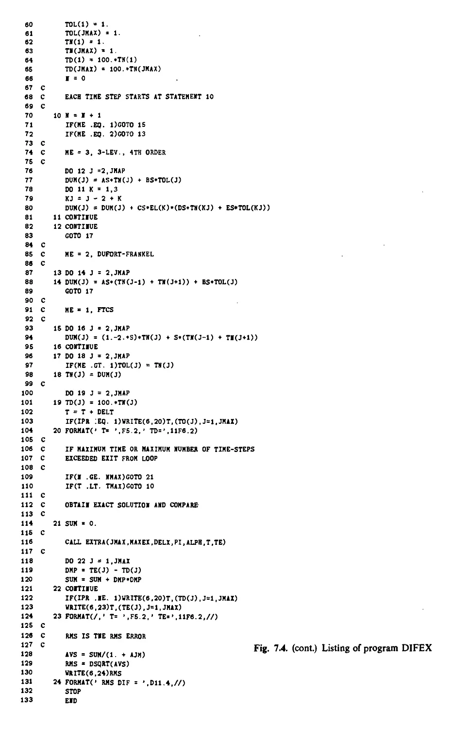
7.1.4 DIFEX: Numerical Results for Explicit Schemes 222
7.2 Implicit Methods 227
7.2.1 Fully Implicit Scheme 227
7.2.2 Crank-Nicolson Scheme 228
7.2.3 Generalised Three-Level Scheme 229
7.2.4 Higher-Order Schemes 230
7.2.5 DIFIM: Numerical Results for Implicit Schemes 231
7.3 Boundary and Initial Conditions 236
7.3.1 Neumann Boundary Conditions 236
7.3.2 Accuracy of Neumann Boundary Condition
Implementation 238
7.3.3 Initial Conditions 241
7.4 Method of Lines 241
7.5 Closure 246
7.6 Problems 247
8. Multidimensional Diffusion Equation 249
8.1 Two-Dimensional Diffusion Equation 249
8.1.1 Explicit Methods 250
8.1.2 Implicit Method 251
8.2 Multidimensional Splitting Methods 251
8.2.1 ADI Method 252
8.2.2 Generalised Two-Level Scheme 254
8.2.3 Generalised Three-Level Scheme 255
8.3 Splitting Schemes and the Finite Element Method 256
8.3.1 Finite Element Splitting Constructions 258
8.3.2 TWDIF: Generalised Finite Difference/
Finite Element Implementation 259
8.4 Neumann Boundary Conditions 266
8.4.1 Finite Difference Implementation 267
8.4.2 Finite Element Implementation 269
8.5 Method of Fractional Steps 271
8.6 Closure 273
8.7 Problems 274
9. Linear Convection-Dominated Problems 276
9.1 One-Dimensional Linear Convection Equation 277
9.1.1 FTCS Scheme 277
9.1.2 Upwind Differencing and the CFL Condition 280
9.1.3 Leapfrog and Lax-Wendroff Schemes 281
9.1.4 Crank-Nicolson Schemes 283
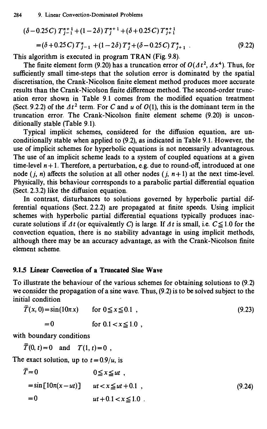
9.1.5 Linear Convection of a Truncated Sine Wave 284

Contents XIII
9.2 Numerical Dissipation and Dispersion 286
9.2.1 Fourier Analysis 288
9.2.2 Modified Equation Approach 290
9.2.3 Further Discussion 291
9.3 Steady Convection-Diffusion Equation 293
9.3.1 Cell Reynolds Number Effects 294
9.3.2 Higher-Order Upwind Scheme 296
9.4 One-Dimensional Transport Equation 299
9.4.1 Explicit Schemes 299
9.4.2 Implicit Schemes 304
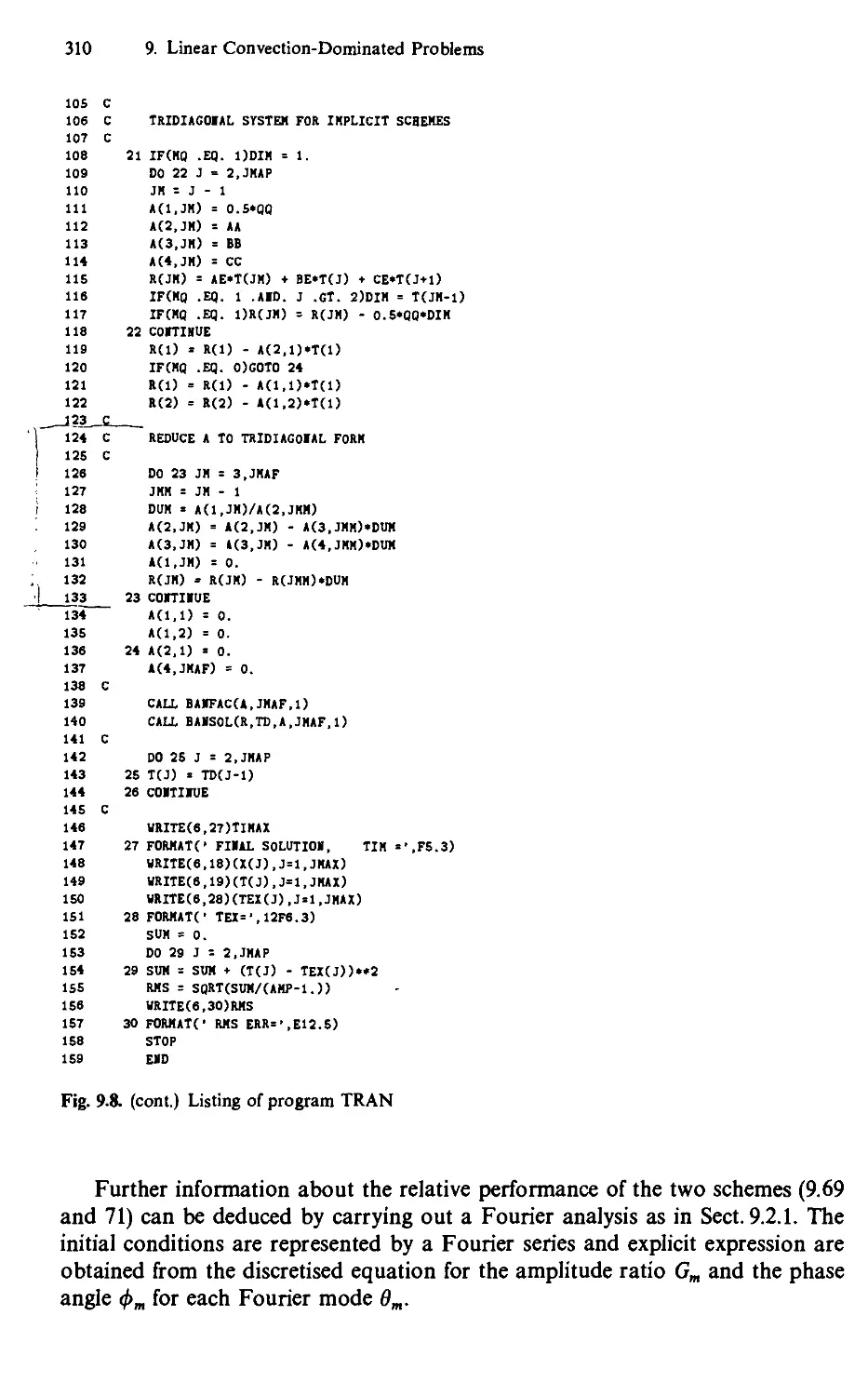
9.4.3 TRAN: Convection of a Temperature Front 305
9.5 Two-Dimensional Transport Equation 316
9.5.1 Split Formulations 317
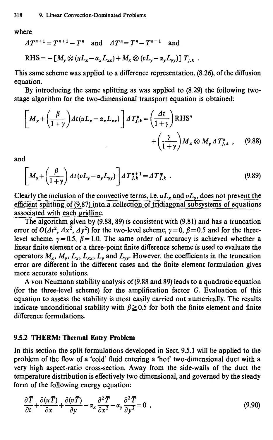
9.5.2 THERM: Thermal Entry Problem 318
9.5.3 Cross-Stream Diffusion 326
9.6 Closure 328
9.7 Problems 329
10. Nonlinear Convection-Dominated Problems 331
10.1 One-Dimensional Burgers' Equation 332
10.1.1 Physical Behaviour 332
10.1.2 Explicit Schemes 334
10.1.3 Implicit Schemes 337
10.1.4 BURG: Numerical Comparison 339
10.1.5 Nonuniform Grid 348
10.2 Systems of Equations 353
10.3 Group Finite Element Method 355
10.3.1 One-Dimensional Group Formulation 356
10.3.2 Multidimensional Group Formulation 357
10.4 Two-Dimensional Burgers' Equation 360
10.4.1 Exact Solution 361
10.4.2 Split Schemes 362
10.4.3 TWBURG: Numerical Solution 364
10.5 Closure 372
10.6 Problems 373
Appendix
A.1 Empirical Determination of the Execution Time
of Basic Operations 375
A.2 Mass and Difference Operators 376
References 381
Subject Index 389
Contents of Computational Techniques for Fluid Dynamics 2
Specific Techniques for Different Flow Categories 397

1. Computational Fluid Dynamics: An Introduction
This chapter provides an overview of computational fluid dynamics (CFD) with
emphasis on its cost-effectiveness in design. Some representative applications are
described to indicate what CFD is capable of. The typical structure of the equations
governing fluid dynamics is highlighted and the way in which these equations are
converted into computer-executable algorithms is illustrated. Finally attention is
drawn to some of the important sources of further information.
1.1 Advantages of Computational Fluid Dynamics
The establishment of the science of fluid dynamics and the practical application of
that science has been under way since the time of Newton. The theoretical
development of fluid dynamics focuses on the construction and solution of the governing
equations for the different categories of fluid dynamics and the study of various
approximations to those equations.
The governing equations for Newtonian fluid dynamics, the unsteady Navier-
Stoices equations, have been known for 150 years or more. However, the
development of reduced iorms of these equations (Chap. 16) is still an active area of
research as is the turbulent closure problem for the Reynolds-averaged Navier-
Stokes equations (Sect. 11.5.2). For non-Newtonian fluid dynamics, chemically
reacting flows and two-phase flows the theoretical development is at a less advanced
stage.
Experimental fluid dynamics has played an important role in validating and
delineating the limits of the various approximations to the governing equations. The
wind tunnel, as a piece of experimental equipment, provides an effective means of
simulating real flows. Traditionally this has provided a cost-effective alternative to
full-scale measurement. In the design of equipment that depends critically on the
flow behaviour, e.g. aircraft design, full-scale measurement as part of the design
process is economically unavailable.
The steady improvement in the speed of computers and the memory size since
the 1950s has led to the emergence of computational fluid dynamics (CFD). This
branch of fluid dynamics complements experimental and theoretical fluid dynamics
by providing an alternative cost-effective means of simulating real flows. As such it
offers the means of testing theoretical advances for conditions unavailable exper-

2 1. Computational Fluid Dynamics: An Introduction
imentally. For example wind tunnel experiments are limited to a certain range of
Reynolds numbers, typically one or two orders of magnitude less than full scale.
Computational fluid dynamics also provides the convenience of being able to
switch off specific terms in the governing equations. This permits the testing of
theoretical models and, inverting the connection, suggests new paths for theoretical
exploration.
The development of more efficient computers has generated the interest in CFD
and, in turn, this has produced a dramatic improvement in the efficiency of the
computational techniques. Consequently CFD is now the preferred means of
testing alternative designs in many branches of the aircraft, flow machinery and, to
a lesser extent, automobile industries.
Following Chapman et al. (1975), Chapman (1979,1981), Green (1982), Rubbert
(1986) and Jameson (1989) CFD provides five major advantages compared with
experimental fluid dynamics:
(i) Lead time in design and development is significantly reduced.
(ii) CFD can simulate flow conditions not reproducible in experimental model
tests,
(iii) CFD provides more detailed and comprehensive information,
(iv) CFD is increasingly more cost-effective than wind-tunnel testing.
(v) CFD produces a lower energy consumption.
Traditionally, large lead times have been caused by the necessary sequence of
design, model construction, wind-tunnel testing and redesign. Model construction
is often the slowest component. Using a well-developed CFD code allows
alternative designs (different geometric configurations) to be run over a range of
parameter values, e.g. Reynolds number, Mach number, flow orientation. Each
case may require 15 min runs on a supercomputer, e.g. CRAY Y-MP. The design
optimisation process is essentially limited by the ability of the designer to absorb
and assess the computational results. In practice CFD is very effective in the early
elimination of competing design configurations. Final design choices are still
confirmed by wind-tunnel testing.
Rubbert (1986) draws attention to the speed with which CFD can be used to
redesign minor components, if the CFD packages have been thoroughly validated.
Rubbert cites the example of the redesign of the external contour of the Boeing 757
cab to accommodate the same cockpit components as the Boeing 767 to minimise
pilot conversion time. Rubbert indicates that CFD provided the external shape
which was incorporated into the production schedule before any wind-tunnel
verification was undertaken.
Wind-tunnel testing is typically limited in the Reynolds number it can achieve,
usually short of full scale. Very high temperatures associated with coupled heat
transfer fluid flow problems are beyond the scope of many experimental facilities.
This is particularly true of combustion problems where the changing chemical
composition adds another level of complexity. Some categories of unsteady flow
motion cannot be properly modelled experimentally, particularly where geometric
unsteadiness occurs as in certain categories of biological fluid dynamics. Many

1.1 Advantages of Computational Fluid Dynamics 3
geophysical fluid dynamic problems are too big or too remote in space or time to
simulate experimentally. Thus oil reservoir flows are generally inaccessible to
detailed experimental measurement. Problems of astrophysical fluid dynamics are
too remote spatially and weather patterns must be predicted before they occur. All
of these categories of fluid motion are amenable to the computational approach.
Experimental facilities, such as wind tunnels, are very effective for obtaining
global information, such as the complete lift and drag on a body and the surface
pressure distributions at key locations. However, to obtain detailed velocity and
pressure distributions throughout the region surrounding a body would be
prohibitively expensive and very time consuming. CFD provides this detailed
information at no additional cost and consequently permits a more precise
understanding of the flow processes to be obtained.
Perhaps the most important reason for the growth of CFD is that for much
mainstream flow simulation, CFD is significantly cheaper than wind-tunnel testing
and will become even more so in the future. Improvements in computer hardware
performance have occurred hand in hand with a decreasing hardware cost.
Consequently for a given numerical algorithm and flow problem the relative cost of
a computational simulation has decreased significantly historically (Fig. 1.1).
Paralleling the improvement in computer hardware has been the improvement in the
efficiency of computational algorithms for a given problem. Current improvements
in hardware cost and computational algorithm efficiency show no obvious sign of
reaching a limit. Consequently these two factors combine to make CFD
increasingly cost-effective. In contrast the cost of performing experiments continues to
increase.
The improvement in computer hardware and numerical algorithms has also
brought about a reduction in energy consumption to obtain computational flow
simulations. Conversely, the need to simulate more extreme physical conditions,
higher Reynolds number, higher Mach number, higher temperature, has brought
about an increase in energy consumption associated with experimental testing.
The chronological development of computers over the last thirty years has been
towards faster machines with larger memories. A modern supercomputer such as
O 100
u
z
O 10
<
I-
3
a.
2
O
u
7094
, . f IBM 360-50
709& V± #' 360-67
CDC6400-^f« 370-195
,[_ 66oo*/^a-4 ^°
TAR
360-91 7600 TML CRAY 1
1-4 • ^
> .01 - 1-4 ^^J}SP
/"
- ¢,,, . 1/10 EACH 8 YRS NA^£ Fi8- 1-1. Relative cost of
- ' ' computation for a given
i i I ■'■» I i i i i I i i i i I i i i i I i i i i I i i i i I algorithm and flow (after
19SS 1960 196S 1970 197S 1980 198S Chapman, 1979; reprinted
YEAR NEW COMPUTER AVAILABLE with permission of AIAA)

4 1. Computational Fluid Dynamics: An Introduction
the CRAY Y-MP is capable of operating at more than 2000 Megaflops (Dongarra
1989). A Megaflop is one million floating-point arithmetic operations per second.
More recent supercomputers, e.g. the NEC SX3, are capable of theoretical speeds
of 20000 Megaflops. The speed comes partly from a short machine cycle time, that
is the time required for each cycle of logic operations. The CRAY Y-MP has a cycle
time of 6 nanoseconds (6 x 10-9 s) whereas the NEC SX3 has a cycle time of 2.9 ns.
A specific operation, e.g. a floating point addition, can be broken up into a
number of logic operations each one of which requires one machine cycle to
execute. If the same operation, e.g. floating point addition, is to be applied
sequentially to a large number of elements in a vector, it is desirable to treat each
logic operation sequentially but to permit different logic operations associated with
each vector element to be executed concurrently. Thus there is a considerable
overlap and a considerable speed-up in the overall execution time if the
computational algorithm can exploit such a pipeline arrangement.
Modern supercomputers have special vector processors that utilise the pipeline
format. However vector processors have an effective "start-up" time that makes
them slower than scalar processorslor very shorFvectors. One caiTderineXBreak-
even vector length, Afb7Tor which the vector processor has the same speed as a
scalar processor. For very long vectors (N = oo) the theoretical vector processor
speed is achieved.
To compare the efficiency of different vector-processing computers it is (almost)
standard practice to consider Nl/2 (after Hockney and Jesshope 1981), which is the
vector length for which half the asymptotic peak vector processing performance
{N = oo) is achieved. The actual Nl/2 is dependent on the specific operations being
performed as well as the hardware. For a SAXPY operation (S = AX+Y),
Nll2 = 37 for a CRAY X-MP and Nl/2 = 238 for a CYBER 205. For most modern
supercomputers, 30 _ Nl/2 _ 100.
The speed-up due to vectorisation is quantifiable by considering Amdahl's law
which can be expressed as (Gentzsch and Neves 1988)
G = [_(l-P) + P/Ry1 and R=V{N)/S (1.1)
where G is the overall gain in speed of the process (overall speed-up ratio)
V(N) is the vector processor speed for an N component vector process
S is the scalar processor speed for a single component process
P is the proportion of the process that is vectorized and
R is the vector processor speed-up ratio.
As is indicated in Fig. 1.2 a vector processor with a theoretical (N = oo) vector
speed-up ratio, R = 10, must achieve a high percentage vectorisation, say P>0.75,
to produce a significant overall speed-up ratio, G. But at this level dG/dP > dG/dR.
Thus modification of the computer program to increase P will provide a much
bigger increase in G than modifying the hardware to increase V and hence R. In
addition unless a large proportion of the computer program can be written so that
vector lengths are significantly greater than Nl/2, the overall speed-up ratio, G, will
not be very great.

1.1 Advantages of Computational Fluid Dynamics 5
Fig. 1.2. Amdahl's Law
50 75 100
Percent Vectorized, 100 P
The ability to increase the overall execution speed to the limit set by the
hardware depends partly on the ability of the operating system and compiler to
vectorise the computational algorithm and partly on choosing computational
algorithms that are inherently vectorisable (Ortega and Voigt 1985). The
structuring of computational algorithms to permit vectorisation is an important
research topic but is beyond the scope of this book (see Gentzsch and Neves 1988).
The long term trend would appear to be towards making the operating system and
compiler take care of the vectorisation with less emphasis on the user having to
manipulate the basic algorithm.
With a pipeline architecture, an efficient vector instruction set and as small a
cycle time as possible the major means of further increasing the processing speed is
to introduce multiple processors operating in parallel. Supercomputers are
typically being designed with up to sixteen processors in parallel. Theoretically this
should provide up to a factor of sixteen improvement in speed. Experiments by
Grassl and Schwarzmeier (1990) with an eight-processor CRAY Y-MP indicate
that 84% of the theoretical improvement can be achieved for a typical CFD code
such as ARC3D (Vol. 2, Sect. 18.4.1).
The concept of an array of processors each operating on an element of a vector
has been an important feature in the development of more efficient computer
architecture (Hockney and Jesshope 1981). The Illiac IV had 64 parallel processors
and achieved an overall processing speed comparable to the CRAY-1 and CYBER-
205 even though the cycle time was only 80 ns. However Amdahl's law, (1.1), also
applies to parallel processors if R is replaced by NP, the number of parallel
processors, and P is the proportion of the process that is parallelisable. The relative
merits of pipeline and parallel processing are discussed in general terms by Levine
(1982), Ortega and Voigt (1985) and in more detail by Hockney and Jesshope (1981)
and Gentzsch and Neves (1988).
The development of bigger and cheaper memory modules is being driven by the
substantial commercial interest in data storage and manipulation. For CFD
applications it is important that the complete program, both instructions and
variable storage, should reside in main memory. This is because the speed of data
transfer from secondary (disc) storage to main memory is much slower than data
transfer rates between the main memory and the processing units. In the past the

6 1. Computational Fluid Dynamics: An Introduction
main memory size has typically limited the complexity of the CFD problems under
investigation.
The chronological trend of increasing memory capacity for supercomputers is
impressive. The CDC-7600 (1970 technology) had a capacity of 4 x 105 64-bit
words. The CYBER-205 (1980 technology) has a capacity of 3 x 107 64-bit words
and the CRAY-2 (1990 technology) has a capacity of 109 64-bit words.
Significant developments in minicomputers in the 1970s and microcomputers
in the 1980s have provided many alternative paths to cost-effective CFD. The
relative cheapness of random access memory implies that large problems can be
handled efficiently on micro- and minicomputers. The primary difference between
microcomputers and mainframes is the significantly slower cycle time of a
microcomputer and the simpler, less efficient architecture. However the blurring of the
distinction between microcomputers and personal workstations, such as the SUN
Sparcstation, and the appearance of minisupercomputers has produced a
price/performance continuum (Gentzsch and Neves 1988).
The coupling of many, relatively low power, parallel processors is seen as a very
efficient way of solving complex CFD problems. Each processor can use fairly
standard microcomputer components; hence the potentially low cost. A typical
system, QCDPAX, is described by Hoshino (1989). This system has from 100 to
1000 processing units, each based on the L64132 floating point processor. Thus a
system of 400 processing units is expected to deliver about 2000 Megaflops when
operating on a representative CFD code.
To a certain extent the relative slowness of microcomputer-based systems can
be compensated for by allowing longer running times. Although 15 mins on a
1 10 ,02 103
COMPUTER SPEED, mftow
105
Fig. 13. Computer speed and memory requirements for CFD (after Bailey, 1986; reprinted with
permission of Japan Society of Computational Fluid Dynamics)

1.2 Typical Practical Problems 7
Fig. 1.4. Surface pressure distribution on a typical military aircraft. Surface pressure contours,
JCP = 0.02 (after Arlinger, 1986; reprinted with permission of Japan Society of Computational
Fluid Dynamics)
supercomputer appears to be the accepted norm (Bailey 1986) for routine design
work, running times of a few hours on a microcomputer may well be acceptable in
the research and development area. This has the advantage of allowing the CFD
research worker adequate time to interpret the results and to prepare additional
cases.
The future trends for computer speed and memory capacity are encouraging.
Predictions by Simon (1989) indicate that by 2000 one may expect sustained
computer speeds up to 106 Megaflops and main memory capacities of 50000
Megawords. This is expected to be adequate (Fig. 1.3) for predictions of steady
viscous (turbulent) compressible flow around complete aircraft and to allow global
design optimisation to be considered seriously.
1.2 Typical Practical Problems
Computational fluid dynamics, particularly in engineering, is still at the stage of
development where "problems involving complex geometries can be treated with
simple physics and those involving simple geometry can be treated with complex
physics" (Bailey 1986). What is changing is the accepted norm for simplicity and
complexity. Representative examples are provided below.
1.2.1 Complex Geometry, Simple Physics
The surface pressure distribution on a typical supersonic military aircraft is shown
in Fig. 1.4. The freestream Mach number is 1.8 and the angle of attack is 8°. The
aircraft consists of a fuselage, canopy, engine inlets, fin, main delta wing and
forward (canard) wings. In addition control surfaces at the trailing edge of the delta
wing are deflected upwards 10°. Approximately 19000 grid points are required in
each cross-section plane at each downstream location. The complexity of the

8 1. Computational Fluid Dynamics: An Introduction
geometry places a considerable demand on the grid generating procedure. Arlinger
(1986) uses an algebraic grid generation technique based on transfinite
interpolation (Sect. 13.3.4).
The flow is assumed inviscid and everywhere supersonic so that an explicit
marching scheme in the freestream direction can be employed. This is equivalent to
the procedure described in Sect. 14.2.4. The explicit marching scheme is
particularly efficient with the complete flowfield requiring 15 minutes on a CRAY-1.
The finite volume method (Sect. 5.2) is used to discretise the governing equations.
Arlinger stresses that the key element in obtaining the results efficiently is the
versatile grid generation technique.
1.2.2 Simpler Geometry, More Complex Physics
The limiting particle paths on the upper surface of a three-dimensional wing for
increasing freestream Mach number, JWB, are shown in Fig. 1.5. The limiting
particle paths correspond to the surface oil-flow patterns that would be obtained
experimentally. The results shown in Fig. 1.5 come from computations (Hoist et al.
1986) of the transonic viscous flow past a wing at 2° angle of attack, with an aspect
ratio of 3 and a chord Reynolds number of 8 x 106.
For these conditions a shock wave forms above the wing and interacts with the
upper surface boundary layer causing massive separation. The region of separation
changes and grows as Mx increases. The influence of the flow past the wingtip
makes the separation pattern very three-dimensional. The terminology, spiral
node, etc., indicated in Fig. 1.5 is appropriate to the classification of three-
dimensional separation (Tobak and Peake 1982).
The solutions require a three-dimensional grid of approximately 170000 points
separated into four partially overlapping zones. The two zones immediately above
and below the wing have a fine grid in the normal direction to accurately predict
the severe velocity gradients that occur. In these two zones the thin layer Navier-
Stokes equations (Sect. 18.1.3) are solved. These equations include viscous terms
only associated with the normal direction. They are an example of reduced Navier-
Stokes equations (Chap. 16). In the two zones away from the wing the flow is
assumed inviscid and governed by the Euler equations (Sect. 11.6.1).
The grid point solutions in all zones are solved by marching a pseudo-transient
form (Sect. 6.4) of the governing equations in time until the solution no longer
changes. To do this an implicit procedure is used similar to that described in
Sect. 14.2.8. The zones are connected by locally interpolating the overlap region,
typically two cells. Hoist indicates that stable solutions are obtained even though
severe gradients cross zonal boundaries.
By including viscous effects the current problem incorporates significantly more
complicated flow behaviour, and requires a more sophisticated computational
algorithm, than the problem considered in Sect. 1.2.1. However, the shape of the
computational domain is considerably simpler. In addition the computational grid
is generated on a zonal basis which provides better control over the grid point
locations.

1.2 Typical Practical Problems 9
Fig. l^a-d. Particle paths for upper wing surface flow. («) Moo = 0.80 (b) M„ = 0.85 (c) M„=0.90
(d) M„ = 0.95 (after Hoist et al, 1986; reprinted with permission of Japan Society of Computational
Fluid Dynamics)
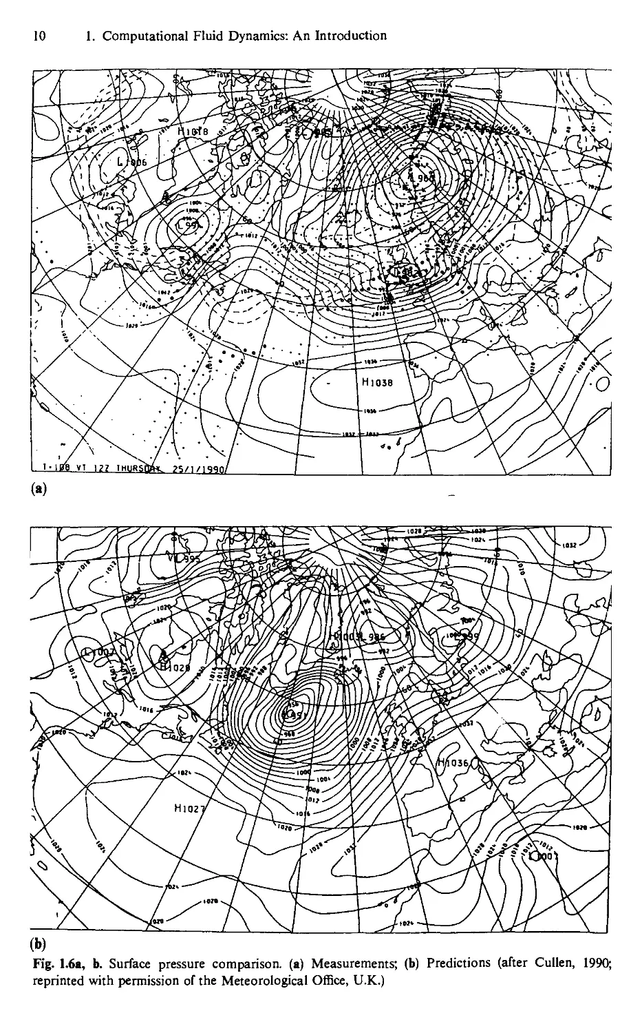
1.2.3 Simple Geometry, Complex Physics
To illustrate this category a meteorological example is used instead of an
engineering example. Figure 1.6 shows a four-day forecast (b) of the surface pressure
compared with measurements (a). This particular weather pattern was associated
with a severe storm on January 29,1990 which caused substantial property damage
in the southern part of England. The computations predict the developing weather
pattern quite closely.

10 1. Computational Fluid Dynamics: An Introduction
~^l
e
' 'V
•v \ ^v (
^7—"~ /^y
/f^r !K
TsKLt"
^--~_ \ / /\ ^CV,****vA/*Av SX^*^^J~ ^X.JiM'-i
s.
.'•<*^
// / S/^T/
- -'' •¥».
■^-/fo?^
vl§Sl§§l
8^¾]¾¾¾^¾¾¾^¾^
/illy/i v^-**3^?j!
^^^3¾^¾
^01^¾¾
vsl*i^*l^3^^?
*-*s>, ^
3¾¾¾
»f/ft
:>-H-H
iLJ^
Hfcf
Z/y'^j
/ / \ • r/ _^)\h ^
Ir I
(a)
HI038
\
'■lUfr vi i?7 iMURSrntt. ?s/i/iqqn/
•o
Fig. 1.6a, b. Surface pressure comparison, (a) Measurements; (b) Predictions (after Cullen, 1990;
reprinted with permission of the Meteorological Office, U.K.)

1.3 Equation Structure 11
The governing equations (Cullen 1983) are essentially inviscid but account for
wind, temperature, pressure, humidity, surface stresses over land and sea, heating
effect, precipitation and other effects (Haltiner and Williams 1980). The equations
are typically written in spherical polar coordinates parallel to the earth's surface
and in a normalised pressure coordinate perpendicular to the earth's surface.
Consequently difficulties associated with an irregular computational boundary and
grid generation are minimal.
Cullen (1990) indicates that the results shown in Fig. 1.6 were obtained on a
192 x 120 x 15 grid and used a split explicit finite difference scheme to advance the
solution in time. This permits the complete grid to be retained in main memory. 432
time steps are used for a 4j day forecast and require 20 minutes processing time on
a CYBER 205.
Cullen (1983) reports that the major problem in extending accurate large-scale
predictions beyond 3 to 4 days is obtaining initial data of sufficient quality. For
more refined local predictions further difficulties arise in preventing boundary
disturbances from contaminating the interior solution and in accurately
representing the severe local gradients associated with fronts.
For global circulation modelling and particularly for long-term predictions the
spectral method (Sect. 5.6) is well suited to spherical polar geometry. Spectral
methods are generally more economical than finite difference or finite element
methods for comparable accuracy, at least for global predictions. The application
of spectral methods to weather forecasting is discussed briefly by Fletcher (1984)
and in greater detail by Bourke et al. (1977). Chervin (1989) provides a recent
indication of the capability of CFD for climate modelling.
The above examples are indicative of the current status of CFD. For the future
Bailey (1986) states that "more powerful computers with more memory capacity
are required to solve problems involving both complex geometries and complex
physics". The growth in human expectations will probably keep this statement
current for a long time to come.
1.3 Equation Structure
A connecting feature of the categories of fluid dynamics considered in this book is
that the fluid can be interpreted as a continuous medium. As a result the behaviour
of the fluid can be described in terms of the velocity and thermodynamic properties
as continuous functions of time and space.
Application of the principles of conservation of mass, momentum and energy
produces systems of partial differential equations (Vol. 2, Chap. 11) for the velocity
and thermodynamic variables as functions of time and position. With boundary
and initial conditions appropriate to the given flow and type of partial differential
equation the mathematical description of the problem is established.
Many flow problems involve the developing interaction between convection
and diffusion. A simple example is indicated in Fig. 1.7, which shows the
temperature distribution of fluid in a pipe at different times. It is assumed that the fluid

12 1. Computational Fluid Dynamics: An Introduction
1.0
T
).0
x/ -1.0
1.0
T
t. 0.5/u
'V-
xL -1.0
l.Or '-'-M
T
'-nA-
-1.0
1.0
1.0
2.0
2.0
-AH
-Ar"
Fig. 1.7.
One-dimensional temperature
distribution
is moving to the right with constant velocity u and that the temperature is constant
across the pipe.
The temperature as a function of x and t is governed by the equation
8T 8T 82T n e ^^
—+ u- a—^ = 0 forx.<x<xR and f>0 .
dt dx dx2 l_ _ r
(1.2)
With a suitable nondimensionalisation, appropriate boundary and initial
conditions are
T(xL,t)=T(xR,t) = 0 and
r(x,0) = cos7rx, -0.5^*^0.5
= 0 , x<-0.5 and x>0.5 .
(1.3)
(1.4)
Equations (1.2-4) provide a mathematical description of the problem. The term
<xd2T/dx2 is the diffusion term and a is the thermal diffusivity. This term is
responsible for the spread of the nonzero temperature both to the right and to the
left; if a~Is small the spread is small. Computational techniques for dealing with
equations containing such terms are dealt with in Chaps. 7 and 8.
The term udT/dx is the convection term and is responsible for the temperature
distribution being swept bodily to~lhe right with the known velocity u. The
treatment of this term and the complete transport equation (1.2) are considered in
Chap. 9. In more than one dimension convective and diffusive terms appear
associated with each direction (Sect. 9.5).
Since u is known, (1.2) is linear in T. However, when solving for the velocity field
it is necessary to consider equations with nonlinear convective terms. A prototype

1.3 Equation Structure 13
for such a nonlinearity is given by Burgers' equation (Sect. 10.1)
du du d2u
dt dx dx2
The nonlinear convective term, u du/dx, permits very steep gradients in u to develop
if a is very small. Steep gradients require finer grids and the presence of the
nonlinearity often necessitates an additional level of iteration in the computational
algorithm.
Some flow and heat transfer problems are governed by Laplace's equation,
d24> 8^>
~8x2+~dy
2+-^=0. (1.6)
This is the case for a flow which is inviscid, incompressible and irrotational. In that
case <j> is the velocity potential (Sect. 11.3). Laplace's equation is typical of the type
of equation that governs equilibrium or steady problems (Chap. 6). Laplace's
equation also has the special property of possessing simple exact solutions which
can be added together (superposed) since it is linear. These properties are exploited
in the techniques described in Sect. 14.1.
For many flow problems more than one dependent variable will be involved
and it is necessary to consider systems of equations. Thus one-dimensional
unsteady inviscid compressible flow is governed by (Sect. 10.2)
§+|-W, + E)]=0, <Uc)
where p is the pressure and E is the total energy per unit volume given by
£=^-+0.5 gu2 , (1.8)
and y is the ratio of specific heats. Although equations (1.7) are nonlinear the
structure is similar to (1.5) without the diffusive terms. The broad strategy of the
computational techniques developed for scalar equations will also be applicable to
systems of equations.
For flow problems where the average properties of the turbulence need to be
included the conceptual equation structure could be written as follows
du du d ( du\
Jt+uYx-Yx\aYxrs' (L9)

14 1. Computational Fluid Dynamics: An Introduction
is now a function of the dependent variable u, and S is a source term
containing additional turbulent contributions. However, it should be made clear
(Sects. 11.4.2 and 11.5.2) that turbulent flows are at least two-dimensional and often
three-dimensional and that a system of equations is required to describe the flow.
1.4 Overview of Computational Fluid Dynamics
The total process of determining practical information about problems involving
fluid motion can be represented schematically as in Fig. 1.8.
The governing equations (Chap. 11) for flows of practical interest are usually so
complicated that an exact solution is unavailable and it is necessary to seek a
computational solution. Computational techniques replace the governing partial
differential equations with systems of algebraic equations, so that a computer can
be used to obtain the solution. This book will be concerned with the computational
techniques for obtaining and solving the systems of algebraic equations.
For local methods, like the finite difference, finite element and finite volume
methods, the algebraic equations link together values of the dependent variables at
adjacent grid points. For this situation it is understood that a grid of discrete points
is distributed throughout the computational domain, in time and space.
Consequently one refers to the process of converting the continuous governing equations
FOR EACH ELEMENT OF FLUID :
Conservotion of moss => Continuity Equotion
Newton's second low => (Euler Equotions )
of motion I Novier-Stokes Equotions I
Conservotion of energy => Energy Equotion
Equotion of stote
T
Solve the equotions
plus boundory conditions
Velocity Distribution
Pressure
Density
Temperature -
u(x,y,z,t), v(x,y,z,t), w(x,y,z,t)
P(x.y.z,t)
p(x,y,z.t)
T(x,y,z,t)
T
Deduce flow behoviour
flow seporotion
flow rotes
heot transfer
forces on bodies
(skin friction, drag, lift)
efficiencies
(turbine, diffuser)
Fig. 1.8. Overview of computational
fluid dynamics

1.4 Overview of Computational Fluid Dynamics 15
to a system of algebraic equations as discretisation (Chap. 3). For a global method,
like the spectral method, the dependent variables are replaced with amplitudes
associated with different frequencies, typically.
The algebraic equations produced by discretisation could arise as follows. A
typical finite difference representation of (1.2) would be
r;+1 -T) , u(T*j+1-r;_t) _ a(r;_t -2r; + r;+1)
At + 2Ax - Ax2 ' (lAV)
where x=jAx and t=n At.
If the solution is known at all grid points Xj at time level n, (1.10) can be used to
provide an algorithm for Tj + l, i.e.
T"J+1 = T"j-(^(T"j+1-T"j.1)+^yr'J.1-2r'J+r'J+1). (l.ii)
Repeated use of (1.11) generates the solution at all interior grid points, Xj, at time
level n+1. Incrementing n and substituting the values Tn+l into the right-hand
side of (1.11) allows the discrete solution to be marched forward in time.
For a local method, e.g. the finite difference method, the required number of
grid points for an accurate solution typically depends on the dimensionality, the
geometric complexity and severity of the gradients of the dependent variables. For
the flow about a complete aircraft a grid of ten million points might be required. At
each grid point each dependent variable and certain auxiliary variables must be
stored. For turbulent compressible three-dimensional flow this may require
anywhere between five and thirty dependent variables per grid point. For efficient-
computation all of these variables must be stored in main memory.
Since the governing equations for most classes of fluid dynamics are nonlinear
the computational solution usually proceeds iteratively. That is, the solution for
each dependent variable at each grid point is sequentially corrected using the
discretised equations. The iterative process is often equivalent to advancing the
solution over a small time step (Chap. 6). The number of iterations or time steps
might vary from a few hundred to several thousand.
The discretisation process introduces an error that can be reduced, in principle,
by refining the grid as long as the discrete equations, e.g. (1.10), are faithful
representations of the governing equations (Sect. 4.2). If the numerical algorithm that
performs the iteration or advances in time is also stable (Sect. 4.3), then the
computational solution can be made arbitrarily close to the true solution of the
governing equations, by refining the grid, if sufficient computer resources are
available.
Although the solution is often sought in terms of discrete nodal values some
methods, e.g., the finite element and spectral methods, do explicitly introduce a
continuous representation for the computational solution. Where the underlying
physical problem is smooth such methods often provide greater accuracy per
unknown in the discretised equations. Such methods are discussed briefly in
Chap. 5.

16 1. Computational Fluid Dynamics: An Introduction
1.5 Further Reading
The purpose of the present text is to provide an introduction to the computational
techniques that are appropriate for solving flow problems. More specific
information is available in other books, review articles, journal articles and conference
proceedings.
Richtmyer and Morton (1967) construct a general theoretical framework for
analysing computational techniques relevant to fluid dynamics and discuss specific
finite difference techniques for in viscid compressible flow. Roache (1976) examines
viscous separated flow for both incompressible and compressible conditions but
concentrates on finite difference techniques. More recently, Peyret and Taylor
(1983) have considered computational techniques for the various branches of fluid
dynamics with more emphasis on finite difference and spectral methods. Holt
(1984) describes very powerful techniques for boundary layer flow and in viscid
compressible flow. Book (1981) considers finite difference techniques for both
engineering and geophysical fluid dynamics where the diffusive mechanisms are
absent or very small.
Thomasset (1981), Baker (1983) and Glowinski (1984) examine computational
techniques based on the finite element method and Fletcher (1984) provides
techniques for the finite element and spectral methods. Canuto et al. (1987) analyse
computational techniques based on spectral methods. Haltiner and Williams
(1980) discuss computational techniques for geophysical fluid dynamics.
The review articles by Chapman (1975, 1979, 1981), Green (1982), Krause
(1985), Kutler (1985) and Jameson (1989) indicate what engineering CFD is
currently capable of and what will be possible in the future. These articles have a
strong aeronautical leaning. A more general review is provided by Turkel (1982).
Cullen (1983) and Chervin (1989) review the current status of meteorological CFD.
Review papers on specific branches of computational fluid dynamics appear in
Annual Reviews of Fluid Dynamics, in the lecture series of the von Karman
Institute and in the monograph series of Pineridge Press. More advanced
computational techniques which exploit vector and parallel computers will not be
covered in this book. However Ortega and Voigt (1985) and Gentzsch and Neves
(1988) provide a comprehensive survey of this area.
Relevant journal articles appear in AIAA Journal, Journal of Computational
Physics, International Journal of Numerical Methods in Fluids, Computer
Methods in Applied Mechanics and Engineering, Computers and Fluids, Applied
Mathematical Modelling, Communications in Applied Numerical Methods,
Theoretical and Computational Fluid Dynamics, Numerical Heat Transfer, Journal of
Applied Mechanics and Journal of Fluids Engineering. Important conferences are
the International Conference series on Numerical Methods in Fluid Dynamics,
International Symposium series on Computational Fluid Dynamics, the AIAA
CFD conference series, the GAMM conference series, Finite Elements in Flow
Problems conference series, the Numerical Methods in Laminar and Turbulent
Flow conference series and many other specialist conferences.

2. Partial Differential Equations
In this chapter, procedures will be developed for classifying partial differential
equations as elliptic, parabolic or hyperbolic. The different types of partial
differential equations will be examined from both a mathematical and a physical
viewpoint to indicate their key features and the flow categories for which they occur.
The governing equations for fluid dynamics (Vol. 2, Chap. 11) are partial
differential equations containing first and second derivatives in the spatial
coordinates and first derivatives only in time. The time derivatives appear linearly but
the spatial derivatives often appear nonlineariy. Also, except for the special case of
potential flow, systems of governing equations occur rather than a single equation.
2.1 Background
For linear partial differential equations of second-order in two independent
variables a simple classification (Garabedian 1964, p. 57) is possible. Thus for the
partial differential equation (PDE)
Ad2u „ d2u „d2u du du „ n ,„ „x
dxz dxdy dyz dx dy
where A to G are constant coefficients, three categories of partial differential
equation can be distinguished. These are
elliptic PDE: B2 - 4 AC < 0 ,
parabolic PDE: B2-4AC = 0 , (2.2)
hyperbolic PDE: B2-4AC>0 .
It is apparent that the classification depends only on the highest-order derivatives in
each independent variable.
For two-dimensional steady compressible potential flow about a slender body
the governing equation, similar to (11.109), is
o-"i>g+g-.

18 2. Partial Differential Equations
Applying the criteria (2.2) indicates that (2.3) is elliptic for subsonic flow (MB < 1)
and hyperbolic for supersonic flow (MB > 1).
If the coefficients, A to G in (2.1), are functions of x, y, u, du/dx or du/dy, (2.2) can
still be used if A, B and C are given a local interpretation. This implies that the
classification of the governing equations can change in different parts of the
computational domain.
The governing equation for steady, compressible, potential flow, (11.103), can be
written in two-dimensional natural coordinates as
d2<t> d2<j>
(l-M2)-f+-^=0, (2.4)
where s and n are parallel and perpendicular to the local streamline direction, and M
is the local Mach number. Applying conditions (2.2) on a local basis indicates that
(2.4) is elliptic, parabolic or hyperbolic as M<1, M=l or M>\. A typical
distribution of local Mach number, M, for the flow about an aerofoil or turbine
blade, is shown in Fig. 11.15. The feature that the governing equation can change its
type in different parts of the computational domain is one of the major complicating
factors in computing transonic flow (Sect. 14.3).
The introduction of simpler flow categories (Sect. 11.2.6) may introduce a change
in the equation type. The governing equations for two-dimensional steady,
incompressible viscous flow, (11.82-84) without the du/dt and dv/dt terms, are
elliptic. However, introduction of the boundary layer approximation produces a
parabolic system of PDEs, that is (11.60 and 61).
For equations that can be cast in the form of (2.1) the classification of the PDE
can be determined by inspection, using (2.2). When this is not possible, e.g. systems
of PDEs, it is usually necessary to examine the characteristics (Sect. 2.1.3) to
determine the correct classification.
The different categories of PDEs can be associated, broadly, with different types
of flow problems. Generally time-dependent problems lead to either parabolic or
hyperbolic PDEs. Parabolic PDEs govern flows containing dissipative mechanisms,
e.g. significant viscous stresses or thermal conduction. In this case the solution will
be smooth and gradients will reduce for increasing time if the boundary conditions
are not time-dependent. If there are no dissipative mechanisms present, the solution
will remain of constant amplitude if the PDE is linear and may even grow if the PDE
is nonlinear. This solution is typical of flows governed by hyperbolic PDEs. Elliptic
PDEs usually govern steady-state or equilibrium problems. However, some steady-
state flows lead to parabolic PDEs (steady boundary layer flow) and to hyperbolic
PDEs (steady inviscid supersonic flow).
2.1.1 Nature of a Well-Posed Problem
Before proceeding further with the formal classification of partial differential
equations it is worthwhile embedding the problem formulation and algorithm
construction in the framework of a well-posed problem. The governing equations

2.1 Background 19
and auxiliary (initial and boundary) conditions are well-posed mathematically if the
following three conditions are met:
i) the solution exists,
ii) the solution is unique,
iii) the solution depends continuously on the auxiliary data.
The question of existence does not usually create any difficulty. An exception
occurs in introducing exact solutions of Laplace's equation (Sect. 11.3) where the
solution may not exist at isolated points. Thus it does not exist at the location of the
source, r=rs in (11.53). In practice this problem is often avoided by placing the
source outside the computational domain, e.g. inside the body in Fig. 11.7.
The usual cause of non-uniqueness is a failure to properly match the auxiliary
conditions to the type of governing PDE. For the potential equation governing
inviscid, irrotational flows, and for the boundary layer equations, the appropriate
initial and boundary conditions are well established. For the Navier-Stokes
equations the proper boundary conditions at a solid surface are well known but
there is some flexibility in making the correct choice for farfield boundary
conditions. In general an underprescription of boundary conditions leads to non-
uniqueness and an overprescription to unphysical solutions adjacent to the
boundary in question.
There are some flow problems for which multiple solutions may be expected on
physical grounds. These problems would fail the above criteria of mathematical
well-posedness. This situation often arises for flows undergoing transition from
laminar to turbulent motion. However, the broad understanding of fluid dynamics
will usually identify such classes of flows for which the computation may be
complicated by concern about the well-posedness of the mathematical formulation.
The third criterion above requires that a small change in the initial or boundary
conditions should cause only a small change in the solution. The auxiliary
conditions are often introduced approximately in a typical computational
algorithm. Consequently if the third condition is not met the errors in the auxiliary
data will propagate into the interior causing the solution to grow rapidly,
particularly for hyperbolic PDEs.
The above criteria are usually attributed to Hadamard (Garabedian 1964,
p. 109). In addition we could take a simple parallel and require that for a well-posed
computation:
i) the computational solution exists,
ii) the computational solution is unique,
iii) the computational solution depends continuously on the approximate auxiliary
data.
The process of obtaining the computational solution can be represented
schematically as in Fig. 2.1. Here the specified data are the approximate
implementation of the initial and boundary conditions. If boundary conditions are
placed on derivatives of u an error will be introduced in approximating the
boundary conditions. The computational algorithm is typically constructed from

20 2. Partial Differential Equations
computational
algorithm,
o«f(a)
^
computational
solution, u
Fig. 2.1. Computational procedure
the governing PDE (Sect. 3.1) and must be stable (Sect. 4.3) in order for the above
three conditions to be met.
Therefore for a well-posed computation it is necessary that not only should both
the underlying PDE and auxiliary conditions be well-posed but that the algorithm
should be well-posed (stable) also. It is implicit here that the approximate solution
produced by a well-posed computation will be close, in some sense, to the exact
solution of the well-posed problem. This question will be pursued in Sect. 4.1.
2.1.2 Boundary and Initial Conditions
It is clear from the discussion of well-posed problems and well-posed computations
in Sect. 2.1.1 that the auxiliary data are, in a sense, the starting point for obtaining
the interior solution, particularly for propagation problems. If we don't distinguish
between time and space as independent variables then the auxiliary data specified on
dR, Fig. 2.2, is "extrapolated" by the computational algorithm (based on the PDE)
to provide the solution in the interior, R.
Fig. 2.2. Computational domain R
Auxiliary conditions are specified in three ways:
i) JDirichlet condition, e.g. u=f on dR.
ii) Neumann (derivative) condition, e.g. du/dn=foi du/ds = g on dR,
iii) mixed or Robin condition, e.g. du/dn + ku=f, k>0 on dR.
In auxiliary conditions ii) and iii), d/dn denotes the outward normal derivative.
For most flows, which require the solution of the Navier-Stokes equations in
primitive variables (u, v, p, etc.), at least one velocity component is given on an inflow
boundary. This provides a Dirichlet boundary condition on the velocity. For the
velocity potential equation governing in viscid compressible flow, the condition that
d(j>/dn = 0 at the body surface is a Neumann boundary condition. Mixed conditions
are rare in fluid mechanics but occur in convective heat transfer. Computationally,
Dirichlet auxiliary conditions can be applied exactly as long as f is analytic.
However, errors are introduced in representing Neumann or mixed conditions
(Sect. 7.3).

2.1 Background 21
2.1.3 Classification by Characteristics
For partial differential equations that are functions of two independent variables the
classification into elliptic, parabolic or hyperbolic type can be achieved by first
seeking characteristic directions along which the governing equations only involve
total differentials.
For a single first-order PDE in two independent variables,
a single real characteristic exists through every point and the characteristic direction
is defined by (Fig. 2.5)
I-!-
Along the characteristic direction, (2.5) reduces to
du C . du C
—=— and --=- . (2.7)
dt A dx B y '
Equation (2.5) is a hyperbolic PDE and it is possible to integrate (2.7) as ordinary
differential equations along a grid defined by (2.6), as long as the initial data are given
on a non-characteristic line.
The same concept of characteristic directions can be used in conjunction with
PDEs of second order in two independent variables, e.g. (2.1). Since it is found from
(2.1 and 2) that only the coefficients of the highest derivatives determine the category
of PDE, it is convenient to write (2.1) as
dx2 dxdy dy2
^TZ2 + B—~ + C-J + H = 0, (2.8)
where H contains all the first derivative terms etc. in (2.1) and A, B and C may be
functions of x, y. It is possible to obtain, for each point in the domain, two directions
along which the integration of (2.8) involves only total differentials. The existence of
these (characteristic) directions relates directly to the category of PDE.
For ease of presentation the following notation is introduced:
du du d2u d2u d2u
dx dy dx2 ' dxdy ' dy2
P-1Z> Q=~.> *-T3 . *=—:. T=—2. (2.9)
A curve K is introduced in the interior of the domain on which P, Q, R, S, Tand u
satisfy (2.8). Along a tangent to K the differentials of P and Q satisfy
dP = Rdx + Sdy , (2.10)
dQ = Sdx+Tdy , (2.11)

22 2. Partial Differential Equations
and (2.8) can be written as
AR + BS + CT+H = 0 . (2.12)
In (2.10 and 11), dy/dx defines the slope of the tangent to K. Using (2.10 and 11), R
and Tcan be eliminated from (2.12) to give
:^)'-@h-m+-]^s}- ■ <->
If dy/dx is chosen such that
"(£)'-s(s)+c-° • (214)
(2.13) reduces to the simpler relationship between dP/dx and dQ/dx,
^isMM--
The two solutions to (2.14) define the characteristic directions for which (2.15) holds.
Comparing (2.14) with (2.2) it is clear that if (2.8) is:
i) a hyperbolic PDE, two real characteristics exist,
ii) a parabolic PDE, one real characteristic exists,
iii) an elliptic PDE, the characteristics are complex.
Thus a consideration of the discriminant, B2 — 4 AC, determines both the type of
PDE and the nature of the characteristics.
The classification of the partial differential equation type has been undertaken in
Cartesian coordinates, so far. An important question is whether a coordinate
transformation, such as will be described in Chap. 12, can alter the type of the partial
differential equation.
Thus new independent variables (4 if) are introduced in place of (x, y) and it is
assumed that the transformation, £, = £,{x, y) and r\ = r\(x, y) is known. Derivatives are
transformed as (Sect. 12.1)
du du du .„ . ^
&r{«*+*«a>' (2'16)
where £,x = d£/dx, etc. After some manipulation, (2.8) becomes
dZ2+B dtdr, + C dr,2
A'^+B'^ + C'^ + H' = ° > (2-17)

2.1 Background 23
where
A' = Al;2x + BZxty+Ct2y ,
B' = 2Atxtix+B(l;xny+l;ynx)+2Ctyny , and (2.18)
C' = An2x + Bnxt]y + Cn2y .
The discriminant, (B')2 - 4A'C, then becomes
(B')2 -4A'C = J2[B2 -4AC] , (2.19)
where the Jacobian of the transform is J = E,X ny —£,y nx. Equation (2.19) gives the
important result that the classification of the PDE is precisely the same whether it is
determined in Cartesian coordinates from (2.8) or in (<J, n) coordinates from (2.17 and
18). Thus, introducing a coordinate transformation does not change the type of
PDE.
To extend the examination of characteristics beyond two independent variables
is less useful. In m dimensions (m—1) dimensional surfaces must be considered.
However, an examination of the coefBcients multiplying the highest-order
derivatives can, in principle, furnish useful information. For example, in three
dimensions (2.8) would be replaced by
d2u „ 82u fi2u n 82u d2u „ 82u
1-5+B—-iC-^+D—- + E-T + F-—
ox dxdy oy dxoz oz dydz
^+B7^ + C^ + D—- + E-I + F— + H = 0 . (2.20)
It is necessary to obtain a transformation, <J = <J(x, y, z), n = n(x, y, z), £ = (,(x, y, z) such
that all cross derivatives in (<J, tj, Q coordinates disappear. This approach will fail for
more than three independent variables, in which case it is convenient to replace
(2.20) with
where N is the number of independent variables and the coefBcients ajk replace A to
■F in (2.20). The previously mentioned transformation to remove cross derivatives is
equivalent to finding the eigenvalues A of the matrix A with elements aJk (see
footnote).
The following classification, following Chester (1971, p. 134), can be given:
i) If any of the eigenvalues A is zero, (2.21) is parabolic,
ii) If all eigenvalues are non-zero and of the same sign, (2.21) is elliptic,
iii) If all eigenvalues are non-zero and all but one are of the same sign, (2.21) is
hyperbolic.
For three independent variables Hellwig (1964, p. 60) provides an equivalent
Underlined bold type denotes matrix or tensor

24 2. Partial Differential Equations
classification in terms of the coefficients multiplying the derivatives in the
transformed equations.
In more than two independent variables useful information can often be
determined about the behaviour of the partial differential equation by considering
two-dimensional surfaces, i.e. by choosing particular coordinate values. Thus for
(2.20) the character of the equation can be established in the plane x = constant by
temporarily freezing all terms involving x derivatives and treating the resulting
equation as though it were a function of two independent variables.
2.1.4 Systems of Equations
A consideration of Chap. 11 indicates that the governing equations for fluid
dynamics often form a system, rather than being a single equation. A two-
component system of first-order PDEs, in two independent variables, could be
written
, du „ du dv „ dv _
. du a du . dv b dv
A2id^+B2lTy+ 22d^+B21Yy=El •
(2.22)
(2.23)
Since both u and i; are functions of x and y the following relationships hold:
(2.24)
*-(!MS)" ■
(2.25)
For the problem shown in Fig. 2.3 it is assumed that the solution has already been
determined in the region ACPDB. As before, two directions, dy/dx, through P are
09
o
C
CL
Q
r>
O
o'
3
Initial conditions
Fig. 23. Schematic representation of the
computational domain for a propagation
problem

2.1 Background 25
sought along which only total differentials, du and dv, appear. For the system of
equations (2.22, 23) this is equivalent to seeking multipliers, Lt and L2, such that
Lt x(2.22) + L2x(2.23) =>mtdu + m2dv = (LlEl+L2E2) . (2.26)
Expansion of the terms making up (2.26) establishes the relationships
LlAll + L2A2l=mldx , LlBll+L2B2l =»1^3; ,
L1A12 + L2A22=m2dx , LlB12 + L2B22=m2dy .
Eliminating mt and m2 and rearranging gives
(2.27)
(A^dy-B^dx) (A2ldy-B2ldx)irLllQ
(Al2dy-Bl2dx) (A22dy-B22dx)j LAJ
Since this system is homogeneous in Lt it is necessary that
dct[Ady-Bdx~\=0 , (2.29)
for a nontrivial solution. For the above example, (2.29) takes the form
fdyV
(AllA22 — A2lAl2) \-j—J —(AuB22 — A2lBl2 + BuA22
-B2i>4i2)^+(BiiBm-B2iBi2) = 0 . (2.30)
Equation (2.30) has two solutions and the nature of the solutions depends on the
discriminant
DIS = (AllB22-A2lB12 + A22Bll-A12B21)2
-4(X11X22-X21X12)(BUB22-B21B12) , (2.31)
which also determines the classification of the system (2.22,23). The different
possibilities are indicated in Table 2.1.
On characteristics the derivatives du/dx, du/dy, dv/dx and dv/dy are not defined
uniquely. In fact, in crossing the characteristics discontinuities in the normal
derivatives can occur whereas tangential derivatives are continuous.
An example using the above classification can be developed as follows. The
governing equations for two-dimensional compressible potential flow, (11.103), can
T»Me 2.1. Classification of (2.22,23)
DIS Roots of (2.30) Classification of the system (2.22,23)
positive
zero
negative
2real
1 real
2 complex
hyperbolic
parabolic
elliptic

26 2. Partial Differential Equations
be recast in terms of the velocity components, i.e.
fu2 . \ 8u
a>-Xhc +
fuv\du fuv\dv (v2 \dv n ,„ „^
bJ^+Wfe+b-%"° (232)
and
-|"4=0 . (2.33)
oy ox
Equations (2.32, 33) have the same structure as (2.22, 23). The evaluation of (2.31)
gives
DIS = 4(M2-1), where M2=(u2 + v2)/a2 ,
and indicates that the system (2.32,33) is hyperbolic if M> 1. This is the same result
as was found in considering the compressible potential equation (2.4). This is to be
expected since, although the equations are different, they govern the same physical
situation.
The construction used to derive (2.28 and 29) can be generalised to a system of n
first-order equations (Whitham 1974, p. 116). Equation (2.28) is replaced by
-id) ~~ r=0 ' k=1> ••>"• (234)
The character of the system (Hellwig 1964, p. 70) depends on the solution of (2.29).
i) If n real roots are obtained the system is hyperbolic,
ii) If v real roots, 1 ^v^n — 1, and no complex roots are obtained, the system is
parabolic,
iii) If no real roots are obtained the system is elliptic.
For large systems some roots may be complex and some may be real; this gives a
mixed system. The most important division is between elliptic and non-elliptic
partial differential equations since elliptic partial differential equations preclude
time-like behaviour. Therefore the system of equations will be assumed to be elliptic
if any complex roots occur.
The above classification extends to systems of second-order equations in two
independent variables since auxiliary variables can be introduced to generate an
even larger system of first-order equations. However, there is a risk that both A and
Bare singular so that it may be necessary to consider combinations of the equations
to avoid this degenerate behaviour (Whitham 1974, p. 115).
For systems of more than two independent variables (2.29) can be partially
generalised as follows. A system of first-order equations in three independent
variables could be written
4Jr+SJM£-D , (2.35)
ox dy dz

2.1 Background 27
where q is the vector of n dependent variables. Equation (2.35) leads to the nth order
characteristic polynomial (Chester 1971, p. 272)
det[<4A, + BAJ1+CA2] = 0 , (2.36)
where A„ Xy, A2 define a normal direction to a surface at (x,y,z). Equation (2.36)
generalises (2.29) and gives the condition that the surface is a characteristic surface.
Clearly, for a real characteristic surface (2.36) must have real roots. If n real roots are
obtained the system is hyperbolic.
It is possible to ask what the character of the partial differential equation is with
respect to particular directions. For example setting A, = A2 = 1 and solving for ky
indicates that (2.35) is elliptic with respect to the y direction if any imaginary roots
occur. Clearly each direction can be examined in turn.
Here we provide a simple example of a system of equations based on the steady
incompressible Navier Stokes equations in two dimensions. In nondimensional
form these are
ux+vy=Q , (2.37a)
1
Re
1
Re
uu,+i»i,+p,-—(u„+uw)=0 , (2.37b)
uvx+vvy+py- — (vxx + vyy)=0 , (2.37c)
where u, = du/dx, etc., Re is the Reynolds number and u, v, p are the dependent
variables. Equations (2.37) are reduced to a first-order system by introducing
auxiliary variables R = vx, S = vy and T=uy. Thus (2.37) can be replaced with
(2.38)
The particular choices for (2.38) are made to avoid the equivalent of A and B in (2.35)
being singular. The character of the above set of equations can be determined by
replacing d/dx with A, and d/dy with Xy and setting the determinant to zero, as in
(2.36). The result is
(l/Re)A*(A* + A?)2 = 0 . (2.39)
Setting Xy= 1 indicates that A, is imaginary. Setting A,= 1 indicates that imaginary
roots exist for ky. Therefore it is concluded that the system (2.37) is elliptic.
uy
ux+vy
-R,
-i?,/Re
+sx
S,/Re
-S„/Re
+ TX
-VRe+p,
+ Py
= T,
o o o
II II II
= uS-
= uR-
-vT ,
-vS .

28 2. Partial Differential Equations
The general problem of classifying partial differential equations may be pursued
in Garabedian (1964), Hellwig (1964), Courant and Hilbert (1962) and Chester
(1971).
2.1.5 Classification by Fourier Analysis
The classification of partial differential equations by characteristics (Sects. 2.1.3 and
2.1.4) leads to the interpretation of the roots of a characteristic polynomial, e.g.
(2.36). The roots determine the characteristic directions (or surfaces in more than
two independent variables).
However, the same characteristic polynomial can be obtained from a Fourier
analysis of the partial differential equation. In this case the roots have a different
physical interpretation, although the classification of the partial differential
equation in relation to the nature of the roots remains the same. The Fourier
analysis approach is useful for systems of equations where higher than first-order
derivatives appear, since it avoids the construction of an intermediate, but enlarged,
first-order system. The Fourier analysis approach also indicates the expected form
of the solution, e.g. oscillatory, exponential growth, etc. This feature is exploited in
Chap. 16 in determining whether stable computational solutions of reduced forms of
the Navier-Stokes equations can be obtained in a single spatial march.
Suppose a solution of the homogeneous second-order scalar equation
, d2u „ d2u „ d2u n
^+WV"° (240)
is sought of the form
1 00 CO
^n j=-a> k=-<x>
The amplitudes of the various modes are determined by the boundary conditions.
However, the nature of the solution will depend on the (ax)j and {ay)k coefficients,
which may be complex. If A, B and C are not functions of u the relationship between
ax and ay is the same for all modes so that only one mode need be considered in
(2.41). Substituting into (2.40) gives
— Aa\ — Boxoy—C<jy=0 or
A(ax/ay)2 + B(ax/ay) + C=0 . (2.42)
This is a characteristic polynomial for ax/ay equivalent to (2.29). The nature of the
partial differential equation (2.40) depends on the nature of the roots, and hence on
A, B and C as indicated by (2.2).
The Fourier analysis approach produces the same characteristic polynomial
from the principal part of the governing equation as does the characteristic analysis.
However, if ay is assumed real, the form of the solution is wavelike in the y direction.

2.1 Background 29
Then the solution of the characteristic polynomial (2.42) formed from the complete
equation indicates the form of the solution in the x direction.
An examination of (2.41) indicates the similarity with the Fourier transform
definition (Lighthill 1958, p. 8),
ti(ox,oy) = J J u(x,y)cxp(-iaxx)cxp(-iayy)dxdy ,
(2.43)
or, notationally, tJ = Fu.
To analyse the character of partial differential equations, use is made of the
following results:
dx y 8y
(2.44)
Thus the characteristic polynomial is obtained by taking the Fourier transform of
the governing equation. As an example (2.40) is transformed to
[A(ioxy + B(ioxioy) + C(ioyy~\ti=0 ,
(2.45)
and (2.42) follows directly. The characteristic polynomial derived via the Fourier
transform is often called the symbol of the partial differential equation.
The Fourier transform approach to obtaining the characteristic polynomial is
applicable if A, B or C are functions of the independent variables. If A, B or C are
functions of the dependent variables it is necessary to freeze them at their local
values before introducing the Fourier transform.
The application of the Fourier analysis approach to systems of equations can be
illustrated by considering (2.37). Freezing the coefficients u and v in (2.37b, c) and
taking Fourier transforms of u, v and p produces the following homogeneous system
of algebraic equations:
iff.
i<x„
\(uox + voy) + — (pl + o2y)
0
\{uox + voy) + — {o2x + o2y)
0
iff
iff,
)
X
'y_
'a
t
J _
which leads to the characteristic polynomial, det[ ] = 0, i.e.
- (al + oj) [i(uff, + fff„) + (l/Re) (ff? + ff?)]=0 .
=0 ,
(2.46)
(2.47)
However, (2.47) contains the group i(uax + vay), which corresponds to first
derivatives of u and v. But the character of the system (2.37) is determined by the
principal part, which explicitly excludes all but the highest derivatives. In this case
(2.47) coincides with (2.39) and leads to the conclusion that (2.37) is an elliptic system.
It is clear in comparing (2.46) with (2.38) that the Fourier analysis approach avoids

30 2. Partial Differential Equations
the problem of constructing an equivalent first-order system and the possibility that
it may be singular.
The roots of the characteristic polynomial produced by the Fourier analysis are
interpreted here in the same way as in the characteristic method to determine the
partial differential equation type. An alternative classification based on the
magnitude of the largest root of the characteristic polynomial is described by
Gelfand and Shilov (1967).
The Fourier analysis approach is made use of in Sect. 16.1 to determine the
character of the solution produced by a single downstream march. In that situation
all terms in the governing equations, not just the principal part, are retained in the
equivalent of (2.47).
2.2 Hyperbolic Partial Differential Equations
The simplest example of a hyperbolic PDE is the wave equation,
dt2 dx
2-t-j = 0. (2.48)
For initial conditions, u(x, 0) = sin nx, du/dt(x, 0) = 0, and boundary conditions,
u(0, t) = u(l, t)=0, (2.48) has the exact solution
u(x, t) = sin nx cos nt . (2.49)
The lack of attenuation is a feature of linear hyperbolic PDEs.
The convection equation, considered in Sect. 9.1, is a linear hyperbolic PDE.
The equations governing unsteady inviscid flow are hyperbolic, but nonlinear, as
are the equations governing steady supersonic inviscid flow (Sect. 14.2).
2.2.1 Interpretation by Characteristics
Hyperbolic PDEs produce real characteristics. For the wave equation (2.48) the
characteristic directions are given by dx/dt= ± 1. In the (x, t) plane, the
characteristics through a point P are shown in Fig. 2.4.
For the system of equations (2.32,33) there are two characteristics, given by
dy_
dx
uv /u2 + v2 \1'2'
w-r
(2.50)
Clearly the characteristics depend on the local solution and will, in general, be
curved (Courant and Friedrichs, 1948).
For the first-order hyperbolic PDE (2.5) a single characteristic, dt/dx = A/B,
passes through every point (Fig. 2.5). If A and B are constant the characteristics are
straight lines. If A and B are functions of u, x or t, they are curved. For the linear

2.2 Hyperbolic Partial Differential Equations 31
0(- characteristic
B - characteristic ja
Xj-tj
Xj*tj
slope
Fig. Z4. Characteristics for the wave equation
Fig. 2S. Characteristics for a first-order
hyperbolic PDE, (2.5)
convection equation considered in Sect. 9.1 the ratio B/A is just the velocity. For
three-dimensional steady inviscid supersonic flow the characteristic surface forms a
cone about the local flow direction as indicated in Fig. 11.14.
For hyperbolic PDEs it is possible to use the characteristic directions to develop
a computational grid on which the compatibility conditions, for example (2.15),
hold. This is the strategy behind the method of characteristics, Sect. 2.5.1. For
reasons to be discussed in Sect. 14.2.1, this method is now mainly of historic interest.
However it is useful for determining far-field boundary conditions (Sect. 14.2.8).
2.22 Interpretation on a Physical Basis
As noted above, hyperbolic PDEs are associated with propagation problems when
no dissipation is present. The occurrence of real characteristics, as in Fig. 2.4, implies
that a disturbance to the solution u at P can only influence the rest of the solution in
the domain CPD. Conversely the solution at P is influenced by disturbances in the
domain APB only.
In addition, if initial conditions are specified at t = 0, i.e. on AB in Fig. 2.4, these
are sufficient to determine the solution at P, uniquely. This can be demonstrated, for
(2.48) as follows.
New independent variables (<J, if) are introduced as
so that (2.48) reduces to
82u
dtfr,
= 0
which has the general solution
«U;.»fl=/«)+flfa).
(2.51)
(2.52)
(2.53)

32 2. Partial Differential Equations
where/and g are arbitrary twice-differentiable functions. If (2.48) is solved as a pure
initial value problem it is appropriate to introduce the initial conditions
du
u(x,0) = S(x) , -(x,0)=T(x) .
at
(2.54)
It can be shown (Ames 1969, p. 165) that, for t = 0,
/(x) = 0.5
g(x) = 0.5
S(x) + $T(r)dr] + C ,
o J
S(x)-X\T(r)dr] + D ,
o J
(2.55)
where C and D are integration constants. It then follows from (2.53) that the general
solution of (2.48) with initial conditions given by (2.54) is
u(x, 1)=0.5
JC + t ~|
S(x + t)+S(x-t)+ J T(r)dr
In particular, if the point P has coordinates (xit t:), the solution at P is
u(xt, 1,)=0.5
Sixt+tt) + S(x,-tt) +
J T(r)dr\,
(2.56)
(2.57)
i.e. the solution at P is determined uniquely by the initial conditions on AB (Fig. 2.4).
For hyperbolic equations there is no dissipative (or smoothing) mechanism
present. This implies that if the initial data (or boundary data) contain
discontinuities they will be transmitted into the interior along characteristics, without
attenuation of the discontinuity for linear equations. This is consistent with the
result indicated in Sect. 2.1.3 that discontinuities in the normal derivatives can occur
in crossing characteristics.
It should be emphasised here that in considering the equations that govern
supersonic inviscid flow, which are hyperbolic, the discontinuities must be small to
be consistent with isentropic flow.- For supersonic inviscid isentropic flow the
governing equations (2.32, 33) produce characteristic directions given by (2.50). If
the solution is such that the characteristics run together a non-unique solution
would result (Whitham 1974, p. 24); in practice a shock-wave occurs. However,
there is a change in entropy across the shock-wave and this invalidates the
assumption of isentropic flow on which (2.32 and 33) are based. Therefore the
shock-wave forms a boundary (internal or external) of the domain in which (2.32
and 33) are valid.
2.2.3 Appropriate Boundary (and Initial) Conditions
It has already been indicated (Sect. 2.2.2) that for the wave equation (2.48) the initial
conditions (2.54) are suitable, and, depending on the extent of AB, will determine the

2.2 Hyperbolic Partial Differential Equations 33
solution, uniquely, in the domain APB (Fig. 2.4). It is also possible to specify
boundary conditions (Sect. 2.1.2), for example as on CD and EF in Fig. 2.8.
Here we reconsider the equations (2.22,23), since these are directly applicable to
supersonic inviscid flow (with particular choices of Allt etc.), and ask what are
appropriate choices of the auxiliary conditions so that a unique solution to (2.22 and
23) is possible. The characteristic directions arising from the equivalent of (2.50) will
be labelled a and /J characteristics. Three cases (shown in Fig. 2.6) are considered
initially.
The case shown in Fig. 2.6a is equivalent to that shown in Fig. 2.4. That is, data
for both u and v on a non-characteristic curve, AB, uniquely determine the solution
CASE (o)
Fig. 2.6*-c Auxiliary data specifications for (2.22 and 23)
CASE (c) when hyperbolic

34 2. Partial Differential Equations
tf
uor v ^
1
Fig. 2.7. Boundary conditions for the
unsteady interpretation of (2.22 and 23)
/
s\ S
specified^' \/ V /
^ A / \ /
~ N / \ / \ /
X=o u and v B
specified
§ /
/
/
x
up to P. For the case shown in Fig. 2.6b AB is a non-characteristic curve but AD is a
P characteristic. For this case u or v should be given on one curve matched to v or u
on the other. Thus both u and v are known at A. A similar situation occurs for the
case shown in Fig. 2.6c except that both AB and AD are characteristic curves.
Equations (2.22 and 23) may be interpreted as unsteady equations by replacing y
with t. A consideration (Fig. 2.7) of the computational domain x^O and £^0
indicates that a point P close to the boundary x = 0 is partly determined by
boundary conditions on AC and partly by initial conditions on AB, assuming that
the governing PDEs are hyperbolic. Appropriate auxiliary conditions for this case
are u and v specified on AB and coru specified on AC.
These examples, Figs. 2.6 and 2.7, illustrate the general rule for hyperbolic PDEs
that the number of auxiliary conditions is equal to the number of characteristics
pointing into the domain (Whitham 1974, p. 127). The direction along the
characteristic needs to be chosen consistently. For time-dependent problems the
positive direction will be in the direction of increasing time. For multidimensional
steady hyperbolic spatial problems in primitive variables one characteristic
("associated" with the continuity equation) coincides with the local streamline. Thus
through a boundary point this characteristic defines the positive direction and
indicates the positive direction for the other characteristics through the same point.
2.3 Parabolic Partial Differential Equations
Parabolic PDEs occur when propagation problems include dissipative mechanisms,
such as viscous shear or heat conduction. The classical example of a parabolic PDE
is the diffusion or heat conduction equation
du
dt''
'~dx2
(2.58)

2.3 Parabolic Partial Differential Equations 35
Equation (2.58) will be used to introduce different computational techniques in
Chap. 7.
For initial conditions u = sin7rx and boundary conditions u(0, t)=u(l, t)=0,
(2.58) has the exact solution
u(x, t)=sin nx exp( — n2t) .
(2.59)
The exponential decay in time shown by (2.59) may be contrasted with the
oscillatory solution (2.49) of the wave equation (2.48).
The transport equation (Sects. 9.4 and 9.5) is a linear parabolic PDE, and
Burgers' equation, considered in Sect. 10.1, is a nonlinear parabolic PDE.
However, the Cole-Hopf transformation (Fletcher 1983) permits Burgers' equation
to be converted into the diffusion equation (2.58). The unsteady Navier-Stokes
equations are parabolic. These equations are used both for unsteady problems and
when a pseudo-transient formulation (Sect. 6.4) is introduced to solve a steady
problem. For purely steady flow, boundary layers (Chap. 15) and shear layers are
typically governed by parabolic PDEs, with the flow direction having a time-like
role. Many of the reduced forms of the Navier-Stokes equations (Chap. 16) are
governed by parabolic PDEs.
2.3.1 Interpretation by Characteristics
Interpretation of (2.58) as (2.8) with y=t indicates that y4 = l,B=C=0so that (2.58)
is parabolic. Solution of (2.14) indicates that there is a single characteristic direction
defined by dt/dx=0. A typical computational domain for (2.58) is indicated in
Fig. 2.8. In contrast to the situation for hyperbolic equations, derivatives of u are
always continuous in crossing the t = tt line. Characteristics do not play such a
significant role as for hyperbolic PDEs. There is no equivalent to the method of
characteristics for parabolic PDEs. Clearly, laying out a computational grid to
follow the local characteristics would never advance the solution in time.
23.2 Interpretation on a Physical Basis
Parabolic problems are typified by solutions which march forward in time but
diffuse in space. Thus a disturbance to the solution introduced at P (in Fig. 2.8) can
I
"(°.»)*9(t)^
■ 1
A1
. Domain of influence.
'(Mi)
*t
i
|g(M)-Mt)
I"
\\\\\\\\\\\\\\\\\\>"x \\\\\\>\\,\>\\^ Fig. 2.8. Computational domain for a
u(x,o)*Uo(x)
x a 1 parabolic PDE

36 2. Partial Differential Equations
influence any part of the computational domain for t^ti- However, the magnitude
of the disturbance quickly attenuates in moving away from P. For steady two-
dimensional boundary layer flow (Chap. 15) the characteristics are normal to the
flow direction and imply no upstream influence.
The incorporation of a dissipative mechanism also implies that even if the initial
conditions include a discontinuity, the solution in the interior will always be
continuous. Partial differential equations in more than one spatial direction that are
parabolic in time become elliptic in the steady state (if a steady-state solution exists).
2.3.3 Appropriate Boundary (and Initial) Conditions
For (2.58) it is necessary to specify Dirichlet initial conditions, e.g.
u(x,0)=uo(x) for 0=^=1 . (2.60)
Appropriate boundary conditions would be
ii(0,0=ff(0 and Ji(l,0=A(0 . (2.61)
For the boundaries CD and EF (Fig. 2.8) any combination of Dirichlet, Neumann or
mixed boundary conditions (Sect. 2.1.2) is acceptable. However, it is desirable, in
specifying Dirichlet boundary conditions, to ensure continuity with the initial
conditions at C and E. Failure to do so will produce a solution with severe gradients
adjacent to C and E, which may create difficulties for the computational algorithm.
For systems of parabolic PDEs, initial conditions on CE and boundary conditions
on CD and EF are necessary for all dependent variables.
2.4 Elliptic Partial Differential Equations
For fluid dynamics, elliptic PDEs are associated with steady-state problems. The
simplest example of an elliptic PDE is Laplace's equation,
d24> d^
8x2 + dy2
^ + 7^=° > (2-62)
which governs incompressible, potential flow. For boundary conditions
(j>(x,0)=sin nx , 4>{x, l)=sin 7rxexp(-7r) , 4>{Q,y)=<j){\.,y)=Q ,
(2.62) has the solution
(j>(x, y)=sin nx exp( - ny) (2.63)
in the domain 0^x_ 1, O^y^ 1.

2.4 Elliptic Partial Differential Equations 37
The Poisson equation for the stream function, (11.88), in two-dimensional
rotational flow is an elliptic PDE. As noted above, the steady Navier-Stokes
equations and the steady energy equation are also elliptic.
For second-order elliptic PDEs of the form (2.1), an important maximum
principle exists (Garabedian 1964, p. 232). Namely, both the maximum and
minimum values of <j) must occur on the boundary dR, except for the trivial case that
<j> is a constant. The maximum principle is useful in testing that computational
solutions of elliptic PDEs are behaving properly.
2.4.1 Interpretation by Characteristics
For the general second-order PDE (2.1), which is known to be elliptic, i.e. A AC < B2,
the characteristics are complex and cannot be displayed in the (real) computational
domain. For elliptic problems in fluid dynamics, identification of characteristic
directions serves no useful purpose.
2.4.2 Interpretation on a Physical Basis
The most important feature concerning elliptic PDEs is that a disturbance
introduced at an interior point P, as in Fig. 2.9, influences all other points in the
computational domain, although away from P the influence will be small. This
implies that in seeking computational solutions to elliptic problems it is necessary to
consider the global domain. In contrast, parabolic and hyperbolic PDEs can be
solved by marching progressively from the initial conditions. Discontinuities in
boundary conditions for elliptic PDEs are smoothed out in the interior.
4 ord^/dn
N specified
4 or d4/dn
specified
Fig. 2.9. Typical domain for an elliptic PDE
2.4 J Appropriate Boundary Conditions
The ability to influence all other points in the domain from an interior point implies
that boundary conditions are required on all boundaries (Fig. 2.9). The boundary
conditions can be any combination of Dirichlet, Neumann or mixed (Sect. 2.1.2)
boundary conditions. However, if a Neumann condition, d(j>ldn=f{s), is applied on

38 2. Partial Differential Equations
all boundaries, where n is the outward normal and s is measured along the boundary
contour, care must be taken that the specification is consistent with the governing
equation. From Green's theorem,
§fds=-\V2<j)dV . (2.64)
dR R
Clearly, if the governing equation is the Laplace or Poisson equation, (2.64) implies
an additional global constraint on the Neumann boundary condition specification.
When (2.62) represents steady, incompressible, potential flow and <j> is the velocity
potential, f is just the normal velocity. Thus for steady, incompressible, potential
flow, (2.64) coincides with the conservation of mass, (11.7). The computational
implementation of (2.64) is discussed in Sect. 16.2.2. For systems of elliptic PDEs
boundary conditions are required on all boundaries for all dependent variables.
For parabolic and hyperbolic PDEs it is always possible to obtain the local
solution immediately adjacent to a boundary by a series expansion. Attempts to do
the same with an elliptic PDE typically produce an infinite solution, due to the fact
that elliptic PDEs are not well-posed for the case where boundary conditions are not
specified on a closed boundary.
2.5 Traditional Solution Methods
In this section we briefly describe three techniques that may be considered pre-
computer methods, requiring only hand or primitive machine calculation. These
methods work well for simple model problems but are less effective for the more
complicated equations governing fluid flow. However, they are sometimes useful in
suggesting a method of solution or obtaining an approximate or local solution.
2.5.1 The Method of Characteristics
This method is only applicable to hyperbolic PDEs. It is described here for a second-
order PDE in two independent variables, which was considered previously in Sect.
2.1.3,
1— B— C —
dx2 dxdy dy2
A^ + Bj^~ + C-, + H = 0. (2.65)
Solution of (2.14) will furnish two roots,
dv dv
-f=F and -/=G . (2.66)
dx dx
For two adjacent points on the characteristics defined by (2.66) the compatibility
equation (2.15) can be approximated by

2.5 Traditional Solution Methods 39
o(- characteristics
B - characteristics
Fig. 2.10. Method of characteristics
A-?-AP + CAQ + HAy=0 .
ax
(2.67)
It may be recalled from Sect. 2.1.3 that P = du/dx and Q = du/dy so that, for the
same two adjacent points,
Au = PAx + QAy .
(2.68)
It will be assumed that u, P and Q are known along some non-characteristic
boundary (Fig. 2.10). Initially both the solution and the locations for interior
points, like d and e, are unknown. Two equations can be obtained from (2.66) to
provide the location of d. These are
y*-ya = f*(xt-xa) and
yi-yb=Gbi(xt-^b) . where
^,=0.5(^ + ^) and GM=0.5(Gk+G,) .
(2.69)
(2.70)
Effectively, the curved lines ad and bd have been replaced by straight lines
determined by averaging the slope at the end points.
If x, and yd were known it would be possible to obtain P, and 0, from (2.67) in
the form
^1^-(^-^) + ^(0,-0.)+^(^-^)=0 (2.71)
AbiGbi{Pi-Pb) + Cbi{Qi-Qb) + Hbi{yi-yb)=0 . (2.72)
If P, and 0<( were known (2.68) could be used, as follows, to obtain u/.
^-^=^(^-^.) + 0-(^-^) • - (2-73)
In practice (2.69-73) must be solved iteratively to obtain xt, yd, Pd, Qd and u,. For
the first step of the iteration the following approximations are used:
Fa4=Fa , Gu=Gb , etc.
(2.74)

40 2. Partial Differential Equations
Typically two or three iterations are required as long as d is not too far from a and b.
The method progresses by marching along the grid defined by the local
characteristics which are determined as part of the solution. The above formulation
is described in a fluid dynamic context by Belotserkovskii and Chushkin (1965).
The method of characteristics has been widely used in one-dimensional unsteady
gas dynamics and for steady two-dimensional supersonic inviscid flow. However,
the method is rather cumbersome when extended to three or four independent
variables, or if internal shocks occur. For supersonic inviscid flow the method of
characteristics is useful for determining the number and form of appropriate far-
field boundary conditions.
2.5.2 Separation of Variables
This method is applicable to PDEs of any classification. It will be illustrated here for
the diffusion equation
du d2u
dt~dx2
(2.75)
in the domain shown in Fig. 2.11. The initial and boundary conditions are also
shown in Fig. 2.11. The method introduces a general separable solution
u(x,t)=X(x)T(t) .
Substitution into (2.75) gives
d2X
dx'
- + XX = 0 and
(2.76)
(2.77)
dT , „
at
(2.78)
where k is an arbitrary constant. Equation (2.77) has an infinite number of solutions
of the form
Xk(x) = Aksmkx ,
(2.79)
where Xk = k2, k = 1,2,3 . . . and Ak are constants to be determined by the boundary
and initial conditions. Consequently (2.78) also has an infinite number of solutions
u(o,t)
•1
!
t
u(x,oW(x) "
i
N(TT.t)
\
Fig. 2.11. Auxiliary conditions for (2.75)

2.5 Traditional Solution Methods 41
of the form
Tk(t)=Bkexp(-k2t) , (2.80)
where Bk are constants to be determined by the initial and boundary conditions.
Substituting (2.79 and 80) into (2.76) implies the general solution
00
u (x, t) = £ Ck sin kx exp( - k21) . (2.81)
k=l
Equation (2.81) satisfies the boundary conditions of the problem. The constants Ck
are obtained from satisfying the initial conditions
£ Cksinkx = u(x,0)=f(x) , i.e. (2.82)
k=l
*=©!/(s,si
sin ksds . (2.83)
For this particular problem the contribution from exp( — k2t) for large k is very small
for t>0. Therefore it is usually only necessary to retain 10 or 20 terms in the
expansion (2.81).
The separation of variables method relies on the availability of a coordinate
system for which dR coincides with coordinate lines. It also implies that the
operators in the PDE will separate. Consequently, although the method is effective
on model problems it does not find much direct use for the rather complicated
equations governing fluid motion, often in irregular domains. However, an
interesting discussion of the method is provided by Gustafson (1980, pp. 115-138).
2.5.3 Green's Function Method
For a PDE written in the general manner
Lu=f, (2.84)
a solution can be constructed, in principle, by "inverting" the operator L. The
solution is expressed in integral form as
u(p) = $G(p,q)f(q)dVq , (2.85)
R
where G(p,q) is the Green's function. In general G(p,q) contains information
equivalent to the operator L, the boundary conditions and the domain.
Consequently the major difficulty in using the Green's function method is in determining
what the Green's function should be to suit the particular problem. The subsequent
evaluation of (2.85) is usually straightforward.
Green's functions can be obtained for relatively simple linear equations like
Laplace's equation and the Poisson equation. For example, a point source of unit

42 2. Partial Differential Equations
strength in three dimensions has the Green's function
S(p,q)=l/4nrpq , (2.86)
where rpq is just the distance between p and q. This formula is effectively equivalent to
the two-dimensional velocity potential given by (11.53) with m= 1. Carrying out the
required differentiation indicates that
-V\S(p,q) = 5(p,q) , (2.87)
where d(p, q) is the Dirac delta centred at p and V* is the Laplacian evaluated at q. A
property of the Dirac delta function is that
$w(q)5(p,q)dVq = w(p) and 5(p,q) = 0 if p*q . (2.88)
In (2.88) w(q) is an arbitrary smooth function.
A solution procedure can be established by invoking Green's second identity,
UuV2v-vV2u)dV+ f ( u^—v^-)dS=0 . (2.89)
In the present situation, u in (2.89) is identified with the solution of the Poisson
equation
V2u=-/ on R, u = 0 on 8R (2.90)
and
v = G(p,q) = S(p,q)+g(p,q) with t;=0 on dR . (2.91)
Consequently (2.89) reduces to
\vfdV=-\uW2vdV . (2.92)
The function g(p, q) is chosen so that Vqg = 0 in R and G(p, q)=0 when q is on dR. As
a result, (2.88 and 92) give the solution
u(p) = JG(p,q)f(q)dVq. (2.93)
R
The Green's function method is implicit in the panel method (Sect. 14.1) and is used
almost directly in the boundary element method (Sect. 14.1.3).
For some elliptic PDEs it is possible to construct an equivalent variational
principle and to use a Rayleigh-Ritz procedure (Gustafson 1980, p. 161). Although
such a technique is standard for structural applications of the finite element method,
the elliptic PDEs that occur in fluid dynamics do not usually possess an equivalent
variational form.

2.6 Closure
In this chapter we have examined the classification of PDEs into hyperbolic,
parabolic and elliptic type. All three types occur for various simplifications of the
fluid dynamic governing equations (Chap. 11). However, systems of equations may
also be of mixed type. Hyperbolic PDEs are usually associated with propagation
problems without dissipation (wave-like motion remains unattenuated) and
parabolic PDEs are usually associated with propagation problems with dissipation. In
fluid dynamics the dissipation usually comes from the viscous or heat conduction
terms or eddy-viscosity type turbulence modelling. Elliptic PDEs are associated
with steady-state problems.
Each type of PDE requires different boundary (and initial) conditions and may
lend themselves to particular solution techniques. For example the method of
characteristics is 'natural' for hyperbolic PDEs in two independent variables. For
the nonlinear equations governing fluid dynamics the classification of the PDE can
change locally. Consequently boundary conditions should be chosen to suit the
classification of the PDE adjacent to the boundary.
The changing classification of the governing PDEs in different parts of the
domain can be illustrated by considering supersonic viscous flow past a two-
dimensional wing. For this example the governing equations are the Navier-Stokes
equations which, due to the appearance of the second derivatives, are strictly elliptic
when interpreted according to Sect. 2.1.2. However, such a classification takes no
account of the magnitude of the relevant terms. In fact the viscous terms are only
significant close to the surface where the streamwise viscous dissipation is an order-
of-magnitude smaller than the cross-stream viscous dissipation; and the governing
equations are mixed parabolic/hyperbolic. Away from the body all the viscous
terms are small and the equation system is effectively hyperbolic. When shock
waves occur the severe gradients away from the body cause the viscous (and heat
conduction) terms to be significant so that the governing equations are locally
elliptic (within the thickness of the shock-wave). This is sufficient to replace the
discontinuous solution (in the inviscid approximation) with a severe, but
continuous, gradient.
Clearly the strict mathematical classification of the governing PDEs should be
tempered by a knowledge of the physical processes involved to ensure that correct
auxiliary conditions are specified and appropriate computational techniques are
used.
2.7 Problems
Background (Sect. 2.1)
2.1 a) Transform Laplace's equation, d2(j>ldx2 + d2(j>ldy2 = 0, into generalised
coordinates £, = l;(x,y), t]=t](x,y) and show that the resulting equation is
elliptic.
b) Transform the wave equation, d2<j>ldt2 — d2<j)ldx2=Q, into generalised
coordinates <J=«J(t,x), rj=rj(t,x) and show that the resulting equation is
hyperbolic.

44 2. Partial Differential Equations
2.2 Convert the Kortweg-de Vries equation (Jeffrey and Taniuti 1984 and (9.27)),
du du d3u
dt dx dx3
into an equivalent system of first-order equations by introducing auxiliary
variables p=du/dx, etc. Deduce that the resulting system of equations is
parabolic.
23 The nondimensional equations governing steady inviscid incompressible flow
are
du dv _
dx dy
du du dp
dx dy dx
dv dv dp
dx dy dy
Determine the type of the system of partial differential equations.
Hyperbolic PDEs (Sect. 2.2)
2.4 Show by inspection that the second-order PDE d2u/dxdt = 0 is hyperbolic.
Consider the equivalent system
-—1;=0 and
dt
dx
Deduce that this system is hyperbolic and that the x and t axes are
characteristics.
23 Consider the modified wave equation
d^u_Rdht
dt2 Pdx
i-PjZ2 + " = 0 ■ (2-94)
Show, by inspection that this equation is hyperbolic. Consider the related
system of equations
--w-0 ,
dv dw „
ar^=° • <2-95)
dt H dx

2.7 Problems 45
Show that this system is hyperbolic and determine the characteristic directions.
What is the connection between (2.94) and (2.95)? Does this explain the extra
characteristic in (2.95)?
2.6 The governing equations for one-dimensional unsteady isentropic inviscid
compressible flow are
dg udg gdu _
dt dx dx
du du I dp „
—+u—+-/=0 ,
dt ox q ox
where P = kgy and a2 = yp/g. Here a is the speed of sound. Show that
this system is hyperbolic and that the characteristics are given by
dx/dt = u + a.
Parabolic PDEs (Sect. 2.3)
2.7 (a) Convert the equation d$/dt-<xd2$/dx2 = 0 to an equivalent system by
introducing an auxiliary variable p=d(j>ldx. Show that the system is parabolic,
(b) Analyse d(j>/dt -a(d2(j>ldx2 + d24>ldy2)=0 in a similar way and show that it
is parabolic.
2.8 Consider the transport equation du/dt + 2cdu/dx—dd2u/dx2 = 0 with initial
conditions u(x,0)=exp(cx/d) and boundary conditions u(0,t)=exp(—c2t/d)
and u(l, t)=(d/c) du/dx(l, t). Show that the equation is parabolic and determine
the solution.
2.9 The equations governing steady incompressible boundary layer flow over a flat
plate can be written
du dv _
dx dy
du du 1 d2u
Ox oy Re dy
Show that this system is parabolic and suggest suitable initial and boundary
conditions for u and v.
Elliptic PDEs (Sect. 2.4)
2.10 Consider the equations
^" ^v — n ^" ^v — n
dx dy ' dy dx
Show that this system is elliptic,
(a) directly,
(b) by introducing the variable ¢, where u = d4>j'dx and v = d(j>jdy.

46 2. Partial Differential Equations
2.11 Show that the expressions u=x/(x2 + y2), v=y/(x2+)/2) are a solution of (2.96).
2.12 Show that the equations
U~dx~ + V~d~y R^\dx2 + dy2
dv dv 1 d2v 82v\ n
3x dy Re\dx2 by2)
form an elliptic system and that they are satisfied by the expressions
u=-2[al+a3y + k{exp[k(x-x0)~\ + exp[-k(x-x0)~\}cos(ky)']/(ReD) ,
t;=-2[a2 + a3x-fe{exp[fe(x-Xo)]+exp[—fc(x-Xo)]}sin(fc.y)]/(ReD) ,
where
D = [a0 + alx + a2y + a3xy+{exp[k(x-x0)']+exp[-k(x-xQ)']}cos(ky)~\
and 00,^,02,03,¾ and x0 are arbitrary constants.
Traditional Methods (Sect. 2.5)
2.13 Consider the solution of d2T/dx2+ d2T/dy2 = 0 on a unit square, with
boundary conditions
7-(0,)/) = 0 , 7-(1,)/)=0 , T(x,0) = r0, . . . , T(x, 1) = 0 .
Apply the separation of variables technique to obtain
00
T(x,y) = ^] Ak sin(fc7uc) sinh \_kn(y —1)] with
k = l
A =(2r0/fe«)[(-!)*-!]
k sinh(ibr)
2.14 The equation 5<£/dt — ad2<£/<bc2 = 0 is to be solved in the domain 0_x_l,
t>0 with boundary conditions <j)(Q,t)=Q, <£(l,t) = <£R and initial condition
4>(x, 0)=0. Show, via the separation of variables technique, that the solution is
± , v1 2(/>R(-l)kexp(-fe27r2at)sin(A:7rx)
*-*"* + tI jfai ■
2.15 Show that the expression
1 ( (x-y)2
exp'
Ant \ 4t
is the Green's function for the heat conduction problem considered in Problem
2.14, by showing that it satisfies (2.75) with y fixed.

3. Preliminary Computational Techniques
In this chapter an examination will be made of some of the basic computational
techniques that are required to solve flow problems. For a specific problem the
governing equations (Chap. 11) and the appropriate boundary conditions
(Chaps. 11 and 2) will be known. Computational techniques are used to obtain an
approximate solution of the governing equations and boundary conditions.
For example, for three-dimensional unsteady incompressible flow, velocity and
pressure solutions, u(x, y, z, t), v(x, y, z, t), w(x, y, z, t) and p(x, y, z, t), would be
computed. The process of obtaining the computational solution consists of two
stages that are shown schematically in Fig. 3.1. The first stage converts the
continuous partial differential equations and auxiliary (boundary and initial)
conditions into a discrete system of algebraic equations. This first stage is called
discretisation (Sect. 3.1). The process of discretisation is easily identified if the finite
difference method is used (Sect. 3.5) but is slightly less obvious with the finite
element, finite volume and spectral methods (Chap. 5).
GOVERNING
PARTIAL
DIFF. EOS.
AND B.C. 'S

DISCRETISATION
=>
SYSTEM OF
ALGEBRAIC
EQUATIONS
EQUATION
SOLVER
P
APPROXIMATE
SOLUTION,
u(x,y. z,t),
ETC.
Fig. 3.1. Overview of the computational solution procedure
The replacement of individual differentiated terms in the governing partial
differential equations by algebraic expressions connecting nodal values on a finite
grid introduces an error. Choosing the algebraic expressions in a way that produces
small errors is considered in Sect. 3.2. The achieved accuracy of representing the
differentiated terms is examined in Sects. 3.3 and 3.4. Equally important as the
error in representing the differentiated terms in the governing equation is the error
in the solution. A simple finite difference program is provided in Sect. 3.5 so that the
solution error can be examined directly.
In discussing unsteady problems the discretisation process is often identified
with the reduction of the governing partial differential equations to a system of
ordinary differential equations in time. This is understandable in the sense that
techniques for solving ordinary differential equations (Lambert 1973) are so well-
known that further discussion may not be required. However, in applying a
particular method, the system of ordinary differential equations must be converted
to a corresponding system of algebraic equations to obtain the computational
solution.

48 3. Preliminary Computational Techniques
The second stage of the solution process (Fig. 3.1) requires an equation solver to
provide the solution of the system of algebraic equations. This stage can also
introduce an error but it is usually negligible compared with the error introduced in
the discretisation stage, unless the method is unstable (Sect. 4.3). Appropriate
methods for solving systems of algebraic equations are discussed in Chap. 6.
Systems of algebraic equations typically arise in solving steady flow problems. For
unsteady flow problems the use of explicit techniques (e.g. Sect. 7.1.1) may reduce
the equation-solving stage to no more than a one-line algorithm.
3.1 Discretisation
To convert the governing partial differential equation(s) to a system of algebraic
equations (or ordinary differential equations), a number of choices are available.
The most common are the finite difference, finite element, finite volume and spectral
methods.
The way the discretisation is performed also depends on whether time
derivatives (in time dependent problems) or equations containing only spatial derivatives
are being considered. In practice, time derivatives are discretised almost exclusively
using the finite difference method. Spatial derivatives are discretised by either the
finite difference, finite element, finite volume or spectral method, typically.
3.1.1 Converting Derivatives to Discrete Algebraic Expressions
The discretisation process can be illustrated by considering the equation
8T 82T
ot ox
= 0¾ . (3-1)
which governs transient heat conduction in one dimension, f is the temperature
and a. is the thermal diffusivity. The overbar (~) denotes the exact solution. Typical
boundary and initial conditions to suit (3.1) are
T(0,t) = b , T(l,t)=d and (3.2)
T(x,0) = To(x) , 0^x=l . (3.3)
The most direct means of discretisation is provided by replacing the derivatives by
equivalent finite difference expressions. Thus, using (3.21, 25), (3.1) can be replaced
by
Tf^-TJ- _a(T^l-2TJ'+TJ\l)
At ~ Ax2 (A)
The step sizes At, Ax and the meaning of the subscript ;' and superscript n are
indicated in Fig. 3.2. In (3.4) T] is the value of T at the (;', n)th node.

3.1 Discretisation 49
t A
t=nAt
2At
At
n*1-
n •
n-1-
n=2-
n*1-
n*0-
Fig. 3.2. The discrete grid
1 j=2 j=3 j-1 j H
0 Ax 2Ax (j-l)Ax
■^
■♦•x
(J-1) Ax
The process of discretising,(3.1) to give (3.4) implies that the problem of finding
the exact (continuous) solution T(x, t) has been replaced with the problem of
finding discrete values T", i.e. the approximate solution at the (;, n)th node
(Fig. 3.2). In turn, two related errors arise, the truncation error and the solution
error. The truncation error introduced by the discretisation of (3.1) will be
considered in Sects. 3.3 and 3.4. The corresponding (solution) error between the
approximate solution and the exact solution will be examined in Sect. 4.1.
The precise value of the approximate solution between the nodal (grid) points is
not obvious. Intuitively the solution would be expected to vary smoothly between
the nodal points. In principle, the solution at some point (xr, tr) that does not
coincide with a node can be obtained by interpolating the surrounding nodal point
solution. It will be seen (Sect. 5.3) that this interpolation process is automatically
built into the finite element method.
It is apparent that, whereas (3.1) is a partial differential equation, (3.4) is an
algebraic equation. With reference to Fig. 3.2, (3.4) can be manipulated to give a
formula (or algorithm) for the unknown value Tj + l in terms of the known values
Tj at the nth time level, i.e.
TJ+l = TJ+^(TJ-i-^TJ+TJ+i)
(3.5)
To provide the complete numerical solution at time level (n + 1), (3.5) must be
applied for all the nodes ;'=2,. .., J—1, assuming that Dirichlet boundary
conditions provide the values r" + 1 and T"}+1.
3.1.2 Spatial Derivatives
It has already been seen how the finite difference method discretises spatial
derivatives, e.g. d2T/8x2 in (3.1) becomes (7/.^27/+ r/+1)/Jx2 in (3.4).
The finite element method (Sect. 5.3) achieves discretisation by first assuming
that the local solution for Tcan be interpolated. Subsequently the local solution is

50 3. Preliminary Computational Techniques
substituted into a suitably weighted integral of the governing equation and the
integrals evaluated. A typical result (using linear elements on a uniform mesh)
would be
(^/6)(77.7-77^) ( (2^/3)(77^-771) ( (Ax/e^T^-T^,)
At At At
(2(77^-277-+771^)
Ax
(3.6)
Dividing both sides of (3.6) by Ax produces a result that is similar in structure to
(3.4). Equation (3.6) is derived in Sect. 5.5.1.
The spectral method (Sect. 5.6) proceeds in a similar manner to the finite
element method except that the assumed solution for T is of the form
r=J afiMx), (3.7)
y=i
where a}(t) are unknown coefficients to be determined as part of the solution and
(j>j(x) are known functions of x (see Sect. 5.6). The final form of the discretised
equation using the spectral method can be written
-=tpjaJ> (3-8)
At
where ps are known algebraic coefficients.
Whatever method is used to perform the discretisation the subsequent solution
of the equations, e.g. using (3.5), is obtained directly from the algebraic equations
and is, in a sense, independent of the means of discretisation.
3.13 Time Derivatives
The replacement of df/dt in (3.1) with the one-sided difference formula
(Tj'+l — T")IAt only uses information at time-levels n and n + 1. Because time only
proceeds in the positive direction, information at time-levels n + 2 and greater is not
available. In (3.4) the finite difference representation of the spatial derivative
d2T/dx2 has been evaluated at time-level n and provides an explicit algorithm for
Tj+1. If the spatial terms were evaluated at time-level n+1 the following implicit
algorithm would be obtained:
-sTf+t + Q + tyTf*1 -sTtf^Tf , (3.9)
where s = <xAt/Ax2. Equation (3.9) can only be solved as part of a system of
equations formed by evaluating it for all nodes;'=2,.. ., J— 1 (See Sect. 7.2^
If the centred difference formula (TJ + l-TJ~1)/2At were used to replace 8T/dt
in (3.1) the following explicit algorithm can be constructed for T" + l:

3.2 Approximation to Derivatives 51
r;+1 = r;-1+(2aJt/zix2)(77^-277+77^). (3.10)
The algorithm (3.10) is more accurate than (3.5) but more complicated since it
involves three levels of data, n — 1, n, n+1, rather than two. This particular
algorithm is not practical since it is unstable (Sect. 7.1.2). However the use of
centred time differencing with other equations, e.g. the convection equation
(Sect. 9.1), is stable.
There is an alternative approach to discretising time derivatives which builds
on the connection with ordinary differential equations. Equation (3.1) can be
written as
AT1
- = LT, (3.11)
where L is the differential operator <xd2/dx2. After spatial discretisation, (3.11)
becomes
f = L.7} (3.12)
where Lm is an algebraic operator resulting from the spatial discretisation. Equation
(3.12), repeated for each node, represents a system of ordinary differential equations
in time. Consequently, in principle, any of the techniques for integrating ordinary
differential equations (Gear 1971) can be applied to (3.12). In general the
integration can be written
r; + 1 = T7+ | LtTjdt' . (3.13)
The Euler scheme for evaluating (3.13) is
77+1 = r7+[Lbry]"dt, (3.14)
which is identical with (3.5) if L, is the finite difference operator given in (3.4).
Because of the errors associated with the spatial discretisation operator L„ there is
usually no advantage in using a very high-order integration formula in (3.13). Some
of the more effective algorithms in this category are considered in Sect. 7.4.
3.2 Approximation to Derivatives
In Sect. 3.1 typical algebraic formulae were presented to illustrate the mechanics of
discretising derivatives like d2T/dx2. Here such algebraic formulae are constructed,
first by inspection of a Taylor series expansion and secondly via a general
procedure. In each case an estimate of the error involved in the discretisation
process is readily available.

52 3. Preliminary Computational Techniques
3.2.1 Taylor Series Expansion
As the first step in developing an algorithm to compute values of f that appear in
(3.1), the space and time derivatives of fat the node (j, n) are expressed in terms of
the values of T at nearby nodes. Taylor series expansions such as
and
are used in the process. These series may be truncated after any number of terms,
the resulting (trunca^onj error beiog dominated by the next term in the expansion
if Ax<£ 1 in (3.15) or if At<£ 1 in (3.16). Thus we may write
f-"=f-+4S]>^p]>^> (317)
The term 0(Ax3) is interpreted as meaning there exists a positive constant K,
depending on T, such that the difference between f at the (; +1, n)th node and the
first three terms on the right-hand side of (3.17), all evaluated at the (;', n)th node, is
numerically less than KAx2 for all sufficiently small Ax. Clearly the error involved
in this approximation rapidly reduces in magnitude as the size of Ax decreases.
A consideration of (3.17) suggests that a finite difference expression for dT/dx
could be obtained directly. Thus, by rearranging (3.17),
It is apparent that using the finite difference replacement
rarr 77V1
\_dx }j ~ A
—-- . (3.19)
Ax
is accurate to O(Ax). The additional terms appearing in (3.18) are referred to as the
truncation error. Equation (3.19) is called a forward difference approximation. By
expanding Tf-^ as a Taylor series about node (;', n) and rearranging, a backward
difference approximation can be constructed: \
|~—T II.
— 7\"
—-^- . (3.20)
Ax
This, like (3.19), introduces an error of O(Ax). A geometric interpretation of (3.19
and 20) is provided in Fig. 3.3. Equation (3.19) evaluates [df/dx]" as the slope BC;
(3.20) evaluates [df/dx]"} as the slope AB.

3.2 Approximation to Derivatives 53
Fig. 3.3 Finite difference representations of dT/dx
Equations (3.19 and 20) have been obtained by introducing a Taylor series
expansion in space. The Taylor series expansion in time, (3.16), can be manipulated
to give the forward difference approximation
(3.21)
which introduces an error of O(At), assuming that At4,1 and higher-order
derivatives are bounded.
3.2.2 General Technique
The finite difference expressions provided in Sect. 3.2.1 have been constructed by a
simple manipulation of a single Taylor expansion. A more methodical technique
for constructing difference approximations is to start from a general expression, e.g.
— \=aT*j_l + bTl} + cT''J+l + 0(Axm) ,
(3.22)
where a, b and c are to be determined and the term 0(Jxm) will indicate the
accuracy of the resulting approximation.
Using (3.15) we may write
aTHJ_l + bT'} + cT'}+l = (a+b+c)Tn] + (-a+c)Ax\ —
, Ax2\~d2Tl" , Ax2r82Tln
+(fl+c)T-L&?l+(-fl+c)-rL&?l
Setting
a+b+c=0 , ( — a + c)Ax=l gives
a = c-l/Ax and b=—2c+l/Ax for any c
+
(3.23)

54 3. Preliminary Computational Techniques
Choosing c so that the third term on the right-hand side of (3.23) disappears
produces the most accurate approximation possible with three disposable
parameters. That is
c=-a= l/2Ax and b = 0 .
Substitution of these values into (3.23) gives
R^T 1 , ™ ™ * Ax2[d3Tl"
Therefore the centred (or central) difference approximation to [df/dx]1}, is
which has a truncation error of 0(Ax2). Clearly the centred difference
approximation produces a higher-order truncation error than the forward (3.19) or
backward (3.20) difference approximations. Equation (3.24) evaluates [dT/dxJ} as
the slope AC in Fig. 3.3.
Using a similar representation to (3.22) the following centred difference form for
[d2T/dx2~\] can be obtained as
rd2rln _r}_1
C J+l +0(Ax2) . (3.25)
Ax1
The above technique, (3.22), can be used to obtain one-sided difference formulae by
expanding about an appropriate node. The same technique, (3.22), can also be used
to develop multidimensional formulae or difference formulae on a non-uniform
grid (Sect. 10.1.5).
3.2.3 Three-point Asymmetric Formula for [df/dx]"
The general technique for obtaining algebraic formulae for derivatives (Sect. 3.2.2)
is used to derive the three-point one-sided representation for [df/dx]". The starting
point is the following general expression, in place of (3.22),
EH
+ bTnJ+l + cT'}+2 + 0(Axm) , (3.26)
where a, b, and c are to be determined. T"+1 and T"j+1 are expanded about ;' as
Taylor series (Sect. 3.2.1). Substituting into (3.26) and rearranging gives
VdTl" - rdTl"
"PI
, bAx2 c{2Ax)2 ,,-,

3.3 Accuracy of the Discretisation Process 55
Comparing the left- and right-hand sides of (3.27) indicates that the following
conditions must be imposed on a, b and c to obtain the smallest error:
,, , bA*2 c{2Ax)2 n
a+b+c=0 , bAx + c2Ax=l , —-—+ =0 .
This gives the values
a=-—, b=— , and c=-— ,
Ax Ax Ax
and
rar"|" _-1.5Tmj + 2Tm]+l-0J5Tj+2 Ax2Yd3TlT
\px\j~ Ax 3 [fix1 J,
+ ...,
which agrees with the result given in Table 3.3. This formula has a truncation error
of 0(Ax2) like the centred difference formula (3.24).
If more terms are included in (3.26), e.g.
[£]>-'
+ bTmj+l + cT'J+2 + dT'J+3 + eTmJ+4 ,
extra conditions to determine the coefficients a to e are obtained from (3.27)
extended by requiring that the coefficients multiplying higher-order derivatives are
zero. However schemes based on higher-order discretisations often have more
severe stability restrictions (Sect. 4.3) than those based on low-order discretisations.
Consequently an alternative strategy is to choose some of the coefficients a to e to
reduce the error and some to improve the stability. A similar approach is taken in
constructing schemes to solve ordinary differential equations (Hamming 1973,
p. 405).
3.3 Accuracy of the Discretisation Process
Discretisation is necessary to convert the governing differential equation into an
equivalent system of algebraic equations that can be solved using a computer. The
discretisation process invariably introduces an error unless the underlying exact
solution has a very elementary analytic form. Thus the centred difference formula
(3.24) is exact for polynomials up to quadratic, whereas the one-sided formulae
(3.19,20) are exact only for linear polynomials. The exactness can be inferred from
the fact that all terms in the truncation error are zero for polynomials of sufficiently
low order.

56 3. Preliminary Computational Techniques
In general the error for a finite difference representation of a derivative can be
obtained by making a Taylor series expansion about the node at which the
derivative is being evaluated (Sect. 3.2.2), and the evaluation of the leading term in
the remainder provides a close approximation to the error if the grid size is small.
However, the complete evaluation of the terms in the Taylor series relies on the
exact solution being known.
A more direct way of comparing the accuracy of various algebraic formulae for
derivatives is to consider a simple analytic function, like f=expx, and to compare
the value of the derivative obtained analytically and obtained from the
discretisation formula. Table 3.1 shows such a comparison for dT/dx evaluated at x=l,
with f =expx as the analytic function; the step size Ax = Q.\. Generally the three-
point formulae, whether symmetric or asymmetric, are considerably more accurate
than either the (two-point) forward or backward difference formulae, but
considerably less accurate than the five-point symmetric formula. It is apparent (Table 3.1)
that the leading term in the Taylor expansion (T.E.) gives a good estimate of the
error, if Ax is sufficiently small. For this particular example all higher-order
derivatives in the Taylor expansion equal exp x. For a more general problem where
higher-order derivatives may be larger a step size of less than 0.1 may be necessary
to ensure the error is closely approximated by the leading term in the truncation
error.
Table 3.1. Comparison of formulae to evaluate dT/dx at x= 1.0
Case
Exact
3PT SYM
FOR DIFF
BACK DIFF
3PT ASYM
5PTSYM
Algebraic formula
(7,+ ,-7,-,)/2Jx
(7,+ ,-7,)/Jx
(7-,-7}. ,)1 Ax
(-1.57, + 27, + ,-0.57,
(7,-2 -87,., + 87,+ ,-
+ 2)M*
-7,+2)/12Jx
m,
Z7183
Z7228
2.8588
2.5868
2.7085
2.7183
Error
0.4533 x 10-2
0.1406x10-°
-0.1315 xKT°
-0.9773 x 10 ~2
- 0.9072 x 10 "5
Leading term
in T.E.
—
0.4531 x KT2
0.1359 xHT°
-0.1359 xHT°
-0.9061 xlO"2
-0.9061 x 10"5
Typical algebraic formulae for d2T/dx2 evaluated at x= 1.0 for function values
of T =expx are shown in Table 3.2. The function values are evaluated at intervals
Ax=Q.\. As before, the three-point symmetric formula is accurate, but now the
three-point asymmetric formula is inaccurate. As with the evaluation of the first
derivative formulae, the leading term in the Taylor expansion provides an accurate
estimate of the error.
The algebraic formulae for the leading term in the truncation error expressions
are shown in Tables 3.3 and 3.4. These formulae are obtained by making a Taylor
expansion about the;th node as in Sect. 3.2.1. In Table 3.3, Txxx = d3T/dx2, etc. For
this particular example (f=expx), TXXX = TXXXX, etc. Thus the magnitude of the
error depends primarily on powers of Ax. Consequently, as Ax is reduced it is

3.3 Accuracy of the Discretisation Process 57
Table 32. Comparison of formulae to evaluate d2f/dx2 at x= 1.0
Case
Algebraic formula
&1
Error
Leading term
in T.E.
Exact —
3PT SYM (7)., -27)+7% ,)/Jx2
3PTASYM (7)-27)+,+_7)+2)/Jx2
5PT SYM (- 7).2_+167,. ,-307,
+ 167)+,-7)+2)/i2Jx2
2.7183
2.7205
3.0067
2.7183
—
0.2266 x 10 ~2
0.2884 xKT°
- 0.3023 x 10 "5
—
0.2265 x 10
0.2718x10
-0.3020 x 10
Table 33. Truncation error leading term (algebraic): dT/dx
Case
Algebraic formula
Truncation error
leading term
3PTSYM
FOR DIFF
BACKDIFF
3PT ASYM
5PTSYM
(7)+,-7).,)/2Jx
(7)+,-7))/Jx
(7)-7).,)/Jx
(-1.57)+27)+,-057)+1)/4c
(7).,-87).,+87)+,-7) + 2)/12Jx
Ax'T^/e
AxT,J2
-AxT^/2
-Ax2Txxx/3
-Ax*Tmxpa
Table 3.4. Truncation error leading term (algebraic): d1T/dx1
Case
Algebraic formula
Truncation error
leading term
3PTSYM
3PT ASYM
5PTSYM
(.7).,-27)+7)+,)/^2
(7)-27)+,+ 7)+2)/Jx2
(-7).,+ 167).,-307)
+ 167)+,-7)+2)/12Jx2
Ax'T^/U
AxTxxx
-Ax*Txxxxxx/90
expected that the truncation error, when using the five-point formula, will reduce
far more quickly than the error when using the two-point forward or backward
difference formulae.
The reason for the large error associated with the three-point asymmetric
formula shown in Table 3.2 is apparent in Table 3.4 where the leading term in the
truncation error is seen to be only first-order accurate.
Roughly the directly computed error, E, may be written
E = A(Ax)k
and the truncation error as
TE = B{Axf
where k is the exponent of the grid size in the leading term of the truncation error, as

58 3. Preliminary Computational Techniques
10
9»E
♦ 5 PT SYM
10
-logwE
,• 3 PT SYM
FOR DIFF
/,
y
/
.♦ 5 PT SYM
.• 3 PT SYM
-■ FOR DIFF
0.4
0.8
1.2
1.6 2.0
-log|0Ax
0.4
0.8
1.2
1.6 2.0
-logl0 Ax
Fig. 3.4. Convergence results for the evaluation of Fig. 3.5. Convergence results for the valuation
df/dx. £ = |[df/dx]FD/[df/dx]„-1| of d2f/dx2. £ = |[d2f/&2]FD/[d2f/dx2]„-1|
in Tables 3.3 and 3.4 for example. Therefore it is expected that the directly computed
error will reduce with Ax in the manner shown in Tables 3.3 and 3.4. This is
confirmed by the results shown in Figs. 3.4 and 3.5. By plotting on a log-scale, k is
given by the slope of the data, and corresponds to the exponent of the gridsize in the
leading term in the truncation error. It is clear from the data plotted that the various
cases are achieving the expected convergence rate implied by the truncation error
leading terms in Tables 3.3 and 3.4. The convergence rate can still be estimated from
the truncation error even when the exact solution is unknown. Thus one may infer
from a truncation error with a fourth-order (k = 4) leading term (5PT SYM) that the
solution error decreases at a much faster rate with grid refinement than the solution
error corresponding to a truncation error with a second-order (k = 2) leading term
(3PT SYM).
3.3.1 Higher-Order vs Low-Order Formulae
From the results presented so far it might appear that a higher-order formula on a
fine grid should always be used. However this is deceptive. First, the evaluation of a
higher-order formula involves more points and hence is less economical than the
evaluation of a low-order formula. From a practical perspective, the accuracy that
can be achieved for a given execution time, or the computational efficiency, is more
important than the accuracy alone; the accuracy can always be increased by
refining the grid. Computational efficiency is considered in Sect. 4.5.
Second, higher-order formulae show a relatively small accuracy advantage over
low-order formulae for a coarse grid but demonstrate a much greater accuracy
advantage when the grid is refined. However for a particular problem it is often the
case that the general accuracy level required of the answers is appropriate to a
coarse grid or that a coarse grid is necessary because of computer memory or

3.3 Accuracy of the Discretisation Process 59
execution time limitations. The superiority of the higher-order formulae shown in
Figs. 3.4 and 3.5 is also dependent on the smoothness of the exact solution. Inviscid
supersonic flows can produce discontinuous solutions, associated with the presence
of shock waves (Liepmann and Roshko 1957, p. 56). If the solution is discontinuous
the validity of the techniques (Sects. 3.2.1 and 3.2.2) for constructing the difference
formulae is compromised since there is no guarantee that successive terms in the
truncation error expansion reduce in magnitude. As a result the inclusion of more
points in the finite difference expression and the cancellation of more terms in the
truncation error expansions implies nothing about the corresponding solution
accuracy. This can be seen for the exact solution shown in Fig. 3.6.
Using the three-point symmetric formula: {_dT/dx]x=l = — 0.5/Ax
Using the five-point symmetric formula: [dT/dx]x=l = — 7/(l2Ax)
Since the exact solution is [dT/dx]x„t = — oo, the five-point formula is not
appreciably more accurate than the three-point formula.
y
1.0
[*-Ax ►[< Ax—>
«-Ax >|< Ax->]
Fig. 3.6. Discontinuous (exact) solution
1.0 x
For viscous problems at high Reynolds number (i.e. little natural dissipation)
discontinuities cannot occur but very severe gradients do occur. If the gradient is
severe enough and the grid coarse enough higher-order schemes are not
advantageous. This can be illustrated by the function
j; = tanh[fe(x-l)] .
This is plotted for three values of k in Fig. 3.7. Clearly, there is a gradient centred at
x = 1 whose severity grows with k. The first derivative dy/dx has been evaluated at
x = 0.96 using the three-point and five-point symmetric formulae (Table 3.1) for
decreasing Ax with k = 5 and 20.
The result is shown in Fig, 3.8. It is noticeable that the five-point formula only
produces superior accuracy if the grid is sufficiently refined. The necessary degree of
refinement increases as the gradient becomes sharper (increasing k). For some
intermediate values of Ax the five-point formula produces a less accurate
evaluation of the derivative. The corresponding comparison for the second derivative
evaluation is shown in Fig. 3.9. The same general trend is apparent, namely that the

60 3. Preliminary Computational Techniques
1.0
y
0.5 h
0.5
1.0 L
k = 20.0>
0¾ o!i 5:8.
k-5.0
Fig. 3.7. Analytic function
y = tanh[/c(l-x)]
k-1.0
"l!2 fc i!i lis
X
lo9,oE
-logl0E
k»5
./
« 5PT SYM
,»3PT SYM
-2
k.5
^
z
.♦5PTSYM
' 3PT SYM
0.4 0.8 1.2 1.6 2.0
-log|0 Ax
0.4 0.8 1.2 1.6 2.0
-log|0 Ax
-log,0E
lo9,oE
k,20
MSSSl
S
jxt
7*
♦ 5PT SYM
/O* 3PT SYM
•{y^ -2
k .20
♦ ♦'
J' -
/.^2"
♦ 5 PT SYM
SYM
0.4 0.8 1.2 1.6 2.0
-log|0 Ax
0.4 0.8 1.2 1.6 2.0
-log|0Ax
Fig. 3.8. Convergence of [dy/<fcc]FD: influence Fig. 3.9. Convergence of [d2.y/dx2]FD: influence
of solution smoothness. , of solution smoothness.
E = \ldy/dx^D/ldy/dx]tT-l\ £ = |[d2y/dx2]n>/[d2y/&2]„-l|
higher-order formula only provides a substantial improvement when the grid is
refined.
When severe gradients occur, the magnitude of higher-order derivatives is
much larger than that of low-order derivatives. Consequently, on a given grid

3.4 Wave Representation 61
higher-order terms in the truncation error expression do not diminish at such a
rapid rate as when the underlying exact solution is smooth. For the same reason,
unless the grid is made very fine the magnitude of the higher derivative in the
leading term of the truncation error may be so large for a higher-order
discretisation that the overall error is comparable to that of a low-order discretisation.
As a general comment, at least second-order discretisations should be used for
reasons that are discussed in Sect. 9.4. The use of higher-order discretisations may
be justified in special circumstances.
3.4 Wave Representation
Many fluid flow phenomena demonstrate a wave-like motion. Therefore it is
conceptually useful to consider the exact solution as though it were broken up into
its separate Fourier components. This raises the question of whether the
discretisation process represents waves of short and long wavelength with the same
accuracy.
3.4.1 Significance of Grid Coarseness
The finite difference method replaces a continuous function g(x) with a vector of
nodal values (gj) corresponding to a vector of discrete grid points (xj). The choice of
an appropriate grid spacing Ax is dependent on the smoothness of g(x). A poor
choice is illustrated in Fig. 3.10a, and a reasonable choice is shown in Fig. 3.10b. To
obtain an accurate representation of g(x) shown in Fig. 3.10a would require a much
smaller grid spacing Ax than for g(x) shown in Fig. 3.10b.
9(x)r
Fig. 3.10a, b. Discrete representation of g(x). Grid spacing too coarse (») and reasonable (b)
A Fourier representation of g(x) (assumed periodic) in the interval 0£x^2n is
9(x)= £ gmemx , (3.28)
m= — oo
where i=(—1)1/2, m is the wave number and gm is the amplitude of the Fourier
mode of wavelength X = 2n/m given by (Hamming 1973, p. 509)
1
9m = ^-J9ix)e-imxdx
(3.29)

62 3. Preliminary Computational Techniques
The vector of nodal values, (gj), can also be given a Fourier representation. This has
the form
Q> = Z 9^imiAx , (3-30)
m= 1
where the modal amplitudes gm are given by
g^Ax^gjC-W' . (3.31)
The discrete nature of the grid restricts the range of wavelengths that can be
represented. In particular, wavelengths shorter than the cut-off wavelength X = 2Ax
cannot be represented. Consequently (g3) should be interpreted as a long-wave
approximation of g(x). Similarly, T"+ \ the approximate solution obtained from
(3.5) should be considered a long-wave approximation to the exact solution of (3.1).
This aspect is considered further in Sect. 9.2 and is exploited in multigrid methods
(Sect. 6.3.5).
3.4.2 Accuracy of Representing Waves
The accuracy of finite difference approximations, when wave-like motion is to be
expected, may be assessed by application to progressive waves such as
f(x,t) = «{e[i",(JC",'),} = cos[m(x-gt)] . (3.32)
where i = (—1)1/2, 9J denotes the real part, m is the wave number, as in (3.28), and q
is the propagation speed of the wave which is moving in the positive x direction. At
a fixed point xj the wave motion is periodic with a period P = 2n/(qm).
At the (;, n)-th node, the exact value of the first and second derivatives of fare
—=-msin[m(x,.-gt„)] , (3.33)
d2T
-^=-m2coslm(Xj-qtn)] . . (3.34)
Substitution of (3.32) into the three-point formula
i)
[_dxjj 2Ax
gives
\~dT~]n 1
Ihc \=2Ax^0S^m^Xj~^Jl + w^J-cosfCm^-gOl-mdx})
_—m sin[m(x, - qtn)~\ sin(mAx)
mAx
(3.35)

3.4 Wave Representation 63
Thus the amplitude ratio of the first derivative representation is
^,,,.¾.^. ,,36,
3pt loT/dx] mAx
Making use of (3.32), the central difference approximation to d2T/dx2 gives
f5_1-2fj + f;+1 ,/[sin(mzlx/2)]\2 r , „ nm
Ax2 —W( (1/2) ) °"W^ • (337)
The amplitude ratio of the second derivative representation is
A1W„, /sin(0.5mdx)\2
AR(2)= —e———- . (3.38)
An examination of (3.36) shows that the use of the finite difference
approximation has introduced a change in the amplitude of the derivative. For long
wavelengths, that is X>20Ax, the amplitude of the first derivative is reduced by a
factor between 0.984 and 1.000 in using the centred difference approximation.
However, when there are less than 4 grid spacings in one wavelength (short
wavelengths) the amplitude of the derivative is less than 0.64 of its correct value.
For a wavelength of X = 20Ax, the centred difference representation of d2T/dx2
reduces the amplitude by 0.992. However, at a wavelength of k = 2Ax the amplitude
of the second derivative is reduced by 0.405. As noted in Sect. 3.4.1, long
wavelengths are represented more accurately than short wavelengths.
When the forward difference approximation to {.dT/dxJj, (3.19), is compared
with the exact value of the derivative, for T given by (3.32), it is found that errors are
introduced in both phase and amplitude. The true amplitude is multiplied by the
factor [sin(mAx/2)/(mAx/2)~\ and the phase is decreased by mAx/2, which is
equivalent to a spatial lead of Ax/2. For the above examples the amplitude and phase
errors disappear as Ax-*Q, i.e. the long wavelength limit.
3.43 Accuracy of Higher-Order Formulae
In Sect. 3.4.2 it was indicated that the accuracy of discretisation could be assessed
by looking at a progressive wave travelling with constant amplitude and speed, q.
The exact solution is given by (3.32). Here this example will be used to see if higher-
order difference formulae represent waves more accurately than low-order
formulae. Specifically, a comparison will be made of the symmetric three-point and
five-point formulae for dT/dx and d2T/dx2 given in Tables 3.1 and 3.2.
Following the same development as for (3.36) the amplitude ratio for the five-
point symmetric representation for dT/dx (Table 3.1) is
.tw«, /4 1 , \s\nmAx .„ „„,
AR 1 = (---cosmAx) — . 3.39
5pt \3 3 J mAx
The long and short wavelength behaviour of (3.39) is shown in Table 3.5. The

64 3. Preliminary Computational Techniques
Table 3.5. Amplitude ratios for a progressive wave
Derivative
df
dx
Derivative
d2f
Scheme
3PTSYM
5PTSYM
Scheme
3PT SYM
5PTSYM
Amplitude ratio
Long wavelength
(/1 = 20 Ax)
0.9836
0.9996
Long wavelength
(/1 = 20 Ax)
0.9918
0.9999
Amplitude ratio
Short wavelength
(X=4Ax)
0.6366
0.8488
Short wavelength
(X=2Ax)
0.4053
0.5404
amplitude ratio for the five-point representation o(d2T/dx2 (Table 3.2) is given by
AR(2) ^{l-0.25[cos(0.5^x)]^f^^)2
5pt 3 \ 0.5mAx )
(3.40)
The long and short wavelength behaviour of (3.40) is shown in Table 3.5. The
results shown in Table 3.5 indicate that both schemes are more accurate for long
wavelengths, with the five-point scheme being particularly accurate. However,
neither scheme is very accurate for short wavelengths. This result is consistent with
the previous comments (Sect. 3.3) about the relative lack of advantage in using a
higher-order scheme on a coarse grid.
For a given wave being modelled, refining the grid (i.e. allowing more points to
represent each wavelength) shifts the problem from a short wavelength to a long
wavelength problem. Consequently the main conclusion to be drawn from Table
3.5 is the need to use a sufficiently refined grid to accurately compute wavelike
motions.
3.5 Finite Difference Method
As implied in Sect. 3.1 the basis for the finite difference method is the construction
of a discrete grid (Fig. 3.2), the replacement of the continuous derivatives in the
governing partial differential equations with equivalent finite difference expressions
and the rearrangement of the resulting algebraic equation into an algorithm, as in
(3.5). In this section the above aspects are linked together and a simple finite
difference program is provided.
3.5.1 Conceptual Implementation
The various steps in applying the finite difference method to a given problem are
represented schematically in Fig. 3.11.

3.5 Finite Difference Method
65
SET UP
GRID
INITIALISE
DEPENDENT
VARIABLES
CONSTRUCT FINITE DIFFERENCE
ANALOGUE OF P.D.E. AND B.C.j
FINAL
TIME
REACHED
•n.l - »n + At
ADJUST (IF NECESSARY)
BOUNDARY VALUES
Tf*1 AND Tjn>l
yes
FOR EACH INTERIOR
GRID POINT (j.n)
EVALUATE ALGORITHM
TO GIVE T:n*'
Solution
Process
«— — — J
SOLUTION
Fig. 3.11. Schematic of the finite difference solution process
T0(x)
dTA/8x
given
!*8\wv*c«\ insulation
B T
kVVVV^Vtt^V^VV^^^^^
T8 or
3T8/8x
given
x = 0
x=1
Fig. 3.12. Unsteady heat
conduction in a rod
The procedure can be made specific by applying it to the following transient
heat conduction (diffusion) problem. An insulated rod (Fig. 3.12) initially has a
temperature of T(x, 0)=0°C. At t=0 hot reservoirs (T= 100°C) are brought into
contact with the two ends, A and B. The problem is to find (numerically) the
subsequent temperature T(x, t) of any point in the rod.
The governing equation for this problem is (3.1)
df d2f n
8t 8x2
For the solution of this equation, the initial conditions (3.3) serve to initialise the
dependent variables T° (Fig. 3.2). One of the simplest finite difference analogues of
the diffusion equation is obtained by replacing the time derivative with a forward
difference approximation and the spatial derivative with a centred difference
approximation (as in Sect. 3.1.1). This leads, via (3.5), to the forward time, centred
space (FTCS) scheme
r;+1=57-^+(1-25)7-1+57-^ ,
(3.41)
where s = ocAt/Ax2. Equation (3.41) is applied at all internal nodes; = 2,..., J - 1.
In a typical heat conduction problem the boundary values T\+ i and T"/i are
given by the boundary conditions (3.2). The solution process is repeated, advancing
in time («= 1,2,.. .), until the required final time is reached.

66 3. Preliminary Computational Techniques
3.5.2 DIFF: Transient Heat Conduction (Diffusion) Problem
In Sect. 3.5.1 the implementation of the finite difference method is described
qualitatively; here a corresponding computer program, DIFF, is provided. DIFF
applies the FTCS scheme, (3.41), to the transient heat conduction (diffusion)
problem shown in Fig. 3.12.
The listing of program DIFF is shown in Fig. 3.13 and the various parameters
used by DIFF are described in Table 3.6.
i
2 C SOLVES ID TRAISIEIT HEAT COKDUCTIOI EQUATIOI USIKG
3 C FTCS SCHEME
4 C
5 DIMEISIOI TI(41).DU1I(41),TD(41),X(41),TE(41)
6 C
7 C IIPUT DATA;
8 C
9 C JMAX * THE IUMBER OF POUTS ALOIG THE ROD
10 C MAXEX " TIE IUMBER OF TERMS II TIE EXACT SOLUTIOI
11 C (MAX * THE MAXIMUM IUMBER OF TIME STEPS
12 C ALPH = THE THERMAL DIFFUSIVITY
13 C S = ALPH«DELT/DELI/DELI
14 C TMAX " TIE MAXIMUM TIME
15 C
16 0PEI<1,FILE='DIFF.DAT')
17 0PEI<6,FILE='DIFF.0UT')
18 READ<1,1)JMAX,MAXEX,IMAX, ALPH, S, TMAX
19 1 FORMAT<3IS,E10.3,FS.2,FS.O)
20 PI = 3.1415927
21 C
22 C TD = DIMEISIOIAL TEMPERATURE
23 C Tl = IOIDIMEISIOIAL TEMPERATURE
24 C
25 JMAP = JMAX - 1
26 AJM - JMAP
27 DELX = l./AJM
28 DELT = DELX»DELI»S/ALPH
29 HRITE<6,2)JMAX,MAXEX,IMAX,TMAX
30 2 FORMATC JMAX=',IS,' MAXEX*',IS,' IMAX=',IS,' TMAX=',F8.2)
31 WRITE(6,3)S,ALPH,DELT,DELX
32 3 FORMATC S-'.FS.S,- ALPH =■,E10.3,• DELT =■.E10.3,
33 1' DELX =\E10.3,//)
34 VRITE(6,4)S
35 4 FORMATC FTCS(EXPLICIT) SCHEME,■,SX,■ S = \FS.3,//)
36 C
37 C SET IHTIAL COIDITIOIS
38 C
39 DO S J * l.JMAP
40 S TI(J) = 0.
41 1-0
42 T = 0.
43 SJ = 1.0 - 2.0»S
44 C
45 C SET BOUIDARY COIDITIOIS
46 C EACH TIME STEP STARTS AT STATEMEIT 6
47 C
48 6 Tl(l) = 1.
49 TI(JMAX) = 1.
50 IF(T .LT. O.Ol)TI(l) = O.S
51 IF(T .LT. O.OOTKJKAX) - O.S
52 TD(1) = 100.»TI(1)
53 td(Jmax) = ioo..t»(jmax) Fig. 3.13. Listing of program DIFF

3.5 Finite Difference Method 67
64 c
66 C COMPUTE F.D. SOLUTIOI
56 C
57 DO 7 J = 2.JNAP
58 DUM(J) = SJ»TI(J) + S»<TI<J-1) ♦ Tl(Jtl))
59 7 COITIIUE
60 DO 8 J = 2.JNAP
61 8 TI(J) = DUM(J)
62 C
63 DO 9 J = 2.JNAP
64 9 TD(J) = 100.«TI<J)
65 T = T + DELT
66 WUTE<6,10)T,<TD<J),J=1,JMAX)
67 10 FORMATC T* '.FS.O,' TD=',11F6.2)
68 C
69 C IF HAXIHUN TINE OR NAXIHUH IUHBER OF TINE-STEPS EXCEEDED
70 C EXIT FRON LOOP
71 C
72 IF<I .GE. INAXJGOTO 11
73 IF(T .LT. THAXJGOTO 6
74 C
75 C OBTAII EXACT SOLUTIOI AID CONPARE
76 C
77 11 SUN = 0.
78 DO 13 J = l.JNAX
79 AJ = J - 1
80 I(J) = DELX*AJ
81 TE(J) * 100.
82 DO 12 H = l.HAXEX
83 AH = H
84 DAN = <2.»AH - 1.)
85 DM = DAN»PI»X(J)
86 DTN = -ALPH«DAN»DAN*PI»PI»T
87 C
88 C LIMIT THE IRGUMBIT SIZE OF EXP(DTN)
89 C
90 IF(DTN .LT. - 87JDTN = -87.0
91 12 TE(J) = TE(J) - 400./DAN/PI»SII(DXN)»EXP(DTN) r
92 SUN = SUN ♦ CTE<J) - TD<J))«2
93 13 COITIIUE
94 HRITE(8,14)T,(TE(J),J=1,JNAX)
95 14 FORNAT(/,' T» \FS.O,' TE=',11F6.2,//)
»6 C
97 C RMS IS TIE RMS ERROR
98 C
99 AVS = SUN/(1. ♦ AJN)
100 WIS = SQRT(AVS)
101 HRITE(6,1S)RNS
102 IS FORNATC RNS DIF * ',Ell.4,//)
103 STOP
104 eid Fig. 3.13. (cont.) Listing of program DIFF
Program DIFF reads in the various control parameters (line 16), sets Ax and At
and writes out the various parameters. The solution is computed at each time step
n+1 (Fig. 3.11) until either NMAX or TMAX (lines 72, 73) are exceeded. Then the
exact solution is computed (lines 74-91) from
MAXEXr 4QQ -
TE(xJ,t„)=100- £ ———
sin[(2m- ljTtxJe1-^2'"-1)2"2'"' . (3.42)
This solution is obtained by the separation of variables approach (Sect. 2.5.2).
Simultaneously the rms error is obtained from

68
3. Preliminary Computational Techniques
Table 3.6. Parameters used in program DIFF
Parameter
JMAX
MAXEX
NMAX
ALPH
S
TIMAX
TD
TN
TE
DX
DT
TIM
X
RMS
Description
Number of points along the rod
Number of terms in the exact equation
Maximum number of time steps
Thermal diffusivity a
aAt/Ax2
Maximum time
Dimensional temperature array
Nondimensional temperature array
Exact (dimensional) temperature array
Ax
At
Time
Location, 0 < x < 1.0
rms error in the solution
RMS =
JMAX \ I ~|l/2
£ (r,.-TE,.)2 WjmaxJ .
(3.43)
For the initial conditions T(x, 0)=0 and boundary conditions T(0,t)=T(l,t)
= 100 the computer output generated by DIFF, corresponding to s=0.5, is given
in Fig. 3.14 and plotted in Fig. 3.15.
The value of s is used in DIFF to set the time step At; the value of Ax = Q.l.
Reducing s reduces At and leads to a smaller rms error in the solution. This is
apparent from the results shown in Table 3.7 with T(0,0) = f (1,0) = 50. The result
corresponding to s=0.167 is a special case which is discussed further in Sect. 4.1.2.
A consideration of lines 50 and 51 of DIFF (Fig. 3.13) indicates that the values
of f(0,0) and =(1,0) are averaged between their values implied by the initial
JMAX" 11 HAXEX» 10 MHAX= 500 TMAX» 2999.00
S« .500 ALPH « .100E-04 DELT - .500E+03 DELX • .100E+00
rrcs(explicit) scheme,
S = .500
T> 500. TD" 50.00 25.00 .00 .00 .00
T> 1000. TD-100.00 50.00 12.50 .00 .00
T- 1500. TD-100.00 56.25 25.00 6.25 .00
T> 2000. TD'100.00 62.50 31.25 12.50 3.13
T> 2500. TD-100.00 65.63 37.50 17.19 6.25
T« 3000.
TD-100.00 68.75 41.41 21.88 10.16
,00 .00 .00 .00 25.00 50.00
00 .00 .00 12.50 50.00100.00
00 .00 6.25 25.00 56.25100.00
00 3.13 12.50 31.25 62.50100.00
13 6.25 17.19 37.50 65.63100.00
25 10.16 21.88 41.41 68.75100.00
T- 3000. TE-100.00 68.33 41.53 22.49 11.68 8.25 11.68 22.49 41.53 68.33100.00
RMS DIF
•9418E+00
Fig. 3.14. Typical output from DIFF; s=Q.5

3.6 Closure 69
Fig. 3.15. Solution of (3.41) with s = 0.5: stable
behaviour
0 0.5 x 1.0
conditions and those implied by the boundary conditions. The effect of setting
f(0,0)= f(1,0) = 0, (i.e. as given by the initial conditions) is also shown in Table
3.7. Clearly this leads to a much larger solution error If f (0,0) = f (1,0)= 100 the
error is of a similar magnitude to that for T(0,0)= T(l, 0) = 0.
Table 3.7. rms error for t = t_^.
rms error rms error
s f(0,0) = f (1,0) = 50 . f(0,0)=f(l ,0)=0 .
0.5 0.492 2.251
0.3 0.187 0.953
0,167 0.00169 0.440
3.6 Closure
Discretisation is seen to introduce an error that can be assessed by considering the
truncation error, at least for the finite difference method. The truncation error is
likely to be a progressively more accurate indicator of the solution error as the grid
is refined (Sect. 4.1.2).
The particular formulae used to represent derivatives can be chosen by
eliminating successive terms from the truncation error (Sect. 3.2.2). However such an
approach often needs to be modified to choose some of the coefficients so that the
resulting algorithm is stable (Sect. 4.3).
It is apparent from the specific examples considered in Sects. 3.3 and 3.4 that
higher-order formulae are not likely to be significantly more accurate than low-
order formulae if the exact solution contains discontinuities or severe gradients. In
addition, in representing wave-like motion, short wavelengths are predicted less
accurately than long wavelengths.
The provision of a simple finite difference program, DIFF, permits many of the
features of the finite difference method to be illustrated. By way of example it is
shown that the accuracy of the finite difference solution of the diffusion equation is
quite sensitive to the way that the discontinuity in the boundary and initial
condition specification is handled. Computational solutions of the diffusion
equation for different schemes and boundary conditions are discussed in Chap. 7.
IUU

70 3. Preliminary Computational Techniques
3.7 Problems
Approximation to Derivatives (Sect. 3.2)
3.1 Use the general technique (Sect. 3.2.2) to determine the coefficients a to d in
the formula
-^■»aTj + bTj+l+drJ+2 + dTj+3 .
What is the truncation error of this formula?
3.2 A three-level explicit discretisation of dT/dt — ad2T/dx2 = 0 can be written
0.5TJ-l-2T1+1.5Tl+1
At
— a
(1+^)(7)^-
)^-27)+7)+^ ^(7)^-27)+7)+^-1]
Ax1 Ax2 J '
(a) Expand each term as a Taylor series to determine the truncation error of
the complete equation for arbitrary values of d.
(b) Use the general technique to choose d as a function of s so that the scheme
is fourth-order accurate in Ax. The formulae after (4.11) are useful for this
problem.
Accuracy of Discretisation (Sect. 3.3)
3 J For y = sin roc/2 obtain dy/dx at x = 0.5 with Ax = 0.1 using:
dx 2 Ax
dx Ax
U dx ~ \2Ax
and compare the accuracy of the results.
3.4 Repeat Problem 3.3 with Ax = 0.05, 0.025, 0.0125 and determine whether the
convergence with Ax is consistent with the leading term of the truncation
error. It is recommended that a computer program is written to solve this
problem- Double precision may be required to resolve the error associated
with scheme (c).
33 For y=simix/2 obtain d2y/dx2 at x = 0.5 with Ax=0.1, 0.05, 0.025, 0.0125
using:
t*\ d2y ~yjz±z2yj±ii±L
dxz Axz

3.7 Problems 71
dx2~ UAx2
and compare the accuracy of the results and the convergence with the leading
term in the truncation error. It is recommended that a computer program is
written to solve this problem, using double precision if required.
Wave Representation (Sect. 3.4)
3.6 For a progressive wave
T(x, t)=cos [m(x—qi)~\
show that the use of 8T/dtx( T"/1- T])/At is equivalent to
~8t= [2i)sin(0-5mqAt)sin\m\ x-<?(t + ~2~) f '
and that the use of 8T/8tx(l.5THj + l-2Tnj + 0.5T''j~l)/At is equivalent to
^ = (l)sin(0.5m^t)(3sin{m[x-,(t + ^)]}
Show that, in the limit sin(0.5mqAt)-+0.5mqAt and cos(0.5mqAt)-*l.O, the
above two expressions are almost equivalent. Show further that, in
the limit 0.5mqAt-*0, the above expressions coincide with the exact
evaluation of d f/dt.
Finite Difference Method (Sect. 3.5)
3.7 Modify program DIFF to use the following five-point symmetric scheme
for interior points:
^^-^--2/12+4^/3-2.5^ + 4^/3-7^2/12
dx2 ^ Ax2
For; = 2 use
^7^11^^/12-5^./3 + 0.5^.^ + 7^2/3-7^3/12
dx2 ~ Ax2
and the equivalent formula for;'=JMAX — 1.
(a) Obtain solutions with Ax=0.\ for s=0.3, 0.2, 0.1.
(b) How does the solution accuracy compare with that of the FTCS scheme?

72 3. Preliminary Computational Techniques
3.8 Modify program DIFF to introduce the following scheme, in place of FTCS
scheme:
0.57^-27^ + l.5Tnj +1 «( r;_ t -2Tnj + Tnj+1) _
At Ax2 ~
For the first time step use the forward time formula dT/dtx( Tn+l-Tn)/At.
(a) Obtain solutions with <dx = 0.1 for s=0.5, 0.3, 0.1 and compare with the
solutions produced by the FTCS scheme.
(b) Is the accuracy behaviour with decreasing s what you would expect?
[ifinf. Consider the truncation error expression in Problem 3.2.]

4. Theoretical Background
In practice the algebraic equations that result from the discretisation process,
Sect. 3.1, are obtained on a finite grid. It is to be expected, from the truncation
errors given in Sects. 3.2 and 3.3, that more accurate solutions could be obtained on
a refined grid. These aspects are considered further in Sect. 4.4. However for a given
required solution accuracy it may be more economical to solve a higher-order finite
difference scheme on a coarse grid than a low-order scheme on a finer grid, if the
exact solution is sufficiently smooth. This leads to the concept of computational
efficiency which is examined in Sect. 4.5.
An important question concerning computational solutions is what guarantee
can be given that the computational solution will be close to the exact solution of
the partial differential equation(s) and under what circumstances the
computational solution will coincide with the exact solution. The second part of this
question can be answered (superficially) by requiring that the approximate
(computational) solution should converge to the exact solution as the grid spacings At, Ax
shrink to zero (Sect. 4.1). However, convergence is very difficult to establish directly
so that an indirect route, as indicated in Fig. 4.1, is usually followed. The indirect
route requires that the system of algebraic equations formed by the discretisation
process (Sect. 3.1) should be consistent (Sect. 4.2) with the governing partial
differential equation(s). Consistency implies that the discretisation process can be
reversed, through a Taylor series expansion, to recover the governing equation(s).
In addition, the algorithm used to solve the algebraic equations to give the
approximate solution, T, must be stable (Sect. 4.3). Then the pseudo-equation
CONSISTENCY + STABILITY=CONVERGENCE
(4.1)
GOVERNING
PARTIAL
DIFFERENTIAL
EQUATION.
L(T)
II
±
EXACT
SOLUTION
T
<=
: D'ucretijotion :
: Consistency
.Convergence .
"os Ax,At-*0-
SYSTEM
OF
ALGEBRAIC
EQUATIONS
Stobility
APPROXIMATE
SOLUTION
T
Fig. 4.1. Conceptual relationship between consistency, stability and convergence

74 4. Theoretical Background
is invoked to imply convergence. The conditions under which (4.1) can be made
precise are given by the Lax equivalence theorem (Sect. 4.1.1).
It is very difficult to obtain theoretical guidance for the behaviour of the
solution on a grid of finite size. Most of the useful theoretical results are strictly
only applicable in the limit that the grid size shrinks to zero. However the
connections that are established between convergence (Sect. 4.1), consistency
(Sect. 4.2) and stability (Sect. 4.3) are also qualitatively useful in assessing
computational solutions on a finite grid.
4.1 Convergence
A solution of the algebraic equations (Fig. 4.1) which approximate a given
partial differential equation is said to be convergent if the approximate solution
approaches the exact solution of the partial differential equation for each value of
the independent variable as the grid spacing tends to zero. Thus we require
THj->T(xj, tn), as Ax, At->0.
The difference between the exact solution of the partial differential equation
and the exact solution of the system of algebraic equations is called the solution
error, denoted by e"; that is
e'j = T(Xj,tm)-T] . (4.2)
The exact solution of the system of algebraic equations is the approximate solution
of the governing partial differential equation. The exact solution of the system of
algebraic equations is obtained when no numerical errors of any sort, such as those
due to round-off, are introduced during the computation. The magnitude of the
error, e", at the (;, n)-th node typically depends on the size of the grid spacings, Ax
and At, and on the values of the higher-order derivatives at that node, omitted from
the finite difference approximations to the derivatives in the given differential
equation.
Proof that a solution to the system of algebraic equations converges to the
solution of the partial differential equation is generally very difficult, even for the
simplest cases. For the approximate solution to the diffusion equation, using the
very simple FTCS algorithm (3.41), a proof of convergence for s^j is given by
Noye (1984, pp. 117-119). Convergence is very difficult to show when the given
partial differential equation is more complicated than the diffusion equation and
the method of discretisation is less direct.
A few flow problems possess exact solutions so that, for these cases,
convergence can be inferred by obtaining computational solutions on progressively
refined grids (Sect. 4.1.2).
4.1.1 Lax Equivalence Theorem
For a restricted class of problems convergence can be established via the Lax
equivalence theorem (Richtmyer and Morton 1967, p. 45): "Given a properly posed

4.1 Convergence 75
linear initial value problem and a finite difference approximation to it that satisfies
the consistency condition, stability is the necessary and sufficient condition for
convergence".
Although the theorem is expressed in terms of a finite difference approximation
it is applicable to any discretisation procedure that leads to nodal unknowns, e.g.,
the finite element method. The Lax equivalence theorem is of great importance,
since it is relatively easy to show stability of an algorithm and its consistency with
the original partial differential equation, whereas it is usually very difficult to show
convergence of its solution to that of the partial differential equation.
Most "real" flow problems are nonlinear and are boundary or mixed initial/
boundary value problems so that the Lax equivalence theorem cannot always be
applied rigorously. Consequently the Lax equivalance theorem should be
interpreted as providing necessary, but not always sufficient, conditions. In the form of
(4.1) the Lax equivalence "equation" is useful for excluding inconsistent
discretisations and unstable algorithms.
4.1.2 Numerical Convergence
For the equations that govern fluid flow, convergence is usually impossible to
demonstrate theoretically. However, for problems that possess an exact solution,
like the diffusion equation, it is possible to obtain numerical solutions on a
successively refined grid and compute a solution error. Convergence implies that
the solution error should reduce to zero as the grid spacing is shrunk to zero.
For program DIFF (Fig. 3.13), solutions have been obtained on successively
refined spatial grids, Ax=0.2,0.1,0.05 and 0.025. The corresponding rms errors are
shown in Table 4.1 for s=0.50 and 0.30. It is clear that the rms error reduces like
Ax2 approximately. Based on these results it would be a reasonable inference that
refining the grid would produce a further reduction in the rms error and, in the
limit of A x (for fixed s) going to zero, the solution of the algebraic equations would
converge to the exact solution.
The establishment of numerical convergence is rather an expensive process
since usually very fine grids are necessary. As s is kept constant in the above
example the timestep is being reduced by a factor of four for each halving of A x. In
Table 4.1 the solution error is computed at t = 5000 s. This implies the finest grid
solution at s=0.30 requires 266 time steps before the solution error is computed.
For the diffusion equation (3.1) with zero boundary values and initial value
T(x,0) = sin(nx), Ogx^l, the rms solution error |e|rms is plotted against grid
Table 4.1. Solution error (rms) reduction with grid refinement
rms error
s = aAt/Ax2 Ax=Q.2 Ax = 0.l Ax = 0.QS Jx = 0.025
0.50 1.658 0.492 0.121 0.030
0.30 0.590 0.187 0.048 0.012

76 4. Theoretical Background
log]0(Ax) Fig. 4.2. Numerical convergence for the FTCS method
-2.0 -1.8 -1.6 -1.4 -1.2 0
i i l i i i i i i_A_
-2
-4
o"
IQ
-6 °_
2.
-8
-10
spacing A x in Fig. 4.2. The increased rate of convergence (fourth-order
convergence) for s=£, compared with other values of s^ (second-order convergence), is
clearly seen, i.e. the convergence rate is like Ax* for s=£, and like Ax1 otherwise. As
will be demonstrated in Sect. 4.2, the superior convergence rate for s=\ is to be
expected from a consideration of the leading term in the truncation error.
Typically, for sufficiently small grid spacings Ax, At, the solution error will reduce like
the truncation error as Ax, At-+0.
4.2 Consistency
The system of algebraic equations generated by the discretisation process is said to
be consistent with the original partial differential equation if, in the limit that the
grid spacing tends to zero, the system of algebraic equations is equivalent to the
partial differential equation at each grid point.
Clearly, consistency is necessary if the approximate solution is to converge to
the solution of the partial differential equation under consideration. However, it is
not a sufficient condition (Fig. 4.1), for even though the system of algebraic
equations might be equivalent to the partial differential equation as the grid
spacing tends to zero, it does not follow that the solution of the system of algebraic
equations approaches the solution of the partial differential equation. For instance,
choosing s>^ in program DIFF causes the solution using the FTCS algorithm
(3.41) to diverge rapidly. Thus as indicated by the Lax equivalence theorem (Sect.
4.1.1), both consistency and stability are required for convergence.
The mechanics of testing for consistency requires the substitution of the exact
solution into the algebraic equations resulting from discretisation, and the
expansion of all nodal values as Taylor series about a single point. For consistency the
resulting expression should be made up of the original partial differential equation
plus a remainder. The structure of the remainder should be such that it reduces to
zero as the grid is refined.
<n

4.2 Consistency 77
In this section the FTCS scheme (Sect. 4.2.1) and the fully implicit scheme
(Sect. 4.2.2) will be analysed to see if they are consistent discretisations of the
diffusion equation (3.1).
4.2.1 FTCS Scheme
The FTCS scheme (3.41) was used in Sect. 3.5.2 to obtain the solution of the one-
dimensional diffusion equation. The substitution of T", the exact solution of the
diffusion equation at the (;*, n)-th node, for the approximation T" gives
T"j + 1 = sf;_1+(l-2s)f; + sfj+1 . (4.3)
We wish to determine how closely (4.3) corresponds to the diffusion equation (3.1)
at the (;', n)-th node. Substitution of Taylor series expansions about the (;*, n)-th
node for each term of (4.3) produces, on simplification,
[ef~\n [82f~\n
i^\rbs\,+E>-° ■where (t4)
v-^Wir&WX^'1-^ ■ (4-5)
It can be seen that the partial differential equation (4.4) differs from the diffusion
equation (3.1) by the inclusion of the extra terms contained in E", which is called
the truncation error. The extra terms can be identified with the discretisation of the
derivatives df/dt and d2f/dx2 by (3.21) and (3.25), respectively.
Clearly, as the grid spacings become smaller and smaller, the truncation error
E" tends to zero at the fixed point (x}, t„). In the limit as Ax, At->0, the FTCS
algorithm (3.41) is equivalent to the diffusion equation. This property is called
consistency.
For the FTCS algorithm the truncation error £" is generally 0(At, Ax2).
However, since T satisfies the diffusion equation (3.1) it also satisfies
82f 8 82T 82 8? ,8*f
-T=a--T=ct-^—=r—7 . (4.6)
8t2 8t 8x2 8x2 8t 8x* K '
Therefore the truncation error may be written
+ 0{At2,Ax*) . (4.7)
E"j=0.5<xAx2(s—-
8*T~
If s=£, the first term in the above expression vanishes and the truncation error is
0(At2,Ax% or, what is the same thing for fixed s, 0(Ax*). In this case, the
truncation error goes to zero faster than for any other value of s as the grid spacing
is reduced. It may be recalled from Sect. 4.1.2 that the solution error also goes to
zero faster for s=£ than for any other value (Fig. 4.2).

78 4. Theoretical Background
From the above it is clear that the same algebraic manipulation permits both
the consistency and the likely convergence rate to be established.
4.2.2 Fully Implicit Scheme
Consistency will be investigated here for the fully implicit discretisation (7.20) of the
diffusion equation (3.1). The fully implicit scheme is
-57^+(1+25)7^-57^ = 7^ . (4.8)
To demonstrate consistency it is easier to start from the equivalent form of (4.8),
applied to the exact solution,
7'n+l T" frn+l iti+1 i T«+h
j ~h x(1J~l ~ ' +JJ+i >-Q
At Ax1
<xyij~l V, ;+i;=0- (4.9)
First, the terms T*t\ and T'Xl are expanded about the (;, n + l)-th node and
substituted into (4.9). The result is
(4.10)
Second, the terms f"+1, [Txx]nj + l, etc. in (4.10) are expanded about the (;', n)-th
node. The result is
[f,];+(o.5do[r„W^Vr„:]i+ • • •
-^TxxrJ+M[Txx,r]+^M2)[fxx,,rJ+... +(^ W,];
+ MlTxt,Tj+ .--) + (^)(1^1+ ...)...] = 0. (4.11)
From the governing equation
T, = aTxx , T„ = <x2Tx. , Tm = <x3Tx> y (4.12)
and s = <xAt/Ax2 or Ax2 = <xAt/s. Therefore (4.11) can be simplified to
[r,-«f„]" + £;=0 , (4.13)
where the truncation error is
£;--o.5^i + i)[fj;-(^)(1 + I + ^)K,,;i;+... . ,4.14)

4.3 Stability 79
It is clear that as At tends to zero, E" tends to zero and (4.13) coincides with
the governing equation. Consequently (4.8) is consistent with the governing
equation.
In (4.14) all spatial derivatives have been converted to equivalent time
derivatives. Using (4.12) it would be possible to express the truncation error in terms
of the spatial grid size and derivatives only, as in (4.7). A comparison of (4.14) and
(4.7) indicates that there is no choice of s that will reduce the truncation error of the
fully implicit scheme to 0(Ax*).
It might appear from the above two examples that consistency can be taken for
granted. However, attempts to construct algorithms that are both accurate and
stable can sometimes generate potentially inconsistent discretisations, e.g. the
DuFort-Frankel scheme, Sect. 7.1.2.
4.3 Stability
This is the tendency for any spontaneous perturbations (such as round-off error) in
the solution of the system of algebraic equations (Figs. 3.1 and 4.1) to decay. A
stable solution produced by the FTCS scheme with s=0.5 is shown in Fig. 3.15. A
typical unstable result (s=0.6) is shown in Fig. 4.3. These results have been
obtained with Ax=Q.\ and the same initial and boundary conditions as used to
generate Fig. 3.15.
\ n/ Fig. 4.3. Solution of (3.41) with s = 0.6;
* ' * ' unstable behaviour
0 0.5 x 1.0
It is clear from Fig. 4.3 that an unphysical oscillation originates on the line of
symmetry and propagates to the boundaries. The amplitude of the oscillation
grows with increasing time.
The concept of stability is concerned with the growth, or decay, of errors
introduced at any stage of the computation. In this context, the errors referred to
are not those produced by incorrect logic but those which occur because the
computer cannot give answers to an infinite number of decimal places. In practice,
each calculation made on the computer is carried out to a finite number of
significant figures which introduces a round-off error at every step of the
computation. Hence the computational solution to (3.41) is not T"+l, but *T"+l, the
numerical solution of the system of algebraic equations.

80 4. Theoretical Background
A particular method is stable if the cumulative effect of all the round-off errors
produced in the application of the algorithm is negligible. More specifically,
consider the errors
$;=r;-*rj (4.15)
introduced at grid points (;, n), where /=2, 3,. . . , J—I and n=0,1,2. It is usually
not possible to determine the exact value of the numerical error (,) at the (;', n)-th
grid point for an arbitrary distribution of errors at other grid points. However, it
can be estimated using certain standard methods, some of which will be discussed
in this section. In practice, the numerical solutions are typically more accurate than
these estimates indicate, because stability analyses often assume the worst possible
combination of individual errors. For instance, it may be assumed that all errors
have a distribution of signs so that their total effect is additive, which is not always
the case.
It can be shown that, for linear algebraic equations produced by discretisation,
the corresponding error terms satisfy the same homogeneous algebraic equations
as the values of T. For instance, using the FTCS scheme (3.41) means that we are
actually calculating *T"j+l using *7,;_1, *T) and *THJ+l, so that
*rn+i = s(*r„_i)+(1_2s)(*r„) + s(*r„+i) (416)
Substitution of (4.15) into (4.16), followed by application of (3.41), which applies
since the exact solutions of the algebraic equations, T", satisfy the FTCS algorithm,
yields the homogeneous algebraic equation
^=5^+(1-25)^ + 5^ . (4.17)
Assuming given boundary and initial values, the initial errors, £°, ) = 2, 3, . . .,
J— 1, and the boundary errors £" and <JJ, n = 0, 1, 2,. . . for this equation, will all
be zero. Unless some (round-off) error is introduced in calculating the value of T]
at some interior node, the resulting errors in the solution will remain zero.
The two most common methods of stability analysis are the matrix method and
the von Neumann method. Both methods are based on predicting whether there
will be a growth in the error between the true solution of the numerical algorithm
and the actually computed solution, i.e. including round-off contamination.
An alternative interpretation of stability analysis is to suppose that the initial
conditions are represented by a Fourier series. Each harmonic or mode in the
Fourier series will grow or decay depending on the discretised equation, which
typically furnishes a specific expression for the growth (or decay) factor for each
mode. If a particular mode can grow without bound, the discretised equation has
an unstable solution. This interpretation of stability (Richtmyer and Morton 1967,
pp. 9-13) is exploited directly in the von Neumann method of stability analysis
(Sects. 4.3.4 and 4.3.5). The unbounded growth of a particular mode is still possible
if the discretised equations are solved exactly, i.e. with no (round-off) errors being
present. If (round-off) errors are introduced the same unstable nature of the
discretised equations will cause unacceptable growth of the errors. Consequently

4.3 Stability 81
the procedures for analysing the stability of the discretised equations are the same
irrespective of the manifestation of the inherent stability or instability.
4.3.1 Matrix Method: FTCS Scheme
In this technique we express the set of equations governing the error propagation in
matrix, form and examine the eigenvalues of the associated matrix. Initially this
method will be illustrated for the FTCS scheme (3.41).
Substituting j = 2, 3,. . . , J- 1 into (4.17) and noting that the errors at the
boundary are zero, so that £" =0 and £" = 0 for all n, gives
£3+1=(l-2s)fi + *fi ,
«+1=s£3+(l-2s)£"3 + S« ,
?}+1=sg-1+(l-2s)?} + s!rj+l , (4.18)
«ti = s«_a + (1 - 2s)«_ f .
This may be written in matrix form as
$n+l = A? , « = 0,1,..., (4.19)
where A is a (J—2) square matrix and §" is a vector of length (J —2) defined by
"(i-2s) s i r «
s (1 —2s) s
s . s .. £J
A =
« =
«-i
s (l-2s)
It can be shown that the errors £" are bounded as n increases if the eigenvalues A,- of
the matrix A are all distinct and have absolute values less than or equal to one; that
is, if
|A;| = 1 , for all A .
Now the eigenvalues of the tridiagonal matrix A are, from (9.48),
^■-""'"'y^
, ;=1,2, ..., J-2 .
The stability condition (4.20) permits only values of s for which
— 1 < 1 — 4s sin2
jn
.2(./-1)
<1
(4.20)
(4.21)
(4.22)
The right-hand side of this inequality is satisfied for all; and s, while the left-hand
side requires

82 4. Theoretical Background
ssirr
jn
K2(J-l)J-2 '
<i
which is true for all./ if s ^ j. The FTCS algorithm is therefore stable for s ^ ^.
The form of (4.19) is the same if (4.18) is applied to the solution rather than the
computational error. Consequently the matrix method can also be interpreted in
terms of growth of the individual modes in a Fourier series representation of the
initial conditions.
Alteration of the nature of the boundary conditions at x = 0 and/or x = 1 only
slightly modifies this method, as will be indicated in Sect. 4.3.3.
43.2 Matrix Method: General Two-Level Scheme
The matrix method will be demonstrated in this section for the general two-level
scheme applied to the diffusion equation (7.24). That is
rrn + 1 'T'n
^ -^—(xpL^T"*1
M -r-n-J ~<X{\-P)LXXT1 = 0 ,
(4.23)
where LxxTj=(Tj.l-2TJ+TJ+l)/Jx2.
In (4.23) a is the thermal diffusivity and /J is the parameter that controls the
degree of implicitness (Sect. 7.2). The numerical error (4.15) is governed by an
equation equivalent to (4.23). This is
-s^;i11+(i+2s/»){;+1-s^;:11=s(i-/»)«-i+[i-2s(i-/0]«
+s(i-/0£;+1 .
(4.24)
Equation (4.24) is appropriate to internal nodes. With Dirichlet boundary
conditions no equations are required at the end-points. When (4.24) is repeated for all
nodal points,; = 2, 3, . . ., J— 1, a matrix of equations can be written,
ASH+i = BSH , where
A =
(4.25)
and
B=
l + 2sp
-sP
l-2s(l-
5(1-0
-sP
l+2sp
-P)
) 1-
-sp
sP
\ + 2sp
-sP
s(l-p)
-2s(l-p) s(l-
-sP
l + 2sp
P)
5(1-0) 1-25(1-0) 5(1-0)
5(1-0) 1-25(1-0)

4.3 Stability 83
The algorithm (4.23) is stable if the magnitude of the eigenvalues of A iB are
bounded by unity. Because of the structure of A and B this is equivalent to
(¼
(*a)j
<n.o
(4.26)
Because of the symmetric tridiagonal nature of A and B, analytic expressions are
available for the eigenvalues (Mitchell and Griffiths 1980, p. 10):
A^=l + 2s0-2s0cos
J-\
= l+4s/Jsin:
\2(J-l)
and
AB=l-2s(l-0) + 2s(l-0)cos
J-\
= l-4s(l-0)sin2
jn
V2(J-1)
Therefore stability requires
1 -4s(l -p)sin2 [;tc/2(J- 1)]
ST=
if sin
if sin
l+4s0sin2[;7r/2(J-l)]
jn
<1
2(J-1)
2(J-1)
= 0 , ST=1
= 1 , ST=
l-4a(l-/J)
l + 4s0
^1 ,
i.e. l-4s(l-0)<l + 4sft which is satisfied and l-4s(l-0)^ -l-4s0 so that
2>4s(l -2R or sg 0.5/(1 -20) if /3<0.5.
Thus if /?<0.5, stability requires that s^O.5/(l-20). If 0^0.5, (4.23) is
unconditionally stable. The desirable feature of unconditional stability is pursued in
Sect. 7.2.
433 Matrix Method: Derivative Boundary Conditions
The matrix method can also be used when Neumann (derivative) boundary
conditions occur. Suppose that
8f
dx
=5 , at x=0 .
(4.27)
This can be implemented by introducing a fictitious point T0 such that
[fjr'=Z£r °r To=T2-2SAx.

84 4. Theoretical Background
Applying this equation to the error distribution and combining with (4.24) gives the
following equation centered at node 1:
(1 + 2s/0fl+1-2s0£$+1 = [l-2s(l-/D]£i+2s(l-0)£$-IsSAx .
Consequently when all the equations are considered
A4m+1 = B^ + C , where
(4.28)
(4.29)
A =
l + 2s0 -2sp
-sp l + 2sp -sp
-sp l + 2sp -sp
-sp l + 2s0
C=
— 2s5A x
0
0
0
0
B=
1-25(1-0) 2s{\-p)
s(l-0) 1-25(1-/0
5(1-0)
5(1-0)
1-25(1-0) 5(1-0)
5(1-0) 1-25(1-0)
As before, stability requires that |(A4-i#)J ^ 1.0.
For the general case where explicit formulae are not available for the
eigenvalues of A ~ lB it is convenient to form
^n+l = D4n + A-lC
(4.30)
where D=A~lB .
The maximum eigenvalues of D can be found using the power method (Carna-
han et al. 1969, p. 226). This requires evaluating
Xn+l = DX"
(4.31)
until Xn+l coincides with X". After convergence Xn+l is the eigenvector
corresponding to the maximum eigenvalue, which is given by the maximum element
of Xn+1. It is usual to scale the maximum element of X" to unity at each
iteration. The starting values, X°, are arbitrary. Carnahan, Luther and Wilkes
provide a program and discuss possible difficulties with the method.
For the generalised two-level scheme (4.23) the maximum eigenvalues of
D=A~lB for both Dirichlet and Neumann boundary conditions at x = 0 are
shown in Table 4.2 for a range of values of 0 and s. These results were generated
using the power method. For the Dirichlet boundary condition at x=0 the results
are consistent with the requirement
s^
0.5
1-20
if 0gO.5

4.3 Stability 85
Table 42. Numerical stability data for generalised two-level scheme
p
0.00
0.30
0.60
s
0.50
0.51
0.52
1.20
1.30
1.20
1.30
Dirichlet b.c.
at x = 0
Max. eigenvalue
0.9660
-1.0053
-1.0446
-0.9534
-1.0161
0.9221
0.9159
Neumann b.c.
at x = 0
Max. eigenvalue
0.9899
-1.0289
-1.0686
0.9753
-1.0273
0.9742
0.9721
for stability (<!„,„ ^ 1). It is clear that implementation of the Neumann boundary
condition (4.27) slightly reduces the stability of the scheme for corresponding
values of /J and s.
43.4 Von Neumann Method: FTCS Scheme
The von Neumann analysis is the most commonly used method of determining
stability criteria as it is generally the easiest to apply, the most straightforward and
the most dependable. Unfortunately, it can only be used to establish necessary and
sufficient conditions for the stability of linear initial value problems with constant
coefficients.
Practical problems typically involve variable coefficients, nonlinearities and
complicated types of boundary conditions. In which case the method can only be
applied locally and with the nonlinearities temporarily frozen. For this more
general situation the von Neumann method provides necessary, but not always
sufficient, conditions for stability. Strictly it is only applicable for interior points.
But the von Neumann method can provide heuristic information about the
influence of derivative boundary conditions on the numerical stability if it is
applied separately to the algorithms used at the boundaries (Trapp and Ramshaw
1976).
In the von Neumann method, the errors distributed along grid lines at one time
level are expanded as a finite Fourier series. Then the stability or instability of the
computational algorithm is determined by considering whether separate Fourier
components of the error distribution decay or amplify in progressing to the next
time level. Thus an initial error vector £° is expressed as a finite complex Fourier
series, so that at x3 the error is
J-2
£?= Z ^ie-j , /=2, 3, .. ., J-1 , (4.32)
m=l
where i=(-l)1/2 and 9m = mnAx. The Fourier series (4.32) has the same form as

86 4. Theoretical Background
(3.30) except that here the errors are assumed to be penodic in the interval of
interest, 0^ x£ 1. As long as the computational algorithm is linear, it is sufficient to
study the propagation of the error due to just a single term, exp(\8mj), of the
Fourier series representation (4.32). Therefore, in the following, the subscript m has
been dropped from 8m.
In view of the form of the initial error distribution, a solution of the "error"
equation (4.17) appropriate to the FTCS scheme is sought in the separation-of-
variables form as
£;=(G)"ew , (4.33)
where the time dependence of this Fourier component of the error is contained in
the complex coefficient (G)", and the superscript n implies G is raised to the power n.
Substitution of (4.33) into the "error" equation (4.17) produces the equation
(G)n+leiej=s(G)"eieu-l) + (l-2s){G)neiej+s(G)neie{J+l) .
Algebraic manipulation gives
G=l-4ssin2(0/2) . (4.34)
The term G can be interpreted as the amplification factor for the mth Fourier mode
of the error distribution as it propagates one step forward in time, since from (4.33)
tn+ 1
^-=G . (4.35)
It may be noted that G is a function of s and 8. That is, G(s, 8) depends on the size
of the grid spacing and the particular Fourier mode being considered, since
s=aAt/Ax2 and 8 = mnAx. The errors will remain bounded if the absolute value of
G, also called the gain, is never greater than unity for all Fourier modes 8. Thus the
general stability requirement is
|G|^1 , for all 8 . (4.36)
From (4.34) the stability requirement for the FTCS scheme is
- 1 g 1 - 4s sin2(8/2) £ 1 , for all 8 , (4.37)
which is true if s^ 1/2. This result is the same as found by the matrix method.
43.5 Von Neumann Method: General Two-Level Scheme
The von Neumann stability analysis will be illustrated here for the general two-
level implicit scheme (7.24). The round-off errors associated with solving this
scheme are propagated by the same equation,
At
-<xpLxAnj+-^-P)LxAnj=0 , (4.38)

4.3 Stability 87
where
Ax2
Lxxq,j— . 2
a. is the thermal diffusivity and /J is a parameter that controls the degree of
implicitness.
The von Neumann stability analysis proceeds by introducing a Fourier series
(4.32) for the error between the true numerical solution and the numerical solution
contaminated by round-off errors, <J, defined by (4.15). Since (4.38) is linear, only a
single Fourier component is introduced in the expression for <J", that is
?} = (G)neiej , (4.39)
where i = (—1)1/2 and/ is the grid number. Substitution gives
LxJHJ = (GTel9iJ-i)-2(GTeiej+(GTeieu+1)
/™ mi2(cos0-l)
Ax*
Consequently (4.38) becomes
(Griei,MG)V,; w|2(cosg-l)
At Ax2
+41-0(0^^7^-0
,2(cos0-l)
~Ax~2
Dividing through by (G)"eie} gives
[G-l]/Jt-a0G[2(cos0-l)]/Jx2 + a(l-M2(cos0-l)]Adx2=O
or
l-4S(l-/?)sin2(0/2)
l+4s/?sin2(0/2) • ( '
For stability \G\ = 1 for any choice of 0. For the limiting values
sin (9/2) = 0 , G = l
sin(0/2)=l , G = [l-4s(l-0)]/[l+4s£|
IfG^l , l-4s(l-0)^l+4s0 or s>0 .
If G> — 1 , l-4s(l-p)=-l-4sp or s^O.5/(l-20) .
These restrictions agree with the result given in Sects. 43.2 and 7.2.2. For more
complicated equations it may be necessary to establish stability by evaluating the
equivalent of (4.40) for a range of values of 0, P and s, etc. This is often done
numerically.

88 4. Theoretical Background
For algorithms that couple three time levels together, e.g. Sect. 7.2.3, a
quadratic equation in G must be solved to obtain the stability restrictions. For most
fluid flow problems a system of governing equations is required. The von Neumann
stability analysis then leads to an amplification matrix G in place of the
amplification factor G. The corresponding stability condition is
|AJgl.O for all m . (4.41)
where km are the eigenvalues of G.
In this section it is assumed that the underlying physical problem is stable.
However it may happen that one needs to compute flows that are concerned with
physical instability; for example transition from laminar to turbulent flow. For
such flows a growing solution with time must be acceptable. This can be allowed
for by requiring the magnitude of the eigenvalues in the matrix method (Sect. 4.3.1)
and the amplification factor in the von Neumann method (Sect. 4.3.4) to be less
than l + 0(At). This condition replaces the inequalities (4.20,36). This aspect is
discussed further by Richtmyer and Morton (1967, p. 70).
Stability of the discretised equations is discussed more fully by Mitchell and
Griffiths (1980), Isaacson and Keller (1966) and Richtmyer and Morton (1967). It is
generally accepted that the matrix method of determining stability is not so reliable
as the von Neumann method. The reasons for this are discussed in relation to the
one-dimensional transport equation (9.56) by Morton (1980) and Hindmarsh efral.
(1984). The problem of stability of the discretised equations adjacent to boundaries
lies beyond the scope of this book (see Sod 1985, Chap. 5).
4.4 Solution Accuracy
Strictly, the previous discussion of convergence, consistency and stability has been
concerned with the behaviour of the approximate solution in the limit Ax, At->0.
However in practice approximate solutions are obtained on a finite grid and the
corresponding accuracy is of considerable importance.
The determination of the consistency, Sect. 4.2, produces an explicit expression
for the truncation error. For an exact solution of the partial differential equation it
is possible to evaluate the accuracy of the representation of the individual
derivative terms as in Sect. 3.3. Combining the individual terms together gives an
indication of how closely the algebraic equation agrees with the partial differential
equation. As is to be expected from Sect. 3.3, evaluation of the leading term in the
truncation error of the complete equation provides a close estimate of the error.
As indicated in Sect. 4.2 the order of the truncation error will usually coincide
with the order of the solution error if the grid spacings are sufficiently small and if
the initial and boundary conditions are sufficiently smooth. It is common for the
implied improvement in accuracy (from the truncation error) of higher-order
schemes over say a second-order scheme, not to be achieved due to insufficient
smoothness in the initial conditions for the particular grid. Refining the grid will

4.4 Solution Accuracy 89
very often produce a superior accuracy for the higher-order scheme but at an
absolute accuracy level that is far higher, and hence far more expensive, than is
necessary. Thus an engineering accuracy of 1 % in the rms error of the solution
might be required. A fourth-order scheme may only demonstrate superior accuracy
over a second-order scheme when the grid has been refined to the point where the
rms error is perhaps 0.01%. An example of such an effect of non-smooth initial
data on the accuracy is given by Fletcher (1983).
For problems governed by hyperbolic partial differential equations,
discontinuities can form in the interior of the domain, and these effectively limit the accuracy
that can be achieved, unless they are isolated from the rest of the domain and a
local solution sought.
One way of determining the accuracy of a particular algorithm on a finite grid is
to apply it to a related but simplified problem, which possesses an exact solution. In
this regard Burgers' equation (Sect. 10.1) is useful since it models the convective and
diffusive terms in the momentum equations and since exact solutions can be
obtained for many combinations of initial and boundary conditions. However
accuracy is also problem dependent, and an algorithm which is accurate for a
model problem may not necessarily be so accurate for the (more complicated)
problem of interest.
A second technique for assessing accuracy is to obtain solutions on successively
refined grids (assuming the computing capacity is available) and to check that, with
successive refinement, the solution is not changing to some predetermined
accuracy. This assumes that the approximate solution will converge to the exact
solution in the limit At, Ax, etc.->0 and that the approximate solution on the finest
grid can be used in place of the exact solution. Since this is usually impossible to
guarantee for "real" problems, it is useful to compare the computational solutions
with reliable experimental results (of known accuracy) for the same problem. For
example, the pressure distribution on a body surface could be used to check that
the refined grid solution is reasonable. However experimental data are usually not
available in sufficient detail, for a particular problem, to permit an evaluation of a
global rms error.
Assuming that the accuracy of the approximate solution can be assessed it is
important to consider the related question of how the accuracy may be improved.
At the broadest level the answer to this question may lie in making a different
choice for the dependent variables, e.g. vorticity and stream function instead of
velocity and pressure. Alternatively, a different choice of independent variables
may be appropriate. For example polar coordinates will produce more accurate
solutions for pipe flow than Cartesian coordinates for the same number of grid
points.
At a more specific level the use of higher-order schemes or grid refinement
would be expected to produce more accurate solutions. However it is not very
meaningful to consider such choices without taking into account the execution
time and consequently the computational efficiency (Sect. 4.5). For the moment one
specific technique, Richardson extrapolation, for improving the accuracy will be
considered.

90 4. Theoretical Background
4.4.1 Richardson Extrapolation
It has already been shown that convergence can be demonstrated numerically
(Sect. 4.1.2) by obtaining solutions on successively refined grids. For sufficiently fine
grids the solution error reduces like the truncation error (Table 4.1). This last
feature motivates Richardson extrapolation, which is used to improve the solution
accuracy on a finite (but fine) grid. The basic idea is to add together suitably
weighted solutions on successively refined grids to cancel the leading term in the
truncation error. However the form of the truncation error arises from Taylor
series expansions over the local grid spacing. It is not surprising, therefore, to find
that Richardson extrapolation often requires a relatively fine grid to be effective.
Consider two solutions of the diffusion equation obtained using the FTCS
scheme with two x-steps, Axa and Axb, but with the same value of s. A composite
solution is constructed as
Te=aT. + bTb , (4.42)
where a and b are coefficients to be determined. Expansion of the FTCS scheme
applied to Tc as a Taylor series about the (;, n)-th node gives
YdT~\* rd2r~iB
L* M^l+flC£'];+W];"° ' (443)
where, from (4.7),
[£j;=O.5aJxfl2(s~V0) + O(zlx4) ,
If Axb = AxJ2 the leading term in the composite truncation error can be eliminated
if
a+0.25b = 0 .
But from (4.42) it is clear that a + b= 1. Therefore
a= —5 and b=| ,
and the composite solution Tc=(4/3)Tb-(1/3)7,, will be expected to have a
solution error of 0(Ax*) on a sufficiently refined grid. Some typical rms errors are
shown in Table 4.3 with s=0.5. The error is reducing like 0(A x4) for the finer grids.
However, although the accuracy level associated with Richardson extrapolation is
superior on a fine grid, the reverse is true on a coarse grid.
The FTCS scheme is unusual in the sense that a fourth-order scheme can be
obtained by the special choice s= 1/6 without the need for Richardson
extrapolation. This is not the case for other schemes such as the fully implicit scheme (7.19)
and the Crank-Nicolson scheme (7.22). But both of these schemes can be made

4.4 Solution Accuracy 91
Table 43. rms errors
Scheme
FTCS, s=0.5
FTCS, s = 0.5, RE
FTCS, s = 1/6
for Richardson extrapolation
Ax = 0A
0.4915
0.9744
0.0017
Ax = 0.05
0.0869
0.0104
0.542 x 10
RE)
-*
A x=0.025
0.0153
0.634 x 10"3
0.339 x 10"5
fourth-order accurate by applying Richardson extrapolation. If Axb=Axa/2 the
appropriate composite solution is
Tc=±Tb-\Ta , (4.44)
as above.
In the general case the choice of the coefficients a and b is determined by the
power p of the leading Ax term in the expression for the truncation error (after
converting At terms into equivalent Ax terms) and the ratio of the grid sizes, Axa
and Axb. Thus
Ax^F
1 V Ax
a= -^ , . ,. =r and b= ,) »'—• (4-45)
AXy
(£.' -
Implementing Richardson extrapolation for an unsteady problem like the
diffusion equation, it is possible to treat the solutions Tb and Ta as independent
solutions obtained on different grids at the final time at which Te is to be computed.
Since Richardson extrapolation does not affect the evolving solution, but only the
final solution, Dahlquist and Bjorck (1974) refer to this as passive Richardson
extrapolation. If Tc is computed at the end of every time-step and this solution
forms the initial solution for computing both Ta and Tb during the next time-step
one has active Richardson extrapolation (Dahlquist and Bjorck 1974, p. 340).
It is instructive to compare the various schemes shown in Table 4.3 on the basis
of execution time (CPT). For an integration over a finite time, CPT can be
represented as
„„„ k <xk
CPT=-
AxAt sAx3
where k is a constant of proportionality. Therefore
_lxtk _2.25<xk _6ak
Thus it can be seen that the solution corresponding to CPTJ=05RE for Axa=0.l,
Axb=0.05 is 50% more accurate than the solution corresponding to CPTJ=0 5 at

92 4. Theoretical Background
x = 0.025 but has one-seventh of the execution time. However, the solution
corresponding to CPTJ=1/6 for Jx = 0.05 is approximately twelve times as accurate as
the solution corresponding to CPTJ=0 5> RE for Jxfc=0.025 and has one-third of the
execution time. Clearly the use of Richardson extrapolation is effective but is not so
efficient as the special case s=£. However such special cases are rare, particularly
for equations and algorithms more complicated than the FTCS scheme applied to
the diffusion equation.
4.5 Computational Efficiency
The question of what accuracy can be achieved with a given algorithm is closely
connected with the computational efficiency of the particular algorithm. The
computational efficiency may be defined as the accuracy achieved per unit
execution time. Thus an algorithm that achieves a modest accuracy on a coarse grid
with a small execution time may be computationally as efficient as another
algorithm that achieves a higher accuracy on a refined grid requiring a large
execution time.
The computational efficiency (CE) can be defined by
CE=—— ,
eCPT '
where e is the error in the approximate solution in some appropriate norm (e.g. the
rms norm) and CPT is the execution (CPU) time. The computational efficiency is a
useful measure with which to determine whether higher-order finite difference
schemes or higher-order finite elements are worth introducing.
For most flow problems the use of high-order (say fourth-order or higher) finite
difference schemes and high-order (say cubic or higher) finite elements are not
justified, in terms of improved computational efficiency, particularly in three
dimensions. However, at least second-order finite difference schemes or linear finite
elements should be used to avoid the introduction of excessive numerical
dissipation and dispersion (Sect. 9.2).
In developing different computational schemes it Is preferable to compare
computational efficiency rather than accuracy or economy alone. If different
computational schemes are compared on the same computer it is possible to
directly measure the execution time. Care must be taken to ensure that the
computer is being used in a dedicated mode, if the CPU time is not available. Also
the execution time to read in data and to print out the results should be excluded or
allowed for.
43.1 Operation Count Estimates
As an alternative to the direct measurement of the CPU time, an operation count
estimate can be determined from a computer listing and some knowledge of the

4.5 Computational Efficiency 93
relative execution time of basic operations. This can be done at various levels of
complexity. The following approach is found to give consistent estimates.
First a timing program is run to determine the approximate execution time
associated with each type of operation. A typical timing program and a discussion
of the procedure is given in Appendix A.l. The main purpose is to obtain the
relative execution time of the various operations, since these can vary widely
between different computers, operating systems and compilers. Relative execution
times are shown in Table 4.4 for typical micro, supermicro and mainframe
computers running FORTRAN.
The second step is to identify the major classes of operations that account for
most of the overall execution time. For the NEC-APC IV results shown in Table 4.4
the following categories of operations would be worth isolating:
(a) floating point operations (FL)
(b) fixed point operations (FX)
(c) replacements, i.e. equals signs (R)
(d) logical statements, i.e. IF, GOTO, etc. (L)
(e) mathematical library functions, i.e. SIN, EXP, etc. (M).
To reduce the operation count to a single number it is necessary to assign a
relative weighting to the above operations, i.e. the operation count might be
measured in equivalent floating point operations. A typical weighting for the NEC-
APC IV would be (based on Table 4.4)
lFLeq = 20FX=10R = 10L=0.1M .
For lines 48 to 73 of DIFF (Sect. 3.5.2), and excluding WRITE statements, the
Table 4.4. Relative execution time for basic operations
Operation Microcomputer Supermicro Mainframe
(NEC-APC IV)* (SUN Sparc Stl)b (IBM-3090)C
add(FL) 1.0 1.0 1.0
sub. (FL) 1.0 1.0 0.8
mult. (FL) 1.1 1.0 0.8
div. (FL) 1.4 5.8 3.1
replace ( = ) 0.1 1.0 0.1
IF state. 0.1 0.9 0.2
add(FX) 0.05 0.6 0.2
sub. (FX) 0.05 0.6 0.2
mult. (FX) 0.4 0.6 0.6
div. (FX) 0.5 5.4 3.2
power 2.7 20 16.0
SQRT 2.0 29 16.0
SIN 10.0 29 17.6
EXP 6.7 33 15.0
" Microsoft Fortran 77 running under MSDOS (8086/8087 floating point hardware in single precision)
* Fortran 77, unoptimised compiler running under UNIX
• FORTV52, unoptimised compiler running under VM/XA2 operating system

94 4. Theoretical Background
following operation count is obtained.
OPCT=[3FL + 6FX + 5R + 4L + (MC-2)(5FL+10FX + 3R)]N, ,
where Nx is the number of x-steps and N, is the number of t-steps. If Nx= 11 the
operation count per time step is OPCT = 56FLeq. In obtaining the above
operation count a subscripted array has been assigned one fixed point operation to
locate the subscript.
Operation count estimates are particularly useful in identifying parts of the
computer program that are expensive and in comparing the likely economy of
different algorithms prior to coding and testing. Because of the variability between
different computers and the effort required to obtain precise results, operation
counts are most effective when used to look for order-of-magnitude differences in
execution time. In addition the operation count procedure needs to be adjusted
when used with vector and parallel-processing computers (Gentzsch and Neves
1988).
4.6 Closure
For the equations that govern fluid motion it is not possible to demonstrate
convergence directly. However, it is usually straightforward to show that the
discretised form of the equations is consistent (Sect. 4.2). It is usually possible to
show that a "linearised" version of the governing equations is stable (Sect. 4.3),
although this may require a computer-based computation. Consequently the Lax
equivalence theorem tends to provide a necessary rather than sufficient condition
for convergence. In practice verification of stability usually requires numerical
evaluation.
The matrix and von Neumann methods for determining stability are strictly
only applicable to linear equations, although both methods will give some
guidance if the nonlinearity is frozen locally. An alternative energy methodj:an handle
some nonlinear equations directly. This method is described by Richtmyer and
Morton (1967, p. 132).
It should be stressed that real flow problems are computed on finite grids and
that theoretical properties, deduced from allowing the grid to converge to zero size,
may not be realisable on a particular finite grid. This is more likely to be a problem
with higher-order schemes.
The use of a Taylor series expansion to establish consistency (Sect. 4.2) is also
important in providing an explicit expression for the truncation error. Because of
the close correlation between the truncation error and the solution error, at least
on a fine grid, anything that can be done to reduce the truncation error is also likely
to reduce the solution error. This may entail making a specific choice for
s( = <xAt/Ax2) as in the FTCS scheme or it may involve combining solutions so that
the leading term in the truncation error is eliminated as in Richardson
extrapolation (Sect. 4.4.1).

4.7 Problems 95
For steady problems there is another alternative, called the deferred correction
method (Smith 1965, p. 140). In this method a preliminary solution is computed
and used to evaluate the leading term in the truncation error. This term is "added"
to the original discretised equation as a source term and an improved solution
obtained. In principle the improved solution can be used to reevaluate the leading
term in the truncation error and the whole process repeated. Usually a single
improved solution is computationally most efficient.
Elimination of the leading term in the truncation error can also be used to
construct higher-order schemes. After the initial discretisation the leading term in
the truncation error is discretised and "added" to the original scheme. An example
of this approach is provided in Sect. 9.3.2.
Practical flow problems often require a computational solution in complicated
three-dimensional domains, involving thousands of nodal unknowns. For such
large-scale problems the assessment of the relative computational efficiency of
competing numerical schemes is an essential prerequisite to the main body of the
computational investigation. Finlayson (1980) provides work estimates and
accuracy comparisons of the finite difference, finite element and orthogonal collocation
(Sect. 5.1) methods applied to ordinary differential equations, and one- and two-
dimensional partial differential equations.
4.7 Problems
Convergence (Sect. 4.1)
4.1 Modify program DIFF to use the following five-point symmetric scheme in
place of the FTCS scheme. For interior points use
d2T ( 1 4 4 1 \ /
and for; = 2 use
and the equivalent formula for/=JM AX — 1. These are the same
modifications as required for Problem 3.7.
(a) Obtain solutions with s=0.3, for Ax = 0.2, 0.1 and 0.05.
(b) Compare the reduction in the rms error with A x with that of the FTCS
scheme (Table 4.1).
4.2 Repeat Problem 4.1 with the following scheme in place of the FTCS scheme,
in program DIFF,
0.57^-27^+1.57^+1 a(r;_1-2r;+r;+1)
At Ax2 _

96 4. Theoretical Background
For the first time step use the forward time difference formula
8t ~ At
These are the same modifications as required for Problem 3.8.
Consistency (Sect. 4.2)
4.3 Establish that the scheme introduced in Problem 4.1 is consistent with the
governing equation df/dt — <xd2T/dx2 = 0. Is the order of the truncation error
in agreement with the convergence rate found in Problem 4.1? Consider both
interior points and points (/=2, JMAX — 1) adjacent to the boundary!
4.4 Test the consistency of the scheme introduced in Problem 4.2. Is the
convergence rate obtained in Problem 4.2 in agreement with the order of the
truncation error?
Stability (Sect. 4.3)
4.5 Apply the von Neumann stability analysis to determine the stability limits of
the scheme introduced in Problem 4.1 for:
(a) interior points,
(b) points adjacent to the boundary,/=2 and JMAX —1.
It may be convenient to evaluate numerically the expression for the amplitude
ratio \G\ as 6 and s are varied.
4.6 Use the von Neumann stability analysis to establish the stability limits for the
scheme introduced in Problem 4.2. This will require the solution of a
quadratic equation in |G|.
4.7 Confirm the stability limits obtained in Problems 4.5 and 4.6 by obtaining
numerical solutions for "unstable" values of s.
4.8 Examine the stability of a discretisation of df/dt — <xd2T/dx2 = 0 based on a
forward time representation for dT/dt and the formula obtained in Problem
3.1 for 82f/8x2.
4.9 Apply the matrix method to the following discrete system,
mm T]+l/At) - a iplxx r;+1+(l - p)Lxx r;] = 0 ,
where
MxATj= 6ATj^l + (l-26)ATj + 6ATJ+l.
This scheme is the same as Eq. (7.31) with y = 0. Obtain the following stability
restriction on s and discuss the implications:
s = (0.5 -26)/(1 -2p) .
Solution Accuracy (Sect. 4.4)
4.10 For the scheme considered in Problem 4.1 develop a Richardson extrapolated
algorithm that will eliminate the leading term in the truncation error. Deter-

4.7 Problems 97
mine numerically whether this scheme is more accurate and if the theoretical
convergence rate can be achieved.
4.11 For the scheme considered in Problem 4.2 obtain a Richardson extrapolated
algorithm and compare numerical solutions with those obtained in Problems
4.1 and 4.2.
Computational Efficiency (Sect. 4.5)
4.12 For the scheme considered in Problem 4.10 determine the operation count
and compare with that of the FTCS scheme when both are achieving the same
accuracy.
4.13 For the scheme considered in Problem 4.11 determine the operation count
and compare with:
(a) FTCS scheme when both are achieving the same accuracy,
(b) the Richardson-extrapolated FTCS scheme.
4.14 Discuss which is the "best" scheme of those considered in this chapter, taking
into account computational efficiency, stability restrictions and ease of
coding.

5. Weighted Residual Methods
Weighted residual methods (WRMs) are conceptually different from the finite
difference method in that a WRM assumes that the solution can be represented
analytically. For example, to obtain the solution of the diffusion equation (3.1) the
following approximate solution would be assumed:
T= X a,(t)Mx) , (5.1)
y=i
where a3{t) are unknown coefficients and <f>}{x) are known analytic functions. The
terms $}{x) are often referred to as trial functions and (5.1) as the trial solution. By
forcing the analytic behaviour to follow (5.1) some error is introduced unless J is
made arbitrarily large. It may be recalled that the finite difference method defines a
solution at nodal points only.
In Sect. 5.1 various weighted residual methods are indicated. In Sect. 5.1.1 some
of these WRMs are applied to a simple ordinary differential equation to provide a
tangible basis for comparison. The finite volume method, described in Sect. 5.2, is
closely related to the subdomain method (Sect. 5.1). However in implementation,
finite volume discretisation resembles a finite difference method. In Sect. 5.2.2 the
particular difficulties of applying the finite volume method, when second
derivatives are present, are indicated and a computer program, FIVOL is developed
(Sect. 5.2.3) to solve Laplace's equation in an irregular domain.
In this chapter the finite element and spectral methods will be developed from
the Galerkin method which is a member of the class of methods of weighted
residuals. The description of the finite element and spectral methods will be
provided primarily through the medium of worked examples, which will emphasise
the mechanics of applying the methods. The examples will also show, at least for
the finite element method, a connection with some of the finite difference methods
to be considered in Chaps. 7-10. Both the finite element and spectral methods are
discussed at greater length by Fletcher (1984), and the spectral method by Canuto et
al. (1987).
In Sects. 5.3-5.5 the finite element method is considered. First the increased
accuracy of linear and quadratic interpolation in one and two dimensions with grid
refinement is demonstrated. Specific examples implementing the finite element
method are provided in Sects. 5.4 and 5.5. This includes computer programs,
STURM for the Sturm-Liouville problem (Sect. 5.4.2) and DUCT for viscous flow
in a rectangular duct (Sect. 5.5.2). The ability to handle distorted computational

5.1 General Formulation 99
domains is a feature of the finite element method; the use of isoparametric elements
for this purpose is discussed in Sect. 5.5.3.
The spectral method applied to the diffusion equation with straightforward
Dirichlet boundary conditions is developed in Sect. 5.6.1. In Sect. 5.6.2 the
difficulties of applying a spectral method with Neumann boundary conditions are
discussed and the more general formulation indicated. The closely-related pseudo-
spectral method is described in Sect. 5.6.3.
5.1 General Formulation
Many computational methods can be interpreted as methods of weighted residuals
(WRMs). A comprehensive description of WRMs and applications up to 1972 is
given by Finlayson (1972). Here WRMs will be developed sufficiently to
demonstrate the connection between the finite element, spectral and finite volume
methods.
The starting point for a WRM is to assume an approximate solution. Equation
(5.1) can be extended slightly by writing
j
T(x, y, z, t)= T0(x, y, z,t)+Y, aft)$j(x, y, z) , (5.2)
where T0(x, y, z, t) is chosen to satisfy the boundary and initial conditions, exactly if
possible. The approximating (trial) functions (j>j(x, y, z) are known. In one spatial
dimension the approximating functions might be polynomials or trigonometric
functions, e.g.
<t>j(x)=xJ~l or <l)j(x) = sinjitx .
The coefficients aft) are unknown and are to be determined by solving a system of
equations generated from the governing equation. For time-dependent problems a
system of ordinary differential equations (in time) will be solved for aft); for steady
problems a system of algebraic equations will be solved.
It is assumed that the governing equation, for example the heat conduction
equation, can be written
(TT 82T
~dF~a~dx~2
£(7)=--a-^=0 , (5.3)
where the overbar denotes the exact solution. If the approximate solution, (5.2), is
substituted into (5.3) it will not be identically zero. Thus we can write
L(T) = R , (5.4)
where R is referred to as the equation residual. R is a continuous function of x, y, z
and t in the general case. If J is made sufficiently large then, in principle, the
coefficients aft) can be chosen so that R is small over the computational domain.

100 5. Weighted Residual Methods
The coefficients aj(t) are determined by requiring that the integral of the
weighted residual over the computational domain is zero, i.e.
tffWm(x,y,z)Rdxdydz = 0. (5.5)
By letting m= 1,. . . , M a system of equations for the a/s is generated. For the
unsteady case considered here, this will be a system of ordinary differential
equations. For the steady case a system of algebraic equations is generated.
It may be noted that (5.5) is closely related to the weak form of the governing
equation, i.e.
JJJ w»(*> y> z) L(f) dxdydz=0 . (5.6)
which allows discontinuities in the exact solution to appear (Lax and Wendroff
1960).
Different choices for the weight (test) function Wm in (5.5) give rise to different
methods in the class of methods of weighted residuals. Some of these methods are:
(i) Subdomain Method. The computational domain is split up into M subdomains
Dm, which may overlap, and
H'.-l loK. (57)
=0 outside Dm .
The subdomain method coincides with the finite volume method (Sect. 5.2) in its
evaluation of (5.5). Equations (5.5 and 7) provide an appropriate framework for
enforcing conservation at the discretised equation level. In this way the
conservation properties inherent in the governing equations are preserved. This is a
particular advantage in obtaining accurate solutions for internal flows or flows
with shock waves.
(ii) Collocation Method
Wm(x) = 5(x-xm) , (5.8)
where 5 is the Dirac delta function and x=(x, y, z). The substitution of (5.8) into
(5.5) indicates that the collocation method is obtained by setting R(xm) = 0. Thus
finite difference methods are typically collocation methods without the use of an
approximate solution.
The orthogonal collocation method (Finlayson 1980) is a particularly effective
interpretation of this method. In the orthogonal collocation method, the
approximating functions in (5.2) are chosen from orthogonal polynomials and the
unknowns in (5.2) are the nodal values (of T). The collocation points xm are chosen
from the roots of one of the approximating function orthogonal polynomials.
(iii) Least-squares Method
dR
W.-5- ■ (5.9)

5.1 General Formulation 101
Equation (5.9) is equivalent to the requirement that
JJJ R2 dx dy dz is a minimum .
(iv) Galerkin Method
Wm{x,y,z) = <j>m{x,y,z) , (5.10)
i.e. the weight functions are chosen from the same family as the approximating
(trial) functions. If the approximating functions form a complete set (for
polynomials a complete set would be 1, x2, x3,.. ., xM), (5.5) indicates that the residual
is orthogonal to every member of a complete set. Consequently as M tends to
infinity the approximate solution, T, will converge to the exact solution T.
5.1.1 Application to an Ordinary Differential Equation
A comparison of the various methods of weighted residuals is made by obtaining
the solution to the ordinary differential equation
dy
-f--y=0 for O^x^l , (5.11)
dx
with boundary condition y=\ at x=0. This problem has the exact solution
j; = expx.
A suitable approximate solution, equivalent to (5.2), is
y=\ + f.ajx1 . (5.12)
j=i
This approximate solution automatically satisfies the boundary condition. In
contrast to the situation for (5.2), the coefficients a3 in (5.12) are constants.
Substitution of (5.12) into (5.11) produces the equation residual
N
R=-l + YjaJ(jxJ-l-xJ) . (5.13)
./= i
The coefficients aj are determined by setting the integral of the weighted residual
over the computational domain equal to zero. Thus, following (5.5),
l
j" Wm{x) R{x) dx=0 . (5.14)
o
The different methods of weighted residuals are produced by different choices
for the weights Wm(x). For example, the Galerkin method uses Wm(x) = xm~l for
m=l, N. Evaluation of (5.14) for each value of m produces a system of equations
that can be written
SA = D ; (5.15)

102
5. Weighted Residual Methods
A is the vector of unknown coefficients a}. For the Galerkin method an element of S
is given by
1
j+m—l j + my
and an element of D by dm = l/m. For the choice N = 3, (5.15) becomes
(5.16)
1/2 2/3 3/4 '
1/6 5/12 11/20
1
1/2
(5.17)
_ 1/12 3/10 13/30J \_a3J [_ l/3_
which has the solution
^ = 1.0141 , a2 = 0.4225 , a3=0.2817 . (5.18)
Substitution of (5.18) into the approximate solution (5.12) produces the result
3;=l + 1.0141x+0.4225x2+0.2817x3 . (5.19)
This solution is compared with the exact solution in Table 5.1.
Table 5.1. Galerkin solutions of dy/dx-y = 0
X
0.
0.2
0.4
0.6
0.8
1.0
Solution
err. (rms)
^im.
Approximate solution
Linear (N =
1.0
1.4
1.8
2.2
2.6
3.0
0.2857
0.5271
= D
Quadratic
1.0
1.2057
1.4800
1.8229
22349
27143
0.00886
0.0583
(JV = 2)
Cubic {N = 3)
1.0
1.2220
1.4913
1.8214
22259
2.7183
0.00046
0.00486
Exact
. solution,
y = exp(x)
1.0
1.2214
1.4918
1.8221
22251
2.7183
—
—
The solution error for different values of N is plotted in Fig. 5.1. It is clear that
the solution error reduces rapidly as N is increased. It can be seen from Table 5.1
that both the rms solution error and the rms equation residual R^ decrease rapidly
as N increases. For the general problem the exact solution is not available and
consequently the solution error cannot be computed. However the equation
residual can be evaluated and this gives a qualitative indication of the closeness to
the exact solution.

5.1 General Formulation 103
Fig. 5.1. Error distribution for Galerkin
solution of dy/dx—y=0
Some of the other methods of weighted residuals discussed in Sect. 5.1 are
applied to (5.11). For N = 3 the least-squares method produces the following system
of equations in place of (5.17):
(5.20)
The subdomain method with intervals, Ogx^l/3, 1/3^x^2/3 and 2/3^x^1.0
produces the following system of equations:
1/3 1/4
1/4 8/15
_l/5 2/3
1/5
2/3
33/35_
fli
a2
_fl3_
=
1/2
2/3
1-3/4 J
5/18 8/81 11/324
3/18 20/81 69/324
1/18 26/81 163/324
fli
a2
«3
=
1/3
1/3
1/3
(5.21)
A collocation method with the residual evaluated at x=0, 0.5 and 1.0 gives the
following system of equations:
(5.22)
The solutions for a,, a2 and a3 corresponding to the various methods are shown in
Table 5.2 and the corresponding approximate solutions (5.12) in Table 5.3.
The optimal rms solution is obtained by minimising the rms error with three
unknown coefficients. It is more appropriate to compare the various weighted
residual solutions with this rather than the exact solution. Clearly the Galerkin,
least squares and subdomain methods are producing solutions close to optimal.
1.0 0.
0.5 0.75
0. 1.0
0.
0.625
2.0
fli
a2
a,
=
1.0
1.0
1.0

104 5. Weighted Residual Methods
Table 5.2. Comparison of coefficients for approximate solutions of
dy/dx-y = Q
Scheme"^
Galerkin
Least squares
Subdomain
Collocation
Optimal rms
Taylor series
Coefficient
"i
1.0141
1.0131
1.0156
1.0000
1.0138
1.0000
"2
0.4225
0.4255
0.4219
0.4286
0.4264
0.5000
"3
0.2817
0.2797
0.2813
0.2857
0.2781
0.1667
Table S3. Comparison of approximate solutions of dy/dx—y = 0
X
0.
0.2
0.4
0.6
0.8
1.0
Solution
error
(rms)
Galerkin
1.0000
1.2220
1.4913
1.8214
2.2259
2.7183
0.000458
Least
squares
1.0000
1.2219
1.4912
1.8214
2.2260
2.7183
0.000474
Sub-
domain
1.0000
1.2213
1.4917
1.8220
2.2265
2.7187
0.000576

Collocation
1.0000
1.2194
1.4869
1.8160
2.2206
2.7143
0.004188
Optimal
rms
1.0000
1.2220
1.4915
1.8219
2.2263
2.7183
0.000434
Taylor
senes
1.0000
1.2213
1.4907
1.8160
2.2053
2.6667
0.022766
Exact
1.0000
1.2214
1.4918
1.8221
2.2255
2.7183
—
The accuracy of the collocation method is sensitive to the choice of the sample
points. Evaluating the residual at x=0.1127, 0.50 and 0.8873 produces a solution
identical with the Galerkin method.
The solutions given in Table 5.3 are plotted in Fig. 5.2, and it is clear that
weighted residual methods are effective (with the possible exception of the
collocation method) in minimising the solution error over the whole domain. In
contrast, the Taylor series expansion, which matches the exact solution at x = 0.0
produces a large solution error away from x = 0.0.
The various methods of weighted residuals are compared at greater length by
Fletcher (1984, pp. 32-39) who makes the following observation: "the Galerkin
method produces results of consistently high accuracy and has a breadth of
application as wide as any method of weighted residuals". In the present situation
the importance of the Galerkin method is that it leads directly to the Galerkin finite
element method and the (Galerkin) spectral method.

5.2 Finite Volume Method 105
0002
I
-0002
-0004
-0006
subdonrain
Fig. 5.2. Error distribution for weighted
residual solutions (N = 3) o(dy/dx-y = 0
5.2 Finite Volume Method
This method is similar to the subdomain method, except that there is no explicit
introduction of an approximate solution like (5.2). The method is particularly
concise if only first derivatives are present (Sect. 5.2.1). If second derivatives occur
(Sect. 5.2.2) then additional manipulation is required.
5.2.1 Equations with First Derivatives Only
Here the finite volume method will be illustrated for the general first-order
equation
8q dF dG n
dt ox oy
(5.23)
which by appropriate choice of q, F and G represents the various equations of
motion. For example if q = Q, F = qu and G = qv (5.23) is the two-dimensional
version of the continuity equation (11.10).

106
5. Weighted Residual Methods
Applying the subdomain method to (5.23) for the finite volume ABCD shown in
Fig. 5.3 gives
, J8q 8F 8G\J , n
J 1\-^+t-+t )dxdy=° -
or applying Green's theorem,
-r$qdV+ J Hnds = 0 ,
<" ABCD
where H=(F, G). In Cartesian coordinates,
Hnds=Fdy-Gdx .
(5.24)
(5.25)
(5.26)
Equation (5.25) is just a statement of conservation. For the particular choice q = Q,
F=qu, G = qv, (5.25) coincides with an integral statement of the conservation of
mass. Consequently the finite volume method is a discretisation of the governing
equation in integral form (Sect. 11.2), in contrast to the finite difference method,
which is usually applied to the governing equation in differential form.
An approximate evaluation of (5.25) would be
d
Ut a a
(5.27)
where s/ is the area of the quadrilateral, ABCD in Fig. 5.3, and the average value of
q over the quadrilateral is associated with qJk. In (5.27),
AyAB=ya-yA , *xAB = xB-xA and
FAB = 0.S(Fj,k.l+FJtk) , 0^=0.5(0,.,^t + GjJ ,
k-i
Fig. S3. Two-dimensional finite volume

5.2 Finite Volume Method 107
with similar expressions for AyBC, etc. If s/ is not a function of time, (5.27) becomes
j*dqJik/dt+0.5(FJtk-l+Fjtk)/lyAB-0.5(Ghk-l+Gjik)AxM
+0.5(Fjtk + FJ+Uk)AyBC-0.5(Ghk + Gj+Uk)AxBC
+0.5(Flk+Flk+i)AyCD-0.S(Gjtk + GJtkJ,i)AxCD
+0.5(Fj-uk + Fhk)AyDA-0.S(Gj.uk + GJik)AxDA=0 . (5.28)
If the global grid (;, k) is irregular the finite volume equation (5.28) provides a
discretisation in Cartesian coordinates without the need to introduce generalised
coordinates (Chap. 12). If the global grid is uniform and coincides with lines of
constant x and y, (5.28) becomes
AxAy-qj,k-0.5(Gjik-1 + Ghk)Ax+03(Fj,k + Fj+uk)Ay
+0.5(Gjik + Gjik+l)Ax-0.5(Fj-Uk + FJik)Ay = 0 ,
or
d n | Fj+Uk~Fj-Uk GJ.k+l-GJ,k-l /S™
Ttqj-k+ lAx + lAy ' (5'2y)
which coincides with a centred difference representation for the spatial terms in
(5.23).
The finite volume method, which has been used for both incompressible and
compressible flow, has two major advantages. First it has good conservation (of
mass, etc.) properties. Second it allows complicated computational domains to be
discretised in a simpler way than either the isoparametric finite element formulation
(Sect. 5.5.3) or generalised coordinates (Sect. 12.2).
5.2.2 Equations with Second Derivatives
In Sect. 5.2.1 the finite volume method is applied to (5.23), in which only first
derivatives appear, and produces a relatively straightforward discretisation
formula (5.28). If second derivatives are present in the governing equation the finite
volume method requires some modification.
This situation is illustrated here by seeking solutions of Laplace's equation
3*3-•

108 5. Weighted Residual Methods
Fig. 5.4 Computational domain for the solution of Laplace's
equation
in the computational domain shown in Fig. 5.4 with the following Dirichlet
boundary conditions:
on WX, ¢=0
onXY,$=S-^ (5.31)
rXY
on YZ, ¢ = —
on ZW, ¢=^- .
rwz
With this choice of boundary conditions, (5.30) has the exact solution
¢=^- , (5.32)
which permits the accuracy of the computational solutions to be assessed directly.
If Laplace's equation (5.30) had been written in polar coordinates the
computational domain shown in Fig. 5.4 would be regular. However, by deliberately
solving this problem in Cartesian coordinates the ability of the finite volume
method to handle distorted domains is illustrated, while retaining the advantage of
an easily computed exact solution. Program FIVOL (Sect. 5.2.3) is sufficiently
general to be applicable to other domain shapes once the interior grid points have
been determined, e.g., using the techniques discussed in Sects. 13.2-4.
The finite volume method proceeds by applying the subdomain method to
(5.30) for the finite volume ABCD shown in Fig. 5.5, giving
1 ^^TrW- f Hnds=0 >
ABCD \VX a)? J ABCD
(5.33)

5.2 Finite Volume Method 109
^1
>-
^^ N.
^ ' N S
X \X^
z' S >C
^A
k*l
N^-^½
s
\
J-l
V
\ ^k
>^
V--" \
"^ \ \--k-'
^\ Nj.fc
Fig. 5.5. Finite volume for a distorted
grid
where
*/ A ^ A M A
H- n ds=—dy — —- ax
dx ' dy
Following the same steps as in Sect. 5.2.1, (5.33) is evaluated approximately by
^1^,^-(^1,,,,^
+^1-,,,,^-^1-,,,,
AxnA=0
(5.34)
Different techniques for evaluating [3^/3x]yit_ 1/2, etc. are discussed by Peyret
and Taylor (1983, p. 111). Here [d<t>ldx]hk-1/2 is evaluated as the mean value over
the area B'BCD'AA'B' in Fig. 5.5. Thus
[£L*^b)''(£Mdd'**' (5'3S)
and
J 4dyx$}tk_l/iyA.B, + 4BAyB.c. + $j_kAyc.D. + $AAyD.A.
A'B'CD-

110 5. Weighted Residual Methods
and similarly for
j" <t>dx .
ABCD'
If the mesh is not too distorted,
AyAB^-AycD~AyAB and AyB'Cx-AyD.A-x/iyk_Uk and
SAB = SA-B-cD' = ^xABAyk.Uk-AyABAxk-ltk . (5.37)
Therefore (5.35) becomes
sTb ^ (5.38)
Vdx\i.k-i,i
L^ Jj.k-l/2
-1^,,(4^-^^) +Axk-Uk($B-$A)~]
^AB
Developing equivalent expressions for [d$/dx~\j+l/2,k, etc. permits (5.34) to be
written as
Q.AB(4>j,k-).-<!>j.k) + PAB(4>B-4>A) + QBc{<!>i+l,k-4>i,k)+PBc{<t>C-4>B)
+ QcD{<t>j,k+).-<!>i,k) + PcD{<!>D-<!>c) + QDA(4>j-Uk-<t>),k) + PDA{<t>A-4>D) ,
= 0 , (5.39)
where
QAB = (AxAB + AyAB)/SAB , PAB = (AxABAxk-Uk + AyABAyk-Uk)/SAB
Qbc = (AxIc + Aylc)ISBC , PBc = (AxBcAxj+lj + AyBCAyJ+uj)/SBC
QcD=(AxlD + AylD)ISCD , PCD=(AxCD/ixk+Uk + /iycD<!tyk+i,k)/SCD and
QDA=(AxlA + Ay2DA)/SDA , PDA^XDAAxj-u+AyDtAyj-uySot .
In (5.39) 4>A, xA, yA are evaluated as the average of the four surrounding nodal
values. Thus
^,=0.25(^ + ^.^ + ^,^ + ^,^) .
Substitution into (5.39) generates the following nine-point discretisation of (5.30):
025(PCD-PDAWj_Uk+l+[QcD+025(PBC-PDA)MJtk+l
+025(PK-PCD)4j+Uk+l + lQDA+0.25(PCD-PM)Mj-ltk
-(QAB+QBC+QcD + QDA)4j,k + lQBC+0.25(PAB-PCD)-\tJ+l.k
+025(PDA-PAB)^Uk.l+lQAB+0.25(PDA-PBC)Uj,k-i
+025(PAB-PBC)$J+Uk_l=0 . (5.40)

5.2 Finite Volume Method 111
In (5.40) QAB and PAB, etc. can be evaluated once and for all when the grid points
are determined.
Equation (5.40) is solved conveniently using successive over-relaxation (SOR),
Sect. 6.3. Equation (5.40) is manipulated to give an estimate of (j>j£l, thus
nk = {0.25(PCD-PDA)^.Uk+l + lQCD+0-25(PBC-PDA)^j,k+l
+0.25(PBC-PCD)tJ+uk+l + lQDA+0K(PcD-PAB)W j-i,k
+ LQbc+025(Pab -PCD)Wj+Uk
+ 0.25(PDA-PAB)tj-Uk-l+lQAB+0H(PDA-PBc)Wj,k-l
+0.25(PAB-PBC)tj+Uk-iy/(QAB + QBC + QCD+QDA) (5.41)
and the improved solution is
KV = Pj,k + mk-Pj,k) , (5.42)
where A is the relaxation parameter (Sect. 6.3).
An interesting feature of the finite volume method is that Neumann (derivative)
boundary conditions can be handled as readily as Dirichlet boundary conditions
by direct substitution into (5.34).
5.23 FIVOL: Finite Volume Method Applied to Laplace's Equation
The above method has been incorporated into a computer program, FIVOL, a
listing of which is given in Fig. 5.6. The main parameters used in FIVOL are
described in Table 5.4.
FIVOL reads in and writes out the control parameters (lines 1-25). The grid is
set up and the initial solution (for SOR) and the exact solution computed (lines
38-53). Since only the converged solution is of interest, the exact solution is also
used as the initial solution for SOR. This leads to rapid convergence of the SOR
scheme. The boundary conditions are set (lines 57-64); strictly this part of the code
is not necessary since the boundary conditions have been evaluated, implicitly, by
line 51.
The grid related parameters (QAB, PAB, etc.) for each side are set (lines 68-123).
The SOR iterative procedure evaluates (5.41) (lines 135-143), (5.42) at line 146
computes ll^-^H™, (line 149) and exits the iteration loop (lines 127-151) if the
tolerance (EPS) is satisfied. The final solution and exact solution are written out
(lines 166-167) and ||<£-<£||rms computed and written out (lines 171-172).
Typical output for a 6 x 6 grid is shown in Fig. 5.7. By starting from the exact
solution it is apparent that convergence of the SOR scheme is rapid. The large
value of ||</> —^Urmj is mainly due to the large change in the solution close to rwz.
The accuracy increases as the grid is refined (Table 5.5) but more SOR
iterations are required to reach convergence. The discretised equation (5.40)
reduces to the centred finite difference scheme on a uniform rectangular grid
^•-i.t~2^M + ^J+i.t , ^hk-i-^ik + ^.k+i =Q (543)
Ax2 Ay2

112
5. Weighted Residual Methods
l
2 C
3 C FIVOL APPLIES THE FIHITE VOLUME METHOD TO THE SOLUTIOI OF
4 C LAPLACES EQUATIOI II CARTESIAN COORDIIATES 01 A POUR GRID.
5 C THE DISCRETISED EQUATIOI IS SOLVED BY SOR
6 C
7 DIMEISIOI X(21,21),Y(21,21),qAB(21,21),PAB(21.21),qBC(21,21),
8 1PBC(21,21),QCD(21,21),PCD(21,21).QDA(21.21),PDA(21,21),
9 2PHI(21.21),PHIX(21,21)
10 C
11 0PEI(1,FILE='FIV0L.DAT')
12 0PEI(6,FILE='FIV0L.0UT')
13 READ(l,l)JMAX,XMAX,mX
14 READ(1,2)RH,RX.RY,RZ,THEB,THEI,EPS,0M
15 1 F0RMAT(8IS)
16 2 FORMAT(8E10.3)
17 C
18 HRITE(6,3)
19 HRITE(6,4)JMAX,XMAX,IMAX,EPS,0M
20 HRITE(6,S)RH,RX,RY,RZ,THE8,THEI
21 3 FORMATC UPUCE EQUATIOI BY FIIITE VOLUME METHOD',//)
22'. 4 FORMATC JMAX=\ 12,' KMAX=',I2,' «MAX=',IS,
23 1SX,' EPS=',E10.3,' 0M=',FS.3)
24 S FORMATC RH='.FS.3,' RX=',FS.3,' RY=',FS.3,' RZ=',FS.3,
25 1SX,' THEB=',FS.l,- THEI=',FS.1,//)
26 C
27 JMAP = JMAX - 1
28 XMAP = XMAX - 1
29 AJM - JMAP
30 AXM = XMAP
31 DRHX = (RX - RH)/AJM
32 DRZY = (RY - RZ)/AKM
33 DTH = (THEI-THEB)/AXM
34 PI = 3.141S927
35 C
36 C SET X, Y, EXACT AXD IIITIAL PHI
37 C
38 DO 7 X = l.XMAX
39 AX = X - 1
40 THX = (THEB + AX»DTH)»PI/180.
41 CX = COS(THX)
42 SX = SII(THK)
43 DR = DRM + (DRZY - DRHX)»AX/AXM
44 RHZ = RH + (RZ - RH)»AX/AXM
45 DO 6 J = l.JMAX
46 AJ = J - 1
47 R = RHZ + AJ»DR
48 X(J,X) = R»CX
49 Y(J,X) = R»SX
50 PHIX(J.X) = SX/R
51 PHI(J.X) = PHIX(J.X)
52 6 COITIIUE
53 7 COITIIUE
54 C
55 C SET BOUXDARY VALUES OF PHI
56 C
57 DO 8 J = l.JMAX
58 PHI(J,1) = 0.
S9. PHI(J.XMAX) = PHIX(J.XMAX)
60 8 COITIIUE
Fig. 5.6. Listing of program FIVOL

5.2 Finite Volume Method
61
62
63
64
65
66
67
68
69
70
71
72
73
74
7S
76
77
78
79
80
81
82
83
84
85
86
87
88
89
90
91
92
93
94
95
96
97
98
99
100
101
102
103
104
10S
106
107
108
109
110
111
112
113
114
US
116
117
118
C
C
C
C
C
C
C
C
C
C
c
c
c
c
c
D09K= l.KMAX
PHIU.K) = PHIX(l.K)
PHI(JMAX.K) = PHIX(JMAX.K)
9 corriniE
SET GRID RELATED PARAMETERS
DO 11 K = 2.KMAP
KM = K - 1
KP = K + 1
DO 10 J = 2.JMAP
JM = J - 1
JP = J + 1
XA = 0.2S»(X(J,K) + X(JM,K) +
YA = 0.2S»(Y(J,K) + Y(JM,K) +
XB = 0.2S»(X(J,K) + X(J,KM) +
YB = 0.2S»(Y(J,K) + Y(J,KM) +
XC = 0.2S»(X(J,K) + X(JP,K) +
YC = 0.2S»(Y(J,K) + Y(JP,K) +
XD = 0.2S»(X(J,K) + X(J,KP) +
YD = 0.2S»(Y(J.K) + Y(J,KP) +
SIDE AB
DXA = XB - XA
DYA = YB - YA
DXK » X(J,K) - X(J.K-l)
DYK = Y(J,K) - Y(J,K-1)
SAB = ABS(DXA»DYK - DXK'DYA)
X(JM,KM)
Y(JM,KM)
X(JP,KM)
Y(JP,KM)
X(JP,KP)
Y(JP,KP)
X(JM.KP)
Y(JM,KP)
QAB(J.K) = (DXA'DXA + DYA»DYA)/SAB
PAB(J.K) = (DXA»DIK + DYA»DYK)/SAB
SIDE BC
DXB = XC - XB
DYB = YC - YB
DXJ = X(J.K) - XU+l.K)
DYJ = Y(J,K) - Y(J+1,K)
SBC = ABS(DYJ»DXB - DXJ»DYB)
QBC(J,K) = (DXB.DXB + DYB»DYB)/SBC
PBC(J.K) = (DXB.DXJ + DYB»DYJ)/SBC
SIDE CD
DXC = XD - XC
DYC = YD - YC
DXK = X(J,K) - X(J,K+1)
DYK = Y(J,K) - YU.K+1)
SCD = ABS(DXC»DYK - DYC»DXK)
QCD(J.K) = (DXCDXC + DYC»DYC)/SCD
PCD(J.K) = (DXCDIX + DYC»DYK)/SCD
SIDE DA
DXD - XA - XD
DYD = YA - YD
DXJ = X(J,K) - X(J-1,K)
DYJ = Y(J,K) - Y(J-1,K)
+ X(J,KM))
+ Y(J,KM))
+ X(JP,K))
+ Y(JP,K))
+ X(J,KP))
+ Y(J,KP))
+ X(JM,K))
+ Y(JM,K))
Fig. 5.6. (cont.) Listing of program FIVOL

114
5. Weighted Residual Methods
119 SDA = ABS(DXJ»DYD - DYJ'DXD)
120 QDA(J.K) = (DXD»DXD + DYD«DYD)/SDA
121 PDA(J.K) = (DXD'DXJ + DYD»DYJ)/SDA
122 io coitiiue
123 li coitiiue
124 C
125 C ITERATE USING SOR
126 C
127 DO 14 N = l.NMAX
128 SUM = 0.
129 DO 13 K = 2.KHAP
130 KM = K - 1
131 KP = K + 1
132 DO 12 J = 2.JMAP
133 JM = J - 1
134 JP = J + 1
13s phd = 0.2s»(pcd(j,k)-pda(j,k))»phi(jm,kp)
136 phd = phd + (qcd(j.k) + 0.2s»(pbc(j,k)-pda(j,k)))»phkj,kp)
137 phd = phd + 0.2s»(pbc(j.k)-pcd(j.k))»phi(jp,kp)
138 phd = phd + (qda(j.k) + 0.2s.(pcd(j.k)-pab(j,k)))»phkjm,k)
139 phd = phd + (qbc(j.k) + 0.2s»(pab(j,k)-pcd( j.k)))»phkjp,k)
140 phd = phd + 0.2s«(pda(j,k) - pab(j,k))»phi(jm,km)
141 phd = phd + (qab(j,k) + 0.2s.(pda(j.k)-pbc(j,k)))»phkj,kh)
142 phd = phd + 0.2s»(pab(j,k) - pbc(j.k))»phi(jp,km)
143 phd = phd/(qab(j,k)+qbc(j,k)+qcd(j,k)+qda(j,k))
144 dif = phd - phi(j.k)
14s sum = sum + dif»dif
146 phi(j.k) = phkj.k) + om'dif
147 12 coitiiue
148 13 coitiiue
149 rms = sqrt(sum/(ajm-1.)/(akm-1.))
iso if(rms .lt. eps)goto 16
1s1 14 coitiiue
1s2 hrite(6,1s)imax,rms
1s3 is formatc coivergeice iot achieved ii',ie,' steps',sx,' rms='
154 1E12.S)
155 C
156 C COMPARE SOLUTIOI VITH EXACT
157 C
158 16 SUM = 0.
159 DO 21 K = l.KMAX
160 VRITE(6,17)K
161 17F0RMAT(/,' K=',I2)
162 DO 18 J - l.JMAX
163 DIF = PHKJ.K) - PHIX(J.K)
164 SUM = SUM + DIF'DIF
165 18 COITIIUE
166 HRITE(6,19)(PHI(J.K),J=1,JMAX)
167 HRITE(6,20)(PHIX(J,K).J=1,JMAX)
168 19 FORMATC PHI=',10F7.4)
169 20 FORMATC PHX=',10F7.4)
170 21 COITIIUE
171 RMS = SQRT(SUM/(AJM-1.)/(AKM-1.))
172 VRITE(6,22)1,RMS
173 22F0RMAT(/,' CONVERGED AFTER ',13.' STEPS',4X.' RMS=',E12.S)
174 STOP
175 EID
Fig. 5.6. (cont.) Listing of program FIVOL

5.2 Finite Volume Method 115
Table 5.4. Parameters used in program FIVOL
Parameter
JMAX
KMAX
NMAX
RW
RX
RY
RZ
THEB
THEN
EPS
OM
PHI
PHIX
PHD
XA, YA
DXA
DXK
RMS
Description
Number of points in the radial direction
Number of points in the circumferential direction
Maximum number of iterations
rw (Fig. 5.4)
rx (Fig. 5.4)
r, (Fig. 5.4)
rz (Fig. 5.4)
Bwx (Fig. 5.4)
Ozy (Fig. 5.4)
Tolerance for convergence of SOR
Relaxation parameter X in (5.42)
<S>
<t>
<t>*
xA,yA
A*AB
<**»-!.»
IP—Tin*. W"*1-*!™.
LAPLACE EQUATION BT FINITE VOLUME METHOD
JHU- 6 KMAX- 6 UMAX- 50 EPS-
RV- .100 RX-1.000 RY-1.000 RZ- .100
.100E-04 OH-1.500
THEB- .0 THEN- 90.0
K- 1
PHI- .0000 .0000 .0000 .0000 .0000 .0000
PHI- .0000 .0000 .0000 .0000 .0000 .0000
K- 2
PHI- 3.0902 1.2439 .7445 .5205 .3929 .3090
PHX- 3.0902 1.1036 .6718 .4828 .3768 .3090
K- 3
PHI- 5.8779 2.3473 1.4036 .9828 .7441 .5878
PHX- 5.8779 2.0992 1.2778 .9184 .7168 .5878
K- 4
PHI- 8.0902 3.1786 1.8990 1.3345 1.0163 .8090
PHX- 8.0902 2.8893 1.7587 1.2641 .9866 .8090
K- 5
PHI- 9.5106 3.6209 2.1680 1.5349 1.1802 .9511
PHX- 9.5106 3.3966 2.0675 1.4860 1.1598 .9511
K- 6
PHI-10.0000 3.5714 2.1739 1.5625 1.2195 1.0000
PHX-10.0000 3.5714 2.1739 1.5625 1.2195 1.0000
CONVERGED AFTER 15 STEPS RMS- .13259E+00
Fig. 5.7. Typical output from FIVOL

116 5. Weighted Residual Methods
Table 5.5. Finite volume solution errors with grid refinement
(rw = rz = 0.1, rx = rr= 1.0, 6WX = 0, 8zr = 90, X = 1.5)
No of iterations
Grid ||0 — <p || „„, to convergence
6x 6 0.1326 15
11x11 0.0471 19
21x21 0.0138 51
which has second-order convergence, i.e. halving the grid (if fine enough) reduces
the error by a factor of 4 (22). For the non-uniform grid results shown in Table 5.5
the convergence rate is less than second order. Increasing grid distortion is
expected to reduce the convergence rate further (see Problem 5.4).
The finite volume method is widely used for transonic inviscid flow (Sect. 14.3) and
for viscous flow (Sect. 17.2.3).
5.3 Finite Element Method and Interpolation
The finite element method was developed initially as an adhoc engineering
procedure for constructing matrix solutions to stress and displacement calculations in
structural analysis. The method was placed on a sound mathematical foundation
by considering the potential energy of the system and giving the finite element
method a variational interpretation.
However, very few fluid dynamic (or heat transfer) problems can be expressed in
a variational form. But for many situations, the Galerkin method is equivalent to
the Ritz method for solving variational problems. Consequently most of the finite
element applications in fluid dynamics have used the Galerkin finite element
formulation. Here we will focus exclusively on the Galerkin formulation of the
finite element method.
A traditional engineering interpretation of the finite element method is given by
Zienkiewicz (1977). A more mathematical perspective of the method is provided by
Strang and Fix (1973), Oden and Reddy (1976) and Mitchell and Wait (1977).
Computational techniques for mainly structural applications of the finite element
method can be found in Bathe and Wilson (1976). The application of the traditional
finite element method to fluid mechanics is treated by Thomasset (1981) and Baker
(1983).
In comparison with the (traditional) Galerkin method defined in Sect. 5.1, the
Galerkin finite element method has two particularly important features. Firstly the
approximate solution (5.2) is written directly in terms of the nodal unknowns, i.e.
j
T= Z Tjtj(x,y,z) . (5.44)

5.3 Finite Element Method and Interpolation 117
Equation (5.44) can be interpreted as an interpolation of the local nodal point
solution Tj. By working directly with the nodal unknowns one level of
computation is saved at the equation-solving stage (Chap. 6) and the nodal solution has
direct physical significance. Also the similarity with the finite difference method is
easier to see and the interpretation of the finite element method as a means of
discretising (Sect. 3.1) the (continuous) governing partial differential equation
becomes more obvious.
The approximating functions, </>j(x, y, z) in (5.44), are often called trial or
interpolation functions in the mathematical literature and shape functions (with the
symbol Nj replacing <£,•) in the engineering literature. The second important feature
is that the approximating functions <^(x, y, z) are chosen, almost exclusively, from
low-order piecewise polynomials restricted to contiguous elements. This produces
relatively few non-zero terms which, with appropriate ordering (Jennings 1977,
Chap. 5), can be located close to the main diagonal of the matrix of equations. This
is important at the equation-solving stage (Chap. 6) since it implies that the
solution of the matrix of equations will be more economical.
The finite element method achieves discretisation in two stages, both of which
introduce errors (but not always additive errors). First a piecewise interpolation is
introduced over discrete or finite elements to connect the local solution to the
nodal values. This aspect will be examined in this section. The second stage uses a
weighted residual construction (Sect. 5.1) to obtain algebraic equations connecting
the solution nodal values. The mechanics of implementing the second stage and the
solution behaviour are illustrated in developing programs STURM (Sect. 5.4.2)
and DUCT (Sect. 5.5.2).
53.1 Linear Interpolation
Linear one-dimensional approximating functions, (j>j{x), are shown in Fig. 5.8. The
function $j(x) takes the values
element A element B
xj-2 xj-l xj xj.l xj^2
X
Fig. 5JJ. One-dimensional linear approximating functions

118 5. Weighted Residual Methods
4>j = 0 for X < Xj-i ,
<j)s = x~Jti~l for xj-i^x^ Xj (element A) , (5.45)
Xj Xj- i
4>j = 1 for x = Xj ,
ft = Xj+i~x for xj ^ x ^ xj+! (element B) , (5.46)
xj+1 — xj
(j>j = 0 for x > xJ+1 .
Thus <j>j is non-zero only for the range xj-i < x < xj+l. In a similar manner the
approximating function <£J+1 is non-zero only between nodes; and;+ 2.
For linear approximating functions, (5.44) has the form
T = 7}_! <&_! + 7} <j*j in element X , (5 4?)
T=Tj <j>j + TJ+ !<£,+ ! in element B ,
i.e. only two terms contribute in each element due to the local nature of the
approximating functions (Fig. 5.8). In element A, <j>j is given by (5.45) and ¢,-_ t by
^_1=_£Zi_. (5.48)
Xj-i Xj
In element B, (j>j is given by (5.46) and (j>j+1 by
^+1=.JLZ^_. (5.49)
xj+1 Xj
The above construction will be used to obtain a linear interpolation of the
function
y = 1 + cos(0.57tx) + sin(nx) (5.50)
in the range 0 ^ x ^ 1. Equation (5.50) is shown in Fig. 5.9. The nodal values ys are
obtained from the exact solution yj = y(xj). In a particular element the local
interpolated solution yla is given by
ym = yj-i4j-dx) + y]4j(x) in element A and
ttn = 30 <M*) + yj+ i^+i W in element B .
In element A, <£,-_ t and ¢,- are given by (5.48) and (5.45), respectively. In element B,
4>j and <j)j+ j are given by (5.46) and (5.49).
The linearly interpolated solution (5.51) is plotted in Fig. 5.9. For a two-element
division of the interval 0 ^ x ^ 1 the interpolated solution is clearly rather
inaccurate at the element midpoints, e.g. at
x = 0.25 , y = 2.63099 , yia = 2.35356 ,
x = 0.75 , y = 2.08979 , yia = 1.85355 .

5.3 Finite Element Method and Interpolation 119
Fig. 5.9 One-dimensional finite element
interpolation
1.01 ' *
0 0.5 x 1.0
However, the accuracy improves rapidly as the number of elements subdividing the
interval 0 ^ x ^ 1 is increased (Table 5.6). The rms error for linear interpolation,
Table 5.6, is reducing like Ax2, where Ax is the span of each element. This is typical
of linear interpolation.
Table 5.6. Finite element interpolation errors for (5.50)
Linear interpolatior
Number of
elements
2
4
6
8
rms
error
0.18662
0.04786
0.02138
0.01204
Quadratic interpolation
Number of
elements
1
2
3
4
rms
error
0.04028
0.01599
0.00484
0.00206
At this point the reader seeing this material for the first time may prefer to jump
over quadratic interpolation and two-dimensional interpolation, and to pursue the
discretisation process and equation solution for the Sturm-Liouville equation
(Sect. 5.4).
53.2 Quadratic Interpolation
The use of linear interpolation, as in Figs. 5.8, 9, imposes a constraint on the
approximate solution that it must vary linearly between the nodal points. We see
(Table 5.6) that this introduces an error on a finite grid. Estimates for such
(interpolation) errors are given by Mitchell and Wait (1977, p. 119), which are
useful when the exact solution is not available. For the same grid spacing we would
expect a smaller interpolation error if quadratic interpolation is used.
As a one-dimensional quadratic approximating function, </>7(Fig. 5.10) takes the
values
quadratic
interpolation

120 5. Weighted Residual Methods
element A
element B
Fig. 5.10. One-dimensional
quadratic approximating
functions
^. = 0
¢, = 0
for x < Xj-2
X X;_ 2
Xj — Xj-2
x~~ xj+l
Xj — Xj+i
~xj-l
Xj Xy-!
xj+2
xj + 2
for Xj-2 ^ x ^ Xj (element A)
for xj g> x ^ Xj+2 (element E) ,
for x > Xj+2 .
(5.52)
(5.53)
The approximating functions are recognisable as Lagrange interpolation functions.
Thus (j>3 = 1 at node; and <£,• = 0 at nodes;'—2,;'—1,/+1 and;+ 2. For quadratic
interpolation (5.44) takes the following form in element A:
T^Tj^tj-i + Tj-^j-L + Tjtj,
and in element B
T= Tj$j + Tj+l$j+l + Tj+2$j+2 .
i.e. only three terms contribute in each element.
For the sample problem (5.50) a suitable quadratic interpolation is
ttn = yj-2 4>]-i(x) + yj-1 4>j-iix) + y;4>M) in element A ,
yi« = yj<i>M) + yj+1 4j+1W + yj+2 $j+2(*) in element B ,
where, in element X (xj-2 ^ x ^ Xj) ,
(5.54)
(5.55)
(5.56)
0,-2 =
x —x,_
c;-l
X X •• _ 2
X:— j X
-xf_
•7-2
X — X:
*}-2~Xi
X — Xj
xj- 1 — Xj
(5.57)
•7-2
-x,-_
7-2
x —
Xj_!
X, —X
V-l
and similarly for element B (xj _: x ^ xJ+2).

5.3 Finite Element Method and Interpolation 121
The case of a single quadratic element spanning the interval 0 ^ x ±£ 1 is shown
in Fig. 5.9. The quadratically interpolated solution is clearly more accurate than
the linearly interpolated solution with the same number of nodes. The effect of grid
refinement (increasing the number of quadratic elements) is to rapidly reduce the
rms error (Table 5.6). The rate of reduction shown in Table 5.6 is like Ax3 for
quadratic elements. Consequently quadratic interpolation becomes progressively
more accurate, compared with linear interpolation, as the grid is refined.
In principle, cubic and higher-order interpolation are also available, in practice
it is unusual to use interpolation that is of higher order than quadratic. Although
higher-order interpolation is more accurate it generates systems of equations that
have many more non-zero terms than when low-order interpolation is used;
consequently higher-order interpolation is computationally more expensive,
particularly in two and three dimensions. Achieving the proper balance between
accuracy and economy, i.e. in choosing methods that are computationally efficient
(Sect. 4.5), is one of the more interesting strategic considerations in computational
fluid dynamics.
We can expect the finite element method solution error to reduce at the same
rate as the interpolation error, with grid refinement. Generally the solution error
will be larger on a given grid, since there is an additional error due to the nodal
point solution not coinciding with the exact solution. As a rough guide, the use of
linear approximating functions generates solutions of about the same accuracy as
produced by second-order finite difference methods and the use of quadratic
approximating functions provides about the same accuracy as third-order finite
difference methods.
533 Two-Dimensional Interpolation
The concept of finite elements, from which the name of the method is taken,
becomes more useful in more than one dimension. Thus in two dimensions, the
local solution is interpolated, separately, in each of the four elements A, B, C and D,
which surround the (j, fe)-th node (Fig. 5.11). The approximate solution, equivalent
to (5.44), is expressed conveniently in terms of an element-based coordinate system
(¢, rj). For bilinear interpolation the approximate solution can be written
r= £ r,*,(& i,), (5.58)
i= l
where in each element -1^^1, -1^//^1 (Fig. 5.11). From (5.58) four terms
contribute in each element. The approximating function $,(£, tj) takes the form
0,(6 1,) = 0.25(1+£,0(1+1,,1,) . (5.59)
For example, in element C of Fig. 5.15

122 5. Weighted Residual Methods
J-1
k1
D
J-1
k
A
♦ i n=i
5-1 "-j*
C
■»*-'
J
k
B
J.l
k.i
?■!
J.l
k
Fig. 5.11. Global/local nodal numbering
J -1 J
k-l k-l
^ = 0.25(1-0(1-1,),
4>2 = 0.25(1+3(1-,,),
03 = 0.25(1 + 5)(1+1/),
<£4 = 0.25(1 -0(1 +1,),
k-l
(5.60)
so that ¢, = 1 when <J = £,,, r\ = r\, and ¢, = 0 at all other nodes. For lines of
constant <J or r\ the approximating functions, ¢,, demonstrate the same type of
variation as the one-dimensional approximating functions (Fig. 5.8).
A three-dimensional view of a bilinear interpolating function centered at the
(;', fe)-th node is shown in Fig. 5.12. An examination of (5.58) and Fig. 5.12 indicates
Fig. 5.12. Bilinear interpolation function

5.3 Finite Element Method and Interpolation 123
that T is continuous as element boundaries are crossed; however derivatives of T
are not.
Just as in one dimension, two-dimensional (bi)quadratic interpolating functions
may be defined within a particular element (Fig. 5.13). For Lagrange elements the
approximate solution, equivalent to (5.44), takes the form
T= £ TM^rj) ,
(5.61)
i= l
(5.62)
where the biquadratic Lagrange approximating functions are given by
corner nodes: M^l) = 0.25 £(£(1 + ^)^(1+^) '
midside nodes (£, = 0): <£,(£, /7) = 0.5(1 - £2)17,17( 1 + t]tif) ,
midside nodes fo, = 0): <£,(£, tj) = 0.5( 1 -t,2) £, £( 1 + £, £) ,
internal node: <£,(£, rj) = (1 - £2)(1 -t]2) .
The quadratic Lagrange approximating functions are interpolatory as before, i.e.
¢, = 1 when £ = £, , t] = tji >
<£, = 0 at all other nodes .
The form of the approximating function (5.62) can be visualised by considering
constant values of £ or rj; then the approximating function resembles a one-
dimensional approximating function, Fig. 5.10. This follows from the fact that the
two-dimensional Lagrange approximating functions are just products of the cor-
M
i"2
k.l
)-2
k
k-1
i-2
k-2
•
J-l
k+2
k+1
J-l
k
k-1
i-i
k-2
——
1
D
A
1
1
J
k+2
I,
c
i
k B
1.,
i
k-2
•
k+2
•i*1
k+1
i*i
k
•i.*1
k-1
i+i
k-2
<
J*2
k*2
k+1
j'2
k
t2'
k-1
i+2
k-2
•
•
•
■
Fig. 5.13. Two-dimensional
quadratic Lagrange elements

124 5. Weighted Residual Methods
responding one-dimensional Lagrange approximating functions. This has
important ramifications for interpolation in more than one dimension, particularly in
relation to constructing dimensionally split schemes (Sect. 8.3).
Two-dimensional interpolation on finite elements will be illustrated here for the
function
/= [1-O.8cos(0.57tx)][cos(0.57ry)] ,
(5.63)
which is shown in Fig. 5.14 for the domain — 1 _ x _ 1, — 1 = .y = 1.
This domain can be conveniently split into four elements (Fig. 5.15) over which
the solution is to be interpolated (bi)linearly in terms of the nine nodal values/, =/.
In a particular element, say C, the interpolated solution /n is given by
/n= tsfM^ri),
(5.64)
i=i
where (<J, t]) is a local element-based coordinate system. For the element C,
Fig. 5.14. Two-dimensional functio
/=[1-O.8cos(0.5nx)] [cos(0.5;t)>)]
n-1
D
A
4 ■ ' 3'
6-1 ^
C
.1 n-l 2
B
yl.O
6-1
y»0
x—1.0
x.O
y--1.0
x » 1.0 Fig. 5.15. Linear elements in two dimensions

5.3 Finite Element Method and Interpolation 125
£ = 2x - 1 and r\ = 2y - 1 .
The (bi)linear interpolating functions ¢, are given by (5.60) and more generally by
(5.59).
The interpolated solution with only four elements is not very accurate. For
example at
x = 0.5 , y = 0.5 , /= 0.45711 , fin = 0.375 .
The complete interpolated solution of (5.63) is shown in Fig. 5.16. However the
accuracy of the solution increases rapidly as the number of elements spanning the
domain is increased (Table 5.7). The bilinear interpolation results shown in
Table 5.7 indicate that the rms error is reducing like Ax2( = Ay2).
A more accurate interpolation may be obtained using (biquadratic
interpolation. Each element then has nine nodal values (Fig. 5.13) which are interpolated
by
fia= iJWiU;,*),
(5.65)
Fig. 5.16. (Bi)linear
interpolation of (5.63)
Table 5.7. Errors for two-dimensional finite element interpolation
Bilinear interpolation
Biquadratic interpolation
Number of
elements
rms
error
Number of
elements
rms
error
4
16
64
0.08527
0.02199
0.00557
—
4
16
64
—
0.01199
0.00151
0.00019

126 5. Weighted Residual Methods
where the interpolating functions <f>i(%,ti) are given by (5.62). As indicated in
Table 5.7 elements with biquadratic interpolation are more accurate than elements
with bilinear interpolation, for the same number of nodal points. With reference to
Table 5.7, 16 contiguous linear elements contain the same number of nodal points
as 4 contiguous quadratic elements. As more quadratically interpolated elements
are used to span the domain — 1 ^ x ^ 1, — 1 ^ y ^ 1, the rms error reduces like
Ax3( = Ay3).
Lagrange approximating functions can be introduced in three dimensions. For
trilinear interpolation eight-node brick elements replace four-node rectangular
elements in two dimensions. For triquadratic interpolation, 27-node brick elements
replace 9-node rectangular elements in two dimensions (Zienkiewicz 1977, p. 171).
In two and three dimensions, cubic and higher-order interpolation is possible but
not of much interest due to the large number of nodes that become coupled
(Fletcher 1984, p. 96).
It is possible to eliminate the central node from the quadratic rectangular
element shown in Fig. 5.13; this leads to Serendipity elements and interpolation in
which no internal nodes are present. Such elements are possible for quadratic or
higher-order interpolation in any number of dimensions. Serendipity elements are
described by Zienkiewicz (1977, p. 155).
5.4 Finite Element Method and the Sturm-Liouville Equation
In Sect. 5.1.1 the Galerkin method is defined as a member of the class of methods of
weighted residuals. In introducing the form of the approximate (interpolating)
solution for the finite element method, i.e. (5.44), it is stressed that the nodal values
are the unknowns and the approximating functions are low-order piecewise
polynomials. Here the Galerkin finite element method will be applied to the Sturm-
Liouville equation, to illustrate the mechanics of the method.
5.4.1 Detailed Formulation
A simplified Sturm-Liouville equation can be written as
d2Y L
—T+Y=F= - £ a,sin(/-0.5)tuc (5.66)
ax (=1
with boundary conditions
7(0) = 0 and 4^0)=° • (5-67)
ax
For the particular form of F shown in (5.66), the exact solution is

5.4 Finite Element Method and the Sturm-Liouville Equation
127
The Galerkin finite element method starts by introducing a trial solution,
equivalent to (5.44), for the approximate solution Y as
Y= E Yjh(x) , (5.69)
;=i
and 4>j{x) are linear approximating functions that can be expressed, conveniently,
in an element-based coordinate system x(£) as (Fig. 5.17):
in element A, <f>j(& = 0.5(1 + <*) , £ =
in element B, £,(<!;) = 0.5(1 - <*) , £ =
20-(^+^,)/2]
/iXj
2[x-(xj + xJ+1)/2]
<4*/+i
(5.70)
Substitution of (5.69) into (5.5) produces an equation residual
d2Y
(5.71)
Application of the weighted residual equation (5.5) with Wm(x) = (j>m{x) gives
<d2Y
|^W(S
+ Y-F)dx = 0 .
(5.72)
It may be noted that the integration is made over the domain 0 ^ x ^ 1. Since the
approximate solution is expressed, in (5.69) in terms of nodal values Y}, the highest
derivative permitted to appear in (5.72) is the first (Mitchell and Wait 1977, p. 51).
Therefore an integration by parts is applied as follows:
i(*£M*3-K*)(=>-
(5.73)
Since 7(0) = 0, no equation need be formed with m = 0 (Fig. 5.17). For m ^ 1,
(j)m(0) = 0. At x = 1, dY/dx = 0 therefore (5.73) becomes
K*£M(*)&>-
(5.74)
Y<x)
EL J
J-l
xj-i v1
Fig. 5.17. Sturm-
Liouville problem

128 5. Weighted Residual Methods
Substituting (5.74 and 69) into (5.72), and rearranging, gives
m = 1,. . . , J .
Since all the terms in the integrals are known, (5.75) is really a system of algebraic
equations that can be written
BY=G, (5.76)
where bmJ is an element of B given by
Yj is an element of Y and gm is an element of G, i.e.
gm = ]$mFdx. (5.78)
o
Equation (5.77) is most easily evaluated by converting the integral to one over £ for
each element in turn (Fig. 5.17). Because $„ is also given by (5.70) only the elements
adjacent to the ;' = mth node produce a non-zero contribution. For node m = J
only one element contributes to the evaluation of (5.77 and 78). Thus B is
tridiagonal, i.e. only the following terms are non-zero (1 ^ j ^ J — 1):
, 1 Ax,
bjJ+l-AxJ+l+ 6 '
and for node m = J
, 1 Axj
^-^Ax-^-T'
Axj 3
The step sizes, Axs and Axi+ u are shown in Fig. 5.18.

5.4 Finite Element Method and the Sturm-Liouville Equation 129
element B
element B
element A «■ **■
Fig. 5.18 a, b. Element and nodal contributions to the discretised equations, (a) Linear interpolation,
(b) Quadratic interpolation, corner node
At first sight, since F is known from (5.66), (5.78) can be evaluated directly.
However, in the more general case where F is known but a complicated function of
x, it is convenient to interpolate F in the same manner as Y, i.e.
;=i
(5.80)
where the nodal values Fj are given directly by (5.66). Substituting (5.80) into (5.78)
gives
;=i o
For linear approximating functions, (5.81) can be evaluated as (1 ^j ^J— 1)
gj=(^y_,+(iz+^y,+(^yJ+l
(5.82)
and for m = J,gj = (Axj/6)Fj. t + (Axj/3)Fj .
For the special case Axj = AxJ+1 = Ax it is instructive to write out (5.76) in full,
and divide through by Ax. The result is (1 ^ j'• £ J — 1)
(5.83)
Clearly the first group of terms coincides with a finite difference representation of
d2 Y/dx2. The second and third terms indicate an evaluation of Y and F which is a
weighted average of three adjacent nodal values. The weighting (£,§,£) is
characteristic of linear elements applied on a uniform grid.

130 5. Weighted Residual Methods
Since the system of equations (5.76) is tridiagonal, an economical solution is
available using the Thomas algorithm (Sect. 6.2.2).
Solutions have been obtained with the following values of a, in (5.66):
al = l.O , a2 = -0.5 , a3 = 0.3 , a4 =-0.2, a5 = 0.1.
For equally spaced points the rms error for various values of J is shown in
Table 5.8. The rms error is defined by
11/2
Y-Y\
rms
Jffl
The reduction in error with reducing Ax shown in Table 5.8 is proportional to Ax2.
This agrees with the theoretically predicted result for linear interpolation and is
also the same order as for three-point centered finite difference formulae (e.g.
Table 7.1).
Table 5JJ. rms error for the simplified Sturm-
Liouville equation
J
6
11
21
41
81
Ax
0.2
0.1
0.05
0.025
0.0125
lir-riU
7.830 xl0~3
1.860 xl0~3
0.447 x 10-3
0.109 x 10-3
0.027x10-'
5.4.2 STURM: Computation of the Sturm-Liouville Equation
In Sect. 5.4.1 the finite element method, with linear interpolation, is applied to the
simplified Sturm-Liouville equation (5.66) with boundary conditions given by
(5.67). In this subsection a computer program, STURM, will be described to obtain
finite element solutions to (5.66 and 67) with linear and quadratic interpolation.
For quadratic interpolating functions (5.57), the equations, (5.77 and 81) for bm }
and gm have the following form for corner nodes in the interior:
b - -1 AxJ
J'J-2~6Axj 15 '
_ 4 2Axj
bjJ-l~jAx~j+~[5~'
*"--K^+^)+iWj'+i) ' (5-84)
bjJ+l~3AxJ+l+~[5~'
h ~ 1 AxJ+1
JJ+2 6AxJ+l 15 '

5.4 Finite Element Method and the Sturm-Liouville Equation 131
and
The specific form of (5.84 and 85) results from the restrictions *,-_ t = 0.5(x,_2 + x})
and xj+l — 0.5(Xj + xJ+2)- These restrictions can be relaxed but this leads to more
complicated algebraic expressions.
At the boundary node m = J, (5.77 and 81) take the form
bj.j-
bj.j-
bj.j
-1
"2 ~ 6Axj
4
3Axj
-1
6Axj
( Axj\
Axj
"IT'
2Ax,
+ 15
AAxj
15 »
>
and
^2Axj
(5.86)
■■♦(^>
(5.87)
For equations obtained using quadratic interpolation but centered at midside
nodes, (5.77, 81) have the form
b 1.1-1
hi=
bl.l+l
4
3Axj
8
3Axj
4
3Axj
2 Ax,
+ 15 '
16 Ax,
+ 15
2Ax,
+ 15 '
(5.88)
and
The system of equations (5.76) is tridiagonal if linear interpolation is used
and alternating tridiagonal and pentadiagonal if quadratic interpolation is used.
Efficient modifications of Gauss elimination are available for solving (5.76) for
either situation and are described in Sects. 6.2.2 and 6.2.3.
Program STURM applies the Galerkin finite element method to the
Sturm-Liouville equation (5.66). A listing of STURM is given in Fig. 5.19. The main
parameters used in STURM are described in Table 5.9.
STURM reads in (and writes out) the control parameters (lines 11-21). The x
locations, exact solution and nodal values of the right-hand side functions, F in

132
5. Weighted Residual Methods
2 c
3 C STURM COMPUTES THE SOLUTIOI OF THE STURM-LIOUVILLE PROBLEM.
4C P = Q = 1, F = -SIG(AL«SII(L-O.S)«PI«X), USIIG THE FIIITE ELEMEHT
5 C METHOD 01 A UIIFORM GRID KITH EITHER LIHEAR OR QUADRATIC
6 C IITERPOLATIOI.
7 C THE 8AIDED SYSTEM IS SOLVED WITH BANFAC, BAISOL (SECTION 6.2).
8 C
9 DIMENSIOI Y(6S),YEX(6S),X(6S),B(S,6S),G(6S),F(es),A(S),YD(6S)
10 C
11 0PEN(1,FILE='STURM.DAT')
12 0PEI(6,FILE='STURM.0UT>)
13 READd.Dirr.iPR.n.A
14 1 FORMAT(3IS.SE10.3)
15 C
16 IFUHT .EQ. 1)HRITE(6,2)
17 IF(IHT .EQ. 2)HRITE(6,3)
18 URITE(6,4)II,A
19 2 FORMATC STURM-LIOUVILLE PROBLEM. FEM:LIHEAR INTERPOLATION')
20 3 FORMATC STURM-LIOUVILLE PROBLEM, FEM:QUADRATIC INTERPOLATION')
21 4 FORMATC. NX=\ 13.' A=' ,SE10.3.//)
22 C
23 PI = 3.141S927
24 IIP = IX - 1
25 ANX = NXP
26 DX = l./AIX
27 DXS = DX'DX
28 C
29 C SET GRID. EXACT SOLUTION AID RHS(F)
30 C
31 DO S I = l.II
32 AI = I - 1
33 X(I) = AI'DX
34 F(I) = 0.
35 YEX(I) = 0.
36 DO 5 L = 1,5
37 AL = L
38 AL = (AL - O.S)«PI
39 DUM = A(L)»SII(AL»X(D)
40 F(I) = F(I) - DUM
41 YEX(I) = YEX(I) - DUM/(1. - AL»AL)
42 S COITINUE
43 C
44 C SET UP ARRAYS, B AND G
45 C
46 DO 7 I = 2.NX.IIT
47 IM = I - 1
48 IF(INT .EQ. 2)GOT0 6
49 B(1,IM) = 0.
50 B(2.IM) = l./DXS + 1./6.
51 B(3,IM) = -2./DXS + 2./3.
52 8(4,11!) = 8(2,1«)
53 B(S.IM) = 0.
54 G(IM) = (F(I-l) + 4.«F(I) + F(I+l))/6.
ss goto 7 Fig. 5.19. Listing of program STURM
(5.66), are set (lines 28^42). The contributions to B and G in (5.76) are evaluated
(lines 43-69) and an adjustment made to account for the boundary conditions. The
banded system of equations (5.76) is solved by a call to BANFAC (line 83) to
factorise B into L. U form and a call to BANSOL (line 86) to solve the factorised
system. BANFAC and BANSOL are listed and described in Sect. 6.2.3. The rms
error between Y, the solution returned by BANSOL, and the exact solution is
computed and the output generated (lines 87-103).

5.4 Finite Element Method and the Sturm-Liouville Equation 133
56 e Bd.m) =■ o.
57 B(2,IM) = 4.«(1./DXS + 0.1)/3.
58 B(3,IM) = 4.«(-2./DXS + 0.8)/3.
59 B(4,IM) = B(2,IM)
60 B(S,IM) - 0.
61 G(IM) = 0.4«(F(I-1) + 8.«F(I) + F(I+l))/3.
62 B(1,I) = 2.«(-0.26/0X8 - 0.1)/3.
63 B(2,I) » 2.«(2./DXS + 0.2)/3.
64 B(3,I) = 2.«(-3.S/DXS + 0.8)/3.
65 B(4,I) = B(2,I)
66 B(S,I) = B(1,I)
67 G(I) = -0.1«(F(I-l)+F(I+3)) + 0.2«(F(I)+F(I+2)) + 0.8«F(I+1)
68 G(I) = 2.«G(I)/3.
69 7 COITIIUE
70 C
71 C ADJUST FOR BOUIDARY COIDITIOIS
72 C
73 B(2,l) = 0.
74 B(l,2) = 0.
75 B(3,IIP) = O.S«B(3,IXP)
76 B(4,IXP) = 0.
77 B(S,IXP) = 0.
78 IFdIT .H). l)G(IXP) = (F(IXP) + 2.»F(IX))/6.
79 IFdIT .EQ. 2)G(IXP) = 2.«(-0.1«F(IXP-l) + 0.2«F(IXP) + 0.4«F(IX))
80 C
81 C SOLVE BAIDED SYSTEM OF EQUATIOIS
82 C
83 CALL BAIFAC(B,IIP,IIT)
64 C
85 C
86 CALL BAISOL(G,YD,B,IXP,IIT)
87 C
88 C
89 C COMPUTE RMS ERROR
90 C
91 SUM = 0.
92 DO 9 I * 2,IX
93 Yd) = YD(I-l)
94 DY » Yd) - YEX(I)
95 SUM = SUM + DY«DY
96 IFdPR .EQ. 0)GOTO 9
97 HRITE(6,8)I,X(I),Y(I),YEXd),DY
98 8 FORMATC I=',I3,' X=',F7.S,' Y=",F7.S,' YEX=',F7.S,' DY=',
99 1F7.S)
100 9 COITIIUE
101 RMS = SQRT(SUM/AIX)
102 VRITE(6,10)RMS,IX
103 10 FORMAT(//,' RMS=',E10.3,' IX*',13)
104 STOP
ios eid Fig. 5.19. (cont.) Listing of program STURM
Typical output for linear interpolation with Ax=0.125 is shown in Fig. 5.20.
This solution corresponds to the following choice of coefficients a, in (5.66):
^ = 1.000, a2=-1.000, a3 = 1.000, a4=-1.000, a5 = 1.000
The results shown in Fig. 5.20 indicate that the solution error is generally
smaller close to a Dirichlet boundary condition than close to a Neumann
boundary condition.
A comparison of the rms solution errors for linear and quadratic interpolation
with grid refinement is shown in Table 5.10.

134
5. Weighted Residual Methods
Table 5.9. Parameters used in program STURM
Parameter
Description
INT = 1, linear interpolation; = 2, quadratic interpolation
IPR = 0, only print rms error; = 1, also print solution
NX number of points in the x direction, including x = 0 and x = 1.0
A coefficients, a„ in (5.66)
F nodal values of right-hand side of (5.66)
YEX exact solution, ?, (5.68)
B B in (5.76)
G G in (5.76)
BANFAC see Sect. 6.Z3
BANSOL see Sect. 6.Z3
RMS rms error
STURM-LIOUVILLE PROBLEH, FEH:LINEAR INTERPOLATION
MX- 9 A- .1001+01 -.100E+01 .100B+01 -.100E+01
.100E+01
2 X- .12500 Y- .11631 YEX- .11721 DY—.00089
3 X- .25000 Y- .22691 YEX- .22733 DY—.00042
4 X- .37500 Y- .33732 YEX- .33833 DY—.00100
5 X- .50000 Y- .44403 YEX- .44633 DY—.00230
6 X- .62500 Y= .53796 YEX- .53943 DY—.00147
- 7 X- .75000 Y- .62765 YEX- .62899 DY—.00134
- 8 X- .87500 Y- .71190 YEX- .71739 DY—.00549
» 9 X-l.00000 Y- .74987 YEX- .75848 DY—.00861
RHS- .380E-02 NX- 9
Fig. 5.20. Typical output from STURM
Noteworthy features of Table 5.10 are that:
i) Higher-order interpolation (i.e. quadratic) is only slightly more accurate on a
very coarse grid than low-order (linear) interpolation.
ii) The accuracy of higher-order interpolation increases at a faster rate than low-
order interpolation as the grid is refined.
iii) Theoretical rates of convergence are achieved approximately (Ax2 for linear
interpolation; Ax3 for quadratic interpolation).
Table 5.10. Solution errors for the Sturm-Liouville problem
Grid size,
Ax
Linear interpolation
Quadratic interpolation
1/8
1/12
1/16
1/20
0.00380
0.00163
0.000904
0.000562
0.00148
0.000178
0.000056
0.000023

5.5 Further Applications of the Finite Element Method 135
It may be recalled that for the finite element method the approximating
functions and weight functions are non-zero only in the small region surrounding
the particular node. Consequently the finite element method is a local method. As
with the finite difference method the (algebraic) equations generated by the finite
element method connect together nodal values in a small region only. However, the
number of connected nodes for the finite element method in multidimensions is
considerably greater than for the finite difference method (Sect. 8.3 and Fletcher,
1984).
5.5 Further Applications of the Finite Element Method
In this section the finite element method is applied to the diffusion equation
(Sect. 5.5.1), the Poisson equation (Sect. 5.5.2) and Laplace's equation (Sect. 5.5.3).
The first problem illustrates the usual finite element practice of discretising only the
spatial terms. The time derivative term is discretised as a separate step. The second
problem introduces two spatial coordinates and, as a result, a more complicated
structure in the discretised equations. The third problem outlines the isoparametric
formulation which is useful if the computational domain is irregular.
5.5.1 Diffusion Equation
In this subsection the Galerkin finite element method is applied to the one-
dimensional diffusion (heat conduction) equation
df d2T
w-«^-0 , (5.90)
over the interval O^x^ 1 and t^O. Initial conditions of the form f(x, 0)=To(x)
and boundary conditions T(0, t) = a and T{\, t) = b are assumed.
Introducing the same linear approximating functions (5.70) as used for the
Sturm-Liouville problem and applying the Galerkin finite element method in the
same way produces the following result for internal nodes, on a uniform grid:
For the Dirichlet boundary conditions indicated above no discretised equations
are required at the boundary nodes.
Since the finite element formulation is applied in space only, the treatment of
the term dT/dt in (5.90) is the same as the treatment of the undifferentiated (in
space) term Y in (5.66). Not surprisingly the same (1/6,2/3,1/6) weighting occurs in
both (5.91) and in (5.83). If dT/dt is replaced by A T"+ l/At and the right-hand side of
(5.91) is evaluated as a weighted average between the nth and the (n + l)-th time
levels, as in (7.24), the result is

136 5. Weighted Residual Methods
i/^;_y\ 2(at;+1\ i(at;x\
6\ Jt / 3\ Jt / 6\ Jt y
_ /(1-1)(77^-277+77^) , j8(r;.y-2r;+1 + r;+V)
\, Jx2 + <dx2
where jS is a parameter controlling the degree of implicitness. Equation (5.92) can be
written compactly as
M A Tn + l
^-^ a[(l-0I«r/-H8I„r; + 1] = O , (5.93)
where ATj, + i = TJ'+i-Tj' and the mass and difference operators, Mx and Lxx
respectively, are given by
Mx = & f, i) and Lxx = (l/Ax2, -2/Ax2, I/Ax2) .
A comparison with the implicit finite difference scheme (7.24) indicates that the
only difference is the spreading of the time derivative term over adjacent nodes in
the finite element formulation. Equation (7.24) can be put in the same form as (5.93)
if the following mass operator is defined:
M{"=(0, 1, 0) .
The similarity in structure of (5.93) and the equation it is created from, (5.90),
suggests that the finite element method can be interpreted as a term-by-term
discretisation process like the finite difference method. This interpretation is
examined in Appendix A.2 and used in Sect. 8.3.
Equation (5.93) can be rearranged to give the implicit algorithm
(Af, -At«pLxx) T] + i = [Mx + At<x(l-P)LXX] T) . (5.94)
The significance of the structure of (5.94) may be better appreciated after reading
Sect. 7.2. Repeated application of (5.94) centred at each node produces a tridiagonal
system of equations which can be solved using the Thomas algorithm (Sect. 6.2.2).
It will be seen that for the finite difference scheme, (7.24), setting p = 0 generates
an explicit algorithm. This is not the case for the present scheme due to the
'implicit' nature ofM,. However, due to the symmetric nature of operators Mx and
Lxx it is possible to obtain an explicit scheme from (5.94) for the particular choice
At = Ax2/(6ap).
Equation (5.94) is consistent with (5.90) with a truncation error of 0(At2, Ax2) if
)3=0.5 and unconditionally stable if /? ^0.5. For the particular choice )3=0.5, (5.94)
has been applied to the example considered in Sect. 7.2.5 and the results are
presented in Table 7.6.
(5.92)

5.5 Further Applications of the Finite Element Method 137
5.5.2 DUCT: Viscous Flow in a Rectangular Duct
Here the finite element method will be used to discretise a representative two-
dimensional problem. Fully developed viscous (laminar) flow in a rectangular duct
(Fig. 5.21) is governed by the z momentum equation
dp fd2w d2w
= ^(^2+^2). (5-95)
where the axial velocity w(x, y) is to be determined for a given pressure gradient
dp/dz and viscosity \i.
It is computationally advantageous to nondimensionalise (5.95) by introducing
*--t- y«=yi> *--*-/-^- (5-96)
Equation (5.95) becomes (dropping the subscript nd)
fb\2d2w d2w
\aj ox oy
with boundary conditions
w=0 at x=±l , y=±\ . (5.98)
Following a similar procedure as for the Sturm-Liouville equation, Sect. 5.4.1, a
trial solution is introduced for w as
1
w=Iw#j), (5.99)
r=i
where $t(x, y) are two-dimensional interpolating functions, typically given by the
equivalent of (5.60) or (5.62). For the present problem (bi)linear interpolation will
be introduced over individual elements, as in Fig. 5.15.
Substitution of (5.99) into (5.97), application of the Galerkin formulation, (5.5,
10), and some manipulation produces a system of algebraic equations
BW=G , (5.100)
Fig. 5.21. Viscous flow in a rectangular duct

138 5. Weighted Residual Methods
where W contains the unknown nodal values w,- in (5.99), an element of B is given by
-l -iLVa/ °x °x °y °y J
and an element of G is given by
gm= } )<t>m\dxdy . (5.102)
-l -l
The parameter m ranges over all the internal nodes, i.e. 2^j^NX—l, l^k^NY
— 1. The integrals in (5.101) are best evaluated over each element, individually,
using element-based coordinates (<J, tf) as in (5.64). Only the four contiguous
rectangular elements surrounding node m make nonzero contributions to the
global integrals in (5.101 and 102).
The structure of (5.101 and 102) is similar to that of (5.77 and 78), except that
now the integration is over two dimensions instead of one. The form of the
interpolating functions (j>t{x, y) is such that contributions to the integration can be
determined as products of one-dimensional integrations (Appendix A.2).
For a uniform grid (5.100) takes a particularly concise form
bV 1
My®Lxx +MX<g>Lyy \wj k = -1 , (5.103)
+ y •& M-,xx | '"JO M-lyy
where the subscripts;, k are part of the global grid, Fig. 5.11. In (5.103) Lxx and Lyy
are directional difference operators
Lxx = (\/Ax2, -2/'Ax2, 1/Ax2) ,
Lyy= (l/Ay2, -2/Ay2, \/Ay2)T , (5.104)
Mx and My are directional mass operators
Af, = AfJ = (if,i) (5.105)
and ® is the tensor product. The "operators have the following meaning:
L**Wi-*- JZ2 '
Mywj,k = ^wJ.k-i + 3wj,k+:sWjik + l , and
6) Ax2 |3| Ax2
MWj-i,t-i-2wJtt-1-l-wJ+ltt-1
6) Ax2
+ ,.^-ltt.1 ^>tl-r^+!,>-!. (5 1Q6)
The construction ofMx<S)LyywJk follows a similar path.

5.5 Further Applications of the Finite Element Method 139
An equivalent three-point finite difference discretisation of (5.97) is
{b\2Wj-Uk-2wj,k + wj+Uk + wj^t-lw^ + wj^t = _
\aj Ax2 Ay2
which can be written in the form of (5.103) by defining
^„„ = ^„=(0,1,0) .
The individual mass and difference operators appearing in (5.103) are identical
with the operators appearing in (5.93). What is different is that the integration over
two dimensions has introduced the (tensor) product of one-dimensional operators.
Use is made of the above difference and mass operator notation in Sect. 8.3. This
notation is discussed more fully in Appendix A.2. The significance of the notation is
that it permits a term-by-term finite element discretisation in a manner equivalent
to that of the finite difference method.
The system of equations formed by applying (5.103) at each internal node (;'=2,
J — 1; k=2, K — 1) is solved very conveniently using SOR (Sect. 6.3), in a manner
like that used in Sect. 5.2.3. To fit in with the listing of program DUCT (Fig. 5.22),
the algorithm is written as
w|k=0.75[l.+(PARl/6)(wJ_1,k + 1+w;+1>k+1 + w^11,k_1 + wj:i1,k_1)
+ PAR2Kk+1 + w^i1) + PAR3(w^11,k + wJ+1,k)]/PARl , (5.108)
where PAR 1 = (b/a)2/Ax2 +1/Ay2 ,
PAR2 = l-{b/a)2/Ax2+2/Ay2y3 ,
PAR3 = l2(b/a)2/Ax2 - 1/Ay2y3 .
Equation (5.108) provides an estimate and (5.109) an improvement,
^njXl=Kk+HKk-Kk), . (5.109)
where A is the SOR relaxation parameter.
The above formulation is implemented by program DUCT (Fig. 5.22) to
provide the velocity distribution in a rectangular duct (Fig. 5.21). DUCT reads in
(and writes out) the various control parameters (lines 10-21). The exact and initial
solutions are set up (lines 37-51). Since the number of iterations (SOR) to reach
convergence is of no interest in this problem the exact solution is used as the initial
solution for SOR. Subroutine VEL (line 47 and Fig. 5.23) computes the exact
solution, obtained using the separation of variables method (Sect. 2.5.2), as
/g\2 NEM NEM // jyi + .,)/2-1 \
w= -j) X X ..... , ,, ., cos(0.5i7rx)cos(0.5;7ry)
(5.110)
/ o \ 3 NEM NEM
««-2(A) I I (WTM/ar+J*]}) , (5.111)
\n J 1=1.3.5,... 7=1,3.5
where the total flow rate qt = jjwdx dy.

140
5. Weighted Residual Methods
2 c
3 C DUCT.FOR COMPUTES THE FULLY DEVELOPED VISCOUS LAMIIAR FLOH II A
4 C RECTAIGULAR CHAIIEL OF ASPECT RATIO, B/A (= BAR), BY FEM (LIHEAR
5 C ELEMEITS) AID FDM OPT CEITERED DIFFEREICES).
6 C SOR IS USED TO OBTAII ITERATIVE SOLUTIOI
7 C
8 DIMENSION UEI(41,41),UA(41,41)
9 C
10 0PEN(1,FILE='DUCT.DAT')
11 0PEI(6,FILE=,DUCT.0UT')
12 READ(1,1)IX,ME,IEM,IPR,ITMX,BAR,EPS,0M
13 1 FORMAT(SIS,3E10.3)
14 C
15 IF(HE .EQ. 1)VRITE(6,2)
16 IF(ME .EQ. 2)HRITE(6,3)
17 2 FORMATC DUCT FLOH BY FEM: LINEAR ELEMEITS')
18 3 FORMATC DUCT FLOH BY FDM: 3PT CEI. DIFF.')
19 VRITE(6,4)IX,IEX,BAR,ITMX,EPS,0M
20 4 FORMATC IX=\I3,' IEM=',I2,' 8/A=',FS.2,' MAX ITER =\I4,
21 1' COIV TOL = \E10.3,' OM = \F6.3,//)
22 C
23 PI = 3.141S927
24 NH - IX/2 + 1
25 IY = IX
26 IXP = IX - 1
27 IYP = NXP
28 AIX = IXP
29 DX = 2./AIX
30 DXS = DX'DX
31 DY = DX
32 DYS = DXS
33 BAS = 8AR«8AR/DXS
34 PARI = BAS + l./DYS
35 PAR2 = (2./DYS - BAS)/3.
36 PAR3 = (2.«BAS - l./DYS)/3.
37 C
38 C SET UP EXACT AID INITIAL SOLUTIOIS ,
39 C
40 DO 7 J = 1,NX
41 AJ = J - 1
42 X = -1. + AJ«DX
43 DO S K = 1,IY
44 AX * K - 1
45 Y = -1. + AK'DY
46 C
47 CALL VEL(X,Y,IEM,PI,BAR,WD,QLX)
48 C
49 UEI(J.K) = VD
50 HA(J,K) = WD
51 5 COITIIUE
52 IF(IPR .EQ. 0)flOTO 7
53 HRITE(6,6)(HEX(J,K),K=1,IY)
54 6 FORMATC HE=',10F7.4)
55 7 COITIIUE
56 WRITE(6,8)
57 8 formatC) Fig. 5.2Z Listing of program DUCT

5.5 Further Applications of the Finite Element Method 141
58 c
59 C ITERATE USIIG SOR
60 C
61 DO 13 I = l.ITMX
62 SUM = 0.
63 DO 12 J = 2,IIP
64 JM = J - 1
65 JP = J + 1
66 DO 11 K = 2.IYP
67 KM ■= K - 1
68 KP = K + 1
69 IF(ME .EQ. 2)GOTO 9
70 DUM = 1. + PAR1/6.«(HA(JM,KP) + UA(JP.KP) + HA(JM.KM) + HA(JP.KM))
71 DUM = DUM + PAR2«(HA(J,KP) + HA(J,KM)) + PAR3«(HA(JM,K) +HA(JP,K))
72 WDD = 0.7S«DUM/PAR1
73 GOTO 10
74 9 DUM = 1. + BAS»(HA(JM,K) + HA(JP,K)) + (HA(J,KM) + HA(J,KP))/DYS
75 WDD = O.S«DUM/PARl
76 10 DIF = HDD - HA(J,K)
77 SUM = SUM + DIF'DIF
78 HA(J,K) = HA(J,K) + OM«DIF
79 li coitiiue
80 12 COITIIUE
81 RMS = SqRT(SUM/(AIX-l.)/(AIX-l.))
82 IF(RMS .LT. EPSjflOTO 15
83 13 COITIIUE
84 HRITE(6.14)ITMX,RMS
85 14 FORMATC COIVERGEICE IOT ACHIEVED II'.IS,- STEPS',SX,
86 1' ITER RMS * \E12.S)
87 C
88 C COMPARE SOLUTIOI WITH EXACT
89 C
90 IS SUM = 0.
91 QL = 0.
92 DO 18 J = 2,IIP
93 DO 16 K = 2.IYP
94 DIF = HA(J,K) - HEX(J.K)
95 SUM = SUM + DIF'DIF
96 QL = QL + HA(J,K)
97 16 COITIIUE
98 IFUPR .EQ. OJGOTO 18
99 HRITE(6,17)(WA(J,K),K=2,IYP)
100 17 FORMATC HA=',11F7.4)
101 18 COHTIIUE
102 QL = QL«DX«DY
103 RMS = SQRT(SUM/(AHX-1.)/(AIX-1.))
104 VRITE(6,19)1,RMS
105 URITE(6,21)UA(Ifl,Ifl),VEX(NH,IH)
106 URITE(6,20)QL,QU
107 19 FORMAT(/,' COIVERGED AFTER ',13, • STEPS',SX, "SOL RMS =\E12.S,//)
108 20 FORMATC COMP. FLOW RATE = ".E12.S,' EXACT FLOW RATE = \E12.S)
109 21 FORMATC H(C/L)=',E12.S,• HEX(C/L)=',E12.S,//)
110 STOP
111 EID
Fig. 5.2Z (cont.) Listing of program DUCT
DUCT (lines 58-83) evaluates (5.108) and (5.109) iteratively until \\wfik- wM W^
is less than the tolerance EPS. Subsequently (lines 87-106) the solution is compared
with the exact solution and written out. The main parameters used by the program
DUCT are given in Table 5.11. Typical output produced by program DUCT for a
linear finite element solution obtained on a 6 x 6 grid is shown in Fig. 5.24.

142 5. Weighted Residual Methods
1 Fig. 5.23. Listing of subroutine VEL
2 SUBROUTIIE VEL(X,Y,I,PI,BAR,H,qD
3 C
4 C FOR GIVEI I,Y COMPUTES AXIAL VELOCITY II CHAIIEL
5 C AID COMPUTES THE FLOH RATE
6 C
7 COI = (8./PI/PI)««2
8 IAI = O.S«PI«X
9 YAI = O.S«PI«Y
10 V = 0.
11 QL = 0.
12 DO 2 I = 1,1,2
13 AI = I
14 CX = COS(AKXAI)
15 DO 1 J = 1,1,2
16 AJ = J
17 CY = COS(A3»YAI)
18 IJ = (I+JV2 - 1
19 IFUJ .EQ. OjSIfl = 1.0
20 IF(IJ .GT. OJSIG = (-l.)»IJ
21 DEI = AI«AJ«((AI«BAR)«2 + AJ'AJ)
22 DUM = SIfl«CX«CY/DEI
23 V = V ♦ DUM
24 QL = QL ♦ l./DEI/AJ/AI
25 1 COITIIUE
26 2 COHTIIUE
27 V = COI«H
28 QL = (16./PI/PI)«C0I«QL
29 RETURI
30 EID
Table 5.11. Parameters used in program DUCT
Parameter Description
NX
ME
NEM
IPR
ITMX
EPS
OM
X,Y
VEL
WEX
WA
WDD
RMS
QL
QLX
( = NY), number of points in the x and y directions
= 1, linear FEM; = 2, 3PT FDM
number of terms in the equation for the exact solution
print control parameter
maximum number of iterations (SOR)
tolerance (SOR)
relaxation parameter (SOR), X
nondimensional coordinates x, y
subroutine to compute the exact velocity at (x, y) and the total flow rate
exact axial velocity, w
computed axial velocity, w
WU
\\Wj.t-WJ.k\\rm,, WWj.k-Wj.dnt,
computed total flow rate
exact total flow rate, q,
The effect of grid refinement for both the finite element and finite difference
methods is shown in Table 5.12. It is apparent that both methods are converging
like Ax1, Ay1 with the finite difference method producing a slightly smaller rms
error but a slightly larger error in the flow rate, q,.

5.5 Further Applications of the Finite Element Method 143
DUCT FLOW BY FEM: LINEAR ELEMENTS
NX- 6 NEH-21 B/A- 1.00 MAX ITER = 30 CONV TOL - .100E-04 OM - 1.500
VE-
VE-
VE-
VE-
VE-
WE=
.0000
.0000
.0000
.0000
.0000
.0000
.0000
.1386
.1926
.1926
.1386
.0000
.0000
.1926
.2750
.2750
.1926
.0000
.0000
.1926
.2750
.2750
.1926
.0000
.0000
.1386
.1926
.1926
.1386
.0000
.0000
.0000
.0000
.0000
.0000
.0000
VA- .1453 .1990 .1989 .1453
VA- .1990 .2842 .2842 .1989
VA- .1989 .2842 .2842 .1989
VA- .1453 .1989 .1989 .1453
CONVERGED AFTER 10 STEPS SOL RMS - .72390E-02
V(C/D- .28421E+00 VEX(C/D- .27502E+00
COMP. FLOV RATE - .52952E+00 EXACT FLOW RATE - .56227E+00
Fig. 5.24. Typical output from DUCT
Table 5.1Z Accuracy of DUCT solutions with grid refinement (6/a= 1)
Grid
Method
FEM
FDM
6x
rms
0.007239
0.006480
:6
<ti
0.5295
0.4949
llx
rms
0.001571
0.001480
11
<ti
0.5540
0.5446
21
rms
0.000256
0.000205
x21
<ti
0.5598
0.5583
Exact
<ti
0.5623
0.5623
5.53 Distorted Computational Domains: Isoparametric Formulation
When the finite element method first became popular, arbitrarily 1965-1970,
triangular elements were used extensively because they permitted complicated
geometric shapes to be represented. Triangular elements and the appropriate
interpolating formulae are described by Zienkiewicz (1977, p. 164).
The ability to handle non-uniform and distorted computational domains has
always been an important feature of the finite element method. However, distorted
rectangular elements can also be introduced to represent complicated
computational domains, by exploiting the isoparametric transformation. Rectangular
elements are usually preferred to triangular elements since they are easier to
interface with grid generation programs (Chap. 13), particularly in three
dimensions. However, Jameson (1989) describes an effective procedure based on
tetrahedral elements for representing the domain external to a complete aircraft.

144 5. Weighted Residual Methods
4 o»1 3
1 1—1 2
Fig. 525. Isoparametric mapping
A typical situation, requiring an isoparametric transformation of rectangular
elements, is illustrated in Fig. 5.25. The elements shown in the physical space (x, y)
are distorted. However, these can be readily transformed into uniform elements in
(4 if) space by defining (for bilinear interpolation)
x= X M& f)*i and y = £ fait, >l)yi .
(5.112)
1=1
i=i
where (x„ y,) are the coordinates of the /th corner node of B in physical space and
¢, (£, tj) are the same bilinear approximating functions as defined by (5.59). The use
of the isoparametric formulation affects the evaluation of the weighted residual
integral (5.5).
For example, the application of the Galerkin finite element method to the
problem of solving Laplace's equation in a distorted domain (Sect. 5.2.3) produces
a linear system of equations, equivalent to (5.100), i.e.
BW=G .
An element of B is given by
WXYZ \
d<l>}d<l>m dfydfa
+-
dx dx dy dy
dxdy
(5.113)
(5.114)
where m is the node at which the weight function is centred and ;' is the contributing
node. In (5.114) the integration is carried out over the area WXYZ (Fig. 5.4).
However, direct evaluation of (5.114) in physical space would be impossible to
generalise to arbitrary domains.
The philosophy behind the isoparametric formulation is that it is
straightforward to carry out the integration (numerically) in the transformed (<J, rf) space
where the elements are uniform. To illustrate this, attention will be focussed on the
first term in (5.114), i.e.

5.6 Spectral Method
MJ(*)(&)** •
The derivatives dfy/dx and d<f>j/dy are related to dfy/dl; and dfy/dtj by
(d4>3m\ (d4>3idx\
[dtj/dr,) L \dtydy) '
where the Jacobian [J] is given by
LJ1J8x/ft 8y/a?\
\dx/dt] dy/dt]J
The terms in the Jacobian are evaluated from (5.112). For example
dy £ (dfa
145
K
l=l
-Z^M*
^
(5.115)
(5.116)
(5.117)
(5.118)
From (5.116) the following explicit expressions for dfy/dx (and d<j>Jdx) in (5.115)
are available
SJjJ(d_y\(dJj\_(d_y\(dA
dx Lww Ww
det J
(5.119)
In (5.115), dxdy=dctJd£dt]. Substitution of (5.119) into (5.115) produces the
following contribution to bm } from each element:
'.- \ \
1
dy\(dti
_ (d_y\ (djj\ 1 V(d_y\ (d^\ _ (dy\ (dfr.
dtdr,
(5.120)
The advantage of the isoparametric formulation is that all terms in (5.120) are
functions of (<J, rf) and the elements are uniform in (<J, rf) space, as indicated in
Fig. 5.25. Thus the integration can be carried out, conveniently, using Gauss
quadrature (Isaacson and Keller 1966, p. 327). The isoparametric formulation is
described, in greater detail, by Zienkiewicz (1977, p. 188).
5.6 Spectral Method
The spectral method uses the same form of approximate solution as the
(traditional) Galerkin method, (5.1). Like the (traditional) Galerkin method the
approximating functions and weight functions are non-zero throughout the
computational domain. In this sense the spectral and (traditional) Galerkin methods

146 5. Weighted Residual Methods
are global methods (Fletcher 1984). In contrast to the situation for the finite
element method, the unknown coefficients aj(i) in the approximate solution (5.1)
cannot be identified with nodal unknowns.
The most important difference between the spectral method and the
(traditional) Galerkin method is that the spectral method uses orthogonal functions for
the approximating and weight functions. The approximating and weight functions
are orthogonal if
JJJ^(X»?»z)$m(x,y,z)dxdydz^0 whenm=j
= 0 whenm#; .
Fourier series, Legendre polynomials and Chebyshev polynomials are examples of
orthogonal functions.
It will be seen in the example to be presented shortly that the use of orthogonal
approximating and weight functions simplifies the structure of the (ordinary
differential) equations created by the spectral method. In addition, if the boundary
conditions are appropriate the spectral method can generate solutions of very high
accuracy with relatively few terms in the approximate solution, if the exact solution
is sufficiently smooth. These aspects are discussed by Fletcher (1984, Chap. 5) and
by Canuto et aL (1987).
5.6.1 Diffusion Equation
The mechanics of implementing the spectral method can be most easily understood
by considering an example. The diffusion equation
dT_ d^T
~dt a8x
-0(^=0 (5.121)
in the computational domain O^x^ 1 will be examined so that direct comparison
with the finite difference and finite element methods will be possible. The following
boundary and initial conditions are assumed:
f (0, t) = 0, T(1, t) = 1 and f{x, 0) = sinfrx)+x . (5.122)
The starting point for the spectral method is the introduction of the
approximate solution
j
T=sin(nx)+x+ £ a}(t)sin(jnx) , (5.123)
j=i
where aj(t) are the unknown coefficients. The form of (5.123) automatically satisfies
the boundary and initial conditions. Substitution of (5.123) into (5.121) produces a
residual
R= ^] -j?- + (x(jn)2aj sin(;'7rx)+a7r2sin(7rx) .

(5.126)
5.6 Spectral Method 147
Evaluation of the weighted integral, i.e. (5.5) with (5.10),
i
j[sin(mnx)R~\dx = 0 , gives
o
^] -—■ +<x(jn)2cij )[sin(mnx)sin(jnx)~\dx
l
+ <xn2l[sm(mnx)sin(nx)~\dx=0 . (5.124)
o
The advantage of using orthogonal functions in (5.124) is that the first integral is
non-zero only if j = m and the second integral is non-zero only if m=l.
Consequently (5.124) becomes
da~
-^+<x(mn)2am+rm = 0 , m=l,. . . , J , (5.125)
at
where
rm = an2 if m = 1 ,
=0 ifm#l .
The solution of (5.125) can be written down directly as
ai = e-"2'-l ,
am = 0 , m = 2,. .., J .
Equation (5.123) then becomes
r=sin(7rx)e_"2'+x , (5.127)
which is, in fact, the exact solution of (5.121). This has occurred, fortuitously,
because of the particular choice of boundary and initial conditions (5.122). A more
realistic situation is provided if the initial condition is given by
T(x,0) = 5x-4x2 (5.128)
and if 5x—4x2 replaces sin(7rx)+x in the approximate solution (5.123). The
application of the spectral method with (5.128) is similar to that given above except
that (5.126) becomes
rm = — , m= 1,3,5,..., (5.129)
m
=0 , m = 2, 4, 6, . .. .

148 5. Weighted Residual Methods
If dam/dt in (5.125) is replaced with a forward time difference formula
(aUi+1_ aUi)/^t. the following explicit algorithm can be obtained:
anm+i = anm-AtUamK)2a"m + rm] . (5.130)
For this case, (5.130) has been integrated with a step-size A t = 0.001. The results for
different J are shown in Table 5.13. Also included in Table 5.13 are the exact
solution T and an approximate solution Tb that only contains errors associated
with the numerical integration scheme. The exact solution is obtained by the
separation of variables technique (Sect. 2.5.2) as
f=x+4 £ {2/[(2/- l)7r]}3sin[(2;- l)j«]exp{-a[(2/- l)7t]2t} . (5.131)
;=i
The approximate solution Tb is obtained by assuming a solution of the form
Tb = x+4 £ {2/[(2/- l)7t]}3sin[(2/- l}xx]Xj(t) . (5.132)
j=i
Substitution into (5.121) then requires the solution of
^ + [(2/-l)7r]2X; = 0. (5.133)
This is obtained using the same time differencing as for am in (5.130) and the same
time-step, At=0.00l. Substitution into (5.132) gives the solution for Tb shown in
Table 5.13.
The results shown in Table 5.13 indicate that T becomes more accurate as J is
increased. However, it should be remembered that the error between T and the
exact solution f comes partly from the approximation inherent in the spectral
Table 5.13 Spectral solutions, at x = 0.5, of (5.121)
t
0.00
0.02
0.04
0.06
0.08
0.10
0.12
0.14
0.16
0.18
0.20
Approximate solution T
J=\
1.500
1.314
1.162
1.037
0.935
0.851
0.782
0.725
0.679
0.641
0.610
7 = 3
1.500
1.347
1.199
1.075
0.973
0.889
0.820
0.764
0.717
0.679
0.648
J = 5
1.500
1.338
1.191
1.067
0.965
0.881
0.812
0.755
0.709
0.671
0.640
— Approximate
solution Th
1.500
1.340
1.193
1.069
0.967
0.883
0.814
0.757
0.711
0.673
0.642
Exact
solution
T
1.500
1.341
1.194
1.071
0.969
0.885
0.816
0.759
0.713
0.675
0.643

5.6 Spectral Method 149
method and partly from the error in the time differencing introduced to obtain
numerical solutions of (5.125). The difference between the two approximate
solutions, Tand Tb, is due to the error in the spectral method, only. Clearly the use of
relatively few unknowns in the approximate solution provides a solution of high
accuracy. This is typical of spectral methods (Fletcher 1984, Chap. 6).
Applications of the spectral method are given in Sects. 15.3.3 and 17.1.6. The
traditional areas of application of the spectral method are in global meteorological
modelling (Bourke et al. 1977) and in the direct simulation of turbulence (Hussaini
and Zang 1987). Both of these areas require governing equations that include
nonlinear terms particularly for the convection.
In order for the spectral method to generate an efficient computational
algorithm it is necessary to introduce transform techniques to handle the nonlinear
terms. Conceptually this can be thought of as introducing local nodal unknowns T,
in place of the aj(t) coefficients in (5.123) performing the nonlinear products in
terms of T, and re-evaluating the equivalent at coefficients. Transform techniques
are discussed by Fletcher (1984, Chap. 5) and by Canuto et al. (1987).
5.6.2 Neumann Boundary Conditions
In Sect. 5.6.1 the spectral method was applied to the diffusion equation (5.121) with
Dirichlet boundary conditions and this led to explicit ordinary differential
equations (5.125) for the unknown coefficients am in the trial solution.
Here a problem with more difficult boundary conditions will be considered to
demonstrate that the spectral method often entails additional manipulation, during
the discretisation stage. Specifically, the diffusion equation (5.121) is to be solved in
the domain 0^x^1.0, t= 0, for initial and boundary conditions
f(x,0) = 3-2x-2x2 + 2x3 , (5.134)
^(0,()=-2 and f(l, 0=1.0. (5.135)
Rather than attempting to incorporate the initial and boundary conditions into the
approximate solution, as in (5.123), a general approximate solution is introduced as
j
T(x,t) = b0(t)+YJiaJ(t)sm(j2nx)+b}(t)cos(j2nx)'] . (5.136)
j=i
For (5.136) to satisfy the boundary conditions (5.135) the coefficients must be
related as
£a,(2jy)=-2 , £¢,= 1 • (5.137)

150 5. Weighted Residual Methods
Using (5.137), a, and b3 can be eliminated from (5.136) to give
r=cos(J27tx) + ( -—— )sin(J27rx)+ £ a^sinC;'^*)]-/^ )sin[J(27t;c)]
+ £ ^{cos[;(27rx)]-cos[J(27rx)]} . (5.138)
j = 0
Implementation of the Galerkin spectral method (Fletcher 1984, p. 30), requires
that the weight functions in (5.5) are identical with the functions in (5.138), i.e.
Wm(x) = sinlm(2nx)-]-(jjsin[J(27rx)] , l^m^J-1 , 9)
^m(x) = cos[m(27rx)]-cos[J(27rx)]-, O^m^J-1 .
Substitution of (5.138) into the diffusion equation (5.121) and evaluation of (5.5)
based on (5.139) produces the following systems of ordinary differential equations:
dam
dt
[a(27rm)2]am+y £ Z.fe + [a(27rJ)2]al= -2oc(2nm) , 1 £m£J-1 ,
(5.140)
^= + [M2nmf\bm + ']£ & + l<x(2nJ)2-\b\ = <x(2nJ)2 , 1 £ m £ J -1 ,
(5.141)
and
^JT = % {% + L«(2nJ)^ = «(2nJ)2 . (5.142)
Equations (5.140) form a system of coupled ordinary differential equations for the as
coefficients that are independent of the ordinary differential equations (5.141, 142)
for the bj coefficients. These two systems are marched in time to provide values of
Oj(t) and bj(t) that are substituted into (5.138) to give the computational solution
T(x,t).
However, whatever marching algorithm is used to advance the a,-, bj coefficients
in time, it will be necessary to undertake an initial factorisation and a matrix
multiplication at every time-step. Since the current problem is linear and accurate
solutions can be obtained with relatively few terms in the approximate solution
(5.136), the additional execution time associated with the coupling is not excessive.
The starting values, a°, bj are obtained by fitting the approximate solution
(5.136) to the initial solution (5.134), i.e.
11 1 - 1 -
b0=-r , aj=2JT(x,0)sin(j2nx)dx , bj=2$T(x,0)cos(j2nx)dx .
6 o o
(5.143)
The numerical solution of this problem is to be sought in Problem 5.17.

5.6 Spectral Method 151
An alternative procedure called the tau method, which is closely related to the
Galerkin method, is also available. In the tau method the weight functions are
chosen to match the approximating functions in (5.136), i.e.
Wm{x) = sin[m(27tx)] , 1 ^ m ^ J - 1 ,
Wm(x) = cos[_m(2nx)'] , l£m£J.
Substitution of (5.136) into (5.121) and evaluation of (5.5) based on (5.144) produces
the following system of ordinary differential equations:
^+«(2h»^-0, 1S»SJ-1, (5145)
^+oc(2nm)2bm=0 , l^m^J .
at
The system of equations (5.145) are explicit and have solutions
am(t) = am(0)e-«<2"'")2' , l£m£J-l,
ft«W = ft«(0)e-«(2"->2', lgm^J , (5.146)
where am(0) andbm(0) are given by (5.143) and a}{t) and bQ(t) are given by (5.137).
For the current problem, use of (5.136, 137 and 144) provides a more efficient
algorithm than the spectral Galerkin formulation, based on (5.138 and 139). In
general the tau method handles difficult boundary conditions with more flexibility
than does the Galerkin spectral method (Sect. 5.6.1). The tau method is described
by Fletcher (1984, p. 207) and Canuto et al. (1987).
5.63 Pseudospectral Method
The Galerkin spectral method (Sect. 5.6.1) produces very accurate solutions with
relatively few unknown coefficients a, in the approximate solution (5.123).
However, when nonlinear terms are involved the evaluation of products of approximate
solutions becomes very time-consuming. This lack of economy motivates the use of
collocation (5.8) instead of a Galerkin formulation. Collocation facilitates seeking
the solution in terms of nodal unknowns, like the finite difference and finite element
methods, rather than in terms of the unknown coefficients a3 in the approximate
solution. The explicit use of nodal unknowns also permits boundary conditions to
be incorporated more efficiently than does the Galerkin spectral method. In the
literature the collocation spectral method is usually referred to as the
pseudospectral method (Orszag 1971).
Here the pseudospectral method will be illustrated for the diffusion equation

152 5. Weighted Residual Methods
with boundary and initial conditions
u(-l, 0=-1 , u(l,t)=l , u(x,0)=sin(nx)+x . (5.148)
The time derivative in (5.147) is discretised using a finite difference approximation.
Using Euler time differencing, as in Sect. 5.6.1, produces the algorithm,
( d2u\"
un+l=un+ a —5 J At . (5.149)
The pseudospectral method requires that (5.149) be satisfied at each collocation
point (xj) and introduces an approximate solution
u(x,0=E ak(07;-iW - (515°)
that will allow spatial derivatives to be evaluated. The approximate functions in
(5.150) are Chebyshev polynomials, defined in the interval — 1 _x = 1. Chebyshev
polynomials permit accurate determination of spatial derivatives and are generally
preferred to trigonometric functions if u is nonperiodic. Chebyshev polynomials
and their general use are described by Fox and Parker (1968). Specific recurrence
relations that arise in conjunction with the spectral and pseudospectral methods
are given by Gottlieb and Orszag (1977, pp. 159-161).
The direct use of (5.150) leads to the following expression for d2u/dx \j in (5.147):
dx2
"Aa'~l?—■ (5151)
Thus the steps in the pseudospectral method to advance the solution from time
level n to n + 1 can be expressed as:
i) given it] evaluate aj from (5.150);
ii) given aj evaluate [<52u/dx2]" from (5.151);
hi) evaluate tSj+l from (5.149).
It can be seen that although step (ii) takes place in spectral space, i.e. in terms of
ak, step (iii) takes place in physical space, i.e. in terms of uy Step (i) is the
transformation from physical space to spectral space.
The efficiency of the pseudospectral method depends on the economical
execution of the three steps. The evaluation of aj from (5.150) appears to require the
solution of a linear system Ta"=a", with T being dense. The direct use of Gauss
elimination (Sect. 6.2.1) to obtain a" implies 0((Af + l)3) operations. Fortunately,
the use of Chebyshev polynomials evaluated at collocation points x} given by
Xj = COS
(5.152)
N
ll

5.6 Spectral Method 153
allows a fast Fourier transform (FFT) to be used to evaluate a", in 0((N+l)
log(Af+l)) operations. Fast Fourier transforms (Cooley and Tukey 1965) are
described in more detail by Brigham (1974).
The direct evaluation of d2u/dx2 from (5.151) at all grid points x} requires
0((N+1)2) operations. However, the use of Chebyshev polynomials makes
available various recurrence relationships leading to a lower operation count to
complete step (ii). In particular, spatial derivatives can be defined directly in terms
of undifferentiated Chebyshev polynomials, i.e.
^=I4U Tk-dx) (5.153a)
and
^=Z42)^-iW- (5.153b)
Explicit relationships between a[l\ a£2) and ak in (5.150) are given by Gottlieb
and Orszag (1977, p. 160). Specifically, the following recurrence relations permit all
the a**1', ai2) coefficients to be obtained in 0(N) operations
41) = 41^ + 2tek+1 , 2^k<N ,
fli2) = «fta+2*aWi . 2 = fc=N-l ,
and
0^=0.5^ + ¾ , cfi?>=0.5($> + (#>
and
4,^=^),=0, 42)=42l1=o.
Consequently d2u/dx2\j can be evaluated using an FFT in 0((N — l)\og(N —1))
operations. Since each step of the pseudospectral algorithm is economical the
overall algorithm is very efficient.
Nonlinear terms in the governing equation are handled by the pseudospectral
method in a particularly economical manner. Consider the inviscid Burgers
equation (10.2)
Following the same procedure as above, the pseudospectral method consists of
the following steps to advance the solution from time level n to n+1:
i) given xi\ evaluate aj from (5.150);
ii) given aj evaluate [du/dxYj from (5.153a, 154);

154 5. Weighted Residual Methods
iii) evaluate w"=u"[du/dx]J;
iv) evaluate u1+l = unj — WjAt.
The evaluation of the nonlinear term, step (iii), takes place in physical space, which
avoids the expensive multiplication of individual coefficients in the expansions such
as (5.150) and (5.153).
The concept of transforming between spectral space and physical space using
the FFT to efficiently evaluate nonlinear terms is also used with the Galerkin
spectral method (Orszag 1971). A detailed example in a meteorological context is
provided by Haltiner and Williams (1980, pp. 193-196).
The pseudospectral method has one disadvantage compared with the Galerkin
spectral method. In treating nonlinear terms the pseudospectral method allows
aliasing errors to occur (Fletcher 1984). That is, the product of two series solutions,
as is implicit in step (iii) above, causes new higher frequencies, k>N+ 1, to arise.
However, since the collocation process only considers N — l discrete internal points
the high frequencies are not properly accounted for. In practice a slight corruption
of the lower frequency amplitudes occurs.
For physical problems with little natural dissipation a time integration can
become unstable due to the accumulation of aliasing errors producing a nonlinear
instability. This is often a problem in weather prediction. For "engineering" flows
there is usually sufficient dissipation, for example due to turbulence, that aliasing
errors can be ignored. In this case the pseudospectral method is generally preferred
to the Galerkin spectral method because of its greater economy and more effective
treatment of boundary conditions.
The Galerkin spectral method (Sect. 5.6.1) obtains the solution entirely in
spectral space, i.e. in terms of the coefficients a, in (5.123). The pseudospectral
method, as described above, works partly in spectral space and partly in physical
space, with the FFT used to shift between spectral and physical space. It is possible
to reinterpret the pseudospectral method so that it resembles a discretisation in
physical space like the finite difference and finite element methods. The essential
steps in this interpretation (due to Ku and Hatziavramidis 1984) are described
below.
The nodal values u" are related to the spectral coefficients ak through (5.150),
which can be written collectively as
u=Ta . (5.156)
The coefficients a" are given explicitly in terms of h" by
a=Tu, (5.157)
where an element of f is

5.6 Spectral Method 155
and
Ci = cN+1=2 , Cj=l , l<i<N+l .
Equations (5.153a) evaluated at all grid points x} can be written
^=7a(1) . (5.159)
But a(1) can be linked to a via (5.154),
a^ = G^q , (5.160)
where Ga) is an (N+ 1) x (N+ 1) matrix with elements
Gjti>=0 , if fc=l or fc+leven, (5.161)
= 2(/-l)/ck , otherwise .
The coefficients ct = 2, ck = \ for fe>l.
Clearly, from (5.159, 160 and 157) one obtains
du ~ -
-—TG^a=TGwTu=Gwu . (5.162)
Consideration of a single element of the vector du/dx indicates that (5.162)
provides, directly, a discretisation formula for du/dx\j in terms of all the u} nodal
values. This may be contrasted with the tridiagonal structure of Ga) if a centred
finite difference expression were used to represent du/dx\j.
In an equivalent way, (5.153b) can be written
2 = Ia{2) (5.163)
5½
dx
and
fl(2) = G(1)a<1) = G(1)G<1)a=G<2>a . (5.164)
Elements of G{2) can be evaluated from (5.161). From (5.163, 164 and 157)
^=TG<2>q=TG™Tu=G{2)u . (5.165)
The matrices G(1) and G{2) can be evaluated once and for all and stored.
Subsequently all operations, e.g. at each time level, are executed in physical space.
The application of the present construction to the diffusion equation (5.147)
would replace steps (i) and (ii) with the evaluation of [d2u/dx2]" from (5.165). It may
be noted that this is an 0(N2) process whereas the evaluation of steps (i) and (ii)

156 5. Weighted Residual Methods
involve two fast Fourier transforms and an 0(N) recurrence. Because of the
overheads involved in applying the FFT the use of (5.165) is competitive for N
typically less than 100 (Ku et al. 1987).
For the rather extreme case of N=2 in (5.150) the above pseudospectral
procedure produces the same discretisation of the diffusion equation (5.147) as the
FTCS scheme (3.4).
The explicit matrix interpretation of the pseudospectral method will be
considered further in Sect. 17.1.6 in relation to computing solutions for incompressible
viscous flow. More advanced treatments of various aspects of spectral methods
may be found in Gottlieb and Orszag (1977), Fletcher (1984), Voigt et al. (1984),
Peyret (1986) and Canuto et al. (1987).
5.7 Closure
The method of weighted residuals provides a general framework for comparing
many approximate methods (Fletcher 1984, pp. 32-39). Here the Galerkin finite
element, Galerkin spectral and finite volume methods have been considered, in
more detail.
Like finite difference methods, both the finite volume and finite element
methods are local methods. Consequently both methods produce discretised
equations that are sparse, although not as sparse, typically, as a finite difference
method. Both the finite element method, through the isoparametric formulation,
and the finite volume method are suitable for irregular computational domains.
Both methods can also be applied with generalised coordinates (Chap. 12).
The finite volume method has the additional advantage of discretising, directly,
the conservation form (Sect. 11.2) of the governing equations. This implies that the
discretised equations preserve the conservation laws, allowing for the discretisation
error.
By contrast the spectral method is a global method. In practice this makes it a
more difficult method to implement but does permit approximate solutions of high
accuracy with relatively few terms in the approximate solution, (5.2). The relative
merits of the finite difference, finite element and spectral methods are compared by
Fletcher (1984, Chap. 6). Another powerful global method, orthogonal collocation,
is compared with the finite difference and finite element methods by Finlayson
(1980, Chaps. 4-6).
5.8 Problems
Weighted Residual Methods: General Formulation (Sect. 5.1)
5.1 The equation d2y/dx2 + y=[l— (57t/6)2]sin(57tx/6), subject to the boundary
conditions y(0)=0, y( 1)=0.5, is to be solved in the domain 0_x_ 1.0 using
the following methods of weighted residuals:

5.8 Problems 157
(a) Galerkin,
(b) subdomain (0 = x=0.5; 0.5 = x = 1.0),
(c) least-squares.
Assume an approximate solution of the form
y=al(x-x3)+a2{x2-x3)+0.5x3 .
Compare the computational solutions with the exact solution .y=sin(57tx/6).
With a suitable nondimensionalisation the diffusion or heat conduction
equation can be written
dt dx2 '
For initial conditions 8(x,0) = sin(nx)+x and boundary conditions 0(0,£)=0,
0(l,t)=l.O, solutions to the above equation are to be obtained in the
computational domain 0_x_ 1.0, 0_£_0.20, using the following methods:
(a) Galerkin,
(b) subdomain,
(c) collocation.
The following approximate solution should be used
N
d=sin(nx)+x+YJ <*j(t)(xJ-xJ+l) ■
J"1
Application of the above methods of weighted residuals to the nondimen-
sional heat conduction equation produces a system of ordinary differential
equations for the coefficients aft). These equations are marched in time via
numerical integration.
Obtain solutions (after writing a computer program) for N = 3, 5, 7 for the
three methods and compare the accuracy and rate of convergence. The exact
solution for this problem is
8 = sm(7tx)c~'2'+x .
Viscous flow in a rectangular duct is governed by (5.97)
fb\2d2w 82w t n
\aj dx2 dy2
subject to boundary conditions w=0atx=±l,y=±l. The 'exact' solution
for this problem is given by (5.110), if NEM is large enough. Approximate
solutions are to be obtained using the
(a) Galerkin,
(b) subdomain,
(c) collocation

158 5. Weighted Residual Methods
'=Yaj(l-x2)Hl-y2y ,
methods. As an approximate solution, use
N
W =
7-1
which is suggested by the appropriate form of the limiting one-dimensional
velocity profiles (b/a=0 and oo). Obtain solutions for N = l, 2 and 3 and
compare with the finite element solutions obtained in Sect. 5.5.2. Comment on
the accuracy per nodal unknown in relation to the appropriateness of the
assumed approximate solution. In this regard include (5.110) with small
values of NEM, since it is also a Galerkin solution (Fletcher 1984, p. 13).
Finite Volume Method (Sect. 5.2)
5.4 Obtain solutions to Laplace's equation in the region shown in Fig. 5.4, using
FIVOL, for the following parameter values:
(a) iy = 0.10, rx = 4.00, /-,.= 1.00, rz=0.10, 6WX=0, 6ZY = 90 ;
(b) />=0.10, rx = 8.00, ry=1.00, rz='0.10, 6WX=0, 6zr = 90 .
For each case obtain results for the three grids, JMAX = KMAX = 6, 11, 21.
Compare the accuracy and rate of convergence with the results shown in
Table 5.5.
53 Extend program FIVOL to solve the equation
The source term S may be treated in the same way as dq/dt in (5.23). Test the
program for the case S = [cos(20)—sin(20)]/r2 by obtaining solutions for the
same parameter values as used to obtain Table 5.5 and <x= 1. Compare the
solutions with the exact solution <f = (sin#)/r. The boundary conditions for
the above choice of S are given by (5.31).
5.6 The finite volume method, as described in Sect. 5.2, is to be applied to the
situation where a Neumann boundary condition is given on WX, e.g.
dy
1
'wx
The rest of the formulation is the same and the problem has the same exact
solution as in Sect. 5.2.
To obtain equations on WX follow the same procedure as shown in Fig. 5.5
but use a "half-sized" finite volume centred on WX and only extending into
the computational domain. The equivalent of (5.34) can be obtained directly,
and approximated as in FIVOL except that d<f>/dx\wx mav be obtained from
the boundary condition. The term d<f>/dx\wx can be evaluated conveniently
from a three-point finite difference approximation since WX coincides with
the x direction. Make the necessary modifications to FIVOL and test for the
same conditions as shown in Table 5.5.

5.8 Problems 159
Finite Element Method and Interpolation (Sect. 5.3)
5.7 Apply linear and quadratic finite element interpolation to the function
y=(1+sin ;rx)e~2jc
over the range 0_x_ 1.0. Obtain the interpolated function values for 3, 5, 9
and 17 equally spaced nodal points spanning the computational range.
Calculate the rms error based on 20 equally spaced points in the range
0_x_1.0, and demonstrate that the theoretically predicted convergence
rates are achieved.
5.8 For the function considered in Problem 5.7 carry out linear and quadratic
finite element interpolation on a geometrically growing grid with a growth
factor of 1.2 for the following cases (0_x^ *,,,„):
(a) Ax=0.2, 0.24, 0.288, 0.3456, . . . ;
(b) Ax=0.l, 0.12, 0.144, . . .;
(c) Ax=0.05, 0.06, 0.072,... .
Terminate the grid as soon as x> 1.0. For quadratic interpolation adjust each
midpoint so that x}-! =0.5(x,_2 + X;), etc. Compute the rms errors based on
201 equally spaced points and compare with the equally spaced interpolated
solution for approximately the same number of points spanning the domain.
Consider the solution behaviour and contributions to the rms error in
different parts of the computational domain and determine whether an
interpolated solution of a prescribed accuracy could be obtained more
economically by selective placement of the nodal points.
5.9 Obtain linear and quadratic interpolated solutions, on finite elements, of the
function
y=(1 + sin nx) e " 2jcsin (ny)
in the computational domain 0 _ x _ 1,0 ^y _ 1. Compute the rms error on a
uniform grid five times finer than the finest nodal-point grid. Obtain the rms
error for the same number of elements as shown in Table 5.7 and compare the
accuracy and rate of convergence with the results shown in Table 5.7.
Finite Element Method; Sturm-Liouville Equation (Sect. 5.4)
5.10 As indicated in Appendix A.2, the contributions to the various
one-dimensional finite element operators are obtained from the formulae
Mx=—\<l>j<l>kdx ,
AxJ ax
1 rd<l>jd<i>k
L**= ~~r~\~r^~dx ■
Ax' dx dx

160 5. Weighted Residual Methods
Show (by evaluation of the integrals) that, for linear elements on a uniform
grid, the above operators centered at the feth node have the values
w /1 2 1\ T ( 0.5 n 0.5 \ T ( 1 2 1
5.11 Modify program STURM so that it will cope with boundary conditions of the
form
y(0) = <> . %^ = b ■
This will require modification to the evaluation of bmj and gm when m = J,
taking into account all non-zero contributions arising in (5.73). Also some
adjustment of the tridiagonal system of equations will be necessary prior to
solution by BANFAC/BANSOL. Test the modifications by solving
numerically the equation
d2y . „ A 25tt2\ f5nx
^+y=F={i-^r\-T
with boundary conditions y(0)= 1, dy/dx(l)=—5n/l2 in the range O^x^ 1.0.
This problem has the exact solution y=cos(5nx/6). Obtain solutions using
both linear and quadratic interpolation for the grid sizes shown in Table 5.10
and compare the accuracy and convergence rate.
5.12 Apply the Galerkin finite element method, with linear and quadratic
interpolation, to the equation
*y - n
Tx~y=0
with the boundary condition y(0)= 1.0 in the range 0^x^ 1.0. This problem
has the exact solution y = cxpx. Solve the implicit equations using
BANFAC/BANSOL as in STURM. Obtain solutions on a uniform grid of
increasing refinement until the rms accuracy is approximately equal to those
shown in Table 5.3. Comment on the relative merit (e.g. accuracy and
computational efficiency) of using local low-order approximating functions
(as in the finite element method) with global higher-order approximating
functions as in the traditional MWR (Sect. 5.1).
Finite Element Method—Further Applications (Sect. 5.5)
5.13 Obtain solutions for viscous flow in a rectangular duct, using program DUCT
on an 11 x 11 grid, for various values of b/a until the centreline solution across
the smaller dimension is within 1 % rms of the one-dimensional parabolic
profile, e.g. u= 1.5(1 -y2)-

5.8 Problems 161
5.14 Modify program DUCT to solve Laplace's equation in the domain
0_ x_: 1.0, O^y^ 1.0, subject to the boundary conditions
w(x,0) = cos(0.5ttx) , w(l,y)=Q , w(x, l) = e°-5,tcos(0.57rx) ,
** (0,,)-0.
ox
This problem has the exact solution w = cos(0.57t;c)exp(0.57ry). When applying
the finite element method to this problem the evaluation of the Galerkin
equations centred on the line x=0 will only involve integrations over two
contiguous elements. For homogeneous Neumann boundary conditions
(5.101) is still valid since the terms arising from the integration by parts are all
zero. Demonstrate that evaluation of the Galerkin equations over the two
contiguous elements makes no difference to Ljy but replaces (5.104,105) with
the expressions
L"=(°'-^^); ^=(4¾
Obtain numerical solutions to the above problem on 6x6, 11x11 and
21x21 grids and compare the accuracy of the finite element and finite
difference solutions.
5.15 Modify program DUCT to solve the equation
dx + dy "dx2 Pdy2
in the domain 0^x^ 1.0, 0^,_ 1.0, subject to the boundary conditions
4>(x,0) = cx" , $(l,y) = clW ,
j(O,y) = 0" , 4(x,l) = cl"f ■
This combination has the exact solution <j>(x,y) = cxp(x/cc)exp(y/P). For the
parameter values a = 1.0, /7= 1.0, obtain solutions with a linear finite element
formulation and a three-point finite difference formulation on 6 x 6, 11x11
and 21x21 grids. Compare the accuracy and convergence rates of the finite
element and finite difference solutions.
Spectral Method (Sect. 5.6)
5.16 Apply the spectral method to the diffusion equation (as described in
Sect. 5.6.1) with initial conditions
f(x,0) = 5x-4x2
and Dirichlet boundary conditions
f(0,t) = 0 , f(1,0 = 1 •

162 5. Weighted Residual Methods
Demonstrate that the results shown in Table 5.13 can be reproduced. Also
obtain solutions for J=7 and 9 and compare with the approximate solution
Tb and exact solution T.
5.17 Apply the spectral method to the diffusion equation with the initial condition
f(x,0)=3-2x-2x2 + 2x3 ,
and mixed Dirichlet and Neumann boundary conditions (as in Sect. 5.6.2)
dT(0,t)
dx
-=-2, 7(1,0=1.0.
Obtain numerical solutions with <x= 1.0 using J=3, 5 and 7 in (5.136) up to
f=0.1. Compare the computational solutions with the exact solution
f=3-2x- £ ( * Ysin[(2;-lfrsje-"2^ W
to determine the rate of convergence with J. Confirm numerically that the
steady-state solution rM = 3 — 2x is achieved by numerically integrating to
large time.

6. Steady Problems
Many of the examples considered in Chaps. 3-5 have included time as an
independent variable and the construction of the algorithms has taken this into account
However many problems in fluid dynamics are inherently steady, and the
governing equations are often elliptic in character (Sect. 2.4).
As indicated in Sect. 3.1.2 any of the major methods, finite difference, finite
element, finite volume or spectral can be used to discretise the steady flow
equations, and will produce systems of equations that can be written
A(V)V=B, (6.1)
where V is the vector of unknown nodal values or coefficients in the trial solution
(5.2). A contains the algebraic coefficients arising from discretisation and, in
general, may depend on the solution (V) itself. B is made up of algebraic coefficients
associated with discretisation and known values of V, e.g. that are given by the
boundary conditions.
The matrix A( V) is typically sparse (few nonzero elements) and the nonzero
terms are close to the diagonal, for finite difference, finite element and finite volume
methods. For the spectral method A(V) will be full (few zero elements). In Fig. 6.1
the elements p, q, r, s and t in A are associated with the corresponding nodal
positions. The elements p and t associated with nodes (;', k +1) and
(;, k — 1) are displaced from the diagonal of A by N, the number of unknown nodes
in the x-direction.
It is possible to construct iterative techniques for the solution of (6.1) as it
stands. However, it can be more efficient to set up an outer iteration for which (6.1)
is made linear at each step so that direct methods (Sect. 6.2) can be employed.
Newton's method is of this type and is considered in Sect. 6.1.
+ p—I— k*1
—q — r — s — k
4-l-fk-r
j-i j j*i
XX X
XXX X
P qr s t
x xxx x
X xxx
X XX.
Fig. 6.1. Typical nonzero element pattern
in A after a finite difference discretisation

164 6. Steady Problems
If A does not depend on V only one step of the outer iteration is required, i.e.
(6.1) can be written
AV=B . (6.2)
Direct methods (Sect. 6.2) or iterative methods (Sect. 6.3) may be used to solve (6.2).
Subroutines FACT and SOLVE are provided in Sect. 6.2.1 to carry out the direct
solution of A V=B, when A is full, using Gauss elimination. When A is tridiagonal
or alternating tridiagonal and pentadiagonal, subroutines BANFAC and BAN-
SOL obtain the solution V&teo by Gaussian elimination, but much more efficiently
than subroutines FACT and SOLVE. For certain structures of A, such as that
produced by a finite difference discretisation of the Poisson equation, special
procedures are available (Sect. 6.2.6).
Iterative methods (point Jacobi, Gauss-Seidel and SOR) are illustrated in
Sect. 6.3.2 for the Poisson equation arising from the viscous duct flow problem
(Sect. 5.5.2). The influence of grid refinement on the optimum relaxation parameter
and the convergence rate of point SOR is examined. The extension of point SOR to
line SOR and ADI is demonstrated and a comparison with point SOR made.
Conjugate gradient (Sect. 6.3.4) and multigrid (Sect. 6.3.5) methods are described
primarily as means of accelerating "classical" iterative techniques.
Some iterative methods, when applied directly to (6.1), are conceptually similar
to constructing an equivalent unsteady formulation of the original problem. When
it is recognised that the transient solution is of no particular value it is possible to
modify the time-dependent terms so that convergence to the steady state is
achieved with as small an execution time as possible. This is the motivation for
pseudo-transient methods (Sect. 6.4).
6.1 Nonlinear Steady Problems
Steady flow problems are often nonlinear due to the nature of the convective terms
or, less often, due to the dependence of the flow properties on the solution, e.g.
viscosity on the temperature, typically.
Newton's method in several independent variables is a potentially useful
technique for solving steady flow problems because of the rapid convergence when
close to the solution. The method will be illustrated here for two problems. First a
system of highly nonlinear algebraic equations will be solved. Second the two-
dimensional steady Burgers' equations (Sect. 10.4) will be considered, since these
equations have the same nonlinear structure as the incompressible Navier-Stokes
equations (Sect. 11.5).
6.1.1 Newton's Method
Newton's method is a powerful technique for solving nonlinear equations like (6.1).
This method is shown schematically in Fig. 6.2.

6.1 Nonlinear Steady Problems 165
STARTING
SOLUTION
V<k»k = 0
EVALUATE
R(k)
k = k+1
EVALUATE
TEST
IR(k,llrm,
<e
— yes.
CONVERGED
SOLUTION
V
no_ ^.
EVALUATE AND
FACTORfSE J(k'
-~i
freeze
J
EVALUATE
AV«k»= -(J ">»)-'R(k'
_«._J
Fig. 6.2. Schematic representation of Newton's method
If (6.1) is written
R = A(V)V-B=0 , (6.3)
then Newton's method can be written as
where k is the iteration level and J(k) is the Jacobian. An element of /<k) is
Equation (6.4) can be rewritten in the form
/Wjp<*+1)=-J?« . (6.6)
Equation (6.6) is a linear system of equations that is to be solved for the correction
vector A V{k+1)= V{k+1)- V(k) at each stage of the iteration.
An attractive feature of Newton's method is that it demonstrates quadratic
convergence if the current iteration V(k) is sufficiently close to the converged
solution Vc. Quadratic convergence implies
V<k+l>-VJx\\V<k>-Vr
(6.7)
A criterion for the convergence of Newton's method can be developed as follows
(after Isaacson and Keller 1966). If/<0) has an inverse with its norm bounded by a,
i.e.
\\J{0)-l\\Za ,
and if the first correction vector A Vw has a norm bounded by b, i.e.
\\AVw\\=\\-(Jm)-lRm\\^b ,

166 6. Steady Problems
and if R(0) has continuous second derivatives which satisfy
j=i dV{dVj
for all V in \A V(Y)\ <2b, and if the constants satisfy the relation
atc<0.5 , (6.8)
then Newton's method will converge to the solution
lim Fw = Fe ,
k-co
at which R(Vc)=0 and || V™- Vc\\ ^b/(2k~l).
The vector norms are maximum norms, e.g. | V\ =max| V,\ and the matrix norms are
i
maximum natural norms, e.g.
||/||=max£|Jy| •
i ./=1
It should be noted that the evaluation of the inequality (6.8) involves the same
order of work as attempting to solve the problem itself. The main difficulty with
Newton's method is that the radius of convergence, b, decreases as N increases
(Rheinboldt 1974), so that Vm must be close to Ve to ensure convergence.
The main contribution to the execution time in using Newton's method is the
factorisation of /<k), in the solution of (6.6). It is possible to reduce the execution
time by freezing the value of /<k) for a number of steps Ak. That is /<k) need only be
factorised once every Ak steps. However more iterations are required, typically, to
reach the converged solution. Methods for solving nonlinear systems of equations,
including Newton's method, are discussed by Ortega and Rheinboldt (1970).
6.1.2 NEWTON: Flat-Plate Collector Temperature Analysis
For a flat-plate solar collector, shown schematically in Fig. 6.3, an energy balance
for the absorber and two glass covers might produce the following system of
nonlinear equations connecting the absolute temperatures of the absorber (7\) and
the two glass covers (T2 and T3):
Rt=(Tt+0.068237^)-(T\ + 0.05848r2)-0.01509=0 ,
R2 = (Ti + 0.0584870-(2T\ + 0.1169672)+(T%+0.05848T3)=0 , (6.9)
R3 = (T \ + 0.05848r2) - (2.05 T%+0.2534r3) + 0.06698=0.
In (6.9) 7\, r2 and T3 are absolute temperatures/1000 to make the equations better
conditioned.

6.1 Nonlinear Steady Problems 167
1 Solar radiation I
i I I
Fig. 6-3. Flat plate solar collector
glass cover
' temperature, T3
glass cover
temperature, T2
absorber
temperature, T,
Muhicomponent Newton's method (Sect. 6.1.1) applied to (6.9) requires the
solution, at each iteration step (k), of
(6.10)
for ATlk+l). The solution is then updated by
J(k+l)_J(k) + J7'(k+l) _
Jn (6.10), J^dRjSTj.
For this problem,
({AT\+0.06823) -(4T\ +0.05848)
(4T\+0.05848) -(87^ + 0.11696) (47^+0.05848)
0. (4T32+0.05848) -(8.27^+0.2534)
This problem has been incorporated into a computer program, NEWTON. A flow
chart for NEWTON is shown in Fig. 6.4 and the listings of the subroutines
0.
(6.11)
Set Initial
T values
Calculate
residuals
(RESID)
Solution converged ?
Maximum number of
iterations exceeded ?
Increment
Solve
ferAl***
(SOLVE)
Factorise
Jacobian
(FACT)
Calculate
Jacobian
(JACOB)
Fig. 6.4. Flow chart for program NEWTON

168
6. Steady Problems
1 c
2 C IEWT0I APPUES lEVTOI'S METHOD TO SOLVE A lOILIIEAR SYSTEM OF
3 C ALGEBRAIC EQUATIOIS. R(T).
4 C RESID EVALUATES THE RESIDUALS
5 C JACOB EVALUATES THE JACOBIAI
6 C FACT FACTORISES THE JACOBIAI IITO L.U
7 C SOLVE SOLVES THE LIIEAR SYSTEM FOR DT
8 C
9 DOUBLE PRECISIOI SUM,RMSR,RMST,DSQRT
10 DIMEISIOI T(SO).AJ(SO,SO).R(SO),JPVT(SO),TEX(SO)
11 C
12 OPEI(l,FILE='IEtfTOI.DAT*)
13 0PEH(6,FILE='IEtfT0I.0UT')
14 READ(1,1)I,ITMX,EPS
15 READ(1,2)(T(J),J=1,I)
16 READ(1,3)(TEX(J),J=1.I)
17 1 FORMAT(2IS,E10.3)
18 2 F0RMAT(10FS.2)
19 3 F0RMAT(7F10.7)
20 C
21 HRITE(6.4)I,ITMX,EPS
22 4 FORMATC IEUTOIS METHOD FOR I =',13,' ITMX= '13,' EPS= ',E10.3)
23 HRITE(6,S)(T(J),J=1,I)
24 S FORMATC HIT SOLI =',3FS.2.//)
25 AI = I
26 IT = 0
27 6 COITIIUE
28 C
29 C CALCULATE RESIDUALS
30 C
31 CALL RESID(I,T,R)
32 C
33 SUM - 0.
34 DO 7 I = 1,1
35 7 SUM = SUM + R(I)«R(I)
36 RMSR = DSQRT(SUM/AI)
37 SUM = 0.
38 DO 8 I = 1.1
39 8 SUM = SUM + (T(I) - TEX(I))««2
40 RMST = DSQRT(SUM/AI)
41 HRITE(6,9)RMSR,RMST,(R(J),J=1,3)
42 9 FORMATC RMS RH=',D11.4,' RMS T =',011.4,' R=',3D11.4)
43 IF(RMST .LT. EPSJGOTO 12
44 IT -. IT + 1
45 IFUT .EQ. ITMXjGOTO 12
46 C
47 C CALCULATE JACOBIAI
48 C
49 CALL JACOB(I,T,AJ)
50 C
51 C FACTORISE TIE JACOBIAI IITO L.U
52 C
53 CALL FACT(I,AJ,JPVT)
54 C
55 IF(JPVT(I) .EQ. -1)HRITE(6,10)
56 10 FORMATC ZERO PIVOT DETECTED')
57 IF(JPVT(I) .EQ. -DGOTO IS
Fig. &5. Listing of program NEWTON

6.1 Nonlinear Steady Problems 169
58 C
59 C
60 C
61
62 C
63 C
64 C
65
66
67
68
69 C
70 C
71 C
72
73
74
75
76
77
78
11
SOLVE FOR THE CORRECTION DT
CALL SOLVE(I,AJ,JPVT,R)
IICREMEIT T
DO 11 I = 1,1
DT = -R(I)
T(I) = TU) + DT
GOTO 6
GENERATE OUTPUT
12 HRITE(6,13)IT.RMST
13 FORMAT(//,' AFTER ',13,' ITERATIOIS THE RMS RESIDUAL IS \E12.S)
14
IS
WRITE(6,14)(T(I),I=1,I)
FORMATO T = '7F10.7)
corriiuE
STOP
EID
Fig. 6^. (cont.) Listing of program NEWTON
indicated in Fig. 6.4 are provided in Figs. 6.5-7. The various parameters used by
program NEWTON are shown in Table 6.1. The residuals (6.9) are calculated in
RESID (Fig. 6.6) and a test is made (NEWTON, lines 43-45) to stop if the rms
residual is below tolerance or if the maximum number of iterations has been
exceeded. Subroutine JACOB (Fig. 6.7) evaluates the terms in the Jacobian (6.11).
The linear system (6.10) is solved in two stages. First the Jacobian is factorised into
LU form by subroutine FACT and subsequently the reduced system is solved by
SOLVE. Subroutines FACT and SOLVE are described in Sect. 6.2.1.
The solution of (6.9) by program NEWTON is shown in Fig. 6.8. The solution
indicates that the temperatures of the absorber surface and two glass covers are
415 K (142°C), 379 K (106°C) and 334 K (61°C), respectively. The rms error and rms
residual are showing approximate quadratic convergence, as in (6.7), as the
converged solution is approached. This example demonstrates how effective
Newton's method is for small systems of highly nonlinear algebraic equations.
1 SUBROUTIIE RESID(I,T,R)
2 C
3 C EVALUATES RESIDUALS REQUIRED BY HEVTOI'S METHOD
4 C
5 DIMEISIOI T(50),R(50),T4(50)
6 C
7 DO 1 J * 1,1
8 DUM = T(J)
9 1 T4(J) = DUM«DUM«DUM«DUM
10 C = 0.05848
11 DUM = T4(2) + C«T(2)
12 DAM = T4(3) + C«T(3)
13 R(l) = T4(l) + 0.06823«T(1) - DUM - 0.01509
14 R(2) = T4(l) + C«T(1) - 2.«DUM + DAM
15 R(3) = DUM - 2.0S«T4(3) - 0.2S34«T(3) + 0.06698
16 RETURI
17 EID
Fig. 6.6. Listing of subroutine RESID

170 6. Steady Problems
i
2 C
3 C
4 C
S
6 C
7
8
9
10
11
12
13
14
IS
16
17
18
19
20
21
22
SUBROUTIIE JACOB(I,T,AJ)
EVALUATES JACOBIAI REQUIRED BY lEVTOI'S METHOD
DIMEHSIOI T(S0),AJ(S0,S0),T3(S0)
DO 2 I = 1.1
DO 1 J = 1,1
1 AJ(I,J) = 0.
DUM = T(I)
T3(I) = 4.«DUM«DUM«DU1I
2 COHTIIUE
C = 0.0S848
AJ(1,1) = T3(l) + 0.06823
AJ(1,2) = - T3(2) - C
AJ(2,1) = T3(l) + C
AJ(2,2) = - 2.«T3(2) - 0.11696
AJ(2,3) = T3(3) + C
AJ(3,2) = T3(2) + C
AJ(3,3) = - 2.0S*T3(3) - 0.2S34
RETURI
EID
Fig. 6.7. Listing of subroutine JACOB
Table 6.1. Parameters used by the program NEWTON
Parameter Description
N
IT
ITMX
EPS
T
R
RMSR
RMST
AJ
JPVT
DT
number of equations
iteration counter
maximum number of iterations
tolerance on rms solution error
temperature, dependent variable
equation residuals, (6.9) holds JTon return from SOLVE
rms residual
rms solution error, || T— T^^,
Jacobian, J
index of ifcth pivot row (in FACT)
JPVT(A0= — 1, if zero pivot occurs
AT, correction to T
NGVTONS METHOD FOR N - 3 ITMX- 10 EPS- .100E-04
INIT SOU! - .30 .30 .30
RMS
RMS
RMS
RMS
RMS
RB-
RB-
RB-
RB-
Rfl-
.70230-02
.94000-02
.1317D-02
.23720-04
.5353D-OS
RMS T -
RMS T -
RMS T -
RMS T -
RMS T -
.8307D-01
.2SS5D-01
.314SD-02
.46470-04
.48670-07
R- •
R-
R-
R-
R-
-.12160-01
.13440-01
.17380-02
.29280-04
.65880-08
.69710-09
.77220-02
.14490-02
.28810-04
.55700-08
-.10070-05
.49930-02
.28850-03
.44790-06
.33990-08
MTER 4 ITERATIONS TBE RMS RESIDUAL IS .48667E-07
T - .4151283 .3794904 .3335792
Fig. 6.8. Typical output produced by program NEWTON

6.1 Nonlinear Steady Problems 171
6.13 NEWTBU: Two-Dimensional Steady Burgers' Equations
The unsteady form of these equations are discussed more fully in Sect. 10.4. Here
the steady two-dimensional Burgers' equations
8u du 1 fd2u 82u\
8y_ .Sv_J_(SH 8^ (6,12)
8x + Vdy Re\dx2 + dp
with Dirichlet boundary conditions on u and v are to be solved using Newton's
method after discretisation using three-point centred difference formulae. The
discretised form of (6.12) can be written
Ruj,k = HkL*uhk + vj,kLyUj,k- — (LxxUjtk + LyyUjtk)=0 ,
Rvj,k = HkLxVj.k + Vj.kLyVJik- — (LxxVj,k + LyyVj,k) =0 ,
where
L*uj.k =
Uj+l.k~Uj-l,k
J-k 2Ax ' (6.14)
T u -UJ-Lk-2Uj.k + UJ+Lk
.LxxUhk- —2 ,
r /0.5 n 0.5\T
and
1 2 1 ^T
The solution is sought in the domain shown in Fig. 6.9.
The boundary values of u and v are taken from the exact solution (Fletcher
1983)
u=-—--- and v=-——~, 6.15
Re<p ox Re$ dy
where
4> = ai + a2x + azy + a4.xy+as{ei{x-xo)+<i~k{x~xo))cos{ky) (6.16)

172 6. Steady Problems
u*«(x.y<nax). v-v(x.y<nax)
y*ymax
u .u(-l,y)
v • v(-l,y)
y*o
k-NY^
If J-
1
k 11
,_.L-
|r )
+1
j.NX
Fig. 6.9. Computation domain for
solution of (6.12)
u*u(l,y)
v"v(l,y)
x.-l
u»U(x,o), vzv(x.o)
x«1
and ¢[, a2, a3, a4, as, A and x0 are chosen to produce different behaviour of the
exact solution.
The evaluation of (6.13) at all internal nodes provides 2(NX -2)(NY- 2)
equations that must be solved for uJtk and vjk for all internal nodes. The solution
process, using Newton's method, can be written as
/<">d?<" + !>=_#"> ,
(6.17)
where Aq is made up of Aujk, Avjtk and the vector R contains Rujk and Rvj k
evaluated at each internal node. The superscript (n) is used here to denote the
iteration level. The Jacobian J contains terms like
dRujtk/8uj_Uk = -Q.5ujik/Ax-l/(ReAx2) ,
dRuJtk/duJtk=(2/Rc)(l/Ax2+ l/Ay2) + (0.5/Ax)(uJ+uk-Uj-uk) ,
8RuJik/duJ+Uk=0.5uJtk/Ax-l/(KeAx2) ,
dRuJtk/8uJik.l=-0.5vJJAy-l/(KeAy2) ,
8Rulk/duJtk + l =0.5¾k/Ay- l/(ReAy2) ,
SRUjJ8vjik = (0.5/Ay)(uJik + l-Ujik. t) .
Similar terms arise associated with RvJk.
The above formulation is implemented in program NEWTBU. Listings of
NEWTBU, EXBUR to provide the exact solution, RESBU to evaluate (6.13) and
JACBU to evaluate (6.18) are given in Figs. 6.10-13. Table 6.2 lists the parameters
used in NEWTBU.
The equations (6.13) are located in R in the order,
Ru22, Rv22, K"2,3> ^2.3. • • • . K"2,Nr-l. Rv2,NY-l, Ru3,2, ^3.2. • • •
and in q the velocities are ordered in a corresponding manner,
"2.2> u2,2» "2,3> v2,2 "2,Nr-l> v2.NY-l> u3.2> u3.2> • • • •

6.1 Nonlinear Steady Problems 173
The exact solution of (6.12), given by (6.15) with parameter values
a1=a2 = H0.13 , a3=a4=0 , a5 = 1.0 , X = 5 ,
Re =10, 3>ra„ = rc/30 and x0 = 1.0,
has been used as the starting solution for u and v. However, program
NEWTBU applied on a 5 x 5 grid, i.e. 18 unknown u and v nodal values, fails to
produce a converged solution. To obtain a converged solution it is necessary to
i
2 C
3 C IEVTBU APPLIES lEVTOI'S METHOD TO SOLVE BURGERS' EQUATIOIS
4 C FOR U(X,Y) AID V(X,Y).
5 C EX8UR EVALUATES THE EXACT S0LUTI0I OF BURGERS' EQUATIOIS
6 C RESBU EVALUATES THE RESIDUALS
7 C JACBU EVALUATES THE JACOBIAI
8 C FACT FACTORISES THE JACOBIAI IITO L.U
9 C SOLVE SOLVES THE LIIEAR SYSTEM FOR DT
10 C IRD COITROLS READ/WRITE OF STARTIIG SOLUTIOI
11 C IPI IS THE IICREMEIT FOR PRIITIIG ITERATIVE RMS
12 C
13 DOUBLE PRECISIOI SUM,DSQRT,R,U,V
14 DIMEISIOI U(21,21),V(21,21),UE(21,21),VE(21,21),A(S),R(SO)
15 l,AJ(SO,SO),JPVT(SO),RD(SO)
16 COHMOI DX,DY,RE,IX,IY,DTI
17 C
18 0PEI(1,FILE='IEWTBU.DAT*)
19 0PEI(6,FILE='IEtfTBU.0UT*)
20 0PEI(7,FILE*'IEVTBU.ST0*)
21 READ(l,l)IX,n,ITMX,IRD,IPI,EPS,RE,OM,DT
22 READ(1,2)(A(J),J=1,S),AL
23 1 F0RMAT(SIS,4E10.3)
24 2 F0RMAT(SF8.2,FS.2)
25 C
26 IXP = IX - 1
27 IYP = IY - 1
28 I = (IX -2)»(IY - 2)*2
29 HRITE(6,3)I,ITMX,IRD,IPI
30 3 FORMATC IEWTOIS METHOD FOR I »■,I3,SX,*ITMX=*,13,
31 1' IRD=*,I2,' IPI=',I2)
32 WRITE(6,4)DT,EPS,RE,0M
33 4 FORMATC DT=*,E12.S,' EPS=',E10.3,' RE=*,E10.3,
34 1' 0M=*,E10.3)
35 HRITE(6,S)(A(J),J=1,S),AL
36 S FORMATC A=*,SF8.2,' AL=',FS.2,//)
37 C
38 C CALCULATE EXACT SOLUTIOI
39 C
40 CALL EXBUR(UE,VE,A,AL)
41 C
42 C GEIERATE IIITIAL SOLUTIOI
43 C
44 IFURD .LT. 2JG0T0 8
45 C
46 C IRD » 2 OBTAII STARTIIG SOLUTIOI FROM IEWTBU.STO (UIIT 7)
47 C
48 DO 7 K = l.IY
49 READ(7,6)(U(K,J),J=1,IX)
50 READ(7,6)(V(K,J),J=1,IX)
51 6 F0RMATU0F8.S)
52 7 COITIIUE
53 GOTO 11
54 C
Fig. 6.10. Listing of program NEWTBU

174
6. Steady Problems
ss 8 do 10 J = 1,11
56 DO 9 K = l.IY
57 U(K,J) = UE(K,J)
58 V(K,J) = VE(K,J)
59 9 COITIIUE
60 10 COITIIUE
61 C
62 11 DO 12 K * l.IY
63 12 HRITE(6,13)(UE(K,J),J=1,IX)
64 13 FORMATC UE**,7F10.4)
65 DO 14 X - l.IY
66 14 URITE(6,15)(VE(K,J),J=1,II)
67 IS FORMATC VE=\7F10.4)
68 C
69 AI = I
70 IT - 0
71 ITP = 0
72 OMH = ON
73 DTI = l./DT
74 16 COITIIUE
75 C
76 C CALCULATE RESIDUALS
77 C
78 CALL RESBU(U,V,R)
79 C
80 SUM = 0.
81 DO 17 I = 1,1
82 RD(I) = R(I)
83 17 SUM - SUM + R(I)«R(I)
64 18 RMS = DSQRT(SUM/AI)
85 IFUT .GE. ITP)mUTE(6,19)IT,RMS,(R(J),J=l,3)
86 19 FORMATC IT=*,I3,' RMS=',D11.4,' R=*,3D11.4)
87 C
88 C TEST FOR COIVERGEICE OR MAXIMUM IUM8ER
89 C OF ITERATIOIS EXCEEDED
90 C
91 IF(RMS .LT. EPSJGOTO 23
92 IF(IT .GE. ITPJITP = ITP + IPI
93 IT = IT + 1
94 IF(IT .EQ. ITMXJGOTO 23
95 IF(RMS .GT. 1.0E+03)GOTO 30
96 C
97 C CALCULATE JACOBIAI
98 C
99 CALL JACBU(U,V,AJ)
100 C
101 C FACTORISE THE JACOBIAI IITO L.U
102 C
103 CALL FACT(I.AJ.JPVT)
104 C
105 IF(JPVT(I) .EQ. -1)HRITE(6,20)
106 20 FORMATC ZERO PIVOT DETECTED*)
107 IF(JPVTd) .EQ. -DGOTO 30
108 C
109 C SOLVE FOR THE CORRECTIOI, DT
110 C
111 CALL SOLVE(I,AJ,JPVT,RD)
112 C
113 C IICREMEIT U AID V
114 C
Fig. 6.10. (cont.) Listing of program NEWTBU

6.1 Nonlinear Steady Problems 175
IIS
116
117
118
119
120
121
122
123
124
12S C
126 C
127 C
128
129
130
131
132
133
134
13S
136
137 C
138
139
140
141
142
143
144
14S
21
22
DO 22 J = 2,IIP
DO 21 K = 2.IYP
MB = 2«(K-2) + 2«(IY-2)«(J-2)
DU = - RD(HB+1)
DV = - RD(HB+2)
U(K.J) = U(K,J) + DU»OM
V(K,J) = V(K,J) + DV«OM
comiuE
COITIIUE
GOTO 16
GEIERATE OUTPUT
23 HRITE(6,24)IT,RKS
24 FORMAT(//,' AFTER ',13,' ITER,
1D12.S)
DO 25 K » l.IY
2S WRITE(6,26)(U(K,J),J=1,IX)
26 FORHATC U=',7F10.4)
27
28
29
30
DO 27 K = 1,IT
HRITE(6,28)(V(K,J),J=1,IX)
FORHATC V»\7F10.4)
IF(IRD .EQ. OJGOTO 30
DO 29 K = 1,IY
HRITE(7,6)(U(K,J),J*1,IX)
HRITE(7,6)(V(K,J),J»1,IX)
comiuE
COITIIUE
STOP
EID
ITERATIOIS TIE RMS RESIDUAL IS
Fig, 6.10. (cont.) Listing of program NEWTBU
l
2 SUBROUTIIE EXBUR(UE,VE,A,AL)
3 C
4 C CALCULATES TIE EXACT SOLUTIOI OF TIE TVO-DIMEISIOIAL BURGERS'
5 C EQUATIOIS USIIG TEE COLE-EOPF TRAISFORNATIOI
6 C
7 DINEISIOI A(5),UE(21,21),VE(21,21),PB(21,21)
8 COMMOI DX,DY,RE,IX,IY.DTI
9 PI = 3.141S927
10 XZ = 1.0
11 YKAX = PI/6./AL
12 1IY « IY - 1
13 DY = YMAX/AIY
14 AIX = IX - 1
15 DX = 2./AIX
16 DO 2 J = 1,11
17 AJ - 3 - 1
18 X = -1. + AJ'DX
19 ID * X - XZ
20 DEI - EXP(AL«XD) + EXP(-AL«XD)
21 DDX = EXP(AL«XD) - EIP(-AL«XD)
22 DO IX ' l.IY
23 AK = K - 1
24 Y = AK'DY
25 SY = SII(AL«Y)
26 CY = COS(AL«Y)
27 PH(K,J) = A(l) + A(2)«X + A(3)«Y + A(4)«X«Y + A(S)«DEX«CY
28 PIX = A(2) + A(4)«Y + A(S)«AL«DDX«CY
29 PIY = A(3) + A(4)«X - A(S)«AL«DEX«SY
30 UE(K,J) = - 2.«PHX/PH(K,J)/RE
31 VE(K,J) = - 2.«PHY/PH(K,J)/RE
32 1 COITIIUE
33 2 COITIIUE
34 RETURI
3s eid Fig. 6.11. Listing of subroutine EXBUR

176 6. Steady Problems
l
2 SUBROUTIIE RESBU(U,V,R)
3 C
4 C EVALUATES RESIDUALS OF 2D STEADY BURGERS' EQUATIOIS
5 C
6 DOUBLE PRECISIOI R,U,V,CX,CY,CCX,CCY,Dlm
7 DIMEISIOI U(21,21),V(21,21).R(SO)
8 COMMOI DX,DY,RE.IX,IY,DTI
9 C
10 IXP = IX - 1
11 IYP = IY - 1
12 CX = O.S/DX
13 CY = O.S/DY
14 CCX = l./RE/DX/DX
15 CCY = l./RE/DY/DY
16 ICT = 1
17 C
18 DO 2 J = 2,IIP
19 JM = J - 1
20 JP « J + 1
21 DO 1 K = 2,IYP
22 KM « K - 1
23 KP = K + 1
24 Dim = CX»U(K,J)»(U(K,JP)-U(K.JM)) + CY»V(K,J)»(U(KP,J)-U(KM.J))
25 R(ICT) = DUM - CCX«(U(K,JM)-2.«U(K,J)+U(K,JP)) - CCY«(U(KM,J)
26 1 - 2.»U(K,J) + U(KP,J))
27 DUM = CX»U(K.J)»(V(K.JP)-V(K,JM)) + CY»V((t,J)«(V(KP,J)-V(KM,J))
28 R(ICT+1) = DUM - CCX»(V(K.JM)-2.»V(K,J)*V(K,JP)) - CCY»(V(KM,J)
29 1 - 2.»V(K,J) + V(KP,J))
30 ICT = ICT + 2
31 1 COITIIUE
32 2 COITIIUE
33 C
34 RETURI
35 eid Fig. 6.1Z Listing of subroutine RESBU
underrelax the correction of q(n). Thus the following equation is used:
?(" + i) = ?(") + wz)?(" + D (6.19)
with <y = 0.15. However, the convergence rate is then quite slow (Fig. 6.14). This
situation is not unusual in applying Newton's method to the discretised equations
governing flow problems. Namely that the corrections calculated by Newton's
method are sufficiently large as to throw the current solution outside of the radius
of convergence (Sect. 6.1.1), if the corrections are implemented in full.
Equation (6.19) suggests a related strategy. This is to treat Aqln + l) obtained
from the solution of (6.17) as a search direction. For three values of co, new
solutions
rt+» = f* + comAf + l>
are obtained and corresponding residuals R?£+1) evaluated. For each value oom an
rms residual iC,tml is calculated and a quadratic dependence of R.%*^ on co
assumed. Then the value of co, and hence ^n + 1), is chosen that leads to the
minimum i?rras for the given search direction Aqln + l). However, this strategy can be
computationally expensive if the residuals Ru and Rv are complicated.

6.1 Nonlinear Steady Problems
l
2 SUBROUTIIE JACBU(U,V,AJ)
3 C
4 C EVALUATES TIE JACOBIAI OF THE 2D STEADY BURGERS' EQUATIOIS
5 C
6 DOUBLE PRECISIOI U,V,CX,CY,CCX,CCY
7 DIMEISIOI U(21,21),V(21,21),AJ(50,50)
8 COMMOI DX,DY,RE,IX,IY,DTI
9 C
10 t - (IX - 2)«(IY - 2)«2
11 DO 2 J = 1,1
12 DO 1 K = 1,1
13 1 AJ(K,J) = 0.
14 2 COITIIUE
15 C
16 IXP = IX - 1
17 IYP = IY - 1
18 CX = O.S/DX
19 CY * O.S/DY
20 CCX = l./RE/DX/DX
21 CCY * l./RE/DY/DY
22 C
23 DO 7 J = 2, IIP
24 JM > J - 1
25 JP « J + 1
26 DO 6 K ■= 2,IYP
27 KM = K - 1
28 KP = K + 1
29 MB ■= 2»(K-2) + 2»(IY-2)»(J-2)
30 LU ■= MB + 1
31 LV = MB + 2
32 ML * MB - 2«(IY - 2)
33 IF(ML .LT. 0)GOTO 3
34 AJ(LU,ML+1) = - CX«U(K,J) - CCX
35 AJ(LV,ML+2) » - CX«U(K,J) - CCX
36 3 AJ(LU,MB+1) = 2.«(CCX+CCY) + CX«(U(K,JP)-U(K, JM)) + DTI
37 AJ(LU,MB+2) = CY«(U(KP,J) - U(KM,J))
38 AJ(LV,MB+1) = CX«(V(K,JP) - V(K,JM))
39 AJ(LV,MB+2) = 2.«(CCX+CCY) + CY«(V(KP,J) - V(KM,J)) + DTI
40 MR * MB + 2«(IY-2)
41 IF(MR .GT. I-2)G0T0 4
42 AJ(LU,MR+1) = CX«U(K,J) - CCX
43 AJ(LV,MR+2) = CX«U(K,J) - CCX
44 4 MK * MB - 2
45 IF(MK .LT. 0)GOTO S
46 AJ(LU,MK+1) = - CY«V(K,J) - CCY
47 AJ(LV,MK+2) = - CY«V(K,J) - CCY
48 S MT = MB + 2
49 IF(MT .GT. I-2)G0T0 6
50 AJ(LU,MT+1) = CY»V(K,J) - CCY
51 AJ(LV,MT+2) = CY»V(K,J) - CCY
52 6 COITIIUE
53 7 COITIIUE
54 C
55 RETURI
56 EID
Fig. 6.13. Listing of subroutine JACBU

178
6. Steady Problems
Table 6.Z Parameters used by program NEWTBU
Parameter
Description
NX, NY
ITMX
IRD
IPN
EPS
RE
OM
DT
N
UE, VE
A
U, V
R
RD
AJ
DU, DV
number of grid points in the x and y directions
maximum number of iterations
= 0, 1 generate starting solution from subroutine EXBUR
= 1,2 write final solution to file NEWTBU.STA
= 2 read starting solution from NEWTBU.STA
print sample of the residuals every IPN iterations
tolerance on the rms equation residuals
Reynolds number, Re, (6.13)
under-relaxation factor, w, (6.19)
time step, used by pseudotransient version (Sect. 6.4)
number of equations to be solved
exact solution, u, v
ait . .., a, (6.16)
dependent variables (6.13)
equation residuals (6.13)
= R after return from RESBU
contains corrections, Aq, on return from SOLVE
Jacobian, /,(6.17)
corrections to u and v; Aq in (6.17)
HEVTOHS METHOD FOR N
DT- .50000E+03 EPS-
A - 110.13 110.13
18 ITO=400 IRD- 1 IPH-20
.100E-04 RE* .100E+02 OK- .150E+00
.00 .00 1.00
OX-

DEUX-
0E-
0E-
VE-
VE-
VE-
VE-
VE-
IT- 0
IT- 20
IT- 40
IT- 60
IT- 80
IT-100
.9990
.9990
.9990
.9989
.9988
.0000
.1317
.2679
.4142
.5774
RHS-
RHS-
RHS-
RHS-
RHS-
RHS-
.9586
.9583
.9572
.9553
.9524
.0000
.1277
.2598
.4010
.5577
.1496D+00
.2854D-01
.5504D-02
.1024D-02
.1892D-03
.3499D-04
AFTER 115 ITERATIONS THE
0-
0-
0-
0-
0-
V-
V-
V-
V-
V»
.9990
.9990
.9990
.9989
.9988
.0000
.1317
.2679
.4142
.5774
.9586
.9605
.9603
.9577
.9524
.0000
.1282
.2605
.4017
.5577
R-
R-
R-
R-
R-
R-
.4888
.4863
.4786
.4655
.4462
.0000
.0753
.1515
.2297
.il09
-.2169D+0C
-.8407D-0;
-.3259D-03
-.0559
-.0565
-.0584
.0614
-.0657
.0000
.0090
.0179
.0266
.0349
-.0991
-.0991
-.0991
-.0992
-.0992
.0000
.0012
.0023
.0034
.0045
) -.2850D-01 -.2188D+00
1 -.11050-02 -.84830-02
1 -.4283D-04 -.3289D-03
-.1264D-04 -.1662D-05 -.1277D-04
-.4914D-0J
-.19300-01
RHS RESIDUAL
.4888
.4835
.4748
.4625
.4462
.0000
.0748
.1507
.2290
.3109
i -.6470D-07 -.4977D-06
1 -.2559D-08 -.1981D-07
IS
.0559
,0567
0585
,0615
,0657
,0000
0090
,0179
.0266
,0349
98726D-05
-.0991
-.0991
-.0991
-.0992
-.0992
.0000
.0012
.0023
.0034
.0045
Fig. 6.14. Typical output from
program NEWTBU

6.1 Nonlinear Steady Problems 179
An alternative, and more effective, strategy to (6.19) is based on combining
Newton's method with a pseudotransient formulation (Sect. 6.4). The current
problem is solved by the pseudotransient Newton's method in Sect. 6.4.1.
6.1.4 Quasi-Newton Method
An alternative approach (often called the quasi-Newton method) to solving
systems of nonlinear algebraic equations, is to replace (6.4) by
y(k+i)=y(k)_a)(k)jjik)Rik) t (620)
where H{k) is an approximation to (/<k))~1 which is systematically modified at each
step of the iteration so that it approaches (/k>)_1 as the converged solution is
approached. The modification of Hlk) at each step is considerably more economical
than the factorisation of /<k). Equation (6.20) can be written as
V(k+i)=y(k)_coWgk) > (621)
where %(k) = H(k)R(k), and can be interpreted as a search direction. The scalar co(k) is
chosen so that /?{J£1) is a minimum in the search direction, §<k). This last feature
provides a much larger radius of convergence than the conventional Newton's
method, when N is large. A typical algorithm, the BFGS formula (Fletcher 1980,
p. 44), would upgrade F<k+1) using (6.21). Subsequently
p(k)=_C0(k)fjik)R(k) >
/f«=l/J»«y» , and
fj(.k + 1) _ ffik) _ ft <*>( f{(k)y(k)p(k)T + p(k) (k)Tff(kh
+^k)(i+^vk)rtf<kyky(k)^(k)r • (6-22)
Although /is typically sparse, the structure of (6.22) indicates that H is dense. For
k=0, H(0) is set equal to the identity matrix /.
The effectiveness of quasi-Newton methods often depends on / having special
properties, such as positive definiteness (Jennings 1977a). Thus the applicability to
fluid flow computational formulations needs to be examined on a case-by-case
basis. Much of the literature on quasi-Newton methods relates to unconstrained
minimisation (e.g. Powell 1976; Fletcher 1980). Specific discussions of quasi-
Newton methods are available in Broyden (1965), Ortega and Rheinboldt (1970)
and Shanno (1983). A typical application of a quasi-Newton method to a fluid flow
problem is provided by Engelman et al. (1981).

180 6. Steady Problems
6.2 Direct Methods for Linear Systems
For elliptic problems that are governed by linear equations, e.g. potential flow (Sect.
11.3) or at intermediate stages of Newton's method, it is necessary to solve a linear
system of algebraic equations
AV=B (6.23)
for the components of the vector V where all coefficients in the matrix A and vector
B are known. Gauss elimination (Dahlquist and Bjorck 1974, pp. 147-159) is the
preferred technique for solving (6.23) but the efficient implementation of the method
depends on the structure of A. Three categories of A are worth identifying:
(a) A contains few or no zero coefficients. A is said to be full or dense.
(b) A contains many zero coefficients. A is said to be sparse.
(c) A contains many zero coefficients and the non-zero coefficients are clustered
close to the main diagonal. A is said to be sparse and banded.
Computer programs based on the assumption that A is full are more general
but also computationally more expensive. Such programs could also be applied to
sparse and/or banded matrices, but more economical special procedures are
available for these categories. Whatever the structure of A, Gauss elimination
requires two stages. First A is factorised into lower triangular, L, and upper
triangular, U, factors. Second, the factored form of (6.23) is solved as
UV=LlB . (6.24)
Because of the structure of V, (6.24) only involves a back-substitution, once L ~ iB
has been formed.
6.2.1 FACT/SOLVE: Solution of Dense Systems
When A is dense, all coefficients in A are operated on to form L and U. Subroutine
FACT (Fig. 6.15) performs the factorisation LU=A. The subsequent
back-substitution (6.24) is performed by subroutine SOLVE (Fig. 6.16).
At each step of the factorisation a multiple of the current row k is subtracted
from each subsequent row i to eliminate vk. The multiplier is aik/akk and akk is
called the pivot. If the pivot is zero or very small then Gauss elimination fails or is
very inaccurate. To avoid this situation partial pivoting is introduced. To eliminate
vk a search is made of the feth column in the range i=k+l,N to find the largest
pivot aik (FACT, lines 17-24). If the largest pivot is zero then an error condition is
flagged [JPVT(N)= — 1] and a return is made to the calling program.
Assuming the largest pivot is not zero, a row interchange is made (FACT, lines
39-41) to bring the largest pivot, aUk, into the position (k, k). For each column j
(j=k+l, N) coefficients in the rth row (i = k+l, N) are modified (FACT, lines
38-46) according to

6.2 Direct Methods for Linear Systems 181
1 SUBROUTIIE FACT(I,A,JPVT)
2 C
3 C FACTORISES A IITO PERMUTED L.U SO THAT PERM«A = L«U
4 C JPVT(X) GIVES IIDEX OF KTH PIVOT ROH
5 C SETS JPVT(I) = -1 IF ZERO PIVOT OCCURS
6 C
7 DIMEISIOI A(SO,SO),JPVT(SO)
8 «1 = 1-1
9 C
10 C GAUSS ELIMIIATIOI WITH PARTIAL PIVOTIIG
11 C
12 DO S X = 1,1«
13 KP = K + 1
14 C
15 C SELECT PIVOT
IS C
17 L = K
18 DO 1 I = KP,I
19 IF(ABS(A(I,K)) .GT. ABS(A(L,K)))L = I
20 l comiuE
21 JPVT(K) = L
22 S = A(L,K)
23 A(L,X) = A(X,X)
24 A(X,X) = S
25 C
26 C CHECK FOR ZERO PIVOT
27 C
28 IF(ABS(S) .LT. 1.0E-1S)GOTO 6
29 C
30 C CALCULATE MULTIPLIERS
31 C
32 DO 2 I = XP.I
33 A(I.X) = -A(I,X)/S
34 2 corriiUE
35 C
36 C IITERCHAIGE AID ELIMIIATE BY COLUHIS
37 C
38 DO 4 J = XP.I
39 S = A(L,J)
40 A(L,J) = A(X.J)
41 A(X,J) = S
42 IF(ABS(S) .LT. 1.0E-1S)GOTO 4
43 DO 3 I = XP.I
44 A(I,J) = A(I,J) + A(I,X)«S
45 3 COITIIUE
46 4 COITIIUE
47 S COITIIUE
48 RETURI
49 6 JPVT(I) = -1
50 RETURI
si eid Fig. d.15. Listing of subroutine FACT
af)akJ . (6.25)
Arrays in computers are stored by columns (index i in atJ). Therefore it is more
efficient to make the innermost loop in FACT (lines 43-45) operate on the first
index.
Subroutine SOLVE first manipulates B (lines 12-21) to interchange with the
pivot row and to modify b{, i=k+1, N by subtractmg multiples of the pivot row,
b' = bi~(^)bk ' (6'26)

182
6. Steady Problems
1 SUBROUTIIE SOLVE(I,A,JI>VT,B)
2 C
3 C SOLVES LIIEAR SYSTEM, A«X <» B
4 C ASSUMES A IS FACTORISED irTO L.U FORM (BY FACT)
5 C RETURIS SOLUTIOI, X, II B
6 C
7 DIMEISIOI A(SO,SO).JPVT(SO).B(SO)
8 C
9 C FORWARD ELIMIIATIOI
10 C
11 IM = I - 1
12 DO 2 K = l.IM
13 KP = K + 1
14 L = JPVT(K)
15 S = B(L)
16 B(L) = B(K)
17 B(K) = S
18 DO 1 I = KP,I
19 B(I) = B(I) + A(I,K)«S
20 l coitiiue
21 2 COITIIUE
22 C
23 C BACK SUBSTITUTIOI
24 C
25 DO 4 KA = l.IM
26 KM = I - KA
27 K = KM + 1
28 B(K) - B(K)/A(K,K)
29 S = - B(K)
30 DO 3 I = l.KM
31 B(I) = B(I) + A(I.K)«S
32 3 COITIIUE
33 4 COITIIUE
34 B(l) = B(l)/A(l,l)
35 RETURI
36 eid Fig. 6.16. Listing of subroutine SOLVE
corresponding to the equivalent operation (6.25) in FACT. The final solution is
obtained by SOLVE (lines 25-34) by back-substitution. That is
vN = —— and v, = [bt- £ aUkvk) au .
To reduce storage the solution V overwrites and is returned as B.
Implementing Gauss elimination in two parts, subroutines FACT and SOLVE,
is useful when solutions for multiple right-hand sides, B in (6.23) are required. This
is because FACT requires 0(N2) operations, whereas SOLVE requires 0(N2)
operations. Subroutines FACT and SOLVE, in slightly fuller form, are discussed at
greater length by Forsythe et al. (1977, Sect. 3.3).
Typically spectral methods (Sect. 5.6) and panel methods (Sect. 14.1) produce
matrices A with a dense structure. In contrast, the finite element and finite
difference methods produce matrices A that are sparse and, with the use of splitting
(factorisation) techniques (Sect. 8.2), narrowly banded.
When A is sparse, but not necessarily banded, Gauss elimination is often
implemented by storing A as a single array containing the magnitude of aUJ with an
associated pointer array, I A, providing information about the location of (i,j). The
major difficulty in coding sparse Gauss elimination is that fill-in of A occurs. That
is, during the elimination process entries in A that were previously zero become
non-zero. The different strategies for updating A and I A are discussed by Jennings

6.2 Direct Methods for Linear Systems 183
(1977, Chap. 5), and, at a more advanced level, by Duff (1981), George and Liu
(1981) and Duff et al. (1986). Packages for implementing sparse Gauss elimination
are available, e.g. Duff (1981, pp. 1-29).
6.2.2 Tridiagonal Systems: Thomas Algorithm
The use of three-point finite difference formulae or finite elements with linear
interpolation leads, after splitting (Sect. 8.2), to a tridiagonal structure for A in
(6.23). The use of higher-order finite difference schemes or higher-order finite
elements produces a larger bandwidth in A. The Thomas algorithm is suitable for
solving (6.23) when A is tridiagonal. The extension of the Thomas algorithm to the
case when A is pentadiagonal is described in Sect. 6.2.4. For systems of equations, A
has a block (tridiagonal) structure typically. The treatment of A for this case is
considered in Sect. 6.2.5.
When the nonzero elements lie close to the main diagonal it is useful to consider
variants of Gauss elimination that take advantage of the banded nature of A. An
example is provided by the convection-diffusion problem of Sect. 9.3. Using centred
difference formulae the following algorithm (in the present notation) is obtained
-(1+0.5^,).^ + 2^-(1-0.5^).^ = 0
which, when repeated for every node, gives
&i Cl
a2 b2 c2
a( bi q
(6.27)
»1
f2
»i
»N-l
- VN
=
' d,
d2
dt
dN-i
4v .
(6.28)
aN- 1 "N- 1 CN- 1
where at= -(l + 0.5/?ceii), bt=2, c,= -(l-0.5i?ceii). Nonzero values of d, are
associated with source terms, or, for d^ and dN, with boundary conditions. All terms
in A, other than those shown, are zero. The change in notation, particularly in
relation to bh from that in Sect. 6.2.1, may be noted.
The Thomas algorithm for solving (6.28) consists of two parts (Fig. 6.17).
First (6.28) is manipulated into the form
1 c\
1 c',
l c;
CN-1
1
"l
»i
»N
=
d\
d\
d'N

184 6. Steady Problems
x x
XXX
XXX
X X
*N
?nl
1 ♦
1 ♦
1 ♦
Fig. 6.17. The Thomas
algorithm for solving a tridia-
gonal system of equations
i.e. the a, coefficients have been eliminated and the bt coefficients normalised to
unity. For the first equation
l~b, ' l~b, '
and for the general equation
(6.29)
c< =
bi-aic'i-i
di=r ;—
(6.30)
The equations are modified, as in (6.30), in a forward sweep (Fig. 6.17). The second
stage consists of a back-substitution (backward sweep in Fig. 6.17),
vN = d'N and
v—d'j — vi+lc'i .
(6.31)
The Thomas algorithm is particularly economical; it requires only 5N—4
operations (multiplications and divisions). But to prevent ill-conditioning (and
hence round-off contamination) it is necessary that
W>KI + |q| .
The use of splitting for multidimensional problems (Sect. 8.2) typically generates
tridiagonal systems of equations that can be solved efficiently using the Thomas
algorithm.
6.23 BANFAC/BANSOL: Narrowly Banded Gauss Elimination
When A is narrowly banded subroutines BANFAC and BANSOL are suitable for
performing Gauss elimination. Subroutine BANFAC (Fig. 6.18) carries out the
forward sweep or repeated forward sweeps to render A upper triangular. Sub-

6.2 Direct Methods for Linear Systems 185
l
2 SUBROUTIIE BAIFAC(B,I,IIT)
3 C
4 C FACTORISES BAID MATRIX ARISIIG FROM LIIEAR OR QUADRATIC ELEMEITS
s c irro l.u
6 C
7 DIMEISIOI 8(5,65)
8 IF(IIT . EQ. 2)G0T0 2
9 C
10 C IIT = 1, LIIEAR ELEMEITS = TRIDIAGOIAL SYSTEM
11 C
12 IP = I - 1
13 DO 1 J = l.IP
14 JP = J + 1
15 B(2,JP) = B(2,JP)/B(3,J)
16 B(3,JP) = B(3,JP) - B(2,JP)»B(4,J)
17 1 COITIIUE
18 RETURI
19 C
20 C IIT = 2, QUADRATIC ELEMEITS = PEITADIAGOIAL SYSTEM
21 C ASSUMES FIRST EQUATIOI FORMED AT MIDSIDE IODE
22 C
23 2 IH = 1/2
24 DO 5 I = 1,2
25 JS = 3 - I
26 DO 4 J « JS.Ifl
27 JA = 2»(J-1)
28 IF(I .EQ. 2)G0T0 3
29 C
30 C 1=1, FIRST PASS, REDUCE TO TRIDIAGOIAL
31 C
32 JB = JA + 2
33 B(l.JB) » B(1,JB)/B(2,JB-1)
34 B(?..JB) = B(2,JB) - B(l,JB)»B(3.JB-1)
35 B(3.JB) = B(3,JB) - B(l,JB)»B(4.JB-1)
36 GOTO 4
37 C
38 C 1=2. SECDID PASS, REDUCE TO UPPER TRIAIGULAR
39 C
40 3 JB = JA + 3
41 B(2,JB-1) = B(2,JB-l)/B(3,JB-2)
42 B(3.JB-1) = B(3,JB-1) - B(2,JB-1)»B(4,JB-2)
43 IF(JB .GT. DGOTO 4
44 B(2,JB) = B(2.JB)/B(3,JB-1)
45 B(3,JB) = B(3.JB) - B(2.JB)»B(4,JB-1)
46 B(4.JB) = B(4,JB) - B(2.JB)»B(S,JB-1)
47 4 COITIIUE
48 S COITIIUE
49 RETURI
so eid Fig. 6.18. Listing of subroutine BANFAC
routine BANSOL (Fig. 6.19) modifies the right-hand side, B in (6.23), and solves the
resultant system of equations by back-substitution.
For INT=2, BANFAC and BANSOL have been coded to make use of the
particular structure of A that is produced by one-dimensional quadratic elements.
That is, A is alternately "tridiagonal" (three contiguous non-zeros per row) and
"pentadiagonal" (five contiguous non-zeros per row), corresponding to equations
associated with midside or corner nodes (Fig. 5.10), respectively.
For this case the factorisation process (BANFAC) consists of two sweeps. The
first sweep operates only on the "pentadiagonal" rows to eliminate the extreme
coefficient akk_2- The second sweep reduces the matrix to upper triangular form.
The precise implementation depends on whether the first and last equations in

186
6. Steady Problems
l
2 SUBROUTINE BANSOL(R,X,B,N.INT)
3 C
4 C USES L.U FACTORISATION TO SOLVE FOR X, GIVEN R
5 C
S DIMENSION R(65),X(65),B(5,65)
7 IF(irr .Eq. 2)GOT0 3
8 C
9 C INT = 1, TRIDIAGONAL SYSTEM
10 C
11 NP = N - 1
12 DO 1 J = l.NF
13 JP - J + 1
14 1 R(JF) = R(JF) - B(2,JP)»R(J)
IB X(N) = R(N)/B(3,N)
16 DO 2 J = l.NP
17 JA = N - J
18 X(JA) = (R(JA) - B(4,JA)»X(JA+1))/B(3,JA)
19 2 CONTIIUE
20 RETURN
21 C
22 C INT - 2. PEITADIAGONAL SYSTEM
23 C ASSUMES FIRST EqUATION FORKED AT MIDSIDE NODE
24 C SET IBC = 0 IF LAST EQUATION FORMED AT MIDSIDE NODE
25 C SET IBC - 1 IF LAST EQUATION FORMED AT CORIER NODE
26 C
27 3 IBC = 1
28 NB = (/2
29 IF(2»IH .EQ. N)R(Ntl) * 0.
30 IF(2»IB .EQ. N)B(2,N+1) = 0.
31 DO 6 I = 1,2
32 DO 6 J = 1,11
33 JA = 2»J
34 DO 4 K = 1,1
35 JB - JA - 1 + K
36 4 RUB) * RUB) - B(I,JB)»R(JB-1)
37 S CONTIIUE
38 6 COmiUE
39 NEI = NB - IBC
40 X(N) = R(N)/B(3,N)
41 IF(IBC .EQ. l)X(I-l) = (R(N-l) - B(4,N-1)»X(N))/B(3,I-1)
42 DO 7 J - 1,NE«
43 JA ^ N - 2»J + 1 - IBC
44 X(JA) = (R(JA) - B(4,JA)»X(JA+1) - B(5.JA)»X(JA+2))/B(3,JA)
45 X(JA-l) = (R(JA-l) - B(4,JA-1)»X(JA))/B(3,JA-1)
48 7 COITIIUE
47 RETURN
48 end Fig. 6,19. Listing of subroutine BANSOL
(6.23) are associated with midside or corner nodes. Dirichlet boundary conditions
correspond to midside nodes; Neumann boundary conditions correspond to
corner nodes. The reader may find it helpful to examine the code relating to the
option, INT = 2, after looking at Sect. 6.2.4.
An example of the use of BANFAC/BANSOL for both tridiagonal and
alternating tridiagonal/pentadiagonal matrices is provided by the solution of the
Sturm-Liouville problem (Sect. 5.4.2).
A useful test that the subroutines solving (6.23) have been coded correctly is to
multiply up the left-hand side of (6.23), after Fhas been obtained, and to ensure
that the left-hand side is equal to the right-hand side. However, this does not
guarantee an accurate solution V if A is ill-conditioned. That is if the equations
forming the system (6.23) are close to linear dependence. Ill-conditioned systems,
and the effect on solution accuracy, are discussed by Gerald (1978, pp. 106-113)
and Dahlquist and Bjorck (1974, pp. 174-185).

6.2 Direct Methods for Linear Systems 187
6.2.4 Generalised Thomas Algorithm
The use of higher-order finite difference and finite element schemes leads to
bandwidths larger than tridiagonal. However, the Thomas algorithm can be
generalised without difficulty. Suppose that the following pentadiagonal system is
to be solved:
*i
/i
Cl fl
b3 c3 f3
b,
ci
ft
eN-l aN-l bN-i CN-i
es "n bN
»1
vi
»N
=
di
di
Js_
The first stage consists of eliminating all the e{ terms to give
&1 Ci fi
a2 b2 c2 f2
a's b'3 c'3 /'3
a'( b'i c'i fi
aN-l bN-i CN-i
a's b'N
»1
V;
=
d\
dN
where
a'—cii-eibi-Ja'i-i ,
b'—bi-etc'i-Ja'i-i ,
cj=q-^/'i-iM-i .
f',=fi .
d'i = d,-eid'i.l/a-i-l .
(6.32)
The next stage is essentially the same as the first stage of the conventional Thomas
algorithm. That is, all the a't terms are eliminated to give

188 6. Steady Problems
1 C'i fx
1 c'i f'i
1 cl f'i
cN-l
1
»1
=
d'l
d's
(6.33)
where
c, =
c|-
*;-
b'r
d'r
-«;/;-1
-a|ci-i
/;•
-a;<-i'
(6.34)
The solution of (6.33) then requires a back-substitution of the general form
Vi = d'{-d{vl+i-fivl+2 ■ (6.35)
It is apparent that the pentadiagonal system requires two forward sweeps and one
backward sweep.
The various stages of the generalised Thomas algorithm can be interpreted as a
sequence of operations (forward sweeps) to reduce the matrix A to upper-triangular
form at which point a back-substitution can be performed to obtain V. Clearly the
greater the bandwidth of A the less economical will be the above algorithm.
If the bandwidth itself contains a large number of embedded zeros then
alternative sparse matrix techniques (Jennings 1977a, Chap. 5) are usually more
economical, although more difficult to code.
6.2.5 Block Tndiagonal Systems
The Thomas algorithm for solving tridiagonal systems of equations is given in
Sect. 6.2.2. This algorithm is required, typically, when a single governing equation is
discretised using an implicit algorithm (Sect. 7.2). However, many flow problems
are governed by systems of equations (Sect. 10.2 and Chap. 11). Attempts to
implement implicit algorithms produce, typically, block tridiagonal rather than
scalar tridiagonal systems of equations. However the Thomas algorithm can be
extended to handle this situation without difficulty.

6.2 Direct Methods for Linear Systems 189
A block tridiagonal system of equations, equivalent to (6.28) can be written as
*i £i
«2 *2 £.2
ii *■ £i
tn-i
Sn
£n-i
*N
v2
v-t
yN-i
vN
=
rfl
d2
d,
dN-i
dN
(6.36)
where qt, bt, c{ are M x M submatrices and Vt and dt are M-component subvectors.
The number M corresponds to the number of equations formed at each grid point,
e.g. M = 5 for three-dimensional viscous compressible flow (Sect. 11.6.3).
Consequently V, is the solution subvector associated with a particular grid point.
Equation (6.36) represents a system of N blocks of equations, where each block
associated with a particular grid point contains M equations.
The solution of (6.36) follows the solution of (6.28) closely. First, the block
tridiagonal matrix, (6.36), is converted into upper triangular form by eliminating the
submatrices qt. By analogy with (6.29) the first block of equations gives
£'i = (*i)~1c1 and </; =(^)-1^
and for the general block
(6.37)
*; = *f-«^-i , 4 = (69-^ , ^ = (^(4-^-1} •
(6.38)
Explicit matrix inverses are shown in (6.37 and 38). In practice it is more
economical to solve the M component subsystem, e.g. ^^=^ is solved forcj. After
execution of (6.37 and 38), (6.36) is of upper triangular form with cj and d[ replacing
ct and rfj and the unit matrix / replacing bt.
The second stage, equivalent to (6.31) requires a back-substitution
VN = d'N and
yi=d,i-civi+l.
(6.39)
The operation count for the block Thomas algorithm is 0(5NM2/3) operations,
which is clearly preferable to 0((NM)3/3) for full Gauss elimination. However, if it
were possible to split the block tridiagonal system (6.36) into M scalar tridiagonal
systems the total operation count would be 0(5NM) operations, i.e. roughly an
M2/3 saving for NPM. Consequently there is an incentive to construct implicit
algorithms that allow some of the equations to decouple, e.g. Sect. 14.2.8. The block
Thomas algorithm described above follows Isaacson and Keller (1966, pp. 58-61).

190 6. Steady Problems
6.2.6 Direct Poisson Solvers
The Poisson equation (and the related Laplace's equation) occurs sufficiently often
in fluid dynamics to make special procedures for solving the discretised Poisson
equation worth investigating. A three-point finite difference discretisation of the
two-dimensional Poisson equation produces a system of equations (6.23) for which
A has the form shown in Fig. 6.1.
For a uniform grid (Ax = Ay) in a rectangular domain 0-^^1,0=^^1, one
block of the system of equations can be written
IVk.,+gVk + IVk+l = hk , k=l,...,M, (6.40)
where M is the number of active points in the y direction. Each vector Vk contains
N unknown vJik values associated with one grid line (y=yk) in the x-direction. The
matrix g is tridiagonal of order N with non-zero entries 1, — 4,1 associated with the
points (7—1, k), (j, k) and (./+1, k), respectively. The vector hk contains all the right-
hand side contributions to B in (6.23) coming from a single x grid line (y=yk).
Two techniques, cyclic reduction and Fourier series representation, are
particularly efficient in solving (6.40). The preferred strategy (Swartztrauber 1977) is to
start with cyclic reduction to reduce the size M of (6.40) and then to solve the
reduced system using a Fourier series representation.
In cyclic reduction the block for the feth (even) line of (6.40), multiplied by —g, is
added to the blocks for the (k— l)-th and (fe+ l)-th lines to eliminate Vk.l and
Vk+l. The result is
iyk-2+f]Vk+lVk+2 = hk» , where
£(1) = 2I-gg=(^2l+g)(y/2I-g) and (6.41)
^ = ^-1-^ + ^+1 •
This process can be repeated as many times as required. After I reductions, (6.40)
becomes
/^-2-+^^+/^+2- = ^° , " where (6.42)
gw=-U(g-Pil)
~ i=l
and jS''=2 cos[(2fc-l)7t/2'+1].
In principle the reduction can be continued until the boundary conditions
determine Vk-2' and Vk+2' (Dorr 1970). This permits back-substitution to
determine all the intermediate Vk vectors. However, in practice, it is more efficient to
terminate the process after / reductions and to switch to a Fourier series
representation.
If Dirichlet boundary conditions are applied on all boundaries the following
would be an appropriate Fourier series representation:

6.2 Direct Methods for Linear Systems 191
»j.k= tU^sin(l^) for *= 1. • • •. Af, , (6.43)
where M, is the number of x gridlines left in (6.42) after I reductions. The coefficients
USik are obtained by solving the tridiagonal systems
tf..*-i +W.*+y..*+i = tfIfk for s=l,. . ., N , (6.44)
where
h(xj, yk) is an element of A(,) in (6.42) and
'0.5s7tN
■-(
1 + 2 sin'
N+l
(6.46)
The fast Fourier transform (Cooley et al. 1970; Brigham 1974) is used to solve (6.43
and 45). Slightly different forms of these equations and (6.46) occur with different
choices of the boundary conditions (Swartztrauber 1977).
For an JV=M grid the optimum number of cyclic reductions is given by
Swartztrauber (1977) as /=log2(log2N)-l. The combined algorithm FACR(/),
which was first described by Hockney (1970), has an operation count of
Af2log2(log2A0. For AT =1000, /=2, the FACR(2) algorithm is approximately 30
times faster than the ADI algorithm (Sect. 6.3.2) applied to a Poisson equation. The
implementation of FACR(/) on supercomputers is discussed by Hockney and
Jesshope (1981, pp. 346-351) as are strategies for solving discretised Poisson
equations in three dimensions (Hockney and Jesshope 1981, pp. 351-352).
For detailed discussions of direct methods for the Poisson equation and the fast
Fourier transform the reader is referred to Hockney and Jesshope (1981),
Swartztrauber (1977) and Dorr (1970) and the references cited therein.
It should be made clear that the speed of cyclic reduction and the Fourier series
representation comes from the symmetric, constant coefficient nature of the
discrete Laplacian on a uniform rectangular grid. For an arbitrary grid, discretisation
of the Poisson equation, e.g. via the finite volume method (Sect. 5.2), an
isoparametric finite element formulation (Sect. 5.5.3) or the use of generalised coordinates
(Chap. 12), leads to an algebraic equation with variable coefficients. For example,
with generalised coordinates this could be written
or, equivalent to (6.40),
CkVk-l + GkVk+DkVk+l=hk. (6.48)

192 6. Steady Problems
As before, Gk is tridiagonal and Ck and Dk are diagonaL However, the cancellation
that led to (6.41) does not occur with (6.48).
In applying the Fourier series representation to (6.47) a dense system of
equations for l/Jk replaces the tridiagonal system (6.44). Consequently the Fourier
series representation applied to (6.47) is no more economical than Gauss
elimination (Sect. 6.2.1) applied directly to (6.47). Depending on the grid, (6.47) may also
include non-zero contributions associated with grid points (./-1, k+l), (j—l,
k- 1), (;+ 1, k+1) and (; +1, k-1).
6.3 Iterative Methods
Iterative methods can be applied directly to the nonlinear system of equations (6.1);
however, it is easier to generalise iterative techniques by considering the linear
form (6.2). All iterative techniques can be viewed as procedures for successively
modifying an initial guess so that the solution is systematically approached.
Generally, simple iterative methods will not converge unless A, in (6.2), has large
elements on the main diagonal (6.52).
63.1 General Structure
The general structure of stationary iterative techniques is illustrated by rewriting
(6.2) as
(N-P)V=B , (6.49)
where A/is close to A in some sense, i.e. |A/|»|i4|, but computationally efficient to
factorise, e.g. N might be tridiagonal. Equation (6.49) can be rewritten as
NV<n+l> = pyM + B or
yC+U = jy-ipyin) + jy-lB or (6 50)
y(n+l)=y(n)_y-lR(n) ^ (6L51)
where R(n) is the vector of equation residuals at the nth step of the iteration, i.e.
RW = AV(H)-B .
As the exact solution is approached JJ? <n)J tends to zero, so that monitoring \R <n)J
indicates the progress towards convergence. The general iterative method consists
of an initial guess, V(l), and the successive improvement using (6.51). The various
methods differ, primarily, in the choice for N.
The scheme (6.51) will converge if the spectral radius, (i.e. the magnitude of the
maximum eigenvalue) of N~ lP is less than unity. This condition often corresponds
to the more restrictive condition that A is diagonally dominant, i.e.

6.3 Iterative Methods 193
Mi/I >Z My I- (6-52)
■
The Jacobi method is one of the simpler iterative schemes for solving (6.2). In
this method
N=DI and £=(1+17) ,
where DI is the diagonal matrix and L and U are the strictly lower and upper
triangular matrices respectively. Thus (6.50) becomes
vri) = (Bl-fdAtlvf^JAtt. (6.53)
The Jacobi method in the above form is uneconomic, requiring too many iterations
to reach convergence. However, it can be significantly improved by either Cheby-
shev acceleration (Hageman and Young 1981, Chap. 4) or conjugate gradient
acceleration (Sect. 6.3.4).
A more immediate improvement to the Jacobi method is provided by the
Gauss-Seidel method in which values of »J"+1) are used on the right-hand side of
(6.53) as soon as they are available.
In this case
N=DI-L , P=U (6.54)
and the equivalent of (6.53) is
^ = (^-1^^- t ^f)Ua- (6-55)
Gauss-Seidel iteration is typically twice as fast as Jacobi iteration but cannot be
accelerated. If A is diagonally dominant, (6.52), the convergence of Jacobi and
Gauss-Seidel methods is guaranteed.
Successive overrelaxation (SOR) provides a significant improvement over
Gauss-Seidel by evaluating v(n + 1) as a weighted average of v^ and (ui" + 1,)Gs- Thus
the SOR scheme can be written as
»r»=x (b,-£ vr11-^^ ^)/^1+(1 -m° • (6-56)
The term X is the relaxation parameter. The restriction 0 < X < 2, is necessary for
convergence of SOR. In terms of (6.51) the SOR scheme corresponds to
N= = -L . (6.57)
A.

194 6. Steady Problems
The number of iterations for convergence is sensitive to the choice of L An
optimum choice is given by
^ = 1+(1-^ ' (6-58)
where n is the largest eigenvalue of[—DI~ 1A. However, finding fi explicitly can be
as expensive as solving the original problem. Therefore a preferred strategy is to
obtain an estimate of n as the iteration (6.56) proceeds. Equation (6.58) then
provides an improved value for X. Details are provided by Hageman and Young
(1981, Chap. 9).
The SOR scheme with a good estimate of Xopt is considerably more efficient
than either the Jacobi or Gauss-Seidel methods. However, in the original form it is
not possible to apply acceleration techniques, Chebyshev or conjugate gradient, to
SOR. But by making a small modification to give the symmetric successive
overrelaxation (SSOR) method it is possible to introduce acceleration techniques.
The SSOR method consists of two stages. In the first the SOR scheme is used. In
the second stage the unknowns are iterated in the reverse order using the SOR
scheme with the same value of k as in the first stage. The SSOR method
corresponds to the following choice for N in (6.51):
*-«™^pa. (6.59,
It should be emphasised that the SSOR method is less efficient than the SOR
method, unless acceleration techniques are included.
6.3.2 Duct Flow by Iterative Methods
In this section we apply the three iterative methods, Jacobi, Gauss-Seidel and
successive over-relaxation (SOR), to the problem of fully developed laminar flow in
a square duct. These three iterative methods are discussed in Sect. 6.3.1, as explicit
or point algorithms. Using the Thomas algorithm (subroutines BANFAC and
BANSOL, Sect. 6.2.3), these iterative methods can also be applied as implicit or line
algorithms; line SOR and ADI will also be described in this section.
The current example, the duct-flow problem, is also used to illustrate the finite
element method in Sect. 5.5.2 and a computer program, DUCT (Fig. 5.22), is
provided. Viscous flow in a duct is governed by the nondimensional equation (5.97)
a) dx2 dy
2+73-+l=0» (6-60)
with boundary conditions w=0 at x= +1, y= + 1. The parameter b/a is the duct
aspect ratio, Fig. 5.21. A three-point finite difference discretisation of (6.60) is
\aj Ax2 Ay2

6.3 Iterative Methods 195
Applying the Jacobi scheme (Sect. 6.3.1) to (6.61) produces the algorithm
l + fb\ ^-i.* + ^i.* + wm-i+^.^i /PAR1 (6>62)
\a/ Ax* Ay* J/
where (n) is the iteration index and PARI =(b/a)2/Ax2 + I/Ay2. In the Jacobi
scheme all grid-point values on the right-hand side of (6.62) are evaluated at the nth
iteration level.
In the Gauss-Seidel scheme grid-point values are evaluated at the latest
iteration level available. Thus if the iteration sweeps repeatedly in the y direction
(increasing k) for successive x values (increasing;) the Gauss-Seidel equivalent of
(6.62) would be
wftT»=0.s["l + ffl'<+& + »$" + wK-l+?&+*"1/pari . (6.63)
In the SOR scheme the solution of (6.63), now called vv$, is combined with the
previous solution, wfk, as •
wfk+ D = Aw$ + (1-k)wfk = wfk + X(w$ - wfk) , (6.64)
where X is the relaxation factor. The Gauss-Seidel scheme is obtained when X=l.
The SOR scheme applied to (6.61) in the range 0<A<2 will produce a converged
solution.
The three iterative methods are also applied with the finite element
discretisation of (6.60), which is described in Sect. 5.5.2. For example, the equivalent of (6.63)
is given by (5.108).
Table 6.3 provides a comparison of the number of iterations to reach
convergence for the duct-flow problem, solved by the program DUCT, on an 11 x 11 grid.
Table 63. Number of iterations to convergence (b/a = 1.0)
Point Point Point ADI- ADI-
FDM FDM FEM FDM FEM
A (TOL= 1 x 10"5) (TOL= 1 x 10~6) (TOL= 1 x 10"6) (TOL= 1 x 10"6) (TOL= 1 x 10-6) A,
Jacobi
0.8
0.9
1.0 (GS)
1.1
1.2
1.3
1.4
1.5
1.55
1.6
1.7
1.8
41
39
33
28
24
21
18
15
12
11
11
14
21
87
74
62
51
43
36
29
23
18
15
17
21
28
64
55
45
38
32
26
21
17
12
13
15
20
29
19
16
14
12
12
12
12
11
11
11
12
19
18
17
16
15
14
13
14
15
16
17
0.9
1.1
1.3
1.7
2.1
2.5
2.8
3.3
3.7
4.1
4.5

196 6. Steady Problems
Convergence is assumed when ||/?(")||rnis<TOL Results for two tolerances are
presented. The starting solution for the iteration is the exact solution of (6.60). For
a finite grid this solution is not the same as the solution of the discretised equations
(6.61). Starting from the solution wfl=0 requires more iterations, as can be
appreciated by comparing the results shown in Tables 6.3 and 6.4.
The results shown in Table 6.3 indicate that the SOR scheme, with the optimum
value of X, converges more quickly than the Gauss-Seidel scheme, which converges
more quickly than the Jacobi scheme. For the finite difference method the
reduction of the rms value of the change in the solution, wj"t+1) — w(fk, is plotted against
iteration number n in Fig. 6.20.
-3.00
40
60 80
Iteration number, n
Fig. 6.20. Convergence history for point FDM (TOL= 1 x 10"6)
The results shown in Table 6.3 indicate that the point finite element method
(5.108,109) converges more rapidly than the point finite difference method for
values of k ^ 1.7. However the computational work per iteration is greater for the
finite element method, so that it is not necessarily more efficient than the finite
difference method for this problem.
All the algorithms given above, that is (6.62-64) have been explicit. It is possible,
and desirable, to consider groups of nodal unknowns implicitly, as long as the
resultant system of equations can be solved efficiently. This can be done by forming
tridiagonal systems of equations associated with each line (constant k) in the x
direction. Thus (6.61) is then written as an algorithm as

6.3 Iterative Methods 197
[ Ax2 )Wj-uk + [ Ax2 )Wj-k \Ax2 p+1-k
= 1 + wM-i 2wjk + wj,k+1 ^
Ay
This system can be solved conveniently using BANFAC/BANSOL (Sect. 6.2.3).
Since the coefficients multiplying w(*) are constant on the left-hand side of (6.65),
BANFAC is only required for the grid-line k = 2. The same factorisation is used by
BANSOL for all grid-lines. The combination of (6.65) and (6.64) is known as
successive line overrelaxation (SLOR).
The ADI formulation (Varga 1962, Chap. 7) is similar to SLOR but with the
implicit direction alternating at each iteration. Thus in place of (6.65) the following
two-stage algorithm is used. For the first stage the following tridiagonal system
associated with each line (constant k) in the x direction is solved:
- Wl*+(1+2*.M3 -*,w#i.*=M y2+*X%-1
+ (l-2A,Kl + V»#U • (6-66)
For the second stage the following tridiagonal system associated with each line
(constant j) in the y direction is solved:
- W.t-li+(i+UyWti " - ^wfctfl=V y2+^;Juk
+ (l-24)w<.*» + 4w<.*'1>t , (6.67)
where ky is chosen to accelerate convergence and Xx=(bAy/aAx)2Xy. Strategies for
choosing Xy are discussed by Varga (1962) and Wachpress (1966).
The above ADI scheme is equivalent to the ADI scheme described in Sect. 8.2.1.
Comparable formulae to (6.66,67) can be obtained for the finite element method by
adapting (8.35, 36). The number of iterations for the ADI finite difference method
and ADI finite element method are shown in Table 6.3. Both methods give better
convergence than the corresponding point algorithms for X not at the optimum
value.
The convergence rate is a strong function of grid refinement. As the grid is
refined the number of iterations to convergence increases and the optimum k
becomes larger. This situation is illustrated in Table 6.4, which is based on a
starting solution wj^=0.
The iterative algorithms considered above can be written as
The reduction in the rate of convergence as the grid is refined corresponds to the
maximum eigenvalue of G approaching unity. Some means of accelerating the
convergence rate is clearly desirable. Hageman and Young (1981) discuss conjugate
gradient and Chebyshev acceleration techniques. However, applied to Jacobi or

198 6. Steady Problems
Table 6.4. Effect of grid refinement on convergence: Duct
problem by point SOR (FDM)
Number of iterations
to convergence
Grid Optimum A (TOL= 1 x 10"6)
6x6 1.30 12
11 x 11 1.55 23
21x21 1.74 41
41x41 1.86 79
Gauss-Seidel schemes neither Chebyshev nor conjugate gradient acceleration
produce a faster rate of convergence than SOR with an optimum value of the
relaxation factor X. As a very robust algorithm, Hageman and Young recommend
SOR with an adaptive algorithm for choosing X. A subroutine for this purpose
is provided by Hageman and Young (1981, pp. 368-372). Jennings (1977a,
pp. 210-212) discusses the use of Aitken acceleration.
It should be pointed out that for iterative techniques, such as those described
above, to be effective the problem being solved should be strongly elliptic, e.g.
second-order derivatives are present but not first-order derivatives. Often this leads
to the matrix of equations, e.g. those formed from (6.61), being symmetric and
positive definite. The matrix A is symmetric and positive definite if AT=A and
xTAx>0for allx#0.
Examples of equations that are effectively solved by the above iterative
techniques are the Poisson equation (for the stream function or pressure) that arises in
viscous flow problems based on the stream function vorticity formulation
(Sect. 17.3) and the potential equation that often arises in in viscid flow problems
(Chap. 14), particularly transonic flow (Sect. 14.3).
If first derivatives of significant magnitude are present the above techniques are
very ineffective and may fail to converge. For example, applying the point SOR
(FDM) technique to the two-dimensional Burgers' equations considered in
Sect. 6.1.3, on a 21 x 11 grid, requires X^ 1.0 for convergence. After 270 iterations
the equation residuals are reduced to about 1.4 x 10-5. For comparison, an
approximate factorisation of the unsteady Newton's method (Sect. 6.4.1) achieves
the same degree of convergence in 15 iterations.
Significant first derivatives occur in the momentum equations for the primitive
variables (Sect. 17.1), the transport equation for the vorticity (Sect. 17.3) and the
energy equation (Sect. 11.24).
633 Strongly Implicit Procedure
This strongly implicit procedure (SIP) scheme starts from the general stationary
iterative technique (6.49) and factorises N into L U for the situation where A arises
from three-point centred difference discretisations in two dimensions. In this case A
has the structure shown in Fig. 6.1.

6.3 Iterative Methods 199
Stone (1968) showed that this could be done in a way that produces three
diagonals in L and three diagonals in U of which the main diagonal elements are
unity. Forming N = LU indicates that P consists of two diagonals multiplying
vt+!,;_ i and p,_! j+!. For a linear system of equations (6.2) the elements of L, f/and
P can be evaluated once and for all.
The algorithm is implemented in two stages. First a forward sweep solves
Lw* + 1)=B+PVw . (6.68)
This is followed by a back-substitution
yy(»+i) = w(n+i) _ (669)
The algorithm is robust and is often more efficient than the ADI scheme (6.66,67).
Schneider and Zedan (1981) have developed a modified strongly implicit (MSI)
algorithm that is applicable to either five-point or nine-point two-dimensional
discretisations, i.e. it can be applied to three-point finite difference discretisations or
linear finite element discretisations. Here the five-point version of MSI will be
described; the reader is referred to Schneider and Zedan for the nine-point version.
The MSI algorithm is executed using (6.68 and 69). However L, {7 and P differ
from the form used by Stone. In the MSI algorithm L has four non-zero entries per
row, (7 has three non-zero off-diagonal entries plus unity on the diagonal and P has
two entries. If Fis numbered in the increasing; and then increasing k directions,
(6.68) becomes
/;■.twj:t+1» = fcJ.t+pj>t[Uj+2>t_1-a(-2pJ,t+2t;J•+1,t+t;J■t-1)](",
+piklVj-2,k+i-«(-2vj,k+2vj_uk + vlk+i)y)
-[^^J•,t-l + ^.^J■+1,t-1 + cJ■tt;J•-1,J("+1, . (6.70)
The back-substitution (6.69) is implemented as
^+1, = wi:t+1,-(ffJ,it;j+1>t + ¾j.tt;J._1,t+1 + fJ,tt;J,t+1)("+1, . (6.71)
In (6.70 and 71) coefficients c, d, e and/are part of L, coefficients g, h and t are
the part of (/and coefficients p1 and p2 are part of P. The coefficients are related to
the elements of A by
_ Qj.t , _ _ ,
cj,k—< — - » <*j,k--cj,k9j,k-\. » e}.k-^},k — c}.kn},k-it
l~a9j,k-\.9j+l,k-l
Pj,k = dj,k9j+i,k-i » Plk = ej,khj-i,k >
fj.k = aj.k-chktJ,k-l-djtkhj+ltk-1-ehkgJ_uk + 2a(plk + plk) , (6.72)
9].k = <i]+i,k-d],ktj+i,k-i-2*Pj,k » hj.k
t _aj.k+i-*Pj,k
h.k- j •
-ej,ktj-i.k
Ik

200 6. Steady Problems
The parameter a is used to accelerate convergence; a=0.5 is close to optimal.
Schneider and Zedan (1981) indicate that MSI is typically two to four times more
economical than SIP and does not require grid renumbering after every iteration as
does SIP.
Application of strongly implicit procedures, related to the above formulations,
are reported by Rubin and Khosla (1981), Zedan and Schneider (1985) and Lin
(1985).
6.3.4 Acceleration Techniques
The various iterative techniques described in Sects. 6.3.1-6.3.3 are effective but for
some problems demonstrate rather slow convergence after the residual R
has undergone an initial rapid reduction. If the error in the iterative solution,
e= F(n)— Vc, is expanded as a Fourier series, the initial rapid reduction in the
residual corresponds to the reduction in the amplitude of the short wavelength
modes in the Fourier series, The subsequent reduction in the amplitude of the long
wavelength modes often proceeds at a much slower rate.
However, it is possible to modify the iterative techniques already considered to
accelerate convergence. Two of the more effective techniques are Chebyshev
acceleration and conjugate gradient acceleration (Hageman and Young 1981).
Here we will describe the key features of conjugate gradient acceleration.
Initially it will be assumed that the matrix A in (6.2) is symmetric positive
definite. That is, xT Ax>0 for any choice of jc. The discretisation of Laplace's
equation with centred finite difference expressions produces a linear system of
equations for which A is symmetric positive definite.
The steps in the traditional conjugate gradient method (Hestenes and Stiefel
1952) can be described as follows:
j\ y(« +1) _ y0>) _f_ jjfa)p(«)
ii) 1P + 1> = IP>-XMUW ,
iii) eC+U^/fC+iyfl(»+U t
y) />(" + l)_/j("+l) + a(-> + l)/>(")
vi) U(n+1)=AP(n+1)
(6.73)
The algorithm is relatively economical since only one matrix-vector multiplication,
step (vi), is required. It may be noted that the residual, Rin+1), is evaluated

6.3 Iterative Methods 201
recursively, from step (ii), instead of from Rin + l) — B—AV{n + 1). The parameter
g(n+1) is monitored to indicate proximity to convergence. In contrast to the SOR
scheme (Sect. 6.3.1) there are no empirically chosen parameters in the conjugate
gradient method.
In (6.73) P(n) constitutes a search direction which at the beginning of the
iteration is given by P(0) = J?0). The choice for a(B+1) in (6.73) ensures that the
search directions P(i) are mutually ^-conjugate (orthogonal) in the sense that
p«)Tjp(j) = 0 f()r ,-#;- (674)
In addition the overall algorithm ensures that J?(')T #•" = () for i'#y. These feature
produce a robust algorithm that, in the absence of round-off errors, would obtain
the solution of a system of N linear algebraic equations (6.2) in no more than N
iterations. The choice of X(n) in (6.73) ensures that the equivalent quadratic function
F( V)=0.5 VTA V- VTB (6.75)
has a minimum in the PM direction at F(" + 1).
If the residual R is expanded as a series based on the eigenfunctions of A it is
found that each step of the conjugate gradient method has the effect of
approximately eliminating the contribution from each eigenvector in turn (Jennings 1977b).
Consequently if some of the eigenvalues of A are bunched, convergence is achieved
in less than N iterations.
In addition if it is possible to premultiply (6.2) so that the eigenvalues of the
resulting matrix are more bunched than for A and the spread of the eigenvalues
(Amin, Am„) is reduced, the subsequent application of the conjugate gradient method
to the "preconditioned" system converges faster. The best choice for the precondi-
tioner would be A ~1 since then the solution follows trivially. A good choice is N~1,
which appears in the general form of a stationary iterative technique (6.51). Thus
(6.2) is replaced by
N~lAV=N~lB . (6.76)
To use the above conjugate gradient method it is necessary to make N~lA
symmetric. This can be done by forming WA/-1 A W~l where W is chosen,
typically, so that WT W= N. Consequently (6.76) is replaced by
AV=B , where (6.77)
A=WN'lAW~l , V=WV and B=WNlB.
The application of the conjugate gradient method to (6.77) is called a
preconditioned conjugate method and, with a good choice for A', will produce more
rapid convergence than the direct application to (6.2).

202 6. Steady Problems
In practice (6.77) is not formed explicitly. Instead (6.73) is replaced by
a y(n +1) _ y(») _i_ jjM/>(»)
ii) 5{n+l) = 5{n)-k{n)U{n) ; ^+^=^^+^=^^-1^^1) ,
iii) £,(-^) = (^(- + ^)^+1) ,
iv) <x<n+1) = Q<n+1)/Q<n) , (6.78)
y\ p(n+l)_fi(n+l) + a(n+l)p(n) . p(n+1) _ ff?p(n+1)
vi) U(n+1) = N~1AP(n + 1) ; £/<"+l)=WU{n+l) ,
vii) /l<"+1> = e
tp(n+l)\T JJ(n+l)
In the above sequence, 5 and ^ play the roles of pseudoresiduals and the value of
£>("+1} indicates the closeness to convergence.
Different choices of N, and hence W, correspond to different iteration schemes
in Sect. 6.3.1. Thus (6.78) can be interpreted as a conjugate gradient acceleration of
the basic scheme. An alternative, but very effective, preconditioner can be
constructed by approximately factorising A into lower triangular, L, and upper triangular,
U, matrices (Jackson and Robinson 1985).
For a finite difference discretisation of the steady transport equation, (9.81)
without the time-dependent term, the resulting system of equations, equivalent to
(6.2), will not be symmetric due to the influence of the discretised first derivative
terms, udT/dx and vdT/dy, The conjugate gradient method can still be used with
modifications (Axelsson and Gustafsson 1979).
One such scheme, ORTHOMIN (due to Vinsome 1976), is described here. In
the presence notation (6.78) is replaced by
y(n +1) _ )K(") + ;),<"> p (")
n-l
/x»> = (5<»>+ £ a(».o/xo ( where (6>79)
i = 0
a<»-'') =
(ZASM)TP(i)
(ZAP(!))TP
(i)
jzm«yp"
(ZAPin))TPM '
Z^N-^Af .
If all terms are retained in the £ in the expression for P(n) the method requires
i
considerable storage and is rather uneconomic. In practice good performance is
obtained with i'=0,. . . , 4.
Markham (1984) has compared various preconditioned conjugate gradient-
type methods for asymmetric systems of equations. ORTHOMIN is effective but

6.3 Iterative Methods 203
Markham finds that the biconjugate gradient method of Fletcher (1976) and
variants of it are more efficient. However Jackson and Robinson (1985) find that
minimum residual methods are more effective than the biconjugate gradient
method if the test problem is very asymmetric. Thus there is no universally
preferred conjugate gradient method if A is of general form.
It is possible to symmetrise a general matrix equation (6.2) by replacing it with
ATA V=ATB . (6.80)
This approach is not generally recommended because if A is at all ill-conditioned
A TA will be even more so, with a consequent loss of accuracy when (6.80) is solved
for V. However Khosla and Rubin (1981) have solved the equations governing
incompressible viscous flow past a circular cylinder at Re = 100 by symmetrising
the governing equations as in (6.80) and applying a SIP (Sect. 6.3.3) preconditioned
conjugate gradient method. The SIP method alone requires approximately 240
iterations for convergence on a 61 x 24 grid, whereas the SIP preconditioned
conjugate gradient method requires only about 40 iterations for convergence.
63.5 Multigrid Methods
These methods are applicable to both linear systems (6.2) and nonlinear systems
(6.1). A typical method will be described initially for linear systems, the extension to
nonlinear systems being described subsequently.
Multigrid methods work with a sequence of grids m= 1,. .. , M, where the grid
size ratio A m+1/Am=0.5. The linear system to be solved on the finest grid is written
AMVM = BM . (6.81)
An approximation to VM is provided by the solution on the next coarser grid,
VM~1. Similarly for an intermediate grid the solution, Vm, is a good approximation
to the solution on the next finer grid, F*+1.
If an approximation to the solution of Am+1 )Km+1 = fim+1 is denoted by
Fm+1°so that
ym+l=ym+l.,+ 1Vm+l ^ then (6>82)
im+ 1 JI/M+ 1 _ J?m+ 1 Am+ * 1^ + l»a= J?m+ 1 if* 83)
The correction, Wm+1, and the residual (or defect), Rm+1, are closely approximated
by the correction and residual on the next coarser grid, Wm and Rm, if they are
smooth enough, i.e. if the amplitudes of high frequency components are small. The
highest frequency that can be represented on a discrete grid, A m, is 2A m (Sect. 3.4.1).
Relaxation (iterative) procedures, such as Jacobi, Gauss-Seidel and SOR
described in Sect. 6.3.1, remove high frequency components in a few iterations. It is
the removal of the low frequency components of the error, and equivalently of the
residual, that causes the slow convergence of relaxation methods on a fixed grid.

204 6. Steady Problems
However, a low frequency component on a fine grid becomes a high frequency
component on a coarse grid. Consequently multigrid methods seek to exploit the
high frequency smoothing of relaxation methods in the following way.
For a given (m+ l)-th grid a few (v1) relaxation steps are made to smooth the
high frequency components in the correction and in the residual. From (6.83) this
can be written symbolically as
Wm+1-v' = RELAXvl(Wm+1,Am+i, Rm+1) and 6g4)
DBI+ l.v1 _ puif 1 jm+1 jj/m+l.v1
For a linear system of equations the relaxation can be applied to either the original
equation (6.2) or to the residual/correction equation (6.83). For nonlinear systems
of equations the relaxation must be applied to the original equation (6.1).
The equivalent residual distribution on the mth grid, Rm, is computed from
/?m+1,v' by a restriction operator /JH+1. This can be written symbolically as
Rm = IZ+iRm+Uvl ■ (6.85)
Appropriate forms of the restriction operator will be indicated later. The process of
relaxation and restriction is continued until the coarsest grid, m= 1 is reached.
On the coarsest grid it is economical to continue the relaxation (or any other
iterative method) until the converged correction, fV1, is obtained. Alternatively
A1 W1=R1 or (6.2) can be solved by a direct method (Sect. 6.2). It may be noted
that Wl is non-zero if R1 is non-zero, in general.
The correction W2, can be obtained from Wl by prolongation (interpolation).
This is written symbolically as W2 = l\Wl or, more generally,
Appropriate forms of the prolongation operator /™+1 will be indicated later. On
the finer grid, m+1, a few (v2) relaxation steps are made, i.e.
Wm+Uv2 = RELAXv2(lVm+1,Am+1, Rm+1) , (6.87)
before prolongating to the next finer grid.
A single multigrid cycle starting from the finest grid, m = M, consists of the
repeated application of (6.84 and 85) until the coarsest grid is reached, the exact or
complete iterative solution of A1 W1=R1 and the repeated application of (6.86 and
87) until the finest grid, m = M, is again reached. This is called a V-cycle and a flow
chart is shown in Fig. 6.21.
The cycle is repeated until satisfactory convergence on the finest grid is
achieved. Ten cycles to reduce the change in the solution to 10-5 for successive
cycles might be typical if (6.2) were a Poisson equation on a uniform grid. For the
first cycle W is set equal to the initial guess of the fine-grid solution, V***".
The restriction operator, /™+1 in (6.85), permits the residual distribution on the
coarser grid Rm to be constructed from the residual distribution on the finer grid

6.3 Iterative Methods 205
Old approximation, V
M,a
I
*M.Wn-VM,a,Rm-BM
Wm-'"- RELAX"'(W,"" AT Rm)
1
Rm-,-C-,(Rm-AmWm-'")
1?V^L
New approximation. V^i VM,a* WM
Wm,"i RELAX"2 (W,m A? Rm)
m»m+l
wm*,-C*'wm
Solve A'W'-R'exactly
Old
approximation
Restriction
New
approximation!
«— Prolongation
Fig. 6.21. Flow chart for the multigrid V-cycle
Rm+1.Ona. physical grid, withy and k denoting grid point locations in x and y on
the coarser grid, the simplest choice is given by direct injection, /^ = /^1. This is
stable and computationally efficient for strongly elliptic problems, e.g. Laplace's
equation in Sect. 5.2.3. However for weakly elliptic nonlinear problems, i.e. high Re
viscous flow (Chap. 17), a more stable choice is given by the five- and nine-point
operators,
rm _
Jm+1 —
0 2 0
2 8 2
0 2 0
and 16
1 2 1
2 4 2
LI 2 1.
(6.88)
The prolongation (interpolation) operator in (6.86) is usually based on bilinear
interpolation in two dimensions. Thus if the j, k grid point labels are associated
with the coarser, m, grid then

206 6. Steady Problems
<*+1 = <* , (6.89a)
<±+*.*=°-5K* + <±i.*) » (689b)
<A%+*=a25K* + <+i.* + <*+i + wjVi,*+i) • (689c)
The wm+1 at points (j,k±$) are handled as in (6,89b). It should be noted that
grid points (j, k) on the coarser grid will be relabelled (2/+ 1, 2k + 1) on the finer
grid,
For nonlinear problems it is possible to combine a multigrid method with
Newton's method (Sect. 6.1.1). A linear system is solved for the correction to the
solution at every step of the Newton iteration (6.6). The multigrid algorithm in
Fig. 6.21 can be applied iteratively to solve (6.6).
However, a multigrid method can be applied directly to the nonlinear system
(6.1) without the neeSToTlntroducing Newton's metfiod. The essential difference
from the algoritHm" described in Fig. 6.21 is that at the restriction stage, (6.85), both
jpi+i.v' an(j tfrc approximate solution, Fm+la, must be restricted onto the coarser
grid m. At the mth level a solution of
AmVm-"=Rm + AmI2+1Vm+Ua (6.90)
is sought in place of (6.83).
In practice the solution V"1-" is obtained by relaxation and further restriction to
the coarsest grid, exact solution on the coarsest grid and then relaxation and
prolongation to successively finer grids, in a manner equivalent to that shown in
Fig. 6.21. Once the solution V™'" is available, the correction
fVm=ym,a_Im+iym+l,a (691)
is computed and prolongated to the (m+l)-th grid. There a revised solution,
ym+i,a + jm+i jym^ is reiaxe(j to gjve ym+i,v* essentially as in the linear case.
The nonlinear scheme is referred to as the full approximation storage (FAS)
method by Brandt (1977) to distinguish it from the correction storage (CS) method
given in Fig. 6.21. Since the FAS method passes both the solution and the residual
to coarser grids it is slightly more expensive (about 5%-10%) than the CS scheme;
generally it should not be used for solving linear problems. Like the CS method, the
FAS method relies on the smoothing of the solution correction W and the residual
R for part of its effectiveness.
The description of both the CS and the FAS methods has started with an
approximation to the solution on the finest grid, m = M, and has followed a V-cycle
to the coarsest grid and back again to improve that solution. This is an appropriate
strategy if a good approximation to the solution, VM, is available.
If nothing is known about the solution it is better to start with the solution on
the coarsest grid, obtained either directly or by (conventional) iteration. A high-
order interpolation is made to the next finer grid and r multigrid V-cycles are
applied to improve the solution. The high-order interpolation plus r multigrid V-
cycle process is repeated on successively finer grids until m = M is reached, and the
multigrid V-cycle is repeated until convergence.

6.3 Iterative Methods 207
This is the basis of the full multigrid (FMG) method, which is a generalisation of
both the FAS and CS methods. The FMG method is shown schematically in
Fig. 6.22 for a linear system of equations. The function INT(F™, m) represents a
cubic interpolation of Vm first in the x direction and then, for all x(m+1} grid points,
in the y direction. The function MGI( V™''' \ A m, Bm) denotes one pass through the
multigrid V-cycle shown in Fig. 6.21.
Solve A'V'-B'exoctly
m-1
*
m a m* 1
r = o
i
vm-°.iHrivm-\m)
,
r
I
r.r*l
i
Vn'r-MGI(Vm,r-,.Am.Bm)
]£/ilR"u
Ny<e?
!i\,ye» S*
n-MV^
? yr
Jyei
Solution of AM VM- BM
i
>
Fig. &22. Flow chart for the FMG method
The multigrid strategy can be viewed as an acceleration technique like the
conjugate gradient method (Sect. 6.3.4) applied to a basic iterative scheme
(Sects. 6.3.1-6.3.3). Alternatively the basic iterative scheme is interpreted as a
smoother for the multigrid method just as it was treated as a preconditioner for the
conjugate gradient method. As with conjugate gradient acceleration, the use of an
incomplete (approximate) line L.U factorisation of A for the smoothing process
(6.84,87) is found to be very effective (Sonneveld et al. 1985). This is particularly the
case when A is very asymmetric, i.e. for convection-dominated problems (Chaps. 9
and 10).
Multigrid methods are described in detail by Brandt (1977), Stuben and
Trottenberg (1982) and Hackbusch (1985), amongst others. Brandt, Stuben and
Trottenberg and Briggs (1987a) provide FORTRAN programs for a simple
multigrid method applied to a Poisson equation. The description given here follows
Stuben and Trottenberg primarily; but Briggs (1987b) probably provides an easier
orientation. Applications of multigrid methods to inviscid flow are indicated in
Sects. 14.2.9 and 14.3.5 and to viscous incompressible flow in Sects. 17.2.3 and
17.3.1.

208 6. Steady Problems
£-«la+BI- <**>
6.4 Pseudotransient Method
An alternative to the solution of the algebraic equations produced by discretising
the steady problem is to construct an equivalent unsteady problem and to march
the transient solution until the steady state is reached. Time then plays the role of
an iteration parameter.
Thus if Laplace's equation
is discretised using centred finite difference formulae with Ax = Ay, the Jacobi
method gives, for internal nodes (on ay, k grid as in Fig. 6.1),
^^=0.25(^^ + ^^+^^,,+^2^,) . (6.93)
To generate an equivalent unsteady method, (6.92) would be replaced by
dv__ (fa fa
dt~*\di? dy
Discretisation using finite difference formulae and A x = A y gives the algorithm
^^1-45)^ + 5(^,,^+^,,^ + ^,, + ^,,) , (6.95)
where s = a A t/A x2. The choice s=0.25 reproduces (6.93). Thus there is a clear link
between the unsteady formulation and the iterative techniques considered in
Sect. 6.3.
A major advantage of the unsteady formulation is that it makes available the
various splitting techniques discussed in Sect. 8.2. For example (6.94) solved by the
ADI method would generate equations (8.14 and 15). The solution of these
equations is obtained by solving the subsystems of equations associated with each
grid line using the Thomas algorithm (Sect. 6.2.2). This is illustrated in Fig. 6.23.
Since the transient solution is not of interest it is customary to choose a
sequence of time-steps to minimise the number of time-steps to convergence. The
sequence is problem dependent but is typically geometric with the range of time-
steps corresponding to the range of eigenvalues associated with the x-gridline and
y-gridline tridiagonal matrices (Wachpress 1966, Chap. 6).
For flow problems it is often found that the approach to the steady state is
considerably more rapid in some parts of the computational domain than in others.
For the flow over a backward-facing step (Sect. 17.3.3) the solution in the separated
flow region behind the step is much slower to converge than in the regions far from
the step. The spatial dependence of the convergence rate suggests the following
modification to (6.94):
dv_ (fa (fa
]dt~\dx2 + dy2
c^y)^ = ^—2+—2), (6.96)

6.4 Pseudotransient Method 209
STARTING
SOLUTION
ADJUST At
(ACCELERATED
CONVERGENCE)
STEADY
SOLUTION
V
yoi-
MVn»l _ vnM
SWEEP ALONG
x- GRIDLINES
, V"+ AV*
SWEEP
ALONG
y-
GRIDLINES
yn»i _ yn +^y"»l
THOMAS
ALGORITHM
(EACH GRIDLINE)
Fig. 6^3. Pseudotransient method with
splitting for a two-dimensional problem
where c(x, y) is adjusted empirically to balance the convergence rate in the different
parts of the computational domain. The splitting scheme is then applied in the
conventional manner (Sect. 8.2).
6.4.1 Two-Dimensional, Steady Burgers' Equations
Here we illustrate the effectiveness of the pseudotransient method by combining it
with Newton's method applied to the two-dimensional steady Burgers' equations
(Sect. 6.1.3), The unsteady equivalents of (6.12) are
dt+ udx + vYy~ Re"va^+a7/~
dv dv dv 1 fd2v d2v\ n
^ + U^ + VTy-Re{d^+dp) = 0-
The discretised form of (6.97), equivalent to (6.13), is
- + /^,^=0 ,
(6.97)
At
VJ.k
»u
»5.*
(6.98)
At
+ Rvnjt+kl=0 ,
where Ru^X1 and Rv'X1 are giyen by (6.13).
It may be noted that the steady-state terms have been evaluated at time-level
n+1. This is to make the pseudotransient form compatible with Newton's method
and to allow the time level n +1 to be directly equivalenced to the iteration level in

210 6. Steady Problems
Newton's method (Sect. 6.1.1). An examination of (6.13) indicates that Rujk and
RvJik are functions of h"^1, u)t\tk, cjjt1, etc. Therefore expanding Ru)*^ and
Rv]X1 about time (iteration) level n, as in Sect. 8.2.2, allows (6.98) to be written as
*»lV
(6.99)
^«.»=0
where Aun + 1 = un + 1 — u", etc. The term q includes both u and v and the indices I, m
denote all possible values of j and k that lead to non-zero partial derivatives. That
is l=j— 1,7,7+ Um = k — l,k,k+l. Equations (6.99) can be combined into a single
equation as
At
+J\Aq=-R ,
(6.100)
which may be compared with the conventional Newton's method (6.17). The effect
of choosing small values of At is to make the augmented Jacobian (£/At+J) more
diagonally dominant.
Equation (6.100) is a more effective means of "under-relaxing" Newton's
method than (6.19). For the solution of Burgers' equation a typical output
produced by the program NEWTBU based on (6.100) is shown in Fig. 6.24. It is
HEVTOHS METHOD FOR H - 18 ITHX- 50 IRD- 1 IPH- 5
DT- .10000E-01 EPS- .100E-04 RE- .100E+02 OH- .100E+01
A - 110.13 110.13 .00 .00 i.00
UE-
UE-
UE-
UE-
UE-
VE-
VE-
VE»
VE-
VE-
IT- 0
IT- 5
IT- 10
IT- 15
IT- 20
.9990
.9990
.9990
.9989
.9988
.0000
.1317
.2679
.4142
.5774
RMS-
RMS"
RHS-
RHS-
RNS-
.9586
.9583
.9572
.9553
.9524
.0000
.1277
.2598
.4010
.5577
.1496D+00
.17560-01
.20630-02
.24650-03
.29630-04
.4888
.4863
.4786
.4655
.4462
.0000
.0753
.1515
.2297
.3109 "
-.21690+00
-.10710-01
-.10720-02
-.11600-03
-.13080-04
0559
0565
0584
0614
0657
0000
0090
0179
0266
0349
-.28500-
-.23090-
-.20970-
-.21030-
-.22190-
-.0991
-.0991
-.0991
-.0992
-.0992
.0000
.0012
.0023
.0034
.0045
•01
02
03
04
05
.21880+00
.17030-01
.17480-02
.19050-03
.21570-04
AFTER 23 ITERATIONS THE RMS RESIDUAL IS .831740-05
U- .9990 .9586 .4888 -.0559 -.0991
U- .9990 .9605 .4835 -.0567 -.0991
U- .9990 .9603 .4748 -.0585 -.0991
U- .9989 .9577 .4625 -.0615 -.0992
U- .9988 .9524 .4462 -.0657 -.0992
V- .0000 .0000 .0000 .0000 .0000
V- .1317 .1282 .0748 .0090 .0012
V- .2679 .2605 .1507 .0179 .0023
V- .4142 .4017 .2290 .0266 .0034
V- .5774 .5577 .3109 .0349 .0045
Fig. 6.24. Typical output from
program NEWTBU, incorporating (6.100)

6.5 Strategies for Steady Problems 211
apparent that convergence is much more rapid with (6.100) than with (6.17,19). The
convergence of (6.100) is dependent on the choice of At. A large value of At implies
convergence like the full Newton's method. But for the two-dimensional Burgers'
equations this implies a divergence (Sect. 6.1.3). A small value of At implies a slower
rate of convergence but has the advantage of greatly expanding the radius of
convergence. This overcomes a major disadvantage of Newton's method in Table
6.5. As long as the equations being solved, (6.98), have a unique solution, choosing a
sufficiently small At will find the solution from any reasonable starting solution.
The modifications to NEWTBU to implement (6.100) are given by lines 36 and
39 of subroutine JACBU (Fig. 6.13). As implemented in NEWTBU the major
disadvantages of Newton's method are associated with the lack of economy of
forming /and factorising the augmented Jacobian {I/At+J}. The factorisation of
/is an 0(N3) process which is prohibitively expensive if N is large. In addition, the
retention of all locations of / in main memory for reasonable economy places a
severe limitation on the largest system of equations that can be solved.
Many entries in / are zero, and of those that are non-zero, only a few are large.
This implies, in the present problem, that Ru and Rv are strong functions of some
nodal unknowns uJk, v]tk but very weak functions of other nodal unknowns.
Consequently it is desirable to consider approximations to / that capture the
strong dependence, but ignore the weak dependence if this leads to smaller
Jacobians or structures of / that lend themselves to approximate factorisation
(Sect. 8.2) in an efficient manner. The price to be paid may be more iterations to
reach convergence. But if each iteration is sufficiently economical the price is
acceptable.
When the approximate factorisation (splitting) techniques described in Sect. 8.2
are applied to nonlinear problems they can be related to an approximate
factorisation of (6.100). This aspect is clarified in Sect. 10.4, where the two-dimensional
Burgers' equations (the current problem) are solved by an approximate
factorisation of (6.100).
6.5 Strategies for Steady Problems
Most flow problems are governed by systems of coupled partial differential
equations (Chap. 11). For flow formulations involving velocity potential
(Sect. 14.3), stream function (Sect. 17.3) or incompressible flows involving pressure
(Sects. 17.1 and 17.2) one of the governing equations is typically diagonally
dominant. In some instances this equation may also be linear. Consequently the
iterative techniques (Sect. 6.3) are then applicable, particularly multigrid methods
(Sect. 6.3.5), as are the special direct solvers (Sect. 6.2.6) if the grid is uniform.
When velocities or vorticity appear as dependent variables the governing
equations usually include nonlinear convective terms (Chap. 10). Discretisation of
such equations produce nonlinear systems of equations like (6.1) that are not
diagonally dominant, unless the (viscous) diffusion terms are much larger than the

212 6. Steady Problems
convective terms. The choice of solution method is then often between a Newton or
quasi-Newton solver and a pseudotransient, approximate factorisation solver. The
relative strengths and weaknesses of the two approaches are summarised in Tables
6.5 and 6.6.
Table 6.5. Newton's method
Advantages: (i) Rapid convergence (few iterations)
(ii) Can be modified to overcome many explicit disadvantages
(iii) Approximate solution can be exploited
Disadvantages: (i) Small radius of convergence if large number of unknowns
(ii) Factorisation of J at each iteration is computationally expensive
(iii) Factorisation of J requires large memory for full storage
(iv) Fails to converge if J becomes ill-conditioned
Table 6.6. Pseudotransient formulation plus approximate factorisation
Advantages: (i) Each iteration is economical
(ii) Very large radius of convergence
(iii) Small memory requirement (splitting uncouples gridlines)
(iv) Detects if problems not steady
(v) Approximate solution can be exploited
Disadvantage: (i) Slow convergence (large number of iterations)
For viscous flow problems at high Reynolds number (Chaps. 17 and 18) J
becomes ill-conditioned and this often prevents convergence of Newton's method
even when starting from a nearby converged solution.
For some problems it is not known, a priori, if a steady solution exists. By
constructing an unsteady formulation an* oscillatory pseudosteady solution can be
automatically detected.
Historically Newton's method has been used more often with finite element
methods and the pseudotransient splitting approach has been used more often with
finite difference and finite volume methods. However the pseudotransient approach
can be interpreted as providing a diagonally augmented system of equations to be
solved iteratively, as in (6.100). Consequently, even if the augmented equations are
not formally diagonally dominant (6.S2) they are suitable for solution using
multigrid techniques (Sect. 6.3.5) and usually produce more rapid convergence.
6.6 Closure
In this chapter we have briefly reviewed techniques for solving the algebraic
equations that result from discretisation (Sect. 3.1), particularly for steady
problems.

6.7 Problems 213
The algebraic equations produced by discretising the fluid dynamic governing
equations (Chaps. 14-18) are nonlinear, typically. Consequently some iterative
procedure is inevitable. It is conceptually useful to think of an outer iteration to
cope with the nonlinear nature of the discretised equations. At each step of the
outer iteration a linear system of equations is solved. This system may be solved by
direct (Sect. 6.2) or iterative methods (Sect. 6.3).
Newton's method (Sect. 6.1.1) and the pseudotransient formulation (Sect. 6.4)
are candidates for the outer iteration. Although Newton's method (Sect. 6.1.1)
achieves quadratic convergence when close to the solution, its small radius of
convergence for large numbers of nodal unknowns makes it a less effective method,
in its basic form, than the pseudotransient formulation (Sect. 6.4).
For multidimensional problems the value of split implicit schemes (Sect. 8.2) is
directly proportional to the efficiency of solving systems of equations that are
narrowly banded (Sect. 6.2.2-6.2.5) at each stage of the outer iteration.
Iterative techniques at each stage of the outer iteration are usually most
effective for systems that are strongly diagonally dominant. This often occurs with
discretisations of the transonic inviscid flow governing equations (Sect. 14.3) and
this has led to the development of special iterative techniques (Sect. 14.3.5).
However a particular feature of the multigrid technique (Sect. 6.3.5) is that it permits
solution on the coarsest grid by a direct method in an economical manner. Thus
the multigrid technique is available whether the system of equations is diagonally
dominant or not.
6.7 Problems
Nonlinear Steady Problems (Sect. 6.1)
6.1 For the solar collector problem considered in program NEWTON,
introduce modifications to calculate J in (6.10) only every p steps. Compare
the number of iterations to convergence and the overall operation count for
various values of p. It will be more meaningful to start from a solution for T(0)
that requires a larger number of iterations than in Fig. 6.8 to reach
convergence.
6.2 Run program NEWTBU for values of Re = 5, 2, 1. For each case pick the
value of oo that produces the most rapid convergence. What do you notice
about the dependence of the number of iterations to convergence on Re? Can
you correlate this with the relative magnitude of terms in (6.12) and the
consequent diagonal dominance of J in (6.17)?
6.3 Modify program NEWTBU so that the solution is chosen from
rt+l> = j» + a>mA9<m + 1> ,
where oom corresponds to the minimum Rraa in the search direction defined by
Aq(n +1}. Compare the number of iterations and CPU time to convergence with
the results shown in Figs. 6.14 and 6.24.

214 6. Steady Problems
Direct Method for Linear Systems (Sect. 6.2)
6.4 Write a computer program to solve (6.27) with /?ce„ = 0.5 using subroutines
BANFAC and BANSOL for v}, /=2,. .. , 10. Boundary conditions are
»i = 0. »i i = 10- This problem has the exact solution (9.46).
vj= -0.0060834+0.00365 (5/3)J' for j = 1,.. ., 11 . (6.101)
6.5 A five-point scheme corresponding to (6.27) is
(l + RccU)Vj,2-H2 + RccH)vj_i + 30vj-H2-Rccll)vj+1
+(l-Kcc,K-+2 = 0. (6.102)
Modify subroutines BANFAC and BANSOL to solve the pentadiagonal
system found from the above equation. Assume sufficient boundary
conditions are available to evaluate Uy_2>vj-iat the left-hand boundary andvi+l,
vJ+2 at the right-hand boundary. Implement this scheme for/= 3,... ,9 and
K«„ = 1.0. Use
Pj.=(e10*J-l)(e10-l) with x^O.lO-l) (6.103)
to obtain boundary values for vlt v2, v10 and on. Equation (6.103) provides
the exact solution of the problem which (6.102) discretises. Thus the solution
of (6.102) should be close to (6.103).
6.6 Write a computer program to implement the solution of block tridiagonal
systems of equations with 2x2 blocks. Test by discretising.
^!l_2—-0 d ^-05 —
dx2 dx dx2 dx
2 -2-=0 and --0.5- = 0 (6.104)
for boundary conditions T=0 and S= 1 at x=0, r=2sinh(l), S=cosh(l) at
x = 1 using three-point centred finite difference formulae. Obtain solutions in
the interval 0_x_1.0 with <dx = 0.1. The exact solution to (6.104), and the
Dirichlet boundary conditions given, is r=2sinh(x), S=cosh(x).
Iterative Methods (Sect. 6.3)
6.7 For b/a = 3 and 10 obtain solutions to the duct problem (Sect. 6.3.2)
corresponding to Table 6.3 for the Jacobi, Gauss-Seidel and SOR methods applied
with finite difference discretisation. What is the effect of increasing aspect
ratio?
6.8 Modify program DUCT to introduce the ADI scheme (6.66, 67) and
confirm the results shown in Table 6.3. Convergence is often faster if a
sequence of iteration parameters, A*,"', is used. Determine the effectiveness of
the following choice, for the case b/a= 1, Ax = Ay:
y \sin(0.5nl/N)J '
^= ■ /nc „„J. /=1,-.., N-l, (6.105)

6.7 Problems 215
where N is the number of divisions on each side of the duct. Equation (6.105)
gives a cycle, which is repeated if required. The appropriate strategy for
choosing the iteration parameter sequence is discussed by Varga (1962) and
Wachpress (1966).
6.9 Apply a F-cycle multigrid method to the duct problem (Sect. 6.3.2) for
conditions corresponding to Table 6.4 and compare the number of iterations
to convergence and the overall operation count with the results shown in
Table 6.4.
Pseudotransient Methods (Sect. 6.4)
6.10 Apply the pseudotransient Newton's method (program NEWTBU) with J
only evaluated every p iterations. Determine the influence of p on the number
of iterations to convergence and the overall operation count.
6.11 Modify program NEWTBU so that individual elements of J are set to
zero if they are less than TOL. For TOL= 10-5, 10-3, 10-1, determine how
many elements of J are set to zero and the influence on the number of
iterations to convergence. Would the resulting pattern of non-zero elements in
J permit a more efficient solution of (6.100) than using subroutines FACT and
SOLVE; for example using an iterative technique based on (6.51).
6.12 Can program NEWTBU be made to converge faster if a sequence of At's is
used? Introduce a geometric cycle of time steps
At = At(0)rl. /=1,..., p,
where the geometric ratio, rw 1.2 and p«5 to 40. Experiment with different
combinations of Atl0), r and p.

7. One-Dimensional Diffusion Equation
From a computational perspective the diffusion equation contains the same
dissipative mechanism as is found in flow problems with significant viscous or heat
conduction effects. Consequently computational techniques that are effective for
the diffusion equation will provide guidance in choosing appropriate algorithms
for viscous fluid flow (Chaps. 15-18).
In this chapter the one-dimensional diffusion equation will be used as a vehicle
for developing explicit and implicit schemes. Attention will be given to the stability
and accuracy of the various schemes. The problem of accurately implementing
boundary and initial conditions will also be considered.
The one-dimensional diffusion or heat conduction equation
dT d2T n
dt dx2
(7.1)
has already been introduced as a model parabolic partial differential equation
(Sect. 2.3) and used to illustrate the discretisation process (Sect. 3.1) and the
implementation of the finite difference method (Sect. 3.5).
In (7.1) J may be interpreted as the velocity, vorticity, temperature or
concentration depending on whether the diffusion of momentum, vorticity, heat or mass is
being considered. If f is the temperature, (7.1) governs the flow of heat in a rod
which is insulated along its edges but can transfer heat to the surroundings via the
ends of the rod {A and B in Fig. 7.1).
Two types of boundary condition are common. First the dependent variable is
a known function of time. In the notation of (7.1) this would be (for the end A)
T(0,t)=b(t) .
f0(x)
= >
'A or
alA/dx
given
X:
l' B f
>nnnnnnnnnn insulotion nNNNNnnnnnnnnnnnI b or
1 oTB/dx
S^\VS\V^^VS^\Vt\^^ given
= 0 x = l
(7.2)
Fig. 7.1. One-dimensional, unsteady
beat conduction

7.1 Explicit Methods 217
This is a Dirichlet boundary condition (Sect. 2.1.2). In practice b is often a constant.
Second, the spatial derivative of the dependent variable may be specified. To suit
(7.1) this could be written (for the end A),
|j(M = c«. (7.3)
This is a Neumann boundary condition (Sect. 2.1.2). As with Dirichlet boundary
conditions, c is often a constant.
To obtain unique solutions of (7.1) it is also necessary to specify initial
conditions. These are given by
f(x,0) = ro(x). (7.4)
The exact solution f(x,t) satisfies (7.1) in conjunction with (7.4) and (7.2) or (7.3)
applied at x=0 and x= 1.0.
To obtain the approximate solution, (7.1) is discretised (Sect. 3.1) and the
resulting algebraic equation is manipulated to generate an algorithm. The
algorithm gives the solution at the (n + l)'-th time level (Fig. 3.2) in terms of the known
solution at the nth and earlier time levels. The overall procedure is described in
Sect. 3.5.
7.1 Explicit Methods
For explicit methods a single unknown, e.g. T" + 1, appears on the left hand side of
the algebraic formula resulting from discretisation.
7.1.1 FTCS Scheme
If a two-point forward difference approximation is introduced for the time
derivative and a three-point centred difference approximation is introduced for the
spatial derivative in (7.1), the result is
t'j+1-t'j a(r;-1-2r;+r;+1)=0
At Ax"
(7.5)
Equation (7.5) will be referred to as the FTCS (forward time centred space) scheme.
It can be seen that the spatial derivative has been evaluated at the nth time level, i.e.
at a known time level. Rearranging (7.5) gives the algorithm
Tnj + 1 = sTn}-1 + (l-2s)T'} + sTnj+1 , (7.6)
where the discretisation parameter s = a At/Ax2 .
The grid points connected together by (7.6) are shown in Fig. 7.2. Substitution
of f, the exact solution of (7.1), into (7.5) and expansion of the various terms as a

218 7. One-Dimensional Diffusion Equation
n+1
J-1 J j+l
FTCS
n + 1
n-1
j-1 j j+l
Richordson
n+1
n-1
j-1 j j+l
DuFort-Fronkel
n+1 o-
j-1 j j+l
n+lo-
n-1
n+1»
n 6—
j-1 j j+l
j-1 j j+l
Crank-Nicolson 3LFI
Fig. 1.2. Active nodes for diffusion equation algebraic schemes
Lineor F.E.M./
Cronk-Nicolson
Taylor series about the (y',n)-th node (as in Sect. 3.2.1) gives
~dT d2T
dt " dx2
+ Enj=0 ,
where the truncation error E"j is given by
F" =
r.j —
'^lH-L^ Ax2 d4T
Y~dtr"<X 12 dxA
+ 0(At2,Ax*)
(7.7)
It can be seen that (7.5) is consistent (Sect. 4.2) with (7.1).
From the leading term in £" the FTCS scheme will be referred to as being first-
order accurate in time and second-order accurate in space. However, it should be
remembered that this statement is strictly only correct in the limit At, Ax-*0. In
practice, solutions are obtained on a grid of finite spacings and the magnitude of
terms like d2T/dt2 is not known, a priori.
Application of the von Neumann stability analysis (Sect. 4.3) indicates that the
amplification factor G is given by
G=l-4ssin2(-j ,
where s=<xAt/Ax2 andO = mnAx. For any value of 0, \G\£ 1 ifs^0.5. Thus (7.6) will
produce stable solutions if s^O.5. It has already been seen (Sect. 4.2.1) that the
particular choice s = 1/6 introduces a cancellation of terms in the truncation error
and (7.6) then has a truncation error of 0(At2, Ax*).
The above properties of the FTCS scheme applied to the diffusion equation
(7.1) are summarised in Table 7.1. It may be noted that the form of the truncation

Table 7.1. Algebraic (discretised) schemes for the diffusion equation dT/dt—ad2T/dx2=0
Scheme
Algebraic form
Truncation error" (£) Amplification factor
(leading term) G(0=>»mdx)
Stability
restrictions Remarks
FTCS
J-
AT"/1
At
-ai„7>0
/ l\ d*T
a(dx2/2) s—I - l-4ssir
\ 6/5x*
s^0.5 s=a-
At
Ax*
L„ [1,-2,1]
Ax*
DuFort-Frankel
r;+'-rj-'
-[r;.
2dr Ax2
-(rj-' + r;+')+r;+I]=o
aJx:
\ 12/ ax*
2scos0+(l-4s2sin20)'
(l+2f)
None AT"j + 1 = T"j + 1-T"j
Crank-Nicolson A T'
;ziz:
r.+, /75+77+-\ /jx2\a*r
l-2ssin2(0/2)
l+2ssin2(0/2)
None
Three-level
fully implicit
3AT"j + 1 lAT'j
2 At 2 At
-aL„rj+'=0
(Ax2\d*T
l±ti[A+s(l-cosO)]"2
2[l+fs(l-cosff)]
None AT"j = T"j-T"j-1
m
X
a
er
s.
Linear F.E.M.
/Crank-Nicolson
at-.*1 /r;+r;+I\ /jx2\a*r
M, «L„ — — )=0 a —
Jt \ 2 / \l2/ax*
(2 - 3s)+cos 0(1 + 3s)
(2 + 3s) + cos 0(1-3s)
None M, = {if,i}
□:i
" The truncation error has been expressed solely in terms of Ax and x-derivatives as in the modified equation method (Section 9.2.2). Thus the algebraic scheme is
equivalent to dT/dt-a32T/dx2 + E(T)=0

220 7. One-Dimensional Diffusion Equation
error shown in Table 7.1 is equivalent to (7.7). The accuracy of numerical solutions
using the FTCS scheme is shown in Table 7.3.
7.1.2 Richardson and DuFort-Frankel Schemes
In (7.6) the use of a two-point one-sided difference formula produces a first-order
contribution to the truncation error and the use of a three-point centred difference
formula produces a second-order contribution to the truncation error. Therefore a
logical improvement to (7.6) would be the scheme
2At Ax
=0 , (7.8)
due to Richardson (Fig. 7.2). However, although the scheme is of 0(At2, Ax2), a von
Neumann stability analysis (Noye 1983, p. 138) indicates that the scheme is
unconditionally unstable for s > 0. Thus it is of no practical use. It may be noted
that the unstable behaviour refers to the equation as a whole. When the centred
difference approximation for the time derivative is introduced into the convection
equation (9.2) a stable algorithm can be obtained, (9.15).
The Richardson scheme (7.8) can be modified to produce a stable algorithm.
This is achieved by replacing T) in (7.8) with 0.5(7^ + 7^ + 1). The resulting
equation is
t"j+1-t"j-1 atrj-.-yr'+rr'j+r;,.]
lAt Ax2 K }
Equation (7.9), which is known as the DuFort-Frankel scheme (Fig. 7.2), can be
manipulated to give the explicit algorithm
r5+1-(lls)(r^ + r^K^)rrl • (X10)
The DuFort-Frankel scheme is three-level in time unless s = 0.5, for which it
coincides with the FTCS scheme. For a three-level scheme, two time-levels of the
solution must be stored and an alternative two-level scheme is required for the first
time step.
Application of the von Neumann stability analysis (Sect. 4.3) to (7.10) produces
the amplification factor G given in Table 7.1. Since |G|^ 1 for any value of 0 with
s > 0, it follows that the DuFort-Frankel scheme is stable for any value of A t. There
is a price to pay for this very favorable stability result. A Taylor expansion of the
exact solution substituted into (7.9) about the (y,n)-th node produces the result
Thus for consistency At/Ax must -*0 as At, Ax-*0, i.e. it is required that At ^ Ax

7.1 Explicit Methods 221
for consistency. However tx(At/Ax)2 = sAt and we expect s to be of 0(1) for diffusion
problems. Therefore the DuFort-Frankel scheme is consistent with (7.1) but will be
inaccurate if sAt is large. The alternative form of the truncation error (Table 7.1)
indicates that if s = (l/12)1/2, the DuFort-Frankel scheme has a truncation error of
0(AxA). A corresponding solution accuracy is indicated in Table 7.3.
From a practical point of view there is still an effective restriction on the size of
At when using the DuFort-Frankel scheme, even though it arises from an accuracy
restriction rather than a stability restriction, as with the FTCS scheme.
7.13 Three-Level Scheme
A general explicit three-level discretisation of (7.1) can be written as
aTnj + 1 + bTnj + cT'j-1-(dLxxTnJ + eLxxTnj-1)=0 , (7.12)
where
1,,,7)=(7)^-27)+7)^)/^2 .
The parameters a, b, c, d and e may be determined by expanding each term in (7.12)
as a Taylor series about node (_/, ri) and requiring that (7.12) is consistent with (7.1).
Examples of this procedure are provided in Sects. 3.2.2 and 3.2.3. This procedure
permits (7.12) to be rewritten with only two disposable constants, y and /?, instead
of five. Thus (7.12) is replaced by
(l + yMTT1 T-j)_y(T-j ^1) _ ^-^^, + ^^.-^^ . (7.13)
A Taylor series expansion of (7.13) about node (j, ri) indicates consistency with (7.1)
and a truncation error given by
E"j=asAx2^(o.5 + y+P-^-) + 0(Ax*) , (7.14)
where s = <xAt/Ax2. In (7.14) all time derivatives have been replaced with spatial
derivatives, using the governing equation, as in Table 7.1.
Clearly (7.13) has a truncation error of fourth order if /? is given by
P=-0.5-y+^-. (7.15)
12s
Equation (7.13) produces the algorithm
rrl=(^)r""(TT7)rrl+(TT7)L-((1-^r"+^rl)' (xl6)
where 14,7)=7^-27)+7}^.

222 7. One-Dimensional Diffusion Equation
Equation (7.16) turns out to be only conditionally stable, with the maximum
value of s for stability being a function of y. This can be established by applying the
von Neumann stability analysis (Sect. 4.3) to (7.13). This requires solution of the
following quadratic equation for G:
G2(l + y)-G[l+2y + 2s(l-#(cos0-l)] + [y-2j?s(cos0-l)]=O . (7.17)
For stability it is necessary that |G|^1 for all values of 0. This generates the
stability map as a function of y and s shown in Fig. 7.3. At y=0, (7.17) has a more
restrictive stability limitation on s (s^0.34) than the FTCS scheme. For very large
values of y the stability limitation becomes s^0.5, the same as for the FTCS
scheme. The accuracy of the three-level scheme (7.13) is examined in Sect. 7.1.4.
0.50
cuo
0.30
UNSTABLE ,,..
STABLE
20 4J0 60 Fig. 7.3. Stability map for (7.13
7 ' and 15)
7.1.4 DIFEX: Numerical Results for Explicit Schemes
In this section the FTCS scheme (Sect. 7.1.1), the DuFort-Frankel scheme
(Sect. 7.1.2) are compared with the three-level scheme (Sect. 7.1.3). All three
methods are incorporated into program DIFEX (Fig. 7.4), which is an
extension of DIFF (Fig. 3.13).
Solutions are sought in the computational domain 0^x^1.0 and 2.00^t
^9.00, with initial conditions given at £ = 2.00 by the exact solution (3.42) divided
by 100. Boundary conditions are
T(0,t) = T(l,t) = l.O . (7.18)
The accuracy of the various schemes is assessed by evaluating the rms difference
between the computed and exact solutions at J=9.00. The exact solution is
computed in subroutine EXTRA (Fig. 7.5). For the DuFort-Frankel scheme
and the three-level scheme two levels of initial data are required at £=2.00 and
t=2.00-At.
The major parameters used by program DIFEX (Fig. 7.4) are defined in
Table 7.2. A typical solution, produced by the three-level scheme on a relatively
coarse grid, is shown in Fig. 7.6.

7.1 Explicit Methods
223
1 C DIFEX SOLVES TEE DIFFUSIOI (ID TRAISIEIT EEAT COKDUCTIOI)
2 C EQU1TIOI USIIG VARIOUS EXPLICIT SCHEMES
3 C
4 DIMEISIOI TI(41),DUM(41),TD(41),TE(41),T0L(41),EL(3)
5 DOUBLE PRECISIOI SUM,AVS,RMS,DSQRT,DMP
8 C
7 OPEI(l,FILE='DIFEX.DAT')
8 OPEI(S,FILE«*DIFEX.OUT')
9 READ(1,1)ME,IPR,JMAX,MAXEX,IKAX,ALPS,S,THAI,TST,GAM
10 1 FORMAT(SIS,E10.3,FS.3,3FS.2)
11 C
12 PI * 3.1415927
13 JMAP = JMAI - 1
14 AJM * JMAP
15 DELI = l./AJM
IS DELT - DEU«DELI«S/ALPB
17 C
18 IF(ME .EQ. 1)VRITE(6,2)
19 IF(ME .EQ. 2)VRITE(6,3)
20 IF(ME .Eg. 3)VRITE(6,4)
21 2 FORMATC FTCS SCEEKE',//)
22 3 FORMATC DUFORT-FRAIXEL SCEEKE',//)
23 4 FORMAT(* 3-LEVEL, 4TI-0RDE11 SCEEME',//)
24 VRITE(e.'s) JMAI,MAIEX.IMAI.TMAI.TST,GAM
25 S FORMATC JMAX*',IS,' MAXEX«',IS,' IKAX=',IS,
2S 1' TKAX=',FS.2,' TST=',FS.2,' GAM*',FS.2)
27 WRITE(8,6)S,ALPS,DELT,DELI
28 S FORMATC S«',FS.3,' ALPS = *,E10.3,* DELT ■ '.E10.3,
29 1' DELI = *,E10.3,//)
30 C
31 IF(ME .Eg. 2)AS » 2.*S/(1.+2.*S)
32 IF(ME .Eg. 2)BS = (1. - 2.*S)/(1. + 2.»S)
33 IF(ME .IE. 3)G0T0 7
34 AS * (l.+2.«GAM)/(l.+GAM)
35 BS ' -GAM/(1.+GAM)
38 CS = S/O.+GAN)
37 DS » 1.5 + GAM - 1./12./S
38 ES = -0.5 - GAM + 1./12./S
39 EL(1) ' 1.
40 EL(2) » -2.
41 EL(3) - 1.
42 7 COITIIUE
43 C
44 C OBTAII IIITIAL COIDITIOIS FROM EXACT SOLUTIOI
45 C
4S T « TST - 2.»DELT
47 DO 9 I = 1,2
48 T = T + DELT
49 C
50 CALL EXTRA(JMAX,M1XEX.DELX,PI,AU>E,T,TE)
51 C
52 DO 8 J = 2,JMAP
53 IF(I .Eg. l)TOL(J) => TE(J)/100.
54 IF(I .Eg. 2)TI(J) = TE(J)/100.
55 8 COITIIUE
SS 9 COITIIUE
57 C
58 C SET BOUIDARY COIDITIOIS
59 C
Fig. 7.4. Listing of program DIFEX

60
61
62
63
64
65
66
67
68
69
70
71
72
73
74
75
76
77
78
79
80
81
82
83
84
85
86
87
88
89
90
91
92
93
94
95
96
97
98
99
100
101
102
103
104
10S
106
107
108
109
110
111
112
113
114
US
116
117
118
119
120
121
122
123
124
12S
126
127
128
129
130
131
132
133
C
C
C
C
C
C
C
C
C
C
C
C
C
C
C
C
C
C
C
C
c
c
c
c
c
10
11
12
TOL(l) = 1.
TOL(JNAX) • 1.
TK(1) * 1.
TI(JNAX) = 1.
TD(1) = 100.»T»(1)
TD(JNAX) = 100.*T»(JNAX)
1 = 0
EACH TINE STEP STARTS AT STATENEKT 10
1=1 + 1
IF(NE .EQ. DGOTO IS
IF(NE .EQ. 2)G0T0 13
NE = 3, 3-LEV., 4TH ORDER
DO 12 J =2,JNAP
DUN(J) = AS»T»(J) ♦ BS»TOL(J)
DO 11 K = 1,3
KJ = J - 2 + K
DUM(J) = DUN(J) ♦ CS»EL(K)»(DS»T»(KJ) + ES»TOL(KJ))
COXTIIUE
COXTIIUE
GOTO 17
NE = 2, DUFORT-FRAXKEL
13 DO 14 J = 2.JNAP
14 DUM(J) = AS»(T»(J-1) + TKJ+1)) + BS»TOL(J)
IS
16
17
GOTO 17
ME ■ 1. FTCS
DO 16 J = 2.JNAP
DUM(J) = (l.-2.»S).TK(J) + S.(TK(J-1) + TI(J+D)
CONTIIUE
DO 18 J = 2.JNAP
IF(NE .GT. l)TOL(J) = T»(J)
18 T»(J) = DUN(J)
DO 19 J = 2.JNAP
19 TD(J) = 100.»TK(J)
20
21
22
23
24
T = T + DELT
IF(IPR :EQ. 1)WRITE(6,20)T,(T0(J),J=1,JN4X)
FORMATC T= *,FS2,' TD=\11F6.2)
IF NIXINUN TINE OR MAXIMUM NUMBER OF TINE-STEPS
EXCEEDED EXIT FROM LOOP
IF(I .GE. HNAX)GOTO 21
IF(T .LT. TNAX)GOTO 10
OBTAII EXACT S0LUTI01 AND COMPARE
SUM = 0.
CALL EXTBA(JNAX,NAXEX.DELX,PI,ALPH,T,TE)
DO 22 J = l.JNAX
DNP = TE(J) - TD(J)
SUM = SUM + DNP»DNP
COITIIUE
IF(IPR .IE. 1)WRITE(6,20)T,(TD(J),J=1,JNAX)
VRITE(6,23)T,(TE(J),]-l,JNAX)
FORMAT(/,' T= \FS.2,' TE= • ,11F6.2,//)
RMS IS TIE RMS ERROR
Fie.
AVS = SUM/(1. + AJM)
RMS * DSqRT(AVS)
WRITE(6,24)RNS
FORMATC RMS DIF = *,D11.4,//)
STOP
EID
Fig. 7.4. (cont.) Listing of program DIFEX

7.1 Explicit Methods 225
l
2
3 c
4 C
s c
6
7 C
8
9
10
11
12
13
14
IS
16
17 C
18 C
19 C
20
21
22
23
24
25
26
SUBROUTIIE EITRA(JHAX,HAXEX,DELI,PI,ALPS,T,TE)
EXACT SOLUTIOI OF TEE TRAISIEIT EEAT COIDUCTIOI PROBLEM
DINEISIOI X(41),TE(41)
DO 2 J - l.JMAI
AJ = J - 1
I(J) = DELI«AJ
TE(J) = 100.
DO 1 M « l.MAIEI
AN - N
DAM = (2>AM - 1.)
DIM = DAM«PI«I(J)
DTM = -ALPE»DAH»DAH»PI»PI»T
LIMIT TIE ARGUMETT SIZE OF EXP(DTM)
IFCDTM .LT. - 2SJDTM = -25.0
DTM = EXP(DTM)
IF(DTM .LT. 1.0E-10)0OTO 2
1 TE(J) « TE(J) - 4O0./DAH/PI»SII(DXH)»DTM
2 COITIIUE
RETURI
EID
Fig. 7.5. Listing of subroutine EXTRA
Table 12. Parameters used by program DIFEX
Parameter
Description
ME
IPR
JMAX
MAXEX
NMAX
ALPH
S
TMAX
TST
GAM
TD
TN
TOL
TE
DELX
DELT
EL
T
X
RMS
= 1, FTCS scheme
= 2, DUFORT-FRANKEL scheme
= 3, 3-level, fourth-order scheme
controls output; IPR = 1 for TD solution
number of points in the x direction
number of terms in the exact solution
maximum number of time-steps
thermal diffusivity, a
= adt/Ax2
maximum time
initial time
parameter y in (7.16)
dimensional temperature array
noodimensional temperature array, 7"" in (7.16)
nondimensional temperature array, r""1 in (7.16)
exact (dimensional) temperature array
Ax
At
coeScients in the difference operator Zi,
time
location Ogxg 1.0
rms error in the solution

226 7. One-Dimensional Diffusion Equation
3-LEVEb, 4TH-ORDER SCHEME
JMAX" 11 MAXEX* 10 NHAX" 500 TMAX=» 9.00 TST=» 2.00 GUI' 0.00
S=» .300 ALPH » .100E-01 DEM » .300E+00 DELX » .100E+00
T=» 9.20 TD»100.00 84.12 69.80 58.45 51.16 48.65 51.16 58.45 69.80 84.12100.00
T=» 9.20 TE=»100.00 84.12 69.80 58.45 51.17 48.66 51.17 58.45 69.80 84.12100.00
RMS die » .41690-02 Fig. 7.6. Typical output produced by program DIFEX
The accuracy of various solutions, using program DIFEX, is compared in
Table 7.3. Two values of s = 0.3 and 0.41 have been used to allow the three-level
fourth-order scheme (7.13) to be compared with the FTCS and DuFort-Frankel
schemes. In addition the two special cases, FTCS with s= 1/6 and DuFort-Frankel
with s=(l/12)1/2, are included. Both of these cases correspond to truncation error
cancellation.
Table 13. Computational solutions of (7.1) using explicit schemes
Case
FTCS
FTCS
FTCS
D.-F.
D.-F.
D.-F.
3L-4TH
3L-4TH
3L-4TH
3L-4TH
s
1/6
0.30
0.41
0.289
0.30
0.41
0.30
0.30
0.30
0.41
y
0.0
0.5
1.0
1.0
RMS
(Jx = 0.2)
0.7266 x 10'2
0.6439
1.2440
0.0498
0.0244
0.8481
0.0711
0.1372
0.2332
0.7347
RMS
(Jx=0.1)
0.4921 x 10"'
0.1634
0.3023
0.2328 x 10 "2
0.0136
0.2085
0.00416
0.00665
0.00916
0.0229
RMS
(Jx=0.05)
0.3279x10"*
0.0413
0.0755
0.1152x10-'
0.00395
0.05250
0.00022
0.00029
0.00054
0.00140
approx.
conv.
rate, r
3.9
29
2.0
4.3
1.8
2.0
4.2
4.5
4.1
4.0
At s=0.3 the FTCS scheme demonstrates a second-order convergence rate, The
approximate convergence rate has been obtained from the ratio of the rms error on
the <dx = 0.1 and 0.05 grids, i.e.
r=log{RMSJ;c=0.1/RMSJ;c=0.05}/log(2)
The DuFort-Frankel scheme is considerably more accurate than the FTCS
scheme. This is related to the proximity of the special value, s= 1/(12)1/2=0.289, for
which a fourth-order rate of convergence is achieved. The three-level fourth-order
scheme (with y = 0) is less accurate than the DuFort-Frankel scheme on a coarse
grid (Ax=0.20). The tendency for higher-order schemes to require a finer grid to
demonstrate superior accuracy is common. As y is increased the accuracy of the
three-level fourth-order scheme on a given grid reduces although a fourth-order

7.2 Implicit Methods 227
rate of convergence is maintained, approximately. For s=0.41 and y= 1.0 the
three-level fourth-order scheme demonstrates comparable accuracy to the
DuFort-Frankel scheme on a coarse grid but is substantially more accurate on a
fine grid.
The results shown in Table 7.3 indicate that it is straightforward to construct
higher-order schemes by truncation error cancellation. Such schemes, typically,
produce higher accuracy on a fine grid, but often with more severe stability
restrictions. The degree of improvement in accuracy may not be as great for the
nonlinear equations governing fluid motion as for the diffusion equation, which has
a very smooth solution in the present situation.
7.2 Implicit Methods
For implicit schemes the spatial term d2T/dx2 in (7.1) is evaluated, at least
partially, at the unknown time level (n + 1). In practice this leads to a coupling of
the equations for each node (j,n+1) at the (n+ l)-th time level, and the need to
solve a system of algebraic equations to advance the solution.
7.2.1 Fully Implicit Scheme
The simplest implicit finite difference representation for (7.1) is
(T"j + 1- T'j) a(T'jll-2T'j + l + T'jU) _n '
At Ax2 ■ U '
To generate a useful algorithm (7.19) is rewritten as
-sTmjl} + (l+2s)Tmj + 1-sTmjtt = Tmj . (7.20)
A Taylor expansion about the (j,n)-th node indicates that this scheme has a
truncation error
This is the same order as for the explicit (FTCS) scheme, (7.5) with s # 1/6, although
the multiplying constant is larger.
Application of the von Neumann stability analysis (Sect. 4.3) produces the
following expression for the amplification factor:
G = [l+2s(l-cos0)]_1 .
For any choice of 0, \G\ ^ 1 if s>0. That is, (7.20) is unconditionally stable. This is
clearly an improvement over the conditionally stable explicit scheme (7.5).

228
7. One-Dimensional Diffusion Equation
However, to solve (7.20) it is necessary to consider all the nodes j and the
corresponding equations. Thus a matrix of equations can be written for the
unknown values J" + 1:
(l + 2s) -s
-s (l+2s) -s
-s (l+2s) -s
— s
(1+25)
r.+l
r.+l
7*«+ 1
Tn + 1
1 J-\
=
r- —l
<*2
<*3
4
dj-i
(7.21)
In (7.21)
d2=r;+5r;+1 ,
dj=T% dj-^T'j^ + sTy1 ,
where J" + 1 and J}+1 are known from the Dirichlet boundary conditions. It is
apparent that the system of equations is tridiagonal. Consequently the Thomas
algorithm (Sect.6.2.2) can be used to solve (7.21) in 5(J —2)-4 operations (only
multiplications and divisions are counted).
In practice, allowing for the setting up of the equations, the solution of the
implicit system of equations (7.21) via the Thomas algorithm, requires twice as
much computer time, typically, as solving the same number of explicit equations
(7.6). The time-step can be made considerably larger than the limiting explicit time-
step, Atexp = Q.5Ax2/tx; however, then the accuracy of the solution will be less.
7.2.2 Crank-Nicolson Scheme
An alternative implicit algorithm for (7.1) is provided by the Crank-Nicolson
scheme (Fig. 7.2) which is
(Tnj + 1-Tnj)
At
-^0.51^ + 0.5^2^)=0 ,
(7.22)
where
Effectively this scheme evaluates the spatial derivative at the average of the nth and
(n+ l)-th time levels, i.e. at the (n+ l/2)-th time level. If a Taylor expansion is made
about (J, n +1/2), (7.22) is found to be consistent with (7.1) with a truncation error of

7.2 Implicit Methods 229
0(At2, Ax2). This is a considerable improvement over the fully implicit and FTCS
schemes that are only first-order accurate in time.
A von Neumann stability analysis indicates that the Crank-Nicolson scheme is
unconditionally stable, Table 7.1. A rearrangement of (7.22) gives the algorithm
-Q.5sTnj±l + (l + s)Tnj + 1-0.5sTnj$l
= 0.5s Tmj-1 + (1-5)7*;+°-5s r"+i - (7-23)
which may be compared with (7.20). By considering all spatial nodes (7.23)
produces a tridiagonal system of equations which can be solved efficiently using the
Thomas algorithm.
Because of the second-order temporal accuracy, the Crank-Nicolson scheme is
a very popular method for solving parabolic partial differential equations. The
properties of the Crank-Nicolson scheme are summarised in Table 7.1.
A generalisation of (7.22) can be obtained by writing
4ZT!_a [(1 -/?) Lxx T"j+PLXX T"j + 1l=0, (7.24)
where AT)+l = Tyl-T) and 0gj?gl. If j?=0 the FTCS scheme is obtained.
If /?=0.5 the Crank-Nicolson scheme is obtained and if /?= 1.0 the fully implicit
scheme is obtained.
A von Neumann stability analysis of (7.24) indicates that a stable solution is
possible for
0 5Jx2
no restriction if 1/2^0^ 1 .
It may be noted that the Crank-Nicolson scheme is on the boundary of the
unconditionally stable regime. For many steady flow problems it is efficient to
solve an equivalent transient problem until the solution no longer changes
(Sect. 6.4). However, often the solution in different parts of the computational
domain approaches the steady-state solution at significantly different rates; the
equations are then said to be stiff (Sect. 7.4). Unfortunately the Crank-Nicolson
scheme often produces an oscillatory solution in this situation which, although
stable, does not approach the steady state rapidly. Certain three-level (in time)
schemes are more effective than the Crank-Nicolson scheme in this regard.
7JL3 Generalised Three-Level Scheme
For the diffusion equation, a generalised three-level scheme that includes (7.24) can
be written
{l+y)*P + i--^-*l{\-P)LxxT) + flLxxTr^=Q , (7.25)

230 7. One-Dimensional Diffusion Equation
where AT" = T) — T)~*. The inclusion of the extra time-level implies a larger
memory requirement to store the solution. However, the modern trend is for
computer memories to become cheaper and larger. A second effect is that
additional execution time is required, typically 10%-15%, to manipulate the
additional terms.
A particularly effective three-level scheme is given by the choice: y =0.5, /?= 1.0.
This scheme has a truncation error of 0(At2, Ax2), is unconditionally stable, can be
solved using the Thomas algorithm and damps out the spurious oscillations,
discussed above in relation to stiff problems. We will refer to this scheme as the
three-level fully implicit (3LFI) scheme and will make further use of it when
discussing approximate factorisation (Sects. 8.2 and 8.3). The 3LFI scheme has the
useful feature of being /1-stable (Sect. 7.4).
The properties of some of the various numerical schemes for representing the
diffusion equation (7.1) are shown in Table 7.1. Many more schemes are given by
Richtmyer and Morton (1967, p. 189).
7.2.4 Higher-Order Schemes
The starting point for this section will be the discretised equation, (7.25), modified
to embrace both finite difference and finite element three-level schemes. Thus (7.25)
is replaced by
(l+yJM^^^V^^-arjSL^rr^(1-01^7-53=0 , (7.26)
where
ATnj + 1 = T]+1-Tnj , AT) = T)-Tyl , and
The similarity in the structure of (7.26) and (7.13) is noteworthy. For the finite
element method, Mx = {£, f, £}, so that
MxJ7}=^7}_1 + fJ7} + ^7}+1 . (7.27)
For the finite difference method, Mx = {0,1,0}. The parameters y and /? may be
chosen to provide particular levels of accuracy and/or stability. In Sect. 7.2.2 the
various schemes correspond to y = 0. The particular choice y=0, /?=0.5 gives the
Crank-Nicolson method. Results for both finite element and finite difference forms
of the Crank-Nicolson method are provided in Table 7.3. The choice y=0.5, /?= 1.0
is discussed, briefly, in Sect. 7.2.3. In this section y will be treated as a free parameter
but /? will be treated as a function of y.

7.2 Implicit Methods 231
A Taylor series expansion of (7.26) about node (j,ri) produces the following
expression for the truncation error leading term:
E] = «SAx2^(o.5 + y+^-A + 0(Ax*) , (7.28)
where the mass operator is written as
Mx = {S, 1-23,3} . (7.29)
This includes both the finite difference ((5 = 0) and finite element (<5=£)
formulations. The form of the truncation error (7.28) has eliminated all time derivatives,
as in Table 7.1.
The schemes considered previously (Sect. 7.2.3, etc.) have corresponded to the
choice /?=0.5 + y. However, it is clear that fourth-order accuracy should be possible
for the choice
§ L
P=0.5 + y+ i* . (7.30)
s
In turn this motivates the choice Mx = (-fa, f, -fa), since this will produce a fourth-
order truncation error with /? = 0.5 + y.
Equation (7.26) is applied at every node producing a tridiagonal system of
equations of the form
A}T)t\ + BJTl + i + CJT)X\ = {\+2y)MxT)-yMxT)-i + {\-P)sL'xxT''J , -
(7.31)
where
Aj=Cj=(l + y)3-sP , Bj = (l+y)(l-2S) + 2sP and
Lixr}=r;_1-2r;+r;+1 .
Although the solution of (7.31) requires a higher operation count than the fully
implicit or Crank-Nicolson schemes it is considerably more accurate (Sect. 7.2.5).
7.2.5 DIFIM: Numerical Results for Implicit Schemes
In this section the accuracy of the higher-order scheme (7.31) is compared with the
accuracy of the lower-order implicit schemes and the low and high-order explicit
schemes of Sect. 7.1.
Program DIFIM is an extension of program DIFF to obtain the
computational solution of (7.1) subject to the boundary conditions (7.18) by repeatedly
solving (7.31) to advance the solution in time for all interior nodes. The solution of
(7.31) is undertaken by subroutines BANFAC and BANSOL. Since A}, Bj and C,
are independent of time it is only necessary to call BANFAC once, at the first time-
step. A listing of program DIFIM is provided in Fig. 7.7. Program DIFIM can
invoke five options as shown in Table 7.4, which correspond to different choices of

232
7. One-Dimensional Diffusion Equation
l
2 c
3 C DIFIM.FOR SOLVES TEE DIFFUSIOI EQUATIOI USIIG
4 C VARIOUS IMPLICIT SCHEMES
5 C
6 DOUBLE PRECISIOI SUM,AVS,RMS,DSqRT,DMP
7 DIMEISIOI DUM(6S),TE(41),ACS,65),0(65)
8 DIMEISIOI ELX(3),EMX(3),T0L(41),TI(41),T0(41)
9 C
10 0PEI(1,FILE='DIFIM.DAT')
11 OPEI(6,FILE*'DIFIM.OUT')
12 READ(1,1)KE,IPR,JMAX,MAXEX.IMAX,ALPS,S.TMAX.TST,GAM
13 1 F0RMAT(SIS,E10.3,FS.3,3F5.2)
14 C
15 PI = 3.1415927
16 JMAP = JMAX - 1
17 AJM = JMAP
18 DELI = l./AJM
19 DELT = DELX*DELX*S/ALPE
20 C
21 IF(ME .EQ. 1)VRITE(6,4)
22 IF(ME .EQ. 2)VRITE(6,S)
23 IF(ME .EQ. 3)VRITE(6,6)
24 IF(ME .EQ. 4)VRITE(6,7)
25 IF(ME .EQ. S)VRITE(6,8)
26 VRITE(6,2)JMAX,MAXEX,IMAX,TMAX,TST,GAM
27 2 FORMATC JMAX=',IS,' MAXEX='
28 1' TKAX=\F8.2,' TST=\F5.2,
29 VRITE(6,3)S,ALPS.DELT,DELI
30 3 FORMATC S= ',FS.3,' ALPS =
31 1' DELI = \E10.3.//)
32 4 FORMATC DIFFUSIOI EQUATIOI:
33 S FORMATC DIFFUSIOI EQUATIOI:
34 6 FORMATC DIFFUSIOI EQUATIOI:
36 7 FORMATC DIFFUSIOI EQUATIOI:
36 8 FORMATC DIFFUSIOI EQUATIOI: COMP',//)
37 C
38 C IMPLICIT PARAMETERS
39 C
40 BET = O.S + GAM
41 IF(ME .EQ. 3)BET = BET - 1./12./S
42 IF(ME .EQ. 4)BET = BET + 1./12./S
43 IF(ME .EQ. 1 .OR. ME .EQ. 3)EMI(1) = 0.
44 IF(ME .EQ. 2 .OR. ME .EQ. 4)EMI(1) = 1./6.
45 IF(ME .EQ. S)EMX(l) = 1./12.
46 EMX(2) = 1. - 2.«EMI(1)
47 EMX(3) = EMX(l)
48 AD = BK(1)*(1. + GAM) - BET»S
49 BD « EMX(2)»(1. + GAM) + 2.»BET»S
50 CD = AD
El ELX(l) = 1.
52 ELI(2) = -2.
53 ELI(3) = 1.
54 JMAF = JMAX - 2
55 C
56 C OBTAII IIITIAL COIDITIOIS FROM TEE EXACT SOLUTIOI
57 C
Fig. 7.7. Listing of program DIFIM
P as a function of y and different choices for Mx. Case 1 with y = 0 corresponds to
the Crank-Nicolson scheme (7.26). Many of the major parameters used by
program DIFIM are the same as used in program DIFEX (Table 7.1).
Additional parameters are shown in Table 7.5. A typical solution corresponding to
ME = 3 and y = 0 is shown in Fig. 7.8.
.15,'
1 IMAX=\IS
1 GAM=\
■E10.3,'
FDM-
FEM-
FDM-
FEM-
-2ID'
-2ID'
-4TE1
-4TM'
FS.2)
DELT =
.//)
,//)
.//)
.//)

7.2 Implicit Methods
233
58 T = TST - 2.»DELT
59 DO 10 I = 1,2
60 T = T + DELT
61 C
62 CALL EXTRAOMAX,MAXEX,DELX,PI,ALPH,T,TE)
63 C
64 DO 9 J = 2.JMAP
65 IF(I .EQ. l)TOL(J) = TEO)/100.
66 IF(I .EQ. 2)TIO) = TEO)/100.
67 9 COITIIUE
68 10 COITIIUE
69 C
70 C SET BOUIDARY COIDITIOIS
71 C
72 TOL(l) = 1.
73 TOLOMAX) « 1.
74 TI(1) = 1.
75 TI(JKAI) = 1.
76 TOO) » 100.»TI(1)
77 TO(JKAI) « 100.»TKJHAX)
78 1*0
79 C
60 C EACH TIME STEP STARTS AT STATEKEIT 11
81 C
82 11 I = I + 1
83 C
64 C SET UP THE TRIDIAGOIAL SYSTEM OF EQUATIOIS
85 C
86 DO 14 J « 2.JMAP
87 JM « J - 1
88 IF(I .GT. DGOTO 12
89 A(l.JM) = 0.
90 A(2,JM) = AD
91 A(3,JM) ' BD
92 A(4,JM) * CD
93 A(S,JM) = 0.
94 12 DOM) = 0.
95 DO 13 K = 1,3
9« KJ = J - 2 + K
97 DOM) = DOM) + EMXOOKO. + 2.»GAM)»TI(KJ) - GAM»TOL(KJ))
98 DOM) = DOM) + S»ELX(K)»(1.-BET)»TI(K.J)
99 13 COITIIUE
100 14 COITIIUE
101 DO) = DO) - A(2,1)»TI(1)
102 DOMAF) = DOMAF) - *(■>, JMAF)»TIOMAX)
103 C
104 C SOLVE BAIDED SYSTEM OF EQUATIOIS
105 C
106 IF(I .EQ. DCALL BAIFAC(A,JMAF,1)
107 C
108 CALL BAIS0L(D,DUM,A,JMAF,1)
109 C
110 DO IS J = 2.JMAP
111 TOL(J) = TI(J)
112 IS TI(J) = DUM(J-l)
113 C
114 DO 16 J « 2.JMAP
115 16 TOO) = 100.»TIO)
116 T = T + DELT
117 IF(IPR .EQ. l)WRITE(6,17)T,(T0O),>l,JMAX)
118 17 FORMATO T= ',F5.2,' T0=',UF6.2)
Fig. 7.7. (cont.) Listing of program DIFIM

234 7. One-Dimensional Diffusion Equation
119 C
120 C
121 C
122 C
123
124
12S C
126 C
127 C
128
129 C
130
131
132
133
134
13S
136
137
138 C
139 C
140 C
141
142
143
144
14S
146
18
19
20
21
IF MAXIMUM TINE OR MAXIMUM IUMBEX OF TIKE-S
EXIT FRON LOOP
IF(I .GE. mX)GOTO 18
IF(T .LT. TNAX)GOTO 11
OBTAII EXACT SOLUTIOI AID COMPARE
CALL EXTRA (JNAX, NAXEX, DELI, PI, ALPE, T, TE)
SUN = 0.
DO 19 J = l.JNAX
DNP = TE(J) - TO(J)
SUN = SUN + DNP^DNP
COITI WE
IF(IPR .IE. 1)WRITE(6,17)T,(T0(J),J=1,JNAX)
WRITE(6,20)T.(TECJ),J=l,JNAX)
FORNATC/,' T= \FS.2,- TE=\ 11F6.2,//)
RMS IS TEE RMS ERROR
AVS = SUN/CI. + AJN)
RMS - DSQRT(AVS)
WRITE(6,21)RNS
FORNATC RHS DIF = '.D11.4.//)
STOP
EID
Fig. 7.7. (cont.) Listing of program DIFIM
Table 7.4. Different options implemented in program DIFIM
Case (ME) Descriptor Mx /J
1
2
3
4
5
FDM-2ND order
FEM-2ND order
FDM-4TH order
FEM-4TH order
COMPosite
(0, 1, 0)
(1/6, 2/3, 1/6)
(0, 1, 0)
(1/6, 2/3, 1/6)
(1/12, 5/6, 1/12)
0.5 +y
0.5 + y
0.5+y~ l/(l2s)
0.5+y+l/(12i)
0.5+y
Table 7.5. Additional parameters used in program DIFIM
Parameter Description
ME parameter controlling choice of method (Table 7.4)
GAM parameter y used in (7.26)
BET parameter fi used in (7.26) and Table 7.4
EMX mass operator, Mx
ELX difference operator, Lxx
AD, BD, CD Aj, Bj and C, used in (7.31)

7.2 Implicit Methods 235
DIFFUSION EQUATION: FEM-4TH
JHAX- 11 KAXEX- 10 MUX- 500 THAJC- 12.00 TST- 4.50 GAM- .00
S» 1.000 ALPH - .100E-01 DEbT - .100E+01 DEUC - .100E+00
T- 12.50 TD-100.00 88.55 78.22 70.02 64.76 62.94 64.76 70.02 78.22 88.55100.00
T- 12.50 TE-100.00 88.54 78.21 70.00 64.74 62.92 64.74 70.00 78.21 88.54100.00
RMS Dir ■ .1522D-01 Fig. 7A. Typical output produced by program DIFIM
Table 7.6. Accuracy of the implicit schemes (Table 7.4) when solving (7.1)
y
0.
0.
0.
0.
0.
1.0
1.0
1.0
1.0
1.0
RMS
(Jx=0.2)
0.3895
0.8938
0.2393
0.2393
0.2393
2090
1.760
2.367
1.395
1.867
RMS
(Jx=0.1)
0.1466
0.1787
0.01526
0.01522
0.01525
0.03003
0.2475
0.1246
0.09269
0.1087
RMS
(Jx = 0.05)
0.03993
0.04185
0.001053
0.000897
0.001034
0.03245
0.04668
0.008129
0.005912
0.007097
approx conv.
rate, r
1.9
2.1
3.9
4.1
3.9
3.0'
2.4
3.9
4.0
3.9
'Based on RMS^=a2/RMS^_0.o5
Program DIFIM has been used to compare the various methods shown in
Table 7.4. Comparative results are presented in Table 7.6 for the solution accuracy
on various grids (Jx = 0.2,0.1 and 0.05) at t= 12.0. These results were obtained with
a=0.01 and the initial condition defined by the exact solution (3.42) at £=4.5.
Dirichlet boundary conditions have been imposed on J at x = 0 and 1.0. The
approximate convergence rate has been obtained as in Table 7.3.
All the results presented in Table 7.6 have been obtained at s=1.0. The
nominally second-order methods (cases 1 and 2) are showing approximately
second-order convergence and the nominally fourth-order methods (cases 3,4 and
5) are showing fourth-order convergence. This is occurring at both y = 0 and y= 1.
Generally, increasing y reduces the level of accuracy while maintaining
approximately the same convergence rate. For coarse grids the accuracy
demonstrated by the higher-order schemes (cases 3-5) is not significantly higher than that
demonstrated by the lower-order schemes (cases 1 and 2), particularly at large y.
However on a fine grid the difference in accuracy is substantial. Cases 3, 4 and 5
show comparable accuracy on coarse and fine grids at y=0. However at y = 1, case
4 is more accurate than cases 3 or 5, particularly on a coarse grid.

236 7. One-Dimensional Diffusion Equation
Table 7.7. Comparison of implicit and explicit schemes, s=0.41
Case
FDM-2ND,
FDM-4TH,
FTCS,
FDM-2ND,
FDM-4TH,
FDM-4TH,
imp
imp
exp
imp
imp
exp
y
0.
0.
0.
1.
1.
1.
RMS
(Jx=0.2)
0.7502
0.03718
1.2440
0.7625
0.6482
0.7347
RMS
(Jx=0.1)
0.2004
0.002407
0.30230
0.1681
0.03155
0.02290
RMS
(Jx=0.05)
0.05127
0.000206
0.07550
0.04938
0.00192
0.00140
Approx conv.
rate, r
2.0
3.5
2.0
1.8
4.0
4.0
Some of the implicit and explicit schemes are compared in Table 7.7, for both
y = 0 and y= 1.0 with s = 0.41. These results have been obtained at t=9.00 with the
initial specification of Tat £=2.00. On a coarse grid the various schemes
demonstrate comparable accuracy. However, on a fine grid the implicit schemes are
considerably more accurate.
The generally high levels of accuracy achieved with fine grids are partly a
reflection of the smoothness of the exact solution and the relative simplicity of the
governing equation. As noted in Sect. 7.1, such high levels of accuracy should not
be expected when dealing with fluid dynamic problems. However, the selection of
the coefficients in the discretised equation, as in (7.26), to reduce the truncation
error is a valid technique, as long as the stability of the algorithm is sufficient.
Generally the improved stability behaviour of implicit schemes, compared with
explicit schemes, permits more flexibility in the choice of the free parameters, i.e. y
and 0 in (7.26).
7.3 Boundary and Initial Conditions
In Sects. 7.1 and 7.2 Dirichlet boundary conditions are used and where two levels of
data are necessary as initial conditions, these are provided by the exact solution.
Consequently the only source of error in the solutions arises from the discretisation
of the derivatives in the governing equations (7.1). In this section boundary and
initial conditions will be considered in situations where additional errors are
introduced in implementing the boundary and initial conditions.
7.3.1 Neumann Boundary Conditions
The algorithms developed so far, for example (7.6), are appropriate to internal
nodes. To use these formulae for boundary values, i.e. T*+1 in Fig. 7.9, would
require knowledge of the solution outside the computational domain. Therefore
special formulae must be developed at the boundaries. For Dirichlet boundary
conditions (7.2) there is no difficulty. Where a value for T\ is required the
substitution T"i = bn is made, from (7.2).

7.3 Boundary and Initial Conditions 237
CaT/ax];,0 .<:(»„)
->(T;-T")/2Ax
n«l
n o
j=0
[3f/3x];;J -elf,,.,)
XsO
Explicit treatment
n*l o —
j = 0
n
n
x = o
Implicit treatment
•(T;*'-T0n*')/2Ax
= .n.l
Fig. 7.9. Treatment of Neumann
boundary conditions
Neumann boundary conditions (7.3) pose a greater problem. A one-sided finite
difference expression, using only information inside the domain, can be introduced
for [dT/dxlt in (7.3). The result is
T-'lT 1 T-'IM
Ax
-=c"H
(7.32)
In a typical application the FTCS scheme (7.6) would be used to obtain the value of
T"j + 1 at all interior nodes, j=2,. .., J- 1. At the boundary, x=0, (7.32) gives
Tn1+1 = Tn2+1-cn+1Ax
(7.33)
The major problem here is that (7.33) has a truncation error of 0(Ax) whereas the
FTCS scheme has a truncation error of 0(Ax2). Since the diffusion equation is a
parabolic equation (Sect. 2.3) the lower accuracy of the solution at the boundary
will affect the accuracy of the solution in the interior for all later time.
Therefore it is desirable to represent the Neumann condition (7.3) with an
algebraic expression that has the same truncation error as the expression used for
the interior nodes. This can be achieved in the following way. Equation (7.3) is
represented by
Tn2-Tn0
2Ax
-=c"
(7.34)
To achieve a truncation error of 0(Ax2) (7.34) includes the fictitious node (0, n)
which lies outside the computational domain (Fig. 7.9). However, if the
computational domain is extended, notionally, to include this point, then (7.34) can be
combined with an interior equation, for example (7.5) centred at (1, n), to eliminate
Tn0. The result is
7Tx = - IsAxd1 + (1 - 2s) T\ + 2s Tn2
(7.35)
and the truncation error is of 0(At, Ax2) everywhere in the domain. If an implicit
scheme is being used in the interior, for example (7.19), (7.34) is evaluated at time-
level n+1 and combined with (7.20) to give (Fig. 7.9)
(1 +2s) 7V1 -2s Tn2+1 = T\ -2sAxc>
«+i
(7.36)

238 7. One-Dimensional Diffusion Equation
which becomes the first equation in the tridiagonal system equivalent to (7.21). This
system can be solved by the Thomas algorithm. The construction used to create
(7.35 and 36) is also applicable if Neumann boundary conditions are required at
x=l(Fig.7.1).
It is expected that the use of different formulae at the boundaries may alter the
stability properties. Strictly the relatively straightforward von Neumann stability
analysis (Sect. 4.3) is only applicable to internal equations,* although Trapp and
Ramshaw (1976) suggest that the von Neumann analysis can be applied, heu-
ristically, at boundaries. Alternatively the matrix method may be used to determine
the stability of the complete system of equations, including those formed at the
boundaries.
For the diffusion equation Mitchell and Griffiths (1980, pp. 47-53) discuss the
application of the matrix method to a Crank-Nicolson formulation with various
boundary conditions. They show that with Dirichlet boundary conditions the
Crank-Nicolson scheme is unconditionally stable. With Neumann boundary
conditions the Crank-Nicolson scheme is stable but one eigenvalue of the
amplification matrix is unity which produces an oscillatory solution. For the general
mixed boundary condition an additional restriction is necessary on the parameters
in the boundary condition to ensure stability.
73.2 Accuracy of Neumann Boundary Condition Implementation
The implementation of Neumann boundary conditions (Sect. 7.3.1) with the
diffusion equation will be combined with some of the schemes described in Sects. 7.1
and 7.2 and the impact on the overall accuracy will be indicated. Here solutions to
the diffusion equation
dT d2T n
(7.37)
will be obtained in the spatial interval 0.1 -gx^ 1.0, with boundary conditions
dT
dx
= c=2 — 2tt sin (0.05tt) exp
-«l£
at x=01
(7.38)
and J=2at x = 1.0.
Initial conditions are chosen to be
f=2x + 4cos(0.5;tx) at t=0 .
This problem has the exact solution
f=2x + 4cos(0.57tx)exp -a(x) t\ ,
which will be used to assess the accuracy of the computational solution.
(7.39)
(7.40)

7.3 Boundary and Initial Conditions 239
Numerical solutions of the above problem have been obtained using a modified
form of program DIFEX (Fig. 7.4). The rms errors for different size grids are
shown in Table 7.8. The rms errors were computed at £=9.00. To avoid errors in
implementing the initial conditions the exact solution (7.40) has supplied the initial
conditions at £=0.80. All solutions shown in Table 7.8 have been obtained with
s=0.30.
Table 7.8. Explicit interior schemes with Neumann boundary condition at x=0.1
Interior
method
FTCS
FTCS
3L-4TH,y =
3L-4TH, y =
= 0
= 1
Boundary
condition
formula
(7.32)
(7.34)
(7.34)
(7.34)
Jx=0.225
0.1958
0.1753x10-2
0.4244x10-2
0.8684x10-2
rms error
Jx=0.1125
0.07978
0.4235x10"'
0.9142x10"'
0.2034x10-2
Jx=0.05625
0.03539
0.1064x10"'
0.2144x10-'
0.4867x10"'
Approximate
convergence
rate, r
1.2
2.0
21
2.1
The combination of boundary condition implementation (7.32) and the FTCS
scheme is seen to produce a relatively inaccurate solution which increases in
accuracy roughly linearly with grid refinement. Thus the first-order spatial
accuracy associated with (7.32) is over-riding the second-order spatial accuracy
associated with the FTCS scheme. This is confirmed by the error distribution for the
Jx=0.225 grid shown in Table 7.9. The solution is least accurate at x=0.1 where
the Neumann boundary condition is applied and becomes progressively more
accurate as x = 1.00 is approached.
Table 7.9. Error distribution for Jx=0.225 in Table 7.8
x =
FTCS+(7.32)
FTCS+(7.34)
3L-4TH,
y = 0+(7.34)
0.1
-0.3799
0.332x10"'
0.832x10-2
0325 0.550
-0.1989 -0.08366
-0.221x10-2 -0.272x10-2
0.421x10-2 0.166x10-2
0.775
-0.02610
-0.173x10-2
0.572x10"'
1.000
0.000
0.000
0.000
The second-order first derivative specification (7.34) can be combined with the
FTCS scheme to produce the algorithm (7.35) at x=0.1. The rms errors for this
combination are shown in Table 7.8. Clearly more accurate solutions are being
obtained than with the first-order Neumann boundary condition specification
[7.32). Equation (7.34) has a second-order truncation error as has the FTCS
scheme. The combination is demonstrating, Table 7.8, second-order convergence.
\n examination of the error distribution, Table 7.9, for this combination indicates
that the error at x=0.1, where the Neumann boundary condition is applied, is
smaller than the error elsewhere.

240 7. One-Dimensional Diffusion Equation
The second-order boundary condition specification (7.34) can be combined
with the fourth-order internal scheme (7.16). This is done most easily by using (7.34)
to obtain T"0 explicitly, and then applying (7.16) centred at node 1. The rms errors
for various degrees of grid refinement are shown in Table 7.8 for two values of y.
Generally, increasing y reduces the accuracy. The second-order truncation error of
the boundary condition specification is sufficient to reduce the global convergence
rate to second order. In fact the accuracy for both values of y is less than the
accuracy of the FTCS scheme. A consideration of the error distribution, Table 7.9,
indicates that the error produced by the 3L-4TH scheme is significantly larger close
to x=0.1, where the derivative boundary condition is applied, but is smaller close
to x = 1.00, than the error produced by the FTCS scheme.
In principle a higher-order representation for dT/dx than (7.34) could be
introduced that involved additional nodal values, T", etc. However, besides
producing a more complicated algorithm it would be necessary to establish the
stability restriction on s. Strictly this should be undertaken with the matrix, method
(Sect. 4.3). Often introducing higher-order boundary condition formulae reduces
the working range of s associated with the interior algorithm.
The first- and second-order boundary condition specifications (7.32, 34) have
also been combined with some of the implicit schemes described in Sect. 7.2, to
produce the solution errors shown in Table 7.10. The rms errors are computed at
t= 15.00. The exact solution (7.40) has been used to provide the initial solution at
£ = 5.20. The solutions shown in Table 7.10 have been obtained at s= 1.0. The two
interior methods, FDM-2ND and FDM-4TH, correspond to ME = 1 and 3,
respectively, in Table 7.4.
Table 7.10. Implicit interior schemes with Neumann boundary condition at x=0.1
Interior
method
FDM-2ND(ME = 1)
FDM-2ND(ME = 1)
FDM-4TH,y=0
FDM-4TH, y=1.0
Boundary
condition
formulae
(7.32)
(7.34)
(7.34)
(7.34)
Jx = 0.225
0.1448
0.01478
0.00912
0.01478
rms error
Jx = 0.1125
0.07138
0.00363
0.00223
0.00539
Jx = 0.05625
0.03344
0.00087
0.00053
0.00141-
Approx.
convergence
rate, r
1.1
2.1
2.1
1.9
The combination of the first-order boundary condition specification (7.32) and
the second-order FDM scheme produces an overall first-order convergence rate
and a solution accuracy that is comparable to that produced by the corresponding
explicit scheme, Table 7.8. This comparable accuracy is in spite of the larger s used
to produce the implicit results. This provides indirect confirmation that the first-
order boundary condition specification is dominating the rms error evaluation.
A significant reduction in error is achieved by utilising the second-order
boundary condition specification (7.34) particularly on the finest grid. The
accuracy is not as great as produced in combination with the FTCS scheme, although

7.4 Method of Lines 241
the convergence rate is second order. Switching to a fourth-order interior scheme,
FDM-4TH, produces a slightly more accurate solution but with only a second-
order convergence rate. For y=1.0 the accuracy is less than for y=0, which is
consistent with the behaviour of the explicit scheme.
To achieve a higher-order convergence rate it would be necessary to introduce a
more accurate finite difference representation for the Neumann boundary
condition at x = 0.10. Since this would couple, typically, four or five grid points it
would necessitate a modification to the Thomas algorithm for solving the matrix of
discretised equations.
133 Initial Conditions
Initial conditions, of the form (7.4) do not cause any difficulty for a two-level
scheme, like (7.6 or 20), except at the boundary if a Dirichlet boundary condition is
enforced. It can happen that, at a boundary x = 0 say, the value of f(0,0) specified
by the initial condition is different from the value of 7(0,0) specified by the
boundary condition. The preferred strategy is to average the values of T(0, 0) for
the first time-level, n = 0, but to revert to the proper boundary condition for
subsequent time. In Table 3.7 this strategy is compared with the alternative of
specifying T(0, 0) by the initial conditions for the first time level, n=0. For this
particular example the averaging strategy is seen to produce a more accurate
solution.
Three-level schemes, like (7.25), require two levels of known data; therefore they
must be supplemented at the start of the integration. This should be done with a
two-level scheme that achieves the same or better accuracy. Thus a second-order
two-level scheme like the Crank-Nicolson method is appropriate. Alternatively a
first-order temporal scheme like the FTCS scheme can be used as long as the
second level of initial data is computed on a fine grid to compensate for the first-
order accuracy. Richardson extrapolation (Sect. 4.4.1) is useful for this purpose.
7.4 Method of Lines
Algorithms developed in Sects. 7.1 and 7.2 introduce discretisation formulae for
both the time derivative and the spatial derivative terms in (7.1) simultaneously.
This often permits cancellation of terms in the respective truncation error
expressions so that higher-order accuracy is achieved.
However, an alternative philosophy is to discretise the spatial term first
reducing the partial differential equation to a system of ordinary differential
equations for the nodal values. Thus (7.1) becomes, noting the change in dependent
variable from T to u,
duj a(uj-i-2uj+uJ+i)
dt Ax2
(7.41)

242 7. One-Dimensional Diffusion Equation
where a second-order three-point finite difference expression has been used to
discretise d2u/dx2 in (7.1). The process of reducing (7.1) to (7.41) is an example of the
method of lines (Holt 1984) or semi-discretisation.
An attractive feature of the method of lines is that the various techniques for
solving systems of ordinary differential equations (Gear 1971; Lambert 1973;
Seward et al. 1984) are available to solve the semi-discrete form of the original
partial differential equation. However, it should be emphasised that the
construction of the semi-discrete form introduces an error associated with the spatial
discretisation. Consequently the "best" choice for solving the resulting system will
usually be an algorithm of lower order than if the system of ordinary differential
equations contains no approximation. The more effective methods for solving
initial value problems governed by ordinary differential equations can usually be
categorised as either linear multistep methods or Runge-Kutta methods.
The repeated application of (7.41) at all internal nodes produces a system that
can be written
du
—=Au. (7.42)
dt ~
If the spatial term in (7.1) had been nonlinear (7.42) would be written more
generally as
(7.43)
(7.44)
(7.45)
A general linear multistep method applied to (7.45) can be written
£«,«"+l = -dt£A/"+l, (7.46)
where the solution un+m is being sought. If /?m=0, this solution is obtained
explicitly; if /?m#0, (7.46) is an implicit algorithm for u"+m.
The simplest case, m = \, gives
^^ + 00^ = ^(/^/- + /^/-+1) , (7.47)
which includes the Euler scheme (at = —a0 = 1, /?0= 1, f}t = 0),
u"+l-un = Atf . (7.48)
dt
The scalar equivalents
du ,
— = A.U
dt
du
dt~J '
and
of (7.42 and 43)
are

7.4 Method of Lines 243
Applied to the linear system (7.42), in the form of (7.41), this coincides with the
FTCS scheme (7.5). Equation (7.47) also includes the trapezoidal scheme
u"+1-u" = Jt(0.5/" + 0.5/"+1) . (7.49)
Applied to (7.41) the trapezoidal scheme coincides with the Crank-Nicolson
scheme (7.22).
The two-step interpretation of (7.46) is
x2u"+2+ ^^ + ^- = 41(00/- + 01/-^ + 02/^2) ■ (7.50)
When applied to (7.41) with /?2=0, (7.50) provides the solution uj+2, explicitly, and
is identical with (7.12). If )?2#0, (7.50) applied to (7.41) includes both (7.25) and
(7.26). For example, the 3LFI scheme (Sect. 7.2.3) corresponds to the choice
a2= 1.5, <*! = -2.0, a2 = 0.5, P0=Pi = Q> j?2= 10. In fact all of the schemes
developed in Sects. 7.1 and 7.2 can be interpreted as linear multistep methods.
For the solution of ordinary differential equations it is customary to use linear
multistep methods of considerably higher order (involving more steps) and in a
predictor-corrector mode. An explicit scheme provides the predictor and an
implicit scheme the corresponding corrector (Gear 1971, p. 136). However, if a
high-order strategy is applied to the system of equations arising from the semi-
discretisation of a partial differential equation, e.g. (7.41), a large storage area is
required to store the un+i and Fn+i vectors. In addition the use of a high-order
scheme to march in time would be inefficient since the solution errors would
probably be dominated by the low-order discretisation of the spatial terms, unless
the exact solution is very smooth.
The need to avoid the storage of a large number of solutions at previous time
steps motivates the use of one-step methods, such as Runge-Kutta schemes to solve
semi-discrete systems. The general K-stage Runge-Kutta scheme applied to (7.45)
can be written
R
u"+l = un + At £cr/r , (7.51a)
with
R
/'=/(t+Ata„y+At £ brs/') , r=l, 2,..., R , (7.51b)
and
ar=f>„, r= 1, 2,..., R . (7.51c)
Equation (7.51) includes implicit Runge-Kutta schemes which are computationally
expensive since (7.51b) is a nonlinear equation which must be solved iteratively for
each of the /T at each time-step. Consequently there is more interest in explicit
Runge-Kutta schemes for which the upper summation limits in (7.51b, c) are

244 7. One-Dimensional Diffusion Equation
replaced by r— 1. Thus the Euler scheme (7.48) can be interpreted as a single-stage
(R= 1) explicit Runge-Kutta scheme with ct = l,bn=0, at =0.
There is an infinite number of second-order two-stage explicit Runge-Kutta
schemes. A typical one is the improved Euler scheme
u* = u" + Atfn and (7.52)
u"+* = un+0.5 At(f+f*) .
Many third-order three-stage explicit Runge-Kutta schemes are available
(Lambert 1973). The following fourth-order, four-stage explicit Runge-Kutta scheme
has been widely used for solving initial value problems governed by ordinary
differential equations:
M-+1 = M-+4^(/"+2/'* + 2/**+/***) , where (7.53)
6
u* = if+Q.5Atfn , f* =f(tn+1/2, u*)
u** = u"+0.5Atf* , f** =f(tn+1/2,u**)
u***=u" + Atf** , f***=f(tn,u***) .
Clearly higher-order Runge-Kutta schemes require more evaluations of/ When
solving semi-discrete systems, e.g. (7.43), the repeated evaluation of all the terms
associated with the spatial discretisation often dominates the overall execution time.
If the scalar equation (7.44) is considered along with the initial condition,
u(Q)=u0, the corresponding exact solution has the form
u(t)=u0ext+ua . (7.54)
For the physical solution to correspond to a stable process for the interval
0^ t^ oo, it is necessary that X ^0. Absolute stability of a linear multistep method
(7.46) is analysed by applying it to (7.44) and constructing the stability polynomial
£^-^)^=0. (7.55)
i = 0
Absolute stability is obtained for a given XAt (Lambert 1973, p. 66) if all the roots, r„
of (7.55) satisfy
|r.|<l • (7.56)
This is essentially equivalent to the restriction required for stability of a discretised
partial differential equation using the von Neumann stability analysis (Sect. 4.3).
For the Euler scheme, absolute stability is achieved if — 2-£XAf£Q. Since X<0,
this corresponds to At<2/\A\. For the trapezoidal scheme absolute stability implies
XAt<0; thus the trapezoidal scheme is stable for any choice of At.
An equivalent criterion of absolute stability to (7.56) is provided by Lambert
(1973, p. 136) and leads to the limit —2^XAt^0 for both the one-stage (Euler
scheme) and two-stage explicit Runge-Kutta schemes (7.52). However, the four-

7.4 Method of Lines 245
stage explicit Runge-Kutta scheme (7.53) has the slightly enlarged stability interval
-US^XAt^O.
In the method of lines, systems of ordinary differential equations occur. Thus it is
appropriate to test the absolute stability of equations of the form (7.42). The stability
polynomial (7.55) can still be derived if X is replaced by Xk, the eigenvalues of A. In
general Xk will be complex. However, for a physically stable problem it will be
necessary that the real part of Xk, RlXk, is non-positive.
As an example, the application of the Euler scheme (7.48) to (7.41) produces the
following criterion for absolute stability:
-2^RlXkAt^0 . (7.57)
For a system of M equations based on (7.41), A is tridiagonal with eigenvalues
given by (9.48), i.e.
q{-2 + 2cos[(M/(M+l)]}
Xk - (7.58)
Consequently the severest restriction on At coming from (7.56) is
4a At A 0.5 Ax2 „m
-2g——J- or At g (7.59)
Ax* a.
Thus the same stability restriction on At is obtained as for the FTCS scheme (7.5).
This is to be expected since the Euler time-stepping method applied to (7.41)
coincides with the FTCS scheme. Application of the trapezoidal rule (7.49) to (7.41)
leads to the restriction RlXkAt^0. But since RlXk^0 from (7.58) there is no
restriction on At. The trapezoidal rule applied to (7.41) coincides with the Crank-
Nicolson scheme (7.22). As these examples suggest, the absolute stability of the
algorithm solving a system of ordinary differential equations is equivalent to the
stability of the algorithm solving the related discretised partial differential equation
(Sect. 4.3).
If the system obtained from applying the method of lines is nonlinear, e.g. (7.43),
the determination of the stability of the algorithm depends on the eigenvalues of the
Jacobian dF/dU. However, now the eigenvalues depend on the solution and may
need to be monitored while the solution is being obtained.
The exact solution of the system of equations (7.42) formed from (7.41) can be
written as
U=fjXkc^ek + Ua, (7.60)
where the eigenvalues Xk are given by (7.58) and ek are the corresponding
eigenvectors. The coefficients a.k are determined by the initial conditions U0(xj). From
(7.58) it is clear that the eigenvalues cover a considerable range, particularly on a
refined grid. This implies that the contributions to the solution of different
eigenvectors in (7.60) will decay at different rates.

246 7. One-Dimensional Diffusion Equation
If an explicit scheme is used to solve (7.42) the restriction on the time-step will be
determined by |/?/At|max. However, the time over which the integration will be
required will be determined by \Rttk\min. The ratio |/Mt|max/|KMt|min is called the
stiffness ratio. If this ratio is very large, perhaps 104-106, the system of ordinary
differential equations is said to be stiff. Clearly algorithms that have no restriction on
the time-step are desirable for solving stiff systems.
Such unconditional stability is guaranteed if the numerical method is /1-stable
(Dahlquist 1963), i.e. its region of absolute stability contains the whole of the left-
hand half plane RlAAt<0. But ^-stability is rather demanding. No explicit linear
multistep or explicit Runge-Kutta scheme is /1-stable. A second-order /1-stable
implicit linear multistep method is the highest order possible.
A related, but less severe, stability concept is /1(a) stability (Widlund 1967), which
is illustrated in Fig. 7.10. A method is /1(a) stable if an infinite wedge, symmetric
about the negative real axis and of half-angle a, can be constructed within which the
method is absolutely stable. If all the eigenvalues of A are real, as is the case for (7.41),
a numerical method that is /1(0) stable will be effective even if the system is stiff.
ImXAt
RlXAt
Fig. 7.1
To obtain the solution of steady flow problems the numerical algorithm is often
based on an equivalent pseudo-transient construction (Sect. 6.4). To achieve the
steady-state solution as efficiently as possible, implicit schemes are constructed to
exploit the known stability behaviour of equivalent algorithms for ordinary
differential equations (Beam and Warming 1979). Such implicit algorithms (Chaps 8-10, 14,
17 and 18) are usually equivalent to linear multistep methods of low order.
The matching of computational algorithms to the characteristics of vector and
parallel processors (Ortega and Voigt 1985; Gentzsch and Neves 1988) has renewed
interest in explicit methods, even for obtaining steady-state solutions via a pseudo-
transient formulation. These are often based on Runge-Kutta time-marching
schemes in conjunction with a method-of-lines construction (Chaps. 14 and 18).
7.5 Closure
Explicit schemes, up to fourth-order, have been constructed for the one-dimensional
diffusion equation. Higher-order accuracy has been achieved by balancing the

7.6 Problems 247
truncation errors associated with discretising the spatial term d2 T/dx2 at different
time levels n and the time derivative df/dt at different spatial locations;. In practice
this requires choosing certain free parameters, as in (7.15), so that low-
order terms in the truncation error are identically zero.
Explicit schemes usually impose a maximum value on At (through the s
parameter) for stable solutions. Higher-order explicit schemes typically have more severe
stability restrictions on At. For the DuFort-Frankel scheme it is necessary to limit At
to obtain accurate solutions even though stable solutions can be obtained with very
large values of At.
Implicit schemes often achieve unconditional stability at the price of additional
computational effort. As long as the implicit scheme can be restricted to tridiagonal
form the total computational effort is about double that of solving an equivalent
explicit scheme. The inclusion of additional terms at the implicit (n + 1) time level
allows more flexibility in constructing higher-order schemes. However, the results
(Table 7.6) suggest that a fine grid may be necessary to obtain a significant
improvement in accuracy.
If the problem governed by the diffusion equation requires a derivative boundary
condition specification, additional errors arise in discretising the boundary
condition. For problems governed by a parabolic partial differential equation it is
important that derivative boundary conditions be discretised with formulae of the
same order of accuracy as those used in the interior.
By discretising the spatial term only, the governing partial differential equation
(PDE) is converted to the semi-discrete form, consisting of a system of ordinary
differential equations (ODEs) in time. Consequently various algorithms developed
specifically for ODEs become available for solving the PDE. However, it is
emphasised that the equivalent system of ODEs contains errors arising from the spatial
discretisation. This mitigates against the use of very high-order ODE solvers. The use
of the semi-discrete form is convenient when a spectral method is employed to
discretise the spatial terms (Sects. 5.6, 15.3.3 and 17.1.6).
7.6 Problems
Explicit Methods (Sect. 7.1)
7.1 Derive a) (7.14), b) (7.17).
7.2 Carry out an approximate operation count for the FTCS, DuFort-Frankel and
3L-4TH (y = 0) schemes at s=0.30 and compare the computational efficiency.
13 Construct a two-level five-point scheme that is fourth-order accurate.
Asymmetric five-point formulae will be necessary adjacent to the boundaries. Test the
stability of the scheme using the von Neumann analysis. Obtain numerical
results to confirm the stability restrictions and convergence rate if possible.
7.4 Consider (7.13) with negative values of y to see if stable and accurate solutions
can be obtained. For y= — 0.5 can (7.13) be modified to look more like a
DuFort-Frankel scheme, i.e. by changing the /? structure of the spatial
derivative discretisation? If so, determine whether a stable, higher-accuracy "DuFort-
Frankel" scheme, can be constructed.

248 7. One-Dimensional Diffusion Equation
Implicit Methods (Sect. 7.2)
7.5 Derive (7.30).
7.6 Apply a von Neumann stability analysis to (7.31), with /? given by (7.30), to
determine the y, s envelope for stable operation for the cases: a) (5 = 0, b) 3
= 1/12, c) d = 1/6.
7.7 For S = 1/6, y = 0, /? = 1 and s = 1/6, (7.31) becomes explicit. Compare solutions
for this case with those produced by the FTCS scheme. Explore other
parameter combinations that make (7.31) explicit.
7.8 Use program DIFIM to obtain solutions for cases ME = 4, 5 with y = 0.5.
Compare the accuracy and convergence rate with the data shown in Table 7.6.
7.9 Obtain an approximate operation count for the cases ME = 1,4 and y=0 in
Table 7.6 and compare the computational efficiency with s = 1.0 with that of the
FTCS scheme at s = 0.5 and the DuFort-Frankel scheme at s=0.3.
Boundary and Initial Conditions (Sect. 7.3)
7.10 Modify program DIFEX to implement:
a) first-order accurate Neumann boundary condition (7.32),
b) second-order accurate Neumann boundary condition (7.34), and reproduce
the results given in Table 7.8.
Programs DIFEX and EXTRA will need to be modified to suit the problem
defined by Eqs. (7.37) to (7.40)
7.11 Modify program DIFIM to implement:
a) first-order accurate Neumann boundary condition (7.32),
b) second-order accurate Neumann boundary condition (7.34), and obtain the
results indicated in Table 7.10. For JMAX = 6 compare the error distribution
with that shown in Table 7.9.
Programs DIFIM and EXTRA will need to be modified to suit the problem
defined by Eqs. (7.37) to (7.40).
7.12 For the DuFort-Frankel scheme starting from the exact solution (subroutine
EXTRA) at £=2.00, introduce the FTCS scheme on a finer x and t grid to
obtain the second level of starting data. For s = 0.3 and s = 0.5 compare the
accuracy of the FTCS-started DuFort-Frankel solution at t = 9.00 with that
obtained by starting from two levels of data given by the exact solution at
t=2.00 and 2.00-At.
Method of Lines (Sect. 7.4)
7.13 Modify program DIFEX to apply the four-stage Runge-Kutta method and
obtain results to compare with Table 7.3, for s = 0.41.
7.14 For the scheme developed in Problem 7.13 carry out:
i) a Taylor series expansion to determine the truncation error leading term
ii) a von Neumann stability analysis to determine any restriction on s
iii) an operation count to compare the computational efficiency with that of
the FTCS scheme.

8. Multidimensional Diffusion Equation
A broad conclusion from Chap. 7 is that implicit schemes are more effective than
explicit schemes for problems with significant dissipation, as exemplified by the
one-dimensional diffusion equation.
In extending implicit schemes to multidimensions, special procedures are
necessary if economical algorithms are to be obtained. The special procedures are
often built around some means of splitting the equation on a convenient coordinate
basis (Sects. 8.2, 8.3 and 8.5). The use of splitting constructions also requires careful
attention being given to the implementation of derivative (Neumann) boundary
conditions (Sect. 8.4). The splitting techniques developed in this chapter are
applicable to finite difference, finite element and finite volume methods.
8.1 Two-Dimensional Diffusion Equation
In two dimensions, the diffusion equation is written
df d2f d2T
dt x dx2 y dy2
For the region shown in Fig. 8.1, Dirichlet boundary conditions are
f(0,y,t) = a(y,t) .
f(Uy,t) = b(y,t) ,
f(x,0,t) = c(x,t) ,
T(x,l,t) = d(x,t) ,
f|x,l,l).d|x,t|
(8.1)
y--l
T(0.y.»)
•«(y.»)
JL
Ay
r
M
Ax
j-l J
-kaNY-
-k»l
.k
-k-1
T(l.y.»)
*b(y,»)
j»l
j»NX
yaQl
xzO
T(x,0,»)»c(x,»)
-k=l
Xzl
(8.2)
Fig. 8.1. Two-dimensional
domain and Dirichlet boundary
conditions

250 8. Multidimensional Diffusion Equation
and initial conditions
f(x,y,0) = To(x,y) . (8.3)
In this section, typical explicit and implicit schemes for the one-dimensional
diffusion equation are extended to two dimensions to see if they are directly
applicable.
8.1.1 Explicit Methods
The FTCS scheme, in two dimensions, is
^l^-0LxLxxTlk-0LyLyyTlk = 0 where (8.4)
T T" - J~1-1<~ZI J-k + I J+l-*: -tr
Lxx* j.k- ^ 2 ' eIC>
As an algorithm this becomes
^ = ^-^ + (1-25,-25,)27, + 5,2^,,
+SyTl^1+syTnlk+1 , (8.5)
where sx = a, At/Ax2 and sy = a, At/Ay2. A Taylor series expansion about the (j, k, ri)
node indicates that (8.5) is consistent (Sect. 4.2) with (8.1) and has a truncation error
of 0(At, Ax2, Ay2).
A von Neumann stability analysis demonstrates that (8.5) will be stable if
sx + sy^0.5 . (8.6)
It may be noted that if sx = sy=s, (8.6) gives s ^0.25, which is more restrictive than
the corresponding expression in one dimension (Sect. 7.1.1). However, if small time-
steps must be used to obtain a sufficiently accurate solution, the restrictive stability
condition may not be critical.
For the case a=<xx = <xy and Ax = Ay, Mitchell and Griffiths (1980, p. 55) provide
an extension to (8.4), i.e.
ATI
n+l
Af--«LXXT',,k-aLyyT"lk-«2AtLxxLyyTnlk = 0 , (8.7)
which is stable in the range 0<s^0.5. Although (8.7) is a nine-point scheme it can
be implemented economically in two stages
T*k = (l+aAtLyy)Tlk and (8.8)
T]Xl = i\+oiAtLxx)Ttk . (8.9)

8.2 Multidimensional Splitting Methods 251
This scheme extends to a three-stage algorithm in three dimensions while
maintaining the "one-dimensional" stability range 0<s^0.5. By contrast, the three-
dimensional FTCS scheme with Ax = Ay = Az is stable in the range 0<s^ 1/6.
One of the more interesting explicit algorithms is the hopscotch method
(Gourlay 1970). This method can be interpreted, in its simplest form, as a two-stage
FTCS scheme. In the first stage, (8.5) is applied at all grid points for which j + k + n
is even; that is, on a grid pattern corresponding to the black squares on a
chessboard. In the second-stage the following equation is solved at all grid points for
which j+k + n is odd, i.e. on the red squares of an "equivalent" chess-board.
(l+2Sx+2sy)T)xl=n*+s*(n±i\*+n+i\j+mhUi+t'jXU) . (8.10)
The terms evaluated at tn+1 on the right-hand side of (8.10) are known from the first
stage. The simple hopscotch method has a truncation error of 0(At, Ax2, Ay2) but,
in contrast to the FTCS scheme, is unconditionally stable. Mitchell and Griffiths
(1980, p. 77) discuss the hopscotch family of methods in more detail.
8.1.2 Implicit Method
Following the same procedure as for one-dimensional problems, it is possible to
obtain an implicit scheme by evaluating the spatial derivatives in (8.1) at the time-
level (n+1). The resulting algorithm is
- sx Tmj±lk+Q +2sx+2sy) T'jX ' -s, T'jtlk
-s,rtfii-5,ntti = 7l* • (8-11)
This scheme has a truncation error of 0(At,Ax2,Ay2) and is unconditionally
stable. However, the difficulty here is in obtaining, economically, the solution of the
equations that result from applying (8.11) at every node.
For the present equation, (8.11), it is possible to number the nodes so that three
terms are on or adjacent to the main diagonal but the other two terms are
displaced, effectively, by the number of internal nodes across the grid (say, NX—2
in Fig. 8.1). Consequently, the Thomas algorithm cannot be used. Using
conventional Gauss elimination (Sect. 6.2.1) would be prohibitively expensive; using
sparse Gauss elimination would still be unacceptably uneconomical for refined
grids.
8.2 Multidimensional Splitting Methods
The problem with the two-dimensional implicit scheme can be overcome by
splitting the solution algorithm (system of algebraic equations) into two half-steps
to advance one time-step. At^each half-step, only terms associated with^a particular
coordinate direction are treated implicitly. Consequently, only three implicit terms

252 8. Multidimensional Diffusion Equation
appear and these can be grouped adjacent to the main diagonal. As a result, the
very efficient Thomas algorithm can be used to obtain the solution. The overall
process of treating each time-step as a sequence of simpler substeps is referred to as
(time-)splitting.
8.2.1 ADI Method
The best known example of a splitting technique is the alternating direction
implicit (ADI) method (Peaceman and Rachford 1955). We will examine the ADI
method in detail and then introduce a generalisation of the splitting approach.
The ADI interpretation of (8.1) is written in two half time-steps as follows.
During the first half-step the following discretisation is used:
/
TU-T",
j.k
j.k
At/2
-<txLxxTtk-*yLyyTlk=0
and during the second
rn + 1 Tit
j.k —i),k
/
At/2
-a,L.
t* j,k~ KyLyyT !k — 0
j.k
(8.12)
(8.13)
During the first half-step the solution J is known at time-level n but is unknown
at the (n +1/2) time-level, denoted by *. However, unknown nodal values T* are
associated with the x-direction only (i.e. constant value of k in Fig. 8.2). Equation
(8.12) can be rewritten as one member of a system of equations as
-0.55,^.4 + (1+5,)7-^-0.55,77+^
= 0.55,7-^+(1-5,)7^ + 0.55,7^
(8.14)
Other members of the system are formed around the other nodes in the same row k.
Thus, the solution of the system of equationsjsivesjthe intermediate solution 77^,
) = 2,..., NX — 1. for one value,^p^fc only. Sequentially, systems of equations are
solveTTor r*k,y=2rr.77NX—1, for each row, /c = 2, . . ., NY—1, using the
Thomas algorithm.
Ir + l
It *
lr 1
i
1
I
'
\
, i
j-i i H
Sweep in the
x-direction
(constont k)
during the
first half
time-step
Sweep in the y-direction (constant j)
during the second half time-step Fig. &2. ADI implementation

8.2 Multidimensional Splitting Methods 253
During the second half-step (8.13) is used, but in the form
-0.5s, T)X-1 +(1 +h) T'jX ' -0.5s, T'jXi,
= 0.5sxTf-Uk+(l-sx)Ttk + 0.5sxTf+lik .
(8.15)
During the second half-step the solution at time-level n +1 is unknown but the
solution at the intermediate time-level * is known. A system of equations associated
with_all_the nodes along one grid line in the v-direction 0 fixed) is solved forT^ti,
k=2, . . . , NY—J. The process is repeated for each gnd"line,;'=2, . . . , NX — 1, in
turn.
The stability of the ADI scheme can be ascertained by applying the von
Neumann stability analysis to obtain the amplification factor for each half-step.
The stability of the complete time-step is determined by the product of the two half-
step amplification factors, i.e.
;=G'G"=|-j-
-2s, sin2 (0,/2)'
+ 2sxsin2(0x/2)_
l-2sxsin2(0x/2Y
1+2s, sin2 (0,/2) _
(8.16)
An examination of (8.16) indicates that |G|^1 for any value of sx, s,, 0x,9y.
However, a consideration of \G'\ and \G"\ indicates that whereas the full step is
unconditionally stable, each half-step is only conditionally stable. But only the full
step is of interest.
The composite scheme (8.12 and 13) is consistent with (8.1) and has a truncation
error of 0(At2, Ax2, Ay2). The second-order time accuracy follows from the
symmetry of the scheme, just as the second-order accuracy of the Crank-Nicolson
scheme followed from the symmetry about the time-level (n + 1/2).
However, to achieve a global truncation error of 0(At2), it is necessary to
introduce boundary values for the intermediate solution T*k that are compatible
with the interior algorithms (8.14 and 15). For example, if Dirichlet boundary
conditions are imposed, the evaluation of T^Xtk = bl+i'2 at x=l produces an
algorithm that has a truncation error of 0(A t). To produce a truncation error of
0(At2) it is necessary to evaluate T&x,k fr°m (8.12 and 13) as
k=0.5(« + «+1)-0.25dtL_(«+1-«).
(8.17)
A similar problem arises with approximate factorisation schemes; appropriate
boundary condition specifications are discussed in Sects. 8.3.2 and 8.4.
Thus, it may be concluded that the ADI scheme, in two dimensions, has the
desirable attributes of being unconditionally stable, second-order accurate and
economical to solve. The ADI scheme extends to the three-dimensional diffusion
gguation where three steps, each occupying At/3, replace (8.14 and 15). In three
dimensions, the API scheme is economical, spatially secondHprder accurate-&ut is
only conditionally stable. It is necessary that sx, s,, sr^1.5 for stability where
s2 = tx2At/Az2.

254 8. Multidimensional Diffusion Equation
8.2.2 Generalised Two-Level Scheme
We now seek to generalise the splitting concept. A general two-level implicit finite
difference scheme for (8.1) can be written
^jf— (1 - m*,Lxx TU + zyLyy T"hk)
-Pi^L^TH1+ ^^,1^) = 0 , where (8.18)
al j,k — l j.k ~ l j.k ■
Here A T]X1 can be thought of as the correction to the solution at time-level n
in order to advance to time-level (n+1). In order to minimize the build-up of
round-off error it is useful to have AT]*,,1 appear explicitly in the computer
program. The role of /? in (8.18) is to weight the time-levels n and (n + 1); this same
idea was used in (7.24).
Equation (8.18) will be manipulated to give an implicit algorithm in AT]^1-
First the term T)\l is expanded as a Taylor series about the nth time-level, as in
(3.16), viz.
rr^rh+^]l+o,^li+....
which can be approximated by
TjX l = T"j,k + At (^A + 0(At2) . (8.19)
Substituting (8.19) into (8.18) gives
AT"+1
—r (ax Lxx T\ k + a.yLyyT"jik)
-/^^^+0,1^7^)=0 , (8.20)
or, after rearrangement,
i\-^At{axLxx+0LyLyy)^ATn)Xi = At(pLxLxx + 0LyLyy)Tlk . (8.21)
Algebraic operators appropriate to both directions appear on the left hand side of
(8.21). In_order to jnake use of the Thomas algorithm, (8.21) is replaced by the
approximate factorisation
(1 -PAt*xLxx){\ -PAt«yLyy) AT)X1 = At(*xLxx+xyLyy) T\k . (8.22)

8.2 Multidimensional Splitting Methods 255
Comparing (8.21) and (8.22) indicates that (8.22) contains an additional term, on
the left hand side, ~
That is, (8.22) approximates (8.21) to 0(At2).
Equation (8.22) can be implemented as a two-stage algorithm at each time-step.
As the first stage the following system_ofeguations is solved on every grid-Line jn
the x-direction (constant k in frig. 8.2):
(1 -PAt<xxLxx)ATf,k = At(zxLxx+aLyLyy)Tlk ' (8.23)
for AT*k> which can be thought of as an intermediate approximation to AT'X1-
When Lxx is a three-point centred difference operator, (8.23) is a tridiagonal system
that can be solved efficiently using the Thomas algorithm (Sect. 6.2.2). During the
second stage, the following system of equations is solved:
(1 - PAt<xyLn)A T'jX ' = A Tfik (8.24)
on every grid-line in the y-direction (constant j in Fig. 8.2). The structure of (8.23,
24) is similar to that of the ADI scheme (8.14,15). For more complicated equations
the evaluation of all the spatial terms on the right hand side of (8.23) is a major
contribution to the execution time. The present implementation only requires one
evaluation of the spatial terms per time-step. In contrast, the ADI scheme requires
two evaluations. The algorithm (8.23, 24) is due to Douglas and Gunn (1964).
The two-stage algorithm (8.23, 24) is unconditionally stable for /J^0."5aridTias
a truncation error of 0(At2, Ax2, Ay2) if /?=0.5. The approximate factorisation
construction extends to three dimensions and, in contrast to the ADI scheme, is
unconditionally stable for ft^0.5.
If the present formulation is used to obtain solutions of steady problems as the
steadjHstate limit of the transient solution (Se^^4XJL^H?MjQ- define
RHS = (*xLxx+xyLyy)Tlk (8-25)
in (8.23). As_the steady-state solution is approached RHSjendsJo zeroj_thus
monitoring the value of^HS_hid]cjites^he_proximity to the steady-state solution.
8.23 Generalised Three-Level Scheme
For the one-dimensional diffusion equation a generalised three-level implicit
scheme was given by (7.25). A corresponding three-level scheme is written in two
dimensions as
+P(axLxx+a,I^)T'jXl , where (8.26)
ATlk=Tlk-T):k' .

256 8. Multidimensional Diffusion Equation
With the same construction as was used to develop (8.23, 24) from (8.18), the
following two-stage algorithm is obtained from (8.26). During the first stage
generates a tridiagonal system of equations associated with each grid line in the x-
direction.
During the second stage of every time-step, the following equation is used:
(i+y)
1 -77^3 AtoiyLyy A T]X l = A TJ<k . (8.28)
For the particular choice /?= 1, y=0.5 the two-stage algorithm, given by (8.27, 28),
is consistent with (8.1) with a truncation error of 0(At2, Ax2, Ay2), and is
unconditionally stable. For the first time-step (n = 0), a two-level scheme, such as
given by (8.23, 24), is required.
The splitting schemes discussed in this section extend naturally to three
dimensions (Mitchell and Griffiths 1980, p. 85). The modern approach to splitting
whereby a term, typically of 0(A t2), is added to the implicit equation to construct
the factorisation is discussed at length by Gourlay (1977). Higher-order split
schemes are possible for the diffusion equation in two and three dimensions. Some
of these are discussed by Mitchell and Griffiths (1980, pp. 61, 87).
83 Splitting Schemes and the Finite Element Method
Here we apply the Galerkin finite element method (Sect. 5.3) to the
two-dimensional diffusion equation (8.1) with boundary and initial conditions given by (8.2, 3)
and determine whether the splitting schemes developed in Sect. 8.2 must be
modified to include the finite element form of the discretised equations.
Rectangular elements are used with bilinear interpolating functions (5.59) in each
element. If the Galerkin finite element method is applied on a grid that is uniform in
the x and y directions, the result can be written (after dividing all terms by Ax Ay) as
•Blr
Mx®MJ—\ =oixMy® Lxx Tjtk + oiyMx <g> Lyy 7}>t , (8.29)
where <g) denotes the tensor (or outer) product (Mase 1970, p. 15); Mx and My are
directional mass operators and Lxx and Lyy are directional difference operators
(Appendix A.2). The directional mass operators are
Mx = (Hi) and My=(ilif , (8.30)

8.3 Splitting Schemes and the Finite Element Method 257
and the directional difference operators are
1 2_ _1_\ _/j 2_ J^r
Ax2' Ax2'Ax2) yy {Ay2' Ay2'Ay2
^=(^---7^7^ and Lyy=[ira>--jr2>T^I • (°1)
Thus, the term My® LxxTik gives a nine-point representation of d2T/dx2. With
reference to Fig. 8.3,
+ T
1 j^j>-l,t-l~27;>t-1 + 7j+1>t-1
JxI f • (8.32)
/>n«l
j-i J i*i i-i j i*i
sweep in x - direction sweep in y- direction
(constant k) (constont j)
(a) Finite element formulation
>n*l
-^k*l
«£ /- /k_, c/ AC c/k-i
j-1 j j*l j-1 j j*l
sweep in x- direction sweep in y- direction
(constont k) (constant j)
Fig. 8Ja, b. Active nodes for split
(b) Finite difference formulation schemes (8.23, 24); (8.39, 40)
The finite difference representation introduced earlier, for example (8.4) and
following, can be incorporated into the framework of (8.29) by defining the finite
difference directional mass operators as
M?=(iOr=(0, 1, 0) ,
so that the finite difference expressions will contain only three terms.
The major difference between finite element and finite difference discretisation
in multidimensions is that the finite element method evaluates spatial derivatives
over a region whereas the finite difference method evaluates spatial derivatives
along a particular coordinate direction. Generally, the finite element formulation is
more accurate but also less economical, since more terms must be evaluated.

258 8. Multidimensional Diffusion Equation
If quadratic Lagrange elements are used instead of linear Lagrange elements
each of the mass and difference operators contains five terms so that a typical
tensor product, Mx<g>LyyTi<k, contains 25 terms. However, such an expression is
consistent with the derivative d2T/dy2 being represented to 0(Ay3) typically.
83.1 Finite Element Splitting Constructions
In this section, two means of splitting the finite element equations will be
developed. The first produces an algorithm similar to the ADI scheme (8.14, 15). The
second algorithm obtains solutions in terms of the corrections A Tjy k as in (8.23,24).
As with the treatment of the one-dimensional diffusion equation a finite
difference representation will be introduced for dT/dt in (8.29) and the spatial terms
will be evaluated as a weighted average of the nth and (n + l)-th time-levels. Thus,
(8.29) is replaced by
Mx® My^jf-=(«xMy® Z^ + a^M,® L„)[(l-/J) 2^ + ^1] . (8.33)
Equation (8.33) is the finite element equivalent of (8.17). The ADI finite element
splitting is obtained by adding Ata^L^ <g) Lyyl$2Tn + l -(1 ~P)2Tn] to the left
hand side of (8.33) so that it becomes
(Mx-aJAtL^) <g> (My-xyPAtLyy) T^1
= [Mx + xx(l-P)AtLxxl <g> lMy + ay(l-?)AtLyy] T\k (8.34)
Equation (8.34) can be implemented very efficiently in two stages. In the first stage,
(Mx-zJAtLxx) Tfik = [My + uy(l-P)AtLyy3 T'Jik (8.35)
produces a tridiagonal system on each x gridline. In the second stage,
(M,-a,0AtL„) 7^ = 1¾+ 0,(1-0^1*,] Tfk (8.36)
produces a tridiagonal system on. each y gridline.
If /?=0.5 the only difference between the finite element ADI construction (8.35,
36) and the finite difference ADI construction (8.14, 15), is the appearance of
the mass operators in (8.35, 36). The ADI finite element algorithm is
economical, second-order accurate in time and space and is unconditionally stable if
/?^0.5 +((5- 0.25)/s where 6 is defined by (8.44) and s is sx or sy.
An alternative splitting can be developed in the following way. The term T]X1 >
on the right hand side of (8.33) is expanded about the nth time-level as a Taylor
series and terms of 0(A i1) are discarded. After rearrangement, the result can be
written
IMX ®My-PAt(axMy <g> Lxx + <xyMx <g> L>,)] AT)Xl
= AtdxxMy <g) Lxx + OLyMx® Lyy) T]tk .
(8.37)

8.3 Splitting Schemes and the Finite Element Method 259
If the additional term f}2At2<xx<xyLxx <g) L^AT'X1 is added to the left hand side of
(8.37) the following splitting is obtained:
(Mx-PAtaxLxx) <g> (My-pAtxyLyy) AT^1
= At(xxMy®Lxx + txyMx®Lyy)Tlk , (8.38)
which is implemented as
(Mx-PAtxxLxx)AT*k = At(axMy®Lxx+xyMx <g> L,y) T\k (8.39)
for all grid lines in the x-direction and as
(M.-PAta^ATlt^ATh (8.40)
for all grid lines in the y-direction.
Equations (8.39 and 40) may be compared with (8.23 and 24). The right hand
side of (8.39) takes longer to evaluate than the right hand side of (8.23). The right
hand sides are evaluated at time-level n. As can be seen from Fig. 8.3, nine nodes are
active at time-level n for the finite element method compared with five for the finite
difference method. However, the evaluation of (8.39) and the solutions of the
tridiagonal systems of equations is negligibly different for the two formulations.
Computational experiments indicate that the finite element method is slower,
overall, than the finite difference method but usually provides more accurate
solutions.
The computational algorithm (8.39,40) is consistent with (8.1) with a truncation
error of 0(At2, Ax2, Ay2) if 0=0.5. The same splitting (8.39,40) would be obtained if
quadratic Lagrange elements (Sect. 5.3.2) were used instead of linear Lagrange
elements, but the operators Mx, Lyy, etc., would have a maximum of five terms
instead of three (Fletcher 1984, p. 122).
83.2 TWDIF: Generalised Finite Difference/Finite Element Implementation
The various splitting schemes considered in Sects. 8.2.2, 8.2.3 and 8.3.1 can be
combined into a single generalised three-level scheme that embraces both finite
difference and finite element formulations. This will be demonstrated here for the
region shown in Fig. 8.1.
The temperature distribution in the domain 0^x_^,0^>>_1 is governed by
(8.1) with the particular boundary conditions
T(0,y,t)=2Q + SQy ,
f(l,y,t)=20 + 80[y-e-0-5"2'sin(0.57ty)] , (8.41)
f(x, 0,t) = 20 ,
f (x, l,t)=20 + 80O-e-°-w'sin(0.57tx)] .

260 8. Multidimensional Diffusion Equation
For this example, the following analytic solution is available:
f=2O + 8O[y-e-°-w'sin(O.57tx)sin(O.57t>0] . (8.42)
The generalised scheme can be introduced by applying a three-level finite difference
discretisation to (8.29) with a = ax = a,, to give
= a(My®Lxx + Mx®Lyy)l(l-P)Tlk + PTl+k1l ,
(8.43)
which is equivalent to (8.26). However, here the directional mass operators (8.30)
will be generalised to
MX = M;={(5, 1-2(5,(5} • (8.44)
Clearly, the finite difference scheme, Sects. 8.2.2 and 8.2.3, corresponds to 6 = 0 and
the finite element scheme, Sect. 8.3.1, corresponds to (5 = 1/6.
The approximate factorisation of (8.43) produces the following two-stage
algorithm in place of (8.39, 40).
First stage:
[M* " ((1^) L»] A T*« = RHS" ' where <8-45)
RHSn = [aAt(My <g> Lxx+Mx <g> Lyy) TnJik + yMx <g> My Jrj>t]/[1 +y] . (8.46)
Second stage:
[My-(^)Lyy]AT"y = ^U • (8.47)
For equations formed at points adjacent to boundaries, boundary values of
A T* in (8.45) and A T"+1 in (8.47) must be provided. The appropriate form for these
boundary values can be determined most easily by forming (8.45, 47) into a single
composite scheme by eliminating A T*. It is then clear that boundary values for
ATn + 1 required to solve (8.47) can be obtained directly from (8.41), whereas
boundary values for A T* must be computed from (8.41) via (8.47) reversed, e.g. on
7 = NX(x = l),
Anx,k=[My-(^yyyyT&!k . (8.48)
If the boundary conditions (8.41) are not time dependent then zero boundary
values for AT* and ATn + 1 are generated. Known boundary values of dependent

8.3 Splitting Schemes and the Finite Element Method 261
variables, AT* and ATn + i, are transferred to the right hand side of (8.45) and
(8.47), respectively, before solution.
The above algorithm is implemented in program TWDIF (Fig. 8.4). In the
first stage, (8.45) generates tridiagonal systems of equations associated with each x-
gridline. These are solved using subroutines BANFAC and BANSOL (Figs. 6.18
and 6.19). Equation (8.46) is evaluated in subroutine REDIF (Fig. 8.5). In the
second stage, (8.47) produces tridiagonal systems of equations associated with each
y gridline which are solved using subroutines BANFAC and BANSOL. The major
parameters used in program TWDIF are defined in Table 8.1. Typical output
for the finite difference Crank-Nicolson scheme on a coarse grid is shown in
Fig. 8.6.
Program TWDIF is used to compare the Crank-Nicolson, two-level fully
implicit (2LFI) and three-level fully implicit (3LFI) finite difference schemes with
the Crank-Nicolson finite element scheme. The results are summarised in Table 8.2.
For the three-level fully implicit scheme (3LFI) the first step is evaluated using the
Crank-Nicolson scheme. Also included in Table 8.2 are rms errors obtained with a
modified Crank-Nicolson scheme with 6 = 1/12 in (8.44).
The Crank-Nicolson and 3LFI finite difference schemes are of comparable
accuracy particularly on a fine grid. This is to be expected since both schemes have
second-order truncation errors. The very accurate 3LFI solution on a coarse grid is
considered to be an anomaly. The two-level fully implicit scheme (2LFI) is
considerably less accurate, and this is consistent with its truncation error of 0( A t,
Ax2, Ay2). The Crank-Nicolson finite element scheme has a second-order
truncation error and demonstrates comparable accuracy to the Crank-Nicolson finite
difference scheme. However, a Crank-Nicolson scheme with (5 = 1/12 in (8.44)
produces a significantly more accurate solution on both coarse and fine grids. This
is to be expected since this scheme has a truncation error of 0(At2, Ax4, Ay4).
The schemes shown in Table 8.2 are coded as nine-point schemes. However,
subroutine REDIF can be evaluated more efficiently for finite difference schemes
by recognising that Mx and My only contain one non-zero entry each.
Consequently, the non-zero contributions to DMX and DMY in subroutine REDIF can
be grouped into three-component vectors.
Although the finite element scheme is formally a nine-point scheme, the
symmetry of the mass operators (8.44) and the requirement of evaluating (8.46) only
on sweeps in the x-direction permit the following economical- procedure to be
employed. First (8.46) is rewritten as
3
RHS= Z {£**(• MYTc+M^LYT,.} , where (8.49)
MYT,. = (^-) '£ Mym.Tlm, (8.50)

262
8. Multidimensional Diffusion Equation
1 c
2 C TVDIF APPLIES APPROXIMATIOI FACTORISATIOI TO SOLVE
3 C THE UISTEADY HEAT COIDUCTIOI PROBLEM FOR T(X,Y) .
4 C REDIF EVALUATES THE RIGHT-HAID SIDE.
5 C
6 DOUBLE PRECISIOI SUMT,RMST,DSQRT,AI
7 DINEISIOI T(41,41),DT(41,41),R(41,41),EIU(3),EMY(3),
8 1B(S,41),RRT(41),DDT(41),SIX(41),SIY(41),Y(41),ERR(41,41)
S COMMOI DX.DY.ENX.EHY.IX.IY.R.T.DT
10 OPEI(l,FILE='TVDIF.DAT')
11 0PEI(6,FILE='TVDIF.0UT')
12 READ(1,1)IBC,IX,IY,NE,GAN,BET
13 READ(1,2)ALF,DTIN,DTNCH,TMAX
14 1 F0RMAT(4IS,2FS.2)
15 2 F0RIUT(4E10.3)
16 C
17 PI = 3.141592654
18 PIH * O.S»PI
19 IIS = II + 1
20 IYS = IY + 1
21 IIP = II - 1
22 IYP = IY - 1
23 IFdBC .EQ. 1)1X1 = IIP
24 IFdBC .EQ. DIYI * IYP
26 IFdBC .EQ. 2)1X1 = IX
26 IF(IBC .EQ. 2)IYI = IY
27 IXPP =1X1-1
28 IYPP = IYI - 1
29 Al * IXPP»IYPP
30 AIX * IXP
31 DX = 1./A1X
32 AIY = IYP
33 DY = l./AIY
34 SX = ALF»DTIM/DX/DX
35 SY = ALF»DTIM/DY/DY
36 EMU) = 0.
37 IF(ME .EQ. 2)EHX(1) = 1./6.
38 IFQtE .EQ. 3)011(1) = 1./12.
39 EMI(2) = 1. - 2.»EMX(1)
40 EMI(3) = EMI(l)
41 DO 3 J = 1,3
42 3 EMY(J) = EKX(J)
43 VRITE(6,4)n,IY,HE,GAX,BET,SX,SY
44 4 FORMATC UISTEADY HEAT COIDUCTIOI WITH IX,IY =',213,/,
45 1' ME =',13,' GAM =',FS.2,' BETA =',FS.2,' SX.SY =',2F6.3)
46 IF(ME .EQ. 1)VRITE(6,S)EMX
47 S FORMATC APPROX. FACT., 3PT FDM, EMX=',3E10.3)
48 IF(ME .EQ. 2)VRITE(6,6)EMX
49 6 FORMATC APPROX. FACT., LIIEAR FEM, EKX=',3E10.3)
50 IFCIBC .EQ. 1)VRITE(6,7)
51 IF(IBC .EQ. 2)VRITE(6,8)
52 7 FORMATC DIRICBLET B.C.')
53 8 FORMATC DIRICBLET AID IEUMAII B.C.')
64 WRITE(6,9)DTIM,DTMCH,TMAX
55 9 FORMATC DTIM =',E10.3,' PRUT IIT. =',E10.3,' TMAX =',E10.3,//)
56 C
57 C GEIERATE IIITIAL SOLUTIOI
58 C
59 DO 11 J = 1,IX
60 AJ = J - 1
61 X = AJ»DX
62 SIX(J) » SII(PIH»X)
Fig, 8.4. Listing of program TWDIF

8.3 Splitting Schemes and the Finite Element Method
263
63 DO 10 K = 1,IY
64 IK = K - 1
65 Y(K) = AK»DY
66 SIY(K) » SII(PIE»Y(K))
67 10 TCK.J) = 80.»(Y(K) - SIX(J)»SIY(K)) + 20.
68 11 COITIIUE
69 IFCIBC .EQ. OGDTO 14
70 DO 12 J = 1,11
71 12 T(IYS,J) = T(IYP,J) + 160.»DY
72 DO 13 K * 1.IYS
73 13 TCK.IXS) = T(K,IXP)
74 14 COITITCE
75 GAME > GAM
76 GAK - 0.
77 BETH * BET
78 BET = O.S
79 TIK = 0.
80 TMCE = -0.00001 + DTMCE
81 DIM = - O.S»ALF»PI»PI
82 DO 17 J = 1,11
83 DO IS K = 1,IY
64 DT(K,J) * 0.
85 IS ROC,J) = 0.
86 DO 16 K = 1,5
87 16 B(K,J) * 0.
88 17 COITIIUE
89 18 CCXA « BET»DTIM»ALF/DX/DX/(1.+GAM)
90 CCYA « BET»DTIM»ALF/DY/DY/(1.+GAM)
91 TFAC = EXP(DIM»(TIM+DTIM)) - EIP(DIM»TIM)
92 C
93 CALL REDIF(ALF,GAN,DTIN,IXI,IYI)
«4 C
95 C TRIDIAGOIAL SYSTEMS II TEE X-DIRECTIOI
96 C
97 DO 21 K > 2.IYI
98 DO 19 J s 2,1X1
M JM * J - 1
100 B(2,JM) = EMX(l) - CCXA
101 B(3,JN) > EMI(2) + 2.»CCXA
102 B(4,JM) = EMX(3) - CCXA
103 19 RRT(JM) = R(K,J)
104 B(2,l) : 0.
105 IFCIBC .EQ. l)DT(K.IX) = - 80.»SIX(K)»TFAC
108 IFCIBC .EQ. 1)DUM=(EHY(1)-CCYA)»SIY(K-1)+(EMY(2)+2.»CCYA)»SIY(K)
107 1 + (EMY(3)-CCYA)»SIY(K+1)
108 IFCIBC .EQ. l)RRT(JM) = RRT(JM) + B(4,JM)»80.»TFAC»DUM
109 IFCIBC .EQ. 2)DT(K,IXS) ' DT(K.IXP)
110 IFCIBC .EQ. 2)B(2,JM) = BC2.JM) + BC4.JM)
HI BC4.JM) = 0.
112 C
113 CALL BAIFAC(B,IXPP,1)
114 CALL BAIS0L(RRT,DDT,B,IXPP,1)
US C
116 DO 20 J = 2,1X1
117 JM = J - 1
118 20 R(K,J) = DDT(JM)
119 21 COITIIUE
120 C
121 C TRIDIAGOIAL SYSTEMS II TEE Y-DIRECTIOI
122 C
123 DO 24 J > 2,1X1
124 DO 22 K < 2.IYI
125 KM « K - 1
Fig. 8.4. (cont.) Listing of program TWDIF

264
8. Multidimensional Diffusion Equation
126
127
128
129
130
131
132
133
134
13S
136 C
137
138
139 C
140 C
141 C
142
143
144
14S
146
147
148
149
ISO
1S1
1S2
1S3
1S4
15S
156
1S7
1S8
159
160
161
162
163
164
16S C
166 C
167 C
168
169
170
171
172
173
174
175
176
177
178
179
180
181
182
183
184
185
186
187
188
189
B(2,KM) = EMY(l) - CCYA
8(3,KM) = EMY(2) + 2.»CCYA
8(4,KM) = EMY(3) - CCYA
22 RRT(KM) = R(K.J)
8(2,1) = 0.
IFdBC .EQ. 1)DT(KY,J) = - 80.•SIX(J)»TFAC
IF(IBC .EQ. l)RRT(KM) = RRT(KM) - B(4,KM)»I
IFdBC .Eg. 2)DT(KYS,J) = DTdYP.J)
IFdBC .Eg. 2)B(2,KM) = B(2,KM) + B(4,KM)
B(4,KM) = 0.
CALL BAIFAC(B,IYPP,1)
CALL BAISOL(RRT,DDT,B,rYPP,l)
IICREMEIT T
DO 23 K = 2,rri
KM = K - 1
DT(K,J) = DDT(KM)
23 T(K,J) = T(K,J) + DDT(KM)
24 corrnuE
IF(IBC .EQ. l)DT(KY.IX) = - 80.»TFAC
IFdBC .EQ. 2)DT(IYS,IXS) = DT(IYP.IXP)
TIM = IIM + DTIM
TFAC = EXP(DIM»TIM)
IF(IBC .EQ. 2)G0T0 26
DO 25 K = 1,IY
T(K,IX) = 20. + 80.»(Y(K) - TFAC*SIY(K))
25 T(IY,K) = 20. + 80.»(1. - TFAC»SIY(K))
GOTO 29
26 DO 27 J = 1,K
27 T(IYS,J) » T(IYP,J) + 160.»DY
do 28 k = i,rrs
28 T(K,IXS) = T(K.IXP)
29 GAM = GAME
BET = BETH
IF(TIM .GE. TMCJOOOTO 30
IFCTIM .LE. TMAX)GOTO 18
GOTO 37
COMPARE VITE EXACT SOLUTIOI
30 TNCE = TNCH + DTMCE
SOMT = 0.
do 33 ka = i,mr
K = 1 + IY - KA
DO 31 J = 1,H
IE = 20. + 80.»(Y(K) - TFAC»SIX(J)»SIY(K))
ERR(K.J) = T(K,J) - TE
31 SUMT = SUMT + (T(K,J) - TE)»»2
WRITE(6,32)(r(K,J),J=l,IX)
32 FORMATC T=',11F7.3)
33 COITIIUE
DO 34 KA : 1,IY
K = 1 + IY - KA
34 WRITE(6,3S)(ERR(K,J),J=1,IX)
35 FORMATC E=',11F7.3)
RMST = DSQRT(SUMT/AI)
WRITE(6,36)TIM,RMST
36 FORMATC TIME =',E11.4,' RMST =",D11.4
IF(TIM .LE. TMAX)GOTO 18
37 COITIIUE
STOP
EID
Fig. 8.4. (cont.) Listing of program TWDIF

8.3 Splitting Schemes and the Finite Element Method 265
1
2 C
3 C
4 C
S C
6
7
8
9
10
11
12
13
14
IS
16
17
18 C
19
20
21.
22
23
24
26
26
27
28
29
30
31
32
SUBROUTII
EVALUATES
UISTEADY
DIMEISIOI
1DMX(3,3),
COMMOI Dl
IE REDIF(ALF,GAN,DTIN,IXI,IYI)
i RIGHT-HAID SIDE OF TIE
HEAT COIDUCTIOI EQUATIOI
1 DT(41,41),T(41,41),R(41,41),
,DirU3.3),E)rt(3).EMY(3)
[.DY.EHX.EHY.IX.IY.R.T.DT
CCX = ALF/DX/DX
CCY « ALF/DY/DY
DO 1 I =
DNXd.l)
DNX(I,2)
DNX(I,3)
DMY(1,I)
DMY(2,I)
1 DMY(3,I)
DO S J «
DO 4 K «
RTD « 0.
DO 3 N «
MJ » J -
DO 2 I *
IK * K -
1.3
= CCX'EHYU)
= -2.»DMX(I.1)
» DMX(I,1)
* CCY»EHX(I)
» -2.»DMY(1,I)
= DMY(1,I)
2,1X1
2.IYI
1.3
2 + N
1.3
2 + 1
2 RTD ' RTD + (DMX(I,M)+DITf(I,M))»T(IK,MJ)»DTIM
1 + G1M*E1U(N)*EMY(I)«DT(IK,NJ)
3 COITIIUE
4 R(K,J) »
S COITIIUE
RETURI
EID
RTD/(1. + GAM)
Fig. 8A Listing of subroutine REDIF
Table 8.1. Parameters used by program TWDIF
Parameter Description
ALF a = a, = a, in (8.1)
GAM, BET y, 0 in (8.43)
EMX, EMY Mx, M, in (8.44)
IBC = 1, Dirichlet boundary conditions everywhere
= 2, Neumann boundary conditions at x = 1 and y = 1
ME = 1, finite difference method;
= 2, linear finite element method
NX, NY maximum number of grid points in the x and y directions
DX, DY Ax, Ay
SX, SY sx, s, after (8.5)
DTIM At
DTMCH increment of time for printing output
TIM time
TMCH comparative time for determining printing
TMAX maximum time
T nodal temperature, T) k in (8.43)
TE T in (8.42)
DT Jr;.tin(8.46)
DDT ATJ<k and AT)*k 1 on return from BANSOL
B tridiagonal matrix; left-hand sides of (8.45) and (8.47)
R RHS'jn (8.46); also used to store ATJk in (8.47)
RMST \\T-T\\,m

266 8. Multidimensional Diffusion Equation
UNSTEADY HEAT CONDUCTION WITH NX,NY -6 6
HE » 2 GAM » .00 BETA » .50 SX.SY = 1.000 1.000
APPROX. FACT., LINEAR FEM, EMX= .167E+00 .667E+00 .167E+00
DIRICHLET B.C.
DTIM « .400E+04 PRINT INT. » .160E+05 THAX - .161E+05
T»100
T= 84
T- 68
T» 52
T» 36
T» 20
E=»
E»
E=
E»
E=»
E=
TIME
000 88.775 78.650
000 73.351 63.742
000 58.954 50.790
000 45.433 39.505
000 32.549 29.433
000 20.000 20.000
000 .000 .000
000 .026 .047
.035
.031
.017
.000
70.614 65.455
56.109 51.193
44.300 40.109
34.790 31.742
26.954 25.351
20.000 20.000
.000 .000
000
000
000
000
.063
.054
.031
.000
.057
.074
.063
.035
.000
.047
.057
.047
.026
.000
63.677
49.455
38.614
30.650
24.775
20.000
.000
.000
.000
.000
.000
.000
» .1600E+05 RMST » .47100-01
Fig. 8.6. Typical output produced by
program TWDIF
Table 82. rms errors for Dirichlet boundary conditions at t = 24,000 with a = 1 x 10 " 5 and sx = s, -1.00
Jx = Jy
0.20
0.10
0.05
Crank-
Nicolson,
FDM(ME = 1)
5. = 0, )9 = 0.50
0.02682
0.00648
0.00157
2LFI
FDM(ME = 1)
7 = 0,)9=1.00
0.40880
0.08874
0.02065
3LFI
FDM(ME=1)
7 = 0.5,)9 = 1.00
0.00306
0.00528
0.00150
Crank-
Nicolson
FEM(ME = 2)
7 = 0,)9 = 0.50
0.03364
0.00686
0.00159
Crank-
Nicolson
5=1/12
7 = 0,)9 = 0.50
0.002820
0.000134
0.000082
and m'=m — k+2, l' = l—j+2. MYT and LYT are three-component arrays
associated with grid points;'— \,j and; +1 when RHS is centred at node (j, k). The
structure of (8.49) follows from evaluating all y operators in (8.46) first.
However, the evaluation of MYT and LYT from (8.50, 51) is the same whether
the Galerkin node is located atj—l,jorj+l. Consequently, it is more efficient to
evaluate only MYT3 using (8.50) and only LYT3 using (8.51). Values of MYT2 and
MYTt required in (8.49) are obtained by passing along the values of MYT3 and
MYT2 from the evaluation at the previous Galerkin node, i.e. j— 1 instead of/.
LYT2 and LYTt are obtained in an equivalent manner.
The above technique has been used by Fletcher and Srinivas (1984) in obtaining
the incompressible viscous flow past a backward-facing step using the stream
function vorticity formulation described in Sect. 17.3.3.
8.4 Neumann Boundary Conditions
In Sects. 8.2 and 8.3, the splitting schemes are described and implemented with
Dirichlet boundary conditions. For the one-dimensional diffusion equation first-
and second-order implementations of Neumann boundary conditions are
considered in Sect. 7.3.1.

8.4 Neumann Boundary Conditions 267
Here, procedures will be described for combining Neumann boundary
conditions with the splitting schemes of Sects. 8.2 and 8.3. A typical multidiffusion
problem has mixed Dirichlet/Neumann boundary conditions. To provide a
concrete example, the first and third boundary conditions in (8.2) are retained but the
second and fourth boundary conditions are replaced with
— (1, y, t) =g(y, t) and — (x, 1, t) =h(x, t) , (8.52)
where g(y, t) and h(x, t) are known functions.
8.4.1 Finite Difference Implementation
The various schemes considered in Sects. 8.2 and 8.3 are spatially second-order
accurate. A second-order accurate implementation of the Neumann boundary
conditions (8.52) is
^"J'-'-'-ftM and Thk + l~*'-k-l-hj(t). (8.53)
The boundary conditions (8.53) will be implemented in conjunction with the
generalised two-level scheme, Sect. 8.2.2.
For points lying on the boundaries x=1 and y=l, the right hand side of (8.23)
can be evaluated after (8.53) has been used to generate additional points Tj+iyk and
Tjyk+i that lie just outside the computational domain proper. However, the
operators on the left hand sides of (8.23 and 24) require the construction of
corrections A Tf+ 1>t and A T"Xii ■ These can be obtained from (8.53) by evaluation
at successive time intervals, i.e.
AT]t\<k = AT)±lk+2AxAgnk + l , where (8.54a)
A9l+l=9Vl-9l and (8.54b)
ATl+k1+1 = ATl+k-i+2AyAhnJ + 1 . (8.54c)
The splitting into (implicit) one-dimensional operators then requires modification
of the relevant components of Lxx and Lyy, using (8.54). Thus, at y'=NX the
introduction of (8.54a) leads to the following equation replacing (8.23) during the
first stage:
(1 -0LjAtL™x)A Tftk = At^L^ + XyL^Tl,
-2Ax(l-aJAtLxx3)(l-uyPAtLyy)Agl + i , (8.55)
where L™x = {2, -2, 0}/Ax2. However, during the second stage, (8.24) is used
without modification. At k=NY, (8.23) is used without modification during the first
stage. However, during the second stage, (8.24) is replaced by

268 8. Multidimensional Diffusion Equation
(l-ayPAtL'?y)ATl+ki = ATZk-(l-txyPAtLyy3)2AyAh';+1 (8.56)
where L;y = {0, -2,2}T/Ay2 .
The above procedures have been applied to the example considered in
Sect. 8.3.2 with d?/dx(l,y,t) = Q and df/dy(x,l,t) = SO, replacing the relevant
Dirichlet boundary conditions. However, for this particular choice of boundary
conditions g and h in (8.52) are constants so that the right hand sides of (8.55 and
56) coincide with the right hand sides of (8.23 and 24). For the present case, the
exact solution is given by (8.42). Solutions have been obtained with the schemes
indicated in Sect. 8.3.2; the rms errors are summarised in Table 8.3.
Table 83. rms errors for Dirichlet/Neumann boundary conditions at t-24,000 with a= 1 x 10"5 and
s, = s, = 1.00
Crank- Crank- Crank-
Nicolson 2LFI 3LFI Nicolson Nicolson
FDM(ME = 1) FDM(ME = 1) FDM(ME = 1) FEM(ME = 2) 5 = 1/12
Jx( = Jy) y = O,0 = O.5 y = 0,/?=1.0 y = 0.5, yS=1.0 y = O,0 = O.5 y = 0,0=0.5
0.20 0.12940 1.58100 0.03985 0.15720 0.01341
0.10 0.03199 0.41120 0.02640 0.03358 0.00070
0.05 0.00779 0.10080 0.00744 0.00788 0.00021
Trends are similar to those associated with Dirichlet boundary conditions
(Table 8.2) except that the rms error levels are larger for all methods when
Neumann boundary conditions must be satisfied. A typical error distribution is
shown in Fig. 8.7. It is clear that the largest errors are occurring on and adjacent to
boundaries where Neumann boundary conditions are applied. A similar effect was
apparent (Table 7.9) with the one-dimensional diffusion equation and with the
Sturm-Liouville problem (Sect. 5.4). The largest errors when all boundary
UNSTEADY BEAT CONDUCTION WITH NX,NY » 6 6
MB » 1 CAN » .00 BETA » .50 SX,SY » 1.000 1.000
APPROX. FACT., 3PT TDK, £MX» .000E+00 .100E+01 .000E+00
DIRICHLET AND NEUMANN B.C.
DTIM » .400E+04 PRINT INT. » .240E+05 THAI = .250E+05
T-100.000 92.370 85.487 80.024 76.517 75.309
T=» 84.000 76.743 70.197 65.002 61.667 60.517
T» 68.000 61.827 56.259 51.839 49.002 48.024
T=» 52.000 47.515 43.469 40.259 38.197 37.487
T» 36.000 33.642 31.515 29.827 28.743 28.370
T» 20.000 20.000 20.000 20.000 20.000 20.000
E»
E>
E>
E>
E=»
E»
TIME
.000 -.067
.000 -.063
.000 -.054
.000 -.039
.000 -.021
.000 .000
=» .2400E+05
-.127
-.121
-.103
-.074
-.039
.000
-.174
-.166
-.141
-.103
-.054
.000
RMST » .
-.205 -.
-.195 -.
-.166 -.
-.121 -.
-.063 -.
.000
1294D+00
Fig. 8.7. Error distribution with Dirichlet/
Neumann boundary conditions

8.4 Neumann Boundary Conditions 269
conditions are of Dirichlet type occur in the interior at the points furthest from the
boundaries.
An interesting feature of the results shown in Table 8.3 is the high accuracy
associated with the "fourth-order" interior scheme, 5 = 1/12 in (8.44). It may be
recalled that, for the one-dimensional diffusion equation (Sect. 7.3.2), the
introduction of a second-order accurate boundary condition limited the accuracy even if
a higher-order interior scheme was used.
8.4.2 Finite Element Implementation
For governing equations, such as (8.1), in which second derivatives are present the
implementation of Neumann boundary conditions enters into the finite element
discretisation process. This was illustrated for the one-dimensional Sturm-LiouviUe
problem in Sect. 5.4.1.
Application of the Galerkin finite element method to (8.1) produces the
following weighted integral statement (Sect. 5.1):
f f . ST. J ff .( d2T d2T
dxdy
(8.57)
In contrast to the development given in Sect. 5.1, the approximate solution for T
has not yet been introduced in (8.57). Here 4>m is the weight function associated with
the Galerkin node. Two cases are of interest in relation to implementing Neumann
boundary conditions. First, m is a node on the boundary x= 1 (Fig. 8.1); second, m
is a node on the boundary y=l. It will be assumed that </>m is a bilinear
interpolating function (Sect. 5.3) although the approach is applicable to any order
of interpolation. Because of the local nature of <f>m(x, y) only two elements make a
non-zero contribution to the eventual evaluation of (8.57). The two cases of interest
are shown in Fig. 8.8.
The terms on the right hand side of (8.57) are integrated by parts. That is,
jk£**-j[*43>-jj££**
(8.58)
elem. D
elem, C
L
L
-1
T
B
T
B
R
R
i
k.l
^m't'tGolerkin)
node
mth (Golerkin) node
i-i \i H
»1—
(b) ,
L
T
B
R
L
T
B
R
.
k-1
elem.C elem. D
k-1
x»l
Fig. 8JJ. Implementation of Galerkin finite element method at
boundaries, (a) boundary x = 1; (b) boundary y = 1

270 8. Multidimensional Diffusion Equation
For the boundary x = 1 the evaluation over the line integrals in (8.58 and 59) Only
produce a net non-zero contribution on boundary R in each element. The
weighting function <f>m is zero on boundaries B and L of element C and L and T of
element D. The line integral contribution from boundary B of element D identically
cancels the contribution from boundary T of element C.
A conventional approximate solution is introduced for T appearing in the area
integrals
r=2>,(x,y)ri. (8.60)
From (8.52), dT/dx\x=1=g(t). A one-dimensional interpolation of g(t) is
introduced by
0(0=1^000,(0- (8-61)
4
For Lagrange interpolation, </>,(x, y) = 4>$(x)(f>*(y). Evaluation of the various
integrals in (8.57-59) on a uniform grid and division by Ax Ay gives
Imx <g> My ^ j J«x(^+My <g> Lxx Tj.k)+xyMx <g> Lyy TUA . (8.62)
The structure of (8.62) is the same as the interior form (8.29) except for the
additional term <xxMygk/Ax associated with the Neumann boundary condition. But
since only two elements contribute, the operators Mx and Lxx have the form
l,l-,o\ and Lxx=\^,-±2
Mx = i7>^0> and A»=i^-y, -TUT'0!* • (8-6¾
Operators My and Lyy are the same as in (8.30 and 31).
Implementation of the Neumann boundary condition on y=\ follows an
equivalent path except that the line integrals in (8.58, 59) only produce a net
nonzero contribution on boundaries T in elements C and D in Fig. 8.8b. The result
equivalent to (8.62) is
\mx <g> My ~\=\axMy <g> Lxx Tlk+ay(^i+Mx (g> Lyy TjA
(8.64)
In (8.64) operators Mx and Lxx are given by (8.30 and 31) but My and Lyy have the
components
llf , r f 1 1
,-,-j and L„= JO, -^,-,
M,= 0,-,- and Lyy=\0,-—2,—2\ . (8.65)

8.5 Method of Fractional Steps 271
It is of interest to compare the treatment of Neumann boundary conditions by
the finite difference and finite element methods. The equivalent finite difference
form to (8.29) is
if] k=0Lx Lxx Tj-k+Xy Lyy Tj-k' (8'66)
where Lxx and Lyy are given by (8.31). Introduction of (8.53) on x = 1 produces the
following local form for (8.66):
m,r
2«x[ j^+Lxx TJtk ) +a, Lyy Tlk , (8.67)
where Lxx is now given by (8.63) and Lyy by (8.31) as before.
In introducing the concept of mass operators it has been noted (Sects. 5.5 and
8.3.1) that an equivalent finite difference representation can be constructed by
lumping the mass operators. Thus, in (8.62) the mass operators would be
M?={0, 0.5, 0} and Mf/ = {0, 1, 0}r . (8.68)
The resulting form of (8.62) is identical with (8.67). Thus, for bilinear Lagrange
interpolation on rectangular finite elements, it is possible to implement Neumann
boundary conditions with the Galerkin finite element method by introducing an
additional set of points Tj+itk and Tjik+i given by (8.53) and to apply an interior
formula, such as (8.29), throughout. It should be stressed that although this
approach is expedient for coding efficiency, it should only be used after the
equivalence has been demonstrated.
Typical results using the finite element method with Neumann boundary
df/dx(l, y, 0=0 and df/dy(x, 1, 0 = 80, are shown in Table 8.3. The trends are
similar to those with Dinchlet boundary conditions except that the errors are
generally larger when Neumann boundary conditions are present. This same trend
was apparent with the finite difference method.
8.5 Method of Fractional Steps
For the implicit methods described in this chapter the overall strategy has been to
discretise and then to manipulate or modify the resulting algebraic equations to
generate the 'one-dimensional' algorithms like (8.27 and 28).
An alternative strategy to the above is to split the governing equation, for
example~(8.1) into a pair of equations, each of which is locally one dimensional"
Thus, (8.1) is replaced by
.dT d2T
~dt~*y~d?
0.5--^-^-=0 and (8.69)

272 8. Multidimensional Diffusion Equation
.8T_ d2T
~di~ax~te2
°-5^7-«x^^-=0 • (8.70)
The equations are discretised and solved sequentially at each time-step. This class
of methods was developed by Soviet mathematicians and is described in detail by
Yane'nko (1971) and Marchuk (1974). Mitchell and Griffiths (1980, pp. 70-74) refer
to this class of methods as locally one-dimensional methods.
An explicit implementation of (8.69, 70) is
nr'Ml+M'^,)7!* and (8.71)
^^=(1 +0LxAtLxx)T]Xm ■ (8.72)
This scheme coincides with (8.8 and 9) if a = ax=ar The algorithm (8.71, 72) has a
truncation error of 0(At, Ax2, Ay2) and, if Ax = Ay, is stable for s=0.5.
A Crank-Nicolson (implicit) implementation of (8.69 and 70) is
(1 -0.5ayAtLyy) r;jt1/2=(l +0.5 a, AtLyy) Tnhk (8.73)
and
(1 -0.5^1^) Til1 =(1 +0.5 *xAtLxx) T'jX1'2 . (8.74)
Equations (8.73, 74) lead to tridiagonal systems of equations along y and x gridlines
respectively; consequently, the solution can be advanced in time economically
using the Thomas algorithm. The scheme (8.73, 74) is second-order accurate in time
and space with appropriate boundary condition specification and unconditionally
stable in two and three dimensions.
Equations (8.73 and 74) can be combined into a single composite scheme by
eliminating Tnjk~1/2 as long as the Lxx and Lyy operators commute. That is, the same
formula is produced by LxxLyyT"j+k1/2 as by LyyLxxT)*kU2. The resulting
composite scheme coincides with the ADI composite scheme produced by eliminating
Tftk from (8.12 and 13).
However, a major difference occurs in the treatment of boundary conditions.
For the methoB of fractional steps applied in the two-dimensional domain shown
in Fig. 8.1 a Dirichlet boundary condition on x=l, T(l,y,t) = b(y,t) is
implemented, traditionally, at the intermediate time-level as
T&!L2=b"+1'2 , (8.75)
and similarly for boundary conditions on other boundaries. This treatment
effectively reduces the accuracy of theoverall scheme to first order in time.
Dwoyer and Thames (1981) examine tFe problem of correctly implementing
boundary conditions in conjunction with a two-dimensional transport equation
(Sect. 9.5). Mitchell and Griffiths (1980) show that the correct boundary condition
on x = 1, when using (8.71 and 72), is
T^i2=(\+0LyAtLyy)bl . (8.76)

8.6 Closure 273
This suggests that, when using (8.73,74), compatible intermediate Dirichlet
boundary conditions on x = 1 may be obtained by solving
(1 -0.5 xyAtLyy) TnN^l2 = (l +0.5 <xyAtLyy)bnk . (8.77)
It may be noted that the method of fractional steps does not provide an
economical algorithm in terms of the corrections AT",+k 1, as was possible with
approximate factorisation (Sect. 8.2.2 and following). Also, the method of fractional
steps does not provide a direct evaluation of the steady-state residual (8.25), which
is important when solving steady problems with a pseudotransient formulation
(Sect. 6.4).
8.6 Closure
Multidimensional explicit methods are appropriate if small time-steps are necessary
to obtain a sufficiently accurate solution. In addition it is often easier to apply a
multidimensional explicit method efficiently on a parallel-processing computer.
For multidimensional parabolic partial differential equations, e.g., the diffusion
equation, implicit schemes are often more effective than explicit schemes, primarily
due to their inherently more stable behaviour, particularly if the accuracy of the
spatial solution is more critical than that of the temporal solution. Additionally, an
implicit formulation provides more flexibility for constructing higher-order
schemes (Mitchell and Griffiths 1980, p. 61).
To retain the economy of the Thomas algorithm with a multidimensional
implicit formulation, it is necessary to introduce some form of directional splitting^
The recommended construction is to cast the equations as a linear system for the
correction A T?k1 and to introduce an approximate factorisation, e.g. (8.22), which
permits a multistage algorithm to be applied with each stage requiring the solution
of a tridiagonal system of equations.
Approximate factorisation is effective with both the finite difference and finite
element methods. The appearance of directional mass operators in the finite
element approximate factorisation algorithm (8.39,40) provides a means of
obtaining a spatially more accurate scheme; that is, by choosing (5=1½ in (8.44). The
higher accuracy is achieved with both Dirichlet (Sect. 8.3) and Neumann (Sect. 8.4)
boundary conditions.
However, to maintain second-order temporal accuracy special attention must
be given to the implementation of the boundary conditions for the intermediate
solution correction ATfk that arises with the approximate factorisation
construction. Although the finite difference and finite element methods handle
Neumann boundary conditions in conceptually different ways, the form of the
discretised equations are often structurally equivalent.
The splitting (approximate factorisation) techniques developed in this
chapter are applicable, with minor modification, to the two-dimensional transport

274 8. Multidimensional Diffusion Equation
equation (Sect. 9.5), the two-dimensional Burgers' equations (Sect. 10.4) and the
equations governing various classes of fluid flow, particularly when the Navier-
Stokes equations are to be solved, e.g. Sects. 17.2.1, 17.3.3, 18.3 and 18.4.
8.7 Problems
Two-Dimensional Diffusion Equation (Sect. 8.1)
8.1 Apply the von Neumann stability analysis to (8.7) and show that the scheme is
stable if 0<s=0.5.
8.2 For Ax = Ay deduce what truncation error (8.7) has if s= 1/6.
8.3 Modify program TWDIF to implement (8.7) and verify the theoretical
results of Problems 8.1 and 8.2.
Multidimensional Splitting Methods (Sect. 8.2)
8.4 Apply the von Neumann stability analysis to a three-dimensional equivalent
of the ADI scheme (8.14 and 15) and the approximate factorisation scheme
(8.23 and 24). Show that the three-dimensional ADI scheme is conditionally
stable but that the approximate factorisation scheme is unconditionally stable.
8.5 Modify program TWDIF to implement the ADI scheme (8.14 and 15) and
compare the accuracy and economy with that of the approximate factorisation
scheme ME= 1, y=0, /7=0.5.
8.6 Repeat the comparison shown in Table 8.2 for sx = sy = 0.5 and 1.5, and
explain the results. For sx=sy =0.5 compare the results with the scheme
developed in Problem 8.3.
Splitting Schemes and the Finite Element Method (Sect. 8.3)
8.7 Modify the program developed in Problem 8.5 to implement ADI-FEM (8.35,
36) and compare the accuracy with that of the solutions presented in Table 8.2.
8.8 Show that the scheme (8.43, 44) with y=0, /?=0.5 is equivalent to the scheme
ll-(0.5xAt-SAx2)LxxlTtk = [l+(0.5xAt+dAy2)LyylTlk ,
ll-(0.5uAt-SAy2)Lyy3TlP = ll+(0.5<xAt+dAx2)Lxx3Tfk .
For the special case 6 = 1/12, this scheme coincides with the spatially fourth-
order scheme of Mitchell and Fair weather (1964).
8.9 Replace (8.48) with AT$Xk evaluated at tn+V2 from (8.41) in program
TWDIF. Compare the solution accuracy with that given in Table 8.2.
Neumann Boundary Conditions (Sect. 8.4)
8.10 Apply program TWDIF with Neumann boundary conditions to obtain
solutions for the methods given in Table 8.3 for the cases sx = sy = 0.5 and 1.5.
Discuss the results.

8.7 Problems 275
8.11 Modify the program developed in Problem 8.3 to obtain the solution with
Neumann boundary conditions comparable to the case considered in Table
8.3 with sx=sy=0.5.
8.12 Modify the ADI program developed in Problem 8.5 to solve the same test case
as Table 8.3 is based on. Compare the solution accuracy with that given in
Table 8.3.
Method of Fractional Steps (Sect. 8.5)
8.13 Modify the program developed in Problem 8.5 to implement (8.73 and 74) and
test on the case considered in Table 8.2.
8.14 Modify the program developed in Problem 8.12 to implement the Dirichlet
boundary condition on x = 1 using (8.77) and compare the accuracy of the
solutions with that of the conventional method of fractional steps.

9. Linear Convection-Dominated Problems
For most flow problems the motion of the fluid is an important determining factor
of the overall flow behaviour. In the equations governing fluid dynamics (Chap. 11)
the fluid motion is characterised by the velocity components u, v, w in the x, y, z
(Cartesian coordinates) directions. In the one-dimensional x-momentum equation
fdu du\ dp d2u ,n ^
the velocity component u appears in the inertia term (du/dt+udu/dy) and the
viscous diffusion term n(d2u/dx2). The other terms are density (g), pressure (p) and
(constant) viscosity (p).
Previously, in considering the diffusion equation, we examined the behaviour of
terms like d2u/dx2. Now we consider convective terms, like udu/dx, and how they
can be best handled, computationally.
The convective term has two separate features that must be taken into account.
To begin with it contains first derivatives in the spatial coordinate. If a symmetric
three-point formula is used to represent the term du/dx, non-physical oscillations
develop in the solution if the viscous term is small compared with the convective
term. This behaviour is related to the dispersion-like influences (Sect. 9.2) in the
truncation error. For steady flow this phenomenon will be examined in Sect. 9.3.
If asymmetric algebraic formulae are used to represent du/dx then, although
the smoothness of the resulting solution is often improved, the accuracy of the
representation of du/dx is typically one order lower than the corresponding
representation obtained with a symmetric algebraic formula spanning the same
number of gridpoints. For low-order asymmetric formulae this can introduce terms
in the truncation error that are of comparable magnitude to important physical
terms being represented.
This aspect will be considered in Sect. 9.2 for the pure convection equation, in
Sect. 9.3 for the steady convection-diffusion equation and in Sect. 9.4 for the
transport equation. The transport equation is formed from (9.1) by linearising the
convective term (i.e. replacing udu/dx with edu/dx), dropping the pressure gradient
term dp/dx and assuming that e and q are known.
The second important feature of the convective term is that it is nonlinear in the
dependent variable. For supersonic inviscid flow (Sect. 11.6.1) the nonlinear nature
of the convective terms permits shock waves to appear. The nonlinear nature of the
convective terms will be discussed, primarily in relation to Burgers' equation, in
Chap. 10.

9.1 One-Dimensional Linear Convection Equation 277
9.1 One-Dimensional Linear Convection Equation
To examine the problems of including convection the following linear equation will
be considered:
!r+"£" ■ ™
where u is the known velocity and T is a passive scalar, e.g. temperature. Equation
(9.2) is hyperbolic (Sect. 2.2) in character. Equation (9.2) can be interpreted as a
model for the convective part of the energy equation (11.44).
If u is constant and positive then a general solution of (9.2) can be written as
T(x,t) = F(x-ut) , (9.3)
where the initial condition is given by
f(x,0)=F(x) , (9.4)
and F(x) is known. If F(x) is specified over the complete x range, — oo^x^oo,
then the solution at some specific location (xt, tt) in the (x, t) plane is equal to the
solution at xt — utl at time t=0, i.e.
f(x1-t1) = F(x1 -at1)=7i(x1-«r1, 0) .
This is illustrated in Fig. 9.1. The solution Tis constant along lines such as AB,
which is a characteristic for this equation (Fig. 2.5).
^, Fig. 9.1. Dependence of the solution
A(x,-ut,,0) x on the initial data
9.1.1 FTCS Scheme
The simplest algorithm for the diffusion equation is the FTCS scheme (7.5). The
corresponding forward time, centred space (FTCS) finite difference representation
for (9.2) is
T'j + l-T'j uiT'j^-Tl-J^ (9;5)
At 2Ax

dT 8T
Table 9.1. Algebraic (discretised) schemes for the convection equation Vu—=0
dt dx
O
o
a
<
a.
o
a
O
o
o
T
Scheme
Algebraic form
Truncation error" (£)
(leading terms)
Amplification factor
G (9 = nrnAx)
Stability Remarks
restrictions
FTCS
At
+ uL,T"j = 0
Cu(Ax/2)-
82T
-(X)(1
+ 2C2)
d3T
Jx1
l-iCsinS
At
unstable C = u —
Ax
2Ax
Upwind
J
AT]*1 (rj-rj.,)
At
- + u-
= 0
Ax
(Ax\ d2T
-(T>-C,a?
/dx2\ d3T
+U(_)(1_3C+2C2)_
i-c(i-cos8)-iCsine cgi jr;+1=rj+1-rj
Leapfrog
J_
1
2Jt
+ uL,T"j = 0
<~
\ d3T
■)(i-cv
-iCsin0±(l-C2sin20)* CS1

Table 9.1. (cont.)
Scheme
Algebraic form
Truncation error"(E)
(leading terms)
Amplification factor Stabiity Remarks.
G (9=mnAx) restrictions
AT".*1 (Ax2\ d3T
Lax-Wendroff — + uLxT".-Q.5uCAxLxxT". u (1-C2)—-
At \ 6 / 8x3
._!_. =0 +uC(^l)(,-C^
T
dx*
l-iCsin0-2C2sin:
(1 2 1]
[Ax2 Ax2 Ax2)
AT".*1 (T". + T".*l\ (Ax2\
Crank-Nicolson —+uLxl— — 1 = 0 ul )(1+0.5C2)
re
d3T (l-O.5iCsin0)
dx3 (l+O.5iCsin0)
None
O
a
n
i
O
9
Three-level SAT".*1 \ AT". /^*2\
fully implicit 2-17~2l7+"L'r"+1=° ^^ ]
d3T
dx7
l±ii(3 + i8Csin8)*
~~7 2C \~
2l 1+i—sin8 I
None
at:*1 /t'.+t:*^
Linear REM./ M, —+uL,[— — )=0
Crank-Nicolson At \ 2 /
nn
/dxJ
2 ^x2\a3r
" /dx7
(2 + cos8-1.5iCsin8)
(2+cos8+1.5iCsin8)
None
M
' l6'3 6J
O
o
2
' The truncation error (£) has been expressed in terms of Ax and x-derivatives as in the modified equation approach (Sect. 9.2.2). Thus the algebraic scheme is equivalent
to dT/dt + udT/dx + £(7")=0.

280 9. Linear Convection-Dominated Problems
As an algorithm (9.5) can be written
r;+1=r;-o.5C(r;+1-r;_1), (9.6)
which is consistent with (9.2) with a truncation error of 0(At, Ax2). In (9.6), C is
called the Courant number and is defined by
C=u^ . (9.7)
Ax
Application of the von Neumann stability analysis to (9.6) produces an
amplification factor G for the mth component of the initial error distribution that is given
by
G=l-iCsin0 . (9.8)
Clearly, | G\ ^ 1 for all 9 so that (9.6) is unconditionally unstable. It may be recalled
that the equivalent (FTCS) scheme was conditionally stable for the diffusion
equation. It follows, from the lack of stability, that the FTCS scheme is of nb
practical use for pure convection problems. For completeness the properties of the
FTCS scheme applied to (9.2) are summarised in Table 9.1.
9.1.2 Upwind Differencing and the CFL Condition
An alternative scheme is obtained by introducing a backward difference formula
for df/dx assuming that u is positive. Thus, (9.2) is discretised by
T". + l — Tn- u(T" — T" 1
At Ax
which as an algorithm, becomes
Tyl=(\-C)T"j + CTnj-l . (9.10)
For negative u(9.10) is replaced by T] + l = (1 -\C\) T) + \C\ T"J+l. Equation (9.10)
indicates that the solution T"+1, is determined by information upwind of node
(;', n). Hence, (9.10) will be referred to as an upwind scheme (Table 9.1). Numerical
solutions using the upwind scheme are provided in Sect. 9.1.5.
The von Neumann stability analysis applied to (9.10) gives the amplification
factor shown in Table 9.1. Stable solutions are obtained if
C=u^-<\ . (9.11)
Ax
The inequality C^l is referred to as the Courant-Friedrichs-Lewy (CFL)
condition. This condition applies, generally, to explicit schemes for hyperbolic
partial differential equations. Physically, the CFL condition indicates that a

9.1 One-Dimensional Linear Convection Equation 281
particle of fluid should not travel more than one spatial step-size Ax in one time-
step At.
For the particular case C=l, (9.10) gives Tnj + l = T"j^l, which is the exact
solution of (9.2); this can be seen from Fig. 9.1.
A Taylor series expansion, about node (j, ri), of the exact solution substituted
into (9.10) produces the result
^+U^+0-5MW-0-5uAxJ^ + O(At2' AX2)=° ■ (912)
Thus, (9.10) is consistent with (9.2) but has a truncation error, whose leading terms
are 0(At, Ax). From (9.2)
df df A d2f ,d2f
-z~=—u^— and -r-^-=u --^- ,
dt dx dt2 dx2
so that (9.12) can be written as
°—+u- 0.5uAx(l-C)-^ + O(At2, Ax2) = 0 .
dt dx ox*
If (9.10) is interpreted as having a truncation error of 0(At2, Ax2), (9.10) is seen
to be consistent with
df df ,d2T n /nt„
!H+UJx-* ^=° ' (913)
instead of (9.2). Therefore, the use of the two-term, upwind finite difference
representation for dT/dx, combined with the forward difference formula for dT/dt,
is seen to introduce an artificial (numerical) diffusivity a' = 0.5u Ax{\ — C). Clearly,
the artificial diffusivity is zero when C= 1; this is not surprising since the solution
given by (9.10) then coincides with the exact solution.
It might appear that setting A t to give C= 1 would avoid the artificial diffusivity
problem. Although this is true for the linear convection equation, it is not possible
to ensure C=\ everywhere for nonlinear equations, like Burgers' equation
(Sect. 10.1), where u (in Q is spatially varying.
9.13 Leapfrog and Lax-Wendroff Schemes
Following the same approach as for the diffusion equation we seek a more accurate
representation of (9.2) by introducing centred differences in both time and space.
This gives the leapfrog method
2At 2Ax K ' '

282 9. Linear Convection-Dominated Problems
which as an algorithm becomes
r;+1 = r;-1-C(r;+1-r;_1) . (9.15)
Equation (9.15) is consistent with (9.2) with a truncation error of 0(At2, Ax2). The
application of the von Neumann stability analysis to (9.15) produces the
amplification factor G shown in Table 9.1. It can be seen that \G\ = 1.0 if Cg 1 but | G\ > 1.0
for some values of 9 if C> 1. Thus, if the CFL condition is satisfied, the leapfrog
scheme is neutrally stable. This is desirable since it implies no damping of the
solution as time advances; which is what the physical process of convection (9.2)
also implies.
It can be seen that the solution T]+l given by (9.15) leaps over the solution at
7"; hence, the descriptive name: leapfrog method. However, the structure of (9.15)
implies the grid is treated like a chessboard; the solution on black 'squares' is
completely independent of the solution on red 'squares'. This can lead to two 'split'
solutions. Roache (1972, p. 60) discusses strategies, such as averaging the solution
at time-levels n and n +1, to overcome this problem.
Haltiner and Williams (1980, p. Ill) have analysed the leapfrog scheme (9.15)
applied to a problem with a harmonic initial condition, i.e. (9.4) becomes
F(x) = exp(ijmAx) where m is the wave number (Sect. 9.2). Haltiner and Williams
obtain an analytic solution of (9.15) which consists of two waves or modes
associated with the fact that three time-levels are linked by (9.15). One mode
corresponds to the physical solution and the other is a spurious computational
mode which propagates in the opposite direction to the physical solution and
whose magnitude alternates in sign at each time step.
For the linear convection equation, the computational mode can be suppressed
by an appropriate choice of the additional level of initial conditions, i.e. T"~l as
well as T". However, for nonlinear problems the "computational" mode, inherent
in the leapfrog scheme, may develop and aggravate the separation of the solutions
at consecutive time steps referred to above. Strategies such as averaging essentially
suppress the "computational mode" with little effect on the physical mode.
Being a three-level scheme the leapfrog method requires the use of an
alternative method for the first time-step. The leapfrog method is recommended
(Morton, 1971) for hyperbolic problems like the convection equation (9.2); this may
be contrasted with the unstable nature of the (equivalent) Richardson scheme for
the diffusion equation.
The Lax-Wendroff method has been a very effective (and popular) algorithm for
solving the equations that govern inviscid, compressible flow (Sects. 10.2 and
11.6.1). For the convection equation (9.2), the Lax-Wendroff scheme coincides with
Leith's method (Roache 1972, p. 77). These methods are based on constructing a
second-order representation for the term df/dt from a Taylor series expansion.
Thus,
df T1 + 1-Tn, _ d2T
-r-*-^—: 0.5 At—-j-
dt At dt2
= j A J -0.5Atu2^4 ■
At dx2

9.1 One-Dimensional Linear Convection Equation 283
Introducing the centred finite difference expression for d2T/dx2 gives the
Lax-Wendroff representation of (9.2) as
r»+i = r»_o.5C(r;+1-r5_1)+o.5C2(r;_1-2rj+r;+1). (9.16)
The Lax-Wendroff scheme is consistent with (9.2) with a truncation error of 0(A t2,
Ax2) and is stable if the CFL condition C_ 1.0 is satisfied (Table 9.1). Numerical
solutions using the Lax-Wendroff scheme are provided in Sect. 9.1.5.
9.1.4 Crank-Nicolson Schemes
The Crank-Nicolson scheme is very effective when applied to the one-dimensional
diffusion equation. In this section, Crank-Nicolson finite difference and finite
element schemes are applied to the one-dimensional convection equation (9.2).
The Crank-Nicolson finite difference scheme can be written
TB + 1 TB
-1——i+«(o.5L,r5+o.5L,r;+1)=o , (9.17)
where LxTj=(TJ+1 — T^ t)/2Ax. Equation (9.17) produces the following tridiago-
nal algorithm:
-0.25CT]±ll + Tnj + l+0.25CTnjti=0.25CTnj_1 + Tnj-Q.25CT,;+1 , (9.18)
which can be solved efficiently using the Thomas algorithm (Sect. 6.2.2). The
Crank-Nicolson scheme (9.17) is consistent with (9.2) and has a truncation error of
0(At2, Ax2). A von Neumann stability analysis produces the amplification factor
G shown in Table 9.1. It is clear that the Crank-Nicolson scheme is unconditionally
stable.
The application of the Galerkin finite element method with linear interpolation
in space to (9.2) produces the following system of ordinary differential equations:
M>\j[\ +»LxTj=0 , (9.19)
where the mass operator Mx = {%, §, £}. Introducing Crank-Nicolson differencing
for d T/dt gives the scheme
mJT" + l~ ^1 + 1^0.5(77 + Tj"+ly] = 0 , (9.20)
which may be compared with (9.17). The mass operator can be generalised, as in
(8.44) to
Mx = {S,l-2S,S} , (9.21)
where S=% produces the finite element form and (5=0 produces the finite difference
form. Substituting (9.21) into (9.20) produces the tridiagonal algorithm

284 9. Linear Convection-Dominated Problems
(S-0.25C) Tnji}+ (1-26) T]+1 +(S + 0.25C) T'jU
=(6+0.25C)T^l+(l-2d)TnJ+(d-0.25QT';+1 . (9.22)
This algorithm is executed in program TRAN (Fig. 9.8).
The finite element form (9.20) has a truncation error of 0(A t2, Ax*). Thus, for
sufficiently small time-steps that the solution error is dominated by the spatial
discretisation, the Crank-Nicolson finite element method produces more accurate
results than the Crank-Nicolson finite difference method. The second-order
truncation error shown in Table 9.1 comes from the modified equation treatment
(Sect. 9.2.2) of the At2 term. For C and u of 0(1), this is the dominant term in the
truncation error. The Crank-Nicolson finite element scheme (9.20) is
unconditionally stable (Table 9.1).
Typical implicit schemes, considered for the diffusion equation, are
unconditionally stable when applied to (9.2), as indicated in Table 9.1. However, the
use of implicit schemes for hyperbolic equations is not necessarily advantageous.
The use of an implicit scheme leads to a system of coupled equations at a given
time-level n +1. Therefore, a perturbation, e.g. due to round-off, introduced at one
node (j, ri) affects the solution at all other nodes (j, n+1) at the next time-level.
Physically, this behaviour corresponds to a parabolic partial differential equation
(Sect. 2.3.2) like the diffusion equation.
In contrast, disturbances to solutions governed by hyperbolic partial
differential equations (Sect. 2.2.2) are propagated at finite speeds. Using implicit
schemes with hyperbolic partial differential equations typically produces
inaccurate solutions if At (or equivalently Q is large. If At is small, i.e. C^ 1.0 for the
convection equation, there is no stability advantage in using implicit methods,
although there may be an accuracy advantage, as with the Crank-Nicolson finite
element scheme.
9.1.5 Linear Convection of a Truncated Sine Wave
To illustrate the behaviour of the various schemes for obtaining solutions to (9.2)
we consider the propagation of a sine wave. Thus, (9.2) is to be solved subject to the
initial condition
f(x,0)=sin(107tx) for 0^x^0.1, (9.23)
=0 for 0.1 <xg 1.0 ,
with boundary conditions
f(0,0 = 0 and T(l,t) = 0 ,
The exact solution, up to t = 0.9/u, is
f=0 O^x^ut ,
=sin[107t(x-ut)] ut<x^ut+0.l , (9.24)
=0 ut+0.1<x^l.O .

9.1 One-Dimensional Linear Convection Equation 285
For a value u=0.1 the exact solutions at t = 0 and 8 are shown in Fig. 9.2. The sine
wave propagates with no reduction in amplitude at a speed u=0.1.
The various schemes described in Sects. 9.1.2-4 are implemented in program
TRAN (Fig. 9.8), with a=0. Program TRAN computes solutions to the one-
dimensional transport equation and is described in Sect. 9.4.3. For the present
problem the exact solution (9.24) is evaluated in subroutine EXSOL (Fig. 9.9).
Computational solutions have been obtained with 41 equally spaced points in
the interval 0_x_1.0 and with a Courant number C=0.8. The output from
program TRAN at t=8.0 (i.e. after 40 time-steps) for the upwind scheme (9.10) is
shown in Fig. 9.2. The computational solution is smooth, but compared with the
exact solution, appears to have 'melted' (or diffused) away; this is consistent with
the introduction of artificial viscous terms, as in (9.13).
The solution'for the Lax-Wendroff scheme (9.16) is shown in Fig. 9.3 for values
t=8.0 and C=0.8. It may be recalled that the structure of the Lax-Wendroff
scheme is equivalent to the FTCS scheme (which is unstable) with additional
diffusive terms added, where
a,dd = 0.5 Cu Ax
1.8 -r
e.8 ..
9.6 ..
e.4
e.2
Ji exact
|I t=e.e
!
it**
iiiitiiiiiiiliiimiiii*'
i.e _
8.2 8.4 9.6 8.8 1.8
x
Fig. 92. Upwind solution for the convection
equation with C = 0.8
8.8 . .II
9.6 ..
8.4 .
fi
exact
t=e.e
8.2
exact
t=8.9
kii|iu*iMM"*"""»g»x-f-' —U*i
8.2 8.4 8.6* ».8 1.
Fig. 93. Lax-Wendroff solution for the
convection equation with C = 0.8
The Lax-Wendroff solution is characterised by a primary wave of reduced
amplitude travelling more slowly than the exact solution and the appearance of ancillary
waves in the 'wake' of the primary wave. If the initial condition (9.23) were given a
Fourier representation and the individual components (modes) propagated and
reconstructed to generate the Lax-Wendroff solution at £=8.0, the 'wake' would be
consistent with the short wavelength components travelling more slowly than the

286 9. Linear Convection-Dominated Problems
dominant component. The trailing wave pattern is referred to as a 'dispersion'
wake. Dispersion will be discussed in Sect. 9.2
It may be noted that the upwind and Lax-Wendroff schemes reproduce the
exact solution if C=1.0. But the implicit schemes, such as the finite difference
Crank-Nicolson scheme, do not. The Crank-Nicolson finite difference solution at
£ = 8.0 with C=0.8 is shown in Fig. 9.4. The solution indicates a primary wave
which is travelling more slowly than the exact solution and a substantial dispersion
wake.
i.e ,.
e.8
9.6 ..
e.4 .
e.2
Fig. 9.4. Crank-Nicolson finite difference
solution for the convection equation with
C=0.8
The corresponding Crank-Nicolson finite element solution is slightly more
accurate than the solution shown in Fig. 9.4; the maximum amplitude is larger and
the dispersion wake is smaller. However, at C=0.8 and u=01 the errors are
dominated by the At2 terms. For C=0.1 and larger values of u the fourth-order
spatial accuracy becomes more important and the Crank-Nicolson finite element
scheme is considerably more accurate than the other schemes.
The flow patterns shown in Figs. 9.2-4 will be reconsidered at the end of
Sect. 9.2. It should be emphasised that a relatively coarse mesh (Ax, At) and a
relatively 'difficult' initial condition have been used to highlight some of the
problems in computing convection-dominated flows. However, it is still true that
obtaining computational solutions to the (pure) diffusion equation is considerably
easier than when convection is present.
9.2 Numerical Dissipation and Dispersion
In fluid dynamics many phenomena are governed by systems of equations that are
"hyperbolic" in character; they contain little or no dissipation. Solutions are

9.2 Numerical Dissipation and Dispersion 287
characterised by wave-trains that propagate with little or no loss of amplitude. It is
important that numerical schemes do not introduce non-physical dissipation, for
example as in (9.10) and Fig. 9.2. It is also important that the numerical schemes do
not alter the speed at which waves propagate; that is, the numerical schemes should
not introduce artificial dispersion, producing the result shown in Fig. 9.4.
The solution for the propagation of a plane wave that is subjected to both
dissipation and dispersion can be written as
T=R}TtLmpe-p(m)'eimlx-"(m)U , (9.25)
where Tmxp is real and positive, m is the wave-number which is related to the
spatial wavelength X by A = 2n/m. In (9.25), p(m) determines how rapidly the
amplitude of the wave attenuates and q(m) is the propagation speed of the wave.
If the motion of a plane wave represented by (9.25) is governed by the linear
convection equation (9.2), p(m) and q(m) take the values
p(m) = 0 and q(m) = u ,
i.e. waves of any wavelength are propagated at the same speed with no damping.
It is instructive to consider two equations that are closely related to the
convection equation (9.2); these are
df df d2f n , ln^
— + u- a-T=0 and 9.26
ot ox ox1
df df d3f
» +"^+^-° ' (9'27)
Equation (9.26) is the transport equation which will be considered in Sect. 9.4.
Equation (9.27) is the linear Korteweg de Vries equation. For plane waves
governed by (9.26), the solution (9.25) has the parameter values
p(m)=<xm2 and q(m) = u , (9.28)
i.e. the amplitude of the wave is attenuated by the diffusive term but the wave
propagation speed is unaffected. Since m = 2n/X, short wavelengths are attenuated
much more rapidly than long wavelengths. For plane waves governed by (9.27)
p(m) = 0 and q(m) = u-Pm2 , (9.29)
i.e. the amplitude of the wave is unaltered but the wave propagates at a speed
depending on its wavelength. If waves of more than one wavelength are present
they propagate at different speeds, i.e. they disperse. The change in wave
propagation speed is more pronounced for short wavelengths (large m). Thus, if /? is
positive short wavelengths travel much more slowly.
We can now formally define dissipation as the attenuation of the amplitude of
plane waves and dispersion as the propagation of plane waves of different wave-
number m at different speeds q(m). Through the role of the higher-order derivatives

288 9. Linear Convection-Dominated Problems
in (9.26 and 27) we can also associate positive dissipation with the appearance of
even-ordered spatial derivatives multiplied by coefficients of alternating sign.
Similarly, a reduction in wave propagation speed can be associated with the
appearance of odd-ordered spatial derivatives multiplied by coefficients of
alternating sign.
In examining the consistency (Sect. 4.2) of the discretised equation, e.g. (9.9), it is
apparent that the computational algorithm, e.g. (9.10), is equivalent to the original
partial differential equation plus the truncation error, on a finite grid. But the
truncation error consists, typically, of successive higher even- and odd-ordered
derivatives. The link between dissipation, dispersion and higher-order derivatives
in the truncation error will be pursued in Sect. 9.2.2.
9.2.1 Fourier Analysis
Quantitative information can be obtained about the numerical dissipation and
dispersion introduced by a particular computational algorithm by comparing
Fourier representations of the exact and numerical solutions. Thus, for the specific
example considered in Sect. 9.1.5, a Fourier representation of the initial condition
(9.23) would be
f(x,0)= £ Tmem* .
m= — oo
Using the separation of variables approach (Sect. 2.5.2) the exact solution at any
intermediate time is
T(x,t)= £ rmeim^-"", (9.30)
m— — oo
which will reconstruct the exact solution (9.24). The Fourier components in (9.30)
all convect with the same velocity u and are not subject to any reduction in
amplitude since there is no diffusive term in (9.2).
In a parallel manner a Fourier representation can be introduced for the
solution of the computational algorithm, e.g. the upwind scheme (9.10), in the form
OO
T(x,t)= £ 7*» c-jK»)«et..u-«f)(l f (9.31)
m= -oo
and since the algebraic equation of interest (9.10) is linear the components of the
Fourier representation can be considered independently.
During one time-step A t the m th component of the approximate solution will
have decreased in amplitude by exp[ — p(m)At~\ and will have advanced a distance
q{rn)At. During the same time-step the mth component of the exact solution will
have maintained constant amplitude while advancing a distance uAt. If the
computational algorithm is to introduce no artificial dissipation or dispersion, p(m)
must be zero and q(m) must equal u.

9.2 Numerical Dissipation and Dispersion 289
Expressions for p(m) and q(m) can be obtained by substituting (9.31) into (9.10)
and constructing the amplitude ratio of the mth component of the Fourier
representation for a single time-step, i.e.
f Q-pimHt+At) eim(x-«(m)(»+a01
m~ J* Q~P(m)t eim(x-«(m)»l
= e-(p('»)+i'»9('«)la» (9.32)
But from the substitution into (9.10), the amplitude ratio is
Gm = l + C[cos(mJx)-l]-iCsin(mJx) , (9.33)
which, not surprisingly, is precisely the same expression (see Table 9.1) as is
obtained in assessing the von Neumann stability of the upwind scheme (9.10).
From (9.32, 33),
\G\m=c-'lm)* = l-4C(l-C)sin2(0.5mJx) . (9.34)
For a stable solution p(m)^0, so instability may be associated with negative
dissipation. But (9.34) also gives a measure of how dissipative the particular
algorithm (9.10) will be. The dissipation parameter p(m) depends both on C and on
the wave-number parameter mAx. Attenuation is largest for mAx = n, i.e. for the
shortest wavelengths.
The wave propagation speed q(m) is related to the phase <j>m of the amplification
ratio Gm. From (9.32,33)
4>m=-mq(m)At
_, -Csin(mJx) .....
=tan i+cccosMx)-ir (935)
4>m is the change of phase experienced by the mth component during one time-step
A t. For the exact solution,
<f>ex= —muAt——CmAx .
Thus,
4>m=q(m)J -1 \tan-i( -CsinjmAx) \
<f>„ u \CmAxj \l + ClcQs(mAx)-ly ' {
The propagation speed (or equivalently, the phase change) is accurate for small
values of mAx but the error grows as mAx-*n.
If 0 < C <0.5, q(m) < u for m A x large.
If 0.5<C<1.0, q(m)>u for mAx large.

290 9. Linear Convection-Dominated Problems
Consideration of the different computational algorithms in Sect. 9.1 leads to
different expressions on the right hand side of (9.33). In turn different expressions
for p(m) and q(m) are obtained, through (9.32).
By introducing a Fourier representation for both the exact and approximate
solutions, and considering the amplification ratio of the mth component, it is
possible to obtain expressions for the dissipation and dispersion in the
numerical scheme for any value of mAx, Morton (1971, pp. 244-245) has used this
approach for the numerical schemes considered in Sect. 9.1.
The shortest wavelength that a discrete grid can represent is X = 2Ax. This
corresponds to mAx = n. Long wavelengths correspond to mAx-*0. If the
numerical scheme introduces any dissipation or dispersion it is expected, from
(9.26-29), that short wavelengths will be much more seriously affected than long
wavelengths. From a practical viewpoint, it is preferable to model the long
wavelength behaviour (small m Ax) accurately and to check that any spurious short
wavelength behaviour is physically or numerically attenuated. This strategy is also
consistent with the analysis of Sect. 3.4.2.
9.2.2 Modified Equation Approach
We have seen that dissipation and dispersion can be associated with the occurrence
of second and third spatial derivatives, as in (9.26 and 27). This suggests that an
examination of the truncation error may also permit the dissipative and dispersive
tendencies of a particular computational algorithm to be identified. However, the
truncation error must be interpreted in a special way.
It is assumed that L(f) = 0 represents the differential equation and La(T) = 0
represents the algebraic equation, e.g. (9.9). Therefore, the previous development of
the truncation error £" can be written
L(f)=La(f)-£;(f) = 0 . (9.37)
Now, the following expression for the truncation error must be obtained:
Li(T) = L(T) + E(T) = 0 , (9.38)
where the algebraic equation has been expanded as a Taylor series in the
approximate solution. Equation (9.38) is manipulated so that E(T) contains only
spatial derivatives. For this purpose (9.38) is repeatedly differentiated to eliminate
pure and cross derivatives in t. This is in contrast to the situation for (9.37) where
L(T) = 0 may be used to simplify the truncation error.
The equation L( T) + £(jT)=0 is a differential equation with an infinite number
of terms. This is called the modified equation (Warming and Hyett 1974) and is the
differential equation that the algebraic equation would solve if sufficient boundary
conditions were available. The modified equation can be used to demonstrate
consistency and the order of accuracy of the computational algorithm, as before. In
the modified equation odd-order derivatives are associated with dispersion and
even-ordered derivatives are associated with dissipation. Therefore, by considering

9.2 Numerical Dissipation and Dispersion 291
the lowest odd- and even-order terms in the modified equation we can deduce the
dissipative and dispersive properties of the algebraic scheme, but only for long
wavelengths. This is because the modified equation is based on a Taylor expansion
that assumes small A t and A x. However, as noted above, it is the long wavelength
behaviour that is generally of greater interest.
Using the modified equation approach it is possible to show that the Lax-
Wendroff scheme (9.16) applied to (9.2) has as the leading terms in the truncation
error
(^-)"(1-C2W+(^)"C(1-C)^-
As noted previously, the Lax-Wendroff scheme is consistent with (9.2) to
0(At2,Ax2). The above truncation error indicates second-order dispersion and
third-order dissipation. The modified equation approach has been used to generate
the truncation errors shown in Tables 7.1, 9.1 and 9.3, so that the numerical
dissipation and dispersion associated with long wavelengths (small mAx) can be
assessed.
The modified equation analysis has the advantage that it extends to nonlinear
equations, whereas Fourier analysis (Sect. 9.2.1) is only applicable to linear
equations. Klopfer and McRae (1983) use a modified equation analysis to
construct generalised Lax-Wendroff schemes for one-dimensional unsteady
propagation of shocks, which are governed by the Euler equations (10.40).
For the equations governing fluid dynamics (Chap. 11) the analysis of
computational algorithms using the modified equation approach requires a
substantial amount of algebraic manipulation. Warming and Hyett recommend a
systematic tabulation to keep track of individual terms. It is expected that symbolic
manipulation using a computer, e.g. via MACS YMA, would be very effective in this
area. The possibilities for symbolic manipulation in computational fluid dynamics
are discussed by Steinberg and Roache (1985).
9.23 Further Discussion
A consideration of the truncation errors shown in Table 9.1 for the upwind, Lax-
Wendroff and Crank-Nicolson schemes applied to the example at the end of
Sect. 9.1 is facilitated if attention is focussed on the Fourier components that make
up the solution. The results shown in Figs. 9.2-4 and Table 9.1 indicate that
excessive numerical dissipation effectively obliterates the small dispersion errors
for the upwind scheme and attenuates some of the dispersion errors in the Lax-
Wendroff solution. The Crank-Nicolson schemes are dominated by dispersion
errors which act to significantly slow down the propagation speed of individual
Fourier components. Although the Crank-Nicolson schemes are stable for
increasing Courant number the dispersion errors grow like C2 (Table 9.1). For
small C, and hence small A t, the dispersion error of the Crank-Nicolson finite
element scheme (Table 9.1) is considerably smaller than that of the other schemes
considered in Sect. 9.1.

292 9. Linear Convection-Dominated Problems
The use of Fourier analysis and the modified equation analysis permits the
construction of more accurate schemes designed to reduce dissipation and
dispersion errors. This can be illustrated with the Taylor-Galerkin (Donea 1984) finite
element method. In this method (9.2) is first discretised in time to give
+"t-=0 .
At dx
(9.39)
However, a more accurate representation ofdT/dt at time level n can be written
" At2d3T
dT
~di
Tn+l_tn g2T
At dt2
From (9.2),
d2f nd2f
dv
- = u
dx1
and
dt-
-=u2
6 dt3
d^_dT
dx2 dt
-0(At3) .
Therefore a more accurate [than (9.39)] semi-discretisation of (9.2) is given by
[~ u2At2 d2lTn+1-Tn dT ne2Ad2T n m.n.
1 t—^t-2 ; +"-;—0.5u2At--,=0 . (9.40)
L 6 dx2\ At dx dx2
The application of a uniform-grid, linear interpolation Galerkin finite element
formulation (Sect. 5.4) to (9.40) gives
M,
C2 1
:—t-Ax2Lxx UTnj + l-Tnj) + CAxLxTnJ-0.5C2Ax2LxxTnJ = 0 ,
(9.41)
which is a generalisation of the Lax-Wendroff scheme (9.16). The mass operator
Mx = {%, |, §}, arises from the finite element formulation. The term (C2/6)LXX
(T]+1 — T]) appears due to retaining additional terms in the Taylor series
expansion oidf/dt. Equation (9.41) has a truncation error of 0(A t3, Ax3), which
may be contrasted with the second-order truncation error of the Lax-Wendroff
scheme (9.16). Donea (1984) has examined the dissipation, dispersion behaviour via
a Fourier analysis (Sect. 9.2.1) and finds that (9.41) is superior to the Lax-Wendroff
scheme for all wavelengths and for Courant numbers in the interval 0<C< 1.
The above strategy can be generalised by adding in controlled (anti-)dissipation
and (anti-)dispersion as part of the Taylor series construction. Baker and Kim
(1987) develop such a formulation and call it the Taylor-Weak statement (TWS) of
the Galerkin finite element formulation. The TWS algorithm has four disposable
constants. Specific choices of these parameters reproduce 17 well-known finite
difference and finite element methods. An optimum choice can be made, in
principle, for the linear convection equation (9.10). However, for more general
nonlinear hyperbolic conservation equations, e.g. the Euler equations (10.40), an
optimum choice will be solution dependent, although desirable dissipation,
dispersion attributes can still be obtained in a gross sense.

9.3 Steady Convection-Diffusion Equation 293
We may infer the general guideline that first-order formulae for derivatives
should be avoided. A first-order representation for the nth derivative in the
governing equation will generate spatial derivatives of order (n+1) and higher in
the modified equation (which is the equivalent governing equation actually solved).
This is particularly serious for the convective terms (n = 1), since the introduction of
spurious second or third derivatives can change the character of the solution
significantly.
9.3 Steady Convection-Diffusion Equation
For many flow problems dissipative mechanisms are only significant in a narrow
layer, typically adjacent to a boundary. Computational solutions obtained with
grids appropriate to the main flow region are often oscillatory when the true
solution changes rapidly across the boundary layer. The steady convection-
diffusion equation is a useful model equation with which to illustrate the
phenomenon.
This equation can be written in one dimension as
dT d2T
"—-<*TrT=° . (9.42)
It represents the steady-state balance between convection and diffusion; time plays
no role at all. If (9.42) is combined with boundary conditions
f(0) = 0 and f (1)= 1.0 (9.43)
the exact solution is obtained in the interval 0 _ x ^ 1 as
f=[e"^-1.0]/[e"/0,-1.0] , (9.44)
which is shown in Fig. 9.5. The solution is characterised by a uniform distribution
of T combined with a boundary layer adjacent to x= 1.0.
1-0r "A""!-?' 2«ll"J
o Ax-8.1, "ceii"2
a Ax-8.85,Rce,,-l
exact,
u/cc-28
0-5h
0 B-A-o-A-t»-A-0-A- f)
-0-5
•A^J-A-O-A-O-A-O^* O
05 w 10
Fig. 9.5. Cell Reynolds number
influence on the solution of the convection
diffusion equation

294 9. Linear Convection-Dominated Problems
93.1 Cell Reynolds Number Effects
If centred three-point finite difference expressions are substituted for the derivatives
in (9.42), the following algorithm is obtained:
-(1 + 0.5/^,,)7^ + 27-,-(1-0.5/^,,)7^=0,
(9.45)
where RceU = uAx/a, i.e. /?«„ is a Reynolds (strictly Peclet) number based on the
characteristic length A x.
A Taylor series expansion of (9.45) about the y'th node indicates that it is
consistent with (9.42) with a truncation error of 0(Ax2). Equation (9.45) is implicit
but when equations are obtained for all nodes a tridiagonal system of equations is
obtained_which can be solved economically (Sect. 6.2.2).
For this relatively simple case, it is also possible to write an exact solution of
(9.45) as
Tj=A0 + B,
, ri+o.sjtc.„-
°L 1-0.5/?«,,.
(9.46)
where A0 and B0 are chosen to satisfy the boundary conditions (9.43). For the case
u/a = 20 and Ax = 0.05, 0.1 and 0.2, solutions to (9.46) are shown in Fig. 9.5. The
solution for A x=0.05, which is equivalent to /*«,,= 1, is in reasonable agreement
with the exact solution (9.44). The solution with the intermediate grid, Rcell = 2, is
accurate except in the boundary layer adjacent to x = 1. However, the solution on
the coarsest grid, Rccll = 4, is not only inaccurate but also oscillatory.
From (9.46) it can be seen that oscillatory solutions are avoided if Rccii ^2. It is
also instructive to relate the solution behaviour shown in Fig. 9.5 to the eigenvalues
of the matrix of equations (9.45) when combined with boundary conditions (9.43).
This system has the form
A T=B ,
(9.47a)
i.e.
b c
a b c
a b c
a b
T2
T3
Tj-2
-aT,
0
0
-cTj
(9.47b)
where a= —(1+0.5/?«,,), b=2 and c=-(1-0.5««,,). The eigenvalues of the
above tridiagonal matrix are related to a, b and c as
Xj=b + 2{acyi2 cos(j^\ , j= 1, 2, . .. , J-2 .
(9.48)

9.3 Steady Convection-Diffusion Equation 295
It can be seen that the condition ac — 0 is required for the eigenvalues to be real.
Substituting for a and c gives the condition
(1 +0.5Kce„)(l-0.5*„.„)= 0 or RcM = 2 . (9.49)
Thus, for this example, the oscillatory solutions coincide with the occurrence of
complex eigenvalues.
For A, in (9.47a) of general form, bounds on the eigenvalues k are given by the
Gershgorin circle theorem (Jennings 1977, p. 35)
|A-a„|SEKI •
That is, the eigenvalues of A lie in the union of circles associated with each row
of A. The centre of each circle is given by the diagonal entry au and the radius by
the sum of the magnitudes of the off-diagonal elements in each row. Carey and
Sepehrnoori (1980) use the Gershgorin circle theorem to analyse (9.47a) for
different values of /?«„. In the range 0 < RctH — 2 the centre of the Gershgorin circle
lies at { — 2<x/Ax2, 0} in the complex plane with radius 2tx/Ax2, and all
eigenvalues lie on the negative real axis. As Rceli increases, i.e. as a decreases, the
radius reduces and the centre of the circle moves closer to the origin. At RceU = 2 the
centre is at (—u/Ax, 0) with radius u/Ax = 2a/Ax2, For Rcell>2 the radius remains
constant at u/Ax but the centre migrates to the origin and the eigenvalues are
complex. When /?„„ = oo, the circle centre is at the origin and the eigenvalues are
purely imaginary.
The limitation Rccll — B for non-oscillatory solutions, applies to other methods,
such as the finite element method. Finlayson (1980, p. 241) provides values of B for
finite element and orthogonal collocation methods. However, B is typically less
than 10.
It should be emphasised that oscillatory solutions may occur if RceU>B.
Whether they actually do occur also depends on the flow geometry and imposition
of boundary conditions. For example, decelerating flow ahead of an obstruction
often produces an oscillatory solution if Rccll>B. However, oscillation-free
solutions for uniform or accelerating flow can be obtained even though Rcell > B.
As might be expected, the replacement of the centred finite difference
representation for dT/dx in (9.42) with the upwind finite difference expression
(Tj—Tj-J/Ax prevents the oscillations from occurring. The upwind scheme
produces the following algorithm in place of (9.45):
-(l+Rccll)TJ-l+2(l+0.5Rctn)Tj-TJ+1 = 0 . (9.50)
Consideration of (9.48) shows that the upwind scheme has real eigenvalues for all
values of RceU. The solution for the upwind scheme with u/a = 20 and Ax=0.2 is
shown in Fig. 9.6. As expected, the solution is not oscillatory but is not very
accurate either.

296 9. Linear Convection-Dominated Problems
10
T I
0-5
-0-51
Fig. 9.6. Upwind solution of the con
o &X=9.2,R ,,=4,(upwind) / vection diffusion equation
■ AX=9.2,R" =4,(center) '"
— exact, ce"
0-5 „ 10
A Taylor series expansion of (9.50) indicates that it is consistent with (9.42) to
0(Ax) only. If (9.50) is treated as being accurate to 0(Ax2) it is found to be
consistent with the equation
:--.(1+0.5^)^
u—-a(l+0.5Rccn)^7J=0, (9.51)
i.e. the use of the first-order upwind difference formula has introduced an artificial
diffusivity 0.5RceUx. This may be compared with the artificial diffusion introduced
by the upwind scheme for the convection equation, see (9.13). For accurate
solutions a consideration of (9.51) would suggest the practical limit
0.5Kcell<U ,
which is more restrictive than (9.49).
If a Neumann boundary condition is introduced in place of the Dirichlet
boundary condition at x = 1.0 the character of the solution is not radically
altered. For large values of u/a. the centred-difference scheme (9.45) produces
solutions with even greater oscillations than those in Fig. 9.6.
9.3.2 Higher-Order Upwind Scheme
The very oscillatory behaviour of the three-point centred difference representation
for d T/dx in (9.42) and the very dissipative nature of the two-point upwind scheme
(9.50) suggests that a four-point representation ofdf/dx will be necessary to obtain
satisfactory results. For u positive the following representation would be
appropriate:
^aTj.2+bTj.l+cTj+TJ+l . (9.52)

9.3 Steady Convection-Diffusion Equation 297
Following the general procedure of Sect. 3.2.2 the following scheme is obtained:
dx 2Ax 3Ax x/
For u negative (9.53) is replaced by
dT=Tj+1-Tj-1 | ¢(7^-37,+37^-7,+2) | 0^x2)
dx 2Ax 3 Ax
Equation (9.53) has been deliberately written as a modification to the three-point
centred finite difference representation. The parameter q controls the size of the
modification.
A Taylor series expansion about node j indicates that
d3
7^-37^ + 37-,.-7^ =
-Ax3 ,
dx
3T Ad4T 1
That is, the modification can be used to counteract specific terms in the Taylor
series expansion for the complete equation. In particular, the choice a=0.5
eliminates the Ax2d3T/dx3 term and makes (9.53) of Q(Ax3). Based on the
association of wiggles with dispersion and with odd-ordered derivatives (Sect. 9.2)
it can be anticipated that (9.53) with q=0.5 -combined with the previous
discretisation oi a1T/dxJ', will produce a more accurate solution, with fewer
wiggles, than (9.45). 1
Using (9.53) gives the following implicit algorithm after discretising (9.42):
|««ii Tj-2 -[1 +(4 + 0.5) Kcell] TJ-l+(2 + q Keen)Tj
_^l + ^|_0.5^cellJr.+ 1 = 0, (9.54)
which reduces to (9.45) if q = 0. The structure of (9.54) introduces the complication
of a quadridiagonal matrix to be solved. This is achieved in an efficient manner by
using the generalised Thomas algorithm (Sect. 6.2.4) with/=0. The required
coding, additional to subroutines BANFAC (Fig. 6.18) and BANSOL (Fig. 6.19), is
indicated in Fig. 9.8, lines 126-133,
Equation (9.54) is combined with boundary conditions (9.43) to produce a
computational solution to be compared with (9.44). Typical results on a coarse
grid, A x = 0.2, RceU=4, for various values of q are shown in Table 9.2. The case q=0
coincides with the three-point centred scheme (9.43), which produces the oscillatory
solution plotted in Figs. 9.5 and 9.6.
The case q = 0.5 is considerably more accurate although still slightly oscillatory.
Increasing q is seen to produce a smoother solution but a more diffuse solution
similar to the solution produced by the two-point upwind scheme (9.50) shown in

298 9. Linear Convection-Dominated Problems
Table 9.2. Coarse grid solutions of (9.42,43) using (9.54)
X
Exact solution
= 0
= 0.5
= 1.0
= 1.5
0.
0.
0.
0.
0.
0.
0.2
0.0000
0.0164
0.0000
0.0000
0.0004
0.4
0.0000
-0.0328
-0.0003
0.0002
0.0032
0.6
0.0003
0.1148
0.0058
0.0036
0.0222
0.8
0.0018
-0.3279
-0.0760
0.0597
0.1491
1.0
1.0000
1.0000
1.0000
1.0000
1.0000
Fig. 9.6. On a finer grid the case q=0,5 produces the most accurate solutions (not
shown).
The equivalent ordinary differential equation actually solved by (9.54) can be
obtained by expanding as a Taylor series about node j. The result is
dx Rctlldx2+{ q) 6 dx3
For practical problems with typically small values of tx/u, Rcell is 0(1) or larger.
This implies that the formal truncation error of representing the individual
derivatives in (9.42) may have different influences on the solution accuracy of (9.54).
Thus for q=£0,5, the third term in (9.55) is likely to have the dominant influence on
the solution error. This suggests for problems with small diffusivities a it is
appropriate to represent the convective terms, like udT/dx in (9.42), more
accurately than the diffusive terms.
The results shown in Table 9.2 are consistent with (9.55). An increasing q value
is seen to introduce positive dissipation. However, it should be remembered
(Sect. 9.2) that (9.55) is more relevant to the long wavelength behaviour. Equation
(9.55) indicates that (9.54) with q=0.5 and Kce„ = 1.0 is formally fourth order.
However, for nonlinear convective problems Rccll will depend on the local solution
so that it will not be possible to achieve fourth-order accuracy throughout the
computational domain. The particular choice q=0.375 has been analysed by
Leonard (1979) and is considered in relation to a two-dimensional problem in
Sect. 17.1.5.
It is apparent from the analysis of Sects. 9.2 and 9.3 that odd-ordered spatial
derivatives in the truncation error are associated with wiggles in the solution
whereas even-ordered spatial derivatives are associated with dissipation or
unstable growth depending on the sign of the multiplying coefficient. The tendency to
cause wiggles without loss of amplitude will be referred to as a dispersion-like
phenomenon even though the concept of dispersion is strictly only meaningful for
unsteady flows. If a given steady flow is interpreted as the culmination of a
transient flow (with steady boundary conditions) after a very large time, any

9.4 One-Dimensional Transport Equation 299
dispersion-like wiggles can be thought of as emanating from the balance between
dispersion effects and the imposition of boundary conditions.
9.4 One-Dimensional Transport Equation
The one-dimensional transport equation can be written
dT df d2T n mr„
^+"^-a^=° ' (956)
where T is a passive scalar (e.g. temperature) which is being convected with a
known velocity u(x, t) and being diffused (Fig. 1.7). If f is the temperature then a is
the thermal diffusivity. To examine the behaviour of computational solutions of
(9.56) we will assume that u and a are constants. Like the diffusion equation
(Chap. 7) the transport equation is strictly parabolic (Sect. 2.3) and requires the
same type of boundary and initial conditions, for example (7.2-4), as the diffusion
equation.
However, when «/a becomes large the first two terms in (9.56) would be
expected to dominate. Then the transport equation will demonstrate behaviour
similar to the convection equation (9.2). It may be recalled that exact solutions of
the convection equation are typically wave motions that propagate with no
damping (reduction in amplitude). Therefore, for large values of «/a in the
transport equation (9.56), solutions may be expected to demonstrate wave-like
motion that is slightly damped.
From a consideration of the convection diffusion equation, which represents a
steady-state limit of the transport equation, we may also expect spatial wave-like
motions to appear in approximate solutions of (9.56) if symmetric three-point
algebraic representations are used for the convective term with large values of u/x.
In this section we examine some of the algebraic schemes (FTCS, DuFort-
Frankel, etc.), that have been investigated previously for the diffusion (Chap. 7) and
convection (Sect. 9.1) equations, to see if the simultaneous appearance of
convection and diffusion introduces any new difficulties.
9.4.1 Explicit Schemes
The FTCS scheme applied to (9.56) produces the algebraic equation
t-j^-t-j mt)+1-t)^) a(r;_1-2r;+r;+1)=
At 2Ax Ax2
which, as an algorithm, can be written
r;+1=(s+o.5C) r;_!+(1-2s) r;+(s-o.5Qr;+1 ,
where s = <xAt/Ax2 and C=uAt/Ax.
(9.57)
(9.58)

300 9. Linear Convection-Dominated Problems
A Taylor series expansion about the (j, n)-th node indicates that (9.58) is
consistent with (9.56) with a truncation error of 0(At, Ax2). If (9.58) is treated as
being of 0(At2, Ax2) it is consistent with
dT df d2T Atd2T n mM
— + «- «_+—_=0 , 9.59
dt dx dx2 2 or
i.e. an additional term, previously interpreted as the leading term in the truncation
error, is included in the partial differential equation that (9.58) is consistent with.
Following the modified equation approach (Sect. 9.2), time derivatives can be
eliminated in favour of spatial derivatives to give
dT dT , d2T ( J ^At2 Ax2\d3T
( Ax2 AtAx2\d*T
+ [Q.5a2At-au2At2+Q.25u4At3-a—-+u2^—-)—r=0 , (9.60)
\ 12 6 J ox*
where a! = u2 A t/2. Thus, it can be seen that the use of a first-order time differencing
scheme in the transport equation introduces first-order dissipation and dispersion.
For large values of «/a the artificial diffusion term <x'd2T/dx2 can easily be
comparable to the physical diffusion term unless the magnitude of A t is limited.
Unless dAT/dxA is large, the last term in (9.60) is unlikely to be significant.
Therefore, an accuracy limitation on A t is
i-^ or C2<2s or RCCJ =jj<-^
At^-j or C2<2s or Rctll =-)«- . (9.61)
Clearly, there is a strong incentive to use second-order time differencing when
solving the transport equation.
It may be recalled that forward time differencing combined with centred spatial
differencing produces an algorithm that is conditionally stable for the diffusion
equation and always unstable for the convection equation. For the transport
equation the von Neumann stability analysis produces the value for the
amplification factor G shown in Table 9.3. For stable solutions, |G|^1 implies the
following restrictions (Noye 1983, p. 215):
0 = C2^2sgl . (9.62)
Equation (9.62) includes the 'diffusive' limit (Sect. 7.1.1). Strictly, (9.62) allows
solutions for which /?ce„ = u^x/a = C/s>2.0, so that oscillatory solutions may be
expected. Also, from (9.61), such solutions would be inaccurate.
If a centred time difference expression is combined, as in the Richardson
scheme (7.8), with a centred spatial difference expression to represent (9.56), the
resulting algorithm is unconditionally unstable unless s=0 which degenerates to
the leapfrog scheme (9.15) for the convection equation (9.2).

9.4 One-Dimensional Transport Equation 301
The DuFort-Frankel scheme, applied to the transport equation, is
j ~ l J , J1 J+l~* J-It
lAt 2Ax
g[r;_1-(r;-1 + r;+1)+r;+1]
Ax"
(9.63)
The von Neumann analysis indicates that if the Courant number C ^ 1 there is no
restriction on s. A Taylor series expansion about the (_/, n)-th node indicates that, in
contrast to the diffusion equation, it is necessary to ensure that A t< Ax (C2 < 1 in
Table 9.3) if (9.63) is" to be consistent with (9.56). This is a very severe restriction.
If an upwind difference expression for d T/dx replaces the centred difference
representation in (9.57) the result, as an algorithm, can be written, for positive u,
TnJ + i=(s + C)T''^i + ^-2s-C)T'} + STnJ+i . (9.64)
A Taylor series expansion indicates that (9.64) is consistent with (9.56) to
0(At, Ax). The truncation error for the upwind scheme shown in Table 9.3
indicates that an artificial diffusivity
<x'=0.5uAx(l-C)
has been introduced. This same term appeared for the convection equation
(Table 9.1). For the upwind scheme to generate accurate solutions of the transport
equation it is required that
2
a <<x or Rccll<
\-C
The application of the von Neumann stability analysis to (9.64) gives the value
for the amplification factor G shown in Table 9.3. The necessary condition for
stability, |G|^1, leads to the requirement
2s+Cgl , (9.65)
which is equivalent to
0.5 Ax2 /n£^
which is considerably more restrictive than the limit for the diffusion equation
(Table 7.1).
The major restrictions for the schemes considered so far are associated with the
need to obtain accurate solutions when the derivatives are discretised with first-
order approximations. The Lax-Wendroff scheme (9.16) provides a means of
achieving second-order accuracy in both time and space. For the transport

Table 93. Algebraic (discretised) schemes for the transport equation dT/dt + udT/dx-ad2T/dx2 = 0
Scheme
Algebraic form
Truncation error'(£)
(leading terms)
Amplification factor G
(O^rmiAx)
Stability
Restrictions
Remarks
FTCS
L.
AT)*1
At
+ uLxT"j-aLxxT"j=0
Cu(Ax/2)
d2T
Jx2
, 83T
-lCaAx-u(Ax2/6)(l + 2C2)]—
dx3
!-2s(l-cos0)-iCsin0
0£C2£2s£l
R«„«2/C
for accuracy
AT"*1 (T"—T" ) d2T
Upwind —7— + " ' . J"'—aL„r;=0 -u(Ax/2)(\ -C)—-[Cadx
At
Ax
-u(dx2/6)(l-3C + 2C2)]—
ox3
1 -(2s + C)(l -cos0)-iCsin0
C + 2sSl
R«„« 2/d-C)
for accuracy
(r»*i_r--i)/2j£ + uLjr»
DuFort-Frankel
-^{rj-i-trr' + rj*1)
a2r
aC2 —+ (l-C2)[udx2/6
dx2
-2a2C2/u]
dx3
B±[B2-8s(l+2s)]*
(2 +4s)
where B= 1 + 4scos0-i2Csin0
Cgl
C2«l
for accuracy
+ rj+1}-o

Lax-Wendroff
_L
AT)*1
At
+ uLxT)-a*L„T) = 0
where a**=a + 0.5uCAx
, d3T
-[Ca Ax-u(Ax2 /6)(1 -C2)] 1 -2s*(l -cos0)-iCsin0
ox3
+ [Ca2/u(dx/2)-adx2/12
-uC(dx3/8)(C2-l)]—-
ox
where s* = a*At/Ax2
0£C2£2s*£l
to avoid spatial
oscillations
Crank-Nicolson
ill!:
AT)*1
At
+ {uLx-
,
-*LXX}
\T"+T"*l)^o
u(Ax2 /6)(1 +0.5C2)
a3r
ax3
, a*r
-a(dx2/12)(l + 3C2)—-
ox
1 - s(l - cos 0) - i 0.5Csin 0
l+s(l-cos0) + iO.5Csin0
None
^cell 5 2
to avoid spatial
oscillations
Three-level
fully implicit
3jr;+1 ut;
2 At 2 At
u(Ax2 /6)(1 + 2C2)
337
ax3
, o*7
-a(dx2/12)(l + 12C2)—
ox
1 ±i>'[3 + 16s(l -cos0) + i8Csin0]*
2(l+§[2s(l-cos0) + iCsin0])
None
to avoid spatial
oscillations
Linear F.E.M
Crank-Nicolson
Mx—!— + uLA '' \ uCW/12)
on At ( 2 J
□I! -"-{^j-
a3r
ax7
8*T
+ a(Ax2/\2)(\-3C2) —
ox
2 + 3cos0-3s(l-cos0)-il.5Csin0
2 + 3cos0 + 3s(l-cos0) + il.5Csin0
None
R«nS2
to avoid spatial
oscillations
The algebraic scheme is equivalent to dT/dt + udT/dx-aS1Tldx1 + £(T)=0
1 1
/,«— {-1,0,1}, £„- — {1,2,1}, M„ = {U.i}. C-KJt/Jx, j«aJ«/JxJ, Ke,„-C/j-uJx/a
2Jx
Jx2

304 9. Linear Convection-Dominated Problems
equation (9.56) the Lax-Wendroff scheme can be interpreted as an FTCS scheme
with a modified diffusivity, a* = a(l +0.5 CRccll). As Kce„-+oo the truncation errors
and stability restrictions revert to those given in Table 9.1.
9.4.2 Implicit Schemes
For the diffusion equation implicit schemes are effective in removing the stability
restriction s^0.5. Here, the most effective one-dimensional two-level scheme for
the diffusion equation, the Crank-Nicolson scheme, will be applied to the transport
equation. Strictly, the present scheme should be described as a trapezoidal scheme,
since the original Crank-Nicolson scheme was developed for the diffusion
equation. However, the labels Crank-Nicolson and trapezoidal will be used
interchangeably to refer to any two-level scheme that evaluates the spatial
derivatives symmetrically about the (n + l/2)-th time-level.
For the transport equation the Crank-Nicolson scheme gives
Tn+l Ti /IT" T" 1 7*11 + 1 7*n + l\
Tj ~Tj+o.5u(Tj+i~Tj-i)+Tj+irlTj-1)
At \ 2Ax 2Ax J
\ Ax1 Ax2 J
which can be written as an algorithm
-(s+0.5C) T)t\ + 2(1 + s) T) + l -(s-0.5 C) T)X[
=(s+0.5C)T"J-1 + 2(l-s)Tnj+(s-0.5C)TnJ+1 . (9.68)
A Taylor series expansion of (9.68) about the (j, n)-th node indicates that it is
consistent with (9.56) with a truncation error of 0(At2, Ax2). Thus, the problem of
artificial diffusion arising from first-order truncation errors is avoided.
A von Neumann stability analysis of (9.68) produces the expression for the
amplification factor G shown in Table 9.3, with no restriction on the magnitude of
C or s for stability. But for solutions to be spatially non-oscillatory, the restriction
Rcell -g 2 is required.
For the long wavelength components (small mAx) of the solution the
dissipation and dispersion properties of computational algorithms for the transport
equation can be inferred from the truncation errors listed in Table 9.3. Generally,
the implicit schemes behave well. The physical dissipation in the system reduces the
gross dispersion errors associated with short wavelengths (mAx-yn) that occur
with the convection equation. In particular, the finite element Crank-Nicolson
scheme, shown in Table 9.3, has small dissipation and dispersion errors for small
values of C. To obtain information about the short wavelength components it is
necessary to carry out a Fourier analysis (Sect. 9.2.1). This technique is applied to a
convecting temperature front in the next section.

9.4 One-Dimensional Transport Equation 305
9.43 TRAN: Convection of a Temperature Front
In this section some of the schemes described in Sects. 9.4.1 and 9.4.2 will be applied
to the problem of a temperature front convecting with a velocity u through a fluid
of thermal diffusivity a. For large values of the cell Reynolds (strictly Peclet)
number, Rctll = uA x/a, the front width is restricted to a few grid spacings (Fig. 9.11)
and all of the schemes described in Sects. 9.4.1 and 9.4.2 produce oscillatory
solutions primarily associated with dispersion errors (Sect. 9.2).
Consequently, two new schemes will be developed here that produce much
better dispersion-related behaviour. Both schemes will be based on Crank-
Nicolson time differencing. The first scheme is an extension of the Crank-Nicolson
mass operator scheme (9.20) that was applied to the linear convection equation
(Sect. 9.1.5). For the one-dimensional transport equation (9.56) this becomes
Mx(^nj + 1A~T''i\+(uLx-aLxx)0.S(T'} + T'}+1)=0 , (9.69)
where Mx = {S, 1 - 2d, 3} and Lx and Lxx are the conventional three-point centred
difference formulae. The parameter d will be chosen to reduce dispersion errors. It is
clear that (9.69) will produce a tridiagonal system of equations that can be solved
efficiently. A von Neumann stability analysis indicates that (9.69) is stable as long as
(5^0.25.
Using the modified equation approach (Sect. 9.2.2) indicates that (9.69) is
solving the following equivalent equation, as far as the longwave behaviour is
concerned,
dT dT d2T A J\ C2 ,\d3T
dt dx dx2 \6 12 J dx3
f \ C2 \d*T
-^(_+_-,)_+..._„. ,,.70,
Formally, (9.69) is a second-order scheme. The choice 6= 1/6+C2/12 is seen to
suppress the lowest-order dispersion term in the truncation error. If, in addition,
C2<0.5, the lowest-order dissipation term in the truncation error introduces
positive dissipation. However, the optimal choice for S requires C^ 1.0 for stability.
An alternative means of obtaining better dispersion behaviour is to use the
four-point upwind finite difference Crank-Nicolson scheme
T"3* ~TjHuL^-olLxx)0.5{T) + T) + ')=0 , (9.71)
where, for u^0
Ax ZAx

306 9. Linear Convection-Dominated Problems
Equation (9.72) is the four-point convective operator introduced in conjunction
with the steady convection-diffusion equation, Sect. 9.3.2.
Incorporation of (9.72) into (9.71) produces a quadridiagonal system of
equations to be solved at each time-step. This requires using the generalised
Thomas algorithm (Sect. 6.2.4). In program TRAN the generalised Thomas
algorithm is implemented by making an additional forward sweep (lines 126-133)
to render the system of equations tridiagonal. For the current application the
generalised Thomas algorithm requires approximately 80% more operations than
the conventional Thomas algorithm. The scheme represented by (9.71, 72) is stable
as long as q^ — 3//?ce„. This is not a practical restriction since generally only non-
negative values of q are of interest.
The equivalent modified equation (Sect. 9.2.2) to (9.71) is
dT dT d2T A ,/(1-¾) C2\d3T
- + «- a—-^ + uAx-i[— h
dt ' " dx "dx2 \ 6 12 J dx3
Ax3 fl-2Rccllq C2\dAT n mw
In (9.73) uAx3/Rccll = olAx2. For flows for which Rccll P 1 the dispersive term is seen
to be the largest term in the truncation error. This term can be eliminated by the
choice <j=0.5+0.25C2. For this choice of q and large values of RcM the lowest-
order dissipative term introduces positive dissipation.
The above schemes, (9.69, 71), and the schemes developed in Sects. 9.4.1 and
9.4.2 are applied to the propagating temperature front problem, Fig. 9.7. At t=0
a sharp front is located at x=0. For subsequent time the front convects to the
right with a speed u and its profile loses its sharpness under the influence of the
thermal diffusivity a. Consequently, for a given value of t, the larger the value of
Rccll = uAx/tx, the sharper the profile of the front.
T
1.0
-2.0 0.0 » 2.0
Fig. 9.7. Initial conditions for propagating
temperature front
The governing equation for this problem is (9.56). For sufficiently small values
of time the following are suitable boundary conditions:
T(-2,t) = l.O, T(2,t)=0.0 . (9.74)
An exact solution, by the separation-of-variables technique, is

9.4 One-Dimensional Transport Equation 307
The various schemes, which are implemented in program TRAN, are
indicated in Table 9.4. A listing of TRAN is provided in Fig. 9.8 and the main
parameters are described in Table 9.5. The exact solution (9.75) is evaluated in the
subroutine EXSOL (Fig. 9.9). Typical output from program TRAN, produced by
the Lax-Wendroff scheme, is shown in Fig. 9.10.
Table 9.4. Various schemes implemented by program TRAN
ME
Description
FTCS scheme (9.58)
Lax-Wendroff scheme (9.58) with s* = s+0.5C2
Explicit four-point upwind scheme (9.57, 72); EX-4PU
Crank-Nicolson, finite difference; 8 = 0, q = fr, CN-FDM
Crank-Nicolson, finite element; 8 = 1/6, q = 0, CN-FEM
Crank-Nicolson, mass operator; 8 = 1/6 + C 2/12, q = 0; CN-MO
Crank-Nicolson, four-point upwind; 8 = 0, q = Q.5 + Q.25C2; CN-4PU
Table 9.5. Parameters used in program TRAN
Parameter
Description
ME
ME
ME
ME
JMAX
NTIM
TIMAX
JPR
NEX
LN
C
U
ALPH
S
RCEL
Q
EM
DT, DX, X
T
TEX
AA, BB, CC
AE, BE, CE
A
BANFAC
BANSOL
R
TD
= 1, FTCS scheme (9.58)
= 2, Lax-Wendroff scheme (9.16)
=3, explicit four-point upwind scheme (9.57, 72)
= 4, general Crank-Nicolson scheme (9.69, 71)
number of points in the interval Ogxg 1
number of time steps
time of comparison with exact solution
= 1, propagating sine-wave;
= 2, propagating temperature front
N in (9.75), used in EXSOL
L in (9.75), used in EXSOL
Courant number (9.11)
u in (9.2, 56)
thermal diffusivity a in (9.56)
s = aAt/Ax2
cell Reynolds number, uAx/a, Sect. 9.3
q in (9.53, 72)
8 in (9.69)
At, Ax, x
dependent variable (9.2, 56)
exact solution, (9.24 or 75)
coefficients multiplying rj_1? T" and 7"J+1 for e;
coefficients multiplying T"jl}, T)*1 and T"jtl foi
elements in the tridiagonal matrix (9.18)
factorises A into upper triangular
solves A T=R{ot T]*1
right-hand side of tridiagonal scheme (9.22)
solution for T",*1 on return from BANSOL
for implicit schemes

308 9. Linear Convection-Dominated Problems
1 c
2 C TRAH SOLVES THE LIIEAR TRANSPORT EQUATIOI USIIG
3 C VARIOUS EXPLICIT AID IMPLICIT SCHEMES
4 C
5 DIMEISIOK R(6S),T(6S),TD(6S),TEX(6E),A(E,6E)
6 1,0(4),1(65)
7 0PEH(1,FILE='TRAI.DAT')
8 0PEI(6,FILE='TRAH.0UT')
9 READ(1,1)ME,JMAX,ITIM,HEX,JPR,LI
10 READ(i,2)C,U,S,Q,EM
11 1 F0RMAT(6IS)
12 2 F0RMAT(2FS.2,3E10.3)
13 C
14 IF(JPR .EQ. 1)WRITE(6,3)
IE IF(JPR .EQ. 2)WRITE(6,4)
16 3 FORMATC PROPAGATIIG SIKE-WAVE')
17 4 FORMATC PROPAGATIHG TEMP-FROKT')
18 JMAF = JMAX - 2
19 JMAP = JMAX - 1
20 AMP = JMAP
21 DX = 1.0/AMP
22 IF(JPR .EQ. 2)DX = 4./AMP
23 DT = C»DX/U
24 EL = L»
25 ALPH = S»DX»DX/DT
26 IF(ALPH .LT. 1.0E-10)ALPH = l.OE-10
27 RCEL = U»DX/ALPH
28 QQ = Q»C/3.
29 IF(ME .LT. 3)QQ = 0.
30 C
31 MQ = 0
32 IF(ABS(QQ) .CT. O.OOODMQ = 1
33 ATIM = 1ITIM
34 TIM - 0.
35 TIMAX = DT»ATIM
36 C
37 IF(ME .EQ. 1)WRITE(6,S)ME
38 IF(ME .EQ. 2)VRITE(6,6)ME
39 IF(ME .EQ. 3)WRITE(6,7)ME
40 IF(ME .EQ. 4)VRITE(6,8)ME
41 5 FORMATC ME = ', 12,' FTCS DIFFEREICIIG'')
42 6 FORMATC ME «',12,' LAX-WEIDROFF')
43 7 FORMATC ME=',I2,' EXPLICIT 4PT UPVMD')
44 8 FORMATC ME =', 12,' CEIERAL CRAHK-IICOLSOI')
45 WRITE(6,9)JMAX,ITIM,C,U,DX,DT
46 9 FORMATC JMAX=',I3,' ITIM=',I3,' C=',F5.2,', U=',FE.2,
47 1' DX=',FS.3,' DT=',F5.3)
48 VRITE(6,10)S,ALPE,RCEL,Q,QQ
49 VRITE(6,11)I(EX,LI,EM
50 10 FORMATC S*',FS.2,' ALPH*'.E10.3,' RCEL=',F6.3,
51 1' Q=',FS.2,' QQ=',F6.3)
52 11 FORMATC IEX=',IS,' EL=',IS,' EM=',E10.3)
53 C
Fig. 9.8. Listing of program TRAN
For a cell Reynolds number, /?«„•= 1.0, solutions for the various explicit and
implicit schemes are compared in Table 9.6. All methods produce smooth solutions
with the Lax-Wendroff scheme being the most accurate explicit scheme. The most
accurate implicit scheme is (9.71) with q = 0.5, which corresponds to the third-order
treatment of udT/dx.
For higher cell Reynolds numbers, results are presented for various Crank-
Nicolson implicit schemes in Table 9.7 (Kce„ = 3.33) and Table 9.8 (Kcert = 100). The
Crank-Nicolson finite difference scheme serves as a reference. This solution is

9.4 One-Dimensional Transport Equation 309
54
SS
56
57
58
59
60
61
62
63
64
65
66
67
68
69
70
71
72
73
74
75
76
77
78
79
80
81
82
83
84
85
86
87
88
89
90
91
92
93
94
95
96
97
98
99
100
101
102
103
104
Fig.
c
c
c
c
c
c
c
c
c
c
12
IF(ME .GT. 3)G0TO 12
SS = S
IF(ME .EQ. 2)SS - S + O.S»C»C
AA = (O.S»C + SS) + 3.»QQ
BB = 1. - 2.»SS - 3.»QQ
CC = -O.S»C + SS + QQ
GOTO 13
AA = EM - 0.2S»C - O.S»S - l.S»QQ
BB = 1.0 - 2.0»EM + S + l.S»QQ
CC = EM + 0.2S»C - O.S»S - O.S»QQ
AE - EM +0.2S»C + l.S»QQ + O.S»S
BE = 1. - 2.»EM - l.S»QQ - S
CE = EM - 0.2S»C + O.S»QQ + O.S»S
13 VRITE(6,14)AA,BB,CC,AE,BE,CE
14
IS
16
17
18
19
20
9.8.
FORMATC AA=\F8.S,' BB=',F8.S,' CC=',F8.S,' AE*',F8.S,'
1F8.S,' CE=\F8.S,/)
IIITIALISE T AID EVALUATE TEX
CUX EXSOL(JPR,JMAX,X,T,TEX,IEX,DX,U,ALPH,TIMAX,EL)
DO 16 J = l.JMAX
DO IS K = 1,5
A(K,J) = 0.
COITIIUE
WMTE(6,17)TIM
FORMATC IIITIAL SOLUTIOI, TIM =',FS.3)
WRITE(6,18)(X(J),J=1,JMAX)
WMTE(6,19)(T(J),J = 1,JMAX)
FORMATC X=',12F6.3)
FORMATC T='.12F6.3)
MARCB SOLUTIOI II TIME
DO 26 1 = 1,ITIM
IF(ME .GT. 3)G0T0.21
EXPLICIT SCEEMES
D(l) = T(l)
D(2) = T(l)
D(3) = T(2)
DO 20 J - 2.JMAP
IF(ME .EQ. 3)0(4) = D(l)
D(l) = D(2)
D(2) = D(3)
D(3) = T(J+1)
T(J) = AA»D(1) + BB»D(2) + CC»D(3)
IF(ME .EQ. 3)T(J) = T(J) - QQ»D(4)
COITIIUE
GOTO 26
(cont.) Listing of program TRAN
' BE=\
oscillatory showing an overshoot trailing the front which is particularly marked for
Kce„ = 100 (Table 9.8 and Fig. 9.11). The two low dispersion schemes (9.69, 71) are
seen to be effective for Kce„ = 3.33 in suppressing unphysical oscillations.
For RccU= 100 the mass operator scheme with S=%+C?/12 produces a sharp
non-oscillatory temperature front. But the four-point upwind scheme produces a
more spread out temperature front with a slightly oscillatory behaviour upwind
and downwind of the front. In Fig. 9.11 grid-point values produced by the Crank-
Nicolson mass operator (CN-MO) scheme are plotted only where they differ from
the exact solution.

310 9. Linear Convection-Dominated Problems
10S c
106 C
107 C
108
109
110
111
112
113
114
US
116
117
118
119
120
121
122
-J23_C_
124 C
12S C
126
127
128
129
130
131
132
133
134
13S
136
137
138 C
139
140
141 C
142
143
144
14S C
146
147
148
149
ISO
1S1
1S2
1S3
1S4
1SS
1S6
1S7
1S8
1S9
21
22
23
24
TRIDIAGOIAL SYSTEM FOR IMPLICIT SCEEMES
IF(MQ .EQ. 1)DIM = 1.
DO 22 J = 2.JMAP
JM = J - 1
A(1,JM) = O.S»QQ
A(2,JM) = AA
A(3,JM) = BB
A(4,JM) = CC
R(JM) = AE»T(JM) + BE»T(J) + CE»T(J+1)
IF(MQ .EQ. 1 .AID. J .GT. 2)DIM = T(JM-l)
IF(MQ .EQ. l)R(JM) = R(JM) - O.S»QQ»DIM
coitikue
R(l) = R(l) - A(2,1)»T(1)
IF(MQ .EQ. 0)GOTO 24
R(l) = R(l) - A(1,1)»T(1)
R(2) = R(2) - A(1,2)»T(1)
REDUCE A TO TRIDIAGOIAL FORM
DO 23 JM : 3.JMAF
JMM = JM - 1
DUM = A(1,JM)/A(2,JMM)
A(2,JM) = A(2,JM) - A(3,JMM)»DUM
A(3,JM) = 1(3,JM) - A(4,JMM)»DUM
A(1,JM) = 0.
R(JM) = R(JM) - R(JMM)»DUM
COITIIUE
A(l.l) = 0.
A(l,2) = 0.
A(2,l) = 0.
A(4,JMAF) = 0.
CALL BA«FAC(A,JMAF,1)
CALL BAIIS0L(R,TD,A,JMAF,1)
DO 25 J = 2.JMAP
2S T(J) = TD(J-l)
26
COITIIUE
WRITE(6,27)TIMAX
27 FORMATC FIIAL SOLUTIOI, TIM =',FS.3)
WRITE(6,18)(X(J),J=l,JMAX)
WRITE(6,19)(T(J),J-l,JMAX)
WRITE(6,28)(TEX(J),J=1,JMAX)
28 FORMATC TEX*',12F6.3)
29
30
SUM = 0.
DO 29 J = 2.JMAP
SUM = SUM + (T(J) - TEX(J))»*2
RMS = SQRT(SUM/(AMP-1.))
WRITE(6,30)RMS
FORMATC RMS ERR=',E12.S)
STOP
EID
Fig. 9.8. (cont.) Listing of program TRAN
Further information about the relative performance of the two schemes (9.69
and 71) can be deduced by carrying out a Fourier analysis as in Sect. 9.2.1. The
initial conditions are represented by a Fourier series and explicit expression are
obtained from the discretised equation for the amplitude ratio Gm and the phase
angle 4>m for each Fourier mode 0m.

9.4 One-Dimensional Transport Equation 311
l
2
3
4
S
6
7
8
9
10
11
12
13
14
IS
16
17
18
19
20
21
22
23
24
25
26
27
28
29
30
31
32
33
34
35
36
37
38
39
40
41
42
43
44
SUBKOUTIIE EXSOLCPK.JMAX.X.T.TEX.KEX.DX.U.ALPH.TIMAX.EL)
SETS THE IIITIAL T SOLUTIOI AID FIIAL EXACT (TEX) SOLUTIOI
DIMEISIOI T(6S).TEX(6S).X(6S)
JHAP = JMAX - 1
PI = 3.141592654
IF(JPR .EQ. 1)XST = 0.
IF(JPR .EQ. 2)XST = - 2.0
DO 1 J - l.JNAX
AJ = J - 1
X(J) = 1ST + AJ»DX
T(J) = 0.
1 TEX(J) = 0.
IFCJPK .EQ. 2)G0T0 3
EXACT SOLUTIOI FOK PROPAGATIIG SHE-WAVE
JM = 0.1001/DX + 1.0
IIC = U»TIHAX/DX + 0.001
DO 2 J = l.JM
T(J) = SII(10.»PI»X(J))
JP = J + IIC
2 TEX(JP) = T(J)
RETURI
EXACT SOLUTIOI FOR PROPAGATIIG TEMP-FROIT
3 T(l) = 1.0
TEX(l) = 1.0
DO S J -■ 2,JHAP
IF(X(J) .LT. CT.)T(J) = 1.0
IF(ABS(X(J)) .LT. 1.0E-04)T(J)
DEM = 0.
DO 4 K = 1.IEX
AK = 2»K - 1
DUM = AK»PI/EL
SIE = SII(DUM»(X(J)-U»TIMAX))
DIM = - ALPH»DUM»DUM»TIMAX
IFCDIM .LT. -20JG0T0 S
4 DEM = DEM + (SIE/AK)»EXP(DIM)
5 TEX(J) = O.S - 2.»DEM/PI
RETURI
EID
Fig. 9.9. Listing of subroutine EXSOL
PROPAGATIHG TEMP-FROHT
HE » 2 LAX-WENDROFF
JMAX" 21 NTIH=» 10 C» .25 U» .50 DX» .200 DT=»
S» .25 ALPH» .100E+00 RCEL" 1.000 Q> .00 QQ»
NEX* 100 EL- 20 EH" .OOOE+00
AA» .40625 BB» .43750 CO .15625 AE> .00000 BE=»
.100
.000
.00000 CE> .00000
INITIAL SOLUTION,
X»-2.000-1.800-1.
TIK
600-
.000
.400-1.200-1.000
X« .400 .600
T=» 1.000 1.000
T=» .000 .000
FINAL SOLUTION,
.800 1.000 1.200
1.000 1.000 1.000
.000 .000 .000
TIM =»1.000
X»-2,
X» .
T» 1.
T» .
TEX" 1,
TEX" ,
000-
400
000
593
000
588
800-1.600-1,
600 .800 1,
1.000 1.
.261 .
1.000 1.
.251 .
400-1.200-1.
.000
.422
.000
.412
000
000
137
000
132
200
000
059
000
059
RMS ERR> .44842E-02
400
000
000
000
400
999
020
000
022
.800
.600
.000
.000
.800
.600
.997
.005
.998
.007
.600
.800
.000
.000
.600
.800
.991
.001
.993
.002
.400
.000
.000
.000
.400
.000
.973
.000
.978
.000
-.200 .000 .200
1.000 .500 .000
-.200 .000 .200
.934 .862 .747
.941 .868 .749
Fig. 9.10. Typical output from program TRAN

312
9. Linear Convection-Dominated Problems
li
NO ^ O NO •$ fS
880888
C) 0 0 0 0 0
r- m »n m <n r- 00
S 8888088
0000000
I
s
(N Tt 0 »n O fn ^t
<N -* <N © m <N <N
0000000
O O* O" O* O* O O*
§
On r- On O r- en (N
sssssss
0 d G 0 0 0 G
d & 0 0 0 0 0
0
II
x
■<3
— « w 00 « 00 m
in Tt no m Tt m in
(N (N (N (N (N (N (N
o' 0 0 0 0 0 o'
s
(N Tf (S - M Tl -
- - (N m ff> •■ -
^- ^- ^- ^- m ^- ^-
d d d d d d d
0
0
0
oo 00 m o\ <n <ft >o
oo On On Q r- OO OO
»n in m-i n© in »n »n
o o o o' o o' o
.0
¢8 .
r- r- r- r- r- r- r-
O" 0 0 d d 0 0
00 r- <N <N O ~* <n
no r- no r- r- no no
00 00 00 00 00 00 00
0 d 0 0 0 d 0
0
I
-* r- Tt 0 no r- On
^- ^- m ^ ^- m m
On On On On On On On
d d d d d d d
0
1
8.
i
H
NO
On
tc
o
— oo sf
O r N 1
x H fl
& P « Su
X z z z
«000

9.4 One-Dimensional Transport Equation 313
s
o
d
o
II
x
OO (N (N
S88
odd
-* -* m (N
(N -¾ (N (N
OOOO
d d d d
-n m so (N
in r- v> »n
OOOO
C5 0 0 O
~ <N — 0
d d d d
r» Q (N SO
00 — 0
(N (N (N (N
d d d d
(N so (N m
t 0 t t
fl fl fl fl
d d d d
s
»n ^- Tt
dddo
II
O
8
0
S
8.
s
H
(2
m Q 00 »n
On n© 00 On
r- r- r- r-
0 0 ^ ^
O ^" r- m
On On OO OO
OO OO OO OO
On -n r- O
Tt 00 *t *r>
On On On On
o* o* o* o*
On N© On (N
r» -n r» r»
O* O On O*
O 0
» II
H o< s
■g U, Tt S,
5 z z z
«000
d
II
o"
d
II
«
■<3
II
o
t-r
.O
8.
§
H
00
§
8
d
s
m
1 2
0 0
8 0
d d
O <N
O <N
0 0
CTs
0
d
00
0
d
1
O
O
d
§
d
|
OOOO
8388
c5 c5 © ©
§00 »n (N
SS8
d d d d
m r- m v>
-n 00 (N ^
O — <N O
d d d d
in sp -n
OOOO
S3
00 »n Tt
On V) r- t^
©*©*©*©*
<ri 00 00
(N »n On
OO On On
d 0 d
s
m 0
Vt Vt <
<N 0
r- 0
?5 0 ■
jn ^
O 0
U II
ago
w a. -.
3 z z z
«000

314 9. Linear Convection-Dominated Problems
^¢¢¢¢¢¢¢¢¢^¢¢¢¢0^0006^ »'
A
t+
i ©i
k
+ CN-FDM
JOCN-4PU
*CN-M0
- EXACT
-l.B
*+
+
0.0
+',
Fig. 9.11. Temperature front at
t = 1.00 for K„„ = 100
-»i»$&6d><D0O)
1.0
2.0
For the Crank-Nicolson mass operator scheme (9.69) the following expressions
are obtained:
G = ft1 -(2S+s)(l-cos0J]2 + (0.5CsinflJ2y ^
tan</>m =
[l-(2(5-s)(l-cos 6>J]2+(0.5 CsinflJ2,
- Csin0m[l- 25(1- cos 6 J]
[1-26(1 -cos 0J]2 -[0.5 Csinf}m]2-[s(l -cos 0J]2
The corresponding expressions for the exact solution are
G„,m=exp[-CJx2//?cell] and tan0„,m = tan(-C0J .
(9.76)
(9.77)
(9.78)
For conditions corresponding to Tables 9.7 and 9.8 the ratio Gm/Gn,m and </>m are
presented in Tables 9.9 and 9.10 for various values of 9m.
Table 9.9.
Scheme
CN-FDM
CN-MO
CN-4PU
Wavelength behaviour for Rccll
0J« =
Gm/G,x.m
Gm/Gti.m
GJGa.M
0.05
0.996
0.996
0.996
= 3.33, C = 1.0, Ax-
0.25
0.858
0.841
0.827
= 0.10
0.50
0.619
0.573
0.438
0.75
0.389
0.683
0.216
1.00
0.251
1.003
0.231
exact
CN-FDM
CN-MO
CN-4PU
-9.00
-8.94
-9.00
-8.96
-45.00
-39.19
-45.37
-40.65
-90.00
-56.58
-100.21
-71.29
-135.00
-49.09
-164.20
-130.14
-180.00
0.00
-180.00
-180.00

9.4 One-Dimensional Transport Equation
315
Table 9.10. Wavelength behaviour for K„„=100, C = 1.0, Jx=0.10
Scheme
CN-FDM
CN-MO
CN-4PU
exact
CN-FDM
CN-MO
CN-4PU
»./*-
G„/G„.„
GJG„m
G„/G„.„
0.05
1.000
1.000
1.000
-9.00
-8.94
-9.00
-8.96
0.25
0.995
0.994
0.958
-45.00
-38.94
-45.00
-40.27
0.50
0.984
0.980
0.674
-90.00
-53.13
-90.01
-61.30
0.75
0.970
0.967
0.277
-135.00
-38.95
-135.08
-73.14
1.00
0.961
1.000
0.010
-180.00
0.00
-180.00
-180.00
For the Crank-Nicolson four-point upwind scheme (9.71) the amplitude ratio
Gm and phase angle </>m are
^l-S*(l-cosgm)]2 + {0.5CsinrJm[l+q(l-cosrJJ/6]p*
G =
[l+s*(l-cos0m)]2 + {O.5Csin0m[l+q(l-cos0J/6]}:
and
tan0m =
-Csin0m[l + q(l-cos0m)/6]
l-[s*(l-cos0m)]2-{O.5Csin0m[l+q(l-cos0m)/6]}2
(9.79)
(9.80)
where s* = s + qC{\ — cos 0m)/3. The amplitude ratio and phase angle variation with
6m for Kce„ = 3.33 and 100 are shown in Tables 9.9 and 9.10, respectively.
For Rccll = 3.33 (Table 9.9) the finite difference Crank-Nicolson scheme is seen
to show poor agreement with the exact phase angle particularly for short
wavelengths, 6m-*n. By contrast, the mass operator and four-point schemes show good
phase agreement. Both schemes tend to be rather dissipative at intermediate
wavelengths (9m « n/2) and the four-point upwind scheme is dissipative for shorter
wavelengths as well.
For /*«„ = 100 (Table 9.10) the Crank-Nicolson finite difference scheme
maintains the amplitude for all wavelengths but introduces very significant phase errors
for short wavelengths. This is consistent with the oscillatory temperature front
solution shown in Fig. 9.11. The four-point upwind scheme shows some phase error
for intermediate wavelengths but compensates for this by having significant
attenuation of short wavelengths. The corresponding temperature front solution
(Fig. 9.11) shows some oscillation and some smoothing out of the sharp
temperature profile. The Crank-Nicolson mass operator scheme maintains the amplitude
as well as the Crank-Nicolson finite difference scheme, but also achieves excellent
phase behaviour. Consequently, the sharp profile of the temperature front
(Fig. 9.11) is not unexpected.
Although the variable <5 mass-operator scheme and the variable q four-point
upwind scheme are both effective in reducing dispersion errors, their influence
arises from the discretisation of different terms in the governing equation (9.56).

316 9. Linear Convection-Dominated Problems
The mass operator is associated with the time derivative df/dt, whereas the four-
point upwind differencing is associated with the convective term udT/dx. It follows
that the optimal mass-operator strategy is not available for the one-dimensional
steady convection-diffusion equation (Sect. 9.3) However, for multidimensional
transport equations, mass operators appear in the finite element method associated
with undifferentiated spatial directions. Consequently, the variable 6
mass-operator mechanism for reducing dispersion-like behaviour is available for both steady
and unsteady multidimensional transport equations (Sect. 9.S).
A similar Fourier analysis to the present is provided by Pinder and Gray (1977,
pp. 150-162) for conventional finite difference and finite element schemes applied
to the one-dimensional transport equation. A Fourier analysis of the Taylor-
Galerkin formulation (Sect. 9.2.3) applied to the one-dimensional transport
equation is provided by Donea et al. (1984).
In this section the various analytical techniques, von Neumann stability,
modified equation approach and Fourier analysis, have been used to analyse some
conventional schemes for convection-dominated problems and to design some
better schemes.
9.5 Two-Dimensional Transport Equation
The additional complications of considering the multidimensional transport
equation are comparable to those in progressing from the one-dimensional to
multidimensional diffusion equation. In two dimensions, the transport equation can be
written
df df df d2f d2f n .. „„
-T- + U—+V- oix--j-txy—T=0 . (9.81)
dt dx dy dx2 y dy2
The more severe stability restriction that occurred for explicit two-dimensional
algorithms for the diffusion equation is also apparent for explicit representations of
9.81. For example, the two-dimensional version of the FTCS scheme (9.58)
produces- the algorithm
^^(5,+0.50 75.,.4+(1-25,-25,) 75.4+(5,-0.50 r;+1.»
+ (sy+0.5Cy)Tlk-1+(sy-0.5Cy)Tlk + l , where (9.82)
sx = a.xAt/Ax2 , Cx = uAt/Ax , sy = txyAt/Ay2 , Cy = vAt/Ay .
A von Neumann stability analysis of (9.82) indicates that for a stable solution, the
following restrictions apply (Hindmarsh et al. 1984)
C2 C2
(s, + sy)^0.5 , -^+-^^2 . (9.83)
S, Sj,
If s, = sy = s then s ^0.25 for stability which is twice as severe as in one dimension.

9.5 Two-Dimensional Transport Equation 317
The other major problem in multidimensions is the introduction of artificial
diffusion, and particularly artificial cross-wind diffusion associated with first-order
differencing schemes. As we have already seen the use of a first-order time
differencing or upwind differencing for the convective terms introduces artificial
diffusion (and dispersion) terms. In two dimensions the equivalent first-order
differencing scheme introduces artificial diffusivities
a!x=-0.5uAx(Cx-l) and <x'y = -0.5vAy(Cy-1) . (9.84)
The errors introduced by these terms are particularly severe when the velocity
vector is at 45° to either coordinate direction (de Vahl Davis and Mallinson 1976).
This is discussed further in Sect. 9.5.3.
9.5.1 Split Formulations
Implicit algorithms for the two-dimensional transport equation avoid most of the
stability difficulties of the explicit schemes but have the problem of achieving an
efficient solution algorithm; just as for the diffusion equation.
Here, an examination is made of a typical split formulation for the two-
dimensional transport equation. Application of thTGaleflcin finiteelement method
(Sect. 5.3) with bilinear rectangular elements, to the transport equation (9.81)
produces the result
Mx <g> My — =[-uM, <g) Lx-vMx <g> Ly + a.xMy <g) Lxx
+ XyMx®Lyy']T}tk ,
where Lx = (-1,0, l)/2Ax, Ly = (1,0, - \)T/2Ay and Mx = (£, f, £) for a uniform
grid. The operators Lxx, Lyy and My are given by (8.30 and 31).
Equation (9.85) may be compared with (8.29). The additional terms in (9.85)
come from the convective terms. However, the directional mass operators in the
convective terms behave in the same manner as for the diffusion terms. That is, for
the finite element method, they spread the influence of the differential operators, Lx
and Ly, in the normal direction. This follows from the tensor product <g) and the
form of the operators Mx and My. Equation (9.85) can be generalised by defining
Mx = (dx, l-25x, <5J , M, = (6„ 1 -26,, Sy)T , (9.86)
where (5V and Sv are parameters that may be chosen to improve the schemejust as
^in (9.21) was chosen in Sect. 9.4.3 lo minimise dispersion errors. The choice,
(57=(5,,=0, produces a three-point finite difference scheme; the choice, dx = Sy=^,
gives the linear finite element scheme.
With a three-level representation for df/dt, (9.85) can be written as
Mx®My\{\+i)^^— y ^1 = (1-0)RHS" + 0RHS" + 1 , (9.87)

318 9. Linear Convection-Dominated Problems
where
AT„+l = T„+l_T„ and ATn=Tn_jn-l an(J
RHS= -[My <g> (uLx-axLxx) + Mx <g> {vLy-OLyLyy)~\ TJik .
This same scheme was applied to a difference representation, (8.26), of the diffusion
equation.
By introducing the same splitting as was applied to (8.29) the following two-
stage algorithm for the two-dimensional transport equation is obtained:
\Mx + (177) At{uLx ~ "xLxx) 1 A T*k = (lTy~) RHS"
+ (r^)M*®MyATlk . (9-88)
and
[^ + (1^7) At(vL,-«,Lj\ATXl = ATZk . (9.89)
Clearly the inclusion of the convective terms, i.e. uLx and vLv, does not prevent the
^efficient splitting of r9.8?l^ijqtCLaxpJlectign_of Jrjdiagonal subsystems of equations
associated with ejich jj^djine.
The algorithm given by (9.88, 89) is consistent with (9.81) and has a truncation
error of 0(At2, Ax2, Ay2) for the two-level scheme, y=0, /7=0.5 and for the three-
level scheme, y=0,5, /3= 1.0, The same order of accuracy is achieved whether a
linear finite element or a three-point finite difference scheme is used to evaluate the
operators Mx, My, Lx, Lxx, Ly and Lyy. However, the coefficients in the truncation
error are different in the different cases and the finite element formulation gives
more accurate solutions.
A von Neumann stability analysis of (9.88 and 89) leads to a quadratic equation
(for the three-level scheme) for the amplification factor G, Evaluation of this
equation to assess the stability is most easily carried out numerically. The results
indicate unconditional stability with /? ^ 0.5 for both the finite element and finite
difference formulations.
9.5.2 THERM: Thermal Entry Problem
In this section the split formulations developed in Sect. 9,5.1 will be applied to the
problem of the flow of a 'cold' fluid entering a 'hot' two-dimensional duct with a
very high aspect-ratio cross-section. Away from the side-walls of the duct the
temperature distribution is effectively two dimensional, and governed by the steady
form of the following energy equation:
dT d(uT) d(vT) d2T d^T
dt+ dx +~dy~~ "*&? "'fy
+ -^+-^-^^2-^^-2=° » (9-9Q)

9.5 Two-Dimensional Transport Equation 319
where <xx = ay=<x, the thermal diffusivity. Equation (9.90) is expressed in unsteady
form to facilitate a pseudo-transient solution strategy (Sect. 6.4). If the velocity
components u and v are known (9.90) is a linear two-dimensional transport
equation.
It is convenient to solve (9.90) in nondimensional form, after introduction of the
nondimensional variables
T'=-
T-T0
T„-Tn
x =-
2.5x
aRe
u =-
i
_y
— »
a
v =
vRe
2JZ
f =
2.5umt
Re=-
4au„
and Pr =
aRe
k
(9.91)
txCp '
where T0 and Tv are the entry and wall temperatures, um is the mean axial velocity
and Re and Pr are the Reynolds and Prandtl numbers, respectively (Sect. 11.2.5).
The particular choice for x' and the other nondimensional variables ensures that
the temperature profile develops over approximately the same range of x' for
different choices of Re. If the above nondimensionalisation is substituted into (9.90)
the same equation results in terms of primed variables with
10 J 1.6
<Xx = n ^ ? and av=—-
PrRe2 y Pr
(9.92)
In the rest of this section primes will be dropped from nondimensional variables.
For the computational domain shown in Fig. 9.12, appropriate boundary
conditions are
7(0,^)=0 , onx = 0 and
dT n
—=0 onx = xmax
(9.93)
T(x, ± 1)=1 , ony=±l .
Application of the group finite element formulation (Sect. 10.3 and Fletcher
1983) with linear interpolation on rectangular elements produces a system of
ordinary differential equations
y .1
T -o.
uml.Stvy2)
v » 0.
s \ \
T s1.0 , u»v«0.
x_^ \ %
2a
\ v t—<. s v—r-^r—r—T^r-v-r—r~^—«■
g-0.
u «1.5(1-y2)
v » 0.
Fig. 9.12. Computational
q domain for thermal entry
x =Xmax problem

320 9. Linear Convection-Dominated Problems
Mx®My
dT
~dt
= {M,<SH-Lx(uT)+axLxxn
j.k
+ Mx®l-Ly{vT)+OLyLyyT-\}hk, (9.94)
which differs from (9.85) only by the inclusion of u and v in the convective operators
Lx and Ly. Consequently, the two-stage algorithm (9.88, 89) is implemented in
program THERM (Fig. 9.13) with Lx and Ly operating on uTand vT, respectively.
Program THERM is written to operate on any prescribed velocity
distribution. However, to facilitate the comparison of the temperature solution with a
semi-analytic solution (Brown 1960) a fully developed velocity distribution is
assumed
u = l.5(l-y2) , v = 0 . (9.95)
To avoid the discontinuity in the solution at A (Fig. 9.12) the following boundary
condition on x = 0 is implemented in THERM:
7(0,^) = ^32 • (9.96)
This produces an inlet temperature profile that is zero except close to the corners
x=0, y=±l.
The evaluation of RHS" in (9.88) is carried out in subroutine RETHE
(Fig. 9.14). The major parameters used in program THERM and subroutine
RETHE are described in Table 9.11. Typical output from THERM is shown in
Fig. 9.15 for the approximate factorisation finite difference method.
The centre-line solution is compared with the semi-analytic solution (Brown
1960) which is evaluated in subroutine TEXCL (Fig. 16.5; Vol. 2, p. 268). The semi-
analytic solution is based on a reduced form of (9.90) which neglects the axial
diffusion term txxd2T/dx2. The justification for this is discussed in Sect. 16.1.4. It may
be noted that the resulting semi-analytic solution is a good approximation to the
solution of the present problem except close to the entrance (x=0) and for small
values of Re. Because of the limitations on Brown's solution it will be referred to as
semi-exact in program THERM and Table 9.12.
The centre-line solutions for a relatively coarse grid are shown in Table 9.12
and are plotted in Fig. 9.16. The rms errors shown in Table 9.12 are based on the
centre-line solution and exclude the point 7 = 2 because of the possible doubtful
relevance of the semi-exact solution close to the entrance x=0.
Also shown in Table 9.12 and Fig. 9.16 are results obtained with the four-point
upwind discretisation ofd(uT)/dx replacing Lx in (9.94) and the equivalent of (9.88)
and (9.89). This is the same four-point upwind discretisation that was examined in
Sects. 9.3.2 and 9.4.3. A consistent treatment of a two-dimensional problem implies
that a four-point upwind discretisation should also be introduced for d(vT)/dy.
This is not done in program THERM because v is zero in the current example
and consequently, the term d(vT)/dy has no influence on the solution. The four-
point upwind scheme is not applied at 7 = 2 because of the difficulty of ascribing an
appropriate value to Tok.

9.5 Two-Dimensional Transport Equation
1 c
2 C TEEM APPLIES APPROXINATIOI FACTORISATIOI TO SOLVE
3 C TEE UISTEADY THERMAL EJfTRY PROBLEM FOR T(X,Y)
4 C
5 DIMEISIOI T(41,42),DT(41,42),R(41,42),U(41,42),V(41.42).
6 1EMK3),EMY(3),B(S.6S),RRT(6S),DDT(6S),CX(3),CY(3).TEX(42)
7 2,ALF(10),DYFL(10),CXQ(4)
8 COMMOI CX,CXQ,CY,CCX,CCY,EHX,EHY,IX,IY.R,T,DT,U.V
9 DATA ALF/1.6815953,5.6698573,9.6682425.13.6676614.17.6673736,
10 121.6672053,25.6670965,29.6670210,33.6669661,37.6664327/
11 DATA DYFL/-0.9904370,1.1791073.-1.2862487,1.3620196.-1.4213257,
12 11.4704012.-1.5124603.1.5493860,-1.5823802,1.6122503/
13 C
14 0PEI(1.FILE='THERM.DAT')
15 0PEI(6,FILE='THERM.0UT')
16 READ(1.1)IX,IY,ME,ITMAX,GAM,BET,Q
17 READ(1,2)DTIN,EPS,RE.PR.XNAX
18 1 F0RMAT(4IS.3FS.2)
19 2 F0RMAT(3E10.3,2F5.2)
20 C
21 IXS = IX + 1
22 IIP = IX - 1
23 IYP = IY - 1
24 IYPP = IYP - 1
25 IYH = IY/2 + 1
26 AIX = IIP
27 DX = XMAI/AIX
28 AIY = IYP
29 DY = 2./AIY
30 ALX = 10./RE/RE/PR
31 ALY = 1.6/PR
32 CX(1) = -O.S/DX
33 CX(2) = 0.
34 CX(3) = O.S/DX
35 CY(1) = -O.S/DY
36 CY(2) = 0.
37 CY(3) = O.S/DY
38 CXQ(l) = Q/DX/3.
39 CXQ(2) = -3.«0X0(1)
40 CXQ(3) = -CXCK2)
41 CXQ(4) = -CXQ(l)
42 CCX = ALX/DX/DX
43 CCY = ALY/DY/DY
44 IF(ME .IE. 2)Q = 0.
45 EMXU) = 0.
46 IF(ME .EQ. 3)EMX(1) = 1./6.
47 EHX(2) » 1. - 2.«EMX(1)
48 EMX(3) - EMX(l)
49 DO 3 J = 1,3
50 3 EHY(J) = EMX(J)
51 C
52 IF(ME .EQ. 1)VRITE(6,4)IX,IY,ME,ITMAX
53 IF(ME .EQ. 2)VRITE(6,S)IX,IY,ME,ITMAX
54 IF(ME .EQ. 3)VRITE(6,6)IX,IY,KE,ITNAX
55 4 FORMATC THERMAL EITRY PROBLEM: 3PT FDM, IX,IY =',213,- ME =',
56 112.' ITMAX ='.I3)
57 5 FORMATC THERMAL EITRY PROBLEM: 4PT UPWIID FDM. IX,IY =',213,
58 1' ME =',12,' ITMAX=\I3)
59 6 FORMATC THERMAL EITRY PROBLEM: LII FDM, IX,IY =',213,- ME
60 112,- ITMAX =-,13)
61 VRITE(6,7)GAM,BET,DTIM,XMAX,PR,RE,Q
62 7 FORMATC GAM =',FS.2,' BETA ='.FS.2,' DTIM =' ,F6.3,' XMAX=\
63 1FS.2,- PR ".FE.2,' RE=',FS.l,' Q=',FS.2,/)
64 C
65 C GEIERATE IIITIAL SOLUTIOI
66 C
Fig. 9.13. Listing of program THERM

322
9. Linear Convection-Dominated Problems
67 DO 9 K = l.KY
68 AK -- K - 1
69 Y = -1. + AK«DY
70 T(K,1) = Y««32
71 T(K.KXS) = 1.
72 U(K,1) = l.S*(l. - Y«Y)
73 V(K,1) = 0.
74 DO 8 J = 2.IXS
75 U(K,J) = U(K,1)
76 V(K,J) = 0.
77 IF(J .EQ. IXS)G0T0 8
78 AJ = J - 1
79 T(K,J) = T(K,1) + AJ«DX«(T(K,IXS)-T(K,l))/XHAX
80 8 C0.1TIIUE
81 9 COITIIUE
82 DO 12 J - l.IXS
83 DO 10 K = l.KY
84 DT(K.J) = 0.
85 10 R(K,J) = 0.
86 DO 11 K = 1,5
87 11 B(K,J) = 0.
88 12 COmiUE
89 GAM = GAM
90 GAM = 0.
91 BETH = BET
92 BET = 0.5
93 ITER = 0
94 C
95 13 DBT = BET«DTIM/(1.+GAM)
96 CXA = O.S«DBT/DX
97 CYA = 0.5«DBT/DY
98 CCXA = DBT'CCX
99 CCYA = DBT'CCY
100 C
101 CALL RETHE(RMST,GAM,DTIH)
102 C
103 IFCRMST .LT. EPS)GOTO 24
104 IFCRMST .GT. 1.0E+04)G0T0 24
105 C
106 C TRIDIAGOIAL SYSTEMS II THE X-DIRECTIOI
107 C
108 DO 19 K - 2,HYP
109 DO IS J = 2,HI
110 JH = J - 1
111 B(2,JM) = EMX(l) - CCXA - CXA«U(K,JH)
112 B(3,JM) = EHK2) + 2.«CCXA
113 B(4,JM) = EHX(3) - CCXA + CXA«U(K,J+1)
114 RRT(JH) = R(K,J)
115 IF(ME .IE. 2)GOTO IS
116 LST = 1
117 IF(J .EQ. 2)LST = 2
118 B(1,JH) = 0.
119 DO 14 L=LST,4
120 LJ = J + L - 3
121 14 B(L,JM) = B(L.JM) + CXQ(L)«U(K,LJ)«DBT
122 IS COITIIUE
123 B(2,l) = 0.
124 B(2,JM) = B(2,JM) + B(4,JM)
125 B(4.JM) = 0.
126 IF(ME .IE. 2)G0T0 17
127 C
128 C REDUCE TO TRIDIAGOIAL FORM
129 C
130 DO 16 JN = 3.IXP
131 JMM = JM - 1
132 DUM = B(1,JH)/B(2,JW0
Fig. 9.13. (cont.) Listing of program THERM

9.5 Two-Dimensional Transport Equation 323
133 B(2,JM) = B(2,JM)
134 B(3,JM) = BC3.JM)
135 B(1,JM) = 0.
136 RRT(JM) = RRT(JM)
137 16 COITIIUE
138 B(l,2) = 0.
139 C
140 17 CALL BAIFAC(B,IXP,1)
141 CALL BAIS0L(RRT,DDT,B,IXP,1)
142 C
143 DO 18 J = 2,IX
144 JM = J - 1
145 18 R(K,J) = DDT(JM)
146 19 COITIIUE
147 C
148 C TRIDIAGOIAL SYSTEMS II THE Y-DIRECTIOI
149 C
150 DO 22 J = 2.IX
151 DO 20 K = 2.IYP
152 KM = K - 1
153 B(2,KM) = EMY(l) - CCYA - CYA«V(KM,J)
154 B(3,KM) = EMY(2) + 2.«CCYA
155 B(4,KM) * EMY(3) - CCYA + CYA«V(K+1,J)
156 20 RRT(KM) = R(K.J)
157 B(2,l) = 0.
158 B(4,KM) = 0.
159 C
160 CALL BAIFAC(B.IYPP.l)
161 CALL BAISOL(RRT.DDT.B,IYPP,l)
162 C
163 C IICREMEIT T
164 C
165 DO 21 K = 2.IYP
166 KM = K - 1
167 DT(K,J) = DDT(KM)
168 21 T(K,J) = T(K,J) + DDTOCM)
169 22 COITIIUE
170 DO 23 K = 2.IYP
171 T(K.IXS) = T(K.IXP)
172 23 DT(K.IXS) = DT(K.IXP)
173 ITER = ITER + 1
174 GAM * GAMH
175 BET = BETH
176 IFUTER .LE. ITMAX)0OTO 13
177 C
178 C COMPARE WITH SEMI-EXACT SOLVTIOI
179 C
180 24 SUM = 0.
181 DO 25 J = 2,IX
182 AJ = J - 1
183 X = AJ«DX
184 C
185 CALL TEXCL(X,TDX,PR,ALF.DYFL)
186 C
187 TEX(J) = TDX
188 IF(J .EQ. 2)G0T0 2S
189 DIF = T(IYH.J) - TDX
190 SUM = SUM + DIF«DIF
191 25 COITIIUE
192 RMS = SQRT(SUM/(AKX-1.0))
193 WRITE(6,26)ITER,RMST,RMS
194 26 FORMATC AFTER '.13,' ITERATIOIS, RMS-RHS =',E10.3.
195 1- RMS-ERR ='.E10.3)
196 WRITE(6.27)(T(IYH.J).J=2.IX)
197 WRITE(6.28)(TEX(J).J=2.IX)
198 27 FORMATC C/L TEMP «',11F«.3)
199 28 formatc ex temp »• .HF6.3) Fig. 9.13. (cont.) Listing of program THERM
200 STOP
201 EID
- B(3.JMM)«DUM
- B(4.JMM)«DUM
- RRT(JMM)«DUM

324 9. Linear Convection-Dominated Problems
1
2
3 C
4 C
5 C
6 C
7
8
9
10
11
12
13
14
IS
16
17
18
19
20 C
21
22
23
24
25
26
27
28
29
30
31
32
33
34
35
36
37
38
39
40
41
42
43
44
45
46
SUBROVTIIE RETHE(RMST,GAH,DTIH)
EVALUATES RIGHT-HAID SIDE OF THE
TVO-DINEISIOIAL TRAISPORT EQUATIOI
DOUBLE PRECISIOI RTD,SUMT,AI.DSQRT
DIMEISIOI DT(41,42),T(41.42),R(41,42),U(41,42),V(41
1DHX(3,3).DMY(3,3),E)IX(3).E)IY(3),CX(3),CY(3),CX(K4)
COMMOI CX,CXQ,CY.CCX,CCY,EHX,EHY,IX,IY,R,T,DT,U,V
IIP = IX - 1
IYP = IY - 1
DO 1 I = 1,3
DMX(I.l) = CCX«EHY(I)
DHXCI.2) = -2.«DMX(I,1)
DHXU.3) = DMX(I.l)
DKY(l.I) = CCY'EMXU)
DKYC2.I) = -2.«DMY(1,I)
1 DKY(3,I) = DMY(l.I)
SUMT = 0.
DO 6 J =2,11
DO S K = 2.IYP
RTD = 0.
DO 4 1 = 1,3
IK = K - 2 + I
DO 2 M = 1,3
MJ = J - 2 + M
DUM = DMX(I.M) + DMY(I.M) - CX(H)«EHY(I)«U(IK,HJ)
1 - CY(I)«EH(M)«V(IK,MJ)
2 RTD = RTD + DUM«T()IK,HJ>DTIH
1 + GAM«EMX(M)«EKY(I)«DT(n(,MJ)
MST = 1
IF(J .EQ. 2)HST = 2
DO 3 M = MST,4
MJ = J - 3 + M
3 RTD = RTD - CXQ(M)«EMY(I)«U(IK,MJ)«T(IK.MJ)«DTIM
IF(J .EQ. 2)RTD = RTD - CXQ(1)«EMY(I)«U(IK,1)«T(IK,
4 CONTIIUE
SUMT = SUMT + RTD'RTD
S R(K,J) = RTD/(1. + GAM)
6 COITIIUE
Al = IXP«(IYP-1)
RMST = DSQRT(SUKT/AI)/DTIH
RETURI
E»D
.42),
1)«DTIM
Fig. 9.14. Listing of subroutine RETHE
It is clear that all methods are giving good agreement with the semi-exact
solution, in view of the coarseness of the grid. The particularly close agreement of
the linear finite element method is consistent with the steady-state modified
equation which is actually being solved.
The relative behaviour of the mass operator construction and the four-point
upwind discretisation for the convective terms can be compared by considering the
steady-state modified equation for a scheme incorporating both features. This is
d(uT) d(vT) d2T d2T
dx + dy *xdx2 "ydy2
+(uAx2/6)il{l-2qx-6dx)d^+lqx+(6Sx-0.5)/Rctn, J0J + - • •
f 83T d*T~)
+ (1)^/6)1(1-2^-6^)^3- + ^+(^-0.5)/^,,,,1^1+... = 0,

9.5 Two-Dimensional Transport Equation 325
Table 9.11. Parameters used in program THERM
Variable
Description
ME
ITMAX
GAM, BET
q
NX, NY
DTIM
EPS
RE, PR
XMAX
ALX, ALY
CX, CY
CXQ
EMX, EMY
T;U, V
TEX
TEXCL
DT
DDT
B
R
RMS; RMST
= 1, approximate factorisation, three-point finite difference method, AF-FDM
= 2, approximate factorisation, four-point upwind scheme, q = 0.5, AF-4PU
= 3, approximate factorisation, linear finite element method, 6 = 1/6, AF-FEM
maximum number of iterations
y, /? in (9.88, 89)
parameter controlling four-point upwind scheme, q, in (9.97)
number of points in the x and y directions
At
tolerance on the magnitude of RHS", (9.88)
Reynolds number, Prandtl number
downstream extent of the computational domain
ax, a,, in (9.90, 92)
L„ Lt in (9.88, 89)
increment to Lx to generate Lj,*'
M„ M, in (9.88, 89)
temperature; x and y velocity components
semi-exact centre-line temperature
calculates TEX for given x and Pr; requires ALF and DYFL; described in
Sect. 16.1.4
jr;.tin(9.88)
JTf_k and AT"tXx on return from BANSOL
quadridiagonal and tridiagonal matrix; left-hand sides of (9.88, 89)
RHS" in (9.88), evaluated in RETHE; also used to store A Tf_k in (9.89)
\TCl
II RHS"
THERMAL ENTRY PROBLEH: 3PT FDM, NX,NY
GAM * .50 BETA - 1.00 DTIM - .200 XMAX
11 11 MX « 1 ITMAX » 25
2.00 PR' .70 RE=100.0 Q * .00
AFTER 20 ITERATIONS, RMS-RHS - .857E-05 RMS-ERR •
C/L TEMP - .459 .744 .881 .945 .975 .988 .995
EX TEMP - .493 .786 .909 .962 .984 .993 .997
.180E-01
.998 .999 1.000
.999 .999 1.000
Fig. 9.15. Typical output from program THERM
where qx and qy are the free parameters introduced into the four-point upwind
discretisation of d(uT)/dx and d(vT)/dy, respectively. The parameters dx and dy
replace 6 in the definitions of Mx and My, (9.94). The cell Reynolds numbers are
defined as
•Rcell,*- "
uAx
and /?«„,,
vAy
(9.98)
In the present example, v=0 so that Rceli y=0. In contrast to the situation for the
convection-diffusion equation, RceiUx is a function of position.
It is clear from (9.97) that either of the choices qx=qy=0.5, Sx=dy=0, or qx = qy
= 0,Sx=dy=^ will eliminate the "dispersive" third-order derivatives. However, the
ensuing treatment of the dissipative fourth-order derivatives is somewhat different,

326 9. Linear Convection-Dominated Problems
Table 9.12. Centre-line solutions for thermal entry problem, 11 x 11 grid, Re = 100, Pr = 0.70, y=0.5,
0=1.0
x rms
0.000 0.200 0.400 0.600 0.800 1.000 1.200 1.400 1.600 1.800 2.000 error
(semi-)exact 0.000 0.493 0.786 0.910 0.962 0.984 0.993 0.997 0.999 1.000 1.000 —
AF-FDM 0.000 0.459 0.744 0.881 0.945 0.975 0.988 0.995 0.998 0.999 1.000 0.018
AF-4PU,
¢ = 0.5 0.000 0.452 0.754 0.898 0.959 0.984 0.994 0.998 0.999 1.000 1.000 0.011
AF-FEM 0.000 0.462 0.794 0.910 0963 0.984 0.994 0.997 0.999 0.999 1.000 0.003
TEM
+AF-FDM
ORF-4PU
ORF-FEM
— EXACT
0.0 1.0 2.0
Fig. 9.16. Comparison of centre-line temperature
distribution
particularly for large values of the cell Reynolds numbers. Both approaches
introduce positive dissipation, but for the mass operator scheme the dissipation
diminishes with increasing cell Reynolds number whereas for the four-point
upwind scheme it does not. The results shown in Table 9.12 are consistent with
(9.97).
9.53 Cross-Stream Diffusion
The use of two-point upwind differencing to represent convective terms introduces
an artificial diffusivity <x'=0.5uAx (Tables 9.1 and 9.3) for one-dimensional
problems. In multi-dimensions the impact of artificial diffusivity is more usefully
considered in relation to the local flow direction. Thus in two dimensions the
streamwise and cross-stream artificial diffusivities are of greater physical interest
than artificial diffusivities expressed relative to the coordinate directions.
The two-dimensional steady convection diffusion equation can be written (with
a = a.x = a.y and u, v constant)

9.5 Two-Dimensional Transport Equation 327
It will be assumed that two-point upwind differencing is used to discretise
df/dx and df/dy and that three-point centred differencing is used to discretise
d2T/dx2 and d2T/dy2. A Taylor-series expansion of the resulting discrete equation
indicates consistency to 0(Ax2, Ay2) with
dT dT , ,fi2T , ,d2T
«^:+t:-(«+^-(«+^it=0 - (910°)
where tx'x=Q.5uAx and <x'y=0.5vAy. Equation (9.100) indicates the presence of
artificial diffusivity associated with each coordinate direction and is clearly a direct
extension of the one-dimensional result (9.51).
It is convenient to transform (9.100) based on a cartesian coordinate system,
tangential to the local flow direction,
dT_ fd2T d2T\ ,d2T , d^T_ ,d^T
ds \ds2+dn2} "'d?*"""^"""^
« —-«( -^ + ^2 )-^-^-^J^--<^ • (9-101)
where
a.'x=0.5q{Axcos3a. + Aysm3a) ,
a.'sn=Q.5q{Ays.ina. — Axcosoi)sm2a. ,
a!n=0.5q(A x cos a sin2a + A y sin a cos2a) .
In (9.101) s and n denote directions tangential and normal to the local flow
direction, respectively. In addition the uniform flow q makes an angle a with the x
axis, so that
u = qcosa and y = qsina . (9.102)
The first three terms in (9.101) arise from the direct transformation of (9.99). The
last three terms are artificial diffusion terms. For the case Ax = Ay it is clear that the
cross-stream artificial diffusivity aj, is a maximum at a = 45° but is zero if the flow is
aligned with either the x or the y axis. In contrast the stream-wise artificial
diffusivity is a maximum at a = 0 or 90° and falls to a minimum at a = 45°.
At first sight it might appear that streamwise artificial diffusion is of more
concern since for Ax=Ay, \<x',\ ^\<x'„\ for all a in the range 0^a^90°. However, for
most flows, d2T/ds2 is very small; an exception is the region adjacent to a
stagnation point. In contrast for free shear layers or boundary layers (Chap. 16)
d2T/dn2>d2T/ds2 and d2T/dn2 is of comparable magnitude to the convective term
q dT/ds. Consequently cross-stream artificial diffusion may introduce significant
errors if a low-order discretisation of the convective terms is utilised and the local
flow direction does not coincide with the coordinate lines. Conversely methods that
add purely streamwise artificial diffusion, e.g. Brooks and Hughes (1982), are
effective in producing oscillation-free accurate solution for many types of flow
problems.

328 9. Linear Convection-Dominated Problems
Cross-stream artificial diffusion is examined theoretically and numerically by
de Vahl Davis and Mallinson (1976), Raithby (1976) and Griffiths and Mitchell
(1979).
9.6 Closure
The various computational techniques introduced in conjunction with the
diffusion equation in Chap. 7 have been applied to a sequence of equations: a linear
convection equation, steady convection diffusion equation and transport equation.
This sequence can be interpreted as models, of varying degrees of complexity, for
the equations (Chap. 11) governing flow problems. Related techniques will be
applied to the fluid dynamic governing equations in Chaps. 14-18.
The examination of the model equations has drawn attention to the need to
recognise and control numerical dissipation and dispersion. This is particularly
troublesome when first-order algebraic representations are used with diffusion
either absent or of a much smaller magnitude than convection. The second
situation, of convection dominating diffusion, also permits non-physical
oscillations to occur if symmetric three-point algebraic formulae are used to discretise
the convective terms on a coarse grid. However, the introduction of mass
operators, which are a feature of the finite element method, provide a mechanism for
exercising some control over dispersion-like oscillations. Through the splitting
constructions, introduced in Sect. 8.3, mass operators are available in steady and
unsteady multidimensional problems.
An alternative means of controlling dispersion-like oscillations is provided by
the introduction of a four-point upwind discretisation of the convective terms. This
technique is effective although it may introduce additional higher-order dissipation.
The four-point upwind discretisation can be incorporated into implicit algorithms
but typically produces a quadridiagonal system of equations that can be solved
by the Thomas algorithm after first reducing the system to tridiagonal form. The
use of a four-point scheme also introduces the possible need of additional
boundary conditions at inflow boundaries or the local reduction to a three-point
scheme.
Comparison of the methods of analysis used in this chapter emphasises the
cost-effectiveness of the modified equation approach (Sect. 9.2.2) for constructing
improved algorithms. Because of the underlying Taylor series expansion this
approach only provides information about the long wavelength behaviour.
The short wavelength behaviour requires a Fourier analysis (Sect. 9.2.1) which,
in practice, also provides a von Neumann stability analysis (Sect. 4.3). However,
although the modified equation approach extends directly to nonlinear schemes
and equations, the Fourier analysis requires a local linearisation which may detract
from its effectiveness for nonlinear flow problems (Chaps. 10, 11 and 14-18).

9.7 Problems 329
9.7 Problems
1-D Linear Convection Equation (Sect. 9.1)
9.1 Obtain the expression for the truncation error shown in Table 9.1 for the Lax-
Wendroff scheme.
9.2 Apply the von Neumann stability analysis to the Crank-Nicolson mass
operator form (9.22) and confirm that there is no stability restriction.
9.3 Apply program TRAN to the convecting sine wave problem (Sect. 9.1.5) using
the Crank-Nicolson mass operator scheme and compare solutions with those
shown in Figs. 9.2-4.
Numerical Dissipation and Dispersion (Sect. 9.2)
9.4 Apply the Fourier analysis, Sect. 9.2.1, to the one-dimensional convection
equation for the following schemes:
(i) Upwind difference scheme,
(ii) Lax-Wendroff scheme,
(iii) Crank-Nicolson finite difference scheme,
with C = 0.8 and Jx = 0.5. Obtain results equivalent to Table 9.9; it is
recommended that a computer program be written to do this. Analyze the
solutions shown in Figs. 9.2-4 in relation to the Fourier analysis.
9.5 Apply the modified equation approach to:
(i) Upwind difference scheme,
(ii) Lax-Wendroff scheme,
(iii) Crank-Nicolson finite difference scheme,
for the one-dimensional convection equation and confirm the results given in
Table 9.1. Compare the predicted behaviour with that of the Fourier analysis
of Problem 9.4 and the results shown in Figs. 9.2-4.
9.6 Construct a generalised, three-level discretisation, equivalent to (8.26), of the
one-dimensional convection equation. By considering the truncation error
determine if there are optimal choices of y and /? for minimising dispersion and
dissipation errors. Modify program TRAN to run this case and test on the
convecting sine-wave problem.
Steady Convection-Diffusion Equation (Sect. 9.3)
9.7 Incorporate the centred difference scheme (9.45) and the upwind scheme (9.50)
into a computer program and confirm the results shown in Figs. 9.5 and 9.6.
9.8 Implement the program developed in Problem 9.7 for u/a = 5 and
Ax = 0.1 with a Neumann boundary condition, dT/dx = g at x = 1.0. Choose g
to satisfy Eq. (9.44). Compare the solution with a corresponding Dirichlet
boundary condition case.
9.9 Introduce symmetric five-point schemes for dT/dx and d2T/dx2, by
minimising the truncation error with one adjustable parameter left in each

330 9. Linear Convection-Dominated Problems
expression. Apply this scheme to the convection diffusion equation with
Dirichlet boundary conditions (9.43). Use the exact solution (9.44) to supply
the additional boundary conditions required. Modify subroutines BANFAC
and BANSOL to solve the resulting pentadiagonal matrix. Obtain solutions
to compare with those given in Table 9.2 and determine whether specific
choices of the two adjustable parameters will produce more accurate, but
stable, solutions.
1-D Transport Equation (Sect. 9.4)
9.10 Apply the modified equation analysis to the Lax-Wendroff and Crank-
Nicolson discretisations of the one-dimensional transport equation and
confirm the results given in Table 9.3.
9.11 For the explicit four-point upwind scheme, i.e. (9.71) with T" replacing 0.5(T]
+ T"+1)in the spatial operator, determine an optimal value of q to reduce the
size of the truncation error. Apply the von Neumann stability analysis to
determine any stability limits. Run program TRAN with the optimum q, if
stable, for conditions corresponding to Table 9.6 and compare results.
9.12 Modify program TRAN to implement the three-level fully implicit scheme
(Table 9.3). Obtain solutions to the propagating temperature front problem
(Sect. 9.4.3) for increasing cell Reynolds numbers and determine empirically
the limit for oscillation-free solutions. Repeat for the Crank-Nicolson finite
difference and finite element schemes.
2-D Transport Equation (Sect. 9.5)
9.13 By considering the truncation error of the Crank-Nicolson mass operator
formulation of the two-dimensional transport equation (9.81) determine
optimum values of Sx and Sy in (9.86) to minimise dispersion errors. Apply a
von Neumann analysis to (9.88 and 89) with y = 0 and /? = 0.5 to establish
whether the optimal values will produce stable solutions.
9.14 For program THERM compare AF-FDM; AF-4PU (¢=0.5) and AF-FEM
for the number of iterations to reach convergence. Do this for the three
marching algorithms, (a) y = 0, /3=0.5, (b) y = 0, 0= 1.0, (c) y=0.5, /3=1.0, and
for grids, 11x11 and 21x21.
9.15 Based on the results in Table 9.12, Problem 9.14 and any additional solutions
from THERM compare the computational efficiency of AF-FDM, AF-4PU
and AF-FEM.

10. Nonlinear Convection-Dominated Problems
In Chap. 9 linear convection-dominated problems are considered. It is
demonstrated there that care is required in discretising, particularly the convective terms,
to avoid introducing spurious higher-order derivatives (in the modified equation
sense) that may be of comparable magnitude to physically important terms in the
governing equation. This is a particular problem with two-point upwind dif-
jerencing^
The identification of higher-order derivatives in the modified equation
(Sect. 9.2.2) with the processes of dissipation and dispersion allows more accurate
computational algorithms to be developed. For example, a four-point upwind
scheme avoids excessive dispersion-related oscillations (Sects. 9.3.2 and 9.4.3)
without introducing unacceptable dissipation, as is the case with the two-point upwind
scheme.
For the energy equation (Sect. 11.2.4) the convective terms are linear if the
velocity field is known. However the convective terms in the momentumequations
(Sects. 11.2.2 and 11.2.3) are nonlinear. In this chapter the additional complications,
associated with nonlinear convection, are considered. The one-dimensional
Burgers' equation is a suitable model for this purpose since it possesses the same
form of convective nonlinearity as the incompressible Navier-Stokes equations
(Sect. 11.5) and has readily evaluated exact solutions for many combinations of
initial and boundary conditions.
The convective nonlinearity must be suppressed in applying the von Neumann
stability analysis. This is done by treating solution-dependent coefficients
multiplying derivatives as being temporarily frozen. The modified equation approach to
analysing nonlinear computational algorithms is applicable (Klopfer and McRae
1983) but the appearance of products of higher-order derivatives makes the
construction of more accurate schemes less precise (Sect. 10.1.4) than was the case
for linear equations (Sect. 9.4.3).
The nonlinear nature of the convective terms permits severe gradients in the
dependent variables to develop. This suggests the use of a nonuniform grid locally
refined in the vicinity ofjjie rapid solution change. The influence of a nonuniform
grid on the truncation error and solution accuracy are examined briefly in
Sect. 10.1.5. This subject is treated at greater length in Chap. 12.
The governing equations for fluid dynamics (Chap. 11) usually occur as
systems, as well as being nonlinear. The additional complications of constructing
computational algorithms for systems of^nonlinearequations are considered, in a
preliminary fashion, in Sect. 10.2.

332 10. Nonlinear Convection-Dominated Problems
The Galerkin finite element method (Chap. 5) produces accurate and
economical algorithms for linear convection-dominated problems (Sects. 9.1.4,
9.4.3 and 9.5). However, the treatment of convective nonlinearities is potentially
uneconomical in multidimensions or if higher-order interpolation is used. The lack
of economy can be overcome by adopting a group finite element formulation; this is
described in Sect. 10.3.
The split schemes, developed in Sects. 8.2, 8.3 and 9.5, are extended to the two-
dimensional Burgers' equations in Sect. 10.4.2. The two-dimensional Burgers'
equations, like the one-dimensional form, have a readily available exact solution, at
least in the steady-state limit, thereby permiting direct evaluation of the accuracy of
specific computational algorithms (Sect. 10.4.3).
10.1 One-Dimensional Burgers' Equation
In one dimension, Burgers' equation (Burgers 1948) is
dii ,du d2u /,«,\
i»+uirx-ves=0- (101)
Burgers' equation is similar to the transport equation (9.56) except that the
convective term is now nonlinear. This is the same form of nonlinearity as appears
in the momentum equations, Sects 11.2.2 and 11.2.3. To emphasise the connection
with the momentum equations, the diffusivity a in (9.56) has been replaced with the
kinematic viscosity v in (10.1). Further discussion of Burgers' equation is provided
by Fletcher (1983a) and Whitham (1974).
10.1.1 Physical Behaviour
If the 'viscous' term is dropped from (10.1) the result is the inviscid Burgers'
equation
which may be compared with (9.2). The nonlinearity in (10.2) allows discontinuous
solutions to develop. The way jhat this can occur lljllustratedschematicallyjn
Fig, ion. A wave is converting from left to right and solutions for successive times
^^j^^^K^indicated. Points on the wave with larger values of u convect faster
and consequently overtake_partsj)Hhe wave convectingjyith smaller values of u.
For^lOJ) tojiaye a un]quejolutio^(^nd^physJcaTIy-sensibJej^iU) it is necessary
to postulate a shock jab in Fig. 1CL1) across which u changes discontinuously.
The comparable wave development for the 'viscous'_Burggrs' equation (10.1) is
show!TinTTg7T0T2.^He~eflect oflh^^fco^term vd2u(dx?is twofold. First, it
rediices~the~amplitude of the wave for increasing t (just as for the transport

10.1 One-Dimensional Burgers' Equation
333
ft. Fig. 10.1. Formation of a
multivalued solution of the inviscid
Burgers' equation (10.2)
Fig. 10.2, Evolution of the
solution of Burgers' equation (10.1)
equation). Second, it rjrevents multivalued solutions, as in Fig. 10.1, from de-
yeloging. ~
The above features make Burgers' equation a very suitable model for testing
computational algorithms for flows where severe gradients or shocks are
anticipated. This role as a test-bed for computational algorithms is facilitated by the
Cole-Hopf transformation (Cole 1951; Hopf 1950) which allows exact solutions of
Burgers' equation to be obtained for many combinations of initial and boundary
conditions. Examples of this use of Burgers' equation are provided by Fletcher
(1983a). In Sect. 10.1.4 Burgers' equation is used to demonstrate various
computational algorithms for convection-dominated flows.
.There is an alternative way of handling the nonlinear convective term. This
requires rewriting (10.1) in conservation or divergence form,
(10.3)
where F = 0.5ii2. The appearance of the groups of terms, like F, arises naturally in
the derivation of the equations governing fluid flow (Sect. 11.2.1) and is often
directly modelled in computational algorithms, particularly for compressible flow
(Sects. 14.2 and 18.3). The same idea is used in the group finite element formulation
(Sect. 10.3).
The appearance of the nonlinear convective term in (10.2) also permits aliasing
to occur. If an initial condition u(x, 0), associated with (10.2), is decomposed into its

334 10. Nonlinear Convection-Dominated Problems
Fourier components, as was done to generate (9.30), the subsequent evolution of
the solution, which is governed by (10.2), will generate a rapid growth in the
spectrum of wavelengths with significant amplitudes, through the product of the
Fourier components implied by the nonlinear term udu/dx.
When a solution is obtained on a grid of spacing Ax the smallest wavelength
that can be resolved is 2Ax. The energy associated with wavelengths shorter than
2Ax reappears associated with long wavelengths. This phenomenon is called
aliasing (Hamming 1973, p. 505). Unfortunately the aliased shortwave
contribution to the solution distorts the true longwave solution and may even cause
instability (referred to as nonlinear instability) where very long time integrations
are made, as in computational weather forecasting.
It may be recalled (Sect. 9.2) that if any dissipation, physical or computational,
is present it attenuates the amplitude of the short wavelengths very significantly; in
this case the errors introduced by aliasing are minimal. This is the situation for
most engineering flow problems, which possess physical dissipation, typically.
However, many classes of geophysical fluid motion are characterised by the
convection of wave-trains with little or no physical dissipation. Then aliasing, and
nonlinear instability, can be a problem.
10.1.2 Explicit Schemes
An FTCS finite difference representation of (10.1) is
At + 2Ax Ax2 ' ( '
The contribution u" to the convective term is the local solution at the node (;', n).
Since this is available directly, the various schemes (e.g. DuFort-Frankel, etc.),
described for the linear transport equation (Sect. 9.4), can also be applied to
Burgers' equation.
The concepts of truncation error and the modified equation are also relevant to
nonlinear equations like Burgers' equation. In applying the von Neumann stability
analysis the contribution u] to the convective term is temporarily frozen, since the
stability analysis is strictly only applicable to linear equations. Although the
application of the von Neumann analysis to nonlinear equations cannot be
rigorously justified it is found to be effective in practice.
An obvious FTCS representation of (10.3), equivalent to (10.4), is
^-^/7+1-^/-1 v(u;_1-2u;+u;+1)=0
At 2Ax Ax2
The algorithm formed from (10.5) is implemented in program BURG (Fig. 10.4)
when ME=1.

10.1 One-Dimensional Burgers' Equation 335
A potentially more accurate treatment of the convective term is provided by a
four-point upwind discretisation. This was applied to the equivalent linear
convective term in Sects. 9.3.2 and 9.4.3. The four-point upwind discretisation ofdF/dx is
introduced by replacing (Fj+l — FJ-l)/2Ax in (10.5) with L^F where, for u
positive,
Lg)F=Fj+i-rj-i ^-2-3^ + 3^-^)
2Ax 3Ax
If u is negative (10.6) is replaced by
Lg)F = ft,i-f>-i+g(FJ-i-3FJ + 3f>,1-f>,a)
2Ax 3Ax
Equations (10.6 and 7) have truncation errors of 0(Ax2) for any choice of q,
except <j=0.5 when they are of 0(Ax3). For the propagating shock problem
considered in Sect. 10.1.4, the explicit four-point upwind scheme (10.5, 6) is
implemented in program BURG (Fig. 10.4) when ME = 3.
The equations that govern unsteady one-dimensional inviscid shock flows
(Sects. 10.2and 14.2) are similar in structure tojhejconserya^tionformofthejnj^scid
Burgers' equation, i.e.
dhf=° > W*>
dt ox
where F=0.5ti2. Previously the Lax-Wendroff scheme (9.16) was applied to the
linear counterpart, i.e. (9.2), of (10.8). Since F is nonlinear the replacement of
d2u/dt2 with an equivalent spatial derivative is more complicated than in
Sect. 9.1.3. Thus from (10.8)
d2u_ d2F_ d (dF\ djL_AdA--Ad.L
dt2~ dxdt~ dx\dt) &a dt ~ 8t~ dx '
where A = dF/dii. For Burgers' equation, A = u. Making use of the above relations
gives
^MApi . (10.9)
dt2 dx\ dx)
With a suitable discretised form for d(AdF/dx)/dx, the Lax-Wendroff scheme,
applied to (10.8), is
«5+1=«5-o-5^(F;+i-F;-i)+o.5^J[^+i(F;+1-F;)
-Aj-iiTl-FI-M , (10.10)

336 10. Nonlinear Convection-Dominated Problems
where, for Burgers' equation, AJ+i = Uj+i=0.5(Uj+uJ+1), etc. Equation (10.10) has
a truncation error of 0(At2, Ax2) and is stable if \umiXAt/Ax\ ^ 1.0.
Because of the explicit appearance of the Jacobian A at the half steps, j—j and
j+$, (10.10) is computationally less economical than the equivalent algorithm
(9.16) for the linear convection equation. A more economical evaluation is obtained
by replacing (10.10) with an equivalent two-stage algorithm
«j*+i = 0.5(«J + «;+ ^-0.5-^(^+ !-F;) and (10.11)
Axx
At
Tx"
«? + 1 = «J-Tl(^A*-^-*)- (10.12)
Equation (10.11) generates an intermediate solution u*+i, nominally at (n+^)At,
which allows F*+i, etc., in (10.12) to be evaluated. The two-stage scheme (10.11,12)
is equivalent to (9.16) if F = u. For ease of coding, values of F at j+^ are stored in
F(j). This is done in program BURG (Fig 10.4) for option ME = 2.
Historically (Richtmyer and Morton 1967) the two-stage algorithm (10.11, 12)
has been successful for predicting inviscid compressible flow behaviour. Attempts
to extend it to viscous flow, e.g. Thommen (1966), have been disadvantaged by the
reduction in formal accuracy to 0(At, Ax2). This gives accurate steady-state results
but the time step is restricted by the CFL stability condition. For transient
problems the time step must be restricted further to achieve acceptable accuracy.
Thommen's extension of (10.11, 12) to discretise (10.3) can be written
uf+i = 0.5(u''J + u] + 1)-0.5^(F]+1-F])
+0.55^.5(^-2^ + ^)+0.5(^-2^+^)] , (10.13)
"5 + 1 = ^~^(Fj*+*~f*-*) + s(^-1_2";+""+l) ' (10-14)
where s = vAt/Ax2. This scheme is implemented in program BURG (ME = 2).
An examination of (10.13) indicates that four grid points are involved in evaluating
the viscous term; this implies additional boundary conditions to evaluate uJ+2-
Equations (10.13 and 14) produce stable solutions if
At(A2At + 2v)^Ax2 . (10.15)
Peyret and Taylor (1983, p. 56) indicate that a practical explicit criterion for a
stable solution is At^Ax2/(2v + \A\Ax).
Equations (10.13 and 14) can be interpreted as one member of the SJ_ y family
introduced by Lerat and Peyret (1975). This family of methods is discussed by
Peyret and Taylor (1983, pp. 53-57). The related SJ family for the inviscid Burgers'

10.1 One-Dimensional Burgers' Equation 337
equation is discussed in Sect. 14.2.2. The parameter y determines the proportional
evaluation of the viscous term, in (10.13) centred at grid points; and;+1. For the
Thommen scheme, a = /?=}>=0.5.
A general classification of difference schemes for the inviscid Burgers' equations
(10.2) that includes the SJ family is provided by Yanenko et al. (1983). The
classification also includes implicit schemes and covers the one-dimensional
unsteady Euler equations (10.40,41). Yanenko et al. describe and reference many
schemes of Soviet origin that are not well-known in the Western literature.
10.13 Implicit Schemes
Applying implicit schemes to nonlinear equations such as Burgers' equation is not
guite as straigjitforward as for linear equations (Chap. 9). A CranT^Kicolson
implicit formulation of (10.3) is
^j—=-Q.5Lx{F)+F) + l)+Q.5vLxx{u) + u) + l) , (10.16)
where Atfj + l = tfj + l-ifj,Lx=(-l,0,l)/2Ax and L„=(l, -2, l)/Ax2. To make
use of the very efficient Thomas algorithm (Sect. 6.2.2) it is necessary to reduce
(10.16) to a system of linear tridiagonal equations for the solution u] + l. The
appearance of the nonlinear implicit term F"+1 poses a problem.
However, this problem can be overcome in the same way that was used in
introducing the solution correction term AT] + 1 with the split schemes (Sect.$.2).
That is, a Taylor series expansion of F)+1 is made about the nth time-level. Thus
Fnj + 1=Fnj + AAunj + 1+0(At2) ,
where A = ldF/duyj = u"j for (10.3). Therefore from (10.16), the following
tridiagonal algorithm can be constructed:
^-—=-0.5Lx(2FnJ + unJAunj + 1) + 0.5vLxx(unj + unj + 1) or (10.17)
uy1+0.5At[Lx(unJunj + 1)-vLxxunj + 1] = unJ+0.5v/itLxxu''j . (10.18)
Informing (10.18) it is clear that LXF" has cancelled out. In tridiagonal form (10.18)
can be written as
a^tl + b)^1 + c)t^X\ = d) , (10.19)

338 10. Nonlinear Convection-Dominated Problems
where a)= -0.25(Jt/Ax^j^^-O.Ss,
bnj = l+s ,
c3=0.25-^-«J+1-0.55 ,
Ax
vAt
d1=0.5sun!^l+(l-s)unl + 0.5suni+l and 5=-^ .
Ax
It is clear that thej:oefficients a]_and_c]_are functions for if and so must be
.reevaluated at every time step. However the form of (10X9) permits direct use of the
.Thomas algorithm (Sect.J>.2.2). ""
The implicit scheme (10.18) has a truncation error of 0(At2,Ax2) and is
unconditionally stable in the von Neumann sense. The linearised Crank-Nicolson
scheme (10.17) can be extended to include the mass-operator form and the four-
^ojnUipwincrdiscretisation of the convective term (Sect. 9.4.3]TFo"llowing(9.69 and
71)7a generalised~Crank-Nicolson discretisation of (10.3) is written
Mn~^~)=_0'5L'4,(2^+""J^+1)+0'5vL"("J'+""+1) * (10'20)
where Mx = {5, 1 — 25,5} and L^F is given by (10.6) for u positive. The truncation
error for (10.20) is 0(At2, Ax2). In quadridiagonal form (10.20) can be reduced to
ejKj+l + ajKj + J + ijKj + '+cjKj^^d; , (10.21)
where
' 6 AxU>~2 '
At
di= -(0.25 + 0.Sq)-T-i^.i+S-0.Ss ,
Ax
At
V.= l+0.5q—rt-25 + s ,
Ax J
o.25-|V^«;+1+a-o.5s,
6J Ax
d) = (5 + a5s)«;_1+(l -25 -s)unj+(d+0.5s)unJ+1 .
The quadridiagonal system of equations (10.21) can be solved using the generalised
Thomas algorithm, Sect. 6.2.4. Inpractice, the quadridiagonal system (10.21) is
redjieed--lQ-Iridiagpnal form (lines 134-144_in Fig. 10.4) and subsequently
subroutines BANFAC and BANSOL_j*re_applied in the conventional manner. JThe

10.1 One-Dimensional Burgers' Equation 339
generalised Crank-Nicolson algorithm (10.21) is implemented in program
BURG when ME = 4 or greater.
Stable solutions of (10.21) are obtained if 6½ 0.25 and q^O. As might be
expected from Sect. 9.4.3, specific choices of d and q will reduce dispersion-related
oscillations. This is pursued in Sect. 10.1.4.
10.1.4 BURG: Numerical Comparison
In this subsection the various explicit (Sect. 10.1.2) and implicit (Sect. 10.1.3)
schemes will be applied to the propagation of a shock wave governed by the
"viscous" Burgers' equation (10.3). At t=0 the shock wave is located at x=0. The
initial conditions are
u„(x) = u(x,0)=1.0 for -xmix^x^0 ,
«o(*) = «(*»0) = 0 or 0<xgxmax .
The following boundary conditions are applied at x = + x„
«(-*„.«»0=1-0 , u(xmu,t)=0 .
(10.22)
(10.23)
For this combination of initial and boundary conditions, (10.3) has an exact
solution given by
u= J" [(x-£)/0e-°-5ReGd£/ J" e-°-5ReGd£
— QO
where
(10.24)
G(£x,t)=^o(T)^'+a5(X, ® and Re=-
n t V
i _
^(£0^+^^ " and Re-
b * v
Equation (10.24) is plotted in Fig 10.3 for two values of Re. In using (10.24) as the
101 -=—i Re.,0
-1.0
1.0
fO
"\
\ »»0.36
V
Rfl»50
._, 1
-1.0
0
X
Fig. 103. Exact solution
1 of Burgers' equation
IX)

340
10. Nonlinear Convection-Dominated Problems
1 c
2 C BURG SOLVES BURGERS EQUATION FOR A PROPAGATING 'SEOCK'
3 C
4 DIMENSION R(65),U(65),UD(65),UE(65),»(5,65)
5 1,EF(4),X(6S),AA(2),BB(2),CC(2)
6 0PEH(1,FILE='BURG.DAT')
7 OPEH(6,FILE*'BURG.OUT')
8 READ(1,1)ME,JMAX,HTIM,XMAX,AD
9 READ(1,2)C,S,Q,EM
10 1 F0RMAT(3IS,2E10.3)
11 2 F0RMAT(FS.2,3E10.3)
12 C
13 JMAF = JMAX - 2
14 JMAP = JMAX - 1
15 AMP = JMAP
16 DX = 2.«XMAX/AMP
17 DT = C«DX
18 SA = AD«C«C
19 ALPH = S«DX«DX/DT
20 IF(ALPH .LT. 1.0E-10)ALPH = l.OE-10
21 RCEL = DX/ALPH
22 QQ = Q«C/3.
23 IF(ME .LT. 3)QQ = 0.
24 MQ = 0
25 IF(ABSCQQ) .GT. 0.000DMQ - 1
26 C
27 ATIM = ITIM
28 TIM = 0.
29 TIMAX = DT«ATIM
30 C
31 VRITEC6.3)
32 3 FORMATC PROPAGATMG SHOCK WAVECBURGERS EQUATIOK)')
33 IF(ME .EQ. 1)VRITE(6,4)ME
34 IF(ME .EQ. 2)VRITE(6,5)ME
35 IF(ME .EQ. 3)VRITE(6,6)ME
36 IF(ME .GE. 4)WRITE(6,7)ME
37 4 FORMAT(SE KE =,12,31.185 FTCS DIFFERENCING)
38 S FORMATCSE ME =,I2,3X,13E LAX-VEIDROFF)
39 6 FORMATCSE ME =,I2,3X,20E EXPLICIT 4PT UPVMD)
40 7 FORMAT(SE ME -,I2,3X,23E GENERAL CRAHK-IICOLSOI)
41 WRITE(6,8)JMAX,ITIM,C,DX,DT,XMAX
42 8 FORMATC JMAX=',I3,' KTIM=',I3,' C=',FS.2,
43 1' DX=',FS.3,' DT=',FS.3,' XMAX=',FS.2)
44 VRITE(6,9)S,ALPE,RCEL,a,EM,SA
45 9 FORMATC S=',FS.2,' ALPH='.E10.3,• RCEL=',F6.1,' Q=',FS.2,
46 1' EM=',F6.3,' SA=',E10.3)
47 C
48 IF(ME .GT. 3)G0T0 10
49 AA(1) = O.S«C + 3.»QQ
50 BB(1) = - 3.«QQ
51 CC(1) = -O.S«C + QQ
52 IF(ME .IE. 2)C0T0 11
53 AA(1) = 0.
54 BB(1) = 0.5«C
55 CC(1) = -0.5«C
56 AA(2) = C
57 BB(2) = -C
58 cc(2) = o. Fig. 10.4. Listing of program BURG
exact solution it is necessary to limit the time and the smallest value of Re so that
the boundary conditions (10.23) are consistent with the exact solution.
The various schemes described in Sects. 10.1.2 and 10.1.3 are implemented in
program BURG (Fig. 10.4) according to the value of the parameter ME, as in
Table 10.1. The choice (5 = 1/6, <j = 0 produces the Crank-Nicolson, group finite
element scheme. The group finite element formulation (Sect. 10.3) is necessary to
discretise the dependent variable F explicitly. For solutions of (10.3) with small

10.1 One-Dimensional Burgers' Equation 341
59 GOTO 11
60 10 AA(1) = EH + 0.5'S
61 BB(1) = 1.0 - 2.0«EM - S
62 CC(1) = EM + O.S«S
63 11 VRITE(6.12)AA,BB,CC
64 12 FORMATC AA=',2F8.S,' BB=\2F8.S,' CC='.2F8.S,/)
65 C
66 C IIITIALISE U AID EVALUATE UEX
67 C
68 CALL EXSE(JHAX,X,U,UE,DX,XHAX.4LPE,TIHAX)
69 C
70 UD(1) = U(l)
71 UD(JMAX) = U(JMAX)
72 DO 14 J = l.JHAX
73 DO 13 K = 1,5
74 13 A(K,J) = 0.
75 14 COITIIUE
76 VRITE(6.1S)TIH
77 IS FORMATC IIITIAL SOLUTIOI, TIM =',FS.3)
78 WRITE(6,16)(X(J).J=1,JMAX)
79 VRITE(6,17)(U(J),J=1,JHAX)
80 16 FORMATC X=',12F6.3)
81 17 FORMATC U=',12F6.3)
82 C
83 C MARCE SOLUTIOI II TIME
84 C
85 DO 27 I = l.ITIH
86 IF(ME .GT. 3)G0T0 21
87 C
88 C EXPLICIT SCEEMES
89 C
90 IP = 1
91 18 IFUP .EQ. l)EF(l) = 0.S«U(1)«U(1)
92 IF(IP .EQ. 2)EF(1) = 0.5«UD(1)«UD(1)
93 EF(2) = EF(1)
94 EF(3) = EF(2)
95 IF(IP .EQ. 1)EF(4) = 0.S«U(2)«U(2)
96 IF(IP .EQ. 2)EF(4) = 0.5«UD(2)«UD(2)
97 DO 20 J = 2.JHAP
98 IF(ME .EQ. 3)EF(1) = EF(2)
99 EF(2) = EF(3)
100 EF(3) = EF(4)
101 IFUP .EQ. 1)EF(4) = O.S«U(J+l)«U(J+l)
102 IF(IP .EQ. 2)EF(4) = O.S«UD(J+l)«UD(J+l)
103 DUM = S«(U(J-1) - 2.«U(J) + U(J+1))
104 IF(ME .IE. 2 .OR. IP .EQ. 2)G0T0 19
105 JP = J+l
106 IF(J .EQ. JMAP)JP = J
107 DUM = 0.S«DUH+0.S«S«(U(J)-2.«U(J+1)+U(JP+1))+0.S«(U(JP)-U(J))
108 19 UD(J) = U(J) + AA(IP)«EF(2) + BB(IP)«EF(3) + CC(IP)«EF(4) + DUM
109 IF(ME .EQ. 3)UD(J) = UD(J) - QQ«EF(1)
110 20 COITIIUE
111 IF(ME .IE. 2 .OR. IP .EQ. 2)G0T0 25
112 IP = IP + 1
113 goto 18 Fig. 10.4. (cont.) Listing of program BURG
values of the viscosity v it is desirable to add some artificial dissipation to the right-
hand side of (10.16). The following expression is added:
0.5v.dtL„(FJ + FJ + 1) .
After linearising LxxFnj + 1, the modified form of (10.20) is implemented as
Mxunj +' +a5dt[LW(«J«J + V vLxxu»j +1 - v.dtL„(«J«J + ln
= Mxunj+0.5vAtLxxunj . (10.25)

342
10. Nonlinear Convection-Dominated Problems
114 C
US C TRIDIAGOKAL SYSTEM FOR IMPLICIT SCHEMES
116 C
117 21 IF(MQ .EQ. 1)DIM = U(l)
118 DO 22 J = 2.JMAP
119 JM = J - 1
120 IF(JM .KE. 1)DIM = U(JM-l)
121 A(1,JM) = O.S«QQ«DIM
122 A(2,JM) = EM - O.S«S - (0.2S«C + 1.S«QQ)«U(JM)
123 AC3.JM) = 1.0 - 2.0«EM + S + l.S*QQ«U(J)
124 A(4.JM) = EM - O.S«S + (0.2S«C - O.S«QQ)«U(J+l)
125 IF(ME .IE. S )G0T0 22
126 A(2,JM) = A(2,JM) - O.S«SA«U(JM)
127 A(3,JM) = A(3,JM) + SA«U(J)
128 A(4,JM) = A(4,JM) - O.S«SA«U(J+l)
129 22 R(JM) = AA(1)«U(JM) + BB(1)«U(J) + CC(1)«U(J+1)
130 R(l) = R(l) - A(2,1)«U(1)
131 IF(MQ .EQ. 0)GOTO 24
132 R(l) = R(l) - A(1.1)«U(1)
133 R(2) = R(2) - A(1,2)«U(0
134 C
135 C REDUCE A TO TRIDIAGOKAL FORM
136 C
137 DO 23 JM = 3.JMAF
138 JKK = JM - 1
139 DUM = A(1.JM)/A(2.JMM)
140 A(2.JM) = A(2,JM) - A(3,JKK)«DUM
141 A(3,JM) = A(3,JM) - A(4,JKM)«DUM
142 A(l.JM) = 0.
143 R(JM) = R(JM) - R(JMM)«DUM
144 23 COKTIIUE
145 A(l,l) = 0.
146 A(l,2) = 0.
147 24 A(2,l) = 0.
148 AC4.JMAF) = 0.
149 C
150 CALL BAKFAC(A,JMAF,1)
151 CALL BAKS0L(R,UD,A,JMAF,1)
152 C
153 2S DO 26 J = 2.JMAP
154 IF(ME .LE. 3)U(J) = UD(J)
155 IF(ME .GT. 3)U(J) = UD(J-l)
156 26 COKTIIUE
157 27 COITIIUE
158 C
159 VRITE(6,28)TIMAX
160 28 FORMATC FIKAL SOLUTIOI, TIM =',FS.3)
161 VRITE(6.16)(X(J).J=1.JMAX)
162 VRITE(6,17)(U(J),J=1,JMAX)
163 WRITE(6,29)(UE(J),J=1,JMAX)
164 29 FORMATC UE=',12F6.3)
165 SUM = 0.
166 DO 30 J = 2.JMAP
167 30 SUM = SUM + (U(J) - UE(J))««2
168 RMS = SQRT(SUM/(AMP-1.))
169 WRITE(6,31)RMS
170 31 FORMATC RMS ERR='.E12.S)
171 STOP
172 EID
Fig. 10.4 (cont.) Listing of program BURG

10.1 One-Dimensional Burgers' Equation 343
Table 10.1. Various schemes implemented in program BURG
ME Description
1 FTCS scheme (10.5)
2 two-stage Lax-Wendroff scheme (10.13, 14)
3 Explicit four-point upwind scheme (10.5, 6)
4 Crank-Nicolson, fin. diff.; 8=0, q=0 in (10.20); CN-FDM
4 Crank-Nicolson, fin. elem.; 8 = 1/6, q=0 in (10.20); CN-FEM
4 Crank-Nicolson, mass oper.; 8=0.12, q =0 in (10.20); CN-MO
4 Crank-Nicolson, 4pt. upwind; 8=0, q=0.5 in (10.20); CN-4PU
5 generalised Crank-Nicolson plus additional dissipation
The parameter \a is chosen empirically. Equation (10.25) is implemented when
ME=5.
The various parameters used in program BURG are described in Table 10.2.
The exact solution (10.24) is evaluated in subroutines EXSH (Fig. 10.5) and ERFC
(Fig. 10.6). Typical output produced by program BURG for the FTCS scheme is
shown in Fig. 10.7.
Table 10.2. Parameters used in program BURG
Parameter Description
ME =1, FTCS scheme (10.5)
=2, two-stage Lax-Wendroff scheme (10.13, 14)
= 3, explicit four-point upwind scheme (10.5, 6)
=4, generalised Crank-Nicolson (10.20)
= 5, generalised Crank-Nicolson plus additional dissipation
JMAX number of points in the interval, -xnMT^xSxmix
NTIM number of time steps
TIMAX time of comparison with exact solution
XMAX xm, in (10.22)
AD artificial dissipation, v. in (10.25)
C reference Courant number, C = u(l)At/Ax
ALPH viscosity, v in (10.3)
S, SA s=vAt/Ax2, s. = v„C2 (Table 10.5)
RCEL reference cell Reynolds number, «(l)Jx/v
Q q in (10.6)
EM 8 in (10.20)
DT, DX, X At, Ax, x
U dependent variable, u in (10.3)
EF F in (10.3)
UE exact solution, u in (10.24)
A A, BB, CC coefficients multiplying F".,, etc., for explicit schemes
coefficients multiplying uj.,, etc., for implicit schemes
A elements in quadridiagonal matrix (10.21)
R vector containing d" in (10.21)
UD intermediate explicit solution; first-stage Lax-Wendroff
UD for uj*' on return from BANSOL

344
10. Nonlinear Convection-Dominated Problems
2 SUBROUTINE EXSB(JHAX,X,U,UE,DX,XHAX,ALPE,TIHAX)
3 C
4 C SETS TEE INITIAL U SOLUTION AND FINAL EXACT (UEX) SOLUTION
5 C
6 DIMENSIOI U(65),UE(65),X(65)
7 JMAP = JMAX - 1
8 PI = 3.141592654
9 XST = -XMAX
10 DO 1 J = l.JNAX
11 AJ = J - 1
12 X(J) = XST + AJ«DX
13 U(J) = 0.
14 1 UE(J) = 0.
15 U(l) = 1.0
16 UE(1) = 1.0
17 C
18 DO 2 J = 2,JMAP
IS IF(X(J) .LT. O.)U(J) = 1.0
20 IF(ABS(X(J)) .LT. 1.0E-04)U(J) = O.S
21 AJ = X(J)
22 XB = - AJ
23 XA = AJ - TIMAX
24 PQ = SQRT(0.2S*PI)
25 PP = SQRT(PI«TIHAX«ALPE)
26 XB * XB«PQ/PP
27 XA = XA«PQ/PP
28 C
29 C ERFC CALCULATES TEE CONPLEHEITARY ERROR FVICTIOI
30 C
31 CALL ERFC(XA.EXA)
32 CALL ERFC(XB.EXB)
33 C
34 SUKA = PP«EXA
35 SUKB = PP"EIB
'36 DUM = 0.5«(AJ-0.S«TIMAX)/ALPE
37 IFCDUM .GT. 20JDUM = 20.
38 IF(DUK .LT.-20.)DUK =-20.
39 SUMC = EXP(DUM)
40 UE(J) = SUKA/(SUMA + SUMC«SUMB)
41 2 CONTIIUE
42 RETURI
43 end Fig. 10.5. Listing of subroutine EXSH
2 SUBROUTIKE ERFC(X.ERC)
3 C
4 C COMPLEMENTARY ERROR FUNCTION
5 C
6 B = ABS(X)
7 IF(B .LT. 4)G0T0 1
8 D = 1.0
9 GOTO 2
10 1 C = EXP(-B*B)
11 T = 1./(1. + 0.327S91KB)
12 D = 0.254829S92«T - 0.284496736«T«T + 1.421413741«T«T«T
13 1 - 1.4S31S2027«T«T«T«T + 1.061405429«T«T«T«T«T
14 D = 1. - D«C
15 2 IF(X .LT. 0.)D = -D
16 ERC = 1. - D
17 RETURI
18 ekd Fig. 10.6. Listing of subroutine ERFC

10.1 One-Dimensional Burgers' Equation 345
PROPAGATING SHOCK WAVE(BURGERS EQUATION)
HE » 1 FTCS DIFFERENCING
JMAX* 21 NTIH* 20 C- .25 DX» .200 DT» .050 XMAX" 2.00
S=» .25 ALPH" -200E+00 RCEL- 1.0 Q= .00 EM" .000 SA» .000E+00
AA" .12500 .00000 BB=» .00000 .00000 CC=» -.12500 .00000
INITIAL SOLUTION, TIN - .000
X»-2.000-1.800-1.600-1.400-1.200-1.000 -.800 -.600 -.400 -.200 .000 .200
X=» .400 .600 .800 1.000 1.200 1.400 1.600 1.800 2.000
U" 1.000 1.000 1.000 1.000 1.000 1.000 1.000 1.000 1.000 1.000 .500 .000
U- .000 .000 .000 .000 .000 .000 .000 .000 .000
FINAL SOLUTION, TIN =»1.000
X=-2.000-1.800-1.600-1.400-1.200-1.000 -.800 -.600 -.400 -.200 .000 .200
X* .400 .600 .800 1.000 1.200 1.400 1.600 1.800 2.000
U- 1.000 1.000 1.000 1.000 1.000 .999 .997 .991 .975 .940 .869 .751
U- .588 .407 .247 .132 .063 .027 .010 .003 .000
UE» 1.000 1.000 1.000 1.000 1.000 .999 .996 .989 .973 .937 .868 .753
UE» .591 .409 .247 .132 .063 .027 .011 .004 .000
RMS ERR" .14106E-02
Fig. 10.7. Typical output from program BURG
For a value of the viscosity, v = 0.2, a representative cell Reynolds number is
^ceii = u(l)Ax/v = 1.0. This implies that the convective and dissipative terms in (10.3)
are of the same order. Solutions for KceU= 1.0, obtained with the various explicit
and implicit schemes provided in Sects. 10.1.2 and 10.1.3, are given in Table 10.3.
All methods give smooth results. The FTCS scheme is the most accurate explicit
scheme and the Crank-Nicolson four-point upwind scheme with q=0.5 is the most
accurate implicit scheme.
Representative solutions for a viscosity v = 0.03 (Kce„ = 3.33) are shown in Table
10.4. The Crank-Nicolson finite difference scheme produces a solution that
indicates dispersion-like wiggles particularly behind the shock. Both the Crank-
Nicolson finite element scheme and the Crank-Nicolson four-point upwind scheme
produce smooth, accurate solutions for this case. The shock is spread over about
nine grid points so that the computational algorithms can resolve the sharp
gradient in u without difficulty.
If v = 0.001 (Rccll = 100) the shock is much sharper (Table 10.5 and Fig. 10.8)
and is likely to cause dispersion-related oscillations.
In principle it is possible to construct low-dispersion schemes following the
procedure in Sect. 9.4 of generating the modified equation (Sect. 9.2.2) and choosing
q or S in (10.20) to cancel the coefficient of the lowest-order odd derivative. The
nonlinear nature of (10.3) causes many additional products to be generated which
do not fit into the dispersive/dissipative pattern of Sect. 9.2.2. If an equivalent linear
scheme is constructed by locally freezing the nonlinear coefficients, the following
optimum values for S and q are obtained:
,„„ = >+<^, (10.26,
,„„ = 0.5+<vW (.0.27)

Table 10.3. Propagating shock solution at t= 1.00, for Rcel,=
Scheme ^~~^^^
Exact
FTCS
Lax-Wendroff
EX-4PU,<j = 0.5
CN-FDM
CN-FEM
CN-4PU, q=0.5
-0.40
0.973
0.975
0.979
0.971
0.975
0.973
0.972
-0.20
0.937
0.940
0.943
0.936
0.939
0.936
0.936
0.00
0.868
0.869
0.869
0.869
0.867
0.865
0.867
0.20
0.753
0.751
0.748
0.757
0.747
0.748
0.753
= 1.0, c =
0.40
0.591
0.588
0.583
0.598
0.582
0.589
0.593
0.25, Ax =
0.60
0.409
0.407
0.403
0.415
0.403
0.411
0.410
0.2a ^t=0.0<
0.80
0.247
0.247
0.244
0.248
0.246
0.252
0.247
1.00
0.132
0.132
0.131
0.129
0.135
0.136
0.131
1.20
0.063
0.063
0.063
0.059
0.067
0.064
0.063
1.40
0.027
0.027
0.027
0.025
0.030
0.027
0.028
1.60
0.011
0.010
0.010
0.009
0.013
0.010
0.012
rms
error
—
0.0014
0.004
0.003
0.003
0.002
0.0007
z
0
0
0
a
O
0
3
I

Table 10.4. Propagating shock solution at £= 1.00 for R„„ = 3.33, c = 1.00, dx = 0.10, ^1 = 0.10
Scheme ^""^
Exact
CN-FDM
CN-FEM
CN-4PU,q =
X
= 0.5
0.00
1.000
0.998
1.000
1.000
0.10
0.999
0.995
1.000
1.000
0.20
0.995
1.020
0.999
1.000
0.30
0.969
1.021
0.986
0.980
0.40
0.847
0.814
0.846
0.847
0.50
0.500
0.438
0.491
0.501
0.60
0.153
0.157
0.153
0.144
0.70
0.031
0.043
0.023
0.022
0.80
0.005
0.011
0.002
0.004
0.90
0.001
0.003
0.000
0.001
1.00
0.000
0.001
0.000
0.000
rms
error
—
0.015
0.003
0.003
Table 10.5. Propagating shock solution at £ = 2.00 for R«„= 100, c= 1.00, s„ = 0.25, Jx = 0.10, dt = 0.\0
Scheme ^^
Exact
CN-FDM
CN-MO,£ =
X
= 0.12
0.50
1.000
1.004
1.000
0.60
1.000
0.984
1.001
0.70
1.000
0.987
0.995
0.80
1.000
1.086
1.010
090
1.000
0.996
1.011
1.00
0.500
0.413
0.522
1.10
0.000
0.028
-0.046
1.20
0.000
0.000
0.007
1.30
0.000
0.000
-0.001
1.40
0.000
0.000
0.000
1.50
0.000
0.000
0.000
rms
errors
—
0.020
0.009
CN-4PU, <j = 0.5 1.000 1.000 1.000 1.009 0.983 0.572 -0.056 -0.007 0.000 0.000 0.000 0015

348 10. Nonlinear Convection-Dominated Problems
Fig. 10.8. Velocity distribution at
fK t = 2.00 with R«u=100
•C KD(D(D<D(D(D(D(D(D<D(D(DlD<D<DO(D<DQ<D6Mflt'Qn
+ CN-FDM
©CN-4PU
*CN-M0
— EXACT
ftQ(D(D<D(D<D<D<D
-i.a a. a l.a 2.a
X
Clearly these values are a natural extension of the optimal values derived in
Sect. 9.4.3 for the convecting temperature front. However, the use of (10.26) or
(10.27) are less successful than in Sect. 9.4.3, mainly due to the additional nonlinear
terms not accounted for.
Consequently an alternative strategy has been adopted here. That is to choose 6
and q empirically and to introduce sufficient artificial dissipation to eliminate most
of the ripples without diffusing the shock front over too many grid points. The
results shown in Table 10.5 and Fig. 10.8 indicate that this is a successful strategy
and that even the Crank-Nicolson finite difference scheme is producing quite
accurate solutions with judicious use of artificial dissipation.
However, this example is well suited to the use of artificial dissipation, since the
exact solution is constant except at the shock. Consequently a large value of v,, in
(10.25) has no influence on the solution except in the immediate vicinity of the
shock. A better technique is to make v,, a function of the solution so that it only
assumes a significant value at the shock. This technique is discussed in Sect. 14.2.3.
The one-dimensional Burgers' equation with a shock-like (i.e. thin) internal
layer can be computed with spectral methods (Sect. 5.6). A direct application of the
Galerkin spectral method produces a solution that demonstrates global
oscillations for a nine-term Legendre polynomial solution at v = 0.01 (Fletcher 1984,
pp. 194-198). Basdevant et al. (1986) obtain solutions with v=0.01/tt for spectral
tau and collocation (pseudospectral) methods (Sect. 5.6.3) based on Chebyshev
polynomials. Without co-ordinate transformation it is found that 256 collocation
points must be used to avoid oscillatory solutions. It is concluded that spectral
methods, being global, are not as well suited to the calculation of thin internal
layers as are local methods, such as finite difference and finite element methods.
10.1.5 Nonuniform Grid
When severe gradients occur either internally or adjacent to a boundary, more
accurate solutions can be obtained by grid refinement. However, for a uniform grid

10.1 One-Dimensional Burgers' Equation 349
throughout the computational domain, grid refinement can be computationally
expensive, particularly in multidimensions.
An obvious alternative is to introduce a grid which is refined only in the parts of
the computational domain where severe gradients are to be expected. The
mechanics of generating such a grid are discussed in Chap. 13. Here the use of
nonuniform grids for one-dimensional steady problems will be examined, primarily to
contrast the expected improvement in the solution accuracy through local grid
refinement with the possible reduction in the order of the truncation error.
The convection-diffusion equation (Sect. 9.3)
dT d2T
«t:-«t?=o - (10-28)
with u and a constant and boundary conditions r(0)=0, f (1)= I, produces a severe
boundary gradient adjacent to x = 1 (Fig. 9.5) for large values of u/a.
Local grid refinement adjacent to x = 1 can be achieved by allowing the grid to
grow geometrically. That is,
Kj+i
-Xj=rx(xj-Xj-i) = rxAX] , (10.29)
where rx is the grid growth factor. For the particular example shown in Fig. 9.5 a
value of rx less than one would be appropriate to place more grid points close to
x= 1.0. Typically rx is constant through all or a large part of the computational
domain.
A general three-point representation of dT/dx on a nonuniform grid that
produces the smallest truncation error can be obtained using the technique
described in Sect. 3.2.2. A Taylor series expansion of such a three-point
discretisation about Xj is
(l+rx)Axj
[dT Ax) d3T (Ax)\ , d*T "I ..._
where rx is defined by (10.29) and Axj=x}—x^_ i. This representation is of second
order but introduces an additional third-order error that is not present for a
uniform grid (/-,= 1.0).
Application of the Galerkin finite element method to (10.28) with linear
interpolation (Sect. 5.3.1) produces a "three-point" representation of dT/dx. A
Taylor series expansion of the finite-element three-point representation of df/dx is
T^-Tj^JdT Axj _l)fl+Axlrl±l^T 1
(l+rx)AXj Idx+ 2 (x J dx2 + 6 rx+1 dx3 + J; ( '
This representation introduces a first-order dissipative term whose sign depends on
whether the grid is geometrically growing or diminishing in the positive x direction.

350 10. Nonlinear Convection-Dominated Problems
Clearly if (rx— 1) or Ax3 are not small the influence of the term for large u/a. may be
significant compared with <xd2f/dx2 in (10.28).
A three-point representation oid2T/dx2 in (10.28) that minimises the truncation
error has the following Taylor series expansion about xy.
[
T —T
"f
(\+rx)Ax)
d2T Axj _U^I *Xjr3x + ld*T
dx2+ 3 (r* ]dx3+ 12 rx+ldx*'
(10.32)
The left-hand side of (10.32) also results from a linear Galerkin finite element
discretisation oid2f/dx2. It is apparent that the use of a nonuniform grid leads to
the appearance of a first-order truncation error.
Substitution of the left-hand sides of (10.30 and 32) into (10.28) produces the
tridiagonal scheme:
-(0.5^^+1)^-, + 10.5RcJ^+(l+^-j
Tj
+ (-^-)^1=0. (10.33)
The substitution of the left-hand sides of (10.31 and 32) produces the slightly
simpler tridiagonal scheme
-(0.5^,, + 1)^.^ + (1+^^ + ^0.5^,,-1^.^=0 , (10.34)
where Rccn = uAxj/a. Solutions based on (10.33 and 34) have been obtained with
u/a = 20 and 11 points in the interval 0 ±? x ^1 and are presented in Tables 10.6 and
10.7. For a uniform grid, rx=\, the cell Reynolds number Rccll = 2; this case is
plotted in Fig. 9.5.
For the uniform-grid case the rms error is dominated by the local errors at the
grid points close to x = 1. Reducing rx is seen to reduce the rms error (Table 10.6)
with solutions of (10.34) being considerably more accurate than those of (10.33).
Since rx < 1.0 the use of (10.34) introduces positive dissipation. When using (10.33)
the choice rx = 0.80 produces the minimum rms solution error. This corresponds to
Table 10.6. Variation of the rms error with rx for
solutions of (10.28) at u/a = 20
rms error"-
(10.33)
rx 0.70
0.0338
0.80
0.0276
0.90
0.0319
1.00
0.0455
(10.34) 0.0048 0.0080 0.0197 0.0455

10.1 One-Dimensional Burgers' Equation 351
Table 10.7. Solutions to (10.28) using a nonuniform grid rx = 0.S, u/a = 20
X
T, exact
r, (10.33)
r, (10.34)
- 0.753
0.0072
0.0006
0.0035
0.827
0.0312
0.0111
0.0229
0.885
0.1010
0.0615
0.0879
0.932
0.2584
0.2050
0.2439
0.970
0.5480
0.5013
0.5376
1.000
1.0000
1.0000
1.0000
rms
error
—
0.0276
0.0080
a relatively uniform error distribution (Table 10.7). For growth factors rx < 0.80,
although the local solution error is smaller close to x = 1.0, it becomes larger at
smaller values of x. For more complicated governing equations in multidimensions,
grid growth factors in the range 0.8 ^rx^ 1.2 are usually appropriate.
The use of a nonuniform grid with a severe internal gradient can be illustrated
using a modified form of Burgers' equation
du /-_n,.du d2u
dt dx dx
+(u-0.5)--v—2=0 . (10.35)
Compared with (10.1) an additional term, — 0.5du/dx, has been introduced. For the
initial and boundary conditions given by (10.22 and 10.23), the inclusion of the
additional term is equivalent to allowing the grid to migrate with the shock so that
the shock does not move relative to the grid. As a result, (10.35) has a particularly
simple steady-state solution
uss=0.5\l-tmh(^—\ . (10.36)
Decreasing v sharpens the gradient centred at x=0. Equation (10.35) can be written
in conservation form as
du dF d2u n /tn„
Tt+Tx-V^=0 • (1037)
where F = 0.5(u2 — u). Since only steady-state solutions of (10.37) are required it is
appropriate to introduce the fully implicit linearised two-level discretisation,
Aun+1 ( dF \
-^^vLxx(u'j + Au'j+i)-LjF'j+—Aur1j , (10.38)
where Lxx and Lx are given by the left-hand sides of (10.32), (10.30 and 31) and
dF/du^u -0.5.
The application of (10.31) to dF/dx is an example of the group finite element
formulation (Sect. 10.3), since F is a nonlinear group. The following tridiagonal
system of equations for Auj + i is obtained:
{\ + MlLx{u-Q.5)-vLxx-]}Au] = At{vLxxu)-LxFl) . (10.39)

352 10. Nonlinear Convection-Dominated Problems
Equation (10.39) is integrated until Au"j + i is negligibly small corresponding to a
solution of (vLxxuj— LxFj)=0.
For a shock centred at x = 0 it is convenient to introduce a grid growing
geometrically in both the positive and negative x directions from x = 0. Solutions
based on (10.30, 31) for v = 0.08 with 11 points in the interval, - xmax ^ x ^ xmax, are
shown in Tables 10.8 and 10.9. For rx=1.0 the solutions correspond to Rccll = 5
based on u( 1)= 1.0.
Table 10.8. Variation of the rms errors with rx for the
solution of (10.39) with v = 0.08
rms error^^
(10.30)
(10.31)
rx 1.00
0.0084
0.0084
1.10
0.0093
0.0090
1.20
0.0123
0.0082
1.30
0.0161
0.0068
Table 10.9. Solutions of (10.39) using a nonuniform grid, r,-1.3, with v = 0.08
X
u, exact
u, (10.30)
u, (10.31)
-1.368
1.000
0.999
0.999
-0.882
0.996
1.001
1.002
-0.509
0.960
0.993
0.967
-0.221
0.799
0.807
0.788
0.000
0.500
0.500
0.500
0.221
0.201
0.193
0.212
0.509
0.040
0.007
0.033
0.882
0.004
-0.001
-0.002
1.368
0.000
0.001
0.001
rms
error
—
0.0161
0.0068
The errors shown in Table 10.8 indicate that the use of the discretisation for
dF/dx given by the left-hand side of (10.30) contributes to a reduction in accuracy
with increasing rx. In contrast, the use of (10.31) does cause a reduction in rms error
for rx sufficiently large. However, the improvement in accuracy is not very great.
For rx= 1.3 the two solutions are compared with the exact solution in Table 10.9.
Both solutions are exact at x=0.0 and the major contributions to the rms error
comes from the four points, x= +0.221, +0.509.
The application of a nonuniform grid to "real" flow problems usually requires
considerable numerical experimentation to arrive at the best choice for the grid
growth factor, rx, and the discretisation scheme. For unsteady problems with
locally severe gradients it may be necessary to make the grid adapt to the local
solution. That is, the region of local refinement may change with time. Such
adaptive grid techniques (Thompson et al. 1985; Kim and Thompson 1990) are
beyond the scope of this book.
Nonuniform grids may also be required where the computational boundary
does not coincide with the local grid. Noye (1983) provides a summary of
traditional techniques for handling this situation. A more modern approach to
irregular boundaries is through the use of generalised curvilinear coordinates
(Chap. 12), so that the computational boundary automatically coincides with a grid
line.

10.2 Systems of Equations 353
10.2 Systems of Equations
The material presented in Sect. 10.1 and previous chapters is related to the
occurrence of a single governing equation. However, fluid dynamic phenomena are
described, usually, by systems of equations (Chap. 11). An exception is inviscid,
incompressible flow which is governed by Laplace's equation (Sect. 11.3). The
purpose of this section is to consider a system of governing equations and to apply
to it representative discretisations that have already been applied to a single
governing equation.
One-dimensional unsteady compressible inviscid flow is governed by a system
of three equations: continuity (Sect. 11.2.1), x-momentum (Sect. 11.2.2) and energy
(Sect. 11.2.4). After a suitable nondimensionalisation (Sect. 14.2.3) the system of
equations can be written
da dF
-f+—=0 , where (10.40)
at ox
h
QU
9=
P
\ y(y-i)
+0.5qu2
and F= " y . (10.41)
In (10.41) q is the density, u is the velocity, p is the pressure and y is the specific heats
ratio.
Although q, u and p are the dependent variables, discretisation is applied
directly to q and F. This will be illustrated here for the two-stage Lax-Wendroff
scheme (10.11, 12). Applied to (10.40) this gives
*Ai/2 = 0.5(f/ + f/+1)-0.5^(F/+1-F/) and (10.42)
9Vl = 9)-f^m-FUii)- (10.43)
At each stage of the solution development, q, u and p are evaluated from a (10.41) so
that the components of /"can be determined.
Klopfer and McRae (1983) use the modified equation approach (Sect. 9.2.2) to
correct the main (dispersion) error for the Lax-Wendroff scheme applied to the
Euler equations, (10.40) modelling the one-dimensional shock tube problem
(Problem 14.8). The resulting scheme is more accurate, less oscillatory but typically
requires a smaller Atmax for stable solutions.
Implicit schemes can also be constructed for systems of equations. Thus, a
j^rank-Nicolson treatment of (10.40) would be
^+1-^=-a25^[(#7+1-fy_1)+(F;;11-F;+11)]. (io.44)

354 10. Nonlinear Convection-Dominated Problems
To produce a linear system of algebraic equations for Aq"+1 the nonlinear terms
Fn+l are expanded as
Fn + l=Fn + AAqn + l + ... (10.45)
where A ( = dF/dq) is a 3 x 3 matrix evaluated from (10.41). The specific form of A
can be deduced from (14.99). Substituting (10.45) into (10.44) and rearranging gives
-025%-Aj. ,Aqpl +[Aq]+l + 0.25^Ai+lAq]X[
Ax Ax
= -a5^(F;+1-F;_1). (io.46)
_Equation (10.46) is a 3 x 3 block tridiagonal system of equations for A q"+' that can
be solved by the block Thomas algorithm (Sect. 6.2.5). The 3x3 block size follows
directly from the number of governing equations at each grid point. Having
obtained Aq"*1 from (10.46) the solution at the nth time step is obtained from qj + 1
= q] + Aq]+1.
The stability of the discretised scheme, e.g. (10.46), can be assessed using the von
Neumann analysis (Sect. 4.3) as for scalaFequations. since the von Neumann
analysis is only applicable to linear equations it is convenient to linearise (10.40)
before discretisation.
That is
dt-dx"'
where A = dF/dq as in (10.45). The von Neumann stability analysis proceeds in the
manner described in Sect. 4.3.4 except that an amplification matrix G is produced
in place of the amplification factor G in (4.33). For the Crank-Nicolson scheme
(10.46) the result is
G^l+O.Si-^sinflJ (l-O.Si^^sinflj . (10.47)
If Xm are the eigenvalues of G, stability requires that | Xm \ = 1.0 for all m. The stability
will depend on the local magnitude of the eigenvalues of A (14.32). Apart from the
appearance of the Jacobian matrix A the structure of (10.47) is very similar to that
for the Crank-Nicolson scheme applied to the linear convection equation
(Table 9.1).
The system of equations (10.40) is considered at greater length in Sect. 14.2.3
(VoL2) where a prdglam,~SHDO^isnprovjcled" rjase3~onjthje two^slage' L^T"
Wendroff scheme (10.42, 43), andJ^MacCormack scheme (14.49, 50). A typical
solution for a propagating shock wave is shown in Fig. 10.9, after 25 time steps. This

10.3 Group Finite Element Method 355
. =n
OOOCDOOOOOOClCffl00
Fig. 10.9. Propagating shock profile, P2/Pl = 1.5, y = 1.4, v = 2 (14.53)
OL.-W.+flRTIF.VISC.
-EXACT SOLUTION
KD
OqOOOO
B.* 8.5 0.6
X
solution is obtained with a uniform grid Ax = 0.01 in the interval 0 ^ x ^ 1.0. At
t = 0 the shock is located at x = 0.5; subsequently it propagates to the right with a
nondimensional shock speed = 1.195.
Artificial dissipation has been added to (10.40) to produce a smoother solution.
The form of the artificial dissipative terms is indicated by (14.53). Broadly it is
similar to the term added to the one-dimensional Burgers' equation (10.3) to give
(10.25). However, v, the equivalent of va in (10.25), is a function of the local solution
so that it only has a significant value at the shock.
Comparing the results of Fig. 10.9 with Fig. 10.8 it is clear that the computed
shock profile for the "real" governing equat^n_i^le^ss_sharpjy_defined than for the
one-dimensional Burgers' equation. This is partly due to the relative complexityjpf
the equationsand is partly a reflection ofjherelative accuracy of the Lax-Wendroff
and Crank-Nicolson schemes.
10.3 Group Finite Element Method
The finite element method has been applied to the Sturm-Liouville problem in
Sect. 5.4, the one-dimensional diffusion equation in Sect. 5.5.1, the two dimensional
diffusion equation in Sect. 8.3 and the two-dimensional transport equation in
Sect. 9.5.2. In all these applications the governing equations are linear.
However, the fluid dynamic governing equations (Chap. 11) typically contain
nonlinear convective terms. In primitive variables the convective terms are quad-
ratically nonlinear for incompressible flow and cubically nonlinear for
compressible flow.
The conventional finite element method introduces a separate approximate
solution, like (5.44) for each dependent variable appearing in the governing
equation. Application of the Galerkin method produces large numbers of products
of nodal values of dependent variables, particularly from the nonlinear convective

356 10. Nonlinear Convection-Dominated Problems
terms. This feature contributes to an inherent lack of economy of the finite element
method in multidimensions (Fletcher 1984, p. 243).
However, the contribution to the lack of economy from the nonlinear terms can
be avoided by introducing the group finite element formulation (Fletcher 1979,
1983b). The group formulation is generally applicable to nonlinear problems but is
particularly effective in dealing with convective nonlinearities.
The group formulation requires two steps:
i) the equations are cast in conservation form', for example (10.3),
ii) a single approximate solution is introduced for the group of terms appearing in
the differential terms, for example F in (10.3).
10.3.1 One-Dimensional Group Formulation
The group finite element method will be illustrated for the one-dimensional
Burgers' equation in conservation form (10.3). Separate approximate solutions,
equivalent to (5.44), are introduced for u and F in (10.3) as
u=2>,u, and F=£0i*i , (10.48)
i i
where F, represents F evaluated at the /th node. Substitution into (10.3) and
evaluation of the weighted residual equation (5.5) based on the Galerkin weighting
function produces a system of ordinary differential equations. On a uniform grid
this system can be written
"UJ/
M.J -J + LxFj - vLxxUj=0 , (10.49)
where Mx = fal& Lx={-l,0,l}/2Ax and Lxx = {\, -2, I}/Ax2, for linear
interpolating functions, <j>„ in (10.48). With Crank-Nicolson time discretisation,
(10.49) produces an algorithm that is given by (10.20) with d=% and q=0.
If the expression LXF} is expressed in terms of u} the result can be written
1,,^=0.5(11,. t + uJ+1) |"j+ l~AUx'-1 j • (10.50)
If the conventional finite element method is applied to (10.1) the discretisation of
the convective term udu/dx, on a uniform grid, is
dx 3 [ 2Ax J v '
The linear terms du/dt and d2u/dx2 produce the same discretisation as in (10.49).
The discretised form generated by the conventional finite element method has
been combined with Crank-Nicolson time differencing to produce the solution of
the one-dimensional Burgers' equation shown in Fig. 10.10 as CN-FEM(C). The

10.3 Group Finite Element Method 357
U
j£ )(MH&<P(D<D(DOQ)(P(D<D0@(D(DC^^6dSC
+CN-FEM1C)
OCN-FEM(G)
\— EXACT
Fig. 10.10. Comparison of conventional and
group finite element methods for the one-
dimensional Burgers' equation at r = 2.0.
CN-FEM(C)=conventional finite element
formulation CN-FEM(G) = group finite
element formulation
barn a)cd<dsea
-i.a
a.0
2.0
group finite element formulation is implemented by (10.20) with 6=% and q=0. In
Fig. 10.10 it is shown as CN-FEM(G).
The solutions shown in Fig. 10.10 are based on 41 equally-space points in the
interval —2.0^x^2.0 and correspond to the boundary and initial conditions
considered in Sect. 10.1.4. The cell Reynolds number, based on u(l), is Rcell = 5. The
conventional finite element solution is indicating a larger oscillation trailing the
shock than the group finite element solution. In other parts of the computational
domain the solutions are similar.
Numerical convergence behaviour of the conventional and group finite element
methods applied to the one-dimensional Burgers' equation is compared by
Fletcher (1983c). For linear, quadratic and cubic interpolation both formulations
are of comparable accuracy. In one spatial dimension both formulations
demonstrate similar economy.
103.2 Multidimensional Group Formulation
The group finite element formulation is demonstrated, here, on the
two-dimensional Burgers' equations (10.57 and 58). The equivalent divergence vector form of
these equations is
dq dF dG (c?q d^q
8t dx dy \dx2 dy
Mt^
(10.52)
where
q={u, v} , F={u2,uv} , G={uv,v2} ,
-_(0.5u(u2 + v2) 0.5v(u2 + v2y
(10.53)

358 10. Nonlinear Convection-Dominated Problems
As well as the approximate solutions for u and v, additional approximate solutions
are introduced for the groups u2, uv, v2 and the components of S. A typical
approximate solution (for rectangular elements) is
4
«»=X(K»M(&i7), (10.54)
where </>,(£, rj) are bilinear interpolating functions (5.59). The term («p), represents
the evaluation of uv at the /th node.
Application of the Galerkin finite element method, as in Sect. 5.3, produces the
discretised equations
Mx®My\^ 1 =RHS , where /^10.55)
RHS= -My®LxF-Mx®LyG
+ v (My <g> Lxx+MX® Lyy)q+Mx®MyS
The similarity in structure with (9.85) is noteworthy. This is a feature of the group
fojin^ation^that is, at the level at_which the_discretisation takes place, the
equations are linear, although indeterminate. Substitution for the nodal groups jn_
termsof the unknown nodal variables introduces the nonlineanty but also makes
the systenTSeterminate.
The~tehsor "products of the mass operator and difference operator, e.g.
My <g) LXF, in (10.56) indicate that the group finite element formulation is producing
a nine-point discretisation of dF/dx. Strictly it is only a six-point discretisation
since one coefficient in Lx is zero. If the conventional finite element method, is
applied to (10.57 and 58) the connectivity is much greater. The connectivity is
defined here as the number of nodal groups produced by discretising the convective
term.
An increase in the connectivity will increase the operation count and hence the
execution time. The connectivity grows with more dimensions, higher-order
interpolation or a higher-order nonlinearity in the governing equation. In order to
estimate the likely impact on the overall execution time, an operation count
comparison is provided in Table 10.10.
The Burgers' equations and compressible Navier-Stokes equations (Sect. 11.6.3)
possess quadratically and cubically nonlinear convective terms, respectively. The
connectivity for the conventional finite element method with linear interpolation is
seen to rise (Table 10.10) with both increased number of dimensions and an
increase in the order of the nonlinearity. By contrast, the connectivity of the group
formulation is affected by the increase in the number of dimensions but not by the
increase in the degree of nonlinearity.
A large connectivity translates into a large operation count to evaluate the
steady-state residual. It is assumed that the systems of ordinary differential
equations formed by the discretisation are marched in time using split formulations

10.3 Group Finite Element Method 359
Table 10.10. Connectivity and operation counts for the conventional and group finite element
formulations with linear interpolation
Equation
system
2-D
Burgers'
3-D
Burgers'
2-D vise
comp N-S
3-D vise
comp N-S
Convective
nonlinearity
quadratic
quadratic
cubic
cubic
Conventional F.E.M.
Connectivity
(convective
nonlinearity)
49
343
225
3375
Residual
operation
count
828
12603
6772
217065
Group F.E.M.
Connectivity
(convective
nonlinearity)
9
27
9
27
Residual
operation
count
206
1308
404
2349
Conv. R.O.C
Group R.O.C
4
9
17
92
like those developed in Sects. 8.2, 8.3 and 9.5. Typically at each time step the
evaluation of the steady-state residual, RHS in (10.56), takes about 50% of the
execution time. Consequently the residual operation count for a single time step
correlates approximately with the total execution time.
The results shown in Table 10.10 indicate that the group finite element
formulation is comparatively more economical as the order of the nonlinearity or
the number of dimensions is increased. For three dimensional viscous flow the
group formulation will evaluate the steady state residual almost one hundred times
more economically than the conventional finite element formulation. This
corresponds to approximately a factor of fifty improvement in the overall execution
time. If higher-order interpolation than linear is used the relative economy of the
group formulation, compared with the conventional finite element formulation,
becomes even greater.
The relative execution times for the conventional and group finite element
discretisations of the two-dimensional Burgers' equations predicted in Table 10.10
are confirmed in practice (Fletcher 1983b). The fourfold improvement shown in
Table 10.10 corresponds to a measured ratio of the execution times of two and
a half.
For the steady two-dimensional Burgers' equation with v=0.1 the relative
accuracy of the group and conventional finite element formulations can be assessed
from the results shown in Fig. 10.11. These results were obtained on a uniform grid
with Ax=Ay. The rms errors decrease with grid refinement at about the same rate,
and for a given grid, are of about the same magnitude. Both schemes are seen to be
more accurate than a three-point finite difference discretisation of (10.57 and 58).
The convergence properties are based on a computed solution (Fletcher 1983b)
which has a more moderate gradient, but predominantly in the x direction, than
that shown in Fig. 10.12.

360
10. Nonlinear Convection-Dominated Problems
gn
*.
-
o
o-
m
tfi
X. -
XT.
X o
1
=3 -
So
— o-
o "*■
o .
-J
1
o
o-
r»
o
o
~o
o
o
D
a
20 0.40
a
M
a
1
3-FD
LFE(C)
LFE (G)
i
0.(0
0
o
I
0
i
10
9
o
1 1
1.00
D
O
o
1 1 1
1.20 1.4
Fig. 10.11. Spatial convergence
properties for the discretisations of the
steady two-dimensional Burgers'
equations. 3-FD = three point finite
difference discretisation; LFE(C)
= conventional finite element
formulation with linear interpolation;
LFE(G) = group finite element
formulation with linear interpolation
-LOG (10) OX
The exact solution is given by (10.63 and 64) with
a1 = a2 = 110, a3 = a4 = 0, a5 = 1.0, A = 5, x0=1.0 and v = 0.1 .
This solution is tabulated in Fig. 6.14.
The group formulation has also been investigated by Christie et al. (1981), who
refer to it as the "product approximation". Christie et al. have demonstrated that
the group formulation is theoretically as accurate as the conventional finite element
method for representative model problems.
The broad conclusion from this subsection is that a group finite element
formulation must be used in preference to the conventional finite element
formulation to achieve acceptable economy when discretising the nonlinear equations
governing fluid dynamics (Chap. 11) in more than one dimension. However, the use
of a group formulation is not expected to reduce the solution accuracy.
10.4 Two-Dimensional Burgers' Equation
Just as the one-dimensional transport equation has a multidimensional
counterpart (Sect. 9.5) so the one-dimensional Burgers' equation can be extended to
multidimensions. The two-dimensional Burgers' equations are
du dii du (d2u d2u
—\-u \-v VI 5--I
dt dx dy \dx dy
—. + "—+»—-*[ -^2+-^2) = ° (1057)
and
dv _dv _dv fd2v d2v
dt dx dy \3x2 dy
17+Ssr + S—"I ^2-+^5 ) = 0 • (10.58)

10.4 Two-Diraensional Burgers' Equation 361
The two-dimensional Burgers' equations coincide with the two-dimensional
momentum equations for incompressible laminar flow (Sect. 11.5.1) if the pressure
terms are neglected.
10.4.1 Exact Solution
Like the one-dimensional Burgers' equation exact solutions can be constructed
(Fletcher 1983d) using the Cole-Hopf transformation. In two dimensions the
Cole-Hopf transformation introduces a single function O to which u and t; in
(10.57, 58) are related as
-2v— -2v7T
'ST-- •—J*' (10S9»
As a result, (10.57 and 58) are transformed to a single equation
30 /320 320\ n Itn^
iH-W+wn' (ia60)
which is the two-dimensional diffusion equation (8.1). For appropriate boundary
and initial conditions, (10.60) has an exact solution which, through (10.59) can be
used to provide exact solutions of (10.57, 58).
The main interest is in the steady form of (10.57, 58). Therefore exact solutions
of the steady part of (10.60), i.e.
32Q 3^0
3x2 dy
2+X^=0 (1061)
will be sought. The following exact solution of (10.61) provides considerable
control over the corresponding velocity solutions of (10.57 and 58):
^> = a1 + a2x + a3y + a4xy + aileMx~Xo) + e~Mx~Xo)2cos(ky) , (10.62)
where aj-aj, X and x0 are chosen to give appropriate features to the exact solution.
Using (10.59) the corresponding exact solutions of (10.57 and 58) are
._ -2v{a2 + a^y + Xa5leX(x-Xo)-e'Ux-Xo)2cos(Xy)}
~{ai+a2x + a3y+a4xy+a5[eMx~Xo) + e~X(x~Xo)2cos(ky)}
and
(10.63)
._ -2v{a3 + a4x-Aa5iy<*-*°> + e-A(*-* o)]sin(^)} }
(a1 + a2x + a3>' + a4x>' + aj[e'l(x~Xo, + e~'l(x~Xo,]cos(A>')}
A typical exact solution for a steady 'flow' with a severe internal gradient is shown
in Fig. 10.12. This solution is generated by the parameter choice

362 10. Nonlinear Convection-Dominated Problems
ai = a2 = 1.3xl013, a3 = a4=0, a5 = 1.0, X=2S, x0=l and v=0.04 .
(10.65)
The exact solution (10.63, 64) is particularly useful for assessing the accuracy of
various algorithms (Fletcher 1983c), as in Fig. 10.11.
10.4.2 Split Schemes
The development of split schemes for multidimensional equations like the two-
dimensional Burgers' equations follows closely the path indicated in Sects. 8.2, 8.3
and 9.5. The nonlinearity introduces an additional complication. Hov/ this is
handled will be illustrated using the two^dTmensionaTSurgers' equations in conser-
yation form (10.52L ~
Equations_(10,55 and 56), which are the discretised form of (10.52), represent
b^th_^grourj_finite element and alinite difference discretisation if the mass
operators are given- the following interpretation:
Mx = (Sx,l-2d^x) , My=(Sy, 1-23,, dy)T , (10.66)
as in (9.86). The choice Sx = Sy = 0 gives a conventional three-point finite difference
_discretisationT the choice 5~=dy=j; gives a group Galerkin finite element
formulation based on bilinear interpolation.

10.4 Two-Dimensional Burgers' Equation 363
following two-level fully implicit (v=0, /? = 1) time discretisation of (10.55) will be
usedr
M,(8)mJ^T+1 = RHS"+1 , (10.67)
which will lead to a split scheme equivalent to the augmented Newton's method
(Sect. 6.4.1). To develop a linear system of equations for Aqn+1 from (10.67) it is
necessary to linearise the nonlinear terms F, G and S in RHS"+1 (10.56) about the
nth time level. This gives
Fn+l = Fn + AAqn+1 + ...,
Gn+1=Gn + BAqn+1 + ..., (10.68)
Sn+1=Sn + CAqn+1 + ...,
where A, B and C are evalutated from (10.53) as
and
C
dS V(3u2 + v2) 2uv "1
=^=(°-5/v)L 2uv (u2 + 3v2)\'
Substitution into (10.67) permits the following approximate factorisation to be
constructed: "
tMx + At(LxA-vLxx-0.5MxC)^Aqlk = AtRHS" , (10.70)
lMy+At(LyB-vLyy-0.5MyC)]Aql+k1 = Aqlk . (10.71)
The appearance of the Jacobian matrices A, etc., makes (10.70 and 71)_block-
Jnd^gor^alojij^rid^ines_injhe x and_j^irections, respectively. Since A, etc.,
depend on the solution it is necessary to refactoriselhe block tridiagonal system at
every iteration n. The block tridiagonal system can be solved efficiently usingTne*
block Thomas algorithm (Sect. 6.2.5).
The von Neumann stability analysis is applied to (10.70, 71) by temporarily
freezing A, etc. The analysis indicates that the split algorithm (10.70,71) is
unconditionally stable. Jn_rjractice_using_too_large_a umejstep canintroduce a
nonlinear instability.
The split scheme has a truncation error of Q(At, Ax2, Ay2). Since only the
steady-state solution is of interest it is possible to consider modifications to the left-
hand sides of (10.70 and 71) that permit the steady state to be reached with less
computational effort. In the steady-state limit RHS"=0, so that modifications to
the left-hand side have no effect on the steady-state solution, even though they may

364 10. Nonlinear Convection-Dominated Problems
influence the transient solution. The preferred strategy is to choose left-hand sides
that can be solved more efficiently at each step of the iteration without increasing
substantially the number of iterations required to reach the steady state.
It was noted in Sect. 6.2.5 that m scalar tridiagonal systems can be solved more
efficiently than one mxm block tridiagonal system of equations. Equations (10.70
and 71) may be each treated as two sequential scalar tridiagonal systems by
deleting off-diagonal terms in (10.69). A further economy may be achieved by
replacing (10.69) with
HV- -(19-^)(19- <-,
This means that the same left-hand side is used for each scalar component of (10.70
and 71). That is, the left-hand side need only be factorised (BANFAC) once for two
solutions (BANSOL) with different right-hand sides, drRHS" and JrRHSj.
Equation (10.72) with (10.70 and 71) is implemented in program TWBURG
(Fig. 10.13).
10.4.3 TWBURG: Numerical Solution
The split algorithm (10.70, 71) is implemented in program TWBURG
(Fig. 10.13)Jo obtain steady-state solutions of (10.52) in the computational domain
— 1 ^x5H and 0^y^ymx,~wHere ymix = n/6L Dirichlet boundary conditions are
obtained from the exact solution (10.63, 64). The initial conditions are obtained
from a linear interpolation of the boundary conditions in the x direction.
The major parameters used in program TWBURG are described in
Table 10.11. Three alternative implementations of (10.70, 71) are available. When
ME=1 three-point centred finite difference discretisations are introduced for Lx,
Lxx, etc., and 5x = 5y=0, When ME = 2 the four-point upwind discretisation, used
in Sects. 9.3.2, 9.4.3 and 9.5.2, is used for both Lx and Ly. For Lx*} the four points
(_/—2, k) to (j+1, k) are used; for Ly*] the four points (j, k — 2) to (j, k + l) are used.
For a typical exact solution, Fig. 10.15, u is negative adjacent to x= 1. Strictly in
this region the four points (j— 1, k)-(j+2, k) should be used to evaluate LXA). This
is not done in TWBURG for coding simplicity. When ME = 3 the mass operator
parameters 5X and 5y are chosen empirically to produce a more accurate solution.
The right-hand side of (10.70) is evaluated in subroutine RHSBU
(Fig. 10.14) and the exact solution (10.63, 64) is evaluated in subroutine EXBUR
(Fig. 6.11) with the dimensions of UE, VE, etc., changed to 21 x 21. In addition the
value of x0 (10.65) is set in EXBUR (line 10). Typical output from TWBURG is
indicated in Fig. 10.15.
Solutions produced by the three methods corresponding to the parameter
choice of (10.65) are shown in Tables 10.12 and 10.13 for a 6x6 grid. The
corresponding errors in the solution as a function of x are plotted in Figs. 10.16 and
10.17. Even on such a coarse grid all methods produce comparable accuracy with
the largest solution errors coinciding with the location of the severe internal

10.4 Two-Dimensional Burgers' Equation 365
gradient (Fig. 10.12). From the results of Sects. 9.4 and 10.1.4 a greater disparity
between the methods might be expected if the gradient were more severe. However,
these solutions do indicate that the splitting algorithms can be extended to
nonlinear equations without difficulty and that potentially more accurate schemes,
AF-4PU and AF-MO, can be implemented reasonably economically.
2 C
3 C TVBURC APPLIES APPR0XIHATI0I FACT0RISATI0I TO SOLVE
4 C THE STEADY 2-D BURGERS' EQUATIOIS FOR U(X,'Y) AID V(X,Y)
5 C
6 DIMEISIOI RU(21,21),RV(21,21).U(21,21),V(21.21),UE(21,21),
7 1VE(21,21),B(S.6S),RRU(6S),DDU(6S),RRV(6S),DDV(6S),CX(3),CY(3),
8 2CXQ(4) ,CYQ(4) ,EH(3) ,EMY(3) ,DMX(3 ,3) ,DMY(3 .3) . A(S)
9 COHHOI DX.DY.RE.IX.IY.CX.CXQ.CY.CYQ.DMX.DMY.EMX.EMY.RU.RV.U.V
10 0PEI(1,FILE='TVBURG.DAT')
11 0PEI(6,FILE='TWURG.0UT')
12 READ(1.1)II.IY,KE,ITMAX,IPR,BET.QX,QY
13 READ(1,2)DTIN,EPS,RE,EH1,EH2
14 READ(1.3)(A(J),J=1,S),AL
15 1 F0R*AT(SIS,3FS.2)
16 2 F0RMAT(SE10.3)
17 3 F0R*AT(2E10.3.4FS.2)
18 C |
19 IIP * IX - 1
20 IIPP • IXP - 1
21 IYP = IY - 1
22 IYPP = IYP - 1
23 Al = IXPP»IYPP
24 C
25 CALL EXBUR(UE,VE.A,AL)
26 C
27 CX(1) = -O.S/DX
28 CX(2) = 0.
29 CX(3) = O.S/DX
30 CY(1) = -O.S/DY
31 CY(2) = 0.
32 CY(3) = O.S/DY
33 CXQ(l) = QX/DX/3.
34 CXQ(2) = -3.»0X0(1)
35 CXQ(3) = -CXQ(2)
36 CXQ(4) = -CXQ(l)
37 CYQ(l) = QY/DY/3.
38 CYQ(2) = -3.»CYQ(1)
39 CYQ(3) = -CYQ(2)
40 CYQ(4) = -CYQ(l)
41 CCX = l./DX/DX/RE
42 CCY = l./DY/DY/RE
43 IF(NE .IE. 2)0X = 0.
44 IF(ME .IE. 2)QY = 0.
45 EMX(l) = 0.
46 EMY(l) = 0.
47 IF(NE .EQ. 3)EHX(1) = EN1
48 IF(NE .EQ. 3)ENY(1) : EH2 .
49 EM(2) = 1.- 2,»EMX(1)
50 EMI(3) = EMX(l)
51 EMY(2) =1.- 2.»EMY(1)
52 EMY(3) = EMY(l)
53 DO 4 I = 1.3
54 DMX(I.l) = CCX»EMY(I)
55 DHXU.2) = -2,»DMX(I,1)
56 DMI(I.3) = DNX(I,1)
57 DMY(l.I) = CCY»EMX(I)
58 DMY(2,I) = -2,»DMY(1.I)
59 4 dmyo.i) = dmy(i,i) Fig. 10.13. Listing of program TWBURG

366 10. Nonlinear Convection-Dominated Problems
60 IF(NE .EQ. 1)VRITE(6,S)IX,IY.ME,ITMAX
61 IF(ME .EQ. 2)VRITE(6,6)IX,IY,ME,ITMAX
62 IF(ME .EQ. 3)VRITE(6,7)IX,IY,ME,ITMAX
63 S FORMATC 2-D BURGERS EQUATIOI: AF-FDM, IX,IY ^,213,- ME =>
64 112,' ITMAX=\I3)
65 6 FORMATC 2-D BURGERS EQUATIOI: AF-4PU, IX,IY =',213, ' ME -•
66 112.' ITMAX=',I3)
67 7 FORMATC 2-D BURGERS EQUATIOI: AF-MO, IX,IY =',213,• ME =',
68 112,' ITMAX=',I3)
69 VRITE(6,8)BET,DTIM,RE,QX,QY,EMX(1),EMY(1)
70 8 FORMATC BETA=',FS.2,' DTIM=',FS.3,• RE=',FS.l,' QX='.F4.2
71 1,' QY*\F4.2,' EMX=\FS.3,' EMY=',FS.3)
72 ¥RITE(6,9)(A(J),J=1,S),AL,DX,DY
73 9 FORMATC A= •.2E10.3.3FS.2,' AL=',FS.2,' DX,DY=>.2F8.S,/)
74 C
75 C GEIERATE IIITIAL SOLUTIOI
76 C
77 DO 10 J = l.IX
78 V(l.J) = VE(l.J)
79 V(IY,J) = VE(IY.J)
80 U(1,J) = UE(l.J)
81 10 U(IY,j) = UE(IY.J)
82 DO 12 K = 2.IYP
83 U(K,1) = UE(K.l)
84 U(K.IX) = UE(K.IX)
85 V(K,1) = VE(K.l)
86 V(K.IX) = VE(K.IX)
87 DO 11 J = 2,IXP
88 AJ = J - 1
89 U(K,J) = U(K,1) + O.S»AJ»DX»(U(K,IX)-U(K,D)
90 11 V(K,J) = V(K,1) + O.S»AJ»DX»(V(K,IX)-V(K,l))
91 12 COITIIUE
92 IFQPR .LE. DGOTO 17
93 DO 13 K = 1.IY
94 13 WRITE(6.14)(UE(K,J).J=1,IX)
95 14 F0RMATC4H UE=,7F10.4)
96 DO IS K = 1.IY
97 IS WRITE(6,16)(VE(K,J),J=1,IX)
98 16 F0RMATC4H VE=,7F10.4)
99 17 DO 20 J = l.IX
100 DO 18 K = 1,IY
101 RUCK,J) = 0.
102 18 RV(K.J) = 0.
103 DO 19 K = 1,5
104 19 B(K,J) = 0.
105 20 COITIIUE
106 ITER = 0
107 C
108 21 DBT = BEKDTIM
109 CXA = O.S»DBT/DX
110 CYA = O.S»DBT/DY
111 CCXA = DBT»CCX
112 CCYA = DBT»CCY
113 C
114 CALL RHSBU(RMSU,RMSV,ME,DTIM)
US C
116 IFCRMSU .LT. EPS)GOTO 34
117 IFCRMSU .GT. 1.0E+04)G0T0 34
118 C
119 C TRIDIAGOIAL SYSTEMS II THE X-DIRECTIOI
120 C
Fig. 10.13. (cont.) Listing of program TWBURG

10.4 Two-Dimensional Burg
121 DO 27 K - 2.IYP
122 DO 23 J = 2.IXP
123 JM = J - 1
124 JP = J + 1
125 B(2,JM) = EMX(l) - CCXA - CXA»U(K,JM) - O.S»EMX(l)»DBT»RE»
126 1(U(K.JM)»U(K.JM) + V(K,JM)»V(K.JM))
127 B(3,JM) = EMX(2) + 2.»CCXA - O.S»EMX(2)»DBT»RE»(U(K,J)»U(K,J)
128 1 + V(K,J)»V(K,J))
129 B(4,JM) = EMX(3) - CCXA + CXA»U(K.JP) - O.S»EMX(3)»DBT»RE»
130 1(U(K,JP)»U(K,JP) + V(K.JP)»V(K,JP))
131 RRU(JM) = RU(K.J)
132 RRV(JM) = RV(K.J)
133 IF(ME .IE. 2)G0T0 23
134 LST = 1
135 IF(J .EQ. 2)LST = 2
136 B(l.JM) = 0.
137 DO 22 L=LST,4
138 LJ = J + L - 3
139 22 B(L,JM) = B(L,JM) + CXQ(L)»U(K,LJ)»DBT
140 23 COITIIUE
141 B(2,l) = 0.
142 B(4,JM) = 0.
143 IF(NE .IE. 2)G0T0 2S
144 C
145 C REDUCE TO TRIDIAGOIAL FORK
146 C
147 DO 24 JN = 3.IXPP
148 JMM = JM - 1
149 DUM = B(1,JM)/B(2,JMM)
150 B(2,JM) = B(2,JM) - B(3,JMM)»DUH
151 B(3,JM) = B(3,JM) - B(4,JMM)»DUM
152 B(1,JM) = 0.
153 RRU(JM) = RRU(JM) - RRU(JMM)»DUH
154 24 RRV(JM) = RRV(JM) - RRV(JMM)»DUM
155 B(l,2) * 0.
156 C
157 25 CALL BAIFAC(B,IXPP,1)
158 CALL BAIS0L(RRU,DDU,B,IXPP,1)
159 CALL BAIS0L(RRV,DDV,B,IXPP,1)
160 C
161 DO 26 J = 2.IXP
162 JM = J - 1
163 KU(K.J) = DDU(JM)
164 26 RV(K,J) ■ DDV(JM)
165 27 COITIIUE
166 C
167 C TRIDIAGOIAL SYSTEMS II THE Y-DIRECTIOI
168 C
169 DO 33 J = 2.IXP
170 DO 29 K = 2.IYP
171 KM ■ K - 1
172 KP = K + 1
173 B(2,KM) = EMY(l) - CCYA - CYA»V(KM,J) - O.S»EMY(l)»DBT»RE»
174 1(U(KM,J)»U(KM,J.1 + V(KM, J)»V(KM, J))
175 B(3,KM) = EMY(2) + 2.»CCYA - O.S»EMY(2)»DBT»RE»(U(K,J)»U(K.J)
176 1 + V(K,J)»V(K,J))
177 B(4,KM) = EMY(3) - CCYA + CYA»V(KP,J) - O.S»EMY(3)»DBT»RE»
178 1(U(KP,J)»U(KP,J) + V(KP,J)»V(KP,J))
179 RRU(KM) = RU(K.J)
180 RRV(KM) = RV(K.J)
181 IF(ME .IE. 2)G0T0 29
Fig. 10.13. (cont.) Listing of program TWBURG

368
10. Nonlinear Convection-Dominated Problems
182
183
184
18S
186
187
188
189
190
191
192
193
194
19S
196
197
198
199
200
201
202
203
204
20S
206
207
208
209
210
211
212
213
214
21S
216
217
218
219
220
221
222
223
224
22S
226
227
228
229
230
231
232
233
234
23 S
236
237
238
239
240
241
242
C
C
C
C
C
C
C
C
C
C
28
29
30
31
LST = 1
IF(K .EQ. 2)LST = 2
B(l.KM) = 0.
DO 28 L=LST,4
LK = K + L - 3
B(L,KM) = B(L,KM) + CYQ(L)»V(LK,J)»DBT
COITIIUE
B(2,l) = 0.
B(4,KH) = 0.
IF(ME .IE. 2)G0T0 31
REDUCE TO TRIDIAGOKAL FORM
DO 30 KM = 3.HYPP
KMM = KM - 1
DUM = B(1,KM)/B(2,KMM)
B(2,KM) = B(2.KM) - B(3,KMM)»DUM
B(3,KM) = BC3.KM) - B(4,KMM)»DUM
B(1,KM) = 0.
RRU(KM) = RRU(KM) - RRU(KMM)»DUM
RRV(KM) = RRV(KM) - RRV(KMM)»DUM
B(l,2) = 0.
CALL BAKFAC(B.KYPP.l)
CALL BAIS0L(RRU,DDU,B,»YPP,1)
CALL BAIS0L(RRV,DDV,B,IIYPP,1)
IICREMEIT U AND V
DO 32 K = 2,HYP
KM = K - 1
U(K.J) = U(K.J) + DDU(KM)
32 V(K,J) = V(K,J) + DDV(KM)
33
34
35
36
37
38
39
40
41
COITIKUE
ITER * ITER + 1
IFUTER .LE. ITMAX)GOTO 21
COMPARE WITH EXACT SOLUTIOK
SUMU = 0.
SUKV - 0.
DO 36 J = 2.HXP
DO 35 K = 2,HYP
DU = U(K.J) - UE(K.J)
DV = V(K.J) - VE(K,J)
SUMU = SUMU + DU*DU
SUKV = SUMV + DV»DV
COITIKUE
RMSUE = SQRT(SUMU/AK)
RMSVE = SQRT(SUMV/AK)
WRITE(6,37)ITER.RMSU,RMSV,RMSUE,RMSVE
FORMATC AFTER-,13.1 ITERATIOKS, RMS-RHS=>
1' RMS-ERR=",2E10.3)
DO 38 K = l.KY
WRITE(6,39)(U(K,J),J=1,KX)
FORMATC U=',7Fi0.4)
DO 40 K = l.KY
WRITE(6.41)(V(K,J),J=1.KX)
FORMATC V=',7F10.4)
STOP
END
,2E10.3,
Fig. 10.13, (cont.) Listing of program TWBURG

10.4 Two-Dimensional Burgers' Equation 369
Table 10.11. Parameters used in program TWBURG
Parameter
Description
ME
NX, NY
ITMAX
IPR
BET
QX, QY
DTIM, DX, DY
EPS
RE
EMI, EM2
A
CX.CY
CXQ, CYQ
EMX, EMY
DMX, DMY
U, V
UE.VE
DDU, DDV
RU, RV
RRU, RRV
B
RMSU, RMSV
RMSUE, RMSVE
= 1, approx. fact., three-point f.d. method, AF-FDM
= 2, approx. fact., four-point upwind scheme, AF-4PU
= 3, approx. fact., mass operator scheme, AF-MO
number of points in the x and y directions
maximum number of iterations
> 1, print the exact solution u and v.
weights the nth and (n + l)-th time levels, =1 in Tables 10.12 and 10.13
qx, qy in the four-point upwind discretisation L{*\ LJ*'
M, Jx, Ay
tolerance on |RHS" ||rms (10.70) for steady state convergence
Reynolds number, Re= 1/v
5X, 5, in (10.66)
ax to a, in (10.65)
Lx, Ly in (10.70, 71)
increment to Lx, Ly to produce L'*\ L'*'
Mx, M, in (10.70, 71)
M, <g> Lxx, Mx <g> L„ in (10.56)
dependent variables
exact solution, (u, v), given by (10.63 and 64)
components of Aq*k and Aq'X' on return from BANSOL
components of RHS" in (10.70); temporary storage for Aqjk
one-dimensional components of RU, RV required by BANSOL
quadridiagonal and tridiagonal matrix; left-hand side of (10.70, 71)
components of ||RHS"||rm,
Table 10.12.
Exact
AF-FDM
AF-4PU,
<J, = 1-0,.7,=
Variation of u
X
= 0.0
-1.00
1.0000
1.0000
1.0000
with x for >-/}W=0.4, NX = 6,
-0.60
1.0000
1.0022
1.0003
-0.20 0.20
0.5375 -0.0333
0.5221 -0.0322
0.5247 -0.0326
NY
= 6
0.60
-0.0250
-0.0250
-0.0256
1.00
-0.0200
-0.0200
-0.0200
rms
error
—
0.0066
0.0054
AF-MO
5X = 5 , = 0.26
1.0000 1.0004 0.5257 -0.0365
-0.0233
-0.0200 0.0045

370
10. Nonlinear Convection-Dominated Problems
l
2
3 SUBROUTINE RHSBU(RHSU.MISV,HE,DTIM)
4 C
5 C EVALUATES RIGHT-HAlD SIDE OF TEE 2-D BURGERS' EQUATIOI
6 C
7 DOUBLE PRECISIOI RUD,RVD,SUMU,SUMV,AI.DSQRT
8 DIMEISIOI RU(21,2l),RV(21,21),U(21,21),V(21,21),
9 1BKX(3,3),DMY(3,3),EMX(3),EHY(3),CX(3),CY(3),CXQ(4),CYQ(4)
10 2,F(2),G(2),ES(2)
11 COWIOI DX,DY,]lE,M,IY,CX,CXQ,CY,CYQ,DMX,D)r!r,EMX,EMY,RU,RV,U,V
12 IIP = IX - 1
13 »YP = IY - 1
14 SUKU = 0.
15 SUMV = 0.
16 DO 7 J =2,IXP
17 DO 6 K = 2.IYP
18 RUD = 0.
19 RVD = 0.
20 DO 2 I = 1,3
21 IK = K - 2 + I
22 DO 1 M = 1,3
23 XJ = J - 2 + N
24 F(l) = U(IK.MJ)»U(IK.MJ)
25 F(2) = U(IK.MJ)»V(IK.MJ)
26 0(2) = V(IK,MJ)»V(IK,MJ)
27 G(l) = F(2)
28 ES(1) = 0.5»RE»U(IK.MJ)»(F(1) + G(2))
29 ES(2) = O.S»RE»V(IK,MJ)»(F(l) + G(2))
30 DUM = CX(M)»EMY(I)»F(1) + CY(I)»EMX(M)»G(1)
31 RUD = RUD+(DKX(I,M)+DMY(I,M))»U(IK,MJ)+EMX(M)»EJ(Y(I)»ES(l) - DUM
32 DUM = CX(M)»EMY(I)»F(2) + CY(I)»EMX(M)»G(2)
33 1 RVD = RVD+(DKX(I,M)+DMY(I,M))»V(IK,MJ)+EIU(M)»EJ(Y(I)»ES(2) - DUM
34 2 COITIIUE
35 IF(ME .IE. 2)G0T0 S
36 MST = 1
37 IF(J .EQ. 2)MST = 2
38 DO 3 M = MST,4
39 MJ = J - 3 + M
40 RUD = RUD - CXQ(M)»U(K,MJ)»U(K,MJ)
41 3 RVD = RVD - CXQ(M)»U(K,MJ)«V(K,MJ)
42 IF(J .EQ. 2)RUD = RUD - CXQ(1)»U(K,1)»U(K,1)
43 IF(J .EQ. 2)RVD = RVD - CXQ(l)»U(K,l)»V(K,l)
44 1ST = 1
45 IF(K .EQ. 2)»ST = 2
46 DO 4 I = 1ST,4
47 IK = K - 3 + I
48 RUD =■ RUD - CYQ(I)*U(IK,J)*V(IK,J)
49 4 RVD = RVD - CYQ(I)*V(IK,J)»V(IK,J)
50 IF(K .EQ. 2)RUD = RUD - CYQ(1)»U(1,J)*V(1,J)
51 IF(K ,EQ. 2)RVD = RVD - CYQ(1)*V(1,J)*V(1,J)
52 5 SUMU = SUMU ♦ RUD*RUD
53 SUMV = SUMV ♦ RVD»RVD
54 RUCK,J) = RUD»DTIM
55 6 RV(K,J) = RVD»DTIM
56 7 COITIIUE
57 Al = (IXP-1)»(IYP-1)
58 RMSU = DSQRT(SUKU/AI)
59 RMSV = DSQRT(SUMV/AI)
60 RETURN
61 EID
Fig. 10.14. Listing of subroutine RHSBU

10.4 Two-Dimensional Burgers' Equation 371
2-D BURGERS EQUATIOH: XT-MO, MX.HY » 6 6 ME » 3 ITMXX" 20
BETA" 1.00 DTIM* .010 RE* 50.0 QX* .00 QY= .00 EMX* .260 EOT* .260
X» .100E+14 .100E+14 .00 .00 1.00 XW5.00 DX,DY=» .40000 .00419
UE»
US"
US»
US"
US"
US"
VE»
VE»
VE»
VE»

VIVE"
AFTER
U»
U»
U»
U»
U»
U»
v»
v»
v»
v»
v»
v»
1.0000
1.0000
1.0000
1.0000
1.0000
1.0000
.0000
.1051
.2126
.3249
.4452
.5774
1.0000
1.0000
1.0000
1.0000
1.0000
1.0000
.0000
.1051
.2126
.3249
.4452
.5773
21 ITERATIOHS, RMS
1.0000
1.0000
1.0000
1.0000
1.0000
1.0000
.0000
.1051
.2126
.3249
.4452
.5774
1.0000
1.0002
1.0003
1.0004
1.0003
1.0000
.0000
.1051
.2126
.3250
.4453
.5773
.5505
.5491
.5448
.5375
.5271
.5132
.0000
.0600
.1204
.1818
.2447
.3097
-.0333
-.0333
-.0333
-.0333
-.0333
-.0333
.0000
.0000
.0000
.0000
.0000
.0000
■RBS> .624E-04 .801E
.5505
.5426
.5349
.5275
.5203
.5132
.0000
.0586
.1180
.1790
.2425
.3097
-.0333
-.0354
-.0364
-.0365
-.0354
-.0333
.0000
-.0004
-.0008
-.0009
-.0007
.0000
-.0250
-.0250
-.0250
-.0250
-.0250
-.0250
.0000
.0000
.0000
.0000
.0000
.0000
-05 RMS-
-.0250
-.0239
-.0233
-.0233
-.0238
-.0250
.0000
.0002
.0004
.0005
.0004
.0000
-.0200
-.0200
-.0200
-.0200
-.0200
-.0200
.0000
.0000
.0000
.0000
.0000
.0000
-ERR* .449E-02
-.0200
-.0200
-.0200
-.0200
-.0200
-.0200
.0000
.0000
.0000
.0000
.0000
.0000
.120E-02
Fig. 10.15. Typical output from program TWBURG
a!
3
I
3
8,
a?
a
+ RF-FDM
©RF-4PU
♦ RF-MO
- EXRCT
^ /
* 1
\ 1
\ /
V
+
111"
UJ
>
I
>
LB
+ AF-FDM
ORF-4PU
«RF-M0
- EXACT
8.0
1.8
Fig. 10.16. Error distribution for the u solution
of the two-dimensional Burgers' equation at
)7^=0.4
Fig. 10.17. Error distribution for the v solution
of the two dimensional Burgers' equation at
)-/^=0.4

372 10. Nonlinear Convection-Dominated Problems
Table 10.13. Variation of v with x for y/ym,x = 0A, NX = 6, NY = 6
X
Exact
AF-FDM
AF-4PU
^ = 1.0,9,=0.0
AF-MO
5, = 5, = 0.26
-1.00
0.3249
0.3249
0.3249
0.3249
-0.60
0.3249
0.3251
0.3246
0.3250
-0.20
0.1818
0.1774
0.1781
0.1790
0.20
0.0000
0.0003
0.0003
-0.0009
0.60
0.0000
0.0000
-0.0002
0.0005
1.00
0.0000
0.0000
0.0000
0.0000
Error
—
0.0018
0.0015
0.0012
10.5 Closure
Computational techniques, introduced in conjunction with the diffusion equation
in Chaps. 7 and 8, and the linear convection and transport equations in Chap. 9
have been extended to a family of nonlinear equations, Burgers' equations, in one
and two dimensions. Burgers' equations contain the same form of convective
nonlinearity as in many of the fluid dynamic governing equations.
Burgers' equations possess readily computable exact solutions for many
combinations of initial and boundary conditions. For this reason they are appropriate
model equations on which to test various computational techniques. This feature
has been exploited, for the one-dimensional Burgers' equation, in Sects. 10.1.4 and
10.3.1 and, for the two-dimensional Burgers' equations, in Sects. 10.3.2 and 10.4.3.
To take advantage of the Thomas algorithm it is necessary to linearise the
convective nonlinearity. This is required for both implicit schemes in one
dimension (Sect. 10.1.3) and for split schemes in multidimensions (Sect. 10.4.2). This
linearisation extends_to systems of equations (Sect. 10.2) without difficulty.
The Fourier analysis which was directly applicable to linear equations
(Sects. 9.2.1 and 9.4.3) is still made use of in the von Neumann stability analysis
after freezing the nonlinearity. The modified equation approach (Sect. 9.2.2) is
applicable to nonlinear equations. However, products of higher-order derivatives
appear in sufficient number and magnitude as to make the identification of
dissipative and dispersive properties less precise. It is usually helpful to analyse the
equivalent linear equation as an intermediate step, since this equation often
demonstrates qualitatively equivalent dissipative and dispersive behaviour. The
construction of more accurate schemes often requires a certain amount of
empiricism imposed on the guidelines provided by the corresponding linear equations.
Most of the computational techniques developed for linear equations extend to
nonlinear equations. However convective nonlinearities are often handled more
effectivel^in conserved variables, e.g. F in (10.3)TConserved variables will be used,
where appropriate, in Chaps. 14-1JT ~~

10.6 Problems 373
The nonlinear nature of the governing equation makes the application of the
conventional Galerkin finite element method uneconomical, particularly in multi-
dimensions and if higher-order interpolation is used. This problem is overcome by
casting the equations in conservation form and in introducing approximate
solutions for the conserved groups. The group formulation is often more accurate
particularly where the conservation form of the governing equations is preferred on
physical grounds.
10.6 Problems
ID Burgers' Equation (Sect. 10.1)
10.1 Determine the truncation error of the scheme, (10.20), with the nonlinear
coefficients frozen, for the two cases: (i) q = 0, (ii) 5 = 0. Show that the
optimum values of 5 and q are given by (10.26) and (10.27), respectively.
10.2 Modify program BURG to implement a Crank-Nicolson finite difference
discretisation of (10.1) and compare the solution with that of the Crank-
Nicolson finite difference discretisation of (10.3) for the conditions associated
with Table 10.5. How does the comparison change when the integration is
made to a larger time?
10.3 Modify program BURG to implement (10.26 and 27) and compare
solutions for the intermediate cell Reynolds number conditions appropriate
to Table 10.4.
10.4 Program BURG can be used to obtain steady-state solutions of (10.37)
with F=0.5(u2 — u). Implement these changes for the general three-level
scheme, equivalent to (8.26), and obtain solutions with i) y = 0, /3= 1, ii) y = 0,
/3 = 0.5, iii) y = 0.5, /3=1.0. Compare the number of iterations to reach the
steady state, for the conditions corresponding to Table 10.9, but with a
uniform grid.
10.5 For the convection diffusion equation (10.28) code the nonuniform
discretisation (10.30-32) and confirm the results shown in Tables 10.6 and 10.7.
10.6 Develop a four-point upwind discretisation on a nonuniform grid with one
free parameter (equivalent to q). Assume that rx is constant but not equal to
unity. Apply this discretisation to the modified Burgers' equation (10.37)
with the two-level fully implicit marching scheme (10.38). Compare the
accuracy of the solutions with those shown in Tables 10.8 and 10.9 for
various values of the free parameter.
Systems of Equations (Sect. 10.2)
10.7 Modify program SHOCK (Vol. 2, Fig. 14.17) to implement the explicit four-
point upwind scheme introduced in Sect. 9.4.3. Obtain solutions
corresponding to those shown in Fig. 10.9 with sufficient artificial dissipation to
suppress excessive oscillations. It may be necessary to use a small value of At

374 10. Nonlinear Convection-Dominated Problems
(small Courant number, Q to obtain stable solutions Compare the
sharpness of the shock profile with that shown in Fig. 10.9.
10.8 Extend the Crank-Nicolson finite difference scheme (10.44) to generate a
Crank-Nicolson mass operator scheme with variable 5 for the system of
equations (10.40). Modify SHOCK (Fig. 14.17) to execute this scheme and
compare the quality of the solution with that shown in Fig. 10.9, for 5
chosen empirically.
Group Finite Element Method (Sect. 10.3)
10.9 Implement the conventional finite element method with Crank-Nicolson
time differencing in program BURG, for the one-dimensional Burgers'
equation, and compare the solution accuracy with that produced by the
group finite element method and the Crank-Nicolson mass operator scheme
for the conditions corresponding to Table 10.5.
10.10 Estimate the connectivity and residual operation count for the conventional
and group finite element formulations applied to the two-dimensional
Burgers' equations for quadratic interpolation.
10.11 Modify program TWBURG to implement the conventional finite
element method applied to (10.57, 58) and compare the accuracy and economy
with that of the group finite element method applied to (10.52) for the
conditions corresponding to Tables 10.12 and 10.13. How does the
comparison change on a finer grid?
2-D Burgers' Equation (Sect. 10.4)
10.12 Write a program, based on subroutine EXBUR, to generate exact
solutions of the two-dimensional Burgers' equations that produce more
severe internal gradients.
10.13 Obtain solutions using program TWBURG on 6x6, 11x11 and 21 x21
grids for the conditions corresponding to Tables 10.12 and 10.13, with
Q^5X, <5y^0.30, 0^^, qy^l.0. Decide on optimal choices for 5X, 5y and
qx, qy for each grid.
10.14 Execute program TWBURG with the following choice of parameters:
a,=a2 = 0.01101, a3 = a4=0, a5 = 1.0, k — 5, x0 = 10and v = 0.1. This choice
produces a moderate boundary gradient adjacent to x = 1.0. What are
optimal choices for 5X, 5y and qx, qy on an 11x11 grid for this case?

Appendix
A.1 Empirical Determination of the Execution Time
of Basic Operations
A computer program, COUNT, is provided in Fig. A.1 which allows the execution
time of various types of operation to be determined approximately. The type of
operation corresponding to different values of ICT are given in Table A.1.
For each operation a nested pair of DO loops is executed. The inner loop
repeats the given operation 10000 times. The outer loop repeats the inner loop N
times. For N sufficiently large the time from the input of ICT and N (line 15) to the
output of ICT and N (line 48) can be determined manually. Alternatively a timing
subroutine, if available, can be used to measure the CPU time between lines 15
and 48.
Table A.1. Operations considered in Program COUNT
ICT
1
2
3
4
5
6
7
8
9
10
11
12
Operation
Empty DO loops
Replacement
Addition and replacement
Subtraction and replacement
Multiplication and replacement
Division and replacement
Integer IF statement
Power and replacement
Square root and replacement
Sin and replacement
Exponential and replacement
Array addition and replacement
Execution time
(sees) for N = 1000
12.3
15.8
19.1
19.1
19.0
34.8
15.3
81.9
111
112
123
25.1
The execution times shown in Table A.1 are appropriate to the Supermicro-
computer (SUN Sparc Stl) in Table 4.4. The execution time for ICT = 1 is
subtracted from cases ICT = 2 and 7. For all other cases the execution time for
ICT = 2 is subtracted. For the fixed point operations (FX) shown in Table 4.4 the
integer statement (line 6) is activated and the library function evaluations (lines 38,
40 and 42) are replaced with labelled CONTINUE statements to satisfy the GOTO
statement (line 21). It is recommended that program COUNT be compiled in an
unoptimised mode to obtain consistent results.

376 Appendix
1 C COUHT FACILITATES THE DETERMIKATIOI OF THE EXECUTIOI
2 C TIME FOR SPECIFIC OPERATIOIS, DEPEIDIIG 01 THE VALUE OF ICT.
3 C I IS THE NUMBER OF OUTER LOOPS.
4 C
5 DIHEISIOI E(10000),F(10000),6(10000)
6 C IITEGER A,B,C,E,F,G
7 B = 3.0
8 C = 2.0
9 IA = 8
10 DO 21 J = 1,10000
11 F(J) = 2.0
12 21 G(J) = 1.0
13 VRITE(»,22)
14 22 F0RMAT(5X,'VALUE FOR ICT AID I',/)
15 READ(»,»)ICT,I
16 C
17 DO 14 I = 1,1(
18 DO 13 J - 1,10000
19 C
20 G0T0(1,2,3,4,5,6,7,8,9,10,11,12),ICT
21 1 COITIIUE
22 GOTO 13
23 2 A = C
24 GOTO 13
25 3 A = B + C
26 GOTO 13
27 4 A = B - C
28 GOTO 13
29 S A = B»C
30 GOTO 13
31 6 A = B/C
32 GOTO 13
33 7 IFU .GT. 0)GOTO 13
34 GOTO 13
35 8 A = B»»IA
36 GOTO 13
37 9 A = SQRT(B)
38 GOTO 13
39 10 A = SII(B)
40 GOTO 13
41 11 A = EXP(B)
42 GOTO 13
43 12 E(J) = F(J) + G(J)
44 13 COITIIUE
45 14 COITIIUE
46 C
47 VRITE(»,1S)ICT,I
48 15 FORMAT(SX,' ICT=',I7,SX,' 1=',17)
49 STOP
so eid Fig. A.l. Listing of Program COUNT
A.2 Mass and Difference Operators
It is indicated in Sects. 5.5.1 and 5.5.2 that the finite element method can be
interpreted as providing a term-by-term discretisation if directional mass and
difference operators are identified explicitly. The origin of these operators within
the Galerkin finite element formulation, Sects. 5.1 and 5.3, will be indicated here in
relation to the two-dimensional transport equation (9.81)

A.2 Mass and Difference Operators 377
An approximate solution is introduced for f as
r=£r,Mcy), (A.2)
i- 1
where </>;(x, y) are two-dimensional bilinear Lagrange interpolating functions,
equivalent to (5.60). Equation (A.2) is substituted into (A.l), the Galerkin weighted
residual integral (5.5 and 10) is evaluated and the result can be written
Mx®MyT+uMy®LxT+vMx ®LyT-<xxMy®LxxT-<xyMx®LyyT=0 ,
(A.3)
where <g) is the tensor product and t=dT/dt. The terms Mx and My are
directional mass operators and are defined by
where
A = 2/(l+rx), B = 2/(l+r,).
The directional difference operators are given by
v Ax''Ax\' xx Ux2' rxAx2'rxAx\
T T (A.5)
L" = B{V0, ~Jy] ' L» = B\^A?' '7^'Jf\ '
where rx and ry are grid growth ratios
r.-SiiZi, r, = ^±^, (A.6)
so that on a uniform grid rx = ry=l.
It can be seen that there is a term-by-term correspondence between the original
equation (A. 1) and the discretised equation (A.3). The source of this correspondence
can be found by considering a single term df/dx in (A.l). Application of the finite
element method to (A.l) includes the following contribution from df/dx:
where 2_, denotes the contributions from the elements adjacent to node m. The
e
Lagrange interpolating functions </>m can be written as the product of one-
dimensional interpolating functions
*» = #W, (A.8)

378 Appendix
where <t>£\ 4>i/) are given by (5.45 and 46). Consequently the contributions to the
integral in (A.7) can be split into directional components
/ = 1(11^^^1^^^)^ • (A.9)
As a result it is convenient to introduce the operators
B
and
K
x,
Ayk-
A
Ax^
—IJW
,/2 e
1/2 e
W
dx
dy
)
-dx
(A.10)
(A.11)
where it is assumed that the mth Galerkin node coincides with the global grid point
(j, k), so that
^Xj. il2 = Xj-Xj. 1 and Ayk^l/2 = yk-yk^1 • (A. 12)
Thus the term df/dx in (A.l) is discretised as My <g> LXT. On the global grid, this
has the form
1 \Ti+i,k-\ -Tj~i%k.
6| lAx
(A. 13)
Where second derivatives occur in the governing equation (A.l), application of
integration by parts leads to the following definition of the operator Lxx, at an
interior point:
Comparable definitions to those given in (A. 10,11 and 14) are available for Mx, Ly
and Lyy, respectively. In practice the integrals in (A. 10), etc., are evaluated by
introducing element-based coordinates (£, ^) as in (5.58-60). For linear elements,
0^ = 0.5(1+^) with 6.= ±1 and -1 = £ = 1. (A.15)
Equations (A. 10,11,14) are applicable for any order of Lagrange interpolation. For
quadratic interpolation the operators in (A.4, 5) would have five components
associated with corner nodes and three components associated with mid-side
nodes.
It is apparent from (A.5) that the form of the Lx and Lxx operators is similar to
finite difference discretisation. In contrast, the mass operators (A.4) arise from the

A. 2 Mass and Difference Operators 379
integral nature of the Galerkin method. Therefore, in a three-dimensional problem
dT/dx would be discretised as
df/dx->My<g>Mz<g)LXT . (A.16)
For brick elements with trilinear interpolation this implies that My®Mz®Lx
would be at most a 27-point operator.
On a uniform grid there is a connection between the role of the mass operators
and Pade differencing. A fourth-order evaluation of df/dx using Pade differencing
is obtained by solving the tridiagonal system
or
MX — = LXT. (A.18)
xdx x
It may be noted that here the mass operator is applied in the same direction as the
derivative is taken. In contrast in the Galerkin finite element method,
dT/dx->My®LxT , (A. 19)
and an explicit formula involving the transverse direction appears. However, on a
uniform grid (A. 19) is also a fourth-order accurate discretisation.
To obtain fourth-order accuracy in discretising d2 f/dx2 using the equivalent
of (A.18) or (A. 19), it is necessary to generalise the form of the mass operator,
as in (8.44) to MX = MJ = {<5,1 -25, 5}. The choice 5 = 1/12 gives fourth-order
accuracy, Table 8.2.

References
Chapter 1
Arlinger, B.G. (1986): "Computation of Supersonic Flow including Leading-Edge Vortex Flows using
Marching Euler Techniques", in Proc. Int. Symp. Comp. Fluid Dynamics, ed. by K. Oshima (Japan
Computational Fluid Dynamics Society, Tokyo) Vol. 2, pp. 1-12
Bailey, F.R. (1986): "Overview of NASA's Numerical Aerodynamic Simulation Program", in Proc. Int.
Symp. Comp. Fluid Dynamics, ed. by K. Oshima (Japan Computational Fluid Dynamics Society,
Tokyo) Vol. 1, pp. 21-32
Baker, A.J. (1983): Finite Element Computational Fluid Mechanics (McGraw-Hill, New York)
Book, D.L. (ed.) (1981): Finite-Difference Techniques for Vectorised Fluid Dynamics Calculations,
Springer Ser. Comput. Phys. (Springer, New York, Berlin, Heidelberg)
Bourke, W., McAveney, B., Puri, K., Thurling, R. (1977): Methods Comput. Phys. 17, 267-325
Chapman, D.R., Mark, H., Pirtle, M.W. (1975): Astronaut. Aeronaut. 22-35
Chapman, D.R. (1979): AIAA J. 17, 1293-1313
Chapman, D.R. (1981): In 7th Int. Conf. Numer. Methods in Fluid Dynamics, ed. by W.C. Reynolds,
R.W. MacCormack, Lecture Notes in Physics, Vol. 141 (Springer, Berlin, Heidelberg) pp. 1-11
Chervin, R. (1989): Cray Channels 11, 6-9
Cullen, M.J.P. (1983): J. Comput. Phys. 50, 1-37
Cullen, M.J.P. (1990): Private communication
Dongarra, J. (1989): "Performance of Various Computers Using Standard Linear Equations Software in
a Fortran Environment", Tech. Memo 23, Argonne National Laboratory, Argonne, 111.
Fletcher, C.A J. (1984): Computational Galerkin Methods, Springer Ser. Comput. Phys. (Springer, Berlin,
Heidelberg)
Gentzsch, W., Neves, K.W. (1988): "Computational Fluid Dynamics: Algorithm & Supercomputers",
Agardograph 311, NATO
Glowinski, R. (1984): Numerical Methods for Nonlinear Variational Problems, Springer Ser. Comput.
Phys. (Springer, Berlin, Heidelberg)
Grassl, C, Schwarzmeier, J. (1990): Cray Channels 12, 18-21
Green, J.E. (1982): In Numerical Methods in Aeronautical Fluid Dynamics, ed. by P.L. Roe (Academic
Press, London) pp. 1-32
Haltiner, GJ., Williams, R.T. (1980): Numerical Prediction and Dynamic Meteorology, 2nd ed. (Wiley,
New York)
Hockney, R.W., Jesshope, C.R. (1981): Parallel Computers (Adam Hilger, Bristol)
Hoist, T.L., Thomas, S.D., Kaynak, U., Grundy, K.L., Flores, J., Chaderjian,.NM. (1986):
"Computational Aspects of Zonal Algorithms for Solving the Compressible Navier-Stokes Equations in
Three Dimensions", in Proc. Int. Sym. Comp. Fluid Dynamics, ed. by K. Oshima (Japan
Computational Fluid Dynamics Society, Tokyo) Vol. 1, pp. 113-122
Holt, M. (1984): Numerical Methods in Fluid Dynamics, 2nd ed., Springer Ser. Comput. Phys. (Springer,
Berlin, Heidelberg)
Hoshino, T. (1989): PAX Computer, Highly Parallel Processing in Scientific Calculation (Addison-
Wesley, Reading, Mass.)
Jameson, A. (1989): Science 245, 361-371
Krause, E. (1985): Comput. Fluids 13, 239-269
Kutler, P. (1985): AIAA J. 23, 328-338

382 References
Levine, R.D. (1982): Sci. Am. 246, 112-125
Ortega, J.M., Voigt, R.G. (1985): SIAM Rev. 27, 147-240
Peyret, R., Taylor, T.D. (1983): Computational Methods for Fluid Flow, Springer Ser. Comput. Phys.
(Springer, Berlin, Heidelberg)
Richtmyer, R.D., Morton, K.W. (1967): Difference Methods for Initial Value Problems, 2nd ed. (Wiley,
New York)
Roache, P.J. (1976): Computational Fluid Dynamics (Hermosa, Albuquerque, N.M.)
Rubbert, P.E. (1986): "The Emergence of Advanced Computational Methods in the Aerodynamic
Design of Commercial Transport Aircraft", in Proc. Int. Symp. Comp. Fluid Dynamics, ed. by K.
Oshima (Japan Computational Fluid Dynamics Society, Tokyo) Vol. 1, pp. 42-48
Simon, H. (1989): Supercomputer Course Notes, Canberra, Australia
Thomasset, F. (1981): Implementation of Finite Element Methods for Navier-Stokes Equations, Springer
Ser. Comput. Phys. (Springer, Berlin, Heidelberg)
Tobak, M., Peake, D. (1982): Annu. Rev. Fluid Mech. 14, 61-85
Turkel, E. (1982): Comput. Fluids 11, 121-144
Chapter 2
Ames, W.F. (1969): Numerical Methods for Partial Differential Equations (Barnes and Noble, New York)
Belotserkovskii, O.M., Chushkin, P.I. (1965): In Basic Developments in Fluid Dynamics, ed. by M. Holt
(Academic, New York) pp. 1-126
Chester, CR. (1971): Techniques in Partial Differential Equations, (McGraw-Hill, New York)
Courant, R., Friedrichs, K.O. (1948): Supersonic Flow and Shock Waves (Interscience, New York)
Courant, R., Hilbert, D. (1962): Methods of Mathematical Physics, Vol II (Interscience, New York)
Fletcher, C.A.J. (1983): "The Galerkin Method and Burgers' Equation", in Numerical Solution of
Differential Equations, ed. by J. Noye (North-Holland, Amsterdam) pp. 355-475
Garabedian, P. (1964): Partial Differential Equations (Wiley, New York)
Gelfand, I.M., Shilov, G.E. (1967): Generalised Functions, Vol. 3. Theory of Differential Equations
(Academic, New York)
Gustafson, K.E. (1980): Partial Differential Equations and Hilbert Space Methods (Wiley, New York)
Hellwig, G. (1964): Partial Differential Equations, An Introduction (Blaisdell, New York)
Jeffrey, A., Taniuti, T. (1964): Nonlinear Wave Propagation with Applications to Physics and Magneto-
hydrodynamics (Academic, New York)
Lighthill, M.J. (1958): Fourier Analysis and Generalised Functions (Cambridge University Press,
Cambridge)
Whitham, G. (1974): Linear and Nonlinear Waves (Wiley, New York)
Chapter 3
Gear, C.W. (1971); Numerical Initial Value Problems in Ordinary Differential Equations (Prentice-Hall,
Englewood Cliffs, N.J.)
Hamming, R.W. (1986): Numerical Methods for Scientists and Engineers (Dover, New York)
Lambert, J.D. (1973): Computational Methods in Ordinary Differential Equations (Wiley, Chichester)
Liepmann, H., Roshko, A. (1957): Elements of Gas Dynamics (Wiley, New York)
Chapter 4
Carnahan, B., Luther, H.A., Wilkes, J.O. (1969): Applied Numerical Analysis Wiley, New York)
Dahlquist, G., Bjorck, A. (1974): Numerical Methods, trans, by N. Anderson (Prentice-Hall, Englewood
Cliffs, N.J.)
Finlayson, B.A. (1980): Nonlinear Analysis in Chemical Engineering (McGraw-Hill, New York)
Fletcher, C.A.J. (1983): J. Comput. Phys. 51, 159-188

References 383
Gentzsch, W., Neves, K.W. (1988): "Computational Fluid Dynamics: Algorithms & Supercomputers",
Agardograph 311, NATO
Hindmarsh, A.C., Gresho, P.M., Griffiths, D.F. (1984): Int. J. Numer. Methods Fluids, 4, 853-897
Isaacson, E., Keller, H.B. (1966): Analysis of Numerical Methods (Wiley, New York)
Mitchell, A.R., Griffiths, D.F. (1980): The Finite Difference Method in Partial Differential Equations
(Wiley, Chichester)
Morton, K.W. (1980): Int. J. Numer. Methods Eng. 15, 677-683
Noye, J. (1984): Chap. 2 in Numerical Solution of Differential Equations, ed. by J. Noye (North-Holland,
Amsterdam)
Richtmyer, R.D., Morton, K.W. (1967): Difference Methods for Initial-Value Problems (Interscience, New
York)
Smith, G.D. (1985): Nonlinear Solution of Partial Differential Equations, 3rd ed. (Oxford University Press,
Oxford)
Sod, G.A. (1985): Numerical Methods in Fluid Dynamics (Cambridge University Press, Cambridge)
Trapp, J.A., Ramshaw, J.D. (1976): J. Comput. Phys. 20, 238-242
Chapter 5
Baker, A.J. (1983): Finite Element Computational Fluid Mechanics (McGraw-Hill, New York)
Bathe, K.J., Wilson, E.L. (1976): Numerical Methods in Finite Element Analysis (Prentice-Hall,
Englewood Cliffs, N.J.)
Bourke, W., McAvaney, B., Puri, K., Thurling, R. (1977): Methods Comput. Phys. 17, 267-325
Brigham, E.O. (1974): The Fast Fourier Transform (Prentice-Hall, Englewood Cliffs, N.J.)
Canuto, C, Hussaini, M.Y., Quateroni, A., Zang, T.A. (1987): Spectral Methods in Fluid Dynamics,
Springer Ser. Comput. Phys. (Springer, Berlin, Heidelberg)
Cooley, J.W., Tukey, J.W. (1965): Math. Comp. 19, 297-301.
Finlayson, B.A. (1972): The Method of Weighted Residuals and Variational Principles (Academic, New
York)
Finlayson, B.A. (1980): Nonlinear Analysis in Chemical Engineering (McGraw-Hill, New York)
Fletcher, C.A.J. (1984): Computational Galerkin Methods, Springer Ser. Comput. Phys. (Springer, Berlin,
Heidelberg)
Fox, L, Parker, I.B. (1968): Chebyshev Polynomials in Numerical Analysis (Oxford University Press,
Oxford)
Gottlieb, D., Orszag, S.A. (1977): Numerical Analysis of Spectral Methods: Theory and Applications
(SIAM, Philadelphia)
Haltiner, G.J., Williams, R.T. (1980): Numerical Prediction and Dynamic Meteorology, 2nd ed. (Wiley,
New York)
Hussaini, M.Y., Zang, T.A. (1987): Ann. Rev. Fluid Mech 19, 339-367
Isaacson, E., Keller, H.B. (1966): An Analysis of Numerical Methods (Wiley, New York)
Jameson, A. (1989): Science 245, 361-371
Jennings, A. (1977): Matrix Computation for Engineers and Scientists (Wiley, Chichester)
Ku, H.C., Hatziavramidis, D. (1984): J. Comput. Phys. 56, 495-512
Ku, H.C., Taylor, T.D., Hirsch, R.S. (1987): Comput. Fluids, 15, 195-214
Lax, P., Wendroff, B. (1960): Commun. Pure Appl. Math. 13, 217-237
Mitchell, A.R., Wait, R. (1977): The Finite Element Method in Partial Differential Equations (Wiley,
Chichester)
Oden, J.T., Reddy, J.N. (1976): An Introduction to the Mathematical Theory of Finite Elements (Wiley,
New York)
Orszag, S.A. (1971): Stud. Appl. Math. 50, 293-327
Peyret, R. (1986): "Introduction to Spectral Methods", Lect. Ser. 1986-04, Von Karman Inst, for Fluid
Dynamics, Belgium
Peyret, R., Taylor, T.D. (1983): Computational Methods for Fluid Flow, Springer Ser. Comput. Phys.
(Springer, New York, Berlin, Heidelberg)

384 References
Strang, G., Fix, G.J. (1973): An Analysis of the Finite Element Method (Prentice-Hall, Englewood Cliffs,
N.J.)
Thomasset, F. (1981): Implementation of Finite Element Methods for Navier-Stokes Equations, Springer
Ser. Comput. Phys. (Springer, Berlin, Heidelberg)
Voigt, R.G., Gottlieb, D., Hussaini, M.Y. (1984): Spectral Methods for Partial Differential Equations
(SIAM, Philadelphia)
Zienkiewicz, O.C. (1977): The Finite Element Method, 3rd ed. (McGraw-Hill, London)
Chapter 6
Axelsson, O., Gustafsson, I. (1979): J. Inst. Math. Its Appl. 23, 321-337
Brandt, A. (1977): Math. Comput. 31, 333-390
Briggs, W.L. (1987a): In Multigrid Methods, ed. by S. McCormick, SIAM Frontier Series, Vol. 3 (SIAM,
Philadelphia)
Briggs, W.L. (1987b): A Multigrid Tutorial (SIAM, Philadelphia)
Brigham, E.O. (1974): The Fast Fourier Transform (Prentice-Hall, Englewood Cliffs, N.J.)
Broyden, C. (1965): Math. Comput 19, 577-593
Cooley, J.W., Lewis, P.A.W., Welch, P.D. (1970): J. Sound and Vibrations, 12, 315-337
Dahlquist, G., Bjorck, A. (1974): Numerical Methods, trans, by N. Anderson (Prentice-Hall, Englewood
Cliffs, N.J.)
Dorr, F.W. (1970): SIAM Rev. 12, 248-263
Duff, I.S. (1981): "A Sparse Future", in Sparse Matrices and Their Uses, ed. by I.S. Duff (Academic,
London) pp. 1-29
Duff, I.S., Erisman, A., Reid, J.K. (1986): Direct Methods for Sparse Matrices (Clarendon, Oxford)
Engelman, M.S., Strang, G., Bathe, K.J. (1981): Int. J. Numer. Methods Eng. 17, 707-718
Fletcher, C.A.J. (1983): Int. J. Numer. Methods Fluids 3, 213-216
Fletcher, R. (1976): In Numerical Analysis, ed. by G.A. Watson, Lecture Notes in Mathematics, Vol. 506
(Springer, Berlin, Heidelberg)
Fletcher, R. (1980): Practical Methods of Optimization, Vol 1, Unconstrained Optimization (Wiley,
Chichester)
Forsythe, G.E., Malcolm, M.A., Moler, C.B. (1977): Computer Methods for Mathematical Computations
(Prentice-Hall, Englewood Cliffs, N.J.)
George, A., Liu, J. (1981): Computer Solution of Large Sparse Positive Definite Systems (Prentice-Hall,
Englewood Cliffs)
Gerald, C (1978): Applied Numerical Analysis, 2nd ed. (Addison-Wesley, Reading, Mass.)
Hackbusch, W. (1985): Multigrid Methods and Applications, Springer Ser. Comput. Math. (Springer,
Berlin, Heidelberg)
Hageman, L.A., Young, D.M. (1981): Applied Iterative Methods (Academic, New York)
Hestenes, M.R., Stiefel, EX. (1952): Nat. Bur. Stand. J. Res. 49, 409^*36
Hockney, R.W. (1970): Meth. Comp. Phys., 9, 135-211
Hockney, R.W., Jesshope, C.R. (1981): Parallel Computers (Adam Hilger, Bristol)
Isaacson, E., Keller, H.B. (1966): Analysis of Numerical Methods (Wiley, New York)
Jackson, C.P., Robinson, P.C. (1985): Int. J. Numer. Methods Eng. 21, 1315-1338
Jennings, A. (1977a): Matrix Computation for Engineers and Scientists (Wiley, Chichester)
Jennings, A. (1977b): J. Inst. Math. Its Appl. 20, 61-72
Khosla, P.K., Rubin, S.G. (1981): Comput. Fluids 9, 109-121
Lin, A. (1985): Int. J. Numer. Methods Fluids 5, 381-391
Markham, G. (1984): "A Survey of Preconditioned Conjugate-Gradient-type Methods Applied to
Asymmetric Systems", CERL Report TPRD/L/AP 137/M83
Ortega, J.M., Rheinboldt, W.C. (1970): Iterative Solution of Nonlinear Equations in Several Variables
(Academic, New York)
Powell, M.J.D. (1976): "A View of Unconstrained Optimization", in Optimization in Action, ed. by
L.C.W. Dixon (Academic, London) pp. 117-152

References 385
Rheinboldt, W.C. (1974): "On the Solution of Large, Sparse Sets of Nonlinear Equations", TR-324,
University of Maryland
Rubin, S.G., Khosla, P.K. (1981): Comp. Fluids 9, 163-180
Schneider, G.E., Zedan, M. (1981): Numer. Heat Transfer 4, 1-19
Shanno, D.F. (1983): Comput. Chem. Eng. 7, 569-574
Sonneveld, P., Wesseling, P., de Zeeuw, P.M. (1985): In Multigrid Methods for Integral and Differential
Equations, ed. by D.J. Paddon, H. Holstein (Oxford Science Publications, Oxford) pp. 117-167
Stone, H.L. (1968): SIAM J. Numer. Anal. 5, 530-558
Stuben, K., Trottenberg, U. (1982): In Multigrid Methods, ed. by W. Hackbusch, U. Trottenberg, Lecture
Notes in Mathematics, Vol. 960 (Springer, Berlin, Heidelberg)
Swartztrauber, P.N. (1977): SIAM Rev. 19, 490-501
Varga, R. (1962): Matrix Iterative Analysis (Prentice-Hall, Englewood Cliffs, N.J.)
Vinsome, P.K.W. (1976): "ORTHOMIN, An Iterative Method for Solving Sparse Sets of Simultaneous
Linear Equations", in Proc. 4th Symp. on Reservoir Engineering (SPE of AIME, Los Angeles)
pp. 150-159
Wachpress, E.L. (1966): Iterative Solution of Elliptic Systems and Applications to the Neutron Diffusion
Equations of Reactor Physics (Prentice-Hall, Englewood Cliffs, N.J.)
Zedan, M., Schneider, G.E. (1985): Numer. Heat Transfer 8, 537-557
Chapter 7
Beam, R.M., Warming, R.F. (1979): "An Implicit Factored Scheme for the Compressible Navier-Stokes
Equations II: The Numerical ODE Connection," AIAA Paper 79-1446
Dahlquist, G. (1963): BIT 3, 27^3
Gear, C.W. (1971): Numerical Initial Value Problems in Ordinary Differential Equations (Prentice-
Hall, Englewood Cliffs, NJ.)
Gentzsch, W., Neves, K.W. (1988): "Computational Fluid Dynamics: Algorithms & Supercomputers",
Agadograph 311, NATO
Holt, M. (1984): Numerical Methods in Fluid Dynamics, 2nd ed., Springer Ser. Comput. Phys. (Springer,
Berlin, Heidelberg)
Lambert, J.D. (1973): Computational Methods in Ordinary Differential Equations (Wiley, Chichester)
Mitchell, A.R., Griffiths, D.F. (1980): The Finite Difference Method in Partial Differential Equations
(Wiley-Interscience, New York)
Noye, B.J. (1983): In Numerical Solution of Differential Equations, ed. by J. Noye (North-Holland,
Amsterdam)
Ortega, J.M., Voigt, R.G. (1985): SIAM Rev. 27, 149-240
Richtmyer, R.D., Morton, K.W. (1967): Difference Methods for Initial- Value Problems (Interscience, New
York)
Seward, W.L., Fairweather, G., Johnston, R.L. (1984): IMA J. Numer. Anal. 4, 375-425
Trapp, J.A., Ramshaw, J.D. (1976): J. Comput. Phys. 20, 238-242
Widlund, O.B. (1967): BIT 7, 65-70
Chapter 8
Douglas, J., Gunn, J.E. (1964): Numer. Math. 6, 428^*53
Dwoyer, D., Thames, F. (1981): "Accuracy and Stability of the Time-Split Finite Difference Schemes",
AIAA Paper 81-1005.
Fletcher, C.A.J. (1984): Computational Galerkin Methods, Springer Ser. Comput. Phys. (Springer, Berlin,
Heidelberg)
Fletcher, C.A.J., Srinivas, K. (1984): Comp. Meth. Appl. Mech. Eng. 46, 313-327
Gourlay, A.R. (1970): J. Inst Math. Its Appl. 6, 375-390
Gourlay, A.R. (1977): "Splitting Methods for Time Dependent Partial Differential Equations", in The
State of the Art in Numerical Analysis, ed. by D. Jacobs (Academic, London)

386 References
Marchuk, G.I. (1974): Numerical Methods in Weather Prediction (Academic, New York)
Mase, G.E. (1971): Continuum Mechanics (McGraw-Hill, New York)
Mitchell, A.R., Fairweather, G. (1964): Numer. Math. 6, 285-292
Mitchell, A.R, Griffiths, P.F. (1980): The Finite Difference Method in Partial Differential Equations
(Wiley-Interscience, New York)
Peaceman, D.W., Rachford, H.H. (1955): SIAM J. 3, 28-41
Yanenko, N. N. (1971): The Method of Fractional Steps, trans, by M. Holt (Springer; New York, Berlin,
Heidelberg)
Chapter 9
Baker, A.J., Kim, J.W. (1987): Int. J. Numer. Methods Fluids, 7, 489-520
Brooks, A.N., Hughes, T.J.R. (1982): Comput. Methods Appl. Mech. Eng. 32, 199-259
Brown, G.M. (1960): AIChE J. 6, 179-183
Carey, G.F., Sepehrnoori, K. (1980): Comput. Methods Appl. Mech. Eng. 22, 23-48
de Vahl Davis, G., Mallinson, G.D. (1976): Comput. Fluids A, 29-43
Donea, J. (1984): Int. J. Numer. Methods Eng. 20, 101-119
Donea, J., Giuliani, S., Laval, H., Quartapelle, L. (1984): Comput. Methods Appl. Mech. Eng. 45,
123-145
Finlayson, B.A. (1980): Nonlinear Analysis in Chemical Engineering (McGraw-Hill, New York)
Fletcher, C.A.J. (1983): Comput. Methods Appl. Mech. Eng. 37, 225-243
Griffiths, D.F., Mitchell, A.R. (1979): In Finite Elements for Convection Dominated Flows, ed. by T.J.R.
Hughes (ASME, New York), pp. 91-104
Haltiner, G.J., Williams, R.T. (1980): Numerical Prediction and Dynamic Meteorology, 2nd ed. (Wiley,
New York)
Hindmarsh, A.C., Gresho, P.M., Griffiths, D.F. (1984): Int J. Numer. Methods Fluids 4, 853-897
Jennings, A. (1977): Matrix Computation for Engineers and Scientists (Wiley, Chichester)
Klopfer, G.H., McRae, D.S. (1983): AIAA J. 21, 487^94
Leonard, B.P. (1979): Comput. Methods Appl. Mech. Eng. 19, 59-98
Morton, K.W. (1971): Proc. R. Soc. London, Ser. A 323, 237-253
Noye, J. (1983): Chap. 2 in Numerical Solution of Differential Equations, ed. by J. Noye (North-
Holland, Amsterdam)
Pinder, G.F., Gray, W.G. (1977): Finite Element Simulation in Surface and Subsurface Hydrology
(Academic, New York)
Raithby, G.D. (1976): Comput. Methods Appl. Mech. Eng. 9, 75-94
Roache, P.J. (1976): Computational Fluid Dynamics (Hermosa, Albuquerque, N.M.)
Steinberg, S., Roache, P.J. (1985): J. Comput. Phys. 57, 251-284
Warming, R.F., Hyett, B.J. (1974): J. Comput. Phys. 14, 159-179
Chapter 10
Basdevant, C, Deville, M., Haldenwang, P., Lacroix, J.M., Onazzoni, Peyret, R., Orlandi, P., Patera,
A.T. (1986): Comput. Fluids 14, 23-41
Burgers, J.M. (1948): Adv. Appl. Mech. 1, 171-19
Christie, I., Griffiths, D.F., Mitchell, A.R, Sanz-Serna, J.M. (1981): Inst. Appl. J. Numer. Anal. 1,
253-266
Cole, J.D. (1951): Q. Appl. Math. 9, 225-236
Fletcher, C.A.J. (1979): J. Comput. Phys. 33, 301-312
Fletcher, C.A.J. (1983a): Chap. 3 in Numerical Solution of Differential Equations, ed. by J. Noye (North-
Holland, Amsterdam) pp. 355-475
Fletcher, C.A.J. (1983b): Comput. Methods Appl. Mech. Eng. 37, 225-243
Fletcher, C.AJ. (1983c) J. Comput. Phys. 51, 159-188
Fletcher, C.A.J. (1983d) Int. J. Numer. Methods Fluids 3, 213-216

References 387
Fletcher, C.A.J. (1984): Computational Galerkin Methods, Springer Ser. Comput. Phys. (Springer, Berlin,
Heidelberg)
Hamming, R.W. (1973): Numerical Methods for Scientists and Engineers, 2nd ed. (McGraw-Hill, New
York)
Hopf, E. (1950): Commun. Pure Appl. Math. 3, 201-230
Kim, H.J., Thompson, J.F. (1990): AlAA J. 28, 470-477
Klopfer, G.H. McRae, D.S. (1983): AlAA J. 21, 487^*94
Lerat, A., Peyret, R. (1975): Rech. Aerosp. 1975-2, 61-79
Noye, J. (1983): Chap. 2 in Numerical Solution of Differential Equations, ed. by J. Noye (North-
Holland, Amsterdam) pp. 130-353
Peyret, R., Taylor, T.D. (1983): Computational Methods for Fluid Flow, Springer Ser. Comput. Phys.
(Springer, Berlin, Heidelberg)
Richtmyer, R.D., Morton, K.W. (1967): Difference Methods for Initial-Value Problems (Interscience, New
York)
Thommen, H.U. (1966): Z. Angew. Math. Phys. 17, 369-384
Thompson, J.F., Warsi, Z.U.A., Martin, C.W. (1985): Numerical Grid Generation, Foundations and
Applications (North-Holland, New York)
Whitham, G. (1974): Linear and Nonlinear Waves (Wiley, New York)
Yanenko, N.N, Fedotova, Z.I., Tusheva, L.A., Shokin, Y.I. (1983): Comput. Fluids 11, 187-206

Subject Index
A, A (a) stability of ordinary differential
equations 246
acceleration, Chebyshev 193
acceleration, conjugate gradient 193
accuracy
- and grid coarseness 61, 111, 134, 235
- and interpolation 119, 121, 125, 134
- on a nonuniform grid 350-352
- of solution 58, 73, 88-92, 95, 97, 104,
108, 235, 236
- of solution and grid refinement 89
- of solution with Neumann boundary
conditions 238-240
- of solution and Richardson extrapolation
90-92
- of spectral method 146, 149
adaptive grid techniques (reference) 352
advantages of CFD 1 - 6
alternating direction implicit (ADI) method
- finite element algorithm 258
- for steady problems 197
- in three dimensions 253
- for transient problems 252-253
AF-FDM scheme 325, 326, 369, 371, 372
AF-FEM scheme 325, 326
AF-MO scheme 369, 371, 372
AF-4PU scheme 325, 326, 369, 371, 372
algebraic grid generation 8
aliasing 154, 334
Amdahl's law 4, 5
amplification factor and stability 86
amplification matrix and systems of
equations 354
amplitude error 63
amplitude of Fourier mode 61
amplitude ratio, discretisation accuracy
62-64, 289-290
amplitude ratio, one-dimensional transport
equation 314, 315
approximate factorisation 254-256
- and finite element methods 256-259
- and Neumann boundary condition
implementation 267-271
- and pseudotransient method 208, 209
- and the role of mass operators 258
- and 2D Burgers' equation 362-364
- and 2D diffusion equation 251-256
- and 2D transport equation 317, 318
approximate functions
- for finite element method 116-126
- for spectral method 145-146
- for weighted residual methods 99-101
approximate solution 47, 49, 73, 74, 76, 377
- for finite element method 126, 127
- for spectral method 146
- for weighted residual methods 98-105
back-substitution 180, 182, 184, 185
BANFAC: factorise tridiagonal matrix
184-186
BANSOL: solution (back-substitution) of
tridiagonal system 184-186
BFGS algorithm (quasi-Newton method) 179
biconjugate gradient method 203
block Thomas algorithm 189
block tridiagonal system of equations 188, 189
boundary conditions 19, 20, 32-34, 36,
37-38, 101, 126, 137
- accuracy 133, 238-240
- diffusion equation 48, 135, 146, 152, 216,
217
- Dirichlet (see also Dirichlet boundary
condition) 20
- finite element method 127
- Neumann (see also Neumann boundary
condition) 20
- numerical implementation 236-238,
267-271
- spectral method 146, 147, 149-151
- stability 83-85
boundary, initial condition interaction,
accuracy of 68, 69
boundary formulation of the finite element
method 131
boundary layer 35, 293
BURG: numerical comparison for ID Burgers'
equation 339-348
Burgers' equation 332-374
Burgers' equation, one dimensional (ID) 12,
332-352

390 Subject Index
Burgers' equation, one dimensional (cont.)
- accuracy on a nonuniform grid 351-352
- exact solution for 339
- explicit schemes for 334-336
- implicit schemes for 337-338
- inviscid 332
- low dispersion schemes for 345, 348
- physical behaviour 332-334
- stationary 351
Burgers' equation, two dimensional (2D) 164,
357-372
- exact solution 361-362
- split schemes for 362-364
cell Reynolds number 294-298, 324, 325
- oscillatory solution 295
CFD-geophysical 16
CFD-meteorological 16
CFL condition 278
characteristic polynomial 27 - 30
characteristics 18, 21-28, 30, 32-40
- method of 38-40
Chebyshev acceleration of iterative schemes
(reference) 193, 194
Chebyshev polynomial 146, 152, 153
CN-FDM scheme
- and ID Burgers' equation 343, 346-348
- and ID transport equation 307, 312-315
CN-FEM scheme
- and ID Burgers' equation 343, 346, 347
- and ID transport equation 307, 312, 313
CN-FEM(C) scheme 356, 357
CN-FEM(G) scheme 357
CN-MO scheme
- and ID Burgers' equation 343, 347, 348
- and ID transport equation 307, 309,
313-315
CN-4PU scheme
- and ID Burgers' equation 346-348
- and ID transport equation 307, 312-315
Cole-Hopf transformation 333, 361
collocation
- orthogonal 95, 100, 156
- spectral (pseudospectral) method 151, 154
- (weighted residual) method 100, 103, 104
compatibility condition (method of
characteristics) 31, 38
compressible flow 7, 13, 16-18, 107,
353-355
- inviscid 353-355
computational efficiency and operation count
estimates 92-94
computer
- architecture 5
- hardware 4
- speed 4-7
conjugate gradient method 200
- as an acceleration technique 201-203
connectivity 358—359
conservation
- of energy 11
- of mass 11, 38, 107
- of momentum 11
conservation form of Burgers' equation 333
consistency 73, 75-79
- connection with truncation error 77-78
- of DuFort Frankel scheme 220, 221
- of FTCS scheme 77-78
- of fully implicit scheme 78
- and modified equation method 290
continuity equation 34, 105
convection 11, 12, 276
convection diffusion equation 293-298
- and cell Reynolds number 294-296
- and nonuniform grid accuracy 349-350
- and oscillatory solution 294-295
convection equation, linear 31, 277-286
- algebraic schemes for 278-279
- numerical algorithms for 277-283
- sine wave propagation 284-286
convective nonlinearity 331
- cubic 359
- quadratic 359
convective term, asymmetric discretisation
276
convergence 58, 73-76
- Newton's method 165, 170, 176
- numerical 58, 60, 75-76, 116, 134, 226,
235, 236, 239, 240
- numerical, for 2D Burgers' equation 359,
360
- pseudotransient Newton's method 210
- quadratic, for Newton's method 165, 170
- radius of 166, 179
- rate 76, 78, 116, 134, 226, 235, 236, 239,
240
- rate, numerical 235, 236, 239, 240
- rate of iteration and strong eliipticity 198
coordinate system, element based 121, 124,
127
- generalised 352
coordinate transformation 22-23
correction storage (CS) method (see also
multigrid method) 206
cost of software and hardware 3-6
COUNT program to obtain basic operation
execution time 375
Courant (CFL) number 278
Crank-Nicolson scheme
- and four-point upwind scheme 305
- generalised for ID Burgers' equation 338,
339

Subject Index 391
- generalised for 2D diffusion scheme 261
- for linear convection equation 283, 284,
286, 291
- and mass operator method 305
- and Richardson extrapolation 90
- for systems of equations 353-355
- for ID Burgers' equation 337, 338
- for ID diffusion scheme 228-229
- for ID transport equation 304-305
cross-stream diffusion 317, 326 - 327
cycle time, computer 4, 5
cyclic reduction for Poisson equation 190,
191
deferred correction method 95
degenerate system of partial differential
equations 26, 27
design and CFD 1, 2, 5
DIFEX: explicit schemes applied to diffusion
equation 222-227, 236
DIFF: elementary finite difference program
66-68
difference operators 376-379
- directional 377
diffusion equation, one dimensional (ID) 34,
40, 65, 135, 146-149, 216-241
- algebraic schemes for 219
- explicit methods for 217-222, 226
- implicit methods for 227-231
- separation of variables solution 67
diffusion equation, two dimensional (2D)
249-251
- and ADI method 252-253
- and approximate factorisation method
254-256
- explicit methods for 250
- generalised implicit scheme 254
- implicit methods for 251
- splitting methods for 251-259
diffusion, numerical 281, 285
diffusion, physical 11, 12
DIFIM: implicit schemes applied to the
diffusion scheme 231 -236
direct Poisson solvers 190-192
direct solution methods for linear algebraic
systems 164, 180-182
Dirichlet boundary conditions 20, 36, 37, 108
discretisation 15,47-60,136
- accuracy 55-64
- accuracy for first derivatives 56-58
- accuracy via Fourier analysis 62-64
- accuracy for second derivatives 56-58
- accuracy and truncation error 56-58
- of derivatives by general technique 53-55
- of derivatives by Taylor series expansion
52-53
- grid coarseness 61
- higher-order formulae 58-60, 63-64
- and ordinary differential equation
connection 51
- and solution smoothness 58-60
- of spatial derivatives 49
- of time derivatives 50-51
- and wave representation 61-64
discriminant 22, 23, 25
dispersion, numerical 286-292
- and Fourier analysis 288-290, 314, 315
- of a plane wave 287
- and truncation error 297, 298, 300, 305
- and 2D transport equation 317
dispersion wake 286
dissipation
- artificial 341, 348
- numerical 286-292
- physical 31, 43, 59
- of a plane wave 287
- and truncation error 298, 300, 304-306
- and 2D transport equation 326
divergence form of the governing equations
333
Douglas Gunn splitting algorithm 255
DUCT viscous flow in a rectangular duct
137-143, 194-195
DuFort-Frankel scheme 220-221, 226, 301,
302
efficiency, computational (see also
computational efficiency) 58
eigenvalue 23, 81, 83, 84, 245
- annihilation and conjugate gradient
method 201
- maximum, and the power method 84
- and oscillatory solution 294, 295
element-based coordinates 378
elliptic partial differential equation 17, 18,
21-23, 25-27, 29, 36-38, 42-46
- boundary and integral conditions for 38
energy method of stability analysis (reference)
94
ERFC: complementary error function
evaluation 344
error growth and stability 79, 81, 85, 86
error of solution 74, 89, 90, 92, 94, 102, 104,
121, 130, 134, 143
- and convection diffusion equation 298
- and linear convection equation 285-286
- and mixed Dirichlet/Neumann boundary
condition 268
- and Neumann boundary conditions 239,
240
- and ID Burgers' equation 346, 347
- and ID diffusion equation 226, 235, 236

392 Subject Index
error of solution (cont.)
- and ID transport equation 312, 313
- and 2D Burgers' equation 371, 372
- and 2D diffusion equation 266
- and 2D transport equation 326
Euler discretisation scheme 51, 152, 242
- stability restriction 245
Euler equations 8, 353
EXBUR: exact solution of 2D Burgers'
equation 175
execution time for basic operations 375
explicit schemes
- for ID Burgers' equation 334-337,
346-347
- for ID diffusion equation 217-227
- for ID transport equation 299-303
- for 2D diffusion equation 250-251
•- for 2D transport equation 316-317
EXSH: exact solution of ID Burgers' equation
344
EXSOL: exact solution of ID transport
equation 311
EXTRA: exact solution of ID diffusion
equation 222, 225
EX-4PU scheme for ID transport equation
307
FACR algorithm 191
factorisation, approximate (see also
approximate factorisation) 254
FACT/SOLVE: solution of dense systems of
algebraic equations 180-182
fast Fourier transform 153, 156
finite difference discretisation 47-53, 56-60
finite difference method 13-15, 64-69, 92,
95, 100, 143
- and matrix structure 163
finite difference operators 138, 228, 230, 250,
270, 279, 303, 335
finite element method 15, 116-145, 256-266
- and bilinear interpolation 121-122, 125
- and biquadratic interpolation 123-126
- and diffusion equation 135-136
- and discretisation 48-50, 129, 136, 139
- and interpolation 116
- and linear interpolation 117 — 119
- and Poisson equation 137-138
- and quadratic interpolation 119-121
- and Sturm-Liouville equation 126-135
finite elements 121-123,126
finite volume method 15,105-116
- accuracy and grid refinement 116
- and discretisation 48
- and first derivatives 105-107
- iterative convergence and grid refinement
116
- and Laplace's equation 111-116
- and second derivatives 107-111
first derivative operator and Galerkin weighted
integral 378
FIVOL: finite volume method applied to
Laplace's equation 111-115
flat plate solar collector 166, 167
flow separation 8
four point upwind scheme (see also upwind
scheme) 296-298
Fourier (stability) analysis 80, 85-88
- for linear convection equation 288-290
- for ID transport equation 310, 314-315
Fourier analysis, pde classification 28-30
Fourier representation of wave-like motion
61, 62
Fourier series as approximating and weight
functions 146
Fourier series method for Poisson equation
190, 191
Fourier transform and symbol of pde 29
FTCS scheme 65, 156, 217-220, 226, 236,
239
- and Burgers' equation 334, 346
- and Euler schemes 243
- fourth-order accuracy 77
- and linear convection equation 277, 278
- and Richardson extrapolation 91
- stability of 81-82, 85-86
- and 2D diffusion equation 250
fully implicit scheme for diffusion equation
227-228
Galerkin finite element method 126-144,
355-359
- boundary implementation 269
Galerkin spectral method 147, 150
Galerkin (weighted residual) method
101-104, 377
Gauss elimination 152,180-183
- narrowly banded 184-186
- sparse 182-183
Gauss quadrature 145
Gauss-Seidel iterative method 193-196
general three-level scheme for ID diffusion
equation 229, 230
- for 2D diffusion equation 255
generalised coordinates 22, 43, 107, 156
global constraint and elliptic partial differential
equation 38
global method vs local method 14, 15, 145,
156
Green's function method 41 -42
Green's theorem 38
grid generation 7, 8
grid growth ratio 349, 377

Subject Index 393
grid nonuniformity and solution accuracy
348-352
- and truncation error 349, 350
grid refinement
- and accuracy 58-61, 75, 89-92, 119, 121,
134, 143, 226, 235-240, 266
- and iterative convergence 192, 195, 198
group finite element method 355-360
- comparison with conventional finite element
method 358-360
- computational efficiency 356
- one-dimensional formulation 356
- operation count for 358-359
- two-dimensional formulation 357-358
- and ID Burgers' equation 340
- and 2D transport equation 319-320
heat conduction equation 34, 48, 64-66,
135, 216-217
higher order difference formulae 58-60,
63-64
higher order explicit schemes for diffusion
equation 221, 226
higher order implicit schemes for diffusion
equation 230, 231
hopscotch method 251
hyperbolic partial differential equation
17-19, 21-23, 25-27, 30-38, 43-45
- boundary conditions for 32—34
- characteristics for 30-31
- and discontinuity propagation 89
- domains of dependence and influence 31
- initial conditions for 31
ill-conditioned system of equations 186
implicit schemes
- for diffusion equation 228—236
- for the ID Burgers' equation 337-339
- for the ID transport equation 304-306
implicitness parameter 82, 87, 136
initial conditions 19, 20, 241
instability, nonlinear 154
- physical 88
integral form, governing equation 106
interpolation 116-126
- bilinear 121-122, 125, 144
- biquadratic 123-125
- error 119, 121, 125
- function 118, 120, 121-123, 377
- higher-order 121, 126, 134
- linear 117-119, 134
- multigrid 204-207
- quadratic 119-121, 134
inviscid Burgers' equation 332, 333, 335, 337
inviscid flow 7-8, 13, 16, 18-20, 30, 32-33,
44-45, 59, 116, 353-355
isoparametric formulation 143-145
iterative methods for algebraic systems of
equations 192-207
- convergence acceleration 200-207
- convergence acceleration via iterative
sequence 197, 214, 215
- convergence rate and grid refinement 198
- convergence rate and strong ellipticity
198
- Gauss-Seidel method 193
- general structure 192
- implicit algorithms 196-200
- Jacobi method 193
- point vs line methods 195
- SLOR method 197
- SOR method 193
JACBU: evaluates Jacobian of 2D Burgers'
equations 177,211
JACOB: evaluates Jacobian required by
Newton's method 169, 170
Jacobi iterative method 193-197
- and pseudotransient method 208
Jacobian
-Newton 165,169,170,172,211,212
- transformation 23, 145
Korteweg de Vries equation 44
Lagrange interpolation function 120, 123,
124, 126
Laplace's equation 13,107-116
Lax equivalence theorem 74
Lax-Wendroff scheme
- and linear convection equation 281—283,
291-292
- and systems of equations 353—355
- two-stage 335, 336, 346, 353-354
- and ID transport equation 301, 303, 307,
312
leapfrog scheme for linear convection equation
281, 282
least-squares (weighted residual) method 100,
103
Leith's scheme 282
locally one-dimensional method (see also
method of fractional steps) 272
LU factorisation and Gauss elimination 169
LU-factorisation, incomplete 207
MacCormack scheme, explicit 354
Mach number 18
MACSYMA, symbolic manipulation 291
mass operator
- and bilinear interpolation 256
- boundary evaluation 270-271

394 Subject Index
mass operator (cont.)
- computational scheme 307, 338, 362,
376-379
- directional 136, 138, 139, 377
- and Galerkin weighted integral 378
- generalised 231, 260, 283, 305, 317, 325,
338, 362
- generalised, and dispersion 305, 345
- and linear interpolation and fourth-order
accuracy 379
- and Pade differencing 379
- and three dimensional discretisation 379
matrix
- banded 163
- dense 163
- diagonal dominance 192
- fill-in 182
- positive definite 179
- sparse 163, 182
- spectral radius 192
- structure for finite difference scheme 163
maximum principle for elliptic partial
differential equations 37
megaflop 4, 6
method of characteristics 38-40
method of fractional steps 271-273
method of lines and ordinary differential
equations 241-246
microcomputers and CFD 6
minicomputers and CFD 6
modified equation method 290-291
- and ID transport equation 305, 306
- and 2D transport equation 324
multigrid method 203 - 207, 211
- correction storage (CS) for linear problems
206
- full (FMG) 207
- problems 207
- and prolongation (interpolation) operator
204
- and restriction operator 204-205
- and V-cycle 205
multistep-method, linear, for ordinary
differential equations 242
Navier-Stokes equations 19-20, 28, 35, 37,
43
- reduced form 1, 8, 28
- thin layer form 8
Neumann boundary conditions 20, 36-38,
236-241
- and accuracy 133, 238-240, 268
- finite difference implementation 267-268
- finite element implementation 269-271
- and finite volume method 111
- numerical implementation 237-238
- and spectral method 149
- and splitting 266-271
- and stability 83-85
NEWTBU, inclusion of augmented Jacobian
210-211
NEWTBU: two dimensional Burgers'
equation 171-179
NEWTON: flat plate collector analysis
166-170
Newton's method 163—166
nondimensionalisation 12, 148
numerical dissipation
- and dispersion 287-293
- dispersion and discretisation schemes 292
- dispersion and Fourier analysis 288—290
- and modified equation method 290-291
one-sided differencing 50, 54
operation count
- and block Thomas algorithm 189
- empirical determination 92-94
- and finite element method 358, 359
optimal-rms solution and weighted residual
method 103
ordinary differential equations 241-246
- and absolute stability 244
- and linear multistep methods 242-243
- and Runge-Kutta schemes 243-245
orthogonal collocation 95, 100, 156
orthogonal function 146, 147
ORTHOMIN algorithm 202
panel method 182
parabolic partial differential equation 17, 18,
21-23,25-26, 34-38
- boundary conditions for 36
parallel processing 5, 6, 16
partial differential equations (pde) 17-42
- boundary and initial conditions for 18-20
- classification by characteristics 17, 21-24
- classification by symbol (Fourier) analysis
28-30
- and coordinate transformation 22-23
- first-order 21, 24
- linear 12
- principal part 28
- second order 17, 21
- and symbol 29
- system of equations 24-28
Peclet number 294, 305
pentadiagonal systems of equations/matrix
131, 185-188
phase, change of 289
phase error 63
pipeline architecture 4, 5
pivoting, partial and Gauss elimination 180

Subject Index 395
plane-wave propagation 287
point source 41
Poisson equation 37-38, 41-42, 137
Poisson solvers, direct 190-192
potential flow 36
power method for maximum eigenvalue
determination 84
Prandtl number 319
preconditioned conjugate gradient method
201 -203
predictor corrector scheme for ordinary
differential equations 243
primitive variables 34
product approximation 360
prolongation operator (see also multigrid
method) 204-206
pseudospectral method 151-154
- in physical space 154-156
pseudotransient method 208-212
- comparison with Jacobi iteration 208
- and Newton's method 210
- and 2D steady Burgers' equation 209
quadridiagonal matrix 297, 338
- and the Thomas algorithm 297, 306
quasi-Newton method 179
RESBU: evaluates residuals of 2D Burgers'
equations 176
RESID: evaluates residuals required by
Newton's method 169
residual, equation 99, 104, 127, 146, 176
- evaluation for finite element method 261,
266
- and multigrid method 203-207
restriction operator (see also multigrid method)
204
Reynolds number 2, 8, 27, 59, 294, 305, 319,
325, 339, 369
RHSBU: evaluates right-hand side of 2D
Burgers' equations 370
Richardson extrapolation 89-92, 241
- active 91
- and operation count 91-92
- passive 91
Richardson scheme 220
Robin boundary condition 20
round-off error 74, 79, 80, 86
Runge-Kutta method 242-245
- explicit 242, 244
- implicit 243
search direction and modified Newton's
method 176
semi-discrete form of partial differential
equations 242
separation of variables method 40-41
Serendipity elements 126
shape (interpolation) functions 117
shock formation 332
shock wave 7, 32, 43
- propagation 353-355
- propagation and Burgers' equation 339,
346-348, 357
- and stationary Burgers' equation 351, 352
smoothness of solution and accuracy of
representation 58, 60, 61, 236
spectral method 11, 15, 16, 47, 48, 50, 98,
99, 104, 145-156, 182
- and Burgers' equation 348
- and diffusion equation 146-149
- and Neumann boundary conditions
149-151
- and nonlinear terms 149
- in physical space 154
splitting (see approximate factorisation)
stability 15, 55, 73-75, 79-88
- absolute, for ordinary differential equations
244
- of ADI scheme 253
- at boundaries 88, 238
- of convection equation schemes 278, 279
- of diffusion equation schemes 219
- matrix method and FTCS scheme 81
- matrix method and generalised two-level
scheme 82
- matrix method and Neumann boundary -
conditions 83-85
- von Neumann method and FTCS scheme
85-86
- von Neumann method and generalised
two-level scheme 86-88
- polynomial for ordinary differential
equations 244
- of three-level scheme for ID diffusion
scheme 222
- of transport equation schemes 302, 303
steady flow problems, overall strategy 211,
212
stiff systems of equations 229, 246
- and steady-state convergence 229, 230
streamline diffusion (artificial) 327
strongly implicit procedure (SIP) 198-199
- modified (MSI) algorithm 199-200
STURM: computation of the Sturm-Liouville
equation 130-134
Sturm-Liouville equation 126-135
subdomain method 100, 103, 105, 106, 108
successive over-relaxation (SOR) iterative
method 111, 139, 193-198
supercomputer 2
supersonic flow 7, 8, 18, 30, 59

396 Subject Index
symmetric SOR (SSOR) iterative method 194
system of algebraic equations 163-164
- nonlinear 164
system of governing equations 24-28, 331,
353-355
tau method 151
Taylor series expansion 52
Taylor weak statement (TWS) of finite element
method 292
Taylor-Galerkin finite element method 292
temperature 3, 11, 12, 48, 65, 166, 277, 305,
318
temperature front convection 305-306, 312,
313
tensor product 138, 139, 256, 377
term-by-term finite element discretisation 136,
139
test function 100
TEXCL: semi-exact centreline solution 320,
325
THERM: thermal entry problem 318-326
thermal diffusivity 48, 82
Thomas algorithm 130, 136, 183-184
- block 188-189
- generalised 187-188
- and line iteration method 194
three level explicit scheme 221, 226
three level fully implicit scheme 227
three level generalised implicit scheme 229
TRAN: convection of a temperature front
305-316
transfinite interpolation 8
transport equation, one dimensional (ID) 12,
35, 299-316
- algebraic schemes 302, 303
- explicit schemes for 299-303, 312
- implicit schemes for 304-306, 312, 313
- phase behaviour of discrete schemes 310,
314, 315
- separation of variables solution of 306 .
transport equation, two dimensional (2D)
316-328, 376-377
- split formulations for 317-318
trapezoidal scheme for ordinary differential
equations 243
trial function 98-101
- and finite element method 117
trial solution and finite element method 127,
137
triangular elements 143
tridiagonal systems of algebraic equations
136, 183-184, 252
truncation error 49, 52-57, 61
- cancellation 77, 90, 221, 226, 231
- and consistency 76-79
- and dissipation and dispersion 290-291
- leading term 56, 57
turbulence, direct solution 149
TWBURG: 2D Burgers' equation numerical
solution 364-372
TWDIF: generalised FD/FE implementation
259-266
upwind scheme, four point 296-298
- accuracy 298, 312, 313
- and gopt 345
- and suppression of dispersion 298
- and ID transport equation 305, 306
- and ID Burgers' equation 335, 338
- and 2D transport equation 324-326
- and 2D Burgers' equation 364
upwind scheme, two point
- and convection diffusion equation 295, 296
- and cross-stream diffusion 317
- and linear convection equation 278, 279, 281
- and ID transport equation 301, 302
V-cycle, multigrid 204
vector processing 4, 5, 16
VEL: velocity in channel at specified location
142
velocity 47, 89, 137, 277, 319
velocity potential 13
viscous dissipation 34
viscous flow 59, 98, 116, 137, 156, 276, 332,
336, 359
von Neumann method of stability analysis
85-88
- and convective nonlinearity 372
wave equation 30
wave number 61
wave propagation and dissipation dispersion
287-290
wave propagation speed 62, 289
wave representation 60—64
wavelength 61
- attenuation and dispersion 287
- behaviour for ID transport equation 314,
315
- and error distribution 200
weak form of governing equation 100
weather forecasting 3, 11
weight function 100, 101, 135, 146
weighted residual method 98-101
- and comparison of constituent methods
101-105
well-posed problem 18-20
wind-tunnel experiments vs CFD 2
zonal method 8

Contents of
Computational Techniques for Fluid Dynamics 2
Specific Techniques for Different Flow Categories
11. Fluid Dynamics: The Governing Equations
11.1 Physical Properties of Fluids
11.2 Equations of Motion
11.2.1 Continuity Equation
11.2.2 Momentum Equations: Inviscid Flow
11.2.3 Momentum Equations: Viscous Flow
11.2.4 Energy Equation
11.2.5 Dynamic Similarity
11.2.6 Useful Simplifications
11.3 Incompressible, Inviscid Flow
11.4 Incompressible Boundary Layer Flow
11.4.1 Laminar Boundary Layer Flow
11.4.2 Turbulent Boundary Layer Flow
11.4.3 Boundary Layer Separation
11.5 Incompressible, Viscous Flow
11.5.1 Laminar Flow
11.5.2 Turbulent Flow
11.6 Compressible Flow
11.6.1 Inviscid Compressible Flow
11.6.2 Compressible Boundary Layer Flow
11.6.3 Compressible Viscous Flow
11.6.4 Boundary Conditions for Compressible Viscous Flow
11.7 Closure
11.8 Problems
12. Generalised Curvilinear Coordinates
12.1 Transformation Relationships
12.1.1 Generalised Coordinates
12.1.2 Metric Tensor and the Physical Features
of the Transformation
12.1.3 Restriction to Orthogonal and Conformal Coordinates
12.2 Evaluation of the Transformation Parameters
12.2.1 Centred-Difference Formulae
12.2.2 Finite Element Evaluation
12.2.3 Finite Volume Evaluation
12.2.4 Additional Errors Associated with the Use
of Generalised Coordinates

398 Contents of Computational Techniques for Fluid Dynamics 2
12.3 Generalised Coordinate Structure of Typical Equations
12.3.1 General First-Order Partial Differential Equations
12.3.2 General Second-Order Partial Differential Equation
12.3.3 Equations Governing Fluid Flow
12.4 Numerical Implementation of Generalised Coordinates
12.4.1 LAGEN: Generalised Coordinate Laplace Equation
12.5 Closure
12.6 Problems
13. Grid Generation
13.1 Physical Aspects
13.1.1 Simply-Connected Regions
13.1.2 Multiply-Connected Regions
13.2 Grid Generation by Partial Differential Equation Solution
13.2.1 Conformal Mapping: General Considerations
13.2.2 Sequential Conformal Mapping
13.2.3 One-step Conformal Mapping
13.2.4 Orthogonal Grid Generation
13.2.5 Near-Orthogonal Grids
13.2.6 Solution of Elliptic Partial Differential Equations
13.3 Grid Generation by Algebraic Mapping
13.3.1 One-Dimensional Stretching Functions
13.3.2 Two Boundary Techniques
13.3.3 Multisurface Method
13.3.4 Transfinite Interpolation
13.4 Numerical Implementation of Algebraic Mapping
13.4.1 ALGEM: Grid Generation for a Streamlined Body
13.5 Closure
13.6 Problems
14. Inviscid Flow
14.1 Panel Method
14.1.1 Panel Method for Inviscid Incompressible Flow
14.1.2 PANEL: Numerical Implementation
14.1.3 Connection with the Boundary Element Method
14.1.4 Lifting Aerofoil Problem
14.1.5 Higher-Order Panel Methods and the Extension
to Three Dimensions
14.1.6 Panel Method for Inviscid, Compressible Flow
14.2 Supersonic Inviscid Flow
14.2.1 Preliminary Considerations
14.2.2 MacCormack's Predictor-Corrector Scheme
14.2.3 SHOCK: Propagating Shock Wave Computation
14.2.4 Inclined Cone Problem
14.2.5 Moretti A-Scheme
14.2.6 Computation of Strong Shocks

Contents of Computational Techniques for Fluid Dynamics 2 399
14.2.7 FCT Propagating Shock Wave by an FCT Algorithm
14.2.8 Implicit Schemes for the Euler Equations
14.2.9 Multigrid for Euler Equations
14.3 Transonic Inviscid Flow
14.3.1 General Considerations
14.3.2 Transonic Small Disturbance Equation
14.3.3 Full Potential Equation
14.3.4 Transonic Inviscid Flow: Generalised Coordinates
14.3.5 Solution of the Algebraic Equations
14.3.6 Non-isentropic Potential Formulation
14.3.7 Full-Potential Equation, Further Comments
14.4 Closure
14.5 Problems
15. Boundary Layer Flow
15.1 Simple Boundary Layer Flow
15.1.1 Implicit Scheme
15.1.2 LAMBL: Laminar Boundary Layer Flow
15.1.3 Keller Box Scheme
15.2 Complex Boundary Layer Flow
15.2.1 Change of Variables
15.2.2 Levy-Lees Transformation
15.2.3 Davis Coupled Scheme
15.3 Dorodnitsyn Boundary Layer Formulation
15.3.1 Dorodnitsyn Finite Element Method
15.3.2 DOROD: Turbulent Boundary Layer Flow
15.3.3 Dorodnitsyn Spectral Method
15.4 Three-Dimensional Boundary Layer Flow
15.4.1 Subcharacteristic Behaviour
15.4.2 Generalised Coordinates
15.4.3 Implicit Split Marching Algorithm
15.5 Closure
15.6 Problems
16. Flows Governed by Reduced Navier-Stokes Equations
16.1 Introduction
16.1.1 Order-of-Magnitude Analysis
16.1.2 Fourier Analysis for Qualitative Solution Behaviour
16.1.3 Qualitative Solution Behaviour of the Reduced
Navier-Stokes Equations
16.1.4 THRED: Thermal Entry Problem
16.2 Internal Flow
16.2.1 Internal Swirling Flow
16.2.2 Flow in a Straight Rectangular Duct
16.2.3 Flow in a Curved Rectangular Duct

400 Contents of Computational Techniques for Fluid Dynamics 2
16.3 External Flow
16.3.1 Supersonic Flow
16.3.2 Subsonic Flow
16.3.3 Incompressible Flow
16.3.4 Viscous, Inviscid Interactions
16.3.5 Quasi-Simultaneous Interaction Method
16.3.6 Semi-Inverse Interaction Method
16.3.7 Viscous, Inviscid Interaction
Using the Euler Equations
16.4 Closure
16.5 Problems
17. Incompressible Viscous Flow
17.1 Primitive Variables: Unsteady Flow
17.1.1 Staggered Grid
17.1.2 MAC Formulation
17.1.3 Implementation of Boundary Conditions
17.1.4 Developments of the MAC Method
17.1.5 Higher-Order Upwinding Differencing
17.1.6 Spectral Methods
17.2 Primitive Variables: Steady Flow
17.2.1 Artificial Compressibility
17.2.2 Auxiliary Potential Function
17.2.3 SIMPLE Formulations
17.2.4 Finite Element Formulation
17.3 Vorticity, Stream Function Variables
17.3.1 Finite Difference Formulations
17.3.2 Boundary Condition Implementation
17.3.3 Group Finite Element Formulation
17.3.4 Pressure Solution
17.4 Vorticity Formulations for Three-Dimensional Flows
17.4.1 Vorticity, Vector Potential Formulation
17.4.2 Vorticity, Velocity Formulation
17.5 Closure
17.6 Problems
18. Compressible Viscous Flow
18.1 Physical Simplifications
18.1.1 Eddy Viscosity Turbulence Modelling
18.1.2 Constant Total Enthalpy Flow
18.1.3 Thin Layer Approximation
18.2 Explicit Schemes
18.2.1 Explicit MacCormack Scheme
18.2.2 Runge-Kutta Schemes
18.3 Implicit Schemes
18.3.1 Implicit MacCormack Scheme

Contents of Computational Techniques for Fluid Dynamics 2 401
18.3.2 Beam and Warming Scheme
18.3.3 Group Finite Element Method
18.3.4 Approximate LU Factorisation
18.4 Generalised Coordinates
18.4.1 Steger Thin Layer Formulation
18.4.2 Approximate Factorisation Finite Element Method
18.5 Numerical Dissipation
18.5.1 High Reynolds Number Flows
18.5.2 Shock Waves
18.6 Closure
18.7 Problems
References
Subject Index
Contents of Computational Techniques for Fluid Dynamics 1
Fundamental and General Techniques