Peter E. Kloeden Eckhard Platen
Numerical Solution
of Stochastic
Differential Equations
»S») Springer

Peter E. Kloeden Eckhard Platen
Numerical Solution
of Stochastic
Differential Equations
Springer

Peter E. Kloeden
School of Computing and Mathematics, Deakin University
Geelong 3217, Victoria, Australia
Eckhard Platen __
Institute of Advanced Studies, SMS, CFM, Australian National University
Canberra, ACT 0200, Australia
Managing Editors
I. Karatzas
Departments of Mathematics and Statistics, Columbia University
New York, NY 10027, USA
M.Yor
Laboratoire de Probabilites, Universite Pierre et Marie Curie
4 Place Jussieu, Tour 56, F-75230 Paris Cedex, France
Second Corrected Printing 1995
Mathematics Subject Classification (1991): 60H10, 65C05
ISBN 3-540-54062-8 Springer-Verlag Berlin Heidelberg New York
ISBN 0-387-54062-8 Springer-Verlag New York Berlin Heidelberg
Library of Congress Cataloging-in-Publication Data.
Kloeden, Peter E. Numerical solution of stochastic differential equations/Peter E. Kloeden, Eckhard
Platen, p. cm. - (Applications of mathematics; 23) "Second corrected printing" - T. p. verso.
Includes bibliographical references (p. - ) and index.
ISBN 0-387-54062 (acid-free). - ISBN 3-540-54062-8 (acid-free)
1. Stochastic differential equations - Numerical solutions. I. Platen. Eckhard. II. Title. III. Series.
QA274.23.K56 1992b 519.2.-dc20 95-463 CIP
This work is subject to copyright. All rights are reserved, whether the whole or part of the material
is concerned, specifically the rights of translation, reprinting, reuse of illustrations, recitation,
broadcasting, reproduction on microfilm or in any other way, and storage in data banks. Duplication
of this publication or parts thereof is permitted only under the provisions of the German Copyright
Law of September 9, 1965, in its current version, and permission for use must always be obtained
from Springer-Verlag. Violations are liable for prosecution under the German Copyright Law.
© Springer-Verlag Berlin Heidelberg 1992
Printed in the United States of America
SPIN: 10642587 41/3111 - 5 4 3 2 1 - Printed on acid-free paper

Dedicated to Our Parents

Authors' Comments
on the Corrected Printing
The timely appearance of our book in July 1992 and its enthusiastic reception
has lead to its being sold out in little more than two years. Springer's decision
to reprint the book has provided us with the opportunity to correct some
minor mathematical and typographical errors in the first printing of the book,
as well as to update the status of papers previously listed in the References
as to appear. We thank all of those readers who have kindly pointed out
misprints and errors to us and would appreciate receiving any suggestions for
further improvements that could be incorporated into a future revised edition
of the book.
March 1995

Preface
The aim of this book is to provide an accessible introduction to stochastic
differential equations and their applications together with a systematic presentation
of methods available for their numerical solution.
During the past decade there has been an accelerating interest in the
development of numerical methods for stochastic differential equations (SDEs).
This activity has been as strong in the engineering and physical sciences as it
has in mathematics, resulting inevitably in some duplication of effort due to an
unfamiliarity with the developments in other disciplines. Much of the reported
work has been motivated by the need to solve particular types of problems,
for which, even more so than in the deterministic context, specific methods
are required. The treatment has often been heuristic and ad hoc in character.
Nevertheless, there are underlying principles present in many of the papers,
an understanding of which will enable one to develop or apply appropriate
numerical schemes for particular problems or classes of problems.
The present book does not claim to be a complete or an up to date account
of the state of the art of the subject. Rather, it attempts to provide a
systematic framework for an understanding of the basic concepts and of the basic
tools needed for the development and implementation of numerical methods for
SDEs, primarily time discretization methods for initial value problems of SDEs
with Ito diffusions as their solutions. In doing so we have selected special topics
and many recent results to illustrate these ideas, to help readers see potential
developments and to stimulate their interest to contribute to the subject from
the perspective of their own discipline and its particular requirements. The
book is thus directed at readers from quite different fields and backgrounds.
We envisage three broad groups of readers who may benefit from the book:
(i) those just interested in modelling and applying standard methods,
typically from the social and life sciences and often without a strong background
in mathematics;
(ii) those with a technical background in mathematical methods typical of
engineers and physicists who are interested in developing new schemes as well
as implementing them;
(iii) those with a stronger, advanced mathematical background, such as
stochasticians, who are more interested in theoretical developments and
underlying mathematical issues.
The book is written at a level that is appropriate for a reader with an engineer's
or physicist's undergraduate training in mathematical methods. Many chapters
begin with a descriptive overview of their contents which may be accessible to

PREFACE
IX
those from the first group of readers mentioned above. There are also several
more theoretical sections and chapters for the more mathematically inclined
reader. In the "Suggestions for the Reader" we provide some hints for each of
the three groups of readers on how to use the different parts of the book.
We have tried to make the exposition as accessible to as wide a readership
as possible. The first third of the book introduces the reader to the theory
of stochastic differential equations with minimal use of measure theoretic
concepts. The reader will also find an extensive list of explicit solutions for SDEs.
The application of SDEs in important fields such as physics, engineering,
biology, communications, economics, finance, ecology, hydrology, filtering, control,
genetics, etc, is emphasized and examples of models involving SDEs are
presented. In addition, the use of the numerical methods introduced in the book
is illustrated for typical problems in two separate chapters.
The book consists of 17 Chapters, which.are grouped into 6 Parts. Part I on
Preliminaries provides background material on probability, stochastic processes
and statistics. Part II on Stochastic Differential Equations introduces
stochastic calculus, stochastic differential equations and stochastic Taylor expansions.
These stochastic Taylor expansions provide a universally applicable tool for
SDEs which is analogous to the deterministic Taylor formula in ordinary
calculus. Part III on Applications of Stochastic Differential Equations surveys
the application of SDEs in a diversity of disciplines and indicates the essential
ideas of control, filtering, stability and parametric estimation for SDEs. The
investigation of numerical methods begins in Part IV on Time Discrete
Approximations with a brief review of time discretization methods for ordinary
differential equations and an introduction to such methods for SDEs. For the
latter we use the simple Euler scheme to highlight the basic issues and types of
problems and objectives that arise when SDEs are solved numerically. In
particular, we distinguish between strong and weak approximations, depending on
whether good pathwise or good probability distributional approximations are
sought. In the remaining two parts of the book different classes of numerical
schemes appropriate for these tasks are developed and investigated.
Stochastic Taylor expansions play a central role in this development. Part V is on
Strong Approximations and Part VI on Weak Approximations. It is in these
two Parts that the schemes are derived, their convergence orders and stability
established, and various applications of the schemes considered.
Exercises are provided in most sections to nurture the reader's
understanding of the material under discussion. Solutions of the Exercises can be found
at the end of the book.
Many PC-Exercises are included throughout the book to assist the reader to
develop "hands on" numerical skills and an intuitive understanding of the basic
concepts and of the properties and the issues concerning the implementation of
the numerical schemes introduced. These PC-Exercises often build on earlier
ones and reappear later in the text and applications, so the reader is encouraged
to work through them systematically. The companion book
P- E. Kloeden, E. Platen and H. Schurz: The Numerical Solution of Stochastic
Differential Equations through Computer Experiments. Springer (1993).

X
PREFACE
contains programs on a floppy disc for these PC-Exercises and a more detailed
discussion on their implementation and results. Extensive simulation studies
can also be found in this book.
To simplify the presentation we have concentrated on Ito diffusion processes
and have intentionally not considered some important advanced concepts and
results from stochastic analysis such as semimartingales with jumps or
boundaries or SDEs on manifolds. For a more theoretical and complete treatment
of stochastic differential equations than we give here we refer readers to the
monograph
N. Ikeda and S. Watanabe: Stochastic Differential Equations and Diffusion
Processes. North-Holland, Amsterdam (1981; 2nd Edition, 1989).
In the few instances that we shall require advanced results in a proof we shall
state a reference explicitly in the text. In addition, in the case studies of
different applications of SDEs and numerical methods in Chapters 7, 13 and 17
we shall indicate the names of the authors of the papers that we have consulted.
Otherwise, and in general, further information and appropriate references for
the section under consideration will be provided in the Bibliographical Remarks
at the end of the book.
Two types of numbering system are used throughout the book. Equations
are numbered by their section and number in the section, for example (2.1),
and are referred to as such in this section and within the chapter which includes
it; the chapter number appears as a prefix when the equation is referred to in
other chapters. The resulting numbers, (2.1) or (3.2.1) say, will always appear
in parentheses. Examples, Exercises, PC-Exercises, Remarks, Theorems and
Corollaries are all numbered by their chapter, section and order of occurrence
regardless of qualifier. They will always be prefixed by their qualifier and
never appear in parentheses, for example Theorem 3.2.1. Figures and Tables
are each, and separately, numbered by the same three number system, with the
third number now referring only to the occurrence of the Figure or the Table,
respectively. The only exception to these numbering systems is in the "Brief
Survey of Stochastic Numerical Methods" at the beginning of the book, where
just a single number is used for each equation.
During the writing of this book we have received much encouragement,
support and constructive criticism from a large number of sources. In particular,
we mention with gratitude L. Arnold, H. Follmer, J. Gartner, C. Heyde, G.
Kallianpur, A. Pakes, M. S0renson and D. Talay, as well as each others'
institutions, the Institute for Dynamical Systems at the University of Bremen,
the Institute of Advanced Studies at the Australian National University and
the Institute for Applied Mathematics of the University of Hamburg. Special
thanks also go to H. Schurz and N. Hofmann who programmed and tested the
PC-Exercises in the book and produced the figures.
Berlin, May 1991
Peter E. Kloeden
Eckhard Platen

Contents
Suggestions for the Reader xvii
Basic Notation xxi
Brief Survey of Stochastic Numerical Methods xxiii
Part I. Preliminaries
Chapter 1. Probability and Statistics 1
1.1 Probabilities and Events 1
1.2 Random Variables and Distributions 5
1.3 Random Number Generators 11
1.4 Moments 14
1.5 Convergence of Random Sequences 22
1.6 Basic Ideas About Stochastic Processes 26
1.7 Diffusion Processes 34
1.8 Wiener Processes and White Noise 40
1.9 Statistical Tests and Estimation 44
Chapter 2. Probability and Stochastic Processes 51
2.1 Aspects of Measure and Probability Theory 51
2.2 Integration and Expectations 55
2.3 Stochastic Processes 63
2.4 Diffusion and Wiener Processes 68
Part II. Stochastic Differential Equations
Chapter 3. Ito Stochastic Calculus 75
3.1 Introduction 75
3.2 The Ito Stochastic Integral 81
3.3 The Ito Formula 90
3.4 Vector Valued Ito Integrals 96
3.5 Other Stochastic Integrals 99
Chapter 4. Stochastic Differential Equations 103
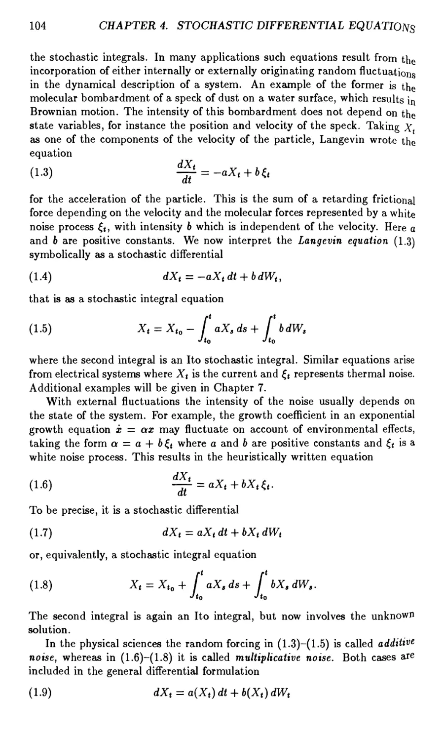
4.1 Introduction 103
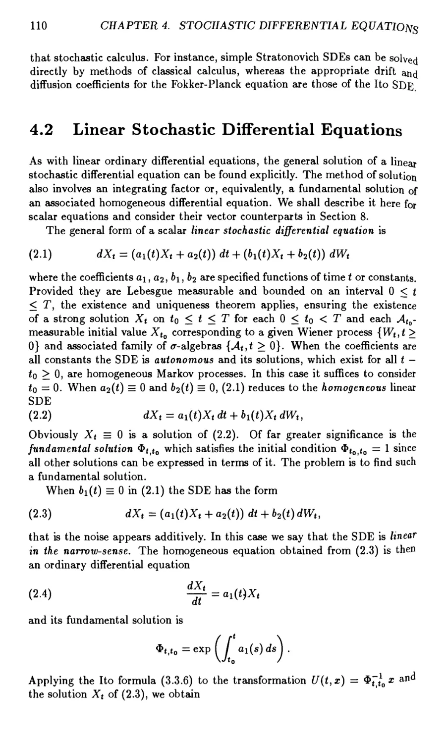
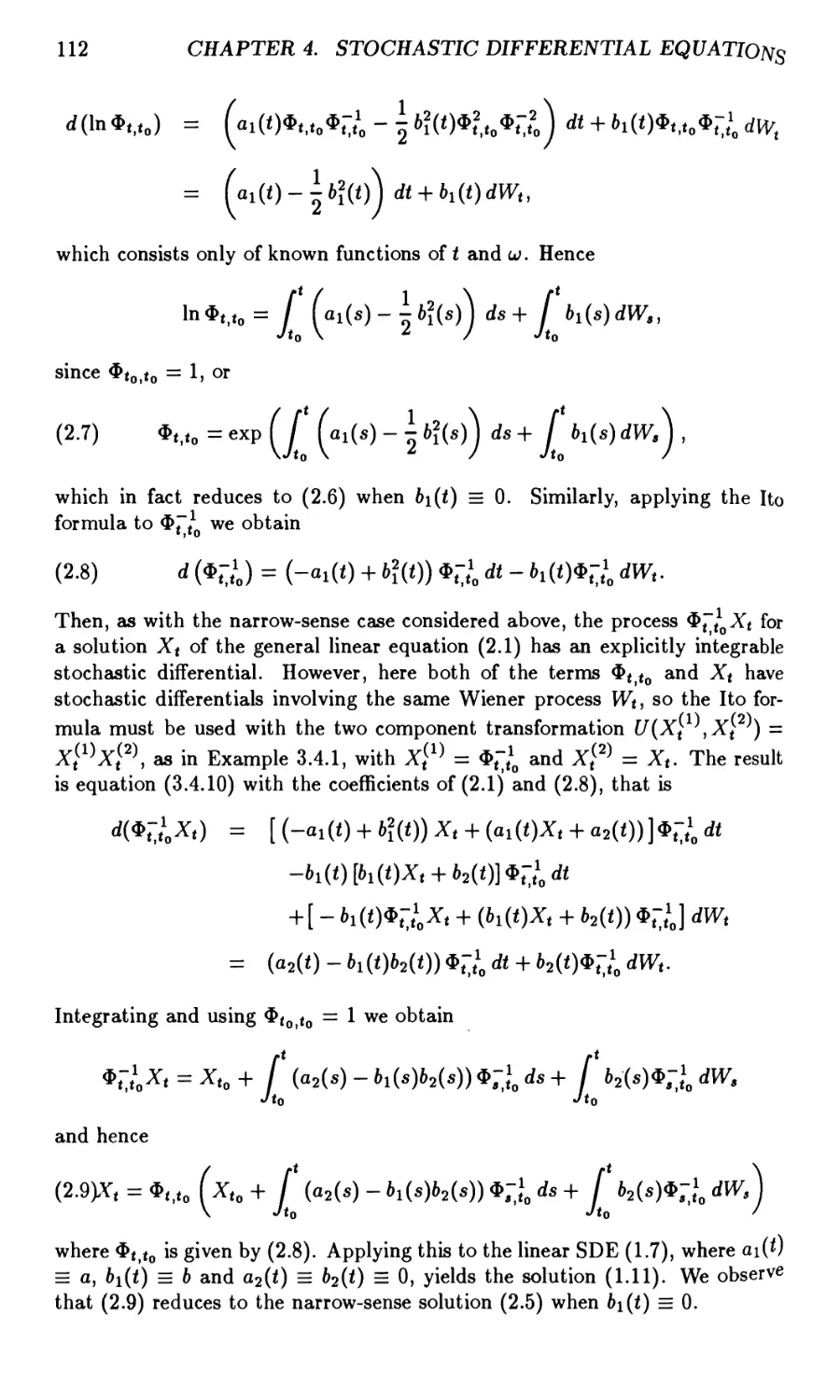
4.2 Linear Stochastic Differential Equations 110

XII CONTENTS
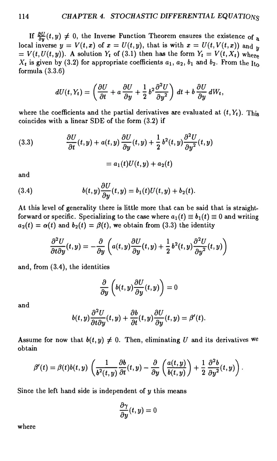
4.3 Reducible Stochastic Differential Equations 113
4.4 Some Explicitly Solvable Equations 117
4.5 The Existence and Uniqueness of Strong Solutions 127
4.6 Strong Solutions as Diffusion Processes 141
4.7 Diffusion Processes as Weak Solutions 144
4.8 Vector Stochastic Differential Equations 148
4.9 Stratonovich Stochastic Differential Equations 154
Chapter 5. Stochastic Taylor Expansions 161
5.1 Introduction 161
5.2 Multiple Stochastic Integrals 167
5.3 Coefficient Functions 177
5.4 Hierarchical and Remainder Sets 180
5.5 Ito-Taylor Expansions 181
5.6 Stratonovich-Taylor Expansions 187
5.7 Moments of Multiple Ito Integrals 190
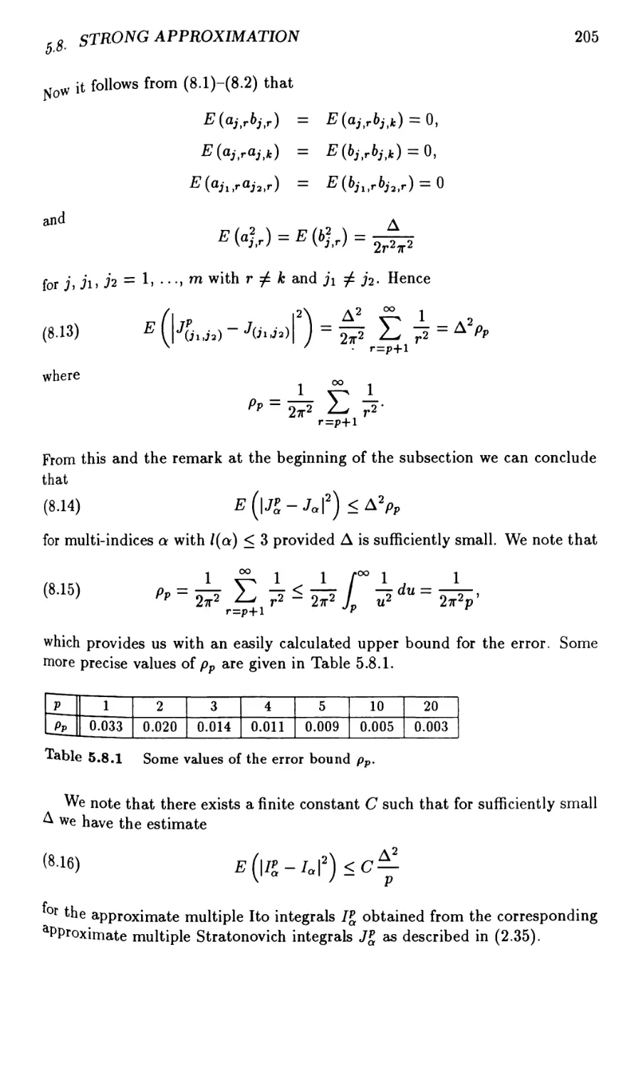
5.8 Strong Approximation of Multiple Stochastic Integrals 198
5.9 Strong Convergence of Truncated Ito-Taylor Expansions 206
5.10 Strong Convergence
of Truncated Stratonovich-Taylor Expansions 210
5.11 Weak Convergence of Truncated Ito-Taylor Expansions 211
5.12 Weak Approximations of Multiple Ito Integrals 221
Part III. Applications of Stochastic Differential Equations
Chapter 6. Modelling with Stochastic
Differential Equations 227
6.1 Ito Versus Stratonovich 227
6.2 Diffusion Limits of Markov Chains 229
6.3 Stochastic Stability 232
6.4 Parametric Estimation 241
6.5 Optimal Stochastic Control 244
6.6 Filtering 248
Chapter 7. Applications of Stochastic Differential Equations 253
7.1 Population Dynamics, Protein Kinetics and Genetics 253
7.2 Experimental Psychology and Neuronal Activity 256
7.3 Investment Finance and Option Pricing 257
7.4 Turbulent Diffusion and Radio-Astronomy 259
7.5 Helicopter Rotor and Satellite Orbit Stability 261
7.6 Biological Waste Treatment, Hydrology and Air Quality 263
7.7 Seismology and Structural Mechanics 266
7.8 Fatigue Cracking, Optical Bistability
and Nemantic Liquid Crystals 269
7.9 Blood Clotting Dynamics and Cellular Energetics 271

CONTENTS XIII
7.10 Josephson Tunneling Junctions, Communications
and Stochastic Annealing 273
Part IV. Time Discrete Approximations
Chapter 8. Time Discrete Approximation
of Deterministic Differential Equations 277
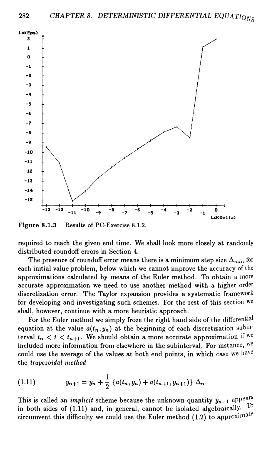
8.1 Introduction 277
8.2 Taylor Approximations and Higher Order Methods 286
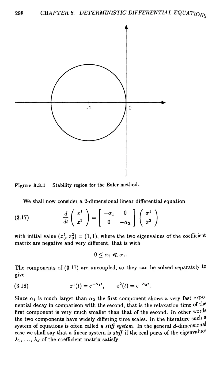
8.3 Consistency, Convergence and Stability 292
8.4 Roundoff Error 301
Chapter 9. Introduction to Stochastic
Time Discrete Approximation 305
9.1 The Euler Approximation 305
9.2 Example of a Time Discrete Simulation 307
9.3 Pathwise Approximations 311
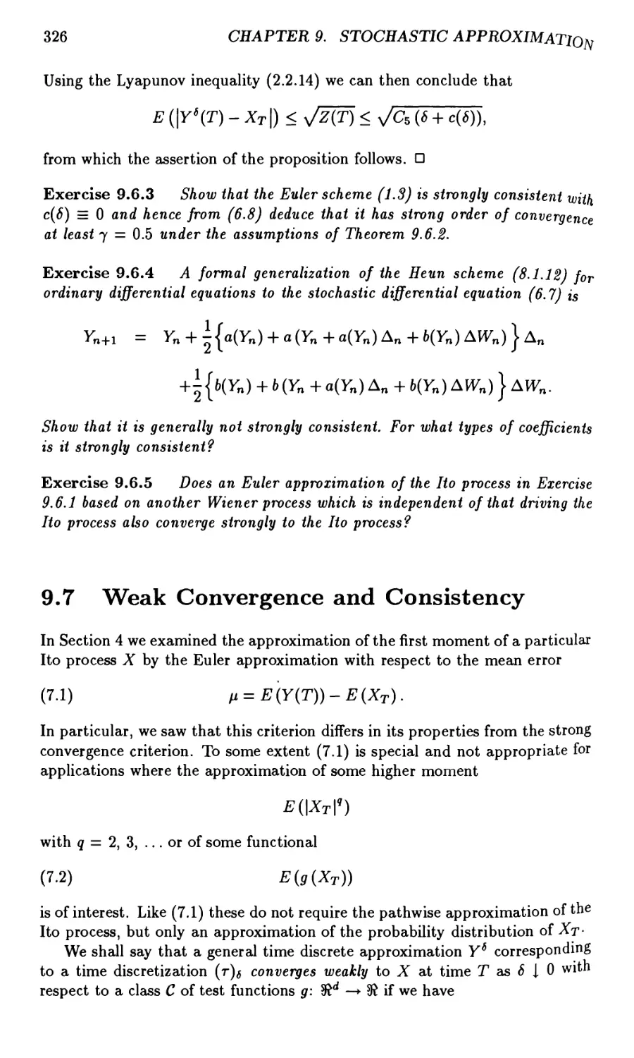
9.4 Approximation of Moments 316
9.5 General Time Discretizations and Approximations 321
9.6 Strong Convergence and Consistency 323
9.7 Weak Convergence and Consistency 326
9.8 Numerical Stability 331
Part V. Strong Approximations
Chapter 10. Strong Taylor Approximations 339
10.1 Introduction 339
10.2 The Euler Scheme 340
10.3 The Milstein Scheme 345
10.4 The Order 1.5 Strong Taylor Scheme 351
10.5 The Order 2.0 Strong Taylor Scheme 356
10.6 General Strong Ito-Taylor Approximations 360
10.7 General Strong Stratonovich-Taylor Approximations 365
10.8 A Lemma on Multiple Ito Integrals 369
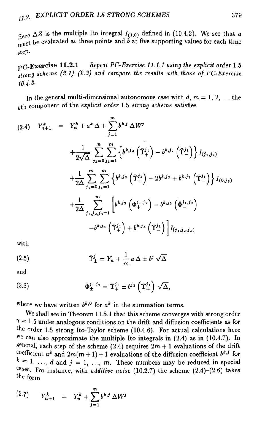
Chapter 11. Explicit Strong Approximations 373
11.1 Explicit Order 1.0 Strong Schemes 373
11.2 Explicit Order 1.5 Strong Schemes 378
11.3 Explicit Order 2.0 Strong Schemes 383
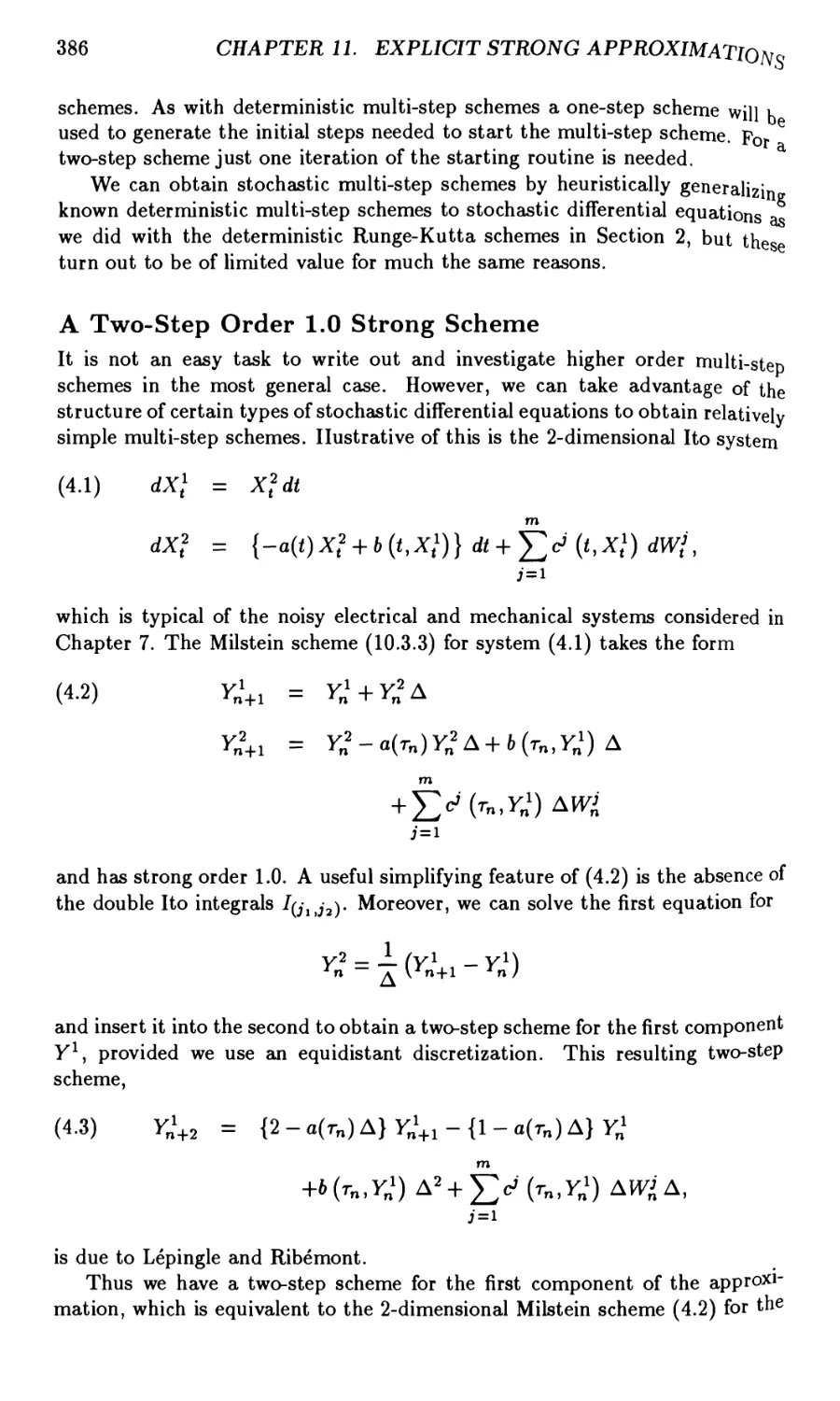
11.4 Multistep Schemes 385
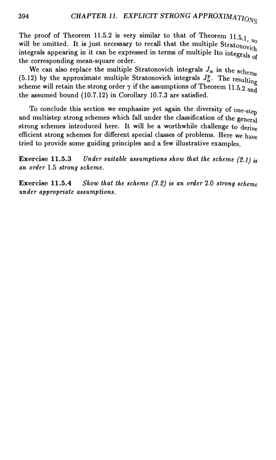
11.5 General Strong Schemes 390

XIV CONTENTS
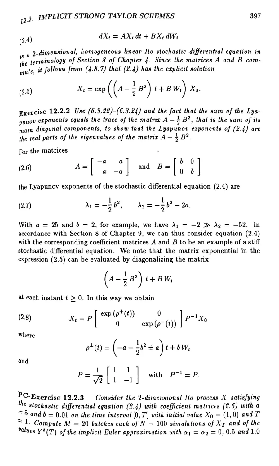
Chapter 12. Implicit Strong Approximations 395
12.1 Introduction 395
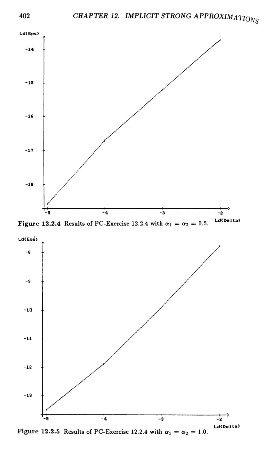
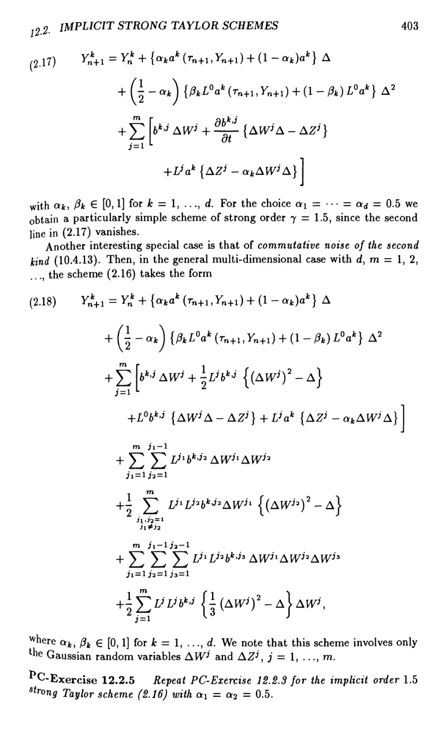
12.2 Implicit Strong Taylor Approximations 396
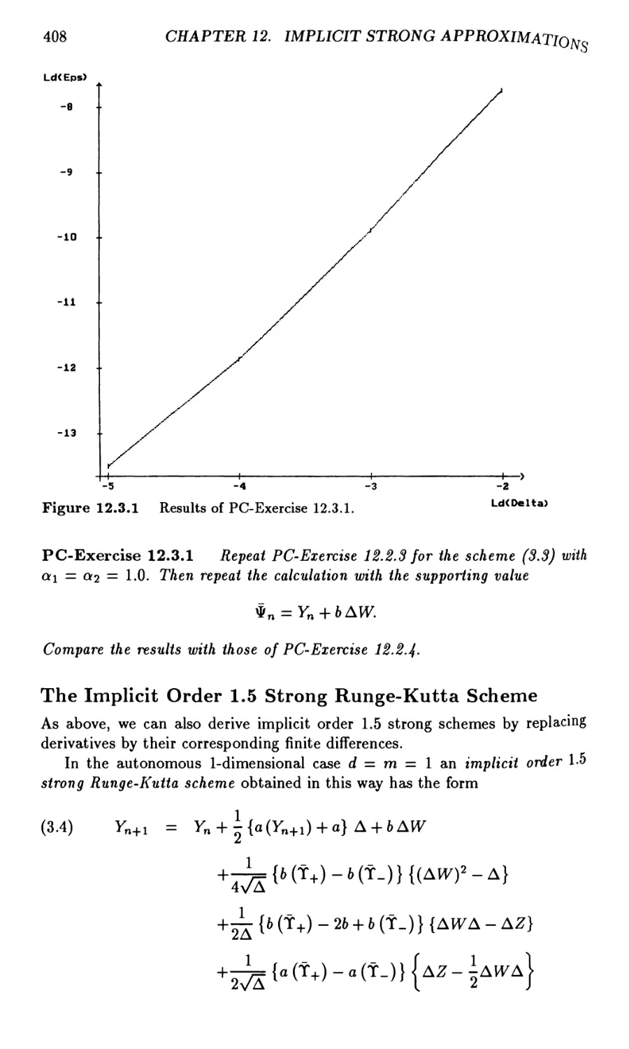
12.3 Implicit Strong Runge-Kutta Approximations 406
12.4 Implicit Two-Step Strong Approximations 411
12.5 A-Stability of Strong One-Step Schemes 417
12.6 Convergence Proofs 420
Chapter 13. Selected Applications
of Strong Approximations 427
13.1 Direct Simulation of Trajectories 427
13.2 Testing Parametric Estimators 435
13.3 Discrete Approximations for Markov Chain Filters 442
13.4 Asymptotically Efficient Schemes 453
Part VI. Weak Approximations
Chapter 14. Weak Taylor Approximations 457
14.1 The Euler Scheme 457
14.2 The Order 2.0 Weak Taylor Scheme 464
14.3 The Order 3.0 Weak Taylor Scheme 468
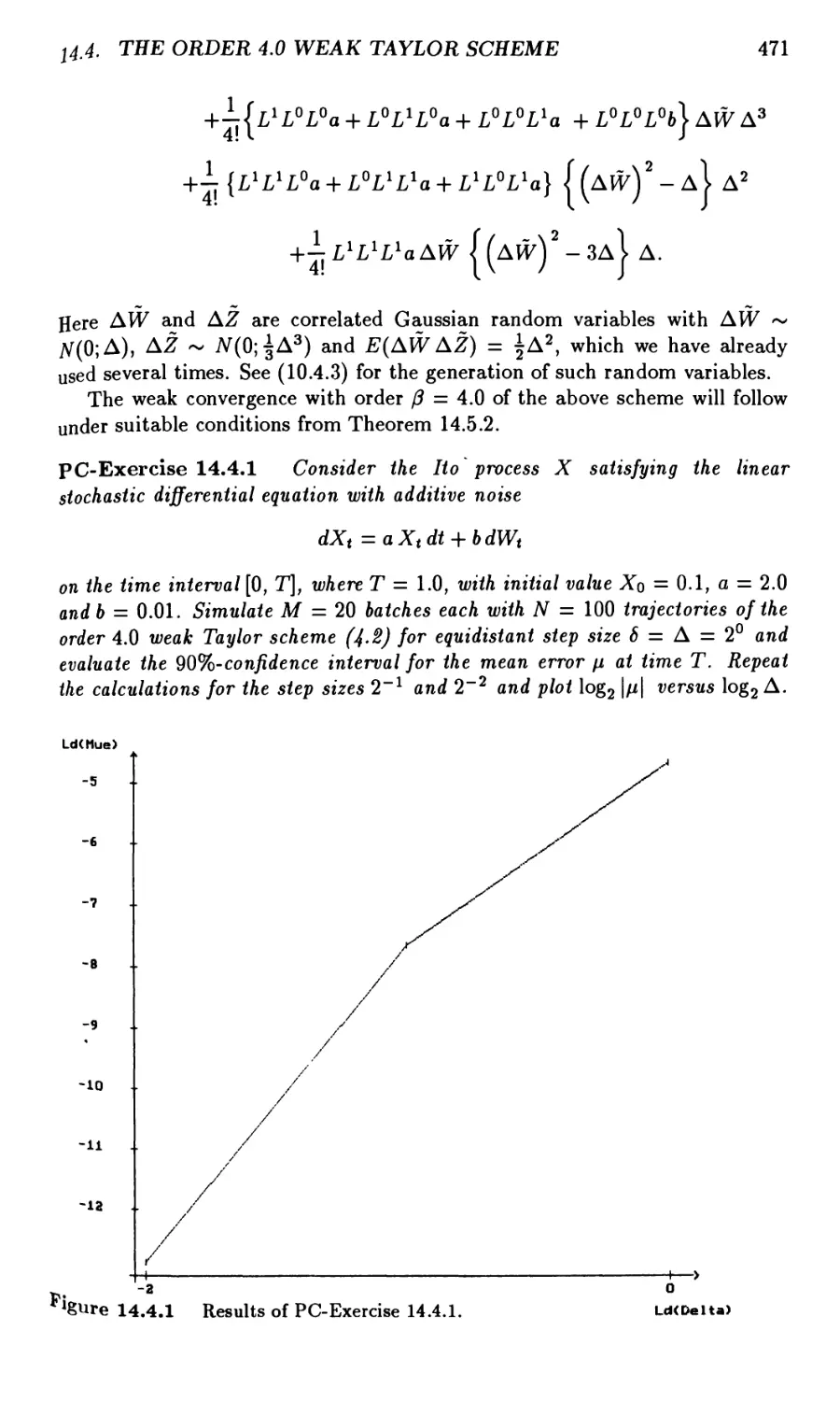
14.4 The Order 4.0 Weak Taylor Scheme 470
14.5 General Weak Taylor Approximations 472
14.6 Leading Error Coefficients 480
Chapter 15. Explicit and Implicit Weak Approximations . . . 485
15.1 Explicit Order 2.0 Weak Schemes 485
15.2 Explicit Order 3.0 Weak Schemes 488
15.3 Extrapolation Methods 491
15.4 Implicit Weak Approximations 495
15.5 Predictor-Corrector Methods 501
15.6 Convergence of Weak Schemes 506
Chapter 16. Variance Reduction Methods 511
16.1 Introduction 511
16.2 The Measure Transformation Method 513
16.3 Variance Reduced Estimators 516
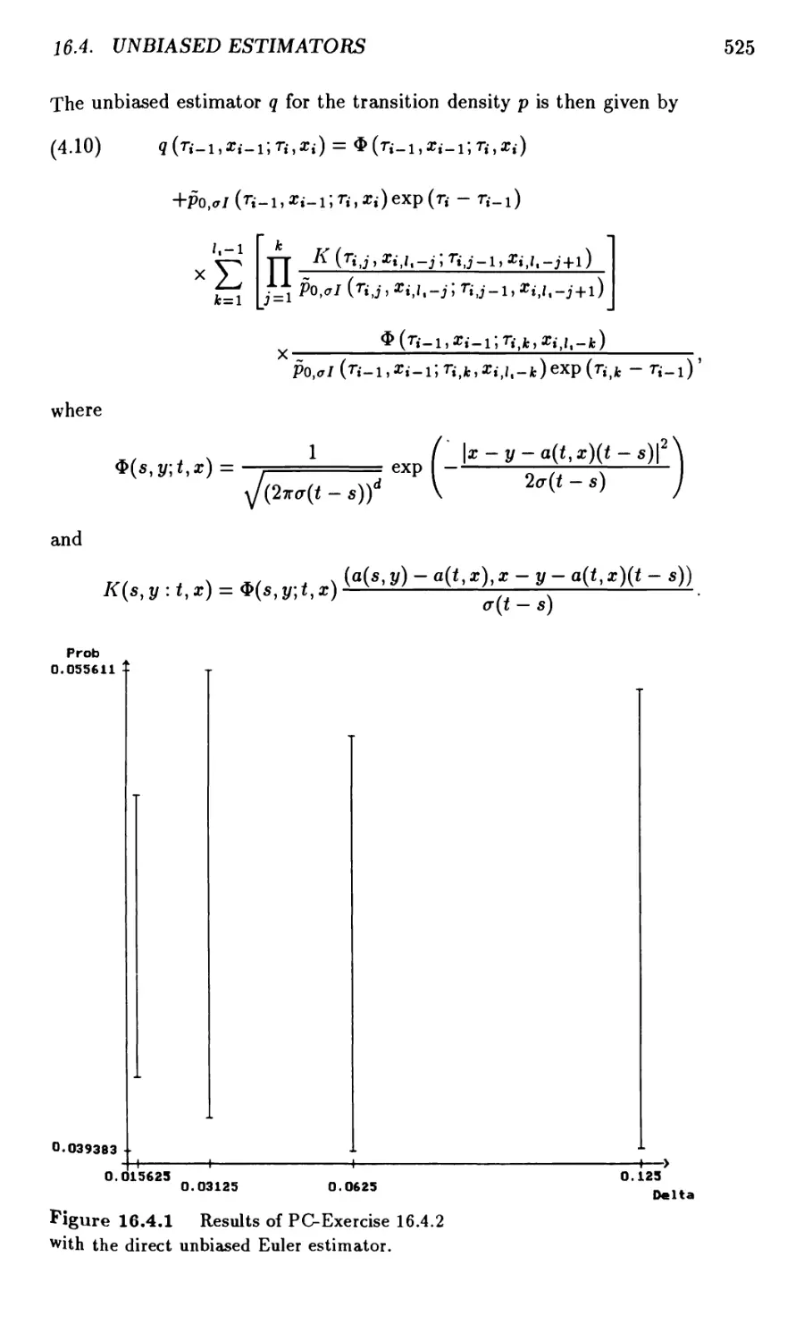
16.4 Unbiased Estimators 522
Chapter 17. Selected Applications of Weak Approximations 529
17.1 Evaluation of Functional Integrals 529
17.2 Approximation of Invariant Measures 540
17.3 Approximation of Lyapunov Exponents 545

CONTENTS XV
Solutions of Exercises 549
Bibliographical Notes 587
References 597
Index 625

Suggestions for the Reader
We mentioned in the Preface that we have tried to arrange the material of
this book in a way that would make it accessible to as wide a readership as
possible. Since prospective readers will undoubtedly have different backgrounds
and objectives, the following hints may facilitate their use of the book.
(i) We begin with those readers who require only sufficient understanding
of stochastic differential equations to be able to apply them and appropriate
numerical methods in different fields of application. The deeper mathematical
issues are avoided in the following flowchart which provides a reading guide to
the book for those without a strong background in mathematics.
§1.1 — §1.2 — §1.3 — §1.6 — §1.7 — §1.8
1
| §3.11
I
| §4.1 -+§4.4 |
I
Chapter 6
I
Chapter 7
I
| Chapter 8 |
i
§9.1 — §9.2 — §9.3 — §9.4 — §9.6 — §9.7
I
| §10.1 -+ §10.2 -+ §10.3 -+ §10.4 -+ §10.5 |
i
| §11.1-+§11.2-+§11.3-+§11.4 |
i
| §12.1 -+§12.2-+§12.3-+§12.4 |
i
r§T3.1-> §13.2-» §13.3 I
i
| §14.1 -+ §14.2 -+ §14.3 -+ §14.41
i
| §15.1 -+ §15.2 -+ §15.3 -+ §15.4 -+ §15T|
, + .
I §16.1 J
| Chapter 17 |

XVIII
SUGGESTIONS FOR THE READER
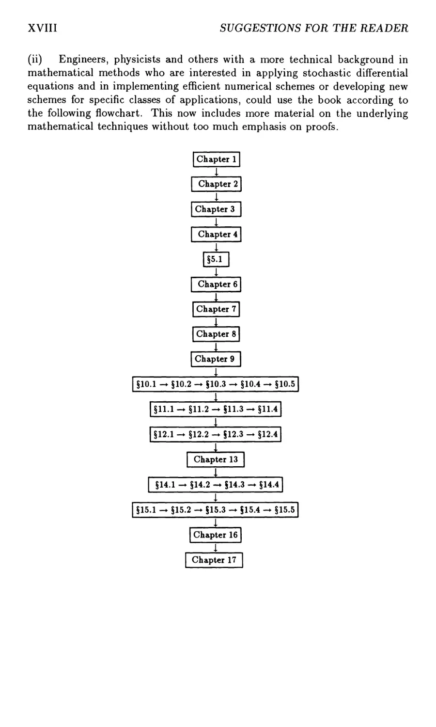
(ii) Engineers, physicists and others with a more technical background in
mathematical methods who are interested in applying stochastic differential
equations and in implementing efficient numerical schemes or developing new
schemes for specific classes of applications, could use the book according to
the following flowchart. This now includes more material on the underlying
mathematical techniques without too much emphasis on proofs.
Chapter 1
I
| Chapter 2 |
I
| Chapter 3 |
I
Chapter 4
1
| §5.1 |
I
| Chapter 6 |
1
| Chapter 71
1
| Chapter 8 |
i
| Chapter 9 |
i
§10.1 — §10.2 — §10.3 — §10.4 — §10.5
i
|§11.1 —§11.2 —§11.3 —§11.4|
i
| §12.1 — §12.2 — §12.3 — §12.41
1
| Chapter 13 |
i
| §14.1-§14.2-§14.3-§14.4 |
i
§15.1 — §15.2 — §15.3 — §15.4 — §15.5
I
Chapter 16
I
I Chapter 17 I

SUGGESTIONS FOR THE READER
XIX
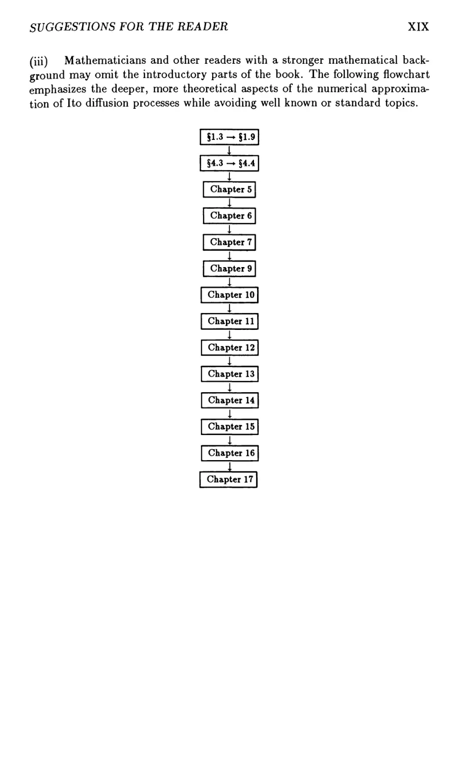
(iii) Mathematicians and other readers with a stronger mathematical
background may omit the introductory parts of the book. The following flowchart
emphasizes the deeper, more theoretical aspects of the numerical
approximation of I to diffusion processes while avoiding well known or standard topics.
§1.3 — §1.9
1
§4.3 — §4.4
I
Chapter 5
I
Chapter 61
I
Chapter 7J
1 .
Chapter 9 |
I
Chapter 10
I
Chapter 11
I
Chapter 12
I
Chapter 13
I
Chapter 14
I
Chapter 15
I
Chapter 16
j
Chapter 17

Basic Notation
0 the empty set
a E A a is an element of the set A
a £ A a is not an element of the set A
Ac the complement of the set A
A U B the union of sets A and B
AC\ B the intersection of sets A and B
A\ B the set of elements of set A that are not in set B
:= defined as or denoted by
= identically equal to
« approximately equal to
~ with distribution
3ft the set of real numbers
3ft+ the set of non-negative real numbers
(a, 6) the open interval a < x < b in 3ft
[a, b] the closed interval a < x < b in 3ft
a V 6 the maximum of a and b
a A 6 the minimum of a and 6
n! the factorial of the positive integer n
[a] the largest integer not exceeding a
3ft the c/-dimensional Euclidean space
x = (a;1,..., zd) a vector £ G 3ftd with ith component x% for i = 1,
(#,?/) the scalar product of vectors £, y G 3ftd
|z| the Euclidean norm of a vector x G 3ftd
£ transpose of the vector £
A = [a*'-7] a matrix i4 with ijth component a*J
i the square root of —1
Re(z) the real part of a complex number z
Im(z) the imaginary part of a complex number z

XXII
BASIC NOTATION
f : Q\ —► Q2 a function / from Qi into Q2
1a the indicator function of the set A
/' the first derivative of a function / : 3ft1 —► 3ft1
/" the second derivative of a function / : 3ft1 —► 3ft1
/(*) the Hh derivative of a function / : 3ft1 — 3ft1
<9r»u, -J-^7 the zth partial derivative of a function u : 3ftd —► 3ft1
<9*,u, (flfr) u the fcth order partial derivative of u with respect to xx
C(3ftm,3ftn) the space of continuous functions / : 3ftm -* 3ftn
Ck (3ftm,3ftn) the space of k times continuously differentiate functions
/ : »n — Kn
B the c-algebra of Borel subsets of 3ft1
C the <r-algebra of Lebesgue subsets of 3ft1
E(X) the expectation of the random variable X
6ij the Kronecker delta symbol
0(rp) expression divided by rp remains bounded as r —► 0
o(rp) expression divided by rp converges to zero as r —► 0
a.s. almost surely
w.p.l with probability 1
Other notation will be defined where it is first used. Note that vectors and
matrices will usually be indexed with superscripts. Parentheses will then be
used when taking powers of their components, for example with (x1)3 denoting
the cube of x%. Square brackets [•] will often be used to visually simplify nested
expressions, with the few instances where it denotes the integer part of a real
number being indicated in the text. Function space norms will always be
written with double bars || • ||, often with a distinguishing subscript.

A Brief Survey
of Stochastic Numerical Methods
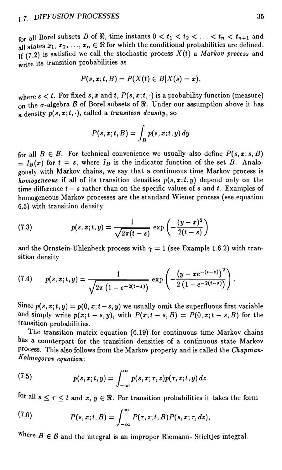
An Ito process X = {Xut > 0} has the form
(1) Xt = X0+ f a(Xs)ds+ f b(Xs)dWs
Jo Jo
for t > 0. It consists of an initial value Xo = xo, which may be random, a
slowly varying continuous component called the drift and a rapidly varying
continuous random component called the diffusion. The second integral in (1)
is an Ito stochastic integral with respect to the Wiener process W — {Wti t >
0}. The integral equation (1) is often written in the differential form
(2) dXt =a(Xt)dt + b(Xt)dWt
and is then called an Ito stochastic differential equation (SDE). For simplicity,
in this survey we shall restrict attention to a 1-dimensional Ito process X with
a 1-dimensional driving Wiener process W.
Unfortunately explicitly solvable SDEs such as those listed in Section 4 of
Chapter 4 are rare in practical applications. There are, however, now a number
of papers which deal with numerical methods for SDEs, yet the gap between
the well developed theory of stochastic differential equations and its application
is still wide. A crucial task in bridging this gap is the development of efficient
numerical methods for SDEs, a task to which this book is addressed. Obviously
such methods should be implementable on digital computers. They typically
involve the simulation of a large number of different sample paths in order to
estimate various statistical features of the desired solution. Modern
supercomputers with their parallel architecture are well suited to such calculations; see
Petersen (1987).
Here we shall survey various time discrete numerical methods which are
appropriate for the simulation of sample paths or functional of Ito processes
on digital computers.
Numerical Approaches to Stochastic Differential Equations
To begin we shall briefly mention several different approaches that have been
suggested for the numerical solution of SDEs. On the very general level there
is a method due to Boyce (1978) by means of which one can investigate, in
principle at least, general random systems by Monte Carlo methods. For SDEs
this method is somewhat inefficient because it does not use the special structure

XXIV BRIEF SURVEY OF STOCHASTIC NUMERICAL METHODS
of these equations, specifically their characterization by their drift and diffusion
coefficients.
Kushner (1977) proposed the discretization of both time and space
variables, so the approximating processes are then finite state Markov chains.
These can be handled on digital computers through their transition
matrices. In comparison with the information encompassed succinctly in the drift
and diffusion coefficients of an SDE, transition matrices contain a
considerable amount of superfluous information which must be repeatedly reprocessed
during computations. Consequently such a Markov chain approach seems
applicable only for low dimensional problems on bounded domains. Similar
disadvantages also arise, in higher dimensions at least, when standard numerical
methods are used to solve parabolic partial differential equations, such as the
Fokker-Planck equation and its adjoint, associated with functionals of the
solutions of SDEs. These are, of course, also methods for computing the probability
densities of Ito diffusions.
The most efficient and widely applicable approach to solving SDEs seems
to be the simulation of sample paths of time discrete approximations on digital
computers. This is based on a finite discretization of the time interval [0, T]
under consideration and generates approximate values of the sample paths step
by step at the discretization times. The simulated sample paths can then be
analysed by usual statistical methods to determine how good the approximation
is and in what sense it is close to the exact solution. The state variables here
are not discretized as in Kushner's Markov chain approach and the structure of
the SDE as provided by the drift and diffusion coefficients is used in a natural
way. An advantage of considerable practical importance of this approach is
that the computational costs such as time and memory required increase only
polynomially with the dimension of the problem. Variance reduction methods
allow a considerable decrease in the required sample size.
Time Discrete Approximations
Early simulation studies and theoretical investigations by Clements & Anderson
(1973), Wright (1974), Clark & Cameron (1980) and others showed that not all
heuristic time discrete approximations of an SDE (2) converge in a useful sense
to the solution process as the maximum step size 6 tends to zero. In particular,
it was found that one cannot simply use a deterministic numerical method for
ordinary differential equations, such as a higher order Runge-Kutta method.
Consequently a careful and systematic investigation of different methods is
needed in order to select a sufficiently efficient method for the task at hand.
We shall consider a time discretization (r)6 with
(3) 0 = r0 < rx < • • • < rn < • • • < rN = T
of a time interval [0,T], which in the simplest equidistant case has step size
N
(4)

BRIEF SURVEY OF STOCHASTIC NUMERICAL METHODS XXV
We shall see in Chapter 9 that general time discretizations, even with random
times, are possible, but usually a maximum step size 6 must be specified.
The simplest heuristic time discrete approximation is the stochastic
generalization of the Euler approximation which is sometimes called the Euler-
Maruyama approximation (see Maruyama (1955)), but often just the Euler
approximation. For the SDE (2) it has the form
(5) Yn+i = Yn + a(Yn) An + b(Yn) AWn
for n = 0, 1, ..., N — 1 with initial value
(6) Y0 = x0l
where
(7) An = rn+1 -rn = 6
and
(8) AWn = WTn+l - WTn
for n = 0, 1, ..., N — 1. Essentially, it is formed by fixing the integrands
in (1) to their values at the beginning of each discretization time subinterval.
The recursive scheme (5) obviously gives values of the approximation only
at the discretization times. If values are required at intermediate instants,
then either piecewise constant values from the preceding discretization point
or some interpolation, especially a linear interpolation, of the values of the two
immediate enclosing discretization points could be used.
The random variables AWn defined in (8) are independent N(0]An)
normally distributed random variables, that is with means and variances
E(AWn) = 0 and E ((AWn)2) = A„,
respectively, for n = 0, 1, ..., N — 1. In simulations we can generate such
random variables from independent, uniformly distributed random variables
on [0,1], which are usually provided by a pseudo-random number generator on
a digital computer. We shall discuss and test random number generators in
Sections 3 and 9 of Chapter 1.
The Strong Convergence Criterion
In problems such as those that we shall consider in Chapter 13 involving direct
simulations, filtering or testing estimators of Ito processes it is important that
the trajectories, that is the sample paths, of the approximation be close to
those of the Ito process. This suggests that a criterion involving some form
of strong convergence should be used. Mathematically it is advantageous to
consider the absolute error at the final time instant T, that is
(9)
€{6) = E(\XT-YN\),

XXVI BRIEF SURVEY OF STOCHASTIC NUMERICAL METHODS
which can be estimated from the root mean square error via the Lyapunov
inequality
(10) c(6) = E(\XT - YN\) < ^e(\Xt-Yn\2).
The absolute error (9) is certainly a criterion for the closeness of the sample
paths of the Ito process X and the approximation Y at time T.
We shall say that an approximating process Y converges in the strong sense
with order 7 G (0,oo] if there exists a finite constant K and a positive constant
60 such that
(11) E(\XT-YN\)<Kfrt
for any time discretization with maximum step size 6 G (0,6o)- In the
deterministic case with zero diffusion coefficient 6 = 0 this strong convergence
criterion reduces to the usual deterministic criterion for the approximation of
ordinary differential equations. The order of a scheme is sometimes less in the
stochastic case than in the corresponding deterministic one, essentially because
the increments AWn of the Wiener process are of root mean square order 61/2
and not 6. In fact, the Euler approximation (5) for SDEs has strong order 7
= 0.5 in contrast with the order 1.0 of the Euler approximation for ordinary
differential equations.
Important contributions which also influenced the future development of
higher order strong approximations include Milstein (1974), McShane (1974),
Rao, Borwankar & Ramakrishna (1974), Kloeden & Pearson (1977), Wagner
& Platen (1978), Clark (1978), Platen (1981), Rumelin (1982), Talay (1982a),
Newton (1986a) and Chang (1987).
The Weak Convergence Criterion
In many practical situations, some of which will be described in Chapter 17,
it is not necessary to have a close pathwise approximation of an Ito process.
Often one may only be interested in some function of the value of the Ito
process at a given final time T such as one of the first two moments E(Xt)
and E((Xt)2) or, more generally, the expectation E(g(Xr)) for some function
g. In simulating such a functional it suffices to have a good approximation
of the probability distribution of the random variable Xt rather than a close
approximation of sample paths. Thus the type of approximation required here
is much weaker than that provided by the strong convergence criterion.
We shall say that a time discrete approximation Y converges in the weak
sense with order j3 G (0,00] if for any polynomial g there exists a finite constant
K and a positive constant 60 such that
(12) \E(g(XT))-E(g(YN))\<K6^
for any time discretization with maximum step size S G (0,60). In Section 7
of Chapter 9 we shall generalize slightly the class of test fuctions g used here.
When the diffusion coefficient in (1) vanishes identically this weak convergence
criterion with g(x) = x also reduces to the usual deterministic convergence
criterion for ordinary differential equations.

BRIEF SURVEY OF STOCHASTIC NUMERICAL METHODS XXVII
Under assumptions of sufficient smoothness Milstein (1978) and Talay
(1984) showed that an Euler approximation of an Ito process converges with
weak order /? = 1.0, which is greater than its strong order of convergence 7 =
0.5. On the other hand, Mikulevicius & Platen (1991) showed that the Euler
scheme converges, but with weak order less than 1.0, when the coefficients of
(1) are only Holder continuous, that is Lipschitz-like with a fractional power.
Higher order weak approximations have been extensively investigated by
Milstein (1978), Talay (1984), Platen (1984) and Mikulevicius & Platen (1988).
In particular, weak approximations of the Runge-Kutta type have been
proposed and studied by Greenside & Helfand (1981), Talay (1984), Platen (1984),
Klauder & Petersen (1985a), Milstein (1985), Haworth & Pope (1986) and Ave-
rina & Artemev (1986). In addition, Wagner (1987) has investigated the use of
unbiased weak approximations, that is with (3 = 00, for estimating functional
of Ito diffusions.
Stochastic Taylor Formulae
Another natural way of classifying numerical methods for SDEs is to compare
them with strong and weak Taylor approximations. The increments of such
approximations are obtained by truncating the stochastic Taylor formula, which
was derived in Wagner &; Platen (1978) by an iterated application of the Ito
formula. It was then generalized and investigated in Azencott (1982), Platen
(1982) and Platen &; Wagner (1982). A Stratonovich version of the stochastic
Taylor formula was presented in Kloeden &; Platen (1991a) and can be found
together with results on multiple stochastic integrals in Chapter 5.
The stochastic Taylor formula allows a function of an Ito process, that is
f(Xt)y to be expanded about f(Xto) in terms of multiple stochastic integrals
weighted by coefficients which are evaluated at Xto. These coefficients are
formed from the drift and diffusion coefficients of the Ito process and their
derivatives up to some specified order. The remainder term in the formula
contains a finite number of multiple stochastic integrals of the next higher
multiplicity, but now with nonconstant integrands. For example, a stochastic
Taylor formula for the Ito process (1) for t G [to,T] may have the form
(13) f(Xt) = f(Xt0) + Cl(XtB) f ds + c2(XtB) f dW,
Jto Jt0
+c3(Xto) [ [" dWtldW,a + R
Jt0 Jt0
with coefficients
Cl(«) = a (*)/'(*)+ i (6 (*))2/"(*),
c2(x) = 6 (*)/'(*),
c3(x) = b(x){b(x)f"{z) + V(x)f'{x)}.

XXVIII BRIEF SURVEY OF STOCHASTIC NUMERICAL METHODS
Here the remainder R consists of higher order multiple stochastic integrals
with nonconstant integrands involving the function /, the drift and diffusion
coefficients and their derivatives. A stochastic Taylor formula can be thought
of as a generalization of both the Ito formula and the deterministic Taylor
formula.
If we use the function f(x) = x in the stochastic Taylor formula (13) we
obtain the following representation for the Ito process (1):
(14) Xt = Xto+a(Xto) ( ds + b(Xt0) ( dWs
Jto Jto
+b(Xt0)b'(Xt0) f r dWSldW>3+R.
Jto Jto
By truncating stochastic Taylor expansions such as (14) about successive
discretization points we can form time discrete Taylor approximations which we
may interpret as basic numerical schemes for an SDE. In addition we can
compare other schemes, such as those of the Runge-Kutta type, with the time
discrete Taylor approximations to determine their order of strong or weak
convergence. We shall see that we must include the appropriate terms from the
corresponding stochastic Taylor expansion, that is the necessary higher
multiple stochastic integrals, to obtain a numerical scheme with a higher order of
strong or weak convergence.
Strong Taylor Approximations
The simplest strong Taylor approximation of an Ito diffusion is the Euler
approximation
(15) Yn+1 = Yn+aAn+6AWn
for n = 0, 1, ..., N — 1 with initial condition (6), where An and AWn are defined
by (7) and (8), respectively, with the AWn independent N(0]An) normally
distributed random variables. Here we have written a for a (Yn) and b for b (Yn),
a convention which we shall henceforth use for any function. In addition, as
here, we shall not repeat the standard initial condition (6) in what follows. It
was shown in Gikhman & Skorokhod (1972a) that the Euler scheme converges
with strong order 7 = 0.5 under Lipschitz and bounded growth conditions on
the coefficients a and 6.
If we include the next term from the stochastic Taylor formula (14) in the
scheme (15) we obtain the MUstein scheme
(16) Yn+1 = Yn + a An + b AWn + ±66' {(AWn)2 - An}
for n = 0, 1, ..., Af — 1; see Milstein (1974). The additional term here is from
the double Wiener integral in (14), which can be easily computed from the
Wiener increment AWn since
(17) jTn+1 /" dWSl dW„ = i {(AWnf - A„} .

BRIEF SURVEY OF STOCHASTIC NUMERICAL METHODS XXIX
We shall see that the Milstein scheme (16) converges with strong order 7 = 1.0
under the assumption that E((Xq)2) < 00, that a and b are twice continuously
differential)le, and that a, a', 6, b' and b" satisfy a uniform Lipschitz condition.
For a multi-dimensional driving Wiener process W = (W1, ..., Wm) the
generalization of the Milstein scheme (16) involves the multiple Wiener integrals
(18) W)= r+1 f2 dWi\dWll
for ji, 32 € {!>••• j m) with jx ^ j2> which cannot be expressed simply as in
(16) in terms of the increments AVV^1 and AW-j2 of the corresponding Wiener
processes. In Section 8 of Chapter 5 we shall suggest one possible way of
approximating higher order multiple stochastic integrals like (18); see also Kloeden,
Platen & Wright (1992).
Generally speaking we obtain more accurate strong Taylor approximations
by including additional multiple stochastic integral terms from the
stochastic Taylor expansion. Such integrals contain additional information about the
sample paths of the Wiener process over the discretization subintervals. Their
presence is a fundamental difference between the numerical analysis of
stochastic and ordinary differential equations.
For example, the strong Taylor approximation of order 7 = 1.5 is given by
(19) y„+i = Yn + aAn+bAWn + ^bb' {(AWn)2 - An}
+&a'AZn + ±{aa' + ±6V'JA*
+ Lb' + hH"\{AWnAn-AZn}
+±6 [bb" + (6')2} U (AWn)2 - An J AWn
for n — 0, 1, ..., Af — 1. Here the additional random variable AZn is required
to represent the double integral
(20) AZn= fU+1 [" dW9ld82,
which is normally distributed with mean, variance and correlation
E(AZn) = 0, £((AZn)2)=i(A„)3 and E(AWn AZn) = | (A„)2 ,
respectively. All other multiple stochastic integrals appearing in the truncated
Taylor expansion used to derive (19) can be expressed in terms of An, AWn
and AZn, thus resulting in (19). It was shown in Wagner & Platen (1978)
and Platen (1981a) that the scheme (19) converges with strong order 7 = 1.5
when the coefficients a and 6 are sufficiently smooth and satisfy Lipschitz and

XXX BRIEF SURVEY OF STOCHASTIC NUMERICAL METHODS
bounded growth conditions. We note that there is no difficulty in generating
the pair of correlated normally distributed random variables AWn, AZn using
the transformation
(21) AWn = C„,i A'J2 and AZn = ± (c.,1 + ^= Cn,2) AZJ\
where Cn,i and Cn,2 are independent normally Af(0; 1) distributed random
variables.
Following Platen (1981a), we shall describe in Chapter 10 how schemes of
any desired order of strong convergence can be constructed from the
corresponding strong Taylor approximations. The implementation of such schemes
requires the generation of multiple stochastic integrals such as I(jxj2) and of
higher multiplicity, which can be done by means of an approximation method
which we shall describe in Chapter 5. Those readers who do not wish to use
such multiple stochastic integrals could follow Clark (1978) and Newton
(1986a,b), in which schemes only involving the increments of the Wiener
process are proposed. These schemes, which we shall describe in Section 4 of
Chapter 13, are similar to the strong Taylor approximations above, but with
the random variables modified. Moreover, they are optimal within the classes
of strong orders 7 = 0.5 or 1.0, respectively.
Strong Runge-Kutta,
Two-Step and Implicit Approximations
A practical disadvantage of the above strong Taylor approximations is that
the derivatives of various orders of the drift and diffusion coefficients must
be determined and then evaluated at each step in addition to the coefficients
themselves. There are time discrete approximations which avoid the use of
derivatives, which we shall call Runge-Kutta schemes in analogy with similar
schemes for ordinary differential equations. However, we emphasize that it is
not always possible to use heuristic adaptations of deterministic Runge-Kutta
schemes for SDEs because of the difference between ordinary and stochastic
calculi.
A strong order 1.0 Runge-Kutta scheme is given by
(22)yn+1 = yn + aAn + 6^^nPyn + i{6(fn)-6}{(A^n)2-An} A"1'2
with supporting value
rn = Yn + bA1J2
for n — 0, 1, ..., N — 1. This scheme can be obtained heuristically from the
Milstein scheme (16) simply by replacing the derivative there by the
corresponding finite difference; see Platen (1984). Clark & Cameron (1980) and Rumelin
(1982) have shown that Runge-Kutta schemes like (22) converge strongly with
at most order 7 = 1.0. More general Runge-Kutta schemes can be found in
Chapter 11, but they have usually only the strong order of convergence 7 =

BRIEF SURVEY OF STOCHASTIC NUMERICAL METHODS XXXI
1.0 if just the increments AWn of the Wiener process are used; higher
multiplicity stochastic integrals must be used to obtain a higher order of strong
convergence.
For the case of additive noise, 6 = const., a two-step order 1.5 strong scheme
takes the form
(23) Yn+1 = Yn + 2aAn- a,(yn_1)6(yn_1) AWn-X An + Vn + Vn-i
with
Vn = bAWn + a'bAZn,
where AWn and AZn are the same as in (21); see Kloeden & Platen (1991c).
Additional multi-step schemes will be described in Chapter 12.
A typical implicit order 1.5 strong scheme for additive noise is
(24) 7n+1 = Yn + ±{a(Yn+i) + a}An + bAWn
+\ {« (t„+) - « (f")} [aZu - \AWn A„} A;1'2
with supporting values
f$=Yn + aAn±bAlJ\
where AWn and AZn are the same as in (21); see Kloeden & Platen (1992).
Implicit or fully implicit schemes are needed to handle stiff SDEs, which will
be discussed in Section 8 of Chapter 9 and in Chapter 12; see Petersen (1987),
Drummond & Mortimer (1990) and Hernandez & Spigler (1993).
Another type of strong approximation was investigated in Gorostiza (1980)
and Newton (1990). In the 1-dimensional case the time variable is discretized
in such a way that a random walk takes place on a prescribed set of threshholds
in the state space, with the approximating process remaining on a fixed level
for a random duration of time and then switching with given intensity to the
next level above or below it.
Finally, the reader is referred to Doss (1978), Sussmann (1978) and Talay
(1982a) for other investigations of strong approximations of Ito diffusions.
Weak Taylor Approximations
When we are interested only in weak approximations of an Ito process, that
is a process with approximately the same probability distribution, then we
have many more degrees of freedom than with strong approximations. For
example, it suffices to use an initial value Y0 — ^o with a convenient probability
distribution which approximates that of Xq in an appropriate way. In addition
the random increments AWn of the Wiener process can be replaced by other
more convenient approximations AWn which have similar moment properties
to the AWn. In a weak approximation of order /? = 1.0 we could, for instance,

XXXII BRIEF SURVEY OF STOCHASTIC NUMERICAL METHODS
choose independent AWn for n = 0, 1, ..., N — 1 with moments
(25)
where
(26)
[ 0 : r = 1 and 3
E^AWny) =| A„ : r = 2
I Zr(An) : r = 4,5,...
\Zr(An)\<KAl
for r = 4, 5, ... and some finite constant K > 0. This means we could use an
easily generated two-point distributed random variable taking values ±\/An
with equal probabilities, that is with
(27) P (AWn = ±y/ZZ) = \-
The simplest useful weak Taylor approximation is the weak Euler scheme
(28) Yn+1 = Yn+aAn+6AWn
for n = 0, 1, ..., N - 1. It follows from results in Talay (1984) that (28)
has weak order /? = 1.0 if the coefficients a and 6 are four times continuously
differentiate with these derivatives satisfying a growth bound. This contrasts
with the order 7 = 0.5 of the strong Euler scheme (15).
We can construct weak Taylor approximations of higher order /? = 2.0, 3.0,
... by truncating appropriate stochastic Taylor expansions. For example, the
weak Taylor approximation of order (3 = 2.0 has, following Milstein (1978) and
Talay (1984), the form
(29) yn+1 = Yn + aAn+6AH'n + i66/ UAWn)2-An\
+ Lb' + i626"j {AWn An - AZn)
for n — 0, 1, ..., N — 1. Here AWn approximates AWn and AZn the multiple
stochastic integral (20). As with the weak Euler scheme (28) we can choose
random variables AWn and AZn which have approximately the same moment
properties as AWn and AZn, For example, we could use
(30) AWn=AWn and AZ„ = iAW„A„
with the AW„ independent iV(0; An) normally distributed, or we could use
(31) AWn = Al/2Tn and AZn = ±A3J2Tn

BRIEF SURVEY OF STOCHASTIC NUMERICAL METHODS XXXIII
where the Tn are independent three-point distributed random variables with
(32) p(Tn=±V3)=i and P(Tn = 0) = |.
Multi-dimensional and higher order weak Taylor approximations also involve
additional random variables, but these are much simpler than those in strong
approximations as will be seen in Chapter 14.
It was shown under appropriate assumptions in Platen (1984) that a Taylor
approximation converges with any desired weak order (3 — 1.0, 2.0, ... when the
multiple stochastic integrals up to multiplicity /? are included in the truncated
stochastic Taylor expansion used to construct the scheme.
Weak Runge-Kutta and Extrapolation Approximations
It is often convenient computationally to have weak approximations of the
Runge-Kutta type which avoid the use of derivatives of the drift and diffusion
coefficients, particularly the higher order derivatives. An order 2.0 weak Runge-
Kutta scheme proposed by Talay (1984) is of the form
(33) yn+i = Yn +ja(fn)-i6(fn)&'(fn)J A„
+ (-7= & (An ~ Bn) + V2b (f n) Bn J A„/2
+ l\ (b (f „) 6' (f „) - bb') B2n - bb'AnBn\ A„
with supporting value
rn=Yn + Ua- Ibb'} An + -^ bAn A1'2 + ±bb'A2n A„
for n = 0, 1, ..., N— 1, where the An and Bn are independent random variables
which are, for example, standard normally distributed or as in (32).
The scheme (33) still uses the derivative b' of the diffusion coefficient 6. It
is also possible to avoid using this derivative, as in the following order 2.0 weak
Runge-Kutta scheme from Platen (1984):
(34)yn+1 = Yn + i {a(fn)+ a) An + i {6 (T+) + 6 (T") + 26} AWn
with supporting values
fB=yB + oA„ + 6AWrn and T± = Yn + a A„ ± &A„'2

XXXIV BRIEF SURVEY OF STOCHASTIC NUMERICAL METHODS
for n = 0, 1, ..., N — 1, where the AWn can be chosen as in (30) or (31).
Higher order approximations of functionals can also be obtained with lower
order weak schemes by extrapolation methods. Talay h Tubaro (1990)
proposed an order 2.0 weak extrapolation method
(35) V/2(T) = 2E {g {Y6(T))) - E (g (Y26(T)))
where Y6(T) and Y2S(T) are the Euler approximations at time T for the step
sizes 6 and 26, respectively. Higher order extrapolation methods from Kloeden,
Platen & Hofmann (1995) will also be presented in Section 3 of Chapter 15.
Essentially, many order f3 weak scheme can be extrapolated with formulae
similar to (35) to provide order 2(3 accuracy for /? = 1.0,2.0,....
An order 2.0 weak predictor-corrector scheme for SDEs proposed in Platen
(1991), which has the corrector
(36) Yn+1 =Yn + ±{a (tn+1) + a} An + *n
with
*„ = b AWn + 166' | (A^„)2 - A„| + ± Lb' + \ bH"\ AWn An
and the predictor
(37) f n+1 = Yn + a An + *n + i a'b AWn An + i | aa' + i 62a" | A2,
where Al^n can be as in (30) or (31)—(32), is an example of a simplified weak
Taylor scheme, where An can be as in (30) or (31)—(32). The corrector (36)
resembles the implicit order 2.0 weak scheme
(38) Yn+i = Yn + i {a(Yn^) + a} An + *n.
Higher order Runge-Kutta, predictor-corrector and implicit weak schemes
as well as extrapolation methods will be examined in Chapter 15.
Runge-Kutta schemes with convergence only in the first two moments have
been considered in Greenside & Helfand (1984), Haworth & Pope (1986),
Helfand (1979), Klauder & Petersen (1985a) and Petersen (1987). This
convergence criterion is weaker than the weak convergence criterion (10) considered
here. Obviously, a scheme which converges with some weak order /? will not
only converge in the first two moments, but also in all higher moments with
this same order /? when they exist.
Finally, Wagner (1987) has proposed another way of approximating weak
approximations of diffusion processes which is based on the Monte Carlo
simulation of functional integrals and uses unbiased, variance reduced
approximations to estimate functionals of Ito diffusion processes. This will be described in

BRIEF SURVEY OF STOCHASTIC NUMERICAL METHODS XXXV
Chapter 16. Milstein (1988a) and Chang (1987) have also investigated variance
reduction techniques.
We conclude this brief survey with the remark that the theoretical
understanding and practical application of numerical methods for stochastic
differential equations are still in their infancy. An aim of this book is to stimulate an
interest and further work on such methods. For this the Bibliographical Notes
at the end of the book may be of assistance.

Chapter 1
probability and Statistics
The basic concepts and results of probability and stochastic processes needed
later in the book are reviewed here. The emphasis is descriptive and PC-
Exercises (PC= Personal Computer), based on pseudo-random number
generators introduced in Section 3, are used extensively to help the reader to develop
an intuitive understanding of the material. Statistical tests are discussed briefly
in the final section.
1.1 Probabilities and Events
If we toss a die, then, excluding absurd situations, we always observe one of
six basic outcomes; it lands with its upper face indicating one of the numbers
1, 2, 3, 4, 5 or 6. We shall denote these outcomes by u\, u;2, u>3, W4, w$ and
u>6, respectively, and call the set of outcomes Q = {u\} U2, ^3, ^4, ^5, ^6} the
sample space. If we toss the die N times and count the number of times N{ that
outcome a;,- occurs, we obtain a relative frequency fi(N) = N{/N. This number
usually varies considerably with N} but experience tells us that as N becomes
larger it approaches a limit limyy—00 fi(N) = pi, which we call the probability
of outcome a;,-. Clearly 0 < pi < 1 for each i = 1, 2, ..., 6 and ^2i=:1Pi = 1;
for a fair die each pi = 1/6, giving a uniform distribution of probabilities over
the outcomes.
Often we are interested in combinations of outcomes, that is subsets of the
sample space Q such as the subset {u;i, W3, u^} of odd indexed outcomes. If we
can distinguish such a combination by either its occurence or its nonoccurence
we call it an event. Clearly if a subset A is an event, then its complement Ac =
{vi EQ : u>i £ A} must also be an event. In particular, the whole sample space
ft is an event, which we call the sure event since one of its outcomes must always
occur; its complement, the empty set 0, is also an event but can never occur. We
might think that every subset A of Q should be an event, in which case we could
determine its probability P(A) from those of its constituent outcomes, that is
as P(A) — ^2W €APi. However this corresponds to a situation of complete
information about each of the outcomes, information which we may not always
possess. For example, we may have only kept records of the occurences of odd
or even indexed outcomes, but not of the actual outcomes themselves. Then we
only distinguish and determine probabilities for the four subsets 0, O = {u;i,
^3, u;5}, E = {u;2, u>4, luq} and Q, which are thus the only events in this case.
Actually, we could introduce new basic outcomes O (odd) and E (even) here;

2
CHAPTER 1. PROBABILITY AND STATISTICS
then the sample space is {O, E} and all of its subsets are events. This shows
that we have some flexibility in the choice of the sample space.
Whatever the sample space Q and the collection A of events, we would
always expect that 0 and Q are events and that
(1.1) AC,A D B and AU B are events if A and B are events.
Here the event A\JB occurs if either the event A or the event B occurs, whereas
AC\B occurs if both A and B occur. Then, supposing that we have determined
the probability of each event from frequency records either of the event itself
or of its constituent components, we would always expect these probabilities
to satisfy
(1.2) 0 < P(A) < 1, P(AC) = 1 - P(A), P(0) = 0, P(Q) = 1
and
(1.3) P(AUB) = P(A) + P(B) ifADJ5 = 0
for any events A and B. From these we could then deduce for any positive
integer n that
n n
(1.4) M Ai and fj A{ are events if A\, A2,..., An are events
*=i i=i
and that
/ n \
(1.5) P I M A{ J = y^P(Aj) if Ai,A2)... jAn are mutually exclusive,
\,=i / «=i
that is if A{ D Aj =0 for all «, j = 1, 2, ..., n with i ^ j.
A similar situation applies when we have a countably infinite number of
outcomes. Suppose we count the number of telephone calls arriving at an
exchange during a specified time period. This will be a finite nonnegative
integer i = 1, 2, ..., but, in principle, it can be arbitrarily large. An appropriate
choice of sample space here is the countably infinite set Q = {u;0, wi, u;2,
...}, where the outcome u>i corresponds to the arrival of i calls. If we repeat
these counts over sufficiently many time periods, we could then use the limits
of relative frequencies of occurence to determine the probability p,- for each
outcome a;,-, obtaining 0 < pi < 1 for each i = 0, 1, 2, ... with YlTLoPi = 1-
As in the die example we call a subset of Q an event if we can distinguish it by
either its occurence or nonoccurence; not every outcome Vi need be an event.
(Strictly speaking, no outcome a;,- can be an event since it is an element and
not a subset of the sample space Q. However the singleton set {a;,} may be
an event,in which case we call it an elementary event, although it need not be
an event). There may now be an infinite number of events, such as En = {u;o,
^2, •• •, ^>2n} corresponding to an even number of calls not exceeding 2n, for
each n = 0, 1, 2, — Their countable union E = (J^Li &n = {^o> w2, u;4, ...}

j J. PROBABILITIES AND EVENTS
3
occurs if there is an even number of calls, no matter how large, and so should
also be an event if all of the En are events. In general, we would expect that
oo oo
(1.6) M Ai and M A,- are events if A\, A2, A3,... are events
«=i «=i
and that
(00 \ 00
U ^* J = 5Z ^(^«) if Ai, A2, A3,... are mutually exclusive
»=i / «=i
for any countable collection A\, A2, A3, ... of events. Apart from this
modification, things are then much the same as for a finite number of basic outcomes.
An obvious difference is that a uniform distribution of probabilities over all
outcomes is now impossible.
For uncountably many basic outcomes matters are not so straightforward.
Suppose that we wish to determine the speed of a car from its speedometer
which ranges from 0 to 250 km/h. The interval 0 < u < 250 seems to be an
appropriate choice for the sample space Q, but here the intrinsic limitations in
the calibration of the speedometer prevent us from ever reading with complete
accuracy any specific nonzero speed a); the best we can do is to assertain
that the speed lies within some small interval (u> — c, u> + e) around u>. Such
subintervals are the natural events here. The singleton set {0} might also be
an event since we can easily detect zero speed, though possible not solely from
a speedometer. As in the previous examples, we would expect to obtain events
when we took unions or intersections of events, and to be able to combine
their probabilities accordingly. However, there may now be uncountably many
events and this can cause problems. For example, if each singleton set A^ —
{u;} is an event and has zero probability P{AU}) = 0, then Q = UJA^ju; G &}
is an uncountable union if Q is uncountable. Obviously, P(Q) = 1, yet for any
countable collection of the A^ we would have Y^iL\ ^(Ai>J = 0. Worse still,
the uncountable union or intersection of events need not itself be an event.
We can fortunately avoid these difficulties by restricting attention to countable
combinations of events.
In each of the preceding examples the essential probabilistic information
can be succinctly summarized in the corresponding triplet (Q, A, P) consisting
of the sample space Q, the collection of events A and the probability measure
P, where A and P satisfy the properties (1.1)—(1.7). We call such a triplet (Q,
A, P) a probability space. In our discussion above we have glossed over the
conceptual subtleties associated with the use of limits of relative frequencies to
define and to determine probabilities. These can lead to serious problems if we
try to develop a logically consistent theory of probability from this direction.
To circumvent these difficulties it is now usual to develop probability theory
axiomatically, with a probability space as its starting point. The probabilities
are now just numbers assigned to each event and the relative frequencies only
suggestive of how such numbers might be obtained. This axiomatic approach
to probability theory was first propounded by Kolmogorov in the 1930s. We

4
CHAPTER 1. PROBABILITY AND STATISTICS
shall return to it in Chapter 2 and present definitions there. Some terminology
will however be useful before then. In particular, the collection of events A is
known technically as a a-algebra or a-field. While P(0) = 0 always holds, there
may also be nonempty events A with P(A) = 0; we call these null events. The
sample space £1 is the sure event, and we say that any other event A with P(A)
= 1 occurs almost surely (a.s.) or with probability one (w.p.l).
Regardless of how we actually evaluate it, the probability P(A) of an event
A is an indicator of the likelihood that A will occur. Our estimate of this
likelihood may change if we possess some additional information, such as that
another event has occured. For example, if we toss a fair die the probability of
obtaining a 6 is P({cue}) = pe = 1/6 and the probability of obtaining an even
number, that is the probability of the event E = {u;2, u^, u^}, is P(E) = p2
+ Pa + Pe = 1/2. If we know that an even number has been thrown, then,
since this occurs in one of three equally likely ways, we might now expect that
the probability of its being the outcome u6 is 1/3. We call this the conditional
probability of the event {ojq} given that the event E has occured and denote
it by P({ue}\E)i noting that
where P(E) > 0. In general, we define the conditional probability P(A\B) of
A given that an event B has occured by
(1.8) «M-Zffi
provided P(B) > 0 and define it to be equal to 0 (or we leave it undefined) in
the vacuous case that P(B) = 0. This definition is readily suggested from the
relative frequencies
Nahb _ NAnB I NB
Nb N J N '
where Nahb and Nb are the numbers of times that the events A D B and J5,
respectively, occur out of N repetitions of what we usually call an experiment.
It is possible that the occurence or not of an event A is unaffected by
whether or not another event B has occured. Then its conditional probability
P(A\B) should be the same as P(A), which with (1.8) implies that
(1.9) P(AnB) = P(A)P(B)
In this case we say that the events A and B are independent. For example,
events A and B are independent if P(A) = P(B) = 1/2 and P(A D B) =
1/4. This particular situation occurs if we toss a fair coin twice, with A the
event that we obtain a head on the first toss and B a head on the second toss,
provided that the way we toss the coin the second time is not biased by the
outcome of the first toss. This may seem tautological; in fact, we shall use
the independence of outcomes of a repeated experiment to define independent

1.2. RANDOM VARIABLES AND DISTRIBUTIONS
5
repetitions of the experiment. Finally, we say that n events A\, A2, ..., An are
independent if
(1.10) P(AilnAi9n...nAik) = P(Ail)P(Ai2)---p(Aik)
for all nonempty subsets {z'i, z2, ..., ik} of the set of indices {1, 2,..., n}.
1.2 Random Variables and Distributions
We are often interested in numerical quantities associated with the outcome of
a probabilistic experiment, such as our winnings in a gambling game based on
tossing a die or the revenue made by a telephone company based on the number
of calls made. These numbers, X(u) say, provide us with information about
the experiment, which, of course, can never exceed that already summarized in
its probability space (ft, A> P). They correspond to the values taken by some
function X : ft —► 3ft, which we call a random variable if its information content
is appropriately restricted.
Consider the indicator function I a of a subset A of ft defined by
f 0 : w&A
(2.1) W= , lA
1 : wGA,
which is thus a function from ft into 3ft. For I a to be a random variable we
require A to be an event, or equivalently the subset
0
{u e ft: iA(w) < o] = 4 ^c
ft
a< 0
0<a< 1
1 < a
to be an event for each a G 3ft.
In general, for a probability space (ft, .4, P) we say that a junction X : ft
—* 3i is a random variable if
(2.2) {a;Gft:X(a;)<a}G^ for each a G »,
that is if {a; G ft : X(u>) < a} is an event for each a G 3£. This is not quite
so restrictive as it may seem because it implies that {u G ft : X(u) G B}
is an event for any Borel subset B of 9J, that is any subset of 3£ in the a-
algebra B is generated from countable unions, intersections or complements of
the semi-infinite intervals {x G 3ft; —00 < x < a).
We call the function Px defined for all B G B by
(2.3) px(B) = P({l> G ft : X(u>) G B})
the distribution of the random variable X, and note that the ordered triple (3ft,
B, Px) is a probability space which contains all of the essential information
associated with the random variable X. Since point functions are simpler than
set functions we often restrict attention to the function Fx : 3ft —^ 3ft defined
for each x G 3ft by

6
CHAPTER 1. PROBABILITY AND STATISTICS
(2.4)
FX{x) = Px((-oo,x)) = P({uj G fi : X(u>) < x»,
which we call the distribution function of X. For example, if A is an event the
distribution function for its indicator function 1a is
(2.5)
Fu(*)={
0
l-P(X)
1
x<0
0<x < 1
Kx
Since for any x < y we have {u £ Q : X(u) < x} C {u> G ^ : ^(^>) < 2/}
and hence P({a; G ^ : X(a;) < x}) < P({u> G ^ : X(u) < y}), we can see that
any distribution function Fx satisfies:
(2.6)
with
(2.7)
lim Fx(x) = 0 and
r-*-oo
lim Fx(x) = 1
r-*+oo
Fx(x) nondecreasing in x.
The example (2.5) shows that Fx need not be a continuous function, but from
properties (1.1)—(1.7) and (2.4) we can show that Fx is always continuous from
the right, that is
(2.8)
lim Fx(x + h) = Fx(x) for all x G ft.
Conversely, for any function F : 3£ —► 9J satisfying properties (2.6)-(2.8), we
can define a random variable X which has F as its distribution function. We
can use (3£, B> Px) as the underlying probability space for this random variable,
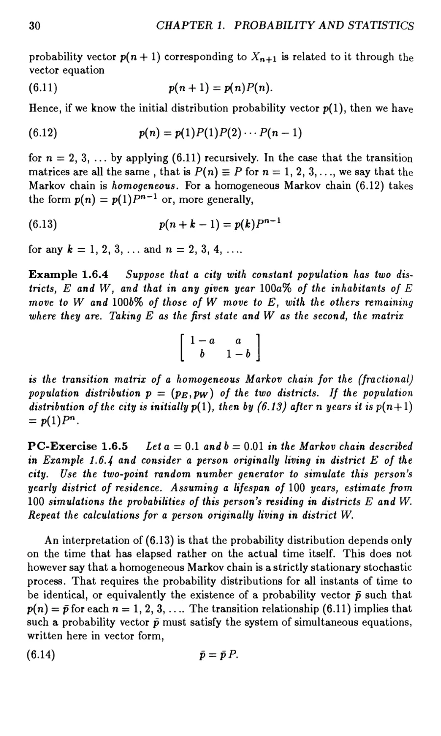
with Px defined for subintervals (—oo, x] in terms of F using (2.4) and then
extended appropriately to the more general Borel subsets. In this setting the
Figure 1.2.1
Distribution (2.5) for P(A) = 1
2'

1.2. RANDOM VARIABLES AND DISTRIBUTIONS
7
random variable is the identity function on 5ft. Often we omit mention of this
probability space and concentrate on the distribution function.
In applications the following examples are frequently encountered.
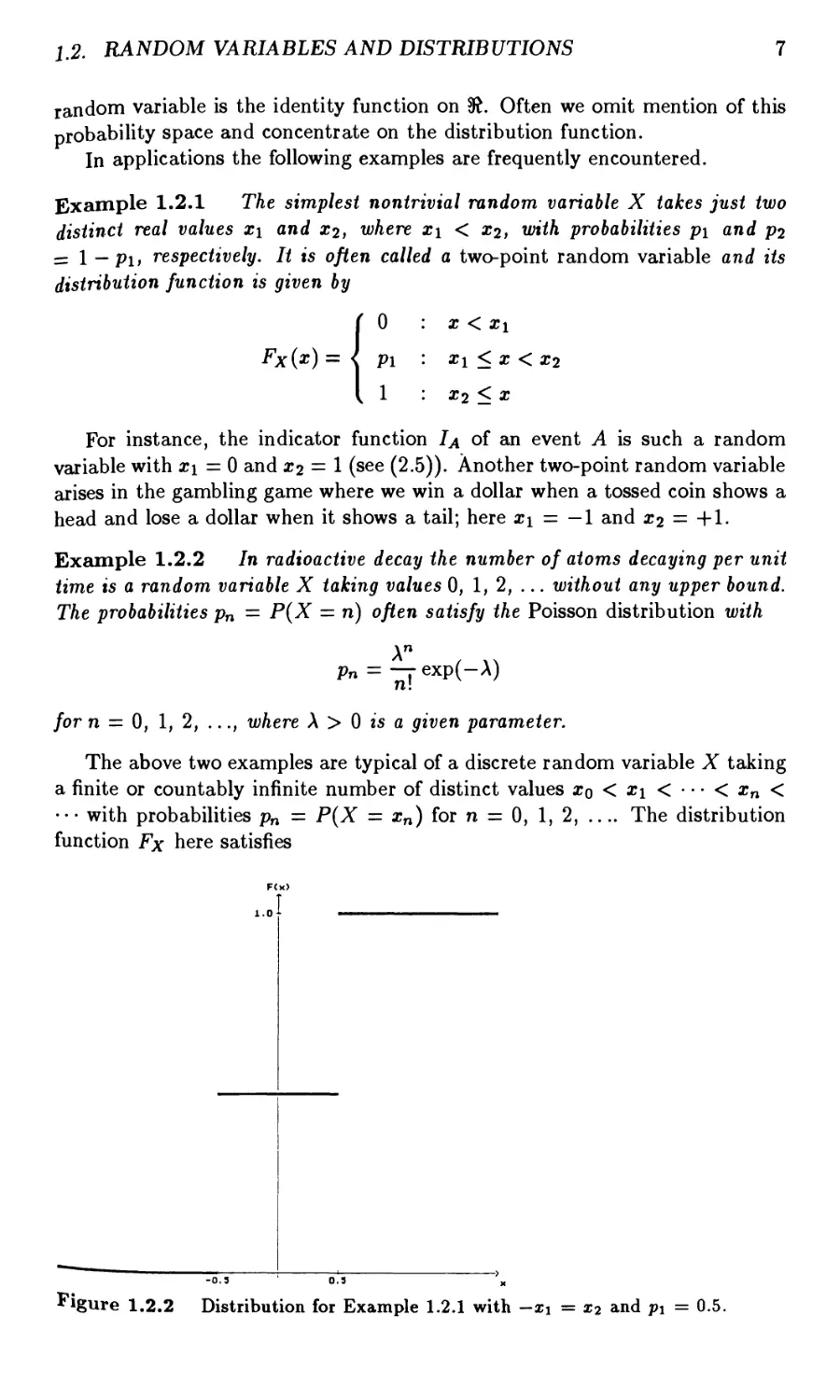
Example 1.2.1 The simplest nontrivial random variable X takes just two
distinct real values x\ and x2i where x\ < X2, with probabilities p\ and p2
= 1 — Pit respectively. It is often called a two-point random variable and its
distribution function is given by
Fx(x) =
0
Pi
1
X < Xi
xi < x < x2
x2 < x
For instance, the indicator function I a of an event A is such a random
variable with x\ — 0 and x2 — 1 (see (2.5)). Another two-point random variable
arises in the gambling game where we win a dollar when a tossed coin shows a
head and lose a dollar when it shows a tail; here x\ = —1 and x2 = +1.
Example 1.2.2 In radioactive decay the number of atoms decaying per unit
time is a random variable X taking values 0, 1, 2, ... without any upper bound.
The probabilities pn = P(X = n) often satisfy the Poisson distribution with
Pn = -^j-exp(-A)
for n = 0, 1, 2, ..., where A > 0 is a given parameter.
The above two examples are typical of a discrete random variable X taking
a finite or countably infinite number of distinct values Xo < x\ < • • • < xn <
"- with probabilities pn = P(X = xn) for n = 0, 1, 2, The distribution
function Fx here satisfies
F<x)
1.0} —————^————
figure 1.2.2 Distribution for Example 1.2.1 with -zi = x2 and pi = 0.5.

8
CHAPTER 1. PROBABILITY AND STATISTICS
Figure 1.2.3 Poisson probabilities for A = 2.
(2.9) Fx(x)
■{
0 : x < xq
YTi^Pi : *n <* <*n+l, n = 0, 1,.
Fx is a step-function with steps of height pn at £ = xn. For such a random
variable the set {xq, x\, X2, . •.} could be used as the sample space Q, with all
of its subsets being events.
In sharp contrast are the random variables taking all possible values in 3£.
We call such a random variable X a continuous random variable if the
probability P({u> G tt : X{u) = x}) is zero for all x G 3J. In this case the distribution
function Fx is often difFerentiable, that is there exists a nonnegative function
p, called the density function, such that F'x(x) = p(z) for each x G 3£; when Fx
is only piecewise difFerentiable this holds everywhere except at certain isolated
points. Then
(2.10)
Fx(x) = /
J — C
p(s) ds
for all £ G 3£, including the above mentioned exceptional points in the piecewise
difFerentiable case. Such a distribution function is usually said to be absolutely
continuous. The following are commonly occuring examples.
Example 1.2.3 Consider a random variable X which only takes values in
a finite interval a < x < b, such that the probability of its being in a given
subinterval is proportional to the length of the subinterval. Then the distribution
function is given by
Fx(x) =
0
x — a
b — a
1
x < a
a < x <b
b< x

1.2. RANDOM VARIABLES AND DISTRIBUTIONS
9
which is differentiable everywhere except atx = a and x = b. The corresponding
density function is given by
p(x)
■u
: x$[a, b]
: xe[a, b]
We say that the random variable X in Example 1.2.3 is uniformly distributed
on [a,b] and denote this by X ~ C/(a,6). Alternatively, we say that it has a
rectangular density function.
The {7(0,1) random variables are a special case of the beta- distributed
random variable with parameters a = /3 = 1. In general, the beta-distribution
with positive parameters a and /? has the density function
(2.11)
where
p(x) =
0 : **[0,1]
: «€[0,1]
B(
a,P)= J xa-l(l-x)p-ldx.
Jo
Example 1.2.4 The life-span of a light bulb is a random variable X which
is often modelled by the exponential distribution
FX(x)
0 : x <0
1 — exp(—Xx) : x > 0
for some intensity parameter X > 0. Fx is differentiable everywhere except for
x = 0 and has the density function
p(x)
-i
0 : x < 0
Aexp(—Xx) : x > 0.
p<x>
1.0 J—
Figure 1.2.4 The rectangular density with a = 0 and 6 = 1.

10 CHAPTER 1. PROBABILITY AND STATISTICS
p(x>
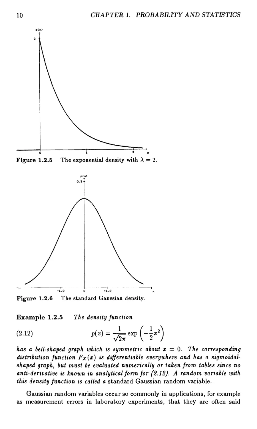
Figure 1.2.5 The exponential density with A = 2.
p(x>
0.3 I
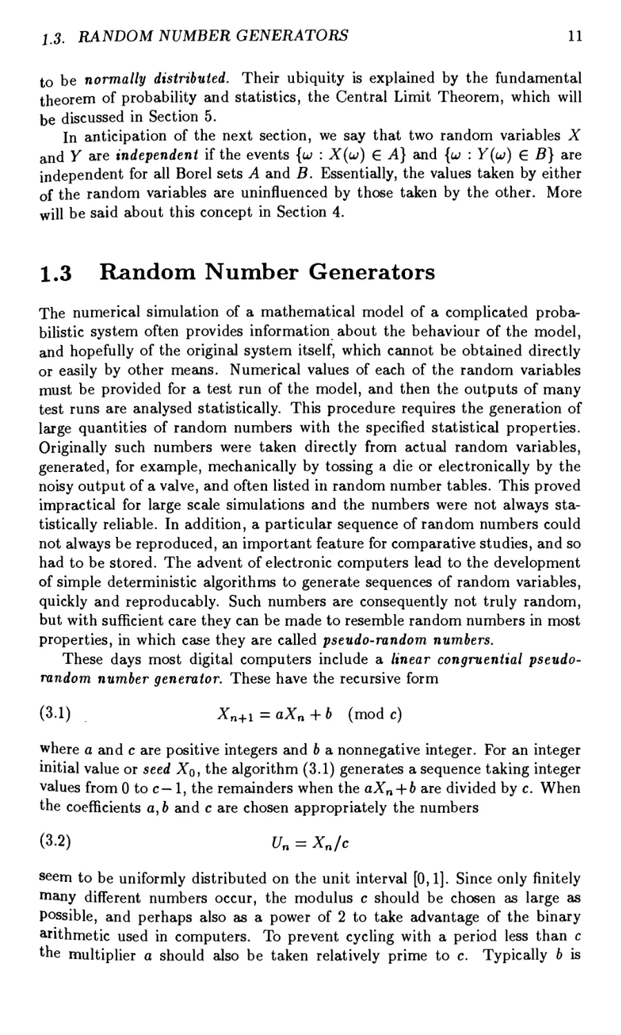
Figure 1.2.6 The standard Gaussian density.
Example 1.2.5 The density function
p.i» pW = -^exp (_!,*)
has a bell-shaped graph which is symmetric about x = 0. The corresponding
distribution function Fx(x) is differentiate everywhere and has a sigmoidal-
shaped graph, but must be evaluated numerically or taken from tables since no
anti-derivative is known in analytical form for (2.12). A random variable with
this density function is called a standard Gaussian random variable.
Gaussian random variables occur so commonly in applications, for example
as measurement errors in laboratory experiments, that they are often said

13. RANDOM NUMBER GENERATORS
11
to be normally distributed. Their ubiquity is explained by the fundamental
theorem of probability and statistics, the Central Limit Theorem, which will
be discussed in Section 5.
In anticipation of the next section, we say that two random variables X
and Y are independent if the events {u : X(u) G A} and {u : Y(u) G B] are
independent for all Borel sets A and B. Essentially, the values taken by either
of the random variables are uninfluenced by those taken by the other. More
will be said about this concept in Section 4.
1.3 Random Number Generators
The numerical simulation of a mathematical model of a complicated
probabilistic system often provides information about the behaviour of the model,
and hopefully of the original system itself, which cannot be obtained directly
or easily by other means. Numerical values of each of the random variables
must be provided for a test run of the model, and then the outputs of many
test runs are analysed statistically. This procedure requires the generation of
large quantities of random numbers with the specified statistical properties.
Originally such numbers were taken directly from actual random variables,
generated, for example, mechanically by tossing a die or electronically by the
noisy output of a valve, and often listed in random number tables. This proved
impractical for large scale simulations and the numbers were not always
statistically reliable. In addition, a particular sequence of random numbers could
not always be reproduced, an important feature for comparative studies, and so
had to be stored. The advent of electronic computers lead to the development
of simple deterministic algorithms to generate sequences of random variables,
quickly and reproducably. Such numbers are consequently not truly random,
but with sufficient care they can be made to resemble random numbers in most
properties, in which case they are called pseudo-random numbers.
These days most digital computers include a linear congruential
pseudorandom number generator. These have the recursive form
(3.1) Xn+1=aXn+6 (mode)
where a and c are positive integers and b a nonnegative integer. For an integer
initial value or seed Xq, the algorithm (3.1) generates a sequence taking integer
values from 0 to c— 1, the remainders when the aXn + b are divided by c. When
the coefficients a, 6 and c are chosen appropriately the numbers
(3-2) Un = XJc
seem to be uniformly distributed on the unit interval [0,1]. Since only finitely
many different numbers occur, the modulus c should be chosen as large as
possible, and perhaps also as a power of 2 to take advantage of the binary
arithmetic used in computers. To prevent cycling with a period less than c
the multiplier a should also be taken relatively prime to c. Typically 6 is

12
CHAPTER 1. PROBABILITY AND STATISTICS
chosen equal to zero, the resulting generator then being called a multiplicative
generator. A much used example was the RANDU generator of the older
IBM Scientific Subroutine Package with multiplier a = 65,539 = 216 + 3 and
modulus c = 231; the IBM System 360 Uniform Random Number Generator
uses the multiplier a = 16,807 = 75 and modulus c = 231 — 1, which is a prime
number.
The reader is referred to specialist textbooks for an extensive discussion on
pseudo-random number generators and their properties. In Section 9 we shall
mention some basic tests for checking their statistical properties and reliability.
For the remainder of this section we shall assume that we have a subroutine
RDN which provides us with 1/(0,1) uniformly distributed pseudo-random
numbers by means of (3.2) and a generator (3.1). We shall show how we
can then use this subroutine to generate pseudo-random numbers with other
commonly encountered distributions, in particular those described in Section
2.
A two-point random variable X (see Example 1.2.1) taking values x\ < x2
with probabilities pi and p2 = 1 _ Pi can be generated easily from a C/(0,1)
random variable U', namely with
[ xi : 0 < U < pi
(3.3) X = \ "
\ x2 : Pl < U < 1.
This idea extends readily to an JV-state random variable X taking values x\
< X2 < " - < %n with nonzero probabilities pi, P2> • •> PN where 52l=1 p% = 1.
With so = 0 and Sj = ]T^=1 Pi for j = 1, 2, ..., Af we set X = Xj+i if Sj < U <
Sj+i for j = 0, 1, 2, ..., Af — 1. We could approximate an infinite-state Poisson
distributed random variable (see Example 1.2.2) by an Af-state random variable
for some large Af by coalescing all of the remaining, less probable, states into
the final state. However, computationally more efficient algorithms for Poisson
random variables have been developed, but will not be given here.
The corresponding method for a continuous random variable X requires the
probability distribution function Fx to be inverted when this is possible. For
a number 0 < U < 1 we define x(U) by U = Fx{x{U))> so x(U) = F^{U) if
F%1 exists, or in general
(3.4) x(U) = M{x:U <Fx(x)}.
This is called the inverse transform method and is best used when (3.4) is easy
to evaluate. For example, the exponential random variable with parameter
A > 0 (see Example 1.2.4) has an invertible distribution function with
x(U) = F-\U) = -\n(l-U)/\ for 0 < U < 1.
When U is [7(0,1) distributed, then so too is 1 — U and a little computational
effort can be spared by using RDN directly to generate 1 — U.
In principle the inverse transform method could be used for any continuous
random variable, but may require too much computational effort to evaluate

1.3. RANDOM NUMBER GENERATORS
13
(3.4). This is the situation with the standard Gaussian random variable, since
the integrals for its distribution function must be evaluated numerically. The
BoX'Muller method for generating standard Gaussian random variables avoids
this problem. It is based on the observation that if U\ and U2 are two
independent £7(0,1) uniformly distributed random variables, then N\ and N2 defined
by
(3.5) Nx = N/-21n(C/1) cos(27rtf2)
N2 = y/-2\n(U1)sm(2wU2)
are two independent standard Gaussian random variables. This can be verified
with a change of coordinates from cartesian coordinates (Ni, N2) to polar
coordinates (r,0) and then to U\ = exp(--|r2) and U2 = 0/2w (see Exercisel.4.11).
A variation of the Box-Muller method which avoids the time consuming
calculation of trigonometric functions is the Polar Marsaglia method. It is
based on the facts that V = 2U - 1 is U(—l, 1) uniformly distributed if U is
£/(0,1) distributed and that for two such random variables V\ and V2 with W
= V? + V22 < 1, W is 17(0,1) distributed and 9 = arctan(Vri/Vr2) is {7(0,2tt)
distributed. Since the inscribed unit circle has 7r/4 of the area of the square
[—1,1]2, the point (VijVjj) wu*l take values inside this circle with probability
7r/4 « 0.7864816- • •. We only consider these points, discarding the others.
Using
cos 0 = t—, sin 6 = .—
VW VW
when W = V* + V2 < 1 we can rewrite (3.5) (see Exercise 1.4.11) as
(3.6) Nx = Viy/-2\n(W)/W
N2 = V2y/-2ln(W)/W
Although a proportion of the generated uniformly distributed numbers are
discarded, this method is often computationally more efficient than the Box-
Muller method when a large quantity of numbers is to be generated.
We shall use the above methods in exercises in the following sections,
assuming that they do indeed generate random numbers with the asserted properties.
In Section 9 we shall examine the validity of this assumption.
PC-Exercise 1.3.1 Write a program for two-point, exponential and
Gaussian random variables based on the above methods to generate a list of
pseudorandom numbers.

14
CHAPTER 1. PROBABILITY AND STATISTICS
1.4 Moments
The values taken by a random variable X can vary considerably. It is useful if
we can isolate some salient features of this variability, such as the average value
and the way in which the values spread out about this average value. The first
of these is an average weighted by the likelihood of occurence and is usually
called the mean value or expected value and denoted by E(X). For a discretely
distributed random variable it is defined as
(4.1) E(X) = Y,*'*>
where / = {0, ±1, ±2, ...}, which is readily suggested by the relative frequency
interpretation of the probabilities; the summation is over all possible index
values taken by the random variable.
When the random variable has an absolutely continuous distribution the
corresponding definition for its mean value is
(4.2) E(X) = P
J — C
xp(x)dx)
since, roughly speaking, p(x) dx is the probability that X takes its value in
the interval (x,x + dx). This assumes that the improper integral (4.2), and
the infinite series (4.1) if countably infinite indices are involved, actually
converge. This does not happen, for example, with the Cauchy probability density
function
(4.3) p(x) =
tt(1 + s2)
since it gives too much weighting to large values of x.
Exercise 1.4.1 Show that the improper integral (4-2) diverges for the
Cauchy density function (4.3).
For a particular random variable X we often use the notation \i — E(X)
for the mean value. A measure of the spread about \i of the values taken by X
is given by its variance which is defined as
(4.4) Vzr(X) = E((X-fif),
provided that the infinite series or improper integral involved converges. The
variance is consequently always nonnegative and is often denoted by a2 =
Var(X), where a is called the standard deviation of X. For the commonly
encountered probability distributions considered in Section 2 the mean values
and variances all exist and are listed in Table 1.4.1.
Exercise 1.4.2 Expand E ((X - /i)2) to show that Var(X) = E(X2) - /i2.
Exercise 1.4.3 Verify the means and variances in Table 1.4-1.

I A. MOMENTS
15
Distribution
Poisson
~~ Uniform U{a)b)
Exponential
Standard Gaussian
Example
1.2.2
1.2.3
1.2.4
1.2.5
Mean /i
A
(o + 6)/2
A"1
0
Variance <r2
A
(6-a)7l2
A"2
1
Table 1.4.1 Means and variances of some common probability distributions.
PC-Exercise 1.4.4 Use the RDN generator on your PC to generate N =
104 U(0,1) uniformly distributed pseudo-random numbers. Partition the
interval [0,1] into subintervals of equal length 5x 10~2 and count the number of
generated numbers falling into each subinterval. Plot a histogram of the relative
frequencies divided by the subinterval length. Does this histogram resemble the
graph of the density function of a [7(0,1) random variable? In addition,
evaluate the sample average /In and sample variance frjj for the generated numbers
x\, x2, --, xn, where
1 N 1 N
(4.5) £" = —5Z*t and a2N = ^—- ^(x* - fiN)2 .
»=i »=i
How do these compare with the mean 1/2 and variance 1/12 of a truly [7(0,1)
distributed random variable? What can you conclude about the statistical
reliability of your RDN generator from this simple test? (Note that we divide by
N — 1 here rather than by N in the sample variance in (4.5 ) as this provides
an unbiased estimator of the true variance.)
PC-Exercise 1.4.5 Repeat PC-Exercise 1.4-4 for exponentially distributed
random numbers with the parameter value A = 2.0. Since the density function
p(x) > 0 for all x > 0, you could partition the finite interval [0, 2], say, into
subintervals of equal length, with all of the values larger than 2 being discarded.
PC-Exercise 1.4.6 Repeat PC-Exercise 1.4-4 for standard Gaussian
random numbers generated by the Box-Muller and Polar Marsaglia methods. For
this, partition the interval [-2.fi, 2.5], say, into 102 subintervals of equal length,
with fixed semi-infinite intervals (—oo, —2.5) and (2.5, oo) for the other values.
The standard Gaussian distribution considered in Example 1.2.5 is a special
case of the general Gaussian distribution with mean \i and variance a2. Its
density function is given by
and still has the bell-shaped graph, which is now centered on the mean value
x = H and is stretched or compressed according to the magnitude of (72, its
Maximum value being l/(y/2ra) and its points of inflection at fi ± a. We often
write X ~ N(fi; a2) for a random variable with this distribution. It is not hard

16
CHAPTER 1. PROBABILITY AND STATISTICS
to see then that the transformed random variable Z = (X — fi)/a satisfies the
standard Gaussian distribution. The inverse transformation X = aZ + \i
converts a standard Gaussian random variable into an N(n\ a2) distributed random
variable X. We can use this to obtain an N(n\a2) distributed pseudo-random
variable X from the output of the Box-Muller or Polar Marsaglia methods.
We remark that in general we obtain another random variable when we
combine random variables by the usual arithmetic operations. For a general
transformation of a random variable, however, we need some restriction on
the transforming function to ensure that the resulting variable satisfies the
condition (2.2). Let us define Y(u) = g(X(u)) for all a; G ^, where X is a
random variable and ^r : 3fJ —»► 3J a function. Then in order that Y be a random
variable we require {v £ Q : Y(v) G B}, or equivalently {u G ^ : X(v) G
g"1(B)}i to be an event for every Borel subset B of 3£. This is certainly the
case when g is continuous or piecewise continuous; in fact, g could be even
more irregular. When Y is a random variable its expected value, if it exists, is
just
/oo
g(x)p(x) dx
when the distribution of X is discrete or absolutely continuous. Typical
functions often considered are the polynomials g(x) = xp or g(x) = (x — /i)p for
integers p > 1. The resulting expected values of Y = g(X) are then called
the pth-moment or the pth-central moment) the variance Var(X) is thus the
2nd order or squared central moment of X. Such moments convey information
about the random variable, but the higher order moments need not always
provide additional information; for example, the Gaussian distribution is
completely characterized by its first two moments, its mean \i and variance (72, and
the Poisson distribution by its mean A.
Exercise 1.4.7 For X ~ N(n)(T2) and k = 0, 1, 2, ... show that E((X -
/i)2*+1) = 0 and E((X - /i)2*) = 1- 3 • 5 • • • (2* - l)<r2k, but ^(IXI"1) = oo.
From the basic properties of integrals, or of infinite series in the discrete
case, we always have
(4.8) E(aXx + PX2) = aE(Xi) + pE(X2)
for any two random variables X\, X2 and any two real numbers a, /?, provided
the mean values here all exist. Also when Xi(u;) < X2(u;), almost surely, we
have
(4.9) E(X{) < E(X2)
Moreover, Jensen's inequality
(4.10) g(E(X)) < E(g(X))
holds for any convex function g : 3? —► 9£, that is satisfying
g(\x + (i _ X)y) < Xg(x) + (1 - X)g(y)

1,4. MOMENTS
17
for all x, y G 3£ and 0 < A < 1. In particular, for g(x) = \x\ and g{x) = x2 it
gives, respectively,
(4.H) \E(X)\<E(\X\) and \E(X)\ < y/WF)
A generalization of this is the Lyapunov inequality: if X is not concentrated
on a single point and if £(|X|*) exists for some s > 0, then for all 0 < r < s
and a € 3*
(4.12) (^IX-an^^aX-al'))1/'.
For a nonnegative random variable X, that is with X(u;) > 0 almost surely,
we have the Markov inequality
(4.13) P({u\X(u)>a))<-E(X) for all a > 0.
From this we can deduce the Chebyshev inequality
(4.14) P ({a/; |X(a;)|2 > a}) < -£(X2) for all a > 0.
Exercise 1.4.8 Prove Me Markov and Chebyshev inequalities.
The mean value or expectation E(X) is the coarsest estimate that we have
for a random variable X. If we know that some event has occured we may be
able to improve on this estimate. For instance, suppose that the event A =
{u £ Q : a < X(u) < b} has occured. Then in evaluating our estimate of the
value of X we need only consider these values of X and weight them according
to their likelihood of occurence, which is now the conditional probability given
this event. The resulting estimate is called the conditional expectation of X
given event A and is denoted by E(X\A). For a discretely distributed random
variable the conditional probabilities for the event A = {u £ Q : a < X(u) <
6} satisfy
{0 : X{ < a or b < Xi
Pi /2la<xi<bPi : <*<**<*
and so the conditional expectation
(4.15) E(X\A) = Y^*iP(X = *M)= E *«»/ E Pi-
i£l a<xt<b I a<Xi<b
For a continuously distributed random variable with a density function p the
corresponding conditional density is
0 : x < a or b < x
P{x\A) = "
P(X) J fa P(S) ds
a<x<b
w'th the conditional expectation

18
CHAPTER 1. PROBABILITY AND STATISTICS
(4.16) E(X\A) = J xp(x\A)dx = f xp(x)dx I f p(x)dx .
J — oo Ja J Ja
Similar results hold for other kinds of events provided that they occur with
nonzero probability. The conditional expectations so obtained satisfy
properties analogous to (4.8)—(4.11) for the usual expectations. Additional properties
of this important concept can be found in Section 2 of Chapter 2.
Exercise 1.4.9 Show that a random variable X distributed exponentially
with parameter A (see Exercise 1.2.4) has conditional expectations
E(X\X >a) = a + E(X) = a + A"1
for any a > 0. Here the event A = {u £ Q : X(w) > a} is abbreviated to
{X > a}. (This identity characterizes the exponential distribution; it says, for
example, that the expected remaining life of a light bulb is independent of how
old the bulb is.)
PC-Exercise 1.4.10 Generate 103 exponentially distributed random
numbers with parameter A = 0.5. Calculate the average of these numbers and the
averages of those numbers > a where a = 1, 2, 3 and 4. Compare these with
the identity in Exercise 1.4-9.
Often we need to consider several random variables X\, X2) ..., Xn at the
same time. These may, for example, be the components of a vector-valued
random variable X : Q —► 3£n or of a matrix-valued random variable, which
are then called a random vector or a random matrix, respectively. As with
a single random variable, we can form a distribution function for n random
variables X\, X2) . •., Xn which are defined on the same probability space; if
they are not, we can always modify them to have a common probability space.
The distribution function Fxlx2—Xn '• ^n ~^ [0> 1]> called the joint distribution
function, is defined by
(4.17) FXlx9.-x*(xi,X2,...,*n)
= P({wefl:Xl-(«)<*l-,i=l,2,...,n})
Its properties are most apparent in the case of two random variables X\ and
X2. Then Fxxx2 satisfies
(4.18) lim FXlXa(*1,*2)=0
Xi—► — OO
for i = 1 or 2,
(4.19) lim FXlX9(xux2) = l
ri,X2->-oo
and
(4.20) Fxxx2 is nondecreasing and continuous from the right in x\ and x2-

I A. MOMENTS
19
Moreover
(4.21) FXlx2(xiix2) = Fx2x1(«2,«i)
and for i\ =1 or 2 and i2 = 2 or 1 the marginal distribution Fx{ satisfies
(4.22) FXii(Xil) = Jim^Fx^x^Xi^Xi,).
Unlike the case of a distribution function of a single variable, properties (4.18)-
(4.22) for a collection of functions must be strengthened to ensure that there
exists a pair of random variables X\, X2 which has these functions as its joint
and marginal distributions. For continuous random variables the joint
distribution function is often differentiate, except possibly at some isolated or
boundary points, and there is a density function p : 3£2 —► 3f~ given by
d2Fx x
in which case
/X\ t>X2
/ p(slis2)dsids2.
•CO J — CO
When the density function is
p(xux2) = —£— exp I-- J2 J'^Xi-uMxj -iij)\
for some vector \i — (/ii, /i2) G 3£2 and some 2x2 positive definite and symmetric
matrix (thus with two real, positive eigenvalues) C = [c,J] with determinant
detC) we say that the random variables are jointly Gaussian with mean vector
H and covariance matrix C"1, the ijth component of C"1 being E((X{ —
Hi)(Xj — Hj)) for i, j — 1, 2. Since there exists an invertible 2x2 matrix S
such that C — S1S, the vector X = ST Z + fi is jointly Gaussian with mean
vector \i and covariance matrix C~l — S^1(S~1)T whenever Z = (Z\,Z2)
has independent standard Gaussian components Z\ and Z2. The Box-Muller
or Polar Marsaglia methods can thus be used to generate pairs of Gaussian
pseudo-random numbers with any mean vector and covariance matrix. This
reflects the important property that linear and orthogonal transformations of
Gaussian random variables yield Gaussian random variables.
Exercise 1.4.11 Show that the random variables N\ andN2 generated by the
Box-Muller and Polar Marsaglia methods (see (3.5) and (3.6)) are Gaussian
with zero mean vector and identity covariance matrix when U\ and U2 are
independent £7(0,1) uniformly distributed random variables.
PC-Exercise 1.4.12 Write a program to generate a pair of Gaussian
Pseudo-random numbers X\, X2 with means ^ — E(X\) = 0, \i2 — E(X2) =
0 and covariances E(Xf) = h, E(Xl) = /i3/3 and E(XiX2) = h2/2 for any h
> 0. Generate 103 pairs of such numbers for h = 0.1, 1 and 10, and evaluate
the sample averages and sample covariances, comparing these with the above
values.

20
CHAPTER 1. PROBABILITY AND STATISTICS
We say that two random variables X\ and X2 are independent if their joint
and marginal distribution functions satisfy
(4.23) FXlX9(xl9x2) = FXl(*i)Fx2(*2)
for all x 1, x2 G 3J. This is equivalent to the independent- event definition given
at the end of Section 2. If both FXl and Fx2 have density functions p\ and p2)
respectively, and if X\ and X2 are independent, then their joint distribution
function Fxlx2 nas a density function p which satisfies
(4.24) p(xu x2) = P\{xl)p2{x2).
Moreover, the product X\X2 of two independent random variables X\ and X2
has expectation given by
(4.25) E(X1X2) = E(X1)E(X2)
and the sum X\ + X2 has variance
(4.26) Var(Xi + X2) = Var(Xi) + Var(X2),
if these moments exist. Hence for two independent random variables both the
means and variances are additive, and the means are also multiplicative.
PC-Exercise 1.4.13 Check numerically whether or not the jointly
Gaussian random variables X\f X2 with means and covariances given in PC-Exercise
1.4.12 might be independent.
Exercise 1.4.14 Verify analytically that the random variables X\ and X2
in PC-Exercise 1.4-12 are dependent.
The properties (4.18)-(4.22) generalize readily to any number n > 2 of random
variables X\, X2i ..., Xn) but require somewhat more complicated terminology
if they are to be expressed succinctly. We let {z'i, i2i ..., ik} be any subset of
{1, 2, ..., n} for 2 < k < n. Then the joint distributions Fx{ Xi ■xin and the
marginal distributions Fxt x{ Xi defined by (4.17) satisfy
(4.27) lim FXlX2...Xn(xuX21 ...,*„) = 0;
3t = l,2 n
(4.28) lim FXlx3...x..(*i,*2,...,*n) = l;
Vi = l,2 n
(4.29) Fxxx2 xn is nonincreasing and continuous from the right in X{
for % = 1, 2, ..., n;
(4.30) ^xtlxi2 •xln(«i1,«t2,- -,*in) = FXlx2 ...xn(«i,«2,..-,«n);

1.4. MOMENTS
21
with the marginal distributions Fxhxi3 xik for 1 < k < n satisfying
(4.31) Fx.1xit-xik{xil,xi9,--- ,xih)
lim FXlX3...Xn(xi,x2,...,x„).
V»*»l»»2 «fc
Similarly the definition and properties (4.23)-(4.26) generalize to n > 2
independent random variables Xi, X2, ..., Xn, with independence occuring if
all of the joint and marginal distribution functions satisfy
(4.32) F*.^...*^
for all {u, 2*2, • ••, h} Q {1, 2, ..., n} and 1 < k < n. If each Fx{ has density
function p*, then Fxlx2 xn has density function p given by
(4.33) p(xi, x2)...,*„) = p(«i)p(«2) • • -p(*n).
In addition, for n independent random variables the product X1X2 • • -Xn has
expectation
(4.34) E(X1X2 ■ ■ ■ Xn) = E(Xi)E{Xi) ■ ■ ■ E(Xn),
whereas the sum 5Z"=1 X,- has variance
(4.35) Var ( £ *, J = £ Var(*<).
provided these quantities exist.
When we are considering n different random variables Xi, X2, ..., X„ at
the same time it is often convenient to use vector notation. For vectors x —
(#1, ..., xn) and 2/ = (2/1, • •., yn) in 3£n we recall that the Euclidean norm \x\
and inner product («,y) are defined by
(4.36) |*| =
. ^2 xi and (*> y) = Yl XiVi>
«=i
respectively. We note that for n = 1 the Euclidean norm coincides with the
absolute value. It can be shown algebraically that these satisfy the triangle
inequality
(4.37) |* + »|<M + |»|
and the Cauchy-Schwarz inequality
(4.38) |(*,y)|<|*||y|
for all x and y in 9£n. The former also holds for other norms on 9£n and
indeed for many vector spaces, such as a function space, on which a norm can
be defined; the latter holds whenever the vector space has an inner product

22
CHAPTER 1. PROBABILITY AND STATISTICS
compatible with a norm, that is with \x\ = yj{x~x) for all vectors x in the
space. An integral version of (4.38) is
(4.39)
/ f(x)g(x)dx\ < f f\x)dx [ g\x)dx,
Ja Ja Ja
provided these integrals are meaningful. A generalization of this is the Holder
inequality
(4.40)
Ja
x)dx
<(fbF(x)dx) (fbg"(x)dx)
where l/p + l/q = 1 with p, q > 1, provided the integrals exist.
The following moment inequalities for random vectors X = (Xi, ..., Xn)
and y = (Yi, ..., yn) are often useful:
(4.41) £7(1* + Y|') < cr (E(\X\r) + E{\Y\*))
with cr = 1 for r < 1 and cr = 2r_1 for r > 1;
(4.42) (E(\X + Y\r))1,r < (E(\X\r))1/r + (E(\Y\r))1/r
for r > 1; and
(4.43) E(\(X,Y)\) < (^(|X|"))1/P (E(\Y\^f"
for p, q > 1 with l/p + 1/g = 1.
Exercise 1.4.15 Prove inequalities (4.4V~(44^)-
1.5 Convergence of Random Sequences
In many situations we have an infinite sequence X\, X2, ..., Xn, ... of random
variables and are interested in their asymptotic behaviour, that is in the
existence of a random variable X which is the limit of the Xn in some sense. There
are several different ways in which such convergence can be defined. Broadly
speaking these fall into two classes, a stronger one in which the realizations of
Xn are required to be close in some way to those of X and a weaker one in
which only their probability distributions need be close. We can assume
without loss of generality that the random variables are all defined on a common
probability space.
The following three convergences are the most commonly used ones in the
strong class.
I. Convergence with probability one (w.p.l):
(5.1)
P {{w € ft : lim \Xn(u) - X(u)\ = 0}) = 1.
\ n—t-oo /

.5. CONVERGENCE OF RANDOM SEQUENCES
23
This is also known as almosi sure convergence.
II. Mean-square convergence: E(X„) < oo for n = 1, 2, ..., E(X2) < oo and
(5.2) limoE(\Xn-X\2)=0.
III. Convergence in probability:
(5.3) lim P({w € ft; |X„(w) - X(u)\ > t}) = 0 for all e > 0.
Convergence in probability is also called stochasiic convergence. It is equivalent
to
<M> J5. *(!+&)=*
which is sometimes more convenient since the expectation in (5.4) defines a
distance function, known as a metric, between the random variables.
Both (I) convergence w.p.l and (II) mean-square convergence imply (III)
convergence in probability, the latter following directly from the Chebyshev
inequality (4.14):
P(\Xn -X\>c) = P (\Xn - X\2 > e2) < ±E (\Xn - X|2).
Generally (III) does not imply either (I) or (II), nor does either of (I) or (II)
imply the other. This can be demonstrated by counterexamples, such as in the
following exercise.
Exercise 1.5.1 Lei Q = [0,1] and lei P([a, b]) = \b — a\ for any subinierval
[a,6] C [0,1]. For n = 1, 2, 3, ... let An = {u G ft : 0 < u> < l/n} and
define Xn - y/nIAn. Evaluate E(X%) and P(Xn > c) for all c > 0 and n =
1, 2, 3, Hence deduce that Xn converges to 0 in probability, but not in the
mean-square sense.
If, however, |Xn(a;)| < |y(a;)|, w.p.l, for some random variable Y with E(Y2)
< oo, then (I) implies (II) and (II) is equivalent to (III). This is a consequence
of the Dominated Convergence Theorem, which will be stated in Section 2 of
Chapter 2 (Theorem 2.2.3).
For the class of weaker convergences we do not need to know the actual
random variables or the underlying probability space(s), but rather we only need
to know the distribution functions. We mention here the following convergences
from this class.
IV. Convergence in distribution:
(5.5) lim Fxn(x) = Fx(x) at all continuity points of Fx-
n—*-oo
Ihis is also known as convergence in law and refers to the distributions of the
random variables Xn and X.
V. Weak convergence:
(5-6) lim / f(x)dFXn(x)= / f(x)dF(x)

24
CHAPTER 1. PROBABILITY AND STATISTICS
for all test functions f : 9J —► 3£, usually continuous functions vanishing outside
of a bounded interval which may depend on the particular function. Sometimes
it is useful to consider weak convergence with respect to other sets of test
functions. The integrals in (5.6) are (improper) Riemann-Stieltjes integrals,
about which we shall say more in Chapter 2. If the distribution functions have
densities, then (5.6) reduces to the more familiar (improper) Riemann integrals:
/oo /»oo
f(x)pn(x)dx= / f(x)p(x)dx.
•oo ./-oo
While they may appear more complicated, the integral limits (5.6) and (5.7)
are often easier to verify in theoretical contexts than are the pointwise limits
(5-5).
Convergence in probability (III) implies convergence in distribution (IV),
but the converse implication does not hold as the following counterexample
shows.
Example 1.5.2 Consider two independent two-point distributed random
variables X and Y, both taking values 0 and 1 with equal probabilities 1/2,
and let Xn = Y for n = 1, 2, 3, — Then Xn and X have the same
distributions, so they obviously converge in distribution, However, they do not converge
in probability because P(\Xn — X\ = 1) = 1/2 for n = 1, 2, 3,
PC-Exercise 1.5.3 Define Yn — X + Zn where X is a [7(0,1) uniformly
distributed random variable and Zn an independent N(0\ 1/n) Gaussian random
variable for n = I, 2, 3, .... For fixed but large n, say n = 103, use the
programs from PC-Exercise 1.3.1 to generate sufficiently many realizations of
Yn. Calculate relative frequencies and plot a histogram to obtain an estimation
of the graph of the density function ofYn. Then estimate the mean-square error
E(\Yn — X\2) for large n. Does this suggest that the Yn converge to X in the
mean-square sense?
The intuitive idea of defining probabilities as the limits of relative
frequencies determined from many repetitions of a given probabilistic experiment
receives some theoretical justification from an asymptotic analysis of sequences
of independent identically distributed (i.i.d.) random variables X\, X2, X3,
Let \i — E(Xn) and o1 = Var(Xn). From this independence it follows (see
(4.35)) that the averaged random variables
n n
also have mean E(An) = \i and variance Var(j4n) = a2/n. The Law of Large
Numbers, one of the fundamental theorems of probability and mathematical
statistics, says that
(5.8) An —► \i as n —► 00
with convergence in probability (III) in its weak version and convergence with
probability one (I) or in mean-square (II) in its strong versions.

.5. CONVERGENCE OF RANDOM SEQUENCES
25
pC-Exercise 1.5.4 Use the random number generators in Section 3 for
uniform, two-point, exponential and Gaussian random numbers to verify the
limit (5-8) in the mean-square sense by averaging (An — /i)2 for sufficiently
many different runs, say 102, and fom = 10, 102 and 103.
Another fundamental result, the Central Limit Theorem, says that the
normalized random variables
(5.9) *n - 7= ,
for which E(Zn) = 0 and Var(Zn) = 1, converge in distribution to a standard
Gaussian random variable Z. This is also true under weaker assumptions than
the i.i.d. assumption on the original random variables X\, X2l A3, ... and
provides an explanation for the dominant role of the Gaussian distribution in
probability and statistics.
Exercise 1.5.5 Show that the Central Limit Theorem provides more
information than the Law of Large Numbers about the limiting behaviour of the
sequence A\, A2, A3, —
PC-Exercise 1.5.6 As in PC-Exercise 1.5.4 generate sequences of random
numbers and calculate their Zn values from (5.9). Using histograms of relative
frequency plots obtain simulated approximations to the graphs of the density
functions for the Zn and show that these approach the graph of the density
function of the standard Gaussian distribution as n is taken larger and larger,
specifically for n = 100, 500 and 1000.
The Bernoulli trials are an illustration of the Law of Large Numbers and
the Central Limit Theorem. They are independent repetitions of an experiment
with two basic outcomes, such as heads and tails when a coin is tossed, with
probabilities p and 1 — p, respectively. If we let Xn — 1 for a head and Xn
= 0 for a tail, then we have an i.i.d. sequence X\, X2, ^3, ••• with mean
E(Xn) — p and variance Var(X„) = p(l — p). The sum Sn = X\ + X2 +
-' + Xn is then just the number n(H) of heads occuring out of n tosses and
An = Sn/n = n(H)/n is the relative frequency of tossing a head in n tosses.
Of course, these relative frequencies are themselves random variables, but the
Law of Large Numbers says that they converge to the common mean p, which
is the probability of throwing a head in a single trial.
As another illustration consider a fair coin and let Xn = +1 for a head and
Xn = -1 for a tail. Then E(Xn) - 0 and Var(X„) = 1, so by the Central
Limit Theorem the random variables Zn = Sn/y/n defined by (5.9) converge
in distribution to a standard Gaussian random variable Z. This is more than
We get from the Law of Large Numbers for the averages An = Sn/n, namely
convergence to 0. Alternatively, the random variables Sn are approximately
^(0;n) distributed for large n. Such a sequence of sums of i.i.d. random
variables is called a random walk on account of the appearance of its graph
when plotted against n.

CHAPTER 1. PROBABILITY AND STATISTICS
Sn
20
10
-10
-20
Sn - randon walk
A .
40 60 /v 80 100
A /
Figure 1.5.1 The random walk in PC-Exercise 1.5.7.
PC-Exercise 1.5.7 Form a random walk Sn using the two-point random
number generator (3.3) and plot Sn against n, joining the successive points
in the (n,Sn) plane by straight line segments. Repeat this for other sequences
corresponding to different initial seeds and compare the plotted paths.
1.6 Basic Ideas About Stochastic Processes
A sequence of random variables X\, X^} ..., Xn, ... often describes, or may
be conveniently imagined to describe, the evolution of a probabilistic system
over discrete instants of time t\ < t^ < • • • < tn < • • •. We then say that it
is a stochastic process and call the totality of its joint distribution functions
{Fxi Xi Xi > ij = 1, 2, ... and j = 1, 2, ...} its probability law. Henceforth
we shall write these distributions as Ft{ %i ...t{. to emphasize the role of the
time instants. A sequence of i.i.d. random variables is a trivial example of a
stochastic process in the sense that what happens at one instant is completely
unaffected by what happens at any other, past or future, instant. Moreover its
probability law is quite simple, since any joint distribution is given by
(6-1) FUit,3...u.(xil,xi3,...,xij) = F(xil)F(xi2)---F(xii),
where F is the common distribution function of the random variables. Another
simple example are the iterates of a first order difference equation such as
(6.2) Xn+1 = 4Xn(l-Xn)

LS. BASIC IDEAS ABOUT STOCHASTIC PROCESSES 27
for n = 1) 2, 3, ...; here each random variable is determined exactly from its
predecessor, and ultimately from the initial random variable X\. For most
interesting stochastic processes encountered in applications the relationship
between the random variables at different time instants lies somewhere between
these two extremes. For instance, the joint distributions may all be Gaussian
in which case we call the process a Gaussian process; they may satisfy (6.1),
but generally need not.
Stochastic processes may also be defined for all time instants in a bounded
interval such as [0,1] or in an unbounded interval such as [0,oo), in which case
we call them continuous time stochastic processes. As an example, let A > 0
be a fixed parameter and for each / > 0 define X(t) to be a Poisson distributed
random variable with parameter Xt. Continuing with the radioactive decay
interpretation of Example 1.2.2, X(t) then represents the number of atoms
decaying in the time interval (0,2].
In general we shall denote the time set under consideration by T and assume
that there is a common underlying probability space (Q, A> P). A stochastic
process X = {X(t), t G T} is thus a function of two variables X : TxCt —► 9J
where X(t) = X(tr) is a random variable for each t G T. For each u G £t we
call X(',w) : T —► 3£ a realization, a sample path or a trajectory of the stochastic
process. The curves plotted in Figure 1.5.1 can be interpreted as the realizations
of a stochastic process. The functions X cannot be completely arbitrary, but
must satisfy information restrictions, both at specific time instants, to ensure
that random variables result, and also between different time instants. The
latter are particularly crucial, mathematically speaking, for continuous time
processes and will be discussed in some detail in Chapter 2.
For both continuous and discrete time sets T it is useful to distinguish
various classes of stochastic processes according to their specific temporal
relationships. Assuming that the expressions exist, the expectations and variances
(6.3) »(t) = E{X{t)), <T2(t) = Va.T{X(t))
at each instant t € T and the covariances
(6.4) C{s, t) = E ((X(s) - p{8))(X(t) - /*(*)))
at distinct instants s,t £T provide some information about the time variability
of a stochastic process.
Example 1.6.1 A Poisson process with intensity parameter A > 0 is a
stochastic process X = {X(t), t > 0} such that (i) X(0) = 0; (ii) X(t)-X(s) is
a Poisson distributed random variable with parameter X(t — s) for all 0 < s <
*; and (Hi) the increments X(t2) - X(ti) and X(t4) - X(t3) are independent
Jor all 0 < ti < *2 < ^3 < *4- Its means, variances and covariances are fi(t)
^ A<, a2(t) = Xt and C(s)t) = Amin{s,2}, respectively, for all s, t > 0.
An important class of stochastic processes are those with independent
increments, that is for which the random variables X(tj+\) - X(tj), j = 0, 1,
A •.., n — 1 are independent for any finite combination of time instants tQ <

28
CHAPTER 1. PROBABILITY AND STATISTICS
t\ < - - - < tn in T. If tQ is the smallest time instant in T then the random
variables X(tQ) and X(tj) — X(tQ) for any other tj in T are also required to be
independent. A Poisson process is an example of a continuous time stochastic
process with independent increments. Another is the standard Wiener process
W = {W(2), t > 0}, that is a Gaussian process with independent increments
for which
(6.5) W(0) = 0 w.p.l, E(W(t)) = 0, Var(W(*) - W(s)) = t - s
for all 0 < s < t. In fact, it can be shown that any continuous time stochastic
process with independent increments and finite second moments E(X2(t)) for
all t is a Gaussian process provided X(t0) is Gaussian for some t0 G T.
The stationary processes are another interesting class of stochastic processes
since they represent a form of probabilistic equilibrium in the sense that the
particular instants at which they are examined are not important. We say that
a process is strictly stationary if its joint distributions are all invariant under
time displacements, that is if
for all U, ti + h G T where i = 1, 2, ..., n and n = 1, 2, 3, ...; in particular,
the X(t) have the same distribution for all t G T. For example, a sequence
of i.i.d. random variables is strictly stationary. On the other hand, if there
is a constant \i and a function c : 3ft —► 3ft such that the means, variances and
covariances of a stochastic process satisfy
(6.7) Kt) = H> <r2(t) = c(0) and C(*,<) = c(t - s)
for all s, t GT, then we call the process wide-sense stationary. This means
the process is only stationary with respect to its first and second moments.
It is straightforward to show that a strictly stationary process is wide-sense
stationary if its means, variances and covariances are all finite, but a wide-
sense stationary process need not be strictly stationary.
Example 1.6.2 The Ornstein-Uhlenbeck process X = {X(t)f t G 3ft+} with
parameter 7 > 0 and initial value X0 G N(0; 1) is a Gaussian process with
means E(X(t)) = 0 and covariances E(X8Xt) = exp(—7^ — s\) for all s, t G
3ft+. Hence it is a wide-sense stationary process. It is also strictly stationary,
as will be seen from equation (7.4)>
Exercise 1.6.3 Show that a standard Wiener process W has covariances
C{s,t) = min{s,2} and hence is not wide-sense stationary.
Conditional probabilities provide a more refined tool than mean values and
covariances for analysing the relationships between the random variables of a
stochastic process at different time instants. To illustrate this let us consider a
sequence of random variables X\, X2, A3, ... taking values in a discrete set X
= {x\y X2, z3, ...}, which may be finite or infinite. We shall suppose that we

LS. BASIC IDEAS ABOUT STOCHASTIC PROCESSES 29
are at a time instant n and know the present outcome £,n, that is the value of
X , as well as the past outcomes Xi = £tl, X2 = £,-2, ..., Xn-\ = Xin_1. Using
this information we wish to predict something about the future outcomes, the
values of X„+i, Xn+2i • • •, in particular the value of the immediate future
random variable Xn+i. For this the conditional probabilities
P(Xn+i = Xj\X\ = XiltX2 = Xj21. . . ,Xn = Z,n)
_ P(Xi = gtl,X2 = Xj2i . . . ,XW = gt-m,Xn+i = Xj)
for each £; G <¥ are useful. Here we have abbreviated our notation for events
using, for example, {Xi = £tl} for {u> £ Q : Xi(u) = £tl}. In principle, we
could determine such conditional probabilities for all «tl, £,-2, ..., X{n in X
and all n = 1, 2, 3, In a deterministic system governed, for instance, by a
first order difference equation such as (6.2) only the present value X{n of Xn is
needed to determine the future value of Xn+\\ the past values of X\) X2) . •.,
Xn-i are involved only indirectly in that they determine the value of Xn. This
is just the common law of causality and there is a stochastic analogue called
the Markov property, that is
(6.8) P(Xn+l = xj\Xn = xin)
= P(Xn+1 = Xj\Xi = xil,X2 = Xi2)...)Xn = xin)
for all possible Xj, Xilt £,2, ..., X{n in ^ with n = 1, 2, 3, — A sequence of
discrete valued random variables with this property is an example of a Markov
process; in particular, we call it a discrete time Markov chain.
While they are peripheral to the theme of this book, we shall look a little
more closely at discrete time Markov chains with a finite number of states X —
{^l, X2, ..., xn} because they allow some important concepts to be introduced
and understood in a relatively simple setting. For each n = 1, 2, 3, ... we define
an ATx AT matrix P(n) = [p',;(n)] componentwise by
(6.9) piJ(n) = P(Xn+1 = xj\Xn = xi)
for i, j = 1, 2, ..., N. Obviously 0 < pilj(n) < 1 and, since Xn+i can only
attain states in X,
(6-10) £p.\i(n) = 1
for each i = 1, 2, ..., N and n = 1, 2, 3, .... We call the matrix P(n) the
transition matrix of the Markov chain and its components (6.9) the transition
Probabilities at time n. A probability vector on ^ is a vector p = (pi, p2i ...,
Pat) G »" with 0 < Pi < 1 for i = 1, 2, ..., N and E^IiP*' = L Thus if
P(n) is the probability vector corresponding to the distribution of the random
triable Xn, that is if Pi(n) = P(Xn = Xi) for i = 1, 2, ..., TV, then the

30
CHAPTER 1. PROBABILITY AND STATISTICS
probability vector p(n + 1) corresponding to Xn+\ is related to it through the
vector equation
(6.11) p(n+l)=p(n)P(n).
Hence, if we know the initial distribution probability vector p(l), then we have
(6.12) p(n)=p(l)P(l)P(2)-P(n-l)
for n = 2, 3, ... by applying (6.11) recursively. In the case that the transition
matrices are all the same , that is P{n) = P for n = 1, 2, 3,..., we say that the
Markov chain is homogeneous. For a homogeneous Markov chain (6.12) takes
the form p{n) — p(l)Pn"1 or, more generally,
(6.13) p(n + k-l) = p(k)Pn-1
for any k = 1, 2, 3, ... and n = 2, 3, 4,
Example 1.6.4 Suppose that a city with constant population has two
districts, E and W, and that in any given year 100a% of the inhabitants of E
move to W and 1006% of those of W move to E, with the others remaining
where they are. Taking E as the first state and W as the second, the matrix
[1-a a 1
[ b 1-6 J
is the transition matrix of a homogeneous Markov chain for the (fractional)
population distribution p = (pe,Pw) of the two districts. If the population
distribution of the city is initially p(l), then by (6.13) after n years it is p(n + l)
= P(i)P".
PC-Exercise 1.6.5 Let a = 0.1 and 6 = 0.01 in the Markov chain described
in Example 1.6.4 and consider a person originally living in district E of the
city. Use the two-point random number generator to simulate this person's
yearly district of residence. Assuming a lifespan of 100 years, estimate from
100 simulations the probabilities of this person's residing in districts E and W.
Repeat the calculations for a person originally living in district W.
An interpretation of (6.13) is that the probability distribution depends only
on the time that has elapsed rather on the actual time itself. This does not
however say that a homogeneous Markov chain is a strictly stationary stochastic
process. That requires the probability distributions for all instants of time to
be identical, or equivalently the existence of a probability vector p such that
p(n) = pfor each n = 1, 2, 3, — The transition relationship (6.11) implies that
such a probability vector p must satisfy the system of simultaneous equations,
written here in vector form,
(6.14)
P = pP.

e. BASIC IDEAS ABOUT STOCHASTIC PROCESSES
31
property (6.11) for a constant transition matrix P ensures that (6.14) has at
least one solution which is a probability vector. Such a solution is called a
stationary probability vector or distribution for the Markov chain. For example
P \a + b' a + b)
is a stationary probability vector for the Markov chain described in Example
1.6.4, a fact which should have been discovered by those readers who did PC-
Exercise 1.6.5. This particular p is the only stationary probability vector for
this transition matrix. Other transition matrices may have more than one
stationary probability vector.
Exercise 1.6.6 Show that all of the probability vectors p\ = (A/2, A/2, 1—A)
for each 0 < A < 1 satisfies (6.14) w*th the transition matrix
P =
A homogeneous Markov chain thus describes a strictly stationary stochastic
process only if the initial random variable X\ is distributed according to one
of its stationary probability vectors.
Certain homogeneous Markov chains with a unique stationary probability
vector p enjoy a powerful property called ergodiciiy relating the long-term
time averages of its realizations to the spatial averaging with respect to the
stationary distribution. For any function / : X —► 9J we can form the time
average
0.5
0.5
0
0.5 0
0.5 0
0 1
(615) | £/(*«)
t = l
of the values f(Xt) taken by a sequence of random variables X\, X2) ..., Xt,
• • • generated by the Markov chain. An obvious question is: what happens
with these averages as T —► 00? In fact, in the special case that f(xk) = 1
for some k and f(xj) = 0 for all other j ^ k the time average (6.15) is just
the relative frequency of the chain's being in state Xk- We recall that for i.i.d.
random variables X\t X2) X3, ... the Law of Large Numbers would tell us
that the limit exists and is equal to the probability p*. In general, we say
that a Markov chain is ergodic if for every initial X\ the limits of the time
averages (6.15) exist and are equal to the average of / over X with respect to
the stationary probability vector p, that is if
A condition guaranteeing the ergodicity of a Markov chain is that all of the
components of its unique stationary probability vector p are nonzero, that is

32
CHAPTER 1. PROBABILITY AND STATISTICS
pi > 0 for i = 1, 2, ..., N. A weaker condition is that all of the components of
some fcth power Pk of the transition matrix are nonzero. Ergodicity is thus an
extension of the Law of Large Numbers to stochastic processes, but says much
more about the stochastic process, for example, implying its eventual mixing
over the states in X according to the stationary distribution.
PC-Exercise 1.6.7 Verify (6.16) numerically for the Markov chain in
Example 1.6.4, taking into account PC-Exercise 1.6.5. Consider functions f : {E,
W}^% with: (i) f(E) = 0, f(W) = 1; (it) f(E) = 1, f(W) = 0; (Hi) f(E)
= 1, f(W) = —1; (iv) f(E) = —1, f(W) = 1. In each case try a variety of
initial distributions p(l) = (pe(^)iPw(^)) = (p> 1 — p) for Xir saV with p = 0,
0.1, 0.2,..., 0.9, 1. Also tryp= 1/11 = 0.09090909 ....
We can handle continuous time Markov chains in a similar way. Let X(t)
be distributed over a finite state space X — {x\, x*i, ..., x^} according to
an TV-dimensional probability vector p(t) for each t > 0. In this context the
Markov property (6.8) takes the form
(6.17) P(X(h) = XjlXfa) = xili...iX(sn) = xin1X(t0) = Xi)
= P(X(t1) = xj\X(t0) = xi)
for all 0 < si < S2 < * • * < sn < to < t\ and all £,, Xj, £tl, £,-2, ..., X{n G X
where n = 1, 2, 3, For each 0 < to < t± we can define an NxN transition
matrix P(to]ti) = \p*'*(to)ti)] componentwise by
piJ(to;h) = P(X(h) = xj\X(t0) = Xi)
for i, j = 1, 2, ..., AT. Clearly then P(to]to) = I and the probability vectors
p(t0) and p(ti) are related by
P(*i)=J<*o)^(*o;*i).
Applying this for t0 < *i < *2 we nave P(^) = p(*o)^(*o;*2) and
p(<2)=p(<i)P(n;<2) = p(M^(*o;<i)P(<i;<2)
for any probability vector p(to)- From this we can conclude that the transition
matrices satisfy the relationship
(6.18) P(to;t2) = P(to;ti)P(ti;t2)
for all to < t\ < *2- In the special case that the transition matrices P(to]t\)
depend only on the time difference ti —10) that is P(to]ti) = P(0]ti —10) for
all 0 < t0 < t\, we say that the continuous time Markov chain is homogeneous
and write P(t) for P(0;t). Then (6.18) reduces to
(6.19) P(s + t) = P(s)P(t) = P(t)P(s)
for all s,t >0.

1,6. BASIC IDEAS ABOUT STOCHASTIC PROCESSES
33
There exists an NxN intensity matrix A = (a1'*) with
lim(_0 ^ f '
i^j
limt_G
^ : « = .
which, together with the initial probability vector p(0), completely
characterizes the homogeneous continuous time Markov chain. If the diagonal
components a*'* are finite for each i = 1, ..., N, then the transition probabilities
satisfy the Kolmogorov forward equation
(6.20)
dp'
M
N
dt
(0-Ep''Wj = o
Jb = l
and the Kolmogorov backward equation
(6.21)
dp'
M
N
dt
(0-£«*VJ'(*) = o
Jb=l
for all i, j = 1, 2, ..., N. The waiting time of a homogeneous continuous
time Markov chain, that is the time between transitions from a state X{ to any
other state, is thus exponentially distributed with intensity parameter A,- =
Example 1.6.8 Consider a stochastic process X(t) taking only the two
values + 1 and — 1 with probabilities (p+(2),p~(2)) = p(t) and switching according
to the homogeneous transition matrix
p(t) =
(l + e-')/2 (l-e"')/2
L(l-e-«)/2 (l + e")/2j
fort > 0. The intensity matrix here is
A =
-0.5 0.5
0.5 -0.5
For the initial probability vector p(0) = p = (0.5,0.5) we find that pP(t) = p(t)
= P for all t > 0, so p is a stationary probability vector for this Markov chain;
ihe corresponding strictly stationary stochastic process is known as random
telegraphic noise.
PC-Exercise 1.6.9 Use exponentially distributed waiting times to simulate
ihe telegraphic noise of Example 1.6.8 on the time interval [0,T] with T = 10.
From a sample of 100 simulations calculate the frequency of being in the state
1 at time T.

34
CHAPTER 1. PROBABILITY AND STATISTICS
We remark that a continuous time Markov chain is called ergodic if
T N
(6.22) Urn i / /(X(0)A = £/(*«)ft,
T-°° i Jo JT^
that is with the time averages (6.15) in (6.16) now written in integral form.
The random telegraphic noise process is an ergodic continuous time Markov
chain.
Exercise 1.6.10 For Example 1.6.8 show that the probability vectors p(t) =
p(0)P(t) —► p as t —► oo for any initial probability vector p(0).
As a final exercise we return to the Poisson process defined in Example 1.6.1,
which is a continuous time Markov chain on a countably infinite state space.
Exercise 1.6.11 Show that the Poisson process is a continuous time
homogeneous Markov chain on the countably infinite state space {0, 1, 2, ...}.
Determine its transition matrix P(t).
1.7 Diffusion Processes
Markov processes taking continuous values in 9J require a somewhat more
complicated mathematical framework than their discrete state counterparts,
especially when they also involve continuous time values. A rich and useful class
of such Markov processes are the diffusion processes, which we shall define
below after first considering some more general background material. In what
follows we shall always suppose that for k = 1, 2, ... every joint distribution
Ftit2...tk(xii #2> •••> xk) of the process X = {X(t), * > 0} under
consideration has a density p(ti,xi] t2ix2\ •••> tkixk)- Then we define the conditional
probabilities
(7.1) P(X(*n+i) G B\X(h) = xuX(t2) = x2i...,X(tn) = xn)
p(ti1xi]t21X2]...)tn,xn]tn+i1y)dy
1
f°°
/ p(ti^i]t2lx2]... ]tnixn\tn+i,y) dy
J — oo
for all Borel subsets B of 3ft, time instants 0 < t\ < t2 < ... < tn < tn+\ and
all states x\, x2i ..., xn G 3ft, provided the denominators are nonzero. (When
the denominator in (7.1) is zero we either define the conditional probability to
be zero or we leave it undefined). In this context the Markov property takes
the form
(7.2) P(X(tn+1) € B\X(ti) = xltX(t2) = x2,...,X(tn) = xn)
= P(X(tn+1)£B\X(tn) = xn)

7. DIFFUSION PROCESSES
35
for all Borel subsets B of 9J, time instants 0 < t\ < t2 < ... < tn < tn+i and
all states x\, x2i • • •> xn € 3J for which the conditional probabilities are defined.
If (7-2) is satisfied we call the stochastic process X{i) a Markov process and
write its transition probabilities as
P(8,zit,B) = P(X(t) e B\X(s) = x),
where s < t. For fixed s, x and 2, P(s, x\t, •) is a probability function (measure)
on the <r-algebra B of Borel subsets of 9J. Under our assumption above it has
a density p(s, £;*,), called a transition density, so
P{s)x\t)B) = / p(s,x,t,y)dy
JB
for all B € B. For technical convenience we usually also define P(six;siB)
= JflM f°r * = s> where /# is the indicator function of the set B.
Analogously with Markov chains, we say that a continuous time Markov process is
homogeneous if all of its transition densities p(s, x\t,y) depend only on the
time difference t — s rather than on the specific values of s and t. Examples of
homogeneous Markov processes are the standard Wiener process (see equation
6.5) with transition density
(7.3) P(8,z;t,y) = -^ = exp ("^^j)
>/27r(* - s)
and the Ornstein-Uhlenbeck process with 7 = 1 (see Example 1.6.2) with
transition density
(7.4) *.,,;«,„) = 1 exp (-^;Xe\{l~X) •
Since p(s,x\t,y) — p(0, x\t — s, y) we usually omit the superfluous first variable
and simply write p(x\t - s,r/), with P(x\t - s,B) = P(0,x;t - s,B) for the
transition probabilities.
The transition matrix equation (6.19) for continuous time Markov chains
has a counterpart for the transition densities of a continuous state Markov
process. This also follows from the Markov property and is called the Chapman-
Kolmogorov equation:
(7-5) p(s,x]t,y)= / p(s)x]T)z)p(r)z]t)y)dz
J—oo
lor all s < r < t and x, y G 5ft. For transition probabilities it takes the form
( roo
(7-6) P(8,z;t,B)= P(r,z;t,B)P(s,x;r,dz),
J—OO
here B £ B and the integral is an improper Riemann- Stieltjes integral.

36
CHAPTER 1. PROBABILITY AND STATISTICS
Exercise 1.7.1 Verify that the transition density (7.3) of a standard Wiener
process satisfies the Chapman-Kolmogorov equation (7.5). What happens to the
r variable in the integrand here?
The transition density of the standard Wiener process is obviously a smooth
function of its variables for t > s. Evaluating the partial derivatives of (7.3)
explicitly, we find that they satisfy the partial differential equations
and
^ !in0=o' ^fixed-
The transition density (7.4) of the Ornstein-Uhlenbeck process satisfies related,
but more complicated partial differential equations (see Exercise 1.7.2 below).
Equation (7.7) is an example of a heat equation which describes the variation
in temperature as heat diffuses through a physical medium. The same equation
describes the diffusion of a chemical substance such as an inkspot. It should
thus not be surprising that a standard Wiener process serves as a prototypical
example of a (stochastic) diffusion process. To be specific, a Markov process
with transition densities p(s, x\t,y) is called a diffusion process if the following
three limits exist for all e > 0, s > 0 and «G$:
(7.9) lim- / p(s)x]t)y)dy = 0)
(7.10) lim;; / (y-x)p(s,x]t,y)dy = a(s,x)
U» l ~S J\y-X\<C
and
(7.11) lim- / (y - x)2p(s,x;t,y)dy = 62(s,z),
U» t - s J\y-X\<£
where a and b are well-defined functions. Condition (7.9) prevents a diffusion
process from having instantaneous jumps. The quantity a(s,z) is called the
drift of the diffusion process and b(s,x) its diffusion coefficient at time s and
position x. (7.10) implies that
(7.12) a(s,x) = \im-}—E(X(t) - X(s)\X(s) = x),
t[s t — S
so the drift a(s, x) is the instantaneous rate of change in the mean of the process
given that X(s) = x. Similarly, it follows from (7.11) that the squared diffusion
coefficient
(7.13) 62(s, x) = lim j^E ((X(t) - X(s))2\X(s) = x)

7. DIFFUSION PROCESSES
37
denotes the instantaneous rate of change of the squared fluctuations of the
process given that X(s) = x.
Exercise 1.7.2 Show that the standard Wiener process is a diffusion process
with drift a(s,x) = 0 and diffusion coefficient b(s,x) = 1, and that the Ornstein-
Uhlenbeck process with 7 = 1 is a diffusion process with drift a(s,x) = —x and
diffusion coefficient b(s,x) = y/2.
When the drift a and diffusion coefficient 6 of a diffusion process are
moderately smooth functions, then its transition density p{s)x\t)y) also satisfies
partial differential equations, which reduce to (7.7) and (7.8) for a standard
Wiener process. These are the Kolmogorov forward equation
(7.14) -£ + -^ {a(t,y)p} --— {b2(t,y)p} = 0, (s,x) fixed,
and the Kolmogorov backward equation
(7.15) Ts+a{s'x)te+\b2{s'X)lh?=0' ^)fixed'
with the former giving the forward evolution with respect to the final state (t, y)
and the latter giving the backward evolution with respect to the initial (s,z).
The forward equation (7.14) is the formal adjoint of the backward equation
(7.15) and is commonly called the Fokker-Planck equation. Both follow from
the Chap man-Kolmogorov equation (7.5) and (7.9)—(7.11). Instead of
presenting a rigorous proof, which is intricate, we shall derive the backward equation
(7.15) in a rough, yet illustrative way. For this we approximate the diffusion
process by a discrete-time continuous state process with two equally probable
jumps from (s, x) to (s + As, x + aAs ± v&2As) where a = a(s, x) and b2 =
b2{s)x)) which is consistent with the interpretations (7.11) and (7.12) of the
drift and diffusion coefficients. For this approximate process we have
P(8,x;t,y) = - {p(s + As,z+;/,r/)+p(s + As,z~";/,r/)}
where x^ = x + aAs ± Vb2As. Taking Taylor expansions up to the first order
in As about (s,x;*,y) we find that
where the partial derivatives are evaluated at (s,ar;<,y). Since this discrete-
time process converges in distribution to the diffusion process, we obtain (7.15)
when we take the limit As -► 0.
Exercise 1.7.3 Use the results of Exercise 1.7.2 to write down the
Kolmogorov forward and backward equations for the Ornstein-Uhlenbeck process
wtih parameter 7=1. Then verify that the transition density (7.4) satisfies
™e backward equation.

38
CHAPTER 1. PROBABILITY AND STATISTICS
For a stationary diffusion process there usually exists a stationary probability
density p(y) such that
m = f
p(s)x]t)y)p(x)dx
for all 0 < s < t and y G 3ft. This density p then satifies the
corresponding stationary or time-independent Fokker-Planck equation, which, in this 1-
dimensional case, is the ordinary differential equation
(7.16) ± {a(y)p(y)} - \^2 {b\y)p(y)} = 0
with drift a and diffusion coefficient b independent of time /. Naturally p(y) >
0 for all y G 9ft and f^ p(y) dy = 1. Such a diffusion process X = {X(t), t >
0} is said to be ergodic if the following time average limit exists and equals the
spatial average with respect to p, w.p.l, that is if
(7.17) lim i / f(X(t))dt= p f(x)p(x)dx,
T-^oo 1 JQ J^^
for all bounded measurable functions / : 3ft —* 5ft. However, unlike its
counterparts (6.16) and (6.20) for Markov chains, (7.17) is usually quite difficult to
verify directly for a diffusion process.
Exercise 1.7.4 Solve (7.16) for the stationary probability density of the
diffusion process with drift a(y) = vy — y2 and diffusion coefficient b(y) = y/2y
for y > 0. Assume that p and its derivative p converge to 0 exponentially fast
as y —► oo. Distinguish the cases where i/<1, 1<i/<2 and v > 2.
We would expect from (7.9) that a diffusion process should have well -
behaved sample paths. In fact these are, almost surely, continuous functions
of time, although they need not be differentiable, as we shall show later for
the Wiener process. We can define the continuity of a stochastic process X(t)
in / in several different ways corresponding to the different convergences of
sequences of random variables introduced in Section 5. In particular we have
at a fixed instant /:
I. Continuity with probability one:
(7.18) P ({u; G fi : lim |X(*,w) - X(i,w)| = 0}) = 1;
II. Mean-square continuity: E(X(t)2) < oo and
(7.19) limE(\X(s)-X(t)\2) = 0;
III. Continuity in probability:
(7.20) lim P({w € fi : \X(s,u) - X(t,w)\ > t}) = 0 for all e > 0; and

7. DIFFUSION PROCESSES
39
jY. Continuity in distribution:
/y 21) nm ^»(a?) = Ft(x) for all continuity points of Ft.
These are related to each other in the same way as the convergences of random
sequences. In particular, (I) and (II) both imply (III), but not each other,
and (HI) implies (IV). Moreover (III) can be written in terms of the metric
(5.4) as
The random telegraphic noise process (Example 1.6.8) is a continuous time
Markov chain with two states -1 and +1, so it is obviously not a diffusion
process. Its sample paths are piecewise continuous functions jumping between
the two values ±1 with equal probability. It follows from its transition matrices
that the covariances are
E(\X(s)-X(t)\2)=2(l-exp(-\s-t\))
for all s, / > 0, so this process is mean-square continuous at any instant / and
hence also continuous in probability and in distribution. It is also known that
the telegraphic noise process is continuous with probability one at any instant /.
This may seem surprising in view of the fact that its sample paths are actually
discontinuous at the times when a jump occurs. There is, however, a simple
explanation. Continuity with probability one at the time instant / means that
the probability P(At) = 0 where At = {u G Q : lim,_t \X(s,u>) - X(t,u)\ £
0}. Continuity of almost all of the sample paths, which we call sample-path
continuity, requires P(A) = 0 where A = Ut>oAt. Since A is the uncountable
union of events At it need not be an event, in which case P(A) is not defined,
or when it is an event it could have P(A) > 0 even though P(At) = 0 for every
i > 0. The second of these is what happens for the telegraphic noise process.
For a diffusion process the appropriate continuity concept is sample-path
continuity. There is a criterion due to Kolmogorov which implies the sample-
path continuity of a continuous time stochastic process X = {X(/), t G T1},
namely the existence of positive constants a,/?,C and h such that
(7-23) E (\X(t) - X(s)\a) < C\t - s\l+P
for all s,t£T with |/ — s\ < h. For example, this is satisfied by the standard
Wiener process W = {W(t)t t > 0}, for which it can be shown that
(7-24) E (\W(t) - W(s)\4) = 3|* - s\2
tor all s, / > 0. Hence the Wiener process has, almost surely, continuous sample
Paths.
Exercise 1.7.5 Use properties (6.5) of a standard Wiener process to prove
(1.24),

40
CHAPTER 1. PROBABILITY AND STATISTICS
We conclude this section with the remark that the uncountability of the time set
is responsible for many subtle problems concerning continuous time stochastic
processes. These require the more rigorous framework of measure and
integration theory for their clarification and resolution. We shall consider some of
these matters in Chapter 2.
1.8 Wiener Processes and White Noise
We have already introduced the standard Wiener process in Section 6 and have
considered some of its basic properties. Recalling (6.5), we define a standard
Wiener process W = {W(t), t > 0} to be a Gaussian process with independent
increments such that
(8.1) W(0) = 0 w.p.l, E(W(t)) = 0, Var(W(0 - W(s)) = t-s
for all 0 < s < t. This process was proposed by Wiener as a mathematical
description of Brownian motion, the erratic motion of a grain of pollen on a
water surface due to its being continually bombarded by water molecules. The
Wiener process is sometimes called Brownian motion, but we will use separate
terminology to distinguish between the mathematical and physical processes.
We can approximate a standard Wiener process in distribution on any finite
time interval by a scaled random walk. For example, we can subdivide the unit
interval [0,1] into N subintervals
o = /W<<w<...</W<...</W = i
of equal length At = l/N and construct a stepwise continuous random walk
5jv(/) by taking independent, equally probable steps of length ±y/At at the
end of each subinterval. As already mentioned in the paragraph preceding
PC- Exercise 1.5.7, we start with independent two-point random variables Xn
taking values ±1 with equal probability. Then we define
(8.2) SN(tW) = (X1+X2 + --- + Xn)y/At
with
(8.3) SN(t) = SN{tW)
on t(nN) < t < t^\ for n = 0, 1, ..., N - 1, where SN(0) = 0. This random
walk has independent increments XivA<, X2vA<, XsVAt, ... for the given
subintervals, but is not a process with independent increments. It follows that
E (SN(t)) = 0, Var (SN(t)) = At
for 0 < / < 1, where [r] denotes the integer part of r G 9fc , that is [r] = k if k <
r < k 4-1 for some integer k. Now Var (5^(0) —> t as N = l/At —► oo for any
At

8. WIENER PROCESSES AND WHITE NOISE
41
g < / < 1. Similarly, it can be shown for any 0 < s < t < 1 that Var(5Ar(/) —
Off(s)) —>t — s as N —> oo. Hence it follows by the Central Limit Theorem (see
Section 5) that Sat(<) converges in distribution as N —► oo to a process with
independent increments satisfying conditions (8.1), that is a standard Wiener
process.
Exercise 1.8.1 Verify that Var(Syv(/) — Sn(s)) —► t — s as N —► oo where
0 < s < t < 1 for the process Sat(<) defined by (8.2) and (8.3).
PC-Exercise 1.8.2 Generate and plot sample paths of the process Sn{1),
defined on 0 < / < 1 by (8.2) and (8.3), for increasing values of N = 10, 20,
100. To compare approximations of the same sample path with, say, N
= 50 and N = 100, generate 100 random numbers X\, X2, ..., X100 and use
them to determine a sample path of S\oo(t). Then add successive pairs to form
Xi = X\ + X2, X2 = X3 + X4, ..., X50 = ^99 + X100 and use X\t X2, ...,
X50 to determine the corresponding sample path of S^o(t).
Exercise 1.8.3 Construct an interpolated random walk on 0 < t < I by
using linear interpolation within each subinterval instead of (8.3). Determine
its means and variances and their limits. Show that this process is not a process
with independent increments, but still converges in distribution to a standard
Wiener process.
We saw at the end of Section 7 that a Wiener process is sample-path
continuous, that is its sample paths are almost surely continuous functions of time.
From (8.1) we see that the variance grows without bound as time increases
while the mean always remains zero. This says that many sample paths must
attain larger and larger values, both positive and negative, as time increases.
In analogy with the strong version of the Law of Large Numbers one finds that
with probability one
(8.4) lim -^ = 0
t—COO /
Exercise 1.8.4 Use the properties (8.1) of a Wiener process to prove (8.4)-
A much sharper growth rate is given by the Law of the Iterated Logarithm,
which says that
(8.5) limsup_m===+1) liminf Km==-i
i-Kjo V2t\n\nt <^~ V2t\n\nt
with probabilty one. This can be interpreted as saying that there is a sequence
*n —► 00 for which the values of the ratios converge to +1 and another sequence
in —► 00 for which they converge to —1. Since it can be shown that {tW(l/t),
c 0} is also a Wiener process, we can rewrite (8.5) in the form
(8-6) limsup . W{t) =+l, liminf , W{t) = -1.
UO v/2<lnln(l/<) Uo ^/2t lnln(l//)

42
CHAPTER 1. PROBABILITY AND STATISTICS
Exercise 1.8.5 Show that t W(l/t) and W(t + s) - W(s), for any fixed s
> 0, are Wiener processes when W(t) is a Wiener process.
PC-Exercise 1.8.6 As in PC-Exercise 1.S.2 generate random walks S^{t)
on 0 < t < I for increasing N to approximate the same sample path in the
limiting process. For fixed N, say 20, evaluate the ratios
SN(h + 0.$)-SN(0.5)
h
for successively smaller values of h and plot the linearly interpolated ratios
against h. Repeat this for larger values of N, say 50 and 100. What do these
results suggest about the differentiability of the limiting sample path at t = 0.5?
Using Exercise 1.8.5, let us now apply (8.6) to show that the process {W(t + s)
- W(s)> i > 0} is not differentiate at / = 0. From (8.6) for any e > 0 there
exist sequences tn)t'n [ 0 (depending on the sample path) such that
W(tn + s)-W(s) ^ (1 _ f) /21nln(l/<»)
tn y tn
and
W(t'n +s) - W(s) <{ Uc) /2kTlnd/Q
*n V n
when n is sufficiently large. Now we have
21nln(l//))// ->oo as / j 0,
so
(W(tn + s)-W(s))/tn-+oo
and
(W(t'n + s)-W(s))/t'n^-oo
asin,i(, | 0. Hence the sample path of W(t) under consideration cannot be
differentiable at / = s. Since the limits hold almost surely and s > 0 was
arbitrary, we have thus shown that the sample paths of a Wiener process are,
almost surely, nowhere differentiable functions of time. We shall give another,
more direct and rigorous proof of this unusual property in Section 4 of Chapter
2.
A Wiener process W(t) has by definition the initial value W(0) = 0, w.p.l.
By sample-path continuity and the Law of the Iterated Logarithm (8.5) it
follows that, almost surely, the sample paths sweep in time repeatedly through
the real numbers, both positive and negative. In some applications it is useful
to have a modification of a Wiener process for which the sample paths all pass
through the same initial point x) not necessarily 0, and a given point y at a
later time / = T. Such a process B0^(t) is defined sample pathwise for 0 < i
<Tby
(8.7) Bl*(t,u) = x + W{t,uj) - ±{W(T,u>) -y + x}

mgm WIENER PROCESSES AND WHITE NOISE
43
and is called a Brownian bridge or a tied-down Wiener process. It is a Gaussian
process satisfying the constraints Bq£(0,l>) = x and B%£(T9u>) = y, so in a
manner of speaking can be considered as to be a kind of conditional Wiener
process. Since it is Gaussian it is determined uniquely by its means and co-
variances, which are
/ si
(8.8) A*(0 = *-y(*-2/) and C(s,/) = min{s,/}- —
for 0 < s,t < T (see (6.3) and (6.4) ).
Exercise 1.8.7 Show that a Brownian bridge B%'%(t) forO <t<Tis
Gaussian with means and covariances (8.8).
PC-Exercise 1.8.8 Modify the random walks Sat(/) on 0 < t < I in PC-
Exercise 1.8.2 to obtain approximations of the Brownian bridge B^'q. For N =
10, 20, ..., 100 plot approximations to the same limiting sample path against
timet forO < t < 1.
In many time-invariant engineering systems the (time-independent)
variance of a stochastic process X(t) can be interpreted as an average power (or
energy) and is written as
,oo
(8.9) Var(X(0) = c(0) = / S(v) dv
J — OO
where c(0) is the value of the covariance c(t — s) at s = t and S(v) denotes the
spectral density measuring the average power per unit frequency at frequency
v. S{y) is real-valued and nonnegative with S(—v) = S(v) for all v, and can
be extracted from (8.9) by an inverse Fourier transform giving
/CO /»00
c(s)exp(—2wii/s)ds = / c(s) cos(2wi/s) ds.
-oo J—oo
This brings us to Gaussian white noise, which can be thought of as a zero-mean
wide-sense stationary process with constant nonzero spectral density S(v) = So.
The name white noise comes from the fact that its average power is uniformly
distributed in frequency, which is a characteristic of white light. Hence its
covariances c(s) satisfy formally
(8.H) c(s) = S0S(s)
for all s, where 6(s) is the Dirac delta function, a generalized function with
6(s) = 0 for all s ^ 0 such that
f(s)6(S)ds = f(0)
*°r all functions / continuous at s = 0. This suggests that Gaussian white noise
^ is an unusual stochastic process. To elaborate on this, let W — {W(t), t >

44
CHAPTER 1. PROBABILITY AND STATISTICS
0} be a standard Wiener process and for fixed h > 0 define a new process Xh
= {X\t), ( > 0) by
(8.12) x^,) = m±RzMl
for all / > 0. This is a wide-sense stationary Gaussian process with zero means
and with covariances
(8.13) c(t - «) = T max |°> 1 — -^l< — «l| ;
it thus has spectral density
(8.14) Sfc(i/) = ^ y f1 - y) cos(2xi/«) d« = T
s\n(2in/hy
TT1/h
This density is very broad for small h and, indeed, converges to 1 for all v
^ 0 as h converges to 0, which suggests that the processes Xh converge in
some sense to a Gaussian white noise process W as h converges to 0 and hence
that a Gaussian white noise process is the derivative of a Wiener process.
We have however already noticed above that, almost surely, the sample paths
of a Wiener process are not differentiate anywhere. Thus a Gaussian white
noise process cannot be a stochastic process in the usual sense, but must be
interpreted in the sense of generalized functions like the Dirac delta function. It
cannot be realized physically, but it can be approximated to any desired degree
of accuracy by conventional stochastic processes with broad banded spectra,
such as (8.12), which are commonly called coloured noise processes.
Exercise 1.8.9 Verify (S.13) and (8.14).
Exercise 1.8.10 Show that the Ornstein-Uhlenbeck process with parameter
7 > 0, that is with covariance function c(s) = exp(—7 |s|), has spectral density
72 + 4t2i/2 '
What happens as 7 —► 00? What does this suggest about the Ornstein-Uhlenbeck
process?
1.9 Statistical Tests and Estimation
So far we have glossed over some very basic issues concerning the use of
pseudorandom number generators. In the preceding PC-Exercises we have assumed
that the pseudo-random number generators actually do generate independent
random numbers with the desired distribution and have never really specified,
for example, just how many terms of a random sequence are required to
provide a good approximation or estimation of their limit. These issues are closely
interconnected and an extensive theory and array of tests have been proposed

g. STATISTICAL TESTS AND ESTIMATION
45
for their resolution. In principle we should only interpret a given sequence of
numbers as the realization of a sequence of random variables with respect to
a set of specified tests that it can pass. Unfortunately none of the tests is
completely definitive and an element of subjectivity is often involved in their
use. Moreover, where answers can be provided they are in the form of
confidence intervals and levels of significance rather than certainties. We shall give
a brief sketch of this important topic here and refer the reader to the extensive
literature for more details.
We can calculate an estimate of an unknown mean value and determine
the number of terms of an approximating sequence needed for a good estimate
with the aid of the Law of Large Numbers (5.8), or the Central Limit Theorem
(5.9) and the Chebyshev inequality (4.14). To see how, consider the Bernoulli
trials with a sequence of i.i.d. random variables X\, Xi, ..., Xni ... taking the
value 1 with probability p and the value 0 with probabilty 1 — p, where p is
unknown. Then E(Xn) = p and Var(Xn) = p(l — p) and so, by independence,
E(Sn) = nP an(l Var(5„) = np{\ —p) for the sum Sn = X\ + X*i + ... + Xn.
Alternatively, E(An) = p and Var(j4„) = p(l — p)/n for the sample averages
An = 5n/n. The weak version of the Law of Large Numbers tells us that An
converges to p in distribution, but gives no more information about the rate of
convergence. For this we can apply the Chebyshev inequality (4.14) to An — p
and the approximation p(l — p) < 1/4 for 0 < p < 1 to obtain
(9.1) P({weft:K_p|>a})<£(^<-^
for all a > 0 and so (omitting the u)
P(\An-p\ < a) = 1 -P(\An -p\ > a) > 1 - -^.
Thus for any 0 < a < 1 and a > 0 we can conclude that the unknown mean p
lies in the interval (An(u) — a, An(u) + a) with at least probability 1 — a when
n :> n(a,a) = l/(4aa2). In statistical terminology we say that the hypothesis
that p lies in the interval (A„(u;) — a, An(u) + a) for n > n(a) a) is acceptable at
a 100a% level of significance, and call (An — a, An+a) a 100(1 — a)% confidence
interval For example, (An — 0.1, An + 0.1) is a 95% confidence interval when
»>n(0.1,0.05) = 500.
The number n^a^) above is usually larger than necessary because of the
coarseness of the inequalities in (9.1). We can sometimes determine a lower
value by using the Central Limit Theorem instead of the Law of Large Numbers.
Since the inequality \An — p\ > a is equivalent to \Zn\ > b where
Zn = (Sn - np) /\/np(\-p)
and b = ay/n/p(l - p) and since, by the Central Limit Theorem, Zn is approx-
mnately standard Gaussian for large n we have
(9-2) P(\An -p\<a) = P(|Z„| < 6) w 2*(6)

46
CHAPTER 1. PROBABILITY AND STATISTICS
for sufficiently large n, where
For a given 100a% significance level we can read the standard Gaussian
statistical tables backwards to determine a value b = 6(a) > 0 satisfying $(&) =
(1 - c*)/2. If we know that, say, p G (^f), then for a given a we solve the
inequality
6(a) = a\/n/p(l - p) < 4ay/n
for
n> n(a,a) = 62(a)/16a2.
This will give us a 100(1-a)% confidence interval (j4„(u;)-a, An(u) + a) when
n > ft{a,a). For example, when a = 0.05 we solve $(6) = 0.475 for b « 1.96, so
for a = 0.1 we calculate n(0.1,0.05) « 25, which is considerably smaller than
the n(0.1,0.05) = 500 determined above.
Exercise 1.9.1 Repeat the above analysis for a sequence of independent
[7(0,1) uniformly distributed random variables to obtain the corresponding
estimates for n(a, a) andh(a,a).
If we do not know the variance a2 or do not have an estimate for it as with
the Bernoulli trials, we can sometimes use the sample variance a2 instead. Let
X\, X2) ..., Xn be n independent Gaussian random variables with known mean
\i and unknown variance a2. As before we define the sample mean fin = An =
Y^=i^j/n an(l ^ne samPle variance as
(9.3) ^ = -^E(*;-/in)2,
;=i
where we divide by n — 1 instead of by n since this has been found to give an
unbiased estimate of the true variance. Henceforth we shall use a hat " ^ on
sample statistics to distinguish them from the true statistics. Then for n > 3
the random variable
satisfies the Student t-distribution with n — 1 degrees of freedom, mean zero
and variance (n - l)/(n - 3). Similarly to (9.2) we have
| n |
<0.9,n-l
<0.99,n-l ]
L !_?_
1.83
| 3.25
20
1.73
2.86
30
1.70
2.76
40
1.68
2.70
60
1.67
2.66
100
1.66
2.62
200
1.65
2.58
Table 1.9.1 Values of ti_a|n_i for the Student t-distribution
with n — 1 degrees of freedom for a = 0.1 and 0.01.

9. STATISTICAL TESTS AND ESTIMATION
47
P(\fin-^<a) = P(\Tn\<t)
where t = ay/n/bn- For a given 100c*% significance level, we check whether or
not the test variable
with hypothesized mean /io satisfies the inequality
\Tn\ < tl-a,n-l
where <i-o,n-i can be found in statistical tables; some typical values of
/i-an-i are given m Table 9.1.1. If this is not the case, then we reject the
null hypothesis Ho that \i = /io. Otherwise, we accept it on the basis of this
test. In addition, we form the corresponding 100(1 — a)% confidence interval
(fin - a, An + a) with *
a = *i-a,„-i>/*n/n-
This contains all of the values of /io for which the null hypothesis would be
accepted by this test.
The t-test requires the original random variables to be Gaussian. When
they are not, we can resort to the Central Limit Theorem and use the test
asymptotically. We take n batches of m random variables X[J\ X^ \ • •., Xm
for j = 1, 2, ..., n, which are independent and identically distributed (i.i.d.)
with mean \i and variance a2. Then we form the sample means Am and the
sample variances (am)2 for each batch j = 1, 2, ..., n and use the Central Limit
Theorem to conclude that the Am are approximately Gaussian. The preceding
t-test is then approximately valid for these batch averages rather than for the
original in practice it has been found that each batch should have at
least m > 15 terms. For pseudo-random number generators each batch could
be determined from a different seed or starting value, thus allowing different
sequences to be tested. If a parallel computer is available, the batches and their
sample statistics can be calculated simultaneously.
PC-Exercise 1.9.2 Simulate M = 20 batches of length N = 100 ofU(0,1)
distributed random numbers and evaluate the 90% confidence interval for their
mean value.
PC-Exercises 1.4.4, 1.4.5 and 1.4.6 required frequency histograms for the
outputs of various random generators to be plotted and compared visually with
the graphs of the density functions that they were supposed to simulate. There
are various statistical tests which allow less subjective comparisons, the \2~
9oodness- of- fit test being one of the most commonly used. To apply it we
need a large number N of values of i.i.d. random variables. From these we form
a cumulative frequency histogram F^(x) which we wish to compare with the
supposed distribution F(x). We subdivide our data values into fc+ 1 mutually
exclusive categories and count the numbers Ni, Af2, ..., N*+i terms falling
lnto these categories; obviously Nx + 7V2 + • • • + Njk+i = N. We compare

48
CHAPTER 1. PROBABILITY AND STATISTICS
these with the expected numbers Np\, Np2> ..., Npk+i for each category for
the distribution F. To do this we calculate the Pearson statistic
which should be small if our null hypothesis Ho that the data generating
mechanism has F(x) as its distribution function is to be acceptable at a reasonable
significance level. It is known that the Pearson statistic is distributed
asymptotically in N according to the x2-distribution with fc-degrees of freedom with
E(\2) = k and Var(x2) = 2fc. To complete the test we pick a 100a%
significance level and determine from statistical tables a value Xi_a * sucn that
P(x2 < Xi-crjb) = 1 — a. If our x2 value from (9.4) satisfies x2 < X2-aki
then we accept our null hypothesis at the significance level 100a%; otherwise
we reject this hypothesis. For instance, Xo.95 30 ^ 43.8 and Xo.99 30 ^ 50.9.
PC-Exercise 1.9.3 Use the x2-goodness-of-fit test with k = 30 degrees of
freedom, N = 103 generated numbers and significance levels 1% and 5% to test
the goodness-of-fit of the [7(0,1) uniformly distributed pseudo-random number
generator on your PC. Repeat these tests for the exponentially distributed
random number generator with parameter A = 1.0 and for the Box-Muller and
Polar Marsaglia N(0\ 1) generators. In each case repeat the calculations using
different seeds for the random number generator.
For continuously distributed random variables the discrete categories of
the x2-goodness-of-fit test are artificial, subjective and do not take fully into
account the variability in the data. These disadvantages are avoided in the
Kolmogorov-Smirnov test. This is based on the Glivenko-Cantelli theorem
which says that D^ —► 0 almost surely as N —► oo, where
DN= sup \FN(x)-F(x)\.
— oo<:r<oo
We recall that the sample frequency histograms Fn here are themselves random
variables. Kolmogorov and Smirnov proved for any continuous distribution F
that y/NDjv converges in distribution as N —► oo to a random variable with
the Kolmogorov distribution
oo
i/W = l-2^(-ir1exp(-2jV)
for x > 0 with H(0) = 0, the values of which can be found in statistical tables.
To apply the test at a 100a% significance level we compare the value of \/~NDn
calculated from our data with the value x\-a satisfying H(xi-a) = 1 — a. If
y/NDN < xi_a we accept at the 100a% significance level the null hypothesis
Ho that the data generating mechanism has F(x) as its distribution function;
otherwise we reject it. In general TV > 35 suffices for this test, but for pseudo-

9. STATISTICAL TESTS AND ESTIMATION
49
andom number generators a larger value should be taken in order to test a
more representative sample of generated numbers. For instance, £0.95 « 136
and xo.99 « 1-^3.
pC-Exercise 1.9.4 Repeat PC-Exercise 1.9.3 using the Kolmogorov-
Smirnov test at 1% and 5% significance levels and N = 103 [7(0,1) random
numbers. Compare the results with those for the x2-test in PC-Exercise 1.9.3.
Over recent decades it has been found that most commonly used
pseudorandom number generators fit their supposed distributions reasonably well.
The results of PC-Exercise 1.9.3 should concur with this perception. In
contrast, the generated numbers often seem not to be independent as they are
supposed to be, which is not surprising since, for congruential generators at
least, each number is determined exactly by its predecessor. However, in
practice statistical independence is an elusive property to confirm definitively for
pseudo-random numbers generated by digital computers, and tests for it are
nowhere near as satisfactory as those above for the goodness-of-fit of
distributions. We shall restrict our remarks here to [7(0,1) uniformly distributed linear
congruential generators as described by (3.1) which have the form Un = Xn/c
where
Xn+i = aXn + b (mod c).
A simple test for independence involves plotting the successive pairs
(U2n-i)U2n) for 7i = 1, 2, ... as points on the unit square with the Uzn-\
as the ^-coordinate and the (72n as the y- coord in ate. These points lie on one of
c different straight lines of slope a/c and a large number of them should fairly
evenly fill the unit square. The presence of patches without any of these points
is an indication of bias in the generator. One way to avoid it is to introduce a
shuffling procedure. For this we generate a string of 20 or more numbers and
choose one number with equal probability from the string. We take this
number as the output of our shuffling procedure and then generate a new number
to replace it in the string. Repeating this step as often as required, we obtain a
shuffled sequence of pseudo-random numbers. We note that this requires more
numbers to be generated than for an unshuffled sequence of the same length
since a random number must also be generated at each step in order to choose
the number to be taken from the string. Shuffling procedures have been found
to be quite effective in reducing patchiness in poor generators.
PC-Exercise 1.9.5 Plot 103 points ((72n-i>^2n) using the linear congruen-
<*«/ generator (3.1) with parameters a = 1229, b = 1 and c = 2048, using the
seed X0 = 0. Add a shuffling procedure to the generator and repeat the above
Plots. Does the shuffling subroutine make a noticeable difference?
pC-Exercise 1.9.6 Repeat PC-Exercise 1.9.5 using the (7(0,1) random
number generator on your PC.
The preceding test is useful in eliminating glaringly biased generators, but is
no guarantee of an unbiased generator. For example, the RANDU generator

50 CHAPTER 1. PROBABILITY AND STATISTICS
Nunbsr of generated points tlK2«n-l>,U(2«n>1 : n = 1000
without shuffling with shuffling
Figure 1.9.1 Result of PC-Exercise 1.9.5.
Xn+i = 65,539Xn (mod 231) appears relatively unbiased, but successive
triples (Xny X„+i, Xn+2) satisfy Xn+2 = (6Xn — 9Xn+i) (mod 231). This
relationship was, however, discovered long after the RAN DU generator was
introduced and lead to its demise. There are many other tests for independence,
including the runs test in which the number and lengths of runs of successively
increasing numbers are analysed statistically, but their validity is still unclear.
To conclude this section we remark that there are generators which are fairly
successful at mimicking the salient properties of truly independent random
sequences on digital computers and that in applications the negative properties
of such sequences often play no role. Thus, while they are far from perfect,
pseudo-random number generators are often adequate for the task at hand. We
shall assume in our simulations that they do have the asserted independence
and distributions. An advantage of pseudo-random generators over random
number generators based on natural physical noise sources is that they are
reproducible.

Chapter 2
probability Theory
and Stochastic Processes
Like Chapter 1, the present chapter also reviews the basic concepts and results
on probability and stochastic processes for later use in the book, but now the
emphasis is more mathematical. Integration and measure theory are sketched
and an axiomatic approach to probability is presented. Apart form briefly
perusing the chapter, the general reader could omit this chapter on the first
reading.
2.1 Aspects of Measure
and Probability Theory
The axiomatic development of probability theory was initiated by Kolmogorov
in the early 1930's. It is based on measure theory, but it has developed
characteristics and methods of its own. The fundamental concept in this approach to
probability theory is the probability space, an ordered triple (Q, A, P)
consisting of an arbitrary nonempty set Q called the sample space, a (T-algebra A of
subsets of Q called events and a probability measure Pon^4 assigning to each
event A G A a number P(A) G [0,1] called its probability.
Definition 2.1.1 A collection A of subsets ofQ is a (T-algebra if
(1-1) fi € A
(1-2) Ac € A ifAeA
oo
(!-3) [JAn G A ifAuA2,...,An,...eA.
n = l
A (7-algebra A is thus a collection of subsets of Q which contains Q and
!s closed under the set operations of complementation and countable unions.
Inese defining properties are minimal and imply that 0 G A and that p£°=i An
f A whenever A\, A2, ...,Ani ... E .4, that is A is also closed under countable
intersections. The possible (7-algebras for a given set Q range from the coarsest
W, 0} to the finest V(Q) consisting of all of the subsets of Q. Often we have
a collection C of subsets of Q which is not a cr-algebra and require a (T-algebra
containing C. Obviously C is contained in V(Q), but there is a smallest a-
^gebra containing C which we denote by -4(C) and call the a-algebra generated
bV C. For example, if C = {C} then .4(C) = {0, C, Cc, 0}. Another example

52 CHAPTER 2. PROBABILITY AND STOCHASTIC PROCESSES
is the (T-algebra B of Borel subsets of 3£, generated by the collection C of semi-
infinite intervals {x G 3£ : —oo < x < c) for all c G 3£.
A measurable space is an ordered pair (Q, .4) consisting of an arbitrary
nonempty set Q and a o~- algebra .4 of subsets of Q. A measure /i on (Q, .4) is
a countably additive set function assigning to each set A G A a nonnegative,
possibly infinite, number /i(A). To be specific
Definition 2.1.2 A measure \i on a measurable space (Q, A) is a
nonnegative valued set function on A satisfying
(1.4) /i(0) = 0
and
(1-5) M IJA,)=>>(A,)
^ oo \ oo
\jAn Uj;^)
U = l / n=l
/or any sequence A\, A2) ..., An, ... £ A with A{ C\Aj = 0 /or t ^ j w/iere i,
j= 1,2,3,....
For any measure pna measurable space (Q, .4) we have a measure space
(«, .4, P). From (1.5) it follows that /a(A) < /a(B) for all A C £ in .4. We
say that /i is finite if /i(fi) < oo, in which case ii(A) < /i(fi) < oo for all A G
A. Definition 2.1.2 does not exclude the trivial case that ii(A) = 0 for all A G
A, but we shall not consider such trivial measures here. For 0 < ii(£l) < oo we
can normalize the measure \i and obtain a probability measure P with P(A)
= ii(A)Iii(Q) G [0,1] for all A G A.
Definition 2.1.3 A probability measure P is a measure on a measurable space
(Q, .4) for which P(Q) = 1.
A probability space (Q, A> P) is thus a measurable space with a probability
measure. From Definitions 2.1.1, 2.1.2 and 2.1.3 we clearly have
(1.6) P(0) = 0, P(Q) = 1;
(1.7) 0 < P(A) < P(B) < 1
for all A, B G A with A C B\
(1.8) P(Ac) = l-P(A)
for all A G -4; and
/ oo \ oo
(1-9) P[\\An)=TiP(An)
for any mutually exclusive A\, A2l ..., An, ... G .4, that is with A{ D Aj = 0
for all i ^ j and i, j = 1, 2, 3, — A little harder to prove is the continuity
result
(1.10) P If) A„\ = to^PiAn)
for any Ai D A2 D ■ ■ ■ D An D ■ ■ ■ with Ai, A2, ..., A„, ... € A.

MEASURE AND PROBABILITY THEORY
53
Another elementary consequence is the deceptively powerful Borel- Cantelli
lemma:
Lemma 2.1.4 For any sequence of events Aif A2, ..., An ... G A
(oo oo \ oo
dim =o if Ep(A")<~-
n=lk=n / n=l
The event HnLi U*Ln ^* consists of all those outcomes occuring in infinitely
many of the events A\, A2i ..., An, ... and is thus a null event if the series
I^Li P(An) converges.
An important measure is the Borel measure \i& on the (7-algebra B of Borel
subsets of 5ft, which assigns to each finite interval [a, b] = {x G 3? : a < x < 6} =
its length, that is //^([a,^]) = 6 — a. Consequently /i^ is not a finite measure,
but it is a-finite on 5ft in that we can write 5ft = U^Li["~n> n] w^n A*B ([—**> n])
= 2n < oo for each n = 1, 2, 3, —
The measure space (3?, 6, /is) is not complete in the sense that there exist
subsets B* of 3? with B* £ B but B* C B for some Bg8 with /i(B) = 0.
Intuitively we would expect such subsets to have zero measure too. A procedure
of measure theory allows us to enlarge the a-algebra B to a a-algebra C and
to extend the measure \ib uniquely to a measure \il on C so that (5ft, £, \il)
is complete, that is L* G £ with hl(L*) = 0 whenever L* C L for some L G
£ with /iz,(£) = 0. In particular, we have ^l(B) = Hb(B) for each J5 G #,
whereas for each L E C \ B there exists a. B E B and an L* G £ so that L
= J5 U L* with jil(£) = I*b(B) and ^(i*) = 0. We call C the cr-algebra of
Lebesgue subsets of 3? and /i£ the Lebesgue measure on 3?.
Many other measures can also be defined on (5ft, £). We say that a measure
// is singular with respect to the Lebesgue measure \il , written /i _L /i£, if there
exists a subset 5g£ with \i{S) > 0, but /iL(5) = 0. On the other hand, we
say that \i is absolutely continuous with respect to /i£, written \i <C /iL> if/x(£)
= 0 whenever /iz,(L) = 0 for any L G £. In general a measure /i on (5ft, C) will
be neither singular nor absolutely continuous with respect to m,, but in these
cases the Lebesgue Decomposition Theorem says that it can always be written
as the sum of a singular and an absolutely continuous measure.
If (^l, -4i) and (Q2) A2) are two measurable spaces we call a function / :
^1 —+ Ct2 measurable, to be precise A\ -.^-measurable, if f^1(A2) = {uj\ G ^1
: /0*>i) G A2} C A\ for all A2 G A2. In particular, we say that a function is
Borel (or Lebesgue) measurable when Q2 = 3ft and A2 = B (or £). When (ft^
•4i> P) is a probability space and (^2, A2) is either (3?, 6) or (5ft, £) we call a
Measurable function / : Qi —► 5ft a random variable, and usually denote it by
X- For a Borel measurable random variable X we can express measurability
e<iuivalently by requiring X~1((-oo,a;]) G «4i, that is to be an event, for every
x € ». As we saw in Section 2 of Chapter 1 a random variable X induces
a Probability distribution Px on (», 6) defined by PX(J3) = P^"1^)) for
aH Bg8. Px is a probability measure, but the resulting probability space
v"» o, px) is not complete. However we can complete it to (5ft, £, Px) by
extending Px to the Lebesgue subsets of 5ft, where for convenience we use the

54 CHAPTER 2. PROBABILITY AND STOCHASTIC PROCESSES
same symbol Px for the extended measure. One advantage of working with this
completed probability space is that every subset of a null event is itself a null
event. Thus if X is a (Lebesgue measurable) random variable and if Y(u) =
X(cu)) w.p.l, then Y is also a random variable; Y is essentially indistinguishable
from X and in this sense can be considered to be equivalent to X. Another
advantage is that Px and, of greater practical significance, the corresponding
distribution function Fx defined by Fx(x) = Px((—°°,£]) for all x G 3£, can
be related to the Lebesgue measure /i£ on (3i,£). For example, when we have
an absolutely continuous probability measure Px <C A*L> then there is a density
function and the integral relationship (1.2.10) holds. On the other hand, when
X is a discrete random variable then we have a singular probability measure
Px-Ljil.
From measure theory we know that a measurable function results when we
perform countably many basic arithmetic operations on measurable functions
defined on a common space, where the operations are defined pointwise with
respect to the common domain of the functions. The same thus also holds
for random variables. In particular, if X and Y are random variables on a
probability space (12, A, P) and if c £ ft, then X + c, cX, X + Y, X - Y,
XY and XjY (provided for the last one that Y = 0 only on null events) are
random variables. Moreover, for a sequence of random variables X\, X2) ...,
Xni ... the functions defined by
max Xh, min Xj,, sup Xk and inf Xj,
l<k<n l<k<n *>! *>1
are random variables, as are
(1.12) limsupX„ = inf supX* and liminf Xn = sup inf X*.
n>lk>n n>l*>«
If the limit supremum and limit infimum in (1.12) are equal, except possibly on
a null event, then their common value limXn is just the limit for convergence
with probability one.
Often the (7-algebra A of events in a probability space (ft, A) P) contains
much more information than is detectable by looking at the values taken by a
particular random variable X. For this reason it is often useful to consider the
(7-algebra A(X) generated by subsets of the form X"l{L) for all L G C. This is
the coarsest (7-algebra consistent with the measurability of X, or equivalently
minimal with respect to the events detectable by X. For example, A(Ia) = {$>
A, Ac, Q] for the indicator Ia of an event A G A (see 1.2.1). The cr-algebra
A(X\j X2, ..., Xn) for a collection of random variables X\) X2) ..., Xn can
be defined in an analogous way.
Finally, we consider product (7-algebras and product measures. Let (fii,
,4i, /ii) and (^2) A2) ^2) be two measure spaces. Then we define the product
a-algebra .4i®.42 on Q\ xQ2 to be the (7-algebra generated by the subsets
Ai xA2 for all A\ G A\ and A2 G A2. The product measure n± x \i2 is the
extension to a measure on A\($A2 of a set function satisfying \i\X\i2 (^1X^2)
= ^1(^1)^2(^2) for any A\ G A\ and A2 G A2. In the case that the measurable
spaces coincide, we write Q2 for QxQ and A2 for .40.4; note that the product

INTEGRATION AND EXPECTATIONS
55
algebra A2 also contains sets which are not product sets, for example the
diagonal set D = {(^,^) • v G ^}. When Ct = 3? and A = C we obtain the cr-
lgebra £2 of two-dimensional Lebesgue subsets and call the product measure
XUL the 2-dimensional Lebesgue measure. Analogous definitions apply for
the n-dimensional products 5ftn and Cn.
2.2 Integration and Expectations
Mathematical expectations and stochastic integration play a central role in this
book. Hence in this section we shall summarize the basic concepts and results
for deterministic integration, expectations and conditional expectations.
The standard integral of deterministic calculus is the Riemann integral,
which is defined as the limit of the sums of areas of approximating rectangles.
Let / : [a,6] —► 5ft be a continuous function on a bounded interval [a, 6] and let
(n) ., (n) ., ^ (n) ^ ^ in) L
a = x\ J < x\} < • • • < x) '<-••< £„+! = b
be an arbitrary partition of [a, b] into n subintervals [#", xn+1] of (not
necessarily equal) length 6^ = x\^\ — x\n' where i = 1,2,... ,n. On each subinterval
we determine the minimum and maximum values of function /,
(2.1) *»<»> = , min /(*), M™ = max /(*),
and form the sums of the areas of the lower and the upper rectangular
approximations to the graph of / on the subintervals, namely
«=1 «=1
If we choose the partitions so that 6^ = maxi<t-<n 6t- —► 0 as n —► oo,
then both of the limits
L = lim Ln, [/ = lim £/n
n—»-oo n—»-oo
exist and are equal. We call their common value the Riemann integral of / on
[<*tb] and denote it by
(R) ( f(x)dx.
J a
Since m<"> < / U»A < M\n) for any f,\n) € k^.^l for » = l,2,...,n,
we have
*»<E/(tf°)<a.
*=1
and hence
1=1

56 CHAPTER 2. PROBABILITY AND STOCHASTIC PROCESSES
that is, when a Riemann integral exists, the approximating rectangles can be
evaluated at any point within a partition subinterval.
Exercise 2.2.1 Determine the lower and upper rectangular sums of the
function f(x) = 2x on the interval [0,1] and use them to evaluate its Riemann
integral on this interval.
Every continuous function is Riemann integrable on a closed and bounded
interval, but not all discontinuous bounded functions are, even if we replace the
minimum and maximum in (2.1) by the infimum and supremum. For example,
the indicator function Iq for the set Q of rational numbers has Ln = 0 and
Un = b — a for n = 1,2,3,... on any bounded interval [a, 6], so is not Riemann
integrable there. It is obviously a Lebesgue measurable function, and so in
a probabilistic context could be a random variable with an expectation and
moments, properties which are usually expressed in terms of integrals. To
handle such functions, we must use the definition of an integral due to Lebesgue.
The Lebesgue integral has the same value as the Riemann integral when the
latter exists, but has the added advantage of being the appropriate definition
for the development of a unified, abstract theory of integration.
Let (Q,.4,/i) be a measure space and suppose that \i is finite, for otherwise
we can restrict attention to the subsets in A with finite \i measure. A simple
function on (Q, A) /i) is a real valued function of the form <j> = Yli=\ ai^Ai > where
a\, a2, ..., ayv G 3? and the sets A\, Ai,..., An G A are pairwise disjoint. The
Lebesgue integral of such a simple function <j> over a measurable subset A G A
is defined as
r N
(2.2) / <t>dti = J2aifi(AnAi).
The Lebesgue integral of a real-valued A : C- measurable function / : Q —► 3? is
then built up systematically from this definition. We shall henceforth omit the
qualifier Lebesgue unless it is necessary to distinguish the integral from another
kind of integral. Suppose that the function / is nonnegative and bounded, that
is with 0 < /(a;) < N for all u G ^ and some finite N. Then we define
/ f d\i — sup / <j>d^i)
J a <t><f J a
where the supremum is taken over all simple functions <j> with <j)(w) < f(w) for
all w G A] it is finite since the integrals of these simple functions are bounded
from above by Nfi(A). As an example of such simple functions consider <j>n =
Z^rJo (2^/n) ^Ei(A)n)i where the subsets
(2.3)
Ei(A; n) = An\u>e(l:-N< f(u) < '-^- n\
{ n n )
belong to A since A does and / is measurable; these <j>n satisfy <j>n{u) < f(u>)
with <j>n{uj) —► f(u) as n —► 00 for all w G A.

2 2. INTEGRATION AND EXPECTATIONS 57
In general, when / is nonnegative but unbounded we define
/ / d\i = sup / fN d\i
J a N J a
where /n^) = "^{/(^Oj ^}, but nere the supremum may be infinite. Finally,
for a measurable function/ of unrestricted sign we write / = /+—/", where
f+(u>) = max{/(u;),0} and /~(u>) = max{-/(u;),0}, and define
(2.4)
[ fdp= f f+d»- f f-dgi,
J A J A J A
provided at least one of the integrals on the right side of (2.4) is finite. If both
are finite we say that / is (Lebesgue) integrable, which is equivalent to |/|
being integrable since |/| = /+ + /". We denote the set of all A: ^-measurable
functions which are integrable on Q (and hence on any subset A G -4) with
respect to \i by Ll{$l,A,\i).
Exercise 2.2.2 Use simple functions approximating the function f(x) = 2x
on the interval [0,1] to evaluate its Lebesgue integral.
From the linearity of the summation in (2.2) we can easily show for any
f>g G L1(Q>A>n) and real constants a,/? that af + j3g G L1(QiAifi) with
(2.5) [ (af + pg)dii = a f f dp + /? / gd^
J A J A J A
(2.6) \fd\i<\gd\i if f(u)<g{u>) for all u G A
J A J A
and
(2.7) I fdli= [ fdfi+ [ fdfi
Jaub J a Jb
for any disjoint subsets A, B G A with finite /i-measure. The pointwise
inequality in (2.6) can be weakened to all a; in A except those in a subset Aq C A of
zero /i-measure, that is for almost all u G A. In addition, we obviously have
(2.8)
I fdi\< /|/|d/i.
J A | J A
A deeper result is the Dominated Convergence Theorem of Lebesgue:
Theorem 2.2.3 Suppose that f,ge Ll(Q,,A,n) where fi(Q) < oo and thai
«'1j/2,/3,. .. is a sequence of A: C-measurable functions with \fn(u)\ < 1^(^)1
for almost allu>eQ and n = 1,2,3,.. ..Then
lim / fndn= / f d\i
n-°° Jet Jet
if
lim fn(u>) = f(u>)
n—+oo
f°r almost allu eQ and n = 1,2,3,....

58 CHAPTER 2. PROBABILITY AND STOCHASTIC PROCESSES
If a Lebesgue integrable function / : 9ft —► 3ft is Riemann integrable on a
bounded interval [a,6], then it is Lebesgue integrable on [a, 6] (with respect to
the Lebesgue measure hl) and the two integrals are equal, that is
(2.9) (R) f f(x)dx= f f(x)dnL.
Ja J[a,b]
For a continuous function / with 0 < f(x) < N for x G [a, b] this follows from
the fact that the subset
Ei(n) =lxe[a,b]:±N< /(*) < — N \
{ n n )
is the union of a finite number of subintervals [£«,,£«j+i] for j = 1, 2, ...,
K(i,n). In each of these we can find an &. such that /(&■) = iW/n and then
calculate the sum of the areas of the corresponding rectangles for all of the
subintervals, obtaining
£ / (6,-) K+i " *.-,-) = -Nul (Ei(n)).
The general result is proved in much the same way. As a consequence we shall
often write the Lebesgue integral (2.9) in the more convenient form fa f(x) dx.
There are however quite elementary functions which are Lebesgue integrable
but not Riemann integrable; for example, the indicator function of the
rational numbers Iq has Lebesgue integral f iQdx = b — a, but is not Riemann
integrable.
As mentioned in Section 1 there are many measures on (3ft, £) other than
the Lebesgue measure /i£. For such measures an integral fA J d\i is sometimes
called a Lebesgue- Siieltjes integral. Of particular interest are those measures
\i which are absolutely continuous with respect to /i£, that is \i <C Pl- This
certainly holds if there is a measurable function p : 9ft —► 9ft which is nonnegative,
except possibly on a set of /i^-measure zero, such that ^(A) = fApd[iL f°r a^
A G C. The converse of this statement also holds and is a major result of
integration theory. It is known as the Radon-Nikodym Theorem and, in fact,
asserts that the function p is unique in the sense that any other function with
the same property differs from p on at most a set of /i^-measure zero. We
often write this relationship between measures symbolically as dfi/d^i = p. If
/ G L1^,^,//), we have fp G L1^,£,//£,) and
/ fdn= / fpdnL
JA J A
for each A G C. In the case that Px <C \*>l for a probability measure Px induced
on (3ft, C) by a random variable X the function p = dPx/duL is the density
of the distribution function Fx and is sometimes called a Radon-Nikodym
derivative.

INTEGRATION AND EXPECTATIONS
59
The above discussion also applies for measures on a measurable product
oace such as (3fn,£n). This raises the question, which is of some practical
• njflcance, as to whether or not an integral with respect to a product measure
X U2 x " 'x ^n on sucn a sPace can be evaluated as a succession of integrals
with respect to each of the constituent measures /ix,/i2,..., \in. To be specific,
let (Hi,>4i>A*i) an(^ (^2,-42,^2) be two complete measure spaces and let / G
i1(fiiXfi2Mix^2,^iX/i2). Can the integral fAlXA:i f d^x^, where Ax G Ax
and A2 G ^2, be evaluated in terms of one or both of the iterated integrals
/ (/ fd^jdpi and / (/ / d/iA <f/i2?
Jax \Ja2 / Ja2 \Jax J
The answer is affirmative and is provided by Fubini's Theorem, which says that
the three integrals are equal. It also says, necessarily, that the intermediate
functions and integrals of a single variable- are integrable on the appropriate
subset A\ or A2. There is a catch here: the function /(u^,-) G L1(Q2,^42,^2)
only for almost all (/ii-measure) u\ G fti rather than for all u\ G fJi, and
analogously for the functions /(^u^). Apart from technicalities in proofs this
is not a problem because the exceptional points have no effect on the value of
the final integral.
The preceding concepts and results specialize to probability spaces and
random variables. Let X be a random variable on a probability space (Q,.4, P)
and let Px be its probability distribution on (3£, £). If X is integrable, that is
if X or equivalently \X\ belongs to ^(QjAjP), then we define the expectation
of X as
(2.10) E(X) = f XdP= f
Jet */»
xdPx
3*
where these integrals are of the Lebesgue or Lebesgue-Stieltjes types. This
definition holds for both continuous and discrete valued random variables, for
if X takes only the discrete values x\, «2>^3) ••• then the integrals in (2.10)
reduce to a finite or an infinite sum and
where A{ = {u G ft : X(u>) = x>} for i = 1,2,3 ,.... The absolute convergence
of the sum (2.11), that is the "integrability" of |X|, is still necessary here in the
infinite case to ensure that we can rearrange terms without causing difficulties.
Obviously here Px -!/*£• In the case that Px < 1*l we obtain integral
expressions for the expectations involving density functions as in Section 4 of
Chapter 1. In both the continuous and discrete valued cases the properties
(2-5) and (2.6) of integrals give us
(2-12) E(aX + PY) = aE(X) + pE{Y)
and
(2>13) E(X) < E(Y) if X < Y w.p.l

60 CHAPTER 2. PROBABILITY AND STOCHASTIC PROCESSES
for any X,Y G £*(£}, .4, P) and a, ft G 3ft, and also Jensen's inequality (1.4.10),
provided the functions involved are integrable. In addition, since a probability
space is finite, we have a generalization of the Markov inequality (1.4.13)
(2.14) P({u € Q : |X(W)| > a}) < ±E(\X\»)
for any a,p > 0; this requires \X\P G L1^,^,/5), which we write as X g
1^(0,^4, P). Using Jensen's inequality we obtain
(2.15) E(\X\q)<(E(\X\p))q/p
for all 0 < q < p, so X G L*(ft, .4, P) for all 0 < q < p whenever Lp(ft,.4,
P). As mentioned in Section 4 of Chapter 1, the number £(|X|P) is called the
pth-moment of the random variable X. One consequence of (2.14) is that mean-
square convergence of a sequence of random variables implies its convergence
in probability. These results also apply for vector and matrix valued random
variables, with the expectation being defined componentwise.
The Radon-Nikodym Theorem plays a central, and informative, role in
the definition of conditional expectations of a random variable. Let X be
an integrable random variable on a complete probability space (Q,.4,P) and
let S be a sub-(7-algebra of A> thus representing a coarser profile of information
than is available in A. We define the conditional expectation of X with respect
to S or the expectation of X conditioned on «S, which we denote by E(X\S),
as any S- measurable random variable Y satisfying
(2.16) f YdP = f XdP,
w.p.l, for all S G S. The existence of Y = E(X\S) and its uniqueness, w.p.l,
are guaranteed by the Radon-Nikodym Theorem. In the special case that
X > 0, w.p.l, we can define a measure \ix on (fi,«S) by
VLX(S) = J XdP
for each S G S. Clearly \ix <C P and the function Y — d^x/dP has the desired
properties. In the general case, we write X = X+ — X" where X* > 0 and
take Y = Y+ —Y~ where the Y* correspond to the X* as above. As examples
wehave£(X|{0,ft}) = £(X);
f phnfAXdP : "GA
(2.17) E(X\S)(u,) = { ™
where 5 = {0, A, AC,Q} for some A G .4 with 0 < P(A) < 1; and E(X\A) = X,
w.p.l. The conditional probability E(X\S) is a random variable on the coarser
probability space (Q,«S,P), and hence on (Q,.4,P) too. In contrast, X need
not be a random variable with respect to (Q,«S,P) since it need not be S.C-

INTEGRATION AND EXPECTATIONS
61
measurable, but when it is we have E(X\S) = X, w.p.l. Roughly speaking, the
onditional expectation E(X\S) is the "best" approximation of X detectable
bv the events in S and is obtained by smoothening X over these events, as
. (2.17). Thus the finer the a- algebra «S, the more E(X\S) resembles the
random variable X. In addition, for nested (7-algebras S C T C A we have
(2.18) E(E(X\T)\S) = E(X\S), w.p.l,
and when X is independent of the events in S we have E(X\S) = E(X), w.p.l.
Exercise 2.2.4 Verify the identity (2.18) for the a-algebras S = ^4({A})
andT = A({A>B}), where A and B are two arbitrary nonempty sets.
In general, conditional expectations have similar properties to those of
ordinary integrals, for example counterparts of the linearity (2.12) and order
preserving (2.13) properties, Jensen's inequality (1.4.10) and the Dominated
Convergence Theorem (Theorem 2.2.3).
If Y is a second random variable on (Q, A) P) we define the expectation of X
conditioned on Y, written E(X\Y), as the conditional expectation E(X\A(Y))
where A(Y) is the (sub-) (7-algebra generated by Y. Then we have
(2.19) E [\X - E(X\Y)\2) <E(\X- f(Y)\2)
for all .4immeasurable functions / : Q —► 9J, so we can think of E(X\Y) as the
best mean-square approximation for X amongst the random variables f(Y) for
all such functions /. Moreover, when X = Ia for some event A G A and S is
a sub-<r-algebra of A, we write P(A\S) for E(Ia\S) and call it the probability
of A conditioned on S. While P(A\S)(u>) appears to satisfy the properties of
a probability measure on A for each u G ^, it is not a probability measure
because it is only defined with probability one on Q, with the exceptional set
depending on the particular event A.
Exercise 2.2.5 Prove inequality (2.19).
Let us now consider a continuous valued random variable X on a complete
probabilty space (Q,A,P). Then, we define the distribution function Fx of X
as a Lebesgue-Stieltjes integral
(2-20) Fx(x)= f ldPx
»/(-oo,r]
for each x G », where Px is the probability distribution of X on (&,£). (In
^napter 1 we found it more convenient to write Px(dx) instead of dPx in
integrals similar to (2.20), particularly on those involving transition properties
°f Markov processes). When Px <. Pl there is an integrable density function
P = dPx/diiL and we can write (2.20) as
(2'21) Fx(x) = / pdfiL
J( — oo,r]

62 CHAPTER 2. PROBABILITY AND STOCHASTIC PROCESSES
for each x G 9ft. Moreover, if p is sufficiently regular, say piecewise continuous
we can evaluate the integral (2.21) as an improper Riemann integral. We could
use a proper Riemann integral if instead we evaluated Fx(x) — Fx(a) for a
bounded interval [atx\. In other cases we can often use a generalization of the
Riemann integral called the Riemann-Stieltjes integral, which is defined on a
bounded interval [a, 6] with respect to a function F of bounded variation on
[a, 6]. Let a = x± < x^ < ... < x„+i = 6 be an arbitrary partition of
[a, b] with £(n) = maxi<j<„ 6; ' —► 0 as n —► oo where 6\n' = a^" { — x\n^
for i = 1,2, ...,n. We define the total variation V*(F) of F on [a, 6] as the
supremum over all such partitions of the sums
£ K-i?0-'(■?") I
t=l
and if V^{F) < oo we say that F is of bounded variation on [a, 6], which we
denote by F G BV(a)b). Now it can be shown that a function F G #V(a,6)
if and only if its derivative F'{x) exists for almost all (/i^-measure) x G [a, 6].
Consequently, an absolutely continuous distribution function Fx, that is one
with a density function, is of bounded variation. There are however distribution
functions of bounded variation which are not absolutely continuous, for instance
if Fx has jumps in its graph. We define the Riemann-Stieltjes integral of a
function / with respect to an F G BV(a, b) on a bounded interval [a, 6] as the
limit
<«2) j&i:'(<*•') ('(#9-'(*'))•
if these exist and are equal, for arbitrary £t- *}e [^"),^;)1] where «<») —► 0 as
n —► oo, and denote it by
(2.23) / f(x)dF(x).
Ja
This integral exists, for example, when / is continuous on [a, 6], in which case
it equals the Lebesgue integral f, ft, fFf d\i^ or the Lebesgue-Stieltjes integral
f[a,b] f dF when F k defined W **(£) = JL F' dVL for any L G £ is a measure on
(9f, £) (this happens if F'{x) > 0 for almost all x G [a, 6] ). When the derivative
F' is continuous on [a, 6] the Riemann-Stieltjes integral (2.23) reduces to the
usual Riemann integral fa f(x)F,(x)dx.
Exercise 2.2.6 Show that a bounded function F is of bounded variation on
an interval [a, 6] if and only if F is the difference of two monotonic real valued
functions on [a, 6].

3 STOCHASTIC PROCESSES
63
2.3 Stochastic Processes
We shall now look more closely at stochastic processes from the perspective
f measure theory. Recall that a stochastic process X = {X(2),2 G T} is a
collection of random variables on a common probability space (ft, .4, P) indexed
bv a parameter t G T C 9ft, which we usually interpret as time. It can thus be
formulated as a function X : Txft —► 9ft such that X(t) •) is .4:^-measurable in
(j £ Q for each t €lT\ henceforth we shall often follow established convention
and write Xt for X(t). When T is a countable set, the stochastic process is
really just a sequence of random variables Xtl, X%2, ..., Xtn, ..., the analysis of
which is relatively straightforward. In contrast, when T is an interval, bounded
or unbounded, the relationship between the Xt random variables at different
instants t can lead to some delicate mathematical problems. We shall address
these in this section, assuming from now that T is an interval.
In many practical situations involving stochastic processes we are not given
the probability space (ft, ,4, P), but rather the finite dimensional distributions,
that is the totality of distribution functions Ftlt2-tn for all finite combinations
of time instants t± < t2 < ... < tn in T with n— 1,2,3, — Kolmogorov showed
how we can then construct a probability space (£2,-4, P) and a function X such
that X is a stochastic process with the given finite dimensional distributions,
provided these distribution functions satisfy consistency and compatibility
relationships like (1.4.27)-( 1.4.31). Essentially he took ft = 3ftT, the set of all
functions u : T —► 3ft, and defined X(2,u;) = u;(2), so that u not only labels the
sample path but is the sample path. Then he defined A to be the (T-algebra
generated by cylinder sets which typically have the form
A-{lj Gft :X(ti9u) G Li for t = l,2,...,n}
where U £T and Li G £, to each of which he assigned the probability
(3.1) P(A)= f lAdFtlta...tm(xltx3,...,xn).
Finally, he extended this set function (3.1) to the whole <r- algebra to obtain
a probability measure. Other probability spaces are possible, and for a given
space there may exist distinct stochastic processes X = {Xtlt G T} and Y =
{*t,<GT} with the same distribution functions. We say that such processes are
equivalent and that one is a version of the other. For example, Xt(w) = 0 and
*t(w) = /{w}(<), the indicator function of the singleton set {a;}, are equivalent
stochastic processes for t G [0,1] on the probability space ([0,1],£,//£,)■ For
equivalent processes we have P(At) = 0 for all f G T where At = {u G ft :
At{u>) zfz Yt{u)}. As the example shows such processes need not have the
same sample paths, even with probability one, for that requires the set A =
iw € Q : Xt(u) ^ Yt(u) for some t G T} to be an event. However, as an
uncountable union of events A = UteT^t may not even be an event, let alone
a null event.
While at the most general level no restrictions are imposed on the rela-
tonship between the random variables Xt at different time instants t G T, in

64 CHAPTER 2. PROBABILITY AND STOCHASTIC PROCESSES
practice it is useful to do so. A very broad class of stochastic processes, called
separable processes, was introduced by Doob in order to circumvent difficulties
arising from the uncountability of the time interval T. He called a stochastic
process X = {Xt,t G T} defined on a complete probability space (Q,.4,P) a
separable process if there is a countably dense subset S = {«i,$2, S3, • • •} of T
called a separant set, such that for any open interval I0 and any closed interval
Ic the subset
A= (J {u G ft : Xt(u) G Ic}
teTM0
of Q differs from the event
A= (J {«GO:X(»€/c}
by a subset of a null event. By the completeness of the probability space the
set A is thus itself an event and P(A) = P(A). Consequently, for a separable
process X = {Xut G T} sets like {u G ft : Xt(o;) > 0 for all / G T} are events
and the functions defined, w.p.l, by
infX5(u;), supX,(u;), limX,(u;)
»<* *<t »—*
are random variables, if they exist. In our previous example the process defined
by Xt{uj) = 0 is a separable process, whereas Yt(u>) = /{w}(<) is not.
Loeve showed that for any stochastic process X = {Xt,t G T} there is
always an equivalent process Xt = {Xt,t G T} defined on the same probability
space which is separable, although his proof required the Xt to be extended
random variables, that is possibly taking values ±00. When the process X =
{Xt, / G T} is continuous in probability for each / G T matters are much nicer:
there is an equivalent separable process Xt = {Xt,t G T} which is jointly
measurable, that is the function X : T x Q —► 3? is measurable with respect to
the product measure (Txft,£x.4,/i£ xP), and for this process any countably
dense subset of T is admissible as a separant set. In this situation, the typical
one encountered in this book, we can without any loss of generality replace the
original process by such a separable version; indeed, we shall always assume
that this has been done.
If a jointly measurably process X = {Xtit G T} is integrable on TxQ, that
is if X G Ll(TxQyCxA,fiL xP), then we can apply Fubini's Theorem to any
[/0,<]xQ C TxQ to conclude that
(3.2) / E(X8)ds = E( [ X8ds
Jt0 \Jt0
In addition we have that Zt(u>) = ft X8(u) ds is well-defined, w.p.l, for almost
all (//^-measure) t G T and is integrable in v. Thus Z% is itself a random
variable on (Q,.4,P).
In Section 7 of Chapter 1 we mentioned the Kolmogorov criterion (1.7.23)
for a stochastic process to be sample-path continuous, that is with almost
surely continuous functions of / as its sample paths. We saw that this criterion
■

3. STOCHASTIC PROCESSES
65
satisfied by the standard Wiener process and thus concluded that this
rocess is sample-path continuous. Strictly speaking, the criterion assures that
there is a jointly measurable and separable version of the process which is
ample-path continuous, the process itself need not be. Compare Xt(u) = 0
and Yt(v) = ^{w}(0- For convenience, we usually talk about this separable,
sample-Patn continuous version as if it were the given process. In fact, the
standard Wiener process is now commonly defined on a canonical probability
space ft = Co([0, oo), 3ft), the space of continuous functions u : [0, oo) —► 3ft with
o,(0) = 0.
Conditional expectations with respect to a family of sub-<7- algebras offer
a succinct way of expressing the temporal relationship of a stochastic process.
Let X = {Xt,t G T} be a jointly measurable and separable stochastic process
on a probability space (ft,.4,P). Then X% is A: ^-measurable for each t eT)
but in general the cr-algebra A contains many more events in addition to those
detectable by Xt at a particular instant / G T, events of the form X^l(L) for
L G C. For the sake of discussion we shall suppose that T = [0, oo) and denote
by At the sub-(7-algebra of A generated by the totality of subsets
(3.3) A = {L>eQ:X8i(L>)eLi for t=l,2,...,n}
of ft for any 0 < si < s2 < ... < sn < t and L\, L2,..., Ln G C where n =
1,2,3, Thus A8 C At for any 0 < s < t and we have an increasing family
{At,t > 0} of sub-(7-algebras of A, this corresponding to the fact that more
information about the stochastic process becomes available with increasing
time. Obviously Xt is At : C-measurable for each t > 0. Conversely, we
may be given an increasing family {Atit > 0} of sub-<r-algebras of A and
require that a stochastic process {Xt,t > 0} defined on a probability space
(ft,^4,F) have Xt At : ^-measurable for each / > 0. In that case we say that
the process {Xt,t > 0} is adapted to the family {At,t > 0} of sub-(7-algebras.
Generally, by enlargening the (7-algebras, we can assume that such an increasing
family {At>t > 0} of sub-(7-algebras is right-continuous, that is it satisfies At
= ne>0^+( for all/ > 0. Further, we can always assume that At is complete
for each / > 0. These assumptions allow many technical simplifications in
proofs. Such a family of sub-(7-algebras is then called a. filtration. Usually we
are given a filtration in addition to the underlying probability space. For a
given stochastic process X the simplest filtration is formed from sets defined
bY (3.3) and is often written {A?,t > 0}.
Let X = {Xt,t > 0} be a stochastic process with
(3-4) E(Xt-X,\A*) = 0> w.p.l,
for all 0 < s < t, where {Atit > 0} is a filtration to which the process is
adapted. Since E(X,\A,) = X$) w.p.l, we can write (3.4) as
(3'5) E(Xt\A8) = XS) w.p.l,
or all 0 < s < t. We call such a process a martingale with respect to {At,t > 0}
or simply a martingale. If the equality sign in (3.5) is replaced by a < then we
a11 X a supermartingale) or a submartingale if it is replaced by a >. Thus a

66 CHAPTER 2. PROBABILITY AND STOCHASTIC PROCESSES
Wiener process is a martingale, but there are also many other processes which
are martingales.
Example 2.3.1 For a standard Wiener process W = {Wt,t > 0} the pro-
cesses W? — t and exp {W% — \t) are martingales with respect to any family
{At,t > 0} of sub-a- algebras to which W is adapted.
A separable martingale X = {Xt)t > 0} with finite pth- moment satisfies the
maximal martingale inequality
(3.6) PllueQ: sup \X8(u>)\>a
\L 0<8<t
for any a > 0 and, for p > 1, the Doob inequality
(3.7) E (^ |X,r) < (jfy)" E(\Xt\p).
These important inequalities find many appplications since they give powerful
uniform estimates of the sample paths of a process over a finite time interval
rather than at a specific time instant, such as provided by the generalized
Markov inequality (2.14), namely
P({v€n:\Xt(U)\>a})<±E(\Xt\>).
Exercise 2.3.2 Apply the maximal martingale and Doob inequalities (3.6)
and (3.7) with p = 2 to W? — t on the interval [0,1]. In both cases simplify the
bound on the right hand side of the inequalities.
Variations of inequalities (3.6) and (3.7) also hold for supermartingales and
sub martingales. Taking limits as t —► oo, we can then obtain estimates for
the sample paths over all time 0 < s < oo provided the limit limt—oo -£7(|J^<|2)
exists. In fact, martingale convergence theorems guarantee the existence of such
limits. For example, for a positive supermartingale {Xt,t > 0} there exists a
nonnegative random variable Xqq with finite mean such that X% —► Xoq, w.p.l,
and E(Xt) —► E{X00) as t —► oo. For a discrete-time martingale X0,Xi,X2,. ••
the identity (3.5) simplifies to
E(Xn\Xn-l) = Xn-li w.p.l,
for n = 1,2,3, Interpreted in a gambling context, it says that the expected
winnings of the next game conditioned by knowledge of what was won in games
up to the present game is exactly the winnings of the present game. Inequalities
(3.6) and (3.7) also have analogues for discrete-time martingales.
Example 2.3.3 Let X be a random variable on a probability space (Q,A,P)
and let {An,n = 0,1,2,...} be an increasing family of sub-a-algebras of A-
Then X0, X\, X2,... defined by
Xn = E(X\An)
for n = 0,1,2,... is a discrete-time martingale.
})<>(W)

2.3. STOCHASTIC PROCESSES
67
The Markov property (see (1.6.5), (1.6.14), (1.7.2)) implies a useful
expression in terms of expectations conditioned on time-dependent (7-algebras of
events. This is possible for both discrete-time and continuous-time processes,
but here we shall concentrate on the technically more complicated continuous-
time case. We consider a separable stochastic process X = {Xtit > 0} defined
on a probability space (ft, .4, i5), which is at least continuous in probability and
is adapted to a filtration {At,t > 0}. Then for each <>0we define A? to be
the sub-<r-algebra of A generated by the totality of subsets of the form (3.3) for
any t < s\ < S2 < - - < sn and L\, L2, ..., Ln where n = 1,2,3, —
Consequently X8 is .4+ immeasurable for each s > t and, in fact, Af is the smallest
(r-algebra with this property. It is the collection of all events detectable by the
stochastic process at some future time if t is considered to be the present. The
Markov property implies that
(3.8) E(Y\At) = E(Y\Xt); w.p.l,
for all t > 0 and all .4^ : ^-measurable Y, for example X8 for any s > t and
IB for any B G .4*. Essentially (3.8) says that the expectation of some future
event given the past and the present is always the same as if given only the
present. It follows from this that
(3.9) E(ZY\Xt) = E(Z\Xt)E(Y\Xt), w.p.l,
for all At :£-measurable Z , all .4^ :£-measurable Y and all t > 0. This says
that the future and the past are conditionally independent given the present.
For a Markov process X = {Xtit > 0} it also follows from (3.8) and (2.18)
that
E(Y\Xt0) = E(E(Y\Xt)\Xt0), w.p.l,
for any 0 < t0 < t and any .4^ : C- measurable Y. This corresponds to the
Chapman-Kolmogorov equation (1.7.6).
Let {Atlt > 0} be a filtration on a probability space (Q,.4,P). We call a
nonnegative random variable r on (Q,.4,P) a Markov time if the event {u G
fi : r(u>) < t} G At for each t > 0. This means that by observing a sample path
^a(^o) over an interval 0 < s < t for a stochastic process adapted to {At, t > 0}
we can always determine whether t(l>o) < t ot t(l>o) > t. In defining Markov
times it is convenient to allow r to take the value +00 in addition to finite
values. Then for a sample-path continuous process {Xt,t > 0} and a closed
subset Fc$
(3-10) t(l>) = inf {t > 0; X«(o/) G F}
defines a Markov time with respect to a family of sub-(7- agebras to which the
Process is adapted, which may take infinite values. We call it the hitting time
°f the set F or the first exit time of its complement Fc. Often we say that
a Markov time is a stopping time, particularly when we are only interested
ln °bserving a process until a certain time which depends on the sample path
under consideration. We remark that r + <,rA/ = min{r,*}, r A <r, r V t =
ma*{r,*} and rV a are Markov times when r and a are Markov times.

68 CHAPTER 2. PROBABILITY AND STOCHASTIC PROCESSES
2.4 Diffusion and Wiener Processes
Let X = {Xt,t > 0} be a vector-valued stochastic process on a probability
space (ft,.4,P) and taking values in 9Jd with Xt being A : £d-measurable for
each t > 0. Similarly to Section 7 of Chapter 1 for a 1-dimensional process, we
define the transition probabilities for such an d-dimensional process by
(4.1) P(*,*;*,L) = P(Xte L\X8 = *)
for all 0 < s < t, x G 3?d and L G Cd. Apart from the obvious change
in dimension, we are now using the slightly more general Lebesgue subsets
of 9Jd instead of the Borel subsets. The Markov property (1.7.2) can be
restated with the obvious changes. We note that the individual components of
a vector Markov process need not themselves be Markov processes. A similar
generalization applies for the definition of a vector diffusion process. Since the
transition densities need not always exist, we shall reformulate the defining
properties (1.7.9)—(1.7.11) in terms of the transition probabilities (4.1) using
the Lebesgue-Stieltjes integrals over subsets of 9Jd. We require the following
limits to exist for any c > 0, s > 0 and x G 3Jd:
(4.2) l™-r— I P(s)x]t)dy) = 0)
t[s t-S J\y-.X\>C
(4.3) lim- / (y-x)P(8,x\t,dy) = a(8,x)
Hs t-8 J\y-X\<e
and
(4.4) lim-^- / (y-x)(y-x)TP(8,x;t,dy) = B(8,z)B(8,x)T
t[s t- S J\y-X\<c
where a is an d-dimensional vector valued function and D = BBT is a
symmetric, positive definite dxd-matrix valued function. We are using the Euclidean
norm (1.4.36) here and interpret the vectors as column vectors, so YYT is an
dxd-matrix with ijth component yt-i/y. If its transition probabilities satisfy
(4.2)-(4.4) we call the process a vector diffusion process. The drift vector a
and the diffusion matrix D have similar interpretations to their 1-dimensional
counterparts, except here the off-diagonal components of D are the
instantaneous rates of change in the conditioned covariances between the corresponding
components of the vector process, namely
d*(«,x) = ljmj^ ((XI - Xi)(X{ - Xi)\X, = x) .
Compare this with (1.7.13) and note that we are using superscripts to index
the components of vector-valued stochastic processes here.
When the drift vector and the diffusion matrix are moderately regular
functions, the transition probabilities (4.1) have densities p(s,z;*,t/) which satisfy

24. DIFFUSION AND WIENER PROCESSES 69
i Kolmogorov forward equation, perhaps better known as the Fokker-Planck
equation,
(«) S + g^W.'M-i^j&W-'M-o
(s x in P fixed) with the initial condition
limp(s, z;/,r/) = <5(z-r/),
where 6 is the Dirac delta function on 3ftd. The density p is thus a fundamental
solution of the parabolic partial differential equation (4.5), which we can write
more compactly in operator form as
ff-r,..
where C* is the formal adjoint of the elliptic operator C defined as
(4.6) Cu(s,x) = J2«i(s,*)-£;(s,*) + \ E^'MaT^-M-
»=i * »,i=i * ■*
The Kolmogorov backward equation is then
(4.7) ^ + Cu = 0
OS
and is satisfied by u(s, x) = p(s, x\ f, y) for fixed t and y. It also has the solution
(4.8) u(s,x) = E(f(Xt)\Xs=x) = I f(y)p(s,x]t,y)dy
corresponding to the final time condition
limu(s,z) = f(x)
for any sufficiently smooth function / : 3ftd -► 3?. Equation (4.8) is often called
the Kolmogorov formula.
For a given (bounded) domain V C 3ftd the inhomogeneous equation
(4-9) ^. + Cu = -l for *€P
with boundary condition w(s,z) = 0 for x G V is satisfied by
u(s,z) = E(t8iX) -s
where
r,>JC(u;) = inf {t > s : Xt(u>) G dV where X8(u) = x}
ls t"e first exit time of the process from V given that it starts at x at time s.

70 CHAPTER 2. PROBABILITY AND STOCHASTIC PROCESSES
Exercise 2.4.1 Use integration by parts to show that
I fCgdx- f gCfdx = 0,
where f,g and their derivatives vanish as x —► oo. Hence derive C* from C
when d = 1.
The simplest nontrivial d-dimensional vector diffusion process corresponds
to the zero drift vector a(s, x) = 0 and the identity diffusion matrix D(s) x) = /.
This is the d- dimensional vector Wiener process Wt = {W}, W?, ..., Wf),
the components of which are pairwise independent standard Wiener processes
satisfying conditions (1.8.1). In fact, similar conditions for a vector process
with independent increments completely characterize a vector Wiener process.
A theorem of Doob says that such a process {Xt = (X},...,Xf), t > 0}
adapted to an increasing family {At,t > 0} of (7-algebras is a vector standard
Wiener process if and only if
(4.10) X'o = 0, E(X't-Xi\A,)=0,
E {{X\ - Xi)(X{ - Xi)\A,) = 6itj (t-s),
w.p.l, for all i, j = 1, ..., d and 0 < s < t, where 6{j is the Kronecker delta
symbol defined by
\ 0 : i + i
for itj = 1,2,... ,d. These conditions are weaker than (1.8.1) in that they
involve conditional expectations with respect to the coarser (7-algebras At rather
than A. The identity (1.7.24) for a 1-dimensional standard Wiener process now
takes the form
E(\Wt-W8\A) = (d2 + 2d)\t-s\2
for a d-dimensional Wiener process. Hence we can use Kolmogorov's criterion
(1.7.23) directly to conclude that there is a jointly measurable and separable
version which is sample-path continuous. As for the one-dimensional case we
shall always assume that we are using such a version.
A standard Wiener process W = {Wt>t > 0} consists of uncountably many
random variables. However, it is possible to represent it on any bounded
interval 0 <t< T in terms of only countably many independent Gaussian random
variables. This representation is very similar to a Fourier series with the
random variables as its coefficients and is called the Karhunen-Loeve expansion of
the process. In the sense of mean-square convergence, we have
CO
(4.11) Wt(u)=52Zn(w)*„(t) for 0<<<T
n=0

DIFFUSION AND WIENER PROCESSES
71
where the ZoiZi,...iZni... are independent standard Gaussian random vari-
bles and the <£o, <£i> • • •> <t>m-- - &*e the nonrandom functions
. m 2\/2T . /(2n+lWA
(4.12) <M0 = (2^^ sin ^ 2T j
for n = 0,1,2, These time functions are themselves orthogonal with respect
to an integral inner product, namely
Jo
if i ^ j for any i, j = 0,1,2,..., and satisfy
oo
^<Ms)<M0 = min{s,*},
n=0
which is the covariance function of the process. In our case the random variables
Zo,^i)^2j--- are determined in an almost identical way to the coefficients of
a Fourier series, with
(4.13) Zn(U) = | ((2^*)2 [ Wt(")Mt)dt
for n = 0,1,2,... and are independent standard Gaussian random variables.
Obviously, both the random variables (4.13) and the time functions (4.12)
depend on the particular time interval 0 < t < T.
The expansion (4.11) has both theoretical and practical uses. For example,
if we differentiate the series term by term the resulting series is divergent. This
again suggests the nondifferentiability of the Wiener process. In addition, we
can use a truncation of the series to generate an approximation of a Wiener
process.
PC-Exercise 2.4.2 Generate 50 independent standard Gaussian
pseudorandom numbers for use as realizations of the first 50 random coefficients Zo,
Z\, ..., Z49 in the series expansion (4.11). Then plot the graphs of the partial
sums
49
2>„(u,)<Mt)
against t on the interval 0 < * < 1.
We can also form Karhunen-Loeve expansions using other nonrandom
functions than those in (4.12), for example the Haar functions defined in the next
exercise.
Exercise 2.4.3 The Haar functions Hn : [0,1] — 3£ defined by Hi(x) = 1
and
H2m^i(x) = J
om/2
_om/2
0
0< x<2~m-1
2-m-l < x < 2-
otherwise

72 CHAPTER 2. PROBABILITY AND STOCHASTIC PROCESSES
Figure 2.4.1 Results of PC-Exercise 2.4.2.
with H2m^{x) = H2m^(x - (j - l)/2m) forj = 1,2,..
... are a complete and orthonormal system with
,2m andm = 0,1,2,
r
Hi(x)Hj(x)dx =
i = j
Sketch the first eight Haar functions and verify directly that they satisfy the
preceding orthonormality condition. Then determine the Karhunen-Loeve
expansion for a standard Wiener process on the interval 0 < t < 1 with respect
to the system of Haar functions.
In Section 8 of Chapter 1 we used the Law of the Iterated Logarithm
property (1.8.5) of a 1-dimensional standard Wiener process to show that its sample
paths are nowhere different iable functions of time. We shall now show directly
that they do not have bounded variation on any finite time interval. We take
a bounded interval a < t < b which we partition into subintervals [^ >H+il
of equal length 2~n(6 - a), where t^ = a + k2~n(b - a) for i = 1,2,... ,2*.
Then we define
2n-l
Sn(w) = £(^t(.)(a;)-^(.,(a;)) - (6 - a)
k=o fc+1
= £(A„,*(u,)-2-n(&-a))
ib=0

24. DIFFUSION AND WIENER PROCESSES 73
where we have written
A„,*(w) = (W^M - W^iu;))2 .
Since Sn is *ne sum °^ independent random variables, each of which has zero
mean, we have E(Sn) = 0 and
(4.14)25(52) = £(£(A„,fc(u,)-2-n(6-a))2J
2n — 1
= £ (E(Alk)-2-»+\b-a)E(Anik) + 2-*"{b-aA
kzzO ^ '
2n-l
= J] (6 " a)22"2n+1 by (1.7.24) and (1.8.1)
= (6-a)22~n+1.
Obviously, then Sn —► 0 as n —► oo in mean-square convergence. More
importantly, by the Markov inequality (2.14) for any e > 0 we have
P ({a, € 0 : l&HI > e}) < ^£ (S2) < (6 - a)2)^""*1.
Hence the positive series ]T^°=i P({u E Q : 15^(^)1 > e}) is bounded above by
(6 — a)2/e2 and so is convergent. By the Borel-Cantelli Lemma 2.1.4 we can
then conclude that the events {u £ Q : \Sn(u>)\ > e} occur for at most finitely
many n, w.p.l. Consequently we have with probability one
2n —1
(4.15) lim Y (V(») (a/) - Wtiu)(u>j)2 = b - a.
In fact, this holds for any partitioning of the interval [a, 6] with
0 as n —► oo
*<"> = max *<"> - 4n)
Provided £~=1 *(n) < oo. From it we can deduce that Wt(u) is, with
probability one, not of bounded variation on [a, 6]. Indeed from (4.15) we have
" "~ a < lim sup max W,(») (a;) - WAn)(u)\ > Uy,(n) (a;) - WWw)
n—oo 0<ib<2n-l I lfc+i lfc I *—' I lfc+i lfc
ib=0
and since, from sample-path continuity,
kt(n)(a;)-^(n)(a;)U0
max
0<*<2n-l

74 CHAPTER 2. PROBABILITY AND STOCHASTIC PROCESSES
Figure 2.4.2 A trajectory of a Wiener process.
K(t)
w.p.l as n —► co, we have
k=0
oo
w.p.l as n —► oo. Thus, almost surely, the sample paths do not have bounded
variation on a < t < b. They cannot then be difFerentiable, except possibly on
a time subset of Lebesgue measure zero. Roughly speaking, (4.15) says that
Wt+t(u) — Wt{u) is of order y/6 and so
Wt+6(v)-Wt(v)
is of order 1/Vo, which suggests that its limit as 6 —► 0+ cannot exist.
PC-Exercise 2.4.4 Generate and plot the linearly interpolated trajectory of
a Wiener process on [0,1] at the time instants tk = fc2~9 for fc = 0, 1, ..., 29
using independent Gaussian increments.

Chapter 3
Ito Stochastic Calculus
This chapter provides an introduction to stochastic calculus, in particular to
stochastic integration. A fundamental result, the Ito formula, is also derived.
This is a stochastic counterpart of the chain rule of deterministic calculus and
will be used repeatedly throughout the book. Section 1 summarizes the key
concepts and results and should be read by nonspecialists. Mathematical proofs
are presented in the subsequent sections.
3.1 Introduction
The stochastic calculus of Ito originated with his investigation of conditions
under which the local properties of a Markov process could be used to
characterize this process. By local properties here we mean quantities such as the
drift and the diffusion coefficient of a diffusion process. These had been used
some time earlier by Kolmogorov to derive the partial differential equations
(1.7.14)—(1.7.15), which now bear his name, for the transition probabilities of a
diffusion process. In contrast, Ito's approach focused on the functional form of
the processes themselves and resulted in a mathematically meaningful
formulation of stochastic differential equations, which until then had been heuristic
and inadequate. A similar theory was developed independently at about the
same time by Gikhman.
An ordinary differential equation
(U) i = -£ = a(t,z)
may be thought of as a degenerate form of a stochastic differential equation,
85 yet undefined, in the absence of randomness. It is therefore useful to review
some of its basic properties. We could write (1.1) in the symbolic differential
form
(l2) dx = a(t,x)dt)
or more accurately as an integral equation
t1-3) x(t) = x0+ f a(s,x(s))ds
J t0

76
CHAPTER 3. ITO STOCHASTIC CALCULUS
where x(t) = x(t; Xo, to) is a solution satisfying the initial condition x(to) = xQm
Some regularity assumption is usually made on a, such as Lipschitz continuity
to ensure the existence of a unique solution x(t;xo,to) for each initial
condition. These solutions are then related by the evolutionary property (1993).
(1.4) x(t\ x0)t0) = x(t; x(s; x0it0), s)
for all to < s < t. Together these say that the future is determined completely
by the present, with the past's being involved only in that it determines the
present. This is a deterministic version of the Markov property (1.7.2); indeed,
(1.4) is just the Chapman-Kolmogorov equation (1.7.5) for degenerate
transition probabilities with densities p(*o,£o;*>£) = 6(x — x(t; £o,*o)), where 6 is
the Dirac delta function (see (1.8.11)).
Following Einstein's explanation of observed Brownian motion during the
first decade of this century, attempts were made by Langevin and others to
formulate the dynamics of such motions in terms of differential equations. The
resulting equations were written in the form as
(1.5) dXt = a(t,Xt)dt + b(t)Xt)Ztdt
with a deterministic or averaged drift term (1.1) perturbed by a noisy, diffusive
term b(t, Xt) &, where the & were standard Gaussian random variables for each
t and b{t) x) a (generally) space-time dependent intensity factor. This symbolic
differential was interpreted as an integral equation
(1.6) Xt(a/) = Xt»+ / a(s,X8(L>))ds + / 6(*,X,(a/))&(a/)<h
Jt0 Jt0
for each sample path. When extrapolated to a limit, the observations of
Brownian motion seemed to suggest that the covariance c(t) = E(£8£8+t) of the
process £t had a constant spectral density, that is with all time frequencies equally
weighted in any Fourier transform of c(t). Such a process became known as
Gaussian white noise, particular in the engineering literature. For the special
case of (1.6) with a = 0, b = 1 we see that £t should be the derivative of pure
Brownian motion, that is the derivative of a Wiener process Wt, thus suggesting
that we could write (1.6) alternatively as
(1.7) Xt(a/) = X«0(a/)+ / a{S)X8(u))ds + / 6(*,X,(a/))dW,(a/).
The problem with this is, as we saw in Section 4 of Chapter 2, that a Wiener
process Wt is nowhere differentiable, so strictly speaking the white noise process
£t does not exist as a conventional function oft; indeed, a flat spectral density
implies that its covariance function c(t) is a constant multiple of the Dirac
delta function 6(t). Thus the second integral in (1.7) cannot be an ordinary
Riemann or Lebesgue integral. Worse still, the continuous sample paths of a
Wiener process are not of bounded variation on any bounded time interval, so
the second integral in (1.7) cannot even be interpreted as a Riemann-Stieltjes
integral for each sample path.

INTRODUCTION
77
For constant b(t,x) = b we would expect the second integral in (1.7), how-
ver it is to be defined, to equal b{Wt(u) — Wto(u)}. This is the starting point
for Ito's definition of a stochastic integral. To fix ideas, we shall consider such
integral of a random function / over the unit time interval 0 < t < 1,
denoting it by /(/), where
(1.8) /(/)(u;) = i f(*>»)dW,(u).
For a nonrandom step function /(2,u;) = fj on tj <t < tj+\ for ,; = 1,2,..., n
where 0 = t\ < t2 < • • • < *n+i = 1 we should obviously take, at least w.p.l,
n
(1.9) '(/)(") = £/,- {^»-^>)}-
This is a random variable with zero mean since it is the sum of random variables
with zero mean. For random step functions appropriate measurability
conditions must be imposed to ensure the nonanticipativeness of the integrand. To
be specific, suppose that {At,t > 0} is an increasing family of a- algebras
such that Wt is ^-measurable for each t > 0. Then we consider a random
step function /(2,u;) = fj(u) on tj < t < tj+\ for j = 1,2, ...,n where
0 = t\ < *2 < * * * < *n+i = 1 and fj is At j-measurable, that is observable by
events that can be detected at or before time tj. We shall also assume that each
fj is mean-square integrable over Q, hence E(ff) < oo for j = 1,2,..., n. Since
£Wi+1 - Wtj\Atj) = 0, w.p.l, it follows that the product fj{Wtj+l - Wtj},
which is Atj+1 -measurable and integrable, has expectation
E(fj {Wti+l - Wti}) = E (fj E (W,.+I - Wti\Ati)) = 0
for each j = 1,2,... ,n. Analogously to (1.9) we define the integral /(/) by
(1.10) J (/)(„) = J2M") (Wi+iH " WiH) '
w.p.l. Since the jth term in this sum is Atj+1- measurable and hence A\-
measurable, it follows that /(/) is .^-measurable. In addition, /(/) is
integrable over Q and has zero mean; in fact, it is mean-square integrable with
(l.U) E(l{ff) = J2E(fJE(\Wtj+l-Wti\2\Ati))
= E*(/;)(«i+i-«i)
°n account of the mean-square property of the increments Wtj+l — Wtj for
^ = l)2,...,n. Finally, from (1.10) we obviously have
(U2) I(°f + pg) = al(f) + pl(g),
W-P.l, for any a,/? e Sff and any random step functions /, g satisfying the above
Properties, that is, the integration operator / is linear in the integrand.

78
CHAPTER 3. ITO STOCHASTIC CALCULUS
For a general integrand / : [0,1] x Q —► 9fc we shall define /(/) as the limit
of integrals I(f^) of random step functions /(n) converging to /. To do this
we need to specify conditions on / and determine an appropriate mode of
convergence for which such an approximating sequence of step functions and
limit exist. For the moment we shall assume that / is continuous in t for all
u G ft and that for each 0 < t < 1 the random variable /(*, •) is ^/-measurable
and mean-square integrable with E(f(t, -))2 continuous in t. Then we form a
partition 0 = <(1n) < *(2n) < < *L+i = 1 with
^^maxfeU^Uo as n - oo
l<j<n I J+1 J J
and define a step function /<n) by /(n>(*,u;) = /(rjn),u;) on tjn) < * < /^\
for some choice of Tj satisfying tj < r;. < 2j+\, where j = l,2,...,n.
For a choice tj' < r^ < *;+!, the random variable f^n\t) •) need not be
./^-measurable for each tj < t < n^ nor independent of the increment
^*>+i ~~ ^*>» that *s ^ne s^eP function /(n) may depend on future events. To
avoid this we must take r>n ^ = J|^ for all ,; = 1,2,..., n and n = 1,2,3,
We shall assume that we have done this and, for now, that the step functions
/(n) converge to the integrand / in an appropriate mode of convergence. The
problem is to characterize the limit of the finite sums
(1.13) / (/<»>) (a/) = J2f{n) (tf\J) {Wtir) H - Wt(n)(u>)}
i=i J+1
with respect to an appropriate mode of convergence. The Wiener process has
well-behaved mean-square properties, in particular E((Wt — Ws)2) = t — s.
Moreover for the step functions /(n) the equality (1.11) gives
(i.i4) ^(/(/(n))2) = E^(/(*in).-)8)('i+i-'i)
and this converges to the Riemann integral fQ E(f(s)-)2)ds for n —► oo since
E(f(t) )2) has been assumed to be continuous in t. Together these suggest that
we should use mean-square convergence, and this is exactly what Ito did. If we
assume that £(l/(n)(*> *) ~ /(<> *)l2) -► 0 as n -► oo for all * G [0,1], then it is
not hard to show that the mean-square limit of the I(f^) exists and is unique,
w.p.l. We shall denote it by /(/) and call it the Ito stochastic integral, or just
the Ito integral, of / on 0 < t < 1. /(/) turns out to be an .^-measurable
random variable which is mean-square integrable on ft with E(I(f)) = 0 and
(115) E(l(f)2)=J*E(f(s,.f)ds.
In addition, /(/) inherits the linearity property (1.12) from the sums (1.13).
Later in this chapter we shall drop the requirement that /has continuous

31, INTRODUCTION 79
arnple paths, where the Ito integral is defined as above and has the same
properties.
The Ito integral is defined similarly on any bounded interval [*o>*], resulting
in a
random variable
(1.16) XtW= f f(s,u,)dW,(u>)
which is .4t-measurable and mean-square integrable with zero mean and
E(X?)= f E(f{,,-?) da.
Jto
From the independence of nonoverlapping increments of a Wiener process in
the step function sum (1.13), and in their mean-square limit, we have
E(Xi2-XtllAti) = 0>
w.p.l, for any t0 < t\ < t2] hence {Xtlt > 0} is a martingale (2.3.5). Then, for
example, the maximal martingale inequality (2.3.6) gives
P ( sup |X.| > a) < ±E (\Xt\2) < 1 f E (/(,, -)2) ds
\to<s<t / a V ' a Jto
for any a > 0.
The time-dependent Ito integrals (1.16) also satisfy the linearity property
(1.12) and the additivity property
/ f(sr)ds= I f(sr)ds+ J' f(sr)ds,
Jto Jt0 Jtx
w.p.l, for any to < t\ < t2) properties which it shares with the conventional
Riemann and Riemann-Stieltjes integrals. However the Ito integral also has
the peculiar property, amongst others, that
(L17) J Ws{u) dW8(u>) = i W?(u>) - ± *,
W-P.l, in contrast to
rt fw(t) /1 \ 1
jf w(s)dw(s) = j^ d[-w*)=-w\t)
from classical calculus for a differentiate function w(t) with w(0) = 0. The
Quality (1.17) follows from the algebraic rearrangement
Ewti{wti+1-wtj} = \w?-\J2{wt)+1-wti}2
°r any 0 = ti < t2 < ... < *n+i = 1 and the fact that the mean-square limit
the sum of squares on the right is equal to t.

80
CHAPTER 3. ITO STOCHASTIC CALCULUS
We could write the equality (1.17) symbolically in terms of differentials
as E((dWt)2) = dtj which has an interesting consequence in the following-
stochastic counterpart of the chain rule. For each t > to we define a stochastic
process Yt by
Yt(u,) = U(t,Xt(u>))
where U(t,x) has continuous second order partial derivatives and Xt is given
by (1.16) or, equivalently, by the stochastic differential dXt = jdW%. If Xt
were continuously differentiate, the chain rule of classical calculus would give
as the differential for Yt
(1.18) dYt = ^(t,Xt) dt + ^(t,Xt) dXt.
This follows from the first few terms in the Taylor expansion for U in AYt =
U(t + A*, Xt + AXt) — U(tt Xt), with the second and higher order terms in At
and AXt being discarded. In this case the only first order partial derivatives of
U remain. In contrast, when Xt is given by (1.16) we need to take into account
that (dXt)2 = f2(dWt)2 and hence E((dXt)2) = E(f2)dt, giving us a first order
"dt" term coming from the second order part of the Taylor expansion for U.
To be specific we have
A^ = U(t + At,Xt+AXt)-U(t,Xt)
(dUA dU A 1
+ •••
where the partial derivatives are evaluated at (t,Xt). Thus, as we shall see in
Section 3, we obtain
(1.19) dYt = {^{t,Xt) + ±f^(t,Xt)}dt + ^-(t,Xt)dXt
with equality interpreted in the mean-square sense. This is a stochastic chain
rule and is known as the Ito formula. It contains an additional term not
present in the usual chain rule (1.18), and this gives rise to the extra term in
integrals like (1.17). For example, with Xt = Wt and Yt = X?, so / = 1 and
U(t,x) = z2, we have
dYt = d (X2) = ldt + 2Xt dXt
or
WtdWt = ^d(W2)-±dt.

32. THE ITO STOCHASTIC INTEGRAL 81
Hence in integral form
fiw.dW. = \j\{W?)-\j\ds
- V-I«
- 2Wt 2*.
since Wo = 0, w.p.l.
It is usual to express the Ito formula in terms of the differentials dt and
$Vt. This is easily done in (1.19) since dXt = fdWt. In the general case a
stochastic differential can also include a "dt" term, that is, it has the form
dXt(u) = e(t,u) dt + f(t,u) dWt(u>).
Then the Ito formula has the form
„, (dU dU lt2d2U\ JA rdU JTI7
(1.20) dYt = [-+e- + -f^dt + f-dWt
where the partial derivatives of U are evaluated at (f, Xt).
When U is linear in x we have
dx*
and the Ito formula (1.20) reduces to the usual chain rule (1.18).
3.2 The Ito Stochastic Integral
In this section we shall consider the Ito stochastic integral and its properties
from a more thorough mathematical perspective, at the same time extending
the definition to a wider class of integrands than that mentioned in Section
1- For this we suppose that we have a probability space (ft, .4, P), a Wiener
process W = {Wtit > 0} and an increasing family {At)t > 0} of sub -a-
algebras of A such that Wt is At- measurable with
E(Wt\Ao) = 0 and E(Wt-WS\AS) = 0,
W-P-1, for all 0 < s < t. Here the cr-algebra At may be thought of as a collection
°t events that are detectable prior to or at time t) so that the ^4t-measurability
ot &t for a stochastic process {Ztlt > 0} indicates its nonanticipativeness with
Aspect to the Wiener process W.
For 0 < T < oo we define a class C\ of functions / : [0, T]xQ — 3£ satisfying
^ '*) /is jointly C x .4-measurable;
(2.2) rT
[ E(f(t,.)2)
Jo
dt < oo;

82
CHAPTER 3. ITO STOCHASTIC CALCULUS
(2.3) E (/(*, -)2) < oo for each 0 < t < T;
and
(2.4) f(t) •) is «4t-measurable for each 0 < t < T.
In addition we consider two functions in C\ to be identical if they are equal
for all (t>u>) except possibly on a subset of/i^xP-measure zero. Then with the
norm
(2-5) \\f\\2,T = \l [TE(f(t,-)*)dt
2'T = V i
L\ is a complete normed linear space, that is a Banach space, provided we
identify functions which differ only on sets of measure zero (in fact, it is a
Hilbert space).
We remark that conditions (2.1)-(2.4) are stronger than / G L2([0,T]xQ,
CxA, /ii,xP) which, by Fubini's Theorem guarantees (2.3) only for almost all
(//^-measure) t G [0,T], rather than for all t G [0,T], as will be required below.
For any partition 0 = 11 < t2 < ... < *n+i = T and any mean-square
integrable ^4tj-measurable random variables fj,.; = 1,2,..., n, we define a step
function / G C\> by f(t>u) = fj(co)) w.p.l, for tj <t < tj+i and j = 1,2,... ,n.
Here the integral in (2.2) takes the form
(2.6) f E(f(tr)>) ^ = f>(#)(*i+1-*;).
We denote by S? the subset of all step functions in C\. Then we can
approximate any function in C\ by step functions in S\ to any desired degree of
accuracy in the norm (2.5). To be specific we have
Lemma 3.2.1 S\ is dense in (£y,|| * Ib.r)-
Proof We shall consider partitions of [0,T] of the form 0 = 4 < 4
< < #+i = T with *j+i - t(jn) — 0 for j = 1,2, ..., n as n — oo.When / is
mean-square continuous in t, that is when E(f(t) -)2) is continuous, we define
a sequence of step functions /(n) by /(n)(f,u;) = /m ,u;), w.p.l, in ty' < t
< 4+\ for j = 1,2,..., n and n = 1,2,3,.... Clearly then /<n) G S% for each
n = 1,2,3,... and
^(|/(n)(<--)-/(<,-)|2)-o
as n —► oo
for each t G [0,T]. Hence by the Lebesgue Dominated Convergence Theorem
2.2.3 applied to the space L1([OiT],CifiiJ) we have
J e(y»\tt )-/(<,-)|2)*-o
as n —► oo.

2 THE ITO STOCHASTIC INTEGRAL
83
Kow a function / E C? is generally not mean-square continuous, but we can
proximate it arbitrarily closely in the norm (2.5) by one that is. To begin,
approximate / by a bounded function fa E C%> defined by
fN(t,u>) = ma.x{-N,mm{f(t,L>),N}}
for some N > 0. Obviously \fa (*,u;)| < N, with fa(t,u>) = /(*,u;) for those
(/,w) for which |/(<,^)| < N. Moreover
J E(\fN(tr)-f(tr)\2)dt<4^ E(\f(tr)\2) <ft<oo,
go by the Dominated Convergence Theorem 2.2.3 applied to the functions
E(\fa (V) - /(Ml2) in ^(M^^l) it follows that
J E(\fN(tr)-f(tr)\2)dt^0 as N^oo.
Then for such an f^ we define a function gk for fc > 0 by
gk(t,L>) = ke-kt / eksfN(s,L>)ds.
Jo
From the properties of fa and the fact that the above integrand does not
involve values of fa for times exceeding t, it follows that gk is jointly CxA-
measurable and that gk(t, •) is .^-measurable for each t G [0, T]. Also from the
bound on \f^\ we have
\9k(t,u,)\<N(l-e-kt),
80 E(9k(t, -)2) is finite and integrable over 0 < t < T; hence gk E £^. Finally,
the sample paths of gk satisfy
\gk(t,u>)-gk(s,L>)\<2kN\t-s\
and are thus continuous. In fact this bound also implies that E(gk(t,)2) is
continuous, that is gk is mean-square continuous. Consequently we can
approximate it by a step function /<n) G S% as in the first part of the proof. For
any given e > 0 we can choose /#, gk and /(n) successively so that
11/ - /at||2,t < gf, \\fa - gk\\2tT < 3^,
||^-/(n)||2,T<^.
Then by the triangle inequality (1.4.37) we have
||/-/(n)||2,T<^
Jch is what we were required to prove. D

84
CHAPTER 3. ITO STOCHASTIC CALCULUS
Now let / be a step function in S% corresponding to a partition 0 = tx ^
t2 < ... < *n+i = T and random variables /i,/2,... ,/„. We define the It0
stochastic integral for this / over the interval [0, T] by
n
(2.7) /(/)H = E/iH {Wi+lH-W>)},
w.p.l. Since /;- is .4^.-measurable and Wtj+1 — Wtj is ^4tj+1-measurable,
where .4^. C Atj+1) their product /;{Wti+1 — Wtj} is «4ti+1-measurable for
j = l,2,...,n\ hence /(/) is «4t -measurable. In addition, each product is inte-
grable over ft, which follows from the Cauchy-Schwarz inequality (1.4.38) and
the fact that each term is mean-square integrable; hence /(/) is integrable. In
fact
n
since E(Wtj+l - Wtj\Atj) = 0. Also /,• and fifi {Wti+1 - Wu) are Atj-
measurable for any i < j. Thus
E(Hf)2) = JlE(f!{Wti„-Wti}2)
n n
+2E E E(fif* {Wt^-Wti) {Wti+1-Wt,})
j=n=i+i
n n
= f E(f(t,-)2)dt,
Jo
where we have used E(Wtj+1-Wtj\Atj) = 0, £({Wii+l - Wi,. }2 l^t,-) = ti+i-<j
and the definition of the Lebesgue (or Riemann) integral for the nonrandom
step function E(f(t,)2). Finally we note that for f,g G S$ anc* «,/? G 3f we
have af + fig G «S|>, with the combined step points of / and g) so by algebraic
rearrangement we obtain, w.p.l,

* 2 THE ITO STOCHASTIC INTEGRAL 85
I(af + /3g) = aI(f) + 0I(g).
Tollecting these results we thus proved
Lemma 3.2.2 For any f,g G S% and a,/? G 3? the Ito stochastic integral
(2.7) satisfies
/n g) /(/) is At-measurable,
(2.9) E(I(f)) = 0,
(2.10) E(lU?)= [ E{f{t,.f)dt,
and
(2.11) I(af + pg) = al(f) + p'l(g), w.p.l.
For an arbitrary function / G Cj> Lemma 3.2.1 provides us with a sequence
of step functions /(n) G S? for which
J E^n\tr)-f(tr)\^dt^0
as n —► oo.
The Ito integrals /(/<")) are well-defined by (2.7) and, since 7(/(n))-/(/(n+m))
= I(f(n) ~ /(n+m)), they satisfy
^(|/(/(n))-/(/(n+m))f)
= e(\i (/(«)_/(»+")) Q
= jf ^(^|/(n)(<.-)-/("+m)('-)|2) dt,
which, by the inequality (a + 6)2 < 2(a2 + 62) gives
(2-12) ^(|/(/(n))-/(/(n+m))|2)
< 2jf E^n\tr)-f(tr)\^dt
+2^T^^,.)-/(n+m)(^-)|2)^-
This says that /(/<")) is a Cauchy sequence in the Banach space L2(QM^),
*J*d so there exists a unique, w.p.l, random variable J in L2(Q,.4, P) such that
(|/(/(»)) _ /|2^ _, o as n —► oo. This J is *4T-measurable since it is the limit
•^-measurable random variables. Moreover we obtain the same limit J for

86 CHAPTER 3. ITO STOCHASTIC CALCULUS
any choice of step functions converging to / in C\. To see this let /(n) be
another sequence of step functions converging to / and suppose that I(f(n))
converges to /. Then
E (|/ - 7~Q < IE (|/ - / (/<">) Q + IE (|/~ - / (/») Q
where we estimate the second term as in {2.12) with /<") replacing /(n+™).
Taking limits as n —* oo we obtain E(\I — /|2) = 0, and hence / = /, w.p.l.
We define the Ito stochastic integral 1(f) of a function / G £? to be the
common mean-square limit of sequences of the sums (2.7) for any sequence of
step functions in S\ converging to / in the norm (2.5). It obviously inherits
the properties listed in Lemma 3.2.2 for the step functions, so we have
Theorem 3.2.3 The Ito stochastic integral 1(f) satisfies properties (2.8)~
(2.11) for functions f £d\.
From the identity 4ab = (a + 6)2 — (a — 6)2, the linearity of Lebesgue and
Ito integrals and property (2.10) of the Ito integral we can show the following
relationship.
Corollary 3.2.4 For any f,g e C?
E(I(f)I(g))= [ E(f(tr)g(tr))dt.
Jo
So far we have only considered the Ito integral /(/) of a function / G £?
over a fixed time interval [0,T]. We shall continue to assume that / G C\
and take any Borel subset B of [0,7*]. Then the Ito integral of / over the
subset B is just the Ito integral I(flB) of f^B over [0,T], where Ib is the
indicator function of B\ clearly fig G C\. Usually we consider subintervals
[*o,*i] of [0,T] and denote the resulting Ito integral by ft 1 f dW$. We could
alternatively define this directly in terms of step functions defined only on
[*o,*i]. For 0 < tQ < ti < t2 < T we have
fhoM] =//[<o,<i] + //[<i,<2]J
except at the instant t = ti, and so from the linearity property (2.11) we obtain,
w.p.l,
(2.i3) rf(s,L>)dw8(u>)= rf(S,L>)dw8(L>)+ rf(S^)dws(w).
Jt0 Jt0 Jti
For a variable subinterval [to,t] C [0,T] we form a stochastic process Z =
{Zt)t0 <t <T}, defined by
(2.14) Zt(u>)= [ f(8,u)dW.(u>),
Jt0

3 2. THE ITO STOCHASTIC INTEGRAL 87
p 1 for to < t < T. Replacing 0 by to and T by t in Theorem 3.2.3, we see
that Zt is -^rmeasurable with E(Zt) = 0 and
(2.15) E{Z>) = j\(f{s,.Y)ds.
From (2.13) and (2.14) we then obtain for any 0 <? <t < T
E (\Zt - Zt,\2) = JE{f{S,.f)ds,
from which it follows that Zt is mean-square continuous. Thus it has a separable
and jointly C x .4-measurable version, which we shall use from now on. In fact
this version has, almost surely, continuous sample paths, which we shall prove
in Theorem 3.2.6 using the following martingale property of Z.
Theorem 3.2.5 For t0 < s <t <T we have
E(Zt-Z9\A9) = 0, w.p.l.
Proof We shall write Z^ for the integral (2.14) when the integrand is a step
function f(n\ Then we have, w.p.l,
Z<in\uj) - Zin\u>) = J /<")(«,«) dWu(«).
Restricting attention to the subinterval [s,2] with a partition s = t\' < ^ <
< t^h = t and /(n)(*jn),u;) = /f°(a/), we see that /jn) is ^(„)-measurable,
whereas E(Wt(n) — Wt(n)\At(n)) = 0, w.p.l, for j = 1, 2, ..., n. Hence
j+i
E (4n) (W>) - Wf(., j |^,.)) = fjn)E (w,,., - W>>l-V>) = 0,
\ l> j+1 jJ j/ \ j+1 j j /
w.p.l, for j = 1,2,... ,n. Taking successive conditional expectations with
respect to the coarser cr-algebras A An), A An) , ..., A An), A$ of the corresponding
l» ln-l l2
sum (2.7) for the Ito integral of the step function /(n)over [s,2], we obtain
(2-16) e(z^-Z^\A,)=0, w.p.l,
on account of the properties of nested conditional expectations. The stated
result then follows because (2.16) is preserved in the mean- square limit. □
Since Zt defined by (2.14) is a mean-square continuous martingale, the
maximal martingale inequality (2.3.6) with (2.15) implies that
(217) p ( sup \z8\ > a) < -1 f E (/(,, -)2) ds
\t0<8<t J a Jto
f°f any a > 0, and the Doob inequality (2.3.7) with (2.15) yields
(218) e( sup \Z$A < 4 fE (/(,,. )*)ds.
\t0<8<t / Jto

88
CHAPTER 3. ITO STOCHASTIC CALCULUS
The difference of two martingales with respect to the same increasing family
of (7-algebras is itself a martingale. Hence for / G Cj> and {/(")} a sequence of
step functions converging to / in £^, the difference Z% — Z^ is a martingale
where Zt and Zf are defined as in (2.14) for / and f^n\ respectively. Then
by the inequality (2.17) we have
P ( sup \Zt - Z<n)| > i) < n2 / E (\f(s, •) - /<»>(,, Of) ds < i
if we choose the step functions /(n) such that
for n = 1,2,3, The infinite series
f>( sup |z,_z<»>|>r)
is thus convergent, and so by the Borel-Cantelli Lemma 2.1.4
N = Pi I J \u> G 0 : sup \zt(u) - z\n\w)\ > -1
is a null event, that is for u G AT the inequality
sup |Zt(u;)-Zt(n)(u;)|>-
t0<*<T' ' n
can occur for at most a finite number of n. Thus foiu^N
lim sup |Zt(a;) - £t(n)(w)| = 0.
n~"*°° <o<*<T I I
Now the sample paths of Z\n\u) are obviously continuous on to < t < T.
Since Zt(u>) is the uniform limit of continuous functions, it is itself continuous.
Thus we have proven
Theorem 3.2.6 A separable, jointly measurable version of Zt defined by
>)
Zt{u)= [ f(8,w)dW.{w)
Jto
fort G [^0)^1 has, almost surely, continuous sample paths.
We recall that A(Zt) denotes the (7-algebra generated by the random
variable Zt. When Zt is defined by (2.14) it is .4(Zt)-measurable and A(Zt) S
At- Thus from the properties of conditional expectations we have for any
to<h<t2<T

32. THE ITO STOCHASTIC INTEGRAL 89
E{Zt,-Zu\A{Ztl))
= E{E{Zt7-Ztl\Atl)\A{Ztl))
= E(0[A{Ztl)) = 0,
w p.l» since Z% is an At-martingale. Consequently
(2.19) E {Zta \A(Ztl )) = E (Ztl \A(Ztl)) = Ztl,
w.p.l) so %* *s a^so an -4(^)-martmgale-
Exercise 3.2.7 Show that
f f(t)dWt=f(T)WT- I f'(t)Wtdt
Jo Jo
for any continuously differentiable function f : [0,T] —* 9J. Find the random
functions, if there are any, for which this formula is valid.
In many ways a sample-path continuous version Zt of an Ito integral (2.14)
resembles a Wiener process. It is At- measurable with Zto = 0 and E(Zt —
ZS\A8) = 0, w.p.l, for to < s < t < T. The main difference is that we have
E (\Zt - Z,\2 \A.) =Je (/(«, -)2\A,) du,
w.p.l, instead of equalling t — s as it would for a Wiener process. When the
integrand / is nonrandom, that is f(t,u) = /(*), we can transform the time
variable to convert Z into a Wiener process. To show this we shall suppose
that to = 0 and define
f(t)= ff(uf
Jo
du
This is nondecreasing, but for simplicity we shall assume that it is strictly
increasing and hence invertible. We define Z-t = Zt^ and A\ - -4t(f)» wnere
H<) is the inverse of t(t). Then Z\ is Aj-measurable with
and
Zo = 0, E(Z't-Zi\A^ =0
E (\z-t - Z-8\2 \A5) = J f{uf du=t-i
W-P-1. Hence by a theorem of Doob (see 2.4.10) the process {Z;j > 0} is a
Wiener process with respect to the family of (7-algebras {A{J > 0}, at least
for0<f <f(T).
E*ercise 3.2.8 Is Z-t = j£ 2sdW8 with i = § /3 a standard Wiener process
wiih respect to the A~t?

90
CHAPTER 3. ITO STOCHASTIC CALCULUS
To conclude this section we shall extend the Ito integral to a wider class of
integrands than those in the space Cj>. We shall say that / belongs to Oj, if /
is jointly CxA-measurable, /(*, •) is ^-measurable for each / G [0,T] and
(2.20) / /(s,u;)2efc<oo,
Jo
w.p.l; hence £%, C C™. We then define /„ G C™ by
f(t,u>) : /0'/(S)u;)2efe<n
/»(*.«")={
0 : otherwise
The Ito stochastic integrals I(fn) of the fn over 0 < t < T are thus well-
defined. It can then be shown that they converge in probability to a unique
w.p.l, random variable, which we shall denote by /(/) and call the Ito stochastic
integral of / G C™ over the interval 0 < / < T. Apart from those properties
explicitly involving expectations, which may now not exist, the Ito integrals of
integrands / G C™ satisfy analogous properties to those of integrands / G L\.
It is no longer a mean-square integrable martingale, but it is the convergence
in probability limit of such martingales. Useful information can be deduced
from this, such as the following counterpart to the estimate (2.17)
(2.21) P ( suP<< \Z,\ > n\ < P (J f(s,u)2 ds>M\+j5
for any / G C™ where Zt is defined as in (2.14). This inequality can be used
to show that Zt has, almost surely, continuous sample paths.
Exercise 3.2.9 Prove inequality (2.21).
3.3 The Ito Formula
The martingale property E{Zt\A$) = Z,, which follows from Theorem 3.2.5,
and its useful technical consequences, is one of the most advantageous features
of the Ito stochastic integral. There is however a price to be paid for this,
namely that stochastic differentials, which are interpreted in terms of stochastic
integrals, do not transform according to the chain rule of classical calculus.
Instead an additional term appears and the resulting expression is called the Ito
formula. Roughly speaking, the difference is due to the fact that the stochastic
differential (dWt)2 is equal to dt in the mean-square sense, which we used in
our formal derivation of the Ito formula in Section 1. We shall now present a
rigorous justification for the Ito formula.
Let e and/ be two functions with y/\e\ and / G C™, so that e and / satisfy
the properties required of a function in C™ except that the integral of e{t^)
is replaced by
rT
|e(s,u;)|(fs < oo, w.p.l.
I

THE ITO FORMULA
91
Then by a stochastic differential we mean an expression
dXt(u>) = e(t,u>) dt + f(t,u>) dWt(u>),
which is just a symbolical way of writing
(3.1) Xt(L>)-Xs(u)= e(u,u)du+ f(utu)dWu(u)t
w.p.l, f°r anv 0 <s <t <T. The first integral in (3.1) is an ordinary Riemann
0r Lebesgue integral for each u G fi and the second is an Ito integral.
Since the Ito integral for an integrand / G C™ is defined as the limit of Ito
integrals for integrands in C?, we shall also consider the special case that y/\e\
and / G C\- In addition we shall always suppose that Xt is a separable, jointly
measurable version of (3.1) with, almost surely, continuous sample paths. When
e and / do not depend on t they are .4o-measurable random variables. The
increments Xt — X8 are then Gaussian and independent on nonoverlapping
intervals with
(3.2) E(Xt - X$) = E(e)(t - s), Var (Xt - X8) = E (f2) (t - s).
Other properties, or their analogues, considered in the previous section for
the special case e = 0 also hold. For example, Xt is ^-measurable provided
Xo is assumed to be .4o-measurable. In addition, from the linearity of the
Lebesgue and Ito integrals, we have
(3.3) d (aX^ + px[2)) = (ae^ + pe^) dt + (af^ + /?/<2)) dWt
for any a,/? G 3?, where
(3.4) dX® = eM dt + ft) dWt
for i = 1 and 2.
For nonlinear combinations or transformations of stochastic differentials we
must use the Ito formula. We shall prove it now for a scalar transformation of
a single stochastic differential, and then consider its multi-component (vector)
form in the next section. For our proof we shall use the following lemma, which
ls a simple consequence of the Taylor and Mean Value Theorems of classical
calculus.
Lemma 3.3.1 Let U : [0,T] xSR -► 3? have continuous partial derivatives
"aT> "§7 and |^. Then for any t,t+ At G [0,T] and x,x + Ax G 3£ there exist
constants 0<a<l,0<p<l such that
(3'5) U(t + At)x + Ax)-U(t)x)
= —(t + aAt,x)At + — (t) x) Ax
\d2u
2dx2
+ oT^-(''* + /?A*MA*)2-

92
CHAPTER 3. ITO STOCHASTIC CALCULUS
We shall write et and ft for e(*,u;) and f(t1cu)) respectively in the following
theorem and proof. In it we would gain little from the stronger assumption that
\/H> f € &t because that does not guarantee that the integrand ft^~(t,Xt)
of the Ito integral there belongs to Cj> too; we can only conclude that it is in
£™> but that also holds when y|e|, / G C™- A multi-dimensional version of
the Ito formula will be given in the next section; see (3.4.6) and (3.4.7).
Theorem 3.3.2 (The Ito Formula) Lei Yt = U^.XA^for 0 < t <T
where U is as in Lemma 3.3.1 and Xt satisfies (3.1) with y/\e\, f G Cj>. Then
(3.6) Yt-Y, = n^(U)Xu) + eu^(u,Xu)
w.p.l, for any 0 < s < t < T.
Proof To begin we suppose that e and / do not depend on 2, so they are
«40-measura<ble random variables. We choose a sample-path continuous version
of Xt and fix a subinterval [s, t] C [0, T], of which we consider partitions of the
form s = *<">< 4n) < < 4+1 = * with A*jn) = t£\ - t}n). Then
n
Yt-Y$ = U(t,Xt)-U(s,X8) = £>C/jn)
i=i
where
AC/}") = U (^i.X.w) - tf (4"Ut(.o)
for j = l,2,...,n. Applying Lemma 3.3.1 on each subinterval [Jj1 ,^+i] f°r
each u> G ft, we have ajn)(u;), /^n)(u;) G [0,1] such that
(3.7) AI/f"> = f^ + af'Af),^.,)^
+f(,r\^)A^)
(^U.w+^AXf5)^)',
w.p.l, where AX,- = X <»> -X <») for j = 1,2,... ,n. By the continuity of -<£"
and ^f, and the sample-path continuity of Xti we have for each j = 1,2,.. •,n
ld2U
+ 2dx2

33 THE ITO FORMULA 93
(3.9) 0(^v+^'a*;i-l?('^--)-0' "*■'•
where 6(n) = maxi<;<„ A^n) -► 0 as n -► oo.
For e and / independent of t) the increments are of the form AXj =
eAt(n) + /AW^n) where AW^0 = W^ - wg0 for j = 1,2,..., n. Hence
(3-10) E{(A^)2-(/A^»))2}
= e2 E (A<!n))2+2e* E AW^n) M
which tends to 0 in probability for 6^ -» 0 as n -»oo. Combining (3.7)-(3.10)
we find for convergence in probability that
(3.11) Yt-Y, = lim T,AUJn>
- .fct{f('r,^)-f('r^,;-»)
1 2^C/ /(„) \\A<(")
+ 2f dx2 V* >Xtr)jA^
tf(n)^0 f—' OX \J Xj J J
n—oo J = l
fc.E3/"0 («$•'• V)((A^,),-^i)-
it—*oo J— 1
+ lim
The first two limits on the right side of (3.11) are the terms on the right
side of (3.6), so we need to show that the last limit vanishes. For this we shall
write I<n) = (AW$n))2 - At<.n) and denote by !<"> the indicator function of
the set
J^) = {wZn:\XtM\<N for i = 1,2,..., j}
T1 ~ 1> 2,..., n. For fixed n the random variables Ty' are independent with
£ (rin)) = 0 and £7 ((rjn))2') = 2 (A<jn))2. From this it follows that

94
CHAPTER 3. ITO STOCHASTIC CALCULUS
£0 (<"•*.<••) «>rH
< 2C|*-s|6(n)^0
since 6^ —► 0 as n —* oo; here
|d2t/
C = max
|x|<7/
dx>{u'x)
< OO.
This implies that the last limit in (3.11) vanishes provided that P (A^ • j —► 1
as N —► oo, but this follows from the fact that
U (47)C C f><") = |W € fi : ^ |XU(W)| > AT J ,
where P (B^N^) —► 0 as N —* oo by inequality similar to (2.21). The proof is
thus complete for functions e and / which do not depend on t. It is similar for
step functions since these do not vary within common partition subintervals.
For general intergrands e and / with ^/|e|, / G C™ we can find sequences
of step functions {e^}, {/^} in C\ such that the integrals
/ |e(n)(u,u;) - e(ti,a/)| efo, / |/(n)(u,u;) - /(",u;)|2 <*u
converge in probability to zero. Then the sequence defined by
*(»)=x,+ r e^ du + r /<"> dwtt
converges in probability to Xr as n —► oo for each s < r < /. By taking
subsequences if necessary, but retaining the original index for simplicity, we can
replace each of these convergences in probability by convergence with
probability one; moreover we can do this uniformly on the interval [sti\. As Ito's
formula holds for step functions we have
(3.12) y/n) - y/n) = u (t, x((n)) - u («, x,(n))

33. THE ITO FORMULA 95
Sd2U
+ 2
+
pl for each n. Now X^ ^ —► Xu in probability as n —► oo. By the triangle
nequality it thus follows for convergence in probability that
■" / (^{u,Xu)+eu^ {u'Xu)+^0 (u'Xu))rfu
and
In fact, taking subsequences if necessary, these can be considered to hold with
probability one. Now each path of the process Xt is continuous, w.p.l, and
thus bounded, w.p.l. This means that for each path all of the terms appearing
in (3.11) are bounded, so we can apply the Lebesgue Dominated Convergence
Theorem 2.2.3 to each continuous sample path to conclude that the first integral
in (3.12) converges, w.p.l, to the first integral in (3.6). Similarly we have
jfltf'gf-^f *-/>£<«■*■>
2
w.p.l. Thus the second integral in (3.12) converges in probability and hence,
using a subsequence if necessary, also with probability one to the second integral
in (3.6). Combining these results we have thus shown that the right side of
(3.12) converges with probability one to the right side of (3.6). This completes
the proof of Theorem 3.3.2. D
Example 3.3.3 Let dXt = ftdWt and Yt = U(t,Xt). With U(t,x) = ex
ihe Ito formula gives
(313) dYi = ±f?Yidt + fiYidWi,
vhtrtas with U(t,x) = exp (x - \ /0* ft du} it gives
(314) dYi=fiYidWi.
Equations (3.13) and (3.14) are examples of stochastic differential equations,
he latter shows that the counterpart of the exponential in the Ito calculus is
exp {Xt ~ i jff*du)=exp Offu dWu ~\ilf*du)

96
CHAPTER 3. ITO STOCHASTIC CALCULUS
rather than the exp(Xt) of conventional calculus. This indicates that
solving Ito stochastic differential equations directly by quadrature will be more
complicated than for ordinary differential equations.
Exercise 3.3.4 Use the Ito formula to show that
d(X?n) =n(2n-l)f?X?n-2dt + 2nftX?n-1dWt
for n > 1, where dXt = ft dWt. Hence determine d (W?n) for n > 1.
3.4 Vector Valued Ito Integrals
Let W = {Wt)t > 0} be an m-dimensional Wiener process with independent
components associated with an increasing family of (7-algebras {At>t > 0}.
That is, Wt = (Wt\Wt2i...iWtm) where the W* for j = 1,2,... ,m are scalar
Wiener processes with respect to {At,t > 0}, which are pairwise independent.
Thus each W* is ^(-measurable with
E {W> \AQ) = 0, E (w{ - W{ \A,) = 0,
w.p.l, for 0 < s < t and j = 1,2,... ,m. In addition,
(4.1) E ((W; - Wi)(W{ - Wt)\A,) = (t-s) 6U,
w.p.l, for 0 < s < t and itj = l,2,...,m, where 6{j is the Kronecker delta
symbol (see (2.4.10)).
We shall consider d-dimensional vector functions e : [0,T] x Q —► 3ffd with
components ek satisfying y/\ek\ G C? (or C\) for k = 1,2, ...,d and dxm-
matrix functions F : [0,T)xfi -»- Sdxm with components F^ G C% (or C\)
for k = 1,2,..., d and j = 1,2,..., m. In analogy with the scalar case we
denote by et and Ft the vector and matrix valued random variables taken by
e and F at an instant t. Then we write symbolically as a d-dimensional vector
stochastic differential
(4.2) (iX( = e(^ + F((i^
the vector stochastic integral expression
(4.3)
Xt-X,= J eudu + J Fu dWu
for any 0 < s < t < T, which we interpret componentwise as
/t «» /•(
ekudu + ^2 F"JdWi
w.p.l, for fc = 1,2,... ,d. When d = 1 this covers the scalar case with several
independent noise processes. For a preassigned .40-measurable ^o the resulting

f VECTOR VALUED ITO INTEGRALS
97
^dimensional stochastic process X = {Xt = (X}, Xf,..., Xf),t > 0} enjoys
•nlilar properties componentwise to those listed in the previous sections for
scalar differentials involving a single Wiener process, with additional properties
relating the different components. The actual properties depend on whether
the \/k*I anc* Fk'* belong to L\ for all components or just to C%. In the
former case with e = 0, for example, we have
E(Xt-X*\A.) = Q
and
(4.5) E ((Xf - Xks) {X\ - Xl) \A.) = £ / E (F*>> ltf) rfti,
;=i ^
w.p.l, for 0 < s < 2 < T and fc,i = l,2,...,d. Here (4.5) follows from the
independence of the components of W and the identity (4.1), which we could
write symbolically as E(dW}dW{) = 6{j dt. As in the scalar case this leads to
additional terms in the chain rule formula for the transformation of the vector
stochastic differential (4.2).
Let U : [0,T] x 3ftd -► 3ft have continuous partial derivatives ^, ^-, 0jf^g
for fc, i = 1,2,..., d, and define a scalar process [Yt) 0 < 2 < T} by
y< = [/(<)xt) = CA(<,xt1,xt2,...,x|'),
w.p.l, where Xt satisfies the differential (4.2). Then the stochastic differential
for Yt is given by
,«, dYt. m+±4g+\±±w
d2u
dt
j=li=l °X%
where the partial derivatives are evaluated at (t,Xt). This is the multi-
component analogue of the Ito formula (3.6), by which name it is also known.
In vector-matrix notation it has the condensed form
(4-7) dYt = |^ + eJVU + ±tr (FtF?V[VU])\ dt + WTF( dW„
where V is the gradient operator, T the vector or matrix transpose operation
ana ctr" the trace of the inscribed matrix, that is the sum of its diagonal
components. Thus VU is the vector of the first order spatial partial derivatives of U
n<3 V[V(7] the matrix of the second order spatial partial derivatives of U. The
Proof of this vector version of the Ito formula is a straightforward modification
?u Pr°of in the scalar case (Theorem 3.3.2). A formal derivation similar to
at in Section 1 is quicker and insightful; it uses the equality in mean of the
aifferentials dWJdW} and fy dt in the Taylor expansion for U.

98 CHAPTER 3. ITO STOCHASTIC CALCULUS
Example 3.4.1 Let X} and X? satisfy the scalar stochastic differentials
(4.8) dX} = e\dt + f}dWi
for i = 1,2 and let U(t)x\)X2) = «i«2- Then the stochastic differential for the
product process
Yt = X}Xf
depends on whether the Wiener processes W} and W2 are independent or
dependent. In the former case the differentials (4-8) can be written as the vector
differential
and the transformed differential is
(4.9) dYt = (e]X2 + e2X]) dt + fix*dW} + f2X] dW2.
In contrast, when W} = W2 = Wt the vector differential for (4.8) is
and there is an extra term f}f2dt in the differential ofYtf which is now
(4.10) dYt = (e]Xf + t*X} + fifi) dt + (f}X? + fiX}) dWt.
Exercise 3.4.2 Show that
d (W^W2) = W2 dWl + Wl dW2
for independent Wiener processes W} and W2 f whereas
d((Wt)2} = ldt + 2WtdWt
whenW} = W? = Wt.
The Ito formula also holds for a vector valued transformation U : [0,T]x5td
—► 9J* resulting in a vector valued process Yt = U(t,Xt). For such processes
the Ito formula (4.6) is applied separately to each component Ytl = Ul(t>Xt)
for/ = 1, 2, ..., k.
Exercise 3.4.3 Show that
d(cos Wt) = -i cos Wt dt - sin Wt dWt
and
d(sin Wt) = -\ sin Wt dt + cos Wt dWt.

„5 OTHER STOCHASTIC INTEGRALS 99
The process Yt = (cos Wt, sin Wt) is a Wiener process on the unit circle. Rewrit-
• a the differentials in Exercise 3.4.3 in terms of the components (Y^Y2) of
V we see that Vj is a solution of the system of stochastic differential equations
dY? = -iy,1 dt -Y2 dWt
dYt2 = -±Yt2dt+YtldWt
or equivalently, of the vector stochastic differential equation
0 -1
1 0
YtdWt
(4.11) dYt = --Ytdt +
with the constraint that
\rt\> = (Ytf + (Y>)* = i.
Exercise 3.4.4 Derive the vector stochastic differential equation satisfied by
the process
Yt = (Yt\Yt2) = (exp(W,)f ^exp(Wi)).
3.5 Other Stochastic Integrals
The Ito integral fQ f(t,L>)dWt(u)) for an integrand / G C\ is equal to the
mean-square limit of the sums
n
(5.1) Sn{u>) = £/ ($n\u>) {^oo (a/) - W^ui)}
y=i
with evaluation points ^n) = t^n) for partitions 0 = <(1n) < t^ < < ^
= T for which
n+l
*<*> = max (V"\ - t<n>) - 0
as n —► oo.
Uther choices of evalution points r- < £|^ < twx are possible, but generally
lead to different random variables in the limit. While arbitrarily chosen evalu-
10n points have little practical or theoretical use, those chosen systematically
by
0r the same fixed 0 < A < 1 lead to limits, which we shall denote here by
(A)/T/(<,u;)
Jo
dW,(cj).

100 CHAPTER 3. ITO STOCHASTIC CALCULUS
These are related in a simple, but interesting manner. We note that the case A
= 0 is just the Ito integral. The other cases 0 < A < 1 differ in that the process
they define with repect to a variable upper integration endpoint is in general
no longer a martingale.
When the integrand / has continuously differentiate sample paths we
obtain from Taylor's Theorem
/((l-»)!<">+ Alft.\,u) = (1-J)/(!<">,„)+A/(i«,u)
+o(|,<;>-<<">|).
Since the higher order terms do not contribute to the limit as S^ —► 0, we see
that the (A)-integrals could then be evaluated alternatively as the mean-square
limit of the sums
(5.3) 5B(«) = £ {(1 - A)/ (*<B\W) + A/ (<j;\,w) }
i=i
x{wf(.,(«)-WfW(w)}.
In the general case the (A)-integrals are usually defined in terms of the sums
(5.3) rather than (5.1) with evaluation points (5.2), and we shall follow this
practice here. As an indication of how the value of these integrals vary with A
we observe that for /(*,u;) = Wt(u>) we have
(5.4) (A) J Wt{w) dWt{w) = \wT{u>f + (A - ^) T.
This follows using (2.4.14) in the following mean-square limits
±wtr{w^-w^}^\w}-\T
i=i
and
n
n 2 n
= E Kft - ^<->) +Ewri<-){wi<-)1-wi<")}
which are multiplied by (1 — A) and A, respectively, to give (5.4). Unlike any of
the others, the symmetric case A = -| of the integral (5.4), which was introduced

n5. OTHER STOCHASTIC INTEGRALS 101
hv Stratonovich, does not contain a term in addition to that given by classical
lculus. It is now known as the Stratonovich integral and denoted by
ft o dWt
i;
to
"2 .
for an integrand / G Cj>\ it can be extended to integrands in £% in the same
way as for Ito integrals.
Usually only the Ito and Stratonovich integrals are widely used. As
suggested by (5.4) the Stratonovich integral obeys the transformation rules of cla-
sical calculus, and this is a major reason for its use. To see this, let h : 9J —> 9J
be continuously differentiate and consider the Stratonovich integral of h(Wt).
By the Taylor formula we have
h (W>\) = h {Wt™) + h' {Wtw) {Wt^[ " Wt^} + higher °rder terms'
so the sum (5.3) with A = \ is
n -\ n 9
Sn = £ h (Wty) [Wt^ - Wty } + - £ h' (Wty) {Wt^ - Wty }
;=1 ' ' >=1
+ higher order terms
rT i rT
- I h(Wi)dWt + -J h'(Wt)dt
in the mean-square sense. Hence
(5.5) / h(Wt)odWt= I h{Wt)dWt + \ I ti(Wt)dt.
Jo Jo 2 y0
Now let U be an anti-derivative of h, so U'(x) = h(x) and hence U"(x) = h'(x).
Applying Ito's formula to the transformation Yt = U{Wt)) we obtain
i rT rT
U(WT)-U(W0) = - ti(Wt)dt+\ h(Wt)dWt.
* Jo Jo
Thus from (5.5) the Stratonovich integral
/ h(Wt)odWt = U(WT)-U(Wo),
Jo
** in classical calculus.
Example 3.5.1 For h(x) = ex an anti-derivative is U(x) = ex, so
J exp(Wt)odWt = exp(WT)-l,
Jo

102 CHAPTER 3. ITO STOCHASTIC CALCULUS
since W0 = 0. Thus Yt = exp(Wt) ts a solution of the Stratonovich stochastic
differential equation
(5.6) dYt = YtodWt.
In contrast the Ito stochastic differential equation
dYt = Yt dWt
has the solution Yt = exp (Wt — ^t) for the same initial value Y0 = 1.
The major advantage of the Stratonovich stochastic integral is that it obeys
the usual transformation rules of calculus. For this reason it is often used to
formulate stochastic differential equations on manifolds such as a circle or sphere,
as is required, for example, for a stability analysis of stochastic dynamical
systems. It is also useful via the identity (5.5) for explicitly evaluating certain Ito
integrals. Stochastic processes defined by Stratonovich integrals over a varying
time interval do not, however, satisfy the powerful martingale properties of
their Ito integral counterparts as we have already mentioned.
Exercise 3.5.2 Use deterministic calculus to solve the Stratonovich
stochastic differential equation
dYt =exp(-Yt)odWt
for Yo = 0. Hence determine the Ito stochastic differential equation that is
satisfied by this solution.

Chapter 4
Stochastic Differential Equations
The theory of stochastic differential equations is introduced in this chapter.
The emphasis is on Ito stochastic differential equations, for which an existence
and uniqueness theorem is proved and the properties of their solutions
investigated. Techniques for solving linear and certain classes of nonlinear stochastic
differential equations are presented, along with an extensive list of explicitly
solvable equations. Finally, Stratonovich stochastic differential equations and
their relationship to Ito equations are examined.
4.1 Introduction
The inclusion of random effects in differential equations leads to two distinct
classes of equations, for which the solution processes have differentiable and
nondifferentiable sample paths, respectively. They require fundamentally
different methods of analysis. The first, and simpler, class arises when an ordinary
differential equation has random coefficients, a random initial value or is forced
by a fairly regular stochastic process, or when some combination of these holds.
The equations are called random differential equations and are solved sample
path by sample path as ordinary differential equations. The sample paths of
the solution processes are then at least differentiable functions. As an example
consider the linear random differential equation
(1.1) i = ¥- = a(v)x + b(t,v)
at
where the forcing process b is continuous in t for each u. For an initial value
*o(u>) at t = 0, the solution is given by
(!-2) x(t,v) = eaW% (xQ{u) + / e—M* b(s,L>)ds} .
s sample paths are obviously differentiable functions of t.
The second class occurs when the forcing is an irregular stochastic pro-
ess such as Gaussian white noise. The equations are then written symboli-
a% as stochastic differentials, but are interpreted as integral equations with
° °r Stratonovich stochastic integrals. They are called stochastic differential
Rations, which we shall abbreviate by SDEs, and in general their solutions
n"erit the nondifferentiability of sample paths from the Wiener processes in

104 CHAPTER 4, STOCHASTIC DIFFERENTIAL EQUATIONS
the stochastic integrals. In many applications such equations result from the
incorporation of either internally or externally originating random fluctuations
in the dynamical description of a system. An example of the former is the
molecular bombardment of a speck of dust on a water surface, which results in
Brownian motion. The intensity of this bombardment does not depend on the
state variables, for instance the position and velocity of the speck. Taking X
as one of the components of the velocity of the particle, Langevin wrote the
equation
(1.3) ^ = -aX, + &6
for the acceleration of the particle. This is the sum of a retarding frictional
force depending on the velocity and the molecular forces represented by a white
noise process &, with intensity b which is independent of the velocity. Here a
and b are positive constants. We now interpret the Langevin equation (1.3)
symbolically as a stochastic differential
(1.4) dXt = -aXtdt + bdWti
that is as a stochastic integral equation
(1.5) Xt = Xt0 - I aXs ds+ I bdWs
Jto Jto
where the second integral is an Ito stochastic integral. Similar equations arise
from electrical systems where Xt is the current and £< represents thermal noise.
Additional examples will be given in Chapter 7.
With external fluctuations the intensity of the noise usually depends on
the state of the system. For example, the growth coefficient in an exponential
growth equation x = ax may fluctuate on account of environmental effects,
taking the form a = a + &£< where a and b are positive constants and £t is a
white noise process. This results in the heuristically written equation
(1.6) ^-=aXt+bX^t.
To be precise, it is a stochastic differential
(1.7) dXt = aXt dt + bXt dWt
or, equivalently, a stochastic integral equation
(1.8) Xt = Xt0 + / aX. ds+ J bX8 dW8.
Jto Jto
The second integral is again an Ito integral, but now involves the unknown
solution.
In the physical sciences the random forcing in (1.3)—(1.5) is called addiiive
noise, whereas in (1.6)—(1.8) it is called multiplicative noise. Both cases are
included in the general differential formulation
(1.9)
dXt = a(Xt)dt + b(Xt)dWt

j. INTRODUCTION
105
r equivalent integral formulation
(U0) Xt = Xt0 + [ a(X,)ds+ f b(X,)dW„
for appropriate coefficients a(x) and &(#), which may be constants. Using Ito
calculus we can verify that
(1.11) Xt = e-atX0 + e~at f e" bdW,
is a solution of (1.3)—(1.5) and that
(1.12) Xt = X0exp ((a- ±bA t + bWt}
is a solution of (1.6)—(1.8). The former is similar to (1.2), but involves an Ito
integral rather than a Riemann integral. We must however impose some
restriction on the initial value Xo here so the solution process Xt is nonanticipative
with respect to the Wiener process Wt, and hence so the Ito integrals in (1.5)
and (1.8), the latter in particular, are meaningful. For this we need X0 to be
independent of Wt for all t > 0, which follows if X0 is «/40-measurable, where
{At,t > 0} is the family of increasing (7-algebras associated with the Wiener
process {Wtlt > 0}, because Xt is then At -measurable for each t > 0.
The explicit solutions (1.11) and (1.12) are the only solutions for their
respective equations and given initial values in the sense that any other solution
is an equivalent stochastic process, that is with the same finite dimensional
probability distributions. In fact, a stronger form of uniqueness holds here:
any equivalent version Xt with continuous sample paths has, almost surely, the
same sample paths as Xt, that is
p( sup |xt-X«|>(A =0
\0<t<T ' ' /
for any T > 0. We then say that the solutions are pathwise unique.
In writing (1.11) and (1.12) we have assumed implicitly that we have a
Prescribed Wiener process {Wt,t > 0}. Were we to change the Wiener process
we would again obtain a unique solution, given by the same formula with the
new Wiener process in it. We call such a solution a strong solution of the
stochastic differential equation and use the term weak solution for when we
are free to select a Wiener process and then find a solution corresponding to
this particular Wiener process. Some stochastic differential equations may only
ave weak solutions and no strong solutions.
As with most ordinary differential equations we cannot generally find ex-
Phcit formulae like (1.11) and (1.12) for the solutions of stochastic differential
Rations and thus need to use a numerical method to determine the solutions
aPproximately. For this we need to know that the equation actually does have a

106 CHAPTER 4. STOCHASTIC DIFFERENTIAL EQUATION
solution, a unique solution preferably, for a given initial value. For an ordinary
differential equation
dx
(1.13) i = —=a(x)
this kind of information is provided by an existence and uniqueness theorem. A
sufficient condition for the existence and uniqueness of a solution x(t\xo) with
initial value «(0;«o) = #o is that a = a(x) satisfies the Lipschitz condition
(1.14) \a(x)-a(y)\<K\x-y\
for all x,y G 9ft, where K is a positive constant. The usual proof involves the
Picard-Lindelof method of successive approximations {#(")} with
^n+1\t) = xq + / a (*(n)(s)) ds
for n = 0,1,2,..., where x^°\t) = xq. The Lipschitz condition (1.14) provides
a crucial inequality
i f* i
c<n+1>(t) - *<">(*) < K / *(n)(s) - ^"^(s)
' Jo ■
(is.
This is used to establish the uniform convergence of the successive
approximations to a continuous solution of the integral equation
*(<) = xo + a(x(s))ds,
Jo
which is thus a solution of the original differential equation (1.13). The
uniqueness of the solution then follows by a similar application of the Lipschitz
condition. A serious deficiency is that this solution may become unbounded after
a small elapse of time. For example, the solution x(t) = £o/(l — £oO of the
differential equation x = x2 blows up at time t = T(xo) = \/xq. To ensure
the global existence of a solution, that is existence for all time t > 0, we need
a growth bound on a = a(x) such as
(1.15) xa(x) or \a(x)\2 < L (l + \x\2)
for all iGS, where L is a positive constant.
An analogous existence and uniqueness result holds for strong solutions of
an SDE (1.8)—(1.9) provided both coefficients a = a(x) and b = b(x) satisfy a
Lipschitz condition (1.14) and a growth bound (1.15). Here the Wiener process
{Wt,t > 0} with associated family of a- algebras {At,t > 0} is preassigned and
the initial value Xq must be Aq- measurable. The proof also uses successive
approximations
X<n+1> = Xt0 + J* a (*<")) ds + [ b (*<»)) dW,

INTRODUCTION
107
r r n = 0,1,2,... where X\ ' = Xq. A simple case assumes that E (Xq) < oo
nd then the growth bound is used to show that
( sup xf)
\0<t<T J
< OO
for any fixed 0 < T < oo. The Lipschitz condition is used in a similar way to
the deterministic case to show the mean-square convergence of the successive
approximations and the mean-square uniqueness of the limiting solution. The
gorel-Cantelli Lemma 2.1.4 is then applied to establish the stronger pathwise
uniqueness of the solutions. We shall present the details of this proof in Section
5. Variations are possible, though technically more complicated. For example,
the requirement that E (Xq) < oo can be dropped and the Lipschitz condition
(1.14) weakened to a local Lipschitz condition
\a(x)-a(y)\ < KN\x-y\
for all \x\, \y\ < N, where K^ is a positive constant for each N > 0. (From
the Mean-Value Theorem of Calculus the latter holds for any continuously
differentiate function a = a(x)). Growth bounds such as (1.15) are not required
for existence or uniqueness, but their absence may result in the sample paths
blowing up in a finite time, that is
\Xt{u)\-+oo as t-+T(Xo(u>)).
Here T(Xo(v)) is called the explosion time. The coefficients of the SDE
(1.16) dXt = -i exp (-2Xt) dt + exp (-Xt) dWt
do not satisfy a growth bound for x < 0. The unique solution
X« = ln(Wi+exp(X0))
of (1.16) exists only for 0 < t < T(X0(u>)) where
T(X0(u>)) = min {t > 0 : Wt(u)) = -exp(X0(u;))} .
From their construction, the successive approximations X^ above are
obviously At-measurable and have, almost surely, continuous sample paths. These
Properties are inherited by a limiting strong solution Xt of the SDE (1.9)-
U-10). Such a solution, or more precisely the family of solutions X^'x with
initial values X^x = x, w.p.l, for all x G 3J, is a homogeneous Markov process
an<l is often called an Ito diffusion.
When the coefficients a = a(x) and b = b(x) of the SDE are sufficiently
8*nooth the transition probabilities of this Markov process have a density p =
p\s>xit,y) satisfying the Fokker-Planck equation

108 CHAPTER 4. STOCHASTIC DIFFERENTIAL EQUATIONS
dp d , . 1 d2 . . n
with a - b2 (see (2.4.5)).
The question of whether or not a process with a density satisfying the
Fokker-Planck equation is necessarily an Ito diffusion underlies the interest
in weak solutions of stochastic differential equations. While it is not true in
general, an affirmative answer can be obtained when the coefficients satisfy
certain basic smoothness and boundedness properties which we shall mention in
Section 7. There is, however, some ambiguity here for usually the diffusion term
a(x) = b(x)2, but not b(x) itself, is specified. Instead of the scalar coefficient
y/a(x), we could also have a vector function b(x) = (b1(x)1b2(x)1... )bk(x))
with £jli(6,'(*))2 = <x) and Xt
may also be the solution of the SDE
k
(1.17) dXt = a(Xt)dt + ^^{X^dW}
t=i
for some k-dimensional Wiener process Wt = (W*, W2,..., Wf) where k >
1. In this way the density may be solve the Fokker-Planck equation of several
different stochastic differential equations. Equations such as (1.17) and more
general vector stochastic differential equations will be considered in Section 8.
Stochastic differential equations can also be formed with more general
coefficients than those in (1.9). The most apparent generalization is to allow the
coefficients to be nonautonomous, that is, to depend explicitly on t so now a =
a(t,x) and b = b(t,x). In this case the resulting solutions are now inhomoge-
neous Markov processes. The coefficients must be at least measurable in t, and
the Lipschitz condition (1.14) and the growth condition (1.15) must hold
uniformly on 0 < t < T to ensure the existence and uniqueness of strong solutions
on 0 < t0 < t < T.
Another common extension is for the coefficients to be random, that is a
= a(<,«,u;) and b = 6(<,«,u;). Appropriate measurability restrictions, such as
.4rmeasurability, must be imposed to ensure that the integrands are nonantic-
ipative. This situation occurs in stability analysis when we linearize about a
solution Xt of (1-9). With Z% — X% — X% we then obtain the linear SDE
(1.18) dZt = a! (Xt) Zt dt + V (Xt) Zt dWt
with coefficients a(2,2,u;) = a\Xt(u))z and 6(2,2,u;) = b'(Xt(u))z.
We shall restrict our attention now to stochastic differential equations
(1.19) dXt = a(tiXt)dt + b(tiXt)dWt
with nonrandom coefficients. A simple modification of the Ito formula (3.3.6)
shows that a function Yt = U^^Xt) of a strong solution of (1.19) satisfies
„, (dU dU 112 d2U \ JA . dU JTT7

INTRODUCTION
109
U = U(t)X) sufficiently smooth, where the coefficients are evaluated at
(t Xt)- We can use this to solve some elementary stochastic differential equa-
r'ns explicitly. For example, we know from Chapter 3 that
Xt = Xq exp
("-H
js a solution of the SDE dXt = XtdWt. Then Yt = U(Xt) = (Xt)2 satisfies
the SDE
dYt = Y,dt + 2Y,dWt,
SO
Yt=Y0exp(2Wi-*)
is a solution of this SDE. In fact, this is a special case of (1.12).
In some applications it is more appropriate to formulate stochastic
differential equations in terms of Stratonovich rather than Ito stochastic integrals. We
call such an equation a Stratonovich stochastic differential equation, writing it
in differential form as
(1.20) dXt = ait.Xt) dt + &(*,X,) o dWt
or in the equivalent integral equation form
(1.21) Xt = Xto+ J a{t)Xt)dt+ I b(t,Xt)odWt
Jt0 Jt0
The V notation here denotes the use of Stratonovich calculus. It turns out
that the solutions of the Stratonovich SDE (1.20)-(1.21) also satisfy an Ito SDE
with the same diffusion coefficient b(tix)) but with the modified drift coefficient
1 r)A
a(t, x) = a(t,x) + - b(t,x) — {t, x).
For example, the Stratonovich SDE
dXt = 2Xt o dWt
and the Ito SDE
dXt = 2Xt dt + 2Xt dWt
nave the same solutions
Xt = Xtoexp(2(Wt-Wto)).
case of additive noise the corresponding Ito and Stratonovich SDEs have
In the
the same drift coefficients a = a.
Various considerations, to be discussed in Chapters 6 and 7, determine
. ether the Ito or the Stratonovich interpretation of an SDE is appropriate
^n^articular context. However, we can always switch to the corresponding
k m the other interpretation to take advantage of the special properties of

110 CHAPTER 4. STOCHASTIC DIFFERENTIAL EQUATIONS
that stochastic calculus. For instance, simple Stratonovich SDEs can be solved
directly by methods of classical calculus, whereas the appropriate drift and
diffusion coefficients for the Fokker-Planck equation are those of the Ito SDE.
4.2 Linear Stochastic Differential Equations
As with linear ordinary differential equations, the general solution of a linear
stochastic differential equation can be found explicitly. The method of solution
also involves an integrating factor or, equivalently, a fundamental solution of
an associated homogeneous differential equation. We shall describe it here for
scalar equations and consider their vector counterparts in Section 8.
The general form of a scalar linear stochastic differential equation is
(2.1) dXt = (axftXt + a2(t)) dt + (b^Xt + b2(t)) dWt
where the coefficients a\, a2i &i, b2 are specified functions of time t or constants.
Provided they are Lebesgue measurable and bounded on an interval 0 < t
< T, the existence and uniqueness theorem applies, ensuring the existence
of a strong solution Xt on to < t < T for each 0 < to < T and each
^Immeasurable initial value Xto corresponding to a given Wiener process {Wtit >
0} and associated family of (7-algebras {At,t > 0}. When the coefficients are
all constants the SDE is autonomous and its solutions, which exist for all t -
to > 0j are homogeneous Markov processes. In this case it suffices to consider
t0 = 0. When a2(t) = 0 and b2(t) = 0, (2.1) reduces to the homogeneous linear
SDE
(2.2) dXt = a^Xt dt + b^Xt dWt)
Obviously Xt = 0 is a solution of (2.2). Of far greater significance is the
fundamental solution $t,t0 which satisfies the initial condition $t0,t0 = 1 since
all other solutions can be expressed in terms of it. The problem is to find such
a fundamental solution.
When &i(*) = 0 in (2.1) the SDE has the form
(2.3) dXt = (axftXt + a2(t)) dt + b2(t) dWu
that is the noise appears additively. In this case we say that the SDE is linear
in the narrow-sense. The homogeneous equation obtained from (2.3) is then
an ordinary differential equation
(2.4) *Z± = ai{$Xt
and its fundamental solution is
$Mo =exp f / ai(s)ds) .
Applying the Ito formula (3.3.6) to the transformation U(t,x) = $t,t0x an^
the solution Xt of (2.3), we obtain

42. LINEAR SDES 111
d(*T,l0Xt) = \l^Xt + (ai(t)Xt + a2(t))*rl)dt + h(t)*rldWt
= a2(t)*T,ldt + b2(t)$rldWt,
since rf x
^ = -*.:.>.«).
The right hand side of
d (*7lXt) = a2(<)^M„ dt + b2(t)*rl dWt
only involves known functions of / and u)) so can be integrated to give
*Mo*« = *Wo*«o + / a2(s)*-lds+ f b2(s)*-ldW,.
Since $t0,t0 = 1 this leads to the solution
(2.5) Xt = *t,t0 (xt0 + jf a2(s)<t>:l ds + Jt 62(«)*m„ dWt)
of the narrow-sense linear SDE (2.3) where
(2.6) <Ptit0=exp(J ai(s)ds).
Example 4.2.1 The Langevin equation (1.4) 25 linear in the narrow-sense
with coefficients a^t) = -a, a2(t) = 0, bx(t) = 0 and b2(t) = b. Thus the
fundamental solution $t,t0 = exp(—a(t — to)) and the solution (2.5) reduces to
(1.11) for to = 0. This solution is an Ornstein-Uhlenbeck process.
The solution (2.5) is a Gaussian process whenever the initial value Xto is
either a constant or a Gaussian random variable. Its mean and second order
moment then both satisfy ordinary differential equations. These are stated
below in (2.10) and(2.11) for the general linear SDE (2.1), but the solution is
now generally not Gaussian.
^xercise 4.2.2 Verify that the solution (2.5) is a Gaussian process when
to w a constant or a Gaussian random variable.
Ine general linear case is more complicated because the associated
homogeneous equation (2.2) is a genuine stochastic differential equation. The fun-
amental solution (2.6) of the narrow-sense linear case satisfies the (ordinary)
ljferential equation d(ln $t,t0) = ai(*) dt. Using this as a clue, it follows by the
to formula (3.3.6) that the transformed process ln$,,0 for the fundamental
solution $Mo of (2.2) satisfies

112 CHAPTER 4. STOCHASTIC DIFFERENTIAL EQUATIONS
d(In *Mo) = (Ml)*.,..*;;,1,, - | 6j(0*t2,,o*M2D) <« + WO^Mo*^ <^(
= («i(0-5 *?(*))* +WO <W«.
which consists only of known functions of < and u>. Hence
in*Mo=y rai(S) -16? («)) ^+y w^w,
since $to,to = 1, or
(2.7) *,,,„ = exp (J L (s) - i 6?(«)) ds + jf 6X(5) dW.) ,
which in fact reduces to (2.6) when b\(t) = 0. Similarly, applying the Ito
formula to $j~/o we obtain
(2.8) d (*,"/„) = (-ai(t) + 6?(0) ^ <*< - W0*m. dWi.
Then, as with the narrow-sense case considered above, the process $^tQXt for
a solution Xt of the general linear equation (2.1) has an explicitly integrable
stochastic differential. However, here both of the terms $t to and Xt have
stochastic differentials involving the same Wiener process Wt, so the Ito
formula must be used with the two component transformation U(X\ \x\ ^) =
Xil)xi2\ as in Example 3.4.1, with x\l) = *,-£ and x[2) = Xt. The result
is equation (3.4.10) with the coefficients of (2.1) and (2.8), that is
<*(*M.*t) = [(-o1(0 + 6?(t))Xt + (a1(0X, + a2(0)]*,-;iA
-bi(t)\bi(t)Xt + b7(t)]*T,todt
+ [-biWTlXt + (b!(t)Xt + 6,(0)*^0] dWt
= (a2(<) - 61(0*2(0) *«:«1„ dt + 6a(t)*t-,10 dW«.
Integrating and using $*„,*„ = 1 we obtain
*rf0Xt = Xt0 + f (a2(s) - 61(«)6a(«)) *-J„ ds + J b2(s)*-l dW,
and hence
(2.9)Xt = *Mo (*to + jf (a2(«) - 61(«)fr2(«)) *7,«10 ds + jf M*)^ <W.)
where $t>to is given by (2.8). Applying this to the linear SDE (1.7), where ai(i)
= a, &!(*) = b and a2(t) = b2(t) = 0, yields the solution (1.11). We observe
that (2.9) reduces to the narrow-sense solution (2.5) when b\(t) = 0.

43, REDUCIBLE SDES 113
If we take the expectation of the integral form of equation (2.1) and use
the zero expectation property (3.2.9) of an Ito integral, we obtain an ordinary
differential equation for the mean m(t) = E (Xt) of its solution, namely
(2.10) ^^ = a1(t)m(t) + a2(t).
\Ve also find that the second order moment P(t) = E (X?) satisfies the ordinary
differential equation
(2-U) ^T = (2«i(0 + ^W)^(0 + 2m(0(«2(0 + ^i(0^W)
+bl(t).
To derive (2.11) we use the Ito formula to obtain an SDE for X? and then take
the expectation of the integral form of this equation. Both (2.10) and (2.11)
are linear and can be solved using integrating factors. In the special case of
a narrow-sense linear SDE (2.3) equation (2.10) remains the same, whereas
equation (2.11) simplifies to
(2.12) ^ = 2ai(t)P{t) + 2m(t)a2(t) + 6»(*).
Exercise 4.2.3 Derive the ordinary differential equation (2,11) for the
second order moment P(t),
Exercise 4.2.4 Solve (2,10) and (2,11) for the Langevin equation (1.4) and
for the SDE (1,1),
In Section 8 the corresponding results are stated for vector linear SDEs.
These also apply to scalar SDEs driven by a vector Wiener process such as
(1.17).
4.3 Reducible Stochastic
Differential Equations
With an appropriate substitution X% — U(t,Y%) certain nonlinear stochastic
dlfferential equations
(3l) dYt = a(t,Yt)dt + b(t,Yt)dWt
can be reduced to a linear SDE in Xt
(3-2) dXt = (axftXt + a2(t)) dt + (6i(*)X« + MO) dWt.

114 CHAPTER 4. STOCHASTIC DIFFERENTIAL EQUATIONS
If %¥r(t,y) ^ 0, the Inverse Function Theorem ensures the existence of a
local inverse y = V(t,x) of x = U{tyy)) that is with x = U{t) V(t,x)) and y
= V(t,U(t,y)). A solution Yt of (3.1) then has the form Yt = V(ttXt) where
Xt is given by (3.2) for appropriate coefficients a\, a2, &i and 62. From the It0
formula (3.3.6)
Jrr/ vx fdU dU ll292f/\Ja .dU JTT7
where the coefficients and the partial derivatives are evaluated at (t,Yt). This
coincides with a linear SDE of the form (3.2) if
(3-3) ^(t,y) + a(t, y) ^{t,y) + \ b'{t, y)0(<, y)
= al(t)U(t,y) + a2{t)
and
(3.4) b(t,y)^(t,y) = bl(t)U(t,y) + b2(t).
At this level of generality there is little more that can be said that is
straightforward or specific. Specializing to the case where a\(t) = bi(t) = 0 and writing
a2(<) = a(t) and 62(0 = /?(<)> we obtain from (3.3) the identity
d2u
dtdy
and, from (3.4), the identities
(*.») = -fy \a{t' y)-dy-{t'y) + 2 * (t' y)"V ( ^ J
yy(^y)^y))=o
and
Assume for now that 6(/,y) ^ 0. Then, eliminating U and its derivatives we
obtain
Since the left hand side is independent of y this means
g«.y) = o
where

43, REDUCIBLE SDES 115
/ x 1 db„ x l,. x 9 (a(t,y) 1 db/A A
This is a sufficient condition for the reducibility of the nonlinear SDE (3.1) to
the explicitly integrable SDE
(36) dXt = a(t)dt + /3(t)dWt
by means of a transformation x = U(t,y). It can be determined from (3.3) and
(3,4) which, in this special case, reduce to
—(t,y) + a(t,y)—{t,y) + -bi(t,y)-^t
lt(i,y) + a(t, y)^t(t, y) + £ b2(t, y)^j(t, y) = a(t)
and
resulting in
b(t,y)^(t,y) = /?(<),
U(t,y) = CexP(j\{s>y)ds)J*T±r)dz
where C is an arbitrary constant. We remark that this method can also be
used to reduce certain linear SDEs to stochastic differentials of the form (3.6).
A variation of the procedure is applicable to reduce a nonlinear autonomous
SDE
(3.7) dYt = a(Yt) dt + 6(Y«) dWt
to the autonomous linear SDE
(3.8) dXt = (axXt + a2) dt + (bxXt + 62) dWt.
by means of a time-independent transformation Xt = U(Yt). In this case the
identities (3.3) and (3.4) take the form
(3.9) *(y)%(y) + \ b2(y)^(y) = a^y) + **
(31°) b(y)j!j(y) = b1U(y) + b2.
fuming that b(y) £ 0 and 6i ^ 0, it follows from (3.10) that
(311) U(y) = Cexp(b1B(y))-b-l
bi
Here

116 CHAPTER 4. STOCHASTIC DIFFERENTIAL EQUATIONS
and C is an arbitrary constant. Substituting this expression for U(y) into (3.9)
gives
(3.12) ^L(y) + I&2_a A Cexp(b1B(y)) = a2-a1^
where
.. . a(y) 1 db
A^ = W)-2Ty(y)-
Differentiating (3.12), multiplying the result by b(y) exp (—b\B(y)) fb\ and then
differentiating again, we obtain the relation
/010, dA d fhdA\ „
This is certainly satisfied if ^A = 0 or if
= 0,
(3.14)
provided &i
is chosen
d
dy
dy
\
so that
bi = -
\ dy J
dA
dy
±Ud-
dy\ d
dA
dy
If 61 ^ 0 the appropriate transformation is
(3.15) U(y) = Cexp(b1B(y)),
whereas if 61 =0 it takes the form
(3.16) U(y) = b2B(y) + C
where 62 is chosen so that (3.10) is satisfied.
Example 4.3.1 For the nonlinear SDE
(3.17) dYt = -i exp(-2Yt) dt + exp(-Y,) dWt
a(y) = —£ exp(-2y) and b(y) = exp(-y), so A(y) = 0. Thus (3.13) is satisfied
with anybi. Forb\ = 0 and 62 = I a solution of (3.10) is U = exp(y) by (3.16)-
Substituting this into (3.9) results in a\ = a2 = 0. Hence Xt = exp(Y*) and
(3.8) reduces to the stochastic differential dXt = dWt} which has solution
Xt = Wt + Xo = Wt+exp(Y0).

44. SOME EXPLICITLY SOLVABLE SDES 117
The original nonlinear SDE (3.7) thus has solution
y« = ln(Wi+exp(y0)),
which is valid until the sample-path dependent explosion time
T(Y0(u>)) = min {t > 0 : Wt(w) + exp(Y0(u;)) = 0} .
Exercise
4.3.2 Show that the SDE
dXt = \ g{Xt)g\Xt) dt + g(Xt) dWu
where g is a given differtntiable function, is reducible and has the general
solution
Xt = h-1(Wt + h(X0))
with
/x ds
m
Exercise 4.3.3 Repeat Exercise 4-3-2 for the SDE
dXt = (ag(Xt) + \g(Xt)g'(Xt)\ dt + g(Xt)dWt
to show that its general solution is
Xt = h-1(at + Wt + h(Xo)).
Exercise 4.3.4 Determine the general solution of the SDE
dXt = (pg(Xt)h(Xt) + \g(Xt)g'(Xt)\ dt + g(Xt)dWt,
where h(x) is given by (3.18), by first reducing it to a Langevin equation.
Exercise 4.3.5 Write the SDE in Exercise 4.3.2 as a Stratonovich SDE and
solve it directly using the rules of classical calculus,
4.4 Some Explicitly Solvable SDEs
p this section we shall list some explicitly solvable stochastic differential equa-
ions and their general solutions, which we have found in various books and
PaPers. These are presented here primarily for use in case studies to check the
Ccuracy of numerical methods, but can also be used for practicing solution
echniques, and for verifying the theoretical estimates that arise, for instance,
n existence and uniqueness considerations. For convenience we include the
mear SDEs already treated in Section 2. All of the nonlinear SDEs in our list
are reducible to these linear SDEs. We classify them according to the relation-

118 CHAPTER 4. STOCHASTIC DIFFERENTIAL EQUATIONS
ship between their drift and diffusion coefficients, and remark that in many
cases where the solution is a standard function of the Wiener process the drift
coefficient is simply the Stratonovich correction term and the corresponding
Stratonovich SDE is drift free. Most of the other examples are variations of
this relationship (see Exercises 4.3.2-4.3.5). We also include some complex
valued SDEs. For brevity we shall not indicate the interval of existence of the
general solutions or the restrictions on the solutions required for them to be
meaningful.
Linear SDEs: Additive Noise
Constant coefficients: homogeneous
(4.1) dXt = -aXtdt + (rdWt
Xt = e~
(x0 + <r f ea8 dW8\
Constant coefficients: inhomogeneous
(4.2) dXt = (aXt + b)dt + cdWt
Xt = eat (x0 + £(1 - e~at) + c f e'ai dW8\ ;
Variable coefficients:
(4.3) dXt = (a(t)Xt + 6(0) dt + c(t) dWt
Xt = »t|t0 (xio + jf ♦"^ b(s) ds + jf »-Jo c(s) dW8^
with fundamental solution
*Mo = exP
For example,
(4.4) dXt = (-l-t Xt + 6(1 + t)A dt + 6(1 + tf dWt
has fundamental solution $t,t0 = ( r+j^J and general solution
x, = (j^£) x° + Hi + <)'W - w„ +1 - (.).
(£«.,*).

4 soME EXPLICITLY SOLVABLE SDES 119
Tl ually the Wiener process will appear in an integral, as for
(4.5) dXt=(£tydt + dWt
which is satisfied by the process
on the interval 0 < t < T.
Linear SDEs: Multiplicative Noise
Constant coefficients: homogeneous
(4.6) dXt = aXt dt + bXt dWt
Xt = X0exp((a-^b2\t + bw\
The two most important examples are the Ito exponential SDE
(4.7) dXt = |xt dt + Xt dWt
X, = X0exp(Wt)
and the corresponding drift-free SDE
(4.8) dXt = Xt dWt
Xt = X0exp(wt-±tY
Constant coefficients: inhomogeneous
(4-9) dXt = (aX, + c)dt + (bXt + d) dWt
Xt = $t (x0 + (c - bd) [ i^ds + d f QJ1 dW.}
w»th fundamental solution
*t = exp (Ya - ^ 62 j < + 6Wt j
ttriable coefficients: homogeneous
(4l°) dXt = a(t)Xt dt + b(t)Xt dWt

120 CHAPTER 4. STOCHASTIC DIFFERENTIAL EQUATIONS
X, = X0 exp (/ (a(s) - ± b2(s)\ ds+ J b(s) dW,} .
Variable coefficients: inhomogeneous
(4.11) dXt = (a(t)Xt + c(t)) dt + (b(t)Xt + d(t)) dWt
X, = *t,t0 (Xt0 + [ *7tl(c(s) - b(s)d(s)) ds + f *-JD d{s) dW,
with fundamental solution
*Mo = exp (J (a(s) - i b2(s)^j ds+ J b(s) dW^j .
Reducible SDEs: Case 1
The Ito SDE
(4.12) dXt = i b(Xt)b'(Xt) dt + b{Xt) dWt
for a given differentiate function b is equivalent to the Stratonovich SDE
(4.13) dXt = b(Xt)odWt.
We can either reduce the Ito SDE (4.12) to a linear SDE (see Exercise 4.3.2)
or integrate the Stratonovich SDE (4.13) directly (see Exercise 4.3.5) to obtain
the general solution
Xt = h-1(Wt + h(Xo))
where
(4.14) y = h(x) = JX*Ly
Most standard functions of a Wiener process satisfy SDEs of the form (4.12).
Examples include the linear SDE (4.7) and the following SDEs.
(4.15) dXt = ^ a(a - l)Xt1_2/a dt + aXt1_1/a dWt
Xt = (wt+Xl'a)a;
(4.16) dXt = \ a2Xt dt + aXt dWt
Xt = X0exp(aWt);
(4.17) dXt = i (In a)2Xt dt + (In a)Xt dWt
Xt = X0aw' = X0 exp (Wt In a);

SOME EXPLICITLY SOLVABLE SDES 121
dXt = (2lnb)-1b-2X> dt + (lnfr)-^-*' dWt
Xt = logfc (aWt + 6X°);
(4.18)
(4.19) dX* = ~\ a2x*dt + a^/l-X2dWt
Xt = sin (aWt + arcsin Xo);
(4.20) dXt = -\ a2Xt dt - a^/l - X? dWt
Xt = cos (aWt + arccos X0);
(4.21) dXt = a2Xt (1 + X2) dt + a (1 + X2) dWt
Xt = tan (aWt + arctan Xo);
(4.22) dXt = a2Xt (l + Xt2) dt - a (l + Xt2) <fWt
Xt = cot (aWt + arccot Xo);
(4.23) dXt = | a2X, (2X2 - l) dt + aXtyJx^-\dWt
Xt = sec(aWt + arcsecXo);
(4-24) dX, = i a2Xt (2X2 - l) dt - aXty/x2-ldWt
Xt = csc(aW< + arccscXo);
(4-25) dXt = ^ a2 tan X, sec2 Xt dt + a sec Xt dWt
Xt = arcsin (a Wt + sinX0);
(4'26) dX, = ~l a2 cot Xt esc2 Xt dt - a esc Xt dWt
Xt = arccos (aWt + cos X0);
(4*27) dX, = -a2 sin Xt cos3 X, dt + a cos2 X, dWt
Xt = arctan (aW^ + tan Xo);

122 CHAPTER 4. STOCHASTIC DIFFERENTIAL EQUATIONS
(4.28) dXt = a2 cos Xt sin3 Xtdt-a sin2 Xt dWt
Xt = arccot (aWt + cotX0);
(4.29) dXt = ^ a2Xt dt + ayjx2+\dWt
Xt = sinh (aWt + arcsinh X0);
(4.30) dXt = | a2Xt dt + ayJx2-ldWt
Xt = cosh (aWt + arccosh X0);
(4.31) dXt = -a2*/ (1 - X2) dt + a (l - X2) dWi
Xt = tanh (a^t + arctanh X0), (see (4.40));
(4.32) dXt = a2Xt (1 - X2) dt - a (l - X2) dW«
Xt = coth (a V^ + arccoth X0);
(4.33) dX%--- a2 tanh X, sech 2X, dt + asech X, dWt
Xt = arcsinh (a JVt + sinh X0);
(4.34) dXt = -~ a2 coth X, csch 2Xt dt + a csch Xt dWt
Xt = arccosh (a Wt + cosh Xo);
(4.35) <iX, = a2 sinh X* cosh3 X, <# + a cosh2 X, <fW,
Xt = arctanh (aWt + tanhX0);
(4.36) dXt = a2 cosh Xt sinh3 Xtdt-a sinh2 X* dWt
Xt = arccoth (a Wt + coth X0);
(4.37) <*X, = 1 dt + 2v^(i^

4 SOME EXPLICITLY SOLVABLE SDES 123
38) dXt = -Xt (2 In Xt + l)dt- 2X, y/- In X, dWt
Xt = exp (- (Wt + v^ln^)2) ;
(4.39) dXt = •£ a2mX?m-l dt + aXtm dW, m±\
Xt = (X10-m-a(m-l)Wt)m-m);
(4.40) dXt = -p2Xt (1 - X2) (ft + 0 (l - X2) <W«
* = (l + X0)exp(/W,) + l-*o' (S6e (4-31));
(4.41) <**« = | Xt1/S dt + X2'3 dWt
xt=(xr+\wtf.
This last SDE has nonunique solutions for Xq = 0; for example, X% = 0 is also
a solution.
Reducible SDEs: Case 2
The Ito SDE
(4.42) dXt = (a b(Xt) + i 6(X«)6'(X«)) A + b(Xt) dWt
is equivalent to the Stratonovich SDE
(4-43) dXt = a b(Xt) dt + b(Xt) o dVFt
and is reducible to the stochastic differential
dYt =adt + dWt
r m = /i(Xt), where /i is given by (4.14). Its general solution is thus
Xt = h-1(at + Wt + h(Xo)).
j of the examples in Case 1 can be modified to provide examples for this case.
n Particular we consider

124 CHAPTER 4. STOCHASTIC DIFFERENTIAL EQUATIONS
(4.44) dXt = (1 + Xt) (1 + X?) dt + (1 + X,2) dWt
Xt = tan (t + Wt + arctan X0);
(4.45) dXt =(\xt + yjx? + l) A + y/x?+ldWt
Xt = sinh (* + Wi + arcsinh Xo);
(4.46) dXt = -(a + /?2Xt)(l - X2) <ft + /?(1 - X2) dWt
(1 + X0) exp(-2at + 2(3Wt) + X0 - 1
' " (1 + X0)exp(-2a* + 2/?Wi) + 1 - X0*
Reducible SDEs: Case 3
The Ito SDE
(4.47) dXt = (ab(Xt)h(Xt) + ^b(Xt)b'(Xt)) dt + b(Xt)dWt
where h is given by (4.14) is reducible to the Langevin SDE (1.4) with 6 = 1
in the variable for Yt = h(Xt). Its general solution is thus
Xt = h'1 (eath(X0) + eat I e-a8 dWs} .
All of the examples in Case 1 can be modified to provide examples for this case.
In particular we consider
(4.48) dXt = - (sin 2Xt + ^ sin 4Xt J dt + >/5 cos2 Xt dWt
Xt = arctan ( e~* tanX0 + >/5c"' / e' dW8\ ;
(4.49) dXt = - tanh Xt (a + i 62 sech 2Xt J A + 6 sech Xt dVFt
Xt = arcsinh (e'"* sinhX0 + e~a' / c"^,] .
Reducible SDEs: Miscellaneous
We shall give some examples of nonlinear reducible SDEs not included in the
preceding three cases. The first is the most general form of a reducible SDE
with polynomial drift of degree n.

SOME EXPLICITLY SOLVABLE SDES 125
4 50) dXt = (aXtn + bXt) dt + cXt dWt
Xt = 0, f Xq1"" + a(l - n) I 0?-1 <*«)
with
et = expttb-±c2y + cWt\
The substitution y = h(x) = «1_n reduces the SDE (4.50) to a linear SDE
with multiplicative noise. A special case for n = 2 is the stochastic Verhulst
equation
(4.51) rfXt = (AX, - Xt2) <ft + aXt dWt
X0exp((\-^aAt + <rWt}
Xt =
1 + X0 / exp ((x - ^ a2) s + <rW.) <fs
For n = 3 we have the stochastic Ginzburg-Landau equation
(4.52) dX, = (-X? +(<*+\*2) Xt) dt + o-XtdWt
X0exp(at + <TWt)
X,=
Q I exp (2,
Jo
1 + 2X1 I exP (2«* + 2oWt) ds
Another example, which uses the exponential substitution y = h(x) =
exp(-ca;), is
(4-53) <fX« = (a exp (cXt) + 6) dt + a dWt
Xt = X0 + bt + <rWt In (1 - ac / exp(cX0 + bcs + acW,)ds) .
Complex-Valued SDEs
ere % — y/—i} zt is a complex-valued Ito process and Wt is a real-valued
Wiener process.
(4-54) dZt = -\ztdt + t Zt dWx
Z, = Z0exp(tW,);

126 CHAPTER 4. STOCHASTIC DIFFERENTIAL EQUATIONS
(4.55) dZt = tZtdWt
Zt = Zoexp(tWt + ^t);
(4.56) dZt = ii Zt dt + y/l Zt dWt
Zt = Z0exp(y/'tWt);
(4.57) dZt = \Zt dt + jZt dWt
Zt = Z0exp (yWt + (\ - ^72)t\;
(4.58) dZt = Z? dt - Z? dWt
Zo
Z,=
1 + Z0Wt
These complex-valued SDEs can be written alternatively as 2-dimensional
vector SDEs in the real and imaginary parts.
Linear SDEs with 2-dimensional Noise
As a generalization of (4.6) we have
(4.59) dXt = aXt dt + blX, dW} + b2Xt dW?
Xt = Xoexp ((a - \ ((61)2 + (62)2)) * + b1 W} + 62W?) .
To compare the output of numerical schemes applied to the above SDEs
with their explicit solutions we must evaluate these solutions numerically. This
is easy to do when the explicit solutions do not contain stochastic integrals, as
in the following PC-Exercise.
PC-Exercise 4.4.1 Use a Gaussian random number generator to simulate
the increments AW{ = W(»+i)h — Wih for i = 0, 1, ..., n — 1 with n = 2
of a standard Wiener process {Wt)t > 0} on the unit interval [0, 1] for iime
steps h appropriate for the resolution of your PC screen. Hence evaluate the
explicit solution Xt of the SDE (4.37) with the initial value X0 = 100 and V^oi
it against t G [0,1].

45 STRONG SOLUTIONS 127
X<t) Figure 4.4.1 Results of PC-Exercise 4.4.1.
150
125
100
75
50 t
4.5 The Existence and Uniqueness
of Strong Solutions
A statement and proof of an existence and uniqueness theorem for strong
solutions of Ito stochastic differential equations, foreshadowed in Section 1, will be
presented in this section. We shall do this in the slightly more general context
of a nonautonomous scalar stochastic differential equation
(5.1) dXt = a(t,Xt)dt + b(t,Xt)dWt.
As mentioned earlier, (5.1) is interpreted as a stochastic integral equation
(5-2) Xt = Xt0+ I a(S)X8)ds+ f b(s,X8)dW8)
Jto Jto
wnere the first integral is a Lebesgue (or Riemann) integral for each sample path
ar*d the second integral is an Ito integral. A solution {Xt, t G [to,T]} of (5.2)
JJ^ist thus have properties which ensure that these integrals are meaningful.
This holds if, for e and / defined by
e(t,u>) = f(l,u) = Q for 0<t<to
and
<t,v) = a(t,Xt(u)), f{t,u) = b(t)Xt{w)) for t0 <t < T,

128 CHAPTER 4. STOCHASTIC DIFFERENTIAL EQUATION
the functions ^/fej and / belong to the spaces C? or C™, which were defined in
Section 2 of Chapter 3. In turn, this follows if the coefficient functions a and
b are sufficiently regular and if the process Xt is regular and nonanticipative
with respect to the given Wiener process W = {Wt,t > 0}, that is .4*-adapted
where A* = {At,t > 0} is the family of a-algebras associated with the Wiener
process. In addition, the integrals in (5.2) should exist, at least w.p.l, for each
i € [^OjT1]- We then call the process X = {Xt) to < t < T} a solution of
(5.2) on [*o,2l- For fixed coefficients a and 6, any solution X will depend on
the particular initial value Xt0 and Wiener process W under consideration. If
there is a solution for each given Wiener process we say that the stochastic
differential equation has a strong solution. Such a solution can be roughly
thought of as a functional of the initial value Xto and of the values Ws of the
Wiener process over the subinterval to < s < t. For a specified initial value Xt
the uniqueness of solutions of (5.1) refers to the equivalence (P almost surely)
of the solution processes that satisfy the stochastic integral equation (5.2). If
there is a solution, then there will be a separable version which has, almost
surely, continuous sample paths. We shall subsequently consider only this kind
of solution. If any two such solutions Xt and Xt have, almost surely, the same
sample paths on [^o,^], that is if
(5.3)
p( sup |xt-Xt|>(A =
\t0<t<T I I /
we say that the solutions of (5.1) are pathwise unique.
The hypotheses of an existence and uniqueness theorem are usually
sufficient, but not necessary, conditions to ensure the conclusion of the theorem.
Some of those that we shall use here are quite strong, but can be weakened in
several ways. In what follows the initial instant 0 < to < T is arbitrary, but
fixed, and the coefficients functions a, b : [t0iT\x$t —> 3? are given. Most of the
assumptions concern these coefficients.
Al (Measurability): a = a{t^x) and b = b(t,x) are jointly (C2-) measurable
in(*,z) G [t0jT]x$t]
A2 (Lipschitz condition): There exists a constant K > 0 such that
\a(t,x)-a(t,y)\<K\z-y\
and
\b(t,x)-b(t,y)\<K\x-y\
for all t e [to,T\ and x, y € ft;
A3 (Linear growth bound): There exists a constant K > 0 such that
\a(t,x)\2<K\l + \x\2)
and
|6(<,x)|2<X2(l + |x|2)
for all t € [to,T] and x, y € £•

STRONG SOLUTIONS
129
We shall henceforth hold fixed a Wiener process W = {Wt>t > 0} and
associated family of (7-algebras {At,t > 0} for which the properties listed
• the first paragraph of Section 4 of Chapter 3 are satisfied. The remaining
assumption concerns the initial value.
^4 (Initial value): Xto is Ato-measurable with E(\Xto\ ) < oo.
The Lipschitz condition A2 provides the key estimates in both the proofs
of uniqueness and of existence by the method of successive approximations. To
these estimates we shall then apply the following inequality of Gronwall, which
is easily proved.
Lemma 4.5.1 (The Gronwall Inequality) Let a, (3 : [to,T] —► 3£ be
integrable with
0 < a(t) < f3(t) + L J a(s) ds
Jto
fort e [to,T] where L > 0. Then
a(t) < p(t) + L J eL^8^{s)ds
forte[t0,T].
Assuming that strong solutions of (5.1) exist, we can show their pathwise
uniqueness using just the measurability assumption Al and the Lipschitz
condition A2. The proof would be simpler if we could also assume that the initial
value had finite second moment, as in assumption A4, because, by Theorem
4.5.3 below, the solutions would then have finite second moments. Without
this property we are forced to use a truncation procedure.
Lemma 4.5.2 If Al and AS hold, then the solutions of (5.2) corresponding
to the same initial value and the same Wiener process are pathwise unique.
Proof Let Xt and Xt be two such solutions of (5.2) on [to,T] with, almost
surely, continuous sample paths. Since they may not have finite second
moments, we shall use the following truncation procedure: for N > 0 and t €
[*o,T] we define
*"<">-{;
|Xu(w)|, \Xu(u>)\ <N for t0 < u < t
otherwise.
Obviously /W is ^-measurable and I(tN) = I(tN)liN) for t0 < s < t. Cc
suently the integrals in the following expression are meaningful:
(5.4) Z(N) = /W^/W^,^).^^,))^
+ I(N) f* j(N) (biSjX,) - b(s,X,)) dW,

130 CHAPTER 4. STOCHASTIC DIFFERENTIAL EQUATION
where Z\ ' — l\ {Xt — Xt). From the Lipschitz condition A2 we then have
(5.5) max | |/<") (a(s,X,) -a(s,X,))\, |/W (b(s,X,) - b(S,X,j)
< KlW
X,-X,\<2KN
for to < s < t. Thus the second order moments exist for Z\ ' and the two
integrals in (5.4). Using the inequality (a+6)2 < 2(a2+62), the Cauchy-Schwarz
inequality (1.4.38) and the property (3.2.10) of an Ito integral we obtain from
(5-4) *(Kf)
< 2E\\JX' lW(a(s,X,)-a(s,Xt))dS\ j
+2E (\J*liN\b(s,X,)-b(s,Xs)dWt\ J
< 2(T-to)J E(\lW(a(s,X,)-a(s,X,j)\2\ ds
+2jf E (|/W (b(s,X,) -b(s,X,))\2^ ds,
which we combine with (5.5) to get
(5.6) K|Z<Wf) -L fE{\Z*N)\2) dS
for t e [to,T] where L = 2(T-t0+l)K2. We then apply the Gronwall inequality
(Lemma 4.5.1) with a(t) = E(\z\N)\2) and /3(t) = 0 to conclude that
and hence that l\N)Xt = l[N)Xt) w.p.l, for each t € [to,T\. Since the sample
paths are continuous almost surely they are bounded almost surely. Thus we
can make the probability
p(l$N)£lVte[to,T]) <p( sup \Xt\>N)+p( sup UJ>AM
V ' \to<t<T J \t0<t<T I I /
arbitrarily small by taking N sufficiently large. This means that P (Xt ± Xt)
= 0 for each t € [t0,T\, and hence that P (xt £ Xt : t e D\ =0 for any count-

5 STRONG SOLUTIONS
131
Klv dense subset D of [tfo,?!- As the solutions are continuous and coincide
* a countably dense subset of [tfoj^l) they must coincide, almost surely, on
°h entire interval [<o,^1- Thus (5.3) holds, that is the solutions of (5.2) are
pai
thwise unique. D
Theorem 4.5.3 Under assumptions A1-A4 the stochastic differential equa-
i'on (5-1) has a pathwise unique strong solution X% on \to)T\ with
sup E(\Xt\2)
t0<t<T v '
< OO.
proof In view of Lemma 4.5.2 we have only to establish the existence of a
continuous solution X% on \l§,T\ for the given Wiener process W = {Wtlt > 0}.
We shall do this by the method of successive approximations, first defining X{ '
= Xto and then
(5.7) *,(n+1) = Xt0 + f a (,, X<»>) ds+ fb (s, X<»>) dW8
for n — 0,1,2, If for a fixed n > 0 the approximation X\n* is .4rmeasurable
and continuous on [<o,^], then it follows from assumptions Al, A2 and A3 that
the integrals in (5.7) are meaningful and that the resulting process X\n ' is
«4rmeasurable and continuous on [<o,^1- As X\ ' is obviously At-measurable
and continuous on [<o,^], it follows by induction that so too is each X\n' for n
= 1,2,3,....
From assumption A4 and the definition of it is clear that
sup e(\x?A2)
t0<t<T \l I /
< OO.
Applying the inequality (a + b + c)2 < 3(a2 + 62 + c2), the Cauchy-Schwarz
inequality (1.4.38), the identity (3.2.10) and the linear growth bound A3 to
(5.7) we obtain
£(|*<(n+1f)
< 3E (\Xt0\>) +ZE (\j\(s,X^) ds\ j
+3£(|y<&(s,X(n))dW,| J
< ZE (\Xt012) + 3(T - t0)E (y* \a (s, *<»>) |' ds)

132
CHAPTER 4. STOCHASTIC DIFFERENTIAL EQUATIONS
< 3E(\Xto\2)+Z(T-t0 + l)K2E([ (l+ |^,(n)|2) ds\
for n = 0,1,2, By induction we thus have
(5.8)
sup tfflxH2) <C0
t0<t<T \l I /
< OO
for n = 1, 2, 3,
Similarly to the derivation of the inequality (5.4), except now factors like
Ij } are not required because of (5.8), we can show that
(5.9) E fen+1) -X,(n)|2) < L f E (\xin+V -*(»>Q ds
for t G [t0, T] and n = 1,2,3,... where L = 2(T-t0 + l)K2. Then using the
Cauchy formula
/ ri '" f * f(8) d8 &!...&„-! = T-±-ri A<-*)n~700*
in repeated iterations of (5.9), we obtain
(5.10) £?(|xt(n+1)-^(n)|a)
J^J\t.s)^E(\x^-x^)ds
- (
for t G \tO)T\ and n = 1, 2, 3, Also, using the growth bound A3 instead of
the Lipschitz condition A2 in the derivation of (5.9) for n = 0, we find that
E ( |X,(n+1) - X\n)
')
< L(T-t0)(l + E(\XtB\2))=Cl.
On inserting this into (5.10) we get
E
(
X(n+1)-X(n)
>\ <CiLn(t-t0)n
J ~~ n\
for t G [to j T\ and n = 0, 1, 2, ..., and hence
(5.11)
sup E |
to<t<T
j^(n + l)_^(n)
J ~~ n\
-t0)n

5 STRONG SOLUTIONS
133
n = 0, 1)2, This implies the mean-square convergence of the successive
roximations uniformly on [<o,T], but we need the almost sure convergence
f their sample paths uniformly on [<o,T]. To show this we define
Zn = sup
to<t<T
X(n+1)-X(n)
f m = 0, 1, 2, ... and so from (5.5) obtain
+ sup l/fKah-K^""1'))^
to<t<T\Jto V '
Using the Doob inequality (2.3.7), the Cauchy-Schwarz inequality (1.4.38) and
the Lipschitz condition A2 we determine
E (|Z„|2) < 2(T-t0)K2 I E UXW - Xl"-1^) ds
+8K2 f E (\xW) - Xf-V?) ds
< 2(T-t0 + 4)K2 I e(
which we combine with (5.11) to conclude that
E(\Zn\2)<
x^-x^-v
)ds,
2\ ^C2Ln-\T-t0)n-1
(n-1)!
for n = 1, 2, 3, ... where C2 = 2CiK2(T-t0 + 4)(T-t0). Then, after applying
the Markov inequality (2.2.14) to each term and summing, we have
n=l x ' n=lv '
wnere the series on the right side converges by the ratio test. Hence the series on
j*e left side also converges, so by the Borel-Cantelli Lemma 2.1.4 we conclude
^t the Zn converge to 0, almost surely, that is the successive approximations
t converge,almost surely, uniformly on \to,T\ to a limit Xt defined by
oo
xt = xt0 + ^{x^+1)-x^}.
n=0
follows from (5.8) that X is mean square bounded on [0,T]. As the limit of
adapted processes, X is .4*-adapted and as the uniform limit of continuous

134 CHAPTER 4. STOCHASTIC DIFFERENTIAL EQUATION
processes it is continuous. In view of this and the growth bound A3, the right-
side of the integral equation (5.2) is well defined for this process Xt. It remains
to show that it then equals the left side. Taking the limit as n —► oo in (5.7) We
see that X is a solution of (5.2). The left side of (5.7) converges to X% uniformly
on [/o,r]- Comparing the right sides, we have by the Lipschitz condition A2
1/ a(s,xW)ds- I a(S)X8)ds\<K f \x^ - X;
\Jt0 Jt0 I Jt0 '
ds
and
f \b(s,X^) - b(s,X,)\2 ds < K2 f |X<») - X,
Jt0 ' ' Jto '
ds
0,
w.p.l, which imply that
w.p.l, and
/ a(SlX^)ds—> / a(8,X9)ds,
Jto Jto
I b(S)X^)dW8 — / b(8,X9)dW„
Jt0 Jt0
in probability, as n —► oo for each t € [*o>?l- Hence the right side of (5.7)
converges to the right side of (5.2), and so the limit process X satisfies the
stochastic integral equation (5.2).
This completes the proof of the existence and uniqueness of a strong
solution of the stochastic differential equation (5.1) for an initial value Xto with
E(\Xt0\2) < oo. D
Variations of Theorem 4.5.3 are possible with weakened assumptions. The
most obvious is to drop the requirement that the initial value Xto satisfies
i£(|Xt0| ) < oo. The proof must then be modified with a truncation
procedure similar to that used in the proof of Lemma 4.5.2, because the successive
approximations and their limit may now not be mean-square bounded.
Another obvious generalization is to replace the global Lipschitz condition A2 by
a local one, that is with the condition holding with possibly different constants
Kjsf for \x\, \y\ < N and each N > 0. This significantly enlarges the class of
admissible coefficients since by the Mean Value Theorem every continuously
differentiable function satisfies a local Lipschitz condition. In this case a
truncation argument must also be used in the proof. A key step is the observation
that if the coefficients of two stochastic differential equations coincide on some
interval —N < x < N, then the first exit times t^ and t^ > t0 of their
solutions (with the same initial value) from this interval are equal, w.p.l, and the
solutions coincide until this common exit time. In the proof of existence here,
for each N > 0 the successive approximations are stopped on reaching ±N and
a limiting solution X{ ' is obtained. As N increases the exit times rN of the
solutions X\ ' increase, and for any two AT, N' the corresponding solutions
X[N) = X[N>) for 0 < t < min{rN,rN/}, w.p.l. Taking the limit as N -♦ °°

5 STRONG SOLUTIONS 135
the desired global solution X%, that is a solution existing on the entire in-
^ i \t0,T], provided a growth bound such as A3 is satisfied. As for ordinary
j'flprential equations a Lipschitz condition, global or local, is not necessary in
j to prove the existence of solutions of stochastic differential equations,
t without such a condition the method of successive approximations cannot
h used and the uniqueness of solutions is not assured. For example, the SDE
jy = \Xt\a dWt has a unique solution Xt = 0 for Xo = 0 when a > 1/2, but
has infinitely many solutions for this initial value when 0 < a < 1/2. This
cornpares with the ordinary differential equation x = xa which has infinitely
many solutions for xq = 0 when 0 < a < 1. The functions xa and |x|a are
not differentiate at x = 0 for 0 < a < 1 and do not satisfy a local Lipschitz
condition in a neighbourhood of x = 0.
In some cases it is possible to replace the Lipschitz condition on b by the
weaker Yamada condition: there exists an increasing function p : [0, oo) —► 3£
with p(0) = 0 and /0+ p~2(u) du = +oo such that
\b(t)x)-b(t,y)\<p(\x-y\)
for all x, y G 3? and t G [<0)^]- This also implies an existence and uniqueness
theorem of strong solutions. For example, p may be p(u) = ua for 1/2 < a <
1 or p(u) = ^/|wlnw|. With the first of these it can be concluded that the SDE
dXt = |Xt|a dWt has the unique strong solution Xt = 0 for X0 = 0 when 1/2
< a < 1.
A useful extension to the existence and uniqueness theorem is to weaken the
linear growth bound A3, which essentially says that the coefficients must not
grow faster than linearly in magnitude for large |x|. This excludes drift terms
such as a(x) = x — x3. For the corresponding ordinary differential equation
x = a(x) the solutions satisfy
ia2 /\ 2 4 ^
- -yx = xa{x) = x — x < x
for all ig», from which it follows that x2(t) < x2(0)e2t for all t > 0; hence
its solutions cannot explode in finite time. In fact, the growth bound on a =
a(*>*) in A3 can be replaced by
xa(t,x)<K2(l + \x\2),
witn 6 = &(*,£) still satisfying the original growth bound, and the existence of
global solution of the stochastic differential equation (5.1) remains true. The
absence of some kind of growth bound on either of the coefficients may lead to
exPlosions in the solutions.
An some instances stronger results can be obtained by strengthening the as-
Ur^ptions of the existence and uniqueness theorem. The next theorem provides
elul upper bounds on the higher even order moments of the solution. When
e initial value is a constant it implies the existence of all such moments.

136 CHAPTER 4. STOCHASTIC DIFFERENTIAL EQUATIONS
Theorem 4.5.4 Suppose that A1-A4 hold and that
£(|Xt0|2")<oo
for some integer n > 1. Then the solution Xt of (5.1) satisfies
(5.12) E (\Xt\2n) <(l + E (|*J2n)) ec(<-<°)
and
(5.13) E (\Xt - Xt0\2n) <D(l + E (\Xt0\2n)) (t - toj-e^'-")
for t G [to)T] where T < oo, C = 2n(2n + \)K2 and D is a positive constant
depending only on n, K and T — to.
Proof It follows from the Ito formula (3.3.6) that \Xt\2n satisfies the
stochastic differential equation
(5.14) |X,|2n = |X,0|2n+ [t2n\Xs\2n-2X8a(siXs)ds
+ / n(2n-\)\X$\2n-2b\S)X$)ds
+ / 2n\X8\2n-2X8b(S)X8)dW8.
Jto
Since E(\Xto\2n) < oo we can use an analogous argument to that in the proof of
Theorem 4.5.3 to show that E(\Xt\2n) < oo for t G [*o,T]. Hence the function
/ defined by /(t,a/) = 0 for 0 < t < t0 and f(t,u>) = 2n \Xt{uj)\2n'2 X,(w)
b(t,Xt(u))) for U < t < T belongs to H\, so by (3.2.9)
e(J 2n \X8\2n-2X8b(s,X8)dW8\ = 0
for each t G ^o,^]- Taking expectations on both sides of (5.14) we obtain
E(\Xt\2n)
< E(\Xt0\2n)+J E(2n |X,|2"-2X,a(S)X,)) ds
+ j E(n(2n-2)\X,\2n-2b2(s,X,)) ds
< E(\Xt0\2n)+n(2n+l)K2JtE(\X,\2n-2(l + \Xi\2)) ds,
where we have used the growth bound A3. Then, since (l+a2)a2n~2 < I-{-2a
we have
2r»

b(s,X,)dW.)
,5 STRONG SOLUTIONS 137
E(\Xt\2n) < E(\Xto\2n)+n(2n+l)K2(t-t0)
+2n(2n+l)K2 f £(|X,|2"-2) ds
and hence from the Gronwall inequality (Lemma 4.5.1)
E f|Xt|2") < /?(<) + 2n(2n + l)K2 f exp (2n(2n + l)K2(t - s)) /3(s) ds
where /?(<) = E(\Xto\2n) + n(2n + l)K2(t -10). We obtain (5.12) when we
evaluate the integral here.
To establish (5.13) we use the inequality (a + 6)2" < 22"-1(a2" + 62n) and
E(\Xt-Xt0\2n)
= e(\[ a(s,X,)ds+ [ b(s,X,)dW,
< 22"-1 j^M/ a(s,X,)ds| \+l
< 22n-1(t-t0)2n-1 f E(\a(s,X,)\2n) ds
+22"-1(i-<o)n-1K2n-l)r I E(\b(s,X,)\2n) ds.
The last line follows from the Holder inequality (1.4.40) and the fact that
(5.15) eI\ f f(s,u)dW,\ J
< (t - <o)n_1K2n - 1)]" J E (|/(S,a,)|2n) ds,
for any / with fn G £y, which can be verified inductively with the help of
the Ito formula. Using the growth bound A3 in the above integrals and the
inequality (1 + a2)n < 22n~1(l + a2n), we obtain
E{\Xt-XtQ\2n) < 22n-1K2n{(T-t0)n + [n(2n-l)]n}
Kit-toT"1 f E((l+\Xs\2)n) ds
J to
< \D{t-t0)n-1 f E(l + \X,\2n)ds

138 CHAPTER 4. STOCHASTIC DIFFERENTIAL EQUATIONS
< \D{i - to)"'1 f (l + E (l + \Xt0\2n) ec<'-<o)) ds
where we have used (5.12), which has already been proved, and
D = 22<2n-1)tf2n {(T - t0)n + [n(2n - l)]n} .
Finally, integrating and then using the inequality (ex — l)/x < ex) we obtain
E(\Xt-Xt0\2n)
< \dh-ur + \dh-ur(i+e(\xtr))^^
< \D(t - t0)n + \D(t- to)" (l + E (\Xt0\2n)) ec('-'»)
< D(l + E (\Xt0\2n)) (t - tore^*-^,
which is the desired result. □
Exercise 4.5.5 By modifying the proof of Theorem 4-5-4 and using the Doob
inequality (2.3.7) derive the following uniform moment estimates:
(5.16) e( sup \X,\2n)
\t0<$<T J
< D{E (\Xto\2n) + (l + E (\Xt0\2n)) (T-torec(T-^}
and
(5.17) e( sup \X,-Xt0\2n)
\t0<s<T J
< D(l + E (\Xt0\2n)) (T - t0reC(T-to),
for positive constants C and D depending only on n, K and T — to.
With similar inequalities to those in the proof of the existence and
uniqueness theorem (Theorem 4.5.3) we can show that the solution of a stochastic
differential equation depends continuously on a parameter when the coefficients
do. For a parameter v we consider a family of stochastic differential equations
in integral form
(5.18) X^ = Xtf + J* a<"> («,X,M) ds + J* 6<"> (s, *(">) dW„
where the initial value X\^ may also depend on the parameter. In the case
that only the initial value depends on the parameter we obtain the continuous

45 STRONG SOLUTIONS
139
endence on initial conditions. Analogous results to those in the following
, orem also hold for sequences if we replace v by 1/n and i/o by 0.
Theorem 4.5.6 Suppose that A1-A4 are satisfied by (5.18) for each i/GS
and that
}irnoE(jxV-X^\2)=0
(5.19)
and
(5.20)
lim sup
v^v°\x\<N
lim sup
v-*v°\x\<N
= 0,
= 0
6<*>(*,*)-6<,*>(t,*)|
for each t G [t0)T] and N > 0. T/ien */ie solutions X^ of (5.18) satisfy
lim sup Eflx^-xM^^O.
u^Uote[to,T] V I /
Proof The solutions Xj exist and are unique and mean-square bounded by
Theorem 4.5.3. Subtracting (5.18) for j/0, squaring and then taking
expectations we obtain
e(\x^-x^\2\
< 3^(|xW-X^|2)
(a^(s,X^)-a^\S,X^))ds\ J
+3£ f I /" (&<")(s,Xj")) -6("0)(S,X("0))) (W,| J
+3(T - <0) jf E (yv\s, *<">) - a^\s, X,-))Q ds
+3 / sr|6(")(S)X("))-6(''0)(S)X('"'))|2>) (is,
y the Cauchy-Schwarz inequality (1.4.38) and the linearity of Ito integrals in
their integrands. Now
+3£

140 CHAPTER 4. STOCHASTIC DIFFERENTIAL EQUATIONS
\a^\t,X^) - a^\t,X^o))\2 + 2 \a^\t,X^o)) - a^\t,X^)\2
< 2
< 2K2
X^ - X*-"0^
+ 2
a^it^^-a^it^^)
and similarly for the 6(") coefficients. Hence
e(\x^-x^\2)
< 3£
d^-^r)
+6(T-<0) / E(\a^\s,X^)-a^\s,X^)^\ ds
+6 / E (\b^\s,X^) - 6("°)(s)X('",))|2>) ds
+$K2(T -10 + 1) / E (\X^ - X^f\ ds
= ft"Xt) + L f E (\xW - X,("o)|2) ds
where /?(")(<) and L denote the corresponding expressions in the preceding line.
Then by Gronwall's inequality (Lemma 4.5.1) we get
E (\x\u) - X(tUo)\2) < fi"\t) + L f eL(f " «)/*">(*) ds
for each t G [<o,^]. By the convergence assumptions (5.19)-(5.20) the /3^u\t)
—► 0 as v —► i/o, and thus the stated result follows. □
We remark that as in Exercise 4.5.5 we can strengthen the convergence of
the preceding theorem to the mean-square uniform convergence
( sup
\t0<t<i
lim E
V-+V* \tn<t<T
X^ - X^
V*
In addition, we can obtain analogous convergence results for the derivatives
•§^X\V\ which are defined in the mean-square sense, and also satisfy stochastic
differential equations.
Example 4.5.7 Consider the solutions of the stochastic differential
equations
dX[v) = va[t1X(t")) dt + dWt

46 DIFFUSION PROCESSES 141
ih the same initial value Xq = Xo for each v > 0. For v = 0 the solution
• obviously X\ } = Xo + Wt. Thus by Theorem 4-5.6 we have
\\rnE (\x\v) - X0 - wf\ = 0
for each t € [0,7].
Exercise 4.5.8 Determine the mean-square limit as v —► 0 o/ //ie solutions
of the stochastic differential equations
dx\u) = a(tiX(t")) dt + vdWt
with the same deterministic initial value X^ = Xq for each v > 0.
4.6 Strong Solutions as Diffusion Processes
Possibly the most attractive and important property of the solutions of
stochastic differential equations is that they are usually Markov processes, in fact
in many cases diffusion processes. As a consequence of this we can apply the
powerful analytical tools that have been developed for Markov and diffusion
processes to the solutions of stochastic differential equations. In discussing
such solutions below we shall always assume that we have chosen a separable
version with, almost surely, continuous sample paths. In addition, we shall
often denote by Xt(<o,£o) the solution with fixed initial value Xto =
founder assumptions A1-A4, which were stated at the beginning of Section 5,
the solution X of the stochastic differential equation (5.1) is a Markov process
on the interval [to,T] with transition probabilities
P(S)x]t,B) = P(Xte B\X8 = x) = P(Xt(s,x) G B)
for all *0 < s < t < T, x G 3ft and Borel subsets B of 3ft.
For an autonomous stochastic differential equation
(6-1) dXt = a(Xt) dt + b(Xt) dWt
the solutions X are homogeneous Markov processes, that is their transition
Probabilities P(s)x)t,B) depend only on the elapsed period of time t — s >
rather than on the specific values of s and t. In this case we usually write
'*»* — s,B) for P(six;t)B) and can, without loss of generality, take s =
• The solution of an autonomous SDE will be a stationary Markov process
^n stationary distribution P if there exists a probability measure P on (3ft, B)
satisfying
(6'2) P(B)= [ P(z;t,B)P(dz)

142 CHAPTER 4. STOCHASTIC DIFFERENTIAL EQUATIONS
for all t > 0, x G 3J and BE B. Various analytical conditions on the coeffi.
cients a and b are known which ensure the existence of a density function p for
such a stationary distribution as the solution of the stationary Fokker-Planck
equation.
In general, the solutions of a stochastic differential equation
(6.3) dXt=a(t,Xt)dt + b(t,Xt)dWt
are diffusion processes with their transition probabilities satisfying the three
limits (1.7.9)—(1.7.11) for the drift a(t,x) and diffusion coefficient b(t,x). We
shall prove this below under assumptions A2-A4 and the additional assumption
that the coefficients of (6.3) are continuous (which implies Al, and is implied
by the Lipschitz condition A2 when the differential equation is autonomous).
A weakening of assumptions A2-A4 is possible provided the existence of unique
solutions still holds.
Theorem 4.6.1 Assume that a and b are continuous and that A2-A4 hold.
Then the solution Xt of (6.3) for any fixed initial value Xto is a diffusion
process on [to,T] with drift a(t,x) and diffusion coefficient 6(<,«).
Proof From inequality (5.13) with n = 2 we have
E(\Xt(s,x)-x\4)<C\t-s\2
for to < s < t < T and some constant C which depends on *o, T and x. Hence
for any e > 0
/ P(s,x\t,dy) < e~4 / |y-s|4P(S,s;M2/)
J\y-x\>e J&
< Ce-4|*-s|2,
so
lim- / P(s)x)t)dy) = 0,
U« t~ S J\y-X\>€
which is the first of the three required limits (1.7.9)-(1.7.11). To verify the
other two limits it suffices for us to show that
(6.4) lim E (Xt(«, x) - x) = a(«, x)
ti* t — s
and
(6.5) \im—E(\Xt(S)x)-x\2) =b2(s,x).
t[s t — S V /
Taking the expectation of the integral equation form of (6.3) for the solution
Xt(s,x) and using property (3.2.9) of Ito integrals, we obtain
E(Xt(stx)-x) = / E(a(utXu(s,x)))du

6 DIFFUSION PROCESSES 143
= (t-s) E (a(s + v(t - «), X,+tf(t_,)(«, x))) cfo.
p om the continuity of the sample paths of Xt(s,«), almost surely, and the
continuity of a we have
lim a (s + v(t - s), X,+t,(t_,)(«, x\ u)) = a(a, x),
f A*
pj, In addition, from the growth bound A3
\a(s + v(t - s),Xt+v(t.l)(8,x))\2 <K2(l+ |X,+,(l_,)(«,x)|a)
and the mean-square boundedness of the solution, we have
E \a(s + v(t - s), X,+tf(t_,)(«, x)) |2 (ft; < oo.
Jo
Hence by a theorem of Lebesgue on the interchange of limit and integration
operations we conclude that
/ E (a (s + v(t - s), X,+tf(t_,)(«,«))) dv — a(a, x)
as t I s, from which (6.4) then follows.
The remaining limit (6.5) is established in a similar way after first using the
Ito formula to obtain a stochastic integral equation for (Xt(s,x) — x)2. The
details are left to the interested reader as an exercise. D
In simple cases we can verify directly that the solution of a stochastic
differential equation is a diffusion process. For example, when the coefficients of
(6.3) are both constants the solution is
Xt = Xt0 + a (t - s) + b (Wt -W,), so
E(Xt - x\X, = x)=a(t-s) and
E ({Xt - xf \X9 = *) = b2(t - s) + a2(t - s)2.
Consequently the transition probabilities P(six]ti-) are Gaussian with means
x + a(t — s) and variances b2(t — s). If the initial value Xto is Gaussian, then
*t is Gaussian and the solution process is a Gaussian process, which is often
ailed a Gauss-Markov process.
Exercise 4.6.2 Show directly that the solution of the Langevin equation
dXt = -Xt dt + dWt
a diffusion process when its initial value Xq is deterministic.
Exercise 4.6.3 Prove (6.5).

144 CHAPTER 4. STOCHASTIC DIFFERENTIAL EQUATION
4.7 Diffusion Processes as Weak Solutions
We shall now turn to the converse problem of whether or not a given diffusion
process with probability density satisfying the Fokker-Planck equation is the
solution of some stochastic differential equation. Closely related to this is the
question of the existence of weak solutions of a stochastic differential equation
From Section 1 we recall that a weak solution is a solution of a stochastic
differential equation for which the coefficients of the equation, but not the Wiener
process, are specified. For a diffusion process these coefficients are obtained
from the drift a(t,x) and diffusion term o-(t,x) = 62(<,«) of the process,
although, as indicated in Section 1, not without ambiguity. On a superficial
level, the question has a simple affirmative answer: if Vi is the diffusion process
with drift a and diffusion term a = 62, or even if just these coefficients are
specified, then we can take the stochastic differential equation
(7.1) dXt = a(t,Xt)dt + b(t,Xt)dWt
with the initial value X%0 = Yto) for any Wiener process W = {Wtit > 0}.
Provided the coefficients satisfy appropriate properties, such as assumptions
A1-A3 of Theorem 4.5.3, there will be a solution X for each Wiener process.
Such a solution is then an equivalent stochastic process to the given diffusion
process Y, that is it has the same probability law. In general, however, it will
not be sample path equivalent to Yt. To guarantee this we must choose the
Wiener process with more care.
Let Y be a given diffusion process on [0,T] with drift a(t,y) and strictly
positive diffusion coefficient 6(2,y). Under assumptions which we shall specify
later we define functions g and a by
g{t>y) = [wk
and
<«) *<■•>-(I+'H+Kfl <'■«-'<'■'»
with a and b evaluated at (2, y), where y = g~l(t,z) is the inverse of z = g(t,y)-
Then we define a process Z% = g(t,Yt), which is a diffusion process with drift
a{t) z) and diffusion coefficient 1, and a process
(7.4) Wt = Zt - Z0 - I fi(«, Z9)ds,
Jo
which will turn out to be a Wiener process. Consequently (7.4) will be
equivalent to the stochastic differential equation
dZt = a(t,Zt)dt + ldWti
which, by (7.2), (7.3) and Ito's formula, will imply that Yt is a solution of the
stochastic differential equation
(7.5) dYt = a(t,Yt)dt + b(t,Yt)dWu
(7.2)

47 WEAK SOLUTIONS 145
t is of (7-1) w^n the Wiener process Wt. In order to justify these steps we
i ^0 impose some regularity conditions on the diffusion process Yt and its
coefficients a and b.
Theorem 4.7.1 Let Y be a diffusion process on [0,T] with coefficients
(t v) an^ Kt>y) > ® satisfying for all y G 5ft and t G [0,T] Me following
conditions:
(\) a(t,y) is continuous in both variables and
\a(t,y)\<K(l + \y\)
for some positive constant K;
(2) b(t,y) *s cont*nuous ,n both variables, b(t,y)~l is bounded, and the partial
derivatives |j and 4£ are continuous and bounded;
(3) There exists a function ip(y) > 1 + \y\ such that
fi) sup0<t<T E (1>(Yt)) < oo,
fii) E(\Yt-Y9\ \Y9 =y) + E(\Yt-Y,\2 \Y, = y) < (t - s) V>(y),
fm) E(\Yt\ \Y. = y) + E (\Yt\2 \Y, = y) < tf(y).
Then W defined by (7.4) is a Wiener process and Y is a solution of the
stochastic differential equation (7.5).
Proof We shall first show that Zt = g(t,Yt) is a diffusion process with drift
a and diffusion coefficient 1. For this we use a change of variables argument.
Since g is monotone in y, Zt is a Markov process and its transition probabilities
are
where the P(s,y\t,B) are the transition probabilities of the given diffusion
process yt and g"1(ti A) = {y : g(t,y) eA}. From the assumptions the function
z = #(*>2/) and its inverse y = g~1(t,z) are continuous, so with y = g"l[tiz)i
* = 9'x(t^) and 6 = 6(e) > 0 we have
lim-i- / Pis.g-^zy^g-1^^))
n* t- s J\z-z\>6
= lim-i- / P(S,y;*,<fy) = 0.
ls is the first requirement (1.7.9) on the transition probabilities for the pro-
ce&s Zt to be a diffusion process. The other two, (1.7.10) and (1.7.11), are also
ented by Zt from the original diffusion process Yt. By the assumptions of
*l theorem, g(t9y) is continuously differentiable in t and twice continuously
erentiable in y. Also by the Taylor Theorem there exist numbers #i, 02 G
^'^such that

146 CHAPTER 4. STOCHASTIC DIFFERENTIAL EQUATION
(7-6) r~* I (e-*)p(*>rl(t,*)\t,9-lM))
1 ~8 «/|*-ei<«(0
= :—; / (g(i,v)-g(s,y))P(s,y]t,dr))
1 ~ s •%(»,y)-*(t,«i)l<*(0
= jr(s + Oi(t-*),y) I P(8,V,t,dri)
°s •%(*,y)-*(t,i?)l<*(0
+7—:'£(*>*) / (v-y)P(s)y;t)drJ)
+rh I iy>(s + 02(i-s),y)(v--y)2P(s,y]t,dT1).
1 - s 4*(*,y)-*(t,«i)l<*(0 292/
The first integral in the last part of (7.6) can be written as
/ P(siy]tidrj) = l- [ P(s,V,t>dri),
■/|*(»,v)-*(«.i)l<*(0 ■'l*(',y)-*(*,i?)l>*(0
and thus converges to 1 as t [ s by the limit (1.7.9) for the transition
probabilities of the given diffusion process Yt and the continuity of the function g.
Similarly, by choosing c sufficiently small, we can make %~i(s + 02(* — s),y)
arbitrarily close to ^(s,y). Finally, from the limits (1.7.10) and (1.7.11) for
the transition probabilities of Yt we see that the limit as t [ s of the right side
of (7.6) equals
which is just a(s, y) defined in (7.3). Thus the requirement (1.7.10) of a diffusion
process is satisfied by the transition probabilities of Z%. The final requirement
(1.7.11) is satisfied with the diffusion coefficient 1 since, similarly to above, we
can show that
-L/
' " s J\g(',y)-
(*i-y)2P(styit,dri)
■*(*,i)l<*(0
= (fy)\:r1i:*)) = i,
since ^ = 1/6 from (7.2). This shows that Z% is a diffusion process and that
the process Wt is well defined by (7.4).
We need now to show that Wt is a Wiener process. Let At denote the <?'
algebra generated by Zt for 0 < s < t. By (7.4) Wt is ^-measurable for eacn
t G [0,T]. Obviously Wp = 0, w.p.l, and Wt has, almost surely, continuous
sample paths. Defining ^(t^z) = rl>(g"1(t,z))i we have by assumption (3i) tha
sup E(jj>(ttZt))= sup E(1>(Yt)) < oo.
0<t<T 0<t<T

47m WEAK SOLUTIONS 147
by the Taylor Theorem there are constants Oi,02 € (0,1) such that
E(Zt+h ~ Zt\Zt) = E(g(t + h,Yt+h) - g(t,Yt)\Yt)
= E^{t + elh,Yt)\Y^ h + E^(t,Yt)(Yt+k-Yt)\Y?)
+±e (0(t,Yt + 02(Yt+h - Yt)) (Yt+h - yt)2|yt) .
From the assumptions on the coefficient b and the definition of function (/, we
have |#(*,2/)l < C\v\ *°r some constant C and, in addition, that the partial
derivatives |* and |-4 are bounded. Then from assumption (3) we obtain
E(Zt+h-Zt\Zt)<C^Zt)h
for some constant C\. Using this, the definition (7.4) of Wt and a growth bound
on the coefficient a, we have
\E(wt+h-Wt\At)\
/' t+h I
E(a(S)Z8)\A8)ds\
/t+h
E(1 + \Y9\ \At)ds
< C3(^,Z«) + l) h
for appropriate constants C2 and C3. Hence
(7-7) lim^^t+fc-WilA) =0.
Similarly, we can show that
E (AWt+H ~ Wt)2 \At) < C4$(t,Zt)h
and also that
(7'8) s>((^-^)2m,) = i.
P,nally, it can be deduced from (7.7) and (7.8) that
E(Wt+h-Wt[At)=0 and E ((Wt+h - Wt)2 \At] = h,

148 CHAPTER 4. STOCHASTIC DIFFERENTIAL EQUATION
w.p.l. Hence, by the theorem of Doob mentioned in Section 4 of Chapter 2, ty
is a Wiener process with respect to the family of (7-algebras {At) 0 < t < yi
This completes the proof of the theorem. □
The rather strong conditions in the preceding theorem are sufficient, but
not necessary for the existence of weak solutions. We remark that in some
cases the SDE may have only weak solutions and no strong solutions.
Example 4.7.2 The stochastic differential equation
dXt = sgnXtdt + dWu
where sgnx = 4-1 if x > 0 and — 1 if x < 0, only has weak solutions, but
no strong solution for the initial value Xo = 0. In fact, if X% is such a weak
solution for the Wiener process W, then —X% is a weak solution for the Wiener
process —W. These solutions have the same probability law, but not the same
sample paths.
Theorem 4.7.1 tells us that there is a Wiener process such that the given
diffusion process satisfies a stochastic differential equation with its drift and
diffusion coefficient and with this particular Wiener process. In the proof we
used not only the drift and diffusion coefficient, but also the diffusion process
itself. If we know only the coefficients we can determine the diffusion process
by a method proposed by Stroock and Varadhan connected with the martingale
problem. This requires us to solve the equation
(7.9) /(xt)-/(X0)+ / Cf(X,)d8 + Mt=Q
Jo
where / is any twice continuously differentiate function vanishing outside of a
bounded interval and Mt is some continuous (locally-) square integrable
martingale and C is the elliptic operator (2.4.6) in the Kolmogorov backward equation
with the given drift and diffusion coefficients. It can be shown under suitable
assumptions that (7.9) has a solution which is unique in law for all such
functions /.
Exercise 4.7.3 Use the Ito formula to derive equation (7.9) for the
Ornstein- Uhlenbec^ process with drift a(x) = —x and diffusion coefficient b(x)
= y2. What is the martingale Mt here?
4.8 Vector Stochastic Differential Equations
The relationship between vector and scalar stochastic differential equations is
analogous to that between vector and scalar stochastic differentials. In what
follows we interpret a vector as a column vector and its transpose as a row
vector. We consider an m- dimensional Wiener process W = {W«,<>0} with
components W}, W?, ..., Wtm, which are independent scalar Wiener processes

4 g VECTOR SDES 149
, respect to a common family of (7-algebras {At,t > 0}. Then we take a
^V'mensional vector function a : [0,T]x5ftd —► 3£d and a dxm-matrix function
TO T] x 3fd —► 3fdxm to form a d-dimensional vector stochastic differential
equation
(8l) dXt = a(<JXt)A + 6(tJXt)dWi.
We interpret this as a stochastic integral equation
(8.2)
Xt = Xi0+ I a{s,Xs)ds+ f b(s,X8)dW,
Jt0 Jto
where the Lebesgue and Ito integrals are determined component by component,
with the ith component of (8.2) being
rt rn rt
Xl = Xi0+ ai(8iX9)ds + ^2 b^{s,Xs)dWl
Analogous definitions of strong and weak solutions apply here, with the
resulting process X% required to be At-measurable. The existence and uniqueness
theorem for strong solutions, Theorem 4.5.3, carries over verbatim to the vector
case provided the absolute values in the assumptions and proof are replaced
by vector and matrix norms, such as the Euclidean norms (1.4.36). Theorems
4.5.4 and 4.5.5 on estimates for the 2nth order moments and on the continuity
in a parameter also carry over to the vector context.
Vector stochastic differential equations arise naturally in systems described
by vector valued states, some examples of which will be presented in Chapter
7. They also occur when certain scalar equations not in the form (8.1) are
reformulated to have this form. For example, when the coefficients of a scalar
equation also depend explicitly on Wt as in
dYt = a(t,YuWt)<H + b(t,YuWt)dWu
we can rewrite the equation as the 2-dimensional vector SDE
dXt=[ ]dt +
w*th state components X} = Yt and X? = Wt. Similarly, we can reformulate
a second order differential equation disturbed by white noise £t such as
Yt = a(t,YuYt) + b(t,YuYt)£t
the 2-dimensional vector stochastic differential equation
dXt = ] dt + ) dWt
\ a(t,Xt) J \ b(t,Xt) J
*llh state components X} = Yt and X? = Yt. We observe in this case that
e scalar process Yt is continuously differentiable whereas its derivative Yt is

150 CHAPTER 4. STOCHASTIC DIFFERENTIAL EQUATION
only continuous, so the vector process X% — (X},X?) is continuous, but not
differentiate.
Another situation in which vector stochastic differential equations arise is
when processes are restricted to lie on certain manifolds, such as the unit circle
Sl which is a 1-dimensional compact manifold. We saw in Section 4 of Chapter
3 that a Wiener process on S1 satisfies the vector differential equation
dXt = -^Xtdt +
0 -1
1 0
XtdWu
with the constraint \Xt\ = 1, where Wt is a scalar Wiener process.
For a sufficiently smooth transformation U : [0,T]x9Jd —► 9J* of the solution
Xt of (8.1) we obtain a fc-dimensional process Yt = U(t,Xt). This process
will have a vector stochastic differential which can be determined by applying
the Ito formula (3.4.6) to each component. The resulting expression is more
transparent in component form
/=1 i=l °X%
for p = 1, 2, ..., k where the terms are all evaluated at (t,Xt). As in the
scalar case, we can use this formula to determine the solutions of certain vector
stochastic differential equations in terms of known solutions of other equations,
for example linear equations.
The general form of a d-dimensional linear stochastic differential equation
is
m
(8.4) dXt = (A(t)Xt + a(t)) dt + J2 {B\t)Xt + b\t)) dW\
/=i
where A(t), B1^), B2(t), ..., Bm(t) are dxd-matrix functions and a(t), bl{t),
b2(t), ..., bm(t) are d-dimensional vector functions. When the B1 are all
identically zero, we say that (8.4) is linear in the narrow-sense and when a and the
bl are all zero we call it a homogeneous equation. Duplicating the argument
used for the scalar case in Section 2, we find that the solution of (8.4) is
(8.5) Xt = *Mo Ut0 + j[Vjo H*)-X>V)*'(*) J
/=1 Jt° /
ds
+
where $t,t0 is the dxd fundamental matrix satisfying $t0)t0 = I and the
homogeneous matrix stochastic differential equation

48 VECTOR SDES 151
m
6) d*MD = A(0*«,.„ <*< + X)b'(0*m. <*<
hich we interpret column vector by column vector as vector stochastic differ-
tial equations. Unlike the scalar homogeneous linear equations, we cannot
nerally solve (8.5) explicitly for its fundamental solution, even when all of
the matrices are constant matrices. If, however, the matrices A, B1, B2, ...,
a^ are constants and commute, that is if
(8.7)
ABl = BlA and Bl Bk = BkBl
for all Jb, / = 1, 2, ..., m, then we obtain the following explicit expression for
the fundamental matrix solution
**,to = eXP
(Hs**
)a c-M + E^K-O
/=i
In the special case that (8.4) is linear in the narrow-sense this reduces to
(8.8) *tit0=exp(i4(t-t0)),
which is the fundamental matrix of the deterministic linear system
x = Ax.
In such autonomous cases $t,t0 = $t-t0,o> so we need only to consider to = 0
and can write $t for $t|0.
Exercise 4.8.1 Solve the random oscillator equation
dXt
0 -1
1 0
Xtdt +
(i)
d^t,
where Xt = (X/,Xt2) an<f Wt 25 a scalar Wiener process, by first showing that
the fundamental matrix is
*t =
cos 2 — sin 2
sin 2 cos t
Exe
■rcise 4.8.2 Verify (8.8).
In the same way as for scalar linear SDEs in Section 2, we can derive vector
d matrix ordinary differential equations for the vector mean m(t) = E(Xt)
and the dxd matrix second moment P(t) = E (XtXj) of a general vector
^ar SDE (8.4). Recall that for (/-dimensional vectors x and y, the product
V is a cfxcf matrix with ijth component ar*V- Thus P(2) is a symmetric
Matrix. We then obtain

152 CHAPTER 4. STOCHASTIC DIFFERENTIAL EQUATlQNs
(8.9) ^ = A{t)m + a(i)
and
dP m
(8.10) — = A(t)P + PA(t)T + '$2Bl(t)PBl(i)T
+a(t)m(t)T + m(t)a(t)T
m
+ £ (Bl(t)m(t)bl(t)T + bl(t)m(t)TBl(t) + &'(0&'(*)T),
with initial conditions m(*0) = £(^t0) and ^(<o) = # (XtoX?o).
Exercise 4.8.3 Derive equations (S.9) and (8.10).
Exercise 4.8.4 Solve the ordinary differential equations (8.9) and (8.10)
corresponding to the 2-dimensional linear SDE
dXt = -2Xt dt +
0 -1
1 0
XtdWu
where X% = (X/,Xt2)T and Wt is a scalar Wiener process.
Exercise 4.8.5 Solve the scalar SDE
dXt = -\xt dt + Xt dW} + Xt dW?,
where W^ and W? are independent scalar Wiener processes.
In the remaining part of this section we shall list several important results
which we shall use later. The reader may wish to omit it now and refer back
to it when the results are first used.
The solution Xt of a vector stochastic differential equation (8.1) is a Markov
process. Under smoothness conditions on its coefficients, like those in the
Existence and Uniqueness Theorem 4.5.3, Xt is also a diffusion process with drift
vector a(t,x) and dxd diffusion matrix D(t,x) = b(t, x)b(t, x)T, or in
component form d?>>(t,x) = YT=i b^fax^'fax) for i, j = 1, 2, ..., d. The
transition probabilities then satisfy the Kolmogorov backward equation with
these coefficients. Generally, the diffusion matrices D are only positive semi-
definite rather than positive definite, and this may lead to singularities in the
transition densities. Many difficulties can thus arise in functional analytical
investigations of these partial differential equations, but, as we shall see, these
can often be circumvented by the use of probabilistic methods. An impor"
tant situation where this happens is in the verification of that the Kolmogorov
formula
(8.11) u(s,x) = E(f(XT)\X, = x)
gives a solution of the Kolmogorov backward equation (2.4.7)

8 VECTOR SDES 153
(8.12) ds
n / s < T, where £ is the elliptic operator (2.4.6), with the final condition
for u _ —
(8.13) «CT, «) = /(,)
f r a sufficiently smooth function / : 9Jd —► 9J.
To be more specific, let C'(9£rf,9£) denote the space of / times continuously
Hifferentiable functions w : 9Jd —> 9J and Cp(3ftd,9fc) the subspace of functions
,. £ C'(3irf»^) f°r wni°n aH partial derivatives up to order / have polynomial
growth, that is for which there exist constants K > 0 and r G {l, 2, 3, ...},
depending on w, such that
|^y)|<*(l + M2r)
for all y G 3ftd and any partial derivative d^w of order j < /. Then we have the
following theorem due to Mikulevicius, which we shall use in the chapters on
weak approximations.
Theorem 4.8.6 Suppose that f G Cp(7+1)(3£d,3£) for some 7 = l, 2, 3, ...
and that X% is a homogeneous diffusion process for which the drift vector and
diffusion matrix components a%, 6,J G Cp ^(9Jd,9J) with uniformly bounded
derivatives. Then u : [0,T]x9Jd —*■ 9J defined by (8.11) satisfies the final value
problem (S.12)-(8.13) with f^ continuous and w(s, •) G Cp(7+1)(3£d, &) /or each
0<s<T.
We remark that the diffusion process may be degenerate here, that is with the
diffusion matrix vanishing at various points in 9Jrf. The I to formula is used
to show that the function u given by (8.11) is a solution of the Kolmogorov
backward equation (8.12). It can be used in a similar way under analogous
smoothness assumptions to show that the Feynman-Kac formula
rT
Xs=x
(8.14) u(six) = Elf(XT)expU g(Xu)du
where g is a bounded function, is a solution of the partial differential equation
(8-15) ^L + Cu + gu = 0
OS
W]th the final condition (8.13) and elliptic operator (2.4.6).
Exercise 4.8.7 Use the Ito formula to verify that (8.11) satisfies (8.12).
An nonlinear filtering and other applications we often encounter a "drifted"
tener process X on a probability space (ft, A, P) with a filtration A* = {Au
€L°.T]}. This is defined by
(8'16) Xt=X0+ f A(s)ds + Wt
Jo

154 CHAPTER 4. STOCHASTIC DIFFERENTIAL EQUATlQNs
for t G [0,T], where A is an «4*-adapted, right-continuous process and W
is an A*-adapted Wiener process with respect to the probability measure P
In general X is not a Wiener process with respect to the given probabilit
measure, but it is sometimes useful to interpret it as one with respect to anothe
probability measure. We can do this by using the Girsanov transformation t
transform the underlying probability measure P on the canonical sample spac
Q = C0([0,T],9J) to an absolutely continuous probability measure Px with the
Radon-Nikodym derivative
(8-17) ^ = exp (- £ A(s)dW, -\ £ \ A(s) |2 ds J .
The .4*-adapted process X turns out then to be a Wiener process on the
canonical probability space (Q, A> Px)- A heuristic justification of the formula
(8.17) will be given in Section 4 of Chapter 6.
We have already mentioned an ergodic theorem for Markov chains in Section
6 of Chapter 1 (see (1.6.22)). An analogous result also holds for Ito diffusions.
We say that a d-dimensional Ito process X — {Xt) t > 0} is ergodic if it has a
unique invariant probability law \i such that
(8.18) lim - ff(X}*) ds= f f(y)d/i(y)t
w.p.l, for any /i-integrable function / : 9Jrf —► 9J and any deterministic initial
condition X0 = x. The following sufficient condition for a process to be ergodic,
which is quite strong, is due to Hasminski.
Theorem 4.8.8 Suppose that the drift a and diffusion coefficient b of an
autonomous Ito process X are smooth with bounded derivatives of any order,
b is bounded and there exists a constant j3 > 0 and a compact subset K C 3?
such that
(8.19) xTa(x)<-p\x\2
for all x G 3ftd \ K. Then X is ergodic.
Exercise 4.8.9 Show that the l-dimensional Ito process with drift and
diffusion coefficients a(x) = 1 — x and b(x) = 1 is ergodic.
4.9 Stratonovich Stochastic
Differential Equations
In Chapter 3 we saw that a stochastic differential equation
(9.1) dXt = a(t,Xt)dt + b(t,Xt)dWt
must be interpreted mathematically as a stochastic integral equation

STRATONOVICH SDES 155
(9.2) Xt = Xt° + / a(s'X^ds + J b(s>x*)dw*
u re the second integral is a stochastic integral. Apart from a brief discussion
• Section 5 of Chapter 3, we have so far taken a stochastic integral to be
Ito stochastic integral, in which case we could call (9.1) an Ito stochastic
differential equation.
With different choices of stochastic integrals we would generally obtain
different solutions for the above integral equation, which would justify our saying
that we have different stochastic differential equations, even though they have
the same coefficients. Of all these integrals, the one proposed by Stratonovich,
in which the integrand is evaluated, essentially, at the midpoint %(tj + tj+i)
of each partition subinterval [ty ,*j+i], is the most appealing because it alone
satisfies the usual transformation rules of classical calculus. If we use the
Stratonovich stochastic integral, it is appropriate to say that we have a Stratonovich
stochastic differential equation. We shall denote it by
(9.3) dXt = a(t,Xt) dt + b(t,Xt)o dWt
or t t
(9.4) Xt = Xto+ I a(s,Xs)ds+ f b{S)X$)odWS)
Jto Jt0
and reserve (9.1) and (9.2) for the Ito case.
In Section 5 of Chapter 3 we defined the Stratonovich integral only for
integrands of the form /(*,u;) and h(Wt(u))). Since there is a slight ambiguity
as to how this should be extended to integrands of the form /i(tf,Xf(u;)) for a
function h = h(t,x) and a diffusion process Xt, we shall define the Stratonovich
integral
(9-5) / h(8,X,(u>))odW,
Jo
to be the mean-square limit of the sums
(9.6) Sn(.) = £> («{-), \ (*tJ., + X^j) {Wt% - Wij.,}
for partitions 0 = *<n> < t(2n) < < t(n% = T with
«<n> = max
l<j<n
-► 0 as n
Amatively, averaging h(t,Xt) over its values at the endpoints ty' and ty^
1 give the same value if h is sufficiently smooth. To ensure that the limit
exists, we need to impose some restrictions on h and X%. Let W = {Wt,t > 0}
e a Wiener process with an associated family {Atit > 0} of increasing a-
gebras. We shall suppose that Xt is a diffusion process in 3? for 0 < t < T
ltn continuous drift a = a(t,x) and diffusion coefficient b = 6(*,z), and that

156 CHAPTER 4. STOCHASTIC DIFFERENTIAL EQUATION
h : [0,T]x9J —► 3ft is continuous in t with the partial derivative || continuous *
both t and x. Finally, we shall suppose that the function / defined by /(t^u) ^
h(t,Xt(u))) belongs to the function space £y, defined in Section 2 of Chapt^
3, which in particular requires Xt to be At-measurable for each 0 < t < T and
/ £(|/i(*,X*)|2) dt <oo.
Under these conditions the above limits exist and are unique, w.p.l, so the
integral (9.5) is meaningful. Moreover the identity (3.5.5) with A = 1/2 generalizes
to
(9.7) J h(t,Xt)odWt = J h(t,Xt)dWt + \j b(t,Xt)^(t,Xt)dt
or, equivalently, in differential form
1 f)h
(9.8) h(t,Xt) o dWt = h(t, Xt) dWt + - b(t,Xt) — (t, Xt) dt.
I OX
The proof is similar. Using the Taylor Theorem and the Mean Value Theorem,
we have
h (<in). \ (*,<»> + *tw )) - h (^ *«<">)
for some (random) Oj G [0,1] for j = 1, 2, ..., n. Since Xt is a diffusion process
AX(») = X(n) — Xt(n)
j J + l J
= a (*5B),*,(.)) A4n) + 6 (t<n), X^,) AW>>
+ higher order terms,
where A*(/° = fW - *<-n) and A^w = WfW -WfW for j = 1, 2 *•
Thus each term in the sum (9.6) equals
\dh\
fc^.^J-OA^ + ig
AX^AW^)
ldh\
= h (t™,Xt„) AWf(;) +~\.b (^W>) (AWV')

STRATONOVICH SDES 157
Idh
+ 2 8x
where
dh
dx
a(t(n\Xty)At<}n)AWty
+ higher order terms,
= S('^(<2-^.r+l^.!;>,))-
Taking into account the continuity of the coefficients and the facts that
E(AWt(n))2 = A^n) and E(At^n) AW^)) = 0, we obtain (9.7) in the mean-
square limit.
From property (3.2.9) of Ito integrals we have
(9.9) eU h(t,Xt)dWt)=0.
Such a property is not, generally, enjoyed by the Stratonovich integral. Taking
expectations of both sides of (9.7) and using (9.9), we obtain
(9.10) EU h(t,Xt)odWt\=±J E(b(t,Xt)^(t,Xt)\dt,
which need not be zero.
When the diffusion process Xt satisfies an Ito SDE (9.1), we see from (9.8)
with h = b that Xt is also a solution of the Stratonovich SDE
(9.11) dXt = a(t, Xt) dt + b(t,Xt)o dWt
with modified drift a defined by
/ x / \ 1 w v db
a(*, x) = a(t, x) - - b(t,x)—(t, x).
Exercise 4.9.1 Let Yt = U(t, Xt), where Xt is a solution of the Stratonovich
bDE (9.S) and U(t,x) is sufficiently smooth. Apply the Ito formula to the
corresponding Ito SDE (9.1) and show that
fdU 8U\ , .dU JJJT
dU J dU Jv
= — <ft + a— odXt)
dt dx
where all of the functions are evaluated at (t,Xt).
effl • 6 tW° stocnastic differential equations (9.1) and(9.11) have the same
counts if the diffusion coefficient b is independent of x) that is when the noise

158 CHAPTER 4. STOCHASTIC DIFFERENTIAL EQUATlQNs
appears additively. In general the drift terms will differ. For example, th
diffusion process
Xt = Xtoexp ((a -±bA (t-t0) + b(Wt- Wto))
is a solution of the Ito SDE
(9.12) dXt = aXt dt + bXt dWt
and of the Stratonovich SDE
■(-J")
dXt = ( a - - b2 J Xt dt + bXt o dWt.
If we start with the Stratonovich SDE (9.3), then the corresponding Ito
SDE is
(9.13) dXt = a(t,Xt)dt + b(t,Xt)dWt
with the drift modified to a defined by
1 fth
a(t,x) = a(t,x) + -b(t,x) — (t,x).
For example, the diffusion process
Xt = Xt0 exp (a(t -10) + b(Wt - Wto))
is a solution of the Stratonovich SDE
(9.14) dXt = aXt dt + bXt o dWt
and of the Ito SDE
=H*)
dXi=[a + -b2]Xidt + bXt dWt.
The Ito and Stratonovich linear SDEs with the same drift and diffusion
coefficients, (9.12) and (9.14) respectively, thus have distinct solutions.
Moreover, these solutions may behave quite differently; for example, convergence to
0, w.p.l, as t —► oo holds for the Ito solution if a < |62, but only if a < 0
for the Stratonovich solution. How we interpret a stochastic differential
equation may thus have critical consequences, which must be borne in mind when
constructing models involving stochastic differential equations.
Whichever interpretation of an SDE is deemed appropriate in a
particular situation, we can always switch to the corresponding SDE in the other
interpretation when this is advantageous. For instance, we can use the
existence and uniqueness results of Section 5 for an Ito SDE (9.13) to obtain
analogous results for the corresponding Stratonovich SDE (9.11). Similarly we
must use the corresponding Ito SDE to determine the appropriate coefficients

STRATONOVICH SDES 159
f the Fokker-Planck equation for a diffusion process arising as the solution of a
ct tonovich equation. On the other hand the Stratonovich stochastic calculus
u vs the same transformation rules of classical calculus, so methods that have
n developed to solve ordinary differential equations can sometimes be used
essfully to solve Stratonovich SDEs.
Fxercise 4.9.2 Determine and solve the Stratonovich SDE correponding to
the Ho SDE
dXt = ldt + 2y/x'tdWt.
To conclude this section we state without proof the vector analogues of
the above relationships between Ito and Stratonovich stochastic integrals and
differential equations. In particular we take Xt to be a solution of the vector
Ito stochastic differential equation
(9.15) dXt = a(t,Xt)dt + b(t,Xt)dWt
where a, X G Sd, b G 3ftdxm and W G Sm. For a dxm matrix valued function
h we define a d-dimensional vector valued function c = c{t,X) componentwise
by
for * = 1, 2, ..., d. Then the Ito and Stratonovich integrals of h(t,Xt) are
related by
/ h(t,Xt)odWt= [ h(t,Xt)dWt+ [ c(t,X,)dt
Jo Jo Jo
or in equivalent differential form
h(t,Xt)odWt = h(t,Xt)dWt + c(t,Xt)dt.
With h = 6 it follows that the Stratonovich SDE corresponding to the Ito SDE
(9.15) is
(9-!6) dXt = a(t,Xt)dt + b(t,Xt)odWt
w"ere the modified drift is defined componentwise by
a*(t,X) = o'(t,X)-c'(<)X)
1 sih* *
= a'(<,X)--^^^(<,X)—-(<,X)
0 obtain the Ito SDE corresponding to a given Stratonovich SDE we must
m°<% the drift to
a(t,X) = a(t,X) + c(t,X),
adding rather than subtracting the correction term.

160
CHAPTER 4. STOCHASTIC DIFFERENTIAL EQUATIQ^
Exercise 4.9.3 Determine the vector Stratonovich SDE describing
Wiener process on the unit circle, that is corresponding to the vector Ito SDR
dX% — — — X% dt +
0
XtdWt
with the constraint \Xt\ = 1, where W% is a scalar Wiener process.
Unlike in the scalar case, the vector Ito and Stratonovich SDEs may now have
the same drift term when the diffusion coefficients depend on X.
Example 4.9.4 The drift correction term c(/,X) = 0 in 2-dimensional
SDEs involving a scalar Wiener process occurs, for instance, when the diffusion
coefficient b = (b1,^2) satisfies
b1(x1)x2) = -b2(xitx2) = «i + *2.

Chapter 5
Stochastic Taylor Expansions
In this chapter stochastic Taylor expansions are derived and investigated. They
generalize the deterministic Taylor formula as well as the Ito formula and allow
various kinds of higher order approximations of functional of diffusion
processes to be made. These expansions are the key to the stochastic numerical
analysis which we shall develop in the second half of this book. Apart from
Section 1, which provides an introductory overview, this chapter could be omitted
at the first reading of the book.
5.1 Introduction
Deterministic Taylor expansions are well known. We shall review them here
using terminology which will facilitate our presentation of their stochastic
counterparts. To begin we shall consider the solution Xt of a 1-dimensional ordinary
differential equation
(1-1) ~X* = a(X*),
with initial value Xto, for t G [to,T] where 0 < t0 < T. We can write this in
the equivalent integral equation form
(!-2) Xt=Xt0+ [ a(X8)ds.
To justify the following constructions we shall require the function a to satisfy
appropriate properties, for example to be sufficiently smooth and to have a
linear growth bound. Let / : 9J —► 9J be a continuously differentiate function.
Ihen by the chain rule we have
(1-3) -f{Xt) = a(Xt)-f(Xt)>
<
which, using the operator
can express as the integral relation
(U) f(Xt) = f(Xt0)+ f Lf(X,)ds
Jto

162
CHAPTER 5. STOCHASTIC TAYLOR EXPANSION
for all t G [<0)^1- When f(x) = x we have Lf = a, L2f = La, ... and (1m
reduces to
(1.6) Xt=Xt0+ f a(X8)ds,
Jto
that is to equation (1.2).
If we now apply the relation (1.5) to the function / = a in the integral in
(1.6), we obtain
(1.7) Xt = Xt0 + J (a(Xt0) + J' La(X2)dz) ds
= Xto + a(Xto) ds+ / La(Xz) dz ds,
which is the simplest nontrivial Taylor expansion for Xt. We can apply (1.5)
again to the function f = La in the double integral to derive
(1.8) Xt = Xt0 + a(Xt0) f ds + La(Xt0) f f dz ds + R3
with remainder
ft /»* pZ
(1.9) R3= / / / L2a(Xu)dudzds,
Jto Jto Jto
for t G [^0,^]- For a general r+ 1 times continuously differentiable function / :
3i —► 3i this method gives the classical Taylor formula in integral form:
(i.io) f(xt) = f(xt0) + J2i±Iir^L'f(xt0)
1=1
+ f ■■■ r Lr+if(xtl)dS1...dSr+1
Jto Jto
for t G [t0iT] and r= 1, 2, 3, ....
The Taylor formula (1.10) has proven to be a very useful tool in both
theoretical and practical investigations, particularly in numerical analysis. It
allows the approximation of a sufficiently smooth function in a neighbourhood
of a given point to any desired order of accuracy. This expansion depends on
the values of the function and some of its higher derivatives at the expansion
point, weighted by corresponding multiple time integrals. In addition, there is
a remainder term which contains the next multiple time integral, but now with
a time dependent integrand.
To expand the increments of smooth functions of Ito processes, for instance
in the construction of numerical methods, it is advantageous to have stochastic
expansion formulae with analogous properties to the deterministic Taylor for~
mula. There are several possibilities for such a stochastic Taylor formula. One
is based on the iterated application of the Ito formula (3.3.6), which we shal

g1 INTRODUCTION 163
11 the Ito-Taylor expansion. We shall indicate it here for the solution Xt of
c 1-dimensional Ito stochastic differential equation in integral form
(lU) Xt=Xt0 + J a(X8)ds + J b(X8)dW8
r Tt£[to,T]> where the second integral in (1.11) is an Ito stochastic integral and
the coefficients a and 6 are sufficiently smooth real-valued functions satisfying
linear growth bound. Then, for any twice continuously differentiate function
f • 3? —* 3ft the Ito formula (3.3.6) gives
(1.12) f(Xt) = /(*«„)
+ jT («(^)£/(^)+.|*2(^)^/(^)) ds
+ J b(X,)-^f(X,)dW,
= /(*«.) + I L°f(X,)ds+ f Llf{X,)dW„
Jt0 Jto
for / G [^o,^1]- Here we have introduced the operators
and
(1.14, t..ȣ.
Obviously, for f(x) = x we have L°f = a and L1/ = 6, in which case (1.12)
reduces to the original Ito equation for Xt) that is to
(1-15) Xt = Xt0+ J a(X8)ds + J b(X8)dW8.
In analogy with the above deterministic expansions, if we apply the Ito formula
(!12) to the functions f = a and / = 6 in (1.15) we obtain
(1-16) Xt = XtB
+ f (a(Xt0)+ [' L°a(Xl)dz+ [' Lla{X,)dWt) ds
Jt0 \ Jt0 Jto J
+ / (t>(Xto)+ [' L°b(Xl)dz+ f Llb(X,)dWz) dW,
Jto \ Jto Jto /
= Xt0+a(Xt0) f ds + b(Xt0) f dW, + R
Jt0 Jto

164 CHAPTER 5. STOCHASTIC TAYLOR EXPANSION
with remainder
R = J [' L°a(X2)dzds + f f Lla(X2)dW2ds
Jto Jto Jto Jto
+ / / L°b(Xz)dzdW,+ I I Llb(X2)dWzdWs.
Jto Jto Jto Jto
This is the simplest nontrivial Ito-Taylor expansion. We can continue it, for
instance, by applying the Ito formula (1.12) to / = Llb in (1.16), in which case
we get
(1.17) Xt = Xt0+a(Xt0) f ds + b(Xt0) f dW,
Jto Jto
Jt0 Jt0
+L1b(Xto) I f'dWzdW, + R
with remainder
rt r*
R = f f L°a(X2)dzds+ f f L1a(X2)dW2ds
Jto Jto Jto Jto
+ f I L°b(X,)dzdW,+ Iff L°Llb(Xu)dudWzdWs
Jto Jto Jto Jto Jto
+ I I I L1L1b(Xu)dWudWzdW,.
Jto Jto Jto
In Section 5 we shall formulate the Ito-Taylor expansion for a general function
/ and arbitrarily high order. Nevertheless, its main properties are already
apparent in the preceding example. In particular, we have an expansion with
the multiple Ito integrals
/ ds, f dW8i I I dW2dW8
Jto Jto Jto Jto
and a remainder term involving the next multiple Ito integrals, but now with
nonconstant integrands. The Ito-Taylor expansion can, in this sense, be
interpreted as a generalization of both the Ito formula and the deterministic Taylor
formula.
We shall now consider another representation for the increments of a
function of an Ito process X) which we shall call the Stratonovich-Taylor expansion-
For this we start with the 1-dimensional Stratonovich stochastic differential
equation in integral form
(1.18) Xt = Xt0+ ( a{Xs)ds+ I b(X8)odW8
Jt0 Jto

- ! WTRODUCTION 165
t £ [toiT], where the second integral in (1.18) is a Stratonovich stochastic
. tegral and the coefficients a and 6 are sufficiently smooth real valued functions
tisfyin& a lmear grow^h bound. From Chapter 4 we recall that when
a = a — -bo
the Ito equation (1.11) and the Stratonovich equation (1.18) are equivalent and
have the same solutions. We know from Exercise 4.9.1 that the solution of a
Stratonovich SDE transforms according to the deterministic chain rule, so for
any twice continuously difFerentiable function / : 9J —► 9J we have
(1.19) /(*«) = f{Xt0) + j\{X,)j-xf{X,)ds
+ j*b(X,)£f(X,)odW,
= /(*«.) + / L°f(X.)ds+ [ Llf{Xt) odW„
Jt0 Jt0
for t G [<o>^n> with the operators
(1.20) L°=a_l
and
(1.21) *■.»£.
Obviously, for f(x) = x we have L? f = a and L}f = 6, in which case (1.19)
reduces to the original Stratonovich equation
(1-22) Xt = Xt0 + / a(X8)ds + / b(X,)odW9.
Jto Jt0
Analogously with the Ito case just considered, we can apply (1.19) to the
integrand functions / = a and / = 6 in (1.20). This gives
(!-23) Xt = Xt0
+ f ffi(X«0)+ [°L°a(X2)dz+ f Lla{X,)odW?\ ds
Jto V Jto Jt0 /
+ / (KXto)+ f'lL°b{X,)dz
Jt0 \ Jto
+ fV-bix^odwAodw,
= Xt0 + a(Xt0) [ ds + b(Xt0) I odW, + R
Jt0 Jto

166 CHAPTER 5. STOCHASTIC TAYLOR EXPANSION
with remainder
R = / [°L°a(X2)dzds+ f f L1a{X2)odW2ds
Jto Jto Jto Jto
+ f f L°b(Xz)dzodW,+ f f LH(Xz)odW2odW3.
Jto Jto Jto Jto
This is the simplest nontrivial Stratonovich-Taylor expansion of f(Xt). We can
continue expanding, for instance, by applying (1.19) to the integrand / = f^i
in (1.23) to obtain
Xt = Xt0 + a(Xt0) f ds + b(Xt0) f odW,
Jto Jt0
+Llb(xt0) I I odwzodw9 + R
Jto Jto
with remainder
R = / f L°a(X2)dzds+ f f Lla(X2)odW2ds
Jto Jto Jto Jto
+ f f L°b(X,)dzodW,+ Iff L°L1b(Xu)duodWzodWs
Jto Jto Jto Jto Jto
+ [ I I L1L1b{Xu)odWuodWzodWs.
Jto Jto Jto
In Section 6 we shall formulate the Stratonovich-Taylor expansion for a
general function / and arbitrarily high order. It will be similar to the Ito-Taylor
expansion, but instead of multiple Ito stochastic integrals it will involve
multiple Stratonovich stochastic integrals. While it appears formally similar to the
Ito-Taylor expansion, the Stratonovich-Taylor expansion will be seen to have
a simpler structure which makes it a more natural generalization of the
deterministic Taylor formula and more convenient to use in stochastic numerical
analysis.
Similar expansions hold for multi-dimensional Ito processes satisfying
nonautonomous stochastic differential equations. In the following sections we
shall refer to the nonautonomous d-dimensional Ito equation
rt ™ rt
(1.24) Xt = Xt0+ a(s,X,)ds + Y, V(s,X,)dWi
Jto j = i Jto
for t G [to,T] and the equivalent Stratonovich equation
(1.25) Xt=Xt0+ ( a(s,X8)ds + f2 f V(8,X9)odW>
Jto j = i Jto

.« MULTIPLE STOCHASTIC INTEGRALS 167
for<G[<o.T']'where
for t = 1, 2, ..., d. In both of these SDEs W = {Wt,te [0, T]} is a standard
Tridimensional Wiener process adapted to an increasing family of sub-(7-algebras
{At,teMY
5.2 Multiple Stochastic Integrals
In this section we shall introduce some notation to allow us to formulate Ito-
Taylor and Stratonovich-Taylor expansions in a way that will considerable
simplify the presentation and proofs.
Multi-indices
We shall call a row vector
(2.1) a = (ii,i2,...,j/),
where
(2-2) JiG {0,1 m}
for i £ {1, 2 /} and m = 1, 2, 3, ..., a multi-index of length
(2.3) /:=/(«)£ {1,2,...}.
Here m will denote the number of components of the Wiener process under
consideration. For completeness we denote by v the multi-index of length zero,
that is with
(2-4) /(„) := 0.
Thus, for example,
/((1,0)) = 2 and /((1,0,1)) = 3.
ln addition, we shall write n(a) for the number of components of a multi-index
a which are equal to 0. For example,
n((l,0,l)) = l, n((0,l,0)) = 2, n((0,0)) = 2.
We denote the set of all multi-indices by M, so
<2-5) M = {(ji, j2,... ,i/) : US {0,1,. ..,m},i€{l,...,/},
for /= 1,2,3, ...}u{v}.

168
CHAPTER 5. STOCHASTIC TAYLOR EXPANSION
Given a G M with 1(a) > 1, we write —a and a— forthe multi-index in J^\
obtained by deleting the first and the last component, respectively, of a. Thus
-(1,0) = (0), (1,0)- = (1),
-(0,1,1) = (1,1), (0,1,1)- = (0,1).
Finally, for any two multi-indices a = (ji, j2i . •., jk) and a = (ji, j2, •.., ]t)
we introduce an operation * on M by
(2.6) «*<* = (jl,J2,"',Jk,jl,J2,>>>,jl),
the multi-index formed by adjoining the two given multi-indices. We shall call
this the concatenation operation. For example, for a = (0,1,2) and a = (1,3)
we have
c**a = (0,1,2,1,3) and a*a = (1,3,0,1,2).
Exercise 5.2.1 Determine 1(a), n(a), —a and a— for a = (0,0,0), (2,0,1)
and (0,1,0,0,2).
Multiple Ito Integrals
To begin we shall define three sets of adapted right continuous stochastic
processes / = {f(t), t > 0} with left hand limits. The first set, HVi is the totality
of all such processes with
(2.7) \f(t,U)\ < oo,
w.p.l, for each t > 0; the second, W(o), contains all those with
(2.8) / |/(*,a/)|<fa<oo,
Jo
w.p.l, for each t > 0; and the third, W(i), all those with
(2.9) f \f(s,u;)\2ds<oo,
Jo
w.p.l, for each t > 0. In addition we write
(2.io) nU) = w(1)
for each .; G {2, ..., m} if m > 2. Below we shall define the sets Ha f°r
multi-indices a £ M with length 1(a) > 1.
Let p and r be two stopping times with
(2.11) 0<p(u;) <t(l>) <T,
w.p.l. Then, for a multi-index a = (ji, j2) ..., ji) G M and a process f €"<*
we define the multiple Ito integral Ia[f(')]ptT recursively by

5 2. MULTIPLE STOCHASTIC INTEGRALS
(2.12) Ia[f()}p,r := <
169
f fir)
1 = 0
/ > 1 and ji = 0
/ > 1 and ji > 1.
vor a = (ii, J2. • ••, i/) with / > 2 we define recursively the set Ha to be
the totality of adapted right continuous processes / = {/(<), t > 0} with left
^and limits such that the integral process {Ia- [f()]p,t, t > 0} considered as a
function of t satisfies
(2.13) ia-\f(•)],, enu,y
As an illustration of this terminolgy we consider the following examples:
h[f()]o,t = fit),
J<0)[rt-)kr,+ l = P" f(')ds,
Jtx
h)lfi-)]p,r = f f{s)dWl
Ao,i)[/(-)]o,« = f n f(sr)dSldW,\
Jo Jo
'(o,2,i)[/()]o,« = f r r f{s,)dSldwidw}3
Jo Jo Jo
for an appropriate process /. For simpler notation in the case that f(t) = 1, or
when the stopping times p and r are obvious from the context, we shall often
abbreviate Ia[f(')]PtT to IaiT or just Ia.
Exercise 5.2.2 Write out in full the multiple Ito stochastic integrals
7"[/(-)]p,t for f(t) = 1, p = 0, r = T and a = (0,0,0), (2,0,1) and (1,2).
Relations Between Multiple Ito Integrals
Jnere is a recursive relationship for multiple Ito integrals, which we shall now
derive. For convenience we write
(214) Ia.t = Ia[l]0,t
and
(2-15) Wt° = *
0r a € Al and 2 > 0, and recall that IA denotes the indicator function of the
Set A.

170
CHAPTER 5. STOCHASTIC TAYLOR EXPANSIONS
Proposition 5.2.3 Let j1; ..., j/ G {0, 1, ..., m} and a = (j1; ...; ja ~
M where I = 1, 2, 3, .... Then
i=0
(2.16) W(la,t = Y,hu i,jj.+„...j,).«
/
+ 2^J{i.=i^o}^o-l,...j,-l,oj,+l,...j,),t
*=i
for all t > 0.
Proof We consider the multi-dimensional linear Ito process X = {Xu t >
0} defined by
Xt =
x(m)
X(ii,h)
xr
O1J2J3)
I(m),t
J0"lj2),t
1UlJ2,J3),t
\ X(tjl>-jl) I V J(ii,...J.),« /
where each component represents a multiple Ito integral. Here for the /3th
component with /? = (jj, ..., j'r) the drift coefficient
-i
and the diffusion coefficient
',; _
0 otherwise
: J=#G{l,...,m}
0 : otherwise,
where (3— = (ji, ..., jr-i) and x@~ is the corresponding component of £•
Obviously Xo is the zero vector. Then, from (2.12) and the Ito formula (3.4.6)
it can be shown that
(2.17)
W{la,t = IU)ttIa,t
= / Ia:, dl(j)t, + /
Jo Jo
dlu)t9 + / IU)t9 /„-,, dW»
Jo
+ /{j,=;*0} / Ia-,sds.
JO

52. MULTIPLE STOCHASTIC INTEGRALS 171
v r / = 1 the relation (2.16) follows directly from (2.17). When / > 2 we obtain
wi i„,t = iUl i(j),, + / /(j),, ia-,, dw;>
Jo
+J{ji=j*o}Jo'i,-"Ji-i.<)).<
from (2.17) and (2.12). The assertion (2.16) then follows by induction with
respect to / if we express I^^8Ia^t8 in terms of (2.16) for lower indices. □
Formula (2.16) describes a relation between different multiple Ito integrals.
In the special case that the multiple integrals are all integrated with respect to
the same component of the Wiener process it reduces to a simpler expression
provided by the following corollary.
Corollary 5.2.4 Suppose that a = (jlt ..., ji) with jx = ■ • • = j, -j g {0,
.,; m) where I > 2. Then fort>0
( jlt1 = i = 0
(2.18) Ia,t = S i / , \
[ j(w7la_it-tI(a_Kt) : j>l
Proof The case j = 0 follows from the usual deterministic integration rule.
For j G {1, •. -, m} the relation (2.16) gives
1-2
(2-19) tI(o-y,t = $^ J0'i,-Ji,oji+i,...,ii-a),t and
«=o
/-l
(2.20) W{ Ia-,t = lla,t + E7(i. *-..<U.+. i.-.),f
1 = 1
On renumbering and inserting (2.19) into (2.20) we get (2.18) for j G {1, ...,
m} too. D
The recursion formula (2.18) for j G {1, •.., rn} has the same form as that
for the Hermite polynomials. Using this we can express the multiple integrals
hhj,-..tj),t as a Hermite polynomial in Jyj|t for any j G {1, . •., rn}. In particular
we have
kj,i,i),t = 3? (70).« ~ 3* 70).«) '
70-,i,i.j),t = 5?(7(4j),«-6<75),« + 3<2)'
kiJJJJ), = gj (70),« - 10* /&),, + 15<2 /<,),«) ,
tUJJjJM = £j (7(6i),« - 15< $),« + 45<2 75),< " 15<3 ) •
tUiJJJjnt = y| (7(7i),t " 21* /&>,« + 105<2 7g)it - 105<3 70)i() .

172 CHAPTER 5. STOCHASTIC TAYLOR EXPANSION
For any j G {1, •.., m] we also have the following special cases of the relation
(2.16):
(2.22) tl^t = ^0',o),t +J(oj),t,
1 hiJU = 7(i,i,o),t + hj,oj),t + J(oj j),t,
J(i),t J(oj),t = 2I(o,jJ),t + J(i,o,i),t + J(o,o),i,
J(i),tJ«,o),t = J0',oj),t + 2/(j,j,o),t + J(o,o),t-
We remark that there are many other useful relations between multiple Ito
integrals, which can be derived as required. These mainly involve multiple Ito
integrals with multi-indices of the same or shorter length.
Exercise 5.2.5 Show that the multiple Ito integrals Ia with multi-indices a
= (0,1), (1,1) and (1,1,1) can be expressed in terms of those with multi-indices
(0), (1) and (1,0).
Exercise 5.2.6 Find expressions for the multiple Ito integrals Ia with multi-
indices a = (0,1), (1,1), (1,1,1) and (1,1,1,1) in terms of those with multi-
indices (0), (1) and (1,0).
Exercise 5.2.7 Show that /(i,o) 25 normally distributed with mean, variance
and correlation
£ (W =0, ^(/(21)0))=iA3, £(I(li0)I(1)) = ±A2.
Multiple Stratonovich Integrals
We shall denote by 2LV and 2£(o) the sets of functions g : 3£+x3£d —► 3£ for which
g(-,X.) G Hv and #(-, X.) G W(o), respectively, where X = {Xu t > 0} is a d-
dimensional Ito process which satisfies the Stratonovich stochastic differential
equation (1.25). In addition for j G {1, •.., rn) we define ?L(j) to be the set of
differentiate functions g : 3£+ x$ld —► 9J such that (j(-,X) G Wy) and
(2.23) / \lJ9(s,X9)\d8 <oo,
Jo
w.p.l, for each t > 0, where
(2.24) ^ = £6M0
Below we shall define recursively sets 2La f°r multi-indices a of length 1(a) Z
2. Let p and r be two stopping times with
(2.25)
0 < p(w) < r(o;) < T,

co MULTIPLE STOCHASTIC INTEGRALS 173
I Then for any j E {1, ..., m} and g E 2Ln) the relationship between Ito
a Stratonovich integrals can be written as
(2.26) f9{s,Xs)odWl
= jT g(S)X8)dWi +/{^0} f \rJg(s,X8)ds
Lz Jp.r
To formulate a recursive definition of multiple Stratonovich integrals we
shall adjoin to the given d-dimensional Ito process X) which satisfies the
Stratonovich equation
(2.27) Xt=Xp+ / a(s,X8)ds + J2 / V(s,X9)odWl,
a (d + l)th and (d + 2)th component
(2.28) X?+1 = J g(S)X8)odWJ\ X?+2 = f X^odW}'
J p J p
for some ji, j2 E {0,1, ..., m}. Here odW, = ds,t E [/?, r] and the function g is
chosen so that the integrals exist. Interpreting X now as a (d + 2)-dimensional
Ito process, it then follows from (2.26) that
(2.29) X?+2 = f f'3g{s,XSl)odWi>°dWil
J p J p
= j X^1 dWll + \hh*o) f hh=h)9(s, X,)ds
= J J'gis^X.JodWJl dWil + i J Iu^jrtoM'uX.Jds!
= J j' g(s1, Xtl) dWil dWk + \ J J" Iiixto&'si'i - X»: )dsi dWll
1 f*
+ 2 / Iiii=h?to}9(suX,l)ds1
01 each t £ [p, t]. From this we have
+ 2I{h^o}ko,h)[Ljlg(;X.)}pt
+ 2 7{Ji=J^°}7(0) te(->X-)\p,t ■

174
CHAPTER 5. STOCHASTIC TAYLOR EXPANSIONS
Then for two such stopping times, a multi-index a = (ji, ..., ji) G M and
a function g G 2La we define the multiple Stratonovich integral Ja[g(',X.)]
recursively by
(2.31) Ja\g{;X.)]p,r = {
{ g{r,XT)
$1 Ja-[9(-,X.)]P,sds
[ rpJa-\s(;X.)}PtSodWi'
1 = 0
I > 1, ji = 0
I > 1. jl > 1
Here we also define recursively the set 2La for « = (ii> • • •> ji) with / > 2 as
the set of all functions g : 3J+ x 3£d —► 9J for which
(2.32)
and
(2.33)
Ja-bO.X.Jk.eWc;,)
J(a-)-[Aji=ii-i9S0}ff(-|^ )]o, € H(Q).
Using (2.31), (2.26) and (2.29) we obtain a relationship between the multiple
Ito and Stratonovich integrals Ia and Ja for a = i> or a = (j\,. • ■ ,ji) € M.
We distinguish the three cases: / = 0, / = 1 and / > 2.
(2.34)
«U<K->*)kr =/«[»(-,X.)]P)T =ff(r,XT),
•^OofaO.^OW = AioW.^)]^ + /{J1^o}^(o)
^(•-*)
P,T
and
•7«k(-,*-)]p.r = /Wl)[J-I?(-,X.)]p,l
+ /{ji = >i-1*0}f(0)
2^-)-[</(--^)U
*>.T
for / > 2.
Remark 5.2.8 It follows from (2.34) that any multiple Stratonovich integral
Ja can be written as a finite sum of multiple Ito integrals Ip with
/(a) + n(a) ^
(/?) : 1(a) even
(/?) : 1(a) odd.
To simplify the notation when g(t,x) = 1, or when the stopping times p and t
are obvious, we shall often write J0[gr(-,X.)]P>T as Ja>T or just Ja. Then from
(2.34) we have
(2.35)
for 1(a) G {0,1},
J a — la
Ja = Ia+~I{j1=j2*0]I(0)

52 MULTIPLE STOCHASTIC INTEGRALS 175
for /(«) = 2,
Ja=Ia+2 (J{h=ia*0} Vis) + J{ja=js*0} J^lO))
for /(*) = 3> and
1 T T T
J a = Ia + 4 Mii=ia*0}/{j3=J4*0}/(0,0)-
+ 2 (7{ii=ia^o}^(o,i3,J4) + J{ia=i3?fio}^(ii.oj4) + J{is=i4*o}J«i,j3.o))
for /(a) = 4.
Exercise 5.2.9 Vcri^f (2.SJJ.
Similarly, we have
(2.36) la = J«
for /(a) G {0,1},
T. = 7. _
2
for /(a) = 2,
Ia = Ja-~ J{ii=ia*0} J(0)
/a - Ja - g U{ii=ia^0} J(0J3) + J{ia=j3^0} J(ji.O))
for /(a) = 3, and
la = Ja + T ^{ii=ia^0}^{i3=i«^0} J(0,0)
4
2
o (Aii=ia^0} J(0J3J4) + Aia=j3^0} J(ii.0^4) + l{j3=j4*0} J(jltj a,0))
for /(a) - 4.
Relations Between Multiple Stratonovich Integrals
There is a recursive relationship for multiple Stratonovich integrals analogous
to that for multiple Ito integrals (2.16) when the integrand is identically equal
t° 1. In order to state it succinctly we shall use the abbreviation
(237) Ja,t = Ja[l)o,t
and, as before, write
(2-38) W? = t.
Then, for a e M and t > 0 we have
^opostion 5.2.10 Let ju ..., j, G {0, 1, ..., m} and a = (ju ..., ji) €
*i where I = 1, 2, 3, .... Then

176 CHAPTER 5. STOCHASTIC TAYLOR EXPANSION
i
(2.39) w!ja,t = ,£jUl mj^ il)>t
* = 0
for all t > 0.
We note that (2.38) has a simpler structure than the corresponding relation
(2.16) for multiple Ito integrals.
Proof Since transformations of solutions of Stratonovich equations satisfy
the deterministic chain rule, we find that
(2.40) X}X*= f X?b1'(X,)odWi+ I X}b^l(X9)odWil
Jo Jo
tatXt = {X},Xf), where
for 61' = 1 and 62*(X,) = Ja-t8 with a = (ju... ,j/) eM,l>l. From this
we obtain
(2.42) Wj Ja,t = Ja*U),t + / J*-,. Wj o dWp,
Jo
where * is the concatenation operation on multi-indices (2.6). For / = 1 this
reduces to
which is just (2.39). The proof for / > 2 then follows by induction from (2.42).
D
The next corollary, which is a direct consequence of (2.39), gives a clear
indication of the simpler structure offered by multiple Stratonovich integrals
when compared with its counterpart for multiple Ito integrals, Corollary 5.2.4.
Corollary 5.2.11 Suppose thai a = (ji, ..., ji) with j\ = • • • = jj = j &
{0, ..., m} where I > 0. Then for t > 0
(2.44) J«,« = £(W-
For later use we now state some special cases of (2.39):
(2.45) iJU),t = ,'(i,o),« + «'(oj),t»
t J0',i),< = JOJ,o),t + J(i,o,j),« + J(oj,i),t,
J(i),« J(oj),t = 2J(ojj),t + J(i,o,i),<»
JU),tJU,o),t = J(j,o j),t + 2J(jj,o),t,

t a COEFFICIENT FUNCTIONS 177
5 J-
here 7' € {0, 1, • • •, rn}. These are simpler than the relations (2.22) for the
^-responding multiple Ito integrals.
AS with multiple Ito integrals it is also possible to express multiple Strat-
ovich integrals in terms of others with multi-indices of the same or shorter
length-
Fxercise 5.2.12 Show that the multiple Stratonovich integrals Ja with
mUlti-indices a = (0,1), (1,1) and (1,1,1) can be expressed in terms of those
with multi-indices (0), (1) and (1,0).
5.3 Coefficient Functions
In this section we shall introduce functions which will be needed later in defining
the coefficients of stochastic Taylor expansions. We shall consider the Ito and
Stratonovich cases separately.
Ito Coefficient Functions
We shall write the diffusion operator for the Ito equation (1.24) as
(3.0 ^ht^ktt^^S
and for j G {1, ..., m} introduce the operator
(3.2) Li = hKj^-
For each a = (jlt ..., jt) and function / G C*(3fe+ x Kd, ft) with h = 1(a) +
rc(a) we define recursively the Ito coefficient function
(3.3) , _/' ■ l = °
H the function / is not explicitly stated we shall always take it to be the identity
^unction f(t,x) = x. For example, in the 1-dimensional case d = m — 1 for
fy-yx) = x we have
/(o) = a, /(l) = &, /(i,i) = ob'
and
1
2l
ere the prime ' denotes the ordinary or partial derivative with respect to
e £ variable, depending on whether or not the function being differentiated
/«U)=«*'+o626"-
ePends only on x or on both t and x.

178
CHAPTER 5. STOCHASTIC TAYLOR EXPANSION
Exercise 5.3.1 For the l-dimensional case with f(x) = x determine the It
coefficient functions /(i,o) and /(l.i.i)
To facilitate the construction of Ito-Taylor expansions we shall now list the
Ito coefficient functions in the autonomous case d = 1 with f(x) = x for all
multi-indices a of length 1(a) < 3. To simplify our presentation we shall uSe
the abbreviation
1 m
(3-4) -4l>)2-
j=i
From (3.3) we can show for j\, j2, j'3 G {1, ..., m} that
(3.5) /(o) = o, f(ji) = b'1,
/(o,o) = ««' + *a", f(0ljl) = ok»>' + erf'1",
/(n.o) =**'«', /0W»)=*,',*i".
/(o,o,o) = a(aa" + (a')2 + <r'a" + <7a'")
+<r (ao'" + 3a'a" + cr"a" + 2<rV" + <ra<4)) ,
/(o.oj.) = a(aV*' + afr''"' + <rV"' + ^'-'")
+<r (a"fr>" + 2a'&>'" + ab>1'" + <r"Vl" + lo'V1'" + aV* <4)) ,
/(<U„o) = « («'^" + a"**1) + o- (a,*,V' + 2a"6>'" + a"'6»">),
/(o,j„j3) = « (k,",/6,v + 6»»6>a") + a (V*"V" + 2V1'V>" + fc»>6»'»'"),
/a.,0,0) = V1 {{a'f + aa" + a'a" + <ra'") ,
fUuO,h) = V1 ("V" + oV'" + <t'V>" + *V>'"),
f(h,h,o) = ^,', («'*,V + *"»') - f(iljaj,) = ^ (*,V*,V + ^V') •
Thus the coefficients a and 6 here must be at least 4 times continuously differ-
entiable.
Exercise 5.3.2 Verify the formulae in (3.5) and determine f(j1,j2ij5j4) '°r
h, •••; U € {1, ..., m}.

eQ COEFFICIENT FUNCTIONS 179
ctratonovich Coefficient Functions
rt re we shall need the operators
(3.6)
and
(3.7)
for; € {!>••
(3.8)
.. ,m}, where
L0- — + YV —
1m
For each a = (ji, ..., j/) and function / G C*(&+ x Sd,&) with /i = 1(a) we
define recursively the Stratonovich coefficient function
L-[*L
/ = 0
When the function / is not explicitly stated in the text we shall always take it
to be the identity function f(t,x) = x. We remark that the Stratonovich
coefficient functions generally do not contain as many higher order derivatives as
the corresponding Ito coefficient functions. For example, in the 1-dimensional
case d = m = 1 for the identity function /(£, x) = x we have
/«,)=*> 4i) = 6' Z(i,i) =w
and
In contrast, we saw earlier that the Ito coefficient function /(o,i) corresponding
to the last of these is equal to ab' + \b2b".
Exercise 5.3.3 For the 1-dimensional case with f(t,x) = x determine the
stratonovich coefficient functions f, . and fjlllV
We shall now list the Stratonovich coefficient functions in the autonomous case
* = 1 with f(x) = x for all multi- indices a of length 1(a) < 3. These follow
rorn (3.9) and will be useful later when we construct Stratonovich -Taylor
exPansions:
(310) 40)=a, 4,, = **, /(o,o)=^

180 CHAPTER 5. STOCHASTIC TAYLOR EXPANSION
40i0i0) = a (««« + («')2), lmji) = a (a^» + «'6>") ,
/(0,ii0) = a(a'V' + «V'') , 4. 00) = * (««" + (a')2) ,
Aoj.J.) = s(^'"' + ^") . 4,0,,,) = * (^'"+ «'*»'),
4.j..o) = ** ^'+*'*'") > 4.j.j.> = ^ (6^v'+6i"6'") >
where ji, J2, J3 G {1 ,..., m}. We note that the functions a and b here need
only be three times continuously differentiate, compared with four times for
their counterparts in the corresponding Ito coefficient functions.
Exercise 5.3.4 Verify the formulae in (3.10) and determine f,. . . . , for
ji, ..., j4 e {1, ..., m}.
5.4 Hierarchical and Remainder Sets
The multiple stochastic integrals appearing in a stochastic Taylor expansion
with constant integrands cannot be chosen completely arbitrarily. Rather, the
set of corresponding multi-indices must form an hierarchical set.
We call a subset A C M an hierarchical set if A is nonempty:
(4-1) .4/0;
if the multi-indices in A are uniformly bounded in length:
(4.2) sup 1(a) < 00;
and if
(4.3) — ot G A for each a G A \ {v},
where v is the multi-index of length zero (see (2.4)). Thus, if a multi-index a
belongs to an hierarchical set, then so does the multi-index —a obtained by
deleting the first component of a.
For example, the sets
{»}, {»,(o),(i)}, {MO), (i), (i,i)}
are hierarchical sets.
If we form a stochastic Taylor expansion for a given hierarchical set, the
the remainder term involves only those multiple stochastic integrals with mutt1'

, tTO-TAYLOR EXPANSIONS 181
• Hices which belong to the corresponding remainder set. For any given hier-
hical set A we define the remainder set B(A) of A by
(4.4) B(A) = {aeM\A:-aeA}.
This means that the remainder set consists of all of the next following multi-
ndices with respect to the given hierarchical set. It is constructed by adding a
further component taking all possible values at the beginning of the "maximal"
multi-indices of the hierarchical set. For example, when m = 1 we have the
remainder sets
5({«}) = {(0),(1)}, B({ti>(0)>(l)}) = {(0>0)>(0>l),(l>0)>(l>l)}
and
«({". (0). (1). (1.1)}) = {(0,0), (0,1), (1,0), (0,1,1), (1,1,1)}.
Exercise 5.4.1 Which of the following sets are hierarchical sets:
0, {(0)}, {Mm. {M0),(o,i)}, {M0),(i), (o,i)}?
Exercise 5.4.2 Determine the remainder sets corresponding to the
hierarchical sets in Exercise 5.4*1-
Exercise 5.4.3 Are the sets
(4.5) Tr = {aeM :/(a)<r},
where r = 1, 2, ..., hierarchical sets?
Exercise 5.4.4 Determine the remainder set B(Tr) for the Tr in Exercise
5.4.3 which are hierarchical sets.
Exercise 5.4.5 Are the sets
(4.6) Ar = {a e M : 1(a) + n(a) < r},
where r = 1, 2, ..., hierarchical sets?
5.5 Ito-Taylor Expansions
We shall now state and prove the Ito-Taylor expansion for a d-dimensional Ito
Process
V-1) X, = Xt0+ a(S,X,)ds+Y^ / V{s,X,)dWl,
Jto j = i Jto
ere t G [*o,r], using the notation introduced in the preceding sections.
eorem 5.5.1 Let p and r be two stopping times with

182
CHAPTER 5. STOCHASTIC TAYLOR EXPANSION
(5.2)
t0 < p(u>) < t(u>) < T,
w.p.l; let A C M be an hierarchical set; and let f : 3£+ x$ld —► 3J. Then th
Ito-Taylor expansion
(5.3) f(r,XT)=1£la[fa(p,Xp)]pT+ £ /»[/o(-,X.)]PiT,
atA aeB(A)
holds, provided all of the derivatives of f, a and b and all of the multiple It0
integrals appearing in (5.3) exist.
We shall prove Theorem 5.5.1 at the end of this section by an iterated
application of the Ito formula.
If we apply the Ito-Taylor expansion (5.3) in the case d — m = 1 for f(t,x)
= x, p = to, t = t and the hierarchical set
A = {aeM : l(a)<3}
to the autonomous Ito process Xt with drift a(x) and diffusion coefficient b(x)i
then we obtain the following expansion:
(5.4) Xt = XtB + aI(0) + bIw+(aa' + ±b2a"\li0fl)
+ (ab' + \ 626") /(o.d + 6a'7(M) + 66'/(u)
+ [a (aa" + (a')2 + bb'a" + | b2a'A + ^ 62(aa'" + 3a'a"
+ ((6')2 + 66") a" + 266V") + \ 6V4)j /(0,o,o)
+ [a (a'6' + ab" + bb'b" + | b2b'"\ + | 62 (a"6' + 2a'6"
+ab'" + ((6')2 + 66") 6" + 266'6'" + 1626<4))
•^(0,0,1)
+
a (6'a' + 6a") + ^ 62 (6'V + 26'a" + 6a"')
a ((6')2 + 66") + ^ 62 (6"6' + 266" + 66'")
7(o,i,i)
+6 (aa" + (a')2 + 66'a" + ± 62a'") 7(1,0io)
+6 (a6" + a'6' + 66'6" + i 626'") 7(Mil)
+6 (a'6' + a"6) 7(Ui0) + 6 ((6')2 + 66") 7(U|1) + 7?.

5 jTO-TAYLOR EXPANSIONS 183
u e we have used the abbreviations introduced in the previous sections.
The following example shows how the Ito-Taylor expansion reduces to the
formula. We take the hierarchical set A = {v}, where v denotes the multi-
■ Hex of length zero (see (2.4)), which has the remainder set
(5.5) *({»}) = {(0),(l),...,(m)}.
Then (5-3) takes the form
(5.6) f(r,Xr) = /,LA,(P,X,)],,T+ £ Ia[fa(;X.)]pT
aeB({v})
r m r
= f{p,X,)+ L°f(S,X,)ds + ^2 Ljf(s,X,)dW>,
Jp j = l Jp
which is obviously the Ito formula. In this case the expansion part contains
only the single term /(p, Xp) and the remainder only the multiple Ito integrals
of multiplicity one.
The Ito-Taylor expansion can, in a sense, be considered as a generalization
of the deterministic Taylor formula. To illustrate this fact we shall consider
the 1-dimensional case with d = 1, f(t,x) = f(x)) a = 1, 6 = 0, p = 0 and r
= t £ [0,T]. This means that we are considering the situation where the Ito
process reduces to the time variable, that is with
(5.7) Xt=t for all te[0,T\.
From (3.1)—(3.3), the Ito coefficient functions with multi- indices a = (ji, ...,
ji) thus vanish if any ji > 1 and the others are given by
\ f : a = v
] fa = { /« : />1 and j, = • ■. = j, = 0
Here we assume that / G C°° and write /O for its /th derivative. For each / =
0, 1, ... we take the hierarchical set
M) r, = {a e M : 1(a) < 1}
ar*d the corresponding remainder set
frM) B (Ti) = {aeM: 1(a) = 1+1}
(see Exercises 5.4.3 and 5.4.4). Then, from the definition of multiple Ito
integrals (2.12), we have
'-[/(*•)]..,,= f-rf(si)dSl...dsk
n ^ Sto < t < oo and multi-indices a = {ji, ..., jk} with j\ = ... = jk =
^ k = 1, 2, ... and / 6 Wa- Using (5.7)-(5.10), for each fc = 0, 1, ... the Ito-
ay!or expansion (5.3) here is then

184 CHAPTERS. STOCHASTIC TAYLOR EXPANSION
(5.11) /(*) = f(Xt0)+ J2 I°lfo(Xt0)}tBit+ £ M/«(*)](o(
crerk\{«} <*€B(rk)
= E/ •• fV0(*..)<fai. -dsi
»=o ° °
+ /"••• P f{k+1)(X*>)ds1...dsk+l
= Wo) + £ V(0(<o)(< - '»)* + [■■ P /(fc+1)(*0 d«i • • • dsk+l.
i=l l' Jt0 Jt0
This is obviously a version of the usual deterministic Taylor expansion.
The most important property of the Ito-Taylor expansion is the fact that it
allows a sufficiently smooth function of an Ito process to be expanded as the sum
of a finite number of terms represented by multiple Ito integrals with constant
integrands and a remainder which consists of a finite number of other multiple
Ito integrals with nonconstant integrands. This expansion is characterized by
the particular choice of the hierarchical set. In practical situations there are
usually sufficiently many degrees of freedom to choose the hierarchical set in
an appropriate way. We shall use the Ito-Taylor expansion later to construct
time discrete approximations of an Ito process.
Exercise 5.5.2 Determine the truncated Ito-Taylor expansion, that is
without the remainder term, in the autonomous case with d = m = 1, f(t,x) = x,
p = 0 and t = t e [0,T] for the hierarchical set A = {v, (0), (1), (1,1)}.
Exercise 5.5.3 Determine the truncated Ito-Taylor expansion for the
Ornstein- Uhlenbeck process (that is with d = m = I, a(t,«) = — x and b(t,x)
= 1, see Exercise 1.7.2) for f(t,x) = x, p = 0 and r = t G [0,T] and the
hierarchical set T/ for each I = 1, 2, ... defined in (5.9).
We shall now prove the Ito-Taylor expansion by an iterated application of
a slightly more general version of the Ito formula than we derived in Section 3
of Chapter 3. To begin we shall formulate this generalized Ito formula in terms
of the notation of the present chapter.
Lemma 5.5.4 Let p and r be two stopping times with
(5.12) t0 <p(w) <t(lj) <T,
w.p.l, and let f : »+ x »d — ft belong to the class C1'2. Then the following
version of the Ito formula holds
m
(5.13) f(r,XT) = /(p,X,) + £J0) [Vf{.,X.)]pT .
i=o

JTO-TAYLOR EXPANSIONS 185
0f For each stopping time p with t0 < p < T < oo, w.p.l, the process
txr t > *o} ls a semi-martingale (see Ikeda and Watanabe (1989)). Thus
tti the Ito formula for semi-martingales and from (2.12) and (3.1)—(3.2) it
follows for all * > T that
(5.14) f(P>Xp) = f(t*P,XtAp)
m
= /(<0,x(0) + ^/0)[^7(.,x)]to]
j = 0
We subtract this from (5.13) to obtain
m m
/(r,Xr)-/(p,X,) - E^^A^-^cr-E^)^^^)]^,
i=o i=o
m
i=o
which proves the lemma. □
We recall from (2.6) the concatenation operation * which adjoins two multi-
indices.
Lemma 5.5.5 Let p and r be two stopping times with
(5.15) t0 < p(u) < t(l>) < T,
n-V.l; let f : 3£+ x»d — ft; an<f /c* a, /3 e M with /(/?) > 1. Tfccn
m
provided fp £ Jia and all of the derivatives and multiple stochastic integrals
Rearing in (5.16) exist.
roof We snau prove this formula by induction on 1(a).
for l(ot) = 0 we have a = v. Hence it follows from (2.12), Lemma 5.5.4,
(3-3) and (2.6) that
(5'17) Ia\ffi(;X.)]ptT = ffi(T,XT)
m
j = 0
m
= Ia[f0(p,Xf)]piT +J2l(J)*a [f(J>p(->X-J\p,T ■
j=0

186 CHAPTER 5. STOCHASTIC TAYLOR EXPANSION
Now let 1(a) = k > 1, where a = (ji, ..., jk). Then, from (2.12) and th
inductive assumption we have
(5.18) Ia[f0(;X.)]fiT = 70k)[/a_ [(/„(-,X)]„.]^
= iu>)[i-[(U(p,x,)]p,
m
+ H70*) 70')— [f<J)*l>(-'X)]n]
m
+ EJo)-[/ciw(-^-)]PiT. D
i=o
Proof of Theorem 5.5.1 We shall prove this theorem by induction on
(5.19) /!(.4) = sup/(a).
For /i(-4) = 0 we have A = {v} with the remainder set
BM) = {(0),(l),-,(m)}.
It follows then from Lemma 5.5.4 with (2.12) and (3.3) that
f(T,XT)=Y,I*\f*(P,Xp)]p,T+ £ IaUa(;X.)]PtT.
aeA aeB(A)
Now let h(A) = k > 1. If we set
£={aeA:l(a)<k-l},
which is an hierarchical set, then by the inductive assumption we obtain
(5.20) /(r,XT) = £j«[/«(P.*p)],,T+ £ /*[/«(-, X)]„T.
aee aeB(e)
Since A is an hierarchical set with /i(<*) = Ar, it follows from (4.3) and (4.4)
that
(5.21) A\£CB(£).
For /? = a G A \ £ the assumptions of Lemma 5.5.4 hold, so we can rewrite
(5.20) as
f(T,XT) = £/«[/«(/>,*,)],,,+ ^ /a[/a(',X)]p)T
oG^ aeA\£
+ J2 *°lf*(:X-)]p,T
o,eB(£)\(A\£)

STRATONOVICH-TAYLOR EXPANSIONS
= 51la\fa(p,Xp)]ptT
187
aee
la [fa (P,*,)],,r + E70)- [f(J>o(-'X.)]p>r
1 = 0
a€B(£)\M\£)
= £ /a [/a (P, *,)],,r + J] /a [/„(-, X.)]pT .
Now because of (4.4) we have
Bx = [B(€)\(A\£)]\J
\J{(j)*a€M:a€A\£}
j=0
= [{aeM\£:-ae£}\{aeM\S:a£A}\
\J{a€M:-aeA\£}
= {aeM\A:-ae£}\J{aeM\A:-aeA\£}
= {a€M\A:-aeA}
= B(A).
This completes the proof of Theorem 5.5.1. □
5.6 Stratonovich-Taylor Expansions
We shall now formulate the Stratonovich-Taylor expansion for the d-
dimensional Ito process
<8-!) Xt = Xtl
0+ / a(s,Xs)ds + J2 / V{s,X,)dW!
J to j = l J to
rt rn *t
= Xi0+ / a(s,Xs)ds + J2 / V(s,X9)odW>,
Jt0 J = 1 J t0
nere t £ [<o,T]. For this we shall use the terminology that was introduced in
he Preceding sections.
e°rem 5.6.1 Let p and r be two stopping times with
) to<p<r<T<oo,

188 CHAPTER 5. STOCHASTIC TAYLOR EXPANSION
w.p.l; let f : 5ft+ x5ftd —► 5ft; and /eM C A< 6e an hierarchical set. Then th
Stratonovich-Taylor expansion
(6.3) /(r,Xr)=£ja [/>,*,)] + £ Ja[l,(;X.j\ ,
holds, provided all of the derivatives of f, a and b and all of the multiph
Stratonovich integrals appearing in (6.3) exist.
We shall give an indication of the proof of the theorem at the end of the section
Let us apply the Stratonovich-Taylor expansion in the case d — m = 1 for
f(t,x) = x, p = t0, t = t and the hierarchical set
A = {a e M : 1(a) < 3}
to an autonomous Ito process. Then we obtain the expansion
(6.4) Xt = Xto +a J(0) + b J^ -\-agf J(0,o) + &!>' J(0,i) + ba'J(10)
+bb'J(1>1) + a(aa" + (a')2) J(0|0|o) + 4 {ab" + a'b') J(0)01)
+a (a"b + a'b') J(0,i,o) + 6 {aa" + U')2) ^(i,o,o)
+a (66" + (6')2) 7(0,1,1) + W + *'*') 7(1,0,1)
+6(a"6 +a'&V(U,o) + 6(66" + (6')2) J(i,i,i) + iZ,
where we have used previously introduced abbreviations. Compare this with
the corresponding Ito-Taylor expansion (5.4).
If we take the hierarchical set A = {v} and its remainder set
B({v}) = {(0),-,(m)},
then we obtain from (6.3)
(6.5) f(r,XT) = J, [/>,*,)] + J2 -J" [/<,(•■*)]
P'T a€0(W) P'T
= f(P,xP)+ r L°f(s,x,)ds
jP
+ £/ Lsf(s,X9)odW't
i = l ^o
which is the Stratonovich counterpart to the Ito formula and is similar to the
deterministic chain rule. It is easy to see that (5.3) reduces to the determinism^
Taylor formula, as in (5.11), in the 1-dimensional case where a = 1 and all o
the b3 = 0. Thus the Stratonovich-Taylor expansion can also be
regarded as
a generalization of the deterministic Taylor formula. It allows us to expana
sufficiently smooth function of an Ito process as the sum of a finite number

STRATONOVICH-TAYLOR EXPANSIONS 189
involving multiple Stratonovich integrals with constant integrands and
iainder term consisting of a finite number of other multiple Stratonovich
3 teerals with nonconstant integrands. Like the Ito-Taylor expansion, it is also
* raCterized by the choice of the hierarchical set. However, for the same hier-
hical set the Ito-Taylor expansion usually involves higher order derivatives
(fa and 6 than does the Stratonovich- Taylor expansion. Because of its
nalogous structure to the deterministic Taylor expansion, the Stratonovich-
Tavlor expansion seems to be a more natural generalization of it than is the
Tto-Taylor expansion. Consequently, the Stratonovich-Taylor expansion may
sometimes be more convenient for, amongst other things, the investigation of
numerical schemes.
Exercise 5.6.2 Determine the truncated Stratonovich-Taylor expansion for
the hierarchical set A = {v, (0), (1), (1,1)} in the case d = m = 1, f(t,x) =
Xtp = 0 andr = t G [0,7].
Exercise 5.6.3 Determine the truncated Stratonovich-Taylor expansions for
the hierarchical sets T/ as defined in (5.9), where / = 1, 2, ... for the function
f(t,x) = x and the Ornstein-Uhlenbeck process (for which d — m = 1, a(t,x)
= —x and b(t,x) = I). Compare the result with the corresponding Ito-Taylor
expansions from Exercise 5.5.3.
The Stratonovich-Taylor expansion is proved by an iterated application of the
Stratonovich formula (6.5) using the following lemma. The concatenation
operation * here simply adjoins the two multi-indices (see (2.5)).
Lemma 5.6.4 Let p and r be two stopping times with to<p<r<T<
oo, w.p.l; let f : 5R+ x5ft<* -► 5ft; and let a, 0 G M with 1(0) > 1. Then
(6.6
m
6) Ja [£(•,*.)] =Ja [/>•*,)] +£^).« [W'*>],r
y, y, j_Q
holds, provided that / G Ha and that all of the multiple Stratonovich integrals
a*id all of the derivatives appearing in (6.6) exist.
"roof The proof is analogous to the proof of Lemma 5.5.5 for Ito-Taylor
expansions, except that here we need to use the definitions of multiple Strat-
0novich integrals (2.31) and of Stratonovich coefficient functions (3.9). □
The proof of Theorem 5.6.1 is then an easy consequence of Lemma 5.6.4. It
mimics that of Theorem 5.5.1 for the corresponding Ito-Taylor expansion, so is
°mitted.
e*cise 5.6.5 Write out full proofs for Lemma 5.6.4 and Theorem 5.6.1.

190 CHAPTER 5. STOCHASTIC TAYLOR EXPANSloN
5.7 Moments of Multiple Ito Integrals
For applications of stochastic Taylor expansions it is often necessary to est*
mate the multiple stochastic integrals appearing in the remainder terms. In thi
section we shall derive several estimates of moments of multiple Ito stochasti
integrals, which we shall use later in the construction of time discrete an
proximations of Ito processes. These estimates may also be useful in other
applications of stochastic Taylor expansions.
Multiple Integrals with Zero First Moments
To begin we shall show that the first moment of a multiple Ito integral vanishes
if it has at least one integration with respect to a component of the Wiener
process. This means that not all of the components of the multi-index a are
equal to 0, which is equivalent to the condition
1(a) ± n(a).
This property is thus a generalization of property (3.2.9) of the Ito integral.
Lemma 5.7.1 Let a € M\{v} with 1(a) ^ n(a), let f G HQ a^d let p and
r be two stopping times with to<p<r<T< oo, w.p.l. Then
(7.1) E(la[f(.))PiT\AP)=0, w.p.l.
Proof In the proof we shall use properties of local martingales, details of
which the reader can find in Ikeda and Watanabe (1989). In view of (2.12) we
can write
(7.2) E (la [/(-)]„,T \AP)=E (/« [f(-)I{.<T)],tT | *p) ■
When a = (ji, ..., jk) with jk G {1,...,ra} the process
{M/(-)/{.<r}],it,P<t<r}
is a local martingale, so (7.1) holds. On the other hand when a = (j\, .. •> jk)
with jk = 0 we apply (2.12) and obtain
(7.3) E (la [/(•)]„,, \AP) = E (f Ia. [f(-)I{.<r}}Pi, ds \AP)
E(la-[f(-)I{.<r}]Ptl\AP)ds.
-I
Then, if jk-i G {1,... ,m}, the process
{la-[f(-)Il.<T}],i.,P<><T}
is a local martingale and thus (7.1) holds. However, if jk-i = 0 we proceed &
above until we reach a component of a which is not equal to 0, and then (7- /
follows. □

- MOMENTS 191
a Second Moment Estimate
\M shall now derive an estimate for the second moment of a multiple Ito integral
i the covariance of two such integrals. In order to present the result and
of in a clear and compact form we shall first introduce some additional
terminology.
Given a multi-index a G M, we define a+ to be the multi-index obtained
f om a by deleting all of the components equal to 0. For example, if a —
(1,0,2,1), then we have
a+= (1,0,2,1)+= (1,2,1).
We shall denote by ko(a) the number of components of a equal to 0 preceding
the first nonzero component of a or until the end of a if all of its components are
zeros. In addition, we shall denote by fc,(a), for i = 1, ..., /(a+), the number of
components of a between the tth nonzero component and the (i+ l)th nonzero
component or the end of a if i = /(<*+). Thus, for a — (0,1,2,0) we have a+
= (1,2),/(a+) = 2and
k0(a) = 1, ii(a) = 0, i2(a) = 1.
We shall also use the combinatorial symbol
for k = 0, 1, ..., i and i = 0, 1, ... with the convention that 0! = 1. Finally,
for any a, /? € M we shall write
(7.5) W(aj) = /(a+) + £ (^(a) + *,(/?)).
«=0
The following lemma is valid for both scalar and vector functions. In the latter
case (/,#) is the usual Euclidean scalar product.
Lemma 5.7.2 Let a, /? G M, let f G WQ, 9 € Hp and let p and r be two
topping times with t0<p<r<T< oo, w.p.l, where r is Ap~measurable.
Then
<7-6) E ((/„ [fi.)]pT, /„ [<,(.)]„,) \Ap)
1 < ^ (r-pr(^)n,fa^ k,a, +
'■' u/(a,/9)! l«=o W,(o)+t,(/») • a+=/?+,
•) Kf,g= sup £?(|(/(«i),flr(«3))| Up) wAere
»i,»a€[p,T] v I '

192 CHAPTER 5. STOCHASTIC TAYLOR EXPANSIONS
rkto _ (*<(«) + *<(/?))!
Moreover, (7.6) holds with equality when f = g = 1.
Proof For all a € M with a = a+ = (ji, ..., ji), all g € ft0 and /, &,- = q
1, ... with i 6 {0, ..., /} we define recursively the multiple stochastic integrals
(7.8) H0+[ko,...,kr,g(-)]p,T
g(r) : l = 0,ko = 0
= j j;Hv[ko-l;g(-)]PtUdu : l = 0,ko>l
fpiL^LH^-[ko,...,kl-1;g(-))PiUdWi' : />1
Now for any g(,t) G W(o,i) and j G {1, ..., rn) we have
(7.9) Ci := f f g(s,t)dWjdt = f f g(s,t)dtdWi =: C2,
J O J p Jp J p
w.p.l, since from the properties of the Ito integral (see Lemma 3.2.2) it can be
shown that
^(|Ci-C2|2) = £7(|Ci|2) -2JE7((Ci,C2)) + ^(|C2|2) =0.
The multiple integrals defined in (7.8) satisfy the relation
(7.10) Ca := [ Ha+[kQ,...M-ukl-g{-)]pudu
Jp
= hq+ [*o,..., */-i,*/ +1;9(')]P)T •
This follows directly from the definition when / = 0. For the case / > 1, using
(7.5) and (7.8), we have
(7.11) Ca = f fW^B^^-Io tz-ii^OU^'*
r (t -u)k
= J ifa+-[io ii-ilri'lU1^
= #a+ [fco, . • • , */-!,*/ + l);^(-)]p,r '
1)!
In addition, we can show by induction for any a E M and / G %a that
(7.12) Ia[f(.)]PiT = Ha+ [*0("),..., *,(„+>(*);/(•)]„•

57 MOMENTS 193
When /(#) = 0 we nave or = a+ = v, so (7.10) follows from (2.12) and (7.5).
When /(<*) = / > 1 for a = (ii, ..., ji) with j/ G {1, ..., m} we have (a-)+
^ /a+)— and ifc/(a+) = 0. From (2.12), the inductive assumption and (7.5) we
then obtain
U/OW = [TIa-[f(-)]Ptu*Wl
Jp
= #a+ [*o(a)»---»*/(o+)-i(a)»0;/(-)]p>r
Finally, when /(a) = / > 1 for a = (ji, ..., ji) with j/ = 0 we have a+ =
(a-)+ and */(«+) > 1- Then from (2.12), the inductive assumption and (7.10)
we have
M/(-)W = fi-V(■)],,» du
Jp
= / HQ+[k0(a),...,ki(Q+)(a)-lif(>)]^udu
Jp
= HQ+ [to(ft).---.*/(o+)(ft).'/(-)]p|T-
This completes the proof of (7.10)
We shall now prove (7.6) by induction on /(ct+) for the case that a+ = /?+.
For this we shall require the identity
(7.13)
Jr(r-.A.-,).*=I^i15, „_„•♦<«
which can be easily shown by integrating by parts. When l(a+) = /(/3+) = 0
we have a+ = 0+ = v. Hence when l(a+) > 1 and /(£+) > 1 it follows from
(7.5) and (7.8) that
(7-14) E ((/„ [f (■)]„, I„ [g(-)]PtT) \AP)
~ E\\ '" f(ui)dui---dui(°)> "/ 9(si)dsi...dsKp))J \APJ
= J I" E \(f(ui)'9(si)) \AP) ds1...dsl(0)dui...du,ia)
< K
S,9
(r_p)'(«)+'W
. _ „w«./?) '^
/,s Wa./ft! 11 °*,(a)+t,(/»)-

Ap
194 CHAPTER 5. STOCHASTIC TAYLOR EXPANSION
The same result follows in an analogous manner when 1(a) = /(/?) = 0. Finally
when /(<*+) = /(/?+) = ' > 1 with a+ = /?+ = (ji, ..., ji) we obtain from (7m'
(7.8) and the inductive assumption
E((la\f(%,T,h\9(-)]P,r) K)
(/ r (t- ui*,(or)
J w. H(fi+)-Vc°m>->k'-My>*mp.«dW*
r (t- u\k'(a)+k'(p) //
#(,*)-[M/?.---,*/-i(0);*(•)],,«) I A) <*«
* *'■»./, *,(a)!*,(/J)!»(a,/J)! 11CM«)+W
where
/-l
™(a,/?) = /-l+ £(*<(<*) + *<(/?)) •
t=0
Then, using the identity (7.9), we have
. K (*/(«) + */(/?)) tfl(a, ff)!(r - ,)»(«*> U fcl(„)
t = 0
a) + */(/?)) tfl(a,ff)!(i
Jt/(a)!Jt/(/?)!w)(a,/?)!w;(a,/?)!
< K§ J'' P)™^'ft C*.M
" *'■' ti/(a,/?)! ll0*.(«)+*(«'
where equality holds if / = # = 1.
Finally, it remains to observe that when a+ ^ /?+ and /(<*+) = /(/?+) tne
result follows from (7.5), (7.8) and the properties of the Ito integral. □
A Uniform Mean-Square Estimate
We shall now establish a uniform mean-square estimate for multiple Ito
integrals, which we shall formulate in a way that is convenient for later purposes.

57. MOMENTS
195
Teinma 5.7.3 Let a e M\ {v}, let g G 7iQ, let S > 0 and /e< p ana1 r 6e
stopping times with r Ap-measurable and to < p < t < p + 6 < T < oo,
w.p-*' Then
HT = E
( sup
\P<S<T
< 4/(a)-n(a)6/(a)+n(a)-l C R^ ds
Jp
RPiS = E ( sup |£(*)|2 Up
\p<*<* '
(7.15)
(7.16)
fors G \p,r].
proof We shall prove the assertion by induction on 1(a). For 1(a) = 1 and
a = (0) it follows from (2.14) that
< oo
(7.17)
HT = E f sup \f g(z)
\P<3<T \Jp
dz\
< E ( sup (s - p) f \g(z)\2 dz \AP)
\P<S<T Jp I /
< E
(6 J* \g(z)\2 dz\Ap^)
< 4l(«)-n(a)5/(a)+n(a)-l ^ Rfi2dz.
Jo
On the other hand, when a = (j) for j G {1, ..., m} it is easy, because of
(2.12), to see that the process
{iM]Ptt,te\p,T\}
!s a martingale. Hence with the help of the Doob inequality (2.3.7) we obtain
(7.18)
HT = E
I sup / g(z)dW
\P<S<T \Jp
< 4 sup E\ \f g(z)dW32\ U, )
P<S<T \\Jp I ' 1
< 4 sup / E (\g(z)\2 \AP) dz
P<><rJp V I '
< 4l(*)-n(a)6l(«)+n(a)-l C R^ dz
Jp

196
CHAPTER 5. STOCHASTIC TAYLOR EXPA
NSIQNS
Now let 1(a) = k + 1 where a = (jlf ..., jk+x) and k > 1. If jk+x = 0, then
(2.12) implies that
(7.19)
HT = E[ sup
l\l'°-
[»(•)]« *
('jfl1-
< £?
< <T£ sup
\P<S<T
[*(•)]
P,z
dz
ia-[g(-)LA K
dz
Using the inductive assumption it then follows that
HT < «ty(0+»(or-)-i4/(ar-)-n(ar-) f Rp
= 4/(a)-n(a)6/(a)+n(a)-l C Rf>zdz.
Jp
Finally, let jjt+i € {1, ..., m}. Then, because of (2.12), the process
{ia\g(-)]Ptt,t€[p,T\}
is a martingale. Hence, using the Doob inequality (2.3.7), we obtain
(7.20) Hr = E[ sup I/*/„-[?(•)],,, <W*+,| Up)
\P<a<r Mp I /
< 4 sup E[\f Ia-[g(-)]p>2dW}*
P<»<T \\J P
< 4 I' e( sup |/0_ [</(•)],
Jp \p<*<r'
\la-\9(-)]Ptt\
With the inductive assumption we then have
HT < 46 4/(a-)-n(a-)^a-)+n(a-)-1 I* RP)Z<
Jp
= 4/(or)-n(a)6/(a)+n(a)-l C Rf>zdz.
Jp
This completes the proof of Lemma 5.7.3. □
With the same ideas and using the same notation as in the preceding pr°°
it is easy to derive the following estimate which is a slight variation of (7.
15)-
0
Ap ) dz
< ASEl sup
\P<S<T
■)
dz

5t MOMENTS
197
ma 5.7.4 Let a e M\ {v}, let g G Ha, let 6 > 0 and let p and r be
slopping times with r Ap-measurable and to<p<r<p + 6<T<oo,
Tp-1- Then
21) E QuPt |/a [g(-))pi,\2 |.4„) < 4'(«)-»(«>*'<«>+»<«)_I_ Rp>r.
(7.:
Estimates of Higher Moments
The next lemma provides an estimate for the higher moments of a multiple Ito
integral.
Lemma 5.7.5 Let a G M, let g G HQ, lei q = 1, 2, ..., let 6 > 0 and let
p and r be two stopping times with r Ap- measurable and to<p<r<p + 6
1/9
< T < °°, w.p.i. 7% en
(7.22) (^(|'ab(-)]p,r|2'|^))
< (2(2q - l)e^)'(a)-"(o) (T - p)'<«)+»(«)fl,
where
(7.23)
*=(#( supj<7(s)|2« |V))
i/«
Proof Let a = (jj, ..., j,), with 1(a) = I, and let Wt° = t. Then from (2.12)
and an assertion on page 78 of Krylov (1980) we have
na,q(p,r) = (^(iMKown^))
i/«
= E
I°- foOl,,., dWl\
■ji(«)
2«
1/9
< (2(2, - l)^)1-"^-))) (T _ ,)"(OV))
fM
i°- [»(•)],,.,
2«
1/1
dsi
< (2(29-l)eT)1-B(0,w))(r-p)»(C».(.)) f Ha.,t(p,B1)da1
JP
< (2(2, - l)eT)'(o)-n(o) (r - ,)'<•>+»(«)£,
which is (7.22). D

198 CHAPTER 5. STOCHASTIC TAYLOR EXPANSION
5.8 Strong Approximation
of Multiple Stochastic Integrals
Multiple stochastic integrals of higher multiplicity cannot always be expressed
in terms of simpler stochastic integrals, especially when the Wiener process
is multi-dimensional. Nevertheless it is still possible to represent them in aji
efficient way. Here we shall present one such method for multiple Stratonovich
integrals based on a Karhunen-Loeve or Fourier series expansion of a Wiener
process similar to that discussed in Section 4 of Chapter 2.
Our starting point is the Brownian bridge process (1.8.7)
\wt-^w±,o<t< a|
formed from the given m-dimensional Wiener process W% = {W}, ..., W™) on
the time interval [0, A]. The componentwise Fourier expansion of this process
(8-1) ^/-^i^a^o + ^a^cos^+^sin^))
with random coefficients
(8.2) «i,4f(^-i^) <"(¥)*
and
(M) bi^l£(Wi-±wi)An^d,
for j = 1, ..., m and r = 0, 1, 2, The series in equation (8.1) is
understood to converge in the mean-square sense. As linear transformations of
Gaussian random variables the coefficients here are Gaussian. Using Exercise
3.2.7 and property 3.2.10 of Ito integrals it can be shown that aJ)r and bj<r are
N(0]A/27r2r2) distributed. Similarly, the coefficients are pairwise independent.
We can then truncate the series in (8.1) to obtain an approximation of the
Brownian bridge process. For each p = 1, 2, ... we write
(8.4) W** = {wi + \ «,„ + ± (a,r cos (*£) + 6,r sin (*£)) •
This process has differentiate sample paths on [0, A]. As we shall see in
Section 1 of Chapter 6, Riemann-Stieltjes integrals with respect to such a process
will converge to Stratonovich stochastic integrals rather than to Ito stochastic
integrals.

sg. STRONG APPROXIMATION 199
Derivation of Multiple Stratonovich Integrals
TT ing the relationship (2.39) and the Fourier expansion (8.1) for the Brownian
h idge we can systematically derive formulae for multiple Stratonovich integrals
t on an interval t G [0, A] for multi-indices a of increasing length. In what
follows we assume j, ji, j2 G {1, ..., m} and t G [0, A]. In addition, we shall
write
-k
T=A'
From (2.31) we have
1 2
(8.5) J(o),t = *, J(o,o),t = 2^ '
1 1 °°
J(j)tt = -£ wi J(o),t + g ai.° + Yl (aJ> cos(2T^) + bj,r sin(27r*)),
and hence
(8.6) J(j,o),t = / -fy),.
jo
c/s
= "^ ^a J(o,o),t + 2 ai,o J(o),t
A °° 1
+^ £ ; K> sin(2T»-0 - bj.r [cos(2Trt) - 1])
r=l
In addition, from (2.39) we have
(8-7) J(oj)tt = jr(j),tjr(o),t ~ jrO',o),t-
Then we find that
(8.8)
Jo
= T" WA J(0,J2),< + 9 aJi,0J(j2),t
rt °°
whe
re
+ / 1l (aii.r cos(27r5) + bji,r sin(27rs)) o dWJ2
J° r=l
= T ^a J(o,i2),< + o ah,oJ(J2),t + ^(ii J2)J(0),« + F0i J2).<
A(ii,i2) = ^ X)r (ah,rbj2yr - bjltraJ3tr) and
r=l

200 CHAPTER 5. STOCHASTIC TAYLOR EXPANSION
1 oo oo
4
r=l fc,r=i
with
Fr(t) = (ajl>raj:i)r - bjltrbJ2tr) [1 - cos(4Trt)]
+ (aii,rfti2,r + 6j1>rai3,r)sin(47r*)
+— W*» (ail|f. sin(2TH) + 6il>r [cos(2TH) - 1])
7rr
and
fcoB(27(t + r)f) cos(2T(fc-r)*) fc |
fsin(2T(fc + r)t) , 8in(27(t - r)t) 1
+<wW( 2(jt + r) + 2(ib_r) )
f cos(27(fc - r)t) cos(27(ik + r)f) r )
+*J.,r*ia,» | 2(£T7) 2(F+7) F^2 /
f sin(27(ik + r)t) sin(27(ik - r)t) \
A
+ 2^
Continuing in this way we can also obtain, in principle at least, further higher
order multiple Stratonovich integrals.
Exercise 5.8.1 Show that
-£ W£ jr(o,o,o),* ■ 2
^(j.o.o),* = -r W^ J(o,o,o),t + "^ aj,o«/(o,o),<
1 _°°_ i /
sin(27rtf) — t
2jr
Representation of Multiple Stratonovich Integrals
Taking t = A in (8.5)—(8.8) and corresponding expressions for the multiple
Stratonovich integrals JQ)t over the interval [0, A] we obtain the following for-
mulae for the Jq,a, which we shall write simply as Ja, for multi-indices a with
length 1(a) < 3. Here j, ju j2, h € {1, ..., m}.
(8.9) J(0) = A, JU) = WL, J(0,o) = ^A2,
■fao) = \* {Wi + ajt0) , J(o,i) = i A (Wl - ajt0) ;
'Cii JO = ^ ^ ^i2 " ^ {ah,oWX ~ aju0W%) + A Ajl)h with

8 STRONG APPROXIMATION 201
oo
r = l
with
J(o,o,o) = J{A\ J(0,i,o) = ^A2n-iA26i,
^-,0,0) = ^Wi + ^A^o + ^AHj,
J(o,oj) = ^jA2 Ml - \ A2a;-,0 + ^A26,
r=l
-\AahfiWZ+±AW£bh,
^-A Wi1 W% - -i """*' ' ' ~ *
3! 7T
^(o,;,,^) = ^A^^-^A^^+A2^^-^^^
1 . „„-.. . .•> „ 1
with
and
+^AWXbh+A2Chj2 + -A2Ah)h
1 °°
r=l
1 ^> r
Qij2 = -^ 22 r2_/2 (raJi,rai2,/ + %i,r^2,/);
r,l = l
-jrO'i,o,j2) ~ ■'(ojijj);
-A W% Bhj3 + A W£ Q ^ - Cj2jl) + A3/2 Z>ilj9js
with

202
CHAPTER 5. STOCHASTIC TAYLOR EXPANSION
DjiJ2J3 - OA3/2 Z^ '
r,/=l
oo /-l
I=lr=l
+6J2,/ (aii,raj3,/+r + fyi.rfys.'+r)
aJ2,/ (aji,rfy3,/-r + a>J3,l-rbjur)
~bJ2,l (aji,r<lJ3,l-r ~ kjurbj^l-r)
2A3/2
EE'
/=1 r=/+l
aJ2,/ (aj3,r-/^'i,r - ajurbj3yr-l)
+fy2,/ (aji,raJ3,r-l + °jltrbj3)r-l)
Similar formulae can also be derived for the multiple Stratonovich integrals
of higher multiplicity.
Exercise 5.8.2 Verify formula (8.9) for the Stratonovich integrals of
multiplicity 1 and 2.
Approximate Multiple Stratonovich Integrals
For each j = 1, ..., m and r = 1, ..., p with p = 1, 2, ... we shall define
independent standard Gaussian random variables £j, Q r, ^ r, //jp and <^jiP by
(8.10) £ = -?= W^, C;,r = y ^ ^rrai)r, ^ = y — ;rr6i)r,
1 °° 1 °° 1
V^P r=p+l V AQfP r=p+l r
where
Pp " 12 2;r2 ^ r2 ap " 180 2tt2 ^ r4'
r=l r=l
Using these random variables we can approximate each of the above multiple
Stratonovich integrals J(j1)...jl) by expressions Jf. . , for p = 1, 2, ..., which
are similar in form to J(jlt...tjt)- Here we also have j, jl5 y2) .73 € {1> • • •» mJ'
(8.11) Jf0) = A, ^.) = >/A<,, J(P0,0) = ^A2,
jrO-.o) = 5A(^ + ai.o)' •ToJ-) = ^(VS</-«iio) where

eg. STRONG APPROXIMATION
I p i
ajt0 = ~^E;0,r - 2v/A^/ii,p;
r = l
203
with
l Ai
^iij2 - 2^ £7 (Oi,r»W ~ 'Ki.rCia.r) 5
r=l
7P
(0,1
■$.■
^(0,1
0,0)
0,0)
Oj)
with
= 3lA3' J(Po,i,o)=3lA5/^'-iA2^
= |An-^a,0 + i-A^.
fc /A A 1 _
J(o,i,j.) = ^A^,^, - ±A3/%,6;i + A»2£Ja - IA^,
+^A3/^i6i2+A^i,3 + lA^Lv
with
and
1 F 1
r=l
C* =_J_ V r (\r r l \
iij* 2w2 ^ r2 - I2 \l ^'1'r^'2'/ ~~ 7 Viurilht)
r*l
— Jp — Tp

204
CHAPTER 5. STOCHASTIC TAYLOR EXPANSIONS
JUuh,j3) ~ ^ &> Jfoj3js) + 2 ail,° JU*,h) + 2^ Abjl ^'2 ^'3
with
£)P . . = L_ f" L
U,]2,]3 ^225/2 Z_, /(/ + :
r% '(' + '>
1 f^ 1
+ f225/2LLr(/_r)
/=1 r=l v '
1 ^ ^ 1
+'225/2ferrfe1Kr-o
02,' (Cj3,l+rT)ji,r ~ CjurVjul+r)
+7?i2,/ (Cji.rCja.'+r + 7?Ji,r'7j3,/+r)
02,/(0i,r%3,/-r+Ci3,/-r'7i1,r)
%2,/ (Cji,rCj3,'-r - ^JurVjzJ-r)
Cj3,J (Cj3,r-irjjur ~ CjltrVj3tr-l)
+7?J2,/ (Cji.rCja.r-/ + Vj^rljss-l)
where for r > p we set r/jr = 0 and Cj,r = 0 for all j = 1, ..., m.
Exercise 5.8.3 Verify formula (8.11) for the approximate Stratonovich
integrals of multiplicity 1 and 2.
Mean-Square Convergence
of Approximate Multiple Stratonovich Integrals
We shall now examine the mean-square error between J£ and JQ. The most
sensitive approximation is Jf. . s because the others are either identical to Ja
or their mean-square error can be estimated by a constant times A7 for some
7 > 3. We have
(8.12)
E
JUi,i2)~J0^h)
= *2E{APhj2-Ahth)2
/ OO >
= A2£;(X J2 r(aJi,rbj2)r-bjl)raJ2}r)
\ r=p+l >

z8 STRONG APPROXIMATION
205
Now
it follows from (8.1)-(8.2) that
E (ajtrbj}r) = E (ajtrbj)k) = 0,
E(aj}raj}k) = E(bj}rbj}k) = 0,
E(aJi,rdhyr) = E(bjurbj2tr) = 0
and
E(al)=E(blr) = ^r2
for j, ji> h = !i • • -i m with r # * and ii # i2- Hence
/ 9\ A 2 °° 1
(8-13) £ (|-7fi1,i2) " 'ti. J3)| =^Eh=A:
^ ' •• — nXl
PP
r=p+l
where
r=p+l
From this and the remark at the beginning of the subsection we can conclude
that
(8.14) E(\JP-Ja\2)<A2Pp
for multi-indices a with 1(a) < 3 provided A is sufficiently small. We note that
(8.15)
Pp
- — V 1 1 [°° 1 1
"2^2 ^, r2 " 2^2 A u2 ~ 2^2
r=p+l
which provides us with an easily calculated upper bound for the error. Some
more precise values of pp are given in Table 5.8.1.
jl]
I_£pJ
I
1 0.033
2
0.020
3
0.014
4
0.011
5
0.009
10
0.005
20
0.003
Aable 5.8.1 Some values of the error bound pp.
We note that there exists a finite constant C such that for sufficiently small
A we have the estimate
(8.16)
E(\Pa-Ia\2)<C^-
or the approximate multiple Ito integrals /£ obtained from the corresponding
aPproximate multiple Stratonovich integrals J£ as described in (2.35).

206
CHAPTER 5. STOCHASTIC TAYLOR EXPANSIONS
5.9 Strong Convergence
of Truncated Ito-Taylor Expansions
In this section we shall use the estimates derived in the last section to investigate
the mean-square error of truncated Ito-Taylor expansions. We shall prove that
they also converge with probability one.
For k — 0, 1, ... we take the truncated Ito-Taylor expansion
(9.1)
**(<)= £/«[/«(<0,*t„)],Oi,
orGAfc
for t G [*o,^n, the function f(t,x) = x and the hierarchical set
(9.2) A* = {a G M : 1(a) + n(a) < k}
(see Exercise 5.4.5). We shall assume that the necessary derivatives and
multiple integrals exist for all a G Ajb U B(Ak). Here we shall always use [a] to
denote the largest integer not exceeding a.
Propostion 5.9.1 Suppose that fQ(to,Xto) G WQ for all a G A* and that
fQ(',X.) G Ha with
(9.3) sup £?(|/a(<,Xt)|2)<CiCi(ar)+,l(ar)
to<t<T v '
for allot G B(Ak). Then
-(/(a) + n(a))
*+i
(9.4) E(\Xt-Xk(t)f)<C3^0^
for all t G [*o,7l, so the truncated Ito-Taylor expansion (9.1) converges to the
Ito process Xt in the mean-square sense.
Proof From the Ito-Taylor formula (5.3) and Lemma 5.7.1 we obtain
(9.5) (E(\Xt-Xk(t)\2)Y/2
= \E
«6B(A*)
.?.,«
<*€B(A»)
Ia[fc(;X.)]tott
'))
1/2
1/2
1/2

50 STRONG CONVERGENCE
207
follows from Lemma 5.7.2 and the definitions of A* and B(At) that we have
to sum only over those a € #(A*) for which
(9.6) 0</(a+)<*+l.
further, it can be shown that
(9.7) *(a) + "(a) = '(a+) + 2n(a) € {* + 1, * + 2}
for all a 6 S(Ajfc). Therefore we have
n(a) € || (*+ 1 - /(a+)) ,\ (* + 2-/(a+))} ,
and, since n(a) is an integer, we must have
(9.8)
«(<*) = -(*+ 2-/(<*+)).
Moreover, the number of elements in B{hk) is obviously finite. In fact, it has
the upper bound
(9.9) #B(A*)<(m+l)*+1.
For ki, rt- = 0, 1, ... where i G {0, 1, ..., /} and / = 0, 1, ... it follows by
induction on k0 + r0 + k\ + r\ that
and, hence, that
(91°) Y[ct:+ri<ctir^k,.+kl
+rr
t=0
Thus from (9.5) with (7.7), (9.3), (9.7), (9.9) and (9.10) we obtain
E (\Xt - Xk(t)f)
< C5
y^ (c,(a)+n(a)
^creB(A») ^
(*-<o)fc+1
-(/(a) + n(a))
\C.
2r»(
l/2>
(* + l)!
< max I C5
/=0,...,i+2 '
h
5(* + 2-0
2[l(* + 2-/)]!
iJll
J -([i(i + 2- 0]!)2
, (C4(t - <0))
*+i
(t + 1)!
< Q
(g4(< ~ <o))'
(t + 1)!
*+i
2^ + 2)
! 2
5(* + D
2(* + 2)
(C4(i-i0))*+1
- C3 [ir*+ni! D

208 CHAPTER 5. STOCHASTIC TAYLOR EXPANSION
We note from the upper bound (9.4) that the mean-square error of the trim
cated Ito-Taylor expansion (9.1) vanishes as k —► oo, so the expansion converge
in the mean-square sense to the Ito process. Under additional assumptions thi
can be strengthened to convergence with probability one uniformly on the in
terval [t0,T\.
Propostion 5.9.2 Suppose in addition to the assumptions of Proposition
5.9.1 that fQ(to,Xio), fQ(',X.) G Ha and
(9.11) sup E^f^X^KC.C1^^
t0<t<T v '
for all a G M. Then the truncated Ito-Taylor expansion Xk(t) converges with
probability one as k —► oo to Xt uniformly in t G [<0i ^1 and
(9.12) Xt = £m Xk(t) =J2I° lf*(*oM]t0tt,
w.p.l, for all t G [t0,T].
Proof We have already noted in (9.9) that the number of elements in #(Aj.)
does not exceed (m + l)fc+1. Using this in the truncated Ito-Taylor expansion
(9.1) and starting from the Ito-Taylor expansion (5.3) we obtain
V<*> := E ( sup \Xt - Xk(t)\2)
\t0<t<T J
= E\ sup | £ Ia[fa(.,X.))tot\
< (m+l)fc+1 J2 E( SUP W\fa(;X.)]tJ2).
From Lemma 5.7.4 and the assumptions of the proposition it then follows that
(9.13) V<*> < (m+l)fc+1 Y. C1Cf)+n(<,)4,(a)-"(°)
o€B(A„)
(T - <o)'(a)+n(o!)
X l(a)\
< rro + n*+i V r (4Q.(r-<o))'(a)+n(a)
o€B(A„) V ;'
For each a G B(A.k) we can combine (9.7) with (9.8) to conclude that
1(a) = l(a+) + n(a)

g STRONG CONVERGENCE
209
= /(<*+) +
-(* + 2-/(<*+))
Inserting this in (9.13) we obtain
(9.14)
V(k) < r (4(m+l)C2(T-t0))^
" 3 [i(*+l)]!
< C4-^
The Chebyshev inequality (1.4.14) thus gives
Tp( sup iXt-XfcMI^
1 °°
< £5>w
6 *=1 *•
< 2C4 —exp(C5) <oo
for any e > 0. The desired result then follows by an application of the Borel-
Cantelli Lemma 2.1.4. □
In conclusion we remark that the uniform mean-square error estimate
(9-15) £(\up \Xt-Xk(t)f)<C^f^
\t0<t<T J li(*+l)J!
can be deduced from the the preceding proof.

210
CHAPTER 5. STOCHASTIC TAYLOR EXPANSION
5.10 Strong Convergence of Truncated
Stratonovich-Taylor Expansions
We shall now estimate the mean-square error of truncated Stratonovich-Taylo
expansions. For k = 0, 1,... we introduce the truncated Stratonovich-Taylo
expansion
(10.1) Z_k(t)= X>«[(£,(<o,X«o)l ,
a6A»t
for t G [to,T1], the function f{t,x) = x and the hierarchical set
(10.2) Ak = {a G M : 1(a) + n(a) < k}
for k = 0, 2, 4, Here the / are the corresponding Stratonovich coefficient
functions (see (3.9)) and we assume that the necessary derivatives and integrals
exist for all a G A* U #(Afc).
Propostion 5.10.1 Let k = 0, 2, 4, Suppose that f (to, Xto) G 7iQ for
alia G A* and that f (-,X.) G Ha with
(10.3) sup tffl/ (t,Xt)\2) <
to<t<T V-* I /
for alia G B(A*). Then
(io.4) £(|x,-zfc(0l2)<c3
/or eac/t t G [*o, ?!•
Ci C'/(Qf)+n(Qf)
-(/(a) + n(a))
(Cjjt-to))
k+l
j(*+l)
The proof is completely analogous to that of the corresponding result for
truncated Ito-Taylor expansions, Proposition 5.9.1, if we use the fact noted in
Remark 5.2.8 that every multiple Stratonovich integral JQ can be represented as
a finite sum of multiple Ito integrals Ip with multi-indices (3 such that
/(/?) +n(/?)</(a)+ n(a).
The above result can be strengthened to almost sure convergence.
Propostion 5.10.2 Suppose in addition to the assumptions of Proposition
5.10.1 ^/a(<0)^0),/a(-,X) ena and
(10.5) sup E (\fa(t,Xt)\*) < C1c5(a)+n(a)
to<t<T V~a I /
for all a G M. Then the truncated Stratonovich-Taylor expansion Z,k(i) c°n'
verges with probability one as k —► oo to X% uniformly in t G [^Oj^l and
(10.6) Xt = Hm Zk(t) = Y" Ja L (to, Xt0)] ,
w.p.J.fort € [to,T].

r 1i WEAK CONVERGENCE 211
. proof is similar to that of Proposition 5.9.2, so it will be omitted.
tp ercise 5.10.3 Prove Propositions 5.10.1 and 5.10.2.
5.11 Weak Convergence of Truncated
Ito-Taylor Expansions
Here we shall determine an estimate for the weak error of truncated Ito-Taylor
expansions. For this we consider the truncated weak Ito-Taylor expansion
(11.1) Mf)= J2 ^[fa(h,Xto)]tot1
for t G [^Oj^L where Tp is the hierarchical set
(11.2) Tp = {aeM: 1(a) < /?}
and the fQ are the Ito coefficient functions (3.3) corresponding to f(t,x) = x.
We assume here that the necessary derivatives and integrals exist for all a G
I>UB(I».
We recall from Section 8 of Chapter 4 that ClP (5ftd, 5ft) denotes the space of /
times continuously differentiate functions g : 5ftd —► 5ft for which g and all of its
partial derivatives of order up to and including / have polynomial growth. For
notational simplicity we shall restrict attention to the autonomous case and
denote by Xt °, or simply Xt if no misunderstanding is possible, the value at
time t of the diffusion process X which starts at X$ at time to — 0. We note
that the coefficient functions fQ do not then depend on t, which we shall thus
omit along with t0.
Propostion 5.11.1 Let /? G {1, 2, ...} and T G (0,oo) be given and
suppose that the drift and diffusion components ak = ak(x) and 6fcj = bki(x)
Mong to the space Cp ^(5ftd,5ft) and satisfy Lipschitz conditions and linear
9rowth bounds for k = 1, 2, ..., d and j = 1, 2, ..., m. Then for each g G
^p (5ftd,5ft) there exist constants K G (0,oo) and r G {1, 2, ...} such that
(Jl-3) sup \E(g{Xt)-g(rip(t))\A0)\<K (l + |X0|2r) r"+1.
We shall prove this Proposition at the end of the section after stating and
Proving a series of lemmata. First, we note in comparing Propostion 5.11.1 with
r°position 5.9.1 that we do not need to include the same terms in a truncated
e&k Ito-Taylor expansion as in a truncated strong Ito-Taylor expansion in
er to obtain a given order of convergence.
*n what follows we shall fix /? at the value given in Proposition 5.11.1. We
shaU also denote by K G (0,oo) and r G {1,2,...} constants, but these will
nerally differ in value from one occurrence to the next.

212 CHAPTER 5. STOCHASTIC TAYLOR EXPANSION
For te[0,T\ we shall write
(H-4) Vt = 1fi(t)= £ Ia[fa(X0)]t,
omitting the superfluous to = 0 from (11.1). Then, from the definition (5.2.12)
of multiple Ito integrals we obtain
(11.5)
with dW° = ds and
(11.6)
m .j _
H= J2 Ia-[fa(X0))t
«erp\{v)
for j = 0, 1, ..., m, where a = (ji,... ,i/(a)).
Lemma 5.11.2 Under the assumptions of Proposition 5.11.1 for each p =
1, 2, ... there exist constants K G (0,oo) and r G {1,2,...} such that
\-.\2q
T := E sup WA
\0<t<T I I
(11.7)
for each q = I, ..., p and j = 0, ..., m.
Ao) <K (l + |X0|2r)
Proof Let us fix p and j. From (11.6), the Doob inequality (2.3.7), (11.2)
and Lemma 5.7.5 we obtain
\
r = b sup
0<t<T
A0
< K
J'l(*)=*
£ Ia-[fa(Xo)]t
V £?( SUp |/0-[/a(X0)](|2VUo)
(„)=■>'
< A1 V £?( sup l/a-I/aproM/'Uo)
< K J2 ^ (l/« (^o)|2* |>lo) -
«er„\{t>}
From the polynomial growth bound on each fa we then have
f<I<(\ + |X0|2r)
for some r € {1,2,...}. Q.

5lL WEAK CONVERGENCE 213
T lina 5.11.3 Under the assumptions of Proposition 5.11.1 for each p =
i 2 there exist constants K £ (0, oo) and r G {1,2, ...} such that
(n.8) ^(osupTi,ti2'|^)<^(i+ix0r)
for each q = I, ..., p.
proof Let us fix p. Using estimates on page 85 of Krylov (1977), which are
similar to those in the proof of Theorem 4.5.6, we obtain from (11.5)
Ht := e( sup bl^Uo)
\0<s<t I /
< KLx0?< + £E(£\H\2<\Ao)ds)
< K (\X0\2q + £f2E(\H\2<\Ao)ds'
for each t £ [0,T]. It then follows from Lemma 5.11.2 that
Ht < K (iXof'+j'fl+lXof^ds)
< K (l + |X0|2r).D
For more compact notation we shall write
(U-9) P, = {l,2,...,d}'
and
(11.10) Fpiy)=l[yr»
h=l
Jor all y = (y\ .. ., y<*) and p = (pu ..., pi) E Pi where / = 1, 2, .... Starting
fr°m (11.5) and (11.10), by a generalization of the Ito formula (4.8.3) to semi-
martingales (see Ikeda and Watanabe (1989)) we obtain
}=0 J°
for aH < € [0,T], / = 1, 2, ... and p € P,, where

214
CHAPTER 5. STOCHASTIC TAYLOR EXPANSION
(11.12)
for j = 1, ..., m and
h^i)=J2bkt^Ff(r)t-Xo)
:,0 9
(n.13) &2(o = E6^'0^^^-^)
k=l
+\£±VVjfa',(*-x.)-
k,l=lj=l
Lemma 5.11.4 Under the assumptions of Proposition 5.11.1 for each p -
1, 2, ... there exist constants K G (0,oo) and r G {1, 2, ...} suc/t Ma/
(11.14) Z(0 :=e( sup |Fjt(ij, - X0)|2</ \a0) <K (l+ \X0\2r) tql
\0<s<t ' / V '
/oralis G [0,T], q = 0, 1, ..., p.22^+1)-' anrfpE fl where I = 1, ..., 2(^+1).
Proof Let us fix p. We shall prove (11.14) by induction on / = 1, ..., 2(/? + l).
1. Let / = 1. It follows from (11.10)-(11.13) and the Doob inequality (2.3.7)
that
sup J2 \ WdW"
o<s<tjr"0\Jo v
£X> sup / li-uwi
Ao
< K
2,
Ao
m d
j=0k=l
bhJdWi\
,2q
Ao
tq.
Then, using Lemma 5.7.4 and Lemma 5.11.2 we obtain
m d s I \
^)<tf £X>( sup \bksJ\2q\Ao)t<<K (l + |X0|2r)
j=o*=i \°<><* I / v
2. Let / = 2, ..., 2(/?+l). It follows analogously with the preceding step that
(m d I P - d \2q I \
o<^<tf^0t^\Jo dy | I J
(d m I r* _ ft2
c/u
2<f
A

,,, WEAK CONVERGENCE
215
< K
X0) dWj
2«
Uo
d m
+K E EE
*,r = l j = l
Jo dykdy
Using Lemma 5.7.5 we then find that
*Ws?57''<*-*>
|2«
Uo
m d /
oy
2«
Uo t*
dm/
+ K Y YE I SUp
m d
< *EE
;=0 Jfc=l
E
2q
Uo <2«
x E I sup
\0<a«
Aq
Uo
1/2
|^p(^-^o)
+* E E\E( sup I^T Mo)e(sup i^i8'
f
Uo
-,1/2
-.1/4
AE\ sup bir^^ -*<>) Uo t2".
[ \o<»<<|oy ay I I /J
From Lemma 5.11.2 and the fact that each differentiation reduces the product
defined by (11.10) by one factor we obtain
max
pePi-
we obtain
e( sup \Ff(r,9-X0)\49\Ao)
\0<s<t I /
E[ sup |Fjt(ij, -X0)\4q
)<3<t
max
*(0 < K(l + \X0\2r)(
+K (l + |Xo|4r)
°ncluding with the induction assumption we finally have
z(t) < k (i + \x0\2r) j^'-1 V + t^-2h2"}
< K (l + |X0|2r) t*1. □
l/2>
>)]"")
<2«

216 CHAPTER 5. STOCHASTIC TAYLOR EXPANSION
The proof of the next lemma follows immediately from the estimates (4.5 jm
and (4.5.17). ' j
Lemma 5.11.5 Under the assumptions of Proposition 5.11.1 for each p ^
1, 2, ... there exists a constant K G (0, 00) such that
(11.15) E ( sup \X\\2q Uo) < K (1 + M2«)
and
(11.16) E (\X» - y\2q \AQ) <K(l + \y\2<) t*
for all y e$d,t e [0,T] and q = 0, 1, ..., p.
Lemma 5.11.6 Under the assumptions of Proposition 5.11.1 we have
(11.17) X?°-rjt = J2 MM**0)],
for all t G [0, T\ and /? = 1, 2, ..., with the remainder set
(11.18) B (I» = {a G M : /(a) = /? + 1} .
Proof Using (11.4) we have
X?°-r,t = X?" - X0 - (ij, - X0)
= X?°-X0- £ Ia[fa(X0)]t.
oer/s\{«}
Hence by the Ito-Taylor formula (5.5.3) the increment X?" — Xo satisfies
Xtx° - x0= £ 7« [/«(*<>)], + E 7« [/«(**0)1«•
«er^\{t;} ae£(i>)
Inserting this expression into our first equation gives (11.7). Finally, the
assertion (11.18) follows from (5.4.4) and (11.2). □
Lemma 5.11.7 Under the assumptions of Proposition 5.11.1 there exist
constants K G (0, oo) and r G {1,2,...} such that
(11.19) F(t) := \e fax?° -X0) - Ff(r,t - X0)\a0)\
< K(l + \X0\r)i"+1
for all t € [0, T], p 6 P; and I = 1, ..., 2/3 + 1.

11 WEAK CONVERGENCE
217
proof
Let / = 1- Then p = (fc) where i G {1, ..., d}, so by (11.10) and Lemma
5 11.6 we have
F(t)=\E(x^-^\Ao)\ = \ £ E(la[fkQ(Xx%\A0)
\oeB(Tp)
According to Lemma 5.7.1 the expectations here are zero for those a with 1(a)
l n(a). Examining the remainder set B(Tp) given by (11.18) we see that
only the term with a satisfying 1(a) = n(a) = (3 + 1 remains, that is for the
multi-index a* = (ju ..., j>+i) where ji = • • • = j>+1 = 0. Thus
H*) < J "f2 \E (/** (X*°) \*o)\ dsx... d^+x.
From the polynomial growth bound on /*. we then have
F(<)< [ •'• [" K (i + e( sup |Xf°|2r|^0)) Ai.-.d^
Finally, using the moment estimate (4.5.16) we obtain
(11.20) F(<)<# (l + |X0|2r) </,+ 1.
/?+i-
2. For / = 2, ..., 2/? + 1 we take the deterministic Taylor expansion of the
function Ff about rjt — Xq obtaining
(11.21)
where
F(t)<t,7ii:-i^ *rW
r=l Arx = l ibr = l
<1L22> ^ *,(<) = |^((^-^)..-(^-^)
STT^^^-Xo)^)
%
^ We shall first estimate Fk for k = 1, ..., d. From the definition (11.10) of
Fp there exists a p G P/_i and a g G {1, ..., /} such that
-jj^Fp. (rjt-X0) = q Fp (m - X0).
Hence
in view of (11.11)
d
m rt
8 f
oy ._Q Jo *

218 CHAPTER 5. STOCHASTIC TAYLOR EXPANSION
We shall use this relation in (11.17), (11.22) and (5.2.12) to estimate
hit) =
\aeB(r«) j=oJo
m
AQ
I / I \
aG£(I>)j=0
Applying Lemma 5.7.2 we have
~ ~.\l/2
aeB(T^)j=0
with /(a) =
and
= 13+1 (see (11.18)),
K^e( sup |/*(X*0|2
\0<a<T
A'^ = £ ( sup
\0<a<T
K-m
2
A
Ao)
■)•
From (11.15) and the polynomial growth bound on fQ we have
#!<*• (l + |X0|2r).
Then, using (11.11)—(11.14), (11.6) and (11.7) analogously as in the proof of
Lemma 5.11.4 we obtain
I<i<K (l + \X0\2r).
Combining these last estimates we thus have
(11.23) Fk(t)<K (l + |X0|2r) </H1-
4. We shall now estimate the Fku...ykr(l) for r = 2, ..., /. For each (fci,. • • i W
G Pr there is a finite q G {1, 2, ...} and f G P/_r such that
dykl...dyk' P
From (11.22) we thus obtain
(11.24) Fkl kr(t) =
F?(r)t-Xo) = qFfl(r)t-X0).
xd?r-d^Ff'{llt-Xo)\Ao)

lL WEAK CONVERGENCE
< g \e (\Ff (r,, - X0)\2 \Ao) E ((**> - T)^)2 ■ ■ ■ (x*' - i,*')' |-4o)]
< 9 [# (l^> (it - X0)\2 \Ao)]1/2 [# (|X*' - ijf'p |^o)
219
1/2
X •• • X
^l^-^p1^)]
l/2r
From (11.17), Lemma 5.7.5, the polynomial growth bound on fQi (11.18) and
Lemma 5.11.5 for each k = 1, ..., d and / = 2, 4, ..., 2r+1 we have
.2/1 , M1/2'
\e(\X^-^\21\a0)\
aGB(r^)
* E K|m/J(*x°)],
1/2/
2/. \-]l/2/
-4o
,)
< £ A^'2 [fl ( sup |/*(^Xo)|a'k)l
< Y K W+W [ 1 + E ( sup |X*° I'' M
< /r(i + |x0|2,)<(/,+1)/2.
Using this with (11.14) in (11.24) we then obtain
("•25) Fkl kr(t) < K (l + |X0r)<'-r^+1)/¥"+1)/2
< X (l + |X0|2r)^+1.
5- Finally, using (11.23) and (11.25) in (11.21), we have
K tr(t)<K(l + \X0\2r)t',+1
for' = 2, ..., 2/? + 1 too. D
roof of Proposition 5.11.1 The function $ is 2(0+1) times differentiable
We use the deterministic Taylor expansion to obtain
(11-26) H0(t):=\E(g(Xt)-g(r,t)\Ao)\

220 CHAPTER 5. STOCHASTIC TAYLOR EXPANSION
£7(MX,)-*(Xo)}-{*0*)-*(*o)})
A0
/ 2/9+1
E E 7i E K<K*o)] W'-*o) + flo(*0
V /=1 ' p€Pi
20+11 1 \
- E 7? E [^(x°)lF?(* - *°)+*° (*) l-^o
'=1 ' f€Pi J
fePi
for each t € [0,T]. Here the remainder terms are of the form
1
(11.27) Ro{Z) =
M6+W E WtiXo + etZHZ-Xo))]
xFp-(Z-Xo)
for Z — Xt and fy, respectively, where 0p-(Z) is a dxd diagonal matrix with
diagonal components
(11.28)
e*'*(Z) = eftZ)€[0,l]
for k = 1, ..., d.
Now, from (11.26) with (11.19) and the polynomial growth bound for g and
its derivatives we obtain
2/9+1 ,
(11.29) H0(t) < E/? £IW*°)|
'=i ' fePi
x |£ (Fj(Xt - X0) - Ff(r}t - X0) \A0)\
+ \E(Ro(Xt)\A0)\ + \E(Ro(rit)\Ao)\
< K(l + \X0\2r) t^1 + E (\Ro (Xt)\ \A0)
+E(\Ro(fh)\\Ao)-
Using (11.27), (11.28), (11.16) and the polynomial growth bound on the
derivatives of g we obtain
(11.30) E(\Ro(Xt)\\A0)<I< (l + |*o|2r) *"+1.
Applying Lemma 5.11.4, by similar arguments we also have
(11.31) E (\Ro („)! \A0) <K(l + \X0\2r) i"+1.

l2. WEAK APPROXIMATIONS 221
Summarizing (11.26), (11.29), (11.30) and (11.31), we finally have
H0(t)<K (l+|X0|2r) T?+l
niformly in t G [0,T]. This completes the proof of Proposition 5.11.1. □
5.12 Weak Approximations
of Multiple Ito Integrals
The main assertion of Proposition 5.11.1 still holds true if we replace the
multiple Ito integrals Ia by other random variables Ia which satisfy corresponding
moment conditions. We shall write
(12.1) Ufi(t)= Yl fa(t0,Xto)iattOti
for*G [to,T\ and/?G {1,2,...}.
Corollary 5.12.1 Suppose under the assumptions of Proposition 5.11.1 that
fort G [to,T\ and P G {1,2,...} there exists a constant K G (0,oo) such that
the moment condition
(12.2)
E [ II ^°*.'o,« _ II U,lo,t M<o
Kk=l k=l
<K(t- t0f+1
holds for all choices of multi-indices ctfc G T/? \ {v} with k = 1, ..., / and I =
1, ..., 2/3+ 1. Then for each g G Cp(/?+1)(^,») there exists constants Kg G
(0,oo) and r G {1, 2, ...} such that
(12.3) \E(g(Xt)-g(Ufi(t))\Ato)\ < K9 (l + \Xt.\*) (t - t0f+l ,
where Xt = x]0'**0.
We leave the proof as an exercise since it is a straightforward extension of the
Proof of Proposition 5.11.1.
Exercise 5.12.2 Prove Corollary 5.12.1.
io evaluate the conditional expectation of the first product in (12.2) we shall
need the following lemma.
Lemma 5.12.3 Let a = (ju ..., jt), 0 = (j[, ..., j') G M with. I, p G {1,
*' ■■•}. Then
(12*4) Ia,tlfitt = I Ia,slp-,sdwi>+ I Ia-t.Ipt.dW>'
Jo Jo

222 CHAPTER 5. STOCHASTIC TAYLOR EXPANSION
+ / Ia-ysI(3-iSI{jl=j^0}ds
Jo
fort > 0.
We shall leave the proof as an exercise too as it is similar to that of Proposition
5.2.3, but here we need to start with a multi-dimensional linear Ito process
with components representing the multiple Ito integrals up to IQ and I*. j^n
application of the Ito formula (3.4.6) then gives the desired result.
Exercise 5.12.4 Verify (12.4).
Using Lemma 5.12.3 and the moment estimates (7.1) and (7.6) for multiple Ito
integrals we shall now state the values of the conditional expectations
E
(IQl --Iak) := E I Ij/afc,to,to+A|.4o j
for A G [0,T — to] and au a2, ..., a* G Tp \ {v} which are relevant in the
moment conditions (12.2) for the cases /? = 1, 2, 3. We have
(12.5) E(IQl--IQk) = 0
when the number of nonzero components of the multi-indices involved,
/
A :=£('(<**)-"(<**))>
is odd. Furthermore, when A is even we find that
(12.6) \E(Iai-..Iak)\<KA'
where
We shall say that the expectation in (12.6) has order p in the time increment
A. Excluding those already given in (12.5) and those of the constants
/(o) = A 7(0,0) = ^a2 7(o,o,o) = jjA3,
the expectations of products of order p = 1, 2 and 3 are as follows. Here ;i>
..., ji = 1, ..., m and 6{j is the Kronecker delta symbol, that is
I 0 : otherwis
otherwise.
(12-7) E(lih)IU2))=A6h<h;

, o "WEAK APPROXIMATIONS
223
E (70i) 7(o,i2)) = E (7(ji) 7(i2,o)) = 2 A2 ^'1'^;
E (7(il,J2) 7(i3,i4)) = O A2 5J1 J3 6J2J4 ;
Eikj^h^kisj*)) - {
( A2 : ji = j2 = h = U
1 ^2 . h # h and ji = j3, j2 = J4
2 ' otJi = j4J2 = j3
I 0 : otherwise
3A2
Jl= J2 = J3 = J4
F(L- ^L- ^L- ^L- s\- I A2 . O'l >K> ja, J4} consists of 2 distinct
£ I'd) '0*) 'Oa) '0^ - \ A . pa.rs Qf .dent.cal numbers
0 otherwise
E (7(ii) 70'2,i3,J4)) = °> ^ (7(ii,o) 7(o,j2)) = TjA36jl)i2;
E(IUuO)I(h,o)) = £(7(Oji)7(o,j2)) = «A36ilj2;
£ (7(0Jl) 7(i2j3,i4)) = ^ (7(il,0) 7(j2,i3j4)) = 0;
^ (7(0,jl,J2) 7(J3,J4)) = E (7(il,0,j2) 7(J3,i4))
= E (7(J1J2,0) 7(J3J4)) = 3I A%1 jJj2,J4'l
E (7(0,0,ji) hj2)) = E (7(0ji,0) 7(j2)) = ^ (70i,0,0) /(/a)) = T\ A36h,J2'>
3!
^ (7(ii,o,o) I(j3to)) = E Uco.ojO /(0j3)) = t A4«iliia;
1 a4<
^ (7(o,ii,o) 7(j2,o)) = # (J(o,ji,o) 7(0j2)) = -jf A%-1)i2;
^ (7(ii,o,o) 7(o,j2)) = E (7(o,o,ii) 70'2,o)) = ^|A46il)i2;
^ (7Oi,i2,o) 7(>3,o)) = # (70'i,J2,o) 7(o,j3)) = # (7(ji,o,j2) 7(j3,o)) - 0;

224 CHAPTER 5. STOCHASTIC TAYLOR EXPANSION
E (hh,o,h) ko,h)) = E (kojuh) 70'3,o)) = E (ko,ji,h) ho,h)) = 0;
E(khh,j3)khh)) = °;
E (7(oji) kh) kh) ku)) = E (kii.o) kh) kh) !u*))
|a3
|A3
• Jl = 32 = J3 - J4
O'l, J2, J3J4} consists of 2 distinct
pairs of identical numbers
: otherwise
E (7(oji) kh) kh,U)) = J]A36JijJj2j^
E(IUl,0)kj2)IU3j4)) = 0A3*ilJ3*i2j4;
E (7(0,ilJ2) 7(i3) 7(J4)) = ^ (7(il,0,i2) 7(j3) 7(J4)) = ^ (7(ilj2,0) /(J3) 70'4))
-(
^A3 : ji = j2J3 = j4 or ji = j4J2 = h
0 otherwise
E(kjlJlJ3)kj*JsJe)) = yA36jlJ46J2jJj3J6\
E(khykje)) =
1 pair and 1 quadruple of identical ji
3 different pairs of identical ji
otherwise
E(kjlJ2J3)kj4)kjsJe)) = yA3[6JlJ46J2jJj3J6+6jljJj2J46J3J6+tjlJs8hJ* J
E(kji,hj3)kj4)kjs)kje)) =
3jA3[^i,i4 (6J2,jJj3,Je + 6J2,Je6J3Js)
+ *J1 J5 (6J2J46J3j6 + 6J2J*6hjJ
+ ^1,J6 (6J2JS6J3J4 + ^JQj^^a-i^J'

5l2. WEAK APPROXIMATIONS 225
E (lUlJ2) 70'3,J4) hi*,]*)) = 3J ^ [*J2 J4 (6jljs6j*j* + 6jlj*6hjs)
+ 6J4 Je (6JIJ36J2JS + 6J2j*6Jljs)] '»
£ (70l,j2) 7(J3,J4) 7(j5) 7(J6)) = 3J A3[2^'i J3 (^2J5^4J6 + fajJjij*)
+ *J2J3 (6JIJS6J4J* +6jljJj4Js)
+°jij4 \°J3,js°J2Je + ^jsjety'ajs)
+2*iaj4 (6jij*6j*j* + 6hJs6h Je)];
£ (70i,i2) 7(i3) 7(i4) 7(i3) 7(j6)) = 2 [^ (70i)''' 7(ie)) - A6JuhE (hh) • • • 7(je)) ] •
We shall now use the above relations to propose some weak approximations
7a of the multiple Ito integrals 7a which satisfy the condition (12.2) for each
of the orders /? = 1, 2 or 3. In all of these cases we set:
7(o) = A, 7(0,0) = 2 a2> 7(o,o,o) = 2jA3.
For /?=l,m=l, 2, ... and j G {1, . •., m} we can set:
(12.8) I(j) = AW^
where the AW^ are independent N(0, A) Gaussian random variables or
independent two-point distributed random variables with
p (awj = ±\/a) = i
For p — 2, m = 1, 2, ... and ji, J2 € {1> • • •, m} we can set:
(12.9) I(j) = AWi, i(0Jl) = iUlt0) = ^AWt,
W) = l(A^i,A^8 + ^.j3).
where the ApW are independent JV(0, A) Gaussian or three-point distributed
r*ndom variables with
p (awj = ±V5a) = i p (aw^ = o) = |,
d the Vjltj2 are independent two-point distributed random variables with

226
CHAPTER 5. STOCHASTIC TAYLOR EXPANSIONS
P(Vjuh = ±A) = ±
for j2 = 1, ...,ji - 1,
VilJl=-A
and
W2,il = " W1.J2
for j2 = j\ + 1, • •., m and ji = 1, ..., m. Obviously the Vjlj2 are not required
when m = 1.
For /? = 3 and m=lwe can set:
(12.10) Ia) = AW*,
7(1,0) = AZ, /(0|i) = AAW-AZl
7(M) = ±((a^-a),
7(o,o,i) = 7(o,i,o) = ^(l.o.o) = g A2 AV7,
7(i,i,o) = 7(i,o,i) = Ao.i.i) = g A ( (A^) - A J ,
where the AW and AZ are correlated Gaussian random variables with AW ~
AT(0;A), AZ - JV(0;£A3) and E {AW AZ) = \A2.
For many stochastic differential equations not all of the multiple stochastic
integrals in an Ito-Taylor expansion may actually appear because their
coefficient functions are zero due to some special structural feature of the equation.
In such situations it is sometimes feasible, practically, to find weak
approximations of multiple stochastic integrals when m > 1 and j3 > 3 too.

Chapter 6
]y[odelling with Stochastic
pifFerential Equations
jmp0rtant issues which arise when stochastic differential equations are used in
applications are discussed in this chapter, in particular the appropriateness of
the Ito or Stratonovich version of an equation. Stochastic stability, parametric
estimation, stochastic control and filtering are also considered.
6.1 Ito or Stratonovich?
The differing Ito and Stratonovich interpretations of stochastic integrals and
stochastic differential equations results from the peculiar property that the
sample paths of a Wiener process are, almost surely, not differentiable or even
of bounded variation. This is, perhaps, not so strange if we remember that such
equations arise from an attempt to add to ordinary differential equations
random fluctuations described by a Gaussian white noise, which can be considered
formally to be the (nonexistent) derivative of a Wiener process. In reality white
noise processes are often meant to be tractable idealizations of real coloured
noise processes, for which the autocorrelation at different time instants is made
arbitrarily small. The stochastic calculi of Ito and Stratonovich provide us with
mathematically valid formulations of stochastic differential equations, but leave
unanswered the question of which interpretation we should use. In fact, the
answer depends on how exactly we intend the white noise processes to
approximate the real noise processes and on how the stochastic differential equation
itself approximates the real situation being modelled.
Physically realizable processes are often smooth with at least a small degree
°f autocorrelation. If R)n* is such a process, close in some way to a Wiener
Process Wu the differential equation
(!•!) dx\n) = a (t, Xty dt + b (*, Xty dR[n)
ls a random differential equation, that is an ordinary differential equation in
e&cn of its sample paths involving Riemann-(or Lebesgue-) Stieltjes integrals
ln ^s integral equation form
•2) X^ = Xt0+ /'a (.,*<">) ds+ fbUxM) dEfr\
Can be solved, in principle at least, by the methods of classical calculus. Since
Se methods are also valid for the Stratonovich calculus, this suggests that

228
CHAPTER 0. MODELLING WITH SDes
the Stratonovich interpretation may be the appropriate one for the limitin
stochastic differential equation obtained by replacing the real process R^n) •
(1.1) by a Wiener process Wt. This can be seen explicitly in the linear equation
(1.3) dx[n) = aX[n) dt + bx[n) dE^n\
where It?1' is the piecewise differentiate linear interpolation of a Wiener pr^
cess Wt on a partition 0 = t^ < t^ < ... < t^ = T defined by
/*»> = wr + (wt„ - Wt„) -^_
for ty' < t < n^i and j = 1, 2, ..., n. This process converges sample pathwise,
almost surely, on to < t < T to Wt as n —► oo if the partition length
6^ = max
l<j<n
0 as n —► oo.
By classical calculus the solution of (1.3) is
Xt(n) = Xt0 exp (a(t - to) + 6 (i?<n) - R^J)) ,
and this converges sample pathwise to
Xt = Xt0 exp (a(t -10) + b(Wt - Wto)),
which is the solution of the Stratonovich SDE
dXi = aXidt + bXiodWi.
A theorem of Wong and Zakai establishes the same result under quite broad
assumptions on the smooth approximating noise processes R)n) and the
coefficients a(t,x) and b(t,x). From this we can assert that the Stratonovich
interpretation of a stochastic differential equation is the appropriate one when
the white noise is used as an idealization of a smooth real noise process. In
such cases the Ito counterpart of the Stratonovich SDE is a useful artifice
which, for example, allows access to the appropriate moment equations or the
Fokker-Planck equation.
In engineering and the physical sciences many stochastic differential
equations are obtained by including random fluctuations in ordinary differential
equations, which have been deduced from phenomological or physical laws.
The underlying systems being modelled here are usually continuous in botn
time and state. In contrast, many biological systems are intrinsically discrete
in either time or state, or both. For example, in genetics and population
dynamics the population size is integer valued, successive generations may no
overlap in time, breeding may occur in separated seasons and environmen~
tal parameters may only change at discrete instants. In these cases diffusion

co DIFFUSION LIMITS 229

processes satisfying Ito stochastic differential equations are a convenient and
athematically tractable approximation to the actual process. For example,
the exponential growth equation
dx
x = —- = ax
dt
and its noisy counterpart
dXt =aXtdt + bXtZtdti
resulting from a noisy growth coefficient a + &&, are often only convenient
continuous time approximations of the discrete time systems
*(*n+i) ~ *(*n) = ax(tn)Atn
and
(1.4) Xt^-Xt^aXt.Atn+bXt^Atn.
In turn these may be continuous state approximations of a discrete state system.
In view of the Central Limit Theorem, as the result of a large number of small
discrete events we can suppose that the £tn in (1.4) are independent standard
Gaussian random variables. Thus we can take
6„A<„ = Wtn+1 - Wtn = AWtn
for a standard Wiener process Wt\ this makes the noise term in (1.4) equal to
bXtnAWtn. If the noise is due to external environmental effects, it can be
argued that the intensity bXtn and the noise AWtn in the transition from the nth
to the (n + l)th time instant should be independent. In other words, the
intensity should be nonanticipative. If we approximate (1.4) by a continuous time
process, that is by a stochastic differential equation, then the Ito interpretation
dXt = aXt dt + bXt dWt
is the appropriate one as we shall seewhen we consider the Euler scheme in
Section 2 of Chapter 10.
From a purely mathematical viewpoint both the Ito and Stratonovich
calculi are correct. Which one we should use in a particular context depends
°n extraneous circumstances. Nevertheless, once a choice has been made the
°ther calculus can be applied when advantageous to the appropriately modified
stochastic differential equation. In this way the strengths of both calculi can
be used to maximum benefit.
^•2 Diffusion Limits of Markov Chains
Many problems in biology and other fields are intrinsically discrete and are
°*ten modelled by Markov chains. When small increments are involved these
arkov chains are usually approximated by mathematically more tractable dif-

230
CHAPTER 6. MODELLING WITH SD£S
fusion processes, the solutions of appropriate Ito stochastic differential equ
tions. Conversely, when a stochastic differential equation is solved numerical]
Markov chains are constructed to approximate its diffusion process solutions
In both cases the validity and accuracy of such approximations are obviouslv
matters of some importance.
In PC-Exercise 1.8.2 we examined the convergence in distribution of a
sequence of random walks to a standard Wiener process on the time interval
[0,1]. This is one of the simplest examples of a sequence of Markov chains
approximating a diffusion process. For each N = 1, 2, 3, ... we partitioned
the time interval [0,1] at the instants <J. = k/N for k = 0, 1, ..., N and
generated a random walk starting at Xq ' = 0 with equally probable spatial
steps of length N~ll2 to the left or right of the current position Xk ' at the
time instant ^+{ to the next position XJ^+{. That is, we evaluated
for k = 0, 1, ..., AT, where the Ck are independent 2-point distributed random
variables taking the values +1 and —1 with equal probabilities 1/2. We
interpolated the random variables Xk ' in a piecewise constant manner on the
time intervals \tSk ,^+1) for k = 0, 1, ..., N — 1 to define a process X^
on the entire time interval [0,1], and then used the Central Limit Theorem to
conclude that the X^' converged in distribution to a standard Wiener
process on the time interval [0,1] as N —► oo. It is obvious here that the Xk '
generated by (2.1) for k = 1, 2, ..., N are the realizations of a Markov chain
on the countably infinite state space
R\
^.l/a = |xi = i-^:i = 0l±ll±2l...|l
which is called the N~ll2-grid, with transition probabilities p*-1** = p'»'+1 =
1/2 and p^ = 0 otherwise, for all t, j = 0, ±1, ±2, ....
In any of the above random walks the step size was the same at every point
of the lattice iEJ^._1/2. A natural generalization is to allow it to depend on the
current location Xk ' with the next position being determined by
(2.2) xz\=*r+a„ (4n)) ±+»N (xr) -^ a
for given functions a^ and b^ defined on RxN-i/2 such that
x + aN{x)—±bN(x)-j= e RlN-U2
for all x G #j^_i/2. The functions a^ and 6^ may be derived from certain
functions a and 6 defined on all of 3f or may converge to such functions. ln
either case we can form an Ito stochastic differential equation

62. DIFFUSION LIMITS 231
(23) dXt=a(Xt)dt + b(Xt)dWt,
, solutions of which will be diffusion processes if the coefficient functions are
ufficiently regular. In general the increments X^+i - X^ } of the Markov
hains defined by (2.2) will not be i.i.d. random variables, so we cannot use the
Tentral Limit Theorem simply to conclude that they converge in distribution
to a diffusion process satisfying (2.3). Such convergence can nevertheless still
be established, but only if additional properties are satisfied by the Markov
chains. A necessary condition is that the Markov chains are consistent with
the diffusion processes satisfying (2.3) in the sense that their conditioned first
and second order moments and probable jump sizes satisfy, asymptotically in
ft —► co at least, similar properties to the three limit conditions (1.7.9)—(1.7.11)
which define diffusion processes. That is, the Markov chains {x\, , k = 0, 1,
..., } should satisfy consistency conditions such as
(2-4) ^NE(xiN+l-XiN>\xW = x)=^E(aN(x)) = a(x),
(2.5) ^NE^(xiN+l-xiN^\X^ = x^ = to^E (%{,))
= 62(x)
and
(2.6) l^NE ^-^1X^ = ^0
for all x E 5ft.
These remarks also apply to more complicated types of driving noises than
the 2-point process considered so far, and for other relationships between the
spatial and temporal step sizes. In such cases it may, however, be difficult to
write down explicitly the state spaces and the transition matrices of the Markov
chains.
Example 6.2.1 A population has IN genes with two alleles a and A. In
the current generation there are i genes of type a and 2N — i of type A. The
n^w generation, also of size 2AT, is selected by 2N trials with replacement,
Wlth each trial yielding an a allele with probability pi = i/2N and an A allele
with probability qi = 1 — p,-. The proportion of genes of type a in successive
9tnerations forms a Markov chain with transition probabilities
P - j\(2N-j)\{Pt) {Qt)
t°ri, j = 1, 2, ..., 2N. If X^' denotes the proportion in the kth generation,
ihat is X[N) = i/2n, it can be shown that

232
CHAPTER 6. MODELLING WITH SD$S
and
Jim,NE ((Xffl - 4"})2 I X^ = ') = x^ ~ *?■
In addition, if the chain is interpolated piecewise constant on time intervals of
equal length A = N~2, then the interpolated process converges in distribution
to a solution of the Ito stochastic differential equation
dXt = Xt(l-Xt)dWt.
Exercise 6.2.2 Construct Markov chains driven by the random telegraphic
noise process (see Exercise 1.6.8) which are consistent with a diffusion process
Xt = at + bWt where a and b are nonzero constants. Then use the Central
Limit Theorem to verify that the appropriate piecewise constant interpolations
of these chains converge in distribution to the diffusion process on any finite
time interval.
6.3 Stochastic Stability
Most differential equations, deterministic or stochastic, cannot be solved
explicitly. Nevertheless we can often deduce alot of useful information, usually
qualitative, about the behaviour of their solutions from the functional form of
their coefficients. Of particular interest in applications is the long term
asymptotic behaviour and sensitivity of the solutions to small changes, for example
measurement errors, in the initial values. From existence and uniqueness
theory we know that the solutions of a differential equation are continuous in their
initial values, at least over a finite time interval. Extending this idea to an
infinite time interval leads to the concept of stability.
For an ordinary differential equation
/« .x dx , x
(3.1) x = — = a(t,x)
we usually talk about the stability of an equilibrium point or steady state x =
c, where a(t,c) = 0 for all t, which we can assume without loss of generality
to equal 0. We say that x = 0 is stable for the differential equation (3.1) if f°r
every e > 0 there exists a6 = 6(to,c) > 0 such that
(3.2) \x(t\t0lx0)\<€ for all t > t0 and \x0\ < 6,
where x(t]to,xo) is the solution of (3.1) with initial value z(<o;<o,£o) = zo- *'
in addition, there is a So = 6o(to) > 0 such that
(3.3) lim x(t\t0,xo) = 0 for all |x0| < 60
t—frOO

e3. STOCHASTIC STABILITY 233
say that x = 0 is asymptotically stable for (3.1). We include the qualifier
iformly if S and So do not depend on to and global if (3.3) holds for any So.
these definitions are due to Lyapunov who introduced a test for the stabil-
tv of an equilibrium point in terms of a function V, now called a Lyapunov
function, resembling the potential energy in a mechanical system. Essentially,
the equilibrium lies at the bottom of a potential energy well and the potential
nergy decreases monotonically along the solutions of the differential equation,
at least in a small neighbourhood of the equilibrium point.
In particular, for a Lyapunov function V it is required that
V(<f0) = 0f V(t,x)>0
for all x ^ 0 and that
(3.4) -^V(t,x(t;to,xQ))<0
for t > to and all xo sufficiently small. By the chain rule
-K(i,z(f;fo,*o))
dV dV dx
= -q£ (t,x(t\io,xo)) + -^ (<,*(<;<<>,*o)) -^
dV dV
= ^(i>x(Uto,Xo)) + — (t,x(t]to,x0)) a(t,x(t]t0ix0)),
so (3.4) follows if
dV dV
for all x in a neighbourhood of 0 and all t > to. We do not need to know the
solutions of (3.1) explicitly to check the validity of this inequality.
Example 6.3.1 The function V(x) = x2 is a Lyapunov function for the
ordinary differential equation
(3.5) ^_™_ - .3
dx
x = —— = — x — x"
dt
which has a unique equilibrium point x = 0. Here
^(x) atx) = -2x2 - 2xA < -2V(x)
ax
f°r all x £$t} so along the solutions of (3.5) we have
— V{t,x(t;t0,xo)) < -2V(t,x(t]t0,x0)).

234 CHAPTER 6. MODELLING WITH SDes
Hence
V (<,*(<; <o,*o)) < n*o)e-2('-'o)
for all t > to and xo, from which we can conclude that x = 0 is globally Un:
formly asymptotically stable for (3.5).
This simple example gives the gist of Lyapunov's method for investigating the
stability of an equilibrium point. It is a powerful method when an appropriate
Lyapunov function can be found, but that is not always easily done. An
extensive theory has been developed, listing necessary or sufficient conditions on
the Lyapunov function for the stability, asymptotic stability and instability of
an equilibrium point. We shall indicate some of these for stochastic differential
equations.
In view of the variety of convergences for stochastic processes there are many
different ways of defining stability concepts for stochastic differential equations.
We shall discuss some of these in relation to a scalar Ito equation
(3.6) dXt = a(t, Xt) dt + b(t, Xt) dWt
with a steady solution Xt = 0, so a(t,0) = 0 and 6(t,0) = 0. Let us assume
that a unique solution Xt = x\°'Xo exists for all t > to and each nonrandom
initial value Xto = xq under consideration. A widely accepted definition of
stochastic stability is a probabilistic one due to Hasminski. We call the steady
solution Xt = 0 stochastically stable if for any e > 0 and to > 0
Ap(gfiW"\*€)=0>
and stochastically asymptotically stable if, in addition,
lim p(lim |X'0'r°|->o) = 1
or stochastically asymptotically stable in the large when
P Qirn \xt0>Xo | — o) = 1 for all x0 G 5ft.
Another definition involving pth-moments is also widely used. In this case
Xt = 0 is called stable in pth-mean if for every e > 0 and to > 0 there exists a
S = 6(to,€) > 0 such that
E (|X/°'r°|P) < 6 for all t > to and |x0| < 6
and asymptotically stable in pth-mean if, in addition, there exists a So = 6o(to)
> 0 such that
tliin £(|x/°'ro|P) =0 for all |x0| < «o-
The qualifiers uniform and global are used in the same way here as for their
deterministic stability counterparts. Of particular interest in applications are the

,0 STOCHASTIC STABILITY 235
— 1 and p = 2 cases, stability in mean and mean-square stability, respectively.
Lyapunov functions can also be used to test for the stochastic stability or
. ,mean stability of the steady solution Xt = 0 of an Ito SDE (3.6). Let V(t,x)
h sufficiently smooth so that the Ito formula can be used. Then V(t>Xt) has
the Ito stochastic differential
dV
dV(t,Xt) = LV(t)Xt)dt + b(t)Xt)—{t,Xt)dWt
ox
or the equivalent integral representation
(3.7) V(t,Xt)-V(to,Xto)
[' f* dV
= J LV(s,X,)ds + J b(s,X,)—(s,X,)dW„
where the operator L is defined by
„, 8V dV ll2d2V
If we can find a function V such that
(3.9) LV(t,x)<0
for all x and t > to, which is easily checked and does not require explicit
knowledge of the solutions Xt of (3.6), then the equality (3.7) can be replaced
by the inequality
/* dV
b{s,Xs)—{s,Xs)dWs.
Taking conditional expectations and using property (3.2.9) of Ito integrals we
obtain
E(V(ttXt)\Ato)<V(t0>Xto),
WP-1, where At is the <r-algebra generated by Xs for to < s < t. This inequality
says that the Lyapunov function V(t, Xt) evaluated along the solutions of (3.6)
Js a super martingale. Hence we can use the maximal martingale inequality
(2.3.6) to obtain
p( sup V(t}Xt)>e) <-V(t0,x0)
\to<t<T / C
for all e > 0 and all T > t0i and thus
(311) p(suVV(t}Xt)>€) <-V(t0ix0).
\t>t0 ) €

236 CHAPTER 6. MODELLING WITH
sdes
If, in addition, there are monotonically increasing continuous functions # -
a(r) and /? = /?(r) of r > 0 with a(0) = /?(0) = 0 such that
(3.12) a(\x\)<V(ttx)<P(\x\)
for all x and t > 0, we can conclude from (3.11) that the steady solution X
= 0 of (3.6) is uniformly stochastically stable. Similarly, if instead of (3.9) We
have for all x and t > 0
(3.13) LV(t,x)<-c(\x\)
for some continuous positive function c = c(r) of r > 0 with c(0) = 0, then we
can prove that the steady solution Xt = 0 is uniformly stochastically stable in
the large. We remark that in many problems it is convenient not to require
all of the necessary partial derivates of V to be continuous at x = 0. The Ito
formula will then not be valid in a neighbourhood of 0, but refinements of the
proofs yield the same results as above.
Example 6.3.2 Consider the linear Ito SDE
(3.14) dXt = aXt dt + bXt dWt
and the Lyapunov function V(x) = x2. Then
LV(x)= (a + ±62)*2,
so (3.IS) holds with c(r) = -(a + \b2)r2 provided d + ^b2 < 0. For this
parameter range the zero solution of (3.14) *5 uniformly stochastically asymptotically
stable in the large. On the other hand the exact solution of (3.14) is
Xt = X0exp ((a - ±bA (t-t0) + b(Wt- Wto)\
and converges to 0 with probability one as t —*- oo if and only if a — \b2 < 0
holds, since
lim = 0, w.p.l.
t-+oo t — to
Exercise 6.3.3 Use an appropriate Lyapunov function to show that the
steady solution Xt = 0 of the Ito SDE
dXt = aXt(l + X2) dt + bXt dWt
is stochastically asymptotically stable if a + ^b2 < 0.
Similar results can be obtained for the pth-mean stabilities, and for »"
dimensional vector stochastic differential equations
dXt = a(t, Xt) dt + b(t, Xt) dWt.

3 STOCHASTIC STABILITY 237
the latter case the operator L takes the form
TV 9V ■ V" i 9V ■ 1 ^ /i.T^ i ^
«=1 *J=1 J
Another method for determining the stability of a steady solution is to
linearize the differential equation about this solution and to analyse the stability
of the zero solution of the resulting linear differential equation. In many cases
its stability or asymptotic stability will imply the corresponding property of the
steady solution of the nonlinear equation. For the scalar differential equation
(3.1) the linear differential equation obtained by linearizing about a steady
solution x = c is
(3.i5) f = m*>
where z = x — c and a(t) = §^(*,c), and has the solution
z(t]io,x0) = z0exp f / a(s)ds).
Thus the zero solution z = 0 of (3.15) is asymptotically stable if and only if
1 /*
(3.16) A = lim sup / a(s) ds < 0.
t-+10 t - to Jto
The limit superior has been used because the usual limit may not exist, as is
the case of a(t) = — 2 + tsint. When the original differential equation (3.1)
is autonomous, the coefficient a(t) in (3.15) is a constant, say a and A = a is
just the eigenvalue of the lxl matrix [a]. For a vector differential equation the
linearized equation has the form
(3.17) ft = A(t)z,
where A(t) is a dxd matrix. In the autonomous case, with A(t) = ia constant
Matrix, the solutions of (3.17) are
z{t'M,zQ) = 20exp((* -t0)A).
ai*d the zero solution of (3.17) is asymptotically stable if and only if the eigen-
Values of the matrix A all have negative real parts. For the nonautonomous
Case matters are much more complicated. The counterparts of the real parts
the eigenvalues are the Lyapunov exponents defined by
(3*18) \(to,z0) = Km8up——\n\z(t]to,z0)\,
i—oo t —to
which (3.16) is a simple example. Asymptotic stability of the zero solution
Us follows if and only if the Lyapunov exponents are negative for all to and zq

238 CHAPTER 6. MODELLING WITH SDes
^ 0. However, in practice, it is generally not easy to determine the Lyapun
exponents explicitly.
We can also use Lyapunov exponents for stochastic differential equation
For this it is more convenient to use Stratonovich SDEs. We shall suppose that
X% is a stochastically stationary solution, not necessarily a point like 0, of
d-dimensional Stratonovich SDE
m
(3.19) dXt = a(t,Xt)dt + J2bk(t>Xt) °dWtk,
Ar= 1
where W = (W1, ..., Wm) is an m-dimensional standard Wiener process. With
Zt = Xt — Xt we obtain the linearized system
(3.20) dZt = A(t,u>)Zt dt + J^ Bk(t,u)Zt o dWtk
Jb = l
where A, B1, B2, ..., Bm are dxd matrices defined componentwise by
and
A(t,u,yj = ^(t,xt(u))
fib*'*
for i, j = 1, 2, ..., d and k = 1, 2, ..., m.
Exercise 6.3.4 Linearize the 2-dimensional Ito SDE
d( x} \ = ( x?
U(2/ V -*>Xt - si" Xt ~ e sin 2X}
+ \ -a(X?)2 + sinX}
dt
dWt,
where a, b and c are constants and W is a scalar Wiener process, about the
steady solution {X},X}) = (0,0). Determine the corresponding Stratonovich
SDE and linearize it about (0,0) too. What is the relationship between the two
linearized SDEs?
In the scalar case d = 1 we can solve (3.20) explicitly (see (4.4.11)). Writing
its solution as
ln|Z«| = ln|Z0|+ / A(8,u>)ds+ f B(s,u)dWs,
and using the fact that
1 fl
lim —— / B(s,u)dWs = 0, w.p.l,
t-oo t - t0 JtQ

STOCHASTIC STABILITY 239
obtain a unique Lyapunov exponent
1 1 [*
A = limsup-—— \n\Zt\ = hmsup-—— / A(s,u)ds, w.p.l.
t-*oo * ~ *0 t—t-oo t — Iq ,/f0
The zero solution of the linearized equation is thus stochastically asymptotically
table if and only if this number A is negative. If in the autonomous case the
tationary solution Xt has a stationary probability density p(x), found by
olving the stationary Fokker-Planck equation (1.7.16) with the appropriately
modified drift coefficient a(x), then we can use ergodicity (4.4.18) and Theorem
4.8.8 to conclude that
1 /' ffi
(321) limsup / A(s,u)ds = / a'(x)p(x)dx.
K ' *-oo t - t0 JtQ JQ
Here the interval a < x < /?, which may be infinite, is the support of the density
function p. In the degenerate case that Xt = 0 the density p(x) = 6(x), the
Dirac delta function, and the integral on the right reduces to the eigenvalue
a'(0) of the scalar equation. We thus have an effective means of evaluating
Lyapunov exponents in the scalar autonomous case.
Exercise 6.3.5 Evaluate the Lyapunov exponent of the zero solution of the
linear Stratonovich SDE
dXt = aXtdt + bXtodWt.
For which values of the parameters a and b is the Lyapunov exponent negative?
For the general d-dimensional case (3.20), we can use the Multiplicative
Ergodic Theorem of Oseledec to assert the existence, w.p.l, of d nonrandom
Lyapunov exponents
Ad < Ad_i < • • • < Ai
and a partitioning of 3id into random subsets ^(u;), £d_i(u;), • • •, #i(u>). For
solutions of (3.20) starting in these sets the limits (3.18) take values A<j, A^-i,
"•> A^ respectively. The stochastic asymptotic stability of the zero solution
°f (3.20) thus follows if and only if Ai < 0. For Xt = 0 and an autonomous
system there is a formula like (3.21) for this top Lyapunov exponent Ai. To
^termine it we change to spherical coordinates r = \z\ and s =z/\z\ for z G
^ \ {0}, in which case the linear Stratonovich system (3.20) transforms into
the system
(3-22) dR, = Rt q° (St) dt+ £ Rt qk(St) o dW?
k=l
(323) dSt = h(StlA)dt + J2KSt,Bk)odWtk
k=i
*Sd x, where S*"1 is the unit sphere in 5ftd and

240
CHAPTER 6. MODELLING WITH SD$S
q° (s) = sTAs, qk (s) = sTBks, h (a, A) = (A - (sT As) I) s.
Equation (3.23) does not involve the radial variable Rt and is an example
a stochastic differential equation on a compact manifold. The advantage f
using the Stratonovich interpretation here is that the transformation laws f
classical calculus apply, and are in fact used to derive (3.22) and (3.23) from
(3.20). From (3.22) we have
lni?, = ln|Z,|= / q(Su)du + J2 <**(5«) dW^
J to k = 1 J to
q(s) = s^As + JT (V (Bk + (5*)T) s - (sTBks)2) ,
k = l ^ /
and hence
1 1 /'
(3.24) limsup-ln|Zi| = limsup-—— / q(Su)du.
t—►oo t t—►oo t — to JtQ
Under appropriate conditions on the matrices A, B1, B2, ..., Bm there exists
an ergodic solution St of (3.23) with invariant probability distribution /i(s) on
Sd~x such that the Ergodic Theorem 4.8.8 applies to the limit on the right hand
side of (3.24) to give the following expression for the top Lyapunov exponent
Ai = / q(s)dfl(s).
JSd-i
While of considerable theoretical benefit, this formula is difficult to use in
practice and usually must be evaluated either numerically as in Section 3 of
Chapter 17 or in terms of asymptotic expansions of the noise parameters. There
is also a formula, which is more complicated, for Ax in the case of a general
ergodic solution Xt ^ 0 of the original nonlinear SDE (3.19).
Exercise 6.3.6 Determine the equations (3.22) and (3.23) for the linearized
Stratonovich SDE derived in Exercise 6.3. J.
To conclude this section on stochastic stability we return briefly to the pth-
moment stabilities, in particular mean-square stability. For a d-dimensional
linear Ito system
m
(3.25) dXt = A(t)Xt dt-^^2 Bk(i)Xt dW*
ib=l
we saw in Section 8 of Chapter 4 that that the dxd matrix valued second momen
P(t) = E(XtXj) satisfies the deterministic matrix differential equation
HP m
?— = A(t)P + PA(t)T + Y^Bk(t)PBk(t)T,

i PARAMETRIC ESTIMATION
241
hich is linear in P. On account of the symmetry of the matrix P, we can
rite this equation as a linear system of the from
(3.26) t = A{t)P
where p is an \d(d + l)-dimensional vector consisting of the free components of
P and ,4(0 is a square matrix. The mean-square stability of the zero solution
of (3.25) can be determined from that of (3.26). Moreover, since
\E(Xt)\<E(\Xt\)<yJE(XtXT),
the mean-square stability will imply the stability of the first moment and,
hence, that of the mean.
Exercise 6.3.7 Derive the linear system (3.26) for the second moment of
the solution of the linearized Ito SDE in Exercise 6.3.4- Hence determine the
parameter values for which the steady solution of the original Ito SDE is mean-
square asymptotically stable.
6.4 Parametric Estimation
Often a modeller can use phenomological or theoretical arguments to justify
the use of a differential equation with a particular structure, but needs to
estimate the appropriate parameter values from observations of the actual system
being modelled. Such parameter estimates are, strictly speaking, random
variables, so something needs to be known about the probability distribution of
their deviations from the true values of the parameters. For example, if we
have a stochastic differential equation with an asymptotically stable ergodic
stationary solution, we might expect that the parameter values obtained from
the observation of a single trajectory over a finite time interval would
converge to the true parameter values as the length of the observation interval
increases without bound. Then we could use various limit theorems to obtain
an indication of the reliability of such estimates.
To illustrate the basic ideas of parametric estimation we shall consider a
scalar stochastic differential equation with additive noise
(4-l) dXt =aa(Xt)dt + dWt
where a is the parameter to be estimated and the function a = a(x) is possibly
n°nlinear. The maximum likelihood estimate d(T) determined from
observations of a trajectory of a solution process (4.1) over the time interval 0 < t <
is the value of a which maximizes the likelihood ratio
(4-2) L(a,T) = exp U^a2 / a2(Xt)dt-af a(Xt)dXt\

242 CHAPTER 6. MODELLING WITH
SDEs
of the process X = {Xtl 0 < t < T} with respect to the Wiener process ty
= {Wt, 0 < t < T}. This is derived using the Girsanov Theorem, alread
mentioned in Section 8 of Chapter 4, which says that the right side of (4.2) •
equal to the Radon-Nikodym derivative dPx/dPyy of the probability measure
Px and P\y, corresponding to the processes X and W, on the function spac
C([0,T],3f). It can be justified heuristically by approximating (4.1) with th
Euler difference scheme
(4.3) Yi^ = Yi+a a(Yi)A + AW{
for i = 0, 1, ..., N - 1 where A = T/N. The increments AW0, AWU ...
AWn-i of the Wiener process are independent AT(0; A) distributed random
variables, so their joint probability density is given by
(4.4) PW = "]7 * exp(--L(A^)2
«=0 y*nt^ \
Writing AYi = Yi+i — Y{ for i = 0, 1, ..., N — 1 we can determine the joint
probability density p^ for AYq,AYu...,AYn-\ independent N(0;A)
distributed as
The Radon-Nikodym derivative of the discrete process Y = {Yi, 1 = 0, 1, • • ■>
N — 1} with respect to the Wiener process W is simply the ratio
(AT) / 1 N-l \
(4.6) ^ = exp^^((AK.)2-(A^)2)J
(1 AT-i JV-1 \
-a2 £ «' 0"<) ^ - « E a W 4y< '
t=0 » = 0 /
Taking limits as N —► 00, we see that the term in the exponent converges to
the difference of the integrals in the formula (4.2).
We differentiate the likelihood ratio (4.2) with respect to a and solve the
equation
(4-7) f^T> = 0

ca PARAMETRIC ESTIMATION 243
obtain the maximum likelihood estimator
to
(4.8) d(T) = i a(Xt)dX*/1 °2(X*)dt.
This is a random variable depending on the particular sample path of the
ucess j
we have
rocess X that is observed over the time interval [0,T]. From (4.1) and (4.8)
(49) a(T)-a = ^ a(Xt)dWtjJ o?{Xt)dt,
where a is the true value of the parameter. If
(4.10) e( [ a2(Xt)dt\ <oo
for all T and if the stochastic differential equation (4.1) has a stationary solution
with density p found by solving the stationary Fokker-Planck equation (1.7.16),
then it follows from the Ergodicity Theorem 4.8.8 that
(4.11) ^J a(Xt)dWt
and
(4.12) ^ / a2(Xt)dt—> f a2(x)p(x)dx
1 JO J9t
with probability one as T —► oo. We can thus conclude from (4.9) that
(4.13) a(T) —+ a
with probability one as T —► oo. Moreover, a version of the Central Limit
Theorem tells us that T1/2 (d(T) — a) converges in distribution as T —► oo to
an AT(0; <j2)-distributed random variable with variance
H.14) a2= (f a2(x)p{x)dx) .
We can use this information to determine confidence intervals for a and to
estirnate an appropriate value of T for a desired confidence level.
Exercise 6.4.1 Consider the Langevin equation
(115) dXt = aXtdt + dWt
and suppose that the true value of a is —1. Determine the maximum likelihood
estimate a(T) and the variance a2.

244
CHAPTER 6. MODELLING WITH SD$S
The preceding discussion pertains to the simplest situations of parametr'
estimation. In the literature many generalizations have been considered, suck
as to multiplicative noise, partial observations of the solution process, incluH
ing time-discrete observations, and coloured noise. In those cases where th
original equation should be interpreted as a Stratonovich stochastic
differential equation, the maximum likelihood estimate should be determined for the
equivalent Ito equation in order to obtain a correct estimate of the true
parameter value. We note that matters are much more complicated when the drift
is nonlinear in the parameter. In Section 2 of Chapter 13 we shall test some
parametric estimators using numerical methods.
6.5 Optimal Stochastic Control
In many applications the state of the system is described by a stochastic
differential equation involving parameters which can be adjusted so that some task
can be achieved in an optimal manner. Typical situations are the regulation of
a chemical reactor or of a satellite orbit with minimum energy expenditure, or
the selection of an investment portfolio with maximum income. Often we can
describe these mathematically in terms of a state equation
(5.1) dXt = a(t,Xuu) dt + &(*, Xu u) dWt
with a control parameter u G 5ftfc which is to be chosen so as to minimize a cost
criterion
(5.2) J(«,*;ti) = E (k(t,Xt)+ f F(t,Xt,u)dt\xs = x\ ,
where K and F are given functions and r is a specified Markov time, which is
often a constant.
In choosing the control parameters we can usually take into account
whatever information we have about the state of the system, that is we implement
controls which are functionals of {^(u;), s < z < t) at each instant t. We can
use Markovian feedback controls of the form u(t,Xt), where u is a nonrandom
Lebesgue measurable function, when we have perfect information about the
state. If we have or make use of no information, then we are restricted to the
openloop controls of the form u(<,u>) which are nonanticipative with respect to
the Wiener process in (5.1). On inserting a control from either of these classes
into (5.1), under appropriate assumptions, we obtain an Ito stochastic
differential equation. We then minimize the cost functional (5.2) with respect to
one of these classes of controls. For Markovian feedback controls the minimurfl
value of the cost functional
(5.3) H(s,x) = min J (s, x\ u(-))
satisfies the Hamilton- Jacobi-Bellman (HJB) equation

e* OPTIMAL STOCHASTIC CONTROL 245
4\ min {F(s, x, u) + LuH(s, x)} = 0
with the final time condition
(5.5) H(T,x) = K(T,x),
where the Markov time r = T and Lu is the operator
jL JQ 1 _1_ #2
(5.6) ^ = y8 + £aW. W)^T + 2 £ ^(«.*."):
. 1 dxi 2 .4^ ' ' dxidxj
with D = bbT. (Compare this with the operator of the Kolmogorov backward
equation (2.4.7)). This is only a necessary condition which the minimum must
satisfy if it exists. However, various mild regularity assumptions imply both
the existence of the minimum and the sufficiency of the condition. The
problem of finding the optimal stochastic control thus reduces to a deterministic
minimization problem, that of solving the HJB equation (5.4). We remark
that an optimal Markovian feedback control found by this means gives a cost
functional value that is at least as good, if not better, than that for an optimal
openloop control. Rather than present a mathematical justification of these
statements here, we shall show how the method works by using it to solve the
linear-quadratic regulator problem.
We consider the dxd matrices A(<), C(t) and R, the dxm matrix <r(<),
the kxk matrix G(t) and the dxk matrix M(t), where all of the matrices
are continuous in t and R is a constant matrix. In addition, we assume that
the C(t) and R are symmetric and positive semi-definite and that the G(t) are
symmetric and positive definite. The linear-quadratic regulator problem is to
minimize the quadratic cost criterion
(5.7) J(s,x\u) = E lx^RXT + f (X?C(t)Xt+uTG(t)u) dt \xs = x J ,
where Xt satisfies the linear stochastic differential equation
(5.8) dXt = (A(t)Xt + M(t)u) dt + <r(t) dWu
°ver the class of Markovian feedback controls. (The state equation (5.8) is
linear in Xt for constant u, but will become nonlinear if a n.onlinear feedback
control u(t,Xt) is used). The HJB equation (5.4) here is
(5,, ™+lTc(!)l + f>(!)l).|£ + |£D,.|JL
t = l t. J =1 J
+ mm
u6»fc
WG{t)u^{M{s)u)id-^\ = ^
where D = <r<7T, with the final time condition

246 CHAPTER 6. MODELLING WITH SD$S
(5.10) H(T,x) = xTRx.
To solve this we guess a solution of the form
(5.11) H(s, x) = xTS(s)x + a(s),
where the S(t) are symmetric positive definite dxd matrices and a(t) £ sjjd
with both continuously differentiate in t. Obviously (5.10) holds if we have
(5.12) S(T) = R and a(T) = 0.
We substitute (5.11) into the left side of (5.9) without the minimization, then
differentiate the expression obtained with respect to x and find that the
derivative vanishes for
(5.13) u = u*(s, x) = -G(s)-lM(s)x.
For these values of u the term being minimized in the HJB equation (5.9)
also vanishes and the resulting partial differential equation reduces to a matrix
ordinary differential Riccati equation
(5.14) ^ = -A(s)TS - SA(s) + SM(s)G(sy1M(s)S - C(s)
as
for S = ^(s), provided a(s) is chosen so that
(5.15) ^ = -tr {a(s)a(s)TS{s)}
where tr denotes the trace of the matrix. Thus we need to solve (5.14) and then
evaluate a(s) from (5.15) subject to the final time conditions (5.12). Using this
expression for S(s), the optimal control u*(t,Xt) is given by (5.13) and the
minimum cost by
(5.16) H(s,x) = xTS(s)x+ tr {<r(t)a(t)TS{t)} dt.
Since equation (5.14) does not involve the noise coefficient <r(s), the integral
term in (5.16) is thus the total additional cost due to the presence of noise
in the control system. The optimal control u*(t,Xt) is linear in X%, so the
corresponding state equation (5.8) is a linear SDE; in the scalar case the
optimal control corresponds a scaled response in the opposite direction to the
displacement. In general, the Riccati equation (5.14) must be solved
numerically, but this can be done off-line and stored for later use since (5.14) only
involves known coefficients.
Exercise 6.5.1 Derive (5.13)-(5.16) for the scalar case d — k = m — 1-
Exercise 6.5.2 State explicitly the optimal control, the optimal cost and ttic
optimal trajectory of the linear-quadratic regulator problem with state equation

, OPTIMAL STOCHASTIC CONTROL 247
dXt = 2udt + 4dWt
and cost functional
J(s,x;u) = e(x? + J (4X? + u2) dt | Xs = xV
Usually for nonlinear state equations (5.1) explicit solutions cannot be found
for the HJB equation. In the case of openloop controls alternative necessary
conditions for optimality can be derived using martingale theory. Let u(-) be
an openloop control and let Xt' be the corresponding solution of the state
equation (5.1) with initial value Xq = £• Then the stochastic process M^'*
defined by
(5.17) M,u() = JiF[stX<\u(s)yd8 + H(itX^))
is a submartingale with respect to the probability measure PM(") determined
from the original probabilty measure P by the Girsanov transformation (see
Section 8 of Chapter 4). The crucial point here is that M^' is a martingale
if and only if the control is optimal. Martingale methods can then be used to
prove a stochastic version of the Pontryagin Maximum Principle.
Situations of partial information often occur because we can only make
noise contaminated observations of some of the state components of the control
system. For instance, we may only be able to observe a process Yu usually of
lower dimension than Xt, which satisfies
(5.18) dYt = H(t)Xt dt + T(t) dWt*,
where WJ* is a Wiener process independent of that in the state equation. For
an estimate Xt of the state Xt we could use the conditional expectation
xt = E(xt\yt),
where yt is the cr-algebra generated by Ys for s < t. As indicated by (2.2.19)
such an estimate is the best mean-square approximation of the state Xt over
aU y^ measurable Zt, that is
(|X<-X<Q < E (\Xt - Zt\2) .
*t seems natural to use this estimate Xt in a feedback control. In fact, for a
hnear-quadratic regulator problem (5.7)-(5.8) with the observation equation
pl8, the optimal control u*(t,Xt) takes the same form (5.13) as for perfect
^formation when Xt is determined by the Kalman-Bucy filter, which will be
c°nsidered in the next section. This is an example of the Separation Principle
01 linear stochastic control theory, which says that a stochastic control problem
rth linear state and observation equations reduces to a deterministic control

248 CHAPTER 6. MODELLING WITH SDE
problem and a linear filtering problem. The Kalman-Bucy filter require
a
deterministic matrix Riccati equation to be solved. In general, partial inform
tion in stochastic control results in an infinite dimensional problem for wh" k
a numerical method must be used.
To conclude this brief sketch of optimal stochastic control we remark th
the optimal controls u*{t,x) may only be piecewise continuous or measurabl
in their variables. Consequently basic existence and uniqueness theorems such
as Theorem 4.5.3 do not apply, but the relevant generalizations have been
developed. The derivation of efficient numerical methods for solving stochastic
control problems is of important practical consequence.
6.6 Filtering
The procedure of determining an estimate of the state of a system from noise
contaminated observations is known as filtering. As indicated in the previous
section, filtering is often a crucial step in solving optimal stochastic control
problems. It is also important in many other situations, such as tracking an
aircraft or reconstructing a radio signal. To be of practical use a filter should be
robust and, usually, implementable on-line. In general, this leads to demanding
computational problems and requires some deep underlying mathematical
theory. There are nevertheless some exceptions, notably the Kalman-Bucy filter
for linear Gaussian systems.
For simplicity we shall give a description of the Kalman-Bucy filter for state
and observation equations with constant coefficients. Suppose that the state
process Xt is a d-dimensional Gaussian process satisfying the (narrow-sense)
linear stochastic differential equation
(6.1) dXt = AXtdt + BdWt
where A is a dx d matrix, B a dx m matrix and W = {Wu t > 0} an
Tridimensional standard Wiener process. To ensure that the solution Xt of (6.1)
is Gaussian, the initial value Xto should be a Gaussian random variable. Then
the mean and covariance matrices of Xt satisfy ordinary differential equations;
see (4.6.9) and (4.6.10). Suppose also that the observed process Yt is an e-
dimensional process, where 1 < e < d, and is related to Xt by the equation
(6.2) dYt = HXtdt + TdWt*
with Yq = 0, where H is a dx e matrix, T an exn matrix and W* = {W*, t>V)
an n-dimensional standard Wiener process which is independent of the Wiener
process W. Finally, for each t > 0, let At be the <r-algebra generated by Xto*
Yg and Ws for 0 < s < t and yt the <r-algebra generated by the observations
Yg for 0 < s < t, so yt C At. The Kalman-Bucy filter uses the conditional
expectation
(6.3)
xt = E(xt\yt)

6 FILTERING 249
ts estimate of the state Xtl this being the best mean-square estimate of Xt
with
(6.4) E (jXt - Xt(} < E (\Xt - Ztf)
f r all e-dimensional 3V measurable processes Zt. This estimate Xt is a yt-
easurable, and hence .^-measurable, Gaussian process with the same mean
the state process Xt, but with a different covariance matrix. In fact, the
error covariance matrix
(6.5)
S(t) = E ((Xt - Xt) (Xt - Xt)T}
satisfies the matrix Riccati equation
(6.6) — = AS + SAT + BBT - SHT (IT7)"1 HS
with the initial value 5(0) = E(XqXq)\ this differs from the linear equation
(4.8.10) for the second moment P(i) = E(XtXj) by the quadratic correction
term. In addition, the estimate Xt satisfies the stochastic differential equation
(6.7) dxt = (a-sht (rrT)-1 H^xtdt + SHT (rrT)-1 dYu
where the observation process Yt appears instead of a Wiener process. The
stochastic integral with respect to Yt here is defined in a similar way to the Ito
integral. The derivation of equations (6.6) and (6.7) is based on the fact that
the best mean-square estimate of an element of a Hilbert space 7i with respect
to a subspace S of 7i is its orthogonal projection onto S. In this case the
appropriate Hilbert space H consists of the mean-square integrable processes /
= {/«, 0 < s < t} adapted to the family of <r-algebras {As, 0 < s < t} and the
subspace S consists of those processes adapted to the observation <r-algebras
{X, 0 < 8 < t }. The inner product here is
(f,g) = E^ fjg.ds^,
with / and g orthogonal if (/, g) = 0. The estimate Xt and the error Xt — Xt
are orthogonal in this sense, and also in the stronger pointwise sense that
EffXt-Xtf Xt} =
.or each t > 0. We note that the Riccati equation (6.6) must be solved numer-
lca|ly, but it only involves the known coefficients of the state and observation
Rations (6.1) and (6.2), so this can be done off-line. The coefficients of the
s >niate equation (6.7) are then known, so this equation can be solved on-line
the observations become available; generally this must be done numerically

250 CHAPTER 6. MODELLING WITH
sOEs
too. Finally, it has been shown that the Kalman-Bucy filter is robust in *l
sense that the estimate changes only slightly with slight changes in the co f
ficients and the nature of the noise processes. This is particularly import
in practice since the actual noises will often be broad-band approximations
Gaussian white noise.
Exercise 6.6.1 Solve the Riccaii equation (6.6) for the scalar case d = e ^
m = n = 1.
Exercise 6.6.2 Show that the Kalman-Bucy filter in the scalar case with X
= X0 where E(X0) = 0 and E(Xq) = a2, that is with
dXt = 0, dYt = Xtdt + dWt*
and Yq = 0, gives the estimate
Xi — 0 11 .
l + <T2t
In using the Kalman-Bucy filter we are essentially determining the
conditional probability distribution of the state Xt in the estimate Xt. This
observation has been used as a starting point for investigating nonlinear filtering
problems. To begin, we suppose that the state process X = {Xt, t > 0} is a
continuous time Markov chain on the finite state space {1, 2, ..., N} with its
AT-dimensional probability vectors p(t), with components pl(t) = P(Xt = i)
for i = 1, 2, ..., AT, satisfying a vector ordinary differential equation
(6.8) Ti=A{t)p
where the A(t) are the time-dependent intensity matrices of the Markov chain
at time t\ see Example 1.6.8. Further, we suppose that the observations Y%
represent an e-dimensional process satisfying
(6.9) dYt = h(Xt) dt + dWt*
with V0 = 0, where W* = {Wf, t > 0} is an e-dimensional Wiener process
which is independent of X. As before we denote the <r-algebra generated by
the observations Ys for 0 < s < t by yt and in addition denote the N x i>
diagonal matrix with nth component hk(i) by Hk for k = 1,2, ..., N. Then
the conditional probabilities of Xt given yt are
N
(6.10) pi(t) = p(xt = i\yt)
= Q\/J2Qjt
1 i=i
for i = 1, 2, ..., AT, which follows from the Fujisaki-Kallianpur-Kunita formula-
Here the iV-dimensional process Qt = (Qf, Qt2, ..., Q») satisfies the linear
stochastic differential equation, called the Zakai equation,

- FILTERING 251
N
n) dQt = A(t)Qt dt + J^Hk Qt dYth
( fc=i
... aspect to the observation process Yt. The appropriate initial condition
here is Qo = P(°Y
Fxercise 6.6.3 Write down the SDE (6.11) for 1-dimensional observations
v of random telegraphic noise with h(±l) = ±1 in equation (6.9).
An analogous result holds when the state process Xt is a nondegenerate
diffusion process satisfying an Ito stochastic differential equation. For simplicity
we suppose that the drift and diffusion matrix are independent of time and are
sufficiently smooth. Then the probability densities p(t,x) satisfy the Fokker-
planck equation (2.4.5), which we write in operator form as
dp
(6.12) ^ = Cp.
In addition suppose that the e-dimensional observation process satisfies an
equation of similar form to (6.9), except now the domain of h is 5ftd for an
d-dimensional diffusion process Xt. Then the conditional probability densities
of Xt given yt are
(6.13) P(t,x) = Qt(x)/ I Qt{x)dx,
where the unnormalized densities Q%(x) satisfy the stochastic partial differential
equation, called the Wong-Zakai equation,
(6.14) dQt(x) = CQt(x) dt + h(x) Qt(x) dYtl
with respect to the observation process Yt where Qo(x) = p(0,x).
For both the Markov chain and diffusion state processes the conditional
probabilities provide information about an estimate of the state in terms of the
observations, but unlike the Kalman-Bucy filter do not give a simple sample
Path representation of the estimate. In the Markov chain case the unnormal-
lzed conditional probabilities satisfy an Ito type stochastic differential equation
(b-11) for which the numerical methods discussed in this book can be applied,
^ee in particular Section 3 of Chapter 13. Appropriate numerical methods for
stochastic partial differential equations like (6.14) are yet to be developed. One
Possible method would be to approximate the diffusion process by a Markov
J^in and then to solve the corresponding ordinary stochastic differential equa-
tl0n (6.11).
Another approach is based on the Kallianpur-Striebel formula. This refers
0 the general nonlinear filtering problem with both the state process X = {Xu
^ 10,T]} and the observation process Y = {Yt,t G [0,T]} satisfying nonlinear
0cnastic differential equations, which we write in integral form as

252 CHAPTER 6. MODELLING WITH Sb£
(6.15) Xt = X0+ [ a(Xs)ds+ f b(X,)dW},
Jo Jo
Yt = f h(Xs)ds + W?
Jo
for t G [0,T]. Here the given probability space is (ft, A, P), W = (Wl, ty2\
= {(Wt * W?)> * € [Oj^]} is a 2-dimensional standard Wiener process with
respect to a family of nondecreasing sub-<r-algebras {^4^, t G [0,T]} and th
initial state Xq is ^40-measurable. As before we denote the <r-algebra generated
by the observations Ys for 0 < s < t by yt. Using the Girsanov transformation
(4.8.17) we introduce a new probability measure P = L^1 P with the Radon-
Nikodym derivative
(6.16) U = exp f-± j h2(X,)ds + j h (X,) dY,}
for t G [0, T]}. The observation process Y is then a Wiener process with respect
to P and is independent of X under P. Furthermore, for each sufficiently
smooth function / the Kallianpur-Siriebel formula for the nonlinear filter
(6.i7) E(f(xt)\yt)=^^;\L;[yt\
& \L% \y%)
holds for all t G [0,T]}, where E denotes the expectation with respect to the
probability measure P.

Chapter 7
a pplications of Stochastic
pifferential Equations
This chapter consists of a selection of examples from the literature of
applications of stochastic differential equations. These are taken from a wide variety of
disciplines with the aim of stimulating the readers' interest to apply stochastic
differential equations in their own particular fields of interest and of providing
an indication of how others have used models described by stochastic
differential equations. Here we simply describe the equations and refer readers to the
original papers for the justification and analysis of the models.
7.1 Population Dynamics,
Protein Kinetics and Genetics
Population Dynamics The simplest deterministic model of population
growth is the exponential equation x — ax where a is the Malthusian growth
coefficient, which is usually a positive constant, but may vary in sign and
magnitude with time t to cater for seasonal variations. The vagaries of the
environment can be modelled by allowing a to vary randomly as a + <r£t for
a zero mean process &. We saw in Section 1 of Chapter 6 that when & is a
Gaussian white noise process we obtain a linear stochastic differential equation,
either an Ito equation or a Stratonovich equation depending on which
interpretation we choose. Both the deterministic and stochastic models here admit
unbounded exponential growth, which is untenable in an environment of finite
resources. Under such circumstances a finite supportable carrying capacity K
is appropriate, with the population decreasing whenever it exceeds this value.
We can incorporate this feature easily into the deterministic model by replac-
lng the growth constant a by the linear factor a(K — x). Then we obtain the
nnear-quadratic Verhulst equation
(U) x = a(K-x)x,
which is often written as
(1-2) x = \x-x>
Wlth aK replaced by A and ax by x.
On randomizing the parameter A in (1.2) to A + cr£t, we obtain a stochastic
dlfferential equation

254 CHAPTER 7. APPLICATIONS OF
(1.3) dXt = (XXt - X?) dt + aXt dWt
SOfiS
using the Ito interpretation, which can be solved explicitly by the reducti
method in Section 3 of Chapter 4; for the explicit solution see equation (4.4.51 \
Some caution is needed in randomizing the parameter A, or more precise)
the original parameters a and K in (1.1), in this fashion. Since negative a.
well as positive values make sense for a growth rate, there are no conceptual
difficulties in randomizing the growth parameter a as above. In contrast bv
its very definition the carrying capacity K must be positive, so randomizing it
as K + <r£t for white noise & will lead to unrealistic stochastic models. One
way around this is to begin with Schoener's deterministic equation
(1.4) x = Rx (E(T -Ax)-C- Tx)
instead of the simpler looking Verhulst equation (1.1), to which it reduces with
parameters a and K defined by
a=R(EA + T), ff = ^.
We shall not elaborate here on the meaning of the parameters in (1.4) other
than to remark that some may naturally take both positive and negative values
and thus be meaningfully randomized as above with white noise fluctuations.
Apart from contrived situations such as laboratory experiments, single
species population dynamics models are usually unrealistic since in nature most
species coexist with others and are affected by their presence in one way or
another. Such interactions may be benevolent, neutral or malevolent, as in
symbiotic, predator-prey or competitive relationships, respectively. These can all
be incorporated in population dynamics models with terms coupling together
separate single species models. A frequently studied deterministic model of
multi-species interaction is the Volterra-Lotka system
(1.5) xi = xi a' + ^V'-V
for i = 1, 2, ..., d in the case of d different species. Randomizing the growth
parameters a* as a% + a1^ leads to a system of stochastic differential equations,
which we shall interpret as Ito equations with independent Wiener processes,
(1.6) dX\ = X\ I a1 + J2bi'JXi J dt + *ixl dWl
for i = 1, 2, ..., d. More generally, we might obtain noise terms of the form
Ej=i <7,,j W> *h • •., Xf) dW\ for i = 1, 2, ..., d if, for example, the coupling
parameters are also randomized. Explicit solutions are not known for equations
(1.6), so they must be solved numerically or a qualitative investigation made
of the boundedness and stability of their solutions.

71 POPULATION DYNAMICS AND GENETICS 255
Protein Kinetics Stochastic counterparts of many ordinary differential
nations modelling chemical kinetics, such as the Brusselator equations, can
derived by randomizing coefficients. For example, the kinetics of the pro-
rtion x of one of two possible forms of certain proteins can be modelled by
ordinary differential equation of the form
n 7) x- a-x + \x(l-x),
where 0 < x < 1 and the other form has proportion y = 1 — x. For random
fluctuations of the interaction coefficient A of the form A + <r£t with white
noise &, the appropriate stochastic version of (1.7) is given by the Stratonovich
stochastic differential equation
(1.8) dXt = {a-Xt + XXt (1 - Xt)) dt + <rXt (1 - Xt) o dWt.
The solutions of (1.8) are not known explicitly, but remain in the interval [0,1],
w.p.l, since at both endpoints the diffusion coefficient vanishes and the drift is
directed into the interval for positive values of the a, which are necessary for
(1.7) to be meaningful.
Genetics The Ito equation equivalent to (1.8),
(1.9) dXt = a(Xt) dt + aXt(l - Xt) dWt
where
a(x) = ( a - x + Xx(l - x) + -<r2x(l - x)(l - 2x) j ,
also has a genetical application, with Xt representing the proportion at time t
of one of two possible alleles of a certain gene. A discrete-time Markov process
can be constructed to model the changes from generation to generation in the
allele proportions due to natural selection, which favours the allele most suited
to the current state of a randomly fluctuating environment, and to mutations
which, in this case, transform one allele form into the other. Essentially, this
discrete-time Markov process converges to a diffusion process Xt satisfying the
equation (1.9) as the total number of alleles becomes arbitrarily large. Similar
arguments have been used to derive a system of Ito equations from Kimura's
discrete- time Markov model of the distributional dynamics of such an allele
amongst d different geographical sites. For example, Shiga obtained the system
°f equations
(1.10) dX\ = «« {Xl..., Xf) dt + yj±X\ (1 - X\) dWl
where
a{ (xl,..., xd) = I v* - (ti* + vl) x{ + «V (1 - Xi) + J^ ™jli (^ " *'")
0r * = 1, 2, ..., d. Here W}, W?, ..., Wf are independent Wiener processes,
5» the relative fitness of the specified gene in the ith region, u* and v* the

256
CHAPTER 7. APPLICATIONS OF SDEs
mutation rates between the two alleles in the ith region, and m-7'* the relati
migration rate from the jth to the ith region.
7.2 Experimental Psychology
and Neuronal Activity
Experimental Psychology The coordination of human movement,
particularly of periodically repeated movement, has been extensively investigated bv
experimental psychologists with the objective of gaining a deeper
understanding of neurological control mechanisms. The neurological system is without
doubt extremely complicated, yet in some situations a single characteristic
appears to dominate and a satisfactory phenomological model can be constructed
to describe its dynamics. One such example is the following experiment
carried out by Kelso. A subject sits at a table with his wrists fixed vertically
on the table and moves the index finger on each hand periodically to the left
and right. Depending on the frequency of this movement and on whether it
is chosen freely by the subject or synchronized with a metronome, just one
of two stable steady states is observed: a symmetric steady state, in which
the two index fingers move inwards and outwards together, and an asymmetric
steady state in which one moves inwards while the other moves outwards. The
dominant characteristic here is the phase difference <j> of the two fingers, with
the symmetric state corresponding to <j> = 0 and the asymmetric one <f>0 = w (
or — 7r, since <j> takes values modulo 2tt). It was always found that the
asymmetric state suddenly gives way to the symmetric state when the frequency of
oscillations exceeds a certain critical value. Moreover, the ratio of this critical
frequency to the frequency freely chosen by the subject was the same for all
subjects.
Haken and his coworkers proposed the ordinary differential equation
(2.1) 0 = -asin<£-26sin2<£
as a deterministic model of the phase dynamics, this being the simplest
periodic one with steady states and stability characteristics consistent with the
experimental observations. Here a and 6 are positive parameters that must
be determined from experimental data. In order to describe fluctuations in
this data, Schoner included an additive noise term a£t in (2.1), obtaining a
stochastic differential equation
(2.2) dXt = -(asmXt + 2bsin2Xt) dt + <rdWtl
with Xt interpreted modulo 2w. This form of noise is meant to model noisy
fluctuations in a very large number of weakly coupled neuronal cells.
While it does not make the equation any easier to solve, we can express
the required 27r-periodicity of Xt directly by writing (2.2) as a Stratonovicn
stochastic differential equation on the unit circle, namely

INVESTMENT FINANCE AND OPTION PRICING 257
dX] = (a + AbX}) (X?)2 dt - aX? o dWt
dXf = - (a + 4bX}) X}X? dt + aX\ o dWu
where X} = cosX, and Xt2 = sinX*.
Neuronal Activity Many stochastic models have been proposed to de-
cribe the spontaneous firing activity of a single neuron. These are usually
based on jump processes and allow arbitrarily large hyperpolarization values
for the membrane potential. Attempts have been made to avoid the latter
difficulty by requiring the depolarization to be state dependent. In addition,
diffusion approximations are often sought in order to simplify the subsequent
mathematical analysis. A model incorporating these features has been derived
by Kallianpur. It involves the Ito stochastic differential equation for the
membrane potential
(2.3) dXt = (-^Xt + aiVE-XJ + PiXt-V!)}
dt
+\A<4 (Ve - Xtf + ea] (Xt - Vj)2 dWt
with Vi < Xt <Ve, for inhibitory and excitatory membrane potentials Vi <
VE. Here W = {Wt, t > 0} is a standard Wiener process and the constants
a, /?, 7 and r are positive. A related model due to Lansky and Lanska, which
can be obtained from (2.3) essentially by setting 7 = 0, has been analysed in
detail in a paper by Giorno, Lansky, Nobile and Ricciardi.
7.3 Investment Finance and Option Pricing
Investment Finance Given the apparent random fluctuations of share
prices on the stock exchange, it seems natural to use stochastic differential
equations in models of share price dynamics or, more generally, in models of
investment finance. One of the first to do this was Merton, whose simple model
contains the basic ideas that have been used in recent, more sophisticated
models. Merton considered an investor who chooses between two different types of
investment, one risky and the other safe. The investor must implement an
mvestment strategy which will maximize some utility function, such as his net
wealth or cash flow, while avoiding bankruptcy. Merton supposed that the
Pnce ps of the safe investment increased steadily according to the exponential
growth ordinary diffferential equation
(3.1)
Ps = a>Ps
r
0r some constant rate a > 0. In addition, he supposed that the price pr of the
lsky investment satisfied a similar equation, but including noisy fluctuations
Wl*h intensity proportional to the price. Thus

258 CHAPTER 7. APPLICATIONS OF
(3.2) i>r = bpr + pprZu
SDes
where & is a Gaussian white noise process, which he interpreted as an It
stochastic differential equation
(3.3) dP[ = bP[ dt + PP[ dWt
where {Wt, t > 0} is a standard Wiener process. Here 6 and f) are positiv
constants and a < b since the risky investment is, potentially at least, more
profitable than the safe one. At each instant of time the investor must select
the fraction / of his wealth that he will put into the risky investment, with the
remaining fraction 1 — / going into the safe one. If his current consumption
rate is c > 0, then it follows from (3.1) and (3.3) that his wealth Xt satisfies
the stochastic differential equation
dXt = f (bXt dt + 0Xt dWt) + (1 - f)aXt dt - cdt,
which can be rewritten as the Ito stochastic differential equation
(3.4) dXt = ({(1 - f)a + fb} Xt -c)dt + fpxt dWt.
When the investor has perfect information about his current wealth, Markovian
feedback controls of the form u(t, Xt) = (/(t.Xt), c(t,Xt)) provide a natural
way for choosing his current investment mixture and consumption rate. If X^ "'
is the corresponding solution of (3.4) he may want to choose u(-) to maximize
the expected value of some utility function U at time T. This gives rise to an
optimal stochastic control problem with profit functional
J(s,x;u(-)) = e(u(x^)) I *«(•> = *)
which is to be maximized. The problem is complicated by the presence of a
nonnegative consumption rate in (3.4), which may result in bankruptcy at a
random first exit time
r («,x;ti(-);w) = inf {* > * : X?(\u>) = 0 | X?U = *} .
Option Pricing Suppose that the price of a risky asset, for example a stock
or an exchange rate, evolves according to the Ito stochastic differential equation
J?
(3.5) Xt = X0+ / b(8,X.)dW.
Jo
for t G [0,T], where W is a Wiener process with respect to an underlying
probability measure P which can be interpeted as the probability measure ot
the risk-neutral world.
For simplicity we shall consider only options on this single risky asset, a5'
suming that there are no dividends and that the interest rate is zero. A
European call option with striking price c, for example, gives the right to buy tne
stock at time T at the fixed price c. The resulting payoff is then given by

TURBULENT DIFFUSION AND RADIO-ASTRONOMY 259
f(XT) = (XT-c)+ = l
Xt — c : Xt > c
(3.6) ' W = ^T " "' " 1 0 : XT < c.
cuppose that we apply a dynamical portfolio strategy or hedging strategy
(Ct»*7t)*€[o,T]»
here at time t G [0,T] we hold the amount rjt in a riskless asset of constant
value, say 1, and the amount Ct in the risky asset. Then the value Vt of the
portfolio at time t is
(3.7) Vt = CtXt + T)t.
An important problem is to determine the fair price of the option. It follows
from the well known formula of Black and Scholes that
(3.8) V0 = E(f(XT)).
The corresponding self-financing hedging strategy, in quite general situations,
leads to a perfect replication of the claim, that is
(3.9) VT = f(XT).
On the other hand, if there is some intrinsic risk, then the situation is more
complicated. This case has been considered by Follmer, Sondermann and
Schweizer.
7.4 Turbulent Diffusion and Radio-Astronomy
Turbulent DifTusion Stochastic differential equations have long been used
to model turbulent diffusion and related phenomena, dating back to Langevin's
equations for Brownian motion. Let Xt 6 5ft3 represent the position of a fluid
particle at time t and Vt its velocity. As a simple model for the Lagrangian
dynamics of such a particle, Obukhov proposed the following 6-dimensional
system of stochastic differential equations:
(4-l) dXt = Vtdt, dVt = adWti
wnere a is a scalar diffusion coefficient and Wt is a 3-dimensional standard
Wiener process. To account for weak frictional forces acting on the particle, he
rePlaced the equations by
(l2) dXt = Vt dt, dVt = -i Vt dt + <rdWu
Here T is a rather large relaxation time for the process Vt} the components
which are now Ornstein-Uhlenbeck processes. Variations of equations (4.1)
and (4.2) have since been considered, for example with coloured noise instead

260 CHAPTER 7. APPLICATIONS OF SDp
of white noise. In some instances Poisson processes have also been used
driving process.
as the
The spectral density of atmospheric turbulent fluctuations contains a w'H
gap in the vicinity of the frequency 1 per hour, that is of period 1 hour Tl
large-scale synoptic fluctuations Vf have a period much larger than 1 h0l
whereas the micro-scale fluctuations Vj- ' have a much smaller period and a
superimposed on the synoptic fluctuations, but are independent of them. At
mospheric scientists have thus used two different relaxation times 7\ and To <*r
T\ for these two types of fluctuations. Consequently, two coupled systems of
stochastic differential equations are needed for a statistical model of turbulent
diffusion with two such time-scales. A typical example, due to By water and
Chung in a slightly different context, has the form
dV^ = (-£ V™ - p (Vf > - Vf >)) dt + „! dW^
dV™ = (_JLtf»> + /j(v*>-vf>)) dt + *2dwW
where W{ ' and W\ are two independent 3-dimensional standard Wiener
processes.
Radio-Astronomy In radio-astronomy signals from a star are analysed to
obtain estimates of certain characteristic parameters of the star. According
to Le Gland such a signal can be represented as a complex-valued stochastic
process
(4.3) ij, = a exp(i (6+ Xt)) + r&
where i — \/—T, a is the signal amplitude and 6 the mean phase, with X% a real-
valued zero-mean process representing the effects of atmospheric turbulence on
the signal. In addition, & is a complex-valued Gaussian white noise process
modelling measurement errors and r is a nonzero number or an invertible matrix
for vector valued signals. For a given process X = {Xt, t > 0}, equation (4.3)
can be written as a complex-valued stochastic differential equation
(4.4) dYt = a exp (i (6 + Xt)) dt + r dWt
where {Wi, t > 0} is a complex-valued Wiener process, that is Wt = W{ +
iW? for independent Wiener processes {Wt\ t > 0} and {Wt2, t > 0}. With
Yt = Ytx + i Yt2, equation (4.4) can be written as two real-valued equations
(4.5) dYtx = acos(b + Xt)dt + r dW1
and
(4.6) dYt2 = a sin (b + Xt) dt + r dW?.
Le Gland used an Ornstein-Uhlenbeck process Xt satisfying the stochastic di'
ferential equation

5 HELICOPTER AND SATELLITE STABILITY 261
47) dXt = -pXtdt + o^lpdW*,
certain parameters j3 and <j, to model the atmospheric turbulence. Here
lW3 ^ > 0} is another Wiener process which is independent of those in (4.5)
and (4.6).
Given the model consisting of equations (4.5)-(4.7) and the observed signal
ry i > 0}, the problem confronting the astronomer is to determine estimates
f the characteristic parameters a and 6 of the star. In addition, appropriate
values of the parameters /?, a and r are required and must either be provided
from other sources or also estimated. Assuming that these latter parameters
are known, one possible method of estimating a and 6 is to consider them
as time-independent processes satisfying the degenerate stochastic differential
equations
dat = 0, dbt = 0
and then to use a nonlinear filter to determine estimates at and bt for them,
subject to the nonlinear observation equations (4.5) and (4.6)..
7.5 Helicopter Rotor
and Satellite Orbit Stability
Helicopter Rotor Stability The possible destabilization of a helicopter
by turbulence in the vicinity of a rotating rotor blade is a matter of obvious
concern. To investigate this problem Pardoux, Pignol and Talay proposed a
model for the dynamics of a rotor blade with two degrees of freedom, in which
the velocity of the helicopter, the geometric characteristics of the rotor blade
and the statistical characteristics of the turbulence around the blade appeared
as parameters. This resulted in a 4-dimensional system of differential equations.
As a first approximation they considered a linear deterministic system of the
form
x = A(t)x + f(t)
where the matrices A(t) and the vectors f(t) are periodic functions with the
period of rotation of the rotor blade. To this they added noise terms, either
coloured or white. In the latter case they obtained the linear Stratonovich
stochastic differential equation
(5-l) dXt = (A(t)Xt + f(t)) dt + (B(t)Xt + g(t)) <r(t) o dWt.
Were Wt is a 1-dimensional Wiener process and <r(t) is the intensity of the
Noise, which, like the matrices B(t) and the vectors g(t), is also periodic with
the same period as that of the rotor blades.
The appropriate type of stability here is that of a unique periodic in law
s°lution Xt such that
lim \Xt-Xt\ = 0, w.p.l,
t—*oo ' '

262 CHAPTER 7. APPLICATIONS OF
SDEs
for any other solution Xt starting at an arbitrary deterministic initial val^e
This stability is also characterized by the negativeness of all of the corresnn a
ing Lyapunov exponents of the solution Xt. These have been evaluated k
Talay using a stochastic numerical procedure (see Section 3 of Chapter 17)
Pardoux and Pignol also considered the more realistic case of coloured noi
in particular noise of the form £e(t) = e~ll2 Z(t/e) for e > 0 sufficiently small'
where Z(t) is a stationary Ornstein-Uhlenbeck process. For e —► 0, Pardon
showed that the top Lyapunov exponent of the counterpart of system (5.1) wj.i
this coloured noise converges to that of the Stratonovich stochastic differential
equation (5.1), which suggests that the behaviour of the model is robust to
changes in the type of noise.
Satellite Orbital Stability The rapid fluctuations on the earth's
atmospheric density and other disturbances in the upper atmosphere must be taken
into account when modelling the dynamics of satellites. Usually these are
incorporated into deterministic models based on Newtonian mechanics in the form
of random forcing or randomized coefficients. One such model that arose from
the problem of stabilizing a satellite in a circular orbit is the following due to
Sagirow:
(5.2) x + b(l + a£t)x + (1 + att)sinx - csin2x = 0
where x is the radial perturbation about the given orbit, £t is a Gaussian white
noise and a, 6 and c are constants, with 6 and c positive. With Xt = {X\,
X?) = (z,i), this can be written as a 2-dimensional Ito stochastic differential
equation
(5.3) <*( ^ ) = ( _6X2_sin^_csin2Xi ) *
+ {-abX?-bsinX})dWt
where {Wtl t > 0} is a standard Wiener process. Alternatively, it may be
argued that the Gaussian white noise is only an approximation of a real noise,
so (5.3) should be written as a Stratonovich stochastic differential equation.
The choice of interpretation will, for instance, have an effect on the outcome
of a stability analysis.
Satellite Attitude Dynamics Another model, which has been investigated
by Balakrishnan, is for the attitude dynamics of a satellite. The basic equations
are the kinematic (Euler) attitude motion equations for a rigid body subjec
to random torques. These are the 3-dimensional first order system
(5.4) Mx + x®Mx + Kx = D£t
where x is the 3-dimensional state (attitude) vector, M, K and D 3x3 rea
symmetric positive definite matrices, & a 3-dimensional vector Gaussian wni
noise process and <g) the vector cross product. Here M is the moment of inert

, WASTE TREATMENT, HYDROLOGY AND AIR QUALITY 263
?.6> Y
ix K a fric^on matrix and D the noise intensity correlation matrix. This
1X1 he written as a 3-dimensional vector Ito stochastic differential equation
can dc
5) dXi = f(Xi)dt + M-1DdWi
here (W^j tf > 0} is a 3-dimensional standard Wiener process and
f(x) = -M~lKx - M~1x®Mx.
The cross product term here is quadratic in the state variables, so this drift
vector does not satisfy a global Lipschitz condition or a global growth bound
and the conventional existence and uniqueness theorems such as Theorem 4.5.3
do not apply. However the dot product
xT - x®Mx = 0
holds for all x G 5ft3, so
xT .Mf(x) = -xTKx < -A \x\2
for some A > 0 and this ensures the global existence of strong solutions of (5.5).
This example shows that models which do not satisfy the commonly assumed
regularity properties may still have well behaved solutions on account of special
structural features of the model.
7.6 Biological Waste Treatment,
Hydrology and Indoor Air Quality
Biological Waste Treatment The continuous flow cultivation of
microorganisms for the biological treatment of urban waste water has attracted
widespread attention. Most of the mathematical models of microbial growth
in current usage trace back to a model of Monod for single strain bacterial
growth in a single substrate. Harris proposed a model of an anaerobic digester
of sewage sludge based on a perfect mixing model of a continuously stirred tank
reactor with noisy fluctuations in the concentrations and feedrates, and with
now equalization prior to the reaction being used to stabilize the process. He
considered five state variables (X\ X2, X3, X4, X5) with X1 the equaUzation
^nk volume, X2 the incoming sludge flow rate, X3 the incoming substrate
Ipollutant) concentration, X4 the substrate concentration leaving the equal-
nation tank for the reactor tank, and X5 the substrate concentration leaving
the reactor tank.
To account for random fluctuations in the influent flow rate and pollutant
concentration due to rainfall and industrial and domestic waste discharge, Har-
ls USed the pair of Ito stochastic differential equations
(61) dX? = ^1 + l-ft|v)^+j27l|(d^1

264 CHAPTER 7. APPLICATIONS OF
SDEs
to model the turbulent flow and concentration pattern. Here the a,-, /3{ an(j
are positive parameters characterizing the noisy fluctuations. Then, using nia *
balance for the equalization tank, he obtained a pair of ordinary differenti 1
equations for the equalization tank volume and the substrate concentratio
leaving the equalization tank:
"■' = (n*r-*?)
(6.3) dX] = [ ^ X* 1 dt
(6.4) dX? = {X?-X*)£dt.
At
Finally, the mass balance for the reactor tank gave an ordinary differential
equation for the substrate concentration leaving the reactor tank:
(6.5) dX? = (a + 6 (Xf - X*)) dt
where a and 6 are factors depending on the growth rate of the micro-organisms,
the yield constant and the noise parameters.
The five equations (6.1)—(6.5) form a nonlinear 5-dimensional vector
stochastic differential equation with no noise terms appearing explicitly in three
of the five component equations, so the corresponding rows in the diffusion
matrix have zero entries. Harris presented a numerical method for this system,
and used it to plot the time evolution of the expected gain in concentration of
the biological oxygen demanding states, that is E(Xf/Xf) against time t for
various values of inputs and parameters.
Hydrology The outflow x from a lake or reservoir depends on the
precipitation P over its catchment area, the evaporation from the water surface, the
seepage flow and other factors which can be combined and represented
abstractly by a parameter $. Hydrologists have modelled the outflow from a
single reservoir by a first order ordinary differential equation
(6.6) x = F(x)
where the function on the right is given by
(6.7) F(x) = APxa -AP$(l-xl>{x))xa
-AExl;(x)xQ - Axp - Bx1'.
The last term in (6.7) is the seepage flow and ^(z) = C + Dx6 is determined
by the ratio of the surface areas of the catchment region and the reservoir. The
constants A, B, C and D are nonnegative, whereas the indices a, /?, 7 an
may also be negative.
Since the precipitation P, evaporation E and catchment abstractions
are subject to fluctuations from many sources, it is reasonable to conside

WASTE TREATMENT, HYDROLOGY AND AIR QUALITY 265
ti to be random variables. Unny and Karmeshu argued that they could be
roXimated by independent Gaussian white noise fluctuations about positive
Jjfan values, namely
P + <Ji#, E + <r2tf and * + <r3&3.
They substituted these into (4.2), using P$ + P<r3£? + $<Ti £} for the product
f P + 0\ it an(i ^ +(J3 £? in the second term, and obtained the Stratonovich
stochastic differential equation
(68) dXt = FiX^dt + ^il-Q + AWiXtXXtWodWt1
-<r2Axl>{Xt)odW?
-<r3AP(l-xl;(Xt))(Xt)QodW?
as a stochastic counterpart of (6.6). Here W}, W2 and Wf are independent
standard Wiener processes. Unny and Karmeshu simulated numerically some
sample paths of various solutions of (6.8). They also considered a cascade of
lakes or reservoirs, such as the Great Lakes of North America, with the output
of one being an additional input into the next. This resulted in a system of
Stratonovich equations of the form (6.8) with additional coupling terms.
Air Quality Air conditioning units are used not only to regulate the
temperature within a room, but also to filter the air to remove pollutants.
Traditionally determinsitic models, based on mass and heat balances, have been
used to help calibrate such units. Restricting attention here to the air quality
in a single room, an established deterministic model for the concentration of a
pollutant such as CO<i is
(6.9) v& = -i(g° + /1g1+g2)Ci+5-iZ
+k(q0(l-f°)+q2)C°
where C* is the indoor concentration and C° the outdoor concentration; q is the
volumetric flow rate for the make-up air <j°, the recirculation g1, the infiltration
9 i the exfiltration g3, and the exhaust q4] f is the filter efficiency for the make-
UP / and the recirculation f1 air; v is the volume of the room; S is the indoor
source emission rate; R is the indoor sink removal rate; and k is a factor which
accounts for the inefficiency of the mixing.
In reality, many of the above parameters cannot be predicted with certainty
due to random fluctuations, which can be quite large. To obtain a more real-
lstic model, Haghighat, Fazio and Unny replaced 5, C°, q° and q2 by random
fluctuations about deterministic values 5, C°, q° and q2 (which may vary in
tin*0, that is by
St = 3 + &\ C? = C0 + tf\
tf = *°+*.(3), ti = ?+&\

266 CHAPTER 7. APPLICATIONS OF
S&E$
where f} , £} , Q ' and £j ' are noise terms. They substituted these into (a o\
(2) (3) ))
neglecting the product £J ;£J , to obtain
(6.10) vdCii=g{Ci,t)dt^H{Ci,t)d£ti
where & = (f} , f} , f} \ (\ '), g is the scalar function
g{C\t) = -k(f + f1ql + q2)Ci + S-R
and H is the (row) vector function with
H(C',t)T =
\T _
k(g°(l-f°) + q2)
*(«° (i - f°) - C) c°
V *(c°-C) /
Using independent Wiener processes for the noise terms, they interpreted (6.10)
as an Ito stochastic differential equation. They also considered coupled systems
of such equations to model the pollutant concentrations in several different
rooms.
Haghighat, Chandrashekar and Unny proposed a model, with a similar
mathematical structure, of the thermal variations within a building subject
to external temperature fluctuations.
7.7 Seismology and Structural Mechanics
Seismology The vertical motion of the ground level during an earthquake,
particularly during the period of strong movement, has been extensively
modelled by Ito or Ito-like stochastic differential equations. For example, Bolotin
assumed that the acceleration z(t) of the ground level z(t) at time t has the
form
(7.i) m = mtt
for some random process & with a deterministic intensity function J. In Par"
ticular, for Gaussian white noise he suggested that I(t) = hte~ai or
(7.2) I(t) = e~Qt - e
-fit
where 0 < a < f) and h > 0 are known constants, are appropriate
representations of the noise intensity. In this case (7.1) can be written as a 2-dimension
vector Ito stochastic differential equation
("» '(3)-(?)*+(;)/(,,flr'

7 SEISMOLOGY AND STRUCTURAL MECHANICS
267
. e zj = *(0 is tne vertical displacement, Zt2 = z(i) the velocity in the
W tical direction and {Wt, t > 0} a standard Wiener process.
a variation of (7.1) was proposed by Shinozuka and Sato, with the Gaussian
hite noise passing through a linear filter with impulse response h(t) after the
plication of an intensity function I(t). This resulted in an integro-differential
relationship
(7.4)
z(t)= fh(t-
Jo
s)I(s)£8ds
instead of (7.1). A typical choice here for the intensity function I(t) is (7.2)
and for the impulse response
h(t) = e
■6utt
where 6 and u; are known constants. Equation (7.4) can then be written as a 2-
dimensional vector stochastic differential equation like (7.3), but with I(t) dWt
replaced by dYt for
Yt= f h(t-s)I(s)dWs.
Jo
In another variation of (7.1) Kozin replaced the acceleration by a time
dependent linear combination of the acceleration and its derivatives. For example,
with a(t) = z{t) he considered equations of the form
(7.5)
5(<) 4 ci(t)a(t) + c0(i)a(i) = I(i) £t
where c\(t) = cio and c0(t) = coo + Coi* 4- co2<2 4- Co3<3 for known coefficients
cio, coo, coi, C02 and C03. For Gaussian white noise (7.5) can be written as a 2-
dimensional vector Ito equation in A] = a(t) and A? = a(t) or a 4-dimensional
equation in Z\ = z(t), Z? = z(i), Zf = z(i) = a(t) and Z\ = z(3)(0 = <*W>
the latter being
(7.6)
( Zt \
Zl
Zf
\zt )
I
zf
\
\ -a(i)Zi - co(i)Zf )
dt +
/0\
0
0
\1/
I(t) dWt
where {Wt, t > 0} is once again a standard Wiener process.
An important use of these models of earthquake dynamics is as excitation
'nPut into a system modelling the dynamics of a structure such as a building
unng an earthquake. Typically, a forced nonlinear oscillator of the form
(7.7)
x + g(x, x)x + u2x = — z{i)
used to describe the dynamics of the structure, where z(t) is the vertical
federation of the ground level obtained from (7.1), (7.4) or (7.5). Equation
•') can be written as a 2-dimensional Ito-like stochastic differential equation

268
CHAPTER 7. APPLICATIONS OF SD£S
<™> <($) = ( -.**; - *xj , x;)x? )*"(?) "2<!
where Z2 is the speed component of the earthquake model, for example (7 i\
or (7.6). ' j
Structural Mechanics An Euler-Bernoulli beam under axial loading
satisfies a fourth order nonlinear partial integro-differential equation under the
Kirchhoff assumption that the axial extension depends only on time t and not
on the distance x along the beam. An axial forcing P(i) produces an end
displacement u(t). If all but the first spatial mode are disregarded, it follows
that the corresponding time-dependent coefficient satisfies the second order
nonlinear ordinary differential equation
(7.9) f + 2Duxt + w? (1 + eu(t)) T + jT3 = 0
where u>i is the first natural frequency of the beam. Random fluctuations in the
external forcing P(t), due for example to wind gusts or earth vibrations, result
in a randomly fluctuating end displacement term u(t). Writing this process
as Ut = Uq + <r£t for a white noise £t, Wedig derived a vector Stratonovich
stochastic differential equation
d(Tf\ ( T?
\T? J { -20^? - (u>* + eUo)T? +j(T?)3
+ ( 2rpi)odwt
where (T1, T2) = (T, f) and Wt is a scalar standard Wiener process. He
investigated the effect of changes in the parameters on the stability of the null
solution of (7.9).
Similar types of models have been constructed for other kinds of mechanical
problems when randomly fluctuating parameters or input forces are included
in an originally deterministic model for greater realism. This may be done
directly in terms of ordinary differential equations or may, as above, involve
the approximation of more complicated equations by ordinary differential
equations. Wedig also considered a similar system of the latter type to model the
effects of a rough surface on the flow of a fluid through a canal. As an
example of the former, Hennig, Grunwald and Platen have developed a model 01
the flow-induced oscillations in a pressurized water reactor control mechanism
consisting of two coupled rods.
dt

8 FATIGUE CRACKING 269
* 8 Fatigue Cracking, Optical Bistability
and Nemantic Liquid Crystals
it tigue Cracking It has been recognized that fatigue failures in solid ma-
ials such as aluminum or steel result from the nucleation and propagation
f cracks. During their course of propagation the cracks encounter various
eS 0f metallurgical structures and imperfections, so in general their rate of
pagation varies with time. Crack growth experiments usually show marked
statistical variation, suggesting that randomness is a characteristic feature of
crack growth. Both laboratory experiments on the fatigue life of test samples
and observations of damage to real structures indicate that fatigue damage,
which is usually measured by the length L of the dominant crack, is affected
by such factors as imposed stress, the properties of the material and
environmental conditions. Various parameters have been used to describe the effects
of random loading on crack growth, in particular the stress intensity range 5,
the stress ratio Q and frequency /i. Let m be the average of external influences
such as temperature, D the intensity of the noise, and c and p material
parameters. Sobczyk proposed the following Stratonovich stochastic differential
equation for the time evolution of the length Lt of the dominant crack in the
material:
(8.1) dLt =mf(Lt)p dt + f(Lt)p o dWt
where p > 0, / = mcg(Q)S2p for some function g of the stress ratio Q, and
{Wt, t > 0} is a standard Wiener process. The exponent p is determined
from experimental data. When p — 1 equation (8.1) is linear and its solutions
exist for all time t > 0. Often materials are found to have values of p >
1, in which case (8.1) is a nonlinear stochastic differential equation and its
solutions may explode in finite time. This explosion time r is generally a
random time depending on the particular sample path and corresponds to the
time of ultimate damage or fatigue failure in the material.
Optical Bistability A single state variable, the total cavity field amplitude
£, has been found adequate to model the absorption of a single-mode laser beam
mjected into a Fabry-Perot cavity filled with, say, sodium vapour. Assuming
that the gas atoms with two levels are driven incoherently by optical pumping
and coherently by the injected laser beam, the frequency of which coincides
exactly with the resonance frequency of the atoms, Gragg derived the ordinary
differential equation
(8-2) x^a-x-lc-^—r
1 + z2
°r the field amplitude, after adiabatically eliminating its phase. Here a is
^amplitude of the injected laser beam and c is the cooperativity parameter,
icn is proportional to the negative of the population inversion of the atoms,
c > 0 corresponds to absorption and c < 0 to stimulated emission. Both a
d c can fluctuate randomly, with the latter being more interesting because

270 CHAPTER 7. APPLICATIONS OF
soEs
it appears multiplicatively in equation (8.2). In particular, Gragg consider a
Gaussian white noise fluctuations ct = c + <r£t in the cooperativity pararriet
about a positive mean c, and obtained the Stratonovich stochastic different* 1
equation
(8.3)
dXt = (a - Xt - 2c^p) dt - 2a j^ o dWt.
He converted this into the equivalent Ito stochastic differential equation and
solved the corresponding Fokker-Planck equation for the stationary
probability density. This has extrema close to the steady states of the deterministic
equation (8.2) for sufficiently small noise intensity. For 0 < c < 4 and large
noise intensity there are two additional maxima not present in the original
deterministic model, thus corresponding to a noise induced optical bistability
Nemantic Liquid Crystal A nemantic liquid crystal is a liquid consisting
of elongated molecules which, on average, align themselves in a preferred
direction. For example, when the liquid is enclosed between two parallel glass plates
this direction is prescribed by the plates. In contrast, with a solid crystal the
position of the molecules is not fixed, but can fluctuate in response to, say, an
imposed magnetic field. If 0 denotes the angle of maximum deformation of the
first mode from the preferred direction, it can be shown that
(8.4) 0 = -a0 + b
»'H»')
for certain positive constants a and 6, where H is the amplitude of the magnetic
field.
Horsthemke and Lefever have considered the effect of random fluctuations in
the magnetic field. Since H appears quadratically in (8.4) rather than linearly,
they argued that it is inappropriate to simply replace H2 by H2 + <r& with
Gaussian white noise in (8.4). Instead they proposed that H should be replaced
by H + <r£t for a stationary Ornstein-Uhlenbeck process & and they then used
a method based on the expansion of solutions of a Fokker-Planck like equation
to derive the Stratonovich stochastic differential equation
(8.5) det = (-a et + b (h2 +1 a2) (et -1 e?)) *
+* y\ °2 + 4#2*2 (et - ie?) o dwu
where W = {Wti t > 0} is a scalar standard Wiener process. The parameters
H and a appear here quite differently than they would have if H2 had been
randomized in a linear manner. In particular, the parameter values in (8.5) are
increased by the nonlinear randomization.
Other models arising from the randomization of parameters which occU
nonlinearly in a preliminary deterministic model can also be found in the boo
by Horshemke and Lefever.

g BLOOD CLOTTING DYNAMICS 271
rr 9 Blood Clotting Dynamics
and Cellular Energetics
nlood Clotting Dynamics The repair of small blood vessels and the patho-
1 gical growth of internal blood clots involve the formation of platelet ag-
regates adhering to portions of the vessel wall. Fogelson has proposed a
microsopic model in which blood is represented by a suspension of discrete
massless platelets in a viscous incompressible fluid. The platelets are initially
noncohesive; however, if stimulated by an above-threshhold concentration of
the chemical adenosine di phosphate (ADP) or by contact with the adhesive
injured proportion of the vessel wall, they become cohesive and secrete more
ADP into the fluid. Cohesion between the platelets and adhesion of a platelet
to the injured wall are modelled by creating elastic links, whereas repulsive
forces are used to prevent a platelet from coming too close to another platelet
or to the wall. These forces effect the fluid only in the neighbourhood of an
aggregate. The platelets and the secreted ADP both move by fluid advection
and diffusion.
In particular, Fogelson considered a steady 2-dimensional flow with
negligible inertial effects, so the velocity u satisfies the Stokes' equations
(9.1) Au-Vp+/ = 0, V-u = 0
where p is the pressure and / the force density due to the interactions between
the platelets. He denoted by X\ ' the 2-dimensional position of the fcth platelet
at time t and assumed that its velocity was the superposition of advection of
the blood flow and a random effect resulting from the local stirring in the blood
induced by the tumbling and colliding of the platelets amongst and with the
much larger red blood cells. He thus obtained the 2-dimensional stochastic
differential equation
(9.2) dX<*> = ti (*<*>) dt + adWu
where Wt is a standard 2-dimensional Wiener process and a is the diffusion
coefficient of the platelets. The number of platelets, and hence of such stochastic
differential equations is extremely large and could vary in time in a
neighbourhood of an injury. The reader is referred to Fogelson's paper for the remaining
details of the model. He had to solve the Stokes' equations (9.1) numerically
10 determine the velocity u and then used the numerical values in each of the
stochastic differential equations (9.2).
Cellular Energetics Cellular energetics is a complex combination of
catabolism and anabolism, the breaking down of certain molecules and the
ynthesis of others. The chemical adenosine tri phosphate (ATP) plays a cen-
J"al role in the transfer of the energy released by catabolism to the anabolic
sites within a cell. A typical catabolic reaction is the aerobic breakdown of
arbohydrates via glycolysis, the Krebs cycle and, ultimately, oxidative
phosphorylation. The irreversible ATP-utilizing anabolic reactions are subject to

272
CHAPTER 7. APPLICATIONS OF SDES
natural random fluctuations in the living cell. Their efficiency, and that of 0
idative phosphorylation, is known to be maintained by the buffering ability f
the adenylate kinase reaction, a reversible reaction between the three adenin
nucleotides ATP, ADP and AMP (adenosine mono phosphate). However, with
current experimental techniques it is not possible to determine the instanta
neous intracellular variations in these efficiencies. To gain some insight int
what may be happening, Veuthey and Stucki proposed a system of stochastic
differential equations modelling these reactions, which they then investigated
by means of numerical simulations.
Veuthey and Stucki used rate laws to obtain the system of differential
equations
(9.3) f = Jp + Ji+Ja
D = _Jp_J1-2Ja
M = Ja
for the concentrations T, D and M of ATP, ADP and AMP, respectively. Here
the phenomenological linear relation
(9.4) Jp = LpXp + Lp0 X0
is the rate of ATP production and
is the rate of oxygen consumption, with Lp, Lpo and L0 the phenomenological
Onsager coefficients summarizing the overall kinetic properties of the process.
X0 is the redox potential of the oxidizable substrate and Xp is the phosphate
potential which has the form
(9.5)
Xp = -«-/? In (|)
for positive parameters a and /?. In addition, J\ = L\Xp is the load flow of
the energy conversion, with the load conductance L\ summarizing all of the
irreversible ATP-utilizing reactions in the cell. Finally, the adenylate kinase
reaction is represented by the relationship Ja = LaXa, with La a constant
proportional to the activity of the adenylate kinase and Xa the adenylate kinase
potential which has the form
(9.6) Xa = -y-6\n(^j
for positive parameters 7 and 6.
For oxidative phosphorylation to occur it is necessary that L\ be matche
to Lp according to L\jLv — \J\ — g2, where q is the degree of coupling °
oxidative phosphorylation and is a dimensionless, normalized measure of tn

10 JOSEPHSON JUNCTIONS 273
oss-coupling ratio Lpoly/LpL0. The model is completed by assuming that
r is subject to real noise fluctuations about a mean Li, that is
(9.7) Li = Li + pt
where pt is an Ornstein-Uhlenbeck process satisfying the stochastic differential
equation
(9.8) dPt = 7Pt + <rdWt.
Equations (9.2)-(9.8) can be rewritten as a 4-dimensional vector stochastic
differential equation in T, D, M and p.
7.10 Josephson Junctions, Communications
and Stochastic Annealing
Josephson Tunneling Junctions A Josephson tunneling junction consists
of two superconductors separated by a thin oxide layer. When the ratio of
the amplitudes of the wave functions of the Cooper pairs of electrons in the
two superconductors remains constant, their phase difference </> satisfies the
Josephson equation
(io.i) 4> = j V,
where e is the unit electron charge, 2wh is Planck's constant and V is the
potential difference across the oxide layer. If the external resistance is very
large, the total current J is constant and consists of a noisy current due to
the resistance R across the oxide layer, a current due to the capacitance Cof
the junction and a current due to the tunneling of Cooper pairs through the
junction with maximum amplitude Imax> the maximum Josephson current.
Thus, / is given by
<10-2) I = ^-Ct + CV + ImaxSm<j>,
where £t is Gaussian white noise with intensity 2kT/R, with k being Boltz-
niann's constant and T the absolute temperature. We can combine (10.1) and
(10.2) to obtain a second order differential equation with additive noise for the
Phase difference <j>
(10-3) £C<+2^< + '—rin< = / + <«'
wnich we interpret as a 2-dimensional vector stochastic differential equation
rth additive noise. Of primary interest here is the relationship between current
7 and the mean voltage E(V) = hE(j>)/2e.

274
CHAPTER 7. APPLICATIONS OF SDES
Communications Noise also plays a central role in modern communicati
theory. An example is in the stable tuning of radio and television sets, whi k
is achieved with a device called a phase-locked loop or PLL. A PLL ties th
phase of an oscillator signal to that of a reference signal. Ideally the phases ar
locked together, but noisy fluctuations in, say, the input voltage often caus
the phases to slip.
For a basic PLL device containing a linear filter it can be assumed that th
phase difference <j> of the input and reference signals satisfies a second order
differential equation with additive white noise £< of the form
(10.4) a<f> + <j> + ab sin </> = & — u>o — a(t,
which, in turn, can be written as a 2-dimensional vector Ito stochastic
differential equation. Here a = RC, the series effect of a resistor and capacitor in
the linear filter of the PLL, 6 is related to the product of the amplitudes of the
two signals and a is the intensity of the white noise. An important task, then
is to use (10.4) to predict the relationship between the mean rate of change of
the phase difference E{<j>) and the detuning u; — u)q. The cycle slip rate per
second, that is the average number of times per second that the phases differ
by 27r, provides a measure of quality of a PLL.
Stochastic Annealing The global minimum of a function V : $ld —> K can
often be located from the asymptotic behaviour of the solutions of the gradient
ordinary differential equation
(10.5) x = -W(z)
for which it is a steady state. This method is known as the simulated annealing
procedure. It has, however, the serious shortcoming that a computed solution
of (10.5) may become trapped at a local minimum of V rather than converge
to the desired, global minimum X. One way to circumvent this difficulty is
to consider the solutions of the related stochastic differential equation with
additive noise
(10.6) dXt = -VV(Xt) dt + a(t) dWu
where {W%^ t > 0} is an d-dimensional standard Wiener process, for an
appropriate choice of scalar diffusion coefficient <r(t). Suppose that W is uniformly
Lipschitz and satisfies the growth bound
\VV{x)\2<K (l + |z|2)
for some constant K > 0 and all x G 5ftd. Then, for <r(i) = c/y/log(t + ty with
c > 0, it can be shown that the distribution of Xt converges to the limit of the
Gibbs densities proportional to exp(—V(x)/T)) as the "absolute temperature
T = <r(t)2 —► 0 for t —► oo, which is concentrated at the global minimum X °
V. Other choices of <r(t) may lead to convergence to a nonglobal local minimuni
with higher probability than to X. In fact, the stronger result
(10.7) 7<£(|*t-*|2log*)

10. JOSEPHSON JUNCTIONS 275
be established for some 7 > 0 and all t sufficiently large. This provides a
bound for the rate of mean-square convergence of Xt to X. An upper
and in (10.7) also holds when V has no local minima other than X. This
ocedure of using the solutions Xt of (10.6) to locate X is called stochastic
anting. Generally, a numerical method is needed to solve stochastic differential
equation (10.6).

Chapter 8
Xime Discrete Approximation of
peterministic Differential Equations
In this chapter we summarize the basic concepts and assertions of the
numerical analysis of initial value problems for deterministic ordinary differential
equations. The material is presented so as to facilitate generalizations to the
stochastic setting and to highlight the differences between the deterministic
and stochastic cases.
8.1 Introduction
In general it is not possible to find explicitly the solution x = x(t]to, xo) of an
initial value problem (IVP)
dx
(1.1) x = — =a(t,x), x(t0) = x0
for the deterministic differential equations that occur in many scientific and
technological models. Even when such a solution can be found, it may be
only in implicit form or too complicated to visualize and evaluate numerically.
Necessity has thus lead to the development of methods for calculating numerical
approximations to the solutions of such initial value problems. The most widely
applicable and commonly used of these are the time discrete approximation
or difference methods, in which the continuous time differential equation is
replaced by a discrete- time difference equation generating values yi, y2, • ■ •>
2/n, ... to approximate x(ti]t0,x0), x(t2\tQ,xQ), ..., x(tn;*0lxo)i ••• at Siven
discretization times t0 < t\ < t2 < • • • < tn < • • •. These approximations
should be quite accurate, one hopes, if the time increments An = <n+i — tn for
n = 0, 1,2, ... are sufficiently small. As a background for the development of
discretization methods for stochastic differential equations, in this chapter we
snall review the basic difference methods used for ordinary differential equations
and consider some related issues such as their convergence and stability.
The simplest difference method for the IVP (1.1) is the Euler method
(1.2)
2/n + l = 2/n + a(<n,yn)An
r
^r a given time discretization t0 < t\ < t2 < • • • < tn < • • • with increments An
"" n+i — tn where n = 0, 1, 2, Once the initial value yo has been specified,
a% 2/o = xo, the approximations yi, y2, ..., yn, • • • can be calculated by
ecursively applying formula (1.2). We can derive (1.2) by freezing the right

278 CHAPTER 8. DETERMINISTIC DIFFERENTIAL EQUATloN
hand side of the differential equation over the time interval tn < t < t
the value a(tn,yn) and then integrating to obtain the tangent to the soluti
x(t\tn,yn) of the differential equation with the initial value x(tn) = yn -pi
difference
(1.3) /n+l = x(in+l\tn,yn) ~ 2/n+l,
which is generally not zero, is called the local discretization error for the nth
time step. This is usually not the same as the global discretization error
(1.4) e„+i = x(tn+i]t0,x0) -yn+i
for the same time step, which is the error with respect to the sought solution of
the original IVP (1.1). Nevertheless, we can use the local discretization error
to estimate the global discretization error. It must be emphasized that (1.3)
and (1.4) assume that we can perform all arithmetic calculations exactly. In
practice, both we and digital computers are restricted to a finite number of
decimal places when doing calculations and roundoff all excess decimal places,
thus introducing roundoff error. We shall denote it by rn+i for the nth time
step.
The key to estimating the size of discretization errors is the Taylor formula
with remainder, which for a twice continuously differentiable function x = x(t)
is
(1.5) *(<„+i) = x(tn) + x(tn) An + i x(0n) A2n
for some 9n satisfying tn < 9n < <n+i- For x(t) = x(t\tn,yn), the solution of
the differential equation with x(tn) = yn, we thus have
(1.6) *(<n+i) = x(tn) + a(tn, x(tn)) An + i x{0n) A2n.
Since x(tn) = yn here, on subtracting (1.5) from (1.6) we find that the local
discretization error (1.3) has the form
/n+1 = i*(0n)A2n.
If we knew that \x(t)\ < M for all t in some interval [t0, T\ of interest, then we
would have the estimate
(1-7) IUl4MA»
for any discretization time subinterval [<n, <n+i] with to < tn < tn+\ < T. VV
can obtain such a bound on x using the fact that

, INTRODUCTION
279
= ^(t,x(t)) + ^(t,x(t))a(t,x(t)).
if a ^ an(^ If are contmuous and if we knew that all solutions x(t) under
consideration remained in some closed and bounded set C for all t0 < t < T,
we could use
I da
+ max
M = max
da<4 \
m{t'x)
dx
(t,x)a(t,x)
where the maxima are taken over (t,x) G po^xC, in the inequality (1.7).
This particular value of M will usually give a gross overestimate, but from (1.7)
we can see that the local discretization error for the Euler method (1.2) is of
order A^.
To estimate the global discretization error we shall assume, for simplicity,
that a = a(t,x) satisfies a uniform Lipschitz condition
\a(t,x)-a(t,y)\<K\x-y\
and that the time discretization involves equidistant time instants tn — <o + rcA
for n = 0, 1, 2, Applying the Taylor formula (1.5) to the solution x(t)
= x(t\t0)x0) we have (1.6) with An = A, but now x(tn) ^ yn in general.
Subtracting (1.2) then gives
(1-8) en+1 = en + {a(tn,x(tn)) - a(tn,yn)} A + - x(0n) A2
and, using the Lipschitz condition on a and a bound on x\ thus
|en+i|<|en| + tf|en|A + -MA2.
We can then show by induction that the difference inequality
(1.9)
|e„+1|<(l + #A)|en| + -MA2
w'th eo = Xo-yo = 0 implies that
since (1 + #A)n < enKA. Hence the global discretization error for the Euler
Method (1.2) satisfies
(U°) |en+1|<i(e^"'o)-l)f A

280 CHAPTER 8. DETERMINISTIC DIFFERENTIAL EQUATlQ^
0.5 t
Figure 8.1.1 Results of PC-Exercise 8.1.1.
for discretization times tn = t0 + nA < T. It is obviously one power of A less
than the local discretization error.
PC-Exercise 8.1.1 Apply the Euler method (1.2) to the IVP
dx , v
— =-5x, *(0) = 1,
with time steps of equal length A = 2~3 and 2~5 over the time interval 0 < *
< 1. Plot the results and the exact solution x(t) = e~5* against t.
In Figure 8.1.1 the upper curve corresponds to the exact solution and the
lower and middle ones to the Euler method with step sizes A = 2"3 and 2 >
respectively. We see that the global discretization error is smaller for the smaller
step size.
In the next PC-Exercise we shall look more closely at the dependence o
the global truncation error on the step size. For this we recall that a function
/(A) = A A1 becomes linear in logarithmic coordinates, that is
loga /(A) = loga A + 7 loga A
for logarithms to the base a ^ 1. In comparative studies we shall take tin
steps of the form A = a~n for n = 1, 2, ... and a > 1. We shall usually halve
the time step successively, in which case logarithms to the base a = 2 will

a1 INTRODUCTION
281
-6 -5 -4 -3
Figure 8.1.2 log2 /(A) versus log2 A.
o
Ld(Delta)
appropriate. In Figure 8.1.2 we plot the values of log2/(A) against log2 A for
the two functions /(A) = A and /(A) = A2 with A = 2"n for n = 0, 1, ..., 6.
PC-Exercise 8.1.2 For the IVP in PC-Exercise 8.1.1 calculate the global
discretization error at time t = 1 for the Euler method with time steps of equal
length A = 1, 2"1, 2~2, ..., 2~13, rounding off to 5 significant digits. Plot the
logarithm to the base 2 of these errors against log2 A and determine the slope
of the resulting curve.
From Figure 8.1.3 we see that the calculated global discretization error en+i
tor the Euler method is proportional to the step size A for A < 2~3, provided
A is not too small. For A < 2~n the error en+i begins to increase here as A
ls further decreased. This does not contradict (1.10), but occurs because en+i
aiso includes the roundoff error. To estimate en+1 we must add the roundoff
err°r rn to the right hand side of (1.9). For |r„| < R for each n we then obtain
the estimate
'"stead of (1.10). For very small A the reciprocal term dominates the bound.
hile it represents the worst case scenario, this bound is still indicative of the
Emulative effect of roundoff error, since for smaller A more calculations are

282 CHAPTER 8. DETERMINISTIC DIFFERENTIAL EQUATlQNs
-7 -5
Figure 8.1.3 Results of PC-Exercise 8.1.2.
Ld(Delta)
required to reach the given end time. We shall look more closely at randomly
distributed roundoff errors in Section 4.
The presence of roundoff error means there is a minimum step size Amin for
each initial value problem, below which we cannot improve the accuracy of the
approximations calculated by means of the Euler method. To obtain a more
accurate approximation we need to use another method with a higher order
discretization error. The Taylor expansion provides a systematic framework
for developing and investigating such schemes. For the rest of this section we
shall, however, continue with a more heuristic approach.
For the Euler method we simply froze the right hand side of the differential
equation at the value a(tn,yn) at the beginning of each discretization subin-
terval tn < t < <n+i- We should obtain a more accurate approximation if we
included more information from elsewhere in the subinterval. For instance, we
could use the average of the values at both end points, in which case we have
the trapezoidal method
(1.11)
2/n + l = Vn + ^ {a(*n,yn) + a(<n + l,yn + l)} A„.
This is called an implicit scheme because the unknown quantity yn+i appearS
in both sides of (1.11) and, in general, cannot be isolated algebraically,
circumvent this difficulty we could use the Euler method (1.2) to approxima

gL INTRODUCTION
283
-11 -9 -7 w -5
Figure 8.1.4 Results of PC-Exercise 8.1.3.
o
Ld(Delta)
the yn+i term on the right hand side of (1.11). Then we obtain the modified
trapezoidal method
2/n+i = Vn +a(tn,yn)An
1
Vn+1 = Vn + « {a(<n,2/n) + a(<n + l>2/n + l)} An,
or
(1.12) yn+1 = yn + - {a(tn,yn) + a(tn+i,yn + a(tn,yn) An)} A„,
which is also known as the improved Euler or Heun method. It is a simple
example of a predict or-correct or method with the predictor yn+i inserted into
the corrector equation to give the next iterate yn+i.
Both the trapezoidal and the modified trapezoidal methods have local
discretization errors of third order in An. This can be verified by comparing the
Taylor formula with third order remainder of the solution x(t]to,xo) of the
differential equation and (1.11) or (1.12) with a(<n+i,2/n+i) or a(<n+i,yn+i)
e*panded about (<n,2/n)- The global discretization error for both methods is
°f second order in A = maxn An, which is again one order less than the local
discretization error.
^C-Exercise 8.1.3 Repeat PC-Exercise 8.1.2 with the usual arithmetic of
^e PC for the modified trapezoidal method (1.12). Compare the results with
those for the Euler method.

284 CHAPTER 8. DETERMINISTIC DIFFERENTIAL EQUATlQNs
Figure 8.1.4 indicates that the global truncation error for the modified
trapezoidal method is proportional to A2 for A < 2~3, whereas that of th
Euler method is proportional to A.
Exercise 8.1.4 Show that the local discretization errors of the trapezoidal
and modified trapezoidal methods are of third order in An.
Even higher order difference methods can be derived by using more accurate
approximations of the right hand side of the differential equation over each
discretization subinterval tn < t < <n+i. These are called one-step methods if
they involve only the values yn and yn+i in addition, of course, to tn and A
Explicit one-step methods are usually written in the general form
(1.13) 2/n+l =2/n + *(fn,2/n,An)An,
for some function \P = ^(t,x, A), which is called the increment function. We
say that it is a pth. order method if its global discretization error is bounded
by the pth power of A = maxn An. If the functions a and \£ are sufficiently
smooth it can be shown that a (p+ l)th order local discretization error implies a
pth order global discretization error; see Theorem 8.3.2 in the next section. For
example, the Euler method (1.2) is a 1st order one-step scheme with ty(t, x, A)
= a(t,x) and the Heun method (1.12) is a 2nd order one-step scheme with
V(t,*, A) = - {a(t,x) + a(t + A,x + a(t,x) A)} .
The function \£ cannot be chosen completely arbitrarily. For instance, it should
be consistent with the differential equation, that is satisfy
Urn *(<,*, A) = (!(<,*),
if the values calculated from (1.13) are to converge to the desired solution of
the differential equation. The Euler method is obviously consistent and the
Heun method is consistent when a(t,x) is continuous in both variables.
Some difference methods achieve higher accuracy by using information from
previous discretization subintervals when calculating yn+i on tn < t < tn+i- ^n
these multi-step methods yn+1 depends on the previous k values yn, yn-i> • ••'
yn-k for some k > 1. An example involving equal time steps A is the 3-step
Adams-Bash ford method
(1.14) yn+i =yn + — {23a(2n,yn)- 16a(*n_i,y„_i) + 5a(*„_2lyn-2)} A'
which turns out to have third order global discretization error. It is derived
by replacing the right hand side of the differential equation on the time
interval tn < t < tn+\ by the unique cubic polynomial passing through tne
points (*n,a(tni2/n)), (*n-i,a(tn-i,2/n-i)) and (*n-2,a(tn-2,2/n-2))- Notice
that these are the only points where the function a has to be evaluated. Since
the evaluations from the previous steps can be saved for use in the current step)
this method essentially requires only the value of a(tn,yn) to be calculated m

i INTRODUCTION 285
, yxth step, once the procedure has been started. In order to start it we must
ify the first 3 values t/o, 2/1 and y2, which is usually done be calculating y\
j y2 with a one-step method starting at yo-
pC-Exercise 8.1.5 Repeat PC-Exercise 8.1.3 using the ?>-step Adams-
Rashford method (1.14) with the Heun method (1.12) as its starting routine.
Exercise 8.1.6 Show that the 3-step Adams-Bashford method (1.14) has
fourth order local discretization error.
Finally, we note that we can sometimes obtain higher order accuracy from
a one-step scheme by the method of extrapolation. For example, suppose we
use the Euler scheme (1.2) with N equal time steps A = T/N on the interval
0 < t < T. If x(T) is the true value at time T and t/Ar(A) the corresponding
value from the Euler scheme, then we have
(1.15) yN(A) = x(T) + e(T)A + 0(A2),
where we have written the global truncation error as e(T)A + 0(A2). If,
instead, we use the Euler scheme with 2N time steps of equal length A/2, then
we have
(1.16) y2N Q a) = x(T) + i e(T) A + 0(A2).
We can eliminate e(T) from (1.15) and (1.16) to obtain
x(T) = 2y2N Q a) - yN(A) + 0(A2).
Thus we have a second order approximation
(1-17) ZN(A) = 2y2N Q a) - yN(A)
for x(t) from the first order Euler scheme. Of course, this requires our
repeating the Euler scheme calculations for half the original time step, but for
complicated differential equations it may involve fewer and simpler calculations
than a second order one-step scheme. This method is known as Richardson or
Romberg extrapolation. It can also be applied to more general one-step schemes
and to multi-step schemes.
"C-Exercise 8.1.7 Compare the error of the Euler and Richardson extrap-
°tation approximations of x(\) for the solution of the initial value problem
dx /ex.
- = -,, *(0) = 1
f°r eqtial time steps A = 2-3, 2-4,..., 2-10. Plot log2 of the errors against
lo62A.

286 CHAPTER 8. DETERMINISTIC DIFFERENTIAL EQUAT[QNs
Ld(Eps)
Figure 8.1.5 Results of PC-Exercise 8.1.7.
8.2 Taylor Approximations
and Higher Order Methods
Ld<Delta)
A one-step difference method with global discretization error of order p is
readily suggested locally by the Taylor formula with (p+ l)th order remainder
dx 1 dpx
(2.1) x(tn+1) = x(tn) + -(tn)An + ... + -—(tn)tfn
1
df*1:
(p+1)! MP+1
(0n)^n+1.
where tn < 0n < Jn+1 and An = <n+i - tn, for any p = 1, 2, 3,
apply this formula to a solution x(t) of the differential equation
We can
(2.2)
dx . .
Tt=a{t'x)
if the function a = a(t,x) and its partial derivatives of orders up to and
including p are continuous as this assures that x(t) is p + 1 times continuously
differentiate. Indeed, from (2.2) and the chain rule, by repeatedly
differentiating a(t,x(t)) we have

2. TAYLOR APPROXIMATIONS
287
dx d2x
_=fl| _ = at+ara,
d3x
,o = a-tt + 2atx a + axx a + atax + axa,
at
and so on, where we have used subscripts to indicate partial derivatives.
Evaluating these expressions at (tn,yn) for the solution x(t) = x{t\ tn,yn) of (2.2)
and omitting the remainder term in (2.1) we obtain a one-step method for
wn+i, which we shall call the pth order truncated Taylor method. This method
obviously has local discretization error of order p+ 1 and can be shown to have
global discretization error of order p. The 1st order truncated Taylor method
is just the Euler method (1.2), the 2nd order truncated Taylor method is
(2.3) yn+i =yn+a(tn,yn)An + — {at(tn,yn) + ax(tn,yn)a(tn,yn)} A2n
and the 3rd order truncated Taylor method
(2.4) t/n+i = yn+aAn + - {at + ax a} A2n
+— {att + 2atxa + axxa2 + atax + a2xa} A*,
where a and its partial derivatives are evaluated at (£n>yn)-
PC-Exercise 8.2.1 Use the 2nd order truncated Taylor method (2.3) with
equal length time steps A = 2~3, ..., 2~10 to calculate approximations to the
solution x(t) = 2/(1 + e~x ) of the initial value problem
dx
— = tx(2-x), *(0) = 1
over the interval 0 < t < 0.5. Repeat the calculations using the 3rd order
truncated Taylor method (2.4)- Plot log2 of the global discretization errors at
time t = 0.5 against log2 A.
In Figure 8.2.1 the upper curve with slope 2 corresponds to the 2nd order
truncated Taylor method and the lower one with slope 3 to the 3rd order
truncated Taylor method.
The coefficients in higher order truncated Taylor methods soon become un-
wieldy and error prone to determine for all but the simplest differential
equations. Moreover, considerable computational effort is needed for the evaluation
°f these coefficients, so these methods are not particularly efficient. They are
almost never used in practice, except to provide a reference point for the devel-
°Pment and analysis of other, more efficient higher order difference schemes.

288 CHAPTER 8. DETERMINISTIC DIFFERENTIAL EQUATlQNs
Ld(Eps)
-13
-15
-17
-19
-21
-23
-25
-27
-29
-31
-33
-35
-37
f
2 nd order Taylor approxinat ion ~>>.-'"
yS^/
\ ^^ y
/
1 /i- 3 rd order Taylor approxination
-H 1 1 1 1 1 1
j>
A
1 )
-8 -6
Figure 8.2.1 Results of PC-Exercise 8.2.1.
-3
Ld<Delta)
One way of simplifying the coefficients in a truncated Taylor method is to
replace the partial derivatives by their forward difference quotients, for example
replacing at(tn,yn) and ax(tn,yn) by
a(*n+l,yn)-a(*n,yn) A a(ln, Vn+l) ~ <*(*n, Vn)
and ,
An
Vn + 1 - Vn
respectively. This will lead to an implicit scheme because yn+i appears on both
sides of the recursion formula and, generally, cannot be solved for algebraically.
As in the trapezoidal method (1.11) we could use the Euler method (1.2), say,
to predict a value of yn+i to use in the terms on the right hand side of the
formula, thus obtaining an explicit method. For the 2nd order truncated Taylor
method this results first in the trapezoidal method (1.11) and then in the Heun
method (1.12). The higher order coefficients will usually be considerably more
complicated, but are at least derivative free.
The standard procedure with most one-step methods
(2.5) yn+i = yn + tf(*n,yn,An)An
is first to derive the function \P = ty(t,x,A) by an heuristic argument and
then to compare the method with a truncated Taylor method or expansion to
determine the order of its discretization error. The Runge-Kutta methods are
typical of this approach. For what will turn out to be the 2nd order methods
of this type, \P is chosen with the form

TAYLOR APPROXIMATIONS
289
(2.6) V(t,x,A) = aa(t,x) + Pa(t+iA,z + ia(t,x)A),
f r certain constants a, j3 and 7, which represents an weighted averaging of the
vht hand side of the differential equation (2.2) over two points. Expanding
the second term about (t,x), we obtain
tf = (a + f3)a + yt3(at+axa)A
+ 2 TV (a« + 2a*r a + «rr a2) A2
4- higher order terms,
where a and its partial derivatives are all evaluated at (<, x). Hence, subtracting
(2.5) with this expansion for \P evaluated at (<n,yn,An) from the 3rd order
truncated Taylor method (2.4) we get
(l-a-/3)aAn + (±-jp\(at + axa)A2n
+ \ (\ ~ l2Pj («« + 2<*tr a + axx a2) A3n
4- - (o-t o-x 4- a2 a) A^ 4- higher order terms,
where everything is now evaluated at (<n,2/n)- The first two terms here drop
out if we choose the weighting parameters a, (3 and 7 so that
(2.7) a+ /3= I, 7/? = |.
In general it will not be possible to eliminate both of the A3 terms by a judicious
choice of parameters f) and 7 because the second of these terms need not vanish
identically. The parameter constraints (2.7) assure that a difference method
with \P given by (2.6) will have local discretization error of order 3 and hence
global discretization error of order 2. Since one of the parameters in (2.7)
can be chosen arbitrarily, this gives an infinite number of 2nd order difference
schemes. Note that the first constraint in (2.7) assures that all of these methods
are consistent, as defined in Section 1. The choice a = /? = 1/2, 7=1 gives the
Heun method (1.12), which is also called the 2nd order Runge-Kutta method.
We can use an analogous derivation for the 4th order Runge-Kutta method,
starting with a weighted average over four points to approximate the right hand
side of the differential equation. Now the comparison is made with the 5th order
truncated Taylor method. The classical 4th order Runge-Kutta method is an
e*plicit method given by
<2-8) »„+i = Vn + I W + 2^2> + 2*<3) + #)} An
where

290 CHAPTER 8. DETERMINISTIC DIFFERENTIAL EQUATION
k{nl) = a(tn,yn),
42) = a^ + jAn^ + iiWAnj,
W = a{in^uyn + k^An).
When a = a(t), a function of t only, the increment yn+i — yn in (2.8) is just a
Simpson rule approximation of the definite integral
/ a(t)dt.
PC-Exercise 8.2.2 Repeat PC-Exercise 8.2.1 using the 4th order Runge-
Kutta method (2.8) with equal length time steps A = 2~2, ..., 2~7
Even higher order Runge-Kutta schemes have been derived. It turns out that
the number of evaluations of the function a needed for apth order Runge-Kutta
method is p for 2 < p < 4, p + 1 for 5 < p < 7 and p + 2 for p > 8. The 4th
order Runge-Kutta methods are the most commonly used, representing a good
compromise between accuracy and computational effort.
Often multi-step methods do not require as many evaluations of the function
a per time step as one-step methods of the same order. An example is the 3-
step Adams-Bashford method (1.14), which, essentially, requires the function
a to be evaluated only at a single point, namely (<n>yn)> for each iteration
once the recursion procedure has been got going. This contrasts with the two
evaluations per iteration needed by the Heun method (1.12), which is also a
second order method. These considerations were of some importance before
digital computers came into widespread usage and the calculations had to be
done manually. They must still be borne in mind today, particularly for lengthy
calculations, both for efficiency and to reduce roundoff error. Most explicit
multi-step methods express yn+i as a linear combination of the values y% and
a(^»)2/») a*» the previous k discretization times, where k is fixed and denotes the
number of steps of the method. In implicit methods the term a(<n+i, yn+i) a^s0
appears. For time steps of equal length A we write such multi-step methods in
the general form
k k
(2.9) yn+i = ^aj-yn+W + Y1& a(*n+i-j»3/n+i-j) A,
i=i i=o
where the ctj and fy are given constants, with /?o = 0 for an explicit scheme
and /?o 7^ 0 for an implicit scheme. Most of these methods are derived by re"
placing the right hand side of the differential equation over tn < t < ^n+i
by a
polynomial passing through the points (tj^atyj^yj)) under consideration. Their
local discretization error can be determined by comparison with truncated Tay-

TAYLOR APPROXIMATIONS
291
I methods. The global discretization error also depends on the order of the
tarting routine, which should be, preferably, at least the same as that of the
jjuilti-step method itself.
Examples of multi-step methods are the midpoint method
(2.10) 2/n+i = yn-i + 2a(*n,yn)A,
the Milne method
(2.H) yn+i = Vn-s + - (2a(*n,y„) - a(*„_i,yn_i) + 2a(*n_2,yn-2)} A
and the Adams-Moulton method
(2.12) yn+i = Vn + ^2 {5a(<n+iiJ/n+i) + 8a(<niy„)-a(<„-.ily„..i)} A.
The first two of these are explicit methods and the third is implicit. They have
local discretization errors of orders 3, 5 and 4, respectively.
Note that an arbitrary choice of coefficients otj and )3j in (2.9) may result
in an inconsistent method. Also, even if the coefficients are determined by
an interpolating polynomial, a multi-step method may have some undesirable
properties, such as being susceptible to numerical instabilities.
PC-Exercise 8.2.3 Calculate the discretization errors in using the Euler
method (1.2) and the midpoint method (2.10) started with the Euler method to
approximate the solution x(t) = §e~3* + 3 of the initial value problem
dx
_ = _3s + lj *((,) = i
over the interval 0 < t < 1. Use time steps of equal length A = 0.1 and plot
on x versus t axes.
The trapezoidal method (1.11) and the Adams-Moulton method (2.12) are
examples of implicit difference methods. These are often more stable than their
explicit counterparts. A root finding method such as the Newton method could
be used at each step to calculate an approximation of the unknown value yn+i-
Another approach is to use an explicit method to predict an approximation
^n+i to yn+i, which is then inserted into the right hand side of the implicit
method to calculate another approximation y^+1. This correction procedure
can then be repeated / > 0 times to produce a final approximation y*+\■ The
resulting method is called a predictor-corrector method. A very simple example
With / = 0 is the Heun or modified trapezoidal method (1.12), which uses the
killer method as its predictor. Besides providing the desired approximate value
at each time step, a predictor- corrector method also gives an easy indication of
t,ne local dicretization error. This could be useful in choosing an appropriate,
Possibly varying, step size.

292 CHAPTER 8. DETERMINISTIC DIFFERENTIAL EQUATlQNs
Eps
1.200391
0.0
0.27114 -
^<^*~
H 1
A
\/
H 1
' \ /Eulerl approkiwat ibi
Midpoint approxination
1 1 1 1
->1
1 3
0.2S
0.S
0.12S 0.375 0.62S
Figure 8.2.2 Results of PC-Exercise 8.2.3.
0.75
0.87S
8.3 Consistency, Convergence and Stability
We usually not know the exact solution of an initial value problem that we are
trying to approximate by a finite difference method. Then, to assure that an
approximation will be reasonably accurate, we have to be able to keep the
unknown discretization and roundoff errors under control and sufficiently small.
We can use certain a priori information about the difference method, that is
information obtainable without explicit knowledge of the exact solution, to tell
us whether this is possible. In particular, we can check if the method is
consistent with the differential equation, if the estimates of the global discretization
error converge to zero with the maximum time step, and if the method is stable,
that is if propagated errors remain bounded.
We shall assume for any differential equation
(3.1)
dx
It
= a(t,x)
f
under consideration that the function a = a(t,x) and its partial derivatives oi
sufficiently high order are continuous everywhere. For most of the comm°n
one-step methods
(3.2)
J/n+l =yn + *(<n,J/n,An)An

CONSISTENCY, CONVERGENCE AND STABILITY 293
fi e increment function \P = V(i, x, A) will then be continuous in all three vari-
bles and satisfy a local Lipschitz condition in x. Such methods are generally
lso consistent with the differential equation (3.1), that is they satisfy
(3.3) ♦(<lx,0) = a(<lx)
everywhere. Comparing (3.2) with a truncated Taylor method, we can then
establish that the local discretization error (1.3) has order p + 1 for some p >
\- when (3.3) is violated we can only get a local discretization error of order 1.
By convergence of a one-step method (3.2) we mean that the global
discretization error (1.4) converges to zero with the maximum time step A =
maxn An, that is
(3.4) lim|e„+i| = lim \x(tn+i\t0,x0) - y„+i| = 0,
where t/o = £o> on anv finite time interval [t0, T]. Of more practical significance
than convergence itself is the rate of convergence, which is provided by the order
of the global discretization error. Since the local discretization error effects the
global discretization error, we cannot expect to have convergence if (3.2) is
not consistent. The following two theorems indicate the precise link between
consistency and convergence, and between the orders of the local and global
discretization errors. To simplify the proofs we shall assume that the increment
function \P of (3.2) satisfies a global Lipschitz condition
(3.5) !♦(<',*', A') - »(<,*, A)| < K (\f -t\+ \x' -x\+ |A' - A|)
in (t,x, A) and a global bound of the form
(3.6) |»(<,*,0)|<L
for all (t, ar), although it is possible to weaken these assumptions.
Theorem 8.3.1 A one-step method (3.2) with increment function \P
satisfying conditions (3.5) and (3.6) is convergent if and only if it is consistent.
Proof It follows from the Lipschitz condition (3.5) that the differential
equation
(3-7) $ = *(*'2'°)
has a unique continuously differentiable solution z(t) = z(f;i0,£o) with the
initial value z(to) = xo. Hence by the Mean Value Theorem there exists a 0n
w'th 0 < 6n < 1 such that
(3-8) z(<n+1) - z(tn) = *(<„ + 0„An,z(tn + 0„A„),O) A„.

294 CHAPTER 8. DETERMINISTIC DIFFERENTIAL EQUATIONS
Writing en = yn — z(tn), where yn satisfies (3.2) with t/o = £o> we have
e„+i = e„+ {*(*„,&,,A„)-»(*„ + 0BAB,z(<B + fl„AB),O)}A„
= en + {*(<„,y„,A„) -*(<„, z(<„),0)} An
+ {*(<„,^(<n),0) - *(<„ + 0BA„,z(tn + 0B AB), 0)} An,
from which we obtain
(3.9) |eB+il < |en| + /s:(|e„| + An)An
+I< (0nAn + \z(tn) - z(tn + 6nAn)\) A„
by means of the Lipschitz condition (3.5). Using the Mean Value Theorem
again and the bound (3.6) we have
\z(tn)-z(tn + 6nAn)\=\*(t + MnAn),0)| 0nAn < L6nAn
for some 0 < 6n < 1. Inserting this into (3.9), we then get
(3.10) |c„+i| < (1 + A'A) |e„| + K (L + 2) A2,
where A = maxn An. We can use induction to show that
|en|<(L + 2)(e*(T-'°)-l) A
on an interval po,^], from which we conclude that the approximations yn
generated by the one-step method (3.2) converge to the solution z(t) = z(t\to,xo)
of(3.7)on[i0,T].
Assuming consistency, the differential equations (3.1) and (3.7) are the
same, so by the uniqueness of solutions of initial value problems z(t) = x(t) for
t0 < t < T. From the above considerations we have thus established
convergence of the one-step method (3.2).
Assuming convergence, we have z(t) = x(t) for to < t < T. If there were a
point (to.xo) where a(t0lxo) ^ \P((<o,£o,0), we would have
dx dz
— (to) = a(t0,x0) # *((to,xo,0) = —(to),
which contradicts the fact that z(t) = x(t). Hence the consistency condition
(3.3) must hold.
This completes the proof of Theorem 8.3.1. □
Theorem 8.3.2 A one-step method (3.2) with increment function $
satisfying the global Lipschitz condition (3.5) and with local discretization error oj
order p-\- 1 has global discretization error of order p.
Proof Let x(t) = x(t;t0,xo) be the solution of the initial value problem (3.1J
and let yn be generated by (3.2) with y0 = x0. Then the global discretization
error (1.4) satisfies

g 3. CONSISTENCY, CONVERGENCE AND STABILITY 295
Cn+l = 2/n + l-z(<n + l)
= en + *(tn , yn , An ) An + x(f n) - x(f „+i)
= en + {* (*n, y„, An) - »(*n, x(*n), An)} An
+ {*(tn,x(tn), An) An + X(tn) - *(*n+l)} ,
where the very last term is the local discretization error. From the global
Lipschitz condition (3.5) and the assumption that the local discretization error
is of order p+1 we obtain
|cn+i| < |e„| + tf|e„| An + £>A?n+1
< (l + KA)\en\ + Dtf+\
where A = maxn An and D is some positive constant, from which it follows
that
|e„|<f (e*f-> - l) A'
on the interval [<o>?1- The global discretization error is thus of order p. □
Exercise 8.3.3 Show that the increment function ty(t,x,A) of the Heun
method (1-12) satisfies a global Lipschitz condition (3.5) in (t, x, A) when a(t, x)
satisfies a global Lipschitz condition in (t,x). Also, show that the Heun method
is consistent and hence convergent with global discretization error of order 2.
We may still encounter difficulties when trying to implement a difference
method which is known to be convergent. For example, the differential equation
(3.11) § = -16*
at
has exact solutions x(t) = xoe~16', which all converge very rapidly to zero. For
this differential equation the Euler method with constant time step A,
t/n+i = (1- 16A)yni
has exact iterates yn = (1 - 16A)n y0. If we choose A > 2"3 these iterates
oscillate with increasing amplitude instead of converging to zero like the exact
solutions of (3.11). This is a simple example of a numerical instability, which,
Jn this particular case, we can overcome simply by taking the time step A <
2 . For some other methods, such as the midpoint method (2.10) investigated
lr* PC-Exercise 8.2.3, the numerical instabilities persist no matter how small we
take A. The structure of these methods can make them intrinsically unstable,
fusing small errors such as roundoff errors to grow rapidly and ultimately
rendering the calculations useless.
The idea of numerical stability of a one-step method is that errors will
remain bounded with respect to an initial error for any differential equation
W-l) with right hand side a(t, x) satisfying a Lipschitz condition. To be specific,

296 CHAPTER 8. DETERMINISTIC DIFFERENTIAL EQUATloN,
we say that a one-step method (3.2) is numerically stable if for each interv
[t0, T\ and differential equation (3.1) with a(t, x) satisfying a Lipschitz conditi
there exist positive constants Ao and M such that
(3.12) \yn-yn\<M |ito-yol
for n = 0, 1, ..., tit and any two solutions yn, yn of (3.2) corresponding to
any time discretizations with maxn An <C Ao. The constants Ao and Ad here
may also depend on the particular time interval t0 < t < T in addition to the
differential equation under consideration. (3.12) is analogous to the continuity
in initial conditions, uniformly on finite time intervals, of the solutions of the
differential equation (3.1). The following result thus comes as no surprise.
Theorem 8.3.4 A one-step method (3.2) is numerically stable if the inert-
ment function \P satisfies a global Lipschitz condition (3.5).
The commonly used one-step methods are numerically stable. However, the
constant M in (3.12) may be quite large. For example, if we replace the minus
sign by a plus sign in the differential equation (3.11), we obtain
yn-£n = (l + 16A)n(y0-£o)
for the Euler method. The numerical stability condition (3.12) requires a bound
like e16(T~*°) for M, in contrast with M < 1, provided A0 < 2~3, for the original
differential equation. The difference is due to the fact that the solutions of the
modified differential equation are diverging exponentially fast, whereas those of
the original are converging exponentially fast. In both cases the Euler method
keeps the error under control, but in the former case the initial error must be
considerably smaller if it is to remain small.
Exercise 8.3.5 Prove Theorem 8.3.4.
To ensure that the errors in the Euler method for (3.11) do not grow, that
is the bound M < 1 in (3.12), we need to take step sizes less than 2~3. This
may seem inordinately small given that the differential equation itself is very
stable. The situation does not improve if we use the higher order Heun method
(1.12). However, the implicit trapezoidal method (1.11) offers a substantial
improvement. In this case it is
(3.13) y„+i =t/„ + -{-16j/„-16t/n+i} A,
which we can solve explicitly to get
-8A^
. +
Here
U-8A
J/n + l = (j
8Ajy-
(3-14)
1 + 8A
<1

3t CONSISTENCY, CONVERGENCE AND STABILITY 297
for any A > 0. For a nonlinear differential equation we usually cannot solve an
•rflplicit method algebraically for y„+i as in (3.13). Nevertheless this example
i jg-hlights a significant advantage of implicit methods, which sometimes makes
the additional work needed to solve numerically for yn+i worthwhile.
In the preceding discussion we tried to ensure that the error would not grow
over an infinite time horizon. This leads to the idea of asymptotic numerical
stability. We shall say that a one-step method (3.1) is asymptotically
numerically stable for a given differential equation if there exist positive constants Aa
and M such that
(3.15) n-^o'yn ~^n' - Ml2>°~2/°l
for any two solutions y and y of (3.2) corresponding to any time discretization
with max„
It is easy to see that the Euler method is asymptotically numerically stable
for the differential equation (3.11) with Aa < 2~3, whereas the implicit
trapezoidal method (3.13) is asymptotically numerically stable for this differential
equation without any restriction on Aa. On the other hand the Euler method
is not asymptotically numerically stable for the differential equation x = 16a?
for any Aa > 0.
Knowing just that a one-step method is numerically stable does not tell us
how to pick an appropriate step size A. In fact, the answer will depend very
much on the particular differential equation under consideration. To obtain an
indication of suitable values of A we consider a class of test equations. These
are the complex-valued linear differential equations
(3-16) Tt=X*'
with A = Ar + *A,-, which have oscillating solutions when A» ^ 0. We can
obviously write (3.16) equivalently as a 2-dimensional differential equation
Ar A|
At Ar
where x = x1 + ix2. The suitable values of the step size A > 0 are expressed
ui terms of the region of absolute stability for the method, consisting of the
complex numbers AA for which an error in yo at to will not grow in subsequent
iterations of the method applied to the differential equation (3.16). Essentially,
these are the values of A and A producing a bound M < 1 in (3.12). For the
Euler method we thus require
|1 + AA| <1,
so its region of absolute stability is the unit disc in the complex plane centered
Exercise 8.3.6 Determine and sketch the region of absolute stability for the
trapezoidal method (1.11).

298 CHAPTER 8. DETERMINISTIC DIFFERENTIAL EQUATlQNs
i
\y
i
0
Figure 8.3.1 Stability region for the Euler method.
We shall now consider a 2-dimensional linear differential equation
with initial value (zq, #o) = (!>!)> where the two eigenvalues of the coefficient
matrix are negative and very different, that is with
0<a2<ai.
The components of (3.17) are uncoupled, so they can be solved separately to
give
(3.18) x1(t) = e-Q*t, x2(t) = e-Q*t.
Since c*i is much larger than a2 the first component shows a very fast
exponential decay in comparison with the second, that is the relaxation time of the
first component is very much smaller than that of the second. In other words
the two components have widely differing time scales. In the literature such a
system of equations is often called a stiff system. In the general d-dimensional
case we shall say that a linear system is stiff if the real parts of the eigenvalues
Ai, ..., Xd of the coefficient matrix satisfy
(3.17)
-c*i 0
0 -a2

8.3. CONSISTENCY, CONVERGENCE AND STABILITY 299
max Re(Afc)^ min Re(Afc).
k=l,...,d k=l,...,d
^ow, if we apply the Euler method (1.2) to (3.17), for the first component to
remain within the region of absolute stability we need a step size
We saw in Figure 8.1.3 of Section 1 that there is a lower bound on the step
size for which the influence of the roundoff error to remain acceptable. But
the upper bound 2/c*i might already be too small to allow for the control over
roundoff errors in the second component. Thus, the Euler scheme may not be
applicable for a stiff system.
A much more stable result is shown when we apply the implicit Euler
scheme
(3.19) i/n+i = Vn + a (f„+i, yn+1) A
to the test equation (3.16). Using similar notation as above we obtain
yn = (l-AA)-ny0
and, hence, for A with Re(A) = Ar < 0 and all A > 0 we have
\yn -yn\ < |yo-yo|
for all n = 0, 1, ... and any two solutions yn, yn of (3.19). Thus, the implicit
Euler method (3.19) applied to the stiff system (3.17) would still behave stably
in its first component when A > 2/ax.
We shall say that a numerical method is A-stable if its region of absolute
stability contains all of the left half of the complex plane, that is all AA with
Re(A) < 0 and A > 0. Hence the implicit Euler method (3.19) is A-stable,
whereas the Euler method (1.2) is not.
Exercise 8.3.7 Check whether or not the trapezoidal method (1.11) is A-
stable.
We shall conclude this section with a few remarks on consistency,
convergence and stability of multi-step methods, for which matters are somewhat
more complicated than for one-step methods. The definition of convergence for
a multi-step method assumes that the starting values are exact, although in
practice these will be calculated approximately by means of a one-step method.
The idea of stability is similar to that for one-step methods, but now some new
phenomena can occur. Suppose we have a fc-step method
k
(3.20) ^(ctn+i-jyn+i-j + fin+i-j a(tn+i-j,yn+i-j)A) = 0.
j=o

300 CHAPTER 8. DETERMINISTIC DIFFERENTIAL EQUATlONs
For the linear differential equation (3.15) this is a linear recursion
k
(3.21) 5^(an+w+/?n+wAA)yn+w =0,
i=o
which is also satisfied by iterated errors en = yn — yn. To solve (3.21) we try
solutions of the form yn = fn and find that £ must be a root, possibly complex
valued, of the polynomial equation
k
(3.22) £(at-+ftAA)?' = 0.
t = 0
Any errors introduced will thus die out if all of the roots lie within the unit
circle in the complex plane, that is have modulus |£| < 1. One of the roots
will be approximately equal to eXA and the corresponding iterates yn = x0 £n
correspond to the differential equation solution values x(tn) = xoeXtn. The
problem now is that (3.22) may have other roots lying outside of the unit circle
and these may lead to iterates of the multi-step method increasing in magnitude
when the differential equation has no such solutions. We say that the multi-
step method (3.20) is stable when all of the roots of (3.22) lie within the unit
complex circle for A sufficiently small. A necessary and sufficient condition for
this is that the roots of the polynomial
I>f = °
lie within the unit complex circle, or possibly also on the unit circle if a root is
simple. The term strong stability is used if all roots except £ = 1 lie inside the
unit circle and weak stability if other roots also lie on the circle. For example,
the Adams-Bashford method (1.14) is strongly stable, whereas the midpoint
(2.10) and the Milne (2.11) methods are weakly stable. The presence of the
extra roots on the unit circle means that (3.22) may have roots lying outside
the unit circle no matter how small A is taken, which can lead to numerical
instabilities. For example, the midpoint method (2.10) has roots
Haa±\/i+Gaa)2'
one of which has modulus greater than 1. Finally, as a partial analogue of
Theorem 8.3.1, we remark that it can be shown that a multi-step method is
convergent if it is consistent and stable.
Exercise 8.3.8 Determine the polynomials (3.22) for the Adams-Bashford
method (1.14) and ihe Adams-Moulton method (2.12).

ROUNDOFF ERROR
301
g 4 Roundoff Error
Roundoff errors occur because, in practice, arithmetic operations can only be
carried out to a finite number of significant decimal places. In principle we could
determine the roundoff error of each calculation, and hence the accumulated
roundoff error, exactly, though this is infeasible in all but the simplest situations
and we have to use estimates instead. Assuming constant roundoff error r at
each step, in Section 1 we derived a theoretical upper bound proportional
to r/A, where A is the maximum time step, for the Euler method. This
assumption is certainly not true, but the implication from it that there is a
minimum time step Amtn below which the total error will begin to increase is
consistent with what actually happens in numerical calculations, as we saw in
PC-Exercise 8.1.2.
More realistic estimates of the accumulated roundoff error can be
determined from a statistical analysis, assuming that the local roundoff errors are
independent, identically distributed random variables. It is commonly assumed
that they are uniformly distributed over the interval
(4.1) [-5 x 10-('+1), 5 x 1(T('+1>] ,
where s is the number of significant decimal places used. To check the
appropriateness of this distribution we could repeat the calculations using double
precision arithmetic and use the difference of single and double precision results
to represent the roundoff error. If double precision arithmetic is not available
we can simulate the same effect by using arithmetic to s decimal places, say s
= 4, instead of single precision and the computer's prescribed precision instead
of double precision.
PC-Exercise 8.4.1 Calculate 300 iterates of
It
2/n + l = - Vn
with initial value yo = 0.1 using the prescribed arithmetic of the PC, at each
step rounding the value of yn+\ obtained to four significant figures. Plot the
relative frequencies of the roundoff errors in a histogram on the interval
[-5x 10"5,5x 10"5]
using 40 equal subintervals.
If the local roundoff errors rn take values in the interval (4.1), then after N
calculations the accumulated roundoff error
N
Rn = Ylrn
n = l
would lie in the interval
[-5AT x 10-('+1),5AT x 10"(a+1)] .

302 CHAPTER 8. DETERMINISTIC DIFFERENTIAL EQUATlQNs
f(x>
0.25
0.1254-
-d
sanple average = 0.0000010678
sanple variance = 0.0000000008
-0.00004 -0.00002 0 0.00002 0.00004
-0.00005 -0.00003 -0.00001 0.00001 0.00003 0.00005
Figure 8.4.1 Histogram of the roundofF error in PC-Exercise 8.4.1.
After N = 10* calculations this is [—0.5,-1-0.5], so all decimal places of accuracy
may be lost. However, this worst case scenario is highly unlikely to occur. If
the rn are uniformly distributed over the interval (4.1) they have mean and
variance
fi = E(rn) = 0, <r2 = Var(rn) = ^ 10"2'.
Thus, if they are also independent, the accumulated roundoff error has mean
and variance
E(RN) = 0, Vzt(Rn) = N<t2.
By the Central Limit Theorem (see (1.5.9)) the normalized random variables
Zs = Rn/&vN are approximately standard Gaussian for large N. From this,
as in Section 9 of Chapter 1, we can conclude that the values of Rn lie with
probability 0.95 in the interval
[-1.96 x W-'y/N/U, 1.96 x lQ—y/N/u]
when JV is large. The ratio of 1.96 x I0~sy/W/U to 5AT x 10"^+1) is
approximately 1/vwV, so for large N the accuracy is in fact considerably better than
predicted by the worst case scenario above. Of course, it may be much worse
in some instances, but these occur with small probabilities.

ROUNDOFF ERROR
303
pC-Exercise 8.4.2 Use the Euler method with equal time steps A = 2~2
for the differential equation
dx
—- = x
dt
over the interval 0 < t < 1 with N = 103 different initial values x(0) between
0 4 and 0.6. Use both four significant figure arithmetic and the prescribed
arithmetic of the PC and determine the final accumulative roundoff error R\/a lw
each case, plotting them in a histogram on the interval [—5 x 10~4; 5 x 10~4]
with 40 equal subintervals. In addition, calculate the sample mean and sample
variance of the R\/a values.
As a final comment we remark that the roundoff error may be considered as
being independent of the discretization error.
PC-Exercise 8.4.3 Repeat PC-Exercise 8.4-2 with N = 200 and with time
steps A = 2~2, 2~3, 2~4 and 2~5, determining R\j& in each case. Plot the
90% confidence intervals for the mean value of the error against A.

Chapter 9
Introduction to Stochastic Time
piscrete Approximation
To introduce the reader to the main issues concerning the time discrete
approximation of Ito processes, we shall examine the stochastic Euler scheme in some
detail in this chapter. We shall consider some examples of typical problems
that can be handled by the simulation of approximating time discrete
trajectories. In addition, general definitions for time discretizations and time discrete
approximations will be given, and the strong and weak convergence criteria for
time discrete approximations introduced. These concepts will all be developed
more extensively in the subsequent chapters.
9.1 The Euler Approximation
One of the simplest time discrete approximations of an Ito process is the
Euler approximation, or the Euler-Mamyama approximation as it is sometimes
called. We shall consider an Ito process X = {Xt, to < t < T } satisfying the
scalar stochastic differential equation
(1.1) dXt = a(t, Xt) dt + b(t,Xt) dWt
on to < t < T with the initial value
(!-2) Xt0 = X0.
For a given discretization t0 = r0 < t\ < ■ ■ ■ < r„ < • • • < tw = T of the time
interval [t0, T], an Euler approximation is a continuous time stochastic process
' = {Y(t), t0 < t < T} satisfying the iterative scheme
(1-3) yn+1 = y„ + a(Tn,Yn) (rB+1 - r„) + b(rn,Yn) (WTn+l - WTn) ,
for " = 0, 1, 2, ..., N - 1 with initial value
<U) Y0=X0,
where we have written
(L5) y„ = Y{rn)

306
CHAPTER 9. STOCHASTIC APPROXIMATE
for the value of the approximation at the discretization time rn. We shall al
write
(1.6) A„ = t„+i - rn
for the nth time increment and call
(1.7) <S = maxAn
n
the maximum time step. For much of this chapter we shall consider equidistant
discretization times
(1.8) Tn=t0 + n6
with 6 = A„ = A = (T — t0)/N for some integer N large enough so that 8 £
(0,1).
When the diffusion coefficient is identically zero, that is when 6 = 0, the
stochastic iterative scheme (1.3) reduces to the deterministic Euler scheme
(8.1.2) for the ordinary differential equation
dX (4 \
The sequence {Yn, n = 0, 1,.. ,,N] of values of the Euler approximation (1.3)
at the instants of the time discretization (r)s = {rn, n = 0, 1, ..., N} can
be computed in a similar way to those of the deterministic case. The main
difference is that we now need to generate the random increments
(1-9) AWn = WTn+1-WTn,
for n = 0, 1, ..., N - 1, of the Wiener process W = {Wtl t > 0}. From
Chapters 1 and 2 we know that these increments are independent Gaussian
random variables with mean
(1.10)
and variance
(in)
E(AWn) = 0
E((AWn)2)=An.
We can use a sequence of independent Gaussian pseudo-random numbers
generated by one of the random number generators introduced in Section 3 ot
Chapter 1 for the increments (1.9) of the Wiener process.
For simpler notation we shall often write
(1.12) / = /(r„,y„)
for each function / defined on 5R+ x &d and n = 0, 1, ..., N - 1 when no
misunderstanding is possible. We can then rewrite the Euler scheme (1.3) in
the abbreviated form
(1.13)
Yn+i =Yn + aAn + bAWn,

g 2 EXAMPLE OF A TIME DISCRETE SIMULATION 307
n = 0, 1, ..-, N— 1. Usually, we shall leave unstated the initial condition
(1.4).
The recursive structure of the Euler scheme, which evaluates approximate
lues to the Ito process at the discretization instants only, is the key to its
ccessful implementation on a digital computer. In this book we shall focus
time discrete approximations with such a recursive structure. We shall use
the term scheme to denote a recursive algorithm which provides the values of a
time discrete approximation at the given discretization instants. We emphasize
that we shall always consider a time discrete approximation to be a continuous
time stochastic process defined on the whole interval [to, T], although we shall
mainly be interested in its values at the discretization times.
For a given time discretization the Euler scheme (1.3) determines values
of the approximating process at the discretization times only. If required,
values can then be determined at the intermediate instants by an appropriate
interpolation method. The simplest is the piecewise constant interpolation with
(1.14) Y(t) = Ynt
for t £ 5ft+, where nt is the integer defined by
(1.15) nt = max{n = 0,1,..., N : rn < t},
that is the largest integer n for which rn does not exceed t. However, the linear
interpolation
(1.16) Y(t) = Yni + <"r"' (YB|+1 - Ynt)
Tnt+i — rni
is often used because it is continuous and simple.
In general, the sample paths of an Ito process inherit the irregularity of
the sample paths of its driving Wiener process, in particular their nondiffer-
entiability. It will not be possible to reproduce the finer structure of such
paths on a computer, so we shall concentrate on the values of a time discrete
approximation at the given discretization instants.
Exercise 9.1.1 Derive the distribution of the random variable Ynt at any
time t > 0 for the Euler approximation with equidistant discretization times of
a sca>la>r Ito process with constant drift and diffusion coefficients.
9-2 Example of a Time Discrete Simulation
0 illustrate various aspects of the simulation of a time discrete approxima-
°n of an Ito process we shall examine a simple example in some detail. We
^all consider the Ito process X = {Xt, t > 0} satisfying the linear stochastic
differential equation

308
CHAPTER 9. STOCHASTIC APPROXIMATlQ
(2.1) dXt = aXt dt + bXt dWt
for t G [0, T] with the initial value X0 G 5ft1-
This is an Ito process with drift
(2.2) a(t,x)=ax
and diffusion coefficient
(2.3) b(t,z) = bx.
We know from (4.4.6) that (2.1) has the explicit solution
(H")
(2.4) Xt=X0exp( [a--b2)t + bWt
for / G [0, T] and the given Wiener process W = {Wu t > 0}. Knowing
the solution (2.4) explicitly gives us the possibility of comparing the Euler
approximation with the exact solution and to calculate the error.
To simulate a trajectory of the Euler approximation for a given time
discretization we simply start from the initial value Yq = X0, and proceed
recursively to generate the next value
(2.5) Yn+i = Yn + a Yn An + b Yn AWn
for n = 0, 1, 2, ... according to the Euler scheme (1.13) with drift and diffusion
coefficients (2.2) and (2.3), respectively. Here AWn is the N(0;An) distributed
Gaussian increment of the Wiener process W over the subinterval rn < t <
Tn + l-
For comparison, we can use (2.4) to determine the corresponding values of
the exact solution for the same sample path of the Wiener process, obtaining
(2.6) XTn = X0exp I (a - | bA rn + 6^ AWi_x J .
PC-Exercise 9.2.1 Generate equidistant Euler approximations on the time
interval [0,1] with equal step size A = 2~2 for the Ito process X satisfying
(2.1) with X0 = 1.0, a = 1.5 and b = 1.0. Plot both the linearly interpolated
approximation and the exact solution for the same sample path of the Wiener
process. See PC-Exercise 4.4.1.
We need to be careful when writing down a time discrete scheme such as
(2.5) to make sure that the resulting expressions are meaningful. For instance,
difficulties may arise because the increments in the noise can take extremely
large values of either sign, even though this can occur only with very small
probability. This will be more serious for nonlinear equations such as (4.4.37J
and (4.4.38) than for the linear equation (2.1).

g 2 EXAMPLE OF A TIME DISCRETE SIMULATION
309
x<t>.
y<t)
3.773374?
0.608848
Figure 9.2.1 Euler approximation and exact solution from PC-Exercise 9.2.1.
x<t>, Y<t)
Fi
lgure 9.2.2 The Euler approximation for the smaller step size A = 2 4.

310
CHAPTER 9. STOCHASTIC APPROXIMATIqn
Figure 9.2.1 illustrates a typical output for PC-Exercise 9.2.1.
It is of no surprise that the Euler approximation differs from the Ito proces
However, we may expect a closer resemblence if we use a smaller step size
PC-Exercise 9.2.2 Repeat PC-Exercise 9.2.1 with step size A = 2~4.
From Figure 9.2.2 we note that the Euler approximation is closer to the It0
process at the endpoint T = 1 when the step size is smaller. We would hope
that the Euler approximation for a finer time discretization would be closer to
the Ito process in some useful sense.
So far we have not specified a criterion to judge the quality, that is the
accuracy, of a time discrete approximation. Obviously, such a criterion should
reflect the main goal of a practical simulation. It turns out that there are two
basic types of tasks connected with the simulation of solutions of stochastic
differential equations. The first occurs in situations where a good pathwise ap-
proximation is required, for instance in direct simulations, filtering problems
or testing statistical estimators. In the second type interest focuses on
approximating expectations of functionals of the Ito process, such as its probability
distribution and its moments. This is relevant in many practical problems
because, usually, such functionals cannot be determined analytically. In the
following sections we shall look at both of these types of objectives in the
context of the above example.
However, we emphasize that one should always be careful in interpreting
the results of individual numerical simulations as they may differ significantly
from the true solution. A statistical analysis of many different simulations is
required for a meaningful comparison.
9.3 Pathwise Approximations
Usually we do not know the solutions of a stochastic differential equation
explicitly, so we use simulations to try to discover something about them. If we
do happen to know a solution explicitly, then, as in the PC-Exercises 9.2.1 and
9.2.2, we can calculate the error of an approximation using the absolute error
criterion. This is simply the expectation of the absolute value of the difference
between the approximation and the Ito process at the time T, that is
(3-1) e = E(\XT-Y(T)\),
which gives a measure of the pathwise closeness at the end of the time interval
[0, T\. When the diffusion coefficient 6 = 0 and the initial value is deterministic,
randomness has no effect and the expectation in (3.1) is superfluous. The
criterion (3.1) then reduces to the deterministic absolute error criterion, that
is the global truncation error (8.1.4).
We shall use the example of the preceding section to examine the absolute
error criterion more closely. Rather than derive a theoretical estimate for the
absolute error here, we shall try to estimate it statistically using computer

3 PATH WISE APPROXIMATIONS 311
Deriments. To this end we shall repeat N different simulations of sample
^s of the Ito process and their Euler approximation corresponding to the
me sample paths of the Wiener process. We shall denote the values at time T
f the kih simulated trajectories by Xt,1: and Vr.jb, respectively, and estimate
the absolute error by the statistic
(3.2)
1 N
"El*7-.*-
Jb=l
^Ttk | •
pC-Exercise 9.3.1 Simulate N = 25 trajectories of the Ito process X
satisfying (2-1) with Xo = 1.0, a — 1.5, b = 1.0 and their Euler approximations
with equidistant time steps of step size A = 2~4 corresponding to the same
sample paths of the Wiener process on the time interval [0, T\ forT = 1.
Evaluate the statistic e defined by (3.2). Repeat this for step sizes A = 2~5, 2~6
d 2~7, and form a table of the corresponding A and i values.
an
~a~1
r c
r 2-4
0.5093
2"5
0.4446
2-e
0.3265
2"'
0.2295
Table 9.3.1 Absolute errors i for different step lengths A.
We list our results for PC-Exercise 9.3.1 in Table 9.3.1 and note the
improvement in the estimate e of the absolute error with decreasing step size
A.
PC-Exercise 9.3.2 Repeat PC-Exercise 9.3.1 using a different seed, that is
initial value, for the random number generator. (This may be done
automatically by the PC, but can be easily programed if not).
We combine our results from PC-Exercises 9.3.1 and 9.3.2 in Table 9.3.2, writing
fi and e2, respectively, for the corresponding absolute error statistic (3.2).
LaI
Liil
jjT
L2-4
[0.5093
[ 0.4692
2-5
0.4446
0.3788
| 2"6 |
0.3265
0.2234
r17
0.2292
0.1477
J-able 9.3.2 Absolute errors ei and £2 for different step lengths A.
Comparing the results in Table 9.3.2 we see in both cases that the
estimate of the absolute error decreases with decreasing step size. However, these
estimates are random variables and take different values in the two batches,
for large N we know from the Central Limit Theorem, mentioned in Section
^ °f Chapter 1, that the error e becomes asymptotically a Gaussian random
ariable and converges in distribution to the nonrandom expectation e of the
absolute value of the error as N -► 00.
In practice it is impossible to generate an infinite number of trajectories.

312
CHAPTER 9. STOCHASTIC APPROXIMATlQ
However, we can estimate the variance a\ of e and then use it to construct
confidence interval for the absolute error e. To do this we arrange the simul a
tions into M batches of N simulations each and estimate the variance of i •
the following way. We denote by Vr,Jbj the value of the Arth generated Eul
trajectory in the jth batch at time T and by Xt,1c,j the corresponding value
the Ito process. The average errors
(3-3) tj = jfT,\XT.*J-Y™\
k = l
of the M batches j — 1, 2, ..., M are then independent and approximately
Gaussian for large N. We have arranged the errors into batches because, as
explained in Section 9 of Chapter 1, we can then use the Student t-distribution
to construct confidence intervals for a sum of independent Gaussian, or in this
case approximately Gaussian, random variables with unknown variance. In
particular, we estimate the mean of the batch averages
1 M 1 M N
(3-4) < = m £ <; = ^ £ £ I*tW - Yt„ I
i=i j=it=i
and then use the formula
1 M
(35) *? = mzt !>-*>'
to estimate the variance a\ of the batch averages. Experience has shown that
the batch averages can be interpreted as being Gaussian for batch sizes N >
15; we shall usually take N = 100. For the Student ^-distribution with M - 1
degrees of freedom an 100(1 — a)% confidence interval for e has the form
(3.6) (c-Ac,c + Ac)
with
(3.7) Ae = ti-a,M-i ]/ jjj,
where ti-aiM-i is determined from the Student t-distribution with M " *■
degrees of freedom. For M = 20 and a = 0.1 we have f i_afM-i ~ 1-73 fr°m
Table 1.9.1. In this case the absolute error e will lie in the corresponding
confidence interval (3.6) with probability 1 — a = 0.9.
PC-Exercise 9.3.3 Simulate M = 10 batches each with N = 100
trajectories of the Ito process X satisfying (2.1) with Xo = 1.0, a = 1.5, b = 0.J-
and their Euler approximations with equidistant time steps of step size A ==
2~4 corresponding to the same sample paths of the Wiener process on the tirat
interval [0, T\forT = 1. Evaluate the 90% confidence interval for the absolute
error e. Repeat this for M = 20, 40 and 100 batches, in each case using tht
batches already simulated, and plot the confidence intervals on e versus M a>xeS'

PATHWISE APPROXIMATIONS
313
0.39201 +
0.282182
20
40
100
Figure 9.3.1 Confidence intervals for increasing numbers of batches.
Our results for PC-Exercise 9.3.3, plotted in Figure 9.3.1, indicate that the
length of the confidence interval for the absolute error decreases as the number
of batches increases. In fact, this is predicted by formula (3.7), which says that
we need to increase the number of batches fourfold in order to halve the length
of the confidence interval. As is evident from the PC-Exercise, it can be very
time consuming computationally to achieve this additional accuracy.
The preceding computations provide us with a method for determining the
number of simulations needed to obtain a confidence interval of specified length
for the absolute error e. Since the length 2Ae of the confidence interval is
inversely proportional to the square root of the number of batches M only,
the required number of batches for a chosen confidence interval of sufficiently
small length may be very large. Consequently, some thought should be given
to decide how much accuracy is really needed in the answer of a given problem.
We shall now look more closely at the relationship between the absolute
error of Euler approximations and the step size.
pC-Exercise 9.3.4 Simulate M = 20 batches each with N = 100 trajec-
tories of the Ito process X satisfying (2.1) with X0 = 1.0, a = 1.5, b = 0.1
ft« their Euler approximations with equidistant time steps of step size A =
corresponding to the same sample paths of the Wiener process on the time
Werval [0, T] for T = 1. Evaluate the 90% confidence interval for the abso-
ute error e. Repeat this for step sizes A = 2-3, 2-4 and 2-5, and plot the
nP>dence intervals on e versus A axes.

314
CHAPTER 9. STOCHASTIC APPR0XIMATIQN
Eps
0.917768 ?
0.149S22
0.03125 „
0.062S 0.125
Figure 9.3.2 Confidence intervals for increasing step size.
0.25
Delta
Figure 9.3.2 shows that the step size A has a definite effect on the magnitude
of the absolute error e and on the length of the confidence interval. We could
include in Figure 9.3.2 the graph of a function
(3.8)
6(A) = K A1/2
for an appropriate constant K which would suggest that the absolute error is
proportional to the square root of the step size. We can see this more clearly
if we plot the results using log2 versus log2 coordinates for which the graph of
(3.8) becomes a straight line with slope 1/2.
PC-Exercise 9.3.5 Reploi the results of PC-Exercise 9.3.4 on log2 e versus
log2 A axes.
The confidence intervals in Figure 9.3.3 follow closely a straight line with
slope 1/2. In fact, we shall prove in Theorem 10.2.2 of Chapter 10 that this
is true for an Euler approximation of a general Ito process and shall call the
exponent 1/2 of A in (3.8) the corresponding order of strong convergence.
We can decompose the random variable e, the mean of the batch averages,
into two parts, that is as
(3.9)
£ — ^sys i Cstati
where

g3t PATHWISE APPROXIMATIONS
315
LcKEP*> .
.0.140275+
-2.736801
-5 -4 -3
Figure 9.3.3 log2 of the absolute error versus log2 A.
Ld(Delta)
(3.10)
Cy, = E(e)
denotes the systematic error and estat the statistical error. From (3.1) and
(3.4) we have
(3.11)
Cy, = E(e)
M N
= E(\XT-Y(T)\)
= c,
that is, the systematic error coincides with the absolute error. In Chapters
101 11 and 12 we shall introduce time discrete approximations with smaller
systematic errors as A —► 0, that is with higher orders of strong convergence
than the Euler approximations.
From (3.9) and (3.10) the statistical error obviously satisfies
(3-!2) C,« = c-e.
*or a large number ATM of independent simulations the Central Limit Theorem
Says that the statistical error is asymptotically Gaussian with mean zero and
and variance

316 CHAPTER 9. STOCHASTIC APPROXIMATION
(3.13) Var(e^) = Var (e - e) = E ((c - e)2)
= ^Var(|XT-y(T)|).
Thus the statistical error depends on the total number NM of simulations and
not separately on either the number N of simulations in each batch or on the
number M of batches used.
Finally, we mention that roundoff errors must also be taken into account
in practical simulations. They are certainly present in the errors calculated
in the above PC-Exercises. Usually, however, we consider idealized estimates
of discretization errors assuming that no roundoff error occurs, just as we did
in Chapter 8 for deterministic numerical schemes, and then investigate the
roundoff error separately.
9.4 Approximation of Moments
In many practical situations we do not need so strong a convergence as the
pathwise approximation considered in the previous section. For instance, we
may only be interested in the computation of moments, probabilities or other
functionals of the Ito process. Since the requirements for their simulation are
not as demanding as for pathwise approximations, it is natural and convenient
to classify them as a separate class of problems.
To help the reader understand this weaker type of convergence, we shall
carry out some computer experiments to investigate the mean error
(4.1) » = E(Y(T))-E(Xt)
for the same linear stochastic differential equation as in Section 2
(4.2) dXt = aXtdt + bXt dWt
for t G [0,T] and its Euler approximation
>Wi = Yn + aYnAn + bYn AWn
for n = 0, 1, 2, ..., AT— 1. Here, as before, An = rn+i — rn denotes the step size
and AWn = WTn+x — WTn the increment of the Wiener process. In Section 7
we shall generalize (4.1) to the approximation of polynomial, and more general,

APPROXIMATION OF MOMENTS
317
functional of the process, including its higher moments. We note that fi can
take negative as well as positive values.
An important feature of this type of approximation is that we do not need
to use the same sample path of the Wiener process when generating X and
V in order to obtain a small mean error. Rather, we require only that the
probability distributions of Xt and Y(T) are sufficiently close to each other,
but not necessarily the actual realizations of the random variables. This is
implied by a much weaker form of convergence than that needed for pathwise
approximations.
For the example (4.2) it is easy to show (see (4.2.10)) that the mean of the
Ito process is
(4.3) E(XT) = E(X0)exp(aT).
As in the last section, we shall arrange the simulated trajectories of the Euler
approximation into M batches with N trajectories in each. Then, we shall
estimate the mean error of the jth batch by the statistic
(4.4)
1 N
Nk=l
for j = 1, 2, ..., M, and their average by the statistic
- M - M N
(4-5) a = ¥£w = ^££^-£(*t).
Similarly, we shall estimate the variance of the batch averages fij by
1 M
The 100(1 — a)% confidence interval of the Student ^-distribution with M — 1
degrees of freedom for the mean error /z is
(4.7) (fi - A/i, ft + A/i)
where
(4-8) AjjL = t1-QtM-i)l^-
Ine mean error fi will thus lie in this confidence interval with at least
probability 1 - a.
PC-Exercise 9.4.1 Generate M — 10 batches of N — 100 trajectories of
we Euler approximation for the Ito process (4-2) with Xo = 1.0, a = 1.5, b
^ 0.1 for step length A = 2"4 and terminal time T = 1. Determine the 90%
c°nfidence interval for the mean error /z. Then repeat this for M = 20, 40
and 100 batches using the batches already simulated and plot the intervals on //
versus M axes.

318
CHAPTER 9. STOCHASTIC APPROXIMATIqn
Hue
-0.264168
-0.306524
20
Figure 9.4.1 Confidence intervals for increasing number of batches.
Figure 9.4.1 shows that a fourfold increase in the number of batches halves
the length of the confidence interval, just as was needed in the previous section
for pathwise approximations. More interesting is the dependence of the mean
error on the step size.
PC-Exercise 9.4.2 Generate M = 20 batches of N — 100 trajectories of the
Euler approximation as in PC-Exercise 9.4.1. Determine the 90% confidence
interval for the mean error /z. Then repeat this for step sizes A = 2~3, 2"
and 2~5, and plot the intervals on /z versus A axes.
We can see from Figure 9.4.2, which contains our results for PC-Exercise
9.4.2, that the choice of step size A has a clear effect on the mean error. It
appears that (i is proportional to A. To highlight this impression we could
include the graph of a linear function
(4.9) /2(A) = # A
with an appropriate constant K in the figure. As in the last section it is usetu
here to plot the results in log2-log2 coordinates. For convenience we shall also
call |/i| the mean error.
PC-Exercise 9.4.3
sus log2 A axes.
Replot the results of PC-Exercise 9.4.2 on log2 |/i| veT'

4t APPROXIMATION OF MOMENTS
319
Hue
,0.052641
-0.533486+
0.015625
0.03125 0.0625
Figure 9.4.2 Confidence intervals for increasing step size.
1—>
0.125
Delta
From Figure 9.4.3 we see that the log2 of the mean error closely follows
a straight line of slope 1 in log2 A. This contrasts with the slope 1/2 for the
strong pathwise approximations in the previous section. In Chapter 14 we shall
examine this functional dependence theoretically for the Euler approximation
and also for other approximations.
We can also decompose the random estimate \i for the mean error /z into a
systematic error fisys and a statistical error fistat^ with
(4.10)
(4.11)
Then
(4.12)
A — ^sys + Us tat
Hsys = E(fl).
where
Ai,y, = E(fi)
I M N \
= E
= E(Y(T))-E(XT)
= /*>

320
CHAPTER 9. STOCHASTIC APPROXIMATE
Ld(Mue)
-1
/
/
/
/
/
-3
-3.865382-1 /
4h 1 1
-6 -5 -4
Figure 9.4.3 log2 of the absolute mean error versus log2 A.
-3
Ld<Delta)
so the systematic error is the same as the mean error. In Chapters 14 and
15 we shall introduce more complicated time discrete approximations with the
objective of decreasing the mean error for a given step size.
For a large number MN of independent simulations we can conclude from
the Central Limit Theorem that the statistical error fistat becomes
asymptotically Gaussian with mean zero and variance
(4.13)
1
Var (/w) = Var(/i) = — Var(y(T)).
This depends on the total number MN of simulations and not separately on the
number M of batches or number N of simulations in each batch. The comment
in the previous section that the proposed degree of accuracy should be chosen
with care applies here too, since a fourfold increase in the number of simulations
is also required here to halve the length of a confidence interval. The successful
implementation of weak approximations is often in direct conflict with the size
of this variance of the estimated functional.
In contrast with pathwise approximations, we can use variance reduction
techniques to construct approximations which give the same first moment ol
a general functional of the Ito process with a much smaller variance. In this
way we can achieve the same accuracy as the Euler approximation with a sub-

TIME DISCRETIZATIONS AND APPROXIMATIONS 321
tantial reduction in computational effort. We shall discuss variance reduction
techniques in Chapter 16.
In conclusion, we remark that roundoff errors also affect weak
approximations. We shall take them into account later in the context of the numerical
stability of the corresponding numerical schemes.
Exercise 9.4.4 Show (4-IS).
9.5 General Time Discretizations
and Approximations
A general class of time discretizations and approximations is introduced in this
section, which can be omitted on the first reading.
For simplicity we have so far concentrated on the equidistant time
discretization
(5.1) (r), = {rn:n = 0,l,...}
of a bounded interval [to,T] with discretization times
(5.2) Tn=t0 + nA
for n = 0, 1, ... and constant step size 6 = A E(0,6o) for some finite So > 0.
In some applications it is desirable to have a more flexible time
discretization, for instance, to allow step size control where the next step size depends
on the current value of the time discrete approximation. In such cases the step
size will be random. There are many other situations in which a variable step
size, random or deterministic, may be useful. In addition, while we do not
consider the approximation of Ito processes with a Poisson jump component
in this book, it is obvious that the discretization times of such approximations
could include the random jump times.
We recall (1.15) where we defined the integer nt as the largest integer n for
which rn does not exceed t, that is
nt = max{n = 0,1,... : rn < t}.
-Then, for a given maximum step size 6 G (0,#o) we define a time discretization
(5-3) (r)« = {T„:n = 0,l,...}
3s a sequence of time instants {rn: n = 0, 1, ...}, which may be random,
satisfying
(5-4) 0 < t0 < tx < • • • < rn < • • • < oo,
(5-5) sup(r„+i - r„) < S and

322
CHAPTER 9. STOCHASTIC APPROXIMATIqn
(5.6) nt < oo,
w.p.l, for all t G 5ft+, where t„+i is ^4Tn-measurable for each n = 0, 1, .
Here {*4<, tf > 0} is a preassigned increasing family of cr-algebras, generally
associated with the Ito or Wiener process under consideration. Also, when we
have a time discretization (r)$ on a bounded interval [to, T] we shall usually
choose ro = *o and r„T = T.
While the discretization points may be random, they cannot be completely
arbitrary. The restriction that rn+i be ATn-measurable for each n = 0, 1,
means that the step size An = rn+1 — rn can depend only on the information
available at the discretization point rn for each n = 0, 1, — In addition
(5.5) says that each step size An can be no larger than the specified maximum
allowable step size 6, whereas condition (5.6) ensures that there can be only a
finite number of discretization instants in any bounded interval.
In the sequel we shall introduce more complicated stochastic schemes than
the Euler scheme. Like the Euler scheme they will only generate discrete time
processes, but we can then construct continuous time processes from them by
interpolation, for example.
We shall call a process Y = {Y(t), t > 0}, which is right continuous with left
hand limits, a time discrete approximation with maximum step size 6 £ (0,60)
if it is based on a time discretization (t)$ such that Y(rn) is ATn-measurable
and Y(rn+i) can be expressed as a function of Y(t0), ..., Y(rn), r0, ..., r„,
rn+i and a finite number / of ATn+1 -measurable random variables Zn+ij for j
= 1, ..., / and each n = 0, 1,
This definition allows the recursive computation of the values of the
approximation at the given discretization times. Since the computation of Y(rn)
should not involve more information than is available at time rn we restrict
Y(rn) to be ATn-measurable. The value of Y(rn+i) may then depend on the
values of Y at earlier discretization times, on the step size and on a finite
number of random variables which generate the noise mainly within the current
time step. We note that the Ito process itself is a time discrete
approximation. A Markov chain on a discrete state space is another example, since we
simply take Y(rn+i) = Y(rn) + Zn+1>1 where Zn+i,i is a random variable
characterized by the transition probabilities of the chain.
Various kinds of interpolation methods are covered by this definition. Since
it asks only for right continuous approximations with left hand limits, it
includes the right continuous piecewise constant interpolations (1.14) as well as
the linear interpolations (1.16) of the values of the approximation at the
discretization times. A time discrete approximation thus defined is a continuous
time stochastic process on 3f+. It corresponds to a scheme, which describes a
recursive algorithm for the generation of the values at the discretization points,
and a prescribed interpolation method.

g STRONG CONVERGENCE AND CONSISTENCY 323
o 6 Strong Convergence and Consistency
Section 3 we considered the pathwise approximation of an Ito process X by
Euler approximation Y and introduced the absolute error criterion
(6.1) e = E(\XT-Y(T)\),
the expectation of the absolute value of the difference between the Ito process
and the approximation at a finite terminal time T.
We shall say that a general time discrete approximation Y6 with maximum
step size 6 converges strongly to X at time T if
(6.2) \imE(\XT-Yf(T)\)=0.
While the Euler approximation is the simplest useful time discrete
approximation, it is, generally, not particularly efficient numerically. We shall thus
derive and investigate other time discrete approximations in the following
chapters. In order to assess and compare different time discrete approximations, we
need to know their rates of strong convergence.
We shall say that a time discrete approximation Y6 converges strongly with
order 7 > 0 at time T if there exists a positive constant C, which does not
depend on 6, and a ^o > 0 such that
(6.3) e(6) = E (\XT - Y6(T)\) <C6^
for each 6 G (0,60).
We note that (6.3) is a straightforward generalization of the usual
deterministic convergence criterion (8.3.4) and reduces to it when the diffusion coefficient
vanishes and the initial value is deterministic. Various other criteria have also
been suggested in the literature, but (6.3) is a natural generalization of the
deterministic one and allows mathematically sharp orders of convergence to
be derived. In fact, we can also establish stronger versions of (6.3) involving
uniform convergence on the interval [t0, T\ (see Theorem 10.6.3). In Chapters
10 and 11 we shall investigate the strong convergence of a number of
different time discrete approximations. We shall see, in particular, that the Euler
approximation has strong order of convergence 7 = 0.5, as suggested by the
computer experiments in Section 3.
Exercise 9.6.1 Does the Euler approximation of an Ito process with
constant drift and diffusion coefficients converge with some strong order 7 > 0.5?
As with deterministic numerical schemes, the concept of consistency of a
stochastic time discrete approximation is closely entwined with that of
convergence and is often easier to verify. We shall say that a discrete time
approximation Y6 corresponding to a time discretization (r)6 = { r„: n = 0, 1, ...}
rth maximum step size 6 is strongly consistent if there exists a nonnegative
function c = c(6) with

324
CHAPTER 9. STOCHASTIC APPROXIMATlQN
(6.4)
such that
(6.5)
and
lim c(6) = 0
\r6 \r6
"n+1 ~~ ln
An
ATJ-a(rnX)
<c(6)
(6.6) E^Wv-Yf-EMv-YftArJ-ltTn.YtiAWnty <
:(6)
for all fixed values Y% = y and n = 0, 1, —
Condition (6.5) requires the mean of the increment of the approximation to
converge to that of the Ito process. In the absence of noise it is equivalent to
the definition of consistency (8.3.3) of a deterministic one-step scheme. From
condition (6.6) it follows that the variance of the difference between the random
parts of the approximation and the Ito process also converges to zero. Thus
strong consistency gives an indication of the path wise closeness. In fact, it
implies the strong convergence of the time discrete approximation to the Ito
process, which we shall now prove in a simple context.
We shall consider the 1-dimensional case d = m = 1 with the Ito process
X satisfying the autonomous stochastic differential equation
(6.7)
dXt =a(Xt)<H + b(Xt)dWu
together with a time discrete approximation Y6 corresponding to an
equidistant time discretization (r)$ with time step An = 6. Let us suppose that the
assumptions of the strong existence and uniqueness theorem, Theorem 4.5.3,
are satisfied, in particular that the coefficients a and 6 satisfy a uniform Lip-
schitz condition and a growth bound. We remark that the following theorem
holds in much more general cases too.
Theorem 9.6.2 Under the assumptions of Theorem 4-5.3 a strongly
consistent equidistant time discrete approximation Y6 of a 1-dimensional autonomous
Ito process X with Y6(0) = Xq converges strongly to X.
Proof For 0 < t < T we set
Z(t)= sup £(|Y^-X,|2)
0<s<t V '
and obtain
Z(t) = sup E
0<s<t
E W+i-tf)- f <Xr)dr- f b{Xr)dWr
„=o Jo Jo

g6t STRONG CONVERGENCE AND CONSISTENCY
325
< Ci sup < E
~ 0<s<t
n.-l
^(EiY^-Y^ArJ-aiY^An)
n=0
+E
n.-l
£ W+l - Yn - E (yn+l " YJt\ATn) - 6(Yn«) AWn)
n=0
+ E
(a(Yl) - a(Xr)) dr
+E
\\£' (b(Yl)-b(Xr))dWrn
J' a(Xr)dr\ J +eI \J' b(Xr)
Using the conditional independence of the summands in the first sum, the Lip-
schitz condition and growth bound for the coefficients a and 6 and an estimate
for the second moment of Xt we derive
Z(t)<
d sup ( £ ^(Vn+i " Yf - E (yB«+1 - Yf| ATn) - 6(Y„«) AWn|2 )
n.-l
+T6 J2 E
n=0
Jyj^l
ArJ-a(Y<)
+K2(1 + T)J" Z(r) dr + K2(1 + T)(l + C2)6 \.
In view of strong consistency it follows from (6.5) and (6.6) that
Z(t) <C3 [ Z{r) dr + C4 (6 + c(S))
Jo
and, thus, by the Gronwall inequality (Lemma 4.5.1) that
Z(t)<C5(6+c(6)).

326 CHAPTER 9. STOCHASTIC APPROXIMATION
Using the Lyapunov inequality (2.2.14) we can then conclude that
E (\YS(T) -XT\)< sfW) < y/C5(S + c(6)),
from which the assertion of the proposition follows. □
Exercise 9.6.3 Show that the Euler scheme (1.3) is strongly consistent with
c(6) = 0 and hence from (6.8) deduce that it has strong order of convergence
at least 7 = 0.5 under the assumptions of Theorem 9.6.2.
Exercise 9.6.4 A formal generalization of the Heun scheme (8.1.12) for
ordinary differential equations to the stochastic differential equation (6.7) is
Yn+i = Yn + ±{a(Yn) + a(Yn+a(Yn)An+b(Yn)AWn)}An
+\{b(Yn) + b(Yn+a(Yn)An+b(Yn)AWn)}AWn.
Show that it is generally not strongly consistent. For what types of coefficients
is it strongly consistent?
Exercise 9.6.5 Does an Euler approximation of the Ito process in Exercise
9.6.1 based on another Wiener process which is independent of that driving the
Ito process also converge strongly to the Ito process?
9.7 Weak Convergence and Consistency
In Section 4 we examined the approximation of the first moment of a particular
Ito process X by the Euler approximation with respect to the mean error
(7.1) (i = E(Y(T))-E(XT).
In particular, we saw that this criterion differs in its properties from the strong
convergence criterion. To some extent (7.1) is special and not appropriate for
applications where the approximation of some higher moment
E(\XT\q)
with q = 2, 3, ... or of some functional
(7.2) E(g(XT))
is of interest. Like (7.1) these do not require the pathwise approximation of the
Ito process, but only an approximation of the probability distribution of Xt-
We shall say that a general time discrete approximation Y6 corresponding
to a time discretization (r)s converges weakly to X at time T as 6 j 0 with
respect to a class C of test functions g: %td —► 5ft if we have

97 WEAK CONVERGENCE AND CONSISTENCY 327
(7.3) \im\E(g(XT))-E(g(Ys(T)))\ = 0
f r all g G C If C contains all polynomials this definition implies the conver-
ence of all moments, so theoretical investigations involving it will require the
xistence of all moments. In the deterministic case with a zero diffusion coeffi-
rient and a nonrandom initial value, (7.3) with g(x) = x reduces to the usual
deterministic convergence criterion, just as the strong convergence criterion
(6.2) does.
To compare different time discrete approximations we need to consider the
rate of weak convergence. We recall from Section 8 of Chapter 4 that Cp(5ftd, $R)
denotes the space of / times continuously differentiate functions g: 5ftd —► 5ft
which, together with their partial derivatives of orders up to and including
order /, have polynomial growth. We shall use such a space as the class of
test functions. Since it contains all of the polynomials it will suffice for most
practical purposes.
We shall say that a time discrete approximation Y6 converges weakly with
order 0 > 0 to X at time T as 6 j 0 if for each g G Cp(/?+1)(5ft<i, 5ft) there exists
a positive constant C, which does not depend on 6, and a finite So > 0 such
that
(7.4) \E(g(XT))-E(g(Ys(T)))\<CS^
for each S G (0, So).
In Chapters 14 and 15 we shall investigate the order of weak convergence
of various time discrete approximations theoretically. In particular, we shall
prove that the Euler approximation usually converges with weak order f) = 1,
in contrast with the strong order 7 = 0.5. We shall see that the strong and
weak convergence criteria lead to the development of different time discrete
approximations which are only efficient with respect to one of the two criteria.
This fact makes it important to clarify the aim of a simulation before choosing
an approximation scheme:
Is a good pathwise approximation of the Ito process required or is the
approximation of some functional of the Ito process the real objective?
Exercise 9.7.1 Consider an Ito process with constant drift and diffusion
coefficients. Does the Euler approximation (1.3) based on another Wiener pro-
cess which is independent of that driving the Ito process also converge with some
weak order P > 0?
The utility of a property that is more easily verified than weak convergence
leads us to weak consistency. We shall say that a time discrete approximation
' with maximum step size 6 is weakly consistent if there exists a nonnegative
Unction c = c(6) with
(7-5) limc(6) = 0
Sl*ch that

328
CHAPTER 9. STOCHASTIC APPROXIMATE
E
Jn+1 ~ Jn
A„
ArJ-a(TnX)
<C{6)
fi(^;(Jii-«)(lirtfK.)
6\T
-6(rBiy„*)6(rBiyB*)
< c(«)
for all fixed values Y^ = y and n = 0, 1,
We note that condition (7.6) involving the mean of the increment of the
approximation is the same as condition (6.5) in the definition of strong
consistency. However, (7.7) differs considerably from the second condition (6.6) for
strong consistency. It is much weaker because only the variance of the
increment of the approximation has to be close to that of the Ito process, whereas
for strong consistency the variance of the difference between the increments of
the approximation and the Ito process must vanish.
Exercise 9.7.2
tent.
Show that the Euler approximation (1.3) is weakly consis-
It is not difficult to see that an Euler approximation based on a Wiener
process different from that driving the Ito process is still weakly consistent,
although it is not strongly consistent; see Exercises 9.6.5 and 9.7.1. The
following exercise illustrates the flexibility that we have in generating the noise
increments in weakly consistent schemes.
Exercise 9.7.3 Show in the l-dimensional case d = m = 1 that the Euler
scheme
yn+1 = yn + a(rn,yn)An + 6(rn,yn)^nAy2,
where the £n are independent two-point random variables with P(£n = il) =
I
2>
1, is weakly consistent
Under quite natural assumptions a weakly consistent scheme is weakly
convergent. As with Theorem 9.6.2 for strong consistency and convergence, we
prove it here for the special case of an Ito process satisfying the l-dimensional
autonomous stochastic differential equation (6.7). The result also holds in much
more general situations. The proof contains the basic ideas and methods
associated with the weak convergence of time discrete approximations, which we
shall later apply repeatedly.
Theorem 9.7.4 Suppose that the drift coefficient a = a(x) and the diffusion
coefficient b = b(x) of an Ito process satisfying (6.7) are four times continuously
differentiable with polynomial growth and uniformly bounded derivatives. Let
Y6 be a weakly consistent time discrete approximation with equidistant time
steps An = S and initial value Y6(0) = Xq which satisfies the moment bounds

g 7. WEAK CONVERGENCE AND CONSISTENCY
(7.8) E(m*x\Yt\2<)<I<(l + E(\X0\2<))
329
forq
(7.9)
= 1, 2, ..., and
E(-tn\Y^-y^\6)<^)
forn = 0, 1, 2, ..., where c(6) is as in (7.5). Then Yb converges weakly to the
given Ito process.
proof We know from Theorem 4.8.6 that the functional
(7.10) u(s,x) = E(g(XT)\Xs = x)
is a solution of the final value problem
(7.H)
(7.12)
du „ du du \~d2u
Ts+Cu = Ts+aTx + 2bJ? = °
u(T,x) = g(x),
with |j(s,ar) continuous and u(s,x) four times continuously differentiable in
x, where all of these partial derivatives have polynomial growth.
We shall denote by Xs,x the Ito process starting at x at time s, so
(7.13)
X't'x = x +
J a(Xl<x)dr+ [ b(X'r'x)dWr.
From (7.11) and the Ito formula (3.3.6) we obtain
(7.14) E (u (r„+1,x;:*) - u(rn,x)\ATn) = 0.
We shall define
(7-15) Hs = \E (g {YS(T))) -E(g (XT)) \,
which by means of (7.10) and (7.12) we can rewrite as
HS = \E(u(T,Y6(T))-u(0,Y*))\
friT — l
= r E Mr»+i>ynV)-"(^)}
I \n=0 /
0r notational simplicity we shall henceforth omit the 6 superscript on the Y„.

330 CHAPTER 9. STOCHASTIC APPROXIMATION
From (7.14) we thus have
(nT-l r
J2 {u(rn+1,Yn+1)-u(rn,Yn)}
n=0 >-
-{u(rn+1,x;:rr) -u(rn,x;:^)}
(nT-l r
£ {«(r„+i,y„+i)-u(rB+i,y„)}
r»=0 *■
- {« (r„+1,X;;;y-) - ti(rB+1,y„)}
In view of its differentiability we can expand u in ar, thus obtaining
ff* =
(nr-l
E
n=0
^(rn+lly„){(y„+1 -y„)- (x;:^- -yB)}
+^(^+i, yn){(yn+i -y„)2- (x;;£- -y„)2}
+ij„(y„+1)-«n(x;;;V-)
where
1^
fin(^)=^TT(T-n+l,yn + ^,Z(^-Vn))(^-ynr
for some 0n>£ E (0,1). We can bound this expression using (7.5)-(7.9), the
polynomial growth of w, a, 6 and their derivatives and the moment estimates
of an Ito process given in Theorem 4.5.4. With all of the partial derivatives in
what follows evaluated at (rn+i, Yn) we have
(7.16) \imH6
TXT — 1
< lim Y e[
6[0
n=0
du
dx
1
+ 2
d2u
dx2
E
E((Yn+1-Yn)-(x;:?r-Yn)\ATn)\
((Yn+1 - Ynf - (x;£- - Yn)2 \Arm) | 4- K A*'2)
* teE^^ISIK^^K)-^-'^

g8 rWMEBJCAL STABILITY
\82u
331
1
+ 2
dx1
< lim V" An
«1° "o
M
!{•(
32«
5a;2
^((Y"+1A;Yn)2lA.)-Krn,yn)
*p*^K0~a(T",y"f)}
r.)-*(r„,y„)2| H
1/2
(yn+1-yn)2
2\ ^1 VZ-i
< lim V A" K JdJ) < MmTK J7(6) = 0.
n=0
610
Thus the time discrete approximation Y6 converges weakly to the given Ito
process. Q
Exercise 9.7.5 Show that weak consistency reduces, roughly speaking, to the
consistency of a deterministic one-step scheme defined by (8.3.3) in the absence
of noise.
Exercise 9.7.6 Use conditional expectations and Theorem 4-8.6 to verify
that the correlation functions
C(t,t + h) = E(XtXt+h)
can also be approximated by weak approximations of X under appropriate as-
sumptions.
9.8 Numerical Stability
We saw in Section 3 of Chapter 8 that the consistency and convergence of a
deterministic numerical scheme alone are no guarantee that the scheme can be
used effectively for a given stiff differential equation. In addition, the
propagation of initial errors and roundoff errors must be kept under control. This
Problem also arises for stiff stochastic differential equations, which are
characterized in the d-dimensional linear case (6.3.20)
dZt = AZt dt + J2BkZto dWtk
*=i
by the relationship
Ai > Adl

332
CHAPTER 9. STOCHASTIC APPROXIMATIq
where A<j < A^-i < ... < Ai are the Lyapunov exponents for this equati
defined in Section 3 of Chapter 6. This generalizes the deterministic notio
of stiffness in Section 3 of Chapter 8 to the stochastic context because th
real parts of the eigenvalues of the coefficient matrix of a deterministic linea
differential equation are its Lyapunov exponents. Thus, stochastic stiffnes
also refers to the presence of two or more widely differing time scales in the
solutions. We note that a stiff linear ordinary differential equation is also stiff
in the stochastic sense.
More generally, we shall say that a stochastic differential equation such as
(6.3.19)
m
dXt = a(t,Xt) dt + Y,bk (t,Xt) o dWtk
k=i
is stiff if its linearized system (6.3.20) is stiff in the above sense. To handle stiff
stochastic differential equations, in particular, and error propagation, in
general, we need a counterpart to the deterministic concept of numerical stability
for stochastic numerical schemes.
Let Y6 denote a time discrete approximation with maximum step size 6 >
0 starting at time to at Y06, with Y6 denoting the corresponding approximation
starting at Y06. We shall say that a time discrete approximation Y6 is
stochastically numerically stable for a given stochastic differential equation if for any
finite interval [t0, T\ there exists a positive constant A0 such that for each e >
0 and each 6 G (0,A0)
(8.1) lim sup P(|Yn« -Yn«|>e)=0.
\YS-YSh* *o<t<T
In addition, we shall say that a time discrete approximation is stochastically
numerically stable if it is stochastically numerically stable for the class of
stochastic differential equations for which the approximation converges to the
corresponding solution of the equation. For brevity we shall usually refer to
stochastic numerical stability as just numerical stability in the sequel.
It will turn out that nearly all the one step stochastic schemes proposed
in this book are numerically stable under sufficient smoothness and regularity
conditions on the drift and diffusion coefficients. By adapting the proof of
Theorem 4.5.3, the existence and uniqueness theorem, or of Theorem 9.6.2 it
is straight forward to show that the Euler method (1.3) is numerically stable
under the assumptions of Theorem 4.5.3.
Exercise 9.8.1 Show under the assumptions of Theorem 4-5.3 that the
Euler method (1.3) is numerically stable.
PC-Exercise 9.8.2 Simulate the exact solution and the Euler
approximation with step size 6 = A = 2~4 corresponding to the same realization of tht
Wiener process for the 1-dimensional stochastic differential equation
dXt = bXtdt + dWt

8 NUMERICAL STABILITY
333
74
70
66
62
58
54
50
46
42
38
34
30
26
22
18
14
10
6
2
X(t> ->
<- Y<t)
Figure 9.8.1 The exact solution and Euler trajectory from PC-Exercise 9.8.2.
with Xo = 1 on the interval [0,T], where T = 1. Plot both paths on the same
X versus t axes. Note that the exact solution here can be simulated using the
correlated Gaussian random variables
/rn + l / v /*7"n+l
dWs.
The propagation of an initial error will thus remain bounded on any
bounded interval for a numerically stable scheme. We emphasize that the
numerical stability criterion applies only to step sizes 6 > 0 that are less than
some critical value Ao, which will usually depend on the time interval [^o/H,
and the differential equation under consideration. This critical value may be
extremely small in some cases. From the above PC-Exercise we can see that
*s the time interval [<o, T\ becomes relatively large, the propagated error of
a numerically stable scheme, which is theoretically still under control, may, in
lact, become so unrealistically large as to make the approximation useless for
some practical purposes. For instance, when simulating first exit times we do
n°t know the appropriate time interval in advance and so must allow for an ar-
bltrarily large interval. In effect, we then need to control the error propagation
0Ver the infinite time interval [<o,oo), which will only be possible for particular
stochastic differential equations.

334
CHAPTER 9. STOCHASTIC APPROXIMATIqn
To cover such situations we shall say that a time discrete approximation y*
is asymptotically numerically stable for a given stochastic differential equatio
if it is numerically stable and there exists a positive constant Aa such that f0
each € > 0 and 6 G (0, Aa)
(8.2) lim lim P ( sup IY* - Y* I > e) = 0,
where we have used the same notation as in (8.1).
PC-Exercise 9.8.3 Repeat PC-Exercise 9.8.2 for the 1-dimensional
stochastic differential equation
dXt = -$Xtdt + dWt
with Xo = 1 on the interval [0, T], where T — \.
Exercise 9.8.4 Show that the Euler method is numerically asymptotically
stable for the stochastic differential equation in PC-Exercise 9.8.3.
As with the A-stability of deterministic differential equations, we can also
consider asymptotical numerical stability of a stochastic scheme with respect to
an appropriately restricted class of stochastic differential equations. We shall
choose the class of complex-valued linear test equations
(8.3) dXt = \Xtdt + dWu
where the parameter A is a complex number with real part Re(A) < 0 and W is a
real-valued standard Wiener process. This represents a simple stochastic
generalization by including additive noise in the deterministic test equations (8.3.16)
used to test for the A-stability of deterministic schemes. In the stochastic case
the critical value Aa will also depend on the parameter A. Obviously, we can
write (8.3) as a 2-dimensional Ito stochastic differential equation with linear
drift and constant diffusion coefficients in terms of the components (Xi,^2)
where X = Xx + iX2. From Theorem 4.8.8 we know that (8.3) has an ergodic
solution when Re(A) < 0, which makes these equations a good choice of test
equations for situations involving additive noise.
Exercise 9.8.5 Write the complex valued equation (8.3) as a 2-dimensional
Ito stochastic differential equation in terms of the real and imaginary parts of
X and A.
Let us suppose that we can write a given scheme with equidistant step size
A = 6 applied to the test equations (8.3) with Re(A) < 0 in the recursive form
(8.4)
Yf+l=YfG(\A) + Z£,

g8. NUMERICAL STABILITY
335
-0.291342
0.75
0.125 0.375 0.625 0.875 t
Figure 9.8.2 The exact solution and Euler trajectory from PC-Exercise 9.8.3.
for n = 0, 1, ..., where G is a mapping of the complex plane C into itself and
the Zfr, Z^, ... are random variables which do not depend on A or on the Y0A,
Y\ , — Then, we shall call the set of complex numbers AA with
(8.5)
Re(A)<0 and |G(AA)| < 1
the region of absolute stability of the scheme. From this region we can determine
the appropriate equidistant step size A such that an error in the approximation
by this scheme of a particular test equation from the class (8.3) will not grow
in subsequent iterations. Obviously, the scheme is asymptotically numerically
stable for such a test equation if AA belongs to the region of absolute stability.
The Euler scheme (1.3) with equidistant step size A > 0 for the stochastic
differential equation (8.3) is
Thus
Y*+1=Y*(l + \A) + AWn.
\Yf-Yf\<\l + \A\n\Yf-Yf\,
where YnA is the solution starting at Y0A. The additive noise terms cancel out
nere, so we obtain the same region of absolute stability as in the deterministic

336
CHAPTER 9. STOCHASTIC APPROXIMATIqn
case. See (8.3.16) and Figure 8.3.1. The implicit Euler scheme
(8.6) ynA+1 =YnA + a (rn+1, YA+1) A + 6 (rn,YnA) AWn
takes the form
for the test equation (8.3), from which we obtain
K-Y*\<\l-\A\-n\Yf-Y0*\
and the same region of absolute stability as for the deterministic implicit Euler
scheme (8.3.18). Thus, for any A with Re(A) < 0 the step size A > 0 can be
chosen arbitrarily large.
Generalizing the deterministic definition, we shall say that a stochastic
scheme is A-stable if its region of absolute stability is the whole of the left half
of the complex plane, that is if it consists of all AA with Re(A) < 0 and A >
0. Hence the implicit Euler scheme (8.6) is A-stable, but not the Euler scheme
(1.3). It is apparent that an A-stable stochastic scheme is also A-stable in the
deterministic sense.
The test equation (8.3) can be interpreted as a linearization of a damped
oscillator with noise added. In this sense A-stability is related to additive noise.
Various problems arise in the case of multiplicative noise. For instance, if we
apply the fully implicit Euler scheme
(8.7) YA+1 =YnA+a (rB+ll YA+1) A + 6 (t„+1, Ya+1) AWn
with Gaussian distributed AWn = WTn+1 — WTn to the 1-dimensional
homogeneous linear Ito stochastic differential equation
dXt = aXtdt + bXtdWt,
then we obtain
n-l
yA_yA TT l
*" " Jo 11 i_aA-6AWV
Jfe=0
However, this expression is not suitable as an approximation because one of its
factors may become infinite. In fact, the first absolute moment i^Y^I) does
not exist, as can be easily seen from Exercise 1.4.7. It seems then that fully
implicit methods involving unbounded random variables, such as (8.7), are not
practicable, except perhaps in special cases such as for a linear equation with a
strongly attracting drift and a very weak noise intensity. As we shall see later,
we need to use random variables such as AWn in strong approximations so
in this book we shall concentrate on implicit strong approximations that have
implicit coefficients only in the nonrandom terms. In contrast, for weak
approximations we need only use bounded random variables to obtain convergence, so

g8 NUMERICAL STABILITY 337
11 v implicit weak approximations are generally possible. An example is the
scheme
(8.8) ynA+1=ynA + a(rn+1,ynA+1)A + 6(rn+1,ynA+1) AWn
where a = a — bb' and the AWn, n = 0, 1, ... are independent two-point
distributed random variables with
(8.9)
P [AWn = ±\/A) =i.
Obviously, the |AWn| are bounded by vA, whereas the Gaussian distributed
increments AWn are unbounded. We note that the drift a in the scheme (8.8)
has been adjusted so that the resulting scheme is consistent.

Chapter 10
Strong Taylor Approximations
In this chapter we shall use stochastic Taylor expansions to derive time
discrete approximations with respect to the strong convergence criterion, which
we shall call strong Taylor approximations. We shall mainly consider the
corresponding strong Taylor schemes, and shall see that the desired order of strong
convergence determines the truncation to be used. To establish the
appropriate orders of various schemes we shall make, frequent use of a technical lemma
estimating multiple Ito integrals. This is Lemma 10.8.1, which is stated and
proved in Section 8 at the end of the chapter, although it will be used earlier.
10.1 Introduction
To simplify our notation in this and in the following chapters, we shall use the
following operators, which were introduced in Chapter 5:
and
(U) *=L? = £»J&
for j = 1, 2, ..., m, where
1 m
(1.4) ak = ak--J2^bkJ
i=i
tor k = \} 2, ..., d. In addition, as in Chapter 5, we shall abbreviate multiple
Ito integrals by
and multiple Stratonovich integrals by
(1,8> JUu-*) = /Tn+1 • • • r °dW>* *'" ° dW>>

340 CHAPTER 10. STRONG TAYLOR APPROXIMATION
for ju ..., ji G {0, 1, ..., ra}, / = 1, 2, ... and n = 0, 1, ... with the conventi0
that n
(1.7) W? = t
for all t G 5ft+. We shall also use the abbreviation
f = f(rn,Yn),
for n = 0, 1, ..., in the schemes for any given function / defined on 3J+ x$ld
and usually not explicitly mention the initial value Yo or the step numbers n
= 0,1,....
If we refer to the order of convergence of a scheme in this chapter, we shall
mean the order of strong convergence (9.6.3) of a corresponding time discrete
approximation. Finally, we shall always suppose that the Ito process X under
consideration satisfies the, in general, nonautonomous stochastic differential
equation
(1.8) Xt = X0+ a(s,Xs)ds + J2 / V{s,X§)dWi
JO j = l^°
in Ito form or
(1.9) Xt=X0+ / a.(*,Xg)d8 + J2 / V{sModW>
Jo j=l Jo
in its equivalent Stratonovich form, for t G [0,T].
10.2 The Euler Scheme
We shall begin with the Euler scheme, also called the Euler-Maruyama scheme,
which we have already looked at in Chapter 9. It represents the simplest strong
Taylor approximation and, generally, as we shall see, attains the order of strong
convergence 7 = 0.5.
In the 1-dimensional case d = m = 1 the Euler scheme has the form
(2.1) Y„+i =Yn + aA + 6AW,
where
(2.2) A = rn+1 - r„ = /(o) = J(o)
is the length of the time discretization subinterval [rn,rn+i] and
(2.3) AW = WTn^ - WTn
is the AT(0; A) increment of the Wiener process W on [rn,rn+i].
In the multi-dimensional case with scalar noise, d = 1, 2, ... and m = 1>
the kth component of the Euler scheme is given by

10 2. THE EULER SCHEME 341
(2.4) Ynk+1=Yt + akA + bkAW,
r r jfc = 1, 2, ..., d, where the drift and diffusion coefficients are d-dimensional
ectors a = (a1, • • •> ad) and 6 = (61, ..., bd). We note that the different
opponents of the time discrete approximation Y are coupled through the
drift and diffusion coefficients, as in the corresponding stochastic differential
equation (1.8).
For the general multi-dimensional case with d, m = 1,2, ... the kth
component of the Euler scheme has the form
m
(2.5) y„*+i = Yn + ak A + £ &*'j A W.
Here
(2.6) AWi = W>n+l-W!n = Iu) = Ja)
is the iV(0; A) distributed increment of the jth component of the m-dimensional
standard Wiener process W on [rn,rn+i], and AWJl and AV03 are
independent for ji ^ J2- The diffusion coefficient 6 = [bk>i] is a dxra-matrix.
The Euler scheme (2.5) obviously corresponds to the truncated Ito-Taylor
expansion containing only the time and Wiener integrals of multiplicity one,
so an Euler approximation can be interpreted as an order 0.5 strong Ito-Taylor
approximation. See (5.5.3).
PC-Exercise 10.2.1 Determine explicitly the l-dimensional Ito process X
satisfying
dXt = -)-Xt dt + Xt dW} + Xt dW?
on the time interval [0,T] with T = 1 for the initial value Xq — 1, where Wl
and W2 are two independent standard Wiener processes (see (J^.J^.59)). Then
simulate M = 20 batches each of N = 100 trajectories of X and their Euler
aPproximations corresponding to the same sample paths of the Wiener processes
with equidistant time steps of step size A = 2~3. Determine the 90%- confidence
interval for the absolute error c at time T; see PC-Exercise 9.3.5. Repeat the
calculations for step sizes 2"4, 2"5 and 2"6, and plot log2 e against log2 A.
In Theorem 10.2.2 below, we shall show, assuming Lipschitz and linear
growth conditions on the coefficients a and 6, that the Euler approximation
nas the order of strong convergence 7 = 0.5, as is suggested by the slope 0.5
°f the curve in Figure 10.2.1. In special cases the Euler scheme may actually
thieve a higher order of strong convergence. For example, when the noise is
a<lditive, that is when the diffusion coefficient has the form
(2-7) b(t,x) = b(t)

342 CHAPTER 10. STRONG TAYLOR APPROXIMATIONs
-3.527515+
Figure 10.2.1 Results of PC-Exercise 10.2.1.
for all (t,x) G 5ft+ x 5ftd and under appropriate smoothness assumptions on a
and 6 it turns out that the Euler scheme has order of strong convergence j —
1.0. See Theorem 10.3.4.
Usually the Euler scheme gives good numerical results when the drift and
diffusion coefficients are nearly constant. In general, however, it is not
particularly satisfactory and the use of higher order schemes is recommended.
Theorem 10.2.2 Suppose thai
(2.8)
(2.9)
(2.10)
(2.11)
and
E(\X0\2)<oo,
£(|x0-yc?|2)1/2<tfi«1/2,
\a(t, x) - a(t, y)\ + \b(t, x) - b(t, y)\ < K2 \x - y\,
|a(*,*)| + |6(*,x)|< tf3(l + |*|)
(2.12) \a(s, x) - a(t, x)\ + \b{s, x) - b(t, x)\ < K4 (1 + \x\) \s - t]1'2
for all s, t G [0,T\ and x, y G 9£d, where the constants K\, ..., IU &° not
depend on 6. Then, for the Euler approximation Y6 the estimate

q2 THE EULER SCHEME 343
(2.13) E(\XT-Y'(T)\)<K66W
. ijs -where the constant K$ does not depend on 6.
Proof In v*ew of the Lipschitz condition (2.10) and the linear growth condi-
. (2.11), it follows from estimate (4.5.16) for the Ito process X that
(2.14) E f sup \XS\2 \a0\ < Ci (l + \X0\2) .
By arguments analogous to those in the proof of (4.5.16) and Lemma 10.8.1 we
can also show
(2.15) E (Qsup^ |y'(s)|2 |.4o) < C2 (l + |y0«|2) ,
where the constant C<i does not depend on 6, for the Euler approximation Y6
interpolated continuously by
(2.16) Y'(t) = Y£+ a (rn,Yt) ds + £ / V (rn> Y<) dW>
for t e [rn,r„+i], n = 0, 1, ....
Then, from (1.8) and (2.16) we obtain
(2.17) Z(t) = e( sup \XS-Y*(s)\2 \a0)
\0<s<t I /
where the terms being summed will be defined below and upper bounds
determined for them. From (2.10), (5.2.6), (5.3.3) and Lemma 10.8.1 we have
in.-l
(2-18) RU) := ^(oSupJ£/(j)[/(j)(r„,XTJ-/a)(rn,yn*)]Ti>Tn+i
+h) l/(i) (Tn.,XrJ - fU) K^n.)]Tn„, | |A>)
< C4 / E ( sup \f(j) (r„., XTn.) - fu) (rB., y„{.) |2 U0) d«
JO \0<s<u I /
< C4tff / Z{u)du
Jo

344
CHAPTER 10. STRONG TAYLOR APPROXIMATION
for each j = 0, ..., m and t G [0,T]. Further, from Theorem 4.5.4 and Lernm
10.8.1 we obtain
in.-l
(2.19) S(tj) := e(suP I £/(;)[/(;) (rn,XrJ-/(i(rn,X)]rn
\0<»<t I n=o ' '+1
I21 \
+7(i) [Ai) (r".>*0 - /cj)(r».. *•)],,,„, | l^oJ
< C5 / e( sup |XTnt-X,|2 Uo) du
< C6(l + \X0\2) 6
for each j = 0, ..., m and < 6 [0,T]. Finally, it follows analogously that
(2.20) T^ := ^(sup |£/(i)[/(i)(rn,X)-/(i)(,X)]rn
\o<5<*| n=0 n> n+1
+^)[/(i)(^,x)-/(i)(,x)]rn>5|2|^
< C7(l + |X0|2)*
for each j = 0, ..., m and 2 G [0,T].
Combining (2.18) to (2.20) we have
(2.21) Z(t)<C3 \X0-Y06\2 + C8(l + \X0\2) 6 + C9 / Z(u)du,
to which we apply the Gronwall inequality (Lemma 4.5.1) to obtain
(2.22) Z(t) < C10 {|*o - Y0'\2 + (l + |Xo|2) 6}
for each t G [0,T]. The conclusion of the theorem then follows immediately
from the definition (2.17) of Z(t). D
Remark 10.2.3 In the above proof we have, in fact, proven a stronger result
than that asserted in the theorem, namely we have established a uniform error
bound over the whole time interval [0,T] rather than an error bound at just
the final instant T.

3. THE MILSTEIN SCHEME
345
X0.3 The Milstein Scheme
\Ve shall now examine a scheme proposed by Milstein, which turns out to be
an order 1.0 strong Taylor scheme.
If, in the 1-dimensional case with d — m = 1, we add to the Euler scheme
(2.1) the term
66//(iii) = i»/{(AW)2-A}
from the Ito-Taylor expansion (5.5.3), then we obtain the Milstein scheme
(3.1) ^n+i = yn + a A + 6 AW + i 66' {(AW)2 - A}
We note that we obtain the same scheme from the truncated Stratonovich-
Taylor expansion (5.6.3) with the hierarchical set A = {v, (0), (1), (1,1)}, that
is
Yn+^Yn + aA + bAW+Ub'iAW)2
where
a = a — — bb'.
Exercise 10.3.1 Show that the Milstein scheme (3.1) is strongly consistent
for bounded bb1.
In Theorem 10.6.3 we shall prove that the Milstein scheme has the order of
strong convergence 7 = 1.0 under the assumption that a G C1,1^* x$ld) and
b G C1,2(5ft+ x5ftd). Thus, with the addition of just one more term to the Euler
scheme to form the Milstein scheme we increase the strong convergence order
from 7 = 0.5 to 7 = 1.0. The strong order 7 = 1.0 of the Milstein scheme
corresponds to that of the Euler scheme in the deterministic case without any
noise, that is with 6 = 0. See Section 1 of Chapter 8. The additional term
in the Milstein scheme marks the point of divergence of stochastic numerical
analysis from the deterministic. In this sense we can regard the Milstein scheme
as the proper generalization of the deterministic Euler scheme for the strong
convergence criterion because it gives the same order of strong convergence as
for the deterministic case.
PC-Exercise 10.3.2 Consider the Ito process X satisfying the linear
^ochastic differential equation
dXt = aXtdt + bXtdWt
°n the time interval [0,7] with T = 1 with X0 = 1.0, a = 1.5, 6 = 0.1, which
was investigated in Section 2 of Chapter 9. Generate M = 20 batches each of
N = 100 simulations of Xt and of the values Y6(T) of the Milstein
approximation (3.1) corresponding to the same sample path of the Wiener process for
Huidistant time steps with 6 = A = 2"3. Then evaluate the 90%-confidence

346 CHAPTER 10. STRONG TAYLOR APPROXIMATION
-3.705836
-6 -5 -4
Figure 10.3.1 Results of PC-Exercise 10.3.2.
Ld<Delta)
interval for the absolute error e. Repeat for step sizes 2 4, 2 5 and 2 6, and
plot log2 € against log2 A.
Figure 10.3.1 suggests a linear dependence of the absolute error e on the
step size A.
In the multi-dimensional case with m = 1 and d = 1, 2, ... the Arth
component of the Milstein scheme is given by
(3.2) Yn\1=Ynk + ak A + bk AW + U^b'^A {(AW)2 - A}.
In the general multi-dimensional case with d,m — 1,2, ... the Arth
component of the Milstein scheme has the form
(3.3) ynfc+1 = yn* + a* A + X>fcj AW' + £ V^'I^
in terms of multiple Ito integrals I(jlj3), or
(3.4) yn*+1 = y„* + a*A + £&^A^+ £ W>JUlJa)
J=l Jl>J2=l

l3. THE MILSTEIN SCHEME
347
{ multiple Stratonovich integrals J(jlyj2) are used. The Milstein approximation
thus represents both the order 1.0 strong Ito-Taylor approximation and the
rder 1.0 strong Stratonovich-Taylor approximation.
We remark that for j\ ^ 32 with j\, 32 = 1, • • •, m the multiple stochastic
integrals
(3.5) J(uJ>) = hhJ.) = r+1 r dWil dWil
appearing in the scheme (3.4) cannot be so easily expressed in terms of the
increments AWJ1 and AWJ2 of the components of the Wiener process as in
the case j\ = ji for which, from (5.2.21) and (5.2.44), we have
(3.6) /01J1) = ^{(A^'')2-A} and J(hJ>) = \(Awil)2-
The application of the Milstein scheme in the multi-dimensional case
becomes practicable with the approximation of the multiple Stratonovich integrals
proposed in Section 8 of Chapter 5. For j\ ^ 32 with ji, 32 — 1> • • •, m we can
use (5.8.11) to approximate the integral J(jltj2) by
(3J) J(u,h) = A (\tiiti, + y/Pi bhAh ~ PhAi*))
A p 1
r=l
where
(38) pp = T2~^^
r=l
and fy, jijtPl rjjtr and Cj,r are independent AT(0; 1) Gaussian random variables
with
(3.9) £i = _LA^i
f°rj = 1, ..., m, r = 1, ...p and p = 1, 2, The size of p obviously
influences the accuracy of J?. . v as an approximation of J(juj2). We can see
from (5.8.16) that we must choose
(3.10) P = p(A)>f
For some positive constant K to obtain the order of strong convergence 7 = 1.0
for the Milstein scheme with these approximations of the multiple Stratonovich
lntegrals.
In many important practical problems the diffusion coefficients have special
Properties which allow the Milstein scheme to be simplified in a way that avoids
the use of double stochastic integrals involving different components of the

348 CHAPTER 10. STRONG TAYLOR APPROXIMATION
Wiener process. For instance, with additive noise (2.7) the diffusion coefficient
depend at most on time t and not on the x variable and the Milstein schem
reduces to the Euler scheme, which involves no double stochastic integrals
Another important special case is that of diagonal noise, where d = rn and
each component Xk of the Ito process X is disturbed only by the corresponds
component Wk of the Wiener process W and the diagonal diffusion coefficient
bk,k depends only on xfc, that is
(3.11) bk*(t,x) = 0 and ^-(t,x) = 0
dx
for each (t, x) G 3f+x3fd and j, k = 1, ..., m with j ^ k. Thus for diagonal noise
the components of the Ito process are coupled only through the drift term. It
is easy to see that the Milstein scheme for diagonal noise reduces to
(3.12) Yn*+1 = Yk + ak A + bk>kAWk + ^ &M^4- {(AW*)2 - A}.
A more general, but important special case is that of commutative noise in
which the diffusion matrix satisfies the commutativity condition
(3.13) Ljlbk>h =Ljnk>j>
for all ji, j2 = 1, • •., ra, k = 1, ..., d and (t,x) G 5ft+ x5ftd. For instance,
additive noise, diagonal noise and linear noise, the last being
(3.14) bk>j(t,x) = bk>j(t)xk
for all x = (x\... ,xd) G 5ftd, t G 5R+ and j = 1, ..., d, k = 1, ..., m, all satisfy
the commutativity condition (3.13).
A closer inspection of the applications in Chapter 7 reveals that many of
them involve commutative noise in one form or another. In formulating a model
in terms of stochastic differential equations it is well worth checking whether
noncommutative noise is essential, and avoiding it if possible.
In view of (3.6) and Proposition 5.2.3 we have
(3.15) Iaij2) + Iih>h) = AW^AW^
for jij'2 = 1, ..., m with j\ ^ J2. Inserting this into (3.4), we see that the
Milstein scheme for commutative noise can be written as
m - m
(3.16) Yn*+1 = Yk +akA+J2bk,JAWj + ^ J^ Ljlbk>j*AWjlAWJ2-
i=i ji,J2=i
PC-Exercise 10.3.3 Consider the scalar Ito process X in PC-Exercise
10.2.1 with d= 1 andm = 2 on the time interval [0,T] with T = 1. ComVuU
M = 20 batches each of N = 100 simulations of Xt and of the values Y (? /

10.3-
THE MILSTEIN SCHEME
349
f the Milstein scheme corresponding to the same sample paths of the Wiener
rocesses for equidistant time steps with step size 6 = A = 2"3. Evaluate the
00% confidence interval for the absolute error e. Repeat for step sizes 2~4, 2"5
nd 2~~6> an^ P^°t 1°S2 € a9ainst l°g2 A- Approximate the muliple integral Jnt2)
bv JP i) w^ P — ^" RePeat wtih P = 10.
Our results for PC-Exercise 10.3.3, plotted in Figure 10.3.2, indicate a
smaller error for the smaller step sizes when p = 10.
The following example due to Clark and Cameron shows that in the non-
commutative case we need the multiple stochastic integrals I(jltj2) = J(jxj2)
for j\ £ h t° obtain the order of strong convergence j = 1.0.
Example 10.3.4 We consider in the two-dimensional case d = m = 2 an
Ito process X = (X1 , X2) with components given by
Since
X}= ( dW} and X? = f X] dW]
Jo Jo
lj>b2>2 =1^0 = Lhb2>1
here, the commutativity condition (3.13) is not satisfied. Nevertheless, we can
apply the numerical scheme (3.16) with equidistant time steps A, obtaining
Lett Eps >
0
-1
~z 1
907493J
ps 2 ^^-^
^ P r i O
^
-1
1 _
^
1 >
Fi
lgUre 10.3.2 Results of PC-Exercise 10.3.3 for p = 2 and p = 10.
LdCDelta)

350 CHAPTER 10. STRONG TAYLOR APPROXIMATIONs
(3.17) Yn\x = Y'+AW1
yn2+1 = Y2 + Y*AW2 + ^AWlAW2
for n = 0, 1, ... with the initial value Yq = Y02 = 0. C/arA: and Cameron
showed that the mean-square error of the second component has the form
(3.18) (E (|Y2(T) - Xl\2)f12 = | T1'2 A1'2.
Hence, for this particular example the scheme (3.16) attains only the strong
order j = 0.5, which is the same as for the Euler scheme. However, if we replace
the term £ AW1 AW2 in (3.17) by the double Ito integral 7(i,2), then we have
the general Milstein scheme (3.3) for our example and this has strong order 7
= 1.0.
We shall now state conditions assuring that the Milstein scheme (3.3) has
the strong order of convergence 7 = 1.0.
Theorem 10.3.5 Suppose that
(3.19) e[\X0\2) <oo,
1 /o
(3.20) £?(|X0-y0'|2) <KX61'2,
(3.21) \<k(t,x)-a(t,y)\ < K3\x-y\
\V'{t,x)-V>{i,y)\ < K2\x-y\
\lJW{t,x)-LhV*{t,y)\ < K2\x-y\
(3.22) \a{t,x)\+\lja{t,x)\ < K3 (1 + |x|)
\bf*{t,z)\ + \lJV*(t,x)\ < K3(l + \x\)
\U LhV'{l,x)\ < #s (1 + 1*1)
and
(3.23) \a(s,x)-a(t,x)\ < KA (1 + |*|) |« - <|1/2
\V>(s,x)-bi>(t,x)\ < Ktil + lxDls-tl1'2
\Ljlb'3(s,x)-LjlbJ3(t,x)\ < K4(l + \x\)\s-t\^2
for all s, t € [0, T], x, y e &d, j = 0, ..., m and jlt j2 = 1, ..., m, where the
constants K\, ..., K4 do not depend on 6.

l0m4. THE ORDER 1.5 STRONG TAYLOR SCHEME 351
Then for the Milstein approximation Y6 the estimate
(3.24) e{\xt-y\t)\)<k56
holds, where the constant K$ does not depend on 6.
The proof of Theorem 10.3.5 follows directly from the much stronger and more
general assertion of Theorem 10.6.3, which we shall state and prove in Section
6.
Exercise 10.3.6 Derive (3.18) using the stochastic Ito-Taylor expansion
(5.5.3).
10.4 The Order 1.5 Strong Taylor Scheme
Generally said, we can obtain more accurate strong Taylor schemes by
including further multiple stochastic integrals from the stochastic Taylor expansion in
the scheme. These multiple stochastic integrals contain additional information
about the sample path of the Wiener process. The necessity of their
inclusion is a fundamental difference between the numerical analysis of stochastic
differential equations and that of deterministic differential equations.
We shall now examine a Taylor scheme which has strong order 7 = 1.5.
By adding more terms from the Ito-Taylor expansion (5.5.3) to the Milstein
scheme (3.1), in the autonomous 1-dimensional case d = m = 1 Platen and
Wagner obtained the order 1.5 strong Ito-Taylor scheme
(4.1) yn+1 = Yn+aA + 6AW + i&6,{(AW02-A}
+a/6AZ + iLz' + i&2a"
/ .. 1
+
(ab' + )-b2b"\{AWA-AZ}
h(bbff + (bf)2)^(AW)2-A^AW.
Here the additional random variable AZ is required to represent the double
integral
(4-2) AZ = 7(1|0) = /Tn+1 f2 dWSl ds2.
We know from Exercise 5.2.7 that AZ is normally distributed with mean
£(AZ) = 0, variance E((AZ)2) = §A3 and covariance E(AZAW) = ^A2. In
Edition, as in PC-Exercise 1.4.12, the pair of correlated normally distributed
r*ndom variables (AW, AZ) can be determined from two independent N(0\l)
distributed random variables U\ and U2 by means of the transformation

352 CHAPTER 10. STRONG TAYLOR APPROXIMATION
(4.3)
AW = Ui VA, AZ = ±A3'2 fux + -Lu2\
All of the other multiple stochastic integrals appearing in the truncated Ito-
Taylor expansion used to derive (4.1) can be expressed in terms of A, AW and
AZ. In particular, the last term in (4.1) contains the triple Ito integral
(4.4)
IUJJ) = \{l(*Wi)2-A)AWi>
where, in this case, i = 1.
Exercise 10.4.1 Derive the terms of the scheme (4.1) from the stochastic
Taylor expansion (5.5.3) with the hierarchical set
{^(oj.aj.a.ij.co.ij.aoj.co.oj.o.i.i)}
and show that it is strongly consistent if a, b and their derivatives of first and
second order are bounded.
In the deterministic case where 6 = 0, the order 1.5 strong Ito-Taylor scheme
(4.1) reduces to the deterministic 2nd order truncated Taylor method (8.2.3).
There is obviously no counterpart to the order 1.5 Ito-Taylor scheme in the
deterministic setting. In the next section we shall see that the 2.0 order strong
Ld(Eps)
-5
-10
-6 -5 -4
Figure 10.4.1 Results of PC-Exercise 10.4.2.
i—>
Ld<Delta)

l0A. TEE ORDER 1.5 STRONG TAYLOR SCHEME 353
Ho-Taylor scheme, which turns out to be equivalent to the 2.0 order strong
Stratonovich-Taylor scheme, is a better stochastic generalization of the
deterministic 2nd order truncated Taylor method.
pC-Exercise 10.4.2 Repeat PC-Exercise 10.3.2 with the order 1.5 strong
Taylor approximation.
In the multi-dimensional case with d = 1, 2, ... and m = 1, that is with
scalar noise, the Arth component of the order 1.5 strong Taylor scheme is given
by
(4.5) Yk+1 = Yk+akA + bkAW
+i Llbk {(AW)2 - A} + Llak AZ
+L°bk {AW A - AZ) + - L°akA2
+i LlLlbk 1\{AW)2 - A j AW.
In the general multi-dimensional case with d, m = 1, 2, ... the fcth component
of the order 1.5 strong Taylor scheme takes the form
(4.6) Ynk+1 = Yk+akA + -L°akA2
+ £ (b^AWi + L°bk-ni0J) + lJakIUfi))
m
+ £ LHk-»hjuh)
J1>J2=1
m
jl,J2,J3 = l
As already happened in the general multi-dimensional version of the Milstein
scheme (3.3), here we also have multiple Ito integrals with respect to different
components of the Wiener process. To implement such a scheme we can
represent these multiple Ito integrals in terms of multiple Stratonovich integrals
by means of the relations (5.2.36) and then use the approximations (5.8.11) for
these multiple Stratonovich integrals:
Let £j> Cj.ii •••! Cj,pi VjAi •••! Vjtpi V>j,p and <f>j}P be independent standard
Gaussian random variables. Then for j, ji, j^, h = 1, ..., m and p = 1, 2, ...
we have
(4-7) IU) = AW* = y/A fc, IUt0) = \a (y/K ^ + aj|0) with

354
CHAPTER 10. STRONG TAYLOR APPROXIMATION
v/2A A 1 n r-—
flj.o = — 2^ 7 0,r - WaPp N,p
w *—* r
r=l
where
7(0J) = AW* A - IUfi), IUJ) = I {(AW")2 - A} ,
for ji ^ j2 where
A?
r=l
and
7(jl,i2,i3) - J(jl,J2,h) " 2 (7O'l=^}7(0j3) + 7{j3=i3}7(il,0))
with </?. . . v as defined in (5.8.11). From the estimate (5.8.16) we thus have
A2
(4.8)
E(\IPa-Ia\2)<C-
for the above approximations of the multiple Ito integrals. We shall see from
(10.6.16) that we need to choose p so that
(4.9)
P = P(A) > -^
K_
A2
for an appropriate positive constant K to ensure that the Taylor scheme (4.6)
with these approximations of the multiple Ito integrals really does have order
1.5 of strong convergence.
In several important practical situations the Taylor scheme (4.6) reduces
to a form in which the multiple stochastic integrals with respect to different
components of the Wiener process do not appear. In the case of additive noise
(2.7), where 6 is a constant or depends only on time t, the order 1.5 strong
Taylor scheme reduces to the form
m
(4.10) Yn*+1 = y^a^A + ^^'A^hlVA2
i=i
+ J2 \LjakAZj + -%-bk>j{AWjA-AZj}
with

0 4 THE ORDER 1.5 STRONG TAYLOR SCHEME
355
(4.11) AZ3 = 7(i,o).
{0Ij= 1, ..., m, as in (4.2).
Another special case is that of diagonal noise (3.11) for which (4.6) reduces
to
(4.12) tf+i = Yk + akA + bk'kAWk
+i iV A2 + i L*6*-* {(AW*)2 - a}
+L°6*'* {AWk A - AZ*} + Lkak AZk
+- LkLkbk'k [i (AW*)2 - a| AWk.
More general than diagonal noise is what we shall call commutative noise of
the second kind, that is for which the diffusion matrix 6 satisfies the second
commutativity condition
(4.13)
Lj*Lj>bk>j>(t,x) = Lj*Ljlbk>j*(t,x)
for k = 1, ..., d and ji, j2, J3 = 1, ..., m for all (t, x) G 5ft x Sftd, as well as the
commutativity condition (3.13). Now, in addition to (3.6), (3.15) and (4.4) we
can derive from (5.2.16) the relations
(4.14) I(jltj2}j3) + J(ja,ji,js) + ^(jaja.ji) + OJs.ja.ji) + OJa.ji J2) + ^(ji.ia.ja)
= <
r AW^AW^AW"8
AW* {(A^)2-a)
[ {(AW"'i)2-3a}aW"i
il #J2, il #J3, J2 =J3
ii = h = i3
f°r ii) J2, J3 = 1, • •., m. Using this we obtain the following version of the
order 1.5 strong Taylor scheme for commutative noise of the second kind:
(4.15) Yn*+1 = Y*+akA + J2bk>JAWj
1 1 m
+i LV A2 + i ]TlW {(A^)2 - A}
+ ^ Y, lJlbkj2 AWjlAWh
jl = lJ2=l
m
+ J^ (L°bk-j {AWj A - AZj} + Vak AZ>)

356 CHAPTER 10. STRONG TAYLOR APPROXIMATION
1 m
>1 *J2
m J1-IJ2-I
+ J2 J2 J2 LjlLHk>j> AWjlAWJ2AW^
jl = l J2=l J3 = l
+\^VVbk>> U (AWj)2 - a\ AWj.
We note that it is not necessary here to generate the AZ* when the drift and
diffusion coefficients satisfy
(4.16) L0bk>J(t,x) = Ljak(t1x)
for all i = 1, ..., m with k = 1, ..., d and all (t,x) G 3Jx5ftd.
Conditions under which the order 1.5 strong Taylor approximation actually
achieves the order 1.5 of strong convergence will be given in Theorem 10.6.3,
which we shall state and prove in Section 6. Finally, we remark that we could
similarly derive an order 1.5 strong Stratonovich-Taylor scheme from the
corresponding truncated Stratonovich-Taylor expansion. We shall not do so here
because such a scheme would already contain most of the terms needed for an
order 2.0 strong Taylor scheme and, in general, is not as efficient numerically
as the order 1.5 strong Ito-Taylor scheme considered above.
Exercise 10.4.3 Derive (4-U)-
10.5 The Order 2.0 Strong Taylor Scheme
In contrast with the last section, we shall now use the Stratonovich-Taylor
expansion and retain those terms which are needed to obtain an order 2.0
strong scheme.
In the autonomous 1-dimensional case d = m = 1 the order 2.0 strong
Taylor scheme, due to the authors, has the form
(5.1) Yn+i = Yn+aA + bAW + -^bb'(AW)2 + ba'AZ
+^ Qa' A2 + ab'{AW A - AZ)
+1 6(&&')' (AW)3 + ±b(b(bb')')' (AW)4
+a(&&')/ <7(o,i,i) + b(ab')' <7(i,0,i)
+ b(ba')' J(1|1|0).

10.
5. THE ORDER 2.0 STRONG TAYLOR SCHEME 357
u e tjie Gaussian random variables AW and AZ are the same as in the
eceding section. In particular, see (4.2) for the definition of AZ. The next
ercise shows how they can be generated approximately together with the
iultiple Stratonovich integrals of multiplicity 3 appearing in the above scheme
Exercise 10.5.1 Derive the following approximate multiple Stratonovich
integrals:
AW = Jp(1) = y/ACu AZ = Jp(10) = ± A (Vao + a1|0) ,
Jfo.i.1) = 5? A2C? " S A3/2 ^ 6l + A2 *U " \ A3/2 a^.o Ci + A2 C[,,
jP^Ia2^^
r=l r=l
r=l r=l
r=l
^ = ~ 2^ XI r2_/2 ( 7 &.'&.' _ I 'fc.rVM )
where £1; £lr 77^,., /zi)P and 0i)P /or r = 1, ..., p and p = 1, 2, ... denote
independent standard Gaussian random variables; see Chapter 5.
PC-Exercise 10.5.2 Repeat PC-Exercise 10.3.2 with the order 2.0 strong
Taylor approximation (5.1). Recall from (5.2.39) that
•7(1,1,0) + -7(1,0,1) + -7(o,i,i) = -7(i,i) A, .7(o,i) + «7(i>0) = J(i) A
and use Exercise 10.5.1 with p = 5 to approximate the required integrals.
For the multi-dimensional case d = 1, 2, ... with scalar noise, that is with
m = 1, the Arth component of the order 2.0 strong Taylor scheme is given by
(5'2) ^n+i = y„* +afcA + 6fcAM/ + ^L16fc(AM/)2 + LVAZ

358 CHAPTER 10. STRONG TAYLOR APPROXIMATION
Ld(Eps>
-5
/
/
/
/
/
-10
/
/
-+-
-+-
Ld(Delta)
-6 -5 -4
Figure 10.5.1 Results of PC-Exercise 10.5.2.
+5 XlV A2 + L°6* {AW A - AZ}
H-ili1!^* (AW)3 + -]LlLlLlbk (AW)4
+L. L b .7(0,1,1)+ L Lb ^(l.o.i)
+L L a J(i,i,o)i
where the operators Z/7 for .; = 0, 1, ..., m were defined in (1.2) and (1.3).
In the general multi-dimensional case with d, m = 1, 2, ... the Arth
component of the order 2.0 strong Taylor scheme satisfies
(5.3) y„*+1 = Yn* + afcA + ±LVA2
m
+ J2 (*>k,j A^" +L°bkJJi0j)+Ljg!B «/(>,o))
i=i
+lJlL0bkJ'Jou0J,) +LjiLhah J0l,i2,o))

o5 THE ORDER 2.0 STRONG TAYLOR SCHEME 359
m
m
iiJa,J3j4 = l
Conditions under which the order 2.0 strong Taylor approximation converges
strongly with order 7 = 2.0 will be given in Theorem 10.6.3. These are
smoothness and growth conditions on the drift and diffusion coefficients of the
stochastic differential equations.
Exercise 10.5.3 Derive the order 2.0 strong Taylor scheme (5.3) from a
truncated Stratonovich-Taylor expansion and show that it is strongly consistent
if a, b and their derivatives of orders up to and including order 4 are bounded.
The multiple Stratonovich integrals appearing in (5.3) can be represented
or approximated similarly as in (5.8.11) and Exercise 10.5.1. In several special
cases the scheme (5.3) reduces to simpler ones which avoid the use of some
of the multiple Stratonovich integrals. In the autonomous case with additive
noise (2.7) the order 2.0 strong Taylor scheme takes the form
1 m
(5.4) yn*+1 = Yn* + a*A + ^VA2 + ^6fc''AW"
m m
+ X>V%0)+ £ ^VJ(jl,i3,o).
i=i ji,J2=i
Exercise 10.5.4 Derive the order 2.0 strong Taylor scheme with additive
noise (5.4) from (5.3).
As with the Milstein scheme, we would also obtain the above order 2.0 strong
Taylor scheme if we started with an Ito-Taylor expansion instead of a
Stratonovich -Taylor expansion. However, the Stratonovich approach is more convenient
because of the simpler form of the coefficient functions and the simpler way in
which the multiple Stratonovich integrals can be aproximated. Moreover, in
the proof that the scheme converges strongly with order 7 = 2.0, the remainder
term in the Ito-Taylor expansion involves higher order derivatives of the
coefficients of the stochastic differential equation than in the Stratonovich-Taylor
expansion.
Finally, we emphasize that it is well worth checking whether or not a
substantial simplification of the strong Taylor scheme is possible when the
stochastic differential equation has some special structure. We shall see an example of
t-his in Section 4 of Chapter 11 for second order stochastic differential equations
Wlth additive noise, which commonly occur in noisy electrical and mechanical
systems.

360 CHAPTER 10. STRONG TAYLOR APPROXIMATION
10.6 General Strong
Ito-Taylor Approximations
In the preceding sections we considered strong Taylor schemes of up to orde
two. Continuing in the same way by adding more terms from the stochasti
Taylor expansions, we can obtain higher order schemes. In this section we shall
describe, using more compact notation, the terms of the Ito-Taylor expansion
which are required for the corresponding strong Taylor scheme to achieve a
desired order of strong convergence. For this we shall use the notation of
Chapter 5 where we derived the stochastic Taylor expansions. We remind the
reader that v denotes the multi-index of zero length l(v) = 0 and Iv =1. jn
addition, writing 6° = a, we have the coefficient functions
(6.1) fa(t,x) = U^.-L^Vl(t,x)
for all (t, x) e 5ftx5ftd and all multi-indices a = (ji, ..., ji) G M. We shall find
that the strong Ito-Taylor scheme of order 7 = 0.5, 1.0, 1.5, ... is associated
with the set of multi-indices
(6.2) Ay = I a e M : 1(a) + n(a) < 2T or 1(a) = n(a) = 7 + - 1,
where 1(a) denotes the length of the multi-index a and n(a) the number of its
zero components.
Exercise 10.6.1 Show that Ay for 7 = 0.5, 1.0, 1.5, ... is an hierarchical
set.
Exercise 10.6.2 Determine Ay explicitly for 7 = 0, 0.5, 1.0, 1.5 and 2.0
when m = 1.
Suppose we have a time discretization (r)$ as defined in (9.5.3). For 7 =
0.5, 1.0, 1.5, 2.0, ... in the general multi-dimensional case d, m = 1, 2, ... we
define the order 7 strong Ito-Taylor scheme by the vector equation
(6.3) yn+l= J2 fa(Tn,Yn)IQ,
aeAy
where IQ is the multiple Ito integral for the index a over the time interval [tVu
rn+i]. In view of Exercise 10.6.2, the strong Taylor schemes (6.3) of order 7 ==
0.5, 1.0, 1.5 and 2.0 coincide with those discussed earlier in this chapter.
The strong Ito-Taylor schemes (6.3) generate recursively approximate values
of the given Ito process at the discretization times. We can interpolate these
schemes in various ways to obtain general time discrete approximations as
defined in Section 5 of Chapter 9. We shall introduce a specific interpolation
to define the corresponding strong Ito-Taylor approximations in a way that
will allow us to prove a strong convergence result which holds uniformly on a
finite time interval. To do this we shall use the definition (5.2.12) of a multiple

gm STRONG ITO-TAYLOR APPROXIMATIONS
361
no integral on a varying time interval and the definition of a general time
discretization from Section 5 of Chapter 9. Let j = 0.5, 1.0, 1.5, 2.0, ... and d,
m sr 1, 2, Then, for a given time discretization (t)$ we define the general
multi-dimensional order 7 strong Ito-Taylor approximation Y = {Y{i), t > 0}
by the vector equation
(6.4) Y(*) = Ynt+ J2 talfaiTnoYnX^t
a£Ay\{v}
= 52la[fa(Tnt,Ynt)]Tntti,
a€Ay
where nt was defined in (9.1.15), starting from a given ^-measurable random
variable Y(0).
It is obvious that the values of a strong Ito-Taylor approximation defined
in this way coincide at the discretization times with those of the corresponding
strong Ito-Taylor scheme. Such strong Ito-Taylor approximations are
continuous processes and their sample paths display an irregular behaviour similar
to that of the driving Wiener process. This would not be so if we had, for
instance, used a piece wise constant or piecewise linear interpolation.
We shall now state a theorem for the convergence of strong Ito-Taylor
approximations, which we shall prove at the end of the section.
Theorem 10.6.3 Let Y6 = {Y6(t), t G [0,7]} be the order 7 strong Ito-
Taylor approximation, for a given 7 = 0.5, 1.0, 1.5, 2.0, ..., corresponding to a
time discretization (r)s, where 6 G (0,1). Suppose that the coefficient functions
fQ satisfy
(6-5) \fa(t,x)-fa(t,y)\<K1\x-y\
for all a e Ay,t e [0, T] and x, y € 5Rd;
(6-6) /-aGC1'2 and faeHa
for alia eAyUB(«47); and
(6-7) \fa(t,x)\<K2(l + \x\)
for all a G Ay UB(Ay), t G [0,T] and x G 5ftd. Then
(6-8) E( sup \Xt-Ys(t)\2\Ao)
\0<t<T J
< K3 (1 + |X0|2) ^ + IU \Xo - Y*(0)|2 .
The constants K\, K2, K3, and KA here do not depend on 6.
ys an immediate consequence of Theorem 10.6.3 and the Lyapunov inequality
(U.12) we have

362 CHAPTER 10. STRONG TAYLOR APPROXIMATION
Corollary 10.6.4 in addition to the assumptions of Theorem 10.6.S that
(6.9) E (|X0|2) < oo
an
d
(6.10) yjE(\X0-Y*(Q)\2) < IU S\
Then
(6.11) e( sup \Xt-Y6(t)\) <K6S\
\0<t<T J
Thus, for the strong Ito-Taylor approximations defined by means of the
above interpolation we have strong convergence of order 7 not only at the
endpoint T, but also uniformly within the whole time interval [0,T].
In fact, we could generalize Theorem 10.6.3 and Corollary 10.6.4 from the
second moment to any pth moment for p > 2 if, instead of (6.9) and (6.10), we
have
e(\x0\p)<00, (e(|x0-y*(o)|p))1/p<"IF-
Then, using Jensen's inequality (1.4.10) and the Doob inequality (2.3.7) it can
eventually be shown that
(e (qsupt \xt - Ys(t)\p^ " < k; s\
In Section 4 we suggested a way of approximating the multiple Ito integrals
appearing in the schemes there. This leads to the problem of determining the
order of strong convergence of a strong Ito-Taylor scheme with the multiple
Ito integrals IQ replaced by the approximate multiple Ito integrals J£. To be
specific, for 7 = 1.0, 1.5, 2.0, ... we shall consider the scheme
(6.12) Yn+1= J2 /a(r„,y„)/5,
a£Ay
with If = 1, where the parameter p may depend on the maximum step size 0.
Corollary 10.6.5 Suppose in addition to the assumptions of Corollary
10.6.4 that
(6.13) e(\Iq-Pq\2) <K76*>+1
on each time interval [rn,rn+i] for each n = 0, I, ... and all a G Ay Then
(6.14) E(\XT-Y\T)\)<KS6\
where Y6 is defined by (6.12).

10
,g. STRONG ITO-TAYLOR APPROXIMATIONS 363
That is, the approximate scheme (6.12) also converges with strong order 7.
forollary 10.6.5 can be proved by an easy application of the arguments which
•]j be used in the proof of Theorem 10.6.3, so we leave the proof to the reader.
In (5.8.16) we obtained the estimate
(6.15) E(\Ia-Pa\2)<C
for sufficiently small maximum step size 6 and all multi-indices a EM with
length /(ct) < 3. Thus, to obtain a strong scheme of order 7 = 1.0, 1.5 or 2.0
we need to choose p so that
(6.16) P>p(6) = §-761-2'.
This result can be easily generalized to higher orders too.
Proof of Theorem 10.6.3 The proof will use the assertion of Lemma 10.8.1
which is stated and proved at the end of the chapter.
From the estimate (4.5.16) we have
(6.17) e(supt\Xs\2\Ao) <Ci(l + |*o|2).
By similar arguments to those in the proof of Lemma 10.8.1 we can show that
(6.18) E f sup^ \Ys(s)\2 \A0] < C2 (l + |Y*(0)|2) ,
where the constant C2 does not depend on the maximum step size 6. In addition,
from the Ito-Taylor expansion (5.5.3) we can represent the Ito process X as
(6.19) Xr= £l«[/a(p,X,)],,r+ £ Ia[f*(;X))P,r
a£Ay aeB(Ay)
for any two stopping times p and r with 0<p<r<T, w.p.l. Thus, we can
write
Xt=X0+ £ {nf^Ia[fa(rn,XTJ}TnTn+i+Ia[fa(rnt,XTJ}\
ae-4-AW k "=°
£ { I]1 Io [/-(•, X.)]r.,r.+1 + h [fa(;X.)]\ .
a€B(A-.) K n=0 )
(6.20)
+
<*€BM-,)
From (6.20) and (6.4) we obtain
(6-21) Z(t) = e(suP |X.-y'(«)|2|^0)
\0<*<t /
< C3\\Xo-Y6(0)\2+ £ R?+ Yl U?

364
CHAPTER 10. STRONG TAYLOR APPROXIMATION
for all t G [0,T], where R* and Uf will be defined below when they are est'
mated. In particular, from Lemma 10.8.1 and the Lipschitz condition (6.5) w
have
in.-l
A0
(I _
SUp J2 7« [/«(r«'^) - /« K.yn)]r r .
+/a[/«(r„l,Xr.()-/0(rB.,yn«()]riij
< C4 f e( sup \fa (r„,, XT„,) - /„ (r„., y„«) |3 \A0) du
JO \0<J<U /
< CAK\ / Z{u)du
Jo
for all a € A^.
In addition, for all a 6 B(A-1) from Lemma 10.8.1, (6.7) and (6.18) we have
in.-l
(6.23)
V? := e( sup £U/a(-.*)]T„,T„+1
+/„ [/«(-, x.)]Tn§i,
< C5 (l + |Xo|2) ^(a),
Uo
where
(6.24)
f 2(/(a)-l) : /(a) = n(a)
0(a) = <
[ /(a) + n(a) - 1 : 1(a) £ n(a)
For all such a we have 1(a) > 7+1 when /(a) = n(a) and 1(a) + n(a) > 27 +1
when /(a) / n(a). Thus, for all a G B(>(7), (6.23) gives
(6.25) U? <C5(l+|X0|2) 6*7.
Combining (6.21), (6.22) and (6.25) we obtain
Z(t) < C7 \X0 - Y6(Q)f + C8 (l + |Xo|2) 627 + C9 J Z(u)du
for all t G [0,T]. By the assumed bounds (6.17) and (6.18) Z(t) is bounded, so
by the Gronwall inequality (Lemma 4.5.1) we obtain
Z{T) < K3 (l + |X0|2) 6** + K4 \X0 - Yl(0)\2 ,
which is the assertion of Theorem 10.6.3. □

7. STRONG STRATONOVICH-TAYLOR APPROXIMATIONS 365
10.7 General Strong
Stratonovich-Taylor Approximations
yje have seen in Sections 3 and 5 that the order 1.0 and 2.0 strong Taylor
chemes have a simple structure when derived from Stratonovich-Taylor
expansions. We shall now describe the terms that must be retained in such an
expansion in order to obtain a scheme with an arbitrary desired order of strong
convergence. In doing so we shall only consider schemes with integer order 7
- 1.0, 2.0, ..., since those of fractional order already contain almost all of the
terms of the following integer order strong Taylor scheme.
por 7 — 1.0, 2.0, 3.0, ... we shall use the hierarchical set
(7.1) A^ = {aeM: 1(a) + n(a) < 2T},
which, for such integer values of 7 is equivalent to the set defined by (6.2). We
remind the reader that the multiple Stratonovich integrals JQ and the Straton-
ovich coefficient functions £ were defined in (5.2.31) and (5.3.9), respectively,
of Chapter 5.
In the general multi-dimensional case d, m = 1, 2, ... we define the order
7 strong Stratonovich-Taylor scheme for 7 = 1.0, 2.0, 3.0, ... by the vector
equation
(7-2) yn + 1= £ ^(Tn^Ja.
aeAy
Obviously, the schemes (7.2) for 7 = 1.0 and 2.0 coincide with those proposed
in Sections 3 and 5.
Then, analogously with the general Ito-Taylor approximations considered in
the previous section, for a given time discretization (r)$ we define the general
multi-dimensional strong Stratonovich-Taylor approximation Y = [Y(t), t >
0} of order 7 = 1.0, 2.0, 3.0, ... by the vector equation
(7.3) Y(t)= £•/«[/>„, Y„)]Tn<
aeAy n>
for t G (rn,Tn+i]. Here d, m = 1, 2, ... and n = 0, 1, In addition, we have
wntten, as usual, Yn = Y(rn) and start from a given A0-measurable random
variable Y0. By interpolating the strong Stratonovich-Taylor scheme (7.2) in
this way we also obtain a continuous approximation with sample paths which
mimic the irregular behaviour of the underlying Wiener process.
We shall now state a theorem, the proof of which we shall sketch at the end
°f the section, for the convergence of the strong Stratonovich-Taylor
approximations (7.3).
Theorem 10.7.1 Let Y6 = {Y6(t),t G [0,T]} be the order7 strong Straton-
°vich -Taylor approximation, for a given 7 = 1.0, 2.0, 3.0, ..., corresponding
0 a time discretization (r)$, where 6 G (0,1). Suppose that the coefficient

366 CHAPTER 10. STRONG TAYLOR APPROXIMATION
functions f satisfy
(7-4) |/0(<^)-/0(<1y)|<^ik-y|
for all a e Ay,t e [0, T] and x, y 6 5ftd;
(7.5) ^eC1'1 and [^ € %a
for all aG^U B{A-1); and
(7-6) |£,(*.*)|<*2(1 + M)
for alia e At I)B(Ay), allt 6 [0,T] and allx € 5ftd. Then
(7.7) tffsup \Xt-Y\t)\2\A0)
\0<t<T J
< K3 (1 + |X0|2) 6*> + K4 \X0 - Yl(0)\2 .
The constants K\} K2, K3, and K4 here do not depend on 6.
Comparing the strong Ito- and Stratonovich-Taylor approximations for 7 =
1.0, 2.0, ... and the assumptions of Theorems 10.6.3 and 10.7.1 we can see
that the Stratonovich-Taylor approximation has a simpler structure and
requires less smoothness of the drift and diffusion coefficients than the Ito-Taylor
approximation.
As an immediate consequence of Theorem 10.7.1 we have the following
corollary on strong convergence of order 7 uniformly on the time interval [0,T]
for the order 7 strong Stratonovich-Taylor approximation (7.3).
Corollary 10.7.2 Suppose in addition to the assumptions of Theorem
10.7.1 that
(7.8) E (|X0|2) < 00
and
(7.9) y^(|xo-y5(0)|2) < iu f.
Then
(7.10) E ( sup \Xt - Y6{t)\) < K6 6\
\0<t<T J
For computational purposes we can also replace the multiple Stratonovicn
integrals JQ appearing in (7.3 ) by the approximate multiple Stratonovich
integrals J£ introduced in Section 8 of Chapter 5. That is, for 7 = 1.0, 2.0, 3.U,
... we can use the scheme
(7.ii) y„+i= ££(r»'y»)jr2-
aeAy

0 7. STRONG STRATONOVICH-TAYLOR APPROXIMATIONS 367
Here we write Jf = 1 and, if necessary, can choose the parameter p to depend
n the maximum step size 6.
Torollary 10.7.3 Suppose in addition to the assumptions of Corollary
10.7.2 thai
(7.12) E(\Ja-jr\2)<K76^
0n each time interval [t„,t„+i] for each n = 0, 1, ... and all a G *47. TAen
(7.13) £(|xT-y'(r)|)</<86\
u^ere y* is defined by (7.11).
Thus, the approximate scheme (7.11) will also converge with strong order 7 if
the multiple Stratonovich integrals are approximated appropriately.
Now, from (5.8.14) and (5.8.15) we have the estimate
(7.14) E(\Ja-JP\2)<Cj
for sufficiently small maximum step size 6 and all multi-indices a G M. with
length 1(a) < 3. We can thus obtain a strong scheme (7.11) of order 7 = 1.0 if
we choose p such that
(7.15) P>p(S) = ^-61-2\
A similar result holds for higher orders too.
Proof of Theorem 10.7.1 The proof is similar to that of Theorem 10.6.3
for the Ito-Taylor approximation, so we shall just indicate its salient features.
From the Stratonovich-Taylor expansion (5.6.3) and equation (7.3) we
obtain the following expression for the difference between the Ito process X and
the strong Stratonovich-Taylor approximation Y6:
(7.16) Xt-Y6(t) = Xo-Y6(0)
+ £ |£^[/a(^^rm)-Za(r„,yff)]
*■ a I -, 1 TmTn+l
+J« [L ('».. *T.t) " U (rn,, Ylt) ] ^ t J
+
aeB(Ay)
for all te [0,T\.

368
CHAPTER 10. STRONG TAYLOR APPROXIMATIONS
To determine the uniform mean-square error between Xt and Y6(t) we neeH
to estimate
(7.17) £t° := E sup
,0<s«
E^ow. + ^bOk.,,
n=l
Uo
for all a G A1 U #(Ay). We can do this as in the proof of Lemma 10.8 1
except here we now have multiple Stratonovich integrals. Using the relation
(5.2.34) between multiple Ito and Stratonovich integrals, together with Lemma
10.8.1 and Remark 5.2.8, we have
£«<#«««) / e( sup |<K*)|2|V) du,
Jto \to<s<u J
where <j> was defined in (6.24) and K does not depend on 6. The rest of the
proof is then similar to that of Theorem 10.6.3. □
10.8 A Lemma on Multiple Ito Integrals
We now state and prove a uniform mean-square estimate for multiple Ito
integrals with respect to a given time discretization, which we have already referred
to earlier in this chapter and shall use frequently in the sequel. The terminology
used here is from Chapter 5.
Lemma 10.8.1 Suppose for a multi-index a G M \ {v}, time discretization
(t)s with S G (0,1) and right continuous adapted process g G HQ that
(8.1)
and let
Rt0)U:=E[ sup |0(s)|2Uo)
\to<s<u I /
< OO,
FtQ:=E\ sup
I t0<z<t
n,-l
Then
(8.2)
FtQ <
n=0
(T-to)6mo)-i)f;oRtoudu
4l(a)-n(a)+26/(a)+n(a)-l £ ^ du
w.p.l, for each t G [<o, T\.
Proof When 1(a) = n(a) (5.2.12) implies that
/(a) = n(a)
1(a) # n(a),
FtQ = El sup
\to<z<t
Jja-\9(-)]TKn,udu^\At0J

l0g, MULTIPLE ITO INTEGRALS
< E ( sup (z - to) f \la- [g(-)]Tn ,u I' du \At0)
\to<z<t Jt0 I " I /
369
/-W-)k.J Mr.. }\At0) du.
< (T-t0) I E\E\ sup I
Jto \ \T»,<><('
Using Lemma 5.7.3 we then obtain
(8.3) K < (T-<0)4'(or-)-n(o-)6'(0-)+n(°-)
*lE\L Rr—tds\At°)du
< (T-<0)«'<«-)+»(«->-i fE{Rr^u\At0)du
Jt0
< (T-t0)6W°)-V f Rt0iUdu,
Jto
which is the desired result in this case.
Now suppose that 1(a) ^ n(a) where a = (ji, ..., ji) and jj = 0. Then
(8.4) ¥f < IE ( sup
t0<z<t
n,-l
£
n=0
X>b(-)]w„+1
K
+2£?( sup L [0(-)]Tn J' |A0) •
By Lemma 5.7.1 the discrete time process
(E^W-)]r..r^.r = 0,l,..J
^n=0
is a discrete square-integrable martingale, so with the aid of the Doob inequality
(2.3.7), Lemma 5.7.1 and Lemma 5.7.3 we obtain
(8.5) E [ sup
t0<z<t
n=0
|-4<o
< sup \E
to<z<t
< sup AE\
n=0
n=0
K

370
n=0
< sup 4E
t0<z<t
CHAPTER 10. STRONG TAYLOR APPROXIMATION
+^(|^[^(0k,.1^J^An,.1)K)^
£M<K-)k,rn+1
n=0
< sup 4£
t0<z<t
+4l(a)-„(«)^l(«)+n(«)-l |T" ^_i>u rfu ^ \
n=0
+4/(or)-n(a)6/(a)+n(a)-l T^"1 ^^du
+4'(«)-n(a)6l(«)+n(«)-l ^ ^^ du ^ \
< sup 4£j ("4'(<*)-«(-)5'(«)+«(-)-i fZ RtBiUdu\At0)
to<z<t \ Jt0 )
< 4l(a)-n(«)+l5l(o)+n(«)-l f ^du.
Jto
To bound the second term on the right of (8.4) we apply (5.2.12) and Lemma
5.7.3 to obtain
(8.6) ' E ( sup L fo(.)] §a f \AtQ\
\to<z<t I x> I /
= 2? I sup
K
< El sap (Z-Tn.) [ k- [ffO]Tn J' <MA„ )
< 6 f El El sup |/a-b()]T„.,J2Mrn.) M<„) d«
Jto \ \T-.<><»' ' ) )
< 54l(a-)-n(a-) /" £ j f jj^^ rfs g/(a-)+„(a-)-l j^ j du
< 4l(«)-n(a)5»(«)+n(a)-l f^^du.
Jto

J0.
.g. MULTIPLE ITO INTEGRALS
371
fombining (8.4), (8.6) and (8.7) gives the desired result in this case.
Finally, in the case that 1(a) ^ n(a) where a = (jx, ..., j\) and j\ = 1, ...,
m we also have a martingale and can use the Doob inequality. With the help
0f Lemma 5.7.3 we get
(8.7) f? = E[ sup IT IQ_[g(-)]Tn^udWl]2 \At0)
\to<z<t \Jto I /
< 4 sup E / /„_ b(-)]Tn ,u <W*
<„<*<< VIA
M.o
- 4/„* v C 8<?<J/o~k(")lr--'*f l"4Tn-j '■4(ojdu
< 44l(a-)-n(«-) /•' E IT ^^ ds sKa-)+n(a-)-l ^\ du
< 4l(«)-n(a)^(a)+n(a)-l /\o „ dtl.
•/to
This is the desired result in the final case, and thus completes the proof of the
lemma. □

Chapter 11
Explicit Strong Approximations
In this chapter we shall propose and examine strong schemes which avoid the
use of derivatives in much the same way that Runge-Kutta schemes do in
the deterministic setting. We shall also call these Runge-Kutta schemes, but
it must be emphasized that they are not simply heuristic generalizations of
deterministic Runge-Kutta schemes to stochastic differential equations. The
notation and abbreviations of the last chapter will continue to be used, often
without direct reference.
11.1 Explicit Order 1.0 Strong Schemes
A disadvantage of the strong Taylor approximations is that the derivatives of
various orders of the drift and diffusion coefficients must be evaluated at each
step, in addition to the coefficients themselves. This can make the
implementation of such schemes a complicated undertaking. There are stochastic schemes
which avoid the use of derivatives of the drift and diffusion coefficients.
However, in view of the differences between deterministic and stochastic calculi,
heuristic generalizations to stochastic differential equations of the widely used
deterministic numerical schemes such as the Runge-Kutta schemes have limited
value. Exercise 9.6.4 and the following PC-Exercise illustrate this problem.
PC-Exercise 11.1.1 Consider the Ito process X satisfying the stochastic
differential equation
(11) dXt = aXtdt + bXtdWt,
with X0 = 1.0, a = 1.5 and b = 0.1 on the time interval [0,7], where T = 1,
and the following heuristic generalization of the Heun method (8.1.12)
(1-2) yn+1 =Yn + ±{a (f n) + a (Yn)} An + ± {6 (tn) + b(Yn)} AWn,
wtih supporting value
t„ = y„ + a(Yn) An + b(Yn) AWn
ajid initial value Y0 = 1.0; here a(x) = ax and b(x) = bx. Generate M = 20
itches each of N = 100 simulations of XT and of the values Y6(T) of (1.2)
Corresponding to the same sample paths of the Wiener process for equidistant

374
LcKEbs)
CHAPTER 11. EXPLICIT STRONG APPROXIMATION
Figure 11.1.1 Results of PC-Exercise H i
-6.48244 4-
Ld<Delta)
time discretizations with step size 6 = A = 2~3, 2 4, 2 5 and 2 6. Plot log2
of the absolute error against log2 A.
While the formally generalized Heun method (1.2) may at first seem
acceptable, the results of PC-Exercise 11.1.1 plotted in Figure 11.1.1 indicate that
it does not converge. This should not be surprising, since we saw in Exercise
9.6.4 that such a scheme is generally not strongly consistent.
Exercise 11.1.2 Show that the scheme
Yn+i =Yn + ±{a (f n) + a) An + b(Yn) AWn
with Tn as in (1.2) is strongly consistent.
Several strongly consistent first order derivative free schemes can be derived
from the Milstein scheme (10.3.3) simply by replacing the derivatives there by
the corresponding difference ratios. However, these differences require the use
of supporting values of the coefficients at additional points. An example is the
following scheme, which we shall call the explicit order 1.0 strong scheme. We
shall first consider some special cases.
In the 1-dimensional case with d = m = 1 an explicit order 1.0 strong scheme
proposed by Platen is given by
(1.3)
Yn+1 = Yn+aA + 6AW + -i= {6(r„,t„) - 6} {(AW)2 - A}


INEXPLICIT ORDER 1.0 STRONG SCHEMES
375
-3.694997+
Figure 11.1.2 Results of PC-Exercise 11.1.3.
with the supporting value
(1.4) Tn=Yn + aA + &VA.
Using the deterministic Taylor expasion it is easy to show that the ratio
:i{6(rn,yn + aA + 6v/A)-6(rn,yn)}
!s a forward difference approximation for b$r- at (rn,Yn) if we neglect higher
terms.
PC-Exercise 11.1.3 Repeat PC-Exercise 11.1.1 using the explicit order 1.0
strong scheme (l.S)-(H). Compare the results with those for the Milstein
scheme (10.3.1) in PC-Exercise 10.3.2.
In the multi-dimensional case d — 1, 2, ... with scalar noise, that is with
171 = 1, the fcth component of the explicit order 1.0 strong scheme has the form
(1.5)
^i=y„* + afcA + 6*AW+-L {bk(Tn}Tn)-bk}{(AW)2-A}

376 CHAPTER 11. EXPLICIT STRONG APPROXIMATloN
with the vector supporting value
(1.6) Tn=Yn + aA + &VA.
In the general multi-dimensional case d, m = 1, 2, ... the Arth component
of the explicit order 1.0 strong scheme is
m
(1.7) Yn*+1 = Y* + akA + J2bkJ AWj
1 m
with the vector supporting values
(1.8) ?'n=Yn + aA + b>VZ
for j = 1, 2, We note that 6 has to be evaluated m + 1 times here for
each time step. There is also a Stratonovich version of (1.7) with a and J^x • \
substituted for a and I(jl j2).
In Section 5 we shall show that the explicit order 1.0 strong scheme
converges with strong order 7 = 1.0 under conditions similar to those for the
Milstein scheme (10.3.3). In actual computations the double Ito integrals with
respect to different components of the Wiener process in (1.7) can be
approximated by the method proposed in Section 3 of Chapter 10.
In the most general case of the scheme (1.7)—(1.8) each component 6fc,; of
the diffusion matrix must be evaluated at the m + 1 vector valued points Yn,
Tjj, ..., T™ for each discretization time. The number of such evalutions may
be less in special cases. For example, in the autonomous case with additive
noise (10.2.7) the scheme (1.7)—(1.8) is just the Euler scheme, in which the
&*,J need to be evaluated at Yn only. For diagonal noise (10.3.11) the scheme
(1.7)-(1.8) reduces to
(1.9) Yn*+1 = Yn* + a* A + 6*»* AW*
+^{^K,t*)-6^}{(A^)2-A}
with the vector supporting value
(1.10) T* =Yn+aA + 6*\/A.
Here we require only two evaluations for each bk>k. When the noise is
commutative, as in (10.3.13), the scheme (1.7)—(1.8) has the Stratonovich analogue
1 m
(1.11) y„*+i=y„*+il*A + -53{6^(rnifn)+6^} AW'

IP-
EXPLICIT ORDER 1.0 STRONG SCHEMES
377
th the vector supporting values
(1.12)
In — *n
where a denotes the corrected Stratonovich drift (10.1.4). Here we need to
valuate each 6*J at two different points for each time step. This scheme turns
out to be rather convenient.
Exercise 11.1.4 Write out the explicit order 1.0 strong scheme (1.11) for
the scalar stochastic differential equation
(1.13)
dXt = -- Xt dt + Xt dWl + Xt dW?,
where Wl and W2 are independent scalar Wiener processes. Does (1.13) have
commutative noise?
PC-Exercise 11.1.5 Repeat PC-Exercise 10.2.1 for equation (1.13) with
the scheme (1.11).
In fact, we could omit the a A term in (1.12) and (1.14) without losing the
strong order of convergence 7 = 1.0.
~3-686435i
-6 -3 -4
Figure H.1.3 Results of PC-Exercise 11.1.6.
-3
Ld<Delta)

378 CHAPTER 11. EXPLICIT STRONG APPROXIMATION
PC-Exercise 11.1.6 Repeat PC-Exercise 11.1.1 for the explicit order i
strong scheme (1.3) using the supporting value
(1.14) fn = Yn + 6\/A
instead of (1-4)- Compare the results with those of PC-Exercise 10.3.2 and
PC-Exercise 11.1.3.
The modified scheme in the preceding PC-Exercise shows a slightly wors
result than for the other schemes. This is because some higher order terms
in the stochastic Taylor expansion are better approximated by the supporting
value (1.4) than by (1.14).
In Theorem 11.5.1 we shall see that many other derivative free schemes can
also be constructed. For certain types of stochastic differential equations
specially constructed explicit order 1.0 schemes may sometimes be more efficient
11.2 Explicit Order 1.5 Strong Schemes
As in the preceding section, we can also derive derivative free schemes of order
1.5 by replacing the derivatives in the order 1.5 strong Taylor scheme (10.4.1)
by corresponding finite differences. For notation al simplicity we shall mainly
state the schemes for the autonomous case.
In the autonomous 1-dimensional case d = m = I such an explicit order 1.5
strong scheme due to Platen has the form
(2.1) Yn+1 = Yn + bAW + ^= (a(t+)-a(t_)} AZ
+i {a(f+) + 2a + a(t_)} A
+^={b(r+)-b(r.)}{(AW)2-A}
+^ (6(t+)-26 + 6(f_)} {AWA-AZ}
+^[&(4+)-6(<l_)-&(?+) + &(f_)
x MAW)2 - a| AW
with
(2.2) t± = Yn + a A ±bVK
and
(2.3) <l± = ?+±&(T+)\/A.

2. EXPLICIT ORDER 1.5 STRONG SCHEMES
379
riere AZ is the multiple Ito integral 7(10) defined in (10.4.2). We see that a
ust be evaluated at three points and 6 at five supporting values for each time
step-
pC-Exercise 11.2.1 Repeat PC-Exercise 11.1.1 using the explicit order 1.5
strong scheme (2.1)-(2.3) and compare the results with those of PC-Exercise
10.4-2.
In the general multi-dimensional autonomous case with d, m = 1, 2, ... the
Jbth component of the explicit order 1.5 strong scheme satisfies
(2.4) y„*+i = ynt + a*A + ^6^A^'
- mm
^EE{',J'('i')-^(i'-)}fe.)
^V j2=0jl=l
- m m
+i e e {bKh (n) -2**»+*»* (t'j)}/(0,i3)
1 m r
+~k Y, rJ'3 (*+Ja) -6*'i3 (*i-,,i3)
-*'J'(fi+,)+»*J,(T'-,)]/C/.J.J.)
with
(2.5) f i = yn + — a A ± Vy/K
m
and
(2.6) &±J* = TV ± 6>2 (tV) VA,
where we have written 6*'° for ak in the summation terms.
We shall see in Theorem 11.5.1 that this scheme converges with strong order
7 = 1.5 under analogous conditions on the drift and diffusion coefficients as for
the order 1.5 strong Ito-Taylor scheme (10.4.6). For actual calculations here
we can also approximate the multiple Ito integrals in (2.4) as in (10.4.7). In
general, each step of the scheme (2.4) requires 2m + 1 evaluations of the drift
coefficient ak and 2ra(ra + 1) + 1 evaluations of the diffusion coefficient bk>j for
^ 1, ..., d and j = 1, ..., m. These numbers may be reduced in special
c*ses. For instance, with additive noise (10.2.7) the scheme (2.4)-(2.6) takes
the form
( m
(2-7) ynfc+1 = Yj; + J2bkJAWj

380 CHAPTER 11. EXPLICIT STRONG APPROXIMATION
-6 -5 -4
Figure 11.2.1 Results of PC-Exercise 11.2.1.
-3
Ld<Delta)
with
(2.8)
and
(2.9)
1 m
+*7s£ {**(*♦) -•*(*-)}iZ'
j = l K
AZ* = lm.
Here we still need m +1 evaluations of the drift coefficient ak at each time step.
For diagonal noise (10.3.11) the autonomous explicit order 1.5 strong
scheme has Mh component
(2.10) Yn*+1 = yn*+6*'*AW*
1 m
+^si:{«'(n)-'(t'-)}AZ>
i
+-
>£Hn)-^'+°'(t<)}

U.2. EXPLICIT ORDER 1.5 STRONG SCHEMES
+-j= {&*•* (?*) - &*'* (tl)} {(AW*)2 - A}
+-^- {&** (f *) - 2&*'fc + 6*-* (tl)} {AWk A - AZk }
381
2A
1
+
4A
&*•* (**) - bk* (*i) - bk-k (t 5.)+6*-* (ti)
x |i(AH^*)2-AJA^fc
with
(2.11) V± = Yn + ±aA±bkVA
and
(2.12) *£ = t* ± bk (f *) >/A.
This scheme requires 2m + 1 evaluations of ak and 4m + 1 evaluations of 6*'*
at each time step.
For the autonomous case of the explicit order 1.5 strong scheme for com-
mutative noise of the second kind (10.4.13) in vector form we have
m
(2.13) yn+1 = y„ + £V'AW"'
1 m
+i3sE {■(*♦)-(*-)}**
+i*£{.(n)-2=^.+.(*-)}
1 m
+^E{^(n)-^(ti)}{(A^)2-A}
x|i(AWJ')2-AJA^'
1 m m
+— £ J^ {^'2 (t^1) - 2&>2 + V* (*L1)} {AWJ2 A - AZj>}
i2=iji=i
1 m J2 — 1
+T?K £ £ {**• (n1) -** (i*)}aw*ah*

382
>1.J2 = 1
m J1-IJ2-I
EEE
with
(2.14)
and
(2.15)
CHAPTER 11. EXPLICIT STRONG APPROXIMATE ,
+jx E r (*+J'0 -^ (^ilj2) - V' (*v) + fc7'2 (&j'jA
x Uawj2)2 - a\ aw*1
+2Z E EE[*(H,J0-*(*i-,J0-*(n*) + *(*'j)
xAWilAWhAWia
Ti = Yn + — aA±bjVA
&£•*' = f J+' ± V* (f J+') \/A.
J2)
The above schemes can often be simplified even more by making use of any
other special structure of a particular stochastic differential equation under
consideration. Nevertheless, the order 1.5 schemes remain quite complicated.
For completeness we state the nonautonomous general multi-dimensional
version of the explicit order 1.5 strong scheme in vector form
Til
(2.16) Yn+1 = y„ + aA + £>'AW"
1 mm
y J2=0ji = l
1 m
+x£{^»+i.y»)-*V(o.i)
+ 2A E E {** (r-f+O -26fc + 6'9 ('W.^-0}7(OJ3)
J2=0jl=l
1 ^ r
+ 2A ^ *,'s(r„,*i+,J"0-6,'S(r»'*'-,y0
-*''s(r„IfV)+k'''(rB,fiO]/aIjaj
fi = y„ + -aA±6JVA
m
*£■>' = t;1 ± 6»'» (r„, T*) v/A,
js)
with
(2.17)
and
(2.18)

3 EXPLICIT ORDER 2.0 STRONG SCHEMES 383
here we have written 6° for a in the summation terms. We can again use
HO 4-7) to approximate the multiple Ito integrals appearing here.
Finally, we state the explicit order 1.5 strong scheme, in vector form, for
the nonautonomous case with additive noise
m
(2.19) Yn+1 = Y„+aA + 5>"AWrf
+iE{a(r«+i'ti) -2a + a(rn+1>fi)} A
1 m
+7Jx^{a(Tn+^)-a(Tn+^-)}AZJ
1 m
+^{^(rn+1)-^{ArA-A?}
% = Yn + — aA±b?VK
3 = 1
with
m
for; = 1, ..., m.
11.3 Explicit Order 2.0 Strong Schemes
In the previous two sections we obtained explicit schemes from Taylor schemes
basically by replacing derivatives by their corresponding finite differences. This
procedure works well for low order explicit schemes, but leads to evermore
complicated formulae as the order is increased. However, we can often take
advantage of some special structure of the equations under consideration to
derive relatively simple higher order explicit schemes which do not involve
derivatives of the drift and diffusion cofficients.
To avoid technical difficulties and complicated expressions we shall restrict
°ur attention here at first to the case of additive noise, that is with diffusion
coefficient satisfying
(3-l) b(t,x)=b(t)
tor all t and x. We recall from the examples in Chapter 7 that additive noise
anses naturally and is appropriate in a wide variety of situations. Moreover,
the Ito and Stratonovich representations coincide for additive noise. However,
We shall use the Stratonovich notation in presenting an explicit order 2.0 strong
scheme here for the additive noise case to facilitate comparison with its coun-
erparts for more complicated types of noise.
For the autonomous 1-dimensional case d = m = 1 an explicit order 2.0
s rong scheme for additive noise due to Chang has the form

384 CHAPTER 11. EXPLICIT STRONG APPROXIMATION^
(3.2) Yn+1 = Yn + i {a (f+) + <*(*_)} A + 6AW
with
t± = y„ + ^a A+ ^6 |AZ± ^2J(Mi0) A - (AZ)2|,
where the random variables AW, AZ and .7(1,1,0) can be approximated a
described in Exercise 10.5.1. We note that a must be evaluated at three different
points for each iteration of the scheme (3.2) and that
27(1,1,0) A = / (Ws)2 ds I ds>( f Ws
Jo Jo wo
2
I =(AZ)2.
In the nonautonomous multi-dimensional case d— 1,2, ... with m = 1 we
propose a similar explicit order 2.0 strong scheme for additive noise with fcth
component
(3.3) Y„*+1 = yn* + I|fl*(rB + |A,f+)+4*(rB + iA>f_UA
+6* AW+\{bk (rB+1) - 6*} {AWA - AZ}
with
r± = Yn + ±aA + ±b{AZ±j2J(1X0)A-(AZy],
for Jb = 1, ..., d.
It can be shown with the help of Theorem 11.5.2, which will be stated and
proved in Section 5, that the scheme (3.3) has order of strong convergence 7 =
2.0 under suitable assumptions on the drift and diffusion coefficients.
Exercise 11.3.1 Verify that the nonautonomous linear stochastic
differential equation with additive noise (4-4-4)
(j77x' + (1 + <>')
dxt = i—xt + (i + t)l\ dt + (i + tydwt
with initial value Xq = 1 has, for t > t0 = 0f the exact solution
Xt = (l + t)2(l + Wt+t).
PC-Exercise 11.3.2 Generate M = 20 batches each of N = 100
simulations of Xt for the Ito process in Exercise 11.3.1, with T = 0.5, and of the
value Y6(T) of the explicit order 2.0 strong scheme (3.3) corresponding to the
same sample paths of the Wiener process for equal step sizes 6 = A = 2~ , 2 >
2~3 and 2~4. See Exercise 10.5.1 for approximating 7(1,1,0) by J?x x Q\ w^ P
= 15. Plot log2 of the absolute error against log2 A.

tl4. MULTISTEP SCHEMES
385
-2
-3.245052
Figure 11.3.1 Results of PC-Exercise 11.3.2.
Ld(Delta)
Figure 11.3.1 shows an increase in the error for step sizes A < 2 3. This
effect is delayed to even smaller A if we use an approximation J?x x Q, with a
larger p.
Explicit order 2.0 strong schemes for stochastic differential equations with
other kinds of special structure, such as with linearly occuring noise (10.3.14),
can also be derived from the order 2.0 Stratonovich-Taylor expansion in a
similar fashion. These schemes still require those multiple stochastic integrals
which survive in the corresponding Taylor expansion.
11.4 Multistep Schemes
We saw in Chapter 8 that deterministic multi-step methods are often more
efficient computationally than one-step methods of the same order because they
Squire, essentially, only one new evalution of the right hand side of the dif-
erential equation for each iteration. In addition, such multi-step schemes are
sometimes more stable for larger time steps, although there are also unstable
multi-step schemes as we saw in Figure 8.2.2 for the midpoint method (8.2.10).
ochastic simulations typically require the calculation of many different
relations of the approximating process, so efficiency and stability are crucial
^tors to be taken into account. In this section we shall briefly introduce
0rne stochastic multi-step schemes, concentrating for simplicity on two-step

386 CHAPTER 11. EXPLICIT STRONG APPROXIMATION<,
schemes. As with deterministic multi-step schemes a one-step scheme will K
used to generate the initial steps needed to start the multi-step scheme. p0r
two-step scheme just one iteration of the starting routine is needed.
We can obtain stochastic multi-step schemes by heuristically generalize
known deterministic multi-step schemes to stochastic differential equations a
we did with the deterministic Runge-Kutta schemes in Section 2, but these
turn out to be of limited value for much the same reasons.
A Two-Step Order 1.0 Strong Scheme
It is not an easy task to write out and investigate higher order multi-step
schemes in the most general case. However, we can take advantage of the
structure of certain types of stochastic differential equations to obtain relatively
simple multi-step schemes. Ilustrative of this is the 2-dimensional Ito system
(4.1) dX\ = X2tdt
m
dXf = {-a(t)X? + b{t,X})} dt^Yl^{^Xlt)dWL
i=i
which is typical of the noisy electrical and mechanical systems considered in
Chapter 7. The Milstein scheme (10.3.3) for system (4.1) takes the form
(4.2) yB1+1 = yBx + yBaA
tf+i = y„s-a(TB)yB2A+6(TB)y„1)A
m
+ XV(r„,Yn1) AWtf
;=i
and has strong order 1.0. A useful simplifying feature of (4.2) is the absence of
the double Ito integrals I(jltj2). Moreover, we can solve the first equation for
and insert it into the second to obtain a two-step scheme for the first component
y1, provided we use an equidistant discretization. This resulting two-step
scheme,
(4-3) y^+a = {2-a(r„)A}yn1+1-{l-a(rn)A}y„1
m
+b(TnX) A2+£V {TnX) AW* A,
i=i
is due to Lepingle and Ribemont.
Thus we have a two-step scheme for the first component of the
approximation, which is equivalent to the 2-dimensional Milstein scheme (4.2) for the

tJ4. MULTISTEP SCHEMES 387
stem (4.1)- We can use the first equation of (4.2) both as a starting routine
r r (4.3) and to calculate approximations of the second component if they are
required.
p£_Exercise H.4.1 Use the two-point scheme (4-3) wi<fe time step 6 = A
^ 2"4 to simulate and plot a linearly interpolated approximate trajectory of the
first component of system (4>6) with
a(t) = 1.0, b(t,x) = xl (l - (z1)2) , c(t,x) = 0.
01
and Xq = — 2.0, Xq = 0 on the interval [0,8]. Use the first equation of the
2-dimensional Milstein scheme (4.1) as the starting routine.
Xwo-Step Order 1.5 Strong Schemes
For the 1-dimensional case d = m = 1 we propose the two-step order 1.5 strong
scheme
(4.4) Yn+i = Yn_1 + 2aA-a'(Yn_1)6(Yn_1) AW„-iA
+Vn + Vn-l
with
Vn = bAWn+(ab' + ±bH"}{AWnA-AZn}
+a'bAZn + ±bb' [{AWnf-A}
+\b(bbf)f^(AWn)2-A^AWn)
where the random variables AWn and AZn are taken as usual; see (10.4.3).
We note that (4.4) can be interpreted as a higher strong order stochastic
generalization of the deterministic midpoint method (8.2.10). In particular, the
scheme (4.4) does not require the second derivative a" to be determined or
evaluated.
In the general multi-dimensional case cf, m — 1, 2, ... we have in vector
form the two-step order 1.5 scheme
m
(4-5) yn+1 = YB_1+2aA-53tf'a(T„_1,yB_i)AW;(_1A
+ Vn + Vn_x
with
Vn = Y^ r AWn + L°^ {AWn A - AZ„ } + Va AZ3n

388
CHAPTER 11. EXPLICIT STRONG APPROXIMATION
Figure 11.4.1 X] versus t for PC-Exercise u 4
+ E Lhbi2 W),W„+1
m
Jl J2 J3 = 1
We can approximate the Ito integrals here by the previously described methods.
We also have a derivative free counterpart of the above scheme
(4.6) yn+1 = Yn_!+2aA
j=i
+K + K-1
with
m
*. = E
6> AWl + - {V (r„+1,y„) - V) /(0,;),T„,r„+1
- mm
+ 77T E E (^ ('V..T>' + ) - V* (r„,fi'-)} /WlJ-a),r„r.+1

lL4. MVLTISTEP SCHEMES
1 m _
1 m r
389
ii,J2,i3=i
with
and
-**»(rB,f£'+)+6>»(TBl?£-)
■'0lj2js)>'-»,Tn + i
m
4n.j3.± = fi.+ ±6ia(7.B>fi.+) Va,
where we have written 6° for the drift a in the second summation term. This
scheme becomes much simpler for additive noise, reducing to
(4.7)
yn+1 = yn_1 + 2aA-^^n_1A^_1VA
with
i m r
+AiAZ!ly/K]
i+i L
where
and
Ai = 5{a(rniti+)-a(rniti-)}
PC-Exercise 11.4.2 Repeat PC-Exercise 10.3.2 for the scheme (4.5) with
the explicit order 1.5 strong scheme as the starting routine.
We shall discuss the proof of convergence of the above two-step schemes
at the end of Section 6 of Chapter 12 in connection with implicit two-step
schemes.

390 CHAPTER 11. EXPLICIT STRONG APPROXIMATION
11.5 General Strong Schemes
We shall now introduce and examine two classes of strong schemes which gener
alize all of the explicit strong schemes considered so far and, in addition, contai
other strong schemes of all orders 7 = 0.5, 1.0, 1.5, 2.0, — These two classe
will be defined in relation to the Ito-Taylor and Stratonovich-Taylor approxi
mations, respectively. In doing so we shall use the hierarchical set introduced
in (10.6.2), that is
Ay - < a e M : 1(a) + n(a) < 27 or 1(a) = n(a) = 7 + - i
for 7 = 0.5, 1.0, 1.5,2.0, ....
Strong Ito Approximations
We shall call a recursive relation of the form
(5.1) Yn^=Yn+ J^ 9a,nIa + Rn
aeAy\{v]
a strong Ho scheme of order 7 for some 7 = 0.5, 1.0, 1.5, 2.0, ... if the
coefficient functions gan are ATn-measurable for n = 0, 1, ..., n? — 1 and
satisfy the estimates
(5.2) E ( max \ga%n - /a(rn, Yn)\2) < K ^-*(°>
for all a € Ay \ {v}, where
f 21(a) -2
(5.3) *(a) =
{ /(a) + n(a)-l
1(a) = n(a)
1(a) ± n(a),
with the Rn satisfying the estimate
(5.4) E[ max
V l<n<nT
'US., 1 I '
_K62\
0<k<n-l
The class of strong Ito schemes is quite broad because the coefficient
functions gQtn and the remainders Rn of quite diverse structures can often easily
satisfy the required measurability condition and the estimates (5.2) and (5.4)-
For instance, it includes many multistep schemes in addition to the exphcl
strong schemes so far considered. However, a strong Ito scheme of order 7
must contain the multiple Ito integral IQ for every multi-index a G Ay \ i1^'
as it may not attain the order 7 if some of these are missing.

l5 GENERAL STRONG SCHEMES 391
Theorem 11-5.1 Let Y6 be a time discrete approximation generated by a
trong H° scheme of order 7 G { 0.5, 1.0, 1.5, 2.0, ... } satisfying the assump-
. s 0f Corollary 10.6.4 for the strong Ito-Taylor approximation of order 7.
Then
(5-5) E(oXfJYZ-X^)^K62y
and hence, Y6 converges strongly with order 7.
proof We shall compare Y6 with the strong Ito-Taylor approximation of
order 7 defined in (10.6.3), which we denote here by Y6.
It follows from (5.1) and (10.6.3) that
(5.6) Ht := E^JY'-Y'f)
= E\ max
\ 0<n<nt
n-1
k=0 aeAy\{v]
<
*=0 Va6^\{«} J I /
*1 E \E{^*? \^[f°^Y£)-fa{Tkrt)]l«
aG-A-AM I X ~ " ' *=0
ln-1
E [/«fa, n')-*«.*]'«
+E max
0<n<n<
fc=0
+#1 E I max
\ 0<n<n*
n-1
Jfe=0
for all * g [0, T]. Then, from Lemma 10.8.1, (5.2)-(5.4), (10.6.5) and (5.6) we
obtain
< K3 f Hudu + IU62'r.
Jo

392
CHAPTER 11. EXPLICIT STRONG APPROXIMATlQN
We apply the Gronwall inequality (Lemma 4.5.1) to (5.7) to obtain the desir a
estimate (5.5), and then apply the Lyapunov inequality (1.4.12)
E (K - XT\) < (E (|yB'r - XT\2))1'2 < KS 6\
from which we conclude that Y6 converges strongly with order 7. □
As in Corollary 10.6.5, we can replace the multiple Ito integrals IQ [n ^u
scheme (5.1) by the approximate multiple Ito integrals J£. The resulting scheme
will also have strong order 7 if the assumptions of Theorem 11.5.1 and the
assumed bound (10.6.13) in Corollary 10.6.5 are satisfied.
As an illustration of the above theorem we shall apply it to show that the
explicit strong scheme
(5.8) yn+1 = Yn + a A + 6 AWn + -^= {6 (r„,f „) - b) {(AWn)2 - A}
with
Tn = Yn+aA + &N/A
proposed in (11.1.3) converges strongly with order 7 = 1.0 under suitable
assumptions on the drift and diffusion coefficients. We shall first rewrite (5.8)
with the help of the usual Taylor expansion and the relation (5.2.12) in the
form
(5.9) Yn+l = Yn + 0(O),n 1(0) + 0(l),n '(1) + 0(l,l),n J(1,1) + #n
with
(5-10) 0(O)>n = a, 9(i)tn = &, 0(l,l),n = W>'
and
(5.11) Rn = lab'A + bn(Yn + $(aA + by/K)>j (aA + 6\/A)2j
1 {{AWnf-A}
for some 9 G (0,1). Obviously, from (5.10) and (5.3.5), we have
/(0) = 0(O),n /(l) = 0(l),n /(l,l) = 0(l,l),n
so condition (5.2) of a strong Ito scheme is automatically satisfied. For
simplicity we shall use an equidistant time discretization and assume that a, &> &
and b" are uniformly bounded. Then, in view of (5.11), the sum X^fc=o
zero mean and bounded finite variance. Moreover, it satisfies the martingale
property (2.3.5), so we can use a discrete version of the Doob inequality (2.3-0
to obtain the estimate
max
i 0<n<nr
n-1

xl 5. GENERAL STRONG SCHEMES
£{(AWfc)2-A}
Jfe=0
393
< K AE\ max
V0<n<nT
n-1
0<n<riT
1 *=0
< 4tf A £ ^(|(A^)2-A|2)
Jfe=0
< 8ATA2.
The scheme (5.8) thus also satisfies condition (5.4) with equal step sizes 6 =
A, so is a strong Ito scheme. Under the assumptions of Theorem 11.5.1 we can
then conclude that (5.8) is of strong order j = 1.0.
Strong Stratonovich Approximations
Our second class of strong schemes is defined in relation to Stratonovich-Taylor
approximations. We shall call a recursive relation of the form
(5.12)
aeAy\{v]
a strong Stratonovich scheme of order j for some 7 = 1.0, 2.0, ... if the
coefficient functions g are ATjl-measurable for n = 0, 1, ..., tit — 1 and
satisfy the estimates
(5-13) E Uix„T K-lm)\2) * K62"*(a)>
for all a G A1 \ {v}, where <f>(a) was defined in (5.3), with the Rn satisfying
the estimate
i2\
(5.14)
E l max
\<n<riT
0<fc<n-l
<K62^.
1
The class of strong Stratonovich schemes encompasses a wide range of one-
step and multistep schemes, like their Ito counterparts. The following theorem
Provides conditions under which a strong Stratonovich scheme of order 7 actu-
aUy converges strongly with order 7.
theorem 11.5.2 Y6 be a time discrete approximation generated by a strong
stratonovich scheme of order 7 G {1.0, 2.0, ... } satisfying the assumptions of
Corollary 10.7.2 for the strong Stratonovich-Taylor approximation of order 7.
Then
<5-l5) e( max W-XT f\ < K 6**
\0<n<nt ' n Tn| J ~
n«> hence, Y6 converges strongly with order 7.

394 CHAPTER 11. EXPLICIT STRONG APPROXIMATE
The proof of Theorem 11.5.2 is very similar to that of Theorem 11.5 i
will be omitted. It is just necessary to recall that the multiple Stratonov* u
integrals appearing in it can be expressed in terms of multiple Ito integral
the corresponding mean-square order.
We can also replace the multiple Stratonovich integrals Ja in the scheme
(5.12) by the approximate multiple Stratonovich integrals </£. The resultin
scheme will retain the strong order 7 if the assumptions of Theorem 11.5.2 anH
the assumed bound (10.7.12) in Corollary 10.7.3 are satisfied.
To conclude this section we emphasize yet again the diversity of one-sten
and multistep strong schemes which fall under the classification of the general
strong schemes introduced here. It will be a worthwhile challenge to derive
efficient strong schemes for different special classes of problems. Here we have
tried to provide some guiding principles and a few illustrative examples.
Exercise 11.5.3 Under suitable assumptions show that the scheme (2.1) i$
an order 1.5 strong scheme.
Exercise 11.5.4 Show that the scheme (3.2) is an order 2.0 strong scheme
under appropriate assumptions.

Chapter 12
Implicit Strong Approximations
In this chapter we shall consider implicit strong schemes which are necessary
for the simulation of the solutions of stiff stochastic differential equations. The
regions of absolute stability of several of these implicit strong schemes and
other explicit strong schemes will also be investigated.
12.1 Introduction
In our discussion of numerical stability in Section 3 of Chapter 8 and in Section
8 of Chapter 9 we mentioned that it is often necessary to use implicit schemes
to simulate the solutions of stiff differential equations. These schemes usually
have a wide range of step sizes suitable for the approximation of dynamical
behaviour, in particular with vastly different time scales, without the excessive
accumulation of unavoidable initial and roundoff errors.
We also saw in Section 8 of Chapter 9 that difficulties can arise in applying
fully implicit schemes to obtain strong approximations of solutions of
stochastic differential equations, because they usually involve reciprocals of Gaussian
random variables which do not have finite absolute moments. Consequently,
finite absolute moments generally will not exist for fully implicit strong
approximations and a strong convergence analysis would not make sense. For mainly
this reason we shall restrict our attention here to "semi-implicit" strong
approximations, which we shall call implicit, with implicit terms obtained from
the corresponding Taylor approximation by suitably modifying the coefficient
functions a and aa! of the nonrandom multiple stochastic integrals J(o) = A
and ^(o,o) = \A2, respectively. For this we use the stochastic Taylor formula
in the form
f(Xt) = f(Xt+A)-{a(Xt)f'(Xt) + U\Xt)f"(Xt)} A
-b(Xt)f{Xt)AW---.,
tor / = a and ad\ respectively.
In implementing an implicit scheme we need to solve an additional algebraic
equation at each time step, which can usually be done with standard numeri-
Cal methods such as the Newton-Raphson method. We shall see that we can
^prove the stability of simulations considerably without too much additional
c°mputational effort by using implicit schemes.

396 CHAPTER 12. IMPLICIT STRONG APPROXIMATE
The orders of strong convergence of the implicit schemes that we shall n
pose in this chapter follow under corresponding assumptions from Theore
11.5.1 and 11.5.2, respectively, and will be discussed in the last section of *h
chapter.
We shall continue to use the notation introduced in Chapter 10 witho
further explanation.
12.2 Implicit Strong Taylor Schemes
In this section we shall systematically examine implicit strong schemes obtained
by adapting corresponding strong Taylor schemes.
The Implicit Euler Scheme
The simplest implicit strong Taylor scheme has strong order j = 0.5. This is
the implicit Euler scheme, which, in the 1-dimensional case d = m = 1, has
the form
(2.1) yn+i=yn + a(rn+iiyn+i)A + 6A^l
where we follow our convention in writing b = 6(rn,Yn). From this and the
explicit Euler scheme (10.2.1) we can easily construct a, family of implicit Euler
schemes
(2.2) yn+1=yn + {aa(rn+i,yn+i) + (l-a)a} A + b AW,
where the parameter a G [0,1] characterizes the degree of implicitness. We
note that for a = 0 we have the explicit Euler scheme (10.2.1) and for a = 1
the scheme (2.1), whereas for a = 0.5 we obtain from (2.2) a generalization of
the deterministic trapezoidal method (8.1.11).
In the general multi-dimensional case d, m = 1, 2, ... the family of implicit
Euler schemes has fcth component
m
(2.3) yrf+1 = yrf + {a,aAj(rn+1,yn+1) + (l-a,)aAj} A + JV'AW*
i=i
with parameters a* G [0,1] for k = 1, ..., d.
We shall use the following 2-dimensional linear Ito stochastic differential
equations in PC-Exercises to test the above family of implicit schemes and
others to be introduced later.
Example 12.2.1 Let W be a 1-dimensional Wiener process and
A =
a1'1 a1'2
a2-1 a2'2
and B = bl =
r b o
0 b
for real numbers a1,1 a1,2, a2,1, a2,2 and 6. Then

no IMPLICIT STRONG TAYLOR SCHEMES 397
4n dXt = AXt dt + BXt dWt
■ a 2-dimensional, homogeneous linear Ito stochastic differential equation in
h terminology of Section 8 of Chapter 4- Since the matrices A and B com-
de H follows from (J.8.7) that (2.4) has the explicit solution
(2.5) Xt =exp((A-±BAt + Bw)j X0.
Exercise 12.2.2 Use (6.3.22)-(6.3.24) and the fact that the sum of the
Lyapunov exponents equals the trace of the matrix A — \ B2, that is the sum of its
main diagonal components, to show that the Lyapunov exponents of (2.4) are
the real parts of the eigenvalues of the matrix A — \B2.
For the matrices
(2.6) A =
-a a
a —a
and B =
b 0
0 6
the Lyapunov exponents of the stochastic differential equation (2.4) are
(2.7)
*. = -£*".
A2 = --b2 -2a.
With a = 25 and 6 = 2, for example, we have Ai = —2 > A2 = —52. In
accordance with Section 8 of Chapter 9, we can thus consider equation (2.4)
with the corresponding coefficient matrices A and B to be an example of a stiff
stochastic differential equation. We note that the matrix exponential in the
expression (2.5) can be evaluated by diagonalizing the matrix
(A - i B2 J t + B Wt
at each instant t > 0. In this way we obtain
(2.8)
where
and
Xt = P
exp(p+(0) 0
0 exp(p-(<))
P~LXo
>W,
p±(t)= (-a-h2±a\ + b\
with P-1 = P.
y/2 [ 1 -1
^C-Exercise 12.2.3 Consider the 2-dimensional Ito process X satisfying
he stochastic differential equation (2.4) with coefficient matrices (2.6) with a
^ 5 and b = 0.01 on the time interval [0,T] with initial value X0 = (1,0) and T
^ 1. Compute M = 20 batches each of N = 100 simulations of Xt and of the
values Y6(T) of the implicit Euler approximation with a\ = a2 = 0, 0.5 and 1.0

398
CHAPTER 12. IMPLICIT STRONG APPROXIMATION
Ld(Eps)
Figure 12.2.1 Results of PC-Exercise 12.2.3 with ct\ = a2 = 0.
LdOelta)
Ld(Eps)
-13.624231'
-15
-16.990099+
/
/
/
Figure 12.2.2 Results of PC-Exercise 12.2.3 with cti = a2 = 0.5.
-2
Lditelta)

J2.2-
IMPLICIT STRONG TAYLOR SCHEMES
399
-responding to the same sample paths of the Wiener process for equidistant
irne steps with step size 6 = A = 2~2. Evaluate the 90% confidence intervals
for the absolute errors e. Repeat for
log € versus log2 6 for the three case
step sizes 6 — 2 3, 2 4 and 2 5 and plot
cases ai = »2 = 0, 0.5 and 1.0, respectively.
We can see from Figure 12.2.1 that the explicit Euler scheme, that is with
— e*2 = 0> does not give an acceptable result for the stiff system under
consideration. On the other hand Figure 12.2.2 indicates that the generalized
trapezoidal scheme with c*i = a 2 = 0.5 is reliable and, from the slope, that it
is an order 7 = 0.5 strong scheme. Figure 12.2.3 suggests similar behaviour for
the implicit Euler scheme with a\ = a 2 = 1.0.
The Implicit Milstein Scheme
The Milstein scheme (10.3.1) is the order 1,0 strong Taylor scheme. We shall
call its implicit counterpart an implicit Milstein scheme. In the 1-dimensional
case d = m = 1 this has the Ito version
(2.9) Yn+1 = Yn + a(Tn+1,Yn+1)A + bAW + ^bb'{(AW)2-A}
and the Stratonovich version
(2.10) Yn+1=Yn+a(Tn+uYn+i)A + bAW + ^bb'(AW)2,
Ld(Eps)
-10
-11
-12
-13
/
-5
-4
figure 12.2.3 Results of PC-Exercise 12.2.3 with «i = a2 = 1.0.
Ld(Delta)

400
CHAPTER 12. IMPLICIT STRONG APPROXIMATION
where a = a — \W. These will generally be different, so we have two disti
types of implicit Milstein schemes.
As with the Euler schemes, we can also interpolate between the explicit a
implicit Milstein schemes of the same type. In the general multi-dimension 1
case d, m = 1, 2, ... with commutative noise (see (10.3.13)) we obtain an It
version of a, family of implicit Milstein schemes with kth component
(2.11) yn*+1 = Ynk + {akak(rn+uYn+l) + (l-ak)ak}A
m
m
1
+ 9 E V>bk^{AWj>AWj*-6juhA},
= J2
otherwise,
2 .
Jl,j2=l
where 6jltj2 is the Kronecker delta symbol
h'h - 1 0 : otl
and a Stratonovich version with Arth component
(2.12) yn*+1 = Yk+{akak(Tn+uYn+1) + (l-ak)ak} A
m - m
+ ^bk>> AWj + ± ^2 Ljlbk>j*AWjlAWh.
i=i iij2=i
Here the parameter a^ G [0,1] indicates the degree of implicitness of the fcth
component for k = 1,..., d. When a^ = 0 we have the explicit Milstein scheme
in the Arth component, and the implicit Milstein scheme when it equals 1.0.
The case a* = 0.5 gives an order j = 1.0 generalization of the deterministic
trapezoidal method (8.1.11).
In the general case the family of implicit Milstein schemes has Arth
component
(2.13) yn*+1 = y„*+{ato*(rB+1,yn+1) + (l-aOa*}A
m m
+ £>*■'• AW"'+ £ W'IUlj3)
i=i j'ij2=i
in its Ito version and
(2.14) yn*+1 = Yk + {akak(Tn+uYn+1) + (l-ak)ak} A
m m
i=i ji>J2=i

2 2. IMPLICIT STRONG TAYLOR SCHEMES 401
• its Stratonovich version, where a* G [0,1] for k = 1,..., d. The multiple
tochastic integrals I(jltj2) and J^ ,j2) here can be approximated by the method
roposed in Section 3 of Chapter 10.
pC-Exercise 12.2.4 Repeat PC-Exercise 12.2.S for the Ito version of the
mplicit Milstein schemes with ct\ = ct<i — 0.5 and 1.0.
Figures 12.2.4 and 12.2.5 suggest that the implicit Milstein schemes with
= a2 = 0.5 and 1.0 have strong order 7 = 1.0.
The Implicit Order 1.5 Strong Taylor Scheme
For the 1-dimensional autonomous case d = m = 1 the implicit order 1.5 strong
Taylor scheme in its simplest version has the form
(2.15) Yn+i = Y„ + -{a(Yn+1) + a} A
+
(aV + h2b" J {AWA - AZ}
+a'& IaZ - i AW a\ + ± 66' {(AW)2 - a}
±&(&&0'{±(A^)2-a}a^,
+
where AW and AZ are Gaussian random variables with zero means and
E((AW)2) = A, E((AZ)2) = ±A3 and E(AWAZ) = ±A2, as in (10.4.3).
In the general multi-dimensional case we obtain the family of implicit order
1.5 strong Taylor schemes with Arth component
(2.16) yn*+1 = y„* + {tt*o* (rB+ll YB+1) + (1 - ak)ak} A
+ Q - a*) {/?*iV (rB+1, yB+1) + (1 - ft) LV } A2
m
+ X>*'j AW" + L°bk^Ii0)j) + Vah {/(i,o) - a*AW"A})
m m
Jl,i2=l ilj2,J3 = l
where the parameters a*, /?* G [0,1] for i = 1, .. .,d. The multiple stochastic
integrals here can also be approximated as in Section 4 of Chapter 10.
The preceding scheme has a simpler structure in some important practical
cases. For instance, for additive noise where b(t,x) = &(<), the scheme (2.16)
reduces to

402 CHAPTER 12. IMPLICIT STRONG APPROXIMATION
Ld(Eps)
-14
-15
-17
-IB
Figure 12.2.4 Results of PC-Exercise 12.2.4 with »i = a2 = 0.5.
Ld(Eps)
1 >
Ld(Delta)
-10
-11
-13
Figure 12.2.5 Results of PC-Exercise 12.2.4 with »i = a2 = 1.0.

22. IMPLICIT STRONG TAYLOR SCHEMES 403
(2.17) n+i = Yn + {"*«* (rB+1,yB+1) + (1 - ak)ak} A
+ (\- <**) {0kL°ak (rn+1>yn+1) + (1 - ft) L°ak} A2
+ £ &*•' AW' + ^— {AWjA - AZj}
j=i •-
+Ljak {AZj -akAWjA}
with orjb, /?*? € [0,1] for k = 1, ..., cf. For the choice a\ = • • • = a<j = 0.5 we
obtain a particularly simple scheme of strong order 7 = 1.5, since the second
line in (2.17) vanishes.
Another interesting special case is that of commutative noise of the second
kind (10.4.13). Then, in the general multi-dimensional case with d, m = 1, 2,
the scheme (2.16) takes the form
(2.18) yn*+1 = y„* + {<*kak (rB+1,yB+i) + (1 - ak)ak} A
+ (!"<**) {&iV (rn+i.Yn+i) + (1 -fo)L°ak} A2
m r 1
+ £ 6*^ AWj + ±LjbkJ {(AWj)2 - A}
7=1
+L°6*J {AWA - AZ'} + Vak {AZj - akAWjA}
i 1 = 1 j'2=1
1 m
+i 2 LjlLi2bkJ*AWjl {(AW'2)2-A}
ii *i2
+ J2 iL J2 UxIJ2bhJ* AW^AWhAWh
+
±JTVVbk>i |I (A^)2-a|a^,
where ak, f3k £ [0,1] for k = 1, ..., d. We note that this scheme involves only
the Gaussian random variables AP0 and AZJ, j = 1, ..., m.
1 C-Exercise 12.2.5 Repeat PC-Exercise 12.2.3 for the implicit order 1.5
strong Taylor scheme (2.16) with ax = a2 = 0.5.

404
CHAPTER 12. IMPLICIT STRONG APPROXIMATlQN
LcKEps)
-14
-15
-17
-5 -4 -3
Figure 12.2.6 Results of PC-Exercise 12.2.5.
^—>
-2
Ld(Delta)
Figure 12.2.6 suggests that the implicit order 1.5 strong Taylor scheme with
c*i = c*2 = 0.5 does indeed have strong order 7 = 1.5.
The Implicit Order 2.0 Strong Taylor Scheme
Analogously as in Section 5 of Chapter 10, we can also derive implicit schemes
with strong order 7 = 2.0 from the Stratonovich-Taylor expansion.
In the 1-dimensional autonomous case d = m = 1 we have the following
Stratonovich version of the implicit order 2.0 strong Taylor scheme:
(2.19) yn+1 = Yn + ^{aOWi) + a} A + bAW
+ab' {AWA-AZ} + a'b IaZ-^AWa\
+^bb'(AW)2 + ±b(bb')' (AW)3
+±b(b(bb')')'(AW)4
+<*(&&')' 7(0,1,1) + &(a&')'j(i,o,i)
+b(a'b)' |j(1|1|0) -i (A^)2aJ.

l22. IMPLICIT STRONG TAYLOR SCHEMES
405
rrjie multiple integrals appearing here can be approximated as in Exercise
10.5.1-
In the general multi-dimensional case d, ra = 1, 2, ... the Arth component
0f the implicit order 2.0 strong Taylor scheme is given by
(2.20) y„*+l = Yn + {"*fl* (rn + l^n + l) + (1 " "*)«*} A
+ Q - «*) {Pkl°ak (rn+1, yn+1) + (1 - ft) LV} A2
m r
+ J2 UkJ *Wj + L°bk>i J(0J) + Ljak { JUt0) - akAWjA}
m r
+ £ Ui,**J'a^Ija)+l°ii',**','V(ojlJa)
+^L°b"^ JUuo,h)
+LhL»ak {JUuh>0)-akAJaij2)}
m
ilj2,J3=l
m
+ £ LhL^LHk^ JUuhihJi),
jl,J2,J3,J4 = l
where a*, ft G [0,1] for * = 1, ..., d.
In special cases the scheme (2.20) also simplifies to ones which do not involve
all of the multiple Stratonovich integrals. For instance, in the autonomous case
with additive noise (10.2.7) the Arth component of the order 2.0 implicit strong
Taylor scheme reduces to
(221) Yn\l = Yn + {«*«* (Yn+l) + (1 - <**)<!*} A
+ Q - a*) {MV (V„+i) + (1 - ft)IiV} A2
m r
+ 5j6*J' AWJ +&&* (J(i.o) ~ <*kAWjA}
m
Jlj2 = l
with a*, ft e [0,1] for it = 1, ..., d. This scheme becomes particularly simple
when a* = 0.5 for Jb = 1, ..., d, as it then differs from the strong order 1.5
Scheme (2.17) only by the inclusion of the last term.

406 CHAPTER 12. IMPLICIT STRONG APPROXIMATION
Ld(Eps)
-15
/
1 1 (__
-5 -4 -3
Figure 12.2.7 Results of PC-Exercise 12.2.6.
Ld<Delta)
There are also Ito counterparts of the above implicit order 2.0 strong
schemes, but the Stratonovich versions are more convenient, as we have already
seen for the explicit schemes themselves.
PC-Exercise 12.2.6 Repeat PC-Exercise 12.2.3 for the implicit order 2.0
strong Taylor scheme (2.20) with c*i = c*2 = 0.5.
Figure 12.2.7 gives the impression that the scheme (2.20) really is an order
2.0 strong scheme.
12.3 Implicit Strong Runge-Kutta Schemes
In this section we shall discuss implicit schemes which avoid the use of
derivatives in the terms involving non-deterministic multiple stochastic integrals.
They are obtained from the corresponding implicit strong Taylor schemes by
replacing the derivatives there by finite differences expressed in terms of
appropriate supporting values. For this reason we shall call them implicit strong
Runge-Kutta schemes, but we emphasize that they are not simply heuristic
adaptations to stochastic differential equations of the deterministic Runge-
Kutta schemes.

l%3. IMPLICIT STRONG RUNGE-KUTTA SCHEMES 407
The Implicit Order 1.0 Strong Runge-Kutta Scheme
rn the 1-dimensional case d = m = 1 the implicit order 1.0 strong Runge-Kutta
scheme is
(3.1) ^n+i = Yn+a(rn+uYn+1) A + bAW
+^(6(^,t„)-6){(A^)2-A}
with supporting value
Tn =Yn + aA + bVZ.
By interpolating between this implicit scheme and the corresponding explicit
scheme (11.1.7), we can form a, family of implicit order 1.0 strong Runge-Kutta
schemes. In the general multi-dimensional case d,m = 1,2, ... these have Hh
component
m
(3.2) Yn*+1 = yn* + {a*a(rn+liyn*+1) + (l-a0a*}A + j;6^A^
i m
+T/T £ {*'Ja(''n,fi,)-*'J'}^,J,)
VA ii,J2=i
with vector supporting values
Ti = yn+aA + ^"VA,
for j = 1, ..., m, and parameters o^ G [0,1] for k — 1, ..., d. The multiple Ito
integrals I(j1j2) here can be approximated as in Section 3 of Chapter 10.
There is also a Stratonovich version of (3.2). For commutative noise
(10.3.13) it reduces to
<3-3) nf+i = >;* + {^fi*K+i,y„*+i) + (i-afc)ii*}A
i m
with vector supporting values
m
*n = Yn + 4 A + ^V AH"
i=i
and parameters ak G [0,1] for k = 1, ..., d. We remark that the term a A can
be omitted from Vn and note that the diffusion coefficient 6 must be evaluated
at two points for each time step.

408
CHAPTER 12. IMPLICIT STRONG APPROXIMATION
Figure 12.3.1 Results of PC-Exercise 12.3.1.
Ld(Delta)
PC-Exercise 12.3.1 Repeat PC-Exercise 12.2.3 for the scheme (3.3) with
oc\ = oii — 1.0. Then repeat the calculation with the supporting value
*n = Yn + bAW.
Compare the results with those of PC-Exercise 12.2.4-
The Implicit Order 1.5 Strong Runge-Kutta Scheme
As above, we can also derive implicit order 1.5 strong schemes by replacing
derivatives by their corresponding finite differences.
In the autonomous 1-dimensional case d = m = 1 an implicit order 1.5
strong Runge-Kutta scheme obtained in this way has the form
(3.4) yn+1 = Yn + ±{a(Yn+1) + a}A + bAW
+ 47A{6(t+)"6(t-)}{(AM°2"A}
+± {* (?+) -26 + 6 (f _)} {AW A - AZ}
+ 2^S {a (t+) " a (f")) {AZ " |A^A}

l%3t IMPLICIT STRONG RUNGE-KUTTA SCHEMES
409
+ 4a{M*+)-K*-)-MT+)+MT-)}
with supporting values
and
x|j(AW)2-AJ
t±=Yn + aA±bVA
*±=f+±6(f+) VK.
AW
For the general multi-dimensional case d, m = 1, 2, ... we have the implicit
order 1.5 strong Runge-Kuiia scheme in vector form
(3.5) yn+i=y„ + -{a(rn+1,yn+1)+a} A
+ 2 \V AW' + - {6* (rB+ll Yn) - f } /(o,;)
2^ (a MO " a (r- f-)} {^> " iA^A} ]
i=i L
+-
1 m
1 m
+^ ^ {^(rn,n-)-2^+^(rn)ti-)}7(0,2
1 m r
+ 2A £ k'3(^,^!'j2)-^(r„,$i'^)
ilj3jS = l L
-^(r^f^+^^.fi1)
nJl.J2.J3)
with vector supporting values
m
and
S^2 = T'+l ± V* (rn,f'+2) VA.
*° avoid too many terms here we have restricted our attention to the degree of
lrtlplicitness ak = 0.5. We note that the diffusion coefficient 6 must be evaluated
at 2m + 1 points for each time step. This scheme also simplifies considerably
n special cases. For instance, with additive noise it becomes
(3-6) yn+1 =Yn + ±{a(rn+llyn+1) + a} A

410
CHAPTER 12. IMPLICIT STRONG APPROXIMATION
Ld(Eps)
-15
-16
-17 4-
-1B
/
/
/
/
Figure 12.3.2 Results of PC-Exercise 12.3.2.
LdtDelta)
with
+J2 W Awj + x ft (r»+i) - ^} iAWJA - AZJ}
+^{a(r-t+)-('--t-)}{Azi-iAwriA
% = Yn + — aA±vVK.
PC-Exercise 12.3.2 flepea* PC-Exercise 12.2.3 with the scheme (3.5).
An Implicit Order 2.0 Strong Runge-Kutta Scheme
To avoid cumbersome notation we shall restrict ourselves to the case of scalar
additive noise and, as before, to the Stratonovich version
of the order 2.0
schemes.
In the autonomous 1-dimensional case d = m = 1 with scalar additive noise
we propose the implicit order 2.0 strong Runge-Kutta scheme
(3.7) yn+1 = Yn + {a (?+) +fl (f _) - \ (a(Yn+i) + a)\ A + bAW
with

l2.4. IMPLICIT TWO-STEP STRONG SCHEMES 411
t± = y„ + |iiA + ^6(AZ±c),
where . ]
AZ=-AZ+-AWA
ai
,nd
C = Jj(,,i,o) A - i (AZ)2 + 1 ((AWO2 + | (2AZ A"> - AW)2) A».
This generalizes in the multi-dimensional case d = 1,2, ... and m = 1 with
5Ca/flr additive noise b(t, x) = b(t) to the implicit order 2.0 strong Runge-Kutta
scheme in vector form
Yn+i = y„ + ja(f+)+a(f_)-i(a(Yn+1) + a)J A + bAW
(3.8)
with
+^{b(rn+1)-b}{AWA-AZ)
T±=y„ + |iiA + ^6(AZ±c)
where AZ and £ are as above.
PC-Exercise 12.3.3 Repeat PC-Exercise 11.3.2 with the scheme (3.8)
with a determined by interpreting the time t as the first component of a 2-
dimensional Ito process {(t, Xt), t > 0}.
Exercise 12.3.4 Use Theorem 11.5.2 to show under appropriate
assumptions that (3.8) is an order 2.0 strong scheme.
12.4 Implicit Two-Step Strong Schemes
We saw in Section 4 of Chapter 11 that the number of evaluations of
derivatives of the drift and diffusion coefficients can be reduced by using multi-step
schemes. Here we shall describe some implicit two-step schemes which can be
used for the efficient simulation of stiff stochastic differential equations.
Jmplicit Two-Step Order 1.0 Strong Schemes
or the autonomous 1-dimensional case d = m = 1 we have the following Ito
Version of an implicit two-step order 1.0 strong scheme:
(l1) Yn+i = Yn_! + {a (rn+i,yn+i) + a}A + Vn + Vn-i with

412 CHAPTER 12. IMPLICIT STRONG APPROXIMATION
Vn = bAWn + \ 66' {(AW„)2 - A} .
The Stratonovich version of this scheme is
(4.2) yn+1 = yn_! + {fl(rn+1,yn+1) + a} A +£„ +£„_!
with
E„ = 6AW„ + ±66'(AWn)2,
and a derivative free Stratonovich version is
(4.3) Yn+i = yn_i + {fi(rn+i,yn+i)+fi} a + i/n + v;.!
with
V„ = 6AWn + -^= {6 (rn,f „) - 6} (AWn)2
where
Tn = yn + aA + 6v/A.
There is a family of implicit order 1.0 two-step strong schemes for which
the fcth component of the J/o version in the general multi-dimensional case d,
m = 1, 2,... is given by
(4.4) yn+1 = (i-7*)y„* + 7*r„*-i
+ [«2,ibafc (r„+i,y„+i) + {7*ai,t + (1 - <*2,lb)}afc
+7fc(l-<*!,*) a* (r„_i,y„_i)] A
with
+ Vtf+7*Vf*_1
i=i ji,J2=i
and parameters Ofi,*, a2)jb, Tib G [0,1] for k = 1, ..., d.
The Stratonovich version of (4.4) is
(4.5) YB+1 = (l-7fc)y„*+7fcV„fc-i
+ [a2,iafc (rn+1,yn+1) + {7*01,* + (1 - a2tk)}ak
+7fc(l-ai,*)afc(r„-i,y„-i)]A
+Z*+7fcZti
with
m m
(4.6) # = 5>*JAH*{ + E dlbkJ'Ju>J,).T..T.+>
i=i ii,J2=i

l24. IMPLICIT TWO-STEP STRONG SCHEMES 413
nd parameters ai,*, a2>k, Ik £ [0,1] for k = 1, ..., d. We can obtain a
j rivative free version of this scheme if, instead of (4.6), we use
m 1 m
(4.7) ldt = E6'JAW^ + 7T £ {^(rn,ti')-6^}J0l,i2),,„,T„+1
i=i v ii,ia=i
with
For commutative noise we can substitute ^AW^AW^2 for the Stratonovich
double integral J(jltj2)tTntrn+l in (4.6) and (4.7) or we may set
1 m
^n = ^E{6fc'JK,tn)+6^}A^
with
2;=i
tn = Yn + aA + £>AV^.
i=i
We note that if we set 7* = 0 in the above schemes, then we obtain our
implicit one-step schemes. On the other hand, if we set a2yk = 0, then we have
our explicit two-step schemes. We can control the stability of these schemes by
an appropriate choice of parameters 7*, a\tk and Qt2,k> In Section 5 we shall
check their regions of absolute stability.
PC-Exercise 12.4.1 Repeat PC-Exercise 12.2.3 for the scheme (4.4) with
parameters 7*. = a\k — <*2,Jfe = 1.0 using the implicit Milstein scheme (2.11)
as the starting routine.
Implicit Two-Step Order 1.5 Strong Schemes
In the autonomous 1-dimensional case d = m = 1 an implicit two-step order
1.5 strong scheme is given by
(4.8) yB+1 = Yn_1 + i{a(Yn+1) + 2a + a(YB_1)}A
+Vn + Vn-i
with
Vn = b AWn + tab' + hb2b"\ {AWnA- AZn}
+a'b jAZn - I AWn a\ + i 66' {(AWnf - a}
+\b(bb')' [l(AWn? - AJ AWn.

414
CHAPTER 12. IMPLICIT STRONG APPROXIMATION
We have in the general multi-dimensional case d, m = 1, 2, ... the foll0win
family of implicit two-step order 1.5 strong schemes with kth component:
(4.9)
+ 2K(rn+i,V„+i) + (l + 7*)«fc+7fca*(r„-i,Yn_1)} A
1 m
-^(i-7fc)ELia*(r«-i-y«-i)A^-iA
+vnk + lkvk_l
with
6fc,i AWrJ + £,o6*,j { AW^A - AZ3n }
+LV{a^-±AW;(a}]
m
+ £ ^^/0-lJl),r.,T.+I
ii j2=i
+ V^ LjlLJ2bk>J3L- ■ ■ \
^ 2_^ u u u i0i,j2,j3),rn,rn+i
ilj2,J3=l
and 7* G [0,1] for it = 1, ..., d.
A derivative free version of the above family of implicit two-step order 1.5
strong schemes (4.9) has fcth component
(4.10) Yk+1 = (l-7k)Yk +T*y„*-i
+\ {«* (r„+i,y„+i) + (1 +Tib)a* + 7*°* (r„_i,y„-i)} A
1 m
-■i(l-7fc)v/A£{afc (r._1,tlt1) -a» (»■„_! .f^)} AW^
i=i
+Vk+jkVk_1
with
V:
\ 1
'„' = i;kJAWi + _{ft*J(rw+1,yfl)_ft»J}7(0J)iTBiTB+i
i=i L
+17K {a* (Tn> n+) " ^ (r"'t«")} {AZ« " 5AW»A}]

415
l2m4. IMPLICIT TWO-STEP STRONG SCHEMES
1 m r 1
jl,J2 = l LV
+i {6*->» (r„,ffc+) -26*->' + **•>' (rn,f^-)} 7(0,i3),Tn,Tn+1
1 A
+ 2A. E
jlj2,J3=l
with
bk<h (rnMlJ'+)-f>kJ' (rnMlJ'-)
-bkj3(rn,Vn^)+bk^(rn,Vn1-)
•'(jl,i3,J3),T„,Tn+,
m
and Tfc € [0,1] for Is = 1, ..., d.
If we set jk = 0 in the above two-step schemes we obtain implicit one-step
schemes. We shall see later from (6.7) that it is possible to derive other schemes
with different degrees of implicitness than the a* = 0.5 values used above.
PC-Exercise 12.4.2 Repeat PC-Exercise 12.2.3 for the scheme (4.9) with
jk = 1.0 using the implicit order 1.5 strong Taylor scheme (2.16) as the starting
routine.
The Implicit Two-Step Order 2.0 Strong Scheme
As before, we shall consider only the Stratonovich versions of order 2.0 schemes.
For the autonomous 1-dimensional case d = m = 1 with additive noise we
have the implicit two-step order 2.0 strong scheme
(4.11)
with
Yn+1 = y„-i + i{a(Yn+1) + 2a + a(y„_1)} A
+Vn + Vn-i
Vn = bAWn + a'bf.AZn-^AWnA\
+fl"ta{j(l.l,0),r.,r.+I-|(AW„)aA}.
We note that if g!1 = 0, as in the linear case, then the final term in Vn with the
Multiple integral J(i,i,o) vanishes.

416
CHAPTER 12. IMPLICIT STRONG APPROXIMATION
In the non autonomous multi-dimensional case with scalar additive noise ri
= 1,2,... and m = 1 there is a family of implicit two-step order 2.0 stron
schemes for which the kth component is
(4.12)
+^{a*(rn+1,yn+1) + (l+7ik)flfc+7ifcfl*(r„_1>yn_1)} a.
"2 (1 - lk)Llak (rn.uYn-i) AWn.x A
-£(l-7*)IiW(AW„)2A
+Vr„*+7fcVr„*_1 with
V„* = &*AW„ + ^-{AWBA-AZ„}
+LV {aZ„-|aw„a}
+lW {j(U,o),Tn,Tn+1-i(A^„)2A|(
where 7* G [0,1] for k = 1, ..., d.
Ld<Eps>
-4
/
/
/
/
/
1 1—
-4 -3 -2
Figure 12.4.1 Results of PC-Exercise 12.4.3.
Ld<Delta)

12.5. A-STABILITY OF STRONG ONE-STEP SCHEMES 417
^11 of the schemes introduced in this section follow from formula (6.7),
which will be given in Section 6. Other two-step strong schemes, including
derivative free ones can also be derived from (6.7). However, this is more
conveniently done for special classes of stochastic differential equations which
allow simplifications in the formulation of the schemes.
pC-Exercise 12.4.3 Repeat PC-Exercise 11.3.2 for the scheme (4.12) with
7. = 1.0 using the implicit order 2.0 strong Taylor scheme (2.20) with a* =
0.5 as the starting routine.
12.5 A-Stability of Strong One-Step Schemes
Here we shall investigate the region of absolute stability, which we defined in
Section 8 of Chapter 9, for some of the explicit and implicit strong schemes
presented in Chapters 10, 11 and 12.
We recall that we introduced complex-valued test equations (9.8.3)
(5.1) dXt = \Xtdt + dWt
where A is a complex number with real part Re(X) < 0 and W is a real-valued
standard Wiener process. When we apply a one-step scheme to (5.1) we often
obtain a recursive expression of the form
(5.2) Yn+1=G(\A)Yn + Zn,
where the Zn are random variables which do not depend on A or on the Y0,
Yi, — The region of absolute stability of the scheme is then the subset of the
complex plane consisting of those AA with Re(X) < 0 and real-valued A > 0
which are mapped by G into the unit circle, that is with
(5.3) |G(AA)|<1.
If this region coincides with the left half of the complex plane, we say the
scheme is A-stable.
In Section 8 of Chapter 9 we found that the region of absolute stability
°f the explicit Euler scheme (10.2.4) is the open disc of unit radius centered
°n the point (—1,0), that is the complex number —1 + Qi. It is easy to see
that this set is also the region of absolute stability for the Milstein schemes
(10.3.3) and (10.3.4). In addition we saw that the implicit Euler scheme (9.8.6)
ls A-stable. For the families of implicit Euler and Milstein schemes, (2.3) and
(2.13) respectively, with a common implicitness parameter a G [0,1] in both
c°mponents, the mapping G in (5.2) is
(5-4) G(AA) = (l-aAA)"1(l + (l-a)AA).

418
CHAPTER 12. IMPLICIT STRONG APPROXIMATION
Inequality (5.3) for the G in (5.4) is equivalent to the inequality of comnl
moduli
|l + (l-a)AA|2<|l-aAA|2,
which in turn is equivalent to
(5.5) (1 - 2 a) (A2 + A2) A2 + 2 Ax A < 0
where A = Ai + 1A2. For \ < a < 1 this is satisfied by all A with Ax < 0 so
the schemes are then A-stable. For 0 < a < \ we can write (5.5) as
(A1A + ^l)2 + (A2A)2<^2,
where A = (1 — 2a)_1, so the region of absolute stability is the interior of the
circle with radius A and centered at — A + (h.
Exercise 12.5.1 Show that the implicit order 1.5 strong Runge-Kutta
scheme (3.5) is A-stable.
Exercise 12.5.2 Show that the mapping G for the implicit order 2.0 strong
Runge-Kutta scheme (3.8) is given by
g(\a)=(i + ±\a\ (i + |aa + a2a2)
Figure 12.5.1 Region of absolute stability of the Runge-Kutta scheme (12.3.8)-

j2.5. A-STABILITY OF STRONG ONE-STEP SCHEMES
419
nd that the corresponding region of absolute stability satisfies the polar
coordinate inequality
4r cos2 0 + (2 + 3r2) cos 0 + r3 < 0
K/tfA
iff < 0 < §tt, w/iere r = >/a| + A| A ani 0 = arctan(A2/Ai).
For some higher order schemes terms such as L°a are required. These may
have to be determined from the real 2-dimensional form of (5.1), that is
(5.6)
(3)-
Ai —A2
A2 Ai
x?
dt +
0
dWt
where Xt = X] + tX2, and then converted back into complex notation. For
example, L°a for (5.6) becomes X2 X.
Exercise 12.5.3 Determine L°a for
*(x},x?) =
Ai —A2
A2 Ax
(XI
and show that it can be written equivalently in complex notation as X2 X.
Exercise 12.5.4 For the families of implicit order 1.5 and 2.0 strong Taylor
schemes (2.16) and (2.20), respectively, with common implicitness parameters
Q> P € [0> 1] *n both components show that
G(XA) = fl-aXA- (\-<x) PX2A2\
x(l + (l-a)AA+Q-a)(l-/?)A2A2)
and that their region of absolute stability is given by the polar coordinate
inequality
{2 + (1 - a)(l - 2 a)r2} cos0 + 2(1 - 2a)r cos2 0
+I(l-2a)2(l-2/?)r3<0
Wlth -7r < 0 < |7r. Hence deduce that these schemes are A-stable if and only
ifQ = i /?€ [0,1] or a, 0 € [±,l].
determining the region of absolute stability is more complicated when the
lrnplicitness parameters have different values in the different components of
"e scheme. In these cases it is often more manageable to use the real 2-
/^ttiensional equation (5.6) and the corresponding real 2-dimensional scheme.
*he complex equation (5.2) then takes the real 2-dimensional vector form

420
(5.7)
CHAPTER 12. IMPLICIT STRONG APPROXIMATION
yn+1 = G (Ai A, A2 A) Yn + noise terms
where G (X\ A, A2 A) is a real 2x2 matrix and the region of absolute stabilit
is now determined from the real inequalities
(5.8)
Ai<0 and |G(AiA,A2A)|< 1
involving the matrix norm \G\ = |[<7,,J]| = y]C«j=i(flf''J)2-
For the family of implicit Milstein schemes (2.13) we have
G(AiA,A2A) =
1 — axAiA c*iA2A
—a2A2A 1 — a2AiA
-l
l + tl-a^AiA -(l-a!)A2A
(l-a2)A2A l + (l-a2)AiA
and the second inequality in (5.8) is equivalent to
2
<
l + (l-c*i)AiA -(l-a!)A2A
(l-a2)A2A l + (l-a2)AiA
1 — aiAiA c*iA2A
—a2A2A 1 — a2AiA
which reduces to
(1 - ai - a2) (A? + A^) A2 + 2 Ai A < 0.
These implicit Milstein schemes are thus A-stable for implicitness parameters
<*i, <x2 G [0,1] satisfying
1 <c*i+a2 <2.
For example, one component could be fully explicit and the other fully implicit,
if this were computationally convenient. When 0 < a\ + a2 < 1 the regions
of absolute stability are the interior of circles of radius A and centre —A + Oh
where A = (1 — a\ — a2)_1.
Exercise 12.5.5 Determine the regions of absolute stability for the
families of implicit order 1.5 and 2.0 strong Taylor schemes (2.16) and (2.20),
respectively, with different implicitness parameters c*i,/?i and a2,/?2 in ^e *w0
components of the schemes.
12.6 Convergence Proofs
The orders of strong convergence of the implicit schemes presented in this
chapter follow from Theorem 11.5.1 if they are based on the Ito-Taylor expansion
and from Theorem 11.5.2 if they are based on the Stratonovich-Taylor expa"'

12 6. CONVERGENCE PROOFS 421
'on- However, we must first show that the schemes can be represented as
trong Ko or Stratonovich schemes as required by these theorems. In doing
We shall gain some insight into how implicit schemes can be derived in a
systematic way.
We shall begin with the general strong Ito schemes which we defined in
n 1.5.1) by the recursive relation
(g.l) Yn+i = Yn + 2^, 9a,nla + Rn,
<x£Ay\{v}
where the conditions (11.5.2)—(11.5.4) must be satisfied. Applying the Ito-
Taylor expansion (5.5.3) with A = A2 and /(<, x) = x at time t + A to the Ito
process Xt,x starting at x at time tf, we obtain the expansion
(6.2) X\$t = *+ £ f*>IQ,+R2(t)
a'£A2\{v}
= x + a A + i L°a A2 + MA(<)
with
m
MA(t) = ^(6*A^+L06»7(0>i) + L''a/tiio))
i=i
+ £ L»V>V>I{hthtJ3)
jl,J2,J3 = l
m
+ 2 ^i/'i/^i^j^ + Mt),
Jl,J2,J3,J4 = l
where ^(0 represents the remainder term. Here the coefficient functions are
evaluated at (tf, x) G S£+ x$td and the multiple stochastic integrals are over the
^me interval [t,t + A], that is Ia = Ia,ttt+A-
The only nonrandom multiple Ito integrals in (6.2) are contained in the
^rras a A and ^L°aA2. Consequently, these are the only terms that we can
change in forming an implicit scheme if we are to avoid the type of problem
aue to inverses of Gaussian random variables in the fully implicit Euler scheme
(9.8.7).
Applying the Ito-Taylor expansion (5.5.3) again, but now with A = A1.5
aric* /(*,#) = <*(<,#), and rearranging, we get

422 CHAPTER 12. IMPLICIT STRONG APPROXIMATloN
(6.3) a(t,x) = a(t + A,X^A)- £ aa.Ia. + Rlms(t)
= a(< + A,^;rA)-L°aA + JVA(<)
with
1 m
NA(t) = --L0L0aA2-^(L>aA^+L0^a/(oJ) + ^L0a/(jo))
i=i
m
m
where again the coefficient functions are evaluated at (t,x) and the multiple
stochastic integrals are over the time interval [t,t + A].
Repeating this procedure once more, but with A = A\ and f(t,x) =
L°a(tf,x), we obtain
(6.4) L°a(t, x) = L°a (t + A,X#A) + PA(t)
with
m
PA(t) = -L°L°aA-^2LjL°aAWj
m
ii,i2=i
Taking real numbers a, /? E [0,1], we can insert (6.3) and (6.4) into (6.2)
as follows
(6.5) Xft'*A = x + a a A + (1 - a)a A + i L°a A2 + MA(<)
= x + {a [a (< + A, Xf'£J + ATA(<)] + (1 - ar)a} A
= x + {a [a (t + A,X#A) + NA(t)] + (1 - a)a} A
+ (\-a) {/?i°a + (1 " /?)L°«} A' + M^)
= x + {aa (t + A, X«£J + (1 - a)a} A

12 6. CONVERGENCE PROOFS 423
+ Q - ") {^°a (t + A, X«£A) + (1 - /?)L°a} A2
+aJVA(0 A + Q - a\ (3PA(t)A2 + MA(<).
This contains implicit terms with a (t + A, ^*^fA) and L°a (t + A,Xt'_jfA). It
is the starting point for the derivation of implicit strong Taylor schemes, with
those terms being discarded which are not required to satisfy the conditions
(11.5-2) - (11.5.4) of Theorem 11.5.1 for the resulting truncation to have a
desired order of convergence. To justify this we need first to show that the
approximation Y satisfies an a priori estimate
e( max \Yn\2q)
\0<n<nT )
< OO
for q = 1, 2, ... and to assume that the coefficient functions fa present have
polynomial growth. In this way it can be shown that the implicit strong Taylor
schemes and, under corresponding regularity assumptions also the other one-
step schemes of this chapter, converge with the asserted strong order.
The derivation of implicit two-step schemes starts from the identity
M) Xt>*2A = (1-0 **& + [W (1-01*
+ (*&* - *&) + [i - * (i - 01(*& - *)
for all ^, f G [0,1]. Using (6.5) to express the increments
(Xt+2A ~ x1+a) and (*t+A - x) >
we end up with a two-step representation for X^2a- ^n example of such a
representation will be given in (6.7) at the end of the section. This expansion
can then be used to construct two-step strong Taylor schemes of the desired
strong order. The proof of their strong convergence then follows by an obvious,
slight generalization of Theorem 11.5.1. There is also no difficulty in replacing
the derivatives in these two-step schemes by the appropriate finite differences to
°btain the corresponding derivative free schemes, as was done for the explicit
two-step schemes in Section 4 of Chapter 11. The strong convergence with
the asserted order of the other implicit two-step schemes in Section 4 of this
^apter follows in much the same way as for the Taylor schemes.
A similar expansion to (6.5) based on the Stratonovich-Taylor formula can
a»so be derived. It turns out to be the same as (6.5), but with a, V and Ja
lnsteadofa, U and Ia.
We conclude this section by stating the general multi-dimensional, implicit
w°-step expansion announced above in its Stratonovich version, which de-
Cribes all of the terms which are needed to derive an implicit two-step order

424
CHAPTER 12. IMPLICIT STRONG APPROXIMATION
2.0 strong Taylor scheme. It is derived from (6.6) with <j> = 1 and Tfc = £ v\;
shall use the abbreviations
V — YTn-l,Xn-l Y . — Vrn-l,^n-l
An — ATn , An+i — ATn + i
and / = f(rniXn) for the functions / = a, 6, L,°a, ..., where Xn^i is the valu
of X at rn_i. The Hh component is then
(6.7) Xk+l = {\-lk)Xk + lkXkn_,
+ <*2,*a* (r„+i,Xn+1) + (1 - a2,* + 7ib<*i,ib)a*
+7* (1 - ai.Jb) a* (rn.i.Xn-!)
+ [ U - a2,fc) A,*iV (r„+i,Xn+i)
+ { G " a2,fc) (1" ^k) +1{\~ ai'*) ^.fc}^*
+7 Q " oi.*) (1 " Pi,k)L°ak (n.-!,*,,-!)] A2
m
i=i
- £
J1.J2=1
<*2,klJlIJ'&kJulJ,),T.,Tm+l
with
V* =
+l<xi,kLhLhak (r„_i,X„_i) ^(iIja),T._I,r.
+V»+7V„*-i
£ ^ AWX + L°6^ J(0J),Tn,Tn+1 + LV %0),r„,T„+I
+ £ UJ,^'J^0I,i,),r»,r„+1+i°ii,^J(0,i1J3),rn,r„+1
jl,J2,J3 = l

.26, CONVERGENCE PROOFS 425
m
+ higher order terms,
where the parameters alffc, a2,fc, /?i,*, /?2,*, Ik € [0,1] for k = 1, ..., d.
Variations of the above schemes can be obtained by extrapolating instead
of interpolating the constituent schemes, that is by choosing the parameters
a\ k> a2,Jfc> /?i,Jb, /?2,fc and 7* outside of the interval [0,1].
Exercise 12.6.1 Show under appropriate assumptions that the two-step
order 1.5 strong scheme (11.4.4) converges with strong order 7 = 1.5.
Exercise 12.6.2 Under sufficient conditions prove that the implicit order
2.0 strong Taylor scheme (2.19) converges with strong orders = 2.0.
Exercise 12.6.3 the order of strong convergence of the implicit two-step order
1.5 strong scheme (4-8).

Chapter 13
Selected Applications of Strong
approximations
Several applications of the strong schemes that were derived in the preceding
chapters will be indicated in this chapter. These are the direct simulation
of trajectories of stochastic dynamical systems, including stochastic flows, the
testing of parametric estimators and Markov chain filters. In addition, some
results on asymptotically efficient schemes will be presented.
13.1 Direct Simulation of Trajectories
An important practical application of strong approximations is the direct
simulation of stochastic dynamical systems. The examples in the preceding
chapters on strong approximations are typical of such direct simulations. In specific
applications, like those described in Chapter 7, direct simulations of the
trajectories of the stochastic differential equation can provide useful information
on, or suggestions about, the qualitative behaviour of the model under
investigation. In this section we shall describe some examples of direct simulations
which can be interpreted as stochastic flows. Broadly speaking, a stochastic
flow is a probabilistic model for the simultaneous random motion of an
ensemble of particles in "space", for instance, the diffusion of aerosol particles in a
gas.
The Duffing-Van der Pol Oscillator
We shall look at a simplified version of a Duffing-Van der Pol oscillator
x + x — (a — x2) x = ax£
driven by multiplicative white noise £, where a is a real-valued parameter (see
also equation (7.7.9)). The corresponding Ito stochastic differential equation is
2-dimensional, with components X1 and X2 representing the displacement x
and speed i, respectively, namely
(11) dX] = Xfdt
dX? = [xl (a - (X})2) - X?} dt + <tX} dWt
where W = {Wt, t > 0} is a 1-dimensional standard Wiener process and a >
" controls the strength of the induced multiplicative noise.

428
CHAPTER 13. SELECTED APPLICATION
The deterministic version of (1.1) with a = 0 has the steady states
(1.2) X1 = 0, X2 = 0 for all a
and
(1.3) ^=±7^, X2 = 0 for a>0,
the first of which is also a degenerate stationary state of the stochastic
differential equation (1.1).
We shall begin by looking at the phase plane of the deterministic system
PC-Exercise 13.1.1 Use the Milstein scheme (10.3.2) with equidistant step
size A = 2~7 to simulate linearly interpolated trajectories of the Duffing-Van
der Pol oscillator (1.1) with a = 1.0 and a = 0.0 over the time interval [0,71
with T = 8, starting at (X%, X%) = (-ke, 0) for k = 11, 12, ..., 20, where e
= 0.2. Plot the results on the (X1, X2) phase plane.
From Figure 13.1.1 we see that the typical trajectory starting with nonzero
displacement and zero speed is oscillatory and is attracted to one or the other
of the nontrivial steady states (±1,0). We could determine the regions of
attraction of these two steady states by appropriately marking each initial
value on the phase plane according to the steady solution which attracts the
trajectory starting there.
We shall now include noise with small strength and repeat the above
calculations.
PC-Exercise 13.1.2 Repeat PC-Exercise 13.1.1 with a = 1.0 and a = 0.2
using the same driving sample path of the Wiener process for each trajectory
starting at the different initial values.
We observe in Figure 13.1.2 that the trajectories are now random in
appearance, with paths usually remaining near to each other until they come
close to the origin (0,0), after which they separate and are attracted into the
neighbourhood of either (—1,0) or (1,0).
Finally, we shall examine the effect of a stronger multiplicative noise in the
Duffing-Van der Pol oscillator over a long period of time.
PC-Exercise 13.1.3 Repeat PC-Exercise 13.1.1 with a = 1.0 and a = 0.5
using the same sample path of the Wiener process for each of the initial values,
but now plotting the displacement component X} against time t.
It is now quite obvious that while the noisy trajectories are initially
attracted by one or the other of the points (±1,0), not all of them remain
indefinitely in the vicinity of the same point. Instead, after spending a period
of time near one of the points, the trajectories switch over to the other point,
which first happens in Figure 13.1.3 at about the time t = 128. This might be
interpreted as a form of tunneling.
To convince ourselves of the reliability of the above results, we could repea
the calculations using a smaller step size or some other strong scheme. Whne

13.1-
DIRECT SIMULATION OF TRAJECTORIES
429
Figure 13.1.1 Results of PC-Exercise 13.1.1
for the Duffing-Van der Pol oscillator without noise.
,''/•' / / V^£r>
11
X2
-.6
^<
\ \ \
^pi^'
'if^-<:r~c:-'//
-4
XI
-6 i
ri8ure 13.1.2 Results of PC-Exercise 13.1.2
°r the Duffing-Van der Pol oscillator with white

430
CHAPTER 13. SELECTED APPLICATlQf
iV5
Xi(t)
4
1/
Ml
fez m

DIRECT SIMULATION OF TRAJECTORIES
431
4
2 +
16
17
18
19
21
24
-4)
Xl(t)
4
1S2
-4
Figure 13.1.3 Results of PC-Exercise 13.1.3: displacement X] versus t
for different particles satisfying the Duffing-Van der Pol equation with noise.

432 CHAPTER 13. SELECTED APPLICATION
the quantitative details may then differ, the qualitative picture should be mi k
the same. With this check we may be able to avoid results that are onl
an artifice of a particular numerical scheme. It turns out that higher ord
schemes can, for instance, ensure the preservation over a long period of tim
of the important diffeomorphism property that neighbouring particles rerriai
neighbours.
Stochastic Flow on a Circle
The above simulations of trajectories of the noisy Duffing-Van der Pol equation
with the same trajectory of the driving Wiener process for different initial values
is an example of a stochastic flow. Of special interest are stochastic flows on
manifolds, such as the unit circle S1 and the 2-dimensional torus T2. These
arise, for instance, in stability and bifurcation problems.
Carverhill, Chappel and Elworthy considered the gradient stochastic flow
on S1 described in terms of the Stratonovich stochastic differential equation
(1.4) dX?>x = sin (Xt°'r) o dW} + cos (x?>x) o dW?
with initial value x G [0,27r), which is driven by two independent standard
Wiener processes W1 and W2. Equation (1.4) has period 2n and can be
interpreted modulo 27r, which gives the standard embedding of S1 in Si1.
Here we shall apply the Milstein scheme to (1.4) for different initial values
x G [0,27r), but always with the same realization of the driving Wiener process
W = (W1, W2), taking values modulo 2n. Thus, we shall need to approximate
the multiple Ito integral J(i,2)- This will provide us, approximately at least,
with a simulation of the corresponding stochastic flow on the unit circle 51
identified as the interval [0,27r). We can imagine that a different particle is
located at each initial point and interpret the resulting flow as the motion over
time of this ensemble of particles.
PC-Exercise 13.1.4 Simulate the gradient stochastic flow of N — 10
particles on the unit circle S1 over the time interval [0,T] with T = 5 by applying
the Milstein scheme with step size A = 2~7 to the stochastic differential
equation (1.4), modulo 2n, for the initial values x = 2irk/N where fc = 1, ..., #•
Plot the linearly interpolated trajectories on the same x versus t axes for 0 <
x < 2?r and 0 < t < T.
Figure 13.1.4 shows that most neighbouring particles move closer together
and leave their initial location. Eventually, the particles appear to form a
cluster which moves like a Brownian motion on the circle. Repeating the
calculations with a different realization of the driving Wiener process produces
another cluster, which behaves similarly.
PC-Exercise 13.1.5 Repeat PC-Exercise 13.1.4 using a different seed for the
random number generator.

13.1. DIRECT SIMULATION OF TRAJECTORIES
433
x<t>
2 +
Figure 13.1.4 Results of PC-Exercise 13.1.4:
stochastic flow on a circle.
The dynamical behaviour observed here is a consequence of the flow's having
a negative Lyapunov exponent.
Stochastic Flow on a Torus
It is interesting to generalize the 1-dimensional flow on the circle S1 to a 2-
dimensional flow on the torus T2. We recall that a torus is a surface of
revolution formed by revolving a circle about a non-intersecting axis in 5ft3. The
standard torus T2 can be identified with the rectangle [0,27r)2 in 5ft2, with each
point characterized by two angular coordinates.
Baxendale proposed a parametrized stochastic flow on T2 in terms of a
2-dimensional Stratonovich stochastic differential equation
(1.5) dX°'* = '£tV(x°'*)odWJ
i=i
with diffusion coefficients
(1-6) *(,) = ^(«V)=(2;)-in(«1),

434 CHAPTER 13. SELECTED APPLICATION
*(«) = ^(.V)=(-»«)«n(^),
*«(,) = 64(x1,x2)=(-^)cos(x2).
Here W1, W2, W3 and W4 are independent, 1-dimensional standard Wiener
processes and a G [0, n/2] is a parameter. Baxendale's stochastic flow on T2
is obtained from (1.5) by interpreting the solution Xt,x modulo 2ir in both
components. It can thus be plotted on the rectangle [0,27r)2 with the points
(x,27r) and (27r,y) being identified with (x,0) and (0,y), respectively, for all x
y in [0,27r]. We can visualize it by applying a numerical scheme to (1.5) with
the same realization of the driving Wiener process W = (W1, W2, W3y WA)
for a grid of initial values in [0,27r]2 and plotting the grid of calculated values
at selected times.
PC-Exercise 13.1.6 Use the Milstein scheme with step size A = 0.01 and
the same realization of the driving Wiener process W to simulate 225
trajectories of (1.5) with parameter a = 0.1 starting at the points of a uniform 15x15
grid in [0,27r]2. Plot the grid of calculated values at time T = 0.5, using line
segments to join those corresponding to adjacent initial values. Continue the
calculations for larger values ofT.
Figure 13.1.5 illustrates the fact that the two components of the flow are
coupled for a = 0.1, with the initial grid becoming more and more distorted
as the flow evolves in time. Eventually, all of the particles will cluster into a
single moving point.
PC-Exercise 13.1.7 Repeat PC-Exercise 13.1.6 for parameter a = 1.0 for
the times T = 0.5, 1.0, 2.5 and 3.0. Plot the points at each of these times in
[0.27T]2.
From Figure 13.1.6 we see that after some time the particles cluster along
strings and form randomly moving substructures. It can be shown that the flow
here has a negative Lyapunov exponent, which accounts for the contraction
to form the strings, and a positive Lyapunov exponent which accounts for the
random motion on the strings. If we repeated the calculations for the uncoupled
case a = 0.0, we would obtain a single randomly moving cluster of particles
since both of the Lyapunov exponents are now negative.

j32. TESTING PARAMETRIC ESTIMATORS 435
13.2 Testing Parametric Estimators
We have already considered the problem of estimating parameters in the drift
efficient of a stochastic differential equation in Section 4 of Chapter 6. Even
■f the statistical consistency of a proposed estimator has been established
theoretically, it is still of practical interest to test the estimator by direct simulation,
for instance, because the observations are often only available at discrete times.
We shall do this here for two specific examples.
The Ornstein-Uhlenbeck Process
We shall consider the Ornstein-Uhlenbeck process (see Example 4.2.1)
(2.1)
Jo
supposing that the true value of a is —1 and that the process starts at Xq —
0. From (6.4.8) we have the maximum likelihood estimator
(2.2) d(T)=/ X,dX'/1 (X'?ds-
Usually, only time discrete observations at discretization instants are available,
so only an approximation of this estimator can be evaluated, the simplest being
117* — 1 i nj> — 1
(2.3) a1(T) = £ XT„ (XTn+1 - XTn) / £ (XTn)2 An
n=0 ' n=0
where
An = rn+i — rn.
We observe that a\ (T) maximizes the discrete time maximum likelihood ratio
(6.4.6).
We shall also consider a variation of this approximate estimator. Using the
Ito formula (3.3.6), we can write the integral in the numerator of (2.2) as
f^1 X, dX. = \ {(XTn+l)2 - {XTJ - An} .
*fl addition, we can approximate the integral in the denominator of (2.2) by
jf "+1 {X,f ds*\ {(XT„+1)2 + (XTn)2} A„.
nserting these into (2.2), we obtain a second approximate estimator
(2-<) «2(T) = {{XTf - (X0f - r) / £ {(XTn+l)2 + (XTJ2} A„-

436
X2<t)
6
4 +
CHAPTER 13. SELECTED APPLICATlQN
T = 0.5
Ttt-
++}
m
n
/_^
^
^
_J
H H-
H h-
X2<t)
6 I
XKt)
XKt)

2. TESTING PARAMETRIC ESTIMATORS
437
T = 3.5
Xl(t)
Fl8ure 13.1.5 Results of PC-Exercise 13.1.6: flow on a torus
Wotted as a moving grid with a = 0.1.
xict)

438
CHAPTER 13. SELECTED APPLICATlQN
alpha = i
6 -
5 -
4
3 ■
2 ■
1 .
0 -
• *
*
*
*
w
*
*
. *
*
*
*
*
*
* *
*
*
*
*
6
*
*
*
*
*
*
* *
K *
*
*
*
*
*
*
*
*
1
*
*
*
«
*
* *
* *
* *
* *
*
*
*
* *
*
* *
* * *
*
*
*
*
*
2
*
*
*
*
*
*
*
*
1
3
*
*
*
*
*
*
*
*
* *
* *
*
*
*
*
*
*
* *
*
* *
*
* *
*
* *
*
* *
* *
* * * t: =
* * * *
* * * *
*
~ * * *
* ~ *
* ** *
* *
* * *
* * * *
* *
*****
*
*
*
*
*
*
*
4
* *
*
*
*
*
*
* *
* *
*
* *
*
* * *
*
* ~ *
* *
* * *
*
*
* **
*
*
. * « « *
*
* * *
* * *
* * *
*
I 1 )
5 6
X2<t)
6
4 I
alpha = 1
t = 1
i * *
* * *
***
* * * **
***** *
* * * * *
* * - * * *
* * * * * * * * *
* *****:***
* * ******* \
* * * * * * * * ^ **
~ ~ ** * & *
* ****** n»* *..
***** * *i
* *^ * * * **
* * ******
* * * *
* ** * **
*«**,

13.2.
6
TESTING PARAMETRIC ESTIMATORS
alpha = 1
t = 2.5
4 T
2 t
**
* * *
**
*****
******
* *
**»
* * ***** #*
«*"* .-■--,
** * *** ^ **
*** ** * **** **
*"fti
Xl(t)
439
X2(t)
6
4 I
* *
* *
%L * *$*
alpha = 1
t = 3
Xl(t>
?,gure 13.1.6 Results of PC-Exercise 13.1.7: flow on the torus with a = 1.0.

440
CHAPTER 13. SELECTED APPLICATION
In the following PC-Exercise a simulated trajectory of the Ornstein-Uhlenbe k
process (2.1) will be used to compare the two estimators <*i(T) and a2(T) f
sufficiently large times T.
PC-Exercise 13.2.1 Simulate a single trajectory of the process (2.1) wui
a = — 1 and Xq = 0 using the order 2.0 strong Taylor scheme (10.5.J) ^.-ji
equidistant step size An = A = 2~3 and evaluate the estimators (*i(T) and
&2(T) with the same step size A. Plot linearly interpolated values for the same
step sizes of the estimators against T forT E [0,6400].
We observe from Figure 13.2.1 that both estimators converge asymptotically
to the true value a = — 1 of the parameter, with (*2(T) converging more rapidly
A Population Growth Model
Several elementary models of population growth were introduced in Section 2
of Chapter 6 and in Section 1 of Chapter 7. Here we shall consider a similar
model described by the Ito equation
(2.5)
Xt = Xo+0 I X, (1 - X,) ds+ / s/x~,
Jo Jo
dWs
with initial value Xq = 1.0, where /? represents the growth rate of the population
which must often be estimated in practical applications.
alpha(t)
1
alphal<6400)=-0.9334
alpha2(6400)=-!.007704
Figure 13.2.1 Results of PC-Exercise 13.2.1: the estimators «i(T) and a^CO-

2. TESTING PARAMETRIC ESTIMATORS
a<t>
2.40162 +
beta(6400)=1.9396
f
A\,
0 1600 3200 4800 6400 A
800 2400 4000 5600 t
Figure 13.2.2 Results of PC-Exercise 13.2.2: the estimator /?i(T).
From Heyde, S0renson and others an estimator for /? is
(2.6) P(T) = J {\-Xs)dXsl J (l-Xs)2Xsds.
By the Ito formula (3.3.6), we can write
£"+1 X, dX, = i | (XTn+I)2 - {XTnf - jyi X, ds} .
Hence, with analogous approximations to those used above, we obtain
aPproximate estimator
{- - nr-l
*t - X0 - \ {(XT)2 - (X0)2} + \Y1 (*'- + X^) A«
n=0
(2-7) *{\nT:[(i-xrn+yxTn+1+(i-xTsxTn}An\ .
I n=0 J
^ shall now test this estimator for the true parameter value /?.

442 CHAPTER 13. SELECTED APPLICATlON
PC-Exercise 13.2.2 Use the explicit order 1.0 strong scheme (11.1.3) Wii
equidistant step size A = 2~3 to simulate an approximate trajectory of the u
process (2.5) with ft = 2.0 and initial value Xq = 0.5. Evaluate the approxim
estimator P\(T) and plot linearly interpolated values of P\(T) against T forT
£ [0,6400].
13.3 Discrete Approximations
for Markov Chain Filters
In Section 6 of Chapter 6 we mentioned a nonlinear filter (6.6.10) which allows
the computation of the conditional probabilities for the states of a finite state
Markov chain based on noisy observations. In this section we shall apply strong
approximations of stochastic differential equations to approximate the optimal
continuous time Markov chain filter, which is the solution of an Ito stochastic
differential equation.
Let (Q, Ay P) be the underlying probability space and suppose that the
state process £ = {&, t £ [0,X]} is a continuous time homogeneous Markov
chain (see (1.6.17)—(1.6.21)) on the finite state space S = {ai, 02, ..., a^}. Its
d-dimensional probability vector p(t), with components
for i = 1, ..., <f, then satisfies the vector ordinary differential equation
dt ~AP'
where A is the intensity matrix. In addition, suppose that the observation
process W = {Wt, t £ [0, T]} is the solution of the stochastic equation
■■=/■
Jo
(3.1) wt= / h(t§)ds + w;,
Jo
where W* = {W^, t £ [0,T]} with Wq = 0 is a Wiener process with-respect
to the probability measure P and is independent of £. Here y% denotes the
cr-algebra generated by the observations Ws for 0 < s < t < T. Our reason
for denoting the observation process by W rather than by Y, as we did m
Chapter 6, will be made clear below. While we only consider a 1-dimensional
observation process here, most of the results that we shall present also hold in
a natural extension to the general multi-dimensional case.
Our task is to filter as much information about the state process ^ as we
can from the observation process W. With this aim we shall evaluate tne
conditional expectation
E{g{iT)\yT)
for a given function g : S —► 3ft.

l3, MARKOV CHAIN FILTERS
443
We note that W is, generally, not a Wiener process with respect to the
probability measure P, but is only a "drifted" Wiener process. However, by
applying the Girsanov transformation (4.8.17), we can construct a probability
measure P, where
/32) dP-L^dP with
(3.3) Lt = exp Li £ h2 (&) ds + £ h (6) dWU ,
such that W is a Wiener process with respect to P. Moreover, £ and W are
independent under P. This set up allows a much easier analysis of the filtering
problem.
We write the un-normalized conditional probability X\ for the state a,- G S
at time t as the conditional expectation
xi = E{i{ai}(zt)Lt\yt)
with respect to the probability measure P. It follows from the Kallianpur-
Striebel formula that the conditional probabilities of £t given yt are
d
k
(3.4) P& = ai\yt) = e{i{ai}(6) \yt) = x\/j^xkt
for a,- G 5 and t G [0,T], where the d-dimensional process Xt = {X}, ..., X?}
of the un-normalized conditional distribution satisfies the homogeneous linear
stochastic equation, known as the Zakai equation,
(3-5) Xt = p(0) + [ AXsds+ f HXsdWs
Jo Jo
for t G [0,T]. Here the second integral is an Ito integral and H is the dx
d diagonal matrix with tith component /i(a,). Suppose that we are given a
function g : S -► & such that
E(\g(tt)\2)<oo
*or t G [0,T], which is no restriction since S is finite. Then the optimal least
squares estimate for g(£t) with respect to the observations Ws for 0 < s < t,
t'hat is the cr-algebra yt, is given by the conditional expectation
(3-6) Ma) = E(g(£t)\yt)
d
= 52g(ak)P(Zt = ak\yt)

444
CHAPTER 13. SELECTED APPLICATIONS
jb=i ' Jb=i
which we shall call the optimal filter.
To compute the optimal filter (3.6) we need, in general, to know a complete
sample path of the observation process W on the subinterval [0,/] and to have
a way of solving the Ito equation (3.5). In practice, however, it is impossible
to detect W completely on [0,2], so electronic devices are used to obtain
increments of the integral observations over small time intervals, which might be
interpreted in the simplest case as the increments of W
/ dW„ ..., / dW„
Jt0 Jrn
or, with more sophisticated devices, could also include multiple Ito integrals
such as
/ / dWrds, ..., / / dWrds, ....
With such observations of multiple Ito integrals, it is possible to construct a
strong time discrete approximation Y6 with maximum step size 6 of the solution
X of the stochastic differential equation (3.5). The corresponding approximate
Markov chain filter for a given function g is then
(3.7) nto)=£S(at)WX>/'*
Jfe=l ' k-\
for t G [0,T]. If we use the Euler scheme (10.2.4), for example, it can be shown
(see Newton (1983)) that we have an error of the form
We saw in Chapter 10 that the achievable order of strong convergence for a
time discrete approximation is restricted if it uses only the increments of the
Wiener process. For instance, for the noncommutative noise system considered
in Example 10.3.4 such an approximation can achieve at most the strong order
7 = 0.5, which, as the above estimate shows, can be already obtained using
the simple Euler scheme. For a higher order of strong convergence we need,
in general, to use a time discrete approximation which involves higher order
multiple Ito integrals. We have discussed such schemes extensively in Chapters
10 and 11.
Given an equidistant time discretization of the interval [0, T] with step size
6 = A = T/N for some N = 1, 2, ..., we shall define the partition a-algebra
Vlf as the cr-algebra generated by the increments
rA i-2A pNA
AW0= dWSiAW1= dWs, ..., AWN.1= / dWi.
J0 J A J(N-1)A

l3m3. MARKOV CHAIN FILTERS
445
Thus, V\i contains the information about the increments of W for this time
discretization. Moreover, it is all that is needed to apply the Milstein scheme to
the linear stochastic differential equation (3.5), since the noise appears here
diagonally and, hence, commutatively (see (10.3.11) and (10.3.14)). The Milstein
scheme (10.3.12) then simplifies to
(3.8) ^n + l
Vn-L1 —
I + AA + HAWn + ^^AWrf-A)!!2] Yn
with initial value Yq = Xo, where J is the dxd unit matrix. It follows from
Theorem 10.3.5 that (3.8) converges with strong order j = 1.0. In addition,
Newton has shown that the anologue for the Milstein scheme of the approximate
filter (3.7) also converges with this order, that is its error satisfies
E(\llt(g)--nst(g)\)<K8.
We can obtain higher accuracy if we use the order 1.5 strong Taylor
approximation (10.4.5), but then we would need the additional integral observations
AZn = /(ifo),nAf(n+l)A = / / dWr ds,
JnA JnA
on the intervals [nA, (n+l)A] for n = 0, ..., N — 1, to ensure strong convergence
of order 7 = 1.5. If these were not available, we could instead look for some
"best" scheme amongst the class of order 1.0 strong schemes. This, as we shall
see in the next section, yields the order 1.0 asymptotically efficient scheme
(3.9) Yn
+1 -
I + AA + H AWn + ^ ((AWn)2 - A) H2
+\a2 A2 + ±(AH + HA) AWn A
+±H3((AWn)3-ZAWnA) yn
with y0 = X0i which is due to Newton. We can obtain (3.9) directly from
the order 1.5 strong Taylor scheme (10.4.5) by replacing all of the multiple Ito
mtegral expressions there that are not ^-measurable by their V^-conditional
expectations, that is by replacing each AZn by
E(*Zn\Pk) = ^(/(ii0).„a,(»+i)a|^)
= E (J(i,0),„A,(n+l)A I ?n) = 2 AWn A'
which follows from (5.2.36) and (5.8.9), where E denotes the expectation with
Aspect to the probability measure P under which W is a Wiener process.

446
CHAPTER 13. SELECTED APPLICATION
In the next section we shall see that one cannot obtain better accuracy K
repeating this procedure for strong Taylor schemes of higher order since th
leading error coefficient is already contained in the scheme (3.9). Howev
we can obtain better accuracy if we do the conditioning with respect to th'
partition a-algebra V\f generated by the observations AWo> ..., AWN
AZ0l •••, AZiv-i over the time interval [0,T]. With this information we can
implement order 1.5 schemes such as the order 1.5 strong Taylor scheme. Jn
addition, we could look for the "best" scheme among the class of order 1 k
schemes, for example by replacing the multiple stochastic integrals in the order
2.0 strong Taylor scheme (10.5.2) which are not "Pjy5-measurable by their V15-
conditional expectations. In particular, we need to replace the Stratonovich
integrals J(o,i,i), J(i,ofi)» •'(l.i.o) bv
E(J(o9i9i)\Vk*) = ^A(AWn)2 + ±A2-±AWnAZni
E(J(1M\Vtf) = -±A(AWn)2-±A* + AWnAZn-{-^
E(JilAt0)\vh5) = \A{AWn? -\AWnAZn+{-^,
respectively, where we have used the relations (5.8.9) to evaluate the
expectations. For the linear stochastic differential equation (3.5) we thus obtain the
order 1.5 asymptotically efficient scheme
(3.10)
<n+l —
I + AA + H AWn + I (AWn)2 H2
1 42 A2
+-A2 A2 + AHAZn + HA {AWn A - AZn)
+jiH3(AWn)3 + ^H4(AWn)4
+H>A^A(AWn)2 + ±*2-\*WnAZn}
-HAH | ^ A (AWn)2 + ^ A2 - AWn AZn + ^
-)
+AH>\U(AWn)2-UwnAZn + {^-
n2
with V0 = X0 and
Yn
A = a-\h2.

,3. MARKOV CHAIN FILTERS
447
Example 13.3.1 Consider the random telegraphic noise process introduced
•n Example 1.6.8, that is the two state continuous time Markov chain £ on the
date space S = {—1,+1} with intensity matrix
A =
-0.5 0.5
0.5 -0.5
and initial probability vector p(0) = (0.9,0.1). Suppose that the observation
process W satisfies the stochastic equation (3.1) with
■{
0 : ak = -1
We want to determine the actual state of the chain on the basis of these
observations, that is to compute the conditional probability vector
Pit) = (p (& = -i N ,p(tt = +i \yt)) ■
We could say that £t has most likely the value +1 if P (£t = + 1 l^t) > 0.5,
and the value —1 otherwise. To do this in practice, we need to evaluate the
conditional probability
p (& = +i \yt) = e (/{+1} (&) \yt) = n, (/{+1}),
which is the optimal filter here. We can use a filter U* (/{+i}) based on a time
discrete approximation to obtain a good approximation ofUt (/{+i}).
PC-Exercise 13.3.2 Suppose in Example 13.3.1 that we have a realization
of the Markov chain on the interval [0,4] with
f +1 : 0<<<i
Compute the approximate filters IlJ (/{+1}) for the same realization of the
Wiener process W* using the Euler, Milstein, order 1.5 strong Taylor and
order 1.5 asymptotically efficient schemes with equidistant step size 6 = A =
2~~ . Plot and compare the calculated sample paths.
We see from Figure 13.3.1 that the Euler scheme succeeds in detecting the
Jump in the unobserved state at time t = 0.5, but also computes meaningless
negative "probabilities". The printout for the Milstein scheme in Figure 13.3.2
shows better numerical stability. In Figure 13.3.4, the order 1.5 asymptotically
efficient scheme appears to detect the unobserved state a little better than the
0rder 1.5 strong Taylor scheme in Figure 13.3.3.

448
CHAPTER 13. SELECTED APPLICATIQN
0.9901
0.007862
-H
n
0.5 " 1.5 " 2.5 "" 3.5
Figure 13.3.2 Milstein scheme in PC-Exercise 13.3.2

l3t3. MARKOV CHAIN FILTERS
449
p(t>
0.989628?
0.00602
0.9 " i.5 ~ 2.5 " 3.5
Figure 13.3.3 1.5 Taylor scheme in PC-Exercise 13.3.2
p<t>
0.988946 ?
0-005657
0.5 i.5 2.5 " 3.5
Figure 13.3.4 1.5 asympt. eff. scheme in PC-Ex. 13.3.2

450 CHAPTER 13. SELECTED APPLICATloN
PC-Exercise 13.3.3 Simulate the observation process of Example i9 o
using a realization of the telegraphic noise process as in PC-Exercise is 9 o
Apply each of the four approximate Markov chain filters in PC-Exercise 7 9 q
to detect the state of the Markov chain at time T = 1 and estimate the freque
of failure of the filter. Take equidistant step sizes S = 2~3, 2~4 and 2~5
generate M = 20 batches with N = 100 simulations. Plot the 90%-confiden
intervals against 6.
Example 13.3.1 is rather nice, but in practice the intensity matrix of some
Markov chain filters yields a stochastic differential equation (3.5) which is stiff
In these cases we need to use the implicit schemes from Chapter 12 to ensure
that the numerical results are reliable.
Example 13.3.4 Consider Example 13.3.1 with the intensity matrix
replaced by
A =
-50.0 50.0
50.0 -50.0
and the initial probability vector p(0) = (0.9,0.1). Now the state process usually
jumps very quickly between +1 and —1.
PC-Exercise 13.3.5 Repeat PC-Exercise 13.3.2 for Example 13.3.4 using
the explicit and implicit Euler and Milstein schemes, using parameters c*i =
c*2 = 1.0 in the implicit versions.
It is apparent from Figure 13.3.5 with the Euler scheme results above and
the Milstein scheme results below that the implicit filters in Figure 13.3.6 detect
the state of the system better in some sense than their explicit counterparts.
The corresponding 90% confidence intervals should also show that the implicit
filters perform better than their explicit versions for this particular system.
PC-Exercise 13.3.6 Repeat PC-Exercise 13.3.3 for Example 13.3.4
comparing the explicit approximate filters with the implicit Markov chain filters
based on the corresponding explicit and implicit Euler and Milstein schemes.

J3jm MARKOV CHAIN FILTERS
451
7
-2
P(t)
0.9
I
°«a52aa I
1.9
3.9
3.9
Fi
*gure 13.3.5 Explicit Euler and Milstein schemes

452
p<t>
0.9
-0.3698324
CHAPTER 13. SELECTED APPLICATION
0.5
i.5
3.9
P<t)
0.9
0.314905
-H
0.9 " 1.9 " 2.9
Figure 13.3.6 Implicit Euler and Milstein schemes
3.9

l3j. STRONG ASYMPTOTICALLY EFFICIENT SCHEMES 453
^3.4 Strong Asymptotically Efficient Schemes
\Ve saw in the previous section, in the context of filtering problems, that we can
often achieve only a restricted strong order of convergence for time
discretizations because we have access to only the simplest integral observations of the
driving Wiener process. In such situations we can look for those schemes which
minimise the leading coefficient in the expansion of the mean-square errors as
power series in the maximum step size. In this section we shall summarize
some results on such schemes, due to Newton, which we shall call
asymptotically efficient.
Let X = {Xt, t G [0,T]} be a d-dimensional Ito process satisfying the
stochastic differential equation
(4.1) Xt = X0+ I a(Xs)ds + f b(Xs)dWs
Jo Jo
for t G [0,T], where W is a 1-dimensional Wiener process and, for simplicity,
suppose that Xq is nonrandom. As before, we take an equidistant time
discretization with step size 6 = A = T/N for some N = 1, 2, ... and denote by
Vlf the partition cr-algebra generated by the increments
[A i>2A [NA
AW0= dWSi AWt= dW„...,AWN-i= dWs.
Jo J A J(N-l)A
For any sequence {Z6, 8 G (0,1)} of V\j-measurable random variables we
have
(4.2) lim inf —, ^ 1 il_L_J > j
'- E{\6^c^{Xr-E{Xr\vm\PlN) + ^~
for all c G &d, w.p.l. Thus the conditional expectation E (XT\VlN) is the
best "Pjy-measurable least squares approximation of Xt- Compare this with
(2.2.19). This suggests the following concept of efficiency for V]^-measurable
approximations of the solution of (4.1):
A time discrete approximation Y6 is order 1.0 asymptotically efficient if
(43) Hminf E(^r{Xr-^)f^) + l ^
"» ^(|«-»CT(^T-JE?(^T|^))r|^) + l
f°r all c € »d, w.p.l.
We shall now list some schemes which will turn out to be order 1.0
asymptotically efficient. If we replace the AZ„ = 7(10) terms in the order 1.5 strong
Baylor scheme (10.4.5) by the conditional expectations
E(AZn\V1N) = \AWnA,

454 CHAPTER 13. SELECTED APPLICATION
we obtain the scheme
(4.4) Yn+1 = Yn + aA + &AWn + iz,1&{(AWn)2-A}
2
+
where, as previously,
+i (Lla + LQb) AWnA + ±L°aA2
\LlLH^(AWnf-A\AWn
dxk + 2 ^
and
^xy^+iE/*^
The scheme (3.9) for the linear stochastic differential equation (3.5) is a
special case of this scheme. Another example is the following Runge-Kutta type
scheme:
(4.5) Yn+1 = Yn + ifao + aOA
+^ (3760 + 3062 - 2763) AWn
+^(860 + 61-962)(3A)1/2
where
a0 = a(y„), 60 = 6(y„),
ai
and
= a(Yn + a0A + b0 AWn), h = b (y„ - | 60 {AW„ + (3A)1'2}J
62 = 6 (V„ + 160 {3AW„ + (3A)1'2}) ,
*3 = 6(Vn-|a0A + H(&1-&o)AWn-^&1(3A)1/2).
Finally, using the corrected drift
&=a-^Llb

l3A. STRONG ASYMPTOTICALLY EFFICIENT SCHEMES 455
f the Stratonovich stochastic differential equation corresponding to (4.1), we
lso have the following Stratonovich version of a Runge-Kutta type scheme:
(4.6) >Wi = yn + \ (<ko + fli) A + J (60 + 26i + 262 + 63) AWn
where
oo = a (Yn), 60 = 6 (Yn), 6i = 6 f Yn + ± 60 AWn\ ,
4 = a (Vn + ±fi (3A - (AWn)2) + b2AWn) ,
62 = 6 (Yn + i a (3A + (AWn)2) + 16X AWn)
and
63 = ^Yn + \a (3A - (AWn)2) +62 AWn) .
Newton established the following result.
Theorem 13.4.1 that a and b are Lipschitz continuous with all derivatives of
a up to and including order 3 and all derivatives ofb up to and including order
4 of polynomial growth. Then, each of the schemes (4-4)> (4-5) and (4-6) is an
order 1.0 asymptotically efficient scheme.
We refer the reader to Newton (1991) for the proof, which involves stochastic
Taylor expansions and a detailed analysis of the influence of the leading error
coefficient. In particular, Newton showed that the 'Pjy-conditional distribution
of the normalized error
1=±(xT-E(xT\V1If))
converges with probability one to a normal distribution with mean zero and
covariance matrix ^t, with {>£<, t G [0,T]} being the unique solution of the
Matrix Stratonovich equation
(4.7) *T = J [vfl(.Yt)T«t + »TVfl(X,)
+±L[a,b](Xt)L\a,b](Xt)T]dt
+ J fv6(Xt)T *, + *]" V6(Xt)] o dWt,

456
CHAPTER 13. SELECTED APPLICATION*
where V is the gradient operator and L[a,6] is the Lie bracket operator of
and 6 defined by "~~
L[a, 6] (x) = (Vfl(x))T b(x) - (V6(x))T a(x).
It can be shown that many order 1.0 strong schemes, such as the Milstein
scheme, are not order 1.0 asymptotically efficient. These asymptotically
efficient schemes require more computational effort than, say, the Euler or Milstein
schemes, but can give better results in certain circumstances.
Simulation studies comparing the Euler, Milstein and order 1.5 strong
Taylor schemes with the order 1.0 asymptotically efficient schemes (4.4), (45)
and (4,6) provide an indication of the advantages and disadvantages of such
schemes. As an example, we shall consider the computation of approximate
Markov chain filters to detect from noisy observations the current state of the
continuous time Markov chain £ on the state space S given in Example 13.3.1
PC-Exercise 13.4.2 Repeat PC-Exercise 13.3.3 for Example 13.3.1 using
the order 1.0 asymptotically efficient schemes (4-4)> (4-5) and (4-6).
The dynamics of the different components in the above example all have nearly
the same time scales, so the explicit schemes presented in this section provide
satisfactory numerical results. However, they may not be adequate or reliable
for a stiff stochastic differential equation, such as the one in Example 13.3.4,
and implicit schemes may have to be used.

Chapter 14
Weak Taylor Approximations
In this chapter we shall use truncated stochastic Taylor expansions as we did in
Chapter 10, but now to derive time discrete approximations appropriate for the
weak convergence criterion. We shall call the approximations so obtained weak
Taylor approximations and shall investigate the corresponding weak Taylor
schemes. As with strong approximations, the desired order of weak
convergence also determines the truncation that must be used. However, this will be
different from the truncation required for strong convergence of the same order,
in general involving fewer terms. In the final section we shall state and prove a
convergence theorem for general weak Taylor approximations. Throughout the
chapter we shall use the notation and abbreviations introduced in Chapter 10.
14.1 The Euler Scheme
We have already considered the Euler scheme in varying degrees of detail in
Chapters 9 and 10. The Euler approximation is the simplest weak Taylor
approximation and attains the order of weak convergence /? = 1.0 under suitable
smoothness and growth conditions on the drift and diffusion coefficients, which
was first shown by Milstein and Talay.
We recall from (10.2.5) that for the general multi-dimensional case d, m =
1,2, ... the fcth component of the Euler scheme has the form
m
(1.1) Yn*+1 = Yn* + ak A + J2bkJ AWJ>
i=i
with initial value Y0 = Xo, where
A = rn+1 - rn and AWj = W}n+l - W3Tn.
In what follows we shall use the Euler approximation Y6 = { Y6(t), t G [0,T]}
defined in (10.2.16), that is the solution of the Ito equation formed by freezing
the drift and diffusion coefficients at their values at the beginning of each
subinterval of the time discretization (r)s. For notational clarity we shall often
°niit the superscript S from Y6 in complicated expressions.
The Euler scheme (1.1) corresponds to the truncated Ito-Taylor expansion
(5.5.3) which contains only the ordinary time integral and the simple Ito
integral. We shall see from a general convergence result for weak Taylor
approximations, to be stated in Theorem 14.5.1 of Section 5, that the Euler approximation

458 CHAPTER 14. WEAK TAYLOR APPROXIMATION
has order of weak convergence /? = 1.0 if, amongst other assumptions, a anH a
are four times continuously differentiate. This means that the Euler sen
(1.1) is the order 1.0 weak Taylor approximation. e
Exercise 14.1.1 Show that the 1-dimensional Ito process X satisfying
dX, = I Xt dt + ± Xt dW? + ±Xt dW?
with the initial value Xq — 0.1, where Wl and W2 are two independent standard
Wiener processes, has expectation
£(XT) = 0.1exp
(H
PC-Exercise 14.1.2 For the Ito process X in Exercise 14.1.1 simulate M
— 20 batches each of N = 100 trajectories of the Euler approximation Y6 using
the Euler scheme (LI) with equidistant time steps of step size 6 = A = 2~"2.
Determine the 90%-confidence interval for the mean error
» = E{YS(T))-E(XT)
at time T = 1. Repeat the calculations for step sizes 2~3, 2~4 and 2~5, and
plot log2 \fi\ versus log2 A.
For weak convergence we only need to approximate the measure induced
by the Ito process X, so we can replace the Gaussian increments AW^ in (1.1)
by other random variables AWJ with similar moment properties. We can thus
obtain a simpler scheme by choosing more easily generated noise increments.
This leads to the simplified weak Euler scheme
M
(1.2) Yn*+1 = Yn* + ak A + ^bk>> AW",
i=i
where the AW* for j = 1, 2, ..., m must be independent ATn+1 -measurable
random variables with moments satisfying the conditions
\e (AW') I + \E ((a\VjY J + \E ((aW'Y) - A
<KA2
for some constant K; see also (5.12.7). A very simple example of such a AW
in (1.2) is a two-point distributed random variable with
P (AWj = ±Va\ = i
Exercise 14.1.3 Verify that the above two-point distributed random
variables satisfy the moment conditions required by the simplified weak Euler
scheme (1.2).

l4l THE EULER SCHEME
459
Ld<Hue)
,3.484628?
Figure 14.1.1 Results of PC-Exercise 14.1.2.
PC-Exercise 14.1.4 Repeat PC-Exercise 14-1.2 using the simplified weak
Euler scheme (1.2) with the noise increments generated by two-point distributed
random variables. Compare the results with those of PC-Exercise 14.1.2.
As mentioned above, we shall be able to conclude from Theorem 14.5.1 that
the Euler scheme (1.1) converges weakly with order /? = 1.0 when the drift
and diffusion coefficients a and 6 are four times continuously differentiable.
Many stochastic differential equations occuring in applications, however, do
not possess this degree of smoothness. Nevertheless, we can show directly that
the Euler scheme still converges weakly, but with order /? < 1.0 when the
coefficients are only Holder continuous. For greater clarity we shall prove this
here only for a d-dimensional I to process with m = 1, that is with scalar noise,
but first we shall need to introduce some additional terminology. The more
Practically minded reader can omit the rest of this section.
We say that a function /: 3£fc —► 3J' is Holder continuous with index v G
(0,1) if there exists a positive constant K such that
l/0O-/(y)l<ff|*-y|"
for all x, y £ R*. For x = (x1, ..., xd) € &d and T] = (tju ..., rjd) with ^ = 0,
*■> ■ ■ ■ for _;' = 1, ..., d we shall abbreviate partial differentiation by
«-(£)"-(£)
with

460 CHAPTER 14. WEAK TAYLOR APPROXIMATION
for fc = 1, 2, ..., and write
dl u = 82 ti,
where / = \rj\ = rji + ... + rjd > 1 with
d® u = d® u = u.
We shall denote by %y the space of functions u : [0,X]x3Jrf —► Si with partial
derivatives $[$* w Holder continuous with index / — [/] in x and index (/ — 2r -
s)/2 in < for all 2r + s < /, where / G £ := (0,1) U (1,2) U (2,3). Here [/] is
the integer part of/, that is the largest integer that does not exceed /. On T$)
we shall use the norm
(1.3) ||ti||?> = £ sup ItfflJ «(*,*)!
2r+5<[/] *'*
V /|g[g>(<,x)-g[g>(<,xQ|\
+
0</-
In addition, we shall denote by %W the space of all functions u G H? which
do not depend on the time parameter tf, and by || • ||W its norm, which can be
obtained from (1.3) by omitting all time dependency.
We recall that k A / is the minimum of k and /, and that (x,y) is the
Euclidean inner product (1.4.36) on $ld. Finally, we define the dxd-matrix
(1.4) B(t1x) = b(t1x)b(t,x)T
for all (t,x) G [0,T]x3£d, where 6 is the vector diffusion coefficient and 6T its
transpose.
Theorem 14.1.5 Let X = {Xt, t G [0,T]} be a d-dimensional Ito process
with scalar noise, so m = 1, for which all moments of Xt exist, with
(1.5) (fl(<,*)C,0>A|C|2
for all t G [0,T] and x, C G S£d ani some positive constant \, and
(1.6) a, BGW^
for some I e C. In addition, suppose that Y6 = { Yt6, t G [0,T]} « ^e EuleT
approximation (10.2.16) corresponding to a time discretization (t)& and if10,
g-.W* -+$t satisfies
(1.7) *€W<l+2).

j4j. THE EULER SCHEME
461
(/) = .
r 1/2
1/(3-0
ll
: /€(0,1)
: /€(1,2)
: /€(2,3)
Then
(l8) \E(g(XT))-E(g(Ys(T)))\<K6xW
with
(1.9)
where K does not depend on 6.
We note from this theorem, which is due to Mikulevicius and Platen, that
the Euler approximation converges weakly for some order /? > 0 when a and B
are Holder continuous. For it to have order /? = 1.0, we need these coefficients
to be only a little more than twice continuously differentiable, rather than four
times as required by Theorem 14.5.1. We note that it is easy to prove (1.9) in
the case / = 1 with x(l) = \ using the Lipschitz continuity of g and Theorem
10.2.2 under assumptions like those in Theorem 14.1.5.
In the proof of Theorem 14.1.5 we shall use the following lemma.
Lemma 14.1.6 Suppose that a and B are bounded. Then for each rj G (0,1]
there exists a positive constant Kv such that
(1.10) \E(f(s,Y\s))-f(Tn„Yl) \ArJ\<KM<P6M
for all s G [0,T] and f G ttip with I G [17,1) U (1,2) U (2,3), where *(/) was
defined in (1.9) and nt in (9.1.15).
Proof Let w G Co°(S£d) be a smooth nonnegative function with support in
{x G $ld: |x| < 1 } and
/.
w(x)dx = 1.
For e, h G (0,1) we define the mollifier function
w€(x) = jd w (|)
and the convolution
1 ft+h f
fh'€(t,x) = - J J J(uAT,y)w€(x-y)dydu
for (t,x) e [0,T]x&d. Then fh>€ is continuously differentiate in t and smooth
lr* the variable x and satisfies the inequalities
(111) sup |/(<( *)-/*■<(<, *)| < ||/||^ (/t('/2)A1 + e'A1),
t,x V '
(U2) sup |<£/"■<(<,*)! < A'll/ll^eC-^0,

462
(1.13)
CHAPTER 14. WEAK TAYLOR APPROXIMATE
sup |fi,/*-'(*,*)| < K\\f\\<Ph(-l+</V*°,
t,X
for i = 1 and 2, where the positive constant K does not depend on /, /} e or ,
For convenience we shall now write Y instead of Y6. By the triangle i
equality we have
(1.14) \E{f(s,Y(s))-f(rn.,Yn.) |>tT„.)|
< 2 sup |/(t,x)-/"■<(<, s)|
t,X
+ \E (fh-'(s,Y(s)) - /*■' (rn.,yn.) |A„.) |.
From the Ito formula (3.3.6), (1.6), (1.12) and (1.13) we obtain
(1.15) \E(fh><(s,Y(s))-fh'<(rn„Yn.) \at..)\
E
dtf^(u,Y(u))
+ 0 £ B^(rn.,Yn.)dx.dx,/"•<(«,Y(«))
i,i=i
+Ea,'(r«.-y».)^'/','e(u'y(u))
«=i
(iti
-4r„
where the positive constant K does not depend on /, /, e or h.
Using (1.11) and (1.15) in (1.14) we thus have
\E(f(s,Y(s))-f(rn„Yn.)\ATJ\
+ inf (e'A1 + eV-VA06)\.
e€(0,l) V > )
The asserted bound (1.10) then follows when we evaluate these infima for the
different cases of the index /. Q

14.1. THE EULER SCHEME
proof of Theorem 14.1.5 We recall the operator
d d
l° = dt + £Vdx> + - £ Bk'ldx>dx,
463
t=i
*,j=i
introduced in (10.1.1). It follows from Theorem 5.2 on page 361 of Ladyzhen-
skaya, Solonikov and Uraltseva (1968) that there exists a unique solution v €
#£! of the final value problem
L°v = 0
v(T,x) = g(x)
(1.16)
(1.17)
with
(1.18) ll#a)<*IWl('+a).
From (116) and the Ito formula (3.3.6) we have
(1.19) E (v (0, X0)) = E(v (T, XT)) = E (g (XT)).
Thus, from (1.16), (1.17), (1.19) and the Ito formula (3.3.6) we obtain
\E(g(XT))-E(g(Y(T)))\
= \E(v(T,Y(T)))-E(v(0,Xo))\
= \E(v(T,Y(T)))-E(v(0,Yo))\
tT ft d
2
E\
Jfe,/=1
d
+ ^afc(rn.,ynJ3rfci;(S,y(S))
i
+dtv(s,Y(s))-L°v(s,Y(s))
*=i
ds
< f \e( J2{Bk,'(Tn.,Yn.)-Bk''(Tn.,Y(s))}dx,.dx,v(s,Y(s)))
J° I Vt,/=1 '
+ jQ |^(E[«fc(r„.,y„.)-a*(rn.,y(s))]^«(s,y(s)))
ds

464 CHAPTER 14. WEAK TAYLOR APPROXIMATION
-Bk<1 (r„., Y(«)) dx>dx, v (,, Y(s)) \ATni) I
+/TEi;({k(a*(r».'y«.)^,;(s'y«.)
-o*(rn.,y(«))a,*»(«,y(«))|^..)|
+ U(o*(r„.,ynJ[^t;(rn.>ynJ-^t;(«iy(«))]|A..)||jd«.
Now, the functions Bk)ldxkdxi v, dxkdxi v, afc9rfc i; and drk i; belong to the space
Wy , so we can use (1.6) and Lemma 14.1.6 to obtain the desired inequality
(1.8). D
14.2 The Order 2.0 Weak Taylor Scheme
As with strongly convergent schemes, we can derive more accurate weak Taylor
schemes by including further multiple stochastic integrals from the stochastic
Taylor expansion. However, now the objective is to obtain more information
about the probability measure of the underlying Ito process, rather than about
its sample paths. Most of the schemes in this section are due originally to
either Milstein or Talay.
Here we shall consider the weak Taylor scheme, which will be of weak order
/? = 2.0, obtained by adding all of the double stochastic integrals from the Ito-
Taylor expansion (5.5.3) to the Euler scheme. In the autonomous 1-dimensional
case d — m — 1 we have the order 2.0 weak Taylor scheme
(2.1) Yn+1 = Yn + aA + 6AW + i66/{(AK02-A}
+a/6AZ + i(aa/ + ia//62) A2
+ (ab' + i 6"62 J {AW A - AZ} .
Once again AZ represents the double Ito integral /(i,o)- We can use (10.4.3)
to generate the pair of correlated Gaussian random variables AW and AZ.
We have much more freedom with the weak convergence criterion than witfl
the strong convergence criterion as to how we can generate the noise increments

2. THE ORDER 2.0 WEAK TAYLOR SCHEME
465
. a time discretization scheme. For instance, we can avoid the second random
variable AZ in the preceding scheme (2.1) and only use a single random variable
a yv with analogous moment properties to AW with AZ replaced by |A^A.
Tn the above autonomous 1-dimensional case we have the simplified order 2.0
weak Taylor scheme
(2.2)
Yn
+ 1 -
Y„ + a A + 6 A W + ^ 66' J (A W) * - A j
+| (a'b + ab' + ^b"bA AW A
+!(-■+ !.*)*.
where AW must be *4Tn+1 -measurable and satisfy the moment conditions
(2.3) \E (a^) I + \e ((A^)3j I + \e ((AW)5) I
((AW) j - A + \e ((AW)4 j - 3A2
<KA3
for some constant K. These conditions will follow from condition (5.12) in the
general convergence result Theorem 14.5.2. Also see (5.12.9). We remark that
the *4rn+1-measurability holds automatically if we choose the AW at each step
to be independent.
An N(0; A) Gaussian random variable certainly satisfies the moment
conditions (2.3) and so does a three-point distributed random variable AW with
(2.4)
P (AW = ±\/3A) = i P (AW = o) = ^.
Exercise 14.2.1 Show that a three-point distributed random variable with
(2.4) satisfies the moment conditions (2.3).
PC-Exercise 14.2.2 Consider the Ito process X from (9.4-2) satisfying the
linear stochastic differential equation
dXt = aXtdt + bXtdWt
°n the time interval [0,T], where T = 1, with initial value Xq = 0.1 and a =
1.5, 6 = 0.01. Generate M = 20 batches each of N = 100 trajectories of the
°rder2.Q weak Taylor approximation Y6 using the order2.0 weak Taylor scheme
(2.1) with equidistant time steps 6 = A = 2~2. Determine the 90%-confidence
lnterval for the mean error
» = E{YS(T))-E(XT).

466 CHAPTER 14. WEAK TAYLOR APPROXIMATION
Repeat the calculations for step sizes 2~3', 2~4 ani2~5, and plot \og2 \fi\ aQa-
log2A.
Figure 14.2.1 indicates a higher than linear dependence of the mean err
on the step size A for the order 2.0 weak Taylor scheme (2.1).
PC-Exercise 14.2.3 Repeat PC-Exercise 14-2.2 for the simplified order 2 P
weak Taylor scheme (2.2) with noise increments generated by the three-point
distributed random variable (2.4). Compare the results with those of Pq.
Exercise 14.2.2.
In the multi-dimensional case d = 1, 2, ... with m = 1, the fcth component
of the order 2.0 weak Taylor scheme with scalar noise is given by
(2.5) Yn*+1 = Yk + ak A + bk AW + ^ Llbk {(AW)2 - A}
+i L°ak A2 + L°bk {AW A - AZ}
+L1ak AZ,
where the operators L° and L1 were defined in (10.1.1) and (10.1.3); see also
(5.3.1) and (5.3.2).
In the general multi-dimensional case d, m = 1, 2, ... the kth component
of the order 2.0 weak Taylor scheme takes the form
(2.6) Yk+1 = Yk + akA + ^L°akA2
m
+ 53 {bk>>'AW* -r L°bk>i I(0J) + Vak J(j,0)}
m
Here we have multiple Ito integrals involving different components of the
Wiener process. As we saw in Chapter 10, these are generally not easy to
generate. Consequently (2.6) is more of theoretical interest than of practical
use. However, for weak convergence we can substitute simpler random variables
for the multiple Ito integrals. In this way we obtain from (2.6) the following
simplified order 2.0 weak Taylor scheme with kth component
(2-7) y„*+1 = y„fc + a*A + iiVA2
AW'
+ £ Uk>> + i A (L°bk>> + Uak) |
1 rn
+- J2 L>*bk>'* (AWhAWh + VhJ,) .
ii.j3=i

12. THE ORDER 2.0 WEAK TAYLOR SCHEME
467
L(j<Mue)
-it)
-5 -4
Figure 14.2.1 Results of PC-Exercise 14.2.2.
Here the AW* for j = 1, 2, ..., m are independent random variables
satisfying the moment conditions (2.3) and the Vjltj2 are independent two-point
distributed random variables with
(2.8)
ioTJ2 = 1, .... ji — 1,
(2.9)
and
(2.10)
P(VilJa = ±A) = i
Vjlj1=~*
Vh,h = ~Vj
2,Jl
for j2 = ji -f 1, ..., m and j\ = 1, ..., m. We can obviously choose the AW*
ln (2.7) as in (2.4). See also (5.12.9) regarding the choice of random variables.
The next theorem provides conditions under which the above schemes con-
verge weakly with order j3 = 2.0.
Theorem 14.2A Suppose in the autonomous case that Yq and Xq have the
s<Mie probability law with all moments finite. In addition, suppose that a and b
are six times continuously differentiable with all of these derivatives uniformly
bounded and that the products bk^b1^ for j = 1, ..., m and k, I = 1, ..., d
have a linear growth bound. Then the schemes (2.1), (2.2), (2.5), (2.6) and
\*-7) all converge weakly with order ft = 2.0.

468 CHAPTER 14. WEAK TAYLOR APPROXIMATION
The proof of a similar theorem was first given by Talay. The proof of Theor
14.2.4 will also follow from Theorem 14.5.2, which we shall state and prove '
Section 5. We shall see in Theorem 14.5.2 that the assumptions here can h
considerably weakened. By taking the time t to be the first component of th
Ito process the theorem also covers the nonautonomous case.
14.3 The Order 3.0 Weak Taylor Scheme
We shall now consider weak Taylor schemes of order 3.0. These generally
contain a large number of terms, because, as we shall see from Theorem 14.5.2
we need to include all of the multiple Ito integrals of multiplicity three from
the Ito-Taylor expansion in order to ensure that the scheme converges weakly
with order 3.0. We shall see later that such higher order weak schemes have
a crucial theoretical importance and allow the construction of much simpler
schemes with the same weak order of convergence.
In the general multi-dimensional case rf, m = 1, 2, ... the kth component
of the order 3.0 weak Taylor scheme, which is due to Platen, takes the form
m m
(3.1) y„*+1 = ynfc + afcA + £6^AW" + £Pafc/(ii0)
mm m
jl=0j2 = l jl,J2 = 0
m m
+ £ HLhLhhk'hhiuh,hy
jl,J2=0j3=l
As we have already mentioned, this scheme is mainly of theoretical interest
because the multiple integrals of higher multiplicity are difficult to generate and,
in addition, the corresponding coefficient functions become rather complicated.
To obtain more usable schemes we shall look at some special cases.
In the scalar case d = 1 with scalar noise m = 1 we propose the following
simplified order 3.0 weak Taylor scheme
(3.2) Yn+1 = Yn + aA + bAW + ^LHUAWy -a\
+LlaAZ + \L0aA2 + L°b {a\V A - Az}
+i (L°L°b + ^L'a-r LlL°a) AW A2
+i (LlLla + LlL°b + L°Llb) j (aw) ' - a| A
+^L°L°a A3 + \LlLlb [ (aw)* - 3a| AW,

14.3- THE ORDER 3.0 WEAK TAYLOR SCHEME
where AW and AZ are correlated Gaussian random variables with
AW - W(0; A), AZ~N (0; i A3 J
469
and covanance
(a*Az) = 1,
Simple random variables than these Gausssian ones could also be used for the
noise increments, provided they satisfy the moment properties which will follow
from condition (5.12) of Theorem 14.5.2. See (5.12.10) too.
pC-Exercise 14.3.1 Repeat PC-Exercise 14-2.2 with a = -5.0 and b = 0.1
for the simplified order 3.0 weak Taylor scheme (3.2).
Figure 14.3.1 suggests an approximately cubic dependence of the mean error
on the step size for the scheme (3.2).
Another special case of practical importance involves additive noise (10.2.7).
For the general multi-dimensional case d, m = 1, 2, ... an order 3.0 weak Taylor
scheme for additive noise has componentwise form
(3-3)
yk
Jn+1
m 1
= Yn* + ak A + Y,bkJ A™j + i LV A' + i L°L°ak A3
i=i
p*gure 14.3.1 Results of PC-Exercise 14.3.1.

470 CHAPTER 14. WEAK TAYLOR APPROXIMATION
m r
+ ]T L'ak A& + L°bk'j {AW* A - AZ' }
+| (L0L°bk>> + L°Uak + UL°ak) AW" A2]
1 m
+- J2 LJ,Lj*ak {AW»AW»-I{jl=J3}A}&.
h Ja = l
Here the AWJ and A27 for each ; = 1, ..., 77i are correlated Gaussian random
variables as in the previous scheme (3.2), but are independent for different j.
Conditions under which the above schemes converge weakly with order ft
= 3.0 will be provided by Theorem 14.5.2.
14.4 The Order 4.0 Weak Taylor Scheme
To construct the order 4.0 weak Taylor scheme we need also to include all of
the fourth order multiple Ito integrals from the Ito-Taylor expansion (5.5.3).
Since many terms are involved, we shall write ak as bk>° in order to simplify
the resulting formulae. Then, in the general multi-dimensional case d, m = 1,
2, ... we can write the kth component of the order 4.0 weak Taylor scheme as
4 m
(4.1) Yk+l=Yk + Yi £ Vl-Vl-*hkJ'I(jl,...j,).
/=1 jif...,ji=0
In practice the order 4.0 weak Taylor scheme, which is also due to Platen, seems
to be useful only in special cases, for example for scalar stochastic differential
equations with additive noise, that is with &(<,#) = b(t) for all (t,x).
For the 1-dimensional case d = m = 1 with additive noise, we obtain from
(4.1) the following simplified order 4.0 weak Taylor scheme for additive noise:
(4.2) Yn+1 = Yn+aA + bAW + ^L0aA2 + LxaAZ
+L°bfAWA-Az\
+± {L°L°b + L°Lla + LlL»a) AW A2
+LlLla <2AWAZ-^ (aw)* A-^A2|
+i-L0L0aA3 + ±L0L0L°aA4
3! 4!

l4.4. THE ORDER 4.0 WEAK TAYLOR SCHEME
471
+±i{LlL°L°a + L°LlL°a + L°L°Lla + L°L°L°b} AW A3
+± {L1^^ + L0!,1^ + L^^a} [ (aw)2 - AJ A2
+^LlLlLlaAW [(a^)2-3a| A.
Here AW and AZ are correlated Gaussian random variables with AW ~
tf(0;A), AZ ~ N(0;±A3) and ^(A^AZ) = ±A2, which we have already
used several times. See (10.4.3) for the generation of such random variables.
The weak convergence with order /? = 4.0 of the above scheme will follow
under suitable conditions from Theorem 14.5.2.
PC-Exercise 14.4.1 Consider the Ito process X satisfying the linear
stochastic differential equation with additive noise
dXt =aXtdt + bdWt
on the time interval [0, T], where T = 1.0, with initial value Xq = 0.1, a = 2.0
andb = 0.01. Simulate M = 20 batches each with N = 100 trajectories of the
order 4.0 weak Taylor scheme (4*2) for equidistant step size 6 = A = 2° and
evaluate the 90%-confidence interval for the mean error [i at time T. Repeat
the calculations for the step sizes 2"1 and 2~2 and plot log2 \n\ versus log2 A.
^gure 14.4.1 Results of PC-Exercise 14.4.1
Ld<Delta)

472 CHAPTER 14. WEAK TAYLOR APPROXIMATION
14.5 General Weak Taylor Approximations
In the preceding sections we have considered weak Taylor approximations f
up to order /? = 4.0. Higher order schemes can be obtained by adding in a
appropriate way more terms from the I to-Taylor expansion. We shall show her
that a weak Taylor scheme of order /? = 1.0, 2.0, ... needs all of the multiple Ito
integrals from the Ito-Taylor expansion of up to and including order /?. This
rule leads to weak Taylor schemes differing from the strong Taylor schemes
(10.6.3) of the corresponding order. These will involve an index set 1^, to be
defined in (5.3), rather than the set Ay defined by (10.6.2). This underlines the
clear difference between weak and strong convergences in stochastic numerical
analysis, as well as in other branches of stochastics.
In what follows we shall use the notation from Chapter 5 where we
formulated the Ito-Taylor expansion. In particular, for the function f(t,x) = x we
have the Ito coefficient functions (5.3.3)
(5.1) fa(t,*) = Lil-••&-* &(t,x)
for all (t,x) G $lx$ld and all multi-indices a = (ji,...,.;'/) G M, where we have
used b° = a and the differential operators V for j = 0, 1,..., m are given by
(5.3.1) and (5.3.2). We note that the fa do not depend on t in the autonomous
case. In addition, for a multi-index a = (ji,... ,j'/) G M we define the multiple
Ito integral
(5.2) 70,TniTn+1 = f "+l ["■■ f" dWil ■ ■ • dWtl dWll -
Jrn JTn JTn
where we set dW® = ds.
We shall see that a weak Taylor scheme of order /? = 1.0, 2.0, 3.0, ... is
associated with the set of multi-indices
(5.3) Tp = {aeM: /(a) </?},
where 1(a) denotes the number of components of the multi-index a. Obviously,
T^ contains all multi-indices with /? or fewer components. We recall from
Exercise 5.4.3 that the sets Tp are hierarchical sets for all /? = 1.0, 2.0, 3.0,
We can thus use them to form Ito-Taylor expansions.
Let (t)6 be a time discretization as defined in (9.5.3). In the general
multidimensional case d, m = 1, 2, ... for (3 = 1.0, 2.0, 3.0, ... we define the weak
Taylor scheme of order (5 by the vector equation
(5.4) Yn+1 = Yn+ £ /a(rn,yn)/a,TniTn+1
"er>\{v}
= 2-f J<x\Tn,*n) ^a,Tnjn+1
a£T0

j4.5. GENERAL WEAK TAYLOR APPROXIMATIONS
473
with coefficient functions fa corresponding to f(t,x) = x. Here Y0 = X0 is
assumed to be a nonrandom constant. It is easy to see that for /? = 1.0, 2.0,
3.0 and 4.0 the schemes given by (5.4) coincide with the weak Taylor schemes
presented earlier in the chapter.
We recall that Cp(3Jd,$ft) denotes the space of / times continuously differ-
entiable functions g : Sftd —► 3£ for which g and all of its partial derivatives of
orders up to and including / have polynomial growth; see Theorem 4.8.6 and
the paragraph preceding it. We state the following theorem in terms of an
autonomous Ito diffusion process X with drift a = a(x) and diffusion coefficient
I) — b(x). It goes back to Talay in the case /? = 2.0 and was proved by Platen
in the general case /? > 1.0.
Theorem 14.5.1 In the autonomous case let Y6 be a weak Taylor
approximation of order P for some /? = 1.0, 2.0, ... corresponding to a time
discretization (t)&. Suppose that a and b are Lipschitz continuous with components ak,
bk>i G c£(/H1)(£d,£) for allk = 1, ..., d and j = 0, 1, ..., m, and that the
fa corresponding to f(t,x) = x satisfy the linear growth bound
(5.5) \fa(t,x)\<K(l + \x\),
where K < oo, for all x e $d, t e [0,T] and a G I>. Then for each g G
Cp ^(S£d,S£) there exists a constant Cg, which does not depend on 6, such
that
(5.6) \E(g(XT)-g(YS))\<C96^
that is Y6 converges weakly with order P to X at time T as 6 —► 0.
The assertion of Theorem 14.5.1 will follow from the more general result in
Theorem 14.5.2 and from Exercise 14.5.3, where it is to be shown that the
above weak Taylor approximations satisfy the conditional moment and
regularity assumptions of this theorem.
We note that Theorem 14.5.1 also applies to the nonautonomous case if we
take the time t as the first component of the Ito process X. However, it imposes
stronger than necessary conditions on the derivatives of the coefficients a and 6
with respect to the time variable tf, since the same result can be proved directly
using regularity conditions of lower order on the time derivatives than on state
variable derivatives.
If we interpolate the weak Taylor approximations in the same way as we
did for the strong Taylor approximations in (10.6.4), then we can show that
Slich an interpolated weak Taylor approximation of order (3 converges weakly
°n the whole interval [0, T] with order /? as 6 —► 0. This means that there is a
constant Cg independent of 6 such that (5.6) holds not only for t = T, but for
all*G [0,T\.
We emphasize the important fact that the order of weak convergence does
n°t depend on the specific choice of the test function g. All we need is that g
18 sufficiently smooth and of polynomial growth. The convergence of the first,
^cond and higher order moments of the approximations Yj> to those of Xt is
Automatically covered with the obvious choices of g.

474 CHAPTER 14. WEAK TAYLOR APPROXIMATE
Now we shall state a more general result on weak convergence for
class of time discrete approximations, which includes time discrete Ma k G
chains on a discrete state space as well as weak Taylor approximations p V
simplicity we shall also do this for the autonomous case.
Theorem 14.5.2 Let Y6 be a time discrete approximation of an
tonomous Ito process X corresponding to a time discretization (r)6, such th
all moments of the initial value Xq exist, that is
(5.7) e(\X0?)
<oo
for i = 1, 2, ..., and such that Yq converges weakly with order /? to XQ as
8 —> 0 for some fixed (5 = 1.0, 2.0, — Suppose that the drift and diffusion
coefficients are Lipschitz continuous with components
(5.8) o*,6*-''€C2/,+1) (»",»)
for all k = 1, ..., d and j = 1, ..., m and satisfy the linear growth bound
(5.9) |a(*)| + |6(*)|<ff(l + |*|),
where K < oo, for all x G S£d. In addition, suppose that for each p = 1, 2, ...
there exist constants K < oo and r G {1, 2, ...}, which do not depend on 8,
such that for each q G {1, . •., p)
<5-10) S(o<^Jy«|21'4o)-/'(1 + |y°|2r)
and
(5.11) E (|yn*+1 - Ytfq \ATn) <K(l+ 0maxn |Y/|2r) (rn+1 - r„)«
for n = 0, 1, ..., tit — 1, and such that
(5.12)
v/>=i h=i \aer/J\{«} ,
< K (\ + max |y/|2r) P (rn+1 - r„)
for all n = 0, 1, ..., nr — 1 an^ (pi, •.., Pi) G {1, ..., d}1, where / = 1, •••>
2/?+ 1 and Y6>*>h denotes the phth component of Y6. Then the time discrete
approximation Y6 converges weakly with order 0 as 8 —► 0 to the Ito process a
at time T.
We shall prove Theorem 14.5.2 at the end of the section. The most impor'
tant assumption of the theorem is condition (5.12) which provides a rule o
how to construct a time discrete approximation Y6 of weak order (3. In it ti

5. GENERAL WEAK TAYLOR APPROXIMATIONS 475
onditional moments of the increments of Y6 are compared with those of the
orresponding weak Taylor approximation. We shall see in the proof that they
behave approximately like those of the Ito process itself. The initial moment
rondition (5.7) together with the Lipschitz continuity of the coefficients a and
i ensure the existence of moments of all orders of the Ito process X. From
condition (5.8) we see that more smoothness of a and 6 is needed for higher
order convergence. Condition (5.9) ensures the regularity of the corresponding
weak Taylor approximation. It holds if, for instance, the coefficients a and 6
and all of their derivatives are bounded. Conditions (5.10) and (5.11) require
the regularity of the time discretization itself. In particular, (5.10) is necessary
to make the weak convergence criterion meaningful.
Summarizing the above, we can obtain a higher order weak approximation
Y6 if we construct it in such a way that the conditional moments of its
increments approximate those of the Ito process X sufficiently closely and if we
have sufficient smoothness of the drift and diffusion coefficients, together with
some regularity of the approximation itself.
Exercise 14.5.3 Show that the assumptions of Theorem 14-5.1 imply those
of Theorem 14.5.2.
Exercise 14.5.4 Check whether or not condition (5.12) is satisfied by the
simplified weak Taylor schemes given in (2.2), (2.7), (3.2) and (3.3); see
(5.12.8) - (5.12.10).
In the special case of a nonrandom time discretization (r)$ it can be easily
seen from the proof of Theorem 14.5.2 to follow that for each g G Cp(/H1)(&d, &)
there exists a finite constant Cg not depending on 6 such that
(5.13) max \E(g(XTJ) - E (g (Y^))\ < Cg SP.
In this sense, as we mentioned already in the first theorem, we have uniform
weak convergence of order /? on the interval [0,7].
We now list some useful results in preparation for the proof of Theorem
14.5.2. We shall make extensive use of the diffusion process
(5.14) X;«=y + J a(X'*) du +J iffi') dWu,
for s < t < T, which starts at y € $td at time s £ [0,T] and has the same
drift
and diffusion coefficients as the Ito process X = {Xt]0 <t<T} which
we are approximating. As in (4.8.11), for a given function g G Cp(/*+1)(&d,&)
We define the functional
(5-!5) u{,,y) = E{g(X'T*))
for (*,y) G [0,T]x3Jd. Hence we have
(5-l6) U(0,X0) = E(g (X°-X°)) = E(g(XT)).

476 CHAPTER 14. WEAK TAYLOR APPROXIMATION
From Theorem 4.8.6 we know that u is the unique solution of the Kolmogo
backward equation
(5.17) L°u(s,y) = 0
for (s,t/) G (0,T)x3£d with the final time condition
u(T,y) = g(y)
for all y G S£d. Moreover, we have
(5.18) u(sr)eC2p(P+l) (%*,$)
for each y G S£d. By the Ito formula (3.3.6) it then follows that
(5.19) E(u(rn,X;:-**)-u{Tn-1,y)\AT„_l)=0
for all n = 1, ..., nr and y G $ld. As with the estimate (4.5.13) it can be shown
that for each p = 1, 2, ... there exists a finite constant K such that
(5.20) E (|X£-» - y\2q 1^.,) <K(1 + \y\2") (r„ - r^)'
for all g = 1, ..., p, all n = 1, ..., «t and all y G S£d.
We shall write
(5-21) <„= £M/a(rn-i,y)]Tn_I)Tn,
for each t/ G S£d and n = 1, ..., ny, and, as in Section 11 of Chapter 5,
/
(5-22) Fpiy)=l[y^
h=l
for all y = (t/1,..., yd) G $ld and p = (pi,...,p/) G P/, where
P, = {1,...,<*}'
for / = 1, 2, .... Also, in what follows the K and r G { 1, 2, ... } will denote
constants, which will generally take different values in the different places that
they appear.
According to Lemma 5.11.7 there then exist finite constants K and r € {!»
2, ... } such that
(5.23)
E [f, fay - Y^) - Ff (xTr:-l'Yi-> - Y^) \at^
<K (l+lY^j) ifiTn-Tn-i)

l4.5. GENERAL WEAK TAYLOR APPROXIMATIONS
477
for each n = 1, ..., nT and p G Pi for / = 1, ..., 2(/3 + 1). In addition, by
Lemma 5.11.4 for each p = 1, 2, ... there exist finite constants K and r G {1,
2 ... } such that
(5.24) E (|F, (<„ - y) f 1-4^) <K(l + \yf) 6' (rn - tw^)"
for each g = 1, ..., p, n = 1, ..., nT and p G Pi for / = 1, ..., 2(/J + 1).
Proof of Theorem 14.5.2 We need to estimate the difference
(5.25) H:=\E(g(YtT))-E(g(XT))\.
In view of (5.16) and the final time condition for the Kolmogorov backward
equation (5.17) we have
H=\E(u(T,Y*T)-u(0,Xo))\.
Since V0* converges weakly to Xq with order j3 as 8 —► 0 we obtain
H <
e (£(«(r„,yff)-«(r„_1,yB«_1))
^n=l
+ K6P.
We shall write henceforth Y for Y6 except where we wish to emphasize the role
of 8. From the relation (5.19) we have
(5.26) H <
E^\{u(Tn,Yn)-u(Tn-UYn-{)}
-^(r^-'^-O-tiCr,,.!,^!)}])
< Hi + H3 + K6P
+ KS"
where
(5.27) Hi =
and
(5.28) H2 =
E(f^({u(rn,Yn)-u(Tn.1,Yn.1)}
^(f;({«(r».^",)-t|(r»'y»-i)}
-{«(r„,x;:-y«-')-«(rn>yn_1)}

478
CHAPTER 14. WEAK TAYLOR APPROXIMATION
Using the smoothness of u expressed in (5.18) we can expand the increrne
of u in H\ by the deterministic Taylor formula, obtaining
(5.29) #i =
nT rr 2/3+1
^n=l ^ L /=1 ' f£Pt
+ Rn,fi(Yn)
r 2/3+1
Here the remainder terms have the form
^AZ) = (23 + 2)1 ^ af«(rniYn_1+ffftn(Z)(Z-yn_1))
(5.30)
x^r(Z-yn.i)
Vn-l
for Z = Yn and 7]n^ *, respectively, where 0fn(Z) is a, dxd diagonal matrix
with
(5.31) 9k/n(Z) € (0,1)
for k = 1, ..., d.
From (5.29) we have
f nT , 2/3+1
* * * £ E7i£l#«<r".y-i)l
Vn=l *> 1=1 ' p€P|
(5.32) x |£7 (fp-(Y„ - yn_0 - Fp- (ij^f1 - Y„-i) |^r._.) |
+£ {\Rn<p (Yn)\ IAn.,) + £ (|*m (^'O | Mr..,) })
and from (5.30), (5.18), (5.31) and (5.11)
(5.33) ^(1^(^)11^..,)
< K E (^(l#«(
+ 0*n(yn)(y»-y»-i))fUr1._I))
1/2
?€Pj(/}+,)
x^ii^-Y^)!2^..,))
< K (E (l + |y„|2r + |Y„ - Yn-lf Mr..,))
1/2
1/2

14.5. GENERAL WEAK TAYLOR APPROXIMATIONS 479
x(E(|yn-y„_1r+1)K_1))1/2
for n = 1, • • •, ^t- In a similar way from (5.30), (5.21), (5.8) and the moment
properties of multiple Ito integrals (see Lemma 5.7.5), we find that
(5.34) E (\Rn,p (fa1) | ^r..,) <K(l + |y„-!|2r) 6P (rn - r^)
for n = 1, .. -, nT. Hence, applying (5.18), (5.23), (5.21), (5.12), (5.33), (5.34),
(5.11) and (5.10) to (5.32), we obtain the estimate
(5.35) Ht < Eif^K (l + o<max_i|Yfc|2r)j ^(tv,-^)
< ^^(i + E^inr))
< ■O"(i + £(|y0|2r))
< KS".
Here the constant K differs from line to line, as indicated earlier.
We can derive an estimate for H? in an analogous way, but now using the
inequality (5.23) instead of (5.12). To begin we have
(5.36) H2<e[J2\ Eyf El^^-i)!
x |^ (*> {%7l - Yn-i) - fp-(x;:-Y»-> - yn_o l^.,) |
+e (^ („£-•) | i^..,) +£7(1^,,^ (x;;-y-)| Mr..,)})
^ E\ E \K {l + iy«-ii2r) ^ (r» - r«-i)
+^(|^W:-y-*)IK_1)})
for n = 1, ..., nT. We can estimate the remainder in (5.36) as in (5.34), but
now using (5.20). Hence we obtain
H2 < E\f^K (l + |Yfc|2')j ^(tw-tw-x)

480 CHAPTER 14. WEAK TAYLOR APPROXIMATION
< ^(i + ^^ini")).
Then, from (5.10) and the fact that Yq has finite moments we have
(5.37) H2<K6P.
Combining (5.25), (5.26), (5.35) and (5.37) we have the desired result that
H=\E(g(YjtT))-E(g(XT))\<Ct^,
where the constant Cg depends on the particular function g that we have been
using. This completes the proof of Theorem 14.5.2. □
14.6 Leading Error Coefficients
In Theorem 14.5.2 we described conditions under which time discrete
approximations converge weakly with a given order. For theoretical, and sometimes
practical, purposes it is helpful to know at least the structure of the leading
coefficients of the error expansion with respect to powers of the step size 8.
Using the same notation as in the previous section we shall formulate a theorem
here which provides a characterization of these leading error coefficients. This
theorem was first proved by Talay and Tubaro for the cases /? = 1.0 and 2.0.
We shall fix /? G {1.0,2.0,...} and choose an order /? weak approximation
Y6 of an autonomous Ito processs X = {Xt] t E [0,T]}, with Yq = A"o,
corresponding to an equidistant time discretization (r)$ of [0,T] with step size 6. In
addition, we shall suppose that the following are satisfied: the conditions (5.7)
for the moments of Xq\ the linear growth bound (5.9) for the Lipschitz
continuous drift and diffusion coefficients; conditions (5.10) and (5.11) concerning
the regularity of Y6\ and
(6.1) g.a'yJeCPiV,*)
for each k = 1, ..., d and j = 1, ..., m. Finally, we shall assume for all n = 0,
1, ..., nT-l,/ = l, ...,4/? + landp = (pi,...,pi)€fl := {1,.. .,<*}'that
the partial derivative of u (see (14.5.15))
for all y G ftd and that
(6.2)|e( n (O " ^'A " II ( £ /£» (r„,y„*) /«,r..r.+I)

H6. LEADING ERROR COEFFICIENTS
481
<A
^.)-Ec^(nf)«7+1
0<Jfe<r
for certain functions cltp G C|?(5Rd,8i), 7 = /?,..., 2/?- 1, where Y6'^ denotes
the p/»th component of Y6.
Theorem 14.6.1 Under the above assumptions, for an order /3 weak
approximation Y6 the error expansion of the functional satisfies
(6.3)
2/3-1
E(g(Y\T)))-E(g(XT))- £>,,7(T)P
<Cg6W,
where the leading error coefficients \l)gn(T) for 7 = /?, ..., 2/? — 1 are we//
defined real numbers which, like the constant Cg, do not depend on 6.
The main assertion of the theorem is the fact that there exist leading error
coefficients at least up to the power 2/?— 1 of 6 which do not depend on 6. This
will be used in Section 3 of Chapter 15 to construct extrapolation methods.
In the 1-dimensional case d = m = 1 where Y6 is the Euler approximation
(14.1.1) the leading error coefficient is
(6.4)
where
(6.5)
*,,i{T) =
l=l'p€P,j0
chf(X,)d^u(s,X,)ds
ci,(i) = ~\ |aa' + |62a"|
ci,(i,i) = -\{2abb' + b2(2a' + (b'f + bb")}
ci,(i,i.i) = 362ft6'
ci,(i,1,1,1) = °> ci,(i,i,i,i,i) = 0.
Fortunately, the explicit form of the leading error coefficients is not important
m many applications.
For the proof of Theorem 14.6.1 we shall need the following lemma.
Lemma 14.6.2 Suppose that the above asumptions hold and let f3 €
{1,2,...}, 6 € (0,1) and n = 1, ..., nr be given. Then, for any function
w ■ [0,T\x*P — 5R with w(t,-) G Cf?^,*) for all t G [0,T] and w(-,x) G
C/?([0,T],9J) for all x G 3Jd, there exist a finite constant K and functions </>o,
■ ■ •» <t>20-i '• [0,7] xSR'1 —+ 9J depending on w such that

482
(6.6)
*£?(u,(rB,XTll_J)- ^6r / E(+r{a,X.))da
< K 52^+i
CHAPTER 14. WEAK TAYLOR APPROXIMATION
2/3-1
E
r=0
Proof Applying the Ito-Taylor expansion (5.5.3) with hierarchical set T
and using the properties of multiple Ito integrals, we obtain in a straight for
ward manner an expansion for E(6w(rniXTn_l)) and the estimate
EU W(8,X9) ds\ - E (Su^Tn-i,*^))
(2p-\
<K62*+*
-E ^> {LTviTn-uX^j^^
Similarly expanding E (<6(L°)riw(Tn_i1XTn_1)) we obtain
£?f jT" w(s,Xa)ds\-E(6w(rn.uXTn_l))
f2^Z} r rr. r xr,
-<£[/..,(i) "-<••*» *(^15i
-E,WM".(,-a,..,)M;,(r|+1)!])
Continuing in the same way we get
(6.7)
2/3-1 .Tn
£(*u;(rB__,XT__J) - £ 5rCr / " £((I°)'«'(«,^)) <*s
r=0 ^r»-i
<K62^\
where £0, • • •> C20-1 are fixed real numbers.
On the other hand from the deterministic Taylor expansion we have
(6.8)
SE (tV (Tn.Xr._J) - SE (w (r„_i,XT._ J)
-«E^((|)'-(^.^-.))^
</_.a'+1.
Then, applying (6.7) but analogously to *£((£)'t»(r„_i,X,__ J) in the above
formula, we obtain the desired estimate (6.6). □

l4mg. LEADING ERROR COEFFICIENTS
483
proof of Theorem 14.6.1 The proof is similar to that of Theorem 14.5.2.
vye shall use the notation introduced there and analogous arguments without
specifying further details.
As in (5.25)-(5.28) we can write
(6.9)
with
(6.10) Hi
H = E(g (YJT)) -E(g (XT)) = H^H2
- *(E
vn=l
{«(rBiy,|)-«(r.iyil'.i)}
and
(6.U) H2 = E(J£[{u(rn,r,%-(!>)-u(Tn,Y*_1)}
-^u(rn,X;r-Y^yu(rn,Y^)}]).
Using (6.10) and the smoothness of w, we can expand the increments of u
in H\ by the usual deterministic Taylor formula to obtain
(6.12) HX = *(£{ £±£(^(^-0)
Vn = l ^ L /=1 ' pep,
l
7i
PePi
xFp(Yf -Y^O + Rn,2p(Yf)
L /=1 p£Pt
nT r40+l
E?E(«f«W-i))
'^ (^ " yn-l) + RnM (fS^ ] })
c^^fp-(y„« -y^O - Ff ($$ -y«-i) I■4*—)
+«».a/jM)-ft..a/» (&)})•

484 CHAPTER 14. WEAK TAYLOR APPROXIMATION
Applying (6.2) we have from (6.12)
4/3+1 1 2(3-1 tit I
4/3+1 1 2/3-1 nr
EJEEI
/=1 ' p€Pj 7=/? n = 1
Now, from (5.13) we can conclude that
4/3+1 2/3-1 nT
/ = 1 p^Pi 7=0 « = 1
<tfS2'.
Hence, with the help of (6.6), it follows from (6.13) that
4/3+1 1 2/3-1 .t
(6.13)
4/3+1 2/3-1 nT
(6.14)
/=1 • p€P, 7=/? °
2/3-1 f 4/3+1 T
7=/3 [ /=1 ' ftP^0
ds
ds\ P
<K62(3.
Similarly as (5.37), it follows from (6.11) that
(6.15) \H2\<K62f*.
Thus, combining (6.9), (6.14) and (6.15), we obtain the desired estimate
(6.16)
2/3-1
H~ E^.-rCT)*7
7=/3
<K62?
where for 7 = /?,..., 2/?— 1 the ^gn{T) are real numbers which do not depend
on 6. D

Chapter 15
Explicit and Implicit Weak
Approximations
We saw in the previous chapter that higher order weak Taylor schemes require
the determination and evaluation of derivatives of various orders of the drift and
diffusion coefficients. As with strong schemes, we can also derive Runge-Kutta
like weak approximations which avoid the use of such derivatives. Here too,
these will not be simply heuristic generalizations of deterministic Runge-Kutta
schemes. We shall also introduce extrapolation methods, implicit schemes and
predictor-corrector methods in this chapter.
15.1 Explicit Order 2.0 Weak Schemes
In the autonomous case d = 1, 2, ... with scalar noise m = 1 Platen proposed
the following explicit order 2.0 weak scheme:
(1.1) Yn+1 = yn + |(a(f)+a)A
+\ (6(t+) + fc(t-)+26) AW'
+i(6(T+)-6(T-)){(A^)2-A}A-i/'
with supporting values
t = Yn+aA + 6AW,
and
T±=Yn + aA±6v/A.
Here AW must be -4Tn+1 -measurable and satisfy the moment conditions
(14.2.3). For instance, AW could be Gaussian or it could be three-point
distributed with
(1.2) P (AW = ±V3A) = i P {AW = o) = |.
Obviously, for each iteration we need to evaluate the drift a at two points and
the diffusion coefficient 6 at three points. In addition, we need to generate
one random variable. Comparing (1.1) with the corresponding simplified weak
Taylor scheme (14.2.2), we see that (1.1) avoids the derivatives in (14.2.2) by
using additional supporting values.

486
CHAPTER 15. WEAK APPROXIMATION
-10
-li
-12
-13 4-
Figure 15.1.1 Results of PC-Exercise 15.1.1.
PC-Exercise 15.1.1 Repeat PC-Exercise 14.2.2 with a = 1.5 and b = 0.01
using the explicit order 2.0 weak scheme (LI) with 6 = A = 2~3, ..., 2~6 and
compare the results with those of PC-Exercise 14-2.2.
There is a multi-dimensional counterpart of (1.1). For the autonomous case
with d, m = 1, 2, ... the multi-dimensional explicit order 2.0 weak scheme has
the vector form
(1.3) Yn+i=Yn + \ (a(?)+a) A
1 m r
+- Y, iy (4) + * (&-) + ™) AW
Y (v (u+) + ** (#-) -26i) A^J
+i£[(t'W-''(*)){(A*'),-A}
+ £ f*7' (&+) "^ (&-)) {^"A^ + Vrj} A'l/2
i=i L
+

j5.J. EXPLICIT ORDER 2.0 WEAK SCHEMES
487
with supporting values
m
t = Y„ + a A + £V AW", R!t = Yn+aA±V<JK
and
where the random variables AW* and Vrj are defined in (14.2.8)-(14.2.10).
In Section 5 of Chapter 14 we stated conditions on a and 6 under which the
scheme (1.3) converges with weak order /? = 2.0; see Theorem 14.5.2.
For additive noise the explicit weak scheme (1.3) reduces to
(1.4) y„+i = Yn + ijafYn+aA + ^AWM+alA
m
+ ^2VAWj.
i=i
In the deterministic case, that is with 6=0, this is just the Heun method
(8.1.12).
Several other schemes, which are not completely derivative free, have also
appeared in the literature. For example, for the nonautonomous 1-dimensional
case d = m = 1 Milstein proposed the scheme
(1.5) Yn+i = yn + ^6APy+i(a-66/)A + i66/ (a^)2
+ia(rn+i,yn+aA + 6Aw) A
+±b(Tn+uYn+aA + ±bAw\ AW
+\b(rn+1,Yn+aA-±bAW\ AW,
where the random variable A W is as for the scheme (1.1). At each step here
we have to evaluate the drift a at two points, the diffusion coefficient 6 at four
points and its derivative 6' at one point, as well as generating a single random
variable.
Another scheme involving the derivative b' was proposed by Talay. In the
autonomous 1-dimensional case d = m = 1 it has the form
(16) yn+1 = Yn + v/2 6(f) AW + -j=b{AW-Aw}

488 CHAPTER 15. WEAK APPROXIMATE
+ (a(t)-i6(t)6'(t))A
+\bb'(Aw)\l-b(y)b'(r) (aw)2
-^66' (AW + AW)2
with the supporting value
t = yn + -^6APy + i (a"^66') A + ±66'(a^)2,
where AW and AW are independent random variables satisfying the moment
conditions (14.2.3), that is they can be chosen like AW in the scheme (1.1).
Each step here requires a, 6 and 6' to be evaluated at two points, together with
the generation of two random variables.
Exercise 15.1.2 Show that the scheme (1-1) satisfies condition (14-5.12) of
Theorem 14-5.2 for weak convergence with order (3 = 2.0.
PC-Exercise 15.1.3 Repeat PC-Exercise 14-2.2 for the schemes (1.5) and
(1.6) with Gaussian AW and AW. Compare the results with those of PC-
Exercise 15.1.1.
15.2 Explicit Order 3.0 Weak Schemes
Here we shall present some order 3.0 weak schemes which do not involve
derivatives of the drift and diffusion coefficients. These are naturally more
complicated than the order 2.0 weak schemes proposed in the previous section, so we
shall first consider the simpler setting of additive noise.
In the autonomous case d = 1, 2, ... with m = 1 we have in vector form
the explicit order 3.0 weak scheme for scalar additive noise
(2.1) Yn+l = Yn + aA + bAW
+\ [°(y» + (a + a<") A + (C + />) b^/K) -a+-a++a]
x f(c + />) awVa + a + Cp |(a^)2-a|

tf.2. EXPLICIT ORDER 3,0 WEAK SCHEMES
489
a±=a(Yn + aA±by/K<t>)
a* =a(yn + 2aA±6>/2A^)>
where <f> is either £ or p. Here we use two correlated Gaussian random variables
&W ~ N(0; A) and AZ - AT(0; £ A3) with E(AWAZ) = ±A2, together with
two independent two-point distributed random variables £ and p with
In this scheme, which is due to Platen, we have to evaluate the drift coefficient
a at six points for each time step.
PC-Exercise 15.2.1 Consider the scalar linear stochastic differential
equation with additive noise (4-4-1)
dXt =aXtdt + bdWt
on the time interval [0,T] with T = 1, X0 = 0.1 at time t0 = 0, a = —4.0
andb = 0.1. Simulate M = 20 batches each of N = 100 values Y6(T) of the
explicit order 3.0 weak scheme (2.1) with equidistant step size 6 = A = 2° and
determine the 90%-confidence interval for the mean error
ix = E{Y\T))-E{XT).
Repeat the calculations for step sizes A = 2_1 and1~2 and plot \og2\fi\ against
log2 A.
In the autonomous case d = 1, 2, ... with general scalar noise m = 1 we
have the following generalization of the scheme (2.1) which we shall call the
explicit order 3.0 weak scheme for scalar noise:
(2.2) Yn+1 = Yn + aA + bAW + ^HaA + ^HbAZ
+J4Ga<A£ + ^=Gt<j(A^)2-AJ
2 _ . . . 1
V2A
+i F++ (a + (C + P)y/AAW + </> | (AVV)2 - A j)
+^ (n+++k++n+_+n~) aw
+ 2iA (F»++ + Fr" - F»"+ - F»+~) { M2 - 3} A™Cp

490 CHAPTER 15. WEAK APPROXIMATION
-7
/
/
/
/
/
-2 0
Figure 15.2.1 Results of PC-Exercise 15.2.1. Ld(Deita)
with
where
and
Hg = g++g---g--(g++g-),
Ga = ±(9+-9-)--4(9+-9-),
F+± = g(Yn + (a + a+) A + b(V£±b+p^/a) - g+
-g(Yn+aA±bpVAJ + g,
F-* = g(Yn + (a + a-)&-bC>/A±b-p>/A)-g-
-g(Y„ + aA±bpVAJ +g
g±=g{Yn + aA±bCVA)
g±=g(Yn+2aA±V2b<;y/A),

15.3. EXTRAPOLATION METHODS
491
with g being equal to either a or b. The random variables AW, AZ, C and p
here are as specified earlier for the scheme (2.1).
It remains an open and challenging task to derive simpler derivative free
order 3.0 weak schemes, at least for important classes of stochastic differential
equations.
pC-Exercise 15.2.2 Repeat PC-Exercise 14-2.2 using the explicit order 3.0
weak scheme (2.2) and compare the results with those of PC-Exercise 15.1.3.
15.3 Extrapolation Methods
In Chapter 8 we mentioned the Richardson extrapolation method (8.1.17) which
improves the order /? = 1.0 of a deterministic Euler approximation by
extrapolating the calculations for a given step size and twice the step size to give a
result of order /? = 2.0 accuracy. Here we shall use a similar approach for the
approximate evaluation of the functional
E(g(XT))
of an autonomous Ito process X = {Xt, t E [0, T]} at time T, where g is a given
smooth function. It will turn out that extrapolation provides an efficient, yet
simple way of obtaining a higher order weak approximation.
Only equidistant time discretizations of the time interval [0, T] with rnT =
T will be used in what follows. As before, we shall denote the time discrete
approximation under consideration with step size 6 > 0 by Y6, with value Y6(rn)
= Y„ at the discretization times rn, and the correponding approximation with
twice this step size by Y26, and so on.
As an introduction, suppose that we have simulated the functional
E(g(Y\T)))
for an order 1.0 weak approximation using, say, the Euler scheme (14.1.1) or
the simplified Euler scheme (14.1.2) with step size 6. Suppose that we repeat
the calculations with double the step size 26 to simulate the functional
E(g(Y™(T))).
We can then combine these two functionals to obtain the order 2.0 weak
extrapolation
(3.1) Vg\2(T) = IE (g (Y'(T))) - E (g (Y2*(T))),
which was proposed by Talay and Tubaro.
PC-Exercise 15.3.1 Consider the Ito process X satisfying the linear
stochastic differential equation
dXt = aXtdt + bXtdWt

492
CHAPTER 15. WEAK APPROXIMATION
with Xq = 0.1, a = 1.5 and b = 0.01 on the time interval [0, T] where T —
1. Use the Euler scheme (14.1.1) to simulate the order 2.0 weak extrapolati^
Vg>2(T) for g(x) = x and 6 = 2"3. Generate M = 20 batches of N - iqo
trajectories each and determine the 90% confidence interval for
fi2 = Vl2(T)-E(g(XT)).
Repeat the calculations for step sizes 6 = 2~4, 2~5 and 2~6 and plot the results
on log2 |/i2| versus log2 6 axes.
We can use an order 2.0 weak approximation Y6, such as the order 2.0 weak
Taylor scheme (14.2.1), the simplified order 2.0 weak Taylor scheme (14.2.2) or
the explicit order 2.0 weak scheme (15.1.1), and extrapolate to obtain a fourth
order approximation of the functional. The order 4.0 weak extrapolation has
the form
(3.2)
W = ^T
21
ME (g (YS(T))) - \1E (g (Y2S(T)))
+E(g(Y*l(T)))
-7
-10
Figure 15.3.1 Results of PC-Exercise 15.3.1.
Ld(Delta)

j5.3. EXTRAPOLATION METHODS
493
pC-Exercise 15.3.2 Repeat PC-Exercise 15.3.1 with a = —5.0 and b =
oO using the order 4.0 weak extrapolation (3.2) and the order 2.0 weait Taylor
scheme (14-2.1) for 6 = 2"2, 2"3 and 2"4, wrt/i
W = V/4(T)-£?(^(Xt))
Similarly, we can extrapolate an order 3.0 weak approximation Y6, such as
the order 3.0 weak Taylor scheme (14.3.1), the simplified order 3.0 weak Taylor
scheme (14.3.2) or the order 3.0 weak schemes (15.2.1) and (15.2.2), to obtain a
sixth order approximation of the functional. The order 6.0 weak extrapolation
is defined by
(3.3) Vg\6(T) =
1
2905
4032£ (g (Y6(T))) - lbl2E (g (Y26(T)))
+448£ (g (Y36(T))) - 63£ (g (Y4*(T)))
In general, for any /? = 1.0, 2.0, ... it turns out that we can obtain an order
2/3 weak approximation by extrapolating an order /? weak approximation. Let
Y6 be an order /? weak approximation of an autonomous Ito diffusion X on an
interval [0, T]. Then for a given sequence of step sizes
Ld(Mue)
-10
-11
-12
Figure 15.3.2 Results of PC-Exercise 15.3.2.
-2
Ld(Dalta)

494 CHAPTER 15. WEAK APPROXIMATION
(3.4) 6i = dt 6
for / = 1, ..., /?+l with
(3.5) 0 < di < • • • < d/j+i < oo
an order 2/? weak extrapolation is given by the expression
(3.6)
where
(3.7)
and
(3.8)
V6
v9,
7fi<T)
0+1
= Y,a,E(g(Yi<(T)))
1=1
0+1
j=i
0+1
X>(d,)7 = o
for each 7 = /?,..., 2/? - 1.
We note that /?+l simulations of functionals are necessary for the evaluation
of an order 2/? weak extrapolation. It is clear that the extrapolations (3.1), (3.2)
and (3.3) are covered by the above definition. Moreover, we can see from (3.5)
that sequences of step sizes other than the ones proposed are also possible.
Exercise 15.3.3 Show that (3.2) and (3.3) satisfy conditions (3.6)-(3.8)
for f} = 2.0 and 3.0, respectively.
The following theorem shows that an order 2/? weak extrapolation does
indeed converge weakly with order 2/?.
Theorem 15.3.4 Under the assumptions of Theorem 14-6.1 for any given
/? = 1.0, 2.0, ... the order 2/? weak extrapolation (3.6) satisfies the estimate
(3-9) \Vg6^(T)-E(g(XT))\<C96^,
where the constant Cg does not depend on 6.
Proof The proof is a straight forward application of the leading error
expansion given in (14.6.3). From (3.6), (14.6.3) and (3.4) we easily obtain
(3.10) Kv(T)-E(g(XT))\
= \z°iE(g(Y'>(T)))-E(g{XT))\
|/=1 I
0+1 , 2/3-1 . -
J>\E(g(XT))+ 5>fl7(T)(*/)7 \-E(9(Xt))\+K62^

(3.U) V/4(T) = ±
l5.4. IMPLICIT WEAK APPROXIMATIONS 495
where the \j)gn(T) are the coefficients in the leading error expansion. Applying
(3.7), (3.4) and (3.8), it follows from (3.10) that
\Vg\2(,(T)-E(g(XT))\<K6W,
which completes the proof. D
Exercise 15.3.5 Show that
lSE(g(Y6(T)))-9E(g(Y26(T)))
+2E{g{Y36(T)))
is an order 4.0 weak extrapolation ifY6 is the order 2.0 weak Taylor scheme.
15.4 Implicit Weak Approximations
In Section 8 of Chapter 9 we became aware of the necessity of implicit schemes
for the numerical integration of stiff stochastic differential equations. We
noticed that the use of discrete bounded random variables in weak schemes allows
the construction of fully implicit schemes, that is with the diffusion coefficient
implicit as well as the drift coefficient.
In this section we shall describe a few implicit weak schemes which are
suitable for stiff stochastic differential equations. In general, however, such
schemes also require an algebraic equation to be solved at each time step, thus
imposing an additional computational burden.
The Implicit Euler Scheme
The simplest implicit weak scheme is the implicit Euler scheme, which in the
general multi-dimensional case <f, m = 1, 2, ... has the form
m
(4.1) Yn^=Yn+a(Tn^Yn^)A + ^2V(rn,Yn)AW^
i=i
where the AW* for j = 1, ..., m and n = 1, 2, ... are independent two-point
distributed random variables with
(4.2) p (AW> = ±Va) = |.

496 CHAPTER 15. WEAK APPROXIMATlnN
We can also form a family of implicit Euler schemes
(4.3) y„+i = y„ + {(l-a)a(rnjy„) + ao(rB+1,yn+1)} A
m
+ £6* (rniYn) AW"
i=i
with the AW^ as in (4.1). The parameter a here can be interpreted as the
degree of implicitness. With a = 0.0 the scheme (4.3) reduces to the
simplified Euler scheme (14.1.2), whereas with a = 0.5 it represents a stochastic
generalization of the trapezoidal method (8.1.11). Under assumptions of suffi-
cent regularity, it follows from Theorem 14.5.2 that the schemes (4.3) converge
weakly with order /? = 1.0. According to (12.5.4)-(12.5.5) the implicit Euler
scheme (4.3) is A-stable for a G [0.5,1], whereas for a G [0,0.5) its region of
absolute stability is the interior of the circle of radius r = (1 — 2a)"1 centered
at —r + Oi.
PC-Exercise 15.4.1 Consider the 2-dimensional Ito process X in Example
12.2.1 satisfying the stochastic differential equation (12.2.4) w^ coefficient
matrices given by (12.2.6) with a = 5.0 and b — 0.001 and initial value XQ =
(1.0,0) on the interval [0,T] where T = 1. Compute M = 20 batches each of
N = 100 values Y6(T) of the implicit Euler scheme (4.3) with a = 0.0,0.5
and 1.0 for step size 8 = A — 2~3. Evaluate the 90% confidence intervals for
the mean error
fi = E(Y6(T))-E(XT)
at time T = 1. Repeat the calculations for step sizes 8 = 2~4, 2~5 and2~6 and
plot the results on separate fi versus 8 axes for the three cases a = 0.0, 0.5 and
1.0. Finally, replot the results on log2 |/i| versus \og28 axes.
The Fully Implicit Euler Scheme
In view of the definitions of Ito and Stratonovich stochastic integrals, we cannot
construct a meaningful implicit Euler scheme simply by making implicit the
diffusion coefficient in the implicit Euler scheme in an analogous way to the
drift coefficient. As we saw in Section 9 of Chapter 4 the solution of such a
scheme would not, in general, converge to that of the given Ito equation. 1°
be meaningful an implicit Euler scheme should be at least weakly consistent
(see (9.7.5)-(9.7.7)).
Exercise 15.4.2 Show that the scheme (9.8.8) is in general not weakly
consistent.
To obtain a weakly consistent implicit approximation we need to appropriate y
modify the drift term.
In the 1-dimensional autonomous case d = m = 1 the fully implicit &u
scheme has the form

l5m4. IMPLICIT WEAK APPROXIMATIONS 497
(4.4) Yn+i = Yn + a(Yn+l) A + 6(Yn+i) AW,
where AW" is as in (4.2) and a is the corrected drift coefficient defined by
(4.5) a-a- bo'.
Note how the correction term here differs by the absence of the factor | from
that in the corrected drift a of the corresponding Stratonovich stochastic
differential equation (4.9.11).
In the general multi-dimensional case d, m = 1, 2, ... we have, in vector
notation, a family of implicit Euler schemes
(4.6) Yn+i = Yn + {aarj (rn+i,Yn+i) + (1 - a)a„ (rniYn)} A
m
+ £ {l?ft* (Tn+l^n + l) + (1 " fl)» (Tn,Yn)} AW",
i=i
where the AW^' are as in (4.1) and the corrected drift coefficient a^ is defined
by
(4.7) *n=-ltt*J%?-
j=lfc=l ^
The choice a = 77 = 1 in (4.6) gives us the fully implicit Euler scheme. For
rj = 0.5 the corrected drift av = a is the corrected drift of the corresponding
Stratonovich equation, and for a = 0.5 the scheme (4.6) yields further stochastic
generalizations of the deterministic trapezoidal method (8.1.11).
Once again Theorem 14.5.2 provides conditions which ensure that the
implicit Euler schemes (4.6) converge weakly with order /? = 1.0. They are similar
to those of the explicit Euler scheme (14.1.1).
Exercise 15.4.3 Show that the scheme (4-6) for a = rj = 0.5 and d = m
= 1 is weakly consistent.
Exercise 15.4.4 Using the definition in Section 8 of Chapter 9 check
whether the scheme (4.6) with a = rj = 1 is A-stable.
PC-Exercise 15.4.5 Repeat PC-Exercise 15.4-1 for the implicit Euler sch-
e*ne (4.6) with a = rj = 1.
The Implicit Order 2.0 Weak Taylor Scheme
We shall now adapt the order 2.0 weak Taylor scheme to obtain implicit
schemes.
In the autonomous 1-dimensional case d = m = 1 the implicit order 2.0
Weak Taylor scheme has the form

498
CHAPTER 15. WEAK APPROXIMATION
-15.5609031
ALPHA=0.9 ->,
Ld<Delta)

15.4. IMPLICIT WEAK APPROXIMATIONS
499
Figure 15.4.1 Results of PC-Exercise 15.4.1.
(4.8) Yn+1 = Yn + a(Yn+1)A + bAW
-| {a(y„+1)a'(y„+1) + i62(y„+1)a"(Y„+1)| A2
+\bb>{(Aw)2-A}
+| |-a'6 -H a6' + 16"62| AW A
where AW' is N(0; A)-Gaussian or three-point distributed with
(4.9) P (AW = ±%/3a) = i P (AW = o) = |.
For the general multi-dimensional case d, m = 1, 2, ... Milstein proposed
the following family of implicit order 2.0 weak Taylor schemes:
(4.10)
yn+i = yn + {a« (r„+i, Y„+i) + (1 - a)a) A
1 m
+- ^2 LhV> (AWhAWj> + Vhth)
ii>j3=i

500 CHAPTER 15. WEAK APPROXIMATION
+ f^ I6* + \ (LV + (J - 2«)^a) a| AW"'
+i(l - 2a) {/?L°a + (1 -/?)L°a (rn+1,y„+1)} A2,
where a, /? E [0,1] and the random variables AVV^ and Vjltj2 can be chosen as
in (14.2.4) and (14.2.8)-(14.2.10).
When a = 0.5 the scheme (4.10) simplifies to
(4.ii) yB+1 = y„ + i{a(T„+1,yn+1) + o}A
m 1 m
i=i i=i
i m
+- Yj LJlbJ2 (avVj1 Avyja + vjlj2).
jl,J2 = l
We note that the last two terms in (4.11) vanish for additive noise with 6 =
const. It is easy to check that the scheme (4.11) is A-stable.
PC-Exercise 15.4.6 Repeat PC-Exercise 15.4.1 with a = 5.0, 6 = 10"6 and
6 = A = 2~5, ..., 2~8 for the implicit order 2.0 weak Taylor scheme (4-11)-
The Implicit Order 2.0 Weak Scheme
We can also avoid derivatives in the above implicit schemes by using similar
approximations as in the explicit order 2.0 weak scheme.
In the autonomous case d = 1,2, ... with scalar noise m = 1 Platen proposed
the following implicit order 2.0 weak scheme
(4.12) yn+1 = yn + i(a + a(Yn+1))A
+\ (*>(t+)+6(f-)+26) AW
+i(6(t+)-6(f-)){(Aw)2-A}A-1'2
with supporting values
?± = yn + oA±6\/A,
where AW must be as in (4.8).

j5.5. PREDICTOR-CORRECTOR METHODS
501
There is a multi-dimensional counterpart of (4.12). For the autonomous
case with d, m = 1, 2, ... the implicit order 2.0 weak scheme has the vector
form
(4.13)
Yn+1=Yn + ^(a + a(Yn+1))A
AWj
i m r
+i£r(*0+6,'0*-)+26'
+lf [(•'(*)-''(*)) {(A*')'-A}
+ E r (#+) " ** (^:) ) {A^j A^ + ^.i}
'*i
A-l/2
with supporting values
and
where the random variables AW^ and Vrj are as in (4.10). We note that the
scheme (4.13) is A-stable.
In conclusion, we remark that specific assumptions for the implicit schemes
(4.10) and (4.13) to converge with weak order 2.0 follow again from Theorem
14.5.2. An expansion of the I to process, which is useful for deriving such
implicit schemes, will be given at the end of Section 6 of this chapter.
PC-Exercise 15.4.7 Repeat PC-Exercise 15.4-6 for the implicit order 2.0
weak scheme (4.13).
15.5 Predictor-Corrector Methods
We mentioned in Chapter 8 that deterministic predictor-corrector methods are
used mainly because of their numerical stability, which they inherit from the
lmplicit counterparts of their corrector schemes. In addition, the difference
between the predicted and the corrected values at each time step provides an
lndication of the local error. In principle, these advantages carry over to the
stochastic case. Here we shall describe a few predictor-corrector methods, due

502 CHAPTER 15. WEAK APPROXIMATION
to Platen, for stochastic differential equations. They use as their predict
weak Taylor or explicit weak schemes and as their correctors the correspond'
implicit schemes made explicit by using the predicted value Yn+i instead f
Yn+i on the right hand side of the implicit scheme. The asserted weak ord
of convergence of these schemes follows from Theorem 14.5.2 and expansions
that will be given in Section 6 at the end of the chapter.
An order 1.0 Predictor-Corrector Method
In the autonomous 1-dimensional scalar noise case, d = m = 1 we have the
modified trapezoidal method of weak order (3 = 1.0 with corrector
(5.1) yn+1 = yn + i {a(Yn+1)+a} A + bAW
and predictor, the weak Euler scheme,
(5.2) Yn+1 = Yn+a A + bAW.
Here the AW can be chosen as Gaussian iV(0; A) distributed random variables
or as two-point distributed random variables with
(5.3) P(AW=±\/A) =i.
Using the family of implicit Euler schemes (4.6) as corrector, in the general
multi-dimensional case d, m = 1, 2, ... we can form the following family of
order 1.0 weak predictor-corrector methods with corrector
(5.4) Yn+1 = Yn + {aa,(rB+1>yn+1) + (l-a)a„(rB,Yn)} A
m
+ E{^K+i,yn+i) + (i-i?)*,"(rn>yn)} aw*
for a, tj G [0,1], where
(5.5) *- = -l£t*J7&.
i=iik=i
and with predictor
(5.6) yn+i = Yn + a A + £>' AW"\
i=i
where the AW* are as in (5.3).
We note that the corrector (5.4) with r\ > 0 allows us to include some degre
of implicitness in the the diffusion term too.

j 5.5. PREDICTOR-CORRECTOR METHODS
503
-9
Figure 15.5.1 Results of PC-Exercise 15.5.1
PC-Exercise 15.5.1 Repeat PC-Exercise 15.4-1 with a = 5.0 and b
for the predictor-corrector method (5.4)~(5.6) with a — 0.5 and rj = 0.
0.1
From Figure 15.5.1 we can see that the predictor-corrector method (5.4)-
(5.6) with a = 0.5 and rj = 0 is numerically stable and, in fact, of weak order
2.0 for the example under consideration. The higher than expected order here
is a consequence of the special structure of both the scheme and the particular
example.
Order 2.0 Weak Predictor-Corrector Methods
We shall now combine the order 2.0 weak Taylor scheme and its implicit
counterpart to form an order 2.0 predictor-corrector method.
In the autonomous 1-dimensional scalar noise case, d = m = 1, a possible
order 2.0 weak predictor-corrector method has corrector
(5.7)
with
Yn+i = Yn + ±{a (Yn+1) + a} A + tfn
*„ = bAW+hb' j (awY - a| + i (ab' + h2b"\ AW A

504 CHAPTER 15. WEAK APPROXIMATION
and predictor
(5.8) yn+1 = Yn + aA + *n
+la'bAWA+ I (aa' + ^a"b2) A2,
where the AJ¥ are AT(0; A) Gaussian or three-point distributed with
(5.9) P (AW = ±\/3A) = ^ P (AW = o) = ^.
For the general multi-dimensional case d, m = 1, 2, ... this generalizes to
a method with corrector
(5.10) Yn+i = Yn + i {a (rn+1> Yn+1) + a} A + *n,
where
i=i ^ J ii,i2=i
and predictor corresponding to the order 2.0 weak Taylor scheme
1 1 m
(5.11) Yn+1 = Yn + aA + *n + -L°aA2 + -^VaAWiA1
where the independent random variables AW* and Vjlj2 can be chosen as in
(14.2.7).
PC-Exercise 15.5.2 Repeat PC-Exercise 15.4.1 with a = 5.0 and b = 0.8
for the predictor-corrector method (5.10) - (5.11).
Figure 15.5.2 shows for this particular example that the predictor-corrector
method (5.10)—(5.11) is numerically stable and of weak order /? > 3.0.
We can also formulate a weak order 2.0 predictor-corrector method which
avoids the need to determine and evaluate the derivatives of a and 6.
In the autonomous case d = 1, 2, ... with scalar noise m = 1 a derivative
free order 2.0 weak predictor-corrector method has corrector
(5.12) yn+1 =Yn + ±{a (YB+1) + a} A + *„,
where
^„ = i(6(f+)+6(f-)+26) AW
-i(6(f+)-6(?-)){(A^)2-A}A-i/'

j5.5. PREDICTOR-CORRECTOR METHODS
505
-6 -5 -4
Figure 15.5.2 Results of PC-Exercise 15.5.2.
H >
Ld<Delta)
with supporting values
t* = Yn+a A ±6^A,
and with predictor
(5.13)
with the supporting value
y„+i=Y„ + -{a(f)+a} A + <j>n
f = Yn + aA + bAW.
Here the AW can be chosen as in (5.8). Essentially, T is used as an initial
predictor which is corrected in (5.13), with the output Yn+i being itself corrected
in (5.12).
We also have a multi-dimensional counterpart of (5.12)—(5.13). For the
autonomous case with d, m = 1, 2, ... the method has corrector
(5.14)
where
V„+i =Yn + -{a (Yn+1) + a} A + ^n,
*• = *E k (*t)+ **(#.) +^

506 CHAPTER 15. WEAK APPROXIMATION
m 1
+ Yl (^ (P+) +lp(Ur_) - 2V) A"1/2 AH"
m -.
+ £ ^ (^+)"fcJ (^)) (A^' A^ + Vrj) A'U2
with supporting values
R!k = Yn + aA±Vy/K and ^ = Yn ± V y/R,
and with predictor
(5.15) yB+1 = y„ + i{a(f)+o} A + <£„
with the supporting value
m
T = Yn+aA + £V'AH".
i=i
Here the independent random variables AW* and V^j can be chosen as in
(14.2.7).
PC-Exercise 15.5.3 Repeat PC-Exercise 15.4.1 with a = 5.0 and b = 0.08
using the predictor-corrector method (5.12)-(5.13).
At each step in the above schemes we first compute the predicted
approximate value yn+i and then the corrected value Yn+i. Their difference
%n+l — ^11+1 — Yn
+ 1
provides us with information about the local error at each step, which we could
use on-line to improve the simulations. For instance, if the mean of Zn+\ lS
rather large, we should change to a finer time step and repeat the calculation.
15.6 Convergence of Weak Schemes
We shall now indicate the key steps required by Theorem 14.5.2 to show t
weak convergence, with the asserted order, of various schemes introduced i
this chapter. Before looking at specific schemes, we shall write down for *
simple 1-dimensional case d = m = 1 the conditional moments of the incremen

15.6. CONVERGENCE OF WEAK SCHEMES
507
0f weak Taylor schemes, which satisfy the crucial condition (14.5.12). This will
make it easier to verify this condition for the specific schemes.
Conditional Moments of Increments
Following the usual convention, we shall use the error abbreviation 0(Ak) to
indicate that the remaining terms satisfy
limO(A*)/A* <oo.
We shall also omit explicit dependence on Yn, absorbing it into the 0(Ak) term.
In the case /? = 1.0, it is easily shown that the Euler scheme (14.1.1) satisfies
the conditions
(6.1) E(Yn+1-Yn\ATn) = aA + 0(A2),
^(|yn+1-yn|2|An) = 62a + o(a2),
E[(Yn+1-Ynf\ATn) = 0(A2).
For /3 = 2.0, the order 2.0 weak Taylor scheme (14.2.1) satisfies the
conditions
(6.2) E (Yn+1 - Yn | ATn) = a A + \ [aa' + 1 &V') A2 + O (A3),
E ((y„+1 - Y„)2 | Arm) = b2 A + | [2a (a + 66') + 62(2a' + (6')2
+66")]a2 + 0(A3),
E ((Y„+1 - y„)3 | ATn) = 362 (a + 66') A2 + O (A3),
E ((Y„+1 - Y„)4 | ATn) = 364 A2 + O (A3),
E({Yn+1-Ynf\ATn)=0(A3).
Finally, in the case (3 = 3.0, we find that the order 3.0 weak Taylor scheme
(H.3.1) satisfies
(6.3) ^(yn+1-yn|Aj=aA + ^aa/ + i6v) A2 + .4 A3 + O (A4)
with

508 CHAPTER 15. WEAK APPROXIMATIONS
A = i [a ((a')2 + a" (a + 66')) + i 62{2aa'" + 3a'a" + 2a'"66'
+a"(66" + (6')2)+ia(«")62}];
2?((Y„+i-Y„)2|A..) = b2A + \
i\jll2(i„i , /j./\2
2a(a + 66') + 62(2a' + (6')
+66")
A2 + flA3 + 0(A4)
with
with
B = i|2a{a(3a' + (6')2 + 66")+66'(3a' + (6')2)}
+a62 (7a" + 86'6" + 266'") + 62{4 (a')2 + 766'a"
+ (6')2 (4a' + (6')2) + 86 (6')2 6" + 466"a'
+| 62 (4a'" + 5 (6")2 + 86'6'" + 66<'»>) }|;
E ((YB+1 - Ynf \ATn)= 362 (a + 66') A2 + C A3 + O (A4)
C = a2(a + 366') + ia62(9a' + ll(6')2 + 766")
+i 62 ibb' (lOa' + 8(6')2) + i 62 (7a" + 286'6" + 466")|;
E ((Yn+1 - Yn)4 \ATn)= 364 A2 + D A3 + O (A4)
ith
D = 2b2
and
\a (3a + 966') + ^ 62 (6a' + 19 (6')2 + 766")
E ((YB+1 - Y„)5 | ATm) = 1564 (a + 266') A3 + O (A4);
E ((Y„+1 - Y„)6 | .4T„) = 1566 A3 + O (A4);
^((Yn+1-Yn)7|A„)=0(A4).

15.6. CONVERGENCE OF WEAK SCHEMES
509
Having these expressions for the conditional moments of the increments of
the weak Taylor approximations, it is now easy to check whether or not the
condition (14.5.12) is satisfied, provided we can show that the a priori estimates
(14.5.10) and (14.5.11) hold. Such a priori estimates are readily obtained by
standard methods using the Gronwall inequality in Lemma 4.5.17 under the
assumption, for instance, of boundedness of all of the derivatives of a and 6.
The mixed moments of multiple Ito integrals described in (5.12.7) will be
useful in determining the multi-dimensional generalizations of (6.1)—(6.3).
Expansion for Implicit Schemes
Here we shall describe expansions of Ito processes which will enable us to derive
second order weak implicit and predictor-corrector schemes. For this we shall
slightly modify our notation for multiple stochastic integrals and coefficient
functions in Chapter 5, now writing
f(j),n = f(j){?n,XTn), /(iij3),n = /(ji,j3) (rn> Xrn ) ,
7(j),n = 70) Wrntrn+1 > 7(ji Ja),n = kh,h) \.^rntrn+1 > Xn = Xrn
for n = 0, 1, 2, ... and j, ji, j2 = 1, ..., m.
Thus, for a sufficiently smooth function / we obtain
m m
(6.4) /(Xn+i) « f(Xn) + $^/(j),n I(j),n + Yl fUuh),n 7(ii,j2),n
i=o ii,J2=o
for n = 0, 1, ... by retaining only the terms of local weak order less than three
from the Ito-Taylor expansion (5.5.3) of /. See Section 11 of Chapter 5 for
more details. In particular, with the choice f(x) = x in (6.4), we obtain the
following approximation for the increment of the Ito process:
m m
(6.5) Xn + i -Xn « ^2f(j)fnl(j)tn+ Yl fUiJ2)tnl0ith)tn
i=o ii,J2=o
for n = 0, 1, Here we have omitted all those terms that are not relevant
for a second order weak approximation, and shall continue to do so in the
expressions that follow.
From (6.5) we have
m
(6.6) Xn + 1 - Xn « [/0/(o),n + (1 - /o) /(0),n] A + 53/0)fn k>)>"
i=i
m
ii,J2=o
for any /0 G Si1. Inserting expansion (6.4) applied to the coefficient function
/(o),n+i after rearanging into (6.6), we then obtain

510
CHAPTER 15. WEAK APPROXIMATION
(6.7) Xn+1 - Xn » /0 < /(0),n+l - 22f(j,0),n I(j),n \ A
i=o
i=i ii,i2=o
+ (l-/0)/(o)fnA.
As in the order 2.0 simplified weak Taylor scheme, we can substitute AW* for
70),"> Aoj),n = Ai.o).* = 2A^A for 7(o,j),n and /(j,o),n, and
for 70i,j2),n with ii» J2 € {1, ..., rn) and ji ^ j2- This gives us
(6.8) Xn+l-Xn « {/o/(0),n + l + (l-/o)/(0),n} A
m mm
+ £/(i),n A^ +EE fUiJ*).nIUiJ2).n
i=i ji=oj2=i
m
+ (1 - 2/0) £/0\0),n ^(j,0),n.
i=o
For any /iq £ Si1 we can insert the remaining terms of the expansion (6.4)
applied to the coefficient /(o),n+i in^° (6-8) to get
(6.9) Xn+l -Xn* {/0/(o),„+i + (1 - /o) /(0),n} A
+ - {/l0(l - 2/0)/(0,0),n+l + (1 - Ao)/(0,0),n} A2
m r i i
+ E f(J).n + « Ao J).» A + O (1 " 2/0) Ai.0),n A
i = l L
m
AH"
iij2=i
From expansion (6.9), via Theorem 14.5.2, we can now derive the implicit weak
schemes (4.8), (4.10) and (4.11), and with an application of the deterministic
Taylor expansion the schemes (4.12) and (4.13). The corrector expressions
(5.7), (5.10), (5.12) and (5.14) also follow from (6.9).

Chapter 16
Variance Reduction Methods
In this chapter we shall describe several methods which allow a reduction in the
variance of functionals of weak approximations of Ito diffusions. One method
changes the underlying probability measure by means of a Girsanov
transformation, another uses general principles of Monte-Carlo integration. Unbiased
estimators are also constructed.
16.1 Introduction
In the preceding chapters we used weak approximations of an Ito process X
satisfying the stochastic equation
ft m ft
(1.1) Xt = X0+ a(s,Xs)ds + T V(syXs)dWJ.
Jo j=1 Jo
to evaluate functionals of the form
(1-2) E(g(XT)),
where g is a given function. Until now we have only considered direct time
discrete approximations Y of the Ito process X, in the sense that the solution
of the stochastic equation (1.1) is discretized directly. In this chapter we shall
introduce additional classes of approximations which allow a reduction in the
variance of an estimator of the functional (1.2).
When applying a direct, time discrete weak approximation Y previously,
we evaluated (1.2) with the functional
(1-3) E(g(YnT))
using the estimator
M w = -7X>(r»rK)),
r=l
which is just the arithmetic mean of N independent simulations of the random
variable g(YnT). Here YnT (u>r) denotes the rth simulation of Y at time rnT =

512
CHAPTER 16. VARIANCE REDUCTION METHQ^S
We have already seen in Section 4 of Chapter 9 that we can represent th
difference of the estimator (1.4) and the desired functional (1.2)
(1.5) fi = rjN-E(g(XT))
by the sum of the systematic error
(1.6) /!,„ = E{fi) = E(g (YBr)) -E(g (XT))
and the statistical error
Ustat = P> — Psysi
which, for N —► oo, is asymptotically Gaussian distributed with mean zero and
variance
(1.7) Var (/w) = Var (ft) = 1 Var (g (YBr)).
In particular, we noticed that the length of confidence intervals decreased
only with order N~ll2 as N —► oo. Hence, in order to obtain sufficiently
small confidence intervals it is important to begin with a small variance in the
random variable g(YnT). With a direct simulation method one tries to fix the
variance of g (YnT) to a value which is close to that of the variance of g (Xt).
However, this variance, which depends completely on g and the given stochastic
differential equation, may sometimes be extremely large. This problem leads
to the question of whether it is possible to construct other estimators which
have nearly the same expectation, but smaller variance.
One way to construct such an estimator will be described in Section 2. It
is based on a Girsanov transformation of the underlying probability measure
and involves a modified Ito process X and a correcting process 0, which are
chosen so that the values of their functionals are related by
(1.8) E(g(xT)e)=E(g(XT)),
that is so that g [Xt) 0 and g (Xt) have the same expectations. We shall see
that we can control the variance of g [Xt) 0, and reduce it considerably, with
an appropriate choice of At-
In Section 3 we shall consider other variance reducing estimators which are
derived using the general principles of Monte-Carlo integration. Finally, in
Section 4 we shall describe unbiased estimators tj which avoid any systematic
weak errors, that is with
(1.9) E(r,) = E(g(XT)).
With such estimators we can focus our attention completely on the reduction
of the variance of rj.
The aim of the following sections is to illustrate these variance reduction
methods in the context of special classes of problems and examples. However,

16.2. THE MEASURE TRANSFORMATION METHOD
513
in general, it may not be easy to construct an adapted and efficient variance
reducing or unbiased estimator for a given, specific problem.
16.2 The Measure Transformation Method
Suppose we are given a d-dimensional Ito process Xs,x = {X^'x, s < t < T},
starting at x G $ld at time s G [0,T), in terms of the stochastic equation
rt rn .t
M) xr = *+ a(z,x;ndz + '£t bf(z,x;*)dwi.
J 3 j_j J 3
Our aim is to approximate the functional
(2.2) u(s,x) = E{g(X^x))
for a given real-valued function g and time s = 0.
If we assume that the function g and the drift and diffusion coefficients a
and 6 are sufficiently smooth (see Theorem 4.8.6), then the function u defined
by (2.2) satisfies the Kolmogorov backward equation (2.4.7). That is,
(2.3) L°u(s,x) = 0
for (s,x) G (0,T)x&d with
(2.4) u(T,y) = g(y)
for all t/G$d, where L° is the operator
Jfe=l k,l=lj = l
Milstein proposed the use of the Girsanov transformation (4.8.16)—(4.8.17)
to transform the underlying probability measure P so that the process W
defined by
(2.5) W} = W{ - f d? (*,*,°'r) dz
Js a Wiener process with respect to the transformed probability measure P
with Radon-Nikodym derivative
(2-6) ^ = 0'/00-
Here the Ito process X°'x satisfies the stochastic equation
(2.7) X°'x = x +
J**(*,*°s) dz+Ejy {''*!*) dWi

514 CHAPTER 16. VARIANCE REDUCTION METHODS
= x + J* [a (z,X°S) - |v (z,*?■*) tf (z,X°.') 1 dz
m rt
+£ v(z,x°<*)dwi
and the correction process 0 satisfies the equation
(2.8) et = e0 + J2 e*# (*. *°'r) ^
with 0o / 0, where the d? denote given real-valued functions for j = 1, ..., m
We note that X°'x is d-dimensional, whereas 0 is only 1-dimensional.
Obviously, the process X0,x in (2.7) is an Ito process with respect to P with
the same drift and diffusion coefficients as the Ito process Xs,x in (2.1). From
this fact and (2.6), it follows that
(2.9) E(g(x^)) = Jg(x^)dP
= Jg(x°T*)dP
= j g (*°-*) 0T/0o dP = E(g (x°T'x) eT/e0) .
Hence, we can estimate the expectation of the random variable
(2.10) g (*°'r) 0T/0o
to evaluate the functional (2.2). This result does not depend on the choice of
the functions d*, j = 1, ..., m, so we can use them as parameters to reduce
the variance of the random variable (2.10).
The following situation is interesting from a theoretical viewpoint. Suppose
that u(tf,x) > 0 everywhere and that the corresponding solutions of (2.7) and
(2.8) exist. In addition, we choose the parameter functions 6? as
for all (t,x) e [0,T]xftd and j = 1, ..., m. Then, from the Ito formula (3.4.6)
with the aid of (2.7), (2.8), (2.11) and (2.3), it follows that
(2.12) u(t,X?'x)Ot=u(0,x)e0
for all* G [0,T].

16.2. TEE MEASURE TRANSFORMATION METHOD
515
Exercise 16.2.1 Show (2.12).
Combining (2.4) and (2.12), we can conclude that
(2.13) t*(0,ar) = ^(^r)eT/eo.
Hence, with the choice of parameter functions (2.11) the variable
(2.14) g (*£'*) 9t/6o
is nonrandom and the variance is reduced to zero.
If we could simulate the expression (2.14) approximately using our proposed
weak approximations for the stochastic equations (2.7) and (2.8), we would
expect, in general, to obtain a small variance for the estimator (see PC-Exercise
16.2.3 below). Unfortunately, for the construction of the parameter functions
in (2.11) we need to know the solution u of the Kolmogorov backward equation,
but this is exactly what we are trying to determine by means of the
simulation. Nevertheless, the above discussion shows that it is possible to obtain a
substantial reduction in the variance of the estimator by an application of a
measure transformation.
A practical way of implementing such a method is to, somehow, find or guess
a function u which is similar to the solution u of the Kolmogorov backward
equation (2.3)-(2.4). We can then use u instead of u to define parameter
functions of the form
(2-15> ^') = -^)t^')^')
for all (t, x) € [0, T] x$td and j = 1, ..., m. Then
g (x°-*) eT/e0
will still be a random variable, but with small variance if u is chosen sufficiently
close to u.
The weak schemes, especially the higher order ones, that we studied in the
preceding chapters can be readily applied to provide weak approximations of
the process (Xo,r,0) to estimate the functional
E(g(x0T'*)eT/Qo)=E(g(x°T'*)).
We assumed above that u is strictly positive, which follows if g is strictly
Positive, but this is often not the case. When g > —c for some c > 0 the
function g + 2c is strictly positive, whereas if g is unbounded we can write g as
the difference of its positive and negative parts
9 = 9+ ~ 9~ = (9+ + c) ~ {9~ + c)

516 CHAPTER 16. VARIANCE REDUCTION METHOds
for c > 0. We can then apply the above method with functional involving th
positive functions #, </+ + c and g~ + c rather than with g itself.
The above method has been found to be worthwhile, both in terms of pro_
viding smaller confidence intervals and requiring less computational effort in
cases where the variance of the arithmetic averaging estimator (1.4) is large
Exercise 16.2.2 Check that g lXT,xJ 0t/6o is nonrandom and equal to
e(9(x°'))
for the linear stochastic equation
(2.16) Xt = x+ f aX2dz+ f ($XzdWz
Jo Jo
with d = m = 1 when g{y) = y2 and d1 is defined by (2.11).
PC-Exercise 16.2.3 Evaluate E f (Xt) ) using the measure
transformation method for the linear problem in Exercise 16.2.2 with ot = 1.5, /? = 1.0,
x = 0.1 and T = 1. Apply the Euler scheme with equidistant step size 6 = A
= 2~4 to generate M = 20 batches each with N = 15 trajectories. Determine
the 90% confidence intervals for the mean error \i. Repeat the calculations for
step sizes A = 2~5, 2"6 and 2~7. Plot the confidence intervals against A.
16.3 Variance Reduced Estimators
In this section we shall describe another way of constructing variance reduced
random variables for the simulation of functional of Ito processes. These
results are due to Wagner and are based on the theory of Monte-Carlo integration.
We begin with a d-dimensional Ito process
(3.1) X< = X0+ / a(s,X,)d8+ I b(s,Xs)dWs
Jo Jo
with scalar noise, m = 1, and wish to evaluate the functional
(3.2) E(g(XT))<oo.
Suppose that we are given a time discretization
0 = To < Ti < • • • < TN = T
of the interval [0, T\. As in Section 7 of Chapter 1, we shall denote by p(s, y\t*y
the transition density of the Ito process (3.1) for the transition from the pom
y at time s to the point x at time t, where t > s. In addition, we shall deno
the probability measure of the initial value X0 by p(dx). Using the Marko

16.3. VARIANCE REDUCED ESTIMATORS 517
property and the Chapman-Kolmogorov equation (1.7.5), we can represent the
functional (3.2) in the form
E(g(XT)) = / ■■•/ / ]T^(r»-1'x»-i;r»'Xi)^(x^)
(3.3) xp(dx0)dx1 -dxN.
If we set
(3.4) dfi(() = p (dx0) dxi-' dxN
and
N
(3.5) F(0 = Y[p(Ti-uxi.1;Ti,xi)g(xN)1
where C = (#o, • •, zn) GT:= (3£d) , then we can write (3.3) as the finite-
dimensional integral
(3.6) E(g(XT)) = J F(Od(i(C).
A simple Monte-Carlo estimator for this integral is the one-point estimator
no
(3.7) ih =
D(0'
where £ is a random variable with density D with respect to the measure dp,.
If we assume that
(3.8) £>((*o,...,*at))>0
for all (#o,...,£jv) = C € r with g(x^) / 0, then it follows from (3.6) and
(3.7) that
(3.9) EM = ,(3g)
The estimator (3.7) is thus unbiased. However, in general, the function F here
!s not known explicitly.
The Variance Reducing Euler Estimator
The estimator (3.7) is nevertheless still useful if we can somehow approximate
°r estimate the finite-dimensional density of the Ito process

518
CHAPTER 16. VARIANCE REDUCTION METHODS
N
(3.io) Q((*o,...,*at))= n*(r*-i'*«-i;r"**)
by a similar, but known density. For instance, we could use the density of a
weak time discrete approximation of the Ito process, the simplest being the
Euler approximation.
In what follows we shall represent the density of the Euler approximation
in the form
N
(3.H) Q(0 = l[pa,(r(Ti_1,Xi-1;TilXi)
i = l
for all C = (#o, • • • ,£jv) G T with the density for Gaussian increments
1
(3.12) Pa,o(s,y\t,x) =
^deta(s,y)(27r(t-s))d
^^(-^rb)^"1^^'^)'
where
A = x-y-a(s,y)(t- s).
Here we are assuming that the symmetric matrix
(3.13) a(s,y) = b(s,y)b(s,y)T
is strictly positive definite for all (s,t/) G [0,T] x $ld and use the standard
notation for the determinant det, the scalar product (•,•), the matrix inverse
a'1 and the vector and matrix transpose 6T.
We define the variance reducing Euler estimator as
(3-14) fjE = ^g(xN),
where C = (#o,. •., £;v) G T is a random variable with density D with respect
to dfi. We note that the systematic error of (3.14) does not depend on D and
thus coincides with that of the direct Euler estimator obtained from (3.14)
by replacing D with Q defined in (3.11), which, in turn, is equivalent to the
systematic error of the weak Euler scheme discussed in Section 1 of Chapter
14. An appropriate choice of the free parameter D in (3.14) then provides a
means for reducing the variance of the estimator.
The Optimal Density
In order to determine the optimal version Dopt of D we need to assume tha
we know the transition density p(s, t/; t, x) of the Ito process. For the one-poi*1
estimator (3.7) it is easy to show that the random variable

16.3. VARIANCE REDUCED ESTIMATORS
519
(3.15)
DoPt(0 = \F[Q\/ j\F(z)\dp(z)
= Q(Q\9(*N)\/E(\g(XT)\),
where £ = (#o, • • •, £n) £ I\ has variance
<316> VK (^m)" (/|f(C)l *(0)' - (//«>-«"«)' •
Exercise 16.3.1 S/iou; ^.itf/
On the other hand, from the Lyapunov inequality (1.4.12), for any given
density D we obtain the inequality
(317) Var(ll) = E
no
-nmr
>- («)H//«>H' t
> (jf|f(C)l<MC)) -(/rF(0^(C)) •
This shows that the minimum possible variance, which is zero when g is only
positive or only negative, is attained with the Dopt defined in (3.15), which
justifies its being designated the optimal density.
Usually the transition density p(s> y\ t> x) of the Ito process, and hence Dopt,
is not known. The method of choosing D close to Dopt in the one-point
estimator (3.7) is known as importance sampling because the density is high in those
regions making the most important contributions to the functional.
When g changes sign, we can write it as the sum of its positive and negative
parts and apply the above procedure to each part separately. The near
optimal choice of the corresponding densities D+ and D~ is then called stratified
sampling, but we shall not say anymore about it here.
The Direct Euler Estimator
The optimal density Dopt obviously depends on the shape of the given function
g. Here we shall consider the simple case that g takes only two distinct values.
Such a function can be easily transformed to another, which we shall also denote
by g for simplicity, satisfying
(3.18)
\g(y)\ = const
for all y e »d. From (3.15) we then obtain

520 CHAPTER 16. VARIANCE REDUCTION METHODS
(3.19) Dopt(0 = Q(C)
for all ( G T, which is just the finite-dimensional density (3.10) of the original
Ito process (3.1). Thus, we can approximate Dopt in (3.19) simply by th
density of the Euler approximation Q defined in (3.11) or by other explicitly
given densities of weak schemes. If we use the Euler density Q in place of
D in the variance reducing Euler estimator (3.14), we obtain the direct Euler
estimator
(3.20) rjE = g (xN)
for all C = (£oi---i£jv) £ T. Consequently, the direct Euler estimator (3.20)
is a good variance reducing estimator for functions g satisfying (3.18).
Ito Processes with Constant Coefficients
Another useful special case is when the drift and diffusion coefficients of the Ito
process are constants, since the results obtained can also be used to provide an
approximation of the optimal density when these coefficients differ only slightly
from constants.
We shall assume here that
a(s, y) = a and 6(s, t/)6(s, t/)T = a(s, y) = a
for all (s,t/) G [0,T]x3£d, where a and a > 0 are constants. It is obvious from
(3.10) and (3.11) that the density of the Ito process then coincides with that
of the Euler scheme, that is
(3.21) Q(C) = Q(C)
for all C £ r. For this case it then follows from (3.15) that the optimal density
is
N
(3.22) DaAO = dXo (xN) Y[Dilfi_lttN(xi),
1=1
where
(3.23) dXo (xN) = pata (0,*0; T, xN) \g (xN) /E (\g (XT)\)
and
/0O/,x ^ / x Pa,o (n-i,^i-i;n-,^)p0)<y (n,x,;T,X7v)
(3.24) Di>Xt_uXN (xi) = -z—7- mfp v
Pa,a{Ti_UXi_i,l,XN)
for all C = (x0l ...,ijv)er, with pa><7 defined in (3.12). It is not difficult to
show that DiyXt_ltXN(xi) is the density of a Gaussian random variable Xi witn
vector mean
(3.25) *,_! T^T- + *N T'~T'~l
1 - r,_i 1 — r,_i
and covariance matrix

16.3. VARIANCE REDUCED ESTIMATORS
521
(3.26) ,(T-,)(»-,.,)
V I — Ti-i
for given t, x,_i, xn.
Exercise 16.3.2 Show (3.25) and (3.26) for d = 1, a = const, a = const.
Before we can begin simulating the conditional Gaussian random variables
-ci, • • •> xN-i steP by step , we need to generate the starting value #o according
to p(dxo) and then x^ using the density dXo(xN). From (3.23) and (3.24) we
note that only the second of these densities depends on the particular function g
under consideration. It is useful to find approximations for dXo(xN) for special
classes of functions </, for instance, the indicator functions.
Functionals involving Indicator Functions
In Chapters 14 and 15 we restricted attention to functions g which were
sufficiently smooth. We shall now investigate what happens in the 1-dimensional
case d = m = 1 if we use the indicator function
{1 : y€[c>c]
0 : *LL
for all y G 9J1 where —oo < c < c < oo. Obviously,
(3.28) E(g(XT)) = P(XTe\c,c]),
so with this functional we are estimating the probability that Xt lies in the
interval [c,c\. A possible approximation for dXo(xN) in (3.22)-(3.23) is the
uniform density
(3.29) d(x,v) = —/[c,c](*;v),
for a uniformly distributed random variable on \c,c\.
We shall use the following example in PC-Exercises to illustrate the
possibilities of the variance reduction technique.
Example 16.3.3 Let X be the 1-dimensional Ito process with initial value
Xq = 0, driven by additive noise with drift and diffusion coefficients
a(s,y) = g " 2smy and Hsi2/) = L
Consider the functional (3.2) with the indicator function
g(y) = /[o.3,o.4](y)
for y £ 3J1 an(i fina\ i%mt T - \.

522
CHAPTER 16. VARIANCE REDUCTION METHOds
Prob
0.059584
0.038684
0.015625 0.125
0.03125 0.0625 _ lt
Delta
Figure 16.3.1 Results of PC-Exercise 16.3.4 with the direct Euler estimator.
PC-Exercise 16.3.4 For Example 16.3.3 use the direct Euler estimator
(3.20) to simulate M = 20 batches each of N — 200 trajectories and
estimate the probability P(Xt G [0.3,0.4]) for equidistant step sizes A = r,+i — r,-
= 2~3, ..., 2~6. Plot the corresponding 90% confidence intervals against A.
PC-Exercise 16.3.5 Repeat PC-Exercise 16.3-4 using the variance
reducing Euler estimator (3.14), taking as the density D the expression Da,a *n
(3.22) with a = 0.5, a = 1.0 and approximating dXo(xN) in (3.22) by the
d(xN) in (3.29) with c = 0.3 and c = 0.4.
A comparison of Figures 16.3.1 and 16.3.2 shows that a considerable
reduction in the variance of the estimation of the desired functional can be achieved
with the variance reducing Euler estimator. We remark that it would require
an immense amount of computer time to obtain a comparable variance with
the direct Euler estimator.
16.4 Unbiased Estimators
The weak approximations that we have considered so far all produce some
systematic error. In this section we shall see how ideas from the theory of Monte-
Carlo integration can be used to construct estimators which have no bias. The

16.4. UNBIASED ESTIMATORS
523
Prob
0,048848 JT
0.04749
0.015625
0.03125 0.0625
Figure 16.3.2 Results of PC-Exercise 16.3.5
with the variance reduced Euler estimator.
0.125
Delta
following results are due to Wagner, who obtained unbiased estimators by
replacing the transition densities p(r,_i, x,_r, r,, #,) of the Ito process in the
estimator (3.5)-(3.7) by the corresponding unbiased Monte-Carlo estimators
g(r,_i, x,_i; 77, #,). These unbiased estimators result from the application of
a powerful Monte-Carlo method due to von Neumann and Ulam to an integral
equation which is related to the Kolmogorov backward equation. They allow
us to introduce the variance reducing unbiased estimator
N
JJ^tv-i,*,-!;?-,-,*,)
(4.1)
rju =
»=i
D((x0,...,xN))
9(xn)
where £ = (xq> ...,£#) G r is a random variable with density D with respect
to the measure dfi (see (3.4)) and <z(r;_i, x,_i; r,-, #,-) for given i, r,_i, x,_i,
Ti, X{ denotes a random variable with the property
(4.2)
E{q{ri.uXi-i\Ti,Xi)) = p(r,_i,x,_i;rJ-,xJ).
If we choose the density D in the estimator (4.1) to be the Euler density Q
given in (3.11), then we call rju the direct unbiased Euler estimator. However,
here we can also reduce the variance by chosing D close to the optimal density

524 CHAPTER 16. VARIANCE REDUCTION METHODS
Dopty in which case we shall call rju the unbiased variance reducing Euler
estimator.
We shall describe the unbiased estimator q for the transition density p [n
the simple case of additive noise of the kind
(4.3) b(s,y)b(s,y)T =crl,
where a > 0 is a constant and / is the d x d identity matrix. In addition we
shall assume that the drift a(s, y) is Holder continuous and bounded.
To simulate the unbiased estimator q, for each i G {1, ..., AT}, we need
to generate a number U of auxiliary random time instants Tij in the interval
fa-i, Ti] for j = /,-, /,- - 1, ..., 1 with
(4.4) r,_i = ritli < 7i-f/i_i < < 7i-,i < Tit0 = n.
The number /,*, which is random, is obtained automatically by the following
procedure: starting with rJ)0 = ?"», for j = 1,2,... choose
with probability
(4.5) P(Titj = ri-i) = exp(-(r,j_i -tv_i)),
otherwise choose r,-j as a random variable taking values in the interval fo_i,
Tij_i] with probability density
(4.6)
exp(Tjj-n-i) .
Ti-"T"i-,(''j)~exp(r,-,i_1-r1_1)-r
repeat this procedure until r;_i is chosen as the value for Tij and take this j
as the number /,.
Then, at the auxiliary times Tij we need to generate auxiliary points Xij
e $d of the trajectory for each j '= 1, ..., /,- - 1 and i = 1, 2, ..., N. For
convenience we shall also write
(4.7) xito = x,_o and x,,/. = £»-.
Analogously with (3.25)-(3.26), we generate the auxiliary points #; j for j = 1>
...,/, — 1 and i=l,2,..., JV* as Gaussian random variables with vector mean
and covariance matrix
(4.8) zij-i " "■"-' +Xi
Ti - Ti,/i-j + l Ti - Titli-j + i
. j (Ti ~ TiJi-j) (Ti,li-j ~ Ti,li-j + l)
(4.9)
Ti - *U-j + l

16A. UNBIASED ESTIMATORS
525
The unbiased estimator q for the transition density p is then given by
(4.10) qiTi-itXi-l'tTitXi) = ^(Ti^^Xi-^Ti.Xi)
+Po,<7i(Ti-i,Xi-uTi}Xi)exp(Ti - r,_i)
f,-i
Jfe=l
k
tt K (Ti,j> gf,/,-j; r«j-1, £»,/,-j+i)
j=i ^o>^^(r«J'x«^.-i5r*,i-i'x*','.-i+i)
Po,<7/(n-i,^i-r,^»,ib,^i,/,-ib)exp(r1()jb - rj_i)'
where
$(s,t/;<,x) =
^(27r<r(< - s))c
exp -
|s-t/-q(*,s)(<-s)|2
2<r(< - s)
and
K(s, y:t,x) = $(s, t/; t, x) -^ * '— * ^ .
(T(t — S)
Prob
0.055611
0.039383 1
H 1 1
0.015623
0.03125 0.0625
Figure 16.4.1 Results of PC-Exercise 16.4.2
with the direct unbiased Euler estimator.
0.12S
Delta

526
CHAPTER 16. VARIANCE REDUCTION METHODS
Wagner proved the following theorem, the proof of which we shall omit
using general results from the theory of Monte-Carlo integration.
Theorem 16.4.1 Suppose for the variance reducing estimator (4-1) that the
above assumptions hold, that D satisfies condition (3.8) and that p and g art
such that
(4.11)
/ E(\g(y+Wt)\)p(dy)
< oo
for all t > 0, where W is a d-dimensional Wiener process. Then the variance
reducing unbiased estimator (4-1) satisfies
(4.12)
E(t1u) = E(g(XT)).
We shall use Example 16.3.3 from the last section to illustrate how unbiased
estimators work. Our direct unbiased Euler estimator has the form
(4.13)
N
II«(n-i,*i-r, *!,*•)
Vn =
»=1
Q((Xo,...,Xiv))
y(^iv),
Prob
0.050854 ?
0.047804 4-
0.015625
0.03125 0.0625
Figure 16.4.2 Results of PC-Exercise 16.4.3
with the variance reducing unbiased Euler estimator.
0.12S
Delta

16.4. UNBIASED ESTIMATORS
527
where the #o, •••, %N are determined from a realization of the Euler scheme
and the g(r,_i, x,_i; r,-, #,) are generated by (4.10) using the auxiliary times
ritj and points x,j.
pC-Exercise 16.4.2 Repeat PC-Exercise 16.3.4 w^h the direct unbiased
Euler estimator (4-13).
To construct a variance reducing unbiased Euler estimator
N
(414) **=i=h (fxn—^r* (xyv)
we can use the same Da(r as in the last section, which was given by (3.21) and
(3.25).
PC-Exercise 16.4.3 Repeat PC-Exercise 16.3.4 w^h the variance reducing
unbiased Euler estimator (4>14)-
A comparison of Figures 16.4.1 and 16.4.2 shows that a considerable
reduction in variance is also possible for unbiased estimators.

Chapter 17
Selected Applications
of Weak Approximations
In this final chapter we indicate several examples of applications of weak
approximations. We begin with the evaluation of Wiener function space integrals,
which generalize stochastic quadrature formulae, and then use weak schemes to
approximate invariant measures. Finally, we compute the top Lyapunov
exponents for linear stochastic differential equations. We believe that the techniques
outlined here bear much potential for the development of effective numerical
methods for higher dimensional partial differential equations, in particular
nonlinear ones.
17.1 Evaluation of Functional Integrals
In a number of problems in mathematical physics and other fields Wiener
function space integrals, which are also called functional integrals or Wiener
integrals, play an important role. For instance, they arise in the analysis of wave
scattering in random media (see Blankenship and Baras (1981)) and
representations of the Schrodinger equation, which is just the time reversed Kolmogorov
backward equation (4.8.15). The corresponding partial differential equation
has the form
ft 1 J7* /)2
(i.i) ^«(<-x) + 2 E^^ru(/'X) + K(<'XH<'X) = 0
d .. * • 1 y\ d*
Jb = l
for 0 < t < T and x € 3£m with final time condition
t»(r,x) = /(7»,
where V and / are given. From the Feynman-Kac formula (4.8.14) we have
rT
(1.2) u(i,x) = E[f(T,WT)exp[ V (s,Ws) ds
n
Wt=x
where W = {W8, s > t} is an m-dimensional Wiener process starting at x
= (x1, ..., xm) G S£m at time t. The expectation here is with respect to the
probability measure of the Wiener process W.
The evaluation of the functional integral (1.2) is a typical problem for the
weak approximations that we considered in Chapters 14-16. On the other
hand, evaluating u(t,x) in (1.2) for all possible (t,x) is the same as solving the

530 CHAPTER 17. SELECTED APPLICATIONS
parabolic equation (1.1). Weak aproximations for stochastic differential
equations thus provide a tool for solving second order partial differential equations
which can be particular efficient in higher dimensions if parallel computers are
available.
For given, sufficiently smooth functions /, <j> and a we introduce the
functional
(1.3) F = EU(T,Wt)4>(J a(s,W,)ds\Y
where W is an m-dimensional Wiener process starting at x = (x1, ..., xm) £
3?m at time t — 0. Using the (m+ l)-dimensional Ito process X — {Xt = (X},
..., Xtm+1), t > 0} which satisfies the stochastic equation
(1.4) X* = xk+[ dWsk, for ifc = l,...,m,
X?*1 = J a(s,X,) ds,
where Xs = (Xj, ..., XJ"), we can rewrite the functional (1.3) in the form
(1.5) F = E(f{T,XT)<pljoa[s,Xs)dS\\
= E(f(r,xT)<t>(x?+1))
where
= E(g(XT)),
9(y) = f{T,(y\...,ym))<t>(ym+1)-
The expression (1.5) is now a functional of an multi-dimensional Ito process, so
we can approximate it using a weak scheme. We note that the structure of the
stochastic equation (1.4) is quite simple, so there are good propects of finding
efficient weak schemes of high order with which to evaluate the functional (1.5).
Example 17.1.1 For m = T - 1 in (H)-(1.5) with
f(W) = h <*G/2)=expG/2), a(t,y*) = -\(y*)2
and Xq — 0 we obtain the functional
F=£;(expBrTO2ds))-

17.1. EVALUATION OF FUNCTIONAL INTEGRALS
531
Exercise 17.1.2 Show for Example 17.1.1 that the function
^x) = exp(i(T-0^(^^)^ + il„(TT^riT))
fort G [0,T] and x G 3?1 satisfies the equation (1.1) with / = 1 and V(t,x) =
\x2, and that the functional (1.5) takes the value
F = «(0,0)=yT^.
We shall now apply some of the previously discussed weak schemes with
equidistant step size A to the problem (1.4)—(1.5).
The Euler scheme (14.1.1) for (1.4) is
(1.6) yn*+1 = Y* + AWl for *=l,...,ro,
Y£\l = ynm+1 + a(rn,yn) A
with y0 = x and yom+1 = 0, where Yn = (Y*,..., Y™). Here the AW% are
independent N(0; A) Gaussian random variables or two-point distributed random
variables with
p (aw* = ±Va) = \
for k = 1, ..., m and n = 0, 1, — Using (1.6) with a step size 6 — A, we
define the random variable
(1.7) /? = / (r,y„T) * ( a £ a (r„,y„) J
with t\t — T/A. Its expectation provides an approximation for the functional
(18) F = E(f(T,XT)<f>U a(SlXx)ds\]
with weak order /? = 1.0, that is
(1.9) |F-£?(/?) I <K6.
PC-Exercise 17.1.3 Apply the Euler scheme with step size 6 — A = 2~3
for Example 17.1.1 (see Exercise 17.1.2) to simulate M — 20 batches each of N
= 100 realizations of the random variable F* and evaluate the 90% confidence
interval for the mean error
» = F-E(Ft).
Repeat the calculations for step sizes 6 — A = 2~4, 2~5 and 2~6. Plot the
confidence intervals on fi versus 6 axes and also log2 \n\ versus log2 b~ axes.

532
CHAPTER 17. SELECTED APPLICATION
Hue
0.003154
0.0
-0.027543
0.015625
0.0625
0.125
Delta
LcKNue)
-5.590794
-8.521732+ t
/
/
/
Ld(Delta)
Figure 17.1.1 Results of PC-Exercise 17.1.3 with the Euler scheme.

17.1. EVALUATION OF FUNCTIONAL INTEGRALS
533
If we apply the order 2.0 weak extrapolation method (15.3.1) to the above
Euler scheme with step sizes A = 6 and A = 26, where T/26 is an integer, we
obtain the random variable
(1.10) F°=2F°-Ff.
Under the assumptions of Theorem 15.3.4, the expectation E^F^) approximates
F with weak order /? = 2.0, that is
(1.11) \f~e(f!>)\<K62.
When f(T,y) = 1 and the AM^J are Gaussian, the expression (1.10) reduces
to the stochastic quadrature formula in Chorin (1973).
The implicit weak scheme (15.4.13) for (1.4) takes the form
(1.12) Yn*+1 = Y* + AW*, for *=l,...,ro,
ynm+V = y„m+1 + ^{a(rn+i,yn+i)+a(rn,yn)}A
with Y0 = x and Y0m+1 = 0, where Yn = (Yn\..., Ynm), and is in fact explicit
because the Yn do not include the Ym+1 component. Here the AW% can
be chosen as independent N(Q\ A) Gaussian random variables or three-point
distributed random variables with
P (AW* = ±n/3a) = i, P (A^ = 0)=l
for k = 1, ..., m and n = 0, 1, We define the random variable
(1.13) F* = /(T,y„r)^(A£a(rn)yn)
^ n=0
~2A {a(r°'x) + a(rn^n0} )
using (1.12) with step size 6 = A and tit = T/A. Its expectation E(F$)
then approximates F with weak order /? = 2.0. We can interpret (1.13) as a
stochastic generalization of the trapezoidal formula for Riemann integrals.
PC-Exercise 17.1.4 Repeat PC-Exercise 17.1.3 with (1.13), A = 2"1, ...,
2"~4 and the implicit order 2.0 weak scheme (1.12).
We can apply the order 4.0 extrapolation method (15.3.11) to the implicit
order 2.0 weak scheme (1.12) with step sizes A = 6,26 and 36, where T/66 is
an integer, to obtain the random variable
(1.14) F* = ± [l8F3* - 9Fi6 + 2Fi6] .

534
CHAPTER 17. SELECTED APPLICATIONS
Hue
-0.015837?
-0.147151
0.0623
0.125
0.25
H >
Delta
LcKMue)
-2.848736?
-5.559029
/
/
/
/
/
/
/
-4
Figure 17.1.2 Results of PC-Exercise 17.1.4
with the implicit order 2.0 weak scheme.
H >
Ld<Delta)

17.1. EVALUATION OF FUNCTIONAL INTEGRALS
535
Then, under the assumptions of Theorem 15.3.4, the expectation E(F*)
approximates the functional F with weak order 4.0, that is
f-e(f*)\ <ks4.
Another order 4.0 weak extrapolation is given in (15.3.2). It uses step sizes
A = 6, 26 and 46 with T/46 an integer and the random variable
(1.15) % = £j- [32F3* - UFi6 + F34*] .
The expectation E(F$) also approximates F with weak order 4.0, that is
If - e (Fty I < i<64
under the assumptions of Theorem 15.3.4.
PC-Exercise 17.1.5 Repeat PC-Exercise 17.1.4 with (1.15) and the
implicit order 2.0 weak scheme (1.12).
Similarly, we could use an order 3.0 weak scheme for additive noise, such as
the order 3.0 weak Taylor scheme (14.3.3), to approximate F with weak order
3.0. Extrapolating as in (15.3.3) with step sizes A = 6, 26, 36 and 46 would
then provide us with an order 6.0 weak approximation for the functional F.
Exercise 17.1.6 Derive the order 3.0 weak Taylor scheme (14-3.3) for
(1.4).
Exercise 17.1.7 Write down an order 6.0 weak approximation method for
the functional F.
We shall now consider the special case of an exponential functional with /
= 1 and <£(t/m+1) = exp(t/m+1) in (1.3), which then has the form
(1.16) F = E exp
J a(8,WB)d8jY
where W = {Wti t > 0} is an m-dimensional Wiener process starting at x =
(ar1, ..., xm) e 3ftm. It is easy to see that we have
(1.17) F = E(X?+1)
for the Ito process X = {Xt = (X}, ..., Xtm+1), t > 0} satisfying the stochastic
equation
(1.18) X* = x*+ / dW*
Jo
for k = 1,

536
CHAPTER 17. SELECTED APPLICATION
-1.6787374
H f-
0.125
0.25
0.5
Delta
LcKMue)
-3
/
/
Figure 17.1.3 Results of PC-Exercise 17.1.5 with extrapolation.
Ld<Delta)

17.1. EVALUATION OF FUNCTIONAL INTEGRALS
537
Xr+1 = l-^Jta(s1Xs)x^1ds1
where once again Xs = (X},... ,X5m).
Gladyshev and Milstein proposed an order 4.0 weak scheme specifically for
the stochastic equation (1.18). This is a one-step scheme in the first m
components, which are uncoupled, and a two-step scheme in the last component,
namely
(1.19) Yn*+1 = yn*+AVVn*, for * = l,...,ro,
y%* = ^m+1 + ^{^i+2/i2+2^3 + /v4}
with
Kx = a(rn,yn)ynm+1A
I<2 = a(rn+1>yn+i)|ynm+1 + i/fi|A
#3 = a(rn+1>yn+i)|ynm+1 + i/f3}A
tf4 = a(rn+2,yn+2){ynm+1 + A'3} A
with y0 = x, yom+1 = 1, where Yn = (Y*, ..., Y™). Here T/2A is an integer
and the AW* are independent A^(0; A) Gaussian random variables for k — 1,
..., m and n = 0, 1, The proof that this scheme converges with weak
order 4.0 is similar to that of Theorem 15.7.1. Note the similarity of the
last component of (1.19) with the deterministic Runge-Kutta scheme (8.2.8).
Although it is a two-step scheme, we do not need a starting routine here as we
can just use an even indexed term Y^1 and these depend only on their even
indexed predecessors.
Under sufficient smoothness of a, it is easy to show that the expectation of
the random variable
(1.20) F$ = yn™+1
for step size 6 = A approximates the functional F in (1.16) with weak order /?
= 4.0, that is
If-E^)! <K64.
We note that the above schemes may result in estimators with rather large
variances. This problem can be handled with the variance reduction techniques
discussed in Chapter 16, although the nice, simple structure of the stochastic
equations (1.4) and (1.18) may then be lost. Other weak approximations from
Chapters 14 and 15 are appropriate for the corresponding stochastic equations
that arise when such variance reduction techniques are used.

538 CHAPTER 17. SELECTED APPLICATION
To conclude this section we shall apply the measure transformation method
described in Section 2 of Chapter 16 with the parameter function
(i.2i) dl(t'y1) = TTT1rtyl
to Example 17.1.1. From (16.2.7) and (16.2.8) we then obtain the system of
stochastic equations
(1.22) Z\ = x+ f dWs- f d(s,Z}) ds
Jo Jo
zf = i-\J\z})2zUs
Zf = 1+ / d(s,Z})Z?dW..
Jo
According to (16.2.9) we have
(1.23) F = u(t,y) = E(Z%Z$).
We can use a weak approximation Y to approximate the solution of the
stochastic system (1.22) in (1.23) and expect the functional
(1-24) F{ = Y^T
to have a relatively small variance.
PC-Exercise 17.1.8 Repeat PC-Exercise 17.1.4 w^h variance reduction
using (1.22)- (1.24) and the implicit order 2.0 weak scheme (15.4-12).
A comparison of Figures 17.1.1-17.1.4 shows that the variance reduction
technique yields an enormous improvement in the result relative to the
necessary computation time.
In this section we have seen how the solutions of the Schrodinger equation
can be approximated numerically by solving an associated stochastic differential
equation. We remark that it is possible to extend the described method to more
general parabolic partial differential equations, in particular higher dimensional
ones. This is still, however, very much an open area of research.

17.1. EVALUATION OF FUNCTIONAL INTEGRALS
539
Mue
0.010259
-0.002597+
0.0625
0.125
H >
Delta
LcKMue)
/
y
x
y
/
/
/
-4 -3 -2 -1
Ld<Delta)
Figure 17.1.4 Results of PC-Exercise 17.1.8 with variance reduction.

540 CHAPTER 17. SELECTED APPLICATIONS
17.2 Approximation of Invariant Measures
In this section we shall consider an autonomous rf-dimensional Ito process
t* m f*
(2.1) Xt = X0+ a(Xs)ds + J2 * (*') dWi
Jo j=i^°
for t > 0, which is driven by an m-dimensional Wiener process W = (W1, .
Wm). We shall assume that X = {Xtl t > 0} is ergodic. Thus, by (4.8.18), it
has a unique invariant probability law \i such that
(2.2) limy / f(Xs)ds= I /(y)rf/i(y),
*-*°° * Jo Jw
w.p.l, for all /i-integrable functions / : 3^ —> 3? and any admissible initial
value Xo. We recall that Theorem 4.8.8 provides a sufficient condition for an
Ito process X to be ergodic.
In many applications we know on theoretical grounds that an Ito process
X has a unique invariant probability law \x and are interested in evaluating a
functional of the form
(2.3) F= f f(y)dii(y)
Jw
for a given function / : 3?d —► Si, but we do not know \i explicitly. For instance,
when f(y) = y the functional (2.3) is simply the asymptotic first moment
limt-.oo E(Xt). In the next section we shall consider another example where it
is the upper Lyapunov exponent of a linear stochastic system (2.1).
An example of an ergodic Ito process is the Ornstein-Uhlenbeck process
(2.4) Xt = Xo - J Xs ds + / y/2 dW„
Jo Jo
which has as its invariant measure /i the standard Gaussian law 7V(0; 1) with
density (see (1.2.12))
(2.5) p(y) = _^exp (_!/).
Using (2.2) with f(y) = t/2, we see that the asymptotic second moment of the
Ornstein-Uhlenbeck process satisfies
(2.6) lim 1 / (Xs)2 ds = l°° y2p(y)dy = lim E ((Xt)2) = F = 1.
Thus, if we did not already know the answer, we could use the expression
T
(2.7) Ft = tL iX')2ds
for large T as an estimate for the asymptotic second moment of X. We note
that Ft here involves just one sample path of the Ito process X, though taken

17.2. INVARIANT MEASURES
541
over a rather long time interval [0,X]. We can determine it approximately by
evaluating the sum
1 TlT~1
(2-8) * = £ £ W)2
i n=0
for a single trajectory of a time discrete approximation Y6 with equidistant step
size S = A = T/tit. Later we shall see that F|> converges under appropriate
assumptions to the desired functional F given in (2.3) as T —> oo and 6 —► 0.
This method, proposed by Talay, of using a single simulated trajectory to
approximate a functional of the form (2.3) can also be used for other functions
/ and more general ergodic Ito processes X. We shall specify some additional
weak schemes below which are useful for this purpose.
When the invariant law /i is absolutely continuous it has a density, which
we shall denote by p. Under appropriate conditions this invariant probability
density satisfies the stationary Kolmogorov backward equation (2.4.7)
as well as the stationary Fokker-Planck equation (2.4.5)
(2.10) C*p = 0,
where C is the elliptic operator defined in (2.4.6) and C* is its adjoint.
Experience has shown that standard difference methods are usually inadequate for
such partial differential equations in higher dimensions. The simulation method
discussed above thus offers an alternative means for calculating the density p of
an invariant law \x or, equivalently, the stationary solution of a Fokker-Planck
equation, and may sometimes be the only effective method available.
Talay has proposed a criterion for assessing time discrete approximations
Y6 which are used to calculate limits of the form
(2.11) F* = lim -1 "£ / ft'),
1 n=0
where 8 = T/nr is kept fixed. A time discrete approximation Y6 is said to
converge with respect to the ergodic criterion with order /3 > 0 to an ergodic
Ito process X as 6 —► 0 if for each / G CJ?^4,9fc) there exist a positive constant
Cy, which does not depend on 6, and a 6o > 0 such that
(2.12) \Fs-F\<Cf6P
for 6 e (0,«o). Here F and F6 are defined in (2.3) and (2.11), respectively, and
C]?(!ltd,$t) denotes the space of smooth functions which, together with their
derivatives of all orders, have at most polynomial growth.
In view of the ergodicity relationship (2.2) we can interpret F as E(f(XOQ))
and F6 as E(f(Y^Q)). Thus, the ergodic convergence criterion (2.12) can be

542
CHAPTER 17. SELECTED APPLICATION
considered to be an extension of the weak convergence criterion (9.7.4) to th
infinite time horizon T = oo.
Under appropriate assumptions it follows (see Talay (1990)) that the
multidimensional Euler scheme
(2.13)
yn+1 = yn + aA + ^'A^,
where the AVV-j are independent iV(0; 1) Gaussian random variables, converges
with respect to the ergodic criterion (2.12) with order (3 = 1.0.
The simplified order 2.0 weak Taylor scheme (14.2.7) has the form
(2.14) Yn+1 = yn + aA + |i°aA2
AW"
1 m
J 1,72 = 1
where the AW^ are independent N(0\ 1) Gaussian random variables and the
Vjlj2 are as in (14.2.8)-(14.2.10). We shall see from Theorem 17.2.1 to be
stated below that this scheme converges with respect to the ergodic criterion
with order (3 = 2.0. The same is true for the multi-dimensional explicit order
2.0 weak scheme (15.1.3)
(2.15)
y„+i=y„ + i(a(f)+a)A
1 m r
i=i L
AWi A"1/2
+E(*'(s+)+*'(^)-2*')
1/2
r*j
with supporting values
T = Yn + a A + ]£V A W*, ^ = yn+oA±V>/A
ano

17.2. INVARIANT MEASURES
543
where the random variables AW^ and Vj1j3 are as in the scheme (2.13).
A theorem of the following type is proved in Talay (1990).
Theorem 17.2.1 Let m = 1 and suppose that the drift and diffusion
coefficients ak, bk for k = 1, ..., d have bounded derivatives of all orders, with the
bk also bounded; that there is a constant C\ > 0 such that
d
(2.16) J2 **(*)*'(*)C*C' > Cx |C|2
Jfe,/=1
for all x, £ = (C1, ..., Qd) G %td; and that there exists a compact set K and a
constant Ci > 0 such that
(2.17) xTa(x) < -C2 \x\2
forallxe$ld\K.
Then, the schemes (2.14) and (2.15) with Gaussian AWn converge with
respect to the ergodic criterion with order (3 = 2.0 as 6 —► 0.
We anticipate that most of the weak schemes of a given weak order /?
introduced in Chapters 14 and 15 also converge with respect to the ergodic
criterion with the same order /? under appropriate assumptions.
PC-Exercise 17.2.2 For the Ornstein-Uhlenbeck process (2.4) with Xq =
0, use the Euler scheme (2.IS) with step size 6 = A = 2~3 to simulate the sum
F6 in (2.8) with T G [0,25600] to estimate the second moment of the invariant
law. Plot the linearly interpolated values of F6 against T.
PC-Exercise 17.2.3 Repeat PC-Exercise 17.2.2 using the scheme (2.15).
PC-Exercise 17.2.4 Consider PC-Exercise 17.2.2, but now estimating the
probabilities
/■(r+l)e
/i([re,(r+l)e])= / d/i(y)
Jrc
for r = —10, —9, ..., 8, 9 and e = 0.3. Plot the results in a histogram.
Such simple 1-dimensional equations are not typically encountered in
applications. However, we note that good numerical results are also obtained in
the multi-dimensional case, with the required computational effort increasing
only polynomially with the dimension of the state.

544
CHAPTER 17. SELECTED APPLICATIONS
Fdelta
1.145886 I
1.065082 -I-
1
I |<- simulated trajectory
-+-
—I—
128
H-
256
S12
64 *"" 192 """ 320 448 """ T/50
Figure 17.2.1 Asymptotic second moment from PC-Exercise 17.2.2.
f(x>
0.5 T
-3 -1.8 -0.6 b.6 1.8
Figure 17.2.2 Histogram for PC-Exercise 17.2.4.

17.3. LYAPUNOV EXPONENTS
545
17.3 Approximation of Lyapunov Exponents
Investigations of the stability of a stochastic dynamical system are of crucial
importance in engineering and other fields of applications. An indication can
be seen in the examples of helicopter rotor blade stability and satellite orbital
stability outlined in Section 5 of Chapter 7.
The stability of such systems is characterized by the negativeness of their
upper Lyapunov exponents, which we defined in Section 3 of Chapter 6. In
general, it is not possible to determine Lyapunov exponents explicitly, so a
numerical approach is needed. Talay (1989b) has proposed such a method, to be
described here, which uses simulations of approximate trajectories of a system
to evaluate an approximation of its upper Lyapunov exponents. Essentially,
it is an application of the results of the last section on the approximation of
functionals of invariant measures.
We shall start from a d-dimensional linear Stratonovich stochastic
differential equation
m
(3.1) dZt = AZt dt + ^2 Bkz* ° dwt>
where d > 2 and W is an m-dimensional Wiener process. As we have seen
in Section 3 of Chapter 6, we obtain equations like (3.1) when we linearize
nonlinear stochastic differential equations about stationary solutions.
The projection
? -A
'" \zt\
of the solution Z% of (3.1) onto the unit sphere Sd~x then satisfies the
Stratonovich stochastic differential equation (see (6.3.23))
m
(3.2) dSt = h(StlA)dt + £]/i (SuBk)odW?,
where for any d x d matric C
(3.3) h(s,C)= (C-(sTCs)l)s.
Under appropriate assumptions on the matrices A, B1, ..., Bm, from (6.3.24)
we see that the upper Lyapunov exponent Ai of the system (3.1) is given by
(3.4) A1=/ q(s)dfl(s)
where
(3.5) ,(,) = sTAs + £ (iST (Bk + (B")T) s - (sTB*s)2^
and p. is the invariant probability measure of the process S = {St, t > 0} on
5d-i_

546
CHAPTER 17. SELECTED APPLICATION
The problem of approximating Lyapunov exponents is thus one of
approximating a functional of an invariant probability law of a diffusion process so
we can use the methods proposed in the last section. This, it turns out is
not an easy task on account of the sensitivity of the results to the numerical
stability of the numerical scheme that is used. To illustrate this we shall look
at an example due to Baxendale for which an explicit formula for the upper
Lyapunov exponent is known. Here d = 2, m = 1 and equation (3.1) is
(3.6)
with coefficient matrices
(3.7) A =
dZt = AZt dt + BZt o dWt
a 0
0 6
B =
0 -a
a 0
where a, 6 and a are real-valued parameters. Baxendale has shown that the
top Lyapunov exponent Ai here is given by
(3.8) A1 = |(a + 6) + |(a-6)
/ cos(20)exp ( 1—y cos(20) J d6
-b
I'eXP(^
The functions (3.3) and ( 3.5) for this example are
1(a-[a(51)2 + 6(52)2])
cos(20) dO
)
(3.9)
(3.10)
and
(3.11)
h(s,A) =
52(6-[a(51)2 + 6(s2)2]) )'
h(s,B) =
—as"
as1
i\2
q(s) = a(s*y + b(sr-
,2\2
The projected process St here lives on the unit circle S1, so we can represent
it in terms of polar coordinates, specifically, the polar angle </>. The resulting
process
. ?2>
(3.12) </>t = arctan
(I)
satisfies the stochastic equation
(3.13) <£t = <£0 + -(6-a) / sin(2<£u) du + a f dWu,
* Jo Jo
which we interpret modulo 2ir. Moreover, it follows from (3.11) that
(3.14) q (St) = q(<f>t) = a(cos^)2 + 6(sin^t)2 .

17.3. LYAPUNOV EXPONENTS
547
Fdelta
0
-0.484482
-0.499099+
128
256
384
512
64 "~" 192 """ 320 "" 448 ~_ T
Figure 17.3.1 Results of PC-Exercise 17.3.2: Lyapunov exponent approximated
with the explicit order 2.0 weak scheme.
Exercise 17.3.1 Show that <f>t satisfies (3.13).
We shall consider the case where the upper Lyapunov exponent is negative,
so the system is stable and many potential numerical schemes are
asymptotically numerically stable. For a — 1.0, 6 = —2.0 and a = 10 formula (3.8) for
the upper Lyapunov exponent gives Ai = —0.489 We shall investigate the
behaviour of the approximate functional
ny-l
(3.15)
* = £E*M)
n=0
with these parameter values, using different time discrete approximations Y6
oi<t>.
PC-Exercise 17.3.2 Simulate the Lyapunov exponent \\ of (3.6) for the
parameters a = 1.0, 6 = —2.0 and a = 10 by (3.15) using the explicit order 2.0
weak scheme (2.15) with 6 = A = 2"9, T = 512 and Y0 = <f>0 = 0.0. Plot the
linearly interpolated values of F} against t for 0 < t < T.
We see from Figure 17.3.1 that Ff tends to value of Ai as t —► oo.
In contrast, however, when the Stratonovich stochastic differential equation
(3.2) is stiff, particularly for dimensions d > 3, we may encounter numerical

548
CHAPTER 17. SELECTED APPLICATIONS
difficulties with many schemes. It will be necessary in such cases to use a weak
implicit scheme to simulate the approximate trajectories for use in (3.15). As
with many of the theoretical results and practical applications described in this
book this is also an area open to more extensive research.

Solutions of Exercises
Solutions of Exercises for Chapter 1
Exercise 1.4.1 An anti-derivative of xxp(x) = x/(l -fa;2) is In \/l -f x2, so the
one sided improper integrals J^ xp(x)dx and J0°° xp(x)dx both diverge. Hence the
two sided improper integral f™ xp(x)dx diverges.
Exercise 1.4.2 E((X - p)2) = E(X2 - 2Xp + p2) = E(X2) -2pE(X) +/*2 =
E{X2) -p2 since p = E{X).
Exercise 1.4.3
a). Let X be Poisson distributed with parameter A > 0. Then pi = ^j- e~x for i = 0,
1, ..., so
E(X) = £ .'p. = Ae"^ -f—T = Ae" V = A
E(X2) = fv^Ae-g,-^-
1=0 1=1
and
i=l i=2 /
. -a / v- A-1 . . v- A
= Ae
Hence, by Exercise 1.4.2, Var(X) = E(X2) - (E(X))2 = A + A2 - A2 = A.
b). Let X be C/(a,6) uniformly distributed. Then
E(X)
= [Thdx = w^){b2-a2) = ^b+^
and
r x2
£(**) = / 1^— dx = —±—(b3-a3) = ±(b2+ab + a2).
Hence Var(X) = J (ft2 + aft + a2) - \ (b + a)2 = £ (ft - a)2.
c). Let X be exponentially distributed with parameter A > 0. Then
E(X)
f°° 1 1
= / xAe_A:c dx = lim ^ (l - (Ax + l)e~Xx) = T and
Jo *-*°° A A

550 SOL UTIONS OF EXERCISES
E (X2) = f x2Xe-Xxdx = Km^ ^ (2 - {X2x22Xx + 2)e~Xx) = JL,
so Var(X) = 2A"2 - (A"1)2 = A"2.
d). For a standard Gaussian random variable X the expectation E(X) = 0 because
zp(z) = -tie"^ has an anti-derivative — -te'^1 so the one-sided improper
integrals exist with
/o
v^ x^(x)dx = lim (e" 2 j2 - l) = -1,
■ 00
/ V2^ xp{x)dx = lim N - c" a*2 J = 1,
from which it follows that £(X) = J^° xp(x)dx exists and has the value (-1 +
1)v2tt = 0. Integrating by parts
-= / x2e~**2 dz = -= lim (-xe~*x ) + —== / e~**2 dx
V2tt 70 V2tt *-*«> V / V2?r J0
1 V2t 1
and similarly J_ z2p(z) dx = ^. Hence the two-sided improper integral exists, giving
Var(X) = E(X2) - 02 = -j= f xV**3 <2x = i + i = 1.
2 2
Exercise 1.4.7 Let X ~ N(/z; a2) and let k = 0, 1, 2, Using the substitutions
z = (x — a0/<t and / = z2/2
= <T2*2(2*-1)/%/- / <(2*-1)/2e-'dt
= <r2^
= 1 • 3 • 5 - - - (2Jfc — l)<r2 = (2* - 1)!!<72,
where T is the Gamma function.
With similar substitutions and integration by parts for k > 1
/ (x-/x)2fc+1e-^I-rfx = <T2fc+1 /
Jo Jo
22fc+1e-^3dz
<r2*+1 Urn (-,"e-*'a ) + 2* / i2*-^-*'' dz ) ,

SOL UTIONS OF EXERCISES 551
which gives a reduction formula I(2k +1) = 2k I(2k-1). As in the solution of Exercise
1.4.3(d) 1(1) — V2tt/2. A similar reduction formula holds for the integral from —oo
to 0, but with 1(1) having the opposite sign (the integrand is an odd function). Hence
the two-sided improper integrals all exist and vanish, giving
E((X - M)2fc+1) = ^L= f" (x - n)2k^e-^~ dx = 0
V2tc<t2 J_00
for each k = 0, 1, 2, —
Finally E(\X\~2) = oo follows from |x|~1c-a*3 > M^e"1 for 1*1 < * and the
divergence of the improper integral J |x|-1 dx.
Exercise 1.4.8 Let X be a random variable with probability density p and let g :
[0,oo) —► [0,oo) be a nondecreasing function such that ^(^(1^1) < oo. Since p(x) >
0
E(g(\X\)) = I g(\x\)p(x)dx> f g(\x\)p(x)dx
J — oo «/|x|>a
> / g(a)p(x)dx = g(a)P(\X\>a)
for all a > 0
P(\X\ >a)< E(g(\X\))/g(a).
Using g(x) — x for a non-negative random variable X > 0 gives the Markov inequality
and g(x) — x2 the Chebyshev inequality.
Exercise 1.4.9 Let X be exponentially distributed with parameter A > 0 and let
a > 0. Then
E(X\X>a) = I xp(x)dxj I p(x)dx= I x\e~Xx dx I f Xe~Xx dx
= lim {(a + A-1)e-Aa-(x + A-1)e-A:r} / lim {e~Xa - e~Xx}
x—<x> l } I x—<x> l J
= (a + rx)e-Xale-Xa = a + A"1 = a + E(X).
Exercise 1.4.11 Let Xi, X2 be uniformly (7(0,1) distributed with joint density
^(^1,^2), let Yi, Y2 be the Box-Muller random variables
Yi = \/-21nXi cos(27rX2), Y2 = >/-2lnXi sin(27rX2)
and let
xi =x1(y1,y2) = e-*(yl+yl\ x2 = x2(yuy2) = — arctan ( — ) .
Then the joint density g(yi, 3/2) of (Vi, ^2) is given by
Q(yuV2) = p(xi(yuy2),x2(yuy2))
det
dyj
= 1.±e-i(v?+v22)
2*
1 _lv2 1 _JL 2
which is the product of the densities of two independent standard Gaussian random
variables. Thus the Box-Muller variables Yi, Y2 are independent 7V(0; 1) random
variables.

552
SOLUTIONS OF EXERCISES
For the Polar-Marsaglia random variables apply the above procedure to the pairs f
independent uniformly distributed random variables W1 V\/yW and W, V2/yfw
respectively.
Exercise 1.4.14 A theorem states that Gaussian random variables X\y X2 are
independent if and only if they are uncorrelated, that is E{X\X2) = 0. Thus X\ ^
7V(0; h) and X2 ~ ^(0; h3/3) with E{XiX2) = h2/2 for h > 0 are dependent.The proof
follows by showing that the joint density p(x\, x2) / p\ {x\ )j>2{x2), the product of the
individual densities. Here the covariance matrix C_1 = [E((Xi — m)(Xj — pA)] so
with detC = 12/h*. Thus
h h2/2
h2/2 hz/Z
4/h -6/h2
-6/h2 12/h3
p(xux2) = ^ exp I -- ^c,,J(x,- -ta)(xj -tij) J
2ich2
V2xh
exp (-- (4/i"1Xi - 12xxx2h~2 + \2x22h~z)\
H t) • ~7^nexp (~* $)=Mx>)Mx2)
Exercise 1.4.15 Inequality (4.41) follows from the inequality (a +b)r < cr(ar + 6r)
for r > 0 and a, 6 > 0 where cr = 1 if r < 1 and cr = 2r_1 if r > 1. Inequalities (4.42)
and (4.43) are just the Minkowski and Holder inequalities, respectively. Proofs in
the context of Lp spaces can be found, for example, in Kolmogorov and Fomin (1975)
or Royden (1968).
Exercise 1.5.1 Let Xn = y/nIAn where An = {u G [0,1] : 0 < w < l/n} . Then
P(Xn >e) = P (yfilAn > e) = P (An) = l/n
for 0 < e < y/n. Thus
lim P(|X„-0|>c)= Urn P(Xn>c) = 0
n—*oo n—*oo
for all e > 0, so Xn converges in probability to X = 0. However
E (X2n) = E (nI2An) =E(nIAn) = nE(IAn) = nP(An) = n . (l/n) = 1.
Hence limn_*oo E(\Xn - X\2) = 1, so Xn does not converge to X in the mean-square
sense.
Exercise 1.5.5 The Law of Large Numbers says only that the random variables
An converge in probability to the mean /*, a deterministic number. The Central
Limit Theorem says that the random variables
Zn = (Sn - n/i) /<Ty/n = \fn (An — fl) /<T

SOLUTIONS OF EXERCISES
553
converge in distribution to a standard Gausian random variable. It thus also provides
information about how the errors An — [i are distributed about the limiting value 0.
Exercise 1.6.3 Let Wt be a standard Wiener process and let 0 < s < t. Then
C(s,t) = E((Wt-E(Wt))(W3-E(W3))) = E(WtW3)
= E((Wt -Ws + W9) Ws) = E((Wt - Ws) Ws) + E (W2S)
= E(Wt - Ws) E(W9) + E (W2S) =0-0 + 5 = 5
since Wa and Wt — Wa are independent for s < t. Analogously, C(s11) = t for t < s.
Hence
C(s, t) = min{5, t) = i (\s + t\ - \s - t\).
This is not a function of (t — s) only, so the Wiener process is not stationary in the
wide-sense.
Exercise 1.6.6 For any A £ [0,1]
pxP = (A/2, A/2,1-A)
0.5 0.5 0
0.5 0.5 0
0 0 1
= (±(A/2 + A/2),±(A/2 + A/2),l-A)
= (A/2, A/2,1- A) =px.
Exercise 1.6.10 For any initial probability vector p(0) = (p, 1 — p) with p 6 [0, l]
p(t) = p(0)P(t)=(p,l-p)
(l + e-')/2 (l-e-)/2
(l-e"')/2 (l + e-')/2
= (1(1 _e-)+|«-*, ±(l + e-)-l*-')
Exercise 1.6.11 Let 0 < t\ < t2 < ... < tn and integers 0 < ii < 12 ... < in • In
view of the independent increments of the Poisson process Nt
P{N,l=i1,Nta = i2) = P(N,l=i1,N,a-Ntl=i2-ii)
= P(Ntl=ii)P(Nt2-Ntl=i2-h)
= «i'.-.. («2-«ir'-\-(.a-.,)
(ta-ti)!
Hence
P (NH = iuN,3 =i2,...,Ntn= in)
= P(Ntl=i1)P(Nt3-Ntl=i2-i1)---P(N,n-Ntn_l=in-in-i)
ii!(i2-ii)!"-(i»-i»-i)!

554
SOLUTIONS OF EXERCISES
>(KT ' \V - \ P(^»-1 =in-l1Ntn =in)
(tn -»„_i)!
P (Ntl = iltNt3 = 12,. • ■, JV.... = in~i,Nu =jj
^(MI=ll,JV,a=l2,...,JV,1._I =!„_,)
Thus the Poisson process is a Markov process. It is a homogeneous Markov process
because
P (Nt+h -Nt = i) = ^e~h=P (Na+h -N, = i)
for all 5, t > 0 and integers i > 0, and similarly for all of the finite-dimensional
distributions. In fact, it is a homogeneous Markov chain on {0,1,2,...} with transition
probabilities pi,j(t) = 0 if j < i and piJ(t) = ^"'e'VO - »)! if l < i-
Exercise 1.7.1 For the transition densities of a standard Wiener process
p(s1x;t1z)p(t1 z;t1y)dz
f
J — c
y_002TV/(r-S)(t-r) \2\r-s t-rJJ
= ^feyexp(-^f)Li7exp(-itt2)^
with the substitution
„ _ „<A _ (, x(t-r)+y(T-s)\ I t-s
This is the Chapman-Kolmogorov equation in terms of transition probabilities. The
parameter r cancels out here.
Exercise 1.7.2 For a standard Wiener process a(s,x) = 0 and b(s,x) = 1 because
a(s,x) = ]im-!—E(Wt-W3\W3=x)
= lim -^— E (Wt - W3) = lim —^- 0 = 0
t[3 t — S t[3 t — S
and
62(s,x) = Urn —£((Wt-Wa)2|iya = x)
t[3 t — S V ' '
= lim —^- E ((Wt - W3)2) = lim -^— •(t-s) = l.
t[3 t — S V ' t[3 t — S

SOLUTIONS OF EXERCISES
555
For the Ornstein-Uhlenbeck process with paramter 7=1 the substitution
u = u(y) = (y- xe~(t-3)) /y/l-e-W-')
and e —► oo gives
1 f°°
a(s,x) = lim—- / (y - x)p(s,x;t, y) dy
*S J — oo
= Um^ r »-« exp fjr^;-3)n dy
= ?ff 7^7 £ ^ (^(l-e-(-))- x (1 - e-<->)) exp (-±„2) «<„
l-e(t-a>
= —x • lim = —x • 1 = — x
tis t — S
and
1 f°°
62(5,x) = lim;; / (y-x)2p(s1x;t1y)dy
tis t-s J_oo
1 r~ (y-x)2 / (y-xc"^->)2\ J
= fr ^ ,/_ 0,(1 _ rfH) «P (- 2(1 - e-»<->) J *
= limA-e-2^) + ,2(l-e-(-)n
U* \ < — 5 < — 5 J
using
and
= (2 + z2-0)-l = 2,
, / « exp « du = . / exp u ) du = 1
—== / uexp [—-u2) du = 0.
Hence a(s,z) = — x and 6(5, x) = v2 for the Ornstein-Uhlenbeck process with
parameter 7=1.
Exercise 1.7.3 Since a(s,z) = — x and 62(s,z) = 2 for the Ornstein-Uhlenbeck
process with parameter 7=1, the Kolmogorov forwards and backwards equations
are
dP , d t x &P „ , ^ ^ #2J> „
a7 + ^(-^-^ = 0 and al-xaf + rf = 0'
respectively. It can then be verified directly that (7.4) satisfies the backwards
equation.
Exercise 1.7.4 Integrate the differential equation
£(h-v2)p)-\£
il(h-v2)P)-^(^r)=o

556
SOLUTIONS OF EXERCISES
over the half-line y > 0 and use the assumed asymptotic behaviour of p to obtain the
first order separable differential equation
(vy-yi)P)-j-y(y2p) = o, ie j-p=(^-l-^p.
This has the general solution p = Nyu~2e~y, which has a singularity at y = 0 when v
< 2. The constant of integration TV is so that f°° p(y) dy = 1. For v < 1 the integral
diverges and the only stationary probability density is the delta function 6(y) centered
on 0, whereas for 1 < v < 2 the singularity is integrable. For all v > 1 the improper
integral converges and a suitable normalizing constant N can be determined.
Exercise 1.7.5 For a standard Wiener process the increments Wt — Ws ~ 7V(0; |/-
s|), so from Exercise 1.4.7 with k = 2 and <r2 = \t — s\ it follows that
E (\Wt - Ws\*) = 1 • 3<r4 = 3|< - s\2.
Exercise 1.8.1 Var(SN(<) - SN{s)) = 0 if <(/} < s < t < <<£>. Let t(N) < 3 <
V<Li(SN(t)-SN(s)) = Var I ^ ^vS) = Var I ^ X,- J A*
\i=i+i / \t=j+i /
k
= ^ Var (Xt) At = (k- j) At = [-
\t-s]
At
At
—► <-5 as A< = —■ —► 0.
N
Here [x] denotes the integer part of x.
Exercise 1.8.3 For t(nN) < t < t<£\ define
SN(t) = SN (4">) + (Ss (C) - S„ («„">)) -±^
= SN(tW)+VN(t-tiN>)Xn+1,
SO
£ (S„ (*)) = E (SN (t(nN))) +VN(t-t%)E {Xn+l) = 0 + v/JV (t - (W) 0 = 0
and, in view of the independence of Sat(<„) and X„+i,
Var(S„ (0) = E {(SN (t)f) = E ((S„ (t^))2) + N (t - t^)2 E (X2n+1)
-^t + 0 = t as N-^oo since \t - t{nN)\ < At = l/N.
Here [x] denotes the integer part of x. However for t^ < si < s2 < 53 < rn+i
SN(S2) - SN(si) = V77(52 -5i)Xn+l, SN(S3)-SN(S2) = ^N (*3 ~ S2) Xn+U

SOLUTIONS OF EXERCISES
557
so Sn does not have independent increments.
Exercise 1.8.4 For a standard Wiener process
lim E f ^1 ) = lim ±E(W(t)) = lim i • 0 = 0
and
lim E (^P) = lim 1 £ (W2(<)) = lim ^ = lim ± = 0,
from which it follows that iim.t—-<x> W(t)/t — 0 w.p.l.
Exercise 1.8.5 Recall that a linear combination of Gaussian variables is also
Gaussian. Let W be a standard Wiener process and define X(t) = W(t + s) — W(s) for
all / > 0 and some fixed 5 > 0. Then X(t) ~. 7V(0;/) because
£(X(0) = £(W(< + ^)) - £(^(5)) = 0-0 = 0
and
E (X(tf) = E(W(t + s)2) - 2£((Wr(t + 5) - V7(5))V7(5)) - E(W(s)2)
= t + s-0'0-s = t.
Moreover X(t + h) - X(t) = W(t + s + h) - W(t + s), so X also has independent
increments and is thus a standard Wiener process.
Now define Y(t) = tW(l/t) for all * > 0. From Exercise 1.8.4 tW{l/t) = W{s)/s —
0 as 5 = 1/t — 0, so define Y(0) = 0. Then Y(t) ~ JV(0; *) because
E(Y(t)) = £(* W(l/t)) = t E(W(l/t)) = 0
and
E (y (02) = t2E (W (t)2) = t2 • (1//) = *.
That Y has independent increments follows from
Y(t) - Y(s) = t W(l/t) - s W(l/s) = t (W(l/t) - W(l/s)) + (*-*) W(l/s)
and the independence of the terms in the final expression. Hence Y is also a standard
Wiener process.
Exercise 1.8.7 The Brownian bridge process B0 '* is Gaussian since it is a linear
transformation of a Gaussian process with
T
and
E «*"(*)) = ^ «T -t) + ty + (T- t)E(W(t))) = I («(T - *) + *») = /»(<)
^ ((^»(o)a) = mo2+izf^ £(^J(0) = m2 + ^j^-1,

558 SOLUTIONS OF EXERCISES
The expectation and variance remain the same under the substitution (x,y t)
(y, z,T - /), so B0'*(T - t) has the same distribution as B^'^t). Finally, with 0 <
C(Slt) = E((B^ (s) -M(s)) «xy (<)-/*(<)))
st
E(WsWt)--E(WtWT)--E(W3WT) + ^E(W>)
• , ^ st ts st m
= min{j,<}---- + —-T
= min {*,*}- —
Exercise 1.8.9 E (Xh(t)) = 0 for all h > 0, so for 5 + h < t
E(Xh(s)Xh(t)) = ±E((W(t + h)-W(t))(W(8 + h)-W(s)))
= -jpE(W(t + h) - W(t)) E {W{s + h) - W{s)) = 0-0 = 0
and lot s < t < s + h
E(Xh(s)Xh(t)) = ±E((W(t + h)-W(t))(W(s + h)-W(s)))
= ±E((W(s + h)-W(t))2) = ± (s + h-t)
h \ h )
Similar expressions hold on reversing the roles of s and i, so
C(s, t) = E (Xh{s) Xh{t)) = -i max I 0,1 - ^-=-^ 1 = c(t - s).
Hence
Sh(v) = t c{s)cos(-2*vs)ds = - / f 1 - ^ ) cos(-2jtj/s) ds
2 fH (, s\ to u 2 1 - cos(2Tt/fe)
_ (sin(xi/h) \
V iri/h J
Exercise 1.8.10 For the Ornstein-Uhlenbeck process with parameter 7 > 0
I e-^Me-2'"" ds = 2 f°° c(s)e(l-2'r"')s ds
J —00 Jo
1 1 _ 27
y + 2irti> y — 2iriv y2 + 4jr2f2

SOL UTIONS OF EXERCISES 559
Obviously S(v) —► 0 as 7 —► 00, so the covariance c(t) tends to a delta function centered
on 0, the covariance function of Gaussian white noise. Thus the Ornstein-Uhlenbeck
behaves more and more like Gaussian white noise as its parameter 7 increases without
bound.
Exercise 1.9.1 Let the X, be a sequence of i.i.d. C/(0,1) random variables and let
/in = E (An) = - and Var (^n) = —.
I iln
By the Chebyshev inequality
i>(K-/«»l>«)<^v«M„) = I5ij?,
which is no larger than 1 — a if
1
n > n (a, a) =
12a2a'
By the Central Limit Theorem with Zn = (An — /*n)\/l2/n and b = a\/l2n
P (\An -tin\<a) = P (\Zn\ < b) « 2*(6),
which is no larger than 1 — a if
_, , 1 ^-1(l-a/2)\2
n > n (a, a) = — —
For example with a = 0.1 and a = 0.05
,(0.1,0.05) = ^ « 167, 6(0.1,0.05) = ^*=!lL=^25l) " « 32.
Solutions of Exercises for Chapter 2
Exercise 2.2.1 Let z\n' = i/n for i = 0, 1, ..., n. Since /(x) = 2x is increasing on
[0,1] the lower rectangular sums
x. - E/ci-')(«K,.-«!-,)-E"(iTi-:)
1 = 0
n-l
2 fn. — lln
= 1 ► 1 as n —► oo
i=0
A V" - 2 (n~ 1)n _ _ I
n2 ^ _ n2 2 _ n
and the upper rectangular sums
n-l n-l
". - E/oWi^-l-J-E3^^-:)
2 fL 2 n(n + l) , , 1
fc=i
2 v^ , 2 ..... . -,
— > A; = — = 1 + >1 as n — oo.
n2 *—' n2 2 n

560 SOLUTIONS OF EXERCISES
Hence the Riemann integral fQ 2x coexists and equals 1.
Exercise 2.2.2 Here 0 < f(x) < 2 and the subsets E? = £,([0,1]; n) = {x £ [o, i] .
2i/n < f{x) < 2(i + l)/n} = [x/n, (i + l)/n]. For the simple function <f>n(x) = 2i/n
for x 6 £," the Lebesgue integral
•Ao.li ^n ^n n
2 \^ . 2 (n- l)n , 1
= —r > i = -r = 1 >1 as n -► oo,
n2 £—** n2 2 n
t=0
so the Lebesgue integral J! , /d/x exists and equals 1.
Exercise 2.2.4 Here S = {0, A, Ac, Q] and T = {0, A, Ac, B, Bc, AuB, (AUB)C, An
£,(An£)c,Q}, so
E(X\S)(u) = --tFz I XdP for u£C where 0/CeS
and
E(X\T)(u) = —±— f XdP for w6C where H^CeT.
F\c) Jc
Hence for u € C = A, Ac or Q
£(£(X|T)|S)(u,) = j^ J E(X\T)dP
P(C)
kSXmLXdP)dP
1crLXdPidp=TmIcXdPP{C)
P(C)
-Lj| XiP=E(X\S)(w).
Exercise 2.2.5 Let f'(Y) = E (X\Y) so E (f'(Y)\Y) = E (X\Y). Since
E ((X - f'(Y)) (f'(Y) - f(Y))) = E(E(X- f'(Y) | Y) (f'(Y) - f(Y)))
= E(E(X-X\Y) (f(Y) - f(Y))) = 0
it follows that
E((X-f(Y))2) = E((X-f(Y) + r(Y)-f(Y))2)
= E((X-r(Y)f) + E((f(Y)-f(Y)f)
+2E((X-r(Y))(f'(Y)-f(Y)))
> E((X-f'(Y)f).
Exercise 2.2.6 Let F = Fi — F2 where J\ and F2 are bounded and monotonic on
[a, b]. Then F1 and F2 have bounded variation on [a, b]. Since
V?(F) = V?(F1-F2)< Va6 (F1) + V0fc(F2)

SOLUTIONS OF EXERCISES
561
it follows that F has bounded variation on [a, b]. Now let F have bounded variation
on [a, b] and define Fi and F2 by
f (*) = Vax(F) - (Vax(F) - F(x)) = F1(x) - F2(x)
for each x £ [a, 6]. The functions Fi and F2 are bounded and monotonic on [a, 6].
Exercise 2.3.2 Since
E ((W2 - t)2) = E (Wt) - 2tE (W2) + t2 = 3<2 - 2t • * + t2 = 2t2
the maximal martingale inequality with p = 2 gives
'Cs.i"f-,ia')s7*(("f-')')"?*'
and the Doob inequality with p = 2
£?( sup K-<|2>) <*E((W?-t)2) =&t2.
\0<s<t / V '
Exercise 2.4.1 Integrating by parts once for the first order partial derivatives and
twice for the second order gives
r fa<lLdXt= lim a'fg- [" g-g-(aif)dxi = - [" g-g-la'fidxi
I OXi xi-+±<x> J OXi J OX{
and
/ fdi'3l£hrdx'dx> = i u,5 d"3fJ7dx>- i ■£■&''*)£■ dXii*i
J^2 OXiOXj J^Xi-*±<x> OXj J^ OXi OXj
since the boundary limits vanish by assumption, so
-l'(-S£"'fl+*££(£H)*
= / gC*i
*fdx.
Exercise 2.4.3 Let d = 2m/2 for i = 2m + k where k = 1, 2, ..., 2m and let
[t7,^] be the interval on which Hj(x) is nonzero. For j < i the interval [/\ U] is
either disjoint from [fr^i] or contained in it, so
/ Hi(x)Hj(x)dx = C3 J Hi(x)dx = 0
Jo Jo

562
SOLUTIONS OF EXERCISES
because Hi is an odd function on [i*,/i]. In addition for each j' > 1
/ ' H3{x)H}{x)dx = (2m/2)2 2-"-1 + (2m/2)2 2-—1 = \ + \ = 1
for each j > 1. Thus the Haar functions form an orthonormal system of functions.
The Karhunen-Loeve expansion in terms of the Haar functions Wt(u;) =r
Yl™=i Zn(w)Hn(t) has coefficients
Zn= f WtHn(t)dt= f* WtHn(t)dt = Cn(wt^-Wtn^ -Cn(wt:-Wt})9
where /J is the midpoint of the interval [/n,/J], which are thus 7V(0;1) distributed
random variables.
Solutions of Exercises for Chapter 3
Exercise 3.2.7 Let / be a nonrandom function and define step functions /(n) by
/(")(*) = /(*?) for* € [*>,*?+1) where; = 0 1, 2, ... n - 1. Then
/ /(/) dWt = lim ZSp* mean square convergence
Jo n-°°
where
giving
/T n—1
f^\t)dWt = ^/^(tf) (WtUi - Wtn)
i=i
n-l
= f{n)(T)WT - /<">(0)Wo - £ WtUl (/n)(<"+i) - /(n)(C))
>=o
- f(T)WT- I Wtf'(t)dt in mean square,
Jo
/ f(t)dWt = f(T)WT- [ Wtf'(t)dt.
Jo Jo
This will also hold for continuously differentiable random functions which are Ar
measurable and have independent increments.
Exercise 3.2.8 Here i = i(t) = JQt{2s)2 ds = § *3 has inverse * = t(i) = (f ?)1/3, so
Jo '
pi*)
zi = Zt{t) = 2s dWa
Jo
is a standard Wiener process with respect to the <x-algebras A{.
Exercise 3.2.9 Let a = {u € Q : supto<a<t \ZM(u)\ > N} and B = {w G ^ :
$' f(3,u)2d3<M}. Then
P(A) = P(An(£cu£)) = P(An£c) + P(An£)

SOLUTIONS OF EXERCISES
563
< P(BC) + P (lB J' /(*, u,)2 ds>N\<P (Bc) + ±E ((IBZt)2)
< P(Bc)^^E^IBj\(f(s)2)ds^<P(Bc)^^.
Exercise 3.3.4 Let Yt = U{t,Xt) where dXt = ft dWt and U(t, x) = x2n, so
Ut{t,x) = 0, Ux(t,x) = 2nx2n~1 and Uxx(t,x) = 2n(2n - l)x2n-2. Thus by the Ito
formula
d(X2n) = dYt = ±f?Uxxdt + ftUxdWt
= n{2n - l)f2X2n~2 dt + 2nftX2n~1 dWt.
For ft = 1 and hence Xt = Wt this reduces to
d (W2n) = n(2n - \)W2n~2 dt + 2nW2n~1 dWt.
Exercise 3.4.2 Use Example 3.4.1. With e\ = 0 and /• = 1, X\ = W{ for i = 1,
2. If W1 and W2 are independent (4.10) applies giving
d (W}Wf) = W2 dWlt + W} dW2,
whereas if W1 = W2 = W then (4.10) applies giving
d({Wt)2) = ldt + 2WtdWt.
Exercise 3.4.3 Apply the Ito formula to Yt = U(Xt) with U(x) = cos x, sin x and
Xt = Wt, that is with et = 0 and /t = 1, to obtain
d (cos Wt) = i -£t (cos Wt) dt + 4- (cos Wt) dWt = -i cos Wt <2t - sin Wt <*Wt
2 ax2 ax 2
and
1 d2 d 1
<2 (sin Wt) = j- — (sin Wt) <** + y- (sin Wt) tfWt = —i sin Wt dt + cos Wt dWt.
Z CLX CLX Z
Exercise 3.4.4 Apply the Ito formula U(x) = ex1 xex and Xt = Wtl that is with
et = 0 and ft = 1, to obtain
= i e^1 d< + e^1 dH^, = ^ y,1 dt + y,1 dW,
Z Z
and
= I (If/' + 26^) A + (W.e^ + e1*) dWt
z
= -2 (y,2 + 2Y,1) dt + (yt2 + y,1) «rov

564 SOL UTIONS OF EXERCISES
Exercise 3.5.2 Using ordinary calculus for the separable differential equation dv
= e~ydw gives
w = I dw = I ey dy = ey — 1
Jo Jo
so y = ln(l +w). Thus the Stratonovich SDE has solution Yt = In (1 + Wt). Applying
the Ito formula to U(x) = ln(l + x) and dXt = dWt then gives
dYt = \£iW+*))\„Wt«+±w+*))\„w,w
= w^dt+TTwtdWt=-r~2Y'dt+e~Y,dW'-
Solutions of Exercises for Chapter 4
Exercise 4.2.2 Xt is Gaussian as the linear combination of Gaussian random
variables because f f(t)dWt is Gaussian for a deterministic / and Xt0 is assumed to be
deterministic or Gaussian.
Exercise 4.2.3 Applying the Ito formula to U(x) = x2
d (X2) = ((oiXe + a2) • 2Xt + i(6iXe + b2f • 2) dt + (hXt + 62) ■ 2Xt dWt,
so
p#(0^ = ^(x?)^ = i?(ii(x?))
= E [(2fllXt2 + 2a2Xt + b\X2 + 2M2Xt + 6^) d*] + £ [(261X? + 2b2Xt) dWt]
= (2ai£(Xt2) + 2a2£(Xt) + 62£(X2) + 2hb2E(Xt) + *>2) d/+ 0
since the expectation of the Ito integral (differential form here) vanishes. Hence
P' = (2oi + 62) P + 2 (a2 + 6162) m + b\
where m = E (Xt).
Exercise 4.2.4 For the Langevin equation (1.7)
m' = -am, P' = -2aP + b2.
These are first order linear ordinary differential equations with solutions
m(t) = m(0)e"at, P(t) = P(0)e"2at + £ (l - e~2at) .
For the bilinear SDE (1.7) m = am and P' = (2a + b2) P with solutions
m(t) = m(0)eat, P(t) = P(0)e(2a+b2)t.
Exercise 4.3.2 Since (O'M = V^'OO = $00 and (*_1)"M = ^VO*) the
Ito formula applied to Xt = h~l(Wt + h(Xo)) gives
dXt = i (/T1)" (Wt + /*(X0)) d* + (V1)' (Wt + fc(Xo)) dWt
= ±0(Xt)0'(Xt)d*+0(Xt)dWt.

SOLUTIONS OF EXERCISES
565
Exercise 4.3.3 Applying the Ito formula to Xt = h 1(at + Wt + h(Xo)) gives
dXt = {a (/T1)' (a/ + Wt + fc(Xo)) + | (/T1)" (a/ + Wt + *(*o))} <**
+ (V-1)#(at + W + fc(X0))<Wre
= {ag (Xt) + iy (Xt) </' (Xt)} ^ + </ (Xt) W.
Exercise 4.3.4 /i' = l/g and /i" = -g'/g2. Applying the Ito formula to Yt = h(Xt)
dXt = adt + b dWt = fagh + ]-gg'\ dt + g dWt
for
gives
dYt = (ah* + \*>2h"\ dt + bh' dWt = ph(Xt) dt + dWt = /3Yt + dWt.
This Langevin equation has solution Yt = h(Xt) = e^Y0 + e^e JQ e ^* dWs, so the
original SDE has solution
Xt = h~1 (e0th(Xo) + ept I e-0adW„).
Exercise 4.3.5 The equivalent Stratonovich SDE is dXt = g(Xt)odWt. By ordinary
calculus the separable ODE dh = dx/g(x) = dw has solution h(x) = w+const.. Hence
the Stratonovich SDE has solution h(Xt) = Wt + h(X0), that is Xt = h~l(Wt +
M*o)).
Exercise 4.5.8 The X, converge to the solution x(t\ 0, xo) of the ordinary
differential equation x = a(/, x) with the same initial value x(0) = xq. This follows
from Theorem 4.5.6 with aSu\t,x) = a(t1 x) and b^u\t}x) = v for all v > 0.
Exercise 4.6.2 Xt = e_(t-a)Xa + e"^"s) fi e-(r_a) dWT is a diffusion process
because
= —i-(l-e"(t"s))x + 0-^-x as*-^s+
/ — 5 V 7
= j-L- (1 - e-('-a>)2 x2 + ^- (1 - e"<»->) x£ re-(—> /' e^""> dWr)
+_l_£(L-<<-<) J'e-('->) dwX]
— 0 + 0 + 1 = 1 aS(_>s+i
using l'Hopital's rule.

566
SOLUTIONS OF EXERCISES
Exercise 4.6.3 From (1.7.10) with c —► oo and / —► s+
J^E(\Xt-x\2)=Tl-j(y-x)2P(s,y;t,x)dx^b2(s,x).
Exercise 4.7.3 Let Yt = f(Xt) where dXt = -Xt dt + y/2 dWt. By the Ito formula
dYt = (-Xtf'(Xt) + \ (v5)2/"(*e)) dt + y/2f\Xt) dWt
= Cf(Xt)dt + \/2f'{Xt)dWt.
Integrating and writing Mt for the martingale J y/2f'(Xs)dWs
f(Xt) = f(Xo)+ I Cf(Xt)dt + Mt.
Jo
Exercise 4.8.1 For A the matrix in the drift coefficient, A2k = (-l)kI and A2**1
= (-l)kA. By (8.8)
oo oo
= Ejkhl)kt2kI+^J^.{-1)kt2k+lA=costI+sintA-
*=0
Now $t 1 = $J here, so by (8.5)
Xt = Wo + $t / &71 ( I2 \ dW3 = $tX0 +<r2$t / ( ™* ^ <Wa.
Exercise 4.8.2 Equation (8.6) reduces to the deterministic matrix differential
equation d$t,t0 = A$t)t0 dt which has solution given by (8.8).
Exercise 4.8.3 This is a multi-dimensional version of Exercise 4.2.3. See Arnold
(1974), pages 131- 132, for details.
Exercise 4.8.4 Let dXt = AXtdt + BXtdWt. Here B2 = -I and A = -2/
commutes with B1 so by (8.5) and (8.8) the solution Xt = $tXo where
ft* = exp ((a - ±£2) t + BW^j = exp (-|/« + BW^j .
Exercise 4.8.5 Here the SDE (8.4) has lxl matrices A = -■§ and B1 = B2 = 1,
which all commute, so the solution is
Xt = X0$t = Xo exp (-|« + W? + Wt2) .

E(u(T,XT)\Xa = z) = u(8,z) + E[ / [ — +C)u(t,Xt)dt\Xa = x)+0,
SOL UTIONS OF EXERCISES 567
Exercise 4.8.7 For dXt = a(t,Xt)dt + b(t,Xt)dWt and Yt = u(t,Xt) the Ito
formula gives
dYt =(JL+C) «(«, Xt) dt + 6(t,Xt)j^u(t, Xt) dWt.
Integrating and taking conditional expectations
Of (*«)<■■
since the expectation of the Ito integral vanishes. Thus
E(f(Xt)\X.=x) = u(8,x)
if 7 d v
u(T,XT) = f(XT) and ( — +C)u = 0.
Exercise 4.8.9 Theorem 4.8.8 can be applied with
x • a(x) = x(l — x) = x — x2 < -x2 — x2 = —-x2,
since x < \x2 for all x with |x| > 2.
Exercise 4.9.1 With subscripts for partial derivatives of £/, which are all evaluated
at (t,Xt), the Ito formula for Yt = U(t,Xt) and dXt = adt + bdWt is
dYt = (ut + aUx + \b2Uxx\ dt + 6C/X <Wt
= (tf*+fil/,)<& + (^(6I7.)(6I/,),«I< + 617, dWt) = {Ut + aUx)dt + bUxodWt
= Utdt+Ux{adt + bo dWt) = Utdt + Uxo dXt
since a = a — ^bbx.
Exercise 4.9.2 Here a = a - \bbx = 1 - §2x1/22§x"1/2 = 1 - 1 = 0, so
dXt = ldt + 2yJTtdWt = 2y/Tt o dWt.
Hence x~1'2dx = 2 o dWt, so 2xx'2 = 2Wt + const and the desired solution is Xt =
Exercise 4.9.3 The Stratonovich SDE is dXt = -xIdt + BXt o dWt since BTB =
I, so
a(x) = -J* - \BTBx = -\x - -Ix = -xl.
v 2 2 2 2

568 SOL UTIONS OF EXERCISES
Solutions of Exercises for Chapter 5
Exercise 5.2.1 a = (0,0,0): 1(a) = 3, n(a) = 3, -a = (0,0), a- = (0,0);
a = (2,0,1): 1(a) = 3, n(a) = 1, -a = (0,1), a- = (2,0);
a = (0,1,0,0,2): 1(a) = 5, n(a) = 3, -a = (1,0,0,2), a- = (0,1,0,0).
Exercise 5.2.2 /(o,o,o)[l]o,r = fi f°* f°2 dsx ds2 ds3 = ^T3,
/(2ioi1)[i]o,t = j0T /;3 r dwi dS2dwi3, /(1|2)[i]0lT = ;0T /;2 ^ d^2.
Exercise 5.2.5 7(0il) = /(o)/(i) - /(i,o), J(i,i) = \ ((h))2 _ k*)) »
/(i,i,i) = if [(h)) -3/(i)7(o)J-
Exercise 5.2.6 Exercise 5.2.5 with
/(..1.1.D = IT ((/(!))4 - 6 (/(1))2 /(o) + 3 (/(o))2) ■
Exercise 5.2.7 E (/(i,o)) = / E (Wa) ds = 0,
E((li0,1))2)=E(fsdW,fsdW,) = fsUs=l;A3,
E (/(i)/(o,i)) = E (fdW. fsdW,) = fsds = ±A2,
^((W2) = Hi^lD - W)Y) = A2£((/(1))2) -2A£(/(1)/(0,1))
+ £((/(0,1))2)=A3(l-l + |) = |A3.
Exercise 5.2.9 Apply (5.2.34).
Exercise 5.2.12 J(01) = J(0)J(1) - J(1)0), J(i,i) = ^ (J(i))\ J(i,i,i) =
A('<i>)8-
Exercise 5.3.1 /(1|0) = 6a', /(1)1)1) = 6 ((b')2 + 66") .
Exercise 5.3.2 Apply (5.3.3). /ollj3lj3lj4) = ^ i^2' (6'3'6'" + 6'36'<") +
^^3//^/ + 2bJ3'bu" + 6J36J4,,,)1.
Exercise 5.3.3 /(i Q) = 6a', /^ i} = 6 [66" + (6')2] .
Exercise 5.3.4 Use Exercise 5.3.2 as /, . = ft*. ,0 ,_ ,.\.
Exercise 5.4.1 {t>, (1)}, {t>, (0), (1), (0,1)}.
Exercise 5.4.2 B ({*, (1)}) = {(0), (0,1), (1,1)}, B ({*, (0), (1), (0,1)}) = {(1, l).

SOL UTIONS OF EXERCISES 569
(1,0), (0,0), (1,0,1), (0,0,1)}.
Exercise 5.4.3 Yes.
Exercise 5.4.4 B (Tr) = {a £ M : 1(a) = r + 1} for r = 1, 2, ....
Exercise 5.4.5 Yes.
Exercise 5.5.2
Xt = Xo + a(0,Xo) / ds + b(0,Xo) f dW3
Jo Jo
+6(0,Xo)JU(0,X0) / [* dWSldW32.
Exercise 5.5.3 For ar = (1,0, 0,..., 0) with /r (ar) = r
i
Exercise 5.6.2
Xt = Xo+si(0,Xo) f ds + b(0,Xo) 1 dW,
Jo Jo
+6(0,Xo)^6(0,X0) / I' dW9lodW3,
Exercise 5.6.3 The same result as for Exercise 5.5.3 asa = o, 7(o,...,o) = J(o,...,o)
and /(i.o,...,o) = J(i,o,...,o)
Exercise 5.6.5 Analogous to the proofe of Lemma 5.5.5 and Theorem 5.5.1,
respectively.
Exercise 5.8.1 Integrate J(J)o)it from (5.8.6) with respect to time: «/(j,o,o),t =
Jo ^(j>o),sds to obtain the desired formula.
Exercise 5.8.2 Evaluate the integrals in (5.8.5)-(5.8.7) with A = /.
Exercise 5.8.3 Verify that the random variables in (5.8.10) are precisely those
needed in (5.8.11) to give the formulae (5.8.9).
Exercise 5.10.3 Analogous to the proofs of Propositions 5.9.1 and 5.9.2,
respectively.
Exercise 5.12.2 The proof of Corollary 5.12.1 is a slight modification of the proof
of Proposition 5.11.1.
Exercise 5.12.4 See the remarks after Lemma 5.12.3.

570
SOLUTIONS OF EXERCISES
Solution of Exercises for Chapter 6
Exercise 6.2.2 Let Ct = ±1 with E(Ct) = 0 and E(tf) = 1 and let
Then
TV E (AX(kNA = a + by/NE(Ct) = a + 0 - a
and
as TV —♦ oo.
Exercise 6.3.3 For V(x) = z2 and a < -\b2 < 0
LV(x) = ax(l + x2) • 2x + -(6x)2 • 2 = (2a + 62) x2 + 2ax4 < 0.
Exercise 6.3.4 Here the linearization of the Ito SDE about (x\,X2) — (0,0) has
the same coefficients in Ito and Stratonovich forms
where
and
dZt = AZt dt + BZt dWt = AZt dt + BZt o dWt
A =
[dx
=
t
lx1 = x2=0
' dbx 1
dxj l*i=*
=
2 = 0|
[ -
=
0
l-2c
" 0 0 "
1 0
1
-b
»
since the correction term vanishes. The Stratonovich version of the original nonlinear
SDE has drift coefficients
a1 = a1, a2 = a2 — (a)2(x2)3 + ax2 sin x\,
which has the same linearization AZ about (0, 0). Hence the linearization of the
nonlinear Stratonvich SDE coincides with that of the nonlinear Ito SDE in our case.
Exercise 6.3.5 The solution is Xt = Xo exp(at + bWt) so
- In |Xt| = - In |X0| + a + b-Wt — 0 + a + 0 = a = A as * — oo.
Thus the Lyapunov exponent A is negative when a is negative, whatever the value of
b.
Exercise 6.3.6 For the matrices A and B in the solution to Exercise 6.3.4
q°(s) = sT As = -2cs1s2-b(s2)2, q^s) = sTBs = 5i52, sT (B + BT) s = 2siS2
Hence
q(s) = sTAs^-sT (B + BT) s - (sTBs)2
= -2cs\S2 — b(s2)2 + sis2 — (S1S2)2 = (1 - 2c)sis2 - b(s2)2 — (sis2) ,

SOLUTIONS OF EXERCISES
571
and
his A) - (A - sTAsl) s - ( 2c(*i)2*2 + M*2)2 + »2 \
h(.,A) - (A s Asl) s - ^ _(1 + 2c)si _ bs2 + 2csi(s2)2 + 6(s2)3 J .
Hs,B)=(B-sTBsl)s=(s-^)2y
The equations (3.22)-(3.23) are then
dRt = Rtq°(St) dt + Rtq^St) o dWt, dSt = h(St, A) dt + h(StlB) o dWt.
Exercise 6.3.7 Let P = [p,,J], where pla = p2'1, and p = {p\,P2,Pz) =
(j?1,1,?1,2,?2,2). Then with 7 = 1 + 2c
P' = AP + PAT + £P£T =
so /?' = Ap where
A =
-yp1'1 - bp^+p2'2 phl - 2-yp1'2 - 2bp2>2
0 2 0 1
-7 -b 1
L 1 -27 -26
Its eigenvalues are the roots of the cubic
A3 + 36A2 + 2 (27 + b2) A - 2 + 467 = 0
and the zero solution is mean-square asymptotically stable when the real parts of
these eigenvalues are all negative.
Exercise 6.4.1 Here
a(T) = I Xt dXtl J X2 dt and <r2 = (-y= / x2e"x2 dx] = 2.
Exercise 6.5.1 Let subscripts denote partial derivatives of H. The HJB equation
H3 + Cx2 + AxHx + \g2Exx + min {Gu + MuHx) = 0
2 u€* l J
achieves its minimum where ^ [<7tt2 + MuHx) = 2<7u + MHX =0, that is at «* =
-\MG~lHx. The HJB equation is then
Ha + Cx2 + AxHx + ^<t2#xx - -M2G~l (Hx)2 = 0.
2 4
Assuming if (5, x) = S(s)x2 + a(s) with a' = —S(s)(t2 and cancelling x2 this gives
5/ + C + 2A5-M2G-152 = 0.
Exercise 6.5.2 Here A = 0, C = 4, <7 = R = 1, Af = 2 and <x = 4. S
satisfies the Riccati equation S' = 4(52 - 1) with S(T) = 1 and solution S(s) = 1.
The optimal control u* = — 2Sx = —2x, so the optimal path satisfies the SDE

572
SOLUTIONS OF EXERCISES
dX*t = -4Xt* d1 -I- AdWt with the solution A7 = e4t (a'o + 4 /J e"Ae dW3Y Also
a' = 165 = — Jf> with a(2') = 0 has solution a(s) = ]6(T —s). This gives the optimal
cost 11(3, x) = S(s) x2 + a(s) = x2 + 16(T - 5).
Exercise 6.6.1 Let C = H2/T2 > 0. Then the Riccati equation (6.6) takes the
form
5' = -CS2 + 2AS + B2 = -C(S- 5") (5 - 5+) ,
with real-valued 5* = (A± VA2 + B2C)/C. This is a separable differential equation
solved by integrating
5+ -5"
-C(5+ -5-) d* =
(5-5")(5-5+)
d5
((5-5+) (5-5-)J
d5
to obtain
S(t) = (5+ - 5-Cie-at) / (l - Cie-at)
where a = 2y/A2 + B2C and Ci is the integration constant.
Exercise 6.6.2 Here A = B = 0 and H = T = 1, so S' = -52 with 5(0) = a2 has
solution 5(/) = <t2/(1 + <r2*) and
Let /(*) = exp (f*S(s)ds\. Then d(XtI(t)) = 5(/)/(/)dyt so integrating with X0
= Vo = 0 gives
£tI(t) = S(t)I(t)Yt- I Ya{S{t)I{t))'dt = S{t)I{t)Yt
Jo
as (SI)' = 57 + SI' = {S' - S2)I = 0. Hence Xt = S(t)Yt.
Exercise 6.6.3 Here k = 1 and hi(i) = (-1),+ 1 for i = 1, 2 so
dQt = AQtdt + HiQtdWt=\ ~™ _0°5 \Qtdt+\ LQ "x \QtdWt
where QT = (Q(1),Q(2)).
Solutions of Exercises for Chapter 8
Exercise 8.1.4 The modified Euler or Heun method is the second order Runge-
Kutta method with parameters given in equation (8.2.7). Its local discretization error
is derived in Section 2 of Chapter 8 in the context of these Runge-Kutta methods.
For the trapezoidal method let y(t) be the solution with y(tk) = Vn and let A(t) =
a(t, y(t)). Using the Taylor expansion of A at tn with second order remainder term
y(t
/". + !
n+l)-S/n = / A(s)ds
Jtn
= J n + 1 (A(tn) + A'(tn)(s - tn) + 1a"(M*))(* " *»)') <**
= a(tn, yn)An + i A#(*„)A* + 1 / ^ A##(M*))(* - *n)2 «**

SOL UTIONS OF EXERCISES 573
= \<tn, Vn)An + | (fl(*n, 0n) + i4'(*„)A„) An + 1 / A"(0n(s))(s - *n)2 <*S
1
J/(<n4l) - »n - T (°(<n,J/n) + o(<„+i,J/(tn+l))) A„
= ~^^„)A3n + 1 r+1 A"(*„(,))(, - <n)2 d*
Here 9n(s) 6 [<n, 5] and Bn 6 [<n,<n+i]- The local discretization error is thus of order
three.
Exercise 8.1.6 Let Pn+i be the interpolating quadratic for the points (/n-2, fln-2),
(/n_i, an-i) and (/n,fln) where an = a(tn,y(tn)). It is known that there is a
continuous function E(t) such that
n
a(t,y(t))-Pn+1(t) = E(t) Y[ (*-*.•)•
t = n-2
The Adams-Bashford method (1.14) is derived from
y(tk+i) - y(tk) = / Pn+i(0^,
so its local discretization error is given by
f„+i= / (o(«,y(0)-Pn+i(0)*= / £(*) II (*"*•)*
which is fourth order.
Exercise 8.3.3 It needs only be shown that the second term in \£ satisfies a Lips-
chitz condition.
\a (*' + A\ x + a(t\ x')A') - a (t + A, x + a(*, x)A) |
< A' (|t# + A' - * - A| + \x + a(t\ x')A' - x - a(t, x)A|)
< A' (|*# - t\ + |A# - A| + |x' - x| + |a(*', x') - a(*, x)||A| + |a(*, x)|| A' - A|)
< A' (|*# - *| + |A' - A| + |x' - x| + K (|*# - t\ + |x' - x|) |A| + L|A' - A|) .
This is global in (*,x) and local in A. However A can be restricted without loss of
generality to A < 1, with the values of ^ being frozen at ^(/, x, 1) for larger A. The
modified & is then globally Lipschitz in all three variables.
Exercise 8.3.5 Let En = yn — yn- Then
\En+i\ = \En + A (*(*„, y„, A) - ¥(*„, y„, A))|
< \En\ + A |tf (t„, y„, A) - ¥(*„, y„, A)|
< \Ek\ + AK \yn - yn\ < (1 + JTA) |£„|.
Hence with M = (1 + if A)nT
|£„| < (1 + A'A)n \Eo\ < (1 + ArA)nT |£0| < M |£0|

574
SOLUTIONS OF EXERCISES
for n = 0, 1, ..., fir-
Exercise 8.3.6 Solving j/n+i = yn + §AAyn + ^AAj/n+i gives
(l- 2AA)^+! = (1+ 2AA)yn °r yw+1 = l-iAAyn"
Absolute stability holds for
|l+|AA
1-iAA
< 1 i.e. for
1 + -AA
1--AA
2
i.e. for the real part of AA being negative. The region of absolute stability is thus
the left half of the complex plane.
Exercise 8.3.7 The trapezoidal method is A-stable because its region of absolute
stability is the left half of the complex plane.
Exercise 8.3.8 For a(t1 x) = Xx the Adams-Bashford method (1.14) is
2/n+i = yn + —A (23Ay„ - 16Aj/„_i + 5Aj/„_2)
and the Adams-Moulton method (2.12) is
2/n+i = yn + —A (5Aj/n+i - S\yn + \yn-i).
Hence the required polynomials are, respectively,
C3_(1 + |AA)c2 + iAAC_AAA = 0,
and
(i-JLaa)C'-(i-!a4)c--^ = o.
Solutions of Exercises for Chapter 9
Exercise 9.1.1 Ynt = X0 + arnt + bWrnf ~ N (X0 + arn,;62rn<) .
Exercise 9.4.4
Var (/istat) = Var (/i -/z^ys)
(M JV \
ijjv E E y^ -£ (*r) - (£ (y(T)) -E (Xt))
/ M N \
M N
tW E £ e ((y^ - * (y™2) = a7* Var(y(T))'
(MiV)2
j=i *=i

SOLUTIONS OF EXERCISES
575
Exercise 9.6.1 Yes. The Euler scheme approximation of an Ito diffusion with
constant drift and diffusion coefficients coincides with the Ito diffusion itself so we
have 7 = oo.
= 0,
Exercise 9.6.3
e (^- |v,?+1 -yZ-e (yn'+1 - yn< | ATn) - b (Tn,y*) aw„|2) = o.
Exercise 9.6.4
E^\Yn+1-Yn-E(Yn+1-Yn\ATn)-b(Yn)^Wn\2Sj=0(An).
For b(x) = const, the scheme is strongly consistent.
Exercise 9.6.5 No. The trajectories do not converge pathwise to each other.
Exercise 9.7.1 Yes. The probability measures of both Wiener processes are
identical.
Exercise 9.7.2
E (JE (J- (yn+1 - Ynf \ATn) - ft2(-yn)Q = O (Ai)
Exercise 9.7.3 We obtain the same relations as in Exercise 9.7.2.
Exercise 9.7.5 In the absence of noise it follows from (9.7.6) that
| ^nt + l — Ynt
lim
A —0
-«(y».)
= lim \1>{r„,,Y„„A)-a(Yn,)\ = 0
A—0
and so similarly to (8.3.3) we obtain
lim 1>(t,y,&) = a(t,y),
A—0
whenever Yn is fixed at the value y.
Exercise 9.7.6 Using conditional expectations we have
E {XtXHk) = E(E (XHh | At) X,) .
Under appropriate assumptions it follows from Theorem 4.8.6 that the function
frt,h{x) = E (Xt+h\ Xt = x)

576
SOLUTIONS OF EXERCISES
is sufficiently smooth and of polynomial growth together with its derivatives.
Obviously, the same also holds for the function g(x) = iit,h(x) x, so we can write
E (XtXHh) = E (Ht,h (Xt) Xt) = E(g (Xt))
which is a functional in the usual form.
Exercise 9.8.1 As in the proof of Theorem 4.5.3 from the Lipschitz continuity of
a and 6 we obtain
Zt = sup E (\YTS, - YT6t \2) < \Y0S - Y06\2 + K f Z3 ds.
0<s<t V / J0
The Gronwall inequality and the Chebyshev inequality then yield the desired limit
(9.8.1).
Exercise 9.8.4 We have
tf+i - £?+, = y„* - ft - 5 (Yf - ft) 6 = (1- 5S)n+1 (Y06 - ft) .
For 6 < Ao = 2/5 and e > 0 by the Chebyshev inequality we obtain
lim lim P ( sup \Y* - Y* I > e ) < lim P (\Y06 - Y061 > e) = 0.
Exercise 9.8.5 With Xt = X] +tX? and A = Ai + t A2 we have
dX\ = (AiX? - A2Xt2) dt + dWt
dXf = (X2Xl^X1Xt) dt.
Solutions of Exercises for Chapter 10
Exercise 10.3.1
£(K2kT^i-4-)-aH2)=0'
E (^ |y»+i -Yn-E (Vn+i - Yn\ATn) -b(Yn) AWn|2) = \e (|wf) A.
Exercise 10.3.6 It follows from (5.5.3) that
X,2 = X2Tni + f Wln> dW2, + f (Wl - <J dW?
JrnB JrnB
for all 5 6 [0,T], so we have
E (|ft„„ - X*T\2) =e(\[T (±A< - (Wl - <.)) W
1-&
Exercise 10.4.1 For the terms (10.4.1) look at (5.5.4). From (5.2.22) we have 7(0,i)
= AWn A — AZn. For strong consistency it suffices that
E ^ f^Y,! ^ _ a wq = i (aa, + iiVj a2>

SOLUTIONS OF EXERCISES
577
E (i |y„+i -Yn-E (y„+, - Yn | ATm) - b (Yn) AW„|2) < k{\e (|64'|2) A
\E{\a%\>) * + \e^ + \*v\) A3 + i£(|6(66» + (6')2)|2) A3}.
+
Exercise 10.4.3 It follows from (5.2.16) and (5.2.22) for jx ^ j2l jx ^ j3| j2 ^ j3
that
Ai1.i2.j3) + Ai2.j1.i3) + Ai2.i3.i1) = Aii)Ai2.is)»
Ai3.i2.il) + Ai3.il.i2) + Ail.i3.i2) = Ail)Ai3.i2)'
Aii) (Ai2.i3) + Ai3.i2)) = Aii)Ai2)Ai3)'
2 (Aii.i2.i2) +Ai2.ii.ia) + Ai2.i2.i1)) = 2Aii)Ai2.i2) = Aii) ((Ai2)) - AJ 1
6Aii.ii.il) = AiO ((Aii))2 -3a).
Exercise 10.5.1 Use (5.8.10) and (5.8.11) to see that the multiple Stratonovich
integrals are just as described.
Exercise 10.5.3 Take the hierarchical set
A2.o = {o6A<: /(a) + n(a) < 4}
and use the truncated Stratonovich expansion (5.6.3) with f(t,x) = x to obtain the
representation for the time increments of the scheme (10.5.3).
In the same way as in Exercise 10.4.1 note that the relations (9.6.5) and (9.6.6) hold
true, but now including still more higher order terms on their right hand sides than
in Exercise 10.4.1.
Exercise 10.5.4 Use (5.3.9) to see which coefficient functions become zero in
(10.5.3).
Exercise 10.6.1 for 7 = 0.5, 1.0, 1.5, ... and a 6 A-y we have
1(a) + n(a) < 27 or 1(a) = n(a) = 7 + -.
Hence we also have /(—a) + n(—a) < 2y for each »6^\ {*>}, which means that —a
6 A-y. But this gives condition (5.4.3) in the definition of an hierarchical set.
Exercise 10.6.2 A0 = {t>}, A0.b = A0 U {(0), (1)}, A1.0 = A0.5 U {(1,1)},
A1.5 = A1.oU{(0,l),(l,0),(0,0),(l,l,l)},
A2.o = Ai.5U {(0,1,1), (1,0,1), (1,1,0), (1,1,1,1)}.
Solutions of Exercises for Chapter 11
Exercise 11.1.2
E (JE (^f^ \Arm)-a (y„)f) < (\aa')2 A2 + (\a"b^ A2 + O (A3) ,

578
SOLUTIONS OF EXERCISES
E (1 |y„+1 -Yn-E (y„+i - Yn | .4r„) - 6 (Yn) &Wn|2) < (|a"ai)2 A2+0 (a3) .
Exercise 11.1.4 The commutativity condition (10.3.13) is satisfied and by (10.1.4)
we have a = —§£• Hence it follows from (11.1.11) and (11.1.12) that
Vn+i = Yn (l - 1A + i (2 - ^A + AW1 + AW2) (AW1 + AW2)) .
Exercise 11.3.1 Use the Ito formula (3.3.6) for the function
xt = f (*, wt) = (1 + if (1 +1 + wt)
to obtain the desired stochastic equation.
Exercise 11.5.3 Using the deterministic Taylor formula it follows from (11.2.1)
that
Vn+i = Yn + aA + bAW + -j={a'bVA + a"abA3/2 + --.} /(i,o)
+ {a/a + ia//(62+a2A) + ---} /(o.o)
+ {&'6 + &"&aA +...} 7(11)
+ {b'a + h>"(a2A + b2)+---}l{QA)
G .
+^/(i.i.D + "
ith
G = {6(»+)-6(».)}-{6(T+)-ft(^-)}
= {[6 (*+)-* W]-[*(•-)-* (n)]}
-{[6(t+)-6]-[6(t.)-6]}
= {26; (?+) 6 (?+) n/a} - {26;6n/a} + • • •
= 2A (&&')'(& + a>/A)+....
Hence from the coefficient functions of the order 1.5 strong Taylor scheme (10.4.1)
it can be seen that the conditions (11.5.1)-(11.5.4) of Theorem 11.5.1 are satisfied
under appropriate assumptions on a and b.
Exercise 11.5.4 From (11.3.2) we have
Vn+i = yn + i{(a(T+)-a)-(a(t_)-a)} A + aA + 6AV7
= yn+aA + &AWr + -fi/fiA2+a/&AZ
+^a" A (±a2 A2 + ab AZ + 62 (AZ)2 A"1 + (2J(lfli0)A - b2 (AZ)2 A'2))
= yn + aAH-6AV7 + -fi'fiA2 + a/6AZ + a//62J(ltli0)
+7 2 V A3 + -fiV AZ A + • • •
8 2

SOLUTIONS OF EXERCISES
579
Hence using Theorem 11.5.2 and comparing the above with the order 2.0 strong Taylor
scheme (10.5.4) with additive noise we see that the scheme (11.3.2) is of strong order
7 = 2.0.
Solutions of Exercises for Chapter 12
Exercise 12.2.2 For B = bl we have /i(s, B) = 0, so equation (6.3.23) reduces to
the ordinary differential equation s — h,(s,A)8 where A = A — \B2. Assuming that
the matrix A, is diagonalizable with eigenvalues \i(A) and A2(il), so A? = PA
where P"1 = PT and
A_r*iU) °
I 0 \2(A)
the differential equation (6.2.23) transforms to .s = h(& A),s, that is
i1 = ((l-uT^UJ-UT^u))*1
s2 = ((l-U^A^-d^A.U))
s2
where .5 = (s1,^2)"1" = P~ls ( in the nondiagonalizable case we can use the Jordan
canonical form). The limsup in formula (6.3.24) thus attains the value equal to the
larger of the real parts of the eigenvalues of A and gives the top Lyapunov
exponent. Since the sum of the Lyapunov exponents and the sum of the real parts of the
eigenvalues both equal the trace of the matrix A = A — \B2, we see that the second
Lyapunov exponent is equal to the real part of the other eigenvalue.
Exercise 12.3.4 From (12.3.8) we get
with
Q = {[a(y+)-a] + [a(V-_)-a]-i[a(yn+1)-a]}A
= 2{a'(iaA + 6AZA-1)+ia"62((AZ)2 + (c)2) A"2} A
-\ {&.' (^A + t AW) + \gf'b2 (AW)2} A + • • •
= -a'aA2+a"b(2 \-AZ + ^AWa] --AWa\
+-"b2{\ \(^Z)2 + AZAWA + j(AWA)2] A-1
+-/(i,i.o) - \ (AZ)2 A"1 + ±A (AW)2 - iA (AW)2
+yj: (2AZ A-1 - AW)2 a|+--
= io'aA+o'6AZ + o"62J(1,1,0) + '

580
SOLUTIONS OF EXERCISES
Comparing this with the scheme (10.5.4) and using Theorem 11.5.2 we can conclude
that (12.3.8) has strong order 7 = 2.0.
Exercise 12.5.2 For the test equation (12.5.2) the implicit order 2.0 strong Runge-
Kutta scheme gives
(l + iAa) yn+i = (l + IAA + A2A2) Yn + AWn + 2A6t/»,
so
G (AA) = (l + i AA) (l + I AA + A2 A2) .
Hence the complex modulus inequality \G(XA) \ < 1 takes the form
|l + ^AA + A2A2| < |l + ^AA| .
Writing A = Ai + iA2 and using polar coordinates with X\ = r cos 6 and A2 = r sin
0, this becomes
4r2cos2 9 + 3r (l + r2) costf + 1 + -r2 -fr4< rcos6 + 1 + -r2.
4 4
As t > 0 this simplifies to
4rcos20+ (2 + 3r2)cos0 + 1 + r3 < 0.
Exercise 12.5.3 The time and second order spatial partial derivatives of a1 =
Aix1 - A2z2 and a2 = X2xl + Aix2 vanish, so L° ak = a2|4 + a2^4 for A; = 1 and
2. Hence
IV = ((A1)2 - (A2)2) x1 - 2X1X2x21 L°a2 = 2X1X2x1 + ((A1)2 - (A2)2) x2.
Moreover, in complex notation we have
A2* = (Ai + xAiH*1 + xx2) = ((Aj)2 - (A2)2 + 2iX1X2)(x1 + ix2) = iV + ilV.
Exercise 12.5.4 Using complex notation with a = Xx and b = 1 + 1O we have X a
= A2x and L3b = 0. Thus with a* = a and /?* = /? the implicit order 1.5 strong
Taylor scheme (12.2.16) gives
Yn+i = yn + {aAyn+1 + (i-a)Ayn}A
+ (5 " a) {^A2yn+1 +11" ^)A2yn} a2 +noise terms'
which we can write as Yn+i = G(XA)Yn + noise where <7(AA) equals
(l - aXA -(\-«) /?A2A2)-1 (l + (1 - a)AA + (i - a) (1 - /?)A2A2) .
The implicit order 2.0 strong Taylor scheme (12.2.20) gives the same expression except
that the noise terms differ. The inequality |<7(AA)| < 1 is equivalent to
1 + (1 - a)AA + (i - a) (1 - /?)A2A2| < ll - aAA - Q - a\ pX2A

SOLUTIONS OF EXERCISES
581
Using A = rcos0 + trsintf, so A2 = r2 cos 20 + tr2sin20, and simplifying we obtain
the stated polar coordinate. For 0 = ±ir/2 we have cos0 = 0 and the left hand side of
the inequality reduces to j(l — 2ck)2(1 — 2/3)r3 which is either negative or identically
zero for the stated parameter values. Also with cost = — 1 the left hand side of the
inequality is the cubic
-2 + 2(1 - 2a)r - (1 - a - p)(l - 2a)r2 + i(l - 2a)2(l - 2/?)r3,
which has no positive real root if and only if the parameters are as stated. From this
we see that the region of absolute stability contains the entire left hand side of the
complex plane if and only if the parameters are as stated.
Exercise 12.5.5 We use real coordinates with a and L°a from Exercise 12.5.3,
writing both schemes in the form Yn+\ = A~lBYn + noise where the 2x2 matrices
A and B have components
a1'1 = l-aiA1A-i(l-2a1)/?1((Ai)2-(A2)2)A2
a1,2 = aiA2A + -(l-2ai)/?i2A!A2A2
a2,1 = -a2A2A-i(l-2a2)/?22A1A2A2
a2'2 = l-a2A1A-i(l-2a2)/?2((A1)2-(A2)2)A2
ftM = i + (1 _ ai)AiA + i(l - 2*0(1 - Pi)((Xi)2 - (A2)2)A2
b1* = -(1 - aOA2A - i(l - 2ai)(l - ft)2AjA2A2
b2'1 = (1 - a2)A2A - i(l - 2a2)(l - ft)2AjA2A2
b2>2 = 1 + (1 - a2)AjA + i(l - 2«0(1 " A)((A02 " (A2)2)A2.
Then G = A~lB and |G| < 1 is equivalent to \B\2 < \A\2, that is £2J=1(&,,J)2 <
Y^2 =1{At,J)2. With polar coordinates rcosO = AiA and rsintf = A26, so 2AiA2A2
= r2 sin 20 and ((Ai)2 — (A2)2)A2 = r2 cos 29, we obtain the equivalent inequality
i [(1 - 2«02(1 - 2ft) + (1 " 2«*)2(1 " 2ft)] r3
2 + - {(1 - 2a0(l - an - ft) + (1 - 2a2)(l - a2 - ft)} r2
2(1 -on - «2)r cos2 9 < 0.
COS0
This describes the region of absolute stability and reduces to the inequality in
Exercise 12.5.4 when aK = on and ft = ft
Exercise 12.6.1 Use representation (12.6.7) with 7 = 1.0, ori,* = ft,* = 1.0, ot2,k
= /32)k = 0 and observe that the scheme (11.4.4) coincides with it up to terms which
do not disturb the order 7 = 1.5 of strong convergence. Under appropriate conditions

582
SOLUTIONS OF EXERCISES
order 7 = 1.5 strong convergence can then be shown as in the proof of Theorem
11.5.1.
Exercise 12.6.2 Similarly to the previous exercise, using 7* = 0 and a2)k = -.
Exercise 12.6.3 Use (12.6.7) with 7* = 1.0, ai)k = c*2,* = \ and compare with the
scheme (12.4.8), neglecting those terms which are not necessary for strong convergence
with order 7 = 1.5
Solutions of Exercises for Chapter 14
Exercise 14.1.1 E(Xt) = E(X0) + § £ E(XS) ds = E(X0)exp (f *).
Exercise 14.1.3 E(AWJ) = E((AWJ)3) = 0, E((AW>)2) = ±A + \A = A.
Exercise 14.2.1 E(AW) = E((AW)3) = E((AWf) = 0,
E((AW)2) = I 3A + I 3A = A, E((AW)*) = 7 9A2 + 7 9A2 = 3A2.
6 6 6 6
Exercise 14.5.3 According to the definition of a weak Taylor scheme (14.5.4) Y0
= Xo is a nonrandom constant, so it follows that (14.5.7) holds. Also (14.5.8) and
(14.5.9) follow directly from the assumptions of Theorem 14.5.1. With Lemma 5.7.5
it is easy to see from (14.5.4) that (14.5.11) holds. The relation (14.5.12) is trivial for
a weak Taylor scheme. It remains to show that the moments of Ys are bounded. For
simplicity we shall consider only the case d = to = 1 and denote all constants by K.
Using the notation of Chapter 5 we can write
yt=Xo+ / a3ds+ f bsdWa
Jo Jo
with
a* = 2^ f°(Tn.iYn.) Ja-,rn,,*, ba = ^ /a (rn,, Yn,) /a-,rn, ,s
>l(cr)=° jl(c)=1
Applying the Doob inequality (2.3.7) we obtain
z, = (e ^suHy.i2'))1' < ^{(^(ixoi2'))1^
+ I El sup / azdzl )) + I El sup / b.dW.l |)
\ \o<'<'Uo I // \ \°^'l-'o I //
+Hl/H''))''+G^T)*Hli'Nj"
i/q
As in the proof of Lemma 5.7.5 we get
Zt < K |l + f (E (\ax\^))1,q dz + J' (E W))1'" dz\

SOLUTIONS OF EXERCISES
583
and hence by an application of Lemma 5.7.5 and the growth condition (14.5.5)
Zt < Wl+ / Zads\.
Finally we use the Gronwall inequality (Lemma 4.5.1) to conclude that Zt is bounded
for all* € [0,T].
Exercise 14.5.4 We shall fix /? = 1.0, 2.0, ... and denote by IQ,t0it the weak
approximation of a multiple Ito integral IQ}t0,t for any aE^\ {v}. If we can show
for all choices of multi-indices a* € Tp \ {v} with k = 1, 2, ..., / and / = 1, ..., 2/? +1
that
E I l]/afc.to,t ~ l]/«fc.'o,t
<K (t-t0)
/Hi
see (5.12.2) too, then it is obvious that condition (14.5.12) also holds for the simplified
schemes under consideration. On the other hand the relations (5.12.8)-(5.12.10)
provide examples of weak approximations of multiple Ito integrals which satisfy the
above condition and are used in the schemes mentioned.
Solutions of Exercises for Chapter 15
Exercise 15.1.2 Omitting higher order terms with respect to condition (14.5.12)
we have from (15.1.1)
Yn+i-Yn = aA + i(a(y)-a) A + 6AW
+j{(*(n-*)+(*(n-*)}^
+\{(b(Y+)-b) + (^Y-)-b)}{(AW)*-A}A-^
+ •••
= aA + bAW + -aa'A2 + l-a'bAWA + -a"b2 (AW)2 A
+-a6; AW A + -b"b2 AW A + -b'b {(AW)2 - a\
Examining the simplified order 2.0 weak Taylor scheme (14.2.2) then makes it easy
to verify condition (14.5.12) for the scheme (15.1.1).
Exercise 15.3.5 From Theorem 14.6.1 we have for 6 £ (0,1)
3
E (g (Y6(T))) - E(g(XT)) = £>9,,(T)^ + O («4) .
1=2
Thus from (15.3.11) we obtain
V/4(T)-£(<,(XT)) = i[^,2(T){18-9-4 + 2.9}«2
+ V>9,3(T) {18 - 9 • 8 + 2 • 27} «3] + O («4)
= o(*).

584 SOLUTIONS OF EXERCISES
Exercise 15.3.3 We have to show (9.7.6)-(9.7.7). With (15.6.6) we obtain
e (\e (^ (y„+i - y„) | ATn) - a (rn, yn)Q
and
= E(\E(a (arj (rn+i, yn+i) - av (rn, Yn)) + K (rn, Yn) - a)
+7, (6(rn+i, yn+i) - b) AW* A"1 | ATn) |2) < A'*
i;^(l(yn+1-yn)2-62|^n)Q
= E (\e ((6(rn, yn) A^)2 A"1 - b2 \ Arr^ Q + 0(6) < K6.
Solutions of Exercises for Chapter 16
Exercise 16.2.1 We apply the Ito formula (3.4.6) to the function
f(t1Xt,Qt) = u(t1Xt) Gt
with Xt from (16.2.7) and 0t from (16.2.8). With (16.2.11) and (16.2.3) this yields
u(t,Xt) 0t = u(0,x) 0o
+£{:%«.*.»■£
' dxk
d}(z,Xz)0z^u(z,Xz)
+
ak{z,X2)-YJ^',{^Xz)
A EhK3 (*• *obi* (*• *>) e*dfcu (*• *>)
+ ^bk>> (z,XM)d> (z,Xz)ezj^u(z,Xz) \dz
k=\ '
E f I E6^ (*'**) ezJx^U M*) +0*" (*»**) rfi (*'**) I W*
= u(O,x)0o.
Exercise 16.2.2 It follows from (4.4.6) that
»(j, x) = £ ((X^x)2) = x2 exp ((2a + 62) (* - s)) .
Also from (16.2.11) we have d1^,^) = —26, so from (4.4.6) again we get
X2 = x2 exp ((2a + 362) (*-*) + 26 (W - W,))
and
0t = 0o exp (-262(* - 5) - 26 (Wt - Wsj) .

SOLUTIONS OF EXERCISES
585
This means
g W) 0r/0o = (X£*)20r/0o
= x2 exp ((2a + b2) T) = «(0, x) = E (g (X°'x)) .
Exercise 16.3.1 From (16.3.15) it follows that
Exercise 16.3.2 From (16.3.24) and (16.3.12) we obtain
with
vhere
V =
V*
2(T-rl--i)(rl--rl--i)(T-rl-)
V = -[(T-rO + (rt-rt_1)](T-rt)(xt-xt_1-a(rt-rt_1))2
- [(T - rt) + (r,- - r,-_i)] (rt - rj_i) (x*r - x,- - a (T - rt))2
+ (r, - rt_i) (T - r,-) ( {** -Xi-a(T- r,-)}
+ {x, -Xi_i - a(r, - r,-_i)})
= [(T- r,-_i)xi - (T- r,)xi_i - (r< - ri_i)i^]2
V =
T - T{ T{ - Ti-i
Xi — X,_i — Xn
T-Ti-
T - TV-!
2(7
T - r,--i
Thus we have a Gaussian density with respect to x, with the asserted mean (16.3.25)
and variance (16.3.26).
Solutions of Exercises for Chapter 17
Exercise 17.1.2 The function u satisfies «(T, x) = 1 = /(x),
du(t,x)
dt
and

586
SOLUTIONS OF EXERCISES
where a = exp(2(T — <)), from which it follows that
dt + 2 dx2 2 * ~ '
Exercise 17.1.6 With Yn = (Y*,...,ynm) and 1° = ft + \ £™=i oJh^ we have
tf+i = Y*+AW* for k = l,...,m
+ E [£« (-• *0 **' + J (*°£ + &*°) « (-• *0 **> *]
+i E ^T^aK^){A^A^-7{jl=J3}A}A.
Exercise 17.1.7 Extrapolate the scheme from Exercise 17.1.6 with the order 6.0
weak extrapolation method (15.3.3).
Exercise 17.3.1 We note that (s\)2 + (s2t)2 = 1 for * > 0. Then it follows from
the Ito formula that
h = <f>o + f[sUl(a-(a(s\)2+b(sl)2))
+ sW,(b-(a(s1,)2+b(4)2))]dz
Jo
= <Ao+ / (b-a)s\sldz+ J cdWz
Jo Jo
= <£o + hb -a) ( sin (2<£z) dz + v f dWz.

Bibliographical Notes
Chapter 1: Probability and Statistics
Ash (1970), Chung (1975), Karlin k Taylor (1970, 1981), Papoulis (1966),
Parzen (1962) and Shiryayev (1984) provide comprehensive introductions to
probability and stochastic processes. Gardiner (1983) is a useful handbook on
stochastic methods in physics and other sciences. See Groeneveld (1979) for a
computational approach to elementary probability and basic statistical tests.
1.3 Ripley (1983a) gives a tutorial introduction to pseudo-random number
generation. Books including this subject are Ermakov (1975), Morgan (1984),
Ripley (1983b) and Rubinstein (1981) and Yakowitz (1977). See also Brent
(1974), Box k Muller (1958) and Marsaglia k Bray (1964). Random number
generation on supercomputers is considered in Petersen (1988) and Anderson
(1990). Some new nonlinear congruential pseudo-random number generators
are proposed in Eichenauer k Lehn (1986), Niederreiter (1988) and Eichenauer-
Hermann (1991).
1.4 & 1.5 See Ash (1970), Ito (1984), Jacod k Shiryaev (1987), Shiryayev
(1984).
1.6 Markov chains are treated in Chung (1975) and Karlin k Taylor
(1970). See also Shiryayev (1984) or Cinlar (1975).
1.7 fc 1.8 See Jazwinski (1970), Papoulis (1966), Parzen (1962), Sko-
rokhod (1982), van Kampen (1981b), Wong k Hajek (1985) and Stroock k
Varadhan (1982).
1.9 See Groeneveld (1979), Kleijnen (1974), (1975) and Liptser k
Shiryaev (1977) in addition to the books listed in 1.3.
Chapter 2: Probability Theory and Stochastic Processes
2.1 &: 2.2 Axiomatically developed probability theory originated with
Kolmogorov (1933). Introductory texts are Ash (1970) and Ito (1984), with
Doob (1953), Loeve (1977) and Feller (1957), (1972) providing more advanced
treatments. See Dynkin (1965) and Wong (1971) for conditional probabilities.
Background material on measure theory and integration can be found in Ash
(1972), Kolmogorov k Fomin (1975) and Royden (1968).
2.3 See Doob (1953), Dynkin (1965) and Gikhman k Skorohod (1979).
Martingales are treated in Metivier (1982), Metivier k Pellaumail (1980) and
Protter (1990).
2.4 See Hida (1980), Ito k McKean (1974), Karatzas k Shreve (1988),
Risken (1984) and Stroock k Varadhan (1982). Limit theorems for random
walks are given in Skorokhod&Slobodenjuk (1970).

588
BIBLIOGRAPHICAL NOTES
Chapter 3: Stochastic Calculus
The books by Elliot (1980), Gikhman k Skorokhod (1979), Karatzas &
Shreve (1988), McKean (1969), McShane (1974), Rao (1979) and Wong & Ha-
jek (1985) are standard texts on stochastic calculus. Introductory treatments
can also be found in texts on stochastic differential equations such as Arnold
(1974), Gard (1988), Gikhman k Skorokhod (1972a, b), Oksendal (1985) and
Pugachev k Sinitsyn (1987), as well as on other applications of stochastic
processes. Ikeda k Watanabe (1981), (1989) and Stroock k Varadhan (1982)
provide more advanced treatments. The papers of Ito (1951a, b) are historically
significant. See Emery (1989) for stochastic calculus on manifolds.
3.2 Pugachev k Sinitsyn (1987) also give a list of explicit stochastic
integrals.
3.5 See Stratonovich (1966, 1968), McShane (1974), and Wong k Zakai
(1965a, 1965b, 1969). Protter (1990) develops stochastic calculus using semi-
martingales. See also Bichteler (1981), Jacod (1979), Metivier k Pellaumail
(1980) and Meyer (1976).
Chapter 4: Stochastic Differential Equations
Gikhman k Skorokhod (1972 a,b) and Ikeda k Watanabe (1981), (1989)
are standard treatises on stochastic differential equations. More introductory
texts are Arnold (1974), Gard (1988), Oksendal (1985) and Pugachev k
Sinitsyn (1987). Honerkamp (1990), Horsthemke k Lefever (1984), Schuss (1980),
Sobczyk (1990) and van Kampen (1981b) emphasize applications. See also
Syski (1967), Friedman (1975), Stroock (1979), Stroock k Varadhan (1982),
Wong (1971) and Wong k Hajek (1985).
4.1 Random differential equations are studied in Barucha-Reid (1979),
Bunke (1972) and Soong (1973). Doss (1977) and Sussmann (1978) examine
the relationship between ordinary and stochastic differential equations. See
also McShane (1974) and van Kampen (1981a).
4.2 See Arnold (1974), Richardson (1964), McKenna k Morrison (1970),
(1971).
4.3 See Arnold (1974), Gard (1988) and Gikhman k Skorokhod (1972a).
4.4 Several examples are from Arnold (1974), Gard (1988), Horsthemke k
Lefever (1984) and Pugachev k Sinitsyn (1987). The complex-valued stochastic
differential equations are taken from Klauder k Petersen (1985a, b).
4.5 Existence and uniqueness proofs are given in many books. Weaker
assumptions are considered in Gikhman k Skorokhod (1972a). Non-Lipschitzian
examples are considered by Balakrishnan (1985). Properties of strong
solutions are discussed by Karandikar (1981). Existence and uniqueness theorems
for more general types of stochastic differential equations are considered by
Gikhman k Skorokhod (1972a), Ikeda k Watanabe (1981), (1989), McShane
(1974) and Protter (1990). Also see Zhank k Padgett (1984).
4.6 See Ito k McKean (1974) and Stroock k Varadhan (1982). See Ikeda
k Watanabe (1981), (1989), Krylov (1980) and Stroock k Varadhan (1982).
4.8 See Mikulevicius (1983) and Stroock k Varadhan (1982). The ergodic
result is from Hasminski (1980).

BIBLIOGRAPHICAL NOTES
589
4.9 Stratonovich (1963), (1966), (1968). Stratonovich equations are
included in most books on SDEs, in particular, see Ikeda k Watanabe (1981) or
Arnold (1974).
Chapter 5: Stochastic Taylor Expansions
5.1 The Ito-Taylor formula was first derived and used in Wagner k Platen
(1978) and Platen k Wagner (1982). A generalization for Ito process with jump
component is described in Platen (1982b) and for semi-martingale equations
in Platen (1981b), (1982a). Azencott (1982) gave a generalization. Sussmann
(1988) describes product expansions of exponential Lie series. In Kloeden k
Platen (1991a) the Stratonovich-Taylor formula is derived. Yen (1988) found a
stochastic Taylor formula for two-parameter stochastic differential equations.
5.2 In Liske, Platen k Wagner (1982) relations between multiple stochastic
integrals are discussed. A more detailed investigation about relations between
multiple Ito and Stratonovich integrals can be found in Kloeden k Platen
(1991b).
5.3 See Platen k Wagner (1982) and Platen (1984).
5.4 See Platen (1984).
5.5 See Wagner k Platen (1978), Platen k Wagner (1982) and Platen
(1984).
5.6 See Kloeden k Platen (1991a).
5.7 See Platen fcWagner (1982), Platen (1981a), (1984). First attempts to
approximate multiple stochastic integrals are made in Liske, Platen k Wagner
(1982) and Liske (1982). The section is based on the results in Kloeden, Platen
k Wright (1992). See also Milstein (1988).
5.9 See Platen kWagner (1982).
5.10 The result is similar to that in Platen k Wagner (1982).
Chapter 6: Modelling with Stochastic Differential Equations
6.1 See Horsthemke k Lefever (1984), McShane (1971), (1974), (1976),
Turelli (1977) and van Kampen (1981a). The Wong-Zakai Theorem is stated
and proved in Wong k Zakai (1965a, 1965b, 1969). A more general convergence
result is due to Papanicolaou k Kohler (1974).
6.2 Jacod k Shiryaev (1987), Kushner (1974), (1984), Platen k Rebolledo
(1985) investigate the convergence of Markov chains to diffusions. Applications
to genetics can be found in Kimura k Ohta (1971).
6.3 Early literature on stochastic stability is surveyed by Kozin (1969).
Lyapunov function techniques are discussed by Hasminski (1980) and Kushner
(1967). See also Arnold (1974), Mortensen (1969), and Gard (1988). The
role of Lyapunov exponents in stochastic stability is reviewed in the conference
proceedings by Arnold k Wihstutz (1986). For explicit examples of Lyapunov
exponents see Arnold k Kloeden (1989) and Auslender k Milstein (1982).
6.4 This section follows Kozin (1983). Also see Le Breton (1976), Liptser
&Shiryayev (1977), Basawa&Prakasa Rao (1980), Bellach (1983), Florens-
Zmirou (1989), Dacunha-Castellek Florens-Zmirou (1986), Donhal (1987),
S0rensen (1990) and Heyde (1989).

590
BIBLIOGRAPHICAL NOTES
6.5 Astrom (1970), Davis (1984), Krylov (1980) and Kushner (1971),
(1977), (1984).
6.6 Books on filtering include Kallianpur (1980), Davis (1984), Jazwin-
ski (1970) and Pugachev k Sinitsyn (1987). See Wonham (1965), Fujisaki,
Kallianpur k Kunita (1972), Zakai (1969), Clark (1978), Di Masi k Rung-
galdier (1981), Newton (1984), (1986a,b), Picard (1984), (1986a,b,c) and
Hernandez (1988) for developments in nonlinear filtering including numerical
methods.
Chapter 7: Applications of Stochastic Differential Equations
Bellman (1964), Chandrasekhar (1943 ), Horsthemke k Lefever (1984),
Ricciardi (1977), Schuss (1980), van Kampen (1981b), Gardiner (1983) and
Sobczyk (1991) contain many examples of applications of stochastic
differential equations.
7.1 Population dynamics: Gard (1988), Gard k Kannan (1976), Schoener
(1973), Turelli (1977). Protein Kinetics: Arnold, Horsthemke k Lefever (1978).
See Ehrhardt (1983) for the noisy Brusselator. Genetics: Kimura k Ohta
(1971), Levkinson (1977), Shiga (1985). See Benson (1980) for chemical
kinetics.
7.2 Experimental Psychology: Schoner, Haken k Kelso (1986). Neuronal
Activity: Kallianpur (1987), Giorno, Lansky, Nobile k Ricciardi (1988), Lansky
k Lanska(1987).
7.3 Finance and Option Pricing : Merton (1971), (1973), Black k Scholes
(1973), Barrett k Wright (1974), Fahrmeir k Beeck (1976), Karatzas k Shreve
(1988), Karatzas (1989), Follmer k Sondermann (1986) and Follmer (1991).
Dothan (1990) is a book on prices in financial markets. Johnson k Shanno
(1987) determined option prices with simulations using the Euler scheme.
7.4 Turbulent Diffusion: By water k Chung (1973), Drummond, Duane,
Horgan (1984), Durbin (1983), Obukhov (1959), Pope (1985), Yaglom (1980).
Radio-Astronomy: Chandrasekhar (1954), Le Gland (1981).
7.5 Heliocopter Rotor Stability: Pardoux k Pignol (1984), Pardoux k Ta-
lay (1988), Talay (1988a). Satellite Orbital Stability: Sagirow (1970). Satellite
Altitude Dynamics: Balakrishnan (1985).
7.6 Biological Waste Treatment: Harris (1976), (1977), (1979), Miweal,
Ognean k Straja (1987). Hydrology: Bodo, Thomson k Unny (1987), Finney,
Bowles k Windham (1983), Unny (1984), Unny k Karmeshu (1983). Air
Quality: Haghighat, Chandrashekar k Unny (1987), Haghighat, Fazio k Unny
(1988).
7.7 Seismology: Bolotin (1960), Fischer k Engelke (1983), Kozin (1977),
Shinozuka (1972), Shinozuka k Sato (1967). Structural Mechanics: Friedrich,
Lange k Lindner (1987), Hennig k Grunwald (1984), Shinozuka k Wen (1972),
Wedig (1988), Shinozuka (1971), (1972), Shinozuka k Jan (1972), Shinozuka
k Sato (1967).
7.8 Fatigue Cracking: Sobczyk (1986). Optical Bistability: Gragg (1981),
Horsthemke k Lefever (1984), Smith k Gardiner (1988). Nemantic Liquid

BIBLIOGRAPHICAL NOTES
591
Crystals: Horsthemke k Lefever (1984). Ivanov k Shvec (1979) simulated
collisions in plasmas.
7.9 Blood clotting: Fogelson (1984). Celluar Energetics: Veuthey k Stucki
(1987).
7.10 Josephson Tunneling Junctions: Horsthemke k Lefever (1984).
Communications: Horsthemke k Lefever (1984). Stochastic Annealing: Geman k
Hwang (1986), Goldstein (1988).
Chapter 8: Time Discrete Approximation of Deterministic
Stochastic Differential Equations
Blum (1972), Bulirsch k Stoer (1980), Butcher (1987), Dahlquist k Bjorck
(1974), Gear (1971), Grigorieff (1972), Henrici (1962), Wilkes (1966) and
Lambert (1973) are a selection of textbooks on numerical methods for ordinary
differential equations.
8.2 See Butcher (1987) for Runge-Kutta methods.
8.3 Dahlquist k Bjorck (1974), Dahlquist (1963). See Lambert (1973) for
stiff equations.
8.4 Henrici (1962) gives a statistical analysis of roundoff errors.
Chapter 9: Introduction to Stochastic Time Discrete
Approximations
Different approaches have been suggested for the numerical solution of
SDEs. A very general method is mentioned by Boyce (1978), Kohler k Boyce
(1974) and allows, in principle, the study of general random systems by Monte-
Carlo simulations not using the special structure of SDEs. Kushner (1977)
proposed as approximating processes time discrete finite state Markov chains
which seem to be efficient mainly in low dimensional problems with bounded
domains (see also Section 17.4). Dashevski k Liptser (1966) and Fahrmeir
(1976) used analog computers to handle SDEs numerically.
A widely applicable and efficient approach is the simulation of approximate
sample paths on digital computers. These methods are well particularly suited
to parallel computers. See Petersen (1987), (1990).
Clements k Anderson (1973), Clark k Cameron (1980), Fahrmeier (1976),
Riimelin (1982), Wright (1974) and others show that not all heuristic time
discrete approximations converge in a useful sense. Consequently a careful
and systematic investigation of different methods is needed. Surveys or more
systematic treatments can be found in Gard (1988), Milstein (1988a), Pardoux
&Talay (1985), Hernandez (1989), Kloeden k Platen (1989) and Talay (1990).
9.1 Maruyama (1955) was one of the first to use and investigate the mean-
square convergence of the Euler method. A corresponding result for the Ito
process with jump component can be found in Gikhman k Skorokhod(1979);
see also Atalla (1986). Yamada (1976) and Allain (1974) considered strong
approximations. Results concerning the weak convergence of the Euler
approximation are contained for instance in Billingsley (1968), Grigelionis k
Mikulevicius (1981), Jacod k Shiryaev (1987), Platen k Rebolledo (1985),
Mikulevicius k Platen (1991). See also Franklin (1965). Gorostiza (1980) and

592
BIBLIOGRAPHICAL NOTES
Newton (1990) investigated approximations with random time steps jumping
only from threshold to threshold. See Tudor k Tudor (1983) and Tudor (1989)
for extensions to muIti-parameter and delay SDEs.
9.2 Simulation studies for special examples of SDEs can be found for
example in Pardoux k Talay (1985), Liske k Platen (1987), Newton (1991),
Klauder k Petersen (1985a) or Kloeden, Platen k Schurz (1993). Leblond k
Talay (1986) developed an expert system which writes FORTRAN computer
programs for numerical schemes for specified drift and diffusion coefficients.
See also Talay (1989).
9.3 Higher order time discrete strong approximations of Ito diffusions
have been proposed and investigated for instance by Milstein (1974), McShane
(1974), Wright (1974), Rao, Borwankar k Ramakrishna (1974), Glorennec
(1977), Kloeden k Pearson (1977), Wagner k Platen (1978), Clark (1978),
Nikitin k Razevig (1978), Razevig (1980), Platen (1980a, b), Clark k Cameron
(1980), Talay (1982a), (1982b), Jannsen (1982), (1984a, b), Riimelin (1982),
Shimizu k Kawachi (1984), Tetzlaff k Zschiesche (1984), Chang (1987),
Milstein (1988a, b), Golec k Ladde (1989), Drummond, Duane k Horgan (1983),
Guo (1982), (1984), Casasus (1982), Drummond, Hoch k Horgan (1986), Ko-
zlov k Petryakov (1986), Greiner, Strittmatter k Honerkamp (1987). Strong
approximations for Ito processes with jumps can be found in Dsagnidse k
Tschitaschvili (1975), Wright (1980) and Platen (1982b). Bally (1989a, b),
Protter (1985) and Marcus (1978), (1981) considered strong approximations
for semi-martingale equations.
9.4 Weak approximations of higher order are proposed and investigated for
instance in Milstein (1978), Helfand (1979), Greenside k Helfand (1989), Talay
(1984), (1986), (1987a), Platen (1984), (1987), Pardoux k Talay (1985),
Milstein (1985), Mikulevicius k Platen (1991). Artemev (1984), (1985), Kanagawa
(1985), (1989), Klauder k Petersen (1985a, b), Averina k Artemev (1986),
Haworth k Pope (1986), Romisch (1983), Romisch k Wakolbinger (1987),
Petersen (1987), (1990), Chang (1987), Milstein (1988a), Wagner (1989a, b), Gel-
brich (1989). Mikulevicius k Platen (1988) considered the case of a SDE with
jump component. Gerardi, Marchetti k Rosa (1984) simulated diffusions with
boundary conditions. Platen (1983), (1985) approximated first exit times.
9.5 For the case of discontinuous coefficients see Jannsen (1984a). The
definitions follow Platen (1984) and Mikulevicius k Platen (1988).
9.6 See 9.3.
9.7 See 9.4.
9.8 Definitions on numerical stability are contained in Pardoux k Talay
(1985), Klauder k Petersen (1985a), Petersen (1987), Milstein (1988a),
Drummond k Mortimer (1990), Hernandez k Spigler (1993), Kloeden k Platen (1992)
or Saitofe Mitsui (1993).
Chapter 10: Strong Taylor Approximations
10.1 See 5.2 and 5.3
10.2 See 9.1. The proof of Theorem 10.2.2 follows Platen (1981a).
10.3 The scheme originates from Milstein (1974). Clark ^Cameron (1980)
showed that one needs in the non-commutative case the double Ito integrals to

BIBLIOGRAPHICAL NOTES
593
obtain first strong order as described in the example. Doss (1977), Sussmann
(1978), Yamato (1979) and Talay (1983a, b) studied a similar question.
10.4 & 10.5 See Wagner k Platen (1978), Platen (1981a), Platen (1984),
Milstein (1988a) and Kloeden k Platen (1992).
10.6 The proof of the theorem can be found in Platen (1984) and (1981a).
10.7 The result is new.
10.8 The lemma is contained in Platen (1981a).
Chapter 11: Explicit Strong Approximations
11.1 Clements k Anderson (1973) and Wright (1974) showed by
computational experiments that not all stochastic generalizations of well
established numerical methods as Runga-Kutta schemes converge to the desired
solution. Rumelin (1982) investigated systematically Runge-Kutta type schemes
for stochastic differential equations with strong order 1.0. The schemes (1.3),
(1.5), (1.7), (1.9) and (1.11) are contained in Platen (1984). A slightly more
complicated version of the scheme (1.11) can be also found in Gard (1988).
11.2 The proposed schemes (2.1), (2.7), (2.10), (2.13), (2.16) and (2.19)
are mentioned in Platen (1984) or are new. The method (2.20) is due to Chang
(1987).
11.3 The scheme (3.2) was also proposed by Chang (1987). Its
generalization (3.3) seems to be new.
11.4 (4.8) is due to Lepingle k Ribemond (1990). A 1.5 strong order two
step method for the case of additive noise can be found in Milstein (1988a).
The schemes (4.4), (4.5), (4.6) and (4.7) seem to be new or can be found in
Kloeden k Platen (1992).
11.5 The proof of Theorem 11.5.1 was given in Platen (1984).
Chapter 12: Implicit Strong Approximations
12.1 Implicit schemes were proposed or investigated by Talay (1982b),
Klauder k Petersen (1985), Milstein (1988a), Smith k Gardiner (1988), McNeil
k Craig (1988), Drummond k Mortimer (1990), Hernandez k Spigler (1993),
Petersen (1990) and Kloeden k Platen (1992). The described implicit Euler
and Milstein schemes are straight forward implicit counterparts of their explicit
versions and for were mentioned in Talay (1982b) or Milstein (1988a). In
Milstein (1988a) an implicit 1.5 strong order scheme for additive noise can be
found. The other implicit order 1.5 strong schemes are described in Kloeden
k Platen (1992) or new.
12.3 All the schemes are mainly new or proposed in Kloeden k Platen
(1992). An implicit 1.5 strong method of Runge-Kutta type for additive noise
is also given in Milstein (1988a).
12.4 The implicit two-step schemes seem to be new.
12.5 A-stability was discussed, for instance, by Milstein (1988a),
Hernandez kSpigler (1993), Petersen (1990) or KloedenkPlaten (1992). The last
paper also defines stiff stochastic differential equations.
Chapter 13: Selected Applications of Strong Approximations
13.1 The influence of periodic excitations and noise on Duffing-Van der
Pol oscillators is investigated by several authors, e.g. Ebeling, Herzel, Richert

594
BIBLIOGRAPHICAL NOTES
k Schimansky-Geier (1986). The stochastic flow on the circle was considered
by Carverhill, Chappel k Elworthy (1986) and Baxendale (1986). The last
author also studied the given example of families of stochastic flows on the
torus. Further references including isotropic flows can be found in Baxendale
k Harris (1986) or Darling (1990) and Kloeden, Platen k Schurz (1991). The
basic theory on stochastic flows and diffeomorphisms is described in Ikeda k
Watanabe (1989) or Kunita (1984), (1990). See Emery (1989) for stochastic
calculus on manifolds
13.2 There exists an extensive literature on parametric estimation for
stochastic differential equations, e.g. S0rensen (1990), Heyde (1989), Kiichler k
S0renson (1989), Brown k Hewitt (1975), Novikov (1972), Liptser k Shiryayev
(1978), Kozin (1983), Bellach (1983), Lanska (1979), Taraskin (1974), Linkov
(1984), Balakrishnan (1976). A few authors such as Kazimierczyk (1989) and
Kloeden, Platen, Schurz k S0rensen (1995) have studied the behaviour of
estimators numerically.
13.3 Discrete Approximations for Markov chain filters were extensively
considered in Clark (1978), (1982), Newton (1984), (1986b) (1991). The
section follows the results of Newton (1984) and Kloeden, Platen k Schurz (1993).
The proposed order 1.5 asymptotically efficient scheme is new.
13.4 The proposed 1.0 asymptotically efficient schemes are due to Newton
(1991).
Chapter 14: Weak Taylor Approximations
14.1 The Euler scheme appears in Milstein (1978) as a weak scheme.
Theorem 14.1.5 is proved in Mikulevicius k Platen (1986).
14.2 The order 2.0 weak Taylor schemes mentioned here were proposed by
Milstein (1978) and Talay (1984). Talay (1984) proved the second order weak
convergence for a whole class of schemes.
14.3 Order 3.0 weak Taylor schemes are given in Platen (1984) and for
additive noise in Milstein (1988a).
14.4 The order 4.0 weak Taylor scheme for additive noise is new.
14.5 In Talay (1984) the assertion of Theorem 14.5.1 was proved for weak
order 2.0. In Platen (1984) this result was generalized to the general case.
Theorem 14.5.2 is proved in Platen (1984).
14.6 The first result on extrapolation methods for stochastic differential
equations is that of Talay and Tubaro (1990). They derived an expansion of the
leading error coefficients for the Euler scheme. In Kloeden, Platen k Hofmann
(1995) the general representation of the leading error coefficients described in
Theorem 14.6.1 was proved.
Chapter 15: Explicit and Implicit Weak Approximations
15.1 The class of order 2.0 weak schemes was characterized in Talay (1984).
The completely derivative free explicit order 2.0 weak schemes (1.1) and (1.3)
were proposed in Platen (1984). Milstein (1985), (1988a) describes the scheme
(1.5) and Talay (1984) proposed the method (1.6) where he used also random
variables as defined in (14.2.8)-(14.2.10).

BIBLIOGRAPHICAL NOTES
595
15.2 The presented schemes are described in Platen (1984).
15.3 By the use of the Euler approximation Talay k Tubaro (1990) proved
the order 2.0 weak extrapolation method (3.1). In Kloeden, Platen k Hofmann
(1995) the order 4.0 and 6.0 weak extrapolations are described together with
the proof of Theorem 15.3.4.
15.4 Some results on implicit weak schemes can be found in Milstein
(1985), (1988a) for the case of additive noise. The schemes (4.12) and (4.13)
are new.
15.5 Results on predictor-corrector methods can be found in Platen (1991).
15.6 The remarks on the convergence proofs for explicit and implicit weak
schemes relate to those in Platen (1984).
Chapter 16: Variance Reduced Approximations
16.1 Variance reduction is a basic technique in Monte-Carlo integration.
Monographs on Monte-Carlo theory are Hammersly k Handscomb (1964), Er-
makov (1975), Mikhailov (1974), Rubinstein (1981), Ermakov k Mikhailov
(1982), Ermakov, Nekrutink Sipin (1984), Kalosk Whitlock (1986).
16.2 The results presented here are from Milstein (1988a).
16.3 & 16.4 In these sections we follow Wagner (1988a, b) and (1989a,b).
Variance reduction using Hermite polynomials was proposed by Chang (1987)
applying Chorin's Monte-Carlo estimator for Gaussian random variables, see
Chorin (1971), (1973a,b) and Maltz&Hitzl (1979).
Chapter 17: Selected Applications of Weak Approximations
17.1 In Kac (1949) and Feynman k Hibbs (1965) representations of the
solutions of the Schrodinger equation can be found. Chow (1972) describes
applications for function space integrals to problems in wave propagation in random
media. Donsker k Kac (1950) already studied functional integrals numerically
as early as 1950. Fortet (1952), Gelfand k Chentsov (1956), Gelfand, Frolov k
Chentsov (1958) continued this direction. Stochastic quadrature formulas are
derived in Cameron (1951), Vladimirov (1960), Konheim k Miranker (1967),
Tatarski (1976), Sabelfeld (1979), Yanovich (1976) and Egorov, Sobolevski k
Yanovich (1985). Second order approximation formulas were given in Fosdick
(1965), Fosdick k Jordan (1968). Chorin (1973a) found a surprisingly
simple method which Blankenship k Baras (1981) and Hald (1985) generalized to
wide classes of functionals. Gladyschev k Milstein (1984) and Milstein (1988a)
proposed the scheme (1.19). The approximations (1.14) and (1.15) seem to be
new. Example 17.1.1 is due to Milstein (1988a). Dyadkin k Zhukova (1968)
and Wagner (1987a, b) avoided any bias in the computation of functional
integrals. Variance reduction is considered in Chorin (1973a), Maltz k Hitzl
(1979), Ventzel, Gladyschev k Milstein (1985), Fosdick k Jordan (1968),
Kalos (1984), De Raedt k Lagendijk (1985), Binder (1985), Kalos k Whitlock
(1986), Wagner (1988b). Clark (1984), (1985) considered strong
approximations for stochastic linear integrals.
17.2 The results of this section are due to Talay (1990).
17.3 The section presents results on numerical approximations of Lyapunov
exponents of stochastic differential systems given in Talay (1991) and Grorud

596
BIBLIOGRAPHICAL NOTES
k Talay (1990). Important references on Lyapunov exponents for linear and
nonlinear stochastic systems are Arnold (1987), Arnold k San Martin (1986)
and Arnold k Wihstutz (1986).

References
Allain, M.F.
1974 Sur quelques types d' approximation des solutions d' equations
differentielles stochastiques. These 3eme cycle, Univ. Rennes.
Anderson, S.L.
1990 Random number generators on vector supercomputers and other advanced
structures. SIAM Review 32, 221-251.
Arnold, L.
1974 Stochastic Differential Equations. Wiley, New York.
1987 Lyapunov exponents of nonlinear stochastic systems. In Nonlinear
Stochastic Dynamic Engineering Systems, Proc. IUTAM Sympos. Innsbruck, 1987
( G.I. SchueUer & F. Ziegler, editors), Springer.
Arnold, L., Horsthemke, W. , and Lefever, R.
1978 White and coloured external noise and transition phenomena in nonlinear
systems. Z. Phys. B29, 867.
Arnold, L. , and Kloeden, P.E.
1989 Explicit formulae for the Lyapunov exponents and rotation number of two-
dimensional systems with telegraphic noise. SIAM J. Applied Math. 49,
1242-1274.
Arnold, L., and San Martin, L.
1986 A control problem related to the Lyapunov spectrum of stochastic flows.
Matematica Applicada e Computational 5 (1), 31-64.
Arnold, L., and Wihstutz, V. (editors)
1986 Lyapunov Exponents. Springer Lecture Notes in Mathematics Vol. 1186.
Artemev, S.S
1984 Comparison of certain methods of numerical solution of stochastic
differential equations. Preprint 84-474, Akad. Nauk SSSR, Vychisl. Tsentr.
Novosibirsk, 25pp. (In Russian)
1985 A variable step algorithm for the numerical solution of stochastic
differential equations. Methody Mekhaniki Sploshnoi Sredy 16 (2), 11-23. (In
Russian).
Ash, R.B.
1970 Basic Probability Theory. Wiley and Sons, New York.
1972 Real Analysis and Probability. Academic Press, New York and London.

598
REFERENCES
Astrom, K.L.
1970 Introduction to Stochastic Control Theory. AcademicPress, New York.
Atalla, M.A.
1986 Finite-difference approximations for stochastic differential equations. In
Probabilistic Methods for the Investigation of Systems with an Infinite
Number of Degrees of Freedom. Collection of Scientific Works. Kiev, pp.
11-16. (In Russian).
Auslender, E.I., and Milstein, G.N.
1982 Asymptotic Expansion of the Lyapunov index for linear stochastic systems
with small noise. Prikl. Matem. Mekhan. 46, 358-365. (In Russian).
Averina, T.A., and Artemev, S.S.
1986 A new family of numerical methods for solving stochastic differential
equations. Dokl. Akad. Nauk SSSR 288 (4), 777-780. (In Russian).
Azencott, R.
1982 Formule de Taylor stochastique et developpement asymptotique d'
integrates de Feynman. Springer Lecture Notes in Mathematics Vol. 921,
pp. 237-285.
Balakrishnan, A.V.
1976 Likelihood ratios for time continuous data models; white noise approach.
Springer Lecture Notes in Control and Inform. Sc. Vol. 2.
1985 On a class of stochastic differential equations which do not satisfy a Lip-
schitz condition. Springer Lecture Notes in Control and Inform. Sc. Vol.
78, pp. 27-35.
Bally, V.
1989a Approximation for the solutions of stochastic differential equations, I: Lp-
convergence. Stochastics Stoch. Rep. 28, 209-246.
1989b Approximation for the solutions of stochastic differential equations, II:
Strong convergence. Stochastics Stoch. Rep. 28, 357-385.
Barrett, J.F., and Wright, D.J.
1974 The random nature of stockmarket prices. Operations Research 22, 175-
177.
Barucha-Reid, A.T. (editor)
1979 Approximate Solution of Random Equations. North Holland, New York.
Basawa, I. V., and Prakasa Rao, B.L.S.
1980 Statistical Inference for Stochastic Processes. Academic Press, London.
Baxendale, P.
1986 Asymptotic behaviour of stochastic flows of diffeomorphisms. Springer
Lecture Notes in Mathematics Vol. 1203, pp. 1-19.
Baxendale, P., and Harris, T.
1986 Isotropic stochastic flows. Annals Probab. 14, 1155-1179.

REFERENCES
599
Bellach, B.
1983a Parameter estimators in linear stochastic differential equations and their
asymptotic properties. Math. Operationsforschung Statist., Ser. Statist.
14 (1), 141-191.
1983b Parametric estimators in linear stochastic differential equations. In
Random Vibrations and Reliability ( K. Hennig, editor). Akademie-Verlag,
Berlin, pp. 137-144.
Bellman, R. (editor)
1964 Stochastic Processes in Mathematical Physics and Engineering, Proc.
Sympos. Appl. Math., Vol. 16, Amer. Math. Soc, Providence RI.
Benson, S.W.
1980 The Foundations of Chemical Kinetics. McGraw-Hill, New York.
Bichteler, K.
1981 Stochastic integration and Lp-theory of semi-martingales. Ann. Prob. 9,
49-89.
Billingsley, P.
1968 Convergence of Probability Measures. Wiley, New York.
Binder, K.
1985 The Monte-Carlo method for the study of phase transitions: a review of
recent progress. J. Comput.. Phys. 59, 1-55.
Black, F., and Scholes, M.
1973 The pricing of options and corporate liabilities. J. Pol. Econ. 81, 637-659.
Blankenship, G.L., and Baras, J. S.
1981 Accurate evaluation of stochastic Wiener integrals with applications to
scattering in random media and nonlinear filtering. SIAM J. Appl. Math.
41, 518-552.
Blum, E.K.
1972 Numerical Analysis and Computation Theory and Practice. Addison-
Wesley, Reading MA.
Bodo, B.A., Thompson, M.E., and Unny, T.E.
1987 A review on stochastic differential equations for applications in hydrology.
J. Stoch. Hydrol. Hydraulics 1, 81-100.
Bolotin, V. V.
1960 Statistical theory of the seismic design of structures. Proc. 2nd WEEE
Japan, p. 1365.
Bouleau, N.
1990 On effective computation of expectations in large or infinite dimension. J.
Comput. Appl. Math. 31, 23-34.
Box, G., and Muller, M.
1958 A note on the generation of random normal variables. Ann. Math. Stat.
29, 610-611.

600
REFERENCES
Boyce, W.E.
1978 Approximate solution of random ordinary differential equations. Adv.
Appl. Prob. 10, 172-184.
Brent, R. P.
1974 A Gaussian pseudo number generator. Commun. Assoc. Comput. Mach.
17, 704-706.
Brown, B. M., and Hewitt, J. T.
1972 Asymptotic likelihood theorem for diffusion processes. J. Appl. Prob. 12,
228-238.
Bunke, H.
1972 Gewohnliche Differentialgleichungen mit zufalligen Parameter. Akademie-
Verlag, Berlin.
Butcher, J.C.
1987 The Numerical Analysis of Ordinary Differential Equations. Runge- Kutta
and General Linear Methods. Wiley, Chirchester.
Bywater, R.J., and Chung, P.M.
1973 Turbulent flow fields with two dynamically significant scales. AIAA papers
73-646, 991-10.
Cameron, R. H.
1951 A "Simpson's rule" for the numerical evaluation of Wiener's integrals in
function space. Duke Math. J. 18, 111-130.
Caverhill, A., Chappel, M., and Elworthy, K.D.
1986 Characteristic exponents for stochastic flows. Springer Lecture Notes in
Mathematics Vol. 1158.
Casasus, L.
1982 Sobre la resolution numerica de ecuaciones differentiates estocastias.
Acta IX Jornadas Matematicas Hispano-Lusas, Vol. II, Universidad de
Salamancha.
Chandrasekhar, S.
1943 Stochastic Problems in Physics and Astronomy. Rev. Mod. Physics 15,
2-89.
Chang, C.C.
1987 Numerical solution of stochastic differential equations with constant
diffusion coefficients. Math. Comput. 49, 523-542.
1988 Random vortex methods for the Navier-Stokes equations. J. Comput. Phys.
76, 281-300.
Chorin, A. J.
1971 Hermite expansions in Monte-Carlo computation. J. Comput. Phys. 8,
472-482.
1973a Accurate evaluation of Wiener integrals. Math. Comput. 27, 1-15.
1973b Numerical study of slightly viscous flow. J. Fluid Mech. 57, 785-786.

REFERENCES
601
Chow, P.L.
1972 Applications of function space integrals to problems in wave propagation
in random media. J. Math. Phys. 13, 1224-1236.
Chung, K.L.
1975 Elementary Probability with Stochastic Processes. Springer.
Cinlar, E.
1975 Introduction to Stochastic Processes. Prentice-Hall, Englewood Cliffs, N.J.
Clark, J.M.C.
1978 The design of robust approximations to the stochastic differential equations
of nonlinear filtering. In Communication Systems and Random Process
Theory (J.K. Skwirzynski, editor). Sijthoff & Noordhoff, Alphen naan den
Rijn, pp. 721-734.
1982 An efficient approximation scheme for a class of stochastic differential
equations. Springer Lecture Notes in Control and Inform. Sc, Vol. 42, pp.
69-78.
1984 Asymptotically optimal ratic formulae for stochastic integrals. Proc. 23rd
Conf. Decisions and Control, Las Vegas. IEEE, pp. 712-715.
1985 A nice discretization for stochastic line integrals. Springer Lecture Notes
in Control and Inform. Sci. Vol. 63, pp. 131-142.
1989a The discretization of stochastic differential equations: a primer. In Road-
Vehicle Systems and Related Mathematics: Proc. 2nd DMV-GAMM
Workshop, Torino, 1987 (H. Neunzert, editor). Teubner, Stuttgart, and
Kluwer Academic Publishers, Amsterdam, pp. 163-179.
1989b The simulation of pinned diffusions. Proc. 29th Conf. Decision and
Control, Honolulu, pp. 1418-1420.
Clark, J.M.C, and Cameron, R.J.
1980 The maximum rate of convergence of discrete approximations for stochastic
differential equations. Springer Lecture Notes in Control and Inform. Sc.
Vol. 25, pp. 162-171.
Clements, D.J., and Anderson, B.D.O.
1973 Well behaved Ito equations with simulations that always misbehave. IEEE
Trans. Autom. Control AC-18, 676-677.
Dacunha-Castelle, D., and Florens-Zmirou, D.
1986 Estimators of the coefficients of a diffusion from discrete observations.
Stochastics 19, 263-284.
Darling, R.W.R.
1990 Isotropic stochastic flows: a survey. Report ICM 90-011. Intitute for
Constructive Mathematics, Univ. South Florida, Tampa. 21 pages.
Dahlquist, G.
1963 A special stability problem for linear multistep methods. BIT 3, 27-43.
Dahlquist, G., and Bjorck, A.
1974 Numerical Methods. Prentice-Hall, New York.

602
REFERENCES
Dashevski, M.L., and Liptser, R.S.
1966 Simulation of stochastic differential equations connected with the disorder
problem by means of analog computer. Autom. Remote Control 27, 665-
673. (In Russian)
Davis, M.H.A.
1984 Lectures on Stochastic Control and Nonlinear Filtering. Tata Institute of
Fundamental Research, Bombay. Springer.
De Raedt, H., and Lagendijk, A.
1985 Monte-Carlo simulation of quantum statistical lattice models. Physics
Reports 127, 233-307.
Di Masi, G., and Rungaldier, W.
1981 An approximation to optimal nonlinear filtering with discontinuous
observations. In Stochastic Systems: The Mathematics of Filtering and
Identification and Applications, Proc. NATO Study Institute, pp. 583-590.
Dohnal, G.
1987 On estimating the diffusion coefficient. J. Appl. Prob. 24, 105-114.
Donsker, M.D., and Kac, M.
1950 A sampling method for determining the lowest eigenvalue and principal
eigenfuctions of Schrodinger's equations. J. Res. Nat. Bur. Standards 44,
551-557.
Doob, J.L.
1953 Stochastic Processes. Wiley and Sons, New York.
Doss, H.
1977 Liens entre equations differentielles stochastiques et ordinaires. Ann. Inst.
Henri Poincare 13, 99-125.
Dothan, M.U.
1990 Prices in Financial Markets. Oxford Univ. Press, Oxford.
Drummond, I.T., Duane, S., and Horgan, R.R.
1983 The stochastic method for numerical simulations: higher order corrections.
Nuc. Phys. B220 FS8, 119-136.
1984 Scalar diffusion in simulated helical turbulence with molecular diffusivity.
J. Fluid Mech. 138, 75-91.
Drummond, I.T., Hoch, A., and Horgan, R.R.
1986 Numerical integration of stochastic differential equations with variable
diffusivity. J. Phys. A: Math. Gen. 19, 3871-3881.
Drummond, P. D., and Mortimer, I. K.
1990 Computer simulation of multiplicative stochastic differential equations. J.
Comput. Phys. 93, 144-170.
Dsagnidse, A.A., and Tschitashvili, R.J.
1975 Approximate integration of stochastic differential equations. Tbilisi State
University, Inst. Appl. Math. "Trudy IV", Tibilisi, pp. 267-279. (In
Russian)

REFERENCES
603
Durbin, P. A.
1983 Stochastic differential equations and turbulent dispersion. NASA RP-1103.
Dyadkin, I.G., and Zhykova, S.A.
1968 About a Monte-Carlo algorithm for the solution of the Schrodinger
equation. Zh. Vychisl. Matem. i Matem. Fiz. 8, 222-229.
Dynkin, E. B.
1965 Markov Processes, Vol. I and Vol. II. Springer.
Ebeling, W.; Herzel, H.; Richert, W., and Schimansky-Geier, L.
1986 Influence of noise on Duffing-Van der Pol oscillators. Z. Angew. Mech. 6
(3), 141-146.
Egorov, A.D., Sobolevski, P.I., and Yanovich, L. A.
1985 Approximation methods for the computation of Wiener integrals. Nauka i
Technika, Minsk. (In Russian).
Ehrhardt, M.
1983 Invariant probabilities for systems in a random environment — with
applications to the Brusselator. Bull. Math. Biol. 45, 579-590.
Eichenauer, J., and Lehn, J.
1986 A non-linear congruential pseudo random number generator. Statist.
Paper 27, 315-326.
Eichenauer-Hermann, J.
1991 Inverse congruential pseudo random number generators avoid the planes.
Math. Comput. 56, 297-301.
Elliot, R. J.
1980 Stochastic Calculus and Applications. Springer.
Emery, M.
1989 Stochastic Calculus in Manifolds. Springer.
Ermakov, S. M.
1975 The Monte-Carlo Method and Related Questions. Nauka, Moscow. (In
Russian)
Ermakov, S.M., Nekrutin, V.V., and Sipin, A.S.
1984 Stochastic Processes for the Solution of Classical Equations in
Mathematical Physics. Nauka, Moscow (In Russian).
Fahrmeir, L.
1974 Schwache Konvergenz gegen Diffusionsprozesse. Z. angew. Math. Mech.
54, 245.
1976 Approximation von stochastischen DifFerenzialgleichungen auf Digital- und
Hybridrechnem. Computing 16, 359-371.
Fahrmeir, L., and Beeck, H.
1976 Zur Simulation stetiger stochastischer Wirtschaftsmodelle. 7th Prague
Conference on Information Theory, Statistics, Decision Functions and
Random Processes.

604
REFERENCES
Faure, O.
1991 Numerical pathwise approximations of stochastic differential equations,
(preprint)
Feller, W.
1957 An Introduction to Probability Theory and its Applications, Vol. 1, 2nd
edition. Wiley, New York.
1972 An Introduction to Probability Theory and its Applications, Vol. 2. Wiley,
New York.
Feynman, R.P., and Hibbs, A.R.
1965 Quantum Mechanics and Path-Integrals. McGraw-Hill, New York.
Finney, B. A., Bowles, D. S., and Windham, M. P.
1983 Random differential equations in river quality modelling. Water Resources
Res. 18, 122- 134.
Fischer, U., and Engelke, M.
1983 Polar cranes for nuclear power stations in earthquake areas. In Random
Vibrations and Reliability (K. Hennig, editor). Akademie-Verlag, Berlin,
pp. 45-54.
Florens-Zmirou, D.
1984 Theoreme de limite centrale pour une diffusion et sa discretisee. Comptes
Rendus Acad. Sci. Paris, Serie 1, 299, 19.
1989 Approximate discrete time schemes for statistics of diffusion processes.
Statistics 20, 547 -557.
Fogelson, A. L.
1984 A mathematical model and numerical method for studying platelet
adhesion and aggregation during blood clotting. J. Comput. Phys. 50,
111-134.
Follmer, H.
1991 Probabilistic aspects of options. Nevanlinna Institute Research Report.
Follmer, H., and Sondermann, D.
1986 Hedging of non-redundant contingent claims. In Contributions to
Mathematical Economics (W. Hildebrandt & A. Mas-Colell, editors), pp. 205-
223.
Fortet, R.
1952 On the estimation of an eigenvalue by an additive functional of a stochastic
process, with special reference to Kac-Donsker method. J. Res. Nat. Bur.
Standards 48, 68-75
Fosdick, L.D.
1965 Approximation of a class of Wiener integrals. Math. Comput. 19,225-233.
Fosdick, L.D., and Jordan, H.F.
1968 Approximation of a conditional Wiener integral. J. Comput. Phys. 3,
1-16.

REFERENCES
605
Franklin, J. N.
1965 Difference methods for stochastic ordinary differential equations. Math.
Comput. 19, 552- 561.
Friedman, A.
1975 Stochastic Differential Equations and Applications, Vol. I and Vol. II.
Academic Press, New York.
Friedrich, H., Lange, C, and Lindner, E.
1987 Simulation of Stochastic Processes, Akad. der Wiss. der DDR, Institut fur
Mechanik, FMC Series no. 35, Karl-Marx-Stadt (Chemnitz), 154 pp.
Fujisaki, M., Kallianpur, G., and Kunita, H.
1972 Stochastic differential equations for the nonlinear filtering problem. Osaka
J. Math. 9, 19-40.
Gard, T.C.
1988 Introduction to Stochastic Differential Equations. Marcel Dekker, New
York.
Gard, T.C, and Kannan, D.
1976 On a stochastic differential equations modeling of predator-prey evolution.
J. Appl. Prob. 13, 429-443.
Gardiner, C. W.
1983 Handbook of Stochastic Methods for Physics, Chemistry and Natural
Sciences. Springer.
Gear, C.W.
1971 Numerical Initial Value Problems in Ordinary Differential Equations.
Prentice-Hall, Englewood Cliffs, N.J.
Gelbrich, M.
1989 Lp-Wasserstein-Metriken und Approximation stochastischer Differential-
gleichungen, Dissertation A, Humboldt-Universitat Berlin
Gelfand, I.M., Frolov, A.S., and Chentsov, N.N.
1958 Computation of Wiener integrals by the Monte-Carlo method. Izv. Vysch.
Uchehn. Zaved. Mat. 5, 32-45. (In Russian).
Geman, S., and Hwang, C.
1986 Diffusions for global optimization. SIAM J. Control Optim. 24, 1031-1043.
Gerardi, A., Marchetti, F., and Rosa, A.M.
1984 Simulation of diffusions with boundary conditions. Systems and Control
Letters 4, 253.
Gikhman, I. I., and Skorokhod, A. V.
1972a Stochastic Differential Equations, Springer.
1972b Stochastic Differential Equations and their Applications. Naukova Dumka,
Kiev. (In Russian).
1979 The Theory of Stochastic Processes, Vol. I-III. Springer.

606
REFERENCES
Giorno, V.; Lansky, P.; Nobile, A. G., and Ricciardi, L. M.
1988 Diffusive approximation and first passage time for a model neuron III. A
birth and death process. Biol. Cybern. 58, 387-404.
Gladyshev, C. A., and Milstein, G. N.
1985 Runge-Kutta method for the computation of Wiener integrals of
exponential type. Zh. Vychisl. Mat. i Mat. Fiz. 24, 1136-1149. (In Russian).
Glorennec, P.Y.
1977 Estimation a priori des erreurs dans la resolution numerique d' equations
dif'ferentielles stochastiques. Seminaire de Probabilites, Univ. Rennes,
Facsicule 1, 57-93.
Goldstein, L.
1988 Mean-square rates of convergence in the continuous time simulation
annealing algorithm in 9Rd. Adv. Appl. Math. 9, 35-39.
Golec, J., and Ladde, G.
1989 Euler-type approximation for systems of stochastic differential equations.
J. Appl. Math. Simul. 28, 357-385.
Gorostiza, L.G.
1980 Rate of convergence of an approximate solution of stochastic differential
equations. Stochastics 3, 267-276. Erratum Stochastics 4 (1981), 85.
Gragg, R. F.
1981 Stochastic Switching in Absorptive Optical Bistability. Ph.D. Thesis, Univ.
Texas at Austin.
Greenside, H.S., and Helfand, E.
1981 Numerical integration of stochastic differential equations II. Bell System
Tech. J. 60, 1927-1940.
Greiner, A., Strittmatter, W., and Honerkamp, J.
1987 Numerical integration of stochastic differential equations. J. Statist.
Physics 51, 95-108.
Grigelonius, B., and Mikulevicius, R.
1981 On weak convergence of semimartingales. Lietuvos Matem. Rink. 21 (3),
9-25.
Grigorieff, R. D.
1972 Numerik gewohnlicher Differentialgleichungen. Teubner, Stuttgart.
Groeneveld, R.A.
1979 An Introduction to Probability and Statistics using BASIC. Marcel-Dekker,
New York.
Grorud, A., and Talay, D.
1990 Approximation of Lyapunov exponents of nonlinear stochastic differential
systems on compact manifolds. Springer Lecture Notes in Control and
Inform. Sci. Vol. 144, pp. 704-713
Guo, S.J.
1982 On the mollifier approximation for solutions of stochastic differential
equations. J. Math. Kyoto Univ. 22, 243-254.

REFERENCES
607
1984 Approximation theorems based on random partitions for stochastic
differential equations and applications. Chinese Ann. Math. 5, 169-183.
Haghighat, F., Chandrashekar, M., and Unny, T. E.
1987 Thermal behaviour in buildings under random conditions. Appl. Math.
Modelling 11, 349- 356.
Haghighat, F., Fazio, P., and Unny, T. E.
1988 A predictive stochastic model for indoor air quality. Building and
Environment 23, 195- 201.
Hald, O.H.
1985 Approximation of Wiener integrals. Report PAM-303, Univ. California,
Berkeley.
Hammersley, J.M., and Handscomb, D.C.
1964 Monte-Carlo Methods. Methuen, London.
Harris, C.J.
1976 Simulation of nonlinear stochastic equations with applications in modelling
water pollution. In Mathematical Models for Environmental Problems,
(C.A. Brebbi, editor). Pentech Press, London, pp. 269-282 Seite 558
1977 Modelling, simulation and control of stochastic systems. Inter. J. Systems
Sc. 8, 393-411.
1979 Simulation of multivariate nonlinear stochastic systems. Inter. J. Numer.
Meth. Eng. 14, 37-50.
Harrison, J. M., and Pliska, S.R.
1981 Martingales and stochastic integrals in the theory of continuous trading.
Stoch. Proc. Appl. 11, 215-260.
Hasminski, R. Z.
1980 Stochastic Stability of Differential Equations. Sijthoff & Noordhoff, Alphen
naan den Rijn.
Haworth, D.C, and Pope, S.B.
1986 A second-order Monte-Carlo method for the solution of the Ito stochastic
differential equation. Stoch. Anal. Appl. 4, 151-186.
Helfand, E.
1979 Numerical integration of stochastic differential equations. Bell System
Tech. J. 58, 2239-2299.
Hennig, K., and Grunwald, G.
1984 Treatment of flow induced pendulum oscillations. Kernenergie 27, 286-292.
Henrici, P.
1962 Discrete Variable Methods in Ordinary Differential Equations. Wiley, New
York.
Hernandez, D.B.
1988 Computational studies in continuous time nonlinear filtering. In Analysis
and Control of Nonlinear Systems (C.I. Byrnes, C.E. Martin and R.E.
Sacks, editors), North-Holland, Amsterdam, pp. 239-246.

608
REFERENCES
1989 Sistemi dinamici stocastici. Pitagore Editrice, Bologna.
Hernandez, D.B., and Spigler, R.
1993 Convergence and stability of implicit Runge-Kutta methods for systems
with multiplicative noise. BIT 33, 654-669.
Heyde, C.C.
1989 Quasi-likelihood and optimality for estimating functions: some current
unifying themes. Bull. Int. Statist. Inst. 53, Book 1, 19-29.
Hida, T.
1980 Brownian Motion. Springer.
Honerkamp, J.
1990 Stochastische Dynamische Systeme. VCH-Verlag, Weinheim.
Horsthemke, W., and Lefever, R.
1984 Noise Induced Transitions. Springer.
Ikeda, N., and Watanabe, S.
1981 Stochastic Differential Equations and Diffusion Processes. North-Holland,
Amsterdam.
1989 Stochastic Differential Equations and Diffusion Processes. 2nd edition.
North-Holland, Amsterdam.
Ito, K.
1951a On Stochastic Differential Equations. Memoirs Amer. Math. Soc. 4.
1951b Multiple Wiener integrals. J. Math. Soc. Japan 3, 157-169.
1984 Introduction to Probability Theory. Cambridge Univ. Press, Cambridge.
Ito, K., and McKean Jr, H. P.
1974 Diffusion Processes and their Sample Paths. Springer.
Ivanov, M. F., and Shvec, V. F.
1979 Numerical solution of stochastic differential equations for modelling
collisions in a plasma. Chisl. Metody Mekh. Sploshn. Sredy, Gas Dinavnika,
10, 64-70. (In Russian)
Jacod, J.
1979 Calcul stochastique et problemes de martingales. Springer Lecture Notes
in Mathematics Vol. 714.
Jacod, J., and Shiryaev, A.N.
1987 Limit Theorems for Stochastic Processes. Springer.
Janssen, R.
1982 Diskretisierung stochastischer Differentialgleichungen. Preprint no. 51, FB
Mathematik, Universitat Kaiserslautern.
1984a Difference-methods for stochastic differential equations with discontinuous
coefficients. Stochastics 13, 199-212.
1984b Discretization of the Wiener process in difference methods for stochastic
differential equations. Stoch. Processes Appl. 18, 361-369.

REFERENCES
609
Jazwinski, A.
1970 Stochastic Processes and Filtering Theory. Academic Press, London.
Johnson, H., and Shanno, D.
1987 Option pricing when the variance is changing. J. Finan. Quant. Anal. 22,
143-151.
Kac, M.
1949 On distributions of certain Wiener functionals. Trans. Amer. Math. Soc.
65, 1-13.
Kalos, M.H. (editor).
1984 Monte-Carlo Methods in Quantum Problems (NATO ASI, Series C, Vol.
125). Reidel, Boston.
Kalos, M.H., and Whitlock, P.A.
1986 Monte-Carlo Methods. Vol. 1, Basics. Wiley, New York.
Kanagawa, S.
1985 The rate of convergence in Maruyama's invariance principle. Proc. 4th
Inter. Vilnius Confer. Prob. Theory Math. Statist., Vilnius 1985, 142-
144.
1989 The rate of convergence for approximate solutions of stochastic differential
equations. Tokyo J. Math. 12, 33-48.
Kallianpur, G.
1980 Stochastic Filtering Theory. Springer.
1987 Weak convergence of stochastic neuronal models. Springer Lecture Notes
in Biomathematics Vol. 70, 116-145.
Karandikar, R. L.
1981 Pathwise solutions of stochastic differential equations. Sankhya 43A, 121-
132.
Karatzas, I.
1989 Optimization problems in the theory of continuous trading. SIAM J.
Control Optim. 27, 1227-1259.
Karatzas, I., and Shreve, S.E.
1988 Brownian Motion and Stochastic Calculus. Springer.
Karlin, S., and Taylor, H. M.
1970 A First Course in Stochastic Processes, 2nd edition. Academic Press, New
York.
1981 A Second Course in Stochastic Processes. Academic Press, New York.
Kazimierczyk, P.
1989 Consistent ML estimator for drift parameters of both ergodic and noner-
godic diffusions. Springer Lecture Notes in Control and Inform. Sci. Vol.
136, 318-327.
Kimura, M., and Ohta, T.
1971 Theoretical Aspects of Population Genetics. Princeton Univ. Press,
Princeton.

610
REFERENCES
Klauder, J.R., and Petersen, W.P.
1985a Numerical integration of multiplicative-noise stochastic differential
equations. SIAM J. Numer. Anal. 22, 1153-1166.
1985b Spectrum of certain non-self-adjoint operators and solutions of Langevin
equations with complex drift. J. Statist. Physics 39, 53-72.
Kleijnen, J.P.C.
1974 Statistical Techniques in Simulation, Part I. Marcel-Dekker, New York.
1975 Statistical Techniques in Simulation, Part II. Marcel-Dekker, New York.
Kloeden, P.E., and Pearson, R.A.
1977 The numerical solution of stochastic differential equations. J. Austral.
Math. Soc, Series B, 20, 8-12.
Kloeden, P.E., and Platen, E.
1989 A survey of numerical methods for stochastic differential equations. J.
Stoch. Hydrol. Hydraul. 3, 155-178.
1991a The Stratonovich- and Ito-Taylor expansions. Math. Nachr. 151, 33-50.
1991b Relations between multiple Ito and Stratonovich integrals. Stoch. Anal.
Appl. 9, 86-96.
1992 Higher-order implicit strong numerical schemes for stochastic differential
equations. J. Statist. Physics 66, 283-314.
Kloeden, P.E.; Platen, E., and Hofmann, N.
1995 Extrapolation methods for the weak approximation of Ito diffusions. SIAM
J. Numer. Anal, (to appear)
Kloeden, P.E.; Platen, E., and Schurz, H.
1991 The numerical solution of nonlinear stochastic dynamical systems: a brief
introduction. J. Bifur. Chaos 1, 277-286
1992 Higher order approximate Markov chain filters. In Stochastic Processes, A
Festschrift in Honour of Gopinath Kallianpur. (S. Cambanis et al., editors).
Springer, pp. 181-190.
1993 The Numerical Solution of Stochastic Differential Equations Through
Computer Experiments. Springer.
Kloeden, P.E.; Platen, E.; Schurz, H., and S0renson, M.
1995 On the effects of discretization on estimators of diffusions, (to appear)
Kloeden, P.E.; Platen, E., and Wright, I.
1992 The approximation of multiple stochastic integrals. J. Stoch. Anal. Appl.
10, 431-441.
Konheim, A.G., and Miranker, W.L.
1967 Numerical evaluation of path-integrals. Math. Comput. 21, 49-65.

REFERENCES
611
Knuth, D.E.
1979 The Art of Computer Programming, Vol. 1: Fundamental Algorithms.
Addison-Wesley, Reading MA.
1981 The Art of Computer Programming, Vol. 2: Seminumerical Algorithms.
Addison-Wesley, Reading MA.
Kohler, W. E., and Boyce, W. E.
1974 A numerical analysis of some first order stochastic initial value problems.
SIAM J. Appl. Math. 27, 167-179.
Kolmogorov, A.N.
1933 GrundbegrifFe der Wahrscheinlichkeitsrechnung. Springer.
Kolmogorov, A.N., and Fomin, S.V.
1975 Introductory Real Analysis. Dover, New York.
Kozin, F.
1969 A survey of stability of stochastic systems. Automatica 5, 95-112.
1977 An approach to characterizing, modelling and analyzing earthquake
excitation records. CISM Lecture Notes Vol. 225, pp. 77-109. Springer.
1983 Estimation of parameters for systems driven by white noise. In Random
Vibrations and Reliability ( K. Hennig, editor). Akademie-Verlag, Berlin,
pp. 163-172.
Kozlov, R. I., and Petryakov, M. G.
1986 The construction of comparison systems for stochastic differential
equations and numerical methods. Nauka Sibirsk Otdel. Novosibirsk, pp. 45-
52. (In Russian).
Krylov, N. V.
1980 Controlled Diffusion Processes. Springer.
Kuchler, U., and S0rensen, M.
1989 Exponential families of stochastic processes: A unifying semimartingale
approach. Inter. Statist. Rev. 57, 123-144.
Kunita, H.
1984 Stochastic differential equations and stochastic flows of diffeomorphisms.
Springer Lecture Notes in Mathematics Vol. 1097, 143-303.
Kurth, P., and Zschiesche, U.
1987 Numerische Approximation von Markowprozessen. Wiss. Zeitschrift TU
Magdeburg 31 (5), 26-29.

612
REFERENCES
Kushner, H.J.
1967 Stochastic Stability and Control. Academic Press, New York.
1971 Introduction to Stochastic Control. Holt, New York.
1974 On the weak convergence of interpolated Markov chains to a diffusion.
Ann. Prob. 2, 40-50.
1977 Probability Methods for Approximations in Stochastic Control and for
Elliptic Equations. Academic Press, New York.
1984 Approximation and Weak Convergence Methods for Random Processes
with Applications to Stochastic Systems Theory. MIT Press, Cambridge
MA.
Kushner, H.J., and Di Masi, G.
1978 Approximation for functionals and optimal control on jump diffusion
processes. J. Math. Anal. Appl. 63, 772-800.
Ladyzhenskaya, O., Solonnikov, V. A., and Uraltseva, N. N.
1968 Linear and quasilinear equations of the parabolic type. Amer. Math. Soc.
Providence RI.
Lambert, J.D.
1973 Computational Methods in Ordinary Differential Equations. Wiley, New
York.
Lanska, V.
1979 Miminum contrast estimation in diffusion processes. J. Appl. Prob. 16,
65-75.
Lansky, P., and Lanska, V.
1987 Diffusion approximation of the neuronal model with synaptic reversal
potentials. Biol. Cybern. 56, 19-26.
Leblond, J., and Talay, D.
1986 Simulation of diffusion processes with PRESTO building systems like
PRESTO with ADAGIO. Proc. French-Belgian Statisticians' Congress,
November 1986, Rouen. (J.P. Raoult, editor).
Le Breton, A.
1976 On continuous and discrete sampling for parameter estimation in diffusion
type processes. Math. Prog. Stud. 5, 124-144.
Le Gland, F.
1981 Estimation de parametres dans les processus stochastiques en observation
incomplete: Application a un probleme de radio-astronomie. Dr. Ing.
Thesis, Univ. Paris IX (Dauphine).
Lepingle, D., and Ribemont, B.
1990 Un schema multipas d' approximation de 1' equation de Langevin. Stoch.
Processes Appl. 37, 61-69.
Levkinson, B.
1977 Diffusion approximations in population genetics — how good are they?
Proc. Conf. Stochastic Differential Equations and Applications, Park City
Utah 1076. Academic Press, New York.

REFERENCES
613
Linkov, J.N.
19784 On the asymptotic behaviour of likelihood functions for certain problems
for semi-martingales. Teor. Sluch. Proc, 12(1), 141-191. (In Russian)
Liptser, R. S., and Shiryayev, A. N.
1977 Statistics of Random Processes, Vol. I and Vol. II. Springer.
Liske, H.
1982 On the distribution of some functional of the Wiener process. Theory of
Random Processes, Naukova Dumka Kiew, 10, 50-54. (In Russian)
Liske, H., and Platen, E.
1987 Simulation studies on time discrete diffusion approximations. Math.
Comp. Simul. 29, 253-266.
Liske, H., Platen, E., and Wagner, W.
1982 About mixed multiple Wiener integrals. Preprint P-Math-23/82, IMath,
Akad. der Wiss. der DDR, Berlin.
Loeve, M.
1977 Probability Theory I, 4th edition. Springer.
Maltz, S.H., and Hitzl. D.L.
1979 Variance reduction in Monte-Carlo computations using multi-dimensional
Hermite polynomials J. Comput. Phys. 32, 345-376.
Marcus, S. I.
1978 Modelling and analysis of stochastic differential equations driven by point
processes. IEEE Trans. Inform. Theory 24, 164-172.
1981 Modelling and approximations of stochastic differential equations driven
by semimartingales. Stochastics 4, 223-245.
Marsaglia, G., and Bray, T. A.
1964 A convenient method for generating normal variables. SIAM Review 6,
260-264.
Maruyama, G.
1955 Continuous Markov processes and stochastic equations. Rend. Circolo
Math. Palermo 4, 48-90.
McKean Jr, H. P.
1969 Stochastic Calculus. Academic Press, New York.
McKenna, J., and Morrison, J. A.
1970 Moments and correlation functions of a stochastic differential equation. J.
Math. Phys. 11, 2348-2360.
1971 Moments of solutions of a class of stochastic differential equations. J. Math.
Phys. 12, 2126-2136.
McNeil, K.J., and Craig, I.J.D.
1988 An unconditional stable numerical scheme for nonlinear quantum optical
systems— quantised limit cycle behaviour in second harmonic generation.
Univ. Waikato, Research Report no. 166.

614
REFERENCES
McShane, E.J.
1971 Stochastic differential equations and models of random processes. Proc.
Sixth Berkeley Sympos. Prob. Math. Stat., pp. 263-294.
1974 Stochastic Calculus and Stochastic Models. Academic Press, New York.
1976 The choice of a stochastic model for a noisy system. Math. Prog. Study
6, 79-92.
Merton, R.C.
1971 Optimum consumption and portfolio rules in a continuous-time model. J.
Econ. Theory 3, 373-413.
1973 Theory of rational option pricing. Bell J. Econ. Manag. Sc. 4, 141-183.
Metivier, M.
1982 Semimartingales: A Course on Stochastic Processes. De Gruyter, New
York.
Metivier, M., and Pellaumail, J.
1980 Stochastic Integration. Academic Press, New York.
Meyer, P. A.
1976 Theorie des Integrates Stochastiques. In Seminaire de Probabilites X,
Springer Lecture Notes in Mathematics Vol. 511, pp. 245-400.
Mikhailov, G.A.
1974 Some problems with the Monte-Carlo theory. Nauka. Novosibirsk. (In
Russian).
Mikulevicius, R.
1983 On some properties of solutions of stochastic differential equations. Lietu-
vos Matem. Rink. 4, 18-31.
Mikulevicius R., and Platen, E.
1988 Time discrete Taylor approximations for Ito processes with jump
component. Math. Nachr. 138, 93-104.
1991 Rate of convergence of the Euler approximation for diffusion processes.
Math. Nachr. 151, 233-239
Milstein, G.N.
1974 Approximate integration of stochastic differential equations. Theor. Prob.
Appl. 19, 557-562.
1978 A method of second-order accuracy integration of stochastic differential
equations. Theor. Prob. Appl. 23, 396-401.
1985 Weak approximation of solutions of systems of stochastic differential
equations. Theor. Prob. Appl. 30, 750-766.
1988a The Numerical Integration of Stochastic Differential Equations. Urals
Univ. Press, Sverdlovsk. 225 pp. (In Russian). (English translation: Kluwer
Academic Publishers, 1995).

REFERENCES
615
1988b A theorem on the order of convergence of mean-square approximations
of solutions of systems of stochastic differential equations. Theor. Prob.
Appl. 32, 738-741.
Mi wail, R., Ognean, T., and Straja, S.
1987 Stochastic modelling of a biochemical reactor. Hungar. J. Indus. Chem.
15, 55-62.
Morgan, B.J.J.
1984 Elements of Simulation. Chapman & Hall, London.
Mortenson, R. E.
1969 Mathematical problems of modelling stochastic nonlinear dynamical
systems. J. Statist. Phys. 1, 271-296
Newton, N.J.
1984 Discrete Approximations for Markov Chains. Ph.D. Thesis, Univ. London.
1986a An asymptotically efficient difference formula for solving stochastic
differential equations. Stochastics 19, 175-206.
1986b Asymptotically optimal discrete approximations for stochastic differential
equations. In Theory and Applications of Nonlinear Control systems (C.
Byrnes and A. Lindquist, editors). North-Holland, Amsterdam.
1990 An efficient approximation for stochastic differential equations on the
partition of symmetrical first passage times. Stochastics Stoch. Rep. 29,
227-258.
1991 Asymptotically efficient Runge-Kutta methods for a class of Ito and Strat-
onovich equations. SIAM J. Appl. Math. 51, 542-567.
Niederreiter, H.
1988 Remarks on nonlinear pseudo random numbers. Metrika 35, 321-328.
Nikitin, N.N., and Razevig, V.D.
1978 Methods of computer simulation of stochastic differential equations. Zh.
Vichisl. Mat. i Mat. Fiz. 18, 106-117. (In Russian)
Novikov, A. A.
1972 Sequential estimation of the parameters of diffusion type processes. Math.
Notes 12, 812-818.
Obukhov, A. M.
1959 Description of turbulence in terms of Lagrangian variables. Adv. Geophys.
6, 113-115.
0ksendal, B.
1985 Stochastic Differential Equations. Springer.
Papanicolaou, G.C., and Kohler, W. E.
1974 Asymptotic theory of mixing stochastic differential equations. Comm.
Pure Appl. Math. 27, 641-668

616
REFERENCES
Papoulis, A.
1965 Probability, Random Variables and Stochastic Processes. McGraw-Hill,
New York.
Pardoux, E., and Pignol, M.
1984 Etude de la stabilite de la solution d'une EDS bilineaire a coefficients
periodiques: Application au mouvement d'une pale helicoptere. Springer
Lecture Notes in Control and Inform. Sc. Vol. 63, pp. 92-103.
Pardoux, E., and Talay, D.
1985 Discretization and simulation of stochastic differential equations. Acta
Appl. Math. 3, 23-47.
1988 Stability of nonlinear differential systems with parametric excitation. In
Nonlinear Stochastic Dynamic Engineering Systems. (G.I. Schueller and
F. Ziegler, editors). Proc. IUTAM Sympos., Innsbruck 1987. Springer.
Parzen, E.
1962 Stochastic Processes. Holden-Day, San Francisco.
Petersen, W.P.
1987 Numerical simulation of Ito stochastic differential equations on
supercomputers. Springer IMA Series Vol. 7, 215-228.
1988 Some vectorized random number generators for uniform, normal and Pois-
son distributions for CRAY X-MP. J. Supercomputing 1, 318-335.
1990 Stability and accuracy of simulations for stochastic differential equations.
IPS Research Report No. 90-02, ETH Zurich.
Picard, J.
1984 Approximation of nonlinear filtering problems and order of convergence.
Springer Lecture Notes in Control and Inform. Sc. Vol. 61, pp. 219-236.
1986a Nonlinear filtering of one-dimensional diffusions in the case of a high signal-
to-noise-ratio. SIAM J. Applied Math. 46, 1098-1125.
1986b Filtrage de diffusions vectorielles faiblement bruitees. Springer Lecture
Notes in Control and Inform. Sc. Vol. 83.
1986c An estimate of the error in time discretization of nonlinear filtering
problems. Theory and Applications of Nonlinear Control Systems (C.I. Byrnes
and A. Lindquist, editors). North-Holland, Amsterdam, pp. 401-412.
Platen, E.
1980a Weak convergence of approximation of Ito integral equations. Z. angew.
Math. Mech. 60, 609-614.
1980b Approximation of Ito integral equations. Springer Lecture Notes in Control
and Inform. Sc. Vol. 25, pp. 172-176.
1981a An approximation method for a class of Ito processes. Lietuvos Matem.
Rink. 21, 121-133.
1981b A Taylor formula for semimartingales solving a stochastic differential
equation. Springer Lecture Notes in Control and Inform. Sc. Vol. 36, pp.
157-164.

REFERENCES
617
1982a A generalized Taylor formula for solutions of stochastic differential
equations. Sankhya 44A, 163-172.
1982b An approximation method for a class of Ito processes with jump
component. Lietuvos Matem. Rink. 22, 124-136
1983 Approximation of first exit times of diffusions and approximate solution of
parabolic equations. Math. Nachr. Ill, 127-146.
1984 Zur zeitdiskreten Approximation von Itoprozessen. Diss. B., IMath, Akad.
der Wiss. der DDR, Berlin.
1985 On first exit times for diffusions. Springer Lecture Notes in Control and
Inform. Sc. Vol. 69, pp. 192-195.
1987 Derivative free numerical methods for stochastic differential equations.
Springer Lecture Notes in Control and Inform. Sc. Vol. 96, pp. 187-
193.
1991 Weak predictor-corrector methods for stochastic differential equations, (to
appear).
1992 Higher order weak approximation of Ito diffusions by Markov chains.
Probab. Eng. Info. Sci. 6, 391-408.
Platen, E., and Rebolledo, R.
1985 Weak convergence of semimartingales and discretization methods. Stoch.
Processes. Appl. 20, 41-58.
Platen, E., and Wagner, W.
1982 On a Taylor formula for a class of Ito processes. Prob. Math. Statist. 3,
37-51.
Pope, S. B.
1985 Pdf methods in turbulent reactive flows. Prog. Energy Comb. Sc. 11,
119-192.
Protter, P.
1985 Approximations of solutions of stochastic differential equations driven by
semimartingales. Ann. Prob. 13, 716-743.
1990 Stochastic Integration and Differential Equations. Springer.
Pugachev, V.S., and Sinitsyn, I.N.
1987 Stochastic Differential Systems: Analysis and Filtering. Wiley, New York.
Rao, M. M.
1979 Stochastic Processes and Integration, Sijthoff & Noordhoff, Alphen naan
den Rijn.
Rao, N.J., Borwankar, J.D., and Ramakrishna, D.
1974 Numerical solution of Ito integral equations. SIAM J. Control 12, 124-139.
Razevig, V. D.
1980 Digital modelling of multi-dimensional dynamic systems under random
perturbations. Autom. Remote Control 4, 177-186. (In Russian)

618
REFERENCES
Ricciardi, L. M.
1977 Diffusion Processes and Related Topics in Biology. Springer Lecture Notes
in Biomathematics Vol. 14.
Richardson, J. M.
1964 The application of truncated hierarchy techniques in the solution of a
stochastic linear differential equation. In Stochastic Processes in
Mathematical Physics and Engineering. Proc. Sympos. Appl. Math. Vol. 16
(R. Bellman, editor). Amer. Math. Soc, Providence RI, pp. 290-302.
Ripley, B. D.
1983a Computer generation of random variables: a tutorial. Inter. Statist. Rev.
45, 301-319.
1983b Stochastic Simulation. Wiley, New York.
Risken, H.
1984 The Fokker-Planck Equation: Methods of Solution and Applications.
Springer.
Romisch, W.
1983 On an approximate method for random differential equations. In
Problems of Stochastic Analysis in Applications. Wiss. Beitrage der Inge-
nieurhochschule Zwickau, Sonderheft (J. vom Scheidt, editor), pp. 327-
337.
Romisch, W., and Wakolbinger, A.
1987 On the convergence rates of approximate solutions of stochastic equations.
Springer Lecture Notes in Control and Inform. Sc. Vol. 96, pp. 204-212.
Royden, H.L.
1968 Real Analysis. 2nd Edition. Macmillan, London.
Rubinstein, R.Y.
1981 Simulation and the Monte-Carlo Method. Wiley, New York.
Rumelin, W.
1982 Numerical treatment of stochastic differential equations. SIAM J. Numer.
Anal. 19, 604-613.
Sabelfeld, K. K.
1979 On the approximate computation of Wiener integrals by the Monte-Carlo
method. Zh. Vichisl. Mat. i Mat. Fiz. 19, 29-43. (In Russian).
Sagirow, P.
1970 Stochastic Methods in The Dynamics of Satellites. ICMS Lecture Notes
Vol. 57. Springer.
Saito, Y., and Mitsui, T.
1993 T-Stability of numerical schemes for stochastic differential equations. WS-
SIAA 2, 333-344.
Schoner, G., Haken, H., and Kelso, J.A.S.
1986 A stochastic theory of phase transitions in human hand movement. Biol.
Cybern. 53, 247-257.

REFERENCES
619
Schoener, T. W.
1973 Population growth regulated by intraspecific competition for energy or
time: some simple representations. Theor. Pop. Biol. 4, 56-84.
Schuss, Z.
1980 Theory and Applications of Stochastic Differential Equations. Wiley, New
York.
Shiga, T.
1985 Mathematical results on the stepping stone model of population genetices.
In Population Genetics and Molecular Evolution. ( T. Ohta and K. Aoki,
editors). Springer, pp. 267-279.
Shimizu, A., and Kawachi, T.
1984 Approximate solutions of stochastic differential equations. Bull. Nagoya
Inst. Tech. 36, 105-108.
Shinozuka, M.
1971 Simulation of multivariate and multidimensional random differential
processes. J. Acoust. Soc. Amer. 49, 357-367.
1972 Monte-Carlo solution of structural dynamics. J. Comp. Structures 2, 855-
874.
Shinozuka, M., and Jan, C. M.
1972 Digital simulation of random processes and its applications. J. Sound and
Vibrat. 25, 111-128.
Shinozuka, M., and Sato,Y.
1967 Simulation of nonstationary random processes. J. Eng. Mech. Div. ASCE
93 EMI, 11.
Shinozuka, M., and Wen, Y. K.
1972 Monte-Carlo solution of nonlinear vibrations. AIAA J. 10, 37-40.
Shiryayev, A. N.
1984 Probability Theory. Springer.
Shkurko, I.O.
1987 Numerical solution of linear systems of stochastic differential equations.
In: Numerical Methods for Statistics and Modeling. Collected Scientific
Works. Novosibirsk, pp. 101-109. (In Russian)
Skorokhod, A. V.
1982 Studies in the Theory of Stochastic Processes. Dover, New York.
Skorokhod, A. V., and Slobodenjuk, N. P.
1970 Limit Theorems for Random Walks. Naukova Dumka, Kiev. (In Russian).
Smith, A.M., and Gardiner, C.W.
1988 Simulation of nonlinear quantum damping using the positive
representation. Univ. Waikato Research Report.
Sobczyk, K.
1986 Modelling of random fatigue crack growth. Eng. Fracture Mech. 24,
609-623.

620
REFERENCES
1991 Stochastic Differential Equations. Kluwer, Dordrecht.
Soong, T. T.
1973 Random Differential Equations in Science and Engineering. Academic
Press, New York.
S0rensen, M.
1990 On quasi-likelihood for semi-martingales. Stoch. Processes Appl. 35, 331-
346.
Stoer, J., and Bulirsch, R.
1980 Introduction to Numerical Analysis. Springer.
Stratonovich, R. L.
1963 Topics in the Theory of Random Noise, Vol. I and Vol. II. Gordon &;
Breach, New York.
1966 A new representation for stochastic integrals and equations. SI AM J.
Control 4, 362-371.
1968 Conditional Markov Processes and their Application to the Theory of
Optimal Control. American Elsevier, New York.
Stroock, D. W.
1979 Lectures on Topics in Stochastic Differential Equations. Tata Institute of
Fundamental Research, Bombay. Springer.
Stroock, D. W., and Varadhan, S. R. S.
1982 Multidimensional Diffusion Processes. Springer.
Sussmann, H.
1978 On the gap between deterministic and stochastic differential equations.
Ann. Prob. 6, 19-41.
1988 Product expansions of exponential Lie series and the discretization of
stochastic differential equations. Springer IMA Series Vol. 10, pp. 563-582.
Syski, R.
1967 Stochastic Differential Equations. Chapter in Modern Nonlinear Equations
by T. J. Sastry. McGraw-Hill, New York.
Talay, D.
1982a Convergence pour chaque trajectoire d'un schema d' approximation des
EDS. Comptes Rendus Acad. Sc. Paris, Serie I, 295, 249-252.
1982b Analyse Numerique des Equations Differentielles Stochastiques. These
3eme cycle, Univ. Provence.
1983a How to discretize a stochastic differential equation. Springer Lecture Notes
in Mathematics Vol. 972, pp. 276-292.
1983b Resolution trajectorielle et analyse numerique des equations differentielles
stochastiques. Stochastics 9, 275-306.
1984 Efficient numerical schemes for the approximation of expectations of
functional of the solution of an SDE and applications. Springer Lecture Notes
in Control and Inform. Sc. Vol. 61, pp. 294-313.

REFERENCES
621
1986 Discretisation d' une EDS et calcul approche d' esperances de fonctionnelles
de la solution. Math. Mod. Numer. Anal. 20, 141-179.
1987 Classification of discretization schemes of diffusions according to an ergodic
criterium. Springer Lecture Notes in Control and Inform. Sc. Vol. 91, pp.
207-218.
1988a Calcul numerique des exposants de Lyapounov d' une pale d' helicoptere.
Publ. de la R.C.P. de Mecanique Aleatoire.
1988b Simulation and numerical analysis of stochastic differential systems. In
Effective Stochastic Analysis (P. Kree and W. Wedig, editors). Springer.
1989 PRESTO: Mode d' emploi. INRIA Report no. 106.
1990 Second order discretization schemes of stochastic differential systems for
the computation of the invariant law. Stochastics Stoch. Rep. 29, 13-36.
1991 Approximation of upper Lyapunov exponents of bilinear stochastic
differential equations. SIAM J. Numer. Anal. 28, 1141-1164.
Talay, D., and Tubaro, L.
1990 Expansion of the global error for numerical schemes solving stochastic
differential equations. Stoch. Anal. Appl. 8, 483-509.
Taraskin, A. F.
1974 On the asymptotic normality of vector-valued stochastic integrals and
estimates of a multi-dimensional diffusion process. Theory Prob. Math.
Statist. 2, 209-224.
Tatarskij, V.I.
1976 On the numerical approximation of conditioned Wiener integrals and
some Feynman functional integrals. Metody Monte-Karlo v vychislitelnoj
matematike i matematichesko fizike, Novosibirsk, pp. 75-90 (In Russian).
Tetzlaff, U., and Zschiesche, H.
1984 Approximate solutions for Ito differential equations using the Taylor
expansion for semigroups of operators. Wiss. Z. TH Leuna-Merseburg 26,
332-339.
Tudor, C.
1989 Approximation of delay stochastic differential equations with constant
retardation by usual Ito equations. Rev. Roum. Math. Pures Appl. 34,
55-64.
Tudor, C, and Tudor, M.
1983 On the approximation in quadratic mean for the solution of two parameter
stochastic differential equations in Hilbert spaces. Anal. Univ. Bucuresti
32, 73-88.
Turelli, M.
1977 Random environments and stochastic calculus. Theor. Pop. Biol. 12,
140-178.

622
REFERENCES
Unny, T.E.
1984 Numerical integration of stochastic differential equations in catchment
modelling. Water Resources Res. 20, 360-368.
Unny, T.E., and Karmeshu
1983 Stochastic nature of outputs from conceptual reservoir model
cascades. J. Hydrol. 68, 161-180.
van Kampen, N.G.
1981a Ito versus Stratonovich. J. Statist. Phys. 24, 175-187.
1981b Stochastic Processes in Physics and Chemistry. North-Holland,
Amsterdam.
Ventzel, A. D., Gladyshev, C. A., and Milstein, G. N.
1985 Piecewise constant approximation for the Monte-Carlo calculation of
Wiener integrals. Theory Prob. Appl. 24, 745-752.
Veuthey, A.-L., and Stucki, J.
1987 The adenylate kinase reaction acts as a frequency filter towards fluctuations
of ATP utilization in the cell. Biophys. Chem. 26, 19-28.
Vladimirov, V. S.
1960 On the numerical approximation of Wiener integrals. Usp. Mat. Nauk 15,
129-135 (In Russian).
Wagner, W.
1987a Unbiased Monte-Carlo evaluation of certain functional integrals. J. Corn-
put. Phys. 71, 21-33.
1987b Unbiased Monte-Carlo evaluation of functionals of solutions of stochastic
differential equations variance reduction and numerical examples. Preprint
P-Math-30/87 Inst. Math. Akad. der Wiss. der DDR.
1988a Unbiased multi-step estimators for the Monte-Carlo evaluation of certain
functionals. J. Comput. Physics 79, 336-352.
1988b Monte-Carlo evaluation of functionals of solutions of stochastic differential
equations. Variance reduction and numerical examples. Stoch. Anal.
Appl. 6, 447-468.
1989a Unbiased Monte-Carlo estimators for functionals of weak solutions of
stochastic differential equations. Stochastics Stoch. Rep. 28, 1-20.
1989b Stochastische numerische Vefahren zur Berechnung von Funktionalinte-
gralen. Report R-Math 02/89 Inst. Math. Akad. d. Wiss. DDR. 149
pp.
Wagner, W., and Platen, E.
1978 Approximation of Ito integral equations. Preprint ZIMM, Akad. der Wiss.
der DDR, Berlin.
Wedig, W.
1988 Pitchfork and Hopf bifurcations in stochastic systems — effective methods
to calculate Lyapunov exponents. In Effective Stochastic Analysis (P. Kree
and W. Wedig, editors). Springer.

REFERENCES
623
Wilkes, M. V.
1966 A Short Introduction to Numerical Analysis. Cambridge Univ. Press,
Cambridge UK.
Wong, E.
1971 Stochastic Processes in Information and Dynamical Systems, McGraw-Hill,
New York.
Wong, E., and Hajek, B.
1985 Stochastic Processes in Engineering Systems. Springer.
Wong, E., and Zakai, M.
1965a On the relation between ordinary and stochastic differential equations . J.
Eng. Sc. 3, 213-229.
1965b On the convergence of ordinary integrals to stochastic integrals. Ann.
Math. Statist. 36, 1560-1564.
1969 Riemann-Stieltjes approximation of stochastic integrals. Z. Wahrsch.
verw. Gebiete 12, 87-97.
Wonham, W.M.
1965 Some applications of stochastic differential equations to optimal nonlinear
filtering. SIAM J. Control 2, 347-369.
Wright, D.J.
1974 The digital simulation of stochastic differential equations. IEEE Trans.
Autom. Control AC-19, 75-76.
1980 Digital simulation of Poisson stochastic differential equations. Int. J.
Systems. Sc. 11, 781-785.
Yaglom, A.M.
1980 Application of stochastic differential equations to the description of
turbulent equations. Springer Lecture Notes in Control and Inform. Sc. Vol.
25, pp. 1- 13.
Yakowitz, S. J.
1977 Computational Probability and Simulation. Addison-Wesley, Reading MA.
Yamada, T.
1976 Sur 1' approximation des solutions d' equations differentielles stochastiques.
Z. Wahrsch. verw. Gebiete 36, 153-164.
Yamato, A.M.
1979 Stochastic differential equations and nilpotent Lie algebras. Z. Wahrsch.
verw. Gebiete 47, 213-239.
Yanovich, L. A.
1976 Approximate calculation of continual integrals with respect to Gaussian
measures. Nauka i Tekhnika. Minsk. (In Russian).
Yen, V.V.
1988 A stochastic Taylor formula for functional of two-parameter semi-
martingales. Acta Vietnamica, 13 (2), 45-54.

624
REFERENCES
Zakai, M.
1969 On the optimal filtering of diffusion processes. Z. Wahrsch. verw. Gebiete
11, 230-343.
Zhank, B. G., and Padgett, W. J.
1984 The existence and uniqueness of solutions to stochastic differential-
difference equations. Stoch. Anal. Appl. 2, 335-345.

Index
Absolute error 31 Off.
criterion 310, 323
Absolute stability region 297, 335, 417
Adams-Bashford method 3-step 284
Adams-Moulton method 291
Adapted 65
Additive noise 104, 118, 334, 341
Air quality 265
Almost surely 4
Approximation
pathwise 310, 339ff.
time discrete 277, 307ff., 322,
326ff.
Asymptotically efficient scheme
order 1.0 445
order 1.5 446
A-stable 299, 335ff., 417
Balakrishnan 262
Batch 31 Iff.
average 312
Baxendale 433, 545
Bernoulli trials 25, 45ff.
Black 259
Bolotin 266
Borel subset 5
Borel-Cantelli Lemma 53
Box-Muller method 13, 19
Brownian bridge 42ff., 198
Brownian motion 40, 76, 104
Bywater 260
Cameron 349
Carverhill 432
Cauchy formula 132
Cauchy probability density 14
Cellular energetics 271
Central Limit Theorem 25, 41, 45ff.,
311, 315, 320
Chain rule 80, 161, 165
Chandrashekar 266
Chang 383
Chapman-Kolmogorov equation 35
Chappel 432
Chemical kinetics 255
^-distribution 48
Chorin 533
Chung 260
Clark 349
Coefficient function
Ito 177ff.
Stratonovich 179ff.
Coloured noise 44, 259
Communication theory 274
Commutative noise 348, 376, 400
of the second kind 355, 403
Commutativity condition 348
second 355
Concatenation operation 168, 189
Confidence interval 45, 312, 317
Congruential generator 11, 49
Consistency 323fF.
conditions 231
strong 323
weak 327
Consistent 284, 292ff., 323, 327
Continuity
in distribution 39
in probability 38
mean-square 38
sample-path 39, 43, 64fF.
with probability one 38
Continuous
absolutely 8, 53, 58
from the right 6
process 68
Control parameter 244
Convergence
almost sure 23
in distribution 23fF.
in law 23

626
INDEX
Convergence
in probability 23ff.
mean-square 23ff.
uniform 138
w.p.l 22ff.
Covariance matrix 19
Crack growth 269
Cylinder sets 63
Density
conditional 17
function 8
Derivative free scheme 374
Diagonal noise 348, 376
Difference method 277ff.
Differential equation 75, 103, 106
Diffusion
coefficient 36, 142
Ito 107
matrix 68, 152
process 36ff., 142, 144ff.
vector 68
turbulent 259
Dirac delta function 43
Direct Euler estimator 519ff.
Direct simulation 310
Discretization
error 278, 293
method 277ff.
Distribution 5
09
exponential 9, 15
finite dimensional 63
function 6, 61
general Gaussian 15
joint 20
Kolmogorov 48
marginal 19, 21
Poisson 7, 15, 27
uniform 15
Dominated Convergence Theorem 57
Doob 64, 70
Drift 36, 142
modified 109, 157
vector 68
Duffing-Van der Pol oscillator 428
Earthquake dynamics 267
Einstein 76
Elliptic operator 69, 153
Elworthy 432
Equilibrium point 232
Ergodic 34, 38, 154
criterion 541
Ergodicity 31
Error covariance matrix 249
Estimator
parametric 435
unbiased 515, 522
variance reduced 516ff., 522
Euclidean norm 21
Euler estimator variance reducing 518
unbiased 501
Euler method 277, 305ff., 316, 340ff.,
457ff.
deterministic 277, 306
fully implicit 337, 498
implicit 299, 337, 396, 495ff.
simplified weak 458
Euler-Maruyama approximation 305ff.
Event 1, 51
null 4
sure 1, 4
Existence theorem 106, 127ff.
Expectation 59
conditional 17, 60
Experimental psychology 256
Explicit
strong scheme 373ff.
order 1.0 374
order 1.5 378ff.
order 2.0 383ff.
weak scheme
order 2.0 485, 542
order 2.0 multi-dimensional
486
order 3.0 488ff.
Explosion time 107, 117, 269
Extrapolation
order 2 ft weak 494
order 2.0 weak 491
order 4.0 weak 492
order 6.0 weak 493
Fatigue cracking 269
Fazio 266
Feynman-Kac formula 153, 529
Filtering 257ff.
problem 310
nonlinear 251 ff.

INDEX
627
Filtration 65, 153
First exit time 67, 134
Fogelson 271
Fokker-Planck equation 37ff., 69,
107ff., 144, 251
stationary 142
Fubini's Theorem 59
Fujisaki-Kallianpur-Kunita formula
250, 443
Function convex 16
Functional 310, 521
integral 529
Fundamental solution 110
Follmer 259
Gaussian standard distribution 14
Gauss-Markov process 143
Genetics 255
Gibbs densities 274
Gikhman 75
Ginzburg-Landau equation 125
Giorno 257
Girsanov transformation 154, 252,
443, 512
Gladyshev 537
Global existence 106
Global truncation error 310
Goodness-of-fit test 47
Gragg 269f.
Growth bound 106, 128, 135
Grunwald 268
Haar function 71
Haighighat 266ff.
Haken 256
Hamilton-Jacobi-Bellman equation
244
Harris 263
Hasminski 154, 234
Hedging strategy 259
Helicopter rotor stability 261
Hennig 268
Hermite polynomial 171
Heun method 283, 288, 487
Heyde 441
Hierarchical set 180ff., 206, 210, 211
Homogeneous equation 150
Horsthemke 270
Hydrology 264
Holder continuous 459
Implicit
scheme 282, 288, 396ff., 452
schemes expansion 421, 509
weak scheme order 2.0 500
Importance sampling 519
Independent 4, 5, 11
identically distributed (i.i.d) 24
increments 27
Indicator function 5
Inequality
Cauchy-Schwarz 21
Chebyshev 17
Doob 66
Gronwall 129, 325, 344, 509
H61der 22
Jensen's 16, 60
Lyapunov 17, 326
Markov 17, 60
maximal martingale 66
triangle 21
Inner product 21, 253
Integrable mean-square 77
Integral
Ito 78, 81ff., 227ff.
Lebesgue 56
Lebesgue-Stieltjes 58ff.
Riemann 24, 55ff.
Riemann-Stieltjes 24, 62, 198
stochastic 77
Stratonovich 101, 227ff.
Intensity matrix 33ff.
Interpolation 322
linear 307, 322
piecewise constant 307, 322
Invariant measure 540
Inverse Function Theorem 114
Inverse transform method 12
Investment
finance 257
strategy 257ff.
Ito 75
diffusion 107
formula 80, 92ff., 97, 108, 150,
164ff.
formula semi-martingale 185
Ito-Taylor
approximation
general 360fF.
1.0 strong 346ff.
expansion 163ff., 181ff. 345, 421
truncated 206fF.

628
INDEX
I to-Taylor
scheme 1.5 strong 351ff.
Joint distribution function 18
Jointly measurable 64
Josephson equation 273
Josephson tunneling junction 273
Kallianpur 248ff., 257
Kallianpur-Striebel formula 25Iff.
Kalman-Bucy filter 247ff.
Karhunen-Loeve expansion 70fF., 198
Karmeshu 265
Kelso 256
Kimura 255
Kolmogorov 3, 51, 63, 75
backward equation 33, 37, 69,
153, 245, 513, 529
criterion 39
formula 69, 152
forward equation 33, 37, 69
Kolmogorov-Smirnov test 48
Kozin 267
Kronecker delta symbol 70
Krylov 197, 213
Langevin 76, 104
equation 104, 111, 143, 243
Lanska 257
Lansky 257
Laser beam 269
Law of Large Number 24ff., 31, 41, 45
Law of the Iterated Logarithm 41fF.
Le Gland 260
Leading error coefficient 480ff.
Lebesgue Decomposition Theorem 53
Lefever 270
Lepingle 386
Level of significance 45
Likelihood ratio 24Iff.
Linear
filter 274
growth bound 128, 135
narrow-sense 110, 150
noise 348
-quadratic regulator 245fF.
Lipschitz condition 106, 128
global 134, 293
local 107, 134
Logarithmic coordinates 280
Lyapunov 233
exponent 237ff., 262, 332, 397,
433, 545ff.
function 233
Malthusian growth 253
Markov
chain 29ff.,230, 250
continuous time 32fF.
discrete time 29
ergodic 31, 34
filter 25Iff., 442
homogeneous 30ff.
process 29, 35, 67, 75, 141
continuous time 35ff.
homogeneous 35, 107
stationary 142
property 29, 34, 67
time 67
Markovian feedback control 244
Martingale 65
convergence theorem 66
discrete-time 66
problem 148
Matrix
random 18
second moment 152
Maximum likelihood estimator 241ff.,
435
Mean error 316ff., 326
Mean value 14, 113
Mean Value Theorem 134
Measurable 52ff.
Borel 53
function 54
Lebesgue 53
space 52
Measure 52ff.
Borel 53
complete 53
finite 52
invariant 540
Lebesgue 53ff.
product 54
space 52
transformation method 513
Merton 257
Microbial growth 263
Midpoint method 291

INDEX
629
Mikulevicius 153, 461
Milne method 291
Milstein 345, 464, 487, 499, 537
scheme 345ff.
commutative noise 348
diagonal noise 348
implicit 399
Moment
2nd order 16, 113
pth- 16, 60
pth-central 16
Monod 263
Multiple Ito integral 164, 168ff., 190ff.,
221, 339, 368,444,472
approximation 353ff.
Multiple Stratonovich integral 166,
172ff., 198ff., 339, 347
approximation 198ff., 353ff., 357
Multiplicative Ergodic Theorem 239
Multiplicative noise 104, 119, 428
Multistep method 284, 290, 299, 385ff.
Multi-index 167, 180, 191
Nemantic liquid crystal 270
Neurological system 257
Neuronal activity 257
Newton 444, 453ff.
Newton-Raphson method 291, 395
Nobile 257
Nonanticipative 77
Nonunique solution 123
Normally distributed 11
Null hypothesis 47ff.
Numerical stability 234, 295, 331ff.
Observation process 25Iff., 442
Obukhov 259
One-step method 284
Open loop control 244
Optical bistability 269
Optimal
control 246
filter 444
Option pricing 258
Ornstein-Uhlenbeck process 28, 35ff.,
44, 111, 148, 435, 540
Orthogonal functions 71, 249
Parametric estimation 24Iff., 435
Pardoux 261
Partition <x-algebra 444ff.
Pathwise unique 105, 128ff., 131
Pearson statistic 48
Picard-Lindelof 106
Pignol 261
Platen 268, 351, 374, 379, 461, 468,
470, 473, 489, 500
Poisson process 27, 34
Polar Marsaglia method 13, 19
Polynomial growth 153
Population
dynamics 253
growth model 440
Predictor-corrector method 283, 291
order 1.0 weak 502
order 2.0 weak 503ff.
Probability 1, 51
conditional 4, 61
density stationary 38
distribution 54
law 26
measure 3, 5Iff.
one 4
space 3, 5Iff.
canonical 65
vector stationary 30ff.
Process
Gaussian 27ff., 40, 111
separable 64
stationary 28
Protein kinetics 255
Pseudo-random number 11
Gaussian 306
generator 47ff.
Radio-astronomy 260
Radon-Nikodym
derivative 58, 242ff., 252, 443
Theorem 58, 60
Random
differential equation 103, 227
oscillator equation 151
telegraphic noise 33, 39, 251
variable 5, 53ff.
Gaussian 306
continuous 8
independent 20
standard Gaussian 10
two-point 7

630
INDEX
Random
walk 25, 40ff., 230
Realization 27
Rectangular density function 9
Reducibility 115ff.
Region of absolute stability 297, 335,
417
Relative frequency 1, 25, 301ff.
Remainder set 180ff.
Ribemont 386
Riccati equation 246, 249
Ricciardi 257
Richardson extrapolation 285
Romberg extrapolation 285
Roundoff error 278ff., 316, 321
accumulated 301 ff.
Runge-Kutta method 288ff., 373
Runge-Kutta scheme implicit
strong order 1.0 407
strong order 1.5 408
strong order 2.0 410
Runs test 50
Sagirow 262
Sample
average 15
mean 46
path 27
space 1, 3, 51
space canonical 154
variance 15, 46
Satellite
altitude dynamics 262
orbital stability 262
Sato 267
Schoner 256
Schoner's equation 254
Scholes 259
Schrodinger equation 529
Schweizer 259
Seismology 266
Semi-martingale 185, 213
Share price 257
Shiga 255
Shinozuka 267
Shuffling 49
(T-algebra 4, 5Iff.
product 54
(T-field 4
Simpson rule 290
Simulation trajectories 428fF.
Singular measure 53
Sobczyk 269
Solution 128
fundamental 110
nonunique 123
strong 127ff.
weak 144fF.
Sondermann 259
S0renson 441
Stability
in mean 235
mean-square 235
pth-moment 240
strong 300
weak 300
Stable 292 /
asymptotically 232fF.
in pth-mean 234
numerically 297, 334
in pth-mean 234
numerically 295fF.
stochastically 234
asymptotically 234
asymptotically in the large
234
numerically 332
State process 442
Stationary process 28ff.
strictly 28
wide-sense 28
Statistical
error 315, 320, 512
estimator testing 310
Steady state 232
Step size control 321
Stiff 331
system 298
Stochastic
annealing 274
control 258
differential 91, 104
flows 428ff.
vector 98
Stochastic differential equation 96,
103ff.
autonomous 110
explicitly solv.. 117ff.
linear 110, 150, 307, 316
matrix 150
nonautonomous 340

INDEX
631
Stochastic differential equation
nonlinear 113, 115
nonunique 123
reducible 113ff.
solution 128
stiff 331, 397
Stratonovich 109, 154ff., 164
system of 99
vector 99, 148ff.
Stochastic flow 428ff.
gradient 432
on a circle 432
on a torus 433
Stochastic partial differential equation
251
Stochastic process 26ff., 63
Stokes' equation 271
Stopping time 67
Stratified sampling 519
Stratonovich SDE 109, 154ff.
Stratonovich-Taylor
approximation
1.0 strong 346ff.
general 365ff.
expansion 164ff., 187ff., 345
truncated 21 Off.
Strong Ito scheme 390, 421
Strong Ito-Taylor scheme
general 390
order 7 360
Strong Stratonovich scheme 393
Strong Stratonovich-Taylor scheme
order 7 365
Strong Taylor scheme implicit
order 1.5 401
order 2.0 404
Strong consistency 323ff.
Strong convergence 323ff.
order 314, 323
rate of 323
with order 7 323
Strong scheme implicit 396ff.
Strong solution 105, 128, 141
pathwise unique 105, 128ff., 131
Strongly consistent 323
Stroock 148
Structural mechanics 268
Stucki 272
Student t-distribution 46, 312ff., 318
Submartingale 65
Successive approximation 106
Supermartingale 65
Systematic error 315, 319, 512
Talay 261, 464, 468, 473, 487, 491,
541, 545
Taylor
expansion 162, 286
method 287
scheme 360ff., 365ff.
1.5 strong 351ff.
2.0 strong 356ff.
Time discretization 32Iff.
Time increments 277
Trace 97
Trajectory 27
Transition
density 34
matrix 29, 32
probability 29, 141
Trapezoidal method 282, 498
modified 283, 502
Tubaro 491
Tunneling 428
Turbulence 259, 261
Two-step
expansion implicit 421
scheme 386ff.
implicit order 1.0 411
implicit order 1.5 413
implicit order 2.0 415
order 1.0 386
order 1.5 387
Uniformly distributed 9
Unique solution 105, 128
pathwise 105, 128ff.
Uniqueness theorem 106, 127ff.
Unny 265, 266
Varadhan 148
Variance 14
reduction method 321, 513
Variation bounded 62
Variation total 62
Vector mean 19, 152
Vector random 18
Verhulst equation 125, 253ff.
Veuthey 272
Volatility 258ff.

632
INDEX
Volterra-Lotka system 254
Wagner 351, 515ff.
Waiting time 33
Weak Taylor
approximation order 1.0 457
scheme 472
order 2.0 464ff., 507
implicit 497
simplified 465ff., 542
order 3.0 468ff., 507
additive noise 469
simplified 468
order 4.0 470
simplified 470
Weak convergence 23, 326ff.
rate of 327
with order ft 327
Weak solution 105, 108, 144ff.
Weak stability 300
Weakly consistent 327ff.
Wedig 268
White noise
43, 76, 227ff.
Wiener process
m-dimensional
70, 96,148
standard
28, 35ff., 39ff., 70
Wong 228
Yamada condition 135
Zakai 228
equation 250ff., 443

This book provides an introduction to stochastic calculus and
stochastic differential equations, in both theory and applications,
emphasizing the numerical methods needed to solve such equations.
Many new results on higher-order methods for strong sample path
approximations and for weak functional approximations, including
implicit, predictor-corrector, extrapolation and variance-reduction
methods are presented.
Besides serving as a basic text on such methods, the book offers the
reader ready access to a large number of potential research
problems in a field that is just beginning to expand rapidly and is widely
applicable.
To help the reader to develop an intuitive understanding of the
underlying mathematics and hand-on numerical skills , exercises and over
100 PC-Exercises are included.
ISBN 3-540-54062-8
ISBN 0-387-54062-8