/


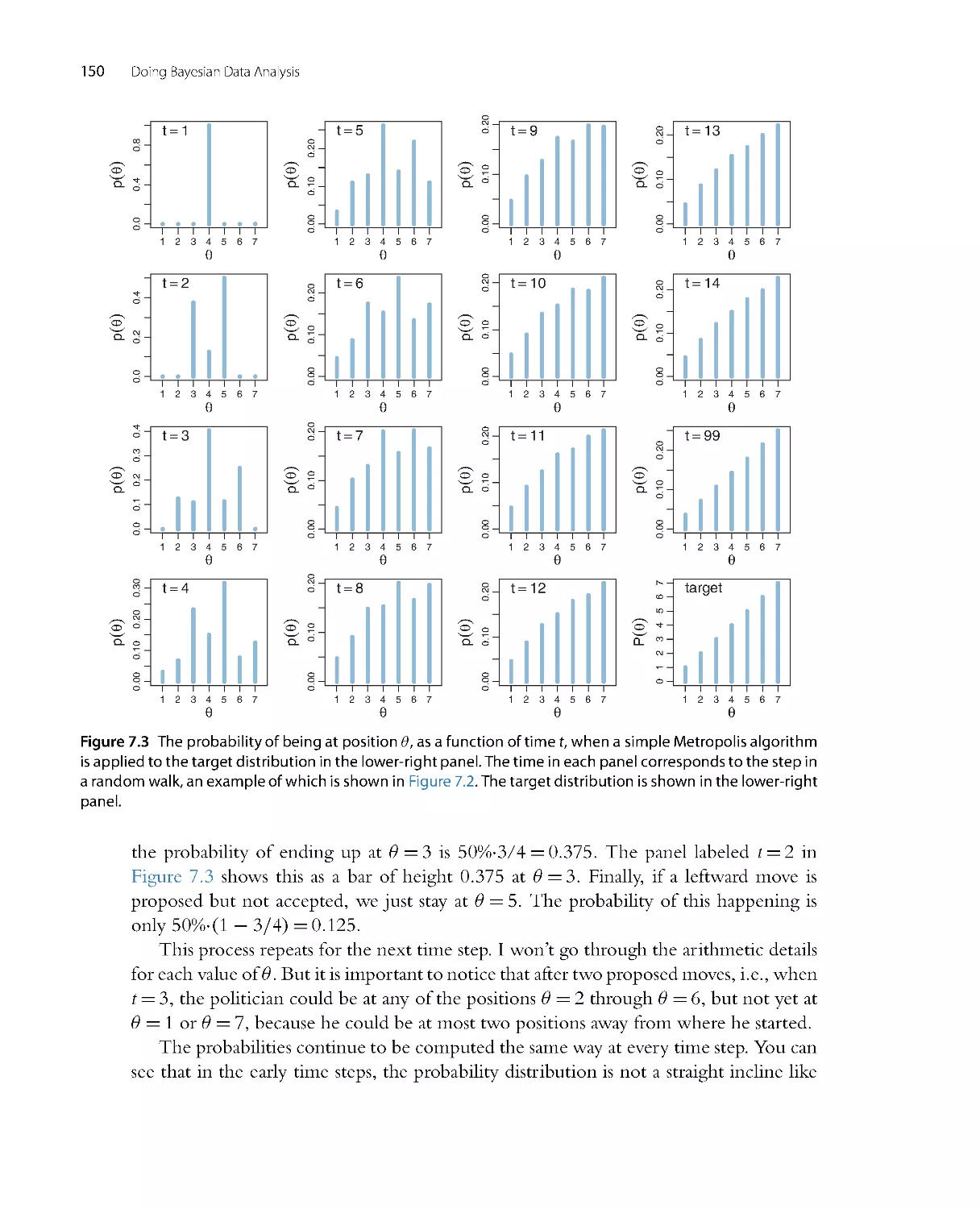


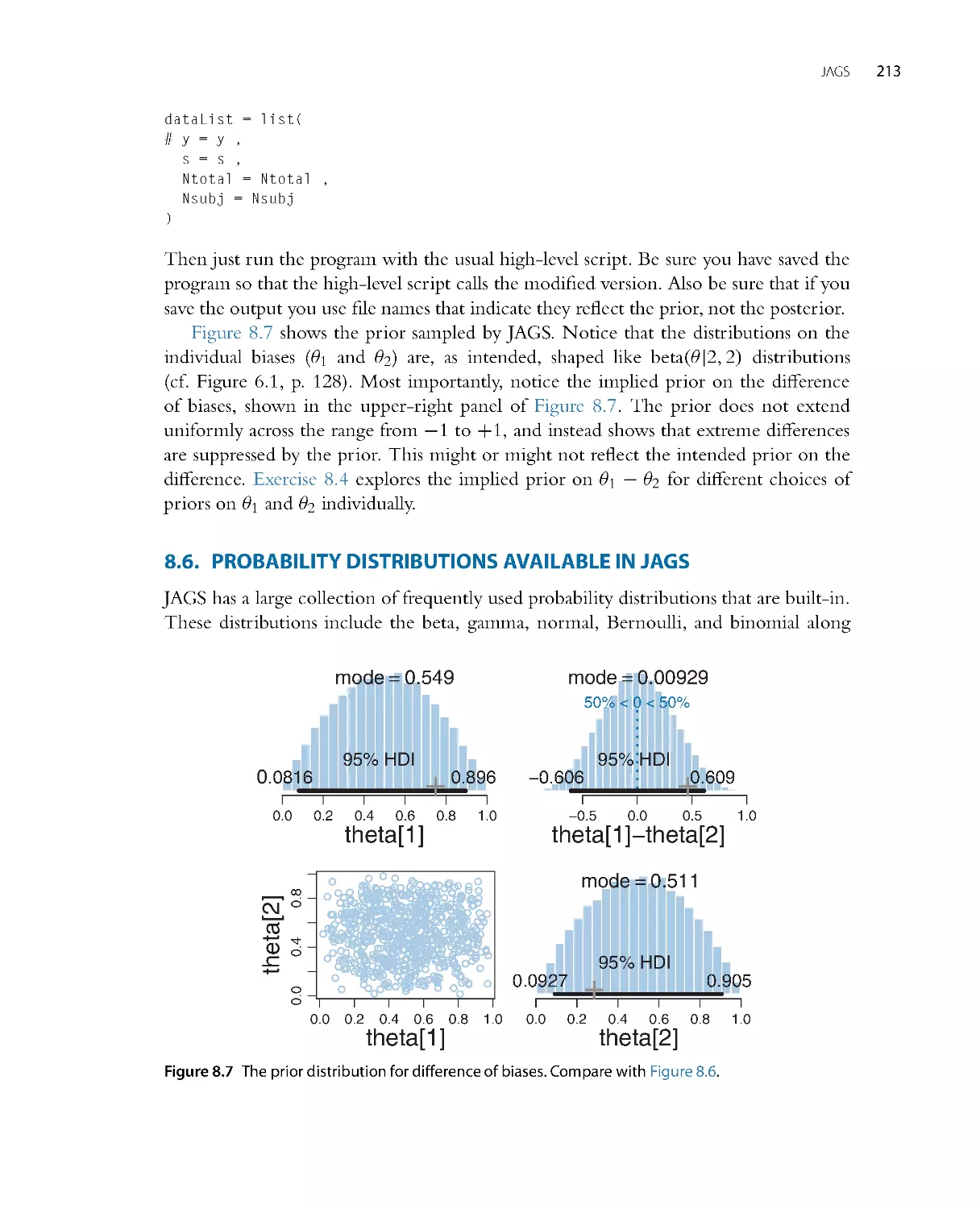


Автор: John K. Kruschke
Теги: mathematics mathematical physics higher mathematics databases data analysis academic press
ISBN: 978-0-12-405888-0
Год: 2014


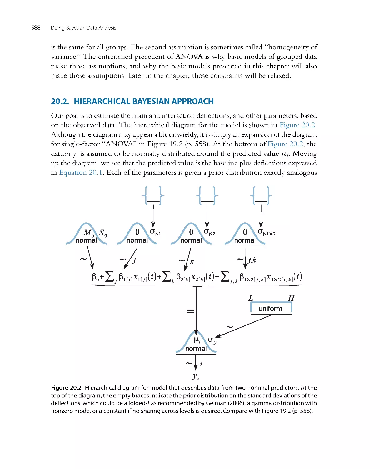
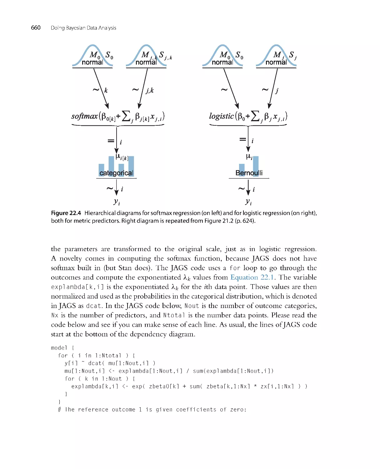
Текст
Doing Bayesian
Data Analysis
Doing Bayesian
Data Analysis
A Tutorial with R, JAGS,
and Stan
EDITION
2
JOHN K. KRUSCHKE
Dept. of Psychological and Brain Sciences
Indiana University, Bloomington
AMSTERDAM • BOSTON • HEIDELBERG • LOND ON
NEW YORK • OXFORD • PARIS • SAN DIEGO
SAN FRANCISCO • SINGAPORE • SYDNEY • TOKYO
Academic Press is an imprint of Elsevier
Academic Press is an imprint of Elsevier
32 Jamestown Road, London NWI 7BY, UK
525 B Street, Suite 1800, San Diego, CA 92101-4495 , USA
225 Wyman Street, Waltham, MA 02451 , USA
The Boulevard, Langford Lane, Kidlington, Oxford OX5 1GB, UK
Copyright © 2015, 2011 Elsevier Inc. All rights reserved.
No part of this publication may be reproduced or transmitted in any form or by any means, electronic or mechanical,
including photocopying, recording, or any infor mation storage and retrieval system, without permission in wr iting from
the publisher. Details on how to seek per mission, further infor mation about the Publishers permissions policies and our
ar rangement with organizations such as the Copyright Clearance Center and the Copyright Licensing Agency, can be
found at our website: www.elsevier.com/permissions.
This book and the individual contr ibutions contained in it are protected under copyright by the Publisher (other than as
may be noted herein).
Notices
Knowledge and best practice in this field are constantly changing. As new research and exper ience broaden our
understanding, changes in research methods, professional practices, or medical treatment may become necessary.
Practitioners and researchers must always rely on their own exper ience and knowledge in evaluating and using any
information, methods, compounds, or exper iments descr ibed herein. In using such information or methods they should
be mindful of their own safety and the safety of others, including parties for whom they have a professional responsibility.
To the fullest extent of the law, neither the Publisher nor the authors, contributors, or editors, assume any liability for
any injury and/or damage to persons or property as a matter of products liability, negligence or otherwise, or from any
use or operation of any methods, products, instructions, or ideas contained in the mater ial herein.
ISBN: 978-0 -12 -405888 -0
Library of Cong ress Cataloging-in-Publication Data
Kruschke, John K.
Doing Bayesian data analysis : a tutorial with R, JAGS, and Stan / John K. Kruschke. – 2E [edition].
pages cm
Includes bibliog raphical references.
ISBN 978-0-12-405888-0
1. Bayesian statistical decision theory. 2. R (Computer program language) I. Title.
QA279.5.K79 2014
519.5
42–dc23
2014011293
British Library Cataloguing in Publication Data
A catalogue record for this book is available from the British Library
For information on all Academic Press publications
visit our website at store.elsevier.com
Dedicated to my mother, Mar ilyn A. Kruschke,
and to the memory of my father, Earl R. Kruschke,
both of whom brilliantly exemplified and taught sound reasoning.
And, in honor of my father,
who dedicated his first book to his children,
I also dedicate this book to mine:
Claire A. Kruschke and Loren D. Kruschke.
CHAPTER 1
What’s in This Book (Read This First!)
Contents
1.1 . RealPeopleCanReadThisBook.......................................................... 1
1.1 .1 Prerequisites...................................................................... 2
1.2 . What’sinThisBook ..................................................................... 3
1.2 .1 You’rebusy.What’stheleastyoucanread?........................................... 3
1.2 .2 You’re really busy!Isn’tthereevenlessyoucanread? .................................. 4
1.2 .3 You want to enjoy the view a little longer. But not too muchlonger..................... 4
1.2 .4 Ifyoujustgottarejectanullhypothesis............................................... 5
1.2 .5 Where’stheequivalentoftraditionaltestXinthisbook?............................... 5
1.3 . What’sNewintheSecondEdition?....................................................... 6
1.4 . GimmeFeedback(BePolite) ............................................................. 8
1.5 . ThankYou!............................................................................. 8
Oh honey I’m searching for love that is true,
But driving through fog is so dang hard to do.
Please paint me a line on the road to your heart,
I’ll rev up my pick up and get a clean start.1
1.1. REAL PEOPLE CAN READ THIS BOOK
This book explains how to actually do Bayesian data analysis, by real people (like
you), for realistic data (like yours). The book starts at the basics, with elementary
notions of probability and programming. You do not need to already know statistics
and programming. The book progresses to advanced hierarchical models that are used
in realistic data analysis. This book is speaking to a person such as a first-year graduate
student or advanced undergraduate in the social or biological sciences: Someone who
grew up in Lake Wobegon,
2 but who is not the mythical being that has the previous
training of a nuclear physicist and then decided to lear n about Bayesian statistics. (After
the publication of the first edition, one of those mythical beings contacted me about
1 This chapter provides a road map to the book, which hopes to have you fall in love with Bayesian analysis
even if you previously had unhappy relationships with statistics. The poem plays with those ideas.
2 A popular weekly radio show on National Public Radio, called A Prairie Home Companion, features fictional
anecdotes about a small town named Lake Wobegon. The stories, written and orated by Garrison Keillor,
always end with the phrase, “And that’s the news from Lake Wobegon, where all the women are strong,
all the men are good looking, and all the children are above average.” So, if you grew up there, ...
Doing Bayesian Data Analysis, 2nd Edition
Copyright © 2015 Elsevier Inc.
http://dx.doi.org/10.1016/B978-0-12-405888-0.00001 -5
All rights reserved.
1
2
Doing Bayesian Data Analysis
the book! So, even if you do have the previous training of a nuclear physicist, I hope the
book speaks to you too.)
Details of prerequisites and the contents of the book are presented below. But first
things first: As you may have noticed from the beginning of this chapter, the chapters
commence with a stanza of elegant and insightful verse composed by a famous poet. The
quatrains
3 are for med of dactylic4 tetrameter,
5 or, colloquially speaking, “country waltz”
meter. The poems regard conceptual themes of the chapter via allusion from immortal
human motifs in waltz timing.
If you do not find them to be all that funny,
If they leave you wanting back all of your money,
Well, honey, some waltzing’s a small price to pay, for
All the good lear ning you’ll get if you stay.
1.1 .1 . Prerequisites
There is no avoiding mathematics when doing data analysis. On the other hand, this
book is definitely not a mathematical statistics textbook, in that it does not emphasize
theorem proving or for mal analyses.
6 But I do expect that you are coming to this book
with a dim knowledge of basic calculus. For example, if you understand expressions like
xdx =
1
2x2
, you’re probably good to go. Notice the previous sentence said “under-
stand” the statement of the integral, not “generate” the statement on your own. When
mathematical derivations are helpful for understanding, they will usually be presented
with a thorough succession of inter mediate steps, so you can actually come away feeling
secure and familiar with the tr ip and destination, rather than just feeling car sick after
being thrown blindfolded into the back seat and driven around curves at high speed.
The beginnings of your journey will go more smoothly if you have had some basic
exper ience programming a computer, but previous programming experience is not
crucial. A computer program is just a list of commands that the computer can execute.
3 quatrain [noun]: Four lines of verse. Unless it’s written “qua train,” in which case it’s a philosopher
comparing something to a locomotive.
4 dactylic [adjective]: A metrical foot in poetry comprising one stressed and two unstressed syllables. Not to
be confused with a pterodactyl, which was a flying dinosaur, and which probably sounded nothing like a
dactyl unless it fell from the sky and bounced twice: THUMP-bump-bump.
5 tetrameter [noun]: A line of verse containing four metrical feet. Not to be confused with a quadraped,
which has four feet, but is averse to lines.
6 The first edition mentioned at this point that “any mathematical statistician would be totally bummed at
the infor mality, dude.” The statement was meant to be funny, with the slang self-referentially instantiating
infor mality. Even the oracle of truth, Wikipedia, says that “‘Dude’ is generally used infor mally to address
someone” (http://en.wikipedia.org/wiki/Dude, retrieved Febr uary 02, 2014) and “[slang] lowers, if
temporarily, ‘the dignity of formal or serious speech or writing’” (http://en.wikipedia.org/wiki/Slang,
retrieved February 02, 2014). But some readers were offended by such undignified writing, and therefore
the joke is now only available to people who read footnotes.
What ’s in This Book (Read This First!)
3
For example, if you’ve ever typed an equal sign in an Excel spreadsheet cell, you’ve
written a programming command. If you’ve ever wr itten a list of commands in Java, C,
Python, Basic or any other computer programming language, then you’re set. We will be
using programming languages called R, JAGS, and Stan, which are free and thoroughly
explained in this book.
1.2. WHAT’S IN THIS BOOK
This book has three major parts. The first part covers foundations: The basic ideas of
Bayesian reasoning, models, probabilities, and programming in R.
The second part covers all the crucial ideas of moder n Bayesian data analysis while
using the simplest possible type of data, namely dichotomous data such as agree/disagree,
remember/forget, male/female, etc. Because the data are so simplistic, the focus can be
on Bayesian techniques. In particular, the moder n techniques of “Markov chain Monte
Carlo” (MCMC) are explained thoroughly and intuitively. Because the data are kept
simple in this part of the book, intuitions about the meaning of hierarchical models
can be developed in glor ious graphic detail. This second part of the book also explores
methods for planning how much data will be needed to achieve a desired degree of
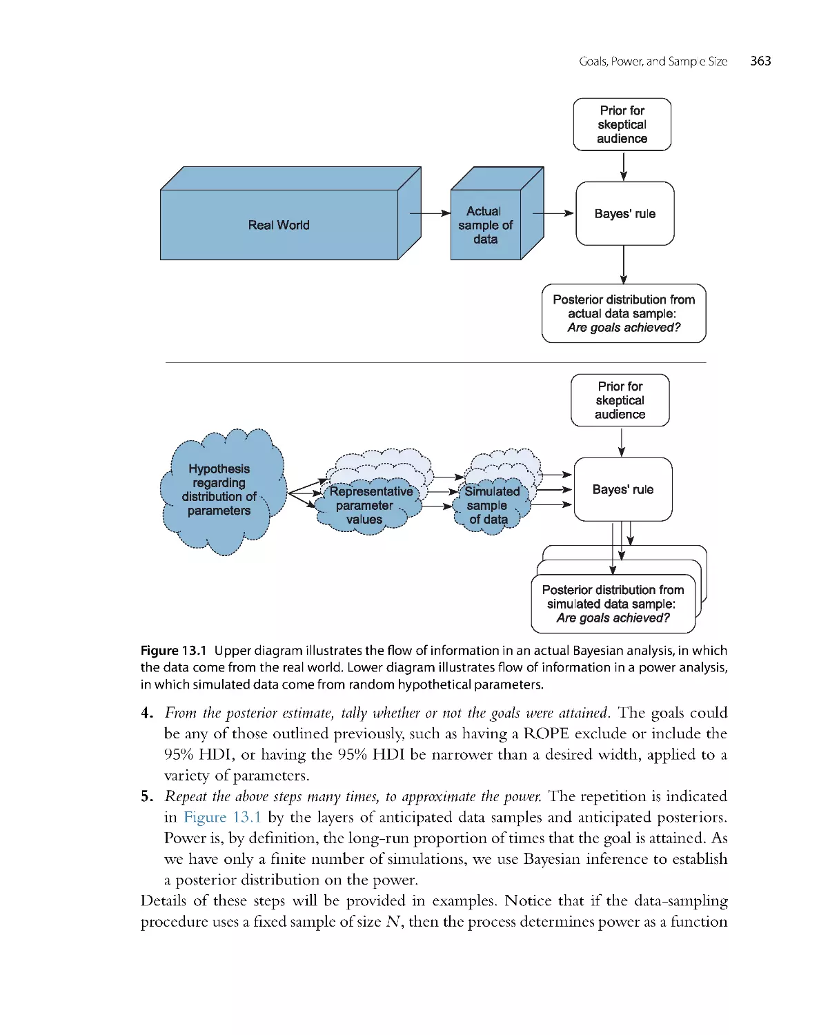
precision in the conclusions, broadly known as “power analysis.”
The third part of the book applies the Bayesian methods to realistic data. The
applications are organized around the type of data being analyzed, and the type of
measurements that are used to explain or predict the data. Different types of measurement
scales require different types of mathematical models, but otherwise the underlying
concepts are always the same. More details of coverage are provided below.
The chapters of the book are designed to be read in order, for a “grand tour” of basic
applied Bayesian analysis. Especially through parts one and two, the chapters probably
make the most sense if read in order. But shorter routes are possible, as descr ibed next.
1.2 .1 . You’re busy. What’s the least you can read?
Here is a minimalist excursion through the book:
•
Chapter 2: The idea of Bayesian inference and model parameters. This chapter
introduces important concepts; don’t skip it.
•
Chapter 3: The R programming language. Read the sections about installing the
software, including the extensive set of programs that accompany this book. The rest
can be skimmed and returned to later when needed.
•
Chapter 4: Basic ideas of probability. Merely skim this chapter if you have a high
probability of already knowing its content.
•
Chapter 5: Bayes rule!
•
Chapter 6: The simplest for mal application of Bayes rule, referenced throughout the
remainder of the book.
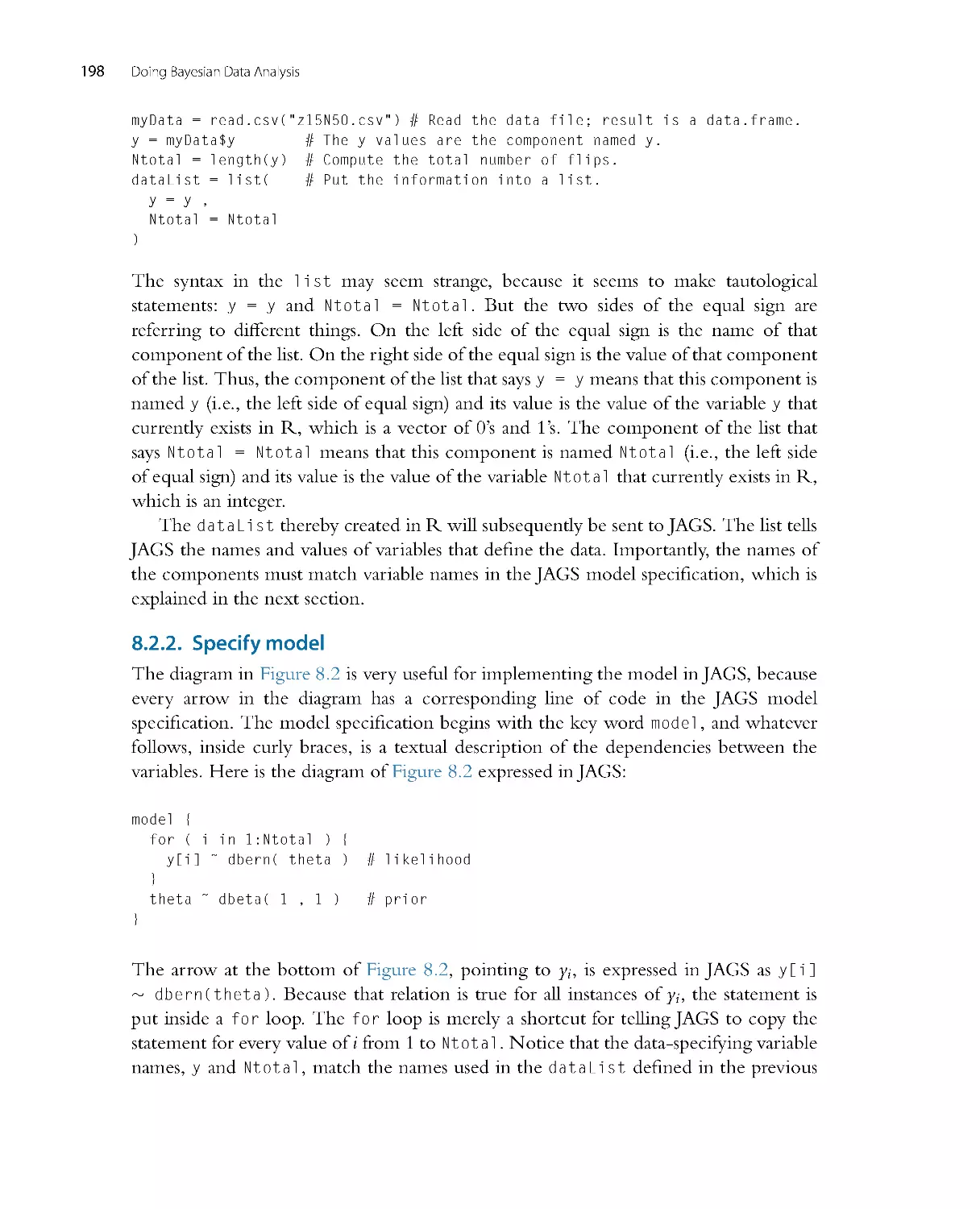
4
Doing Bayesian Data Analysis
•
Chapter 7: MCMC methods. This chapter explains the computing method that
makes contemporary Bayesian applications possible. You don’t need to study all the
mathematical details, but you should be sure to get the gist of the pictures.
•
Chapter 8: The JAGS programming language for implementing MCMC.
•
Chapter 16: Bayesian estimation of two groups. All of the foundational concepts from
the aforementioned chapters, applied to the case of compar ing two groups.
1.2.2. You’re really busy! Isn’t there even less you can read?
If all you want is a conceptual foundation and the fastest possible hands-on experience,
and if you have some previous knowledge of classical statistics such as a t test, then
I recommend the following. First, read Chapter 2 of this book for the conceptual
foundation. Then read the article by Kruschke (2013a), which describes Bayesian
estimation of two groups (analogous to a traditional t test). Essentially, you’ve just
leapfrogged to Chapter 16 of this book. For your hands-on experience, the article has
accompanying software, and there is a version that has been implemented in JavaScr ipt
for use in your web browser without need to install other software. For details, see the
We b s i t e http://www.indiana.edu/~kruschke/BEST/.
1.2 .3 . You want to enjoy the view a little longer. But not too much longer
After the minimalist excursion suggested above, if you want to delve into further specific
applications, you will need to read these sections:
•
Chapter 9: Hierarchical models. Many realistic applications involve hierarchical, or
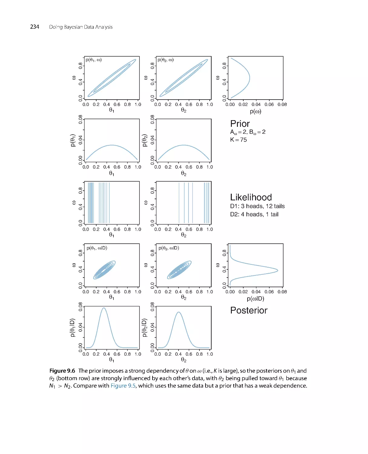
“multilevel,” structure. One of the things that makes Bayesian methods so exciting is
their seamless applicability to hierarchical models.
•
Chapter 15: Overview of the generalized linear model. To know what type of model
might apply to your data, you need to know the canonical catalog of conventional
models, many of which fall under the umbrella of the generalized linear model.
•
Individual chapters from Chapters 16–24. Go to the chapter relevant to the data
structure you’re interested in (which you’ll understand because you previously read
Chapter 15).
•
Chapter 13: Statistical power analysis and planning of research, from a Bayesian
perspective. This chapter is not essential on a first reading, but it’s important not
to skip forever. After all, failing to plan is planning to fail.
•
Section 25.1, which has recommendations for how to report a Bayesian analysis. If
you want your research to influence other people, you’ve got to be able to tell them
about it. (Well, I suppose there are other means of persuasion, but you’ll have to lear n
those from other sources.)
What ’s in This Book (Read This First!)
5
1.2 .4 . If you just gotta reject a null hypothesis...
Traditional statistical methods are often focused on rejecting a null hypothesis, as opposed
to estimating magnitudes and their uncertainty. For a Bayesian perspective on null
hypotheses, read these chapters:
•
Chapter 11: The per ils of p values in traditional null-hypothesis significance testing.
•
Chapter 12: Bayesian approaches to null value assessment.
1.2 .5 . Where’s the equivalent of traditional test X in this book?
Because many readers will be coming to this book after having already been exposed
to traditional statistics that emphasize null hypothesis significance testing (NHST), this
book provides Bayesian approaches to many of the usual topics in NHST textbooks.
Ta b l e 1 . 1 lists var ious tests covered by standard introductory statistics textbooks, along
with the location of their Bayesian analogues in this book.
The ar ray of tests mentioned in Ta b l e 1 . 1 are all cases of what is called the “generalized
linear model.” For those of you already familiar with that ter m, you can glance ahead to
Table 15.3, p. 444, to see which chapters cover which cases. For those of you not yet
familiar with that term, do not worry, because all of Chapter 15 is devoted to introducing
and explaining the ideas.
A superficial conclusion from Ta b l e 1 . 1 might be, “Gee, the table shows that
traditional statistical tests do something analogous to Bayesian analysis in every case,
therefore it’s pointless to bother with Bayesian analysis.” Such a conclusion would be
wrong. First, traditional NHST has deep problems, some of which are discussed in
Chapter 11. Second, Bayesian analysis yields r icher and more informative inferences
than NHST, as will be shown in numerous examples throughout the book.
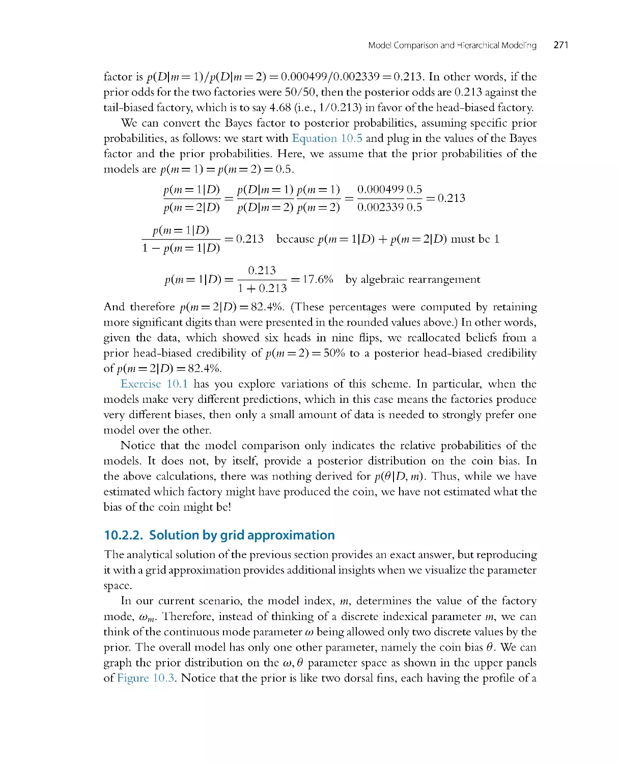
Ta b l e 1 . 1 Bayesian analogues of null hypothesis significance tests.
Traditional analysis name
Bayesian analogue
Binomial test
Chapters 6–9 and 21
t test
Chapter 16
Simple linear regression
Chapter 17
Multiple linear reg ression
Chapter 18
One-way ANOVA
Chapter 19
Multifactor ANOVA
Chapter 20
Logistic regression
Chapter 21
Multinomial logistic regression
Chapter 22
Ordinal regression
Chapter 23
Chi-square test (contingency table)
Chapter 24
Power analysis (sample size planning)
Chapter 13
6
Doing Bayesian Data Analysis
1.3. WHAT’S NEW IN THE SECOND EDITION?
The basic progression of topics remains the same as the first edition, but all the details have
been changed, from cover to cover. The book and its programs have been completely
rewr itten. Here are just a few highlights of the changes:
•
There are all new programs in JAGS and Stan. The new programs are designed to be
much easier to use than the scripts in the first edition. In particular, there are now
compact high-level scripts that make it easy to run the programs on your own data.
This new programming was a major undertaking by itself.
•
The introductory Chapter 2, regarding the basic ideas of how Bayesian inference re-
allocates credibility across possibilities, is completely rewr itten and greatly expanded.
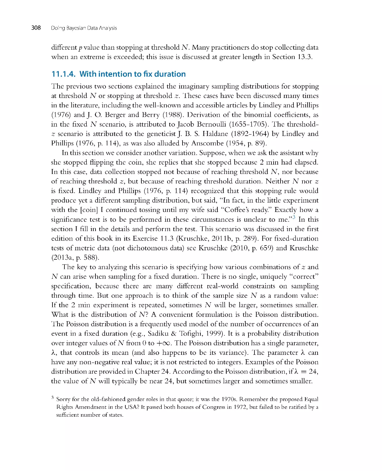
•
There are completely new chapters on the programming languages R (Chapter 3),
JAGS (Chapter 8), and Stan (Chapter 14). The lengthy new chapter on R includes
explanations of data files and structures such as lists and data frames, along with
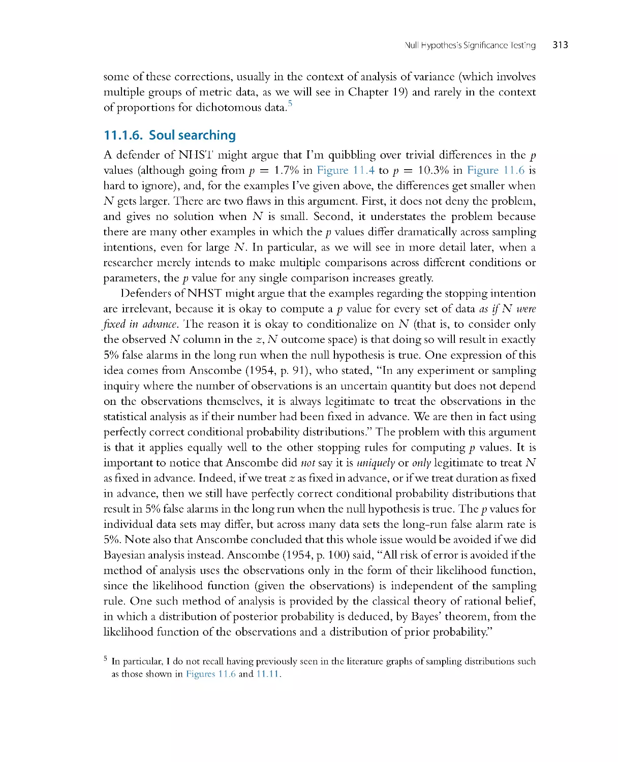
several utility functions. (It also has a new poem that I am particularly pleased
with.) The new chapter on JAGS includes explanation of the RunJAGS package
which executes JAGS on parallel computer cores. The new chapter on Stan
provides a novel explanation of the concepts of Hamiltonian Monte Carlo. The
chapteronStanalsoexplainsconceptualdifferences in program flow between Stan
and JAGS.
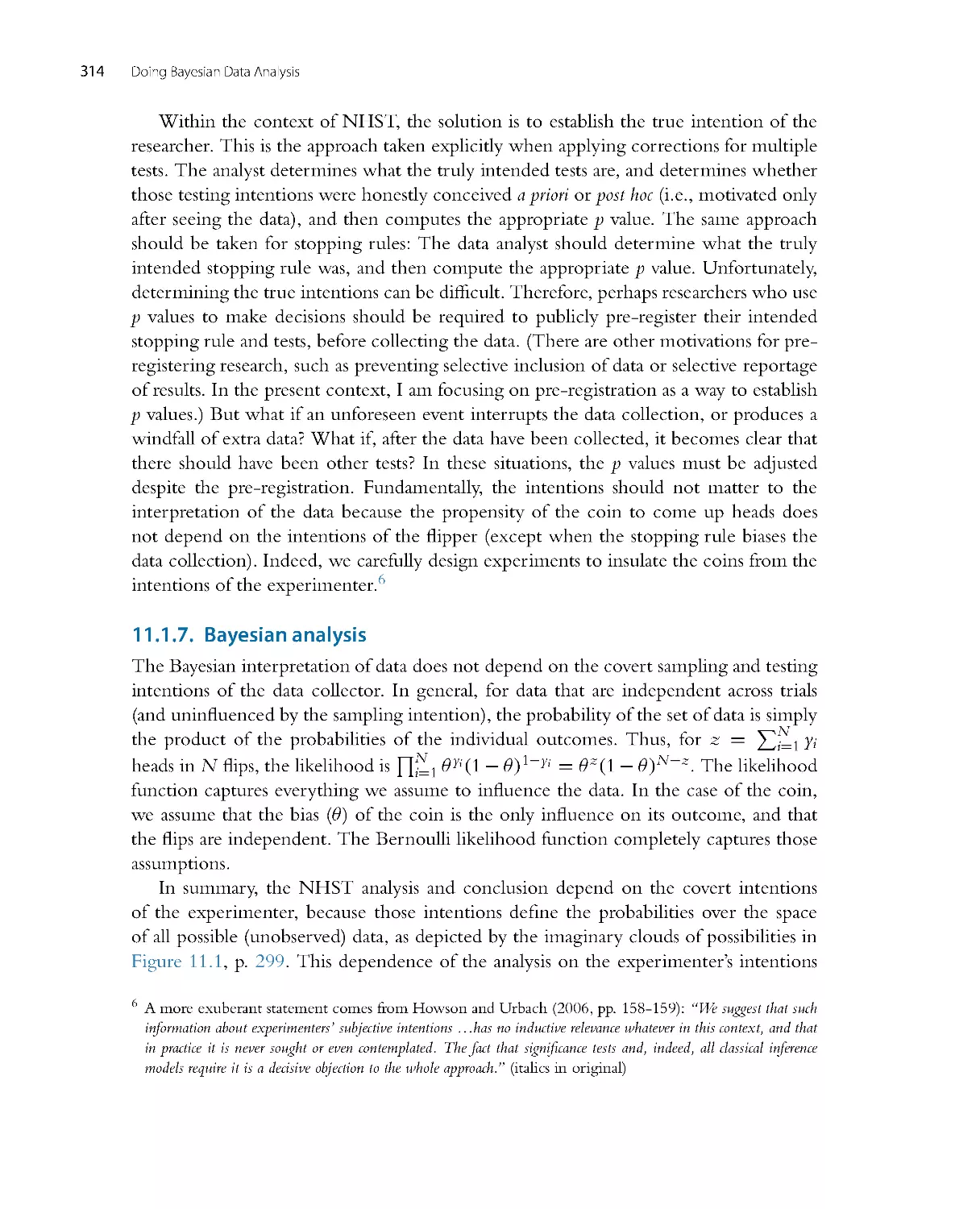
•
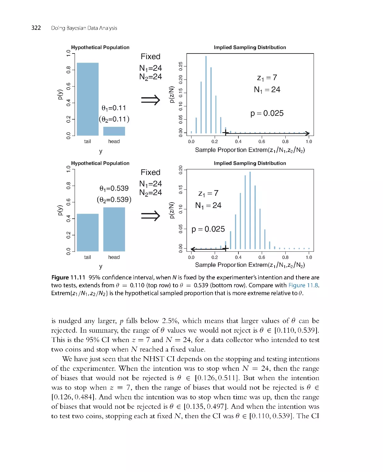
Chapter 5 on Bayes’ rule is greatly revised, with a new emphasis on how Bayes’ rule
re-allocates credibility across parameter values from prior to posterior. The material
on model comparison has been removed from all the early chapters and integrated
into a compact presentation in Chapter 10.
•
What were two separate chapters on the Metropolis algor ithm and Gibbs sampling
have been consolidated into a single chapter on MCMC methods (as Chapter 7).
•
There is extensive new material on MCMC convergence diagnostics in Chapters 7
and 8. There are explanations of autocorrelation and effective sample size. There is
also exploration of the stability of the estimates of the highest density interval (HDI)
limits. New computer programs display the diagnostics, as well.
•
Chapter 9 on hierarchical models includes extensive new and unique material on the
crucial concept of shrinkage, along with new examples.
•
All the material on model comparison, which was spread across various chapters in
the first edition, in now consolidated into a single focused chapter (Chapter 10) that
emphasizes its conceptualization as a case of hierarchical modeling.
•
Chapter 11 on null hypothesis significance testing is extensively revised. It has new
material for introducing the concept of sampling distr ibution. It has new illustrations
of sampling distributions for var ious stopping rules, and for multiple tests.
•
Chapter 12, regarding Bayesian approaches to null value assessment, has new material
about the region of practical equivalence (ROPE), new examples of accepting the
What ’s in This Book (Read This First!)
7
null value by Bayes factors, and new explanation of the Bayes factor in ter ms of the
Savage-Dickey method.
•
Chapter 13, regarding statistical power and sample size, has an extensive new section
on sequential testing, and recommends making the research goal be precision of
estimation instead of rejecting or accepting a particular value.
•
Chapter 15, which introduces the generalized linear model, is fully revised, with
more complete tables showing combinations of predicted and predictor variable
types.
•
Chapter 16, regarding estimation of means, now includes extensive discussion of
comparing two groups, along with explicit estimation of effect size.
•
Chapter 17, regarding regression on a single metr ic predictor, now includes extensive
examples of robust regression in JAGS and Stan. New examples of hierarchical
regression, including quadratic trend, graphically illustrate shrinkage in estimates of
individual slopes and curvatures. The use of weighted data is also illustrated.
•
Chapter 18, on multiple linear regression, includes a new section on Bayesian var iable
selection, in which various candidate predictors are probabilistically included in the
reg ression model.
•
Chapter 19, on one-factor ANOVA-like analysis, has all new examples, including
a completely worked out example analogous to analysis of covar iance (ANCOVA),
and a new example involving heterogeneous var iances.
•
Chapter 20, on multi-factor ANOVA-like analysis, has all new examples, including
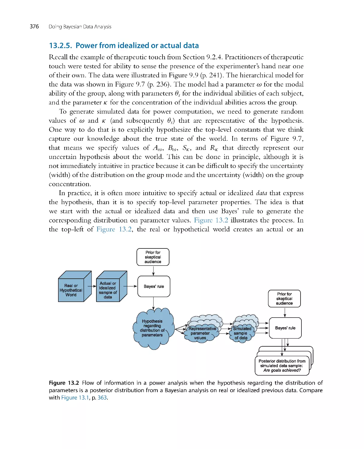
a completely worked out example of a split-plot design that involves a combination
of a within-subjects factor and a between-subjects factor.
•
Chapter 21, on logistic regression, is expanded to include examples of robust logistic
regression, and examples with nominal predictors.
•
There is a completely new chapter (Chapter 22) on multinomial logistic regression.
This chapter fills in a case of the generalized linear model (namely, a nominal
predicted variable) that was missing from the first edition.
•
Chapter 23, regarding ordinal data, is greatly expanded. New examples illustrate
single-group and two-group analyses, and demonstrate how interpretations differ
from treating ordinal data as if they were metr ic.
•
There is a new section (25.4) that explains how to model censored data in JAGS.
•
Many exercises are new or revised.
Oh, and did I mention that the cover is different? The cor respondence of the doggies
to Bayes’ rule is now made explicit: The folded ears of the posterior doggie are a
compromise between the perky ears and floppy ears of the likelihood and prior doggies.
The marginal likelihood is not usually computed in MCMC methods, so the doggie in
the denominator gets sleepy with nothing much to do. I hope that what’s between the
covers of this book is as friendly and engaging as the doggies on the cover.
8
Doing Bayesian Data Analysis
1.4. GIMME FEEDBACK (BE POLITE)
I have worked thousands of hours on this book, and I want to make it better. If
you have suggestions regarding any aspect of this book, please do email me:
johnkruschke@gmail.com. Let me know if you’ve spotted egregious er rors or innocuous
infelicities, typo’s or thoughto’s. Let me know if you have a suggestion for how to clar ify
something. Especially let me know if you have a good example that would make things
more interesting or relevant. I’m interested in complete raw data from research that
is interesting to a broad audience, and which can be used with acknowledgement but
without fee. Let me know also if you have more elegant programming code than what
I’ve cobbled together. The outside margins of these pages are intentionally made wide
so that you have room to scr ibble your ridicule and epithets before re-phrasing them
into kindly stated suggestions in your email to me. Rhyming couplets are especially
appreciated.
Since the publication of the first edition I have received hundreds of email messages
from readers. I have replied to many, but I am truly embarrassed by the fact that I have
not been able to reply to all of them, and some have gone unacknowledged. If I don’t
respond to your email in a timely manner, it is likely that your message got buried under
the avalanche of subsequent emails. You are welcome to send a follow-up email to try
to provoke a response from me. In any case, if your email is lengthy or has attachments
or asks about a problem in some complicated analysis you are trying, chances are that I’ll
react by saying to myself, “That’s very interesting, but I’ll have to think about it when
I have more time and reply later.” Then, no matter what time it is, later never comes.
Whether I am able to reply or not, I appreciate all your messages.
1.5. THANK YOU!
I would like to thank the many readers who posted reviews and recommendations of the
first edition on sites such as Amazon.com, Goodreads.com, blogs, and social networking
sites. At the time of this wr iting, there were 46 reviews on Amazon.com,6atAmazon.
co.uk (United Kingdom), 2 at Amazon.ca (Canada), and 1 at Amazon.cn (China). There
were 4 reviews at Goodreads.com plus many ratings. Numerous people have reviewed
or recommended the book on their blogs. Many people have given a “shout out” to
the book on social networking sites. I am ver y grateful to all of you for taking the
time to wr ite reviews, and pleased that your reviews have generally been very positive!
I hope that this second edition elicits continued impulse to post new reviews about
the second edition, as the revisions have been a huge effort to make the book even
better.
I also thank the authors of professional reviews of first edition, including
Andrews (2011), Bar ry (2011), Colvin (2013), Ding (2011), Fellingham (2012),
Goldstein (2011), Smithson (2011), and Vanpaemel and Tuerlinckx (2012). My apologies
What ’s in This Book (Read This First!)
9
to any reviewers whom I have missed; please let me know. I think it is valuable to raise
the visibility of Bayesian methods in professional circles, and I am very grateful to all
these authors for taking the time and effort to compose reviews.
Several people have written computer programs that extended or improved programs
related to the first edition of the book. In particular, the programs for Bayesian estimation
of two groups (“BEST”; Kruschke, 2013a, cf. Chapter 16 of this book) were re-
packaged in R by Mike Meredith, in JavaScript by Rasmus Bååth, and in Python by
Andrew Straw. For links to their work, see http://www.indiana.edu/~kruschke/BEST/.
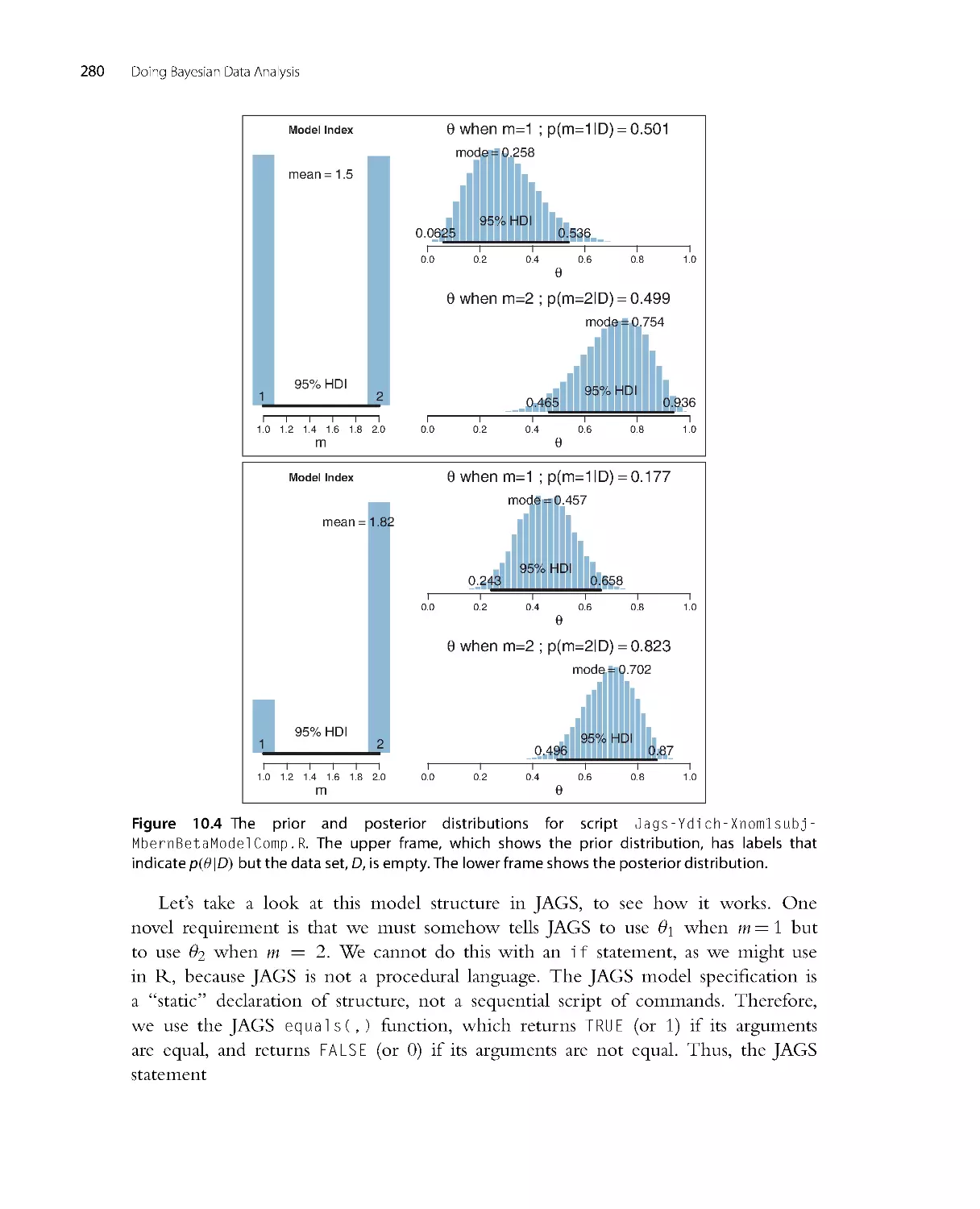
Systems for creating hierarchical diagrams, akin to Figure 9.13 (p. 252), were created
by Rasmus Bååth for LibreOffice and R, and by Tinu Schneider for LATEX and TikZ.
For links to their work, see http://doingbayesiandataanalysis.blogspot.com/2013/10/
diagrams-for-hierarchical-models-new.html. Thank you all for your extensive efforts
and contributions to making Bayesian methods accessible to a wider audience.
Many colleagues have organized workshops or courses for Doing Bayesian
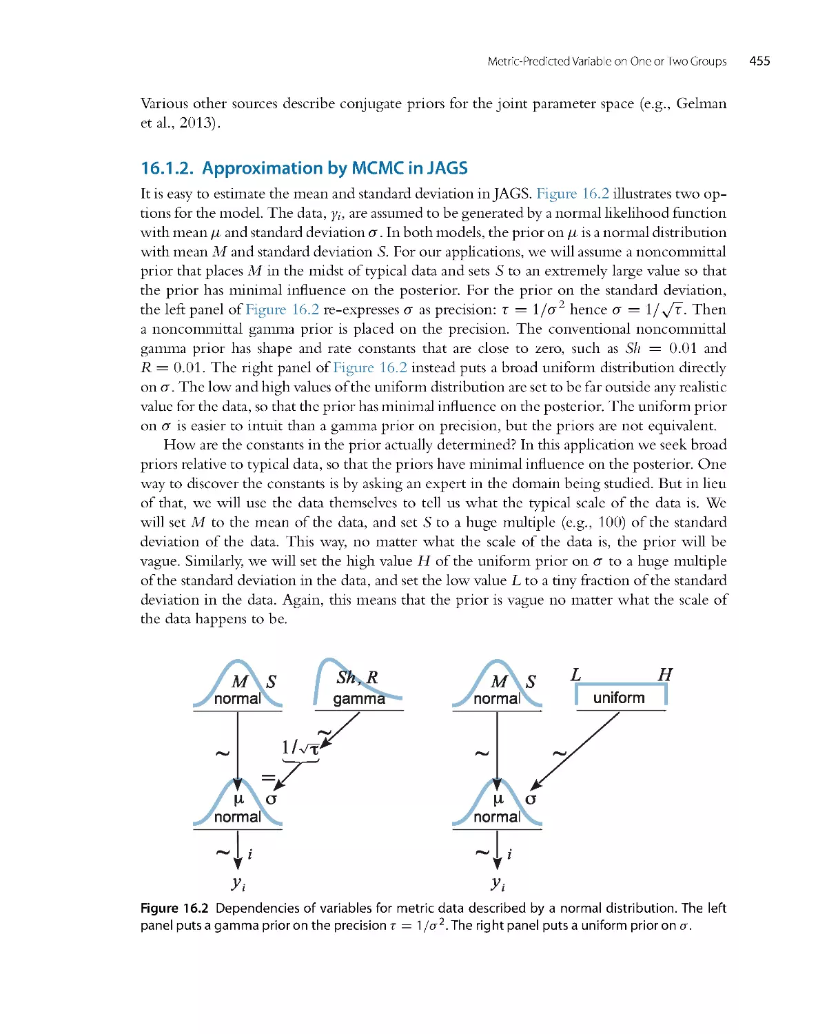
Data Analysis. A list of workshops appears at https://sites.google.com/site/
doingbayesiandataanalysis/. At each of those workshops many more people were
involved than I can possibly mention by name here, but they include William Jacoby
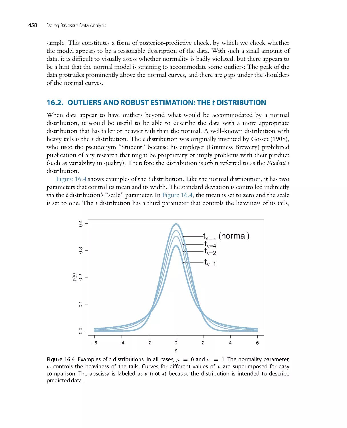
and Dieter Burrell at the Interuniversity Consortium for Political and Social Research
Summer Program at the University of Michigan; William Pridemore, James Russell,
James Walker, and Jeff DeWitt at the Indiana University Social Science Research
Commons; Hans-Joachim Knopf at the University of St. Gallen Summer School in
Empirical Research Methods, Switzerland; Hans Olav Melberg at the University of
Oslo, Norway; Mark Nawrot and colleagues at North Dakota State University; Ulf
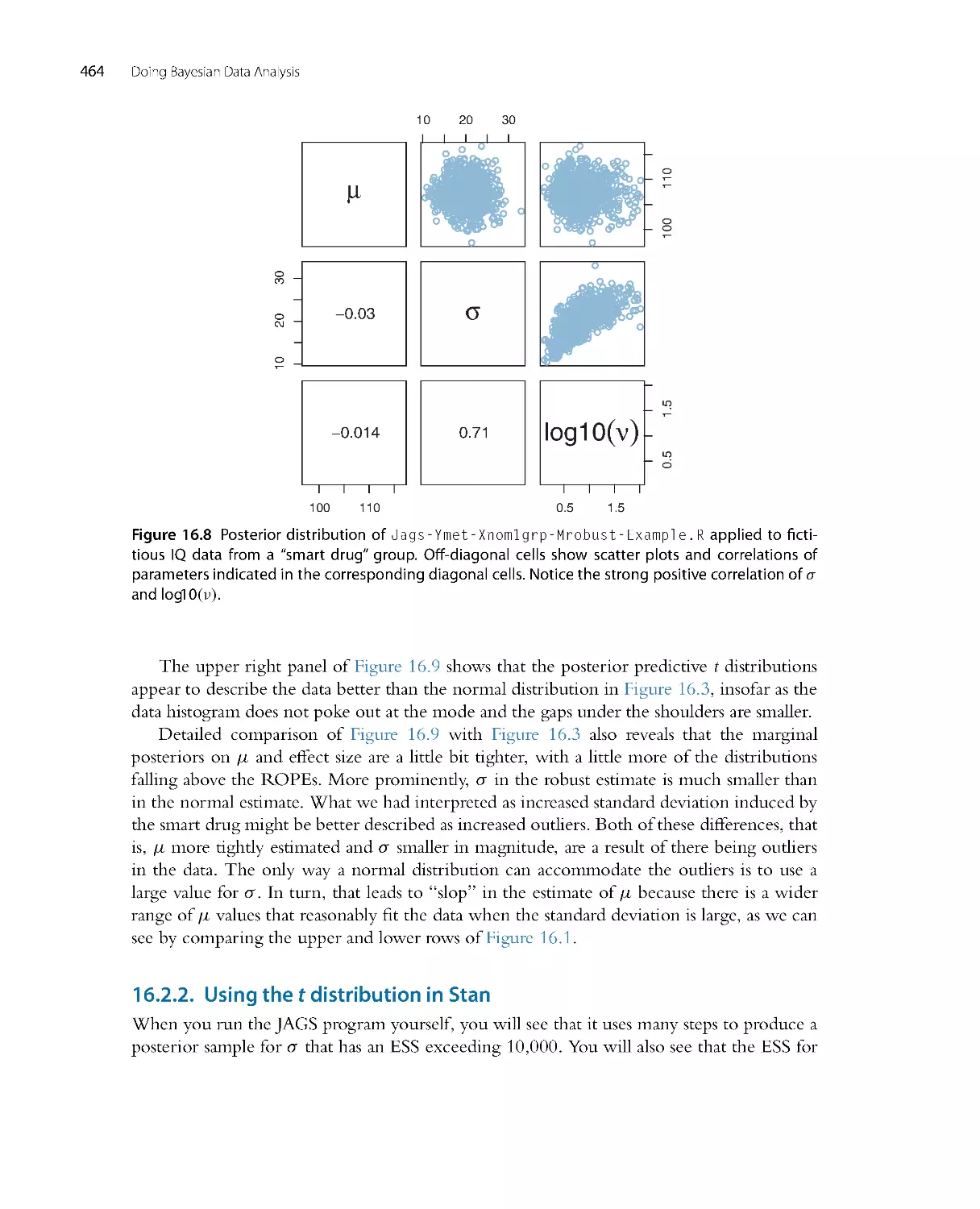
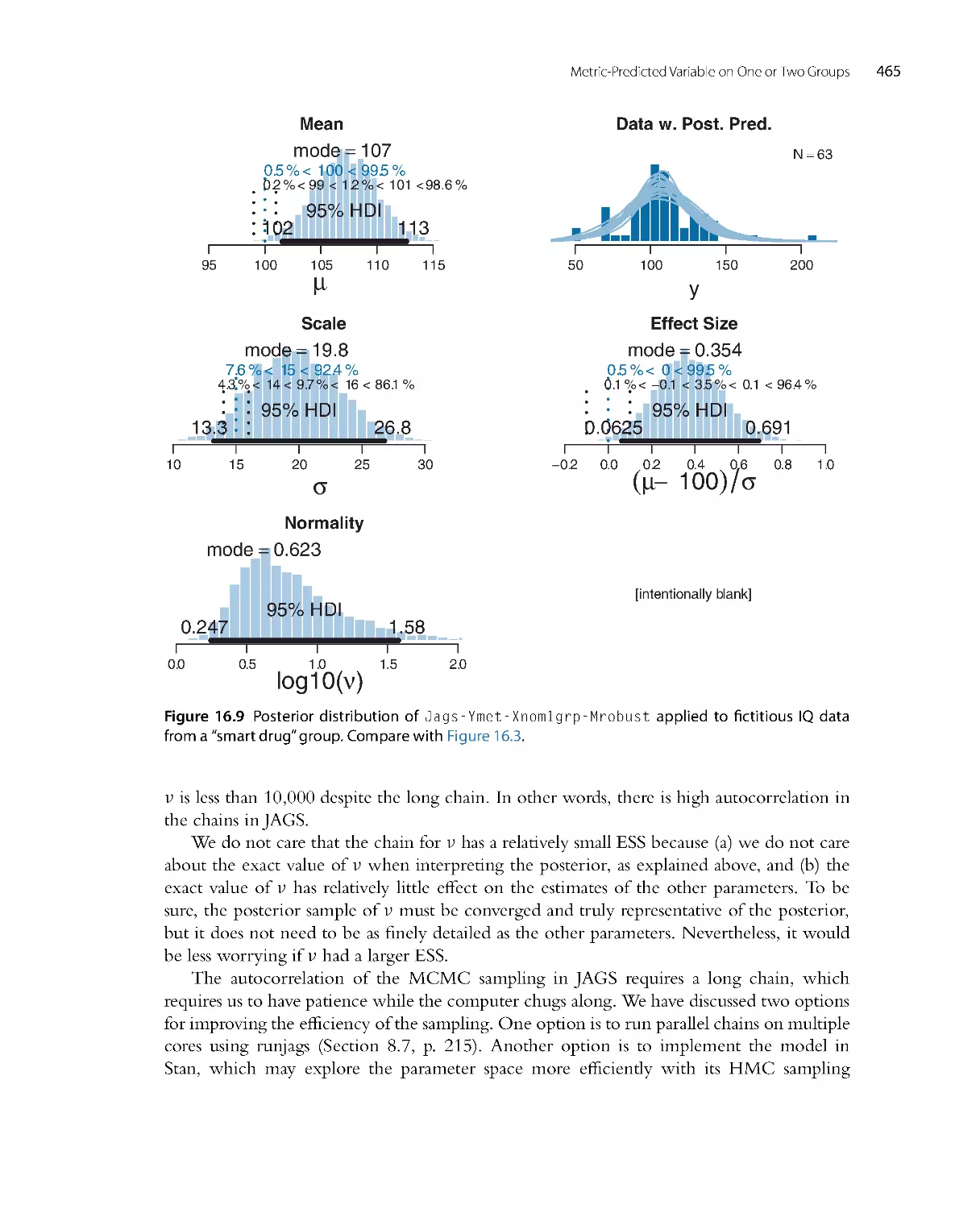
Ahlstrom and colleagues at the Federal Aviation Administration Human Factors Lab,
New Jersey; Tim Pleskac and colleagues at Michigan State University; John Curtin at the
University of Wisconsin, Madison; Michael Roberts and colleagues including Chester
Fornar i, Bryan Hanson, and Humberto Barreto at DePauw University; Jan Andrews,
Ming-Wen An, and colleagues at Vassar College; Kelly Goedert and colleagues at Seton
Hall University; Gregory Francis and Zygmunt Pizlo at Purdue University; Boicho
Kokinov and colleagues at the New Bulgar ian University, Sofia; Nathalie Rothert and
the workshop program committees at the Association for Psychological Science; Duncan
Brumby and the tutorials program committees of the Cognitive Science Society; Andrew
Delamater at the Easter n Psychological Association (and thanks to James McClelland
for introducing my talk there); William Mer riman at the Midwester n Psychological
Association; Xiangen Hu and Michael Jones at the Society for Computers in Psychology.
My apologies to those whom I have inadvertently left off this list. I thank you all for
your time and effort. I hope that the workshops and courses genuinely facilitate doing
Bayesian data analysis by the attendees.
The book has been used by a number of instructors in their courses, and a few of
them have sent me notes of their experiences. In particular, Jeffrey Witmer at Oberlin
10
Doing Bayesian Data Analysis
College sent extensive comments. Adrian Brasoveanu at the University of Califor nia,
Santa Cruz, and John Miyamoto at the University of Washington, also conveyed or
posted information about their courses. The review by Vanpaemel and Tuerlinckx (2012)
reported exper iences from classroom use. Thanks to all the instructors who have boldly
tried the first edition in their courses. I hope that the second edition is even more useful
for the classroom and self study.
Over recent years there have been many students in my classes who have made
insightful comments and suggestions. Some of these include Young Ahn, Gregory Cox,
Junyi Dai, Josh de Lueew, Andrew Jahn, Arash Khodadadi, and Torr in Liddell. Thanks
to Tor rin Liddell also for help with checking the proofs of the book. I thank Anne
Standish for researching and recommending a discussion forum for the book’s blog.
I am grateful to the many people who have left thoughtful comments at the blog and
discussion forum. Thanks also to several careful readers who reported er rors in the first
edition. And thanks to Jacob Hodes for being so interested in Bayesian analysis that he
would travel to a conference to talk with me about it.
The first edition of this book was 6 years in the making, and many colleagues and
students provided helpful comments dur ing that per iod. The most extensive comments
came from Luiz Pessoa, Michael Kalish, Jerome Busemeyer, and Adam Krawitz; thank
you all! Particular sections were insightfully improved by helpful comments from Michael
Erickson, Robert Nosofsky, Geoff Iverson, and James L. (Jay) McClelland. Various
parts of the book benefited indirectly from communications with Woojae Kim, Charles
Liu, Eric-Jan Wagenmakers, and Jeffrey Rouder. Pointers to data sets were offered by
Teresa Treat and Michael Trosset, among others. Very welcome supportive feedback
was provided by Michael D. Lee, and also by Adele Diederich. A Bayesian-supportive
working environment was provided by many colleagues including Richard Shiffrin,
Jerome Busemeyer, Peter Todd, James Townsend, Robert Nosofsky, and Luiz Pessoa.
Other department colleagues have been very supportive of integrating Bayesian statistics
into the cur riculum, including Linda Smith and Amy Holtzworth-Munroe. Various
teaching assistants have provided helpful comments; in particular I especially thank Noah
Silbert and Thomas Wisdom for their excellent assistance. As this book has evolved over
the years, suggestions have been contr ibuted by numerous students, including Aaron
Albin, Thomas Smith, Sean Matthews, Thomas Parr, Kenji Yoshida, Bryan Bergert, and
perhaps dozens of others who have contributed insightful questions or comments that
helped me tune the presentation in the book.
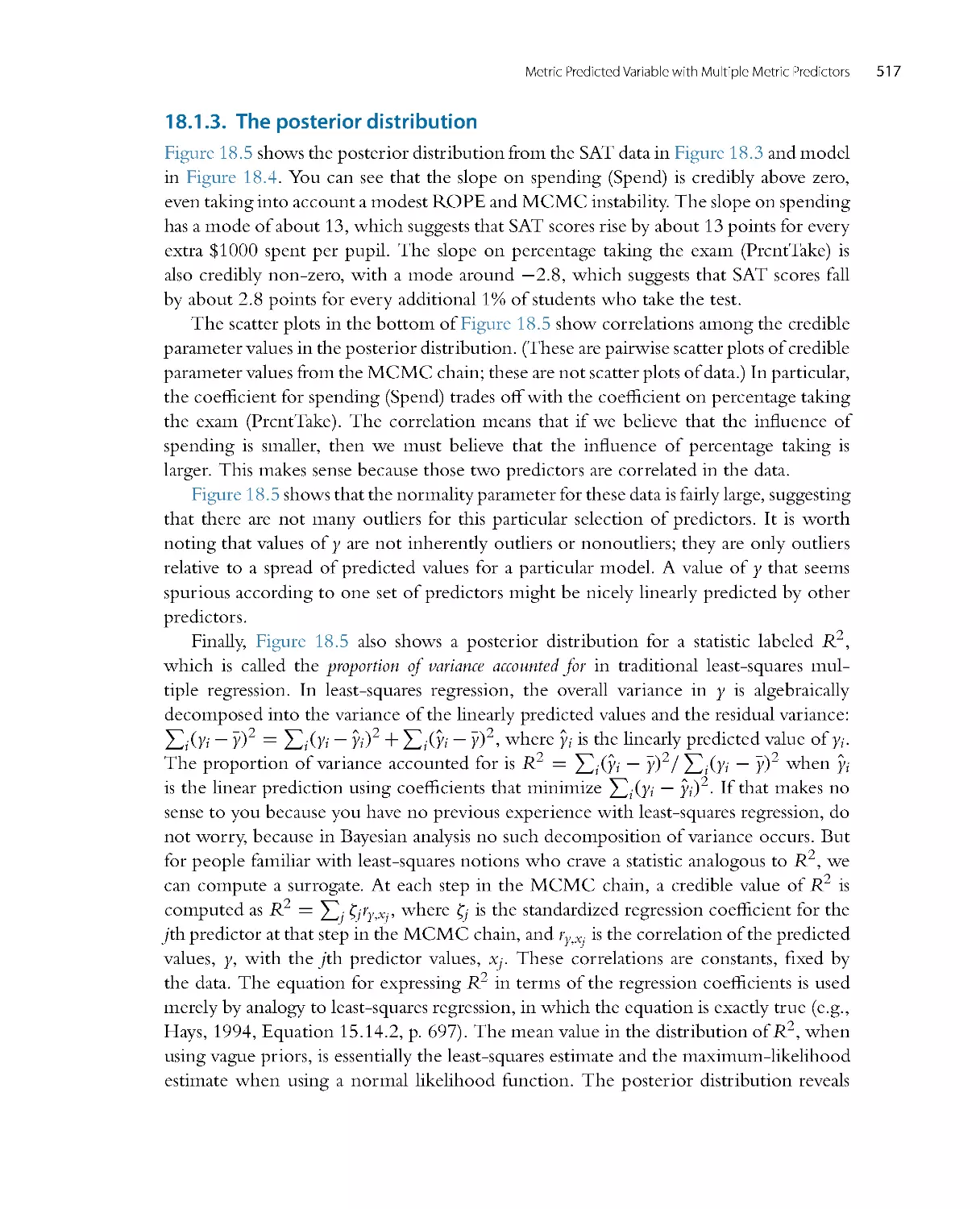
Gratefully acknowledged are the creators of the software R (R Core Team, 2013),
RStudio (RStudio, 2013), JAGS (Plummer, 2003, 2012), RunJAGS (Denwood, 2013),
BUGS (Lunn, Thomas, Best, & Spiegelhalter, 2000; A. Thomas, O’Hara, Ligges, &
Sturtz, 2006), and Stan (Stan Development Team, 2012). Also gratefully acknowledged
are the creators of the typesetting software LATEX(http://www.latex-project.org/)
and MikTeX (http://miktex.org/), the editor TeXmaker (http://www.xm1math.net/
What ’s in This Book (Read This First!)
11
texmaker/), and the drawing application of LibreOffice (http://www.libreoffice.org/),
in which this book was composed by the author.
To all the people who have made contributions but whom I have inadvertently
forgotten to mention, I extend my apologies and genuine appreciation.
Finally, my deepest gratitude goes to Dr. Rima Hanania, who has been my constant
and most esteemed companion throughout all the years of wr iting this book.
PART I
The Basics: Models,
Probability, Bayes’ Rule,
and R
In this part of the book, the basic ideas of Bayesian analysis are presented with intuitive
and simple examples. Ideas of probability are defined, and Bayes’ rule is extensively
introduced. A chapter on the computer language R explains many of its core functions.
13
CHAPTER 2
Introduction: Credibility, Models,
and Parameters
Contents
2.1 . Bayesian Inference Is Reallocation of Credibility Across Possibilities . .......................... 16
2.1 .1 Dataarenoisyandinferencesareprobabilistic....................................... 19
2.2 . PossibilitiesAreParameterValuesinDescriptiveModels.................................... 22
2.3 . TheStepsofBayesianDataAnalysis...................................................... 25
2.3 .1 Dataanalysiswithoutparametricmodels? .......................................... 30
2.4 . Exercises.............................................................................. 31
I just want someone who I can believe in,
Someone at home who will not leave me grievin’.
Show me a sign that you’ll always be true,
and I’ll be your model of faith and virtue.1
The goal of this chapter is to introduce the conceptual framework of Bayesian data
analysis. Bayesian data analysis has two foundational ideas. The first idea is that Bayesian
inference is reallocation of credibility across possibilities. The second foundational idea
is that the possibilities, over which we allocate credibility, are parameter values in
meaningful mathematical models. These two fundamental ideas for m the conceptual
foundation for every analysis in this book. Simple examples of these ideas are presented
in this chapter. The rest of the book merely fills in the mathematical and computational
details for specific applications of these two ideas. This chapter also explains the basic
procedural steps shared by every Bayesian analysis.
1 This chapter introduces ideas of mathematical models, credibility of parameter values, and the semantics
of models. The poem plays with the words “model,” “believe,” and “true” in an everyday context, and
hints that Bayesian methods (personified) may be someone to believe in. (And yes, g rammatically, the first
line should be “in whom I can believe,” but the poem is supposed to be colloquial speech. Besides, the
grammatically correct version is iambic not dactylic!)
Doing Bayesian Data Analysis, 2nd Edition
Copyright © 2015 Elsevier Inc.
http://dx.doi.org/10.1016/B978-0-12-405888-0.00002 -7
All rights reserved.
15
16
Doing Bayesian Data Analysis
2.1. BAYESIAN INFERENCE IS REALLOCATION OF CREDIBILITY
ACROSS POSSIBILITIES
Suppose we step outside one morning and notice that the sidewalk is wet, and wonder
why. We consider all possible causes of the wetness, including possibilities such as recent
rain, recent garden irrigation, a newly erupted underground spring, a broken sewage
pipe, a passerby who spilled a drink, and so on. If all we know until this point is
that some part of the sidewalk is wet, then all those possibilities will have some prior
credibility based on previous knowledge. For example, recent rain may have greater prior
probability than a spilled drink from a passerby. Continuing on our outside jour ney, we
look around and collect new observations. If we observe that the sidewalk is wet for as
far as we can see, as are the trees and parked cars, then we re-allocate credibility to the
hypothetical cause of recent rain. The other possible causes, such as a passerby spilling
a drink, would not account for the new observations. On the other hand, if instead we
observed that the wetness was localized to a small area, and there was an empty drink cup
a few feet away, then we would re-allocate credibility to the spilled-drink hypothesis,
even though it had relatively low prior probability. This sort of reallocation of credibility
across possibilities is the essence of Bayesian inference.
Another example of Bayesian inference has been immortalized in the words of the
fictional detective Sherlock Holmes, who often said to his sidekick, Doctor Watson:
“How often have I said to you that when you have eliminated the impossible, whatever
remains, however improbable, must be the truth?” (Doyle, 1890, chap. 6) Although this
reasoning was not described by Holmes or Watson or Doyle as Bayesian inference, it is.
Holmes conceived of a set of possible causes for a crime. Some of the possibilities may
have seemed very improbable, apriori. Holmes systematically gathered evidence that
ruled out a number of the possible causes. If all possible causes but one were eliminated,
then (Bayesian) reasoning forced him to conclude that the remaining possible cause was
fully credible, even if it seemed improbable at the start.
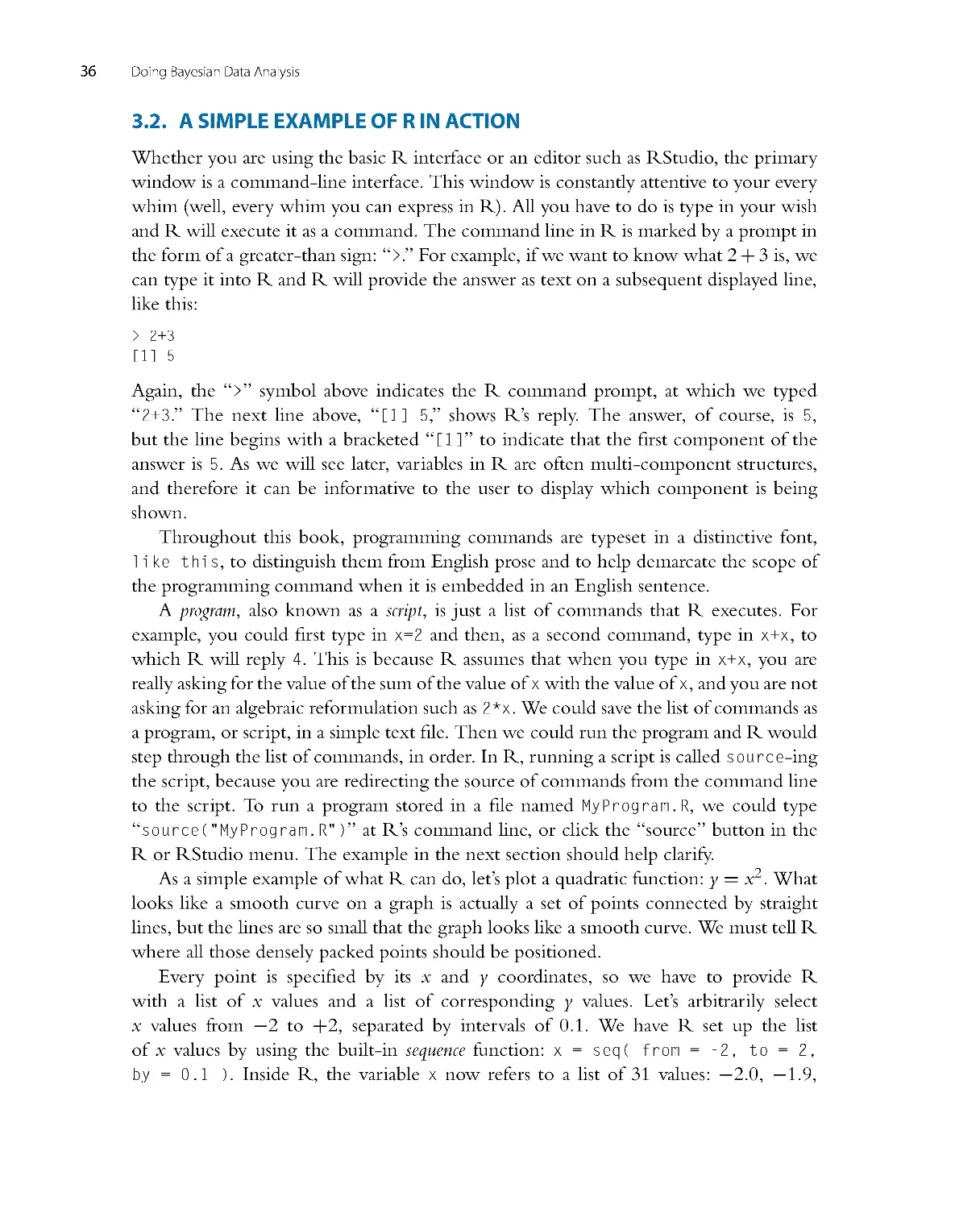
Figure 2.1 illustrates Holmes’ reasoning. For the pur poses of illustration, we suppose
that there are just four possible causes of the outcome to be explained. We label the
causes A, B, C, and D. The heights of the bars in the graphs indicate the credibility
of the candidate causes. (“Credibility” is synonymous with “probability”; here I use
the everyday term “credibility” but later in the book, when mathematical for malisms
are introduced, I will also use the term “probability.”) Credibility can range from zero
to one. If the credibility of a candidate cause is zero, then the cause is definitely not
responsible. If the credibility of a candidate cause is one, then the cause definitely is
responsible. Because we assume that the candidate causes are mutually exclusive and
exhaust all possible causes, the total credibility across causes sums to one.
The upper-left panel of Figure 2.1 shows that the prior credibilities of the four
candidate causes are equal, all at 0.25. Unlike the case of the wet sidewalk, in which
Introduction: Credibility, M odels, and Parameters
17
Prior
Possibilities
C
r
e
d
i
b
i
l
i
t
y
0
.
0
0
.
2
0
.
4
0
.
6
0
.
8
1
.
0
ABCD
Posterior
Possibilities
C
r
e
d
i
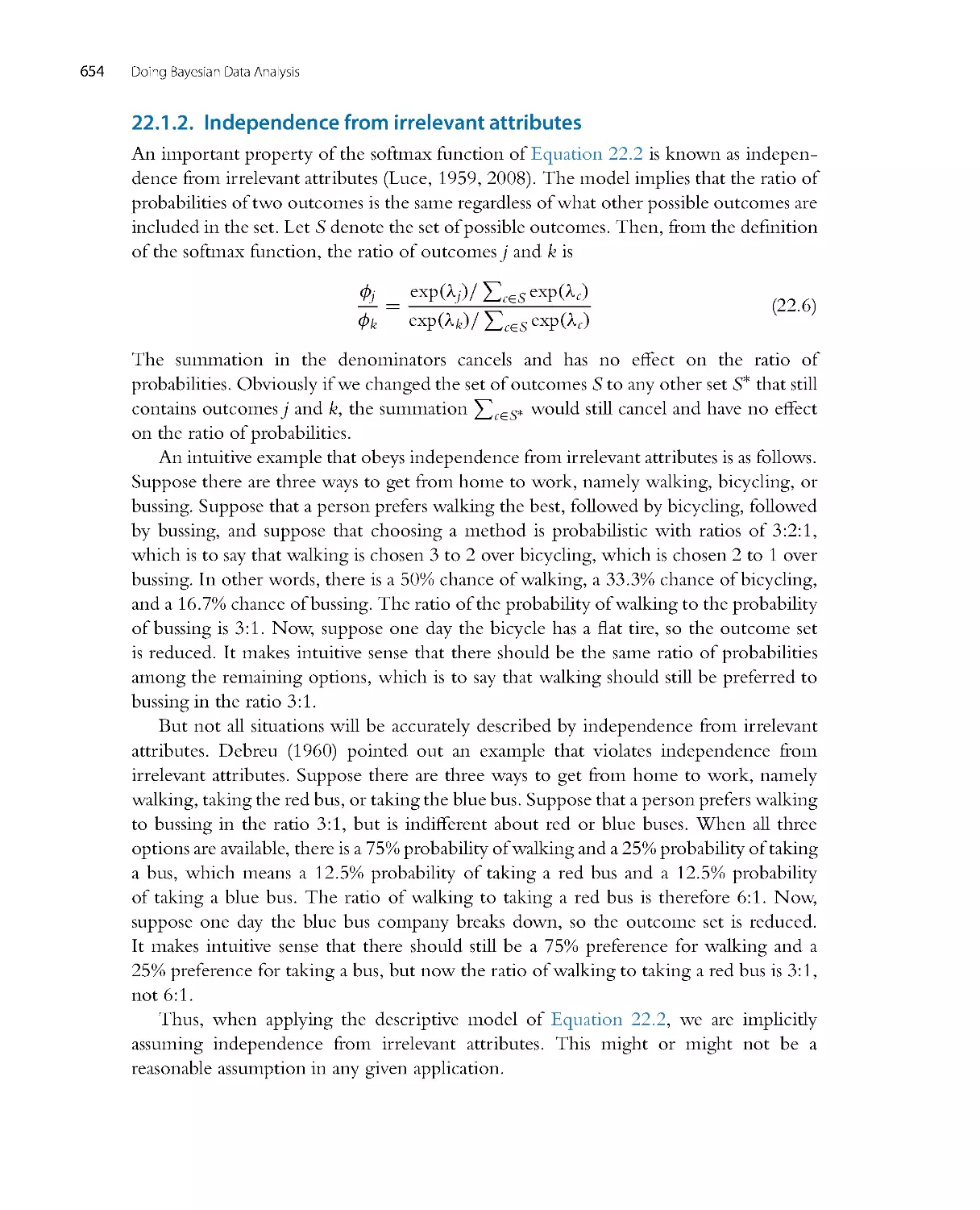
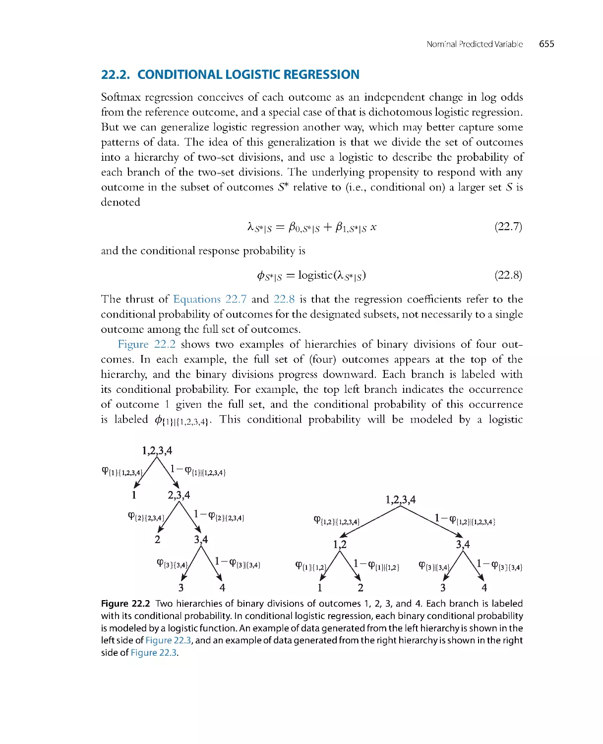
b
i
l
i
t
y
0
.
0
0
.
2
0
.
4
0
.
6
0
.
8
1
.
0
Ais
impossible
Prior
Possibilities
C
r
e
d
i
b
i
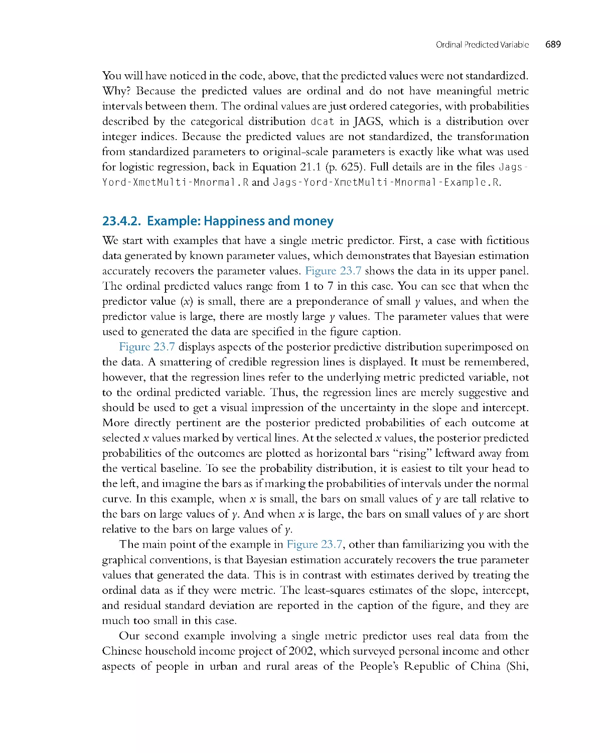
l
i
t
y
0
.
0
0
.
2
0
.
4
0
.
6
0
.
8
1
.
0
Posterior
Possibilities
C
r
e
d
i
b
i
l
i
t
y
0
.
0
0
.
2
0
.
4
0
.
6
0
.
8
1
.
0
Bis
impossible
ABCD
ABCD
ABCD
ABCD
Prior
Possibilities
C
r
e
d
i
b
i
l
i
t
y
0
.
0
0
.
2
0
.
4
0
.
6
0
.
8
1
.
0
ABCD
Posterior
Possibilities
C
r
e
d
i
b
i
l
i
t
y
0
.
0
0
.
2
0
.
4
0
.
6
0
.
8
1
.
0
Cis
impossible
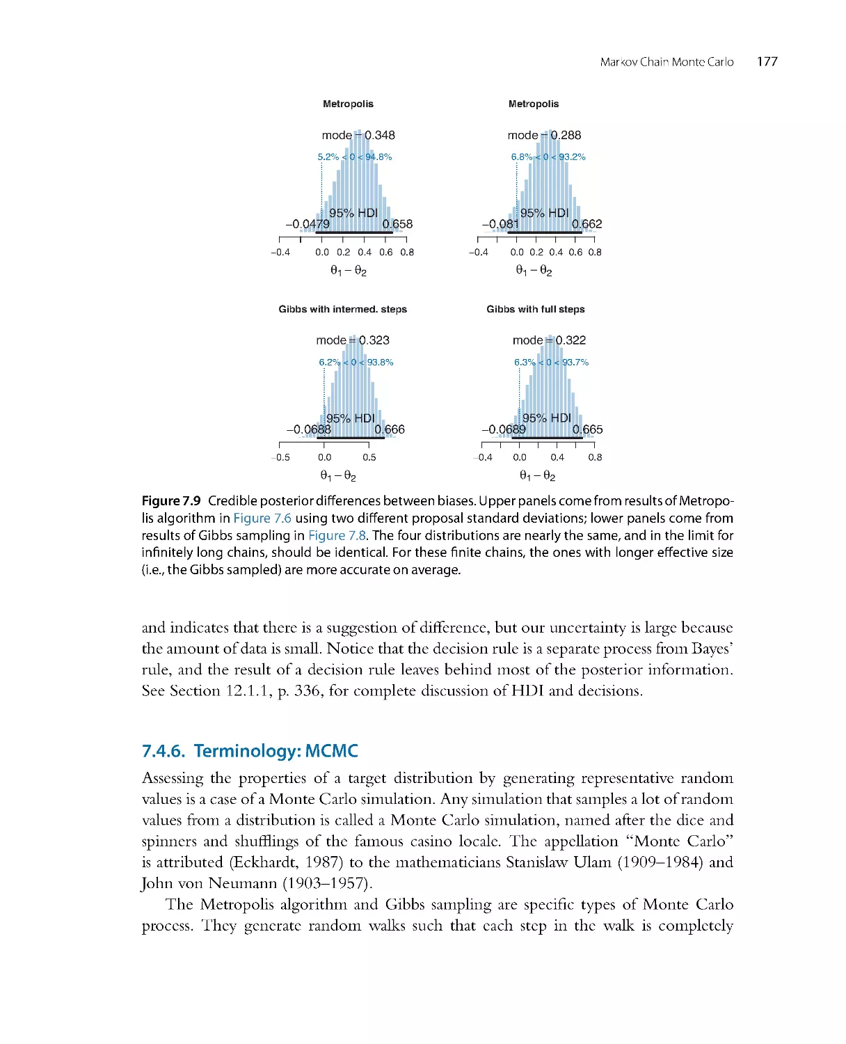
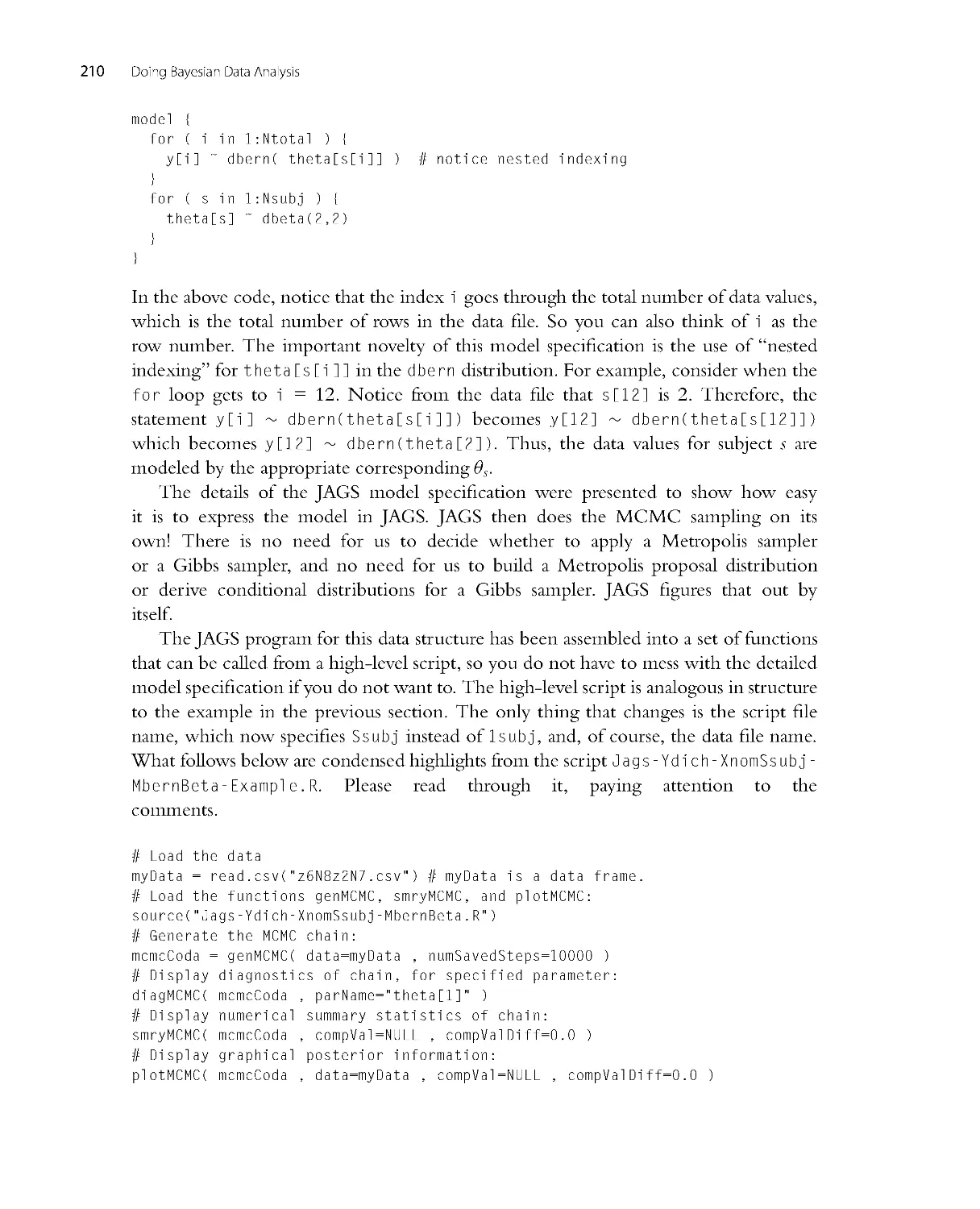
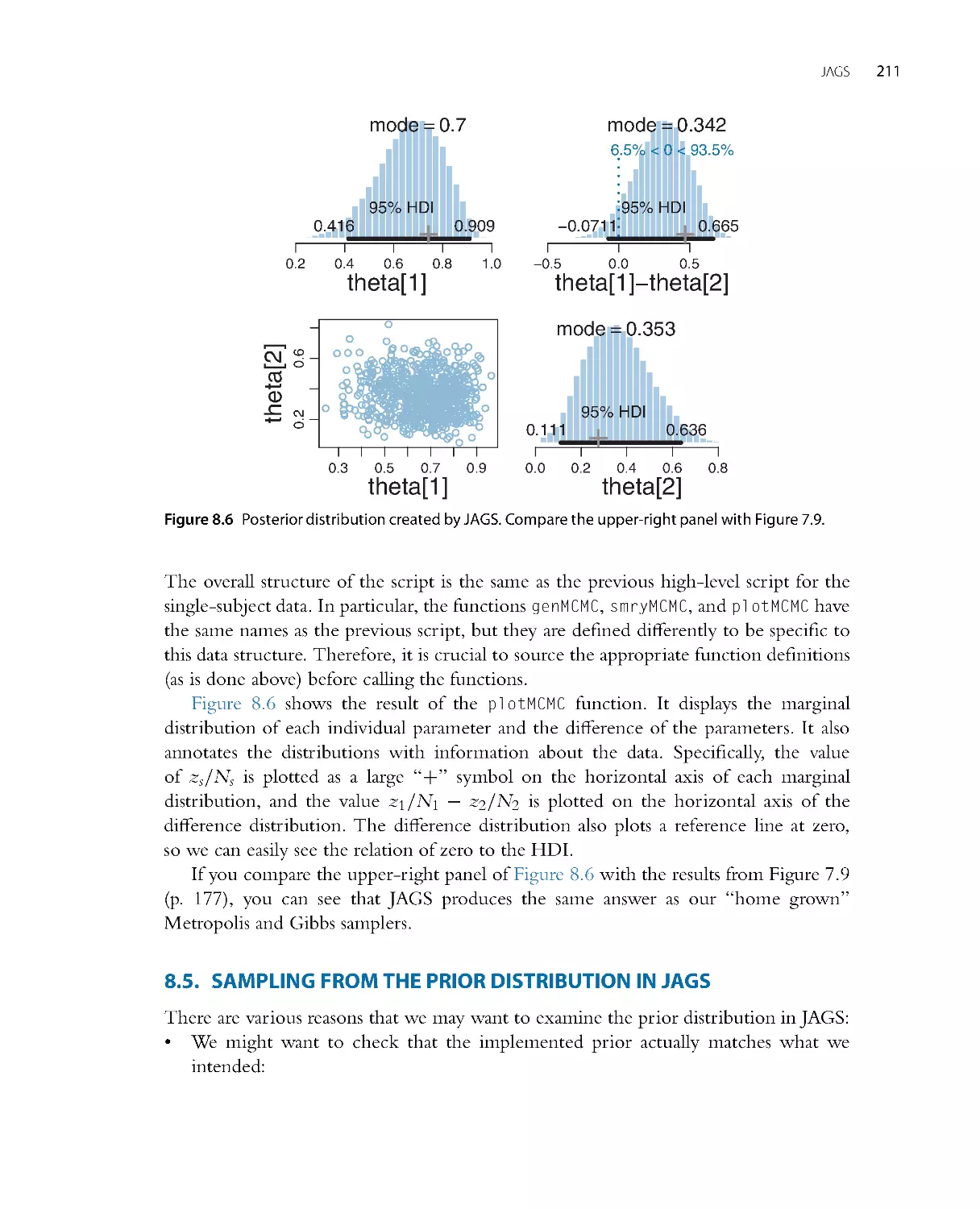
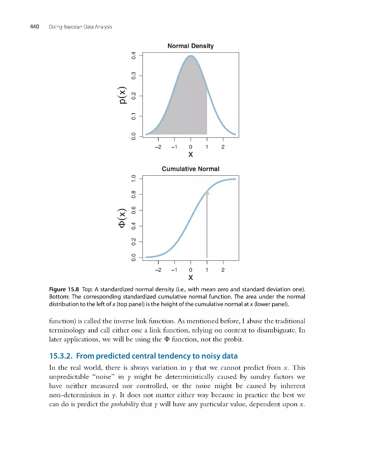
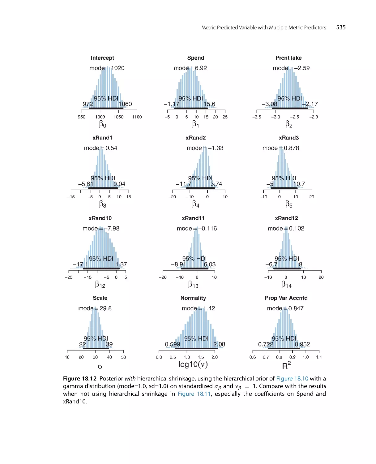
Figure 2.1 The upper-left graph shows the credibilities of the four possible causes for an outcome. The
causes, labeled A, B, C, and D, are mutually exclusive and exhaust all possibilities. The causes happen
to be equally credible at the outset; hence all have prior credibility of 0.25. The lower-left graph shows
the credibilities when one cause is learned to be impossible. The resulting posterior distribution is used
as the prior distribution in the middle column, where another cause is learned to be impossible. The
posterior distribution from the middle column is used as the prior distribution for the right column.
The remaining possible cause is fully implicated by Bayesian reallocation of credibility.
prior knowledge suggested that rain may be a more likely cause than a newly erupted
underground spring, the present illustration assumes equal prior credibilities of the
candidate causes. Suppose we make new observations that rule out candidate cause A.
For example, if A is a suspect in a crime, we may learn that A was far from the crime
scene at the time. Therefore, we must re-allocate credibility to the remaining candidate
causes, B through D, as shown in the lower-left panel of Figure 2.1 . The re-allocated
distribution of credibility is called the posterior distribution because it is what we believe
after taking into account the new observations. The poster ior distribution gives zero
credibility to cause A, and allocates credibilities of 0.33 (i.e., 1/3) to candidate causes B,
C, and D.
The poster ior distribution then becomes the prior beliefs for subsequent observa-
tions. Thus, the prior distr ibution in the upper-middle of Figure 2.1 is the poster ior
distribution from the lower left. Suppose now that additional new evidence rules out
candidate cause B. We now must re-allocate credibility to the remaining candidate
18
Doing Bayesian Data Analysis
causes, C and D, as shown in the lower-middle panel of Figure 2.1 . This posterior
distribution becomes the prior distr ibution for subsequent data collection, as shown in
the upper-r ight panel of Figure 2.1. Finally, if new data rule out candidate cause C, then
all credibility must fall on the remaining cause, D, as shown in the lower-right panel of
Figure 2.1, just as Holmes declared. This reallocation of credibility is not only intuitive,
it is also what the exact mathematics of Bayesian inference prescribe, as will be explained
later in the book.
The complementary for m of reasoning is also Bayesian, and can be called judicial
exoneration. Suppose there are several possible culprits for a crime, and that these suspects
are mutually unaffiliated and exhaust all possibilities. If evidence accrues that one suspect
is definitely culpable, then the other suspects are exonerated.
This for m of exoneration is illustrated in Figure 2.2. The upper panel assumes that
there are four possible causes for an outcome, labeled A, B, C, and D. We assume that
the causes are mutually exclusive and exhaust all possibilities. In the context of suspects
for a crime, the credibility of the hypothesis that suspect A committed the crime is the
Prior
Possibilities
C
r
e
d
i
b
i
l
i
t
y
0
.
0
0
.
2
0
.
4
0
.
6
0
.
8
1
.
0
ABCD
ABCD
Posterior
Possibilities
C
r
e
d
i
b
i
l
i
t
y
0
.
0
0
.
2
0
.
4
0
.
6
0
.
8
1
.
0
Dis
responsible
Figure 2.2 The upper graph shows the credibilities of the four possible causes for an outcome. The
causes, labeled A, B, C and D, are mutually exclusive and exhaust all possibilities. The causes happen
to be equally credible at the outset, hence all have prior credibility of 0.25. The lower graph shows the
credibilities when one cause is learned to be responsible. The nonresponsible causes are “exonerated”
(i.e., have zero credibility as causes) by Bayesian reallocation of credibility.
Introduction: Credibility, M odels, and Parameters
19
culpability of the suspect. So it might be easier in this context to think of culpability
instead of credibility. The prior culpabilities of the four suspects are, for this illustration,
set to be equal, so the four bars in the upper panel of Figure 2.2 are all of height 0.25.
Suppose that new evidence fir mly implicates suspect D as the culprit. Because the other
suspects are known to be unaffiliated, they are exonerated, as shown in the lower panel
of Figure 2.2. As in the situation of Holmesian deduction, this exoneration is not only
intuitive, it is also what the exact mathematics of Bayesian inference prescribe, as will be
explained later in the book.
2.1 .1 . Data are noisy and inferences are probabilistic
The cases of Figures 2.1 and 2.2 assumed that observed data had definitive, deter ministic
relations to the candidate causes. For example, the fictional Sherlock Holmes may have
found a footprint at the scene of the cr ime and identified the size and type of shoe with
complete certainty, thereby completely ruling out or implicating a particular candidate
suspect. In reality, of course, data have only probabilistic relations to their underlying
causes. A real detective might carefully measure the footprint and the details of its tread,
but these measurements would only probabilistically nar row down the range of possible
shoes that might have produced the print. The measurements are not perfect, and the
footprint is only an imperfect representation of the shoe that produced it. The relation
between the cause (i.e., the shoe) and the measured effect (i.e., the footprint) is full of
random variation.
In scientific research, measurements are replete with randomness. Extraneous influ-
ences contaminate the measurements despite tremendous efforts to limit their intrusion.
For example, suppose we are interested in testing whether a new drug reduces blood
pressure in humans. We randomly assign some people to a test group that takes the drug,
and we randomly assign some other people to a control group that takes a placebo. The
procedure is “double blind” so that neither the participants nor the administrators know
which person received the drug or the placebo (because that information is indicated by
a randomly assigned code that is decrypted after the data are collected). We measure the
participants’ blood pressures at set times each day for several days. As you can imagine,
blood pressures for any single person can vary wildly depending on many influences,
such as exercise, stress, recently eaten foods, etc. The measurement of blood pressure is
itself an uncertain process, as it depends on detecting the sound of blood flow under a
pressurized sleeve. Blood pressures are also very different from one person to the next.
The resulting data, therefore, are extremely messy, with tremendous var iability within
each group, and tremendous overlap across groups. Thus, there will be many measured
blood pressures in the drug group that are higher than blood pressures in the placebo
group, and vice versa. From these two dispersed and overlapping heaps of numbers, we
want to infer how big a difference there is between the groups, and how certain we can
20
Doing Bayesian Data Analysis
be about that difference. The problem is that for any particular real difference between
the drug and the placebo, its measurable effect is only a random impression.
All scientific data have some degree of “noise” in their values. The techniques of
data analysis are designed to infer underlying trends from noisy data. Unlike Sherlock
Holmes, who could make an observation and completely rule out some possible causes,
we can collect data and only incrementally adjust the credibility of some possible trends.
We will see many realistic examples later in the book. The beauty of Bayesian analysis
is that the mathematics reveal exactly how much to re-allocate credibility in realistic
probabilistic situations.
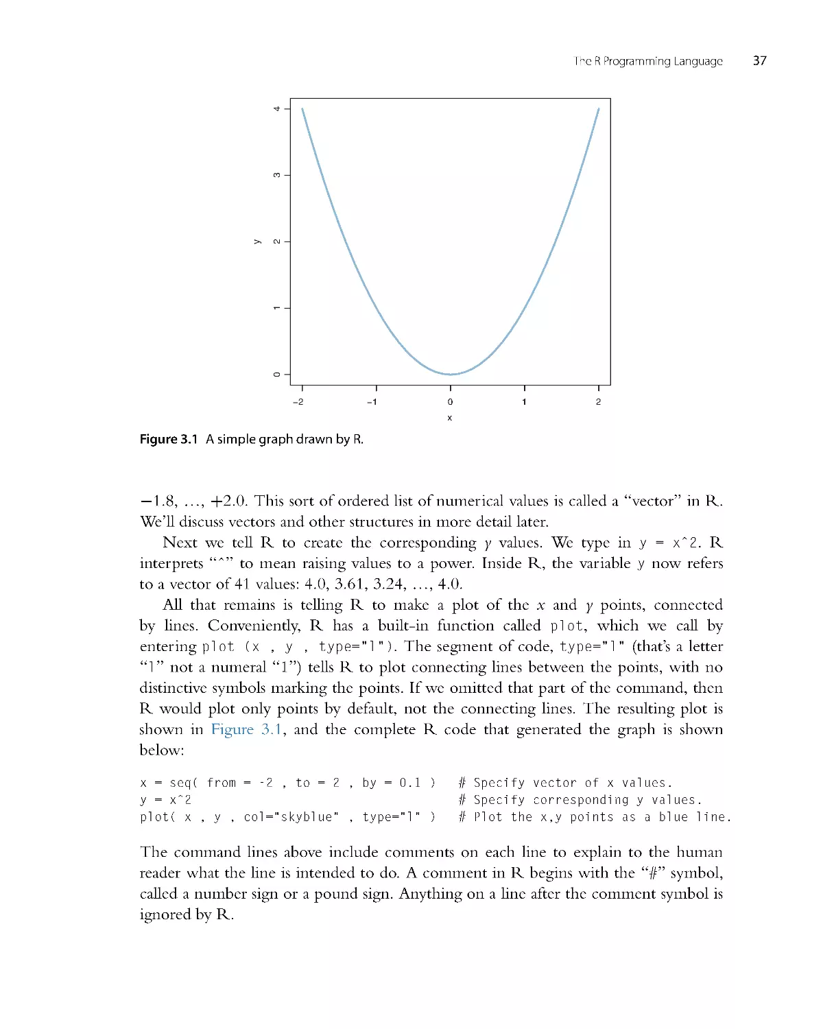
Here is a simplified illustration of Bayesian inference when data are noisy. Suppose
there is a manufacturer of inflated bouncy balls, and the balls are produced in four
discrete sizes, namely diameters of 1.0, 2.0, 3.0, and 4.0 (on some scale of distance
such as decimeters). The manufacturing process is quite var iable, however, because of
randomness in degrees of inflation even for a single size ball. Thus, balls of manufactured
size 3 might have diameters of 1.8 or 4.2, even though their average diameter is 3.0 .
Suppose we submit an order to the factory for three balls of size 2. We receive three balls
and measure their diameters as best we can, and find that the three balls have diameters
of 1.77, 2.23, and 2.70. From those measurements, can we conclude that the factory
cor rectly sent us three balls of size 2, or did the factory send size 3 or size 1 by mistake,
or even size 4?
Figure 2.3 shows a Bayesian answer to this question. The upper graph shows the four
possible sizes, with blue bars at positions 1, 2, 3, and 4. The prior credibilities of the
four sizes are set equal, at heights of 0.25, representing the idea that the factory received
the order for three balls, but may have completely lost track of which size was ordered,
hence any size is equally possible to have been sent.
At this point, we must specify the form of random variability in ball diameters.
For pur poses of illustration, we will suppose that ball diameters are centered on their
manufactured size, but could be bigger or smaller depending on the amount of inflation.
The bell-shaped curves in Figure 2.3 indicate the probability of diameters produced by
each size. Thus, the bell-shaped curve centered on size 2 indicates that size-2 balls are
usually about 2.0 units in diameter, but could be much bigger or smaller because of
randomness in inflation. The horizontal axis in Figure 2.3 is playing double duty as a
scale for the ball sizes (i.e., blue bars) and for the measured diameters (suggested by the
bell-shaped distributions).
The lower panel of Figure 2.3 shows the three measured diameters plotted as circles
on the horizontal axis. You can see that the measured diameters are closest to sizes 2
or 3, but the bell-shaped distributions reveal that even size 1 could sometimes produce
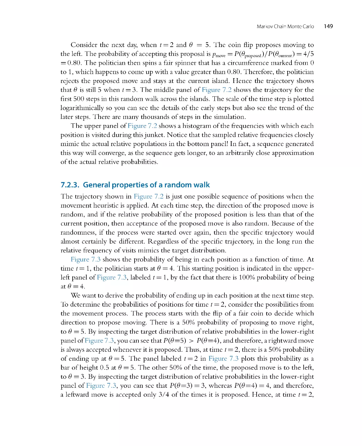
balls of those diameters. Intuitively, therefore, we would say that size 2 is most credible,
given the data, but size 3 is also somewhat possible, and size 1 is remotely possible,
but size 4 is rather unlikely. These intuitions are precisely reflected by Bayesian analysis,
Introduction: Credibility, M odels, and Parameters
21
Prior
Possibilities
C
r
e
d
i
b
i
l
i
t
y
0
.
0
0
.
2
0
.
4
0
.
6
0
.
8
1
.
0
1234
1234
Posterior
Possibilities
C
r
e
d
i
b
i
l
i
t
y
0
.
0
0
.
2
0
.
4
0
.
6
0
.
8
1
.
0
Figure 2.3 The upper graph shows the prior credibilities of the four candidate means in normal
distributions, located at values of 1, 2, 3, and 4. Superimposed on the means are the corresponding
normal distributions. The horizontal axis is playing double duty as a scale for the means (marked by
the blue bars) and for the data (suggested by the normal distributions). The three observed data values
are plotted as circles on the floor of the lower panel. Bayesian reallocation of credibility across the
four candidate means indicates that the mean at 2 is most credible given the data, the mean at 3 is
somewhat credible, and so on.
which is shown in the lower panel of Figure 2.3. The heights of the blue bars show the
exact reallocation of credibility across the four candidate sizes. Given the data, there is
56% probability that the balls are size 2, 31% probability that the balls are size 3, 11%
probability that the balls are size 1, and only 2% probability that the balls are size 4.
Infer ring the underlying manufactured size of the balls from their “noisy” individual
diameters is analogous to data analysis in real-world scientific research and applications.
The data are noisy indicators of the underlying generator. We hypothesize a range of
possible underlying generators, and from the data we infer their relative credibilities.
As another example, consider testing people for illicit drug use. A person is taken
at random from a population and given a blood test for an illegal drug. From the result
of the test, we infer whether or not the person has used the drug. But, crucially, the
test is not perfect, it is noisy. The test has a non-trivial probability of producing false
positives and false negatives. And we must also take into account our prior knowledge
22
Doing Bayesian Data Analysis
that the drug is used by only a small proportion of the population. Thus, the set of
possibilities has two values: The person uses the drug or does not. The two possibilities
have prior credibilities based on previous knowledge of how prevalent drug use is in
the population. The noisy datum is the result of the drug test. We then use Bayesian
inference to re-allocate credibility across the possibilities. As we will see quantitatively
later in the book, the posterior probability of drug use is often sur prisingly small even
when the test result is positive, because the prior probability of drug use is small and the
test is noisy. This is true not only for tests of drug use, but also for tests of diseases such
as cancer. A related real-world application of Bayesian inference is detection of spam
in email. Automated spam filters often use Bayesian inference to compute a poster ior
probability that an incoming message is spam.
In summary, the essence of Bayesian inference is reallocation of credibility across
possibilities. The distribution of credibility initially reflects prior knowledge about the
possibilities, which can be quite vague. Then new data are observed, and the credibility is
re-allocated. Possibilities that are consistent with the data gar ner more credibility, while
possibilities that are not consistent with the data lose credibility. Bayesian analysis is the
mathematics of re-allocating credibility in a logically coherent and precise way.
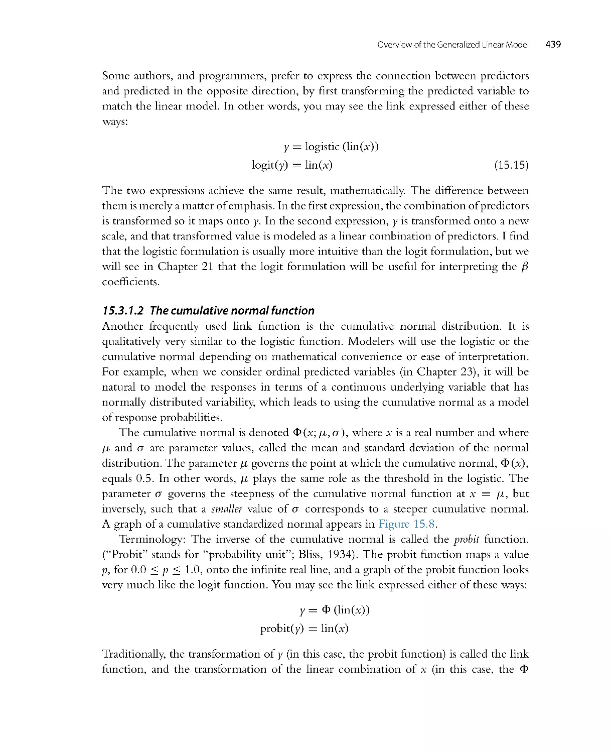
2.2. POSSIBILITIES ARE PARAMETER VALUES IN DESCRIPTIVE MODELS
A key step in Bayesian analysis is defining the set of possibilities over which credibility is
allocated. This is not a trivial step, because there might always be possibilities beyond the
ones we include in the initial set. (For example, the wetness on the sidewalk might have
been caused by space aliens who were crying big tears.) But we get the process going
by choosing a set of possibilities that covers a range in which we are interested. After
the analysis, we can examine whether the data are well described by the most credible
possibilities in the considered set. If the data seem not to be well described, then we can
consider expanding the set of possibilities. This process is called a posterior predictive
check and will be explained later in the book.
Consider again the example of the blood-pressure drug, in which blood pressures are
measured in one group that took the drug and in another group that took a placebo. We
want to know how much difference there is in the tendencies of the two groups: How
big is the difference between the typical blood pressure in one group versus the typical
blood pressure in the other group, and how certain can we be of the difference? The
magnitude of difference describes the data, and our goal is to assess which possible descriptions
aremoreorlesscredible.
In general, data analysis begins with a family of candidate descr iptions for the data.
The descriptions are mathematical formulas that characterize the trends and spreads in
the data. The formulas themselves have numbers, called parameter values, that determine
the exact shape of mathematical forms. You can think of parameters as control knobs on
Introduction: Credibility, M odels, and Parameters
23
mathematical devices that simulate data generation. If you change the value of a parameter, it
changes a trend in the simulated data, just like if you change the volume control on a
music player, it changes the intensity of the sound coming out of the player.
In previous studies of statistics or mathematics, you may have encountered the so-
called nor mal distribution, which is a bell-shaped distribution often used to descr ibe
data. It was alluded to above in the example of the inflated bouncy balls (see Figure 2.3).
The nor mal distr ibution has two parameters, called the mean and standard deviation.
The mean is a control knob in the mathematical for mula for the nor mal distribution
that controls the location of the distr ibution’s central tendency. The mean is sometimes
called a location parameter. The standard deviation is another control knob in the
mathematical formula for the nor mal distr ibution that controls the width or dispersion
of the distribution. The standard deviation is sometimes called a scale parameter.The
mathematical for mula for the normal distribution converts the parameter values to a
particular bell-like shape for the probabilities of data values.
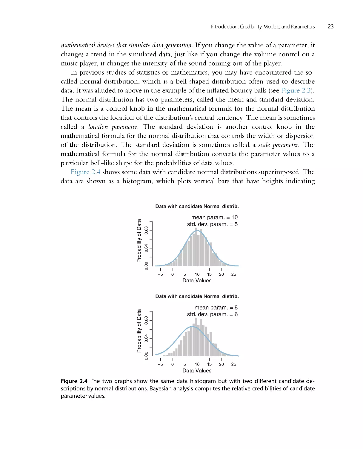
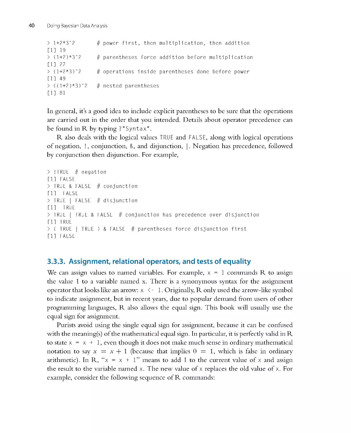
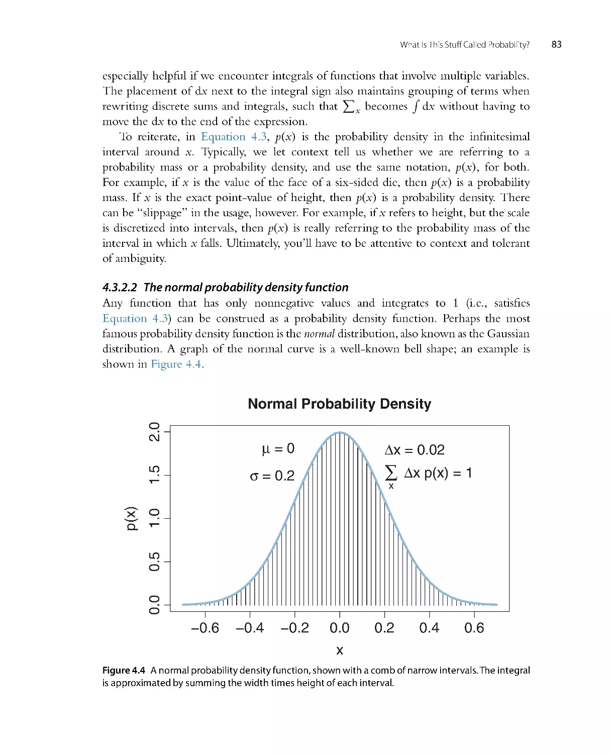
Figure 2.4 shows some data with candidate nor mal distr ibutions super imposed. The
data are shown as a histogram, which plots vertical bars that have heights indicating
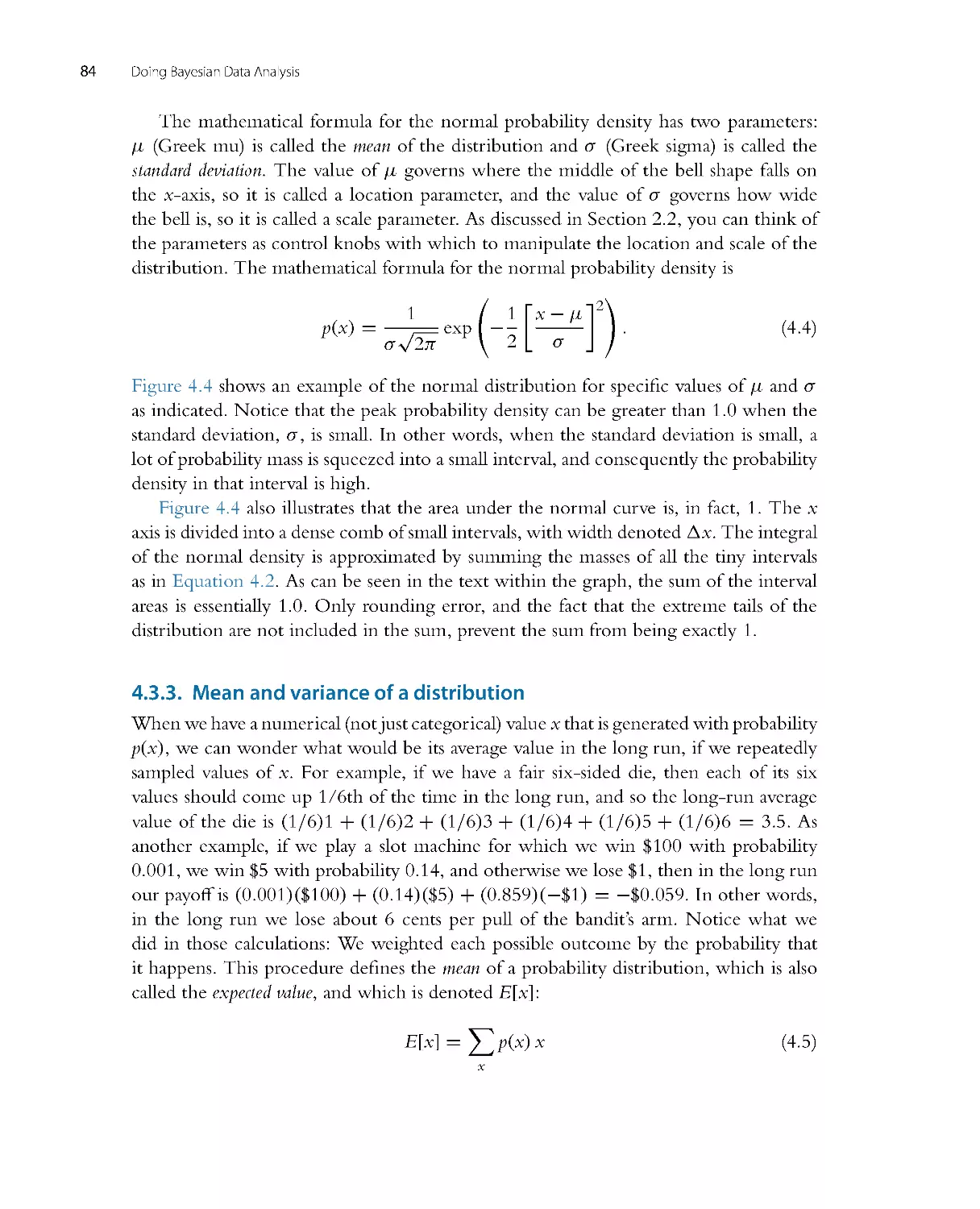
Data with candidate Normal distrib.
Data Values
P
r
o
b
a
b
i
l
i
t
y
o
f
D
a
t
a
−50
510152025
0
.
0
0
0
.
0
4
0
.
0
8
mean param. = 10
std. dev. param. = 5
Data with candidate Normal distrib.
Data Values
P
r
o
b
a
b
i
l
i
t
y
o
f
D
a
t
a
−50
510152025
0
.
0
0
0
.
0
4
0
.
0
8
mean param. = 8
std. dev. param. = 6
Figure 2.4 The two graphs show the same data histogram but with two different candidate de-
scriptions by normal distributions. Bayesian analysis computes the relative credibilities of candidate
parameter values.
24
Doing Bayesian Data Analysis
how much of the data falls within the small range spanned by the bar. The histogram
appears to be roughly unimodal and left-r ight symmetr ic. The upper panel super imposes
a candidate descr iption of the data in the form of a normal distribution that has a mean
of 10 and a standard deviation of 5. This choice of parameter values appears to descr ibe
the data well. The lower panel shows another choice of parameter values, with a mean of
8 and a standard deviation of 6. While this candidate descr iption appears to be plausible,
it is not as good as the upper panel. The role of Bayesian inference is to compute the
exact relative credibilities of candidate parameter values, while also taking into account
their prior probabilities.
In realistic applications, the candidate parameter values can form an infinite contin-
uum, not only a few discrete options. The location parameter of the nor mal distribution
can take on any value from negative to positive infinity. Bayesian inference operates
without trouble on infinite continuums.
There are two main desiderata for a mathematical descr iption of data. First, the
mathematical form should be comprehensible with meaningful parameters. Just as it
would be fruitless to descr ibe the data in a language that we do not know, it would
be fruitless to describe the data with a mathematical for m that we do not understand,
with parameters that we cannot interpret. In the case of a normal distribution, for
example, the mean parameter and standard-deviation parameter are directly meaningful
as the location and scale of the distribution. Throughout this book, we will use
mathematical descriptions that have meaningful parameters. Thus, Bayesian analysis re-
allocates credibility among parameter values within a meaningful space of possibilities
defined by the chosen model.
The second desideratum for a mathematical description is that it should be descrip-
tively adequate, which means, loosely, that the mathematical for m should “look like”
the data. There should not be any important systematic discrepancies between trends in
the data and the for m of the model. Deciding whether or not an apparent discrepancy
is important or systematic is not a definite process. In early stages of research, we
might be satisfied with a rough, “good enough” descr iption of data, because it captures
meaningful trends that are interesting and novel relative to previous knowledge. As the
field of research matures, we might demand more and more accurate descr iptions of data.
Bayesian analysis is very useful for assessing the relative credibility of different candidate
descr iptions of data.
It is also important to understand that mathematical descr iptions of data are not
necessarily causal explanations of data. To say that the data in Figure 2.4 are well described
by a nor mal distribution with mean of 10 and standard deviation of 5 does not explain
what process caused the data to have that form. The parameters are “meaningful” only
in the context of the familiar mathematical for m defined by the nor mal distribution; the
parameter values have no necessary meaning with respect to causes in the world. In some
applications, the mathematical model might be motivated as a descr iption of a natural
Introduction: Credibility, M odels, and Parameters
25
process that generated the data, and thereby the parameters and mathematical form can
refer to posited states and processes in the world. For example, in the case of the inflated
bouncy balls (Figure 2.3), the candidate parameter values were inter preted as “sizes”
at the manufacturer, and the underlying size, combined with random inflation, caused
the observed data value. But reference to physical states or processes is not necessary
for merely describing the trends in a sample of data. In this book, we will be focusing
on generic data description using intuitively accessible model for ms that are broadly
applicable across many domains.
2.3. THE STEPS OF BAYESIAN DATA ANALYSIS
In general, Bayesian analysis of data follows these steps:
1. Identify the data relevant to the research questions. What are the measurement scales
of the data? Which data variables are to be predicted, and which data variables are
supposed to act as predictors?
2. Define a descriptive model for the relevant data. The mathematical form and its
parameters should be meaningful and appropriate to the theoretical pur poses of the
analysis.
3. Specify a prior distr ibution on the parameters. The prior must pass muster with the
audience of the analysis, such as skeptical scientists.
4. Use Bayesian inference to re-allocate credibility across parameter values. Interpret
the posterior distribution with respect to theoretically meaningful issues (assuming
that the model is a reasonable description of the data; see next step).
5. Check that the posterior predictions mimic the data with reasonable accuracy (i.e.,
conduct a “poster ior predictive check”). If not, then consider a different descr iptive
model.
Perhaps the best way to explain these steps is with a realistic example of Bayesian data
analysis. The discussion that follows is abbreviated for pur poses of this introductory
chapter, with many technical details suppressed. For this example, suppose we are
interested in the relationship between weight and height of people. We suspect from
everyday exper ience that taller people tend to weigh more than shorter people,
but we would like to know by how much people’s weights tend to increase when
height increases, and how certain we can be about the magnitude of the increase.
In particular, we might be interested in predicting a person’s weight based on their
height.
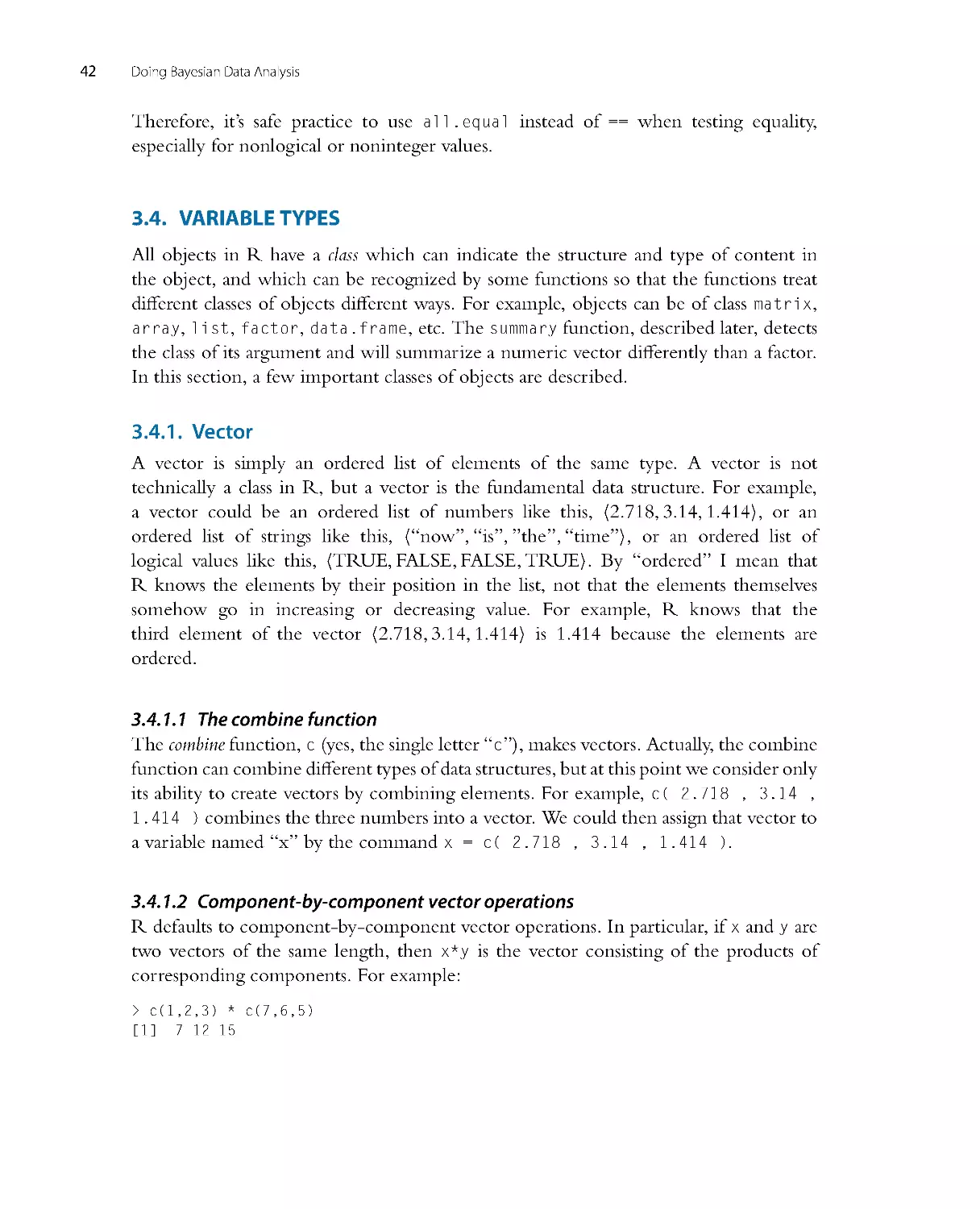
The first step is identifying the relevant data. Suppose we have been able to collect
heights and weights from 57 mature adults sampled at random from a population of
interest. Heights are measured on the continuous scale of inches, and weights are
measured on the continuous scale of pounds. We wish to predict weight from height. A
scatter plot of the data is shown in Figure 2.5 .
26
Doing Bayesian Data Analysis
55
60
65
70
75
80
5
0
1
0
0
1
5
0
2
0
0
2
5
0
Data with credible regression lines
Height in Inches
W
e
i
g
h
t
i
n
P
o
u
n
d
s
0
β1 (slope)
2468
mode = 4.11
0%<0<100%
95% HDI
2.64
5.7
Figure 2.5 Data are plotted as circles in the scatter plot of the left panel. The left panel also shows a
smattering of credible regression lines from the posterior distribution superimposed on the data. The
right panel shows the posterior distribution of the slope parameter (i.e ., β1 in Equation 2.1).
The second step is to define a descriptive model of the data that is meaningful
for our research interest. At this point, we are interested merely in identifying a basic
trend between weight and height, and it is not absurd to think that weight might be
proportional to height, at least as an approximation over the range of adult weights and
heights. Therefore, we will describe predicted weight as a multiplier times height plus a
baseline. We will denote the predicted weight as ˆy (spoken “y hat”), and we will denote
the height as x. Then the idea that predicted weight is a multiple of height plus a baseline
can be denoted mathematically as follows:
ˆ
y=β1x+β0
(2.1)
The coefficient, β1 (Greek letter “beta”), indicates how much the predicted weight
increases when the height goes up by one inch.2 The baseline is denoted β0 in
Equation 2.1, and its value represents the weight of a person who is zero inches tall.
You might suppose that the baseline value should be zero, apriori, but this need not be
the case for descr ibing the relation between weight and height of mature adults, who
have a limited range of height values far above zero. Equation 2.1 is the for m of a line,
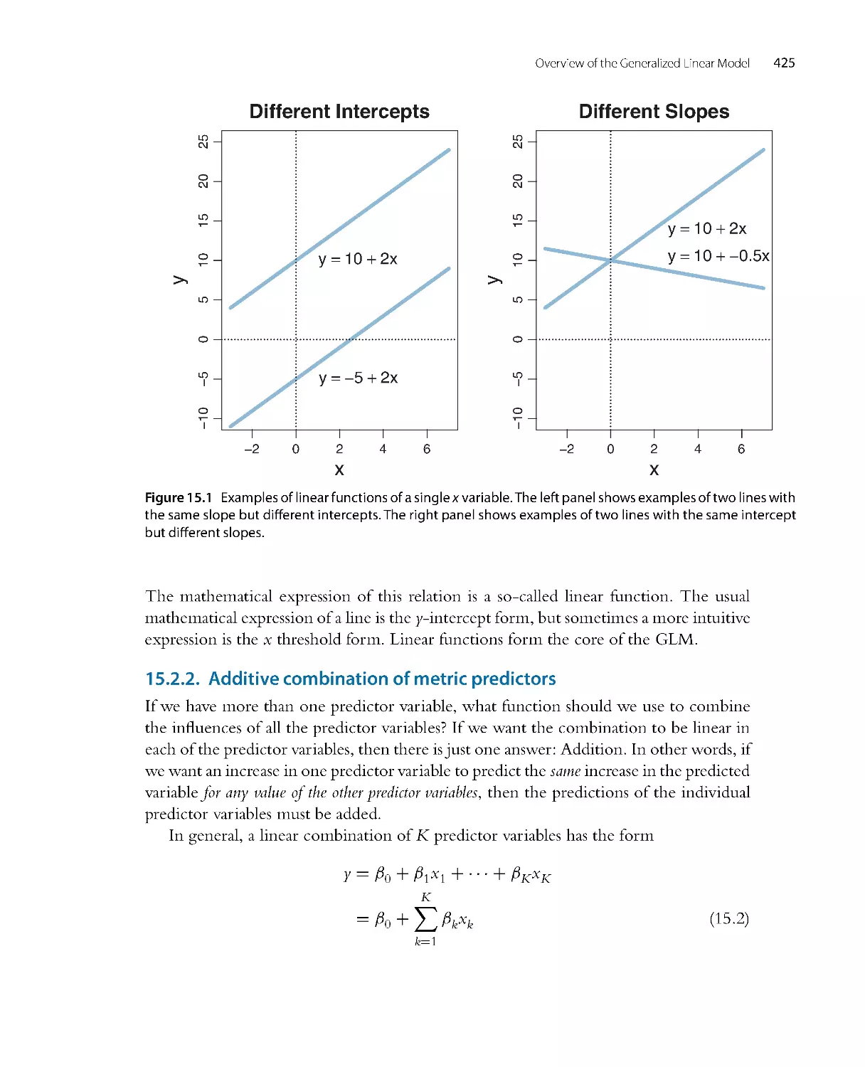
2 Here is a proof that β1 indicates how much that ˆy goes up when x increases by 1 unit. First, at height x,
the predicted weight is ˆyx = β1 x + β0 . Second, at height x + 1, the predicted weight is ˆyx+1 = β1(x +
1) + β0 = β1 x + β1 + β0 . Therefore, the change in predicted weight is ˆyx+1 −ˆ
yx=β1.
Introduction: Credibility, M odels, and Parameters
27
in which β1 is the slope and β0 is the intercept, and this model of trend is often called
linear regression.
The model is not complete yet, because we have to descr ibe the random var iation of
actual weights around the predicted weight. For simplicity, we will use the conventional
nor mal distribution (explained in detail in Section 4.3.2 .2), and assume that actual
weights y are distr ibuted randomly according to a nor mal distr ibution around the
predicted value ˆy and with standard deviation denoted σ (Greek letter “sigma”). This
relation is denoted symbolically as
y ∼ normal(ˆy, σ)
(2.2)
where the symbol “∼” means “is distributed as.” Equation 2.2 is saying that y values near
ˆ
y are most probable, and y values higher or lower than ˆy are less probable. The decrease
in probability around ˆy is governed by the shape of the normal distribution with width
specified by the standard deviation σ .
The full model, combining Equations 2.1 and 2.2, has three parameters altogether:
the slope, β1, the intercept, β0, and the standard deviation of the “noise,” σ . Note that
the three parameters are meaningful. In particular, the slope parameter tells us how much
the weight tends to increase when height increases by an inch, and the standard deviation
parameter tells us how much var iability in weight there is around the predicted value.
This sort of model, called linear regression, is explained at length in Chapters 15, 17,
and 18.
The third step in the analysis is specifying a prior distribution on the parameters. We
might be able to infor m the prior with previously conducted, and publicly ver ifiable,
research on weights and heights of the target population. Or we might be able to argue
for a modestly infor med prior based on consensual exper ience of social interactions.
But for purposes of this example, I will use a noncommittal and vague prior that places
virtually equal prior credibility across a vast range of possible values for the slope and
intercept, both centered at zero. I will also place a vague and noncommittal prior on
the noise (standard deviation) parameter, specifically a unifor m distr ibution that extends
from zero to a huge value. This choice of prior distr ibution implies that it has virtually
no biasing influence on the resulting poster ior distribution.
The fourth step is inter preting the poster ior distribution. Bayesian inference has re-
allocated credibility across parameter values, from the vague prior distr ibution, to values
that are consistent with the data. The poster ior distribution indicates combinations of
β0, β1,andσ that together are credible, given the data. The right panel of Figure 2.5
shows the posterior distr ibution on the slope parameter, β1 (collapsing across the other
two parameters). It is important to understand that Figure 2.5 shows a distr ibution
of parameter values, not a distribution of data. The blue bars of Figure 2.5 indicate
the credibility across the continuum of candidate slope values, analogous to the blue
28
Doing Bayesian Data Analysis
bars in the examples of Sherlock Holmes, exoneration, and discrete candidate means
(in Figures 2.1 –2.3). The poster ior distr ibution in Figure 2.5 indicates that the most
credible value of the slope is about 4.1, which means that weight increases about 4.1
pounds for every 1-inch increase in height. The poster ior distribution also shows the
uncertainty in that estimated slope, because the distribution shows the relative credibility
of values across the continuum. One way to summar ize the uncertainty is by marking
the span of values that are most credible and cover 95% of the distr ibution. This is
called the highest density interval (HDI) and is marked by the black bar on the floor of
the distribution in Figure 2.5 . Values within the 95% HDI are more credible (i.e., have
higher probability “density”) than values outside the HDI, and the values inside the
HDI have a total probability of 95%. Given the 57 data points, the 95% HDI goes from
a slope of about 2.6 pounds per inch to a slope of about 5.7 pounds per inch. With more
data, the estimate of the slope would be more precise, meaning that the HDI would be
nar rower.
Figure 2.5 also shows where a slope of zero falls relative to the posterior distr ibution.
In this case, zero falls far outside any credible value for the slope, and therefore we could
decide to “reject” zero slope as a plausible description of the relation between height and
weight. But this discrete decision about the status of zero is separate from the Bayesian
analysis per se, which provides the complete posterior distr ibution.
Many readers may have previously learned about null hypothesis significance testing
(NHST) which involves sampling distributions of summary statistics such as t,fromwhich
are computed p values. (If you do not know these terms, do not wor ry. NHST
will be discussed in Chapter 11.) It is important to understand that the poster ior
distribution in Figure 2.5 is not a sampling distribution and has nothing to do with
p values.
Another useful way of understanding the posterior distribution is by plotting
examples of credible regression lines through the scatter plot of the data. The left panel
of Figure 2.5 shows a random smatter ing of credible regression lines from the posterior
distribution. Each line plots ˆy = β1x + β0 for credible combinations of β1 and β0.The
bundle of lines shows a range of credible possibilities, given the data, instead of plotting
only a single “best” line.
The fifth step is to check that the model, with its most credible parameter values,
actually mimics the data reasonably well. This is called a “poster ior predictive check.”
There is no single, unique way to ascertain whether the model predictions systematically
and meaningfully deviate from the data, because there are innumerable ways in which
to define systematic deviation. One approach is to plot a summary of predicted data
from the model against the actual data. We take credible values of the parameters, β1,
β0,andσ , plug them into the model Equations 2.1 and 2.2, and randomly generate
simulated y values (weights) at selected x values (heights). We do that for many, many
Introduction: Credibility, M odels, and Parameters
29
55
60
65
70
75
80
5
0
1
0
0
1
5
0
2
0
0
2
5
0
Data with 95% HDI & Mean of Posterior Predictions
Height in Inches
W
e
i
g
h
t
i
n
P
o
u
n
d
s
Figure 2.6 The data of Figure 2.5 are shown with posterior predicted weight values superimposed at
selected height values. Each vertical bar shows the range of the 95% most credible predicted weight
values, and the dot at the middle of each bar shows the mean predicted weight value.
credible parameter values to create representative distr ibutions of what data would look
like according to the model. The results of this simulation are shown in Figure 2.6 .
The predicted weight values are summar ized by vertical bars that show the range of the
95% most credible predicted weight values. The dot at the middle of each bar shows
the mean of the predicted weight values. By visual inspection of the graph, we can
see that the actual data appear to be well descr ibed by the predicted data. The actual
data do not appear to deviate systematically from the trend or band predicted from
the model.
If the actual data did appear to deviate systematically from the predicted form, then
we could contemplate alter native descriptive models. For example, the actual data might
appear to have a nonlinear trend. In that case, we could expand the model to include
nonlinear trends. It is straightforward to do this in Bayesian software, and easy to estimate
the parameters that descr ibe nonlinear trends. We could also examine the distr ibutional
properties of the data. For example, if the data appear to have outliers relative to what
is predicted by a normal distribution, we could change the model to use a heavy-tailed
distr ibution, which again is straightforward in Bayesian software.
30
Doing Bayesian Data Analysis
We have seen the five steps of Bayesian analysis in a fairly realistic example. This
book explains how to do this sort of analysis for many different applications and types
of descr iptive models. For a shorter but detailed introduction to Bayesian analysis for
compar ing two groups, with explanation of the perils of the classical t test, see the
article by Kruschke (2013a). For an introduction to Bayesian analysis applied to multiple
linear regression, see the article by Kruschke, Aguinis, and Joo (2012). For a perspective
on poster ior predictive checks, see the article by Kruschke (2013b) and Section 17.5 .1
(among others) of this book.
2.3 .1 . Data analysis without parametric models?
As outlined above, Bayesian data analysis is based on meaningfully parameterized
descr iptive models. Are there ever situations in which such models cannot be used or
are not wanted?
One situation in which it might appear that parameterized models are not used is with
so-called nonparametr ic models. But these models are confusingly named because they
actually do have parameters; in fact they have a potentially infinite number of parameters.
As a simple example, suppose we want to descr ibe the weights of dogs. We measure the
weights of many different dogs sampled at random from the entire spectrum of dog
breeds. The weights are probably not distr ibuted unimodally, instead there are probably
subclusters of weights for different breeds of dogs. But some different breeds might
have nearly identical distributions of weights, and there are many dogs that cannot be
identified as a particular breed, and, as we gather data from more and more dogs, we
might encounter members of new subclusters that had not yet been included in the
previously collected data. Thus, it is not clear how many clusters we should include
in the descr iptive model. Instead, we infer, from the data, the relative credibilities of
different cluster ings. Because each cluster has its own parameters (such as location and
scale parameters), the number of parameters in the model is infer red, and can grow
to infinity with infinite data. There are many other kinds of infinitely parameterized
models. For a tutor ial on Bayesian nonparametr ic models, see Gershman and Blei (2012);
for a recent review, see Müller and Mitra (2013); and for textbook applications, see
Gelman et al. (2013). We will not be considering Bayesian nonparametr ic models in
this book.
There are a var iety of situations in which it might seem at first that no parameter ized
model would apply, such as figur ing out the probability that a person has some rare
disease if a diagnostic test for the disease is positive. But Bayesian analysis does apply even
here, although the parameters refer to discrete states instead of continuous distr ibutions.
In the case of disease diagnosis, the parameter is the underlying health status of the
individual, and the parameter can have one of two values, either “has disease” or “does
Introduction: Credibility, M odels, and Parameters
31
not have disease.” Bayesian analysis re-allocates credibility over those two parameter
values based on the observed test result. This is exactly analogous to the discrete
possibilities considered by Sherlock Holmes in Figure 2.1, except that the test results
yield probabilistic information instead of perfectly conclusive information. We will do
exact Bayesian computations for this sort of situation in Chapter 5 (see specifically
Table 5.4).
Finally, there might be some situations in which the analyst is loathe to commit to any
parameter ized model of the data, even tremendously flexible infinitely parameter ized
models. If this is the case, then Bayesian methods cannot apply. These situations are
rare, however, because mathematical models are enormously useful tools. One case of
trying to make inferences from data without using a model is a method from NHST
called resampling or bootstrapping. These methods compute p values to make decisions,
and p values have fundamental logical problems that will be discussed in Chapter 11.
These methods also have very limited ability to express degrees of certainty about
characteristics of the data, whereas Bayesian methods put expression of uncertainty front
and center.
2.4. EXERCISES
Look for more exercises at https://sites.google.com/site/doingbayesiandataanalysis/
Exercise 2.1. [Purpose: To get you actively manipulating mathematical
models of probabilities.] Suppose we have a four-sided die from a board game. On
a tetrahedral die, each face is an equilateral triangle. When you roll the die, it lands with
one face down and the other three faces visible as a three-sided pyramid. The faces are
numbered 1-4, with the value of the bottom face printed (as clustered dots) at the bottom
edges of all three visible faces. Denote the value of the bottom face as x. Consider the
following three mathematical descr iptions of the probabilities of x.ModelA:p(x) = 1/4.
Model B: p(x) = x/10. Model C: p(x) = 12/(25x). For each model, deter mine the
value of p(x) for each value of x. Descr ibe in words what kind of bias (or lack of bias) is
expressed by each model.
Exercise 2.2. [Purpose: To get you actively thinking about how data cause
credibilities to shift.] Suppose we have the tetrahedral die introduced in the previous
exercise, along with the three candidate models of the die’s probabilities. Suppose that
initially, we are not sure what to believe about the die. On the one hand, the die might
be fair, with each face landing with the same probability. On the other hand, the die
might be biased, with the faces that have more dots landing down more often (because
the dots are created by embedding heavy jewels in the die, so that the sides with more
dots are more likely to land on the bottom). On yet another hand, the die might be
32
Doing Bayesian Data Analysis
biased such that more dots on a face make it less likely to land down (because maybe
the dots are bouncy rubber or protrude from the surface). So, initially, our beliefs about
the three models can be described as p(A) = p(B) = p(C) = 1/3. Now we roll the
die 100 times and find these results: #1’s = 25, #2’s = 25, #3’s = 25, #4’s = 25. Do
these data change our beliefs about the models? Which model now seems most likely?
Suppose when we rolled the die 100 times we found these results: #1’s = 48, #2’s = 24,
#3’s = 16, #4’s = 12. Now which model seems most likely?
CHAPTER 3
The R Programming Language
Contents
3.1 . GettheSoftware....................................................................... 35
3.1 .1 A look at RStudio ................................................................. 35
3.2 . ASimpleExampleofRinAction......................................................... 36
3.2 .1 Gettheprogramsusedwiththisbook .............................................. 38
3.3 . BasicCommandsandOperatorsinR..................................................... 38
3.3 .1 GettinghelpinR ................................................................. 39
3.3 .2 Arithmeticandlogicaloperators.................................................... 39
3.3 .3 Assignment,relationaloperators,andtestsofequality................................ 40
3.4 . VariableTypes ......................................................................... 42
3.4 .1 Vector........................................................................... 42
3.4
.
1.1 Thecombinefunction............................................................. 42
3.4
.
1.2 Component-by
-
componentvectoroperations........................................ 42
3.4
.
1.3 Thecolonoperatorandsequencefunction........................................... 43
3.4
.
1.4 Thereplicatefunction............................................................. 44
3.4
.
1.5 Gettingatelementsofavector..................................................... 45
3.4 .2 Factor........................................................................... 46
3.4 .3 Matrixandarray.................................................................. 48
3.4 .4 Listanddataframe ............................................................... 51
3.5 . LoadingandSavingData ............................................................... 53
3.5 .1 The read.csv and read.table functions.......................................... 53
3.5 .2 SavingdatafromR................................................................ 55
3.6 . SomeUtilityFunctions.................................................................. 56
3.7 . ProgramminginR...................................................................... 61
3.7 .1 VariablenamesinR............................................................... 61
3.7 .2 Runningaprogram............................................................... 62
3.7 .3 Programmingafunction........................................................... 64
3.7 .4 Conditions and loops ............................................................. 65
3.7 .5 Measuringprocessingtime........................................................ 66
3.7 .6 Debugging...................................................................... 67
3.8 . GraphicalPlots:OpeningandSaving..................................................... 69
3.9 . Conclusion............................................................................ 69
3.10. Exercises.............................................................................. 70
Doing Bayesian Data Analysis, 2nd Edition
Copyright © 2015 Elsevier Inc.
http://dx.doi.org/10.1016/B978-0-12-405888-0.00003 -9
All rights reserved.
33
34
Doing Bayesian Data Analysis
You said, dear Descartes, that “je pense, donc je suis,”
Deriving existence from uncertainty.
Now, you are gone, and we say, “au revoir,”
Doubtless we think, René, therefore we R.1
In this book, you will learn how to actually do Bayesian data analysis. For any but the
simplest models, that means using a computer. Because the computer results are so central
to doing real Bayesian data analysis, examples of using the R computer programming
language will be integrated into the simplest “toy” problems, so that R will not be an
extra hurdle later.
The material in this chapter is rather dull reading because it basically amounts to a
list (although a carefully scaffolded list) of basic commands in R along with illustrative
examples. After reading the first few pages and nodding off, you may be tempted to skip
ahead, and I wouldn’t blame you. But much of the material in this chapter is crucial, and
all of it will eventually be useful, so you should at least skim it all so you know where to
retur n when the topics arise later.
Here are a few of the essential points of this chapter:
•
Software installation. Section 3.1 descr ibes how to install the R programming
language. Section 3.1 .1 describes how to install the R editor called RStudio.
Section 3.2.1 describes how to install the programs wr itten for this book.
•
Data for mats. Section 3.5.1 descr ibes how to read data files into R. To understand
the resulting format, you’ll need to understand the data.frame structure from
Section 3.4.4, which in turn requires understanding the list and matrix and
factor structures (which is why those structures are explained before getting to
the data.frame structure).
•
Running programs. Section 3.7 .2 explains how to run programs in R, and points
out that it is important to set R’s working directory to the folder in which the
programs reside.
The R programming language is great at doing Bayesian statistics for a number of reasons.
First, it’s free! You can get it via the web and easily install it on your computer. Second,
it’s already a popular language for doing Bayesian statistics, so there are lots of resources
available. Third, it is a powerful and easy, general-pur pose computing language, so you
can use it for many other applications too. The Bayesian MCMC packages that we will
rely on later can be accessed from other programming environments but we’ll use R.
1 This chapter introduces the prog ramming language R. The poem provides motivation for using R,
primarily in the form of an extended setup for the final pun on the word “are.” Further background:
The French philosopher and mathematician, René Descartes (1596–1650), wondered how he could be
certain of anything. The only thing he could be certain of was his own thoughts of uncertainty, and
therefore he, as thinker, must exist. In English, the idea is captured by the phrase, “I think therefore I am.”
Changed to plural, the phrase becomes “we think therefore we are.”
The R Programming Language
35
If you would like to learn more about the history of R, see its web page at http://www.
r-project.org/ which also has extensive documentation about the R language.
3.1. GET THE SOFTWARE
It’s easy to get and install R, but there are a lot of optional details in the process, and the
hardest part of installation is figuring out which little details do not apply to you!
Basic installation of R is easy. Go to http://cran.r-project.org/. (Web site addresses
occasionally change. If the address stated here does not work, please search the web
for “R language.” Be sure the site is legitimate before downloading anything to your
computer.) At the top of that web page is a section headed “Download and Install R”
followed by three links: Linux, MacOS, and Windows. These three links refer to the
type of operating system used on your computer. Get the version that matches your
computer’s operating system. For example, if you click Windows, the next page that
appears has a var iety of links. The only one you need to click is “base,” which will get
you to the most recent version of R for downloading. There are a few subsequent details
specifictoeachoperatingsystemthatyouhavetonavigateonyourown,butremember
that centuries ago lots of people crossed various oceans in tiny wooden boats without
any electronics, so you can navigate the small per ils of R installation.
2
3.1 .1 . A look at RStudio
The R programming language comes with its own basic user interface that is adequate
for modest applications. But larger applications become unwieldy in the basic R user
interface, and therefore it helps to install a more sophisticated R-friendly editor. There
are a number of useful editors available, many of which are free, and they are constantly
evolving. At the time of this wr iting, I recommend RStudio, which can be obtained
from http://www.rstudio.com/. (Web site addresses occasionally change. If the address
stated here does not work, please search the web for “RStudio.” Be sure the site is
legitimate before downloading anything to your computer.) Just go to the web site, find
the download link, and get the version appropriate to your computer operating system.
There are various ways to invoke R. One way is by starting R directly. For example,
in Windows, you could just double-click the R icon, or find R in the list of programs
from the Start menu. A second way to invoke R is via your favorite R editor. For
example, invoke RStudio, which then automatically and transparently communicates
with R. A third way to invoke R, and the best way for our purposes, is to associate files that
have a “.R” extension on their filename with RStudio. Then, when the file is opened,
your computer knows to invoke RStudio and open the file in RStudio. An example of
doing this will be provided soon.
2 Of course, lots of people failed to cross the ocean, but that’s different.
36
Doing Bayesian Data Analysis
3.2. A SIMPLE EXAMPLE OF R IN ACTION
Whether you are using the basic R interface or an editor such as RStudio, the primary
window is a command-line interface. This window is constantly attentive to your every
whim(well,everywhimyoucanexpressinR).Allyouhavetodoistypeinyourwish
and R will execute it as a command. The command line in R is marked by a prompt in
the form of a greater-than sign: “>.”Forexample,ifwewanttoknowwhat2+ 3is,we
can type it into R and R will provide the answer as text on a subsequent displayed line,
like this:
> 2+3
[1] 5
Again, the “>” symbol above indicates the R command prompt, at which we typed
“ 2+3.” The next line above, “[1] 5,” shows R’s reply. The answer, of course, is 5,
but the line begins with a bracketed “[1]” to indicate that the first component of the
answer is 5. As we will see later, var iables in R are often multi-component structures,
and therefore it can be infor mative to the user to display which component is being
shown.
Throughout this book, programming commands are typeset in a distinctive font,
like this, to distinguish them from English prose and to help demarcate the scope of
the programming command when it is embedded in an English sentence.
A program, also known as a script, is just a list of commands that R executes. For
example, you could first type in x=2 and then, as a second command, type in x+x,to
which R will reply 4. This is because R assumes that when you type in x+x,youare
really asking for the value of the sum of the value of x with the value of x, and you are not
asking for an algebraic reformulation such as 2*x. We could save the list of commands as
a program, or scr ipt, in a simple text file. Then we could run the program and R would
step through the list of commands, in order. In R, running a scr ipt is called source-ing
the script, because you are redirecting the source of commands from the command line
to the scr ipt. To run a program stored in a file named MyProgram.R, we could type
“source("MyProgram.R")” at R’s command line, or click the “source” button in the
R or RStudio menu. The example in the next section should help clarify.
As a simple example of what R can do, let’s plot a quadratic function: y = x2 .What
looks like a smooth curve on a graph is actually a set of points connected by straight
lines, but the lines are so small that the graph looks like a smooth curve. We must tell R
where all those densely packed points should be positioned.
Every point is specified by its x and y coordinates, so we have to provide R
with a list of x values and a list of cor responding y values. Let’s arbitrarily select
x values from −2to+2, separated by intervals of 0.1. We have R set up the list
of x values by using the built-in sequence function: x = seq( from = - 2, to = 2,
by = 0.1 ). Inside R, the variable x now refers to a list of 31 values: −2.0, −1.9,
The R Programming Language
37
−2
−1
0
1
2
0
1
2
3
4
x
y
Figure 3.1 A simple graph drawn by R.
−1 .8, ..., +2.0. This sort of ordered list of numer ical values is called a “vector” in R.
We’ll discuss vectors and other structures in more detail later.
Next we tell R to create the corresponding y values. We type in y=x
ˆ 2.R
inter prets “ ˆ ” to mean raising values to a power. Inside R, the var iable y now refers
to a vector of 41 values: 4.0, 3.61, 3.24, ..., 4.0.
All that remains is telling R to make a plot of the x and y points, connected
by lines. Conveniently, R has a built-in function called plot, which we call by
enter ing plot (x,y,type="l"). The segment of code, type="l" (that’s a letter
“l” not a numeral “1”) tells R to plot connecting lines between the points, with no
distinctive symbols marking the points. If we omitted that part of the command, then
R would plot only points by default, not the connecting lines. The resulting plot is
shown in Figure 3.1, and the complete R code that generated the graph is shown
below:
x = seq( from = -2 , to=2,by=0
.
1) #Specify vector of x values.
y=xˆ2
# Specify corresponding y values.
plot(x,y,col="skyblue" , type="l" ) # Plot the x,y points as a blue line.
The command lines above include comments on each line to explain to the human
reader what the line is intended to do. A comment in R begins with the “#”symbol,
called a number sign or a pound sign. Anything on a line after the comment symbol is
ignored by R.
38
Doing Bayesian Data Analysis
3.2 .1 . Get the programs used with this book
The program above is stored as a file named SimpleGraph.R in the folder of programs
that accompany the book. For the latest updates about programs used with this book,
see the book’s web site at https://sites.google.com/site/doingbayesiandataanalysis/, and
the book’s blog at http://doingbayesiandataanalysis.blogspot.com/. (Web site addresses
occasionally change. If either of the addresses stated here does not work, please search
the web for “Doing Bayesian Data Analysis” in quotes. Be sure the site is legitimate
before downloading anything to your computer.) Specifically, find the link to the zip
file that contains all the programs used with this book. Save the zip file at a convenient
location on your computer where you nor mally save your data files and documents. (Do
not save it in a protected area such as Programs in the Windows operating system.) Be
sure to “unzip” the file or “extract all” of the programs from the zipped folder.
The simplest way to open the program is to associate the file with RStudio and
then open the file. For example, in the Windows operating system, find the file
SimpleGraph.R . Right-click it and select “Open with...” and then browse to RStudio.
Be sure to select (i.e., check) the box that says to always use RStudio to open files of this
type. Then, the file will open in the RStudio editor, ready for running and additional
editing as desired.
One of the benefits of opening a program directly and letting it automatically invoke
RStudio, instead of opening RStudio and subsequently loading the program, is that
RStudio sets the working directory to the folder in which the program resides. The working
directory is where R first looks for auxiliary programs and where R saves output files.
If you invoke RStudio from scratch, instead of via a program file, then the working
directory is a default generic folder and consequently R will not know where to find
auxiliary programs used with this book. More information about setting the working
directory will appear later.
One of the programs accompanying this book has filename ExamplesOfR.R.That
file contains most of the examples in this chapter (other than SimpleGraph.R).
I recommend that you open it in R and try the examples as you read about them.
Or just type in the examples at the command line.
3.3. BASIC COMMANDS AND OPERATORS IN R
The rest of this chapter describes some of the important features of the R programming
language. There are many other sources available online, including the introductory
manual, the latest version of which should be available at this address: http://cran.r -
project.org/doc/manuals/r-release/R-intro.pdf . If that link no longer works by the
time you read this, do a little searching of documentation on the R home page or on
the web.
The R Programming Language
39
3.3 .1 . Getting help in R
The plot function has many optional details that you can specify, such as the axis
limits and labels, font sizes, etc. You can learn more about those details by getting help
from R. Type the command ?"plot" and you can read all about it. In particular, the
information directs you to another command, par, that controls all the plot parameters.
To learn about it, type ?"par". In general, it actually is helpful to use R’s built-in
help. To get a list of all sorts of online documentation, much of it wr itten in readable
prose instead of telegraphic lists, type help.start() including the empty parentheses.
In particular, the list of manuals displayed by help.start() includes An Introduction
to R, which is highly recommended. Another useful way to find help with R is
through web search. In your favorite web searcher, type in the R terms you want
help with.
Also very useful is the double question mark, which is an abbreviation for the
help.search function, and which searches the entire help database for entries that
contain the specified word or phrase. While ?"plot" returns the single help page that
explains the plot function, ??"plot" retur ns a list of dozens of help pages that contain
the word “plot.” (For more details, you can type ?"?" and ?"??" at R’s command
prompt.)
A highly recommended resource is a summary of basic R commands that can be
found on a compact list available at this address:
http://cran.r -project.org/doc/contr ib/Short-refcard.pdf
Other versions of reference cards can be found by searching the web with the phrase
“ R reference card.”
Much of the time you’ll lear n about features of R on an as-needed basis, and usually
that means you’ll look for examples of the sort of thing you want to do and then imitate
the example. (Or, the example might at least provoke you into realizing that there is a
better way to do it than the method in the example!) Therefore, most of the examples
in this book have their full R code included. Hopefully, it will help you to study those
examples as needed.
If you are already familiar with the programming languages Matlab or Python,
you can find thesauruses of synonymous commands in R at this Web site: http://
mathesaurus.sourceforge.net/.
3.3 .2 . Arithmetic and logical operators
The four arithmetic operators are typed as +, -, *,and/. Power is typed as ˆ. When
operators are specified successively, they are processed left to right, except that power has
precedence over multiplication and division, which have precedence over addition and
subtraction. Make sure you understand the output returned by each of the following
examples:
40
Doing Bayesian Data Analysis
> 1+2*3ˆ2
# power first, then multiplication, then addition
[1] 19
> (1+2)*3ˆ2
# parentheses force addition before multiplication
[1] 27
> (1+2*3)ˆ2
# operations inside parentheses done before power
[1] 49
> ((1+2)*3)ˆ2 # nested parentheses
[1] 81
In general, it’s a good idea to include explicit parentheses to be sure that the operations
are carr ied out in the order that you intended. Details about operator precedence can
be found in R by typing ?"Syntax".
R also deals with the logical values TRUE and FALSE, along with logical operations
of negation, !, conjunction, &, and disjunction, |. Negation has precedence, followed
by conjunction then disjunction. For example,
> !TRUE # negation
[1] FALSE
> TRUE & FALSE # conjunction
[1] FALSE
> TRUE | FALSE # disjunction
[1] TRUE
> TRUE | TRUE & FALSE # conjunction has precedence over disjunction
[1] TRUE
> ( TRUE | TRUE ) & FALSE # parentheses force disjunction first
[1] FALSE
3.3 .3 . Assignment, relational operators, and tests of equality
We can assign values to named variables. For example, x=1commands R to assign
the value 1 to a var iable named x. There is a synonymous syntax for the assignment
operator that looks like an arrow: x<-1
. Originally, R only used the ar row-like symbol
to indicate assignment, but in recent years, due to popular demand from users of other
prog ramming languages, R also allows the equal sign. This book will usually use the
equal sign for assignment.
Purists avoid using the single equal sign for assignment, because it can be confused
with the meaning(s) of the mathematical equal sign. In particular, it is perfectly valid in R
to state x=x+1, even though it does not make much sense in ordinary mathematical
notationtosayx = x + 1 (because that implies 0 = 1, which is false in ordinary
arithmetic). In R, “x=x+1” means to add 1 to the cur rent value of x and assign
the result to the variable named x. The new value of x replaces the old value of x.For
example, consider the following sequence of R commands:
The R Programming Language
41
>x=2
#assign the value 2 to x
>x=x+1 #add1tothevalue of x and assign the result to x
>x
# show the value of x
[1] 3
In practice, this possible misinterpretation of an R command as a mathematical statement
of equality is rare or nonexistent. Besides, R uses the single equal sign for assignment-
like operations in arguments of functions and in definitions of list structures (as will be
explained subsequently). Therefore, I am not deterred from using the single equal sign
for assignment.
Beware, however, not be confuse the assignment operator = with a test for equality,
which is denoted in R by a double equal sign. The double equal sign tests for equality
and retur ns a value of TRUE or FALSE. For example:
>x=2 #assign the value 2 to the variable named x
>x
# show the value of x
[1] 2
>x==2#checkwhetherthevalueofxisequalto2
[1] TRUE
There are also relational operators for inequalities:
>x!=3#checkwhetherthevalueofxisNOTequalto3
[1] TRUE
>x<3 #check whether the value of x is less than 3
[1] TRUE
>x>3 #check whether the value of x is greater than 3
[1] FALSE
If you use <- for the assignment operator instead of =, be certain not to accidentally
insert a space: The expression x<-3assigns the value 3 to x, but the expression x
<-3tests whether x is less than the value −3andreturnsTRUE or FALSE (or an error
message if x does not exist).
The double equal sign for testing equality, used above, is brittle and can give
unintended results due to the limited precision of representing numbers in the computer’s
memory. For example, in most computers, the value of 0.5 − 0 .3 does not equal the
value of 0.3 − 0.1, even though mathematically they are equivalent. Therefore, R has
another function, all.equal, for testing equality up to the degree of precision for the
computer being used. For example:
>x=0
.
5-0
.
3
>y=0
.
3-0
.
1
> x == y # although mathematically TRUE, it’s FALSE for limited precision
[1] FALSE
> all.equal(x,y) # equal up to precision of computer
[1] TRUE
42
Doing Bayesian Data Analysis
Therefore, it’s safe practice to use all.equal instead of == when testing equality,
especially for nonlogical or noninteger values.
3.4. VARIABLE TYPES
All objects in R have a class which can indicate the structure and type of content in
the object, and which can be recognized by some functions so that the functions treat
different classes of objects different ways. For example, objects can be of class matrix,
array, list, factor, data.frame,etc.Thesummary function, described later, detects
the class of its argument and will summar ize a numeric vector differently than a factor.
In this section, a few important classes of objects are descr ibed.
3.4.1. Vector
A vector is simply an ordered list of elements of the same type. A vector is not
technically a class in R, but a vector is the fundamental data structure. For example,
a vector could be an ordered list of numbers like this, 2.718, 3.14, 1.414,oran
ordered list of str ings like this, “now”, “is”, ”the”, “time”, or an ordered list of
logical values like this, TRUE, FALSE, FALSE, TRUE. By “ordered” I mean that
R knows the elements by their position in the list, not that the elements themselves
somehow go in increasing or decreasing value. For example, R knows that the
third element of the vector 2.718, 3.14, 1.414 is 1.414 because the elements are
ordered.
3.4 .1 .1 The combine function
The combine function, c (yes, the single letter “c”),makesvectors.Actually,thecombine
function can combine different types of data structures, but at this point we consider only
its ability to create vectors by combining elements. For example, c( 2.718 , 3.14 ,
1.414 ) combines the three numbers into a vector. We could then assign that vector to
a variable named “x” by the command x = c( 2.718 , 3.14 , 1.414 ).
3.4 .1 .2 Component-by-component vector operations
R defaults to component-by-component vector operations. In particular, if x and y are
two vectors of the same length, then x*y is the vector consisting of the products of
cor responding components. For example:
> c(1,2,3) * c(7,6,5)
[1] 71215
The R Programming Language
43
R automatically applies a scalar operation to all elements of a vector. For example:
> 2 * c(1,2,3)
[1]246
> 2 + c(1,2,3)
[1]345
3.4 .1 .3 The colon operator and sequence function
The colon operator, :, makes sequences of integers. For example, 4:7 creates the
vec to r 4, 5, 6, 7. The combine function and the colon operator are used very of-
ten in R programming. The colon operator has precedence over basic arithmetical
operators, but not over the power operator. Consider carefully the output of these
examples:
> 2+3:6
# colon operator has precedence over addition
[1]5678
> (2+3):6
# parentheses override default precedence
[1]56
> 1:3ˆ2
# power operator has precedence over colon operator
[1]123456789
> (1:3)ˆ2
# parentheses override default precedence
[1]149
In general, to be sure that the computations are executed in the order that you intend,
include explicit parentheses.
The sequence function, seq, is very handy for creating vectors that consist of
regular sequences of numbers. In its basic form, the user specifies the starting value
of the sequence, the ending value, and the increment between successive values,
like this:
> seq( from=0 , to=3 , by=0.5 )
# length not specified
[1] 0.0 0.5 1.0 1.5 2.0 2.5 3.0
If the increment is not an exact divisor of the distance between the starting and ending
values, the sequence will not exceed the ending value. For example:
> seq( from=0 , to=3 , by=0.5001 )
# will not exceed end value
[1] 0.0000 0.5001 1.0002 1.5003 2.0004 2.5005
The seq function is clever and will infer whatever value is omitted by the user.
This capability can be very useful, for example if we want a sequence of a certain
length and do not care about the exact end point or the increment. Consider these
examples:
44
Doing Bayesian Data Analysis
> seq( from=0 , by=0.5 , length.out=7 ) # end not specified
[1] 0.0 0.5 1.0 1.5 2.0 2.5 3.0
> seq( from=0 , to=3 , length.out=7 ) # increment not specified
[1] 0.0 0.5 1.0 1.5 2.0 2.5 3.0
> seq( to=3 , by=0.5 , length.out=7 ) # start not specified
[1] 0.0 0.5 1.0 1.5 2.0 2.5 3.0
3.4 .1 .4 The replicate function
The replicate function, rep, is also very useful for creating vectors. Here are some
examples:
> ABC = c("A ","B","C") # define a vector for replication
>rep(ABC,2)
[1] "A" "B" "C" "A" "B" "C"
> rep( ABC, times=2 )
[1] "A" "B" "C" "A" "B" "C"
> rep( ABC, times=c(4,2,1) )
[1] "A" "A" "A" "A" "B" "B" "C"
> rep( ABC, each=2 )
[1] "A" "A" "B" "B" "C" "C"
> rep( ABC, each=2, length=10)
[1] "A" "A" "B" "B" "C" "C" "A" "A" "B" "B"
> rep( ABC, each=2, times=3)
[1] "A" "A" "B" "B" "C" "C" "A" "A" "B" "B" "C" "C" "A" "A" "B" "B" "C" "C"
Notice above that rep has three optional arguments after the first argument (which is the
structure to be replicated). When only one integer is entered, as in the second line above,
then rep assumes it is the number of times that the entire structure should be replicated.
According to the R help file, “Nor mally just one of the additional arguments is specified,
but if each is specified with either of the other two, its replication is performed first,
and then that implied by times or length.out.” If you intend that each component
should be replicated first, be sure to use the each argument explicitly, or use the times
argument in its vector form.
Here is an example to test your understanding of the rep function:
> rep( ABC, each=2, times=c(1,2,3,1,2,3) )
[1] "A" "A" "A" "B" "B" "B" "B" "C" "C" "C" "C" "C"
What happened in that example is that the each=2 argument was applied first,
thereby creating (inter nally) the vector c("A","A","B","B","C","C"), which has six
components. After that, the times=c(1,2 ,3 ,1 ,2 ,3) argument was applied, which
created one copy of the first “A,” followed by two copies of the second “A,” followed
by three copies of the first “B,” and so forth. In other words, the same result could be
created by the following nested application of rep:
The R Programming Language
45
> rep( rep( ABC, each=2 ) , times=c(1,2,3,1,2,3) )
[1] "A" "A" "A" "B" "B" "B" "B" "C" "C" "C" "C" "C"
3.4 .1 .5 Getting at elements of a vector
Yoohoo, time to wake up! The methods of this section will be used often. In R, we
can get at elements of a vector by referencing their position in the vector. There are
three ways to reference elements: by numer ical position, by logical inclusion, and by
name. All three ways refer to positions by using square brackets after the vector name,
like this: x[...]. What differs between the methods is what goes between the square
brackets.
We can refer to elements by their numerical position. For example, suppose we
define a vector x=c( 2.718 , 3 .14 , 1.414 , 47405 ). We can get the elements of
the vector by referr ing to the rank positions inside square brackets after the vector name.
Thus, x[c(2,4)] returns the second and fourth elements, as the vector 3.14, 47405.
Another way to get at elements is by telling R which position not to include, by using
a negative sign. For example, if you want all the elements except the first and third, you
can type x[c(-1, -3)].
Another way to access elements of a vector is by a sequence of logical
true and false values that specify whether or not to return the cor responding
element. For example, x[c(FALSE,TRUE,FALSE,TRUE)] also retur ns the vector 3.14,
47405.
The elements of a vector can also, optionally, have names.Forexample,wecan
name the elements of the vector x with the command, names(x)=c( "e" , "pi" ,
"sqrt2" , "zipcode" ). Notice that the names are in quotes. Then we get at the
components of the vector by specifying their names in square brackets. For example,
x[c("pi","zipcode")] retur ns the vector 3.14, 47405 along with the names of those
components.
To recapitulate and summarize, here are some different ways to get at the elements
of a vector:
>x=c(2.718 , 3.14 , 1.414 , 47405 )
# define the vector
> names(x) = c( "e" , "pi" , "sqrt2" , "zipcode" ) # name the components
> x[c(2,4)]
# which indices to include
pi zipcode
3.14 47405.00
> x[c(-1,-3)]
# which indices to exclude
pi zipcode
3.14 47405.00
> x[c(FALSE,TRUE,FALSE,TRUE)] # for each position, include it?
pi zipcode
3.14 47405.00
46
Doing Bayesian Data Analysis
> x[c("pi","zipcode")]
# names of indices to include
pi zipcode
3.14 47405.00
3.4.2. Factor
Factors are a type of vector in R for which the elements are categorical values that could
also be ordered. The values are stored inter nally as integers with labeled levels. The best
way to explain factors is by example.
Suppose we have data regarding the socio-economic status of five people, coded as
one of “low,” “medium,” or “high.” Here are the data, in the vector named x:
>x=c("high" , "medium" , "low" , "high" , "medium" )
The ter ms “high,” “medium,” and “low” get a bit unwieldy in large data sets, and
therefore it can be useful to recode them into categorical indices, such as “1” for “low,”
“2” for “medium,” and “3” for “high.” The data become a vector of indices along with a
legend from translating from the indices to names for the indices. The resulting structure
is called a “factor.” In R, the factor function converts the vector x to a factor:
>xf=factor(x)
To see what the factor xf looks like, we can type “xf” at R’s command line and see
what R retur ns:
>xf
[1] high medium low
high medium
Levels: high low medium
Notice that R has extracted “levels” from the vector and listed them after the contents
of the factor. The factor function read the contents of vector x and kept track of all
the distinct elements, calling them the levels of the factor. By default, it ordered the
levels alphabetically. It then recoded the contents of the vector in terms of the integer indices of
the alphabetized levels. Thus, the or iginal element “high” becomes integer “1” because
“high” is alphabetically first among the three levels. You can think of the real contents
of the factor as being the integer indices of the levels, along with a legend that decodes
each integer into a level name. To see the integer indices of the levels explicitly, we can
ask R to show us the factor as a numeric vector:
> as.numeric(xf)
[1]13213
The factor command extracts the levels and orders them alphabetically by default.
Unfortunately, alphabetical order depends on local language customs (e.g., uppercase
The R Programming Language
47
letters might go before lowercase letters or after), and alphabetical order might not be
the most meaningful order for a given application. If we want to specify a particular
order for the levels, we can do so with additional arguments in the factor function, like
this:
> xfo = factor( x , levels=c("low","medium","high") , ordered=TRUE )
> xfo
[1] high medium low
high medium
Levels: low < medium < high
Notice now that the levels are displayed with less-than signs to indicate that they are
ordered. And, when we examine the integer indices internal to the factor, they are
coded according to the desired order, such that the first element, “high,” is coded as
integer 3, not as 1:
> as.numeric(xfo)
[1]32132
It is good practice to explicitly specify the levels and their order ing when making a
factor.
Sometimes we will want to reorder the levels of a factor that has already been created.
This can happen, for example, when reading in a data file using default settings, but
subsequently reordering to make the levels more meaningful. To reorder, just use the
factor function again, explicitly indicating the desired levels and order. For example,
we create factor xf as before:
>x=c("high" , "medium" , "low" , "high" , "medium" )
> xf = factor( x ) # results in default ordering
>xf
[1] high medium low
high medium
Levels: high low medium
> as.numeric(xf)
[1]13213
But now we reorder the levels by applying the factor function to the existing factor xf:
> xf = factor( xf , levels=c("low","medium","high") , ordered=TRUE )
>xf
[1] high medium low
high medium
Levels: low < medium < high
> as.numeric(xf)
[1]32132
Notice that explicitly reordering the levels has also changed the underlying integer
coding of the elements in the vector, as it should. It is good practice to specify the
order ing of the levels explicitly.
48
Doing Bayesian Data Analysis
We might want to relabel the levels of a factor. For example, the vector x used
elements named low, medium, and high. The levels argument of the factor function
must refer to those exact terms for reading in the data. But for the resulting output, the
levels can be relabeled to whatever might be more meaningful for the application, such
as “Bottom SES,” “Middle SES,” and “Top SES.” We accomplish the relabeling in R
with the labels argument:
> xfol = factor( x , levels=c("low","medium","high") , ordered=TRUE ,
labels=c("Bottom SES","Middle SES","Top SES") )
> xfol
[1] Top SES
Middle SES Bottom SES Top SES
Middle SES
Levels: Bottom SES < Middle SES < Top SES
Notice that the original data ter ms (low, medium, high) are no longer accessible in
the factor. It is important to realize that relabeling the levels does not change their order or their
integer coding. For example, if we specify labels=c("Right","Left", "UpsideDown"),
the integers will be unchanged, but their labeling will no longer be meaningful.
Factors will appear frequently when R reads data from files. Factors can be very
useful for some functions in R. But factors can be confusing if you are not aware that a
variable is being stored by R as a factor and not as a vector. Factors can also be confusing
if the default order ing of their levels is not intuitive.
3.4 .3 . Matrix and array
A matrix is simply a two-dimensional ar ray of values of the same type. A matr ix can be
created in R using the matrix command. The first argument specifies the contents of
the matr ix, in order. Other arguments specify the size of the matr ix, the order in which
the matr ix should be filled, and, optionally, the names of the dimensions and rows and
columns. (The names are specified as a list, which is a structure that is descr ibed
explicitly very soon, in Section 3.4 .4.) Please note the comments in the following
examples:
> matrix( 1:6 , ncol=3 ) # contents are 1:6, filled by column
[,1] [,2] [,3]
[
1
,
]135
[
2
,
]246
> matrix( 1:6 , nrow=2 ) # or you can specify number of rows
[,1] [,2] [,3]
[
1
,
]135
[
2
,
]246
The R Programming Language
49
> matrix( 1:6 , nrow=2 , byrow=TRUE ) # filled by row instead of by column
[,1] [,2] [,3]
[
1
,
]123
[
2
,
]456
> matrix( 1:6 , nrow=2 ,
# with names of dimensions and rows and columns
+
dimnames=list( TheRowDimName=c("Row1Name","Row2Name") ,
+
TheColDimName=c("Col1Name","Col2Name", "Col3Name") ) )
TheColDimName
TheRowDimName Col1Name Col2Name Col3Name
Row1Name135
Row2Name246
In the final example above, the “+” symbols at the beginning of some command lines are
merely R’s way of displaying that those lines are continuations of the same command,
instead of new commands. You do not type in the plus symbols when you enter the
command, just as you do not type in the greater-than symbol at the beginning of a
command.
Just as with vectors, the components of matr ices can be accessed via their indices or
their names. The following shows two ways to access the element in the second row and
third column of the matrix x:
>x=matrix(1:6,nrow=2 ,
+
dimnames=list( TheRowDimName=c("Row1Name","Row2Name") ,
+
TheColDimName=c("Col1Name","Col2Name", "Col3Name") ) )
> x[2,3] # use numerical indices
[1] 6
> x["Row2Name","Col3Name"] # use row, column names
[1] 6
As you may have infer red by now, the indices are ordered such that the first index refers
to the row and the second index refers to the column.
An entire row or column of a matr ix can be accessed by specifying its entire range
or by leaving its range unspecified. For example:
> x[2,1:3] # specify range of columns for inclusion
Col1Name Col2Name Col3Name
246
> x[2,] # leave range of columns blank to include all columns
Col1Name Col2Name Col3Name
246
> x[,3] # all rows from column 3, returned as a vector
Row1Name Row2Name
56
Be very careful to include the comma when specifying a row or column of a matrix.
If you use a numerical index for a row or column and accidentally leave out the comma,
R will not complain, but will instead retur n the element at that position in the ordered
contents. Consider these examples:
50
Doing Bayesian Data Analysis
> x[2,] # 2nd row (returned as vector)
Col1Name Col2Name Col3Name
246
> x[,2] # 2nd column (returned as vector)
Row1Name Row2Name
34
> x[2] # no comma; returns 2nd element.
[1] 2
Notice in the final example above, when there was no comma, R returned the second
element in the contents of the matr ix. Although it is perfectly valid to refer to the
elements of a matrix this way, without using row and column referents, it should usually
be avoided unless there is some specific application that is made more efficient.
An array is a generalization of a matr ix to multiple dimensions. There is really no
need for a separate matrix function because it is merely the two-dimensional case of
the array function. In the array function, the first argument specifies the ordered
contents, the second argument specifies the size of each dimension, and an optional
third argument specifies the names of the dimensions and levels within dimensions.
(The names are specified as a list, which is a structure that is descr ibed explicitly very
soon, in Section 3.4 .4.) It is important to understand that the ar ray function fills the
array by incrementing the first index (row) first, then incrementing the second index
(column) next, then incrementing the third index (layer) next, and so forth. Unlike the
matrix function, there is no built-in way to load the contents into the array in a different
order ing of dimensions.
Here is an example of a three-dimensional ar ray. I have refer red to the third
dimension as a “layer.” Notice that the contents are the integers 1-24, and they are
filled into the array by first incrementing the row, then the column, and then the layer.
> a = array( 1:24 , dim=c(3,4,2),#3rows, 4 columns, 2 layers
+
dimnames = list( RowDimName = c("R1","R2","R3") ,
+
ColDimName = c("C1","C2","C3","C4") ,
+
LayDimName = c("L1","L2") ) )
>a
, , LayDimName = L1
ColDimName
RowDimName C1 C2 C3 C4
R
11471
0
R
22581
1
R
33691
2
, , LayDimName = L2
ColDimName
RowDimName C1 C2 C3 C4
R113161922
R214172023
R315182124
The R Programming Language
51
> a["R3",,"L2"] # returns all columns of R3 and L2, as a vector
C1C2C3C4
15182124
> a["R3","C4",] # returns all layers of R3 and C4, as a vector
L1 L2
12 24
3.4 .4 . List and data frame
The list structure is a generic vector in which components can be of different types, and
named. The list structure was used in previous examples to specify dimension names in
the matrix and array functions. Below is an example of a list in which the first element
is a vector of integers named “a,” the second element is a matr ix of integers named “b,”
and the third element is a str ing named “c.”
> MyList = list( "a"=1:3 , "b"=matrix(1:6,nrow=2) , "c"="Hello, world." )
> MyList
$a
[1]123
$b
[,1] [,2] [,3]
[
1
,
]135
[
2
,
]246
$c
[1] "Hello, world."
The named components of a list can be refer red to by appending the list name with
a“$” and the component name. Consider these examples:
> MyList$a
# the contents of the list item named "a"
[1]123
> MyList$a[2]
# the second element of the list item named "a"
[1] 2
The contents of the list can also be accessed with (numer ical) indices inside square
brackets. There is an additional layer of nuance for referr ing to named components,
however. We can get element i from a list, including its name, by putting i inside single
square brackets. We can get the contents of element i by putting i inside double square
brackets. Consider these examples:
> MyList[[1]]
# the contents of the first list item
[1]123
52
Doing Bayesian Data Analysis
> MyList[[1]][2] # the second element of the first list item
[1] 2
> MyList[1]
# the first list item, including its name
$a
[1]123
> MyList[1][2] # does not make sense in this case
$<NA>
NULL
A data frame is much like a matr ix, insofar as it has several columns of equal length. But
each column can be of a different type, and, in particular, columns can be factors. A data
frameisreallyatypeoflist in which each component is thought of as a named column
of a matrix, with different columns possibly of different types. The elements of a data
frame can be accessed as if it were a list or as if it were a matr ix. Consider this example:
> d = data.frame( Integers=1:3 , NumberNames=c("one","two","three") )
>d
Integers NumberNames
1
1
one
2
2
two
3
3
three
In the display of data frame d, above, the column of numbers on the far left side shows
the row names supplied, by default, by the data.frame function. Do not confuse those
row names with the contents of the columns.
The elements of the data frame can be accessed as for a list, by using names or single
brackets or double brackets:
> d$NumberNames # notice this is a factor
[1] one two three
Levels: one three two
> d[[2]]
# the second element contents
[1] one two three
Levels: one three two
> d[2]
# the second element with its name
NumberNames
1
one
2
two
3
three
The elements of the data frame can also be accessed as for a matrix, using row and
column indices:
> d[,2]
# elements can be accessed as if it’s a matrix
[1] one two three
Levels: one three two
The R Programming Language
53
> d[2,]
# elements can be accessed as if it’s a matrix
Integers NumberNames
2
2
two
Data frames are important because they are the default format for data loaded into R by
the often-used function read.table, as we will explore next.
3.5. LOADING AND SAVING DATA
This book uses a typical convention for arranging data in which every row of a data
file contains one measurement instance, which might be one person in a survey, or
one tr ial in a response-time exper iment. Each row contains the value of the key
measurement to be explained or predicted, and each row also contains values that indicate
predictors or explanatory var iables for that instance. Examples, shown below, will
clar ify.
3.5.1. The read.csv and read.table functions
Consider a small sample of people, from whom we record their gender, hair color, and
ask a random number between 1 and 10. We also record each person’s first name, and
which of two groups they will be assigned to. It is typical to save this sort of data as a
computer file in a format called comma separated values,orCSV format. In CSV for mat,
there is a column for each type of measurement, and a row for each person (or item)
measured. The first row specifies the column names, and the infor mation in each column
is separated by commas. Here is an example:
Hair,Gender,Number,Name,Group
black,M,2,Alex,1
brown,F,4,Betty,1
blond,F,3,Carla,1
black,F,7,Diane,2
black,M,1,Edward,2
red,M,7,Frank,2
brown,F,10,Gabrielle,2
CSV files are especially useful because they are generic text files that virtually
any computer system can read. A disadvantage of CSV files is that they can
take up a lot of memory space, but these days computer memory is cheap and
plentiful.
54
Doing Bayesian Data Analysis
CSV files are easily loaded into R’s memory using the read.csv function. Suppose
that the data above are saved in a file called HGN.csv. Then the data can be loaded into
a variable I’ve named HGNdf as follows:
> HGNdf = read.csv( "HGN.csv" )
The resulting variable, HGNdf,isadata frame in R. Thus, the columns of HGNdf are
vectors or factors, named according to the words in the first row of the CSV file, and all
of length equal to the number of data rows in the CSV file.
It is important to note that columns with any character (non-numer ic) entries are
turned into factors (recall that Section 3.4 .2 descr ibed factors). For example, the Hair
column is a factor:
> HGNdf$Hair
[1] black brown blond black black red brown
Levels: black blond brown red
> as.numeric(HGNdf$Hair)
[1]1321143
The levels of the factor are alphabetical by default. We might want to reorder the levels
to be more meaningful. For example, in this case we might want to reorder the hair
colors from lightest to darkest. We can do that after loading the data, like this:
> HGNdf$Hair = factor( HGNdf$Hair , levels=c("red","blond","brown", "black"))
>
> HGNdf$Hair
[1] black brown blond black black red brown
Levels: red blond brown black
>
> as.numeric(HGNdf$Hair)
[1]4324413
There might be times when we do not want a column with character entries to be
treated as a factor. For example, the Name column is treated by read.csv as a factor
because it has character entr ies:
> HGNdf$Name
[1] Alex Betty Carla Diane Edward Frank Gabrielle
Levels: Alex Betty Carla Diane Edward Frank Gabrielle
Because the names are never repeated, there are as many factor levels as entries in the
column, and there might be little use in structur ing it as a factor. To convert a factor to
an ordinary vector, use the function as.vector,likethis:
The R Programming Language
55
> HGNdf$Name = as.vector( HGNdf$Name )
> HGNdf$Name
[1] "Alex" "Betty" "Carla" "Diane" "Edward" "Frank" "Gabrielle"
There might be times when a column of integers is read by read.csv as a numeric
vector, when you intended it to be treated as indexical levels for grouping the data. In
other words, you would like the column to be treated as a factor, not as a numeric vector.
This happened in the present example with the Group column:
> HGNdf$Group
[1]1112222
Notice above that no levels are associated with the Group column. It is easy to convert
the column to a factor:
> HGNdf$Group = factor( HGNdf$Group )
> HGNdf$Group
[1]1112222
Levels: 1 2
The read.csv function is a special case of the more general read.table function.
You can learn more about it by typing ?"read.table" at R’s command prompt. For
example, you can tur n off the default action of making character columns into factors.
3.5 .2 . Saving data from R
In most real research situations, data are obtained from some measurement device or
survey outside of R. The collected data are then loaded into R using a function such
as read.csv, as explained above. Sometimes, however, we want to save reformatted or
transformed data from R.
One way to save a data table is with the write.csv function. For example, the
command
write.csv( HGNdf , file="HGN.csv" , row.names=FALSE , quote=FALSE )
saves the data frame HGNdf as the file named HGN.csv, without including the row names
and without putting all character elements inside double quotes (which write.csv
would otherwise do by default). It is important to understand that the resulting file
loses all information about levels in factors, because it is only a raw text file with no
summary information.
If you want to save data frames with all the factor infor mation intact, then you can use
the save command. The resulting file is in a special R for mat, not generic text, and the
standard filename extension for this type of file is “.Rdata.” For example, the command
save( HGNdf , file="HGN.Rdata" )
56
Doing Bayesian Data Analysis
saves the data frame HGNdf as the file named HGN.Rdata with all its factor information,
and with the name of data frame (i.e., “HGNdf ”). If desired, several different var iables
can all be saved in a single Rdata file, simply by specifying them as the initial comma-
separated arguments in the save command. All the var iables are saved along with their
names.
To retrieve an Rdata file, use the load function:
> load( "HGN .Rdata" )
The load function executes without explicitly showing the user any changes in R’s
inter nal state. But R has, in fact, loaded the var iables into its working memory. You
can see the objects that R has in its active memory by typing
> objects()
[1] "HGNdf"
The output from the objects function shows that R has HGNdf in its memory, in this
case because it loaded that var iable from the file HGN.Rdata. In the editor RStudio, a
convenient way to see what objects are in R’s memory is by looking at the Workspace
window (usually in the upper right or RStudio’s display). The Workspace window shows
all the objects, organized by type.
3.6. SOME UTILITY FUNCTIONS
A function is a process that takes some input, called the arguments, and produces some
output, called the value. This section reviews some useful utility functions in R.
The summary function detects the type, or “class,” of the argument provided to it,
and returns a summary appropriate for that class of object. For example, if we construct
a vector consisting of numerical values, summary provides the minimum value in the
vector, median value, etc., as shown by this example:
>x=c(rep(1,100) , rep(2,200) , rep(3,300) ) # 100 1’s, 200 2’s, 300 3’s
> summary(x)
Min. 1st Qu. Median
Mean 3rd Qu.
Max.
1.000 2.000 2.500 2.333 3.000 3.000
However, if we convert the vector to a factor, then the summary function provides a
table with the frequency of each level:
> xf = factor(x)
> summary(xf)
123
100 200 300
The R Programming Language
57
If you put a data frame into the summary function, it will provide a summary of each
column appropriate to the class of information in each column.
Other useful functions for examining data objects are head, tail,andstr.Thehead
function returns the first few components of the variable put in its argument. The str
function retur ns a compact display of the structure of its argument. Type ?"head" (etc.)
in R to learn more.
The aggregate function is very useful for summarizing data according to factor
characteristics. To illustrate, recall the hair-gender-number data from Section 3.5 .1,in
which each person provided a self-generated number between 1 and 10. The data were
read into a data frame named HGNdf, with the Group column converted to a factor.
Suppose we want to know the median value of the numbers selected by each gender
within each hair color. The aggregate function provides the answer. The first argument,
specified as “x=,” is the data we want summar ized. The “by=” argument is a list of factors
for grouping the data. The “FUN=” argument is the function that should be applied to
the groups of data. For example:
> aggregate( x=HGNdf$Number , by=list(HGNdf$Gender,HGNdf$Hair) , FUN=median )
Group.1 Group.2
x
1
M
red 7.0
2
F blond 3.0
3
F brown 7.0
4
F black 7.0
5
M black 1.5
Notice that the names of the columns in the output were given defaults that are unrelated
to the original var iable names. If we want more meaningful output, we have to explicitly
name the variables:
> aggregate( x=list(Number=HGNdf$Number) ,
+
by=list(Gender=HGNdf$Gender,Hair=HGNdf$Hair) , FUN=median )
Gender Hair Number
1
M red
7.0
2
F blond
3.0
3
F brown
7.0
4
F black
7.0
5
M black
1.5
Alter natively, we can use the formula for mat for the arguments. In formula for mat, the
first argument is a for mula that uses the column names from the data frame to express
what we want aggregated. For example, to specify that we want the Number aggregated
by Group and Gender, we would use the for mula Number ∼ Group + Gender.Butwe
also have to tell the function what data frame we are referr ing to, and this is done with
the data argument. Thus,
58
Doing Bayesian Data Analysis
> aggregate( Number ̃ Gender + Hair , data=HGNdf , FUN=median )
Gender Hair Number
1
M red
7.0
2
F blond
3.0
3
F brown
7.0
4
F black
7.0
5
M black
1.5
The formula for mat is used by many functions in R that take data frames as ar-
guments. The aggregate function has several other arguments, and it can also be
used to summar ize time series. Of course, you can type ?"aggregate" for more
infor mation.
The aggregate function is also useful for counting how many times various levels
of a factor occur, or how many times combinations of factor levels occur. For example,
suppose we would like to know how many times each hair color occurs for each gender.
We use the aggregate function by applying the sum function, aggregating on the gender
and hair-color factors. But what value do we sum? We want to sum the number of rows
of each combination, so we create a new column that contains all 1s, to explicitly indicate
that each row contains a count of 1. Thus,
> aggregate( x=list(Count=rep(1,NROW(HGNdf))) , # column of 1’s
+
by=list(Gender=HGNdf$Gender,Hair=HGNdf$Hair) , FUN=sum )
Gender Hair Count
1
M red
1
2
F blond
1
3
F brown
2
4
F black
1
5
M black
2
The result, above, shows that there was 1 male with red hair, 1 female with blond hair,
2 females with brown hair, and so on. Notice that combinations with zero counts, such
as females with red hair, are not displayed.
Another way to generate a table of counts is with the table function. Here is an
example of its use and its output:
> table(list(Gender=HGNdf$Gender,Hair=HGNdf$Hair))
Hair
Gender red blond brown black
F
0121
M
1002
The result, above, displays a table of all levels of gender crossed with all levels of hair
color, explicitly marking combinations that do not occur with counts of zero. This form
of output can be useful for human comprehension. But because there are several data
values per row, it does not comply with the usual for mat for data files that are used in
The R Programming Language
59
this book, which assume a single measurement “instance” per row. The format produced
by the aggregate function, in the previous paragraph, is appropriate for the usual data
files.
The apply function is handy for collapsing ar rays across specified dimensions, and
applying a function to the data within the collapsed dimensions. For example, recall from
Section 3.4.3 the three-dimensional ar ray named a:
>a
, , LayDimName = L1
ColDimName
RowDimName C1 C2 C3 C4
R
11471
0
R
22581
1
R
33691
2
, , LayDimName = L2
ColDimName
RowDimName C1 C2 C3 C4
R113161922
R214172023
R315182124
Suppose we want to know the sums of the values within columns and layers, collapsed
across rows. This means we want to retain the second and third dimensions, while
collapsing across the other dimension. The appropriate command is:
> apply( a , MARGIN=c(2,3) , FUN=sum )
LayDimName
ColDimName L1 L2
C1642
C21551
C32460
C43369
Notice that the MARGIN= argument specifies which dimensions to retain, uncollapsed.
If the dimensions are named, you can specify the retained dimensions by their names
instead of by their indexical number.
The melt command, from the reshape2 package, is very useful for rearranging data
so that there is one datum per row. To use the package, you must first install it on your
computer:
install.packages("reshape2")
You only need to install the package once, then never again. For any new session of R,
however, you must load the package into R’s working memory, like this:
60
Doing Bayesian Data Analysis
library(reshape2)
At this point, R knows the var ious commands defined in the reshape2 package.
To illustrate the melt command, first recall the ar ray a defined earlier:
>a
, , LayDimName = L1
ColDimName
RowDimName C1 C2 C3 C4
R
11471
0
R
22581
1
R
33691
2
, , LayDimName = L2
ColDimName
RowDimName C1 C2 C3 C4
R113161922
R214172023
R315182124
Notice that the array is three-dimensional, with a datum in every one of the 24 cells. We
would like to rearrange the data so that there is one datum per row, with each row also specifying
the levels of the array from which the datum came. This is done by the melt command:
> am = melt(a)
>am
RowDimName ColDimName LayDimName value
1R
1C
1L
1
1
2R
2C
1L
1
2
3R
3C
1L
1
3
4R
1C
2L
1
4
5R
2C
2L
1
5
6R
3C
2L
1
6
7R
1C
3L
1
7
8R
2C
3L
1
8
9R
3C
3L
1
9
10
R1
C4
L1
10
11
R2
C4
L1
11
12
R3
C4
L1
12
13
R1
C1
L2
13
14
R2
C1
L2
14
15
R3
C1
L2
15
16
R1
C2
L2
16
17
R2
C2
L2
17
18
R3
C2
L2
18
19
R1
C3
L2
19
20
R2
C3
L2
20
21
R3
C3
L2
21
22
R1
C4
L2
22
23
R2
C4
L2
23
24
R3
C4
L2
24
The R Programming Language
61
Notice that the values that were in the array a, namely the numbers 1-24, are now
arranged one per row, in the column named “value.” The result of melt is a data
frame, with the level identifiers being factors. You can read more about the many other
capabilities of the reshape2 package in the article by Wickham (2007), and in the
reference manual available at http://cran.r-project.org/web/packages/reshape2/.
3.7. PROGRAMMING IN R
Instead of typing all the commands one at a time at the command line, you can type
them into a text document and then have R execute the document. The document is
called a program or script. We saw an example in the program SimpleGraph.R, back in
Section 3.2.
RStudio is a nice environment for developing programs in R. If you have associated
filenames that end in “.R” with RStudio, then opening the file will open it in RStudio’s
editing window. For starting a new program, in RStudio use the pull-down menu items
File → New → R Scr ipt. A blank editing window will open, where you can type your
program.
Some important points for newbie programmers:
•
Be sure you save your program in a folder where you can find it again, with a filename
that is easy to recognize weeks later.
• Besuretosavetheprogrameverytimeyoumakeasmallworking change.
•
If you are about to make a big change, save the current working version and start
the modified version with a new filename. This way, when your modified version
doesn’t work, you still have the old working version to fall back on.
•
Put lots of explanatory comments in your code, so that you can understand what
you were doing when you come back to the program months later. To include
a comment in a program, simply type a “#” character, and everything after that
character, on the same line, will be ignored by the R interpreter. There is a
per il inherent in comments, however: They easily become obsolete and confusing
if you change the programming code without also changing the corresponding
comment. This is a problem I frequently encounter in my own programming, and
I hope that the programs I’ve created for this book do not have too many obsolete
comments.
3.7 .1 . Variable names in R
You should name var iables meaningfully, so that the programming commands are easy
for a reader to understand. If you name your variables cryptically, you will curse your
poor judgment when you retur n to the program weeks later and you have no idea what
your program does.
62
Doing Bayesian Data Analysis
You can use fairly long, descriptive names. If the names get too long, however, then
the program becomes unwieldy to type and read. For example, suppose you want to
name the crucial final output of a program. You could name it tempfoo, but that’s not
very meaningful, and might even lead you to think that the variable is unimportant. Ins-
tead, you could name it theCrucialFinalOutputThatWillChangeTheWorldForever,
but that would be burdensome to type and read as it gets reused in the program. So,
you might best name it something like finalOutput, which is meaningful but not
too long.
Computer programmers typically use a naming convention called camelBack notation.
This is a way of connecting several words into a contiguous variable name without
using spaces between words. For example, suppose you want to name a var iable “final
output.” You are not allowed to name a var iable with a space in it because R (and
most other languages) inter prets spaces as separators of var iables. One way to avoid
using spaces is to connect the words with explicit connectors such as an underscore
or a dot, like this: final_output or final.output. Many programmers do use and
recommend those naming conventions. But the underscore notation can be difficult
to read in some displays, and the dot notation is interpreted by some programming
languages (including R in some contexts) as referr ing to subcomponents or classes of
structured variables, which can confuse people (or computers) who are familiar with
that meaning of a dot. Therefore, the spaces are simply dropped, with successive words
capitalized: finalOutput. The initial word is typically not capitalized, but some people
have different uses for initial-capitalized variable names. R is case sensitive: the var iable
myVar is different than the var iable myvar!
I will try to use camelBack notation in all the programs in this book. I may occasion-
ally lapse from bactrian beauty, instead slithering into snakeback notation (finaloutput)
or gooseneck notation (final_output) or ant notation (final.output). If you see these
lower forms, quietly shun them, knowing that when you create your own programs, you
will use the more highly evolved dromedary design.
3.7 .2 . Running a program
Running a program is easy, but exactly how to do it depends on how you are interacting
with R.
Important: First set the working directory. Many programs read data from another
computer file, or save data to another file. The programs need to know where to find
or put those files. The default location might have no relevance to your work and
may cause problems. Therefore, you must be sure that R knows what directory (also
known as a folder) to use for getting and saving data. This location is called the working
directory. Typically you want the working directory to be the folder in which the cur rent
The R Programming Language
63
program resides. In R’s basic command window, set the working directory by selecting
menu items File → Change dir. In RStudio, set the working directory by selecting menu
items Session → Set Working Directory. (The menu structures occasionally change with
updated versions of R and RStudio.) In RStudio, to be sure that the working directory
really is set properly, look in the lower-r ight window and click the Files tab. Then click
the circular arrow to the right of the files tab to refresh the file listing. Check that it
displays the items in the intended working directory. If it does not show the intended
working directory contents, then use the folder navigation links at the top of the list
of files to find the desired folder, and click the tab marked “More” to set the working
directory.
As has been described previously, the easiest way to have R’s working directory set
to the folder of your program is by invoking RStudio via the program, instead of by
opening RStudio before opening the program. With R and RStudio closed, open the
desired .R program file, for example in Windows by double clicking the file icon. If
files of type .R are not yet associated with an application, your computer will ask you
what application to use to open the file. Select the application RStudio, and select the
option that tells the computer always to use RStudio for files of that type. Then RStudio
will open with the .R program open in its editing window, and, importantly, with that
program’s folder as R’s working directory.
To run an entire program, we tell R to get its commands from a source other
than the interactive command line. We give it the source command at the interactive
command prompt, to tell it to accept all the commands from the alternative source.
For example, to run the SimpleGraph.R program from Section 3.2, we could just type
source("SimpleGraph.R"). This command will work only if the file SimpleGraph.R
is in R’s cur rent working directory.
Typically you will be working interactively with a program that is open in an
editing window. If you have already associated filenames that have .R extensions
with RStudio, then when you open the file it will automatically open in RStu-
dio’s editing window. Alter natively, you can navigate to a program from RStudio’s
menu, using File → Open File. Be sure to set the working directory appropriately
(see above).
Once the program is open in an editing window, it is easy to run all or only
part of it via menu buttons on the editor. For example, in RStudio, the top right
of the editing window has buttons marked “Run” and “Source.” The Run button
will run the line on which the cursor is presently positioned, or multiple lines if
they are presently selected, and will echo the lines in the command window. The
Source button will run the entire program without echoing the lines in the command
window.
Notice that the source function is different than the load function. The source
function reads the refer red-to text file as if it were a script of commands for R to execute.
64
Doing Bayesian Data Analysis
The commands might create new var iables, but they are read as commands. The load
function, on the other hand, expects to read a file that is in compressed Rdata for mat
(not a text file) and specifies variables and their values.
3.7 .3 . Programming a function
A function takes input values, called “arguments,” and does something with them. In
general, a function in R in defined by code of the for m:
functionName = function( arguments ) { commands }
The commands inside the curly braces can extend over many lines of code. When the
function is called, it takes the values of the arguments in parentheses and uses them in
the commands in the braces. You invoke the function by commanding R thus:
functionName( arguments=argumentValues )
As a simple example, consider this definition:
asqplusb = function(a,b
=
1){
c=a
ˆ
2+b
return( c )
}
The function is named asqplusb and it takes the value a, squares it, and adds the value
b. The function then returns the result as output. Here is an example:
> asqplusb( a=3 , b=2 )
[1] 11
In a function call, explicitly labeled arguments may go in any order:
> asqplusb( b=2 , a=3 )
[1] 11
However, arguments without explicit labels must be in the order used in the definition
of the function. Notice that these two function calls give different results:
> asqplusb(3,2)
[1] 11
> asqplusb(2,3)
[1] 7
The function definition gave argument b a default value of 1 by specifying b=1 in
the list of arguments. This means that if the function is called without an explicit value
for b provided, the default value will be used. The argument a was not given a default
value, however, and must always be specified in a call to the function. Consider these
examples:
The R Programming Language
65
> asqplusb( a=2 ) # b gets default value
[1] 5
> asqplusb( b=1 ) # error: a has no default value
Error in aˆ2 : ’a’ is missing
> asqplusb( 2 ) # argument value is assigned to first argument
[1] 5
In the last example above, there was only one unlabeled argument provided in the
function call. R assigns that value to the first argument in the definition, regardless of
whether the argument was defined with a default value.
3.7 .4 . Conditions and loops
There are many situations in which we want a command to be executed only under
certain conditions. A special case of that is executing a command a certain number of
times. The R language can be programmed with conditions and loops to satisfy these
needs.
The basic conditional statement uses an if-else structure. This might be best explained
by example. Suppose we want to enter a value, x, and have R reply with “small” if x ≤ 3
andwith“big”ifx>3.Wecantype
if(x<=3){ #ifxisless than or equal to 3
show("small") # display the word "small"
}else{
# otherwise
show("big") # display the word "big"
}
# end of ’else’ clause
If we tell R that x=5 before executing the lines above, then the word “big” appears in the
command window as a reply from R.
Notice the arrangement of curly braces across lines in the if-else structure above. In
particular, the line containing “else” begins with a closing curly brace, which tells R
that the “else” clause is continuing the preceding “if.” A line that begins with “else”
causes an er ror:
>if(x<=3){show("small") }
> else { show("big") }
Error: unexpected ’else’ in "else"
There are a var iety of ways to have R execute a set of commands repeatedly. The
most basic is the for loop. We specify a vector of values that R steps through, executing
a set of commands for each value of the vector. Here is an example:
66
Doing Bayesian Data Analysis
>for(countDownin5:1){
+
show(countDown)
+}
[1] 5
[1] 4
[1] 3
[1] 2
[1] 1
Notice that the index countDown took on each of the values in the vector 5:1,andthe
command show(countDown) was executed. The entr ies in the vector do not need to be
numer ic. For example, they can be strings:
> for ( note in c("do","re","mi") ) {
+
show(note)
+}
[1] "do"
[1] "re"
[1] "mi"
There will be many examples of conditions and loops in the programs used later in the
book. R has other ways for constructing loops and conditions (such as while), and ways
for breaking out of loops (such as break). Type ?"Control" to read about them.
3.7 .5 . Measuring processing time
It can be useful to know how long a process is taking in R, either to anticipate when a
very long process will be completed, or to assess where a program is being inefficient. A
simple way to measure processing time is with the proc.time function, which retur ns
the cur rent computer-system time. To measure the duration of a process, use proc.time
at the beginning and end of the process, and compute the difference between the times.
Here is an example:
startTime = proc.time()
y = vector(mode="numeric",length=1.0E6)
for(iin1:1.0E6 ) { y[i] = log(i) }
stopTime = proc.time()
elapsedTime = stopTime - startTime
show(elapsedTime)
user system elapsed
3.17
0.02
3.20
In other words, it took R 3.17 seconds (on my computer) to compute the logarithm
of every integer from 1 to 1,000,000 and store the results in a vector. Instead of using a
loop, let’s do the same computation in vector ized for m and see how long it takes:
The R Programming Language
67
startTime = proc.time()
y = log(1:1.0E6)
stopTime = proc.time()
elapsedTime = stopTime - startTime
show(elapsedTime)
user system elapsed
0.09
0.01
0.11
You can see that the vector operation took only about 3% of the time needed for the
loop! In general, for loops are slow relative to vector ized operations.
3.7.6. Debugging
This book includes dozens of programs that can be used without modification for real
research; all you need to do is load your data. An important goal of the book is also for
you to be able to modify the programs for application to different data structures and
models. For this pur pose, you will need to be able to debug programs as you modify
them. To “debug” means to find, diagnose, and correct er rors in programs.
To avoid producing errors in the first place, here are a few hints:
•
When creating a new program, always start with a new file name. Do not overwr ite
existing, working programs with a new program of the same name.
•Whe
n
c
r
e
a
t
i
n
gfor loops, beware of naming the for-loop index as merely a single
letter such as “i”or“j”. Such single letters are extremely easy to confuse and mistype
and misperceive! Instead, name the indices meaningfully and distinctly for each index.
Forexample,namearowindexsomethinglikerowIdx instead of just i, and name
a column index something like colIdx insteadofjustj.
•
Use explicit parentheses to be sure that operators are applied in the intended order.
In particular, beware of operator precedence when using the colon operator to
define index limits in for loops. For example, suppose there are N components
of vector theVector and you want to display all but the last two components. This
command, for ( vIdx in 1:N-2 ) { show(theVector[vIdx]) }, will not do
what you want! There should be parentheses around N-2.
•
Use visual white space to make your code easily readable by real human beings. Some
R programmers like to suppress spaces because it makes the code more compact. But
in my experience, space-free code can be extremely difficult to read and can be much
more prone to er rors.
•
Use indenting to meaningfully group sections of the program. In particular, use
RStudio’s automatic indenting and parenthesis matching to help keep track of
embedded loops and functions. In RStudio, select a section of a program or the entire
program and then press ctrl-I (or menu Code → Reindent Lines) to see embedded
sections properly indented.
68
Doing Bayesian Data Analysis
A list of common mistakes in R could go on and on. For example, it is easy to mistakenly
use a single equal sign, =, when intending to test for equality, which should use a
double equal sign, == (or the all.equal function instead). If you want to check for the
maximum or minimum across components of a set of vectors, it is easy to mistakenly use
the min function instead of the pmin function. The pmin function has not been discussed
above, but it will be descr ibed in Section 5.5 . If you use the attach function successively
on two different data frames that happen to have some shared column names, then the
later attached variables will mask the earlier variables. (The attach function has not
been previously discussed; you know how to get help.) It is natural to encounter many
mistakes as you advance through programming in any language. But do not be deter red
because, as an anonymous sage once remarked, “If we learn from our mistakes, shouldn’t
we try to make as many mistakes as possible?”
When you encounter an error, here are some hints regarding how to diagnose and
repair the problem.
•
The error messages displayed by R can sometimes be cryptic but are usually very
helpful to isolate where the er ror occurred and what caused it. When an er ror
message appears, don’t just ignore what it says. Be sure to actually read the er ror
message and see if it makes sense.
•
Isolate the first point in the code that causes an error. Run the code sequentially a
line at a time, or in small blocks, until the first er ror is encountered. Fix this er ror,
and it might cure subsequent problems too.
•
When you have found that a particular line of code causes an er ror, and that line
involves a complex nesting of embedded functions, check the nested functions from
the inside out. Do this by selecting, with the cursor, the inner-most variable or
function and running it. Then work outward. An example of doing this is presented
in Section 4.5 .
•
If you have defined a new function that had been working but mysteriously has
stopped working, be sure that it is not relying on a var iable that is defined outside
the function. For examples, suppose that you specify N=30 at the command line
without putting it into the program. Then, in the program, you define a function,
addN = function(x){x+N}. The function will work without complaint until
you start a new R session that does not have N defined. In general, be wary of
using variables inside a function without explicitly putting them as arguments in
the function definition.
When you are dealing with complex programs that involve functions calling functions
calling functions, the simple suggestions above can be inadequate. R has several advanced
facilities devoted to interactive debugging. These include the functions debug, browser,
and traceback. A thorough explanation of these functions could easily fill a large
chapter by itself, and the required examples would be more complex than we can tackle
The R Programming Language
69
after only this short introduction to R. Therefore I invite you to investigate the functions
in more detail when you discover need for them. RStudio also has editing facilities for
advanced debugging. You can investigate them at the RStudio web page, http://www.
rstudio.com/ide/docs/debugging/overview.
3.8. GRAPHICAL PLOTS: OPENING AND SAVING
Creating and saving graphs in R is easy. Unfortunately, because graphical devices are
different on different computer operating systems, the R commands for opening display
windows and saving graphs can be different on different systems. I have created simple
functions for opening graphical windows and saving their contents that can be used
identically on Windows, Macintosh, and Linux operating systems. The functions are
openGraph and saveGraph, and they are defined in the file DBDA2E-utilities.R .Here
is an example of their use:
source("DBDA2E-utilities.R")
# read defn. of openGraph, saveGraph
openGraph( width=3 , height=4 )
# open a graphics window
plot( x=1:4 , y=c(1,3,2,4) , type="o" ) # make a plot in the screen window
saveGraph( file="temp" , type="pdf" ) # save the graph as "temp.pdf"
Notice that the first line above sourcedtheprogramDBDA2E-utilities.R,which
holds the definitions of the functions. If that program is not in the cur rent working
directory, then R will not know where to find the program and R will retur n an
error. Therefore, be sure to have the program in your current working directory. The
saveGraph command saves the graph in the current working directory, so make sure
that the working directory is set appropriately.
The openGraph command takes width and height arguments, as shown in the
example above. It defaults to a 7 × 7 window if no width and height are specified.
The saveGraph command takes file and type arguments. The file should specify
the root part of the filename, because the saveGraph function will append the format
type as an extension to the filename. The saveGraph function allows the following
for mats: pdf, eps (encapsulated postscr ipt), jpg, jpeg (same as jpg), and png. You can use
multiple saveGraph commands successively to save the same graph in different for mats.
Chapter 4.5 (p. 93) provides an example of using var ious other arguments in the plot
command. The example in that section also shows some ways to superimpose lines and
annotations on a plot.
3.9. CONCLUSION
This chapter has surveyed only the most basic ideas and capabilities of R. It is worth
repeating here that an excellent summary of basic R functions is available at http://cran.
r-project.org/doc/contr ib/Short-refcard.pdf . R has many elaborate packages that have
70
Doing Bayesian Data Analysis
been developed for different applications. I would list var ious web resources here, but
aside from the main sites for R and RStudio, other sites are continuously evolving and
changing. Therefore, search the web for the latest packages and documentation. There
are also numerous books about R and specific applications of R.
3.10. EXERCISES
Look for more exercises at https://sites.google.com/site/doingbayesiandataanalysis/
Exercise 3.1. [Purpose: Actually doing Bayesian statistics, eventually, and the
next exercises, immediately.] Install R on your computer. (And if that’s not exercise,
I don’t know what is.)
Exercise 3.2. [Purpose: Being able to record and communicate the results of
your analyses.] Open the program ExampleOfR.R. At the end, notice the section that
produces a simple graph. Your job is to save the graph so you can incorporate it into
documents in the future, as you would for reporting actual data analyses. Save the graph
in a format that is compatible with your word processing software. Import the saved file
into your document and explain, in text, what you did. (Notice that for some word
processing systems you could merely copy and paste directly from R’s graphic window
to the document window. But the problem with this approach is that you have no other
record of the graph produced by the analysis. We want the graph to be saved separately
so that it can be incor porated into various reports at a future time.)
Exercise 3.3. [Purpose: Getting experience with the details of the command
syntax within R.] Adapt the program SimpleGraph.R so that it plots a cubic function
(y=x
3)overtheintervalx ∈[−3, +3]. Save the graph in a file format of your choice.
Include a properly commented listing of your code, along with the resulting graph.
CHAPTER 4
What Is This Stuff Called Probability?
Contents
4.1 . TheSetofAllPossibleEvents............................................................. 72
4.1 .1 Coinflips:Whyyoushouldcare..................................................... 73
4.2 . Probability:OutsideorInsidetheHead.................................................... 73
4.2 .1 Outsidethehead:Long-runrelativefrequency........................................ 74
4.2
.
1.1 Simulatingalong-runrelativefrequency ............................................. 74
4.2
.
1.2 Derivingalong-runrelativefrequency................................................ 76
4.2 .2 Insidethehead:Subjectivebelief.................................................... 76
4.2
.
2.1 Calibratingasubjectivebeliefbypreferences .......................................... 76
4.2
.
2.2 Describingasubjectivebeliefmathematically ......................................... 77
4.2 .3 Probabilitiesassignnumberstopossibilities.......................................... 77
4.3 . ProbabilityDistributions................................................................. 78
4.3 .1 Discretedistributions:Probabilitymass............................................... 78
4.3 .2 Continuousdistributions:Rendezvouswithdensity ................................... 80
4.3.2.1 Properties of probability density functions . . ........................................... 82
4.3.2.2 The normal probability density function . . . ........................................... 83
4.3 .3 Meanandvarianceofadistribution................................................. 84
4.3
.
3.1 Meanasminimizedvariance ....................................................... 86
4.3 .4 Highestdensityinterval(HDI)....................................................... 87
4.4 . Two-WayDistributions.................................................................. 89
4.4 .1 Conditionalprobability ............................................................ 91
4.4 .2 Independenceofattributes......................................................... 92
4.5. Appendix:RCodeforFigure4.1.......................................................... 93
4.6 . Exercises............................................................................... 95
Oh darlin’ you change from one day to the next,
I’m feelin’ deranged and just plain ol’ perplexed.
I’ve learned to put up with your raves and your rants:
The mean I can handle but not variance.1
Inferential statistical techniques assign precise measures to our uncertainty about possibil-
ities. Uncertainty is measured in ter ms of probability, and therefore we must establish the
properties of probability before we can make inferences about it. This chapter introduces
the basic ideas of probability. If this chapter seems too abbreviated for you, an excellent
beginner’s introduction to the topics of this chapter has been wr itten by Albert and
Rossman (2001, pp. 227-320).
1 This chapter discusses ideas of probability distributions. Among those ideas are the technical definitions
of the mean and var iance of a distribution. The poem plays with colloquial meanings of those words.
Doing Bayesian Data Analysis, 2nd Edition
Copyright © 2015 Elsevier Inc.
http://dx.doi.org/10.1016/B978-0-12-405888-0.00004 -0
All rights reserved.
71
72
Doing Bayesian Data Analysis
4.1. THE SET OF ALL POSSIBLE EVENTS
Suppose I have a coin that I am going to flip. How likely is it to come up a head? How
likely is it to come up a tail?2 How likely is it to come up a torso? Notice that when
we contemplate the likelihood of each outcome, we have in mind a set of all possible
outcomes. Torso is not one of the possible outcomes. Notice also that a single flip of a
coin can result in only one outcome; it cannot be both heads and tails in a single flip.
The outcomes are mutually exclusive.
Whenever we ask about how likely an outcome is, we always ask with a set of possible
outcomes in mind. This set exhausts all possible outcomes, and the outcomes are all
mutually exclusive. This set is called the sample space. The sample space is determined
by the measurement operation we use to make an observation of the world. In all of
our applications throughout the book, we take it for granted that there is a well-defined
operation for making a measurement. For example, in flipping a coin, we take it for
granted that there is a well-defined way to launch the coin and catch it, so that we
can decide exactly when the coin has stopped its motion and is stable enough to be
declared one outcome or the other.
3 As another example, in measuring the height of a
person, we take it for granted that there is a well-defined way to pose a person against a
ruler and decide exactly when we have a steady enough reading of the scale to declare a
particular value for the person’s height. The mechanical operationalization, mathematical
formalization, and philosophical investigation of measurement could each have entire
books devoted to them. We will have to settle for this single paragraph.
Consider the probability that a coin comes up heads when it is flipped. If the coin is
fair, it should come up heads in about 50% of the flips. If the coin (or its flipping mech-
anism) is biased, then it will tend to come up heads more than or less than 50% of the
flips. The probability of coming up heads can be denoted with parameter label θ (Greek
letter theta); for example, a coin is fair when θ = 0.5 (spoken “theta equals point five”).
We can also consider our degree of belief that the coin is fair. We might know that the
coin was manufactured by a gover nment mint, and therefore we have a high degree of
belief that the coin is fair. Alter natively, we might know that the coin was manufactured
by Acme Magic and Novelty Company, and therefore we have a high degree of belief
that the coin is biased. The degree of belief about a parameter can be denoted p(θ).Ifthe
coin was minted by the federal government, we might have a strong belief that the coin
2 Many coins minted by governments have the picture of an important person’s head on one side. This side
is called “heads” or, technically, the “obverse.” The reverse side is colloquially called “tails” as the natural
opposite of “heads” even though there is rarely if ever a picture of a tail on the other side!
3 Actually, it has been argued that flipped coins always have a 50% probability of coming up heads, and only
spun coins can exhibit unequal head-tail probabilities (Gelman & Nolan, 2002). If this flip-spin distinction
is important to you, please mentally substitute “spin” for “flip” whenever the text mentions flipping a
coin. For empirical and theoretical studies of coin-flip probabilities, see, e.g ., Diaconis, Holmes, and
Montgomery (2007).
What Is This Stuff Called Probability?
73
is fair; for example we might believe that p(θ = 0.5) = 0.99, spoken “the probability
that theta equals 0.5 is 99 percent.” If the coin was minted by the novelty company, we
might have a strong belief that the coin is biased; for example we might believe that
p(θ = 0.5) = 0.01 and that p(θ = 0.9) = 0.99.
Both “probability” of head or tail outcome and “degree of belief ” in biases refer to
sample spaces. The sample space for flips of a coin consists of two possible outcomes:
head and tail. The sample space for coin bias consists of a continuum of possible values:
θ=0.0,θ =0.01,θ =0.02,θ =0.03,andallvaluesinbetween,uptoθ =1.0.
When we flip a given coin, we are sampling from the space of head or tail. When we
grab a coin at random from a sack of coins, in which each coin may have a different bias,
we are sampling from the space of possible biases.
4.1 .1 . Coin flips: Why you should care
The fairness of a coin might be hugely consequential for high stakes games, but it isn’t
often in life that we flip coins and care about the outcome. So why bother studying the
statistics of coin flips?
Because coin flips are a surrogate for myriad other real-life events that we do care
about. For a given type of heart surgery, we may classify the patient outcome as survived
more than a year or not, and we may want to know what is the probability that
patients survive more than one year. For a given type of drug, we may classify the
outcome as having a headache or not, and we may want to know the probability of
headache. For a survey question, the outcome might be agree or disagree, and we want
to know the probability of each response. In a two-candidate election, the two outcomes
are candidate A and candidate B, and before the election itself we want to estimate,
from a poll, the probability that candidate A will win. Or perhaps you are studying
ar ithmetic ability by measur ing accuracy on a multi-item exam, for which the item
outcomes are correct or wrong. Or perhaps you are researching brain lateralization of
a particular cognitive process in different subpopulations, in which case the outcomes
are right-lateralized or left-lateralized, and you are estimating the probability of being
left-lateralized in the subpopulation.
Whenever we are discussing coin flips, which might not be inherently fascinating
to you, keep in mind that we could be talking about some domain in which you
are actually interested! The coins are merely a gener ic representative of a universe of
analogous applications.
4.2. PROBABILITY: OUTSIDE OR INSIDE THE HEAD
Sometimes we talk about probabilities of outcomes that are “out there” in the world.
The face of a flipped coin is such an outcome: We can observe the flip, and the probability
of coming up heads can be estimated by observing several flips.
74
Doing Bayesian Data Analysis
But sometimes we talk about probabilities of things that are not so clearly “out there,”
and instead are just possible beliefs “inside the head.” Our belief about the fairness of
a coin is an example of something inside the head. The coin may have an intr insic
physical bias, but now I am refer ring to our belief about the bias. Our beliefs refer to a
space of mutually exclusive and exhaustive possibilities. It might be strange to say that
we randomly sample from our beliefs, like we randomly sample from a sack of coins.
Nevertheless, the mathematical properties of probabilities outside the head and beliefs
inside the head are the same in their essentials, as we will see.
4.2 .1 . Outside the head: Long-run relative frequency
For events outside the head, it’s intuitive to think of probability as being the long-run
relative frequency of each possible outcome. For example, if I say that for a fair coin the
probability of heads is 0.5, what I mean is that if we flipped the coin many times, about
50% of the flips would come up heads. In the long run, after flipping the coin many,
many times, the relative frequency of heads would be very nearly 0.5.
We can determine the long-run relative frequency by two different ways. One way
is to approximate it by actually sampling from the space many times and tallying the
number of times each event happens. A second way is by der iving it mathematically.
These two methods are now explored in turn.
4.2 .1 .1 Simulating a long-run relative frequency
Suppose we want to know the long-run relative frequency of getting heads from a fair
coin. It might seem blatantly obvious that we should get about 50% heads in any long
sequence of flips. But let’s pretend that it’s not so obvious: All we know is that there’s
some underlying process that generates an “H” or a “T” when we sample from it. The
process has a parameter called θ , whose value is θ = 0.5 . If that’s all we know, then
we can approximate the long-run probability of getting an “H” by simply repeatedly
sampling from the process. We sample from the process N times, tally the number of
times an “H” appeared, and estimate the probability of H by the relative frequency.
It gets tedious and time-consuming to sample a process manually, such as flipping
a coin. Instead, we can let the computer do the repeated sampling much faster (and
hopefully the computer feels less tedium than we would). Figure 4.1 shows the results
of a computer simulating many flips of a fair coin. The R programming language has
pseudo-random number generators built into it, which we will use often.
4 On the first
flip, the computer randomly generates a head or a tail. It then computes the proportion
4 Pseudo-random number generators (PRNGs) are not actually random; they are in fact deterministic.
But the properties of the sequences they generate mimic the properties of random processes. The methods
used in this book rely heavily on the quality of PRNGs, which is an active area of intensive research
(e.g ., Deng & Lin, 2000; Gentle, 2003).
What Is This Stuff Called Probability?
75
125102050
200 500
0
.
0
0
.
2
0
.
4
0
.
6
0
.
8
1
.
0
Running Proportion of Heads
Flip Number
P
r
o
p
o
r
t
i
o
n
H
e
a
d
s
Flip Sequence = HHTHHTHTTT...
End Proportion = 0.494
Figure 4.1 Running proportion of heads when flipping a coin. The x-axis is plotted on a logarithmic
scale so that you can see the details of the first few flips but also the long-run trend after many flips.
R code for producing this figure is discussed in Section 4.5 .
of heads obtained so far. If the first flip was a head, then the proportion of heads is
1/1 = 1.0. If the first flip was a tail, then the proportion of heads is 0/1 = 0.0. Then
the computer randomly generates a second head or tail, and computes the proportion
of heads obtained so far. If the sequence so far is HH, then the proportion of heads
is 2/2 = 1.0. If the sequence so far is HT or TH, then the proportion of heads is
1/2 = 0.5 . If the sequence so far is TT, then the proportion of heads is 0/2 = 0.0.
Then the computer generates a third head or tail, and computes the proportion of heads
sofar,andsoonformanyflips.Figure 4.1 shows the running proportion of heads as the
sequence continues.
Notice in Figure 4.1 that at the end of the long sequence, the proportion of heads
is near 0.5 but not necessar ily exactly equal to 0.5. This discrepancy reminds us that
even this long run is still just a finite random sample, and there is no guarantee that
the relative frequency of an event will match the true underlying probability of the
event. That’s why we say we are approximating the probability by the long-run relative
frequency.
76
Doing Bayesian Data Analysis
4.2 .1 .2 Deriving a long-run relative frequency
Sometimes, when the situation is simple enough mathematically, we can der ive the exact
long-run relative frequency. The case of the fair coin is one such simple situation.
The sample space of the coin consists of two possible outcomes, head and tail. By
the assumption of fair ness, we know that each outcome is equally likely. Therefore,
the long-run relative frequency of heads should be exactly one out of two, i.e., 1/2, and
the long-run relative frequency of tails should also be exactly 1/2.
This technique is easily extended to other simple situations. Consider, for example,
a standard six-sided die. It has six possible outcomes, namely 1 dot, 2 dots, ..., 6 dots.
If we assume that the die is fair, then the long-run relative frequency of each outcome
should be exactly 1/6.
Suppose that we put different dots on the faces of the six-side die. In particular,
suppose that we put 1 dot on one face, 2 dots on two faces, and 3 dots on the remaining
three faces. We still assume that each of the six faces is equally likely. Then the long-run
relative frequency of 1 dot is exactly 1/6, and the long-run relative frequency of 2 dots
is exactly 2/6, and the long-run relative frequency of 3 dots is exactly 3/6.
4.2 .2 . Inside the head: Subjective belief
How strongly do you believe that a coin minted by the US government is fair? If you
believe that the coin could be slightly different than exactly fair, then how strongly do
you believe that the probability of heads is θ = 0.51? Or θ = 0.49? If instead you
are consider ing a coin that is ancient, asymmetric, and lopsided, do you believe that it
inherently has θ = 0.50? How about a coin purchased at a magic shop? We are not
talking here about the true, inherent probability that the coin will come up heads. We
are talking about our degree of belief in each possible probability.
To specify our subjective beliefs, we have to specify how likely we think each possible
outcome is. It can be hard to pin down mushy intuitive beliefs. In the next section, we
explore one way to “calibrate” subjective beliefs, and in the subsequent section we discuss
ways to mathematically describe degrees of belief.
4.2 .2 .1 Calibrating a subjective belief by preferences
Consider a simple question that might affect travelers: How strongly do you believe that
there will be a snowstor m that closes the interstate highways near Indianapolis next New
Year’s Day? Your job in answer ing that question is to provide a number between 0 and 1
that accurately reflects your belief probability. One way to come up with such a number
is to calibrate your beliefs relative to other events with clear probabilities.
As a comparison event, consider a marbles-in-sack experiment. In a sack we put 10
marbles: 5 red, and 5 white. We shake the sack and then draw a marble at random. The
probability of getting a red marble is, of course, 5/10 = 0.5 . We will use this sack of
marbles as a compar ison for consider ing snow in Indianapolis on New Year’s Day.
What Is This Stuff Called Probability?
77
Consider the following two gambles that you can choose from:
•
Gamble A: You get $100 if there is a traffic stopping snowstorm in Indianapolis next
New Year’s Day.
• GambleB:Youget$100ifyoudrawaredmarblefromasackofmarbleswith5red
and 5 white marbles.
Which gamble would you prefer? If you prefer Gamble B, that means you think there
is less than a 50-50 chance of a traffic-stopping snowstorm in Indy. So at least you now
know that your subjective belief about the probability of traffic-stopping snowstorm is
less than 0.5 .
We can nar row down the degree of belief by considering other comparison gambles.
Consider these two gambles:
•
Gamble A: You get $100 if there is a traffic stopping snowstorm in Indianapolis next
New Year’s Day.
•
Gamble C: You get $100 if you draw a red marble from a sack of marbles with 1 red
and 9 white marbles.
Which gamble would you prefer? If you now prefer Gamble A, that means you think
there is more than a 10% chance of traffic-stopping snowstorm in Indy on New Year’s
Day. Taken together, the two comparison gambles have told you that your subjective
probability lies somewhere between 0.1 and 0.5 . We could continue to consider prefer-
ences against other candidate gambles to calibrate your subjective belief more accurately.
4.2 .2 .2 Describing a subjective belief mathematically
When there are several possible outcomes in a sample space, it might be too much effort
to try to calibrate your subjective belief about every possible outcome. Instead, you can
use a mathematical function to summar ize your beliefs.
For example, you might believe that the average American woman is 5
4 tall, but be
open to the possibility that the average might be somewhat above or below that value.
It is too tedious and may be impossible to specify your degree of belief that the average
height is 4
1
,or4
2
,or4
3
, and so on up through 61
,6
2
,and63
etc. So you
might instead describe your degree of belief by a bell-shaped curve that is highest at 54
and drops off symmetr ically above and below that most-likely height. You can change
the width and center of the curve until it seems to best capture your subjective belief.
Later in the book, we will talk about exact mathematical for mulas for functions like
these, but the point now is merely to understand the idea that mathematical functions
can define curves that can be used to descr ibe degrees of belief.
4.2 .3 . Probabilities assign numbers to possibilities
In general, a probability, whether it’s outside the head or inside the head, is just a way
of assigning numbers to a set of mutually exclusive possibilities. The numbers, called
“probabilities,” merely need to satisfy three properties (Kolmogorov, 1956):
78
Doing Bayesian Data Analysis
1. A probability value must be nonnegative (i.e., zero or positive).
2. The sum of the probabilities across all events in the entire sample space must be
1.0 (i.e., one of the events in the space must happen, otherwise the space does not
exhaust all possibilities).
3. For any two mutually exclusive events, the probability that one or the other occurs
is the sum of their individual probabilities. For example, the probability that a fair
six-sided die comes up 3-dots or 4-dots is 1/6 + 1/6 = 2/6.
Any assignment of numbers to events that respects those three properties will also have
all the properties of probabilities that we will discuss below. So whether a probability is
thought of as a long-run relative frequency of outcomes in the world, or as a magnitude
of a subjective belief, it behaves the same way mathematically.
4.3. PROBABILITY DISTRIBUTIONS
A probability distribution is simply a list of all possible outcomes and their cor responding
probabilities. For a coin, the probability distr ibution is tr ivial: We list two outcomes
(head and tail) and their two corresponding probabilities (θ and 1 − θ ). For other sets
of outcomes, however, the distribution can be more complex. For example, consider
the height of a randomly selected person. There is some probability that the height
will be 60.2
, s ome probability that the height will be 68.9
, and so forth, for every
possible exact height. When the outcomes are continuous, like heights, then the notion
of probability takes on some subtleties, as we will see.
4.3 .1 . Discrete distributions: Probability mass
When the sample space consists of discrete outcomes, then we can talk about the
probability of each distinct outcome. For example, the sample space of a flipped coin
has two discrete outcomes, and we talk about the probability of head or tail. The sample
space of a six-sided die has six discrete outcomes, and we talk about the probability of
1 dot, 2 dots, and so forth.
For continuous outcome spaces, we can discretize the space into a finite set of
mutually exclusive and exhaustive “bins.” For example, although heights of people are
a continuous scale, we can divide the scale into a finite number of intervals, such as
< 51
,51 to 53
,53
to 55
,55
to 57
,...,> 83
. Then we can talk about the
probability that a randomly selected person falls into any of those intervals. Suppose that
we randomly sample 10,000 people and measure the heights very accurately. The top
panel of Figure 4.2 shows a scatter plot of the 10,000 measurements, with vertical dashed
lines marking the intervals. In particular, the number of measurements that fall within
the interval 63 to 65
is 1,473, which means that the (estimated) probability of falling
in that interval is 1, 473/10, 000 = 0.1473.
What Is This Stuff Called Probability?
79
50
55
60
65
70
75
80
0
4
0
0
0
8
0
0
0
Total N = 10000
P
e
r
s
o
n
#
3
1
2
3
6
1
6
2
4
3
7
9
1
9
1
4
7
3
1
9
3
0
1
9
1
5
1
4
9
6
9
7
4
4
3
5
1
4
6
4
9
1
1
2
Height (inches)
P
r
o
b
a
b
i
l
i
t
y
D
e
n
s
i
t
y
50
55
60
65
70
75
80
0
.
0
0
0
.
0
4
0
.
0
8
prob. mass
bin width
=
1473 10000
65−63
= 0.074
50
55
60
65
70
75
80
0
4
0
0
0
8
0
0
0
Total N = 10000
P
e
r
s
o
n
#
1
2
4
8
1
1
2
5
5
2
1
1
0
1
6
9
2
6
8
3
8
8
5
3
1
6
6
5
8
0
8
9
5
7
9
7
3
9
7
9
9
3
6
8
5
2
6
4
4
5
6
5
4
0
9
2
5
5
1
8
0
9
6
5
0
3
1
1
8
7
4
1
1
Height (inches)
P
r
o
b
a
b
i
l
i
t
y
D
e
n
s
i
t
y
50
55
60
65
70
75
80
0
.
0
0
0
.
0
4
0
.
0
8
prob. mass
bin width
=
665 10000
64−63
= 0.066
Figure 4.2 Examples of computing probability density. Within each main panel, the upper plot shows
a scatter of 10,000 heights of randomly selected people, and the lower plot converts into probability
density for the particular selection of bins depicted.
80
Doing Bayesian Data Analysis
The probability of a discrete outcome, such as the probability of falling into an
interval on a continuous scale, is refer red to as a probability mass. Loosely speaking,
the term “mass” refers the amount of stuff in an object. When the stuff is probability
and the object is an interval of a scale, then the mass is the proportion of the outcomes in
the interval. Notice that the sum of the probability masses across the intervals must be 1.
4.3 .2 . Continuous distributions: Rendezvous with density5
If you think carefully about a continuous outcome space, you realize that it becomes
problematic to talk about the probability of a specific value on the continuum, as opposed
to an interval on the continuum. For example, the probability that a randomly selected
person has height (in inches) of exactly 67.21413908 ... is essentially nil, and that is true
for any exact value you care to think of. We can, however, talk about the probability
mass of intervals, as we did in the example above. The problem with using intervals,
however, is that their widths and edges are arbitrary, and wide intervals are not very
precise. Therefore, what we will do is make the intervals infinitesimally narrow, and
instead of talking about the infinitesimal probability mass of each infinitesimal interval,
we will talk about the ratio of the probability mass to the interval width. That ratio is
called the probability density.
Loosely speaking, density is the amount of stuff per unit of space it takes up. Because
we are measuring amount of stuff by its mass, then density is the mass divided by the
amount space it occupies. Notice that a small mass can have a high density: A milligram
of the metal lead has a density of more than 11 grams per cubic centimeter, because
the milligram takes up only 0.000088 cubic centimeters of space. Importantly, we can
conceive of density at a point in space, as the ratio of mass to space when the considered
space shrinks to an infinitesimal region around the point.
Figure 4.2 shows examples of this idea. As previously mentioned, the upper panel
shows a scatter plot of heights (in inches) of 10,000 randomly selected people, with
intervals of width 2.0. To compute the average probability density in the interval
63 to 65
, we divide the interval’s probability mass by the interval’s width. The
probability mass is (estimated as) 1, 473/10, 000 = 0.1473, and the interval width is
2.0 units (i.e., 65 − 63), hence the average probability density in the interval is 0.074
(rounded). This is the average probability density over the interval. For a more precise
density over a narrower interval, consider the lower panel of Figure 4.2.Theinterval
63 to 64
has (estimated) mass of 665/10, 000, and hence the average probability
density in the interval is (665/10, 000)/(64 − 63) = 0.066 (rounded). We can continue
nar rowing the intervals and computing density.
5 “There is a mysterious cycle in human events. To some generations much is given. Of other generations
much is expected. This generation of Americans has a rendezvous with destiny.” Franklin Delano
Roosevelt, 1936.
What Is This Stuff Called Probability?
81
The example in Figure 4.2 illustrates the estimation of density from a finite sample
across noninfinitesimal intervals. But to compute density for an infinitesimal interval,
we must conceive of an infinite population continuously spread across the scale. Then,
even an infinitesimal interval may contain some nonzero (though infinitesimal) amount
of probability mass, and we can refer to probability density at a point on the scale. We
will soon see mathematical examples of this idea.
Figure 4.3 shows another example, to emphasize that probability densities can
be larger than 1, even though probability mass cannot exceed 1. The upper panel
of Figure 4.3 shows heights in inches of 10,000 randomly selected doors that are
manufactured to be 7 feet (84 inches) tall. Because of the regularity of the manufacturing
process, there is only a little random variation among the heights of the doors, as can be
seen in the figure by the fact that the range of the scale is small, going only from 83.6
to 84.4
. Thus, all the probability mass is concentrated over a small range of the scale.
83.6
83.8
84.0
84.2
84.4
0
4
0
0
0
8
0
0
0
Total N = 10000
P
e
r
s
o
n
#
1
3
3
9
1
4
2
2
7
2
1
3
4
1
8
5
3
2
0
4
4
7
6
0
5
7
3
0
9
1
2
9
8
2
1
0
3
4
1
0
1
1
9
1
8
7
4
0
6
1
6
4
8
2
3
0
0
2
0
5
1
1
9
6
7
3
2
2
3
8
3
2
1
Height (inches)
P
r
o
b
a
b
i
l
i
t
y
D
e
n
s
i
t
y
83.6
83.8
84.0
84.2
84.4
0
1
2
3
4
prob. mass
bin width
=
730 10000
83.935 − 83.91
= 2.829
Figure 4.3 Example of probability density greater than 1.0. Here, all the probability mass is concentrated into
a small region of the scale, and therefore the density can be high at some values of the scale. The annotated
calculation of density uses rounded interval limits for display. (For this example, we can imagine that the points
refer to manufactured doors instead of people, and therefore the y axis of the top panel should be labeled
“Door” instead of “Person.”)
82
Doing Bayesian Data Analysis
Consequently, the probability density near values of 84 inches exceeds 1.0. For example,
in the interval 83.9097
to 83.9355
, there is a probability mass of 730/10, 000 = 0.073.
But this mass is concentrated over a bin width of only 83.9355 − 83.9097 = 0.0258,
hence the average density within the interval is 0.073/0.0258 = 2.829. There is nothing
myster ious about probability densities larger than 1.0; it means merely that there is a high
concentration of probability mass relative to the scale.
4.3 .2 .1 Properties of probability density functions
In general, for any continuous value that is split up into intervals, the sum of the
probability masses of the intervals must be 1, because, by definition of making a
measurement, some value of the measurement scale must occur. We can write that fact
as an equation, but we need to define some notation first. Let the continuous var iable
be denoted x. The width of an interval on x is denoted x (the symbol “”isthe
Greek letter, capital delta). Let i be an index for the intervals, and let [xi , xi+x] denote
the interval between xi and xi +x. The probability mass of the ith interval is denoted
p([xi, xi +x]). Then the sum of those probability masses must be 1, which is denoted
as follows:
i
p([xi,xi+x])= 1
(4.1)
Recall now the definition of probability density: It is the ratio of probability mass
over interval width. We can rewr ite Equation 4.1 in terms of the density of each interval,
by dividing and multiplying by x, as follows:
i
x
p ([xi, xi +x])
x
=1
(4.2)
In the limit, as the interval width becomes infinitesimal, we denote the width of the
interval around x as dx instead of x, and we denote the probability density in the
infinitesimal interval around x simply as p(x). The probability density p(x) is not to be
confused with p([xi , xi +x]), which was the probability mass in an interval. Then the
summation in Equation 4.2 becomes an integral:
i
x
dx
p([xi , xi +x])
x
p(x)
=1t
h
a
t
i
s
,
dxp(x) =1
(4.3)
In this book, integrals will be wr itten with the dx term next to the integral sign, as in
Equation 4.3, instead of at the far right end of the expression. Although this placement
is not the most conventional notation, it is neither wrong nor unique to this book. The
placement of dx next to the integral sign makes it easy to see what var iable is being
integrated over, without have to put subscr ipts on the integral sign. This usage can be
What Is This Stuff Called Probability?
83
especially helpful if we encounter integrals of functions that involve multiple var iables.
The placement of dx next to the integral sign also maintains grouping of terms when
rewr iting discrete sums and integrals, such that
x
becomes
dx without having to
move the dx to the end of the expression.
To reiterate, in Equation 4.3, p(x) is the probability density in the infinitesimal
interval around x. Typically, we let context tell us whether we are referr ing to a
probability mass or a probability density, and use the same notation, p(x),forboth.
For example, if x is the value of the face of a six-sided die, then p(x) is a probability
mass. If x is the exact point-value of height, then p(x) is a probability density. There
can be “slippage” in the usage, however. For example, if x refers to height, but the scale
is discretized into intervals, then p(x) is really referr ing to the probability mass of the
interval in which x falls. Ultimately, you’ll have to be attentive to context and tolerant
of ambiguity.
4.3 .2 .2 The normal probability density function
Any function that has only nonnegative values and integrates to 1 (i.e., satisfies
Equation 4.3) can be construed as a probability density function. Perhaps the most
famous probability density function is the normal distr ibution, also known as the Gaussian
distribution. A graph of the normal curve is a well-known bell shape; an example is
shown in Figure 4.4 .
−0.6
−0.4
−0.2 0.0 0.2 0.4 0.6
0
.
0
0
.
5
1
.
0
1
.
5
2
.
0
Normal Probability Density
x
p
(
x
)
μ=0
σ=0.2
Δx = 0.02
∑x
Δxp(x)=1
Figure 4.4 A normal probability density function, shown with a comb of narrow intervals. The integral
is approximated by summing the width times height of each interval.
84
Doing Bayesian Data Analysis
The mathematical for mula for the normal probability density has two parameters:
μ (Greek mu) is called the mean of the distribution and σ (Greek sigma) is called the
standard deviation. The value of μ governs where the middle of the bell shape falls on
the x-axis, so it is called a location parameter, and the value of σ gover ns how wide
the bell is, so it is called a scale parameter. As discussed in Section 2.2, you can think of
the parameters as control knobs with which to manipulate the location and scale of the
distr ibution. The mathematical for mula for the nor mal probability density is
p(x) =
1
σ
√
2π
exp
−
1
2
x−μ
σ
2
.
(4.4)
Figure 4.4 shows an example of the nor mal distr ibution for specific values of μ and σ
as indicated. Notice that the peak probability density can be greater than 1.0 when the
standard deviation, σ , is small. In other words, when the standard deviation is small, a
lot of probability mass is squeezed into a small interval, and consequently the probability
density in that interval is high.
Figure 4.4 also illustrates that the area under the normal curve is, in fact, 1. The x
axis is divided into a dense comb of small intervals, with width denoted x.Theintegral
of the normal density is approximated by summing the masses of all the tiny intervals
as in Equation 4.2. As can be seen in the text within the graph, the sum of the interval
areas is essentially 1.0 . Only rounding error, and the fact that the extreme tails of the
distribution are not included in the sum, prevent the sum from being exactly 1.
4.3 .3 . Mean and variance of a distribution
When we have a numer ical (not just categor ical) value x that is generated with probability
p(x), we can wonder what would be its average value in the long run, if we repeatedly
sampled values of x. For example, if we have a fair six-sided die, then each of its six
values should come up 1/6th of the time in the long run, and so the long-run average
value of the die is (1/6)1 + (1/6)2 + (1/6)3 + (1/6)4 + (1/6)5 + (1/6)6 = 3.5 . As
another example, if we play a slot machine for which we win $100 with probability
0.001, we win $5 with probability 0.14, and otherwise we lose $1, then in the long run
our payoff is (0.001)($100) + (0.14)($5) + (0.859)(−$1) =−$0.059. In other words,
in the long run we lose about 6 cents per pull of the bandit’s arm. Notice what we
did in those calculations: We weighted each possible outcome by the probability that
it happens. This procedure defines the mean of a probability distribution, which is also
called the expected value, and which is denoted E[x]:
E[x]=
x
p(x) x
(4.5)
What Is This Stuff Called Probability?
85
Equation 4.5 applies when the values of x are discrete, and so p(x) denotes a probability
mass. When the values of x are continuous, then p(x) denotes a probability density and
the sum becomes an integral over infinitesimal intervals:
E[x]=
dxp(x) x
(4.6)
The conceptual meaning is the same whether x is discrete or continuous: E[x] is the
long-run average of the values.
The mean value of a distr ibution typically lies near the distribution’s middle,
intuitively speaking. For example, the mean of a normal distr ibution tur ns out to be
the value of its parameter μ. In other words, it tur ns out to be the case that E[x]=μ.
A specific example of that fact is illustrated in Figure 4.4, where it can be seen that the
bulk of the distribution is centered over x = μ; see the text in the figure for the exact
value of μ.
Here’s an example of computing the mean of a continuous distr ibution, using
Equation 4.6 . Consider the probability density function p(x) = 6x(1 − x) defined over
the interval x ∈[0, 1]. This really is a probability density function: It’s an upside down
parabola starting at x = 0, peaking over x = 0.5, and dropping down to baseline again
at x = 1. Because it is a symmetric distr ibution, intuition tells us that the mean should
be at its midpoint, x = 0.5. Let’s check that it really is:
E[x]=
dxp(x) x
=
1
0
dx6x(1−x)x
=6
1
0
dx
x
2
−x
3
=6
1
3
x
3
−
1
4
x
4
1
0
=6
1
3
13
−
1
4
14
−
1
3
03
−
1
4
04
= 0.5
(4.7)
We will be doing relatively little calculus in this book, and Equation 4.7 is about as
advanced as we’ll get. If your knowledge of calculus is rusty, don’t wor ry, just keep
reading for conceptual understanding.
The var i an ce of a probability distr ibution is a number that represents the dispersion of
the distr ibution away from its mean. There are many conceivable definitions of how far
the values of x are dispersed from their mean, but the definition used for the specific ter m
86
Doing Bayesian Data Analysis
“variance” is based on the squared difference between x and the mean. The definition
of var iance is simply the mean squared deviation (MSD) of the x values from their mean:
varx =
dxp(x) (x − E[x])2
(4.8)
Notice that Equation 4.8 is just like the for mula for the mean (Equation 4.6)except
that instead of integrating x weighted by x’s probability, we’re integrating (x − E[x])2
weighted by x’s probability. In other words, the var iance is just the average value of
(x − E[x])2 . For a discrete distr ibution, the integral in Equation 4.8 becomes a sum,
analogous to the relationship between Equations 4.5 and 4.6 . The square root of the
variance, sometimes refer red to as root mean squared deviation (RMSD), is called the
standard deviation of the distr ibution.
The variance of the nor mal distribution turns out to be the value of its parameter σ
squared. Thus, for the normal distr ibution, varx = σ 2. In other words, the standard
deviation of the normal distribution is the value of the parameter σ . In a nor mal
distribution, about 34% of the distribution lies between μ and μ + σ (see Exercise 4.5).
Take a look at Figure 4.4 and visually identify where μ and μ + σ lie on the x axis (the
values of μ and σ are indicated in the text within the figure) to get a visual impression
of how far one standard deviation lies from the mean. Be careful, however, not to
overgeneralize to distr ibutions with other shapes: Non-normal distributions can have
very different areas between their mean and first standard deviation.
A probability distr ibution can refer to probability of measurement values or of
parameter values. The probability can be inter preted either as how much a value could
be sampled from a generative process, or as how much credibility the value has relative
to other values. When p(θ) represents credibility values of θ , instead of the probability
of sampling θ , then the mean of p(θ ) can be thought of as a value of θ that represents
a typical credible value. The standard deviation of θ , which measures how wide the
distribution is, can be thought of as a measure of uncertainty across candidate values.
If the standard deviation is small, then we believe strongly in values of θ near the mean.
If the standard deviation is large, then we are not very certain about what value of θ to
believe in. This notion of standard deviation as representing uncertainty will reappear
often. A related measure of the width of a distr ibution is the highest density interval,
described below.
4.3 .3 .1 Mean as minimized variance
An alter native conceptual emphasis starts with the definition of variance and derives
a definition of mean, instead of starting with the mean and working to a definition
of var iance. Under this alter native conception, the goal is to define a value for the
central tendency of a probability distr ibution. A value represents the central tendency of
the distribution if the value is close to the highly probable values of the distr ibution.
What Is This Stuff Called Probability?
87
Therefore, we define the central tendency of a distribution as whatever value M
minimizes the long-run expected distance between it and all the other values of x.
But how should we define “distance” between values? One way to define distance is
as squared difference: The distance between x and M is (x − M )2. One virtue of this
definition is that the distance from x to M isthesameasthedistancefromM to x,
because (x − M)2 = (M − x)2. But the primary virtue of this definition is that it makes
a lot of subsequent algebra tractable (which will not be rehearsed here). The central
tendency is, therefore, the value M that minimizes the expected value of (x − M )2 .
Thus, we want the value M that minimizes
dxp(x)(x − M )2 . Does that look familiar?
It’s essentially the formula for the var iance of the distribution, in Equation 4.8, but here
thought of as a function of M . Here’s the punch line: It turns out that the value of M
that minimizes
dxp(x)(x − M )2 is E[x]. In other words, the mean of the distr ibution
is the value that minimizes the expected squared deviation. In this way, the mean is a
central tendency of the distr ibution.
As an aside, if the distance between M and x is defined instead as |x − M |, then the
value that minimizes the expected distance is called the median of the distribution. An
analogous statement applies to the modes of a distribution, with distance defined as zero
for any exact match, and one for any mismatch.
4.3 .4 . Highest density interval (HDI)
Another way of summarizing a distr ibution, which we will use often, is the highest
density interval, abbreviated HDI.6 The HDI indicates which points of a distribution
are most credible, and which cover most of the distribution. Thus, the HDI summar izes
the distr ibution by specifying an interval that spans most of the distribution, say 95% of
it, such that every point inside the interval has higher credibility than any point outside
the interval.
Figure 4.5 shows examples of HDIs. The upper panel shows a normal distribution
with mean of zero and standard deviation of one. Because this nor mal distr ibution is
symmetr ic around zero, the 95% HDI extends from −1 .96 to +1.96 . The area under the
curve between these limits, and shaded in grey in Figure 4.5, has area of 0.95 . Moreover,
the probability density of any x within those limits has higher probability density than
any x outside those limits.
6 Some authors refer to the HDI as the HDR, which stands for highest density region, because a region can
refer to multiple dimensions, but an interval refers to a single dimension. Because we will almost always
consider the HDI of one parameter at a time, I will use “HDI” in an effort to reduce confusion. Some
authors refer to the HDI as the HPD, to stand for highest probability density, but which I prefer not to
use because it takes more space to write “HPD interval” than “HDI.” Some authors refer to the HDI as
the HPD, to stand for highest posterior density, but which I prefer not to use because prior distributions
also have HDIs.
88
Doing Bayesian Data Analysis
−3
−2
−1
0
1
2
3
0
.
0
0
.
1
0
.
2
0
.
3
0
.
4
x
95% HDI
−1 .96
1.96
0.4
0.5
0.6
0.7
0.8
0.9
1.0
0
1
2
3
4
x
95% HDI
0.61
0.95
012345 6
0
.
0
0
.
1
0
.
2
0
.
3
0
.
4
0
.
5
x
0.67
2.44
3.88
5.5
95% HDI (split)
p
(
x
)
p
(
x
)
p
(
x
)
Figure 4.5 Examples of 95% highest density intervals (HDIs). For each example, all the x values inside
theintervalhavehigherdensitythananyx value outside the interval, and the total mass of the points
inside the interval is 95%. The 95% area is shaded, and it includes the zone below the horizontal arrow.
The horizontal arrow indicates the width of the 95% HDI, with its ends annotated by (rounded) x values.
The height of the horizontal arrow marks the minimal density exceeded by all x values inside the
95% HDI.
What Is This Stuff Called Probability?
89
The middle panel of Figure 4.5 shows a 95% HDI for a skewed distribution. By
definition, the area under the curve between the 95% HDI limits, shaded in grey in the
figure, has area of 0.95, and the probability density of any x within those limits is higher
than any x outside those limits. Importantly, notice that the area in the left tail, less than
the left HDI limit, is larger than the area in right tail, greater than the right HDI limit.
In other words, the HDI does not necessar ily produce equal-area tails outside the HDI.
(For those of you who have previously encountered the idea of equal-tailed credible
intervals, you can look ahead to Figure 12.2, p. 342, for an explanation of how HDIs
differ from equal-tailed intervals.)
The lower panel of Figure 4.5 shows a fanciful bimodal probability density function.
In many realistic applications, multimodal distr ibutions such as this do not arise, but this
example is useful for clarifying the definition of an HDI. In this case, the HDI is split
into two subintervals, one for each mode of the distribution. However, the defining
characteristics are the same as before: The region under the curve within the 95% HDI
limits, shaded in grey in the figure, has total area of 0.95, and any x within those limits
has higher probability density than any x outside those limits.
The formal definition of an HDI is just a mathematical expression of the two essential
characteristics. The 95% HDI includes all those values of x for which the density is
at least as big as some value W , such that the integral over all those x values is 95%.
For mally, the values of x in the 95% HDI are those such that p(x)>W where W
satisfies
x : p(x)>W dxp(x) = 0.95.
When the distribution refers to credibility of values, then the width of the HDI is
another way of measur ing uncertainty of beliefs. If the HDI is wide, then beliefs are
uncertain. If the HDI is nar row, then beliefs are relatively certain. As will be discussed
at length in Chapter 13, sometimes the goal of research is to obtain data that achieve
a reasonably high degree of certainty about a particular parameter value. The desired
degree of certainty can be measured as the width of the 95% HDI. For example, if μ
is a measure of how much a drug decreases blood pressure, the researcher may want to
have an estimate with a 95% HDI width no larger than 5 units on the blood pressure
scale. As another example, if θ is a measure of a population’s preference for candidate A
over candidate B, the researcher may want to have an estimate with a 95% HDI width
no larger than 10 percentage points.
4.4. TWO-WAY DISTRIBUTIONS
There are many situations in which we are interested in the conjunction of two
outcomes. What is the probability of being dealt a card that is both a queen and aheart?
What is the probability of meeting a person with both red hair and green eyes? When
playing a board game involving a die and a spinner, we have degrees of belief about both
the die and the spinner being fair.
90
Doing Bayesian Data Analysis
Ta b l e 4 . 1 Proportions of combinations of hair color and eye color
Hair color
Eye color
Black
Brunette
Red
Blond
Marginal (eye color)
Brown
0.11
0.20
0.04 0 .01
0.37
Blue
0.03
0.14
0.03 0 .16
0.36
Hazel
0.03
0.09
0.02 0.02
0.16
Green
0.01
0.05
0.02 0.03
0.11
Marginal (hair color) 0.18
0.48
0.12
0.21
1.0
Some rows or columns may not sum exactly to their displayed marginals because of rounding error from the
original data. Data adapted from Snee (1974).
As a specific example for developing these ideas, consider Ta b l e 4 . 1 ,whichshows
the probabilities of various combinations of people’s eye color and hair color. The data
come from a particular convenience sample (Snee, 1974), and are not meant to be
representative of any larger population. Ta b l e 4 . 1 considers four possible eye colors,
listed in its rows, and four possible hair colors, listed across its columns. In each of its
main cells, the table indicates the joint probability of particular combinations of eye color
and hair color. For example, the top-left cell indicates that the joint probability of brown
eyes and black hair is 0.11 (i.e., 11%). Notice that not all combinations of eye color and
hair color are equally likely. For example, the joint probability of blue eyes and black
hair is only 0.03 (i.e., 3%). We denote the joint probability of eye color e and hair color
h as p(e, h). The notation for joint probabilities is symmetric: p(e, h) = p(h, e).
We may be interested in the probabilities of the eye colors overall, collapsed across
hair colors. These probabilities are indicated in the r ight margin of the table, and they are
therefore called marginal probabilities. They are computed simply by summing the joint
probabilities in each row, to produce the row sums. For example, the marginal probability
of green eyes, ir respective of hair color, is 0.11 . The joint values indicated in the table do
not all sum exactly to the displayed marginal values because of rounding er ror from the
or iginal data. The marginal probability of eye color e is denoted p(e), and it is computed
by summing the joint probabilities across the hair colors: p(e) =
h p(e, h).
Of course, we can also consider the marginal probabilities of the var ious hair colors.
The marginal probabilities of the hair colors are indicated on the lower margin of
Ta b l e 4 . 1 . For example, the probability of black hair, ir respective of eye color, is 0.18.
The marginal probabilities are computed by summing the joint probabilities within each
column. Thus, p(h) =
e
p(e, h).
In general, consider a row var iable r and a column variable c. When the row var iables
are continuous instead of discrete, then p(r , c) is a probability density, and the summation
for computing the marginal probability becomes an integral, p(r) =
dcp(r , c),where
the resulting marginal distr ibution, p(r), is also a probability density. This summation
What Is This Stuff Called Probability?
91
process is called marginalizing over c or integrating out the var iable c. Of course, we can also
deter mine the probability p(c) by marginalizing over r : p(c) =
drp(r, c).
4.4.1. Conditional probability
We often want to know the probability of one outcome, given that we know another
outcome is true. For example, suppose I sample a person at random from the population
refer red to in Ta b l e 4 . 1 . Suppose I tell you that this person has blue eyes. Conditional
on that infor mation, what is the probability that the person has blond hair (or any other
particular hair color)? It is intuitively clear how to compute the answer: We see from the
blue-eye row of Ta b l e 4 . 1 that the total (i.e., marginal) amount of blue-eyed people is
0.36, and that 0.16 of the population has blue eyes and blond hair. Therefore, of the 0.36
with blue eyes, the fraction 0.16/0.36 has blond hair. In other words, of the blue-eyed
people, 45% have blond hair. We also note that of the blue-eyed people, 0.03/0.36 = 8%
have black hair. Ta b l e 4 . 2 shows this calculation for each of the hair colors.
The probabilities of the hair colors represent the credibilities of each possible hair
color. For this group of people, the general probability of having blond hair is 0.21,
as can be seen from the marginal distribution of Table 4.1 . But when we learn that a
person from this group has blue eyes, then the credibility of that person having blond
hair increases to 0.45, as can be seen from Ta b l e 4 . 2 . This reallocation of credibility across
the possible hair colors is Bayesian inference! But we are getting ahead of ourselves; the
next chapter will explain the basic mathematics of Bayesian inference in detail.
The intuitive computations for conditional probability can be denoted by simple
formal expressions. We denote the conditional probability of hair color given eye color as
p(h|e), which is spoken “the probability of h given e.” The intuitive calculations above are
then written p(h|e) = p(e, h)/p(e). This equation is taken as the definition of conditional
probability. Recall that the marginal probability is merely the sum of the cell probabilities,
and therefore the definition can be wr itten p(h|e) = p(e, h)/p(e) = p(e, h)/
h p(e, h).
That equation can be confusing because the h in the numerator is a specific value of hair
color, but the h in the denominator is a variable that takes on all possible values of hair
color. To disambiguate the two meanings of h, the equation can be wr itten p(h|e) =
p(e, h)/p(e) = p(e, h)/
h∗ p(e, h
∗
),whereh
∗
indicates possible values of hair color.
Ta b l e 4 . 2 Example of conditional probability
Hair color
Eye color Black
Brunette
Red
Blond
Marginal (eye color)
Blue
0.03/0.36 0 .14/0.36 0 .03/0.36 0 .16/0.36 0 .36/0.36 = 1.0
= 0.08
= 0.39
= 0.08
= 0.45
Of the blue-eyed people in Ta b l e 4 . 1 , what proportion have hair color h?Eachcell showsp(h|blue) = p(blue, h)/p(blue)
rounded to two decimal points.
92
Doing Bayesian Data Analysis
The definition of conditional probability can be wr itten using more general variable
names, with r referr ing to an arbitrary row attr ibute and c refer ring to an arbitrary column
attr ibute. Then, for attr ibutes with discrete values, conditional probability is defined as
p(c|r) =
p(r, c)
c∗ p(r, c∗)
=
p(r, c)
p(r)
(4.9)
When the column attr ibute is continuous, the sum becomes an integral:
p(c|r) =
p(r, c)
dcp(r, c)
=
p(r, c)
p(r)
(4.10)
Of course, we can conditionalize on the other variable, instead. That is, we can consider
p(r|c) instead of p(c|r). It is important to recognize that, in general, p(r|c) is not equal
to p(c|r). For example, the probability that the ground is wet, given that it’s raining, is
different than the probability that it’s raining, given that the ground is wet. The next
chapter provides an extended discussion of the relationship between p(r|c) and p(c|r).
It is also important to recognize that there is no temporal order in conditional
probabilities. When we say “the probability of x given y”wedonot mean that y has
already happened and x has yet to happen. All we mean is that we are restr icting our
calculations of probability to a particular subset of possible outcomes. A better gloss
of p(x|y) is, “among all joint outcomes with value y, this proportion of them also has
value x.” So, for example, we can talk about the conditional probability that it rained the
previous night given that there are clouds the next mor ning. This is simply referr ing to
the proportion of all cloudy mornings that had rain the night before.
4.4 .2 . Independence of attributes
Suppose I have a six-sided die and a coin. Suppose they are fair. I flip the coin and it
comes up heads. Given this result from the coin, what is the probability that the rolled
die will come up 3? In answering this question, you probably thought, “the coin has no
influence on the die, so the probability of the die coming up 3 is 1/6 regardless of the
result from the coin.” If that’s what you thought, you were assuming that the spinner
and the coin are independent.
In general, when the value of y has no influence on the value of x,weknowthat
the probability of x given y simply is the probability of x in general. Written for mally,
that idea is expressed as p(x|y) = p(x) for all values of x and y. Let’s think a moment
about what that implies. We know from the definition of conditional probability, in
Equations 4.9 or 4.10,thatp(x|y) = p(x, y)/p(y). Combining those equations implies
that p(x) = p(x, y)/p(y) for all values of x and y. After multiplying both sides by p(y),
we get the implication that p(x, y) = p(x)p(y) for all values of x and y. The implication
goes the other way, too: When p(x, y) = p(x)p(y) for all values of x and y,thenp(x|y) =
What Is This Stuff Called Probability?
93
p(x) for all values of x and y. Therefore, either of these conditions is our mathematical
definition of independence of attr ibutes. To reiterate, to say that attr ibutes x and y are
independent means that p(x|y) = p(x) for all values of x and y, which is mathematically
equivalent to saying that p(x, y) = p(x)p(y) for all values of x and y.
Consider the example of eye color and hair color back in Ta b l e 4 . 1 (page 90). Are the
attr ibutes independent? Intuitively from everyday experience, we know that the answer
should be no, but we can show it mathematically. All we need, to disprove independence,
is some eye color e and some hair color h for which p(h|e)
= p(h),orequivalentlyfor
which p(e, h)
= p(e)p(h). We already dealt with such a case, namely blue eyes and blond
hair. Ta b l e 4 . 1 shows that the marginal probability of blond hair is p(blond) = 0.21,
while Ta b l e 4 . 2 shows that the conditional probability of blond hair given blue eyes
is p(blond|blue) = 0.45. Thus, p(blond|blue)
= p(blond). We can instead disprove
independence by cross-multiplying the marginal probabilities and showing that they do
not equal the joint probability: p(blue) · p(blond) = 0.36 · 0.21 = 0.08
= 0.16=
p(blue, blond).
As a simple example of two attr ibutes that are independent, consider the suit and
value of playing cards in a standard deck. There are four suits (diamonds, hearts, clubs,
and spades), and thirteen values (ace, 2, ..., 9, jack, queen, king) of each suit, making
52 cards altogether. Consider a randomly dealt card. What is the probability that it is
a heart? (Answer: 13/52 = 1/4.) Suppose I look at the card without letting you see it,
and I tell you that it is a queen. Now what is the probability that it is a heart? (Answer:
1/4.) In general, telling you the card’s value does not change the probabilities of the
suits, therefore value and suit are independent. We can ver ify this in terms of cross
multiplying marginal probabilities, too: Each combination of value and suit has a 1/52
chance of being dealt (in a fairly shuffled deck). Notice that 1/52 is exactly the marginal
probability of any one suit (1/4) times the marginal probability of any one value (1/13).
Among other contexts, independence will come up when we are constructing
mathematical descriptions of our beliefs about more than one parameter. We will create a
mathematical descr iption of our beliefs about one parameter, and another mathematical
descr iption of our beliefs about the other parameter. Then, to describe what we believe
about combinations of parameters, we will often assume independence, and simply
multiply the separate credibilities to specify the joint credibilities.
4.5. APPENDIX: R CODE FOR FIGURE 4.1
Figure 4.1 was produced by the script RunningProportion.R. To run it, simply
type source("RunningProportion.R") at R’s command line (assuming that your
working directory contains the file!). Each time you run it, you will get a dif-
ferent result because of the pseudo-random number generator. If you want to set
the pseudo-random number generator to a specific starting state, use the set.seed
94
Doing Bayesian Data Analysis
command. The example in Figure 4.1 was created by typing set.seed(47405) and
then source("RunningProportion.R").
If you want to control the window size created for the graph and subsequently save
the figure, you can load the graphics functions defined in the utility programs that
accompany this book. Here is a sequence of commands that open and save a separate
graphics window:
source("DBDA2E-utilities.R") # Definitions of openGraph, saveGraph, etc.
set.seed(47405)
# Optional, for a specific pseudo-random sequence.
openGraph(width=6,height=6)
source("RunningProportion.R")
saveGraph(file="RunningProportionExample",type="jpg")
The previous paragraphs explain how to use the scr ipt RunningProportion.R,
but if you want to explore its inter nal mechanics, you can open it in RStudio’s editing
window. You will see a script of commands like this:
N=500
# Specify the total number of flips, denoted N.
pHeads = 0.5 # Specify underlying probability of heads.
# Generate a random sample of N flips (heads=1, tails=0):
flipSequence = sample( x=c(0,1), prob=c(1-pHeads,pHeads), size=N, replace=TRUE)
# Compute the running proportion of heads:
r = cumsum( flipSequence ) # Cumulative sum: Number of heads at each step.
n=1:N
# Number of flips at each step.
runProp=r/n
#Component by component division.
# Graph the running proportion:
plot( n , runProp , type="o" , log="x" , col="skyblue" ,
xlim=c(1,N) , ylim=c(0.0,1.0) , cex.axis=1.5 ,
xlab="Flip Number" , ylab="Proportion Heads" , cex.lab=1.5 ,
main="Running Proportion of Heads" , cex.main=1.5 )
# Plot a dotted horizontal reference line:
abline( h=pHeads , lty="dotted" )
# Display the beginning of the flip sequence:
flipLetters = paste( c("T","H")[flipSequence[1:10]+1] , collapse="" )
displayString = paste0( "Flip Sequence=",flipLetters , "..." )
text(N,.
9,displayString , adj=c(1,0.5) , cex=1.3 )
# Display the relative frequency at the end of the sequence.
text(N,.
8,paste("End Proportion =",runProp[N]) , adj=c(1,0.5) , cex=1.3 )
The first two commands, above, merely specify the number of flips and the
underlying probability of heads for the simulated coin. The fourth line introduces a
new function that is predefined in standard distributions of R, namely the sample
function. It generates pseudo-random samples from the set of elements defined by the
user-supplied argument x, which in this case is a vector containing a 0 (zero) and a 1
(one). The argument prob specifies the probability with which each component of x
What Is This Stuff Called Probability?
95
should be sampled. You can read more about the sample function by typing ?sample
at R’s command line.
The sixth line, above, uses the cumulative sum function, cumsum, which is pre-
defined in R. You can read about the cumsum function by typing ?cumsum at R’s
command line. The function computes, at each component of a vector, the cumulative
sum up to that component. For example, cumsum ( c(1,1,0,0,1) ) produces the
vector 12223.
As you read through the remaining lines of R code, above, it helps to run each line
individually in R to see what it does. For example, to see the contents of the var iable
runProp,justtyperunProp and R’s command line. To lear n about the var ious arguments
of the plot function, type ?plot at R’s command line.
The line that defines the variable flipLetters may seem a bit mysterious. Whenever
you encounter a complex command like this in R, it can be a good strategy to unpack
the commands from the inside out (as was mentioned in Section 3.7 .6 in relation to
diagnosing programming errors). Try enter ing these commands in R (or just select the
text in RStudio and click Run):
flipSequence[1:10]
flipSequence[1:10]+1
c("T","H")[flipSequence[1:10]+1]
paste( c("T","H")[flipSequence[1:10]+1] , collapse="" )
4.6. EXERCISES
Look for more exercises at https://sites.google.com/site/doingbayesiandataanalysis/
Exercise 4.1. [Purpose: To gain experience with the apply function in R, while
dealing with a concrete example of computing conditional probabilities.]
The eye-color hair-color data from Ta b l e 4 . 1 are built into R as the array named
HairEyeColor. The ar ray is frequencies of eye and hair color for males and females.
Run the following code in R:
show( HairEyeColor ) # Show data
EyeHairFreq = apply( HairEyeColor, c("Eye","Hair"), sum ) # Sum across sex
EyeHairProp = EyeHairFreq / sum( EyeHairFreq ) # joint proportions, Table 4.1
show( round( EyeHairProp,2))
HairFreq = apply( HairEyeColor , c("Hair") , sum ) # Sum across sex and eye
HairProp = HairFreq / sum( HairFreq ) # marginal proportions, Table 4.1
show( round( HairProp,2))
EyeFreq = apply( HairEyeColor , c("Eye") , sum ) # Sum across sex and eye
EyeProp = EyeFreq / sum( EyeFreq ) # marginal proportions, Table 4.1
show( round( EyeProp,2))
EyeHairProp["Blue",] / EyeProp["Blue"] # conditional prob, Table 4.2
96
Doing Bayesian Data Analysis
In your write-up, include each line above and its results. Explain what each line does
(in a bit more detail than the inline comments). Extend the above commands by also
computing the probabilities of the hair colors given Brown eyes, and the probabilities of
the eye colors given Brown hair.
Exercise 4.2. [Purpose: To give you some experience with random
number generation in R.] Modify the coin flipping program in Section 4.5
RunningProportion.R to simulate a biased coin that has p(H) = 0.8. Change the
height of the reference line in the plot to match p(H). Comment your code. Hint: Read
the help for the sample command.
Exercise 4.3. [Purpose: To have you work through an example of the logic
presented in Section 4.2 .1.2.] Deter mine the exact probability of drawing a 10 from
a shuffled pinochle deck. (In a pinochle deck, there are 48 cards. There are six values: 9,
10, Jack, Queen, King, Ace. There are two copies of each value in each of the standard
four suits: hearts, diamonds, clubs, spades.)
(A) What is the probability of getting a 10?
(B) What is the probability of getting a 10 or Jack?
Exercise 4.4. [Purpose: To give you hands-on experience with a simple
probability density function, in R and in calculus, and to reemphasize that
density functions can have values larger than 1.] Consider a spinner with a [0,1]
scale on its circumference. Suppose that the spinner is slanted or magnetized or bent in
some way such that it is biased, and its probability density function is p(x) = 6x(1 − x)
over the interval x ∈[0, 1].
(A) Adapt the program IntegralOfDensity.R to plot this density function and
approximate its integral. Comment your code. Be careful to consider values of x only in
the interval [0, 1]. Hint: You can omit the first couple of lines regarding meanval and
sdval, because those parameter values pertain only to the nor mal distribution. Then set
xlow=0 and xhigh=1,andsetdx to some small value.
(B) Der ive the exact integral using calculus. Hint: See the example, Equation 4.7.
(C) Does this function satisfy Equation 4.3?
(D) From inspecting the graph, what is the maximal value of p(x)?
Exercise 4.5. [Purpose: To have you use a normal curve to describe
beliefs. It’s also handy to know the area under the normal curve between μ
and σ.]
(A) Adapt the code from IntegralOfDensity.R to determine (approximately) the
probability mass under the normal curve from x = μ − σ to x = μ+σ . Comment your
code. Hint: Just change xlow and xhigh appropriately, and change the text location so
that the area still appears within the plot.
What Is This Stuff Called Probability?
97
(B) Now use the nor mal curve to describe the following belief. Suppose you believe
that women’s heights follow a bell-shaped distribution, centered at 162 cm with about
two-thirds of all women having heights between 147 and 177 cm. What should be the
μ and σ parameter values?
Exercise 4.6. [Purpose: Recognize and work with the fact that Equation 4.9
can be solved for the joint probability, which will be crucial for developing
Bayes’ theorem.] School children were surveyed regarding their favorite foods. Of the
total sample, 20% were 1st graders, 20% were 6th graders, and 60% were 11th graders.
For each grade, the following table shows the proportion of respondents that chose each
of three foods as their favor ite:
Ice cream Fruit French fries
1st graders 0.3
0.6 0.1
6th graders 0.6
0.3 0.1
11th graders 0.3
0.1 0.6
From that infor mation, construct a table of joint probabilities of grade and favor ite
food. Also, say whether grade and favorite food are independent or not, and how you
ascertained the answer. Hint: You are given p(grade) and p(food|grade). You need to
deter mine p(grade,food).
CHAPTER 5
Bayes’ Rule
Contents
5.1 . Bayes’Rule............................................................................. 100
5.1 .1 Derivedfromdefinitionsofconditionalprobability.................................... 100
5.1 .2 Bayes’ruleintuitedfromatwo-waydiscretetable..................................... 101
5.2 . AppliedtoParametersandData.......................................................... 105
5.2 .1 Data-orderinvariance..............................................................107
5.3 . CompleteExamples:EstimatingBiasinaCoin..............................................108
5.3 .1 Influenceofsamplesizeontheposterior.............................................112
5.3 .2 Influenceofthepriorontheposterior............................................... 113
5.4 . WhyBayesianInferenceCanBeDifficult................................................... 115
5.5 . Appendix:RCodeforFigures5.1,5.2,etc...................................................116
5.6 . Exercises...............................................................................118
I’ll love you forever in every respect
(I’ll marginalize all your glaring defects)
But if you could change some to be more like me
I’d love you today unconditionally.1
On a typical day at your location, what is the probability that it is cloudy? Suppose
you are told it is raining, now what is the probability that it is cloudy? Notice that
those two probabilities are not equal, because we can be pretty sure that p(cloudy)<
p(cloudy|raining). Suppose instead you are told that everyone outside is wear ing
sunglasses. Most likely, it is true that p(cloudy)>p(cloudy|sunglasses).Noticehowwe
have reasoned in this meteorological example. We started with prior credibility allocated
over two possible states of the sky: cloudy or sunny. Then we took into account some
other data, namely, that it is raining or that people are wear ing sunglasses. Conditional on
the new data, we re-allocated credibility across the possible states of the sky. When the
data indicated rain, then cloudy was more credible than when we started. When the data
instead indicated sunglasses, then cloudy was less credible than when we started. Bayes’
1 This chapter is about Bayes’ r ule, which shows how marginal probabilities relate to conditional probabilities
when taking data into account. The terms “marginal” and (un-)“conditional” are used in the poem with
their colloquial meanings. The poem also plays with the reversal of meaning between conditional and
unconditional: The poem says that the conditional love, p(love|change), is g reater than the marginal love,
p(love), but ironically says that satisfying the condition would bring unconditional love.
Doing Bayesian Data Analysis, 2nd Edition
Copyright © 2015 Elsevier Inc.
http://dx.doi.org/10.1016/B978-0-12-405888-0.00005 -2
All rights reserved.
99
100 Doing Bayesian Data Analysis
rule is merely the mathematical relation between the prior allocation of credibility and
the posterior reallocation of credibility conditional on data.
5.1. BAYES’ RULE
Thomas Bayes (1702-1761) was a mathematician and Presbyter ian minister in England.
His famous theorem was published posthumously in 1763, thanks to the extensive
editor ial efforts of his friend, Richard Price (Bayes & Price, 1763). The simple rule has
vast ramifications for statistical inference, and therefore as long as his name is attached to
the rule, we’ll continue to see his name in textbooks.
2 But Bayes himself probably was
not fully aware of these ramifications, and many historians argue that it is Bayes’ successor,
Pierre-Simon Laplace (1749-1827), whose name should really label this type of analysis,
because it was Laplace who independently rediscovered and extensively developed the
methods (e.g., Dale, 1999; McGrayne, 2011).
There is another branch of statistics, called frequentist, which does not use Bayes’ rule
for inference and decisions. Chapter 11 describes aspects of the frequentist approach and
its perils. This approach is often identified with another towering figure from England
who lived about 200 years later than Bayes, named Ronald Fisher (1890-1962). His
name, or at least the first letter of his last name, is immortalized in one of the most
common measures used in frequentist analysis, the F -ratio.
3 It is curious and re-assuring
that the overwhelmingly dominant Fisherian approach of the 20th century is giving way
in the 21st century to a Bayesian approach that had its genesis in the 18th century (e.g .,
Lindley, 1975; McGrayne, 2011).4
5.1 .1 . Derived from definitions of conditional probability
Recall from the intuitive definition of conditional probability, back in Equation 4.9 on
p. 92, that
p(c|r) =
p(r, c)
p(r)
(5.1)
In words, the definition simply says that the probability of c given r is the probability
that they happen together relative to the probability that r happens at all.
Now we do some very simple algebraic manipulations. First, multiply both sides of
Equation 5.1 by p(r) to get
p(c|r) p(r) = p(r, c)
(5.2)
2 The first edition of this book visited Bayes’ tomb. You can see photos at the blog, http://
doingbayesiandataanalysis.blogspot.com/2012/02/book- visits- bayes.html
3 But Fisher did not advocate the type of null hypothesis significance testing that contemporary social
science performs; see Gigerenzer, Krauss, and Vitouch (2004).
4 The first edition of this book visited Fisher’s remains. You can see photos at the blog, http://
doingbayesiandataanalysis.blogspot.com/2012/03/book- visits- fisher.html
Bayes’ Rule 101
Second, notice that we can do the analogous manipulation starting with the definition
p(r|c) = p(r, c)/p(c) to get
p(r|c) p(c) = p(r, c)
(5.3)
Equations 5.2 and 5.3 are two different expressions equal to p(r , c), so we know those
expressions are equal each other:
p(c|r) p(r) = p(r|c) p(c)
(5.4)
Now divide both sides of that last expression by p(r) to arrive at
p(c|r) =
p(r|c) p(c)
p(r)
(5.5)
But we are not quite done yet, because we can re-wr ite the denominator in ter ms of
p(r|c), just as we did back in Equation 4.9 on p. 92. Thus,
p(c|r) =
p(r|c) p(c)
c∗ p(r|c∗)p(c∗)
(5.6)
In Equation 5.6,thec in the numerator is a specific fixed value, whereas the c∗ in the
denominator is a var iable that takes on all possible values. Equations 5.5 and 5.6 are
called Bayes’ rule. This simple relationship lies at the core of Bayesian inference. It may
not seem to be particularly auspicious in the form of Equation 5.6, but we will soon see
how it can be applied in powerful ways to data analysis. Meanwhile, we will build up a
little more intuition about how Bayes’ rule works.
5.1 .2 . Bayes’ rule intuited from a two-way discrete table
Consider Ta b l e 5 . 1 , which shows the joint probabilities of a row attr ibute and a column
attr ibute, along with their marginal probabilities. In each cell, the joint probability p(r , c)
Ta b l e 5 . 1 A table for making Bayes’ rule not merely special but spatial
Column
Row
...
c
...
Marginal
.
.
.
.
.
.
r
···
p(r, c) = p(r|c) p(c)
···
p(r) =
c ∗ p(r|c
∗
) p(c
∗
)
.
.
.
.
.
.
Marginal
p(c)
When conditionalizing on row value r , the conditional probability p(c|r) is simply the cell probability,
p(r , c), divided by the marginal probability, p(r). When algebraically re-expressed as shown in the table,
this is Bayes’ r ule. Spatially, Bayes’ r ule gets us from the lower marginal distribution, p(c), to the conditional
distr ibution p(c|r) when focusing on row value r .
102 Doing Bayesian Data Analysis
is re-expressed by the equivalent for m p(r|c) p(c) from the definition of conditional
probability in Equation 5.3. The marginal probability p(r) is re-expressed by the
equivalent form
c∗ p(r|c
∗
) p(c
∗
), as was done in Equations 4.9 and 5.6 . Notice that the
numerator of Bayes’ rule is the joint probability, p(r , c), and the denominator of Bayes’
rule is the marginal probability, p(r). Looking at Ta b l e 5 . 1 ,youcanseethatBayes’rule
gets us from the lower marginal distribution, p(c), to the conditional distr ibution p(c|r)
when focusing on row value r . In summary, the key idea is that conditionalizing on
a known row value is like restr icting attention to only the row for which that known
value is true, and then nor malizing the probabilities in that row by dividing by the
row’s total probability. This act of spatial attention, when expressed in algebra, yields
Bayes’ rule.
A concrete example of going from marginal to conditional probabilities was provided
in the previous chapter, regarding eye color and hair color. Let’s revisit it now. Ta b l e 5 . 2
shows the joint and marginal probabilities of various combinations of eye color and
hair color. Without knowing anything about a person’s eye color, all we believe about
hair colors is expressed by the marginal probabilities of the hair colors, at the bottom
of Ta b l e 5 . 2 . However, if we are told that a randomly selected person’s eyes are blue,
then we know that this person comes from the “blue” row of the table, and we
can focus our attention on that row. We compute the conditional probabilities of the
hair colors, given the eye color, as shown in Ta b l e 5 . 3 . Notice that we have gone
from the “prior” (marginal) beliefs about hair color before knowing eye color, to
the “posterior” (conditional) beliefs about hair color given the observed eye color.
For example, without knowing the eye color, the probability of blond hair in this
population is 0.21. But with knowing that the eyes are blue, the probability of blond
hair is 0.45 .
The example involving eye color and hair color illustrates conditional reallocation of
credibility across column values (hair colors) when given information about a row value
(eye color). But the example uses joint probabilities p(r , c) that are directly provided
Ta b l e 5 . 2 Proportions of combinations of hair color and eye color
Hair color
Eye color
Black Brunette Red Blond Marginal (Eye color)
Brown
0.11 0.20
0.04 0.01 0.37
Blue
0.03 0 .14
0.03 0.16 0.36
Hazel
0.03 0 .09
0.02 0.02 0.16
Green
0.01 0.05
0.02 0.03 0 .11
Marginal (hair color) 0.18 0.48
0.12 0.21 1 .0
Some rows or columns may not sum exactly to their displayed marginals because of rounding er ror
from the original data. Data adapted from Snee (1974). This is a Table 4.1 duplicated here for
convenience.
Bayes’ Rule 103
Tab l e 5 . 3 Example of conditional probability
Hair color
Eye color Black
Brunette
Red
Blond
Marginal (Eye color)
Blue
0.03/0.36 0.14/0.36 0 .03/0.36 0 .16/0.36 0 .36/0.36 = 1.0
= 0.08
= 0.39
= 0.08
= 0.45
Of the blue-eyed people in Ta b l e 5 . 2 , what proportion has hair color h?Eachcellshowsp(h|blue) = p(blue, h)/p(blue)
rounded to two decimal points. This is a Table 4.2 duplicated here for convenience.
as numer ical values, whereas Bayes’ rule instead involves joint probabilities expressed
as p(r|c) p(c), as shown in Equation 5.6 and Ta b l e 5 . 1 . The next example provides a
concrete situation in which it is natural to express joint probabilities as p(r|c) p(c).
Consider trying to diagnose a rare disease. Suppose that in the general population, the
probability of having the disease is only one in a thousand. We denote the true presence
or absence of the disease as the value of a parameter, θ , that can have the value θ = ̈
if disease is present in a person, or the value θ = ̈
if the disease is absent. The base
rate of the disease is therefore denoted p(θ = ̈
) = 0.001. This is our prior belief that a
person selected at random has the disease.
Suppose that there is a test for the disease that has a 99% hit rate, which means that if a
person has the disease, then the test result is positive 99% of the time. We denote a positive
test result as T =+, and a negative test result as T =−
. The observed test result is the
datum that we will use to modify our belief about the value of the underlying disease
parameter. The hit rate is expressed formally as p(T =+|θ = ̈
) = 0.99 . Suppose also
that the test has a false alar m rate of 5%. This means that 5% of the time when the disease
is absent, the test falsely indicates that the disease is present. We denote the false alar m
rateasp(T=+|θ= ̈
) =0.05.
Suppose we sample a person at random from the population, administer the test, and
it comes up positive. What is the posterior probability that the person has the disease?
Mathematically expressed, we are asking, what is p(θ = ̈
| T =+)? Before determining
the answer from Bayes’ rule, generate an intuitive answer and see if your intuition matches
the Bayesian answer. Most people have an intuition that the probability of having the
disease is near the hit rate of the test (which in this case is 99%).
Ta b l e 5 . 4 shows how to conceptualize disease diagnosis as a case of Bayes’ rule.
The base rate of the disease is shown in the lower marginal of the table. Because the
background probability of having the disease is p(θ = ̈
) =0.001,itisthecasethatthe
probability of not having the disease is the complement, p(θ = ̈
) =1−0.001=0.999.
Without any infor mation about test results, this lower marginal probability is our prior
belief about a person having the disease.
Ta b l e 5 . 4 shows the joint probabilities of test results and disease states in terms of
the hit rate, false alarm rate, and base rate. For example, the joint probability of the test
104 Doing Bayesian Data Analysis
Ta b l e 5 . 4 Joint and marginal probabilities of test results and disease states
Disease
Test result
θ=̈
(present)
θ=̈
(absent)
Marginal (test result)
T=+
p(+| ̈
)p(̈
)
= 0.99 ·0.001
p(+| ̈
)p(̈
)
= 0.05 ·(1−0.001)
θ p(+|θ)p(θ )
T=−
p(−| ̈
)p(̈
)
= (1−0.99)·0.001
p(−| ̈
)p(̈
)
= (1−0.05)·(1−0.001)
θ p(−|θ)p(θ )
Marginal
(disease)
p(̈
) =0.001
p(̈
) =1−0.001
1.0
For this example, the base rate of the disease is 0.001, as shown in the lower marginal. The test has a hit rate of 0.99
and a false alarm rate of 0.05, as shown in the row for T =+
.
For an actual test result, we restr ict attention to the
cor responding row of the table and compute the conditional probabilities of the disease states via Bayes’ r ule.
being positive and the disease being present is shown in the upper-left cell as p(T =
+,θ=̈
) =p(T=+|θ= ̈
)p(θ= ̈
) = 0.99 · 0 .001. In other words, the joint
probability of the test being positive and the disease being present is the hit rate of the
test times the base rate of the disease. Thus, it is natural in this application to express the
joint probabilities as p(row|column)p(column).
Suppose we select a person at random and administer the diagnostic test, and the
test result is positive. To deter mine the probability of having the disease, we should
restr ict attention to the row marked T =+and compute the conditional probabilities
of p(θ |T =+) via Bayes’ rule. In particular, we find that
p(θ= ̈
|T=+)=
p(T=+|θ= ̈
)p(θ= ̈
)
θ p(T =+|θ)p(θ )
=
0.99 · 0.001
0.99 ·0.001+ 0.05 · (1 − 0.001)
= 0.019
Yes, that’s cor rect: Even with a positive test result for a test with a 99% hit rate,
the poster ior probability of having the disease is only 1.9%. This low probability is a
consequence of the low-prior probability of the disease and the non-negligible false
alarm rate of the test. A caveat regarding inter pretation of the results: Remember that
here we have assumed that the person was selected at random from the population,
and there were no other symptoms that motivated getting the test. If there were other
symptoms that indicated the disease, those data would also have to be taken into
account.
To summar ize the example of disease diagnosis: We started with the prior credibility
of the two disease states (present or absent) as indicated by the lower marginal of
Ta b l e 5 . 4 . We used a diagnostic test that has a known hit rate and false alarm rate, which
Bayes’ Rule 105
are the conditional probabilities of a positive test result for each disease state. When
an observed test result occurred, we restricted attention to the corresponding row of
Ta b l e 5 . 4 and computed the conditional probabilities of the disease states in that row via
Bayes’ rule. These conditional probabilities are the posterior probabilities of the disease
states. The conditional probabilities are the re-allocated credibilities of the disease states,
given the data.
5.2. APPLIED TO PARAMETERS AND DATA
The key application that makes Bayes’ rule so useful is when the row var iable represents
data values and the column variable represents parameter values. A model of data specifies
the probability of particular data values given the model’s structure and parameter values.
The model also indicates the probability of the var ious parameter values. In other words,
a model specifies
p(data values | parameters values)
along with the prior, p(parameters values)
and we use Bayes’ rule to convert that to what we really want to know, which is how
strongly we should believe in the var ious parameter values, given the data:
p(parameters values | data values)
Comprehension can be aided by thinking about the application of Bayes’ rule to
data and parameters in ter ms of a two-way table, shown in Ta b l e 5 . 5 . The columns
of Table 5.5 correspond to specific values of the parameter, and the rows of Table 5.5
cor respond to specific values of the data. Each cell of the table holds the joint probability
of the specific combination of parameter value θ and data value D, denoted p(D, θ),and
which we know can be algebraically re-expressed as p(D|θ) p(θ). The prior probability
Ta b l e 5 . 5 Applying Bayes’ rule to data and parameters
Model parameter
Data
...
θ value
...
Marginal
.
.
.
.
.
.
.
.
.
D value
···
p(D, θ) = p(D|θ)p(θ ) ··· p(D) =
θ∗ p(D|θ∗)p(θ∗)
.
.
.
.
.
.
.
.
.
Marginal ...
p(θ )
...
When conditionalizing on row value D, the conditional probability p(θ |D) is the cell probability
p(D, θ) divided by the marginal probability p(D). When these probabilities are algebraically re-
expressed as shown in the table, this is Bayes’ r ule. This table is merely Ta b l e 5 . 1 with its rows and
columns re-named.
106 Doing Bayesian Data Analysis
of the parameter values is the marginal distr ibution, p(θ), which appears in the lower
margin of Table 5.5 . Table 5.5 is merely Table 5.1 with its rows and columns re-
named.
When we observe a particular data value, D , we are restr icting our attention to one
specific row of Ta b l e 5 . 5 , namely, the row cor responding to the observed value, D.The
poster ior distribution on θ is obtained by dividing the joint probabilities in that row by
the row marginal, p(D). In other words, the posterior distr ibution on θ is obtained
by conditionalizing on the row with the observed data value, and that operation is
Bayes’ rule.
It might help at this point to recapitulate the progression of ideas in the last few
sections. In particular, Ta b l e 5 . 1 showed Bayes’ rule in general form, using generic rows
and columns. That table emphasized how the factors of Bayes’ rule are positioned in a
joint probability table, and how Bayes’ rule amounts to moving attention from a margin
of the table to a row of the table. Next, Ta b l e 5 . 4 showed a numerical example in which
columns were underlying states of health (i.e., having or nor having a disease) and in
which rows were observed data (i.e., testing positive or negative). That table emphasized
a concrete case of the general form in Ta b l e 5 . 1 . In disease diagnosis, we started with
the marginal probabilities of the disease in Ta b l e 5 . 4 , then re-allocated credibility across
the disease states when the test result moved our attention to one row of the table.
Finally, we re-expressed Table 5.1 as Table 5.5 by supposing that the rows are data values
and the columns are parameter values. Bayes’ rule is shifting attention from the prior,
marginal distribution of the parameter values to the posterior, conditional distr ibution
of parameter values in a specific datum’s row. It is this form, in Table 5.5 , that we will use
throughout the remainder of the book. Additional examples will be presented very soon.
The factors of Bayes’ rule have specific names that will be used regularly throughout
the book, as indicated here:
p(θ|D)
posterior
=
p(D|θ)
likelihood
p(θ)
prior
/ p(D)
evidence
(5.7)
The denominator is
p(D) =
θ∗
p(D|θ∗)p(θ∗)
(5.8)
where the superscript asterisk in θ
∗
is merely a reminder that the denominator’s θ
∗
is
distinct from the specific θ value in the numerator of Equation 5.7 . The “prior,” p(θ ),
is the credibility of the θ values without the data D. The “posterior,” p(θ|D),isthe
credibility of θ values with the data D taken into account. The “likelihood,” p(D|θ),is
the probability that the data could be generated by the model with parameter value θ .
The “evidence” for the model, p(D), is the overall probability of the data according to
Bayes’ Rule 107
the model, deter mined by averaging across all possible parameter values weighted by the
strength of belief in those parameter values.
The denominator of Bayes’ rule, labeled in Equation 5.7 as the evidence for the model,
is also called the marginal likelihood. The term “evidence” is intuitively suggestive and
takes fewer syllables and characters than “marginal likelihood,” but the ter m “evidence”
is also more ambiguous. The term “marginal likelihood” refers specifically to the
operation of taking the average of the likelihood, p(D|θ), across all values of θ ,weighted
by the prior probability of θ . In this book, I will use the terms “evidence” and “marginal
likelihood” interchangeably.
Up to this point, Bayes’ rule has been presented only in the context of discrete-valued
variables. It also applies to continuous variables, but probability masses become proba-
bility densities and sums become integrals. For continuous var iables, the only change in
Bayes’ rule is that the marginal likelihood changes from the sum in Equation 5.8 to an
integral:
p(D) =
dθ∗p(D|θ∗)p(θ∗)
(5.9)
where the superscr ipt asterisk in θ
∗
is merely a reminder that it is distinct from the
specific θ value in Equation 5.7. This continuous-variable version of Bayes’ rule is what
we will deal with most often in real applications later in the book.5
5.2 .1 . Data-order invariance
Bayes’ rule in Equation 5.7 gets us from a prior belief, p(θ), to a poster ior belief, p(θ|D),
when we take into account some data D. Now suppose we observe some more data,
which we’ll denote D
. We can then update our beliefs again, from p(θ |D) to p(θ|D
, D).
Here’s the question: Does our final belief depend on whether we update with D first
and D second, or update with D first and D second?
The answer is: It depends! In particular, it depends on the model function that defines
the likelihood, p(D|θ). In many models, the probability of data, p(D|θ), does not depend
in any way on other data. That is, the joint probability p(D, D
|θ) equals p(D|θ)· p(D|θ).
In other words, in this sort of model, the data probabilities are independent (recall
that independence was defined in Section 4.4.2). Under this condition, then the order
of updating has no effect of the final poster ior.
This invar iance to order ing of the data makes sense intuitively: If the likelihood
function has no dependence on data ordering, then the poster ior shouldn’t have any
dependence on data order ing. But it’s trivial to prove mathematically, too. We simply
5 Recall from the discussion after Equation 4.3 on p. 82 that integ rals in this book are written with the
differential, such as dθ , placed next to the integral sign instead of at the end of the formula. Such placement
is neither wrong nor unique to this book and has notational and conceptual advantages discussed on p. 82.
108 Doing Bayesian Data Analysis
wr ite down Bayes’ rule and use the independence assumption that p(D
, D|θ) = p(D|θ)
p(D|θ):
p(θ|D
,D)=
p(D
, D|θ)p(θ)
θ∗ p(D, D|θ∗)p(θ∗)
Bayes’ rule
=
p(D|θ)p(D|θ) p(θ)
θ∗ p(D|θ∗)p(D|θ∗) p(θ∗)
by assumption of independence
=
p(D|θ)p(D|θ)p(θ )
θ∗ p(D|θ∗)p(D|θ∗) p(θ∗)
multiplication is commutative
= p(θ|D, D
)
Bayes’ rule
In all of the examples in this book, we use mathematical likelihood functions that
generate independent data, and we assume that the observed data came from a procedure
that can be usefully descr ibed by such likelihood functions. One way of thinking about
this assumption is as follows: We assume that every datum is equally representative of the
underlying process, regardless of when the datum was observed, and regardless of any
data observed before or after.
5.3. COMPLETE EXAMPLES: ESTIMATING BIAS IN A COIN
We will now consider an extensive set of examples that will build your understanding
of how prior distributions and data interact to produce poster ior distr ibutions. These
examples all involve estimating the underlying bias in a coin. Recall from Section 4.1.1
that we don’t necessarily care about coins, per se, but coins represent things we do
care about. When we observe the number of heads that result from flipping a coin,
and we estimate its underlying probability of coming up heads, the exercise represents,
for example, observing the number of correct responses on a multiple choice exam
and estimating the underlying probability of being cor rect, or observing the number of
headaches cured by a drug and estimating the underlying probability of curing.
A note about ter minology: When I refer to the “bias” in a coin, I will sometimes
be refer ring to its underlying probability of coming up heads. Thus, when a coin is fair,
it has a “bias” of 0.50. Other times, I might use the term “bias” in its colloquial sense
of a departure from fairness, as in “head biased” or “tail biased.” Although I will try to be
clear about which meaning is intended, there will be times that you will have to rely on
context to deter mine whether “bias” means the probability of heads or departure from
fairness. I hope the ambiguity does not bias you against me.
Recall from Section 2.3 (p. 25) that the first step in Bayesian data analysis is identifying
the type of data being described. In this case, the data consist of heads and tails. We
Bayes’ Rule 109
will denote the outcome of a flip as y. When the outcome is heads, we say y = 1,
and when the outcome is tails, we say y = 0. Although we are denoting the outcome
with numerical values for mathematical convenience later, it should be remembered that
heads and tails are merely categorical, with no metric attributes. In particular, heads is
not greater than tails, nor are heads and tails separated by a distance of 1 unit, nor is
heads something while tails is nothing. The values of 1 and 0 are used merely as labels
with useful algebraic properties in subsequent formulas.
The next step in Bayesian data analysis is creating a descr iptive model with meaningful
parameters. We denote the underlying probability of coming up heads as p(y = 1).
We want to describe that underlying probability with some meaningfully parameter ized
model. We will use a particularly simple model and directly describe the underlying
probability of heads as the value of the parameter θ (Greek letter theta). This idea can be
wr itten for mally as p(y = 1|θ) = θ , which could be said aloud this way: “The probability
that the outcome is heads, given a value of parameter θ , is the value of θ .” Notice that
this definition requires that the value of θ is between 0 and 1. A nice quality of this model
is that θ is intuitively meaningful: its value is directly inter pretable as the probability that
the coin comes up heads.6
For our formal model, we need a mathematical expression of the likelihood function
in Bayes’ rule (Equation 5.7). We already have an expression for the probability of heads,
namely p(y = 1|θ) = θ , but what about the probability of tails? A moment’s thought
suggests that the probability of tails is simply the complement of the probability of heads,
because heads and tails are the only possible outcomes. Therefore, p(y = 0|θ) = 1 −θ .We
can combine the equations for the probabilities of heads and tails into a single expression:
p(y|θ) = θ
y
(1 − θ)(1−y)
(5.10)
Notice that when y = 1, Equation 5.10 reduces to p(y = 1|θ) = θ ,andwheny = 0,
Equation 5.10 reduces to p(y = 0|θ) = 1 − θ . The probability distribution expressed by
Equation 5.10 is called the Bernoulli distr ibution, named after the mathematician Jacob
Bernoulli (1655-1705).7
As an aside, from Equation 5.10 we can also figure out the formula for the likelihood
of a whole set of outcomes from multiple flips. Denote the outcome of the ith flip as yi
6 We could have created a different model of the underlying probability of coming up heads. For example,
we could have defined p(y = 1|φ) = φ/2 +0.5, where φ (Greek letter phi) can range from −1to+1. This
model could be said aloud this way: “The probability that the outcome is heads, given a value of parameter
φ, is the value of φ divided by 2 plus 0.5 .” In this model, the coin is fair when φ = 0, because then
p(y = 1|φ = 0) = 0.5 . The coin is utterly tail-biased when φ =−1 because then p(y = 1|φ =−1) = 0.
The coin is utterly head-biased when φ =+1 because then p(y = 1|φ = 1) = 1. Notice that the parameter
φ is meaningful as an expression of bias, but the value of φ does not directly express the probability of heads.
7 The first edition of this book visited Jacob Bernoulli’s grave. You can see photos at the blog, http://
doingbayesiandataanalysis.blogspot.com/2013/06/doing- bayesisan- data- analysis- at- jacob.html
110 Doing Bayesian Data Analysis
and denote the set of outcomes as {yi}. We assume that the outcomes are independent of
each other, which means that the probability of the set of outcomes is the multiplicative
product of the probabilities of the individual outcomes. Therefore, we der ive the
following formula for the probability of the set of outcomes:
p({yi}|θ) =
i
p(yi|θ)
by assumption of independence
=
i
θyi (1 − θ)(1−yi)
from Equation 5.10
=θ
iyi(1−θ)
i (1−yi )
by algebra
=θ
#heads (1 − θ)#tails
(5.11)
The final line of Equation 5.11 is a consequence of the fact that yi is 1 for heads and yi
is 0 for tails; hence,
i yi = #heads and
i 1 − yi = #tails. Later, we will also refer to
#heads as z, the number of flips as N , and hence the #tails as N − z . Equation 5.11 will
be useful later for numerical computations of Bayes’ rule.
Now that we have defined the likelihood function in Equation 5.10, the next step
(recall Section 2.3, p. 25) is establishing a prior distribution over the parameter values.
At this point, we are merely building intuitions about Bayes’ rule, and therefore, we will
use an unrealistic but illustrative prior distribution. For this pur pose, we suppose that
there are only a few discrete values of the parameter θ that we will entertain, namely
θ=0.0,θ =0.1,θ =0.2,θ =0.3,andsoforthuptoθ =1.0.Youcanthinkofthisas
meaning that there is a factory that manufactures coins, and the factory generates coins
of only those 11 types: Some coins have θ = 0.0, some coins have θ = 0.1, some coins
have θ = 0.2, and so forth. The prior distr ibution indicates what we believe about the
factory’s production of those types. Suppose we believe that the factory tends to produce
fair coins, with θ near 0.5, and we assign lower prior credibility to biases far above or
below θ = 0.5 . One exact expression of this prior distr ibution is shown in the top panel
of Figure 5.1. That panel shows a bar plotted at each candidate value of θ , with the
height of the bar indicating the prior probability, p(θ ). You can see that the heights have
a triangular shape, with the peak of the triangle at θ = 0.5, and the heights decreasing
toward either extreme, such that p(θ = 0) = 0andp(θ = 1) = 0. Notice that this graph
is just like the Sherlock Holmes examples in Figure 2.1 (p. 17), the exoneration example
in Figure 2.2 (p. 18), and especially the normal-means example in Figure 2.3 (p. 21),
where we considered a discrete set of candidate possibilities.
The next steps of Bayesian data analysis (recall Section 2.3, p. 25) are collecting
the data and applying Bayes’ rule to re-allocate credibility across the possible parameter
values. Suppose that we flip the coin once and observe heads. In this case, the data D
consist of a single head in a single flip, which we annotate as y = 1 or, equivalently,
z = 1 with N = 1. From the for mula for the likelihood function in Equation 5.10,
Bayes’ Rule 111
0.0
0.2
0.4
0.6
0.8
1.0
0
.
0
0
0
.
1
0
0
.
2
0
Prior
θ
p
(
θ
)
0.0
0.2
0.4
0.6
0.8
1.0
0
.
0
0
.
4
0
.
8
Likelihood
θ
p
(
D
|
θ
)
Data: z=1,N=1
0.0
0.2
0.4
0.6
0.8
1.0
0
.
0
0
0
.
1
0
0
.
2
0
Posterior
θ
p
(
θ
|
D
)
Figure 5.1 Bayes’ rule applied to estimating the bias of a coin. There are discrete candidate values of θ .
At each value of θ , the posterior is computed as prior times likelihood, normalized. In the data, denoted
D, the number of heads is z and the number of flips is N.
we see that for these data the likelihood function becomes p(D|θ) = θ . The values of
this likelihood function are plotted at the candidate values of θ in the middle panel of
Figure 5.1 . For example, the bar at θ = 0.2 has height p(D|θ) = 0.2, and the bar at
θ = 0.9 has height p(D|θ) = 0.9.
The posterior distribution is shown in the lower panel of Figure 5.1. At each candi-
date value of θ , the poster ior probability is computed from Bayes’ rule (Equation 5.7)as
the likelihood at θ times the prior at θ divided by p(D). For example, consider θ = 0.2,
scanning vertically across panels. In the lower panel at θ = 0.2, the poster ior probability
is the likelihood from the middle panel at θ = 0.2 times the prior in the upper panel at
112 Doing Bayesian Data Analysis
θ = 0.2, divided by the sum, p(D) =
θ ∗ p(D|θ ∗)p(θ ∗). This relationship is true at all
values of θ.
Notice that the overall contour of the poster ior distr ibution is different from the
prior distr ibution. Because the data showed a head, the credibility of higher θ values has
increased. For example, in the prior distr ibution, p(θ = 0.4) equals p(θ = 0.6),butin
the posterior distr ibution, p(θ = 0.4|D) is less than p(θ = 0.6|D). Nevertheless, the prior
distribution has a notable residual effect on the posterior distribution because it involves
only a single flip of the coin. In particular, despite the data showing 100% heads (in a
sample consisting of a single flip), the poster ior probability of large θ values such as 0.9
is low. This illustrates a general phenomenon in Bayesian inference: The posterior is a
compromise between the prior distr ibution and the likelihood function. Sometimes this
is loosely stated as a compromise between the prior and the data. The compromise favors
the prior to the extent that the prior distr ibution is shar ply peaked and the data are few.
The compromise favors the likelihood function (i.e., the data) to the extent that the
prior distribution is flat and the data are many. Additional examples of this compromise
are explained next.
5.3 .1 . Influence of sample size on the posterior
Suppose we fill in the candidate values of θ with 1,001 options, from 0.000, 0.001,
0.002, up to 1.000 . Figure 5.1 would then be filled in with a dense forest of vertical
bars, side by side with no visible space between them. But Bayes’ rule applies the same
as before, despite there being 1,001 candidate values of θ instead of only 11. Figure 5.2
shows two cases in which we start with the tr iangular prior used previously, but now
filled in with 1,001 candidate values for θ . In the left side of Figure 5.2, the data consist
of 25% heads for a small sample of N = 4 flips. In the r ight side of Figure 5.2,thedata
again consist of 25% heads, but for a larger sample of N = 40 flips. Notice that the
likelihood functions in both cases have their modal (i.e., maximal) value at θ = 0.25.
This is because the probability of 25% heads is maximized in the likelihood function
(Equation 5.11)whenθ = 0.25. Now inspect the poster ior distributions at the bottom
of Figure 5.2 . For the small sample size, on the left, the mode (peak) of the poster ior
distr ibution is at θ = 0.40, which is closer to the mode of the prior distribution (at
0.5) than the mode of the likelihood function. For the larger sample size, on the r ight,
the mode of the posterior distribution is at θ = 0.268, which is close to the mode of
the likelihood function. In both cases, the mode of the posterior distribution is between
the mode of the prior distribution and the mode of the likelihood function, but the
poster ior mode is closer to the likelihood mode for larger sample sizes.
Notice also in Figure 5.2 that the width of the posterior highest density intervals
(HDI) is smaller for the larger sample size. Even though both samples of data showed
25% heads, the larger sample implied a smaller range of credible underlying biases in
Bayes’ Rule 113
0.0
0.2
0.4
0.6
0.8
1.0
0
.
0
0
0
0
0
.
0
0
1
5
Prior
θ
p
(
θ
)
mode=0.5
−
−
−
−
−
−
−
−
−
−
−
−
−
−
−
−
−
−
−
−
−
−
−
−
−
−
−
−
−
−
−
−
−
−
−
−
−
−
−
−
−
−
−
−
−
−
−
−
−
−
−
−
−
−
−
−
−
−
−
−
−
−
−
−
−
−
−
−
−
−
−
−
−
−
−
−
−
−
−
−
−
−
−
−
−
−
−
−
−
−
−
−
−
−
−
−
−
−
−
−
−
−
−
−
−
−
−
−
−
−
−
−
−
−
−
−
−
−
−
−
−
−
−
−
−
−
−
−
−
−
−
−
−
−
−
−
−
−
−
−
−
−
−
−
−
−
−
−
−
−
−
−
−
−
−
−
−
−
−
−
−
−
−
−
−
−
−
−
−
−
−
−
−
−
−
−
−
−
−
−
−
−
−
−
−
−
−
−
−
−
−
−
−
−
−
−
−
−
−
−
−
−
−
−
−
−
−
−
−
−
−
−
−
−
−
−
−
−
−
−
−
−
−
−
−
−
−
−
−
−
−
−
−
−
−
−
−
−
−
−
−
−
−
−
−
−
−
−
−
−
−
−
−
−
−
−
−
−
−
−
−
−
−
−
−
−
−
−
−
−
−
−
−
−
−
−
−
−
−
−
−
−
−
−
−
−
−
−
−
−
−
−
−
−
−
−
−
−
−
−
−
−
−
−
−
−
−
−
−
−
−
−
−
−
−
−
−
−
−
−
−
−
−
−
−
−
−
−
−
−
−
−
−
−
−
−
−
−
−
−
−
−
−
−
−
−
−
−
−
−
−
−
−
−
−
−
−
−
−
−
−
−
−
−
−
−
−
−
−
−
−
−
−
−
−
−
−
−
−
−
−
−
−
−
−
−
−
−
−
−
−
−
−
−
−
−
−
−
−
−
−
−
−
−
−
−
−
−
−
−
−
−
−
−
−
−
−
−
−
−
−
−
−
−
−
−
−
−
−
−
−
−
−
−
−
−
−
−
−
−
−
−
−
−
−
−
−
−
−
−
−
−
−
−
−
−
−
−
−
−
−
−
−
−
−
−
−
−
−
−
−
−
−
−
−
−
−
−
−
−
−
−
−
−
−
−
−
−
−
−
−
−
−
−
−
−
−
−
−
−
−
−
−
−
−
−
−
−
−
−
−
−
−
−
−
−
−
−
−
−
−
−
−
−
−
−
−
−
−
−
−
−
−
−
−
−
−
−
−
−
−
−
−
−
−
−
−
−
−
−
−
−
−
−
−
−
−
−
−
−
−
−
−
−
−
−
−
−
−
−
−
−
−
−
−
−
−
−
−
−
−
−
−
−
−
−
−
−
−
−
−
−
−
−
−
−
−
−
−
−
−
−
−
−
−
−
−
−
−
−
−
−
−
−
−
−
−
−
−
−
−
−
−
−
−
−
−
−
−
−
−
−
−
−
−
−
−
−
−
−
−
−
−
−
−
−
−
−
−
−
−
−
−
−
−
−
−
−
−
−
−
−
−
−
−
−
−
−
−
−
−
−
−
−
−
−
−
−
−
−
−
−
−
−
−
−
−
−
−
−
−
−
−
−
−
−
−
−
−
−
−
−
−
−
−
−
−
−
−
−
−
−
−
−
−
−
−
−
−
−
−
−
−
−
−
−
−
−
−
−
−
−
−
−
−
−
−
−
−
−
−
−
−
−
−
−
−
−
−
−
−
−
−
−
−
−
−
−
−
−
−
−
−
−
−
−
−
−
−
−
−
−
−
−
−
−
−
95% HDI
0.112
0.888
0.0
0.2
0.4
0.6
0.8
1.0
0
.
0
0
0
.
0
4
0
.
0
8
0
.
1
2
Likelihood
θ
p
(
D
|
θ
)
Data: z=1,N=4
mode=0.25
0.0
0.2
0.4
0.6
0.8
1.0
0
.
0
0
0
0
0
.
0
0
1
5
Posterior
θ
p
(
θ
|
D
)
mode=0.4
−
−
−
−
−
−
−
−
−
−
−
−
−
−
−
−
−
−
−
−
−
−
−
−
−
−
−
−
−
−
−
−
−
−
−
−
−
−
−
−
−
−
−
−
−
−
−
−
−
−
−
−
−
−
−
−
−
−
−
−
−
−
−
−
−
−
−
−
−
−
−
−
−
−
−
−
−
−
−
−
−
−
−
−
−
−
−
−
−
−
−
−
−
−
−
−
−
−
−
−
−
−
−
−
−
−
−
−
−
−
−
−
−
−
−
−
−
−
−
−
−
−
−
−
−
−
−
−
−
−
−
−
−
−
−
−
−
−
−
−
−
−
−
−
−
−
−
−
−
−
−
−
−
−
−
−
−
−
−
−
−
−
−
−
−
−
−
−
−
−
−
−
−
−
−
−
−
−
−
−
−
−
−
−
−
−
−
−
−
−
−
−
−
−
−
−
−
−
−
−
−
−
−
−
−
−
−
−
−
−
−
−
−
−
−
−
−
−
−
−
−
−
−
−
−
−
−
−
−
−
−
−
−
−
−
−
−
−
−
−
−
−
−
−
−
−
−
−
−
−
−
−
−
−
−
−
−
−
−
−
−
−
−
−
−
−
−
−
−
−
−
−
−
−
−
−
−
−
−
−
−
−
−
−
−
−
−
−
−
−
−
−
−
−
−
−
−
−
−
−
−
−
−
−
−
−
−
−
−
−
−
−
−
−
−
−
−
−
−
−
−
−
−
−
−
−
−
−
−
−
−
−
−
−
−
−
−
−
−
−
−
−
−
−
−
−
−
−
−
−
−
−
−
−
−
−
−
−
−
−
−
−
−
−
−
−
−
−
−
−
−
−
−
−
−
−
−
−
−
−
−
−
−
−
−
−
−
−
−
−
−
−
−
−
−
−
−
−
−
−
−
−
−
−
−
−
−
−
−
−
−
−
−
−
−
−
−
−
−
−
−
−
−
−
−
−
−
−
−
−
−
−
−
−
−
−
−
−
−
−
−
−
−
−
−
−
−
−
−
−
−
−
−
−
−
−
−
−
−
−
−
−
−
−
−
−
−
−
−
−
−
−
−
−
−
−
−
−
−
−
−
−
−
−
−
−
−
−
−
−
−
−
−
−
−
−
−
−
−
−
−
−
−
−
−
−
−
−
−
−
−
−
−
−
−
−
−
−
−
−
−
−
−
−
−
−
−
−
−
−
−
−
−
−
−
−
−
−
−
−
−
−
−
−
−
−
−
−
−
−
−
−
−
−
−
−
−
−
−
−
−
−
−
−
−
−
−
−
−
−
−
−
−
−
−
−
−
−
−
−
−
−
−
−
95% HDI
0.098
0.681
0.0
0.2
0.4
0.6
0.8
1.0
0
.
0
0
0
0
.
0
0
3
0
.
0
0
6
Prior
θ
p
(
θ
)
mode=0.5
−
−
−
−
−
−
−
−
−
−
−
−
−
−
−
−
−
−
−
−
−
−
−
−
−
−
−
−
−
−
−
−
−
−
−
−
−
−
−
−
−
−
−
−
−
−
−
−
−
−
−
−
−
−
−
−
−
−
−
−
−
−
−
−
−
−
−
−
−
−
−
−
−
−
−
−
−
−
−
−
−
−
−
−
−
−
−
−
−
−
−
−
−
−
−
−
−
−
−
−
−
−
−
−
−
−
−
−
−
−
−
−
−
−
−
−
−
−
−
−
−
−
−
−
−
−
−
−
−
−
−
−
−
−
−
−
−
−
−
−
−
−
−
−
−
−
−
−
−
−
−
−
−
−
−
−
−
−
−
−
−
−
−
−
−
−
−
−
−
−
−
−
−
−
−
−
−
−
−
−
−
−
−
−
−
−
−
−
−
−
−
−
−
−
−
−
−
−
−
−
−
−
−
−
−
−
−
−
−
−
−
−
−
−
−
−
−
−
−
−
−
−
−
−
−
−
−
−
−
−
−
−
−
−
−
−
−
−
−
−
−
−
−
−
−
−
−
−
−
−
−
−
−
−
−
−
−
−
−
−
−
−
−
−
−
−
−
−
−
−
−
−
−
−
−
−
−
−
−
−
−
−
−
−
−
−
−
−
−
−
−
−
−
−
−
−
−
−
−
−
−
−
−
−
−
−
−
−
−
−
−
−
−
−
−
−
−
−
−
−
−
−
−
−
−
−
−
−
−
−
−
−
−
−
−
−
−
−
−
−
−
−
−
−
−
−
−
−
−
−
−
−
−
−
−
−
−
−
−
−
−
−
−
−
−
−
−
−
−
−
−
−
−
−
−
−
−
−
−
−
−
−
−
−
−
−
−
−
−
−
−
−
−
−
−
−
−
−
−
−
−
−
−
−
−
−
−
−
−
−
−
−
−
−
−
−
−
−
−
−
−
−
−
−
−
−
−
−
−
−
−
−
−
−
−
−
−
−
−
−
−
−
−
−
−
−
−
−
−
−
−
−
−
−
−
−
−
−
−
−
−
−
−
−
−
−
−
−
−
−
−
−
−
−
−
−
−
−
−
−
−
−
−
−
−
−
−
−
−
−
−
−
−
−
−
−
−
−
−
−
−
−
−
−
−
−
−
−
−
−
−
−
−
−
−
−
−
−
−
−
−
−
−
−
−
−
−
−
−
−
−
−
−
−
−
−
−
−
−
−
−
−
−
−
−
−
−
−
−
−
−
−
−
−
−
−
−
−
−
−
−
−
−
−
−
−
−
−
−
−
−
−
−
−
−
−
−
−
−
−
−
−
−
−
−
−
−
−
−
−
−
−
−
−
−
−
−
−
−
−
−
−
−
−
−
−
−
−
−
−
−
−
−
−
−
−
−
−
−
−
−
−
−
−
−
−
−
−
−
−
−
−
−
−
−
−
−
−
−
−
−
−
−
−
−
−
−
−
−
−
−
−
−
−
−
−
−
−
−
−
−
−
−
−
−
−
−
−
−
−
−
−
−
−
−
−
−
−
−
−
−
−
−
−
−
−
−
−
−
−
−
−
−
−
−
−
−
−
−
−
−
−
−
−
−
−
−
−
−
−
−
−
−
−
−
−
−
−
−
−
−
−
−
−
−
−
−
−
−
−
−
−
−
−
−
−
−
−
−
−
−
−
−
−
−
−
−
−
−
−
−
−
−
−
−
−
−
−
−
−
−
−
−
−
−
−
−
−
−
−
−
−
−
−
−
−
−
95% HDI
0.112
0.888
0.0
0.2
0.4
0.6
0.8
1.0
0
.
0
e
+
0
0
1
.
0
e
−
1
0
Likelihood
θ
p
(
D
|
θ
)
Data: z=10,N=40
mode=0.25
0.0
0.2
0.4
0.6
0.8
1.0
0
.
0
0
0
0
.
0
0
3
0
.
0
0
6
Posterior
θ
p
(
θ
|
D
)
mode=0.268
−
−
−
−
−
−
−
−
−
−
−
−
−
−
−
−
−
−
−
−
−
−
−
−
−
−
−
−
−
−
−
−
−
−
−
−
−
−
−
−
−
−
−
−
−
−
−
−
−
−
−
−
−
−
−
−
−
−
−
−
−
−
−
−
−
−
−
−
−
−
−
−
−
−
−
−
−
−
−
−
−
−
−
−
−
−
−
−
−
−
−
−
−
−
−
−
−
−
−
−
−
−
−
−
−
−
−
−
−
−
−
−
−
−
−
−
−
−
−
−
−
−
−
−
−
−
−
−
−
−
−
−
−
−
−
−
−
−
−
−
−
−
−
−
−
−
−
−
−
−
−
−
−
−
−
−
−
−
−
−
−
−
−
−
−
−
−
−
−
−
−
−
−
−
−
−
−
−
−
−
−
−
−
−
−
−
−
−
−
−
−
−
−
−
−
−
−
−
−
−
−
−
−
−
−
−
−
−
−
−
−
−
−
−
−
−
−
−
−
−
−
−
−
−
−
−
−
−
−
−
−
−
−
−
−
−
−
−
−
−
−
−
−
−
−
−
−
−
−
−
−
−
−
−
−
−
−
−
−
−
−
−
95% HDI
0.151
0.412
Figure 5.2 The two columns show different sample sizes with the same proportion of heads. The prior
is the same in both columns but plotted on a different vertical scale. The influence of the prior is
overwhelmed by larger samples, in that the peak of the posterior is closer to the peak of the likelihood
function. Notice also that the posterior HDI is narrowerforthelargersample.
the coin. In general, the more data we have, the more precise is the estimate of the
parameter(s) in the model. Larger sample sizes yield greater precision or certainty of
estimation.
5.3 .2 . Influence of the prior on the posterior
In Figure 5.3, the left side is the same small sample as the left side of Figure 5.2,butthe
prior in Figure 5.3 is fl atter. Notice that the posterior distribution in Figure 5.3 is very
close to the likelihood function, despite the small sample size, because the prior is so
flat. In general, whenever the prior distribution is relatively broad compared with the
likelihood function, the prior has fairly little influence on the posterior. In most of the
applications in this book, we will be using broad, relatively flat priors.
The r ight side of Figure 5.3 is the same larger sample as the r ight side of Figure 5.2,
but the prior in Figure 5.3 is sharper. In this case, despite the fact that the sample has a
larger size of N = 40, the prior is so shar p that the posterior distr ibution is noticeably
influenced by the prior. In real applications, this is a reasonable and intuitive inference,
114 Doing Bayesian Data Analysis
0.0
0.2
0.4
0.6
0.8
1.0
0
.
0
0
0
0
0
.
0
0
1
0
0
.
0
0
2
0
Prior
θ
p
(
θ
)
mode=0.5
−
−
−
−
−
−
−
−
−
−
−
−
−
−
−
−
−
−
−
−
−
−
−
−
−
−
−
−
−
−
−
−
−
−
−
−
−
−
−
−
−
−
−
−
−
−
−
−
−
−
−
−
−
−
−
−
−
−
−
−
−
−
−
−
−
−
−
−
−
−
−
−
−
−
−
−
−
−
−
−
−
−
−
−
−
−
−
−
−
−
−
−
−
−
−
−
−
−
−
−
−
−
−
−
−
−
−
−
−
−
−
−
−
−
−
−
−
−
−
−
−
−
−
−
−
−
−
−
−
−
−
−
−
−
−
−
−
−
−
−
−
−
−
−
−
−
−
−
−
−
−
−
−
−
−
−
−
−
−
−
−
−
−
−
−
−
−
−
−
−
−
−
−
−
−
−
−
−
−
−
−
−
−
−
−
−
−
−
−
−
−
−
−
−
−
−
−
−
−
−
−
−
−
−
−
−
−
−
−
−
−
−
−
−
−
−
−
−
−
−
−
−
−
−
−
−
−
−
−
−
−
−
−
−
−
−
−
−
−
−
−
−
−
−
−
−
−
−
−
−
−
−
−
−
−
−
−
−
−
−
−
−
−
−
−
−
−
−
−
−
−
−
−
−
−
−
−
−
−
−
−
−
−
−
−
−
−
−
−
−
−
−
−
−
−
−
−
−
−
−
−
−
−
−
−
−
−
−
−
−
−
−
−
−
−
−
−
−
−
−
−
−
−
−
−
−
−
−
−
−
−
−
−
−
−
−
−
−
−
−
−
−
−
−
−
−
−
−
−
−
−
−
−
−
−
−
−
−
−
−
−
−
−
−
−
−
−
−
−
−
−
−
−
−
−
−
−
−
−
−
−
−
−
−
−
−
−
−
−
−
−
−
−
−
−
−
−
−
−
−
−
−
−
−
−
−
−
−
−
−
−
−
−
−
−
−
−
−
−
−
−
−
−
−
−
−
−
−
−
−
−
−
−
−
−
−
−
−
−
−
−
−
−
−
−
−
−
−
−
−
−
−
−
−
−
−
−
−
−
−
−
−
−
−
−
−
−
−
−
−
−
−
−
−
−
−
−
−
−
−
−
−
−
−
−
−
−
−
−
−
−
−
−
−
−
−
−
−
−
−
−
−
−
−
−
−
−
−
−
−
−
−
−
−
−
−
−
−
−
−
−
−
−
−
−
−
−
−
−
−
−
−
−
−
−
−
−
−
−
−
−
−
−
−
−
−
−
−
−
−
−
−
−
−
−
−
−
−
−
−
−
−
−
−
−
−
−
−
−
−
−
−
−
−
−
−
−
−
−
−
−
−
−
−
−
−
−
−
−
−
−
−
−
−
−
−
−
−
−
−
−
−
−
−
−
−
−
−
−
−
−
−
−
−
−
−
−
−
−
−
−
−
−
−
−
−
−
−
−
−
−
−
−
−
−
−
−
−
−
−
−
−
−
−
−
−
−
−
−
−
−
−
−
−
−
−
−
−
−
−
−
−
−
−
−
−
−
−
−
−
−
−
−
−
−
−
−
−
−
−
−
−
−
−
−
−
−
−
−
−
−
−
−
−
−
−
−
−
−
−
−
−
−
−
−
−
−
−
−
−
−
−
−
−
−
−
−
−
−
−
−
−
−
−
−
−
−
−
−
−
−
−
−
−
−
−
−
−
−
−
−
−
−
−
−
−
−
−
−
−
−
−
−
−
−
−
−
−
−
−
−
−
−
−
−
−
−
−
−
−
−
−
−
−
−
−
−
−
−
−
−
−
−
−
−
−
−
−
−
−
−
−
−
−
−
−
−
−
−
−
−
−
−
−
−
−
−
−
−
−
−
−
−
−
−
−
−
−
−
−
−
−
−
−
−
−
−
−
−
−
−
−
−
−
−
−
−
−
−
−
−
−
−
−
−
−
−
−
−
−
−
−
−
−
−
−
−
−
−
−
−
−
−
−
−
−
−
−
−
−
−
−
−
−
−
−
−
−
−
−
−
−
−
−
−
−
−
−
−
−
−
−
−
−
−
−
−
−
−
−
−
−
−
−
−
−
−
−
−
−
−
−
−
−
−
−
−
−
−
−
−
−
−
−
−
−
−
−
−
−
−
−
−
−
95% HDI
0.034
0.967
0.0
0.2
0.4
0.6
0.8
1.0
0
.
0
0
0
.
0
4
0
.
0
8
0
.
1
2
Likelihood
θ
p
(
D
|
θ
)
Data: z=1,N=4
mode=0.25
0.0
0.2
0.4
0.6
0.8
1.0
0
.
0
0
0
0
0
.
0
0
1
0
0
.
0
0
2
0
Posterior
θ
p
(
θ
|
D
)
mode=0.268
−
−
−
−
−
−
−
−
−
−
−
−
−
−
−
−
−
−
−
−
−
−
−
−
−
−
−
−
−
−
−
−
−
−
−
−
−
−
−
−
−
−
−
−
−
−
−
−
−
−
−
−
−
−
−
−
−
−
−
−
−
−
−
−
−
−
−
−
−
−
−
−
−
−
−
−
−
−
−
−
−
−
−
−
−
−
−
−
−
−
−
−
−
−
−
−
−
−
−
−
−
−
−
−
−
−
−
−
−
−
−
−
−
−
−
−
−
−
−
−
−
−
−
−
−
−
−
−
−
−
−
−
−
−
−
−
−
−
−
−
−
−
−
−
−
−
−
−
−
−
−
−
−
−
−
−
−
−
−
−
−
−
−
−
−
−
−
−
−
−
−
−
−
−
−
−
−
−
−
−
−
−
−
−
−
−
−
−
−
−
−
−
−
−
−
−
−
−
−
−
−
−
−
−
−
−
−
−
−
−
−
−
−
−
−
−
−
−
−
−
−
−
−
−
−
−
−
−
−
−
−
−
−
−
−
−
−
−
−
−
−
−
−
−
−
−
−
−
−
−
−
−
−
−
−
−
−
−
−
−
−
−
−
−
−
−
−
−
−
−
−
−
−
−
−
−
−
−
−
−
−
−
−
−
−
−
−
−
−
−
−
−
−
−
−
−
−
−
−
−
−
−
−
−
−
−
−
−
−
−
−
−
−
−
−
−
−
−
−
−
−
−
−
−
−
−
−
−
−
−
−
−
−
−
−
−
−
−
−
−
−
−
−
−
−
−
−
−
−
−
−
−
−
−
−
−
−
−
−
−
−
−
−
−
−
−
−
−
−
−
−
−
−
−
−
−
−
−
−
−
−
−
−
−
−
−
−
−
−
−
−
−
−
−
−
−
−
−
−
−
−
−
−
−
−
−
−
−
−
−
−
−
−
−
−
−
−
−
−
−
−
−
−
−
−
−
−
−
−
−
−
−
−
−
−
−
−
−
−
−
−
−
−
−
−
−
−
−
−
−
−
−
−
−
−
−
−
−
−
−
−
−
−
−
−
−
−
−
−
−
−
−
−
−
−
−
−
−
−
−
−
−
−
−
−
−
−
−
−
−
−
−
−
−
−
−
−
−
−
−
−
−
−
−
−
−
−
−
−
−
−
−
−
−
−
−
−
−
−
−
−
−
−
−
−
−
−
−
−
−
−
−
−
−
−
−
−
−
−
−
−
−
−
−
−
−
−
−
−
−
−
−
−
−
−
−
−
−
−
−
−
−
−
−
−
−
−
−
−
−
−
−
−
−
−
−
−
−
−
−
−
−
−
−
−
−
−
−
−
−
−
−
−
−
−
−
−
−
−
−
−
−
−
−
−
−
−
−
−
−
−
−
−
−
−
−
−
−
−
−
−
−
−
−
−
−
−
−
−
−
−
−
−
−
−
−
−
−
−
−
95% HDI
0.033
0.672
0.0
0.2
0.4
0.6
0.8
1.0
0
.
0
0
0
0
.
0
0
6
0
.
0
1
2
Prior
θ
p
(
θ
)
mode=0.5
−
−
−
−
−
−
−
−
−
−
−
−
−
−
−
−
−
−
−
−
−
−
−
−
−
−
−
−
−
−
−
−
−
−
−
−
−
−
−
−
−
−
−
−
−
−
−
−
−
−
−
−
−
−
−
−
−
−
−
−
−
−
−
−
−
−
−
−
−
−
−
−
−
−
−
−
−
−
−
−
−
−
−
−
−
−
−
−
−
−
−
−
−
−
−
−
−
−
−
−
−
−
−
−
−
−
−
−
−
−
−
−
−
−
−
−
−
−
−
−
−
−
−
−
−
−
−
−
−
−
−
−
−
−
−
−
−
−
−
−
−
−
−
−
−
−
−
−
−
−
−
−
−
−
−
−
−
−
−
−
−
−
−
−
−
−
−
−
−
−
−
−
−
−
−
−
−
−
−
−
−
−
−
−
−
−
−
−
−
−
−
−
−
−
−
−
−
−
−
−
−
−
−
−
−
−
−
−
−
−
−
−
−
−
−
−
−
−
−
−
−
−
−
−
−
−
−
−
−
−
−
−
−
−
−
−
−
−
−
95% HDI
0.381
0.619
0.0
0.2
0.4
0.6
0.8
1.0
0
.
0
e
+
0
0
1
.
0
e
−
1
0
Likelihood
θ
p
(
D
|
θ
)
Data: z=10,N=40
mode=0.25
0.0
0.2
0.4
0.6
0.8
1.0
0
.
0
0
0
0
.
0
0
6
0
.
0
1
2
Posterior
θ
p
(
θ
|
D
)
mode=0.4
−
−
−
−
−
−
−
−
−
−
−
−
−
−
−
−
−
−
−
−
−
−
−
−
−
−
−
−
−
−
−
−
−
−
−
−
−
−
−
−
−
−
−
−
−
−
−
−
−
−
−
−
−
−
−
−
−
−
−
−
−
−
−
−
−
−
−
−
−
−
−
−
−
−
−
−
−
−
−
−
−
−
−
−
−
−
−
−
−
−
−
−
−
−
−
−
−
−
−
−
−
−
−
−
−
−
−
−
−
−
−
−
−
−
−
−
−
−
−
−
−
−
−
−
−
−
−
−
−
−
−
−
−
−
−
−
−
−
−
−
−
−
−
−
−
−
−
−
−
−
−
−
−
−
−
−
−
−
−
−
−
−
−
−
−
−
−
−
−
−
−
−
−
−
−
−
−
−
−
−
−
−
−
−
−
−
−
−
−
−
−
−
−
−
−
−
−
−
−
−
−
−
−
−
−
−
−
−
−
−
−
−
−
−
−
−
−
−
−
−
−
−
−
−
−
−
−
−
−
−
95.1% HDI
0.281
0.51
Figure 5.3 The left side is the same small sample as the left side of Figure 5.2 but with a flatter prior.
The right side is the same larger sample as the right side of Figure 5.2 but with a sharper prior.
because in real applications a shar p prior has been infor med by genuine prior knowledge
that we would be reluctant to move away from without a lot of contrary data.
In other words, Bayesian inference is intuitively rational: With a strongly infor med
prior that uses a lot of previous data to put high credibility over a narrow range of
parameter values, it takes a lot of novel contrary data to budge beliefs away from the prior.
But with a weakly informed prior that spreads credibility over a wide range of parameter
values, it takes relatively little data to shift the peak of the poster ior distr ibution toward
the data (although the poster ior will be relatively wide and uncertain).
These examples have used arbitrary prior distr ibutions to illustrate the mechanics
of Bayesian inference. In real research, the prior distr ibutions are either chosen to be
broad and noncommittal on the scale of the data or specifically informed by publicly
agreed prior research. As was the case with disease diagnosis in Ta b l e 5 . 4 (p. 104), it can
be advantageous and rational to start with an infor med prior, and it can be a serious
blunder not to use strong prior information when it is available. Prior beliefs should
influence rational inference from data, because the role of new data is to modify our
beliefs from whatever they were without the new data. Prior beliefs are not capricious and
Bayes’ Rule 115
idiosyncratic and covert, but instead are based on publicly agreed facts or theor ies. Prior
beliefs used in data analysis must be admissible by a skeptical scientific audience. When
scientists disagree about prior beliefs, the analysis can be conducted with multiple priors,
to assess the robustness of the poster ior against changes in the prior. Or, the multiple
priors can be mixed together into a joint prior, with the poster ior thereby incor porating
the uncertainty in the prior. In summary, for most applications, specification of the prior
turns out to be technically unproblematic, although it is conceptually very important to
understand the consequences of one’s assumptions about the prior.
5.4. WHY BAYESIAN INFERENCE CAN BE DIFFICULT
Deter mining the poster ior distribution directly from Bayes’ rule involves computing
the evidence (a.k .a. marginal likelihood) in Equations 5.8 and 5.9 . In the usual case
of continuous parameters, the integral in Equation 5.9 can be impossible to solve
analytically. Historically, the difficulty of the integration was addressed by restricting
models to relatively simple likelihood functions with corresponding formulas for prior
distributions, called conjugate priors, that “played nice” with the likelihood function
to produce a tractable integral. A couple cases of this conjugate-prior approach will
be illustrated later in the book, but this book will instead emphasize the flexibility of
modern computer methods. When the conjugate-prior approach does not work, an
alternative is to approximate the actual functions with other functions that are easier
to work with, and then show that the approximation is reasonably good under typical
conditions. This approach goes by the name “var iational approximation.” This book
does not provide any examples of variational approximation, but see Grimmer (2011)
for an overview and pointers to additional sources.
Instead of analytical mathematical approaches, another class of methods involves
numerical approximation of the integral. When the parameter space is small, one
numerical approximation method is to cover the space with a comb or grid of points and
compute the integral by exhaustively summing across that grid. This was the approach
we u s ed in Figures 5.2 and 5.3, where the domain of the parameter θ was represented by a
fine comb of values, and the integral across the continuous parameter θ was approximated
by a sum over the many discrete representative values. This method will not work for
models with many parameters, however. In many realistic models, there are dozens
or even hundreds of parameters. The space of possibilities is the joint parameter space
involving all combinations of parameter values. If we represent each parameter with a comb
of, say, 1,000 values, then for P parameters there are 1,000P combinations of parameter
values. When P is even moderately large, there are far too many combinations for even
a modern computer to handle.
Another kind of approximation involves randomly sampling a large number of
representative combinations of parameter values from the posterior distribution. In
116 Doing Bayesian Data Analysis
recent decades, many such algor ithms have been developed, generally referred to as
Markov chain Monte Carlo (MCMC) methods. What makes these methods so useful is
that they can generate representative parameter-value combinations from the posterior
distribution of complex models without computing the integral in Bayes’ rule. It is the
development of these MCMC methods that has allowed Bayesian statistical methods to
gain practical use. This book focuses on MCMC methods for realistic data analysis.
5.5. APPENDIX: R CODE FOR FIGURES 5.1, 5.2, etc.
Figures 5.1, 5.2, etc., were created with the program BernGrid.R, which is in the
program files for this book. The file name refers to the facts that the program estimates
the bias in a coin using the Ber noulli likelihood function and a grid approximation for the
continuous parameter. The program BernGrid.R defines a function named BernGrid.
Function definitions and their use were explained in Section 3.7.3 (p. 64). The BernGrid
function requires three user-specified arguments and has several other arguments with
function-supplied default values. The three user-specified arguments are the grid of
values for the parameter, Theta, the prior probability masses at each of those values,
pTheta, and the data values, Data, which consists of a vector of 0’s and 1’s. Before calling
the BernGrid function, its definition must be read into R using the source command.
The program also uses utility functions defined in DBDA2E-utilities.R.Hereisan
example of how to use BernGrid, assuming that R’s working directory contains the
relevant programs:
source("DBDA2E-utilities.R") # Load definitions of graphics functions etc.
source("BernGrid.R")
# Load the definition of the BernGrid function
Theta = seq(0,1,length=1001 ) # Specify fine comb for Theta.
pTheta = pmin( Theta , 1-Theta ) # Triangular shape for pTheta.
pTheta = pTheta/sum(pTheta)
# Make pTheta sum to 1.0
Data = c(rep(0,3),rep(1,1))
# Same as c(0,0,0,1). 25% heads with N=4.
openGraph(width=5,height=7) # Open a graphics window.
posterior = BernGrid( Theta, pTheta , Data , plotType="Bars" ,
showCentTend="Mode" , showHDI=TRUE , showpD=FALSE )
saveGraph(file="BernGridExample",type="jpg")
The first two lines above use the source function to read in R commands from files. The
source function was explained in Section 3.7 .2. The next line uses the seq command
to create a fine comb of θ values spanning the range from 0 to 1. The seq function was
explained in Section 3.4.1 .3.
Thenextlineusesthepmin command to establish a tr iangular-shaped prior on
the Theta vector. The pmin function has not been used previously in this book. To
Bayes’ Rule 117
learn what it does, you could type ?pmin at the R command line. There you will find
that pmin deter mines the component-wise minimum values of vectors, instead of the
single minimum of all components together. For example, pmin( c(0,. 25,. 5, .7 5,1),
c(1,. 75 ,. 5, .25,0) ) yields c(0,. 25,. 5, .25,0). Notice how the values in the result
go up then down, to for m a tr iangular trend. This is how the triangular trend on pTheta
is created.
Thenextlineusesthesum command. It takes a vector argument and com-
putes the sum of its components. The next line uses the rep function, which was
explained in Section 3.4 .1.4, to create a vector of zeros and ones that represent
the data.
The BernGrid function is called in the penultimate line. Its first three arguments
are the previously defined vectors, Theta, pTheta,andData. The next arguments
are optional. The plotType argument can be "Bars" (the default) or "Points". Tr y
running it both ways to see the effect of this argument. The showCentTend argument
specifies which measure of central tendency is shown and can be "Mode" or "Mean" or
"None" (the default). The showHDI argument can be TRUE or FALSE (the default). The
mass of the HDI is specified by the argument HDImass, which has a default value of 0.95.
You will notice that for sparse g rids on θ , it is usually impossible to span grid values that
exactly achieve the desired HDI, and therefore, the bars that minimally exceed the HDI
mass are displayed. The showpD argument specifies whether or not to display the value
of the evidence from Equation 5.8. We will have no use for this value until we get into
the topic of model compar ison, in Section 10.1.
The previous paragraphs explained how to use the BernGrid function. If you want
to know its internal mechanics, then you can open the function definition, BernGrid.R,
in RStudio’s editing window. You will discover that the vast majority of the program
is devoted to producing the graphics at the end, and the next largest part is devoted to
checking the user-supplied arguments for consistency at the beginning. The Bayesian
part of the program consists of only a few lines:
# Create summary values of Data
z=sum(Data)#numberof1’sinData
N = length( Data )
# Compute the Bernoulli likelihood at each value of Theta:
pDataGivenTheta = Thetaˆz * (1-Theta)ˆ(N-z)
# Compute the evidence and the posterior via Bayes’ rule:
pData = sum( pDataGivenTheta * pTheta )
pThetaGivenData = pDataGivenTheta * pTheta / pData
The Ber noulli likelihood function in the R code is in the form of Equation 5.11 .
Notice that Bayes’ rule appears wr itten in the R code very much like Equations 5.7
and 5.8.
118 Doing Bayesian Data Analysis
5.6. EXERCISES
Look for more exercises at https://sites.google.com/site/doingbayesiandataanalysis/
Exercise 5.1. [Purpose: Iterative application of Bayes’ rule, and seeing how
posterior probabilities change with inclusion of more data.] This exercise
extends theideas of Table 5.4 , so at this time, please review Table 5.4 and its discussion in
the text. Suppose that the same randomly selected person as in Ta b l e 5 . 4 gets re-tested
after the first test result was positive, and on the re-test, the result is negative. When
taking into account the results of both tests, what is the probability that the person has
the disease? Hint: For the prior probability of the re-test, use the poster ior computed
from the Ta b l e 5 . 4 . Retain as many decimal places as possible, as rounding can have a
sur prisingly big effect on the results. One way to avoid unnecessary rounding is to do
the calculations in R.
Exercise 5.2. [Purpose: Getting an intuition for the previous results by using
“natural frequency” and “Markov” representations]
(A) Suppose that the population consists of 100,000 people. Compute how many
people would be expected to fall into each cell of Ta b l e 5 . 4 . To compute the expected
frequency of people in a cell, just multiply the cell probability by the size of the
population. To get you started, a few of the cells of the frequency table are filled
in here:
θ=̈
θ
=̈
D=+
freq(D=+,θ = ̈
)
= p(D=+,θ = ̈
)N
= p(D=+|θ= ̈
)p(θ= ̈
)N
=99
freq(D=+,θ = ̈
)
= p(D=+,θ = ̈
)N
= p(D=+|θ= ̈
)p(θ= ̈
)N
=
freq(D =+)
= p(D=+)N
=
D=--
freq(D=−, θ = ̈
)
=p(D=−,θ= ̈
)N
= p(D=−|θ= ̈
)p(θ= ̈
)N
=1
freq(D=−, θ = ̈
)
=p(D=−,θ= ̈
)N
= p(D=−|θ= ̈
)p(θ= ̈
)N
=
freq(D =−)
= p(D =−)N
=
freq(θ = ̈
)
=p(θ= ̈
)N
= 100
freq(θ = ̈
)
=p(θ= ̈
)N
= 99, 900
N
= 100, 000
Notice the frequencies on the lower margin of the table. They indicate that out of
100,000 people, only 100 have the disease, while 99,900 do not have the disease. These
marginal frequencies instantiate the prior probability that p(θ = ̈
) = 0.001. Notice
also the cell frequencies in the column θ = ̈
, which indicate that of 100 people
with the disease, 99 have a positive test result and 1 has a negative test result. These cell
frequencies instantiate the hit rate of 0.99. Your job for this part of the exercise is to fill
in the frequencies of the remaining cells of the table.
Bayes’ Rule 119
(B) Take a good look at the frequencies in the table you just computed for the
previous part. These are the so-called “natural frequencies” of the events, as opposed to
the somewhat unintuitive expression in ter ms of conditional probabilities (Gigerenzer &
Hoffrage, 1995). From the cell frequencies alone, deter mine the proportion of people
who have the disease, given that their test result is positive. Before computing the
exact answer ar ithmetically, first give a rough intuitive answer merely by looking at
the relative frequencies in the row D =+
.
Does your intuitive answer match the
intuitive answer you provided when originally reading about Ta b l e 5 . 4 ? Probably not.
Your intuitive answer here is probably much closer to the cor rect answer. Now compute
the exact answer arithmetically. It should match the result from applying Bayes’ rule
inTable5.4 .
(C) Now we’ll consider a related representation of the probabilities in terms of
natural frequencies, which is especially useful when we accumulate more data. This
type of representation is called a “Markov” representation by Krauss, Martignon, and
Hoffrage (1999). Suppose now we start with a population of N = 10, 000, 000 people.
We expect 99.9% of them (i.e., 9,990,000) not to have the disease, and just 0.1% (i.e.,
10,000) to have the disease. Now consider how many people we expect to test positive.
Of the 10,000 people who have the disease, 99%, (i.e., 9,900) will be expected to test
positive. Of the 9,990,000 people who do not have the disease, 5% (i.e., 499,500) will
be expected to test positive. Now consider re-testing everyone who has tested positive
on the first test. How many of them are expected to show a negative result on the retest?
Use this diagram to compute your answer:
N=10,000,000
·p(θ = ̈
)
·p(θ = ̈
)
10,000
9,990,000
↓·p(D=+|θ = ̈
)
↓·p(D =+|θ = ̈
)
↓·p(D=−|θ= ̈
)
↓·p(D=−|θ= ̈
)
When computing the frequencies for the empty boxes above, be careful to use the proper
conditional probabilities!
(D) Use the diagram in the previous part to answer this: What proportion of people,
who test positive at first and then negative on retest, actually have the disease? In other
words, of the total number of people at the bottom of the diagram in the previous part
(those are the people who tested positive then negative), what proportion of them are
in the left branch of the tree? How does the result compare with your answer to Exercise 5.1?
120 Doing Bayesian Data Analysis
Exercise 5.3. [Purpose: To see a hands-on example of data-order invariance.]
Consider again the disease and diagnostic test of the previous two exercises.
(A) Suppose that a person selected at random from the population gets the test and
it comes back negative. Compute the probability that the person has the disease.
(B) The person then gets re-tested, and on the second test the result is positive.
Compute the probability that the person has the disease. How does the result compare with
your answer to Exercise 5.1?
Exercise 5.4. [Purpose: To gain intuition about Bayesian updating by using
BernGrid.] Open the program BernGridExample.R . You will notice there are several
examples of using the function BernGrid. Run the scr ipt. For each example, include the
R code and the resulting graphic and explain what idea the example illustrates. Hints:
Look back at Figures 5.2 and 5.3, and look ahead to Figure 6.5. Two of the examples
involve a single flip, with the only difference between the examples being whether the
prior is unifor m or contains only two extreme options. The point of those two examples
is to show that a single datum implies little when the prior is vague, but a single datum
can have strong implications when the prior allows only two very different possibilities.
PART II
All the Fundamentals
Applied to Inferring a
Binomial Probability
In the next few chapters, we will develop all the foundational concepts and methods
of Bayesian data analysis, which are applied to the simplest type of data. Because of the
simplicity of the data, we can focus on the Bayesian methods and scaffold the concepts
clearly and efficiently. The subsequent part of the book applies the methods developed
in this part to more complex data structures.
121
CHAPTER 6
Inferring a Binomial Probability via
Exact Mathematical Analysis
Contents
6.1 . TheLikelihoodFunction:BernoulliDistribution.............................................124
6.2 . ADescriptionofCredibilities:TheBetaDistribution......................................... 126
6.2 .1 Specifyingabetaprior............................................................. 127
6.3 . ThePosteriorBeta ...................................................................... 132
6.3 .1 Posterioriscompromiseofpriorandlikelihood....................................... 133
6.4 . Examples.............................................................................. 134
6.4 .1 Priorknowledgeexpressedasabetadistribution..................................... 134
6.4 .2 Priorknowledgethatcannotbeexpressedasabetadistribution ....................... 136
6.5 . Summary.............................................................................. 138
6.6. Appendix:RCodeforFigure6.4 ..........................................................138
6.7 . Exercises...............................................................................139
I built up my courage to ask her to dance
By drinking too much before taking the chance.
Ifellonmybuttwhenshesaidseeyalater;
Less priors might make my posterior beta.1
This chapter presents an example of how to do Bayesian inference using pure analytical
mathematics without any approximations. Ultimately, we will not use the pure analytical
approach for complex applications, but this chapter is important for two reasons. First,
the relatively simple mathematics in this chapter nicely reveal the underlying concepts
of Bayesian inference on a continuous parameter. The simple for mulas show how
the continuous allocation of credibility changes systematically as data accumulate. The
examples provide an important conceptual foundation for subsequent approximation
methods, because the examples give you a clear sense of what is being approximated.
Second, the distr ibutions introduced in this chapter, especially the beta distribution, will
be used repeatedly in subsequent chapters.
We continue with situations in which the observed datum has two nominal levels,
and we would like to estimate the underlying probability of the two possible outcomes.
1 This chapter is about using the beta distribution as a prior distribution for the Bernoulli likelihood
function, in which case the posterior distribution is also a beta distribution. The poem explains another
way to make a posterior beta.
Doing Bayesian Data Analysis, 2nd Edition
Copyright © 2015 Elsevier Inc.
http://dx.doi.org/10.1016/B978-0-12-405888-0.00006 -4
All rights reserved. 123
124 Doing Bayesian Data Analysis
One stereotypical case is the flip of a coin, in which the observed outcome could be
heads or tails, and we want to estimate the underlying probabilities of the two outcomes.
As has been emphasized before (e.g ., Section 4.1 .1, p. 73), the coin merely stands in for a
real-world application we care about, such as estimating the success probability of a drug,
or the probability correct on an exam, or the probability of a person being left handed,
or the probability of successful free throw by a player in basketball, or the probability
that a baby is a girl, or the probability that a heart surgery patient will survive more than
a year after surger y, or the probability that a person will agree with a statement on a
survey, or the probability that a widget on an assembly line is faulty, and so on. While
we talk about heads and tails for coins, keep in mind that the methods could be applied
to many other interesting real-world situations.
We require in this scenario that the space of possibilities for each datum has just
two values that are mutually exclusive. These two values have no ordinal or metr ic
relationship with each other, they are just nominal values. Because there are two nominal
values, we refer to this sort of data as “dichotomous,” or “nominal with two levels,” or
“binomial.” We also assume that each observed datum is independent of the others.
Typically, we will also assume that the underlying probability is stationary through time.
Coin flipping is the standard example of this situation: There are two possible outcomes
(head or tail), and we assume that the flips are independent of each other and that the
probability of getting a head is stationary through time.
In a Bayesian analysis, we begin with some prior allocation of credibility over possible
probabilities of the coin coming up heads. Then, we observe some data that consist
of a set of results from flipping the coin. Then, we infer the poster ior distr ibution of
credibility using Bayes’ rule. Bayes’ rule requires us to specify the likelihood function
and that is the topic of the next section.
6.1. THE LIKELIHOOD FUNCTION: BERNOULLI DISTRIBUTION
The Bernoulli distribution was defined back in Equation 5.10 (p. 109). We repeat it here
for convenience. The outcome of a single flip is denoted y and can take on values of 0
or 1. The probability of each outcome is given by a function of parameter θ :
p(y|θ) = θ
y
(1 − θ)(1−y)
(6.1)
Notice that Equation 6.1 reduces to p(y = 1|θ) = θ ,sotheparameterθ can be
interpreted as the underlying probability of heads for the coin flip. The for mula in
Equation 6.1 expresses the Bernoulli distribution, which is a probability distr ibution over
the two discrete values of y, for any fixed value of θ . In particular, the sum of the
Inferring a Binomial Probability via Exact Mathematical Analysis 125
probabilities is 1, as must be true of a probability distr ibution:
yp(y|θ)=p(y=
1|θ)+p(y=0|θ)= θ +(1−θ)= 1.
Another perspective on Equation 6.1 is to think of the data value y as fixed by an
observation, and the value of θ as variable. Equation 6.1 then specifies the probability
of the fixed y value as a function of candidate values of θ . Different values of θ yield
different probabilities of the datum y. When thought of in this way, Equation 6.1 is the
likelihood function of θ .
Notice that the likelihood function is a function of a continuous value θ ,whereas
the Bernoulli distr ibution is a discrete distr ibution over the two values of y.The
likelihood function, although it specifies a probability at each value of θ ,isnot a
probability distribution. In particular, it does not integrate to 1. For example, suppose
we have observed that y = 1. Then, the integral of the likelihood function is
10 dθθy
(1 − θ)(1−y) =
10 dθθ= 1
2 , which does not equal 1.
In Bayesian inference, the function p(y|θ) is usually thought of with the data, y,
known and fixed, and the parameter, θ , uncertain and var iable. Therefore, p(y|θ) is
usually called the likelihood function for θ ,andEquation 6.2 is called the Bernoulli
likelihood function. Don’t forget, however, that the very same for mula is also the probability
of the datum, y, and can be called the Ber noulli distribution if θ is considered to be fixed
and y is thought of as the variable.
We also previously figured out the formula for the probability of a set of outcomes,
back in Equation 5.11 (p. 110), which again we repeat here for convenience. Denote
the outcome of the ith flip as yi, and denote the set of outcomes as {yi}. We assume
that the outcomes are independent of each other, which means that the probability of
the set of outcomes is the multiplicative product of the probabilities of the individual
outcomes. If we denote the number of heads as z =
i yi and the number of tails as
N−z =
i (1 − yi),then
p({yi}|θ) =
i
p(yi|θ)
by assumption of independence
=
i
θyi (1 − θ)(1−yi)
from Equation 6.1
=θ
iyi(1−θ)
i (1−yi)
by algebra
=θ
z
(1 − θ)N−z
(6.2)
This for mula is useful for applications of Bayes’ rule to large data sets. I will sometimes
lapse ter minologically sloppy and refer to the formula in Equation 6.2 as the Bernoulli
126 Doing Bayesian Data Analysis
likelihood function for a set of flips, but please remember that the Ber noulli likelihood
function really refers to a single flip in Equation 6.1 .2
6.2. A DESCRIPTION OF CREDIBILITIES: THE BETA DISTRIBUTION
In this chapter, we use purely mathematical analysis, with no numer ical approximation,
to der ive the mathematical for m of the posterior credibilities of parameter values. To do
this, we need a mathematical descr iption of the prior allocation of credibilities. That is,
we need a mathematical formula that descr ibes the prior probability for each value of
the parameter θ on the interval [0, 1].
In principle, we could use any probability density function supported on the interval
[0, 1]. When we intend to apply Bayes’ rule (Equation 5.7, p. 106), however, there are
two desiderata for mathematical tractability. First, it would be convenient if the product
of p(y|θ) and p(θ), which is in the numerator of Bayes’ rule, results in a function of the
same form as p(θ ). When this is the case, the prior and posterior beliefs are described
using the same for m of function. This quality allows us to include subsequent additional
data and derive another posterior distr ibution, again of the same for m as the prior.
Therefore, no matter how much data we include, we always get a poster ior of the
same functional for m. Second, we desire the denominator of Bayes’ rule (Equation 5.9,
p. 107), namely
dθ p(y|θ)p(θ), to be solvable analytically. This quality also depends on
how the for m of the function p(θ ) relates to the form of the function p(y|θ). When the
forms of p(y|θ) and p(θ ) combine so that the posterior distribution has the same form
as the prior distribution, then p(θ ) is called a conjugate prior for p(y|θ). Notice that the
prior is conjugate only with respect to a particular likelihood function.
In the present situation, we are seeking a functional form for a prior density over
θ that is conjugate to the Ber noulli likelihood function in Equation 6.1 .Ifyouthink
about it a minute, you’ll notice that if the prior is of the form θ
a
(1 − θ)b, then when
you multiply the Ber noulli likelihood with the prior, you’ll again get a function of the
same for m, namely θ (y+a) (1 − θ)(1−y+b) . Therefore, to express the pr ior beliefs over θ ,
we seek a probability density function involving θ a(1 − θ)b .
2 Some readers might be f amiliar with the binomial distribution, p(z|N , θ) =
N
z
θz (1 − θ)(N−z)
,and
wonder why it is not used here. The reason is that here we are considering each flip of the coin to
be a distinct event, whereby each observation has just two possible values, y ∈{0, 1}. Therefore, the
likelihood function is the Ber noulli distribution, which has two possible outcome values. The probability
of the set of events is then the product of the individual event probabilities, as in Equation 6.2.If
we instead considered a single “event” to be the flipping of N coins, then an observation of a single
event could have N + 1 possible values, namely z ∈{0, 1, ..., N }. Then we would need a likelihood
function that provided the probabilities of those N + 1 possible outcomes, g iven the fixed value N that
defines a single observational event. In this case, the probabilities of the values would be given by the
binomial distribution. The binomial distribution is explained in the section accompanying Equation 11.5
on p.303.
Inferring a Binomial Probability via Exact Mathematical Analysis 127
A probability density of that form is called a beta distribution.Formally,abeta
distribution has two parameters, called a and b, and the density itself is defined as
p(θ |a, b) = beta(θ |a, b)
= θ (a−1) (1 − θ)(b−1) /B(a, b)
(6.3)
where B(a, b) is simply a nor malizing constant that ensures that the area under the beta
density integrates to 1.0, as all probability density functions must. In other words, the
nor malizer for the beta distribution is the beta function
B(a, b) =
1
0
dθθ(a−1) (1 − θ)(b−1)
(6.4)
Remember that the beta distr ibution (Equation 6.3) is only defined for values of θ
in the interval [0, 1], and the values of a and b must be positive. Notice also that in
the definition of the beta distr ibution (Equation 6.3), the value of θ is raised to the
power a−1, not the power a, and the value of (1−θ)is raised to the power b−1, not the
power b.
Be careful to distinguish the beta function, B(a, b) in Equation 6.4,fromthebeta
distribution,beta(θ|a, b) in Equation 6.3. The beta function is not a function of θ because
θ has been “integrated out,” the function only involves the var iables a and b.Inthe
programming language R, beta(θ |a, b) is dbeta(θ ,a ,b),andB(a, b) is beta(a,b).3
Examples of the beta distribution are displayed in Figure 6.1. Each panel of Figure 6.1
plots p(θ|a, b) as a function of θ forparticularvaluesofa and b, as indicated inside each
panel. Notice that as a gets bigger (left to r ight across columns of Figure 6.1), the bulk
of the distribution moves rightward over higher values of θ ,butasb gets bigger (top to
bottomacrossrowsofFigure 6.1), the bulk of the distribution moves leftward over lower
values of θ . Notice that as a and b get bigger together, the beta distr ibution gets nar rower.
The var iables a and b are called the shape parameters of the beta distribution because they
determine its shape, as can be seen in Figure 6.1 . Although Figure 6.1 features mostly
integer values of a and b, the shape parameters can have any positive real value.
6.2 .1 . Specifying a beta prior
We would like to specify a beta distribution that describes our prior beliefs about θ .You
can think of a and b in the prior as if they were previously observed data, in which there
3 Whereas it is true that B(a, b) =
10 dθθ(a−1) (1 − θ)(b−1) , the beta function can also be expressed as
B(a, b) = (a)(b)/ (a + b),where is the Gamma function: (a) =
∞
0 dtt(a−1) exp(−t). The Gamma
function is a generalization of the factorial function, because, for integer valued a, (a) = (a − 1)!.InR,
(a) is gamma(a). Many sources define the beta function this way, in terms of the Gamma function. We
will not be using the Gamma function.
128 Doing Bayesian Data Analysis
0.0
0.4
0.8
0
.
0
1
.
0
2
.
0
3
.
0
θ
p
(
θ
|
a
,
b
)
a=0.1,b =0.1
0.0
0.4
0.8
0
.
0
1
.
0
2
.
0
3
.
0
θ
p
(
θ
|
a
,
b
)
a=1,b =0.1
0.0
0.4
0.8
0
.
0
1
.
0
2
.
0
3
.
0
θ
p
(
θ
|
a
,
b
)
a=2,b =0.1
0.0
0.4
0.8
0
.
0
1
.
0
2
.
0
3
.
0
θ
p
(
θ
|
a
,
b
)
a=3,b =0.1
0.0
0.4
0.8
0
.
0
1
.
0
2
.
0
3
.
0
θ
p
(
θ
|
a
,
b
)
a=4,b=0.1
0.0
0.4
0.8
0
.
0
1
.
0
2
.
0
3
.
0
θ
p
(
θ
|
a
,
b
)
a=0.1,b =1
0.0
0.4
0.8
0
.
0
1
.
0
2
.
0
3
.
0
θ
p
(
θ
|
a
,
b
)
a=1,b =1
0.0
0.4
0.8
0
.
0
1
.
0
2
.
0
3
.
0
θ
p
(
θ
|
a
,
b
)
a=2,b =1
0.0
0.4
0.8
0
.
0
1
.
0
2
.
0
3
.
0
θ
p
(
θ
|
a
,
b
)
a=3,b =1
0.0
0.4
0.8
0
.
0
1
.
0
2
.
0
3
.
0
θ
p
(
θ
|
a
,
b
)
a=4,b=1
0.0
0.4
0.8
0
.
0
1
.
0
2
.
0
3
.
0
θ
p
(
θ
|
a
,
b
)
a=0.1,b =2
0.0
0.4
0.8
0
.
0
1
.
0
2
.
0
3
.
0
θ
p
(
θ
|
a
,
b
)
a=1,b =2
0.0
0.4
0.8
0
.
0
1
.
0
2
.
0
3
.
0
θ
p
(
θ
|
a
,
b
)
a=2,b =2
0.0
0.4
0.8
0
.
0
1
.
0
2
.
0
3
.
0
θ
p
(
θ
|
a
,
b
)
a=3,b =2
0.0
0.4
0.8
0
.
0
1
.
0
2
.
0
3
.
0
θ
p
(
θ
|
a
,
b
)
a=4,b=2
0.0
0.4
0.8
0
.
0
1
.
0
2
.
0
3
.
0
θ
p
(
θ
|
a
,
b
)
a=0.1,b =3
0.0
0.4
0.8
0
.
0
1
.
0
2
.
0
3
.
0
θ
p
(
θ
|
a
,
b
)
a=1,b =3
0.0
0.4
0.8
0
.
0
1
.
0
2
.
0
3
.
0
θ
p
(
θ
|
a
,
b
)
a=2,b =3
0.0
0.4
0.8
0
.
0
1
.
0
2
.
0
3
.
0
θ
p
(
θ
|
a
,
b
)
a=3,b=3
0.0
0.4
0.8
0
.
0
1
.
0
2
.
0
3
.
0
θ
p
(
θ
|
a
,
b
)
a=4,b=3
0.0
0.4
0.8
0
.
0
1
.
0
2
.
0
3
.
0
θ
p
(
θ
|
a
,
b
)
a=0.1,b =4
0.0
0.4
0.8
0
.
0
1
.
0
2
.
0
3
.
0
θ
p
(
θ
|
a
,
b
)
a=1,b =4
0.0
0.4
0.8
0
.
0
1
.
0
2
.
0
3
.
0
θ
p
(
θ
|
a
,
b
)
a=2,b =4
0.0
0.4
0.8
0
.
0
1
.
0
2
.
0
3
.
0
θ
p
(
θ
|
a
,
b
)
a=3,b =4
0.0
0.4
0.8
0
.
0
1
.
0
2
.
0
3
.
0
θ
p
(
θ
|
a
,
b
)
a=4,b =4
Figure 6.1 Examples of the beta distribution (Equation 6.1). The shape parameter a increases from left
to right across the columns, while the shape parameter b increases from top to bottom across the rows.
were aheadsandbtailsinatotalofn = a+bflips.Forexample,ifwehavenoprior
knowledge other than the knowledge that the coin has a head side and a tail side, that’s
tantamount to having previously observed one head and one tail, which cor responds to
a=1andb=1.YoucanseeinFigure6.1thatwhena=1andb=1,thebeta
distribution is uniform: All values of θ are equally probable. As another example, if we
Inferring a Binomial Probability via Exact Mathematical Analysis 129
think that the coin is probably fair but we’re not very sure, then we can imagine that the
previously observed data had, say, a = 4headsandb = 4tails.YoucanseeinFigure 6.1
that when a = 4andb = 4, the beta distr ibution is peaked at θ = 0.5, but higher or
lower values of θ are moderately probable too.
Often we think of our prior beliefs in ter ms of a central tendency and certainty about
that central tendency. For example, in thinking about the probability of left handedness
in the general population of people, we might think from everyday experience that
it’s around 10%. But if we are not very certain about that value, we might consider
the equivalent previous sample size to be small, say, n = 10, which means that of
10 previously observed people, 1 of them was left handed. As another example, in
thinking about the probability that a government-minted coin comes up heads, we
might believe that it is very nearly 50%, and because we are fairly certain, we could
set the equivalent previous sample size to, say, n = 200, which means that of 200
previously observed flips, 100 were heads. Our goal is to convert a prior belief expressed
in ter ms of central tendency and sample size into equivalent values of a and b in the beta
distribution.
Toward this goal, it is useful to know the central tendency and spread of the beta
distribution expressed in terms of a and b. It turns out that the mean of the beta(θ|a, b)
distributionisμ =a/(a+b)andthemodeisω= (a−1)/(a+b−2)fora >1and
b > 1(μ is Greek letter mu and ω is Greek letter omega). Thus, when a = b, the mean
and mode are 0.5. When a > b, the mean and mode are greater than 0.5, and when
a < b, the mean and mode are less than 0.5 . The spread of the beta distr ibution is related
to the “concentration” κ = a + b (κ is Greek letter kappa). You can see from Figure 6.1
that as κ = a + b gets larger, the beta distribution gets narrower or more concentrated.
Solving those equations for a and b yields the following for mulas for a and b in ter ms of
the mean μ,themodeω, and the concentration κ :
a=μκ and b=(1−μ)κ
(6.5)
a=ω(κ−2)+1a
n
db=(1−ω)(κ−2)+1forκ>2
(6.6)
The value we choose for the prior κ can be thought of this way: It is the number of
new flips of the coin that we would need to make us teeter between the new data and
the prior belief about μ. If we would only need a few new flips to sway our beliefs, then
our prior beliefs should be represented by a small κ . If we would need a large number
of new flips to sway us away from our prior beliefs about μ, then our prior beliefs are
worth a very large κ . For example, suppose that I think the coin is fair, so μ = 0.5, but
I’m not highly confident about it, so maybe I imagine I’ve seen only κ = 8 previous
flips.Then,a = μκ =4andb =(1−μ)κ =4,which,as wesawbefore,isabeta
distribution peaked at θ = 0.5 and with higher or lower values less probable.
The mode can be more intuitive than the mean, especially for skewed distr ibutions,
because the mode is where the distr ibution reaches its tallest height, which is easy to
130 Doing Bayesian Data Analysis
visualize. The mean in a skewed distribution is somewhere away from the mode, in the
direction of the longer tail. For example, suppose we want to create a beta distribution
that has its mode at ω = 0.80, with a concentration cor responding to κ = 12. Then,
using Equation 6.6, we find that the cor responding shape parameters are a = 9and
b = 3. The lower panels of Figure 6.2 show plots of beta distributions for which
the mode falls at θ = 0.8. On the other hand, if we create a beta distr ibution that
has its mean at 0.8, we get the distributions shown in the upper panels of Figure 6.2,
where it can be seen that the modes are considerably to the r ight of the mean, not
atθ=0.8.
Yet another way of establishing the shape parameters is by starting with the mean
and standard deviation, σ , of the desired beta distr ibution. You must be careful with
this approach, because the standard deviation must make sense in the context of a beta
density. In particular, the standard deviation should typically be less than 0.28867, which
0.0 0.2
0.4
0.6 0.8
1.0
θ
p
(
θ
|
a
,
b
)
μ=0.8,κ=7
a=5.6,b =1.4
0.0 0.2
0.4
0.6 0.8
1.0
0
1
2
3
4
5
0
1
2
3
4
5
θ
p
(
θ
|
a
,
b
)
ω=0.8,κ=7
a=5,b =2
0.0
0.2
0.4
0.6 0.8
1.0
θ
p
(
θ
|
a
,
b
)
μ=0.8, κ = 22
a=17.6,b =4.4
0.0
0.0 0.2
0.2
0.4
0.4
0.6
0.6 0.8
0.8
1.0
1.0
0
1
2
3
4
5
0
0
1
1
2
2
3
3
4
4
5
5
θ
p
(
θ
|
a
,
b
)
ω=0.8, κ = 22
a=17,b =5
Figure 6.2 Beta distributions with a mean of μ = 0.8 in the upper panels and a mode of ω = 0.8 in the lower
panels. Because the beta distribution is usually skewed, it can be more intuitive to think in terms of its mode
instead of its mean. When κ is smaller, as in the left column, the beta distribution is wider than when κ is larger,
as in the right column.
Inferring a Binomial Probability via Exact Mathematical Analysis 131
is the standard deviation of a unifor m distr ibution.
4 For a beta density with mean μ and
standard deviation σ , the shape parameters are
a=μ
μ(1 − μ)
σ2
−1
and b=(1−μ)
μ(1 − μ)
σ2
−1
(6.7)
For example, if μ = 0.5 and σ = 0.28867, Equation 6.7 implies that a = 1andb = 1.
Asanotherexample,ifμ=0.5andσ=0.1,thena=12andb=12,whichistosay
that a beta(θ |12, 12) distr ibution has a standard deviation of 0.1.
I have created convenient utility functions in R that implement the parameter
transformations in Equations 6.5–6 .7. The functions are loaded into R by typing
source("DBDA2E-utilities.R"), when that file is in the cur rent working directory.
Hopefully, the function names are self-explanatory, and here is an example of their use:
> betaABfromMeanKappa( mean=0.25 , kappa=4 )
$a
[1] 1
$b
[1] 3
> betaABfromModeKappa( mode=0.25 , kappa=4 )
$a
[1] 1.5
$b
[1] 2.5
> betaABfromMeanSD( mean=0.5 , sd=0.1 )
$a
[1] 12
$b
[1] 12
The functions return a list of named components. Therefore, if you assign the
result of the function to a variable, you can get at the individual parameters by their
component names, as in the following example:
> betaParam = betaABfromModeKappa( mode=0.25 , kappa=4 )
> betaParam$a
[1] 1.5
> betaParam$b
[1] 2.5
In most applications, we will deal with beta distr ibutions for which a ≥ 1and
b ≥ 1, that is, κ>2. This reflects prior knowledge that the coin has a head side and a
4 The standard deviation of the beta distribution is
√μ(1 − μ)/(a + b + 1). Notice that the standard
deviation gets smaller when the concentration κ = a + b gets larger. While this fact is nice to know,
we will not have use for it in our applications.
132 Doing Bayesian Data Analysis
tail side. In these situations when we know κ>2, it can be most intuitive to use the
parameter ization of the beta distr ibution in ter ms of the mode in Equation 6.6.There
are some situations, however, in which it may be convenient to use beta distr ibutions
in which a < 1and/orb < 1, or for which we cannot be confident that κ>2. For
example, we might believe that the coin is a trick coin that nearly always comes up
heads or nearly always comes up tails, but we don’t know which. In these situations,
we cannot use the parameter ization in ter ms of the mode, which requires κ>2, and
instead we can use the parameter ization of the beta distribution in ter ms of the mean in
Equations 6.5 .
6.3. THE POSTERIOR BETA
Now that we have deter mined a convenient prior for the Bernoulli likelihood function,
let’s figure out exactly what the poster ior distr ibution is when we apply Bayes’ rule
(Equation 5.7, p. 106). Suppose we have a set of data comprising N flips with z heads.
Substituting the Bernoulli likelihood (Equation 6.2) and the beta prior distribution
(Equation 6.3) into Bayes’ rule yields
p(θ|z, N) = p(z, N|θ)p(θ)/p(z, N)
Bayes’ rule
=θ
z
(1 − θ)(N −z) θ(a−1)(1 − θ)(b−1)
B(a, b)
p(z, N )
by definitions of Bernoulli and beta distributions
=θ
z
(1 − θ)(N−z) θ(a−1) (1 − θ)(b−1)
B(a, b)p(z, N )
by rearranging factors
= θ ((z+a)−1) (1 − θ)((N−z+b)−1)
B(a, b)p(z, N)
by collecting powers
= θ ((z+a)−1) (1 − θ)((N−z+b)−1)
B(z+a,N −z+b)
(6.8)
The last step in the above derivation, from B(a, b)p(z, N) to B(z + a, N − z + b),
was not made via some elaborate covert analysis of integrals. Instead, the transition
was made simply by thinking about what the nor malizing factor for the numerator
must be. The numerator is θ ((z+a)−1) (1 − θ)((N −z+b)−1) , which is the numerator of
abeta(θ|z + a, N − z + b) distr ibution. For the function in Equation 6.8 to be a
probability distr ibution, as it must be, the denominator must be the normalizing factor for
the corresponding beta distr ibution, which is B(z+ a, N − z +b) by definition of the beta
function.
5
Equation 6.8 tells us a key point: If the prior distribution is beta(θ|a, b), and the data
have z heads in N flips, then the posterior distribution is beta(θ |z + a, N − z + b).
5 As an aside, becauseB(a,b)p(z,N) = B(z+ a,N − z + b), we re-arrange to find that p(z,N) =
B(z + a, N − z + b)/B(a, b), which will be useful in Section 10.2.1 .
Inferring a Binomial Probability via Exact Mathematical Analysis 133
The simplicity of this updating for mula is one of the beauties of the mathematical
approach to Bayesian inference. You can think about this updating formula with
reference to Figure 6.1 . Suppose the prior is beta(θ|1, 1), as shown in the second
row and second column of Figure 6.1 . We flip the coin once and observe heads. The
poster ior distr ibution is then beta(θ|2, 1), as shown in the second row and third column
of Figure 6.1 . Suppose we flip the coin again and observe tails. The posterior distribution
is now updated to beta(θ|2, 2), as shown in the third row and third column of Figure 6.1 .
This process continues for any amount of data. If the initial prior is a beta distribution,
then the poster ior distr ibution is always a beta distr ibution.
6.3 .1 . Posterior is compromise of prior and likelihood
The posterior distribution is always a compromise between the prior distr ibution and
the likelihood function. The previous chapter (specifically Section 5.3) gave examples by
using grid approximation, but now we can illustrate the compromise with a mathematical
formula. For a prior distribution expressed as beta(θ |a, b), the prior mean of θ is
a/(a + b). Suppose we observe z heads in N flips, which is a proportion of z/N
heads in the data. The posterior mean is (z + a)/[(z + a) + (N − z + b)]=
(z + a)/(N + a + b). It turns out that the posterior mean can be algebraically re-ar ranged
into a weighted average of the prior mean, a/(a + b), and the data proportion, z/N ,as
follows:
z+a
N+a+b
poster ior
=
z
N
data
N
N+a+b
weight
+
a
a+b
prior
a+b
N+a+b
weight
.
(6.9)
Equation 6.9 indicates that the poster ior mean is always somewhere between the prior
mean and the proportion in the data. The mixing weight on the data proportion
increases as N increases. Thus, the more data we have, the less is the influence
of the prior, and the poster ior mean gets closer to the proportion in the data. In
particular, when N = a + b, the mixing weights are 0.5, which indicates that the
prior mean and the data proportion have equal influence in the posterior. This result
echoes what was said earlier (Equation 6.5) regarding how to set a and b to represent
our prior beliefs: The choice of prior n (which equals a + b) should represent the
size of the new data set that would sway us away from our prior toward the data
proportion.
Figure 6.3 illustrates an example of Equation 6.9. The prior has a = 5andb = 5,
henceapriormeanofa/(a+b)=0.5,andthedatashowz = 1 withN =10,
hence a proportion of heads of z/N = 0.1. The weight on the prior mean is (a + b)/
(N + a + b) = 0.5, as is the weight on the data proportion. Hence, the mean of
the posterior should be 0.5 · 0.5 + 0.5 · 0.1 = 0.3, which indeed it is, as shown in
Figure 6.3.
134 Doing Bayesian Data Analysis
0.0
0.2
0.4
0.6
0.8
1.0
Prior (beta)
θ
d
b
e
t
a
(
θ
|
5
,
5
)
mean=0.5
95% HDI
0.212
0.788
0.0
0.2
0.4
0.6
0.8
1.0
0
.
0
0
0
.
0
2
0
.
0
4
Likelihood (Bernoulli)
θ
Data: z=1,N=10
p
(
D
|
θ
)
z/N = 0.1
0.0
0.2
0.4
0.6
0.8
1.0
0
1
2
3
4
0
1
2
3
4
Posterior (beta)
θ
mean=0.3
d
b
e
t
a
(
θ
|
6
,
1
4
)
95% HDI
0.114
0.497
Figure 6.3 An illustration of Equation 6.9, showing that the mean of the posterior is a weighted
combination of the mean of the prior and the proportion of heads in the data.
6.4. EXAMPLES
6.4 .1 . Prior knowledge expressed as a beta distribution
Suppose someone has a coin that we know to be a regular, unaltered coin freshly minted
by a federal government. The person flips (or spins) the coin 20 times and it happens to
come up heads 17 times, that is, 85% heads. What do you believe to be the underlying
probability of heads for the coin? Despite the result from the 20 flips, the strong prior
knowledge about the coin suggests that the result was a fluke and that the underlying
probability of heads is, nevertheless, around 0.5. The left column of Figure 6.4 illustrates
this reasoning. The top-left panel shows a beta prior distr ibution that expresses strong
prior knowledge that the coin is fair. The prior uses a mode of ω = 0.5 and an effective
Inferring a Binomial Probability via Exact Mathematical Analysis 135
prior sample size of κ = 500, which translates into beta shape parameters of a = 250
and b = 250 using Equation 6.6 . Scanning down to the lower-left panel, you can see
that the posterior beta distribution is still loaded heavily over θ = 0.5. It would take a
lot more data to budge us away from the strong prior.
Consider a different situation, in which we are trying to estimate the probability that
a particular professional basketball player will successfully make free throws. Suppose that
all we know about the player is that he is in the professional league. Suppose we also
know that professional players tend to make about 75% of their free throws, with most
players making at least 50% but at most about 90%. This prior knowledge is expressed
in the upper-middle panel of Figure 6.4, which used a beta distr ibution with mode
ω = 0.75 and equivalent prior sample of κ = 25, so that the width of the 95% HDI of
the prior captures our prior knowledge about the range of abilities in the professional
league. Suppose we observe 20 free throws of the player, who successfully makes 17
of the attempts. This 85% success rate in the sample is impressive, but is this our best
estimate of the player’s ability? If we appropriately take into account the fact that most
professional players only make about 75%, our estimate of this particular player’s ability
is tempered. The poster ior distribution in the lower-middle panel of Figure 6.4 shows
a mode just under 80%.
Finally, suppose we study a newly discovered substance on a distant planet, using a
remotely controlled robot. We notice that the substance can be blue or green, and we
would like to estimate the underlying probability of these two forms. The robot takes
20 random samples and finds that 17 are blue. The right column of Figure 6.4 shows
0.0
0.2
0.4
0.6
0.8
1.0
0
2
4
6
8
1
2
Prior (beta)
θ
d
b
e
t
a
(
θ
|
1
0
0
,
1
0
0
)
mode=0.5
95% HDI
0.431 0 .569
0.0
0.2
0.4
0.6
0.8
1.0
0
.
0
0
0
0
0
0
.
0
0
0
1
5
Likelihood (Bernoulli)
θ
p
(
D
|
θ
)
Data: z=17,N=20
max at 0.85
0.0
0.2
0.4
0.6
0.8
1.0
0
2
4
6
8
1
2
Posterior (beta)
θ
d
b
e
t
a
(
θ
|
1
1
7
,
1
0
3
)
mode=0.532
95% HDI
0.466 0.597
0.0
0.2
0.4
0.6
0.8
1.0
0
2
4
6
Prior (beta)
θ
d
b
e
t
a
(
θ
|
1
8
.
2
5
,
6
.
7
5
)
mode=0.75
95% HDI
0.558
0.892
0.0
0.2
0.4
0.6
0.8
1.0
0
.
0
0
0
0
0
0
.
0
0
0
1
5
Likelihood (Bernoulli)
θ
p
(
D
|
θ
)
Data: z=17,N=20
max at 0.85
0.0
0.2
0.4
0.6
0.8
1.0
0
2
4
6
Posterior (beta)
θ
d
b
e
t
a
(
θ
|
3
5
.
2
5
,
9
.
7
5
)
mode=0.797
95% HDI
0.663
0.897
0.0
0.2
0.4
0.6
0.8
1.0
0
1
2
3
4
5
Prior (beta)
θ
d
b
e
t
a
(
θ
|
1
,
1
)
0.0
0.2
0.4
0.6
0.8
1.0
0
.
0
0
0
0
0
0
.
0
0
0
1
5
Likelihood (Bernoulli)
θ
p
(
D
|
θ
)
Data: z=17,N=20
max at 0.85
0.0
0.2
0.4
0.6
0.8
1.0
0
1
2
3
4
5
Posterior (beta)
θ
d
b
e
t
a
(
θ
|
1
8
,
4
)
mode=0.85
95% HDI
0.66
0.959
Figure 6.4 Examples of updating a beta prior distribution. The three columns show the same data with
different priors. R code for this figure is described in Section 6.6.
136 Doing Bayesian Data Analysis
the estimate of this probability, starting with a prior that uses only the knowledge that
two colors exist. In this case, the mode of the poster ior distr ibution is at 85%.
6.4 .2 . Prior knowledge that cannot be expressed as a beta distribution
The beauty of using a beta distribution to express prior knowledge is that the posterior
distribution is again exactly a beta distribution, and therefore, no matter how much
data we include, we always have an exact representation of the poster ior distribution
and a simple way of computing it. But not all prior knowledge can be expressed by a
beta distr ibution, because the beta distribution can only be in the for ms illustrated by
Figure 6.1. If the prior knowledge cannot be expressed as a beta distr ibution, then we
must use a different method to derive the poster ior. In particular, we might revert to
grid approximation as was explained in Section 5.5 (p. 116). I provide an example here
to illustrate the limits of using a beta prior.
Suppose that we are estimating the underlying probability that a coin comes
up heads, but we know that this coin was manufactured by the Acme Magic and
Novelty Company, which produces coins of two types: Some have probability of
heads near 25%, and others have probability of heads near 75%. In other words,
our prior knowledge indicates a bimodal prior distr ibution over θ , with peaks over
θ = 0.25 and θ = 0.75 . Unfortunately, there is no beta distr ibution that has this
for m.
We can instead try to express the prior knowledge as a grid of discrete values
over θ . In this case, there is no uniquely cor rect way to do this, because the prior
knowledge is not expressed in any specific mathematical for m. But we can improvise. For
example, we might express the prior as two triangular peaks centered over 0.25 and 0.75,
like this:
Theta = seq(0,1,length=1000 ) # Fine teeth for Theta.
# Two triangular peaks on a small non-zero floor:
pTheta = c( rep(1,200),seq(1,100,length=50),seq(100,1,length=50), rep(1,200) ,
rep(1,200),seq(1,100,length=50),seq(100,1,length=50), rep(1,200) )
pTheta = pTheta/sum(pTheta)
# Make pTheta sum to 1.0
TheexpressionaboveforpTheta is specifying the relative height of p(θ ) at each grid
point in Theta.BecauseTheta has 1,000 components, we need pTheta to have 1,000
components. The first part of pTheta is rep(1,200), which says to repeat the height 1
a total of 200 times. Thus, the first 200 components of pTheta are a flat floor. The next
part of pTheta is an incline: seq(1,100,length=50) goes from a height of 1 to a height
of 100 in 50 steps. Then, the next part is a decline in 50 steps: seq(100,1,length=50).
This gets us back to the floor, and the process repeats. The resulting prior can be seen
in the top panel of Figure 6.5.
Inferring a Binomial Probability via Exact Mathematical Analysis 137
Now suppose we flip the coin and observe 13 tails and 14 heads. We can enter the
data and compute the posterior distr ibution using these commands:
Data = c(rep(0,13),rep(1,14))
posterior = BernGrid( Theta, pTheta , Data , plotType="Bars" ,
showCentTend="None" , showHDI=FALSE , showpD=FALSE )
(Don’t forget you must source BernGrid.R before using it.) The results are shown
in Figure 6.5. Notice that the posterior has three bumps, which clearly could not be
descr ibed by a beta distribution. The three bumps are a compromise between the two
peaks of the prior and the middle peak of the likelihood. In this case, it seems that the
prior and the data conflict: The prior says the coin should be biased away from θ = 0.5,
but the data suggest that the coin might be fair. If we collected a lot more data, the
0.0
0.2
0.4
0.6
0.8
1.0
0
.
0
0
0
0
.
0
0
4
0
.
0
0
8
Prior
θ
p
(
θ
)
0.0
0.2
0.4
0.6
0.8
1.0
0
e
+
0
0
4
e
−
0
9
8
e
−
0
9
Likelihood
θ
p
(
D
|
θ
)
Data: z=14,N=27
0.0
0.2
0.4
0.6
0.8
1.0
0
.
0
0
0
0
.
0
0
4
0
.
0
0
8
Posterior
θ
p
(
θ
|
D
)
Figure 6.5 An example for which the prior distribution cannot be expressed by a beta distribution.
138 Doing Bayesian Data Analysis
posterior would eventually overwhelm the prior, regardless of whether or not the prior
was consistent with the data.
6.5. SUMMARY
The main point of this chapter was to demonstrate how Bayesian inference works
when Bayes’ rule can be solved analytically, using mathematics alone, without numer ical
approximation. More specifically, this chapter illustrated a case in which the likelihood
has a conjugate prior distribution, whereby the poster ior distr ibution has the same math-
ematical form as the prior distr ibution. This situation is especially convenient because
we have a simple and exact mathematical description of the poster ior distr ibution, no
matter what data are included.
Unfortunately, there are two severe limitations with this approach. First, only simple
likelihood functions have conjugate priors. In realistic applications that we encounter
later, the complex models have no conjugate priors, and the poster ior distributions
have no simple form. Second, even if a conjugate prior exists, not all prior knowledge
can be expressed in the mathematical form of the conjugate prior. Thus, although it
is interesting and educational to see how Bayes’ rule can be solved analytically, we will
have to abandon exact mathematical solutions when doing complex applications. We
will instead use Markov chain Monte Carlo (MCMC) methods.
This chapter also introduced you to the beta distribution, which we will continue
to use frequently throughout the remainder of the book. Thus, despite the fact that we
will not be using analytical mathematics to solve Bayes’ rule, we will be using the beta
distribution to express prior knowledge in complex models.
6.6. APPENDIX: R CODE FOR FIGURE 6.4
The program BernBeta.R defines a function BernBeta for producing graphs like those
in Figure 6.4 . The function behaves much like the function BernGrid that was explained
in Section 5.5 (p. 116). Here is an example of how to use BernBetaExample.R.You
must have R’s working directory set to the folder that contains the files BernBeta.R and
DBDA2E-utilities.R.
source("DBDA2E-utilities.R") # Load definitions of graphics functions etc.
source("BernBeta.R")
# Load the definition of the BernBeta function
# Specify the prior:
t=0.75
# Specify the prior mode.
n=25
# Specify the effective prior sample size.
a=t*(n-2)+1
# Convert to beta shape parameter a.
b = (1-t)*(n-2) + 1 # Convert to beta shape parameter b.
Prior = c(a,b)
# Specify Prior as vector with the two shape parameters.
Inferring a Binomial Probability via Exact Mathematical Analysis 139
# Specify the data:
N=20
# The total number of flips.
z=17
# The number of heads.
Data = c(rep(0,N-z),rep(1,z)) # Convert N and z into vector of 0’s and 1’s.
openGraph(width=5,height=7)
posterior = BernBeta( priorBetaAB=Prior, Data=Data , plotType="Bars" ,
showCentTend="Mode" , showHDI=TRUE , showpD=FALSE )
saveGraph(file="BernBetaExample",type="jpg")
The first two lines above use the source function to read in R commands from files.
The source function was explained in Section 3.7 .2.
The next section of code, above, specifies the prior. The function BernBeta assumes
that the prior is a beta distr ibution, and the function requires the user to provide the beta
shape parameters, a and b, as a vector for the argument priorBetaAB, in a for m like this:
BernBeta( priorBetaAB=c(a,b) , . .. ). Because it can sometimes be unintuitive to
think directly in terms of a and b, the code above instead starts by specifying the mode
t and effective prior sample size n, and then converts to the equivalent a and b shape
parameters by implementing Equation 6.6.
The next section of code, above, specifies the data. The function BernBeta needs the
data to be specified as a vector of 0’s and 1’s. The example instead begins by specifying
the number of flips and the number of heads, and then uses the rep function to create
a cor responding data vector.
The BernBeta function itself is called near the end of the script above. The
user must specify the arguments priorBetaAB and Data, but there are also several
optional arguments. They behave much like the cor responding arguments in function
BernGrid explained in Section 5.5 (p. 116). In particular, you might want to try
showCentTend="Mean"
, which displays the means of the distr ibutions instead of the
modes.
If you want to specify the prior in ter ms of its mean instead of its mode, then you
must implement Equation 6.5:
# Specify the prior:
m=0.75
# Specify the prior mean.
n=25
# Specify the effective prior sample size.
a=m*n
# Convert to beta shape parameter a.
b = (1-m)*n
# Convert to beta shape parameter b.
Prior = c(a,b) # Specify Prior as vector with the two shape parameters.
The output of BernBeta, other than a graphical display, is the vector of a and b shape
parameters for the poster ior.
6.7. EXERCISES
Look for more exercises at https://sites.google.com/site/doingbayesiandataanalysis/
Exercise 6.1. [Purpose: For you to see the influence of the prior in each
successive flip, and for you to see another demonstration that the posterior
140 Doing Bayesian Data Analysis
is invariant under re-orderings of the data.] For this exercise, use the R function
explained in Section 6.6 (BernBeta.R). (Don’t forget to source the function before
calling it.) Notice that the function retur ns the posterior beta values each time it is
called, so you can use the retur ned values as the prior values for the next function call.
(A) Start with a prior distr ibution that expresses some uncertainty that a coin is
fair: beta(θ |4, 4). Flip the coin once; suppose we get a head. What is the posterior
distr ibution?
(B) Use the poster ior from the previous flip as the prior for the next flip. Suppose
we flip again and get a head. Now what is the new poster ior? (Hint: If you type
post = BernBeta( c(4,4) , c(1) ) for the first part, then you can type post =
BernBeta( post , c(1) ) for the next part.)
(C) Using that posterior as the prior for the next flip, flip a third time and get a tail.
Now what is the new posterior? (Hint: Ty p e post = BernBeta( post , c(0) ).)
(D) Do the same three updates but in the order T, H, H instead of H, H, T. Is the
final posterior distr ibution the same for both orderings of the flip results?
Exercise 6.2. [Purpose: Connecting HDIs to the real world, with iterative data
collection.] Suppose an election is approaching, and you are interested in knowing
whether the general population prefers candidate A or candidate B. There is a just-
published poll in the newspaper, which states that of 100 randomly sampled people, 58
preferred candidate A and the remainder prefer red candidate B.
(A) Suppose that before the newspaper poll, your prior belief was a unifor m
distribution. What is the 95% HDI on your beliefs after lear ning of the newspaper poll
results?
(B) You want to conduct a follow-up poll to nar row down your estimate of the
population’s preference. In your follow-up poll, you randomly sample 100 other people
and find that 57 prefer candidate A and the remainder prefer candidate B. Assuming
that peoples’ opinions have not changed between polls, what is the 95% HDI on the
poster ior?
Exercise 6.3. [Purpose: Apply the Bayesian method to real data analysis. These
data are representative of real data (Kruschke, 2009).] Suppose you train people
in a simple learning experiment, as follows. When people see the two words, “radio” and
“ocean,” on the computer screen, they should press the F key on the computer keyboard.
They see several repetitions and learn the response well. Then you introduce another
cor respondence for them to lear n: Whenever the words “radio” and “mountain” appear,
they should press the J key on the computer keyboard. You keep training them until they
know both correspondences well. Now you probe what they’ve learned by asking them
about two novel test items. For the first test, you show them the word “radio” by itself
and instruct them to make the best response (F or J) based on what they lear ned before.
Inferring a Binomial Probability via Exact Mathematical Analysis 141
For the second test, you show them the two words “ocean” and “mountain” and ask
them to make the best response. You do this procedure with 50 people. Your data show
that for “radio” by itself, 40 people chose F and 10 chose J. For the word combination
“ocean” and “mountain,” 15 chose F and 35 chose J. Are people biased toward F or
toward J for either of the two probe types? To answer this question, assume a unifor m
prior, and use a 95% HDI to decide which biases can be declared to be credible. (Consult
Chapter 12 for how to declare a parameter value to be not credible.)
Exercise 6.4. [Purpose: To explore an unusual prior and learn about the beta
distr ibution in the process.] Suppose we have a coin that we know comes from a
magic-trick store, and therefore we believe that the coin is strongly biased either usually
to come up heads or usually to come up tails, but we don’t know which. Express this
belief as a beta prior. (Hint: See Figure 6.1, upper-left panel.) Now we flip the coin
5 times and it comes up heads in 4 of the 5 flips. What is the posterior distr ibution?
(Use the R function of Section 6.6 (BernBeta.R) to see graphs of the prior and
posterior.)
Exercise 6.5. [Purpose: To get hands on experience with the goal of predicting
the next datum, and to see how the prior influences that prediction.]
(A) Suppose you have a coin that you know is minted by the government and has
not been tampered with. Therefore you have a strong prior belief that the coin is fair.
You flip the coin 10 times and get 9 heads. What is your predicted probability of heads
for the 11th flip? Explain your answer carefully; justify your choice of prior.
(B) Now you have a different coin, this one made of some strange mater ial and
marked (in fine print) “Patent Pending, Inter national Magic, Inc.” You flip the coin 10
times and get 9 heads. What is your predicted probability of heads for the 11th flip?
Explain your answer carefully; justify your choice of prior. Hint: Use the prior from
Exercise 6.4.
CHAPTER 7
Markov Chain Monte Carlo
Contents
7.1 . ApproximatingaDistributionwithaLargeSample ......................................... 145
7.2 . ASimpleCaseoftheMetropolisAlgorithm................................................ 146
7.2 .1 ApoliticianstumblesupontheMetropolisalgorithm.................................146
7.2 .2 Arandomwalk...................................................................147
7.2 .3 Generalpropertiesofarandomwalk............................................... 149
7.2 .4 Whywecare.....................................................................152
7.2 .5 Whyitworks.....................................................................152
7.3 . TheMetropolisAlgorithmMoreGenerally................................................. 156
7.3 .1 MetropolisalgorithmappliedtoBernoullilikelihoodandbetaprior.................... 157
7.3 .2 SummaryofMetropolisalgorithm..................................................161
7.4 . TowardGibbsSampling:EstimatingTwoCoinBiases........................................162
7.4 .1 Prior,likelihoodandposteriorfortwobiases.........................................163
7.4 .2 Theposteriorviaexactformalanalysis.............................................. 165
7.4 .3 TheposteriorviatheMetropolisalgorithm.......................................... 168
7.4 .4 Gibbssampling.................................................................. 170
7.4 .5 Isthereadifferencebetweenbiases?............................................... 176
7.4 .6 Terminology: MCMC ..............................................................177
7.5 . MCMCRepresentativeness,Accuracy,andEfficiency........................................ 178
7.5 .1 MCMCrepresentativeness.........................................................178
7.5 .2 MCMCaccuracy..................................................................182
7.5 .3 MCMCefficiency.................................................................187
7.6 . Summary.............................................................................. 188
7.7 . Exercises...............................................................................189
You furtive posterior: coy distribution.
Alluring, curvaceous, evading solution.
Although I can see what you hint at is ample,
I’ll settle for one representative sample.1
1 This chapter is about methods for approximating a posterior distribution by collecting from it a large
representative sample. These methods are important because complex posterior distributions are otherwise
very challenging to get a handle on. The poem says merely that complexly shaped posterior distributions
are evasive, but instead of demanding a precise solution, we will do practical analysis with a representative
sample. Some people have suggested that the poem seems to allude to something else, but I don’t know
what they could mean.
Doing Bayesian Data Analysis, 2nd Edition
Copyright © 2015 Elsevier Inc.
http://dx.doi.org/10.1016/B978-0-12-405888-0.00007-6
All rights reserved. 143
144 Doing Bayesian Data Analysis
This chapter introduces the methods we will use for producing accurate approximations
to Bayesian posterior distr ibutions for realistic applications. The class of methods is
called Markov chain Monte Carlo (MCMC), for reasons that will be explained later in
the chapter. It is MCMC algor ithms and software, along with fast computer hardware,
that allow us to do Bayesian data analysis for realistic applications that would have been
effectively impossible 30 years ago. This chapter explains some of the essential ideas of
MCMC methods that are crucial to understand before using the sophisticated software
that make MCMC methods easy to apply.
In this chapter, we continue with the goal of infer ring the underlying probability θ
that a coin comes up heads, given an observed set of flips. In Chapter 6, we considered
the scenar io when the prior distribution is specified by a function that is conjugate to
the likelihood function, and thus yields an analytically solvable poster ior distr ibution. In
Chapter 5, we considered the scenario when the prior is specified on a dense grid of
points spanning the range of θ values, and thus the posterior is numer ically generated
by summing across the discrete values.
But there are situations in which neither of those previous methods will work. We
already recognized the possibility that our prior beliefs about θ could not be adequately
represented by a beta distribution or by any function that yields an analytically solvable
poster ior function. Grid approximation is one approach to addressing such situations.
When we have just one parameter with a finite range, then approximation by a grid is
a useful procedure. But what if we have several parameters? Although we have, so far,
only been dealing with models involving a single parameter, it is much more typical,
as we will see in later chapters, to have models involving several parameters. In these
situations, the parameter space cannot be spanned by a grid with a reasonable number of
points. Consider, for example, a model with, say, six parameters. The parameter space is,
therefore, a six-dimensional space that involves the joint distr ibution of all combinations of
parameter values. If we set up a comb on each parameter that has 1,000 values, then the
six-dimensional parameter space has 1,0006 = 1,000,000,000,000,000,000 combinations
of parameter values, which is too many for any computer to evaluate. In anticipation of
those situations when grid approximation will not work, we explore a new method called
Markov chain Monte Carlo, or MCMC for short. In this chapter, we apply MCMC to
the simple situation of estimating a single parameter. In real research you would probably
not want to apply MCMC to such simple one-parameter models, instead going with
mathematical analysis or grid approximation. But it is very useful to learn about MCMC
in the one-parameter context.
The method described in this chapter assumes that the prior distr ibution is specified
by a function that is easily evaluated. This simply means that if you specify a value for
θ , then the value of p(θ ) is easily determined, especially by a computer. The method
also assumes that the value of the likelihood function, p(D|θ), can be computed for any
Markov Chain Monte Carlo 145
specified values of D and θ . (Actually, all that the method really demands is that the
prior and likelihood can be easily computed up to a multiplicative constant.) In other
words, the method does not require evaluating the difficult integral in the denominator
of Bayes’ rule.
What the method produces for us is an approximation of the poster ior distr ibution,
p(θ |D), in the form of a large number of θ values sampled from that distribution.
This heap of representative θ values can be used to estimate the central tendency
of the poster ior, its highest density interval (HDI), etc. The poster ior distribution is
estimated by randomly generating a lot of values from it, and therefore, by analogy
to the random events at games in a casino, this approach is called a Monte Carlo
method.
7.1. APPROXIMATING A DISTRIBUTION WITH A LARGE SAMPLE
The concept of representing a distribution by a large representative sample is foundational
for the approach we take to Bayesian analysis of complex models. The idea is applied
intuitively and routinely in everyday life and in science. For example, polls and surveys
are founded on this concept: By randomly sampling a subset of people from a population,
we estimate the underlying tendencies in the entire population. The larger the sample,
the better the estimation. What is new in the present application is that the population
from which we are sampling is a mathematically defined distribution, such as a posterior
probability distr ibution.
Figure 7.1 shows an example of approximating an exact mathematical distribution
by a large random sample of representative values. The upper-left panel of Figure 7.1
plots an exact beta distribution, which could be the posterior distr ibution for estimating
the underlying probability of heads in a coin. The exact mode of the distribution and
the 95% HDI are also displayed. The exact values were obtained from the mathematical
formula of the beta distribution. We can approximate the exact values by randomly
sampling a large number of representative values from the distr ibution. The upper-r ight
panel of Figure 7.1 shows a histogram of 500 random representative values. With only
500 values, the histogram is choppy, not smooth, and the estimated mode and 95% HDI
are in the vicinity of the true values, but unstable in the sense that a different random
sample of 500 representative values would yield noticeably different estimates. The
lower-left panel shows a larger sample size of 5,000 representative values, and the lower-
right panel shows a larger sample yet, with 50,000 representative values. You can see
that for larger samples sizes, the histogram becomes smoother, and the estimated values
become closer (on average) to the true values. (The computer generates pseudorandom
values; see Footnote 4, p. 74.)
146 Doing Bayesian Data Analysis
0.0 0.2 0.4 0.6 0.8 1.0
0
1
2
3
4
Exact Distribution
θ
p
(
θ
)
mode = 0.7
95% HDI
0.491 0.864
Sample N = 500
θ
0.0 0.2 0.4 0.6 0.
.0
mode = 0.723
95% HDI
0.477 0.875
Sample N = 5000
θ
0.0 0.2 0.4 0.6 0.8 1.0
mode = 0.696
95% HDI
0.497 0.864
Sample N = 50000
θ
0.0 0.2 0.4 0.6 0.
81
81
.
0
mode = 0.698
95% HDI
0.492 0.864
Figure 7.1 Large representative samples approximate the continuous distribution in the upper-left
panel. The larger the sample, the more accurate the approximation. ( This happens to be a beta(θ |15, 7)
distribution.)
7.2. A SIMPLE CASE OF THE METROPOLIS ALGORITHM
Our goal in Bayesian inference is to get an accurate representation of the posterior
distribution. One way to do that is to sample a large number of representative points
from the poster ior. The question then becomes this: How can we sample a large number
of representative values from a distr ibution? For an answer, let’s ask a politician.
7.2 .1 . A politician stumbles upon the Metropolis algorithm
Suppose an elected politician lives on a long chain of islands. He is constantly traveling
from island to island, wanting to stay in the public eye. At the end of a grueling day of
photo opportunities and fundraising,2 he has to decide whether to (i) stay on the cur rent
island, (ii) move to the adjacent island to the west, or (iii) move to the adjacent island to
2 Maybe I shouldn’t blithely make cynical jokes about politicians, because I believe that most elected
representatives really do try to do some good for their constituencies. But saying so isn’t as entertaining
as the cheap joke.
Markov Chain Monte Carlo 147
the east. His goal is to visit all the islands proportionally to their relative population, so
that he spends the most time on the most populated islands, and proportionally less time
on the less populated islands. Unfortunately, he holds his office despite having no idea
what the total population of the island chain is, and he doesn’t even know exactly how
many islands there are! His entourage of advisers is capable of some minimal information
gathering abilities, however. When they are not busy fundraising, they can ask the mayor
of the island they are on how many people are on the island. And, when the politician
proposes to visit an adjacent island, they can ask the mayor of that adjacent island how
many people are on that island.
The politician has a simple heuristic for deciding whether to travel to the proposed
island: First, he flips a (fair) coin to decide whether to propose the adjacent island to the
east or the adjacent island to the west. If the proposed island has a larger population than
the current island, then he definitely goes to the proposed island. On the other hand,
if the proposed island has a smaller population than the current island, then he goes to
the proposed island only probabilistically, to the extent that the proposed island has a
population as big as the current island. If the population of the proposed island is only
half as big as the cur rent island, the probability of going there is only 50%.
In more detail, denote the population of the proposed island as Pproposed ,andthe
population of the cur rent island as Pcurrent . Then he moves to the less populated island
with probability pmove=Pproposed /Pcurrent . The politician does this by spinning a fair spinner
marked on its circumference with uniform values from zero to one. If the pointed-to
value is between zero and pmove ,thenhemoves.
What’s amazing about this heuristic is that it works: In the long run, the probability
that the politician is on any one of the islands exactly matches the relative population of
the island!
7.2 .2 . A random walk
Let’s consider the island hopping heur istic in a bit more detail. Suppose that there are
seven islands in the chain, with relative populations as shown in the bottom panel of
Figure 7.2. The islands are indexed by the value θ , whereby the leftmost, western island
is θ = 1 and the rightmost, eastern island is θ = 7. The relative populations of the islands
increase linearly such that P (θ) = θ . Notice that uppercase P () refers to the relative
population of the island, not its absolute population and not its probability mass. To
complete your mental picture, you can imagine islands to the left of 1 and to the r ight
of 7 that have populations of zero. The politician can propose to jump to those islands,
but the proposal will always be rejected because the population is zero.
The middle panel of Figure 7.2 shows one possible trajectory taken by the politician.
Each day corresponds to one-time increment, indicated on the vertical axis. The plot of
the trajectory shows that on the first day (t = 1), the politician happens to start on the
148 Doing Bayesian Data Analysis
θ
F
r
e
q
u
e
n
c
y
1234567
0
4
0
0
0
1
0
0
0
0
⇑
1234567
1
2
5
2
0
1
0
0
5
0
0
θ
T
i
m
e
S
t
e
p
⇑
1234567
0
2
4
6
θ
P
(
θ
)
Figure 7.2 Illustration of a simple Metropolis algorithm. The bottom panel shows the values of the
target distribution. The middle panel shows one random walk, at each time step proposing to move
either one unit right or one unit left, and accepting the proposed move according the heuristic
described in the main text. The top panel shows the frequency distribution of the positions in
the walk.
middle island in the chain, hence θcurrent =4. To decide where to go on the second day, he
flips a coin to propose moving either one position left or one position right. In this case,
the coin proposed moving right, hence θproposed = 5. Because the relative population at
the proposed position is greater than the relative population at the cur rent position (i.e.,
P(5)>P(4)), the proposed move is accepted. The trajectory shows this move, because
when t=2,then θ =5.
Markov Chain Monte Carlo 149
Consider the next day, when t = 2andθ = 5. The coin flip proposes moving to
the left. The probability of accepting this proposal is pmove = P (θproposed )/P(θcurrent ) = 4/5
= 0.80 . The politician then spins a fair spinner that has a circumference marked from 0
to 1, which happens to come up with a value greater than 0.80 . Therefore, the politician
rejects the proposed move and stays at the cur rent island. Hence the trajectory shows
that θ is still 5 when t = 3. The middle panel of Figure 7.2 shows the trajectory for the
first 500 steps in this random walk across the islands. The scale of the time step is plotted
logar ithmically so you can see the details of the early steps but also see the trend of the
later steps. There are many thousands of steps in the simulation.
The upper panel of Figure 7.2 shows a histogram of the frequencies with which each
position is visited dur ing this junket. Notice that the sampled relative frequencies closely
mimic the actual relative populations in the bottom panel! In fact, a sequence generated
this way will converge, as the sequence gets longer, to an arbitrarily close approximation
of the actual relative probabilities.
7.2 .3 . General properties of a random walk
The trajectory shown in Figure 7.2 is just one possible sequence of positions when the
movement heur istic is applied. At each time step, the direction of the proposed move is
random, and if the relative probability of the proposed position is less than that of the
cur rent position, then acceptance of the proposed move is also random. Because of the
randomness, if the process were started over again, then the specific trajectory would
almost certainly be different. Regardless of the specific trajectory, in the long run the
relative frequency of visits mimics the target distr ibution.
Figure 7.3 shows the probability of being in each position as a function of time. At
time t = 1, the politician starts at θ = 4. This starting position is indicated in the upper-
left panel of Figure 7.3, labeled t = 1, by the fact that there is 100% probability of being
atθ=4.
We want to derive the probability of ending up in each position at the next time step.
To determine the probabilities of positions for time t = 2, consider the possibilities from
the movement process. The process starts with the flip of a fair coin to decide which
direction to propose moving. There is a 50% probability of proposing to move right,
to θ = 5. By inspecting the target distribution of relative probabilities in the lower-right
panel of Figure 7.3,youcanseethatP (θ =5)>P(θ =4), and therefore, a r ightward move
is always accepted whenever it is proposed. Thus, at time t = 2, there is a 50% probability
of ending up at θ = 5. The panel labeled t = 2inFigure 7.3 plots this probability as a
bar of height 0.5 at θ = 5.Theother50%ofthetime,theproposedmoveistotheleft,
to θ = 3. By inspecting the target distribution of relative probabilities in the lower-right
panel of Figure 7.3,youcanseethatP(θ =3) = 3, whereas P (θ =4) = 4, and therefore,
a leftward move is accepted only 3/4 of the times it is proposed. Hence, at time t = 2,
150 Doing Bayesian Data Analysis
0
.
0
0
.
4
0
.
8
θ
p
(
θ
)
t=1
0
.
0
0
.
2
0
.
4
θ
p
(
θ
)
t=2
0
.
0
0
.
1
0
.
2
0
.
3
0
.
4
θ
p
(
θ
)
t=3
0
.
0
0
0
.
1
0
0
.
2
0
0
.
3
0
θ
p
(
θ
)
t=4
0
.
0
0
0
.
1
0
0
.
2
0
θ
p
(
θ
)
t=5
0
.
0
0
0
.
1
0
0
.
2
0
θ
p
(
θ
)
t=6
0
.
0
0
0
.
1
0
0
.
2
0
θ
p
(
θ
)
t=7
0
.
0
0
0
.
1
0
0
.
2
0
θ
p
(
θ
)
t=8
0
.
0
0
0
.
1
0
0
.
2
0
θ
p
(
θ
)
t=9
0
.
0
0
0
.
1
0
0
.
2
0
θ
p
(
θ
)
t=10
0
.
0
0
0
.
1
0
0
.
2
0
θ
p
(
θ
)
t=11
0
.
0
0
0
.
1
0
0
.
2
0
θ
p
(
θ
)
t=12
0
.
0
0
0
.
1
0
0
.
2
0
θ
p
(
θ
)
t=13
0
.
0
0
0
.
1
0
0
.
2
0
θ
p
(
θ
)
t=14
0
.
0
0
0
.
1
0
0
.
2
0
θ
p
(
θ
)
t=99
1234567
1234567
1234567
1234567
1234567
1234567
1234567
1234567
1234567
1234567
1234567
1234567
1234567
1234567
1234567
1234567
0
1
2
3
4
5
6
7
θ
P
(
θ
)
target
Figure 7.3 The probability of being at position θ , as a function of time t, when a simple Metropolis algorithm
is applied to the target distribution in the lower-right panel. The time in each panel corresponds to the step in
a random walk, an example of which is shown in Figure 7.2 . The target distribution is shown in the lower-right
panel.
the probability of ending up at θ = 3 is 50%·3/4 = 0.375 . The panel labeled t = 2in
Figure 7.3 showsthisasabarofheight0.375atθ = 3. Finally, if a leftward move is
proposed but not accepted, we just stay at θ = 5. The probability of this happening is
only 50%·(1 − 3/4) = 0.125.
This process repeats for the next time step. I won’t go through the ar ithmetic details
for each value of θ . But it is important to notice that after two proposed moves, i.e., when
t = 3, the politician could be at any of the positions θ = 2 through θ = 6, but not yet at
θ = 1orθ = 7, because he could be at most two positions away from where he started.
The probabilities continue to be computed the same way at every time step. You can
see that in the early time steps, the probability distr ibution is not a straight incline like
Markov Chain Monte Carlo 151
the target distr ibution. Instead, the probability distr ibution has a bulge over the starting
position. As you can see in Figure 7.3,bytimet = 99, the position probability is virtually
indistinguishable from the target distribution, at least for this simple distr ibution. More
complex distr ibutions require a longer duration to achieve a good approximation to the
target.
The graphs of Figure 7.3 show the probability that the moving politician is at each
value of θ . But remember, at any given time step, the politician is at only one particular
position, as shown in Figure 7.2 . To approximate the target distr ibution, we let the
politician meander around for many time steps while we keep track of where he has
been. When we have a long record of where the traveler has been, we can approximate
the target probability at each value of θ by simply counting the relative number times
that the traveler visited that value.
Here is a summary of our algorithm for moving from one position to another. We
are cur rently at position θcurrent . We then propose to move one position right or one
position left. The specific proposal is determined by flipping a coin, which can result in
50% heads (move r ight) or 50% tails (move left). The range of possible proposed moves,
and the probability of proposing each, is called the proposal distribution. In the present
algor ithm, the proposal distr ibution is very simple: It has only two values with 50-50
probabilities.
Having proposed a move, we then decide whether or not to accept it. The acceptance
decision is based on the value of the target distribution at the proposed position, relative
to the value of the target distr ibution at our current position. Specifically, if the target
distribution is greater at the proposed position than at our current position, then we
definitely accept the proposed move: We always move higher if we can. On the other
hand, if the target position is less at the proposed position than at our cur rent position,
we accept the move probabilistically: We move to the proposed position with probability
pmove = P (θproposed )/P(θcurrent ),whereP (θ) is the value of the target distribution at θ .We
can combine these two possibilities, of the target distr ibution being higher or lower
at the proposed position than at our current position, into a single expression for the
probability of moving to the proposed position:
pmove = min
P(θproposed )
P(θcurrent )
,1
(7.1)
Notice that Equation 7.1 says that when P(θproposed )>P(θcurrent ),thenpmove = 1. Notice
also that the target distr ibution, P (θ), does not need to be normalized, which means
it does not need to sum to 1 as a probability distr ibution must. This is because what
matters for our choice is the ratio, P (θproposed )/P(θcurrent ), not the absolute magnitude of
P (θ ). This property was used in the example of the island-hopping politician: The target
distribution was the population of each island, not a normalized probability.
152 Doing Bayesian Data Analysis
Having proposed a move by sampling from the proposal distribution and having
then deter mined the probability of accepting the move according to Equation 7.1,we
then actually accept or reject the proposed move by sampling a value from a unifor m
distribution over the interval [0, 1]. If the sampled value is between 0 and pmove ,thenwe
actually make the move. Otherwise, we reject the move and stay at our cur rent position.
The whole process repeats at the next time step.
7.2.4. Why we care
Notice what we must be able to do in the random-walk process:
•
We must be able to generate a random value from the proposal distr ibution, to create
θproposed .
•
We must be able to evaluate the target distr ibution at any proposed position, to
compute P (θproposed )/P(θcurrent ).
•
We must be able to generate a random value from a uniform distribution, to accept
or reject the proposal according to pmove .
By being able to do those three things, we are able to do indirectly something we could
not necessarily do directly: We can generate random samples from the target distribution.
Moreover, we can generate those random samples from the target distr ibution even when
the target distribution is not nor malized.
This technique is profoundly useful when the target distr ibution P (θ) is a posterior
proportional to p(D|θ)p(θ). Merely by evaluating p(D|θ)p(θ ), without normalizing it
by p(D), we can generate random representative values from the poster ior distribution.
This result is wonderful because the method obviates direct computation of the
evidence p(D), which, as you’ll recall, is one of the most difficult aspects of Bayesian
inference. By using MCMC techniques, we can do Bayesian inference in rich and
complex models. It has only been with the development of MCMC algor ithms and
software that Bayesian inference is applicable to complex data analysis, and it has only
been with the production of fast and cheap computer hardware that Bayesian inference
is accessible to a wide audience.
7.2 .5 . Why it works
In this section, I’ll explain a bit of the mathematics behind why the algor ithm works.
Despite the mathematics presented here, however, youwillnotneedtouseanyofthis
mathematics for applied data analysis later in the book. The math is presented here only to
help you understand why MCMC works. Just as you can drive a car without being able
to build an engine from scratch, you can apply MCMC methods without being able to
program a Metropolis algorithm from scratch. But it can help you interpret the results
of MCMC applications if you know a bit of what is going on “under the hood.”
Markov Chain Monte Carlo 153
To get an intuition for why this algor ithm works, consider two adjacent positions and
the probabilities of moving from one to the other. We’ll see that the relative transition
probabilities, between adjacent positions, exactly match the relative values of the target
distribution. Extrapolate that result across all the positions, and you can see that, in
the long run, each position will be visited proportionally to its target value. Now the
details: Suppose we are at position θ . The probability of moving to θ + 1, denoted
p(θ → θ + 1), is the probability of proposing that move times the probability of
accepting it if proposed, which is p(θ → θ + 1) = 0.5 · min (P(θ + 1)/P(θ),1).On
the other hand, if we are presently at position θ + 1, the probability of moving to θ is
the probability of proposing that move times the probability of accepting it if proposed,
which is p(θ + 1 → θ)= 0.5 · min (P(θ)/P(θ + 1),1). The ratio of the transition
probabilities is
p(θ →θ+1)
p(θ+1 → θ)
=
0.5 min (P(θ +1)/P(θ),1)
0.5 min (P(θ)/P(θ +1),1)
=
⎧
⎨
⎩
1
P(θ)/P(θ+1) if P(θ + 1)>P(θ)
P(θ +1)/P(θ)
1
if P(θ + 1)<P(θ)
=
P(θ +1)
P(θ)
(7.2)
Equation 7.2 tells us that dur ing transitions back and forth between adjacent
positions, the relative probability of the transitions exactly matches the relative values
of the target distribution. That might be enough for you to get the intuition that, in the
long run, adjacent positions will be visited proportionally to their relative values in the
target distr ibution. If that’s true for adjacent positions, then, by extrapolating from one
position to the next, it must be true for the whole range of positions.
To make that intuition more defensible, we have to fill in some more details. To do
this, I’ll use matr ix arithmetic. This is the only place in the book where matrix arithmetic
appears, so if the details here are unappealing, feel free to skip ahead to the next section
(Section 7.3,p.156). What you’ll miss is an explanation of the mathematics underlying
Figure 7.3, which depicts the key idea that the target distribution is stable:Ifthecurrent
probability of being in a position matches the target probabilities, then the Metropolis
algorithmkeepsitthatway.
Consider the probability of transitioning from position θ to some other posi-
tion. The proposal distr ibution, in the present simple scenar io, considers only po-
sitions θ + 1andθ − 1 . The probability of moving to position θ − 1isthe
probability of proposing that position times the probability of accepting the move
if it is proposed: 0.5 min (P(θ − 1)/P(θ ),1). The probability of moving to posi-
tion θ + 1 is the probability of proposing that position times the probability of
154 Doing Bayesian Data Analysis
accepting the move if it is proposed: 0.5 min (P(θ + 1)/P(θ ),1). The probability of
staying at position θ is simply the complement of those two move-away probabilities:
0.5 [1 − min (P(θ − 1)/P(θ),1)] + 0.5 [1 − min (P(θ + 1)/P(θ),1)].
We can put those transition probabilities into a matr ix. Each row of the matr ix is
a possible current position, and each column of the matr ix is a candidate moved-to
position. Below is a submatrix from the full transition matrix T , showing rows θ − 2to
θ+2,andcolumnsθ −2toθ+2:
⎡
⎢
⎢
⎢
⎢
⎢
⎢
⎢
⎢
⎢
⎢
⎢
⎢
⎢
⎣
.
.
.
p(θ−2 →θ−1)
00
0
.
.
.
p(θ−1→θ−1) p(θ−1→θ)
00
0
p(θ→θ−1)
p(θ→θ)
p(θ→θ+1)
0
00p(θ+1→θ) p(θ+1→θ+1)
.
.
.
00
0p(θ+2 →θ+1)
.
.
.
⎤
⎥
⎥
⎥
⎥
⎥
⎥
⎥
⎥
⎥
⎥
⎥
⎥
⎥
⎦
which equals
⎡
⎢
⎢
⎢
⎢
⎢
⎢
⎢
⎢
⎢
⎢
⎢
⎢
⎢
⎢
⎢
⎢
⎢
⎢
⎢
⎢
⎢
⎢
⎢
⎢
⎢
⎢
⎢
⎢
⎢
⎢
⎢
⎢
⎢
⎢
⎣
.
.
.
0.5min
P(θ−1)
P(θ−2) ,1
00
0
.
.
.
0.5
1−min
P(θ−2)
P(θ−1) ,1
+ 0.5
1−min
P(θ)
P(θ−1) ,1
0.5min
P(θ)
P(θ−1) ,1
00
00
.
5
min
P(θ−1)
P(θ) ,1
0.5
1− min
P(θ−1)
P(θ) ,1
+ 0.5
1− min
P(θ+1)
P(θ) ,1
0.5min
P(θ+1)
P(θ) ,1
0
00
0
.
5
min
P(θ)
P(θ+1) ,1
0.5
1− min
P(θ)
P(θ+1) ,1
+ 0.5
1− min
P(θ+2)
P(θ+1) ,1
...
00
0
0
.
5
min
P(θ+1)
P(θ+2) ,1
...
⎤
⎥
⎥
⎥
⎥
⎥
⎥
⎥
⎥
⎥
⎥
⎥
⎥
⎥
⎥
⎥
⎥
⎥
⎥
⎥
⎥
⎥
⎥
⎥
⎥
⎥
⎥
⎥
⎥
⎥
⎥
⎥
⎥
⎥
⎥
⎦
(7.3)
The usefulness of putting the transition probabilities into a matr ix is that we can then
use matrix multiplication to get from any current location to the probability of the next
locations. Here’s a reminder of how matr ix multiplication operates. Consider a matrix T .
The value in its r th row and cth column is denoted Trc . We can multiply the matrix on
its left side by a row vecto r w, which yields another row vector. The cth component of the
Markov Chain Monte Carlo 155
product wT is
r
wr Trc . In other words, to compute the cth component of the result,
take the row vector w and multiply its components by the cor responding components
in the cth column of W , and sum up those component products.
3
To use the transition matr ix in Equation 7.3,weputthecurrent location probabilities
into a row vector, which I will denote w because it indicates w here we are. For example,
if at the current time, we are definitely in location θ =4, then w has 1.0 in its θ = 4
component, and zeros everywhere else. To deter mine the probability of the locations at
the next time step, we simply multiply w by T . Here’s a key example to think through:
When w =[...,0,1,0,...] with a 1 only in the θ position, then wT is simply the row
of T cor responding to θ ,becausethecth component of wT is
r
wrTrc = Tθc ,where
I’m using the subscript θ to stand for the index that cor responds to value θ .
Matr ix multiplication is a very useful procedure for keeping track of position
probabilities. At every time step, we just multiply the cur rent position probability vector
w by the transition probability matrix T to get the position probabilities for the next time
step. We keep multiplying by T , over and over again, to derive the long-run position
probabilities. This process is exactly what generated the graphs in Figure 7.3.
Here’s the climactic implication: When the vector of position probabilities is the target
distribution, it stays that way on the next time step! In other words, the position probabilities
are stable at the target distribution. We can actually prove this result without much
trouble. Suppose the current position probabilities are the target probabilities, i.e.,
w =[..., P(θ −1), P(θ), P(θ + 1), ...]/Z,whereZ =
θ P(θ) is the normalizer for
the target distribution. Consider the θ component of wT . We will demonstrate that the
θ component of wT is the same as the θ component of w , for any component θ .Theθ
component of wT is
r
wr Trθ . Look back at the transition matr ix in Equation 7.3,and
you can see then that the θ component of wT is
r
wrTrθ = P(θ−1)/Z · 0.5min
P(θ)
P(θ−1)
,1
+ P(θ)/Z ·
0.5
1− min
P(θ − 1)
P(θ)
,1
+ 0.5
1− min
P(θ + 1)
P(θ)
,1
+ P(θ+1)/Z · 0.5min
P(θ)
P(θ+1)
,1
(7.4)
To simplify that equation, we can consider separately the four cases: Case 1: P(θ ) >
P(θ−1) and P(θ) > P(θ+1);Case2:P(θ) > P(θ−1) and P(θ) < P(θ+1);
Case 3: P(θ) < P(θ − 1) and P(θ) > P(θ + 1);Case4:P(θ) < P(θ − 1) and
P(θ ) < P(θ+1).Ineachcase,Equation 7.4 simplifies to P(θ )/Z. For example, consider
Case 1, when P(θ) > P(θ −1) and P(θ) > P(θ +1). Equation 7.4 becomes
3 Although we don’t do it here, we can also multiply a matrix on its right side by a column vector, which
yields another column vector. For a column vector v,therth component of Tv is
c
Trcvc.
156 Doing Bayesian Data Analysis
r
wrTrθ = P(θ−1)/Z · 0.5
+ P(θ)/Z ·
0.5
1−
P(θ − 1)
P(θ)
+ 0.5
1−
P(θ + 1)
P(θ)
+ P(θ+1)/Z · 0.5
= 0.5 P(θ −1)/Z
+ 0.5P(θ)/Z − 0.5P(θ)/Z
P(θ−1)
P(θ)
+ 0.5P(θ)/Z − 0.5P(θ)/Z
P(θ+1)
P(θ)
+ 0.5 P(θ+1)/Z
= P(θ)/Z
If you work through the other cases, you’ll find that it always reduces to P(θ )/Z.In
conclusion, when the θ component starts at P (θ )/Z,itstaysatP (θ)/Z.
We have shown that the target distribution is stable under the Metropolis algorithm,
for our special case of island hopping. To prove that the Metropolis algor ithm realizes
the target distribution, we would need to show that the process actually gets us to the
target distr ibution regardless of where we start. Here, I’ll settle for intuition: You can see
that no matter where you start, the distr ibution will naturally diffuse and explore other
positions. Examples of this were shown in Figures 7.2 and 7.3 . It’s reasonable to think
that the diffusion will settled into some stable state and we’ve just shown that the target
distribution is a stable state. To make the argument complete, we’d have to show that
there are no other stable states, and that the target distr ibution is actually an attractor into
which other states flow, rather than a state that is stable if it is ever obtained but impossible
to actually attain. This complete argument is far beyond what would be useful for the
pur poses of this book, but if you’re interested you could take a look at the book by
Robert and Casella (2004).
7.3. THE METROPOLIS ALGORITHM MORE GENERALLY
The procedure descr ibed in the previous section was just a special case of a more general
procedure known as the Metropolis algor ithm, named after the first author of a famous
article (Metropolis, Rosenbluth, Rosenbluth, Teller, & Teller, 1953).4 In the previous
section, we considered the simple case of (i) discrete positions, (ii) on one dimension,
and (iii) with moves that proposed just one position left or r ight. That simple situation
made it relatively easy (believe it or not) to understand the procedure and how it works.
The general algorithm applies to (i) continuous values, (ii) on any number of dimensions,
and (iii) with more general proposal distributions.
4 Nicholas Metropolis (1915–1999) was first author of the article, but history suggests that he had little to
do with the invention of the algorithm itself , which might better be attributed to the second and third
authors of the article, Marshall and Arianna Rosenbluth (Gubernatis, 2005).
Markov Chain Monte Carlo 157
The essentials of the general method are the same as for the simple case. First, we
have some target distribution, P(θ ), over a multidimensional continuous parameter space
from which we would like to generate representative sample values. We must be able
to compute the value of P (θ) for any candidate value of θ . The distr ibution, P(θ ),
does not have to be normalized, however. It merely needs to be nonnegative. In typical
applications, P (θ) is the unnormalized posterior distribution on θ , which is to say, it is
the product of the likelihood and the prior.
Sample values from the target distr ibution are generated by taking a random walk
through the parameter space. The walk starts at some arbitrary point, specified by the
user. The starting point should be someplace where P (θ) is nonzero. The random walk
progresses at each time step by proposing a move to a new position in parameter space
and then deciding whether or not to accept the proposed move. Proposal distributions
can take on many different forms, with the goal being to use a proposal distribution
that efficiently explores the regions of the parameter space where P(θ ) has most of its
mass. Of course, we must use a proposal distribution for which we have a quick way to
generate random values! For our purposes, we will consider the generic case in which the
proposal distr ibution is nor mal, centered at the cur rent position. (Recall the discussion
of the normal distr ibution back in Section 4.3.2 .2, p. 83 .) The idea behind using a
normal distr ibution is that the proposed move will typically be near the current position,
with the probability of proposing a more distant position dropping off according to the
normal curve. Computer languages such as R have built-in functions for generating
pseudorandom values from a nor mal distr ibution. For example, if we want to generate
a proposed jump from a normal distribution that has a mean of zero and a standard
deviation (SD) of 0.2, we could command R as follows: proposedJump = rnorm(1,
mean = 0, sd = 0.2), where the first argument, 1, indicates that we want a single random
value, not a vector of many random values.
Having generated a proposed new position, the algor ithm then decides whether
or not to accept the proposal. The decision rule is exactly what was already
specified in Equation 7.1 . In detail, this is accomplished by computing the ratio
pmove = P (θproposed )/P(θcurrent ). Then a random number from the uniform interval [0, 1] is
generated; in R, this can be accomplished with the command runif(1). If the random
number is between 0 and pmove , then the move is accepted. The process repeats and,
in the long run, the positions visited by the random walk will closely approximate the
target distribution.
7.3 .1 . Metropolis algorithm applied to Bernoulli likelihood and beta prior
In the scenario of the island-hopping politician, the islands represented candidate
parameter values, and the relative populations represented relative poster ior probabilities.
In the scenar io of coin flipping, the parameter θ has values that range on a continuum
from zero to one, and the relative poster ior probability is computed as likelihood times
prior. To apply the Metropolis algorithm, we conceive of the parameter dimension
158 Doing Bayesian Data Analysis
as a dense chain of infinitesimal islands, and we think of the (relative) population of
each infinitesimal island as its (relative) posterior probability density. And, instead of the
proposed jump being only to immediately adjacent islands, the proposed jump can be to
islands farther away from the current island. We need a proposal distr ibution that will let
us visit any parameter value on the continuum. For this purpose, we will use the familiar
nor mal distr ibution (recall Figure 4.4, p. 83).
We will apply the Metropolis algor ithm to the following familiar scenario. We
flip a coin N times and observe z heads. We use a Ber noulli likelihood function,
p(z, N|θ)= θ
z
(1 − θ)(N −z)
. We start with a prior p(θ ) = beta(θ |a, b).Fortheproposed
jump in the Metropolis algorithm, we will use a normal distr ibution centered at zero
with standard deviation (SD) denoted as σ . We denote the proposed jump as θ ∼
normal(μ = 0, σ),wherethesymbol“
∼” means that the value is randomly sampled
from the distr ibution (cf. Equation 2.2, p. 27). Thus, the proposed jump is usually close
to the cur rent position, because the mean jump is zero, but the proposed jump can be
positive or negative, with larger magnitudes less likely than smaller magnitudes. Denote
the current parameter value as θcur and the proposed parameter value as θpro = θcur +θ .
The Metropolis algorithm then proceeds as follows. Start at an arbitrary initial value
of θ (in the valid range). This is the cur rent value, denoted θcur . Then:
1. Randomly generate a proposed jump, θ ∼ normal(μ = 0, σ) and denote the
proposed value of the parameter as θpro = θcur + θ .
2. Compute the probability of moving to the proposed value as Equation 7.1,specifi-
cally expressed here as
pmove = min
1,
P (θpro )
P (θcur)
generic Metropolis for m
= min
1,
p(D|θpro )p(θpro )
p(D|θcur)p(θcur )
P is likelihood times prior
= min
1,
Bernoulli(z, N |θpro )beta(θpro |a, b)
Bernoulli(z, N |θcur)beta(θcur|a, b)
Ber noulli likelihood and beta prior
= min
1,
θz
pro (1 − θpro )(N −z)θ (a−1)
pro (1 − θpro )(b−1) /B(a, b)
θz
cur
(1 − θcur)(N −z)θ(a−1)
cur
(1 − θcur)(b−1) /B(a, b)
by Equations 6.2 and 6.3
If the proposed value θpro happens to land outside the per missible bounds of θ ,the
prior and/or likelihood is set to zero, hence pmove is zero.
3. Accept the proposed parameter value if a random value sampled from a [0, 1] unifor m
distribution is less than pmove , otherwise reject the proposed parameter value and tally
the current value again.
Markov Chain Monte Carlo 159
Repeat the above steps until it is judged that a sufficiently representative sample has been
generated. The judgment of “sufficiently representative” is not trivial and is an issue that
will be discussed later in this chapter. For now, the goal is to understand the mechanics
of the Metropolis algorithm.
Figure 7.4 shows specific examples of the Metropolis algorithm applied to a case
with a beta(θ|1, 1) prior, N = 20, and z = 14. There are three columns in Figure 7.4,
for three different runs of the Metropolis algor ithm using three different values for σ in
the proposal distr ibution. In all three cases, θ was arbitrar ily started at 0.01, merely for
pur poses of illustration.
The middle column of Figure 7.4 uses a moderately sized SD for the proposal
distribution, namely σ = 0.2, as indicated in the title of the upper-middle panel where
it says “Prpsl.SD = 0.2 .” This means that at any step in the chain, for whatever value θ
happens to be, the proposed jump is within ±0.2 of θ about 68% of the time (because a
nor mal distribution has about 68% of its mass between −1and+1 SDs). In this case, the
proposed jumps are accepted roughly half the time, as indicated in the center panel by the
annotation Nacc/Npro = 0.495, which is the number of accepted proposals divided by
Prpsl.SD = 0 .02, Eff.Sz. = 468.9
θ
0.0
0.2
0.4
0.6
0.8
1.0
mode = 0.715
95% HDI
0.493
0.862
0.0
0.2
0.4
0.6
0.8
1.0
4
9
9
0
0
4
9
9
4
0
4
9
9
8
0
End of Chain
θ
S
t
e
p
i
n
C
h
a
i
n
Nacc
Npro
= 0.936
0.0
0.2
0.4
0.6
0.8
1.0
Beginning of Chain
θ
S
t
e
p
i
n
C
h
a
i
n
Prpsl.SD = 0.2, Eff.Sz. = 11723.9
θ
0.0
0.2
0.4
0.6
0.8
1.0
mode = 0.724
95% HDI
0.486
0.86
0.0
0.2
0.4
0.6
0.8
1.0
4
9
9
0
0
4
9
9
4
0
4
9
9
8
0
End of Chain
θ
S
t
e
p
i
n
C
h
a
i
n
Nacc
Npro
= 0.495
0.0
0.2
0.4
0.6
0.8
1.0
4
0
6
0
8
0
0
2
0
4
0
6
0
8
0
1
0
0
0
2
0
4
0
6
0
8
0
0
2
0
1
0
0
Beginning of Chain
θ
S
t
e
p
i
n
C
h
a
i
n
Prpsl.SD = 2, Eff.Sz. = 2113.4
θ
0.0
0.2
0.4
0.6
0.8
1.0
mode = 0.682
95% HDI
0.481
0.857
0.0
0.2
0.4
0.6
0.8
1.0
4
9
9
0
0
4
9
9
4
0
4
9
9
8
0
End of Chain
θ
S
t
e
p
i
n
C
h
a
i
n
Nacc
Npro
= 0.0624
0.0
0.2
0.4
0.6
0.8
1.0
1
0
0
Beginning of Chain
θ
S
t
e
p
i
n
C
h
a
i
n
Figure 7.4 Metropolis algorithm applied to Bernoulli likelihood with beta(θ |1, 1) prior and z = 14
with N = 20. For each of the three columns, there are 50,000 steps in the chain, but for the left column,
the proposal standard deviation (SD) is 0.02, for the middle column SD = 0.2, and for the right column
SD=2.0.
160 Doing Bayesian Data Analysis
the total number of proposals in the chain. This setting of the proposal distr ibution allows
the chain to move around parameter space fairly efficiently. In particular, you can see
in the lower-middle panel that the chain moves away quickly from the unrepresentative
starting position of θ = 0.01. And, the chain visits a var iety of representative values in
relatively few steps. That is, the chain is not very clumpy. The upper-middle panel shows
a histogram of the chain positions after 50,000 steps. The histogram looks smooth and is
an accurate approximation of the true underlying poster ior distribution, which we know
in this case is a beta(θ|15, 7) distribution (cf. Figure 7.1,p.146). Although the chain is
not very clumpy and yields a smooth-looking histogram, it does have some clumpiness
because each step is linked to the location of the previous step, and about half the steps
don’t change at all. Thus, there are not 50,000 independent representative values of the
poster ior distr ibution in the chain. If we take into account the clumpiness, then the
so-called “effective size” of the chain is less, as indicated in the title of upper-middle
panel where it says “Eff.Sz. = 11723.9 .” This is the equivalent number of values if they
were sampled independently of each other. The technical meaning of effective size will
be discussed later in the chapter.
The left column of Figure 7.4 uses a relatively small proposal SD, namely σ = 0.02,
as indicated in the title of the upper-left panel where it says “Prpsl.SD = 0.02.” You can
see that successive steps in the chain make small moves because the proposed jumps are
small. In particular, in the lower-left panel you can see that it takes many steps for the
chain to move away from the unrepresentative starting position of θ = 0.01. The chain
explores values only very gradually, producing a snake-like chain that lingers around
particular values, thereby producing a for m of clumpiness. In the long run, the chain
will explore the poster ior distribution thoroughly and produce a good representation,
but it will require a very long chain. The title of the upper-left panel indicates that the
effective size of this 50,000 step chain is only 468.9.
The right column of Figure 7.4 uses a relatively large proposal SD, namely σ = 2,
as indicated in the title of the upper-left panel where it says “Prpsl.SD = 2.” The
proposed jumps are often far away from the bulk of the poster ior distribution, and
therefore, the proposals are often rejected and the chain stays at one value for many
steps. The process accepts new values only occasionally, producing a very clumpy
chain. In the long run, the chain will explore the poster ior distr ibution thoroughly
and produce a good representation, but it will require a very long chain. The title
of the upper-right panel indicates that the effective size of this 50,000 step chain is
only 2113.4.
Regardless of the which proposal distribution in Figure 7.4 is used, the Metropolis
algor ithm will eventually produce an accurate representation of the posterior distribu-
tion, as is suggested by the histograms in the upper row of Figure 7.4. What differs is
the efficiency of achieving a good approximation. The moderate proposal distribution
will achieve a good approximation in fewer steps than either of the extreme proposal
Markov Chain Monte Carlo 161
distributions. Later in the chapter, we will discuss criteria for deciding that a chain has
produced a sufficiently good approximation, but for now suppose that our goal is to
achieve an effective size of 10,000. The proposal distribution in the middle column of
Figure 7.4 has achieved this goal. For the proposal distr ibution in the left column of
Figure 7.4, we would need to run the chain more than 20 times longer because the
effective size is less than 1/20th of the desired size. Sophisticated implementations of
the Metropolis algorithm have an automatic preliminary phase that adjusts the width of
the proposal distr ibution so that the chain moves relatively efficiently. A typical way to
do this is to adjust the proposal distr ibution so that the acceptance ratio is a middling
value such as 0.5. The steps in the adaptive phase are not used to represent the poster ior
distribution.
7.3 .2 . Summary of Metropolis algorithm
In this section, I recapitulate the main ideas of the Metropolis algor ithm and explicitly
point out the analogy between the island-hopping politician and the θ -hopping
coin bias.
The motivation for methods like the Metropolis algor ithm is that they provide a
high-resolution picture of the posterior distribution, even though in complex models
we cannot explicitly solve the mathematical integral in Bayes’ rule. The idea is that we
get a handle on the posterior distr ibution by generating a large sample of representative
values. The larger the sample, the more accurate is our approximation. As emphasized
previously, this is a sample of representative credible parameter values from the posterior
distribution; it is not a resampling of data (there is a fixed data set).
The clever ness of the method is that representative parameter values can be randomly
sampled from complicated poster ior distr ibutions without solving the integral in Bayes’
rule, and by using only simple proposal distributions for which efficient random number
generators already exist. All we need to decide whether to accept a proposed parameter
value is the mathematical for mulas for the likelihood function and prior distribution,
and these for mulas can be directly evaluated from their definitions.
We have seen two examples of the Metropolis algor ithm in action. One was the
island-hopping politician in Figure 7.2 . The other was the θ -hopping coin bias in
Figure 7.4 . The example of the island-hopping politician was presented to demonstrate
the Metropolis algor ithm in its most simple form. The application involved only
a finite space of discrete parameter values (i.e., the islands), the simplest possible
proposal distribution (i.e., a single step right or left), and a target distribution that was
directly evaluated (i.e., the relative population of the island) without any reference to
mathematical for mulas for likelihood functions and prior distributions. The simple for ms
of the discrete space and proposal distr ibution also allowed us to explore some of the
basic mathematics of transition probabilities, to get some sense of why the Metropolis
algorithm works.
162 Doing Bayesian Data Analysis
The example of the θ -hopping coin bias in Figure 7.4 used the Metropolis algorithm
in a more realistic setting. Instead of a finite space of discrete parameter values, there was
a continuum of possible parameter values across the interval from zero to one. This is
like an infinite str ing of adjacent infinitesimal islands. Instead of a proposal distr ibution
that could only go a single step left or right, the nor mal proposal distr ibution could
jump anywhere on the continuum, but it favored nearby values as gover ned by the SD
of its bell shape. And, instead of a simple “relative population” at each parameter value,
the target distribution was the relative density of the poster ior distribution, computed
by evaluating the likelihood function times the prior density.
7.4. TOWARD GIBBS SAMPLING: ESTIMATING TWO COIN BIASES
The Metropolis method is very useful, but it can be inefficient. Other methods can be
more efficient in some situations. In particular, another type of sampling method that
can be very efficient is Gibbs sampling. Gibbs sampling typically applies to models with
multiple parameters, and therefore, we need to introduce an example in which there
is more than one parameter. A natural extension of previous examples, which involved
estimating the bias of a single coin, is estimating the biases of two coins.
In many real-world situations we observe two proportions, which differ by some
amount in the specific random samples, but for which we want to infer what underlying
difference is credible for the broader population from which the sample came. After all,
the observed flips are just a noisy hint about the actual underlying biases. For example,
suppose we have a sample of 97 people suffer ing from a disease. We give a random
subset of them a promising drug, and we give the others a placebo. After 1 week, 12 of
the 51 drug-treated people have gotten better, and 5 of the 46 placebo-treated people
have gotten better. Did the drug actually work better than the placebo, and by how
much? In other words, based on the observed difference in proportions, 12/51 versus
5/46, what underlying differences are actually credible? As another example, suppose you
want to find out if mood affects cognitive performance. You manipulate mood by having
83 people sit through mood-inducing movies. A random subset of your participants
is shown a bittersweet film about lovers separated by circumstances of war but who
never forget each other. The other participants are shown a light comedy about high
school pranks. Immediately after seeing the film, all participants are given some cognitive
tasks, including an arithmetic problem involving long division. Of the 42 people who
saw the war movie, 32 correctly solved the long division problem. Of the 41 people
who saw the comedy, 27 cor rectly solved the long division problem. Did the induced
mood actually affect cognitive perfor mance? In other words, based on the observed
difference in proportions, 32/42 versus 27/41, what underlying differences are actually
credible?
Markov Chain Monte Carlo 163
To discuss the problem more generally and with mathematical precision, we need to
define some notation. To make the notation generic, we will talk about heads and tails of
flips of coins, instead of outcomes of participants in groups. What was called a group is
now called a coin, and what was the outcome of a participant is now called the outcome
of a flip. We’ll use the same sort of notation that we’ve been using previously, but with
subscripts to indicate which of the two coins is being referred to. Thus, the hypothesized
bias for heads in coin j ,where j = 1orj = 2, is denoted θj. The actual number of heads
observed in a sample of Nj flips is zj ,andtheith individual flip in coin j is denoted yji .
We assume that the data from the two coins are independent: The performance
of one coin has no influence on the perfor mance of the other. Typically, we design
research to make sure that the assumption of independence holds. In the examples above,
we assumed independence in the disease-treatment scenar io because we assumed that
social interaction among the patients was minimal. We assumed independence in the
mood-induction exper iment because the exper iment was designed to enforce zero social
interaction between participants after the movie. The assumption of independence is
crucial for all the mathematical analyses we will perfor m. If you have a situation in which
the groups are not independent, the methods of this section do not directly apply. In
situations where there are dependencies in the data, a model can try to for mally express
the dependency, but we will not be pursuing those situations here.
7.4.1. Prior, likelihood and posterior for two biases
We are consider ing situations in which there are two underlying biases, namely θ1 and θ2 ,
for the two coins. We are trying to determine what we should believe about these biases
after we have observed some data from the two coins. Recall that I am using the term
“bias” as the name of the parameter θ ,andnot to indicate that the value of θ deviates
from 0.5. The colloquial meaning of bias, as unfair, might also sneak into my writing
from time to time. Thus, a colloquially “unbiased” coin technically “has a bias of 0.5.”
To estimate the biases of the coins in a Bayesian framework, we must first specify what
we believe about the biases without the data. Our prior beliefs are about combinations of
parameter values. To specify a prior belief, we must specify the credibility, p(θ1 , θ2),for
every combination θ1, θ2.Ifweweretomakeagraphofp(θ1, θ2), it would be three
dimensional, with θ1 and θ2 on the two horizontal axes, and p(θ1 , θ2) on the vertical
axis. Because the credibilities form a probability density function, their integral across
the parameter space must be one:
dθ1dθ2p(θ1 , θ2) = 1.
For simplicity in these examples, we will assume that our beliefs about θ1 are
independent of our beliefs about θ2. For example, if I have a coin from Canada
and a coin from India, my belief about bias in the coin from Canada could be
completely separate from my belief about bias in the coin from India. Independence
of attr ibutes was discussed in Section 4.4 .2, p. 92. Mathematically, independence means
that p(θ1 , θ2) = p(θ1)p(θ2) for every value of θ1 and θ2 ,wherep(θ1) and p(θ2) are the
164 Doing Bayesian Data Analysis
marginal belief distr ibutions. When beliefs about two parameters are independent, the
mathematical manipulations can be greatly simplified. Beliefs about the two parameters
do not need to be independent, however. For example, perhaps I believe that coins are
minted in similar ways across countries, and so if a Canadian coin is biased (i.e., has
a θ value different than 0.5), then an Indian coin should be similarly biased. At the
extreme, if I believe that θ1 always exactly equals θ2 , then the two parameter values
are completely dependent upon each other. Dependence does not imply direct causal
relationship, it merely implies that knowing the value of one parameter constrains beliefs
about the value of the other parameter.
Along with the prior beliefs, we have some observed data. We assume that the
flips within a coin are independent of each other and that the flips across coins are
independent of each other. The veracity of this assumption depends on exactly how the
observations are actually made, but, in properly designed experiments, we have reasons
to trust this assumption. Notice that we will always assume independence of data within
and across groups, regardless of whether we assume independence in our beliefs about the
biases in the groups. For mally, the assumption of independence in the data means the
following. Denote the result of a flip of coin 1 as y1, where the result can be y1 = 1(heads)
or y1 = 0 (tails). Similarly, the result of a flip of coin 2 is denoted y2. Independence of
the data across the two coins means that the data from coin 1 depend only on the bias
in coin 1, and the data from coin 2 depend only on the bias in coin 2, which can be
expressed for mally as p(y1|θ1, θ2) = p(y1|θ1) and p(y2|θ1, θ2) =p(y2|θ2).
From one coin we observe the data D1 consisting of z1 heads out of N1 flips, and
from the other coin we observe the data D2 consisting of z2 heads out of N2 flips. In
other words, z1 =
N1
i = 1 y1i ,wherey1i denotes the ith flip of the first coin. Notice
that z1 ∈{0, ..., N1} and z2 ∈{0, ..., N2}. We denote the whole set of data as
D ={z1, N1, z2, N2}. Because of independence of sampled flips, the probability of D is
the product of the Ber noulli distr ibution functions for the individual flips:
p(D|θ1 , θ2) =
y1i∈D1
p(y1i |θ1, θ2)
y2j ∈D2
p(y2j|θ1 , θ2)
=
y1i∈D1
θ y1i
1 (1 − θ1)(1−y1i )
y2j ∈D2
θ
y2j
2 (1 − θ2)(1−y2j)
=θ
z1
1 (1 − θ1)(N1−z1) θz2
2 (1 − θ2)(N2−z2)
(7.5)
The poster ior distribution of our beliefs about the underlying bias is der ived in the
usual way by applying Bayes’ rule, but now the functions involve two parameters:
p(θ1, θ2|D) = p(D|θ1, θ2)p(θ1 , θ2)
p(D)
= p(D|θ1, θ2)p(θ1 , θ2)
dθ1dθ2p(D|θ1, θ2)p(θ1 , θ2)
(7.6)
Markov Chain Monte Carlo 165
Remember, as always in the expression of Bayes’ rule, the θj’s in left side of the equation
and in the numerator of the right side are referr ing to specific values of θj, but the θj’s
in the integral in the denominator range over all possible values of θj.
What has just been descr ibed in the previous few paragraphs is the general Bayesian
framework for making inferences about two biases when the likelihood function consists
of independent Bernoulli distributions. What we have to do next is specify a particular
mathematical form for the prior distr ibution. We will work through the mathematics of
a particular case for two reasons: First, it will allow us to explore graphical displays of
two-dimensional parameter spaces, which will inform our intuitions about Bayes’ rule
and sampling from the posterior distribution. Second, the mathematics will set the stage
for a specific example of Gibbs sampling. Later in the book when we do applied Bayesian
analysis, we will not be doing any of this sort of mathematics. We are doing the math
now, for simple cases, to understand how the methods work so we can properly inter pret
their outputs in realistically complex cases.
7.4 .2 . The posterior via exact formal analysis
Suppose we want to pursue a solution to Bayes’ rule, in Equation 7.6 above, using formal
analysis. What sort of prior probability function would make the analysis especially
tractable? Perhaps you can guess the answer by recalling the discussion of Chapter 6.
We learned there that the beta distr ibution is conjugate to the Ber noulli likelihood
function. This suggests that a product of beta distr ibutions would be conjugate to a
product of Bernoulli functions.
This suggestion tur ns out to be true. We pursue the same logic as was used for
Equation 6.8 (p. 132). First, recall that a beta distr ibution has the for m beta(θ|a, b) =
θ (a−1) (1 − θ)(b−1) /B(a, b),whereB(a, b) is the beta normalizing function, which by
definition is B(a, b) =
10 dθθ(a−1) (1 − θ)(b−1) . We assume a beta(θ1|a1, b1) prior on
θ1, and an independent beta(θ2|a2, b2) prior on θ2 ,sothatp(θ1, θ2) = beta(θ1|a1, b1) ·
beta(θ2|a2, b2). Then:
p(θ1 , θ2 |D) = p(D|θ1, θ2)p(θ1, θ2)/p(D)
general form of Bayes’ rule
=θ
z1
1 (1 − θ1)(N1−z1) θz2
2 (1 − θ2)(N2−z2)p(θ1, θ2)/p(D)
Bernoulli likelihood from Equation 7.5
=
θz1
1 (1 − θ1)(N1−z1) θz2
2 (1 − θ2)(N2−z2) θ(a1−1)
1
(1 − θ1)(b1−1) θ(a2−1)
2
(1 − θ2)(b2−1)
p(D)B(a1, b1)B(a2, b2)
independent beta prior
=
θ(z1+a1−1)
1
(1 − θ1)(N1−z1+b1−1)θ(z2+a2−1)
2
(1 − θ2)(N2−z2+b2−1)
p(D)B(a1, b1)B(a2, b2)
(7.7)
166 Doing Bayesian Data Analysis
We know that the left side of Equation 7.7 must be a probability density function, and we
see that the numerator of the r ight side has the for m of a product of beta distributions,
namely beta(θ1|z1 +a1, N1 −z1 +b1) times beta(θ2|z2 +a2, N2 −z2 +b2). Therefore, the
denominator of Equation 7.7 must be the corresponding normalizer for the product of
beta distributions:
5
p(D)B(a1, b1)B(a2, b2) = B(z1 +a1, N1−z1 +b1) B(z2 +a2, N2 −z2 +b2) (7.9)
Recapitulation: When the prior is a product of independent beta distributions, the
poster ior is also a product of independent beta distributions, with each beta obeying
the update rule we der ived in Chapter 6. Explicitly, if the prior is beta(θ1|a1, b1) ·
beta(θ2|a2 , b2),andthedataarez1, N1, z2, N2 , then the poster ior is beta(θ1|z1+a1, N1−
z1+b1) · beta(θ2|z2+a2, N2 −z2 +b2).
One way of understanding the posterior distr ibution is to visualize it. We want to
plot the probability densities as a function of two parameters, θ1 and θ2.Onewaytodo
this is by placing the two parameters, θ1 and θ2, on two horizontal axes, and placing the
probability density, p(θ1, θ2), on a vertical axis. The surface can then be displayed in a
picture as if it were a landscape viewed in perspective. Alternatively, we can place the
two parameter axes flat on the drawing plane and indicate the probability density with
level contours, such that any one contour marks points that have the same specific level.
An example of these plots is described next.
Figure 7.5 shows graphs for an example of Bayesian updating from Equation 7.6.
In this example, the prior begins with mild beliefs that each bias is about 0.50, using a
beta(θ|2, 2) distr ibution for both biases. The upper panels show a perspective plot and a
contour plot for the prior distribution. Notice that it is gently peaked at the center of the
parameter space, which reflects the prior belief that the two biases are around 0.5, but
without much certainty. The perspective plot shows vertical slices of the prior density
parallel to θ1 and θ2. Consider slices parallel to the θ1 axis, with different slices at different
values of θ2. The profile of the density on every slice has the same shape, with merely
different heights. In particular, at every level of θ2, the profile of the slice along θ1 is a
beta(θ1|2, 2) shape, with merely an overall height that depends on the level of θ2.When
the shape of the profile on the slices does not change, as exemplified here, then the joint
distribution is constructed from the product of independent marginal distr ibutions.
5 By rearranging terms of Equation 7.9, a convenient consequence is that
p(D) =
B(z1+a1, N1 −z1 +b1)B(z2+a2, N2 −z2 +b2)
B(a1, b1)B(a2, b2)
(7.8)
This is analogous to the result we found previously for one parameter, in Equation 6.8 and Footnote 5
on p. 132.
Markov Chain Monte Carlo 167
t
h
e
t
a
[
1
]
t
h
e
t
a
[
2
]
p
(
t
h
e
t
a
[
1
]
,
t
h
e
t
a
[
2
]
)
Prior
θ1
θ
2
0.0
0.2
0.4
0.6
0.8
1.0
0
.
0
0
.
2
0
.
4
0
.
6
0
.
8
1
.
0
t
h
e
t
a
[
1
]
t
h
e
t
a
[
2
]
p
(
D
|
t
h
e
t
a
[
1
]
,
t
h
e
t
a
[
2
]
)
Likelihood
θ1
θ
2
0.0
0.2
0.4
0.6
0.8
1.0
0
.
0
0
.
2
0
.
4
0
.
6
0
.
8
1
.
0
z1=6,N1=8,z2=2,N2=7
t
h
e
t
a
[
1
]
t
h
e
t
a
[
2
]
p
(
t
h
e
t
a
[
1
]
,
t
h
e
t
a
[
2
]
|
D
)
Posterior
θ1
θ
2
0.0
0.2
0.4
0.6
0.8
1.0
0
.
0
0
.
2
0
.
4
0
.
6
0
.
8
1
.
0
Figure 7.5 Bayesian updating of independent beta(θ |2, 2) priors with the data annotated in the
middle-right panel. Left panels show perspective surface plots; right panels show contour plots of the
same distributions.
168 Doing Bayesian Data Analysis
The contour plot in the upper-right panel of Figure 7.5 shows the same distr ibution
as the upper-left panel. Instead of showing vertical slices through the distr ibution, the
contour plot shows hor izontal slices. Each contour corresponds to a slice at a particular
height. Contour plots can be challenging to interpret because it is not immediately
obvious what the heights of the contours are, or even whether two adjacent contours
belong to different heights. Contours can be labeled with numer ical values to indicate
their heights, but then the plot can become very cluttered. Therefore, if the goal is a
quick intuition about the general layout of the distribution, then a perspective plot is
preferred over a contour plot. If the goal is instead a more detailed visual determination
of the parameter values for a particular peak in the distribution, then a contour plot may
be preferred.
The middle row of Figure 7.5 shows the likelihood functions for the specific data
displayed in the panels. The plots show the likelihood for each possible combination of
θ1 and θ2. Notice that the likelihood is maximized at θ values that match the proportions
of heads in the data.
The resulting poster ior distr ibution is shown in the lowest row of Figure 7.5.At
each point in the θ1 , θ2 parameter space, the posterior is the product of the prior and
likelihood values at that point, divided by the nor malizer, p(D).
Summary: This section provided a graphical display of a prior, likelihood, and
posterior on a two-parameter space, in Figure 7.5 . In this section, we emphasized the use
of mathematical forms, with priors that are conjugate to the likelihood. The particular
mathematical for m, involving beta distributions, will be used again in a subsequent
section that introduces Gibbs sampling, and that is another motivation for including the
mathematical formulation of this section. Before getting to Gibbs sampling, however,
we first apply the Metropolis algor ithm to this two-parameter situation. We will see later
that Gibbs sampling generates a posterior sample more efficiently than the Metropolis
algor ithm.
7.4 .3 . The posterior via the Metropolis algorithm
Although we have already solved the present example with exact mathematical analysis,
we will apply the Metropolis algor ithm to expand our understanding of the algorithm for
a two-parameter case and subsequently to compare the Metropolis algor ithm with Gibbs
sampling. Recall that the Metropolis algor ithm is a random walk through the parameter
space that starts at some arbitrary point. We propose a jump to a new point in parameter
space, with the proposed jump randomly generated from a proposal distr ibution from
which it is easy to generate values. For our present purposes, the proposal distribution is
a bivariate normal. You can visualize a bivariate normal distr ibution by imagining a one-
dimensional normal (as in Figure 4.4, p. 83), sticking a pin down vertically through its
peak, and spinning it around the pin, to form a bell-shaped surface. The use of a bivariate
Markov Chain Monte Carlo 169
nor mal proposal distribution implies that the proposed jumps will usually be near the
cur rent position. Notice that proposed jumps can be in any direction in parameter space
relative to the cur rent position.
6 The proposed jump is definitely accepted if the posterior
is taller (more dense) at the proposed position than at the current position, and the
proposed jump is probabilistically accepted if the posterior is shorter (less dense) at the
proposed position than at the current position. If the proposed jump is rejected, the
cur rent position is counted again. Notice that a position in parameter space represents a
combination of jointly credible parameter values, θ1, θ2.
Figure 7.6 shows the Metropolis algorithm applied to the case of Figure 7.5 (p. 167),
so that you can directly compare the results of the Metropolis algor ithm with the results
of formal analysis and grid approximation. By comparing with the contour plot in the
lower-r ight panel of Figure 7.5 (p. 167), you can see that the points do indeed appear
to explore the bulk of the posterior distribution. The sampled points in Figure 7.6 are
connected by lines so that you can get a sense of the trajectory taken by the random
0.0
0.2
0.4
0.6
0.8
1.0
0
.
0
0
.
2
0
.
4
0
.
6
0
.
8
1
.
0
Eff.Sz.θ1 = 276, Eff.Sz.θ2 = 253.1
θ1
θ1
θ
2
θ
2
Npro = 50000,
Nacc
Npro
= 0.93, Prpsl.SD = 0.02
0.0
0.2
0.4
0.6
0.8
1.0
0
.
0
0
.
2
0
.
4
0
.
6
0
.
8
1
.
0
Eff.Sz.θ1 = 6704, Eff.Sz.θ2 = 6349.4
Npro = 50000,
Nacc
Npro
= 0 .41, Prpsl.SD = 0.2
Figure 7.6 Metropolis algorithm applied to the prior and likelihood shown in Figure 7.5 ,p.167. The left panel
shows a chain with a narrow proposal distribution and the right panel shows a chain with a moderate-width
proposal distribution, as indicated by annotation “Prpsl.SD” in each panel. Npro is the number of proposed
jumps, and Nacc is the number of accepted proposals. Many of the plotted points have multiple superimposed
symbols where the chain lingered during rejected proposals. Notice that the effective size of the chain, indicated
at the top of the plot, is far less than the length of the chain (Npro ). Only 1,000 of the Npro steps are displayed
here.
6 The proposal distribution does not have to be a rotationally symmetric bivariate normal. For example,
it could be a bivariate normal with nonzero covariances, so that proposals are more likely to be made in
some diagonal directions more than others. The proposal distribution could even be nonnor mal. It is only
for the present illustrative purposes that we assume a simple symmetric proposal distribution.
170 Doing Bayesian Data Analysis
walk. But the ultimate estimates regarding the poster ior distr ibution do not care about
the sequence in which the sampled points appeared, and the trajectory is irrelevant to
anything but your understanding of the Metropolis algorithm.
The two panels of Figure 7.6 show results from using two different widths for the
proposal distribution. The left panel shows results from a relatively nar row proposal
distribution, that had a standard deviation of only 0.02. You can see that there were only
tiny changes from one step to the next. Visually, the random walk looks like a clumpy
strand that gradually winds through the parameter space. Because the proposed jumps
were so small, the proposals were usually accepted, but each jump yielded relatively little
new infor mation and consequently the effective sample size (ESS) of the chain is very
small, as annotated at the top of the panel.
The r ight panel of Figure 7.6 shows results from using a moderate width for the
proposal distr ibution, with a SD of 0.2. The jumps from one position to the next
are larger than the previous example, and the random walk explores the posterior
distribution more efficiently than the previous example. The ESS of the chain is much
larger than before. But the ESS of the chain is still far less than the number of proposed
jumps, because many of the proposed jumps were rejected, and even when accepted,
the jumps tended to be near the previous step in the chain.
In the limit of infinite random walks, the Metropolis algor ithm yields arbitrarily
accurate representations of the underlying posterior distr ibution. The left and right
panels of Figure 7.6 would eventually converge to an identical and highly accurate
approximation to the posterior distribution. But in the real world of finite random
walks, we care about how efficiently the algorithm generates an accurate representative
sample. We prefer to use the proposal distr ibution from the r ight panel of Figure 7.6
because it will, typically, produce a more accurate approximation of the posterior
than the proposal distribution from left panel, for the same number of proposed
jumps.
7.4 .4 . Gibbs sampling
The Metropolis algor ithm is very general and broadly applicable. One problem with
it, however, is that the proposal distribution must be properly tuned to the posterior
distribution if the algor ithm is to work well. If the proposal distr ibution is too nar row or
too broad, a large proportion of proposed jumps will be rejected and the trajectory will
get bogged down in a localized region of the parameter space. Even at its most efficient,
the effective size of the chain is far less than the number of proposed jumps. It would be
nice, therefore, if we had another method of sample generation that was more efficient.
Gibbs sampling is one such method.
Gibbs sampling was introduced by Geman and Geman (1984), who were studying
how computer vision systems could infer properties of an image from its pixelated camera
input. The method is named after the physicist Josiah Willard Gibbs (1839–1903), who
Markov Chain Monte Carlo 171
studied statistical mechanics and thermodynamics. Gibbs sampling can be especially
useful for hierarchical models, which we explore in Chapter 9. It turns out that Gibbs
sampling is a special case of the Metropolis-Hastings algor ithm, which is a generalized
form of the Metropolis algor ithm, as will be briefly discussed later. An influential article
by Gelfand and Smith (1990) introduced Gibbs sampling to the statistical community;
a brief review is provided by Gelfand (2000), and interesting details of the history of
MCMC can be found in the book by McGrayne (2011).
The procedure for Gibbs sampling is a type of random walk through parameter space,
like the Metropolis algorithm. The walk starts at some arbitrary point, and at each point
in the walk, the next step depends only on the current position, and on no previous
positions. What is different about Gibbs sampling, relative to the Metropolis algorithm,
is how each step is taken. At each point in the walk, one of the component parameters
is selected. The component parameter could be selected at random, but typically the
parameters are cycled through, in order: θ1 , θ2, θ3, ..., θ1, θ2, θ3, .... The reason that
parameters are cycled rather than selected randomly is that for complex models with
many dozens or hundreds of parameters, it would take too many steps to visit every
parameter by random chance alone, even though they would be visited about equally
often in the long run. Suppose that parameter θi has been selected. Gibbs sampling then
chooses a new value for that parameter by generating a random value directly from
the conditional probability distr ibution p(θi|{θj
=i }, D). The new value for θi , combined
with the unchanged values of θj
=i , constitutes the new position in the random walk.
The process then repeats: Select a component parameter and select a new value for that
parameter from its conditional posterior distribution.
Figure 7.7 illustrates this process for a two-parameter example. In the first step, we
want to select a new value for θ1 . We conditionalize on the values of all the other
parameters, θj
=1 , from the previous step in the chain. In this example, there is only
one other parameter, namely θ2. The upper panel of Figure 7.7 shows a slice through
the joint distribution at the cur rent value of θ2. The heavy curve is the poster ior
distribution conditional on this value of θ2, denoted p(θ1|{θj
=1 }, D),whichisp(θ1|θ2 , D)
in this case because there is only one other parameter. If the mathematical for m of
the conditional distr ibution is appropriate, a computer can directly generate a random
value of θ1 . Having thereby generated a new value for θ1 , we then conditionalize
on it and determine the conditional distr ibution of the next parameter, θ2,asshown
in the lower panel of Figure 7.7. The conditional distribution is denoted for mally as
p(θ2|{θj
=2 }, D), which equals p(θ2|θ1, D) in this case of only two parameters. If the
mathematical form is convenient, our computer can directly generate a random value of
θ2 from the conditional distr ibution. We then conditionalize on the new value θ2,and
the cycle repeats.
Gibbs sampling can be thought of as just a special case of the Metropolis algorithm,
in which the proposal distr ibution depends on the location in parameter space and the
172 Doing Bayesian Data Analysis
t
h
e
t
a
[
1
]
t
h
e
t
a
[
2
]
p
(
t
h
e
t
a
[
1
]
,
t
h
e
t
a
[
2
]
|
D
)
Posterior
t
h
e
t
a
[
1
]
t
h
e
t
a
[
2
]
p
(
t
h
e
t
a
[
1
]
,
t
h
e
t
a
[
2
]
|
D
)
Posterior
Figure 7.7 Two steps in a Gibbs sampling. In the upper panel, the heavy lines show a slice through
the posterior conditionalized on a particular value of θ2 , and the large dot shows a random value of θ1
sampled from the conditional density. The lower panel shows a random generation of a value for θ2 ,
conditional on the value for θ1 determined by the previous step. The heavy lines show a slice through
the posterior at the conditional value of θ1, and the large dot shows the random value of θ2 sampled
from the conditional density.
component parameter selected. At any point, a component parameter is selected, and
then the proposal distribution for that parameter’s next value is the conditional poster ior
probability of that parameter. Because the proposal distribution exactly mirrors the posterior
probability for that parameter, the proposed move is always accepted. A rigorous proof of this
idea requires development of a generalized form of the Metropolis algor ithm, called the
Metropolis-Hastings algor ithm (Hastings, 1970). A technical overview of the relation
is provided by Chib and Greenberg (1995), and an accessible mathematical tutorial is
given by Bolstad (2009).
Markov Chain Monte Carlo 173
Gibbs sampling is especially useful when the complete joint posterior, p({θi}|D),
cannot be analytically deter mined and cannot be directly sampled, but all the conditional
distr ibutions, p(θi|{θj
=i }, D), can be determined and directly sampled. We will not
encounter such a situation until later in the book, but the process of Gibbs sampling
can be illustrated now for a simpler situation.
We continue now with estimating two coin biases, θ1 and θ2 , when assuming that
the prior belief distribution is a product of beta distr ibutions. The posterior distr ibution
is again a product of beta distr ibutions, as was derived in Equation 7.7 (p. 165). This
joint posterior is easily dealt with directly, and so there is no real need to apply Gibbs
sampling, but we will go ahead and do Gibbs sampling of this poster ior distr ibution for
purposes of illustration and compar ison with other methods.
To accomplish Gibbs sampling, we must deter mine the conditional poster ior distri-
bution for each parameter. By definition of conditional probability,
p(θ1|θ2, D) = p(θ1 , θ2|D)/p(θ2|D)
conditional is joint divided by marginal
= p(θ1, θ2|D)
dθ1 p(θ1, θ2|D)
marginal is integral of joint
For our current application, the joint poster ior is a product of beta distr ibutions, as was
derived in Equation 7.7,p
. 165. Therefore, substituting into the equation above, we
have
p(θ1|θ2, D) = p(θ1, θ2|D)
dθ1 p(θ1 , θ2|D)
=
beta(θ1|z1 +a1, N1 −z1 +b1) beta(θ2|z2 +a2, N2 −z2 +b2)
dθ1 beta(θ1|z1+a1, N1 −z1 +b1) beta(θ2|z2+a2, N2 −z2 +b2)
=
beta(θ1|z1+a1, N1−z1 +b1) beta(θ2|z2+a2, N2 −z2 +b2)
beta(θ2|z2 +a2, N2 −z2 +b2)
dθ1 beta(θ1|z1 +a1, N1 −z1+b1)
because beta(θ2| ...) is constant w.r.t . θ1
=
beta(θ1|z1 +a1, N1 −z1 +b1) beta(θ2|z2 +a2, N2 −z2+b2)
beta(θ2|z2+a2, N2 −z2 +b2)
because integral of prob. distrib. must be 1
= beta(θ1|z1 +a1, N1 −z1 +b1)
(7.10)
From these considerations, you can also see that the other conditional poster ior
probability is p(θ2|θ1, D) = beta(θ2|z2+a2 , N2−z2+b2). We have just derived what may
have already been intuitively clear: Because the posterior is a product of independent beta
distributions, it makes sense that p(θ1|θ2, D) = p(θ1|D). Nevertheless, the derivation
illustrates the sort of analytical procedure that is needed in general. In general, the
174 Doing Bayesian Data Analysis
poster ior distr ibution will not be a product of independent marginal distr ibutions as
in this simple case. Instead, the for mula for p(θi|θj
=i , D) will typically involve the values
of θj
=i.
The conditional distributions just derived were displayed graphically in Figure 7.7.
The upper panel shows a slice conditional on θ2 , and the heavy curve illustrates
p(θ1|θ2 , D) which is beta(θ1|z1+a1 , N1−z1+b1). The lower panel shows a slice conditional
on θ1,andtheheavycurveillustratesp(θ2|θ1 , D), which is beta(θ2|z2+a2 , N2−z2+b2).
Having successfully der ived the conditional posterior probability distr ibutions, we
now figure out whether we can directly sample from them. In this case, the answer is yes,
we can, because the conditional probabilities are beta distr ibutions, and our computer
software comes prepackaged with generators of random beta values.
Figure 7.8 shows the result of applying Gibbs sampling to this scenar io. The left panel
shows every step, changing one parameter at a time. Notice that each step in the random
walk is parallel to a parameter axis, because each step changes only one component
parameter. You can also see that at each point, the walk direction changes to the other
parameter, rather than doubling back on itself or continuing in the same direction. This
is because the walk cycled through the component parameters, θ1, θ2 , θ1 , θ2, θ1, θ2, ...,
rather than selecting them randomly at each step.
0.0
0.2
0.4
0.6
0.8
1.0
0
.
0
0
.
2
0
.
4
0
.
6
0
.
8
1
.
0
Eff.Sz.θ1 = 30227.3, Eff.Sz.θ2 = 29358.7
θ1
θ
2
N = 50000
0.0
0.2
0.4
0.6
0.8
1.0
0
.
0
0
.
2
0
.
4
0
.
6
0
.
8
1
.
0
Eff.Sz.θ1 = 25000, Eff.Sz.θ2 = 25000
θ1
θ
2
N = 25000
Figure 7.8 Gibbs sampling applied to the posterior shown in Figure 7.5,p.167. The left panel shows all the
intermediate steps of chain, changing one parameter at a time. The right panel shows only the points after
complete sweeps through all (two) parameters. Both are valid samples from the posterior distribution. Only
1,000 of the N steps are displayed here. Compare with the results of the Metropolis algorithm in Figure 7.6 .
Notice that the effective size of the Gibbs sample is larger than the effective size of the Metropolis sample for
the same length of chain.
Markov Chain Monte Carlo 175
The right panel of Figure 7.8 only shows the steps after each complete cycle
through the parameters. It is the same chain as in the left panel, only with the
inter mediate steps not shown. Both the left and the right panels are representative
samples from the posterior distr ibution, and they would converge to the same continuous
distribution in the limit of an infinitely long chain. The software we will use later in the
book (called JAGS) records only complete cycles, not inter mediate single-parameter
steps.
If you compare the results of Gibbs sampling in Figure 7.8 with the results of the
Metropolis algor ithm in Figure 7.6 (p. 169), you will see that the points produced by
Gibbs sampling and the Metropolis algorithm look similar in where they fall, if not in
the trajectory of the walk that produces them. In fact, in the infinitely long run, the
Gibbs and Metropolis methods converge to the same distribution. What differs is the
efficiency of getting to any desired degree of approximation accuracy in a finite run.
Notice that the effective size of the Gibbs sampler, displayed in the panel annotations of
Figure 7.8, is much greater than the effective size of the Metropolis algor ithm displayed
in Figure 7.6 . (The r ight panel of Figure 7.8 shows that the effective size is the same as
the number of complete cycles of the Gibbs sampler in this case, but this is not generally
true and happens here because the conditional distr ibutions are independent of each
other.)
By helping us visualize how Gibbs sampling works, Figure 7.8 also helps us understand
better why it works. Imagine that instead of changing the component parameter at every
step, we linger a while on a component. Suppose, for example, that we have a fixed
value of θ1 , and we keep generating new random values of θ2 for many steps. In ter ms
of Figure 7.8, this amounts to lingering on a vertical slice of the parameter space, lined
up over the fixed value of θ1. As we continue sampling within that slice, we build up
a good representation of the poster ior distr ibution for that value of θ1.Nowwejump
to a different value of θ1, and again linger a while at the new value, filling in a new
vertical slice of the poster ior. If we do that enough, we will have many vertical slices,
each representing the posterior distr ibution along that slice. We can use those vertical
slices to represent the posterior, if we have also lingered in each slice proportionally to
the posterior probability of being in that slice! Not all values of θ1 are equally likely in
the posterior, so we visit vertical slices according to the conditional probability of θ1 .
Gibbs sampling carr ies out this process, but lingers for only one step before jumping to
anewslice.
So far, I have emphasized the advantages of Gibbs sampling over the Metropolis
algor ithm, namely, that there is no need to tune a proposal distr ibution and no
inefficiency of rejected proposals. I also mentioned restr ictions: We must be able to der ive
the conditional probabilities of each parameter on the others and be able to generate
random samples from those conditional probability distr ibutions.
176 Doing Bayesian Data Analysis
But there is one other disadvantage of Gibbs sampling. Because it only changes one
parameter value at a time, its progress can be stalled by highly correlated parameters. We
will encounter applications later in which credible combinations of parameter values
can be very strongly cor related; see, for example, the correlation of slope and intercept
parameters in Figure 17.3, p. 481. Here I hope merely to plant the seeds of an intuition
for later development. Imagine a posterior distr ibution over two parameters. Its shape
is a narrow r idge along the diagonal of the parameter space, and you are inside, within,
this nar row ridge, like being inside a long-nar row hallway that runs diagonally to the
parameter axes. Now imagine doing Gibbs sampling from this poster ior. You are in the
hallway, and you are contemplating a step along a parameter axis. Because the hallway is
nar row and diagonal, a step along a parameter axis quickly encounters a wall, and your
step size must be small. This is true no matter which parameter axis you face along.
Therefore, you can take only small steps and only very gradually explore the length of
the diagonal hallway. On the other hand, if you were stepping according to a Metropolis
sampler, whereby your proposal distr ibution included changes of both parameters at
once, then you could jump in the diagonal direction and quickly explore the length of
the hallway.
7.4 .5 . Is there a difference between biases?
Until this point, we have focused on the mechanics of Gibbs sampling (and the
Metropolis algor ithm) without answer ing the question, How different are the biases of
the two coins? Fortunately, the representative sample from the joint poster ior distribution
gives us an answer. Notice that every step in the chain (either from Gibbs or Metropolis)
is a combination of θ1 and θ2 values that are jointly credible. Therefore, at each step
in the chain, a credible difference is θ1 − θ2. Across the full chain, we have a large
representative sample of credible differences. (We cannot get a sense of the difference
of parameters merely by looking at the marginal distr ibutions of those parameters; see
Section 12.1.2 .1, p. 340.)
Figure 7.9 shows histograms of θ1 − θ2 from the posterior distribution, generated by
each of the chains in Figures 7.6 and 7.8. In the limit of an infinite chain, they would
all converge to the same true underlying posterior distr ibution, but any finite chain is
an approximation. In principle, on average, the results from a chain with larger effective
size should be more accurate than a smaller effective size, although the smaller might get
lucky and happen to be more accurate on a given random walk. In this case, therefore,
the results from the Gibbs sampling are probably more accurate than the results from the
Metropolis algorithm.
Figure 7.9 reveals that a difference of zero is clearly among the 95% most credible
differences (i.e., within the 95% HDI), and we would not want to declare that there is a
difference. The Bayesian posterior gives complete infor mation about credible differences
Markov Chain Monte Carlo 177
Metropolis
θ1 −θ2
−0.4
0.0 0.2 0.4 0.6 0.8
mode = 0.348
5.2%<0<94.8%
95% HDI
− 0.0479
0.658
Metropolis
θ1 −θ2
−0 .4
0.0 0.2 0.4 0.6 0.8
mode = 0.288
6.8%<0<93.2%
95% HDI
− 0.081
0.662
Gibbs with intermed. steps
θ1 −θ2
−0.5
0.0
0.5
mode = 0.323
6.2%<0<93.8%
95% HDI
− 0.0688
0.666
Gibbs with full steps
θ1 −θ2
−0 .4 0.0
0.4
0.8
mode = 0.322
6.3%<0<93.7%
95% HDI
− 0.0689
0.665
Figure 7.9 Credible posterior differences between biases. Upper panels come from results of Metropo-
lis algorithm in Figure 7.6 using two different proposal standard deviations; lower panels come from
results of Gibbs sampling in Figure 7.8 . The four distributions are nearly the same, and in the limit for
infinitely long chains, should be identical. For these finite chains, the ones with longer effective size
(i.e., the Gibbs sampled) are more accurate on average.
and indicates that there is a suggestion of difference, but our uncertainty is large because
the amount of data is small. Notice that the decision rule is a separate process from Bayes’
rule, and the result of a decision rule leaves behind most of the poster ior information.
See Section 12.1.1, p. 336, for complete discussion of HDI and decisions.
7.4 .6 . Terminology: MCMC
Assessing the properties of a target distribution by generating representative random
values is a case of a Monte Carlo simulation. Any simulation that samples a lot of random
values from a distribution is called a Monte Carlo simulation, named after the dice and
spinners and shufflings of the famous casino locale. The appellation “Monte Carlo”
is attributed (Eckhardt, 1987) to the mathematicians Stanislaw Ulam (1909–1984) and
John von Neumann (1903–1957).
The Metropolis algorithm and Gibbs sampling are specific types of Monte Carlo
process. They generate random walks such that each step in the walk is completely
178 Doing Bayesian Data Analysis
independent of the steps before the cur rent position. Any such process in which each step
has no memory for states before the cur rent one is called a (first-order) Markov process,
and a succession of such steps is a Markov chain (named after the mathematician Andrey
Markov, 1856–1922). The Metropolis algorithm and Gibbs sampling are examples of a
Markov chain Monte Carlo (MCMC) process. There are many others. It is the invention of
MCMC algorithms, along with software for automatically creating samplers for complex
models (such as BUGS, JAGS, and Stan), and fast cheap computers, that allow us to do
Bayesian data analysis for complex realistic data.
7.5. MCMC REPRESENTATIVENESS, ACCURACY, AND EFFICIENCY
We have three main goals in generating an MCMC sample from the posterior
distribution:
1. The values in the chain must be representative of the poster ior distribution. They
should not be unduly influenced by the arbitrary initial value of the chain, and
they should fully explore the range of the poster ior distr ibution without getting
stuck.
2. The chain should be of sufficient size so that estimates are accurate and stable.In
particular, the estimates of the central tendency (such as median or mode), and the
limits of the 95% HDI, should not be much different if the MCMC analysis is run
again (using different seed states for the pseudorandom number generators).
3. The chain should be generated efficiently, with as few steps as possible, so not to
exceed our patience or computing power.
These goals are achieved only more or less, not absolutely, in real applications. In
principle, the mathematics of MCMC guarantee that infinitely long chains will achieve
a perfect representation of the poster ior distribution, but unfortunately we do not have
infinite time or computer memory. Therefore, we must check the quality of finite
MCMC chains to deter mine whether there are signs of unrepresentativeness or instability.
For typical models of moderate complexity such as those in this book, the MCMC
chains are usually well behaved, and checking them is routine. As models increase in
complexity, their MCMC chains may be more problematic and checking them can be
more important and more challenging.
7.5 .1 . MCMC representativeness
Checks for unrepresentativeness usually look for linger ing influence of the initial
value and for orphaned chains that have somehow settled into unusual regions of
parameter space. There is (at the time of this writing) no single universally best
method for conducting these checks. Cur rent practice often focuses on two methods:
visual examination of the trajectory, and consideration of a numer ical description of
convergence.
Markov Chain Monte Carlo 179
0
100 200 300 400 500
0
.
0
0
.
4
0
.
8
Iterations
P
a
r
a
m
.
V
a
l
u
e
100
200
300 400
500
5
1
0
1
5
2
0
last iteration in chain
s
h
r
i
n
k
f
a
c
t
o
r
median
97.5%
0
5
10
15
20
25
0
.
0
0
.
4
0
.
8
Lag
A
u
t
o
c
o
r
r
e
l
a
t
i
o
n
ESS = 31.3
0.0 0.2 0.4 0.6 0.8 1.0
0
1
2
3
4
5
6
7
Param. Value
D
e
n
s
i
t
y
|
||
|||
95% HDI
MCSE =
0.0227
theta
Figure 7.10 Illustration of MCMC diagnostics. Three chains were generated by starting a Metropolis
algorithm at different initial values, with proposal SD=0.02 (cf. Figure 7.4)fordataz = 35, N = 50. Only
steps 1–500 are shown here. See Figure 7.11 for later steps in the chain.
The first method to detect unrepresentativeness is a visual examination of the chain
trajectory. A graph of the sampled parameter values as a function of step in the chain
is called a trace plot. Examples appeared previously in Figure 7.4, and new examples
appear in Figures 7.10 and 7.11. One way to enhance the visibility of unrepresentative
parts of the chain is to superimpose two or more chains (that have been sampled
with independent pseudo-random numbers). If the chains are all representative of the
posterior distr ibution, they should overlap each other. Figure 7.10 shows the early steps
of three MCMC trajector ies started at different initial values. The upper-left panel of
Figure 7.10 shows the trace plot. The vertical axis is the parameter value, and the
hor izontal axis is the step in the chain, labeled as “iterations.” The trajector ies reveal that
it takes a few hundred steps for the three chains to converge to the same region of the
parameter. This visual assessment suggests that the first several hundred steps of the chain
should be excluded from the sample because they are not representative. The preliminary
steps, during which the chain moves from its unrepresentative initial value to the modal
region of the poster ior, is called the burn-in period. For realistic applications, it is routine
to apply a burn-in per iod of several hundred to several thousand steps. Later steps in
the chains are shown in Figure 7.11 . In particular, the upper-left panel of Figure 7.11
180 Doing Bayesian Data Analysis
2000 4000 6000 8000 10000
0
.
5
0
.
7
Iterations
P
a
r
a
m
.
V
a
l
u
e
1
.
0
1
.
2
1
.
4
1
.
6
last iteration in chain
s
h
r
i
n
k
f
a
c
t
o
r
median
97.5%
01
02
03
04
0
0
.
0
0
.
4
0
.
8
Lag
A
u
t
o
c
o
r
r
e
l
a
t
i
o
n
ESS = 605.8
2000 4000 6000 8000 10000
0.4 0.5
0.6 0.7
0.8 0.9
0
1
2
3
4
5
6
Param. Value
D
e
n
s
i
t
y
|||
|||
95% HDI
MCSE =
0.00254
theta
Figure 7.11 Illustration of MCMC diagnostics. Three chains were generated by starting a Metropolis
algorithm at different initial values, with proposal SD=0.02 (cf. Figure 7.4)fordataz = 35, N = 50.
Steps 500–10,000 are shown here. See Figure 7.10 for earlier steps in the chain.
shows the trace plot, where it can be seen that the three chains meander fairly smoothly
and overlap each other. If any chain were isolated from the others, it would be a sign
that convergence had not been achieved. If any chain lingered for extended durations
at (nearly) the same value, or changed values only very gradually, it might also be a
sign of failure to converge. In the present case, fortunately, the chains are thoroughly
overlapping, which is a good sign that suggests representativeness. But, the chains do
meander relatively slowly, which is a sign of inefficiency (to be discussed more below).
It is important to understand that the logic of checking for representativeness goes only
one way: If the chains are representative, then they should overlap and mix well. But
the converse is not necessarily true. The chains might overlap, but all be stuck in the
same unrepresentative part of parameter space. Fortunately, this is rarely a problem for
moderately complex models with chains started at reasonable initial values.
Another useful visual representation appears in the lower-r ight panels of Figures 7.10
and 7.11. These plots show smoothed histograms of the parameter values sampled in
each chain. Smoothed histograms are also called density plots. Unlike histograms, which
show the exact proportion of points in each histogram bin, density plots average across
overlapping intervals to produce a smooth representation of probability density. (You can
Markov Chain Monte Carlo 181
learn about the details by typing ?density at the command line in R.) The lower-right
panel of Figure 7.10 shows that the density plots of the three chains do not overlap very
well dur ing the burn-in period. This is a clear visual indicator that the chains have not
converged. On the other hand, the lower-r ight panel of Figure 7.11 shows that the
density plots of the three chains do overlap well after the burn-in per iod. This suggests,
but does not guarantee, that the chains are producing representative values from the
poster ior distr ibution. Notice also that the density plots display the estimated 95% HDI
for each chain. The HDI limits are slightly different for each chain, of course, because
each chain is a finite random sample from the posterior distribution. In the limit, for
infinite chains, the HDI limits of different chains will all converge to the same values. For
finite chains, the display provides a visual impression of the variability in the estimates
due to the finite sample size of the chain. (The meaning of “MCSE,” displayed in the
density plots, is explained below.)
Besides the visual checks of convergence, there are also numerical checks. One
popular numer ical check is a measure of how much variance there is between chains
relative to how much var iance there is within chains. The idea is that if all the chains have
settled into a representative sampling, then the average difference between the chains
should be the same as the average difference (across steps) within the chains. But, if one
or more chains is orphaned or stuck, it will increase the between-chain var iance relative
to the within-chain var iance. The lower-left panels of Figures 7.10 and 7.11 show plots
of this measure. You can see that dur ing the bur n-in per iod (Figure 7.10), the measure
greatly exceeds 1.0. After the burn-in period (Figure 7.11), the measure quickly gets
very close to 1.0 .
The specific numerical measure is called the Gelman-Rubin statistic (Gelman &
Rubin, 1992), or the Brooks-Gelman-Rubin statistic (Brooks & Gelman, 1998), or the
“potential scale reduction factor,” or simply the “shrink factor” as plotted in Figures 7.10
and 7.11. Intuitively, its value is 1.0 if the chains are fully converged, but its value is larger
than 1.0 if there are or phaned or stuck chains. As a heur istic, if the Gelman-Rubin
statistic is greater than 1.1 or so, you should worry that perhaps the chains have not
converged adequately. The exact definition of the Gelman-Rubin statistic involves a lot
of details that are not essential for the purposes of this book. Therefore, interested readers
are encouraged to learn more by reading the or iginal articles or secondary summar ies
such as Gill (2009, p. 478) or Ntzoufras (2009, p. 143). The plots in the left columns
of Figures 7.10 and 7.11 were produced by functions from the coda package created by
Martyn Plummer et al. Later in the book, you will be introduced to the JAGS system for
MCMC sampling, also created by Martyn Plummer, and the coda package will come
along with the JAGS system. Meanwhile, another way to learn more about the Gelman-
Rubin statistic is by installing the coda package into R. At R’s command line, type
install.packages("coda"), then load it into memory by typing library(coda),
and then find out about the diagnostic measure by typing ?gelman.diag.
182 Doing Bayesian Data Analysis
7.5 .2 . MCMC accuracy
After we have some assurance that the chains are genuinely representative samples from
the poster ior distr ibution, the second main goal is to have a large enough sample for
stable and accurate numerical estimates of the distribution. The larger the sample, the
more stable and accurate (on average) will be the estimates of the central tendency and
HDI limits. But, as we saw in Figure 7.4 (p. 159), some chains can be more clumpy
than others. Successive steps in a clumpy chain do not provide independent infor mation
about the parameter distribution.
What we need, therefore, are measures of chain length and accuracy that take into
account the clumpiness of the chain. And for that, we need a measure of clumpiness. We
will measure clumpiness as autocorrelation, which is simply the correlation of the chain
values with the chain values k steps ahead. There is a different autocor relation for each
choice of k.
Figure 7.12 shows an example of computing autocorrelation. The upper panels show
an MCMC chain of 70 steps, superimposed with the same chain translated a certain
number of steps ahead. The vertical axis plots the parameter value, and the horizontal
axis plots the step in the chain, here labeled as the “index.” The number of steps between
the chain and its super imposed copy is called the lag. The three columns show three
different lags. The middle row shows the values of the or iginal chain (on the vertical
axis) plotted against the lagged values of the chain (on the horizontal axis). The scatter
plot makes it easy to visualize the cor relation of the original and lagged values. To help
understand the cor respondence of the upper row and middle row, a point in each scatter
plot is marked by a square, and the cor responding values in the upper row are framed by
a rectangle. Specifically, the value of the chain at about index 50 is nearly 16. At a lag of
10 (about index 60), the value of the chain is about 13. The square in the middle-right
panel surrounds the point plotted at about 13, 16, and the rectangle in the upper-r ight
panel surrounds those values at about index 50 in the original chain.
The autocor relation can be computed for any lag of interest. The autocorrelation
function is the autocorrelation across a spectrum of candidate lags. For our applications,
we are typically interested in lags from around 1 to 20 or so. The lower panel of
Figure 7.12 shows the autocor relation function for the chain. Because lags are discrete,
the autocor relations are plotted as bars at each integer lag. The autocorrelation at lag k is
denoted ACF(k), and you can see the cor respondence of the ACF annotating the three
scatter plots and the bar heights. The plot of the ACF reveals that this chain is highly
autocor related, which means that it changes only gradually from step to step. In other
words, this chain is fairly clumpy.
ACFs were also displayed in Figures 7.10 and 7.11, in their upper-right panels. There
are multiple chains being plotted, with a distinct ACF for each chain. Instead of using bar
graphs to plot the ACFs, the figures use points connected by lines because it is easier to
Markov Chain Monte Carlo 183
ooo
ooo
o
oooo
oo
o
o
o
o
oo
o
ooo
ooooo
o
o
o
o
o
ooo
oo
ooo
oo
o
o
oo
oooo
ooo
o
oo
o
oo
o
ooo
oo
ooo
o
0 10203040506070
6
8
1
0
1
2
1
4
1
6
Lag=1
Index 1:70
V
a
l
u
e
xx
xxx
x
xxxx
x
x
x
x
x
x
xx
x
xxx
xxxxx
x
x
x
x
x
xxx
xx
xxx
xx
x
x
xx
xx
xx
xxx
x
xx
x
xx
x
xxx
xx
xxx
x
ox
6810121416
6
8
1
0
1
2
1
4
1
6
ACF(1) = 0.96
Lagged Value [2:70]
V
a
l
u
e
[
1
:
6
9
]
ooo
ooo
o
oooo
oo
o
o
o
o
oo
o
ooo
ooooo
o
o
o
o
o
ooo
oo
ooo
oo
o
o
oo
oooo
ooo
o
oo
o
oo
o
ooo
oo
ooo
o
0 10203040506070
6
8
1
0
1
2
1
4
1
6
Lag=5
Index 1:70
V
a
l
u
e
x
x
xxxx
x
x
x
x
x
x
xx
x
xxx
xxxxx
x
x
x
x
x
xxx
xx
xxx
xx
x
x
xx
xx
xx
xxx
x
xx
x
xx
x
xxx
xx
xxx
x
o
x
6810121416
6
8
1
0
1
2
1
4
1
6
ACF(5) = 0.75
Lagged Value [6:70]
V
a
l
u
e
[
1
:
6
5
]
ooo
ooo
o
oooo
oo
o
o
o
o
oo
o
ooo
ooooo
o
o
o
o
o
ooo
oo
ooo
oo
o
o
oo
oooo
ooo
o
oo
o
oo
o
ooo
oo
ooo
o
0 10203040506070
6
8
1
0
1
2
1
4
1
6
Lag=10
Index 1:70
V
a
l
u
e
x
x
x
x
x
x
x
xx
x
xxx
xxxxx
x
x
x
x
x
xxx
xx
xxx
xx
x
x
xx
xx
xx
xxx
x
xx
x
xx
x
xxx
xx
xxx
x
o
x
6810121416
6
8
1
0
1
2
1
4
1
6
ACF(10) = 0.55
Lagged Value [11:70]
V
a
l
u
e
[
1
:
6
0
]
0
5
10
15
20
0
.
0
0
.
2
0
.
4
0
.
6
0
.
8
1
.
0
Lag
A
C
F
Figure 7.12 Autocorrelation of a chain. Upper panels show examples of lagged chains. Middle panels
show scatter plots of chain values against lagged chain values, with their correlation annotated. Lowest
panel shows the autocorrelation function (ACF).
see the superimposed ACFs. You can see that the chains are highly autocor related, insofar
as the autocorrelations remain well above zero for large lags. Therefore, the parameter
values at successive steps in the chain are not providing independent infor mation about
the posterior distribution, because each successive step is partially redundant with the
previous step. The upshot is that it takes a lot of steps of these chains to generate
independent information about the poster ior distribution.
We would like some measure of how much independent information there is in
autocor related chains. In particular, we can ask, what would be the sample size of a
completely non-autocorrelated chain that yielded the same infor mation? An answer to
184 Doing Bayesian Data Analysis
this question is provided by a measure called the effective sample size (proposed by Radford
Neal in Kass, Carlin, Gelman, & Neal, 1998, p. 99), which divides the actual sample size
by the amount of autocor relation. Formally, denote the actual number of steps in the
chain as N .TheESSis
ESS=N
1+2
∞
k=1
ACF(k)
(7.11)
where ACF(k) is the autocor relation of the chain at lag k. For practical computation,
the infinite sum in the definition of ESS may be stopped when ACF(k)<0.05
(because, typically, ACF(k + 1)<ACF(k)). In R, the ESS can be computed by the
effectiveSize function in the coda package (which uses a different algor ithm than
Equation 7.11).
The upper-right panels of Figures 7.10 and 7.11 annotate the ACFs with the total
ESS across the multiple chains. For example, in Figure 7.11, there are three chains, each
with N = 9,500 (i.e., each chain goes from “iteration” 500–10,000), yielding 28,500
steps overall. But the autocorrelation is so high that the ESS is only 605.8 . The first
decimal value is included in the display of ESS merely as a reminder that the ESS is an
estimated continuous number, not to be confused with an actual sample.
How big should the ESS be for an accurate and stable picture of the posterior
distribution? The answer depends on which detail of the posterior distribution you want
a handle on. For aspects of the distr ibution that are strongly influenced by dense regions,
such as the median in unimodal distr ibutions, the ESS does not need to be huge. But
for aspects of the distribution that are strongly influenced by sparse regions, such as the
limits of the 95% HDI, the ESS needs to be relatively large. The reason is that sparse
regions of the distribution are relatively rarely sampled in the chain, and therefore, a long
chain is required to generate a high-resolution picture of sparse regions such as 95% HDI
limits. One simple guideline is this: For reasonably accurate and stable estimates of the
limits of the 95% HDI, an ESS of 10,000 is recommended. This is merely a heur istic
based on exper ience with practical applications, it is not a requirement. If accuracy of
the HDI limits is not crucial for your application, then a smaller ESS may be sufficient.
To get an intuition for the (in-)stability of the estimates of the 95% HDI limits, we
will repeatedly generate MCMC chains from a known distribution, which has precisely
known true 95% HDI limits. In particular, a standardized nor mal distribution has 95%
HDI limits at very nearly −1.96 and +1.96. We will repeatedly generate MCMC chains
from the normal distr ibution, each time using an ESS of 10,000. For each MCMC
sample, we will estimate the 95% HDI. Then we will look at the estimates and assess
how much they depart from the known true values.
Figure 7.13 shows the results of 50,000 repetitions (each using an ESS of 10,000).
The upper panels show that the estimate of each HDI limit, where it can be seen that
Markov Chain Monte Carlo 185
95% HDI Lower Limit
− 2.1
− 2.0
− 1.9
− 1.8
median = −1 .95
44.2% < −1 .96 < 55.8%
95% HDI
−2 .06
− 1.85
95% HDI Upper Limit
1.8
1.9
2.0
2.1
median = 1.95
55.4% < 1.96 < 44.6%
95% HDI
1.85
2.06
− 2.10
− 2.00
− 1.90
− 1.80
1
.
8
0
1
.
9
0
2
.
0
0
2
.
1
0
95% HDI Lower Limit
9
5
%
H
D
I
U
p
p
e
r
L
i
m
i
t
Width of 95% HDI
3.75 3.80 3.85 3.90 3.95 4.00 4.05
median = 3.91
64%<3.92<36%
95% HDI
3.84
3.98
Figure 7.13 Estimated 95% HDI limits for random samples from a standardized normal distribution
that have an ESS of 10,000. Repeated runs yield a distribution of estimates as shown here; there were
50,000 repetitions. Upper panels show estimate of HDI limits. Lower panels show estimate of HDI width.
True values are indicated by dashed lines.
the median estimate of ±1.95 is a little less extreme than the true value of ±1.96. The
distribution of the estimated HDI limit has a SD of about 0.053 . The sample of parameter
values should have a SD of 1.0 because it comes from a standardized normal. Hence, the
SD of the estimate of the 95% HDI limit, when using an ESS of 10,000, is roughly 5%
of the SD of the MCMC chain.
The width of the HDI is slightly underestimated, but not by as much as might be
suggested by the marginal distr ibutions of the HDI limits. The estimates of the HDI
limits are strongly cor related, as shown in the lower-left panel of Figure 7.13.(See
Section 12.1 .2.1, p. 340, for more discussion.) The distribution of the estimated widths
is shown in the lower r ight panel, where it can be seen that the median estimated width
186 Doing Bayesian Data Analysis
95% HDI Lower Limit
− 2.3
−2.1
−1 .9
− 1.7
median = −1.94
42.4% < −1.96 < 57.6%
95% HDI
−2.11
− 1.78
95% HDI Upper Limit
1.7 1.8 1.9 2.0 2.1 2.2 2.3
median = 1.94
58.2% < 1.96 < 41.8%
95% HDI
1.78
2.11
−2.2
−2 .1
−2.0
−1 .9
−1.8
−1 .7
1
.
8
1
.
9
2
.
0
2
.
1
2
.
2
95% HDI Lower Limit
9
5
%
H
D
I
U
p
p
e
r
L
i
m
i
t
Width of 95% HDI
3.6 3.7 3.8 3.9 4.0 4.1 4.2
median = 3.89
66.4% < 3.92 < 33.6%
95% HDI
3.75
4.03
Figure 7.14 Estimated 95% HDI limits for random samples from a standardized normal distribution
that have an ESS of only 2,500. Repeated runs yield a distribution of estimates as shown here; there
were 50,000 repetitions. Upper panels show estimate of HDI limits. Lower panels show estimate of HDI
width. True values are indicated by dashed lines.
is only slightly less than the true width. The true width of the 95% HDI is 3.920, and
the median of the estimated widths is 3.907, which indicates that the estimated width is
about 99.7% of the true width in this case.
The SD of the HDI estimate gets bigger for skewed tails of distr ibutions, and for
smaller ESS. For instance, when the ESS is only 2,500 instead of 10,000, the estimated
HDI is more unstable across repeated Monte Carlo runs, as shown in Figure 7.14.When
compared with Figure 7.13, it can be seen that the smaller ESS produces, on average,
slightly worse underestimates of the HDI limits and width, and less stable estimates.
Another useful measure of the effective accuracy of the chain is the Monte Carlo
standard error (MCSE). First, some background concepts and terminology. Consider
Markov Chain Monte Carlo 187
randomly sampling values x1, ..., xN from a nor mal distr ibution, and computing the
mean of the sample, x =
1
N
Ni=1 xi. The sample mean will be a noisy indicator of
the underlying mean μ of the normal generating distribution. If we sample N values
many times, sometimes the sample mean x will be greater than μ and sometimes less
than μ. The SD of the sample mean, across repetitions, is called the standard error of
the sample mean, and its estimated value is simply SE = SD/
√
N ,whereSDisthe
standard deviation of the sample. Thus, as the sample size increases, the standard error
decreases. In other words, the bigger the sample, the less noise there is in the estimate
of the underlying mean, and the standard error itself provides a quantitative suggestion
of how big the estimation noise is. The notion of standard er ror for independent values
is extended to Markov chains merely by substituting the ESS for the actual sample size.
Thus, a simple formulation of the MCSE is
MCSE = SD/
√
ESS
(7.12)
where SD is the standard deviation of the chain and ESS is as defined in Equation 7.11 .
This is a simple version of MCSE; for more elaborate considerations see Flegal, Haran,
and Jones (2008).
Examples of the MCSE are displayed in the lower-r ight panels of Figures 7.10
and 7.11. The MCSE indicates the estimated SD of the sample mean in the chain,
on the scale of the parameter value. In Figure 7.11, for example, despite the small ESS,
the mean of the posterior appears to be estimated very stably.
Here is a recapitulation regarding accuracy and stability of MCMC results. Visual
inspection of the trace plots and density plots, and the Gelman-Rubin statistic, can
suggest whether the bur n-in period has been suitably passed. Second, those indicators
can also suggest whether or not the chains are well mixed and representative of
the posterior. Remember, the diagnostics logically can only probabilistically indicate
violations of representativeness and cannot guarantee representativeness. Next, the
measures of ESS and MCSE suggest how stable and accurate the chain is. As a heur istic,
if you want reasonable stability in the estimates of the limits of the 95% HDI, an
ESS of (at least) 10,000 is desirable. If you want a particular accuracy in the estimate
of the posterior mean, consult the MCSE, which is inter preted on the scale of the
parameter.
7.5 .3 . MCMC efficiency
The third of our main goals for MCMC is efficiency, so we do not exceed our patience
and computing power. It is often the case in realistic applications that there is strong
autocor relation for some parameters, and therefore, an extremely long chain is required
to achieve an adequate ESS or MCSE. There are var ious ways to (attempt to) improve
the efficiency of the MCMC process.
188 Doing Bayesian Data Analysis
•
Run chains on parallel hardware. Most new computers have four or more processors,
and each can be recruited to run a chain simultaneously, in parallel. Running parallel
chains does not improve the amount of infor mation per step in each chain, but it
does improve the amount of infor mation per increment of real time. The package
runjags is nice for running parallel chains, as we will see in Chapter 8.
•
Adjust the sampling method; for example, use a Gibbs sampler instead of a Metropolis
sampler, as illustrated in the improvement in ESS from Figures 7.6 to 7.8 .This
approach requires great knowledge of various samplers and what types of model
structures and substructures work best with which samplers. We will not explore
these nuances in this book and will instead let sophisticated software tackle this issue
for us. One sampling method that can be relatively efficient is Hamiltonian Monte
Carlo, which is implemented in the Stan software introduced in Chapter 14.
•
Change the parameter ization of the model. In some cases, the var ious parameters of
the model can be algebraically re-expressed in equivalent different for ms but MCMC
operates more efficiently in one form than another. For example, two parameters
α and β might be re-expressed as μ = (α + β)/2andδ = (α − β)/2, hence
α = μ + δ and β = μ − δ . (This particular reparameterization might have little effect
on MCMC sampling but is mentioned to illustrate the idea.) One application of this
idea is mean-center ing of data in regression analysis, as we will see in Chapter 17.
We will see few other examples of this approach because applications can require
a nuanced understanding of technicalities specific to individual models, which goes
beyond the intended purpose of this book.
A method for reducing autocor relation that does not improve efficiency is thinning
the chain. In thinning, only every kth step in the chain is stored in the computer’s
memory. For example, when thinning to every 10th step, only steps 1, 11, 21, 31, and
so on, are retained. The resulting thinned chain is less autocorrelated than the original
complete chain. But the thinned chain also has less infor mation than the original chain,
and estimates from a thinned chain are (on average) less stable and accurate than from the
or iginal chain (Link & Eaton, 2012). After all, each step in the or iginal chain did provide
some new information. And, of course, the thinned chain takes just as many steps as the
or iginal chain to generate, so there is no savings in time during the generation of the
chain. The only reason to thin a chain is if stor ing the full or iginal chain would take too
much computer memory, or if subsequent processing of the full or iginal chain would
take too much time.
7.6. SUMMARY
Let’s regain perspective on the forest of Bayesian inference after focusing on the trees
of MCMC. Recall that the overarching goal of Bayesian analysis is identifying the
credibility of parameter values in a descriptive model of data. Bayes’ rule provides an exact
Markov Chain Monte Carlo 189
mathematical for mulation for the poster ior distribution on the parameter values. But
the exact for m requires evaluation of an integral that might be intractable for realistically
complex models. Therefore, we approximate the poster ior distribution, to arbitrar ily
high accuracy, using MCMC methods. Because of recent developments in MCMC
algor ithms, software that cleverly applies them in complex models, and hardware that
runs them incredibly quickly, we can now use MCMC methods to analyze realistically
complex models that would have been impossible only a few decades ago.
This chapter focused on explaining the concepts of MCMC, applied to simple
examples that illustrate the concepts. (Software for realistic applications is introduced
in the next chapter.) This chapter introduced a simple case of the Metropolis algorithm
in the guise of a politician hopping across adjacent islands. Some basic mathematical
intuitions were established in that case of discrete parameter values. A more general
form of the Metropolis algor ithm was then applied to estimating a continuous parameter,
namely, the bias in a coin. After that, Gibbs sampling was introduced and applied to the
estimation of the difference of biases from two coins. The Metropolis and Gibbs methods
are two types of MCMC samplers. There are many others that are not discussed in this
chapter. All the MCMC methods converge to an accurate representation of the poster ior
distribution in the infinitely long run, but they differ in how efficiently they generate
representative samples for different models in finite runs.
The chapter concluded, in Section 7.5, with a discussion of diagnostics and heur istics
for assessing whether an MCMC chain is representative of the poster ior distribution
and is sufficiently accurate. Figures 7.10 and 7.11 showed visual and numer ical repre-
sentations of MCMC chains, including trace plot, density plot, autocorrelation plot,
and plot of the Gelman-Rubin statistic, along with two numer ical indicators, the ESS
and MCSE.
In subsequent chapters, we will use software that automatically sets up MCMC
samplers for complex models. We will not need to manually tune proposal distributions
in Metropolis samplers. We will not need to derive conditional distr ibutions for Gibbs
samplers. We will not need to figure out which of var ious sampling algor ithms should
be applied. But we will need to evaluate the output of the MCMC samplers and
decide whether it is sufficiently representative and accurate. Thus, it is crucial to retain
from this chapter the concepts of what MCMC does, and the details of how to
assess it.
7.7. EXERCISES
Look for more exercises at https://sites.google.com/site/doingbayesiandataanalysis/
Exercise 7.1. [Purpose: Experiment with the Metropolis algorithm as
displayed in Figure 7.4 .] Open the program named BernMetrop.R from the files
190 Doing Bayesian Data Analysis
that accompany this book. The scr ipt implements a Metropolis algorithm for Figure 7.4
Midway through the scr ipt, you will find a line that specifies the SD of the proposal
distribution:
proposalSD = c(0.02,0.2,2.0)[2]
The line may look strange but it’s merely a vector of constants with an index at the
end to specify which component should be used. Thus, it’s a simple way of specifying
three options and then selecting one option. Run the scr ipt three times, once with each
option (i.e., once with [1], once with [2], and once with [3]). There is also a line that
specifies the seed for the random number generator; comment it out so that you get a different
trajectory than the ones shown in Figure 7.4 . Notice at the end of the script that you can
specify the for mat of the graphic file for saving the resulting graph. Include the graphs
in your wr ite-up and descr ibe whether they show similar behavior as the corresponding
trajectories in Figure 7.4.BesuretodiscusstheESS.
Exercise 7.2. [Purpose: To explore the autocorrelation function in Fig-
ure 7.12.] At the end of the script BernMetrop.R, add these lines:
openGraph(height=7,width=3.5)
layout(matrix(1:2,nrow=2))
acf( acceptedTraj , lag.max=30 , col="skyblue" , lwd=3 )
Len = length( acceptedTraj )
Lag=10
trajHead = acceptedTraj[ 1
: (Len-Lag) ]
trajTail = acceptedTraj[ (1+Lag) : Len
]
plot( trajHead , trajTail , pch="." , col="skyblue" ,
main=bquote( list( "Prpsl.SD" == .(proposalSD) ,
lag == .(Lag) ,
cor == .(round(cor(trajHead,trajTail),3)))) )
(A) Before each line, add a comment that explains what the line does. Include the
commented code in your write-up.
(B) Repeat the previous exercise, with the lines above appended to the scr ipt. Include
the resulting new graphs in your write-up. For each run, verify that the height of the
ACF bar at the specified lag matches the cor relation in the scatterplot.
(C) When the proposal distribution has SD=2, why does the scatter plot have a dense
line of points on the diagonal? (Hint: Look at the trajectory.)
Exercise 7.3. [Purpose: Using a multimodal prior with the Metropolis
algorithm, and seeing how chains can transition across modes or get stuck
within them.] In this exercise, you will see that the Metropolis algorithm operates
with multimodal distributions.
(A) Consider a prior distribution on coin bias that puts most credibility at 0.0, 0.5,
and 1.0, which we will for mulate as p(θ) = (cos(4πθ) + 1)2/1.5.
Markov Chain Monte Carlo 191
(B) Make a plot of the prior. Hint: theta = seq(0,1 ,length=501); plot
(theta , (cos(4*pi*theta)+1) ˆ 2/1.5 )
(C) In the script BernMetrop.R, find the function definition that specifies the prior
distribution. Inside that function definition, comment out the line that assigns a beta
density to pTheta, and instead put in a tr imodal prior like this:
#pTheta = dbeta( theta,1,1)
pTheta = (cos(4*pi*theta)+1)ˆ2/1.5
To have the Metropolis algorithm explore the prior, we give it empty data. Find the
line in the scr ipt that specifies the data and set myData = c(). Run the scr ipt, using a
proposal SD=0.2. Include the graphical output in your wr ite-up. Does the histogram of
the trajectory look like the graph of the previous part of the exercise?
(D) Repeat the previous part but now with myData = c(0,1,1). Include the
graphical output in your wr ite-up. Does the poster ior distr ibution make sense? Explain
why.
(E) Repeat the previous part but now with proposal SD=0.02. Include the graphical
output in your wr ite-up. Does the posterior distr ibution make sense? Explain why not;
what has gone wrong? If we did not know from the previous part that this output was
unrepresentative of the true poster ior, how could we try to check? Hint: See next part.
(F) Repeat the previous part but now with the initial position at 0.99: trajec-
tory[1] = 0 .99. In conjunction with the previous part, what does this result tell us?
CHAPTER 8
JAGS
Contents
8.1 . JAGSanditsRelationtoR................................................................193
8.2 . ACompleteExample....................................................................195
8.2 .1 Loaddata........................................................................ 197
8.2 .2 Specifymodel .................................................................... 198
8.2 .3 Initializechains....................................................................200
8.2 .4 Generatechains...................................................................202
8.2 .5 Examinechains ................................................................... 203
8.2.5.1 The plotPost function........................................................... 205
8.3 . SimplifiedScriptsforFrequentlyUsedAnalyses.............................................206
8.4 . Example:DifferenceofBiases ............................................................ 208
8.5 . SamplingfromthePriorDistributioninJAGS...............................................211
8.6 . ProbabilityDistributionsAvailableinJAGS................................................. 213
8.6 .1 Definingnewlikelihoodfunctions...................................................214
8.7 . FasterSamplingwithParallelProcessinginRunJAGS........................................ 215
8.8 . TipsforExpandingJAGSModels..........................................................218
8.9 . Exercises...............................................................................218
I’m hurtin’ from all these rejected proposals;
My feelings, like peelings, down garbage disposals.
S’pose you should go your way and I should go mine,
We’ll both be accepted somewhere down the line.1
8.1. JAGS AND ITS RELATION TO R
JAGS is a system that automatically builds Markov chain Monte Carto (MCMC)
samplers for complex hierarchical models (Plummer, 2003, 2012). JAGS stands for just
another Gibbs sampler, because it succeeded the pioneering system named BUGS, which
stands for Bayesian inference using Gibbs sampling (Lunn, Jackson, Best, Thomas, &
Spiegelhalter, 2013; Lunn, Thomas, Best, & Spiegelhalter, 2000). In 1997, BUGS had a
Windows-only version called WinBUGS, and later it was reimplemented in OpenBUGS
which also runs best on Windows operating systems. JAGS (Plummer, 2003, 2012)
1 This chapter is about the software package “JAGS,” which stands for Just Another Gibbs Sampler. In Gibbs
sampling, unlike Metropolis sampling, all proposed jumps are accepted, but all jumps are along a line
parallel to a parameter axis. The quatrain personifies two different parameters in Gibbs sampling: they go
orthogonal directions but both are accepted somewhere down the line.
Doing Bayesian Data Analysis, 2nd Edition
Copyright © 2015 Elsevier Inc.
http://dx.doi.org/10.1016/B978-0-12-405888-0.00008 -8
All rights reserved. 193
194 Doing Bayesian Data Analysis
retained many of the design features of BUGS, but with different samplers under
the hood and better usability across different computer-operating systems (Windows,
MacOS, and other forms of Linux/Unix).
JAGS takes a user’s description of a hierarchical model for data, and returns an
MCMC sample of the poster ior distr ibution. Conveniently, there are packages of
commands that let users shuttle information in and out of JAGS from R. Figure 8.1
shows the packages that we will be using for this book. In particular, in this chapter
you will learn how to use JAGS from R via the rjags and runjags packages. Later, in
Chapter 14, we will take a look at the Stan system.
To install JAGS, see http://mcmc-jags.sourceforge.net/. (Web site addresses occa-
sionally change. If the address stated here does not work, please search the web for “Just
Another Gibbs Sampler.” Be sure the site is legitimate before downloading anything
to your computer.) On the JAGS web page, follow the links under “Downloads.”
As you navigate through the links, you want to be sure to follow the ones for JAGS
and for Manuals. Because installation details can change through time, and because
the procedures are different for different computer platforms, I will not recite detailed
installation instructions here. If you encounter problems, please check that you have the
latest versions of R and RStudio installed before installing JAGS, and then try installing
JAGS again. Note that merely saving the JAGS installation executable on your computer
does not install it; you must run the executable file to install JAGS, analogous to installing
R and RStudio.
Once JAGS is installed on your computer, invoke R and, at its command line, type
install.packages("rjags") and install.packages("runjags"). As suggested by
Figure 8.1, these packages let you communicate with JAGS via commands in R.
Figure 8.1 Relation of R programming language to other software tools. On the left, RStudio is an
editor for interacting with R. The items on the right are various programs for generating MCMC samples
of posterior distributions. The items in the middle are packages in R that interact with the MCMC
generators.
JAGS 195
8.2. A COMPLETE EXAMPLE
Because of its simplicity and clarity, we have repeatedly considered the Bayesian
estimation of the bias of a coin. The idea was introduced in Section 5.3, where the
problem was addressed via grid approximation. Then, Chapter 6 showed how Bayes’
rule could be solved analytically when the prior distribution is a beta density. Next,
Section 7.3.1 showed how the poster ior distribution could be approximated with a
Metropolis sampler. In the present section, we will again approximate the poster ior
distribution with an MCMC sample, but we will let the JAGS system figure out what
samplers to use. All we have to do is tell JAGS the data and the model.
A parameter ized model consists of a likelihood function, which specifies the
probability of data given the parameter values, and a prior distribution, which specifies
the probability (i.e., credibility) of candidate parameter values without taking into
account the data. In the case of estimating the bias of a coin, the likelihood function is
the Ber noulli distr ibution (recall Equation 6.2, p. 125). For MCMC, we must specify a
prior distr ibution that can be computed quickly for any candidate value of the parameter,
and we will use the beta density (recall Equation 6.3, p. 127). Here, we introduce some
new notation for these familiar likelihood and prior distr ibutions. To indicate that the
data, yi , come from a Bernoulli distribution that has parameter θ ,wewrite:
yi ∼ dbern(θ)
(8.1)
Spoken aloud, Equation 8.1 would be stated, “yi is distributed as a Bernoulli distr ibution
with parameter θ .” We should also say that Equation 8.1 applies for all i. Equation 8.1
is merely a mnemonic way to express the relation between the data and the model
parameters; what it really means mathematically is the formula in Equation 6.2 (p. 125).
The mnemonic forms will be used extensively throughout the remainder of the book.
To indicate that the prior distr ibution is a beta density with shape constants A and B,
we write:
θ ∼ dbeta(A, B)
(8.2)
Spoken aloud, Equation 8.2 would be stated, “θ is distr ibuted as a beta density with shape
constants A and B.” What it really means mathematically is the for mula in Equation 6.3
(p. 127), but this mnemonic form will be very useful.
Figure 8.2 shows a diagram that illustrates Equations 8.1 and 8.2 . Each equation
cor responds to an arrow in the diagram. Starting at the bottom, we see that the data
value yi is pointed at by an arrow coming from an icon of a Ber noulli distribution.
The hor izontal axis is not marked, to reduce clutter, but implicitly the two vertical bars
are located at y = 0andy = 1 on the hor izontal axis. The heights of the two bars
indicate the probability of y = 0andy = 1, given the parameter value θ . The height
of the bar at y = 1 is the value of the parameter θ ,becausep(y = 1|θ) = θ .The
ar row pointing to yi is labeled with the “is distr ibuted as” symbol, “∼,” to indicate the
relation between yi and the distr ibution. The arrow is also labeled with “i” to indicate
that this relation holds for all instances of yi . Continuing up the diagram, we see that
196 Doing Bayesian Data Analysis
Figure 8.2 Diagram of model with Bernoulli likelihood and beta prior. The pictures of the distributions
are intended as stereotypical icons, and are not meant to indicate the exact forms of the distributions.
Diagrams like this should be scanned from the bottom up, starting with the data yi and working upward
through the likelihood function and prior distribution. Every arrow in the diagram has a corresponding
line of code in a JAGS model specification.
the parameter θ is pointed at by an ar row coming from an icon of a beta distribution.
The hor izontal axis is not marked, to reduce clutter, but implicitly the icon suggests
that values of θ on the hor izontal axis are restricted to a range from 0 to 1. The specific
shape of the beta distribution is determined by the values of the shape parameters, A
and B. The icon for the beta distribution is based roughly on a dbeta(2, 2) distribution,
but this shape is merely suggestive to visually distinguish it from other distr ibutions such
as unifor m, normal, and gamma.
Diagrams like Figure 8.2 should be scanned from the bottom up. This is because
models of data always start with the data, then conceive of a likelihood function that
descr ibes the data values in terms of meaningful parameters, and finally deter mine a
prior distribution over the parameters. Scanning the diagram from bottom to top may
seem awkward at first, but it is necessitated by the conventions for plotting distr ibutions:
the dependent value is displayed on the bottom axis and the parameters of the function
are best displayed above the bottom axis. If this book’s wr itten language were also to
flow from bottom to top, instead of from top to bottom, then we would not feel
any inconsistency.2 To reiterate: when descr ibing a model, the descr iption logically
2 There is another directional inconsistency between written English and mathematical notation that you
are probably so familiar with that you forgot it exists. When writing an integer, ascending powers of 10 are
written right-to-left instead of left-to-right. Therefore, during reading of English, when you encounter
the leftmost digit of an integer you cannot determine what power of 10 it indicates until you find the
rightmost digit and work your way backwards. If you can get used to scanning numbers right-to-left, you
can get used to scanning hierarchical diagrams bottom-to-top.
JAGS 197
flows from data to likelihood (with its parameters) to prior. If the representational
medium is graphs of distr ibutions, then the logical flow goes from bottom to top. If the
representational medium is text such as English or computer code, then the logical flow
goes from top to bottom.
Diagrams like the one in Figure 8.2 are very useful for two important reasons:
1. They help with conceptual clar ity, especially as we deal with more complex
models. The diagrams capture the conceptual dependencies among data and
parameters without getting bogged down with details of the mathematical
for mulas for the distr ibutions. Although Equations 8.1 and 8.2 fully specify
relations of the var iables in the model, the diagram explicitly spatially connects
the cor responding var iables so that it is easy to visually comprehend the chain
of dependencies among variables. Whenever I am creating a model, I draw its
diagram to be sure that I really have all its details thought out coherently.
2. The diagrams are very useful for implementing the model in JAGS, because
every arrow in the diagram has a corresponding line of code in the JAGS model
specification. We will soon see an example of specifying a model in JAGS.
We will now go through a complete example of the sequence of commands in R
that generate an MCMC sample from JAGS for this model. The script that contains
the commands is named Jags-ExampleScript.R, in the bundle of programs that
accompany this book. You are encouraged to open that script in RStudio and run the
cor responding commands as you read the following sections.
8.2 .1 . Load data
Logically, models of data start with the data. We must know their basic scale and structure
to conceive of a descriptive model. Thus, the first part of a program for analyzing data
is loading the data into R.
In real research, data are stored in a computer data file created by the research. A
gener ic for mat is text with comma separated values (CSV) on each row. Files of this
format usually have a file name with a .csv extension. They can be read into R with
the read.csv function which was introduced in Section 3.5.1 (p. 53). The usual format
fordatafilesisoney value per row, with other fields in each row indicating identifying
information for the y value, or covar iates and predictor s of the y value. In the present
application, the data values are 1’s and 0’s from flips of a single coin. Therefore, each
row of the data file has a single 1 or 0, with no other fields on each row because there
is only one coin.
To bundle the data for JAGS, we put it into a list structure, which was introduced
in Section 3.4.4 (p. 51). JAGS will also have to know how many data values there are
altogether, so we also compute that total and put it into the list,3 as follows:
3 It is possible to compute the number of data values inside a JAGS data block instead of computing the
value in R and delivering it to JAGS, but this aspect of JAGS model specification will not be introduced
until later in the book.
198 Doing Bayesian Data Analysis
myData = read.csv("z15N50.csv") # Read the data file; result is a data.frame.
y = myData$y
# The y values are the component named y.
Ntotal = length(y) # Compute the total number of flips.
dataList = list( # Put the information into a list.
y=y,
Ntotal = Ntotal
)
The syntax in the list may seem strange, because it seems to make tautological
statements: y=yand Ntotal = Ntotal. But the two sides of the equal sign are
referr ing to different things. On the left side of the equal sign is the name of that
component of the list. On the r ight side of the equal sign is the value of that component
of the list. Thus, the component of the list that says y=ymeans that this component is
named y (i.e., the left side of equal sign) and its value is the value of the var iable y that
cur rently exists in R, which is a vector of 0’s and 1’s. The component of the list that
says Ntotal = Ntotal means that this component is named Ntotal (i.e., the left side
of equal sign) and its value is the value of the var iable Ntotal that cur rently exists in R,
which is an integer.
The dataList thereby created in R will subsequently be sent to JAGS. The list tells
JAGS the names and values of var iables that define the data. Importantly, the names of
the components must match variable names in the JAGS model specification, which is
explained in the next section.
8.2 .2 . Specify model
The diagram in Figure 8.2 is very useful for implementing the model in JAGS, because
every ar row in the diagram has a corresponding line of code in the JAGS model
specification. The model specification begins with the key word model,andwhatever
follows, inside curly braces, is a textual description of the dependencies between the
variables. Here is the diagram of Figure 8.2 expressed in JAGS:
model {
for(iin1:Ntotal ) {
y[i] ̃ dbern( theta ) # likelihood
}
theta ̃ dbeta(1,1) #prior
}
The ar row at the bottom of Figure 8.2, pointing to yi , is expressed in JAGS as y[i]
∼ dbern(theta). Because that relation is true for all instances of yi , the statement is
put inside a for loop. The for loop is merely a shortcut for telling JAGS to copy the
statement for every value of i from 1 to Ntotal. Notice that the data-specifying variable
names, y and Ntotal, match the names used in the dataList defined in the previous
JAGS 199
section. This correspondence of names is crucial for JAGS to know the values of the
data in the model specification.
The next line in the model statement progresses logically to the specification of the
prior, that is, the next arrow up the diagram in Figure 8.2. This particular version uses
shape constants of A = 1andB = 1 in the prior, thus: theta ∼ dbeta(1,1).
The model statement progresses logically from likelihood to prior only for the benefit
of the human reader. JAGS itself does not care about the order ing of the statements,
because JAGS does not execute the model statement as an ordered procedure. Instead,
JAGS merely reads in the declarations of the dependencies and then compiles them
together to see if they form a coherent structure. The model specification is really just
a way of saying, “the ankle bone’s connected to the shin bone” and “the shin bone’s
connected to the knee bone.”
4 Both statements are true regardless of which one you say
first. Thus, the following model specification, which declares the prior first, is equivalent
to the model specification above:
model {
theta ̃ dbeta(1,1) #prior
for(iin1:Ntotal ) {
y[i] ̃ dbern( theta ) # likelihood
}
}
While stating the prior first is not a logical problem for JAGS, stating the prior first can
be a conceptual problem for humans, for whom it may be difficult to understand the role
of theta before knowing it is a parameter in a Ber noulli function, and before knowing
that the Bernoulli function is being used to describe dichotomous data.
To get the model specification into JAGS, we create the specification as a character
string in R, then save the string to a temporary text file, and subsequently send the
text file to JAGS. Here is the R code for setting the model specification as a string and
writing it to a file arbitrar ily named TEMPmodel.txt:
modelString="#open quote for modelString
model {
for(iin1:Ntotal ) {
y[i] ̃ dbern( theta )
}
theta ̃ dbeta(1,1)
}
" # close quote for modelString
writeLines( modelString , con="TEMPmodel.txt" ) # write to file
4 The bone linkages allude to the well-known spiritual song, Dem Bones (a.k .a ., Dry Bones or Dem Dry
Bones), composed by James Weldon Johnson (1871–1938). The lyrics of the song are not exactly as
phrased here. The original song goes through the linkages from foot to head, using ascending pitches, and
subsequently from head to foot, using descending pitches.
200 Doing Bayesian Data Analysis
The bundling of the model specification into a str ing, and saving it to a file, is the same
for every model we will ever wr ite for JAGS. Only the model specification changes
across applications.
You may have noticed that there was a comment inside modelString,above.JAGS
employs comment syntax just like R. Therefore, we can embed comments in JAGS
model specifications, which can be very useful in complicated models. It is worth
repeating that the model specification is not inter preted by R, it is merely a character
string in R. The str ing is sent to JAGS, and JAGS processes and inter prets the model
specification.
8.2 .3 . Initialize chains
This section is about how to specify the starting values of the MCMC chains. JAGS
can do this automatically using its own defaults. Therefore, you do not have to fully
comprehend this section on a first reading, but you should definitely be aware of it
for subsequent review. Although JAGS can automatically start the MCMC chains at
default values, the efficiency of the MCMC process can sometimes be improved if we
intelligently provide reasonable starting values to JAGS. To do this, we have to figure
out values for the parameters in the model that are a reasonable descr iption of the data,
and might be in the midst of the posterior distr ibution.
In general, a useful choice for initial values of the parameters is their maximum
likelihood estimate (MLE). The MLE is the value of the parameter that maximizes
the likelihood function, which is to say, the value of the parameter that maximizes the
probability of the data. The MLE is a reasonable choice because the poster ior distribution
is usually not radically far from the likelihood function if the prior is noncommittal. For
example, review Figure 7.5, p. 167, which showed a case in which the peak of the like-
lihood function (i.e., the MLE) was not far from the peak of the posterior distr ibution.
It turns out that for the Ber noulli likelihood function, the MLE is θ = z/N .Inother
words, the value of θ that maximizes θ
z
(1 − θ)(N −z) is θ = z/N .Anexampleofthis
fact can be seen in the likelihood function plotted in Figure 6.3, p. 134. For our current
application, the data are 0’s and 1’s in the vector y, and therefore z is sum(y) and N is
length(y). We will name the ratio thetaInit, and then bundle the initial value of the
parameter in a list that will subsequently get sent to JAGS:
thetaInit = sum(y)/length(y)
initsList = list( theta=thetaInit )
In initsList, each component must be named as a parameter in the JAGS model
specification. Thus, in the list statement above, the component name, theta, refers to
theta in the JAGS model specification. The initsList is subsequently sent to JAGS.
When there are multiple chains, we can specify different or identical initial values
for each chain. The rjags package provides three ways of initializing chains. One way
JAGS 201
is to specify a single initial point for the parameters, as a single named list as in the
example above, and having all chains start there. A second way is to specify a list of
lists, with as many sub-lists as chains, and specifying specific initial values in each
sub-list. A third way is to define a function that returns initial values when called.
(Defining of functions in R was described in Section 3.7 .3, p. 64 .) The rjags package
calls the function as many times as there are chains. An example of this third method is
provided below.
Starting the chains together at the MLE is not universally recommended. Some
practitioners recommend starting different chains at greatly dispersed points in parameter
space, so that the chains’ eventual convergence may be taken as a sign that burn-
in has been properly achieved and that the full parameter space has been explored.
In particular, this procedure is recommended for inter preting the Gelman-Rubin
convergence statistic. In my exper ience, however, for the relatively simple models used
in this book, appropriate burn-in and convergence is rarely a problem. And, for some
complex models, if the chains are initialized at randomly dispersed arbitrary points, they
might never converge during a reasonable finite run, with some chains being or phaned
indefinitely (although orphaned chains are usually less of a problem in Stan than
in JAGS).
A compromise approach is to start the chains at random points near the MLE.
One way to do this is, for each chain, to resample from the data and compute the
MLE for the resampled data. Resampled data will tend to have approximately the same
proportion of heads, but sometimes more and sometimes less. Here is an example of
a function that returns a named list with a different value for theta ever y time it is
called:
initsList = function() {
resampledY = sample( y , replace=TRUE )
# resample values from y
thetaInit = sum(resampledY)/length(resampledY) # compute proportion (MLE)
thetaInit = 0.001+0.998*thetaInit
# keep away from 0,1
return( list( theta=thetaInit ) )
# return as a named list
}
The third line in the function, above, is a protective measure that keeps the initial value
of theta in a valid range for JAGS. For example, a prior of beta(θ|2, 2) has zero density
at θ = 0andθ = 1, and JAGS balks at zero prior probabilities, and therefore the chain
cannot be started at those extremes.
To demonstrate how the initsList function works, suppose the data y consist of
75% 1’s:
> y = c(rep(0,25),rep(1,75))
When the initsList function is called, it retur ns a list with a component named theta
thathasavaluenear75%,asyoucanseeinthe following sequence of repeated calls:
202 Doing Bayesian Data Analysis
> initsList()
$theta
[1] 0.70958
> initsList()
$theta
[1] 0.77944
> initsList()
$theta
[1] 0.72954
8.2 .4 . Generate chains
Now that we have assembled the data, composed the model specification, and established
the initial values of the chains, we are ready to have JAGS actually generate the MCMC
sample from the poster ior distribution. We do this in three steps. The first step gets all
the information into JAGS and lets JAGS figure out appropriate samplers for the model.
The next step runs the chains for a burn-in period. Finally, the third step runs and records
the MCMC sample that we will subsequently examine.
The first step is accomplished using the jags.model function from the rjags package.
This function sends the model specification, data list, and initial-value list to JAGS
and tells JAGS to figure out appropriate MCMC samplers. Here is an example of the
command:
jagsModel = jags.model( file="TEMPmodel.txt" , data=dataList , inits=initsList ,
n.chains=3 , n.adapt=500 )
The first argument is the name of the file in which the model specification is stored,
that was created at the end of Section 8.2 .2.Thedata argument specifies the list
of data that was created in Section 8.2 .1.Theinits argument specifies the list of
initial values that was created in Section 8.2 .3. If you want JAGS to create its own
initial values for the chains, simply omit the inits argument entirely. The next two
arguments specify the number of chains and the number of steps to take for adapting
(or tuning) the samplers. These arguments default to 1 chain and 1000 adaptation steps
if they are not specified by the user. The jags.model function retur ns an object that
here has been named jagsModel. The object is a list of functions that encapsulate, in
JAGS terms, the model and samplers. We will not delve into the jagsModel object.
Instead, we merely pass it along to subsequent functions that generate the MCMC
sample.
When executing the jags.model command, JAGS checks the model specification,
data list, and initial values, for coherence and consistency. If anything is awry, JAGS
will issue an er ror statement. Sometimes the error statements can be cryptic, but they
usually contain enough information that you can track down the problem. Sometimes
the problem is as simple as a misplaced parenthesis or brace. Sometimes a var iable name
JAGS 203
will be misspelled. Or sometimes you might have a logical problem in the model, or
impossible initial values.
After JAGS has created its model, we tell it to run the chains some number of steps
to accomplish burn in. We do this by using the update command from package rjags:
update( jagsModel , n.iter=500 )
The first argument is the JAGS object previously created by jags.model. The argument
n.iter is the number of iterations, or steps, to take in the MCMC chains. For the present
simple application, only a short burn-in is specified. The update function retur ns no
values, it merely changes the internal state of the jagsModel object. It does not record
the sampled parameter values dur ing the updating.
After bur n-in, we tell JAGS to generate MCMC samples that we will actually use
to represent the posterior distribution. The chains of the parameter values are ar ranged
in a specialized format so that var ious functions from the coda package can be used to
examine the chains. Therefore, the function that generates the MCMC samples is called
coda.samples in the rjags package. Here is an example of its use:
codaSamples = coda.samples( jagsModel , variable.names=c("theta") ,
n.iter=3334 )
As in the update function, the first argument is the JAGS object previously created
by jags.model. The argument n.iter is the number of iterations, or steps, taken
by each chain. Here, n.iter is set to 3334, which will yield a total of 10,002 steps
because there were three chains specified in the jags.model function. Crucially, the
variable.names argument specifies which parameters will have their values recorded
dur ing the MCMC walk. JAGS will only record the trajector ies of parameters that
you explicitly tell it to! The variable.names argument must be a vector of character
strings. In the present application, there is only one parameter, so the vector has only one
element.
The result of the coda.samples function is a coda-formatted object, here named
codaSamples, that contains all the sampled parameter values in all the chains. It is a list
of matr ices. Each component of the list corresponds to a chain, hence in the current
example, which has three chains, the list has three components. In each component is a
matr ix, which has rows indexed by the step in the chain and has columns corresponding
to each parameter.
8.2 .5 . Examine chains
When examining the MCMC samples, the first task is to check that the chains appear to
be well mixed and suitably representative of the posterior distribution. Figure 8.3 shows
diagnostic infor mation for the θ parameter in our ongoing example. The trace plot in the
204 Doing Bayesian Data Analysis
500
1500
2500
3500
0
.
1
0
.
2
0
.
3
0
.
4
0
.
5
Iterations
P
a
r
a
m
.
V
a
l
u
e
500
1500
2500
3500
1
.
0
0
0
1
.
0
1
0
1
.
0
2
0
last iteration in chain
s
h
r
i
n
k
f
a
c
t
o
r
median
97.5%
05101520253035
Lag
A
u
t
o
c
o
r
r
e
l
a
t
i
o
n
ESS = 10002
0.1
0.2
0.3 0.4
0.5
0
.
0
0
.
4
0
.
8
0
1
2
3
4
5
6
Param. Value
D
e
n
s
i
t
y
|||
|||
95% HDI
MCSE =
0.000635
theta
Figure 8.3 Convergence diagnostics for output of JAGS.
upper-left panel shows no signs of or phaned chains. The density plot in the lower-right
shows that the three subchains are well super-imposed, which is echoed by the Gelman-
Rubin statistic in the lower-left panel being very close to 1.0 . The autocorrelation
plot in the upper-right panel shows essentially zero autocor relation for this simple
model, and the effective sample size is essentially as large as the full length of the
chain.
Figure 8.3 was made by a function I created, which, in tur n, calls some functions
from the coda package. The function I created is named diagMCMC,whichstandsfor
diagnostics of MCMC. It is defined in the script called DBDA2E-utilities.R.Touse
the function, its definition must first be loaded into R’s working memory:
source("DBDA2E-utilities.R")
The source command will only work if the file, DBDA2E-utilities.R,isinR’scurrent
working directory. Otherwise, you must specify the directory path to the folder in which
the file resides, such as, source("C:/[yourpath]/DBDA2E- utilities.R"). Then the
diagnostic-plotting function itself is called:
diagMCMC( codaObject=codaSamples , parName="theta" )
The diagMCMC function has two arguments. The first specifies the MCMC coda object
that was created by JAGS. The second argument specifies which parameter to examine.
JAGS 205
In models with many parameters, the function is called repeatedly, once for each
parameter of interest.
8.2 .5 .1 The plotPost function
Figure 8.4 shows the MCMC sample from the poster ior distr ibution. It is much like the
density plot of Figure 8.3, but plotted as a histogram instead of as a smoothed-density
curve, and it is annotated with some different infor mation. Figure 8.4 was created by a
function I created called plotPost, which is defined in DBDA2E-utilities.R.Theleft
panel of Figure 8.4 was created using this command:
plotPost( codaSamples[,"theta"] , main="theta" , xlab=bquote(theta) )
The first argument specified what values to plot; in this case the column named theta
from the codaSamples.TheplotPost function can take either coda objects or regular
vectors for the values to plot. The next arguments merely specify the main title for
the plot and the x-axis label. You can see from the plot in the left panel of Figure 8.4
that the annotations default to displaying the estimated mode of the distr ibution and the
estimated 95% HDI. The mode indicates the value of the parameter that is most credible,
given the data, but unfortunately the estimate of the mode from an MCMC sample can
be rather unstable because the estimation is based on a smoothing algorithm that can be
sensitive to random bumps and ripples in the MCMC sample.
The right panel of Figure 8.4 was created using this command:
plotPost( codaSamples[,"theta"] , main="theta" , xlab=bquote(theta) ,
cenTend="median" , compVal=0.5 , ROPE=c(0.45,0.55) , credMass=0.90 )
Notice that there were four additional arguments specified. The cenTend argument
specifies which measure of central tendency will be displayed; the options are "mode",
theta
θ
0.1
0.2
0.3
0.4
0.5
mode = 0.3
95% HDI
0.184
0.433
theta
θ
0.1
0.2
0.3
0.4
0.5
median = 0.306
99.7% < 0.5 < 0.3%
98.1%<0.45<1.9%<0.55<0%
90% HDI
0.203
0.413
Figure 8.4 Posterior distribution based on output from JAGS, plotted twice using different options in
the plotPost function.
206 Doing Bayesian Data Analysis
"median",and"mean". The mode is most meaningful but also unstable in its MCMC
approximation. The median is typically the most stable. The compVal argument specifies
a “comparison value.” For example, we might want to know whether the estimated bias
differs from the “fair” value of θ = 0.5 . The plot shows the compar ison value and
annotates it with the percentage of the MCMC sample below or above the compar ison
value. The next argument specifies the limits of the region of practical equivalence,
which will be discussed in depth in Section 12.1 .1. For now, we merely note that
it is a buffer interval around the comparison value, and the plot annotates its limits
with the percentage of the distribution below, within, and above the region of practical
equivalence. Finally, the credMass argument specifies the mass of the HDI to display. It
defaults to 0.95, but here I have specified 0.90 instead merely to illustrate its use.
The plotPost function has other optional arguments. The argument
HDItextPlace specifies where the numerical labels for the HDI limits will be placed.
If HDItextPlace=0, the numerical labels are placed completely inside the HDI. If
HDItextPlace=1, the numerical labels are placed completely outside the HDI. The
default is HDItextPlace=0.7, so that the labels fall 70% outside the HDI. The argument
showCurve is a logical value which defaults to FALSE.IfshowCurve=TRUE,thena
smoothed kernel density curve is displayed instead of a histogram.
The plotPost function also takes optional graphical parameters that get passed to
R’s plotting commands. For example, when plotting histograms, plotPost defaults to
putting white borders on each bar. If the bars happen to be very thin, the white borders
can obscure the thin bars. Therefore, the borders can be plotted in a color that matches
the bars by specifying border="skyblue". As another example, sometimes the default
limits of the x-axis can be too extreme because the MCMC chain happens to have a few
outlying values. You can specify the limits of the x-axis using the xlim argument, such
as xlim=c(0,1).
8.3. SIMPLIFIED SCRIPTS FOR FREQUENTLY USED ANALYSES
As was mentioned at the beginning of this example, several pages back, the complete
scr ipt for the preceding analysis is available in the file Jags-ExampleScript.R.Itisvalu-
able for you to understand all the steps involved in the script so you know how to inter-
pret the output and so you can create scripts for your own specialized applications in the
future. But dealing with all the details can be unwieldy and unnecessary for typical, fre-
quently used analyses. Therefore, I have created a catalog of simplified, high-level scr ipts.
The scr ipts in the catalog have elaborate names, but the naming structure allows an
extensive array of applications to be addressed systematically. The file naming system
works as follows. First, all scr ipts that call JAGS begin with “Jags-.
” Thenthenatureof
the modeled data is indicated. The modeled data are gener ically called y in mathematical
JAGS 207
expressions, so the file names use the letter “Y” to indicate this variable. In the present
application, the data are dichotomous (i.e., 0 and 1), and therefore the file name
begins with “Jags-Ydich-.
”Thenextpartofthefilenameindicatesthenatureof
the predictor variables, sometimes also called covar iates or regressors, and gener ically
called x in mathematical expressions. In our present application, there is only a single
subject. Because the subject identifier is a nominal (not metric) var iable, the file name
begins with “Jags-Ydich-Xnom1subj-.” Finally, the nature of the model is indicated.
In the present application, we are using a Ber noulli likelihood with beta prior, so
we complete the file name as “Jags-Ydich-Xnom1subj-MbernBeta.R.” Other scr ipts
in the catalog use different descriptors after Y, X,andM in their file names. The file
Jags-Ydich-Xnom1subj-MbernBeta.R defines the functions that will be used, and the
file Jags-Ydich-Xnom1subj-MbernBeta-Example.R contains the script that calls the
functions.
What follows
below
are
condensed highlights from
the script
Jags-Ydich-Xnom1subj-MbernBeta-Example.R. Please read through it, paying
attention to the comments.
# Load the data
myData = read.csv("z15N50.csv") # must have a component named y
# Load the functions genMCMC, smryMCMC, and plotMCMC:
source("Jags-Ydich-Xnom1subj-MbernBeta.R")
# Generate the MCMC chain:
mcmcCoda = genMCMC( data=myData , numSavedSteps=10000 )
# Display diagnostics of chain, for specified parameter:
diagMCMC( mcmcCoda , parName="theta" )
# Display numerical summary statistics of chain:
smryMCMC( mcmcCoda )
# Display graphical posterior information:
plotMCMC( mcmcCoda , data=y )
Notice that the JAGS process—that was previously an extensive script that assembled
the data list, the model specification, the initial values, and the running of the chains—
has here been collapsed into a single function called genMCMC. Hooray! Thus, by using
this script, you can analyze any data that have this structure merely by reading in
the appropriate data file at the beginning, and without changing anything else in the
scr ipt.
The high-level scr ipts should operate without changes for any data file structured in
the way expected by the function genMCMC. If you want to change the functions in some
way, then you will probably need to do some debugging in the process. Please review
the section on debugging functions, back in Section 3.7 .6 (p. 67).
208 Doing Bayesian Data Analysis
8.4. EXAMPLE: DIFFERENCE OF BIASES
In the previous chapter, we also estimated the difference of biases between coins (or
subjects). It is easy to implement that situation in JAGS. This section will first illustrate
the model structure and its expression in JAGS, and then show the high-level scr ipt that
makes it easy to run the analysis for any data structured this way.
As usual, we start our analysis with the structure of the data. In this situation, each
subject (or coin) has several tr ials (or flips) that have dichotomous (0/1) outcomes.
The data file therefore has one row per measurement instance, with a column for the
outcome y and a column for the subject identifier s. For example, the data file might
look like this:
y,s
1,Reginald
0,Reginald
1,Reginald
1,Reginald
1,Reginald
1,Reginald
1,Reginald
0,Reginald
0,Tony
0,Tony
1,Tony
0,Tony
0,Tony
1,Tony
0,Tony
Notice that the first row contains the column names (y and s), and the columns are
comma-separated. The values under y are all 0’s or 1’s. The values under s are unique
identifiers for the subjects. The column names must come first, but after that, the rows
can be in any order.
The program reads the CSV file and converts the subject identifiers to consecutive
integers so that they can be used as indices inside JAGS:
myData = read.csv("z6N8z2N7.csv")
y = myData$y
s = as.numeric(myData$s) # converts character to consecutive integer levels
The result of the above is a vector y of 0’s and 1’s, and a vector s of 1’s for Reginald
followed by 2’s for Tony. (The conversion of factor levels to integers was discussed in
Section 3.4.2, following p. 46 .) Next, the data are bundled into a list for subsequent
shipment to JAGS:
JAGS 209
Ntotal = length(y)
Nsubj = length(unique(s))
dataList = list(
y=y,
s=s,
Ntotal = Ntotal ,
Nsubj = Nsubj
)
To construct a model specification for JAGS, we first make a diagram of the relations
between var iables. The data consist of observed outcomes yi|s , where the subscr ipt refers
to instances i within subjects s. For each subject, we want to estimate their bias, that is,
their underlying probability of generating an outcome 1, which we will denote θs .We
model the data as coming from a Bernoulli distribution:
yi|s ∼ dbern(θs)
and this cor responds with the lower ar row in Figure 8.5. Each subject’s bias, θs , has an
independent beta-distributed prior:
θs ∼ dbeta(A, B)
and this corresponds with the upper ar row in Figure 8.5 . To keep the example consistent
with the earlier demonstrations, we set A = 2andB = 2 (recall the use of a beta(θ|2, 2)
prior in Figure 7.5, p. 167, Figure 7.6, p. 169, and Figure 7.8, p. 174).
Having created a diagram for the model, we can then express it in JAGS:
Figure 8.5 Diagram of model with Bernoulli likelihood and beta prior for multiple subjects, s.Notice
the indices on the variables and arrows. Every arrow in the diagram has a corresponding line of code
in JAGS model specification.
210 Doing Bayesian Data Analysis
model {
for(iin1:Ntotal ) {
y[i] ̃ dbern( theta[s[i]] ) # notice nested indexing
}
for(sin1:Nsubj ) {
theta[s] ̃ dbeta(2,2)
}
}
In the above code, notice that the index i goes through the total number of data values,
which is the total number of rows in the data file. So you can also think of i as the
row number. The important novelty of this model specification is the use of “nested
indexing” for theta[s[i]] in the dbern distr ibution. For example, consider when the
for loop gets to i = 12. Notice from the data file that s[12] is 2. Therefore, the
statement y[i] ∼ dbern(theta[s[i]]) becomes y[12] ∼ dbern(theta[s[12]])
which becomes y[12] ∼ dbern(theta[2]). Thus, the data values for subject s are
modeled by the appropriate corresponding θs .
The details of the JAGS model specification were presented to show how easy
it is to express the model in JAGS. JAGS then does the MCMC sampling on its
own! There is no need for us to decide whether to apply a Metropolis sampler
or a Gibbs sampler, and no need for us to build a Metropolis proposal distribution
or der ive conditional distributions for a Gibbs sampler. JAGS figures that out by
itself.
The JAGS program for this data structure has been assembled into a set of functions
that can be called from a high-level script, so you do not have to mess with the detailed
model specification if you do not want to. The high-level script is analogous in structure
to the example in the previous section. The only thing that changes is the scr ipt file
name, which now specifies Ssubj instead of 1subj, and, of course, the data file name.
What follows below are condensed highlights from the scr ipt Jags-Ydich-XnomSsubj-
MbernBeta-Example.R. Please read through it, paying attention to the
comments.
# Load the data
myData = read.csv("z6N8z2N7.csv") # myData is a data frame.
# Load the functions genMCMC, smryMCMC, and plotMCMC:
source("Jags-Ydich-XnomSsubj-MbernBeta.R")
# Generate the MCMC chain:
mcmcCoda = genMCMC( data=myData , numSavedSteps=10000 )
# Display diagnostics of chain, for specified parameter:
diagMCMC( mcmcCoda , parName="theta[1]" )
# Display numerical summary statistics of chain:
smryMCMC( mcmcCoda , compVal=NULL , compValDiff=0.0 )
# Display graphical posterior information:
plotMCMC( mcmcCoda , data=myData , compVal=NULL , compValDiff=0.0 )
JAGS 211
theta[1]
0.
.4 0.
.8 1.0
mode = 0.7
95% HDI
0.416
0.909
theta[1]−theta[2]
−0.
.0
0.5
mode = 0.342
6.5%<0<93.5%
95% HDI
− 0.0711
0.665
0.
.5 0.
.9
0
.
2
0
.
6
theta[1]
t
h
e
t
a
[
2
]
theta[2]
0.
.2 0.
20 60
50
30
70
00
4 0.6 0.8
mode = 0.353
95% HDI
0.111
0.636
+
+
+
Figure 8.6 Posterior distribution created by JAGS. Compare the upper-right panel with Figure 7.9.
The overall structure of the script is the same as the previous high-level scr ipt for the
single-subject data. In particular, the functions genMCMC, smryMCMC,andplotMCMC have
thesamenamesasthepreviousscript,buttheyaredefineddifferentlytobespecificto
this data structure. Therefore, it is crucial to source the appropriate function definitions
(as is done above) before calling the functions.
Figure 8.6 shows the result of the plotMCMC function. It displays the marginal
distribution of each individual parameter and the difference of the parameters. It also
annotates the distr ibutions with information about the data. Specifically, the value
of zs /Ns is plotted as a large “+” symbol on the horizontal axis of each marginal
distribution, and the value z1 /N1 − z2/N2 is plotted on the hor izontal axis of the
difference distr ibution. The difference distribution also plots a reference line at zero,
so we can easily see the relation of zero to the HDI.
If you compare the upper-r ight panel of Figure 8.6 with the results from Figure 7.9
(p. 177), you can see that JAGS produces the same answer as our “home grown”
Metropolis and Gibbs samplers.
8.5. SAMPLING FROM THE PRIOR DISTRIBUTION IN JAGS
There are var ious reasons that we may want to examine the prior distribution in JAGS:
•
We might want to check that the implemented prior actually matches what we
intended:
212 Doing Bayesian Data Analysis
•
For example, perhaps what we imagine a beta(θ |A, B) prior looks like is not really
what it looks like.
•
Or, perhaps we simply want to check that we did not make any programming
errors.
•
Or, we might want to check that JAGS is functioning cor rectly. (JAGS is well
developed, and we can have high confidence that it is functioning cor rectly. Yet,
as the proverb says, “trust but verify.”
5)
•
We might want to examine the implied prior on parameter combinations that we
did not explicitly specify. For example, in the case of estimating the difference of two
biases, we put independent beta(θ |A, B) priors on each bias separately, but we never
considered what shape of prior that implies for the difference of biases, θ1 − θ2.We
will explore this case below.
•
We might want to examine the implied prior on mid-level parameters in hierarchical
models, when the explicit prior was specified on higher-level parameters. We will
use hierarchical models extensively in later chapters and will see an example of this
in Section 9.5 .1 .
It is straight forward to have JAGS generate an MCMC sample from the prior: We
simply run the program with no data included. This directly implements the meaning
of the prior, which is the allocation of credibility across parameter values without the
data. Intuitively, this merely means that when there are no new data, the poster ior is the
prior, by definition. Another way to conceptualize it is by thinking of the likelihood
function for null data as yielding a constant value. That is, p(∅|θ) = k, a constant
(greater than zero). You can think of this as merely an algebraic convenience, or as a
genuine probability that the data-sampling process happens to collect no data. In either
case, notice that it asserts that the probability of collecting no data does not depend
on the value of the parameter. When a constant likelihood is plugged into Bayes’ rule
(Equation 5.7, p. 106), the likelihood cancels out (in numerator and denominator) and
the posterior equals the prior.
To run JAGS without the data included, we must omit the y values, but we must
retain all constants that define the structure of the model, such as the number of (absent)
data values and the number of (absent) subjects and so forth. Thus, at the point in the
program that defines the list of data shipped to JAGS, we comment out only the line
that specifies y. For example, in Jags-Ydich-XnomSsubj-MbernBeta.R, comment out
the data, y, but retain all the structural constants, like this:
5 According to a web page by author Suzanne Massie (http://www.suzannemassie.com/reaganYears.html,
accessed 15 September 2013), she taught the Russian proverb, “trust but verify,” to the American President,
Ronald Reagan. The phrase has been used often in the high-stakes world of international politics, and
therefore its use here is intended to be humorous. Trust me.
JAGS 213
dataList = list(
#y=y,
s=s,
Ntotal = Ntotal ,
Nsubj = Nsubj
)
Then just run the program with the usual high-level script. Be sure you have saved the
program so that the high-level scr ipt calls the modified version. Also be sure that if you
save the output you use file names that indicate they reflect the prior, not the poster ior.
Figure 8.7 shows the prior sampled by JAGS. Notice that the distr ibutions on the
individual biases (θ1 and θ2) are, as intended, shaped like beta(θ|2, 2) distr ibutions
(cf. Figure 6.1, p. 128). Most importantly, notice the implied prior on the difference
of biases, shown in the upper-right panel of Figure 8.7 . The prior does not extend
uniformly across the range from −1to+1, and instead shows that extreme differences
are suppressed by the prior. This might or might not reflect the intended prior on the
difference. Exercise 8.4 explores the implied prior on θ1 − θ2 for different choices of
priors on θ1 and θ2 individually.
8.6. PROBABILITY DISTRIBUTIONS AVAILABLE IN JAGS
JAGS has a large collection of frequently used probability distributions that are built-in.
These distr ibutions include the beta, gamma, normal, Bernoulli, and binomial along
theta[1]
mode = 0.549
95% HDI
0.0816
0.896
theta[1]−theta[2]
mode = 0.00929
50%<0<50%
95% HDI
−0.606
0.609
t
h
e
t
a
[
2
]
0.0 0.2 0.4 0.6 0.8 1.0
− 0.5 0.0
0.5
1.0
0.0 0.2 0.4 0.6 0.8 1.0
0
.
0
0
.
4
0
.
8
theta[1]
theta[2]
0.0 0.2 0.4 0.6 0.8 1.0
mode = 0.511
95% HDI
0.0927
0.905
+
+
+
Figure 8.7 The prior distribution for difference of biases. Compare with Figure 8.6 .
214 Doing Bayesian Data Analysis
with many others. A complete list of distr ibutions, and their JAGS names, can be found
in the JAGS user manual.
8.6 .1 . Defining new likelihood functions
Despite the breadth of offerings, there may be occasions when you would like to use
a probability distr ibution that is not built into JAGS. In particular, how can we get
JAGS to use a likelihood function that is not prepackaged? One way is to use the so-
called “Bernoulli ones trick” or the analogous “Poisson zeros tr ick” (e.g ., Lunn et al.,
2013).
Suppose we have some likelihood function, p(y|parameters), for which we have a
mathematical formula. For example, the normal probability distribution has a mathe-
matical for mula specified in Equation 4.4, p. 84 . Suppose, however, that JAGS has no
built-in probability density function (pdf) of that form. Therefore, unfortunately, we
cannot specify in JAGS something like y[i] ∼ pdf(parameters),where“pdf”stands
for the name of the probability density function we would like.
To understand what we will do instead, it is important to realize that what we would
get from y[i] ∼ pdf(parameters) is the value of the pdf when y[i] has its particular
value and when the parameters have their particular randomly generated MCMC values.
All we need to do is specify any valid JAGS code that yields that result.
Here is the “Bernoulli ones tr ick.” First, notice that dbern(1|θ) = θ . In other words,
if we write JAGS code 1 ∼ dbern( theta ), it yields a likelihood that is the value
of theta. If we define, in another line of JAGS code, the value of theta as the desired
likelihood at y[i], then the result is the likelihood at y[i]. Thus, the JAGS model
statements
spy[i] <- pdf( y[i] , parameters)/C#where pdf is a formula
1 ∼ dbern( spy[i] )
together yield the same thing as y[i] ∼ pdf ( parameters ). The variable name
spy[i] stands for scaled probability of yi .
Important caveat: the value of the parameter in dbern must be between zero
and one, and therefore the value of spy[i] must be scaled so that, no matter
what the random parameter values happen to be, spy[i] is always less than 1.
We achieve this by dividing by a large positive constant C, which must be deter-
mined separately for each specific application. It is okay to use a scaled likelihood
instead of the cor rect-magnitude likelihood because MCMC sampling uses only
relative posterior densities of cur rent and proposed positions, not absolute poster ior
densities.
In JAGS, the vector of 1’s must be defined outside the model definition. One way to
do that is with a data block that precedes the model block in JAGS:
JAGS 215
data {
C <- 10000 # JAGS does not warn if too small!
for(iin1:N){
ones[i] <- 1
}
}
model {
for(iin1:N){
spy[i] <- pdf( y[i] , parameters )/C # where pdf is a formula
ones[i] ̃ dbern( spy[i] )
}
parameters ̃ dprior...
}
As a specific example, suppose that the values of y are continuous metr ic values, and we
want to descr ibe the data as a nor mal distribution. Suppose that JAGS had no dnorm
built into it. We could use the method above, along with the mathematical for mula for
the nor mal density from Equation 4.4 (p. 84). Therefore, we would specify
spy[i] <- (exp(-0.5*((y[i]-mu)/sigma)ˆ2)/(sigma*(2*3.1415926)ˆ0.5))/C
Alter natively, there is the “Poisson zeros trick” which uses the same approach
but with the fact that dpois(0, θ) = exp(−θ). Therefore, the JAGS statement 0 ∼
dpois( -log(theta[i]) ) yields the value theta[i].Sowecandefinetheta[i]=
pdf(y[i],parameters) and put -log(theta[i]) into dpois to get the desired likelihood value
in JAGS. But notice that -log(theta[i]) must be a positive value (to be valid for the
Poisson distribution), therefore the likelihood must have a constant added to it to be sure
it is positive no matter what values of y[i] and parameters gets put into it.
Finally, with a bit of programming effort, JAGS can be genuinely extended with
new distributions, completely bypassing the tr icks above. The runjags package im-
plements a few additional probability densities and explains a way to extend JAGS (see
Denwood, 2013). Another approach to extending JAGS is explained by Wabersich and
Vandekerckhove (2014).
8.7. FASTER SAMPLING WITH PARALLEL PROCESSING IN RUNJAGS
Even when using multiple chains in JAGS, each chain is computed sequentially on a
single central processing unit, or “core,” in the computer. At least, that is the usual default
procedure for JAGS called from rjags. But most modern computers have multiple cores.
Instead of using only one core while the others sit idle, we can run chains in parallel on
multiple cores, thereby decreasing the total time needed. For example, suppose we desire
40,000 total steps in the chain. If we run four chains of 10,000 steps simultaneously on
four cores, it takes only about 1/4th the time as running them successively on a single
core. (It is a bit more than the reciprocal of the number of chains because all the chains
216 Doing Bayesian Data Analysis
must be burned in for the full number of steps needed to reach convergence.) For the
simple examples we have explored so far, the time to run the MCMC chains is trivially
brief. But for models involving large data sets and many parameters, this can be a huge
time savings.
The package runjags (Denwood, 2013) makes it easy to run parallel chains in JAGS.
The package provides many modes for running JAGS, and a var iety of other facilities,
but here I will focus only on its ability to run chains in parallel on multiple processors.
For more information about its other abilities, see the article by Denwood (2013) and
the runjags manual available at http://cran.r-project.org/web/packages/runjags/.
To install the runjags package into R, follow the usual procedure for installing
packages. At R’s command line, type
install.packages("runjags")
You only need to do that once. Then, for any session in which you want to use the
runjags functions, you must load the functions into R’s memory by typing
library("runjags")
With runjags loaded into R’s working memory, you can get more infor mation about it
by typing ?runjags at the command line.
The essential difference between running JAGS via rjags and runjags is merely the
functions used to invoke JAGS. As an example, suppose our script has already defined
the model as the file model.txt,thedatalistasdataList, and the initial values as a list
or function initsList. Then, suppose the scr ipt specifies the details of the chains as
follows:
nChains=3
nAdaptSteps=1000
nBurninSteps=500
nUseSteps=10000 # total number of used steps
nThinSteps=2
If we were calling JAGS via rjags, we could use this familiar sequence of commands:
library(rjags)
jagsModel = jags.model(
file="model.txt" ,
data=dataList ,
inits=initsList ,
n.chains=nChains ,
n.adapt=nAdaptSteps )
update(
jagsModel ,
n.iter=nBurninSteps )
codaSamples = coda.samples( jagsModel ,
variable.names=c("theta") ,
n.iter=ceiling(nUseSteps*nThinSteps/nChains) ,
thin=nThinSteps )
JAGS 217
Across the sequence of three commands above, I aligned the arguments vertically, with
one argument per line, so that you could easily see them all. To call JAGS via runjags,
we use the same argument values like this:
library(runjags)
runJagsOut <- run.jags( method="parallel" ,
model="model.txt" ,
monitor=c("theta") ,
data=dataList ,
inits=initsList ,
n.chains=nChains ,
adapt=nAdaptSteps ,
burnin=nBurninSteps ,
sample=ceiling(nUseSteps/nChains) ,
thin=nThinSteps ,
summarise=FALSE ,
plots=FALSE )
codaSamples = as.mcmc.list( runJagsOut )
A key advantage of runjags is specified by the first argument in the run.jags command
above, named method. This is where we can tell runjags to run parallel chains on multiple
cores. The method argument has several options, which you can read about in the help
file. For our pur poses, the two options of primary interest are "rjags," which runs in
ordinary rjags mode, and "parallel," which runs the chains in parallel on different
computer cores.
Some of the arguments are slightly renamed in runjags relative to rjags, but the
cor respondence is easy to understand, and there is detailed help available by typing
?run.jags at R’s command line (and in the runjags manual, of course). For example,
the argument for specifying the number of steps to take after bur nin is n.iter in rjag’s
coda.samples command, and corresponds to sample in runjag’s run.jags command,
but because of the way thinning is implemented, the values must be adjusted as shown.
(This is for rjags version 3-12 and runjags version 1.2 .0-7; beware of the possibility of
changes in subsequent versions.)
Therearetwonewargumentsintherun.jags command: summarise and plots.
The summarise argument tells runjags whether or not to compute diagnostic statistics
for every parameter. The diagnostics can take a long time to compute, especially for
models with many parameters and long chains. The summarise argument has a default
value of TRUE. Be careful, however, to diagnose convergence in other ways when runjags
is told not to.
After run.jags retur ned its output, the final line of code, above, converted the
runjags object to coda format. This conversion allows coda-or iented graphical functions
to be used later in the script.
218 Doing Bayesian Data Analysis
Some important caveats: if your computer has K cores, you will usually want to run
only K −1 chains in parallel, because while JAGS is running you will want to reserve one
core for other uses, such as word processing, or answering email, or watching cute puppy
videos to improve your productivity (Nittono, Fukushima, Yano, & Mor iya, 2012). If
you use all K cores for running JAGS, your computer may be completely swamped
by those demands and effectively lock you out until it is done.
6 Another important
consideration is that JAGS has only four distinct (pseudo-)random number generators
(RNGs). If you run up to four parallel chains, runjags (and rjags too) will use four
different RNGs, which gives some assurance that the four chains will be independent. If
you run more than four parallel chains, however, you will want to explicitly initialize the
RNGs to be sure that you are generating different chains. The runjags manual suggests
howtodothis.
“Okay,” you may be saying, “that’s all terr ific, but how do I know how many
cores my computer has?” One way is by using a command in R from the parallel
package, which gets installed along with runjags. At the R command prompt, type
library("parallel") to load the package, then type detectCores(), with the empty
parentheses.
8.8. TIPS FOR EXPANDING JAGS MODELS
Often, the process of programming a model is done is stages, starting with a simple
model and then incrementally incor porating complexifications. At each step, the model
is checked for accuracy and efficiency. This procedure of incremental building is useful
for creating a desired complex model from scratch, for expanding a previously created
model for a new application, and for expanding a model that has been found to be
inadequate in a posterior predictive check. The best way to explain how to expand
a JAGS model is by example. Section 17.5 .2 (p. 507) summar izes the necessary steps,
exemplified by expanding a linear regression model to a quadratic trend model.
8.9. EXERCISES
Look for more exercises at https://sites.google.com/site/doingbayesiandataanalysis/
Exercise 8.1. [Purpose: Run the high level scripts with other data to see how
easy they are.] Consider the high-level scr ipt, Jags-Ydich-XnomSsubj-Mber nBeta-
Example.R . For this exercise, you will use that script with a new data file, and notice
that you only need to change a single line, namely the one that loads the data file.
6 If you do lock up your computer by using all of its processors, and therefore cannot watch cute puppy
videos, you can still improve your productivity by gazing contentedly at the cute doggies on the cover of
this book.
JAGS 219
In RStudio, open a new blank file by selecting the menu items File → New →
Text file. Manually type in new fictional data in the same format as the data shown in
Section 8.4,p
.208, but with three subjects instead of two. Use whatever names you
fancy, and as many tr ials for each subject as you fancy. Perhaps put a preponderance of
0’s for one subject and a preponderance of 1’s for another subject. Use a lot of tr ials
of one subject, and relatively few trials for another. Save the file with a filename that
ends with “.csv.” Then, in the scr ipt, use that file name in the read.csv command.
In your report, include the data file and the graphical output of the analysis. Are the
estimates reasonable? What is the effect of different sample sizes for the estimates of
different subjects?
Exercise 8.2. [Purpose: Pay attention to the output of smryMCMC.] The graphical
plots from plotMCMC are useful for understanding, but they lack some numerical
details. Run the high-level script, Jags-Ydich-XnomSsubj-MbernBeta-Example.R, and
explain the details in the output from smryMCMC. Explain what the rope and ropeDiff
arguments do.
Exercise 8.3. [Purpose: Notice what gets saved by the high-level scripts.] Run
the high-level scr ipt, Jags-Ydich-XnomSsubj-Mber nBeta-Example.R, and notice what
files are created (i.e., saved) in your computer’s working directory. Explain what these
files are, and why they might be useful for future reference. Hint: In the file Jags-Ydich-
XnomSsubj-Mber nBeta.R, search for the word “save.”
Exercise 8.4. [Purpose: Explore the prior on a difference of parameters
implied from the priors on the individual parameters.]
(A) Reproduce Figure 8.7 in Section 8.5. Explain how you did it.
(B) Change the priors on the individual θ ’s to beta(θ|1, 1) and produce the figure
anew. Descr ibe its panels and explain.
(C) Change the priors on the individual θ ’s to beta(θ|0.5, 0.5) and produce the figure
again. Descr ibe its panels and explain.
CHAPTER 9
Hierarchical Models
Contents
9.1 . ASingleCoinfromaSingleMint..........................................................223
9.1 .1 Posteriorviagridapproximation ................................................... 226
9.2 . MultipleCoinsfromaSingleMint.........................................................230
9.2 .1 Posteriorviagridapproximation ................................................... 231
9.2 .2 ArealisticmodelwithMCMC...................................................... 235
9.2 .3 DoingitwithJAGS............................................................... 239
9.2 .4 Example:Therapeutictouch....................................................... 240
9.3 . ShrinkageinHierarchicalModels......................................................... 245
9.4 . SpeedingupJAGS...................................................................... 249
9.5 . ExtendingtheHierarchy:SubjectsWithinCategories........................................251
9.5 .1 Example:Baseballbattingabilitiesbyposition....................................... 253
9.6 . Exercises...............................................................................260
Oh darlin’, for love, it’s on you I depend.
Well, I s’pose Jack Daniels is also my friend.
But you keep him locked up in the ladies’ loo,
S’pose that means his spirits depend on you too.1
Hierarchical models are mathematical descr iptions involving multiple parameters such
that the credible values of some parameters meaningfully depend on the values of other
parameters. For example, consider several coins minted from the same factory. A head-
biased factory will tend to produce head-biased coins. If we denote the bias of the
factory by ω (Greek letter omega), and we denote the biases of the coins as θs (where the
subscript indexes different coins), then the credible values of θs depend on the values of ω.
The estimate of the bias of any one coin depends on the estimate of factory bias, which is
influenced by the data from all the coins. There are many realistic situations that involve
meaningful hierarchical structure. Bayesian modeling software makes it straightforward to
specify and analyze complex hierarchical models. This chapter begins with the simplest
1 This chapter is about hierarchical models. In hierarchical models, the joint prior distribution can be
factored into terms that have some parameters dependent on other parameters. In other words, there
are chains of dependencies among parameters. The poem expresses other situations in which there are
dependencies and codependencies. Wordplay: Jack Daniels is a brand of whiskey, here being referred
to as a person. The word “spirits” is playing double duty to refer to the alcoholic beverage and the
person’s mood.
Doing Bayesian Data Analysis, 2nd Edition
Copyright © 2015 Elsevier Inc.
http://dx.doi.org/10.1016/B978-0-12-405888-0.00009 -X
All rights reserved. 221
222 Doing Bayesian Data Analysis
possible case of a hierarchical model and then incrementally scaffolds to more complex
hierarchical structures.
There are many examples of data that naturally suggest hierarchical descriptions.
For example, consider the batting ability of baseball players who have different primary
fielding positions. The data consist of (i) the number of hits each player attains, (ii) the
number of opportunities at bat, and (iii) the primary fielding position of the player.
Each player’s ability is descr ibed by a parameter θs , which depends on a parameter ω
that describes the typical ability of players in that fielding position. As another example,
consider the probability that a child bought lunch from the school cafeter ia, in different
schools in different distr icts. The data consist of (i) the number of days each child bought
lunch, (ii) the number of days the child was at school, and (iii) the school and distr ict
of the child. Each child’s probability is descr ibed by a parameter θs , which depends on
a parameter ω that describes the typical buying probability of children in the school.
In this example, the hierarchy could be extended to a higher level, in which additional
parameters descr ibe the buying probabilities of distr icts. As yet another example, consider
the probability that patients recover from heart surgery perfor med by different surgical
teams within different hospitals in different cities. In this case, we can think of each
surgical team as a coin, with patient outcomes being flips of the surgical-team coin. The
data consist of (i) the number of recover ies, (ii) the number of surgeries, and (iii) the
hospital and city of the surgery. Each team’s probability is described by a parameter θs
that depends on a parameter ω that describes the typical recovery probability for the
hospital. We could expand the hierarchy to estimate typical recovery probabilities for
cities. In all these examples, what makes hierarchical modeling tremendously effective is
that the estimate of each individual parameter is simultaneously infor med by data from
all the other individuals, because all the individuals inform the higher-level parameters,
which in tur n constrain all the individual parameters. These structural dependencies
across parameters provide better informed estimates of all the parameters.
The parameters at different levels in a hierarchical model are all merely parameters
that coexist in a joint parameter space. We simply apply Bayes’ rule to the joint parameter
space, as we did for example when estimating two coin biases back in Figure 7.5,
p. 167. To say it a little more for mally with our parameters θ and ω,Bayes’rule
applies to the joint parameter space: p(θ , ω|D) ∝ p(D|θ , ω) p(θ , ω).Whatisspecial
to hierarchical models is that the ter ms on the r ight-hand side can be factored into a
chain of dependencies, like this:
p(θ, ω|D) ∝ p(D|θ, ω)p(θ, ω)
= p(D|θ)p(θ |ω) p(ω)
(9.1)
The refactoring in the second line means that the data depend only on the value of
θ , in the sense that when the value θ is set then the data are independent of all other
parameter values. Moreover, the value of θ depends on the value of ω and the value of
Hierarchical Models 223
θ is conditionally independent of all other parameters. Any model that can be factored
into a chain of dependencies like Equation 9.1 is a hierarchical model.
Many multiparameter models can be reparameter ized, which means that the same
mathematical structure can be re-expressed by recombining the parameters. For example,
a rectangle can be descr ibed by its length and width, or by its area and aspect ratio
(where area is length times width and aspect ratio is length divided by width). A model
that can be factored as a chain of dependencies under one parameterization might not
have a simple factorization as a chain of dependencies under another parameter ization.
Thus, a model is hierarchical with respect to a particular parameterization. We choose a
parameterization to be meaningful and useful for the application at hand.
The dependencies among parameters become useful in several respects. First, the
dependencies are meaningful for the given application. Second, because of the depen-
dencies across parameters, all the data can jointly inform all the parameter estimates.
Third, the dependencies can facilitate efficient Monte Carlo sampling from the poster ior
distribution, because clever algor ithms can take advantage of conditional distr ibutions
(recall, for example, that Gibbs sampling uses conditional distributions).
As usual, we consider the scenario of flipping coins because the mathematics are
relatively simple and the concepts can be illustrated in detail. And, as usual, keep in mind
that the coin flip is just a sur rogate for real-world data involving dichotomous outcomes,
such as recovery or nonrecovery from a disease after treatment, recalling or forgetting
a studied item, choosing candidate A or candidate B in an election, etc. Later in the
chapter we will see applications to real data involving therapeutic touch, extrasensory
perception, and baseball batting ability.
9.1. A SINGLE COIN FROM A SINGLE MINT
We begin with a review of the likelihood and prior distr ibution for our single-
coin scenario. Recall from Equation 8.1 that the likelihood function is the Ber noulli
distribution, expressed as
yi ∼ dbern(θ)
(9.2)
and the prior distr ibution is a beta density, expressed (recall Equation 8.2) as
θ ∼ dbeta(a, b)
(9.3)
Recall also, from Equation 6.6 (p. 129), that the shape parameters of the beta density,
a and b, can be re-expressed in terms of the mode ω and concentration κ of the beta
distribution: a = ω(κ−2)+1andb = (1−ω)(κ −2)+1, where ω = (a−1)/(a+b−2)
and κ = a + b. Therefore Equation 9.3 can be re-expressed as
θ ∼ dbeta ( ω(κ−2)+1, (1−ω)(κ −2)+1)
(9.4)
224 Doing Bayesian Data Analysis
Think for a moment about the meaning of Equation 9.4. It says that the value of θ
depends on the value of ω.Whenω is, say, 0.25, then θ will be near 0.25. The value
of κ gover ns how near θ is to ω, with larger values of κ generating values of θ more
concentrated near ω. Thus, the magnitude of κ is an expression of our prior certainty
regarding the dependence of θ on ω. For the purposes of the present example, we will
treat κ as a constant, and denote it as K .
Now we make the essential expansion of our scenario into the realm of hierarchical
models. Instead of thinking of ω as fixed by prior knowledge, we think of it as another
parameter to be estimated. Because of the manufacturing process, the coins from the mint
tend to have a bias near ω. Some coins randomly have a value of θ greater than ω,and
other coins randomly have a value of θ less than ω.ThelargerK is, the more consistently
the mint makes coins with θ close to ω. Now suppose we flip a coin from the mint and
observe a certain number of heads and tails. From the data, we can estimate the bias θ of
the coin, and we can also estimate the tendency ω of the mint. The estimated credible
values of θ will (typically) be near the proportion of heads observed. The estimated
credible values of ω will be similar to θ if K is large, but will be much less certain if K
is small.
To infer a poster ior distribution over ω, we must supply a prior distribution. Our
prior distr ibution over ω expresses what we believe about how mints are constructed. For
the sake of simplicity, we suppose that the prior distr ibution on ω is a beta distr ibution,
p(ω) = beta(ω|Aω , Bω )
(9.5)
where Aω and Bω are constants. In this case, we believe that ω is typically near (Aω − 1)/
(Aω + Bω − 2), because that is the mode of the beta distribution.
The scenario is summarized in Figure 9.1 . The figure shows the dependency
structure among the variables. Downward pointing arrows denote how higher-level
variables generate lower-level var iables. For example, because the coin bias θ governs the
result of a coin flip, we draw an arrow from the θ -parameter ized Ber noulli distribution
to the datum yi. As was emphasized in Section 8.2 in the discussion of Figure 8.2 (p. 196),
these sorts of diagrams are useful for two reasons. First, they make the structure of the
model visually explicit, so it is easy to mentally navigate the meaning of the model.
Second, they facilitate expressing the model in JAGS (or Stan) because every arrow in
the diagram has a corresponding line of code in the JAGS model specification.
Let’s now consider how Bayes’ rule applies to this situation. If we treat
this situation as simply a case of two parameters, then Bayes’ rule is merely
p(θ , ω|y) = p(y|θ , ω)p(θ , ω)/p(y). There are two aspects that are special about our
present situation. First, the likelihood function does not involve ω,sop(y|θ , ω) can be
rewritten as p(y|θ). Second, because by definition p(θ|ω) = p(θ , ω)/p(ω), the prior on
the joint parameter space can be factored thus: p(θ , ω) = p(θ|ω) p(ω). Therefore, Bayes’
rule for our cur rent hierarchical model has the form
Hierarchical Models 225
p(θ, ω|y) =
p(y|θ, ω)p(θ, ω)
p(y)
=
p(y|θ) p(θ|ω) p(ω)
p(y)
(9.6)
Notice in the second line that the three terms of the numerator are given specific
expression by our particular example. The likelihood function, p(y|θ), is a Bernoulli
distribution in Equation 9.2 . The dependence of θ on ω, p(θ|ω),isspecifiedtobea
beta density in Equation 9.4 . And the prior distr ibution on ω, p(ω),isdefinedtobea
beta density in Equation 9.5. These specific for ms are summar ized in Figure 9.1. Thus,
the gener ic expression in the first line of Equation 9.6 gains specific hierarchical meaning
because of its factorization in the second line.
The concept expressed by Equation 9.6 is important. In general, we are merely
doing Bayesian inference on a joint parameter space. But sometimes, as in this case,
the likelihood and prior can be re-expressed as a hierarchical chain of dependencies
among parameters. There are two reasons this is important. First, the semantics of the
model matter for human interpretation, because the hierarchy is meaningful. Second,
hierarchical models can sometimes be parsed for MCMC samplers very effectively. The
algorithms in JAGS, for example, look for particular model substructures to which
specific samplers can be applied.
Figure 9.1 A model of hierarchical dependencies for data from a single coin. The chain of arrows
illustrates the chain of dependencies in Equations 9.2, 9.4,and9.5 . (At the top of the diagram, the
second instantiation of the arrow to ω is shown in grey instead of black merely to suggest that it is
the same dependence already indicated by the first arrow in black.)
226 Doing Bayesian Data Analysis
Whether or not a model structure can be factored into a chain of hierarchical
dependencies depends on the model’s parameterization. Under some parameterizations
there may be a natural factorization of dependencies, but under another parameter ization
there might not be. In typical applications of hierarchical models, the meaningful chain
of dependencies is primary in the conceptual genesis of the model, and thinking of the
model as a joint distribution on a joint parameter space is secondary.
9.1 .1 . Posterior via grid approximation
It tur ns out that direct for mal analysis of Equation 9.6 does not yield a simple for mula
for the posterior distribution. We can, nevertheless, use grid approximation to get a
thorough picture of what is going on. When the parameters extend over a finite domain,
and there are not too many of them, then we can approximate the poster ior via grid
approximation. In our present situation, we have the parameters θ and ω that both have
finite domains, namely the interval [0, 1]. Therefore, a grid approximation is tractable
and the distributions can be readily graphed.
Figure 9.2 shows an example in which the prior distribution has Aω = 2, Bω = 2,
and K = 100. The left and middle panels of the top row of Figure 9.2 show the joint
prior distribution: p(θ , ω) = p(θ |ω)p(ω) = beta(θ|ω(100 − 2) + 1, (1 − ω)(100 −
2) + 1) beta(ω|2, 2). The contour plot in the middle panel shows a top-down view of
the perspective plot in the left panel. As this is a grid approximation, the joint prior
p(θ , ω) was computed by first multiplying p(θ|ω) and p(ω) at every grid point and then
dividing by their sum across the entire grid. The nor malized probability masses were
then converted to estimates of probability density at each grid point by dividing each
probability mass by the area of a grid cell.
The right panel of the top row (Figure 9.2), showing p(ω) tipped on its side, is a
“marginal” distribution of the prior: if you imagine collapsing (i.e., summing) the joint
prior across θ , the resulting pressed flower
2 is the graph of p(ω). The scale on the p(ω)
axis is density, not mass, because the mass at each interval of the comb on ω was divided
by the width of the interval to approximate density.
The implied marginal prior on θ is shown in the second row of Figure 9.2 .Itwas
computed numerically by collapsing the joint prior across ω. But notice, we did not
explicitly formulate the marginal prior on θ . Instead, we for mulated the dependence of
θ on ω. The dependence is shown in the r ight panel of the second row, which plots
p(θ |ω) for two values of ω. Each plot is a “slice” through the joint prior at a particular
value of ω. The slices are renor malized, however, so that they are individually proper
probability densities that sum to 1.0 over θ .Onesliceisp(θ|ω = 0.75), and the other
2 A popular craft is preservation of flowers by pressing them flat between boards and letting them dry. The
compression of a three-dimensional object into two dimensions is used here as an analogy for marginalizing
a probability distribution.
Hierarchical Models 227
t
h
e
t
a
o
m
e
g
a
p
r
i
o
r
Prior
θ
ω
0.0 0.2 0.4 0.6 0.8 1.0
0
.
0
0
.
2
0
.
4
0
.
6
0
.
8
1
.
0
0.0
1.0
2.0
3.0
0
.
0
0
.
2
0
.
4
0
.
6
0
.
8
1
.
0
Marginal p(ω)
ω
Prior
Aω=2,Bω=2
K=100
0.0 0.2 0.4 0.6 0.8 1.0
0
.
0
1
.
0
2
.
0
3
.
0
θ
M
a
r
g
i
n
a
l
p
(
θ
)
0.0
0.2
0.4
0.6
0.8
1.0
8
θ
p
(
θ
|
ω
=
.
7
5
)
0.0
0.2
0.4
0.6
0.8
1.0
0
4
0
4
8
θ
p
(
θ
|
ω
=
.
2
5
)
t
h
e
t
a
o
m
e
g
a
l
i
k
e
l
i
h
o
o
d
Likelihood
θ
ω
0.0 0.2 0.4 0.6 0.8 1.0
0
.
0
0
.
2
0
.
4
0
.
6
0
.
8
1
.
0
Likelihood
D=9heads,3tails
t
h
e
t
a
o
m
e
g
a
p
o
s
t
e
r
i
o
r
Posterior
θ
ω
0.0 0.2 0.4 0.6 0.8 1.0
0
.
0
0
.
2
0
.
4
0
.
6
0
.
8
1
.
0
0.0
1.0
2.0
3.0
0
.
0
0
.
2
0
.
4
0
.
6
0
.
8
1
.
0
Marginal p(ω|D)
ω
Posterior
0.0 0.2 0.4 0.6 0.8 1.0
0
.
0
1
.
0
2
.
0
3
.
0
θ
M
a
r
g
i
n
a
l
p
(
θ
|
D
)
0.0
0.2
0.4
0.6
0.8
1.0
0
4
8
θ
p
(
θ
|
ω
=
.
7
5
,
D
)
0.0
0.2
0.4
0.6
0.8
1.0
0
4
8
θ
p
(
θ
|
ω
=
.
2
5
,
D
)
Figure 9.2 The prior has low certainty regarding ω, but high certainty regarding the dependence of
θ on ω. The posterior shows that the distribution of ω has been altered noticeably by the data (see
sideways plots of marginal p(ω)), but the dependence of θ on ω has not been altered much (see small
plots of p(θ |ω)). Compare with Figure 9.3, which uses the same data but a different prior.
228 Doing Bayesian Data Analysis
slice is p(θ|ω = 0.25). You can see that the prior puts most credibility on θ values near
ω. In fact, the slices are beta densities: beta(θ|(0.75)(100 − 2) + 1, (1 − 0 .75)(100 − 2) +
1) = beta(θ|74.5, 25.5) and beta(θ|(0.25)(100 − 2) + 1, (1 − 0 .25)(100 − 2) + 1) =
beta(θ |25.5, 74.5).
The likelihood function is shown in the middle row of Figure 9.2.Thedatacomprise
nine heads and three tails. The likelihood distr ibution is a product of Ber noulli distribu-
tions, p({yi}|θ) = θ 9(1− θ)3 . Notice in the graph that all the contour lines are parallel
to the ω axis, and orthogonal to the θ axis. These parallel contours are the graphical
signature of the fact that the likelihood function depends only on θ and not on ω.
The posterior distr ibution in the fourth row of Figure 9.2 is determined by
multiplying, at each point of the grid on θ , ω space, the joint prior and the likelihood.
The point-wise products are nor malized by dividing the sum of those values across the
parameter space.
When we take a slice through the joint poster ior at a particular value of ω,and
renormalize by dividing the sum of discrete probability masses in that slice, we get the
conditional distr ibution p(θ |ω, D). The bottom r ight panel of Figure 9.2 shows the
conditional for two values of ω.NoticeinFigure 9.2 that there is not much difference
in the graphs of the prior p(θ |ω) and the posterior p(θ |ω, {yi}). This is because the prior
beliefs regarding the dependency of θ on ω had little uncertainty.
The distr ibution of p(ω|{yi}), shown in the right panel of the fourth row of
Figure 9.2, is deter mined by summing the joint poster ior across all values of θ .This
marginal distribution can be imagined as collapsing the joint poster ior along the θ axis,
with the resulting pressed flower being silhouetted in the third panel of the bottom row.
Notice that the graphs of the prior p(ω) and the posterior p(ω|{yi}) are rather different.
The data have had a noticeable impact on beliefs about how ω is distributed because the
prior was very uncertain and was therefore easily influenced by the data.
As a contrasting case, consider instead what happens when there is high prior
certainty regarding ω, but low prior certainty regarding the dependence of θ on ω.
Figure 9.3 illustrates such a case, where Aω = 20, Bω = 20, and K = 6. The joint
prior distr ibution is shown in the top row of Figure 9.3, left and middle panels. The
marginal prior on ω is shown in the top row, r ight panel, where it can be seen that p(ω)
is fairly shar ply peaked over ω = .5. However, the conditional distr ibutions p(θ |ω) are
very broad, as can be seen in right panel of the second row.
ThesamedataasforFigure 9.2 are used here, so the likelihood graphs look the same
in the two figures. Notice again that the contour lines of the likelihood function are
parallel to the ω axis, indicating that ω has no influence on the likelihood.
The poster ior distr ibution is shown in the lower two rows of Figure 9.3. Consider
the marginal posterior distribution on ω. Notice it has changed fairly little from the
prior, because the distribution began with high certainty. Consider now the conditional
poster ior distr ibutions in the lower r ight panels. They are very different from their priors,
Hierarchical Models 229
t
h
e
t
a
o
m
e
g
a
p
r
i
o
r
Prior
θ
ω
0.0 0.2 0.4 0.6 0.8 1.0
0
.
0
0
.
2
0
.
4
0
.
6
0
.
8
1
.
0
012345
0
.
0
0
.
2
0
.
4
0
.
6
0
.
8
1
.
0
Marginal p(ω)
ω
Prior
Aω=20,Bω=20
K=6
0.0 0.2 0.4 0.6 0.8 1.0
0
.
0
1
.
0
2
.
0
3
.
0
θ
M
a
r
g
i
n
a
l
p
(
θ
)
0.0
0.2
0.4
0.6
0.8
1.0
0
1
2
3
θ
p
(
θ
|
ω
=
.
7
5
)
0.0
0.2
0.4
0.6
0.8
1.0
0
.
0
1
.
5
3
.
0
θ
p
(
θ
|
ω
=
.
2
5
)
t
h
e
t
a
o
m
e
g
a
l
i
k
e
l
i
h
o
o
d
Likelihood
θ
ω
0.0 0.2 0.4 0.6 0.8 1.0
0
.
0
0
.
2
0
.
4
0
.
6
0
.
8
1
.
0
Likelihood
D=9heads,3tails
t
h
e
t
a
o
m
e
g
a
p
o
s
t
e
r
i
o
r
Posterior
θ
ω
0.0 0.2 0.4 0.6 0.8 1.0
0
.
0
0
.
2
0
.
4
0
.
6
0
.
8
1
.
0
012345
0
.
0
0
.
2
0
.
4
0
.
6
0
.
8
1
.
0
Marginal p(ω|D)
ω
Posterior
0.0 0.2 0.4 0.6 0.8 1.0
0
.
0
1
.
0
2
.
0
3
.
0
θ
M
a
r
g
i
n
a
l
p
(
θ
|
D
)
0.0
0.2
0.4
0.6
0.8
1.0
0
1
2
3
θ
p
(
θ
|
ω
=
.
7
5
,
D
)
0.0
0.2
0.4
0.6
0.8
1.0
0
.
0
1
.
5
3
.
0
θ
p
(
θ
|
ω
=
.
2
5
,
D
)
Figure 9.3 The prior has high certainty regarding ω, but low certainty regarding the dependence of
θ on ω. The posterior shows that the distribution of ω has not been altered much by the data (see
sideways plots of marginal p(ω)), but the dependence of θ on ω has been altered noticeably (see small
plots of p(θ |ω)). Compare with Figure 9.2, which uses the same data but a different prior.
230 Doing Bayesian Data Analysis
because they began with low certainty, and therefore the data can have a big impact on
these distr ibutions. In this case, the data suggest that θ depends on ω in a rather different
way than we initially suspected. For example, even when ω = 0.25, the conditional
posterior puts the most credible value of θ up near 0.6, not near 0.25.
In summary, Bayesian inference in a hierarchical model is merely Bayesian inference
on a joint parameter space, but we look at the joint distr ibution (e.g ., p(θ , ω))interms
of its marginal on a subset of parameters (e.g ., p(ω)) and its conditional distribution for
other parameters (e.g., p(θ |ω)). We do this primar ily because it is meaningful in the
context of particular models. The examples in Figures 9.2 and 9.3 graphically illustrated
the joint, marginal, and conditional distributions. Those examples also illustrated how
Bayesian inference has its greatest impact on aspects of the prior distribution that are least
certain. In Figure 9.2, there was low prior certainty on ω (because Aω and Bω were small)
but high prior certainty about the dependence of θ on ω (because K was large). The
poster ior distribution showed a big change in beliefs about ω, but not much change in
beliefs about the dependence of θ on ω. Figure 9.3 showed the complementary situation,
with high prior certainty on ω and low prior certainty about the dependence of θ on ω.
The aim of this section has been to illustrate the essential ideas of hierarchical
models in a minimalist, two-parameter model, so that all the ideas could be graphically
illustrated. While useful for gaining an understanding of the ideas, this simple, contrived
example is also unrealistic. In subsequent sections, we progressively build more complex
and realistic models.
9.2. MULTIPLE COINS FROM A SINGLE MINT
The previous section considered a scenar io in which we flip a single coin and make
inferences about the bias θ of the coin and the parameter ω of the mint. Now we
consider an interesting extension: what if we collect data from more than one coin
created by the mint? If each coin has its own distinct bias θs , then we are estimating a
distinct parameter value for each coin, and using all the data to estimate ω.
This sort of situation ar ises in real research. Consider, for example, a drug that is
supposed to affect memory. The researcher gives the drug to several people, and gives
each person a memory test, in which the person tries to remember a list of words. Each
word is remembered or not (i.e., a dichotomous measurement). In this application, each
person plays the role of a coin, whose probability of remembering a word is dependent
on the tendency induced by the drug. Let’s index the subjects in the experiment by the
letter s. Then the probability of remember ing by subject s is denoted θs . We assume that
there is some random var iation of subjects around the drug-induced tendency denoted as
ω. In particular, we model the subjects’ variation around ω as θs ∼ dbeta(ω (K − 2) + 1,
(1 − ω)(K − 2) + 1),whereK is a fixed constant for now. We also assume that the
perfor mance of each subject depends only on that subject’s individual θs ,whichis
Hierarchical Models 231
Figure 9.4 A model of hierarchical dependencies for data from several coins created independently
from the same mint. A datum yi|s ,fromtheith flip of the sth coin, depends on the value of the bias
parameter θs for the coin. The values of θs depend on the value of the hyperparameter ω for the mint
that created the coins. The ω parameter has a prior belief distributed as a beta distribution with shape
parameters Aω and Bω .
modeled as yi|s ∼ dbern(θs), where the subscr ipt, i|s, indicates the ith observation within
subject s. The scenario is summarized in Figure 9.4.ItisverymuchlikeFigure 9.1,
but with changes on the subscr ipts to indicate multiple subjects. Notice that the model
involves more than two parameters. If there are S subjects altogether, then there are S + 1
parameters (namely θ1, ..., θS ,andω) being estimated simultaneously. If our primary
research interest is the overall effect of the drug, not the reactions of individual subjects,
then we are most interested in the estimate of ω.
9.2 .1 . Posterior via grid approximation
As a concrete example, suppose we have only two subjects in the same condition (i.e.,
two coins from the same mint). We want to estimate the biases θ1 and θ2 of the two
subjects, and simultaneously estimate ω of the drug that influenced them. Figures 9.5
and 9.6 show grid approximations for two different choices of prior distr ibutions.
For the case illustrated in Figure 9.5, the prior on ω is gently peaked over ω = 0.5,
in the for m of a beta(ω|2, 2) distr ibution; that is, Aω = Bω = 2 in the top-level for mula
of Figure 9.4. The biases of the coins are only weakly dependent on ω according to
the prior p(θj |ω) = beta(θj|ω(5 − 2) + 1, (1 − ω)(5 − 2) + 1);thatis,K = 5inthe
middle-level formula of Figure 9.4 .
232 Doing Bayesian Data Analysis
θ1
ω
0.0 0.2 0.4 0.6 0.8 1.0
0
.
0
0
.
4
0
.
8
p(θ1, ω)
θ2
ω
0.0 0.2 0.4 0.6 0.8 1.0
0
.
0
0
.
4
0
.
8
p(θ2, ω)
0.00 0 .02 0.04 0.06 0 .08
0
.
0
0
.
4
0
.
8
p(ω)
ω
0.0 0.2 0.4 0.6 0.8 1.0
0
.
0
0
0
.
0
4
0
.
0
8
θ1
p
(
θ
1
)
0.0 0.2 0.4 0.6 0.8 1.0
0
.
0
0
0
.
0
4
0
.
0
8
θ2
p
(
θ
2
)
Prior
Aω=2,Bω=2
K=5
θ1
ω
0.0 0.2 0.4 0.6 0.8 1.0
0
.
0
0
.
4
0
.
8
θ2
ω
0.0 0.2 0.4 0.6 0.8 1.0
0
.
0
0
.
4
0
.
8
Likelihood
D1: 3 heads, 12 tails
D2: 4 heads, 1 tail
θ1
ω
0.0 0.2 0.4 0.6 0.8 1.0
0
.
0
0
.
4
0
.
8
p(θ1, ω|D)
θ2
ω
0.0 0.2 0.4 0.6 0.8 1.0
0
.
0
0
.
4
0
.
8
p(θ2, ω|D)
0.00 0 .02 0.04 0.06 0 .08
0
.
0
0
.
4
0
.
8
p(ω|D)
ω
0.0 0.2 0.4 0.6 0.8 1.0
0
.
0
0
0
.
0
4
0
.
0
8
θ1
p
(
θ
1
|
D
)
0.0 0.2 0.4 0.6 0.8 1.0
0
.
0
0
0
.
0
4
0
.
0
8
θ2
p
(
θ
2
|
D
)
Posterior
Figure 9.5 The prior imposes only a weak dependence of θ on ω (i.e., K is small), so the posteriors on θ1
and θ2 (bottom row) are only weakly influenced by each other’s data. Compare with Figure 9.6 ,which
uses the same data but a prior that has a strong dependence.
Hierarchical Models 233
The full prior distribution is a joint distr ibution over three parameters: ω, θ1,and
θ2. In a grid approximation, the prior is specified as a three-dimensional (3D) array that
holds the prior probability at various grid points in the 3D space. The prior probability
at point ω, θ1, θ2 is p(θ1|ω) · p(θ2|ω) · p(ω) with exact normalization enforced by
summing across the entire grid and dividing by the total.
Because the parameter space is 3D, a distr ibution on it cannot easily be displayed on
a2Dpage.Instead,Figure 9.5 shows various marginal distributions. The top row shows
two contour plots: one is the marginal distr ibution p(θ1, ω) which collapses across θ2 ,
and the other is the marginal distr ibution p(θ2, ω) which collapses across θ1.Fromthese
contour plots you can see the weak dependence of θs on ω. The upper-r ight panel shows
the marginal prior distribution p(ω), which collapses across θ1 and θ2.Youcanseethat
the marginal on p(ω) does indeed have the shape of a beta(2, 2) distr ibution (but the
p(ω) axis is scaled for probability masses at the arbitrary grid points, not for density).
The middle row of Figure 9.5 shows the likelihood function for the data, which
comprise 3 heads out of 15 flips of the first coin, and four heads out of five flips of the
second coin. Notice that the contours of the likelihood plot are parallel to the ω axis,
indicating that the likelihood does not depend on ω. Notice that the contours are more
tightly grouped for the first coin than for the second, which reflects the fact that we
have more data from the first coin (i.e., 15 flips v. 5 flips).
The lower t wo rows o f Figure 9.5 show the posterior distribution. Notice that the
marginal poster ior on θ1 is centered near the proportion 3/15 = 0.2 in its subject’s data,
and the posterior on θ2 is centered near the proportion 4/5 = 0.8 in its subject’s data.
The marginal posterior on θ1 has less uncertainty than the marginal posterior on θ2,as
indicated by the widths of the distributions. Notice also that the marginal poster ior on
ω, at the right of the fourth row, remains fairly broad.
That result should be contrasted with the result in Figure 9.6, which uses the same
data with a different prior. In Figure 9.6, the prior on ω isthesamegentlepeak,but
the prior dependency of θs on ω is much stronger, with K = 75 instead of K = 5. The
dependency can be seen graphically in the top two panels of Figure 9.6,whichshow
contour plots of the marginals p(θs , ω). The contours reveal that the distr ibution of θs is
tightly linked to the value of ω, along a ridge or spindle in the joint parameter space.
The plots of the poster ior distribution, in the lower rows of Figure 9.6,revealsome
interesting results. Because the biases θs are strongly dependent on the parameter ω,
the posterior estimates are fairly tightly constrained to be near the estimated value of ω.
Essentially, because the prior emphasizes a relatively narrow spindle in the joint parameter
space, the poster ior is restr icted to a zone within that spindle. Not only does this cause
the poster ior to be relatively peaked on all the parameters, it also pulls all the estimates in
toward the focal zone. Notice, in particular, that the poster ior on θ2 is peaked around 0.4,
far from the proportion 4/5 = 0.8 in its coin’s data! This shift away from the data pro-
portion of subject 2 is caused by the fact that the other coin had a larger sample size, and
234 Doing Bayesian Data Analysis
θ1
ω
0.0 0.2 0.4 0.6 0.8 1.0
0
.
0
0
.
4
0
.
8
p(θ1, ω)
θ2
ω
0.0 0.2 0.4 0.6 0.8 1.0
0
.
0
0
.
4
0
.
8
p(θ2, ω)
0.00 0 .02 0.04 0.06 0 .08
0
.
0
0
.
4
0
.
8
p(ω)
ω
0.0 0.2 0.4 0.6 0.8 1.0
0
.
0
0
0
.
0
4
0
.
0
8
θ1
p
(
θ
1
)
0.0 0.2 0.4 0.6 0.8 1.0
0
.
0
0
0
.
0
4
0
.
0
8
θ2
p
(
θ
2
)
Prior
Aω=2,Bω=2
K=75
θ1
ω
0.0 0.2 0.4 0.6 0.8 1.0
0
.
0
0
.
4
0
.
8
θ2
ω
0.0 0.2 0.4 0.6 0.8 1.0
0
.
0
0
.
4
0
.
8
Likelihood
D1: 3 heads, 12 tails
D2: 4 heads, 1 tail
θ1
ω
0.0 0.2 0.4 0.6 0.8 1.0
0
.
0
0
.
4
0
.
8
p(θ1, ω|D)
θ2
ω
0.0 0.2 0.4 0.6 0.8 1.0
0
.
0
0
.
4
0
.
8
p(θ2, ω|D)
0.00 0 .02 0.04 0.06 0 .08
0
.
0
0
.
4
0
.
8
p(ω|D)
ω
0.0 0.2 0.4 0.6 0.8 1.0
0
.
0
0
0
.
0
4
0
.
0
8
θ1
p
(
θ
1
|
D
)
0.0 0.2 0.4 0.6 0.8 1.0
0
.
0
0
0
.
0
4
0
.
0
8
θ2
p
(
θ
2
|
D
)
Posterior
Figure 9.6 The prior imposes a strong dependency of θ on ω (i.e., K is large), so the posteriors on θ1 and
θ2 (bottom row) are strongly influenced by each other’s data, with θ2 being pulled toward θ1 because
N1 > N2 .ComparewithFigure 9.5, which uses the same data but a prior that has a weak dependence.
Hierarchical Models 235
therefore had more influence on the estimate of ω, which in tur n influenced the estimate
of θ2. Of course, the data from subject 2 also influenced ω and θ1, but with less strength.
One of the desirable aspects of using grid approximation to deter mine the poster ior
is that we do not require any analytical der ivation of formulas. Instead, our computer
simply keeps track of the values of the prior and likelihood at a large number of
grid points and sums over them to deter mine the denominator of Bayes’ rule. Grid
approximation can use mathematical expressions for the prior as a convenience for
deter mining the prior values at all those thousands of grid points. What’s nice is that
we can use, for the prior, any (non-negative) mathematical function we want, without
knowing how to formally normalize it, because it will be nor malized by the grid
approximation. My choice of the priors for this example, summar ized in Figure 9.4,
was motivated merely by the pedagogical goal of using functions that you are familiar
with, not by any mathematical restriction.
The grid approximation displayed in Figures 9.5 and 9.6 used combs of only 50 points
on each parameter (ω, θ1 ,andθ2). This means that the 3D grid had 503 = 125, 000
points, which is a size that can be handled easily on an ordinary desktop computer of
the early 21st century. It is interesting to remind ourselves that the grid approximation
displayed in Figures 9.5 and 9.6 would have been on the edge of computability 50 years
ago, and would have been impossible 100 years ago. The number of points in a grid
approximation can get hefty in a hurry. If we were to expand the example by including
a third coin, with its parameter θ3, then the grid would have 504 = 6, 250, 000 points,
which already strains small computers. Include a fourth coin, and the grid contains over
312 million points. Grid approximation is not a viable approach to even modestly large
problems, which we encounter next.
9.2 .2 . A realistic model with MCMC
The previous sections have used simplified hierarchical models for the pur pose of being
able to graphically display the distributions over parameter space and to gain clear
intuitions about how Bayesian inference works. In this section, we will make the model
realistic by including another parameter and including more subjects.
The previous examples arbitrarily fixed the degree of dependency of θ on ω.The
degree of dependency was specified as the fixed value K of the concentration or
consistency parameter, κ .Whenκ was fixed at a large value, then the individual θs
values stayed close to ω,butwhenκ was fixed at a small value, then the individual θs
values could roam quite far from ω.
In real situations, we do not know the value of κ in advance, and instead we let
the data inform us regarding its credible values. Intuitively, when the data from different
coins show very similar proportions of heads, we have evidence that κ is high. But when
the data from different coins show diverse proportions of heads, then we have evidence
that κ is small.
236 Doing Bayesian Data Analysis
Figure 9.7 A model of hierarchical dependencies for data from several coins created independently
from the same mint, with the characteristics of the mint parameterized by its mode ω and concentra-
tion κ .Thevalueofκ − 2 has a prior distributed as a gamma density with shape and rate parameters
ofSκ andRκ.
If we want to estimate a parameter, we must have prior uncertainty about it, otherwise
we would not be trying to estimate it. If we want to estimate κ with Bayesian inference,
we must for mally express our prior uncertainty about it. Therefore, we expand the
hierarchical model to include a prior distribution on κ , as shown in Figure 9.7 .This
model is just like the hierarchy of Figure 9.4, except that what was a constant K is now
a parameter κ with its own prior distr ibution. Instead of specifying a single value of K ,
we allow a distr ibution of values κ .
Because the value of κ − 2 must be non-negative, the prior distribution on κ − 2must
not allow negative values. There are many distributions with this property, and we must
use one that adequately expresses our prior knowledge. For our present application, we
want the prior to be vague and noncommittal, allowing a broad range of values for the
concentration parameter. One distribution that is convenient for this pur pose, because
it is familiar in traditional mathematical statistics and available in JAGS (and in Stan and
BUGS), is the gamma distribution. We will be using gamma distributions in a var iety of
contexts, just as we have been using beta distributions a lot.
The gamma(κ|s, r ) distr ibution is a probability density for κ ≥ 0, with two
parameters that deter mine its exact form, called its shape s and rate r parameters.
3
3 The formula for the gamma density is gamma(κ|s, r) = (r
s
/(s)) κ s−1
e
−rκ
,where(s) is the gamma
function: (s) =
∞
0 dt ts−1
e
−t
.
These mathematical details can be useful for analytic derivations of
Bayesian posterior distributions, especially when using conjugate priors, but we will not be pursuing
that method here.
Hierarchical Models 237
0
.
0
0
0
0
.
0
1
0
0
.
0
2
0
κ
p
(
κ
|
s
,
r
)
shape=0.01, rate=0.01
mean=1, sd=10
mode=0
0
100
150
0
.
0
0
0
0
.
0
1
0
0
.
0
2
0
κ
p
(
κ
|
s
,
r
)
shape=1, rate=0.02
mean=50, sd=50
mode=0
0
.
0
0
0
0
.
0
1
0
0
.
0
2
0
κ
p
(
κ
|
s
,
r
)
shape=1.56, rate=0.0312
mean=50, sd=40
mode=18
0
50
100
150
05
0
50
100
150
0
50
100
150
0
.
0
0
0
0
.
0
1
0
0
.
0
2
0
κ
p
(
κ
|
s
,
r
)
shape=6.25, rate=0.125
mean=50, sd=20
mode=42
Figure 9.8 Examples of the gamma distribution. The vertical axis is p(κ |s, r ) where s is the shape and r
is the rate, whose values are annotated in each panel.
Figure 9.8 shows examples of the gamma distribution with different values of the
shape and rate parameters. The annotations in the panels of Figure 9.8 also show the
cor responding mean, standard deviation, and mode of the distribution. The top-left
panel shows a frequently used version in which both the shape and rate are set to
equivalent small values. This setting results in the mean being 1 and the standard deviation
being relatively large, with the mode at zero. The other three panels of Figure 9.8 show
cases in which the mean is set to 50, but the standard deviations and modes differ. In the
lower left, the standard deviation equals the mean, in which case the gamma distribution
has shape = 1 (and is, in fact, an exponential distr ibution). In the right panels, the standard
deviation is less than the mean, and you can see how the gamma distribution becomes
less skewed as the standard deviation gets smaller, with the mode getting closer to the
mean. I will use the gener ic shape of the upper-r ight panel of Figure 9.8 as the iconic
gamma distr ibution in model diagrams such as Figure 9.7, because this shape suggests
that the distribution has a left boundary of zero but an infinite extent on positive values.
238 Doing Bayesian Data Analysis
(Other distr ibutions can have shapes that are visually similar, and therefore the icons are
labeled with the name of the intended distr ibution.)
As you can see from Figure 9.8, it is not intuitively obvious how particular values of
the shape and rate parameters correspond with particular visual shapes of the gamma
distribution. Moreover, prior beliefs are most intuitively expressed in ter ms of the
central tendency and a width of the distr ibution. Therefore, it would be useful to
be able to start with values for central tendency and width, and convert them into
cor responding shape and rate values. It tur ns out that the mean of the gamma distr ibution
isμ = s/r,themodeisω = (s−1)/rfors >1,andthestandarddeviationis
σ=
√s/r . Algebraic manipulation then yields the following for mulas for the shape
and rate values in terms of the mean and standard deviation, or mode and standard
deviation:
s=
μ2
σ2
and r=
μ
σ2
for mean μ>0
(9.7)
s=1+ωr where r=
ω+
√
ω2+4σ2
2σ2
for mode ω>0
(9.8)
For example, suppose we desire a gamma distr ibution with a mode of ω = 42
and a standard deviation of σ = 20. We compute the cor responding shape and
rate from Equation 9.8,whichyieldsr = (42 +
√
422+4·202)/(2· 202) =
0.125 and s = 1 + 42 · 0.125 = 6.25, as shown in the lower-right panel of
Figure 9.8.
I have created convenient utility functions in R that implement the parameter
transformations in Equations 9.7 and 9.8 . The functions are loaded into R by typing
source("DBDA2E-utilities.R"), when that file is in the cur rent working directory.
Hopefully the function names are self-explanatory, and here is an example of their use:
> gammaShRaFromMeanSD( mean=10 , sd=100 )
$shape
[1] 0.01
$rate
[1] 0.001
> gammaShRaFromModeSD( mode=10 , sd=100 )
$shape
[1] 1.105125
$rate
[1] 0.01051249
The functions retur n a list of named components. Therefore, if you assign the result of
the function to a variable, you can get at the individual parameters by their component
names, as in the following example:
Hierarchical Models 239
> gammaParam = gammaShRaFromModeSD( mode=10 , sd=100 )
> gammaParam$shape
[1] 1.105125
> gammaParam$rate
[1] 0.01051249
You may find those functions useful when you are setting the constants for prior
distributions. If you want to graph a gamma distribution in R, the gamma density
is provided by dgamma(x,shape=s,rate=r). As we will see in the next section,
JAGS parameter izes the gamma distr ibution with shape and rate parameters in that
order.
9.2 .3 . Doing it with JAGS
Look again at the hierarchical diagram in Figure 9.7 (p. 236). The arrows in that
diagram indicate the dependencies between the variables. The key thing to under-
stand is that every ar row in the hierarchical diagram has a corresponding expression
in the JAGS model specification. The JAGS model specification is a verbal code
for the graphical diagram. Here is a JAGS model specification that corresponds to
Figure 9.7:
model {
for(iin1:Ntotal ) {
y[i] ̃ dbern( theta[s[i]] )
}
for(sin1:Nsubj ) {
theta[s] ̃ dbeta( omega*(kappa-2)+1 , (1-omega)*(kappa-2)+1 )
}
omega ̃ dbeta(1,1)
kappa <- kappaMinusTwo + 2
kappaMinusTwo ̃ dgamma( 0.01 , 0.01 ) # mean=1 , sd=10 (generic vague)
}
The beginning of the model specification expresses the ar row for the Ber noulli likeli-
hood function and uses nested indexing in theta[s[i]], as was explained in Section 8.4
(p. 208). Moving up the diagram in Figure 9.7, the arrow expressing the prior on ω is
coded in JAGS as omega ∼ dbeta(1,1), which is a uniform distr ibution. In general,
the prior on ω can be whatever is an appropriate descr iption of real prior knowledge.
In the present implementation, a vague and noncommittal prior is used for gener ic
application.
Finally, the prior on κ − 2 is implemented by two lines of code in the JAGS model
specification, repeated here:
kappa <- kappaMinusTwo + 2
kappaMinusTwo ̃ dgamma( 0.01 , 0.01 ) # mean=1, sd=10 (generic vague)
240 Doing Bayesian Data Analysis
Notice that the dgamma distr ibution generates a variable called kappaMinusTwo,andthen
kappa itself is kappaMinusTwo + 2. This two-line implementation is needed because
the gamma distribution covers zero to infinity, but κ must be no smaller than 2. The
choice of shape and rate constants in the dgamma distr ibution makes the prior allow
averybroadrangeofκ values, yielding a sensible prior on θs as will be shown later.
Exercise 9.1 explores different priors on κ .
These details of the model specification in JAGS have been presented to demonstrate
how easy it is to implement a hierarchical model in JAGS. If you can draw a coherent
hierarchical diagram, then you can implement it in JAGS. This functionality provides
great flexibility for defining meaningful descriptive models of data. I have created
scr ipts for using the model that require no knowledge of the implementation details,
as explained in the following example.
9.2 .4 . Example: Therapeutic touch
Therapeutic touch is a nursing technique in which the practitioner manually manipulates
the “energy field” of a patient who is suffer ing from a disease. The practitioner holds
her or his hands near but not actually touching the patient, and repatterns the energy
field to relieve congestion and restore balance, allowing the body to heal. Rosa, Rosa,
Sar ner, and Barrett (1998) reported that therapeutic touch has been widely taught and
widely used in nursing colleges and hospitals despite there being little if any evidence of
its efficacy.
Rosa et al. (1998) investigated a key claim of practitioners of therapeutic touch,
namely, that the practitioners can sense a body’s energy field. If this is true, then
practitioners should be able to sense which of their hands is near another person’s hand,
even without being able to see their hands. The practitioner sat with her hands extended
through cutouts in a cardboard screen, which prevented the practitioner from seeing
the experimenter. On each trial, the exper imenter flipped a coin and held her hand a
few centimeters above one or the other of the practitioner’s hands, as dictated by the
flip of the coin. The practitioner then responded with her best guess regarding which
of her hand’s was being hovered over. Each trial was scored as cor rect or wrong. The
exper imenter (and co-author of the article) was 9-years old at the time.
Each practitioner was tested for 10 tr ials. There were a total of 21 practitioners in
the study, seven of whom were tested twice approximately a year apart. The retests
were counted by the authors as separate subjects, yielding 28 nominal subjects. The
proportions correct for the 28 subjects are shown in Figure 9.9. Chance perfor mance is
0.50 . The question is how much the group as a whole differed from chance perfor mance,
and how much any individuals differed from chance perfor mance. The hierarchical
model of Figure 9.7 is perfect for these data, because it estimates the underlying ability
of each subject while simultaneously estimating the modal ability of the group and
Hierarchical Models 241
Proportion Correct
#
P
r
a
c
t
i
t
i
o
n
e
r
s
0.0
0.2
0.4
0.6
0.8
1.0
0
2
4
6
8
Figure 9.9 Data from the therapeutic touch experiment of Rosa et al. (1998). Histogram of proportion
correct for the 28 practitioners.
the consistency of the group. Moreover, the distribution of proportions cor rect across
subjects (Figure 9.9) is essentially unimodal and can be meaningfully described as a beta
distribution. With 28 subjects, there are a total of 30 parameters being estimated.
Below is a scr ipt for running the analysis on the therapeutic touch data. The script
has a structure directly analogous to the scripts used previously, such as the one described
in Section 8.3 . The complete script is the file named Jags-Ydich- XnomSsubj-
MbernBetaOmegaKappa-Example.R. Please read through the excer pt below, paying
attention to the comments:
# Read the data file:
myData = read.csv("TherapeuticTouchData.csv")
# Load the relevant model functions into R’s working memory:
source("Jags-Ydich-XnomSsubj-MbernBetaOmegaKappa.R")
# Generate the MCMC chain:
mcmcCoda = genMCMC( data=myData , sName="s" , yName="y" ,
numSavedSteps=20000 , thinSteps=10 )
# Display diagnostics of chain, for specified parameters:
diagMCMC( codaObject=mcmcCoda , parName="omega" )
diagMCMC( codaObject=mcmcCoda , parName="kappa" )
diagMCMC( codaObject=mcmcCoda , parName="theta[1]" )
# Get summary statistics of chain:
smryMCMC( mcmcCoda ,
compVal=0.5 , diffIdVec=c(1,14,28), compValDiff=0.0 )
# Display posterior information:
plotMCMC( mcmcCoda , data=myData , sName="s" , yName="y" ,
compVal=0.5 , diffIdVec=c(1,14,28), compValDiff=0.0 )
242 Doing Bayesian Data Analysis
The data file must be ar ranged with one column that contains the outcome of the
trials (i.e., 0 or 1 in each row), and another column that contains the identifier of the
subject who generated each outcome. The subject identifier could be a numer ical integer
or a character str ing. The first row of the data file must contain the names of the columns,
and those column names are included as the arguments sName and yName in the functions
genMCMC and plotMCMC. If you look at the file TherapeuticTouchData.csv, you will see
that it has two columns, one column named “y” consisting of 0’s and 1’s, and a second
column named “s” consisting of subject identifiers such as S01, S02, and so on. When
the file is read by the read.csv function, the result is a data frame that has a vector
named “y” and a factor named “s.”
In the call to the genMCMC function, you can see that there are 20,000 saved steps and
thinning of 10 steps. These values were chosen after a short initial run with no thinning
(i.e., thinSteps=1) showed strong autocor relation that would have required a very long
chain to achieve an effective sample size of 10,000 for the ω parameter. To keep the saved
MCMC sample down to a modest file size (under 5 MB), I chose to set thinSteps=10
and to save 20,000 of the thinned steps. This still required waiting through 200,000 steps,
however, and throwing away infor mation. If computer memory is of no concer n, then
thinning is neither needed nor recommended. When you run the scr ipt, you will notice
that it takes a minute for JAGS to generate the long chain. Section 9.4 discusses ways to
speed up the processing.
The diagnostic plots produced by calls to the diagMCMC function all showed
adequate convergence. They are not shown here, but you can see them by running
the script yourself. Only the kappa parameter showed high autocor relation, which is
typical of higher-level parameters that control the variance of lower-level parameters.
Nevertheless, the chains for κ show good overlap and we are not concerned with a very
accurate estimate of its value. Moreover, we will see that the marginal posterior on κ
spans a wide range of values, and the estimates of the other parameters are not hugely
affected by small changes in κ .
A numer ical summary of the poster ior distr ibution is produced by the smryMCMC
function. An argument of the function that is unique to this model is diffIdVec.
It specifies a vector of subject indices that should have their poster ior differences
summar ized. For example, diffIdVec=c(1,14,28) produces summaries of the pos-
ter ior distr ibutions of θ1 − θ14 , θ1 − θ28 ,andθ14 − θ28 . The argument defaults to
showing no differences instead of all differences (which, in this application, would yield
28(28 − 1)/2 = 378 differences).
Finally, a graphical summar y of the poster ior distribution is produced by the
plotMCMC function. It also has the diffIdVec argument to specify which differences
should be displayed. The result is shown in Figure 9.10. The poster ior distribution reveals
several interesting implications, descr ibed next.
Hierarchical Models 243
κ
050100150200250300
mode = 19.6
95% HDI
3.16
168
Group Mode
ω
0.35 0.40 0.45 0.50
mode = 0.44
95.9% < 0.5 < 4.2%
95% HDI
0.364
0.509
theta[1]
0.0 0.1 0.2 0.3 0.4 0.5 0.6 0.7
mode = 0 .386
95.9% < 0.5 < 4.1%
95% HDI
0.178
0.524
theta[1]−theta[14]
−0 .6
−0.4
−0.2 0.0
0.2
0.4
mode = −0 .0445
73.6% < 0 < 26.4%
95% HDI
−0.313
0.129
theta[1]−theta[28]
−0.8
−0 .6
−0.4
−0.2 0.0
0.2
mode = −0 .085
91.1%<0<8.9%
95% HDI
−0.46
0.0675
0.1
0.3
0.5
0
.
1
0
.
3
0
.
5
0
.
7
theta[1]
t
h
e
t
a
[
1
4
]
theta[14]
0.1 0.2 0.3 0.4 0.5 0.6 0.7
mode = 0.43
82.3% < 0.5 < 17.7%
95% HDI
0.274
0.587
theta[14]−theta[28]
−0 .6
−0 .4
−0.2 0.0 0.2
mode = − 0.0384
79.2% < 0 < 20.8%
95% HDI
−0.346
0.119
0.1
0.3
0.5
0
.
3
0
.
5
0
.
7
0
.
9
theta[1]
t
h
e
t
a
[
2
8
]
0.1
0.3
0.5
0.7
0
.
3
0
.
5
0
.
7
0
.
9
theta[14]
t
h
e
t
a
[
2
8
]
theta[28]
0.2 0.3 0.4 0.5 0.6 0.7 0.8 0.9
mode = 0.49
43.9% < 0.5 < 56.1%
95% HDI
0.362
0.721
+
+
+
++
+
Figure 9.10 Marginal posterior distributions for the therapeutic touch data.
The upper-right panel of Figure 9.10 shows the marginal poster ior distr ibution on
the group-level mode, ω. It’s most credible value is less than 0.5, and its 95% HDI
includes the chance value of 0.5, so we would certainly not want to conclude that the
group of practitioners, as a class, detects the energy field of a nearby hand better than
244 Doing Bayesian Data Analysis
chance. (If the group mode had been credibly less than 0.5, we might have infer red that
the practitioners as a group could detect the experimenter’s hand but then systematically
misinter preted the energy field to give a contrary response.)
ThelowerthreerowsofFigure 9.10 show marginal poster iors for θs of selected
individuals. The data conveniently ordered the subject identifiers so that subject 1 had the
worst perfor mance and subject 28 had the best performance, with the others between,
such that subject 14 was near the 50th percentile of the group. Down the diagonal panels
are the estimates of the individual parameters. You can see that the estimate for theta[1]
has its peak around 0.4, even though this subject got only 1 out of 10 tr ials correct, as
indicated by the “+” marked on the hor izontal axis at 0.10. The estimate is pulled above
the subject’s actual performance because there are 27 other subjects all providing data that
indicate typical perfor mance is higher. In other words, the 27 other subjects infor m the
estimate of group-level parameters, and those group-level parameters pull the estimate
of the individual toward what is typical for the group. The same phenomenon can be
seen in the lower-r ight panel, where it can be seen the estimate for the best subject peaks
around 0.5, even though this subject got 8 out of 10 tr ials cor rect, as shown by the “+”
marked at 0.8 on the horizontal axis. The 95% HDI’s of even the worst and best subjects
include 0.5, so we cannot conclude that any of the subjects were perfor ming credibly
differently than chance.
ThelowerthreerowsofFigure 9.10 also show pairs of individual estimates and their
differences. We might be interested, for example, in whether the worst and best subjects
perfor med very differently. The answer is provided by the marginal poster ior on the
difference θ1 −θ28 , plotted in the r ight column. The most credible difference is near −0.1
(which is nowhere near the difference of proportions exhibited by the subjects, indicated
by the “+” on the hor izontal axis), and the 95% HDI includes a difference of zero.
In conclusion, the posterior distr ibution indicates that the most credible values for
the group as a whole and for all the individuals include chance perfor mance. Either
the exper iment procedure was not appropriate for detecting the abilities of therapeutic
touch practitioners, or much more data would be needed to detect a very subtle effect
detectable by the procedure, or there is no actual sensing ability in the practitioners.
Notice that these conclusions are tied to the particular descriptive model we used to
analyze the data. We used a hierarchical model because it is a reasonable way to capture
individual differences and group-level tendencies. The model assumed that all individuals
were representative of the same overarching group, and therefore all individuals mutually
informed each other’s estimates.
It can be very useful to view the prior distribution in hierarchical models, as
sometimes the prior on mid-level parameters, implied by the top-level prior, is not
actually what was intuited or intended. It is easy to make JAGS produce an MCMC
sample from the prior by running the analysis without the data, as was explained in
Section 8.5 (p. 211).
Hierarchical Models 245
The prior for the therapeutic touch data is shown in Figure 9.11. It can be seen
that the prior is unifor m on the group-level mode, ω, and unifor m on each of the
individual level biases, θs . This is good because it was what was intended, namely, to be
noncommittal and to give equal prior credibility to any possible bias.
4
The priors on the differences of individual biases are also shown in Figure 9.11.They
are tr iangular distr ibutions, peaked at a difference of zero. You can understand why this
shape ar ises by examining the scatter plots of the joint distributions in the lower left.
Those scatter plots are unifor m across the two dimensions, so when they are collapsed
along the diagonal that marks a difference of zero, you can see that there are many more
points along the diagonal, and the number of points drops off linearly toward the cor ners.
This triangular prior on the differences might not have been what you imagined it would
be, but it is the natural consequence of independent unifor m priors on the individual
parameters. Nevertheless, the prior does show a modest preference for differences of
zero between individuals.
9.3. SHRINKAGE IN HIERARCHICAL MODELS
In typical hierarchical models, the estimates of low-level parameters are pulled closer
together than they would be if there were not a higher-level distribution. This pulling
together is called shrinkage of the estimates. We have seen two cases of shrinkage, one
in Figure 9.10 and another previously in Figure 9.6 (p. 234). In Figure 9.10,themost
credible values of individual-level biases, θs , were closer to the g roup-level mode, ω,than
the individual proportions correct, z s/Ns . Thus, the var iance between the estimated
values θs is less than the var iance between the data values zs/Ns .
This reduction of var iance in the estimators, relative to the data, is the general
property refer red to by the ter m “shrinkage.” But the ter m can be misleading because
shrinkage leads to reduced variance only for unimodal distr ibutions of parameters. In
general, shrinkage in hierarchical models causes low-level parameters to shift toward
the modes of the higher-level distribution. If the higher-level distribution has multiple
modes, then the low-level parameter values cluster more tightly around those multiple
modes, which might actually pull some low-level parameter estimates apart instead of
together. Examples are presented at the book’s blog (http://doingbayesiandataanalysis.
blogspot.com/2013/03/shrinkage-in-bimodal-hierarchical.html) and in Kruschke and
Vanpaemel (in press).
4 The first edition of this book presented this model parameterized by the group-level mean instead
of the g roup-level mode as is done here. There is nothing logically or mathematically wrong with
parameterizing by the g roup-level mean, but it produces an unintended prior distribution on the individual
θs values. The parameterization by the group-level mode, used in this edition, supersedes the previous
parameterization.
246 Doing Bayesian Data Analysis
κ
51
01
52
02
53
0
mode=2
95% HDI
22.39
Group Mode
ω
0.0 0.2 0.4 0.6 0.8 1.0
mode = 0.722
49.6% < 0.5 < 50.4%
95% HDI
0.0481
0.99
theta[1]
0.0
0.2
0.4
0.6
0.8
1.0
mode = 0 .349
50.5% < 0.5 < 49.5%
95% HDI
0.0297
0.976
theta[1]−theta[14]
−1.0
−0 .5
0.0
0.5
1.0
mode = −0 .00662
50.1% < 0 < 49.9%
95% HDI
− 0.76
0.776
theta[1]−theta[28]
−1.0
−0 .5
0.0
0.5
1.0
mode = − 0.00345
50.4% < 0 < 49.6%
95% HDI
− 0.779
0.762
0.0 0.2 0.4 0.6 0.8 1.0
0
.
0
0
.
2
0
.
4
0
.
6
0
.
8
1
.
0
theta[1]
t
h
e
t
a
[
1
4
]
theta[14]
0.0
0.2
0.4
0.6
0.8
1.0
mode = 0.489
50.3% < 0.5 < 49.7%
95% HDI
0.00582
0.953
theta[14]−theta[28]
−1 .0
−0 .5
0.0
0.5
1.0
mode = − 0.00106
50.4% < 0 < 49.6%
95% HDI
−0 .783
0.758
0.0 0.2 0.4 0.6 0.8 1.0
0
.
0
0
.
2
0
.
4
0
.
6
0
.
8
1
.
0
theta[1]
t
h
e
t
a
[
2
8
]
0.0 0.2 0.4 0.6 0.8 1.0
0
.
0
0
.
2
0
.
4
0
.
6
0
.
8
1
.
0
theta[14]
t
h
e
t
a
[
2
8
]
theta[28]
0.0
0.2
0.4
0.6
0.8
1.0
mode = 0.575
49.7% < 0.5 < 50.3%
95% HDI
0.0478
0.994
+
+
++
+
+
Figure 9.11 Marginal prior distributions for the therapeutic touch data. The upper-left panel, showing
κ , does not plot well because it is a tall narrow peak near 2, with a long short tail extending far right.
The estimated modal values of uniform distributions should be disregarded, as they are merely marking
whatever random ripple happens to be a little higher than the other random ripples.
Hierarchical Models 247
Shrinkage is a rational implication of hierarchical model structure, and is (usually)
desired by the analyst because the shrunken parameter estimates are less affected by
random sampling noise than estimates derived without hierarchical structure. Intuitively,
shrinkage occurs because the estimate of each low-level parameter is influenced from two
sources: (1) the subset of data that are directly dependent on the low-level parameter, and
(2) the higher-level parameters on which the low-level parameter depends. The higher-
level parameters are affected by all the data, and therefore the estimate of a low-level
parameter is affected indirectly by all the data, via their influence on the higher-level
parameters.
It is important to understand that shrinkage is a consequence of hierarchical model
structure, not Bayesian estimation. To better understand shrinkage in hierarchical
models, we will consider the maximum likelihood estimate (MLE) for the hierarchical
model of Figure 9.7. The MLE is the set of parameter values that maximizes the
probability of the data. To find those values, we need the formula for the probability
of the data, given the parameter values. For a single datum, yi|s , that for mula is
p
yi|s|θs, ω,κ
= bern(yi|s|θs) · beta(θs | ω(κ−2)+1, (1−ω)(κ −2)+1)
(9.9)
For the whole set of data, {yi|s}, because we assume independence across data values, we
take the product of that probability across all the data:
p
{yi|s}|{θs}, ω, κ
=
s
i|s
p
yi|s|θs, ω,κ
=
s
i|s
bern(yi|s|θs) · beta(θs | ω(κ−2)+1, (1−ω)(κ −2)+1)
(9.10)
In that for mula, remember that the yi|s values are constants, namely the 0’s and 1’s in the
data. Our goal here is to find the values of the parameters in the for mula that will maxi-
mize the probability of the data. You can see that θs participates in both the low-level data
probability,
i|s bern(yi|s|θs), and in the high-level group probability, beta(θs | ω(κ − 2)
+1, (1−ω)(κ−2)+1). The value of θs that maximizes the low-level data probability is the
data proportion, zs /Ns . The value of θs that maximizes the high-level group probability
is the higher-level mode, ω. The value of θs that maximizes the product of low-level
and high-level falls between the data proportion, zs/Ns , and the higher-level mode, ω.
In other words, θs is pulled toward the higher-level mode.
As a concrete numer ical example, suppose we have five individuals, each of whom
went through 100 trials, and had success counts of 30, 40, 50, 60, and 70. It might seem
reasonable that a good descr iption of these data would be θ1 = z1/N1 = 30/100 = 0.30,
θ2 = z2/N2 = 40/100 = 0.40, and so on, with a higher-level beta distr ibution that is
248 Doing Bayesian Data Analysis
nearly flat. This description is shown in the left panel of Figure 9.12. The probability
of the data, given this choice of parameter values, is the likelihood computed from
Equation 9.10 and is displayed at the top of the panel. Although this choice of parameter
values is reasonable, we ask: are there other parameter values that increase the likelihood?
The answer is yes, and the parameter values that maximize the likelihood are displayed in
the r ight panel of Figure 9.12 . Notice that the likelihood (shown at the top of the panel)
has increased by a factor of more than 20. The θs values in the MLE are shrunken closer
to the mode of the higher-level distribution, as emphasized by the arrows in the plot.
Intuitively, shrinkage occurs because the data from all individuals influence the
higher-level distr ibution, which in turn influences the estimates of each individual. The
estimate of θs is a compromise between the data zs /Ns of that individual and the group-
level distr ibution infor med by all the individuals. Mathematically, the compromise is
expressed by having to jointly maximize
i|s bern(yi|s|θs) and beta(θs | ω(κ − 2) + 1,
(1−ω)(κ −2)+1). The first term is maximized by θs = zs/Ns and the second term
is maximized by θs = ω.Asθs is pulled away from zs/Ns toward ω, the first term gets
smaller but the second ter m gets larger. The MLE finds the best compromise between
the two factors.
In summary, shrinkage is caused by hierarchical structure. We have seen how
shrinkage occurs for the MLE. The MLE involves no prior on the top-level parameters,
0.0
0.2
0.4
0.6
0.8
1.0
−
1
0
1
2
3
Likelihood = 2.6e−142
Data Proportion or Theta Value
d
b
e
t
a
(
θ
|
ω
,
κ
)
ω=0.5 , κ=2.1
θ1θ2θ3θ4θ5
+++++
z1
N1
z2
N2
z3
N3
z4
N4
z5
N5
0.0
0.2
0.4
0.6
0.8
1.0
−
1
0
1
2
3
Likelihood = 5.37e−141
Data Proportion or Theta Value
d
b
e
t
a
(
θ
|
ω
,
κ
)
ω=0.5 , κ=15.8
θ1θ2θ3θ4θ5
+++++
z1
N1
z2
N2
z3
N3
z4
N4
z5
N5
Figure 9.12 Shrinkage of individual parameter values in maximum likelihood estimation (MLE). Within
each panel, the data proportion (zs /Ns ) from each individual is plotted as a “+” symbol, and the
candidate value of θs is plotted as a circle, and the overarching beta distribution is also plotted with
its candidate values of mode (ω) and concentration (κ) annotated. The left panel shows the choice of
θs = zs/Ns with a nearly flat beta distribution. The right panel shows the MLE, which exhibits shrinkage.
Arrows highlight the shrinkage. The likelihood has improved by a factor greater than 20.
Hierarchical Models 249
of course. When we use Bayesian estimation, we supply a prior distr ibution on the top-
level parameters, and infer an entire poster ior distr ibution across the joint parameter
space. The posterior distr ibution explicitly reveals the parameter values that are credible
and their uncertainty, given the data. Exercise 9.3 explores the Bayesian analysis of the
data in Figure 9.12 .
9.4. SPEEDING UP JAGS
In this section, we consider two ways to speed up processing of JAGS. One method
changes the likelihood function in the JAGS model specification. A second method uses
the runjags package to run chains in parallel on multicore computers. The two methods
are discussed in tur n.
When there are many trials per subject, generating the chains in JAGS can be-
come time consuming. One reason for slowness is that the model specification (re-
call Section 9.2 .3) tells JAGS to compute the Bernoulli likelihood for every single
trial:
for(iin1:Ntotal ) {
y[i] ̃ dbern( theta[s[i]] )
}
Although that statement (above) looks like a for-loop in R that would be run in a
sequential procedure, it is really just telling to JAGS to set up many copies of the Bernoulli
relation. Even though JAGS is not cycling sequentially through the copies, there is extra
computational overhead involved. It would be nice if, instead of evaluating a Ber noulli
distribution Ns times, we could tell JAGS to compute θ zs
s
(1 − θs)(Ns−zs) just once.
We can accomplish this by using the binomial likelihood function instead of the
Bernoulli likelihood. The binomial likelihood is p(zs |θs , Ns) =
Ns
zs
θ zs
s
(1 − θs)(Ns −zs)
,
where
Ns
zs
is a constant called the binomial coefficient. It will be explained later,
accompanying Equation 11.5 on p. 303, but for now all you need to know is that it is a
constant. Therefore, when the binomial likelihood is put into Bayes’ rule, the constant
appears in the numerator and in the denominator and consequently cancels out, having
no influence. Thus, we “tr ick” JAGS into computing θ zs
s
(1 − θs)(Ns−zs) by using its
built-in binomial likelihood.5
5 Notice that we are using the binomial likelihood only as a computational short cut, not as a claim about
sampling intentions in data collection. The formula for the binomial distribution is derived by assuming
that the sample size, N s , is fixed in advance and defines the scope of a single data-collection event. Then the
outcome for a single trial can take on values of zs ∈{0, 1, ..., N s} and the binomial likelihood function
gives a probability for each of the possible outcome values. In our applications, we do not necessarily
assume that Ns is fixed, and instead we treat a single “flip” as the elementary data-collection event. See
also footnote 2 on p. 126.
250 Doing Bayesian Data Analysis
The necessary changes in the program are simple and few. First, we compute the zs
and Ns values from thedata. The codebelow assumes that y is a vector of 0’s and 1’s,
and that s is vector of integer subject identifiers. The code uses the aggregate function,
which was explained in Section 3.6 .
z = aggregate( y , by=list(s) , FUN=sum )$x
N = aggregate( rep(1,length(y)) , by=list(s) , FUN=sum )$x
dataList = list(
z=z,
N=N,
Nsubj = length(unique(s))
)
Notice that the dataList (above) no longer includes any mention of y or Ntotal.
The only information sent to JAGS is zs , Ns , and the overall number of subjects,
Nsubj.
Then we modify the model specification so it uses the binomial distr ibution, which
is called dbin in JAGS:
model {
for(sin1:Nsubj ) {
z[s] ̃ dbin( theta[s] , N[s] )
theta[s] ̃ dbeta( omega*(kappa-2)+1 , (1-omega)*(kappa-2)+1 )
}
omega ̃ dbeta(1,1)
kappa <- kappaMinusTwo + 2
kappaMinusTwo ̃ dgamma( 0.01 , 0.01 ) # mean=1 , sd=10 (generic vague)
}
The only change in the model specification (above) was removing the loop for
y[i]∼dbern(theta[s[i]]) and putting the new binomial likelihood inside the subject
loop.
The changes described above have been implemented in programs with file names
beginning with Jags-Ydich-XnomSsubj-MbinomBetaOmegaKappa. Notice in the file
name that the part starting with “-M”saysbinom instead of bern. Notice also that the
part starting with “-Y”stillsaysdich because the data are still dichotomous 0’s and
1’s, only being converted inter nally to z’s a n d N ’s for computational purposes. To run
the binomial version, all you have to do is tell R to load it instead of the Ber noulli
version:
source("Jags-Ydich-XnomSsubj-MbinomBetaOmegaKappa.R")
For the modest amount of data in the therapeutic-touch experiment, the acceleration
achieved by using the binomial instead of the Ber noulli is slight. But for larger data sets,
the reduction in duration can be noticeable. The duration of the MCMC sampling can
Hierarchical Models 251
be measured in R using the proc.time function that was explained in Section 3.7 .5,
p. 66 . Exercise 9.4 shows an example.
An important way to speed the processing of the MCMC is to run them in
parallel with the runjags package, as was explained in Section 8.7, p. 215. The program
Jags-Ydich-XnomSsubj-MbinomBetaOmegaKappa.R has been set up with runjags with
parallel chains as its default. You can alter the setting inside the program, then save the
program and re-source it, and then see how much slower it runs in nonparallel mode.
I have found that it takes about half the time to run with three parallel chains as for
one long chain, achieving about the same ESS either way. Exercise 9.4 provides more
prompts for you to try this yourself.
9.5. EXTENDING THE HIERARCHY: SUBJECTS WITHIN CATEGORIES
Many data structures invite hierarchical descriptions that may have multiple levels.
Software such as JAGS makes it easy to implement hierarchical models, and Bayesian
inference makes it easy to interpret the parameter estimates, even for complex nonlinear
hierarchical models. Here, we take a look at one type of extended hierarchical model.
Suppose our data consist of many dichotomous values for individual subjects from
different categories, with all the categor ies under an overarching common distribution.
For example, consider professional baseball players who, over the course of a year of
games, have many opportunities at bat, and who sometimes get a hit. Players have
different fielding positions (e.g., pitcher, catcher, and first base), with different specialized
skills, so it is meaningful to categor ize players by their primary position. Thus, we
estimate batting abilities for individual players, and for positions, and for the overarching
group of professional players. You may be able to think of a number of analogous
structures from other domains.
This sort of hierarchical model structure is depicted in Figure 9.13.Itisthesame
as the diagram in Figure 9.7 but with an extra layer added for the category level, along
with the subscripts needed to indicate the categories. At the bottom of Figure 9.13,the
individual tr ials are denoted as yi|s,c to indicate instances within subjects s and categories c.
The underlying bias of subject s within category c is denoted θs|c . The biases of subjects
within category c are assumed to be distributed as a beta density with mode ωc and
concentration κc . Thus, each category has its own modal bias ωc , from which all subject
biases in the category are assumed to be drawn. Moving up the diagram, the model
assumes that all the category modes come from a higher-level beta distr ibution that
descr ibes the variation across categories. The modal bias across categories is denoted ω
(without a subscr ipt), and the concentration of the category biases is denoted κ (without
a subscr ipt). When κ is large, the category biases ωc are tightly concentrated. Because
we are estimating ω and κ , we must specify prior distributions for them, indicated at the
top of the diagram.
252 Doing Bayesian Data Analysis
Figure 9.13 A model of hierarchical dependencies for data from several coins (indexed by subscript s)
created by more than one category of mint (indexed by subscript c), with an overarching distribution
across categories.
This model has an over-arching distribution over the category modes, ωc ,thathas
its central tendency ω and scale κ estimated. But, purely for simplicity, the model
does not have an over-arching distribution on the category concentrations κc that
has its central tendency and scale estimated. In other words, the prior on κc applies
independently to each κc in a manner fixed by the prior constants Sκ and Rκ ,and
the κc ’s do not mutually inform each other via that part of the hierarchy. The model
could be extended to include such an overarching distr ibution, as was done in a
version on the book’s blog (http://doingbayesiandataanalysis.blogspot.com/2012/11/
shrinkage-in-multi-level-hierarchical.html).
Whereas the data are really 0’s and 1’s from individual trials, we will assume the data
file has total results for each subject, and is ar ranged with one row per subject, with each
row indicating the number of successes (or heads), zs|c , the number of attempts (or flips),
Ns|c , and the category of the subject, c . Each row could also contain a unique subject
identifier for ease of reference. The categor ies could be indicated by meaningful textual
labels, but we will assume that they are converted by the program into consecutive
Hierarchical Models 253
integers for indexing pur poses. Therefore, in the JAGS code below, we will use the
notation c[s] for the integer category label of subject s.
Expressing the hierarchical model of Figure 9.13 in JAGS is straight forward. For
every ar row in the diagram, there is a cor responding line of code in the JAGS model
specification:
model {
for(sin1:Nsubj ) {
z[s] ̃ dbin( theta[s] , N[s] )
theta[s] ̃ dbeta( omega[c[s]]*(kappa[c[s]]-2)+1 ,
(1-omega[c[s]])*(kappa[c[s]]-2)+1 )
}
for(cin1:Ncat ) {
omega[c] ̃ dbeta( omegaO*(kappaO-2)+1 ,
(1-omegaO)*(kappaO-2)+1 )
kappa[c] <- kappaMinusTwo[c] + 2
kappaMinusTwo[c] ̃ dgamma( 0.01 , 0.01 ) # mean=1 , sd=10 (generic vague)
}
omegaO ̃ dbeta( 1.0 , 1.0 )
kappaO <- kappaMinusTwoO + 2
kappaMinusTwoO ̃ dgamma( 0.01 , 0.01 ) # mean=1 , sd=10 (generic vague)
}
Because the data have been totaled, the expression of the likelihood uses a binomial
(dbin) instead of Ber noulli distr ibution, without looping over trials i, as was explained
previously in Section 9.4. Notice the nested indexing for categories in omega[c[s]],
which uses the mode of the appropriate category for describing the individual theta[s].
The overarching ω and κ (with no subscr ipt) in Figure 9.13 are coded as omegaO and
kappaO.
This example is intended to demonstrate how easy it is to specify a complex
hierarchical model in JAGS. If you can make a coherent model diagram for whatever
application you are consider ing, then you can probably implement that model in JAGS.
In fact, that is the method I use when I am building a new JAGS program: I start by
making a diagram to be sure I fully understand the descriptive model, then I create the
JAGS code ar row by arrow, starting at the bottom of the diagram. In the next section,
we consider a specific application and see the r ichness of the information produced by
Bayesian inference.
9.5 .1 . Example: Baseball batting abilities by position
Consider the sport of baseball. During a year of games, different players have different
numbers of opportunities at bat, and on some of these opportunities a player might
actually hit the ball. In Amer ican Major League Baseball, the ball is pitched very fast,
sometimes at speeds exceeding 90 miles (145 km) per hour, and batters typically hit
254 Doing Bayesian Data Analysis
the ball on about only 23% of their opportunities at bat. That ratio, of hits divided by
opportunities at bat, is called the batting average of each player. We can think of it as an
indicator of the underlying probability that the player will hit the ball for any opportunity
at bat. We would like to estimate that underlying probability, as one indicator of a player’s
ability. Players also must play a position in the field when the other team is at bat.
Different fielding positions have different specialized skills, and those players are expected
to focus on those skills, not necessarily on hitting. In particular, pitchers typically are
not expected to be strong hitters, and catchers might also not be expected to focus so
much on hitting. Most players have a primary fielding position, although many players
perfor m different fielding positions at different times. For pur poses of simplifying the
present example, we will categorize each player into a single primary fielding position.
If you, like me, are not a big sports fan and do not really care about the ability of
some guy to hit a ball with a stick, then translate the situation into something you do
care about. Instead of opportunities at bat, think of opportunities to cure a disease, for
treatments categor ized into types. We are interested in estimating the probability of cure
for each treatment and each type of treatment and overall across treatments. Or think
of opportunities for students to graduate from high school, with schools categorized by
districts. We are interested in estimating the probability of graduation for each school
and each distr ict and overall. Or, if that’s boring for you, keep thinking about guys
swinging sticks.
The data consist of records from 948 players in the 2012 regular season of Major
League Baseball.6 For player s, we have his (it was an all-male league) number of
opportunities at bat, Ns|c , his number of hits, z s|c , and his primary position when in
the field, cs , which was one of nine possibilities (e.g ., pitcher, catcher, and first base). All
players for whom there were zero at-bats were excluded from the data set. To give some
sense of the data, there were 324 pitchers with a median of 4.0 at-bats, 103 catchers with
a median of 170.0 at-bats, and 60 right fielders with a median of 340.5 at-bats, along
with 461 players in six other positions. As you can guess from these data, pitchers are not
often at bat because they are prized for their pitching abilities not necessarily for their
batting abilities.
The CSV data file is named BattingAverage.csv and looks like this:
Player,PriPos,Hits,AtBats,PlayerNumber,PriPosNumber
Fernando Abad,Pitcher,1,7,1,1
Bobby Abreu,Left Field,53,219,2,7
Tony Abreu,2nd Base,18,70,3,4
Dustin Ackley,2nd Base,137,607,4,4
Matt Adams,1st Base,21,86,5,3
...[943 more rows]...
6 Data retrieved 22 December 2012 from http://www.baseball- reference.com/leagues/MLB/2012-
standard-batting.shtml.
Hierarchical Models 255
The first line (above) is the column names. Notice that there are six columns. The first
four columns are the player’s name (Player), primary position (PriPos), hits (Hits), and
at-bats (AtBats). The last two columns are redundant numer ical recodings of the player
name and primary position; these columns will not be used in our analysis and could be
completely omitted from the data file.
A scr ipt for analyzing the data follows the same sequence of steps as previous scr ipts,
and looks like this:
# Read the data
myData = read.csv("BattingAverage.csv")
# Load the relevant model into R’s working memory:
source("Jags-Ybinom-XnomSsubjCcat-MbinomBetaOmegaKappa.R")
# Generate the MCMC chain:
mcmcCoda = genMCMC( data=myData ,
zName="Hits", NName="AtBats", sName="Player",
cName="PriPos", numSavedSteps=11000 , thinSteps=20 )
# Display diagnostics of chain, for specified parameters:
for ( parName in c("omega[1]","omegaO","kappa[1]","kappaO", "theta[1]") ) {
diagMCMC( codaObject=mcmcCoda , parName=parName ,
saveName=fileNameRoot , saveType=graphFileType )
}
# Get summary statistics of chain:
summaryInfo = smryMCMC( mcmcCoda , compVal=NULL )
# Display posterior information:
plotMCMC( mcmcCoda , data=myData ,
zName="Hits", NName="AtBats", sName="Player", cName="PriPos",
compVal=NULL ,
diffCList=list( c("Pitcher","Catcher") ,
c("Catcher","1st Base") ) ,
diffSList=list( c("Kyle Blanks","Bruce Chen") ,
c("Mike Leake","Wandy Rodriguez") ,
c("Andrew McCutchen","Brett Jackson") ,
c("ShinSoo Choo","Ichiro Suzuki") ) ,
compValDiff=0.0 )
Notice that the name of the function-definition file includes “Ybinom” because the data
file codes the data as z and N , and the file name includes “XnomSsubjCcat”because
both subject and category identifiers are used as predictors. There are a few arguments in
the function calls that are specific to this for m of data and model. In particular, we have
to tell the functions which columns of the data frame correspond to the var iables zs|c ,
Ns|c , s,andc. For example, the argument zName="Hits" indicates that the column name
of the zs|c data is Hits, and the argument cName="PriPos" indicates that the column
name of the category labels is PriPos.
The genMCMC command indicates that JAGS should save 11,000 steps thinned by 20.
These values were chosen after an initial short run showed fairly high autocorrelation.
256 Doing Bayesian Data Analysis
The goal was to have an effective sample size (ESS) of at least 10,000 for the key
parameters (and differences of parameters) such as θs and ωc , while also keeping the
saved file size as small as possible. With 968 parameters, 11,000 steps takes more than 77
MB of computer memory. The genMCMC function uses three parallel chains in runjags by
default, but you can change that by altering the innards of the genMCMC function. Even
when using three parallel chains, it takes about 11 min to run on my modest desktop
computer (plus additional time for making diagnostic graphs, etc.).
The last command in the scr ipt, plotMCMC,usesnewargumentsdiffCList and
diffSList. These arguments take lists of vectors that indicate which specific categor ies
or subjects you want to compare. The example above produces plots of the marginal
posterior of the difference between the modes for category Pitcher and category Catcher,
and for subjects Kyle Blanks versus Bruce Chen, etc. The plots are shown in figures
descr ibed next.
JAGS produces combinations of parameter values in the 968-dimensional parameter
space that are jointly credible, given the data. We could look at the results many different
ways, based on whatever question we might ponder. For every pair of players, we could
ask how much their estimated batting abilities differ. For every pair of positions, we
can ask how much their batting abilities differ. (We could also ask questions about
combinations of positions, such as, Do outfielders have different batting averages than
basemen? But we will not pursue that sort of question here.) Selected illustrative results
are shown in Figures 9.14–9.16. (We cannot get a sense of the difference of two
parameters merely by looking at the marginal distr ibutions of those parameters, as will
be explained in Section 12.1 .2.1, p. 340.)
Pitcher
omega[7]
0.10 0.15 0.20 0.25
mode = 0 .122
95% HDI
0.109 0.134
Pitcher − Catcher
Difference of ω’s
− 0.15 −0.10
−0 .05 0.00
mode = −0 .116
100%<0<0%
95% HDI
− 0.132 −0.0994
0.11 0.13
0
.
2
2
0
0
.
2
4
0
Pitcher
C
a
t
c
h
e
r
Catcher
omega[4]
0.10 0 .15 0.20 0.25
mode = 0 .238
95% HDI
0.227 0.248
Catcher
omega[4]
0.22
0.24
0.26
mode = 0 .238
95% HDI
0.227
0.248
Catcher − 1st Base
Difference of ω’s
− 0.04
− 0.02
0.00
mode = −0 .0149
97.7%<0<2.3%
95% HDI
−0 .0289
−0 .000224
0.220 0.240
0
.
2
3
5
0
.
2
5
5
Catcher
1
s
t
B
a
s
e
1st Base
omega[1]
0.22
0.24
0.26
mode = 0.252
95% HDI
0.241 0.261
Figure 9.14 Marginal posterior distributions for baseball batting data. Left quartet shows that the pitchers
have far lower batter abilities than the catchers. Right quartet shows that the catchers have slightly lower
batting abilities than 1st-base men.
Hierarchical Models 257
Kyle Blanks (1st Base)
theta[75]
0.05 0.15 0.25 0.35
mode = 0 .255
95% HDI
0.196 0.309
z=1,N=5
Kyle Blanks ( 1st Base )
− Bruce Chen ( Pitcher)
Difference of θ’s
− 0.10 0.00 0 .10 0.20
mode = 0.124
1%<0<99%
95% HDI
0.0266
0.207
0.20 0.30
0
.
0
5
0
.
1
5
0
.
2
5
Kyle Blanks
B
r
u
c
e
C
h
e
n
Bruce Chen (Pitcher)
theta[156]
0.05 0.15 0.25 0.35
mode = 0 .126
95% HDI
0.0683 0 .206
z=1,N=5
ShinSoo Choo (Right Field)
theta[159]
0.22
0.26
0.30
0.34
mode = 0.272
95% HDI
0.247
0.303
z=169,N=598
ShinSoo Choo ( Right Field )
− Ichiro Suzuki ( Right Field )
Difference of θ’s
− 0.05 0.00 0 .05
mode = − 0.00111
51.1% < 0 < 48.9%
95% HDI
− 0.0405
0.0368
0.24 0 .28 0.32
0
.
2
4
0
.
2
8
0
.
3
2
ShinSoo Choo
I
c
h
i
r
o
S
u
z
u
k
i
Ichiro Suzuki (Right Field)
theta[844]
0.22
0.26
0.30
0.34
mode = 0.274
95% HDI
0.246
0.302
z=178,N=629
++
++
+
+
Figure 9.15 Marginal posterior distributions for baseball batting data. Left quartet: individual estimates for
two players with identical records of 1 hit in only 5 at-bats, but from two different positions. Although
the batting records are identical, the estimated batting abilities are very different. Right quartet: individual
estimates for two right fielders with large numbers of at-bats. The posterior distributions of their individual
performances have narrow HDIs compared with the left quartet, and are shrunken slightly toward the position-
specific mode (which is about 0.247). The posterior distribution of their difference is essentially zero and the
95% HDI of the difference is very nearly contained within a ROPE from −0 .04 to +0.04 (except for MCMC
instability).
Mike Leake (Pitcher)
theta[494]
0.05
0.15
0.25
0.35
mode = 0.187
95% HDI
0.128
0.262
z=18,N=61
Mike Leake ( Pitcher )
− Wandy Rodriguez ( Pitcher )
Difference of θ’s
−0.05 0.05
0.15
0.25
mode = 0.0879
1.7%<0<98.3%
95% HDI
0.00265
0.177
0.15 0.25
0
.
0
6
0
.
1
2
0
.
1
8
Mike Leake
W
a
n
d
y
R
o
d
r
i
g
u
e
z
Wandy Rodriguez (Pitcher)
theta[754]
0.05
0.15
0.25
0.35
mode = 0.105
95% HDI
0.0584 0.154
z=4,N=61
Andrew McCutchen (Center Field)
theta[573]
0.15
0.25
0.35
mode = 0.309
95% HDI
0.276 0.341
z=194,N =593
Andrew McCutchen ( Center Field )
− Brett Jackson ( Center Field )
Difference of θ’s
0.00 0.05 0.10 0 .15 0.20
mode = 0.0769
0.3%<0<99.7%
95% HDI
0.0205
0.136
0.26 0.32
0
.
1
5
0
.
2
5
Andrew McCutchen
B
r
e
t
t
J
a
c
k
s
o
n
Brett Jackson (Center Field)
theta[428]
0.15
0.25
0.35
mode = 0.229
95% HDI
0.184 0.277
z=21,N=120
+++
+
+
+
Figure 9.16 Marginal posterior distributions for baseball batting data. Left quartet: two pitchers each with
61 at-bats but very different numbers of hits. Despite the difference in performance, shrinkage toward
the position-specific mode leaves the posterior distribution of their difference nearly spanning zero. Right
quartet: two center fielders with very different batting averages, and moderately large at-bats. Despite some
shrinkage toward the position-specific mode, the larger set of data makes the posterior distribution of their
difference notably exclude zero.
258 Doing Bayesian Data Analysis
Figure 9.14 shows estimates of position-level batting abilities (the ωc parameters
in the model). Clearly the modal batting ability of pitchers is lower than that of
catchers. The modal ability of catchers is slightly lower than that of first-base men.
Because the individual-level parameters (θs|c ) are modeled as coming from position-
specific modes, the individual estimates are shrunken toward the position-specific
modes.
Figure 9.15 shows estimated abilities of selected individuals. The left panel shows
two players with identical batting records but with very different estimated batting
abilities because they play different positions. These two players happened to have very
few opportunities at bat, and therefore their estimated abilities are dominated by the
position infor mation. This makes sense because if all we knew about the players was
their positions, then our best guess would come from what we knew about other players
from those positions. Notice that if we did not incor porate position infor mation into
our hierarchical model, and instead put all 948 players under a single over-arching
distribution, then the estimates for two players with identical batting records would
be identical regardless of the position they play.
The right panel of Figure 9.15 shows estimated abilities of two right fielders with
many at-bats (and very strong batting records). Notice that the widths of their 95% HDIs
are smaller than those in the left panel because these players have so much more data.
Despite the large amount of data contributing to the individual estimates, there is still
noticeable shrinkage of the estimates away from the proportion of hits (marked by the
“+” signs on the hor izontal axis) toward the modal value of all right fielders, which
is about 0.247. The difference between the estimated abilities of these two players is
centered almost exactly on zero, with the 95% HDI of the difference essentially falling
within a ROPE of −0.04 to +0.04 .
Figure 9.16 shows two comparisons of players from the same positions but with
very different batting records. The left panel shows two pitchers, each with a modest
number of at-bats. Despite the very different proportions of hits attained by these players,
the poster ior estimate of the difference of their abilities only marginally excludes zero
because shrinkage pulls their individual estimates toward the mode of pitchers. The
right panel shows two center fielders, one of whom has a large number of at-bats
and an exceptional batting record. Because of the large amount of data from these
individuals, the poster ior distribution of the difference excludes zero despite within-
position shrinkage.
This application was initially presented at the book’s blog (http://doingbayesiandataan
alysis.blogspot.com/2012/11/shrinkage-in-multi-level-hierarchical.html)and subse-
quently descr ibed by Kruschke and Vanpaemel (in press). In those reports, the models
parameter ized the beta distributions by means instead of by modes, and the models
also put an estimated higher-level distribution on the κc parameters, instead of using
a fixed prior. Despite those differences, they came to similar conclusions as those
shown here.
Hierarchical Models 259
Summary of example. This example has illustrated many important concepts in
hierarchical modeling that are recapitulated and amplified in the following paragraphs.
The example has dramatically illustrated the phenomenon of shrinkage in hierarchical
models. In particular, we saw shrinkage of individual-ability estimates based on category
(fielding position). Because there were so many players contr ibuting to each position, the
position information had strong influence on the individual estimates. Players with many
at-bats (large Ns) had somewhat less shrinkage of their individual estimates than players
with few at-bats (small Ns), who had estimates dominated by the position information.
Why should we model the data with hierarchical categor ies at all? Why not simply put
all 948 players under one group, namely, major-leaguers, instead of in nine subcategories
within major leaguers? Answer: the hierarchical structure is an expression of how you
think the data should be meaningfully modeled, and the model description captures
aspects of the data that you care about. If we did not categor ize by position, then the
estimated abilities of the pitchers would be much more noticeably pulled up toward
the modal abilities of all the nonpitchers. And, if we did not categorize by position,
then the estimated abilities of any two players with identical batting records would also
be identical regardless of their positions; for example, the first-base man and pitcher in
Figure 9.15 would have identical estimates. But if you think that position infor mation
is relevant for capturing meaningful aspects of the data, then you should categor ize by
position. Neither model is a uniquely “cor rect” description of the data. Instead, like
all models, the parameter estimates are meaningful descr iptions of the data only in the
context of the model structure.
An important characteristic of hierarchical estimation that has not yet been discussed
is illustrated in Figure 9.17. The certainty of the estimate at a level in the hierarchy
depends (in part) on how many parameter values are contributing to that level. In the
present application, there are nine position parameters (ωc ) contr ibuting to the overall
mode (ω), but dozens or hundreds of players (θs) contributing to each position (ωc ).
Therefore, the certainty of estimate at the overall level is less than the certainty of estimate
within each position. You can see this in Figure 9.17 by the widths of the 95% HDIs.
At the overall level, the 95% HDI on ω has a width of about 0.09 . But for the specific
positions, the 95% HDI on ωc has a width of about only 0.02. Other aspects of the
data contr ibute to the widths and shapes of the marginal poster ior distr ibutions at the
different levels, but one implication is this: if there are only a few categories, the overall
level typically is not estimated very precisely. Hierarchical structure across categories
works best when there are many categories to infor m the higher-level parameters.
Finally, we have only looked at a tiny fraction of the relations among the 968
parameters. We could investigate many more comparisons among parameters if we
were specifically interested. In traditional statistical testing based on p-values (which
will be discussed in Chapter 11), we would pay a penalty for even intending to make
260 Doing Bayesian Data Analysis
1st Base
omega[1]
0.10
0.15
0.20
0.25
mode = 0 .252
95% HDI
0.2410.261
2nd Base
omega[2]
0.10
0.15
0.20
0.25
mode = 0 .248
95% HDI
0.2380.259
3rd Base
omega[3]
0.10
0.15
0.20
0.25
mode = 0 .255
95% HDI
0.245 0.265
Catcher
omega[4]
0.10
0.15
0.20
0.25
mode = 0 .238
95% HDI
0.2270.248
Center Field
omega[5]
0.10
0.15
0.20
0.25
mode = 0 .256
95% HDI
0.246 0.268
Left Field
omega[6]
0.10
0.15
0.20
0.25
mode = 0.249
95% HDI
0.239 0.258
Pitcher
omega[7]
0.10
0.15
0.20
0.25
mode = 0 .122
95% HDI
0.1090.134
Right Field
omega[8]
0.10
0.15
0.20
0.25
mode = 0.259
95% HDI
0.250.268
Shortstop
omega[9]
0.10
0.15
0.20
0.25
mode = 0 .247
95% HDI
0.235 0.257
Overall
omegaO
0.10
0.15
0.20
0.25
mode = 0.23
95% HDI
0.181
0.271
Figure 9.17 Marginal posterior distributions for baseball batting data. Notice that the estimate of the
overall mode omegaO is less certain (wider HDI) than the estimate of position modes omega[c].One
reason for the different certainties is that there are dozens or hundreds of individuals contributing to
each position, but only nine positions contributing to the overall level.
more comparisons. This is because a p value depends on the space of counter-factual
possibilities created from the testing intentions. In a Bayesian analysis, however, decisions
are based on the posterior distr ibution, which is based only on the data (and the prior),
not on the testing intention. More discussion of multiple comparisons can be found in
Section 11.4 .
9.6. EXERCISES
Look for more exercises at https://sites.google.com/site/doingbayesiandataanalysis/
Exercise 9.1. [Purpose: Try different priors on κ to explore the role of κ
in shrinkage.] Consider the analysis of the therapeutic touch data in Figure 9.10,
p. 243. The analysis used a gener ic gamma distributed prior on κ that had a mean of 1.0
and a standard deviation of 10.0 . We assumed that the prior had minimal influence
Hierarchical Models 261
on the results; here, we examine the robustness of the poster ior when we change
the prior to other reasonably vague and noncommittal distr ibutions. In particular, we
will examine a gamma distr ibuted prior on κ that had a mode of 1.0 and a standard
deviation of 10.0.
(A) What are the shape and rate parameters for a gamma distr ibution that has mean
of 1.0 and standard deviation of 10.0? What are the shape and rate parameters for a
gamma distribution that has mode of 1.0 and standard deviation of 10.0? Hint: use the
utility functions gammaShRaFromMeanSD and gammaShRaFrom ModeSD.
(B) Plot the two gamma distributions, super imposed, to see which values of κ they
emphasize. If you like, make the graphs with this R code:
openGraph(height=7,width=7)
layout(matrix(1:3,ncol=1))
k=seq(0,200,length=10001)
plot( k , dgamma(k,1.105125,0.105125) , ylab="dgamma(k)" ,
type="l" , main="Gamma Distrib’s (SD=10)" )
lines( k , dgamma(k,0.01,0.01) , col="skyblue" )
legend( "topright" , c("Mode 1","Mean 1") ,
lty=c(1,1) , col=c("black","skyblue") , text.col=c("black", "skyblue") )
plot( k , dgamma(k,1.105125,0.105125) , ylab="dgamma(k)" ,
type="l" , ylim=c(.07,.08) , main="Gamma Distrib’s (SD=10), zoomed in" )
lines( k , dgamma(k,0.01,0.01) , col="skyblue" )
legend( "topright" , c("Mode 1","Mean 1") ,
lty=c(1,1) , col=c("black","skyblue") , text.col=c("black", "skyblue") )
plot( k , dgamma(k,1.105125,0.105125) , ylab="dgamma(k)" ,
type="l" , ylim=c(0,8.0e-5) , main="Gamma Distrib’s (SD=10), zoomed in" )
lines( k , dgamma(k,0.01,0.01) , col="skyblue" )
legend( "topright" , c("Mode 1","Mean 1") ,
lty=c(1,1) , col=c("black","skyblue") , text.col=c("black", "skyblue") )
The result is shown in Figure 9.18. Relative to each other, which gamma distr ibution
favors values of κ between about 0.1 and 75? Which gamma distr ibution favors values
of κ that are tiny or greater than 75?
(C) In the program Jags-Ydich-XnomSsubj-MbinomBetaOmegaKappa.R, find the
line in the model specification for the prior on kappaMinusTwo.Runthepro-
gram once using a gamma with mean of 1.0, and run the program a second time
using a gamma with a mode of 1.0. Show the graphs of the posterior distribu-
tion. Hints: in the model specification, just comment out one or the other of the
lines:
#kappaMinusTwo ̃ dgamma( 0.01 , 0.01 ) # mean=1 , sd=10 (generic vague)
kappaMinusTwo ̃ dgamma( 1.105125 , 0.1051249 ) # mode=1 , sd=10
Be sure to save the program before calling it from the scr ipt! In the scr ipt, you might
want to change the file name root that is used for saved graph files.
262 Doing Bayesian Data Analysis
100
150
200
0
.
0
0
0
.
0
4
0
.
0
8
Gamma Distrib’s (SD=10)
k
d
g
a
m
m
a
(
k
)
Mode 1
Mean 1
50
0
50
0
100
150
200
0
.
0
7
0
0
.
0
7
4
0
.
0
7
8
Gamma Distrib’s (SD=10), zoomed in
k
d
g
a
m
m
a
(
k
)
Mode 1
Mean 1
50
0
100
150
200
0
e
+
0
0
4
e
−
0
5
8
e
−
0
5
Gamma Distrib’s (SD=10), zoomed in
k
d
g
a
m
m
a
(
k
)
Mode 1
Mean 1
Figure 9.18 Two gamma distributions superimposed, for use with Exercise 9.1.
(D) Does the poster ior distr ibution change much when the prior is changed? In
particular, for which prior does the marginal poster ior distr ibution on κ have a bigger
large-value tail? When κ is larger, what effect does that have on shrinkage of the θs
values?
(E) Which prior do you think is more appropriate? To properly answer this question,
you should do the next exercise!
Exercise 9.2. [Purpose: Examine the prior on θs implied by the prior
constants at higher levels.] To sample from the prior in JAGS, we just comment
out the data, as was explained in Section 8.5 . In the program Jags-Ydich-XnomSsubj-
MbinomBetaOmegaKappa.R, just comment out the line that specifies z,likethis:
dataList = list(
# z=z,
N=N,
Nsubj = Nsubj
)
Hierarchical Models 263
theta[1]
0.0 0.2 0.4 0.6 0.8 1.0
mode = 0.763
49.2% < 0.5 < 50.8%
95% HDI
0.0476
0.993
theta[1]−theta[14]
−1 .0
−0 .5
0.0
0.5
1.0
mode = −0 .0129
49.7% < 0 < 50.3%
95% HDI
−0.765
0.772
theta[1]−theta[28]
−1 .0
−0 .5
0.0
0.5
1.0
mode = 0.00172
49.6% < 0 < 50.4%
95% HDI
−0.787
0.751
0.0 0.2 0.4 0.6 0.8 1.0
0
.
0
0
.
2
0
.
4
0
.
6
0
.
8
1
.
0
theta[1]
t
h
e
t
a
[
1
4
]
theta[14]
0.0 0.2 0.4 0.6 0.8 1.0
mode = 0.831
49.5% < 0.5 < 50.5%
95% HDI
0.0206
0.968
theta[14]−theta[28]
−1 .0
−0 .5
0.0
0.5
1.0
mode = −0 .0222
50%<0<50%
95% HDI
−0 .747
0.784
0.0 0.2 0.4 0.6 0.8 1.0
0
.
0
0
.
2
0
.
4
0
.
6
0
.
8
1
.
0
theta[1]
t
h
e
t
a
[
2
8
]
0.0 0.2 0.4 0.6 0.8 1.0
0
.
0
0
.
2
0
.
4
0
.
6
0
.
8
1
.
0
theta[14]
t
h
e
t
a
[
2
8
]
theta[28]
0.0 0.2 0.4 0.6 0.8 1.0
mode = 0.264
50.4% < 0.5 < 49.6%
95% HDI
0.0384
0.981
theta[1]
0.0 0.2 0.4 0.6 0.8 1.0
mode=0.41
49.6% < 0.5 < 50.4%
95% HDI
0.0592
0.971
theta[1]−theta[14]
−1 .0
−0 .5
0.0
0.5
1.0
mode = −0.00204
49.8% < 0 < 50.2%
95% HDI
−0 .467
0.481
theta[1]−theta[28]
−1 .0
−0 .5
0.0
0.5
1.0
mode = 0.00301
50%<0<50%
95% HDI
−0 .469
0.486
0.0 0.2 0.4 0.6 0.8 1.0
0
.
0
0
.
2
0
.
4
0
.
6
0
.
8
1
.
0
theta[1]
t
h
e
t
a
[
1
4
]
theta[14]
0.0 0.2 0.4 0.6 0.8 1.0
mode = 0.581
50.1% < 0.5 < 49.9%
95% HDI
0.0532
0.964
theta[14]−theta[28]
− 0.5
0.0
0.5
1.0
mode = −0 .00363
50.4% < 0 < 49.6%
95% HDI
−0.479
0.464
0.0 0.2 0.4 0.6 0.8 1.0
0
.
0
0
.
2
0
.
4
0
.
6
0
.
8
1
.
0
theta[1]
t
h
e
t
a
[
2
8
]
0.0 0.2 0.4 0.6 0.8 1.0
0
.
0
0
.
2
0
.
4
0
.
6
0
.
8
1
.
0
theta[14]
t
h
e
t
a
[
2
8
]
theta[28]
0.0 0.2 0.4 0.6 0.8 1.0
mode = 0.572
49.8% < 0.5 < 50.2%
95% HDI
0.0531
0.966
+
+
++
+
+
+
+
+
+
+
+
Figure 9.19 Priors on θs implied by different gamma distributions on κ .ForusewithExercise 9.2.
Save the program, and run it with the two priors on κ discussed in the previous exercise.
You may want to change the file name root for the saved graphics files. For both priors,
include the graphs of the prior distr ibutions on θs and the differences of θs ’s s u c h a s
theta[1]-theta[28].SeeFigure 9.19.
(A) Explain why the implied prior distribution on individual θs has rounded
shoulders (instead of being essentially uniform) when using a prior on κ that has a mode
of1(insteadofameanof1).
(B) Which prior do you think is more appropriate?
Exercise 9.3. [Purpose: Compare Bayesian shrinkage with MLE shrinkage]
Construct a data set like the data in Figure 9.12 and do a Bayesian analysis like that done
for the therapeutic touch data. Compare the Bayesian parameter estimates with the MLE
estimates (gleaned from Figure 9.12). What does the Bayesian analysis provide that is not
provided by the MLE?
Exercise 9.4. [Purpose: Explore duration of processing by JAGS] Consider
the therapeutic touch data of Figure 9.9,asanalyzedbytheprogramJags-Ydich-
XnomSsubj-MbinomBetaOmegaKappa.R. Open that program in RStudio and find the
section that calls runjags or rjags.
(A) Set the program (if it is not already) to use three parallel chains with runjags.
Be sure to save the program after any changes. Then run the high-level script, Jags-
Ydich-XnomSsubj-MbinomBetaOmegaKappa-Example.R.Besureithasproc.time()
before and after genMCMC so that you can monitor how long it takes to generate the
MCMC chain. Report the elapsed time of the chain generation, and also include the
chain-diagnostic graph of omega, which includes its ESS.
264 Doing Bayesian Data Analysis
(B) Set the program Jags-Ydich-XnomSsubj-MbinomBetaOmegaKappa.R to use
rjags (with a single long chain). Be sure to save the program after any changes. Then run
the high-level script, Jags-Ydich-XnomSsubj-Mbinom BetaOmega Kappa-Example.R.
Be sure it has proc.time() before and after genMCMC so that you can monitor how long
it takes to generate the MCMC chain. Report the elapsed time of the chain generation,
and also include the chain-diagnostic graph of omega, which includes its ESS.
(C) Compare the two runs. What is the difference in run durations? Are the ESSs
about the same?
CHAPTER 10
Model Comparison and Hierarchical
Modeling
Contents
10.1 . GeneralFormulaandtheBayesFactor ................................................... 266
10.2 . Example:TwoFactoriesofCoins.........................................................268
10.2 .1 Solutionbyformalanalysis....................................................... 270
10.2 .2 Solutionbygridapproximation...................................................271
10.3 . SolutionbyMCMC.....................................................................274
10.3 .1 NonhierarchicalMCMCcomputationofeachmodel’smarginallikelihood............. 274
10.3
.
1.1 ImplementationwithJAGS......................................................277
10.3 .2 HierarchicalMCMCcomputationofrelativemodelprobability ....................... 278
10.3
.
2.1 Usingpseudo-priorstoreduceautocorrelation.....................................279
10.3 .3 Modelswithdifferent“noise”distributionsinJAGS.................................. 288
10.4 . Prediction:ModelAveraging............................................................ 289
10.5 . ModelComplexityNaturallyAccountedfor............................................... 289
10.5 .1 Caveatsregardingnestedmodelcomparison...................................... 291
10.6 . ExtremeSensitivitytoPriorDistribution.................................................. 292
10.6 .1 Priorsofdifferentmodelsshouldbeequallyinformed............................... 294
10.7 . Exercises..............................................................................295
The magazine model comparison game
Leaves all of us wishing that we looked like them.
But they have mere fantasy’s bogus appeal,
Cause none obeys fact or respects what is real.1
There are situations in which different models compete to describe the same set of data.
In one classic example, the data consist of the apparent positions of the planets and sun
against the background stars, dur ing the course of many months. Are these data best
descr ibed by an earth-centr ic model or by a solar-centric model? In other words, how
should we allocate credibility across the models?
As was emphasized in Chapter 2 (specifically Section 2.1 and following), Bayesian
inference is reallocation of credibility over possibilities. In model comparison, the focal
1 This chapter is about Bayesian model comparison, which is about relative credibility of models. The
poem refers to comparing ourselves to models of the human type used in advertising, and their relative
credibility. Word play: Listen carefully and you will hear “Bayes factor” sounded out in the verse. Making
that happen took effort!
Doing Bayesian Data Analysis, 2nd Edition
Copyright © 2015 Elsevier Inc.
http://dx.doi.org/10.1016/B978-0-12-405888-0.00010 -6
All rights reserved. 265
266 Doing Bayesian Data Analysis
possibilities are the models, and Bayesian model comparison reallocates credibility across
the models, given the data. In this chapter, we explore examples and methods of Bayesian
inference about the relative credibilities of models. We will see that Bayesian model
comparison is really just a case of Bayesian parameter estimation applied to a hierarchical
model in which the top-level parameter is an index for the models. A central technical
point is that a “model” consists of both its likelihood function and prior distribution,
and model compar ison can be extremely sensitive to the choice of prior, even if the
prior is vague, unlike continuous parameter estimation within models.
10.1. GENERAL FORMULA AND THE BAYES FACTOR
In this section, we will consider model comparison in a general, abstract way. This
will establish a framework and ter minology for the examples that follow. If this abstract
treatment does not make complete sense to you on a first reading, do not despair, because
simple examples quickly follow that illustrate the ideas.
Recall the gener ic notation we have been using, in which data are denoted as D
or y, and the parameters of a model are denoted θ . The likelihood function is denoted
p(y|θ), and the prior distribution is denoted p(θ). We are now going to expand that
notation so we can make reference to different models. We will include a new indexical
parameter m that has value m = 1formodel1,m = 2 for model 2, and so on. Then
the likelihood function for model m is denoted pm(y|θm , m) and the prior is denoted
pm(θm|m). Notice that the parameter is given a subscript because each model might
involve different parameters. Notice also that the probability density is given a subscript,
because different models might involve different distr ibutional for ms.
Each model can be given a prior probability, p(m). Then we can think of the whole
system of models as a large joint parameter space spanning θ1, θ2, ...,andm. Notice the
joint space includes the indexical parameter m. Then, on this joint space, Bayes’ rule
becomes
p(θ1, θ2, ..., m|D) =
p(D|θ1, θ2, ..., m)p(θ1, θ2, ..., m)
m
dθmp(D|θ1, θ2, ..., m) p(θ1, θ2, ..., m)
(10.1)
=
m
pm(D|θm , m) pm(θm|m) p(m)
m
dθm
m
pm(D|θm , m) pm(θm|m) p(m)
.
(10.2)
(As usual in Bayes’ rule, the variables in the numerator refer to specific values, and the
variables in the denominator take on all possible values for the integral or summation.)
Notice the key change in going from Equation 10.1 to Equation 10.2 was conver t ing
the numerator from an expression about the joint parameter space to an expression
of dependencies among parameters. Thus, p(D|θ1, θ2 , ..., m) p(θ1 , θ2 , ..., m) became
m
pm(D|θm , m) pm(θm|m) p(m). The factoring of the likelihood-times-prior into a
chain of dependencies is the hallmark of a hierarchical model.
Model Comparison and Hierarchical Modeling 267
Figure 10.1 Model comparison as a single hierarchical model. Dashed boxes enclose the sub-models
being compared. Left panel shows general conception, with parameters θm for all submodels in a joint
space. Middle panel shows the usual case in which the likelihood and prior reduce to functions of only
θm for each m. Right panel shows the special case in which the likelihood function is the same for all m,
and only the form of the prior is different for different m. (Middle and right panels depict only two
sub-models, but there can be many.)
A hierarchical diagram illustrating these relations appears in Figure 10.1.Theleft
panel shows the general, joint parameter space across all the models, as expressed
in Equation 10.1. The middle panel shows the factor ization into model subspaces,
as expressed in Equation 10.2. The middle panel is meant to emphasize that each
submodel has its own parameters and distr ibutions, suggested by the dashed boxes, but
the submodels are under a higher-level indexical parameter. The prior on the model
index, p(m), is depicted as a bar graph over candidate indexical values m = 1, 2, ... (just
as the graphical icon for a Bernoulli distr ibution includes bars over candidate values of
y=0,1).
The aim of this discussion has been to show that this situation is just like any
other application of Bayes’ rule, but with specific dependencies among parameters,
and with the top-level parameter having a discrete, indexical value. Bayesian inference
reallocates credibility across the values of the parameters, simultaneously across values
of the indexical parameter and across values of the parameters within the component
models.
We can also consider Bayes’ rule applied to the model index alone, that is,
marginalized across the parameters within the component models. This framing is useful
when we want to know the relative credibilities of models overall. Bayes’ rule says that
the posterior probability of model m is2
p(m|D) =
p(D|m) p(m)
m
p(D|m) p(m)
(10.3)
2 Equation 10.3 stands on its own directly from Bayes’ rule, without reference to Equation 10.2 .Butifyou
want to, you can start with Equation 10.2 and take its integral,
dθm , to arrive at Equation 10.3.
268 Doing Bayesian Data Analysis
where the probability of the data, given the model m, is, by definition, the probability
of the data within that model marginalized across all possible parameter values:
p(D|m) =
dθm pm(D|θm , m) pm(θm|m)
(10.4)
Thus, to get from the prior probability of a model, p(m), to its posterior probability,
p(m|D), we must multiply by the probability of the data given that model, p(D|m).
Notice that the probability of the data for a model, p(D|m), is computed by marginalizing across
the prior distribution of the parameters in the model, pm(θm|m). This role of the prior distribution
in p(D|m) is a key point for understanding Bayesian model comparison. It emphasizes that a
model is not only the likelihood function, but also includes the prior on its parameters.
This fact, that a model refers to both the likelihood and the prior, is explicit in the
notation that includes the model index in the likelihood and prior, and is also marked in
Figure 10.1 as the dashed lines that enclose the likelihood and prior for each model. As
we will see, one consequence is that Bayesian model compar ison can be very sensitive
to the choice of priors within models, even if those priors are thought to be vague.
Suppose we want to know the relative posterior probabilities of two models. We can
write Equation 10.3 once with m = 1 and again with m = 2 and take their ratio to get:
p(m = 1|D)
p(m = 2|D)
=
p(D|m = 1)
p(D|m = 2)
BF
p(m=1)
p(m=2)
/
m
p(D|m) p(m)
/
m
p(D|m) p(m)
=1
(10.5)
The ratio at the end, underbraced with “ = 1,” equals 1 and can be removed from the
equation. The ratio underbraced and marked with “BF” is the Bayes factor for models
1 and 2. The Bayes factor (BF) is the ratio of the probabilities of the data in models 1
and 2. Those probabilities are marginalized across the parameters within each model, as
expressed by Equation 10.4. Thus, Equation 10.5 says that the so-called “poster ior odds”
of two models are the “prior odds” times the Bayes factor. The Bayes factor indicates
how much the prior odds change, given the data. One convention for converting the
magnitude of the BF to a discrete decision about the models is that there is “substantial”
evidence for model m = 1 when the BF exceeds 3.0 and, equivalently, “substantial”
evidence for model m = 2 when the BF is less than 1/3 (Jeffreys, 1961; Kass & Raftery,
1995; Wetzels et al., 2011).
10.2. EXAMPLE: TWO FACTORIES OF COINS
We will consider a simple, contrived example in order to illustrate the concepts and
mechanisms. Suppose we have a coin, embossed with the phrase, “Acme Novelty and
Magic Company, Patent Pending.” We know that Acme has two coin factor ies. One fac-
tory generates tail-biased coins, and the other factory generates head-biased coins. The
Model Comparison and Hierarchical Modeling 269
tail-biased factory generates coins with biases distributed around a mode of ω1 = 0.25,
with a consistency (or concentration) of κ = 12, so that the biases of coins from the
factory are distributed as θ ∼ beta(θ| ω1 (κ−2)+1, (1−ω1)(κ−2)+1 ) = beta(θ|3.5, 8.5).
The head-biased factory generates coins with biases distr ibuted around a mode of
ω2 = 0.75, again with a consistency of κ = 12, such that the biases of coins from the
factory are distributed as θ ∼ beta(θ|ω2(κ − 2)+1,(1− ω2)(κ − 2)+1)=beta
(θ|8.5, 3.5).
A diagram representing the two factories is shown in Figure 10.2. The two models
are shown within the two dashed boxes. The left dashed box shows the tail-biased model,
as suggested by the beta-distributed prior that has its mode at 0.25. The right dashed
box shows the head-biased model, as suggested by the beta-distributed prior that has its
mode at 0.75. At the top of the diagram is the indexical parameter m, and we want to
compute the poster ior probabilities of m = 1andm = 2, given the observed flips of the
coin, yi. The diagram in Figure 10.2 is a specific case of the r ight panel of Figure 10.1,
because the likelihood function is the same for both models and only the priors are
different.
Figure 10.2 Hierarchical diagram for two models of a coin. Model 1 is a tail-biased mint; model 2 is a
head-biased mint. This diagram is a specific case of the right panel of Figure 10.1, because the likelihood
function is the same for both models and only the priors are different.
270 Doing Bayesian Data Analysis
Suppose we flip the coin nine times and get six heads. Given those data, what are the
posterior probabilities of the coin coming from the head-biased or tail-biased factories?
We will pursue the answer three ways: via formal analysis, grid approximation, and
MCMC.
10.2 .1 . Solution by formal analysis
Both the tail-biased and head-biased models have prior distributions that are beta density
functions, and both models use the Bernoulli likelihood function. This is exactly the
form of model for which we derived Bayes’ rule analytically in Equation 6.8 (p. 132). In
that equation, we denoted the data as z, N to indicate z heads in N flips. The derivation
showed that if we start with a beta(θ|a, b) prior, we end up with a beta(θ|z+a, N −z+b)
poster ior. In particular, it was pointed out in Footnote 5 on p. 132 that the denominator
of Bayes’ rule, that is, the marginal likelihood, is
p(z, N)=
B(z+a,N −z+b)
B(a, b)
(10.6)
Equation 10.6 provides an exact for mula for the value of p(D|m). Here is a function in
R that implements Equation 10.6:
pD = function(z,N,a,b) { beta(z+a,N-z+b) / beta(a,b) }
That function works fine for modest values of its arguments, but unfortunately it
suffers underflow er rors when its arguments get too big. A more robust version converts
the formula into logar ithms, using the identity that
B(z+a, N −z+b)/B(a, b)= exp
log(B(z+a, N −z+b)/B(a, b))
= exp
log(B(z+a, N −z+b)) − log (B(a, b))
The logar ithmic form of the beta function is built into R as the function lbeta.
Therefore, we instead use the following form:
pD = function(z,N,a,b) { exp( lbeta(z+a,N-z+b) - lbeta(a,b) ) }
Let’s plug in the specific priors and data to compute exactly the posterior
probabilities of the two factories. First, consider the tail-biased factory (model
index m = 1). For its prior distribution, we know ω1 = 0.25 and κ = 12, hence
a1=0.25·10+1=3.5 andb1=(1−0.25)·10+1=8.5.Then, fromEquation 10.6,
p(D|m= 1)=p(z, N|m= 1)=B(z+a1,N −z+b1)/B(a1,b1) ≈ 0.000499, whichyou
can verify in R using pD(z = 6,N = 9 ,a = 3.5,b = 8 .5). Next, consider the head-biased
factory (model index m = 2). For its prior distribution, we know ω2 = 0.75 and κ = 12,
hence a2 = 0.75 ·10+1 = 8.5 and b2 = (1−0 .75)·10+1 = 3.5 . Then, from Equation 10.6,
p(D|m=2)=p(z,N|m=2)=B(z+a2,N −z+b2)/B(a2,b2) ≈0.002339.TheBayes
Model Comparison and Hierarchical Modeling 271
factor is p(D|m = 1)/p(D|m = 2) = 0.000499/0.002339 = 0.213. In other words, if the
prior odds for the two factories were 50/50, then the poster ior odds are 0.213 against the
tail-biased factory, which is to say 4.68 (i.e., 1/0.213) in favor of the head-biased factory.
We can convert the Bayes factor to posterior probabilities, assuming specific prior
probabilities, as follows: we start with Equation 10.5 and plug in the values of the Bayes
factor and the prior probabilities. Here, we assume that the prior probabilities of the
models are p(m=1)=p(m=2)=0.5.
p(m = 1|D)
p(m = 2|D)
=
p(D|m = 1)
p(D|m = 2)
p(m=1)
p(m=2)
=
0.000499
0.002339
0.5
0.5
= 0.213
p(m = 1|D)
1−p(m=1|D)
= 0.213 because p(m = 1|D) + p(m = 2|D) must be 1
p(m=1|D)=
0.213
1 + 0.213
= 17.6% by algebraic rear rangement
And therefore p(m = 2|D) = 82.4%. (These percentages were computed by retaining
more significant digits than were presented in the rounded values above.) In other words,
given the data, which showed six heads in nine flips, we reallocated beliefs from a
prior head-biased credibility of p(m = 2) = 50% to a posterior head-biased credibility
of p(m = 2|D) = 82.4%.
Exercise 10.1 has you explore var iations of this scheme. In particular, when the
models make very different predictions, which in this case means the factories produce
very different biases, then only a small amount of data is needed to strongly prefer one
model over the other.
Notice that the model comparison only indicates the relative probabilities of the
models. It does not, by itself, provide a posterior distribution on the coin bias. In
the above calculations, there was nothing der ived for p(θ |D, m). Thus, while we have
estimated which factory might have produced the coin, we have not estimated what the
bias of the coin might be!
10.2 .2 . Solution by grid approximation
The analytical solution of the previous section provides an exact answer, but reproducing
it with a grid approximation provides additional insights when we visualize the parameter
space.
In our cur rent scenario, the model index, m, determines the value of the factory
mode, ωm . Therefore, instead of thinking of a discrete indexical parameter m,wecan
think of the continuous mode parameter ω being allowed only two discrete values by the
prior. The overall model has only one other parameter, namely the coin bias θ .Wecan
graph the prior distr ibution on the ω, θ parameter space as shown in the upper panels
of Figure 10.3. Notice that the prior is like two dorsal fins, each having the profile of a
272 Doing Bayesian Data Analysis
t
h
e
t
a
o
m
e
g
a
p
r
i
o
r
Prior
θ
ω
0.0 0.2 0.4 0.6 0.8 1.0
0
.
0
0
.
2
0
.
4
0
.
6
0
.
8
1
.
0
0
510152025
0
.
0
0
.
2
0
.
4
0
.
6
0
.
8
1
.
0
Marginal p(ω)
ω
Prior
K=12
0.0 0.2 0.4 0.6 0.8 1.0
0
.
0
1
.
0
2
.
0
3
.
0
θ
M
a
r
g
i
n
a
l
p
(
θ
)
0.0
0.2
0.4
0.6
0.8
1.0
0
1
2
3
4
θ
p
(
θ
|
ω
=
.
7
5
)
0.0
0.2
0.4
0.6
0.8
1.0
0
1
2
3
θ
p
(
θ
|
ω
=
.
2
5
)
t
h
e
t
a
o
m
e
g
a
l
i
k
e
l
i
h
o
o
d
Likelihood
θ
ω
0.0 0.2 0.4 0.6 0.8 1.0
0
.
0
0
.
2
0
.
4
0
.
6
0
.
8
1
.
0
Likelihood
D=6heads,3tails
t
h
e
t
a
o
m
e
g
a
p
o
s
t
e
r
i
o
r
Posterior
θ
ω
0.0 0.2 0.4 0.6 0.8 1.0
0
.
0
0
.
2
0
.
4
0
.
6
0
.
8
1
.
0
0
510152025
0
.
0
0
.
2
0
.
4
0
.
6
0
.
8
1
.
0
Marginal p(ω|D)
ω
Posterior
0.0 0.2 0.4 0.6 0.8 1.0
0
.
0
1
.
0
2
.
0
3
.
0
θ
M
a
r
g
i
n
a
l
p
(
θ
|
D
)
0.0
0.2
0.4
0.6
0.8
1.0
0
1
2
3
4
θ
p
(
θ
|
ω
=
.
7
5
,
D
)
0.0
0.2
0.4
0.6
0.8
1.0
0
1
2
3
θ
p
(
θ
|
ω
=
.
2
5
,
D
)
Figure 10.3 Arepresentationofthejointω, θ parameter space when the mode parameter, ω, is allowed
only two discrete values. (For an example with a continuous distribution on ω, compare with Figure 9.2,
p. 227.)
Model Comparison and Hierarchical Modeling 273
beta distribution, with one fin at ω = 0.25 and the other fin at ω = 0.75. These two fins
cor respond to the two beta distributions shown in Figure 10.2.
Importantly, notice the top-r ight panel of Figure 10.3, which shows the marginal
prior distr ibution on ω. You can see that it is two spikes of equal heights, which means
that the prior puts equal probability on the two candidate values of ω for the two models.
(The absolute scale on p(ω) is ir relevant because it is the probability density for an
arbitrary choice of grid approximation.) The two-spike prior on ω represents the discrete
prior on the model index, m.
One advantage of the visualization in Figure 10.3 is that we can see both models
simultaneously and see the marginal prior distr ibution on θ when averaging across
models. Specifically, the middle panel of the second row shows p(θ),whereyoucan
see it is a bimodal distr ibution. This illustrates that the overall model structure, as a
whole, asserts that biases are probability near 0.25 or 0.75.
The likelihood is shown in the middle row of Figure 10.3, again for data consisting
of z = 6 heads in N = 9 flips. Notice that the level contours of the likelihood depend
only on the value of θ , as they should.
The poster ior distribution is shown in the lower two rows of Figure 10.3 .The
posterior distribution was computed at each point of the θ , ω grid by multiplying prior
times likelihood, and then normalizing (exactly as done for previous grid approximations
such as in Figure 9.2, p. 227).
Notice the marginal poster ior distribution on ω, shown in the right panel of the
fourth row. You can see that the spike over ω = 0.75 is much taller than the spike over
ω = 0.25. In fact, visual inspection suggests that the ratio of the heights is about 5 to 1, which
matches the Bayes factor of 4.68 that we computed exactly in the previous section. (As mentioned
above, the absolute scale on p(ω) is ir relevant because it is the probability density for an
arbitrary choice of grid approximation.) Thus, at the level of model compar ison, the grid
approximation has duplicated the analytical solution of the previous section. The graphs
of the spikes on discrete levels of ω provide a visual representation of model credibilities.
The visualization of the grid approximation provides additional insights, however. In
particular, the bottom row of Figure 10.3 shows the poster ior distribution of θ within
each discrete value of ω, and the marginal distribution of θ across values of ω.Ifwe
restr ict our attention to the model index alone, we do not see the implications for
θ . One way of verbally summarizing the poster ior distr ibution is like this: Given the
data, the head-biased factory (with ω = 0.75) is about five times more credible than
the tail-biased factory (with ω = 0.25), and the bias of the coin is near θ = 0.7 with
uncertainty shown by the oddly-skewed distribution
3 in the bottom-middle panel of
Figure 10.3 .
3 The marginal distribution on θ is just a weighted sum of conditional posterior distributions for each
discrete value of ω. Those conditional posterior distributions are simply beta distributions computed with
the beta updating r ule of Equation 6.8. The weights are simply the posterior probabilities p(ω|D).
274 Doing Bayesian Data Analysis
10.3. SOLUTION BY MCMC
For large, complex models, we cannot derive p(D|m) analytically or with grid approx-
imation, and therefore we will approximate the posterior probabilities using MCMC
methods. We will consider two approaches. The first approach computes p(D|m) using
MCMC for individual models. The second approach puts the models together into a
hierarchy as diagrammed in Figure 10.1, and the MCMC process visits different values
of the model index proportionally to their poster ior probabilities.
10.3 .1 . Nonhierarchical MCMC computation of each model’s
marginal likelihood
In this section, we consider how to compute p(D|m) for a single model m. This section
is a little heavy on the math, and the method has limited usefulness for complex models,
and may be of less immediate value to readers who wish to focus on applications in the
latter part of the book. Therefore this section may be skipped on a first reading, without
loss of dignity. But you will have less to talk about at parties. The method presented in
this section is just one of many; Friel and Wyse (2012) offer a recent review.
To explain how the method works, we first need to establish a basic principle of
how to approximate functions on probability distributions: For any function f (θ ),the
integral of that function, weighted by the probability distribution p(θ), is approximated
by the average of the function values at points sampled from the probability distr ibution.
In math:
dθf(θ)p(θ)≈
1
N
N
θi ∼p(θ )
f (θi)
(10.7)
To understand why that is true, consider discretizing the integral in the left side
of Equation 10.7, so that it is approximated as a sum over many small intervals:
dθf(θ)p(θ) ≈
j[θ p(θj)] f (θj ),whereθj is a representative value of θ in the jth
interval. The term in brackets, θ p(θj ), is the probability mass of the small interval
around θj. That probability mass is approximated by the relative number of times we
happen to get a θ value from that interval when sampling from p(θ). Denote the
number of times we get a θ value from the jth interval as nj , and the total number
of sampled values as N . With a large sample, notice that nj/N ≈ θ p(θj ).Then
dθf(θ)p(θ)≈
j[θ p(θj)] f (θj) ≈
j[nj/N] f (θj) =
1
N
j nj f (θj).Inotherwords,
every time we sample a θ value from the jth interval, we add into the summation
another iteration of the interval’s representative value, f (θj). But there is no need to
use the interval’s representative value; just use the value of f (θ) at the sampled value of
θ , because the sampled θ already is in the jth interval. So the approximation becomes
dθf(θ)p(θ)≈ 1
N
jnjf(θj)≈ 1
N
N
θi ∼p(θ ) f (θi),whichisEquation 10.7 .
Model Comparison and Hierarchical Modeling 275
For the goal of model comparison, we want to compute the marginal likelihood
for each model, which is p(D) =
dθ p(D|θ)p(θ ),wherep(θ) is the prior on the
parameters in the model. In principle, we could just apply Equation 10.7 directly:
p(D) =
dθ p(D|θ)p(θ )
≈
1
N
N
θi ∼p(θ )
p(D|θi)
This means that we are getting random values from the prior. But in practice, the prior
is very diffuse, and for nearly all of its sampled values, p(D|θ) is nearly zero. Therefore,
we might need a ginor mous number of samples for the approximation to converge to a
stable value.
Instead of sampling from the prior, we will use our MCMC sample from the poster ior
distribution, in a clever way. First, consider Bayes’ rule:
p(θ |D) =
p(D|θ)p(θ)
p(D)
We can rear range it to get
1
p(D)
=
p(θ |D)
p(D|θ)p(θ)
Now a trick (due to Gelfand & Dey, 1994; summar ized by Carlin & Louis, 2009): for
any probability density function h(θ), it is the case that it integrates to 1, which expressed
mathematically is
dθ h(θ) = 1. We will multiply the rearranged Bayes’ rule by 1:
1
p(D)
=
p(θ |D)
p(D|θ)p(θ)
=
p(θ |D)
p(D|θ)p(θ)
dθh(θ)
by multiplying by 1
=
dθ h(θ)
p(D|θ)p(θ)
p(θ |D)
by magic
≈
1
N
N
θi ∼p(θ |D)
h(θi)
p(D|θi)p(θi)
(10.8)
where the last line is simply applying Equation 10.7 to the penultimate line. Now I
reveal the magic in the transition from second to third lines of Equation 10.8.The
θ in h(θ) varies over the range of the integral, but the θ in p(θ|D)/p(D|θ)p(θ) is a
276 Doing Bayesian Data Analysis
specific value. Therefore, we cannot treat the two θ ’s as interchangeable without further
justification. However, the value of the ratio p(θ |D)/p(D|θ)p(θ) is the same value for
any value of θ , because the ratio always equals the constant 1/p(D), and therefore we
can let the value of θ in p(θ|D)/p(D|θ)p(θ) equal the value of θ in h(θ) as the latter
varies. In other words, although the θ in p(θ |D)/p(D|θ)p(θ) began as a single value, it
transitioned into being a value that varies along with the θ in h(θ ). This magic tr ick is
great entertainment at parties.
All there is yet to do is specify our choice for the function h(θ ). It would be good
for h(θ ) to be similar to p(D|θ)p(θ ), so that their ratio, which appears in Equation 10.8,
will not get too extremely large or extremely small for different values of θ .Iftheirratio
did get too big or small, that would upset the convergence of the sum as N grows.
When the likelihood function is the Bernoulli distr ibution, it is reasonable that
h(θ ) should be a beta distr ibution with mean and standard deviation corresponding to
the mean and standard deviation of the samples from the posterior. The idea is that the
posterior will tend to be beta-ish, especially for large-ish data sets, regardless of the shape
of the prior, because the Bernoulli likelihood will overwhelm the prior as the amount
of data gets large. Because I want h(θ ) to be a beta distribution that mimics the posterior
distribution, I will set the beta distr ibution’s mean and standard deviation to the mean
and standard deviation of the θ values sampled from the poster ior. Equation 6.7,
p. 131, provides the cor responding shape parameters for the beta distr ibution. To
summar ize: We approximate p(D) by using Equation 10.8 with h(θ ) being a beta
distribution with its a and b values set to imitate the poster ior distr ibution. Note that
Equation 10.8 yields the reciprocal of p(D),sowehavetoinverttheresulttogetp(D)
itself.
In general, there might not be strong theoretical motivations to select a particular
h(θ ) density. No matter. All that’s needed is any density that reasonably mimics the
posterior. In many cases, this can be achieved by first generating a representative sample
of the posterior, and then finding an “off-the-shelf ” density that describes it reasonably
well. For example, if the parameter is limited to the range [0, 1], we might be able to
mimic its poster ior with a beta density that has the same mean and standard deviation
as the sampled posterior, even if we have no reason to believe that the poster ior really
is exactly a beta distribution. If the parameter is limited to the range [0, +∞),thenwe
might be able to mimic its posterior with a gamma density (see Figure 9.8 , p. 237) that
has the same mean and standard deviation as the sampled poster ior, even if we have no
reason to believe that the poster ior really is exactly a gamma distribution.
For complex models with many parameters, it may be difficult to create a suitable
h(θ ),whereθ here represents a vector of many parameters. One approach is to mimic
the marginal poster ior distr ibution of each individual parameter, and to let h(θ ) be the
product of the mimicked marginals. This approach assumes that there are no strong
cor relations of parameters in the posterior distr ibution, so that the product of marginals
Model Comparison and Hierarchical Modeling 277
is a good representation of the joint distr ibution. If there are strong correlations of
parameters in the posterior distribution, then this approach may produce summands
in Equation 10.8 for which h(θi) is large but p(D|θi)p(θi ) is close to zero, and their
ratio “explodes.” Even if the mimicry by h(θ) is good, the probability densities of the
var ious ter ms might get so small that they exceed the precision of the computer. Thus,
for complex models, this method might not be tractable. For the simple application here,
however, the method works well, as demonstrated in the next section.
10.3 .1 .1 Implementation with JAGS
We have previously implemented the Ber noulli-beta model in JAGS, as the introductory
example in Section 8.2, in the program named Jags-Ydich-Xnom1subj-Mbern Beta.R.
We will adapt the program so it uses the priors from the current model comparison, and
then use its MCMC output to compute p(D) in R from Equation 10.8.
In the model section of Jags-Ydich-Xnom1subj-MbernBeta.R, change the prior
to the appropriate model. For example, for m = 2, which has ω = 0.75 and κ = 12, we
simply change the constants in the dbeta prior as follows:
model {
for(iin1:Ntotal ) {
y[i] ̃ dbern( theta )
}
theta ̃ dbeta( 0.75*(12-2)+1 , (1-0.75)*(12-2)+1 )
}
Be sure to save the altered file, perhaps with a different file name than the or iginal. Then
generate the MCMC posterior sample with these commands:
source("Jags-Ydich-Xnom1subj-MbernBeta.R") # or whatever file name you saved as
myData = c(rep(0,9-6),rep(1,6))
# 9 flips with 6 heads
mcmcCoda = genMCMC( data=myData , numSavedSteps=10000 )
theta = as.matrix(mcmcCoda)[,"theta"]
# convert from coda object to vector
Having thereby generated the MCMC chain and put it in a vector named theta,we
then compute p(D) by implementing Equation 10.8 in R:
# Compute mean and standard deviation of MCMC values:
meanTheta = mean(theta)
sdTheta = sd(theta)
# Convert to a,b shape parameters for use in h(theta) function:
aPost = meanTheta
* ( meanTheta*(1-meanTheta)/sdThetaˆ2-1)
bPost = (1-meanTheta) * ( meanTheta*(1-meanTheta)/sdThetaˆ2-1)
# Compute 1/p(D):
oneOverPD = mean( dbeta( theta , aPost , bPost ) /
( thetaˆ6*(1-theta)ˆ(9-6)
* dbeta( theta , 0.75*(12-2)+1 , (1-0.75)*(12-2)+1)))
PD = 1/oneOverPD
show(PD)
278 Doing Bayesian Data Analysis
The result is PD= 0.002338 for one JAGS run, which is remarkably close to the value
computed from for mal analysis. Repeating the above, but with the model statement and
formula for oneOverPD using ω = 0.25, yields PD= 0.000499 for one JAGS run, which
is also remarkably close to the value computed from formal analysis.
10.3 .2 . Hierarchical MCMC computation of relative model probability
In this section, we implement the full hierarchical structure depicted by Figure 10.2
(p. 269), in which the top-level parameter is the index across models. The specific
example is implemented in the R scr ipt Jags-Ydich-Xnom1subj-MbernBetaModel
Comp.R. (The program is a scr ipt run on its own, not packaged as a function and
called from another program, because this example is a specialized demonstration that is
unlikely to be used widely with different data sets.)
The data are coded in the usual way, with y being a vector of 0’s and 1’s. The variable
N is the total number of flips. The model of Figure 10.2 (p. 269) can then be expressed
in JAGS as follows:
model {
for(iin1:N){
y[i] ̃ dbern( theta )
}
theta ̃ dbeta( omega[m]*(kappa-2)+1 , (1-omega[m])*(kappa-2)+1 )
omega[1] <-
.25
omega[2] <-
.75
kappa <- 12
m ̃ dcat( mPriorProb[] )
mPriorProb[1] <-
.5
mPriorProb[2] <-
.5
}
As you read through the model specification (above), note that the Ber noulli likelihood
function and beta prior distr ibution are only specified once, even though they participate
in both models. This is merely a coding convenience, not a necessity. In fact, a later
section shows a version in which distinct beta distributions are used. Importantly,
notice that the value of omega[m] in the beta distribution depends on the model
index, m. The next lines in the model specification assign the particular values for
omega[1] and omega[2]. At the end of the model specification, the top-level prior
on the model index is a categorical distribution, which is denoted dcat in JAGS.
The argument of the dcat distribution is a vector of probabilities for each category.
JAGS does not allow the vector constants to be defined inside the argument, like this:
m ∼ dcat(c(.5, .5)). With the model specified as shown above, the rest of the calls
to JAGS are routine.
Model Comparison and Hierarchical Modeling 279
When evaluating the output, it is important to keep in mind that the sample of
theta values is a mixture of values combining cases of m=1 and m=2 .Ateverystepinthe
MCMC chain, JAGS provides representative values of θ and m that are jointly credible,
given the data. At any step in the chain, JAGS lands on m = 1orm = 2 proportionally to
each model’s poster ior probability, and, for whichever value of m issampledatthatstep,
JAGS produces a credible value of θ for the cor responding ωm . If we plot a histogram
of all the theta values, collapsed across model indices, the result looks like the bottom-
middle panel of Figure 10.3. But if we want to know the posterior distribution of θ
values within each model, we have to separate the steps in the chain for which m = 1
or m = 2. This is trivial to do in R; see the script.
Figure 10.4 shows the prior and posterior distr ibutions of m, θ1,andθ2. The prior
was generated from JAGS in the usual way; see Section 8.5 (p. 211). Notice that the
prior is as intended, with a 50-50 categor ical distr ibution on the model index, and
the appropriate tail-biased and head-biased priors on θ1 and θ2. The lower frame of
Figure 10.4 shows the poster ior distr ibution, where it can be seen that the results match
those of the analytical solution, the grid approximation, and the one-model-at-a-time
MCMC implementation of previous sections.
In particular, the posterior probability of m = 1 is about 18%. This means that dur ing
the MCMC random walk, the value m = 1 was visited on only about 18% of the steps.
Therefore the histogram of θ1 is based on only 18% of the chain, while the histogram of
θ2 is based on the complementary 82% of the chain. If the data were to favor one model
over the other very strongly, then the losing model would have very few representative
values in the MCMC sample.
10.3 .2 .1 Using pseudo-priors to reduce autocorrelation
Here we consider an alter native way to specify the model of the previous section,
using two distinct beta distributions that generate distinct θm values. This method
is more faithful to the diagram in Figure 10.2, and it is also more general because
it allows different functional for ms for the priors, if wanted. For realistic, complex
model compar ison, the implementation techniques descr ibed in this section are needed
(or some other technique altogether, as opposed to the simplification of the previous
section).
In this implementation, there are three parameters in the model, namely m, θ1,andθ2 .
At every step in the MCMC random walk, JAGS generates values of all three parameters
that are jointly credible, given the data. However, at any step in the chain, only the θm
of the sampled model index m is actually used to descr ibe the data. If, at some step in
the chain, the sampled value of m is 1, then θ1 is used to describe the data, while θ2
floats free of the data, constrained only by its prior. If, at another step in the chain, the
sampled value of m is 2, then θ2 is used to descr ibe the data, and θ1 is constrained only
by its prior.
280 Doing Bayesian Data Analysis
Model Index
m
mean = 1.5
95% HDI
12
θ when m=1 ; p(m=1|D) = 0.501
θ
0.0
0.2
0.4
0.6
0.8
1.0
mode = 0 .258
95% HDI
0.0625
0.536
θ when m=2 ; p(m=2|D) = 0.499
θ
1.0 1.2 1.4 1.6 1.8 2.0
0.0
0.2
0.4
0.6
0.8
1.0
mode = 0 .754
95% HDI
0.465
0.936
Model Index
m
mean = 1.82
95% HDI
12
θ when m=1 ; p(m=1|D) = 0.177
θ
0.0
0.2
0.4
0.6
0.8
1.0
mode = 0 .457
95% HDI
0.243
0.658
θ when m=2 ; p(m=2|D) = 0.823
θ
1.0 1.2 1.4 1.6 1.8 2.0
0.0
0.2
0.4
0.6
0.8
1.0
mode = 0 .702
95% HDI
0.496
0.87
Figure 10.4 The prior and posterior distributions for script Jags-Ydich-Xnom1subj-
MbernBetaModelComp.R. The upper frame, which shows the prior distribution, has labels that
indicate p(θ |D) but the data set, D, is empty. The lower frame shows the posterior distribution.
Let’s take a look at this model structure in JAGS, to see how it works. One
novel requirement is that we must somehow tells JAGS to use θ1 when m = 1but
to use θ2 when m = 2. We cannot do this with an if statement, as we might use
in R, because JAGS is not a procedural language. The JAGS model specification is
a “static” declaration of structure, not a sequential scr ipt of commands. Therefore,
we use the JAGS equals(,) function, which retur ns TRUE (or 1) if its arguments
are equal, and returns FALSE (or 0) if its arguments are not equal. Thus, the JAGS
statement
Model Comparison and Hierarchical Modeling 281
theta <- equals(m,1)*theta1 + equals(m,2)*theta2
sets theta to the value of theta1 when m equals 1 and sets theta to the value of theta2
when m equals 2.
Below is the complete model specification for JAGS. Notice that theta1 and theta2
have different dbeta priors. The priors are given ω and κ values that match the examples
of previous sections.
model {
for(iin1:N){
y[i] ̃ dbern( theta )
}
theta <- equals(m,1)*theta1 + equals(m,2)*theta2
theta1 ̃ dbeta( omega1*(kappa1-2)+1 , (1-omega1)*(kappa1-2)+1 )
omega1 <-
.25
kappa1 <- 12
theta2 ̃ dbeta( omega2*(kappa2-2)+1 , (1-omega2)*(kappa2-2)+1 )
omega2 <-
.75
kappa2 <- 12
m ̃ dcat( mPriorProb[] )
mPriorProb[1] <-
.5
mPriorProb[2] <-
.5
}
The model specified above will run in JAGS without any problems in principle. In
practice, however, for model structures of this type, the chain for the model index can be
highly autocorrelated: The chain will linger in one model for a long time before jumping
to the other model. In the very long run, the chain will visit each model proportionally
to its poster ior probability, but it might take a long time for the visiting proportion to
represent the probability accurately and stably. Therefore, we will implement a tr ick in
JAGS to help the chain jump between models more efficiently. The trick uses so-called
“pseudopriors” (Carlin & Chib, 1995).
To motivate the use of pseudopriors, we must understand why the chain may have
difficulty jumping between models. As was mentioned above, at each step in the chain,
JAGS generates values for all three parameters. At a step for which m = 1, then θ1 is used
to describe the data, while θ2 floats unconstrained by the data and is sampled randomly
from its prior. At a step for which m = 2, then θ2 is used to descr ibe the data, while θ1
floats unconstrained by the data and is sampled randomly from its prior. The problem
is that on the next step, when JAGS considers a new random value for m while leaving
the other parameter values unchanged, JAGS is choosing between the current value of
m, which has a value for θm = cur rent that is credible for the data, and the other value
m, which has a value for θm = other from its prior that might be far away from posterior
credible values. Because θm = other might be a poor descr iption of the data, the chain
rarely jumps to it, instead linger ing on the current model.
282 Doing Bayesian Data Analysis
A solution to this problem is to make the unused, free-floating parameter values
remain in their zone of poster ior credibility. Recall that parameter values are generated
randomly from their prior when not being used to descr ibe data. If we make the
prior mimic the posterior when the parameter is not being used to descr ibe data, then
the randomly generated value will remain in the credible zone. Of course, when the
parameter is being used to describe the data, then we must use its true prior. The prior
that is used when the parameter is not describing the data is called the pseudoprior.
Thus, when the model index is m = 1, θ1 uses its true prior and θ2 uses its pseudoprior.
When the model index is m = 2, then θ2 uses its true prior and θ1 uses its pseudoprior.
To implement pseudopriors in JAGS, we can establish indexed values for the prior
constants. Instead of using a single value omega1 for the mode of the prior beta on
theta1, we will instead use a mode indexed by the model, omega1[m], which has
different values depending on m. Thus, instead of specifying a single prior for theta1
like this,
theta1 ̃ dbeta( omega1*(kappa1-2)+1 , (1-omega1)*(kappa1-2)+1 )
omega1 <-
.2 5 # true prior value
kappa1 <- 12 # true prior value
we will specify a prior that depends on the model index, like this:
theta1 ̃ dbeta( omega1[m]*(kappa1[m]-2)+1 , (1-omega1[m])* (kappa1[m]-2)+1 )
omega1[1] <-
.25 # true prior value
omega1[2] <-
.45 # pseudo prior value
kappa1[1] <- 12 # true prior value
kappa1[2] <- 21 # pseudo prior value
In particular, notice that omega1[1] refers to the true prior value because it is the mode
for theta1 when m=1,butomega1[2] refers to the pseudo-prior value because it is the
mode for theta1 when m=2 . The point of the above example is for you to understand
the indexing. How to set the constants for the pseudo-priors is explained in the example
below.
To show clearly the phenomenon of autocorrelation in the model index, the example
will use data and prior constants that are a little different than the previous example. The
dataconsistofz=17headsinN =30flips.Model1hasω1=0.10withκ1=20,
and model 2 has ω2 = 0.90 with κ2 = 20. The JAGS model specification therefore has
true priors specified as follows:
model {
for(iin1:N){
y[i] ̃ dbern( theta )
}
theta <- equals(m,1)*theta1 + equals(m,2)*theta2
theta1 ̃ dbeta( omega1[m]*(kappa1[m]-2)+1 , (1-omega1[m])*(kappa1[m]-2)+1 )
omega1[1] <-
.10 # true prior value
Model Comparison and Hierarchical Modeling 283
omega1[2] <-
.40 # pseudo prior value
kappa1[1] <- 20 # true prior value
kappa1[2] <- 50 # pseudo prior value
theta2 ̃ dbeta( omega2[m]*(kappa2[m]-2)+1 , (1-omega2[m])*(kappa2[m]-2)+1 )
omega2[1] <-
.70 # pseudo prior value
omega2[2] <-
.90 # true prior value
kappa2[1] <- 50 # pseudo prior value
kappa2[2] <- 20 # true prior value
m ̃ dcat( mPriorProb[] )
mPriorProb[1] <-
.5
mPriorProb[2] <-
.5
}
The complete script for this example has file name Jags-Ydich-Xnom1subj-
MbernBetaModelCompPseudoPrior.R .
The values for the pseudo-priors are determined as follows:
1. Do an initial run of the analysis with the pseudo-prior set to the true prior. Note the
character istics of the marginal posterior distributions on the parameters.
2. Set the pseudo-prior constants to values that mimic the currently estimated poster ior.
Run the analysis. Note the character istics of the marginal posterior distributions on
the parameters. Repeat this step if the pseudo-prior distr ibutions are very different
from the posterior distributions.
As an example, Figure 10.5 shows an initial run of the analysis, using the true prior for
the pseudoprior values. The MCMC chain had 10,000 steps altogether. The top part
of the figure shows the convergence diagnostics on the model index. In particular, you
can see from the top-r ight panel that the effective sample size (ESS) of the chain is very
small, in this case less than 500. The top-left panel shows that that within each chain
the model index lingered at one value for many steps before eventually jumping to the
other value.
The lower part of Figure 10.5 shows the poster ior distr ibution on the parameters.
Consider the panel in the left column of the penultimate row, which shows θ1 when
m = 1. This represents the actual poster ior distribution on θ1. Below it, in the bottom-
left panel, is θ1 when m = 2. These values of θ1 are not describing the data, because they
were generated randomly from the prior when JAGS was instead using θ2 to descr ibe the
data. Thus, the lower-left panel shows the prior on θ1 , which has its mode very close to
the model-specified value of ω1 = 0.10. Notice that the (prior) values of θ1 when m = 2
are not very close to the (poster ior) values of θ1 when m = 1. Analogously, the bottom-
r ight panel shows the poster ior distr ibution of θ2 when m = 2, and the panel immediately
above it shows the distr ibution of θ2 when m = 1, which is the prior distribution of θ2
(which has a mode of ω2 = 0.90). Again, notice that the (prior) values of θ2 when m = 1
are not very close to the (poster ior) values of θ2 when m = 2.
284 Doing Bayesian Data Analysis
2000 2500 3000 3500 4000 4500
1
.
0
1
.
4
1
.
8
Iterations
P
a
r
a
m
.
V
a
l
u
e
2000 2500 3000 3500 4000 4500
1
.
0
1
.
2
1
.
4
1
.
6
1
.
8
last iteration in chain
s
h
r
i
n
k
f
a
c
t
o
r
median
97.5%
051015202530
0
.
0
0
.
4
0
.
8
Lag
A
u
t
o
c
o
r
r
e
l
a
t
i
o
n
ESS = 416.5
0.8 1.0 1.2 1.4 1.6 1.8 2.0 2.2
0
2
4
6
Param. Value
D
e
n
s
i
t
y
||
||
95% HDI
MCSE =
0.0156
m
Model Index. p(m=1|D) =0.114, p(m=2|D) =0.886
m
1.0
1.5
2.0
mean = 1.89
95% HDI
2
1
θ1 when m=1 (using true prior)
θ1
0.0
0.2
0.4
0.6
0.8
1.0
mode = 0.378
95% HDI
0.265
0.536
θ2 when m=1; pseudo−prior
θ2
0.0
0.2
0.4
0.6
0.8
1.0
mode = 0.896
95% HDI
0.719
0.982
θ1 when m=2; pseudo−prior
θ1
0.0
0.2
0.4
0.6
0.8
1.0
mode = 0.101
95% HDI
0.0122
0.289
θ2 when m=2 (using true prior)
θ2
0.0
0.2
0.4
0.6
0.8
1.0
mode = 0.702
95% HDI
0.55
0.809
Figure 10.5 Poor jumping between models when not using pseudopriors; that is, when the imple-
mented pseudoprior is the true prior. Compare with Figure 10.6 .
Model Comparison and Hierarchical Modeling 285
With an eye on the lower two rows of Figure 10.5, consider the MCMC steps in
JAGS. Suppose that at some step it is the case that m = 2, which means we are in the
bottom row of Figure 10.5,soθ1 has a value from the bottom-left distribution and θ2 has
a value from the bottom-right distribution. Now JAGS considers jumping from m = 2to
m = 1, using its cur rent values of θ1 and θ2. Unfortunately, θ1 is (probably) set to a value
that is not among the credible values, and therefore JAGS has little incentive to jump to
m = 1. Analogous reasoning applies when m = 1: The present value of θ2 is (probably)
not among the credible values, so JAGS is unlikely to jump to m = 2.
Despite the severe autocor relation in the model index, the initial run has provided
an indication of the poster ior distr ibutions of θ1 and θ2. We use their character is-
tics to set their pseudopriors. In particular, the posterior mode of θ1 is near 0.40,
so we set omega1[2] <-
. 40, and the posterior mode of θ2 is near 0.70, so we
set omega2[1] <-
. 70.Theκ values were deter mined by remembering that the
concentration parameter increases by N (recall the updating rule for Ber noulli-beta
model in Section 6.3). Because the prior κ is 20, and the data have N = 30,
the pseudoprior κ is 50, which is specified in the model statement as kappa1[2]
<- 50 and kappa2[1] <- 50.
Figure 10.6 shows the results when running the model with the new specification
of the pseudopriors. The top-r ight panel shows that the chain for the model index
has virtually no autocorrelation, and the ESS is essentially equal to the total length of
the chain. The bottom two rows show the distr ibutions of θ1 and θ2. Notice that the
pseudo-priors nicely mimic the actual posteriors.
Because the ESS of the model index is far better than in the initial run, we trust its
estimate in this run more than in the initial run. In this second run, with the pseudopriors
appropriately set, the poster ior probability of m = 2 is very nearly 92%. In the initial run,
the estimate was about 89%. While these estimates are not radically different in this case,
the example does illustrate what is at stake.
When examining the output of JAGS, it is important to realize that the chain
for θm is a mixture of values from the true posterior and the pseudoprior. The
values for the true posterior are from those steps in the chain when the model
index cor responds to the parameter. Below is an example of R code, from the
scr ipt Jags-Ydich- Xnom1subj-MbernBetaModelCompPseudoPrior.R,thatextracts
the relevant steps in the chain. The MCMC output of JAGS is the coda object named
codaSamples.
# Convert coda-object codaSamples to matrix object for easier handling:
mcmcMat = as.matrix( codaSamples )
# Pull out the model index for easier handling:
m = mcmcMat[,"m"]
# Extract theta values for each model index:
theta1M1 = mcmcMat[,"theta1"][ m ==1]#true theta1
286 Doing Bayesian Data Analysis
2000 2500 3000 3500 4000 4500
Iterations
P
a
r
a
m
.
V
a
l
u
e
2000 2500 3000 3500 4000 4500
last iteration in chain
s
h
r
i
n
k
f
a
c
t
o
r
median
97.5%
Lag
A
u
t
o
c
o
r
r
e
l
a
t
i
o
n
ESS = 10000
1
.
0
1
.
4
1
.
8
1
.
0
0
1
.
0
2
1
.
0
4
0
51015202530
0
.
0
0
.
4
0
.
8
0.8 1.0 1.2 1.4 1.6 1.8 2.0 2.2
0
2
4
6
Param. Value
D
e
n
s
i
t
y
||
||
95% HDI
MCSE =
0.0027
m
Model Index. p(m=1|D) =0.0793, p(m=2|D) =0.921
m
1.0
1.5
2.0
mean = 1.92
95% HDI
2
1
θ1 when m=1 (using true prior)
θ1
0.0
0.2
0.4
0.6
0.8
1.0
mode = 0.391
95% HDI
0.268
0.532
θ2 when m=1; pseudo−prior
θ2
0.0
0.2
0.4
0.6
0.8
1.0
mode = 0.708
95% HDI
0.546
0.808
θ1 when m=2; pseudo−prior
θ1
0.0
0.2
0.4
0.6
0.8
1.0
mode = 0.393
95% HDI
0.276
0.537
θ2 when m=2 (using true prior)
θ2
0.0
0.2
0.4
0.6
0.8
1.0
mode = 0.689
95% HDI
0.557
0.804
Figure 10.6 Better jumping between models when using pseudopriors; that is, when the implemented
pseudoprior mimics the posterior. Compare with Figure 10.5 .
Model Comparison and Hierarchical Modeling 287
theta1M2 = mcmcMat[,"theta1"][ m ==2]#pseudo theta1
theta2M1 = mcmcMat[,"theta2"][ m ==1]#pseudo theta2
theta2M2 = mcmcMat[,"theta2"][ m ==2]#true theta2
In the above R code, mcmcMat is a matrix with columns named m, theta1,andtheta2,
because those were the monitored variables in the call to JAGS that created the MCMC
chain. The vector m contains a sequence of 1’s and 2’s indicating which model is used
at each step. Then mcmcMat[,"theta1"][m==1] consists of the rows of theta1 for
which the model index is 1. These are the values of theta1 for the true posterior.
Analogously, mcmcMat[,"theta2"][m==2] contains the true posterior values for
theta2.
The focus of model compar ison is the posterior probability of the model index, m,
not the estimates of the parameters in each model. If, however, you are interested in the
parameters within each model, then you will want a sufficiently large MCMC sample
within each model. In the present example, the chain visited m = 1 in only about 8%
of its steps, yielding only about 800 representative values instead of the typically desired
10,000. (The small MCMC sample explains the choppy appearance of the histograms
for m = 1.) To increase the number of values, we could simply increase the length of
the chain, and wait. In large models with lots of data, however, increasing the chain
length might exceed our patience. Instead, we can make JAGS sample more equally
between the models by changing the prior on the models to compensate for their relative
credibilities. From the initial run using 50-50 priors, we note that p(m = 1|D) ≈ 0.11
and p(m = 2|D) ≈ 0.89 . Therefore, in the next run, we set mPriorProb[1] <-
.89 and
mPriorProb[2] <-
. 11. The result is that the chain visits the two models about equally
often, so we get a better representation of the parameters within each model. This may
also provide a better estimate of the relative probabilities of the models, especially if one
model is much better than the other.
But, you might ask, if we don’t use 50-50 priors, how do we know the
posterior probabilities of the models for 50-50 priors? The answer is revealed
through the miracle of algebra. Let BF denote the value of the Bayes factor
for the models (it is a constant). We know from Equation 10.5,p
. 268,that
p(m = 1|D)/p(m = 2|D) = BF · p(m = 1)/p(m = 2). In particular, for 50-50 priors, that
equation reduces to p(m = 1|D)/p(m = 2|D) = BF . Therefore, if we want the poster ior
odds when the prior odds are 50/50, all we need is BF , which is given by rearranging
the general equation: BF =[p(m = 1|D)/p(m = 2|D)]·[p(m = 2)/p(m = 1)].
Another example of model comparison using pseudopriors is presented in Sec-
tion 12.2 .2 .1, p. 351. For more infor mation about pseudopriors in transdimensional
MCMC, see the tutorial article by Lodewyckx et al. (2011), and the original article by
Carlin and Chib (1995), among other useful examples presented by Dellaportas, Forster,
and Ntzoufras (2002), Han and Carlin (2001), and Ntzoufras (2002).
288 Doing Bayesian Data Analysis
10.3 .3 . Models with different “noise” distributions in JAGS
All of the examples to this point have been cases of the structure in the far r ight panel
of Figure 10.1. In that structure, the probability density function, p(D|θ),isthesame
for all models. This probability distribution is sometimes called the “noise” distribution
because it descr ibes the random var iability of the data values around the underlying trend.
In more general applications, different models can have different noise distr ibutions. For
example, one model might descr ibe the data as log-nor mal distr ibuted, while another
model might descr ibe the data as gamma distributed. The distinct noise distr ibutions are
suggested by the middle panel of Figure 10.1, where the likelihood functions have their
probability functions subscripted with different indices: p1(D|θ1, m1 ) vs p2(D|θ2, m2 ).
To implement the general structure in JAGS, we would like to tell JAGS to
use different probability density functions depending on the value of an indexi-
cal parameter. Unfortunately, we cannot use syntax such as y[i] ∼ equals(m,1)
*pdf1(param1) + equals(m,2)*pdf2(param2). Instead, we can use the ones trick
from Section 8.6.1, p. 214. The general for m is shown here:
data {
C <- 10000 # JAGS does not warn if too small!
for(iin1:N){
ones[i] <- 1
}
}
model {
for(iin1:N){
spy1[i] <- pdf1( y[i] , parameters1 )/C # where pdf1 is a formula
spy2[i] <- pdf2( y[i] , parameters2 )/C # where pdf2 is a formula
spy[i] <- equals(m,1)*spy1[i] + equals(m,2)*spy2[i]
ones[i] ̃ dbern( spy[i] )
}
parameters1 ̃ dprior1...
parameters2 ̃ dprior2...
m ̃ dcat( mPriorProb[] )
mPriorProb[1] <-
.5
mPriorProb[2] <-
.5
}
Notice above that each likelihood function is defined as an explicit formula for its
probability density function, abbreviated above as pdf1 or pdf2. Then one of the
probability density values, pdf1 or pdf2, is selected for the current MCMC step by using
the equals construction. Each likelihood function should be specified in its entirety and
both likelihood functions must be scaled by the same constant, C. The prior distr ibutions
on the parameters, including the model index, are then set up in JAGS as usual. Of
course, the prior distr ibutions on the parameters should use pseudopriors to facilitate
efficient sampling of the model index.
Model Comparison and Hierarchical Modeling 289
10.4. PREDICTION: MODEL AVERAGING
In many applications of model compar ison, the analyst wants to identify the best model
and then base predictions of future data on that single best model, denoted with index b.
In this case, predictions of future ˆy are based exclusively on the likelihood function
pb(ˆy|θb , m = b) and the poster ior distribution pb(θb|D, m = b) of the winning model:
p(ˆy|D,m=b)=
dθb pb(ˆy|θb, m = b) pb(θb|D, m = b)
But the full model of the data is actually the complete hierarchical structure that
spans all the models being compared, as indicated in Figure 10.1 (p. 267). Therefore,
if the hierarchical structure really expresses our prior beliefs, then the most complete
prediction of future data takes into account all the models, weighted by their poster ior
credibilities. In other words, we take a weighted average across the models, with the
weights being the posterior probabilities of the models. Instead of conditionalizing on
the winning model, we have
p(ˆy|D) =
m
p(ˆy|D, m)p(m|D)
=
m
dθm pm( ˆy|θm , m) pm(θm|D, m)p(m|D)
This is called model averaging.
The difference between pb(θb|D, m = b) and
m
pm(θm|D, m)p(m|D) is illustrated
by the bottom row of Figure 10.3,p.272. Recall that there were two models of mints
that created the coin, with one mint being tail-biased with mode ω = 0.25 and one
mint being head-biased with mode ω = 0.75 . The two subpanels in the lower-right
illustrate the posterior distributions on θ within each model, p(θ |D, ω = 0.25) and
p(θ |D, ω = 0.75). The winning model was ω = 0 .75 , and therefore the predicted value
of future data, based on the winning model alone, would use p(θ |D, ω = 0.75).Butthe
overall model included ω = 0.25, and if we use the overall model, then the predicted
value of future data should be based on the complete posterior summed across values
of ω. The complete posterior distribution, p(θ|D), is shown in the lowest-middle panel.
You can see the contribution of p(θ|D, ω = 0.25) as the extended leftward tail.
10.5. MODEL COMPLEXITY NATURALLY ACCOUNTED FOR
One of the nice qualities of Bayesian model compar ison is that it naturally compensates
for model complexity. A complex model (usually) has an inherent advantage over a
simpler model because the complex model can find some combination of its parameter
values that match the data better than the simpler model. There are so many more
290 Doing Bayesian Data Analysis
parameter options in the complex model that one of those options is likely to fit the
data better than any of the fewer options in the simpler model. The problem is that
data are contaminated by random noise, and we do not want to always choose the more
complex model merely because it can better fit noise. Without some way of accounting
for model complexity, the presence of noise in data will tend to favor the complex model.
Bayesian model comparison compensates for model complexity by the fact that each
model must have a prior distr ibution over its parameters, and more complex models
must dilute their prior distr ibutions over larger parameter spaces than simpler models.
Thus, even if a complex model has some particular combination of parameter values
that fit the data well, the prior probability of that particular combination must be small
because the prior is spread thinly over the broad parameter space.
An example should clarify. Consider again the case of two factories that mint coins.
One model for a factory is simple: it consistently creates coins that are fair. Its modal
coin bias is ωs = 0.5 and its concentration is κs = 1, 000. This model is simple insofar as
it has limited options for descr ibing data: all the θ values for individual coins must be
very nearly 0.5 . I will call this the “must-be-fair” model. The other model for a factory
is relatively complex: it creates coins of any possible bias, all with equal probability.
While its central coin bias is also ωc = 0.5, its consistency is slight, with κc = 2. This
model is complex because it has many options for descr ibing data: the θ values for
individual coins can be anything between 0 and 1. I will call this the “anything’s-possible”
model.
We saw how to solve the Bayes factor for this situation back in Equation 10.6,
p. 270. An implementation of the formula in R was also provided, as the “pD(z,N,a,b)”
function. For the present example, the logar ithmic implementation is required.
Suppose that we flip a coin N = 20 times and observe z = 15 heads. These data
seem to indicate the coin is biased, and indeed the complex, anything’s-possible model
is favored by the Bayes factor:
> z=15 ; N=20 ; pD(z,N,a=500,b=500)/pD(z,N,a=1,b=1)
[1] 0.3229023
In other words, the probability of the simple, must-be-fair model is only about a third of
the probability of the complex, anything’s-possible model. The must-be-fair model loses
because it has no θ value sufficiently close to the data proportion. The anything’s-possible
model has available θ values that exactly match the data proportion.
Suppose instead that we flip the coin N = 20 times and observe z = 11 heads.
These data seem pretty consistent with the simpler, must-be-fair model, and indeed it
is favored by the Bayes factor:
> z=11 ; N=20 ; pD(z,N,a=500,b=500)/pD(z,N,a=1,b=1)
[1] 3.337148
Model Comparison and Hierarchical Modeling 291
In other words, the probability of the simple, must-be-fair model is more than three times
the probability of the complex, anything’s-possible model. How could this favor ing of
the simple model happen? After all, the anything’s-possible model has available to it the
value of θ that exactly matches the data proportion. Should not the anything’s-possible
model win? The anything’s-possible model loses because it pays the price of having a
small prior probability on the values of θ near the data proportion, while the must-be-
fair model has large prior probability on θ values sufficiently near the data proportion to
be credible. Thus, in Bayesian model comparison, a simpler model can win if the data
are consistent with it, even if the complex model fits just as well. The complex model
pays the price of having small prior probability on parameter values that descr ibe simple
data. For additional reading on this topic, see, for example, the general-audience article
by Jefferys and Berger (1992) and the application to cognitive modeling by Myung and
Pitt (1997).
10.5.1. Caveats regarding nested model comparison
A frequently encountered special case of comparing models of different complexity
occurs when one model is “nested” within the other. Consider a model that implements
all the meaningful parameters we can contemplate for the particular application. We call
that the full model. We might consider various restrictions of those parameters, such
as setting some of them to zero, or forcing some to be equal to each other. A model
with such a restr iction is said to be nested within the full model. Notice that the full
model is always able to fit data at least as well as any of its restr icted versions, because the
restr icted model is merely a particular setting of the parameter values in the full model.
But Bayesian model comparison will be able to prefer the restr icted model, if the data are
well descr ibed by the restricted model, because the full model pays the price of diluting
its prior over a larger parameter space.
As an example, recall the hierarchical model of baseball batting abilities in Figure 9.13,
p. 252. The full model has a distinct modal batting ability, ωc , for each of the nine fielding
positions. The full model also has distinct concentration parameters for each of the nine
positions. We could consider restr icted versions of the model, such as a version in which
all infielders (first base, second base, etc.) are grouped together versus all outfielders (right
field, center field, and left field). In this restr icted model, we are forcing the modal batting
abilities of all the outfielders to be the same, that is, ωleft field = ωcenter field = ωright field
and analogously for the other parameters. Effectively, we are using a single parameter
where there were three parameters (and so on for the other restrictions). The full model
will always be able to fit the data at least as well as the restricted model, because the
parameter values in the restricted model are also available in the full model. But the full
model must also spread its prior distribution thinly over a larger parameter space. The
restr icted model piles up its prior distribution on points where ωleft field equals ωcenter field ,
with zero allocation to the vast space of unequal combinations, whereas the full model
292 Doing Bayesian Data Analysis
must dilute its prior over all those unequal combinations. If the data happen to be well
descr ibed by the parameter values of the restricted model, then the restricted model will
be favored by its higher prior probability on those parameter values.
There is a tendency in statistical modeling to systematically test all possible restrictions
of a full model. For the baseball batting example, we could test all possible subsets of
equalities among the nine positions, which results in 21,147 restricted models.
4 This
is far too many to meaningfully test, of course. But there are other, more important
reasons to avoid testing restricted models merely because you could. The main reason is
that many restricted models have essentially zero prior probability, and you would not
want to accept them even if they “won” a model comparison.
This caveat follows essentially from Bayes’ rule for model comparison as for mulated
in Equation 10.5,p.268. If the prior probability of a model is zero, then its poster ior
probability is zero, even if the Bayes factor favors the model. In other words, do not
confuse the Bayes factor with the posterior odds.
As an example, suppose that a restr icted model, that groups together the seven
positions other than pitchers and catchers, wins a model comparison against the full
model with nine separate positions, in the sense that the Bayes factor favors the restricted
model. Does that mean we should believe that the seven positions (such as first base
and right field) have literally identical batting abilities? Probably not, because the prior
probability of such a restriction is virtually nil. Instead, it is more meaningful to use
the full model for parameter estimation, as was done in Section 9.5. The parameter
estimation will reveal that the differences between the seven positions may be small
relative to the uncertainty of the estimates, but will retain distinct estimates. We will
see an example in Section 12.2.2 where a model comparison favors a restr icted model
that collapses some groups, but explicit parameter estimation shows differences between
those groups.
10.6. EXTREME SENSITIVITY TO PRIOR DISTRIBUTION
In many realistic applications of Bayesian model comparison, the theoretical emphasis is
on the difference between the models’ likelihood functions. For example, one theory
predicts planetary motions based on elliptical orbits around the sun, and another theory
predicts planetary motions based on circular cycles and epicycles around the earth. The
two models involve very different parameters. In these sorts of models, the form of the
prior distr ibution on the parameters is not a focus, and is often an afterthought. But,
when doing Bayesian model compar ison, the for m of the prior is crucial because the
Bayes factor integrates the likelihood function weighted by the prior distr ibution.
4 The number of restricted models is, in this example, the number of possible partitions of the nine
positions. The number of partitions of a set is called its Bell number, which has been extensively studied
in combinatorics (e.g., Rota, 1964).
Model Comparison and Hierarchical Modeling 293
As we have seen repeatedly, Bayesian model comparison involves marginalizing across
the prior distr ibution in each model. Therefore, the poster ior probabilities of the models,
and the Bayes factors, can be extremely sensitive to the choice of prior distribution. If
the prior distribution happens to place a lot of probability mass where the likelihood
distribution peaks, then the marginal likelihood (i.e., p(D|m)) will be large. But if
the prior distr ibution happens to place little probability mass where the likelihood
distribution is, then the marginal likelihood will be small. The sensitivity of Bayes factors
to prior distributions is well known in the literature (e.g., Kass & Raftery, 1995; Liu &
Aitkin, 2008; Vanpaemel, 2010).
When doing Bayesian model compar ison, different for ms of vague priors can
yield ver y different Bayes factors. As an example, consider again the must-be-fair
versus anything’s-possible models of the previous section. The must-be-fair model was
characterized as a beta prior with shape parameters of a = 500 and b = 500 (i.e., mode
ω = 0.5 and concentration κ = 1000). The anything’s-possible model was defined as a
beta prior with shape parameters of a = 1andb = 1. Suppose we have data with z = 65
and N = 100. Then the Bayes factor is
> z=65 ; N=100 ; pD(z,N,a=500,b=500)/pD(z,N,a=1,b=1)
[1] 0.125287
This means that the anything’s-possible model is favored. But why did we choose
those particular shape parameter values for the anything’s-possible model? It was merely
that intuition suggested a unifor m distribution. On the contrary, many mathematical
statisticians recommend a different form of prior to make it uninfor mative according
to a particular mathematical cr iterion (Lee & Webb, 2005; Zhu & Lu, 2004). The
recommended prior is the so-called Haldane prior, which uses shape constants that are
very close to zero, such as a = b = 0.01. (See Figure 6.1, p. 128, for an example of a
beta distribution with shape parameters less than 1.) Using a Haldane prior to express
the anything’s-possible model, the Bayes factor is
> z=65 ; N=100 ; pD(z,N,a=500,b=500)/pD(z,N,a=0.01,b=0.01)
[1] 5.728066
This means that the must-be-fair model is favored. Notice that we reversed the
Bayes factor merely by changing from a “vague” beta(θ |1, 1) prior to a “vague”
beta(θ|.01, .01) prior.
Unlike Bayesian model compar ison, when doing Bayesian estimation of continuous
parameters within models and using realistically large amounts of data, the posterior
distribution on the continuous parameters is typically robust against changes in vague
priors. It does not matter if the prior is extremely vague or only a little vague (and yes,
what I meant by “extremely vague” and “only a little vague” is vague, but the point is
that it doesn’t matter).
294 Doing Bayesian Data Analysis
As an example, consider the two versions of the anything’s-possible model, using
either a “vague” beta(θ |1, 1) prior or a “vague” beta(θ|.01, .01) prior. Using the data
z = 65 and N = 100, we can compute the poster ior distr ibution on θ . Starting with
the beta(θ|1, 1) yields a beta(θ |66, 36) posterior, which has a 95% HDI from 0.554
to 0.738. (The HDI was computed by using the HDIofICDF function that comes with
the utilities program accompanying this book.) Starting with the beta(θ |.01, .01) yields
abeta(θ|65.01, 35.01) poster ior, which has a 95% HDI from 0.556 to 0.742. The HDIs
are virtually identical. In particular, for either prior, the poster ior distr ibution rules out
θ = 0.5, which is to say that the must-be-fair hypothesis is not among the credible values.
For additional discussion and related examples, see Kruschke (2011a) and Section 12.2
of this book.
10.6 .1 . Priors of different models should be equally informed
We have established that seemingly innocuous changes in the vagueness of a vague prior
can dramatically change a model’s marginal likelihood, and hence its Bayes factor in
comparison with other models. What can be done to ameliorate the problem? One
useful approach is to infor m the priors of all models with a small set of representative
data (the same for all models). The idea is that even a small set of data overwhelms any
vague prior, resulting in a new distribution of parameters that is at least “in the ballpark”
of reasonable parameter values for that model. This puts the models on an equal playing
field going into the model compar ison.
Where do the data come from, that will act as the small representative set for
informing the priors of the models? They could come from previous research. They
could be fictional but representative of previous research, as long as the audience of the
analysis agrees that the fictional data are valid. Or, the data could be a small percentage of
the data from the research at hand. For example, a random 10% of the data could inform
the priors of the models, and the remaining 90% used for computing the Bayes factor
in the model comparison. In any case, the data used for infor ming the priors should
be representative of real data and large enough in quantity to usefully overwhelm any
reasonable vague prior. Exactly what that means will depend on the details of the model,
but the following simple example illustrates the idea.
Recall, from the previous section, the compar ison of the must-be-fair model and
the anything’s-possible model. When z = 65 with N = 100, the Bayes factor changed
dramatically depending on whether the “vague” anything’s-possible model used a
beta(θ|1, 1) prior or a beta(θ |.01, .01) prior. Now let’s compute the Bayes factors after
informing both models with just 10% of the data. Suppose that the 10% subset has
6headsin10flips,so the remaining90%ofthedatahas z=65 −6andN=100−10.
Suppose we start with beta(θ |1, 1) for the prior of the anything’s-possible model. We
inform it, and the must-be-fair model, with the 10% subset. Therefore, the anything’s-
Model Comparison and Hierarchical Modeling 295
possible model becomes a beta(θ|1 + 6, 1 + 10 − 6) prior, and the must-be-fair model
becomes a beta(θ|500+6, 500+10−6) prior. The Bayes factor is
> z=65-6 ; N=100-10 ; pD(z,N,a=500+6,b=500+10-6)/pD(z,N,a=1+6,b=1+10-6)
[1] 0.05570509
Now let’s instead start with beta(θ |.01, .01) for the anything’s-possible model. The Bayes
factor using the weakly infor med priors is
> z=65-6 ; N=100-10 ; pD(z,N,a=500+6,b=500+10-6)/pD(z,N,a=0.01+6,b=0.01+10-6)
[1] 0.05748123
Thus, the Bayes factor has barely changed at all. With the two models equally infor med
by a small amount of representative data, the Bayes factor is stable.
The idea of using a small amount of training data to infor m the priors for model
comparison has been discussed at length in the literature and is an active research
topic. A selective overview was provided by J. O. Berger and Per icchi (2001), who
discussed conventional default priors (e.g ., Jeffreys, 1961), “intrinsic” Bayes factors (e.g.,
J. O. Berger & Per icchi, 1996), and “fractional” Bayes factors (e.g., O’Hagan, 1995,
1997), among others.
10.7. EXERCISES
Look for more exercises at https://sites.google.com/site/doingbayesiandataanalysis/
Exercise 10.1. [Purpose: To illustrate the fact that models with more
distinctive predictions can be more easily discriminated.] Consider the scenar io
of Section 10.2.1, in which there were two coin factories, one of which was tail-biased
and the other head-biased. Suppose we flip a coin that we know is from one of the two
factor ies but we do not know which factory, and the prior probabilities of the factor ies
are 50/50. The results show z = 7 heads in N = 10 flips.
(A) If ω1 = 0.25, ω2 = 0.75, and κ = 6, what are the posterior probabilities of the
factories?
(B) If ω1 = 0.25, ω2 = 0.75, and κ = 202, what are the posterior probabilities of
the factories?
(C) Why are the posterior probabilities so different in parts A and B, even though
the modes of the factor ies are the same?
Exercise 10.2. [Purpose: To be sure you really understand the JAGS program
for Figure 10.4.]
(A) Use the script Jags-Ydich-Xnom1subj-Mber nBetaModelComp.R to reproduce
Figure 10.4, including both the prior and the posterior. Explain how you generated the
MCMC sample from the prior. Include the graphical output in your answer, which will
be slightly different than Figure 10.4 because of randomness in the MCMC chain.
296 Doing Bayesian Data Analysis
(B) Make a histogram of the θ values collapsed across both models. It should look
like the bottom-middle panel of Figure 10.3. Explain why.
(C) Use the script to reproduce the previous exercise. That is, change the data to
z=7headsinN=10,andrunthescriptoncewithκ=6andoncewithκ=202.
Do the MCMC results match the analytical results?
Exercise 10.3. [Purpose: To get some hands-on experience with pseudo-
priors.]
(A) Use the script Jags-Ydich-Xnom1subj-Mber nBetaModelCompPseudoPrior.R
to reproduce Figures 10.5 and 10.6. That is, run the scr ipt once with the pseudo-prior
set to the true prior, and then again with the pseudo-prior set to the values shown
in the text. Include the graphical output of the chain diagnostics on the model index.
Your results will differ slightly from Figures 10.5 and 10.6 because of randomness in the
MCMC chain.
(B) Change the pseudo-prior to broad distributions, with omega1[2] = omega2[1] =
0.5 and kappa1[2] = kappa2[1] = 2 .1 . Run the script and report the results, including
the chain diagnostic on the model index. Discuss.
CHAPTER 11
Null Hypothesis Significance Testing
Contents
11.1 . PavedwithGoodIntentions ............................................................ 300
11.1 .1 Definition of p value............................................................ 300
11.1 .2 With intention to fix N ...........................................................302
11.1 .3 With intention to fix z ........................................................... 305
11.1 .4 Withintentiontofixduration.................................................... 308
11.1 .5 Withintentiontomakemultipletests.............................................310
11.1 .6 Soulsearching................................................................. 313
11.1 .7 Bayesiananalysis ............................................................... 314
11.2 . PriorKnowledge.......................................................................315
11.2 .1 NHSTanalysis.................................................................. 315
11.2 .2 Bayesiananalysis ............................................................... 315
11.2
.
2.1 Priorsareovertandrelevant....................................................317
11.3 . ConfidenceIntervalandHighestDensityInterval..........................................317
11.3 .1 CIdependsonintention.........................................................318
11.3
.
1.1 CIisnotadistribution......................................................... 323
11.3 .2 BayesianHDI...................................................................324
11.4 . MultipleComparisons..................................................................325
11.4 .1 NHSTcorrectionforexperimentwiseerror......................................... 325
11.4 .2 Just one Bayesian posterior no matter how you look at it . ...........................328
11.4 .3 HowBayesiananalysismitigatesfalsealarms.......................................328
11.5 . What a Sampling Distribution Is GoodFor................................................ 329
11.5 .1 Planninganexperiment.........................................................329
11.5 .2 Exploringmodelpredictions(posteriorpredictivecheck)............................330
11.6 . Exercises..............................................................................331
My baby don’t value what I really do.
She only imagines who else might come through.
She’ll only consider my worth to be high
If she can’t conceive of some much bigger guy.1
In the previous chapters, we have seen a thorough introduction to Bayesian inference.
It is appropriate now to compare Bayesian inference with NHST. In NHST, the goal
of inference is to decide whether a particular value of a parameter can be rejected. For
1 This chapter is about p values in null hypothesis significance testing (NHST). p values are computed by
considering imaginary, counterfactual possibilities—things that could have happened but didn’t. The poem
brings this idea to an everyday domain, pregnant with possibilities.
Doing Bayesian Data Analysis, 2nd Edition
Copyright © 2015 Elsevier Inc.
http://dx.doi.org/10.1016/B978-0-12-405888-0.00011 -8
All rights reserved. 297
298 Doing Bayesian Data Analysis
example, we might want to know whether a coin is fair, which in NHST becomes the
question of whether we can reject the “null” hypothesis that the bias of the coin has the
specific value θ = 0.50.
The logic of conventional NHST goes like this. Suppose the coin is fair (i.e.,
θ = 0.50). Then, when we flip the coin, we expect that about half the flips should
come up heads. If the actual number of heads is far greater or fewer than half the flips,
then we should reject the hypothesis that the coin is fair. To make this reasoning precise,
we need to figure out the exact probabilities of all possible outcomes, which in turn
can be used to figure out the probability of getting an outcome as extreme as (or more
extreme than) the actually observed outcome. This probability, of getting an outcome
from the null hypothesis that is as extreme as (or more extreme than) the actual outcome,
is called a “p value.” If the p value is very small, say less than 5%, then we decide to reject
the null hypothesis.
Notice that this reasoning depends on defining a space of all possible outcomes from
the null hypothesis, because we have to compute the probabilities of each outcome
relative to the space of all possible outcomes. The space of all possible outcomes is
based on how we intend to collect data. For example, was the intention to flip the
coin exactly N times? In that case, the space of possible outcomes contains all sequences
of exactly N flips. Was the intention to flip until the zth head appeared? In that case,
the space of possible outcomes contains all sequences for which the zth head appears
on the last flip. Was the intention to flip for a fixed duration? In that case, the space
of possible outcomes contains all combinations of N and z that could be obtained
in that fixed duration. Thus, a more explicit definition of a p value is the probability
of getting a sample outcome from the hypothesized population that is as extreme as
or more extreme than the actual outcome when using the intended sampling and testing
procedures.
Figure 11.1 illustrates how a p value is defined. The actual outcome is an observed
constant, so it is represented by a solid block. The space of all possible outcomes is
represented by a cloud generated by the null hypothesis with a particular sampling
intention. For example, from the hypothesis of a fair coin, we would expect to get
50% heads, but sometimes we would get a greater or lesser percentage of heads in the
sample of random flips. The center of the cloud in Figure 11.1 is most dense, with
typical outcomes we would expect from the null hypothesis. The fringe of the cloud is
less dense, with unusual outcomes obtained by chance. The dashed line indicates how
far the actual outcome is from the expected outcome. The proportion of the cloud
beyond the dashed line is the p value: The probability that possible outcomes would
meet or exceed the actual outcome. The left panel of Figure 11.1 shows the cloud of
possibilities with sampling intention A, which might be to stop collecting data when
N reaches a particular value. Notice that the p value is relatively large. The right panel
of Figure 11.1 shows the cloud of possibilities with sampling intention B, which might
Null Hypothesis Significance Testing 299
Figure 11.1 The null hypothesis generates a cloud of imaginary outcomes, most of which fall in the
center of the cloud, but some of which fall beyond the actual outcome marked by block. The p value
is the proportion of the cloud as or more extreme than the actual outcome. Left panel: With sampling
intention A, the cloud of imaginary possibilities has a large proportion that exceeds the actual outcome,
hence the p value is large. Right panel: With sampling intention B, the cloud of imaginary possibilities
has a small proportion that exceeds the actual outcome, hence the p value is small.
be to stop collecting data when the duration reaches a particular value. Notice that the
cloud of possible outcomes is different, and the p value is relatively small.
Compare the two panels and notice that the single actual outcome has different p
values depending on the sampling intention. This belies the common parlance of talking
about “the” p value for a set of data, as if there were only one unique p value for the
data. There are, in fact, many possible p values for any set of data, depending on how the
cloud of imaginary outcomes is generated. The cloud depends not only on the intended
stopping criterion, but also on the intended tests that the analyst wants to make, because
intending to make additional tests expands the cloud with additional possibilities from
the additional tests.
Do the actually observed data depend on the intended stopping rule or intended
tests? No, not in appropriately conducted research. A good experiment (or observational
survey) is founded on the principle that the data are insulated from the experimenter’s
intentions. The coin “knows” only that it was flipped so many times, regardless of what
the experimenter had in mind while doing the flipping. Therefore our conclusion about
the coin should not depend on what the experimenter had in mind while flipping it,
nor what tests the experimenter had in mind before or after flipping it.
The essential constraint on the stopping rule is that it should not bias the data that
are obtained. Stopping at a fixed number of flips does not bias the data (assuming that
the procedure for a single flip does not bias the outcome). Stopping at a fixed duration
does not bias the data. Stopping at a fixed number of heads (or tails) does bias the data,
because a random sequence of unrepresentative flips can cause the data collection to stop
300 Doing Bayesian Data Analysis
prematurely, preventing the subsequent collection of compensatory representative data.
In general, peeking at the data as it accumulates, and continuing to collect additional data
only if there is not yet an extreme outcome, does bias the data, because a random extreme
outcome can stop data collection with no subsequent opportunity for compensatory
data. A focus of this chapter is the effect of the stopping intention on the p val ue;
the effect of the stopping intention on the content of the data is discussed en route.
This chapter explains some of the gory details of NHST, to bring mathematical rigor
to the above comments, and to bring rigor mortis to NHST. You’ll see how NHST is
committed to the notion that the covert intentions of the experimenter are crucial to
making decisions about the data, even though the data are not supposed to be influenced
by the covert intentions of the exper imenter. We will also discuss what the cloud of pos-
sibilities is good for, namely prospective planning of research and predicting future data.
11.1. PAVED WITH GOOD INTENTIONS
In this section, we will derive exact p values for observed coin flips under different
sampling intentions. To make the calculations concrete, suppose we have a coin that we
want to test for fair ness. We have an assistant to flip the coin. The assistant is not told the
hypothesis we are testing. We ask the assistant to flip the coin a few times as we watch.
Here is the sequence of results:
TTHHTTHTTTTTTTTTHTTHHTTH
(11.1)
We observe that of N = 24 flips, there were z = 7 heads, that is, a proportion of 7/24.
It seems that there were fewer heads than what we would expect from the hypothesis of
fairness. We would like to derive the probability of getting a proportion of heads that is
7/24 or smaller if the null hypothesis is true.
11.1 .1 . Definition of p value
To der ive that probability, it can help to be clear about the general for m of what we are
trying to derive. Here’s the idea. The null hypothesis in NHST starts with a likelihood
function and specific parameter value that describes the probabilities of outcomes for
single observations. This is the same likelihood function as in Bayesian analysis. In the
case of a coin, the likelihood function is the Ber noulli distr ibution, with its parameter θ
that descr ibes the probability of getting the outcome “head” on a single flip. Typically
the null value of θ is 0.5, as when testing whether a coin is fair, but the hypothesized
value of θ could be different.
To d e r i v e a p value from the null hypothesis, we must also specify how to generate
full samples of data. The sample generation process should reflect the way that the real
data were actually collected. Perhaps the data collection stopped when the sample size N
reached a predeter mined limit. Or perhaps the data were collected for a fixed duration,
Null Hypothesis Significance Testing 301
like a pollster standing on a street cor ner for 1 hour, asking random passers-by. In this
case, the sample size is random, but there is a typical average sample size based on the
rate of passers-by per unit time. And the sample-generation process must also reflect
other sources of hypothetical samples, such as other tests that might be run. We need
to include those hypothetical samples in the cloud of possibilities that sur rounds our
actually observed outcome.
In summary, the likelihood function defines the probability for a single measurement,
and the intended sampling process defines the cloud of possible sample outcomes. The
null hypothesis is the likelihood function with its specific value for parameter θ ,andthe
cloud of possible samples is defined by the stopping and testing intentions, denoted I .
Each imaginary sample generated from the null hypothesis is summarized by a descr iptive
statistic, denoted Dθ ,I . In the case of a sample of coin flips, the descr iptive summary
statistic is z/N , the proportion of heads in the sample. Now, imagine generating infinitely
many samples from the null hypothesis using stopping and testing intention I ;thiscreates
a cloud of possible summary values Dθ ,I , each of which has a particular probability.
The probability distr ibution over the cloud of possibilities is the sampling distribution:
p(Dθ,I |θ, I).
To compute the p value, we want to know how much of that cloud is as extreme
as, or more extreme than, the actually observed outcome. To define “extremeness” we
must determine the typical value of Dθ ,I , which is usually defined as the expected value,
E[Dθ ,I ] (recall Equations 4.5 and 4.6). This typical value is the center of the cloud of
possibilities. An outcome is more “extreme” when it is farther away from the central
tendency. The p value of the actual outcome is the probability of getting a hypothetical
outcome that is as or more extreme. Formally, we can express this as
p value = p(Dθ,I Dactual|θ, I)
(11.2)
where “” in this context means “as extreme as or more extreme than, relative to
the expected value from the hypothesis.” Most introductory applied statistics textbooks
suppress the sampling intention I from the definition, but precedents for making the
sampling intention explicit can be found in Wagenmakers (2007, Online Supplement A)
and additional references cited therein. For the case of coin flips, in which the sample
summary statistic is z/N ,thep value becomes
p (right tail) = p
(z/N)θ,I ≥ (z/N)actual |θ, I
(11.3)
p (left tail) = p
(z/N)θ,I ≤ (z/N)actual |θ, I
(11.4)
Those p values are called “one tailed” because they indicate the probability of hypothet-
ical outcomes more extreme than the actual outcome in only one direction. Typically
we care about the r ight tail when (z/N )actual is greater than E[(z/N )θ ,I ],andwecare
302 Doing Bayesian Data Analysis
Figure 11.2 Sample space for flips of a coin, in which columns show candidate values for N and rows
show candidate values for z. Left table: Space of possibilities when N is considered fixed, highlighted by
shaded column (at N = 5). Middle table: Space of possibilities when z is considered fixed, highlighted
by shaded row (at z = 4). Right table: Space of possibilities when duration is considered fixed, with
probabilities of sample sizes suggested by differential shading of columns.
about the left tail when (z/N )actual is less than E[(z/N )θ ,I ]. The “two-tailed” p value
can be defined in various ways, but for our purposes we will define the two-tailed p
value as simply two times the one-tailed p value.
To compute the p value for any specific situation, we need to define the space of
possible outcomes. Figure 11.2 shows the full space of possible outcomes when flipping
a coin, showing all possible combinations of z and N . The figure shows only small values
of z and N , but both values extend to infinity. Each cell represents the proportion z/N .
For compactness, each cell of Figure 11.2 collapses across different specific sequences of
heads and tails that have the same z and N . (For example, the cell for z = 1andN = 2
refers to the sequences H , T and T , H .) Each combination of z and N has a particular
probability of occurr ing from a particular null hypothesis and sampling intention. In our
example, the null hypothesis of a fair coin means that θ = 0.5 in the Ber noulli likelihood
function, and therefore the expected outcome should be about 0.5 · N .Withanactual
outcome of z = 7andN = 24 (recall the sequence of flips in Equation 11.1), that means
we want to compute the probability of landing in a cell of the table for which (z/N )θ ,I
is less than 7/24. And to do that, we must specify the stopping and testing intention, I .
11.1 .2 . With intention to fix N
Suppose we ask the assistant why she stopped flipping the coin. She says that her lucky
number is 24, so she decided to stop when she completed 24 flips of the coin. This means
the space of possible outcomes is restr icted to combinations of z and N for which N
is fixed at N = 24. This corresponds to a single column of the z, N space as shown in
the left panel of Figure 11.2 (which shows N = 5 highlighted instead of N = 24
because of lack of space). The computational question then becomes, what is the
probability of the actual proportion, or a proportion more extreme than expected, within
that column of the outcome space?
Null Hypothesis Significance Testing 303
What is the probability of getting a particular number of heads when N is fixed? The
answer is provided by the binomial probability distribution, which states that the probability
of getting z heads out of N flips is
p(z|N,θ)=
N
z
θz(1 − θ)N−z
(11.5)
where the notation
N
z
will be defined below. The binomial distr ibution is derived
by the following logic. Consider any specific sequence of N flips with z heads. The
probability of that specific sequence is simply the product of the individual flips, which
is the product of Bernoulli probabilities
iθyi(1−θ)1−yi =θ
z
(1 − θ)N−z
,whichwe
first saw in Section 6.1, p. 124. But there are many different specific sequences with z
heads. Let’s count how many there are. Consider allocating z heads to N flips in the
sequence. The first head could go in any one of the N slots. The second head could
go in any one of the remaining N − 1 slots. The third head could go in any one of
the remaining N − 2 slots. And so on, until the zth head could go in any one of the
remaining N − (z − 1) slots. Multiplying those possibilities together means that there
are N ·(N −1)·...·(N −(z −1)) ways of allocating z heads to N flips. As an algebraic
convenience, notice that N · (N − 1) · ...· (N − (z − 1)) = N !/(N − z)!,where“!”
denotes factorial. In this counting of the allocations, we’ve counted different order ings
of the same allocation separately. For example, putting the first head in the first slot and
the second head in the second slot was counted as a different allocation than putting the
first head in the second slot and the second head in the first slot. There is no meaningful
difference in these allocations, because they both have a head in the first and second slots.
Therefore, we remove this duplicate counting by dividing out by the number of ways
of per muting the z heads among their z slots. The number of permutations of z items
is z!. Putting this all together, the number of ways of allocating z heads among N flips,
without duplicate counting of equivalent allocations, is N !/[(N − z)!z!].Thisfactoris
also called the number of ways of choosing z items from N possibilities, or “N choose
z” for short, and is denoted
N
z
. Thus, the overall probability of getting z heads in N
flips is the probability of any particular sequence of z heads in N flips times the number
of ways of choosing z slots from among the N possible flips. The product appears in
Equation 11.5.
A graph of a binomial probability distr ibution is provided in the r ight panel of
Figure 11.3,forN = 24 and θ = 0.5. Notice that the graph contains 25 spikes,
because there are 25 possible proportions, from 0/24, 1/24, 2/24, through 24/24. The
binomial probability distr ibution in Figure 11.3 is also called a sampling distribution.This
ter minology stems from the idea that any set of N flips is a representative sample of the
behavior of the coin. If we were to repeatedly run experiments with a fair coin, such
that in every exper iment we flip the coin exactly N times, then, in the long run, the
probability of getting each possible z would be the distribution shown in Figure 11.3.To
304 Doing Bayesian Data Analysis
tail
head
Hypothetical Population
y
p
(
y
)
0
.
0
0
.
2
0
.
4
0
.
6
0
.
8
1
.
0
θ=0.5
⇒
Fixed N
=24
0.0
0.2
0.4
0.6
0.8
1.0
0
.
0
0
0
.
0
5
0
.
1
0
0
.
1
5
Implied Sampling Distribution
Sample Proportion z/N
p
(
z
/
N
)
+
p = 0.032
z=7
N=24
Figure 11.3 The imaginary cloud of possible outcomes when N is fixed. The null hypothesis likelihood
distribution and parameter are shown on the left. The stopping intention is shown in the middle. The
sampling distribution and p value are shown on the right. Compare with Figures 11.4 and 11.5 .
descr ibe it carefully, we would call it “the probability distr ibution of the possible sample
outcomes,” but that’s usually just abbreviated as “the sampling distribution.”
Ter minological aside: Statistical methods that rely on sampling distr ibutions are
sometimes called frequentist methods. A particular application of frequentist methods
is NHST.
Figure 11.3 is a specific case of the general structure shown in Figure 11.1.Theleft
side of Figure 11.3 shows the null hypothesis as the probability distribution for the two
states of the coin, with θ = 0.5. This corresponds to the face in the lower-left cor ner of
Figure 11.1, who is thinking of a particular hypothesis. The middle of Figure 11.3 shows
an arrow marked with the sampling intention. This arrow indicates the intended manner
by which random samples will be generated from the null hypothesis. This sampling
intention also cor responds to the face in the lower-left cor ner of Figure 11.1,whois
thinking of the sampling intention. The r ight side of Figure 11.3 shows the resulting
probability distr ibution of possible outcomes. This sampling distr ibution cor responds to
the cloud of imaginary possibilities in Figure 11.1 .
It is important to understand that the sampling distribution is a probability distr ibu-
tion over samples of data, and is not a probability distr ibution over parameter values. The
r ight side of Figure 11.3 has the sample proportion, z/N , on its abscissa, and does not
have the parameter value, θ , on its abscissa. Notice that the parameter value, θ ,isfixed
at a specific value and appears in the left panel of the figure.
Our goal, as you might recall, is to determine whether the probability of getting the
observed result, z/N = 7/24, is tiny enough that we can reject the null hypothesis.
By using the binomial probability for mula in Equation 11.5, we determine that the
probability of getting exactly z = 7 heads in N = 24 flips is 2.063%. Figure 11.3 shows
Null Hypothesis Significance Testing 305
this probability as the height of the bar at z/N = 7/24 (where the “+” is plotted).
However, we do not want to deter mine the probability of only the actually observed
result. After all, for large N , any specific result z can be very improbable. For example,
if we flip a fair coin N = 1000 times, the probability of getting exactly z = 500 heads is
only 2.5%, even though z = 500 is precisely what we would expect if the coin were fair.
Therefore, instead of deter mining the probability of getting exactly the result z/N
from the null hypothesis, we deter mine the probability of getting z/N or a result even more
extreme than expected from the null hypothesis. The reason for considering more extreme
outcomes is this: If we would reject the null hypothesis because the result z/N is too
far from what we would expect, then any other result that has an even more extreme
value would also cause us to reject the null hypothesis. Therefore we want to know the
probability of getting the actual outcome or an outcome more extreme relative to what we
expect. This total probability is refer red to as “the p value.” The p value defined at this
point is the “one-tailed” p value, because it sums the extreme probabilities in only one
tail of the sampling distribution. (The ter m “tail” here refers to the end of a sampling
distribution, not to the side of a coin.) In practice, the one-tailed p value is multiplied
by 2, to get the two-tailed p value. We consider both tails of the sampling distr ibution
because the null hypothesis could be rejected if the outcome were too extreme in either
direction. If this p value is less than a cr itical amount, then we reject the null hypothesis.
The cr itical two-tailed probability is conventionally set to 5%. In other words, we
will reject the null hypothesis whenever the total probability of the observed z/N or
an outcome more extreme is less than 5%. Notice that this decision rule will cause us
to reject the null hypothesis 5% of the time when the null hypothesis is true,becausethe
null hypothesis itself generates those extreme values 5% of the time, just by chance. The
critical probability, 5%, is the proportion of false alarms that we are willing to tolerate
in our decision process. When considering a single tail of the distribution, the critical
probability is half of 5%, that is, 2.5%.
Here’s the conclusion for our particular case. The actual observation was z/N =
7/24. The one-tailed probability is p = 0.032, which was computed from Equation 11.4,
and is shown in Figure 11.3 . Because the p value is not less than 2.5%, we do not reject
the null hypothesis that θ = 0.5. In NHST parlance, we would say that the result “has
failed to reach significance.” This does not mean we accept the null hypothesis; we merely
suspend judgment regarding rejection of this particular hypothesis. Notice that we have
not determined any degree of belief in the hypothesis that θ = 0.5 . The hypothesis
might be true or might be false; we suspend judgment.
11.1 .3 . With intention to fix z
You’ll recall from the previous section that when we asked the assistant why she stopped
flipping the coin, she said it was because N reached her lucky number. Suppose instead
306 Doing Bayesian Data Analysis
that when we ask her why she stopped she says that her favor ite number is 7, and she
stopped when she got z = 7. Recall the sequence of flips in Equation 11.1 that the 7th
head occurred on the final flip. In this situation, z is fixed in advance and N is the random
variable. We don’t talk about the probability of getting z heads out of N flips, we instead
talk about the probability of taking N flips to get z heads. If the coin is head biased, it
will tend to take relatively few flips to get z heads, but if the coin is tail biased, it will tend
to take relatively many flips to get z heads. This means the space of possible outcomes
is restr icted to combinations of z and N for which z is fixed at z = 7(andthe7thhead
occurs on the final flip). This cor responds to a single row of the z, N space as shown
in the middle panel of Figure 11.2 (which shows z = 4 highlighted merely for ease
of visualization). The computational question then becomes, what is the probability of
the actual proportion, or a proportion more extreme than expected, within that row of the
outcome space? (Actually, it is not entirely accurate to say that the sample space cor responds
to a row of Figure 11.2 . The sample space must have the zth head occur on the N th flip,
but the cells in Figure 11.2 do not have this requirement. A more accurate depiction
would refer to the z − 1th row, suffixed with one more flip that must be a head.) Notice
that the set of possible outcomes in the fixed z space are quite different than in the
fixed N space, as is easy to see by comparing the left and middle panels of Figure 11.2.
What is the probability of taking N flips to get z heads? To answer this question,
consider this: We know that the N th flip is the zth head, because that is what caused
flipping to stop. Therefore the previous N − 1 flips had z − 1 heads in some random
sequence. The probability of getting z − 1 heads in N − 1 flips is
N −1
z−1
θz−1(1−θ)N−z
.
The probability that the last flip comes up heads is θ . Therefore, the probability that it
takes N flips to get z heads is
p(N|z, θ) =
N−1
z−1
θ z−1
(1 − θ)N−z
·θ
=
N−1
z−1
θz(1 − θ)N−z
=
z
N
N
z
θz(1 − θ)N−z
(11.6)
(This distribution is sometimes called the “negative binomial” but that ter m sometimes
refers to other for mulations and can be confusing, so I will not use it here.) This is
a sampling distr ibution, like the binomial distr ibution, because it specifies the relative
probabilities of all the possible data outcomes for the hypothesized fixed value of θ and
the intended stopping rule.
An example of the sampling distribution is shown in the r ight panel of Figure 11.4.
The distr ibution consists of vertical spikes at all the possible values of z/N . The spike at
1.0 indicates the probability of N = 7(forwhichz/N = 7/7 = 1.0). The spike at 0.875
Null Hypothesis Significance Testing 307
tail
head
Hypothetical Population
y
p
(
y
)
0
.
0
0
.
2
0
.
4
0
.
6
0
.
8
1
.
0
θ=0.5
⇒
Fixed z
=7
0.0
0.2
0.4
0.6
0.8
1.0
0
.
0
0
0
.
0
2
0
.
0
4
0
.
0
6
0
.
0
8
0
.
1
0
Implied Sampling Distribution
Sample Proportion z/N
p
(
z
/
N
)
+
p = 0.017
z=7
N=24
Figure 11.4 The imaginary cloud of possible outcomes when z is fixed. The null hypothesis like-
lihood distribution and parameter are shown on the left. The stopping intention is shown in the
middle. The sampling distribution and p value are shown on the right. Compare with Figures 11.3
and 11.5 .
indicates the probability of N = 8(forwhichz/N = 7/8 = 0.875). The spike near
0.78 indicates the probability of N = 9(forwhichz/N = 7/9 ≈ 0.78). The spikes in
the left tail become infinitely dense and infinitesimally short as N approaches infinity.
Now for the dramatic conclusion: Figure 11.4 shows that the p value is 0.017, which
is less than the decision threshold of 2.5%, and therefore we reject the null hypothesis.
2
Compare this with Figure 11.3, for which the p value was greater than 2.5% and we did
not reject the null hypothesis. The data are the same in the two analyses. All that has
changed is the cloud of imaginary possibilities in the sample space. If the coin flipper
intended to stop because N reached 24, then we do not reject the null hypothesis. If the
coin flipper intended to stop because z reached 7, then we do reject the null hypothesis.
The point here is not about where to set the limit for declaring significance (e.g ., 5%,
2.5%, 1%, or whatever). The point is that the p values are different even though the data
are the same.
The focus of this section has been that the p value is different when the stopping
intention is different. It should also be mentioned, however, that if data collection stops
when the number of heads (or tails) reaches a threshold, then the data are biased. Any
stopping rule that is triggered by extremity of data can produce a biased sample, because
an accidental sequence of randomly extreme data will cause data collection to stop and
thereby prevent subsequent collection of compensatory data that are more representative.
Thus, a person could argue that stopping at threshold z is not good practice because it
biases the data; but, that does not change the fact that stopping at threshold z implies a
2 The total probability in the left tail of Figure 11.4 is an infinite sum. It is easily computed by considering
the finite complement to its right. In particular,
∞
n=24p(n|z,θ)=1 −
n=24−1
n=z
p(n|z, θ).
308 Doing Bayesian Data Analysis
different p value than stopping at threshold N . Many practitioners do stop collecting data
when an extreme is exceeded; this issue is discussed at greater length in Section 13.3.
11.1 .4 . With intention to fix duration
The previous two sections explained the imaginary sampling distr ibutions for stopping
at threshold N or stopping at threshold z. These cases have been discussed many times
in the literature, including the well-known and accessible articles by Lindley and Phillips
(1976) and J. O. Berger and Ber ry (1988). Derivation of the binomial coefficients, as
in the fixed N scenario, is attributed to Jacob Bernoulli (1655-1705). The threshold-
z scenar io is attributed to the geneticist J. B. S. Haldane (1892-1964) by Lindley and
Phillips (1976, p. 114), as was also alluded by Anscombe (1954, p. 89).
In this section we consider another var iation. Suppose, when we ask the assistant why
she stopped flipping the coin, she replies that she stopped because 2 min had elapsed.
In this case, data collection stopped not because of reaching threshold N , nor because
of reaching threshold z, but because of reaching threshold duration. Neither N nor z
is fixed. Lindley and Phillips (1976, p. 114) recognized that this stopping rule would
produce yet a different sampling distr ibution, but said, “In fact, in the little exper iment
with the [coin] I continued tossing until my wife said “Coffee’s ready.” Exactly how a
significance test is to be performed in these circumstances is unclear to me.”
3 In this
section I fill in the details and perfor m the test. This scenario was discussed in the first
edition of this book in its Exercise 11.3 (Kruschke, 2011b, p. 289). For fixed-duration
tests of metr ic data (not dichotomous data) see Kruschke (2010, p. 659) and Kruschke
(2013a, p. 588).
The key to analyzing this scenar io is specifying how var ious combinations of z and
N can arise when sampling for a fixed duration. There is no single, uniquely “correct”
specification, because there are many different real-world constraints on sampling
through time. But one approach is to think of the sample size N as a random value:
If the 2 min exper iment is repeated, sometimes N will be larger, sometimes smaller.
What is the distribution of N ? A convenient for mulation is the Poisson distribution.
The Poisson distr ibution is a frequently used model of the number of occurrences of an
event in a fixed duration (e.g ., Sadiku & Tofighi, 1999). It is a probability distribution
over integer values of N from 0 to +∞. The Poisson distribution has a single parameter,
λ, that controls its mean (and also happens to be its var iance). The parameter λ can
have any non-negative real value; it is not restricted to integers. Examples of the Poisson
distribution are provided in Chapter 24. According to the Poisson distribution, if λ = 24,
the value of N will typically be near 24, but sometimes larger and sometimes smaller.
3 Sorry for the old-fashioned gender roles in that quote; it was the 1970s. Remember the proposed Equal
Rights Amendment in the USA? It passed both houses of Cong ress in 1972, but failed to be ratified by a
sufficient number of states.
Null Hypothesis Significance Testing 309
A schematic of this distr ibution on the sample space appears in the right panel of
Figure 11.2 (p. 302). Because the table does not have room for N = 24, the figure high-
lights sample sizes near 5 instead of near 24. The shading of columns suggests that N = 5
occurs often for the fixed duration, but other columns can also occur. For whichever column
of N happens to occur, the distribution of z is the binomial distribution for that N . Thus, the overall
distribution of z, N combinations is a weighted mixture of binomial distributions.
An example of the sampling distribution appears in right side of Figure 11.5.In
principle, the distribution has spikes at every possible sample proportion, including
0/N,1/N,2/N, ..., N/N for all N ≥ 0. But only values of N near λ have a visible
appearance in the plot because the Poisson distribution makes values far from λ ver y
improbable. In other words, the sampling distribution shown in the r ight side of
Figure 11.5 is a weighted mixture of binomial distributions for N snearλ. (The parameter
λ was chosen to be 24 in this example merely because it matches N of the observed data
and makes the plots most comparable to Figures 11.3 and 11.4 .)
The p value for this fixed-duration stopping rule is shown in Figure 11.5 to be
p = 0.024. This p value barely squeaks beneath the rejection limit of 2.5%, and might
be reported as “marginally significant.” Compare this conclusion with the conclusion
from assuming fixed N , which was “not significant,” and the conclusion from assuming
fixed z, which was “significant.” The key point, however, is not the decision cr iter ion.
The point is that the p value changes when the imaginary sample space changes, while
the data are unchanged.
In the example of Figure 11.5, λ was set to 24 merely to match N and make
the example most comparable to the preceding examples. But the value of λ should
tail
head
Hypothetical Population
y
p
(
y
)
0
.
0
0
.
2
0
.
4
0
.
6
0
.
8
1
.
0
θ=0.5
⇒
Fixed Dur.
λ=24
0.0
0.2
0.4
0.6
0.8
1.0
0
.
0
0
0
0
.
0
0
4
0
.
0
0
8
0
.
0
1
2
Implied Sampling Distribution
Sample Proportion z/N
p
(
z
/
N
)
+
p = 0.024
z=7
N=24
Figure 11.5 The imaginary cloud of possible outcomes when duration is fixed. The null hypothesis
likelihood distribution and parameter are shown on the left. The stopping intention is shown is the
middle. The sampling distribution and p value are shown on the right. Sample sizes are drawn randomly
from a Poisson distribution with mean λ.ComparewithFigures 11.3 and 11.4 .
310 Doing Bayesian Data Analysis
really be chosen on the basis of real-world sampling constraints. Thus, if it takes about
6 s to manually toss a coin and record its outcome, the typical number of flips in 2
min is λ = 20, not 24. The sampling distribution for λ = 20 is different than the
sampling distr ibution for λ = 24, resulting in a p value of 0.035 (not 0.024 as in
Figure 11.5). Real-world sampling constraints are often complex. For example, some
labs have limited resources (lab benches, computers, assistants, survey administrators) for
collecting data, and can run only some maximum number of observation events at any
one time. Therefore the distribution of N is truncated at that maximum for any one
session of observations. If there are multiple sessions, then the distr ibution of N is a
mixture of truncated distr ibutions. Each of these constraints produces a different cloud
of imaginary sample outcomes from the null hypothesis, and hence the possibility of a
different p value. As another example, in mail surveys, the number of respondents is a
random value that depends on how many surveys actually get to the intended recipients
(because of erroneous or obsolete addresses) and how many respondents take the effort
to complete the survey and retur n it. As another example, in observational field research
such as wildlife ecology, the number of observations of a species during any session is a
random value.
11.1 .5 . With intention to make multiple tests
In the preceding sections we have seen that when a coin is flipped N = 24 times and
comes up z = 7heads,thep value can be 0.032 or 0.017 or 0.024 or other values. The
change in p is caused by the dependence of the imaginary cloud of possibilities on the
stopping intention. Typical NHST textbooks never mention the dependency of p values
on the stopping intention, but they often do discuss the dependency of p values on the
testing intention. In this section we will see how testing intentions affect the imaginary
cloud of possibilities that determines the p value.
Suppose that we want to test the hypothesis of fair ness for a coin, and we have a
second coin in the same experiment that we are also testing for fair ness. In real biological
research, for example, this might correspond to testing whether the male/female ratio
of babies differs from 50/50 in each of two species of animal. We want to monitor the
false alarm rate overall, so we have to consider the probability of a false alarm from either
coin. Thus, the p value for the first coin is the probability that a proportion, equal to or
more extreme than its actual proportion, could arise by chance from either coin. Thus,
the left-tail p value (cf. Equation 11.4)is
p
(z1/N1)θ1,I1 ≤ (z1/N1)actual OR (z2/N2)θ2 ,I2 ≤ (z1/N1)actual
θ1,θ2,I1,I2
and the r ight-tail p value (cf. Equation 11.3)is
p
(z1/N1)θ1,I1 ≥ (z1/N1)actual OR (z2/N2)θ2 ,I2 ≥ (z1/N1)actual
θ1,θ2,I1,I2
Null Hypothesis Significance Testing 311
Because that notation is a little unwieldy, I introduce an abbreviated notation that I
hope simplifies more than it obscures. I will use the expression Extrem{z1/N1, z2/N2}
to denote the lesser of the proportions when computing the low tail, but the higher of
proportions when computing the high tail. Then the left-tail p value is
p
Extrem{(z1/N1)θ1,I1 , (z2/N2)θ2 ,I2 }≤(z1/N1)actual
θ1,θ2,I1,I2
and the right-tail p value is
p
Extrem{(z1/N1)θ1,I1 , (z2/N2)θ2 ,I2 }≥(z1/N1)actual
θ1,θ2,I1,I2
For concreteness, suppose we flip both coins N1 = N2 = 24 times, and the first
coin comes up heads z1 = 7 times. This is the same result as in the previous examples.
Suppose that we intended to stop when the number of flips reached those limits. The
p value for the outcome of the first coin is the probability that either z1/N1 or z2/N2
would be as extreme, or more extreme, than 7/24 when the null hypothesis is true.
This probability will be larger than when consider ing a single coin, because even if
the imaginary flips of the first coin do not exceed 7/24, there is still a chance that the
imaginary flips of the second coin will. For every imaginary sample of flips from the two
coins, we need to consider the sample proportion, either z1/N1 or z2/N2, that is most
extreme relative to θ .Thep value is the probability that the extreme proportion meets
or exceeds the actual proportion.
Figure 11.6 shows the numer ical details for this situation. The upper-r ight panel
shows the sampling distr ibution of the extreme of z1/N1 or z2/N2, when the null
hypothesis is true and the stopping intention is fixed N for both coins. You can see
that the p value for z1/N1 = 7/24 is p = 0.063. This p value is almost twice as big as
when considering the coin by itself, as was shown in Figure 11.3 (p. 304). The actual
outcome of the coin is the same in the two figures; what differs is the cloud of imaginary
possibilities relative to which the outcome is judged.4
Notice that we do not need to know the result of the second coin (i.e., z2)tocompute
the p value of the first coin. In fact, we do not need to flip the second coin at all. All
we need for computing the p value for the first coin is the intention to flip the second
coin N2 times. The cloud of imaginary possibilities is determined by sampling intentions, not by
observed data.
4 There is a direct mathematical relation between the p values of Figures 11.6 and 11.3. For the single-coin
test in Figure 11.3,wehadp = 0.03195733 for one tail (displayed rounded to 0.032). We use that p value
to compute the probability that two independent coins, each tossed 24 times, would have at least one of
them meet or exceed 7/24. This probability is the same as 1.0 minus the probability that both coins do
not meet or exceed 7/24, which is 1.0 − (1 − 0.03195733)2 = 0.06289339. This should match the p
value for the two-coin scenario in Figure 11.6 . Its one-tailed p is, in fact, 0.06289339 (displayed rounded
as 0.063).
312 Doing Bayesian Data Analysis
tail
head
Hypothetical Population
y
p
(
y
)
0
.
0
0
.
2
0
.
4
0
.
6
0
.
8
1
.
0
θ1=0.5
(θ2=0.5)
⇒
Fixed
N1=24
N2=12
0.0
0.2
0.4
0.6
0.8
1.0
0
.
0
0
0
.
0
5
0
.
1
0
0
.
1
5
0
.
2
0
Implied Sampling Distribution
tail
head
Hypothetical Population
y
p
(
y
)
0
.
0
0
.
2
0
.
4
0
.
6
0
.
8
1
.
0
θ1=0.5
(θ2=0.5)
⇒
Fixed
N1=24
N2=24
0.0
0.2
0.4
0.6
0.8
1.0
0
.
0
0
0
.
0
5
0
.
1
0
0
.
1
5
0
.
2
0
Implied Sampling Distribution
Sample Proportion Extrem(z1/N1,z2/N2)
Sample Proportion Extrem(z1/N1,z2/N2)
p
(
z
/
N
)
+
p = 0.063
z1=7
N1=24
p
(
z
/
N
)
+
p = 0.103
z1=7
N1=24
Figure 11.6 The imaginary cloud of possible outcomes when N is fixed and there are two independent
tests. Upper is for N2 = N1 .LowerisforN2 < N1. The null hypothesis likelihood distribution and param-
eter are shown on the left. The stopping and testing intentions are shown in the middle. The sampling
distribution and p value are shown on the right. Compare with Figure 11.3 .Extrem{z1 /N1 , z2 /N2 } is the
smaller (for left-tailed) of the hypothetically sampled proportions.
Figure 11.6 shows another scenar io in its lower half, wherein the second coin is
flipped only N2 = 12 times instead of 24 times. With so few flips, it is relatively easy
for the second coin to exhibit an extreme outcome by chance alone, even if the null
hypothesis is true. Therefore the p value for the first coin gets even larger than before,
here up to p = 10.3%, because the space of possible outcomes from both coins now
includes many more extreme outcomes.
It might seem artificial to compute a p value for one outcome based on possible
results from other outcomes, but this is indeed a crucial concern in NHST. There is a
vast literature on “correcting” the p value of one outcome when making multiple tests
of other outcomes. As mentioned earlier, typical textbooks in NHST describe at least
Null Hypothesis Significance Testing 313
some of these corrections, usually in the context of analysis of variance (which involves
multiple groups of metr ic data, as we will see in Chapter 19) and rarely in the context
of proportions for dichotomous data.
5
11.1 .6 . Soul searching
A defender of NHST might argue that I’m quibbling over tr ivial differences in the p
values (although going from p = 1.7% in Figure 11.4 to p = 10.3% in Figure 11.6 is
hard to ignore), and, for the examples I’ve given above, the differences get smaller when
N gets larger. There are two flaws in this argument. First, it does not deny the problem,
and gives no solution when N is small. Second, it understates the problem because
there are many other examples in which the p values differ dramatically across sampling
intentions, even for large N . In particular, as we will see in more detail later, when a
researcher merely intends to make multiple comparisons across different conditions or
parameters, the p value for any single comparison increases greatly.
Defenders of NHST might argue that the examples regarding the stopping intention
are irrelevant, because it is okay to compute a p value for every set of data as if N were
fixed in advance. The reason it is okay to conditionalize on N (that is, to consider only
the observed N column in the z, N outcome space) is that doing so will result in exactly
5% false alar ms in the long run when the null hypothesis is true. One expression of this
idea comes from Anscombe (1954, p. 91), who stated, “In any exper iment or sampling
inquiry where the number of observations is an uncertain quantity but does not depend
on the observations themselves, it is always legitimate to treat the observations in the
statistical analysis as if their number had been fixed in advance. We are then in fact using
perfectly correct conditional probability distr ibutions.” The problem with this argument
is that it applies equally well to the other stopping rules for computing p values. It is
important to notice that Anscombe did not say it is uniquely or only legitimate to treat N
as fixed in advance. Indeed, if we treat z as fixed in advance, or if we treat duration as fixed
in advance, then we still have perfectly cor rect conditional probability distributions that
result in 5% false alar ms in the long run when the null hypothesis is true. The p values for
individual data sets may differ, but across many data sets the long-run false alarm rate is
5%. Note also that Anscombe concluded that this whole issue would be avoided if we did
Bayesian analysis instead. Anscombe (1954, p. 100) said, “All risk of er ror is avoided if the
method of analysis uses the observations only in the form of their likelihood function,
since the likelihood function (given the observations) is independent of the sampling
rule. One such method of analysis is provided by the classical theory of rational belief,
in which a distr ibution of posterior probability is deduced, by Bayes’ theorem, from the
likelihood function of the observations and a distribution of prior probability.”
5 In particular, I do not recall having previously seen in the literature graphs of sampling distributions such
as those shown in Figures 11.6 and 11.11 .
314 Doing Bayesian Data Analysis
Within the context of NHST, the solution is to establish the true intention of the
researcher. This is the approach taken explicitly when applying cor rections for multiple
tests. The analyst deter mines what the truly intended tests are, and deter mines whether
those testing intentions were honestly conceived apriorior post hoc (i.e., motivated only
after seeing the data), and then computes the appropriate p value. The same approach
should be taken for stopping rules: The data analyst should deter mine what the truly
intended stopping rule was, and then compute the appropriate p value. Unfortunately,
deter mining the true intentions can be difficult. Therefore, perhaps researchers who use
p values to make decisions should be required to publicly pre-register their intended
stopping rule and tests, before collecting the data. (There are other motivations for pre-
registering research, such as preventing selective inclusion of data or selective reportage
of results. In the present context, I am focusing on pre-registration as a way to establish
p values.) But what if an unforeseen event inter rupts the data collection, or produces a
windfall of extra data? What if, after the data have been collected, it becomes clear that
there should have been other tests? In these situations, the p values must be adjusted
despite the pre-registration. Fundamentally, the intentions should not matter to the
inter pretation of the data because the propensity of the coin to come up heads does
not depend on the intentions of the flipper (except when the stopping rule biases the
data collection). Indeed, we carefully design exper iments to insulate the coins from the
intentions of the experimenter.
6
11.1 .7 . Bayesian analysis
The Bayesian interpretation of data does not depend on the covert sampling and testing
intentions of the data collector. In general, for data that are independent across trials
(and uninfluenced by the sampling intention), the probability of the set of data is simply
the product of the probabilities of the individual outcomes. Thus, for z =
Ni=1 yi
heads in N flips, the likelihood is
Ni=1 θyi(1−θ)1−yi = θ
z
(1−θ)N−z
. The likelihood
function captures everything we assume to influence the data. In the case of the coin,
we assume that the bias (θ) of the coin is the only influence on its outcome, and that
the flips are independent. The Ber noulli likelihood function completely captures those
assumptions.
In summary, the NHST analysis and conclusion depend on the covert intentions
of the experimenter, because those intentions define the probabilities over the space
of all possible (unobserved) data, as depicted by the imaginary clouds of possibilities in
Figure 11.1,p
.299. This dependence of the analysis on the exper imenter’s intentions
6 A more exuberant statement comes from Howson and Urbach (2006, pp. 158-159): “We suggest that such
information about experimenters’ subjective intentions ...has no inductive relevance whatever in this context, and that
in practice it is never sought or even contemplated. The fact that significance tests and, indeed, all classical inference
models require it is a decisive objection to the whole approach.” (italics in original)
Null Hypothesis Significance Testing 315
conflicts with the opposite assumption that the experimenter’s intentions have no effect
on the observed data. The Bayesian analysis, on the other hand, does not depend on the
imaginary cloud of possibilities. The Bayesian analysis operates only with the actual data
obtained.
11.2. PRIOR KNOWLEDGE
Suppose that we are not flipping a coin, but we are flipping a flat-
headed nail. In a social science setting, this is like asking a survey
question about left or right handedness of the respondent, which we
know is far from 50/50, as opposed to asking a survey question about
male or female sex of the respondent, which we know is close to 50/50. When we flip
the nail, it can land with its pointy tail touching the ground, an outcome I’ll call tails, or
the nail can land balanced on its head with its pointy tail sticking up, an outcome I’ll call
heads. We believe, just by looking at the nail and thinking of our previous experience
with nails, that it will not come up heads and tails equally often. Indeed, the nail will
very probably come to rest with its point touching the ground. In other words, we have
a strong prior belief that the nail is tail-biased. Suppose we flip the nail 24 times and it
comes up heads on only 7 flips. Is the nail “fair”? Would we use it to determine which
team gets to kick off at the Superbowl?
11.2 .1 . NHST analysis
The NHST analysis does not care if we are flipping coins or nails. The analysis proceeds
thesamewayasbefore.Aswesawintheprevioussections,ifwedeclarethatthe
intention was to flip the nail 24 times, then an outcome of 7 heads means we do not
reject the hypothesis that the nail is fair (recall Figure 11.3,wherep > 2.5%). Let me
say that again: We have a nail for which we have a strong prior belief that it is tail
biased. We flip the nail 24 times, and find it comes up heads 7 times. We conclude,
therefore, that we cannot reject the null hypothesis that the nail can come up heads or
tails 50/50. Huh? This is a nail we’re talking about. How can you not reject the null
hypothesis?
11.2 .2 . Bayesian analysis
The Bayesian statistician starts the analysis with an expression of the prior knowledge.
We know from prior exper ience that the narrow-headed nail is biased to show tails, so
we express that knowledge in a prior distribution. In a scientific setting, the prior is
established by appealing to publicly accessible and reputable previous research. In our
present fictional example involving a nail, suppose that we represent our prior beliefs
by a fictitious previous sample that had 95% tails in a sample size of 20. That translates
into a beta(θ |2, 20) prior distribution if the “proto-prior,” before the fictional data, was
316 Doing Bayesian Data Analysis
beta(θ|1, 1). If we wanted to go through the trouble, we could instead der ive a prior
from established theor ies regarding the mechanics of such objects, after making physical
measurements of the nail such as its length, diameter, mass, r igidity, etc. In any case, to
make the analysis convincing to a scientific audience, the prior must be cogent to that
audience. Suppose that the agreed prior for the nail is beta(θ|2, 20), then the poster ior
distribution is beta(θ |2 + 7, 20 + 17), as shown in the left side of Figure 11.7.The
posterior 95% highest density interval (HDI) clearly does not include the nail being fair.
On the other hand, if we have prior knowledge that the object is fair, such as a coin,
then the poster ior distr ibution is different. For example, suppose that we represent our
prior beliefs by a fictitious previous sample that had 50% tails in a sample size of 20.
That translates into a beta(θ |11, 11) prior distribution if the “proto-prior,” before the
fictional data, was beta(θ |1, 1). Then the poster ior distribution is beta(θ|11+7, 11+17),
asshownintherightsideofFigure 11.7. The posterior 95% HDI includes the nail
being fair.
The differing inferences for a coin and a nail make good intuitive sense. Our poster ior
beliefs about the bias of the object should depend on our prior knowledge of the object:
0.0
0.2
0.4
0.6
0.8
1.0
Prior (beta)
θ
d
b
e
t
a
(
θ
|
2
,
2
0
)
95% HDI
0.003
0.208
0.0
0.2
0.4
0.6
0.8
1.0
0
e
+
0
0
3
e
−
0
7
Likelihood (Bernoulli)
θ
p
(
D
|
θ
)
Data: z=7,N=24
0.0
0.2
0.4
0.6
0.8
1.0
0
2
4
6
8
0
2
4
6
8
Posterior (beta)
θ
d
b
e
t
a
(
θ
|
9
,
3
7
)
95% HDI
0.088
0.31
0.0
0.2
0.4
0.6
0.8
1.0
Prior (beta)
θ
d
b
e
t
a
(
θ
|
1
1
,
1
1
)
95% HDI
0.298
0.702
0.0
0.2
0.4
0.6
0.8
1.0
0
e
+
0
0
3
e
−
0
7
Likelihood (Bernoulli)
θ
p
(
D
|
θ
)
Data: z=7,N=24
0.0
0.2
0.4
0.6
0.8
1.0
0
1
2
3
4
5
6
0
1
2
3
4
5
6
Posterior (beta)
θ
d
b
e
t
a
(
θ
|
1
8
,
2
8
)
95% HDI
0.254
0.531
Figure 11.7 Posterior HDI for the bias of a Bernoulli process, when the prior assumes a tail-strong nail
(left column) or a fair coin (right column).
Null Hypothesis Significance Testing 317
7 heads in 24 flips of narrow-headed nail should leave us with a different opinion than
7 heads in 24 flips of a coin. For additional details and a practical example, see Lindley
and Phillips (1976). Despite the emphasis here on the important and appropriate role
of prior knowledge, please remember that the prior distr ibutions are overwhelmed with
sufficiently large data sets, and the posterior distr ibutions converge to the same result.
11.2 .2 .1 Priors are overt and relevant
Some people might have the feeling that prior beliefs are no less myster ious than the
exper imenter’s stopping and testing intentions. But prior beliefs are not capricious
and idiosyncratic. Prior beliefs are overt, explicitly debated, and founded on publicly
accessible previous research. A Bayesian analyst might have personal priors that differ
from what most people think, but if the analysis is supposed to convince an audience,
then the analysis must use priors that the audience finds palatable. It is the job of the
Bayesian analyst to make cogent arguments for the particular prior that is used. The
research will not get published if the reviewers and editors think that that prior is
untenable. Perhaps the researcher and the reviewers will have to agree to disagree about
the prior, but even in that case the prior is an explicit part of the argument, and the
analysis should be conducted with both priors to assess the robustness of the posterior.
Science is a cumulative process, and new research is presented always in the context of
previous research. A Bayesian analysis can incorporate this obvious fact.
Some people might wonder, if infor med priors are allowed for Bayesian analyses,
then why not allow subjective intentions for NHST? Because the subjective stopping
and testing intentions in the data collector’s mind only influence the cloud of possible
data that were not actually observed. Informed prior beliefs, on the other hand, are not
about what didn’t happen, but about how the data influence subsequent beliefs: Prior
beliefs are the starting point from which we move in the light of new data. Indeed, it
can be a blunder not to use prior knowledge, as was discussed in Section 5.3.2 (p. 113)
with regard to random disease or drug testing. Bayesian analysis tells us how much
we should re-allocate credibility from our prior allocation. Bayesian analysis does not
tell us what our prior allocation should be. Nevertheless, the priors are overt, public,
cumulative, and overwhelmed as the amount of data increases. Bayesian analysis provides
an intellectually coherent method for determining the degree to which beliefs should
change.
11.3. CONFIDENCE INTERVAL AND HIGHEST DENSITY INTERVAL
Many people have acknowledged per ils of p values, and have suggested that data analysis
would be better if practitioners used confidence intervals (CIs). For example, in a well-
known article in a respected medical journal, Gardner and Altman (1986, p. 746) stated,
“Overemphasis on hypothesis testing and the use of p values to dichotomize significant
318 Doing Bayesian Data Analysis
or non-significant results has detracted from more useful approaches to inter preting
study results, such as estimation and confidence intervals.” As another example, from
the perspective a professor in a department of management in a college of business,
Schmidt (1996, p. 116) said in another well-known article, “My conclusion is that
we must abandon the statistical significance test. In our graduate programs we must
teach that ... the appropriate statistics are point estimates of effect sizes and confidence
intervals around these point estimates. ... I am not the first to reach the conclusion
that significance testing should be replaced by point estimates and confidence intervals.”
Schmidt then listed several predecessors, going back to 1955. Numerous recent articles
and books have been published that recommend use of CIs (e.g ., Cumming, 2012).
Those recommendations have important and admirable goals, a primary one being to
get people to understand the uncertainty of estimation instead of only a yes/no decision
about a null hypothesis. Within the context of frequentist analysis, the CI is a device
for addressing the goal. Unfortunately, as will be explained in this section, the goals
are not well accomplished by frequentist CIs. Instead, the goals are well achieved by
Bayesian analysis. This section defines CIs and provides examples. It shows that, while
CIs ameliorate some of the problems of p values, ultimately CIs suffer the same problems
as p values because CIs are defined in ter ms of p values. Bayesian posterior distr ibutions,
on the other hand, provide the needed infor mation.
11.3 .1 . CI depends on intention
The primary goal of NHST is determining whether a particular “null” value of a
parameter can be rejected. One can also ask what range of parameter values would
not be rejected. This range of nonrejectable parameter values is called the CI. (There
are different ways of defining an NHST CI; this one is conceptually the most
general and coherent with NHST precepts.) The 95% CI consists of all values of
θ that would not be rejected by a (two-tailed) significance test that allows 5% false
alar ms.
For example, in a previous section we found that θ = 0.5 would not be rejected
when z = 7andN = 24, for a data collector who intended to stop when N = 24. The
question is, which other values of θ would we not reject? Figure 11.8 shows the sampling
distribution for different values of θ . The upper row shows the case of θ = 0.126, for
which the sampling distr ibution has a p value of almost exactly 2.5%. In fact, if θ is
nudged any smaller, p becomes smaller than 2.5%, which means that smaller values of θ
can be rejected. The lower row of Figure 11.8 shows the case of θ = 0.511, for which
the sampling distribution shows p is almost exactly 2.5%. If θ is nudged any larger, then
p falls below 2.5%, which means that larger values of θ can be rejected. In summary, the
range of θ values we would not reject is θ ∈[0.126, 0.511]. This is the 95% confidence
interval when z = 7andN = 24, for a data collector who intended to stop when
N = 24. Exercise 11.2 has you examine this “hands-on.”
Null Hypothesis Significance Testing 319
tail
head
Hypothetical Population
y
p
(
y
)
θ=0.126
⇒
Fixed N
=24
0.0
0.2
0.4
0.6
0.8
1.0
0
.
0
0
0
.
0
5
0
.
1
0
0
.
1
5
0
.
2
0
Implied Sampling Distribution
Sample Proportion z/N
p
(
z
/
N
)
+
p = 0.025
z=7
N=24
tail
head
Hypothetical Population
y
p
(
y
)
0
.
0
0
.
2
0
.
4
0
.
6
0
.
8
1
.
0
0
.
0
0
.
2
0
.
4
0
.
6
0
.
8
1
.
0
θ=0.511
⇒
Fixed N
=24
0.0
0.2
0.4
0.6
0.8
1.0
0
.
0
0
0
.
0
5
0
.
1
0
0
.
1
5
Implied Sampling Distribution
Sample Proportion z/N
p
(
z
/
N
)
+
p = 0.025
z=7
N=24
Figure 11.8 95% confidence interval when N is fixed by the experimenter’s intention extends from
θ = 0.126 (top row) to θ = 0.511 (bottom row). Compare with Figures 11.9 and 11.10.
Notice that the CI descr ibes the limits of the θ value, which appear in the left
side of Figure 11.8. The parameter θ descr ibes the hypothetical population. Although
θ exists on a range from 0 to 1, it is quite different than the sample proportion,
z/N , on the r ight of the figure. Notice also that the sampling distr ibution is a
distribution over the sample proportion; the sampling distribution is not a distr ibution
over the parameter θ . The CI is simply the smallest and largest values of θ that yield
p ≥ 2.5%.
We can also deter mine the CI for the experimenter who intended to stop when
z = 7. Figure 11.9 shows the sampling distribution for different values of θ . The upper
rowshowsthecaseofθ = 0.126, for which the sampling distr ibution has p = 2.5%. In
fact, if θ is nudged any smaller, p is less than 2.5%, which means that smaller values of θ
can be rejected. The lower row of Figure 11.9 shows the case of θ = 0.484, for which
the sampling distribution has p = 2.5%. If θ is nudged any larger, p falls below 2.5%,
320 Doing Bayesian Data Analysis
tail
head
Hypothetical Population
y
p
(
y
)
θ=0.126
⇒
Fixed z
=7
0.0
0.2
0.4
0.6
0.8
1.0
0
.
0
0
0
0
.
0
0
5
0
.
0
1
0
0
.
0
1
5
0
.
0
2
0
Implied Sampling Distribution
Sample Proportion z/N
p
(
z
/
N
)
+
p = 0.025
z=7
N=24
tail
head
Hypothetical Population
y
p
(
y
)
0
.
0
0
.
2
0
.
4
0
.
6
0
.
8
1
.
0
0
.
0
0
.
2
0
.
4
0
.
6
0
.
8
1
.
0
θ=0.484
⇒
Fixed z
=7
0.0
0.2
0.4
0.6
0.8
1.0
0
.
0
0
0
.
0
2
0
.
0
4
0
.
0
6
0
.
0
8
0
.
1
0
Implied Sampling Distribution
Sample Proportion z/N
p
(
z
/
N
)
+
p = 0.025
z=7
N=24
Figure 11.9 95% confidence interval when z is fixed by the experimenter’s intention extends from
θ = 0.126 (top row) to θ = 0.484 (bottom row). Compare with Figures 11.8 and 11.10.
which means that larger values of θ can be rejected. In summary, the range of θ values
we would not reject is θ ∈[0.126, 0.484]. This is the 95% CI when z = 7andN = 24,
for a data collector who intended to stop when z = 7.
Further more, we can deter mine the CI for the exper imenter who intended to stop
when a fixed duration expired. Figure 11.10 shows the sampling distr ibution for different
values of θ. The upper row shows the case of θ = 0.135, for which the sampling
distribution has p = 2.5%. If θ is nudged any smaller, p is less than 2.5%, which means
that smaller values of θ can be rejected. The lower row of Figure 11.9 shows the case of
θ = 0.497, for which the sampling distribution has p = 2.5%. If θ is nudged any larger,
p falls below 2.5%, which means that larger values of θ can be rejected. In summary, the
range of θ values we would not reject is θ ∈[0.135, 0.497]. This is the 95% CI when
z = 7andN = 24, for a data collector who intended to stop when time expired.
Null Hypothesis Significance Testing 321
tail
head
Hypothetical Population
y
p
(
y
)
θ=0.135
⇒
Fixed Dur.
λ=24
0.0
0.2
0.4
0.6
0.8
1.0
0
.
0
0
0
0
.
0
0
5
0
.
0
1
0
0
.
0
1
5
0
.
0
2
0
Implied Sampling Distribution
Sample Proportion z/N
p
(
z
/
N
)
+
p = 0.025
z=7
N=24
tail
head
Hypothetical Population
y
p
(
y
)
0
.
0
0
.
2
0
.
4
0
.
6
0
.
8
1
.
0
0
.
0
0
.
2
0
.
4
0
.
6
0
.
8
1
.
0
θ=0.497
⇒
Fixed Dur.
λ=24
0.0
0.2
0.4
0.6
0.8
1.0
0
.
0
0
0
0
.
0
0
4
0
.
0
0
8
0
.
0
1
2
Implied Sampling Distribution
Sample Proportion z/N
p
(
z
/
N
)
+
p = 0.025
z=7
N=24
Figure 11.10 95% confidence interval when duration is fixed by the experimenter’s intention extends
from θ = 0.135 (top row) to θ = 0.497 (bottom row). Compare with Figures 11.8 and 11.9 .
Finally, we can determine the CI for the experimenter who intended to test two
coins, with a fixed N for both coins. Figure 11.11 shows the sampling distr ibution for
different values of θ.7 The upper row shows the case of θ = 0.110, for which the
sampling distribution has p = 2.5%. If θ is nudged any smaller, p is less than 2.5%,
which means that smaller values of θ can be rejected. The lower row of Figure 11.11
shows the case of θ = 0.539, for which the sampling distr ibution has p = 2.5%. If θ
7 The multiple-test confidence interval for Figure 11.11 is conventionally computed as follows. First, the
overall false alarm rate for two independent tests is αEW = 1 − (1 − αPT )2 ,whereαPT is the per-test false
alarm rate. Therefore, when αEW = 0.05, αPT = 1 − (1 − αEW )1/2 = 0.0253. For a two-tailed test, that
means αPT = 0.0253/2 = 0.0127 in each tail. We then use this tail probability to find the confidence
interval limits. Assuming fixed N as in Figure 11.8, the resulting limits are 0.110 to 0.539, just as shown
in Figure 11.11 .
322 Doing Bayesian Data Analysis
tail
head
Hypothetical Population
y
p
(
y
)
θ1=0.11
(θ2=0.11)
⇒
Fixed
N1=24
N2=24
0.0
0.2
0.4
0.6
0.8
1.0
0
.
0
0
0
.
0
5
0
.
1
0
0
.
1
5
0
.
2
0
0
.
2
5
Implied Sampling Distribution
Sample Propor tion Extrem(z 1 N1,z2 N2)
p
(
z
/
N
)
+
p = 0.025
z1=7
N1=24
tail
head
Hypothetical Population
y
p
(
y
)
0
.
0
0
.
2
0
.
4
0
.
6
0
.
8
1
.
0
0
.
0
0
.
2
0
.
4
0
.
6
0
.
8
1
.
0
θ1=0.539
(θ2=0.539)
⇒
Fixed
N1=24
N2=24
0.0
0.2
0.4
0.6
0.8
1.0
0
.
0
0
0
.
0
5
0
.
1
0
0
.
1
5
0
.
2
0
Implied Sampling Distribution
Sample Propor tion Extrem(z 1 N1,z2 N2)
p
(
z
/
N
)
+
p = 0.025
z1=7
N1=24
Figure 11.11 95% confidence interval, when N is fixed by the experimenter’s intention and there are
two tests, extends from θ = 0.110 (top row) to θ = 0.539 (bottom row). Compare with Figure 11.8 .
Extrem{z1 /N1 , z2 /N2 } is the hypothetical sampled proportion that is more extreme relative to θ .
is nudged any larger, p falls below 2.5%, which means that larger values of θ can be
rejected. In summary, the range of θ values we would not reject is θ ∈[0.110, 0.539].
This is the 95% CI when z = 7andN = 24, for a data collector who intended to test
two coins and stop when N reached a fixed value.
We have just seen that the NHST CI depends on the stopping and testing intentions
of the exper imenter. When the intention was to stop when N = 24, then the range
of biases that would not be rejected is θ ∈[0.126, 0.511]. But when the intention
was to stop when z = 7, then the range of biases that would not be rejected is θ ∈
[0.126, 0.484]. And when the intention was to stop when time was up, then the range
of biases that would not be rejected is θ ∈[0.135, 0.497]. And when the intention was
to test two coins, stopping each at fixed N , then the CI was θ ∈[0.110, 0.539].TheCI
Null Hypothesis Significance Testing 323
depends on the exper imenter’s intentions because the intentions determine the cloud
of imaginary possibilities relative to which the actually observed data are judged. Thus,
the inter pretation of the NHST CI is as cloudy as the interpretation of NHST itself,
because the CI is merely the significance test conducted at every candidate value of θ .
BecauseCIsaredefinedbyp values, for every misconception of p values, t here can be a
cor responding misconception of CIs. Although motivated somewhat differently, a similar
conclusion was colorfully stated by Abelson (1997, p. 13): “under the Law of Diffusion
of Idiocy, every foolish application of significance testing will beget a corresponding
foolish practice for confidence limits.”
11.3 .1 .1 CI is not a distribution
A CI is merely two end points. A common misconception of a confidence interval is
that it indicates some sort of probability distr ibution over values of θ . It is very tempting
to think that values of θ in the middle of a CI should be more believable than values of
θ at or beyond the limits of the CI.
There are var ious ways of imposing some form of distribution over a CI. One way
is to super impose the sampling distribution onto the CI. For example, in the context
of estimating the mean of normally distr ibuted data, Cumming and Fidler (2009, p. 18)
stated, “In fact, the [sampling distr ibution of Mdiff from the null hypothesis], if centered
on our [actual] Mdiff , rather than on μ as in [the sampling distr ibution], gives the relative
likelihood of the various values in and beyond our CI being the true value of μ.
Values close to the point estimate Mdiff are the most plausible for μ. Values inside our
[confidence] interval but out toward either limit are progressively less plausible for μ.
Values just outside the [confidence] interval are relatively implausible ...” Cumming
and Fidler (2009) were careful to say that “plausibility” means relative likelihood, and
that μ is not a variable but has an unknown fixed value. Nevertheless, it is all too easy
for readers to inter pret “plausibility” of a parameter value as the poster ior probability of
the parameter value. The distinction becomes especially evident when the method of
Cumming and Fidler (2009) is applied to estimating the bias of a coin. The sampling
distribution is a set of spikes over discrete values of z/N . When that sampling distribution
is transfer red to the CI for θ ,wegetadiscrete set of “plausible” values for θ ,which,of
course, is very misleading because the (unknown but fixed) value of θ could be anywhere
on the continuum from 0 to 1.
There have been other proposals to display distributional infor mation on CIs.
For example, one could plot the p value as a function of the parameter value θ (e.g.,
Poole, 1987; Sullivan & Foster, 1990). The θ values at which the curve hits 2.5% are
the limits of the 95% CI. But notice these curves are not probability distr ibutions: They
do not integrate to 1.0. The curves are plots of p(Dθ,I ≥ Dactual|θ, I) where I is the
stopping and testing intentions, and where D refers to a summary description of the
data such as z/N . Different stopping or testing intentions produce different p curves
324 Doing Bayesian Data Analysis
and different CIs. Contrast the p curve with a Bayesian poster ior distribution, which
is p(θ |Dactual ). Some theorists have explored nor malized p curves, which do integrate
to 1, and are called confidence distributions (e.g ., Schweder & Hjort, 2002; Singh, Xie, &
Strawder man, 2007). But these confidence distr ibutions are still sensitive to sampling
and testing intentions. Under some specific assumptions, special cases are equivalent to
a Bayesian posterior distribution (Schweder & Hjort, 2002). See further discussion in
Kruschke (2013a).
All these methods for imposing a distribution upon a CI seem to be motivated by
a natural Bayesian intuition: Parameter values that are consistent with the data should
be more credible than parameter values that are not consistent with the data (subject to
prior credibility). If we were confined to frequentist methods, then the various proposals
outlined above would be expressions of that intuition. But we are not confined to
frequentist methods. Instead, we can express our natural Bayesian intuitions in fully
Bayesian formalisms.
11.3 .2 . Bayesian HDI
A concept in Bayesian inference, that is somewhat analogous to the NHST CI, is the
HDI, which was introduced in Section 4.3 .4, p. 87 . The 95% HDI consists of those
values of θ that have at least some minimal level of posterior credibility, such that the
total probability of all such θ values is 95%.
Let’s consider the HDI when we flip a coin and observe z = 7andN = 24. Suppose
we have a prior infor med by the fact that the coin appears to be authentic, which we
express here, for illustrative purposes, as a beta(θ|11, 11) distr ibution. The r ight side of
Figure 11.7 shows that the 95% HDI goes from θ = 0.254 to θ = 0.531. These limits
span the 95% most credible values of the bias. Moreover, the poster ior density shows
exactly how credible each bias is. In particular, we can see that θ = 0.5 is within the
95% HDI. Rules for making discrete decisions are discussed in Chapter 12.
There are at least three advantages of the HDI over an NHST CI. First, the HDI has
a direct inter pretation in ter ms of the credibilities of values of θ . The HDI is explicitly
about p(θ|D), which is exactly what we want to know. The NHST CI, on the other
hand, has no direct relationship with what we want to know; there’s no clear relationship
between the probability of rejecting the value θ and the credibility of θ . Second, the HDI
has no dependence on the sampling and testing intentions of the experimenter, because
the likelihood function has no dependence on the sampling and testing intentions of the
experimenter.
8 The NHST confidence interval, in contrast, tells us about probabilities
of data relative to imaginary possibilities generated from the exper imenter’s intentions.
8 The likelihood function is, actually, defined in terms of a sampling intention, namely, the intention to
stop when N = 1. This means merely that we must agree on the operationalization for making a single
observation, and the possible outcomes of a single observation. Both Bayesian and NHST approaches
Null Hypothesis Significance Testing 325
Third, the HDI is responsive to the analyst’s prior beliefs, as it should be. The Bayesian
analysis indicates how much the new data should alter our beliefs. The prior beliefs are
overt and publicly decided. The NHST analysis, on the contrary, does not incorporate
prior knowledge.
11.4. MULTIPLE COMPARISONS
In many research situations, there are multiple conditions or treatments being compared.
Recall, for example, the estimation of baseball batting abilities for players from different
fielding positions, in Section 9.5 .1 (p. 253). We examined several compar isons of dif-
ferent positions (e.g., Figure 9.14) and of different individual players (e.g ., Figure 9.15).
With 9 positions and 948 players, there are hundreds if not thousands of meaningful
comparisons we might want to make. In exper imental research with several conditions,
researchers can make many different compar isons across conditions and combinations of
conditions.
When comparing multiple conditions, a key goal in NHST is to keep the overall false
alar m rate down to a desired maximum such as 5%. Abiding by this constraint depends on
the number of compar isons that are to be made, which in turn depends on the intentions
of the experimenter. In a Bayesian analysis, however, there is just one posterior distr ibu-
tion over the parameters that describe the conditions. That posterior distr ibution is unaf-
fected by the intentions of the experimenter, and the posterior distribution can be exam-
ined from multiple perspectives however is suggested by insight and curiosity. The next
two sections expand on frequentist and Bayesian approaches to multiple comparisons.
11.4 .1 . NHST correction for experimentwise error
When there are multiple groups, it often makes sense to compare each group to every
other group. With nine fielding positions, for example, there are 36 different pairwise
compar isons we can make. The problem is that each compar ison involves a decision with
the potential for false alarm, and the p values for all compar isons increase. We already
saw, in Section 11.1.5 (p. 310), that the intention to make multiple tests increases the
p value because the imaginary cloud of possible outcomes expands. In NHST, we have
to take into account all compar isons we intend for the whole exper iment. Suppose we
set a criterion for rejecting the null such that each decision has a “per-comparison”
(PC) false alar m rate of αPC , e.g., 5%. Our goal is to determine the overall false alarm
rely on this foundation. It is explicit in the likelihood function of Bayes’ r ule. It is also explicit as the
population hypothesis in NHST, as shown, for example, as the Bernoulli distribution in the left sides
of Figures 11.3–11 .5 . In this sense, even a Bayesian analysis is based on the stopping intention that
operationalizes a single measurement.
326 Doing Bayesian Data Analysis
rate when we conduct several compar isons. To get there, we do a little algebra. First,
suppose the null hypothesis is true, which means that the groups are identical, and we
get apparent differences in the samples by chance alone. This means that we get a false
alar m on a proportion αPC of replications of a compar ison test. Therefore, we do not
get a false alar m on the complementary proportion 1 − αPC of replications. If we run c
independent comparison tests, then the probability of not getting a false alar m on any of
the tests is (1− αPC)c
. Consequently, the probability of getting at least one false alar m is
1−(1−αPC)c
. We call that probability of getting at least one false alarm, across all the
compar isons in the exper iment, the “experimentwise” false alar m rate, denoted αEW .
Here’s the rub: αEW is greater than αPC . For example, if αPC = .05 and c = 36, then
αEW=1−(1−αPC)c
= 0.84. Thus, even when the null hypothesis is true, and there
are really no differences between groups, if we conduct 36 independent compar isons,
we have an 84% chance of falsely rejecting the null hypothesis for at least one of the
comparisons. Usually not all compar isons are structurally independent of each other, so
the false alar m rate does not increase so rapidly, but it does increase whenever additional
compar ison tests are conducted.
One way to keep the experimentwise false alar m rate down to 5% is by reducing the
permitted false alar m rate for the individual compar isons, i.e., setting a more stringent
cr iter ion for rejecting the null hypothesis in individual comparisons. One often-used re-
setting is the Bonferonni correction,whichsetsαPC = α
desired
EW /c. For example, if the desired
experimentwise false alar m rate is 0.05, and there are 36 comparisons planned, then
we set each individual compar ison’s false alarm rate to 0.05/36. This is a conservative
correction, because the actual exper imentwise false alar m rate will usually be much less
than α
desired
EW.
There are many different cor rections available to the discer ning NHST aficionado
(e.g., Maxwell & Delaney, 2004, chap. 5). Not only do the cor rection factors depend on
the structural relationships of the comparisons, but the correction factors also depend on
whether the analyst intended to conduct the comparison before seeing the data, or was
provoked into conducting the compar ison only after seeing the data. If the comparison
was intended in advance, it is called a planned comparison. If the compar ison was thought
of only after seeing a trend in the data, it is called a post hoc comparison. Why should
it matter whether a comparison is planned or post hoc? Because even when the null
hypothesis is true, and there are no real differences between groups, there will always
be a highest and lowest random sample among the groups. If we don’t plan in advance
which groups to compare, but do compare whichever two groups happen to be farthest
apart, we have an inflated chance of declaring groups to be different that aren’t truly
different.
The point, for our pur poses, is not which cor rection to use. The point is that the
NHST analyst must make some correction, and the cor rection depends on the number
and type of compar isons that the analyst intends to make. This creates a problem because
Null Hypothesis Significance Testing 327
two analysts can come to the same data but leave with different conclusions because
of the var iety of comparisons that they find interesting enough to conduct, and what
provoked their interest. The creative and inquisitive analyst, who wants to conduct many
compar isons either because of deep thinking about implications of theory, or because of
provocative unexpected trends in the data, is penalized for being thoughtful. A large set
of compar isons can be conducted only at the cost of using a more str ingent threshold
for each comparison. The uninquisitive analyst is rewarded with an easier criter ion for
achieving significance. This seems to be a counter productive incentive structure: You
have a higher chance of getting a “significant” result, and getting your work published,
if you feign nar row mindedness under the pretense of protecting the world from false
alar ms.
To make this concrete, consider again the estimation of baseball batting abilities for
players from different fielding positions, in Section 9.5.1 (p. 253). A basic question
might be whether the batting ability of infielders differs from the batting ability of
outfielders. Therefore an uninquisitive analyst might plan to make the single comparison
of the average of the six non-outfield positions against the average of the three
outfield positions. A more inquisitive or knowledgeable analyst might plan additional
comparisons, suspecting that pitchers and catchers might be different from basemen
because of the different skills demanded for the pitcher-catcher duo. This analyst might
plan four comparisons: outfielders versus non-outfielders, outfielders versus basemen,
outfielders versus average of catchers and pitchers, and basemen versus average of catchers
and pitchers. The more inquisitive and knowledgeable analyst is punished with a more
stringent criterion for declaring significance, even on the compar ison of outfielders
versus non-outfielders that the uninquisitive analyst also made.
Suppose that, upon seeing the data, the detail-or iented analyst discovers that catchers
actually have about the same batting average as basemen, and therefore comparison
should be made between catchers and basemen and between catchers and pitchers.
The analyst should treat this as a post hoc, not planned, comparison. But wait—upon
reflection, it is clear merely from knowledge of the game that catchers have much
different demands than pitchers, and therefore these compar isons should have been
considered from the start. So, perhaps these compar isons should be considered planned,
not post hoc, after all. Suppose also that, upon seeing the data, the analyst notices that
the basemen don’t differ much from the outfielders. Therefore it seems superfluous to
compare them. This lack of compar ison is post hoc, because a compar ison had been
planned. But, in retrospect, it’s clear from background knowledge about the game that
basemen and outfielders actually have similar demands: they all must catch fly balls and
throw to basemen. Therefore the lack of compar ison should have been planned after all.
All this leaves the NHST analyst walking on the quicksand of soul searching. Was the
comparison truly planned or post hoc? Did the analyst commit premeditated exclusion
of compar isons that should have been planned, or was the analyst merely superficial, or
328 Doing Bayesian Data Analysis
was the exclusion post hoc? This problem is not solved by picking a story and sticking to
it, because any story still presumes that the analyst’s testing intentions should influence
the data inter pretation.
11.4 .2 . Just one Bayesian posterior no matter how you look at it
The data from an experiment, or from an observational study, are carefully collected so
to be totally insulated from the exper imenter’s intentions regarding subsequent tests. In
exper iments, each datum should be uninfluenced by the presence or absence of any other
condition or subject in the experiment. For properly conducted exper iments, in which
subjects are kept uninformed about the goals or structure of the exper iment (until after
the experiment is done), there is no way for an individual in one experimental group
to be influenced by the presence or absence of any groups or subjects, before or after.
Moreover, the data are uninfluenced by the experimenter’s intentions regarding the other
groups and sample size.
In a Bayesian analysis, the interpretation of the data is not influenced by the
exper imenter’s stopping and testing intentions (assuming that those intentions do not
affect the data). A Bayesian analysis yields a poster ior distr ibution over the parameters
of the model. The poster ior distribution is the complete implication of the data. The
posterior distr ibution can be examined in as many different ways as the analyst deems
interesting; var ious compar isons of groups are merely different perspectives on the
poster ior distr ibution.
For example, in the baseball data we examined several comparisons of different
positions (e.g ., Figure 9.14) and of different individual players (e.g., Figure 9.15).
Those marginal distr ibutions merely summarize the poster ior distr ibution from var ious
perspectives. The poster ior distribution itself is unchanged by how we look at it. We can
examine any other comparison of parameters without wor rying about what motivated
us to consider it, because the poster ior distribution is unchanged by those motivations,
unlike the cloud of imaginary possibilities from the null hypothesis.
In summary, the Bayesian poster ior distr ibution is appropriately insensitive to the
exper imenter’s stopping and sampling intentions to compare or not compare various
groups. The Bayesian poster ior also directly tells us the credibilities of the magnitudes
of differences, unlike NHST which tells us only about whether a difference is extreme
in a cloud of possibilities determined by the experimenter’s intentions.
11.4 .3 . How Bayesian analysis mitigates false alarms
No analysis is immune to false alar ms, because randomly sampled data will occasionally
contain accidental coincidences of outlying values. Bayesian analysis eschews the use of p
values as a cr iter ion for decision making, however, because p values control false alar ms
on the basis of the analyst’s intentions, not on the basis of the data. Bayesian analysis
Null Hypothesis Significance Testing 329
instead accepts the fact that the poster ior distr ibution is the best inference we can make,
given the observed data and the prior knowledge.
How, then, does a Bayesian analysis address the problem of false alarms? By
incor porating prior knowledge into the structure of the model. Specifically, if we
know that different groups have some overarching commonality, even if their specific
treatments are different, we can nevertheless describe the different group parameters as
having been drawn from an overarching distr ibution that expresses the commonality.
Examples of hierarchical models were given in Figures 9.7 (p. 236, re therapeutic touch)
and 9.13 (p. 252, re baseball batting ability). If several of the groups yield similar data, this
similarity informs the overarching distr ibution, which in turn implies that any outlying
groups should be estimated to be a little more similar than they would be otherwise.
In other words, just as there can be shrinkage of individual estimates toward the group
central tendency, there can be shrinkage of group estimates toward the overall central
tendency. Shrinkage was descr ibed extensively in Section 9.3 (p. 245). The shrinkage
pulls in the estimates of accidental outliers and reduces false alarms (e.g., D. A. Ber ry &
Hochberg, 1999; Gelman, 2005; Gelman, Hill, & Yajima, 2009; Lindquist & Gelman,
2009; Meng & Dempster, 1987). This shrinkage is not an arbitrary “cor rection” like
those applied in NHST. The shrinkage is a rational consequence of the prior knowledge
expressed in the model structure. Hierarchical structure can be put into models that are
assessed using NHST, but Bayesian estimation is especially seamless and straightforward
for implementing and evaluating hierarchical models.
11.5. WHAT A SAMPLING DISTRIBUTION IS GOOD FOR
I hope to have made it clear that sampling distributions (the cloud of imaginary
possibilities) aren’t as useful as poster ior distr ibutions for making inferences from a set
of observed data. The reason is that sampling distributions tell us the probabilities of
possible data if we run an intended exper iment given a particular hypothesis, rather than
the credibilities of possible hypotheses given that we have a particular set of data. That is,
sampling distr ibutions tell us the probability of imaginary outcomes given a parameter
value and an intention, p(Dθ ,I |θ , I ), instead of the probability of parameter values given
the actual data, p(θ |Dactual ). Nevertheless, sampling distributions are appropriate and
useful for other applications. Two of those applications are described in the following
sections.
11.5 .1 . Planning an experiment
So far in this book, we have only considered the analysis of data that have already been
obtained. But a crucial part of conducting research is planning the study before actually
obtaining the data. When planning research, we have some hypothesis about how the
world might be, and we want to gather data that will infor m us about the viability of that
330 Doing Bayesian Data Analysis
hypothesis. Typically we have some notion already about the exper imental treatments or
observational settings, and we want to plan how many observations we’ll probably need
to make, or how long we’ll need to run the study, in order to have reasonably reliable
evidence one way or the other.
For example, suppose that my theory suggests a coin should be biased with θ around
0.60, perhaps a little higher and perhaps a little lower. The coin might represent a
population of voters, hence flipping the coin means polling a person in the population,
and the outcome heads means preference for candidate A. The theory regarding the
bias may have come from previous polls regarding political attitudes. We would like
to plan a survey of the population that will give us precise posterior beliefs about
the true preference for candidate A. Suppose we contemplate a survey that polls 500
people. By simulating the experiment over and over, using the hypothesized random
θ ≈ 0.60 and N = 500, we can generate simulated data, and then derive a Bayesian
posterior distribution for every set of simulated data. For every posterior distr ibution,
we determine some measure of accuracy, such as the width of the 95% HDI. From
many simulated experiments, we get a sampling distribution of HDI widths. From the
sampling distribution of HDI widths, we can decide whether N = 500 typically yields
high enough accuracy for our purposes. If not, we repeat the simulation with a larger N .
Once we know how big N needs to be to get the accuracy we seek, we can decide
whether or not it is feasible to conduct such a study.
Notice that we used the intended experiment to generate a space of possible data
in order to anticipate what is likely to happen when the data are analyzed with Bayesian
methods. For any single set of data (simulated or actual), we recognize that the individual
data points in the set are insulated from the intentions of the design, and we conduct a
Bayesian analysis of the data set. The use of a distr ibution of possible sample data, from an
intended experiment, is perfectly appropriate here because it is exactly the implications
of this hypothetical data distribution that we want to discover.
The issues of research design will be explored in depth in Chapter 13. You might
want to glance at Figure 13.1, p. 363, to see how a cloud of possible data is used as a
“dress rehearsal” for planning actual data collection. In particular, notice that a Bayesian
analysis of actual data, illustrated in the top panel of Figure 13.1, does not use a cloud
of possibilities from a hypothesis, and is quite different from the construction of p values
illustrated in Figure 11.1,p.299.
11.5 .2 . Exploring model predictions (posterior predictive check)
A Bayesian analysis only indicates the relative credibilities of the var ious parameter values
or models under consideration. The poster ior distr ibution only tells us which parameter
values are relatively less bad than the others. The poster ior does not tell us whether the
least bad parameter values are actually any good.
Null Hypothesis Significance Testing 331
For example, suppose we believe that a coin is a heavily biased tr ick coin, and either
comes up heads 99% of the time, or else comes up tails 99% of the time; we just don’t
know which direction of bias it has. Now we flip the coin 40 times and it comes up
heads 30 of those flips. It turns out that the 99%-head model has a far bigger posterior
probability than the 99%-tail model. But it is also the case that the 99%-head model is
a terr ible model of a coin that comes up heads 30 out of 40 flips!
One way to evaluate whether the least unbelievable parameter values are any good is
via a poster ior predictive check. A poster ior predictive check is an inspection of patterns
in simulated data that are generated by typical posterior parameters values. The idea of a
posterior predictive check is as follows: If the posterior parameter values really are good
descr iptions of the data, then the predicted data from the model should actually “look
like” real data. If the patterns in the predicted data do not mirror the patter ns in the actual
data, then we are motivated to invent models that can produce the patter ns of interest.
This use of the posterior predictive check is suspiciously like NHST: We start with
a hypothesis (i.e., the least unbelievable parameter values), and we generate simulated
data as if we were repeating our intended exper iment over and over. Then we see if the
actual data are typical or atypical in the space of simulated data. If we were to go further,
and determine critical values for false alar m rates and then reject the model if the actual
data fall in its extreme tails, then we would indeed be doing something tantamount to
NHST. Some authors do promote this sort of “Bayesian p value.” But I prefer to keep
posterior predictive checks fully Bayesian. The goal of the posterior predictive check is
to drive intuitions about the qualitative manner in which the model succeeds or fails, and
about what sort of novel model formulation might better capture the trends in the data.
Once we invent another model, then we can use Bayesian methods to quantitatively
compare it with the other models. For further discussion, see Section 17.5 .1 and
Kruschke (2013b).
11.6. EXERCISES
Look for more exercises at https://sites.google.com/site/doingbayesiandataanalysis/
Exercise 11.1. [Purpose: To compute p values for stopping at fixed N and
fixed z.] We have a six-sided die, and we want to know whether the probability
that the six-dotted face comes up is fair. Thus, we are consider ing two possible
outcomes: six-dots or not six-dots. If the die is fair, the probability of the six-dotted
face is 1/6.
(A) Suppose we roll the die N = 45 times, intending to stop at that number of rolls.
Suppose we get 3 six-dot rolls. What is the two-tailed p value?
Hints: Use Equation 11.5 (p. 303) to compute the tail probability of the binomial
sampling distr ibution in R. R has var ious relevant functions built in, such as factorial,
332 Doing Bayesian Data Analysis
choose,andevendbinom.
9 To maintain correspondence with Equation 11.5, I will not
use dbinom. Try this script:
N=45;z=3;theta = 1/6
lowTailZ = 0:z
sum( choose(N,lowTailZ) * thetaˆlowTailZ * (1-theta)ˆ(N-lowTailZ) )
Explain carefully what each line of the script does. Why does it consider the low tail
and not the high tail? Explain the meaning of the final result.
(B) Suppose that instead of stopping at fixed N ,westopwhenweget3six-dot
outcomes. It takes 45 rolls. (Notice this is the same result as the previous part.) What is
the two-tailed p value?
Hint: Use Equation 11.6 (p. 306). Try this:
sum( (lowTailZ/N) * choose(N,lowTailZ) * thetaˆlowTailZ * (1-theta) ˆ(N-lowTailZ) )
Explain carefully what that code does and what its result means.
Exercise 11.2. [Purpose: To determine NHST CIs, and notice that they
depend on the experimenter’s intention.] We continue with the scenar io of the
previous exercise: A dichotomous outcome, with N = 45 and z = 3.
(A) If the intention is to stop when N = 45, what is the 95% CI?
Hints: Try this continuation of the R script from the previous exercise:
for ( theta in seq( 0.170 , 0.190 , 0.001) ) {
show( c(
theta ,
2*sum( choose(N,lowTailZ) * thetaˆlowTailZ * (1-theta)ˆ(N-lowTailZ) )
))
}
highTailZ = z:N
for ( theta in seq( 0.005 , 0.020 , 0.001) ) {
show( c(
theta ,
2*sum( choose(N,highTailZ) * thetaˆhighTailZ * (1-theta)ˆ(N-highTailZ) )
))
}
Explain carefully what the code does and what it means!
9 You might find it helpful to use R’s dbinom(x,size,prob) function, where x corresponds to z (a vector
from 0 to N )andsize corresponds to N (a constant) in Equation 11.6. R also has a function for the
negative binomial, dnbinom(x,size,prob). Be very careful if you use the negative binomial density,
because the argument x corresponds to N−z (a vector starting with 0) and the argument size corresponds
to z (a constant) in Equation 11.6 .
Null Hypothesis Significance Testing 333
(B) If the intention is to stop when z = 3, what is the 95% CI? Is the CI the same
as for stopping when N = 45?
Hint: Modify the R script of the previous part for use with stopping at z,likethe
second part of the previous exercise.
Exercise 11.3. [Purpose: To determine the p value when data collection
stops at a fixed duration.] (For another example of NHST for fixed-duration
samples, see Kruschke, 2010.) We continue with the scenar io of the previous exercises:
A dichotomous outcome, with N = 45 and z = 3. Suppose that the die-roller of the
previous exercises stopped rolling because time expired at 6 min. For simplicity, suppose
that during a 6-min interval, the roller could have rolled N = 40, or N = 41, or
N = 42, through N = 50, with equal probability. What is the p value for the observed
outcome? Is it the same p value as when assuming fixed N or fixed z?
Hints: We need to compute the p value for each possible N , and then average them
according to the probability they would happen. For each N , the low tail consists of
outcomes that are a proportion less than or equal to the observed z/N = 3/45. Examine
the follow R script. Explain exactly what it does and interpret its output.
N=45;z=3;theta = 1/6
# Specify possible N values:
Nposs = 40:50
# Specify probability of each N (here all equal):
Nprob = rep(1,length(Nposs)) ; Nprob = Nprob/sum(Nprob)
# For each possible N, compute p value, and compute the weighted total p:
totalP = 0
for(iin1:length(Nposs) ) {
thisN = Nposs[i]
# For this N, determine the max z that is in the low tail:
thisZ = max( (0:thisN)[ (0:thisN)/thisN <= z/N ] )
lowTailZ = 0:thisZ
thisP = 2*sum( choose(thisN,lowTailZ) * thetaˆlowTailZ * (1-theta) ˆ(thisN-lowTailZ) )
totalP = totalP + Nprob[i] * thisP
show( c( thisN , thisP ) )
}
show( totalP )
CHAPTER 12
Bayesian Approaches to Testing a Point
(“Null”) Hypothesis
Contents
12.1 . TheEstimationApproach............................................................... 336
12.1 .1 Regionofpracticalequivalence................................................... 336
12.1 .2 Someexamples................................................................. 340
12.1
.
2.1 Differencesofcorrelatedparameters..............................................340
12.1
.
2.2 WhyHDIandnotequal-tailedinterval?............................................342
12.2 . TheModel-ComparisonApproach....................................................... 343
12.2 .1 Isacoinfairornot?.............................................................. 344
12.2
.
1.1 Bayes’factorcanacceptnullwithpoorprecision....................................347
12.2 .2 Aredifferentgroupsequalornot?................................................. 348
12.2
.
2.1 ModelspecificationinJAGS......................................................351
12.3 . RelationsofParameterEstimationandModelComparison.................................. 352
12.4 . EstimationorModelComparison? ....................................................... 354
12.5 . Exercises.............................................................................. 355
Is he a loser or is he real great?
Words without actions make bad estimates.
I need big outcomes when going gets rough, ’cause
Better than nothing just ain’t good enough.1
Suppose that you have collected some data, and now you want to answer the question,
Is there a non-zero effect or not? Is the coin fair or not? Is there better-than-chance
accuracy or not? Is there a difference between groups or not? In the previous chapter,
I argued that answering this type of question via null hypothesis significance testing
(NHST) has deep problems. This chapter describes Bayesian approaches to the question.
In the context of coin flipping, the question we are asking is whether the probability
of heads has some particular value. For example, if we are asking whether the coin is fair,
we are asking whether a head probability of 0.5 is credible. There are two different ways
of formalizing this question in a Bayesian framework. One way to pose the question
is to ask whether the value of interest (θ = 0.5) falls among the most credible values
1 This chapter explains two Bayesian approaches to evaluating null values, one approach based on param-
eter estimation and the other approach based on comparing nothing with something. The poem sug-
gests the need for estimating magnitudes in real life, as opposed to merely saying something is better than
nothing.
Doing Bayesian Data Analysis, 2nd Edition
Copyright © 2015 Elsevier Inc.
http://dx.doi.org/10.1016/B978-0 -12-405888-0.0.00012-X
All rights reserved. 335
336 Doing Bayesian Data Analysis
in the poster ior. A different way to pose the question sets up a dichotomy between,
on the one hand, a prior distribution that allows only the value of interest, and, on the
other hand, a prior distr ibution that allows a broad range of all possible values. The
posterior believability of the two priors is assessed via Bayesian model compar ison. This
chapter will explore the two approaches in some detail. The conclusions drawn by the
two approaches do not yield the same information, so it is important to choose the
approach that is most appropriate to the situation and the question you want to ask of
your data.
12.1. THE ESTIMATION APPROACH
Throughout this book, we have used Bayesian inference to derive a poster ior distr ibution
over a parameter of interest, such as the bias θ of a coin. We can then use the posterior
distribution to discer n the credible values of the parameter. If the null value is far from
the credible values, then we reject the null value as not credible. But if all the credible
values are virtually equivalent to the null value, then we can accept the null value.
This intuitive decision procedure is given for mal expression in this section.
12.1 .1 . Region of practical equivalence
A region of practical equivalence (ROPE) indicates a small range of parameter values
that are considered to be practically equivalent to the null value for purposes of the
particular application. For example, if we wonder whether a coin is fair, for purposes of
deter mining which team will kick off at a football game, then we want to know if the
underlying bias in the coin is reasonably close to 0.50, and we don’t really care if the
true bias is 0.473 or 0.528, because those values are practically equivalent to 0.50 for
our application. Thus, the ROPE on the bias might go from 0.45 to 0.55 . As another
example, if we are assessing the efficacy of a drug versus a placebo, we might only consider
using the drug if it improves the probability of cure by at least 5 percentage points. Thus,
the ROPE on the difference of cure probabilities could have limits of ±0.05 . There will
be more discussion later of how to set the ROPE limits.
Once a ROPE is set, we make a decision to reject a null value according the following
rule:
A parameter value is declared to be not credible, or rejected, if its entire ROPE lies outside the 95%
highest density interval (HDI) of the posterior distribution of that parameter.
For example, suppose that we want to know whether a coin is fair, and we establish a
ROPE that goes from 0.45 to 0.55. We flip the coin 500 times and observe 325 heads.
If the prior is uniform, the posterior has a 95% HDI from 0.608 to 0.691, which falls
completely outside the ROPE. Therefore we declare that the null value of 0.5 is rejected
for practical purposes. Notice that when the HDI excludes the ROPE, we are not rejecting all
values within the ROPE; we are rejecting only the null value.
Bayesian Approaches to Testing a Point (“Null”) Hypothesis 337
Because the ROPE and HDI can overlap in different ways, there are different
decisions that can be made. In particular, we can decide to “accept” a null value:
A parameter value is declared to be accepted for practical purposes if that value’s ROPE completely
contains the 95% HDI of the posterior of that parameter.
With this decision rule, a null value of a parameter can be accepted only when there is
sufficient precision in the estimate of the parameter. For example, suppose that we want
to know whether a coin is fair, and we establish a ROPE that goes from 0.45 to 0.55. We
flip the coin 1,000 times and observe 490 heads. If the prior is unifor m, the poster ior has
a 95% HDI from 0.459 to 0.521, which falls completely within the ROPE. Therefore
we declare that the null value of 0.5 is confirmed for practical pur poses, because all of
the most credible values are practically equivalent to the null value.
In principle, though rarely in practice, a situation could ar ise in which a highly
precise HDI does not include the null value but still falls entirely within a wide ROPE.
According to the decision rule, we would “accept” the null value despite it having low
credibility according to the posterior distribution. This strange situation highlights the
difference between the posterior distr ibution and the decision rule. The decision rule for
accepting the null value says merely that the most credible values are practically equivalent to the
null value according to the chosen ROPE, not necessarily that the null value has high credibility. If
this situation actually arises, it could be a sign that the ROPE is too large and has been
ill-conceived or is outdated because the available data are so much more precise than the
ROPE.
When the HDI and ROPE overlap, with the ROPE not completely containing the
HDI, then neither of the above decision rules is satisfied, and we withhold a decision.
This means merely that the current data are insufficient to yield a clear decision one way
or the other, according to the stated decision cr iter ia. The poster ior distr ibution provides
complete infor mation about the credible parameter values, regardless of the subsequent
decision procedure. There are other types of decisions that could be declared, if the
HDI and ROPE overlap in different ways. We will not be pursuing those other types of
decisions here, but they can be useful in some applied situations. For further discussion
of the ROPE, under somewhat different appellations of “range of equivalence” and
“indifference zone,” see, for example, Carlin and Louis (2009), Freedman, Lowe, and
Macaskill (1984), Hobbs and Carlin (2008), and Spiegelhalter, Freedman, and Par mar
(1994).
Aside from the intuitive appeal of using a ROPE to declare practical equivalence,
there are sound logical reasons from the broader perspective of scientific method. Serlin
and Lapsley (1985, 1993) pointed out that using a ROPE to affirm a predicted value
is essential for scientific progress, and is a solution to Meehl’s paradox (e.g., Meehl,
1967, 1978, 1997). Meehl started with the premise that all theor ies must be wrong,
in the sense that they must oversimplify some aspect of any realistic scenario. The
magnitude of discrepancy between theory and reality might be small, but there must be
338 Doing Bayesian Data Analysis
some discrepancy. Therefore, as measurement precision improves (e.g., with collection of
more data), the probability of detecting the discrepancy and disproving the theory must
increase. This is how it should be: More precise data should be a more challenging test
of the theory. But the logic of null hypothesis testing paradoxically yields the opposite
result. In null hypothesis testing, all that it takes to “confirm” a (non-null) theory is to
reject the null value. Because the null hypothesis is certainly wrong, at least slightly,
increased precision implies increased probability of rejecting the null, which means
increased probability of “confirming” the theory. What is needed instead is a way to
affir m substantive theories, not a way to disconfir m straw-man null hypotheses. Serlin
and Lapsley (1985, 1993) showed that by using a ROPE around the predicted value of a
theory, the theory can be affirmed. Crucially, as the precision of data increases, and the
width of the ROPE decreases, then the theory is tested more str ingently.2
How is the size of the ROPE determined? In some domains such as medicine, expert
clinicians can be interviewed, and their opinions can be translated into a reasonable
consensus regarding how big of an effect is useful or important for the application. Serlin
and Lapsley (1993, p. 211) said, “Admittedly, specifying [ROPE limits] is difficult. ...
The width of the [ROPE] depends on the state of the art of the theory and of the best
measuring device available. It depends on the state of the art of the theory ...[because]
a histor ical look at one’s research program or an examination of a competing research
program will help determine how accurately one’s theory should predict in order that
it be competitive with other theor ies.” In other words, the limits of the ROPE depend
on the practical purpose of the ROPE. If the purpose is to assess the equivalence of
drug-treatment outcomes, then the ROPE limits depend on the real-world costs and
benefits of the treatment and the ability to measure the outcome. If the pur pose is to
affirm a scientific theory, then the ROPE limits depend on what other theories need to
be distinguished.
The ROPE limits, by definition, cannot be uniquely “correct,” but instead are
established by practical aims, bearing in mind that wider ROPEs yield more decisions
to accept the ROPEd value and fewer decision to reject the ROPEd value. In many
situations, the exact limit of the ROPE can be left indeterminate or tacit, so that
the audience of the analysis can use whatever ROPE is appropriate at the time, as
competing theor ies and measur ing devices evolve. When the HDI is far from the
ROPEd value, the exact ROPE is inconsequential because the ROPEd value would
be rejected for any reasonable ROPE. When the HDI is very narrow and overlaps the
target value, the HDI might again fall within any reasonable ROPE, again render ing
the exact ROPE inconsequential. When, however, the HDI is only moderately nar row
and near the target value, the analysis can report how much of the posterior falls
2 Serlin and Lapsley (1985, 1993) called a ROPE a “good-enough belt” and used frequentist methods, but
the logic of their argument still applies.
Bayesian Approaches to Testing a Point (“Null”) Hypothesis 339
within a ROPE as a function of different ROPE widths. An example is shown at this
book’s blog at http://doingbayesiandataanalysis.blogspot.com/2013/08/how-much-of-
bayesian-poster ior.html.
It is important to be clear that any discrete decision about rejecting or accepting a
null value does not exhaustively capture our knowledge about the parameter value. Our
knowledge about the parameter value is described by the full poster ior distr ibution.
When making a binary decision, we have merely compressed all that r ich detail into
a single bit of information. The broader goal of Bayesian analysis is conveying an
informative summary of the posterior, and where the value of interest falls within that
poster ior. Reporting the limits of an HDI region is more infor mative than reporting
the declaration of a reject/accept decision. By reporting the HDI and other summary
information about the posterior, different readers can apply different ROPEs to decide
for themselves whether a parameter is practically equivalent to a null value. The
decision procedure is separate from the Bayesian inference. The Bayesian part of the
analysis is deriving the poster ior distr ibution. The decision procedure uses the posterior
distribution, but does not itself use Bayes’ rule.
In applications when the Bayesian posterior is approximated with an MCMC sample,
it is important to remember the instability of the HDI limits. Recall the discussion
accompanying Figure 7.13, p. 185, which indicated that the standard deviation of a
95% HDI limit for a normal distribution, across repeated runs with an MCMC sam-
ple that has an effective sample size (ESS) of 10,000, is roughly 5% of the standard devia-
tion of parameter poster ior. Thus, if the MCMC HDI limit is very near the ROPE limit,
be cautious in your interpretation because the HDI limit has instability due to MCMC
randomness. Analytically derived HDI limits do not suffer this problem, of course.
It may be tempting to try to adopt the use of the ROPE in NHST because an NHST
confidence interval (CI) has some properties analogous to the Bayesian posterior HDI.
The analogous decision rule in NHST would be to accept a null hypothesis if a 95% CI
falls completely inside the ROPE. This approach goes by the name of equivalence testing
in NHST (e.g ., Rogers, Howard, & Vessey, 1993; Westlake, 1976, 1981). While the
spirit of the approach is laudable, it has two main problems. One problem is technical:
CIs can be difficult to deter mine. For example, with the goal of equivalence testing for
two proportions, Dunnett and Gent (1977) devoted an entire article to various methods
that approximate the CI for that particular case. With modern Bayesian methods, on the
other hand, HDIs can be computed seamlessly for arbitrary complex models; indeed the
case of two proportions was addressed in Section 7.4.5, p. 176, and the more complex
case of hundreds of grouped proportions was addressed in Section 9.5.1, p. 253. The
second problem with frequentist equivalence testing is foundational: A CI does not
actually indicate the most credible parameter values. In a Bayesian approach, the 95%
HDI actually includes the 95% of parameter values that are most credible. Therefore,
when the 95% HDI falls within the ROPE, we can conclude that 95% of the credible
340 Doing Bayesian Data Analysis
parameter values are practically equivalent to the null value. But a 95% CI from NHST
says nothing directly about the credibility of parameter values. Crucially, even if a 95%
CI falls within the ROPE, a change of stopping or testing intention will change the CI
and the CI may no longer fall within the ROPE. For example, if the two groups being
compared are intended to be compared to other groups, then the 95% CI is much wider
and may no longer fall inside the ROPE. This dependency of equivalence testing on the
set of tests to be conducted is pointed out by Rogers et al. (1993, p. 562). The Bayesian
HDI, on the other hand, is not affected by the intended tests.
12.1 .2 . Some examples
The left side of Figure 9.14 (p. 256) shows the difference of batting abilities between
pitchers and catchers. The 95% HDI goes from −0 .132 to −0 .0994 . If we use a ROPE
from −0 .05 to +0.05 (somewhat arbitrar ily), the HDI falls far outside the ROPE, and
we reject the null, even taking into account the MCMC instability of the HDI limits.
The r ight side of Figure 9.14 (p. 256) shows the difference of batting abilities between
catchers and first basemen. The 95% HDI goes from −0 .0289 to 0.0 (essentially). With
any non-zero ROPE, and taking into account the MCMC instability of the HDI limits,
we would not want to declare that a difference of zero is rejected, instead saying that
the difference is only marginally non-zero. The posterior gives the full infor mation,
indicating that there is a suggestion of difference, but the difference is small relative to
the uncertainty of its estimate.
The r ight side of Figure 9.15 (p. 257) shows the difference of batting abilities between
two individual players who provided lots of data. The 95% HDI goes from −0 .0405
to +0.0368. This falls completely inside a ROPE of −0 .05 to +0.05 (even taking
MCMC instability into account). Thus, we could declare that a difference of zero is
accepted for practical pur poses. This example also illustrates that it can take a lot of data
to achieve a nar row HDI; in this case both batters had approximately 600 opportunities
at bat.
The plotPost function, in the utilities that accompany this book, has options for
displaying a null value and ROPE. Details are provided in Section 8.2.5 .1 (p. 205),
and an example graph is shown in Figure 8.4 (p. 205). In particular, the null value
is specified with the compVal argument (which stands for comparison value), and the
ROPE is specified as a two-element vector with the ROPE argument. The resulting graph
displays the percentage of the poster ior on either side of the compar ison value, and the
percentage of the poster ior within the ROPE and on either side of the ROPE limits.
12.1 .2 .1 Differences of correlated parameters
It is important to understand that the marginal distributions of two parameters do not
reveal whether or not the two parameter values are different. Figure 12.1,initsleft
quartet, shows a case in which the posterior distr ibution for two parameter values
Bayesian Approaches to Testing a Point (“Null”) Hypothesis 341
has a strong positive correlation. Two of the panels show the marginal distributions
of the single parameters. Those two marginal distributions suggest that there is a
lot of overlap between the two parameters values. Does this overlap imply that we
should not believe that they are very different? No! The histogram of the differences
shows that the true difference between parameters is credibly greater than zero, with
a difference of zero falling well outside the 95% HDI, even taking into account
MCMC sampling instability and a small ROPE. The upper left panel shows why:
The credible values of the two parameters are highly cor related, such that when one
parameter value is large, the other parameter value is also large. Because of this high
cor relation, the points in the joint distr ibution fall almost all on one side of the line of
equality.
Figure 12.1 shows, in its r ight quartet, a complementary case. Here, the marginal
distributions of the single parameters are exactly the same as before: Compare the
histograms of the marginal distr ibutions in the two quartets. Despite the fact that
the marginal distr ibutions are the same as before, the bottom right panel reveals that
the difference of parameter values now straddles zero, with a difference of zero firmly
in the midst of the HDI. The plot of the joint distr ibution shows why: Credible values
of the two parameter are negatively cor related, such that when one parameter value is
large, the other parameter value is small. The negative cor relation causes the joint
distribution to straddle the line of equality.
In summary, the marginal distributions of two parameters do not indicate the
relationship between the parameter values. The joint distribution of the two parameters
0
.
0
0
.
2
0
.
4
0
.
6
0
.
8
1
.
0
p(θ1,θ2|D)
θ1
θ
2
θ2
0.0 0.2 0.4 0.6 0.8 1.0
0.2 0.4 0.6 0.8
mode = 0.421
95% HDI
0.223
0.616
θ1
mode = 0.579
95% HDI
0.383
0.776
θ1 −θ2
0.2 0.4 0.6 0.8
− 0.6
−0.20.0 0.2 0.4 0.6 0.8
mode = 0.164
0%<0<100%
95% HDI
0.0696 0.248
0
.
0
0
.
2
0
.
4
0
.
6
0
.
8
1
.
0
p(θ1,θ2|D)
θ1
θ
2
θ2
0.0 0.2 0.4 0.6 0.8 1.0
0.2 0.4 0.6 0.8
mode = 0.421
95% HDI
0.223
0.616
θ1
mode = 0.579
95% HDI
0.383
0.776
θ1 −θ2
0.2 0.4 0.6 0.8
−0 .6
−0.20.0 0.2 0.4 0.6 0.8
mode = 0.162
20.4% < 0 < 79.6%
95% HDI
− 0.223
0.545
Figure 12.1 When there is a positive correlation between parameters, as shown in the left quartet,
the distribution of differences is narrower than when there is a negative correlation, as shown in the
right quartet.
342 Doing Bayesian Data Analysis
might have positive or negative correlation (or even a non-linear dependency), and
therefore the difference of the parameter values should be explicitly examined.
12.1 .2 .2 Why HDI and not equal-tailed interval?
I have advocated using the HDI as the summary credible interval for the poster ior
distribution, also used in the decision rule along with a ROPE. The reason for using the
HDI is that it is very intuitively meaningful: All the values inside the HDI have higher
probability density (i.e., credibility) than any value outside the HDI. The HDI therefore
includes the most credible values.
Some other authors and software use an equal-tailed interval (ETI) instead of an HDI.
A 95% ETI has 2.5% of the distr ibution on either side of its limits. It indicates the 2.5th
percentile and the 97.5th percentile. One reason for using an ETI is that it is easy to
compute.
In symmetric distributions, the ETI and HDI are the same, but not in skewed
distributions. Figure 12.2 shows an example of a skewed distr ibution with its 95% HDI
and 95% ETI marked. (It is a gamma distribution, so its HDI and ETI are easily computed
to high accuracy.) Notice on the r ight there is a region, marked by an arrow, that is
outside the HDI but inside the ETI. On the left there is another region marked by an
ar row, that is inside the HDI but outside the ETI. The ETI has the strange property that
parameter values in the region marked by the right ar row are included in the ETI, even
though they have lower credibility than parameter values in the region marked by the left
ar row that are excluded from the ETI. This property seems undesirable as a summary of
the credible values in a distribution.
20
01
0
3
0
Parameter Value
95% HDI
95% ETI
Inside HDI
Outside ETI
Outside HDI
Inside ETI
Figure 12.2 A skewed distribution has different 95% highest density interval (HDI) than 95% equal-
tailed interval (ETI).
Bayesian Approaches to Testing a Point (“Null”) Hypothesis 343
The strange property of the ETI also leads to weirdness when using it as a decision
tool. If a null value and ROPE were in the region marked by the right ar row, it would
be rejected by the HDI, but not by the ETI. Which decision makes more sense? I think
the decision by HDI makes more sense, because it is saying that the values outside its
limits have low credibility. But the decision by ETI says that values in this region are not
rejected, even though they have low credibility. The complementary conflict happens
in the region marked by the left arrow. If a null value and ROPE overlap that region,
the decision by HDI would be not to reject, but the decision by ETI would be to reject.
Again, I think the decision by HDI makes more sense, because these values have high
credibility, even though they are in the extreme tail of the distr ibution.
Proponents of using the ETI point out that the ETI limits are invar iant under
nonlinear transformations of the parameter. The ETI limits of the transfor med parameter
are just the transformed limits of the or iginal scale. This is not the case for HDI
limits (in general). This property is handy when the parameters are arbitrarily scaled
in abstract model der ivations, or in some applied models for which parameters might be
nonlinearly transfor med for different pur poses. But in most applications, the parameters
are meaningfully defined on the canonical scale of the data, and the HDI has meaning
relative to that scale. Nevertheless, it is important to recognize that if the scale of
the parameter is nonlinearly transformed, the HDI limits will change relative to the
percentiles of the distribution.
12.2. THE MODEL-COMPARISON APPROACH
Recall that the motivating issue for this chapter is the question, Is the null value of a
parameter credible? The previous section answered the question in terms of parameter
estimation. In that approach, we started with a possibly informed prior distribution and
examined the posterior distribution.
In this section we take a different approach. Some researchers prefer instead to pose
the question in ter ms of model compar ison. In this framing of the question, the focus
is not on estimating the magnitude of the parameter. Instead, the focus is on deciding
which of two hypothetical prior distributions is least incredible. One prior expresses
the hypothesis that the parameter value is exactly the null value. The alter native prior
expresses the hypothesis that the parameter could be any value, according to some
for m of broad distr ibution. In some formalizations, the alternative prior is a default
uninformed distr ibution, chosen according to mathematical desiderata. This lack of
being infor med is often taken as a desirable aspect of the approach, not a defect, because
the method might obviate disputes about prior knowledge. We will see, however, that the
model-comparison method can be extremely sensitive to the choice of “uninfor med”
prior for the alter native hypothesis. The model compar ison is not necessar ily meaningful
unless both hypotheses are viable in the first place.
344 Doing Bayesian Data Analysis
Recall the model-compar ison framework of Figure 10.1, p. 267, where the right
panel shows a special case of model compar ison in which the only difference between
models is their prior distr ibution. It is this special case that is used to express the compar-
ison of null and alternative hypotheses. The null hypothesis is expressed as a “spike” prior
on the parameter of interest, such that only the null value has non-zero prior credibility.
The alter native hypothesis is expressed as a broad prior, allowing a wide range of non-null
values of the parameter. We previously saw an example similar to this in Section 10.5,
p. 289, when we compared the must-be-fair model with the anything’s-possible model.
In that case, the must-be-fair model was almost a spike-shaped prior for the null
hypothesis, and the anything’s-possible model was a form of alternative hypothesis.
12.2.1. Is a coin fair or not?
For the null hypothesis, the prior distr ibution is a “spike” at the null value. The prior
probability is zero for all values of θ other than the null value. The probability of the
data for the null hypothesis is
p(z, N |Mnull) = θ
z
null(1 − θnull)(N −z)
(12.1)
where Mnull denotes the null model, that is, the null hypothesis. For the alternative
hypothesis, we assume a broad beta distr ibution. Recall from Footnote 5 on p. 132 that
for a single coin with a beta prior, the marginal likelihood is
p(z, N|Malt) = B(z + aalt, N − z + balt)/B(aalt, balt)
(12.2)
This equation was expressed as functions in R immediately after Equation 10.6 on
p. 270. Combining Equations 12.2 and 12.1 we get the Bayes’ factor for the alternative
hypothesis relative to the null hypothesis:
p(z, N |Malt)
p(z, N |Mnull)
=
B(z + aalt, N − z + balt)/B(aalt, balt)
θz
null(1 − θnull)(N −z)
(12.3)
For a default alter native prior, the beta distr ibution is supposed to be uninfor med,
according to particular mathematical cr iter ia. Intuition might suggest that a uniform
distribution suits this requirement, that is, beta(θ|1, 1). Instead, some argue that the
most appropriate uninformed beta distr ibution is beta(θ |, ),where is a small number
approaching zero (e.g ., Lee & Webb, 2005; Zhu & Lu, 2004). This is called the Haldane
prior (as was mentioned in Section 10.6). A Haldane prior is illustrated in the top-left
plot of Figure 12.3,using = 0.01.
Let’s compute the value of the Bayes’ factor in Equation 12.3,forthedataused
repeatedly in the previous chapter on NHST, namely z = 7andN = 24. Here are the
results for var ious values of aalt and balt:
Bayesian Approaches to Testing a Point (“Null”) Hypothesis 345
0.0
0.2
0.4
0.6
0.8
1.0
5
Prior (beta)
θ
d
b
e
t
a
(
θ
|
0
.
0
1
,
0
.
0
1
)
0.48<0.08%<0.52
0.0
0.2
0.4
0.6
0.8
1.0
0
e
+
0
0
3
e
−
0
7
Likelihood (Bernoulli)
θ
p
(
D
|
θ
)
Data: z=7,N=24
max at 0.292
0.0
0.2
0.4
0.6
0.8
1.0
0
1
2
3
4
0
1
2
3
4
5
Posterior (beta)
θ
d
b
e
t
a
(
θ
|
7
.
0
1
,
1
7
.
0
1
)
mode=0.273
p(D)=2.87e−09
95% HDI
0.122
0.471
0.48<1.67%<0.52
0.0
0.2
0.4
0.6
0.8
1.0
Prior (beta)
θ
d
b
e
t
a
(
θ
|
2
,
4
)
mode=0.25
95% HDI
0.026
0.67
0.48<5%<0.52
0.0
0.2
0.4
0.6
0.8
1.0
Likelihood (Bernoulli)
θ
p
(
D
|
θ
)
Data: z=7,N=24
max at 0.292
0.0
0.2
0.4
0.6
0.8
1.0
0
1
2
3
4
5
0
e
+
0
0
3
e
−
0
7
0
1
2
3
4
5
Posterior (beta)
θ
d
b
e
t
a
(
θ
|
9
,
2
1
)
mode=0.286
p(D)=2.22e−07
95% HDI
0.145
0.462
0.48<1.38%<0.52
Figure 12.3 Left column: Haldane prior. Right column: Mildly informed prior. Vertical dashed lines
mark a ROPE from 0.48 to 0.52. Annotation above the dashed lines indicates the percentage of the
distribution within the ROPE.
p(z, N |Malt)
p(z, N |Mnull)
=
⎧
⎪
⎪
⎪
⎪
⎨
⎪
⎪
⎪
⎪
⎩
3.7227 for aalt = 2, balt = 4
1.9390 for aalt = balt = 1.000
0.4211 for aalt = balt = 0.100
0.0481 for aalt = balt = 0.010
0.0049 for aalt = balt = 0.001
(12.4)
The first case, aalt = 2, balt = 4, will be discussed later. For now, notice that when the
alternative prior is uniform, with aalt = balt = 1.000, the Bayes’ factor shows a (small)
preference for the alternative hypothesis, but when the alternative prior approximates
the Haldane, the Bayes’ factor shows a strong preference for the null hypothesis. As the
alternative prior gets closer to the Haldane limit, the Bayes’ factor changes by orders of
magnitude. Thus, as we have seen before (e.g. Section 10.6, p. 292), the Bayes’ factor is
very sensitive to the choice of prior distr ibution.
You can see why this happens by consider ing Figure 12.3, which shows two priors
in its two columns. The Haldane prior, in the left column, puts extremely small prior
credibility on the parameter values that are most consistent with the data. Because
346 Doing Bayesian Data Analysis
the marginal likelihood used in the Bayes’ factor is the product of the prior and
the likelihood, the marginal likelihood from the Haldane prior will be relatively
small. The lower left plot of Figure 12.3 indicates that the marginal likelihood is
p(D) = 2.87 × 10⁻⁹
, which is small compared to the probability of the data from
the null hypothesis, p(D) = θ
z
null(1 − θnull)(N −z)
= 5.96 × 10⁻⁸
. The r ight column
of Figure 12.3 uses a mildly informed prior (discussed below) that puts modestly high
probability on the parameter values that are most consistent with the data. Because of
this, the marginal likelihood is relatively high, at p(D) = 2.22 × 10⁻⁷
.
If we consider the posterior distribution instead of the Bayes’ factor, we see that
the poster ior distribution on θ within the alter native model is only slightly affected by
the prior. With z = 7andN = 24, for the uniform aalt = balt = 1.00, the 95%
HDI is [0.1407, 0.4828]. For the approximate Haldane aalt = balt = 0.01, the 95%
HDI is [0.1222, 0.4710], as shown in the lower-left plot of Figure 12.3. And for the
mildly infor med prior aalt = 2, balt = 4, the 95% HDI is [0.1449, 0.4624],asshown
in the lower-right plot of Figure 12.3. (These HDI limits were accurately deter mined
by function optimization using HDIofICDF in DBDA2E-utilities.R, not by MCMC.)
The lower and upper limits vary by only about 2 percentage points. In all cases, the 95%
HDI excludes the null value, although a wide ROPE might overlap the HDI. Thus,
the explicit estimation of the bias parameter robustly indicates that the null value should
be rejected, but perhaps only marginally. This contrasts with the Bayes’ factor, model-
compar ison approach, which rejected the null or accepted the null depending on the
alternative prior.
Of the Bayes’ factors in Equation 12.4, which is most appropriate? If your analysis is
driven by the urge for a default, uninfor med alternative prior, then the prior that best ap-
proximates the Haldane is most appropriate. Following from that, we should strongly pre-
fer the null hypothesis to the Haldane alternative. While this is mathematically cor rect, it
is meaningless for an applied setting because the Haldane alter native represents nothing
remotely resembling a credible alternative hypothesis. The Haldane prior sets prior
probabilities of virtually zero at all values of θ except θ = 0andθ = 1. There are very few
applied settings where such a U-shaped prior represents a genuinely meaningful theory.
I recommended back in Section 10.6 .1, p. 294, that the priors of the models
should be equivalently informed. In the present application, the null-hypothesis prior
is, by definition, fixed. But the alter native prior should be whatever best represents a
meaningful and credible hypothesis, not a meaningless default. Suppose, for example,
that we have some mild prior infor mation that the coin is tail-biased. We express this
as fictional prior data containing 1 head in 4 flips. With a unifor m “proto-prior,” that
implies the alternative prior should be beta(θ |1+1, 3+1) = beta(θ |2, 4), as shown in the
upper-rightplotofFigure 12.3. The Bayes’ factor for this meaningful alternative prior
is given as the first case in Equation 12.4, where is can be seen that the null is rejected.
This agrees with the conclusion from explicit estimation of the parameter value in the
Bayesian Approaches to Testing a Point (“Null”) Hypothesis 347
poster ior distr ibution. Exercise 12.1 has you generate these examples for yourself. More
extensive discussion, and an example from extrasensory perception, can be found in
Kruschke (2011a).
12.2 .1 .1 Bayes’ factor can accept null with poor precision
Figure 12.4 shows two examples in which the Bayes’ factor favors the null hypothesis. In
these cases, the data have a proportion of 50% heads, which is exactly consistent with the
null value θ = 0.5 . The left column of Figure 12.4 uses a Haldane prior (with = 0.01),
and the data comprise only a single head in two flips. The Bayes’ factor is 51.0 in favor
of the null hypothesis! But should we really believe therefore that θ = 0.5? No, I don’t
think so, because the poster ior distribution on θ has a 95% HDI from 0.026 to 0.974 .
The r ight column of Figure 12.4 uses a unifor m prior. The data show 7 heads in 14
flips. The resulting Bayes’ factor is 3.14 in favor of the null. But should we really believe
therefore that θ = 0.5? No, I don’t think so, because the poster ior distribution on θ has
a 95% HDI from 0.266 to 0.734.
0.0
0.2
0.4
0.6
0.8
1.0
5
Prior (beta)
θ
d
b
e
t
a
(
θ
|
0
.
0
1
,
0
.
0
1
)
0.48<0.08%<0.52
0.0
0.2
0.4
0.6
0.8
1.0
0
.
0
0
0
.
1
0
0
.
2
0
Likelihood (Bernoulli)
θ
p
(
D
|
θ
)
Data: z=1,N=2
max at 0.5
0.0
0.2
0.4
0.6
0.8
1.0
0
1
2
3
4
0
1
2
3
4
5
Posterior (beta)
θ
d
b
e
t
a
(
θ
|
1
.
0
1
,
1
.
0
1
)
mode=0.5
p(D)=0.0049
95% HDI
0.026
0.974
0.48<4.02%<0.52
0.0
0.2
0.4
0.6
0.8
1.0
0
.
0
1
.
0
2
.
0
3
.
0
Prior (beta)
θ
d
b
e
t
a
(
θ
|
1
,
1
)
0.48<4%<0.52
0.0
0.2
0.4
0.6
0.8
1.0
0
e
+
0
0
3
e
−
0
5
6
e
−
0
5
Likelihood (Bernoulli)
θ
p
(
D
|
θ
)
Data: z=7,N=14
max at 0.5
0.0
0.2
0.4
0.6
0.8
1.0
0
.
0
1
.
0
2
.
0
3
.
0
Posterior (beta)
θ
d
b
e
t
a
(
θ
|
8
,
8
)
mode=0.5
p(D)=1.94e−05
95% HDI
0.266
0.734
0.48<12.52%<0.52
Figure 12.4 Bayes’ factor (model comparison) approach can accept the null even with low precision
on estimate. Left column: Haldane prior. Bayes’ factor is 51.0 in favor of null, but 95% HDI extends from
0.026 to 0.974 (!). Right column: Uniform prior. Bayes’ factor is 3.14 in favor of null, but the 95% HDI
extends from 0.266 to 0.734 (!).
348 Doing Bayesian Data Analysis
Thus, the Bayes’ factor can favor the null hypothesis when the data are consistent
with it, even for small quantities of data. For another example, involving continuous
instead of dichotomous data, see Appendix D of Kruschke (2013a). The problem is that
there is very little precision in the estimate of θ for small quantities of data. It seems
inappropriate, even contradictory, to accept a particular value of θ when there is so
much uncertainty about it.
When using the estimation approach instead of the model-comparison approach,
accepting the null value demands that the HDI falls entirely inside a ROPE, which
typically demands high precision. Nar rower ROPEs require higher precision to accept
the null value. For example, if we use the nar row ROPE from θ = 0.48 to θ = 0.52 as
in Figure 12.4,wewouldneedN = 2400 and z = 1200 for the 95% HDI to fall inside
the ROPE. There is no way around this inconvenient statistical reality: high precision
demands a large sample size (and a measurement device with minimal possible noise).
But when we are trying to accept a specific value of θ , is seems logically appropriate that
we should have a reasonably precise estimate indicating that specific value.
12.2 .2 . Are different groups equal or not?
In many research applications, data are collected from subjects in different conditions,
groups, or categor ies. We saw an example with baseball batting abilities in which players
were grouped by fielding position (e.g., Figure 9.14, p. 256), but there are many other
situations. Exper iments often have different subjects in different treatment conditions.
Observational studies often measure subjects from different classifications, such as gender,
location, etc. Researchers often want to ask the question, Are the groups different
or not?
As a concrete example, suppose we conduct an experiment about the effect of
background music on the ability to remember. As a simple test of memory, each person
tries to memorize the same list of 20 words (such as “chair,” “shark,” “radio,” etc.) . They
see each word for a specific time, and then, after a brief retention interval, recall as many
words as they can. For simplicity, we assume that all words are equally memorable, and
a person’s ability to recall words is modeled as a Ber noulli distribution, with probability
θij for the ith person in the jth condition. The individual recall propensities θij depends
on condition-level parameters, ωj and κj , that descr ibe the overarching recall propensity
in each condition, because θij ∼ dbeta(ωj(κj −2)+1, (1− ωj)(κj −2)+1 ).
The only difference between the conditions is the type of music being played during
learning and recall. For the four groups, the music comes from, respectively, the death-
metal band “Das Kruschke”3
, Mozart, Bach, and Beethoven. For the four conditions,
the mean number of words recalled is 8.0, 10.0, 10.2, and 10.4.
3 To find information regarding the death metal band Das Kruschke, search www.metal- archives.com .
Appropriate to its genre, the band was short-lived. The author has no relation to the band, other than,
presumably, some unknown common ancestor many generations in the past. The author was, however,
Bayesian Approaches to Testing a Point (“Null”) Hypothesis 349
The most straight-forward way to find out whether the different types of music
produce different memory abilities is to estimate the condition-level parameters and
then examine the poster ior differences of the parameter estimates. The histograms in
the upper part of Figure 12.5 show the distributions of differences between the ωj
parameters. It can be seen that ω1 is quite different than ω3 and ω4, and possibly ω2 .
A difference of zero falls well outside the 95% HDI intervals, even taking into account
MCMC instability and a small ROPE. From this we would conclude that Das Kruschke
produces poorer memory than the classical composers.
A model-comparison approach addresses the issue a different way. It compares the
full model, which has distinct ωj parameters for the four conditions, against a restr icted
model, which has a shared ω0 parameter to descr ibe all the conditions simultaneously.
The two models have equal (50/50) prior probabilities. The bottom panel of Figure 12.5
shows the results of a model comparison. The single ω0 model is prefer red over the
distinct ωj model, by about 85% to 15%. In other words, from the model compar ison
we might conclude that there is no difference in memory between the g roups.
Which analysis should we believe? Is condition 1 different from some other condi-
tions, as the parameter estimate implies, or are all the conditions the same, as the model
compar ison seems to imply? Consider carefully what the model comparison actually
says: Given the choice between one shared mode and four different group modes, the
one-mode model is less improbable. But that does not mean that the one-mode model
is the best possible model. In fact, if a different model comparison is conducted, that
compares the one-mode model against a different model that has one mode for group 1
and a second mode that is shared for groups 2 through 4, then the compar ison favors
thetwo-modemodel.Exercise 12.2 has you carry out this alternative comparison.
In principle, we could consider all possible models for med by partitioning the four
groups. For four groups, there are 15 distinct partitions. We could, in principle, put a
prior probability on each of the 15 models, and then do a comparison of the 15 models
(Gopalan & Ber ry, 1998). From the poster ior probabilities of the models, we could
ascertain which partition was most credible, and decide whether it is more credible
than other nearly-as -credible partitions. (Other approaches have been described by
D. A. Ber ry & Hochberg, 1999; Mueller, Parmigiani, & Rice, 2007; Scott & Berger,
2006). Suppose that we conducted such a large-scale model comparison, and found that
the most credible model partitioned groups 2-4 together, separate from group 1. Does
this mean that we should truly believe that there is zero difference between groups
2, 3, and 4? Not necessar ily. If the group treatments are different, such as the four
types of music in the present scenario, then there is almost certainly at least some small
difference between their outcomes. (In fact, the simulated data do come from groups
in a garage band as a teenager. That band did not think it was playing death metal, although the music
may have sounded that way to the critters fleeing the area.
350 Doing Bayesian Data Analysis
ω1 −ω2
−0.2
−0.1 0.0 0.1 0.2
mode = − 0.103
98.8%<0<1.2%
95% HDI
− 0.191 −0 .0171
ω1 −ω3
−0.2
−0.1 0.0 0.1 0.2
mode = −0 .114
99.3%<0<0.7%
95% HDI
−0 .194 −0 .0275
ω1 −ω4
−0 .2
−0.1 0.0 0.1 0.2
mode = − 0.125
99.8%<0<0.2%
95% HDI
−0 .206 −0 .0391
ω2 −ω3
−0.2
−0.1 0.0 0.1 0.2
mode = − 0.00214
57.6% < 0 < 42.4%
95% HDI
−0 .0935 0 .0825
ω2 −ω4
−0.2
−0.1 0.0 0.1 0.2
mode = −0 .0216
66.8% < 0 < 33.2%
95% HDI
− 0 .112 0.0652
ω3 −ω4
−0 .2
−0.1 0.0 0.1 0.2
mode = −0 .00771
59.9% < 0 < 40.1%
95% HDI
− 0.0953 0.0813
0
200
400
600
800
1000
1
.
0
1
.
2
1
.
4
1
.
6
1
.
8
2
.
0
p( Diff Omega M1 | D )=0.151, p( Same Omega M2 | D )=0.849
Step in Markov chain
M
o
d
e
l
I
n
d
e
x
(
1
,
2
)
Figure 12.5 Top: Differences of posterior ωj values for the four groups in the different-omega model.
Notice that ω1 is credibly different from ω3 and ω4 , and possibly different from ω2 . The histograms are a
bit choppy because the MCMC chain visits the different-omega model relatively rarely. Bottom: Trace
plot of the model index shows that the model with a single omega parameter (“Same Omega M2”) is
preferred to a model with a separate omega parameter for each group (“Diff Omega M1”).
with all different means.) We may still want to estimate the magnitude of those small
differences, even if they are small. An explicit poster ior estimate will reveal the magnitude
and uncertainty of those estimates. Thus, unless we have a viable reason to believe that
different group parameters may be literally identical, an estimation of distinct group
parameters will tell us what we want to know, without model comparison.
Bayesian Approaches to Testing a Point (“Null”) Hypothesis 351
12.2 .2 .1 Model specification in JAGS
Although it is somewhat tangential to the conceptual points of this section, here
is the complete model specification for the results presented in Figure 12.5 .These
implementation details are relevant for Exercise 12.2 and they provide a review of
pseudopriors that were introduced in Section 10.3.2 .1.
The data structure has one row per subject, with the number of trials (words) for
subject s denoted nTrlOfSubj[s], the number cor rectly recalled for subject s denoted
nCorrOfSubj[s], and the condition of subject s denoted CondOfSubj[s].Themodel
specification begins with saying that each subject has an individual ability theta[s] from
a condition-specific beta distribution:
model {
for(sin1:nSubj ) {
nCorrOfSubj[s] ̃ dbin( theta[s] , nTrlOfSubj[s] )
theta[s] ̃ dbeta( aBeta[CondOfSubj[s]] , bBeta[CondOfSubj[s]] )
}
The shape parameters of the beta distribution are then re-wr itten in ter ms of the
mode and concentration. Model 1 uses condition-specific omega[j],whileModel2
uses the same omega0 for all conditions. The JAGS function equals(mdlIdx,. .. ) is
used to select the appropriate model for index mdlIdx:
for(jin1:nCond ) {
# Use omega[j] for model index 1, omega0 for model index 2:
aBeta[j] <-
( equals(mdlIdx,1)*omega[j]
+ equals(mdlIdx,2)*omega0 ) * (kappa[j]-2)+1
bBeta[j] <-(1-(equals(mdlIdx,1)*omega[j]
+ equals(mdlIdx,2)*omega0 ) ) * (kappa[j]-2)+1
omega[j] ̃ dbeta( a[j,mdlIdx] , b[j,mdlIdx] )
}
omega0 ̃ dbeta( a0[mdlIdx] , b0[mdlIdx] )
The priors on the concentration parameters are then specified:
for(jin1:nCond ) {
kappa[j] <- kappaMinusTwo[j] + 2
kappaMinusTwo[j] ̃ dgamma( 2.618 , 0.0809 ) # mode 20 , sd 20
}
Notice that the groups have distinct concentration parameters under either model, even
the single-mode model. This is merely a simplification for purposes of presentation. The
concentration parameters could be structured differently across groups, analogous to the
mode parameters.
Finally, the true and pseudoprior constants are set for the condition-level mode and
concentration priors. (Pseudopriors were discussed in Section 10.3 .2.1, p. 279.) The
pseudoprior constants were selected to mimic the posterior reasonably well:
352 Doing Bayesian Data Analysis
# Constants for prior and pseudoprior:
aP<-1
bP<-1
# a0[model] and b0[model]
a0[1] <- 0.48*500
# pseudo
b0[1] <- (1-0.48)*500 # pseudo
a0[2] <- aP
# true
b0[2] <- bP
# true
# a[condition,model] and b[condition,model]
a[1,1] <- aP
# true
a[2,1] <- aP
# true
a[3,1] <- aP
# true
a[4,1] <- aP
# true
b[1,1] <- bP
# true
b[2,1] <- bP
# true
b[3,1] <- bP
# true
b[4,1] <- bP
# true
a[1,2] <- 0.40*125
# pseudo
a[2,2] <- 0.50*125
# pseudo
a[3,2] <- 0.51*125
# pseudo
a[4,2] <- 0.52*125
# pseudo
b[1,2] <- (1-0.40)*125 # pseudo
b[2,2] <- (1-0.50)*125 # pseudo
b[3,2] <- (1-0.51)*125 # pseudo
b[4,2] <- (1-0.52)*125 # pseudo
# Prior on model index:
mdlIdx ̃ dcat( modelProb[] )
modelProb[1] <- 0.5
modelProb[2] <- 0.5
}
The pseudoprior constants used above are not uniquely correct. Other values might
reduce autocorrelation even better.
12.3. RELATIONS OF PARAMETER ESTIMATION AND MODEL
COMPARISON
We have now seen several examples of Bayesian approaches to assessing a null value,
using a model-comparison approach or a parameter-estimation approach. In the model-
comparison approach, a decision is made by putting a threshold on the Bayes’ factor.
In the parameter-estimation approach, a decision is made by putting a threshold on the
parameter (involving the HDI and ROPE). In other words, both approaches involve
decision rules applied to some aspect of a Bayesian poster ior distr ibution.
One key relationship between the two approaches was emphasized in the introduc-
tion to model comparison, back in the hierarchical diagram of Figure 10.1, p. 267. Recall
that model compar ison is really a single hierarchical model in which the submodels
Bayesian Approaches to Testing a Point (“Null”) Hypothesis 353
fall under a top-level indexical parameter. The model-comparison approach to null
assessment focuses on the top-level model-index parameter. The parameter-estimation
approach to null assessment focuses on the parameter distr ibution within the alter native
model that has a meaningful prior. Thus, both approaches are logically coherent and can
be applied simultaneously. Their conclusions about the null value do not have to agree,
however, because they are assessing the null value in different ways, posing the question
at different levels of the model. Neither level is the uniquely “correct” level, but one or
the other level can be more or less meaningful in different applications.
A second relationship between the two approaches is that the Bayes’ factor in the
model comparison approach can be discer ned in the estimation approach by noting how
much the credibility of the null value increases or decreases in the parameter estimation.
Consider, for example, the left side of Figure 12.3,p
. 3 45, which shows parameter
estimation using a Haldane prior. The top-left plot shows a fairly small ROPE around
the null value, indicating that 0.08% of the prior distr ibution falls within the ROPE.
The bottom-left plot shows that the poster ior distr ibution has 1.67% of the distribution
within the ROPE. The ratio of proportions is (approximately) the Bayes’ factor in favor of the null
value. The intuition for this fact is straightforward: The prior puts a certain probability on
the null value, and Bayes’ rule re-allocates probability, producing greater or lesser proba-
bility on the null value. If the null value gets more probability than it had in the prior, then
the null hypothesis is favored, but if the null value gets less than it had in the prior, then
the alternative is favored. In the present example case, the ratio of poster ior probability
in the ROPE to prior probability in the ROPE is 1.67/0.08 = 20.9 . Compare that with
the analytically computed Bayes’ factor from Equation 12.4:1/0.0481 = 20.8.
The right side of Figure 12.3 shows another example. The ratio of poster ior prob-
ability in the ROPE to prior probability in the ROPE is 1.38/5.00 = 0.28. Compare
that with the analytically computed Bayes’ factor from Equation 12.4:1/3.7227 = 0.27.
Figure 12.4,p.347, provides more examples. In its left side, the ratio of posterior to prior
probabilities in the ROPE is 4.02/0.08 ≈ 50, which is nearly the same as the analytically
computed Bayes’ factor of 51. In the right side of Figure 12.4, the ratio of posterior to
prior probabilities in the ROPE is 12.52/4.00 = 3.13, which is nearly the same as the
analytically computed Bayes’ factor of 3.14.
Visualizing the Bayes’ factor as the ratio of posterior to prior probabilities within a
nar row ROPE helps us intuit the apparent contradictions between the conclusions of
the model comparison and the parameter estimation. In the left side of Figure 12.3,
p. 345, the proportion of the distr ibution inside the ROPE increases by a large ratio,
even though most of the posterior distribution falls outside the ROPE. Similarly in the
r ight side of Figure 12.4,p.347, which again shows a large increase in the proportion of
the distribution inside the ROPE, but with most of the distr ibution outside the ROPE.
Thus, the model comparison focuses on the null value and whether its local probability
increases from prior to posterior. The parameter estimation considers the entire posterior
354 Doing Bayesian Data Analysis
distribution, including the uncertainty (i.e., HDI) of the parameter estimate relative to
the ROPE.
The der ivation of the Bayes’ factor by consider ing the null value in parameter
estimation is known as the Savage-Dickey method. A lucid explanation is provided
by Wagenmakers, Lodewyckx, Kuriyal, and Grasman (2010), who also provide some
historical references and applications to MCMC analysis of hierarchical models.
12.4. ESTIMATION OR MODEL COMPARISON?
As mentioned above, neither method for null value assessment (parameter estimation or
model compar ison) is uniquely “cor rect.” The two approaches merely pose the question
of the null value in different ways. In typical situations, I find the estimation approach to
be more transparently meaningful and informative because parameter estimation provides
an explicit posterior distr ibution on the parameter, while the Bayes’ factor by itself does
not provide that infor mation. As I have emphasized, the two methods can be applied to-
gether in an integrated hierarchical model, but when their conclusions agree, the param-
eter estimation provides the infor mation I typically want, and when their conclusions dis-
agree, the parameter estimation still usually provides the more meaningful information.
The model-compar ison approach to null-value assessment has two requirements for
it to be meaningful. First, it must be theoretically meaningful for the parameter value to
be exactly the null value. Second, the alter native-hypothesis prior must be meaningfully
informed. These two requirements simply demand that both priors should be genuinely
meaningful and viable, and they are merely an instance of the general requirement made
back in Section 10.6 .1 (p. 294) that the priors of both models should be meaningful
and equally informed. Regarding the null-hypothesis prior, if it is not really plausible
for two different treatment groups to be exactly the same, is it meaningful to give
credibility to a null model that describes them as exactly the same? Maybe only as an
approximate description, but perhaps not literally. Regarding the alternative-hypothesis
prior, if it does not represent a plausible theory, is it meaningful to say it is more or less
credible than any other prior? Much of the effort in pursuing the model-comparison
approach to null-hypothesis testing goes into justifying an “automatic” prior for the
alter native model that has desirable mathematical properties (e.g ., in the psychological
methods literature, Dienes, 2008, 2011; Edwards, Lindman, & Savage, 1963; Gallistel,
2009; Rouder, Speckman, Sun, Morey, & Iverson, 2009; Wagenmakers, 2007). But,
in my opinion, a default prior is only useful to the extent that it happens to express a
meaningful informed theory.
The estimation approach to null-value assessment uses a decision rule that involves
the HDI and ROPE. Unfortunately, the ROPE has no automatic default limits, and
the decision maker must make a case for a reasonable ROPE. In some applications, the
ROPE can be specified with respect to the magnitude of conventionally “small” effect
Bayesian Approaches to Testing a Point (“Null”) Hypothesis 355
sizes for the domain of research (Cohen, 1988). We have not yet had the need to discuss
a technical definition of effect size, but the topic will arise in Chapter 16. But just as
the labeling of effect sizes as “small” depends on conventional practice, the setting of a
ROPE must be made in the context of cur rent theory, measurement abilities, and the
practical pur pose of the decision. Recall that Serlin and Lapsley (1985, 1993) argued
that research should affir m quantitative predictions, not merely reject null values, and
affirmation of a theory is always relative to cur rently competing theories and the current
state of measurement noise. Thus, the ROPE should be argued reasonably with the
understanding that it may subsequently change.
12.5. EXERCISES
Look for more exercises at https://sites.google.com/site/doingbayesiandataanalysis/
Exercise 12.1. [Purpose: To make sure you understand the Bayes’ factors
regarding a single coin in Figure 12.3 and Equation 12.4, including the Savage-
Dickey method.] Find the file BernBeta.R in the programs that accompany this book.
Open RStudio with the folder of that file as R’s working directory. Source the file so
that R knows about the function BernBeta:
source("BernBeta.R")
Now, suppose we have a coin that is flipped 24 times and shows 7 heads. Enter these
data into R, like this:
z=7 ; N=24
(A) According to the spike null hypothesis, for which the only credible value of θ is
0.5, what is the probability of the data? Hint: It is θ z(1 − θ)(N −z)
. Compute the value.
(B) Ver ify the result of the previous part by approximating a spike prior with a narrow
beta distr ibution. Use the BernBeta function with a beta(θ|2000, 2000) prior, like this:
a=2000 ; b=2000
openGraph(width=5,height=7)
BernBeta( c(a,b) , c(rep(0,N-z),rep(1,z)) , ROPE=c(0.48,0.52) ,
plotType="Bars" , showCentTend="Mode" , showHDI=TRUE , showpD=TRUE )
Include the resulting graph in your report. What is the value of p(D) for this prior? Is
it very close to the value computed for the exact spike prior in the previous part of this
exercise? (It should be.) Explain why they are not exactly equal.
(C) Show the result when using a nearly Haldane prior, like this:
a=0.01 ; b=0.01
openGraph(width=5,height=7)
BernBeta( c(a,b) , c(rep(0,N-z),rep(1,z)) , ROPE=c(0.48,0.52) ,
plotType="Bars" , showCentTend="Mode" , showHDI=TRUE ,showpD=TRUE )
356 Doing Bayesian Data Analysis
Include the resulting graph in your report. What is the value of p(D) for this prior?
Compute and report the Bayes’ factor of this prior relative to the spike (null) prior,
using the formula p(D|Haldane)/p(D|null).
(D) Continuing with the Haldane prior from the previous part, compute the
approximate Bayes’ factor using the Savage-Dickey method. That is, compute and report
the ratio of percentage of prior within the ROPE over percentage of poster ior with the
ROPE.
(E) Suppose we have previous knowledge that in this application there tend to
be more tails than heads. Show the result when using a mildly informed prior,
like this:
a=2 ; b=4
openGraph(width=5,height=7)
BernBeta( c(a,b) , c(rep(0,N-z),rep(1,z)) , ROPE=c(0.48,0.52) ,
plotType="Bars" , showCentTend="Mode" , showHDI=TRUE , showpD=TRUE )
Include the resulting graph in your report. What is the value of p(D) for this prior?
Compute and report the Bayes’ factor of this prior relative to the spike (null) prior,
using the formula p(D|infor med)/p(D|null).
(F) Continuing with the mildly infor med prior from the previous part, compute
the approximate Bayes’ factor using the Savage-Dickey method. That is, compute and
report the ratio of percentage of prior within the ROPE over percentage of poster ior
with the ROPE.
(G) Report the 95% HDIs when starting with the Haldane prior and the
mildly infor med prior. Are the HDIs very different? Were the Bayes’ factors very
different?
(H) Which approach, model comparison or estimation, seems most informative?
Why? Within the model-compar ison approach, which prior, uninformed Haldane or
mildly infor med, seems most meaningful? Why?
Exercise 12.2. [Purpose: Model comparison for different partitions of group
modes, using the script of Section 12.2.2.1.] Open the scr ipt OneOddGroupModel-
Comp2E.R, making sure that R’s working directory includes the var ious utility programs
used with this book.
(A) For this part of the exercise, the goal is to reproduce the findings presented in
Section 12.2.2 .1. First, be sure that the prior probabilities on the models are set to 50/50:
modelProb[1] <- 0.5
modelProb[2] <- 0.5
Run the script and report the results, including the graphs for the model index and
the modes and differences of modes. State what the two models are, and state which
Bayesian Approaches to Testing a Point (“Null”) Hypothesis 357
model is prefer red and by how much. (Hint: Model 2 is the single-mode model, and it
is prefer red.)
(B) Continuing with the previous part, consider the graphs of differences of modes.
What do they imply about differences between groups? Does this conclusion agree or
disagree with the conclusion from the model compar ison? How do you reconcile the
conclusions? (Hint: The model index and the groups modes are all parameters being
simultaneously estimated, so there is no contradiction. The parameters answer different
questions; which questions?)
(C) For this part of the exercise, the goal is to compare the single-mode model against
a different partitioning of the group modes. Instead of letting each group have its own
distinct mode, we will allow a distinct mode for the first group, but restrict groups 2
through 4 to use a single mode. One way to accomplish this is to change this part of the
model specification:
for(jin1:nCond ) {
# Use omega[j] for model index 1, omega0 for model index 2:
aBeta[j] <-
( equals(mdlIdx,1)*omega[j]
+ equals(mdlIdx,2)*omega0 ) * (kappa[j]-2)+1
bBeta[j] <-(1-(equals(mdlIdx,1)*omega[j]
+ equals(mdlIdx,2)*omega0 ) ) * (kappa[j]-2)+1
omega[j] ̃ dbeta( a[j,mdlIdx] , b[j,mdlIdx] )
}
to this:
for(jin1:nCond ) {
# Use omega[j] for model index 1, omega0 for model index 2:
aBeta[j] <-
( equals(mdlIdx,1)*omega[j]
+ equals(mdlIdx,2)*omega0 ) * (kappa[j]-2)+1
bBeta[j] <-(1-(equals(mdlIdx,1)*omega[j]
+ equals(mdlIdx,2)*omega0 ) ) * (kappa[j]-2)+1
}
for(jin1:2){
omega[j] ̃ dbeta( a[j,mdlIdx] , b[j,mdlIdx] )
}
omega[3] <- omega[2]
omega[4] <- omega[2]
In your report, carefully explain what the change does. Make the change, and run the scr ipt
(with the prior probabilities on the models set to 50/50). Report the results, including
the graphs for the model index and the modes and differences of modes. State what the
two models are, and state which model is preferred and by how much. (Hint: Model 2
is the single-mode model, and it is not preferred.)
(D) Continuing with the previous part, consider the graphs of differences of modes.
What do they imply about differences between groups? Does this conclusion agree or
358 Doing Bayesian Data Analysis
disagree with the conclusion from the model compar ison? Even though Model 1 is
preferred, is it really meaningful?
(E) Considering the results of the previous parts, what seems to be the most
meaningful approach to analyzing differences of groups? (I’m hoping you’ll say parameter
estimation, not model compar ison. But you might give arguments to the contrary.) Can
you think of other applications in which model comparison might be more useful?
CHAPTER 13
Goals, Power, and Sample Size
Contents
13.1 . TheWilltoPower...................................................................... 360
13.1 .1 Goalsandobstacles............................................................. 360
13.1 .2 Power ......................................................................... 361
13.1 .3 Samplesize.....................................................................364
13.1 .4 Otherexpressionsofgoals....................................................... 365
13.2 . ComputingPowerandSampleSize......................................................366
13.2 .1 Whenthegoalistoexcludeanullvalue........................................... 366
13.2 .2 FormalsolutionandimplementationinR.......................................... 368
13.2 .3 Whenthegoalisprecision....................................................... 370
13.2 .4 MonteCarloapproximationofpower ............................................. 372
13.2 .5 Powerfromidealizedoractualdata............................................... 376
13.3 . SequentialTestingandtheGoalofPrecision.............................................. 383
13.3 .1 Examplesofsequentialtests......................................................385
13.3 .2 Averagebehaviorofsequentialtests .............................................. 388
13.4 . Discussion............................................................................ 393
13.4 .1 Powerandmultiplecomparisons................................................. 393
13.4 .2 Power:prospective,retrospective,andreplication...................................393
13.4 .3 Poweranalysisrequiresverisimilitudeofsimulateddata............................. 394
13.4 .4 Theimportanceofplanning......................................................395
13.5 . Exercises..............................................................................396
Just how many times must I show her I care,
Until she believes that I’ll always be there?
Well, while she denies that my value’s enough,
I’ll have to rely on the power of love.1
Researchers collect data in order to achieve a goal. Sometimes the goal is to show that
a suspected underlying state of the world is credible; other times the goal is to achieve a
minimal degree of precision on whatever trends are observed. Whatever the goal, it can
only be probabilistically achieved, as opposed to definitely achieved, because data are
replete with random noise that can obscure the underlying state of the world. Statistical
power is the probability of achieving the goal of a planned empirical study, if a suspected
underlying state of the world is true. Scientists don’t want to waste time and resources
pursuing goals that have a small probability of being achieved. In other words, researchers
desire power.
1 The power of “luff ”? Sailors know that there’s not much power in luffing.
Doing Bayesian Data Analysis, 2nd Edition
Copyright © 2015 Elsevier Inc.
http://dx.doi.org/10.1016/B978-0-12-405888-0.00013 -1
All rights reserved. 359
360 Doing Bayesian Data Analysis
13.1. THE WILL TO POWER2
In this section, a framework for research and data analysis will be descr ibed which leads
to a more precise definition of power and how to compute it.
13.1 .1 . Goals and obstacles
There are many possible goals for an experimental or observational study. For example,
we might want to show that the rate of recovery for patients who take a drug is higher
than the rate of recovery for patients who take a placebo. This goal involves showing
that a null value (zero difference) is not tenable. We might want to confir m a specific
effect size predicted by a quantitative theory, such as the curvature of light around a
massive object predicted by general relativity. This goal involves showing that a specific
value is tenable. We might want merely to measure accurately whatever effect is present,
for example when measur ing voter preferences in a political poll. This goal involves
establishing a minimal degree of precision.
Any goal of research can be for mally expressed in various ways. In this chapter I will
focus on the following goals for malized in terms of the highest density interval (HDI):
•
Goal: Reject a null value of a parameter.
–
Formal expression: Show that a region of practical equivalence (ROPE) around the
null value excludes the poster ior 95% HDI.
•
Goal: Affirm a predicted value of a parameter.
–
Formal expression: Show that a ROPE around the predicted value includes the
poster ior 95% HDI.
•
Goal: Achieve precision in the estimate of a parameter.
–
Formal expression: Show that the posterior 95% HDI has width less than a specified
maximum.
There are other mathematical for malizations of the various goals, and they will be
mentioned later. This chapter focuses on the HDI because of its natural inter pretation
for purposes of parameter estimation and measurement of precision.
If we knew the benefits of achieving our goal, and the costs of pursuing it, and if
we knew the penalties for making a mistake while interpreting the data, then we could
express the results of the research in terms of the long-run expected payoff. When we
know the costs and benefits, we can conduct a full decision-theoretic treatment of the
situation, and plan the research and data interpretation accordingly (e.g., Chaloner &
Verdinelli, 1995; Lindley, 1997). In our applications we do not have access to those costs
and benefits, unfortunately. Therefore we rely on goals such as those outlined above.
2 Regarding the title of this section: Other than the fact that researchers desire statistical power, the notion
of statistical power might have profound connections with concepts from Friedrich Nietzsche’s work, The
Will to Power.SeeExercise 13.1.
Goals, Power, and Sample Size 361
The crucial obstacle to the goals of research is that a random sample is only a
probabilistic representation of the population from which it came. Even if a coin is
actually fair, a random sample of flips will rarely show exactly 50% heads. And even if
a coin is not fair, it might come up heads 5 times in 10 flips. Drugs that actually work
no better than a placebo might happen to cure more patients in a particular random
sample. And drugs that truly are effective might happen to show little difference from
a placebo in another particular random sample of patients. Thus, a random sample is a
fickle indicator of the true state of the underlying world. Whether the goal is showing
that a suspected value is or isn’t credible, or achieving a desired degree of precision,
random variation is the researcher’s bane. Noise is the nemesis.
13.1.2. Power
Because of random noise, the goal of a study can be achieved only probabilistically.
The probability of achieving the goal, given the hypothetical state of the world and the
sampling plan, is called the power of the planned research. In traditional null hypothesis
significance testing (NHST), power has only one goal (rejecting the null hypothesis),
and there is one conventional sampling plan (stop at predetermined sample size) and
the hypothesis is only a single specific value of the parameter. In traditional statistics,
that is the definition of power. That definition is generalized in this book to include
other goals, other sampling plans, and hypotheses that involve an entire distribution on
parameters.
Scientists go to great lengths to try to increase the power of their experiments
or observational studies. There are three primary methods by which researchers can
increase the chances of detecting an effect. First, we reduce measurement noise as
much as possible. For example, if we are trying to determine the cure rate of a
drug, we try to reduce other random influences on the patients, such as other drugs
they might be stopping or starting, changes in diet or rest, etc. Reduction of noise
and control of other influences is the primary reason for conducting experiments
in the lab instead of in the maelstrom of the real world. The second method, by
which we can increase the chance of detecting an effect, is to amplify the underlying
magnitude of the effect if we possibly can. For example, if we are trying to show that
a drug helps cure a disease, we will want to administer as large a dose as possible
(assuming there are no negative side effects). In non-exper imental research, in which
the researcher does not have the luxury of manipulating the objects being studied, this
second method is unfortunately unavailable. Sociologists, economists, and astronomers,
for example, are often restr icted to observing events that the researchers cannot control or
manipulate.
Once we have done everything we can to reduce noise in our measurements,
and to amplify the effect we are trying to measure, the third way to increase power
362 Doing Bayesian Data Analysis
is to increase the sample size. The intuition behind this method is simple: With
more and more measurements, random noises will tend to cancel themselves out,
leaving on average a clear signature of the underlying effect. In general, as sample size
increases, power increases. Increasing the sample size is an option in most experimental
research, and in a lot of observational research (e.g., more survey respondents can be
polled), but not in some domains where the population is finite, such as comparative
studies of the states or provinces of a nation. In this latter situation, we cannot create
a larger sample size, but Bayesian inference is still valid, and perhaps uniquely so
(Wester n & Jackman, 1994).
In this chapter we precisely calculate power. We compute the probability of achieving
a specific goal, given (i) a hypothetical distribution of effects in the population being
measured, and (ii) a specified data-sampling plan, such as collecting a fixed number
of observations. Power calculations are very useful for planning an experiment. To
anticipate likely results, we conduct “dress rehearsals” before the actual performance. We
repeatedly simulate data that we suspect we might get, and conduct Bayesian analyses on
the simulated data sets. If the goal is achieved for most of the simulated data sets, then
the planned experiment has high power. If the goal is rarely achieved in the analyses of
simulated data, then the planned exper iment is likely to fail, and we must do something
to increase its power.
The upper part of Figure 13.1 illustrates the flow of infor mation in an actual Bayesian
analysis. The real world provides a single sample of actually observed data (illustrated
as concrete blocks). We use Bayes’ rule, starting with a prior suitable for a skeptical
audience, to der ive an actual poster ior distr ibution. The illustration serves as a reference
forthelowerpartofFigure 13.1, which shows the flow of information in a power
analysis. Starting at the leftmost cloud:
1. From the hypothetical distribution of parameter values, randomly generate representative values.
In many cases, the hypothesis is a poster ior distribution derived from previous
research or idealized data. The specific parameter values serve as one representative
descr iption.
2. From the representative parameter values, generate a random sample of data, using the planned
sampling method. The sample should be generated according to how actual data will
be gathered in the eventual real exper iment. For example, typically it is assumed
that the number of data points is fixed at N . It might instead be assumed that data
will be collected for a fixed interval of time T , during which data points appear
randomly at a known mean rate n/T . Or there might be some other sampling
scheme.
3. From the simulated sample of data, compute the posterior estimate, using Bayesian analysis
with audience-appropriate priors. This analysis should be the same as used for the actual
data. The analysis must be convincing to the anticipated audience of the research,
which presumably includes skeptical scientists.
Goals, Power, and Sample Size 363
Figure 13.1 Upper diagram illustrates the flow of information in an actual Bayesian analysis, in which
the data come from the real world. Lower diagram illustrates flow of information in a power analysis,
in which simulated data come from random hypothetical parameters.
4. From the posterior estimate, tally whether or not the goals were attained. The goals could
be any of those outlined previously, such as having a ROPE exclude or include the
95% HDI, or having the 95% HDI be nar rower than a desired width, applied to a
var iety of parameters.
5. Repeat the above steps many times, to approximate the power. The repetition is indicated
in Figure 13.1 by the layers of anticipated data samples and anticipated poster iors.
Power is, by definition, the long-run proportion of times that the goal is attained. As
we have only a finite number of simulations, we use Bayesian inference to establish
a posterior distribution on the power.
Details of these steps will be provided in examples. Notice that if the data-sampling
procedure uses a fixed sample of size N , then the process determines power as a function
364 Doing Bayesian Data Analysis
of N . If the data-sampling procedure uses a fixed sampling duration T , then the process
deter mines power as a function of T .
13.1 .3 . Sample size
Power increases as sample size increases (usually). Because gather ing data is costly, we
would like to know the minimal sample size, or minimal sampling duration, that is
required to achieve a desired power.
The goal of precision in estimation can always be attained with a large enough sample
size. This is because the likelihood of the data, thought of graphically as a function of
the parameter, tends to get nar rower and nar rower as the sample size increases. This
nar rowing of the likelihood is also what causes the data eventually to overwhelm the prior
distribution. As we collect more and more data, the likelihood function gets narrower
and narrower on average, and therefore the posterior gets narrower and narrower. Thus,
with a large enough sample, we can make the poster ior distribution as precise as we like.
The goal of showing that a parameter value is different from a null value might not be
attainable with a high enough probability, however, no matter how big the sample size.
Whether or not this goal is attainable with high probability depends on the hypothetical
data-generating distr ibution. The best that a large sample can do is exactly reflect the data-
generating distribution. If the data-generating distr ibution has considerable mass straddling
the null value, then the best we can do is get estimates that include and straddle the null
value. As a simple example, suppose that we think that a coin may be biased, and the
data-generating hypothesis entertains four possible values of θ , with p(θ = 0.5) = 25%,
p(θ=0.6)=25%,p(θ=0.7)=25%, andp(θ=0.8)=25%.Because25%ofthe
simulated data come from a fair coin, the maximum probability of excluding θ = 0.5,
even with a huge sample, is 75%.
Therefore, when planning the sample size for an experiment, it is crucial to decide
what a realistic goal is. If there are good reasons to posit a highly certain data-generating
hypothesis, perhaps because of extensive previous results, then a viable goal may be to
exclude a null value. On the other hand, if the data-generating hypothesis is somewhat
vague, then a more reasonable goal is to attain a desired degree of precision in the poste-
r ior. As will be shown in Section 13.3, the goal of precision is also less biased in sequential
testing. In a frequentist setting, the goal of precision has been called accuracy in parameter
estimation (AIPE; e.g ., Maxwell, Kelley, & Rausch, 2008). Kelley (2013, p. 214) states:
The goal of the AIPE approach to sample size planning is [that] the confidence interval for the
parameter of interest will be sufficiently narrow, where “sufficiently narrow” is necessarily context-
specific. Sample size planning with the goal of obtaining a narrow confidence interval dates back
to at least Guenther (1965) and Mace (1964), yet the AIPE approach to sample size planning has
taken on a more important role in the research design literature recently. This is the case due to
the increased emphasis on effect sizes, their confidence intervals, and the undesirable situation of
‘e mbarrassingly wide’ [(Cohen, 1994)] confidence intervals.
Goals, Power, and Sample Size 365
The Bayesian approach to the goal of precision, as descr ibed in this chapter, is
analogous to frequentist AIPE, but Bayesian HDIs do not suffer from the instability
of frequentist confidence intervals when testing or sampling intentions change (as was
discussed in Section 11.3.1, p. 318).
13.1 .4 . Other expressions of goals
There are other ways to express mathematically the goal of precision in estimation. For
example, another way of using HDIs was descr ibed by Joseph, Wolfson, and du Berger
(1995a, 1995b). They considered an “average length criterion,” which requires that
the average HDI width, across repeated simulated data, does not exceed some maximal
value L. There is no explicit mention of power, i.e., the probability of achieving the
goal, because the sample size is chosen so that the goal is definitely achieved. The goal
itself is probabilistic, however, because it regards an average: While some data sets will
have HDI width less than L, many other data sets will not have an HDI width greater
than L. Another goal considered by Joseph et al. (1995a) was the “average coverage
cr iter ion.” This goal starts with a specified width for the HDI, and requires its mass to
exceed 95% (say) on average across simulated data. The sample size is chosen to be large
enough to achieve that goal. Again, power is not explicitly mentioned, but the goal
is probabilistic: Some data sets will have an L-width HDI mass greater than 95%, and
other data sets will not have an L-width HDI mass less than 95%. Other goals regarding
precision are reviewed by Adcock (1997) and by De Santis (2004, 2007). The methods
emphasized in this chapter focus on limiting the worst precision, instead of the average
precision.
A rather different mathematical expression of precision is the entropy of a distr ibution.
Entropy describes how spread out a distr ibution is, such that smaller entropy connotes
a narrower distribution. A distr ibution, that consists of an infinitely dense spike with
infinitesimally narrow width, has zero entropy. At the opposite extreme, a uniform
distribution has maximal entropy. The goal of high precision in the poster ior distribution
might be re-expressed as a goal of small entropy in the poster ior distr ibution. For an
overview of this approach, see Chaloner and Verdinelli (1995). For an introduction to
how minimization of expected entropy might be used spontaneously by people as they
exper iment with the world, see Kruschke (2008). Entropy may be a better measure of
poster ior precision than HDI width especially in cases of multimodal distr ibutions, for
which HDI width is more challenging to determine. I will not further explicate the use
of entropy because I think that HDI width is a more intuitive quantity than entropy, at
least for most researchers in most contexts.
There are also other ways to express mathematically the goal of excluding a null value.
In particular, the goal could be expressed as wanting a sufficiently large Bayes’ factor (BF)
in a model compar ison between the spike-null prior and the automatic alternative prior
366 Doing Bayesian Data Analysis
(e.g., Wang & Gelfand, 2002; Weiss, 1997). I will not further address this approach,
however, because the goal of a criterial BF for untenable car icatured priors has problems
as discussed in the previous chapter. However, the procedure diagrammed in Figure 13.1
is directly applicable to BFs for those who wish to pursue the idea. In the remainder of
this chapter, it will be assumed that the goal of the research is estimation of the parameter
values, starting with a viable prior. The resulting posterior distr ibution is then used to
assess whether the goal was achieved.
13.2. COMPUTING POWER AND SAMPLE SIZE
As our first worked-out example, consider the simplest case: Data from a single coin.
Perhaps we are polling a population and we want to precisely estimate the preferences
for candidates A or B. Perhaps we want to know if a drug has more than a 50%
cure rate. We will go through the steps listed in Section 13.1 .2 to compute the exact
sample size needed to achieve var ious degrees of power for different data-generating
hypotheses.
13.2 .1 . When the goal is to exclude a null value
Suppose that our goal is to show that the coin is unfair. In other words, we want to show
that the 95% HDI excludes a ROPE around θ = 0.50 .
We must establish the hypothetical distr ibution of parameter values from which
we will generate simulated data. Often, the most intuitive way to create a parameter
distribution is as the posterior distribution inferred from prior data, which could be
actual or idealized. Usually it is more intuitively accessible to get prior data, or to
think of idealized prior data, than to directly specify a distribution over parameter
values. For example, based on knowledge about the application domain, we might
have 2000 actual or idealized flips of the coin for which the result showed 65% heads.
Therefore we’ll descr ibe the data-generating hypothesis as a beta distr ibution with a
mode of 0.65 and concentration based on 2000 flips after a unifor m “proto-prior”:
beta(θ | 0.65 · (2000 − 2) + 1, (1 − 0.65) · (2000 − 2) + 1). This approach to creating a
data-generating parameter distr ibution by consider ing previous data is sometimes called
the equivalent prior sample method (Winkler, 1967).
Next, we randomly draw a representative parameter value from the hypothetical
distribution, and with that parameter value generate simulated data. We do that
repeatedly, and tally how often the HDI excludes a ROPE around θ = 0.50. One
iteration of the process goes like this: First, select a value for the “true” bias in the
coin, from the hypothetical distr ibution that is centered on θ = 0.65. Suppose that the
selected value is 0.638 . Second, simulate flipping a coin with that bias N times. The
simulated data have z heads and N − z tails. The proportion of heads, z/N , will tend
to be around 0.638, but will be higher or lower because of randomness in the flips.
Goals, Power, and Sample Size 367
Third, using the audience-appropriate prior for purposes of data analysis, determine the
posterior beliefs regarding θ if z heads in N flips were observed. Tally whether or not
the 95% HDI excludes a ROPE around the null value of θ = 0.50 . Notice that even
though the data were generated by a coin with bias of 0.638, the data might, by chance,
show a proportion of heads near 0.5, and therefore the 95% HDI might not exclude a
ROPE around θ = 0.50 . This process is repeated many times to estimate the power of
the experiment.
Table 13.1 shows the minimal sample size needed for the 95% HDI to exclude θ =
0.5 when flipping a single coin. As an example of how to read the table, suppose you
have a data-generating hypothesis that the coin has a bias very near θ = 0.65 . This
hypothesis is implemented, for pur poses of Table 13.1, as a beta distr ibution with shape
parameters of 0.65 · (2000 − 2) + 1and(1 − 0.65) · (2000 − 2) + 1. The value of 2000
is arbitrary; as descr ibed in the previous paragraph, it’s as if the generating mean of 0.65
was based on fictitious previous data containing 2000 flips. The table indicates that if we
desire a 90% probability of obtaining a 95% HDI that excludes a ROPE from θ = 0.48
to θ = 0.52, we need a sample size of N = 150, i.e., we need to flip the coin at least
150 times in order to have a 90% chance that the 95% HDI falls outside the ROPE.
Notice, in Table 13.1, that as the generating mode increases, the required sample size
decreases. This makes sense intuitively: When the generating mode is large, the sample
proportion of heads will tend to be large, and so the HDI will tend to fall toward the
high end of the parameter domain. In other words, when the generating mode is large,
it doesn’t take a lot of data for the HDI to fall consistently above θ = 0.5. On the other
hand, when the generating mode is only slightly above θ = 0.5, then it takes a large
sample for the sample proportion of heads to be consistently above 0.5, and for the HDI
to be consistently entirely above 0.5 (and the ROPE).
Notice also, in Table 13.1, that as the desired power increases, the required sample
size increases quite dramatically. For example, if the data-generating mode is 0.6, then
as the desired power r ises from 0.7 to 0.9, the minimal sample size rises from 238
to 430.
Table 13.1 Minimal sample size required for 95% HDI
to exclude a ROPE from 0.48 to 0.52, when flipping a
single coin.
Generating Mode ω
Power 0.60 0.65 0.70 0.75 0.80 0.85
0.7
238834025167
0.8
30910952301914
0.9
43015074432716
Note. The data-generating distr ibution is a beta density with
mode ω , as indicated by the column header, and concentration
κ = 2000. The audience prior is a uniform distribution.
368 Doing Bayesian Data Analysis
13.2 .2 . Formal solution and implementation in R
For this simple situation, the exact power can be computed analytically, without need for
Monte Carlo simulation. In this section we derive the relevant for mulas and compute
the power using a program in R (without using MCMC). The program was used to
generate Tables 13.1 and 13.2.
The key idea for the analytical der ivation is that, for this application, there are only a
finite number of possible data sets, namely z ∈{0, ..., N }, and each data set completely
deter mines the posterior distribution (because the audience prior is fixed). Therefore all
we have to do is figure out the probability of each possible outcome, and sum up the
probabilities of the outcomes that achieve the desired goal.
The hypothetical data are generated by first sampling a θ value according to the
data-generating prior, which is a beta distribution that we will denote as beta(θ|a, b),
where the shape constants could be determined by converting from a specified mode
and concentration. This sampling from the distr ibution on θ is illustrated in Figure 13.1
by the ar rows from the hypothesis to the representative parameter value. Next, we
generate N flips of the coin according to the binomial distr ibution. This is illustrated in
Figure 13.1 by the arrows from representative parameter value to simulated sample of
data. We need to integrate this procedure across the entire hypothetical distr ibution to
deter mine the probability of getting z heads. Thus, the probability of getting z heads in
the simulated sample of N flips is
p(z|N ) =
1
0
dθ p(z|N, θ)p(θ)
=
1
0
dθ binomial(z|N , θ) beta(θ|a, b)
=
1
0
dθ
N
z
θz(1 − θ)(N−z) θ(a−1)(1 − θ)(b−1)/B(a, b)
=
N
z
1
0
dθθ(z+a−1) (1 − θ)(N −z+b−1) /B(a, b)
=
N
z
B(z+a, N −z+b)/B(a, b)
(13.1)
The transition to the final line, above, was made by the definition of the beta function,
explained back in Equation 6.4, p. 127. The probability of possible data is sometimes
called the “preposterior marginal distribution of z” (cf. Equation 5 of Pham-Gia &
Turkkan, 1992). For each possible outcome, z, we update the audience-agreeable prior
to render a posterior distribution, and then we assess whether the goal has been achieved
for that outcome. Because the decision is determined by the outcome z, the probability
of the decisions is determined by the probability of the outcomes.
Goals, Power, and Sample Size 369
Equation 13.1 is implemented in the R function minNforHDIpower,inthesetof
programs accompanying this book, but in logarithmic for m to prevent underflow errors.
The function has several arguments, including the generating distr ibution mode and
concentration, called genPriorMode and genPriorN. The audience prior has mode
and concentration specified by audPriorMode and audPriorN. The function allows
specification of a maximum HDI width, HDImaxwid, or a null value and ROPE, nullVal
and ROPE, but not both. The function does not check whether the ROPE fully contains
the HDI, but could be expanded to do so. The function finds the required sample
size by trying a small sample size, checking the power, and incrementing the sample
size repeatedly until a sufficient size is found. The initial sample size is specified by the
argument initSampSize. Take a look at the function definition now, attending to the
embedded comments:
minNforHDIpower = function( genPriorMode , genPriorN ,
HDImaxwid=NULL , nullVal=NULL ,
ROPE=c(max(0,nullVal-0.02),min(1,nullVal+0.02)) ,
desiredPower=0.8 , audPriorMode=0.5 , audPriorN=2 ,
HDImass=0.95 , initSampSize=20 , verbose=TRUE ) {
# Check for argument consistency:
if ( !xor( is.null(HDImaxwid) , is.null(nullVal))){
stop("One and only one of HDImaxwid and nullVal must be specified.")
}
# Load HDIofICDF function if not already present:
if ( !exists("HDIofICDF") ) source("DBDA2E-utilities.R")
# Convert prior mode and N to a,b parameters of beta distribution:
genPriorA = genPriorMode * (genPriorN-2) + 1
genPriorB = ( 1.0
-
genPriorMode ) * (genPriorN-2) + 1
audPriorA = audPriorMode * (audPriorN-2) + 1
audPriorB = ( 1.0
-
audPriorMode ) * (audPriorN-2) + 1
# Initialize loop for incrementing sampleSize:
sampleSize = initSampSize
notPowerfulEnough = TRUE
# Increment sampleSize until desired power is achieved:
while( notPowerfulEnough ) {
zvec = 0:sampleSize # vector of all possible z values for N flips.
# Compute probability of each z value for data-generating prior:
pzvec = exp( lchoose( sampleSize , zvec )
+ lbeta( zvec + genPriorA , sampleSize-zvec + genPriorB )
-
lbeta( genPriorA , genPriorB ) )
# For each z value, compute posterior HDI:
# hdiMat will hold HDI limits for each z:
hdiMat = matrix( 0 , nrow=length(zvec) , ncol=2 )
for ( zIdx in 1:length(zvec) ) {
z = zvec[zIdx]
hdiMat[zIdx,] = HDIofICDF( qbeta ,
shape1=z+audPriorA ,
370 Doing Bayesian Data Analysis
shape2 = sampleSize-z+audPriorB ,
credMass = HDImass )
}
# Compute HDI widths:
hdiWid = hdiMat[,2] - hdiMat[,1]
# Sum the probabilities of outcomes with satisfactory HDI widths:
if ( !is.null( HDImaxwid)){
powerHDI = sum( pzvec[ hdiWid < HDImaxwid ] )
}
# Sum the probabilities of outcomes with HDI excluding ROPE:
if ( !is.null( nullVal)){
powerHDI = sum( pzvec[ hdiMat[,1] > ROPE[2] | hdiMat[,2] < ROPE[1] ] )
}
if(verbose){
cat( " For sample size = ", sampleSize , ", power=",powerHDI ,
"\n" , sep="" ) ; flush.console()
}
if ( powerHDI > desiredPower ) { # If desired power is attained,
notPowerfulEnough = FALSE
# set flag to stop,
}else{
# otherwise
sampleSize = sampleSize + 1
# increment the sample size.
}
} # End while( notPowerfulEnough ).
# Return the sample size that achieved the desired power:
return( sampleSize )
} # End of function.
An example of calling the function looks like this:
source("minNforHDIpower.R") # only needed once per R session
sampSize = minNforHDIpower( genPriorMode=0.75, genPriorN=2000,
HDImaxwid=NULL, nullVal=0.5, ROPE=c (0.48,0.52),
desiredPower=0.8,
audPriorMode=0.5, audPriorN=2,
HDImass=0.95, initSampSize=5, verbose=TRUE )
In that function call, the data-generating distribution has a mode of 0.75 and concen-
tration of 2000, which means that the hypothesized world is pretty certain that coins
have a bias of 0.75 . The goal is to exclude a null value of 0.5 with a ROPE from 0.48
to 0.52. The desired power if 80%. The audience prior is unifor m. When the function
is executed, it displays the power for increasing values of sample size, until stopping at
N = 30 (as shown in Table 13.1).
13.2 .3 . When the goal is precision
Suppose you are interested in assessing the preferences of the general population
regarding political candidates A and B. In particular, you would like to have high
Goals, Power, and Sample Size 371
confidence in estimating whether the preference for candidate A exceeds θ = 0.5 . A
recently conducted poll by a reputable organization found that of 10 randomly selected
voters, 6 preferred candidate A, and 4 preferred candidate B. If we use a unifor m pre-poll
prior, our post-poll estimate of the population bias is a beta(θ|7, 5) distr ibution. As this is
our best information about the population so far, we can use the beta(θ |7, 5) distr ibution
as a data-generating distribution for planning the follow-up poll. Unfortunately, a
beta(θ|7, 5) distribution has a 95% HDI from θ = 0.318 to θ = 0.841, which means that
θ = 0.5 is well within the data-generating distr ibution. How many more people do we
need to poll so that 80% of the time we would get a 95% HDI that falls above θ = 0.5?
It tur ns out, in this case, that we can never have a sample size large enough to achieve
the goal of 80% of the HDIs falling above θ = 0.5. To see why, consider what happens
when we sample a particular value θ from the data-generating distr ibution, such as
θ = 0.4. We use that θ value to simulate a random sample of votes. Suppose N for
the sample is huge, which implies that the HDI will be very narrow. What value of θ
will the HDI focus on? Almost certainly it will focus on the value θ = 0.4 that was
used to generate the data. To reiterate, when N is very large, the HDI essentially just
reproduces the θ value that generated it. Now recall the data-generating hypothesis of
our example: The beta(θ |7, 5) distr ibution has only about 72% of the θ values above 0.5.
Therefore, even with an extremely large sample size, we can get at most 72% of the HDIs
to fall above 0.5.
There is a more useful goal, however. Instead of trying to reject a particular value
of θ , we set as our goal a desired degree of precision in the poster ior estimate. For
example, our goal might be that the 95% HDI has width less than 0.2, at least 80% of
the time. This goal implies that regardless of what values of θ happen to be emphasized
by the posterior distr ibution, the width of the posterior is usually nar row, so that we
have attained a suitably high precision in the estimate.
Table 13.2 shows the minimal sample size needed for the 95% HDI to have maximal
width of 0.2 . As an example of how to read the table, suppose you have a data-
generating hypothesis that the coin has a bias roughly around θ = 0.6. This hypothesis
Table 13.2 Minimal sample size required for 95% HDI
to have maximal width of 0.2, when flipping a single
coin.
Generating Mode ω
Power 0.60 0.65 0.70 0.75 0.80 0.85
0.7
919088868175
0.8
929291908782
0.9
939393929189
Note. The data-generating distr ibution is a beta density with
mode ω, as indicated by the column header, and with concen-
tration κ = 10. The audience-ag reeable prior is uniform.
372 Doing Bayesian Data Analysis
is implemented, for purposes of Table 13.2, as a beta distr ibution with mode of 0.6 and
concentration of 10. The value of 10 is arbitrary; it’s as if the generating distribution
were based on fictitious previous data containing only 10 flips. The table indicates that
if we desire a 90% probability of obtaining an HDI with maximal width of 0.2, we need
a sample size of 93.
Notice in Table 13.2 that as the desired power increases, the required sample size
increases only slightly. For example, if the data-generating mean is 0.6, then as the desired
power rises from 0.7 to 0.9, the minimal sample size r ises from 91 to 93. This is because
the distribution of HDI widths, for a given sample size, has a very shunted high tail,
and therefore small changes in N can quickly pull the high tail across a threshold such
as 0.2 . On the other hand, as the desired HDI width decreases (not shown in the table),
the required sample size increases rapidly. For example, if the desired HDI width is 0.1
instead of 0.2, then the sample size needed for 80% power is 378 instead of 92.
An example of using the R function, defined in the previous section, for computing
minimum sample sizes for achieving desired precision, looks like this:
source("minNforHDIpower.R") # only needed once per R session
sampSize = minNforHDIpower( genPriorMode=0.75, genPriorN=10,
HDImaxwid=0.20, nullVal=NULL, ROPE=NULL,
desiredPower=0.8,
audPriorMode=0.5, audPriorN=2,
HDImass=0.95, initSampSize=50, verbose=TRUE )
In that function call, the data-generating distribution has a mode of 0.75 and concen-
tration of 10, which means that the hypothesized world is uncertain that coins have a
bias of 0.75 . The goal is to have a 95% HDI with width less than 0.20. The desired
power is 80%. The audience prior is uniform. When the function is executed, it displays
the power for increasing values of sample size, until stopping at N = 90 (as shown in
Table 13.2).
13.2 .4 . Monte Carlo approximation of power
The previous sections illustrated the ideas of power and sample size for a simple case in
which the power could be computed by mathematical der ivation. In this section, we
approximate the power by Monte Carlo simulation. The R script for this simple case
serves as a template for more realistic applications. The R scr ipt is named Jags-Ydich-
Xnom1subj-MbernBeta-Power.R, which is the name for the JAGS program for dichoto-
mous data from a single “subject” suffixed with the word “Power.” As you read through
the scr ipt, presented below, remember that you can find infor mation about any general
R command by using the help function in R, as explained in Section 3.3.1 (p. 39).
The script has three main parts. The first part defines a function that does a JAGS
analysis of a set of data and checks the MCMC chain for whether the desired goals have
been achieved. The function takes a data vector as input, named data, and retur ns a list,
Goals, Power, and Sample Size 373
named goalAchieved,ofTRUE or FALSE values for each goal. Notice the comments
that precede each command in the function definition:
# Load the functions genMCMC, smryMCMC, and plotMCMC:
# (This also sources DBDA2E-utilities.R)
source("Jags-Ydich-Xnom1subj-MbernBeta.R")
# Define function that assesses goal achievement for a single set of data:
goalAchievedForSample = function( data ) {
# Generate the MCMC chain:
mcmcCoda = genMCMC( data=data , numSavedSteps=10000 , saveName=NULL )
# Check goal achievement. First, compute the HDI:
thetaHDI = HDIofMCMC( as.matrix(mcmcCoda[,"theta"]) )
# Define list for recording results:
goalAchieved = list()
# Goal: Exclude ROPE around null value:
thetaROPE = c(0.48,0.52)
goalAchieved = c( goalAchieved ,
"ExcludeROPE"=( thetaHDI[1] > thetaROPE[2]
| thetaHDI[2] < thetaROPE[1] ) )
# Goal: HDI less than max width:
thetaHDImaxWid = 0.2
goalAchieved = c( goalAchieved ,
"NarrowHDI"=( thetaHDI[2]-thetaHDI[1] < thetaHDImaxWid ) )
# More goals can be inserted here if wanted...
# Return list of goal results:
return(goalAchieved)
}
The function above accomplishes the lower-right side of Figure 13.1, involving the
white rectangles (not the shaded clouds). The audience prior is specified inside the
genMCMC function, which is defined in the file Jags-Ydich-Xnom1subj- MbernBeta.R.
The function above (goalAchievedForSample) simply runs the JAGS analysis of the
data and then checks whether var ious goals were achieved. Inside the function, the
object goalAchieved is initially declared as an empty list so that you can append as
many different goals as you want. Notice that each goal is named (e.g ., “ExcludeROPE”
and “NarrowHDI”) when it is appended to the list. Be sure that you use distinct names
for the goals.
The next part of the scr ipt accomplishes the lower-left side of Figure 13.1, involving
the shaded clouds. It loops through many simulated data sets, generated from a
hypothetical distribution of parameter values. The value of genTheta is the randomly
generated representative value of the parameter drawn from the hypothetical beta
distribution. The value of sampleZ is the number of heads in the randomly generated
data based on genTheta. Take a look at the comments before each command in the
simulation loop:
374 Doing Bayesian Data Analysis
# Specify mode and concentration of hypothetical parameter distribution:
omega = 0.70
kappa = 2000
# Specify sample size for each simulated data set:
sampleN = 74
# Run a bunch of simulated experiments:
nSimulatedDataSets = 1000 # An arbitrary large number.
for ( simIdx in 1:nSimulatedDataSets ) {
# Generate random value from hypothesized parameter distribution:
genTheta = rbeta( 1 , omega*(kappa-2)+1 , (1-omega)*(kappa-2)+1 )
# Generate random data based on parameter value:
sampleZ = rbinom( 1 , size=sampleN , prob=genTheta )
# Convert to vector of 0’s and 1’s for delivery to JAGS function:
simulatedData = c(rep(1,sampleZ),rep(0,sampleN-sampleZ))
# Do Bayesian analysis on simulated data:
goalAchieved = goalAchievedForSample( simulatedData )
# Tally the results:
if (!exists("goalTally")){#ifgoalTally does not exist, create it
goalTally=matrix( nrow=0 , ncol=length(goalAchieved) )
}
goalTally = rbind( goalTally , goalAchieved )
}
The object goalTally is a matr ix that stores the results of each simulation in successive
rows. The matrix is created after the first analysis inside the loop, instead of before the
loop, so that it can decide how many columns to put in the matr ix based on how many
goals are retur ned by the analysis. The simulation loop could also contain two additional
but optional lines at the end. These lines save the ongoing goalTally matrix at each
iteration of the simulated data sets. This saving is done in case each iteration takes a
long time and there is the possibility that the run would be interrupted before reaching
nSimulatedDataSets. In the present application, each data set is analyzed very quickly
in real time and therefore there is little need to save interim results. For elaborate models
of large data sets, however, each simulated data set might take minutes.
After all the simulated data sets have been analyzed, the final section of the script
computes the proportion of successes for each goal, and the Bayesian HDI around each
proportion. The function HDIofICDF,usedbelow,isdefinedinDBDA2E-utilities.R.
The comments before each line below explain the scr ipt:
# For each goal...
for ( goalIdx in 1:NCOL(goalTally) ) {
# Extract the goal name for subsequent display:
goalName = colnames(goalTally)[goalIdx]
# Compute number of successes:
goalHits = sum(unlist(goalTally[,goalIdx]))
# Compute number of attempts:
goalAttempts = NROW(goalTally)
Goals, Power, and Sample Size 375
# Compute proportion of successes:
goalEst = goalHits/goalAttempts
# Compute HDI around proportion:
goalEstHDI = HDIofICDF( qbeta ,
shape1=1+goalHits ,
shape2=1+goalAttempts-goalHits )
# Display the result:
show( paste0( goalName,
": Est.Power=" , round(goalEst,3) ,
"; Low Bound=" , round(goalEstHDI[1],3) ,
"; High Bound=" , round(goalEstHDI[2],3) ) )
}
On a particular run of the full scr ipt above, the results were as follows:
[1] "ExcludeROPE: Est.Power=0.896; Low Bound=0.876; High Bound=0.914"
[1] "NarrowHDI: Est.Power=0.38; Low Bound=0.35; High Bound=0.41"
When you run the script, the results will be different because you will create a different
set of random data sets. Compare the first line above, which shows that the power for
excluding the ROPE is 0.896, with Table 13.1,p
.3 67, in which the minimum N
needed to achieve a power of 0.9 (when ω = 0.7 and κ = 2000) is shown as 74.
Thus, the analytical and Monte Carlo results match. The output of the exact result from
minNforHDIpower.R shows that the power for N=74 is 0.904 .
If the scr ipt is run again, but with kappa=10 and sampleN=91,weget
[1] "ExcludeROPE: Est.Power=0.651; Low Bound=0.621; High Bound=0.68"
[1] "NarrowHDI: Est.Power=0.863; Low Bound=0.841; High Bound=0.883"
The second line above indicates that the power for having an HDI width less than 0.2
is 0.863 . This matches Table 13.2, which shows that a sample size of 91 is needed to
achieve a power of at least 0.8 for the HDI to have width less than 0.2. In fact, the
output of the program minNforHDIpower.R says that the power is 0.818, which implies
that the Monte Carlo program has somewhat overestimated the power. This might be
because Monte Carlo HDI widths tend to be slightly underestimated, as was described
with Figure 7.13, p. 185.
In general, the script presented here can be used as a template for power calculations
of complex models. Much of the script remains the same. The most challenging
part for complex models is generating the simulated data, in the second part of the
script. Generating simulated data is challenging from a programming perspective merely
to get all the details right; patience and perseverance will pay off. But it is also
conceptually challenging in complex models because it is not always clear how to express
hypothetical parameter distributions. The next section provides an example and a general
framework.
376 Doing Bayesian Data Analysis
13.2 .5 . Power from idealized or actual data
Recall the example of therapeutic touch from Section 9.2 .4. Practitioners of therapeutic
touch were tested for ability to sense the presence of the experimenter’s hand near one
of their own. The data were illustrated in Figure 9.9 (p. 241). The hierarchical model for
the data was shown in Figure 9.7 (p. 236). The model had a parameter ω for the modal
ability of the group, along with parameters θs for the individual abilities of each subject,
and the parameter κ for the concentration of the individual abilities across the group.
To generate simulated data for power computation, we need to generate random
values of ω and κ (and subsequently θs) that are representative of the hypothesis.
One way to do that is to explicitly hypothesize the top-level constants that we think
capture our knowledge about the true state of the world. In terms of Figure 9.7,
that means we specify values of Aω , Bω , Sκ ,andRκ that directly represent our
uncertain hypothesis about the world. This can be done in principle, although it is
not immediately intuitive in practice because it can be difficult to specify the uncertainty
(width) of the distribution on the group mode and the uncertainty (width) on the group
concentration.
In practice, it is often more intuitive to specify actual or idealized data that express
the hypothesis, than it is to specify top-level parameter properties. The idea is that
we start with the actual or idealized data and then use Bayes’ rule to generate the
cor responding distribution on parameter values. Figure 13.2 illustrates the process. In
the top-left of Figure 13.2, the real or hypothetical world creates an actual or an
Figure 13.2 Flow of information in a power analysis when the hypothesis regarding the distribution of
parameters is a posterior distribution from a Bayesian analysis on real or idealized previous data. Compare
with Figure 13.1,p.363 .
Goals, Power, and Sample Size 377
idealized data set. Bayes’ rule is the applied, which creates a poster ior distribution. The
posterior distr ibution is used as the hypothetical distr ibution of parameter values for
power analysis. Specifying actual or idealized data that represent the hypothesis is typically
very intuitive because it’s concrete. The beauty of the this approach is that the hypothesis
is expressed as concrete, easily intuited data, and the Bayesian analysis converts it into the
cor responding parameter distr ibution. Importantly, our confidence in the hypothesis is
expressed concretely by the amount of data in the actual or idealized sample. The bigger
the actual or idealized sample, the tighter will be the poster ior distribution. Thus, instead
of having to explicitly specify the tightness of the parameter distribution, we let Bayes’
rule do it for us.
Another benefit of this approach is that appropriate cor relations of parameters
are automatically created in the poster ior distr ibution of Bayes’ rule, rather than
having to be intuited and explicitly specified (or inappropriately ignored). The present
application does not involve parameters with strong cor relations, but there are many
applications in which correlations do occur. For example, when estimating the standard
deviation (scale) and nor mality (kurtosis) of set of metr ic data, those two parameters
are correlated (see σ and ν in Figure 16.8, p. 378, and Kruschke (2013a)). As
another example, when estimating the slope and intercept in linear regression, those
two parameters are usually cor related (see β1 and β0 in Figure 17.3, p. 393, and
Kruschke, Aguinis, and Joo (2012)).
The scr ipt Jags-Ydich-XnomSsubj-MbinomBetaOmegaKappa-Power.R provides an
example of car rying out this process in R. The first step is merely loading the model
and utility functions for subsequent use:
# Load the functions genMCMC, smryMCMC, and plotMCMC:
# (This also sources DBDA2E-utilities.R)
source("Jags-Ydich-XnomSsubj-MbinomBetaOmegaKappa.R")
Next, we generate some idealized data. Suppose we believe, from anecdotal experi-
ences, that therapeutic-touch practitioners as a group have a 65% probability of cor rectly
detecting the experimenter’s hand. Suppose also we believe that different practitioners
will have accuracies above or below that mean, with a standard deviation of 7% points.
This implies that the worst practitioner will be at about chance, and the best practitioner
will be at about 80% correct. This hypothesis is expressed in the next two lines:
# Specify idealized hypothesis:
idealGroupMean = 0.65
idealGroupSD = 0.07
We then specify how much (idealized) data we have to support that hypothesis. The
more data we have, the more confident we are in the hypothesis. Suppose we are fairly
confident in our idealized hypothesis, such that we imagine we have data from 100
378 Doing Bayesian Data Analysis
practitioners, each of whom contributed 100 tr ials. This is expressed in the next two
lines:
idealNsubj = 100
# more subjects => higher confidence in hypothesis
idealNtrlPerSubj = 100 # more trials => higher confidence in hypothesis
Next we generate data consistent with the values above.
# Generate random theta values for idealized subjects:
betaAB = betaABfromMeanSD( idealGroupMean , idealGroupSD )
theta = rbeta( idealNsubj , betaAB$a , betaAB$b )
# Transform the theta values to exactly match idealized mean, SD:
theta = ((theta-mean(theta))/sd(theta))*idealGroupSD + idealGroupMean
theta[ theta >= 0.999 ] = 0.999 # must be between 0 and 1
theta[ theta <= 0.001 ] = 0.001 # must be between 0 and 1
# Generate idealized data very close to theta’s:
z = round( theta*idealNtrlPerSubj )
# Convert to data format needed by JAGS function:
# Set up an empty matrix for holding the data:
dataMat=matrix(0,ncol=2,nrow=0,dimnames=list(NULL,c("y","s")))
# For each simulated subject,
for ( sIdx in 1:idealNsubj ) {
# Create vector of 0’s and 1’s matching the z values generated above:
yVec = c(rep(1,z[sIdx]),rep(0,idealNtrlPerSubj-z[sIdx]))
# Bind the subject data to the bottom of the matrix:
dataMat = rbind( dataMat , cbind( yVec , rep(sIdx, idealNtrlPerSubj) ) )
}
# Make it a data frame:
idealDatFrm = data.frame(dataMat)
Then we run the Bayesian analysis on the idealized data. We are trying to create a
set of representative parameter values that can be used for subsequent power analysis.
Therefore we want each successive step of joint parameter values to be clearly distinct,
which is to say that we want chains with very small autocorrelation. To achieve this
in the present model, we must thin the chains. On the other hand, we are not trying
to create a high-resolution impression of the poster ior distr ibution because we are not
using the posterior to estimate the parameters. Therefore we only generate as many steps
in the chain as we may want for subsequent power analysis.
# Run Bayesian analysis on idealized data:
mcmcCoda = genMCMC( data=idealDatFrm , saveName=NULL ,
numSavedSteps=2000 , thinSteps=20 )
# Convert coda object to matrix for convenience:
mcmcMat = as .matrix(mcmcCoda)
The above code creates a posterior distribution on parameters ω and κ (aswellasall
the individual θs). Now we have a distr ibution of parameter values consistent with our
Goals, Power, and Sample Size 379
idealized hypothesis, but we did not have to figure out the top-level constants in the
model. We merely specified the idealized tendencies in the data and expressed our
confidence by its amount. The above part of the script accomplished the left side of
Figure 13.2, so we now have a large set of representative parameter values for conducting
a power analysis. The representative values are shown in the upper part of Figure 13.3 .
Notice that the hypothesized values of ω are centered around the idealized data mean.
What was not obvious from the idealized data alone is how much uncertainty there
should be on ω; the poster ior distr ibution in Figure 13.3 reveals the answer. Analogous
remarks apply to the concentration parameter, κ .
The function that assesses goal achievement for a single set of data is structured the
same as before, with only the specific goals changed. In this example, I considered goals
for achieving precision and exceeding a ROPE around the null value, at both the group
level and individual level. For the group level, the goals are for the 95% HDI on the
group mode, ω, to fall above the ROPE around the null value, and for the width of the
HDI to be less than 0.2 . For the individual level, the goals are for at least one of the θs s
omega
0.5
0.6
0.7
0.8
mean = 0.654
95% HDI
0.641 0.669
kappa
0 100 150 200 250
mode = 74.5
95% HDI
45.2
128
omega
0.5
0.6
0.7
0.8
mean = 0.65
95% HDI
0.541
0.774
kappa
05
0
50 100 150 200 250
mode = 23.7
95% HDI
2
195
idealNsubj = 10, idealNtrlPerSubj = 10
idealNsubj = 100, idealNtrlPerSubj = 100
Figure 13.3 Distributions of parameters consistent with idealized data. Upper panel is for large
amountsofidealizeddata,lowerpanelisforsmallamounts.
380 Doing Bayesian Data Analysis
95% HDIs to exceed the ROPE with none that fall below the ROPE, and for all the θs s
95% HDIs to have widths less than 0.2 . Here is the code that specifies these goals:
# Define function that assays goal achievement for a single set of data:
goalAchievedForSample = function( data ) {
# Generate the MCMC chain:
mcmcCoda = genMCMC( data=data , saveName=NULL ,
numSavedSteps=5000 , thinSteps=2 )
# Convert coda object to matrix for convenience:
mcmcMat = as.matrix(mcmcCoda)
# Specify criteria for goals:
nullROPE = c(0.48 ,0.52)
HDImaxWid = 0.2
# Compute HDIs:
HDImat = apply( mcmcMat,2,"HDIofMCMC" )
show( HDImat[,1:5] )
# Define list for recording results:
goalAchieved = list()
# Goal: omega greater than ROPE:
goalAchieved = c( goalAchieved ,
"omegaAboveROPE"=unname( HDImat[1,"omega"] > nullROPE[2] ) )
# Goal: omega HDI width less than max width:
goalAchieved = c( goalAchieved ,
"omegaNarrowHDI"=unname( HDImat[2,"omega"]-HDImat[1,"omega"]
< HDImaxWid ) )
# Goal: at least one theta greater than ROPE with none below:
thetaCols = grep("theta",colnames(HDImat)) # column indices of thetas
goalAchieved = c( goalAchieved ,
"thetasAboveROPE"= (any(HDImat[1,thetaCols] > nullROPE[2])
& !any(HDImat[2,thetaCols] < nullROPE[1])))
# Goal: all theta’s HDI width less than max width:
goalAchieved = c( goalAchieved ,
"thetasNarrowHDI"= all( HDImat[2,thetaCols]
-
HDImat[1,thetaCols]
< HDImaxWid ) )
# More goals can be inserted here if wanted...
# Return list of goal results:
return(goalAchieved)
}
The above function is then called repeatedly for simulated data sets, created from
the hypothetical distr ibution of parameter values. Importantly, notice that we use only
the ω and κ values from the hypothesized distribution of parameters, not the θs values.
The reason is that the θs values are “glued” to the data of the idealized subjects. In
particular, the number of θs ’s i s idealNsubj, but our simulated data could use more or
fewer simulated subjects. To generate simulated data, we must specify the number of
Goals, Power, and Sample Size 381
simulated subjects and the number of tr ials per subject. I will run the power analysis
twice, using different selections of subjects and tr ials. In both cases there is a total of
658 tr ials, but in the first case there are 14 subjects with 47 tr ials per subject, and in
the second case there are seven subjects with 94 trials per subject. Please consider the R
code, attending to the comments:
# Specify sample size for each simulated data set:
Nsubj = 2*7 ; NtrlPerSubj = 47 # 658 flips total
#Nsubj=7;NtrlPerSubj = 2*47 # 658 flips total
# Specify the number of simulated experiments:
nSimulatedDataSets = min(500,NROW(mcmcMat)) # An arbitrary large number.
# Run the simulated experiments:
simCount=0
for ( simIdx in ceiling(seq(1,NROW(mcmcMat), length=nSimulatedDataSets)) ) {
simCount=simCount+1
cat( "\n\n==================== Simulation",simCount,"of", nSimulatedDataSets,
"====================\n\n" )
# Generate random omega and kappa for group distribution:
genOmega = mcmcMat[simIdx,"omega"]
genKappa = mcmcMat[simIdx,"kappa"]
# Generate random theta’s for individuals:
genTheta = rbeta( Nsubj , genOmega*(genKappa-2)+1 , (1-genOmega)*(genKappa-2)+1 )
# Generate random data based on parameter value:
dataMat=matrix(0,ncol=2,nrow=0,dimnames=list(NULL,c("y","s")))
for ( sIdx in 1:Nsubj ) {
z = rbinom( 1 , size=NtrlPerSubj , prob=genTheta[sIdx] )
yVec = c(rep(1,z),rep(0,NtrlPerSubj-z))
dataMat = rbind( dataMat , cbind( yVec , rep(sIdx,NtrlPerSubj) ) )
}
# Do Bayesian analysis on simulated data:
goalAchieved = goalAchievedForSample( data.frame(dataMat) )
# Tally the results:
if (!exists("goalTally")){#ifgoalTally does not exist, create it
goalTally=matrix( nrow=0 , ncol=length(goalAchieved) )
}
goalTally = rbind( goalTally , goalAchieved )
}
The next and final section of the scr ipt, that tallies the goal achievement across
repeated simulations, is unchanged from the previous example, and therefore will not be
shown again here.
We now consider the results of running the script, using 500 simulated exper iments.
When
Nsubj = 2*7 ; NtrlPerSubj = 47 # 658 flips total
382 Doing Bayesian Data Analysis
then
[1] "omegaAboveROPE: Est.Power=0.996; Low Bound=0.987; High Bound=0.999"
[1] "omegaNarrowHDI: Est.Power=0.99; Low Bound=0.978; High Bound=0.996"
[1] "thetasAboveROPE: Est.Power=1; Low Bound=0.994; High Bound=1"
[1] "thetasNarrowHDI: Est.Power=0.266; Low Bound=0.229; High Bound=0.306"
Notice that there is extremely high power for achieving the group-level goals, but there
is low probability that the subject-level estimates will be precise. If we use fewer subjects
with more tr ials per subject, with
Nsubj=7;NtrlPerSubj = 2*47 # 658 flips total
then
[1] "omegaAboveROPE: Est.Power=0.642; Low Bound=0.599; High Bound=0.683"
[1] "omegaNarrowHDI: Est.Power=0.524; Low Bound=0.48; High Bound=0.568"
[1] "thetasAboveROPE: Est.Power=0.996; Low Bound=0.987; High Bound=0.999"
[1] "thetasNarrowHDI: Est.Power=0.906; Low Bound=0.878; High Bound=0.929"
Notice that now there is lower probability of achieving the group-level goals, but a much
higher probability that the subject-level estimates will achieve the desired precision. This
example illustrates a general trend in hierarchical estimates. If you want high precision at
the individual level, you need lots of data within individuals. If you want high precision
at the group level, you need lots of individuals (without necessarily lots of data per
individual, but more is better).
As another important illustration, suppose that our idealized hypothesis was less
certain, which we express by having idealized data with fewer subjects and fewer trials
per subject, while leaving the group mean and standard deviation unchanged. Thus,
# Specify idealized hypothesis:
idealGroupMean = 0.65
idealGroupSD = 0.07
idealNsubj = 10
# instead of 100
idealNtrlPerSubj = 10 # instead of 100
Notice that the idealized group mean and group standard deviation are the same as
before. Only the idealized amount of data contributing to the ideal is reduced. The
resulting hypothetical parameter distribution is shown in the lower part of Figure 13.3.
Notice that the parameter distribution is more spread out, reflecting the uncertainty
inherent in the small amount of idealized data. For the power analysis, we use the
simulated same sample size as the first case above:
Nsubj = 2*7 ; NtrlPerSubj = 47 # 658 flips total
The resulting power for each goal is
Goals, Power, and Sample Size 383
[1] "omegaAboveROPE: Est.Power=0.788; Low Bound=0.751; High Bound=0.822"
[1] "omegaNarrowHDI: Est.Power=0.816; Low Bound=0.781; High Bound=0.848"
[1] "thetasAboveROPE: Est.Power=0.904; Low Bound=0.876; High Bound=0.928"
[1] "thetasNarrowHDI: Est.Power=0.176; Low Bound=0.144; High Bound=0.211"
Notice that the less certain hypothesis has reduced the power for all goals, even though
the group-level mean and standard deviation are unchanged. This influence of the
uncertainty of the hypothesis is a central feature of the Bayesian approach to power
analysis.
The classical definition of power in NHST assumes a specific value for the parameters
without any uncertainty. The classical approach can compute power for different specific
parameter values, but the approach does not weigh the different values by their credibility.
One consequence is that for the classical approach, retrospective power is extremely
uncertain, render ing it virtually useless, because the estimated powers at the two ends
of the confidence interval are close to the baseline false alar m rate and 100% (Gerard,
Smith, & Weerakkody, 1998; Miller, 2009; Nakagawa & Foster, 2004; O’Keefe, 2007;
Steidl, Hayes, & Schauber, 1997; Sun, Pan, & Wang, 2011; L. Thomas, 1997).
You can find another complete example of using idealized data for power analysis,
applied to comparing two groups of metric data, in Kruschke (2013a). The software
accompanying that article, also included in this book’s programs, is called “BEST”
for Bayesian estimation. See the Web site http://www.indiana.edu/~kruschke/BEST/
for links to videos, a web app, an implementation in Python, and an enhanced
implementation in R.
13.3. SEQUENTIAL TESTING AND THE GOAL OF PRECISION
In classical power analysis, it is assumed that the goal is to reject the null hypothesis.
For many researchers, the sine qua non of research is to reject the null hypothesis. The
practice of NHST is so deeply institutionalized in scientific jour nals that it is difficult
to get research findings published without showing “significant” results, in the sense
of p < 0.05. As a consequence, many researchers will monitor data as they are being
collected and stop collecting data only when p < 0.05 (conditionalizing on the current
sample size) or when their patience runs out. This practice seems intuitively not to be
problematic because the data collected after testing previous data are not affected by the
previously collected data. For example, if I flip a coin repeatedly, the probability of heads
on the next flip is not affected by whether or not I happened to check whether p < 0.05
on the previous flip.
Unfortunately, that intuition about independence across flips only tells part of story.
What’s missing is the realization that the stopping procedure biases which data are
sampled, because the procedure stops only when extreme values happen to be randomly
sampled. After stopping, there is no opportunity to sample compensatory values from
384 Doing Bayesian Data Analysis
the opposite extreme. In fact, as will be explained in more detail, in NHST the null
hypothesis will always be rejected even if it is true, when doing sequential testing with
infinite patience. In other words, under sequential testing in NHST, the true probability
of false alar m is 100%, not 5%.
Moreover, any stopping rule based on getting extreme outcomes will provide
estimates that are too extreme. Regardless of whether we use NHST or Bayesian decision
cr iter ia, if we stop collecting data only when a null value has been rejected, then the
sample will tend to be biased too far away from the null value. The reason is that the
stopping rule caused data collection to stop as soon as there were enough accidentally
extreme values, cutting off the opportunity to collect compensating representative values.
We saw an example of stopping at extreme outcomes back in Section 11.1 .3, p. 305. The
section discussed flipping a coin until reaching a certain number of heads (as opposed
to stopping at a certain number of flips). This procedure will tend to overestimate the
probability of getting a head, because if a random subsequence of several heads happens
to reach the stopping criterion, there will be no opportunity for subsequent flips with
tails to compensate. Of course, if the coin is flipped until reaching a certain number of
tails (instead of heads), then the procedure will tend to overestimate the probability of
getting a tail.
One solution to these problems is not to make rejecting the null value be the goal.
Instead, we make precision the goal. For many parameters, precision is unaffected by the
true underlying value of the parameter, and therefore stopping when a cr iter ial precision
is achieved does not bias the estimate. The goal of achieving precision thereby seems to
be motivated by a desire to learn the true value, or, more poetically, by love of the truth,
regardless of what it says about the null value. The goal of rejecting a null value, on the
other hand, seems too often to be motivated by fear: fear of not being published or not
being approved if the null fails to be rejected. The two goals for statistical power might
be aligned with different core motivations, love or fear. The Mahatma Gandhi noted
that “Power is of two kinds. One is obtained by the fear of punishment and the other
by acts of love. Power based on love is a thousand times more effective and per manent
than the one der ived from fear of punishment.”
3
The remainder of this section shows examples of sequential testing with different
decision cr iter ia. We consider decisions by p values, BFs, HDIs with ROPEs, and
precision. We will see that decisions by p values not only lead to 100% false alarms
(with infinite patience), but also lead to biased estimates that are more extreme than the
true value. The two Bayesian methods both can decide to accept the null hypothesis,
and therefore do not lead to 100% false alar ms, but both do produce biased estimates
3 I have seen this quote attr ibuted to Gandhi on many web pages, but I have been unable to find an original
source.
Goals, Power, and Sample Size 385
because they stop when extreme values are sampled. Stopping when precision is achieved
produces accurate estimates.
13.3 .1 . Examples of sequential tests
Figures 13.4 and 13.5 show two sequences of coins flips. In Figure 13.4, the true bias
of the coin is θ = 0.50, and therefore a correct decision would be to accept the null
hypothesis. In Figure 13.5, the true bias of the coin is θ = 0.65, and therefore a cor rect
decision would be to reject the null hypothesis. The top panel in each figure shows the
proportion of heads (z/N ) in the sequence plotted against the flip number, N .Youcan
see that the proportion of heads eventually converges to the underlying bias of the coin,
which is indicated by a horizontal dashed line.
For both sequences, at every step we compute the (two-tailed) p value, condition-
alized on the N . The second panel in each figure plots the p values. The plots also
show a dashed line at p = 0.05. If p < 0.05, the null hypothesis is rejected. You
can see in Figure 13.4 that the early trials of this particular sequence happen to have
a preponderance of tails, and p is less than 0.05 for many of the early trials. Thus, the
null value is falsely rejected. Subsequently the p value r ises above 0.05, but eventually it
would cross below 0.05 again, by chance, even though the null value is true in this case.
In Figure 13.5, you can see that the early trials of the particular sequence happen to hover
around z/N ≈ 0.5 . Eventually the value of z/N converges to the true generating value
of θ = 0.65, and the p value drops below 0.05 and stays there, cor rectly rejecting the null.
The third panels of Figures 13.4 and 13.5 show the BF for each flip of the coin. The
BF is computed as in Equation 12.3, p. 344 . One conventional decision threshold states
that BF > 3orBF< 1/3 constitutes “substantial” evidence in favor or one hypothesis
or the other (Jeffreys, 1961; Kass & Raftery, 1995; Wetzels et al., 2011). For visual and
numer ical symmetry, we take the logar ithm and the decision rule is log(BF)>log(3) ≈
1.1 or log(BF)<log(1/3) ≈−1.1 . These decision thresholds are plotted as dashed
lines. You can see in Figure 13.4 that the BF falsely rejects the null in the early trials
(similar to the p value). If the sequence had not been stopped at that point, the BF would
have changed eventually to the accept null region and stayed there. In Figure 13.5,the
BF falsely accepts the null in the early tr ials of this particular sequence. If the sequence
had not been stopped, the BF would have changed to the reject null zone and stayed
there.
The fourth panels of Figures 13.4 and 13.5 show the 95% HDIs at every flip, assuming
a uniform prior. The y-axis is θ ,andateachN the 95% HDI of the posterior, p(θ|z, N ),
is plotted as a vertical line segment. The dashed lines indicate the limits of a ROPE from
0.45 to 0.55, which is an arbitrary but reasonable choice for illustrating the behavior
of the decision rule. You can see in Figure 13.4 that the HDI eventually falls within
the ROPE, thereby cor rectly accepting the null value for practical purposes. Unlike
386 Doing Bayesian Data Analysis
0
100
200
300
400
500
600
700
0
.
0
0
.
4
0
.
8
z
/
N
0
100
200
300
400
500
600
700
0
.
0
0
.
4
0
.
8
p
v
a
l
u
e
0
100
200
300
400
500
600
700
−
3
−
1
0
1
2
3
l
o
g
(
B
F
)
accept null
reject null
0
100
200
300
400
500
600
700
0
.
0
0
.
4
0
.
8
9
5
%
H
D
I
0
100
200
300
400
500
600
700
0
.
0
0
.
4
0
.
8
H
D
I
w
i
d
t
h
θ=0.5
Figure 13.4 An example of a sequence of flips with testing of cumulative data at every flip. The abscissa
is N. In this case the null hypothesis is true (i.e ., θ = 0.50). This sequence of flips (top panel) happens to
show a preponderance of tails early in the sequence, hence both the p value and Bayes’ factor (BF) reject
the null early on.
Goals, Power, and Sample Size 387
0
100
200
300
400
500
600
700
0
.
0
0
.
4
0
.
8
z
/
N
0
100
200
300
400
500
600
700
0
.
0
0
.
4
0
.
8
p
v
a
l
u
e
0
100
200
300
400
500
600
700
−
2
0
0
1
0
2
0
l
o
g
(
B
F
)
accept null
reject null
0
100
200
300
400
500
600
700
0
.
0
0
.
4
0
.
8
9
5
%
H
D
I
0
100
200
300
400
500
600
700
0
.
0
0
.
4
0
.
8
H
D
I
w
i
d
t
h
θ=0.65
Figure 13.5 An example of a sequence of flips with testing of cumulative data at every flip. The abscissa
is N. In this case the null hypothesis is not true (i.e ., θ = 0.65). This sequence of flips (top panel) happens
to show proportions near 0.5 early in the sequence, hence the Bayes’ factor (BF) accepts the null
early on.
388 Doing Bayesian Data Analysis
the p value and BF, the HDI does not falsely reject the null in the early tr ials, for
this particular sequence. In Figure 13.5, the HDI eventually falls completely outside
the ROPE, thereby correctly rejecting the null value. Unlike the BF, the HDI cannot
accept the null early in the sequence because there is not sufficient precision with so few
flips.
The fifth (lower most) panels of Figures 13.4 and 13.5 show the width of the 95%
HDI at every flip. There is no decision rule to accept or reject the null hypothesis on
the basis of the width of the HDI. But there is a decision to stop when the width falls
to 80% of the width of the ROPE. The 80% level is arbitrary and chosen merely so
that there is some opportunity for the HDI to fall entirely within the ROPE when
data collection stops. As the ROPE in these examples extends from 0.45 to 0.55, the
cr itical HDI width is 0.08, and a dashed line marks this height in the plots. Under this
stopping rule, data collection continues until the HDI width falls below 0.08 . At that
point, if desired, the HDI can be compared to the ROPE and a decision to reject or
accept the null can also be made. In these examples, when the HDI reaches critical
precision, it also happens to fall entirely within or outside the ROPE and yields correct
decisions.
13.3 .2 . Average behavior of sequential tests
The previous examples (Figures 13.4 and 13.5) were designed to illustrate the behavior
of var ious stopping rules in sequential testing. But those two examples were merely for
specific sequences that happened to show correct decisions for the HDI-with-ROPE
method and wrong decisions by the BF method. There are other sequences in which
the opposite happens. The question then is, what is the average behavior of these
methods?
The plots in Figures 13.6 and 13.7 were produced by running 1000 random
sequences like those shown in Figures 13.4 and 13.5 . For each of the 1000 sequences,
the simulation kept track of where in the sequence each stopping rule would stop,
what decision it would make at that point, and the value of z/N at that point. Each
sequence was allowed to continue up to 1500 flips. Figure 13.6 is for when the null
hypothesis is true, with θ = 0.50. Figure 13.7 is for when the null hypothesis is
false with θ = 0.65 . Within each figure, the upper row plots the proportion of the
1000 sequences that have come to each decision by the Nth flip. One curve plots the
proportion of sequences that have stopped and decided to accept the null, another curve
plots the proportion of sequences that have stopped and decided to reject the null,
and a third curve plots the remaining proportion of undecided sequences. The lower
rows plot histograms of the 1000 values of z/N at stopping. The true value of θ is
plotted as a black triangle, and the mean of the z/N values is plotted as an outline
triangle.
Goals, Power, and Sample Size 389
15
50
500
0
.
0
0
.
4
0
.
8
Stop at crit. p value
N
P
r
o
p
o
r
t
i
o
n
Reject Null
15
50
500
0
.
0
0
.
4
0
.
8
Stop at crit. Bayes factor
N
P
r
o
p
o
r
t
i
o
n
Accept Null
Reject Null
0
500 1000 1500
0
.
0
0
.
4
0
.
8
Stop at HDI in/out ROPE
N
P
r
o
p
o
r
t
i
o
n
Accept Null
Reject Null
0
500 1000 1500
0
.
0
0
.
4
0
.
8
Stop at crit. Precision
N
P
r
o
p
o
r
t
i
o
n
Accept Null
Reject Null
True theta = 0.5
Reject Null
Sample z/N at Stop
F
r
e
q
u
e
n
c
y
0.0 0.2 0.4 0.6 0.8 1.0
Reject Null
Sample z/N at Stop
F
r
e
q
u
e
n
c
y
0.0 0.2 0.4 0.6 0.8 1.0
0
3
0
6
0
Reject Null
Sample z/N at Stop
F
r
e
q
u
e
n
c
y
0.0 0.2 0.4 0.6 0.8 1.0
0
2
0
4
0
Reject Null
Sample z/N at Stop
F
r
e
q
u
e
n
c
y
0.0 0.2 0.4 0.6 0.8 1.0
−
1
.
0
0
.
0
1
.
0
Accept Null
Sample z/N at Stop
F
r
e
q
u
e
n
c
y
0.0 0.2 0.4 0.6 0.8 1.0
Accept Null
Sample z/N at Stop
F
r
e
q
u
e
n
c
y
0.0 0.2 0.4 0.6 0.8 1.0
0
1
0
0
2
5
0
Accept Null
Sample z/N at Stop
F
r
e
q
u
e
n
c
y
0.0 0.2 0.4 0.6 0.8 1.0
0
4
0
0
8
0
0
Accept Null
Sample z/N at Stop
F
r
e
q
u
e
n
c
y
0.0 0.2 0.4 0.6 0.8 1.0
0
2
0
0
Undecided
Sample z/N at Stop
F
r
e
q
u
e
n
c
y
0.0 0.2 0.4 0.6 0.8 1.0
0
4
0
8
0
−
1
.
0
0
.
0
1
.
0
0
2
0
0
5
0
0
Undecided
Sample z/N at Stop
F
r
e
q
u
e
n
c
y
0.0 0.2 0.4 0.6 0.8 1.0
−
1
.
0
0
.
0
1
.
0
Undecided
Sample z/N at Stop
F
r
e
q
u
e
n
c
y
0.0 0.2 0.4 0.6 0.8 1.0
0
4
8
1
2
Undecided
Sample z/N at Stop
F
r
e
q
u
e
n
c
y
0.0 0.2 0.4 0.6 0.8 1.0
0
2
0
0
4
0
0
Figure 13.6 Behaviors of the four stopping rules are in the four columns, for θ = 0.50. The top row
shows the proportion of 1000 sequences that make each decision (accept, reject, undecided) at each
flip. The lower rows show the value of z/N when data collection stops. Black triangle marks true θ and
outline triangle marks mean z/N at stopping.
Consider Figure 13.6 for which the null hypothesis is true, with θ = 0.50 . The top
left plot shows decisions by the p value. You can see that as N increases, more and more of
the sequences have falsely rejected the null. The abscissa shows N on a logar ithmic scale,
so you see that the proportion of sequences that falsely rejects the null rises linearly on
log(N ). If the sequences had been allowed to extend beyond 1500 flips, the proportion
of false rejections would continue to r ise. This phenomenon has been called “sampling
to reach a foregone conclusion” (Anscombe, 1954).
The second panel of the top row (Figure 13.6) shows the decisions reached by the
Bayes’ factor (BF). Unlike the p value, the BF reaches an asymptotic false alarm rate far
less than 100%; in this case the asymptote is just over 20%. The BF correctly accepts the
390 Doing Bayesian Data Analysis
50
500
0
.
0
0
.
4
0
.
8
Stop at crit. p value
N
P
r
o
p
o
r
t
i
o
n
Reject Null
15
15
50
500
0
.
0
0
.
4
0
.
8
Stop at crit. Bayes factor
N
P
r
o
p
o
r
t
i
o
n
Accept Null
Reject Null
0
500 1000 1500
0
.
0
0
.
4
0
.
8
Stop at HDI in/out ROPE
N
P
r
o
p
o
r
t
i
o
n
Accept Null
Reject Null
0
500 1000 1500
0
.
0
0
.
4
0
.
8
Stop at crit. Precision
N
P
r
o
p
o
r
t
i
o
n
Accept Null
Reject Null
True theta = 0.65
Reject Null
Sample z/N at Stop
F
r
e
q
u
e
n
c
y
0.0 0.2 0.4 0.6 0.8 1.0
0
1
0
0
2
5
0
Reject Null
Sample z/N at Stop
F
r
e
q
u
e
n
c
y
0.0 0.2 0.4 0.6 0.8 1.0
0
1
0
0
Reject Null
Sample z/N at Stop
F
r
e
q
u
e
n
c
y
0.0 0.2 0.4 0.6 0.8 1.0
0
1
5
0
3
0
0
Reject Null
Sample z/N at Stop
F
r
e
q
u
e
n
c
y
0.0 0.2 0.4 0.6 0.8 1.0
0
4
0
0
Accept Null
Sample z/N at Stop
F
r
e
q
u
e
n
c
y
0.0 0.2 0.4 0.6 0.8 1.0
−
1
.
0
0
.
0
1
.
0
Accept Null
Sample z/N at Stop
F
r
e
q
u
e
n
c
y
0.0 0.2 0.4 0.6 0.8 1.0
0
1
0
0
Accept Null
Sample z/N at Stop
F
r
e
q
u
e
n
c
y
0.0 0.2 0.4 0.6 0.8 1.0
−
1
.
0
0
.
0
1
.
0
Accept Null
Sample z/N at Stop
F
r
e
q
u
e
n
c
y
0.0 0.2 0.4 0.6 0.8 1.0
−
1
.
0
0
.
0
1
.
0
Undecided
Sample z/N at Stop
F
r
e
q
u
e
n
c
y
0.0 0.2 0.4 0.6 0.8 1.0
−
1
.
0
0
.
0
1
.
0
Undecided
Sample z/N at Stop
F
r
e
q
u
e
n
c
y
0.0 0.2 0.4 0.6 0.8 1.0
−
1
.
0
0
.
0
1
.
0
Undecided
Sample z/N at Stop
F
r
e
q
u
e
n
c
y
0.0 0.2 0.4 0.6 0.8 1.0
−
1
.
0
0
.
0
1
.
0
Undecided
Sample z/N at Stop
F
r
e
q
u
e
n
c
y
0.0 0.2 0.4 0.6 0.8 1.0
0
.
0
1
.
5
3
.
0
Figure 13.7 Behaviors of the four stopping rules are in the four columns, for θ = 0.65. The top row
shows the proportion of 1000 sequences that make each decision (accept, reject, undecided) at each
flip. The lower rows show the value of z/N when data collection stops. Black triangle marks true θ and
outline triangle marks mean z/N at stopping.
null, eventually, for the remaining sequences. The abscissa is displayed on a logar ithmic
scale because most of the decisions are made fairly early in the sequence.
The third panel of the top row (Figure 13.6) shows the decisions reached by the HDI-
with-ROPE criterion. Like the BF, the HDI-with-ROPE rule reaches an asymptotic
false alarm rate far below 100%, in this case just under 20%. The HDI-with-ROPE rule
eventually accepts the null in all the remaining sequences, although it can take a large
N to reach the required precision. As has been emphasized in Figure 12.4, p. 347, the
HDI-with-ROPE cr iter ion only accepts the null value when there is high precision in
the estimate, whereas the BF can accept the null hypothesis even when there is little
precision in the parameter estimate. (And, of course, the BF by itself does not provide
an estimate of the parameter.)
Goals, Power, and Sample Size 391
The fourth panel of the top row (Figure 13.6) shows the decisions reached by
stopping at a cr iter ial precision. Nearly all sequences reach the cr iter ial decision at about
the same N . At that point, about 40% of the sequences have an HDI that falls within the
ROPE, whence the null value is accepted. None of the HDIs falls outside the ROPE
because the estimate has almost certainly converged to a value near the cor rect null value
when the precision is high. In other words, there is a 0% false alarm rate.
The lower rows (Figure 13.6) show the value of z/N when the sequence is stopped.
In the left column, you can see that for stopping at p < 0.05 when the null is rejected,
the sample z/N can only be significantly above or below the true value of θ = 0.5 .
For stopping at the limiting N of 1500, before encounter ing p < 0.05 and remaining
undecided, the sample z/N tends to be very close to the true value of θ = 0.5.
The second column (Figure 13.6), for the BF, shows that the sample z/N is quite far
from θ = 0.5 when the null hypothesis is rejected. Importantly, the sample z/N can also
be noticeably off of θ = 0.5 when the null hypothesis is accepted. The third column, for
the HDI-with-ROPE, shows similar outcomes when rejecting the null value, but gives
very accurate estimates when accepting the null value. This makes sense, of course,
because the HDI-with-ROPE rule only accepts the null value when it is precisely
estimated within the ROPE. The fourth column, for stopping at cr iterial precision,
of course shows accurate estimates.
Now consider Figure 13.7 for which the null hypothesis is false, with θ = 0.65 .
The top row shows that the null is eventually rejected for all stopping rules except the
BF. In this case, the BF falsely accepts the null hypothesis almost 40% of the time. The
second row shows that when the decision is to reject the null, only the criterial-precision
rule does not noticeably overestimate θ . The BF overestimates θ the most. The third
row shows that when the BF accepts the null, θ is underestimated. The bottom row
shows those rare cases, only 3 in 1000 sequences, that the cr iter ial-precision stopping
rule remains undecided, in which case θ is slightly underestimated.
In summary, Figures 13.6 and 13.7 have shown that when testing sequentially, p
values (conditionalizing on N ) will always eventually reject the null, even when it is
true, and the resulting estimates of θ tend to be too extreme. Stopping at cr iter ial BF
prevents 100% false alar ms when the null is true, but also often falsely accepts the null
when it is not true. The BF also results in estimates of θ that are even more extreme.
The HDI-with-ROPE rule prevents 100% false alarms when the null is true, and does
not falsely accept the null when it is not true (in this case). The HDI-with-ROPE rule
results in estimates of θ that are extreme, but not as badly as the BF stopping rule. The
price paid by the HDI-with-ROPE rule is that it tends to require larger sample sizes.
Stopping at cr iter ial precision never falsely rejected the null when it was true, and never
falsely accepted the null when it was not true, but did remain undecided in some cases.
It gave virtually unbiased estimates of θ . To achieve the criterial precision, a large sample
was required.
392 Doing Bayesian Data Analysis
The key point is this: If the sampling procedure, such as the stopping rule,
biases the data in the sample then the estimation can be biased whether it’s Bayesian
estimation or not. A stopping rule based on getting extreme values will automatically
bias the sample toward extreme estimates, because once some extreme data appear
by chance, sampling stops. A stopping rule based on precision will not bias the
sample unless the measure of precision depends on the value of the parameter (which
actually is the case here, just not very noticeably for parameter values that aren’t very
extreme).
Thus, if one wants unbiased estimates and low er ror rates, then sampling to achieve
a cr iter ial precision is a method to consider. The down side of stopping at criterial
precision is that it can require a large sample. There may be some situations in which
the costs of a large sample are too high, such as medical trials in which lives are at stake.
A full treatment of these trade-offs falls under the rubrics of Bayesian adaptive design and
Bayesian decision theory. Book-length discussions of these topics are available, and there is
not space here to delve deeply into them. A fundamental idea of decision theory is that
each decision or action is assigned a utility, which is a measure of its cost or benefit. For
example, what is the cost of falsely rejecting the null hypothesis that the new drug is the
same as the old drug? What is the cost of falsely deciding that the new drug is better than
the old drug? What is the cost of overestimating the effectiveness of the drugs? What
is the cost of sampling more data, especially when those data come from sick patients
waiting for effective treatment? Conversely, what are the benefits of correct decisions,
accurate estimations, and less data collection?
In closing this brief section on sequential testing, it is appropriate to recapitulate its
relation to power, which is the main topic of this chapter. Power (defined generally, not
traditionally) is the probability of achieving a specified goal, when the world is descr ibed
by a hypothesized distr ibution over parameter values, and when the data are sampled by
a specified stopping rule. For power analysis, the typically assumed stopping rule is fixed
sample size. What has changed in this section is the stopping rule: We do not stop
when the sample size N reaches a threshold, but instead when a summary statistic of the
sampled data (such as p, BF, HDI, or HDI width) reaches a threshold (respectively 0.05,
3, ROPE limits, and 0.8 ROPE width). Under these stopping rules, the probabilities
of achieving the goals of rejecting or accepting the null are the asymptotic decision
proportions in Figures 13.6 and 13.7 . In other words, those figures illustrate the power
of these various stopping rules in sequential testing. The figures also emphasized that the
resulting parameter estimates are biased when stopping is based on extremeness in the
data rather than precision in the data. The sequential-testing examples also differed from
the previous power examples in the shape of the hypothetical distribution over parameter
values. The examples using sequential testing posited “spike” shaped distributions,
such as θ = 0.50 with no uncertainty, so that the issue of false-alarm rates could be
addressed.
Goals, Power, and Sample Size 393
13.4. DISCUSSION
13.4 .1 . Power and multiple comparisons
In NHST, the overall p value for any particular test is increased when the test is considered
in the space of all other intended tests. An example was discussed in Section 11.1 .5,
p. 310. This must be taken into account in frequentist power analysis. When there are
multiple tests, the power of any one test is reduced.
In a frequentist approach, multiple tests must also be taken into account when the goal
is precision instead of rejecting a null hypothesis. In the frequentist approach, precision
can be measured by a confidence interval (CI). We saw in Section 11.3 .1, specifically
Figure 11.11, p. 322, that CIs depend on the intended tests because p values depend on
the intended tests. Pan and Kupper (1999) discuss frequentist power when the goal is
achieving precision (as opposed to rejecting the null) and when multiple comparisons
are intended.
Bayesian power analysis is not affected by intending multiple tests. In Bayesian
analysis, the decision is based on the poster ior distr ibution, which is deter mined by
the data in hand, whether actual or simulated, and not by what other tests are intended.
In Bayesian analysis, the probability of achieving a goal, that is the power, is deter mined
only by the data-generating process (which includes the stopping rule) and not by the
cloud of counterfactual samples (which includes other tests).
13.4 .2 . Power: prospective, retrospective, and replication
There are different types of power analysis, depending on the source of the hypothetical
distribution over parameter values and the prior used for analyzing the simulated data.
The most typical and useful type is prospective power analysis. In prospective power
analysis, research is being planned for which there has not yet been any data collected.
The hypothetical distribution over parameter values comes from either theory or
idealized data or actual data from related research. De Santis (2007) describes how to
combine results of previous exper iments to construct a data-generating distr ibution. An
example of prospective power analysis was presented in Section 13.2.5,whichshowed
how to use idealized data to create representative hypothetical parameter values.
On the other hand, retrospective power analysis refers to a situation in which we have
already collected data from a research project, and we want to deter mine the power of
the research we conducted. In this case, we can use the poster ior distr ibution, derived
from the actual data, as the representative parameter values for generating new simulated
data. (This is tantamount to a poster ior predictive check.) In other words, at a step in the
posterior MCMC chain, the parameter values are used to generate simulated data. The
simulated data are then analyzed with the same Bayesian model as the actual data, and the
posterior from the simulated data is examined for whether or not the goals are achieved.
394 Doing Bayesian Data Analysis
In traditional power analysis, for which the hypothesis is a spike and the only goal is
to reject the null based on a p value, it is well known that the estimate of retrospective
power has a direct cor respondence with the p value, and therefore retrospective power
is not useful for additional inference beyond the p value (Gerard et al., 1998; Hoenig
& Heisey, 2001; Nakagawa & Foster, 2004; O’Keefe, 2007; Steidl et al., 1997; Sun et
al., 2011; L. Thomas, 1997). Retrospective power analysis does make the power explicit
however. And, in the generalized Bayesian setting descr ibed in this book, retrospective
power analysis can reveal the probabilities of achieving other goals.
Finally, suppose that we have already collected some data, and we want to know the
probability that we would achieve our goal if we exactly replicated the exper iment. In
other words, if we were simply to collect a new batch of data, what is the probability that
we would achieve our goal in the replicated study, also taking into account the results of
the first set of data? This is the replication power. As with retrospective power analysis, we
use the actual posterior der ived from the first sample of data as the data generator. But for
analysis of the simulated data, we again use the actual poster ior from first sample of data,
because that is the best-informed prior for the follow-up experiment. An easy way to
execute this analysis by MCMC is as follows: Use the actual set of data with a skeptical-
audience prior to generate representative parameter values and representative simulated
data. Then, concatenate the original data with the novel simulated data and update the or iginal
skeptical-audience prior with the enlarged data set. This technique is tantamount to
using the poster ior of the original data set as the prior for the novel simulated data.
Computation of replication power is natural in a Bayesian setting, but is difficult or
impossible for traditional NHST (Miller, 2009). NHST has trouble when addressing
replication probability because it has no good way to model a data generator: It has no
access to the poster ior distr ibution from the initial analysis.
13.4 .3 . Power analysis requires verisimilitude of simulated data
Power analysis is only useful when the simulated data imitate actual data. We generate
simulated data from a descriptive model that has uncertainty in its parameter values, but
we assume that the model is a reasonably good descr iption of the actual data. If the
model is instead a poor descr iption of the actual data, then the simulated data do not
imitate actual data, and inferences from the simulated data are not very meaningful.
It is advisable, therefore, to check that the simulated data accurately reflect the
actual data.
When simulated data differ from actual data, strange results can arise in power analysis.
Consider an analysis of replication probability in which the simulated data are quite
different to the actual data. The novel simulated data are combined with the or iginal data
to conduct the replication analysis. The combined data are a mixture of two different
trends (i.e., the actual trend and the different simulated trend), and therefore the estimates
Goals, Power, and Sample Size 395
of the parameters become more uncertain than for the original data alone. It is only when
the simulated sample size becomes large, relative to the original sample size, that the
simulated trend overwhelms the actual trend, and the replication uncertainty becomes
smaller again. If you find in your analyses of replication power that parameter uncertainty
initially gets larger as the simulated sample size increases, then you may have a situation
in which the model does not faithfully mimic the actual data.
13.4 .4 . The importance of planning
Conducting a power analysis in advance of collecting data is very important and valuable.
Often in real research, a fascinating theory and clever exper imental manipulation imply
a subtle effect. It can come as a shock to the researcher when power analysis reveals
that detecting the subtle effect would take many hundreds of subjects! But the shock of
power analysis is far less than the pain of actually running dozens of subjects and finding
highly uncertain estimates of the sought-after effect.
Power analysis can reduce research pain in other ways. Sometimes in real research,
an exper iment or observational study is conducted merely to objectively confirm what
is anecdotally known to be a strong effect. A researcher may be tempted to conduct a
study using the usual large sample size that is typical of related research. But a power
analysis may reveal that the strong effect can be easily detected with a much smaller
sample size.
Power analysis is also important when proposing research to funding agencies.
Proposals in basic research might have fascinating theories and clever research designs,
but if the predicted effects are subtle, then reviewers of the proposal may be justifiably
dubious, and want to be reassured by a power analysis. Proposals in applied research are
even more reliant on power analysis, because the costs and benefits are more immediate
and tangible. For example, in clinical research (e.g ., medicine, phar macology, psychiatry,
counseling), it can be very costly to test patients, and therefore it is important to anticipate
the probable sample size or sampling duration.
While it is important to plan sample size in advance, it can also be important,
especially in clinical applications, to monitor data as they are collected and to stop the
research as soon as possible. It behooves the researcher to discontinue an exper iment as
soon as the data clearly indicate a positive or negative outcome: It would be unethical
to slavishly continue treating patients with an experimental treatment that is clearly
detr imental, and it would be unethical to slavishly continue running patients in a
placebo condition when the exper imental treatment is clearly having positive effects.
The decision regarding when to stop collecting data is a topic of much investigation, and
goes under the name of Bayesian optimal or adaptive design. It will not be discussed further
here, but the interested reader is refer red to books such as the one by S. M. Ber ry, Carlin,
Lee, and Müller (2011), and books in decision theory such as the ones by J. O. Berger
396 Doing Bayesian Data Analysis
(1985) and DeGroot (2004), and various articles, for example D. A. Berry (2006, 2011),
Cavagnaro, Myung, Pitt, and Kujala (2010), and those cited by Roy, Ghosal, and
Rosenberger (2009, p. 427).
13.5. EXERCISES
Look for more exercises at https://sites.google.com/site/doingbayesiandataanalysis/
Exercise 13.1. [Purpose: Comic relief.] Read the complete oeuvre of Friedrich
Nietzsche, with special attention to his posthumous work, The Will to Power (Nietzsche,
1967). Provide a mathematical formalization of the Nietzschian concepts of will and
power, using Bayesian probability theory. Show that the notion of statistical power
is a special case of formalized Nietzschian power, and vice versa. Post your answer
on your personal blog. If this exercise does not destroy you, it will make you
stronger.
Exercise 13.2. [Purpose: Understanding power for flipping a single coin, in
Tables 13.1 and 13.2 .] For this exercise, consider flipping a single coin and infer ring
its bias.
(A) Table 13.2 indicates that when the data-generating distribution is vague, with
κ = 10 and ω = 0.80, then 87 flips are needed for an 80% chance of getting the 95% HDI
width to be less than 0.2 . What is the minimal N needed if the data-generating distribu-
tion is very certain, with κ = 2000? Show the command you used, and report the exact
power for the smallest N that has power greater than 0.8. Hint: Change the appropriate
argument(s) in minNforHDIpower (genPriorMode=0.80, genPriorN=10, HDI-
maxwid=0 .2 , nullVal=NULL, ROPE=c(0.48,0.5 2), desiredPower=0 .8 , aud
PriorMode=0.5, audPriorN=2, HDIm ass=0 .95, initSampSize=5, verbose=TRUE ).
Don’t forget to source the function first.
(B) Regarding the previous part, why might a researcher pursue a goal of precision if
the data-generating hypothesis is already very precise? Hint: The audience prior may be
different than the data-generating hypothesis. Discuss briefly, perhaps with an example.
(C) Table 13.1 indicates that when the data-generating distribution is highly certain,
with κ = 2000 and ω = 0.80, then 19 flips are needed for an 80% chance of getting
the 95% HDI to exclude a small ROPE around θ = 0.5 . What is the minimal N
needed if the data-generating distribution is vague, with κ = 2? Show the command
you used, and report the exact power for the smallest N that has power greater
than 0.8.
(D) For the previous part, the goal was for the HDI to exclude the null value
(i.e., 0.5). Notice that the goal can be satisfied if the HDI is above the null value
or if the HDI is below the null value. (i) When the data-generating prior is a beta
distribution with μ = 0.8 and κ = 2, as in the previous part, what proportion of the
Goals, Power, and Sample Size 397
data-generating biases are greater than the null value? (ii) If the goal is for the HDI to
fall entirely above the null value, what sample size is needed to achieve a power of 0.8?
Hint: Use minNforHDIpower.R with the argument ROPE=c(0,0 .5). Watch the sample
size increase indefinitely, with the power creeping toward an asymptote. Why does the
power never exceed the proportion you computed for (i)?
Exercise 13.3. [Purpose: Hands on experience with Monte Carlo power
simulation in Section 13.2 .5.] The script Jags-Ydich-XnomSsubj-MbinomBetaO
megaKappa-Power.R in Section 13.2.5 was used to estimate power for the therapeutic-
touch experiment of Figure 9.9.
(A) Run the script using nSimulatedDataSets of 50. Show which line of code
you changed to accomplish this. Report the final power estimates. How do your results
compare with the results shown in Section 13.2.5? Hint: The power estimates should
be about the same, but because you used a smaller number of simulated data sets, the
bounds on your power estimate should be wider (less certain).
(B) Now you will run the power simulation starting with idealized data that mimic
the actual data. Refer to the poster ior distribution from the analysis of the actual data
in Figure 9.10, p. 243. Notice the central tendency and HDI on the group-level mode.
We will use those character istics for the idealized data generating hypothesis. Specifically,
near the beginning of the script, set idealGroupMean = 0.44, idealGroupSD = 0 .04,
idealNsubj = 28,andidealNtrlPerSubj = 10. Explain what each of those settings
does and explain why those values were chosen.
(C) Because the idealized data have central tendency near chance perfor mance,
we cannot have high hopes for rejecting the null, and therefore our goal might be
high precision. In the function goalAchievedForSample,settheHDImaxwid to 0.1.
Also, for high precision, we will need more data than was obtained in the original
exper iment, so try setting NSubj to 40 and NtrlPerSubj to 100. Because this is an
exercise, not real research, change the number of simulated data sets to only 20. Report
the lines of code you changed (and any you deleted or commented out). Now run the
simulation and report the final estimated power for each of the goals. Why does the goal
omegaNarrowHDI have high power but the goal thetaNarrowHDI have low power?
(D) For those who want a simple programming exercise in R, try this: Instead of
using idealized data to create hypothetical data-generating parameter values, use the
actual data from the or iginal exper iment. In the first part of the script, just comment out
or delete the lines that create idealized data. Instead, use the actual data in the genMCMC
function. Then repeat the previous part. Are the power estimates about the same?
Exercise 13.4. [Purpose: To explore sequential testing of coin flips.] For this
exercise, your job is to create your own versions of the graphs in Figure 13.4.Ready?
Go! Hints: (continued on next page)
398 Doing Bayesian Data Analysis
•
For a reminder of how to create and plot z/N , see Figure 4.1, p. 75, and its
accompanying descr iption in the text.
•T
o
c
o
m
pu
t
e
a
p value for a proportion, assuming the intention was to stop at N ,you
could use R’s function binom.test. For example: z=9 ; N=10 ; theta=0.5 ;
binom.test( x=z , n =N , p =theta , alternative="two.sided" )$p.value
retur ns the p value. Or you could compute it “from scratch” by using the definitions
of the binomial distr ibution.
•
The BF can be computed from Equation 12.3, p. 344. Be careful to use the beta
function and not the beta distribution.
•
The HDI can be computed with the function HDIofICDF that has been used in
some of the power scripts and functions. It is defined in the utilities functions that
come with this book, and therefore that file must be sourced before the function can
be used. For this application, its basic format is HDIofICDF( qbeta , shape1=1+z ,
shape2=1+N-z ).
CHAPTER 14
Stan
Contents
14.1 . HMCSampling........................................................................ 400
14.2 . InstallingStan......................................................................... 407
14.3 . ACompleteExample...................................................................407
14.3 .1 Reusingthecompiledmodel.....................................................410
14.3 .2 GeneralstructureofStanmodelspecification ...................................... 410
14.3 .3 ThinklogprobabilitytothinklikeStan............................................. 411
14.3 .4 SamplingthepriorinStan ....................................................... 412
14.3 .5 Simplifiedscriptsforfrequentlyusedanalyses...................................... 413
14.4 . SpecifyModelsTop-DowninStan....................................................... 414
14.5 . LimitationsandExtras..................................................................415
14.6 . Exercises..............................................................................415
Fools lob proposals on random trajectories,
Finding requital just once in a century.
True love homes in on a heart that is radiant,
Guided by stars from Sir Hamilton’s gradient.1
Stan is the name of a software package that creates representative samples of parameter
values from a poster ior distribution for complex hierarchical models, analogous to
JAGS. Take a look at Figure 8.1, p. 194, which shows the relation of R to JAGS
and Stan. Just as we can specify models for JAGS and communicate with JAGS from
R via rjags, we can specify models for Stan and communicate with Stan from R
via RStan.
According to the Stan reference manual, Stan is named after Stanislaw Ulam
(1909-1984), who was a pioneer of Monte Carlo methods. (Stan is not named after the
slang term refer ring to an overenthusiastic or psychotic fanatic, formed by a combination
of the words “stalker” and “fan.”) The name of the software package has also been
unpacked as the acronym, Sampling Through Adaptive Neighborhoods (Gelman et al.,
2013, p. 307), but it is usually written as Stan not STAN.
Stan uses a different method than JAGS for generating Monte Carlo steps. The
method is called Hamiltonian Monte Carlo (HMC). HMC can be more effective than the
1 This chapter is about an MCMC sampling scheme that creates proposal distributions that are pulled toward
the mode(s) of the posterior distribution instead of being symmetrical around the current position. The
proposals use trajectories based on the gradient of the posterior, using a mathematical scheme named after
the physicist Sir William Hamilton.
Doing Bayesian Data Analysis, 2nd Edition
Copyright © 2015 Elsevier Inc.
http://dx.doi.org/10.1016/B978-0-12-405888-0.00014 -3
All rights reserved. 399
400 Doing Bayesian Data Analysis
var ious samplers in JAGS and BUGS, especially for large complex models. Moreover,
Stan operates with compiled C++ and allows greater programming flexibility, which
again is especially useful for unusual or complex models. For large data sets or complex
models, Stan can provide solutions when JAGS (or BUGS) takes too long or fails.
However, Stan is not universally faster or better (at this stage in its development). For
some of the applications in this book, JAGS works as fast or faster, and there are some
models that cannot (yet) be directly expressed in Stan.
Stan involves a little extra programming overhead than JAGS, so Stan is a little harder
to learn from scratch than JAGS. But once you know JAGS, it is fairly easy to lear n
the additional details of Stan. Stan also has extensive documentation and a number of
programming abilities not available in JAGS. Because Stan is undergoing rapid develop-
ment at the time of this writing, the goal of this book is not to present a complete library
of programs for Stan. Instead, this chapter presents the ideas, a complete example, and
guidelines for composing programs in Stan. Later chapters include a variety of additional
Stan programs. By the time you learn Stan, some of its details may have changed.
14.1. HMC SAMPLING
Stan generates random representative samples from a posterior distribution by using a
variation of the Metropolis algorithm called HMC. To understand it, we briefly review
the Metropolis algorithm, which was explained in Section 7.3, p. 156. In the Metropolis
algorithm, we take a random walk through parameter space, favoring parameter values
that have relatively high poster ior probability. To take the next step in the walk, there is
a proposed jump from the current position, with the jump sampled randomly from
a proposal distribution. The proposed jump is accepted or rejected probabilistically,
according to the relative densities of the posterior at the proposed position and the
cur rent position. If the poster ior density is higher at the proposed position than at
the cur rent position, the jump is definitely accepted. If the posterior density is lower
at the proposed position than the current position, the jump is accepted only with
probability equal to the ratio of the poster ior densities.
The key feature I want to emphasize here is the shape of the proposal distribution:
In the vanilla Metropolis algor ithm, the proposal distribution is symmetrically centered
on the current position. In multidimensional parameter spaces, the proposal distr ibution
could be a multivariate Gaussian distribution, with its var iances and covariances tuned for
the particular application. But the multivar iate Gaussian is always centered on the current
position and is always the same shape regardless of where the walk roams in parameter
space. This fixedness can lead to inefficiencies. For example, in the tails of the posterior
distribution, the proposals will just as often go away from a posterior mode as go toward
it, and therefore proposals will often be rejected. As another example, if the poster ior
distribution curves through parameter space, a fixed-shape proposal distr ibution that is
Stan 401
well tuned for one part of the poster ior may be poorly tuned for another part of the
posterior.
HMC instead uses a proposal distribution that changes depending on the current
position. HMC figures out the direction in which the posterior distribution increases,
called its gradient, and war ps the proposal distr ibution toward the gradient. Consider
Figure 14.1. The top panel shows a simple posterior distribution on a single parameter
called theta. The current position in the Markov chain is indicated by a large dot on
the abscissa. The two columns of Figure 14.1 show two different cur rent positions.
From either current position, a jump is proposed. In vanilla Metropolis, the proposal
distribution would be a Gaussian centered on the cur rent position, such that jumps
above or below the cur rent position would be equally likely to be proposed. But HMC
generates proposals quite differently.
HMC generates a proposal by analogy to rolling a marble on the poster ior distr ibution
turned upside down. The second row of Figure 14.1 illustrates the upside-down poste-
r ior distribution. Mathematically, the upside-down poster ior is the negative logar ithm of
the poster ior density, and it is called the “potential” function for reasons to be revealed
shortly. Wherever the posterior is tall, the potential is low, and wherever the posterior is
short, the potential is high. The large dot, that represents the current position, is resting
on the potential function like a marble waiting to roll downhill. The proposed next
position is generated by flicking the marble in a random direction and letting it roll
around for a certain duration. In this simple one-parameter example, the direction of
the initial flick is randomly to the r ight or to the left, and the magnitude of the flick
is randomly sampled from a zero-mean Gaussian. The flick imparts a random initial
momentum to the ball, as suggested by the annotation in the second row of Figure 14.1 .
When time is up, the ball’s new position is the proposed position for the Metropolis jump.
You can imagine that the marble will tend to be caught at positions that are downhill
on the potential function relative to the starting position. In other words, the proposed
position will tend to be in regions of higher posterior probability.
The ter minology comes from analogy to the physics of objects in gravity. In
theoretical physics, a moving object has kinetic energy that trades off with potential energy:
A stationary marble at the top of a hill has lots of potential energy but no kinetic energy,
but when it is rolling to the bottom of the hill the marble has exchanged some of its
potential energy for kinetic energy. In idealized frictionless systems, the sum of potential
and kinetic energy is constant, and the dynamics of the system conserve the total energy.
Real rolling balls violate the ideal because they incur friction (and change their angular
momentum as they roll, which complicates the dynamics). A better analogy to the ideal
is a puck sliding (not rolling) on a virtually frictionless surface such as smooth ice or a
cushion of pressur ized air. But ice feels cold and cushions of air involve noisy machines,
so let’s just imagine a pleasantly perfect marble on a smooth hill that has no friction and
no spin.
402 Doing Bayesian Data Analysis
0
.
0
0
.
1
0
.
2
0
.
3
0
.
4
Posterior Distrib.
theta
d
e
n
s
i
t
y
Current Position
0
1
2
3
4
5
Negative Log Posterior (’Potential’)
theta
−
l
o
g
(
d
e
n
s
i
t
y
)
Random
Initial Momentum
0
.
0
0
.
5
1
.
0
1
.
5
2
.
0
Hamiltonian Dynamics
theta
S
t
e
p
s
*
E
p
s
Hamiltonian MC Proposals
theta
D
e
n
s
i
t
y
0
.
0
0
.
1
0
.
2
0
.
3
0
.
4
Posterior Distrib.
theta
d
e
n
s
i
t
y
Current Position
Negative Log Posterior (’Potential’)
theta
−
l
o
g
(
d
e
n
s
i
t
y
)
Random
Initial Momentum
−3
−2
−1
0
1
2
3
−3
−2
−1
0
1
2
3
−3
−2
−1
0
1
2
3
−3
−2
−1
0
1
2
3
−3
−2
−1
0
1
2
3
−3
−2
−1
0
1
2
3
Hamiltonian Dynamics
theta
S
t
e
p
s
*
E
p
s
Hamiltonian MC Proposals
theta
D
e
n
s
i
t
y
−3
−2
−1
0
1
2
3
−3
−2
−1
0
1
2
3
0
.
0
0
.
1
0
.
2
0
.
3
0
.
4
0
1
2
3
4
5
0
.
0
0
.
5
1
.
0
1
.
5
2
.
0
0
.
0
0
.
1
0
.
2
0
.
3
Figure 14.1 Examples of a Hamiltonian Monte Carlo proposal distributions. Two columns show two
different current parameter values, marked by the large dots. First row shows posterior distribution.
Second row shows the potential energy, with a random impulse given to the dot. Third row shows
trajectories, which are the theta value (x-axis) as a function of time (y-axis marked Steps*Eps). Fourth
row shows histograms of the proposals.
The third row of Figure 14.1 showsexamplesofmanytrajectoriestakenbyballs
that start on the cur rent position and are given random impulses. The ordinate (y-
axis) is myster iously labeled as “Steps
∗
Eps.” Its exact meaning will be revealed below,
but you can think of it simply as duration. Time increases as Steps
∗
Eps increases. The
trajectories in Figure 14.1 have random durations constrained within a fairly nar row
Stan 403
range of possibilities. The trajectories show the theta value as a function of time as the
ball rolls after it receives the random initial impulse. The end point of each trajectory is
marked with a small dot; this is the proposed position.
The bottom row of Figure 14.1 shows histograms of all the proposed positions.
In particular, you can see that the proposal distr ibution is not centered on the current
position. Instead, the proposal distribution is shifted toward the mode of the posterior
distribution. Notice that the proposal distr ibutions are quite different for the different
cur rent positions. In both cases, however, the proposals are shifted toward the mode of
the posterior distr ibution. You can imagine that for high-dimensional posterior distributions
that have narrow diagonal valleys and even curved valleys, the dynamics of HMC will find proposed
positions that are much more promising than a vanilla symmetric proposal distribution, and more
promising than Gibbs sampling which can get stuck at diagonal walls (as was described at the very
end of Section 7.4.4).
Once the proposed jump is established, then the proposal is accepted or rejected
according to the Metropolis decision rule as in Equation 7.1, p. 151, except that the
ter ms involve not only the relative poster ior density, but also the momentum at the
cur rent and proposed positions. The initial momentum applied at the cur rent position
is drawn randomly from a simple probability distr ibution such as a normal (Gaussian).
Denote the momentum as φ . Then the Metropolis acceptance probability for HMC
becomes
paccept = min
p(θproposed |D) p(φproposed )
p(θcurrent |D) p(φcurrent )
,1
(14.1)
In an idealized continuous system, the sum of potential and kinetic energy [corre-
sponding to − log(p(θ |D)) and − log(p(φ))] is constant, and therefore the ratio in
Equation 14.1 would be 1, and the proposal would never be rejected. But in practical
simulations, the continuous dynamics are discretized into small intervals of time, and the
calculations are only approximate. Because of the discretization noise, the proposals will
not always be accepted.
If the discrete steps of the trajectory are very small, then the approximation to the
true continuous trajectory will be relatively good. But it will take many steps to go very
far from the or iginal position. Conversely, larger individual steps will make a poorer
approximation to the continuous mathematics, but will take fewer steps to move far from
the or iginal position. Therefore, the proposal distr ibution can be “tuned” by adjusting
the step size, called epsilon or “eps” for short, and by adjusting the number of steps. We
think of the step size as the time it takes to make the step, therefore the total duration
of the trajectory is the number of steps multiplied by the step size, or “Steps
∗
Eps” as
displayed on the y-axis of the trajectories in Figure 14.1. Practitioners of HMC typically
strive for an acceptance rate of approximately 65% (Neal, 2011, p. 142). If the acceptance
rate of a simulation is too low, then epsilon is reduced, and if the acceptance rate of
404 Doing Bayesian Data Analysis
a simulation is too high, then epsilon is increased, with compensating changes in the
number of steps to maintain the trajectory duration.
The step size controls the smoothness or jaggedness of the trajectory. The overall
duration, Steps
∗
Eps, controls how far the proposal ventures from the current position.
This duration is important to tune, because we want the proposal to be closer to
a mode, without overshooting, and without rolling all the way back to the starting
point. Figure 14.2 shows a wide range of trajectories for the same starting positions as
Figure 14.1. Notice that the long trajector ies overshoot the mode and retur n to the
cur rent position. To prevent inefficiencies that would ar ise from letting the trajectories
make a U-tur n, Stan incor porates an algorithm that generalizes the notion of U-turn
to high-dimensional parameter spaces and estimates when to stop the trajector ies before
they make a U-turn back toward the starting position. The algor ithm is called the “no
U-tur n sampler” (NUTS; M. Hoffman & Gelman, 2014). By compar ing the proposal
distributions in Figures 14.1 and 14.2, you can intuit that the ones in Figure 14.1 will
explore the posterior distribution more efficiently.
Other than step size and number of steps, there is a third tuning knob on the proposal
distribution, namely, the standard deviation of the distribution from which the initial
momentum is selected. Figure 14.3 shows examples of proposal distributions starting at
the same cur rent position, with the same trajectory duration, but with different standard
deviations for the random initial momentum. You can see that when the standard
deviation of the momentum distribution is wider, the proposal distribution is wider. As
you can see by comparing Figures 14.1 and 14.3, the most efficient standard deviation is
not too wide and not too nar row. The standard deviation of the momentum distr ibution
is typically set by adaptive algorithms in Stan to match the standard deviation of the
posterior.
Computing a proposal trajectory involves simulating the rolling of the marble down
the potential hillside. In other words, we must be able to compute the gradient (i.e.,
derivative) of the posterior density, at any value of the parameter. This is done efficiently
on high-dimensional parameter spaces only with explicit for mulas for the gradient (as
opposed to using numerical approximation by finite differentials). The formula could
be derived by a human being, but for complex models with hundreds of parameters the
formulas are der ived algor ithmically by symbolic-math syntactical engines. In simulating
a proposal trajectory with discrete steps, the usual method is to first take a half step along
the gradient to update the momentum, before alter nating full steps along the gradients
of potential and momentum, and finishing with another half step of momentum. This
is called a “leapfrog” procedure because of the half steps.
The algor ithms for computing gradients and for tuning proposal trajector ies are
sophisticated and complex. There are many technical hurdles, including a general-
pur pose system for analytically finding der ivatives, dealing with limited-range parameters
Stan 405
Posterior Distrib.
theta
d
e
n
s
i
t
y
Current Position
Negative Log Posterior (’Potential’)
theta
−
l
o
g
(
d
e
n
s
i
t
y
)
Random
Initial Momentum
Hamiltonian Dynamics
theta
S
t
e
p
s
*
E
p
s
Hamiltonian MC Pr oposals
theta
D
e
n
s
i
t
y
Posterior Distrib.
theta
d
e
n
s
i
t
y
Current Position
Negative Log Posterior (’Potential’)
theta
−
l
o
g
(
d
e
n
s
i
t
y
)
Random
Initial Momentum
Hamiltonian Dynamics
theta
S
t
e
p
s
*
E
p
s
Hamiltonian MC Proposals
theta
D
e
n
s
i
t
y
0
.
0
0
.
1
0
.
2
0
.
3
0
.
4
0
1
2
3
4
5
0
1
2
3
4
5
6
−3
−2
−1
0
1
2
3
0
.
0
0
.
1
0
.
2
0
.
3
0
.
4
−3
−2
−1
0
1
2
3
0
1
2
3
4
5
−3
−2
−1
0
1
2
3
0
1
2
3
4
5
6
−3
−2
−1
0
1
2
3
0
.
0
0
.
2
0
.
4
−
3−
2−
10123
−
3−
2−
10123
−
3−
2−
10123
−
3−
2−
10123
0
.
0
0
0
.
1
0
0
.
2
0
0
.
3
0
Figure 14.2 Examples of a Hamiltonian Monte Carlo proposal distributions for two different current
parameter values, marked by the large dots, in the two columns. For this figure, a large range of random
trajectory lengths (Steps*Eps) is sampled. Compare with Figure 14.1 .
of different types, and var ious ways to tune the discretization of the Hamiltonian
dynamics in high-dimensional parameter spaces. As Gelman et al. (2013, p. 307) suggest
in this understatement, “Hamiltonian Monte Carlo takes a bit of effort to program and
tune.” Fortunately, the Stan system makes it relatively easy for the user.
Mathematical theories that accurately describe the dynamics of mechanical systems
have been worked out by physicists. The formulation here, in ter ms of kinetic and
406 Doing Bayesian Data Analysis
Posterior Distrib.
theta
d
e
n
s
i
t
y
Current Position
Negative Log Posterior (’Potential’)
theta
−
l
o
g
(
d
e
n
s
i
t
y
)
Random
Initial Momentum
Hamiltonian Dynamics
theta
S
t
e
p
s
*
E
p
s
Hamiltonian MC Proposals
theta
D
e
n
s
i
t
y
Posterior Distrib.
theta
d
e
n
s
i
t
y
Current Position
Negative Log Posterior (’Potential’)
theta
−
l
o
g
(
d
e
n
s
i
t
y
)
Random
Initial Momentum
Hamiltonian Dynamics
theta
S
t
e
p
s
*
E
p
s
Hamiltonian MC Proposals
theta
D
e
n
s
i
t
y
−3
−2
−1
0
1
2
3
0
.
0
0
.
1
0
.
2
0
.
3
0
.
4
−3
−2
−1
0
1
2
3
0
1
2
3
4
5
−3
−2
−1
0
1
2
3
0
.
0
0
.
5
1
.
0
1
.
5
2
.
0
−3
−2
−1
0
1
2
3
0
.
0
0
.
2
0
.
4
0
.
6
−
3−
2−
10123
0
.
0
0
.
1
0
.
2
0
.
3
0
.
4
−
3−
2−
10123
0
1
2
3
4
5
−
3−
2−
10123
0
.
0
0
.
5
1
.
0
1
.
5
2
.
0
−
3−
2−
10123
0
.
0
0
0
.
1
0
0
.
2
0
Figure 14.3 Examples of a Hamiltonian Monte Carlo proposal distributions for two different variances
of the initial random momentum, indicated in the second row. Compare with Figure 14.1,whichshows
an intermediate variance of the initial random momentum.
potential energy, is named after William Rowan Hamilton (1805-1865). HMC was
descr ibed in the physics literature by Duane, Kennedy, Pendleton, and Roweth (1987)
(who called it “hybrid” Monte Carlo), and HMC was applied to statistical problems by
Neal (1994). A brief mathematical overview of HMC is presented by MacKay (2003,
chap. 30). A more thorough mathematical review of HMC is provided by Neal (2011).
Details of how HMC is implemented in Stan can be found in the Stan reference manual
and in the book by Gelman et al. (2013).
Stan 407
14.2. INSTALLING STAN
Go to the Stan home page at http://mc-stan.org/. (Web site addresses occasionally
change. If the address stated here does not work, please search the web for “Stan
language.” Be sure the site is legitimate before downloading anything to your computer.)
On that page there is a link to RStan. Click that link, and you will see extensive
installation instructions. Be careful to follow every step in detail. Be sure that your
versions of R and RStudio are up to date. I will not include specific details here because
those details will change rapidly as Stan continues to be developed. Be sure to download
the Stan modeling language user’s guide and reference manual. When the RStan library is
loaded in R, most of its functions have help pages. For example, if you want to learn more
about the RStan sampling command, you can type ?sampling at R’s command line.
14.3. A COMPLETE EXAMPLE
The best way to explain programming in Stan with RStan is to show an example. We
begin with the simple scr ipt named Stan-BernBeta-Script.R. The script implements
the model of Figure 8.2, p. 196. The model estimates the bias of a single coin. The data
are flips of a coin, yi ∈{0, 1}, described by a Bernoulli distr ibution, yi ∼ dber n(θ), with
abetaprior,θ ∼ beta(A, B). Like JAGS with rjags, the model for Stan with RStan is
specified as a string in R. Unlike JAGS, however, the model specification begins with
explicit declarations of which var iables are data and which var iables are parameters, in
separately marked blocks before the model statement. Each variable declaration also states
what numeric type the variable is, and any restr ictions on its domain. For example, the
declaration
int<lower=0> N ;
means that N is an integer value that has a lower bound of zero. Here is the complete
model specification, enclosed as a string in R:
modelString = "
data {
int<lower=0> N ;
int y[N] ; // y is a length-N vector of integers
}
parameters {
real<lower=0,upper=1> theta ;
}
model {
theta ̃ beta(1,1) ;
y ̃ bernoulli(theta) ;
}
" # close quote for modelString
408 Doing Bayesian Data Analysis
You will have noticed that every line within a block ends with an explicit end-of-
command marker, which is a semi-colon. This is the syntax used in C++, which is
the underlying language used by Stan. R also interprets a semi-colon as an end-of-
command marker, which can be useful for typing several short commands on a single
line. But whereas R recognizes either a car riage return or a semi-colon as the end of a
command, Stan and C++ recognize only a semi-colon as the end of a command.
Another difference from JAGS is that comments in Stan are indicated by a double
slash “//” instead of by a number sign “#.” This difference again stems from the fact that
Stan specifications are compiled into C++ code, and comments in C++ are indicated
by a double slash.
In the model specification, above, the statements in the model block look analogous
to the for m used by JAGS and BUGS because that was a conscious design principle
for Stan. But the Stan model specification is not identical to JAGS. For example, the
probability densities are denoted as beta instead of dbeta and as bernoulli instead of
dbern.
Another important difference is that Stan allows, in fact encourages, vectorization of
operations. Thus, in Stan we can write a single line to indicate that every yi value com es
from the Ber noulli distr ibution:
y ̃ bernoulli(theta) ;
But in JAGS we would have to wr ite an explicit for loop:
for(iin1:N){
y[i] ̃ dbern(theta)
}
Stan does have for loops, but processing is faster when operations can be vectorized.
With the model specified as discussed above, the next step is to translate the model
into C++ code and compile the C++ code into an executable dynamic shared object
(DSO). The command in RStan for doing this is stan_model. Before it is called,
however, the RStan library must be loaded into R:
library(rstan)
stanDso = stan_model( model_code=modelString )
If there were er rors in the model, Stan would tell you about them here. This translation
and compilation step can take a while, depending on how complex the model is. One
of the key things that Stan is doing at this point is figuring out the gradient functions for
the Hamiltonian dynamics. The resulting DSO is assigned, above, to the var iable named
stanDso.
Once the DSO is created, it can be used for generating a Monte Carlo sample from
the posterior distribution. First we specify the data exactly as we did for JAGS, and then
we generate the MC sample with the sampling command:
Stan 409
# Create some fictitious data:
N=50;z=10;y=c(rep(1,z),rep(0,N-z))
dataList = list(y=y,N=N)
stanFit = sampling( object=stanDso , data=dataList ,
chains=3 , iter=1000 , warmup=200 , thin=1 )
The arguments of the sampling command start with telling Stan what DSO to use.
The next arguments should look familiar from rjags or runjags, except that Stan uses
“warmup” instead of “burnin.” I n S t a n , iter is the total number of steps per chain,
including warmup steps in each chain. Thinning merely marks some steps as not to be
used; thinning does not increase the number of steps taken. Thus, the total number
of steps that Stan takes is chains·iter. Of those steps, the ones actually used as
representative have a total count of chains·(iter−warmup)/thin. Therefore, if you
know the desired total steps you want to keep, and you know the war m-up, chains,
and thinning, then you can compute that the necessary iter equals the desired total
multiplied by thin/chains+warmup.
We did not specify the initial values of the chains in the example above, instead letting
Stan randomly initialize the chains by default. The chains can be initialized by the user
with the argument init, analogous to JAGS. For more infor mation, type “?sampling”
at R’s command line (after previously loading RStan with library(rstan)).
The sampling command returns more information than only the MC sample
of representative parameter values. Also included is the DSO (again), along with
information about the run details. There are var ious ways to examine the MC sample
itself. RStan has methods for the standard R plot and summary commands, and RStan
also has its own version of the traceplot command (for which there is a different
version in the coda package used by JAGS). You can experiment with them easily
from the command line in R. The RStan versions of traceplot and plot have
an argument, pars, which takes a vector of strings that specify which parameters
youwanttoplot.Here,wewillconvertthatoutputofStanintoacoda object so
that we can view the results using the same graphical for mat as we have been using
for JAGS:
# Load rjags, coda, and DBDA2E functions:
source("DBDA2E-utilities.R")
# Convert stan format to coda format:
mcmcCoda = mcmc.list( lapply( 1:ncol(stanFit) ,
function(x) { mcmc(as.array(stanFit)[,x,])}))
# Graph chain diagnostics using DBDA2E function:
diagMCMC( mcmcCoda , parName=c("theta") )
The resulting graph, not shown here, has the same for mat as Figure 8.3, p. 204.
410 Doing Bayesian Data Analysis
14.3 .1 . Reusing the compiled model
Because model compilation can take a while in Stan, it is convenient to store the DSO of
a successfully compiled model and use it repeatedly for different data sets. It is tr ivial to
do this; just use the sampling command again with whatever data set is appropriate. This
ability is especially useful for power analysis, which runs the analysis on many simulated
data sets. Exercise 14.2 suggests how.
14.3 .2 . General structure of Stan model specification
The example presented above is very simple for the pur pose of a first introduction to
Stan. For more complex models, additional components of Stan model specification will
be needed. The general structure of model specifications in Stan consist of six blocks, as
suggested in the following outline:
data {
...
declarations ...
}
transformed data {
...
declarations ... statements ...
}
parameters {
...
declarations ...
}
transformed parameters {
...
declarations ... statements ...
}
model {
...
declarations ... statements ...
}
generated quantities {
...
declarations ... statements ...
}
Notice, for example, that after the data block there can be a transformed data
block, in which statements can be placed that transform the data from the data
statement into new values that can be used in the subsequently specified model.
Analogously, parameters declared in the parameters block can be transformed to
other parameters via statements in the transformed parameters block. At the
end, if you want to monitor quantities generated from the model at each step,
such as predictive values, you can create these in the generated quantities
block.
The var ious blocks are optional (except the model block itself), but must be in
the order shown above. As explained in detail in Section 14.4, the lines in a Stan
model specification are processed in order. Therefore a var iable must be declared
Stan 411
before it is used in a statement. In particular, that explains why the transformed
parameters block must be placed after the parameters block. For an example, see
Exercise 14.1 .
14.3 .3 . Think log probability to think like Stan
If you think a bit about the algor ithm used by Stan, you realize that most of Stan’s
effort is spent on computing the trajectory for Hamiltonian dynamics. From a current
parameter position, the algor ithm randomly generates an initial momentum and jittered
step size and number of steps. Then the Hamiltonian dynamics are deter ministically
computed from the gradient of the potential function, that is, from the gradient of the
(negative) logar ithm of the posterior density. This repeats for many steps. At the end of
the trajectory, the ratio of the posterior density at proposed and cur rent positions (along
with the momentum) is used to deterministically compute an acceptance probability.
A random number from a uniform distr ibution is sampled if the acceptance probability
is less than 1. Notice that the probability of acceptance in Equation 14.1 (p. 403) could
be re-wr itten by taking the logarithm of both sides, so that the acceptance probability
also involves computing the logar ithm of the poster ior density. Thus, the essence of
computation in Stan is dealing with the logar ithm of the posterior probability density
and its gradient; there is no direct random sampling of parameters from distributions.
If there is no random sampling of parameters from distr ibutions, then what could
a model specification like y ∼ normal(mu,sigma) actually mean to Stan? It means to
multiply the cur rent posterior probability by the density of the nor mal distribution at
the datum value y. Equivalently, it means to increment the cur rent log-probability by the
log-density of the nor mal at the datum. In fact, in Stan, you could replace the “sampling
statement”
y ̃ normal(mu,sigma)
with a corresponding command to increment the log-probability:
increment_log_prob( normal_log( y,mu,sigma ))
and get the same result. In the command above, normal_log is the logar ithm of the
nor mal density, and increment_log_prob is the function that adds the result to the
running total of the log-probability.
The two Stan statements above, while yielding the same posterior MCMC sample,
are not completely equivalent, however. The sampling statement assumes that all you
want is a representative sample from the posterior distr ibution, for which all that is
needed is the relative not absolute posterior density, so Stan cleverly removes all the
constants from the formula for the normal density to improve efficiency in computation.
The explicit log-probability for m retains the exact posterior density.
412 Doing Bayesian Data Analysis
One benefit of this computational method for Stan is that you have great flexibility in
specifying whatever distribution you want for your model. All you need to do is express
the log-probability inside the increment_log_prob function. At least, in principle. Stan
must also be able to figure out a gradient for the Hamiltonian dynamics. My point
of mentioning this here is for you to understand a bit better why log-probability and
gradients are so central to the architecture of Stan. For advanced programming details,
please see the Stan reference manual.
14.3 .4 . Sampling the prior in Stan
As was discussed in Section 8.5, p. 211, there are several reasons why we might want to
examine a sample from the prior distribution of a model. This can be especially useful
for viewing the implied prior on mid-level parameters in a hierarchical model, or for
viewing the implied prior on derived parameters such as differences of means.
In the current version of Stan, data cannot have missing values. (Unlike JAGS, which
imputes missing values as if they were parameters to be estimated.) Therefore the prior
distribution cannot be sampled in Stan merely by commenting out the data as we did
with JAGS in Section 8.5. Instead, we comment out the likelihood from the model
specification. Here is an example:
modelString = "
data {
int<lower=0> N ;
int y[N] ;
}
parameters {
real<lower=0,upper=1> theta ;
}
model {
theta ̃ beta(1,1) ;
// y ̃ bernoulli(theta) ; // likelihood commented out
}
" # close quote for modelString
You must recompile the model with the stan_model command. Then sample from the
model exactly as before, with the same data as before.
You can understand why this works by thinking about what the sampling statement
(now commented out) really means. As mentioned in the previous section, the sampling
statement is just incrementing the log-probability according to the data. If we leave that
line out, then the log-probability is influenced only by the other statements in the model,
namely, the statements that specify the prior.
Stan can have convergence problems when sampling from very diffuse, “flat”
distributions because there is such a small gradient. If Stan has trouble sampling
from the prior of your model, you can experiment with the priors to see if less
Stan 413
diffuse priors solve the convergence problem, and still get a sense of the qualita-
tive nature of the implied priors on derived parameters. JAGS does not have this
problem.
14.3 .5 . Simplified scripts for frequently used analyses
As you will fondly recall from Section 8.3, p. 206, I have wrapped the JAGS scr ipts
for frequently used analyses in functions that can be called using a consistent sequence
of commands across different analyses. That way, for example, the single command
plotMCMC will display different sets of graphs for different applications. I have done
the same wrapping for analogous Stan scripts. The file names start with “Stan-” instead
of with “Jags-.”
For example, the simple Bernoulli-beta model descr ibed above is called with the
scr ipt named Stan-Ydich-Xnom1subj-MbernBeta-Example.R. The file name conven-
tion was explained in Section 8.3. The script is virtually identical to the JAGS version,
except that “Jags” is replaced with “Stan” and there are a few extra lines at the end to
illustrate the use of RStan plotting functions:
# Load The data
myData = read.csv("z15N50.csv")
# Load the functions genMCMC, smryMCMC, and plotMCMC:
source("Stan-Ydich-Xnom1subj-MbernBeta.R")
# Specify filename root and graphical format for saving output.
fileNameRoot = "Stan-Ydich-Xnom1subj-MbernBeta-"
graphFileType = "eps" # or "png" or "pdf" etc.
# Generate the MCMC chain:
mcmcCoda = genMCMC( data=myData , numSavedSteps=10000 , saveName=fileNameRoot )
# Display diagnostics of chain, for specified parameters:
parameterNames = varnames(mcmcCoda) # get all parameter names
for ( parName in parameterNames ) {
diagMCMC( mcmcCoda , parName=parName ,
saveName=fileNameRoot , saveType=graphFileType )
}
# Get summary statistics of chain:
summaryInfo = smryMCMC( mcmcCoda , compVal=0.5 , rope=c(0.45,0.55) ,
saveName=fileNameRoot )
# Display posterior information:
plotMCMC( mcmcCoda , data=myData , # compVal=0.5 , rope=c(0.45,0.55) ,
saveName=fileNameRoot , saveType=graphFileType )
# Use Stan display functions instead of DBDA2E functions:
# Load the stanFit object that was saved by genMCMC:
load("Stan-Ydich-Xnom1subj-MbernBeta-StanFit.Rdata")
# Display information:
show(stanFit)
openGraph()
414 Doing Bayesian Data Analysis
traceplot(stanFit,pars=c("theta"))
openGraph()
plot(stanFit,pars=c("theta"))
14.4. SPECIFY MODELS TOP-DOWN IN STAN
For humans, descr iptive models begin, conceptually, with the data that are to be
descr ibed. We first know the measurement scale of the data and their structure.
Then we conceive of a likelihood function for the data. The likelihood function has
meaningful parameters, which we might want to re-express in ter ms of other data
(called covar iates, predictors, or regressors). Then we build a meaningful hierarchical
prior on the parameters. Finally, at the top level, we specify constants that express our
prior knowledge, which might be vague or noncommittal.
A nice feature of JAGS is that models can be specified in that conceptual order: from
data, to likelihood, to successively higher levels of the prior. This for mat was discussed
in Section 8.2.2, p. 198, where it was also explained that JAGS does not care about the
order in which the dependencies are specified in its model statement. JAGS does not
execute the lines in order as a procedure; instead JAGS examines the specifications of
the dependencies, checks them for consistency, and assembles MCMC samplers for the
cor responding model structure.
This bottom-up order ing is not appropriate for model specifications in Stan, however.
Stan translates the model specification directly into cor responding C++ commands,
which are processed in order. For example, we cannot start a model specification with
y ∼ bernoulli(theta) because we have not yet told Stan the value of theta.Stan
would try to fill in the value of theta with a default value from the var iable’s declaration
or with the value from the previous MCMC step, neither of which is want we intend.
Therefore, in Stan, model specifications usually begin with the top level of the prior, and then
lower-level dependencies are filled in, finishing with the likelihood of the data.
The fact that Stan executes the model specification in order can be very useful for
flow control in complex models. For example, unlike JAGS, Stan has while loops,
which keep cycling until a condition has been met. Stan also has if else structures,
not available in JAGS.
I find that when I am initially typing a new model in Stan (“typing” in the sense of
manually poking fingers on a computer keyboard, not “typing” in the sense of declaring
var iable types), I type the model in bottom-up conceptual order, moving the cursor
around to different blocks of the specification as I go. Before any typing, I make a
(hand sketched) diagram of the model as in Figure 8.2, p. 196. Then I start by typing
the likelihood function, such as y ∼ bernoulli(theta) in the model block. Then I
move the cursor to the data block and declare the y and N variables, then I move the
cursor to the parameter block and declare the theta variable. Then I move, conceptually,
Stan 415
to the next level up the model structure, visually moving up the hierarchical diagram
(as in Figure 8.2, p. 196). I place the cursor at the start of the model block, above
the previously specified likelihood function, and type the corresponding specification,
theta ∼ beta(1,1). If this statement had introduced new higher-level parameters or
data, I would then declare them in the appropriate blocks. This process repeats until
reaching the top of the hierarchical structure. After the model has been typed-in using
bottom-up conceptual order, I then check the model specification for accuracy and
efficiency in procedural order, reading the text from top to bottom. I ask myself, Are
variables processed in correct logical order? Are loops and if-else statements really in
the cor rect order? Could the processing efficiency be improved by using different flow
structure or vector ization?
14.5. LIMITATIONS AND EXTRAS
At the time of this writing, one of the main limitations of Stan is that it does not
allow discrete (i.e., categor ical) parameters. The reason for this limitation is that Stan
has HMC as its foundational sampling method, and HMC requires computing the
gradient (i.e., der ivative) of the posterior distribution with respect to the parameters.
Of course, gradients are undefined for discrete parameters. The Stan 2.1.0 refer-
ence manual states, “Plans are in place to add full discrete sampling in Stan 2.0”
(p. 4, Footnote 2). Perhaps by the time you read this book, Stan will allow discrete
parameters.
In particular, the lack of discrete parameters in Stan means that we cannot do model
compar ison as a hierarchical model with an indexical parameter at the top level, as was
done in Section 10.3 .2. There might be ways to work around this restriction by using
clever programming contrivances, but presently there is nothing as straight forward as
the model specification in JAGS.
A facility of Stan that is not present in JAGS is the ability to find the mode of the
posterior distr ibution in the joint parameter space, directly from the formulation of
the model and not from an MCMC sample. If the posterior distr ibution is curved, the
multidimensional mode is not necessarily the same as the marginal modes. We will not
use this facility for the applications in this book, however.
14.6. EXERCISES
Look for more exercises at https://sites.google.com/site/doingbayesiandataanalysis/
Exercise 14.1. [Purpose: Transformed parameters in Stan, and comparison
with JAGS.] For this exercise, we analyze in Stan the therapeutic-touch data from
Section 9.2.4, p. 240. The model structure is depicted in Figure 9.7, p. 236. The relevant
Stan scripts are included in the online suite of programs that accompany the book; see
416 Doing Bayesian Data Analysis
Stan-Ydich-XnomSsubj-MbernBetaOmegaKappa-Example.R. Compare it with the
JAGS version, which is the same file name but starting with Jags-.
(A) Consider the model block of the Stan code called by the scr ipt. What does the
transformed parameters block do?
(B) Consider the model block of the Stan code called by the script. Why is theta
vector ized but not y?
(C) Run the Stan program, and note how long it takes. Run the Jags version and
note how long it takes. Do they produce the same posterior distribution with the same
effective sample size (ESS)? Which is faster? You might find that Stan is no faster, or
even much slower. Thus, there is no guarantee that Stan will work better. Please note
that to make comparisons between Stan and Jags, the ESS of the resulting chains must be
matched, not the number of steps. The summar ies and graphs created by the coda-based
functions are convenient for displaying the ESS computed with the same ESS algorithm
for the outputs of both Stan and JAGS. For a fair compar ison of Stan and JAGS, they
also must be matched for their required burn-in phases, as they might need different
amounts of burn-in to reach converged chains.
Exercise 14.2. [Purpose: Power analysis in Stan.] It was briefly mentioned
in Section 14.3 .1 that the DSO created by the Stan command stan_model could
be reused in multiple calls of the Stan sampling command. For this exercise, your
goal is to implement in Stan the Monte Carlo approximation of power described in
Section 13.2 .4, p. 372. It is straight forward to implement it in Stan using the exactly
analogous function definitions, but this approach, while logically cor rect, is inefficient
because it will recompile the Stan model every time a new simulated data set is analyzed.
The real exercise of this exercise is to modify the function that does the Stan analysis
so that it can either compile the Stan model afresh or reuse an existing DSO. In your
modified version, compile the Stan model outside the loop that runs the analyses on simulated
data, and pass the compiled DSO as an argument into the function that runs an analysis on a
simulated data set. Show your code, with explanatory comments.
PART III
The Generalized Linear
Model
In this part of the book, the methods and concepts explained in the previous parts will
be applied to cases of the generalized linear model (GLM). The GLM encompasses
multiple linear regression, logistic regression, and Bayesian analogues to classical analysis
of var iance (ANOVA) and frequency-table analysis, among other cases. Many realistic
examples will be discussed in detail. The accompanying computer programs are high-
level scripts that can be readily adapted to your own data files, because the scr ipts use
only the few commands needed for loading data and specifying summaries of results.
417
CHAPTER 15
Overview of the Generalized
Linear Model
Contents
15.1 . TypesofVariables...................................................................... 420
15.1 .1 Predictorandpredictedvariables..................................................420
15.1 .2 Scaletypes:metric,ordinal,nominal,andcount..................................... 421
15.2 . LinearCombinationofPredictors ........................................................ 423
15.2 .1 Linearfunctionofasinglemetricpredictor......................................... 423
15.2 .2 Additivecombinationofmetricpredictors..........................................425
15.2 .3 Nonadditiveinteractionofmetricpredictors........................................427
15.2 .4 Nominalpredictors.............................................................. 429
15.2
.
4.1 Linearmodelforasinglenominalpredictor........................................ 429
15.2
.
4.2 Additivecombinationofnominalpredictors........................................430
15.2.4.3 Nonadditive interaction of nominal predictors ......................................432
15.3 . LinkingfromCombinedPredictorstoNoisyPredicteddata..................................435
15.3 .1 Frompredictorstopredictedcentraltendency......................................435
15.3
.
1.1 Thelogisticfunction............................................................436
15.3
.
1.2 Thecumulativenormalfunction ................................................. 439
15.3 .2 Frompredictedcentraltendencytonoisydata......................................440
15.4 . FormalExpressionoftheGLM........................................................... 444
15.4 .1 CasesoftheGLM................................................................ 444
15.5 . Exercises.............................................................................. 446
Straight and proportionate, deep in your core
All is orthogonal, ceiling to floor.
But on the outside the vines creep and twist
’ro und all the parapets shrouded in mist.1
The previous part of the book explored all the basic concepts of Bayesian analysis applied
to a simple likelihood function, namely the Bernoulli distr ibution. The focus on a simple
likelihood function allowed the complex concepts of Bayesian analysis, such as MCMC
1 The poem is a metaphorical description of the generalized linear model (GLM). The core of the GLM is
a linear combination of predictors; the resulting value is proportional to the magnitudes of the predictors,
as described in the poem. The GLM can have a nonlinear inverse link function; this is the twisting vine
in the poem. The GLM has a random noise distribution that obscures the underlying trend; this is the
shrouding mist of the poem.
Doing Bayesian Data Analysis, 2nd Edition
Copyright © 2015 Elsevier Inc.
http://dx.doi.org/10.1016/B978-0-12-405888-0.00015 -5
All rights reserved. 419
420 Doing Bayesian Data Analysis
methods and hierarchical priors, to be developed without interference from additional
complications of elaborate likelihood functions with multiple parameters.
In this new part of the book, we apply all the concepts to a more complex but
versatile family of models known as the generalized linear model (GLM; McCullagh
& Nelder, 1989; Nelder & Wedderburn, 1972). This family of models comprises the
traditional “off the shelf ” analyses such as t tests, analysis of variance (ANOVA), multiple
linear regression, logistic regression, log-linear models, etc. Because we now know from
previous chapters the concepts and mechanisms of Bayesian analysis, we can focus on
applications of this versatile model. The present chapter is important for understanding
subsequent chapters because it lays out the framework for all the models in the remainder
of the book.
15.1. TYPES OF VARIABLES
To understand the GLM and its many specific cases, we must build up a variety of
component concepts regarding relationships between variables and how variables are
measured in the first place.
15.1 .1 . Predictor and predicted variables
Suppose we want to predict someone’s weight from their height. In this case, weight is
the predicted var iable and height is the predictor. Or, suppose we want to predict high
school grade point average (GPA) from Scholastic Aptitude Test (SAT) score and family
income. In this case, GPA is the predicted var iable, while SAT score and income are
predictor var iables. Or, suppose we want to predict the blood pressure of patients who
either take drug A, or take drug B, or take a placebo, or merely wait. In this case, the
predicted var iable is blood pressure, and treatment category is the predictor.
The key mathematical difference between predictor and predicted variables is that
the likelihood function expresses the probability of values of the predicted var iable as a
function of values of the predictor variable. The likelihood function does not describe the
probabilities of values of the predictor var iable. The value of the predictor variable comes
from outside the system being modeled, whereas the value of the predicted variable
depends on the value of the predictor variable.
Because the predicted variable depends on the predictor variable, at least mathemat-
ically in the likelihood function if not causally in the real world, the predicted var iable
can also be called the “dependent” var iable. The predictor var iables are sometimes
called “independent” variables. The key conceptual difference between independent
and dependent var iables is that the value of the dependent var iable depends on the
value of the independent var iable. The term “independent” can be confusing because
it can be used str ictly or loosely. In exper imental settings, the var iables that are
actually manipulated and set by the experimenter are the independent var iables. In this
context of exper imental manipulation, the values of the independent variables truly are
Overview of the Generalized Linear M odel 421
(in principle, at least) independent of the values of other variables, because the
exper imenter has intervened to arbitrarily set the values of the independent var iables.
But sometimes a non-manipulated variable is also referred to as “independent,” merely
as a way to indicate that it is being used as a predictor var iable.
Among non-manipulated var iables, the roles of predicted and predictor are arbitrary,
deter mined only by the inter pretation of the analysis. Consider, for example, people’s
weights and heights. We could be interested in predicting a person’s weight from his
or her height, or we could be interested in predicting a person’s height from his or her
weight. Prediction is merely a mathematical dependency, not necessar ily a descr iption
of underlying causal relationship. Although height and weight tend to co-vary across
people, the two variables are not directly causally related. When a person slouches,
thereby getting shorter, she does not lose weight. And when a person drinks a glass
of water, thereby weighing more, she does not get taller.
Just as “prediction” does not imply causation, “prediction” also does not imply any
temporal relation between the var iables. For example, we may want to predict a person’s
sex, male or female, from his or her height. Because males tend to be taller than females,
this prediction can be made with better-than-chance accuracy. But a person’s sex is not
caused by his or her height, nor does a person’s sex occur only after their height is
measured. Thus, we can “predict” a person’s sex from his or her height, but this does
not mean that the person’s sex occur red later in time than his or her height.
In summary, all manipulated independent var iables are predictor variables, not
predicted. Some dependent variables can take on the role of predictor var iables, if desired.
All predicted variables are dependent variables. The likelihood function specifies the
probability of values of the predicted var iables as a function of the values of the predictor
var iables.
Why we care: We care about these distinctions between predicted and predictor
var iables because the likelihood function is a mathematical descr iption of the dependency
of the predicted var iable on the predictor var iable. The first thing we have to do in
statistical inference is identify what var iables we are interested in predicting, on the
basis of what predictors. As you should recall from Section 2.3, p. 25, the first step of
Bayesian data analysis is to identify the data relevant to the analysis, and which variables
are predictors and which var iable is predicted.
15.1 .2 . Scale types: metric, ordinal, nominal, and count
Items can be measured on different scales. For example, the participants in a foot race
can be measured either by the time they took to run the race, or by their placing in the
race (first, second, third, etc.), or by the name of the team they represent. These three
measurements are examples of metric, ordinal, and nominal scales, respectively (Stevens,
1946).
422 Doing Bayesian Data Analysis
Examples of metric scales include response time (i.e., latency or duration), tempera-
ture, height, and weight. Those are actually cases of a specific type of metr ic scale called
a ratio scale, because they have a natural zero point on the scale. The zero point on
the scale cor responds to there being a complete absence of the stuff being measured.
For example, when the duration is zero, there has been no time elapsed, and when the
weight is zero, there is no downward force. Because these scales have a natural zero point,
it is meaningful to talk about ratios of amounts being measured, and that is why they
are called ratio scales. For example, it is meaningful to say that taking 2 min to solve a
problem is twice as long as taking 1 min to solve the problem. On the other hand, the
scale of historical time has no known absolute zero. We cannot say, for example, that
there is twice as much time in January 2nd as there is time in January 1st. We can refer to
the duration since some arbitrary reference point, but we cannot talk about the absolute
amount of time in any given moment. Scales that have no natural zero are called interval
scales because all we know about them is the amount of stuff in an interval on the scale,
not the amount of stuff at a point on the scale. Despite the conceptual difference between
ratio and interval scales, I will lump them together into the category of metric scales.
A special case of metric-scaled data is count data, also called frequency data. For
example, the number of cars that pass through an intersection during an hour is a count.
The number of poll respondents who say they belong to a particular political party is a
count. Count data can only have values that are nonnegative integers. Distances between
counts have meaning, and therefore the data are metric, but because the data cannot be
negative and are not continuous, they are treated with different mathematical forms than
continuous, real-valued metr ic data.
Examples of ordinal scales include placing in a race, or rating of degree of agreement.
When we are told that, in a race, Jane came in first, Jill came in second, and Jasmine
came in third, we only know the order. We do not know whether Jane beat Jill by a nose
or by a mile. There is no distance or metr ic information in an ordinal scale. As another
example, many polls have ordinal response scales: Indicate how much you agree with
this statement: “Bayesian statistical inference is better than null hypothesis significance
testing,” with 5 = strongly agree, 4 = mildly agree, 3 = neither agree nor disagree, 2 =
mildly disagree, and 1 = strongly disagree. Notice that there is no metr ic infor mation
in the response scale, because we cannot say the difference between ratings of 5 and 4 is
the same amount of difference as between ratings of 4 and 3.
Examples of nominal, a.k .a. categor ical, scales include political party affiliation, the
face of a rolled die, and the result of a flipped coin. For nominal scales, there is neither
distance between categor ies nor order between categories. For example, suppose we
measure the political party affiliation of a person. The categor ies of the scale might
be Green, Democrat, Republican, Libertar ian, and Other (in the United States, with
different parties in different countr ies). While some political theor ies might suggest
that the parties fall on an underlying liberal-conservative scale, there is no such scale in
Overview of the Generalized Linear M odel 423
the actual categor ical values themselves. In the actual categorical labels there is neither
distance nor order ing. As another example of values on a nominal scale, consider eye
color and hair color, as in Table 4.1, p. 90 . Both eye color and hair color are nominal
variables because they have neither distance between levels nor ordering of levels. The
cells of Table 4.1 show count data that may be predicted from the nominal color
predictors, as will be explored in Chapter 24.
In summary, if two items have different nominal values, all we know is that the
two items are different (and what categories they are in). On the other hand, if two
items have different ordinal values, we know that the two items are different and we
know which one is “larger” than the other, but not how much larger. If two items have
different metric values, then we know that they are different, which one is larger, and
how much larger.
Why we care: We care about the scale type because the likelihood function must
specify a probability distr ibution on the appropriate scale. If the scale has two nominal
values, then a Ber noulli likelihood function may be appropriate. If the scale is metr ic,
then a nor mal distr ibution may be appropriate as a probability distribution to describe
the data. Whenever we are choosing a model for data, we must answer the question,
What kind of scale are we dealing with? As you should recall from Section 2.3, p. 25,
the first step of Bayesian data analysis includes identifying the measurement scales of the
predictor and predicted variables.
In the following sections, we will first consider the case of a metr ic-predicted var iable
with metric predictors. In that context of all metric variables, we will develop the
concepts of linear functions and interactions. Once those concepts are established for
metric predictors, the notions will be extended to nominal predictors.
15.2. LINEAR COMBINATION OF PREDICTORS
The core of the GLM is expressing the combined influence of predictors as their
weighted sum. The following sections build this idea by scaffolding from the simplest
intuitive cases.
15.2 .1 . Linear function of a single metric predictor
Suppose we have identified one variable to be predicted, which we’ll call y, and one
variable to be the predictor, which we’ll call x. Suppose we have determined that both
variables are metric. The next issue we need to address is how to model a relationship be-
tween x and y. This is now Step 2 of Bayesian data analysis from Section 2.3, p. 25. There
are many possible dependencies of y on x, and the particular form of the dependency is
determined by the specific meanings and nature of the variables. But in general, across all
possible domains, what is the most basic or simplistic dependency of y on x that we might
424 Doing Bayesian Data Analysis
consider? The usual answer to this question is: a linear relationship. A linear function is
the gener ic, “vanilla,” off-the-shelf dependency that is used in statistical models.
Linear functions preserve proportionality (relative to an appropriate baseline). If you
double the input, then you double the output. If the cost of a candy bar is a linear function
of its weight, then when the weight is reduced 10%, the cost should be reduced 10%.
If automobile speed is a linear function of fuel injection to the engine, then when you
press the gas pedal 20% further, the car should go 20% faster. Nonlinear functions do
not preserve proportionality. For example, in actuality, car speed is not a linear function
of the amount of fuel consumed. At higher and higher speeds, it takes proportionally
more and more gas to make the car go faster. Despite the fact that many real-world
dependencies are nonlinear, most are at least approximately linear over moderate ranges
of the var iables. For example, if you have twice the wall area, it takes approximately twice
the amount of paint. It is also the case that linear relationships are intuitively prominent
(Brehmer, 1974; P. J. Hoffman, Earle, & Slovic, 1981; Kalish, Griffiths, & Lewandowsky,
2007). Linear relationships are the easiest to think about: Tur n the steering wheel twice
as far, and we believe that the car should tur n twice as sharp. Tur n the volume knob
50% higher, and we believe that the loudness should increase 50%.
The general mathematical form for a linear function of a single variable is
y=β0+β1x
(15.1)
When values of x and y that satisfy Equation 15.1 are plotted, they form a line. Examples
are shown in Figure 15.1. The value of parameter β0 is called the y-intercept because it is
where the line intersects the y-axis when x = 0. The left panel of Figure 15.1 shows two
lines with different y-intercepts. The value of parameter β1 is called the slope because
it indicates how much y increases when x increase by 1. The right panel of Figure 15.1
shows two lines with the same intercept but different slopes.
In strict mathematical terminology, the type of transformation in Equation 15.1 is
called affine.Whenβ0
= 0, the transfor mation does not preserve proportionality. For
example, consider y = 10 + 2x.Whenx is doubled from x = 1tox = 2, y increases
from y = 12 to y = 14, which is not doubling y. Nevertheless, the rate of increase in y is the
same for all values of x: Whenever x increases by 1, y increases by β1.Moreover,Equation 15.1
can have either y or x shifted so that proportionality is achieved. If y is simply shifted by
β0 and the shifted value is called y∗
, then proportionality is achieved: y∗
= y−β0 =β1x.
Or, if x is shifted by −β0/β1 and the shifted value is called x∗
, then proportionality is
achieved: y = β1(x − β0/β1) = β1x∗
. This for m of the equation is called x-intercept
for m or x-threshold form, because −β0/β1 is where the line crosses the x-axis, and is
the threshold between negative and positive values of y.
Summary of why we care. The likelihood function includes the form of the
dependency of y on x.Wheny and x are metric var iables, the simplest for m of
dependency, both mathematically and intuitively, is one that preserves proportionality.
Overview of the Generalized Linear M odel 425
−2
−
1
0
−
5
1
0
1
5
2
0
2
5
Different Intercepts
x
y
y=10+2x
y= −5+2x
−2
0246
0246
−
1
0
−
5
0
5
0
5
1
0
1
5
2
0
2
5
Different Slopes
x
y
y=10+2x
y=10+−0.5x
Figure 15.1 Examples of linear functions of a single x variable. The left panel shows examples of two lines with
the same slope but different intercepts. The right panel shows examples of two lines with the same intercept
but different slopes.
The mathematical expression of this relation is a so-called linear function. The usual
mathematical expression of a line is the y-intercept form, but sometimes a more intuitive
expression is the x threshold for m. Linear functions form the core of the GLM.
15.2 .2 . Additive combination of metric predictors
If we have more than one predictor var iable, what function should we use to combine
the influences of all the predictor variables? If we want the combination to be linear in
each of the predictor var iables, then there is just one answer: Addition. In other words, if
we want an increase in one predictor var iable to predict the same increase in the predicted
var iable for any value of the other predictor variables, then the predictions of the individual
predictor var iables must be added.
In general, a linear combination of K predictor var iables has the form
y = β0+β1x1 +···+βKxK
= β0+
K
k=1
βk xk
(15.2)
426 Doing Bayesian Data Analysis
x
1
0
2
4
6
8
10
x
2
0
2
4
6
8
10
y
0
10
20
30
40
y=0+1x1+0x2
y=0+1x1+2x2
y=0+0x1+2x2
y=10+1x1+2x2
x
1
0
2
4
6
8
10
x
2
0
2
4
6
8
10
y
0
10
20
30
40
x
1
0
2
4
6
8
10
x
2
0
2
4
6
8
10
y
0
10
20
30
40
x
1
0
2
4
6
8
10
x
2
0
2
4
6
8
10
y
0
10
20
30
40
Figure 15.2 Examples of linear functions of two variables, x1 and x2 . Upper left: Only x1 has an influence
on y.Upperright:Onlyx2 has an influence on y.Lowerleft:x1 and x2 have an additive influence on y.
Lower right: Nonzero intercept is added.
Figure 15.2 shows examples of linear functions of two var iables, x1 and x2. The graphs
showyplottedonlyoverathedomainwith0≤x1≤10and0≤x2≤10.Itis
important to realize that the plane extends from minus to plus infinity, and the graphs
only show a small region. Notice in the upper left panel, where y = 0 + 1x1 + 0x2,the
plane tilts upward in the x1 direction, but the plane is horizontal in the x2 direction. For
example, when x1 = 10 then y = 10 regardless of the value of x2. The opposite is true
in the upper r ight panel, where y = 0 + 0x1 + 2x2. In this case, the plane tilts upward
in the x2 direction, but the plane is hor izontal in the x1 direction. The lower left panel
shows the two influences added: y = 0 + 1x1 + 2x2 . Notice that the slope in the x2
direction is steeper than in the x1 direction. Most importantly, notice that the slope in
the x2 direction is the same at any specific value of x1 . For example, when x1 is fixed
at0,thenyrisesfromy=0toy=20whenx2goesfromx2=0tox2=10.When
x1isfixedat10,thenyagainrises20units,fromy=10toy=30.
Overview of the Generalized Linear M odel 427
Summary of section: When the influence of every individual predictor is
unchanged by changing the values of other predictors, then the influences are additive.
The combined influence of two or more predictors can be additive even if the individual
influences are nonlinear. But if the individual influences are linear, and the combined
influence is additive, then the overall combined influence is also linear. The formula
of Equation 15.2 is one expression of a linear model, which for ms the core of
the GLM.
15.2 .3 . Nonadditive interaction of metric predictors
The combined influence of two predictors does not have to be additive. Consider, for
example, a person’s self-rating of happiness, predicted from his or her overall health and
annual income. It’s likely that if a person’s health is very poor, then the person is not
happy, regardless of his or her income. And if the person has zero income, then the person
is probably not happy, regardless of his or her health. But if the person is both healthy
and rich, then the person has a higher probability of being happy (despite celebrated
counter-examples in the popular media).
A graph of this sort of nonadditive interaction between predictors appears in the
upper left panel of Figure 15.3. The vertical axis, labeled y, is happiness. The hor izontal
axes, x1 and x2, are health and income. Notice that if either x1 = 0orx2 = 0, then
y = 0. But if both x1 > 0andx2 > 0, then y > 0. The specific form of interaction
plotted here is multiplicative: y = 0 + 0x1 + 0x2 + 0.2x1x2. For compar ison, the upper
right panel of Figure 15.3 shows a non-interactive (i.e., additive) combination of x1
and x2. Notice that the graph of the interaction has a twist or curvature in it, but the
graph of the additive combination is flat.
The lower left panel of Figure 15.3 shows a multiplicative interaction in which the
individual predictors increase the outcome, but the combined variables decrease the
outcome. A real-world example of this occurs with some drugs: Individually, each of
two drugs might improve symptoms, but when taken together, the two drugs might
interact and cause a decline in health. As another example, consider lighter-than-air
travel in the form of ballooning. The levity of a balloon can be increased by fire, as in
hot air balloons. And the levity of a balloon can be increased by hydrogen, as in many
early twentieth century blimps and dirigibles. But the levity of a balloon is dramatically
decreased by the combination of fire and hydrogen.
The lower r ight panel of Figure 15.3 shows a multiplicative interaction in which the
direction of influence of one variable depends on the magnitude of the other var iable.
Notice that when x2 = 0, then an increase in the x1 variable leads to a decline
in y.Butwhenx2 = 10, then an increase in the x1 var iable leads to an increase
in y. Again, the graph of the interaction shows a twist or curvature; the surface is
not flat.
428 Doing Bayesian Data Analysis
x1
0246
810
x
2
0
2
4
6
8
10
y
0
5
10
15
20
y=0+0x1+0x2+0.2x1x2
y=0+1x1+1x2+−0.3x1x2
y=0+1x1+1x2+0x1x2
y=0+−1x1+1x2+0.2x1x2
x1
0246
810
x
2
0
2
4
6
8
10
y
0
5
10
15
20
x1
0246
810
x
2
0
2
4
6
8
10
y
−10
−5
0
5
10
x1
0246
810
x
2
0
2
4
6
8
10
y
−10
−5
0
5
10
15
20
Figure 15.3 Multiplicative interaction of two variables, x1 and x2 . Upper right panel shows zero
interaction, for comparison. Figure 18.8, p. 526, provides additional perspective and insight.
There is a subtlety in the use of the term “linear” that can sometimes cause confusion
in this context. The interactions shown in Figure 15.3 are not linear on the two predictors
x1 and x2. But if the product of the two predictors, x1x2, is thought of as a third predictor,
then the model is linear on the three predictors, because the predicted value of y is a
weighted additive combination of the three predictors. This reconceptualization can be
useful for implementing nonlinear interactions in software for linear models, but we will
not be making that semantic leap to a third predictor, and instead we will think of a
nonadditive combination of two predictors.
A nonadditive interaction of predictors does not have to be multiplicative. Other
types of interaction are possible. The type of interaction is motivated by idiosyncratic
theories for different variables in different application domains. Consider, for example,
predicting the magnitude of gravitational force between two objects from three predictor
variables: the mass of object one, the mass of object two, and the distance between the
objects. The force is proportional to the multiplicative product of the two masses divided
by the squared distance between them.
Overview of the Generalized Linear M odel 429
15.2 .4 . Nominal predictors
15.2 .4 .1 Linear model for a single nominal predictor
The previous sections assumed that the predictor was metr ic. But what if the predictor
is nominal, such as political party affiliation or sex? A convenient for mulation has each
value of the nominal predictor generate a particular deflection of y away from its baseline
level. For example, consider predicting height from sex (male or female2). We can
consider the overall average height across both sexes as the baseline height. When an
individual has the value “male,” that adds an upward deflection to the predicted height.
When an individual has the value “female,” that adds a downward deflection to the
predicted height.
Expressing that idea in mathematical notation can get a little awkward. First consider
the nominal predictor. We can’t represent it appropriately as a single scalar value, such as
1 through 5, because that would suggest that level 1 is closer to level 2 than it is to level 5,
which is not true of nominal values. Therefore, instead of representing the value of the
nominal predictor by a single scalar value x, we will represent the nominal predictor by
avector
−
→
x =x[1] , ..., x[J ],whereJ is the number of categor ies that the predictor
has. As you may have just noticed, I will use a subscript in square brackets to indicate a
particular element of the vector, by analogy to indices in R. Thus, the first component
of
−
→
x is denoted x[1] and the jth component is denoted x[j]. When an individual has
level j of the nominal predictor, this is represented by setting x[j] = 1andx[i
=j]=0.
For example, suppose x is sex, with level 1 being male and level 2 being female. Then
male is represented as
−
→
x =1, 0 and female is represented as
−
→
x =0, 1. As another
example, suppose that the predictor is political party affiliation, with Green as level 1,
Democrat as level 2, Republican as level 3, Libertarian as level 4, and Other as level 5.
Then Democrat is represented as
−
→
x =0, 1, 0, 0, 0, and Libertar ian is represented as
−
→
x =0,0,0,1,0.
Now that we have a formal representation for the nominal predictor var iable, we can
create a formal representation for the gener ic model of how the predictor influences
the predicted variable. As mentioned above, the idea is that there is a baseline level of
the predicted var iable, and each category of the predictor indicates a deflection above or
below that baseline level. We will denote the baseline value of the prediction as β0.The
deflection for the jth level of the predictor is denoted β[j]. Then the predicted value is
y = β0 + β[1]x[1] +···+β[J]x[J]
= β0+
−
→
β·
−
→
x
(15.3)
where the notation
−
→
β·
−
→
x is sometimes called the “dot product” of the vectors.
2 For simplicity of discussion, I will consider the two conventional sex categories of male and female,
acknowledging here that there are other biological and gender-identity categories.
430 Doing Bayesian Data Analysis
Notice that Equation 15.3 has a form similar to the basic linear for m of Equa-
tion 15.1 . The conceptual analogy is this: In Equation 15.1 for a metric predictor,
the coefficient β1 indicates how much y changes when x changes from 0 to 1. In
Equation 15.3 for a nominal predictor, the coefficient β[j] indicates how much y changes
when x changes from neutral to category j.
There is one more consideration when expressing the influence of a nominal
predictor as in Equation 15.3: How should the baseline value be set? Consider, for
example, predicting height from sex. We could set the baseline height to be zero. Then
the deflection from baseline for male might be 1.76 m, and the deflection from baseline
for female might be 1.62 m. On the other hand, we could set the baseline height to
be 1.69 m. Then the deflection from baseline for male would be +0.07 m, and the
deflection from baseline for female would be −0 .07 m. The second way of setting the
baseline is a typical form in gener ic statistical modeling. In other words, the baseline is
constrained so that the deflections sum to zero across the categories:
J
j=1
β[j]=0
(15.4)
The expression of the model in Equation 15.3 is not complete without the constraint
in 15.4. Figure 15.4 shows examples of a nominal predictor expressed in terms of
Equations 15.3 and 15.4. Notice that the deflections from baseline sum to zero, as
demanded by the constraint in Equation 15.4.
15.2 .4 .2 Additive combination of nominal predictors
Suppose we have two (or more) nominal predictors of a metric value. For example, we
might be interested in predicting income as a function of political party affiliation and
sex. Figure 15.4 showed examples of each of those predictors individually (for different
predicted variables). Now we consider the joint influence of those predictors. If the two
influences are additive, then the model from Equation 15.3 becomes
y=β0+
−
→
β1·
−
→
x1+
−
→
β2·
−
→
x2
(15.5)
= β0+
j
β1[j]x1[j] +
k
β2[k] x2[k]
with the constraints
j
β1[j] = 0a
n
d
k
β2[k] = 0
(15.6)
The left panel of Figure 15.5 shows an example of two nominal predictors that have
additive effects on the predicted var iable. In this case, the overall baseline is y = 5. When
Overview of the Generalized Linear M odel 431
1
.
5
0
1
.
5
5
1
.
6
0
1
.
6
5
1
.
7
0
1
.
7
5
x
y
<1,0>
<0,1>
β0 = 1.69
β[1] = 0.07
β[2] = −0 .07
9
0
9
5
1
0
0
1
0
5
x
y
<1,0,0,0,0> <0,1,0,0,0> <0,0,1,0,0> <0,0,0,1,0> <0,0,0,0,1>
β0=101
β[1]=4
β[2] = −3
β[3] = −2
β[4]=6
β[5] = −5
Figure 15.4 Examples of a nominal predictor (Equations 15.3 and 15.4). Upper panel shows a case with
J = 2, lower panel shows a case with J = 5. In each panel, the baseline value of y is on the far left. Notice
that the deflections from baseline sum to zero.
x1 =1, 0, there is a deflection in y of −1, and when x1 =0, 1, there is a deflection
in y of +1. These deflections by x1 are the same at every level of x2. The deflections for
the three levels of x2 are +3, −2, and −1. These deflections by x2 are the same at all
levels of x1 . For mally, the left panel of Figure 15.5 is expressed mathematically by the
additive combination:
y=5+−1,1·
−
→
x 1 +3, −2, −1·
−
→
x2
(15.7)
432 Doing Bayesian Data Analysis
x2 = <1,0,0>
x2 = <0,1,0>
x2 = <0,0,1>
x1 = <1,0>
x1 = <0,1>
Additive (no interaction)
x2
y
8
1
0
x2 = <1,0,0>
x2 = <0,1,0>
x2 = <0,0,1>
x1 = <1,0>
x1 = <0,1>
Non−Additive Interaction
x2
y
0
2
4
6
0
2
4
6
8
1
0
Figure 15.5 Combinations of two nominal variables. Left: Additive combination. Notice that the
difference between levels of x1 is the same for every level of x2 . Right: Nonadditive interaction. Notice
that the difference between levels of x1 is not the same for every level of x2. The labels elevate subscripts
forreadability;thusx1 is displayed as x1andx2 is displayed as x2. Figure 20.1, p. 585, provides additional
perspective and insight.
For example, consider
−
→
x 1 =0,1and
−
→
x 2 =0, 0, 1. According to Equation 15.7,
the value of the predicted variable is y = 5 +−1, 1·0, 1+3, −2, −1·0, 0, 1=
5 + 1 − 1 = 5, which does indeed match the corresponding bar in the left panel of
Figure 15.5 .
15.2 .4 .3 Nonadditive interaction of nominal predictors
In many applications, an additive model is not adequate for describing the combined
influence of two predictors. For example, consider predicting annual income from
political party affiliation and sex (in the contemporary United States). Men, on average,
have a higher income than women. Republicans, on average, have a higher income
than Democrats. But it may be that the influences of sex and political party combine
nonadditively: Perhaps people who are both Republican and male have a higher average
income than would be predicted by merely adding the average income boosts for being
Republican and for being male. (This nonadditive interaction is not claimed to be true;
it is being used only as a hypothetical example.)
We need new notation to formalize the nonadditive influence of a combination of
nominal values. Just as
−
→
x 1 refers to the value of predictor 1, and
−
→
x 2 refers to the
value of predictor 2, the notation
−
→
x 1×2 will refer to a particular combination of values of
predictors 1 and 2. If there are J levels of predictor 1 and K levels of predictor 2, then there
are J × K combinations of the two predictors. To indicate a particular combination of
levels from predictors 1 and 2, the corresponding component of
−
→
x1×2issetto1while
Overview of the Generalized Linear M odel 433
all other components are set to 0. A nonadditive interaction of predictors is formally
represented by including a term for the influence of combinations of predictors, beyond
the additive influences, as follows: y = β0 +
−
→
β1·
−
→
x1+
−
→
β2·
−
→
x2+
−
→
β1×2 ·
−
→
x 1×2.
The r ight panel of Figure 15.5 shows a graphical example of two nominal predictors
that have interactive (i.e., nonadditive) effects on the predicted variable. Notice, in
the left pair of bars (x2 =1, 0, 0), that a change from x1 =1, 0 to x1 =0, 1
produces an increase of +4iny,fromy = 6toy = 10. But for the middle pair of
bars (x2 =0, 1, 0), a change from x1 =1, 0 to x1 =0, 1 produces a change of
−2iny,fromy = 4downtoy = 2. Thus, the influence of x1 is not the same at all
levels of x2. Formally, the r ight panel of Figure 15.5 is expressed mathematically by the
combination:
y=5+−1,1·
−
→
x 1 +3, −2, −1·
−
→
x2
+
−1, +2,
−1,
+1,
−2,+1
·
−
→
x 1×2
(15.8)
The interaction coefficients,
−
→
β 1×2 , have been displayed in two rows like a matr ix to
make it easier to understand which component corresponds to which combination
of levels. The two rows correspond to the two levels of
−
→
x 1 and the three columns
cor respond to the three levels of
−
→
x 2. For example, consider
−
→
x 1 =0,1and
−
→
x2=
0, 0, 1. According to Equation 15.8, the value of the predicted variable is
y = 5 +−1, 1·0, 1+3, −2, −1·0, 0, 1
+
−1, +2,
−1,
+1,
−2,+1
·
0,0,0,
0,0,1
= 5+1−1+1
=6
which does indeed match the cor responding bar in the right panel of Figure 15.5.
An interesting aspect of the patter n in the right panel of Figure 15.5 is that the average
influences of x1 and x2 are the same as in the left panel. Overall, on average, going from
x1 =1, 0 to x1 =0, 1 produces a change of +2iny, in both the left and right
panels. And overall, on average, for both panels it is the case that x2 =1, 0, 0 is +3
above baseline, x2 =0, 1, 0 is −2 below baseline, and x2 =0, 0, 1 is −1below
baseline. The only difference between the two panels is that the combined influence
of the two predictors equals the sum of the individual influences in the left panel, but
the combined influence of the two predictors does not equal the sum of the individual
influences in the right panel. This appears explicitly in Equations 15.7 and 15.8:The
only difference between them is the interaction coefficients, which are (tacitly) zero in
Equation 15.7.
434 Doing Bayesian Data Analysis
In general, the expression that includes an interaction ter m can be written as
y=β0+
−
→
β1·
−
→
x1+
−
→
β2·
−
→
x2+
−
→
β1×2 ·
−
→
x 1×2
(15.9)
= β0+
j
β1[j] x1[j] +
k
β2[k] x2[k] +
j,k
β1×2[j,k] x1×2[j,k]
with the constraints
j
β1[j] = 0a
n
d
k
β2[k] = 0a
n
d
j
β1×2[j,k] = 0fo
ra
llk and
k
β1×2[j,k] = 0f
o
r
a
l
lj
(15.10)
Notice that these constraints were satisfied in the example of Equation 15.8.In
particular, within every row and every column of the matr ix representation of
−
→
β 1×2
,
the coefficients summed to zero.
The notation used here is a bit unwieldy, so do not fret if is not clear to you yet. That’s
my fault, not yours, because I’m only presenting an overview at this point. When we
implement these ideas in Chapter 20 there will be more examples and different notation
for computer programs. The main point to understand now is that the term “interaction”
refers to a nonadditive influence of the predictors on the predicted, regardless of whether the predictors
are measured on a nominal scale or a metric scale.
Summary: We have now seen how predictors of different scale types are weighted
and added together to for m an underlying trend for the predicted var iable. Table 15.1
shows a summary of the cases we have covered. Each column of Table 15.1 cor responds
to a type of predictor, and the cells of the table show the mathematical for m of the
linear combination. As a general notation to refer to these linear functions of predictors,
I will use the expression lin(x). For example, when there is a single metr ic predictor,
Table 15.1 For the generalized linear model: typical linear functions lin(x) of the predictor
variables x, for various scale types of x
Scale type of predictor x
Metric
Nominal
Single Two
Single
Multiple
Single
Multiple
group groups predictor predictors
factor
factors
β0
βx=1
βx=2
β0
+β1 x
β0
+
k βkxk
+
j,k βj×k xj xk
+
higher order
interactions
β0
+
−
→
β·
−
→
x
β0
+
k
−
→
βk·
−
→
xk
+
j,k
−
→
βj×k ·
−
→
x j×k
+
higher order
interactions
The value lin(x) is mapped to the predicted data by functions shown in Table 15.2.
Overview of the Generalized Linear M odel 435
lin(x) = β0 + β1x. All of the cells in Table 15.1 show for ms of lin(x).Evenifthereare
multiple predictors, the notation lin(x) refers to a linear combination of all of them.
Table 15.1 also indicates a few special cases and generalizations not previously men-
tioned. In the left columns of the table, the special cases of one or two groups are shown.
When there is a single group, then the predictor x is merely a single value, namely, an in-
dicator of being in the group. It does not matter if we think of this single value as nominal
or ordinal or metric because all we are describing with the linear core is the central ten-
dency of the group, denoted β0. When there are two groups, the predictor x is a nominal
indicator of group membership. We could subsume the two-group case under the col-
umn for a nominal, single-factor predictor (as was shown, for example, in the top panel
of Figure 15.4), but the two-group case is encountered so often that we give it a column
of its own. Finally, in the columns of Table 15.1 for multiple predictors, the for mulas for
lin(x) include optional terms for higher order interactions. Just as any two predictors may
have combined effects that are not captured by merely summing their separate influences,
there may be effects of multiple predictors that are not captured by two-way combina-
tions. In other words, the magnitudes of the two-way interactions might depend on
the levels of other predictors. Higher order interactions are routinely incorporated into
models of nominal predictors, but relatively rarely used in models of metric predictors.
15.3. LINKING FROM COMBINED PREDICTORS TO NOISY
PREDICTED DATA
15.3 .1 . From predictors to predicted central tendency
After the predictor var iables are combined, they need to be mapped to the predicted
variable. This mathematical mapping is called the (inverse) link function, and is denoted
by f () in the following equation:
y = f (lin(x))
(15.11)
Until now, we have been assuming that the link function is merely the identity function,
f (lin(x)) = lin(x). For example, in Equation 15.9, yequalsthe linear combination of
the predictors; there is no transfor mation of the linear combination before mapping the
result to y.
Before describing different link functions, it is important to make some clar ifications
of ter minology and corresponding concepts. First, the function f () in Equation 15.11
is called the inverse link function, because the link function is traditionally thought of
as transfor ming the value y into a for m that can be linked to the linear model. That
is, the link function goes from y to the predictors, not from the predictors to y.Imay
occasionally abuse convention and refer to either f () or f
−1() as “the” link function, and
rely on context to disambiguate which direction of linkage is intended. The reason for
this terminological sadism is that the arrows in hierarchical diagrams of Bayesian models
436 Doing Bayesian Data Analysis
will flow from the linear combination toward the data, and therefore it is natural for
the functions to map toward the predicted values, as in Equation 15.11 .Butrepeatedly
referr ing to this function as the “inverse” link would strain my patience and violate my
aesthetic sensibilities. Second, the value y that results from the link function f (lin(x)) is
not a data value per se.Instead,f (lin(x)) is the value of a parameter that expresses a central
tendency of the data, usually their mean. Therefore the function f () in Equation 15.11 is
sometimes called the mean function (instead of the inverse link function), and is wr itten
μ = f () instead of y = f (). I will use this notation temporarily for some summary
tables below, but then abandon it because f () does not always refer to the mean of the
predicted data.
There are situations in which a non-identity link function is appropriate. Consider,
for example, predicting response time as a function of amount of caffeine consumed.
Response time decreases as caffeine dosage increases (e.g., Smit & Rogers, 2000, Fig. 1;
although most of the decrease is produced by even a small dose). Therefore a linear
prediction of RT (y)fromdosage(x) would have a negative slope. This negative slope
on a linear function implies that for a very large dosage of caffeine, response time would
become negative, which is impossible unless caffeine causes precognition (i.e., foreseeing
events before they occur). Therefore a linear function cannot be used for extrapolation
to large doses, and we might instead want to use a link function that asymptotes above
zero, such as an exponential function with y = exp
β0 + β1x
. In the next sections we
will consider some frequently used link functions.
15.3 .1 .1 The logistic function
A frequently used link function is the logistic:
y = logistic(x) = 1
1 + exp(−x)
(15.12)
Notice the negative sign in front of the x. The value y of the logistic function ranges
between 0 and 1. The logistic is nearly 0 when x is large negative, and is nearly 1 when x
is large positive. In our applications, x is a linear combinations of predictors. For a single
metric predictor, the logistic can be wr itten:
y = logistic(x; β0, β1) = 1
1 + exp (−(β0 + β1x))
(15.13)
The logistic function is often most conveniently parameter ized in a for m that shows the
gain γ (Greek letter gamma) and threshold θ :
y=logistic(x;γ,θ)=1
1+exp(−γ(x−θ))
(15.14)
Examples of Equation 15.14 are shown in Figure 15.6. Notice that the threshold is the point
on the x-axis for which y = 0.5 . The gain indicates how steeply the logistic rises through that point.
Figure 15.7 shows examples of a logistic of two predictor variables. Above each
panel is the equation for the corresponding graph. The equations are parameterized
Overview of the Generalized Linear M odel 437
−10
−5
10
0
.
0
0
.
2
0
.
4
0
.
6
0
.
8
1
.
0
Different Thresholds
x
y
γ=0.5, θ=−1
γ=0.5, θ=3
−10
−5
05
051
0
0
.
0
0
.
2
0
.
4
0
.
6
0
.
8
1
.
0
Different Gains
x
y
γ=2, θ=4
γ=0.2, θ=4
Figure 15.6 Examples of logistic functions of a single variable. The left panel shows logistics with
the same gain but different thresholds. The right panel shows logistics with the same threshold but
different gains.
in normalized-threshold for m: y = logistic
γ
kwkxk−θ
, with
kw2
k
1/2
=1.
Notice, in particular, that the coefficients of x1 and x2 in the plotted equations
do indeed have Euclidean length of 1.0 . For example, in the upper r ight panel,
0.712 + 0.7121/2
= 1.0, except for rounding er ror. If you start with the linear part
parameterized as β0 +
K
k=1 βk xk , you can convert to the equivalent normalized-
threshold for m as follows: Let γ =
K
k=1 β2
k
1/2
,θ=−
β0/γ ,andwk = βk/γ
for k
= 0.Thenβ0+
K
k=1 βkxk = γ(wkxk − θ)and it is true that
kw2
k
1/2
=1.
The coefficients of the x variables deter mine the orientation of the logistical “cliff.” For
example, compare the two top panels in Figure 15.7, which differ only in the coefficients,
not in gain or threshold. In the top left panel, the coefficients are w1 = 0andw2 = 1, and
the cliff rises in the x2 direction. In the top right panel, the coefficients are w1 = 0.71
and w2 = 0.71, and the cliff rises in the positive diagonal direction.
The threshold deter mines the position of the logistical cliff. In other words, the
threshold determines the x values for which y = 0.5. For example, compare the two
left panels of Figure 15.7. The coefficients are the same, but the thresholds (and gains)
are different. In the upper left panel, the threshold is zero, and therefore the mid-level
of the cliff is over x2 = 0. In the lower left panel, the threshold is −3 , and therefore the
mid-level of the cliff is over x2 =−3.
438 Doing Bayesian Data Analysis
x
1
−6
−4
−2
0
2
4
6
x
2
−6
−4
−2
0
2
4
6
y
0.0
0.2
0.4
0.6
0.8
1.0
y = logistic(1(0x1 + 1x2 − 0))
x
1
−6
−4
−2
0
2
4
6
x
2
−6
−4
−2
0
2
4
6
y
0.0
0.2
0.4
0.6
0.8
1.0
y = logistic(1(0.71x1 + 0.71x2 − 0))
x
1
−6
−4
−2
0
2
4
6
x
2
−6
−4
−2
0
2
4
6
y
0.0
0.2
0.4
0.6
0.8
1.0
y = logistic(2(0x1 + 1x2 − − 3))
x
1
−6
−4
−2
0
2
4
6
x
2
−6
−4
−2
0
2
4
6
y
0.0
0.2
0.4
0.6
0.8
1.0
y = logistic(2(−0.71x1 + 0.71x2 − 3))
Figure 15.7 Examples of logistic functions of two variables. Top two panels show logistics with the
same gain and threshold, but different coefficients on the predictors. The left two panels show logistics
with the same coefficients on the predictors, but different gains and thresholds. The lower right panel
shows a case with a negative coefficient on the first predictor.
The gain determines the steepness of the logistical cliff. Again compare the two left
panels of Figure 15.7. The gain of the upper left is 1, whereas the gain of the lower
left is 2.
Ter minology: The logit function. The inverse of the logistic function is called the
logit function. For 0 < p < 1, logit(p) = log
p/(1 − p)
.Itiseasytoshow(tryit!)that
logit(logistic(x)) = x, which is to say that the logit is indeed the inverse of the logistic.
Overview of the Generalized Linear M odel 439
Some authors, and programmers, prefer to express the connection between predictors
and predicted in the opposite direction, by first transfor ming the predicted variable to
match the linear model. In other words, you may see the link expressed either of these
ways:
y = logistic (lin(x))
logit(y) = lin(x)
(15.15)
The two expressions achieve the same result, mathematically. The difference between
them is merely a matter of emphasis. In the first expression, the combination of predictors
is transformed so it maps onto y. In the second expression, y is transformed onto a new
scale, and that transformed value is modeled as a linear combination of predictors. I find
that the logistic formulation is usually more intuitive than the logit formulation, but we
will see in Chapter 21 that the logit for mulation will be useful for inter preting the β
coefficients.
15.3 .1 .2 The cumulative normal function
Another frequently used link function is the cumulative normal distribution. It is
qualitatively very similar to the logistic function. Modelers will use the logistic or the
cumulative normal depending on mathematical convenience or ease of interpretation.
For example, when we consider ordinal predicted variables (in Chapter 23), it will be
natural to model the responses in ter ms of a continuous underlying variable that has
nor mally distr ibuted variability, which leads to using the cumulative nor mal as a model
of response probabilities.
The cumulative nor mal is denoted (x; μ, σ),wherex is a real number and where
μ and σ are parameter values, called the mean and standard deviation of the nor mal
distribution. The parameter μ gover ns the point at which the cumulative normal, (x),
equals 0.5 . In other words, μ plays the same role as the threshold in the logistic. The
parameter σ governs the steepness of the cumulative nor mal function at x = μ,but
inversely, such that a smaller value of σ corresponds to a steeper cumulative normal.
A graph of a cumulative standardized normal appears in Figure 15.8 .
Ter minology: The inverse of the cumulative normal is called the probit function.
(“Probit” stands for “probability unit”; Bliss, 1934). The probit function maps a value
p,for0.0≤ p ≤ 1.0, onto the infinite real line, and a graph of the probit function looks
very much like the logit function. You may see the link expressed either of these ways:
y = (lin(x))
probit(y) = lin(x)
Traditionally, the transfor mation of y (in this case, the probit function) is called the link
function, and the transfor mation of the linear combination of x (in this case, the
440 Doing Bayesian Data Analysis
−2
−1
0
.
0
0
.
1
0
.
2
0
.
3
0
.
4
Normal Density
x
p
(
x
)
−2
−1
012
012
0
.
0
0
.
2
0
.
4
0
.
6
0
.
8
1
.
0
Cumulative Normal
x
Φ
(
x
)
Figure 15.8 Top: A standardized normal density (i.e., with mean zero and standard deviation one).
Bottom: The corresponding standardized cumulative normal function. The area under the normal
distribution to the left of x (top panel) is the height of the cumulative normal at x (lower panel).
function) is called the inverse link function. As mentioned before, I abuse the traditional
ter minology and call either one a link function, relying on context to disambiguate. In
later applications, we will be using the function, not the probit.
15.3 .2 . From predicted central tendency to noisy data
In the real world, there is always variation in y that we cannot predict from x.This
unpredictable “noise” in y might be deterministically caused by sundry factors we
have neither measured nor controlled, or the noise might be caused by inherent
non-deter minism in y. It does not matter either way because in practice the best we
can do is predict the probability that y will have any particular value, dependent upon x.
Overview of the Generalized Linear M odel 441
Therefore we use the deter ministic value predicted by Equation 15.11 as the predicted
tendency of y as a function of the predictors. We do not predict that y is exactly f (lin(x))
because we would surely be wrong. Instead, we predict that y tends to be near f (lin(x)).
To make this notion of probabilistic tendency precise, we need to specify a probability
distr ibution for y that depends on f (lin(x)). To keep the notation tractable, first
define μ = f (lin(x)). The value μ represents the central tendency of the predicted
y values, which might or might not be the mean. With this notation, we then denote
the probability distribution of y as some to-be-specified probability density function,
abbreviated as “pdf ”:
y∼pdf
μ, [scale,shape,etc.]
As indicated by the bracketed ter ms after μ, the pdf might have various additional
parameters that control the distribution’s scale (i.e., standard deviation), shape, etc.
The for m of the pdf depends on the measurement scale of the predicted var iable. If
the predicted variable is metric and can extend infinitely in both positive and negative
directions, then a typical pdf for describing the noise in the data is a nor mal distribution.
A normal distribution has a mean parameter μ and a standard deviation parameter σ ,
so we would write y ∼ normal(μ, σ) with μ = f (lin(x)). In particular, if the link
function is the identity, then we have a case of conventional linear regression. Examples
of linear regression are shown in Figure 15.9 . The upper panel of Figure 15.9 shows a
case in which there is a single metr ic predictor, and the lower panel shows a case with
two metr ic predictors. For both cases, the black dots indicate data that are nor mally
distributed around a linear function of the predictors.
If the predicted variable is dichotomous, with y ∈{0, 1}, then a typical pdf is the
Bernoulli distribution, y ∼ Bernoulli(μ),whereμ = f (lin(x)) is the probability that
y = 1. In other words, μ is playing the role of the parameter that was called θ in
Equation 5.10, p. 109. Because μ must be between 0 and 1, the link function must
convert lin(x) to a value between 0 and 1. A typical link function for this purpose
is the logistic function, and when the predictor var iables are metric, we have a case of
conventional logistic regression. An example of logistic regression is shown in Figure 15.10.
The black dots indicate data that are Ber noulli distr ibuted, at 0 or 1, with probability
indicated by the logistic surface.
Table 15.2 shows a summary of typical link functions and pdfs for various types of
predicted variables. The previous paragraphs provided examples for the first two rows
of Table 15.2, which cor respond to predicted variables that are metric or dichotomous.
The remaining rows of Table 15.2 are for predicted var iables that are nominal, ordinal,
or count. Each of these cases will be explained at length in later chapters. The point
now is for you to notice that in each case, there is a linear combination of the predictors
converted by an inverse link function in the r ight column to a predicted central tendency
μ, which is then used in a pdf in the middle column.
442 Doing Bayesian Data Analysis
x
1
0
2
4
6
8
10
x
2
0
2
4
6
8
10
y
0
10
20
30
40
50
y~N(m,sd=4),m =10+1x1+2x2
−10
−5
0
5
10
−
1
0
2
0
0
1
0
3
0
Normal PDF around Linear Function
x
y
m=10+2x
y ~ N(m, sd=2)
Figure 15.9 Examples of points normally distributed around a linear function. The upper panel shows
normal distributions superimposed on the linear function to emphasize that the random variability is
vertical, along the y-axis, and centered on the line. The lower panel shows each datum connected to
the plane by a dotted line, to again emphasize the vertical displacement from the plane.
Overview of the Generalized Linear M odel 443
x
1
−6
−4
−2
0
2
4
6
x
2
−6
−4
−2
0
2
4
6
y
0.0
0.2
0.4
0.6
0.8
1.0
y ~ bernoulli(m), m = logistic(1(0.71x1 + 0.71x2 − 0))
Figure 15.10 Examples of points that are Bernoulli distributed around a logistic function of two
predictors. All the points are either at y = 1ory = 0; intermediate values such as y = 0.6 cannot
occur.
Table 15.2 For the generalized linear model: typical noise distributions and inverse link
functions for describing various scale types of the predicted variable y
Scale type of
Typical noise distribution
Typical inverse link function
predicted yy
∼ pdf (μ, [parameters])
μ = f (lin(x), [parameters])
Metric
y ∼ nor mal(μ, σ)
μ = lin(x)
Dichotomous
y ∼ ber noulli(μ)
μ = logistic (lin(x))
Nominal
y ∼ categorical(..., μk, ...) μk =
exp (link(x))
c
exp (linc (x))
Ordinal
y ∼ categorical(..., μk, ...) μk =
((θk − lin(x)) /σ )
−
((θk−1
−
lin(x)) /σ )
Count
y ∼ poisson(μ)
μ = exp (lin(x))
The value μ is a central tendency of the predicted data (not necessarily the mean). The predictor var iable is x,
and lin(x) is a linear function of x, such as those shown in Table 15.1 .
444 Doing Bayesian Data Analysis
The for ms shown in Table 15.2 are merely typical and not necessary. For example, if
metric data are skewed or kurtotic (i.e., have heavy tails) then a non-nor mal pdf could
be used that better describes the noise in the data. Further more, you might have realized
that the case of a dichotomous scale is subsumed by the case of a nominal scale. But
the dichotomous case is encountered often, and its model is generalized to the nominal
scale, so the dichotomous case is treated separately.
15.4. FORMAL EXPRESSION OF THE GLM
TheGLMcanbewrittenasfollows:
μ=f
lin(x), [parameters]
(15.16)
y∼pdf
μ, [parameters]
(15.17)
As has been previously explained, the predictors x are combined in the linear function
lin(x), and the function f in Equation 15.16 is called the inverse link function. The data,
y, are distr ibuted around the central tendency μ according to the probability density
function labeled “pdf.”
The GLM covers a large range of useful applications. In fact, the GLM is even more
general than indicated in Table 15.2 because there can be multiple predicted variables.
These cases are also straight forward to address with Bayesian methods, but they will not
be covered in this book.
15.4 .1 . Cases of the GLM
Table 15.3 displays the var ious cases of the GLM that are considered in this book, along
with the chapters that address them. Each cell of Table 15.3 corresponds to a combination
of lin(x) from Table 15.1 and link with pdf from Table 15.2 . The chapter for each
combination provides conceptual explanation of the descr iptive mathematical model
and of how to do Bayesian estimation of the parameters in the model.
Table 15.3 Book chapters that discuss combinations of scale types for predicted and predictor
variables of Tables 15.1 and 15.2
Scale type of predictor x
Metric
Nominal
Scale type of Single Two
Single
Multiple
Single
Multiple
predicted y
group groups predictor
predictors factor
factors
Metric
Chapter 16
Chapter 17 Chapter 18 Chapter 19 Chapter 20
Dichotomous
Chapters 6–9
Chapter 21
Nominal
Chapter 22
Ordinal
Chapter 23
Count
Chapter 24
Overview of the Generalized Linear M odel 445
The first row of Table 15.3 lists cases for which the predicted var iable is metric.
Moving from left to r ight within this row, the first two columns are for when there are
one or two groups of data. Classical NHST would apply a single-group or two-group t
test to these cases. This case is described in its Bayesian setting in Chapter 16. Moving to
the next column, there is a single metr ic predictor. This cor responds to so-called “simple
linear regression,” and is explored in Chapter 17. Moving rightward to the next column,
we come to the scenario involving two or more metric predictors, which corresponds
to “multiple linear regression” and is explored in Chapter 18.
The next two columns involve nominal predictors, instead of metric predictors, with
the penultimate column devoted to a single predictor and the final column devoted
to two or more predictors. The last two columns correspond to what NHST calls
“one-way ANOVA” and “multifactor ANOVA.” Bayesian approaches are explained
in Chapters 19 and 20. For both the Bayesian approaches to linear regression and the
Bayesian approaches to ANOVA, we will use hierarchical models that are not used in
classical approaches.
In the second row of Table 15.3, the predicted variable is dichotomous. This simplest
of data scales was used to develop all the foundational concepts of Bayesian data analysis
in Chapters 6–9. When the predictors are more elaborate, and especially when the
predictors are metric, this situation is referred to as “logistic regression” because of the
logistic (inverse) link function. It is discussed in Chapter 21.
The next two rows of Table 15.3 are for nominal and ordinal scales on the predicted
variable. Both of these will use a categor ical noise distr ibution, but with probabilities
computed through different link functions. For nominal predicted values, Chapter 22
will explain how logistic regression is generalized to address multiple categor ies. For
ordinal predicted values, Chapter 23 will explain how an underlying metric scale is
mapped to an ordinal scale using thresholds on a cumulative normal distr ibution.
Finally, the bottom row of Table 15.3 refer s to a predicted var iable that measures
counts. We have previously seen this sort of data in the counts of eye color and hair
color in Table 4.1, p. 90 . For this situation, we will consider a new pdf called the Poisson
distribution, which requires a positive-valued mean parameter. After all, counts are
nonnegative. Because the mean must be positive, the inverse link function must provide
a positive value. A natural function that satisfies that requirement is the exponential,
as shown in Table 15.2 . Because the inverse link function is the exponential, the link
function is the logarithm, and therefore these are called “log-linear models.” Chapter 24
provides an introduction.
How to be your own statistical consultant: The key point to understand is that
each cell of Table 15.3 cor responds to a combination of lin(x) from Table 15.1 and link
with pdf from Table 15.2. This organization is well known to every statistical consultant.
When a client brings an application to a consultant, one of the first things the consultant
does is find out from the client which data are supposed to be predictors and which data
446 Doing Bayesian Data Analysis
are supposed to be predicted, and the measurement scales of the data. Very often the
situation falls into one of the cells of Table 15.3, and then the standard models can be
applied. A benefit of Bayesian analysis is that it is easy to create nonstandard var iations
of the models, as appropriate for specific situations. For example, if the data have many
outliers, it is tr ivial to use a heavy-tailed pdf for the noise distribution. If there are lots of
data for each individual, and there are many individuals, perhaps in groups, it is usually
straight forward to create hierarchical structure on the parameters of the GLM. When
you are considering how to analyze data, your first task is to be your own consultant and
find out which data are predictors, which are predicted, and what measurement scales
they are. Then you can determine whether one of the cases of the GLM applies to your
situation. This also constitutes the first steps of Bayesian data analysis, described back in
Section 2.3, p. 25.
15.5. EXERCISES
Look for more exercises at https://sites.google.com/site/doingbayesiandataanalysis/
Exercise 15.1. [Purpose: For real-world examples of research, identify which
statistical model is relevant.] For each of the examples below, identify the predicted
variable and its scale type, identify the predictor var iable(s) and its scale type, and identify
the cell of Table 15.3 to which the example belongs.
(A) Guber (1999) examined average performance by public high school students on
the SAT as a function of how much money was spent per pupil by the state, and what
percentage of eligible students actually took the exam.
(B) Hahn, Chater, and Richardson (2003) were interested in perceived similarity
of simple geometr ic patter ns. Human observers rated pairs of patter ns for how similar
the patter ns appeared, by circling one of the digits 1–7 printed on the page, where 1
meant “very dissimilar” and 7 meant “very similar.” The authors presented a theory of
perceived similar ity, in which patterns are perceived to be dissimilar to the extent that
it takes more geometric transformations to produce one pattern from the other. The
theory specified the exact number of transformations needed to get from one pattern to
the other.
(C) R. L . Berger, Boos, and Guess (1988) were interested in the longevity of rats,
measured in days, as a function of the rat’s diet. One group of rats fed freely, another
group of rats had a very low calorie diet.
(D) McIntyre (1994) was interested in predicting the tar content of a cigarette
(measured in milligrams) from the weight of the cigarette.
(E) You are interested in predicting the gender of a person, based on the person’s
height and weight.
Overview of the Generalized Linear M odel 447
(F) You are interested in predicting whether a respondent will agree or disagree with
the statement, “The United States needs a federal health care plan with a public option,”
on the basis of the respondent’s political party affiliation.
Exercise 15.2. [Purpose: Find student-relevant real-world examples of each type
of situation in Table 15.3.] For each cell of Table 15.3, provide an example of research
involving that cell’s model structure. Do this by finding published articles that describe
research with the corresponding structure. The articles do not need to have Bayesian
data analysis; the articles do need to report research that involves the cor responding types
of predictor and predicted variables. Because it might be overly time consuming to
find published examples of all the cells, please find published articles of at least six cells
spanning at least three different rows. For each example, specify the following:
•
The full citation to the published article (see the references of this book for examples
of how to cite articles),
•
The predictor and predicted variables. Descr ibe their meaning and their type of scale.
Briefly describe the meaningful context for the variables, that is, the goal of the
research.
CHAPTER 16
Metric-Predicted Variable on One
or Two Groups
Contents
16.1 . EstimatingtheMeanandStandardDeviationofaNormalDistribution....................... 450
16.1 .1 Solutionbymathematicalanalysis................................................. 451
16.1 .2 ApproximationbyMCMCinJAGS................................................. 455
16.2 . Outliers and Robust Estimation: The t Distribution ......................................... 458
16.2 .1 Using the t distributioninJAGS ................................................... 462
16.2 .2 Using the t distributioninStan.................................................... 464
16.3 . TwoGroups........................................................................... 468
16.3 .1 AnalysisbyNHST................................................................ 470
16.4 . OtherNoiseDistributionsandTransformingData.......................................... 472
16.5 . Exercises.............................................................................. 473
It’s normal to want to fit in with your friends,
Behave by their means and believe all their ends.
But I’ll be high tailing it, fast and askew,
Precisely ’cause I can’t abide what you do.1
In this chapter, we consider a situation in which we have a metr ic-predicted var iable
that is observed for items from one or two groups. For example, we could measure
the blood pressure (i.e., a metric variable) for people randomly sampled from first-year
university students (i.e., a single group). In this case, we might be interested in how
much the group’s typical blood pressure differs from the recommended value for people
of that age as published by a federal agency. As another example, we could measure the
IQ (i.e., a metr ic variable) of people randomly sampled from everyone self-described as
vegetarian (i.e., a single group). In this case, we could be interested in how much this
group’s IQ differs from the general population’s average IQ of 100.
In the context of the generalized linear model (GLM) introduced in the previous
chapter, this chapter’s situation involves the most trivial cases of the linear core of the
GLM, as indicated in the left cells of Table 15.1 (p. 434), with a link function that is the
1 This chapter describes data with a normal distribution, which is parameterized by its mean and precision.
But data can have outliers, which demand descriptive distributions with high tails or skewed ends. The
poem plays with alternative meanings of the words normal, fit, mean, end, high tail, skew, precise, and
believe.
Doing Bayesian Data Analysis, 2nd Edition
Copyright © 2015 Elsevier Inc.
http://dx.doi.org/10.1016/B978-0-12-405888-0.00016 -7
All rights reserved. 449
450 Doing Bayesian Data Analysis
identity along with a normal distr ibution for descr ibing noise in the data, as indicated
in the first row of Table 15.2 (p. 443). We will explore options for the prior distr ibution
on parameters of the nor mal distribution, and methods for Bayesian estimation of the
parameters. We will also consider alter native noise distr ibutions for describing data that
have outliers.
16.1. ESTIMATING THE MEAN AND STANDARD DEVIATION
OF A NORMAL DISTRIBUTION
The normal probability density function was introduced in Section 4.3 .2.2, p. 83. The
nor mal distribution specifies the probability density of a value y,giventhevaluesoftwo
parameters, the mean μ and standard deviation σ :
p(y|μ, σ) =
1
Z
exp
−
1
2
(y−μ)2
σ2
(16.1)
where Z is the nor malizer, which is a constant that makes the probability density
integrate to 1. It turns out that Z = σ
√2π , but we won’t need to use this fact in
the der ivations below.
To get an intuition for the nor mal distribution as a likelihood function, consider
three data values y1 = 85, y2 = 100, and y3 = 115, which are plotted as large dots
in Figure 16.1. The probability density of any single datum, given particular parameter
values, is p(y|μ, σ) as specified in Equation 16.1. The probability of the entire set of
independent data values is the multiplicative product,
i p(yi|μ, σ) = p(D|μ, σ),where
D ={y1, y2, y3}. Figure 16.1 shows p(D|μ, σ) for different values of μ and σ .Asyoucan
see, there are values of μ and σ that make the data most probable, but other nearby values
also accommodate the data reasonably well. (For another example, see Figure 2.4, p. 23.)
The question is, given the data, how should we allocate credibility to combinations of
μandσ?
The answer is provided by Bayes’ rule. Given a set of data, D , we estimate the
parameters with Bayes’ rule:
p(μ,σ|D)=
p(D|μ, σ)p(μ, σ)
dμ dσ p(D|μ, σ)p(μ, σ)
(16.2)
Figure 16.1 showsexamplesofp(D|μ, σ) for a particular data set at different values
of μ and σ . The prior, p(μ, σ), specifies the credibility of each combination of μ, σ
values in the two-dimensional joint parameter space, without the data. Bayes’ rule says
that the poster ior credibility of each combination of μ, σ values is the prior credibility
times the likelihood, normalized by the marginal likelihood. Our goal now is to evaluate
Equation 16.2 for reasonable choices of the prior distr ibution, p(μ, σ).
Metric-Predicted Variable on One or Two Groups 451
60
80
100 120 140
0
.
0
0
0
.
0
4
0
.
0
8
μ=87.8, σ = 7.35
y
p
(
y
|
μ
,
σ
)
p(D|μ,σ) = 3.85e−08
60
80
100 120 140
0
.
0
0
0
.
0
4
0
.
0
8
μ=87.8, σ = 12.2
y
p
(
y
|
μ
,
σ
)
p(D|μ,σ) = 1.72e−06
60
80
100 120 140
0
.
0
0
0
.
0
4
0
.
0
8
μ=87.8, σ = 18.4
y
p
(
y
|
μ
,
σ
)
p(D|μ,σ) = 2.7e−06
60
80
100 120 140
0
.
0
0
0
.
0
4
0
.
0
8
μ=100, σ = 7.35
y
p
(
y
|
μ
,
σ
)
p(D|μ,σ) = 2.48e−06
60
80
100 120 140
0
.
0
0
0
.
0
4
0
.
0
8
μ=100, σ = 12.2
y
p
(
y
|
μ
,
σ
)
p(D|μ,σ) = 7.71e−06
60
80
100 120 140
0
.
0
0
0
.
0
4
0
.
0
8
μ=100, σ = 18.4
y
p
(
y
|
μ
,
σ
)
p(D|μ,σ) = 5.26e−06
60
80
100 120 140
0
.
0
0
0
.
0
4
0
.
0
8
μ=112, σ = 7.35
y
p
(
y
|
μ
,
σ
)
p(D|μ,σ) = 3.84e−08
60
80
100 120 140
0
.
0
0
0
.
0
4
0
.
0
8
μ=112, σ = 12.2
y
p
(
y
|
μ
,
σ
)
p(D|μ,σ) = 1.72e−06
60
80
100 120 140
0
.
0
0
0
.
0
4
0
.
0
8
μ=112, σ = 18.4
y
p
(
y
|
μ
,
σ
)
p(D|μ,σ) = 2.7e−06
Figure 16.1 The likelihood p(D|μ, σ) for three data points, D ={85, 100, 115}, according to a normal
likelihood function with different values of μ and σ . Columns show different values of μ,androws
show different values of σ . The probability density of an individual datum is the height of the dotted
line over the point. The probability of the set of data is the product of the individual probabilities. The
middle panel shows the μ and σ that maximize the probability of the data. (For another example, see
Figure 2.4, p. 23 .)
16.1 .1 . Solution by mathematical analysis
Because we are already familiar with JAGS and Stan, we could go directly to an MCMC
solution. But this case is simple enough that it can be solved analytically, and the
resulting for mulas motivate some of the traditional parameterizations and priors for
nor mal distributions. Therefore, we take a short algebraic tour before moving on to
MCMC implementations.
It is convenient first to consider the case in which the standard deviation of the
likelihood function is fixed at a specific value. In other words, the prior distribution
on σ is a spike over that specific value. We’ll denote that fixed value as σ = Sy.With
452 Doing Bayesian Data Analysis
this simplifying assumption, we are only estimating μ becauseweareassumingperfectly
certain prior knowledge about σ .
When σ is fixed, then the prior distribution on μ in Equation 16.2 can be easily
chosen to be conjugate to the normal likelihood. (The term “conjugate prior” was
defined in Section 6.2, p. 126.) It turns out that the product of nor mal distributions
is again a nor mal distr ibution; in other words, if the prior on μ is normal, then the
posterior on μ is normal. It is easy to derive this fact, as we do next.
Let the prior distr ibution on μ be nor mal with mean Mμ and standard deviation Sμ .
Then the likelihood times the prior (i.e., the numerator of Bayes’ rule) is
p(y|μ, σ)p(μ, σ) = p(y|μ, Sy) p(μ)
∝ exp
−
1
2
(y−μ)2
S2
y
exp
−
1
2
μ−Mμ
2
S2
μ
notice∝not=
= exp
−
1
2
(y − μ)2
S2
y
+
μ−Mμ
2
S2
μ
= exp
−
1
2
S2
μ(y−μ)2+S2
y
μ−Mμ
2
S2
yS2
μ
= exp
−
1
2
S2
y+S2
μ
S2
yS2
μ
μ2
−
2
S2
yMu+S2
μy
S2
y+S2
μ
μ+
S2
yM2
u +S2
μy2
S2
y+S2
μ
= exp
−
1
2
S2
y+S2
μ
S2
yS2
μ
μ2
−
2
S2
yMu+S2
μy
S2
y+S2
μ
μ
× exp
−
1
2
S2
y+S2
μ
S2
yS2
μ
+
S2
yM2
u
+S2
μy2
S2
y+S2
μ
∝ exp
−
1
2
S2
y+S2
μ
S2
yS2
μ
μ2
−
2
S2
yMu+S2
μy
S2
y+S2
μ
μ
(16.3)
where the transition to the last line is valid because the term that was dropped was merely
a constant. This result, believe it or not, is progress. Why? Because we ended up, in the
innermost parentheses, with a quadratic expression in μ. Notice that the nor mal prior
is also a quadratic expression in μ. All we have to do is “complete the square” inside the
parentheses, and do the same tr ick that got us to the last line of Equation 16.3:
p(y|μ, Sy)p(μ) ∝ exp
⎛
⎝−
1
2
⎡
⎣S2
y+S2
μ
S2
yS2
μ
⎛
⎝μ2
−
2
S2
yMu+S2
μy
S2
y+S2
μ
μ+
S2
yMμ+S2
μy
S2
y+S2
μ
2⎞
⎠
⎤
⎦
⎞
⎠
= exp
⎛
⎝−
1
2
⎡
⎣S2
y+S2
μ
S2
yS2
μ
μ−
S2
yMμ+S2
μy
S2
y+S2
μ
2⎤
⎦
⎞
⎠
(16.4)
Metric-Predicted Variable on One or Two Groups 453
Equation 16.4 is the numerator of Bayes’ rule. When it is normalized, it becomes
a probability density function. What is the shape of the function? You can see that
Equation 16.4 has the same form as a nor mal distr ibution on μ, such that the mean is
(S2
yMμ+S2
μ y)/(S2
y+S2
μ ) and the standard deviation is
S2
yS2
μ /(S2
y+S2
μ).
That for mula is rather unwieldy! It becomes more compact if the normal density is re-
expressed in terms of 1/σ 2 instead of σ . The reciprocal of the squared standard deviation is
called the precision. To get an intuition for precision, notice that a very narrow distribution
is highly precise. When the standard deviation gets smaller, the precision gets bigger. Now,
because the posterior standard deviation is
S2
yS2
μ /(S2
y+S2
μ ), the posterior precision is
S2
y+S2
μ
S2
yS2
μ
=
1
S2
μ
+
1
S2
y
(16.5)
Thus, the posterior precision is the sum of the prior precision and the likelihood precision.
The posterior mean can also be compactly re-expressed in ter ms of precisions. The
posterior mean is (S2
yMμ+S2
μ y)/(S2
y+S2
μ ), which can be re-arranged as
1/S2
μ
1/S2
y+1/S2
μ
Mμ+
1/S2
y
1/S2
y+1/S2
μ
y
(16.6)
In other words, the posterior mean is a weighted average of the prior mean and the datum,
with the weighting corresponding to the relative precisions of the prior and the likelihood.
When the prior is highly precise compared to the likelihood, that is when 1/S2
μ is large
compared to 1/S2
y , then the prior is weighed heavily and the poster ior mean is near the prior
mean. But when the prior is imprecise and very uncertain, then the prior does not get much
weight and the poster ior mean is close to the datum. We have previously seen this sort of
relative weighting of prior and data in the posterior. It showed up in the case of updating a
beta prior, back in Equation 6.9, p. 133.
The formulas for the mean and precision of the poster ior nor mal can be naturally
extended when there are N va lues of y in a sample, instead of only a single value of y.The
formulas can be der ived from the defining for mulas, as was done above, but a short cut can be
taken. It is known from mathematical statistics that when a set of values yi are generated from a
normal likelihood function, the mean of those values, y, is also distr ibuted nor mally, with the
same mean as the generating mean, and with a standard deviation of σ/
√
N . Thus, instead of
conceiving of this situation as N scores yi sampled from the likelihood, normal(yi|μ, σ),we
conceive of this as a single score, y, sampled from the likelihood, normal(y|μ, σ/
√N).Then
we just apply the updating for mulas we previously der ived. Thus, for N scores yi generated
from a normal(yi|μ, Sy) likelihood and a normal(μ|Mμ , Sμ) prior, the posterior distribution
on μ is also normal with mean
1/S2
μ
N /S2
y+1/S2
μ
Mμ+
N /S2
y
N /S2
y+1/S2
μ
y
and precision
454 Doing Bayesian Data Analysis
1
S2
μ
+
N
S2
y
.
Notice that as the sample size N increases, the poster ior mean is dominated by the data mean.
In the der ivations above, we estimated the μ parameter when σ is fixed. We can instead
estimate the σ parameter when μ is fixed. Again the for mulas are more conveniently
expressed in ter ms of precision. It turns out that when μ is fixed, a conjugate prior for the
precision is the gamma distribution (e.g ., Gelman et al., 2013, p. 43). The gamma distribution
was described in Figure 9.8, p. 237. For our purposes, it is not important to state the updating
formulas for the gamma distr ibution in this situation. But it is important to understand the
meaning of a gamma prior on precision. Consider a gamma distribution that is loaded heavily
over very small values, but has a long shallow tail extending over large values. This sort of
gamma distribution on precision indicates that we believe most strongly in small precisions,
but we admit that large precisions are possible. If this is a belief about the precision of a
normal likelihood function, then this sort of gamma distribution expresses a belief that the
data will be more spread out, because small precisions imply large standard deviations. If the
gamma distr ibution is instead loaded over large values of precision, it expresses a belief that
the data will be tightly clustered.
Because of its role in conjugate priors for the normal likelihood function, the gamma
distribution is routinely used as a prior on precision. But there is no logical necessity to
do so, and modern MCMC methods per mit more flexible specification of priors. Indeed,
because precision is less intuitive than standard deviation, it can be more useful instead to
give the standard deviation a uniform prior that spans a wide range.
Summary. We have assumed that the data are generated by a nor mal likelihood function,
parameter ized by a mean μ and standard deviation σ , and denoted y ∼ normal(y|μ, σ).
For purposes of mathematical der ivation, we made unrealistic assumptions that the prior
distribution is either a spike on σ or a spike on μ, in order to make three main
points:
1. A natural way to express a prior on μ is with a normal distribution, because this is
conjugate with the normal likelihood when its standard deviation is fixed.
2. A way to express a prior on the precision 1/σ 2 is with a gamma distr ibution, because
this is conjugate with the nor mal likelihood when its mean is fixed. However in practice
the standard deviation can instead be given a uniform prior (or anything else that reflects
prior beliefs, of course).
3. The formulas for Bayesian updating of the parameter distr ibution are more conveniently
expressed in ter ms of precision than standard deviation. Normal distr ibutions are
described sometimes in terms of standard deviation and sometimes in terms of precision,
so it is important to glean from context which is being referred to. In R and Stan, the
normal distribution is parameterized by mean and standard deviation. In JAGS and BUGS, the
normal distribution is parameterized by mean and precision.
A joint prior, on the combination of μ and σ parameter values, can also be specified, in such a
way that the poster ior has the same form as the prior. We will not pursue these mathematical
analyses here, because our purpose is merely to justify and motivate typical expressions for
the prior distributions on the parameters, so that they can then be used in MCMC sampling.
Metric-Predicted Variable on One or Two Groups 455
Var ious other sources describe conjugate priors for the joint parameter space (e.g ., Gelman
et al., 2013).
16.1 .2 . Approximation by MCMC in JAGS
It is easy to estimate the mean and standard deviation in JAGS. Figure 16.2 illustrates two op-
tions for the model. The data, yi , are assumed to be generated by a normal likelihood function
with mean μ and standard deviation σ . In both models, the prior on μ is a nor mal distr ibution
with mean M and standard deviation S. For our applications, we will assume a noncommittal
prior that places M in the midst of typical data and sets S to an extremely large value so that
the prior has minimal influence on the poster ior. For the prior on the standard deviation,
the left panel of Figure 16.2 re-expresses σ as precision: τ = 1/σ 2 hence σ = 1/√τ .Then
a noncommittal gamma prior is placed on the precision. The conventional noncommittal
gamma prior has shape and rate constants that are close to zero, such as Sh = 0.01 and
R = 0.01. The right panel of Figure 16.2 instead puts a broad uniform distribution directly
on σ . The low and high values of the uniform distribution are set to be far outside any realistic
value for the data, so that the prior has minimal influence on the poster ior. The unifor m prior
on σ is easier to intuit than a gamma prior on precision, but the priors are not equivalent.
How are the constants in the prior actually deter mined? In this application we seek broad
priors relative to typical data, so that the priors have minimal influence on the poster ior. One
way to discover the constants is by asking an expert in the domain being studied. But in lieu
of that, we will use the data themselves to tell us what the typical scale of the data is. We
will set M to the mean of the data, and set S to a huge multiple (e.g., 100) of the standard
deviation of the data. This way, no matter what the scale of the data is, the prior will be
vague. Similarly, we will set the high value H of the uniform prior on σ to a huge multiple
of the standard deviation in the data, and set the low value L to a tiny fraction of the standard
deviation in the data. Again, this means that the prior is vague no matter what the scale of
the data happens to be.
Figure 16.2 Dependencies of variables for metric data described by a normal distribution. The left
panel puts a gamma prior on the precision τ = 1/σ 2 . The right panel puts a uniform prior on σ .
456 Doing Bayesian Data Analysis
Before we examine the model specification for JAGS, consider the following specification
of the data. The data themselves are in the vector named y. Then we define:
dataList = list(
y=y,
Ntotal = length(y) ,
meanY = mean(y) ,
sdY = sd(y)
)
Notice above that the mean and standard deviation of the data are packaged into the list that
gets shipped to JAGS, so JAGS can use those constants in the model specification. The model
in the r ight side of Figure 16.2 is expressed in JAGS as follows:
model {
for(iin1:Ntotal ) {
y[i] ̃ dnorm( mu , 1/sigmaˆ2 )
# JAGS uses precision
}
mu ̃ dnorm( meanY , 1/(100*sdY)ˆ2 ) # JAGS uses precision
sigma ̃ dunif( sdY/1000 , sdY*1000 )
}
Notice that each arrow in Figure 16.2 has a corresponding line in the JAGS code. Notice
that JAGS parameterizes dnorm by mean and precision, not by mean and standard deviation.
Notice also that we can put the expression 1/sigmaˆ2 in the argument of dnorm, instead of
having to define precision as a separate explicit variable.
I have packaged the model and supporting functions in a program that is called from
the high-level scr ipt, Jags-Ymet-Xnom1grp-Mnormal-Example.R.Ifthefilenameseems
myster ious, please review the file name system explained back in Section 8.3, p. 206. The
file name used here indicates that the predicted variable is metr ic (Ymet) and the predictor is
nominal with a single group (Xnom1grp) and the model is a normal likelihood (Mnormal).
The program produces graphical output that is specialized for this model.
For purposes of illustration, we use fictitious data. The data are IQ (intelligence quotient)
scores from a group of people who have consumed a “smart drug.” We know that IQ tests
have been nor med to the general population so that they have an average score of 100 and a
standard deviation of 15. Therefore, we would like to know how differently the smart-drug
group has perfor med relative to the general population average.
The aforementioned script loads the data file, runs JAGS, produces MCMC diagnostics,
and graphs the posterior. Before consider ing the posterior, it is important to check that the
chains are well behaved. The diagnostics (not shown here, but you can run the script and see
for yourself) indicate converged chains with an ESS on both parameters of at least 10,000.
Figure 16.3 shows aspects of the posterior distr ibution, along with a histogram of the data in
the upper right panel.
The upper left panel of Figure 16.3 shows the posterior on the mean parameter. The
estimated 95% HDI extends from 101.35 to 114.21 . This HDI barely excludes a somewhat
arbitrary ROPE from 99 to 101, especially if we also consider MCMC variability in the
Metric-Predicted Variable on One or Two Groups 457
Data w. Post. Pred.
y
50
100
150
200
N=63
Mean
μ
95 100 105 110 115 120
mode = 108
1%<100<99%
0.4%<99<1.6%<101<98%
95% HDI
101
114
Std. Dev.
σ
1520253035
mode = 25.7
0%<15<100%
0%<14<0%<16<100%
95% HDI
21.6
30.9
Effect Size
(μ−100) σ
−0.2 0.0 0.2 0.4 0.6 0.8
mode = 0.295
1%<0<99%
0.1%<−0.1<5.5%<0.1<94.
95% HDI
0.0463
0.549
Figure 16.3 Posterior distribution of Jags-Ymet-Xnom1grp-Mnormal-Example.R applied to
fictitious IQ data from a “smart drug” group.
HDI limit (recall Figure 7.13, p. 185). Thus it appears that the smart drug increases IQ
perfor mance somewhat, but the improvement is not large relative to the uncertainty in the
estimate. Therefore, we might not want to make any strong decision, from these data, that
IQ is credibly increased by the smart drug. This conservative conclusion is reinforced by
consider ing the effect size in the lower right panel of Figure 16.3 . Effect size is simply the
amount of change induced by the treatment relative to the standard deviation: (μ − 100)/σ .
In other words, effect size is the “standardized” change. The posterior on the effect size has
a 95% HDI barely excluding zero, and clearly not excluding a ROPE from −0.1 to 0.1 . A
conventionally “small” effect size in psychological research is 0.2 (Cohen, 1988), and the
ROPE limits are set at half that size for purposes of illustration.
However, the lower left panel of Figure 16.3 suggests that the smart drug did have an effect
on the standard deviation of the group. The posterior of the standard deviation is far outside
any reasonable ROPE around the general-population value of 15. One interpretation of this
result is that the smart drug caused some people to increase their IQ test perfor mance but
caused other people to decrease their IQ test performance. Such an effect on variance has real-
world precedents; for example, stress can increase variance across people (Lazarus & Eriksen,
1952). In the next section we will model the data with a distribution that accommodates
outliers, and we will have to modify this interpretation of an increased standard deviation.
Finally, the upper r ight panel of Figure 16.3 shows a histogram of the data super imposed
with a smattering of normal curves that have credible μ and σ va lues from the MCMC
458 Doing Bayesian Data Analysis
sample. This constitutes a for m of poster ior-predictive check, by which we check whether
the model appears to be a reasonable descr iption of the data. With such a small amount of
data, it is difficult to visually assess whether normality is badly violated, but there appears to
be a hint that the normal model is straining to accommodate some outliers: The peak of the
data protrudes prominently above the normal curves, and there are gaps under the shoulders
of the nor mal curves.
16.2. OUTLIERS AND ROBUST ESTIMATION: THE t DISTRIBUTION
When data appear to have outliers beyond what would be accommodated by a nor mal
distr ibution, it would be useful to be able to describe the data with a more appropriate
distribution that has taller or heavier tails than the nor mal. A well-known distribution with
heavy tails is the t distribution. The t distr ibution was originally invented by Gosset (1908),
who used the pseudonym “Student” because his employer (Guinness Brewery) prohibited
publication of any research that might be proprietary or imply problems with their product
(such as var iability in quality). Therefore the distribution is often referred to as the Student t
distr ibution.
Figure 16.4 shows examples of the t distribution. Like the nor mal distribution, it has two
parameters that control its mean and its width. The standard deviation is controlled indirectly
via the t distr ibution’s “scale” parameter. In Figure 16.4, the mean is set to zero and the scale
is set to one. The t distribution has a third parameter that controls the heaviness of its tails,
−6
−4
−2
0
2
4
6
0
.
0
0
.
1
0
.
2
0
.
3
0
.
4
y
p
(
y
)
tν=1
tν=2
tν=4
tν=∞ (normal)
Figure 16.4 Examples of t distributions. In all cases, μ = 0andσ = 1. The normality parameter,
ν , controls the heaviness of the tails. Curves for different values of ν are superimposed for easy
comparison. The abscissa is labeled as y (not x) because the distribution is intended to describe
predicted data.
Metric-Predicted Variable on One or Two Groups 459
which I will refer to as the “nor mality” parameter, ν (Greek letter nu). Many people might be
familiar with this parameter as the “degrees of freedom” from its use in NHST. But because
we will not be using the t distribution as a sampling distribution, and instead we will be using
it only as a descriptive shape, I prefer to name the parameter by its effect on the distribution’s
shape. The normality parameter can range continuously from 1 to ∞. As can be seen in
Figure 16.4,whenν = 1thet distr ibution has very heavy tails, and when ν approaches ∞
the t distribution becomes nor mal.
Although the t distribution is usually conceived as a sampling distr ibution for the NHST
t test, we will use it instead as a convenient descr iptive model of data with outliers (as is
often done; e.g ., Damgaard, 2007; M. C. Jones & Faddy, 2003; Lange, Little, & Taylor,
1989; Meyer & Yu, 2000; Tsionas, 2002; Zhang, Lai, Lu, & Tong, 2013). Outliers are simply
data values that fall unusually far from a model’s expected value. Real data often contain
outliers relative to a normal distr ibution. Sometimes the anomalous values can be attr ibuted
to extraneous influences that can be explicitly identified, in which case the affected data values
can be corrected or removed. But usually we have no way of knowing whether a suspected
outlying value was caused by an extraneous influence, or is a genuine representation of the
target being measured. Instead of deleting suspected outliers from the data according to some
arbitrary cr iterion, we retain all the data but use a noise distr ibution that is less affected by
outliers than is the nor mal distr ibution.
Figure 16.5 shows examples of how the t distribution is robust against outliers. The curves
show the maximum likelihood estimates (MLEs) of the parameters for the t and nor mal
distributions. More for mally, for the given data D ={yi}, parameter values were found for
the nor mal that maximized p(D|μ, σ), and parameter values were found for the t distr ibution
that maximized p(D|μ, σ , ν). The curves for those MLEs are plotted with the data. The upper
panel of Figure 16.5 shows “toy” data to illustrate that the nor mal is strongly influenced by
an outlier, while the t distribution remains centered over the bulk of the data. For the t
distr ibution, the mean μ is 0.12, which is very close to the center of the cluster of five data
points. The outlying datum is accommodated by setting the nor mality to a very small value.
The normal distr ibution, on the other hand, can accommodate the outlier only by using a
mean that is shifted toward the outlier and a standard deviation that is bloated to span the
outlier. The t distribution appears to be a better description of the data.
It is important to understand that the scale parameter σ in the t distribution is not the
standard deviation of the distr ibution. (Recall that the standard deviation is the square root of
the variance, which is the expected value of the squared deviation from the mean, as defined
back in Equation 4.8, p. 86 .) The standard deviation is actually larger than σ because of the
heavy tails. In fact, when ν dropsbelow2(butisstill≥ 1), the standard deviation of the
mathematical t distr ibution goes to infinity. For example, in the upper panel of Figure 16.5,
ν is only 1.14, which means that the standard deviation of the mathematical t distribution
is infinity, even though the sample standard deviation of the data is finite. At the same time,
the scale parameter of the t distr ibution has value σ = 1.47. While this value of the scale
parameter is not the standard deviation of the distribution, it does have an intuitive relation
to the spread of the data. Just as the range ±σ covers the middle 68% of a normal distr ibution,
the range ±σ covers the middle 58% of a t distribution when ν = 2, and the middle 50%
460 Doing Bayesian Data Analysis
−5
0
5
10
15
0
.
0
0
0
.
0
5
0
.
1
0
0
.
1
5
0
.
2
0
Maximum Likelihood Estimates
y
p
(
y
)
t(μ=0.12, σ = 1.47, ν = 1.14)
normal(μ=2.5, σ = 5.73)
Maximum Likelihood Estimates
y
p
(
y
)
−2
0
2
4
6
8
10
0
.
0
0
.
5
1
.
0
1
.
5
2
.
0
2
.
5
t(μ=1.11, σ = 0.15, ν = 2.63)
normal(μ=1.16, σ = 0.63)
Figure 16.5 The maximum likelihood estimates of normal and t distributions fit to the data shown.
Upper panel shows “toy” data to illustrate that the normal accommodates an outlier only by enlarging
its standard deviation and, in this case, by shifting its mean. Lower panel shows actual data (Holcomb
& Spalsbury, 2005) to illustrate realistic effect of outliers on estimates of the normal.
when ν = 1. These areas are illustrated in the left column of Figure 16.6 . The right column
of Figure 16.6 shows the width under the middle of a t distr ibution that is needed to span
68.27% of the distr ibution, which is the area under a normal distribution for σ =±1.
The lower panel of Figure 16.5 uses realistic data that indicates levels of inorganic
phosphorous, measured in milligrams per deciliter, in 177 human subjects aged 65 or older.
The authors of the data (Holcomb & Spalsbury, 2005) intentionally altered a few data points
to reflect typical transcr iption errors and to illustrate methods for detecting and correcting
such errors. We instead assume that we no longer have access to records of the original
individual measurements, and must model the uncorrected data set. The t distr ibution
accommodates the outliers and fits the distr ibution of data much better than the nor mal.
Metric-Predicted Variable on One or Two Groups 461
−6
−4
−2
0
0
.
0
0
.
2
0
.
4
y
p
(
y
)
ν= Inf
68%
−1
1
−6
−4
−2
0
0
.
0
0
.
2
0
.
4
y
p
(
y
)
ν=5
64%
−1
1
−6
−4
−2
0
0
.
0
0
.
2
0
.
4
y
p
(
y
)
ν=2
58%
−1
1
−6
−4
−2
0
0
.
0
0
.
2
0
.
4
y
p
(
y
)
ν=1
50%
−1
1
−6
−4
−2
0
0
.
0
0
.
2
0
.
4
y
p
(
y
)
ν= Inf
68%
−1
1
−6
−4
−2
0
0
.
0
0
.
2
0
.
4
y
p
(
y
)
ν=5
68%
−1 .11
1.11
−6
−4
−2
0
0
.
0
0
.
2
0
.
4
y
p
(
y
)
ν=2
68%
−1 .32
1.32
−6
−4
−2
0
246
246
246
246
246
246
246
246
0
.
0
0
.
2
0
.
4
y
p
(
y
)
ν=1
68%
−1 .84
1.84
Figure 16.6 Examples of t distributions with areas under the curve. In all cases, μ = 0andσ = 1. Rows
show different values of the normality parameter, ν . Left column shows area under the t distribution
from y =−1toy =+1. Right column shows values of ±y needed for an area of 68.27%, which is the
area under a standardized normal curve from y =−1toy =+1. The abscissa is labeled as y (not x)
because the distribution is intended to describe predicted data.
The use of a heavy-tailed distribution is often called robust estimation because the estimated
value of the central tendency is stable, that is, “robust,” against outliers. The t distribution
is useful as a likelihood function for modeling outliers at the level of observed data. But the
t distr ibution is also useful for modeling outliers at higher levels in a hierarchical prior. We
will encounter several applications.
462 Doing Bayesian Data Analysis
16.2.1. Using the t distribution in JAGS
It is easy to incorporate the t distr ibution into the model specification for JAGS. The
likelihood changes from dnorm to dt with the inclusion of its normality parameter, as follows:
model {
for(iin1:Ntotal ) {
y[i] ̃ dt( mu , 1/sigmaˆ2 , nu ) # JAGS: dt uses precision
}
mu ̃ dnorm( meanY , 1/(100*sdY)ˆ2 )
sigma ̃ dunif( sdY/1000 , sdY*1000 )
nu <- nuMinusOne+1
#numustbe>=1
nuMinusOne ̃ dexp(1/29)
# prior on nu-1
}
Notice above that dt has three parameters, the first two of which are just like the parameters
in dnorm. The third parameter is ν . The final lines of the model specification implement the
prior on ν . The motivation for the prior is as follows. Look at the family of t distr ibutions in
Figure 16.4, and notice that nearly all the variation happens when ν is fairly small. In fact,
once ν gets up to about 30, the t distr ibution is essentially nor mal. Thus, we would like a
prior that gives equal opportunity to small values of ν (less than 30) and larger values of ν
(greater than 30). A convenient distr ibution that captures this allocation is the exponential
distribution. It is defined over positive values. It has a single parameter that specifies the
reciprocal of its mean. Thus, the JAGS expression nuMinusOne ∼ dexp(1/29) says that
the variable named nuMinusOne is exponentially distr ibuted with a mean of 29. The value
of nuMinusOne ranges from zero to infinity, so we must add 1 to make it range from 1
to infinity, with a mean of 30. This is accomplished by the penultimate line in the model
specification. Figure 16.7, upper panel, shows the prior distribution on ν . Notice that it does
indeed put considerable probability mass on small values of ν , but the mean of the distr ibution
is 30 and large values of ν are also entertained. The lower panel of Figure 16.7 shows the
same prior distribution on a logar ithmic scale. The logar ithmic scale is useful for displaying
the distr ibution because it is extremely skewed on the original scale.
It should be emphasized that this choice of prior for ν is not uniquely “correct.” While
it is well motivated and has reasonable operational character istics in many applications, there
may be situations in which you would want to put more or less prior mass on small values
of ν .Theprioronν can have lingering influence on the posterior even for fairly large data
sets because the estimate of ν is influenced strongly by data in the tails of the distr ibution
which, by definition, are relatively rare. To make small values of ν credible in the poster ior,
the data must contain some extreme outliers or many moderate outliers. Because outliers are
rare, even in samples from truly heavy-tailed distr ibutions, the prior on ν must have a fair
amount of credibility on small values.
The scr ipt for running this model is called Jags-Ymet-Xnom1grp-Mrobust-
Example.R. Figure 16.8 shows pair-wise plots of the three parameters. Notice that the
credible values of σ are positively correlated with credible values of log10(ν). This means
that if the distr ibution is more nor mal with larger ν , then the distribution must also be wider
with larger σ . This correlation is a signature of the data having outliers. To accommodate
Metric-Predicted Variable on One or Two Groups 463
exponential(λ=29) shifted+1
ν
50
01
0
0
1
5
0
mean = 30
95% HDI
1
87.7
log10(ν)
0.0
0.5
1.0
1.5
2.0
2.5
mode = 1.47
95% HDI
0.298
2.08
Figure 16.7 The prior on the normality parameter. Upper panel shows the shifted exponential distri-
bution on the original scale of ν . Lower panel shows the same distribution on a logarithmic scale.
the outliers, either ν must be small to provide heavy tails or σ must be large to provide a
wide distr ibution. We saw this same trade-off in the MLE examples of Figure 16.5 .
Figure 16.9 shows other aspects of the poster ior distr ibution. Notice the marginal
posterior on the normality parameter in the lower left panel. Its mode (on the log10 scale) is
only 0.68, which is noticeably reduced from the prior mode of 1.47 in the lower panel of
Figure 16.7 . This indicates that the data are better fit by small-ish values of ν because there
are outliers.
Typically we are not interested in the exact estimated value of ν . We merely want to give
the model flexibility to use heavy tails if the data demand them. If the data are nor mally
distributed, then the poster ior of ν will emphasize large values. Any value of ν greater than
about 30 (≈1.47 on the log10 scale) represents a nearly nor mal distribution, so its exact value
does not have strong consequences for interpretation. On the other hand, small values of ν
can be estimated accurately only by data in the extreme tails of the distr ibution, which, by
their very nature, are rare. Therefore, we cannot anticipate much certainty in the estimate
of ν , and we settle for broad statements about whether the posterior emphasizes small-ish
values of log10(ν) (e.g., under 1.47) or large-ish values of log10(ν) (e.g., over 1.47).
464 Doing Bayesian Data Analysis
μ
10
20
30
1
0
0
1
1
0
1
0
2
0
3
0
−0.03
σ
100
110
−0.014
0.71
0.5
1.5
0
.
5
1
.
5
log10(ν)
Figure 16.8 Posterior distribution of Jags-Ymet-Xnom1grp-Mrobust-Example.R applied to ficti-
tious IQ data from a “smart drug” group. Off-diagonal cells show scatter plots and correlations of
parameters indicated in the corresponding diagonal cells. Notice the strong positive correlation of σ
and log10(ν).
The upper right panel of Figure 16.9 shows that the poster ior predictive t distr ibutions
appear to describe the data better than the normal distr ibution in Figure 16.3, insofar as the
data histogram does not poke out at the mode and the gaps under the shoulders are smaller.
Detailed comparison of Figure 16.9 with Figure 16.3 also reveals that the marginal
poster iors on μ and effect size are a little bit tighter, with a little more of the distributions
falling above the ROPEs. More prominently, σ in the robust estimate is much smaller than
in the nor mal estimate. What we had interpreted as increased standard deviation induced by
the smart drug might be better descr ibed as increased outliers. Both of these differences, that
is, μ more tightly estimated and σ smaller in magnitude, are a result of there being outliers
in the data. The only way a normal distribution can accommodate the outliers is to use a
large value for σ . In turn, that leads to “slop” in the estimate of μ because there is a wider
range of μ values that reasonably fit the data when the standard deviation is large, as we can
see by compar ing the upper and lower rows of Figure 16.1 .
16.2.2. Using the t distribution in Stan
When you run the JAGS program yourself , you will see that it uses many steps to produce a
posterior sample for σ that has an ESS exceeding 10,000. You will also see that the ESS for
Metric-Predicted Variable on One or Two Groups 465
Data w. Post. Pred.
y
50
100
150
200
N=63
Mean
μ
95
100
105
110
115
mode = 107
0.5%<100<99.5%
0.2%<99 <1.2%<101<98.6%
95% HDI
102
113
Scale
σ
10
15
20
25
30
mode = 19.8
7.6%< 15<92.4%
4.3%<14<9.7%< 16<86.1%
95% HDI
13.3
26.8
Effect Size
(μ− 100) σ
−0.
.0
0.
.4 0.
20
20
6 0.8 1.0
mode = 0.354
0.5%< 0<99.5%
0.1%< −0.1 <3.5%<0.1 <96.4%
95% HDI
0.0625
0.691
Normality
log10(ν)
0.
.5
1.
0
0
0
1.5
2.0
mode = 0.623
95% HDI
0.247
1.58
[intentionally blank]
Figure 16.9 Posterior distribution of Jags-Ymet-Xnom1grp-Mrobust applied to fictitious IQ data
from a “smart drug” group. Compare with Figure 16.3 .
ν is less than 10,000 despite the long chain. In other words, there is high autocorrelation in
the chains in JAGS.
We do not care that the chain for ν has a relatively small ESS because (a) we do not care
abouttheexactvalueofν when interpreting the poster ior, as explained above, and (b) the
exact value of ν has relatively little effect on the estimates of the other parameters. To be
sure, the posterior sample of ν must be converged and truly representative of the posterior,
but it does not need to be as finely detailed as the other parameters. Nevertheless, it would
be less worrying if ν had a larger ESS.
The autocorrelation of the MCMC sampling in JAGS requires a long chain, which
requires us to have patience while the computer chugs along. We have discussed two options
for improving the efficiency of the sampling. One option is to run parallel chains on multiple
cores using runjags (Section 8.7, p. 215). Another option is to implement the model in
Stan, which may explore the parameter space more efficiently with its HMC sampling
466 Doing Bayesian Data Analysis
(Chapter 14). This section shows how to run the model in Stan. Its results do indeed show
a poster ior sample of ν with higher ESS than JAGS.
In Stan, the sampling statement for a t distr ibution has the form y ∼ student_t
(nu,mu,sigma). Notice that the normality parameter is the first argument, not the last as
in JAGS (and BUGS). Notice also that the scale parameter is entered directly, not indirectly
as the precision 1/σ 2 as in JAGS (and BUGS). Here is the complete model specification in
Stan, which begins with declar ing all the var iables for the data and parameters before getting
to the model at the end:
data {
int<lower=1> Ntotal ;
real y[Ntotal] ;
real meanY ;
real sdY ;
}
transformed data { // compute the constants for the priors
real unifLo ;
real unifHi ;
real normalSigma ;
real expLambda ;
unifLo <- sdY/1000 ;
unifHi <- sdY*1000 ;
normalSigma <- sdY*100 ;
expLambda <- 1/29.0 ;
}
parameters {
real<lower=0> nuMinusOne ;
real mu ;
real<lower=0> sigma ;
}
transformed parameters {
real<lower=0> nu ;
nu <- nuMinusOne+1;
}
model {
sigma ̃ uniform( unifLo , unifHi ) ;
mu ̃ normal( meanY , normalSigma ) ;
nuMinusOne ̃ exponential( expLambda ) ;
y ̃ student_t( nu , mu , sigma ) ; // vectorized
}
The scr ipt for running this model is called Stan-Ymet-Xnom1grp-Mrobust-
Example.R. It uses a chain length and thinning that match the specifications for the
corresponding JAGS script merely for purposes of comparison, but it turns out that Stan
does not need such long chains as JAGS to produce the same ESS. Figure 16.10 shows the
chain diagnostics for the ν parameter in JAGS and Stan. For both runs, there were 20,000
steps with a thinning of 5. The thinning was done merely to keep the saved file size down
to a modest size for JAGS; thinning is not recommended if computer memory is not an
Metric-Predicted Variable on One or Two Groups 467
5000 10000
20000
0
1
0
0
1
5
0
Iterations
P
a
r
a
m
.
V
a
l
u
e
5000 10000
20000
1
.
0
0
1
.
1
0
1
.
2
0
last iteration in chain
s
h
r
i
n
k
f
a
c
t
o
r
median
97.5%
0
100
150
0
.
.
4
0
.
8
Lag
A
u
t
o
c
o
r
r
e
l
a
t
i
o
n
ESS = 3208.9
0
100
150
0
.
0
0
0
.
0
4
0
.
0
8
0
.
1
2
Param. Value
D
e
n
s
i
t
y
|||| || ||
95% HDI
MCSE =
0.22
nu
nu
0 1000 2000 3000 4000 5000
0
5
0
1
5
0
2
5
0
Iterations
P
a
r
a
m
.
V
a
l
u
e
0 1000 2000 3000 4000 5000
1
.
0
0
1
.
0
4
1
.
0
8
last iteration in chain
s
h
r
i
n
k
f
a
c
t
o
r
median
97.5%
101520253035
0
.
0
5
0
0
0
0
.
4
0
.
8
Lag
A
u
t
o
c
o
r
r
e
l
a
t
i
o
n
ESS = 19333.4
05
05
05
0
50 100 150 200 250
0
.
0
0
0
.
0
5
0
.
1
0
0
.
1
5
Param. Value
D
e
n
s
i
t
y
|||| ||||
95% HDI
MCSE =
0.0889
nu
nu
Figure 16.10 Chain diagnostics for JAGS (above) and Stan (below). Notice difference in autocorrelation
in the upper right panels, and the resulting ESS.
468 Doing Bayesian Data Analysis
issue. As you can see, Stan does an excellent job of sampling the normality parameter ν .
Presumably this is because the Hamiltonian dynamics create proposed moves that efficiently
jump around the parameter space. Stan also does a better job than JAGS in sampling
σ andμ.
16.3. TWO GROUPS
An often-used research design is a compar ison of two groups. For example, in the context
of assaying the effect of a “smart drug” on IQ, instead of compar ing the mean of the
treatment group against an assumed landmark such as 100 (see Figure 16.3), it would make
more sense to compare the treatment group against an identically handled placebo group.
When there are two groups, we estimate the mean and scale for each group. When using
t distr ibutions for robust estimation, we could also estimate the nor mality of each group
separately. But because there usually are relatively few outliers, we will use a single nor mality
parameter to descr ibe both groups, so that the estimate of the normality is more stably
estimated.
Figure 16.11 illustrates the model structure. At the bottom of the diagram, the ith datum
within group j is denoted yi|j . The data within g roup j come from a t distr ibution with mean
μj and scale σj . The normality parameter ν has no subscr ipt because it is used for both groups.
The prior for the parameters is exactly what was used for robust estimation of a single group
in the previous section.
For two groups, there are only a few changes to the Stan model specification for a single
group. The data now include a group identifier. The ith row of the data file specifies the IQ
score as y[i] and the group identity as x[i]. In the data block of the model specification, the
group membership var iable x must be declared. The transfor med data block is unchanged.
The parameter block merely makes the mu and sigma variables vectors of 2 elements (for the
Figure 16.11 Dependency diagram for robust estimation of two groups. At the bottom of the diagram,
yi|j is the ith datum within the jth group.
Metric-Predicted Variable on One or Two Groups 469
2 groups). Finally, in the model block, the likelihood function is put in a loop so that nested
indexing of the group identifier can be used. Here is the complete model specification, with
the changed lines marked by comments:
data {
int<lower=1> Ntotal ;
int x[Ntotal] ;
// group identifier
real y[Ntotal] ;
real meanY ;
real sdY ;
}
transformed data {
real unifLo ;
real unifHi ;
real normalSigma ;
real expLambda ;
unifLo <- sdY/1000 ;
unifHi <- sdY*1000 ;
normalSigma <- sdY*100 ;
expLambda <- 1/29.0 ;
}
parameters {
real<lower=0> nuMinusOne ;
real mu[2] ;
// 2 groups
real<lower=0> sigma[2] ;
// 2 groups
}
transformed parameters {
real<lower=0> nu ;
nu <- nuMinusOne+1;
}
model {
sigma ̃ uniform( unifLo , unifHi ) ;
// vectorized 2 groups
mu ̃ normal( meanY , normalSigma ) ;
// vectorized 2 groups
nuMinusOne ̃ exponential( expLambda ) ;
for(iin1:Ntotal ) {
y[i] ̃ student_t( nu , mu[x[i]] , sigma[x[i]]);//nested index of group
}
}
Notice in the model block that there is essentially one line of code for each arrow in
Figure 16.11. The only arrow that is not in the model block is the additive shift of ν by +1,
which appears in Stan’s transfor med parameters block. When the diagram is implemented in
JAGS, all the arrows appear in the model block.
A scr ipt for running the program is Stan-Ymet-Xnom2grp-MrobustHet-Example.R,
and its format is minimally different from the other high-level scr ipts included with this book.
The substantive changes are in the function definitions in Stan-Ymet-Xnom2grp-Mrob
ustHet.R, which includes the Stan model specification (shown in the previous paragraph)
and the specialized output graphs for this application.
470 Doing Bayesian Data Analysis
The poster ior distr ibution is shown in Figure 16.12 . You can see the marginal poster ior
distributions on the five parameters (μ1 , μ2, σ1 , σ2,andν ) and the posterior distributions of
the difference of means μ2 − μ1, the difference of scales σ2 − σ1, and the effect size, which
is defined as the difference of means relative to the average scale: (μ2 − μ1)/
(σ 2
1+σ2
2 )/2.
The posterior distribution indicates that the difference of means is about 7.7 IQ points, but
the 95% HDI of the difference barely excludes a small ROPE around zero. The posterior
distribution on the effect size also suggests a nonzero difference, but the 95% HDI slightly
overlaps the ROPE spanning ±0.1. The difference of scales (i.e., σ2 − σ1)showsacredible
nonzero difference, suggesting that the smart drug causes greater variance than the placebo.
Recall from Section 12.1 .2.1, p. 340, that the differences of parameter values are
computed from their jointly credible values at every step in the MCMC chain. This is
worth remembering because the credible values of σ2 and σ1 are positively correlated in
the poster ior distribution, and therefore their difference cannot be accurately gleaned by
considering their separate marginal distributions. The two scale parameters are positively
correlated because they both trade off with the nor mality parameter. When the nor mality
parameter is large, then both scale parameters must be large to accommodate the outliers
in the two groups. When the nor mality parameter is small, then both scale parameters are
better off being small to give higher probability to the centrally located data.
The poster ior predictive check in the upper right panels of Figure 16.12 suggests that
the t distribution is a reasonably good descr iption of both groups. Neither group’s data show
clear departures from the smattering of credible t distributions.
16.3 .1 . Analysis by NHST
In traditional NHST, metr ic data from two groups would be submitted to a t-test. The t test
is part of the standard R facilities; learn about it by typing ?t.test at R’s command line.
When applied to the IQ data, here are the results:
> myDataFrame = read.csv( file="TwoGroupIQ.csv" )
> t.test( Score ̃ Group , data=myDataFrame )
Welch Two Sample t test
data: Score by Group
t = -1.958, df = 111.441, p-value = 0.05273
alternative hypothesis: true difference in means is not equal to 0
95 percent confidence interval:
-15.70602585 0.09366161
sample estimates:
mean in group Placebo mean in group Smart Drug
100.0351
107.8413
Notice that the p value is greater than 0.05, which means that the conventional decision
would be not to reject the null hypothesis. This conclusion conflicts with the Bayesian
analysis in Figure 16.12, unless we use a conservatively wide ROPE. The reason that the
t test is less sensitive than the Bayesian estimation in this example is that the t test assumes
normality and therefore its estimate of the within-group var iances is too large when there are
outliers.
Metric-Predicted Variable on One or Two Groups 471
Data for Placebo w. Post. Pred.
y
50
100
150
200
N1=57
Data for Smart Drug w. Post. Pred.
y
50
100
150
200
N2=63
Normality
log10(ν)
0.5
1.0
1.5
mode = 0.526
95% HDI
0.293
0.866
Placebo Mean
μ1
95 100 105 110 115 120
mode = 99.5
95% HDI
95.9
103
Smart Drug Mean
μ2
95 100 105 110 115 120
mode = 107
95% HDI
102
113
Difference of Means
μ2 −μ1
−5
0
5
10
15
20
mode = 7.74
0.7%<0<99.3%
0.5%<−0.5<0.6%<0.5<99%
95% HDI
1.51
14.1
Placebo Scale
σ1
10
15
20
25
30
mode = 11.2
95% HDI
8.17
14.6
Smart Drug Scale
σ2
10
15
20
25
30
mode = 17.7
95% HDI
13.1
23.2
Difference of Scales
σ2 −σ1
−5
0
5
10
15
20
mode = 6.53
0.5%<0<99.5%
0.3%<−0.5<0.5%<0.5<99.2%
95% HDI
1.3
11.8
Effect Size
(μ2 −μ1) (σ1
2 +σ2
2)2
0.0
0.5
1.0
mode = 0.523
0.7%<0<99.3%
0.2%<−0.1<2.3%<0.1<97.6%
95% HDI
0.0859
0.957
Figure 16.12 Posterior distribution for two groups.
472 Doing Bayesian Data Analysis
The t test has other problems. Unlike the Bayesian analysis, the t test provides only a
test of the equality of means, without a test of the equality of variances. To test equality
of variances, we need to run an additional test, namely an F test of the ratio of variances,
which would inflate the p values of both tests. Moreover, both tests compute p va lues ba sed
on hypothetical nor mally distr ibuted data, and the F test is particularly sensitive to violations
of this assumption. Therefore it would be better to use resampling methods to compute the
p values (and correcting them for multiple tests).
I have previously written an extensive but self-contained article about this case of
estimating two groups, with other examples comparing conclusions from NHST and
Bayesian analysis (Kruschke, 2013a). The article includes programs for JAGS that have been
translated into other for mats by friendly enthusiasts; you can find links to their work at
the Web site http://www.indiana.edu/kruschke/BEST/ (where BEST stands for Bayesian
estimation). The article also explains Bayesian power analysis and some of the per ils of
p values, and, in an appendix, Bayes’ factor approaches to assessing null values. If you are
looking for a compact introduction to Bayesian data analysis, perhaps as a gift for a loved
one, or as something to bring to the host of a party you are attending, that article might be
just what you need.2
16.4. OTHER NOISE DISTRIBUTIONS AND TRANSFORMING DATA
When the data are not distr ibuted like the assumed noise distr ibution, then the interpretation
of the parameters can be problematic. For example, if the data have many outliers, and the
assumed noise distribution is nor mal, then the estimate of the standard deviation parameter
is artificially inflated by the outliers. If the data are skewed but the assumed distr ibution is
symmetr ic, then the estimate of the mean parameter is artificially pulled by the skewed data
values. In general, we want the noise distr ibution to accurately mimic the data, so that the
parameters are meaningful.
If the initially assumed noise distribution does not match the data distr ibution, there are
two ways to pursue a better description. The preferred way is to use a better noise distribution.
The other way is to transform the data to a new scale so that they tolerably match the shape of
the assumed noise distribution. In other words, we can either change the shoe to fit the foot,
or we can squeeze the foot to fit in the shoe. Changing the shoe is preferable to squeezing
the foot. In traditional statistical software, users were stuck with the pre-packaged noise
distribution, and had no way to change it, so they transfor med their data and squeezed them
into the software. This practice can lead to confusion in interpreting the parameters because
they are describing the transfor med data, not the data on the or iginal scale. In software such
as JAGS and Stan, however, there is great flexibility in specifying var ious noise distributions
(and higher level structure). We have seen one example in this chapter, in which an initially
assumed nor mal distribution was changed to a t distr ibution. Many other distr ibutions are
available in JAGS and Stan, and we can also specify noise distributions by using the Bernoulli
ones tr ick that was explained in Section 8.6 .1, p. 214.
2 Of course, the article can also be used for lining the bottom of bird cages, or for wrapping fish at the
market.
Metric-Predicted Variable on One or Two Groups 473
As another example of non-normal noise distributions, consider models of response time.
Response time data are typically positively skewed, because response times can only be so
fast, but can often be very slow. There is a debate in the scientific literature regarding what
sort of distribution best descr ibes response times and why. As one recent example, Rouder,
Lu, Speckman, Sun, and Jiang (2005) used the Weibull distr ibution in a hierarchical Bayesian
model to describe response times. Whatever the preferred descr iptive distribution is, probably
it can be implemented in JAGS and Stan. For example, both JAGS and Stan have the Weibull
distr ibution built in.
16.5. EXERCISES
Look for more exercises at https://sites.google.com/site/doingbayesiandataanalysis/
Exercise 16.1 . [Purpose: Practice using different data files in the high-level
scr ipt, with an interesting real example about alcohol preference of sexually
frustrated males.] Shohat-Ophir et al. (2012) were interested in alcohol preferences of
sexually deprived males. The procedure is illustrated in Figure 16.13, and was described
as follows: “One cohort, rejected-isolated, was subjected to courtship conditioning; they
experienced 1-h sessions of sexual rejection by mated females, three times a day, for 4
days. ...Flies in the mated-grouped cohort experienced 6-h sessions of mating with multiple
receptive virgin females (ratio 1:5) for 4 days. Flies from each cohort were then tested in
a two-choice preference assay, in which they voluntarily choose to consume food with or
without 15% ethanol supplementation. (Shohat-Ophir et al., 2012, p. 1351, citations and
figure reference removed)” For each fly, the amount of each type of food consumed was
Day
12345678
Ethanol consumption
Courtship conditioning
Mating
Mated-
grouped
+ virgin
+ mated
Rejected-
isolated
Food +
ethanol
Food
Figure 16.13 Procedure used for investigation of alcohol preference of sexually frustrated males
(Drosophila melanogaster). From Figure 1A of Shohat-Ophir, Kaun, Azanchi, Mohammed, and Heberlein
(2012). Reprinted with permission from AAAS.
474 Doing Bayesian Data Analysis
converted to a preference ratio: the amount of ethanol-supplemented food minus the amount
of regular food divided by the total of both. I constructed 3-day summary preference scores
for each individual fruit fly by summing the consumption of ethanol and non-ethanol across
days 6–8. The amounts of food consumed and the preference ratios are in the data file
named ShohatOphirKAMH2012dataReduced.csv. My thanks to Dr. Galit Shohat-Ophir
for providing the data.
(A) Run Jags-Ymet-Xnom2grp-MrobustHet-Example.R on the preference scores.
Make sure that the ROPE on the means and standard deviation is scaled appropriately to
the data. How big are differences between groups relative to the uncertainty of the estimate?
What do you conclude? (If this result interests you, then you will also be intr igued by the
results in Section 19.3 .2, p. 563 .)
(B) Instead of focusing on the relative amounts of ethanol and regular food consumed,
we might also be interested in the absolute total amount of food consumed. Run the analysis
on the total consumption data, which has column name GrandTotal in the data file. What
do you conclude? In particular, would you want to make an argument to accept the null
hypothesis of no difference? (Review Section 12.1.1, beginning on p. 336.)
Exercise 16.2 . [Purpose: More practice using different data files in the high-level
scr ipt, using a real example, with skewed data.] The typical lifespan of a laboratory
rat that eats ad lib is approximately 700 days. When rats are placed on a restricted diet, their
longevity can increase, but there is a lot of variability in lifespans across different individual
rats. Restricting the diet might not only affect the typical lifespan, but restr icting the diet
might also affect the var iance of the lifespan across rats. We consider data from R. L . Berger,
Boos, and Guess (1988), as reported in Hand, Daly, Lunn, McConway, and Ostrowski (1994,
data set #242), and which are available in the file named RatLives.csv.
(A) Run the two-group analysis on the rat longevity data. Use JAGS or Stan as you
prefer (report which one you used). Report the code you used to read in the data file,
specify the column names for the data, and the ROPEs appropriate to the scale of the
data. Do the groups appear to differ in their central tendencies and variances? Does the
value of the nor mality parameter suggest that the data have outliers relative to a normal
distr ibution?
(B) The data within each group appear to be skewed to the left. That is, within each
group, there are many rats that died relatively young, but there are fewer outliers on the high
end. We could try to implement a skewed noise distribution, or we could try to transfor m
the data so they are approximately symmetr ic within each group. We will try the latter
approach here. To get r id of leftward skew, we need a transfor mation that expands the
r ightward values. We will try squaring the data. Read in the data and append a transformed
data column like this:
myDataFrame = read.csv( file="RatLives.csv" )
myDataFrame = cbind( myDataFrame , DaysLiveSq = myDataFrame$ DaysLiveˆ2 )
yName="DaysLiveSq"
Change the specification of the ROPEs to be appropriate to the transformed data. Do the
groups appear to differ in their central tendencies and var iances on the days-squared scale?
Metric-Predicted Variable on One or Two Groups 475
Does the value of the nor mality parameter suggest that the data have outliers relative to a
normal distribution on the days-squared scale? Is the poster ior effect size on the days-squared
scale much different than the poster ior effect size on the days scale from the previous part?
Exercise 16.3 . [Purpose: For two groups, examine the implied prior on the effect
size and on the differences of means and scales.]
(A) Modify the script Stan-Ymet-Xnom2grp-MrobustHet-Example.R and functions
in Stan-Ymet-Xnom2grp-MrobustHet.R as needed to display the prior distribution. See
Section 14.3.4, p. 412, for details. Explain what changes you made, and include the graphical
output. Does Stan have convergence problems?
(B) Modify the JAGS version of the program to sample from the prior. Refer to
Section 8.5, p. 211, for a reminder of how to sample from the prior in JAGS.
(C) From the previous two parts, is the prior on the effect size and differences suitably
“noncommittal”? Briefly discuss.
CHAPTER 17
Metric Predicted Variable with One
Metric Predictor
Contents
17.1 . SimpleLinearRegression................................................................478
17.2 . RobustLinearRegression ............................................................... 479
17.2 .1 RobustlinearregressioninJAGS...................................................483
17.2
.
1.1 StandardizingthedataforMCMCsampling........................................484
17.2 .2 RobustlinearregressioninStan................................................... 487
17.2
.
2.1 Constantsforvaguepriors.......................................................487
17.2 .3 StanorJAGS?................................................................... 488
17.2 .4 Interpretingtheposteriordistribution..............................................489
17.3 . HierarchicalRegressiononIndividualsWithinGroups.......................................490
17.3 .1 ThemodelandimplementationinJAGS ........................................... 491
17.3 .2 Theposteriordistribution:Shrinkageandprediction.................................495
17.4 . QuadraticTrendandWeightedData ..................................................... 495
17.4 .1 Resultsandinterpretation........................................................ 499
17.4 .2 Furtherextensions...............................................................500
17.5 . ProcedureandPerilsforExpandingaModel...............................................501
17.5 .1 Posteriorpredictivecheck ........................................................ 501
17.5 .2 StepstoextendaJAGSorStanmodel..............................................502
17.5 .3 Perilsofaddingparameters....................................................... 503
17.6 . Exercises.............................................................................. 504
The agri-bank’s threatnin’ to revoke my lease
If my field’s production don’t rapid increase.
Oh Lord how I wish I could divine the trend,
Will my furrows deepen? and Will my line end?1
In this chapter, we consider situations such as predicting a person’s weight from their
height, or predicting their blood pressure from their weight, or predicting their income
from years of education. In these situations, the predicted var iable is metric, and the
single predictor is also metr ic.
1 This chapter discusses linear reg ression (among other topics). Analysts who use linear regression are
sometimes interested in extrapolating a trend line into the future. In the poem, deeper furrows in the
field might mean fresh tilling, while deeper furrows on the forehead would mean worsening worries. The
“end of the line” means one thing for simple linear regression, but it can also refer to family lineage.
Doing Bayesian Data Analysis, 2nd Edition
Copyright © 2015 Elsevier Inc.
http://dx.doi.org/10.1016/B978-0-12-405888-0.00017-9
All rights reserved. 477
478 Doing Bayesian Data Analysis
We will initially descr ibe the relationship between the predicted variable, y,and
predictor, x, with a simple linear model and normally distr ibuted residual randomness
in y. This model is often refer red to as “simple linear regression.” We will generalize the
model in three ways. First, we will give it a noise distr ibution that accommodates outliers,
which is to say that we will replace the normal distribution with a t distribution as we did
in the previous chapter. The model will be implemented in both JAGS and Stan. Next,
we will consider differently shaped relations between the predictor and the predicted,
such as quadratic trend. Finally, we will consider hierarchical models of situations in
which every individual has data that can be described by an individual trend, and we
also want to estimate group-level typical trends across individuals.
In the context of the generalized linear model (GLM) introduced in Chapter 15, this
chapter’s situation involves a linear function of a single metric predictor, as indicated in
the third column of Table 15.1 (p. 434), with a link function that is the identity along
with a normal distribution for describing noise in the data, as indicated in the first row
of Table 15.2 (p. 443). For a reminder of how this chapter’s combination of predicted
and predictor variables relates to other combinations, see Table 15.3 (p. 444).
17.1. SIMPLE LINEAR REGRESSION
Figure 17.1 shows examples of simulated data generated from the model for simple
linear regression. First a value of x is arbitrar ily generated. At that value of x,themean
−10
−5
0
5
10
−
1
0
0
1
0
2
0
3
0
Normal PDF around Linear Function
x
y
m=10+2x
y ~ N(m, sd=2)
−
1
0
0
1
0
2
0
3
0
−10
−5
0
5
10
Normal PDF around Linear Function
x
y
m=10+2x
y ~ N(m, sd=2)
Figure 17.1 Examples of points normally distributed around a linear function. (The left panel repeats
Figure 15.9, p. 442.) The model assumes that the data y are normally distributed vertically around the
line, as shown. Moreover, the variance of y is the same at all values of x.Themodelputsnoconstraints
on the distribution of x. The right panel shows a case in which x are distributed bimodally, whereas in
the left panel the x are distributed uniformly. In both panels, there is homogeneity of variance.
Metric Predicted Variable with One Metric Predictor 479
predicted value of y is computed as μ = β0 + β1 x. Then, a random value for the datum
y is generated from a normal distribution centered at μ with standard deviation σ .For
a review of how to interpret the slope, β1, and intercept, β0, see Figure 15.1 (p. 425).
Note that the model only specifies the dependency of y on x. The model does not
say anything about what generates x, and there is no probability distribution assumed for
descr ibing x.Thex values in the left panel of Figure 17.1 were sampled randomly from
a unifor m distr ibution, merely for purposes of illustration, whereas the x values in the
right panel of Figure 17.1 were sampled randomly from a bimodal distribution. Both
panels show data from the same model of the dependency of y on x.
It is important to emphasize that the model assumes homogeneity of variance:Atevery
value of x, the variance of y is the same. This homogeneity of variance is easy to see in
the left panel of Figure 17.1: The smatter ing of data points in the vertical, y, direction
appears visually to be the same at all values of x. But that is only because the x values
are uniformly distributed. Homogeneity of variance is less easy to identify visually when
the x values are not unifor mly distributed. For example, the r ight panel of Figure 17.1
displays data that may appear to violate homogeneity of variance, because the apparent
vertical spread of the data seems to be larger at x = 2.5 than at x = 7.5 (for example).
Despite this deceiving appearance, the data do respect homogeneity of variance. The
reason for the apparent violation is that for regions in which x is sparse, there is less
opportunity for the sampled y values to come from the tails of the noise distribution. In
regions where x is dense, there are many opportunities for y to come from the tails.
In applications, the x and y values are provided by some real-world process. In the
real-world process, there might or might not be any direct causal connection between x
and y. It might be that x causes y,ory causes x, or some third factor causes both x and y,
or x and y have no causal connection, or some combination of those from multiple types
of causes. The simple linear model makes no claims about causal connections between
x and y. The simple linear model merely descr ibes a tendency for y values to be linearly
related to x values, hence “predictable” from the x values. When describing data with
this model, we are starting with a scatter plot of points generated by an unknown process
in the real world, and estimating parameter values that would produce a smatter ing of
points that might mimic the real data. Even if the descr iptive model mimics the data well
(and it might not), the mathematical “process” in the model may have little if anything
to do with the real-world process that created the data. Nevertheless, the parameters in
the descriptive model are meaningful because they descr ibe tendencies in the data.
17.2. ROBUST LINEAR REGRESSION
There is no requirement to use a normal distr ibution for the noise distr ibution. The
nor mal distr ibution is traditional because of its relative simplicity in mathematical
derivations. But real data may have outliers, and the use of (optionally) heavy-tailed noise
480 Doing Bayesian Data Analysis
Figure 17.2 A model of dependencies for robust linear regression. The datum, yi at the bottom of the
diagram, is distributed around the central tendency μi , which is a linear function of xi .Comparewith
Figure 16.11 on p. 468.
distributions is straight forward in contemporary Bayesian software. Section 16.2 (p. 458)
explained the t distribution and its usefulness for describing data that might have outliers.
Figure 17.2 illustrates the hierarchical dependencies in the model. At the bottom of
the diagram, the datum yi is a t-distr ibuted random value around the central tendency
μi = β0 + β1xi . The rest of the diagram illustrates the prior distribution on the four
parameters. The scale parameter σ is given a noncommittal uniform prior, and the
normality parameter ν is given a broad exponential prior, as they were in the previous
chapter. The intercept and slope are given broad normal priors that are vague on the
scale of the data. Figure 17.2 is just like the diagram for robust estimation of the central
tendency of groups, shown in Figure 16.11 on p. 468, except here the two parameters
β0 and β1 are shown with separate normal priors, whereas in Figure 16.11, the two
parameters μ1 and μ2 had their nor mal priors super imposed.
As an example, suppose we have measurements of height, in inches, and weight, in
pounds, for some randomly selected people. Figures 17.3 and 17.4 show two examples,
for data sets of N = 30 and N = 300. At this time, focus your attention only on the
scatter of data points in the top panels of each figure. The super imposed lines and curves
will be explained later. You can see that the axes of the top panels are labeled height and
weight, so each point represents a person with a particular combination of height and
weight. The data were generated from a program I created (HtWtDataGenerator.R) that
uses realistic population parameters (Brainard & Burmaster, 1992). The simulated data
02
04
06
08
0
−
3
0
0
−
2
0
0
−
1
0
0
0
1
0
0
2
0
0
Data w. Post. Pred. & 95% HDI
w
e
i
g
h
t
height
Intercept
β0
mode = −151
95% HDI
−310
24.5
Slope
β1
mode = 4.53
0.1%< 0<99.9%
0%< −0.5 <0.1%< 0.5 <99.8%
95% HDI
2.01
6.97
− 500
−300
−100
0 100 200
0
2
4
6
8
2
4
6
8
−
4
0
0
−
2
0
0
0
1
0
0
β1
β
0
Scale
σ
mode = 24.7
95% HDI
16.5
35.2
Normality
log10(ν)
mode = 1.15
95% HDI
0.388
1.99
10
20
30
40
50
0.0 0.5 1.0 1.5 2.0
0.5
1.0
1.5 2.0
1
5
2
0
2
5
3
0
3
5
4
0
4
5
log10(ν)
σ
Figure 17.3 Upperpanel:Data(N = 30) with a smattering of credible regression lines and t-noise
distributions superimposed. Lower panels: Marginal posterior distribution on parameters. Compare
with Figure 17.4 .
Intercept
β0
−250 −200
− 150 −100
−50
mode = −141
95% HDI
− 195
−83.8
Slope
β1
mode = 4.49
0%<0<100%
0%< −0.5 <0%< 0.5 <100%
95% HDI
3.62 5.27
0123456
3.5 4.0 4.5 5.0 5.5
−
2
0
0
−
1
5
0
−
1
0
0
−
5
0
β1
β
0
Scale
σ
mode = 24.1
95% HDI
20.8
27.2
Normality
log10(ν)
mode = 0 .674
95% HDI
0.486
0.96
18202224262830
0.4 0.6 0.8 1.0 1.2
0.4
0.6
0.8
1.0
1.2
2
0
2
2
2
4
2
6
2
8
log10(ν)
σ
50
55
60
65
70
75
80
0
1
0
0
2
0
0
3
0
0
4
0
0
Data w. Post. Pred. & 95% HDI
height
w
e
i
g
h
t
Figure 17.4 Upper panel: Data (N = 300) with a smattering of credible regression lines and t-noise
distributions superimposed. Lower panels: Marginal posterior distribution on parameters. Compare
with Figure 17.3 .
Metric Predicted Variable with One Metric Predictor 483
are actually based on three bivariate Gaussian clusters, not a single linear dependency.
But we can still attempt to descr ibe the data with linear regression. The scatter plots in
Figures 17.3 and 17.4 do suggest that as height increases, weight also tends to increase.
Our goal is to determine what combinations of β0, β1, σ ,andν are credible, given
the data. The answer comes from Bayes’ rule:
p(β0,β1,σ,ν|D)=
p(D|β0,β1,σ , ν)p(β0,β1,σ ,ν)
dβ0dβ1dσ dνp(D|β0,β1,σ , ν)p(β0,β1,σ ,ν)
Fortunately, we do not have to wor ry much about analytical der ivations because we can
let JAGS or Stan generate a high resolution picture of the poster ior distr ibution. Our
job, therefore, is to specify sensible priors and to make sure that the MCMC process
generates a trustworthy poster ior sample that is converged and well mixed.
17.2 .1 . Robust linear regression in JAGS
As has been emphasized (e.g., at the end of Section 8.2), hierarchical dependency
diagrams like Figure 17.2 are useful not only for conceptualizing the structure of a model
but also for programming it. Every arrow in Figure 17.2 has a corresponding line of code
in JAGS or Stan. The following sections describe implementations of the model. The
core of the model specification for JAGS is virtually an ar row-to-line transliteration of
the diagram. The seven arrows in Figure 17.2 have seven corresponding lines of code:
model {
for(iin1:Ntotal ) {
zy[i] ̃ dt( mu[i] , 1/zsigmaˆ2 , nu )
mu[i] <- zbeta0 + zbeta1 * zx[i]
}
zbeta0 ̃ dnorm( 0 , 1/(10)ˆ2 )
zbeta1 ̃ dnorm( 0 , 1/(10)ˆ2 )
zsigma ̃ dunif( 1.0E-3 , 1.0E+3 )
nu <- nuMinusOne+1
nuMinusOne ̃ dexp(1/29.0)
}
Some of the parameter names in the code above are preceded by the letter “z”because
the data will be standardized before being sent to the model, as will be descr ibed later,
and standardized data often are referred to by the letter “z.”
One of the nice features of JAGS (and Stan) is that arguments in distributions are
functionally evaluated, so we can put a statement with operations in the place of an
argument instead of only a var iable name. For example, in the dt distribution earlier,
the precision argument has the expression 1/zsigmaˆ2 instead of just a var iable name.
We could do the same thing for dt’s other arguments. In particular, instead of assigning
avaluetomu[i] on a separate line, we could simply insert zbeta0 + zbeta1 * zx[i]
in place of mu[i] in the mean argument of dt. Thus, assignment ar rows in diagrams like
484 Doing Bayesian Data Analysis
Figure 17.2 do not necessarily need a separate line in the JAGS code. However, when
the expression is put directly into an argument, JAGS cannot record the value of the
expression throughout the chain. Thus, in the for m shown earlier, mu[i] is available for
recording along with the parameter values at every step. We are not interested in mu[i]
at every step; therefore, the revised code (exhibited later) will put its expression directly
into the mean argument of dt. On the other hand, the expression for nu will remain on
a separate line (as shown above) because we do want an explicit record of its value.
17.2.1.1 Standardizing the data for MCMC sampling
In principle, we could run the JAGS code, shown earlier, on the “raw” data. In practice,
however, the attempt often fails. There’s nothing wrong with the mathematics or logic;
the problem is that credible values of the slope and intercept parameters tend to be
strongly correlated, and this narrow diagonal posterior distribution is difficult for some
sampling algor ithms to explore, resulting in extreme inefficiency in the chains.
You can get an intuition for why this happens by considering the data in the upper
panel of Figure 17.3 . The super imposed lines are a smatter ing of credible regression lines
from the posterior MCMC chain. All the regression lines must go through the midst of
the data, but there is uncertainty in the slope and intercept. As you can see, if the slope
is steep, then the y intercept (i.e., the y value of the regression line when x = 0) is low,
at a large negative value. But if the slope is not so steep, then the y intercept is not so
low. The credible slopes and intercepts trade off. The middle-r ight panel of Figure 17.3
shows the posterior distr ibution of the jointly credible values of the slope β1 and the
intercept β0. You can see that the cor relation of the credible values of the slope and
intercept is extremely strong.
MCMC sampling from such a tightly correlated distribution can be difficult. Gibbs
sampling gets stuck because it keeps “bumping into the walls” of the distribution. Recall
how Gibbs sampling works: One parameter is changed at a time. Suppose we want to
change β0 while β1 is constant. There is only a very small range of credible values for β0
when β1 is constant, so β0 does not change much. Then we try changing β1 while β0
is constant. We run into the same problem. Thus, the two parameter values change only
very slowly, and the MCMC chain is highly autocorrelated. Other sampling algor ithms
can suffer the same problem if they are not able to move quickly along the long axis of
the diagonal distr ibution. There is nothing wrong with this behavior in principle, but
in practice, it requires us to wait too long before getting a suitably representative sample
from the posterior distribution.
There are (at least) two ways to make the sampling more efficient. One way is to
change the sampling algor ithm itself. For example, instead of using Gibbs sampling
(which is one of the main methods in JAGS), we could try Hamiltonian Monte Carlo
(HMC) in Stan. We will explore this option in a later section. A second way is to
transform the data so that credible regression lines do not suffer such strong cor relation
between their slopes and intercepts. It is this option we explore presently.
Metric Predicted Variable with One Metric Predictor 485
Look again at the data with the superimposed regression lines in Figure 17.3 .The
problem arises because the arbitrary position of zero on the x axis is far away from
the data. If we simply slid the axis so that zero fell under the mean of the data, then
the regression lines could tilt up or down without any big changes on the y intercept.
Sliding the axis so that zero falls under the mean is equivalent to subtracting the mean of
the x values from each x value. Thus, we can transfor m the x values by “mean centering”
them. This alone would solve the parameter-correlation problem.
Butifwe’regoingtobothertomeancenterthex values, we might as well completely
standardize the data. This will allow us to set vague priors for the standardized data that
will be valid no matter the scale of the raw data. Standardizing simply means re-scaling
the data relative to their mean and standard deviation:
zx=
(x−Mx)
SDx
and
zy=
y−My
SDy
(17.1)
where Mx is the mean of the x values and SDx is the standard deviation of the x values.
It is easy to prove, using simple algebra, that the mean of the resulting zx values is zero,
and the standard deviation of the resulting zx values is one, for any initial data set. Thus,
standardized values are not only mean centered, but are also stretched or shrunken so
that their standard deviation is one.
We will send the standardized data to the JAGS model, and JAGS will return credible
parameter values for the standardized data. We then need to convert the parameter values
back to the original raw scales. Denote the intercept and slope for standardized data as
ζ0 and ζ1 (Greek letter “zeta”), and denote the predicted value of y as ˆy. Then:
zˆy =ζ0+ζ1zx
by definition of the model
ˆy −My
SDy
= ζ0+ζ1
(x−Mx)
SDx
from Equation 17.1
ˆ
y = ζ0SDy + My − ζ1MxSDy/SDx
β0
+ ζ1SDy/SDx
β1
x
(17.2)
Thus, for every combination of ζ0, ζ1 values, there is a corresponding combination of
β0, β1 values specified by Equation 17.2.Togetfromtheσ value of the standardized
scale to the σ value on the original scale, we simply multiply by SDy. The normality
parameter remains unchanged because it refers to the relative shape of the distribution
and is not affected by the scale parameter.
2
2 The fact that ν is unchanged by standardization comes from the formula for the t distribution, which
shows that the standardized score of x is isolated in its core, with no other role: p(x|ν , μ, σ) =
ν+1
2
ν
2
√πνσ
1+1
ν
x−μ
σ
2−
ν+1
2
.
486 Doing Bayesian Data Analysis
There is one more choice to make before implementing this method: Should we
use R to standardize the data, then run JAGS on the standardized data, and then in R
transform the parameters back to the original scale? Or, should we send the original
data to JAGS, and do the standardization and transfor mation back to or iginal scale, all
in JAGS? Either method can work. We will do the transformation in JAGS. The reason
is that this method keeps an integrated record of the standardized and original-scale
parameters in JAGS’ coda format, so convergence diagnostics can be easily run. This
method also gives me the opportunity to show another aspect of JAGS programming
that we have not previously encountered, namely, the data block.
The data are denoted as vectors x and y on their or iginal scale. No other information
is sent to JAGS. In the JAGS model specification, we first standardize the data by using
a data block, like this:
data {
Ntotal <- length(y)
xm <- mean(x)
ym <- mean(y)
xsd <- sd(x)
ysd <- sd(y)
for(iin1:length(y) ) {
zx[i] <- ( x[i] - xm)/xsd
zy[i] <- ( y[i] - ym)/ysd
}
}
All the values computed in the data block can be used in the model block. In particular,
the model is specified in ter ms of the standardized data, and the parameters are preceded
by a letter z to indicate that they are for the standardized data. Because the data are
standardized, we know that the credible slope cannot greatly exceed the range ±1, so
a standard deviation of 10 on the slope makes it extremely flat relative to its possible
credible values. Similar considerations apply to the intercept and noise, such that the
following model block has extremely vague priors no matter what the or iginal scale of
the data:
model {
for(iin1:Ntotal ) {
zy[i] ̃ dt( zbeta0 + zbeta1 * zx[i] , 1/zsigmaˆ2 , nu )
}
# Priors vague on standardized scale:
zbeta0 ̃ dnorm( 0 , 1/10ˆ2 )
zbeta1 ̃ dnorm( 0 , 1/10ˆ2 )
zsigma ̃ dunif( 1.0E-3 , 1.0E+3 )
nu <- nuMinusOne+1
nuMinusOne ̃ dexp(1/29.0)
# Transform to original scale:
beta1 <- zbeta1 * ysd / xsd
Metric Predicted Variable with One Metric Predictor 487
beta0<-zbeta0*ysd +ym- zbeta1*xm*ysd/xsd
sigma <- zsigma * ysd
}
Notice at the end of the model block, above, the standardized parameters are trans-
formed to the original scale, using a direct implementation of the correspondences in
Equation 17.2.
A high-level script for using the JAGS model above is named Jags-Ymet-Xmet-
Mrobust-Example.R, with functions themselves defined in Jags-Ymet-Xmet-
Mrobust.R. Running the scr ipt produces the graphs shown in Figures 17.3 and 17.4.
Before discussing the results, let’s explore how to implement the model in Stan.
17.2 .2 . Robust linear regression in Stan
Recall from Section 14.1 (p. 400) that Stan uses Hamiltonian dynamics to find
proposed positions in parameter space. The trajectories use the gradient of the poster ior
distribution to move large distances even in nar row distributions. Thus, HMC by itself,
without data standardization, should be able to efficiently generate a representative
sample from the poster ior distr ibution.
17.2 .2 .1 Constants for vague priors
The only new aspect of the Stan implementation is the setting of the priors. Because the
data will not be standardized, we cannot use the constants from the priors in the JAGS
model. Instead, we need the constants in the priors to be vague on whatever scale the
data happen to fall on. We could query the user to supply a prior, but instead we will
let the data themselves suggest what is typical, and we will set the priors to be extremely
broad relative to the data (just as we did in the previous chapter).
A regression slope can take on a maximum value of SDy/SDx for data that are
perfectly correlated. Therefore, the prior on the slope will be given a standard deviation
that is large compared to that maximum. The biggest that an intercept could be, for data
that are perfectly cor related, is MxSDy/SDx . Therefore, the prior on the intercept will
have a standard deviation that is large compared to that maximum. The following model
specification for Stan implements these ideas:
data {
int<lower=1> Ntotal ;
real x[Ntotal] ;
real y[Ntotal] ;
real meanY ;
real sdY ;
real meanX ;
real sdX ;
}
transformed data { // for constants in priors
real unifLo ;
488 Doing Bayesian Data Analysis
real unifHi ;
real expLambda ;
real beta0sigma ;
real beta1sigma ;
unifLo <- sdY/1000 ;
unifHi <- sdY*1000 ;
expLambda <- 1/29.0 ;
beta1sigma <- 10*fabs(sdY/sdX) ; // fabs is absolute value
beta0sigma <- 10*fabs(meanX*sdY/sdX) ;
}
parameters {
real beta0 ;
real beta1 ;
real<lower=0> nuMinusOne ;
real<lower=0> sigma ;
}
transformed parameters {
real<lower=0> nu ; // actually lower=1
nu <- nuMinusOne+1;
}
model {
sigma ̃ uniform( unifLo , unifHi ) ;
nuMinusOne ̃ exponential( expLambda ) ;
beta0 ̃ normal( 0 , beta0sigma ) ;
beta1 ̃ normal( 0 , beta1sigma ) ;
for(iin1:Ntotal ) {
y[i] ̃ student_t( nu , beta0 + beta1 * x[i] , sigma ) ;
}
}
A script for the Stan model above is named Stan-Ymet-Xmet-Mrobust-Example.R,
with functions defined in Stan-Ymet-Xmet-Mrobust.R. Running it produces graphs
just like those shown in Figures 17.3 and 17.4. Before discussing the results, let’s briefly
compare the performance of Stan and JAGS.
17.2 .3 . Stan or JAGS?
The Stan and JAGS implementations were both run on the data in Figure 17.4,andthey
produced very similar results in terms of the details of the posterior distribution. For
a comparison, both implementations were run with 500 adaptation steps, 1000 bur n-
in steps, and 20,000 saved steps with no thinning, using four chains. On my modest
desktop computer, a run in JAGS took about 180 seconds, while a run in Stan (including
compilation) took about 485 seconds (2.7 times as long). The ESS in JAGS was quite
different for different parameters, being about 5000 for ν and σ but about 16,000 for β0
and β1. The effective sample size (ESS) in Stan was more consistent across parameters
but not as high as JAGS for some, being about 8000 for ν and σ but only about 7000
for β0 and β1.
Metric Predicted Variable with One Metric Predictor 489
Thus, Stan does indeed go a long way toward solving the cor related-parameter
problem for which JAGS needed the intervention of standardizing the data. Stan also
samples the nor mality and scale parameters with less autocor relation than JAGS, as
we saw previously in Figure 16.10 (p. 467). HMC deftly navigates through posterior
distributions where other samplers may have troubles. But Stan took longer in real time
and yielded a smaller ESS for the main parameters of interest, namely the slope and
intercept. Stan’s efficiency with this model might be improved if we used standardized
data as we did for JAGS, but a main point of this demonstration was to show that HMC
is able to navigate difficult posterior distributions. Stan’s efficiency (and JAGS’) might
also be improved if the t distr ibution were reparameter ized, as explained in the Stan
Reference Manual. Although subsequent programs in this section focus on JAGS, keep
in mind that it is straight forward to translate the programs into Stan.
17.2 .4 . Interpreting the posterior distribution
Now that we are through all the implementation details, we will discuss the results of the
analysis shown in Figures 17.3 and 17.4. Recall that both figures show results from the
same data generator, but Figure 17.3 has only 30 data points while Figure 17.4 has 300.
By compar ing the marginal distributions of the posterior across the two figures, you can
see that the modal estimates of the slope, intercept, and scale are about the same, but the
certainty of the estimate is much tighter for 300 data points than for 30 data points. For
example, with N = 30, the slope has modal estimate of about 4.5 (pounds per inch),
with a 95% HDI that extends from about 2.0 to 7.0. When N = 300, again the slope
has modal estimate of about 4.5, but the 95% HDI is narrower, extending from about
3.6 to 5.2.
It is interesting to note that the normality parameter does not have the same estimate
for the two data sets. As the data set gets bigger, the estimate of the nor mality parameter
gradually gets smaller, overcoming the prior which remains fairly dominant with N =
30. (Recall the discussion of the exponential prior on ν in Section 16.2 .1, p. 462.) With
larger data sets, there is more opportunity for outliers to appear, which are inconsistent
with large values of ν . (Of course, if the data are genuinely nor mally distr ibuted, then
larger data sets just reinforce large values of the nor mality parameter.)
In some applications, there is interest in extrapolating or inter polating trends at x
values sparsely represented in the cur rent data. For instance, we might want to predict
the weight of a person who is 50 inches tall. A feature of Bayesian analysis is that we
get an entire distr ibution of credible predicted values, not only a point estimate. To
get the distribution of predicted values, we step through the MCMC chain, and at
each step, we randomly generate simulated data from the model using the parameter
values at that step. You can think of this by looking at the vertically plotted noise
distributions in Figure 17.4. For any given value of height, the noise distributions show
the credible predicted values of weight. By simulating data from all the steps in the
490 Doing Bayesian Data Analysis
chain, we integrate over all those credible noise distr ibutions. An interesting aspect of
the predictive distributions is that they are naturally wider, that is, less certain, the farther
away we probe from the actual data. This can be seen most easily in Figure 17.3.Aswe
probe farther from the data, the spread between credible regression lines gets larger, and
thus the predicted value gets less certain.
The upper panels of Figures 17.3 and 17.4 show the data with a smatter ing of
credible regression lines and t distributions superimposed. This provides a visual posterior
predictive check, so we can qualitatively sense whether there are systematic deviations of
the data from the for m implied by the model. For example, we might look for nonlinear
trends in the data or asymmetry in the distr ibution of weights. The data suggest that there
might be some positive skew in the distribution of weights relative to the regression lines.
If this possibility had great theoretical importance or were strong enough to cast doubt
on the inter pretation of the parameters, then we would want to formulate a model
that incorporated skew in the noise distr ibution. For more infor mation about poster ior
predictive checks, see Kruschke (2013b). Curiously, in the present application, the robust
linear-regression model does a pretty good job of mimicking the data, even though the
data were actually generated by three bivar iate nor mal distr ibutions. Remember, though,
that the model only mimics the dependency of y on x, and the model does not descr ibe
the distribution of x.
17.3. HIERARCHICAL REGRESSION ON INDIVIDUALS WITHIN GROUPS
In the previous applications, the jth individual contributed a single xj , yj pair. But suppose
instead that every individual, j, contr ibutes multiple observations of xi|j, yi|j pairs. (The
subscript notation i|j means the ith observation within the jth individual.) With these
data, we can estimate a regression curve for every individual. If we also assume that
the individuals are mutually representative of a common group, then we can estimate
group-level parameters too.
One example of this scenario comes from Walker, Gustafson, and Frimer (2007),
who measured reading-ability scores of children across several years. Thus, each child
contr ibuted several age and reading-score pairs. A regression line can describe each child’s
reading ability through time, and higher-level distributions can descr ibe the credible
intercepts and slopes for the group as a whole. Estimates of each individual are mutually
informed by data from all other individuals, by virtue of being linked indirectly through
the higher-level distr ibution. In this case, we might be interested in assessing individual
reading ability and rate of improvement, but we might also or instead be interested in
estimating the group-level ability and rate of improvement.
As another example, suppose we are interested in how family income varies with
the size of the family, for different geographical regions. The U.S. Census Bureau has
published data that show the median family income as a function of the number of
Metric Predicted Variable with One Metric Predictor 491
persons in a family, for all 50 states, the Distr ict of Columbia, and Puerto Rico. In this
case, each ter ritory is a “subject” and contr ibutes several pairs of data: Median income
for family size 2, median income for family size 3, and so on, up to family size 6 or 7. If
we had the actual income for each family, we could use those data in the analysis instead
of the median. In this application, we might be interested in estimates for each individual
region, or in the overall estimate. The estimated trend in each region is informed by the
data from all the other regions indirectly through the higher-level distribution that is
informed by all the regions.
Figure 17.5 shows some fictitious data for a worked example. The scales for x and
y are roughly comparable to the height and weight example from the previous section,
but the data are not intended to be realistic in this case. In these data, each subject
contr ibutes several x, y pairs. You might think of these as growth curves for individual
people, but with the caveat that they are not realistic. The top panel of Figure 17.5
shows the data from all the individuals super imposed, with subsets of data from single
individuals connected by line segments. The lower panels of Figure 17.5 show the data
separated into individuals. Notice that different individuals contr ibute different numbers
of data points, and the x values for different individuals can be completely different.
Our goal is to descr ibe each individual with a linear regression, and simultaneously
to estimate the typical slope and intercept of the group overall. A key assumption for our
analysis is that each individual is representative of the group. Therefore, every individual
informs the estimate of the group slope and intercept, which in turn infor m the estimates
of all the individual slopes and intercepts. Thereby we get sharing of infor mation across
individuals, and shrinkage of individual estimates toward the overarching mode. We
will expand our discussion of shrinkage after twisting our minds around the model
specification.
17.3 .1 . The model and implementation in JAGS
Figure 17.6 shows a diagram of the model. It might seem a bit daunting, but if you
compare it with Figure 17.2 on p. 480 you will see that it merely adds a level to the
basic model we are already very familiar with. The diagram is useful for understanding
all the dependencies in the model, and for programming in JAGS (and Stan) because
every arrow in the diagram has a corresponding line in the JAGS model specification.
Starting at the bottom of Figure 17.6, we see that the ith datum within the jth
subject comes from a t distr ibution that has a mean of μi|j = β0,j + β1,j xi|j .Notice
that the intercept and slope are subscr ipted with j, meaning that every subject has its
own slope and intercept. Moving up the hierarchical diagram, we see that the slopes
across the individuals all come from a higher-level normal distribution that has mean
denoted μ1 and standard deviation of σ1, both of which are estimated. In other words,
the model assumes that β1,j ∼ nor mal(μ1, σ1 ),whereμ1 describes the typical slope
of the individuals and σ1 descr ibes the variability of those individual slopes. If every
40
50
60
70
80
90
5
0
1
0
0
1
5
0
2
0
0
2
5
0
All Units
X
Y
50
70
90
5
0
1
5
0
2
5
0
Unit: 1
X
Y
50
70
90
5
0
1
5
0
2
5
0
Unit: 2
X
Y
50
70
90
5
0
1
5
0
2
5
0
Unit: 3
X
Y
50
70
90
5
0
1
5
0
2
5
0
Unit: 4
X
Y
50
70
90
5
0
1
5
0
2
5
0
Unit: 5
X
Y
50
70
90
5
0
1
5
0
2
5
0
Unit: 6
X
Y
50
70
90
5
0
1
5
0
2
5
0
Unit: 7
X
Y
50
70
90
5
0
1
5
0
2
5
0
Unit: 8
X
Y
50
70
90
5
0
1
5
0
2
5
0
Unit: 9
X
Y
50
70
90
5
0
1
5
0
2
5
0
Unit: 10
X
Y
50
70
90
5
0
1
5
0
2
5
0
Unit: 11
X
Y
50
70
90
5
0
1
5
0
2
5
0
Unit: 12
X
Y
50
70
90
5
0
1
5
0
2
5
0
Unit: 13
X
Y
50
70
90
5
0
1
5
0
2
5
0
Unit: 14
X
Y
50
70
90
5
0
1
5
0
2
5
0
Unit: 15
X
Y
50
70
90
5
0
1
5
0
2
5
0
Unit: 16
X
Y
50
70
90
5
0
1
5
0
2
5
0
Unit: 17
X
Y
50
70
90
5
0
1
5
0
2
5
0
Unit: 18
X
Y
50
70
90
5
0
1
5
0
2
5
0
Unit: 19
X
Y
50
70
90
5
0
1
5
0
2
5
0
Unit: 20
X
Y
50
70
90
5
0
1
5
0
2
5
0
Unit: 21
X
Y
50
70
90
5
0
1
5
0
2
5
0
Unit: 22
X
Y
50
70
90
5
0
1
5
0
2
5
0
Unit: 23
X
Y
50
70
90
5
0
1
5
0
2
5
0
Unit: 24
X
Y
50
70
90
5
0
1
5
0
2
5
0
Unit: 25
X
Y
Figure 17.5 Fictitious data for demonstrating hierarchical linear regression, with posterior predicted
lines superimposed. Upper panel: All data together, with individuals represented by connected seg-
ments. Lower panels: Plots of individual data. Notice that the final two subjects have only single data
points, yet the hierarchical model has fairly tight estimates of the individual slopes and intercepts.
Metric Predicted Variable with One Metric Predictor 493
Figure 17.6 A model of dependencies for robust hierarchical linear regression. Compare with Fig-
ure 17.2 on p. 480.
individual seems to have nearly the same slope, then σ1 is estimated to be small, but if
different individuals have very different slopes, then σ1 is estimated to be large. Analogous
considerations apply to the intercepts. At the top level of the hierarchy, the group-level
parameters are given gener ic vague priors.
This model assumes that the standard deviation of the noise within each subject is
the same for all subjects. In other words, there is a single σ parameter, as shown at the
bottom of Figure 17.6. This assumption could be relaxed by providing subjects with
distinct noise parameters, all under a higher level distr ibution. We will see our first
example of this approach later, in Figure 19.6 (p. 574).
To understand the JAGS implementation of the model, we must understand the
for mat of the data file. The data for mat consists of three columns. Each row cor responds
to one point of data and specifies the x, y values of the point and the subject who
contributed that point. For the ith row of the data file, the x value is x[i],they value
is y[i], and the subject index j is s[i]. Notice that the index i in the JAGS model
specification is the row of overall data file, not the ith value within subject j.Themodel
494 Doing Bayesian Data Analysis
specification assumes that the subject indices are consecutive integers, but the data file
can use any sort of unique subject identifiers because the identifiers get converted to
consecutive integers inside the program. The subject indices will be used to keep track
of individual slopes and intercepts.
The JAGS implementation of this model begins by standardizing the data, exactly
like the nonhierarchical model of the previous section:
data {
Ntotal <- length(y)
xm <- mean(x)
ym <- mean(y)
xsd <- sd(x)
ysd <- sd(y)
for(iin1:length(y) ) {
zx[i] <- ( x[i] - xm)/xsd
zy[i] <- ( y[i] - ym)/ysd
}
}
Then we get to the novel part, where the hierarchical model itself is specified. Notice
below that the intercept and slope use nested indexing. Thus, to describe the standardized
y value zy[i], the model uses the slope, zbeta1[s[i]], of the subject who contributed
that y value. As you read the model block, below, compare each line with the ar rows in
Figure 17.6:
model {
for(iin1:Ntotal ) {
zy[i] ̃ dt( zbeta0[s[i]] + zbeta1[s[i]] * zx[i], 1/zsigmaˆ2, nu)
}
for(jin1:Nsubj ) {
zbeta0[j] ̃ dnorm( zbeta0mu , 1/(zbeta0sigma)ˆ2 )
zbeta1[j] ̃ dnorm( zbeta1mu , 1/(zbeta1sigma)ˆ2 )
}
# Priors vague on standardized scale:
zbeta0mu ̃ dnorm( 0 , 1/(10)ˆ2 )
zbeta1mu ̃ dnorm( 0 , 1/(10)ˆ2 )
zsigma ̃ dunif( 1.0E-3 , 1.0E+3 )
zbeta0sigma ̃ dunif( 1.0E-3 , 1.0E+3 )
zbeta1sigma ̃ dunif( 1.0E-3 , 1.0E+3 )
nu <- nuMinusOne+1
nuMinusOne ̃ dexp(1/29.0)
# Transform to original scale:
for(jin1:Nsubj ) {
beta1[j] <- zbeta1[j] * ysd / xsd
beta0[j] <- zbeta0[j] * ysd + ym - zbeta1[j] * xm * ysd / xsd
}
beta1mu <- zbeta1mu * ysd / xsd
Metric Predicted Variable with One Metric Predictor 495
beta0mu <- zbeta0mu * ysd + ym - zbeta1mu * xm * ysd / xsd
sigma <- zsigma * ysd
}
17.3 .2 . The posterior distribution: Shrinkage and prediction
A complete high-level script for running the analysis is in Jags-Ymet-XmetSsubj-
MrobustHier-Example.R, with the cor responding functions defined in Jags-Ymet-
XmetSsubj-MrobustHier.R You will notice that there is nonzero thinning used; this
is merely to keep the saved file size relatively small while attaining an ESS of at least
10,000 for relevant parameters. The MCMC file can get large because there are a
lot of parameters to store. For example, with 25 subjects, and tracking standardized
and original-scale parameters, there are 107 variables recorded from JAGS. The model
uses three parallel chains in runjags to save time, but it can still take a few minutes.
Occasionally, a run will produce a chain that is well behaved for all parameters except
the normality parameter ν . This chain nevertheless explores reasonable values of ν and
is well behaved on other parameters. If this is worr isome, simply run JAGS again until
all chains are well behaved (or translate to Stan).
Figure 17.5 shows the data with a smatter ing of credible regression lines superim-
posed. The lines on the overall data, in the top panel of Figure 17.5, plot the g roup-
level slope and intercept. Notice that the slopes are clearly positive, even though the
collective of data points, disconnected from their individual sources, show no obvious
upward trend.
The lower panels of Figure 17.5 show individual data with a smattering of credible
regression lines super imposed, using individual-level slopes and intercepts. Because of
information shar ing across individuals, via the higher-level distribution, there is notable
shrinkage of the estimates of the individuals. That is to say, the estimates of the individual
slopes are pulled together. This shrinkage is especially clear for the final two subjects,
who each have only a single data point. Despite this dearth of data, the estimates of the
slope and intercept for these subjects are sur prisingly tightly constrained, as shown by
the fact that the smattering of credible lines is a fairly tight bundle that looks like a blurry
version of the poster ior predictive lines in the other subjects. Notice that the estimated
intercepts of the two final subjects are pulled toward the data values, so that predictions
are different for the different individuals. This is another illustration of shrinkage of
estimation in hierarchical models, which was introduced in Section 9.3 (p. 245).
17.4. QUADRATIC TREND AND WEIGHTED DATA
The U.S. Census Bureau publishes information from the Amer ican Community
Survey and Puerto Rico Community Survey, including data about family income and
496 Doing Bayesian Data Analysis
family size.
3 Suppose we are interested in the median family income for different family
sizes, in each of the 50 states, Puerto Rico, and the Distr ict of Columbia. The data
are displayed in Figure 17.7 . You can see that the incomes appear to have a nonlinear,
inverted-U trend as family size increases. Indeed, if you run the data through the linear-
regression model of the previous section, you will notice obvious systematic deviations
away from the poster ior predicted lines.
Because a linear trend appears to be an inadequate description of the data, we will
extend the model to include a quadratic trend. This is not the only way to express a
curve mathematically, but it is easy and conventional. A quadratic has the form y =
b0+b1x+b2x2
. Whenb2 is zero, the form reduces to a line. Therefore, this extended
model can produce any fit that the linear model can. When b2 is positive, a plot of the
curve is a parabola that opens upward. When b2 is negative, the curve is a parabola that
opens downward. We have no reason to think that the curvature in the family-income
data is exactly a parabola, but the quadratic trend might describe the data much better
than a line alone. If the poster ior distribution on the parameters indicates that credible
values of b2 are far less than zero, we have evidence that the linear model is not adequate
(because the linear model would have b2 = 0).
We will expand the model to include a quadratic component for every individual (i.e.,
state) and for the group level. To make the MCMC more efficient, we will standardize
the data and then transfor m the parameters back to the or iginal scale, just as we did for
the linear model (see Equation 17.2,p.485). Because of the quadratic component, the
transformation involves a little more algebra:
zˆy =ζ0+ζ1zx+ζ2z
2
x
by definition of the model
ˆy −My
SDy
= ζ0+ζ1
(x−Mx)
SDx
+ζ2
(x − Mx)2
SD2
x
from Equation 17.1
ˆ
y = ζ0SDy + My − ζ1MxSDy/SDx + ζ2M
2
x
SDy/SD2
x
β0
+
ζ1SDy/SDx − 2ζ2MxSDy/SD2
x
β1
x + ζ2SDy/SD2
x
β2
x
2
(17.3)
The cor respondences in Equation 17.3 are implemented in JAGS, so JAGS keeps track
of the standardized coefficients and the or iginal-scale coefficients.
There is one other modification we will make for the family-income data. The data
report the median income at each family size, but the median is based on different
numbers of families at each size. Therefore, every median has a different amount of
3 Data are from http://www.census .gov/hhes/www/income/data/Fam_Inc_SizeofFam1.xls, retrieved
December 11, 2013. Median family income for years 2009-2011.
12345678
0
5
0
0
0
0
1
0
0
0
0
0
1
5
0
0
0
0
All Units
FamilySize
M
e
d
i
a
n
I
n
c
o
m
e
2
0
0
0
0
1
0
0
0
0
0
Unit: Alabama
FamilySize
M
e
d
i
a
n
I
n
c
o
m
e
2
0
0
0
0
1
0
0
0
0
0
Unit: Alaska
FamilySize
M
e
d
i
a
n
I
n
c
o
m
e
2
0
0
0
0
1
0
0
0
0
0
Unit: Arizona
FamilySize
M
e
d
i
a
n
I
n
c
o
m
e
2
0
0
0
0
1
0
0
0
0
0
Unit: Arkansas
FamilySize
M
e
d
i
a
n
I
n
c
o
m
e
2
0
0
0
0
1
0
0
0
0
0
Unit: California
FamilySize
M
e
d
i
a
n
I
n
c
o
m
e
2
0
0
0
0
1
0
0
0
0
0
Unit: Colorado
FamilySize
M
e
d
i
a
n
I
n
c
o
m
e
2
0
0
0
0
1
0
0
0
0
0
Unit: Connecticut
FamilySize
M
e
d
i
a
n
I
n
c
o
m
e
2
0
0
0
0
1
0
0
0
0
0
Unit: Delaware
FamilySize
M
e
d
i
a
n
I
n
c
o
m
e
2
0
0
0
0
1
0
0
0
0
0
Unit: DistrictOfColumbia
FamilySize
M
e
d
i
a
n
I
n
c
o
m
e
2
0
0
0
0
1
0
0
0
0
0
Unit: Florida
FamilySize
M
e
d
i
a
n
I
n
c
o
m
e
2
0
0
0
0
1
0
0
0
0
0
Unit: Georgia
FamilySize
M
e
d
i
a
n
I
n
c
o
m
e
2
0
0
0
0
1
0
0
0
0
0
Unit: Hawaii
FamilySize
M
e
d
i
a
n
I
n
c
o
m
e
2
0
0
0
0
1
0
0
0
0
0
Unit: Idaho
FamilySize
M
e
d
i
a
n
I
n
c
o
m
e
2
0
0
0
0
1
0
0
0
0
0
Unit: Illinois
FamilySize
M
e
d
i
a
n
I
n
c
o
m
e
2
0
0
0
0
1
0
0
0
0
0
Unit: Indiana
FamilySize
M
e
d
i
a
n
I
n
c
o
m
e
2
0
0
0
0
1
0
0
0
0
0
Unit: Iowa
FamilySize
M
e
d
i
a
n
I
n
c
o
m
e
2
0
0
0
0
1
0
0
0
0
0
Unit: Kansas
FamilySize
M
e
d
i
a
n
I
n
c
o
m
e
2
0
0
0
0
1
0
0
0
0
0
Unit: Kentucky
FamilySize
M
e
d
i
a
n
I
n
c
o
m
e
2
0
0
0
0
1
0
0
0
0
0
Unit: Louisiana
FamilySize
M
e
d
i
a
n
I
n
c
o
m
e
2
0
0
0
0
1
0
0
0
0
0
Unit: Maine
FamilySize
M
e
d
i
a
n
I
n
c
o
m
e
2
0
0
0
0
1
0
0
0
0
0
Unit: Maryland
FamilySize
M
e
d
i
a
n
I
n
c
o
m
e
2
0
0
0
0
1
0
0
0
0
0
Unit: Massachusetts
FamilySize
M
e
d
i
a
n
I
n
c
o
m
e
2
0
0
0
0
1
0
0
0
0
0
Unit: Michigan
FamilySize
M
e
d
i
a
n
I
n
c
o
m
e
2
0
0
0
0
1
0
0
0
0
0
Unit: Minnesota
FamilySize
M
e
d
i
a
n
I
n
c
o
m
e
234567
234567
234567
234567
234567
234567
234567
234567
234567
234567
234567
234567
234567
234567
234567
234567
234567
234567
234567
234567
234567
234567
234567
234567
234567
2
0
0
0
0
1
0
0
0
0
0
Unit: Mississippi
FamilySize
M
e
d
i
a
n
I
n
c
o
m
e
Figure 17.7 Upper panel: Median family income for various family sizes, with separate line for each of
50 states and the District of Columbia and Puerto Rico. Lower panels show data of a subset of individual
states. Credible quadratic trends are superimposed.
498 Doing Bayesian Data Analysis
sampling noise. Typically, there are fewer large-sized families than small-sized families,
and therefore, the medians for the large-size families are noisier than the medians for the
small-size families. The model should take this into account, with parameter estimates
being more tightly constrained by the less noisy data points.
Fortunately, the U.S. Census Bureau reported each median with a “margin of er ror”
that reflects the standard error of the data collected for that point. We will use the
margin of error to modulate the noise parameter in the model. If the margin of error is
high, then the noise parameter should be increased proportionally. If the margin of error
is small, then the noise parameter should be decreased proportionally. More for mally,
instead of using yi ∼ nor mal(μi , σ) with the same σ for every datum, we use yi ∼
normal(μi , wiσ),wherewi reflects the relative standard er ror for the ith datum.
4 When
wi is small, then μi has relatively little wiggle room around its best fitting value. When
wi is large, then μi has can deviate farther from its best fitting value without greatly
changing the likelihood of the datum. Overall, then, this formulation finds parameter
values that better match the data points with small margin of er ror than the data points
with large margin of error. In the JAGS specification below, the or iginal-scale standard
errors are divided by their mean, so that a weight of 1.0 implies the mean standard
er ror.
The quadratic component and weighted noise are implemented in the JAGS model
as follows:
# Standardize the data:
data {
Ntotal <- length(y)
xm <- mean(x)
ym <- mean(y)
wm <- mean(w) # standard error of y
xsd <- sd(x)
ysd <- sd(y)
for(iin1:length(y) ) {
zx[i] <- ( x[i] - xm)/xsd
zy[i] <- ( y[i] - ym)/ysd
zw[i] <- w[i] / wm # set noise weights relative to mean noise
}
}
# Specify the model for standardized data:
model {
for(iin1:Ntotal ) {
zy[i]̃dt( zbeta0[s[i]]+zbeta1[s[i]]*zx[i]+zbeta2[s[i]]*zx[i]ˆ2 ,
1/(zw[i]*zsigma)ˆ2 , nu )
4 In this formulation, the weights wi represent noise or error. In other formulations of weighted regression,
the weights represent precision or inverse error variance, and therefore, σ is divided by the weight instead
of multiplied.
Metric Predicted Variable with One Metric Predictor 499
}
for(jin1:Nsubj ) {
zbeta0[j] ̃ dnorm( zbeta0mu , 1/(zbeta0sigma)ˆ2 )
zbeta1[j] ̃ dnorm( zbeta1mu , 1/(zbeta1sigma)ˆ2 )
zbeta2[j] ̃ dnorm( zbeta2mu , 1/(zbeta2sigma)ˆ2 )
}
# Priors vague on standardized scale:
zbeta0mu ̃ dnorm( 0 , 1/(10)ˆ2 )
zbeta1mu ̃ dnorm( 0 , 1/(10)ˆ2 )
zbeta2mu ̃ dnorm( 0 , 1/(10)ˆ2 )
zsigma ̃ dunif( 1.0E-3 , 1.0E+3 )
zbeta0sigma ̃ dunif( 1.0E-3 , 1.0E+3 )
zbeta1sigma ̃ dunif( 1.0E-3 , 1.0E+3 )
zbeta2sigma ̃ dunif( 1.0E-3 , 1.0E+3 )
nu <- nuMinusOne+1
nuMinusOne ̃ dexp(1/29.0)
# Transform to original scale:
for(jin1:Nsubj ) {
beta2[j] <- zbeta2[j]*ysd/xsdˆ2
beta1[j] <- zbeta1[j]*ysd/xsd - 2*zbeta2[j]*xm*ysd/xsdˆ2
beta0[j] <- zbeta0[j]*ysd + ym - zbeta1[j]*xm*ysd/xsd + zbeta2[j]*xmˆ2*ysd/xsdˆ2
}
beta2mu <- zbeta2mu*ysd/xsdˆ2
beta1mu <- zbeta1mu*ysd/xsd - 2*zbeta2mu*xm*ysd/xsdˆ2
beta0mu <- zbeta0mu*ysd + ym - zbeta1mu*xm*ysd/xsd + zbeta2mu*xmˆ2*ysd/xsdˆ2
sigma <- zsigma * ysd
}
In the JAGS specification above, notice that the mean argument of the student t
distribution includes the new quadratic component. And notice that the precision
argument of the student t distr ibution multiplies zsigma by the datum-specific noise
weight , zw[i]. After the likelihood function, the remaining additions to the model
specification merely specify the prior on the quadratic ter ms and implement the new
transformation to the or iginal scale (Equation 17.3). The complete scr ipt and functions
for the model are in Jags-Ymet-XmetSsubj-MrobustHierQuadWt-Example.R and
Jags-Ymet-XmetSsubj-MrobustHierQuadWt.R. The script is set up such that if you
have a data file without standard er rors for each data point, the weight name is simply
omitted (or explicitly set as wName=NULL).
The Stan version of the specification above is provided in Exercise 17.3 .
17.4 .1 . Results and interpretation
As you can see from the superimposed credible regression curves in Figure 17.7,the
curvature is quite prominent. In fact, the 95% HDI on the quadratic coefficient (not
shown here, but displayed by the scr ipt) goes from −2200 to −1700, which is far from
zero. Thus, there is no doubt that there is a nonlinear trend in these data.
500 Doing Bayesian Data Analysis
Interestingly, shrinkage from the hierarchical structure infor ms the estimates for each
state. For example, inspect the subpanel for Hawaii in Figure 17.7. Its credible trend
lines are curved downward even though its data in isolation curve upward. Because
the vast major ity of states show downward curvature in their data, and because Hawaii
is assumed to be like the other states, the most credible estimates for Hawaii have a
downward curvature. If Hawaii happened to have had a ginormous amount of data, so
that its noise weights were extremely small, then its individual credible curves would
more closely match its individual trend. In other words, shrinkage from the group level
is a compromise with data from the individual.
Care must be taken when interpreting the linear component, that is, the slope. The
slope is only meaningful in the context of adding the quadratic component. In the
present application, the 95% HDI on the slope goes from 16,600 to 21,800. But this
slope, by itself, greatly overshoots the data because the quadratic component subtracts a
large value.
The weighting of data by their standard er ror is revealed by greater uncertainty at
large family sizes than small. For example, consider the subpanel for California (or almost
every other state) in Figure 17.7 . The credible curves have a nar row spread at family size
2 but large spread at family size 7. This is caused in part by the fact that most of the data
for large family sizes have large standard errors, and therefore, the parameters have more
“slop” or flexibility at the large family sizes. (Another cause of spread in credible curves
is var iability within and between units.)
Finally, the posterior distribution reveals that these data have outliers within individ-
ual states because the nor mality parameter is estimated to be very small. Almost all of the
posterior distr ibution is below ν = 4. This suggests that most of the data points within
each individual state fall fairly close to a quadratic-trend line, and the remaining points
are accommodated by large tails of the t distribution.
17.4.2. Further extensions
Even this model has many simplifications for the pur pose of clar ity. One simplification
was the use of only linear and quadratic trends. It is easy in Bayesian software to include
any sort of non-linear trend, such as higher-order polynomial ter ms, or sinusoidal trends,
or exponential trends or any other mathematically defined trend.
This model assumed a single underlying noise for all individuals. The noise could
be modulated by the relative standard er ror of each datum, but the reference quantity,
σ , was the same for all individuals. We do not need to make this assumption. Different
individuals might have different inherent amounts of noise in their data. For example,
suppose we were measuring a person’s blood pressure at var ious times of day. Some
people might have relatively consistent blood pressure while others might have greatly
varying blood pressure. When there is sufficient data for each individual, it could be
useful to expand the model to include subject-specific standard deviations or “noise”
Metric Predicted Variable with One Metric Predictor 501
parameters. This lets the less noisy individuals have a stronger influence on the group-
level estimate than the noisier individuals. The individual noise parameters could be
modeled as coming from a group-level gamma distr ibution: σi ∼ gamma(r , s),wherer
and s are estimated, so that the gamma distr ibution describes the variation of the noise
parameter across individuals. We will see our first example of this approach later in
Figure 19.6 (p. 574).
Another simplification was assuming that intercepts, slopes, and curvatures are
nor mally distr ibuted across individuals. But it could be that there are outliers: Some
individuals might have very unusual intercepts, slopes, or curvatures. Therefore, we could
use t distributions at the group level. It is straight forward in Bayesian software to change
the distributions from normal to student t. The model thereby becomes robust to outliers
at multiple levels. But remember that estimating the nor mality parameter relies on data
in the tails, so if the data set has few individuals and no extreme individuals, there will
be nothing gained by using t distributions at the group level.
Another simplification in the model was that it had no explicit parameters to descr ibe
covariation of the intercepts, slopes, and curvatures across individuals. For example, rat
pups that are bor n relatively small tend to grow at a smaller rate than rat pups that are bor n
relatively larger: The intercept (weight at birth) and slope (growth rate) naturally covary.
In other applications, the cor relation could be the opposite, of course. The point is that
the present model has no explicit parameter to capture such a cor relation. It is straight
forward in Bayesian software to use a multivariate nor mal prior on the intercept, slope,
and curvature parameters. The multivariate nor mal has explicit covariance parameters,
which are estimated along with the other parameters. (See, e.g., the “birats” example
from WinBUGS Examples Volume 2 at http://www.mrc-bsu.cam.ac.uk/wp-content/
uploads/WinBUGS_Vol2.pdf .)
17.5. PROCEDURE AND PERILS FOR EXPANDING A MODEL
17.5 .1 . Posterior predictive check
Compar ing the data to the posterior predictions of the model is called a posterior predictive
check. When there appear to be systematic discrepancies that would be meaningful to
address, you should consider expanding or changing the model so it may be a better
descr iption of the data.
But what extension or alternative model should you try? There is no uniquely
cor rect answer. The model should be both meaningful and computationally tractable.
Meaning can come from mere familiar ity in the catalog of functions learned in traditional
math courses. This familiar ity and simplicity was what motivated the use of a quadratic
trend for the family-income data. Alternatively, meaning can come from theories of
the application domain. For example, for family income, we might imagine that total
income rises as the square root of the number of adults in the family (because each adult
502 Doing Bayesian Data Analysis
has the potential to bring in money to the family) and declines exponentially with the
number of children in the family (because each child requires more time away from
income generation by the adults). That model is completely fictitious and is mentioned
merely for illustration.
The extended model is intended to better descr ibe the data. One way to extend
a model is to leave the original model “nested” inside the extended model, such that
all the or iginal parameters and mathematical for m can be recovered from the extended
model by setting the extended parameters to specific constants, such as zero. An example
is extending the linear model to a quadratic-trend model; when the curvature is set to
zero, the nested linear model is recovered. In the case of nested models, it is easy to
check whether the extension fits the data better merely by inspecting the posterior
distribution on the new parameters. If the new parameter values are far from the setting
that produces the original model, then we know that the new parameters are useful for
descr ibing the data.
Instead of adding new parameters to a nested existing model, we might be inspired
to try a completely different model for m. To assess whether the new model descr ibes
the data better than the or iginal model, Bayesian model comparison could be used,
in principle. The priors on the parameters within the two models would need to be
equivalently informed, as was discussed in Section 10.6 .1 (p. 294).
Some people caution that looking at the data to inspire a model for m is “double dip-
ping” into the data, in the sense that the data are being used to change the prior distr ibu-
tion on the model space. Of course, we can consider any model space we care to, and the
motivation for that model space can evolve through time and come from many different
sources, such as different theories and different background literature. If a set of data
suggests a novel trend or functional form, presumably the prior probability on that novel
trend was small unless the analyst realizes the same trend had occurred unheralded in pre-
vious results. The analyst should keep the low prior probability in mind, either for mally
or infor mally. Moreover, novel trends are retrospective descriptions of particular data
sets, and the trends need to be confirmed by subsequent, independently collected data.
Another approach to a posterior predictive check is to create a posterior predictive
sampling distr ibution of a measure of discrepancy between the predictions and the data.
In this approach, a “Bayesian p value” indicates the probability of getting the data’s
discrepancy, or something more extreme, from the model. If the Bayesian p value is t oo
small, then the model is rejected. From my discussion of p values in Chapter 11, you
might imagine that I find this approach to be problematic. And you would be right. I
discuss this issue in more detail in an article (Kruschke, 2013b).
17.5 .2 . Steps to extend a JAGS or Stan model
One of the great benefits of Bayesian software is its tremendous flexibility for specifying
models that are theoretically meaningful and appropriate to the data. To take advantage
of this flexibility, you will want to be able to modify existing programs. An example of
Metric Predicted Variable with One Metric Predictor 503
such a modification was presented in this chapter in the extension from the linear-trend
model to the quadratic-trend model. The steps in such a modification are routine, as
outlined here:
•
Carefully specify the model with its new parameters. Itcanhelptosketchadiagramlike
Figure 17.6 to make sure that you really understand all the parameters and their
priors. The diagram can also help coding the model, because there is usually a
correspondence of ar rows to lines of code. For example when extending a linear
model to a quadratic, the diagram gets just one more branch, for the quadratic
coefficient, that is structurally identical to the branch for the linear coefficient. The
expression for the mean must be extended with the quadratic term: μi|j = ···
+β2,j x2
i|j , using notation in the code that is consistent with the already-established
code. The group-level distr ibution over the unit-level quadratic coefficients must
also be included. Again, this is easy because the model structure of the quadratic
coefficient is exactly analogous to the model structure of the linear coefficient.
•
Be sure all the new parameters have sensible priors. Be sure the priors for the old parameters
still make sense in the new model.
•
If you are defining your own initial values for the chains, define initial values for all the new
parameters, and make sure that the initial values of the old parameters still make sense
for the extended model. JAGS will initialize any stochastic variables that are not given
explicit initial values. It is often easiest to let JAGS initialize parameters automatically.
•
Tell JAGS to track the new parameters. JAGS records only those parameters that you
explicitly tell it to track. Stan tracks all nonlocal var iables (such as parameters and
transformed parameters) by default.
•
Modify the summary and graphics output to properly display the extended model. Ihave
found that this step is the most time-consuming and often the most er ror-prone.
Because the graphics are displayed by R, not by JAGS, you must modify all of your
R graphics code to be consistent with the modified model in JAGS. Depending on
the role of the parameter in the model and its meaning for inter preting the data, you
might want a plot of the parameter’s marginal poster ior distribution, and perhaps
pairs plots of the parameter crossed with other parameters to see if the parameters
are correlated in the posterior, and probably specialized displays of the posterior
predictive that show trends and predicted spread of data super imposed on the data,
and possibly differences between parameters or other comparisons and contrasts, etc.
17.5 .3 . Perils of adding parameters
When including new parameters, the extended model has new flexibility in fitting the
data. There may be a far wider range of credible values for the previous parameters. For
example, consider again the data that were introduced for the hierarchical linear model,
back in Figure 17.5 (p. 492). We can easily use the hierarchical quadratic-trend model
504 Doing Bayesian Data Analysis
on these data, which yields the posterior credible trends shown in Figure 17.8.5 Notice
that there are many positive or negative curvatures that are consistent with the data. The
curvature and slope trade-off strongly in their fit to the original-scale data, such that a
positive curvature with small slope fits the data as well as a negative curvature with large
slope. Thus, the introduction of the curvature parameter makes the slope parameter less
certain, even though the posterior distr ibution of the curvature parameter is centered
nearly at zero. Specifically, in the linear-trend fit, wherein the curvature is implicitly
forced to be exactly zero, the 95% HDI on the slope goes from +2.2 to +4.1 (not
shown here, but produced in the output of the script). In the quadratic-trend fit, the
curvature has a mode very near zero with a 95% HDI from about −0.10 to +0.07, but
the 95% HDI of the slope goes from about −7.0 to +16.5 . In other words, even though
the quadratic-trend model indicates that there is little if any quadratic trend in the data,
the estimate of the slope is blur red. The magnitude of this apparent blur ring of the slope
depends strongly on the data scale, however. Using standardized data, the 95% HDI on
the slope parameter changes only slightly.
This increase in uncertainty of a parameter estimate is a for m of penalizing
complexity: For nested models, in which the simpler model is the more complex model
with one of the complex model’s parameters fixed (e.g., to zero), then the estimates
of the nested parameters will tend to be less precise in the more complex model.
The degree to which a parameter estimate broadens, when expanding the model,
depends on the model structure, the data, and the parameterization. The “blur ring”
can be especially pronounced if the parameter values can trade-off and fit the data
equally well.
A different way of penalizing complexity comes from Bayesian model compar ison.
The prior on the larger parameter space dilutes the prior probability of any particular
combination of parameter values, thereby favoring the simpler model unless the data are
much better fit by a combination of parameter values that is not available to the simpler
model. It is worth recapitulating that in Bayesian model comparison, the priors for the
two models would need to be equivalently informed, as was discussed in Section 10.6 .1
(p. 294).
17.6. EXERCISES
Look for more exercises at https://sites.google.com/site/doingbayesiandataanalysis/
5 In JAGS, many runs take a long burn-in to converge, and even after that, most runs yield highly auto-
cor related chains for the normality parameter. But all chains show similar smooth marginal distributions
on the normality parameter, and all chains are well behaved on the other parameters. In Stan, burn-in is
rapid, and the normality parameter is smoothly sampled, but most runs yield chains that get temporarily
stuck and show unrepresentative bumps in the group-level means. Exercise 17.3 has you try this yourself.
40
50
60
70
80
90
5
0
1
0
0
1
5
0
2
0
0
2
5
0
All Units
X
Y
50
70
90
5
0
1
5
0
2
5
0
Unit: 1
X
Y
50
70
90
5
0
1
5
0
2
5
0
Unit: 2
X
Y
50
70
90
5
0
1
5
0
2
5
0
Unit: 3
X
Y
50
70
90
5
0
1
5
0
2
5
0
Unit: 4
X
Y
50
70
90
5
0
1
5
0
2
5
0
Unit: 5
X
Y
50
70
90
5
0
1
5
0
2
5
0
Unit: 6
X
Y
50
70
90
5
0
1
5
0
2
5
0
Unit: 7
X
Y
50
70
90
5
0
1
5
0
2
5
0
Unit: 8
X
Y
50
70
90
5
0
1
5
0
2
5
0
Unit: 9
X
Y
50
70
90
5
0
1
5
0
2
5
0
Unit: 10
X
Y
50
70
90
5
0
1
5
0
2
5
0
Unit: 11
X
Y
50
70
90
5
0
1
5
0
2
5
0
Unit: 12
X
Y
50
70
90
5
0
1
5
0
2
5
0
Unit: 13
X
Y
50
70
90
5
0
1
5
0
2
5
0
Unit: 14
X
Y
50
70
90
5
0
1
5
0
2
5
0
Unit: 15
X
Y
50
70
90
5
0
1
5
0
2
5
0
Unit: 16
X
Y
50
70
90
5
0
1
5
0
2
5
0
Unit: 17
X
Y
50
70
90
5
0
1
5
0
2
5
0
Unit: 18
X
Y
50
70
90
5
0
1
5
0
2
5
0
Unit: 19
X
Y
50
70
90
5
0
1
5
0
2
5
0
Unit: 20
X
Y
50
70
90
5
0
1
5
0
2
5
0
Unit: 21
X
Y
50
70
90
5
0
1
5
0
2
5
0
Unit: 22
X
Y
50
70
90
5
0
1
5
0
2
5
0
Unit: 23
X
Y
50
70
90
5
0
1
5
0
2
5
0
Unit: 24
X
Y
50
70
90
5
0
1
5
0
2
5
0
Unit: 25
X
Y
Figure 17.8 Fitting the data of Figure 17.5 with the quadratic-trend model. The flexibility of the
quadratic trend yields more uncertainty in the linear trend, despite the fact that the modal estimate
of the quadratic trend is nearly zero.
506 Doing Bayesian Data Analysis
Exercise 17.1. [Purpose: Apply linear model to quadratic data and do a
posterior predictive check.]
(A) Change the scr ipt Jags-Ymet-XmetSsubj-MrobustHier-Example.R so it uses
the family income data. (Notice how simple it is to do that.) Are the data well descr ibed
by the linear model? What exactly is the “systematic discrepancy” between model and
data? Don’t just say, “the data are curved.” What exactly does that mean in ter ms of how
the data deviate from the model and where?
(B) Is there a way of rejecting the linear model without reference to any other model?
In other words, how might you compute a “Bayesian p value” for this situation? Should
you? See Kruschke (2013b) for information and references.
Exercise 17.2. [Purpose: Observe the autocorrelation in JAGS when data are
not standardized.] Change the (simple, nonhierarchical) JAGS program Jags-Ymet-
Xmet-Mrobust.R so that it uses the raw data instead of the standardized data. Be sure
to rename it so that you don’t destroy the original program. You will have to remove
the standardization from the data block and remove the transformation to the or iginal
scale. Make sure that the prior is appropriate for the or iginal scale (perhaps use the
prior in the Stan version for guidance). Show the diagnostic graphs of the chains and
discuss. Finally, run the chains a long time, with thinning if needed to conserve computer
memory, and show that the chains eventually converge to the same posterior as when
using standardized data.
Exercise 17.3. [Purpose: Examining chain convergence in JAGS and Stan.] As
mentioned in Footnote 5 (p. 504), both JAGS and Stan show some difficulty converging
when the quadratic-trend model is applied to the fictitious data of Figure 17.5 .The
JAGS programs are provided in files Jags-Ymet-XmetSsubj-MrobustHierQuadWt-
Example.R and Jags-Ymet-XmetSsubj-MrobustHierQuadWt.R . The corresponding
Stan programs are provided in files Stan-Ymet-XmetSsubj-MrobustHierQuadWt-
Example.R and Stan-Ymet-XmetSsubj-Mrobust HierQuadWt.R.TheStanmodel
specification is shown below so that you can study it and compare it to the JAGS version
in Section 17.4 without having to be at your computer:
data {
int<lower=1> Nsubj ;
int<lower=1> Ntotal ;
real y[Ntotal] ;
real x[Ntotal] ;
real<lower=0> w[Ntotal] ;
int<lower=1> s[Ntotal] ;
}
transformed data {
// Standardize the data:
real zx[Ntotal] ;
real zy[Ntotal] ;
Metric Predicted Variable with One Metric Predictor 507
real zw[Ntotal] ;
real wm ;
real xm ;
real ym ;
real xsd ;
real ysd ;
xm <- mean(x) ;
ym <- mean(y) ;
wm <- mean(w) ;
xsd <- sd(x) ;
ysd <- sd(y) ;
for(iin1:Ntotal){//could be vectorized...?
zx[i]<-(x[i]-xm)/xsd;
zy[i]<-(y[i]-ym)/ysd;
zw[i]<-w[i]/wm ;
}
}
parameters {
real zbeta0[Nsubj] ;
real zbeta1[Nsubj] ;
real zbeta2[Nsubj] ;
real<lower=0> zsigma ;
real zbeta0mu ;
real zbeta1mu ;
real zbeta2mu ;
real<lower=0> zbeta0sigma ;
real<lower=0> zbeta1sigma ;
real<lower=0> zbeta2sigma ;
real<lower=0> nuMinusOne ;
}
transformed parameters {
real<lower=0> nu ;
real beta0[Nsubj] ;
real beta1[Nsubj] ;
real beta2[Nsubj] ;
real<lower=0> sigma ;
real beta0mu ;
real beta1mu ;
real beta2mu ;
nu <- nuMinusOne+1 ;
// Transform to original scale:
for(jin1:Nsubj){//could be vectorized...?
beta2[j] <- zbeta2[j]*ysd/square(xsd) ;
beta1[j] <- zbeta1[j]*ysd/xsd - 2*zbeta2[j]*xm*ysd/square(xsd) ;
beta0[j] <- zbeta0[j]*ysd + ym - zbeta1[j]*xm*ysd/xsd
+ zbeta2[j]*square(xm)*ysd/square(xsd) ;
}
beta2mu <- zbeta2mu*ysd/square(xsd) ;
beta1mu <- zbeta1mu*ysd/xsd - 2*zbeta2mu*xm*ysd/square(xsd) ;
508 Doing Bayesian Data Analysis
beta0mu <- zbeta0mu*ysd + ym - zbeta1mu*xm*ysd/xsd
+ zbeta2mu*square(xm)*ysd/square(xsd) ;
sigma <- zsigma * ysd ;
}
model {
zbeta0mu ̃ normal(0,10);
zbeta1mu ̃ normal(0,10);
zbeta2mu ̃ normal(0,10);
zsigma ̃ uniform( 1.0E-3 , 1.0E+3 ) ;
zbeta0sigma ̃ uniform( 1.0E-3 , 1.0E+3 ) ;
zbeta1sigma ̃ uniform( 1.0E-3 , 1.0E+3 ) ;
zbeta2sigma ̃ uniform( 1.0E-3 , 1.0E+3 ) ;
nuMinusOne ̃ exponential(1/29.0) ;
zbeta0 ̃ normal( zbeta0mu , zbeta0sigma);//vectorized
zbeta1 ̃ normal( zbeta1mu , zbeta1sigma);//vectorized
zbeta2 ̃ normal( zbeta2mu , zbeta2sigma);//vectorized
for(iin1:Ntotal ) {
zy[i] ̃ student_t(
nu,
zbeta0[s[i]] + zbeta1[s[i]] * zx[i] + zbeta2[s[i]] * square(zx[i]) ,
zw[i]*zsigma ) ;
}
}
Review Section 14.4 (p. 414) for hints about programming Stan.
(A) Run Stan on the family-income data, so it achieves the same ESS as the JAGS
program for the group-level trend coefficients. How long (in real time) do Stan and
JAGS take? Does Stan more consistently converge than JAGS? Does Stan produce better
chains for the nor mality and noise parameters?
(B) Now repeat on the fictitious data of Figure 17.8, which typically gives JAGS and
Stan troubles of differ ing sorts as described Footnote 5 (p. 504). Try to produce examples
of these troubles and discuss. Which type of trouble is more tolerable, autocorrelation in
the normality parameter (in JAGS) or “bumps” in the regression coefficients (in Stan)?
CHAPTER 18
Metric Predicted Variable with Multiple
Metric Predictors
Contents
18.1 . MultipleLinearRegression.............................................................. 510
18.1 .1 Theperilsofcorrelatedpredictors................................................. 510
18.1 .2 Themodelandimplementation...................................................514
18.1 .3 Theposteriordistribution.........................................................517
18.1 .4 Redundantpredictors............................................................519
18.1 .5 Informativepriors,sparsedata,andcorrelatedpredictors.............................523
18.2 . MultiplicativeInteractionofMetricPredictors..............................................525
18.2 .1 Anexample.....................................................................527
18.3 . ShrinkageofRegressionCoefficients..................................................... 530
18.4 . VariableSelection...................................................................... 536
18.4 .1 Inclusionprobabilityisstronglyaffectedbyvaguenessofprior........................539
18.4 .2 Variableselectionwithhierarchicalshrinkage....................................... 542
18.4 .3 Whattoreportandwhattoconclude..............................................544
18.4 .4 Caution:Computationalmethods................................................. 547
18.4 .5 Caution:Interactionvariables ..................................................... 548
18.5 . Exercises.............................................................................. 549
When I was young two plus two equaled four, but
Since I met you things don’t add up no more.
My keel was even before I was kissed, but
Now it’s an ocean with swells and a twist.1
In this chapter, we are concer ned with situations in which the value to be predicted is
on a metric scale, and there are several predictors, each of which is also on a metr ic scale.
For example, we might predict a person’s college grade point average (GPA) from his or
her high-school GPA and scholastic aptitude test (SAT) score. Another such situation is
predicting a person’s blood pressure from his or her height and weight.
We will consider models in which the predicted var iable is an additive combination
of predictors, all of which have proportional influence on the prediction. This kind of
model is called multiple linear regression. We will also consider nonadditive combinations
of predictors, which are called interactions.
1 This chapter discusses multiple metric predictors. Basic linear regression considers additive combinations
of predictors, for which “two plus two equals four.” This chapter also smooches multiplicative interactions
of predictors, which give the regression surface a twist as shown in Figure 18.8 .
Doing Bayesian Data Analysis, 2nd Edition
Copyright © 2015 Elsevier Inc.
http://dx.doi.org/10.1016/B978-0-12-405888-0.00018 -0
All rights reserved. 509
510 Doing Bayesian Data Analysis
In the context of the generalized linear model (GLM) introduced in Chapter 15, this
chapter’s situation involves a linear function of multiple metric predictors, as indicated in
the fourth column of Table 15.1 (p. 434), with a link function that is the identity along
with a nor mal distribution (or similar) for describing noise in the data, as indicated in
the first row of Table 15.2 (p. 443). For a reminder of how this chapter’s combination of
predicted and predictor variables relates to other combinations, see Table 15.3 (p. 444).
If you seek a compact introduction to Bayesian methods, using multiple linear
regression as a guiding example, see the article by Kruschke et al. (2012). Supplementary
mater ials specific to that article are available at the Web site http://www.indiana.edu/
kruschke/BMLR/ where BMLR stands for Bayesian multiple linear regression.
18.1. MULTIPLE LINEAR REGRESSION
Figures 18.1 and 18.2 show examples of data generated by a model for multiple linear
regression. The model specifies the dependence of y on x1 and x2, but the model does not
specify the distr ibution of x1 and x2. At any position, x1, x2, the values of y are nor mally
distributed in a vertical direction, centered on the height of the plane at that position.
The height of the plane is a linear combination of the x1 and x2 values. For mally, y ∼
normal(μ, σ) and μ = β0+β1x1 +β2x2. For a review of how to inter pret the coefficients
as the intercept and slopes, see Figure 15.2 (p. 426). The model assumes homogeneity
of variance, which means that at all values of x1 and x2 ,thevarianceσ 2 of y is
the same.
18.1 .1 . The perils of correlated predictors
Figures 18.1 and 18.2 show data generated from the same model. In both figures, σ =
2, β0 = 10, β1 = 1, and β2 = 2. All that differs between the two figures is the
distribution of the x1, x2 values, which is not specified by the model. In Figure 18.1,
the x1, x2 values are distributed independently. In Figure 18.2,thex1, x2 values are
negatively cor related: When x1 is small, x2 tends to be large, and when x1 is large, x2
tends to be small. In each figure, the top-left panel shows a 3D-perspective view of
the data (y ∼ nor mal(μ, σ = 2)) superimposed on a grid representation of the plane
(μ = 10 + 1x1 + 2x2). The data points are connected to the plane with vertical dotted
lines, to indicate that the noise is a vertical departure from the plane. The other panels of
Figures 18.1 and 18.2 show different perspectives on the same data. The top-r ight panel
of each figure shows the y values plotted against x1 only, collapsed across x2. The bottom-
left panel of each figure shows the y values plotted against x2 only, collapsed across x1.
Finally, the bottom-r ight panel of each figure shows the x1, x2 values, collapsed across y.
By examining these different perspectives, we will see that underlying trends in the data
can be misinter preted when predictors are cor related and not all predictors are included
in the analysis.
Metric Predicted Variable with Multiple M etric Predictors 511
x
1
0246810
x
2
0
2
4
6
8
10
y
0
10
20
30
40
50
y~N(m,sd=2),m =10+1x1+2x2
x1
0
2
4
6
8
10
0246810
y
0
10
20
30
40
50
0246810
x2
0
2
4
6
8
10
y
0
10
20
30
40
50
x1
0
2
4
6
8
10
x
2
0
2
4
6
8
10
010
20
304050
Figure 18.1 Data, y, that are normally distributed around the values in the plane. The x1, x2 values are
independent of each other, as shown in the lower-right panel. The panels show different perspectives
on the same plane and data. Compare with Figure 18.2 .
In Figure 18.1,thex1, x2 values are not correlated, as can be seen in the bottom-
r ight panel. In this case of uncorrelated predictors, the scatter plot of y against x1 (dots
in top-r ight panel) accurately reflects the true underlying slope, β1,shownbythegrid
representation of the plane. And, in the bottom-left panel, the scatter plot of y against
x2 accurately reflects the true underlying slope, β2, shown by the grid representation of
the plane.
512 Doing Bayesian Data Analysis
x
1
0246810
x
2
0
2
4
6
8
10
y
0
10
20
30
40
50
x1
0
2
4
6
8
10
0246810
y
0
10
20
30
40
50
0246810
x2
0
2
4
6
8
10
y
0
10
20
30
40
50
x1
0
2
4
6
8
10
x
2
0
2
4
6
8
10
010
20
304050
y~N(m,sd=2),m =10+1x1+2x2
Figure 18.2 Data, y, that are normally distributed around the values in the plane. The x1 , x2 values
are (anti-)correlated, as shown in the lower-right panel. The panels show different perspectives on the
same plane and data. Compare with Figure 18.1 .
Interpretive per ils arise when predictors are correlated. In Figure 18.2,thex1, x2
values are anticorrelated, as can be seen in the bottom-r ight panel. In this case of
(anti-) correlated predictors, the scatter plot of y against x1 (dots in top-right panel)
does not reflect the true underlying slope, β1, shown by the grid representation of the
plane. The scatter plot of y against x1 trends downward, even though the true slope is
upward (β1 =+1). There is no er ror in the graph; the apparent contradiction is merely
an illusion (visual and mathematical) caused by removing the infor mation about x2.
The reason that the y values appear to decline as x1 increases is that x2 decreases when
Metric Predicted Variable with Multiple M etric Predictors 513
x1 decreases, and x2 has a bigger influence on y than the influence of x1. The analogous
problem arises when collapsing across x1, although less dramatically. The bottom-left
panel shows that the scatter plot of y against x2 does not reflect the true underlying
slope, β2, shown by the grid representation of the plane. The scatter plot of y against
x2 does rise upward, but not steeply enough compared with the true slope β2.Again,
there is no error in the graph; the apparent contradiction is merely an illusion caused by
leaving out the information about x1 .
Real data often have correlated predictors. For example, consider trying to predict
a state’s average high-school SAT score on the basis of the amount of money the state
spends per pupil. If you plot only mean SAT against money spent, there is actually a
decreasing trend, as can be seen in the scatter of data points in the top-r ight panel of
Figure 18.3 (data from Guber, 1999). In other words, SAT scores tend to go down as
spending goes up! Guber (1999) explains how some political commentators have used
this relationship to argue against funding public education.
The negative influence of spending on SAT scores seems quite counterintuitive. It
turns out that the trend is an illusion caused by the influence of another factor which
happens to be cor related with spending. The other factor is the proportion of students
who take the SAT. Not all students at a high school take the SAT, because the test is used
primar ily for college entrance applications, and therefore, it is primarily students who
intend to apply to college who take the SAT. Most of the top students at a high school
will take the SAT, because most of the top students will apply to college. But students
who are weaker academically may be less likely to take the SAT, because they are less
likely to apply to college. Therefore, the more that a high school encourages mediocre
students to take the SAT, the lower will be its average SAT score. It turns out that high
schools that spend more money per pupil also have a much higher proportion of students
who take the SAT. This correlation can be seen in the lower-r ight panel of Figure 18.3.
When both predictors are taken into account, the influence of spending on SAT
score is seen to be positive, not negative. This positive influence of spending can be
seen as the positive slope of the plane along the “Spend” direction in Figure 18.3.The
negative influence, of percentage of students taking the SAT, is also clearly shown. To
reiterate the main point of this example: It seems that the apparent drop in SAT due
to spending is an artifact of spending being correlated with the percentage of students
taking the SAT, with the latter having a whoppingly negative influence on SAT scores.
The separate influences of the two predictors could be assessed in this example
because the predictors had only mild correlation with each other. There was enough
independent var iation of the two predictors that their distinct relationships to the
outcome variable could be detected. In some situations, however, the predictors are
so tightly correlated that their distinct effects are difficult to tease apart. Correlation of
predictors causes the estimates of their regression coefficients to trade-off, as we will see
when we examine the poster ior distribution.
514 Doing Bayesian Data Analysis
%
T
a
k
e
20
40
60
80
S
p
e
n
d
4
6
8
10
S
A
T
T
800
900
1000
1100
SATT ~ N(m,sd=31.5), m = 993.8 + −2 .9 %Take + 12.3 Spend
%Take
20
40
60
80
S
p
e
n
d
46810
S
A
T
T
800
900
1000
1100
%
T
a
k
e
20
40
6080
Spend
4
6
8
10
S
A
T
T
800
900
1000
1100
%Take
20
40
60
80
S
p
e
n
d
4
6
8
10
S
A
T
T
800
900
1000
1100
Figure 18.3 The data (Guber, 1999) are plotted as dots, and the grid shows the best fitting plane. “SATT” is the
average total SAT score in a state. “%Take” is the percentage of students in the state who took the SAT. “Spend”
is the spending per pupil, in thousands of dollars.
18.1 .2 . The model and implementation
The hierarchical diagram for multiple linear regression is shown in Figure 18.4 .Itis
merely a direct expansion of the diagram for simple linear regression in Figure 17.2
(p. 480). Instead of only one slope coefficient for a single predictor, there are distinct slope
coefficients for the multiple predictors. For every coefficient, the prior is normal, just as
shown in Figure 17.2 . The model also uses a t distr ibution to describe the noise around
Metric Predicted Variable with Multiple M etric Predictors 515
Figure 18.4 Hierarchical diagram for multiple linear regression. Compare with Figure 17.2 (p. 480).
the linear predicted value. This heavy-tailed t distribution accommodates outliers, as
was described at length in Section 16.2 and subsequent sections. This model is therefore
sometimes referred to as robust multiple linear regression.
As with the model for simple linear regression, the Markov Chain Monte Carlo
(MCMC) sampling can be more efficient if the data are mean-centered or standardized.
Now, however, there are multiple predictors to be standardized. To understand the code
for standardizing the data (shown below), note that the predictor values are sent into
JAGS as a matr ix named x thathasacolumnforeachpredictorandarowforeach
data point. The data block of the JAGS code then standardizes the predictors by looping
through the columns of the x matrix, as follows:
data {
ym <- mean(y)
ysd <- sd(y)
for(iin1:Ntotal){#Ntotal is the number of data rows
zy[i] <- ( y[i] - ym)/ysd
}
for(jin1:Nx ) {
# Nx is the number of x predictors
xm[j] <- mean(x[,j])#xisamatrix, each column a predictor
xsd[j] <-
sd(x[,j])
for(iin1:Ntotal ) {
zx[i,j] <- ( x[i,j] - xm[j] ) / xsd[j]
}
}
}
516 Doing Bayesian Data Analysis
The model uses the standardized data, zx and zy, to generate credible values for
the standardized parameters. The standardized parameters are then transfor med to the
or iginal scale by generalizing Equation 17.2 (p. 485) to multiple predictors:
zˆy =ζ0+
j
ζjzxj
ˆy −My
SDy
= ζ0+
j
ζj
xj − Mxj
SDxj
ˆ
y=SDyζ0+My−SDy
j
ζjMxj /SDxj
β0
+
j
SDy ζj/SDxj
βj
xj
(18.1)
Theestimateofσy is merely σzy SDy, as was the case for single-predictor linear
regression.
As usual, the model specification has a line of code corresponding to every ar row
in the hierarchical diagram of Figure 18.4. The JAGS model specification looks
like this:
model {
for(iin1:Ntotal ) {
zy[i] ̃ dt( zbeta0 + sum( zbeta[1:Nx] * zx[i,1:Nx] ) , 1/zsigmaˆ2 , nu )
}
# Priors vague on standardized scale:
zbeta0 ̃ dnorm( 0 , 1/2ˆ2 )
for(jin1:Nx ) {
zbeta[j] ̃ dnorm( 0 , 1/2ˆ2 )
}
zsigma ̃ dunif( 1.0E-5 , 1.0E+1 )
nu <- nuMinusOne+1
nuMinusOne ̃ dexp(1/29.0)
# Transform to original scale:
beta[1:Nx] <- ( zbeta[1:Nx] / xsd[1:Nx] )*ysd
beta0 <- zbeta0*ysd + ym - sum( zbeta[1:Nx] * xm[1:Nx] / xsd[1:Nx] )*ysd
sigma <- zsigma*ysd
}
The prior on the standardized regression coefficients, zbeta[j], uses an arbitrary stan-
dard deviation of 2.0 . This value was chosen because standardized regression coefficients
are algebraically constrained to fall between −1and+1 in least-squares regression, and
therefore, the regression coefficients will not exceed those limits by much. A nor mal
distribution with standard deviation of 2.0 is reasonably flat over the range from −1
to +1. The complete program is in the file Jags-Ymet-XmetMulti-Mrobust.R and a
high-level scr ipt that calls it is the file Jags-Ymet-XmetMulti-Mrobust-Example.R.
Metric Predicted Variable with Multiple M etric Predictors 517
18.1 .3 . The posterior distribution
Figure 18.5 shows the poster ior distr ibution from the SAT data in Figure 18.3 and model
in Figure 18.4 . You can see that the slope on spending (Spend) is credibly above zero,
even taking into account a modest ROPE and MCMC instability. The slope on spending
has a mode of about 13, which suggests that SAT scores rise by about 13 points for every
extra $1000 spent per pupil. The slope on percentage taking the exam (PrcntTake) is
also credibly non-zero, with a mode around −2.8, which suggests that SAT scores fall
by about 2.8 points for every additional 1% of students who take the test.
The scatter plots in the bottom of Figure 18.5 show cor relations among the credible
parameter values in the posterior distr ibution. (These are pairwise scatter plots of credible
parameter values from the MCMC chain; these are not scatter plots of data.) In particular,
the coefficient for spending (Spend) trades off with the coefficient on percentage taking
the exam (PrcntTake). The correlation means that if we believe that the influence of
spending is smaller, then we must believe that the influence of percentage taking is
larger. This makes sense because those two predictors are cor related in the data.
Figure 18.5 shows that the normality parameter for these data is fairly large, suggesting
that there are not many outliers for this particular selection of predictors. It is worth
noting that values of y are not inherently outliers or nonoutliers; they are only outliers
relative to a spread of predicted values for a particular model. A value of y that seems
spur ious according to one set of predictors might be nicely linearly predicted by other
predictors.
Finally, Figure 18.5 also shows a poster ior distr ibution for a statistic labeled R2 ,
which is called the proportion of variance accounted for in traditional least-squares mul-
tiple regression. In least-squares regression, the overall variance in y is algebraically
decomposed into the variance of the linearly predicted values and the residual variance:
i(yi−̄
y)2 =
i(yi −ˆ
yi)2 +
i(ˆyi −̄
y)2 ,whereˆyi is the linearly predicted value of yi .
The proportion of var iance accounted for is R2 =
i(ˆyi −̄
y)2/
i(yi −̄
y)2 when ˆyi
is the linear prediction using coefficients that minimize
i(yi −ˆ
yi)2. If that makes no
sense to you because you have no previous exper ience with least-squares regression, do
not wor ry, because in Bayesian analysis no such decomposition of var iance occurs. But
for people familiar with least-squares notions who crave a statistic analogous to R2,we
can compute a sur rogate. At each step in the MCMC chain, a credible value of R2 is
computed as R2 =
j ζjry,xj
,whereζj is the standardized regression coefficient for the
jth predictor at that step in the MCMC chain, and ry,xj is the cor relation of the predicted
values, y, with the jth predictor values, xj . These cor relations are constants, fixed by
the data. The equation for expressing R2 in terms of the regression coefficients is used
merely by analogy to least-squares regression, in which the equation is exactly true (e.g.,
Hays, 1994, Equation 15.14.2, p. 697). The mean value in the distr ibution of R2,when
using vague priors, is essentially the least-squares estimate and the maximum-likelihood
estimate when using a nor mal likelihood function. The poster ior distr ibution reveals
Intercept
β0
mode = 991
95% HDI
948
1040
Spend
β1
mode = 12.4
95% HDI
3.99
21
PrcntTake
β2
900 950 1000 1050
051015202530
−3.5
−3.0
−2 .5
−2.0
mode = − 2.87
95% HDI
−3.32
− 2.44
Scale
σ
mode = 30.4
95% HDI
23.9
39.5
Normality
log10( ν)
mode = 1.4
95% HDI
0.647
2.06
Prop Var Accntd
R2
1520253035404550
0.0 0.5 1.0 1.5 2.0 2.5
0.6 0.7 0.8 0.9 1.0 1.1
mode = 0.823
95% HDI
0.712
0.938
beta[0]
051525
203040
−0 .93
beta[1]
Spend
0.31
− 0.58
beta[2]
PrcntTake
0
5
1
5
2
5
2
0
3
0
4
0
0.034
− 0.03
−0 .0032
σ
950 1000
0.098
− 0.12
− 3.5
− 2.5
0.12
0.35
0.5
1.5
9
5
0
1
0
0
0
−
3
.
5
−
2
.
5
0
.
5
1
.
5
log10(ν)
Figure 18.5 Posterior distribution for data in Figure 18.3 and model in Figure 18.4 . Scatter plots reveal
correlations among credible parameter values; in particular, the coefficient on Spending (“Spend”)
trades off with the coefficient on Percentage taking the exam (“PrcntTake”), because those predictors
are correlated in the data.
Metric Predicted Variable with Multiple M etric Predictors 519
the entire distr ibution of credible R2 values. The posterior distr ibution of R2,defined
this way, can exceed 1.0 or fall below 0.0, because R2 here is a linear combination
of credible regression coefficients, not the singular value that minimizes the squared
deviations between predictions and data.
Sometimes we are interested in using the linear model to predict y values for x
values of interest. It is straight forward to generate a large sample of credible y values
for specified x values. At each step in the MCMC chain, the combination of credible
parameter values is inserted into the model and random y values are generated. From the
distribution of y values, we can compute the mean and highest density interval (HDI)
to summarize the centrally predicted y value and the uncertainty of the prediction. As
was the case for simple linear regression, illustrated back in Figure 17.3 (p. 481), the
uncertainty in predicted y is greater for x values outside the bulk of the data. In other
words, extrapolation is more uncertain than interpolation.
18.1 .4 . Redundant predictors
As a simplified example of cor related predictors, think of just two data points: Suppose
y = 1forx1, x2=1, 1 and y = 2forx1, x2=2, 2. The linear model, y =
β1x1 + β2x2, is supposed to satisfy both data points, and in this case both are satisfied
by 1 = β1 + β2. Therefore, many different combinations of β1 and β2 satisfy the data.
For example, it could be that β1 = 2andβ2 =−1, or β1 = 0.5 and β2 = 0.5, or
β1 = 0andβ2 = 1. In other words, the credible values of β1 and β2 are anticor related
and trade-off to fit the data.
One of the benefits of Bayesian analysis is that correlations of credible parameter
values are explicit in the poster ior distribution. Another benefit of Bayesian analysis
is that the estimation doesn’t “explode” when predictors are strongly cor related. If
predictors are cor related, the joint uncertainty in the regression coefficients is evident
in the poster ior, but the analysis happily generates a poster ior distr ibution regardless of
cor relations in the predictors. In extreme cases, when the predictors are very strongly
cor related, the marginal poster iors will simply reflect the prior distributions on the
regression coefficients, with a strong trade-off in their joint posterior distribution.
For illustration, we will use a completely redundant predictor, namely the proportion
of students not taking the exam. Thus, if PrcntTake is the percentage of students taking
the exam, then PropNotTake = (100 − PrcntTake)/100 is the proportion of students
not taking the exam. For example, if PrcntTake = 37, then PropNotTake = 0.63 .
These sorts of redundant predictors can show up in real analyses. Sometimes, the
redundant predictors are included because the analyst does not realize (initially) that
they are redundant, perhaps because the predictors are labeled differently and come from
different sources and are on seemingly different scales. Other times, the predictors are
not inherently redundant, but happen to be extremely strongly correlated in the data. For
example, suppose we use temperature as a predictor, and we measure the temperature
520 Doing Bayesian Data Analysis
with two thermometers sitting side by side. Their readings should be almost perfectly
cor related, even if one has a Celsius scale and the other has a Fahrenheit scale.
Figure 18.6 shows the poster ior distr ibution. One sign of redundant predictors is
the (very nearly) perfect cor relation between the credible values of the slopes on the
predictors, revealed in the pairwise scatter plots. Because the predictors are redundant,
the credible regression coefficients trade-off with each other but still fit the data equally
well. Consequently, the marginal poster ior distribution of either predictor is extremely
broad, as can be seen in the upper panels of Figure 18.6 . Thus, an extremely broad
marginal poster ior distribution is another clue that there might be redundancies in the
predictors.
Another important clue to redundancy in predictors is autocor relation in the MCMC
chains for the regression coefficients of the predictors. When you run the scr ipt, you will
see that diagnostic graphs of the chains are generated (not shown here). The chains for
the regression coefficients of redundant predictors are highly autocorrelated and very
highly cor related with each other.
Unfortunately, the signs of predictor redundancy in the poster ior distr ibution get
diffused when there are three of more strongly correlated predictors. In particular,
the pairwise scatter plots are not sufficient to show a three-way trade-off of regression
coefficients. Autocorrelation remains high, however.
Of course, the most obvious indicator of redundancy in predictors is not in the
posterior distribution of the regression coefficients, but in the predictors themselves. At
the beginning of the program, the cor relations of the predictors are displayed in the R
console, like this:
CORRELATION MATRIX OF PREDICTORS:
Spend PrcntTake PropNotTake
Spend
1.000
0.593
-0.593
PrcntTake
0.593
1.000
-1.000
PropNotTake -0.593
-1.000
1.000
If any of the nondiagonal cor relations are high (i.e., close to +1orcloseto−1), be
careful when interpreting the poster ior distribution. Here, we can see that the correlation
of PrcntTake and PropNotTake is −1 .0, which is an immediate sign of redundant
predictors.
Traditional methods for multiple linear regression can break down when predictors
are perfectly (or very strongly) correlated because there is not a unique solution for the
best fitting parameter values. Bayesian estimation has no inherent problems with such
cases. The poster ior distr ibution merely reveals the trade-off in the parameters and the
resulting large uncertainty in their individual values. The extent of the uncertainty is
strongly influenced by the prior distribution in this case, because there is potentially
an infinite trade-off among equally well-fitting parameter values, and only the prior
distr ibution tempers the infinite range of possibilities. Figure 18.7 shows the prior
Intercept
β0
−500 0 500 1000
2000
mode = 797
95% HDI
124
1620
Spend
β1
20
01
0
3
0
mode = 12.4
95% HDI
4.5
21.5
PrcntTake
β2
−15 −10
−50
510
mode = − 0.879
95% HDI
− 9.08
5.76
PropNotTake
β3
−1000
0 500 1000
mode = 189
95% HDI
− 616
872
Scale
σ
20
30
40
50
mode = 30.2
95% HDI
24.2
39.3
Normality
log10 (ν)
0.5 1.0 1.5 2.0 2.5
mode = 1.44
95% HDI
0.672
2.07
beta[0]
01020
−1000
0 1000
0.5
1.5
0
1
0
0
0
0
1
0
2
0
−0 .033
beta[1]
Spend
− 1.00
−0 .058
beta[2]
PrcntTake
−
1
0
0
5
−
1
0
0
0
0
1
0
0
0
− 1.00
−0 .025
1.00
beta[3]
PropNotTake
−0 .021
0.0074
0.023
0.02
σ
2
5
3
5
4
5
0 1000
0
.
5
1
.
5
0.01
−0 .097
−10
05
0.00064
−0 .0047
253545
0.30
log10(ν)
Figure 18.6 Posterior distribution for data in Figure 18.3 with a redundant predictor, the proportion of
students not taking the exam. Compare with the result without a redundant predictor in Figure 18.5 .
Notice the perfect correlation between credible values of the regression coefficients on percentage
taking the exam (PrcntTake) and proportion not taking the exam (PropNotTake). The posterior on the
redundant predictors is strongly reflective of the prior distribution, which is shown in Figure 18.7.
Intercept
β0
−2000
0 1000
3000
mode = 841
95% HDI
−532
2550
Spend
β1
− 400
− 200
0 200 400
mode = −3.1
95% HDI
−209
220
PrcntTake
β2
−20
−10
0
10 20
mode = −0.0755
95% HDI
−10.4
11.4
PropNotTake
β3
− 2000
0 1000 2000
mode = 100
95% HDI
−1050
1130
Scale
σ
0
200 400 600
mode = 653
95% HDI
8.56
713
Normality
log10 ( ν)
0.0 0.5 1.0 1.5 2.0 2.5
mode = 1.43
95% HDI
0.323
2.1
beta[0]
−400
0
−1500 0 1500
0.0 1.0 2.0
−
1
0
0
0
2
0
0
0
−
4
0
0
0
−0.84
beta[1]
Spend
−0.26
0.017
beta[2]
PrcntTake
−
1
5
0
1
0
−
1
5
0
0
0
1
5
0
0
−0.47
0.03
0.0048
beta[3]
PropNotTake
0.0037
−0 .0096
0.032
0.006
σ
0
4
0
0
− 1000
2000
0
.
0
1
.
0
2
.
0
0.017
−0 .013
−15010
−0.0035
−0.021
04
0
0
0.0077
log10(ν)
Figure 18.7 The prior distribution for the posterior distribution in Figure 18.6 . Notice that the marginal
posterior distributions of the redundant predictors (in Figure 18.6) is only a little narrower than the
priors shown here.
Metric Predicted Variable with Multiple M etric Predictors 523
distribution for this example, transformed to the or iginal scale of the data.
2 Notice that
the poster ior distr ibution in Figure 18.6 has ranges for the redundant parameters that
are only a little smaller than their priors. If the priors were wider, the poster iors on the
redundant parameters would also be wider.
What should you do if you discover redundant predictors? If the predictors are
perfectly cor related, then you can simply drop all but one, because the predictors
are providing identical information. In this case, retain the predictor that is most
relevant for interpreting the results. If the predictors are not perfectly correlated,
but very strongly cor related, then there are various options directed at extracting an
underlying common factor for the cor related predictors. One option is arbitrar ily to
create a single predictor that averages the cor related predictors. Essentially, each predictor
is standardized, inverted as appropriate so that the standardized values have positive
cor relation, and then the average of the standardized values is used as the unitary
predictor that represents all of the correlated predictors. More elaborate var iations of this
approach use principal components analysis. Finally, instead of creating a deter ministic
transform of the predictors, an underlying common factor can be estimated using factor
analysis or structural equation modeling (SEM). These methods can be implemented in
Bayesian software, of course, but go beyond the intended scope of this book. For an
introduction to SEM in BUGS (hence easily convertible to JAGS and Stan), see the
article by Song and Lee (2012). Another introductory example of Bayesian SEM is
presented by Zyphur and Oswald (2013) but using the proprietary software Mplus.
18.1 .5 . Informative priors, sparse data, and correlated predictors
The examples in this book tend to use mildly infor med priors (e.g ., using infor mation
about the rough magnitude and range of the data). But a benefit of Bayesian analysis is
the potential for cumulative scientific progress by using priors that have been informed
from previous research.
Infor med priors can be especially useful when the amount of data is small compared
to the parameter space. A strongly informed prior essentially reduces the scope of the
credible parameter space, so that a small amount of new data implies a nar row zone of
credible parameter values. For example, suppose we flip a coin once and observe a head.
If the prior distribution on the underlying probability of heads is vague, then the single
datum leaves us with a broad, uncertain poster ior distr ibution. But suppose we have
2 The prior distribution was created in JAGS in a different way than explained in Section 8.5 (p. 211).
In general, to get JAGS to sample from the prior, we give it empty data. In previous models we
accomplished that by commenting out the data (y)inthedataList. But we cannot do that here because
the model needs the y values for computing sd(y), which is used for transforming parameters. Instead,
we comment out the specification of standardized zy in the JAGS data block. The entire loop, for
(iin1:Ntotal){zy[i]<-(y[i]-ym)/ysd},iscommentedout.
524 Doing Bayesian Data Analysis
prior knowledge that the coin is manufactured by a toy company that creates trick coins
that either always come up heads or always come up tails. This knowledge constitutes
a strongly infor med prior distr ibution on the underlying probability of heads, with a
spike of 50% mass at zero (always tails) and a spike of 50% mass at one (always heads).
With this strong prior, the single datum yields a posterior distribution with complete
certainty: 100% mass at one (always heads).
As another example of using strong prior information with sparse data, recall the
linear regression of weight on height for 30 people in Figure 17.3 (p. 481). The marginal
poster ior distribution on the slope has a mode of about 4.5 and a fairly broad 95% HDI
that extends from about 2.0 to 7.0 . Further more, the joint posterior distr ibution on the
slope and intercept shows a strong trade-off, illustrated in the scatter plot of the MCMC
chain in Figure 17.3 . For example, if the slope is about 1.0, then credible intercepts
would have to be about +100, but if the slope is about 8.0, then credible intercepts
would have to be about −400. Now, suppose that we have strong prior knowledge
about the intercept, namely, that a person who has zero height has zero weight. This
“knowledge” might seem to be a logical truism, but actually it does not make much
sense because the example is referr ing to adults, none of whom have zero height. But
we will ignore reality for this illustration and suppose that we know the intercept must be
at zero. From the trade-off in credible intercepts and slopes, an intercept of zero implies
that the slope must be very nearly 2.0 . Thus, instead of a broad poster ior distr ibution
on the slopes that is centered near 4.5, the strong prior on the intercept implies a very
nar row posterior distr ibution on the slopes that is centered near 2.0.
In the context of multiple linear regression, sparse data can lead to usefully precise
posteriors on regression coefficients if some of the regression coefficients have infor med
priors and the predictors are strongly cor related. To understand this idea, it is important
to remember that when predictors are cor related, their regression coefficients are
also (anti-)correlated. For example, recall the SAT data from Figure 18.3 (p. 514)in
which spending-per-pupil and percent-taking-the-exam are cor related. Consequently,
the posterior estimates of the regression coefficients had a negative cor relation, as shown
in Figure 18.5 (p. 518). The correlation of credible regression coefficients implies that a
strong belief about the value of one regression coefficient constrains the value of the other
coefficient. Look carefully at the scatter plot of the two slopes shown in Figure 18.5.It
can be seen that if we believe that the slope on percent-taking-the-exam is −3.2, then
credible values of the slope on spending-per-pupil must be around 15, with an HDI
extending roughly from 10 to 20. Notice that this HDI is smaller than the marginal
HDI on spending-per-pupil, which goes from roughly 4 to 21. Thus, constraining
the possibilities of one slope also constrains credible values of the other slope, because
estimates of the two slopes are cor related.
That influence of one slope estimate on another can be used for inferential advantage
when we have prior knowledge about one of the slopes. If some previous or auxiliary
Metric Predicted Variable with Multiple M etric Predictors 525
research infor ms the prior of one regression coefficient, that constraint can propagate
to the estimates of regression coefficients on other predictors that are cor related with
the first. This is especially useful when the sample size is small, and a merely mildly
informed prior would not yield a very precise poster ior. Of course, the informed prior
on the first coefficient must be cogently justified. This might not be easy, especially in
the context of multiple linear regression, where the inclusion of additional predictors
can greatly change the estimates of the regression coefficients when the predictors are
cor related. A robustness check also may be useful, to show how strong the prior must
be to draw strong conclusions. If the infor mation used for the prior is compelling, then
this technique can be very useful for leveraging novel implications from small samples.
An accessible discussion and example from political science is provided by Western and
Jackman (1994), and a mathematical discussion is provided by Lear ner (1978, p. 175+).
18.2. MULTIPLICATIVE INTERACTION OF METRIC PREDICTORS
In some situations, the predicted value might not be an additive combination of the
predictors. For example, the effects of drugs are often nonadditive. Consider the effects
of two drugs, A and B. The effect of increasing the dose of drug B might be positive
when the dose of drug A is small, but the effect of increasing drug B might be negative
when the dose of drug A is large. Thus, the effects of the two drugs are not additive,
and the effect of a drug depends on the level of the other drug. As another example,
consider tr ying to predict subjective happiness from income and health. If health is low,
then an increase in income probably has only a small effect. But if health is high, then an
increase from low income to high income probably has a large effect. Thus, the effects
of the two factors are not additive, and the effect of one factor depends on the level of
the other factor.
Formally, interactions can have many different specific functional for ms. We will con-
sider multiplicative interaction. This means that the nonadditive interaction is expressed
by multiplying the predictors. The predicted value is a weighted combination of the
individual predictors and, additionally, the multiplicative product of the predictors. For
two metr ic predictors, regression with multiplicative interaction has these algebraically
equivalent expressions:
μ=β0+β1x1+β2x2+β1×2x1x2
(18.2)
= β0+
β1 + β1×2x2
slope of x1
x1 + β2x2
(18.3)
= β0+β1x1+
β2 + β1×2x1
slope of x2
x2
(18.4)
526 Doing Bayesian Data Analysis
These three expressions emphasize different inter pretations of interaction, as illus-
trated in Figure 18.8. The form of Equation 18.2 is illustrated in the left panel of
Figure 18.8. The vertical arrows show that the curved-surface interaction is created by
adding the product, β1×2x1x2 , to the planar linear combination.
The for m of Equation 18.3 is illustrated in the middle panel of Figure 18.8.Itsdark
lines show that the slope in the x1 direction depends on the value of x2.Inparticular,
when x2 =0,thentheslopealongx1isβ1+β1×2x2 =−1+0.2 ·0 =−1.Butwhen
x2 = 10, then the slope along x1 is β1 + β1×2x2 =−1 + 0.2 · 10 =+1. Again, the slope
in the x1 direction changes when x2 changes, and β1 only indicates the slope along x1
whenx2=0.
The form of Equation 18.4 is illustrated in the right panel of Figure 18.8.Itshows
that the interaction can be expressed as the slope in the x2 direction changing when
x1 changes. (Exercise 18.1 has you compute the numer ical slopes.) This illustration is
exactly analogous to the middle panel of Figure 18.8, but with the roles of x1 and x2
exchanged. It is important to realize, and visualize, that the interaction can be expressed
in terms of the slopes on either predictor.
Great care must be taken when inter preting the coefficients of a model that includes
interaction terms (Braumoeller, 2004). In particular, low-order terms are especially
difficult to inter pret when higher-order interactions are present. In the simple two-
predictor case, the coefficient β1 describes the influence of predictor x1 only at x2 = 0,
because the slope on x1 is β1 + β1×2x2,aswasshowninEquation 18.3 and graphed
in the middle panel of Figure 18.8 . In other words, it is not appropriate to say that β1
indicates the overall influence of x1 on y. Indeed, in many applications, the value of x2
02468100
2
46810
y
0
10
20
30
40
y=10+−1x1+2x2+(0.2)x1x2
x
1
x
2
y=10+−1x1+2x2+(0.2)x1x2
x
1
0246810
x
2
0
2
46810
y
0
10
20
30
40
y=10+(−1+0.2x2)x1+2x2
x
1
0246810
x
2
0
2
46810
y
0
10
20
30
40
y=10+−1x1+(2+0.2x1)x2
Figure 18.8 A multiplicative interaction of x1 and x2 parsed three ways. The left panel emphasizes that
the interaction involves a multiplicative component that adds a vertical amount to the planar additive
model, as indicated by the arrows that mark β1×2 x1 x2. The middle panel shows the same function, but
with the terms algebraically re-grouped to emphasize that the slope in the x1 direction depends on
the value of x2 , as shown by the darkened lines that mark β1 + β1×2 x2. The right panel again shows
the same function, but with the terms algebraically re-grouped to emphasize that the slope in the x2
direction depends on the value of x1, as shown by the darkened lines that mark β2 + β1×2 x1.Compare
with Figure 15.3 (p. 428).
Metric Predicted Variable with Multiple M etric Predictors 527
never realistically gets close to zero, and therefore, β1 has no realistic interpretation at
all. For example, suppose we are predicting college GPA (y) from parental income (x1)
and high-school GPA (x2). If there is interaction, then the regression coefficient, β1,on
parental income, only indicates the slope on x1 when x2 (GPA) is zero. Of course, there
are no GPAs of zero, and therefore, β1 by itself is not very informative.
18.2 .1 . An example
To estimate the parameters of a model with multiplicative interaction, we could
create a new program in JAGS or Stan that takes the unique predictors as input and
then multiplies them internally for the desired interactions. This approach would be
conceptually faithful because it maintains the idea that there are two predictors and the
model combines them nonadditively. But instead of creating a new program, we will use
the previously applied additive (noninteraction) model by inventing another predictor
that expresses the product of the individual predictors. To do this, we conceptualize the
interaction ter m of Equation 18.2 as an additional additive predictor, like this:
μ=β0+β1x1+β2x2+β1×2
β3
x1x2
x3
(18.5)
We create the new var iable x3 = x1x2 outside the model and then submit the new
variable as if it were another additive predictor. One benefit of this approach is that we
do not have to create a new model, and it is easy, in cases of many predictors, to set up
interaction variables for many different combinations of var iables. Another key benefit
is that we can examine the cor relations of the single predictors with the interaction
variables. Often the single var iables will be correlated with the interaction variables, and
therefore, we can anticipate trade-offs in the estimated parameter values that widen the
marginal posterior distr ibutions on single parameters.
To illustrate some of the issues involved in inter preting the parameters of a model with
interaction, consider again the SAT data from Figure 18.3. Recall that the mean SAT
score in a state was predicted from the spending per pupil (Spend) and the percentage
of students who took the test (PrcntTake). When no interaction term was included in
the model, the poster ior distribution looked like Figure 18.5, which indicated a positive
influence of Spend and a negative influence of PrcntTake.
We will include a multiplicative interaction of Spend and PrcntTake. Does it make
sense that the effect of spending might depend on the percentage of students taking
the test? Perhaps yes, because if very few students are taking the test, they are probably
already at the top of the class and therefore might not have as much head-room for
increasing their scores if more money is spent on them. In other words, it is plausible
that the effect of spending is larger when the percentage of students taking the test is
528 Doing Bayesian Data Analysis
larger, and we would not be surprised if there were a positive interaction between those
predictors. Therefore, it is theoretically meaningful to include an interaction term in the
model.
The computer code for this example is in one of the sections of the file Jags-Ymet-
XmetMulti-Mrobust-Example.R. The commands read the data and then create a new
variable that is appended as another column on the data frame, after which the relevant
column names are specified for the analysis:
# Read in data:
myData = read.csv( file="Guber1999data.csv" )
# Append the new interaction variable:
myData = cbind( myData , SpendXPrcnt = myData[,"Spend"] * myData[,"PrcntTake"] )
# Specify names of data columns to use in the analysis:
yName = "SATT" ; xName = c("Spend","PrcntTake","SpendXPrcnt")
When the analysis is run, the first thing it does is display the correlations of the
predictors:
CORRELATION MATRIX OF PREDICTORS:
Spend PrcntTake SpendXPrcnt
Spend
1.000
0.593
0.775
PrcntTake 0.593
1.000
0.951
SpendXPrcnt 0.775
0.951
1.000
We can see that the interaction variable is strongly cor related with both predictors.
Therefore, we know that there will be strong trade-offs among the regression coefficients,
and the marginal distr ibutions of single regression coefficients might be much wider than
when there was no interaction included.
When we incorporate a multiplicative interaction into the model, the posterior looks
like Figure 18.9. The marginal distribution for β3, also labeled as SpendXPrcnt, indicates
that the modal value of the interaction coefficients is indeed positive, as we anticipated
it could be. However, the 95% HDI includes zero, which indicates that we do not have
very strong precision in the estimate of the magnitude of the interaction.
Notice that the inclusion of the interaction term has changed the apparent marginal
distributions for the regression coefficients on Spend and PrcntTake. In particular, the
regression coefficient on Spend now clearly includes zero. This might lead a person,
inappropriately, to conclude that there is not a credible influence of spending on SAT
scores, because zero is among the credible values of β1. This conclusion is not appropriate
because β1 only indicates the slope on spending whenthepercentageofstudentstaking
the test is zero. The slope on Spend depends on the value of PrcntTake because of the
interaction.
To properly understand the credible slopes on the two predictors, we must consider
the credible slopes on each predictor as a function of the value of the other predictor.
Intercept
β0
900
1000 1100 1200
mode = 1050
95% HDI
965
1130
Spend
β1
−30
−100102030
mode = 1.48
95% HDI
−12.6
18.4
PrcntTake
β2
−7
−6
−5
−4
−3
−2
−1
mode = −4.22
95% HDI
− 5.69
−2 .52
SpendXPrcnt
β3
−0.4
0.0 0.2 0.4 0.6 0.8
mode = 0.231
95% HDI
− 0.0613
0.465
Scale
σ
20253035404550
mode = 30.1
95% HDI
24
39
Normality
log10( ν )
0.5 1.0 1.5 2.0 2.5
mode =1.49
95% HDI
0.711
2.1
20
40
60
80
−
1
0
0
1
0
2
0
3
0
Value of PrcntTake
S
l
o
p
e
o
n
S
p
e
n
d
4567891
0
−
4
.
0
−
3
.
0
−
2
.
0
−
1
.
0
Value of Spend
S
l
o
p
e
o
n
P
r
c
n
t
T
a
k
e
Figure 18.9 Posterior distribution when including a multiplicative interaction of Spend and PrcntTake.
The marginal distribution of β1 is the slope on Spend when PrcntTake=0, and the marginal distribution
of β2 is slope on PrcntTake when Spend=0. Lower panels show 95% HDIs and median values of slopes
for other values of predictors. Slope on Spend is β1 + β3 · PrcntTake and slope on PrcntTake is β2 + β3 ·
Spend.
530 Doing Bayesian Data Analysis
Recall from Equations 18.3 that the slope on x1 is β1 + β1×2x2. Thus, for the present
application, the slope on Spend is β1 + β3 · PrcntTake because β1×2 is β3 and x2
is PrcntTake. Thus, for any particular value of PrcntTake, we get the distribution
of credible slopes on Spend by stepping through the MCMC chain and computing
β1 + β3 · PrcntTake at each step. We can summar ize the distr ibution of slopes by its
median and 95% HDI. We do that for many candidate values of PrcntTake, and the
result is plotted in the middle panel of Figure 18.9. You can see that when PrcntTake is
large, the credible slopes on Spend clearly exceed zero. You can also mentally extrapolate
that when PrcntTake is zero, the median and HDI will match the marginal distr ibution
of β1 shown in the top of Figure 18.9 .
The bottom panel of Figure 18.9 shows the credible slopes on PrcntTake for particular
values of Spend. At each step in the MCMC chain, a credible slope was computed as
β2 + β3 · Spend. You can see that the median slope on PrcntTake is not constant but
depends on the value of Spend. This dependency of the effect of one predictor on the
level of the other predictor is the meaning of interaction.
In summary, when there is interaction, then the influence of the individual predictors
can not be summar ized by their individual regression coefficients alone, because those
coefficients only descr ibe the influence when the other variables are at zero. A careful
analyst considers credible slopes across a variety of values for the other predictors, as
in Figure 18.9. Notice that this is true even though the interaction coefficient did not
exclude zero from its 95% HDI. In other words, if you include an interaction ter m, you
cannot ignore it even if its marginal posterior distr ibution includes zero.
18.3. SHRINKAGE OF REGRESSION COEFFICIENTS
In some research, there are many candidate predictors which we suspect could possibly
be informative about the predicted var iable. For example, when predicting college GPA,
we might include high-school GPA, high-school SAT score, income of student, income
of parents, years of education of the parents, spending per pupil at the student’s high
school, student IQ, student height, weight, shoe size, hours of sleep per night, distance
from home to school, amount of caffeine consumed, hours spent studying, hours spent
earning a wage, blood pressure, etc. We can include all the candidate predictors in the
model, with a regression coefficient for every predictor. And this is not even consider ing
interactions, which we will ignore for now.
With so many candidate predictors of noisy data, there may be some regression
coefficients that are spur iously estimated to be non-zero. We would like some protection
against accidentally nonzero regression coefficients. Moreover, if we are interested in
explaining var iation in the predicted variable, we would like the descr iption of the data
to emphasize the predictors that are most clearly related to variation in the predicted
Metric Predicted Variable with Multiple M etric Predictors 531
variable. In other words, we would like the descr iption to de-emphasize weak or spur ious
predictors.
One way to implement such a descr iption is by using a t distr ibution for the prior
on the regression coefficients. By setting its mean to zero, its normality parameter to a
small value, and its scale parameter to a moderately small value, the t-distr ibuted prior
dictates that regression coefficients should probably be near zero, where the nar row peak
of the t distr ibution is. But if a regression coefficient is clearly nonzero, then it could be
large, as is allowed by the heavy tail of the t-distr ibuted prior.
Figure 18.10 shows a diagram of a multiple linear regression model that has a
t-distributed prior on the regression coefficients. Compare the diagram with the one
in Figure 18.4 (p. 515), and you will see that the only difference from before is the
prior on the regression coefficients. The empty braces in the top of Figure 18.10 refer
to optional aspects of the model. As was mentioned in the previous paragraph, the
nor mality parameter νβ and the scale parameter σβ could be set to constants, in which
Figure 18.10 Hierarchical diagram for multiple linear regression, with a shrinkage prior across the
slope coefficients. Compare with Figure 18.4 (p. 515). The empty braces at the top of the diagram
indicate aspects that are optional. Typically the normality parameter νβ is fixed at a small value, but
could be estimated instead. The scale parameter σβ couldbefixedatasmallvaluebutcouldbe
estimated, in which case the standard deviation across regression coefficients is mutually informed
by all the predictors.
532 Doing Bayesian Data Analysis
case the braces as the top of the diagram would enclose constants and the arrows would
be labeled with an equal sign. When the prior has constants, it is sometimes called a
regularizer for the estimation.
The t-distr ibuted prior is just one way to express the notion that regression coeffi-
cients near zero should be prefer red but with larger coefficients allowed. Alternatively,
a double exponential distr ibution could be used. A double exponential is simply an
exponential distribution on both +β and −β , equally spread. The double exponential
has a single-scale parameter (and no shape parameter). The double exponential is built
into JAGS and Stan. A well-known regularization method called lasso regression uses a
double exponential weighting on the regression coefficients. For a nice explanation of
lasso regression in a Bayesian setting, see Lykou and Ntzoufras (2011).
Should the scale parameter (i.e., σβ in Figure 18.10) be fixed at a constant value
or should it be estimated from the data? If it is fixed, then every regression coefficient
exper iences the same fixed regularization, independently from all the other regression
coefficients. If the scale parameter is estimated, then the var iability of the estimated
regression coefficients across predictors influences the estimate of the scale parameter,
which in turn influences all the regression coefficients. In particular, if most of the
regression coefficients are estimated to be near zero, then the scale parameter is estimated
to be small, which further shrinks the estimates of the regression coefficients.
Neither one of these approaches (using fixed σβ or estimated σβ ) is inherently
“cor rect.” The approaches express different prior assumptions. If the model estimates
σβ (instead of fixing it), the model is assuming that all the regression coefficients are
mutually representative of the variability across regression coefficients. In applications
where there are many predictors of comparable status, this assumption may be quite
realistic. A minimal requirement, for putting all the regression coefficients under a shared
overarching distribution with an estimated scale, is that the predictors were selected from
some implicit set of reasonably likely predictors, and therefore, we can think of the
overarching distribution as reflecting that set. In applications where there are relatively
few predictors of different types, this assumption might not be appropriate. Beware of
convenience priors that are used in routinized ways.
To illustrate these ideas with a concrete example, consider again the SAT data of
Figure 18.3, but now supplemented with 12 more randomly generated predictors.
The x values were randomly and independently drawn from a normal distribution
centered at zero, and therefore, any cor relation between the predictors and any nonzero
regression coefficient is an accident of random sampling. We will first apply the simple
model of Figure 18.4, for which the regression coefficients have fixed, independent,
vague nor mal priors. The resulting poster ior distribution is shown in Figure 18.11 .
To save space, the results for random predictors 4-9 (xRand4–xRand9) have not been
displayed. Attend specifically to the distributions for the regression coefficients on
spending (Spend) and random predictor 10 (xRand10). The coefficient on Spend is still
Metric Predicted Variable with Multiple M etric Predictors 533
Intercept
β0
900 950 1000 1050 1100
mode = 1000
95% HDI
954
1050
Spend
β1
−
1
001
02
03
0
mode = 10.2
95% HDI
0.792
19
PrcntTake
β2
− 3.5
− 3.0
− 2.5
− 2.0
− 1.5
mode = −2.7
95% HDI
−3.18
−2.25
xRand1
β3
−20−100102030
mode = 1.38
95% HDI
− 8.96
12.3
xRand2
β4
−30
−20 −10
0
mode = −4.74
95% HDI
−15
5.25
xRand3
β5
−20 −10
02
01
02
01 03
0
mode = 5.46
95% HDI
−6.47
18
xRand10
β12
−30
−20 −10
0
mode = −11 .3
95% HDI
−21 .5
−0.714
xRand11
β13
−30
−20 −10
01
01
02
0
mode = −1.46
95% HDI
−13.7
8.91
xRand12
β14
−20−1001020
mode = 2.68
95% HDI
−9
12.7
Scale
σ
1020304050
mode = 29.1
95% HDI
21
40.2
Normality
log10(ν)
0.0 0.5 1.0 1.5 2.0 2.5
mode = 1.46
95% HDI
0.526
2.06
Prop Var Accntd
R2
0.6 0.7 0.8 0.9 1.0 1.1
mode = 0.876
95% HDI
0.758
0.989
Figure 18.11 Posterior without hierarchical shrinkage, using prior of Figure 18.4 . Compare with results
when using shrinkage prior in Figure 18.12, especially the coefficients on Spend and xRand10.
534 Doing Bayesian Data Analysis
estimated to be positive and its 95% HDI falls above zero, but only barely. The inclusion
of additional predictors and their parameters has reduced the certainty of the estimate.
The coefficient on xRand10 is negative, with its 95% HDI falling below zero, to about
the same extent as Spend fell above zero. This apparent relation of xRand10 with SAT
score is spur ious, an accident of random sampling. We know that the apparently nonzero
relation of xRand10 with SAT score is spurious only because we generated the data. For
data collected from nature, such as spending and SAT scores, we cannot know which
estimates are spur ious and which are genuine. Bayesian analysis tells us the best inference
we can make, given the data and our choice of descriptive model.
Now we repeat the analysis using the hierarchical model of Figure 18.10, with νβ
fixed at one (i.e., heavy tails), and with σβ given a gamma prior that has mode 1.0
and standard deviation 1.0 (i.e., broad for the standardized data). The programs for
this analysis are in files Jags-Ymet-XmetMulti-MrobustShrink.R and Jags-Ymet-
XmetMulti-MrobustShrink-Example.R. The resulting poster ior distr ibution is shown
in Figure 18.12 . Notice that the marginal distr ibution for the regression coefficient on
xRand10 is now shifted so that its 95% HDI covers zero. The estimate is shrunken
toward zero because many predictors are telling the higher-level t distr ibution that their
regression coefficients are near zero. Indeed, the estimate of σβ (not displayed) has its
posterior mode around 0.05, even though its prior mode was at 1.0. The shrinkage also
causes the estimate of the regression coefficient on Spend to shift toward zero. Thus,
the shrinkage has suppressed a spurious regression coefficient on xRand10, but it has
also suppressed what might be a real but small regression coefficient on Spend. Notice,
however, that the marginal distr ibution for the coefficient on PrcntTake has not been
much affected by shrinkage, presumably because it is big enough that it falls in the tail
of the t distribution where the prior is relatively flat.
The shrinkage is desirable not only because it shares information across predictors (as
expressed by the hierarchical prior) but also because it rationally helps control for false
alar ms in declar ing that a predictor has a nonzero regression coefficient. As the example
in Figure 18.11 showed, when there are many candidate predictors, some of them may
spur iously appear to have credibly nonzero regression coefficients even when their true
coefficients are zero. This sort of false alarm is unavoidable because data are randomly
sampled, and there will be occasional coincidences of data that are unrepresentative. By
letting each regression coefficient be infor med by the other predictors, the coefficients
are less likely to be spur iously distorted by a rogue sample.
Finally, notice in Figure 18.12 that the marginal posterior distr ibutions on many of
the regression coefficients are (upside-down) funnel shaped, each with a pointy peak near
zero and long concave tails, like this:
. You can imagine that the posterior distr ibution
from the nonshrinkage model, which is gently rounded at its peak, was pinched at a
point on its top edge and lifted over toward zero, like a mommy cat car rying a kitten
by the scruff of its neck back to its bed. A funnel shape is character istic of a poster ior
Metric Predicted Variable with Multiple M etric Predictors 535
Intercept
β0
mode = 1020
95% HDI
972
1060
Spend
β1
mode = 6.92
95% HDI
−1.17
15.6
PrcntTake
β2
mode = −2.59
95% HDI
−3 .08
− 2.17
xRand1
β3
mode = 0.54
95% HDI
−5.61
9.04
xRand2
β4
mode = −1 .33
95% HDI
− 11.7
3.74
xRand3
β5
mode = 0.878
95% HDI
−5
10.7
950 1000 1050 1100
−50510152025
−3 .5
−3.0
− 2.5
−2 .0
−15
−5051015
−20
−10
0
10
−10
0
10
20
xRand10
β12
mode = −7.98
95% HDI
− 17.1
1.37
xRand11
β13
mode = −0.116
95% HDI
− 8.91
6.03
xRand12
β14
mode = 0.102
95% HDI
−6 .7
8
Scale
σ
mode = 29.8
95% HDI
22
39
Normality
log10(ν)
mode = 1.42
95% HDI
0.599
2.08
Prop Var Accntd
R2
−25
−15
−505
−20
−10
0
10
−10
0
10
20
1020304050
0.0 0.5 1.0 1.5 2.0
0.6 0.7 0.8 0.9 1.0 1.1
mode = 0.847
95% HDI
0.722
0.952
Figure 18.12 Posterior with hierarchical shrinkage, using the hierarchical prior of Figure 18.10 with a
gamma distribution (mode=1.0, sd=1.0) on standardized σβ and νβ = 1. Compare with the results
when not using hierarchical shrinkage in Figure 18.11 , especially the coefficients on Spend and
xRand10.
536 Doing Bayesian Data Analysis
distribution exper iencing strong shrinkage. (We have previously seen examples of this,
for example way back in Figure 9.10, p. 243. Another example is shown in Exercise 19.1 .)
If a marginal posterior distr ibution is displayed only by a dot at its central tendency and
a segment for its HDI, without a profile for its shape, then this signature of shrinkage is
missed.
18.4. VARIABLE SELECTION
The motivation of the previous section was an assumption that many predictors might
have weak predictive value relative to the noise in the data, and therefore, shrinkage
would be appropriate to stabilize the estimates. In some applications, it may be
theoretically meaningful to suppose that a predictor has literally zero predictive value.
In this case, the issue is not estimating a presumed weak predictiveness relative to noise;
instead, the issue is deciding whether there is any predictiveness at all. This is almost
antithetical to including the predictor in the first place, because including it means that
we had some prior belief that the predictor was relevant. Nevertheless, we might want
to estimate the credibility that the predictor should be included, in combination with
var ious subsets of other predictors. Deciding which predictors to include is often called
variable selection.
Some prominent authors eschew the var iable-selection approach for typical applica-
tions in their fields. For example, Gelman et al. (2013, p. 369) said, “For the regressions
we typically see, we do not believe any coefficients to be truly zero and we do not
generally consider it a conceptual (as opposed to computational) advantage to get point
estimates of zero—but regularized estimates such as obtained by lasso can be much better
than those resulting from simple least squares and flat prior distributions ...we are not
comfortable with an underlying model in which the coefficients can be exactly zero.”
Other researchers take it for granted, however, that some form of var iable selection must
be used to make sense of their data. For example, O’Hara and Sillanpää (2009, p. 86)
said, “One clear example where this is a sensible way to proceed is in gene mapping,
where it is assumed that there are only a small number of genes that have a large effect
on a trait, while most of the genes have little or no effect. The underlying biology
is therefore sparse: only a few factors (i.e. genes) are expected to influence the trait.”
They later said, however, “In any real data set, it is unlikely that the ‘true’ regression
coefficients are either zero or large; the sizes are more likely to be tapered towards zero.
Hence, the problem is not one of finding the zero coefficients, but of finding those
that are small enough to be insignificant, and shrinking them towards zero “(O’Hara &
Sillanpää, 2009, p. 95).” Thus, we are entertaining a situation in which there are many
candidate predictors that may genuinely have zero real relation to the predicted value or
have relations small enough to be counted as insignificant. In this situation, a reasonable
question is, which predictors can be credibly included in the descr iptive model?
Metric Predicted Variable with Multiple M etric Predictors 537
This section introduces some basic ideas and methods of Bayesian var iable selection,
using some simple illustrative examples. The topic is extensively studied and undergoing
rapid development in the literature. The examples presented here are intended to reveal
some of the foundational concepts and methods, not to serve as a comprehensive
reference for the latest and greatest methods. After studying this section, please see the
various cited references and other literature for more details.
There are various methods for Bayesian var iable selection (see, e.g ., O’Hara &
Sillanpää, 2009; Ntzoufras, 2009). The key to models of variable selection (as opposed
to shrinkage) is that each predictor has both a regression coefficient and an inclusion
indicator, which can be thought of as simply another coefficient that takes on the values
0 or 1. When the inclusion indicator is 1, then the regression coefficient has its usual
role. When the inclusion indicator is 0, the predictor has no role in the model and the
regression coefficient is superfluous.
To formalize this idea, we modify the basic linear regression equation with a new
parameter δj ∈{0, 1}, which is the inclusion indicator for the jth predictor. The predicted
mean value of y is then given by
μi=β0+
j
δjβjxj,i
(18.6)
Every combination of δj values, across the predictors, constitutes a distinct model of
the data. For example, if there are four predictors, then δ1, δ2, δ3 , δ4=1, 1, 1, 1 is a
model that includes all four predictors, and δ1, δ2, δ3 , δ4=0, 1, 0, 1 is a model that
includes only the second and fourth predictors, and so on. With four predictors, there
are 24 = 16 possible models.
A simple way to put a prior on the inclusion indicator is to have each indicator come
from an independent Ber noulli prior, such as δj ∼ dbern(0.5). The constant in the prior
affects the prior probability of models with more or fewer predictors included. With a
prior inclusion bias of 0.5, all models are equally credible, apriori. With a prior inclusion
bias less than 0.5, models with less than half the predictors included are apriorimore
credible than models with more than half the predictors.
It is trivial to incor porate the inclusion parameter in a JAGS model specification,
as will shown presently.3 As in all the regression models we have used, the data are
standardized in the initial data block of the JAGS code, which is not repeated here.
Recall that the standardized data are denoted as zx[i,1:Nx], where the index i denotes
the ith individual and where Nx indicates the number of predictors. The standardized
regression coefficients are denoted as zbeta[1:Nx], and the new inclusion indicators
3 The method for variable selection demonstrated in this section, using discrete inclusion indicators, cannot
be directly implemented in Stan because Stan does not allow discrete parameters (in its present version).
But Stan can be used for hierarchical shrinkage models, which involve continuous parameters.
538 Doing Bayesian Data Analysis
are denoted as delta[1:Nx]. The model specification (which you may compare with
the model specification in Section 18.1.2,p.514)isasfollows:
model {
for(iin1:Ntotal ) {
zy[i] ̃ dt( zbeta0 + sum( delta[1:Nx] * zbeta[1:Nx] * zx[i,1:Nx] ) ,
1/zsigmaˆ2 , nu )
}
# Priors vague on standardized scale:
zbeta0 ̃ dnorm( 0 , 1/2ˆ2 )
for(jin1:Nx ) {
zbeta[j] ̃ dnorm( 0 , 1/2ˆ2 )
delta[j] ̃ dbern( 0.5 )
}
zsigma ̃ dunif( 1.0E-5 , 1.0E+1 )
nu <- nuMinusOne+1
nuMinusOne ̃ dexp(1/29.0)
# Transform to original scale:
beta[1:Nx] <- ( delta[1:Nx] * zbeta[1:Nx] / xsd[1:Nx] )*ysd
beta0 <- zbeta0*ysd + ym - sum( delta[1:Nx] * zbeta[1:Nx] * xm[1:Nx]
/ xsd[1:Nx] )*ysd
sigma <- zsigma*ysd
}
There are only three lines above that use the new inclusion parameter. The first
usage is in the specification of the likelihood for zy[i]. Instead of the predicted
mean involving sum( zbeta[1:Nx] * zx[i,1:Nx] ),itusessum( delta[1:Nx] *
zbeta[1:Nx] * zx[i,1:Nx] ). The second appearance of the inclusion parameter is
the specification of its Ber noulli prior. Finally, near the end of the specification above,
the transfor mation from standardized to or iginal scale also incorporates the inclusion
indicators. This is necessary because zbeta[j] is irrelevant when it is not used to model
the data.
As a first example of applying the variable-selection method, recall the SAT data of
Figure 18.3 and the poster ior distr ibution shown in Figure 18.5. For each of 50 states, the
average SAT score was regressed on two predictors: average spending per pupil (Spend)
and percentage of students who took the test (PrcntTake). With two predictors, there are
four possible models involving different subsets of predictors. Because the prior inclusion
probability was set at 0.5, each model had a prior probability of 0.52 = 0.25.
Figure 18.13 shows the results. Of the four possible models, only two had a non-
negligible posterior probability, namely the model that included both predictors and
the model that included only PrcntTake. As shown in the upper panel of Figure 18.13,
the model with both predictors has a posterior probability of about 70%. This value
is simply the number of times that the MCMC chain had δ1, δ2=1, 1 divided
by the total number of steps in the chain. Like any MCMC estimate, it is based on
Metric Predicted Variable with Multiple M etric Predictors 539
Model Prob = 0.684
Intercept
900 950 1000 1050
media n = 992
95% HDI
947
1030
Spend
beta[1]
01
02
03
0
median = 12.8
95% HDI
4.17
21.4
PrcntTake
beta[2]
− 3.5
− 3.0
−2 .5
−2 .0
media n = −2.88
95% HDI
− 3.32 −2.44
Model Prob = 0.316
Intercept
900 950 1000 1050
media n = 1050
95% HDI
1040 1070
PrcntTake
beta[2]
− 3.5
− 3.0
−2 .5
−2 .0
media n = −2.47
95% HDI
−2 .85 −2.1
Figure 18.13 Posterior probabilities of different subsets of predictors along with the marginal posterior
distributions of the included regression coefficients. The two other possible models, involving only Spend or
only the intercept, had essentially zero probability. The prior probability of each model was 0.52 = 0.25.
a random sample and will be somewhat different on different runs. As shown in the
lower panel of Figure 18.13, the model with only PrcntTake has a poster ior probability
of about 30%. This value is simply the number of times that the MCMC chain had
δ1, δ2=0, 1 divided by the total number of steps in the chain. Thus, the model
involving both predictors is more than twice as credible as the model involving only one
predictor.
Figure 18.13 also shows the marginal poster ior distributions of the included regres-
sion coefficients. These are credible values taken only from the cor responding steps in
the chain. Thus, the histograms in the upper panel involve only ≈70% of the chain for
which δ1, δ2=1, 1, and the histograms in the lower panel involve only the ≈30% of
the chain for which δ1, δ2=0, 1. Notice that the parameter estimates are different
for different models. For example, the estimate of the intercept is quite different for
different included predictors.
18.4 .1 . Inclusion probability is strongly affected by vagueness of prior
We will now see that the degree of vagueness of the prior on the regression coefficient
can have an enor mous influence on the inclusion probability, even though the degree
of vagueness has little influence on the estimate of the regression coefficient itself.
540 Doing Bayesian Data Analysis
Recall that the prior in the model was specified as a gener ic broad distr ibution on the
standardized regression coefficients, like this:
model {
...
# Priors vague on standardized scale:
zbeta0 ̃ dnorm( 0 , 1/2ˆ2 )
# SD=2
for(jin1:Nx ) {
zbeta[j] ̃ dnorm( 0 , 1/2ˆ2 ) # SD=2
delta[j] ̃ dbern( 0.5 )
}
...
}
The choice of SD=2 was arbitrary but reasonable because standardized regression coef-
ficients cannot exceed ±1 in least-squares regression. When running the model on the
SAT data with two candidate predictors, the result was shown in Figure 18.13 (p. 539).
We now re-run the analysis using different arbitrary degrees of vagueness on the
priors for the standardized regression coefficients. We will illustrate with SD=1,likethis:
model {
...
# Priors vague on standardized scale:
zbeta0 ̃ dnorm( 0 , 1/1ˆ2 )
# SD=1
for(jin1:Nx ) {
zbeta[j] ̃ dnorm( 0 , 1/1ˆ2 ) # SD=1
delta[j] ̃ dbern( 0.5 )
}
...
}
and with SD=10,likethis:
model {
...
# Priors vague on standardized scale:
zbeta0 ̃ dnorm( 0 , 1/10ˆ2 )
# SD=10
for(jin1:Nx ) {
zbeta[j] ̃ dnorm( 0 , 1/10ˆ2 ) # SD=10
delta[j] ̃ dbern( 0.5 )
}
...
}
Notice that the prior probability on the inclusion parameters has not changed. The
prior inclusion probability is always 0.5 in these examples.
Figure 18.14 shows the results. The upper pair of panels shows the posterior
probabilities when the prior on the standardized regression coefficients has SD=1 .
Metric Predicted Variable with Multiple M etric Predictors 541
Model Prob = 0.823
Intercept
900 950 1000 1050
median = 993
95% HDI
948
1040
Spend
beta[1]
−5
0510
20
30
median = 12.5
95% HDI
3.84
21.3
PrcntTake
beta[2]
−3.5
− 3.0
− 2.5
−2.0
median = −2 .86
95% HDI
−3 .32
−2.43
Model Prob = 0.177
Intercept
900 950 1000 1050
median = 1050
95% HDI
1040 1070
PrcntTake
beta[2]
− 3.5
−3.0
− 2.5
− 2.0
median = −2 .46
95% HDI
−2.84 −2.09
Model Prob = 0.363
Intercept
900 950 1000 1050
median = 991
95% HDI
947
1030
Spend
beta[1]
0510
20
30
median = 12.9
95% HDI
4.42
21.4
PrcntTake
beta[2]
−3.5
−3 .0
−2.5
−2.0
median = −2.89
95% HDI
−3.36
−2.46
Model Prob = 0.637
Intercept
900 950 1000 1050
median = 1050
95% HDI
1040 1070
PrcntTake
beta[2]
−3 .5
−3.0
−2.5
−2 .0
median = −2.48
95% HDI
− 2.86
−2.09
Figure 18.14 Posterior probabilities of different subsets of predictors along with the marginal posterior
distributions of the included regression coefficients. Upper two panels show results when the prior on the
standardized regression coefficients has SD=1; lower two panels are for SD=10. In both cases, the prior
probability of each model was 0.52 = 0.25.
542 Doing Bayesian Data Analysis
You can see that there is a strong advantage for the two-predictor model, with the
posterior inclusion probability of Spend being about 0.82. The lower pair of panels
in Figure 18.14 shows the poster ior probabilities when the prior on the standardized
regression coefficients has SD=10.Youcanseethatthere is now an advantage for the one-
predictor model, with the posterior inclusion probability of Spend being only about 0.36 .
How could that be? After all, a model with all predictors included must be able to fit
the data at least as well as a model with only a subset of predictors excluded.
The reason for the lower probability of the more complex model is that each
extra parameter dilutes the prior density on the pre-existing parameters. This idea
was discussed in Section 10.5 (p. 289). Consider the PrcntTake-only model. In this
model, one of the most credible values for the regression coefficient on PrcntTake
isβ2=−
2.5. The likelihood at that point involves p(D|β2 =−
2.5) and the
prior density at the point involves p(β2 =−
2.5), with the poster ior probability
proportional to their product. The very same likelihood can be achieved by the model
that also includes Spend, merely by setting the regression coefficient on Spend to zero:
p(D|β2 =−
2.5) = p(D|β2 =−
2.5, β1 = 0). But the prior density at that point,
p(β2 =−
2.5,β1 = 0) = p(β2 =−
2.5) p(β1 = 0), will typically be less than
p(β2 =−2.5),becausethepriorisp(β2 =−2 .5) multiplied by a probability density that
is almost certainly less than one. Thus, models that include more predictors will pay the
cost of lower prior probability. Models with additional predictors will be favored only
to the extent that their benefit in higher likelihood outweighs their cost in lower prior
probability. When the prior on the regression coefficient is broader, the prior density at
any particular value tends to get smaller.
On the other hand, the change in vagueness of the prior distribution has hardly
affected the estimates of the regression coefficients at all. Figure 18.14 shows that the
estimate of the reg ression coefficient on Spend has a 95% HDI from about 4 to 21 for
both prior distributions, regardless of whether its inclusion probability is low or high.
From these results, do we conclude that Spend should be included or not? For me, the
robustness of the explicit estimate of the regression coefficient, showing that it is non-
zero, trumps the model comparison. As has been emphasized previously in Section 10.6
(p. 292) and in Section 12.4 (p. 354), Bayesian model compar ison can be strongly affected
by the degree of vagueness in the priors, even though explicit estimates of the parameter
values may be minimally affected. Therefore, be very cautious when interpreting the
results of Bayesian var iable selection. The next section discusses a way to infor m the
prior by using concurrent data instead of previous data.
18.4 .2 . Variable selection with hierarchical shrinkage
The previous section emphasized the importance of using appropriate priors on the
regression coefficients when doing variable selection, because the vagueness of the priors
Metric Predicted Variable with Multiple M etric Predictors 543
can have surprisingly large influence on the posterior inclusion probabilities. If you have
strong previous research that can infor m the prior, then it should be used. But if previous
knowledge is weak, then the uncertainty should be expressed in the prior. This is an
underlying mantra of the Bayesian approach: Any uncertainty should be expressed in the
prior. Thus, if you are not sure what the value of σβ should be, you can estimate it and
include a higher-level distr ibution to express your prior uncertainty. In other words, in
Figure 18.10 (p. 531), we estimate σβ and give it a prior distribution in place of the open
braces. An additional benefit of this approach is that all the predictors simultaneously
infor m the estimate of σβ , whereby concurrent data from all the predictors provide an
informed prior for each individual predictor.
In the present application, we have uncertainty, and therefore, we place a broad prior
on σβ . The code below shows a few different options in commented lines. In the code,
σβ is denoted sigmaBeta. One option sets sigmaBeta to a constant, which produces
the results reported in the previous section. Another option puts a broad unifor m prior
on sigmaBeta. A uniform prior is intuitively straight forward, but a uniform prior must
always have some arbitrary bounds. Therefore, the next option, not commented out of
the code below, is a gamma distr ibution that has a mode at 1.0 but is very broad with a
standard deviation of 10.0:
model {
...
# Priors vague on standardized scale:
zbeta0 ̃ dnorm( 0 , 1/2ˆ2 )
for(jin1:Nx ) {
zbeta[j] ̃ dt( 0 , 1/sigmaBetaˆ2,1)#Notice sigmaBeta
delta[j] ̃ dbern( 0.5 )
}
zsigma ̃ dunif( 1.0E-5 , 1.0E+1 )
## Uncomment one of the following specifications for sigmaBeta:
# sigmaBeta <- 2.0
# sigmaBeta ̃ dunif( 1.0E-5 , 1.0E+2 )
sigmaBeta ̃ dgamma(1.1051,0.1051) # mode 1.0, sd 10.0
# sigmaBeta <- 1/sqrt(tauBeta) ; tauBeta ̃ dgamma(0.001,0.001)
...
}
The code is in the files named Jags-Ymet-XmetMulti-MrobustVar
Select.R and Jags-Ymet-XmetMulti-MrobustVarSelect-Example.R.Whenitis
run, it produces results very similar to those in Figure 18.13. This similarity suggests
that the earlier choice of 2.0 for sigmaBeta was a lucky proxy for explicitly expressing
higher-level uncertainty.
The example used in these sections has involved only two candidate predictors,
merely for simplicity in explanation. In most applications of variable selection, there are
numerous candidate predictors. As a small extension of the example, it turns out that the
544 Doing Bayesian Data Analysis
SAT data from Guber (1999) had two additional predictors, namely the average student-
teacher ratio (StuTeaRat) in each state and the average salary of the teachers (Salary).
These variables are also plausible predictors of SAT score. Should they be included?
First we consider the correlations of the candidate predictors:
CORRELATION MATRIX OF PREDICTORS:
Spend PrcntTake StuTeaRat Salary
Spend
1.000
0.593
-0.371 0.870
PrcntTake 0.593
1.000
-0.213 0.617
StuTeaRat -0 .371
-0.213
1.000
-0.001
Salary
0.870
0.617
-0.001 1.000
Notice above that Salary is strongly correlated with Spend, and therefore, a model that
includes both Salary and Spend will show a strong trade-off between those predictors
and consequently will show inflated uncertainty in the regression coefficients for either
one. Should only one or the other be included, or both, or neither?
The prior inclusion bias was 0.5 for each predictor, and therefore, each of 24 = 16
models had a prior probability of 0.54 = 0.0625. The prior on the regression coefficients
was hierarchical with σβ having a gamma prior with mode 1.0 and standard deviation
of 10.0, as explained in the previous paragraphs.
Figure 18.15 shows the results. The most probable model, shown at the top of
Figure 18.15, includes only two predictors, namely Spend and PrcntTake, and has a
posterior probability of roughly 50%. The runner up (in the second row of Figure 18.15)
has a posterior probability of about half that much and includes only PrcntTake.
The Salary predictor is included only in the third most probable model, with a poster ior
probability of only about 8%.
Notice that in any model that includes both Spend and Salary, the marginal poster ior
distributions on the two regression coefficients are considerably wider than when
including only one or the other. This widening is due to the cor relation of the two
predictors, and the consequent trade-off in the regression coefficients: A relatively
small regression coefficient on one predictor can be compensated by a relatively large
regression coefficient on the other predictor.
Notice that the predictors that are most likely to be included tend to be the ones
with the largest magnitude standardized regression coefficients. For example, PrcntTake
is included in every credible model, and its regression coefficient is estimated to be
far from zero. The next most probably included predictor is Spend, and its regression
coefficient is clearly nonzero but not by as much. The next most probably included
predictor is Salary, and its regression coefficient barely excludes zero.
18.4 .3 . What to report and what to conclude
From the results of var iable-selection analysis, such as in Figure 18.15, what should
be reported and what should be concluded? Which candidate predictors should be
Model Prob = 0 .075
Intercept
median = 990
95% HDI
926 1050
PrcntTake
beta[2]
median = −2.77
95% HDI
−3 .23
−2 .33
Salary
beta[4]
median = 2.09
95% HDI
0.263 4.22
Model Prob = 0.065
Intercept
median = 1060
95% HDI
987 1170
PrcntTake
beta[2]
median = − 2.9
95% HDI
− 3.35
− 2.44
StuTeaRat
beta[3]
median = − 4.87
95% HDI
− 9.42 −0.424
Salary
beta[4]
median = 2 .46
95% HDI
0.699 4.76
Model Prob = 0 .477
Intercept
median = 993
95% HDI
9491040
Spend
beta[1]
median = 12.5
95% HDI
4.21 21.3
PrcntTake
beta[2]
median = − 2.86
95% HDI
− 3.29
− 2.4
Model Prob = 0 .216
Intercept
median = 1050
95% HDI
10401070
PrcntTake
beta[2]
median = − 2.48
95% HDI
− 2.85
− 2.1
Model Prob = 0 .058
Intercept
median = 1000
95% HDI
943 1070
Spend
beta[1]
median = 12.4
95% HDI
−1.08 24.9
PrcntTake
beta[2]
median = −2.83
95% HDI
− 3.31
− 2.4
Salary
beta[4]
median = −0 .196
95% HDI
− 3.3 2.79
Model Prob = 0 .055
Intercept
median = 1050
95% HDI
944 1140
Spend
beta[1]
median = 10.2
95% HDI
1.62 19.3
PrcntTake
beta[2]
median = − 2.82
95% HDI
− 3.25
− 2.35
StuTeaRat
beta[3]
median = −2 .29
95% HDI
−6.7 2.11
Model Prob = 0 .033
Intercept
median = 1120
95% HDI
1030 1190
PrcntTake
beta[2]
median = − 2.54
95% HDI
−2 .93 −2.18
StuTeaRat
beta[3]
median = − 3.69
95% HDI
− 7.78 1.24
Model Prob = 0 .021
Intercept
median = 1050
95% HDI
959 1160
Spend
beta[1]
median = 5.33
95% HDI
− 9.52 22.1
PrcntTake
beta[2]
median = − 2.86
95% HDI
− 3.37
−2 .37
StuTeaRat
beta[3]
median = − 3.2
95% HDI
− 10.6 1.95
Salary
beta[4]
900 1100
− 3.5
− 2.5
−4
04
900 1100
− 3.5
− 2.5
−10
05
−4
04
900 1100
−20
020
− 3.5
−2.5
900 1100
− 3.5
−2.5
900 1100
−20
020
− 3.5
−2.5
−4
04
900 1100
−20
020
− 3.5
−2.5
−10
05
900 1100
− 3.5
−2.5
−10
05
900 1100
−20
020
− 3.5
−2.5
−10
05
−4
04
median = 1.1
95% HDI
− 3.12 4.56
Figure 18.15 Posterior probabilities of different subsets of predictors along with the marginal pos-
terior distributions of the included regression coefficients. The remaining eight possible models had
essentially zero probability. The prior probability of each model was 0.54 = 0.0625. The histograms of
improbable models are jagged because the MCMC chain visited those models only rarely.
546 Doing Bayesian Data Analysis
included in an explanatory model? How should predictions of future data be made?
Unfortunately, there is no singular “cor rect” answer. The analysis tells us the relative
posterior credibilities of the models for our particular choice of prior. It might make
sense to use the single most credible model, especially if it is notably more credible
than the runner up, and if the goal is to have a parsimonious explanatory description
of the data. But it is important to recognize that using the single best model, when
it excludes some predictors, is concluding that the regression coefficients on the
excluded predictors are exactly zero. For example, in Figure 18.15, if we used only
the best model, then we would be concluding that both student-teacher ratio and
teacher salary have zero relation to SAT scores. When you exclude var iables you are
deciding that the regression coefficient is zero. This might be alright for the pur pose
of parsimonious explanation, but the report should infor m the reader about competing
models.
A forthright report should state the poster ior probabilities of the several top models.
Additionally it can be useful to report, for each model, the ratio of its posterior
probability relative to that of the best model. For example, from Figure 18.15 we can
compute that second-best model has poster ior probability that is only 0.21/0.48 ≈ 0.45
of the best model, and the third-best model has posterior probability that is only
0.08/0.48 ≈ 0.16 of the best model. One arbitrary convention is to report all models
that have a poster ior probability that is at least 1/3 of the poster ior probability of the
best model, which would be only the top two models in this example. But any model
of theoretical interest should be reported.
Another useful perspective on the posterior distribution is the overall posterior
inclusion probability of each predictor. The poster ior inclusion probability of a predictor
is simply the sum of the posterior probabilities of the models that include it: p(δj =
1|D) =
m:δ j=1 p(m|D). Even more simply, it is the proportion of steps in the overall
MCMC chain that include the predictor. In the present example, the marginal inclusion
probabilities are approximately 1.0 for PrcntTake, 0.61 for Spend, 0.22 for Salary,
and 0.17 for StuTeaRat. While the overall inclusion probabilities provide a different
perspective on the predictors than individual models, be careful not to think that the
marginal inclusion probabilities can be multiplied to derive the model probabilities.
For example, the probability of the model that includes Spend and PrcntTake (i.e.,
about 0.48) is not equal to the product of the probabilities of including Spend (0.61),
including PrcntTake (1.0), excluding StuTeaRat (1 − 0.17), and excluding Salary
(1 − 0.22).
The report should also indicate how robust are the model probabilities and inclusion
probabilities when the prior is changed. As was emphasized in Section 18.4 .1,themodel
probabilities and inclusion probabilities can be strongly affected by the vagueness of
the prior on the regression coefficients. If the prior is changed from a gamma on σβ
to a unifor m, what happens to the model probabilities? And, of course, the model
Metric Predicted Variable with Multiple M etric Predictors 547
probabilities and inclusion probabilities are directly affected by the prior on the inclusion
indicators themselves.
For each of the reported models, it can be useful to report the marginal poster ior
distribution of each regression coefficient and other parameters. This can be done
graphically, as in Figure 18.15, but typically a more compressed summary will be needed
for research reports, in which case the central tendency and 95% HDI limits might suffice
for each parameter.
When the goal is prediction of y for interesting values of the predictors, as opposed to
parsimonious explanation, then it is usually not appropriate to use only the single most
probable model. Instead, predictions should be based on as much infor mation as possible,
using all models to the extent that they are credible. This approach is called Bayesian model
averaging (BMA) and was discussed in Section 10.4 (p. 289). To generate predictions,
we merely step through the MCMC chain, and at every step, use the parameters to
randomly simulate data from the model. This procedure is exactly what we have done
for generating posterior predictions for any application. The only difference from before
is that here we call different values of the inclusion coefficients different models. In
reality, there is just one overarching model, and some of its parameters are inclusion
coefficients. Thus, BMA is really no different than posterior predictions derived from
any other application.
4
18.4 .4 . Caution: Computational methods
The computer code that created the examples of this section is in the files
Jags-Ymet-XmetMulti-MrobustVarSelect-Example.R and Jags-Ymet-XmetMulti-
MrobustVarSelect.R. The code is meant primar ily for pedagogical purposes, and it
does not scale well for larger applications, for reasons explained presently.
There are a variety of approaches to Bayesian var iable selection, and MCMC is
just one. MCMC is useful only when there are a modest number of predictors.
Consider that when there are p predictors, there are 2p models. For example, with 10
predictors, there are 1024 models, and with 20 predictors, there are 1,048,576 models.
A useful MCMC chain will need ample opportunity to sample from all the models,
which would require an impractically long chain even for moderately large numbers of
predictors.
Even for a modest number of predictors, the MCMC chain can be badly autocor-
related in the model indices or inclusion indicators. A var iety of sampling algorithms
and models have been proposed to make MCMC var iable selection more efficient
(for reviews, see Ntzoufras, 2009; O’Hara & Sillanpää, 2009). The method presented
4 Alternatively, in applications for which using all (or many) submodels is computationally difficult, Barbieri
and Berger (2004) suggest using the single model that includes all variables for which the marginal
inclusion probability is greater than 0.5, p(δj = 1|D)>0.5, which is called the median probability model.
548 Doing Bayesian Data Analysis
earlier (sometimes attributed to Kuo & Mallick, 1998) is straightforward but may suffer
inefficiency because when an indicator parameter is set to zero dur ing the MCMC walk,
its regression coefficient is sampled from the broad prior (unconstrained by the data)
and may get a value far from anything that mimics the data. The chain will have low
probability of subsequently setting the indicator parameter back to 1. In other words, the
chains for the indicator var iables might be badly autocor related. One consequence is that
the estimated model probabilities and inclusion probabilities can be unstable, so very long
chains are needed. A possible solution is to use the pseudoprior method (Carlin & Chib,
1995), as was discussed in Section 10.3.2 .1 (p. 279). This application of pseudopriors to
variable selection was discussed by Dellaportas, Forster, and Ntzoufras (2002), who called
it Gibbs variable selection. I will not further discuss it here because, while it is straight
forward conceptually, it involves many implementation details (see Ntzoufras, 2009).
For additional examples of estimating inclusion coefficients for multiple regression, using
various approaches and programmed in BUGS (hence easily adapted to JAGS), see Lykou
and Ntzoufras (2011), Ntzoufras (2002), Ntzoufras (2009, Section 11.7), and O’Hara and
Sillanpää (2009).
To conclude this section regarding variable selection, it is appropriate to recapitulate
the considerations at the beginning of the section. Var iable selection is a reasonable
approach only if it is genuinely plausible and meaningful that candidate predictors
have zero relation to the predicted var iable. The results can be sur prisingly sensitive to
the seemingly innocuous choice of prior for the regression coefficients, and, of course,
the prior for the inclusion probability. Because of these limitations, hierarchical shrinkage
priors may be a more meaningful approach.
18.4 .5 . Caution: Interaction variables
The preceding sections, regarding shrinkage of regression coefficients and variable se-
lection, did not mention interactions. When consider ing whether to include interaction
ter ms, there are the usual considerations with respect to inclusion of any predictor, and
additional considerations specific to interaction var iables.
When consider ing the inclusion of interaction terms, and the goal of the analysis
is explanation, then the main criterion is whether it is theoretically meaningful that
the effect of one predictor should depend on the level of another predictor. Inclusion
of an interaction term can cause loss of precision in the estimates of the lower-order
ter ms, especially when the interaction var iable is cor related with component variables.
Moreover, inter pretation of interactions and their lower-order ter ms can be subtle, as
we saw, for example, in Figure 18.9 .
When interaction ter ms are included in a model that also has hierarchical shrinkage
on regression coefficients, the interaction coefficients should not be put under the
same higher-level prior distribution as the individual component coefficients, because
Metric Predicted Variable with Multiple M etric Predictors 549
interaction coefficients are conceptually from a different class of variables than individual
components. For example, when the individual variables are truly additive, then there
will be very small magnitude interaction coefficients, even with large magnitude
individual regression coefficients. Thus, it could be misleading to use the method of
Equation 18.5 with the hierarchical-shrinkage program of Section 18.3, because that
program puts all var iables’ coefficients under the same higher-level distribution. Instead,
the program should be modified so that two-way interaction coefficients are under a
higher-level prior that is distinct from the higher-level prior for the single-component
coefficients. And, of course, different two-way interaction coefficients should be
made mutually informative under a higher-level distribution only if it is meaningful
to do so.
Whenever an interaction term is included in a model, it is important also to include
all lower-order ter ms. For example, if an xi · xj interaction is included, then both of
xi and xj should also be included in the model. It is also possible to include three-
way interactions such as xi · xj · xk , if it is theoretically meaningful to do so. A three-
way interaction means that the magnitude of a two-way interaction depends on the
level of a third var iable. When a three-way interaction is included, it is important to
include all the lower-order interactions and single predictors, including xi · xj , xi · xk ,
xj · xk , xi, xj ,andxk . When the lower-order ter ms are omitted, this is artificially
setting their regression coefficients to zero, and thereby distorting the poster ior estimates
on the other terms. For clear discussion and examples of this issue, see Braumoeller
(2004) and Brambor, Clark, and Golder (2006). Thus, it would be misleading to use
the method of Equation 18.5 with the variable-selection program of Section 18.4
because that program would explore models that include interactions without including
the individual components. Instead, the program should be modified so that only the
meaningful models are available for compar ison. One way to do this is by multiplying
each interaction by its own inclusion parameter and all the component inclusion
parameters. For example, the interaction xj xk is multiplied by the product of inclusion
parameters, δj×k δjδk . The product of these inclusion parameters can be 1 only if all three
are 1. Keep in mind, however, that this also reduces the prior probability of including the
interaction.
18.5. EXERCISES
Look for more exercises at https://sites.google.com/site/doingbayesiandataanalysis/
Exercise 18.1. [Purpose: Understanding multiplicative interaction.] Consider
the r ight panel of Figure 18.8 .UseEquation 18.4 to compute the slope of the dark lines
when x1 = 0andx1 = 10. Show your work (algebraically). Confir m your answer by
computing the slopes from the figure: Visually inspect how much each line rises as x2
goes from 0 to 10, and compute the ratio of the r ise over the run for each line.
550 Doing Bayesian Data Analysis
Exercise 18.2. [Purpose: Understand the effect of including/excluding
predictors, even when they are not correlated. This is also a prelude to analysis
of covariance.] The fictitious data in Figure 18.1,p.511, involves two predictors that
are uncorrelated. The data are in the file MultLinRegrPlotUnif.csv.
(A) Run a multiple regression on the two predictors. What is the correlation of the
two predictors? Are the estimates of the intercept, slopes, and standard deviation close
to the values indicated in Figure 18.1?
(B) Run the regression of y on the single predictor x1. What parameter estimates
have noticeably changed? In particular, why is the estimate of σ so much bigger? Discuss
with respect to the upper right panel of Figure 18.1 .
(C) Repeat the previous two parts, but this time using only lines 101–150 of the data
file (i.e., fewer data points). How does the inter pretation of the regression coefficient on
x1 change when x2 is included?
Exercise 18.3. [Purpose: View the prior distribution.] Figure 18.7 (p. 522)
showed the prior distr ibution for a multiple linear regression. Your job for this exercise
is to produce the graph. To do so, read Footnote 2 (p. 523), about commenting out the
specification of zy[i] in the JAGS data block.
Exercise 18.4. [Purpose: Hands-on experience with variable selec-
tion and its sensitivity to priors.] Your goal in this exercise is to pro-
duce Figure 18.15 (p. 545) and explore some var iations. The relevant programs
are Jags-Ymet-XmetMulti-MrobustVarSelect.R and Jags-Ymet-XmetMulti-
MrobustVarSelect-Example.R. For all the parts of this exercise, read the SAT
data file with all four candidate predictors. At the top of Jags-Ymet-XmetMulti-
MrobustVarSelect-Example.R uncomment and comment out lines so that you have
the equivalent of
myData = read.csv( file="Guber1999data.csv" )
yName = "SATT"
xName = c("Spend","PrcntTake","StuTeaRat","Salary")
fileNameRoot = "Guber1999data-Jags-4X-VarSelect-" # change for distinct saved files
numSavedSteps=15000 ; thinSteps=20
(A) In the program Jags-Ymet-XmetMulti-MrobustVarSelect.R, be sure that
the line
sigmaBeta ̃ dgamma(1.1051,0.1051) # mode 1.0, sd 10.0
is being used (i.e., is the only line of its section not commented out). Run the high-level
scr ipt. Does its output resemble Figure 18.15 (p. 545)? (It should.)
(B) In the program Jags-Ymet-XmetMulti-MrobustVarSelect.R, comment out
the line for sigmaBeta that gives it a gamma prior, and instead use
sigmaBeta <- 10.0
Metric Predicted Variable with Multiple M etric Predictors 551
Run the high-level scr ipt. In what ways is the poster ior different than the previous part?
Discuss model probabilities, inclusion probabilities, and HDIs of regression coefficients.
(C) Set the prior on sigmaBeta back to the gamma distribution of the first part.
Now change the prior on the inclusion indices so that
delta[j] ̃ dbern( 0.2 )
Run the high-level script. In what ways is the posterior different than the first part? Dis-
cuss model probabilities, inclusion probabilities, and HDIs of regression coefficients.
CHAPTER 19
Metric Predicted Variable with One
Nominal Predictor
Contents
19.1 . DescribingMultipleGroupsofMetricData............................................... 554
19.2 . TraditionalAnalysisofVariance.......................................................... 556
19.3 . HierarchicalBayesianApproach......................................................... 557
19.3 .1 ImplementationinJAGS......................................................... 560
19.3 .2 Example:Sexanddeath..........................................................561
19.3 .3 Contrasts.......................................................................565
19.3 .4 Multiplecomparisonsandshrinkage.............................................. 567
19.3 .5 Thetwo-groupcase............................................................. 568
19.4 . IncludingaMetricPredictor.............................................................568
19.4 .1 Example:Sex,death,andsize..................................................... 571
19.4 .2 AnalogoustotraditionalANCOVA.................................................571
19.4 .3 Relationtohierarchicallinearregression........................................... 573
19.5 . Heterogeneousvariancesandrobustnessagainstoutliers.................................. 573
19.5 .1 Example:Contrastofmeanswithdifferentvariances................................ 575
19.6 . Exercises..............................................................................579
Put umpteen people in two groups at random.
Social dynamics make changes in tandem:
Members within groups will quickly conform;
Difference between groups will soon be the norm.1
This chapter considers data structures that consist of a metr ic predicted variable and
a nominal predictor. This sort of structure is often encountered in real research. For
example, we might want to predict monetary income from political party affiliation,
or we might want to predict galvanic skin response to different categor ies of visual
stimulus, or, as we will investigate later in the chapter, we might want to predict
life span from categor ies of sexual activity. This type of data structure can arise from
exper iments or from observational studies. In exper iments, the researcher assigns the
categor ies (at random) to the experimental subjects. In observational studies, both the
nominal predictor value and the metric predicted value are generated by processes outside
1 The models in this chapter are analogous to traditional analysis of var iance (ANOVA), which partitions
variance into within-group variance and between-group variance. The poem suggests that for groups of
people, within-group variance tends to decrease while between-group variance tends to increase.
Doing Bayesian Data Analysis, 2nd Edition
Copyright © 2015 Elsevier Inc.
http://dx.doi.org/10.1016/B978-0-12-405888-0.00019 -2
All rights reserved. 553
554 Doing Bayesian Data Analysis
the direct control of the researcher. In either case, the same mathematical descr iption
can be applied to the data (although causality is best infer red from experimental
intervention).
The traditional treatment of this sort of data structure is called single-factor analysis
of variance (ANOVA), or sometimes one-way ANOVA. Our Bayesian approach will
be a hierarchical generalization of the traditional ANOVA model. The chapter will also
consider the situation in which there is also a metr ic predictor that accompanies the
primary nominal predictor. The metric predictor is sometimes called a covar iate, and
the traditional treatment of this data structure is called analysis of covariance (ANCOVA).
The chapter also considers generalizations of the traditional models, because it is straight
forward in Bayesian software to implement heavy-tailed distr ibutions to accommodate
outliers, along with hierarchical structure to accommodate heterogeneous variances in
the different g roups, etc.
In the context of the generalized linear model (GLM) introduced in Chapter 15, this
chapter’s situation involves a linear function of a single nominal predictor, as indicated
in the fifth column of Table 15.1 (p. 434), with a link function that is the identity, along
with a normal distribution for describing noise in the data, as indicated in the first row
of Table 15.2 (p. 443). For a reminder of how this chapter’s combination of predicted
and predictor variables relates to other combinations, see Table 15.3, p. 444.
19.1. DESCRIBING MULTIPLE GROUPS OF METRIC DATA
As emphasized in Section 2.3 (p. 25), after identifying the relevant data, the next step of
Bayesian data analysis is for mulating a meaningful mathematical descr iption of the data.
For our present application, each group’s data are described as random var iation around a
central tendency. The central tendencies of the groups are conceptualized as deflections
from an overall baseline. Details of this model were introduced back in Section 15.2 .4.1
(p. 429), and illustrated in Figure 15.4 (p. 431). The ideas are briefly recapitulated in the
following.
Figure 19.1 illustrates the conventional description of grouped metr ic data. Each
group is represented as a position on the hor izontal axis. The vertical axis represents the
var iable to be predicted by group membership. The data are assumed to be nor mally
distributed within groups, with equal standard deviation in all groups. The group means
are deflections from overall baseline, such that the deflections sum to zero. Figure 19.1
provides a specific numerical example, with data that were randomly generated from
the model. For real data, we do not know what process generated them, but we infer
credible parameter values of a meaningful mathematical descr iption.
As you may recall from Section 15.2 .4.1, we represent the nominal predictor by a
vector
−
→
x =x[1] , ..., x[J ],whereJ is the number of categories that the predictor
Metric Predicted Variable with One Nominal Predictor 555
9
0
9
5
1
0
0
1
0
5
1
1
0
x
y
<1,0,0,0,0> <0,1,0,0,0> <0,0,1,0,0> <0,0,0,1,0> <0,0,0,0,1>
σ
=
2
σ
=
2
σ
=
2
σ
=
2
σ
=
2
β
0
=
1
0
1
β
[
1
]
=
4
β
[
2
]
=
−
5
β
[
3
]
=
−
2
β
[
4
]
=
6
β
[
5
]
=
−
3
Figure 19.1 Description of data as normally distributed around group means that are conceptualized
as deflections from an overall baseline. Data are indicated by circular dots (jittered left-right for
visibility). The standard deviation of the data within groups is assumed to be the same for all groups
and is indicated as σ . Baseline and deflections are indicated by arrows and β values. Notice that the
deflections from baseline sum to zero.
has. When an individual falls in group j of the nominal predictor, this is represented by
setting x[j] = 1andx[i
=j] = 0. The x axis of Figure 19.1 marks the levels of
−
→
x using
this notation. The predicted value, denoted μ, is the overall baseline plus the deflection
of a group:
μ=β0+
j
β[j]x[j]
(19.1)
= β0+
−
→
β·
−
→
x
where the notation
−
→
β·
−
→
x is called the “dot product” of the vectors. In Equation 19.1,
the coefficient β[j] indicates how much the predicted value of y changes when x changes
from neutral to category j. The overall baseline is constrained so that the deflections sum
to zero across the categor ies:
j
β[j]=0
(19.2)
The expression of the model in Equation 19.1 is not complete without the constraint
in Equation 19.2.
The sum-to-zero constraint is implemented in the JAGS (or Stan) program in
two steps. First, at any point in the MCMC chain, JAGS finds jointly credible values
of a baseline and deflections without directly respecting the sum-to-zero constraint.
556 Doing Bayesian Data Analysis
Second, the sum-to-zero constraint is imposed by simply subtracting out the mean of
the deflections from the deflections and adding it to the baseline. The algebra is now
descr ibed for mally. Let’s denote the unconstrained values of the parameters by α,and
denote the sum-to-zero versions by β . At any point in the MCMC chain, the predicted
value is
μ=α0+
j
α[j] x[j]
(19.3)
= (α0+α)
β0
+
j
(α[j] − α)
β[j]
x[j]
(19.4)
where α =
1
J
J
j=1
α[j]
It’s easy to show that the β[j] values in Equation 19.4 really do sum to zero:
J
j=1 β[j] =
J
j=1(α[j] − α) =
J
j=1 α[j] −
J
j=1α=Jα−Jα=0.Alatersectionshowshow
Equations 19.3 and 19.4 are implemented in JAGS.
The descriptive model presented in Figure 19.1 is the traditional one used by classical
ANOVA (which is descr ibed a bit more in the next section). More general models
are straight forward to implement in Bayesian software. For example, outliers could
be accommodated by using heavy-tailed noise distributions (such as a t distr ibution)
instead of a normal distribution, and different groups could be given different standard
deviations. A later section of this chapter explores these generalizations.
19.2. TRADITIONAL ANALYSIS OF VARIANCE
The terminology, “analysis of variance,” comes from a decomposition of overall data
variance into within-group var iance and between-group variance (Fisher, 1925). Alge-
braically, the sum of squared deviations of the scores from their overall mean equals the
sum of squared deviations of the scores from their respective group means plus the sum of
squared deviations of the group means from the overall mean. In other words, the total
variance can be partitioned into within-group var iance plus between-group variance.
Because one definition of the word “analysis” is separation into constituent parts, the
ter m ANOVA accurately describes the underlying algebra in the traditional methods.
That algebraic relation is not used in the hierarchical Bayesian approach presented
here. The Bayesian method can estimate component var iances, however. Therefore, the
Bayesian approach is not ANOVA, but is analogous to ANOVA.
Traditional ANOVA makes decisions about equality of groups (i.e., null hypotheses)
on the basis of p values. As was discussed at length in Chapter 11, and illustrated
Metric Predicted Variable with One Nominal Predictor 557
in Figure 11.1 on p. 299, p values are computed by imaginary sampling from a null
hypothesis. In traditional ANOVA, the null hypothesis assumes (i) the data are normally
distributed within groups, and (ii) the standard deviation of the data within each group
is the same for all groups. The second assumption is sometimes called “homogeneity of
variance.” These assumptions are important for mathematical der ivation of the sampling
distribution. The sample statistic is the ratio of between-group variance to within-group
variance,calledtheF ratio after Ronald Fisher, and therefore the sampling distr ibution
is called the F distr ibution. For the p value to be accurate, the assumptions of nor mality
and homogeneity of var iance should be respected by the data. (Of course, the p value also
assumes that the stopping intention is fixed sample size, but that is a separate issue.) These
assumptions of nor mally distr ibuted data with homogeneous var iances are entrenched
in the traditional approach. That entrenched precedent is why basic models of grouped
data make those assumptions, and why the basic models presented in this chapter will
also make those assumptions. Fortunately, it is straight forward to relax those assumptions
in Bayesian software, where we can use different variance parameters for each group, and
use non-nor mal distributions to descr ibe data within groups, as will be shown later in
the chapter.
19.3. HIERARCHICAL BAYESIAN APPROACH
We start with the basic descriptive model that was illustrated in Figure 19.1.Ourgoalis
to estimate its parameters in a Bayesian framework. Therefore, all the parameters need
to be given a meaningfully structured prior distribution, which is shown in Figure 19.2.
As usual, the hierarchical diagram is scanned from the bottom to the top. At the bottom
of Figure 19.2, we see that the data, yi , are distr ibuted normally around the predicted
value, μi . The predicted value is specified by Equation 19.1,whichisshowninthe
center of the hierarchical diagram. All the parameters have generic noncommittal prior
distributions. Thus, the within-group standard deviation, σy, is given a broad uniform
prior distribution (as recommended by Gelman, 2006). The baseline parameter, β0,
is given a nor mal prior distribution, made broad on the scale of the data. The group
deflection parameters, βj, are given a nor mal prior distribution that has a mean of
zero, because the deflection parameters are supposed to sum to zero. (The sum-to-zero
constraint is algebraically imposed later, as described below.)
A key novelty of the Bayesian approach is the treatment of σβ , which is the standard
deviation of the distribution of deflection parameters. The diagram in Figure 19.2 shows
the prior on σβ as a set of empty braces, to suggest that there are options for the prior.
One option is that we could just set σβ to a constant. This setting would cause each
group deflection to be estimated separately from the other groups, insofar as no group
has any influence on the value of σβ . Setting σβ to a large constant results in estimates
most analogous to traditional ANOVA.
558 Doing Bayesian Data Analysis
Figure 19.2 Hierarchical diagram for model that describes data from several groups of a single factor.
At the top of the diagram, the empty braces indicate the prior distribution on the between-group
standard deviation, σβ , which could be a folded-t as recommended by Gelman (2006), a gamma
distribution with non-zero mode, or a constant if no sharing across groups is desired.
Instead of fixing σβ at a constant, it can be estimated from the data (Gelman, 2005).
If the data suggest that many of the groups have small deflections from baseline, then
σβ is estimated to be small. Notice that a small value of σβ imposes strong shrinkage
of the estimates of the group deflections. (Shrinkage was explained in Section 9.3 and
many examples have been given throughout the book.) When σβ is estimated, the data
dictate how much shrinkage to apply to the estimates of the deflection parameters. If
many groups are near baseline, then σβ is estimated to be small and the there is strong
shrinkage of the group deflections, but if many groups are far from baseline, then σβ is
estimated to be large and there is only modest shrinkage of the group deflections.
The for m of prior distr ibution on σβ should reflect genuine prior beliefs and also pro-
duce sensible posterior distr ibutions in real applications. Gelman (2006) recommended
using a distr ibution that does not put too much emphasis on values near zero nor on
values far from zero, because too much emphasis near zero causes extreme shrinkage,
and too much emphasis far from zero causes insufficient shrinkage. He recommended
a half-Cauchy or folded-t distribution, which is the positive side of a t distr ibution.
Metric Predicted Variable with One Nominal Predictor 559
(See Figure 16.4, p. 458, for an illustration of a t distribution.) This distr ibution puts a
finite probability density at zero (unlike a generic gamma (0.001,0.001) distr ibution on
precision), and puts small probability density on large values but with heavy tails that
allow for the possibility of large deflections.
In practice, when data sets are small, even a folded-t prior on σβ can yield implosive
shrinkage. This can happen because the prior on σβ puts moderately large prior
credibility on zero deflections between groups, and the data can be accommodated
by setting the group deflections to zero and using a larger value for the within-group
noise, σy. (In general, when data sets are small, the prior can have a large influence on the
poster ior.) There are various reactions we might have to this situation. We could simply
accept the implosive shrinkage as the logically cor rect implication of the assumptions
about the prior, if we are committed to the distribution as a firm expression of our
prior beliefs. In this case, we need more data to overcome the fir m prior beliefs. But
if the prior was selected as a default, then the implosive shrinkage could instead be a
signal that we should reconsider our assumptions about the prior. For example, the prior
distribution on σβ could instead express a belief that deflections of zero are implausible.
One way to do that is to use a gamma distribution that has a nonzero mode. This option
is implemented in the programs descr ibed below.
2
A crucial pre-requisite for estimating σβ from all the groups is an assumption that
all the groups are representative and informative for the estimate. It only makes sense to
influence the estimate of one group with data from the other groups if the groups can be
meaningfully descr ibed as representative of a shared higher-level distribution. Another
way of conceptualizing the hierarchy is that the value of σβ constitutes an infor med
prior on each group deflection, such that each group deflection has a prior infor med by
all the other groups. Again, this only makes sense to the extent that the groups can act
as prior infor mation for each other. Often this assumption is plausible. For example, in
an experiment investigating blood-pressure drugs, all the groups involve blood pressures
measured from the same species, and therefore all the groups can reasonably infor m an
overarching distr ibution. But if the groups are dominated by a particular subtype, then
it might not be appropriate to put them all under a single higher-level distribution.
For example, if the exper iment involves many different control groups (e.g ., various
placebos, sham treatments, and no treatments) and only one treatment group, then the
presumably small var iance between the control groups will make the estimate of σβ
small, causing excessive shrinkage of the estimated deflection of the treatment group.
One way to address this situation is to use a heavy-tailed distr ibution to describe the
2 In the 1st edition of this book, the problem of implosive shrinkage was addressed by arbitrarily shifting
the folded t distribution away from zero by a small amount (Kruschke, 2011b, p. 496). While that solution
is not inherently wrong, it expresses a belief that values of σβ near zero have zero prior credibility. That
solution is superseded by the smooth gamma distribution used here.
560 Doing Bayesian Data Analysis
group deflections. The heavy tails allow some deflections to be large. The shape of the
higher-level distr ibution does not change the underlying assumption, however, that all
the groups mutually infor m each other. If this assumption is not satisfied, it might be
best to set σβ to a constant.
19.3 .1 . Implementation in JAGS
Implementing the model of Figure 19.2 in JAGS is straight forward. Every arrow in
the diagram has a corresponding line of code in JAGS. The only truly novel part is
implementing the sum-to-zero constraint on the coefficients. We will use the algebraic
forms that were presented in Equations 19.3 and 19.4.
In the JAGS model specification below, the noise standard deviation σy is called
ySigma, the unconstrained baseline α0 from Equation 19.3 is called a0, and the un-
constrained deflection α[j] is called a[j]. The baseline and deflections are subsequently
converted to sum-to-zero values called b0 and b[j], respectively. The
−
→
x value of the
ith individual is not coded in JAGS as a vector. Instead, group membership of the ith
individual is coded by a simple scalar index called x[i], such that x[i] has value j when
the score comes from the jth group. The model specification begins by stating that the
individual yi values come from a nor mal distribution centered at a baseline a0 plus a
deflection a[x[i]] for the group, with standard deviation ySigma:
model {
for(iin1:Ntotal ) { y[i] ̃ dnorm( a0 + a[x[i]], 1/ySigmaˆ2 ) }
The code above does not bother to specify mu[i] on a separate line, although it could
be wr itten that way and produce the same results.
Next, the priors on ySigma and the baseline a0 are specified. From Figure 19.2,you
can see that the prior on ySigma is assumed to be uniform over a range that is wide
relative to the scale of the data. We could just ask the user, “What is a typical var iance
for the type of measurement you are predicting?” and then set the prior wide relative to
the answer. Instead, we let the data serve as a proxy and we set the prior wide relative to
thevarianceinthedata,calledySD. Analogously, the nor mal prior for the baseline a0 is
centered on the data mean and made very wide relative to the var iance of the data. The
goal is merely to achieve scale invar iance, so that whatever is the measurement scale of
the data, the prior will be broad and noncommittal on that scale. Thus,
ySigma ̃ dunif( ySD/100 , ySD*10 )
a0 ̃ dnorm( yMean , 1/(ySD*5)ˆ2 )
The model specification continues with the prior on the deflections, a[j].The
standard deviation of the deflections, σβ ,iscodedasaSigma. The prior on aSigma is a
gamma distribution that is broad on the scale of the data, and that has a nonzero mode
so that its probability density drops to zero as aSigma approaches zero. Specifically, the
Metric Predicted Variable with One Nominal Predictor 561
shape and rate parameters of the gamma distr ibution are set so its mode is sd(y)/2 and
its standard deviation is 2*sd(y), using the function gammaShRaFromModeSD explained
in Section 9.2 .2. The resulting shape and rate values are stored in the two-component
vec to r agammaShRa. Thus,
for(jin1:NxLvl ) { a[j] ̃ dnorm( 0.0 , 1/aSigmaˆ2 ) }
aSigma ̃ dgamma( agammaShRa[1] , agammaShRa[2] )
Finally, the sum-to-zero constraint is satisfied by recenter ing the baseline and
deflections according to Equation 19.4. At each step in the MCMC chain, the predicted
group means are computed as m[j] <- a0 + a[j]. The baseline is computed as the
mean of those group means: b0 <- mean( m[1:NxLvl] ) where NxLvl is the number
of groups (the number of levels of the predictor x). Then the sum-to-zero deflections
are computed as the group means minus the new baseline: b[j] <- m[j] - b0.This
results in adding mean(a[1:NxLvl]) to a0 and subtracting mean(a[1:NxLvl]) from
all the a[j],justasinEquation 19.4, but the more elaborate process used here can be
generalized to multiple factors (as will be done in the next chapter). Thus, the final
section of the model specification is as follows:
# Convert a0,a[] to sum-to-zero b0,b[] :
for(jin1:NxLvl ) { m[j] <- a0 + a[j] }
b0 <- mean( m[1:NxLvl] )
for(jin1:NxLvl ) { b[j] <- m[j] - b0 }
}
The full model is specified in the file Jags-Ymet-Xnom1fac-MnormalHom.R.As
explained in Section 8.3 (p. 206), the filename begins with Jags- because it uses JAGS,
continues with Ymet- because the predicted variable is metr ic, then has Xnom1fac-
because the predictor is nominal involving a single factor, and finishes with MnormalHom
because the model assumes nor mally distributed data and homogeneous var iances. The
model is called from the script Jags-Ymet-Xnom1fac-MnormalHom-Example.R.
19.3 .2 . Example: Sex and death
To illustrate use of the model, we consider the life span of males as a function of the
amount of their sexual activity. The data (from Hanley & Shapiro, 1994) are der ived from
an exper iment wherein “sexual activity was manipulated by supplying individual males
with receptive virgin females at a rate of one or eight virgins per day. The longevity
of these males was recorded and compared with that of two control types. The first
control consisted of two sets of individual males kept with newly inseminated females
equal in number to the virgin females supplied to the experimental males. The second
control was a set of individual males kept with no females. (Partridge & Farquhar, 1981,
p. 580)” The researchers were interested in whether male sexual activity reduced life
562 Doing Bayesian Data Analysis
span, as this was already established for females. A deleterious effect of sexual activity
would be relatively sur prising if found in males because the physiological costs of sexual
activity are presumably much lower in males than in females. Oh, I almost forget to
mention that the species in question is the fruit fly, Drosophila melanogaster.Itisknown
for this species that newly inseminated females will not remate (for at least two days),
and males will not actively court pregnant females. There were 25 male fruit flies in each
of the five groups.
The data are plotted as dots in Figure 19.3 . The vertical axis indicates longevity in
days. The hor izontal axis, labeled “CompanionNumber,” indicates the group. Group
None0 indicates the group of males with zero companions. Group Pregnant1 indicates
the group of males with one pregnant female. Pregnant8 refers to males accompanied
by eight pregnant females. Virgin1 refers to males accompanied by one virgin female,
and Virgin8 indicates the males accompanied by eight virgin females. The scatter plot of
data suggests that the groups with the receptive females, and hence more sexual activity,
had lesser life spans. Our goal is estimate the life spans and the magnitude of differences
between groups. (You may recall from Exercise 16.1, p. 473, that sexually deprived male
fruit flies are driven to alcohol consumption.)
The five groups in this exper iment are all the same type of subjects (male Drosophila)
housed in similar apparatus and handled in similar ways except for the specific
exper imental treatment. Moreover, there was not an overwhelming preponderance
of any one type of treatment. Therefore, it is not unreasonable to let the five
groups mutually infor m each other via the hierarchical model of Figure 19.2,
with all groups influencing the estimation of σβ (the standard deviation of the
deflections).
It is easy to run the model using the high-level script Jags-Ymet-Xnom1fac-
MnormalHom-Example.R. The first step is loading the data file and specifying the column
names of the predicted and predictor variables:
myDataFrame = read.csv( file="FruitflyDataReduced.csv" )
# Specify the column names in the data file relevant to the analysis:
yName="Longevity"
xName="CompanionNumber"
After that, the function that calls JAGS is invoked in the usual way:
# Load the relevant model into R’s working memory:
source("Jags-Ymet-Xnom1fac-MnormalHom.R")
# Generate the MCMC chain:
mcmcCoda = genMCMC( datFrm=myDataFrame , yName=yName , xName=xName ,
numSavedSteps=11000 , thinSteps=10 , saveName=fileNameRoot )
The argument thinSteps=10 in the function call, above, specifies thinning the chain.
As usual, this is merely to keep the saved file size small, but at the cost of somewhat less
Metric Predicted Variable with One Nominal Predictor 563
0
2
0
4
0
6
0
8
0
1
0
0
Data with Posterior Predictive Distrib.
CompanionNumber
L
o
n
g
e
v
i
t
y
None0
Pregnant1 Pregnant8
Virgin1
Virgin8
Pregnant1.Pregnant8
vs
None0
Difference
mode = 0.0992
44.6% < 0 < 55.4%
28.3%<−1.5<32.7%<1.5<39%
95% HDI
−6 .81
7.1
Pregnant1.Pregnant8
vs
None0
Effect Size
−0.5
0.0
0.5
1.0
mode = 0.00351
44.6% < 0 < 55.4%
28.4% < −0.1 < 32.5% < 0.1 < 39.1%
95% HDI
− 0.435
0.49
Pregnant1.Pregnant8.None0
vs
Virgin1
Difference
mode = 6.9
2.4%<0<97.6%
0.8%<−1.5<5.4%<1.5<93.8%
95% HDI
− 0.203
13.1
Pregnant1.Pregnant8.None0
vs
Virgin1
Effect Size
− 0.5
0.0
0.5
1.0
1.5
mode = 0 .458
2.4%<0<97.6%
0.7%<−0.1<5.5%<0.1<93.7%
95% HDI
− 0.00789
0.881
Virgin1
vs
Virgin8
Difference
mode = 16.6
0%<0<100%
0%<−1.5<0%<1.5<100%
95% HDI
8.94
25.3
Virgin1
vs
Virgin8
Effect Size
0.0 0.5 1.0 1.5 2.0 2.5
mode = 1.13
0%<0<100%
0%<−0.1<0%<0.1<100%
95% HDI
0.547
1.68
Pregnant1.Pregnant8.None0
vs
Virgin1.Virgin8
Difference
−15
−10
−5
051015
−5
0
5101520
0
10
20
30
0510152025
mode = 15.3
0%<0<100%
0%<−1.5<0%<1.5<100%
95% HDI
9.64
20.3
Pregnant1.Pregnant8.None0
vs
Virgin1.Virgin8
Effect Size
0.0
0.5
1.0
1.5
mode = 0 .999
0%<0<100%
0%<−0.1<0%<0.1<100%
95% HDI
0.632
1.4
Figure 19.3 Data and posterior distribution for fruit fly longevity. Model assumes normal distributions with
homogeneous variances. (Data are plotted with random left-right jitter for visibility.)
564 Doing Bayesian Data Analysis
stability in the poster ior estimates. Thinning is not necessary if you don’t mind larger
files (in which case the number of saved steps should be increased so that the effective
sample size is at least 10,000).
The next part of the script is the usual display of MCMC chain diagnostics:
# Display diagnostics of chain, for specified parameters:
parameterNames = varnames(mcmcCoda)
show( parameterNames ) # show all parameter names, for reference
for ( parName in parameterNames ) {
diagMCMC( codaObject=mcmcCoda , parName=parName ,
saveName=fileNameRoot , saveType=graphFileType )
}
The diagnostic results, not shown here, indicate that the chains are very well behaved,
but with some autocorrelation in the standard deviation of the group deflections (i.e.,
aSigma inthecodeandσβ in the dependency diagram). Despite the autocorrelation in
the high-level variance parameter, the chains are well mixed and the ESS of all the other
parameters is at least 10,000.
Figure 19.3 shows posterior predictive distributions super imposed over the data. The
curves were created by examining a step in the MCMC chain and plotting normal
curves that have the group means and standard deviation at that point in the chain, and
repeating for many widely spaced steps in the chain. The smatter ing of curves looks
like a sideways mustache on every group’s data. It is important to understand that the
bushiness of the mustache represents the uncertainty of the estimate, whereas the width
of the mustache represents the value of the standard deviation. For example, a wide
mustache that is pencil-thin indicates a large standard deviation that is estimated with
high certainty (i.e., small uncertainty). But a nar row mustache that is bushy indicates a
small standard deviation that is estimated with poor certainty (i.e., large uncertainty).
The bushiness is affected by uncertainty in both the mean and the standard deviation.
To get a visual impression of the uncertainty of the mean alone, focus on the spread of
the peaks of the curves, not the tails.
Figure 19.3 suggests that the nor mal distr ibutions with homogeneous var iances
appear to be reasonable descr iptions of the data. There are no dramatic outliers relative
to the poster ior predicted curves, and the spread of the data within each group appears
to be reasonably matched by the width of the posterior nor mal curves. (Be careful when
making visual assessments of homogeneity of var iance because the visual spread of the
data depends on the sample size; for a reminder see the right panel of Figure 15.9, p. 442.)
The range of credible group means, indicated by the peaks of the nor mal curves, suggests
that the group Virgin8 is clearly lower than the others, and the group Virgin1 might
be lower than the controls. To find out for sure, we need to examine the differences of
group means, which we do in the next section.
Metric Predicted Variable with One Nominal Predictor 565
19.3 .3 . Contrasts
For data structured by groups, the researcher is virtually always interested in compar isons
between groups or between subsets of groups. In the present application, we might be
interested in a large number of paired comparisons. For example, we might be interested
in the difference between each of the four treatment groups and the None0 control
group. We might be interested in the difference between the Virgin1 group and the
Virgin8 group, and the difference between the Pregnant1 group and the Pregnant8
group. We might also be interested in a variety of complex compar isons, which involve
differences between averages of sets of groups. For example, we might be interested in
the difference between the average of the three control groups (None0, Pregnant1, and
Pregnant8) and the average of the two sexually active groups (Virgin1 and Virgin8). Or,
we might be interested in the difference between the average of the two unreceptive
female groups (Pregnant1 and Pregnant8) and the average of the two sexually active
groups. And there are many other comparisons we could make.
It is straight forward to examine the poster ior distribution of credible differences.
Every step in the MCMC chain provides a combination of group means that are jointly
credible, given the data. Therefore, every step in the MCMC chain provides a credible
difference between groups, for whatever difference we care to consider. This is the
same logic that has been used extensively in this book, for example in Section 9.5 .1
regarding baseball batting abilities. Don’t forget that the posterior distr ibution of
credible differences cannot be directly discer ned from the marginal distributions of
individual parameters because the parameters might be cor related, as was explained in
Section 12.1 .2.1 (p. 340).
To construct the credible differences of group 1 and group 2, at every step in the
MCMC chain we compute
μ1−μ2=(β0+β1)−(β0+β2)
= (+1)·β1+(−1)·β2
In other words, the baseline cancels out of the calculation, and the difference is a sum
of weighted group deflections. Notice that the weights sum to zero. To construct the
credible differences of the average of groups 1-3 and the average of groups 4-5, at every
step in the MCMC chain we compute
(μ1+μ2+μ3)/3−(μ4+μ5)/2
= ((β0+β1)+(β0+β2)+(β0+β3))/3−((β0+β4)+(β0+β5))/2
= (β1+β2+β3)/3−(β4+β5)/2
= (+1/3)·β1+(+1/3)·β2+(+1/3)·β3+(−1/2)·β4+(−1/2)·β5
Again, the difference is a sum of weighted group deflections. The coefficients on the
group deflections have the properties that they sum to zero, with the positive coefficients
566 Doing Bayesian Data Analysis
summing to +1 and the negative coefficients summing to −1 . Such a combination is
called a contrast.3 The differences can also be expressed in ter ms of effect size, by dividing
the difference by σy at each step in the chain.
Contrasts can be specified in the high-level script using meaningful group names
instead of arbitrary numer ical indices. For example, the Drosophila data file codes the
group membership of each subject with a meaningful ter m. Here are a few lines from
the Drosophila data file:
Longevity,CompanionNumber,Thorax
35,Pregnant8,0.64
40,None0,0.64
46,Pregnant1,0.64
The first line of the data file above specifies the column names. (The “Thorax” column
has not yet been used, but will make an appearance later in the chapter.) The important
point here is that the CompanionNumber for each subject is indicated by meaningful
labels such as Pregnant8, None0, and Pregnant1. We will take advantage of these
meaningful labels when specifying contrasts.
In the programs I wrote, a contrast is specified as a list with four components. The
first component is a vector of group names whose average constitutes the first element
of the comparison. The second component of the list is a vector of group names whose
average constitutes the second element of the comparison. The third component of the
list is the comparison value, which is typically zero, but could be a nonzero value. The
fourth component of the list is a vector specifying the limits of the ROPE, and which
could be NULL.HereisanexamplefortheDrosophila data:
contrasts = list(
list( c("Virgin1") , c("Virgin8") , compVal=0.0 , ROPE=c(-1.5,1.5) ) ,
list( c("Pregnant1","Pregnant8","None0") , c("Virgin1","Virgin8") ,
compVal=0.0 , ROPE=c(-1.5,1.5) )
)
The code above defines the variable contrasts as a list of lists. Each component list is
a specific contrast that we want to have perfor med. In the contrasts list above, there
are two specific contrasts. The first is a simple paired compar ison between Virgin1 and
Virgin8. The second is a complex contrast between the average of the three control
groups and the average of the two sexually active groups. In both cases, the comparison
value is specified as zero (i.e., compVal=0 .0)andtheROPEisspecifiedasplusorminus
1.5 days (i.e., ROPE=c(-1.5,1.5)). The list of contrasts can be expanded to include all
desired contrasts.
3 Traditionally, the definition of contrast coefficients only requires summing to zero, without the positive
coefficients summing to +1 and the negative coefficients summing to −1.
Metric Predicted Variable with One Nominal Predictor 567
The contrasts list is supplied as an argument to the functions that compute
summary statistics and plots of the poster ior distr ibution (plotMCMC and smryMCMC).
Some examples of the output of plotMCMC are shown in Figure 19.3. The lower panels
show the poster ior distr ibution of the contrasts. The contrasts are displayed on the
or iginal scale (days) and on the scale of effect size. Notice that there is a whopping
difference of about 15 days (effect size of about 1.0) between the average of the control
groups and the average of the sexually active groups, with the 95% HDI falling far
outside any reasonable ROPE. On the other hand, the difference between the average
of the control groups and the Virgin1 group, while having a mode of about 7 days
(effect size just under 0.5), has a posterior distribution that notably overlaps zero and
the ROPE.
In traditional ANOVA, analysts often perform a so-called omnibus test that asks
whether it is plausible that all the groups are simultaneously exactly equal. I find that the
omnibus test is rarely meaningful, however. When the null hypothesis of all-equal groups
is rejected, then the analyst is virtually always interested in specific contrasts. Importantly,
when the null hypothesis of all-equal groups is not rejected, there can still be specific
contrasts that exhibit clear differences (as was shown in Section 12.2 .2, p. 348), so again
the analyst should examine the specific contrasts of interest. In the hierarchical Bayesian
estimation used here, there is no direct equivalent to an omnibus test in ANOVA, and
the emphasis is on examining all the meaningful contrasts. An omnibus test can be done
with Bayesian model comparison, which is briefly described in Section 20.6.
19.3 .4 . Multiple comparisons and shrinkage
The previous section suggested that an analyst should investigate all contrasts of interest.
This recommendation can be thought to conflict with traditional advice in the context
on null hypothesis significance testing, which instead recommends that a minimal
number of comparisons should be conducted in order to maximize the power of each
test while keeping the overall false alar m rate capped at 5% (or whatever maximum
is desired). The issue of multiple compar isons was discussed extensively in Section 11.4
(p. 325), and by specific example in Section 11.1 .5 (p. 310). One theme of those sections
was that no analysis is immune to false alarms, but a Bayesian analysis eschews the use
of p values to control false alarms because p values are based on stopping and testing
intentions. Instead, a Bayesian analysis can mitigate false alar ms by incorporating prior
knowledge into the model. In particular, hierarchical structure (which is an expression
of prior knowledge) produces shrinkage of estimates, and shrinkage can help rein in
estimates of spurious outlying data. For example, in the poster ior distr ibution from the
fruit fly data, the modal values of the poster ior group means have a range of 23.2 . The
sample means of the groups have a range of 26.1 . Thus, there is some shrinkage in the
estimated means. The amount of shrinkage is dictated only by the data and by the prior
structure, not by the intended tests.
568 Doing Bayesian Data Analysis
Caution: The model can produce implosive shrinkage of group deflections when
there are few data points in each group and σβ is estimated (instead of set to a constant).
This strong shrinkage occurs because the data can be accommodated by setting all the
deflections closer to zero (with small σβ ) and with larger noise standard deviation σy.
In other words, the model prefers to attr ibute the overall var iance to within-group
variability rather than to between-group var iability. This preference is not wrong; it
is the cor rect implication of the assumed model structure. If your data involves small
sample sizes in each group, and the estimated group means shrink more than seems to
be a reasonable description of the data, then it may be a sign that the hierarchical prior is
too strong an assumption for the data. Instead, you could set the prior on σβ to a (large)
constant. You can try this yourself in Exercise 19.1.
19.3 .5 . The two-group case
A special case of our cur rent scenar io is when there are only two groups. The model
of the present section could, in principle, be applied to the two-group case, but the
hierarchical structure would do little good because there is virtually no shrinkage when
there are so few groups (and the top-level prior on σβ isbroadasassumedhere).Thatis
why the two-group model in Section 16.3 did not use hierarchical structure, as illustrated
in Figure 16.11 (p. 468). That model also used a t distribution to accommodate outliers
in the data, and that model allowed for heterogeneous variances across groups. Thus, for
two groups, it is more appropriate to use the model of Section 16.3 . The hierarchical
multi-group model is generalized to accommodate outliers and heterogeneous var iances
in Section 19.5.
19.4. INCLUDING A METRIC PREDICTOR
In Figure 19.3, the data within each group have a large standard deviation. For example,
longevities in the Virgin8 group range from 20 to 60 days. With such huge var iance of
longevities within a group, it is impressive that differences across experimental treatments
could be detected at all. For example, the difference between the Virgin1 group and
the control groups has an effect size of approximately 0.45 (see Figure 19.3), but the
uncertainty in its estimate is large. To improve detectability of differences between
groups, it would be useful if some of the within-group variance could be attr ibuted
to another measurable influence, so that the effect of the experimental treatment would
better stand out.
For instance, suppose that there were some separate measure of how robust a subject
is, such that more robust subjects tend to live longer than less robust subjects. We could
try to exper imentally control the robustness, putting only high-robustness subjects in
the experiment. In that way, the variance in longevities, within groups, might be much
smaller. Of course, we would also want to run the experiment with medium-robustness
Metric Predicted Variable with One Nominal Predictor 569
subjects and low-robustness subjects. On the other hand, instead of arbitrarily binning
the robustness as a nominal predictor, we could simply measure the robustness of
randomly included subjects, and use the robustness as a separate metr ic predictor of
longevity. This would allow us to model the distinct influences of robustness and
exper iment treatment.
An analogous idea was explored in the context of multiple reg ression in Exercise 18.2
(p. 550). The influence of a primary metric predictor on a predicted variable may appear
to be weak because of high residual var iance. But a second metric predictor, even if it
is uncorrelated with the first predictor, might account for some of the variance in the
predicted var iable, thereby making the estimate of the slope on the first predictor much
more certain.
The additional metric predictor is sometimes called a covariate. In the experimental
setting, the focus of interest is usually on the nominal predictor (i.e., the exper imental
treatments), and the covariate is typically thought of as an ancillary predictor to
help isolate the effect of the nominal predictor. But mathematically the nominal and
metric predictors have equal status in the model. Let’s denote the value of the metric
covariate for subject i as xcov (i). Then the expected value of the predicted variable for
subject i is
μ(i)=β0+
j
β[j]x[j](i) + βcov x
cov
(i)
(19.5)
with the usual sum-to-zero constraint on the deflections of the nominal predictor stated
in Equation 19.2.Inwords,Equation 19.5 says that the predicted value for subject i is a
baseline plus a deflection due to the group of i plus a shift due to the value of i on the
covar iate.
It is easy to express the model in a hierarchical diagram, as shown in Figure 19.4 .The
model has only one change from the diagram in Figure 19.2, namely the inclusion of the
covariate in the central for mula for μi and a prior distr ibution on the parameter βcov .
The model substructure for the covar iate is just like what was used for linear regression
in Figures 17.2 (p. 480) and 18.4 (p. 515).
Notice that the baseline in Equation 19.5 is playing double duty. On the one hand,
the baseline is supposed to make the nominal deflections sum to zero, so that the baseline
represents the overall mean of the predicted data. On the other hand, the baseline is
simultaneously acting as the intercept for the linear regression on xcov .Itmakessense
to set the intercept as the mean of predicted values if the covariate is re-centered at its
mean value, which is denoted xcov . Therefore Equation 19.5 is algebraically reformulated
to make the baseline respect those constraints. We start by rewriting Equation 19.5
using unconstrained coefficients denoted as α instead of as β , because we will convert
the α expressions into corresponding β values. The first equation below is simply
Equation 19.5 with xcov recentered on its mean, xcov . The second line below merely
570 Doing Bayesian Data Analysis
Figure 19.4 Hierarchical diagram for model that describes data from several groups of a single factor,
along with a single metric covariate. Compare with Figure 19.2 .
algebraically rearranges the terms so that the nominal deflections sum to zero and the
constants are combined into the overall baseline:
μ=α0+
j
α[j] x[j] + αcov (xcov − xcov )
(19.6)
= α0+α−αcovxcov
β0
+
j
(α[j] − α)
β[j]
x[j] + αcov
βcov
xcov
(19.7)
where α =
1
J
J
j=1
α[j]
In the JAGS (or Stan) program for this model, each step in the MCMC chain generates
jointly credible values of the α parameters in Equation 19.6, which are then converted
to β values that respect the sum-to-zero constraint as indicated by the underbraces in
Equation 19.7. The JAGS implementation is in the program Jags-Ymet-Xnom1met1-
MnormalHom.R.
Metric Predicted Variable with One Nominal Predictor 571
19.4 .1 . Example: Sex, death, and size
We continue with the example from Section 19.3 .2, regarding the effect of sexual
activity on longevity of male fruit flies. The data were displayed in Figure 19.3 (p. 563)
along with posterior predictive distributions. The standard deviation of the noise, σy ,
which cor responds to the spread (along the y axis) of the nor mal distr ibutions plotted in
Figure 19.3, had a poster ior modal value of approximately 14.8 days. This large within-
group variance makes it challenging to estimate small between-group differences. For
example, the contrast between the sexually deprived males and the Virgin1 group, shown
in the second panel of the lower row, suggests about a 7-day difference in longevity, but
the uncertainty of the estimate is large, such that the 95% HDI of the difference extends
from about zero to almost 14 days.
It tur ns out that the life span of a fruit fly is highly correlated with its overall size
(which asymptotes at maturity). Larger fruit flies live longer. Because fruit flies were
randomly assigned to the five treatments, each treatment had a range of fruit flies of
different sizes, and therefore much of the within-group var iation in longevity could be
due to var iation is size alone. The researchers measured the size of each fruit fly’s thorax,
and used the thorax as a covar iate in the analysis (Hanley & Shapiro, 1994; Partridge &
Farquhar, 1981).
The high-level scr ipt Jags-Ymet-Xnom1met1-MnormalHom-Example.R shows how
to load the data and run the analysis. The only difference from the previous analysis is
that the name of the covariate must be specified, which in this case is “Thorax.” The
results of the analysis are shown in Figure 19.5 . The panels in the upper row show the data
within each group, plotted as a function of thorax size on the abscissa. Credible poster ior
descr iptions are superimposed on the data. Within the jth group, the superimposed lines
show β0+β[j] +βcov xcov for jointly credible values of the parameters at various steps in the
MCMC chain. The sideways-plotted nor mal distr ibutions illustrate the cor responding
values of σy for each line.
A key feature to notice is that the within-group noise standard deviation is smaller
compared to the previous analysis without the covariate. Specifically, the modal σy is
about 10.5 days. The contrast between the sexually deprived males and the Virgin1
group, shown in the second panel of the lower row, now has a 95% HDI that
extends from about 4 days to almost 14 days, which clearly excludes a difference
of zero and is a more certain estimate than without the covariate. The HDI widths
of all the contrasts have gotten smaller by virtue of including the covar iate in the
analysis.
19.4 .2 . Analogous to traditional ANCOVA
In traditional frequentist methods, use of the model described above (without hier-
archical structure) is called ANCOVA. The best fitting parameter values are der ived
572 Doing Bayesian Data Analysis
0.6
0.7
0.8
0.9
1.0
Pregnant8 Data
with Post. Pred. Distrib.
Thorax
L
o
n
g
e
v
i
t
y
0.6
0.7
0.8
0.9
1.0
0
2
0
4
0
6
0
8
0
1
0
0
None0 Data
with Post. Pred. Distrib.
Thorax
L
o
n
g
e
v
i
t
y
0.6
0.7
0.8
0.9
1.0
Pregnant1 Data
with Post. Pred. Distrib.
Thorax
L
o
n
g
e
v
i
t
y
0.6
0.7
0.8
0.9
1.0
Virgin1 Data
with Post. Pred. Distrib.
Thorax
L
o
n
g
e
v
i
t
y
0.6
0.7
0.8
0.9
1.0
4
0
0
2
0
6
0
8
0
1
0
0
0
2
0
4
0
6
0
8
0
1
0
0
0
2
0
4
0
6
0
8
0
1
0
0
0
2
0
4
0
6
0
8
0
1
0
0
Virgin8 Data
with Post. Pred. Distrib.
Thorax
L
o
n
g
e
v
i
t
y
Pregnant1.Pregnant8
vs
None0
Difference
mode = 2.95
11.1% < 0 < 88.9%
3.3% < −1.5 < 21.9% < 1.5 < 74.7%
95% HDI
−1 .81
8.25
Pregnant1.Pregnant8
vs
None0
Effect Size
mode = 0.27
11.1% < 0 < 88.9%
4.8% < −0.1 < 15.5% < 0.1 < 79.7%
95% HDI
−0.165
0.776
Pregnant1.Pregnant8.None0
vs
Virgin1
Difference
mode = 8.78
0%<0<100%
0%<−1.5<0.1%<1.5<99.9%
95% HDI
4.06
13.6
Pregnant1.Pregnant8.None0
vs
Virgin1
Effect Size
mode = 0.811
0%<0<100%
0%<−0.1<0.1%<0.1<99.9%
95% HDI
0.376
1.3
Virgin1
vs
Virgin8
Difference
mode = 12.4
0%<0<100%
0%<−1.5<0%<1.5<100%
95% HDI
6.71
18.4
Virgin1
vs
Virgin8
Effect Size
mode = 1.15
0%<0<100%
0%<−0.1<0%<0.1<100%
95% HDI
0.602
1.75
Pregnant1.Pregnant8.None0
vs
Virgin1.Virgin8
Difference
mode = 14.9
0%<0<100%
0%<−1.5<0%<1.5<100%
95% HDI
11.3
19
Pregnant1.Pregnant8.None0
vs
Virgin1.Virgin8
Effect Size
−5
0
5
10
−0.5 0.0 0 .5
1.0
0
5
10
15
0.0
0.5
1.0
1.5
0510152025
0.0 0.5 1.0 1.5 2.0
0
5
101520
0.0 0.5 1.0 1.5 2.0
mode = 1.38
0%<0<100%
0%<−0.1<0%<0.1<100%
95% HDI
1.01
1.83
Figure 19.5 Posterior distribution for fruit fly longevity, described by normal distributions with homogeneous
variances and a linear function of a covariate. Upper row shows that the within-group variance is smaller than
in Figure 19.3 . Lower rows show that contrasts are more precise than in Figure 19.3 . In particular, here the
contrast of Pregnant1 and Pregnant8 and None0 vs Virgin1 is clearly nonzero.
as least-squares estimates, and p values are computed from a null hypothesis and
fixed-N sampling intention. As mentioned earlier in the context of ANOVA (Sec-
tion 19.2), Bayesian methods do not partition the least-squares variance to make
estimates, and therefore the Bayesian method is analogous to ANCOVA but is not
ANCOVA. Frequentist practitioners are urged to test (with p values) whether the
assumptions of (a) equal slope in all groups, (b) equal standard deviation in all groups,
and (c) nor mally distributed noise can be rejected. In a Bayesian approach, the
descr iptive model is generalized to address these concerns, as will be discussed in
Section 19.5 .
Metric Predicted Variable with One Nominal Predictor 573
19.4 .3 . Relation to hierarchical linear regression
The model in this section has similar ities to the hierarchical linear regression of
Section 17.3. In particular, Figure 17.5 (p. 492) bears a resemblance to Figure 19.5,
in that different subsets of data are being fit with lines, and there is hierarchical structure
across the subsets of data.
In Figure 17.5, a line was fit to data from each individual, while in Figure 19.5,a
line was fit to data from each treatment. Thus, the nominal predictor in Figure 17.5
is individuals, while the nominal predictor in Figure 19.5 is groups. In either case, the
nominal predictor affects the intercept ter m of the predicted value.
The main structural difference between the models is in the slope coefficients on the
metr ic predictor. In the hierarchical linear regression of Section 17.3, each individual
is provided with its own distinct slope, but the slopes of different individuals mutually
informed each other via a higher-level distr ibution. In the model of Figure 19.5, all the
groups are descr ibed using the same slope on the metric predictor. For a more detailed
compar ison of the model structures, compare the hierarchical diagrams in Figures 17.6
(p. 493) and 19.4 (p. 570).
Conceptually, the main difference between the models is merely the focus of
attention. In the hierarchical linear regression model, the focus was on the slope
coefficient. In that case, we were trying to estimate the magnitude of the slope,
simultaneously for individuals and overall. The intercepts, which describe the levels of
the nominal predictor, were of ancillary interest. In the present section, on the other
hand, the focus of attention is reversed. We are most interested in the intercepts and their
differences between groups, with the slopes on the covar iate being of ancillary interest.
19.5. HETEROGENEOUS VARIANCES AND ROBUSTNESS
AGAINST OUTLIERS
As was mentioned earlier in the chapter, we have assumed normally distributed data
within groups, and equal var iances across the groups, merely for simplicity and for
consistency with traditional ANOVA. We can relax those assumptions in Bayesian
software. In this section, we use t distr ibuted noise instead of nor mal distr ibutions, and
we provide every group with its own standard-deviation parameter. Moreover, we put
a hierarchical prior on the standard-deviation parameters, so that each group mutually
informs the standard deviations of the other groups via the higher-level distribution.
Figure 19.6 shows a hierarchical diagram of the new model. It is merely an extension
of the model in Figure 19.2 . At the bottom of the diagram, the data yi are descr ibed
by a t distribution instead of a normal distribution. The t distr ibution has a normality
parameter ν annotated on its left, with its prior being the usual prior we have seen
previously (e.g ., robust estimation of two groups in Figure 16.11, and robust regression
in Figure 17.2). The main novelty of Figure 19.6 involves the r ight-hand side, which
574 Doing Bayesian Data Analysis
Figure 19.6 Hierarchical diagram for model that describes data from several groups of a single factor,
using a heavy-tailed noise distribution and different standard deviations for each group. Compare with
Figure 19.2 . (The gamma distributions are parameterized by mode and standard deviation.)
shows the hierarchical prior on the scale parameter of the t distribution. Instead of there
being a single σy parameter that applies to all groups, each group has its own scale
parameter, σj . The scale parameters of the groups all come from a gamma distribution
that has mode ω and standard deviation σσ . The mode and standard deviation of the
gamma distr ibution could be set to constants, so that each group’s scale is estimated
separately. Instead, we will estimate the modal scale value, and estimate the standard
deviation of the scale values. The hierarchical diagram shows that both ω and σσ are
given gamma priors that have modes and standard deviations that make them vague on
the scale of the data.
The JAGS implementation of the model is a straight-forward extension of the
previous model. The only novel part is deciding what should be the constants for the
top-level gamma distributions. I have found it convenient to use the same vague prior for
all the top-level gamma distr ibutions, but you may, of course, adjust this as appropriate
for your application. Recall that the shape and rate values were chosen so that the mode
would be sd(y)/2 and the standard deviation would be 2*sd(y):
Metric Predicted Variable with One Nominal Predictor 575
aGammaShRa = unlist( gammaShRaFromModeSD( mode=sd(y)/2 , sd=2*sd(y) ) )
This choice makes the prior broad on the scale of the data, whatever the scale might
happentobe.
In the JAGS model statement, below, you should be able to find cor responding lines
of code for each ar row in Figure 19.6. One bit of code that is not in the diagram is the
conversion from a gamma distribution’s mode and standard deviation to its shape and
rate, from Equation 9.8 (p. 238). Hopefully you can recognize that conversion in the
following JAGS model specification:
model {
for(iin1:Ntotal ) {
y[i] ̃ dt( a0 + a[x[i]] , 1/ySigma[x[i]]ˆ2 , nu )
}
nu <- nuMinusOne+1
nuMinusOne ̃ dexp(1/29)
for(jin1:NxLvl ) { ySigma[j] ̃ dgamma( ySigmaSh , ySigmaRa ) }
ySigmaSh <- 1 + ySigmaMode * ySigmaRa
ySigmaRa <- ( ( ySigmaMode + sqrt( ySigmaModeˆ2 + 4*ySigmaSDˆ2 ) )
/ ( 2*ySigmaSDˆ2 ) )
ySigmaMode ̃ dgamma( aGammaShRa[1] , aGammaShRa[2] )
ySigmaSD ̃ dgamma( aGammaShRa[1] , aGammaShRa[2] )
a0 ̃ dnorm(yMean,1/(ySD*10)ˆ2)
for(jin1:NxLvl ) { a[j] ̃ dnorm( 0.0 , 1/aSigmaˆ2 ) }
aSigma ̃ dgamma( aGammaShRa[1] , aGammaShRa[2] )
# Convert a0,a[] to sum-to-zero b0,b[] :
for(jin1:NxLvl ) { m[j] <- a0 + a[j] }
b0 <- mean( m[1:NxLvl] )
for(jin1:NxLvl ) { b[j] <- m[j] - b0 }
}
The full program is in the file named Jags-Ymet-Xnom1fac-MrobustHet.R,andthe
high-level scr ipt that calls it is the file named Jags-Ymet-Xnom1fac-MrobustHet-
Example.R .
19.5 .1 . Example: Contrast of means with different variances
To illustrate the potential usefulness of a model with unequal variances across groups, I
have contr ived an artificial data set, shown as the dots in Figures 19.7 and 19.8.Inthis
set of data, there are four groups, labeled A, B, C, and D, with means (respectively) of
97, 99, 102, and 104. The standard deviations of the groups are dramatically different,
with groups A and D having very large standard deviations relative to groups B and C.
The data are randomly sampled from normal distr ibutions.
We first examine the results of applying that model that assumes homogeneous
variances (diagrammed in Figure 19.2). The results are shown in Figure 19.7.Youcansee
that the estimated within-group standard deviation seems to be much too big for groups
576 Doing Bayesian Data Analysis
8
0
9
0
1
0
0
1
1
0
1
2
0
Data with Posterior Predictive Distrib.
Group
Y
ABCD
D
vs
A
Difference
mode = 6.44
0.1%<0<99.9%
0%<−1<0.3%<1<99.7%
95% HDI
2.68
9.52
D
vs
A
Effect Size
0.0 0.5 1.0 1.5 2.0
mode = 1.11
0.1%<0<99.9%
0%<−0.1<0.1%<0.1<99.9%
95% HDI
0.454
1.69
C
vs
B
Difference
024681
01
2
−
202468
mode = 2.73
4.5%<0<95.5%
0.9%<−1<14.5%<1<84.5%
95% HDI
−0 .476
5.73
C
vs
B
Effect Size
−0.5 0 .0
0.5
1.0
1.5
mode = 0.456
4.5%<0<95.5%
1.9%<−0.1<8.1%<0.1<90%
95% HDI
− 0.0793
1
Figure 19.7 Fictitious data to illustrate groups with different variances. Here, the model assumes equal
variances across groups. Compare with Figure 19.8 .
Metric Predicted Variable with One Nominal Predictor 577
8
0
9
0
1
0
0
1
1
0
1
2
0
Data with Posterior Predictive Distrib.
Group
Y
ABCD
D
vs
A
Difference
mode = 5.56
1.1%<0<98.9%
0.3%<−1<2.6%<1<97.1%
95% HDI
0.742
10.1
D
vs
A
Effect Size
mode = 0.719
1.1%<0<98.9%
0.4%<−0.1<2.1%<0.1<97.5%
95% HDI
0.102
1.36
C
vs
B
Difference
mode=3
0%<0<100%
0%<−1<0%<1<100%
95% HDI
2.4 3.58
C
vs
B
Effect Size
051
0
−0.5 0.0 0.5 1.0 1.5 2.0
−10
1
2
34
0123456
mode = 2.98
0%<0<100%
0%<−0.1<0%<0.1<100%
95% HDI
2.03 3.98
Figure 19.8 Fictitious data to illustrate groups with different variances. Here, the model assumes
different variances across groups. Compare with Figure 19.7 .
578 Doing Bayesian Data Analysis
B and C, but too small for groups A and D. In other words, the estimate of the within-
group standard deviation ends up being a compromise between the small-var iance and
large-var iance groups.
An important ramification of the estimates of the within-group variance appears
in the contrasts of the means, shown in the bottom of Figure 19.7. The poster ior
distr ibution on μD − μA indicates that the difference is clearly greater than zero. On the
other hand, the poster ior distribution on μC − μB indicates that the difference, while
positive, is uncertain enough that zero is within the 95% HDI. But these conclusions
seem to conflict with what intuition might suggest from the data themselves. The scatter
of data in groups B and C barely overlap, and therefore it seems that the difference should
be credibly nonzero. But the scatter of data in groups A and D overlap quite substantially,
so it would take a lot of data to convince us that the central tendencies are credibly
different.
The problem is that the compar ison of μC and μB is using a standard deviation that
is too big. The large value of σ widens the normal distr ibution for describing the data,
which lets the μ value slide up and down quite a ways while still keeping the data under
the tall part of the nor mal distr ibution. Thus, the estimates of μC and μB are “sloppy”
and the posterior distribution of their difference is artificially wide. On the other hand,
the comparison of μD and μA is using a standard deviation that is too small. The small
value of σ keeps the estimate of μ close to the center of the data. Thus, the estimate of
μD − μA is artificially constrained.
When we analyze the data using the model that allows different var iances in each
group, we get the results shown in Figure 19.8. Notice that the estimated standard
deviations of groups B and C are now much smaller than for groups A and D. The
descr iption seems far more appropriate than when using equal variances for all the
groups.
Importantly, the contrasts of the means in the lower portion of Figure 19.8 are quite
different than in Figure 19.7 and make more sense. In Figure 19.8, the posterior estimate
of the difference μC − μB is clearly greater than zero, which makes sense because the data
of those groups barely overlap. But the posterior estimate of μD − μA ,whilepositive,has
a 95% HDI that overlaps a modest ROPE around zero, which also makes sense because
the data from the two groups overlap a lot and have only modest sample sizes.
Finally, because each group has its own estimated scale (i.e., σj), we can investigate
differences in scales across groups. The difference of scales between groups was
implemented by default for the two-group case back in Figure 16.12 (p. 471). The
multigroup program does not have contrasts of scales built in, but you can easily create
them. For example, at any point after running the mcmcCoda = genMCMC(...) line of
the scr ipt, you can run the following commands to display the poster ior distr ibution of
σ1−σ2:
Metric Predicted Variable with One Nominal Predictor 579
mcmcMat = as.matrix( mcmcCoda ) # convert coda object to a matrix
openGraph()
# open a new graphics window
plotPost( mcmcMat[,"ySigma[1]"] - mcmcMat[,"ySigma[2]"] ,
main=expression(sigma[1]-sigma[2]) , xlab="Difference" ,
cex.main=2 )
In fact, that would make a good exercise; let’s call it Exercise 19.3 .
19.6. EXERCISES
Look for more exercises at https://sites.google.com/site/doingbayesiandataanalysis/
Exercise 19.1. [Purpose: Notice implosive shrinkage on means when sample
size is small, and lack of shrinkage when setting σβ to a large constant.]
(A) Consider the data file named AnovaShrinkageData.csv, which has columns
named Group and Y. How many groups are there? What are the group labels? How
many data points per group are there? What are the means of the groups? (Hints:
Consider using myDataFrame = read.csv(file="AnovaShrinkageData. csv")
then aggregate.)
(B) Adapt the high-level scr ipt Jags-Ymet-Xnom1fac-MnormalHom-Example.R
for reading in AnovaShrinkageData.csv. Set up three contrasts between groups: U
vs A, M vs A, and G vs A. Do any of the contrasts suggest a credible non-zero
difference between groups? For each of the contrasts, what is the estimated difference
between the groups, and what is the actual difference between the sample means
of the groups? Include the resulting graphs in your report; see Figure 19.9 for an
example. Do any of the graphs look like an inverted funnel,
as was mentioned in
Section 18.3?
(C) In the program file Jags-Ymet-Xnom1fac-MnormalHom.R, change the model
specification so that σβ is not estimated but is instead fixed at a large value. Specifically,
find aSigma and make this change:
# aSigma ̃ dgamma( agammaShRa[1] , agammaShRa[2] )
aSigma <- ySD*10
Save the program, and then rerun the high-level scr ipt with the three contrasts from
the previous part. Answer the questions of the previous part, applied to this output. See
Figure 19.9 for an example. When you are done with this part, be sure to change the
program back to the way it was.
(D) Why are the results of the previous two parts so different? Hint: What is the
estimate of aSigma (i.e., σβ ) when it is estimated instead of fixed? Discuss why there
is so much shrinkage of the group means, for this particular data set, when σβ is
estimated.
580 Doing Bayesian Data Analysis
U
vs
A
Difference
mode = 0.82
9.7%<0<90.3%
4.3%<−1<13.3%<1<82.5%
95% HDI
−2.19
18.7
U
vs
A
Effect Size
mode = 0.0785
9.7%<0<90.3%
4.1% < −0.1 < 13.8% < 0.1 < 82.1%
95% HDI
−0.21
1.91
U
vs
A
Difference
−10
0
10
20
30
−10010203040
mode = 19.9
0.4%<0<99.6%
0.3%<−1<0.3%<1<99.4%
95% HDI
5.92
34.7
U
vs
A
Effect Size
−1
0
1
2
3
−10
1
2
34
mode = 1.97
0.4%<0<99.6%
0.3%<−0.1<0.3%<0.1<99.4%
95% HDI
0.521
3.42
Figure 19.9 For Exercise 19.1 . Left: Implosive shrinkage resulting from estimated σβ .Right:Resultsfor
fixed σβ .
Exercise 19.2. [Purpose: Explicit understanding of the prior distribution for
the ANOVA-like model.]
(A) Run the scr ipt Jags-Ymet-Xnom1fac-MnormalHom-Example.R with the
Drosophila longevity data, such that the prior distribution is produced. See Section 8.5
for a reminder about how to generate the prior from JAGS. Hint: You only need to
comment out a single line in the dataList. Change the fileNameRoot in the scr ipt so
that you don’t overwrite the posterior distribution output.
(B) Continuing with the previous part: Make a fine-bin histogram of the lower part
of the prior on σβ (aSigma). Superimpose a curve of the exact gamma distribution
using the shape and rate values from the prior specification. Superimpose a vertical
line at the mode of the exact gamma distr ibution. Hints: Make the histogram by using
Metric Predicted Variable with One Nominal Predictor 581
hist( as.matrix(mcmcCoda)[,"aSigma"] ... ) with the breaks and xlim set so
to reveal the low end of the distributions. Get the shape and rate values of the gamma
by using gammaShRaFromModeSD as in the model specification, and then plot the gamma
using the lines command. Superimpose a vertical line by using the abline(v=. .. )
command. If you’ve done it all cor rectly, the curve for the gamma will closely hug the
histogram, and the vertical line will intersect the mode of the curve.
(C) For every parameter, state whether or not the prior is reasonably broad in the
vicinity of where the poster ior ended up.
Exercise 19.3. [Purpose: Use the heterogeneous-variance model to examine
differences of scales across groups.] Using R code like that explained at the end of
Section 19.5 .1, with the data in Figure 19.8 (NonhomogVarData.csv), create graphs of
the posterior distributions of σ1 − σ2, σ2 − σ3,and(σ1 + σ4)/2 − (σ2 + σ3)/2.
Exercise 19.4. [Purpose: Working with Stan.] This exercise is a bit of a programing
project and therefore might take some time.
(A) Convert the JAGS model in file Jags-Ymet-Xnom1fac-MnormalHom.R to Stan
(see Chapter 14). Run it on the Drosophila longevity data and confir m that it produces
the same posterior distribution (except for randomness in the MCMC sample).
(B) The JAGS version of the program had fairly low autocorrelation for all parameters
except σβ (aSigma). Does Stan show lower autocor relation for this parameter? To
achieve equivalent ESS on the parameters, which of Stan or JAGS takes more real time?
(In answering these questions, set thinning to 1 to get a clear compar ison.)
CHAPTER 20
Metric Predicted Variable with Multiple
Nominal Predictors
Contents
20.1 . DescribingGroupsofMetricDatawithMultipleNominalPredictors......................... 584
20.1 .1 Interaction.................................................................... 585
20.1 .2 TraditionalANOVA ............................................................. 587
20.2 . HierarchicalBayesianApproach......................................................... 588
20.2 .1 ImplementationinJAGS........................................................ 589
20.2 .2 Example:It’sonlymoney........................................................590
20.2 .3 Maineffectcontrasts........................................................... 595
20.2 .4 Interactioncontrastsandsimpleeffects .......................................... 597
20.2
.
4.1 Interactioneffects:Highuncertaintyandshrinkage...............................598
20.3 . RescalingcanChangeInteractions,Homogeneity,andNormality........................... 599
20.4 . HeterogeneousVariancesandRobustnessAgainstOutliers.................................602
20.5 . Within-SubjectDesigns ................................................................ 606
20.5 .1 Whyuseawithin-subjectdesign?Andwhynot?...................................608
20.5 .2 Split-plotdesign............................................................... 610
20.5
.
2.1 Example:KneehighbythefourthofJuly........................................611
20.5
.
2.2 Thedescriptivemodel........................................................612
20.5
.
2.3 ImplementationinJAGS ..................................................... 614
20.5
.
2.4 Results .................................................................... 614
20.6 . ModelComparisonApproach...........................................................616
20.7 . Exercises..............................................................................618
Sometimes I wonder just how it could be, that
Factorsalignedsoyou’dendupwithme.
All of the priors made everyone think, that
Our interaction was destined to shrink.1
This chapter considers data structures that consist of a metric predicted variable and two
(or more) nominal predictors. This chapter extends ideas introduced in the previous
chapter, so please read the previous chapter if you have not already. Data structures of
the type considered in this chapter are often encountered in real research. For example,
we might want to predict monetary income from political party affiliation and religious
affiliation, or we might want to predict galvanic skin response to different combinations
1 One of the topics of this chapter is interaction of nominal predictors. The interaction deflections can
experience a lot of shrinkage in a hierarchical model.
Doing Bayesian Data Analysis, 2nd Edition
Copyright © 2015 Elsevier Inc.
http://dx.doi.org/10.1016/B978-0-12-405888-0.00020 -9
All rights reserved. 583
584 Doing Bayesian Data Analysis
of categories of visual stimulus and categories of auditory stimulus. As mentioned in
the previous chapter, this type of data structure can ar ise from experiments or from
observational studies. In experiments, the researcher assigns the categor ies (at random)
to the experimental subjects. In observational studies, both the nominal predictor values
and the metr ic predicted value are generated by processes outside the direct control of
the researcher. In either case, the same mathematical descr iption can be applied to the
data (although causality is best inferred from exper imental intervention).
The traditional treatment of this sort of data structure is called multifactor analysis of
variance (ANOVA). Our Bayesian approach will be a hierarchical generalization of the
traditional ANOVA model. The chapter also considers generalizations of the traditional
models, because it is straight forward in Bayesian software to implement heavy-tailed
distributions to accommodate outliers, along with hierarchical structure to accommodate
heterogeneous var iances in the different groups.
In the context of the generalized linear model (GLM) introduced in Chapter 15, this
chapter’s situation involves a linear function of multiple nominal predictors, as indicated
in the final column of Table 15.1 (p. 434), with a link function that is the identity along
with a normal distribution for describing noise in the data, as indicated in the first row
of Table 15.2 (p. 443). For a reminder of how this chapter’s combination of predicted
and predictor variables relates to other combinations, see Table 15.3 (p. 444).
20.1. DESCRIBING GROUPS OF METRIC DATA WITH MULTIPLE
NOMINAL PREDICTORS
The ideas of descr ibing metric data as a function of nominal predictors were explained
back in Sections 15.2.4 .1 –15.2.4 .3 (p. 429) and in Section 19.1 (p. 554). Please review
those sections now. The material of those sections will be briefly reprised here.
Suppose we have two nominal predictors, denoted
−
→
x1and
−
→
x 2.Adatumfromthe
jth level of
−
→
x 1 is denoted x1[j], and analogously for the second factor. The predicted
value is a baseline plus a deflection due to the level of factor 1 plus a deflection due to
the level of factor 2 plus a residual deflection due to the interaction of factors:
μ=β0+
−
→
β1·
−
→
x1+
−
→
β2·
−
→
x2+
−
→
β1×2 ·
−
→
x 1×2
= β0+
j
β1[j]x1[j] +
k
β2[k] x2[k] +
j,k
β1×2[j,k] x1×2[j,k]
(20.1)
The deflections within factors and within the interaction are constrained to sum to zero:
j
β1[j] = 0a
n
d
k
β2[k] = 0a
n
d
j
β1×2[j,k] = 0forallk and
k
β1×2[j,k] = 0forallj
(20.2)
Metric Predicted Variable with Multiple Nominal Predictors 585
(Equations 20.1 and 20.2 are repetitions of Equations 15.9 and 15.10, p. 434). The actual
data are assumed to be randomly distr ibuted around the predicted value.
20.1.1. Interaction
An important concept of models with multiple predictors is interaction. Interaction
means that the effect of a predictor depends on the level of another predictor. A little
more technically, interaction is what is left over after the main effects of the factors are
added: interaction is the nonadditive influence of the factors.
Figure 20.1 shows a simple example of interaction. Both factors have only two levels,
so there are four groups altogether. The means of the four groups are plotted as vertical
bars; you should imagine that the actual data points are scattered vertically near the tops
the bars, as in Figure 19.1 (p. 555). The means are repeated three times in Figure 20.1,
with different superimposed lines for different emphases. Within each panel, the left
pair of bars indicates level 1 of factor x1, and the right pair of bars indicates level 2 of
factor x1. Within each pair are the two levels of factor x2.
The baseline, β0, is not marked in Figure 20.1, but it is easy to see that the baseline
must be five because that is the mean of the four bars. The deflection for level 1 of x1 is
−1 .8 and the deflection for level 2 of x1 is +1.8. In other words, to get from the average
of the two left bars to the average of the two right bars, we have to go up 3.6 (i.e., two
times 1.8). This average influence of factor x1 is indicated in the left panel by the pair of
dashed lines that slope upward from the left pair of bars to the r ight pair of bars. For the
other factor, x2 , the deflection is +0.2 for level 1 and −0.2 for level 2. In other words,
within each pair of bars, on average to get from level 1 of x2 to level 2 of x2 we h ave
to go down 0.4 (i.e., two times 0.2). This average influence of factor x2 is indicated in
x1[1]
x1[2]
x2[1]
x2[2]
Deflection from additive
x1
μ
0
2
4
6
8
1
0
x1[1]
x1[2]
x2[1]
x2[2]
Effect of x1 depends on x2
x1
μ
0
2
4
6
8
1
0
x1[1]
x1[2]
x2[1]
x2[2]
Effect of x2 depends on x1
x1
μ
0
2
4
6
8
1
0
Figure 20.1 An example to illustrate the notion of interaction. Each panel plots the same four
means but with different superimposed lines for different emphases expressed in the title of
each panel. The dashed lines indicate the average (i.e., main) effects of the factors. Subscripts
are elevated to regular size for readability; for example x2[1] is displayed as x2[1]. (Compare with
Figure 15.5, p. 432.)
586 Doing Bayesian Data Analysis
the left panel by the dashed lines that slope downward within each pair of bars. These
average effects of the factors are often called the main effects.
If the effects of the two factors were purely additive, then the heights of the bars
would be at the ends of the dashed lines. For example, the far r ight bar should be at
the baseline plus the deflection due to level 2 of x1 plus the deflection due to level 2
of x2 ,whichis5+ 1.8 +−0.2 = 6.6. But you can see that the actual height of the
far right bar is 7.6. The remaining, nonadditive component is marked by a vertical
arrow. Across all four bars, the non-additive interaction components are marked by
vertical arrows. Notice that within each level of a factor, the interaction components
sum to zero. Thus, within the left pair of pairs (i.e., level 1 of x1), the two vertical
ar rows sum to zero. And, for the left bars across the pairs (i.e., level 1 of x2), the two
vertical arrows sum to zero. These sum-to-zero properties were expressed algebraically in
Equation 20.2.
Table 20.1 shows the general algebraic method for computing the sum-to-zero
deflections from the cell means. We start with the cell means, m1×2[j,k] ,wherej refer s to
the row and k refers to the column. (The cell means cor respond to the heights of the bars
in Figure 20.1.) We then compute the marginal means, m1[j] and m2[k] ,andtheoverall
mean, m (in the lower r ight cor ner). Then we work “backwards” from the marginal
means to the deflections. First, we set the baseline β0 equal to the overall mean m.Then
we deter mine the main effect deflections as shown in the margins of Table 20.1;for
example β1[j] = m1[j] − β0. Finally, the interaction deflections are set to the cell means
minus the sum of the main effects; for example β1×2[1,1] = m1×2[1,1] −(β1[1] +β2[1] +β0).
This method generalizes to any number of levels within factors and any number of
factors.
It is straightforward to ver ify that the deflections computed in Table 20.1 satisfy the
sum-to-zero constraints. For example, you can start with β1[1] + β1[2] and substitute
Table 20.1 How to compute sum-to-zero deflections
m1×2[1,1]
β1×2[1,1]
= m1×2[1,1]
−
(β1[1] + β2[1] + β0)
m1×2[1,2]
β1×2[1,2]
= m1×2[1,2]
−
(β1[1] + β2[2] + β0)
m1[1] =
1
K
K
k m1×2[1,k]
β1[1] = m1[1] − β0
m1×2[2,1]
β1×2[2,1]
= m1×2[2,1]
−
(β1[2] + β2[1] + β0)
m1×2[2,2]
β1×2[2,2]
= m1×2[2,2]
−
(β1[2] + β2[2] + β0)
m1[2] =
1
K
K
k m1×2[2,k]
β1[2] = m1[2] − β0
m2[1] =
1
J
J
j m1×2[j,1]
β2[1] = m2[1] − β0
m2[2] =
1
J
J
j m1×2[j,2]
β2[2] = m2[2] − β0
m=
1
J·K
J,K
j,k m1×2[j,k]
β0=m
Star t with the cell means, m1×2[j,k] ,wherej refer s to the row and k refers to the column. Then compute the marginal
means, m1[j], m2[k] ,andm. Then compute the baseline β0 , the main effect deflections β1[j] and β2[k] , and the interaction
deflections β1×2[j,k]
Metric Predicted Variable with Multiple Nominal Predictors 587
the appropriate means to find that the terms all cancel to yield zero. A less tedious
approach is to apply recursively the well-known lemma that deflections from the mean
sum to zero. To wit (as the mathematicians say): Consider numbers y1 through yN .By
definition, their mean is M =
1
N
N
n
yn . The sum of the deflections from the mean is
N
n
(yn−M)=
N
n
yn−
N
n
M=NM −NM =0.Thelemmaisfirstappliedto
the main-effect deflections, then to the interaction deflections.
The average deflection from baseline due to a predictor, in the margins of Table 20.1,
is called the main effect of the predictor. The main effects of the predictors correspond
to the dashed lines in the left panel of Figure 20.1. When there is nonadditive interaction
between predictors, the effect of one predictor depends on the level of the other
predictor. The deflection from baseline for a predictor, at a fixed level of the other
predictor, is called the simple effect of the predictor at the level of the other predictor.
When there is interaction, the simple effects do not equal the main effect.
Now, finally, I can get to the main point of Figure 20.1 . The left panel of Figure 20.1
highlights the interaction as the nonadditive component, emphasized by the heavy
vertical ar rows that mark the departure from additivity. The middle panel of Figure 20.1
highlights the interaction by emphasizing that the effect of x1 depends on the level of x2 .
The heavy lines mark the effect of x1 , that is, the changes from level 1 of x1 to level 2
of x1. Notice that the heavy lines have different slopes: The heavy line for level 1 of x2
has a shallower slope than the heavy line for level 2 of x2. The r ight panel of Figure 20.1
highlights the interaction by emphasizing that the effect of x2 depends on the level of x1 .
The heavy lines mark the effect of x2 , that is, the changes from level 1 of x2 to level 2
of x2. Notice that the heavy lines have different slopes across levels of x1, showing that
the effect of x2 depends on the level of x1.
It may be edifying to compare Figure 20.1, which shows interaction of nominal
predictors, with Figure 18.8 (p. 526), which shows interaction of metric predictors. The
essential notion of interaction is the same in both cases: interaction is the nonadditive
portion of the prediction, and interaction means that the effect of one predictor depends
on the level of the other predictor.
20.1 .2 . Traditional ANOVA
As was explained in Section 19.2 (p. 556), the ter minology, “analysis of var iance,”
comes from a decomposition of overall data var iance into within-group variance and
between-group var iance. That algebraic relation is not used in the hierarchical Bayesian
approach presented here. The Bayesian method can estimate component var iances,
however. Therefore the Bayesian approach is not ANOVA, but is analogous to ANOVA.
Traditional ANOVA makes decisions about equality of groups (i.e., null hypotheses)
on the basis of p values using a null hypothesis that assumes (i) the data are normally
distributed within groups, and (ii) the standard deviation of the data within each group
588 Doing Bayesian Data Analysis
is the same for all groups. The second assumption is sometimes called “homogeneity of
variance.” The entrenched precedent of ANOVA is why basic models of grouped data
make those assumptions, and why the basic models presented in this chapter will also
make those assumptions. Later in the chapter, those constraints will be relaxed.
20.2. HIERARCHICAL BAYESIAN APPROACH
Our goal is to estimate the main and interaction deflections, and other parameters, based
on the observed data. The hierarchical diagram for the model is shown in Figure 20.2.
Although the diagram may appear a bit unwieldy, it is simply an expansion of the diagram
for single-factor “ANOVA” in Figure 19.2 (p. 558). At the bottom of Figure 20.2,the
datum yi is assumed to be nor mally distr ibuted around the predicted value μi.Moving
up the diagram, we see that the predicted value is the baseline plus deflections expressed
in Equation 20.1. Each of the parameters is given a prior distr ibution exactly analogous
Figure 20.2 Hierarchical diagram for model that describes data from two nominal predictors. At the
top of the diagram, the empty braces indicate the prior distribution on the standard deviations of the
deflections, which could be a folded-t as recommended by Gelman (2006), a gamma distribution with
nonzero mode, or a constant if no sharing across levels is desired. Compare with Figure 19.2 (p. 558).
Metric Predicted Variable with Multiple Nominal Predictors 589
to the single-factor model of Figure 19.2 (p. 558). In particular, at the lower-r ight of the
diagram, there is only one within-group standard deviation that is used for all groups,
which is to say that the model assumes homogeneity of var iance.
A key conceptual aspect of the model structure is that top-level distr ibutions apply
separately to the different predictors and interactions. In other words, there is not just
one top-level distr ibution that describes all deflections for all predictors and interactions
together. Instead, the separation reflects a prior assumption that the magnitude of the
effect of one predictor might not be very informative regarding the magnitude of the
effect of a different predictor. But, within a predictor, the magnitude of deflection
produced by one level may infor m the magnitude of deflection produced by other levels
of that same predictor.
2 The interaction deflections have their own prior distribution,
as indicated in the diagram. This separation of variances is not only conceptual, but also
respects the fact that main effects and interactions are often of very different magnitudes.
The diagram in Figure 20.2 does not show the sum-to-zero constraints of Equation 20.2.
These constraints are applied in the computer implementation.
20.2 .1 . Implementation in JAGS
The model is implemented in JAGS in the usual way, with every arrow in Figure 20.2
having a corresponding expression in the JAGS model specification. The model is
specified in file Jags-Ymet-Xnom2fac-MnormalHom.R, and it is called by the high-level
scr ipt Jags-Ymet-Xnom2fac-MnormalHom-Example.R. Like the one-factor model of
the previous chapter, the baseline and deflections are initially denoted by a0, a1[],
a2[],anda1a2[,], and then transformed to sum-to-zero versions that are denoted by
b0, b1[], b2[],andb1b2[,].
Before the model specification itself, the program establishes some constants that will
be used for scaling the prior distr ibution. Specifically, the program computes the mean of
the data, the standard deviation of the data (sd(y)), and the shape and rate constants for a
gamma distribution that has a mode at half sd(y) and standard deviation of twice sd(y):
yMean = mean(y)
ySD = sd(y)
agammaShRa = unlist( gammaShRaFromModeSD( mode=sd(y)/2 , sd=2*sd(y) ) )
2 By analogy to multiple regression with a shrinkage prior in Figure 18.10 (p. 531), if there are many
predictors included in a model, it might be reasonable in principle to include a higher-level distribution
across predictors such that the estimated variance of one predictor informs the estimated variance of
another predictor. This would be especially useful if the application includes many nominal predictors,
each with many levels, but only if the predictors can be thought to be mutually infor mative. Such
applications are rare.
590 Doing Bayesian Data Analysis
The gamma distribution with those shape and rate constants is broad on the scale of the
data and will be used as the prior for the standard deviation parameters. These constants
are used merely as a proxy for querying the researcher about the typical magnitude and
range of the sort of data in the study.
The model specification then proceeds as follows: note that Nx1Lvl is the number
of levels in factor 1 and Nx2Lvl is the number of levels in factor 2. While reading the
specification and comparing it with the hierarchical diagram in Figure 20.2,itcanhelp
to scan the arrows in the diagram from the bottom up.
model {
for(iin1:Ntotal ) {
y[i] ̃ dnorm( mu[i] , 1/ySigmaˆ2 )
mu[i] <- a0 + a1[x1[i]] + a2[x2[i]] + a1a2[x1[i],x2[i]]
}
ySigma ̃ dunif( ySD/100 , ySD*10 )
a0 ̃ dnorm( yMean , 1/(ySD*5)ˆ2 )
for ( j1 in 1:Nx1Lvl ) { a1[j1] ̃ dnorm( 0.0 , 1/a1SDˆ2 ) }
a1SD ̃ dgamma(agammaShRa[1],agammaShRa[2])
for ( j2 in 1:Nx2Lvl ) { a2[j2] ̃ dnorm( 0.0 , 1/a2SDˆ2 ) }
a2SD ̃ dgamma(agammaShRa[1],agammaShRa[2])
for(j1in1:Nx1Lvl){for(j2in1:Nx2Lvl){
a1a2[j1,j2] ̃ dnorm( 0.0 , 1/a1a2SDˆ2 )
}}
a1a2SD ̃ dgamma(agammaShRa[1],agammaShRa[2])
The model specification continues with the conversion to deflections that satisfy the
sum-to-zero constraints. First the predicted cell means are computed, and then they are
converted to sum-to-zero deflections using the method described with Table 20.1:
# Convert a0,a1[],a2[],a1a2[,] to sum-to-zero b0,b1[],b2[],b1b2[,] :
for(j1in1:Nx1Lvl){for(j2in1:Nx2Lvl){
m[j1,j2] <- a0 + a1[j1] + a2[j2] + a1a2[j1,j2] # cell means
}}
b0 <- mean( m[1:Nx1Lvl,1:Nx2Lvl] )
for ( j1 in 1:Nx1Lvl ) { b1[j1] <- mean( m[j1,1:Nx2Lvl])-b0}
for ( j2 in 1:Nx2Lvl ) { b2[j2] <- mean( m[1:Nx1Lvl,j2])-b0}
for(j1in1:Nx1Lvl){for(j2in1:Nx2Lvl){
b1b2[j1,j2] <- m[j1,j2]-(b0+b1[j1] + b2[j2] )
}}
}
20.2 .2 . Example: It’s only money
Although we all know the adage that “money can’t buy happiness,” there is also a ker nel
of truth to the saying that “happiness is expensive.” One of the most effective ways to
become unhappy is to compare your personal income with the incomes of other people,
Metric Predicted Variable with Multiple Nominal Predictors 591
especially people who have a higher income than you. In this section, we will be looking
at some real-world salaries, so prepare yourself for the possibility that the data described
in this section might make you unhappy. If you find yourself becoming glum, just look
at the puppies on the cover of the book.3
People work hard to make a living. I am continually impressed by how many hours
people work, in all walks of life. Whether it’s 50 to 60 h per week (or more) on a far m,
in a factory, in service, or in an office, many people work very hard for long hours.
Despite equal long hours at work, people are paid vastly different amounts of money,
depending on what line of work they are in. A field hand working 60 h a week makes
a small fraction of the salary of a cor porate executive working 60 h a week. Not only
the type of work but also the type of payer affects pay. For example, within academia, a
person doing research on consumer decision making would be paid much more for that
work if she were in a business school than if she were in a department of psychology.
Another influence on salary is experience or senior ity. People with more exper ience
tend to be paid more. In this section, we consider these factors in the microcosm of
academia.
The data are annual salaries of 1,080 tenure-track professors at a large-enrollment,
small-city, midwester n-Amer ican, research-oriented, state university. (Salar ies at big-
city and private universities tend to be higher, while salaries at liberal-arts colleges
and teaching-or iented state universities tend to be lower.) The data span 60 academic
departments that had at least seven members. The data also include the professor’s
senior ity. In Amer ican academia, usually faculty are initially hired as assistant professors
after they have spent up to 10 years in graduate school and postdoctoral positions.
Assistant professors work in a probationary per iod, typically for six or seven years, at
which point they are promoted to associate professor if they have sufficient research and
teaching achievements (otherwise they are “let go”). Professors usually rise through the
ranks from assistant to full over the course of perhaps 10–15 years, and then remain at the
rank of full for the remainder of their career. Only a small subset of professors acquire
an endowed salary or distinguished rank. It should be noted, however, that there are
exceptions to this typical rise through the ranks. For example, a person might previously
have a prominent career in gover nment or business and then be hired directly at full
or higher rank. Moreover, the data do not specify actual years in rank, so it is possible
that all the full professors in one department happen to have only a few years in rank
while all the full professors in another department happen to have many years in rank.
3 Or, take solace in Max Ehrmann’s 1927 Desiderata, which says, in part, “...If you compare yourself with
others, you may become vain and bitter; for always there will be greater and lesser persons than yourself.
Enjoy your achievements as well as your plans. Keep interested in your own career, however humble; it is
a real possession in the changing fortunes of time....You are a child of the universe, no less than the trees
and the stars; you have a right to be here....With all its sham, drudgery, and broken dreams, it is still a
beautiful world. Be cheerful. Strive to be happy.” (Ehrmann, 1995)
592 Doing Bayesian Data Analysis
In summary, there are five ranks: assistant professor (Assis), associate professor (Assoc),
full professor (Full), full professor with endowed salary (Endow), and full professor of
distinguished rank (Disting). Professors can also have administrative ranks but these
were excluded from the analysis; administrative salar ies tend to be higher, all else being
equal.
Data from four of the 60 academic departments are shown in Figure 20.3.Youcan
see within panels that salaries tend to be higher for higher ranks, and you can see across
panels that salaries differ across departments. There might also be interactions, in the
sense that the effect of rank might be of different magnitudes in different departments,
or the effect of department might be of different magnitudes at different ranks. The
0
5
0
0
0
0
1
5
0
0
0
0
2
5
0
0
0
0
3
5
0
0
0
0
Data with Post. Pred.
Pos
Org
S
a
l
a
r
y
Assis
BFIN
Assoc
BFIN
Full
BFIN
Endow
BFIN
Disting
BFIN
0
5
0
0
0
0
1
5
0
0
0
0
2
5
0
0
0
0
3
5
0
0
0
0
Data with Post. Pred.
Pos
Org
S
a
l
a
r
y
Assis
CHEM
Assoc
CHEM
Full
CHEM
Endow
CHEM
Disting
CHEM
0
5
0
0
0
0
1
5
0
0
0
0
2
5
0
0
0
0
3
5
0
0
0
0
Data with Post. Pred.
Pos
Org
S
a
l
a
r
y
Assis
PSY
Assoc
PSY
Full
PSY
Endow
PSY
Disting
PSY
0
5
0
0
0
0
1
5
0
0
0
0
2
5
0
0
0
0
3
5
0
0
0
0
Data with Post. Pred.
Pos
Org
S
a
l
a
r
y
Assis
ENG
Assoc
ENG
Full
ENG
Endow
ENG
Disting
ENG
Figure 20.3 Salary data for four departments and five seniorities. The full set of data includes 60 de-
partments. Posterior predictive distributions are from a model that assumes homogeneous variances
and normally distributed data within cells. (BFIN, business finance; PSY, psychology; CHEM, chemistry;
ENG, English; Pos, position or rank; Org, organization or department.)
Metric Predicted Variable with Multiple Nominal Predictors 593
goal of our analysis is to describe salar ies as a function of two nominal predictors: the
academic department and the rank of the professor.
4 Our analysis will estimate the salary
deflections due to rank and department, along with interactions. The parameter estimates
will provide meaningful infor mation about the trends in the data and the uncertainty in
those trends.
The high-level script that loads the data and calls the model is named Jags-Ymet-
Xnom 2fac-MnormalHom-Example.R. The first task accomplished by the script is reading
in the data file:
myDataFrame = read.csv( file="Salary.csv" )
The column that specifies the rank of each professor is called “Pos” for position. As is
the case for many real-life data files, its levels are coded obscurely, so the next task is
renaming the levels mnemonically and ordering them. This is done with the factor
function that was explained back in Section 3.4.2 (p. 46):
myDataFrame$Pos = factor( myDataFrame$Pos ,
levels=c("FT3","FT2","FT1","NDW","DST") ,
ordered=TRUE ,
labels=c("Assis","Assoc","Full","Endow","Disting") )
The script then specifies which columns of the data frame hold the predicted and
predictor var iables. The first predictor, x1, is plotted on the hor izontal axis of the
graphs, so it should not have so many levels that they would exceed the maximal
width of a graphing window. Therefore, we set position (rank) as the x1 factor, as
follows:
yName = "Salary"
x1Name = "Pos" # column name for rank (position)
x2Name = "Org" # column name for department (organization)
The basic results of the analysis are shown as the poster ior predictive distributions
superimposed on the data in Figure 20.3. The bushiness of the moustache represents the
uncertainty of the estimate, whereas the width of the moustache represents the value of
the standard deviation. The distr ibutions also show that the model assumes homogeneity
of var iance: Whether the data within a group are tightly clustered or broadly spread
out, the predictive distr ibution has the same width for every group. The predictive
distributions also show that the model happily makes predictions for cells that have no
data. The uncertainty, visually represented by bushiness of the moustache, tends to be
higher in the cells with no data or small numbers of data points than in cells that have
lots of data.
4 Although rank (seniority) could be treated as an ordinal variable, we will treat it as a nominal predictor.
594 Doing Bayesian Data Analysis
In this application, we know in advance that the different levels of both factors
almost certainly have nonzero effects, and therefore null hypothesis testing is not the
main focus. Instead, the emphasis is on estimation of the magnitudes of effects and
their uncertainties. Table 20.2 shows a few rows of the summar y table produced by
the smryMCMC function in the scr ipt Jags-Ymet-Xnom2fac-MnormalHom-Example.R.
When you run the scr ipt, your results will differ somewhat because of randomness in
the MCMC process. The summary table has a row for each parameter, and the full table
also has rows for the cell means and for the contrasts of means that will be discussed later.
For each parameter, the table shows the estimated mean, median, mode, and 95% HDI
limits. The column labeled ESS reports the effective MCMC sample size, which was
defined in Equation 7.11 (p. 184). Although the table show many digits, only the first
few digits are stable because of randomness in the MCMC process.
Table 20.2 indicates that the baseline salary across all departments and all ranks is
about $127,000 (shown as parameter b0), but there is large variation across departments
and ranks. For example, on average, assistant professors ear n about $46,000 less than the
baseline (shown as parameter b1[1]), and even regular full professors ear n about $3000
less than the baseline (shown as parameter b1[3]). To those deflections from baseline
due to rank, we also add deflections due to department. For example, on average,
professors of English earn about $19,000 less than baseline (shown as parameter b2[21]),
while professors in business finance earn about $109,000 more than baseline (shown as
parameter b2[8]).
The predicted salary from the main effects alone is the sum of their deflections. For
example, the additive prediction for the salary of a regular full professor in psychology is
the baseline plus the main-effect deflection for full rank plus the main-effect deflection
for psychology, b0 + b1[3] + b2[49]. But the actual salaries in that cell may differ
from that additive prediction, and the estimated interaction deflection is also shown
in Table 20.2 as parameter b1b2[3,49] (which has a value of about −$15,000). Thus,
the predicted salary for regular full professors in psychology is b0 + b1[3] + b2[49] +
b1b2[3,49]. This sum is reported in the full summary table as the parameter m[3,49]
(which is not shown in the excerpts in Table 20.2).
Individual salaries vary tremendously around the predicted cell mean. The estimated
standard deviation within a cell is shown in the final row of Table 20.2 as parameter
ySigma, which has mean value of about $17,000. It is important to remember that this
estimate assumes there is equal standard deviation in every cell, as shown graphically
by the posterior predictive distributions plotted in Figure 20.3. Visual inspection of the
plot suggests that the assumption of homogeneous var iances is not a good description
of the data, because some cells have data tightly clustered (much narrower than the
predicted distr ibution) while other cells have data extensively spread out (much wider
than the predicted distr ibution). Later in the chapter we will use a model that has different
standard deviation parameters for every cell.
Metric Predicted Variable with Multiple Nominal Predictors 595
Table 20.2 Excerpt from summary table produced by function smryMCMC in script
Jags-Ymet-Xnom2fac-MnormalHom-Example.R
HDI
HDI
Parameter
Mean
Median Mode
ESS
low
high
b0
127,124 127,131 127,108 12,299 124,785 129,396
b1[1] Assis
− 46,394
− 46,415 −46,483 13,341 −49,467 −43,310
b1[2] Assoc
− 33,108 −33,096
− 33,052 12,987 −35,987 −30,378
b1[3] Full
−3,156 −3,159 −3,031 12,097 −6,106
−2 29
b1[4] Endow
26,966
26,980
27,285 13,405
22,424 31,583
b1[5] Disting
55,692 55,738
56,531 12,229
48,404 62,670
b2[21] ENG
− 19,412 −19,380
− 19,041 12,280 −27,416 −11,812
b2[49] PSY
6,636
6,653
6,686 12,604
353 12,494
b2[13] CHEM
19,159
19,152
19,221 14,597
12,698
25,582
b2[8] BFIN
109,184 109,200 109,156 14,287 100,185 118,579
b1b2[1,49] Assis PSY
−3,249 −3,136 −2,060 15,000
− 13,588
6,682
b1b2[3,49] Full PSY
− 14,993
− 14,997 −15,474 11,963
− 23,360
−6,463
b1b2[1,13] Assis CHEM −12,741 −12,692 −13,110 13,224 −22,151 −3,457
b1b2[3,13] Full CHEM
12,931
12,971
13,087 12,772
3,471
22,240
ySigma
17,997
17,985
17,953 11,968
17,144
18,852
ESS is effective sample size, defined in Equation 7.11, p. 184 . In all cases, the HDI mass is 95%. All values are in units
of dollars except for the ESS. Although these numbers show many digits, only the first few digits are stable because of
randomness in the MCMC process.
20.2 .3 . Main effect contrasts
In applications with multiple levels of the factors, it is virtually always the case that we
are interested in comparing particular levels with each other. For example, we might be
interested in compar ing two science departments such as chemistry and psychology, or
we might be interested in compar ing business departments against other departments. Of
course we could also compare ranks, such as associate versus assistant professors. These
sorts of compar isons, which involve levels of a single factor and collapse across the other
factor(s), are called main effect compar isons or contrasts.
Main effect contrasts are specified in the scripts that accompany this book by using
math and syntax that was explained in Section 19.3.3 (p. 565). Each main effect contrast
is a list that includes two vectors that specify the names of the levels to be compared.
We can assemble as many contrasts as we want into a list of contrasts. For example, to
compare full professors against associate, and to compare associate against assistant, we
would create this list of lists:
x1contrasts = list(
list( c("Full") , c("Assoc") , compVal=0.0 , ROPE=c(-1000,1000) ) ,
list( c("Assoc") , c("Assis") , compVal=0.0 , ROPE=c(-1000,1000) )
)
596 Doing Bayesian Data Analysis
The list of contrasts is called “x1contrasts” because it specifies the main-effect contrasts
for factor x1, which in this case is rank.5 Both of the contrasts also specify a compar ison
value of 0, and an arbitrary ROPE from −$1,000 to +$1,000. The compar ison value
andROPEcouldbeomittedorspecifiedasNULL. Main effect contrasts for the other
factor are specified analogously. For example,
x2contrasts = list(
list( c("CHEM") , c("ENG") , compVal=0.0 , ROPE=c(-1000,1000) ) ,
list( c("CHEM") , c("PSY") , compVal=0.0 , ROPE=c(-1000,1000) ) ,
list( c("BFIN") , c("PSY","CHEM","ENG") , compVal=0.0 , ROPE=c(-1000,1000) )
)
The final contrast in the list above compares business finance (BFIN) against the average
of the departments of psychology, chemistry, and English.
The results of some of the contrasts specified above are displayed in Figure 20.4.
The histograms show the credible values of the differences, given the data. For example,
the left panel shows that associate professors make about $13,400 more than assistant
professors, on average. The distribution also shows the uncertainty of that estimate,
given these data. The 95% HDI goes from roughly $10,000 to $17,000. The middle
and right panels show differences between departments. For example, the r ight panel
shows that faculty in business finance make about $108,000 more than the average of
faculty in psychology, chemistry, and English (with a 95% HDI from roughly $97,000 to
$117,000).
Assoc
vs
Assis
Difference
0
5000 10000 15000 20000
mode = 13400
0%<0<100%
0%<−1000<0%<1000<100%
95% HDI
9720 16700
CHEM
vs
PSY
Difference
−5000
5000 15000 25000
mode = 13000
0.2%<0<99.8%
0.1% < −1000 < 0.3% < 1000 < 99.6%
95% HDI
3920
21000
BFIN
vs
PSY.CHEM.ENG
Difference
0
40000 80000 120000
mode = 108000
0%<0<100%
0%<−1000<0%<1000<100%
95% HDI
96600117000
Figure 20.4 Three main effect contrasts. The left panel shows a contrast of two ranks. The right panel
shows a “complex” comparison of business finance against the average of three other departments.
5 A future version of the programs might streamline the specification by including the factor name at the
beginning of each contrast instead relying on the arbitrary and non-mnemonic x1 and x2 notation.
Metric Predicted Variable with Multiple Nominal Predictors 597
20.2 .4 . Interaction contrasts and simple effects
Just as we can ask about the magnitude of a difference among particular levels of a
predictor, we can ask how much that difference depends on the levels of the other
predictor. Consider the data back in Figure 20.3, and the poster ior summary in
Table 20.2 . It appears that in the chemistry department the difference between full and
assistant professors is larger than the difference in the psychology department. Is the
increase in pay for r ising to full professor greater in the chemistry department than in
the psychology department? How big is the difference of differences? And what is the
uncertainty of the difference of differences? The answers are displayed in Figure 20.5.
The left panel shows the so-called “simple” comparisons, which are differences between
levels of one factor within a single level of another factor. The r ight panel shows
the difference of the differences, where it can be seen that the difference between
full and assistant professors is about $38,000 more in chemistry than in psychology.
(There are many possible causes of this interaction other than department per se, such as
coincidental differences of years in rank between full professors in the two departments,
or coincidental differences in the proportion of full professors who are shifted into
endowed or distinguished ranks.)
Interaction contrasts are specified in the script analogously to main-effect contrasts.
Each interaction contrast is a list of two lists, in which each sublist specifies vectors of level
names. For example, to specify an interaction contrast of full versus assistant professors
in chemistry and psychology, the syntax is
list( list( c("Full") , c("Assis") ) ,
list( c("CHEM") , c("PSY") ) ,
compVal=0.0 , ROPE=c(-1000,1000) )
Full − Assis @ PSY
Difference in Salary
0 10000
30000
50000
mode = 31700
0%<0<100%
0%<−1000<0%<1000<100%
95% HDI
17000
45700
Full − Assis @ CHEM
Difference in Salary
0e+00
4e+04
8e+04
mode = 67900
0%<0<100%
0%<−1000<0%<1000<100%
95% HDI
54400 83100
Full.v .Assis
(x)
CHEM.v .PSY
Difference of Differences
0
20000 40000 60000
mode = 38200
0%<0<100%
0%<−1000<0%<1000<100%
95% HDI
17200
58400
Figure 20.5 The left and middle panel show two “simple” comparisons: Each is a contrast of ranks within a
level of department. The right panel shows an interaction contrast, namely, the difference of differences in the
simple comparisons.
598 Doing Bayesian Data Analysis
We can specify as many interactions contrasts as we like, all assembled into a list.
The interaction contrasts can also involve averages of combined levels within a factor.
For example, the second interaction contrast below considers the difference between
full and assistant professors in business finance versus the average of three other
departments:
x1x2contrasts = list(
list( list( c("Full") , c("Assis") ) ,
list( c("CHEM") , c("PSY") ) ,
compVal=0.0 , ROPE=c(-1000,1000) ) ,
list( list( c("Full") , c("Assis") ) ,
list( c("BFIN") , c("PSY","CHEM","ENG") ) ,
compVal=0.0 , ROPE=c(-1000,1000) )
)
20.2 .4 .1 Interaction effects: High uncertainty and shrinkage
It is important to realize that the estimates of interaction contrasts are typically much
more uncertain than the estimates of simple effects or main effects. For example, in
Figure 20.5, the widths of the 95% HDIs for the two simple effects are just over 28,000,
but the width of the 95% HDI for the interaction contrast is more than 40,000. This
large uncertainty of an interaction contrast is caused by the fact that it involves at least
four sources of uncertainty (i.e., at least four groups of data), unlike its component
simple effects which each involve only half of those sources of uncertainty. In general,
interaction contrasts require a lot of data to estimate accurately.
The interaction contrasts also can exper ience notable shrinkage from the hierarchical
model. In the present application, for example, there are 300 interaction deflections
(5 levels of senior ity times 60 departments) that are assumed to come from a higher-
level distr ibution that has an estimated standard deviation, denoted σβ 1×2 in Figure 20.2.
Chances are that most of the 300 interaction deflections will be small, and therefore the
estimated standard deviation of the interaction deflections will be small, and therefore
the estimated deflections themselves will be shrunken toward zero. This shrinkage is
inherently neither good nor bad; it is simply the cor rect consequence of the model
assumptions. The shrinkage can be good insofar as it mitigates false alarms about
interactions, but the shrinkage can be bad if it inappropriately obscures meaningful
interactions. Shrinkage can be especially extreme when there are many groups with
relatively few data points within groups (as was illustrated, for example, in Exercise 19.1,
with Figure 19.9, p. 580). If the shrinkage seems too severe to be meaningful in
a particular application, it may be a sign that the hierarchical model structure is an
inappropriate descr iption of the data. If this is the case, the model could be changed
so that σβ 1×2 is set to a constant, which implies that the interaction deflections are not
mutually informative.
Metric Predicted Variable with Multiple Nominal Predictors 599
20.3. RESCALING CAN CHANGE INTERACTIONS, HOMOGENEITY,
AND NORMALITY
When interpreting interactions, it can be important to consider the scale on which
the data are measured. This is because an interaction means non-additive effects when
measured on the current scale. If the data are nonlinearly transfor med to a different scale,
then the non-additivity can also change.
Consider an example, using utterly fictional numbers merely for illustration. Suppose
the average salary of Democratic women is 10 monetary units, for Democratic men
it’s 12 units, for Republican women it’s 15 units, and for Republican men it’s 18
units. These data indicate that there is a nonadditive interaction of political party and
gender, because the change in pay from women to men is 2 units for Democrats,
but 3 units for Republicans. Another way of descr ibing the interaction is to notice
that the change in pay from Democrats to Republicans is 5 units for women but 6
units for men. A researcher might be tempted to interpret the interaction as indicating
some extra advantage attained by Republican men or Democratic women. But such
an interpretation may be inappropriate, because a mere rescaling of the data makes the
interaction disappear, as will be described next.
Increases in salary are often measured by percentages and ratios, not be additive or
subtractive differences. Consider the salary data of the previous paragraph in ter ms
of percentages. Among Democrats, men make 20% more than women (12 vs. 10).
Among Republicans, the men again make 20% more than the women (18 vs. 15).
Among women, Republicans make 50% more than Democrats (15 vs. 10). Among
men, Republicans again make 50% more than Democrats (18 vs. 12). In these ratio
ter ms, there is no interaction of gender and political party: Change from female to
male predicts a 20% increase in salary regardless of party, and change from Democrat to
Republican predicts a 50% increase in salary regardless of gender.
Equal ratios are transfor med to equal distances by a logar ithmic transformation. If we
measure salary in terms of the logar ithm of monetary units, then the salary of Democratic
women is log10(10) = 1.000, the salary of Democratic men is log10(12) = 1.079, the
salary of Republican women is log10 (15) = 1.176, and the salary of Republican men is
log10(18) = 1.255. With this logarithmic scaling, the increase in salary from women to
men is 0.079 for both parties, and the increase from Democrat to Republican in 0.176
for both genders. In other words, when salary is measured on a logar ithmic scale, there
is no interaction of gender and political party.
It may seem strange to measure salary on a logarithmic scale, but there are many
situations for which the scale is arbitrary. The pitch of a sound can be measured in
terms of frequency (i.e., cycles per second), or in ter ms of perceived pitch, which is
essentially the logar ithm of the frequency. The magnitude of an earthquake can be
measured by its energy, or by its value on the Richter scale, which is the logar ithm
600 Doing Bayesian Data Analysis
of energy. The pace of a dragster on a race track can be measured by the average
speed during the run, or by the duration from start to finish (which is the reciprocal of
average speed). Thus, measurement scales are not unique, and are instead determined by
convention.
The general issue is illustrated in Figure 20.6. Suppose that predictor x1 has two
levels, as does predictor x2 . Suppose we have three data points at each combination
of levels, yielding twelve data points altogether. The means at each combination of
levels are shown in the top-left graph of Figure 20.6. You can see that there is an
interaction, with the effect of x1 being bigger when x2 = 2 than when x2 = 1. But
this interaction goes away when the data are transformed by taking the logar ithm, as
shown in the lower left graph. Each individual data point was transfor med, and then
the means in each cell were computed. Of course, the transfor mation can produce the
opposite change: Data with no interaction, as in the lower-left plot, can be made to
have an interaction when they are rescaled as in the upper-left plot, via an exponential
transformation.
1
1
1
0
2
0
3
0
4
0
5
0
Non−crossover Interaction
x1
y
2
2x2
2
1
2
1
1
log transformed
x1
l
o
g
(
y
)
2
2x2
2
1
2
1
1
1
0
2
0
3
0
4
0
5
0
Crossover Interaction
x1
y
2
2x2
2
1
2
1
1
log transformed
x1
l
o
g
(
y
)
2
2x2
2
1
2
1
1
1
0
2
0
3
0
4
0
5
0
Crossover Interaction
x2
y
2
2x1
2
1
2
1
1
1
.
0
1
.
5
2
.
0
2
.
5
3
.
0
3
.
5
1
.
0
1
.
5
2
.
0
2
.
5
3
.
0
3
.
5
1
.
0
1
.
5
2
.
0
2
.
5
3
.
0
3
.
5
log transformed
x2
l
o
g
(
y
)
2
2
2
1
2
1
2
1
2
1
2
1
2
1
x1
2
1
2
⇓⇓⇓
Figure 20.6 Top row shows means of original data; bottom row shows means of logarithmically
transformed data. Left column shows a non-crossover interaction. Middle and right columns show a
crossover interaction, the same in both columns, but plotted against x1orx2 on the abscissa.
Metric Predicted Variable with Multiple Nominal Predictors 601
The transformability from interaction to non-interaction is only possible for non-
crossover interactions. This ter minology, “noncrossover,” is merely a descr iption of the
graph: The lines do not cross over each other and they have the same sign slope. In this
situation, the y-axis can have different portions stretched or shrunken so that the lines
become parallel. If, however, the lines cross, as in the middle column of Figure 20.6,
then there is no way to uncross the lines merely by stretching or shrinking intervals of
the y-axis. The r ight column of Figure 20.6 shows the same data as the middle column,
but plotted with the roles of x1 and x2 exchanged. When plotted this way, the lines do
not cross, but they do have opposite-sign slopes (i.e., one slope is positive and the other
slope is negative). There is no way that stretching or shrinking the y-axis can change
the signs of the slopes, hence the interaction cannot be removed merely by transfor ming
the data. Because these data have crossing lines when plotted as in the middle column,
they are said to have a crossover interaction even when they are plotted as in the
r ight column. (Test your understanding: Is the interaction in Figure 20.1 a crossover
interaction?)
It is important to note that the transformation applies to individual raw data values,
not to the means of the conditions. A consequence of transfor ming the data, therefore,
is alteration of the variances of the data within each condition. For example, suppose
one condition has data values of 100, 110, and 120, while a second condition has data
values of 1100, 1110, and 1120. For both conditions, the var iance is 66.7, so there is
homogeneity of variance. When the data are logarithmically transformed, the variance
of the first group becomes 1.05e−3, but the var iance of the second group becomes
two orders of magnitude smaller, namely 1.02e−5. In the transfor med data there is not
homogeneity of variance.
Therefore, when applying the hierarchical model of Figure 20.2,wemustbeaware
that it assumes homogeneity of variance. If we transfor m the data, we are changing
the var iances within the levels of the predictors. The transfor med var iances might or
might not be reasonably homogeneous. If they are not, then either the data should be
transfor med in such a way as to respect homogeneity of var iance, or the model should
be changed to allow unequal var iances.
The models we have been using also assume a normal likelihood function, which
means that the data in every cell should be nor mally distr ibuted. When the data are
transformed to a different scale, the shape of their distribution also changes. If the
distributions become radically non-normal, it may be misleading to use a model with a
nor mal likelihood function.
In summary, this section has made two main points. First, if you have a noncrossover
interaction, be careful what you claim about it. A noncrossover interaction merely means
nonadditivity on the scale you are using. If this scale is the only meaningful scale, or if
this scale is the overwhelmingly dominant scale used in that field of research, then you
can cautiously interpret the nonadditive interaction with respect to that scale. But if
602 Doing Bayesian Data Analysis
transformed scales are reasonable, then keep in mind that nonadditivity is scale-specific,
and there might be no interaction in a different scale. With a crossover interaction,
however, no rescaling can undo the interaction. Second, nonlinear transformations
change the within-cell var iances and the shapes of the within-cell distr ibutions. Be sure
that the model you are using is appropriate to the homogeneity or nonhomogeneity of
variances in the data, and to the shapes of the distr ibutions, on whatever scale you are
using.
20.4. HETEROGENEOUS VARIANCES AND ROBUSTNESS
AGAINST OUTLIERS
As has been mentioned several times, the traditional model for ANOVA assumes equal
standard deviations in all cells. This assumption was evident in the posterior predictive
distributions shown in Figure 20.3 (p. 592). Unfortunately, this assumption appears to
be a poor description of the data. For example, the posterior predictive distribution
seems to be too wide for the data from assistant professors, but the poster ior predictive
distribution seems to be too narrow for some of the data from endowed or distinguished
professors. The data seem also to contain outliers, in the sense of being beyond what
nor mally distributed data would typically produce.
Fortunately, it is reasonably straight forward to relax the constraints in Bayesian
software such as JAGS and Stan. We did this in the previous chapter for a single-factor
ANOVA-style model, and we take the same approach here for the two-factor model.
The hierarchical model of Figure 20.2 (p. 588) can be enhanced to provide each cell
with its own standard deviation parameter. Instead of a single σy parameter that is used
simultaneously for all cells, each cell has its own σ[j,k] parameter, and those parameters
are described as being gamma-distributed across cells analogously to what was shown in
Figure 19.6 (p. 574). The result is the hierarchical model in Figure 20.7. It might seem
daunting, but its components are all familiar from previous applications.
The model is implemented in the program Jags-Ymet-Xnom2fac-MrobustHet.R
(where “MrobustHet” indicates that the model is robust to outliers and has
heterogeneous variances) and is called from the high-level script Jags-Ymet-Xnom2fac-
MrobustHet-Example.R. The high-level script is essentially the same as before, merely
source-ing Jags-Ymet-Xnom2fac-MrobustHet.R instead of Jags-Ymet-Xnom2fac-
MnormalHom.R. The JAGS model specification implements the prior on σ[j,k] as shown
in Figure 20.7, using the reparameterization of the shape and rate parameters into mode
and standard deviation that was explained in Equation 9.8 (p. 238).
Results of applying the model are shown in Figure 20.8. It is quite clear from
the figure that the poster ior predictive distribution has different standard deviations in
different cells. The “moustache” over assistant professors is much nar rower than the
moustaches over higher seniorities. The bottom row of Figure 20.8 shows the marginal
Metric Predicted Variable with Multiple Nominal Predictors 603
Figure 20.7 Hierarchical diagram for a model that describes data from two nominal predictors,
wherein the noise distribution (at bottom of diagram) is robust to outliers and has a different standard
deviation parameter, σ[j,k] , for every cell. Compare with Figure 20.2 (p. 588), which assumes normally
distributed noise and homogeneous variances across cells.
poster ior distr ibution on the nor mality parameter (ν), which has most of its mass on
small values. Small values of ν indicate heavy tails and suggest that there are outliers in
the data (relative to a normal distribution). The bottom row of Figure 20.8 also shows
the modal cell standard deviation (ω in Figure 20.7), and the standard deviation of the
estimated cell standard deviations (σσ in Figure 20.7). The standard deviation of the cell
standard deviations is very large, which means that there is strong heterogeneity in the
standard deviations across the 300 cells of the data.
0
5
0
0
0
0
1
5
0
0
0
0
2
5
0
0
0
0
3
5
0
0
0
0
Data with Post. Pred.
Pos
Org
S
a
l
a
r
y
Assis
BFIN
Assoc
BFIN
Full
BFIN
Endow
BFIN
Disting
BFIN
0
5
0
0
0
0
1
5
0
0
0
0
2
5
0
0
0
0
3
5
0
0
0
0
Data with Post. Pred.
Pos
Org
S
a
l
a
r
y
Assis
CHEM
Assoc
CHEM
Full
CHEM
Endow
CHEM
Disting
CHEM
0
5
0
0
0
0
1
5
0
0
0
0
2
5
0
0
0
0
3
5
0
0
0
0
Data with Post. Pred.
Pos
Org
S
a
l
a
r
y
Assis
PSY
Assoc
PSY
Full
PSY
Endow
PSY
Disting
PSY
0
5
0
0
0
0
1
5
0
0
0
0
2
5
0
0
0
0
3
5
0
0
0
0
Data with Post. Pred.
Pos
Org
S
a
l
a
r
y
Assis
ENG
Assoc
ENG
Full
ENG
Endow
ENG
Disting
ENG
Normality
log10(ν)
0.5
1.0
1.5
2.0
mode = 0 .752
95% HDI
0.539
1.12
Mode of Cell Sigma’s
param. value
0
2000
4000
6000
mode = 3300
95% HDI
874
5230
SD of Cell Sigma’s
param. value
8000
12000
16000
mode = 11500
95% HDI
9150
14400
Figure 20.8 Salary data for four (of 60) departments and five seniorities. The model assumes heterogeneous
variances and t-distributed data within cells. The bottom row shows marginal posterior distribution of the
normality parameter, the modal cell standard deviation (ω in Figure 20.7), and the standard deviation of
the estimated cell standard deviations (σσ in Figure 20.7). Compare with the results from a model that
assumes homogeneous variances and normally distributed data within cells, shown in Figure 20.3 .(BFIN,
business finance; PSY, psychology; CHEM, chemistry; ENG, english; Pos, position or rank; Org, organization or
department.)
Metric Predicted Variable with Multiple Nominal Predictors 605
Visual inspection of the posterior predictive distributions in Figure 20.8 suggests that
the model trades off interaction against within-cell variance. Consider, for example,
the data for endowed professors. For all four departments, the means of the poster ior
predictive distr ibutions do not align with the means of the data in those cells. But
the poster ior predictive distr ibutions accommodate the off-center data by having large
standard deviations. Thus, the model prefers to shrink the interaction deflections and
accommodate data by expanding the variances in affected cells.
As further evidence that the model with heterogeneous var iances tends to reduce
the magnitude of the interaction deflections for these data, consider Figure 20.9,which
shows the same interaction contrast as Figure 20.5 (p. 597). For the heterogeneous-
variance model, the interaction contrast has magnitude of about $20,800, but for
the homogeneous-var iance model, the interaction contrast had magnitude of about
$38,200. More generally, the estimated value of the standard deviation of the interaction
deflections is smaller in the heterogeneous-var iance model. The parameter being
refer red to is labeled as σβ 1×2 in Figures 20.2 and 20.7, and is called a1a2SD in the
JAGS model specification. For the homogeneous-var iance model, the modal value of
σβ 1×2 is $9,700, but for the heterogeneous-variance model, the modal value of σβ 1×2
is $5,300.
Which model is a better descr iption of the data? The homogeneous-variance
model fails to represent the obviously different var iances in the different cells of the
data, and therefore that model might be overcertain about differences between high-
variance groups and undercertain about differences between low-variance groups (as was
explained with Figures 19.7 and 19.8). On the other hand, the heterogeneous-var iance
model seems too eager to forego interactions in favor of increased within-cell var iances.
Full − Assis @ PSY
Difference in Salary
0 10000
30000
50000
mode = 33500
0%<0<100%
0%<−1000<0%<1000<100%
95% HDI
23300
44500
Full − Assis @ CHEM
Difference in Salary
0 20000
60000
mode = 55300
0%<0<100%
0%<−1000<0%<1000<100%
95% HDI
41100 68200
Full.v .Assis
(x)
CHEM.v .PSY
Difference of Differences
0
20000 40000 60000
mode = 20800
0.7%<0<99.3%
0.6%<−1000<0.4%<1000<99%
95% HDI
4510
39000
Figure 20.9 The left and middle panel show two “simple” comparisons: Each is a contrast of ranks
within a level of department. The right panel shows an interaction contrast, namely, the difference of
differences in the simple comparisons. The model assumes heterogeneous variances and t-distributed
data within cells. Compare with Figure 20.5 (p. 597).
606 Doing Bayesian Data Analysis
In principle, an intrepid programmer could do a Bayesian model compar ison, putting
both models under a higher-level indexical parameter. But the poster ior probabilities of
the model indices might be overly sensitive to the arbitrary vagueness of the priors on
the parameters within each model (as was discussed in Section 10.6). Moreover, both
models assume that the data within cells are distr ibuted symmetrically above and below
their central tendency, either as a nor mal distr ibution or a t -distribution. The data instead
seem to be skewed toward larger values, especially for advanced seniorities. Therefore,
we might want to create a model that describes the data within each cell as a skewed
distribution such as a Weibull (which will not be defined further here because it would
lead us too far afield). And, instead of allowing every cell to have a distinct var iance, we
could allow the model to have distinct variances only for the different senior ities, and not
for the different departments. It is straight forward to create and analyze such a model
in JAGS or Stan. This flexibility to explore and analyze models that are descr iptively
appropriate is a strength of the Bayesian approach.
20.5. WITHIN-SUBJECT DESIGNS
In many situations, a single subject (e.g., person, animal, plant, and device) contributes
data to multiple levels of the predictors. For example, suppose we are studying how
quickly people can respond to stimuli while driving a car and talking on a mobile phone.
We want to establish reference response times, so we are interested in how quickly people
can press a button in response to a stimulus onset. The stimulus could appear in the visual
modality as a light, or in the auditory modality as a tone. The subject could respond
with his/her dominant hand, or with his/her nondominant hand. Thus, there are two
nominal predictors, namely modality and hand. The novel aspect is that a single subject
contributes data to all combinations of the predictors. On many successive trials, the
subject gets either a tone or light, and is instructed to respond with either the dominant
or nondominant hand. Because the levels of the predictors change within subjects, this
situation is called a within-subject design. If there are different people in every cell of
the design (as there were, for example, in the professor salary data) then the levels of the
predictors change across or between subjects, and the design is called between-subjects.
In the scenario just descr ibed, regarding response times with different hands for
stimuli in different modalities, each subject contributes multiple response times for
repeated tr ials within a single combination of levels (such as visual stimulus with
nondominant hand). Therefore, the design is also referred to as having repeated measures.
Sometimes the ter m “repeated measures” is used to refer to measures from the same
subject in different conditions, not only within a single condition, and therefore the
ter ms “repeated measures” and “within-subject” are sometimes used synonymously.
I prefer to use “within-subject” because it refers explicitly to the fact that there are
multiple conditions applied within a subject. In a within-subject design, it could be that
Metric Predicted Variable with Multiple Nominal Predictors 607
each subject provides only a single measurement in each condition. In this case there
would not be repeated measures within cells, only across cells.
When every subject contributes many measurements to every cell, then the model
of the situation is a straight-forward extension of the models we have already considered.
We merely add “subject” as another nominal predictor in the model, with each individual
subject being a level of the predictor. If there is one predictor other than subject, the
model becomes
y=β0+
−
→
β1
−
→
x1+
−
→
βS
−
→
xS+
−
→
β 1×S
−
→
x 1×S
This is exactly the two-predictor model we have already considered, with the second
predictor being subject. When there are two predictors other than subject, the model
becomes
y=β0
baseline
+
−
→
β1
−
→
x1+
−
→
β2
−
→
x2+
−
→
βS
−
→
xS
main effects
+
−
→
β 1×2
−
→
x1×2+
−
→
β 1×S
−
→
x1×S+
−
→
β 2×S
−
→
x 2×S
two-way interactions
+
−
→
β 1×2×S
−
→
x 1×2×S
three-way interaction
This model includes all the two-way interactions of the factors, plus the three-way
interaction. We will not discuss three-way interactions in depth, but the idea is analogous
to two-way interactions. Just as a two-way interaction means that the simple effect of
a factor depends on the level of another (second) factor, a three-way interaction means
that the two-way interaction depends on the level of another (third) factor. For example,
recall the two-way interaction contrast in Figure 20.5 (p. 597), which showed that
difference between full professors and assistant professors was larger in chemistry than in
psychology. Suppose we had a third nominal predictor, such as different universities. It
could be that the two-way interaction has different magnitudes at different universities.
The main point here, however, is that subject merely plays the role of a third nominal
predictor in a standard ANOVA-style model when there are multiple measurements for
each subject in each condition.
There are other situations, however, in which each subject contr ibutes only one
datum to a cell. For example, suppose the value to be predicted is IQ, as measured by a
lengthy exam, with one predictor being type of noise dur ing the exam (e.g., vocal noises,
ocean noises, and quiet) and the other predictor being for mat (e.g ., on paper, computer
only, computer with paper scratch pad). Although it is conceivable that subjects could
be repeatedly tested in each condition, it would be challenging enough to get people to
sit through all combinations even once. Thus, each subject would contr ibute one value
to each condition.
In the situation when each subject contributes only one datum per condition, the
models descr ibed above, with all the interaction terms, break down. Another way of
608 Doing Bayesian Data Analysis
thinking about the problem is with reference to Table 20.1 (p. 586). In that table, the
cell means are perfectly redescribed in ter ms of a baseline plus main-effect deflections
plus interaction deflections. The data are randomly distr ibuted around the cell means
within the cells, and the standard deviation parameter, σy , descr ibes that var iability. But
if there is only a single datum in each cell, then the mean of the cell is thesingledatum,
and the parameters perfectly fit the data with zero noise variance. In other words, there
are more parameters than data, and we have gained nothing by the analysis. Therefore,
instead of attempting to estimate all the interactions of subjects with other predictors,
we assume a simpler model in which the only influence of subjects is a main effect:
y=β0+
−
→
β1
−
→
x1+
−
→
β2
−
→
x2+
−
→
β 1×2
−
→
x 1×2
+
−
→
βS
−
→
xS
In other words, we assume a main effect of subject, but no interaction of subject
with other predictors. In this model, the subject effect (deflection) is constant across
treatments, and the treatment effects (deflections) are constant across subjects. Notice
that the model makes no requirement that every subject contributes a datum to every
condition. Indeed, the model allows zero or multiple data per subject per condition.
Bayesian estimation makes no assumptions or requirements that the design is balanced
(i.e., has equal numbers of measurement in each cell). If there are many observations per
subject in every cell, then one of the previously described models may be considered.
20.5 .1 . Why use a within-subject design? And why not?
The primary reason to use a within-subject design is that you can achieve greater
precision in the estimates of the effects than in a between-subject design. For example,
suppose you are interested in measuring the effect on response time of using the
dominant versus non-dominant hand. Suppose there is a population of four subjects
from whom we could measure data. Suppose that if we could measure every subject
in every condition, we would know that for the first subject, his or her response times
for dominant and nondominant hands are 300 and 320 ms. For the second subject, the
response times are 350 and 370. For the third subject, the response times are 400 and 420,
and for the fourth subject, the response times are 450 and 470. Thus, for every subject,
the difference between dominant and nondominant hands is exactly 20 ms, but there are
big differences across subjects in overall response times. Suppose we have the resources
to measure only two data points in each condition. Suppose we measure response times
from the dominant hands of two of the subjects. Should we measure response times
from the nondominant hands of the same two subjects, or the nondominant hands of
the two other subjects? If we measure from the same two subjects, then the estimated
effect for each subject is 20 ms, and we have high certainty in the magnitude of the effect.
But if we measure from the two other subjects, then the estimated effect of dominant
Metric Predicted Variable with Multiple Nominal Predictors 609
versus nondominant hand is the average of the first two subjects versus the average
of the second two subjects, and the difference is badly affected by the big differences
between subjects. The between-subject design yields lower precision in the estimate of
the effect.
Because of the gain in precision, it is desirable to use within-subject designs. But
there are many dangers of within-subject designs that need to be considered before they
are applied in any particular situation. The key problem is that, in most situations, when
you measure the subject you change the subject, and therefore subsequent measurements
are not measur ing the same subject. The simplest examples of this are mere fatigue or
gener ic practice effects. In measures of response time, if you measure repeatedly from
the same subject, you will find improvement over the first several tr ials because of the
subject gaining practice with the task, but after a while, as the subject tires, there will
be a decline in perfor mance. The problem is that if you measure the dominant hand
in the early trials, and the nondominant hand in the later trials, then the effect of
practice or fatigue will contaminate the effect of handedness. The repeated measurement
process affects and contaminates the measure that is supposed to be a signature of the
predictor.
Practice and fatigue effects can be overcome by randomly distr ibuting and repeating
the conditions throughout the repeated measures, if the practice and fatigue effects
influence all conditions equally. Thus, if practice improves both the dominant and
nondominant hand by 50 ms, then the difference between dominant and nondominant
hands is unaffected by practice. But practice might affect the nondominant hand much
more than the dominant hand. You can imagine that in complex designs with many
predictors, each with many levels, in can become difficult to justify an assumption that
repeated measures have comparable effects on all conditions.
Worse yet, in some situations there can be differential carryover effects from one
condition to the next. For example, having just exper ienced practice in the visual
modality with the nondominant hand might improve subsequent perfor mance in the
auditory modality with the nondominant hand, but might not improve subsequent
performance in the visual modality with the dominant hand. Thus, the car ryover effect
is different for different subsequent conditions.
When you suspect strong differential carryover effects, you may be able to explicitly
manipulate the order ing of the conditions and measure the car ryover effects, but this
might be impossible mathematically and impractical, depending on the specifics of your
situation. In this case, you must revert to a between subjects design, and simply include
many subjects to average out the between-subject noise.
In general, all the models we have been using assume independence of observations:
the probability of the set of data is the product of the probabilities of the individual data
points. When we use repeated measures, this assumption is much less easy to justify.
On the one hand, when we repeatedly flip a coin, we might be safe to assume that its
610 Doing Bayesian Data Analysis
underlying bias does not change much from one flip to the next. But, on the other
hand, when we repeatedly test the response time of a human subject, it is less easy
to justify an assumption that the underlying response time remains unaffected by the
previous trial. Researchers will often make the assumption of independence merely as a
convenient approximation, hoping that by ar ranging conditions randomly across many
repeated measures, the differential car ryover effects will be minimized.
20.5 .2 . Split-plot design
“‘All industr ial exper iments are split-plot experiments.’ This provocative remark has
been attributed to the famous industr ial statistician, Cuthbert Daniel, by Box, Hunter,
and Hunter (2005) in their well-known text on the design of exper iments. Split-
plot experiments were invented by Fisher (1925) and their importance in industr ial
exper imentation has been long recognized (Yates, 1935).” (B. Jones & Nachtsheim, 2009,
p. 340) Split-plot designs are also common in psychology and in agriculture, where they
or iginated and got their name.
Consider an agricultural exper iment investigating the productivity of different soil
tilling methods and different fertilizers. It is relatively easy to provide all the farmers with
the several different fertilizers. But it might be relatively difficult to provide all far mers
with all the machinery for several different tilling methods. Therefore, any particular
far mer will use a single (randomly assigned) tilling method on his whole plot, and tilling
methods will differ between whole plots. Each farmer will split his field into subplots
and apply all the fertilizers to different (randomly assigned) split plots, and fertilizers will
differ across split plots within whole plots. This type of experiment inspires the name,
split-plot design. The gener ic exper iment-design term for the farmer’s field is “block.”
Then, the factor that var ies within every field is called the within-block factor and the
factor that var ies between fields is called the between-block factor. Notice also that each
split plot yields a single measurement (in this case the productivity measured in bushels
per acre), not multiple measurements.
Split plot designs are also common in psychology exper iments. Some factors are
difficult or impossible to manipulate in human subjects, such as political or religious
affiliation, handedness, age, and sex. Other factors are relatively easy to manipulate, such
as whether a text is presented to the subject visually or auditor ily. Each human subject
is analogous to a block or whole plot. Each subject exper iences a single level of the
factor that varies between blocks, that is, between subjects. But each subject experiences
all levels of the factor that varies within blocks, that is, within subjects. In psychology,
therefore, researchers refer to between-subject and within-subject factors in split-plot
designs (e.g ., Maxwell & Delaney, 2004, chap. 12). As with the agricultural scenar io
descr ibed in the previous paragraph, the basic split-plot design assumes there is a single
datum per cell.
Metric Predicted Variable with Multiple Nominal Predictors 611
20.5 .2 .1 Example: Knee high by the fourth of July
For pur poses of illustration, consider an exper iment in agronomy that measured corn
production (in bushels per acre) as a function of how the fields were tilled and how
fertilizer was applied. There were three tilling methods, namely moldboard plow, chisel
plow, and ridge tilling. A moldboard plow tur ns the soil over, whereas a chisel plow
stirs the soil without inverting it. Ridge tilling scrapes the tops of the planting ridges
that rise between furrows. The tilling methods differ in how they mix organic materials
into the soil and how they resist erosion and protect against weeds. Each field used
a single tilling method, hence tilling is the between-block or between-subject factor.
There were three fertilization methods, namely broadcast, deep banding, and surface
banding. In broadcast fertilization, the fertilizer is spread across all the soil. In banding,
the fertilizer is concentrated in bands near the cor n. In surface banding, the fertilizer is
applied near the surface of soil, whereas in deep banding, the fertilizer is applied several
inches below the seed. The location of the fertilizer is especially important for fertilizers
such as phosphorus which are essentially immobile and do not disperse through the soil.
Each field used all three fertilization methods on different subplots, hence fertilizer is
the within-block or within-subject factor.
Figure 20.10 shows data from the experiment. There is a separate panel for each
tilling method. Within panels, each dot shows the corn production of a subplot that
was fertilized as indicated by the abscissa. Subplots from the same field are connected by
1
0
0
1
2
0
1
4
0
1
6
0
1
8
0
Data with Post. Pred.
Fert
Till
Y
i
e
l
d
Broad
Chisel
Deep
Chisel
Surface
Chisel
1
0
0
1
2
0
1
4
0
1
6
0
1
8
0
Data with Post. Pred.
Fert
Till
Y
i
e
l
d
Broad
Moldbrd
Deep
Moldbrd
Surface
Moldbrd
1
0
0
1
2
0
1
4
0
1
6
0
1
8
0
Data with Post. Pred.
Fert
Till
Y
i
e
l
d
Broad
Ridge
Deep
Ridge
Surface
Ridge
Figure 20.10 Corn production yields (bushels per acre) for different tilling (Till) and phosphorus fertilization
(Fert) methods. Panels show different tilling methods (Chisel, chisel plow; Moldbrd, moldboard plow; Ridge,
ridge tilling), which varied between fields. Within panels, abscissa shows different phosphorus fertilizer
placements (Broad, broadcast; Deep, deep banding; Surface, surface banding), which varied within fields. Dots
connected by lines indicate the same field. (Please note that these data are completely fictitious! I made them
up one afternoon after skimming some information online.)
612 Doing Bayesian Data Analysis
lines. There are 12 fields for chisel tilling, 10 fields for moldboard tilling, and 11 fields for
ridge tilling. You can see by the relative heights of the lines that some fields are generally
more productive than other fields, even when treated the same way. This var iation
between fields treated the same could be caused by any number of other factors, such as
differences in weather, soil, insects, or plant disease. Our goal is to describe the trends
in the data, and to estimate the differences between different tilling and fertilization
methods.
20.5 .2 .2 The descriptive model
In the classical ANOVA-style model for a split-plot design, the overall variance is
conceptually decomposed into five components: the main effect of the between-subjects
factor, the main effect of the within-subjects factor, the interaction of the two factors,
the effect of subject within levels of the between-subject factor, and the interaction
of subject with the within-subject factor. Unfortunately, because there is only a single
datum per cell, the five components exactly match the data, which is to say that there
are as many parameters as there are data points. (If every subject contributed multiple
data points to every cell then the five-component model could be used.) Because there
is no residual noise within cells, the classical approach is to treat the final component
as noise, that is, treat the interaction of subject with the within-subject factor as noise.
That component is not included in the model (at least, not distinct from noise). We will
do the same for the descriptive model in our Bayesian analysis. The next few paragraphs
provide mathematical details to justify and explain the points just made. To do this, we
need to define some notation for the five effects. Then we will convert the effects to
sum-to-zero deflections. The sum-to-zero calculations will also be used in the JAGS
implementation of the model.
Notation and terminology. Because we can anthropomorphize each field as a subject
in the experiment, I will use the ter minology of within-subject and between-subject
factors (instead of within/between-field or within/between-block). Then we need some
mathematical notation for the factors and levels. Define B[i] as the ith level of the
between-subject factor, which has I levels total. W [j] is the jth level of the within-
subject factor, which has J levels total. S|B[k|i] is subject k in level i of the between-
subject factor, which has K |i subjects. There can be different numbers of subjects, K |i in
different levels i, as indeed there are in the data of Figure 20.10. (This notation, S|B[k|i],
might be confusing at first, but it is correct: Subject S|B[k|i] is in all levels of factor
W and in one level, namely level i, of factor B.) The single datum in a cell is denoted
yB×W ×S|B[i,j ,k|i].
Marginal means and sum-to-zero deflections. The goal of the next few paragraphs is to
motivate the model by considering the traditional description of the data in terms of
main effects and interactions. We consider the various marginal means, and then how
Metric Predicted Variable with Multiple Nominal Predictors 613
to express them as sum-to-zero deflections. The mean for subject S|B[k|i] (across levels
of W , within the level of B)is
mS|B[k|i] =
1
J
J
j
yB×W ×S|B[i,j ,k|i]
The mean for treatment combination B × W [i, j] (across subjects) is
mB×W [i,j] =
1
K|i
K|i
k|i
yB×W ×S|B[i,j ,k|i]
The mean for level B[i] (across W and S)is
mB[i] =
1
J
J
j
mB×W [i,j]
The mean for level W [j] (across B and S)is
mW[j] =
1
I
I
i
mB×W [i,j]
The overall mean is
m=
1
I·J
I,J
i,j
mB×W [i,j]
We now convert the means to sum-to-zero deflections (analogous to Table 20.1).
We set the baseline to the overall mean, and then define the main effect deflections as
differences from the baseline:
β0=m
(20.3)
βB[i] = mB[i] − β0
=mB[i]−m
(20.4)
βW[j] = mW[j] −β0
= mW[j]−m
(20.5)
For the interaction of the factors, the deflections are
βB×W [i,j] = mB×W [i,j] − (β0 + βB[i] + βW[j])
= mB×W[i,j] − mB[i] − mW[j] +m
(20.6)
614 Doing Bayesian Data Analysis
The deflection of subject k|i is
βS|B[k|i] = mS|B[k|i] −
β0 + βB[i]
= mS|B[k|i] − mB[i]
(20.7)
Finally, the deflections for the interaction of subjects with the within-subject factor are
βW ×S|B[j,k|i] = yB×W ×S|B[i,j ,k|i] −
β0 + βB[i] + βW [j] + βB×W [i,j] + βS|B[k|i]
= yB×W ×S|B[i,j ,k|i] − mB×W [i,j] − mS|B[k|i] + mB[i]
(20.8)
It is straight forward to verify that the total of the sum-to-zero effects (in Equa-
tions 20.3–20.8) exactly equals the data: yB×W ×S|B[i,j ,k|i] = β0 + βB[i] + βW [j] +
βB×W [i,j] + βS|B[k|i] + βW ×S|B[j,k|i] . This leaves no residual var iance for noise. Therefore,
we t reat βW ×S|B[j,k|i] as noise, that is, as random var iation that we can not identify
separately from noise. Consequently, individual data values are modeled as randomly
distributed around the sum of the other effects, as follows:
yB×W ×S|B[i,j ,k|i] ∼ normal(μ[i,j ,k|i] , σ)
(20.9)
μ[i,j ,k|i] = β0 + βB[i] + βW [j] + βB×W [i,j] + βS|B[k|i]
(20.10)
where the deflections all respect the sum-to-zero contraints that fall out of
Equations. 20.3–20.7 .
20.5 .2 .3 Implementation in JAGS
The file named Jags-Ymet-XnomSplitPlot-MnormalHom.R implements the model,
which is called from the high-level script named Jags-Ymet-XnomSplitPlot-
MnormalHom-Example.R. The model specification is simply Equations 20.9 and 20.10
with the usual priors put on the deflection parameters. Notice from Equation 20.9 that
a single noise parameter, σ , is used for all levels of the factors, which is to say that the
model assumes homogeneity of variance.
The only novel part of the JAGS specification, relative to previous models, is
computing the sum-to-zero deflections. The logical procedure is the same as before: first
let the MCMC process find credible values of the baseline and deflections without the
sum-to-zero constraint, and then recenter them to respect the sum-to-zero constraint.
But doing this tur ns out to require some creative use of arrays because JAGS has more
limited ar ray-indexing abilities than R. I will not take the space here to explain its details,
and instead rely on the intrepid reader to inspect the program if interested.
20.5 .2 .4 Results
Figure 20.10 shows the basic results in the for m of poster ior predictive distribu-
tions super imposed on the data. The predictive nor mal distributions are plotted
Metric Predicted Variable with Multiple Nominal Predictors 615
with means at β0 + βB + βW + βB×W (collapsed across βS) and with standard
deviation σ from Equation 20.9. Thus, the nor mal distributions have a width that
represents var iation from the predicted value within a single subject’s curve, not across
subjects.
The results suggest that, overall, the moldboard plow and ridge tilling produced
about equal yields. A compar ison of the yields (specified in the high-level scr ipt named
Jags-Ymet-XnomSplitPlot-MnormalHom-Example.R)isshownintheleftpanelof
Figure 20.11 . Not only is the difference very nearly zero, but the estimate of the
difference is fairly precise, and we might even want to say that the difference is equivalent
to zero for practical pur poses, depending on how we specified the limits of the ROPE.
On the other hand, chisel tilling produces lower yields than the average of moldboard
plow and ridge tilling, as shown in the contrast in the second panel of Figure 20.11.
These two contrasts are on the between-subject factor.
The Bayesian approach yields more powerful estimates of between-subject effects
than traditional NHST. This is because traditional NHST uses different and larger
denominator-error ter ms when computing F ratios for between-subject effects than for
within-subject effects. Bayesian estimation, on the other hand, simply finds parameter
values that are jointly credible, given the data.
The results also suggest that broadcast fertilization is less productive than banding
fertilization. The middle-r ight panel of Figure 20.11 shows the contrast of the average of
the two banding fertilization methods against the broadcast fertilization. The difference
is large and the uncertainty is nar row.
Finally, the right panel of Figure 20.11 shows an interaction contrast. The difference
between banding and broadcast fertilization seems to be especially pronounced for r idge
tilling. So, we compare that difference of fertilization methods for ridge tilling versus
the average of the other two tilling techniques, and the difference of differences is seen
to be large.
Moldbrd
vs
Ridge
Difference
mode = 0.349
39.2% < 0 < 60.8%
0.1%<−5<99.8%<5<0.1%
95% HDI
− 2.56
3.22
−6
−4
−2
0246
Moldbrd.Ridge
vs
Chisel
Difference
mode = 16
0%<0<100%
0%<−5<0%<5<100%
95% HDI
13.4 18.2
−50
5101520
Deep.Surface
vs
Broad
Difference
mode = 13.9
0%<0 <100%
0%<−5<0%<5<100%
95% HDI
11.8 16.5
−5
0
5
10 15
Chisel.Moldbrd.v .Ridge
(x)
Broad.v.Deep.Surface
Difference of Differences
−50510152025
mode = 17
0%<0<100%
0%<−5<0%<5<100%
95% HDI
11.9 22.3
Figure 20.11 Main-effect contrasts and an interaction contrast for the corn-production data in Fig-
ure 20.10. (It is worth reiterating that these data are fictitious and might not reflect reality. The tilling
and fertilization methods may also differ in effects other than current-year yield, such as cost or future-
year soil quality.)
616 Doing Bayesian Data Analysis
Analyzed as a two-factor between-subject design. To understand better the power of
within-subject designs (and split-plot designs as a special case), it can be useful to analyze
the data without taking into account the fact that the same field (i.e., subject) was used
for all levels of fertilizer. We would not want to do this analysis for real research; I am
presenting the analysis here merely to educate your intuition.
Consider the data for chisel tilling with broadcast fertilization, plotted at the top
left of Figure 20.10 (p. 611). There is a lot of variation in yield across the identically
treated fields, because some fields are more productive than others due to influences
other than tilling and fertilizing. In the split-plot design, each field is measured with
all types of fertilization, and therefore we can estimate each field’s background level of
productivity separately from the effects of the manipulated factors. The background level
is suggested by the overall level of the lines connecting data from the same field, shown
in Figure 20.10 (p. 611).
Suppose those same 99 data points came from all different fields instead of from
33 fields each with three fertilization methods. Then we would have a two-factor
between-subject design, which was the primary focus at the beginning of this chapter
in Figure 20.2 (p. 588). The data are replotted in Figure 20.12 with field/subject
coding suppressed, hence no lines connecting data from the same field/subject. Because
the between-subject var iation can only be attr ibuted to noise, the poster ior predictive
distribution has a much larger standard deviation than in Figure 20.10. The contrasts
(showninthebottomrow)aremuchlesscertainthaninFigure 20.11 .Inparticular,
the interaction contrast has experienced more shrinkage and its 95% HDI overlaps zero.
Thus, if you can design research using within-subject factors, heeding the caveats of
Section 20.5 .1, you may be able to estimate effects with greater precision.
20.6. MODEL COMPARISON APPROACH
At the end of Section 19.3 .3, I briefly discussed the omnibus test in ANOVA, and why
I find it to be of only limited usefulness. The omnibus test of a factor or interaction
asks whether there is some nonzero deviation anywhere across levels of a factor or the
interaction. I argued that the omnibus test is not very useful in most applications because
we want to know which groups differ and by how much, not merely whether there is
some nonzero difference somewhere among the groups.
If, however, you would really like to compute the poster ior probability that there is a
nonzero deflection somewhere among the groups, an easy way to do it is with a factor-
inclusion parameter, analogous to predictor-inclusion parameters for variable selection
in multiple linear regression (Section 18.4, p. 536). In the JAGS model specification (in
this case, for a between-subject design as in Jags-Ymet-Xnom2fac-MnormalHom.R), the
factor-deflection parameters are multiplied by factor-inclusion parameters which can
have value 0 or 1. Thus, the line in the JAGS model that was like this:
Metric Predicted Variable with Multiple Nominal Predictors 617
1
0
0
1
2
0
1
4
0
1
6
0
1
8
0
Data with Post. Pred.
Fert
Till
Y
i
e
l
d
Broad
Chisel
Deep
Chisel
Surface
Chisel
1
0
0
1
2
0
1
4
0
1
6
0
1
8
0
Data with Post. Pred.
Fert
Till
Y
i
e
l
d
Broad
Moldbrd
Deep
Moldbrd
Surface
Moldbrd
1
0
0
1
2
0
1
4
0
1
6
0
1
8
0
Data with Post. Pred.
Fert
Till
Y
i
e
l
d
Broad
Ridge
Deep
Ridge
Surface
Ridge
Moldbrd
vs
Ridge
Difference
mode = −0.012
45.2% < 0 < 54.8%
4.6%<−5<88.2%<5<7.2%
95% HDI
−5 .75
6.66
Moldbrd.Ridge
vs
Chisel
Difference
mode = 15.2
0%<0<100%
0%<−5<0%<5<100%
95% HDI
9.96
20.6
Deep.Surface
vs
Broad
Difference
mode = 13.4
0%<0<100%
0%<−5<0.2%<5<99.8%
95% HDI
7.82
18.7
Broad.v.Deep.Surface
(x)
Chisel.Moldbrd.v.Ridge
Difference of Differences
−
1
0−
5051
0
−
50 51
01
52
02
5
−
50 51
01
52
02
5
01
02
03
0
mode = 12.6
1.6%<0<98.4%
0%<−5<11.9%<5<88.1%
95% HDI
−0 .247
23.6
Figure 20.12 Data from Figure 20.10 (p. 611), with field/subject coding suppressed (hence no lines connecting
data from the same field/subject). Because between-subject variation is modeled as noise, the posterior
predictive distribution has a much larger standard deviation, and the contrasts (shown in the bottom row)
are much less certain than in Figure 20.11 (p. 615).
mu[i] <- a0 + a1[x1[i]] + a2[x2[i]] + a1a2[x1[i],x2[i]]
is modified to incorporate factor inclusion parameters like this:
mu[i] <- ( a0 + delta1 * a1[x1[i]] + delta2 * a2[x2[i]]
+ delta1x2 * delta1 * delta2 * a1a2[x1[i],x2[i]] )
The factor-inclusion parameters are given Ber noulli priors that express the prior
probability of including the factors:
delta1 ̃ dbern( 0.5 )
delta2 ̃ dbern( 0.5 )
delta1x2 ̃ dbern( 0.5 )
For a reminder of further details involved in modifying a JAGS model, review Sec-
tion 17.5 .2 (p. 502).
When a factor-inclusion parameter is 1, the factor’s deflections are used to describe
the data. When the factor-inclusion parameter is 0, the factor is not used to describe the
618 Doing Bayesian Data Analysis
data, and the factor-deflection values are ir relevant (and randomly sampled by JAGS from
the prior distr ibution of the deflection parameter). The poster ior probability that the
factor-inclusion parameter is 1 indicates the credibility of the factor-deflection model
relative to a model in which the factor has zero influence, which is analogous to an
omnibus test of the factor.
You may have noticed in the expression for mu[i], above, that the interac-
tion deflection was multiplied by the product of all three inclusion parameters,
delta1x2 * delta1 * delta2, instead of only by delta1x2. This was done so that
the interaction deflections have an influence only if both component factors are also
included. It rarely makes sense to include an interaction without the component factors,
as was discussed in Section 18.4.5 (p. 548). This use of the product of all three inclusion
parameters implies that the prior probability of incor porating the interaction is lower
than the component factors.
Section 18.4 .1 (p. 539) discussed important caveats regarding the vagueness of the
prior distr ibution on the included parameters, and Section 18.4 .4 (p. 547) cautioned
about autocor relation in the MCMC chains. Those caveats apply here as well! In
particular, it is easy to (inappropriately) exclude factors by setting the prior on their
deflections to be extremely broad.
Bayes’ factor approaches to hypothesis tests in ANOVA were presented by Rouder,
Morey, Speckman, and Province (2012) and Wetzels, Grasman, and Wagenmakers
(2012). Morey and Rouder’s BayesFactor package for R is available at the Web site
http://bayesfactor pcl.r-forge.r-project.org/.
20.7. EXERCISES
Look for more exercises at https://sites.google.com/site/doingbayesiandataanalysis/
Exercise 20.1. [Purpose: Using a novel data file and specifying meaningful
contrasts.] The data file SeaweedData.csv (adapted from Qian & Shen, 2007) records
how quickly seaweed regenerates when in the presence of different types of grazers. Data
were collected from eight different tidal areas of the Oregon coast. We want to predict
the amount of seaweed from the two predictors: grazer type and tidal zone. The tidal
zones are simply labeled A–H. The grazer type was more involved, with six levels: No
grazers (None), small fish only (f), small and large fish (fF), limpets only (L), limpets
and small fish (Lf), limpets and small fish and large fish (LfF). We would like to know
the effects of the different types of grazers, and we would also like to know about the
different zones.
(A) Modify the script Jags-Ymet-Xnom2fac-MnormalHom-Example.R so it reads in
the data from SeaweedData.csv. The column name for seaweed amount is SeaweedAmt,
and the column names for the predictors are Grazer and Zone. In the scr ipt, specify
Metric Predicted Variable with Multiple Nominal Predictors 619
Grazer as the predictor that will appear as the abscissa in the plots of the data. For now,
set all the contrasts to NULL. Run the script to check that it works.
(B) What is the average effect of small fish across all the zones? Answer this question
by setting up the following three contrasts: none versus small fish only; limpets only
versus limpets and small fish; the average of none and limpets versus the average of small
fish only and limpets with small fish. Discuss the results.
(C) What is the average effect of limpets? There are several contrasts that can address
this question, but be sure to include the average of none, small fish only, small and large
fish, versus the average of limpets only, limpets and small fish, and limpets with small fish
and large fish.
(D) Are there noticeable differences between zones? In particular, set up a contrast
between zone A and zone D. Briefly discuss the result.
(E) Does the effect of limpets depend on whether it’s in zone A or D? Set up
appropriate interaction contrasts.
(F) Would it make any sense to run the heterogeneous-variance model on these
data? (The answer is no; explain why. Hint: Notice how few data points there are in
each group.)
Try to do the above without looking at the R commands below. But, to reduce any
frustration, here is a hint (you might try different contrasts):
myDataFrame = read.csv( file="SeaweedData.csv" )
yName="SeaweedAmt"
x1Name="Grazer"
x2Name="Zone"
x1contrasts = list(
# effect of small fish, f:
list( c("None") , c("f") , compVal=0.0 , ROPE=c(-5,5) ) ,
list( c("L") , c("Lf") , compVal=0.0 , ROPE=c(-5,5) ) ,
list( c("None","L") , c("f","Lf") , compVal=0.0 , ROPE=c(-5,5) ) ,
# effect of large fish, F:
list( c("f","Lf") , c("fF","LfF") , compVal=0.0 , ROPE=c(-5,5) ) ,
# effect of limpets, L:
list( c("None","f","fF") , c("L","Lf","LfF") , compVal=0.0 , ROPE=c(-5,5) )
)
x2contrasts=list(
list( c("D") , c("A") , compVal=0.0 , ROPE=c(-5,5) )
)
x1x2contrasts = list(
# interaction of limpets in zones
list( list( c("None","f","fF") , c("L","Lf","LfF") ) ,
list( c("D") , c("A") ) ,
compVal=0.0 , ROPE=c(-5,5) )
)
fileNameRoot = "SeaweedData-" # or whatever you prefer
graphFileType = "eps"
# or whatever you prefer
620 Doing Bayesian Data Analysis
Exercise 20.2. [Purpose: Examine effect of transforming data on interaction,
heterogeneity of variance, and skew.]
(A) Use the scr ipt Jags-Ymet-Xnom2fac-MnormalHom-Example.R with the data in
Salary.csv. Run it once, as is, and ver ify that you get results similar to those shown in
Figures 20.3–20.5 . Answer this: Is the interaction contrast in Figure 20.5 a cross-over
interaction or not? Explain.
(B) Transfor m the salary data by taking the logar ithm (base 10). For a review of
what this might do, see Section 20.3 (p. 599). To accomplish the transfor mation, try the
following additions to the script right after reading in the data file:
myDataFrame = cbind( myDataFrame , LogSalary = log10(myDataFrame$ Salary) )
yName="LogSalary"
You will also want to change all the contrast ROPEstoNULL because the scale has changed.
Run the analysis on these transfor med data. Report the graphs analogous to Figure 20.3.
Is there (by visual inspection) heterogeneity of var iance in the transfor med data? Is
the interaction contrast analogous to Figure 20.5 still credibly nonzero? Is there any
noticeable change in the skew of data distr ibutions within groups?
(C) Use the scr ipt Jags-Ymet-Xnom2fac-MrobustHet-Example.R with the data in
Salary.csv. Run it once, as is, and ver ify that you get results similar to those shown in
Figures 20.8 and 20.9 . Is the interaction contrast analogous to Figure 20.5 still credibly
nonzero?
(D) As you did in a previous part of this exercise, transfor m the data by taking the
base-10 logarithm (and change the ROPEs). Run the analysis on the transfor med data.
Is the interaction contrast analogous to Figure 20.5 still credibly nonzero? Does the
resulting description seem any better than the previous part? For example, are the upper
and lower bounds of the poster ior predictive distributions more sensible?
CHAPTER 21
Dichotomous Predicted Variable
Contents
21.1 . MultipleMetricPredictors .............................................................. 622
21.1 .1 ThemodelandimplementationinJAGS........................................... 622
21.1 .2 Example:Height,weight,andgender..............................................626
21.2 . InterpretingtheRegressionCoefficients..................................................629
21.2 .1 Logodds.......................................................................629
21.2 .2 Whentherearefew1’sor0’sinthedata........................................... 631
21.2 .3 Correlatedpredictors............................................................ 632
21.2 .4 Interactionofmetricpredictors................................................... 633
21.3 . RobustLogisticRegression ............................................................. 635
21.4 . NominalPredictors .................................................................... 636
21.4 .1 Singlegroup....................................................................638
21.4 .2 Multiplegroups.................................................................641
21.4 .2 .1 Example: Baseball again . .......................................................641
21.4
.
2.2 Themodel ................................................................... 642
21.4
.
2.3 Results.......................................................................644
21.5 . Exercises..............................................................................646
Fortune and Favor make fickle decrees, it’s
Heads or it’s tails with no middle degrees.
Flippant commandments decreed by law gods, have
Reasons so rare they have minus log odds.1
This chapter considers data structures that consist of a dichotomous predicted var iable.
The early chapters of the book were focused on this type of data, but now we reframe the
analyses in terms of the generalized linear model. Data structures of the type considered
in this chapter are often encountered in real research. For example, we might want to
predict whether a person in a demographic study would be male or female based on
their height and weight. Or we might want to predict whether or not a person will
vote, based on their annual income. Or we might want to predict whether a baseball
batter will get a hit, based on what their primary fielding position is.
The traditional treatment of these sorts of data structure is called “logistic regression.”
In Bayesian software it is easy to generalize the traditional models so they are robust
1 This chapter is about logistic regression, and one of the concepts is called “log odds,” explained in
Section 21.2 .1 . I was fortunate to rhyme “log odds” with “law gods” and then work backwards to their
names, Fortune and Favor.
Doing Bayesian Data Analysis, 2nd Edition
Copyright © 2015 Elsevier Inc.
http://dx.doi.org/10.1016/B978-0-12-405888-0.00021 -0
All rights reserved. 621
622 Doing Bayesian Data Analysis
to outliers, allow different variances within levels of a nominal predictor, and have
hierarchical structure to share information across levels or factors as appropriate.
In the context of the generalized linear model (GLM) introduced in Chapter 15, this
chapter’s situation involves an inverse-link function that is logistic along with a Ber noulli
distribution for descr ibing noise in the data, as indicated in the second row of Table 15.2
(p. 443). For a reminder of how this chapter’s combination of predicted and predictor
var iables relates to other combinations, see Table 15.3 (p. 444).
21.1. MULTIPLE METRIC PREDICTORS
We begin by consider ing a situation with multiple metric predictors, because this case
makes it easiest to visualize the concepts of logistic regression. Suppose we measure the
height, weight, and gender (male or female) of a sample of full-grown adults. From
everyday exper ience, it seems plausible that a tall, heavy person is more likely to be male
than a short, light person. But exactly how predictive of gender is height or weight?
Some representative data are shown in Figure 21.1 . The data are fictitious but realistic,
generated by an accurate model of a large population survey (Brainard & Bur master,
1992). The data are plotted as 1’s or 0’s, with gender arbitrarily coded as male = 1and
female = 0. All 0’s are located on the bottom plane and all 1’s are located on the top
plane. You can see that the 1’s tend to be at larger values of height and weight, while the
0’s tend to be at smaller values of height and weight. (A “top down” view is shown in
Figure 21.4,p.628.)
21.1 .1 . The model and implementation in JAGS
How can we describe the r ise in the probability of 1’s as height and weight increase in
Figure 21.1? We will use a logistic function of a linear combination of the predictors. This
type of model was introduced in Section 15.3 .1.1 (p. 436), and in Figure 15.10 (p. 443).
The idea is that a linear combination of metr ic predictors is mapped to a probability
value via the logistic function, and the predicted 0’s and 1’s are Bernoulli distributed
around the probability. Restated formally:
μ = logistic (β0 + β1x1 + β2x2)
y ∼ Bernoulli(μ)
where
logistic(x) =
1
(1 + exp(−x))
The intercept and slope parameters (i.e., β0, β1,andβ2) are given prior distr ibutions
in the usual ways, although the interpretation of logistic regression coefficients requires
careful thought, as will be explained in Section 21.2 .1.
Dichotomous Predicted Variable 623
x
1
(
w
e
i
g
h
t
)
100
150
200
250
x
2
(
h
e
i
g
h
t
)
60
65
70
75
y
(
s
e
x
:
m
a
l
e
=
1
)
0.0
0.2
0.4
0.6
0.8
1.0
y ~ dbern(m), m = logistic(0.018x1 + 0.7x2 − 50)
0
0
0
0
111
0
1
0
1
11
1
11
0
1
0
1
0
1
0
1
0
1
0
1
0
0
1
1
11
1
0
1
0
0
0
0
0
0
1
0
0
0
1
0
1
1
0
11
0
1
1
0
1
0
1
1
0
0
1
0
1
0
0
1
0
00
0
1
1
0
1
0
1
1
0
1
1
0
1
00
1
1
0
0
0
1
0
0
1
1
0
00
1
0
0
0
1
1
0
0
0
Figure 21.1 Data show gender (arbitrarily coded as male = 1, female = 0) as a function of weight
(in pounds) and height (in inches). All 0’s are located on the bottom plane of the cube, and all 1’s are
located on the top plane of the cube. Logistic surface shows maximum-likelihood estimate. Heavy line
shows 50% level contour.
A diagram of the model is presented in Figure 21.2 . At the bottom of the
diagram, each dichotomous yi value comes from a Ber noulli distr ibution with a “bias”
of μi . (Recall that I refer to the parameter in the Ber noulli distr ibution as the bias,
regardless of its value. Thus, a coin with a bias value of 0.5 is fair.) The μ value is
deter mined as the logistic function of the linear combination of predictors. Finally, the
intercept and slope parameters are given conventional normal priors at the top of the
diagram.
It can be useful to compare the diagram for multiple logistic regression (in Fig-
ure 21.2) with the diagram for robust multiple linear regression in Figure 18.4 (p. 515).
The linear core of the model is the same in both diagrams. What differs across diagrams is
the bottom of the diagram that descr ibes y,becausey is on different types of scales in the
two models. In the present application (Figure 21.2), y is dichotomous and therefore is
descr ibed as coming from a Bernoulli distr ibution. In the earlier application (Figure 18.4,
624 Doing Bayesian Data Analysis
Figure 21.2 Dependency diagram for multiple logistic regression. Compare with the diagram for
robust multiple linear regression in Figure 18.4 (p. 515).
p. 515), y was metr ic and therefore was descr ibed as coming from a t distribution (for
robustness against outliers).
It is straight forward to compose JAGS (or Stan) code for the model in Figure 21.2.
Before getting to the JAGS code itself, there are a couple more preliminary details to
explain. First, as we did for linear regression, we will try to reduce autocorrelation in the
MCMC chains by standardizing the data. This is done merely to improve the efficiency
of the MCMC process, not out of logical necessity. The y values must be 0’s and 1’s and
therefore are not standardized, but the predictor values are metric and are standardized.
Recall from Equation 17.1 (p. 485) that we denote the standardized value of x as z =
(x − x) /sx ,wherex is the mean of x and sx is the standard deviation of x.And,recall
from Equation 15.15 (p. 439) that the inverse logistic function is called the logit function.
We standardize the data and let JAGS find credible parameter values, denoted ζ0 and ζj,
for the standardized data. We then transform the standardized parameter values to the
or iginal scale, as follows:
logit(μ) = ζ0 +
j
ζjzj
= ζ0+
j
ζj
xj−xj
sxj
Dichotomous Predicted Variable 625
=ζ0−
j
ζj
sxj
xj
β0
+
j
ζj
sxj
βj
xj
(21.1)
The transfor mation indicated by the underbraces in Equation 21.1 is applied at every
step in the MCMC chain.
One more detail before getting to the JAGS code. In JAGS, the logistic function is
called ilogit, for inverse logit. Recall from Section 15.3 .1.1 (p. 436) that the inverse
link function goes from the linear combination of predictors to the predicted tendency
of the data, whereas the link function goes from the predicted tendency of the data to the
linear combination of predictors. In this application, the link function is the logit. The
inverse link function is, therefore, the inverse logit, abbreviated in JAGS as ilogit.The
inverse link function is also, of course, the logistic. The ilogit notation helps distinguish
the logistic function from the logistic distr ibution. We will not be using the logistic
distribution, but just for your information, the logistic distr ibution is the probability
density function which has a cumulative probability given by the logistic function. In
other words, the logistic distr ibution is to the logistic function as the nor mal distr ibution
is to the cumulative nor mal function in Figure 15.8 (p. 440). The logistic distribution
is similar to the nor mal distr ibution but with heavier tails. Again, we will not be using
the logistic distr ibution, and the point of this paragraph has been to explain JAGS’ use
of the term ilogit for the logistic function.
The JAGS code for the logistic regression model in Figure 21.2 is presented below.
It begins with a data block that standardizes the data. Then the model block expresses
the dependency ar rows in Figure 21.2, and finally the parameters are transfor med to the
or iginal scale using Equation 21.1:
# Standardize the data:
data {
for(jin1:Nx ) {
xm[j] <- mean(x[,j])
xsd[j] <-
sd(x[,j])
for(iin1:Ntotal ) {
zx[i,j] <- ( x[i,j] - xm[j] ) / xsd[j]
}
}
}
# Specify the model for standardized data:
model {
for(iin1:Ntotal ) {
# In JAGS, ilogit is logistic:
y[i] ̃ dbern( ilogit( zbeta0 + sum( zbeta[1:Nx] * zx[i,1:Nx])))
}
626 Doing Bayesian Data Analysis
# Priors vague on standardized scale:
zbeta0 ̃ dnorm( 0 , 1/2ˆ2 )
for(jin1:Nx ) {
zbeta[j] ̃ dnorm( 0 , 1/2ˆ2 )
}
# Transform to original scale:
beta[1:Nx] <- zbeta[1:Nx] / xsd[1:Nx]
beta0 <- zbeta0 - sum( zbeta[1:Nx] * xm[1:Nx] / xsd[1:Nx] )
}
The line in the JAGS code that specified the Ber noulli distr ibution did not use a separate
line for specifying μi because we did not want to record the μi values.Ifwewantedto,
we would instead explicitly create μi as follows:
y[i] ̃ dbern( mu[i] )
mu[i] <- ilogit( zbeta0 + sum( zbeta[1:Nx] * zx[i,1:Nx] ) )
The complete program is in the file named Jags-Ydich-XmetMulti-Mlogistic.R,
and the high-level script is the file named Jags-Ydich-XmetMulti-Mlogistic-
Example.R.
21.1 .2 . Example: Height, weight, and gender
Consider again the data in Figure 21.4,whichshowthegender(male= 1, female = 0),
height (in inches), and weight (in pounds) for 110 adults. We would like to predict gender
from height and weight. We will first consider the results of using a single predictor,
weight, and then consider the results of using both predictors.
Figure 21.3 shows the results of predicting gender from weight alone. The data
are plotted as points that fall only at 0 or 1 on the y-axis. Superimposed on the data
are logistic curves that have parameter values from var ious steps in the MCMC chain.
The spread of the logistic curves indicates the uncertainty of the estimate; the steepness
of the logistic curves indicates the magnitude of the regression coefficient. The 50%
probability threshold is marked by arrows that drop down from the logistic curve to the
x-axis, near a weight of approximately 160 pounds. The threshold is the x value at which
μ = 0.5, which is x =−β0/β1. You can see that the logistic appears to have a clear
positive (nonzero) rise as weight increases, suggesting that weight is indeed infor mative
for predicting gender. But the rise is gentle, not steep: There is no sharp threshold
weight below which most people are female and above which most people are male.
The lower panels of Figure 21.3 show the marginal poster ior distr ibution on the
parameters. In particular, the slope coefficient, β1, has a mode larger than 0.03 and a
95% HDI that is well above zero (presumably by enough to exclude at least some non-
zero ROPE). A later section will discuss how to interpret the numerical value of the
regression coefficient.
Now we consider the results when using two predictors, namely both height and
weight, as shown in Figure 21.4 . The data are plotted as 1’s and 0’s with x1 (weight)
Dichotomous Predicted Variable 627
100
150
200
250
0
.
0
0
.
2
0
.
4
0
.
6
0
.
8
1
.
0
Data with Post. Pred.
weight
m
a
l
e
Intercept
β0
−12
−10
−8
−6
−4
−2
mode = −5.24
95% HDI
− 7.72
−2.94
weight
β1
0.01
0.03
0.05
0.07
mode = 0.0325
95% HDI
0.0186
0.0485
Figure 21.3 Predicting gender (arbitrarily coded as male = 1, female = 0) as a function of weight
(in pounds), using logistic regression. Upper panel: Data are indicated by dots. Logistic curves are a
random sample from the MCMC posterior. Descending arrows point to threshold weights at which the
probability of male is 50%. Lower panels: Marginal posterior distribution on intercept and slope.
628 Doing Bayesian Data Analysis
0
0
0
0
1
1
1
0
1
0
1
1
1
1
1
1
0
1
0
1
0
1
0
1
0
1
0
1
0
0
1
1
1
1
1
0
1
0
0
0
0
0
0
1
0
0
0
1
0
1
1
0
1
1
0
1
1
0
1
0
1
1
0
0
1
0
1
0
0
1
0
0
0
0
1
1
0
1
0
1
1
0
1
1
0
1
0
0
1
1
0
0
0
1
0
0
1
1
0
0
0
1
0
0
0
1
1
0
0
0
100
150
200
250
6
0
6
5
7
0
7
5
Data with Post. Pred.
weight
h
e
i
g
h
t
Intercept
β0
−100
−80
−60
−40
−20
mode = −49.5
95% HDI
− 67.1
−32.6
weight
β1
0.00 0.02 0 .04 0.06
mode = 0.019
95% HDI
− 5.51e−05
0.0377
height
β2
0.4 0.6 0.8 1.0 1.2 1.4
mode = 0.7
95% HDI
0.438
0.95
Figure 21.4 Predicting gender (arbitrarily coded as male = 1, female = 0) as a function of weight (in
pounds) and height (in inches), using logistic regression. Upper panel: Data are indicated by 0’s and 1’s.
Lines show a random sample from the MCMC posterior of thresholds at which the probability of male
is 50%. Lower panels: Marginal posterior distribution on intercept and slopes.
Dichotomous Predicted Variable 629
on the hor izontal axis and x2 (height) on the vertical axis. You can see from the scatter
plot of points that weight and height are positively cor related. Superimposed on the
data are credible level contours at which p(male) = 50%. Look back at Figure 21.1
(p. 623) for a picture of how a 50% level contour falls on a logistic surface. The 50%
level contour is the set of x1, x2 values for which μ = 0.5, which is satisfied by x2 =
(−β0/β2) + (−β1/β2)x1. On one side of the level contour there is less than 50% chance
of being male, and on the other side of the level contour there is greater than 50%
chance of being male, according to the model (not necessarily in reality). The spread
of the credible level contours indicates the uncertainty in the parameter estimates. The
perpendicular to the level contour indicates the direction in which probability changes
the fastest. The angle of the level contours in Figure 21.4 suggests that the probability
of being male increases rapidly as height goes up, but the probability of being male
increases only a little as weight goes up. This inter pretation is confirmed by the lower
panels of Figure 21.4, which show the marginal poster ior on the regression coefficients.
In particular, the regression coefficient on weight has a modal value less than 0.02 and
its 95% HDI essentially touches zero.
The regression coefficient on weight is smaller when height is included in the re-
gression than when height is not included (compare Figure 21.4 with Figure 21.3). Why
would this be? Perhaps you anticipated the answer: Because the predictors are correlated,
and it’s really height that’s doing most of the predictive work in this case. When weight is
the only predictor included, it has some predictive power because weight correlates with
height, and height predicts gender. But when height is included as a second predictor,
we find that the independent predictiveness of weight is relatively small. This issue of
interpreting correlated predictors is the same here, in the context of logistic regression,
as was discussed at length in Section 18.1.1 (p. 510) in the context of linear regression.
21.2. INTERPRETING THE REGRESSION COEFFICIENTS
In this section, I’ll discuss how to inter pret the parameters in logistic regression. The first
subsection explains how to interpret the numerical magnitude of the slope coefficients in
ter ms of “log odds.” The next subsection shows how data with relatively few 1’s or 0’s can
yield ambiguity in the parameter estimates. Then an example with strongly cor related
predictors reveals tradeoffs in slope coefficients. Finally, I briefly describe the meaning
of multiplicative interaction for logistic regression.
21.2 .1 . Log odds
When the logistic regression formula is wr itten using the logit function, we have
logit(μ) = β0 + β1x1 + β2x2. The for mula implies that whenever x1 goes up by
1 unit (on the x1 scale), then logit(μ) goes up by an amount β1. And whenever x2
goes up by 1 unit (on the x2 scale), then logit(μ) goes up by an amount β2. Thus,
630 Doing Bayesian Data Analysis
the regression coefficients are telling us about increases in logit(μ). To understand the
regression coefficients, we need to understand logit(μ).
The logit function is the inverse of the logistic function. Formally, for 0 <μ<1,
logit(μ) = log (μ/(1 − μ)), where the logarithm is the natural logarithm, that is,
the inverse of the exponential function. It’s easy to verify through algebra that this
expression for the logit really does make it the inverse of the logistic: If x = logit(μ) =
log (μ/(1 − μ)),thenμ = logistic(x) = 1/(1+exp(−x)) and vice versa. Now, in appli-
cations to logistic regression, μ is the probability that y = 1, and therefore we can wr ite
logit (μ) = logit
p(y = 1)
=log
p(y=1)/(1 − p(y=1))
=log
p(y = 1)/p(y = 0)
.
The ratio, p(y = 1)/p(y = 0), is called the odds of outcome 1 to outcome 0, and therefore
logit (μ) is the log odds of outcome 1 to outcome 0.
Combining the previous two paragraphs, we can say that the regression coefficients
are telling us about increases in the log odds. Let’s consider a numerical example.
Rounding the modal values in Figure 21.4, suppose that β0 =−
50.0, β1 = 0.02,
and β2 = 0.70.
•
Consider a hypothetical person who weighs 160 pounds, that is, x1 = 160. If
that person were 63 inches tall, then the predicted probability of being male is
logistic(β0 + β1x1 + β2x2) = logistic(−50.0 + 0.02 · 160 + 0.70 · 63) = 0.063. That
probability is a log odds of log(0.063/(1 − 0.063)) =−2 .70 . Notice the negative
value of the log odds, which indicates the probability is less than 50%. If that person
were 1 inch taller, at 64 inches, then the predicted probability of being male is 0.119,
which has a log odds of −2.00. Thus, when x2 was increased by 1 unit, the probability
went up 0.056 (from 0.063 to 0.119), and the log odds increased 0.70 (from −2 .70
to −2.00) which is exactly β2.
•
Again consider a hypothetical person who weighs 160 pounds, that is, x1 = 160.
Now consider an increase in height from 67 to 68 inches. If the person were 67 inches
tall, then the predicted probability of being male is logistic(β0 + β1x1 + β2x2) =
logistic(−50 .0 + 0.02 · 160 + 0.70 · 67) = 0.525. That probability is a log odds of
log(0.525/(1 − 0 .525)) = 0.10. Notice the positive value of the log odds, which
indicates the probability is greater than 50%. If that person were 1 inch taller, at 68
inches, then the predicted probability of being male is 0.690, which has a log odds
of 0.80. Thus, when x2 was increased by 1 unit, the probability went up 0.165
(from 0.525 to 0.690), and the log odds increased 0.70 (from 0.10 to 0.80) which is
exactly β2.
The two numerical examples show that an increase of 1 unit of xj increases the log odds
by βj. But a constant increase in log odds does not mean a constant increase in probability.
In the first numer ical example, the increase in probability was 0.056, but in the second
numer ical example, the increase in probability was 0.165.
Thus, a regression coefficient in logistic regression indicates how much a 1 unit
change of the predictor increases the log odds of outcome 1. A regression coefficient
Dichotomous Predicted Variable 631
of 0.5 cor responds to a rate of probability change of about 12.5 percentage points per
x-unit at the threshold x value. A regression coefficient of 1.0 corresponds to a rate of
probability change of about 24.4 percentage points per x-unit at the threshold x value.
When x is much larger or smaller than the threshold x value,therateofchangein
probability is smaller, even though the rate of change in log odds is constant.
21.2 .2 . When there are few 1’s or 0’s in the data
In logistic regression, you can think of the parameters as descr ibing the boundary
between the 0’s and the 1’s. If there are many 0’s and 1’s, then the estimate of the boundary
parameters can be fairly accurate. But if there are few 0’s or few 1’s, the boundary can
be difficult to identify very accurately, even if there are many data points overall.
In the data of Figure 21.1, involving gender (male, female) as a function of weight
and height, there were approximately 50% 1’s (males) and 50% 0’s (females). Because
there were lots of 0’s and 1’s, the boundary between them could be estimated relatively
accurately. But many realistic data sets have only a small percentage of 0’s or 1’s. For
example, suppose we are studying the incidence of heart attacks predicted by blood
pressure. We measure the systolic blood pressure at the annual check-ups of a random
sample of people, and then record whether or not they had a heart attack during the
following year. We code not having a heart attack as 0 and having a heart attack as 1.
Presumably the incidents of heart attack will be very few, and the data will have very
few 1’s. This dearth of 1’s in the data will make it difficult to estimate the intercept and
slope of the logistic function with much accuracy.
Figure 21.5 shows an example. For both panels, the x values of the data are identical,
random values from a standardized nor mal distribution. For both panels, the y values
were generated randomly from a Ber noulli distribution with bias given by a logistic
function with the same slope, β1 = 1. What differs between panels is where the threshold
of the logistic falls relative to the mean of the x values. For the left panel, the threshold
is at 3 (i.e., β0 =−3), whereas for the r ight panel, the threshold is at 0. You can see that
the data in the left panel have relatively few 1’s (in fact, only about 7% 1’s), whereas the
data in the right panel have about 50% 1’s. The r ight panel is analogous to the case of
gender as a function of weight. The left panel is analogous to the case of heart attack as
a function of blood pressure.
Yo u c a n s e e i n Figure 21.5 that the estimate of the slope (and of the intercept) is
more certain in the right panel than in the left panel. The 95% HDI on the slope, β1,
is much wider in the left panel than in the r ight panel, and you can see that the logistic
curves in the left panel have greater variation in steepness than the logistic curves in the
r ight panel. The analogous statements hold true for the intercept parameter.
Thus, if you are doing an exper imental study and you can manipulate the x values,
you will want to select x values that yield about equal numbers of 0’s and 1’s for the
y values overall. If you are doing an observational study, such that you cannot control
632 Doing Bayesian Data Analysis
−2
−1
0
123
0
.
0
0
.
2
0
.
4
0
.
6
0
.
8
1
.
0
Data with Post. Pred.
X
Y
Intercept
β0
−4 .5
− 4.0
− 3.5
−3.0
−2 .5
mode = −3 .37
95% HDI
−3 .98
−2.89
X
β1
0.5
1.0
1.5
2.0
mode = 1.22
95% HDI
0.808
1.64
−2
−1
0
123
0
.
0
0
.
2
0
.
4
0
.
6
0
.
8
1
.
0
Data with Post. Pred.
X
Y
Intercept
β0
−0.2 0.0 0.2 0.4
mode = 0 .126
95% HDI
− 0 .0607
0.322
X
β1
0.6 0.8 1.0 1.2 1.4
mode = 0 .921
95% HDI
0.706
1.16
Figure 21.5 Parameter estimates are more uncertain when there are few 0’s or 1’s in the data. The main panels
have data with the same x values, and y values randomly generated by logistic functions with the same slope
(β1 = 1) but different intercepts (β0 =−3andβ0 = 0).
any independent variables, then you should be aware that the parameter estimates may be
sur prisingly ambiguous if your data have only a small proportion of 0’s or 1’s. Conversely,
when inter preting the parameter estimates, it helps to recognize when the threshold falls
at the fringe of the data, which is one possible cause of relatively few 0’s or 1’s.
21.2 .3 . Correlated predictors
Another important cause of parameter uncertainty is correlated predictors. This issue
was previously discussed at length, but the context of logistic regression provides novel
illustration in terms of level contours.
Figure 21.6 shows a case of data with strongly correlated predictors. Both predictors
have values randomly drawn from a standardized nor mal distribution. The y values are
generated randomly from a Bernoulli distr ibution with bias given by slope parameters
β1 = 1andβ2 = 1. The threshold falls in their midst, with β0 = 0, so there are about
half 0’s and half 1’s.
The posterior estimates of the parameter values are shown in Figure 21.6 .Inpartic-
ular, notice that the 50% level contours (the threshold lines) are extremely ambiguous,
with many different possible angles. The right panel shows strong anticorrelation of
credible β1 and β2 values.
Dichotomous Predicted Variable 633
0
0
0
1
1
0
0
1
1
0
0
0
1
1
0
0
1
00
1
1
1
0
1
0
1
0
0
1
1
0
0
1
1
0
0
0
0
1
0
0
1
0
0
0
1
0
0
0
1
0
1
00
0
0
1
0
0
1
1
0
0
1
0
1
11
0
0
1
1
1
1
0
0
1
0
1
0
0
0
1
0
0
1
1
1
0
0
1
1
1
0
1
1
1
0
1
0
1
1
1
1
1
1
0
0
0
0
1
1
0
0
1
0
0
1
0
1
1
0
1
1
1
0
1
0
01
0
1
0
0
1
1
1
0
1
1
1
1
1
1
0
0
1
1
0
1
0
0
1
1
0
1
1
1
1
0
0
0
00
1
0
0
0
1
1
1
1
0
0
0
0
0
1
1
0
1
1
1
0
0
0
0
00
0
0
0
1
1
1
0
1
00
0
−2
−1
−
2
−
1
012
0
1
2
Data with Post. Pred.
X1
X
2
beta[0]
−
0
.
8
−
0
.
4
0
.
0
0
.
2
0
.
4
0.0054
beta[1]
X1
− 0.8
−0.4 0.0 0.2 0.4
−0.034
−0.94
−2
−1
0123
−
2
−
1
0
1
2
3
−1
0123
−
1
0
1
2
3
beta[2]
X2
Figure 21.6 Estimates of slope parameters trade off when the predictors are correlated. Left panel shows
credible 50% level contours superimposed on data. Right panel shows strong anticorrelation of credible β1
and β2 values.
The same ambiguity can arise for cor relations of multiple predictors, but higher-
dimensional correlations are difficult to graph. As in the case of linear regression, it is
important to consider the cor relations of the predictors when interpreting the parameters
of logistic regression. The high-level scripts display the predictor cor relations on the R
console.
21.2 .4 . Interaction of metric predictors
There may be applications in which it is meaningful to consider a multiplicative
interaction of metr ic predictors. For example, in the case of predicting gender (male
vs female) from weight and height, it could be that an additive combination of
the predictors is not very accurate. For example, it might be that only the com-
bination of tall and heavy is a good indicator of being male, while being tall but
not heavy, or heavy but not tall, both indicate being female. This sort of conjunc-
tive combination of predictors can be expressed by their multiplication (or other
ways).
Figure 21.7 shows examples of logistic surfaces with multiplicative interaction of
predictors. Within Figure 21.7, the title of each panel displays the for mula being
plotted. The left column of Figure 21.7 shows examples without interaction, for
reference. The right column shows the same examples from the left column but with a
634 Doing Bayesian Data Analysis
x
1
−2
−1
0
1
2
x
2
−2
−1
0
1
2
m
0.0
0.2
0.4
0.6
0.8
1.0
m = logistic(0x1 + 0x2 + 0x1x2 − 0)
x
1
−2
−1
0
1
2
x
2
−2
−1
0
1
2
m
0.0
0.2
0.4
0.6
0.8
1.0
m = logistic(0x1 + 0x2 + 4x1x2 − 0)
x
1
0.0
0.5
1.0
1.5
2.0
x
2
0.0
0.5
1.0
1.5
2.0
m
0.0
0.2
0.4
0.6
0.8
1.0
m = logistic(4x1 + 4x2 + 0x1x2 − 8)
x
1
0.0
0.5
1.0
1.5
2.0
x
2
0.0
0.5
1.0
1.5
2.0
m
0.0
0.2
0.4
0.6
0.8
1.0
m = logistic(4x1 + 4x2 + 16x1x2 − 16)
Figure 21.7 Multiplicative interaction of metric predictors in logistic regression. Left column shows
examples of no interaction. Right column shows corresponding logistic surfaces with interaction. Title
of each plot shows the coefficients on the predictors.
multiplicative interaction included. In the top row, you can see that including the term
+4x1 x2 makes the logistic surface rise whenever x1 and x2 are both positive or both
negative. In the bottom row, you can see that including a multiplicative interaction (with
an adjustment of the intercept) produces the sort of conjunctive combination descr ibed
in the previous paragraph. Thus, when either x1 or x2 is zero, the logistic surface is nearly
zero, but when both predictors are positive, the logistic surface is high. Importantly, the
50% level contour is straight when there is no interaction, but is curved when there is
interaction.
A key thing to remember when using an interaction ter m is that regression
coefficients on individual predictors only indicate the slope when all the other predictors
are set to zero. This issue was illustrated extensively in the context of linear regression
in Section 18.2 (p. 525). Analogous points apply to logistic regression.
Dichotomous Predicted Variable 635
21.3. ROBUST LOGISTIC REGRESSION
Look again at Figure 21.3 (p. 627), which showed gender as a function of weight alone.
Notice that there are several unusual data points in the lower r ight that represent heavy
females. For these data points to be accommodated by a logistic function, its slope must
not be too extreme. If the slope is extreme, then the logistic function gets close to its
asymptote at y = 1 for heavy weights, which then makes the probability of data points
with y = 0 essentially nil. In other words, the outliers relative to the logistic function
can only be accommodated by reducing the magnitude of the estimated slope.
One way to address the problem of outliers is by considering additional predictors,
such as height in addition to weight. It could be that the heavy females also happen to
be short, and therefore a logistic function with a large slope coefficient on height would
account for the data, without having to artificially reduce its slope coefficient on weight.
Usually we do not have other predictors immediately at hand to account for the
outliers, and instead we use a model that incor porates a description of outliers as such.
Because this sort of model provides parameter estimates that are relatively stable in the
presence of outliers, it is called robust against outliers. We have routinely considered
robust models in previous chapters involving metr ic var iables (e.g ., Section 16.2, p. 458).
In the present context of a dichotomous predicted variable, we need a new mathematical
formulation.
We will describe the data as being a mixture of two different sources. One source is
the logistic function of the predictor(s). The other source is sheer randomness or “guess-
ing,” whereby the y value comes from the flip of a fair coin: y ∼ Bernoulli(μ = 1/2).We
suppose that every data point has a small chance, α , of being generated by the guessing
process, but usually, with probability 1 − α ,they value comes from the logistic function
of the predictor. With the two sources combined, the predicted probability that y = 1is
μ=α·
1
2
+(1−α)·logistic
⎛
⎝β0 +
j
βjxj
⎞
⎠ (21.2)
Notice that when the guessing coefficient is zero, then the conventional logistic model
is completely recovered. When the guessing coefficient is one, then the y values are
completely random. (This could also be achieved by setting all the slope coefficients in
the logistic function to zero.)
Our goal is to estimate the guessing coefficient along with the logistic parameters.
For this, we need to establish a prior on the guessing coefficient, α . In most applications
we would expect the proportion of random outliers in the data to be small, and therefore
the prior should emphasize small values of α. For the example presented below, I have
set the prior as α ∼ dbeta(1, 9). This prior distribution gives values of α greater than
0.5 very low but non-zero probability.
636 Doing Bayesian Data Analysis
The JAGS model specification for robust logistic regression is a modest extension
of the model specification for ordinary logistic regression. As before, it starts with
standardizing the data and ends with transfor ming the parameters back to the or iginal
scale. The mixture of Equation 21.2 is directly expressed in JAGS, with α coded as guess:
for(iin1:Ntotal ) {
y[i] ̃ dbern( mu[i] )
mu[i] <- ( guess * (1/2)
+ (1.0-guess) * ilogit(zbeta0+sum(zbeta[1:Nx] * zx[i,1:Nx])) )
}
guess ̃ dbeta(1,9)
The model definitions are in the file named Jags-Ydich-XmetMulti-Mlogistic
Robust.R and the high-level scr ipt that calls the model is named Jags-Ydich-
XmetMulti-MlogisticRobust-Example.R .
Figure 21.8 shows the fit of the robust logistic regression model for predicting gender
as a function of weight alone. The superimposed curves show μ from Equation 21.2.
Notice that the curves asymptote at levels away from 0 and 1, unlike the ordinary logistic
curves in Figure 21.3. The modal estimate of the guessing parameter is almost 0.2 . This
implies that the asymptotes are around y = 0.1 and y = 0.9. Especially for heavy weights,
the non-1 asymptote lets the model accommodate outlying data while still having a steep
slope at the threshold. Notice that the slope of the logistic is larger than in Figure 21.3.
Figure 21.9 shows pairwise poster ior parameters. In particular, consider the panel that
plots the value of β1 (i.e., the slope on weight) against the value of the guessing parameter.
Notice the strong positive correlation between those two parameters. This means that
as the guessing parameter gets larger, credible values of the slope get larger also.
For some data sets with extreme outliers (relative to the predictions of ordinary
logistic regression), the inclusion of a guessing parameter for robust logistic regression
can make the difference between slope estimates that are unrealistically small and slope
estimates that are large and certain enough to be useful. But if the data do not have
extreme outliers, they can be difficult to detect, as exemplified in Exercise 21.1.There
are other ways to model outliers, as we will see in Exercise 23.2 (p. 701) in the chapter
on ordinal predicted variables.
21.4. NOMINAL PREDICTORS
We now tur n our attention from metr ic predictors to nominal predictors. For example,
we might be interested in predicting whether a person voted for candidate A or candidate
B (the dichotomous predicted var iable), based on the person’s political party and religious
affiliations (nominal predictors). Or we might want to predict the probability that a
Dichotomous Predicted Variable 637
100
150
200
250
0
.
0
0
.
2
0
.
4
0
.
6
0
.
8
1
.
0
Data with Post. Pred.
weight
m
a
l
e
Intercept
β0
−30
−20
−10
−5
mode = −10
95% HDI
−18.7
− 4.65
weight
β1
0.05 0 .10 0.15 0.20
mode = 0.067
95% HDI
0.0294
0.123
’guessing’
Mix. Coef.
0.0
0.2
0.4
0.6
mode = 0.197
95% HDI
0.0212
0.369
Figure 21.8 Predicting gender (arbitrarily coded as male = 1, female = 0) as a function of weight
(in pounds), using robust logistic regression. Upper panel: Data are indicated by dots, the same as in
Figure 21.3 . Curves are a random sample from the MCMC posterior; notice asymptotes away from 0,1
limits. Descending arrows point to threshold weights at which the probability of male is 50%. Lower
panels: Marginal posterior distribution on baseline, slope, and guessing coefficient. Pairwise plots are
shown in Figure 21.9 .
638 Doing Bayesian Data Analysis
beta[0]
0.05
0.10
0.15
0
.
0
5
0
.
1
0
0
.
1
5
− 1.00
beta[1]
weight
−25 −20
−15 −10
−5
− 0.54
0.55
−
2
5
−
2
0
−
1
5
−
1
0
−
5
0.0 0.1 0.2 0.3 0.4 0.5
0
.
0
0
.
1
0
.
2
0
.
3
0
.
4
0
.
5
guessing
Figure 21.9 Pairwise plots for posterior distribution in Figure 21.8 . Notice here that the guessing
coefficient is correlated with the slope, beta[1].
baseball player will get a hit when at bat (dichotomous predicted), based on the player’s
fielding position (nominal predictor).
21.4 .1 . Single group
We start with the simplest, tr ivial case: A single group. In this case, we have several
observed 0’s and 1’s, and our goal is to estimate the underlying probability of 1’s. This is
simply the case of estimating the underlying bias of a coin by observing several flips. The
novelty here is that we treat it as a case of the generalized linear model, using a logistic
function of a baseline.
Back in Chapter 6, we formalized this situation by denoting the bias of the coin as θ ,
and giving θ a beta prior. Thus, the model was y ∼ Ber noulli(θ ) with θ ∼ dbeta(a, b).
Now, the bias of the coin is denoted μ (instead of θ ). The value of μ is given by a logistic
function of a baseline, β0. Thus, in the new model:
y ∼ Ber noulli(μ) with μ = logistic(β0)
Dichotomous Predicted Variable 639
The model expresses the bias in the coin in ter ms of β0.Whenβ0 = 0, the coin is fair
because μ = 0.5 . When β0 > 0, then μ>0.5 and the coin is head biased. When
β0 < 0, then μ<0.5 and the coin is tail biased. Notice that β0 ranges from −∞ to
+∞,whileμ ranges from 0 to 1. Therefore the prior on β0 must also support −∞ to
+∞. The conventional prior is a nor mal distr ibution:
β0 ∼ nor mal(M0, S0)
When M0 = 0, the prior distr ibution is centered at μ = 0.5. Figure 21.10 presents a dia-
gram of the model, which should be compared with the beta prior in Figure 8.2 (p. 196).
Because μ is a logistic function of a nor mally distr ibuted value β0, it is not
immediately obvious what the prior distribution of μ actually looks like. Figure 21.11
gives some examples. In each example, random values of β0 were generated from
its normal prior, and then those values of β0 were converted to values of μ via the
logistic function. The resulting values of μ were then plotted in a histogram. The
histograms in Figure 21.11 are outlined by the exact mathematical for m of the implied
prior on μ, der ived from the reparameterization for mula explained in Section 25.3
(p. 729).2
For some values of prior mean and standard deviation on β0, the prior distr ibution
of μ looks somewhat similar to a beta distribution. But there are many choices of
prior mean and standard deviation that make the distr ibution of μ look nothing like
a beta distribution. In particular, there is no choice of prior mean and standard deviation
that give μ a uniform distr ibution. Also, while the beta-prior constants have a natural
inter pretation in terms of previously observed data (recall Section 6.2.1, p. 127), the
normal-prior constants for the logistic mapping to μ are not as intuitive.
It is straight forward to convert the beta-prior program, Jags-Ydich-Xnom1subj-
MbernBeta.R, to a version that uses the logistic of a baseline. (The new program could
be called Jags-Ydich-Xnom1subj-Mlogistic.R.) The model specification from Jags-
Ydich-Xnom1subj-MbernBeta.R is as follows:
model {
for(iin1:Ntotal ) {
y[i] ̃ dbern( theta )
}
theta ̃ dbeta(1,1)
}
2 The reparameterization for mula, Equation 25.1 (p. 729) in Section 25.3, requires the inverse and
derivative of the logistic function. We already know that the inverse of the logistic is the logit, which
is logistic
−1 (μ) = log(μ/(1 − μ)). It turns out that the derivative of the logistic function is conveniently
expressed in terms of the logistic function itself: logistic
(β) = logistic(β) · (1 − logistic(β)).We
substitute logistic
−1 (μ) for β in the derivative. Then Equation 25.1 (p. 729) is used to plot the probability
density of μ.
640 Doing Bayesian Data Analysis
Figure 21.10 Estimating the underlying bias of a coin using a logistic function of a baseline. When
β0 = 0, then μ = 0.5, and the coin is fair. Compare with the beta prior in Figure 8.2 (p. 196).
μ = logistic(β ~N(0, 0.5))
μ
D
e
n
s
i
t
y
μ = logistic(β ~N(0, 1))
μ
D
e
n
s
i
t
y
μ = logistic(β ~N(0, 2))
μ
D
e
n
s
i
t
y
μ = logistic(β ~N(1, 0.5))
μ
D
e
n
s
i
t
y
μ = logistic(β ~N(1, 1))
μ
D
e
n
s
i
t
y
μ = logistic(β ~N(1, 2))
μ
D
e
n
s
i
t
y
0.0 0.2 0.4 0.6 0.8 1.0
0.0 0.2 0.4 0.6 0.8 1.0
0.0 0.2 0.4 0.6 0.8 1.0
0.0 0.2 0.4 0.6 0.8 1.0
0.0 0.2 0.4 0.6 0.8 1.0
0.0 0.2 0.4 0.6 0.8 1.0
0
.
0
1
.
0
2
.
0
3
.
0
0
.
0
0
.
5
1
.
0
1
.
5
0
.
0
0
.
5
1
.
0
1
.
5
0
1
2
3
4
0
.
0
0
.
5
1
.
0
1
.
5
2
.
0
0
1
2
3
4
Figure 21.11 Prior distributions on μ for different choices of M0 and S0 in Figure 21.10.
Dichotomous Predicted Variable 641
The logistic version could instead use the following:
model {
for(iin1:Ntotal ) {
y[i] ̃ dbern( ilogit( b0 ) )
}
b0 ̃ dnorm( 0 , 1/2ˆ2)
}
The prior on β0 was given a mean of M0 = 0 and a standard deviation of S0 = 2. Notice
that the model specification, above, did not use a separate line to explicitly name μ.If
you want to keep track of μ, you could do it after the fact by creating μ = logistic(β0)
at each step in the chain, or you could do it this way:
model {
for(iin1:Ntotal ) {
y[i] ̃ dbern( mu )
}
mu <- ilogit( b0 )
b0̃dnorm(0,1/2ˆ2)
}
Review Section 17.5 .2 (p. 502) for tips about what other aspects of the program would
need to be changed. For any given data set, the posterior distr ibution created by the
logistic version of the program would not exactly match the poster ior distribution
created by the beta version of the program, because the prior distr ibutions are not
identical. You have the chance to try all this, hands on, in Exercise 21.2 .
21.4 .2 . Multiple groups
The previous section discussed the trivial case of a single group, primarily for the purpose
of introducing concepts. In the present section, we consider a more realistic case in
which there are several groups. Moreover, instead of each “subject” within a group
contributing a single dichotomous score, each subject contr ibutes many dichotomous
measures.
21.4 .2 .1 Example: Baseball again
We will focus on the baseball data introduced in Section 9.5.1 (p. 253), in which
each baseball player has some opportunities at bat and gets a hit on some of those
occasions. Thus, each opportunity at bat has a dichotomous outcome. We are interested
in estimating the probability of getting a hit based on the primary fielding position of
the player. Position is a nominal predictor.
In this situation, each player contributes many dichotomous outcomes, not just one.
Moreover, each player within a position is thought to have his own batting ability distinct
from other players, although all players are thought to have abilities that are representative
642 Doing Bayesian Data Analysis
of their position. Thus, each position is descr ibed as having an underlying ability, and
each player is a random variant of that position’s ability, and the data from a player are
generated by the individual player’s ability.
21.4 .2 .2 The model
The model we will use is diagrammed in Figure 21.12. The top part of the structure is
based on the ANOVA-like model of Figure 19.2 (p. 558). It shows that the modal ability
of position j, denoted ωj , is a logistic function of a baseline ability β0 plus a deflection
for the position, β[j]. The baseline and deflection parameters are given the usual priors
for an ANOVA-style model.
Figure 21.12 Hierarchical diagram for logistic ANOVA-like model. The top part of the structure is based
on the ANOVA-like model of Figure 19.2 (p. 558). The lower part of the structure is based on the models
of Figure 9.7 (p. 236) and Figure 9.13 (p. 252).
Dichotomous Predicted Variable 643
The lower part of Figure 21.12 is based on the models of Figure 9.7 (p. 236) and
Figure 9.13 (p. 252). The ability of position j, denoted ωj , is the mode of a beta
distribution that descr ibes the spread of individual abilities within the position. The
concentration of the beta distribution, denoted κ , is estimated and given a gamma prior.
I’ve chosen to use a single concentration parameter to describe all groups simultaneously,
by analogy to an assumption of homogeneity of variance in ANOVA. (Group-specific
concentration parameters could be used, as shown in Figure 9.13, p. 252.) The ability
of player i in position j is denoted μi|j . The number of hits by player i, out of Ni|j
opportunities at bat, is denoted yi|j , and is assumed to be a random draw from a binomial
distribution with mean μi|j . We use the binomial distr ibution as a computational shortcut
for multiple independent dichotomous events, not as a claim that the measur ing event
was conditional on fixed N , as was discussed is Section 9.4 (p. 249; see also Footnote 5,
p. 249).
The model functions are in the file name Jags-Ybinom-Xnom1fac-Mlogistic.R,
and the high-level scr ipt is the file named Jags-Ybinom-Xnom1fac-Mlogistic-
Example.R . The JAGS model specification implements all the arrows in Figure 21.12 .I
hope that by this point in the book you can scan the JAGS model specification, below,
and understand how each line of code cor responds with the ar rows in Figure 21.12:
model {
for(iin1:Ntotal ) {
y[i] ̃ dbin( mu[i] , N[i] )
mu[i] ̃ dbeta( omega[x[i]]*(kappa-2)+1, (1-omega[x[i]])*(kappa-2)+1 )
}
for(jin1:NxLvl ) {
omega[j] <- ilogit( a0 + a[j])#InJAGS, ilogit is logistic
a[j] ̃ dnorm( 0.0 , 1/aSigmaˆ2 )
}
a0 ̃ dnorm( 0.0 , 1/2ˆ2 )
aSigma ̃ dgamma( 1.64 , 0.32 ) # mode=2, sd=4
kappa <- kappaMinusTwo + 2
kappaMinusTwo ̃ dgamma( 0.01 , 0.01 ) # mean=1 , sd=10 (generic vague)
# Convert a0,a[] to sum-to-zero b0,b[] :
for(jin1:NxLvl ) { m[j] <- a0 + a[j] } # cell means
b0 <- mean( m[1:NxLvl] )
for(jin1:NxLvl ) { b[j] <- m[j] - b0 }
}
The only novelty in the code, above, is the choice of constants in the prior for aSigma.
Recall that aSigma represents σβ in Figure 21.12, which is the standard deviation of
the deflection parameters across groups. The gamma prior on aSigma was made broad
on its scale. The reasonable values of σβ are not very intuitive because they refer to
standard deviations of deflections that are the inverse-logistic of probabilities. Consider
two extreme probabilities near 0.001 and 0.999 . The corresponding inverse-logistic
644 Doing Bayesian Data Analysis
values are about −6.9 and +6.9, which have a standard deviation of almost 10. This
represents the high end of the prior distribution on σβ , and more typical values
will be around, say, 2. Therefore the gamma prior was given a mode of 2 and a
standard deviation of 4. This is broad enough to have minimal influence on moderate
amounts of data. You should change the prior constants if appropriate for your
application.
21.4 .2 .3 Results
Each player’s ratio of hits to at-bats is shown as a dot in Figure 21.13, with the dot size
indicating the number of at-bats. Larger dots cor respond to more data, and therefore
should be more influential to the parameter estimation. The poster ior predictive
distribution is super imposed along the side of each group’s data. The profiles are beta
distributions from the model of Figure 21.12 with credible values of ωj and κ . The beta
distributions have their tails clipped so they span 95%. Each “moustache” is very thin,
meaning that the estimate of the group modes is fairly certain. This high degree of
certainty makes intuitive sense, because the data set is fairly large. The model assumed
equal concentration in every group, which might be a poor descr iption of the data. In
particular, visual inspection of Figure 21.13 suggests that there might be greater variation
within pitchers than within other positions.
Contrasts between positions are shown in the lower panels of Figure 21.13.The
contrasts are shown for both the log odds deflection parameters (βj or b) and the group
modes (ω or omega). Compare the group-mode contrasts with the previously reported
contrasts shown in Figure 9.14 (p. 256). They are very similar, despite the difference in
model structure.
The present model focuses on descr iptions at the group level, not at the individual-
player level. Therefore the program does not have contrasts for individual players built in.
But the JAGS model does record the individual-player estimates as mu[i], so contrasts
of individual players can be conducted.
Which model is better, the ANOVA-style model of Figure 21.12 in this section, or
the tower of beta distributions used in Figures 9.7 (p. 236) and 9.13 (p. 252)? The answer
is: It depends. It depends on meaningfulness, descriptive adequacy, and generalizability.
The tower of beta distr ibutions might be more intuitively meaningful because the mode
parameters of the beta distributions can be directly inter preted on the scale of the
data, unlike the deflection parameters inside the logistic function. Descr iptive adequacy
for these data might demand that each group has its own concentration parameter,
regardless of upper-level structure of the model. The ANOVA-style model may be more
generalizable for applications that have multiple predictors, including covariates. Indeed,
the top structure of Figure 21.12 can be changed to any combination of metric and
nominal predictors that are of interest.
0
.
0
0
.
2
0
.
4
0
.
6
0
.
8
1
.
0
Data with Posterior Predictive Distrib.
PriPos
H
i
t
s
/
A
t
B
a
t
s
1
s
t
B
a
s
e
2
n
d
B
a
s
e
3
r
d
B
a
s
e
C
a
t
c
h
e
r
C
e
n
t
e
r
F
i
e
l
d
L
e
f
t
F
i
e
l
d
P
i
t
c
h
e
r
R
i
g
h
t
F
i
e
l
d
S
h
o
r
t
s
t
o
p
b: Pitcher
vs
Catcher
Difference (in b)
−1 .0
−0.8
−0 .6
−0.4
−0 .2 0.0
mode = −0 .772
100%<0<0%
95% HDI
−0.873 −0.667
omega: Pitcher
vs
Catcher
Difference (in omega)
−0 .14
− 0.10 −0 .06
−0 .02
mode = −0.113
100%<0<0%
95% HDI
−0.126−0.099
b: Catcher
vs
1st Base
Difference (in b)
−0 .20
−0.10
0.00 0 .05
mode = −0 .0668
97.8%<0<2.2%
95% HDI
−0 .135
− 0 .00288
omega: Catcher
vs
1st Base
Difference (in omega)
− 0.03
− 0 .01 0.00 0.01
mode = −0 .0125
97.8%<0<2.2%
95% HDI
−0.025
− 0 .000503
Figure 21.13 Baseball batting data are shown in the upper panel with dot size proportional to
number of at-bats. The posterior predictive distributions are credible beta distributions assuming
homogeneous concentration across positions. Lower panels show selected contrasts, which can be
compared with the contrasts shown in Figure 9.14 (p. 256).
646 Doing Bayesian Data Analysis
21.5. EXERCISES
Look for more exercises at https://sites.google.com/site/doingbayesiandataanalysis/
Exercise 21.1. [Purpose: Robust logistic regression: Building understanding
and seeing its usefulness and difficulty.] When there are extreme outliers,
robust logistic regression makes a big difference in the parameter estimates. But when
the outliers are only modest in extremity or numerosity, they can be difficult to
detect.
(A) Create some data with outliers. Type the following into R:
N=500
# number of data points to generate.
x = runif(N)
# random values from a uniform distribution.
x = (x-mean(x))/sd(x) # standardize the x values.
b0=0
# the true intercept.
b1=4
# the true slope.
guess = 0.1
# the true guessing amount.
# Probability of y=1 is mixture of guessing and logistic:
mu = guess*(1/2) + (1-guess)*1/(1+exp(-(b0+b1*x)))
# Generate random y values:
y = rep(NA,N) # set up place holder for y values
for(iin1:length(x) ) {
y[i] = sample( c(1,0) , size=1 , prob=c(mu[i],1-mu[i]) )
}
# Write the data into a file:
write.csv( cbind( Y=y , X=x ) ,
file=paste0("RobustLogisticExercise-",b0,"-",b1,"-", guess,".csv") ,
row.names=FALSE )
Make sure that the current working directory is set appropriately so that the saved data
file is where you want it.
(B) Run the nonrobust logistic regression on the data. In the top part of the high-
level script, Jags-Ydich-XmetMulti-Mlogistic-Example.R, use the following to read
in the data file:
myData = read.csv("RobustLogisticExercise-0-4-0.1.csv")
yName = "Y" ; xName = "X"
fileNameRoot = "RobustLogisticExercise-0-4-0.1-REGULAR-"
numSavedSteps=15000 ; thinSteps=2
In your report, include the graph of the data with superimposed logistic curves, and the
marginal poster ior distr ibution on β1.Isβ1 accurately estimated?
(C) Run the robust logistic regression on the data. In the top part of the high-level
scr ipt, Jags-Ydich-XmetMulti-MlogisticRobust-Example.R, use the following to
read in the data file:
Dichotomous Predicted Variable 647
myData = read.csv("RobustLogisticExercise-0-4-0.1.csv")
yName = "Y" ; xName = "X"
fileNameRoot = "RobustLogisticExercise-0-4-0.1-ROBUST-"
numSavedSteps=15000 ; thinSteps=2
In your report, include the graph of the data with super imposed logistic curves, and the
marginal poster ior distribution on β1.Isβ1 accurately estimated? Is the estimate of β1
different than for the nonrobust model of the previous part?
(D) Repeat the above three parts, but this time generate random x values from a
normal distribution instead of from a unifor m distribution. That is, change a single
line, from x = runif(N) to x = rnorm(N). You should find that the robust logistic
regression does not recover the true slope (or guessing rate) very well, although a little
better than nonrobust logistic regression. Discuss why. The moral of the examples was
stated at the beginning of the exercises. Is there any disadvantage to using robust logistic
regression?
Exercise 21.2. [Purpose: Practice modifying JAGS programs, and comparing
the beta prior with the logistic-normal prior for the bias of a coin.]
(A) Create a program for estimating the bias of a single coin, using a logistic-
nor mal prior, as outlined in Section 21.4 .1 (p. 638). Hint: Make a copy of Jags-Ydich-
Xnom1subj-MbernBeta.R and call it Jags-Ydich-Xnom1subj-Mlogistic.R.Makethe
required changes in the copied program. Do the same for the high-level scr ipt, Jags-
Ydich-Xnom1subj-MbernBeta-Example.R .
(B) Create graphs of the prior on mu (review Section 8.5, p. 211, for how). See
Figure 21.11 for reference.
(C) Consider a data set with 1 head in 1 flip. Show the poster ior distribution for
the new model, and for the beta-prior model. Are the posterior distr ibutions noticeably
different?
(D) Consider a data set with 30 heads in 40 flips. Show the posterior distribution for
the new model, and for the beta-prior model. And the poster ior distributions noticeably
different?
Exercise 21.3. [Purpose: Agony and frustration for little gain while extending
the logistic “ANOVA” model to have different concentration parameters
for different groups. Sort of like climbing Everest, but it’s less fun to tell
people about this afterwards.] The baseball data in Figure 21.13 suggested that some
positions (especially pitchers) might have different ranges of individual abilities than other
positions. In other words, the model’s assumption of equal concentration (κ) in all groups
might be inadequate. For this exercise, your task is to extend the model of Figure 21.12
648 Doing Bayesian Data Analysis
so it has distinct concentration parameters for each group. Use Figure 9.13 (p. 252)
as a guide for distinct κj without estimating their variability. Or, for overachievers,
use Figure 19.6 (p. 574) as a guide for distinct κj with estimating their var iability.
Copy the files Jags-Ybinom-Xnom1fac-Mlogistic.R and Jags-Ybinom-Xnom1fac-
Mlogistic-Example.R to new files, renamed appropriately, for your starting point.
CHAPTER 22
Nominal Predicted Variable
Contents
22.1 . SoftmaxRegression....................................................................650
22.1 .1 Softmaxreducestologisticfortwooutcomes...................................... 653
22.1 .2 Independencefromirrelevantattributes...........................................654
22.2 . Conditionallogisticregression .......................................................... 655
22.3 . ImplementationinJAGS................................................................659
22.3 .1 Softmaxmodel ................................................................. 659
22.3 .2 Conditionallogisticmodel ....................................................... 661
22.3 .3 Results:Interpretingtheregressioncoefficients.....................................662
22.3
.
3.1 Softmaxmodel ............................................................... 662
22.3
.
3.2 Conditionallogisticmodel......................................................664
22.4 . GeneralizationsandVariationsoftheModels ............................................. 667
22.5 . Exercises..............................................................................668
Just when dichotomous, metric, were sure,
Multiple nominal outcomes occur.
Just when you thought you might rest and relax,
Here come logistics of linking softmax.1
This chapter considers data structures that have a nominal predicted variable. When
the nominal predicted variable has only two possible values, this reduces to the case of
the dichotomous predicted var iable considered in the previous chapter. In the present
chapter, we generalize to cases in which the predicted variable has three or more
categor ical values. For example, we might want to predict a person’s political party
affiliation (a nominal var iable) based on their annual income and years of education.
Or we might want to predict the species of fish (a nominal var iable) we are likely to
observe based on the salinity and temperature of the water.
The traditional treatment of this sort of data structure is called multinomial logistic
regression or conditional logistic regression. We will consider Bayesian approaches to
these methods. As usual, in Bayesian software it is easy to generalize the traditional
models so they are robust to outliers, allow different var iances within levels of a nominal
predictor, and have hierarchical structure to share infor mation across levels or factors as
appropriate.
1 This bit of doggerel is almost self explanatory, but notice that “logistics” simultaneously means the
coordination of a complicated operation and the plural of “logistic.”
Doing Bayesian Data Analysis, 2nd Edition
Copyright © 2015 Elsevier Inc.
http://dx.doi.org/10.1016/B978-0-12-405888-0.00022 -2
All rights reserved. 649
650 Doing Bayesian Data Analysis
In the context of the generalized linear model (GLM) introduced in Chapter 15,
this chapter’s situation involves a link function that is the so-called softmax along with a
categor ical distribution for descr ibing noise in the data, as indicated in the third row of
Table 15.2 (p. 443). For a reminder of how this chapter’s combination of predicted and
predictor variables relates to other combinations, see Table 15.3 (p. 444).
22.1. SOFTMAX REGRESSION
The usual generalizations of logistic regression are of two types: conditional logistic
regression, which will be explored later in the chapter, and so-called multinomial logistic
regression, which we explore in this section. I am not fond of the traditional name, how-
ever, because the model does not use the logistic function per se, so the name “logistic”
is a misnomer, and all the models in this chapter descr ibe multinomial data, so the name
“multinomial” is not informative. Instead, the key descr iptor of the model is its inverse-
link function, which is the softmax function (which will be defined below). Therefore,
I refer to the method as softmax regression instead of multinomial logistic regression.
In the previous chapter, we used the logistic function to go from a linear combination
of predictors to the probability of outcome 1 relative to outcome 0. In this chapter,
we want to generalize to multiple categorical outcomes. The generalization of the
logistic function requires a bit of mathematical development, but it’s really just repeated
algebraic manipulation of exponential functions, so don’t be deterred. To keep the
notation reasonably simple, we will suppose that we have a single metr ic predictor, x.
All the der ivations below easily generalize to multiple predictors. The underlying linear
propensity of outcome k is denoted
λk = β0,k + β1,kx
(22.1)
The subscripts k indicate that there is an equation like Equation 22.1 for every outcome
category. We call the set of possible outcomes S. Now a novelty: The probability of
outcome k is given by the softmax function:
φk = softmaxS ({λk }) =
exp(λk)
c ∈S exp(λc )
(22.2)
In words, Equation 22.2 says that the probability of outcome k is the exponentiated
linear propensity of outcome k relative to the sum of exponentiated linear propensities
across all outcomes in the set S. You may be wondering, Why exponentiate? Intuitively,
we have to go from propensities that can have negative values to probabilities that can
only have non-negative values, and we have to preserve order. The exponential function
satisfies that need.
The softmax function is used in many applications as a way of mapping several real-
valued variables to order-preserving outcome probabilities (e.g ., Bishop, 2006). It is
Nominal Predicted Variable 651
called the softmax function because when it is given another parameter, called the gain γ ,
that amplifies all the inputs, then the softmax assigns the maximum input with nearly
100% probability when the gain is large:
Asγ →∞,
exp(γ λk)
c∈S exp(γ λc)
→
1ifλk = max ({λc })
0 otherwise
The softmax formulation can be useful for applications that use the der ivative (i.e., gradi-
ent) to find optimal input values, because gradient ascent requires smooth differentiable
functions (cf., Kruschke & Movellan, 1991).
It turns out that there are indeter minacies in the system of Equations 22.1 and 22.2 .
We can add a constant C0 to every β0,k , and add a constant C1 to every β1,k ,andget
exactly the same probabilities of responding with each category:
exp
(β0,k + C0) + (β1,k + C1)x
c∈S exp
(β0,c + C0) + (β1,c + C1)x
=
exp
(C0+C1x)+β0,k +β1,kx
c∈S exp
(C0+C1x)+β0,c +β1,cx
=
exp (C0 + C1x) exp
β0,k + β1,k x
c∈S exp (C0 + C1x) exp
β0,c + β1,c x
=
exp
β0,k + β1,k x
c∈S exp
β0,c + β1,c x
=φk
(22.3)
Therefore, we can set the baseline and slope for one of the response categories to arbitrary
convenient constants. We will set the constants of one response category, called the
reference categor y r ,tozero:β0,r = 0andβ1,r = 0.
Because of the indeterminacy in the regression coefficients, we can interpret the
regression coefficients only relative to the reference category. Recall from Section 21.2.1
(p. 629) that the regression coefficients in logistic regression can be conceived in terms of
log odds of outcome 1 relative to outcome 0. In the present application, the regression
coefficients can be conceived in ter ms of the log odds of each outcome relative to the
reference outcome:
log
φk
φr
= log
exp
β0,k + β1,k x
exp
β0,r + β1,r x
= log
exp
β0,k + β1,k x
exp(0+0x)
= β0,k +β1,kx
(22.4)
652 Doing Bayesian Data Analysis
In other words, the regression coefficient β1,k is the increase in log odds of outcome k
relative to the reference outcome r for a one-unit increase in x.
Figure 22.1 shows two examples of data generated from the multinomial logistic
model. The examples use two predictors (x1 and x2) to better illustrate the variety of
patter ns that can be produced by the model. The regression coefficients are displayed
in the titles of the panels within the figure. The regression coefficients are large on the
scale of x so that the transitions across outcomes are visually cr isp. In realistic data, the
regression coefficients are usually of much smaller magnitude and the outcomes of all
types extensively overlap.
For the examples in Figure 22.1, the reference outcome was chosen to be 1, so all the
regression coefficients describe the log odds of the other outcomes relative to outcome 1.
Consider outcome 2, which has log odds specified by the regression coefficients for λ2.
If, for λ2, the regression coefficient on x1 is positive, then the probability of outcome 2,
relative to outcome 1, goes up as x1 increases. And, still for λ2, if the regression coefficient
on x2 is positive, then the probability of outcome 2, relative to outcome 1, goes up as
x2 increases. The baseline, β0, deter mines how large x1 and x2 need to become for
the probability of outcome 2 to exceed the probability of outcome 1: The larger the
baseline, the smaller x1 and x2 need to be.
You can see these trends occur in the two panels of Figure 22.1.Ineachpanel,
locate the region in which the reference outcome (i.e., 1) occurs. If λ2’s coefficient
2
1
3
3
3
3
1
4
2
2
3
2
4
4
4
12
33
3
3
2
1
1
3
2
3
2
4
3
2
4
4
4
2
1
1
1
4
3
3
4
2
2
3
1
3
2
2
4
2
1
2
1
4
3
4
2
44
4
1
3
2
3
3
1
22
1
4
1
2
1
4
3
3
2
2
4
4
2
2
4
4
2
3
4
4
2
3
2
4
3
3
3
3
4
3
3
4
2
2
2
3
3
3
24
4
23
1
2
2
3
2
2
3
2
3
3
4
1
3
44
4
3
3
4
2
1
1
2
2
4
3
4
2
2
3
4
3
1
1
3
2
1
2
3
3
1
3
4
4
2
3
1
4
3
1
3
4
4
3
3
2
2
4
2
4
3
3
1
3
31
3
4
4
4
4
2
4
3
3
1
2
4
2
4
4
3
4
3
1
3
4
4
4
3
1
4
1
4
4
4
3
1
3
3
4
4
1
4
3
3
2
4
1
3
3
4
2
2
4
2
1
2
4
4
2
3
3
3
2
4
3
1
4
4
2
3
1
4
3
1
2
4
4
22
4
2
1
3
4
1
2
2
2
3
4
4
4
3
3
3
4
2
1
4
3
1
1
3
1
1
3
3
4
2
3
3
3
2
2
2
3
1
4
4
2
2
4
2
1
1
4
3
4
1
4
2
4
4
3
2
1
1
1
3
3
2
4
4
4
4
2
1
2
4
4
2
3
4
4
1
31
3
3
4
3
4
3
1
4
1
2
1
4
4
4
3
4
3
4
3
2
3
3
3
3
3
4
4
3
2
2
4
1
4
3
4
1
3
3
3
1
4
3
1
4
3
1
2
1
2
3
2
4
3
4
2
3
4
4
4
3
4
2
1
4
1
3
3
4
2
2
44
3
3
2
2
2
3
3
4
2
1
1
4
4
1
2
3
33
2
4
3
2
4
4
2
2
2
4
3
2
2
4
4
4
1
3
2
4
3
4
4
4
1
3
2
4
2
1
2
3
1
3
2
4
4
3
2
4
1
1
2
2
1
3
2
1
1
1
2
4
4
3
−1 .5
−0 .5 0.5
1.5
−
1
.
5
−
0
.
5
0
.
5
1
.
5
λ2 = 3+5x1+1x2
λ3 = 2+1x1+5x2
λ4 = 0+10x1+3x2
x1
x
2
2
2
3
3
3
3
2
3
2
1
3
2
4
3
3
22
11
3
3
4
2
2
3
2
3
4
4
2
4
4
4
4
1
1
2
2
1
3
1
4
2
1
3
2
3
1
2
4
1
2
1
2
4
3
4
4
44
4
2
3
2
3
3
2
11
2
1
2
4
2
4
3
1
2
4
4
4
1
2
4
4
1
3
4
4
3
3
4
4
3
3
3
4
3
3
2
4
2
1
4
3
3
3
14
4
33
2
2
2
3
1
4
2
1
2
3
3
2
3
33
4
3
3
3
4
1
2
2
2
4
3
4
4
4
2
3
3
2
2
2
1
2
2
3
3
2
3
4
4
1
3
2
4
3
2
3
4
4
2
3
1
4
4
1
4
3
3
2
1
33
3
4
4
4
4
2
4
2
2
2
1
3
1
3
4
3
3
2
1
3
3
3
3
3
2
3
2
4
3
4
1
2
2
2
33
2
4
3
3
4
3
2
3
2
4
1
1
4
4
2
2
4
4
1
3
1
2
1
4
3
2
4
4
1
3
2
4
1
2
2
4
4
44
4
4
2
3
3
2
4
2
2
2
4
1
4
3
3
3
4
4
2
4
3
2
2
3
2
2
1
2
4
3
2
3
3
1
3
2
2
2
4
3
2
1
4
4
2
2
4
3
4
2
4
4
3
1
2
4
2
2
2
3
3
4
3
3
4
4
2
2
4
4
3
1
2
4
4
2
22
3
3
4
3
4
1
2
4
2
1
2
4
4
4
3
3
3
4
3
2
1
3
3
3
2
4
4
3
1
2
3
2
4
3
4
2
3
3
3
2
4
3
2
4
1
2
2
2
1
3
2
1
3
3
2
3
4
4
4
3
3
2
2
4
2
3
3
4
2
1
33
3
3
2
2
4
2
2
4
1
2
2
4
3
2
2
2
33
2
4
3
1
3
4
2
4
2
4
3
4
2
3
4
4
2
2
4
4
3
4
4
4
2
2
2
4
2
2
4
3
2
3
2
4
3
3
2
4
2
2
1
1
2
1
1
2
2
2
4
4
3
3
−1.5
−0.5 0.5
1.5
−
1
.
5
−
0
.
5
0
.
5
1
.
5
λ2 = −3+−5x1+−5x2
λ3 = −4+−1x1+10x2
λ4 = −5+10x1+−1x2
x1
x
2
Figure 22.1 Examples of data generated from the softmax regression model. Above each panel are
the specific instantiations of Equation 22.1 (for two predictors instead of only one predictor), with the
reference outcome chosen to be 1, so λ1 ≡ 0. The outcomes were sampled according to probabilities
computed from the softmax function of Equation 22.2.
Nominal Predicted Variable 653
on x1 is positive, then the region in which outcome 2 occurs will tend to be on
the right of the region where the reference outcome occurs. If λ2’s coefficient on
x1 is negative, then the region in which outcome 2 occurs will tend to be on the
left of the region where the reference outcome occurs. Analogously for x2:Ifλ2’s
coefficient on x2 is positive, then the region in which outcome 2 occurs will tend
to be above the region where the reference outcome occurs. If λ2’s coefficient on
x2 is negative, then the region in which outcome 2 occurs will tend to be below the
region where the reference outcome occurs. These trends apply to the other outcomes
as well.
Another general conclusion to take away from Figure 22.1 is that the regions of the
different outcomes do not necessar ily have piecewise linear boundaries. Later in the
chapter we will consider a different sort of model that always produces outcome regions
that have piecewise linear boundar ies.
22.1 .1 . Softmax reduces to logistic for two outcomes
When there are only two outcomes, the softmax for mulation reduces to the logistic
regression of Chapter 21. The reference outcome is declared to be outcome y = 0, and
the regression coefficients descr ibe the log odds of outcome y = 1 relative to outcome
y = 0. To make this explicit, let’s see how the softmax function of exponentiated linear
propensities becomes the logistic function when there are just two outcome categories.
We start with the definition of the softmax function in Equation 22.2 and algebraically
re-arrange it for the case of two outcome categor ies:
φ1=
exp(λ1)
c ∈{1,0} exp(λc )
=
exp(λ1)
exp(λ1) + exp(λ0)
=
exp(λ1)
exp(λ1) + 1
becauseλ0≡0+0x
=
exp(λ1)/ exp(λ1)
exp(λ1)/ exp(λ1) + 1/ exp(λ1)
=
1
1 + exp(−λ1)
= logistic(λ1)
(22.5)
Thus, softmax regression is one natural generalization of logistic regression. We will see
a different generalization later in the chapter.
654 Doing Bayesian Data Analysis
22.1 .2 . Independence from irrelevant attributes
An important property of the softmax function of Equation 22.2 is known as indepen-
dence from ir relevant attr ibutes (Luce, 1959, 2008). The model implies that the ratio of
probabilities of two outcomes is the same regardless of what other possible outcomes are
included in the set. Let S denote the set of possible outcomes. Then, from the definition
of the softmax function, the ratio of outcomes j and k is
φj
φk
=
exp(λj)/
c ∈S exp(λc)
exp(λk)/
c ∈S exp(λc )
(22.6)
The summation in the denominators cancels and has no effect on the ratio of
probabilities. Obviously if we changed the set of outcomes S to any other set S∗ that still
contains outcomes j and k, the summation
c ∈S∗ would still cancel and have no effect
on the ratio of probabilities.
An intuitive example that obeys independence from ir relevant attributes is as follows.
Suppose there are three ways to get from home to work, namely walking, bicycling, or
bussing. Suppose that a person prefers walking the best, followed by bicycling, followed
by bussing, and suppose that choosing a method is probabilistic with ratios of 3:2:1,
which is to say that walking is chosen 3 to 2 over bicycling, which is chosen 2 to 1 over
bussing. In other words, there is a 50% chance of walking, a 33.3% chance of bicycling,
and a 16.7% chance of bussing. The ratio of the probability of walking to the probability
of bussing is 3:1. Now, suppose one day the bicycle has a flat tire, so the outcome set
is reduced. It makes intuitive sense that there should be the same ratio of probabilities
among the remaining options, which is to say that walking should still be prefer red to
bussing in the ratio 3:1.
But not all situations will be accurately described by independence from ir relevant
attributes. Debreu (1960) pointed out an example that violates independence from
irrelevant attributes. Suppose there are three ways to get from home to work, namely
walking, taking the red bus, or taking the blue bus. Suppose that a person prefers walking
to bussing in the ratio 3:1, but is indifferent about red or blue buses. When all three
options are available, there is a 75% probability of walking and a 25% probability of taking
a bus, which means a 12.5% probability of taking a red bus and a 12.5% probability
of taking a blue bus. The ratio of walking to taking a red bus is therefore 6:1. Now,
suppose one day the blue bus company breaks down, so the outcome set is reduced.
It makes intuitive sense that there should still be a 75% preference for walking and a
25% preference for taking a bus, but now the ratio of walking to taking a red bus is 3:1,
not 6:1.
Thus, when applying the descr iptive model of Equation 22.2, we are implicitly
assuming independence from irrelevant attributes. This might or might not be a
reasonable assumption in any given application.
Nominal Predicted Variable 655
22.2. CONDITIONAL LOGISTIC REGRESSION
Softmax regression conceives of each outcome as an independent change in log odds
from the reference outcome, and a special case of that is dichotomous logistic regression.
But we can generalize logistic regression another way, which may better capture some
patterns of data. The idea of this generalization is that we divide the set of outcomes
into a hierarchy of two-set divisions, and use a logistic to describe the probability of
each branch of the two-set divisions. The underlying propensity to respond with any
outcome in the subset of outcomes S∗
relative to (i.e., conditional on) a larger set S is
denoted
λS∗|S = β0,S∗|S + β1,S∗|S x
(22.7)
and the conditional response probability is
φS∗|S = logistic(λS∗|S )
(22.8)
The thrust of Equations 22.7 and 22.8 is that the regression coefficients refer to the
conditional probability of outcomes for the designated subsets, not necessarily to a single
outcome among the full set of outcomes.
Figure 22.2 shows two examples of hierarchies of binary divisions of four out-
comes. In each example, the full set of (four) outcomes appears at the top of the
hierarchy, and the binary divisions progress downward. Each branch is labeled with
its conditional probability. For example, the top left branch indicates the occurrence
of outcome 1 given the full set, and the conditional probability of this occur rence
is labeled φ{1}|{1,2,3,4} . This conditional probability will be modeled by a logistic
Figure 22.2 Two hierarchies of binary divisions of outcomes 1, 2, 3, and 4. Each branch is labeled
with its conditional probability. In conditional logistic regression, each binary conditional probability
is modeled by a logistic function. An example of data generated from the left hierarchy is shown in the
left side of Figure 22.3 , and an example of data generated from the right hierarchy is shown in the right
side of Figure 22.3 .
656 Doing Bayesian Data Analysis
function of the predictors. We will now explore detailed numerical examples of the
two hierarchies.
In the left hierarchy of Figure 22.2, we opt to split the outcomes into a hierarchy of
binary divisions as follows:
•
1versus2,3,or4
•2
v
e
r
s
u
s
3o
r
4
•3
v
e
r
s
u
s
4
At each level in the hierarchy, the conditional probability of the options is descr ibed by a
logistic function of a linear combination of the predictors. For our example, we assume
there are two metric predictors. The linear combinations of predictors are denoted
λ{1}|{1,2,3,4} = β0,{1}|{1,2,3,4} + β1,{1}|{1,2,3,4} x1 + β2,{1}|{1,2,3,4} x2
λ{2}|{2,3,4} = β0,{2}|{2,3,4} + β1,{2}|{2,3,4} x1 + β2,{2}|{2,3,4} x2
λ{3}|{3,4} = β0,{3}|{3,4} + β1,{3}|{3,4}x1 + β2,{3}|{3,4} x2
(22.9)
and the conditional probabilities of the outcome sets are simply the logistic function
applied to each of the λ values:
φ{1}|{1,2,3,4} = logistic(λ{1}|{1,2,3,4})
φ{2}|{2,3,4} = logistic(λ{2}|{2,3,4})
φ{3}|{3,4} = logistic(λ{3}|{3,4})
(22.10)
The φ values, above, should be thought of as conditional probabilities, as marked on the
arrows in Figure 22.2 .Forexample,φ{2}|{2,3,4} is the probability of outcome 2 given that
outcomes 2, 3, or 4 occurred. And the complement of that probability, 1 − φ{2}|{2,3,4} is
the probability of outcomes 3 or 4 given that outcomes 2, 3, or 4 occur red.
Finally, the most important equations that actually determine the relations between
the expressions above, are the equations that specify the probabilities of the individual
outcomes as the appropriate combinations of the conditional probabilities. These
probabilities of the individual outcomes are deter mined simply by multiplying the
conditional probabilities on the branches of the hierarchy in Figure 22.2 that lead to
the individual outcomes. Thus,
φ1 = φ{1}|{1,2,3,4}
φ2 = φ{2}|{2,3,4} · (1 − φ{1}|{1,2,3,4} )
φ3 = φ{3}|{3,4} · (1 − φ{2}|{2,3,4}) · (1 − φ{1}|{1,2,3,4})
φ4 = (1 − φ{3}|{3,4}) · (1 − φ{2}|{2,3,4}) · (1 − φ{1}|{1,2,3,4})
(22.11)
Notice that the sum of the outcome probabilities is indeed 1 as it should be; that is,
φ1 + φ2 + φ3 + φ4 = 1. This result is easiest to verify in this case by summing in the
order ((φ4+φ3)+φ2)+φ1.
Nominal Predicted Variable 657
2
1
3
1
3
3
2
3
2
4
1
2
2
3
4
22
42
3
4
2
1
1
1
2
1
2
3
1
2
3
2
3
2
1
1
2
2
1
4
2
1
4
3
2
3
2
2
3
2
1
4
1
2
1
3
2
22
3
1
4
1
1
3
2
44
2
3
1
3
2
3
1
4
2
2
3
3
2
2
3
3
2
1
2
2
3
3
2
3
4
3
1
3
3
3
1
2
2
4
2
1
3
1
32
2
34
1
2
2
3
4
2
1
2
2
1
3
1
3
33
4
4
4
3
2
3
1
4
2
3
4
3
4
2
1
3
1
1
1
1
4
1
2
1
1
1
1
2
3
4
1
2
3
1
2
1
2
2
1
3
4
2
3
3
2
1
3
4
1
11
1
3
2
3
2
2
3
4
1
1
2
3
4
3
3
1
3
1
2
1
3
3
3
1
1
3
1
3
3
3
3
1
4
1
33
1
2
3
3
2
3
1
4
1
2
4
1
3
3
2
2
3
3
2
3
4
1
4
3
4
1
3
3
4
4
2
4
3
1
2
3
3
22
3
2
1
3
3
2
4
2
2
1
3
3
3
3
1
3
2
2
1
3
1
1
4
3
1
1
3
4
2
4
1
4
3
2
3
2
1
1
2
3
2
2
3
2
4
1
3
4
2
1
2
4
3
3
1
3
2
1
1
1
1
2
3
3
3
3
4
1
2
3
3
3
1
2
2
4
42
3
3
3
3
2
1
1
2
2
4
1
3
2
3
3
3
1
2
4
2
1
3
1
1
2
2
2
3
2
2
3
1
2
3
3
2
1
4
3
1
3
4
1
3
3
1
4
1
2
4
2
4
3
3
1
1
2
2
2
3
3
2
2
3
2
1
4
2
1
2
33
1
3
2
2
3
2
4
3
2
1
1
3
3
1
2
1
11
2
2
1
2
3
4
2
2
2
4
3
3
4
3
2
2
1
4
2
3
1
2
3
2
2
1
2
3
2
1
4
3
2
1
2
3
3
1
2
3
1
2
2
3
1
2
3
1
1
1
2
3
3
3
− 1.5
−0.5 0.5
1.5
−
1
.
5
−
0
.
5
0
.
5
1
.
5
λ{1}|{1,2 ,3,4} = −4+−5x1+0x2
λ{2}|{2,3 ,4} = −2+1x1+−5x2
λ{3}|{3,4} = −1+3x1+3x2
x1
x
2
4
4
3
4
2
3
4
3
4
4
2
4
4
3
3
44
44
3
4
4
1
1
2
4
3
4
3
2
3
3
3
3
4
2
2
1
3
2
3
3
4
4
2
4
4
4
4
3
4
1
3
1
3
3
3
4
44
3
1
2
4
2
3
4
44
4
4
2
4
4
3
2
3
4
4
3
3
4
4
3
4
4
2
3
4
3
3
3
3
2
3
2
3
3
3
2
4
4
4
4
3
2
2
33
3
33
1
4
4
3
4
4
2
4
4
2
3
2
3
33
3
4
3
3
4
4
2
4
4
3
4
3
4
4
2
3
2
4
1
2
4
4
4
4
3
2
2
3
3
4
2
1
3
4
4
2
3
3
2
3
4
4
3
4
3
2
3
2
2
42
2
3
4
4
4
4
3
4
2
1
4
3
4
3
3
3
3
2
4
2
3
3
3
2
1
3
1
4
3
3
4
4
4
1
33
4
4
3
3
4
3
2
2
2
3
4
4
3
3
4
2
3
3
4
3
4
2
4
3
3
4
3
3
4
2
4
3
3
1
4
3
3
43
3
4
2
3
3
4
4
3
4
2
3
4
3
2
2
3
4
4
2
3
4
2
2
3
1
1
2
2
3
3
2
3
4
4
3
4
2
2
3
3
4
4
3
4
4
4
3
4
3
4
4
3
3
3
4
3
4
1
2
2
3
4
3
3
3
3
4
1
4
4
3
4
2
3
3
1
44
3
4
3
3
3
2
2
3
4
4
2
3
3
3
3
3
2
3
4
4
4
3
2
2
4
3
4
3
1
4
3
1
4
3
3
4
2
2
3
2
3
4
1
3
3
1
4
1
1
3
4
4
2
3
4
2
4
4
3
3
3
4
1
3
4
2
2
3
4
4
33
2
3
4
1
3
4
4
3
3
1
1
3
3
1
4
2
22
4
4
4
4
3
3
4
4
4
3
2
3
2
3
4
4
1
4
3
3
2
4
3
3
2
2
4
3
4
2
3
3
4
2
4
3
3
4
4
3
4
4
4
3
1
4
4
1
4
2
4
3
3
4
−1 .5
− 0.5 0.5
1.5
−
1
.
5
−
0
.
5
0
.
5
1
.
5
λ{1,2}|{1,2 ,3 ,4} = −4+−5x1+0x2
λ{1}|{1,2} = −2+1x1+−5x2
λ{3}|{3,4} = −1+3x1+3x2
x1
x
2
Figure 22.3 Left panel: Example of data generated from the conditional logistic model of Equa-
tions 22.9–22 .11, which express the hierarchy in the left side of Figure 22.2 . Right panel: Example of data
generated from the conditional logistic model of Equations 22.12–22 .14, which express the hierarchy
in the right side of Figure 22.2 . Dashed lines indicate 50% level contours of the conditional logistic
functions.
The left panel of Figure 22.3 shows an example of data generated from the
conditional logistic model of Equations 22.9–22 .11 .Thex1 and x2 values were randomly
generated from unifor m distr ibutions. The regression coefficients are displayed in the
title of the panel within the figure. The regression coefficients are large compared
to the scale of x so that the transitions across outcomes are visually cr isp. In realistic
data, the regression coefficients are usually of much smaller magnitude and outcomes
of all types extensively overlap. You can see in the left panel of Figure 22.3 that
there is a linear separation between the region of 1 outcomes and the region of
2, 3, or 4 outcomes. Then, within the region of 2, 3, or 4 outcomes, there is
a linear separation between the region of 2 outcomes and the region of 3 or 4
outcomes. Finally, within the region of 3 or 4 outcomes, there is a linear separation
between the 3’s and 4’s. Of course, there is probabilistic noise around the linear
separations; the underlying linear separations are plotted where the logistic probability
is 50%.
We now consider another example of conditional logistic regression, again involving
four outcomes and two predictors, but with a different parsing of the outcomes.
The hierarchy of binary partitions of the outcomes is illustrated in the right side of
Figure 22.2 . In this case, we opt to split the outcomes into the following hierarchy of
binary choices:
658 Doing Bayesian Data Analysis
•
1or2versus3or4
•1
v
e
r
s
u
s
2
•3
v
e
r
s
u
s
4
At each level in the hierarchy, the conditional probability of the options is described by
a logistic function of a linear combination of the predictors. For the choices above, the
linear combinations of predictors are denoted
λ{1,2}|{1,2,3,4} = β0,{1,2}|{1,2,3,4} + β1,{1,2}|{1,2,3,4} x1 + β2,{1,2}|{1,2,3,4} x2
λ{1}|{1,2} = β0,{1}|{1,2} + β1,{1}|{1,2} x1 + β2,{1}|{1,2} x2
λ{3}|{3,4} = β0,{3}|{3,4} + β1,{3}|{3,4} x1 + β2,{3}|{3,4} x2
(22.12)
and the conditional probabilities of the outcome sets are simply the logistic function
applied to each of the λ values:
φ{1,2}|{1,2,3,4} = logistic(λ{1,2}|{1,2,3,4} )
φ{1}|{1,2} = logistic(λ{1}|{1,2})
φ{3}|{3,4} = logistic(λ{3}|{3,4})
(22.13)
Finally, the most important equations, that actually determine the relations between
the expressions above, are the equations that specify the probabilities of the individual
outcomes as the appropriate combinations of the conditional probabilities, which can be
gleaned from the conditional probabilities on the branches of the hierarchy in the right
side of Figure 22.2 . Thus:
φ1 = φ{1}|{1,2} · φ{1,2}|{1,2,3,4}
φ2 = (1 − φ{1}|{1,2}) · φ{1,2}|{1,2,3,4}
φ3 = φ{3}|{3,4} · (1 − φ{1,2}|{1,2,3,4} )
φ4 = (1 − φ{3}|{3,4}) · (1 − φ{1,2}|{1,2,3,4})
(22.14)
Notice that the sum of the outcome probabilities is indeed 1 as it should be; that is,
φ1 + φ2 + φ3 + φ4 = 1. This result is easiest to verify in this case by summing in the
order (φ1 + φ2) + (φ3 + φ4). The only structural difference between this example and
the previous example is the difference between the forms of Equations 22.11 and 22.14.
Aside from that, both examples involve coefficients on predictors where the meaning of
the coefficients is determined by how their values are combined in Equations 22.11
and 22.14. The coefficients were given mnemonic subscr ipts in anticipation of the
particular combinations Equations 22.11 and 22.14.
Nominal Predicted Variable 659
The r ight panel of Figure 22.3 shows an example of data generated from the
conditional logistic model of Equations 22.12 –22.14. The regression coefficients are
displayed in the title of the panel within the figure. You can see in the right panel of
Figure 22.3 that there is a linear separation between the region of 1 or 2 outcomes and
the region of 3 or 4 outcomes. Then, within the region of 1 or 2 outcomes, there is
a linear separation between the region of 1 outcomes and the region of 2 outcomes.
Finally, within the region of 3 or 4 outcomes, there is a linear separation between the
3’s and 4’s. Of course, there is probabilistic noise around the linear separations; the linear
separations are plotted as dashed lines where the logistic probability is 50%.
In general, conditional logistic regression requires that there is a linear division
between two subsets of the outcomes, and then within each of those subsets there is
a linear division of smaller subsets, and so on. This sort of linear division is not required
of the softmax regression model, examples of which we saw in Figure 22.1 .Youcansee
that the outcome regions of the softmax regression in Figure 22.1 do not appear to have
the hierarchical linear divisions required of conditional logistic regression. Real data can
be extremely noisy, and there can be multiple predictors, so it can be challenging or
impossible to visually ascertain which sort of model is most appropriate. The choice of
model is driven primarily by theoretical meaningfulness.
22.3. IMPLEMENTATION IN JAGS
22.3 .1 . Softmax model
Figure 22.4 shows a hierarchical diagram for softmax regression. It is directly analogous
to the hierarchical diagram for logistic regression, shown here again for convenience
(repeated from Figure 21.2, p. 624). The juxtaposition of the diagrams presents another
perspective on the fact that logistic regression is a special case of softmax regression.
There are only a few novelties in the diagram for softmax regression in Figure 22.4 .
Most obviously, at the bottom of the diagram is a distr ibution named “categorical.” It
is just like the Bernoulli distribution but with several outcomes instead of only two.
The outcomes are typically named as consecutive integers starting at 1, but this naming
scheme does not connote ordering or distance between values. Thus, yi at the bottom
of the diagram indicates an integer outcome label for the ith data point. Outcome k
has probability denoted μ[k] , and the outcome probabilities are visually suggested by
the heights of the bars in the icon for the categorical distribution, just as the outcomes
of the Ber noulli distr ibution have probabilities indicated by the heights of its two bars.
Moving up the diagram, each outcome’s probability is given by the softmax function.
The subscript [k] in the softmax function merely suggests that the function is applied to
every outcome k.
The model is expressed in JAGS much like logistic regression on metric predictors.
The predictor values are standardized to make MCMC sampling more efficient, and
660 Doing Bayesian Data Analysis
Figure 22.4 Hierarchical diagrams for softmax regression (on left) and for logistic regression (on right),
both for metric predictors. Right diagram is repeated from Figure 21.2 (p. 624).
the parameters are transfor med to the or iginal scale, just as in logistic regression.
A novelty comes in computing the softmax function, because JAGS does not have
softmax built in (but Stan does). The JAGS code uses a for loop to go through the
outcomes and compute the exponentiated λk values f rom Equation 22.1 .Thevariable
explambda[k,i] is the exponentiated λk for the ith data point. Those values are then
nor malized and used as the probabilities in the categor ical distr ibution, which is denoted
in JAGS as dcat. In the JAGS code below, Nout is the number of outcome categor ies,
Nx is the number of predictors, and Ntotal is the number data points. Please read the
code below and see if you can make sense of each line. As usual, the lines of JAGS code
start at the bottom of the dependency diagram.
model {
for(iin1:Ntotal ) {
y[i] ̃ dcat( mu[1:Nout,i] )
mu[1:Nout,i] <- explambda[1:Nout,i] / sum(explambda[1:Nout,i])
for(kin1:Nout ) {
explambda[k,i] <- exp( zbeta0[k] + sum( zbeta[k,1:Nx] * zx[i,1:Nx] ) )
}
}
# The reference outcome 1 is given coefficients of zero:
Nominal Predicted Variable 661
zbeta0[1] <- 0
for(jin1:Nx ) { zbeta[1,j] <- 0 }
# Priors vague on standardized scale:
for(kin2:Nout){#notice this starts at outcome 2
zbeta0[k] ̃ dnorm( 0 , 1/20ˆ2 )
for(jin1:Nx ) {
zbeta[k,j] ̃ dnorm( 0 , 1/20ˆ2 )
}
}
# Transform to original scale ...
}
The dcat distr ibution in JAGS automatically normalizes its argument vector, so we do
not need to prenormalize its argument. Thus, the explicit normalizing we did above,
like this:
y[i] ̃ dcat( mu[1:Nout,i] )
mu[1:Nout,i] <- explambda[1:Nout,i] / sum(explambda[1:Nout,i])
could instead be simplified and stated like this:
y[i] ̃ dcat( explambda[1:Nout,i] )
The simplified form is used in the program Jags-Ynom-XmetMulti-Msoftmax.R,which
is called from the high-level script Jags-Ynom-XmetMulti-Msoftmax-Example.R.
22.3 .2 . Conditional logistic model
The conditional logistic model has all its primary “action” in the outcome-partition
hierarchies of Figure 22.2. You can imagine combining an outcome-partition hierarchy
of Figure 22.2 with the logistic regression diagram on the r ight side of Figure 22.4 to
create a diagram of a conditional logistic model. Each φS∗|S in the outcome-partition
hierarchy would have its own logistic function. Note that every different outcome-
partition hierarchy yields a different conditional logistic model.
Although making a diagram of the model might be challenging, implementing
it in JAGS is easy. Consider the outcome-partition hierarchy on the left side of
Figure 22.2, with cor responding formal expression in Equations 22.9–22.11.The
outcome probabilities, φk ,fortheith data point are coded in JAGS as mu[k,i].Takea
look at the JAGS code, below, to see the direct implementation of Equations 22.9–22.11.
Remember that the logistic function in JAGS is ilogit.
model {
for(iin1:Ntotal ) {
y[i] ̃ dcat( mu[1:Nout,i] )
mu[1,i] <- phi[1,i]
mu[2,i] <- phi[2,i] * (1-phi[1,i])
mu[3,i] <- phi[3,i] * (1-phi[2,i]) * (1-phi[1,i])
662 Doing Bayesian Data Analysis
mu[4,i] <- (1-phi[3,i]) * (1-phi[2,i]) * (1-phi[1,i])
for(rin1:(Nout-1) ) {
phi[r,i] <- ilogit( zbeta0[r] + sum( zbeta[r,1:Nx] * zx[i,1:Nx] ) )
}
}
# Priors vague on standardized scale:
for(rin1:(Nout-1) ) {
zbeta0[r] ̃ dnorm( 0 , 1/20ˆ2 )
for(jin1:Nx ) {
zbeta[r,j] ̃ dnorm( 0 , 1/20ˆ2 )
}
}
# Transform to original scale ...
}
The outcome-partition hierarchy on the r ight-hand side of Figure 22.2, with
cor responding formal expression in Equations 22.12–22.14, is virtually identical. The
only difference is the specification of the outcome probabilities:
model {
for(iin1:Ntotal ) {
y[i] ̃ dcat( mu[1:Nout,i] )
mu[1,i] <- phi[2,i] * phi[1,i]
mu[2,i] <- (1-phi[2,i]) * phi[1,i]
mu[3,i] <- phi[3,i] * (1-phi[1,i])
mu[4,i] <- (1-phi[3,i]) * (1-phi[1,i])
for(rin1:(Nout-1) ) {
phi[r,i] <- ilogit( zbeta0[r] + sum( zbeta[r,1:Nx] * zx[i,1:Nx] ) )
}
}
# Priors same as above ...
# Transform to original scale ...
}
The models are defined in the files named Jags-Ynom-XmetMulti-McondLogistic1.
R and Jags-Ynom-XmetMulti-McondLogistic2.R, and are called from the high-level
scripts named Jags-Ynom-XmetMulti-McondLogistic1-Example.R and Jags-Ynom-
XmetMulti-McondLogistic2-Example.R.
22.3 .3 . Results: Interpreting the regression coefficients
22.3 .3.1 Softmax model
We start by applying the softmax model to some data generated by a softmax model.
Figure 22.5 shows the results. The data are reproduced in the left of the figure, and
the posterior distribution is shown on the right. The data graph includes, in its title,
the values of the regression coefficients that actually generated the data. The estimated
Nominal Predicted Variable 663
2
1
3
3
3
3
1
4
2
2
3
2
4
4
4
12
33
3
3
2
1
1
3
2
3
2
4
3
2
4
4
4
2
1
1
1
4
3
3
4
2
2
3
1
3
2
2
4
2
1
2
1
4
3
4
2
44
4
1
3
2
3
3
1
22
1
4
1
2
1
4
3
3
2
2
4
4
2
2
4
4
2
3
4
4
2
3
2
4
3
3
3
3
4
3
3
4
2
2
2
3
3
3
24
4
23
1
2
2
3
2
2
3
2
3
3
4
1
3
44
4
3
3
4
2
1
1
2
2
4
3
4
2
2
3
4
3
1
1
3
2
1
2
3
3
1
3
4
4
2
3
1
4
3
1
3
4
4
3
3
2
2
4
2
4
3
3
1
3
31
3
4
4
4
4
2
4
3
3
1
2
4
2
4
4
3
4
3
1
3
4
4
4
3
1
4
1
4
4
4
3
1
3
3
44
1
4
3
3
2
4
1
3
3
4
2
2
4
2
1
2
4
4
2
3
3
3
2
4
3
1
4
4
2
3
1
4
3
1
2
4
4
22
4
2
1
3
4
1
2
2
2
3
4
4
4
3
3
3
4
2
1
4
3
1
1
3
1
1
3
3
4
2
3
3
3
2
2
2
3
1
4
4
2
2
4
2
1
1
4
3
4
1
4
2
4
4
3
2
1
1
1
3
3
2
4
4
4
4
2
1
2
4
4
2
3
4
4
1
31
3
3
4
3
4
3
1
4
1
2
1
4
4
4
3
4
3
4
3
2
3
3
3
3
3
4
4
3
2
2
4
1
4
3
4
1
3
3
3
1
4
3
1
4
3
1
2
1
2
3
2
4
3
4
2
3
4
4
4
3
4
2
1
4
1
3
3
4
2
2
44
3
3
2
2
2
3
3
4
2
1
1
4
4
1
2
3
33
2
4
3
2
4
4
2
2
2
4
3
2
2
4
4
4
1
3
2
4
3
4
4
4
1
3
2
4
2
1
2
3
1
3
2
4
4
3
2
4
1
1
2
2
1
3
2
1
1
1
2
4
4
3
−1.5
− 0.5 0.5
1.5
−
1
.
5
−
0
.
5
0
.
5
1
.
5
λ2 = 3+5x1+1x2
λ3 = 2+1x1+5x2
λ4 = 0+10x1+3x2
x1
x
2
Out: 1, Pred: Intercept
beta0[1]
mode = −0 .000807
95% HDI
00
Out: 1, Pred: 1
beta[1,1]
mode = − 0.000807
95% HDI
00
Out: 1, Pred: 2
beta[1,2]
mode = − 0.000807
95% HDI
00
Out: 2, Pred: Intercept
beta0[2]
mode = 3.32
95% HDI
2.25
4.72
Out: 2, Pred: 1
beta[2,1]
mode = 5.5
95% HDI
4.12 7.07
Out: 2, Pred: 2
beta[2,2]
mode = 0.726
95% HDI
− 0.158 1.88
Out: 3, Pred: Intercept
beta0[3]
mode = 2.06
95% HDI
0.781
3.46
Out: 3, Pred: 1
beta[3,1]
mode = 0.824
95% HDI
− 0.434 1.84
Out: 3, Pred: 2
beta[3,2]
mode = 6.01
95% HDI
4.72
7.44
Out: 4, Pred: Intercept
beta0[4]
mode = −0.39
95% HDI
− 2.15
1.42
Out: 4, Pred: 1
beta[4,1]
mode = 12.2
95% HDI
10.1
14.7
Out: 4, Pred: 2
beta[4,2]
−1.0
−0.5 0.0 0.5 1.0
−1.0
−0.5 0.0 0.5 1.0
−1.0
−0.5 0.0 0.5 1.0
−4
−2
0246
0
5
10
15
0
2
4
6
8
−4
−2
0246
0
5
10
15
0
2
4
6
8
−4
−2
0246
0
5
10
15
0
2
4
6
8
mode = 3.59
95% HDI
2.3
4.84
Figure 22.5 Posterior parameter estimates of the softmax model applied to data generated from a softmax
model. Data are shown on the left with the true parameter values (reproduced from Figure 22.1). The four
rows of marginal posterior distributions correspond to the four outcomes, and the columns of distributions
correspond to β0 , β1 ,andβ2 .
parameter values should be near the generating values, but not exactly the same because
the data are merely a finite random sample. Each row of marginal posterior distr ibutions
cor responds to an outcome value. The top row corresponds to the reference outcome 1,
which has regression coefficients set to zero, and the posterior distr ibutions show spikes
at zero that confirm this choice of reference outcome. The second row cor responds to
outcome 2. Its true regression coefficients are shown in the equation for λ2 above the
data graph. You can see that the estimated values are close to the true values. This
cor respondence of true and estimated parameter values obtains for all the outcome
values.
For real data, we usually do not know what process truly generated the data, much
less its true parameter values. All we have is a smatter ing of very noisy data and a
poster ior distribution on the parameter values of the model that we chose to descr ibe the
data. Inter preting the parameters is always contextualized relative to the model. For the
softmax model, the regression coefficient for outcome k on predictor xj indicates that
rate at which the log odds of that outcome increase relative to the reference outcome
for a one unit increase in xj , assuming that a softmax model is a reasonable description
of the data.
664 Doing Bayesian Data Analysis
It is easy to transform the estimated parameter values to a different reference category.
Recall from Equation 22.3 (p. 651) that arbitrary constants can be added to all the
regression coefficients without changing the model prediction. Therefore, to change
the parameters estimates so they are relative to outcome R, we simply subtract βj,R from
βj,k for all predictors j and all outcomes k.WedothisateverystepintheMCMCchain.
For example, in Figure 22.5, consider the regression coefficient on x1 for outcome 2.
Relative to reference outcome 1, this coefficient is positive, meaning that the probability
of outcome 2 increases relative to outcome 1 when x1 increases. You can see this in the
data graph, as the region of 2’s falls to r ight side (positive x1 direction) of the region
of 1’s. But if the reference outcome is changed to outcome 4, then the coefficient on
x1 for outcome 2 changes to a negative value. Algebraically this happens because the
coefficient on x1 for outcome 4 is larger than for outcome 2, so when the coefficient for
outcome 4 is subtracted, the result is a negative value for the coefficient on outcome 2.
Visually, you can see this in the data graph, as the region of 2’s falls to the left side
(negative x1 direction) of the region of 4’s. Thus, inter preting regression coefficients in a
softmax model is rather different than in linear regression. In linear regression, a positive
regression coefficient implies that y increases when the predictor increases. But not in
softmax regression, where a positive regression coefficient is only positive with respect
to a particular reference outcome.
22.3 .3 .2 Conditional logistic model
We now apply the conditional logistic models to the data generated by those models.
The upper halves of Figures 22.6 and 22.7 show the data and the poster ior distr ibutions
of the parameters. (The lower halves of the figures will be discussed later.) Superim-
posed on the data are a smattering of credible 50% threshold lines for each of the
conditional logistic functions. You can see that the true parameter values a recovered
reasonably well.
In the upper half of Figure 22.6, consider the estimates of regression coefficients
for “Lambda 1.” This cor responds to λ{1}|{1,2,3,4} , which indicates the probability of
outcome 1 versus all other outcomes. The estimated coefficient on x1 is negative,
indicating that the probability of outcome 1 increases as x1 decreases. The estimated
coefficient on x2 is essentially zero, indicating that the probability of outcome 1 is
unaffected by changes in x2. This interpretation can also be seen in the threshold lines
superimposed on data: The lines separating 1’s from other outcomes are essentially
vertical. Now consider the regression coefficients for “Lambda 2,” which corresponds to
λ{2}|{2,3,4} and indicates the probability of outcome 2 within the zone where outcome 1
does not occur. The estimated coefficient on x2 is negative, which means that the
probability of outcome 2 increases as x2 decreases, again within the zone where
outcome 1 does not occur. In general, regression coefficients in conditional logistic
regression need to be interpreted for the zone in which they apply.
Nominal Predicted Variable 665
2
1
3
1
3
3
2
3
2
4
1
2
2
3
4
2
2
4
2
3
4
2
1
1
1
2
1
2
3
1
2
3
2
3
2
1
1
2
2
1
4
2
1
4
3
2
3
2
2
3
2
1
4
1
2
1
3
2
2
2
3
1
4
1
1
3
2
4
4
2
3
1
3
2
3
1
4
2
2
3
3
2
2
3
3
2
1
2
2
3
3
2
3
4
3
1
3
3
3
1
2
2
4
2
1
3
1
3
2
2
34
1
2
2
3
4
2
1
2
2
1
3
1
3
33
4
4
4
3
2
3
1
4
2
3
4
3
4
2
1
3
1
1
1
1
4
1
2
1
1
1
1
2
3
4
1
2
3
1
2
1
2
2
1
3
4
2
3
3
2
1
3
4
1
11
1
3
2
3
2
2
3
4
1
1
2
3
4
3
3
1
3
1
2
1
3
3
3
1
1
3
1
3
3
3
3
1
4
1
3
3
1
2
3
3
2
3
1
4
1
2
4
1
3
3
2
2
3
3
2
3
4
1
4
3
4
1
3
3
4
4
2
4
3
1
2
3
3
2
2
3
2
1
3
3
2
4
2
2
1
3
3
3
3
1
3
2
2
1
3
1
1
4
3
1
1
3
4
2
4
1
4
3
2
3
2
1
1
2
3
2
2
3
2
4
1
3
4
2
1
2
4
3
3
1
3
2
1
1
1
1
2
3
3
3
3
4
1
2
3
3
3
1
2
2
4
4
2
3
3
3
3
2
1
1
2
2
4
1
3
2
3
3
3
1
2
4
2
1
3
1
1
2
2
2
3
2
2
3
1
2
3
3
2
1
4
3
1
3
4
1
3
3
1
4
1
2
4
2
4
3
3
1
1
2
2
2
3
3
2
2
3
2
1
4
2
1
2
3
3
1
3
2
2
3
2
4
3
2
1
1
3
3
1
2
1
11
2
2
1
2
3
4
2
2
2
4
3
3
4
3
2
2
1
4
2
3
1
2
3
2
2
1
2
3
2
1
4
3
2
1
2
3
3
1
2
3
1
2
2
3
1
2
3
1
1
1
2
3
3
3
− 1.5
− 1.0
−0.5 0.0
0.5
1.0
1.5
−
1
.
5
−
1
.
0
−
0
.
5
0
.
0
0
.
5
1
.
0
1
.
5
λ{1}|{1,2,3,4}
λ{2}|{2,3,4}
λ{3}|{3,4}
x1
x
2
Lambda: 1, Pred: Intercept
beta0[1]
mode= −3.9
95% HDI
− 4.94
−3.1
Lambda: 1, Pred: 1
beta[1,1]
mode = −4.86
95% HDI
− 6.05 −3.93
Lambda: 1, Pred: 2
beta[1,2]
mode = 0.038
95% HDI
− 0.374 0.403
Lambda: 2, Pred: Intercept
beta0[2]
mode = −2.08
95% HDI
−2.8
− 1.39
Lambda: 2, Pred: 1
beta[2,1]
mode = 0.749
95% HDI
0.162 1.3
Lambda: 2, Pred: 2
beta[2,2]
mode = −5.17
95% HDI
− 6.46
− 3.98
Lambda: 3, Pred: Intercept
beta0[3]
mode = −0.883
95% HDI
− 1.64
− 0.355
Lambda: 3, Pred: 1
beta[3,1]
mode = 2.89
95% HDI
2.03 3.94
Lambda: 3, Pred: 2
beta[3,2]
−6
−5
−4
−3
−2
−1
0
−6
−4
−2
024
−8
−6
−4
−2
024
−6
−5
−4
−3
−2
−1
0
−6
−4
−2
024
−8
−6
−4
−2
024
−6
−5
−4
−3
−2
−1
0
−6
−4
−2
024
−8
−6
−4
−2
024
mode = 2.99
95% HDI
2.04 4 .05
2
1
3
1
3
3
2
3
2
4
1
2
2
3
4
2
2
4
2
3
4
2
1
1
1
2
1
2
3
1
2
3
2
3
2
1
1
2
2
1
4
2
1
4
3
2
3
2
2
3
2
1
4
1
2
1
3
2
2
2
3
1
4
1
1
3
2
4
4
2
3
1
3
2
3
1
4
2
2
3
3
2
2
3
3
2
1
2
2
3
3
2
3
4
3
1
3
3
3
1
2
2
4
2
1
3
1
3
2
2
34
1
2
2
3
4
2
1
2
2
1
3
1
3
33
4
4
4
3
2
3
1
4
2
3
4
3
4
2
1
3
1
1
1
1
4
1
2
1
1
1
1
2
3
4
1
2
3
1
2
1
2
2
1
3
4
2
3
3
2
1
3
4
1
11
1
3
2
3
2
2
3
4
1
1
2
3
4
3
3
1
3
1
2
1
3
3
3
1
1
3
1
3
3
3
3
1
4
1
3
3
1
2
3
3
2
3
1
4
1
2
4
1
3
3
2
2
3
3
2
3
4
1
4
3
4
1
3
3
4
4
2
4
3
1
2
3
3
2
2
3
2
1
3
3
2
4
2
2
1
3
3
3
3
1
3
2
2
1
3
1
1
4
3
1
1
3
4
2
4
1
4
3
2
3
2
1
1
2
3
2
2
3
2
4
1
3
4
2
1
2
4
3
3
1
3
2
1
1
1
1
2
3
3
3
3
4
1
2
3
3
3
1
2
2
4
4
2
3
3
3
3
2
1
1
2
2
4
1
3
2
3
3
3
1
2
4
2
1
3
1
1
2
2
2
3
2
2
3
1
2
3
3
2
1
4
3
1
3
4
1
3
3
1
4
1
2
4
2
4
3
3
1
1
2
2
2
3
3
2
2
3
2
1
4
2
1
2
3
3
1
3
2
2
3
2
4
3
2
1
1
3
3
1
2
1
11
2
2
1
2
3
4
2
2
2
4
3
3
4
3
2
2
1
4
2
3
1
2
3
2
2
1
2
3
2
1
4
3
2
1
2
3
3
1
2
3
1
2
2
3
1
2
3
1
1
1
2
3
3
3
− 1.5
− 1.0
−0.5 0.0
0.5
1.0
1.5
−
1
.
5
−
1
.
0
−
0
.
5
0
.
0
0
.
5
1
.
0
1
.
5
λ{1,2}|{1,2,3 ,4}
λ{1}|{1,2}
λ{3}|{3,4}
x1
x
2
Lambda: 1, Pred: Intercept
beta0[1]
mode = 0.374
95% HDI
0.118 0 .621
Lambda: 1, Pred: 1
beta[1,1]
mode = −1.23
95% HDI
− 1.58−0.979
Lambda: 1, Pred: 2
beta[1,2]
mode = −1 .82
95% HDI
−2.21
−1 .52
Lambda: 2, Pred: Intercept
beta0[2]
mode = −2 .54
95% HDI
−4 .03
−1.44
Lambda: 2, Pred: 1
beta[2,1]
mode = −5 .68
95% HDI
−7.83
−4 .19
Lambda: 2, Pred: 2
beta[2,2]
mode = 1.59
95% HDI
0.883 2.48
Lambda: 3, Pred: Intercept
beta0[3]
mode = −0 .929
95% HDI
−1 .63
−0 .361
Lambda: 3, Pred: 1
beta[3,1]
mode = 2.91
95% HDI
1.96 3 .93
Lambda: 3, Pred: 2
beta[3,2]
−6
−4
−2
0
−10
−5
0
5
−2
0
2
4
−6
−4
−2
0
−10
−5
0
5
−2
0
2
4
−6
−4
−2
0
−10
−5
0
5
−2
0
2
4
mode = 3.05
95% HDI
2.17
4.18
Figure 22.6 Upper half: Posterior parameter estimates of the conditional logistic model of Equation 22.11
for data in left panel of Figure 22.3 (i.e., the model structure matches the data generator). The three rows of
distributions correspond to the three lambda functions. The columns of distributions correspond to β0 , β1 ,
and β2 of the lambda function. Lower half : Posterior parameter estimates of the conditional logistic model of
Equation 22.14 (i.e ., model structure does not match data generator).
In the upper half of Figure 22.7, notice that the estimates for λ2 are more uncertain,
with wider HDI’s, than the other coefficients. This uncertainty is also shown in the
threshold lines on the data: The lines separating the 1’s from the 2’s have a much wider
spread than the other boundaries. Inspection of the scatter plot explains why: There is
only a small zone of data that infor ms the separation of 1’s from 2’s, and therefore the
estimate must be relatively ambiguous. Compare that with the relatively large zone of
data that informs the separation of 3’s from 4’s (described by λ3) and which is relatively
certain.
666 Doing Bayesian Data Analysis
4
4
3
4
2
3
4
3
4
4
2
4
4
3
3
4
4
4
4
3
4
4
1
1
2
4
3
4
3
2
3
3
3
3
4
2
2
1
3
2
3
3
4
4
2
4
4
4
4
3
4
1
3
1
3
3
3
4
4
4
3
1
2
4
2
3
4
4
4
4
4
2
4
4
3
2
3
4
4
3
3
4
4
3
4
4
2
3
4
3
3
3
3
2
3
2
3
3
3
2
4
4
4
4
3
2
2
3
3
3
33
1
4
4
3
4
4
2
4
4
2
3
2
3
33
3
4
3
3
4
4
2
4
4
3
4
3
4
4
2
3
2
4
1
2
4
4
4
4
3
2
2
3
3
4
2
1
3
4
4
2
3
3
2
3
4
4
3
4
3
2
3
2
2
42
2
3
4
4
4
4
3
4
2
1
4
3
4
3
3
3
3
2
4
2
3
3
3
2
1
3
1
4
3
3
4
4
4
1
3
3
4
4
3
3
4
3
2
2
2
3
4
4
3
3
4
2
3
3
4
3
4
2
4
3
3
4
3
3
4
2
4
3
3
1
4
3
3
4
3
3
4
2
3
3
4
4
3
4
2
3
4
3
2
2
3
4
4
2
3
4
2
2
3
1
1
2
2
3
3
2
3
4
4
3
4
2
2
3
3
4
4
3
4
4
4
3
4
3
4
4
3
3
3
4
3
4
1
2
2
3
4
3
3
3
3
4
1
4
4
3
4
2
3
3
1
4
4
3
4
3
3
3
2
2
3
4
4
2
3
3
3
3
3
2
3
4
4
4
3
2
2
4
3
4
3
1
4
3
1
4
3
3
4
2
2
3
2
3
4
1
3
3
1
4
1
1
3
4
4
2
3
4
2
4
4
3
3
3
4
1
3
4
2
2
3
4
4
3
3
2
3
4
1
3
4
4
3
3
1
1
3
3
1
4
2
22
4
4
4
4
3
3
4
4
4
3
2
3
2
3
4
4
1
4
3
3
2
4
3
3
2
2
4
3
4
2
3
3
4
2
4
3
3
4
4
3
4
4
4
3
1
4
4
1
4
2
4
3
3
4
−1.5
− 1.0
−0.5 0.0
0.5
1.0
1.5
−
1
.
5
−
1
.
0
−
0
.
5
0
.
0
0
.
5
1
.
0
1
.
5
λ{1,2}|{1,2,3 ,4}
λ{1}|{1,2}
λ{3}|{3,4}
x1
x
2
Lambda: 1, Pred: Intercept
beta0[1]
−6
−4
−2
mode = −4
95% HDI
−4 .96
−3 .17
Lambda: 1, Pred: 1
beta[1,1]
−6
−4
−2
mode = −4 .73
95% HDI
− 5.75
− 3.75
Lambda: 1, Pred: 2
beta[1,2]
−10
−5
mode = 0.334
95% HDI
− 0 .03280.728
Lambda: 2, Pred: Intercept
beta0[2]
−6
−4
−2
mode = −1.49
95% HDI
− 3.82
0.911
Lambda: 2, Pred: 1
beta[2,1]
−6
−4
−2
mode = 1.5
95% HDI
−0 .113
3.43
Lambda: 2, Pred: 2
beta[2,2]
−10
−5
mode = −4 .95
95% HDI
−7 .59
−3 .21
Lambda: 3, Pred: Intercept
beta0[3]
−6
−4
−2
mode = −1 .04
95% HDI
−1 .5
− 0.579
Lambda: 3, Pred: 1
beta[3,1]
−6
−4
−2
02
0246
02
0246
02
0246
mode = 2.93
95% HDI
2.32 3 .81
Lambda: 3, Pred: 2
beta[3,2]
−10
−5
05
05
05
mode = 3.08
95% HDI
2.44 3 .85
4
4
3
4
2
3
4
3
4
4
2
4
4
3
3
4
4
4
4
3
4
4
1
1
2
4
3
4
3
2
3
3
3
3
4
2
2
1
3
2
3
3
4
4
2
4
4
4
4
3
4
1
3
1
3
3
3
4
4
4
3
1
2
4
2
3
4
4
4
4
4
2
4
4
3
2
3
4
4
3
3
4
4
3
4
4
2
3
4
3
3
3
3
2
3
2
3
3
3
2
4
4
4
4
3
2
2
3
3
3
33
1
4
4
3
4
4
2
4
4
2
3
2
3
33
3
4
3
3
4
4
2
4
4
3
4
3
4
4
2
3
2
4
1
2
4
4
4
4
3
2
2
3
3
4
2
1
3
4
4
2
3
3
2
3
4
4
3
4
3
2
3
2
2
42
2
3
4
4
4
4
3
4
2
1
4
3
4
3
3
3
3
2
4
2
3
3
3
2
1
3
1
4
3
3
4
4
4
1
3
3
4
4
3
3
4
3
2
2
2
3
4
4
3
3
4
2
3
3
4
3
4
2
4
3
3
4
3
3
4
2
4
3
3
1
4
3
3
4
3
3
4
2
3
3
4
4
3
4
2
3
4
3
2
2
3
4
4
2
3
4
2
2
3
1
1
2
2
3
3
2
3
4
4
3
4
2
2
3
3
4
4
3
4
4
4
3
4
3
4
4
3
3
3
4
3
4
1
2
2
3
4
3
3
3
3
4
1
4
4
3
4
2
3
3
1
4
4
3
4
3
3
3
2
2
3
4
4
2
3
3
3
3
3
2
3
4
4
4
3
2
2
4
3
4
3
1
4
3
1
4
3
3
4
2
2
3
2
3
4
1
3
3
1
4
1
1
3
4
4
2
3
4
2
4
4
3
3
3
4
1
3
4
2
2
3
4
4
3
3
2
3
4
1
3
4
4
3
3
1
1
3
3
1
4
2
22
4
4
4
4
3
3
4
4
4
3
2
3
2
3
4
4
1
4
3
3
2
4
3
3
2
2
4
3
4
2
3
3
4
2
4
3
3
4
4
3
4
4
4
3
1
4
4
1
4
2
4
3
3
4
−1.5
− 1.0
− 0.5
0.0
0.5
1.0
1.5
−
1
.
5
−
1
.
0
−
0
.
5
0
.
0
0
.
5
1
.
0
1
.
5
λ{1}|{1,2 ,3 ,4}
λ{2}|{2,3 ,4}
λ{3}|{3,4}
x1
x
2
Lambda: 1, Pred: Intercept
beta0[1]
mode = −5.93
95% HDI
−7.59
− 4.61
Lambda: 1, Pred: 1
beta[1,1]
mode = −2.6
95% HDI
−3.64
− 1.85
Lambda: 1, Pred: 2
beta[1,2]
mode = −2.34
95% HDI
− 3.21
− 1.55
Lambda: 2, Pred: Intercept
beta0[2]
mode = −5.25
95% HDI
− 6.77
− 4.09
Lambda: 2, Pred: 1
beta[2,1]
mode = −5.44
95% HDI
− 7.01
− 4.23
Lambda: 2, Pred: 2
beta[2,2]
mode = 1.13
95% HDI
0.584 1.72
Lambda: 3, Pred: Intercept
beta0[3]
mode = − 1.01
95% HDI
−1.46 −0.568
Lambda: 3, Pred: 1
beta[3,1]
mode = 2.92
95% HDI
2.25 3.73
Lambda: 3, Pred: 2
beta[3,2]
−10
−8
−6
−4
−2
0
−8
−6
−4
−2
024
−4
−2
0
2
4
−10
−8
−6
−4
−2
0
−8
−6
−4
−2
024
−4
−2
0
2
4
−10
−8
−6
−4
−2
0
−8
−6
−4
−2
024
−4
−2
0
2
4
mode = 3.11
95% HDI
2.42 3.81
Figure 22.7 Upper half: Posterior parameter estimates of the conditional logistic model of Equation 22.14 for
data in right panel of Figure 22.3 (i.e., the model structure matches the data generator). The three rows of
distributions correspond to the three lambda functions. The columns of distributions correspond to β0 , β1 ,
and β2 of the lambda function. Lower half : Posterior parameter estimates of the conditional logistic model of
Equation 22.11 (i.e., model structure does not match data structure).
The lower halves of Figures 22.6 and 22.7 show the results of applying the wrong
descr iptive model to the data. Consider the lower half of Figure 22.6, which applies the
conditional logistic model that splits the outcomes first into zones of 1 and 2 versus 3 and
4, whereas the data were generated by the conditional logistic model that splits outcomes
first by 1 versus all other outcomes. You can see that the estimate for “Lambda 1”
(which corresponds to λ{1,2}|{1,2,3,4} ) has negative coefficients for both x1 and x2.The
cor responding diagonal boundary lines on the data do not do a very good job of cleanly
separating the 1’s and 2’s from the 3’s and 4’s. In particular, notice that a lot of 4’s fall
on the wrong side of the boundary. Cur iously in this example, the estimated boundary
Nominal Predicted Variable 667
between the 3’s and 4’s, within their zone, falls at almost the same place as the boundary
between for 1’s and 2’s versus 3’s and 4’s.
The lower half of Figure 22.7 applies the conditional logistic model that first splits 1’s
versus the other outcomes to the data generated by the conditional logistic model that
first splits 1’s and 2’s versus the other outcomes. The results show that the lower-left zone
of 1’s is split off by a diagonal boundary. Then, within the complementary non-1’s zone,
the 2’s are separated by a nearly vertical boundary from the 3’s and 4’s. If you compare
upper and lower halves of Figure 22.7, your can see that the fits of the two models are
not that different, and if the data were a bit noisier (as realistic data usually are), then it
could be difficult to decide which model is a better description.
In principle, the different conditional logistic models could be put into an overarching
hierarchical model compar ison. If you have only a few specific candidate models to
compare, this could be a feasible approach. But it is not an easily pursued approach
to selecting a partition of outcomes from all possible partitions of outcomes when
there are many outcomes. For example, with four outcomes, there are two types of
partition structures, as shown in Figure 22.2 (p. 655), and each type has 12 structurally
distinct assignments of outcomes to its branches, yielding 24 possible models. With 5
outcomes, there are 180 possible models. And, for any number of outcomes, add one
more model to the mix, namely the softmax model. For realistically noisy data, it is
unlikely that any single model will stand head and shoulders about the others. Therefore,
it is typical to consider a single model, or small set of models, that are motivated by being
meaningful in the context of the application, and interpreting the parameter estimates in
that meaningful context. Exercise 22.1 provides an example of meaningful interpretation
of parameter estimates. Exercise 22.4 considers applying the softmax model to data
generated by a conditional logistic model and vice versa.
Finally, when you run the models in JAGS, you may find that there is high
autocor relation in the MCMC chains (even with standardized data), which requires
a very long chain for adequate ESS. This suggests that Stan might be a more efficient
approach. See Exercise 22.5. Examples of softmax regression programmed in BUGS
are given by Ntzoufras (2009, pp. 298–300) and by Lunn, Jackson, Best, Thomas, and
Spiegelhalter (2013, pp. 130–131).
22.4. GENERALIZATIONS AND VARIATIONS OF THE MODELS
The goal of this chapter is to introduce the concepts and methods of softmax and
conditional logistic regression, not to provide an exhaustive suite of programs for all
applications. Fortunately, it is usually straight forward in principle to program in JAGS
or Stan whatever model you may need. In particular, from the examples given in this
chapter, it should be easy to implement any softmax or conditional logistic model on
metr ic predictors.
668 Doing Bayesian Data Analysis
Extreme outliers can affect the parameter estimates of softmax and conditional logistic
regression. Fortunately it is easy to generalize and implement the robust modeling
approach that was used for dichotomous logistic regression in Section 21.3 (p. 635).
The predicted probabilities of the softmax or conditional logistic model are mixed with
a “guessing” probability as in Equation 21.2 (p. 635), with the guessing probability being
1 over the number of outcomes.
Var iable selection can be easily implemented. Just as predictors in linear regression
or logistic regression can be given inclusions parameters, so can predictors in softmax
or conditional logistic regression. The method is implemented just as was demonstrated
in Section 18.4 (p. 536), and the same caveats and cautions still apply, as were explained
throughout that section including subsection 18.4 .1 regarding the influence of the priors
on the regression coefficients.
The model can have nominal predictors instead of or in addition to metr ic predictors.
For inspiration, consult the model diagram in Figure 21.12 (p. 642). A thorough
development of this application would involve discussion of multinomial and Dirichlet
distributions, which are generalizations of binomial and beta distributions. But that
would take me beyond the intended scope of this chapter.
22.5. EXERCISES
Look for more exercises at https://sites.google.com/site/doingbayesiandataanalysis/
Exercise 22.1. [Purpose: Interpreting regression coefficients in softmax
regression.]
(A) Consider a situation in which there is a nominal predicted var iable that has
three values, and there is a single metric predictor. Suppose the outcome 1’s are mostly
on the left end of the predictor, the outcome 2’s are mostly in the mid-range of the
predictor, and the outcome 3’s are mostly on the r ight end of the predictor. We use
the softmax model. If outcome 2 is the reference outcome, what will be the signs
(i.e., positive or negative) of the baseline and slope for outcome 1, and what will
the signs of the baseline and slope for outcome 3? If outcome 1 is the reference
outcome, will the slope for outcome 2 be greater or less than the slope for outcome 3?
Explain. (To check your intuition, you could create a simple data set and run the
model.)
(B) Run the softmax model on the data from the right side of Figure 22.1.
(The top parts of the example files already have the relevant code for loading the
data.) The estimated parameter values should be close to the generating values.
Discuss the meaning of the parameter values, with special emphasis on the reference
outcome.
Nominal Predicted Variable 669
Exercise 22.2. [Purpose: Thinking about the applicability of the assumption of
independence from irrelevant attributes, and the applicability of hierarchical
partition of outcomes.] Suppose ecological researchers are monitor ing the fish
species in an estuary. The researchers check var ious locations around the estuary. At
each location, they measure the temperature of the water, the salinity of the water, and
the counts of var ious species of fish (using sonar or nets from which the fish are quickly
freed unharmed). Each fish is a data point: Species is the predicted nominal value, while
salinity and temperature are the metr ic predictors.
(A) Suppose that the species of fish are known to be highly sensitive to salinity, such
that some are essentially fresh water fish and others are salt water fish. Moreover, suppose
it is known that the species are also fairly sensitive to temperature. With this background
knowledge, discuss whether it might be more appropriate to use a softmax model or a
conditional logistic model.
(B) Suppose that the species of fish are known to be very adaptable, and can survive a
range of salinities and temperatures. With this background knowledge, discuss whether
it might be more appropriate to use a softmax model or a conditional logistic model.
(C) Discuss whether or not independence from irrelevant attributes might apply to
this scenario.
Exercise 22.3. [Purpose: More thinking about the applicability of the
assumption of independence from irrelevant attributes, and the applicability
of hierarchical partition of outcomes.] Suppose marketing researchers want to
predict the brand of car owned by people as a function of their annual income and years
of education.
(A) Discuss whether or not independence from irrelevant attributes might apply to
this scenario.
(B) Discuss whether a softmax model or a conditional logistic model could be
meaningful for this scenario.
Exercise 22.4. [Purpose: Explore softmax versus conditional logistic estimates
of the same data.]
(A) Apply the softmax model to the data generated by the conditional logistic model
that has 1 versus 2, 3, or 4 as its first division. (The top parts of the example files
already have the relevant code for loading the data.) Interpret the estimated regression
coefficients. In particular, why is the coefficient on x2 negative for λ2 , positive for λ3 ,
and around zero for λ4? And, why does it make sense for the coefficient on x1 to be of
smaller magnitude for λ4 than for λ2 and λ3?
(B) Apply the conditional logistic model that has 1 or 2 versus 3 or 4 as its first
division to the softmax data in the left of Figure 22.1. (The top parts of the example files
already have the relevant code for loading the data.) Interpret the estimated regression
670 Doing Bayesian Data Analysis
coefficients. Does the model describe the data reasonably well, despite being the wrong
model? (The answer to that last question is no, not really, because, while the model
divides the 1’s and 2’s nicely, and divides the 3’s and 4’s nicely, it gets a lot of outcomes
on the wrong side of the first division of 1’s or 2’s versus 3’s or 4’s. However, if the data
were realistically noisier, we might not notice.)
Exercise 22.5. [Purpose: Practice with Stan, and (hopefully) speeding up the
softmax model.] Program the softmax model of Jags-Ynom-XmetMulti-Msoftmax.R
in Stan. (Ever notice how the exercises that take the fewest words to state take the most
hours to do?) Note that Stan has a softmax function built in; see the Stan reference
manual. Run it on the data of Figure 22.1 (and check that it gets the same results as
the JAGS model). Compare the real time it takes to generate a result with the same
ESS as JAGS.
CHAPTER 23
Ordinal Predicted Variable
Contents
23.1 . ModelingOrdinalDatawithanUnderlyingMetricVariable................................. 672
23.2 . TheCaseofaSingleGroup............................................................. 675
23.2 .1 ImplementationinJAGS......................................................... 676
23.2 .2 Examples:Bayesianestimationrecoverstrueparametervalues ....................... 677
23.2
.
2.1 Notthesameresultsaspretendingthedataaremetric .............................. 680
23.2
.
2.2 OrdinaloutcomesversusLikertscales.............................................681
23.3 . TheCaseofTwoGroups................................................................682
23.3 .1 ImplementationinJAGS......................................................... 683
23.3 .2 Examples:Notfunny.............................................................683
23.4 . TheCaseofMetricPredictors ........................................................... 685
23.4 .1 ImplementationinJAGS......................................................... 688
23.4 .2 Example:Happinessandmoney.................................................. 689
23.4 .3 Example:Movies—Theydon’tmake’emliketheyusedto............................693
23.4 .4 Whyaresomethresholdsoutsidethedata?........................................ 695
23.5 . PosteriorPrediction.................................................................... 698
23.6 . GeneralizationsandExtensions..........................................................699
23.7 . Exercises..............................................................................700
The winner is first, and that’s all that he knows, whether
Wonbyamileorwonbyanose.But
Second recalls every inch of that distance, in
Vivid detail and with haunting persistence.1
This chapter considers data that have an ordinal predicted var iable. For example, we
might want to predict people’s happiness ratings on a 1-to-7 scale as a function of their
total financial assets. Or we might want to predict ratings of movies as a function of the
year they were made.
One traditional treatment of this sort of data structure is called ordinal or ordered probit
regression. We will consider a Bayesian approach to this model. As usual, in Bayesian
software, it is easy to generalize the traditional model so it is robust to outliers, allows
different var iances within levels of a nominal predictor, or has hierarchical structure to
share information across levels or factors as appropriate.
1 This chapter is about modeling ordinal data. The poem emphasizes the emotional difference between
ordinal and metric measurement.
Doing Bayesian Data Analysis, 2nd Edition
Copyright © 2015 Elsevier Inc.
http://dx.doi.org/10.1016/B978-0-12-405888-0.00023 -4
All rights reserved. 671
672 Doing Bayesian Data Analysis
In the context of the generalized linear model (GLM) introduced in Chapter 15,
this chapter’s situation involves an inverse-link function that is a thresholded cumulative
nor mal with a categor ical distribution for descr ibing noise in the data, as indicated in
the fourth row of Table 15.2 (p. 443). For a reminder of how this chapter’s combination
of predicted and predictor variables relates to other combinations, see Table 15.3
(p. 444).
23.1. MODELING ORDINAL DATA WITH AN UNDERLYING
METRIC VARIABLE
Suppose we ask a bunch of people how happy they are, and we make them respond
on a discrete rating scale with integer values from 1 to 7, with 1 labeled “extremely
unhappy” and 7 labeled “extremely happy.” How do people generate a discrete ordinal
response? It is intuitively plausible that people have some inter nal feeling of happiness
that varies on a continuous metric scale, and they have some sense of thresholds for each
response category. People respond with the discrete ordinal value that has thresholds
that bracket their underlying continuous metric feeling of happiness. A key aspect of
this idea is that the underlying metr ic value is randomly distributed across people (or
across moments within a person). We will assume that the underlying metr ic value is
nor mally distributed.
As another example, suppose we ask a teacher to assign letter grades to essays from a
class of students, and we ask her to respond on a discrete rating scale from 1 to 5, with
those integers labeled “F,” “D,” “C,” “B,” and “A.” How does the teacher generate a
discrete ordinal grade? It is intuitively plausible that she carefully reads each essay and
gets a sense of its quality on an underlying continuous metric scale. She also has some
thresholds for each outcome category, and she assigns the discrete ordinal value that has
thresholds that bracket the underlying metric value. We will assume that the underlying
metric value is nor mally distr ibuted across students (or across time within the teacher).
You can imagine that the distr ibution of ordinal values might not resemble a
nor mal distr ibution, even though the underlying metric values are normally distr ibuted.
Figure 23.1 shows some examples of ordinal outcome probabilities generated from an
underlying normal distr ibution. The hor izontal axis is the underlying continuous metr ic
value. Thresholds are plotted as vertical dashed lines, labeled θ . In all examples, the
ordinal scale has 7 levels, and hence, there are 6 thresholds. The lowest threshold is set
at θ1 = 1.5 (to separate outcomes 1 and 2), and the highest threshold is set at θ6 = 6.5
(to separate outcomes 6 and 7). The normal curve in each panel shows the distribution
of underlying continuous values. What differs across panels are the settings of means,
standard deviations, and remaining thresholds.
The crucial concept in Figure 23.1 is that the probability of a particular ordinal outcome is the
area under the normal curve between the thresholds of that outcome. For example, the probability
Ordinal Predicted Vari able 673
θ1
1.5
θ2
2.5
θ3
3.5
θ4
4.5
θ5
5.5
θ6
6.5
5%
y=1
11%
y=2
21%
y=3
26%
y=4
21%
y=5
11%
y=6
5%
y=7
μ=4
m(y)=4
σ=1 .5
sd(y)=1.47
θ1
1.5
θ2
2.5
θ3
3.5
θ4
4.5
θ5
5.5
θ6
6.5
58%
y=1
15%
y=2
12%
y=3
8%
y=4
4%
y=5
2%
y=6
1%
y=7
μ=1
m(y)=1 .98
σ=2 .5
sd(y)=1 .45
θ1
1.5
θ2
3.1
θ3
3.7
θ4
4.3
θ5
4.9
θ6
6.5
1%
y=1
18%
y=2
20%
y=3
24%
y=4
20%
y=5
18%
y=6
1%
y=7
μ=4
m(y)=4
σ=1
sd(y)=1 .39
θ1
1.5
θ2
2.25
θ3
3
θ4
5
θ5
5.75
θ6
6.5
20%
y=1
8%
y=2
9%
y=3
26%
y=4
9%
y=5
8%
y=6
20%
y=7
μ=4
m(y)=4
σ=3
sd(y)=2 .11
Figure 23.1 Examples of ordinal data generated by the thresholded cumulative-normal model. Ordinal
outcome values (y) are indicated by bars. The horizontal axis is the underlying continuous value, which
has a normal distribution with mean μ and standard deviation σ . The mean and standard deviation of
the ordinal data values (treated as if metric) are annotated as m(y) and sd(y).
674 Doing Bayesian Data Analysis
of outcome 2 is the area under the nor mal curve between thresholds θ1 and θ2 .The
vertical bars in Figure 23.1 indicate the probabilities of the outcomes by the heights of
the bars. Each bar is annotated with its corresponding outcome value and probability
(rounded to the nearest 1%).
How is the area of an interval computed? The idea is that we consider the cumulative
area under the normal up the high-side threshold, and subtract away the cumulative area
under the normal up to the low-side threshold. Recall that the cumulative area under
the standardized normal is denoted (z), as was illustrated in Figure 15.8 (p. 440). Thus,
the area under the nor mal to the left of θk is ((θk − μ)/σ ), and the area under the
nor mal to the left of θk−1 is ((θk−1
−
μ)/σ ). Therefore, the area under the nor mal
curve between the two thresholds, which is the probability of outcome k,is
p(y = k|μ, σ , {θj}) = ((θk − μ)/σ) − ((θk−1
− μ)/σ)
(23.1)
Equation 23.1 applies even to the least and greatest ordinal values if we append two
“virtual” thresholds at −∞ and +∞. Thus, for the least ordinal value, namely y = 1,
the probability is
p(y=1|μ,σ,{θj})=((θ1−μ)/σ)−((θ0−μ)/σ)
= ((θ1 − μ)/σ) − ((−∞
− μ)/σ)
= ((θ1−μ)/σ)−0
(23.2)
And, for the greatest ordinal value, denoted y = K , the probability is
p(y = K|μ, σ , {θj}) = ((θK − μ)/σ) − ((θK−1
− μ)/σ)
= ((∞−μ)/σ ) − ((θK −1
− μ)/σ)
= 1 − ((θK−1
− μ)/σ)
(23.3)
The top panel of Figure 23.1 shows a case in which the thresholds are equally spaced
and the nor mal distr ibution is centered over the middle of the scale, with a moderate
standard deviation. In this case, the bar heights mimic the shape of the normal curve
fairly well. Exercise 23.1 shows you how to verify this in R.
The second panel of Figure 23.1 shows a case in which the mean of the normal
distribution falls below the lowest threshold, and the standard deviation is fairly wide. In
this case, the lowest ordinal response has a high probability because much of the nor mal
distribution falls below the lowest threshold. But higher ordinal responses also occur
because the standard deviation is wide. Thus, in this case, the distribution of ordinal
values does not look very normal, even though it was generated by an underlying
nor mal distribution. An example of real data with this type of distribution will be
discussed later.
Ordinal Predicted Vari able 675
The third and fourth panels of Figure 23.1 show cases in which the thresholds are
not equally spaced. In the third panel, the middle values have relatively nar rowly spaced
thresholds compared to the penultimate thresholds. The nor mal distribution in this case
is not very wide, and the result is a “broad shouldered” distribution of ordinal values.
This type of distr ibution can ar ise, for example, when the end categor ies are labeled too
extremely for them to occur very often (e.g ., How often do you tell the truth? 1 = I
have never told the truth; 7 = I have always told the truth, never even telling a “white
lie”). The fourth panel shows a case in which the middle interval is wide compared to
the others, and the nor mal distr ibution is wide, which yields a three-peaked distr ibution
of ordinal values.
Thus, a nor mally distributed underlying metric value can yield a clearly non-nor mal
distribution of discrete ordinal values. This result does not imply that the ordinal values
can be treated as if they were themselves metr ic and normally distributed; in fact it implies
the opposite: We might be able to model a distribution of ordinal values as consecutive
intervals of a nor mal distribution on an underlying metr ic scale with appropriately
positioned thresholds.
23.2. THE CASE OF A SINGLE GROUP
Suppose we have a set of ordinal scores from a single group. Perhaps the scores are
letter grades from a class and we would like to know to what extent the mean grade
falls above or below a “C.” Or perhaps the scores are agree-disagree ratings and
we would like to know the extent to which the mean ratings fall above or below
the neutral midpoint. Our goal is to descr ibe the set of ordinal scores according to
the model illustrated in Figure 23.1. We will use Bayesian inference to estimate the
parameters.
If there are K ordinal values, the model has K + 1 parameters: θ1, ..., θK −1 , μ,and
σ . If you think about it a moment, you’ll realize that the parameter values trade-off and
are undetermined. For instance, we could add a constant to all the thresholds, but have
the same probabilities if we added the same constant to the mean. In terms of the graph
of Figure 23.1, this is like sliding the x-axis underneath the data an arbitrary distance left
or r ight. Moreover, we could expand or contract the axis to an arbitrary extent, centered
at the mean, but have the same probabilities by making a compensatory adjustment to
the standard deviation (and thresholds). Therefore, we have to “pin down” the axis by
setting two of the parameters to arbitrary constants. There is no uniquely correct choice
of which parameters to fix, but we will fix the two extreme thresholds to meaningful
values on the outcome scale. Specifically, we will set
θ1≡1+0.5 and θK−1≡K−0.5
(23.4)
676 Doing Bayesian Data Analysis
This setting implies that our estimates of the other parameters are all with respect to these
meaningful anchors. For example, in Figure 23.1, the thresholds were set according to
Equation 23.4, and therefore, all the other parameter values make sense with respect to
these anchors.
23.2 .1 . Implementation in JAGS
To estimate the parameters, we need to express Equations 23.1–23.4 in JAGS (or Stan),
and establish prior distributions. The first part of the JAGS model specification says that
each ordinal datum comes from a categor ical distr ibution that has probabilities computed
as in Equations 23.1–23.3 . In the JAGS code below, Ntotal is the total number of
data points, nYlevels is the number of outcome levels, and the matrix pr[i,k] holds
the predicted probability that datum y[i] has value k.Inotherwords,pr[i,k] is
p(yi = k|μ, σ , {θj}). Recall that the cumulative normal function in JAGS (and R) is
called pnorm.Now,seeifyoucanfindEquations 23.1 –23.3 in the first part of the
model specification:
model {
for(iin1:Ntotal ) {
y[i] ̃ dcat( pr[i,1:nYlevels] )
pr[i,1] <- pnorm( thresh[1] , mu , 1/sigmaˆ2 )
for(kin2:(nYlevels-1) ) {
pr[i,k] <- max( 0 , pnorm( thresh[k],mu,1/sigmaˆ2 )
-
pnorm( thresh[k-1] , mu , 1/sigmaˆ2 ) )
}
pr[i,nYlevels] <- 1
-
pnorm( thresh[nYlevels-1] , mu , 1/sigmaˆ2 )
}
In the JAGS model specification above, the cumulative normal probabilities that are
wr itten as
pnorm( thresh[k] , mu , 1/sigmaˆ2 )
could instead be coded as
pnorm( (thresh[k]-mu)/sigma,0,1)
This alternative for m (above) better matches the form in Equation 23.1 and may be used
instead if it suits your aesthetic preferences. I avoid the for m with 0 and 1 because it can
be dangerous, from a programming perspective, to use unlabeled constants.
You may be wondering why the expression for pr[i,k],above,usesthemaximum
of zero and the difference between cumulative normal probabilities. The reason is that
the threshold values are randomly generated by the MCMC chain, and it is remotely
possible that the value of thresh[k] would be less than the value of thresh[k-1],
Ordinal Predicted Vari able 677
which would produce a negative difference of cumulative nor mal probabilities, which
makes no sense. By setting the difference to zero, the likelihood of y = k is zero, and
the candidate threshold values are not accepted.
The model specification continues with the prior distr ibution on the parameters. As
usual, in the absence of specific prior knowledge, we use a prior that is broad on the
scale of data. The mean and standard deviation should be somewhere in the vicinity of
the data, which can only range from 1 to nYlevels on the ordinal outcome scale. Thus,
the prior is declared as:
mu ̃ dnorm( (1+nYlevels)/2 , 1/(nYlevels)ˆ2 )
sigma ̃ dunif( nYlevels/1000 , nYlevels*10 )
The prior on the thresholds centers θk at k + 0.5 but allows a considerable range:
for(kin2:(nYlevels-2)){#1andnYlevels-1 are fixed, not stochastic
thresh[k] ̃ dnorm( k+0.5 , 1/2ˆ2 )
}
}#endofmodel
Notice above that only the non-end thresholds are given priors, because only
they are estimated. The end thresholds are fixed as specified in Equation 23.4 .
But how is Equation 23.4 implemented in JAGS? This requires specifying the
fixed components of the threshold vector in the data list that is delivered to
JAGS separately. The other components of the threshold vector are estimated
(i.e., stochastically set by the MCMC process). Estimated components are given
the value NA, which JAGS interprets as meaning that JAGS should fill them in.
Fixed components are given whatever constant values are desired. Thus, in R,
we state:
thresh = rep(NA,nYlevels-1)
# start by putting NA in all components
thresh[1]=1+0.5
#overwrite 1st component with 1+0.5
thresh[nYlevels-1] = nYlevels - 0.5 # overwrite last component with nYlevels-0.5
dataList = list(
# package thresh into the dataList
thresh = thresh ,
# ... other data and constants
)
The full specification is in the program Jags-Yord-Xnom1grp-Mnormal.R,whichis
called from the high-level scr ipt Jags-Yord-Xnom1grp-Mnormal-Example.R.
23.2 .2 . Examples: Bayesian estimation recovers true parameter values
Figures 23.2 and 23.3 show results of two examples. In both cases, the data were
generated from the model with particular known parameter values, and the goal of the
678 Doing Bayesian Data Analysis
Mean
μ
−1.0
−0.5 0.0 0.5 1.0 1.5 2.0
mode = 0.966
100%<2<0%
95% HDI
0.201
1.61
Data w. Post. Pred.
y
1234567
N=100
Std. Dev.
σ
1.5 2.0 2.5 3.0 3.5 4.0 4.5
mode = 2.49
95% HDI
1.77
3.4
Effect Size
(μ−2) σ
−0.8
−0 .6
− 0.4
−0.2
0.0
mode = − 0.41
100%<0<0%
95% HDI
− 0.651
−0 .179
23456
3
.
4
3
.
8
4
.
2
4
.
6
Threshold
M
e
a
n
T
h
r
e
s
h
o
l
d
Figure 23.2 Bayesian posterior distribution for one group of ordinal data. True generating parameters
areμ =1.0,σ =2.5,θ1 =1.5,θ2 =2.5,θ3 =3.5,θ4 =4.5,θ5 =5.5,andθ6 =6.5.TheBayesian
estimation accurately recovers the generating parameters. Posterior distribution clearly excludes a
comparison value of μ = 2.0. The posterior predictive distribution accurately describes the data
distribution. NHST treating data as metric: The mean is not significantly different from a comparison
value of μ = 2.0: M = 1.95, t = 0.36, p = 0.722, with 95% CI of 1.67–2.23, and with effect size d = 0.036 .
The sample standard deviation is S = 1.40. The t test describes the data as normally distributed, which
clearly is not the case here.
examples is to demonstrate that Bayesian estimation accurately recovers the parameter
values even when μ is extreme and when the thresholds are not evenly spaced.
Figure 23.2 shows an example in which the ordinal data happen to be piled up on one
end of the scale. The data are shown as the histogram in the top-right subpanel of the
figure. (A real case of this sort of distribution will be provided later.) The generating
parameter values are μ = 1.0 and σ = 2.5, with the thresholds equally spaced at
θ1=1.5,θ2=2.5,θ3=3.5,θ4=4.5,θ5=5.5,andθ6=6.5.Asyoucanseein
the marginal poster ior distributions of μ and σ , the Bayesian estimation very accurately
recovers the generating parameters.
The top-r ight subpanel of Figure 23.2 superimposes poster ior predictive probabilities
of the outcomes. At each outcome value, a dot plots the median poster ior predictive
Ordinal Predicted Vari able 679
probability and a vertical segment indicates the 95% HDI of posterior predictive
probabilities. A key aspect of this thresholded cumulative-normal model is that it
accurately describes the ordinal data distribution.
The posterior distr ibution of an effect size is shown in the second row, right column
of Figure 23.2. Effect size for a single group must be defined with respect to a compar ison
value C ; for purposes of illustration, the compar ison value here is chosen to be C = 2.0.
Effect size is defined as the difference between the mean and the compar ison value,
relative to the standard deviation: (μ − C)/σ . (This type of effect size was introduced
in the case of a single group of metric values, as displayed in Figure 16.3, p. 457.)
The poster ior distribution leaves no doubt that the effect size is different from zero.
A similar conclusion is reached by examining the poster ior distr ibution of μ relative
to the comparison value C = 2: We see that credible values of μ are clearly different
from 2. Later, we will see that a conventional t test, treating the ordinal data as if they
were metr ic, comes to a very different conclusion.
The bottom panel of Figure 23.2 shows the poster ior distr ibution on the thresholds.
The plot does not show the marginal distr ibutions of individual thresholds because the
threshold values are strongly cor related with each other, and therefore, the marginal
distributions can be misleading. Remember that, at each step in the MCMC chain,
the parameter values are jointly credible. Consider what happens at a particular step in
the chain. If θ2 is randomly chosen to be a bit higher than usual, the upward shift
of the threshold not only increases the likelihood of outcome 2 but also decreases the
likelihood of outcome 3. To compensate and maintain the likelihood of outcome 3,
threshold θ3 also is chosen to be a bit higher than usual. This domino effect continues
through all the thresholds. Consequently, if one threshold is higher than usual, all
thresholds tend to be higher than usual, and if one threshold is lower than usual, then
all thresholds tend to be lower than usual. In other words, the thresholds are strongly
cor related across steps in the chain. To display this linkage of the thresholds, I have chosen
to plot the threshold values against the mean of the thresholds. At a particular step s in
the MCMC chain, the jointly credible threshold values are θ1(s), ..., θK −1 (s),andthe
mean threshold at that step in the chain is θ(s) =
K −1
k θk(s)/(K − 1). The threshold
values are then plotted as the points θ1(s), θ(s), ..., θK −1 (s), θ(s). Notice that these
points are all at the same height on the vertical axis. At different steps in the chain, the
mean threshold will be higher or lower. You can see in the bottom panel of Figure 23.2
that this plotting method produces distinct clusters of points for each threshold value.
You can see that the clusters for θ1 and θK −1 have fixed values at 1.5 and K − 0.5, as they
should. Each cluster has a vertical dashed line that indicates its mean. The mean values
for the estimated thresholds are very near the values that generated the data. You can
also see that the higher thresholds have greater uncertainty than the lower thresholds,
which makes sense because there are fewer high data points than low data points.
680 Doing Bayesian Data Analysis
Mean
μ
2.5
3.0
3.5
4.0
4.5
mode = 3.6
93.2%<4<6.8%
95% HDI
3.07
4.12
Data w. Post. Pred.
y
N=70
Std. Dev.
σ
1.0
1.5
2.0
2.5
mode = 1.6
95% HDI
1.26
1.96
Effect Size
(μ−4) σ
−1 .0
−0.5
0.0
mode = −0.229
93.2%<0<6.8%
95% HDI
−0 .598
0.0874
1234567
23456
3
.
6
4
.
0
4
.
4
Threshold
M
e
a
n
T
h
r
e
s
h
o
l
d
Figure 23.3 Bayesian posterior distribution for one group of ordinal data. True generating parameters
areμ=3.5andσ = 1.5,withθ1 =1.5,θ2 =3.3,θ3 =3.8,θ4 =4.2,θ5 =4.7,andθ6 =6.5.
The Bayesian estimation accurately recovers the generating parameters. Posterior distribution includes
(does not reject) a comparison value of μ = 4.0. Importantly, the posterior predictive distribution
nicely describes the data distribution. NHST treating data as metric: The mean is significantly different
fromμ =4.0:M =3.47,t =2.47,p =0.016,with95%CIof3.04to3.90,andeffectsized =0.295.
The sample standard deviation is S = 1.79. The t test describes the data as normally distributed which
clearly is not the case here.
A second example is shown in Figure 23.3 . This example illustrates a case in which
the thresholds are not equally spaced, such that the penultimate ordinal values are
emphasized and the overall data distr ibution is bimodal. The caption of the figure reports
the true values of the parameters. You can see from the poster ior distr ibution that the
true parameter values are accurately estimated, including the thresholds. Importantly,
the posterior predictive distr ibution in the top-right subpanel accurately descr ibes the
bimodal distribution of the outcomes.
23.2 .2 .1 Not the same results as pretending the data are metric
In some conventional approaches to ordinal data, the data are treated as if they were
metric and nor mally distr ibuted. When the data of Figure 23.2 are treated this way,
the result is that they are descr ibed as normally distributed with a mean of 1.95 and a
Ordinal Predicted Vari able 681
standard deviation of 1.40, which badly mispredicts the probabilities of the ordinal values
in this case, putting highest predicted probability on an outcome of 2 and nearly equal
predicted probabilities on outcomes 1 and 3. When a NHST t test is applied to the data,
the mean is not significantly different from a compar ison value of μ = 2.0: M = 1.95,
t = 0.36, p = 0.722, with 95% CI of 1.67 –2.23, and with effect size d = 0.036. The
sample standard deviation is S = 1.40. The t test assumes that the data are normally
distributed, which clearly is not the case here.
When the data of Figure 23.3 are treated as metric and nor mally distributed, the
estimated mean is not far from the Bayesian estimate, but the predictions of individual
outcome probabilities are terr ible (because the actual probabilities are bimodal, not
normal), and the t test comes to a different conclusion than the Bayesian analysis: The
mean is significantly different from μ = 4.0: M = 3.47, t = 2.47, p = 0.016, with
95% CI of 3.04 –3.90, and effect size d = 0.295. The sample standard deviation is
S = 1.79.
In the two examples, the conclusions of the two approaches differed. For the data
of Figure 23.2, the cumulative-nor mal Bayesian estimation showed that the underlying
mean differed from a comparison value of 2.0, but the ordinal-as -metr ic t test concluded
that the mean was not significantly different from 2.0 . For the data of Figure 23.3,
the cumulative-nor mal Bayesian estimation showed that the underlying mean had a
95% HDI that included a compar ison value of 4.0, but the ordinal-as -metr ic t test
concluded that the mean was significantly different from 4.0 . Which of the analyses
yields the more trustworthy conclusion? The one that descr ibes the data better. In these
cases, there is no doubt that the cumulative-nor mal model is the better description of
the data. Bayesian estimation is an excellent way to estimate the parameters of the model
and examine the uncertainty of the estimates.
23.2.2 .2 Ordinal outcomes versus Likert scales
In the social sciences, the most common source of ordinal data is questionnaire items
that have an ordinal-response interface. For example, rate how much you agree with the
statement, “Bayesian estimation is more informative than null-hypothesis significance
testing,” by selecting one option from the following: 1 = strongly disagree; 2 = disagree;
3 = undecided; 4 = agree; 5 = strongly agree. This sort of ordinal response interface
is often called a Likert-type response (Likert, 1932, pronounced LICK-ert not LIKE-
ert). Sometimes, it is called a Likert “scale” but the term “scale” in this context is more
properly reserved for refer ring to an underlying metr ic variable that is indicated by the
arithmetic mean of several meaningfully related Likert-type responses (e.g ., Carifio &
Perla, 2007, 2008; Norman, 2010).
A metric Likert scale derives from several ordinal-response items. The idea is that all
the ordinal responses are generated randomly from the same underlying metr ic var iable.
If it is assumed that the ordinal responses are linearly related to the underlying metric
682 Doing Bayesian Data Analysis
scale, then the ordinal values are averaged, and the average is described as nor mally
distributed on a metric scale. More sophisticated approaches can treat the underlying
metr ic scale as a latent factor and generate the ordinal responses with a thresholded
cumulative-normal model.
The main point for our pur poses is that this chapter assumes that we are interested in
descr ibing the ordinal outcomes themselves, not (necessarily) the arithmetic average of
several ordinal responses. If there are many related items on a multiitem questionnaire,
then the model of the ordinal data can use latent factors to express relations among the
items. We will not be explor ing such models in this book, however.
23.3. THE CASE OF TWO GROUPS
There are many situations in which we would like to compare two groups of ordinal
outcomes. Consider a questionnaire that has people indicate how much they agree with
var ious statements about social issues. The ordinal response interface allows people to
select one level of 1 = strongly disagree; 2 = disagree; 3 = undecided; 4 = agree;
and 5 = strongly agree. One statement on the questionnaire is “Left-handed people
should be given equal rights under the law.” Another statement on the questionnaire is
“Homosexual people should be given equal rights under the law.” The two statements
could be given to separate groups of respondents if within-subject contrast effects
are a concer n. We may be interested in how different the responses are to the two
questions.
As another example, suppose we ask people to rate their happiness on a 5-point
ordinal scale, from very unhappy to very happy. One group of people just sat through 10
min of video advertisements for luxury items such as jewelry and sports cars. Another
group of people just sat through 10 min of video advertisements for local charities. We
may be interested in how different the responses are of the two groups.
In both examples in the preceding text, the two groups of outcomes were on the
same ordinal scale. In the first example, both questionnaire statements were answered
on the same disagree–agree scale. In the second example, both groups responded on the
same very unhappy–very happy scale. Therefore, we assume that both groups have the
same underlying metric variable with the same thresholds. What differs across groups
is the mean and standard deviation. Thus, in the case of the questionnaire, ratings of
all statements access the same underlying metr ic scale for disagreement or agreement,
with the same thresholds for ordinal responses, and what differs across statements is the
mean and variance of the feeling of agreement. In the case of the happiness ratings, we
assume that all respondents access a similar underlying metric scale with thresholds for
happiness ratings, and what differs across groups is the mean and var iance of the feeling
of happiness.
Ordinal Predicted Vari able 683
23.3 .1 . Implementation in JAGS
The model specification in JAGS is a simple extension of the specification for one group
that was explained in the previous sections. The extension merely uses two means and
two standard deviations (one for each group). It uses the same thresholds for both groups.
As in the one-group case, the number of outcome levels is denoted nYlevels and the
total number data points across both groups is denoted Ntotal. As was the case for two
groups of metr ic data explored in Section 16.3 (p. 468), the group index of respondent i
is denoted x[i] (and can have values 1 or 2). The JAGS model specification is virtually
identical to the case of one group, except what was mu is now mu[x[i]] and what was
sigma is now sigma[x[i]]:
model {
for(iin1:Ntotal ) {
y[i] ̃ dcat( pr[i,1:nYlevels] )
pr[i,1] <- pnorm( thresh[1] , mu[x[i]] , 1/sigma[x[i]]ˆ2 )
for(kin2:(nYlevels-1) ) {
pr[i,k] <- max( 0 , pnorm( thresh[k],mu[x[i]] , 1/sigma[x[i]]ˆ2 )
-
pnorm( thresh[k-1] , mu[x[i]] , 1/sigma[x[i]]ˆ2 ) )
}
pr[i,nYlevels] <- 1
-
pnorm( thresh[nYlevels-1] , mu[x[i]] , 1/sigma[x[i]]ˆ2 )
}
for(jin1:2){#2groups
mu[j] ̃ dnorm( (1+nYlevels)/2 , 1/(nYlevels)ˆ2 )
sigma[j] ̃ dunif( nYlevels/1000 , nYlevels*10 )
}
for(kin2:(nYlevels-2) ) { # 1 and nYlevels-1 are fixed, not stochastic
thresh[k] ̃ dnorm( k+0.5 , 1/2ˆ2 )
}
}
The complete model specification and other functions are defined in Jags-Yord-
Xnom2grp-MnormalHet.R, and the high-level script that calls the functions is named
Jags-Yord-Xnom2grp-MnormalHet-Example.R.
23.3 .2 . Examples: Not funny
Figure 23.4 shows a case with artificial data to demonstrate accurate recovery of known
parameters. In this case, the ordinal data emphasize the low end of the scale. The true
parameters have different means but equal variances, and the thresholds are equally
spaced. The figure caption provides exact values. The poster ior distribution shows that
the parameter values are accurately recovered, and the posterior predictive distr ibution
accurately descr ibes the distribution of data. However, the uncertainty is large enough
that 95% HDI on the effect size includes zero.
684 Doing Bayesian Data Analysis
Data for A w. Post. Pred.
y
N1=44
Data for B w. Post. Pred.
y
N2=44
1.5 2.0 2.5 3.0 3.5 4.0 4.5
2
.
7
3
.
0
3
.
3
Threshold
M
e
a
n
T
h
r
e
s
h
o
l
d
A Mean
μ1
−3
−2
−1
2
mode = 0.711
95% HDI
−0.579
1.39
B Mean
μ2
−3
−2
−1
2
mode = 1.51
95% HDI
0.703
2.03
Difference of Means
μ2 −μ1
−1
mode = 0 .689
5%<0<95%
2.1%<−0.2<8.2%<0.2<89.7%
95% HDI
−0.289
2.23
A Std. Dev.
σ1
123456
mode = 1.53
95% HDI
0.848
2.88
B Std. Dev.
σ2
6
mode = 1.64
95% HDI
1.05
2.47
Difference of Std. Dev’s
σ2 −σ1
−4
−2
12345
12345
01
01
012345
12345
02
mode = 0 .118
47.8% < 0 < 52.2%
33.8%<−0.2<29.2%<0.2<37%
95% HDI
−1.25
1.23
Effect Size
(μ2 −μ1) (σ1
2 +σ2
2)2
−0 .5
0.0
0.5
1.0
1.5
mode = 0 .526
5%<0<95%
2.5%<−0.1<6.7%<0.1<90.9%
95% HDI
− 0 .0899
1.14
Figure 23.4 Bayesian posterior distribution for two groups of ordinal data. The true generating
parameters are μ1 = 0.7, μ2 = 1.5, σ1 = 1.6, σ2 = 1.6 (notice equal variances), with θ1 = 1.5, θ2 = 2.5,
θ3 = 3.5, and θ4 = 4.5. The Bayesian estimation accurately recovers the generating parameters. The
95% HDIs include zero effect size and zero difference of standard deviations. NHST treating data as
metric: The means are significantly different: M1 = 1.43, M2 = 1.86, t = 2.18, p = 0.032, with effect size
d = 0.466 with 95% CI of 0.036–0.895. An F test of the variances concludes that the standard deviations
are significantly different: S1 = 0.76, S2 = 1.07, p = 0.027. Notice in this case that treating the values
as metric greatly underestimates their variances, as well as erroneously concludes the variances are
different.
Ordinal Predicted Vari able 685
When the data of Figure 23.4 are treated as if they were metr ic and submitted to
NHST, the conclusions are different. In particular, a t test concludes that the means are
significantly different and an F test concludes that the var iances are also significantly
different (see the figure caption for details). These conclusions are not to be trusted
because their p values assume that the data are normally distributed, which is clearly not
the case here.
Figure 23.5 shows a case with real ordinal data that hug one end of the response scale.
The data are funniness ratings of two jokes.
2 For each of 25 jokes, people were asked
“How funny did you find the joke?” on a rating scale from 1 to 7 with 1 marked “Not
at all” and 7 marked “Very.” Figure 23.5 shows results from two of the jokes that were
rated as relatively less funny than others.
3 I won’t report the jokes here because, after
all, people did not think these particular jokes were very funny! As can be seen in the
poster ior distribution of Figure 23.5, Bayesian estimation shows clear differences in the
underlying means and variances of the two jokes, while simultaneously describing the
data distributions very well. However, if the data are treated as metr ic and submitted
to NHST, no significant differences emerge, as detailed in the caption. Again, the
conclusions from NHST are not to be trusted because the p values assume that the
data are normally distributed, which is clearly not the case here.
23.4. THE CASE OF METRIC PREDICTORS
We now consider the case of an ordinal predicted value with metr ic predictors. For
example, we could predict people’s subjective ratings of happiness as a function of their
monetary income and years of education. Or we could predict people’s ratings of the
funniness of a joke as a function of how much alcohol they have consumed and their age.
You can glance ahead at Figures 23.7 and 23.8 for examples of a single metric predictor,
and at Figures 23.9 and 23.10 for examples with two metric predictors.
We will use a model that combines the basic ideas of linear regression with the
thresholded cumulative-normal model of ordinal outcome probabilities. The model
is illustrated in Figure 23.6. The right side of Figure 23.6 shows the familiar linear
regression model, with the metric predictor on the hor izontal axis, and the predicted
value μ on the vertical axis. This portion of the diagram is analogous to the linear
regression diagram in Figure 17.1 (p. 478). The predicted value of the linear regression
is of an underlying metric variable, however, not the observed ordinal var iable. To
2 Data in Figure 23.5 are from an as-yet unpublished study I conducted with the collaboration of Allison
Vollmer as part of her undergraduate honors project.
3 The ratings for the two jokes in Figure 23.5 came from the same subjects, and therefore, an analyst might
instead want to compute a difference in ratings for every subject, and then create a model of the difference
scores. Indeed, for the full set of 25 jokes, it is possible to model subject effects in addition to joke effects.
This would be overkill for present purposes.
686 Doing Bayesian Data Analysis
Data for Joke 1 w. Post. Pred.
y
1234567
N1=177
Data for Joke 6 w. Post. Pred.
y
1234567
N2=177
23456
3
.
6
3
.
8
4
.
0
Threshold
M
e
a
n
T
h
r
e
s
h
o
l
d
Joke 1 Mean
μ1
0.5 1.0 1.5 2.0 2.5 3.0
mode = 1.55
95% HDI
0.942
2.08
Joke 6 Mean
μ2
0.5 1.0 1.5 2.0 2.5 3.0
mode = 2.51
95% HDI
2.16
2.85
Difference of Means
μ2 −μ1
0.0
0.5
1.0
1.5
2.0
2.5
mode = 0.936
0.1%<0<99.9%
0%<−0.2<0.7%<0.2<99.3%
95% HDI
0.33
1.63
Joke 1 Std. Dev.
σ1
1.5 2.0 2.5 3.0 3.5 4.0 4.5
mode = 3.05
95% HDI
2.56
3.76
Joke 6 Std. Dev.
σ2
1.5 2.0 2.5 3.0 3.5 4.0 4.5
mode = 1.92
95% HDI
1.65 2.27
Difference of Std. Dev’s
σ2 −σ1
−2 .5
−2 .0
− 1.5
− 1.0
−0.5 0.0
mode = −1.09
100%<0<0%
100%<−0.2<0%<0.2<0%
95% HDI
− 1.8
−0.519
Effect Size
(μ2 −μ1) (σ1
2 +σ2
2)2
0.0
0.2
0.4
0.6
0.8
mode = 0.368
0.1%<0<99.9%
0%<−0.1<1.1%<0.1<98.9%
95% HDI
0.129
0.595
Figure 23.5 Bayesian posterior distribution for two groups of ordinal data from funniness ratings
of jokes. Notice that the mean funniness ratings and standard deviations are clearly different. NHST
treating data as metric: The means are not significantly different: M1 = 2.59, M2 = 2.91, t = 1.67,
p = 0.096, with effect size d = 0.178 with 95% CI of −0 .032 –0 .387. An F test of the variances concludes
that the standard deviations are not significantly different: S1 = 1.96, S2 = 1.73, p = 0.116.
Ordinal Predicted Vari able 687
Figure 23.6 Thresholded cumulative-normal regression. Right side shows metric predictor variable
mapped to metric underlying variable, as in simple linear regression of Figure 17.1 (p. 478). Left side
shows mapping from metric underlying to observed ordinal variable, displaying Equations 23.1–23 .3
at the corresponding intervals between thresholds.
get from the underlying metr ic var iable to the observed ordinal variable, we use the
thresholded cumulative-nor mal model. The left side of Figure 23.6 shows the mapping
from underlying metr ic to observed ordinal variables, displaying Equations 23.1–23.3
at the corresponding intervals between thresholds. As before, we must pin down the
metric underlying variable by setting anchors as in Equation 23.4: θ1 ≡ 1.5 and
θK−1 ≡K −0.5.
It is important to understand what happens in Figure 23.6 for different values of the
predictor. The figure is displayed with x at a middling value. Notice that if x were s et at a
larger value, then μ would be larger (because of the positive slope in this example). When
μ is larger, the normal distr ibution is pushed upward on the vertical axis (because μ is
the mean of normal distr ibution). Consequently, there is larger area under the nor mal
in higher ordinal intervals, and smaller area under the nor mal in lower ordinal intervals,
which is to say that the probability of higher ordinal values increases and the probability
of lower ordinal values decreases. The analogous logic implies that lower values of the
predictor x produce increased probability of lower ordinal values (when the slope is
positive).
This type of model is often referred to as ordinal probit regression or ordered probit regres-
sion because the probit function is the link function cor responding to the cumulative-
nor mal inverse-link function (as you will fondly recall from Section 15.3.1 .2, p. 439).
But, as you know by now, I find it more meaningful to name the models by their inverse-
link function, which in this case is the thresholded cumulative normal.
688 Doing Bayesian Data Analysis
23.4 .1 . Implementation in JAGS
The model of Figure 23.6 is easy to implement in JAGS (or Stan). In the pro-
gram, we generalize to multiple metric predictors (instead of only one metr ic pre-
dictor). There are only two changes from the model specification of the previous
applications. First, μ is defined as a linear function of the predictors, just as in
the previous programs for multiple regression (linear, logistic, softmax, or condi-
tional logistic). Second, the predictors are standardized to improve MCMC effi-
ciency, again as in the programs for multiple regression. Here is the JAGS model
specification:
# Standardize the data:
data {
for(jin1:Nx ) {
xm[j] <- mean(x[,j])
xsd[j] <-
sd(x[,j])
for(iin1:Ntotal ) {
zx[i,j] <- ( x[i,j] - xm[j] ) / xsd[j]
}
}
}
# Specify the model for standardized data:
model {
for(iin1:Ntotal ) {
y[i] ̃ dcat( pr[i,1:nYlevels] )
pr[i,1] <- pnorm( thresh[1] , mu[i] , 1/sigmaˆ2 )
for(kin2:(nYlevels-1) ) {
pr[i,k] <- max( 0 , pnorm( thresh[k],mu[i] , 1/sigmaˆ2 )
-
pnorm( thresh[k-1] , mu[i] , 1/sigmaˆ2 ) )
}
pr[i,nYlevels] <- 1
-
pnorm( thresh[nYlevels-1] , mu[i] , 1/sigmaˆ2 )
mu[i] <- zbeta0 + sum( zbeta[1:Nx] * zx[i,1:Nx] )
}
# Priors vague on anchored ordinal scale:
zbeta0 ̃ dnorm( (1+nYlevels)/2 , 1/(nYlevels)ˆ2 )
for(jin1:Nx ) {
zbeta[j] ̃ dnorm( 0 , 1/(nYlevels)ˆ2 )
}
zsigma ̃ dunif( nYlevels/1000 , nYlevels*10 )
for(kin2:(nYlevels-2) ) { # 1 and nYlevels-1 are fixed
thresh[k] ̃ dnorm( k+0.5 , 1/2ˆ2 )
}
# Transform to original scale:
beta[1:Nx] <- ( zbeta[1:Nx] / xsd[1:Nx] )
beta0 <- zbeta0 - sum( zbeta[1:Nx] * xm[1:Nx] / xsd[1:Nx] )
sigma <- zsigma
}
Ordinal Predicted Vari able 689
You will have noticed in the code, above, that the predicted values were not standardized.
Why? Because the predicted values are ordinal and do not have meaningful metric
intervals between them. The ordinal values are just ordered categor ies, with probabilities
descr ibed by the categorical distribution dcat in JAGS, which is a distribution over
integer indices. Because the predicted values are not standardized, the transfor mation
from standardized parameters to or iginal-scale parameters is exactly like what was used
for logistic regression, back in Equation 21.1 (p. 625). Full details are in the files Jags-
Yord-XmetMulti-Mnormal.R and Jags-Yord-XmetMulti-Mnormal-Example.R .
23.4 .2 . Example: Happiness and money
We start with examples that have a single metric predictor. First, a case with fictitious
data generated by known parameter values, which demonstrates that Bayesian estimation
accurately recovers the parameter values. Figure 23.7 shows the data in its upper panel.
The ordinal predicted values range from 1 to 7 in this case. You can see that when the
predictor value (x) is small, there are a preponderance of small y values, and when the
predictor value is large, there are mostly large y values. The parameter values that were
used to generated the data are specified in the figure caption.
Figure 23.7 displays aspects of the posterior predictive distribution superimposed on
the data. A smatter ing of credible regression lines is displayed. It must be remembered,
however, that the regression lines refer to the underlying metr ic predicted var iable, not
to the ordinal predicted variable. Thus, the regression lines are merely suggestive and
should be used to get a visual impression of the uncertainty in the slope and intercept.
More directly pertinent are the posterior predicted probabilities of each outcome at
selected x values marked by vertical lines. At the selected x values, the posterior predicted
probabilities of the outcomes are plotted as hor izontal bars “rising” leftward away from
the vertical baseline. To see the probability distr ibution, it is easiest to tilt your head to
the left, and imagine the bars as if marking the probabilities of intervals under the normal
curve. In this example, when x is small, the bars on small values of y are tall relative to
the bars on large values of y.Andwhenx is large, the bars on small values of y are short
relative to the bars on large values of y.
The main point of the example in Figure 23.7, other than familiarizing you with the
graphical conventions, is that Bayesian estimation accurately recovers the true parameter
values that generated the data. This is in contrast with estimates derived by treating the
ordinal data as if they were metr ic. The least-squares estimates of the slope, intercept,
and residual standard deviation are reported in the caption of the figure, and they are
much too small in this case.
Our second example involving a single metr ic predictor uses real data from the
Chinese household income project of 2002, which surveyed personal income and other
aspects of people in urban and rural areas of the People’s Republic of China (Shi,
690 Doing Bayesian Data Analysis
0.8
1.0
1.2
1.4
1.6
1.8
1
2
3
4
5
6
7
X
Y
Intercept
β0
−14
−12
−10
−8
−6
mode = −9 .41
95% HDI
−11 .8
− 7.26
X
β1
7 8 9 10111213
mode = 9.59
95% HDI
8.13
11.3
Std.Dev.
σ
1.6
2.0
2.4
2.8
mode = 2.1
95% HDI
1.84
2.49
23456
3
.
7
4
.
0
Threshold
M
e
a
n
T
h
r
e
s
h
o
l
d
Figure 23.7 Upper panel: Data are shown as dots. Horizontal bars show mean posterior predicted
probability at selected values of the predictor as marked by the vertical lines. Grey segments at tops
(i.e., left end) of bars show the 95% HDI of posterior predicted probability. A smattering of credible
regression lines is superimposed. The true generating parameters are β0 =−10.0, β1 = 10.0, σ = 2.0,
θ1 = 1.5, θ2 = 2.5, θ3 = 3.5, θ4 = 4.5, θ5 = 5.5, θ6 = 6.5 . Lower panels: The Bayesian estimation
accurately recovers the generating parameters, as indicated by the marginal posterior distributions.
Least-squares estimate treating data as metric: β0 =−5.42 (SE=0.61), β1 = 6.71 (SE=0.43), σ = 1.52.
Notice that the slope is badly underestimated by least-squares estimation in this case.
Ordinal Predicted Vari able 691
2009). In particular, one survey item was a person’s total household assets, measured
in Chinese yuan (which had an exchange rate in 2002 of about 8.27 yuan per 1.00
US dollar). Another survey item asked, “Generally speaking, do you feel happy?”
with response options of 1 = not happy at all, 2 = not very happy, 3 = so-so,
4 = happy, and 5 = very happy (and “don’t know,” which was given just 1% of the
time and is excluded from this analysis).4 There were 6,835 data points, as plotted in
Figure 23.8 .
One thing to notice from the data in Figure 23.8 is that most happiness ratings are 4,
with the next most prominent being 3. One way that this preponderance of “4” ratings
is handled by the parameter estimates is by setting the thresholds for categor ies 2 and
3 to relatively low values, as shown in the bottom panel. This makes the interval for 4
relatively wide.
The poster ior distr ibution in Figure 23.8 indicates that the mean happiness rating
clearly increases as assets increase. But it’s not a huge increase: If assets go up by 82,770
yuan (the equivalent of 10,000 US dollars in 2002), then mean happiness increases 0.34
points (on the underlying metric scale). Moreover, at any given level of assets, there
is large var iability in happiness ratings: The marginal posterior distribution of σ has a
mode of about 0.85 (on a response scale that ranges from 1 to 5). Note that the value of
σ is estimated with high certainty, in that its 95% HDI extends only from about 0.83 to
0.88 . This is worth reiterating to be sure the meaning of σ is clear: σ indicates variance
in the data, and it is big, but the posterior estimate of the var iance is also precise because
thesamplesizeislarge.
If we were to treat the ordinal ratings as if they were metric values, the least-squares
estimates of the regression parameters are a bit less than the Bayesian estimates, as reported
in the caption of Figure 23.8, despite this being a case in which the data fall mostly in
the middle of the response scale. For an example of treating these happiness data as
metr ic, see Jiang, Lu, and Sato (2009), who defended the practice by citing comparisons
reported by Fer rer-i -Carbonell and Frijters (2004).
The general trends indicated by this analysis are typical findings in many studies. But
the analysis given here is meant only for pedagogical purposes, not for drawing strong
conclusions about the relation of happiness to money. In particular, this example used
linear trend for simplicity, and more sophisticated analyses (perhaps with other data)
could examine nonlinear trends. Of course, there are many influences on happiness
other than money, and the link between money and happiness can be mediated by other
factors (e.g ., Blanchflower & Oswald, 2004; Johnson & Krueger, 2006, and references
cited therein).
4 As reported by Shi (2009), the actual survey item was reverse scaled, with 1 = very happy and 5 = not
happy at all. The original ordering was changed in the analysis presented here so that very happy is the
high end of the scale.
692 Doing Bayesian Data Analysis
0e+00
2e+05
4e+05
6e+05
1
2
3
4
5
Assets
H
a
p
p
i
n
e
s
s
Intercept
β0
3.08 3.12 3 .16 3 .20
mode = 3.16
95% HDI
3.12
3.19
Assets
β1
3.0e−06
4.5e−06
6.0e−06
mode = 4.14e−06
95% HDI
3.45e−06 4.92e−06
Std.Dev.
σ
0.82 0 .84 0.86 0 .88
mode = 0.854
95% HDI
0.835
0.874
1.5
2.0
2.5
3.0
3.5
4.0
4.5
2
.
8
1
2
.
8
4
2
.
8
7
Threshold
M
e
a
n
T
h
r
e
s
h
o
l
d
Figure 23.8 Upper panel: Happiness as a function of total household assets (N = 6, 835, data from
Shi, 2009). Assets are in 2002 Chinese yaun (2e+05 yuan was equivalent to about 24,200 US dollars in
2002). Horizontal bars show mean posterior predicted probability at selected values of the predictor
as marked by the vertical lines. Grey segments at tops (i.e ., left end) of bars show the 95% HDI of
posterior predicted probability. A smattering of credible regression lines is superimposed. Lower panels
show marginal posterior distribution on parameters. Least-squares estimate treating data as metric:
β0 = 3.425 (SE=0.012), β1 = 3.82e − 6 (SE=3.39e-7), σ = 0.847. Notice that the slope is estimated
to be smaller by least-squares estimation in this case, and predictive probabilities are different than
Bayesian.
Ordinal Predicted Vari able 693
23.4 .3 . Example: Movies—They don’t make ’em like they used to
We now consider a case with two predictors. A movie cr itic rated many movies on a
1–7 scale5
and the data about the movies included their length (i.e., duration in minutes)
and year of release. These data were assembled by Moore (2006) and come from reviews
by Maltin (1996). It’s not necessary that there should be any relation between length or
year of release and the reviewer’s ratings, linear or otherwise. Nevertheless, we can apply
thresholded cumulative-nor mal linear regression to explore possible trends.
Figure 23.9 shows the data and results of the analysis. The upper panel of Figure 23.9
shows a scatter plot in which each point is a movie, with each datum plotted as a numeral
1–7 that indicates the movie’s rating, positioned on axes that indicate the length and
year of the movie. You can see that there is considerable variation in the ratings that
is not accounted for by the predictors, because movies of many different ratings are
intermingled among each other.
Despite the “noise” in the data, the analysis reveals credibly nonzero relationships
between the predictors and the reviewer’s ratings. The marginal posterior distribution
on the regression coefficients indicates that ratings tend to rise as length increases, but
ratings tend to decline as year of release increases. In other words, the reviewer tends to
like old, long movies more than recent, short movies.
To get a visual impression of the linear trend in the data, Figure 23.9 plots a few
credible threshold lines. At a step in the MCMC chain, consider that jointly credible
thresholds and regression coefficients. We can solve for the x1, x2 loci that fall exactly
at threshold θk by starting with the definition of the predicted value μ and setting it
equal to θk :
μ=θk
= β0+β1x1+β2x2
hence,
x2=
θk−β0
β2
+
−β1
β2
x1
(23.5)
The lines determined by Equation 23.5 are plotted in Figure 23.9 at a few different steps
in the MCMC chain, with thresholds from the same step plotted with lines of the same
type (solid, dashed, or dotted). Threshold lines from the same step in the chain must be
parallel because the regression coefficients are constant at that step, but are different at
another step. The threshold lines in Figure 23.9 are level contours on the underlying
metric planar surface, and the lines reveal that the ratings increase toward the top left,
that is, as x1 decreases and x2 increases.
5 The original rating scale reported by Moore (2006) and Maltin (1996) was ordinal 1–4 “stars” in half
steps. Why is it okay to convert this to a 1–7 ordinal scale? By the way, Moore (2006) treated the ordinal
data as if they were metric.
3
5
5
5
4
4
5
4
4
3
5
3
4
1
2
4
5
3
4
5
5
4
2
3
2
4
4
5
4
3
2
2
5
3
4
5
4
1
2
2
5
3
2
1
3
3
3
4
3
2
2
1
7
4
2
5
5
4
5
5
5
1
1
5
5
3
5
1
5
2
6
3
4
6
2
5
36
3
4
6
3
4
3
4
4
5
6
5
4
3
4
2
4
4
6
3
1
4
4
1930
1940
1950
1960
1970
1980
1990
6
0
8
0
1
0
0
1
2
0
1
4
0
Year
L
e
n
g
t
h
Intercept
β0
0
50
100
150
mode = 64.4
95% HDI
30.1
97.7
Year
β1
− 0.06
− 0.04
− 0.02 0.00
mode = −0 .0334
95% HDI
− 0 .0508
−0 .0156
Length
β2
0.02 0.04 0.06 0.08
mode = 0 .0425
95% HDI
0.0235
0.0593
2
3456
3
.
6
4
.
0
Threshold
M
e
a
n
T
h
r
e
s
h
o
l
d
Figure 23.9 Analysis of movie-rating data from Moore (2006). Not shown is the marginal posterior on
σ , which has a modal value of about 1.25 and an 95% HDI from about 1.0 to 1.5.
Ordinal Predicted Vari able 695
Curiously, however, the extreme thresholds fall beyond where any data occur. For
instance, the threshold line for transitioning from 6 to 7 appears at the extreme upper
left of the plotting region and there are no data points at all in the region cor responding
to 7 above the 6-to-7 threshold. The analogous remarks apply to the lower-right corner:
There are no data points in the region cor responding to 1, below the 1-to-2 threshold.
How can this be? The next section explains.
23.4 .4 . Why are some thresholds outside the data?
To motivate an understanding of the thresholds, consider the artificial data presented in
Figure 23.10. These data imitate the movie ratings, but with two key differences. First
and foremost, the artificial data have much smaller noise, with σ = 0.20 as opposed to
σ ≈ 1.25 in the real data. Second, the artificial data have points that span the entire range
of both predictors, unlike the real data which had points mostly in the central region.
Bayesian estimation was applied to the artificial movie data in the same way as the real
movie ratings. Notice that the posterior predictive thresholds plotted in Figure 23.10
very clearly cleave parallel regions of distinct ordinal values. The example demonstrates
that the threshold lines do make intuitive sense when there is low noise and a broad
range of data.
This leaves us needing an intuitive explanation for why the thresholds do not seem
so clear for the real data. Figure 23.11 is designed to drive your intuition. The figure
shows a single predictor on the horizontal axis of the panels, with the probability of
outcome on the vertical axis. Each outcome is marked by a different line style (solid,
dashed, dotted, and so on). All that changes across panels is the amount of noise. In the
top panel, the noise is small, with σ = 0.1. Notice in this case that each outcome clearly
dominates its cor responding interval. For example, outcome 2 occurs with nearly 100%
probability between θ1 = 1.5 and θ2 = 2.5, and outcome 2 rarely occurs outside that
interval. The next panel down has a bit more noise, with σ = 0.5. You can see that
each outcome has maximum probability within its corresponding interval, but there
is considerable smear ing of outcomes into adjacent intervals. This smearing is worse
in the next panel where σ = 1.0 . When the noise is large, as in the bottom panel
where σ = 2.0, there is so much “smearing” of outcomes across thresholds that the
most probable outcome within intervals is not necessar ily the outcome centered on that
interval. For example, between θ1 = 1.5 and θ2 = 2.5 the most probable outcome
is 1, not 2. To understand why this happens, imagine the normal distribution (from
Figure 23.6)centeredonθ1 = 1.5 . A full 50% of the normal falls below θ1 = 1.5, so the
probability of outcome 1 is 50%, but the probability of outcome 2 is much less because
only a small portion of the normal distribution falls within the interval from θ1 = 1.5
toθ2=2.5.
4
5
5
4
5
4
3
4
3
3
7
4
2
2
5
5
3
4
3
2
2
3
5
3
5
5
5
4
5
4
4
3
4
2
5
6
6
3
3
5
6
1
6
5
6
3
3
4
5
3
2
5
4
4
1
4
5
5
3
4
4
4
4
4
5
3
5
4
2
3
2
6
5
5
3
4
2
5
4
5
5
3
5
1
3
5
3
1
4
4
2
1
3
5
4
5
3
2
3
7
2
5
4
5
5
3
7
3
5
1
44
4
4
5
4
3
2
4
5
3
6
3
4
6
3
2
3
2
4
5
3
3
4
3
4
2
5
1
4
5
4
3
5
3
5
4
4
4
5
5
5
4
3
3
4
2
3
5
3
4
6
4
1
3
7
4
5
4
4
5
3
6
5
4
4
3
4
3
4
5
5
3
4
2
5
5
3
2
2
5
3
1
4
2
5
5
5
2
5
5
6
5
3
5
5
1
2
4
4
4
5
4
5
4
2
4
6
4
2
3
5
5
1
3
5
4
3
6
4
2
3
5
2
4
6
4
4
4
4
4
5
4
2
6
2
2
7
6
2
3
4
3
4
5
5
5
2
3
4
3
4
4
2
4
4
6
6
5
5
3
4
5
6
7
6
5
4
6
4
4
5
5
5
2
4
3
5
6
4
4
4
6
2
6
3
4
4
4
2
4
3
4
2
3
3
3
4
5
4
5
5
5
5
2
2
4
2
4
2
5
4
3
2
5
6
1
1
5
3
4
5
5
1
4
1
4
5
4
4
5
7
4
4
1
2
2
6
4
5
4
5
3
4
5
5
3
4
4
5
5
3
5
3
4
2
4
7
3
4
5
2
4
5
5
4
4
2
4
3
6
4
3
4
2
3
4
4
5
2
5
5
5
5
2
4
2
4
4
4
1930
1940
1950
1960
1970
1980
1990
6
0
8
0
1
0
0
1
2
0
1
4
0
Year
L
e
n
g
t
h
Intercept
β0
60
65
70
75
mode = 65.7
95% HDI
61.8
69.8
Year
β1
−0.038
−0 .034
−0.030
mode = −0 .0339
95% HDI
− 0 .0361
−0 .032
Length
β2
0.042 0 .044 0 .046 0 .048 0 .050
mode = 0.0458
95% HDI
0.0436
0.0478
2
3456
3
.
9
0
4
.
0
0
4
.
1
0
Threshold
M
e
a
n
T
h
r
e
s
h
o
l
d
Figure 23.10 Analysis of simulated movie-rating data. These artificial data have very small noise, with
generating σ = 0.20, compared with σ ≈ 1.25 in the actual data of Figure 23.9 .(Theinterceptand
slope parameters are set a bit differently than the actual data so that all outcome values are present in
the range of the predictors.)
5
0
.
0
0
.
4
0
.
8
σ=0.1
x
p
(
y
)
5
0
.
0
0
.
4
0
.
8
σ=0.5
x
p
(
y
)
5
0
.
0
0
.
4
0
.
8
σ=1
x
p
(
y
)
1234
1234
1234
12345
0
.
0
0
.
4
0
.
8
σ=2
x
p
(
y
)
Figure 23.11 The probability of an ordinal response as a function of the predictor x. Thresholds are
arbitrarily set at θ1 = 1.5, θ2 = 2.5, θ3 = 3.5, and θ4 = 4.5. Upper panel is for small noise (σ = 0.1), and
lowerpanelisforlargenoise(σ = 2.0). Note that x values in the data might span only a small range on
the x axis.
698 Doing Bayesian Data Analysis
Suppose that the noise is large and that the range of the predictor values in the data is
nar row relative to the thresholds. For example, suppose that the predictor values in the
data go only from 2 to 4 in the bottom panel of Figure 23.11 . Because of the smear ing of
outcome probabilities, the data would probably have many outcomes of 1 and 5 despite
the fact that the predictor values never are less than θ1 or greater than θ4 .Itisthis
situation that occurs for the real movie data: The most credible parameter values are a
large value for σ with the extreme thresholds set a bit outside the predictor values that
actually occur in the data.
The preceding discussion has refer red to σ as “noise” merely for linguistic ease.
Calling the outcomes “noisy” does not mean the underlying generator of the outcomes
is inherently wildly random. The “noise” is merely variation in the outcome that cannot be
accounted for by the particular model we have chosen with the particular predictors we have chosen.
A different model and/or different predictors might account for the outcomes well with
little residual noise. In this sense, the noise is in the model, not in the data.
23.5. POSTERIOR PREDICTION
Throughout the examples of this chapter, it has been shown that the thresholded
cumulative-normal model makes poster ior predictions of the probabilities of each
outcome. For example, when dealing with a single group of data, the top right panel
of Figure 23.3 (p. 680) shows predicted probabilities with 95% HDIs on each outcome.
As another example, when dealing with a single predictor, the top panel of Figure 23.8
(p. 692) again shows predicted probabilities with 95% HDIs on each outcome at selected
values of the predictor. How is this accomplished and how is it generalized to multiple
predictors?
The answer is this: At each step in the MCMC chain, we compute the predicted
outcome probabilities p(y|μ(x), σ , {θk }) using Equations 23.1–23.4 with μ(x) =
β0+
j βjxj . Then, from the full chain of credible posterior predicted outcome
probabilities, we compute the central tendency (e.g ., mean, median, or mode)
and 95% HDI.
To make this concrete, consider the case of a single metr ic predictor. The value of x
at which we want to know the predicted outcome probabilities is denoted xProbe,and
we assume it has already been given a value earlier in the program. The following code
is processed by R (not by JAGS) and is executed after JAGS has retur ned the MCMC
chain in a coda object named codaSamples. Please read through the following code;
the comments explain each successive line.
# Convert JAGS coda object to a matrix. The matrix has named columns
# for each parameter, with one row per step in the MCMC chain:
mcmcMat = as .matrix( codaSamples )
Ordinal Predicted Vari able 699
# Get the length of the chain:
chainLength = nrow( mcmcMat )
# Merely to simplify reference later, copy the MCMC parameter values
# into new variables:
# Vector of intercepts:
beta0 = mcmcMat[ , "beta0"]
# Vector of slopes:
beta1 = mcmcMat[ , "beta"]
# Matrix of thresholds, row = step in chain, col = threshold:
# (grep is a pattern matcher. Here, grep gets all columns with
# "thresh" beginning the name. In R, get help: ?grep)
thresh = mcmcMat[ , grep("ˆthresh",colnames(mcmcMat))]
# Vector of standard deviations:
sigma = mcmcMat[ , "sigma"]
# Compute predicted outcome probabilities at each step in chain:
# First, declare a matrix to hold the values:
outProb = matrix( NA , nrow=chainLength , ncol=max(y) )
# For each step in the chain...
for ( stepIdx in 1:chainLength ) {
# Compute mu at xProbe:
mu = beta0[stepIdx] + beta1[stepIdx] * xProbe
# Compute the cumulative normal probability up to each threshold:
# (remember, thresh is a matrix with a column for each theshold,
# so the result of next statement is a vector)
threshCumProb = pnorm( ( thresh[stepIdx,]-mu)/sigma[stepIdx] )
# Compute difference of cumulative normal probabilities:
outProb[stepIdx,]=c(threshCumProb,1) - c(0,threshCumProb)
}
# Compute central tendency of each outcome’s predicted prob:
outMed = apply( outProb,2,median , na.rm=TRUE )
# Compute HDI of each outcome’s predicted prob:
outHdi = apply( outProb,2,HDIofMCMC )
The last few lines above used the function apply, which was explained in Section 3.6
(p. 56). The function HDIofMCMC is defined in the utility programs for this book and is
descr ibed in Section 25.2 (p. 725). The result in outMed is a vector of median predicted
probabilities for the outcomes, with the cor responding limits of the HDI’s in the columns
of the matrix outHdi.
23.6. GENERALIZATIONS AND EXTENSIONS
The goal of this chapter is to introduce the concepts and methods of thresholded
cumulative-normal regression (a.k.a. ordinal or ordered probit regressed), not to provide
an exhaustive suite of programs for all applications. Fortunately, it is usually straight
forward in principle to program in JAGS or Stan whatever model you may need. In
700 Doing Bayesian Data Analysis
particular, from the programs provided in this chapter, it should be easy to implement
any case with one or two groups or metr ic predictors.
If there are extreme outliers in the data, it is straight forward to modify the
programs. There are at least two reasonable approaches to outliers. One approach is
to use a heavy-tailed distr ibution instead of a nor mal distribution to descr ibe noise.
Thus, in Figure 23.6, instead of a normal distribution imagine a t distribution. And, in
Equations 23.1–23.3, instead of using a cumulative normal function, use a cumulative t
function. Fortunately, this is easy to do in JAGS (and R and Stan) because the cumulative
t function is built in as the function pt (analogous to pnorm). Everywhere in the program
that pnorm is used, substitute pt, making sure to include the normality parameter (which
could be estimated or fixed at a small value). A second approach to descr ibing outliers is
to treat them not as mean-centered noise but instead as unrelated to the predictor. In par-
ticular, the outcome probabilities from the thresholded cumulative-nor mal model can be
mixed with a random-outcome model that assigns equal probabilities to all the outcomes.
This is the method that was used for dichotomous logistic regression in Section 21.3
(p. 635). The predicted probabilities of the thresholded cumulative-normal model are
mixed with a “guessing” probability as in Equation 21.2 (p. 635), with the guessing
probability being 1 over the number of outcomes. Exercise 23.2 provides details.
Var iable selection can be easily implemented. Just as predictors in linear regression or
logistic regression can be given inclusions parameters, so can predictors in thresholded
cumulative-normal regression. The method is implemented just as was demonstrated in
Section 18.4 (p. 536), and the same caveats and cautions still apply, as were explained
throughout that section including subsection 18.4 .1 regarding the influence of the priors
on the regression coefficients.
The model can have nominal predictors instead of or in addition to metr ic predictors.
For inspiration, consult the model diagram in Figure 21.12 (p. 642). The only change is
putting thresholds on the normal noise distr ibution to create probabilities for the ordinal
outcomes.
23.7. EXERCISES
Look for more exercises at https://sites.google.com/site/doingbayesiandataanalysis/
Exercise 23.1 . [Purpose: Hands on experience with computing the cumulative
normal, to build intuitions for the predicted probabilities in the figures and
for using pnorm in R and JAGS.]
(A) Confir m the interval probabilities displayed in Figure 23.1 by using the pnorm
function in R. Hint: For each panel, do something like the following:
mu=3.5
# change as appropriate
sigma = 2.0
# change as appropriate
thresh = c( 1.5, 2.5, 3.5, 4.5, 5.5, 6.5 )
# change as appropriate
Ordinal Predicted Vari able 701
pToThresh = pnorm( thresh , mu , sigma )
# What does this compute?!?
pToThresh = pnorm( (thresh-mu)/sigma,0,1)#orusethis instead
c( pToThresh,1)-c(0,pToThresh )
# Explain this!
(B) Confirm, approximately, the poster ior predicted probabilities shown in Fig-
ure 23.3 (p. 680) by using the modal poster ior estimates of μ, σ , and thresholds displayed
in the figure. Just “eyeball” the modal thresholds from the dashed vertical lines. Use R
code from the previous part of the exercise.
(C) Confir m, approximately, the poster ior predicted probabilities shown in Fig-
ure 23.8 for assets= 1.6e5 yuan and for assets= 4.9e5 yuan. Use the modal posterior
estimates of the parameters shown in Figure 23.8, and “eyeball” the modal estimates of
the thresholds. Extend the R code from the first part; you’ll have to compute mu from
the intercept and slope at the probed values of x.
Exercise 23.2. [Purpose: Modifying the program to handle outliers.] Suppose
we suspect that the data have a lot of outlying values, relative to an underlying normal
distribution.
(A) In this part, we extend the thresholded cumulative-normal model so it includes
a random guessing mixture. For a review of the idea, see Section 21.3 (p. 635). Copy
Jags-Yord-XmetMulti-Mnormal.R to a new file with a new name for the guessing
model. In the new program, make the following modifications. In the data section of
the JAGS model, add
for(kin1:nYlevels ) {
guessVec[k] <- 1/nYlevels
}
In the model section, change the y[i] line from
y[i] ̃ dcat( pr[i,1:nYlevels] )
to
y[i] ̃ dcat( (1-alpha)*pr[i,1:nYlevels] + alpha*guessVec )
At the end of the model, give the mixture coefficient a prior like this:
alpha ̃ dbeta(1,9)
Runthemodelonthemoviedata.Besureyousource the new program, not the
or iginal program; and, change the fileNameRoot for saving the output files so that
the nonrobust files are not overwritten. Report the results and discuss any differences
from the results of the nonguessing model in Figure 23.9 . In particular: (i) Show
the posterior distr ibution of the guessing parameter (alpha). (ii) Are the regression
coefficients a little more extreme (yes), and why? (iii) Is there anything unusual about the
poster ior distribution on the thresholds (see Figure 23.12), and why? Hint: Even if the
702 Doing Bayesian Data Analysis
24681
01
21
4
3
.
5
4
.
5
Threshold
M
e
a
n
T
h
r
e
s
h
o
l
d
Figure 23.12 For Exercise 23.2 Posterior distribution on thresholds for movie-rating data when the
model is a mixture with random guessing.
thresholds are randomly inverted in the MCMC chain, and the outcome probabilities
from that component are zero, the random component still gives the outcomes a nonzero
probability.
(B) In this part, change the thresholded cumulative-nor mal model to a thresholded
cumulative-t -distribution model (with no random guessing mixture). For a review of
using the t distribution to handle outliers in linear regression, see Section 17.2.1 (p. 483).
Copy Jags-Yord-XmetMulti-Mnormal.R to a new file with a new name and work on
the new copy. You will only need to change the lines of the JAGS model specification that
involve pr[i, .. .] from pnorm to pt (yes, pt not dt, because we want the cumulative
probability function), being sure to include the nor mality parameter. Run the model on
the movie data. Answer the same questions as the previous part. In particular, are the
thresholds ever inverted? Hint: The thresholds will not be inverted in this model because
that would yield zero probability for the outcomes in the affected intervals.
CHAPTER 24
Count Predicted Variable
Contents
24.1 . PoissonExponentialModel............................................................. 704
24.1 .1 Datastructure.................................................................. 704
24.1 .2 Exponentiallinkfunction.........................................................705
24.1 .3 Poissonnoisedistribution........................................................ 707
24.1 .4 ThecompletemodelandimplementationinJAGS..................................708
24.2 . Example:HairEyeGoAgain.............................................................711
24.3 . Example:InteractionContrasts,Shrinkage,andOmnibusTest............................... 713
24.4 . Log-LinearModelsforContingencyTables................................................715
24.5 . Exercises..............................................................................715
Count me the hours that we’ve been together, I’ll
Count you the hours I’m light as a feather, but
’Cause every hour you’re all that I see, there’s
No telling if there’s a contingency.1
Consider a situation in which we observe two nominal values for every item measured.
For example, suppose there is an election, and we poll randomly selected people
regarding their political party affiliation (which is a nominal variable) and their candidate
preference (which is also a nominal var iable). Every person increases the count of one
particular combination of party affiliation and candidate preference. Across the whole
sample, the result is a table of counts for each combination of values of the nominal
variables. The counts are what we are trying to predict and the nominal var iables are the
predictors. This is the type of situation addressed in this chapter.
Traditionally, this sort of data structure could be addressed with a chi-square test
of independence. But we will take a Bayesian approach, and consequently have no
need to compute chi-square values or p values (except for compar ison with the
Bayesian conclusions, as in Exercise 24.3). Bayesian analysis provides rich infor mation,
including credible intervals on the joint proportions and on any desired comparison of
conditions.
In the context of the generalized linear model (GLM) introduced in Chapter 15, this
chapter’s situation involves a predicted value that is a count, for which we will use an
1 This chapter is about predicted data that are on a count-valued measurement scale. Such data are often
arranged in so-called contingency tables. The poem plays with the terms “count” and “contingency.”
Doing Bayesian Data Analysis, 2nd Edition
Copyright © 2015 Elsevier Inc.
http://dx.doi.org/10.1016/B978-0-12-405888-0.00024 -6
All rights reserved. 703
704 Doing Bayesian Data Analysis
Table 24.1 Counts of combinations of hair color and eye color
Hair color
Eye color
Black
Brunette
Red
Blond
Marginal (eye color)
Blue
20
94
84
17
215
Brown
68
7
119
26
220
Green
5
16
29
14
64
Hazel
15
10
54
14
93
Marginal (hair color)
108
127
286
71
592
Data adapted from Snee (1974).
inverse-link function that is exponential along with a Poisson distr ibution for descr ibing
noise in the data, as indicated in the final row of Table 15.2 (p. 443). For a reminder
of how this chapter’s combination of predicted and predictor variables relates to other
combinations, see Table 15.3 (p. 444).
24.1. POISSON EXPONENTIAL MODEL
I refer to the model that will be explained in this section as Poisson exponential because,
as we will see, the noise distr ibution is a Poisson distribution and the inverse-link function
is exponential. Because our models are meant to descr ibe data—as was explained in the
first two steps of Bayesian data analysis in Section 2.3 (p. 25)—the best way to motivate
the model is with a concrete data set that we want to describe.
24.1 .1 . Data structure
Table 24.1 shows counts of hair color and eye color from a classroom poll of students
at the University of Delaware (Snee, 1974). These are the same data as in Table 4.1
(p. 90) but with the or iginal counts instead of proportions, and with levels re-ordered
alphabetically. Respondents self-reported their hair color and eye color, using the labels
shown in Table 24.1. The cells of the table indicate the frequency with which each
combination occur red in the sample. Each respondent fell in one and only one cell of
the table. The data to be predicted are the cell counts. The predictors are the nominal
variables. This structure is analogous to two-way analysis of var iance (ANOVA), which
also had two nominal predictors, but had several metric values in each cell instead of a
single count.
For data like these, we can ask a number of questions. We could wonder about one
predictor at a time, and ask questions such as, “How much more frequent are brown-
eyed people than hazel-eyed people?” or “How much more frequent are black-haired
people than blond-haired people?” Those questions are analogous to main effects in
ANOVA. But usually we display the joint counts specifically because we’re interested
in the relationship between the variables. We would like to know if the distr ibution
Count Predicted Variable 705
of counts across one predictor is contingent upon the level of the other predictor. For
example, does the distr ibution of hair colors depend on eye color, and, specifically, is
the proportion of blond-haired people the same for brown-eyed people as for blue-eyed
people? These questions are analogous to interaction contrasts in ANOVA.
24.1 .2 . Exponential link function
The model can be motivated two different ways. One way is simply to start with
the two-way ANOVA model for combining nominal predictors, and find a way to
map the predicted value to count data. The predicted μ from the ANOVA model
(recall Equations 20.1 and 20.2, p. 584) could be any value from negative to positive
infinity, but frequencies are non-negative. Therefore, we must transfor m the ANOVA
predictions to non-negative values, while preserving order. The natural way to do this,
mathematically, is with the exponential transfor mation. But this transfor mation only gets
us to an underlying continuous predicted value, not to the probability of discrete counts.
A natural candidate for the needed likelihood distr ibution is the Poisson (described later),
which takes a non-negative value λ and gives a probability for each integer from zero to
infinity. But this motivation may seem a bit arbitrary, even if there’s nothing wrong with
it in principle.
A different motivation starts by treating the cell counts as representative of underlying
cell probabilities, and then asking whether the two nominal variables contribute
independent influences to the cell probabilities. For example, in Table 24.1,there’s
a particular marginal probability that hair color is black, and a particular marginal
probability that eye color is brown. If hair color and eye color are independent, then the
joint probability of black hair and brown eyes is the product of the marginal probabilities.
The attr ibutes of hair color and eye color are independent if that relationship holds for
every cell in the table. (Recall the definition of independence in Section 4.4.2, p. 92.)
Independence of hair color and eye color means that the proportion of black hair among
brown-eyed people is the same as the proportion of black hair among blue-eyed people,
and so on for all hair and eye colors.
To check for independence of attributes, we need to estimate the marginal proba-
bilities of the attr ibutes. Denote the marginal (i.e., total) count of the r th row as yr ,and
denote the marginal count of the c th column as yc . Then the marginal proportions are
yr /N and yc /N ,whereN is the total of the entire table. If the attr ibutes are independent,
then the predicted joint probability, ˆ
p(r , c ), should equal the product of the marginal
probabilities, which means ˆp(r, c) = p(r) · p(c),henceˆyr ,c /N = yr /N · yc /N .Because
the models we’ve been dealing with involve additive combinations, not multiplicative
combinations, we convert the multiplicative expression of independence into an additive
expression by using the facts that log(a · b) = log(a) + log(b) and exp(log(x)) = x,as
follows:
706 Doing Bayesian Data Analysis
ˆ
yr,c/N = yr/N · yc/N
ˆ
yr,c =1/N·yr·yc
ˆ
yr ,c
λr ,c
= exp
log(1/N )
β0
+ log(yr )
βr
+ log(yc )
βc
(24.1)
If we abstract the form of Equation 24.1 away from the specific counts, we get the
equation λr,c = exp(β0+βr +βc). The idea is that whatever are the values of the β’s , the
resulting λ’s will obey multiplicative independence. An example is shown in Table 24.2.
The choice of β ’s is shown in the margins of the table, and the resulting λ’s are shown in
the cells of the table. Notice that every row has the same relative probabilities, namely,
10, 100, and 1. In other words, the row and column attributes are independent.
We have dealt before with additive combinations of row and column influences, in
the context of ANOVA. In ANOVA, β0 is a baseline representing the overall central
tendency of the outcomes, and βr is a deflection away from baseline due to being in the
rth row, and βc is a deflection away from baseline due to being in the cth column. The
deflections are constrained to sum to zero, as required by Equation 20.2 (p. 584), and
the example in Table 24.2 respects this constraint.
In ANOVA, when the cell mean is not captured by an additive combination of row
and column effects, we include interaction terms, denoted here as βr ,c . The interaction
ter ms are constrained so that every row and every column sums to zero:
r
βr,c=0
for all c and
c
βr ,c = 0forallr . The key idea is that the interaction terms in the
model, which indicate violations of additivity in standard ANOVA, indicate violations
of multiplicative independence in exponentiated ANOVA. To summarize, the model of
the cell tendencies is Equation 24.1 extended with interaction ter ms:
λr,c = exp
β0+βr+βc+βr,c
(24.2)
with the constraints
r
βr=0,
c
βc=0,
r
βr ,c = 0forallc,a
n
d
c
βr ,c = 0forallr
Table 24.2 Example of exponentiated linear model with zero interaction
β0 = 4.60517
βc=1=0
βc=2 = 2.30259
βc=3 =−2 .30259
βr=1=0
100
1000
10
βr=2 = 2.30259
1000
10000
100
βr=3 =−2 .30259
10
100
1
Margins show the values of the β ’s, and cells show λr,c = exp (β0 + βr + βc) as in Equation 24.1 .
Notice that every row has the same relative probabilities, namely, 10, 100 , 1. In other words, the
row and column attr ibutes are independent. Notice also that the row and column deflections sum
to zero, as required by Equation 20.2 (p. 584).
Count Predicted Variable 707
If the researcher is interested in violations of independence, then the interest is on the
magnitudes of the βr ,c interaction terms, and specifically on meaningful interaction con-
trasts. The model is especially convenient for this pur pose, because specific interaction
contrasts can be investigated to deter mine in more detail where the nonindependence
is arising.
24.1 .3 . Poisson noise distribution
The value of λr ,c in Equation 24.2 is a cell tendency, not a predicted count per se.In
particular, the value of λr ,c can be any non-negative real value, but counts can only be
integers. What we need is a likelihood function that maps the parameter value λr ,c to the
probabilities of possible counts. The Poisson distr ibution is a natural choice. The Poisson
distribution is named after the French mathematician Simon-Denis Poisson (1781–1840)
and is defined as
p(y|λ) = λ
y
exp(−λ)/y!
(24.3)
where y is a non-negative integer and λ is a non-negative real number. The mean of
the Poisson distribution is λ. Importantly, the variance of the Poisson distribution is also
λ (i.e., the standard deviation is
√
λ). Thus, in the Poisson distr ibution, the variance
is completely yoked to the mean. Examples of the Poisson distribution are shown in
Figure 24.1. Notice that the distr ibution is discrete, having masses only at non-negative
integer values. Notice that the visual central tendency of the distribution does indeed
cor respond with λ. And notice that as λ increases, the width of the distribution also
increases. The examples in Figure 24.1 use noninteger values of λ to emphasize that λ
is not necessarily an integer, even though y is an integer.
The Poisson distribution is often used to model discrete occur rences in time (or
across space) when the probability of occurrence is the same at any moment in time (e.g.,
Sadiku & Tofighi, 1999). For example, suppose that customers ar rive at a retail store at
an average rate of 35 people per hour. Then the Poisson distribution, with λ = 35, is a
model of the probability that any particular number of people will ar rive in an hour. As
another example, suppose that 11.2% of the students at the University of Delaware in the
early 1970s had black hair and brown eyes, and suppose that an average of 600 students
per term will fill out a survey. That means an average of 67.2 (= 11.2% · 600) students
per term will indicate they have black hair and brown eyes. The Poisson distribution,
p(y|λ=67.2), gives the probability that any particular number of people will give that
response in a term.
We will use the Poisson distr ibution as the likelihood function for modeling the
probability of the observed count, yr ,c , given the mean, λr ,c ,fromEquation 24.2.The
idea is that each particular r , c combination has an underlying average rate of occur rence,
λr ,c . We collect data for a certain period of time, dur ing which we happen to observe
708 Doing Bayesian Data Analysis
0
0
.
0
0
0
.
1
5
0
.
3
0
y
p
(
y
)
dpois(y|λ = 1.8)
0
.
0
0
0
.
1
5
0
.
3
0
y
p
(
y
)
dpois(y|λ = 8.3)
01
02
03
04
05
02040
010305
04
01
02
03 05
0
0
.
0
0
0
.
1
5
0
.
3
0
y
p
(
y
)
dpois(y|λ = 32.1)
Figure 24.1 Examples of the Poisson distribution. The range of y includes integers from zero to
positive infinity. The value of λ is displayed within each panel. The notation “dpois” means the Poisson
probability distribution of Equation 24.3.
particular frequencies, yr ,c , of each combination. From the observed frequencies, we
infer the underlying average rates.
24.1 .4 . The complete model and implementation in JAGS
In summary, the preceding discussion says that the predicted tendency of the cell counts
is given by Equation 24.2 (including the sum-to-zero constraints), and the probability
of the observed cell count is given by the Poisson distr ibution in Equation 24.3.All
we have yet to do is provide prior distributions for the parameters. Fortunately, we
have already done this (at least structurally) for two-factor “ANOVA.” The resulting
model is displayed in Figure 24.2. The top part shows the prior from two-factor
“ANOVA,” reproduced from Figure 20.2 (p. 588). The mathematical expression in the
middle of Figure 24.2 is the same as in Figure 20.2 except for the new exponential
inverse-link function. The lower part of Figure 24.2 simply illustrates the Poisson noise
distribution.
Count Predicted Variable 709
Figure 24.2 Hierarchical dependency diagram of the Poisson exponential model for two nominal
predictors. Compare with the diagram for two-factor “ANOVA” in Figure 20.2 (p. 588).
The model is implemented in JAGS as a var iation on the model for two-factor
“ANOVA.” As in that model, the sum-to-zero constraint is imposed by re-centering the
deflection parameters that are found by MCMC without the constraint. The deflection
parameters that are directly sampled by the MCMC process are denoted a1, a2,and
a1a2, and the sum-to-zero versions are denoted b1, b2,andb1b2. To understand the
following JAGS code, it is helpful to understand that the data file has one row per cell,
such that the ith line of the data file contains the count y[i] from table row x1[i] and
column x2[i]. The first part of the JAGS model specification directly implements the
Poisson noise distr ibution and exponential inverse-link function:
model {
for(iin1:Ncell ) {
y[i] ̃ dpois( lambda[i] )
lambda[i] <- exp( a0 + a1[x1[i]] + a2[x2[i]] + a1a2[x1[i],x2[i]] )
}
The next part of the JAGS model specifies the prior distr ibution on the baseline and
deflection parameters. The prior is supposed to be broad on the scale of the data, but we
710 Doing Bayesian Data Analysis
must be careful about what scale is being modeled by the baseline and deflections. The
counts are being directly descr ibed by λ, but it is log(λ) being described by the baseline
and deflections. Thus, the prior on the baseline and deflections should be broad on the
scale of the logarithm of the data. To establish a gener ic baseline, consider that if the
data points were distr ibuted equally among the cells, the mean count would be the total
count divided by the number of cells. The biggest possible standard deviation across cells
would occur when all the counts were loaded into a single cell and all the other cells
were zero. We take the logar ithms of those values to define the following constants:
yLogMean = log( sum(y) / (Nx1Lvl*Nx2Lvl) )
yLogSD = log( sd( c( rep(0,Ncell-1) , sum(y))))
agammaShRa = unlist( gammaShRaFromModeSD( mode=yLogSD , sd=2*yLogSD ) )
Those constants are used to set broad priors, as follows:
a0 ̃ dnorm( yLogMean , 1/(yLogSD*2)ˆ2 )
for ( j1 in 1:Nx1Lvl ) { a1[j1] ̃ dnorm( 0.0 , 1/a1SDˆ2 ) }
a1SD ̃ dgamma(agammaShRa[1],agammaShRa[2])
for ( j2 in 1:Nx2Lvl ) { a2[j2] ̃ dnorm( 0.0 , 1/a2SDˆ2 ) }
a2SD ̃ dgamma(agammaShRa[1],agammaShRa[2])
for(j1in1:Nx1Lvl){for(j2in1:Nx2Lvl){
a1a2[j1,j2] ̃ dnorm( 0.0 , 1/a1a2SDˆ2 )
}}
a1a2SD ̃ dgamma(agammaShRa[1],agammaShRa[2])
Near the end of the JAGS model specification, the baseline and deflections are
recentered to respect the sum-to-zero constraints, exactly as was done for two-factor
“ANOVA”:
# Convert a0,a1[],a2[],a1a2[,] to sum-to-zero b0,b1[],b2[],b1b2[,] :
for(j1in1:Nx1Lvl){for(j2in1:Nx2Lvl){
m[j1,j2] <- a0 + a1[j1] + a2[j2] + a1a2[j1,j2] # cell means
}}
b0 <- mean( m[1:Nx1Lvl,1:Nx2Lvl] )
for ( j1 in 1:Nx1Lvl ) { b1[j1] <- mean( m[j1,1:Nx2Lvl])-b0}
for ( j2 in 1:Nx2Lvl ) { b2[j2] <- mean( m[1:Nx1Lvl,j2])-b0}
for(j1in1:Nx1Lvl){for(j2in1:Nx2Lvl){
b1b2[j1,j2] <- m[j1,j2]-(b0+b1[j1] + b2[j2] )
}}
Finally, a novel section of the model specification computes posterior predicted cell
probabilities. Each cell mean (which was computed when re-center ing for sum to zero)
is exponentiated to compute the predicted count for each cell, and then the counts are
nor malized to compute the predicted proportion in each cell, denoted ppx1x2p.The
predicted marginal proportions are also computed, as follows:
Count Predicted Variable 711
# Compute predicted proportions:
for(j1in1:Nx1Lvl){for(j2in1:Nx2Lvl){
expm[j1,j2] <- exp(m[j1,j2])
ppx1x2p[j1,j2] <- expm[j1,j2]/sum(expm[1:Nx1Lvl,1:Nx2Lvl])
}}
for ( j1 in 1:Nx1Lvl ) { ppx1p[j1] <- sum(ppx1x2p[j1,1:Nx2Lvl]) }
for ( j2 in 1:Nx2Lvl ) { ppx2p[j2] <- sum(ppx1x2p[1:Nx1Lvl,j2]) }
}
The model specification and other functions are defined in the file Jags-Ycount-
Xnom2fac-MpoissonExp.R, and a high-level script that calls the functions is the file
Jags-Ycount-Xnom2fac-MpoissonExp-Example.R.
24.2. EXAMPLE: HAIR EYE GO AGAIN2
The analysis was run on the counts of eye and hair colors in Table 24.1. The posterior
predicted cell proportions are shown in Figure 24.3 .ThetopofFigure 24.3 is arrayed
like the cells of Table 24.1, with the or iginal counts in the titles of each panel. The
data proportions (i.e., cell count divided by total count) are displayed as small tr iangles
on the horizontal axis. In this case, the data proportions fall near the middles of the
95% HDIs in each cell. A nice feature of Bayesian analysis is the explicit posterior
predictive uncertainty displayed in Figure 24.3 .
Often we are interested in whether the attributes are independent, in the sense that
the relative proportions of levels of one attribute do not depend on the level of the
other attr ibute. As was explained earlier in the formal motivation of the model, lack
of independence is captured by the model’s interaction deflections. We consider any
interaction contrasts that may be of interest. It is important to notice that independence
refer s to ratios of proportions, which corresponds to differences of underlying deflection
parameters. In other words, it is not very meaningful to consider interaction contrasts of
proportions; instead we consider interaction contrasts of deflection parameters. Suppose
we are interested in the interaction contrast of blue eyes versus brown eyes for black hair
versus blond hair. The lower panels of Figure 24.3 shows the cor responding differences
of the underlying interaction deflection parameters. On the lower left is the difference of
blue and brown eyes for black hair, which you can see has a negative value. This means
that for black hair, the interaction deflection for brown eyes is larger than the interaction
deflection for blue eyes, which makes intuitive sense insofar as we known brown eyes
and black hair is a prominent combination. In the lower-middle panel of Figure 24.3 is
the difference of blue and brown eyes for blond hair, which you can see has a positive
value. Again this makes intuitive sense, as blue eyes and blond hair tend to go together.
The lower-r ight panel shows the interaction contrast (i.e., the difference of differences),
2 The section header is a pun making fun of the protracted use of this example: Here I go again.
712 Doing Bayesian Data Analysis
Eye:Blue Hair:Black
N=20
Proportion
0.00
0.10
0.20
mode = 0.0318
95% HDI
0.0208 0.0492
Eye:Blue Hair:Blond
N=94
Proportion
0.00
0.10
0.20
mode = 0.155
95% HDI
0.127 0.185
Eye:Blue Hair:Brown
N=84
Propor tion
0.00
0.10
0.20
mode = 0.141
95% HDI
0.113 0.168
Eye:Blue Hair:Red
N=17
Proportion
0.00
0.10
0.20
mode = 0.0283
95% HDI
0.017 0.043
Eye:Brown Hair:Black
N=68
Proportion
0.00
0.10
0.20
mode = 0.111
95% HDI
0.0868 0.138
Eye:Brown Hair:Blond
N=7
Proportion
0.00
0.10
0.20
mode = 0.0127
95% HDI
0.006260.0247
Eye:Brown Hair:Brown
N=119
Propor tion
0.00
0.10
0.20
mode = 0.197
95% HDI
0.166 0.231
Eye:Brown Hair:Red
N=26
Proportion
0.00
0.10
0.20
mode = 0.0423
95% HDI
0.0287 0.0609
Eye:Green Hair:Black
N=5
Proportion
0.00
0.10
0.20
mode = 0 .00868
95% HDI
Eye:Green Hair:Blond
N=16
Proportion
0.00
0.10
0.20
mode = 0.025
95% HDI
0.0149 0.0396
Eye:Green Hair:Brown
N=29
Propor tion
0.00
0.10
0.20
mode = 0.0471
95% HDI
0.0328 0.0665
Eye:Green Hair:Red
N=14
Proportion
0.00
0.10
0.20
mode = 0.0217
95% HDI
0.0125 0.0353
Eye:Hazel Hair:Black
N=15
Proportion
0.00
0.10
0.20
mode = 0.0244
95% HDI
0.014 0.038
Eye:Hazel Hair:Blond
N=10
Proportion
0.00
0.10
0.20
mode = 0.0164
95% HDI
0.008870.029
Eye:Hazel Hair:Brown
N=54
Propor tion
0.00
0.10
0.20
mode = 0.0904
95% HDI
0.0679 0.114
Eye:Hazel Hair:Red
N=14
Proportion
0.00
0.10
0.20
mode = 0.0219
95% HDI
0.0125 0.0357
Blue − Brown @ Black
Beta Deflect. Diff.
−2.0
−1.5
−1.0
−0.5 0.0
mode = −1.3
100%<0<0%
100%<−0.1<0%<0.1<0%
95% HDI
−1.77
−0.886
Blue − Brown @ Blond
Beta Deflect. Diff.
0.0
1.0
2.0
3.0
mode = 2.26
0%<0<100%
0%<−0.1<0%<0.1<100%
95% HDI
1.75
2.89
Blue .v .Brown
(x)
Black.v .Blond
Beta Deflect. Diff. of Diff.
−5
−4
−3
−2
−10
mode = −3.6
100%<0<0%
100%<−0.1<0%<0.1<0%
95% HDI
−4.51
−2.76
0.00367 0.0184
Figure 24.3 Upper panels: Posterior distribution of estimated cell proportions for data in Table 24.1 .Triangles
indicate actual data proportions. Lower row: Interaction contrast.
Count Predicted Variable 713
which is strongly nonzero. The nonzero interaction contrast means that the attributes
are not independent.
The posterior distributions of differences in the lower row of Figure 24.3 are displayed
with ROPEs. When specifying a ROPE for the interaction deflection parameters, it is
important to remember that the parameters are on the scale of the logarithm of the
count. Thus, a difference of 0.1 corresponds to about a 10% change in the counts. In
this case, the ROPE was chosen arbitrar ily merely for pur poses of illustration.
24.3. EXAMPLE: INTERACTION CONTRASTS, SHRINKAGE,
AND OMNIBUS TEST
In this section, we consider some contr ived data to illustrate aspects of interaction
contrasts. Like the eye and hair data, the fictitious data have two attributes with four
levels each. Figure 24.4 shows the cell labels and counts in the titles of the panels. The
rows are the levels of attribute A (A1–A4) and the columns are the levels of attribute B
(B1–B4). You can see that in the upper-left and lower-right quadrants, all the cells have
counts of 22. In the upper-right and lower-left quadrants, all the cells have counts of 11.
This pattern of data suggests that there may be an interaction of the attr ibutes, which is
to say that the attributes are not independent.
When the JAGS program of the previous section is run on these data, it produces
the posterior predictive distr ibution shown in Figure 24.4. You can see that cells with
identical counts have nearly identical poster ior predictive distributions, with var iation
between them caused only by randomness in the MCMC chain (a longer chain would
yield less var iation between cells with the same count). You can also see shrinkage in
the predicted cell proportions: The modal predicted proportion for high-count cells is a
little less than the data proportion, and the modal predicted proportion for the low-count
cells is a little more than the data proportion. Exercise 24.2 has you examine shrinkage
and its causes. In particular, you will find that if you change the structural assumptions
about the prior, shrinkage is greatly reduced.
To assess the apparent lack of independence, we conduct interaction contrasts. One
plausible interaction contrast involves the central four cells: A2, B2, A2, B3, A3, B2,
and A3, B3. The interaction contrast asks whether the difference between A2 and A3
isthesameatB2asatB3.TheresultisinthebottomleftofFigure 24.4,whereitcan
be seen that the magnitude of the interaction contrast is non-zero but the 95% HDI
nearly touches zero. Does this imply that there is not a sufficiently strong interaction
and the attr ibutes could be considered to be independent? No, because there are other
interaction contrasts to consider. In particular, we can consider the interaction contrast
that involves comparing the quadrants, averaging over the four cells in each quadrant.
The result is in the bottom r ight of Figure 24.4, where it can be seen that the interaction
contrast is clearly nonzero.
714 Doing Bayesian Data Analysis
A:A1 B:B1
N=22
Propor tion
0.05 0 .10 0.15
mode = 0.0724
95% HDI
0.0499
0.106
A:A1 B:B2
N=22
Proportion
0.05 0 .10 0.15
mode = 0.0745
95% HDI
0.0495
0.106
A:A1 B:B3
N=11
Proportion
0.05 0 .10 0.15
mode = 0.0454
95% HDI
0.0273 0.0713
A:A1 B:B4
N=11
Proportion
0.05 0 .10 0.15
mode = 0 .0455
95% HDI
0.0274 0.071
A:A2 B:B1
N=22
Propor tion
0.05 0 .10 0.15
mode = 0.072
95% HDI
0.0492
0.105
A:A2 B:B2
N=22
Proportion
0.05 0 .10 0.15
mode = 0.0701
95% HDI
0.0496
0.106
A:A2 B:B3
N=11
Proportion
0.05 0 .10 0.15
mode = 0 .0472
95% HDI
0.0278 0.0714
A:A2 B:B4
N=11
Proportion
0.05 0 .10 0.15
mode = 0.0469
95% HDI
0.0275 0.0724
A:A3 B:B1
N=11
Propor tion
0.05 0 .10 0.15
mode = 0.0486
95% HDI
0.0268 0.0713
A:A3 B:B2
N=11
Proportion
0.05 0 .10 0.15
mode = 0 .0471
95% HDI
0.0279 0.0719
A:A3 B:B3
N=22
Proportion
0.05 0 .10 0.15
mode = 0.0718
95% HDI
0.0483
0.105
A:A3 B:B4
N=22
Proportion
0.05 0 .10 0.15
mode = 0 .0732
95% HDI
0.0478
0.104
A:A4 B:B1
N=11
Propor tion
0.05 0 .10 0.15
mode = 0.0454
95% HDI
0.027 0.0716
A:A4 B:B2
N=11
Proportion
0.05 0 .10 0.15
mode = 0.0453
95% HDI
0.0274 0.0718
A:A4 B:B3
N=22
Proportion
0.05 0 .10 0.15
mode = 0.072
95% HDI
0.0484
0.104
A:A4 B:B4
N=22
Proportion
0.05 0 .10 0.15
mode = 0.0734
95% HDI
0.0482
0.106
A2.v .A3
(x)
B2.v .B3
Beta Deflect. Diff. of Diff.
− 0.5
0.5 1.0 1.5 2.0 2.5
mode = 0.815
1.8%<0<98.2%
0.8%<−0.1<2.8%<0.1<96.4%
95% HDI
0.0311
1.84
A1.A2 .v .A3.A4
(x)
B1.B2 .v .B3.B4
Beta Deflect. Diff. of Diff.
0.0 0.5 1.0 1.5 2.0
mode = 0.907
0.1%<0<99.9%
0%<−0.1<0.4%<0.1<99.6%
95% HDI
0.311
1.5
Figure 24.4 Upper panels: Posterior distribution of estimated cell proportions. Triangles indicate actual
data proportions. Lower row: Interaction contrasts.
The model presented here has no way to conduct an “ominbus” test of interaction.
However, like the ANOVA-style models presented in Chapters 19 and 20, it is easy
to extend the model so it has an inclusion coefficient on the interaction deflections.
The inclusion coefficient can have values of 0 or 1, and is given a Ber noulli prior. This
extended model is fine in principle, but in practice the MCMC chain can be highly
Count Predicted Variable 715
autocor related, and pseudo-priors may be helpful (as descr ibed in Section 10.3.2 .1,
p. 279). Also, the results must be carefully filtered so that steps in the chain when
the inclusion coefficient is 1 are examined separately from steps in the chain when
the inclusion coefficient is 0. Even when there is a high posterior probability that the
inclusion coefficient is 1, we still must consider specific interaction contrasts to deter mine
where the interaction “lives” in the data.
The traditional NHST omnibus test of independence for these type of data is the
chi-square test, which I will not take the space here to explain. Readers who are already
familiar with the chi-square test can compare its results to Bayesian interaction contrasts
in Exercise 24.3.
24.4. LOG-LINEAR MODELS FOR CONTINGENCY TABLES
This chapter only scratches the surface of methods for analyzing count data from nominal
predictors. This type of data is often displayed as a table, and the counts in each cell are
thought of as contingent upon the level of the nominal predictor. Therefore, the data
are referred to as “contingency tables.” There can be more than two predictors, and
models are generalized in the same way as ANOVA is generalized to more than two
predictors. The formulation presented here has emphasized the inverse-link expressed as
λ = exp(β0 + βr + βc + βr ,c ) in Equation 24.2, but this equation can also be written as
log(λ) = β0 + βr + βc + βr ,c . This latter for m motivates the usual name for these models:
log-linear models for contingency tables. This is the ter minology to use when you want to
explore these models more deeply. Agresti and Hitchcock (2005) provide a brief review
of Bayesian log-linear models for contingency tables, but the method used in this chapter
is not included, because the hierarchical ANOVA model was only popularized later
(Gelman, 2005, 2006). For a descr iption of Bayesian inference regarding contingency
tables with a model like the one presented in this chapter but without the Gelman-style
hierarchical prior, see Mar in and Robert (2007, pp. 109–118) and Congdon (2005,
p. 134 and p. 202).
24.5. EXERCISES
Look for more exercises at https://sites.google.com/site/doingbayesiandataanalysis/
Exercise 24.1. [Purpose: Trying the analysis on another data set.]
(A) A set of data from Snee (1974) reports counts of criminals on two attr ibutes:
the type of crime they committed and whether or not they regularly drink alcohol. Fig-
ure 24.5 shows the data in the titles of the panels. The data are in the file CrimeDrink.csv.
Run the analysis on the data using the script, Jags-Ycount-Xnom2fac- MpoissonExp-
Example.R.
Crime:Arson Drink:Drinker
N=50
Proportion
0.00
0.10
0.20
0.30
mode = 0.0342
95% HDI
0.02640.0446
Crime:Arson Drink:Nondrink
N=43
Proportion
0.00
0.10
0.20
0.30
mode = 0.0302
95% HDI
0.02210.0393
Crime:Coining Drink:Drinker
N=18
Proportion
0.00
0.10
0.20
0.30
mode = 0.0121
95% HDI
. 007540.0182
Crime:Coining Drink:Nondrink
N=14
Proportion
0.00
0.10
0.20
0.30
mode = 0.00988
95% HDI
0.005610.0153
Crime:Fraud Drink:Drinker
N=63
Proportion
0.00
0.10
0.20
0.30
mode = 0.0457
95% HDI
0.0354 0.0574
Crime:Fraud Drink:Nondrink
N=144
Proportion
0.00
0.10
0.20
0.30
mode = 0.0995
95% HDI
0.0844 0.115
Crime:Rape Drink:Drinker
N=88
Proportion
0.00
0.10
0.20
0.30
mode = 0.0609
95% HDI
0.0493 0.0737
Crime:Rape Drink:Nondrink
N=62
Proportion
0.00
0.10
0.20
0.30
mode = 0.0445
95% HDI
0.03360.0543
Crime:Theft Drink:Drinker
N=379
Proportion
0.00
0.10
0.20
0.30
mode = 0.264
95% HDI
0.243 0.288
Crime:Theft Drink:Nondrink
N=300
Proportion
0.00
0.10
0.20
0.30
mode = 0.208
95% HDI
0.189 0.232
Crime:Violence Drink:Drinker
N=155
Proportion
0.00
0.10
0.20
0.30
mode = 0.108
95% HDI
0.0922 0.124
Crime:Violence Drink:Nondrink
N=110
Proportion
0.00
0.10
0.20
0.30
mode = 0.0781
95% HDI
0.0646 0.0919
Figure 24.5 For Exercise 24.1 . Posterior distribution of estimated cell proportions for crime and
drinking data. Triangles indicate actual data proportions.
Count Predicted Variable 717
(B) What is the posterior estimate of the proportion of crimes that is committed by
drinkers? Is the precision good enough to say that credibly more cr imes are committed
by drinkers than by nondrinkers? (This question is asking about a main-effect contrast.)
(C) What is the posterior estimate of the proportion of crimes that are fraud and
the proportion that are violent (other than rape, which is a separate category in this data
set)? Overall, is the precision good enough to say that those proportions are credibly
different?
(D) Perform an interaction contrast of Fraud and Violence versus Drinker and
Nondrink. What does this interaction contrast mean, in plain language?
Exercise 24.2. [Purpose: Exploring shrinkage of interaction contrasts.]
(A) Run the scr ipt Jags-Ycount-Xnom2fac-MpoissonExp-Example.R using the
FourByFourCount.csv data with countMult=3. Figure 24.6 shows results, for your
reference. Notice the shrinkage of cell-proportion estimates, and the funnel-shaped
poster iors (like this: ) on interaction contrasts.
(B) Modify the model specification in Jags-Ycount-Xnom2fac-Mpoisson Exp.R as
follows. Change
a1a2SD ̃ dgamma(agammaShRa[1],agammaShRa[2])
to
a1a2SD <- yLogSD
and run the analysis again. (Be sure to save the new version of Jags-Ycount-Xnom2fac-
MpoissonExp.R so that the changes are sourced when you run the scr ipt.) Notice
that the shrinkage disappears from the interaction contrast. Discuss why there is strong
shrinkage of the interaction contrasts in the previous part but not in the version of this
part.
(C) Continuing with the results of the previous part, notice that the modal cell
proportions are smaller than the sample proportions. Despite the modes being less than
the data proportions, verify that the posterior cell proportions really do sum to 1.0
on every step in the chain. Why are the modes of the marginals less than the sample
proportions? (Hints: To extract the posterior cell proportions at every step, try something
like the following.
mcmcMat = as.matrix(mcmcCoda)
round(rowSums( mcmcMat[ , grep("ppx1x2p",colnames(mcmcMat))]),5)
Explain what that R code does! The modes are less than the sample proportion because
of marginalizing over the skew in the poster ior.)
Exercise 24.3. [Purpose: Compare results of NHST chi-square test to results
of Bayesian approach.] For this exercise, you must already be familiar with NHST
chi-square tests. Also, you must have installed the reshape2 package, as descr ibed back
718 Doing Bayesian Data Analysis
A:A1 B:B1
N=6
Proportion
0.00 0 .05 0.10 0.15 0.20
mode = 0.0606
95% HDI
0.0331
0.107
A:A1 B:B2
N=6
Propor tion
0.00 0.05 0.10 0.15 0.20
mode = 0.0611
95% HDI
0.0335
0.107
A:A1 B:B3
N=3
Proportion
0.00 0.05 0.10 0.15 0.20
mode = 0.059
95% HDI
0.0248
0.0916
A:A1 B:B4
N=3
Propor tion
0.00 0.05 0.10 0.15 0.20
mode = 0 .0552
95% HDI
0.0254
0.0913
A:A2 B:B1
N=6
Proportion
0.00 0 .05 0.10 0.15 0.20
mode = 0.0619
95% HDI
0.033
0.107
A:A2 B:B2
N=6
Propor tion
0.00 0.05 0.10 0.15 0.20
mode = 0 .0597
95% HDI
0.0337
0.109
A:A2 B:B3
N=3
Proportion
0.00 0.05 0.10 0.15 0.20
mode = 0.0554
95% HDI
0.0242
0.0916
A:A2 B:B4
N=3
Propor tion
0.00 0.05 0.10 0.15 0.20
mode = 0.0588
95% HDI
0.0257
0.091
A:A3 B:B1
N=3
Proportion
0.00 0 .05 0.10 0.15 0.20
mode = 0.0553
95% HDI
0.0242
0.0903
A:A3 B:B2
N=3
Propor tion
0.00 0.05 0.10 0.15 0.20
mode = 0 .0568
95% HDI
0.0253
0.0926
A:A3 B:B3
N=6
Proportion
0.00 0.05 0.10 0.15 0.20
mode = 0 .0623
95% HDI
0.0315
0.105
A:A3 B:B4
N=6
Propor tion
0.00 0.05 0.10 0.15 0.20
mode = 0.0594
95% HDI
0.0313
0.107
A:A4 B:B1
N=3
Proportion
0.00 0 .05 0.10 0.15 0.20
mode = 0.0533
95% HDI
0.0244
0.091
A:A4 B:B2
N=3
Propor tion
0.00 0.05 0.10 0.15 0.20
mode = 0.0551
95% HDI
0.0248
0.0918
A:A4 B:B3
N=6
Proportion
0.00 0.05 0.10 0.15 0.20
mode = 0 .0608
95% HDI
0.0329
0.108
A:A4 B:B4
N=6
Propor tion
0.00 0.05 0.10 0.15 0.20
mode = 0.0599
95% HDI
0.0317
0.107
A2.v .A3
(x)
B2.v .B3
Beta Deflect. Diff. of Diff.
mode = 0.0228
27.8% < 0 < 72.2%
17%<−0.1<22.4%<0.1<60.6%
95% HDI
−0.591
1.52
A1.A2.v.A3.A4
(x)
B1.B2.v.B3.B4
Beta Deflect. Diff. of Diff.
−10
1
2
3
−0.5 0.0 0.5 1.0 1.5 2.0
mode = 0.0413
13.8% < 0 < 86.2%
3.4% < −0.1 < 28.1% < 0.1 < 68.5%
95% HDI
− 0.154
1.1
Figure 24.6 For Exercise 24.2 regarding shrinkage. Upper panels: Posterior distribution of estimated
cell proportions. Triangles indicate actual data proportions. Lower row: Interaction contrast.
Count Predicted Variable 719
in Section 3.6 (p. 56). Before doing the remainder of the exercise, load the reshape2
functions by typing the following at R’s command line:
library(reshape2)
(A) Let’s do a traditional chi-square test of the hair-color eye-color data of Table 24.1.
Type the following commands into R:
myDF = read.csv( file="HairEyeColor.csv" )
myMat = acast( myDF , Eye ̃ Hair , value.var="Count" )
Xsq = chisq.test(myMat)
Xsq$observed
round(Xsq$expected,2)
round(Xsq$residuals,2)
Xsq
Explain each line. What exactly do we conclude from this (omnibus) test? Do we know
which subset of cells is responsible for the “significant” result? How might we find out?
Does the omnibus test really tell us much?
(B) Let’s do a traditional chi-square test of the data in Figures 24.4 and 24.6 .Run
the following lines three times, using countMult=11, countMult=7,andcountMult=3.
myDF = read.csv( file="FourByFourCount.csv" )
countMult = 11 # try 3, 7, and 11
myDF$Count = round( myDF$Count * countMult )
myMat = acast( myDF,ÃB,value.var="Count" )
Xsq = chisq.test(myMat)
Xsq$observed
round(Xsq$expected,2)
round(Xsq$residuals,2)
Xsq
Do the conclusions of the chi-square test match the conclusions of the Bayesian
estimation? (You’ll have to run the Bayesian estimation for countMult=7.) Can you
compare an omnibus chi-square with the Bayesian interaction contrasts? Extra credit for
overachievers: Run the Bayesian estimations with a1a2SD set to a constant instead of
estimated, as in Exercise 24.2 .
CHAPTER 25
Tools in the Trunk
Contents
25.1 . ReportingaBayesiananalysis........................................................... 721
25.1 .1 Essentialpoints................................................................. 722
25.1 .2 Optionalpoints................................................................. 724
25.1 .3 Helpfulpoints .................................................................. 724
25.2 . FunctionsforComputingHighestDensityIntervals........................................725
25.2 .1 RcodeforcomputingHDIofagridapproximation..................................725
25.2 .2 HDIofunimodaldistributionisshortestinterval .................................... 726
25.2 .3 RcodeforcomputingHDIofaMCMCsample...................................... 727
25.2 .4 RcodeforcomputingHDIofafunction ........................................... 728
25.3 . Reparameterization....................................................................729
25.3 .1 Examples.......................................................................730
25.3 .2 Reparameterizationoftwoparameters ............................................ 730
25.4 . CensoredDatainJAGS................................................................. 732
25.5 . WhatNext?........................................................................... 736
She changes her hair, and he changes his style,
She paints on her face, and he wears a fake smile,
She shrink wraps her head, and he stretches the truth,
But they’ll always be stuck with their done wasted youth.1
This chapter includes some important topics that apply to many different models
throughout the book. Please see the list of contents, above. The sections can be read
independently of each other and at any time.
25.1. REPORTING A BAYESIAN ANALYSIS
Bayesian data analyses are not yet standard procedure in many fields of research, and no
conventional format for reporting them has been established. Therefore, the researcher
who reports a Bayesian analysis must be sensitive to the background knowledge of his
or her specific audience, and must frame the description accordingly.
1 One of the topics in this chapter is reparameterization, in which parameters of a model are transformed
into new parameters. For example, a rectangle can be described in terms of its length and width, or in
terms of its area and aspect ratio, where area = length × width and aspect ratio = length/width. Either
way, it’s the same rectangle. The poem personifies reparameterization.
Doing Bayesian Data Analysis, 2nd Edition
Copyright © 2015 Elsevier Inc.
http://dx.doi.org/10.1016/B978-0-12-405888-0.00025 -8
All rights reserved. 721
722 Doing Bayesian Data Analysis
I once assigned an exercise to students in which they had to wr ite up the results of a
Bayesian analysis as it would appear in a research journal. Because I am a psychologist,
a student then ear nestly asked me, “Do we have to wr ite the report as if it were for a
“psychology” journal or for a “science” jour nal?” After swallowing my feeling of injury
at the implication that psychology is not science, I politely asked the student to clar ify
the question. The student said, “For a psychology journal you have to explain what you
did, but for a science journal the reader has to puzzle it out.” I hope that all science
journals will allow you to explain what you did.
Thinking about how to clearly report a Bayesian analysis also gets you to think
clearly about the analysis itself. One recent article in a statistics education jour nal
descr ibed a classroom exercise in which students had to generate topics to include
in a report (Pullenayegum, Guo, & Hopkins, 2012, with discussion on my blog
at http://doingbayesiandataanalysis.blogspot.com/2012/05/how-to-report-bayesian-
analysis.html). The primary focus of the exercise was the conceptual clarification it
encouraged in the students, not the resulting list. Nevertheless, it is interesting that the
list generated by the students missed some points that I had indicated were essential in
the 1st edition of this book, and which appear again below. I hope that the motivation
for the points I offer below helps you to produce clear reports and to better understand
Bayesian analysis.
25.1 .1 . Essential points
Recall the basic steps of a Bayesian analysis from Section 2.3 (p. 25): Identify the data,
define a descr iptive model, specify a prior, compute the poster ior distr ibution, inter pret
the poster ior distr ibution, and, check that the model is a reasonable description of the
data. Those steps are in logical order, with each step building on the previous step. That
logical order should be preserved in the report of the analysis. The essential points listed
below mir ror the basic mechanical steps of Bayesian analysis, preceded by an important
preliminary step that might recede in importance as Bayesian methods become standard
procedure.
•
Motivate the use of Bayesian (non-NHST) analysis: Many audiences, including
jour nal editors and reviewers, are comfortable with NHST and are not familiar
with Bayesian methods. I have found that most editors and reviewers are eager to
publish research that uses the best possible methods, including Bayesian analyses,
but the editors and reviewers appreciate an explanation of why you have used
Bayesian analysis instead of NHST. You may motivate your use of Bayesian data
analysis on several grounds, depending in part on the particular application and
audience. For example, Bayesian models are designed to be appropriate to the data
structure, without having to make approximation assumptions typical in NHST
(e.g ., homogeneity of variances across groups, and nor mally distributed noise). The
Tools in the Trunk 723
inferences from a Bayesian analysis are r icher and more infor mative than NHST
because the posterior distribution reveals joint probabilities of combinations of
parameter values. And, of course, there is no reliance on sampling distributions and
p values to interpret the parameter estimates.
•
Clearly descr ibe the data structure, the model, and the model’s parameters: Ultimately
you want to report the meaningful parameter values, but you can’t do that until you
explain the model, and you can’t do that until you explain the data being modeled.
Therefore, recapitulate the data structure, reminding your reader of the predicted
and predictor var iables. Then descr ibe the model, emphasizing the meaning of the
parameters. This task of describing the model can be arduous for complex hierarchical
models, but it is necessary and crucial if your analysis is to mean anything to your
audience.
•
Clearly describe and justify the prior: It is important to convince your audience
that your prior is appropriate and does not predetermine the outcome. The prior
should be amenable to a skeptical audience. The prior should be at least mildly
infor med to match the scale of the data being modeled. If there is copious previous
research using very similar methods, it should not be ignored. Optionally, as
mentioned again below, it may be helpful to try different priors and report the
robustness of the posterior. When the goal is continuous parameter estimation, the
posterior distr ibution is usually robust against reasonable changes in vague priors,
but when the goal is model comparison (such as with inclusion coefficients) then
the poster ior probabilities of the models can be strongly affected by the choice
priors.
•
Report the MCMC details, especially evidence that the chains were converged and of
sufficient length. Section 7.5 (p. 178) explained in detail how to examine the chains
for convergence, and every program in this book produces diagnostic graphics of
chains for at least some of the parameters. The programs all produce summar ies of
the parameters that include the ESS. Your report should indicate that the chains were
checked for convergence, and your report should indicate the ESS of the relevant
parameters. Usually this section of the report can be brief.
•
Inter pret the posterior: Many models have dozens or even hundreds of parameters,
and therefore it is impossible to summarize all of them. The choice of which pa-
rameters or contrasts to report is driven by domain-specific theory and by the results
themselves. You want to report the parameters and contrasts that are theoretically
meaningful. You can report the poster ior central tendency of a parameter and its
HDI in text alone; histograms of poster iors are useful for the analyst to understand
the posterior and for explanation in a textbook, but may be unnecessary in a
concise report. Describe effects of shrinkage if appropriate. If your model includes
interactions of predictors, be careful how you interpret lower-order effects. Finally,
if you are using a ROPE for decisions, justify its limits.
724 Doing Bayesian Data Analysis
25.1 .2 . Optional points
The following points are not necessarily crucial to address in every report, but should
be considered. Whether or not to include these points depends on the particulars of the
application domain, the points you want to make, and the audience to which the report
is being addressed.
•
Robustness of the posterior for different priors: When there is contention about the
prior, it can be most convincing simply to conduct the analysis with different priors
and demonstrate that the essential conclusions from the poster ior do not change.
This may be especially important when doing model compar isons, such as when
using inclusion coefficients (or using Bayes factors to assess null values). Which priors
should be used? Those that are meaningful and amenable to your audience, such as
reviewers and editors of the journal to which the report is submitted.
•
Poster ior predictive check: By generating simulated data from the credible parameter
values of the model, and examining the qualities of the simulated data, the veracity
of the model can be further bolstered, if the simulated data do resemble the actual
data. On the other hand, if the simulated data are discrepant from the actual data
in systematic and interpretable ways, then the poster ior predictive check can inspire
new research and new models. For a perspective on poster ior predictive checks, see
the article by Kruschke (2013b) and Section 17.5.1 (among others) of this book.
•
Power analysis: If there is only a weak effect in your results, what sample size would
be needed to achieve some desired precision in the estimate? If you found a credibly
nonzero difference, what was the retrospective power of your experiment and what
is its replication power? This sort of infor mation can be useful not only for the
researcher’s own planning, but it can also be useful to the audience of the report to
anticipate potential follow-up research and to assess the robustness of the cur rently
reported results. Chapter 13 described power analysis in depth.
25.1 .3 . Helpful points
Finally, to help science be cumulative, make your results available on the web:
•
Post the raw data: There are at least two benefits of posting the or iginal data. One
benefit is that subsequent researchers can analyze the data with different models.
New insights can be gained by alter native modeling interpretations. The longevity
of the original research is enhanced. A second benefit is that if an exact or near-exact
replication is conducted, the or iginal data set can be concatenated with the new data
set, to enhance sensitivity of the new data. Either way, your work gets cited!
•
Post the MCMC sample of the posterior: There are at least two benefits of making
the posterior publicly available. One is that other researchers can explore the poster ior
for effects and compar isons that were not in the report. Complex models have many
parameters, and no single report can cover every possible perspective on the poster ior
Tools in the Trunk 725
distr ibution. The longevity and impact of the research is thereby enhanced. A second
benefit is that if subsequent researchers do follow-up research with a similar design
and model, then the posted posterior can inform the prior of the subsequent analysis.
Because the full poster ior automatically incor porates all the covariations between all
the parameters, the full poster ior can be more useful than summar ies of marginal
distr ibutions in a report. Either way, your work gets cited!
25.2. FUNCTIONS FOR COMPUTING HIGHEST DENSITY INTERVALS
HDIs have been used routinely throughout the book to descr ibe the widths of
distributions. Recall Figure 4.5 (p. 88) for examples, and review Figure 12.2 (p. 342)
for an explanation of how HDIs differ from equal-tailed intervals. The present section
provides details regarding how the HDIs are computed. The algor ithm for computing an
HDI on a grid approximation applies to any dimensionality and any shape distr ibution.
The algorithms for computing an HDI of an MCMC sample or for a mathematical
function apply only to single parameters with unimodal distributions. The R functions
are defined in the file DBDA2E-utilities.R.
25.2 .1 . R code for computing HDI of a grid approximation
We can imagine the grid approximation of a distr ibution as a landscape of poles sticking
up from each point on the parameter grid, with the height of each pole indicating the
probability mass at that discrete point. We can imagine the highest density region by
visualizing a r ising tide: We gradually flood the landscape, monitoring the total mass
of the poles that protrude above water, stopping the flood when 95% (say) of the mass
remains protruding. The waterline at that moment defines the highest density region
(e.g ., Hyndman, 1996).
The function, listed below, finds the approximate highest density region in a
somewhat analogous way. It uses one extra trick at the beginning, however. It first sorts
all the poles in order of height, from tallest to shortest. The idea is to move down the
sorted queue of poles until the cumulative probability has just barely exceeded 95% (or
whatever mass is desired). The resulting height is the “waterline” that defines all points
inside the highest density. See the comments in the top of the code for details of how
to use the function.
HDIofGrid = function( probMassVec , credMass=0.95 ) {
# Arguments:
# probMassVec is a vector of probability masses at each grid point.
# credMass is the desired mass of the HDI region.
# Return value:
# A list with components:
# indices is a vector of indices that are in the HDI
# mass is the total mass of the included indices
726 Doing Bayesian Data Analysis
# height is the smallest component probability mass in the HDI
# Example of use: For determining HDI of a beta(30,12) distribution
# approximated on a grid:
# > probDensityVec = dbeta( seq(0,1,length=201) , 30 , 12 )
# > probMassVec = probDensityVec / sum( probDensityVec )
# > HDIinfo = HDIofGrid( probMassVec )
# > show( HDIinfo )
sortedProbMass = sort( probMassVec , decreasing=TRUE )
HDIheightIdx = min( which( cumsum( sortedProbMass ) >= credMass ) )
HDIheight = sortedProbMass[ HDIheightIdx ]
HDImass = sum( probMassVec[ probMassVec >= HDIheight ] )
return( list( indices = which( probMassVec >= HDIheight ) ,
mass = HDImass , height = HDIheight ) )
}
25.2 .2 . HDI of unimodal distribution is shortest interval
The algor ithms for computing the HDI of an MCMC sample or of a mathematical
function rely on a crucial property: For a unimodal probability distr ibution on a single
variable, the HDI of mass M is the narrowest possible interval of that mass. Figure 25.1
illustrates why this is true. Consider the 90% HDI as shown. We construct another
interval of 90% mass by moving the limits of the HDI to right, such that each limit is
−3
−2
−1
0
1
2
3
0
.
0
0
.
1
0
.
2
0
.
3
0
.
4
θ
p
(
θ
)
4%
4%
90% HDI width = 3.29
90% width = 3.67
Figure 25.1 For a unimodal distribution, the HDI is the narrowest interval of that mass. This figure
shows the 90% HDI and another interval that has 90% mass.
Tools in the Trunk 727
moved to a point that covers 4%, as marked in grey in Figure 25.1 . The new interval must
also cover 90%, because the 4% lost on the left is replaced by the 4% gained on the r ight.
Consider the grey regions in Figure 25.1. Their left edges have the same height,
because the left edges are defined by the HDI. Their areas are the same, because, by
definition, the areas are both 4%. Notice, however, that the left grey area is narrower
than the r ight grey area, because the left area falls at a point where the distribution
is increasing, but the r ight area falls at a point where the distr ibution is decreasing.
Consequently, the distance between right edges of the two grey zones must be greater
than the HDI width. (The exact widths are marked in Figure 25.1 .) This argument
applies for any size of grey zone, going right or left of the HDI, and for any mass HDI.
The argument relies on unimodality, however.
Given the argument and diagram in Figure 25.1,itisnottoohardtobelievethe
converse: For a unimodal distr ibution on one var iable, for any mass M ,theinterval
containing mass M that has the nar rowest width is the HDI for that mass. The algor ithms
descr ibed below are based on this property of HDIs. The algorithms find the HDI by
searching among candidate intervals of mass M . The shortest one found is declared to
be the HDI. It is an approximation, of course. See Chen and Shao (1999) for more
details, and Chen, He, Shao, and Xu (2003) for dealing with the unusual situation of
multimodal distr ibutions.
25.2 .3 . R code for computing HDI of a MCMC sample
It is important to remember that an MCMC sample is only a random and noisy
representation of the underlying distribution, and therefore the HDI found from the
MCMC sample is also noisy. For details, review the discussion of HDI approximation
error that accompanies Figures 7.13 (p. 185) and 7.14 (p. 186). Below is the code for
finding the HDI of an MCMC sample. It is brief and hopefully self-explanatory after
the discussion of the previous section.
HDIofMCMC = function( sampleVec , credMass=0.95 ) {
# Computes highest density interval from a sample of representative values,
# estimated as shortest credible interval.
# Arguments:
# sampleVec
#
is a vector of representative values from a probability distribution.
# credMass
#
is a scalar between 0 and 1, indicating the mass within the credible
#
interval that is to be estimated.
# Value:
# HDIlim is a vector containing the limits of the HDI
sortedPts = sort( sampleVec )
ciIdxInc = ceiling( credMass * length( sortedPts ) )
728 Doing Bayesian Data Analysis
nCIs = length( sortedPts ) - ciIdxInc
ciWidth = rep( 0 , nCIs )
for(iin1:nCIs ) {
ciWidth[i]=sortedPts[ i + ciIdxInc ] - sortedPts[ i ]
}
HDImin = sortedPts[ which.min( ciWidth ) ]
HDImax = sortedPts[ which.min( ciWidth ) + ciIdxInc ]
HDIlim = c( HDImin , HDImax )
return( HDIlim )
}
25.2 .4 . R code for computing HDI of a function
The function described in this section finds the HDI of a unimodal probability density
function that is specified mathematically in R. For example, the function can find HDI’s
of normal densities or of beta densities or of gamma densities, because those densities
are specified as functions in R.
What the program accomplishes is just a search of HDI’s, converging to the shortest
one, but it does this by using some commands and R functions that may not have been
used elsewhere in the book. One function that the program uses is the inverse cumulative
density function (ICDF) for whatever probability distr ibution is being targeted. We have
seen one case of an ICDF previously, namely the probit function, which is the inverse
of the cumulative-density function for the normal distr ibution. In R, the ICDF of the
normal is the qnorm(x) function, where the argument x is a value between zero and
one. The program for finding the HDI takes, as one of its arguments, R’s name for the
ICDF of the function. For example, if we want to find an HDI of a normal density, we
pass in ICDFname="qnorm".
The crucial function called by the program is R’s optimize routine. The optimize
routine searches and finds the minimum of a specified function over a specified domain.
In the program below, we define a function called intervalWidth that returns the width
of the interval that starts at lowTailPr and has 95% mass. This intervalWidth function
is repeatedly called from the optimize routine until it converges to a minimum.
HDIofICDF = function( ICDFname , credMass=0.95 , tol=1e-8 , ... ) {
# Arguments:
# ICDFname is R’s name for the inverse cumulative density function
#
of the distribution.
# credMass is the desired mass of the HDI region.
# tol is passed to R’s optimize function.
# Return value:
# Highest density interval (HDI) limits in a vector.
# Example of use: For determining HDI of a beta(30,12) distribution, type
# > HDIofICDF( qbeta , shape1 = 30 , shape2 = 12 )
Tools in the Trunk 729
# Notice that the parameters of the ICDFname must be explicitly named;
# e.g., HDIofICDF( qbeta , 30 , 12 ) does not work.
# Adapted and corrected from Greg Snow’s TeachingDemos package.
incredMass = 1.0
-
credMass
intervalWidth = function( lowTailPr , ICDFname , credMass , ... ) {
ICDFname( credMass + lowTailPr , ... )
-
ICDFname( lowTailPr , ... )
}
optInfo = optimize( intervalWidth , c( 0 , incredMass ) , ICDFname=ICDFname ,
credMass=credMass , tol=tol , ... )
HDIlowTailPr = optInfo$minimum
return( c( ICDFname( HDIlowTailPr , ... ) ,
ICDFname( credMass + HDIlowTailPr , ...)))
}
25.3. REPARAMETERIZATION
There are situations in which one parameterization is intuitive to express a distribution,
but a different parameterization is required for mathematical convenience. For example,
we may think intuitively of the standard deviation of a nor mal distribution, but have to
parameter ize the distr ibution in ter ms of the precision (i.e., reciprocal of the variance).
The question is, if we express a probability distribution on one scale, what is the
equivalent distr ibution on a transformed scale? The answer is not difficult to figure out,
especially for single parameters.
Let the “destination” parameter be denoted θ , and suppose that θ = f (φ) for
the “source” parameter φ , with a monotonic and differentiable function f .Letthe
probability distr ibution on φ be denoted p(φ). Then the cor responding probability
distribution on θ is
p(θ) =
p(f −1(θ))
|f (f −1(θ))|
(25.1)
where f
(φ) is the der ivative of f with respect to φ .
Here’s why. Consider a small (actually infinitesimal) interval under the distr ibution
p(φ), at a particular value φ . Call the width of the interval dφ. The probability mass
in that interval is the product of the density and the width: p(φ ) · dφ .Wewantto
construct a probability density on θ , which we denote p(θ) = p
f (φ)
,thathasthe
same probability mass in the cor responding interval at θ = f (φ). The width of the
corresponding interval on θ is dθ = dφ ·|f (φ)| because, by definition of the derivative,
f (φ) = dθ/dφ. So, the probability mass in that interval is p(θ )·dθ = p
f (φ)
·dφ·|f (φ)|.
Therefore, to equate the probability masses in the corresponding intervals, we require
that p
f (φ)
· dφ ·|f (φ)|=p(φ) · dφ, which, when rearranged, yields p
f (φ)
=
p(φ)
|f (φ)| ,whichisEquation 25.1.
730 Doing Bayesian Data Analysis
25.3 .1 . Examples
An example was given in Figure 21.11 (p. 640), which had a nor mal distribution on
parameter β0 transfor med to a distribution over parameter μ via a logistic function. The
question was, What is the implied distr ibution on μ? Footnote 2 on p. 639 explained
the application of Equation 25.1.
As another example, we can apply Equation 25.1 to the case in which θ =
f (φ) = logistic(φ) = 1/[1 + exp(−φ)], and the distribution on φ is given by
p(φ|a, b) =
f (φ)
a
1−f(φ)
b /B (a, b). An example of this distr ibution, for a = 1
and b = 1, is shown in the top-left panel of Figure 25.2 . Notice that the der ivative
of the logistic function f is f
(φ) = exp(−φ)/[1 + exp(−φ)]2 = f (φ) (1 −
f (φ)) = θ(1 − θ). Therefore, according to Equation 25.1, the equivalent probability
density at θ = f(φ) is p(θ) = p(φ)/f(φ) = θ
a
(1 − θ)b/[θ(1 − θ)B(θ|a, b)]=
θ (a−1) (1 − θ )(b−1) /B(a, b) = beta(θ|a, b). The upper row of Figure 25.2 shows this
situation when a = b = 1. An intuitive way to think of this situation is that the
probability on φ is dense near φ = 0, but that is exactly where the logistic transformation
stretches the distribution. On the other hand, the probability on φ is sparse at large
positive or large negative values, but that is exactly where the logistic transformation
compresses the distribution.
As another example, consider a case in which θ = f (ψ ) = 1 − exp(−ψ), with the
probability density p(ψ ) = exp(−ψ). Notice that the derivative of the transformation
is f (ψ ) = exp(−ψ), and therefore the equivalent density at θ = f (φ) is p
f (ψ)
=
p(ψ )/f (ψ ) = 1. In other words, the equivalent density on θ is the unifor m density, as
showninthelowerrowofFigure 25.2.
As a final example, Figure 25.3 shows a uniform distr ibution on standard deviation
transformed to the corresponding distribution on precision. By definition, precision is
the reciprocal of squared standard deviation.
25.3 .2 . Reparameterization of two parameters
When there is more than one parameter being transformed, the calculus becomes
a little more involved. Suppose we have a probability density on a two-parameter
space, p(α1, α2).Letβ1 = f1(α1, α2) and β2 = f2(α1, α2). Our goal is to find the
probability density p(β1, β2) that cor responds to p(α1, α2). We do this by considering
infinitesimal corresponding regions. Consider a point α1, α2. The probability mass of
a small region near that point is the density at that point times the area of the small
region: p(α1 , α2 ) dα1 dα2 . The cor responding region in the transformed parameters
should have the same mass. That mass is the density at the transformed point times
the area of the region mapped to from the originating region. In vector calculus
textbooks, you can find discussions demonstrating that the area of the mapped-to region
Tools in the Trunk 731
φφ
θ
0
.
0
0
.
2
0
.
4
0
.
6
0
.
8
1
.
0
ψ
p
(
ψ
)
−4
−2
4
0
.
0
0
0
.
0
5
0
.
1
0
0
.
1
5
0
.
2
0
0
.
2
5
p
(
φ
)
−4
−2
4
0
.
0
0
.
2
0
.
4
0
.
6
0
.
8
1
.
0
θ
=
f
(
φ
)
⇒
0.0
0.2
0.4
0.6
0.8
1.0
0
.
6
0
.
8
1
.
0
1
.
2
1
.
4
p
(
θ
)
02
02
012345
012345
0
.
0
0
.
2
0
.
4
0
.
6
0
.
8
1
.
0
ψ
θ
=
f
(
ψ
)
⇒
0.0
0.2
0.4
0.6
0.8
1.0
0
.
6
0
.
8
1
.
0
1
.
2
1
.
4
θ
p
(
θ
)
Figure 25.2 Top row : A reparameterization that maps a peaked distribution over φ ∈[−∞, +∞] to a uniform
distribution over θ ∈[0, 1]. Bottom row: A reparameterization that maps a descending exponential distribution
over ψ ∈[0, +∞] to a uniform distribution over θ ∈[0, 1].
0.5
1.0
1.5
2.0
0
.
3
0
.
4
0
.
5
0
.
6
0
.
7
Standard deviation SD
p
(
S
D
)
0.5
1.0
1.5
2.0
0
2
0
4
0
6
0
8
0
1
0
0
Standard deviation SD
P
r
e
c
i
s
i
o
n
t
⇒
0
20
40
60
80
100
0
.
0
0
.
5
1
.
0
1
.
5
2
.
0
Precision t
p
(
t
)
Figure 25.3 A uniform distribution on standard deviation, mapped to the corresponding distribution on
precision.
is | det(J)| dα1 dα2 where J is the Jacobian matrix: Jr,c = dfr(α1, α2)/dαc and det(J) is the
deter minant of the Jacobian matrix. Setting the two masses equal and rearranging yields
p(β1, β2) = p(α1 , α2 )/| det(J )|.YoucanseethatEquation 25.1 is a special case. As we
have had no occasions to apply this transformation, no examples will be provided here.
732 Doing Bayesian Data Analysis
But the method has been mentioned for those intrepid souls who may wish to venture
into the wilder ness of multivariate probability distr ibutions with nothing more than pen
and paper.
25.4. CENSORED DATA IN JAGS
In many situations some data are censored, which means that their values are known only
within a certain range. For example, in response-time exper iments, the exper imenter
is usually willing to wait for a response for only a limited duration such as 5 s, beyond
which the measurement tr ial is ter minated. If the responder was “on task” but did not
respond before the 5 s limit, the datum is still informative, because it means the task
took longer than 5 s. Censored data should not be discarded because the remaining data
are biased to be below the censor ing cut-off in this case. An analogous situation occurs
when measuring life span after a treatment: Often the researcher cannot wait for all
subjects to expire, and the subjects still surviving after the limited measurement duration
contr ibute censored data. Data can also be censored on the low side, for example when
a measuring device has a lower limit. Sometimes data can be interval censored, which
means that there are some intervals in which we do not know the exact value, only the
bounds on the interval. A contrived example of interval censor ing is when we measure
the distance that a putted miniature-golf ball rolls across the carpet, with its path partially
covered by a tunnel. If the ball stops within the tunnel, all we know is that its distance
is somewhere between the entrance and exit of the tunnel.
In all the examples of this section, we are assuming that the censoring is independent
of the variable being measured. For example, we assume that the experimenter’s 5 s
time limit does not affect the responder’s response time, and the responder’s time does
not affect the exper imenter’s limit. Similarly, we assume that tunnel does not affect the
distance travelled by the ball, and we assume that the distance traveled by the ball does
not affect the position of the tunnel.
To illustrate why it is important to include censored data in the analysis, consider a
case in which N = 500 values are generated randomly from a normal distr ibution with
μ = 100 and σ = 15. Suppose that values above 106 are censored, as are values in
the interval between 94 and 100. For the censored values, all we know is the interval
in which they occur red, but not their exact value. Figure 25.4 shows results from two
analyses of the data. The upper quartet of panels in Figure 25.4 shows results when
the censored data are excluded from the analysis. There are only N = 255 uncensored
values, and they have a mean far less than 100. The posterior estimate of μ and σ
are both less than the underlying true values. The lower quartet of Figure 25.4 shows
results when the censored data are retained in the analysis. The poster ior estimate
of μ and σ is very accurate in this case, despite the uncertainty in the censored
data values.
Tools in the Trunk 733
Data w. Post. Pred.
y
405060708090
110
N=255
Mean
μ
889092949698100
mode = 90.2
100%<100<0%
95% HDI
88.7 91.5
Std. Dev.
σ
101112131415
mode = 11.4
100%<15<0%
95% HDI
10.4
12.4
Effect Size
(μ−100) σ
− 1.2
−0 .8
− 0.4
0.0
mode = −0.858
100%<0<0%
95% HDI
−1.01 −0.722
Data w. Post. Pred.
y
405060708090
110
N=500
Mean
μ
979899100101102103
mode = 100
45.4% < 100 < 54.6%
95% HDI
98.7
102
Std. Dev.
σ
13
14
15
16
17
mode = 15.1
42.2% < 15 < 57.8%
95% HDI
13.9
16.4
Effect Size
(μ−100) σ
−0 .2
−0 .1
0.0
0.1
0.2
mode = −0 .00036
45.4% < 0 < 54.6%
95% HDI
− 0 .0877
0.103
Figure 25.4 Data randomly generated from a normal distribution with μ = 100 and σ = 15, then
censored between 94 and 100 and above 106. Upper quartet: Censored data omitted from analysis;
parameter estimates are too small. Lower quar tet: Censored data imputed in known bins; parameter
estimates are accurate.
734 Doing Bayesian Data Analysis
The remainder of this section explains how the analysis of censored data is
implemented in JAGS. The first crucial feature is the coding of the data. The censored
values need to indicate not merely that they were censored, but also which censoring
interval they came from, and the thresholds of the intervals. To save space, the intervals
areherecalled“bins.”SomelinesfromthedatafilefortheexampleinFigure 25.4 follow:
y
ybin thresh1 thresh2 thresh3 # yOrig
79.36 0
94.0
100.0
106.0
# 79.36
82.97 0
94.0
100.0
106.0
# 82.97
NA
1
94.0
100.0
106.0
# 95.61
NA
1
94.0
100.0
106.0
# 99.87
103.28 2
94.0
100.0
106.0
# 103.28
104.40 2
94.0
100.0
106.0
# 104.40
NA
3
94.0
100.0
106.0
# 125.74
NA
3
94.0
100.0
106.0
# 130.60
The column named y contains the main data. Notice that censored values are coded as
NA. Each row of the data file also specifies the bin in which the y value falls, in a column
titled ybin. Notice that the bin numbering for JAGS begins at 0, not at 1. The thresholds
that define the bin limits are specified in the next columns. In this example there are
three thresholds, at 94.0, 100.0, and 106.0 . Values of y less than the first threshold have
ybin=0. Values of y greater than the first threshold but less than the second threshold
have ybin=1. And so on. In principle, the thresholds could be different for each datum
(as long as they are independent of the data), and therefore the threshold values are
repeated on every row of the data file. For conceptual clarity, the or iginal random values
from the nor mal distribution are included in the column labeled yOrig, but no real data
file would have such a column, of course.
There are two aspects to understanding how JAGS models censored data. First, JAGS
simultaneously describes both y and ybin. In this sense JAGS uses a multivar iate model,
predicting two variables from its underlying parameters. The key lines in the model
specification look like this:
y[i] ̃ dnorm( mu , 1/sigmaˆ2 )
ybin[i] ̃ dinterval( y[i] , threshMat[i, ] )
Thefirstlineabovesaysthatthey[i] value comes from a nor mal distribution with mean
mu and standard deviation sigma. The second line above says that the ybin[i] value
comes from an “interval” distribution, for which the first argument is the value y[i] and
the second argument is a vector of the threshold values, here denoted threshMat[i,].
If you think of the interval distribution as a generator of ybin values, then it produces
ybin=0 when y is less than the lowest threshold in threshMat[i,],itproducesybin=1
when y is between the lowest threshold and next lowest threshold in threshMat[i,],
and so on. If you think of the interval distr ibution as a probability distr ibution, then it has
Tools in the Trunk 735
probability 1.0 whenever the value of ybin is appropriate for the value of y relative to the
values of the thresholds in threshMat[i,], and the interval distr ibution has probability
0.0 whenever the value of ybin is not appropriate for the value of y relative to the values
of the thresholds in threshMat[i,].Ifeveryy[i] value were present (i.e., uncensored)
then the line that specifies the interval distr ibution would have no effect on the model
because its probability would always be 1.0.
The second aspect to understanding how JAGS models censored data is the fact that
when JAGS encounters a missing data value, JAGS automatically imputes a random value
generated from the model and the credible parameter values at that step in the MCMC
chain. In other words, JAGS treats missing data values as if they were parameters, and
the whole model (informed by the other data) acts as a prior distribution for generating
the missing parameter. If JAGS knew only that a missing data value y[i] came from a
nor mal distribution, then JAGS would impute a random value sampled from the nor mal
distribution. But JAGS knows also that the missing data value y[i] must satisfy the
interval distribution, and therefore the imputed y[i] value must also come from the
appropriate bin.
The full model specification is otherwise familiar:
model {
for(iin1:Ntotal ) {
y[i] ̃ dnorm( mu , 1/sigmaˆ2 )
ybin[i] ̃ dinterval( y[i] , threshMat[i, ] )
}
mu ̃ dnorm( meanY , 1/(100*sdY)ˆ2 )
sigma ̃ dunif( sdY/1000 , sdY*1000 )
}
The only other essential for implementing the model in JAGS is initializing the chains
for the missing values of y. While JAGS can initialize many parameters automatically, the
imputed data in this model structure need to be initialized explicitly. The data vector,
y, has both known and imputed values, and we only need to initialize the imputed
components, leaving the known values at the values supplied in the data file. There is a
complementar ity between the data vector y, which has NA at imputed components, and
the initial value for the chain y, which has NA at known components. A similar approach
was taken to initializing thresholds in the thresholded cumulative-normal model of
Section 23.2.1 (p. 676). The following R commands set up initial values for the y chain,
denoted yInit:
yInit = rep( NA , length(y) )
# Define placeholder.
for(iin1:length(y) ) {
# For each datum,
if ( is.na(y[i]) ) {
# if y is censored, then:
736 Doing Bayesian Data Analysis
if ( ybin[i]==0 ) {
# if it’s from the lowest bin
yInit[i] = threshMat[i,1]-1
# initialize at below low thresh;
} else if ( ybin[i]==ncol(threshMat) ) {
# if it’s from the highest bin
yInit[i] = threshMat[i,ncol(threshMat)]+1 # initialize at above high thresh;
}else{
# else initialize at middle of bin.
yInit[i] = (threshMat[i,ybin[i]]+threshMat[i,ybin[i]+1])/2
}
}
}
initsList = list( y=yInit ) # Assemble into the list later sent to JAGS.
The model and its supporting functions can be found in the file named Jags-
YmetBinned-Xnom1grp-MnormalInterval.R, and the high-level scr ipt that calls the
functions is Jags-YmetBinned-Xnom1grp-Mnormal Interval-Example.R .
25.5. WHAT NEXT?
If you have made it this far and you are looking for more, you might peruse posts at my
blog, http://doingbayesiandataanalysis.blogspot.com/, and search there for topics that
interest you. When you are ready for more applications of frequently-used statistical
models, consider the book by Ntzoufras (2009), which provides many examples in R
and WinBUGS. The WinBUGS examples can be easily converted to JAGS. The book by
Gelman et al. (2013) uses Stan and covers many advanced topics including nonparametr ic
models such as Gaussian process and Dirichlet process models. Finally, the book by Lee
and Wagenmakers (2014) examines applications of WinBUGS to models of cognitive
processes such as memory, categor ization, and decision making.
BIBLIOGRAPHY
Abelson, R. P
.
(1997). On the surprising longevity of flogged horses: Why there is a case for the significance
test. Psychological Science, 8(1), 12-15.
Adcock, C. J. (1997). Sample size deter mination: A review. The Statistician, 46 , 261-283.
Agresti, A., & Hitchcock, D. B. (2005). Bayesian inference for categorical data analysis. Statistical Methods
& Applications, 14(3), 297-330 .
Albert, J. H ., & Rossman, A. J. (2001). Workshop statistics: Discovery with data, a Bayesian approach. Emeryville,
CA: Key College Publishing.
Andrews, M. (2011). Doing Bayesian data analysis: A tutorial using R and BUGS. British Journal
of Mathematical and Statistical Psychology, 64, 538-540 . http://dx.doi.org/10.1111/j.2044- 8317.2011.
02027.x (Book review).
Anscombe, F. J. (1954). Fixed sample size analysis of sequential observations. Biometrics, 10, 89-100.
Barbieri, M. M., & Berger, J. O. (2004). Optimal predictive model selection. The Annals of Statistics, 32(3),
870-897.
Barry, J. (2011). Doing Bayesian data analysis: A tutorial with R and BUGS. Europe’s Journal of Psychology,
7, 778-779 (Book review).
Bayes, T., & Price, R. (1763). An essay towards solving a problem in the doctrine of chances. By the late
Rev. Mr. Bayes, F.R.S. Communicated by Mr. Price, in a letter to John Canton, A.M.F.R .S. Philosophical
Tr a n s a c t i o n s , 53, 370-418. http://dx.doi.org/10.1098/rstl.1763.0053
Berger, J. O. (1985). Statistical decision theory and Bayesian analysis (2nd ed.). New York: Springer.
Berger, J. O., & Berry, D. A . (1988). Statistical analysis and the illusion of objectivity. American Scientist,
76 (2), 159-165.
Berger, R. L., Boos, D. D., & Guess, F. M . (1988). Tests and confidence sets for comparing two mean
residual life functions. Biometrics, 44(1), 103-115.
Berger, J. O., & Pericchi, L. R. (1996). The intrinsic Bayes factor for model selection and prediction.
Journal of the American Statistical Association, 91(433), 109-122 .
Berger, J. O., & Pericchi, L. R. (2001). Objective Bayesian methods for model selection: Introduction and
comparison. In IMS Lecture notes—Monograph series, Model selection, (Vol. 38, pp. 135-207). Beachwood,
Ohio, USA: Institute of Mathematical Statistics.
Berry, D. A . (2006). Bayesian clinical trials. Nature Reviews Drug Discovery, 5, 27-36 .
Berry, D. A. (2011). Adaptive clinical trials: The promise and the caution. Journal of Clinical Oncology,
29(6), 606-609.
Berry, D. A ., & Hochberg, Y. (1999). Bayesian perspectives on multiple comparisons. Journal of Statistical
Planning and Inference, 82(1-2), 215-227 .
Berry, S. M ., Carlin, B. P
. , Lee, J. J., & Müller, P. (2011). Bayesian adaptive methods for clinical trials.Boca
Raton, FL: CRC Press.
Bishop, C. M. (2006). Pattern recognition and machine learning. New York: Springer.
Blanchflower, D. G., & Oswald, A. J. (2004). Money, sex and happiness: An empirical study. The Scandinavian
Journal of Economics, 106 (3), 393-415.
Bliss, C. I. (1934). The method of probits. Science, 79(2037), 38-39.
Bolstad, W. M. (2009). Understanding computational Bayesian statistics. Hoboken, NJ: Wiley.
Box, G., Hunter, W., & Hunter, S. (2005). Statistics for experimenters: Design, innovation, and discovery (2nd
ed.). New York: Wiley-Interscience.
Brainard, J., & Burmaster, D. E. (1992). Bivariate distributions for height and weight of men and women
in the United States. Risk Analysis, 12(2), 267-275.
Brambor, T., Clark, W. R., & Golder, M. (2006). Understanding interaction models: Improving empirical
analyses. Political Analysis, 14, 63-82.
Braumoeller, B. F. (2004). Hypothesis testing and multiplicative interaction ter ms. International Organization,
58(04), 807-820.
737
738 Bibliography
Brehmer, B. (1974). Hypotheses about relations between scaled variables in the lear ning of probabilistic
inference tasks. Organizational Behavior and Human Performance, 11, 1-27 .
Brooks, S. P
. , & Gelman, A. (1998). Alternative methods for monitoring convergence of iterative
simulations. Jour nal of Computational and Graphical Statistics, 7, 434-455 .
Carifio, J., & Perla, R. (2007). Ten common misunderstandings, misconceptions, persistent myths and urban
legends about Likert scales and Likert response for mats and their antidotes. JournalofSocialSciences, 3,
106-116.
Carifio, J., & Perla, R. (2008). Resolving the 50-year debate around using and misusing Likert scales.
Medical Education, 42, 1150-1152.
Carlin, B. P
., & Chib, S. (1995). Bayesian model choice via Markov chain Monte Carlo methods. Journal
of the Royal Statistical Society: Series B, 57(3), 473-484.
Carlin, B. P
. , & Louis, T. A. (2009). Bayesian methods for data analysis (3rd ed.) . Boca Raton, FL: CRC
Press.
Cavagnaro, D. R., Myung, J. I., Pitt, M. A., & Kujala, J. V. (2010). Adaptive design optimization: A mutual
infor mation-based approach to model discrimination in cognitive science. Neural computation, 22(4),
887-905 .
Chaloner, K., & Verdinelli, I. (1995). Bayesian experimental design: A review. Statistical Science, 10(3),
273-304 .
Chen, M. - H., He, X., Shao, Q. - M., & Xu, H. (2003). A Monte Carlo gap test in computing HPD regions.
In H. Zhang & J. Huang (Eds.), Development of modern statistics and related topics (pp. 38 -52). Singapore:
WorldScientific.
Chen, M. - H., & Shao, Q. - M. (1999). Monte Carlo estimation of Bayesian credible and HPD intervals.
Journal of Computational and Graphical Statistics, 8, 69-92.
Chib, S., & Greenberg, E. (1995). Understanding the Metropolis-Hastings algorithm. The American
Statistician, 49(4), 327-335 .
Cohen, J. (1988). Statistical power analysis for the behavioral sciences (2nd ed.) . Hillsdale, NJ: Erlbaum.
Cohen, J. (1994). The world is round (p < .05). American Psychologist, 49, 997-1003.
Colvin, K. F
.
(2013). Doing Bayesian data analysis: A tutorial with R and BUGS. JournalofEducational
Measurement, 50 , 469-471. http://dx.doi.org/10.1111/jedm.12029 (Book review).
Congdon, P. (2005). Bayesian models for categorical data. West Sussex, England: Wiley.
Cumming, G. (2012). Understanding the new statistics: Effect sizes, confidence inter vals, and meta-analysis.
New York: Routledge.
Cumming, G., & Fidler, F. (2009). Confidence intervals: Better answers to better questions. Zeitschrift für
Psychologie/Journal of Psychology, 217(1), 15-26.
Dale, A. I . (1999). A history of inverse probability: From Thomas Bayes to Karl Pearson (2nd ed.) . New York:
Springer.
Damgaard, L. H. (2007). Technical note: How to use WinBUGS to draw inferences in animal models.
Journal of Animal Science , 85 , 1363-1368.
De Santis, F. (2004). Statistical evidence and sample size deter mination for Bayesian hypothesis testing.
Journal of Statistical Planning and Inference, 124, 121-144.
De Santis, F. (2007). Using historical data for Bayesian sample size determination. Journal of the Royal
Statistical Society: Series A, 170, 95-113.
Debreu, G. (1960). Review of R. D. Luce, individual choice behavior : A theoretical analysis. American
Economic Review , 50 , 186-188.
DeGroot, M. H. (2004). Optimal statistical decisions. New York: Wiley-Interscience.
Dellaportas, P., Forster, J. J., & Ntzoufras, I. (2002). On Bayesian model and variable selection using
MCMC. Statistics and Computing , 12(1), 27-36 .
Deng, L.-Y
. , & Lin, D. K. (2000). Random number generation for the new century. The American
Statistician, 54(2), 145-150.
Denwood, M. J. (2013). runjags: An R package providing interface utilities, parallel computing methods
and additional distributions for MCMC models in JAGS. Jour nal of Statistical Software. Retrieved from
http://cran.r- project.org/web/packages/r unjags/ (in review)
Bibliography 739
Diaconis, P., Holmes, S., & Montgomery, R. (2007). Dynamical bias in the coin toss. SIAM Review, 49(2),
211-235.
Dienes, Z. (2008). Understanding psychology as a science: An introduction to scientific and statistical inference.
Hampshire, UK: Palgrave Macmillan.
Dienes, Z. (2011). Bayesian versus orthodox statistics: Which side are you on? Perspectives on Psychological
Science, 6(3), 274-290.
Ding, C. (2011). Incorporating our own knowledge in data analysis: Is this the right time? PsycCRITIQUES,
56 (Book review). http://dx.doi.org/10.1037/a0024579.
Doyle, A. C. (1890). The sign of four. London: Spencer Blackett.
Duane, S., Kennedy, A. D., Pendleton, B. J., & Roweth, D. (1987). Hybrid Monte Carlo. Physics Letters
B, 195(2), 216-222.
Dunnett, C. W
. , & Gent, M. (1977). Significance testing to establish equivalence between treatments, with
special reference to data in the form of 2 × 2tables. Biometrics, 33, 593-602.
Eckhardt, R. (1987). Stan Ulam, John von Neumann, and the Monte Carlo method. Los Alamos Science,
15, 131-137.
Edwards, W., Lindman, H., & Savage, L. J. (1963). Bayesian statistical inference for psychological research.
Psychological Review, 70, 193-242.
Ehrmann, M. (1995). The desiderata of happiness: A collection of philosophical poems.NewYork:Crown.
Fellingham, G. W
.
(2012). Doing Bayesian data analysis: A tutorial with R and BUGS. The American
Statistician, 66 (2), 139-140 (Book review).
Ferrer-i-Carbonell, A., & Frijters, P. (2004). How important is methodology for the estimates of the
determinants of happiness? The Economic Journal, 114(497), 641-659 .
Fisher, R. A. (1925). Statistical methods for research workers. Edinburgh: Oliver and Boyd.
Flegal, J. M., Haran, M., & Jones, G. L. (2008). Markov chain Monte Carlo: Can we trust the third
significant figure? Statistical Science, 23(2), 250-260.
Freedman, L. S., Lowe, D., & Macaskill, P. (1984). Stopping rules for clinical trials incorporating clinical
opinion. Biometrics, 40 , 575-586 .
Friel, N., & Wyse, J. (2012). Estimating the evidence—A review. Statistica Neerlandica, 66 (3), 288-308.
Gallistel, C. R. (2009). The importance of proving the null. Psychological Review, 116 (2), 439-453.
Gardner, M. J., & Altman, D. G. (1986). Confidence intervals rather than p values: Estimation rather than
hypothesis testing. British Medical Journal , 292(6522), 746-750.
Gelfand, A. E. (2000). Gibbs sampling. Journal of the American Statistical Association, 95(452), 1300-1304.
Gelfand, A. E ., & Dey, D. K. (1994). Bayesian model choice: Asymptotics and exact calculations. Journal
of the Royal Statistical Society: Series B, 56 , 501-514.
Gelfand, A. E., & Smith, A. F . M . (1990). Sampling-based approaches to calculating marginal densities.
Journal of the American Statistical Association, 85(410), 398-409 .
Gelman, A. (2005). Analysis of variance—Why it is more important than ever. The Annals of Statistics,
33(1), 1-53 .
Gelman, A. (2006). Prior distributions for variance parameters in hierarchical models. Bayesian Analysis,
1(3), 515-533 .
Gelman, A., Carlin, J. B., Stern, H. S., Dunson, D. B., Vehtari, A., & Rubin, D. B. (2013). Bayesian data
analysis (3rd ed.). Boca Raton, FL: CRC Press.
Gelman, A., Hill, J., & Yajima, M. (2009). Why we (usually) don’t have to worry about multiple comparisons.
Retrieved from http://www.stat.columbia.edu/~gelman/research/unpublished/multiple2.pdf .
Gelman, A., & Nolan, D. (2002). You can load a die, but you can’t bias a coin. The American Statistician,
56 (4), 308-311.
Gelman, A., & Rubin, D. B. (1992). Inference from iterative simulation using multiple sequences. Statistical
Science, 7, 457-472.
Geman, S., & Geman, D. (1984). Stochastic relaxation, Gibbs distributions, and the Bayesian restoration of
images. IEEE Transactions on Pattern Analysis and Machine Intelligence, 6 , 721-741.
Gentle, J. E . (2003). Random number generation and Monte Carlo methods (2nd ed.). New York: Springer.
Gerard, P. D., Smith, D. R., & Weerakkody, G. (1998). Limits of retrospective power analysis. The Jour nal
of Wildlife Management , 62(2), 801-807.
740 Bibliography
Gershman, S. J., & Blei, D. M. (2012). A tutorial on Bayesian nonparametric models. Journal of Mathematical
Psychology, 56 , 1-12 .
Gigerenzer, G., & Hoffrage, U. (1995). How to improve Bayesian reasoning without instr uction: Frequency
formats. Psychological Review, 102, 684-704.
Gigerenzer, G., Krauss, S., & Vitouch, O. (2004). The null ritual: What you always wanted to know
about significance testing but were afraid to ask. In D. Kaplan (Ed.), The Sage handbook of quantitative
methodology for the social sciences (pp. 391-408). Thousand Oaks, CA: Sage.
Gill, J. (2009). Bayesian methods: A social and behavioral sciences approach (2nd ed.). Boca Raton, FL: CRC
Press.
Goldstein, D. G. (2011). Doing Bayesian data analysis: A tutorial with R and BUGS. Journal of Economic
Psychology, 32(5), 724-725. http://dx.doi.org/10.1016/j.joep.2011.05 .010 (Book review).
Gopalan, R., & Berry, D. (1998). Bayesian multiple comparisons using Dirichlet process priors. Journal of
the American Statistical Associ ation, 93, 1130-1139.
Gosset, W. S. (1908). The probable error of a mean. Biometrika, 6 , 1-25.
Grimmer, J. (2011). An introduction to Bayesian inference via variational approximations. Political Analysis,
19(1), 32-47.
Guber, D. L . (1999). Getting what you pay for: The debate over equity in public school expenditures.
Journal of Statistics Education, 7(2). Retrieved from http://www.amstat.org/publications/JSE/secure/
v7n2/datasets.guber.cfm.
Guber natis, J. E. (2005). Marshall Rosenbluth and the Metropolis algorithm. Physics of Plasmas, 12, 057303
1-5.
Guenther, W. C. (1965). Concepts of statistical inference. New York: McGraw-Hill.
Hahn, U., Chater, N., & Richardson, L. B. (2003). Similarity as transfor mation. Cognition, 87(1), 1-32.
Han, C., & Carlin, B. P
.
(2001). Markov chain Monte Carlo methods for computing Bayes factors:
Acomparativereview. Journal of the American Statistical Association, 96(455), 1122-1132.
Hand, D. J., Daly, F., Lunn, A. D., McConway, K. J., & Ostrowski, E. (1994). A handbook of small data sets.
London: Chapman & Hall.
Hanley, J. A ., & Shapiro, S. H. (1994). Sexual activity and the lifespan of male fruitflies: A dataset that gets
attention. Jour nal of Statistics Education, 2(1). http://www.amstat.org/publications/jse/v2n1/datasets.
hanley.html.
Hastings, W. K. (1970). Monte Carlo sampling methods using Markov chains and their applications.
Biometrika, 57(1), 97-109.
Hays, W. L . (1994). Statistics (5th ed.). Fort Worth, TX: Harcourt Brace College Publishers.
Hobbs, B. P
., & Carlin, B. P
.
(2008). Practical Bayesian design and analysis for drug and device clinical
trials. Journal of Biophar maceutical Statistics, 18(1), 54-80 .
Hoenig, J. M., & Heisey, D. M . (2001). The abuse of power: The pervasive fallacy of power calculations
for data analysis. The American Statistician, 55(1), 19-24.
Hoffman, P. J., Earle, T. C., & Slovic, P. (1981). Multidimensional functional learning (MFL) and some
new conceptions of feedback. Organizational Behavior and Human Performance, 27(1), 75-102.
Hoffman, M. D. & Gelman, A. (2014). The no-U -tur n sampler : Adaptively setting path lengths in
Hamiltonian Monte Carlo. Journal of Machine Learning Research, 15, 1593–1623.
Holcomb, J., & Spalsbury, A. (2005). Teaching students to use summary statistics and graphics to clean and
analyze data. Jour nal of Statistics Education, 13(3). Retrieved from http://www.amstat.org/publications/
jse/v13n3/datasets.holcomb.html.
Howson, C., & Urbach, P. (2006). Scientific reasoning: The Bayesian approach (3rd ed.). Chicago: Open
Court.
Hyndman, R. J. (1996). Computing and graphing highest density regions. The American Statistician, 50(2),
120-126.
Jefferys, W. H., & Berger, J. O. (1992). Ockham’s razor and Bayesian analysis. American Scientist, 80 , 64-72 .
Jeffreys, H. (1961). Theory of probability. Oxford, UK: Oxford University Press.
Jiang, S., Lu, M., & Sato, H. (2009). Happiness in the dual society of urban China: Hukou identity, horizontal
inequality and heterogeneous reference. Global COE Hi-Stat Discussion Paper Series. No. 20, Tokyo, Japan:
Hitotsubashi University. http://gcoe.ier.hit- u .ac.jp/research/discussion/2008/pdf/gd08- 020.pdf
Bibliography 741
Johnson, W., & Krueger, R. F
.
(2006). How money buys happiness: Genetic and environmental processes
linking finances and life satisf action. Journal of Personality and Social Psychology, 90(4), 680-691.
Jones, M. C., & Faddy, M. J. (2003). A skew extension of the t -distribution, with applications. Journal of
the Royal Statistical Society: Series B (Statistical Methodology), 65(1), 159-174.
Jones, B., & Nachtsheim, C. J. (2009). Split-plot designs: What, why, and how. Journal of Quality Technology,
41(4), 340-361.
Joseph, L., Wolfson, D. B., & du Berger, R. (1995a). Sample size calculations for binomial proportions via
highest posterior density intervals. The Statistician, 44, 143-154.
Joseph, L., Wolfson, D. B., & du Berger, R. (1995b). Some comments on Bayesian sample size
deter mination. The Statistician, 44, 167-171 .
Kalish, M. L ., Griffiths, T. L., & Lewandowsky, S. (2007). Iterated learning: Intergenerational knowledge
transmission reveals inductive biases. Psychonomic Bulletin & Review , 14(2), 288.
Kass, R. E., Carlin, B. P
. , Gelman, A., & Neal, R. M . (1998). Markov chain Monte Carlo in practice:
A roundtable discussion. The American Statistician, 52, 93-100.
Kass, R. E., & Raftery, A. E . (1995). Bayes factors. Journal of the American Statistical Association, 90, 773-795.
Kelley, K. (2013). Effect size and sample size planning. In T. D. Little (Ed.), Oxford handbook of quantitative
methods (Vol. 1: Foundations, pp. 206-222). New York: Oxford University Press.
Kolmogorov, A. N. (1956). Foundations of the theory of probability. New York: Chelsea.
Krauss, S., Martignon, L., & Hoffrage, U. (1999). Simplifying Bayesian inference: The general case.
In L. Magnani, N. J. Nersessian, & P. Thagard (Eds.), Model-based reasoning in scientific discovery
(pp. 165-180). New York: Springer.
Kruschke, J. K. (2008). Bayesian approaches to associative learning: From passive to active learning. Learning
& Behavior , 36(3), 210-226.
Kruschke, J. K. (2009). Highlighting: A canonical experiment. In B. Ross (Ed.), The psychology of learning
and motivation (Vol. 51, pp. 153-185). Burlington, MA: Academic Press/Elsevier.
Kruschke, J. K. (2010). Bayesian data analysis. Wiley Interdisciplinary Reviews: Cognitive Science, 1(5), 658-676.
http://dx.doi.org/10.1002/wcs.72
Kruschke, J. K. (2011a). Bayesian assessment of null values via parameter estimation and model comparison.
Perspectives on Psychological Science, 6(3), 299-312.
Kruschke, J. K. (2011b). Doing Bayesian data analysis: A tutorial with R and BUGS (1st ed.). Burlington,
MA: Academic Press/Elsevier.
Kruschke, J. K. (2013a). Bayesian estimation supersedes the t test. JournalofExperimentalPsychology:General,
142(2), 573-603 . http://dx.doi.org/10.1037/a0029146
Kruschke, J. K. (2013b). Posterior predictive checks can and should be Bayesian: Comment on Gelman
and Shalizi, philosophy and the practice of Bayesian statistics. British Journal of Mathematical and Statistical
Psychology, 66 , 45-56. http://dx.doi.org/10.1111/j.2044- 8317.2012.02063.x
Kruschke, J. K., Aguinis, H., & Joo, H. (2012). The time has come: Bayesian methods for data analysis in
the organizational sciences. Organizational Research Methods, 15, 722-752. http://dx.doi.org/10.1177/
1094428112457829
Kruschke, J. K., & Movellan, J. R. (1991). Benefits of gain: Speeded learning and minimal hidden layers
in back-propagation networks. IEEE Transactions on Systems, Man and Cybernetics, 21, 273-280.
Kruschke, J. K., & Vanpaemel, W. (in press). Bayesian estimation in hierarchical models. In J. R. Busemeyer,
J. T. Townsend, Z. J. Wang, & A. Eidels (Eds.), Oxford handbook of computational and mathematical
psychology. Oxford: Oxford University Press.
Kuo, L., & Mallick, B. (1998). Variable selection for regression models. Sankhȳa: The Indian Journal of
Statistics: Series B, 60 , 65-81.
Lange, K. L ., Little, R. J . A., & Taylor, J. M . G. (1989). Robust statistical modeling using the t distribution.
Journal of the American Statistical Association, 84(408), 881-896.
Lazarus, R. S., & Eriksen, C. W
.
(1952). Effects of failure stress upon skilled perfor mance. Journal of
Experimental Psychology, 43(2), 100-105. http://dx.doi.org/10.1037/h0056614
Learner, E. E . (1978). Specification searches. N ew Yo rk : Wiley .
Lee, M. D., & Wagenmakers, E. - J. (2014). Bayesian cognitive modeling: A practical course. Cambridge, England:
Cambridge University Press.
742 Bibliography
Lee, M. D., & Webb, M. R. (2005). Modeling individual differences in cognition. Psychonomic Bulletin &
Review , 12(4), 605-621.
Likert, R. (1932). A technique for the measurement of attitudes. Archives of Psychology, 140, 1-55 .
Lindley, D. V
.
(1975). The future of statistics: A Bayesian 21st century. Advances in Applied Probability, 7,
106-115.
Lindley, D. V. (1997). The choice of sample size. The Statistician, 46 , 129-138.
Lindley, D. V
. , & Phillips, L. D. (1976). Inference for a Bernoulli process (a Bayesian view). The American
Statistician, 30(3), 112-119.
Lindquist, M. A ., & Gelman, A. (2009). Cor relations and multiple comparisons in functional imaging—A
statistical perspective. Perspectives in Psychological Science, 4(3), 310-313.
Link, W. A., & Eaton, M. J. (2012). On thinning of chains in MCMC. Methods in Ecology and Evolution,
3(1), 112-115.
Liu, C. C., & Aitkin, M. (2008). Bayes factors: Prior sensitivity and model generalizability. Journal of
Mathematical Psychology, 52, 362-375.
Lodewyckx, T., Kim, W., Lee, M. D., Tuerlinckx, F., Kuppens, P., & Wagenmakers, E. - J. (2011). A tutorial
on Bayes factor estimation with the product space method. Journal of Mathematical Psychology, 55(5),
331-347.
Luce, R. D. (1959). Individual choice behavior. New York: Wiley.
Luce, R. D. (2008). Luce’s choice axiom. Scholarpedia, 3(12), 8077 (Revision #121550).
Lunn, D., Jackson, C., Best, N., Thomas, A., & Spiegelhalter, D. (2013). The BUGS book: A practical
introduction to Bayesian analysis. Boca Raton, FL: CRC Press.
Lunn, D., Thomas, A., Best, N., & Spiegelhalter, D. (2000). WinBUGS—A Bayesian modelling framework:
Concepts, structure, and extensibility. Statistics and Computing , 10(4), 325-337.
Lykou, A., & Ntzoufras, I. (2011). WinBUGS: A tutorial. WIREs Computational Statistics, 3, 385-396 .
Mace, A. E . (1964). Sample size determination. New York: Reinhold.
MacKay, D. J . C. (2003). Information theory, inference & learning algorithms. Cambridge, UK: Cambridge
University Press.
Maltin, L. (1996). Leonard Maltin’s 1996 movie and video guide. New York: Penguin Books.
Marin, J. - M., & Robert, C. P
.
(2007). Bayesian core: A practical approach to computational Bayesian statistics.
New York: Springer.
Maxwell, S. E., & Delaney, H. D. (2004). Designing experiments and analyzing data: A model comparison
perspective (2nd ed.) . Mahwah, NJ: Erlbaum.
Maxwell, S. E ., Kelley, K., & Rausch, J. R. (2008). Sample size planning for statistical power and accuracy
in parameter estimation. Annual Review of Psychology, 59, 537-563 .
McCullagh, P., & Nelder, J. (1989). Generalized linear models (2nd ed.) . Boca Raton, FL: Chapman and
Hall/CRC.
McGrayne, S. B. (2011). The theory that would not die. New Haven: Yale University Press.
McIntyre, L. (1994). Using cigarette data for an introduction to multiple reg ression. Jour nal of Statistics
Education, 2(1). Retrieved from http://www.amstat.org/publications/jse/v2n1/datasets.mcintyre.
html.
Meehl, P. E. (1967). Theory-testing in psychology and physics: A methodological paradox. Philosophy of
Science, 34, 103-115.
Meehl, P. E. (1978). Theoretical risks and tabular asterisks: Sir Karl, Sir Ronald, and the slow prog ress of
soft psychology. Journal of Consulting and Clinical Psychology, 46 (4), 806.
Meehl, P. E. (1997). The problem is epistemology, not statistics: Replace significance tests by confidence
intervals and quantify accuracy of risky numerical predictions. In L. L . Harlow, S. A. Mulaik, &
J. H . Steiger (Eds.), What if there were no significance tests (pp. 395-425). Mahwah, NJ: Erlbaum.
Meng, C. Y. K., & Dempster, A. P
.
(1987). A Bayesian approach to the multiplicity problem for significance
testing with binomial data. Biometrics, 43(2), 301-311.
Metropolis, N., Rosenbluth, A. W
., Rosenbluth, M. N., Teller, A. H ., & Teller, E. (1953). Equations of
state calculations by fast computing machines. JournalofChemicalPhysics, 21, 1087-1091.
Meyer, R., & Yu, J. (2000). BUGS for a Bayesian analysis of stochastic volatility models. Econometrics Journal,
3(2), 198-215.
Bibliography 743
Miller, J. (2009). What is the probability of replicating a statistically significant effect? Psychonomic Bulletin
& Review, 16 (4), 617-640 .
Moore, T. L . (2006). Paradoxes in film ratings. Jour nal of Statistics Education, 14(1). Retrieved from www.
amstat.org/publications/jse/v14n1/datasets.moore.html
Muller, P., Parmigiani, G., & Rice, K. (2007). FDR and Bayesian multiple comparisons rules. In
J. M . Bernardo et al. (Eds.), Bayesian statistics (Vol. 8). Oxford, UK: Oxford University Press.
Müller, P., & Mitra, R. (2013). Bayesian nonparametric inference—Why and how. Bayesian Analysis, 8(2),
269-302.
Myung, I. J., & Pitt, M. A. (1997). Applying Occam’s razor in modeling cognition: A Bayesian approach.
Psychonomic Bulletin and Review, 4, 79-95 .
Nakagawa, S., & Foster, T. M. (2004). The case against retrospective statistical power analyses with an
introduction to power analysis. Acta Ethologica, 7(2), 103-108.
Neal, R. M. (1994). An improved acceptance procedure for the hybrid Monte Carlo algorithm. Journal of
Computational Physics, 111(1), 194-203.
Neal, R. M . (2011). Mcmc using Hamiltonian dynamics. In S. Brooks, A. Gelman, G. L . Jones, &
X. L. Meng (Eds.), Handbook of Markov chain Monte Carlo (pp. 113-162). New York: Chapman & Hall.
Nelder, J. A., & Wedderburn, R. W . M. (1972). Generalized linear models. Journal of the Royal Statistical
Society: Series A (General), 135(3), 370-384.
Nietzsche, F. (1967). The will to power (W. Kaufmann & R. J. Hollingdale, Trans.). New York: Random
House.
Nittono, H., Fukushima, M., Yano, A., & Moriya, H. (2012). The power of Kawaii: Viewing cute images
promotes a careful behavior and narrows attentional focus. PLoS One, 7(9), e46362.
Norman, G. (2010). Likert scales, levels of measurement and the “laws” of statistics. Advances in Health
Science Education, 15, 625-632.
Ntzoufras, I. (2002). Gibbs variable selection using BUGS. Journal of Statistical Software, 7(7), 1-19. Retrieved
from http://www.jstatsoft.org/v07/i07.
Ntzoufras, I. (2009). Bayesian modeling using WinBUGS. Hoboken, NJ: Wiley.
O’Hagan, A. (1995). Fractional Bayes factors for model comparison. Journal of the Royal Statistical Society:
Series B (Methodological), 57, 99-138.
O’Hagan, A. (1997). Properties of intrinsic and fractional Bayes factors. Te s t , 6(1), 101-118.
O’Hara, R. B., & Sillanpää, M. J. (2009). A review of Bayesian variable selection methods: What, how and
which. Bayesian Analysis, 4(1), 85-117.
O’Keefe, D. J. (2007). Post hoc power, obser ved power, a priori power, retrospective power, prospective
power, achieved power: Sorting out appropriate uses of statistical power analyses. Communication Methods
and Measures, 1(4), 291-299.
Pan, Z., & Kupper, L. L . (1999). Sample size deter mination for multiple comparison studies treating
confidence inter val width as random. Statistics in Medicine, 18, 1475-1488.
Partridge, L., & Farquhar, M. (1981). Sexual activity reduces lifespan of male fr uitflies. Nature, 294,
580-582.
Pham-Gia , T., & Turkkan, N. (1992). Sample size deter mination in Bayesian analysis. The Statistician, 41,
389-392.
Plummer, M. (2003). JAGS: A prog ram for analysis of Bayesian graphical models using Gibbs sampling.
In Proceedings of the 3rd international workshop on distributed statistical computing (dsc 2003), Vienna, Austria.
ISSN 1609-395X.
Plummer, M. (2012). JAGS version 3.3.0 user manual [Computer software manual]. (October 1, 2012).
Poole, C. (1987). Beyond the confidence interval. American Journal of Public Health, 77(2), 195-199.
Pullenayegum, E. M., Guo, Q., & Hopkins, R. B. (2012). Developing critical thinking about reporting
of Bayesian analyses. Jour nal of Statistics Education, 20(1). www.amstat.org/publications/jse/v20n1/
pullenayegum.pdf .
Qian, S. S., & Shen, Z. (2007). Ecological applications of multilevel analysis of variance. Ecology, 88(10),
2489-2495.
R Core Team. (2013). R: A language and environment for statistical computing [Computer software manual].
Vienna, Austria: R Foundation for Statistical Computing. Retrieved from http://www.R - project.
org/.
744 Bibliography
Robert, C. P
., & Casella, G. (2004). Monte Carlo statistical methods (2nd ed.). New York: Springer.
Rogers, J. L ., Howard, K. I ., & Vessey, J. T. (1993). Using significance tests to evaluate equivalence between
two experimental groups. Psychological Bulletin, 113(3), 553-565 .
Rosa, L., Rosa, E., Sarner, L., & Barrett, S. (1998). A close look at therapeutic touch. Journal of the American
Medical Association, 279(13), 1005-1010.
Rota, G. - C. (1964). The number of partitions of a set. The American Mathematical Monthly, 71(5), 498-504 .
Rouder, J. N., Lu, J., Speckman, P., Sun, D., & Jiang, Y. (2005). A hierarchical model for estimating
response time distributions. Psychonomic Bulletin & Review , 12(2), 195-223.
Rouder, J. N., Morey, R. D., Speckman, P. L., & Province, J. M . (2012). Default Bayes factors for ANOVA
designs. Jour nal of Mathematical Psychology, 56 , 356-374.
Rouder, J. N., Speckman, P. L ., Sun, D., Morey, R. D., & Iverson, G. (2009). Bayesian t-tests for accepting
and rejecting the null hypothesis. Psychonomic Bulletin & Review, 16, 225-237.
Roy, A., Ghosal, S., & Rosenberger, W. F
. (2009). Convergence properties of sequential Bayesian D-optimal
designs. Journal of Statistical Planning and Inference, 139, 425-440.
RStudio. (2013). RStudio: Integrated development environment for R (version 0.97.551). Boston, MA. Available
from http://www.rstudio.org/.
Sadiku, M. N . O., & Tofighi, M. R . (1999). A tutorial on simulation of queueing models. International
Journal of Electrical Engineering Education, 36 , 102-120.
Schmidt, F. L. (1996). Statistical significance testing and cumulative knowledge in psychology: Implications
for training of researchers. Psychological methods, 1(2), 115-129.
Schweder, T., & Hjort, N. L. (2002). Confidence and likelihood. Scandinavian Jour nal of Statistics, 29,
309-332.
Scott, J. G., & Berger, J. O. (2006). An exploration of aspects of Bayesian multiple testing. Journal of
Statistical Planning and Inference, 136 (7), 2144-2162.
Serlin, R. C., & Lapsley, D. K. (1985). Rationality in psychological research: The good-enough principle.
American Psychologist , 40(1), 73-83 .
Serlin, R. C., & Lapsley, D. K. (1993). Rational appraisal of psychological research and the good-enough
principle. In G. Keren & C. Lewis (Eds.), Methodological and quantitative issues in the analysis of psychological
data (pp. 199-228). Hillsdale, NJ: Erlbaum.
Shi, L. (2009). Chinese household income project, 2002. ICPSR21741-v1. Ann Arbor, MI: Inter-university
Consortium for Political and Social Research [distributor], 2009-08-14. http://dx.doi.org/10.3886/
ICPSR21741.v1.
Shohat-Ophir, G., Kaun, K. R., Azanchi, R., Mohammed, H., & Heberlein, U. (2012). Sexual deprivation
increases ethanol intake in drosophila. Science, 335 , 1351-1355.
Singh, K., Xie, M., & Strawder man, W. E. (2007). Confidence distribution (CD)—Distribution estimator
of a parameter. In R. Liu et al. (Ed.), Complex datasets and inverse problems (Vol. 54, pp. 132-150).
Beachwood, OH: Institute of Mathematical Statistics.
Smit, H. J., & Rogers, P. J. (2000). Effects of low doses of caffeine on cognitive performance, mood and
thirst in low and higher caffeine consumers. Psychopharmacology, 152(2), 167-173.
Smithson, M. (2011). Doing Bayesian data analysis: A tutorial with R and BUGS. Journal of Mathematical
Psychology, 55(5), 397-398. http://dx.doi.org/10.1016/j.jmp.2011.05.002 (Book review).
Snee, R. D. (1974). Graphical display of two-way contingency tables. The American Statistician, 28(1), 9-12.
Song, X.-Y., & Lee, S.-Y
.
(2012). A tutorial on the Bayesian approach for analyzing structural equation
models. Jour nal of Mathematical Psychology, 56 (3), 135-148.
Spiegelhalter, D. J., Freedman, L. S., & Parmar, M. K. B. (1994). Bayesian approaches to randomized trials.
Journal of the Royal Statistical Society: Series A, 157, 357-416.
Stan Development Team. (2012). Stan: A C++ library for probability and sampling, version 1.1 . Retrieved
from http://mc- stan.org/citations.html.
Steidl, R. J., Hayes, J. P
. , & Schauber, E. (1997). Statistical power analysis in wildlife research. The Jour nal
of Wildlife Management, 61(2), 270-279.
Stevens, S. S. (1946). On the theory of scales of measurement. Science, 103(2684), 677-680 .
Sullivan, K. M., & Foster, D. A. (1990). Use of the confidence interval function. Epidemiology, 1(1), 39-42.
Sun, S., Pan, W., & Wang, L. L . (2011). Rethinking obser ved power : Concept, practice and implications.
Methodology, 7(3), 81-87.
Bibliography 745
Thomas, L. (1997). Retrospective power analysis. Conservation Biology, 11(1), 276-280.
Thomas, A., O’Hara, B., Ligges, U., & Sturtz, S. (2006). Making BUGS open. RNews, 6(1), 12-17 .
Tsionas, E. G. (2002). Bayesian inference in the noncentral Student-t model. Jour nal of Computational and
Graphical Statistics, 11(1), 208-221 .
Vanpaemel, W. (2010). Prior sensitivity in theory testing: An apologia for the Bayes factor. Journal of
Mathematical Psychology, 54, 491-498.
Vanpaemel, W., & Tuerlinckx, F. (2012). Doing Bayesian data analysis in the classroom: An experience based
review of John K. Kruschke’s (2011) ‘Doing Bayesian data analysis: A tutorial with R and BUGS’. Journal
of Mathematical Psychology, 56 , 64-66.
Wabersich, D., & Vandekerckhove, J. (2014). Extending JAGS: A tutorial on adding custom distributions to
JAGS (with a diffusion model example). Behavior Research Methods, 46 , 15-28. Retrieved from http://
www.cidlab.com/supp.php?o=wv13.
Wagenmakers, E.- J. (2007). A practical solution to the pervasive problems of p values. Psychonomic Bulletin
& Review , 14(5), 779-804 .
Wagenmakers, E.- J., Lodewyckx, T., Kuriyal, H., & Grasman, R. (2010). Bayesian hypothesis testing for
psychologists: A tutorial on the Savage? Dickey method. Cognitive Psychology, 60, 158-189.
Walker, L. J., Gustafson, P., & Frimer, J. A . (2007). The application of Bayesian analysis to issues in
developmental research. Inter national Journal of Behavioral Development , 31(4), 366.
Wang, F., & Gelfand, A. E. (2002). A simulation-based approach to Bayesian sample size determination for
performance under a given model and for separating models. Statistical Science, 17 , 193-208.
Weiss, R. (1997). Bayesian sample size calculations for hypothesis testing. The Statistician, 46 , 185-191.
Wester n, B., & Jackman, S. (1994). Bayesian inference for comparative research. The American Political
Science Review, 88(2), 412-423.
Westlake, W. J. (1976). Symmetrical confidence intervals for bioequivalence trials. Biometrics, 32, 741-744.
Westlake, W. J. (1981). Response to bioequivalence testing—A need to rethink. Biometrics, 37, 591-593 .
Wetzels, R., Grasman, R. P
., & Wagenmakers, E. - J. (2012). A default Bayesian hypothesis test for ANOVA
designs. The American Statistician, 66 (2), 104-111.
Wetzels, R., Matzke, D., Lee, M. D., Rouder, J., Iverson, G., & Wagenmakers, E.- J. (2011). Statistical
evidence in experimental psychology: An empirical comparison using 855 t tests. Perspectives on
Psychological Science, 6(3), 291-298.
Wickham, H. (2007). Reshaping data with the reshape package. Journal of Statistical Software, 21(12), 1-20.
http://www.jstatsoft.org/v21/i12.
Winkler, R. L . (1967). The assessment of prior distributions in Bayesian analysis. American Statistical
Association Jour nal , 62(319), 776-800 .
Yates, F. (1935). Complex experiments, with discussion. Journal of the Royal Statistical Society: Series B, 2,
181-223.
Zhang, Z., Lai, K., Lu, Z., & Tong, X. (2013). Bayesian inference and application of robust growth curve
models using Student’s t distribution. Structural Equation Modeling: A Multidisciplinary Journal, 20(1),
47-78.
Zhu, M., & Lu, A. Y. (2004). The counter-intuitive non-informative prior for the Bernoulli family. Journal
of Statistics Education, 12(2). http://www.amstat.org/publications/jse/v12n2/zhu.pdf .
Zyphur, M. J., & Oswald, F. L. (2013). Bayesian estimation and inference: A user’s guide. Journal of
Management . http://dx.doi.org/10.1177/0149206313501200.
INDEX
Note: Page numbers followed by f indicate figures and t indicate tables.
A
ACF. See Autocorrelation function (ACF)
Actual data, 29
Aggregate function, 57, 58
Alcohol, 473–474, 473f
Analysis of covariance (ANCOVA), 554, 571–572
Analysis of variance (ANOVA), 554, 584
between-group variance, 556
equality of groups, 556–557
hierarchical Bayesian approach, 557–568
null hypothesis assumption, 556–557
within-group variance, 556
ANOVA-like analysis, 7
ANOVA-like model, 642f, 643–644
Anything’s-possible model, 290–291, 293, 294
Apply function, 59
Argument function, 64
Array function, 50
as.vector function, 54
Autocor relation, 282–283, 285, 466,
506, 520
Autocor relation function (ACF), 182, 183,
183f, 184
B
Baseball batting abilities
CSV data file, 254–255, 294
data analysis script, 255
hierarchy data, 222
JAGS model specification, 256–258
marginal posterior distributions, 256f, 257f, 260f
opportunities and hits, 253–254
position-level batting abilities, 256f, 258
restr icted model vs. full model, 291–292
selected individuals batting abilities, 257f, 258
BattingAverage.csv, 294
Bayes, Thomas, 100
Bayes’ factor (BF), 268, 618
Haldane prior, 344, 345f, 347, 347f
null hypothesis, 344, 346–347, 348, 354
posterior distribution, 346
ratio of proportions, 353
ROPE, 348
Savage-Dickey method, 354, 355
sequential testing, 385, 389–390
Bayesian analysis, 711, 712f
benefits, 519
data str ucture, 723
false alar m mitigation, 328–329
MCMC sample posting, 723, 724
non-NHST analysis, 722
posterior interpretation, 723
posterior predictive check, 724
posterior robustness, 724
power analysis, 724
prior justification and description, 723
prior knowledge, 315–317
p values, 314–315
raw data posting, 724
Bayesian approaches
null value (see Region of practical equivalence
(ROPE))
parameter-estimation approach (see
Model-comparison method)
Bayesian estimation, 677–682, 695
Bayesian HDI, 324–325
Bayesian inference, 152, 675
ball diameters, 20–21, 21f
bias of a coin, 112
credibility reallocation, 16
degree of noise, 20
fictional Sherlock Holmes, 19
Holmes’ reasoning, 16, 17f
judicial exoneration, 18–19, 18f
manufacturing process, 20
non-trivial probability test, 21–22
posterior distribution, 16–18
random measurement, 19–20
Bayesian inference using Gibbs sampling (BUGS),
193–194
Bayesian model, 504
Bayesian model averaging (BMA), 547
Bayesian p value, 502
Bayesian reasoning, 3
Bayesian software, 502–503, 649, 671
Bayesian statistics, 1–2
747
748 Index
Bayesian variable selection, 537
Bayes’ rule, 3, 124, 222–223, 266, 267–268,
275–276
binomial likelihood function, 249
data and parameter values, 105–108
definition of conditional probability, 100–101
MCMC methods, 115–116
multiple coins flipping scenario, 235
numerical approximation, 115
R code, 116–117
single coin flipping scenario, 224–225
var iational approximation, 115
Bayes, Thomas, 100
BernBeta function, 138–139, 355
Bernoulli-beta model, 413–414
Bernoulli distribution, 124–125, 276, 348, 408,
623, 631
Bernoulli likelihood and beta prior
histog ram, 159–160, 159f
normal distribution, 158
preliminary phase, 160–161
proposal distribution, 159–161
proposal SD, 160
relative posterior probability, 157–158
Bernoulli likelihood function, 125–126, 249
Bernoulli ones trick, 214
Bernoulli versus binomial, 126, 249, 253, 303
Beta distribution
central tendency, 129
component names, 131
concentration, 129
definition, 127
examples of, 127, 128f
mean and standard deviation, 130–131
mode and mean, 129–130, 130f
parameterization, 131–132
posterior beta, 132–133
prior knowledge, 134–138
R code, 138–139
shape parameters, 127
Beta function, 127
Beta prior distribution, 315–316
Beta-prior program, 639–641
Bias of a coin
Bayesian inference, 112
data collection, 110–111
data type identification, 108–109
departure from fairness, 108
descriptive model, 109
likelihood function, 109, 110–111, 111f
numer ical values, 108–109
posterior distribution, 112–113, 136–138
prior distribution, 110
probability of heads, 108
Bimodal distribution, 273
Binomial data, 124
Binomial likelihood function, 249, 250–251
Binomial probability distribution, 303–304, 304f
Binomial versus Bernoulli, 126, 249, 253, 303
Bootstrapping method. See Resampling method
Broad shouldered distribution, 675
Brooks-Gelman-Rubin statistic, 181–182
Burn-in period, 179–181
C
camelBack notation, 62
Central tendency, 87
CIs. See Confidence intervals (CIs)
coda.samples function, 203
Coin flip, 73, 223
multiple coin (see Multiple coins flipping
scenario)
single coin (see Single coin flipping scenario)
Colon operator, 43
Combine function, 42
Comma separated values (CSV) format, 53
Component-by-component vector operations,
42–43
Computer program, 2–3
Conditional logistic regression
binary division hierarchy, 655–656, 655f
data generation, 657, 657f
hierarchical diag rams, 660f, 661
ilogit function, 661–662
linear division, 659
linear separations, 659
mnemonic subscripts, 658
outcome-partition hierarchy, 661, 662
partition structures, 667
posterior distributions, 664
posterior parameter estimates, 664, 665f, 666f
regression coefficients, 664
response probability, 655
Conditional probability, 91–92, 91t
Confidence inter vals (CIs)
Bayesian intuition, 324
confidence distributions, 323–324
distribution (see Sampling distribution)
Index 749
hypothetical population, 319
misconception, 322–323
nonrejectable parameter values, 318
plausibility, 323
point estimates, 317–318
stopping and testing intentions, 322–323
Conjugate prior, 126
Continuous probability distribution, 80–84
Corn production, 611–612, 611f
Correlated parameters, 176, 340–342, 489
Correlated predictors, 632–633, 633f
Count predicted variable
Bayesian analysis, 717–719
crime and drinking data, 715, 716f
eye and hair colors, 704t, 711–713, 712f
interaction contrasts, 713, 714f, 717, 718f
log-linear models, 715
omnibus test, 714–715
shrinkage, 713, 717, 718f
Covariate, 554, 569
Credible threshold lines, 693, 694f
Crime, 715
Crossover interaction, 600, 600f, 601
Cumulative normal function, 439–440, 440f
Cumulative-normal model, 700
Cumulative normal probabilities, 676
Cumulative t function, 700
D
Data fitting, 503–504, 505f
Data frame, 51
Data mimicking, 490
Data structures
ANCOVA, 554
experiments, 553
JAGS, 208
obser vational studies, 553
single-factor ANOVA, 554
Degree of belief, 72–73
Degree of noise, 20
Density plots, 180–181
Descartes, Rene, 34
Dichotomous data, 124
Dichotomous predicted variable
multiple g roup nominal predictors, 641–646
multiplemetric predictors, 622–629
reg ression coefficients, 629–635
robust logistic regression, 635–636
single group nominal predictors, 638–646
Discrete probability distribution, 78–80
Double exponential distribution, 532
Drosophila, 562, 566
Dynamic shared object (DSO), 408
E
Effective sample size (ESS), 170, 184
Entropy, 365
Equally infor med priors, 294–295
Equal-tailed interval (ETI), 342
Equivalent prior sample method, 366
Error messages, 68
Ethanol, 473–474
Expected value, 84–85
Exponential link function, 704t, 705–707, 706t
Extended hierarchical model
hierarchical dependencies, 251–252, 252f
JAGS model specification, 253
over-arching distribution, 252
Extended model, 502
Eye color, 93, 95–96, 102–103, 719
F
Family income, 490–491, 501–502, 506, 508
Family size, 490–491, 500
F distribution, 556–557
Fertilizer, 611
Fisher, Ronald, 100, 556–557
Fisherian approach, 100
Fixed-duration stopping rule, 309, 309f
Formal analysis, 268–273
Bayesian updating, independent beta priors, 166,
167f
beta distribution, 165
contour plot, 167f, 168
probability density function, 165, 166
recapitulation, 166
two-parameter space, 167f, 168
F-ratio, 100, 556–557
Frequentist approach, 100
Fruit fly, 473–474, 563f, 570f, 571
Funniness rating, 685, 686f
F test, 685
G
Gamma distribution, 236–238, 237f
Gaussian distribution. See Nor mal probability
density function
Gelman-Rubin convergence statistic, 201
750 Index
Gelman-Rubin statistic, 181–182
Generalized linear model (GLM), 4, 449–450. See
also Predictor variables
count data, 422
metric scales, 422
nominal scales, 422–423
non-manipulated variables, 421
ordinal scales, 422
genMCMC function, 372
Gibbs sampling
applied to posterior, 174, 174f, 175
beta distributions, 173
component parameter selection, 171–172
conditional posterior distribution, 171, 173–174
conditional probability, 173–174
disadvantages, 175, 176
vs. Metropolis algorithm, 170, 175
Metropolis-Hastings algorithm, 170–172
random walk type procedure, 171
two-parameter example, 171, 172f
working procedure, 175
GLM. See Generalized linear model (GLM)
Grid approximations, 144, 271, 273
multiple coins flipping scenario, 231, 232f,
234f, 235
single coin flipping scenario, 226, 228
Grouped metric data
central tendency, 554
deflections, 554–555
description, 554, 555f, 556
predicted value, 554–555
random variation, 554
sum-to-zero constraint, 555–556
H
Hair color, 54, 58, 90, 91, 93, 95–96, 102,
704–705, 711
Haldane, J. B. S., 308
Haldane prior, 293, 344, 345f
Hamilton, William Rowan, 399, 405–406
Hamiltonian Monte Carlo (HMC), 484
definition, 400
initial random momentum, 404, 406f
kinetic energy, 401
leapfrog procedure, 404
mathematical theory, 405–406
Metropolis acceptance probability, 403
posterior density, 400
potential function, 401
proposal distribution, 400–401, 402f
Steps
*
Eps, 402–403, 404, 405f
Happiness rating, 671, 682, 691
HDIs. See Highest density intervals (HDIs)
Head-biased factories
hierarchical diag ram, 269, 269f
marginal likelihood function, 270
posterior distribution, 273
posterior probabilities, 270–271
prior distribution, 270–271
prior probabilities, 271
Heavy-tailed distribution, 700
Height, 25, 27, 72, 129–130, 168, 420, 421, 429,
430, 447, 477, 621, 622, 626–629
Heterogeneous-var iance model, 605–606, 605f
Heterogeneous variances and robustness
contrasts of means, 578
difference of scales, 578–579
gamma distribution, 573–574
groups with different variances, 575,
576f, 577f
hierarchical diag ram, 573–574, 574f
JAGS implementation, 574–575
t distribution, 573–574
within-g roup standard deviation, 575–578
HGN.csv file, 54
HGNdf variable, 54
Hierarchical Bayesian approach
baseline parameter, 557, 558
contrasts, 565–567
control types, fr uit fly longevity, 561–562
data and posterior distribution, 562, 563f
generic noncommittal prior distributions, 557
half-Cauchy/folded-t distribution, 558–559
heavy-tailed distribution, 559–560
hierarchical diag ram, 557, 558f, 588–589, 588f
JAGS model, 560–561, 562, 589–590
main effect contrast, 595–596, 596f
MCMC chain diagnostics display, 564
multiple comparisons, 567
nor mal distributions with homogeneous
variances, 564
posterior distributions, 558–559
posterior predictive distributions, 563f, 564
prior beliefs, 558–559
salary data, 590–594, 592f
shrinkage, 559, 567, 568, 598
“simple” comparisons, 597, 597f
smr yMCMC function, 594, 595t
Index 751
thinSteps=10 argument, 562–564
top-level distribution, 589
two-group case, 568
uncertainty, 598
Hierarchical linear regression, 573
Hierarchical MCMC
autocor relation, 282–283, 285
JAGS, 278, 279
posterior distribution, 279, 280f, 283
posterior probabilities, 287
prior distributions, 279, 280f
pseudopriors, 281, 282, 283, 284f, 285, 286f
Hierarchical models, 4, 602, 603f
coin flip, 223
definition, 221
dependencies, 223
extended hierarchical model, 251–259
joint parameter space, 222–223
MLE, 247, 249
parameterization, 223
shrinkage, 245, 247, 248f
Hierarchical reg ression
dependencies model, 491, 493f
fictitious data, 491, 492f
JAGS model, 493–494
parameter estimation, 490
posterior distribution, 495
slope estimation, 491
Highest density inter vals (HDIs), 6, 27–28, 87–89,
88f, 184, 185, 185f, 186
equal-tailed inter vals, 725
unimodal probability distribution, 726–727,
726f
HMC. See Hamiltonian Monte Carlo (HMC)
Holmes, Sherlock, 16, 17–18, 19, 20, 27–28,
30–31
Homogeneity of variance, 479, 510, 556–557
I
ilogit function, 625
Income, family, 420, 490–491, 495–498, 497f,
501–502, 506, 508
initsList function, 201–202
Insightful comments and suggestions, 10
Interaction factors, 584–586, 585f, 587
Inverse-link function, 435–436
baseline and deflection, 710
cell probability, 710–711
MCMC process, 709
predictor variables, 435–436
two-factor ANOVA, 708–709, 709f, 710
Island-hopping politician, 161
position probability, 149, 150–151, 150f
proposal distribution, 151
proposed and cur rent island, 147
proposed position, 151
random-walk process, 152
relative population, 147, 148f
target distribution, 149–150, 156
trajectory, 147–148, 148f, 149
J
Jacobian matrix, 730–732
JAGS/Stan model, 6, 239–240, 277–278, 279,
280–281, 285, 466–468, 486–487, 488–489,
503, 506–508. See also Softmax reg ression
baseball batting ability, 256–258
baseline and deflection, 710
Bayesian approaches, 351–352
Bernoulli, Jacob, 109, 308
Bernoulli distribution, 195–196, 196f, 408
Bernoulli likelihood function, 249
beta density, 195
beta distribution, 195–197
binomial likelihood function, 249, 250–251
cell probability, 710–711
censored values, 734
condensed highlights, 207
credible parameter values, 735
CSV file, 208
data analysis, 732, 733f
data str ucture, 208
diag ram of model, 209–210, 209f
extended hierarchical model, 253
file naming system, 206–207
genMCMC function, 207
hierarchical Bayesian, 560–561
high-level script, 210–211
ilogit function, 625
independent beta-distributed prior, 209
installation, 194, 407
JAGS, 408, 409, 414
Jags-ExampleScript.R file, 206
likelihood function, 195, 414
limitations, 415
limited duration, 732
loading data into R, 197–198
logical flow, 196–197
752 Index
JAGS/Stan mod el (Continued)
logistic function, 622, 625
log probability, 411–412
MCMC process, 709
model expansion, 218
model specification, 198–200, 410–411
multivariate model, 734–735
normal and interval distribution, 734–735
parallel processing, 215–218
plotMCMC function result, 211, 211f
power analysis, 416
prior distribution, 211–213, 412–413
probability distributions, 213–215
R commands, 735–736
relation of R programming language, 194, 194f
RStan library, 408, 409
RStudio script, 197
runjags package, 251
sampling command, 408
specification, 735
standardized parameter values, 624–625
string, 407–408
transfor med parameters, 415–416
two-factor ANOVA, 708–709, 709f, 710
variable declaration, 407–408, 414–415
Joint parameter space, 222–223, 224–225,
233–235, 249
Joint posterior distribution, 228
Joint prior distribution, 226–228
Joint probability distribution, 90
L
Laplace, Pier re-Simon, 100
Lasso reg ression method, 532
Least-squares estimates, 689
Likelihood distribution function, 228
multiple coins flipping scenario, 233
single coin flipping scenario, 223–224, 228
Likelihood function, 125, 266
Likert scales, 681–682
Linear model, 506
Linear reg ression, 26, 27. See also Multiple linear
reg ressions; Simple linear reg ression
Load function, 56
Logarithmic scale, 599–600
Logistic function
gain indicates, 436, 437f
orientation, 437
position, 437
terminology, 438–439
threshold, 436–437, 438f
Logistic regression. See also Multiple logistic
reg ressions
cor related predictors, 632–633, 633f
dependency diag ram, 623–624, 624f
gender prediction, 626–629, 627f, 628f
JAGS code, 625–626
log odds, 629–631
metric predictors’ interaction, 633–635, 634f
0’s and 1’s data, 631–632, 632f
Logit function, 438–440, 621–622, 624–625,
629–630
Log-linear models, 715
Long-r un relative frequency, 74–76
M
Marginal likelihood function, 274–278
head-biased factories, 270
tail-biased factories, 270
Marginal posterior distribution, 273, 627f, 693
baseball batting ability, 256f, 257f, 260f
therapeutic touch, 243–244, 243f
Marginal prior distribution, 273
multiple coins flipping scenario, 233
single coin flipping scenario, 226–228
therapeutic touch, 245, 246f
Marginal probability distribution, 90
Margin of error, 498
Markov, Andrey, 178
Markov chain Monte Carlo (MCMC), 3, 4,
115–116
accuracy, 182–187
autocor relation plot, 203–204
Bayesian inference, 152
beta distribution, 145, 146f
convergence diagnostics, 203–204, 204f
density plot, 203–204
diagMCMC function, 204–205
efficiency, 187–188
function I, 204–205
generation, 202–203
goals, 178
hierarchical, 278–287
initial values, 200–202
Metropolis algorithm, 146–156
nonhierarchical, 274–278
one-parameter models, 144
plotPost function, 205–206
Index 753
representativeness, 178–182
sampling, 515–516
terminology, 177–178
trace plot, 203–204
Markov representations of Bayes’ rule, 118, 119
Mathematical model, 31
Matrix command, 48
Maximum likelihood estimate (MLE), 200, 247,
249, 459, 460f, 622, 623f
MCMC. See Markov chain Monte Carlo (MCMC)
Mean, 84–85
Mean centering method, 485
Median of distribution, 87
Metric-predicted variable
dependency, nor mal distribution, 455, 455f
gamma distribution, 454
GLM, 449–450
group identifier, 469
JAGS, 456–458, 457f, 462–464
mean, 452–453
model block, 469
with multiple metric predictors, 509–552
with multiple nominal predictors, 583–620
NHST, 470–472
noise distribution, 472–473
nor mal distribution, likelihood function, 450,
451f
with one metric predictor, 477–508
with one nominal predictor, 553–582
parameter estimation, 450
posterior distribution, 470, 471f
posterior mean, 453
posterior precision, 453
responsetimedata,473
skewed data, 472
standard deviation, 451–452
Metric predictors
additive combination, 425–427, 426f
baseline, 569–570
covar iate, 569
expected value, 569
hierarchical diag ram, 569, 570f
hierarchical linear regression, 573
JAGS implementation, 569–570
NHST, 445
non-additive interaction, 427–428, 428f
ordinal predicted variable, 685–698
posterior distribution, fr uit fly longevity, 571,
572f
single metric predictor, 423–425, 425f
traditional ANCOVA, 571–572
Metropolis algorithm
Bayes’ rule, 161
Bernoulli likelihood and beta prior, 157–161
bivariate nor mal distribution, 168–169
disadvantage, 170
ESS, 170
vs. formal analysis and grid approximation,
169–170, 169f
infinite and finite random walks, 170
matrix arithmetic, 153, 154
matrix multiplication, 154–155
Metropolis, Nicholas, 156
multidimensional continuous parameter space,
157
posterior distribution, 168–170
proposal distribution, 157
θ -hopping coin bias, 161, 162
transition matrix, 155–156
transition probabilities, 153
Model averaging, 289
Model-comparison method
alternative-hypothesis prior, 354
Bayes’ factor, 347–348, 347f, 353–354, 618
Bernoulli distribution, 348
factor-deflection model, 617–618
Haldane prior, 344, 345f
hierarchical diagram, 352–353
interaction deflections, 618
JAGS, 351–352, 616–617
large-scale model, 349–350
null hypothesis, 344, 346–347, 354
null-value assessment, 354–355
omega model, 349, 350f
omnibus test, 616
one-mode model, 349
partitioning, 349–350, 356
posterior distribution, 346
posterior probability, 616–617
uninformed distribution, 343
Mode of distribution, 87
Monte Carlo simulation
complex models, 375
goalTally matrix, 373–374
HDIofICDF function, 374–375
hypothetical parameter distribution,
373–374
JAGS analysis, 372
754 Index
Monte Carlo simulation (Continued)
output, 375
R script, 372
Movie rating, 694f, 695, 696f, 702f
Multinomial logistic reg ression. See Softmax
regression
Multiple coins flipping scenario
full prior distribution, 233
grid approximations, 231, 232f, 234f, 235
hierarchical dependencies, 231f
likelihood function, 233
marginal prior distribution, 233
posterior distribution, 233–235
Multiple g roup nominal predictors, 641–646,
642f, 645f
Multiple linear regressions
correlated predictors, 513
credible reg ression coefficients, 524
definition, 509
grid representation, 510, 511
hierarchical diagram, 514–515, 515f, 531–532,
531f
interpretive perils, 512–513
JAGS model specification, 516
MCMC sampling, 515–516
normal distribution, 510, 511f, 512f
posterior distribution, 517–519, 518f
prior information, sparse data, 524
redundant predictors, 519–523
robust, 514–515
robustness check, 524–525
SAT score, 513, 514f
Multiple logistic regressions, 623–624, 624f
Multiplicative interaction
additive model, 527
different interpretations, 526, 526f
GPA, 526–527
non-additive interaction, 525
posterior distribution, 528, 529f, 530
Spend and PrcntTake, 527–528
Must-be-fair model, 290–291, 293, 294
N
Natural frequency representation of Bayes’ rule,
118
NHST. See Null hypothesis significance testing
(NHST)
Noise, 698
distribution, 288
parameters, 500–501
Noise data
dichotomous scale, 444
linear reg ression, 441, 442f
logistic regression, 441, 443f
probability density function, 440–441
Nominal predicted variable, 649–670
Nominal predictors
additive combination, 430–432, 432f
non-additive interaction, 432–435, 434t
single nominal predictor, 429–430, 431f
Non-additive effects, 599
Non-crossover interaction, 600, 600f, 601–602
Nonhierarchical MCMC
Bayes’ rule, 275–276
Bernoulli distribution, 276
JAGS, 277–278
marginal likelihood, 275
marginal posterior distribution, 276–277
probability distributions, 274
Non-normal distribution, 675
Nonparametric models, 30
Non-trivial probability test, 21–22
Normal distribution, 23, 27, 673f, 674
Normal probability density function, 83–84, 83f
Null hypothesis rejection, 5
Null hypothesis significance testing (NHST), 5,
5t,28
Bayesian posterior, 328
Bonferonni cor rection, 326
counterproductive incentive str ucture,
326–327
experimentwise false alarm rate, 326
false alarm mitigation, Bayesian analysis,
328–329
per-comparison false alarm rate, 325–326
planned comparison, 326, 327
post hoc comparison, 326, 327
primary goal of, 318
prior knowledge, 315
sampling distributions, 329–331
soul searching, 327–328
space of possible outcomes, 298
stopping r ule, 299–300
O
Omnibus test, 616, 713–715
One-tailed probability, 305
OpenBUGS, 193–194
Index 755
Ordinal predicted variable
examples of, 672, 673f
metric predictors, 685–698
posterior prediction, 698–699
single g roup, 675–682
two group, 682–685
Over-arching distribution, 252
P
Pairwise posterior parameters, 636, 638f
Parallel processing, JAGS
coda-or iented graphical functions, 217
considerations, 218
plots argument, 217
rjags vs. runjags, 216–217
runjags package installation, 216
r unning chains in multiple cores, 215–216
summarise argument, 217
Parameter estimation, 450, 490, 504
Parameter values
data histogram, 23–24, 23f
location parameter, 23
mathematical for m, 24–25
mathematical for mulas, 22–23
normal distribution, 23
posterior predictive check, 22
scale parameter, 23
plotPost function, 340
Poisson, Simon-Denis, 707
Poisson distribution, 308
Poisson exponential model
ANOVA model, 705, 706–707
data structure, 704, 704t
inverse-link function (see JAGS/Stan model)
linear model, 705–706, 706t
marg inal proportions, 704t, 705
noise distribution, 707–708, 708f
Poisson noise distribution, 707–708, 708f
Poisson zeros trick, 214, 215
Posterior beta
Bayes’ rule, 132
prior distribution vs. likelihood function, 133,
134f
Posterior distribution, 16–18, 27–28, 228,
489–490, 500, 678f, 679, 683, 684f, 685, 686f,
691, 692f
Bayes’ r ule, 111–115, 111f, 164–165
formal analysis, 165–168
head-biased factories, 273
hierarchical MCMC, 279, 280f, 283
with hierarchical shrinkage, 534, 535f
marginal, regression coefficients, 539, 539f,
540–542, 541f
Metropolis algorithm, 168–170
multiple coins flipping scenario, 233–235
multiple linear regression, 517–519, 518f
multiplicative interaction, 528, 529f, 530
prior distribution, 520, 522f
redundant predictors, 520, 521f
single coin flipping scenario, 227f, 228–230,
229f
tail-biased factories, 273
without hierarchical shrinkage, 532–534,
533f
Posterior HDI, 315–316, 316f
Posterior odds, 268
Posterior prediction, 698–699
Posterior predictive check, 22, 28–29, 501–502
Posterior predictive distribution, 644, 689,
690f
Power analysis
audience-appropriate prior, 366–367
average length criterion, 365
Bayesian analysis, 378–379
BEST, 383
beta distribution, 371–372, 371t
classical approach, 383
data consistency, 378
data-generating distribution, 370–371
data set simulation, 380–381
definition, 361
entropy, 365–366
flow infor mation, 362–364, 363f
goal achievement, 360–361, 379–380
group-level modes, 381–382
hierarchical model, 376
hypothetical distribution, 366–367
idealized hypothesis, 382–383
Jags-Ydich-XnomSsubj-
MbinomBetaOmegaKappa-Power script,
377
minimal sample size, 364–365, 367, 367t
parameter values, 362
posterior distribution, 371, 376–377
posterior estimation, 362, 363
primary methods, 361
repetition, 363
therapeutic-touch practitioners, 377–378
756 Index
Predictor variables. See also Metric predictors;
Nominal predictors
cumulative normal function, 439–440, 440f
dichotomous variable, 445
inverse link function, 435–436
logit function (see Logistic function)
non-identity link function, 436
Poisson distribution, 445
statistical consultant, 445–446
Preposterior marginal distribution, 368
Price, Richard, 100
Prior distribution, 27, 226, 266
head-biased factories, 270–271
single coin flipping scenario, 223–224, 227f,
229f, 230
tail-biased factories, 270–271
Prior odds, 268
Prior probability, 266
Probability
long-run relative frequency, 74–76
possibilities and, 77–78
subjective belief, 76–77
Probability density function, 79f, 80, 81f, 82–83,
126
Probability distribution, 78, 274. See also
Continuous probability distribution; Discrete
probability distribution
distribution list, 213–214
likelihood function, 214–215
Probability mass function, 78–80
proc.time function, 66
Programming languages, 2–3
Proportion of variance, 517–519
Pseudopriors, 281, 282, 283, 284f, 285
Pseudo-random number generators (PRNGs), 74
p values, NHST
analysis of variance, 312–313
Bayesian analysis, 314–315
Bayesian HDI, 324–325
cloud of imaginary outcomes, 299, 299f
cloud of imaginary possibilities, 311, 312f
data collection duration, 300–301
definition, 298–299, 299f
extremeness, 301–302
fairness hypothesis, 300
imaginary sample of flips, 311
intention to fix duration, 308–310
intention to fix number of flips (N), 302–305
intention to fix number of heads (z), 305–308
left- and right-tail p value, 310–311
likelihood function, 300, 301
one tailed and two-tailed p values, 301–302
sample generation process, 300–301
sampling distribution, 301
soul searching, 313–314
space of possible outcomes, 302, 302f
Q
Quadratic coefficients, 503
Quadratic component, 496, 498–499
Quadratic trend, 496
R
Random-outcome model, 700
Rat diet, 446, 474
Rat longevity, 446, 474
Rcode
for coin flipping, 94–95
grid approximation, 725–726
ICDF, 728
MCMC sample, 727–728
optimize routine, 728–729
unimodal probability density function, 728
Realistic data, 3
Real-world process, 479
Real-world sampling constraints, 309–310
Region of practical equivalence (ROPE)
credible parameter values, 336
definition, 338–339
equal-tailed interval, 342–343, 342f
HDI, 337, 342–343, 342f
indication, 336
joint distribution, 341–342, 341f
marginal distribution, 340–341, 341f
MCMC, 339
NHST, 339–340
null hypothesis testing, 337–338
null-value assessment, 354–355
plotPost function, 340
posterior distribution, 339, 353
prior probability, 353
size determination, 338
Regression. See also Logistic regression; Multiple
linear reg ression; Robust linear regression;
Softmax regression
conditional logistic (see Conditional logistic
reg ression)
hierarchical linear, 573
Index 757
linear, 26, 27
simple linear, 478–479, 478f
Regression coefficients
degree of vagueness, 539–540
dichotomous predicted variable, 629–635
marginal posterior distribution, 539, 539f,
540–542, 541f
shrinkage, 530–536
var iable selection, 537–538
Relative posterior probabilities, 268
Relevant data identification, 25, 26f
Reparameterization
Jacobian matrix, 730–732
probability distribution, 729, 730
probability mass, 729
transformed parameters, 730–732
uniform density, 730, 731f
Replicate (rep) function, 44
Resampling method, 31
R function
analytical derivation, 368
beta function, 368
data-generating distribution, 370
initSampSize argument, 369–370
minimum sample sizes, 372
minNforHDIpower function, 369–370
N flips, 368
preposterior marginal distribution, 368
Rhyming couplets, 8
Richter scale, 599–600
Robust against outliers, 635
Robust linear reg ression
data standardization, MCMC sampling, 484–487
hierarchical dependencies, 480, 480f, 483
posterior distribution, 489–490
regression lines and t-noise distributions,
480–483, 481f, 482f
Stan, 487–489
Robust logistic reg ression, 635–636, 637f, 638f
RO P E . See Region of practical equivalence
(ROPE)
R programming language, 3
argument function, 64
arithmetic and logical operators, 39–40
asqplusb function, 64
assignment operator, 40
categorical values, 46
colon operator, 43
combine function, 42
command-line interface, 36
component-by-component vector operations,
42–43
data frame, 51
data saving, 55–56
debugging, 67–69
default value, 64–65
double equal sign, 41–42
factor function, 46–47
for loop, 65
graphical plots, 69
help.search function, 39
if-else structure, 65
installation, 35
levels argument, 48
levels of factor, 46
list structure, 51
logical sequence, 45
matrix and array, 48–51
named components, 51
names, elements of vector, 45
newbie programmers, 61
numerical position, 45
plot function, 37, 39
processing time measurement, 66–67
program/script definition, 36
read.csv and read.table functions, 53–55
replicate function, 44
RStudio, 35, 38
sequence function, 43
simple graph, 37, 37f
SimpleGraph.R file, 38
source vs. load function, 63–64
utility functions, 56–61
variable names, 61–62
vector, 36–37
working directory, 62–63
RStudio, 35
RunJAGS package, 215
S
Salary
professor salary, 591–592, 594, 595t, 606
teacher salary, 543–546
Salary data, 599, 602–603, 604f, 605
Sample space, 72
Sampling distribution, 28
with different θ values, 321–322, 322f
experiment planning, 329–330
758 Index
Sampling distribution (Continued)
with fixed duration, 320, 321f
with fixed N, 318, 319, 319f
with fixed z, 319–320, 320f
model predictions, 330–331
Savage-Dickey method, 354, 355
save command, 55–56
Scholastic aptitude test (SAT), 420, 446, 509, 513,
514f, 517, 524, 527, 528, 532–534, 538,
539–540, 543–546
Seaweed, 618–619
Sequence (Seq) function, 43
Sequential testing
Bayes’ factor, 385, 386f, 387f, 389–390
coins flips, 385, 386f, 387f
HDIs, 385–388, 386f, 387f
HDI-with-ROPE rule, 390, 391
NHST, 383, 384
null hypothesis, 388, 389, 389f
null value, 384
p values, 385, 386f, 387f
ROPE, 386f, 387f, 388
Sherlock Holmes, 16, 17–18, 19, 20, 27–28, 30–31
Shrinkage, 245, 247, 248f
hierarchical Bayesian approach, 559
hierarchical, var iable selection, 542–544, 545f
and prediction, posterior distribution, 495
regression coefficients, 530–536
Simple linear regression, 478–479, 478f
Single coin flipping scenario
Bayes’ rule, 224–225
grid approximation, 226, 228
hierarchical dependencies, 224, 225f
joint posterior distribution, 228
joint prior distribution, 226–228
likelihood function, 223–224, 228
marginal prior distribution, 226–228
parameterization, 226
posterior distribution, 227f, 228–230, 229f
prior distribution, 223–224, 227f, 229f, 230
Single group nominal predictors, 638–641, 640f
Single metric predictor, 423–425
Softmax reg ression
dcat distribution, 659–661
explambda[k,i] variable, 659–661
gain (γ ), 650–651
hierarchical diagram, 659, 660f
logistic regression, 653
log odds, 651–652
posterior parameter estimates, 662–663, 663f
probability of outcome k, 650, 659
property, 654
reference category (r), 651
reference outcome, 652–653
regression coefficients, 652, 663, 664
source-ing script, 36
Spending per pupil, 514f, 524, 527, 530, 538
Split-plot design
descriptive model, 612–614
fertilization method, 611–612, 611f
interaction contrast, 615, 615f
JAGS specification, 614
main-effect contrasts, 615, 615f
tilling method, 610, 611–612, 611f
two-factor between-subject design, 616, 617f
Standard deviation, 27, 84, 86
Structural equation modeling (SEM), 523
Student t distribution, 501
definition, 458
JAGS, 462–464, 463f, 464f, 465f
MLEs, 459, 460f
“nor mality” parameter, 458–459, 468
robust estimation, 461–462
“scale” parameter, 458–459
Stan codes, 465–468
standard deviation, 459–460
Subjective belief, 76–77
“Substantial” evidence, 268
Sum-to-zero deflections, 586, 586t
T
Tail-biased factories, 268–273
hierarchical diag ram, 269, 269f
marginal likelihood function, 270
posterior distribution, 273
posterior probabilities, 270–271
prior distribution, 270–271
prior probabilities, 271
t distribution, 531. See also Student t distribution
Therapeutic touch
data analysis script, 241, 242
hierarchical model, 240–241, 241f
marginal posterior distributions, 243–244, 243f
marginal prior distributions, 245, 246f
Three-peaked distribution, 675
Thresholded cumulative-normal regression,
685–687, 687f
Tidal zone, 618
Index 759
Tilling, 477, 610, 611–612, 611f, 615, 615f, 616
Traditional ANOVA, 587–588
between-group variance, 556
equality of groups, 556–557
hierarchical Bayesian approach, 557–568
null hypothesis assumption, 556–557
within-group variance, 556
t test, 4, 678f, 680–681
Twocoinbiases
Bernoulli distribution functions, 164, 165
bivariate nor mal distribution, 168–169
credible differences, 176–177, 177f
disadvantage, 170
ESS, 170
vs. formal analysis and grid approximation,
169–170, 169f
independent data, 163
infinite and finite random walks, 170
likelihood function, 165
prior beliefs, 163–164
Two-way discrete table
disease diagnosis, 103, 104–105, 104t, 106
hair color and eye color proportions, 102, 102t
hit rate and false alarm rate, 104–105
joint probability, 101–102, 101t, 102–103
low-prior probability, 104
marg inal probability, 101–102
posterior probability, 103
Two-way probability distribution
conditional probability, 91–92
independence and, 92–93
joint probability, 90
marg inal probability, 90
U
Ulam,Stanislaw,399
Utility functions
aggregate function, 57, 58
apply function, 59
arguments, 56
formula format, 57
head function, 57
melt command, 59–60
reshape2 package, 59–60
str function, 57
summar y function, 56–57
table function, 58
V
Variable selection, 668
apriori, 537
computational methods, 547–548
definition, 536
explanatory model, 544–546, 545f
hierarchical shrinkage, 542–544, 545f
inclusion probability, 539–542
interaction variables, 548–549
non-negligible posterior probability, 538–539,
539f
posterior inclusion probability, 546–547
predicted mean value, 537
regression coefficients, 537–538
Variable types, 42–53
Variance, 86
von Neumann, John, 177
W
Weight, 25, 420, 421, 447, 477, 621, 622,
626–629
Weighted noise, 498–499
Weight prediction, 26, 28–29, 29f
WinBUGS, 193–194, 736
Within-subject design
between-subject design, 608–609
carryover effects, 609
definition, 606
obser vations, 609–610
practice and fatigue effects, 609
“repeated measures”, 606–607
split-plot design, 610–616
two-predictor model, 607
wr ite.csv function, 55